PURDUE UNIVERSITY - College of Engineering · purdue university aae451 thiokol final design report...

PURDUE UNIVERSITY

AAE451 THIOKOL FINAL DESIGN REPORT

10/31/06

Team 2

Chris Selby

Jesse Jones

Xing Huang

Tara Trafton

Matt Negilski

Neelam Datta

Ashley Brawner

Michael Palumbo

Table of Contents Page

Chapter 1: Introduction.......................................................................... 2 Chapter 2: Aerodynamics ..................................................................... 2.1 Drag Model................................................................................. 2.2 Lift Model.................................................................................... 2.3 Design Parameters Selection..................................................... 2.3.1 Taper Ratio......................................................................... 2.3.2 Main Wing Airfoil Selection................................................. 2.3.3 Tail Airfoil Selection............................................................ 2.3.4 Dual Boom Design Affect.................................................... 2.3.5 Wing Planform.................................................................... 2.3.6 Aspect Ratio........................................................................

3 3 4 4 4 4 5 6 7 7

Chapter 3: Propulsion............................................................................ 9 Chapter 4: Dynamics and Controls........................................................ 4.1 Tail Sizing................................................................................... 4.2 Control Surface Sizing................................................................ 4.3 Static Stability............................................................................. 4.4 Trim Analysis.............................................................................. 4.5 Feedback Control System...........................................................

14 14 16 16 17 18

Chapter 5: Structures and Weights........................................................ 5.1 Introduction................................................................................. 5.2 Load Factor................................................................................. 5.3 Wing Analysis and Design.......................................................... 5.3.1 Bending Analysis................................................................ 5.3.2 Twisting Analysis................................................................ 5.3.3 Final Wing Design and Construction Method...................... 5.4 Fuselage and Tail Design........................................................... 5.5 Catia Model.................................................................................

20 20 20 21 21 22 22 23 23

Appendix A............................................................................................. Appendix of Code.............................................................................

25 26

Appendix B............................................................................................. List of Symbols.................................................................................. Appendix of Equations......................................................................

30 31 32

ii

Appendix of Figures.......................................................................... Lifting Line Derivation....................................................................... Appendix of Code.............................................................................

34 38 39

Appendix C............................................................................................ Appendix of Tables........................................................................... Appendix of Figures.......................................................................... List of Symbols.................................................................................. Appendix of Equations...................................................................... Appendix of Code.............................................................................

46 47 49 52 53 54

Appendix D............................................................................................ List of Symbols.................................................................................. Tail Sizing......................................................................................... Static Stability Derivatives................................................................. Trim Diagram Equations and MATLAB® Code................................. Feedback Control System................................................................. Appendix of Code.............................................................................

61 62 64 68 68 73 75

Appendix E............................................................................................. Appendix of Equations...................................................................... Appendix of Figures.......................................................................... V-n Diagram Walk-through............................................................... Comparison of Exact Airfoil Structural Properties with Elliptic Approximation................................................................................... Center of Gravity............................................................................... Appendix of Tables........................................................................... Internal Layout of TFM-2……………………………………………….. Appendix of Code.............................................................................

79 80 81 87

88 89 90 91 92

iii

Chapter 1: INTRODUCTION 1

Abstract

This mission called for the design of a high-speed aerial vehicle in the form of a remote-controlled aircraft. There were two missions that the aircraft was required to perform. The first was considered the design mission. This mission required the aircraft to takeoff, climb to an altitude of 20 feet, dash at high-speed for 500 feet, loiter for five minutes and return home at an economical speed. The second mission was to demonstrate an aircraft endurance of seven minutes. Several constraints were placed on the design. The first constraint was that the flight was outdoors, typically the senior design aircrafts are flown indoors at Mollenkopf (a Purdue athletic facility). Secondly, an area for payload must be incorporated and allow for a volume of 30 in3 with a weight of one pound. The aircraft was required to use an electric motor (battery powered) within a budget of $185. The aircraft was also constrained to have a Dutch roll mode damping ratio of at least 0.8. This constraint also required that if a feedback controller was needed, that the feedback control system used implement two feedback gains (off and nominal) which were selectable by the pilot. The aircraft was also required to have four distinct performance properties. They were a take-off distance of less than 120 feet, take-off with minimum climb angle of 35 degrees, descent angle of 5.5 degrees, and stall velocity of at least 30 ft/sec. In addition to meeting these constraints, the aircraft must also be robust to crashes. The final constraint was implemented through the budget of $250. This amount did not include radio-control gear, speed controller, and rate gyro.

The mission specifications for this aircraft were required to be completed in 14 weeks. The design process was set to have an 11 week period and the build and test process set to 3 weeks.

Design Summary

Total length (in) 53.24Wing span (ft) 60Wing root chord (in) 16.47Wing tip chord (in) 7.42Tail span (in) 18Tail height (in) 6Weight (lbf) 5.5

Design Specifications

Stall speed (ft/sec) 30Top speed (ft/sec) 107

Figure 1: 3-View of TFM-2

Chapter 1: INTRODUCTION 2

Chapter 1: INTRODUCTION For initial sizing purposes a constraint diagram was constructed. The constraint diagram shown as figure 1.1, shows the optimism of the group early in the design process. For this diagram the cruise speed was estimated at 150 ft/sec. The constraint diagram provided an estimation of the power loading and wing loading. The design point was found to have a wing loading of 1.26 lbf/ft2 and power loading of 3.0 lbf/hp. This corresponded to a desired horsepower of 1.8. Also the wing area was estimated at 4.3 ft2. In addition to building a constraint diagram, the weight of the aircraft was also estimated. The initial weight was estimated at 5.42 pounds using the MATLAB® code in Appendix A. Initial sizing was found to be a useful starting point for the design process.

Figure 1.1: Initial Sizing Constraint Diagram

Chapter 2: AERODYNAMICS 3

Chapter 2: AERODYNAMICS 2.1 Drag Model

The mathematical models used to model the lift and drag forces are nondimensionalized by the lift and drag coefficients. These coefficients are presented below for clarity.

SV

LCL2

21

∞

≡ρ

Lift Coefficient

SV

DCD2

21

∞

≡ρ

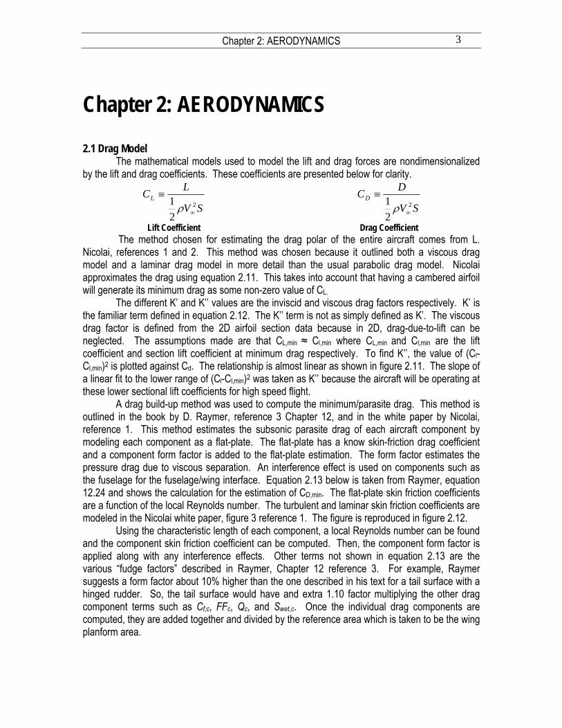
Drag Coefficient The method chosen for estimating the drag polar of the entire aircraft comes from L.

Nicolai, references 1 and 2. This method was chosen because it outlined both a viscous drag model and a laminar drag model in more detail than the usual parabolic drag model. Nicolai approximates the drag using equation 2.11. This takes into account that having a cambered airfoil will generate its minimum drag as some non-zero value of CL.

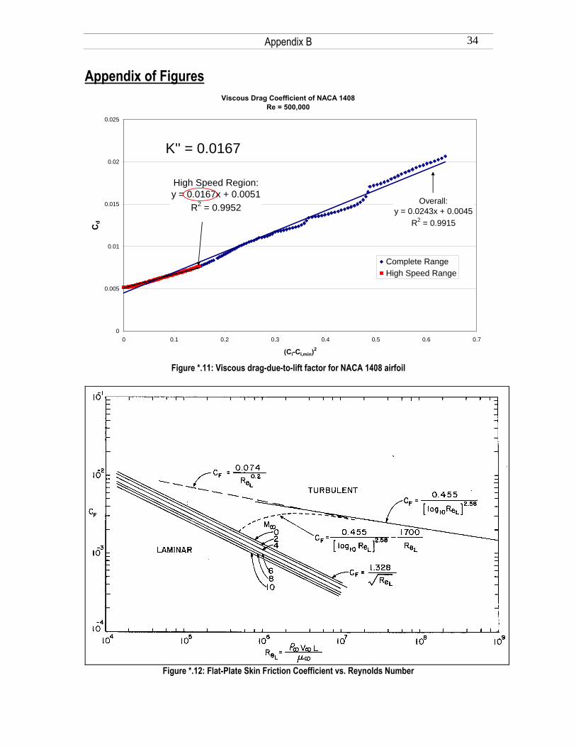
The different K’ and K’’ values are the inviscid and viscous drag factors respectively. K’ is the familiar term defined in equation 2.12. The K’’ term is not as simply defined as K’. The viscous drag factor is defined from the 2D airfoil section data because in 2D, drag-due-to-lift can be neglected. The assumptions made are that CL,min ≈ Cl,min where CL,min and Cl,min are the lift coefficient and section lift coefficient at minimum drag respectively. To find K’’, the value of (Cl-Cl,min)2 is plotted against Cd. The relationship is almost linear as shown in figure 2.11. The slope of a linear fit to the lower range of (Cl-Cl,min)2 was taken as K’’ because the aircraft will be operating at these lower sectional lift coefficients for high speed flight.

A drag build-up method was used to compute the minimum/parasite drag. This method is outlined in the book by D. Raymer, reference 3 Chapter 12, and in the white paper by Nicolai, reference 1. This method estimates the subsonic parasite drag of each aircraft component by modeling each component as a flat-plate. The flat-plate has a know skin-friction drag coefficient and a component form factor is added to the flat-plate estimation. The form factor estimates the pressure drag due to viscous separation. An interference effect is used on components such as the fuselage for the fuselage/wing interface. Equation 2.13 below is taken from Raymer, equation 12.24 and shows the calculation for the estimation of CD,min. The flat-plate skin friction coefficients are a function of the local Reynolds number. The turbulent and laminar skin friction coefficients are modeled in the Nicolai white paper, figure 3 reference 1. The figure is reproduced in figure 2.12.

Using the characteristic length of each component, a local Reynolds number can be found and the component skin friction coefficient can be computed. Then, the component form factor is applied along with any interference effects. Other terms not shown in equation 2.13 are the various “fudge factors” described in Raymer, Chapter 12 reference 3. For example, Raymer suggests a form factor about 10% higher than the one described in his text for a tail surface with a hinged rudder. So, the tail surface would have and extra 1.10 factor multiplying the other drag component terms such as Cf,c, FFc, Qc, and Swet,c. Once the individual drag components are computed, they are added together and divided by the reference area which is taken to be the wing planform area.


2.2 Lift Model The lift coefficient model is taken from Roskam, reference 4, who expresses the lift coefficient as equation 2.21. A Matlab® code call “FlatEarth.m” solves for the coefficients in equation 2.21 using Roskam’s definitions defined in equations 2.22-25.

The stall speed requirement determines the CL,max needed for steady level flight. At stead level flight lift is equal to the weight of the aircraft. CL,max can be determined by setting the lift equal the weight and substituting Vstall as V∞ into the definition of CL. A similar procedure can be done to find CL,min for steady level flight but instead substituting Vmax as V∞. These two lift coefficients are thus set by the mission requirements and the design speed and are shown in equations 2.26 and 2.27. The conversion between 2D and 3D CL,max was taken from Raymer reference 3 and is shown in equation 2.28. The structures and the aerodynamics team decided that a quarter chord sweep of 0 degrees was best. This decision produced simplifications in the computations for both teams. The conversion between 2D and 3D CL,min was found through lifting line theory. The simplifying assumption made was that the lift distribution was elliptical. This is desired because the induced drag is minimized with an elliptic lift distribution as proven by Prandtl. Also, this greatly simplifies the derivation for the lifting line theory results. In the end, the results of lifting lift theory predicts equation 2.29. The derivation of the lifting line theory is presented in Appendix B: Lifting Line Derivation. Equation 2.29 was used to find the 2D Cl,min. This value was then used as a parameter for airfoil selection. The method used to determine the CL,max due to the flaps comes from Nicolai reference 2. The mathematical model used to represent CL,max is shown in equation 2.210. The ΔCL,max in equation 2.210 is the change in CL,max due to flaps and is determined by equation 2.211 where KΛ is an empirical sweep correction found from equation 2.212.

An example on how to use these equations is presented for clarity. Assuming that the weight of the aircraft is 5.5 lbf, the planform is 4.75 ft2, the design speed is 92 ft/sec, and an aspect ratio of 5, CL,max needs to be at least 1.04 from equation 2.26. A clean wing with a NACA 1408 airfoil will produce a CL,max of 0.847. Thus, at this speed a ΔCL,max of 0.193 is needed for steady level flight. With the chord of the flaps configured at 20% MAC and a flap deflection of 30°, ΔCl,max is about 1. Solving equation 2.211 for SWF sizes the span of the flaps. SWF will have to be a minimum of about 1 ft2. This means that each of the two flapperons on the wing must affect about 0.5 ft2. This also means that the span of each flap must be a little over 0.5 ft since the mean chord is approximately 1 ft. 2.3 Design Parameters Selection 2.3.1 Taper Ratio

A taper ratio of 0.45 was recommended by Raymer, reference 3 Chapter 4. This taper ratio is shown through the use of lifting line theory to most accurately produce an elliptical lift distribution along the wing with a drag-due-to-lift less than 1% higher than the ideal. Prandtl proved in the early 20th century that elliptical lift distribution produces the least amount of induced drag. Reducing the drag on the aircraft by using a 0.45 taper ratio will decrease the thrust required for all speeds, allowing a greater maximum speed. 2.3.2 Main Wing Airfoil Selection

After some preliminary mission analysis, it became evident that the high speed dash design point would be the most constraining aspect for the airfoil selection. Stated differently, a


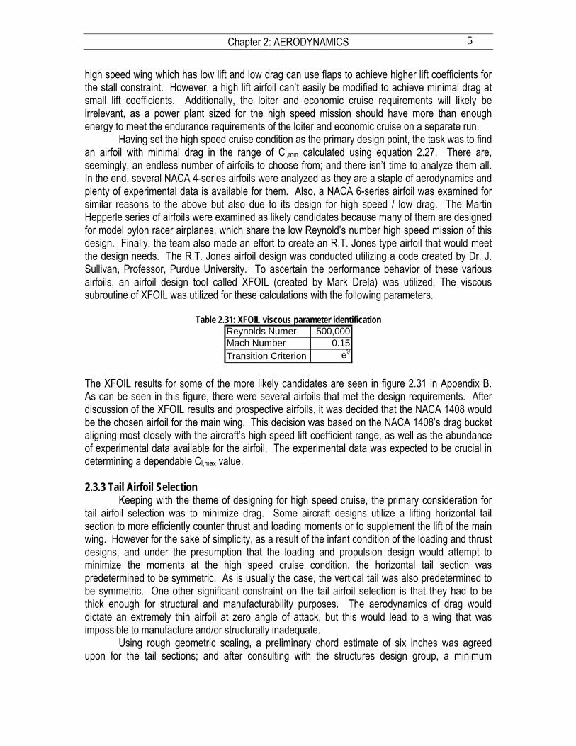
high speed wing which has low lift and low drag can use flaps to achieve higher lift coefficients for the stall constraint. However, a high lift airfoil can’t easily be modified to achieve minimal drag at small lift coefficients. Additionally, the loiter and economic cruise requirements will likely be irrelevant, as a power plant sized for the high speed mission should have more than enough energy to meet the endurance requirements of the loiter and economic cruise on a separate run. Having set the high speed cruise condition as the primary design point, the task was to find an airfoil with minimal drag in the range of Cl,min calculated using equation 2.27. There are, seemingly, an endless number of airfoils to choose from; and there isn’t time to analyze them all. In the end, several NACA 4-series airfoils were analyzed as they are a staple of aerodynamics and plenty of experimental data is available for them. Also, a NACA 6-series airfoil was examined for similar reasons to the above but also due to its design for high speed / low drag. The Martin Hepperle series of airfoils were examined as likely candidates because many of them are designed for model pylon racer airplanes, which share the low Reynold’s number high speed mission of this design. Finally, the team also made an effort to create an R.T. Jones type airfoil that would meet the design needs. The R.T. Jones airfoil design was conducted utilizing a code created by Dr. J. Sullivan, Professor, Purdue University. To ascertain the performance behavior of these various airfoils, an airfoil design tool called XFOIL (created by Mark Drela) was utilized. The viscous subroutine of XFOIL was utilized for these calculations with the following parameters.

Table 2.31: XFOIL viscous parameter identification

Reynolds Numer 500,000Mach Number 0.15Transition Criterion e9

The XFOIL results for some of the more likely candidates are seen in figure 2.31 in Appendix B. As can be seen in this figure, there were several airfoils that met the design requirements. After discussion of the XFOIL results and prospective airfoils, it was decided that the NACA 1408 would be the chosen airfoil for the main wing. This decision was based on the NACA 1408’s drag bucket aligning most closely with the aircraft’s high speed lift coefficient range, as well as the abundance of experimental data available for the airfoil. The experimental data was expected to be crucial in determining a dependable Cl,max value. 2.3.3 Tail Airfoil Selection

Keeping with the theme of designing for high speed cruise, the primary consideration for tail airfoil selection was to minimize drag. Some aircraft designs utilize a lifting horizontal tail section to more efficiently counter thrust and loading moments or to supplement the lift of the main wing. However for the sake of simplicity, as a result of the infant condition of the loading and thrust designs, and under the presumption that the loading and propulsion design would attempt to minimize the moments at the high speed cruise condition, the horizontal tail section was predetermined to be symmetric. As is usually the case, the vertical tail was also predetermined to be symmetric. One other significant constraint on the tail airfoil selection is that they had to be thick enough for structural and manufacturability purposes. The aerodynamics of drag would dictate an extremely thin airfoil at zero angle of attack, but this would lead to a wing that was impossible to manufacture and/or structurally inadequate.

Using rough geometric scaling, a preliminary chord estimate of six inches was agreed upon for the tail sections; and after consulting with the structures design group, a minimum


thickness of 6% was established implying a thickness of less than half an inch. From this point, the strategy was to analyze the drag performance of various symmetric airfoils.

The obvious candidates for symmetric airfoils around 6% thicknesses were the NACA 0006, 0007, and 0008. The team also made an effort to create an R.T. Jones type airfoil that would meet the design needs. The R.T. Jones airfoil design was conducted utilizing a code created by Dr. J. Sullivan, Professor, Purdue University. Drag behavior of the various candidate airfoils were again calculated using XFOIL. The viscous subroutine of XFOIL was utilized for these calculations with the parameters listed in table 2.31. The calculations from XFOIL are plotted in Appendix B as figure 2.31 and figure 2.32. Figure 2.32 is simply a close-up of the smaller angles of attack.

A first attempt was to make the vertical tail and horizontal tails flat plates. Upon analyzing this configuration in XFOIL, the flat plate was discovered to have enormous drag penalties compared to the other airfoils being tested as seen in Appendix B, figure 2.33. The next consideration was discerning the likely angle of attack range for the tail sections at the high speed cruise condition. It was determined that the vertical tail should be relatively easy to attach to the aircraft at a fairly accurate zero angle of attack. Also, there should be no significant steady state forces or moments that would drive the vertical tail from zero degrees angle of attack. In fact, zero degrees angle of attack should represent a stable equilibrium for the vertical tail. This implies that the best airfoil for the vertical tail is the one with the least drag at very small angles of attack which is arbitrarily chosen to be less than 2°. Figure 2.32 shows that the NACA 0006 airfoil and the Jones (6.8%) best met this criteria. The NACA 0006 airfoil was chosen because again, there is a plethora of NACA airfoil data available.

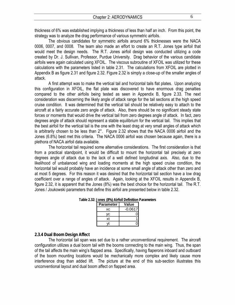
The horizontal tail required some alternative considerations. The first consideration is that from a practical standpoint, it would be difficult to mount the horizontal tail precisely at zero degrees angle of attack due to the lack of a well defined longitudinal axis. Also, due to the likelihood of unbalanced wing and loading moments at the high speed cruise condition, the horizontal tail would probably have an incidence at some small angle of attack other than zero and at most 5 degrees. For this reason it was desired that the horizontal tail section have a low drag coefficient over a range of angles of attack. Again, looking at the XFOIL results in Appendix B, figure 2.32, it is apparent that the Jones (8%) was the best choice for the horizontal tail. The R.T. Jones / Joukowski parameters that define this airfoil are presented below in table 2.32.

Table 2.32: Jones (8%) Airfoil Definition Parameters

Parameter Valuexc -0.0617yc 0xt 1yt 0

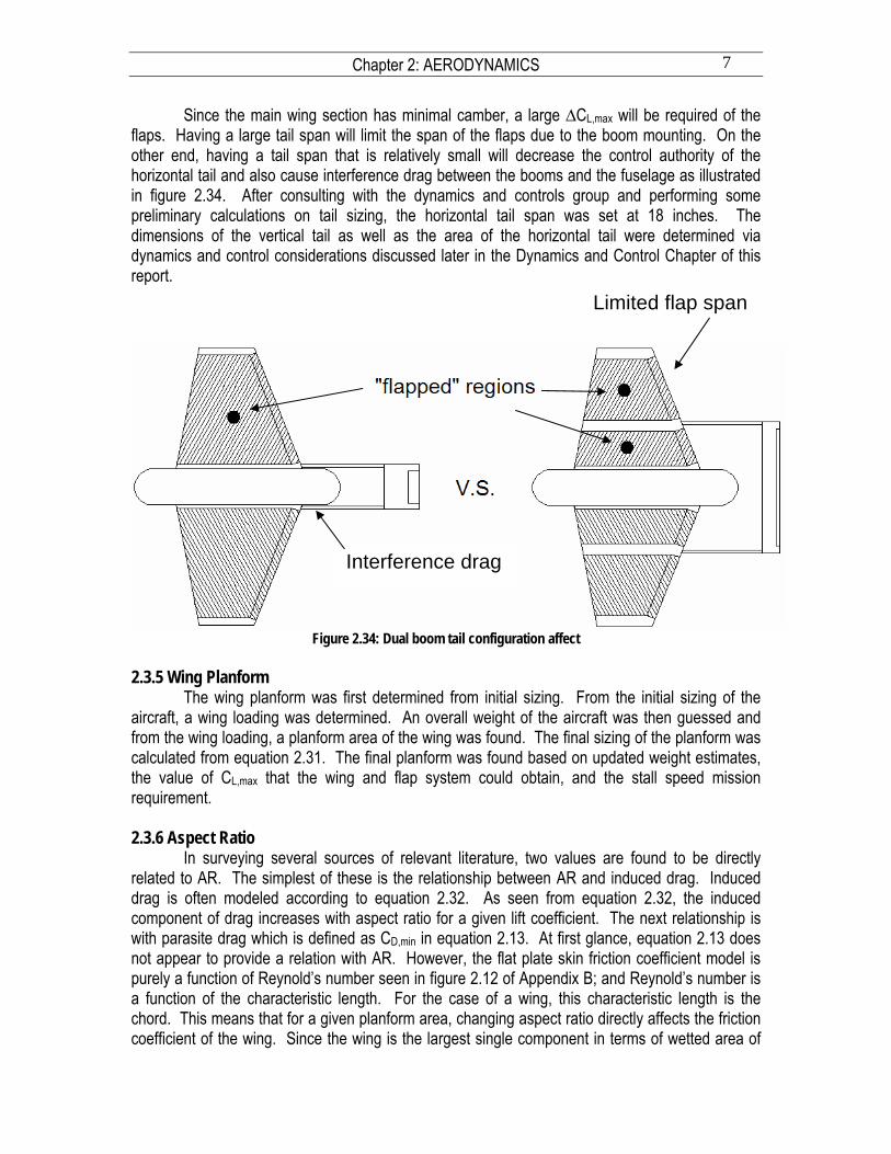
2.3.4 Dual Boom Design Affect The horizontal tail span was set due to a rather unconventional requirement. The aircraft configuration utilizes a dual boom tail with the booms connecting to the main wing. Thus, the span of the tail affects the main wing’s flapped area. Specifically, having flaperons inboard and outboard of the boom mounting locations would be mechanically more complex and likely cause more interference drag than added lift. The picture at the end of this sub-section illustrates this unconventional layout and dual boom affect on flapped area.


Since the main wing section has minimal camber, a large ∆CL,max will be required of the flaps. Having a large tail span will limit the span of the flaps due to the boom mounting. On the other end, having a tail span that is relatively small will decrease the control authority of the horizontal tail and also cause interference drag between the booms and the fuselage as illustrated in figure 2.34. After consulting with the dynamics and controls group and performing some preliminary calculations on tail sizing, the horizontal tail span was set at 18 inches. The dimensions of the vertical tail as well as the area of the horizontal tail were determined via dynamics and control considerations discussed later in the Dynamics and Control Chapter of this report.

Figure 2.34: Dual boom tail configuration affect

2.3.5 Wing Planform

The wing planform was first determined from initial sizing. From the initial sizing of the aircraft, a wing loading was determined. An overall weight of the aircraft was then guessed and from the wing loading, a planform area of the wing was found. The final sizing of the planform was calculated from equation 2.31. The final planform was found based on updated weight estimates, the value of CL,max that the wing and flap system could obtain, and the stall speed mission requirement. 2.3.6 Aspect Ratio

In surveying several sources of relevant literature, two values are found to be directly related to AR. The simplest of these is the relationship between AR and induced drag. Induced drag is often modeled according to equation 2.32. As seen from equation 2.32, the induced component of drag increases with aspect ratio for a given lift coefficient. The next relationship is with parasite drag which is defined as CD,min in equation 2.13. At first glance, equation 2.13 does not appear to provide a relation with AR. However, the flat plate skin friction coefficient model is purely a function of Reynold’s number seen in figure 2.12 of Appendix B; and Reynold’s number is a function of the characteristic length. For the case of a wing, this characteristic length is the chord. This means that for a given planform area, changing aspect ratio directly affects the friction coefficient of the wing. Since the wing is the largest single component in terms of wetted area of

Interference drag

Limited flap span


the aircraft, this effect is significant. Using the above description of CD,min, equation 2.13 can be rewritten as equation 2.33. In this equation, c is inversely proportional to AR and friction coefficient is inversely proportional to Reynold’s number and the rest of the terms are directly proportional. This leaves CD,min to be positively correlated with aspect ratio. At this step, the equations show that induced drag decreases with AR and increases with

ery complex, but by

The trends of figure 2.35 in Appendix B are consistent with intuition. The induced drag

dy demonstrate that to minimize the lift of the plane in the effort to

Refer

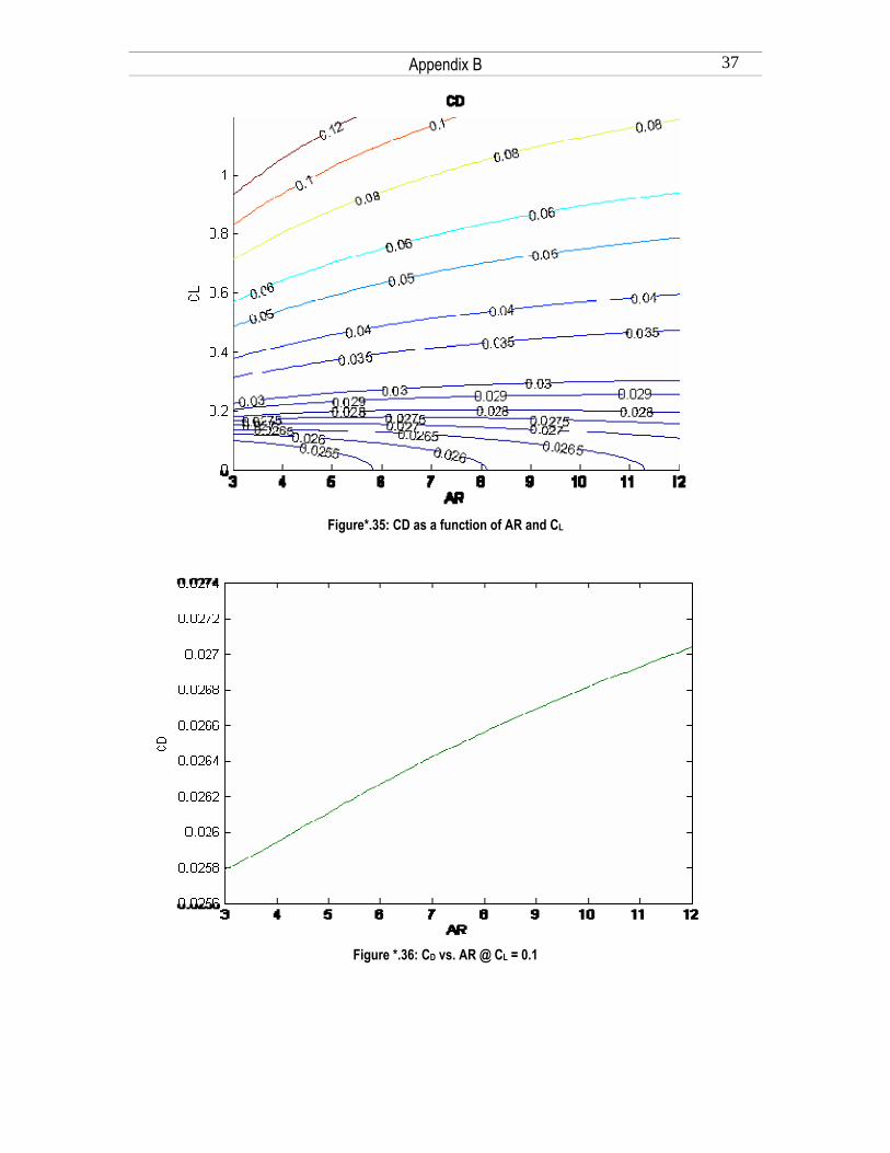
lift coefficient, while parasite drag decreases with AR. Since total drag is the sum of these two drag types, there is no clear answer to what the best AR is for an aircraft. Using drag as a measure of merit for an aspect ratio trade study, the primary variables of interest are AR and lift coefficient. This means that an expression is needed for CD in terms of CL and AR. In equation 2.32, Oswald’s efficiency factor presents itself as an undesirable independent variable. However, Raymer provides an empirical expression for e as a function of AR and LE sweep, equation 2.34. Holding the sweep constant gives the desired result shown in equation 2.34. The expression for parasite drag in equation 2.33 is seemingly, vholding all other geometry (besides AR) fixed, the equation reduces to purely a function of AR. This leaves equation 2.36 as the expression for drag which meets the initial variable/measure of merit statement. The drag coefficient is now in a form that can be analyzed using a Matlab® script and the results are graphically displayed in a more comprehendible manner in Appendix B, figure 2.35. becomes more prominent at higher lift coefficients and so larger AR values lead to reduced drag at high CL values. The design of issue, however, is primarily about speed. The aircraft will cruise with a lift coefficient of about 0.1. At this low end of the lift coefficient spectrum, the parasite drag dominates. The chart clearly depicts the answer to the important design question of what AR to use: for the cruise design point, there is no optimal AR, the smaller the better. This trend is shown explicitly in Appendix B, figure 2.36.

And so, the results of the stu maximize speed the airplane must be constructed with the smallest feasible aspect ratio.

This statement contains some vagueness. Obviously, AR can’t be zero. So what is small enough? The answer must account for the increased complexity of wing analysis below an AR of about 3. In the end, the aspect ratio is set by the span of flaps necessary to achieve the customer’s stall speed requirement as well as the limitations due to transportability concerns. Thus the span of the wing will be small enough to fit in the vehicle used to transport the aircraft to its flight facility. The aspect ratio was chosen to be 5.

ences

. – L. M. Nicolai. (2002). Estimating R/C Model Aerodynamics and Performance. [Electronic

2. – L. M sign. Dayton, Ohio: University of Dayton A.

5. – San 4 Lecture Notes,” Purdue, 2005.

1

version]. Lockheed Martin Aeronautical Co.. . Nicolai. (1975). Fundamentals of Aircraft De

3. – D. Raymer. (2006). Aircraft Design: A Conceptual Approach. (4th Ed.). Reston, Virginia: AIA4. – J. Roskam. (2001). Airplane Flight Dynamics and Automatic Flight Controls. (3rd Ed.).

Lawrence, KS: DARcorporation. karan, Venke, “2005 Fall: AAE 33

Chapter 3: PROPULSION 9

Chapter 3: PROPULSION

The design of the propulsion system began with a conceptual design meeting. Two main propulsion systems were considered; a conventional propeller system and a ducted fan system. By creating a list of pros and cons for each system, the group came to a unanimous decision. The electric ducted fan (EDF), while unconventional, was the most intriguing. The EDF system is relatively new to the remote control hobby aircraft world. While it can be found in use today, it is no where near as popular as the conventional propeller system. The ducted fan maybe new to the hobby world, but it has been around in the aviation world for many decades. A ducted fan is essentially a propeller inside of a circular shroud or duct. The purpose of the shroud is to eliminate the negative effects that occur on the tips of a propeller and increase efficiency. When comparing a propeller and fan that create the same amount of thrust, the fan will be smaller, have more blades, and operate at higher revolutions per minute (RPM). The main benefits of a ducted fan for this design include landing technique, direct drive, and appeal. Thanks to the high static thrust that is typical of an EDF, a hand launch is feasible. A hand launch removes the necessity of landing gear, landing gear retracts, and runway steering. This greatly reduces the drag and the amount of time and effort spent in designing for takeoff and landing. A hand launch was chosen as the method of launching for the design. The landing will have to be a belly landing; which will require added structural reinforcements on the bottom of the aircraft but should be simpler than designing for the point loads applied by landing gear. Due to the comparatively smaller diameter of a fan, a motor is capable of spinning the fan at a higher RPM than a propeller. Because the desired RPMs are high, there is no need for a gearbox. An EDF costs a great deal more than a propeller, but the cost of landing gear and a gear box, which is now unnecessary, balances this cost. While a ducted fan is unconventional and presents an added challenge, the appeal and performance promise to exceed the negatives. As mentioned before, EDFs are still uncommon in most hobby marketplaces. In fact, very few are capable of handling the power required to travel at this design’s high speeds. The average ducted fan is very cheaply made and can only handle a fourth of the horsepower required for this mission. Upon researching available fans, only four were deemed acceptable. Those fans are listed in table 3.1. Upon further research into the world of EDFs, only the Wennmacher Modell Technik (WeMoTec) brand of ducted fans had any information of performance. According to popular opinion of RC aircraft hobbyists, they are the best model aviation ducted fans available for their prices. Kontronik, a German manufacturer of brushless electric motors, has performance data of the WeMoTec fans and their motors posted on their website (reference 1). The WeMoTec brand of fans is also readily available for purchase from many distributors, something the other brands of fans cannot claim.


Diameter Weight Max RPM Cost Manufacturer Model [ in ] [ lbs ] [ RPM ] [ $ ]

Wemotec Midi Fan 3.5 0.231 35,000 $74.95 Wemotec Mini Fan 480 2.72 0.132 45,000 $53.90 Great Planes Hyperflow 2.23 0.081 49,000 $30.00 VASA VasaFan 65 2.6 0.077 45,000 $60.00

Table 3.1: Ducted Fan Canidates This reduces the fans for consideration to only the WeMoTec models. The first is the Mini 480 model and the second is the Midi model. The fans are nearly identical but differ in diameter and blade count. The Midi fan has a larger diameter hub as well. The larger hub allows for a larger, typically more powerful, diameter motor. By using the data from Kontronik, a relationship between RPM and exhaust velocity was established; see Appendix C figure 3.1. A relationship between thrust and exhaust velocity squared was also established, which can be found in Appendix C figure 3.2. By using equation 3.1, and the relations established above it was possible to calculate thrust available throughout a range of speeds. Thrust required to maintain steady level flight is equal to drag; see equation 3.2. The speed at which thrust available no longer exceeds thrust required (or drag) is the maximum theoretical speed. For the Midi and Mini 480 models, those plots can be found in Appendix C figures 3.3 and 3.4. Both of the mentioned plots assume the fans are spun at their maximum RPM. While the research was underway on fan performance, a battery solution was stumbled upon. Thanks to the advice from a local hobby store specialist, an affordable solution was found. Currently, Lithium Polymer (LiPo) battery packs are the most desirable solution on the market; however they are the most expensive. A breakdown of typical hobby application batteries can be found in Appendix C table 3.2. With the budget constraint, even the cheapest batteries in table 3.2 are unreasonable. Thanks to an employee at Hobby Town USA (reference 2), who redirected the design team to a company named A123 Systems (reference 3), a high performance battery capable of the performance required and within the budget was found. The batteries the Hobby Town USA employee redirected the team’s attention to are of Lithium Ion chemistry. Lithium Ion (Li-Ion) cells perform similar to LiPo cells, but are far less dangerous. LiPo batteries are known to explode or combust when not taken care of properly. Li-Ion cells are nearly as expensive as LiPo cells. The breakthrough came when it was discovered that DeWalt, a popular power tool manufacturer (reference 4), uses A123 System’s Li-Ion batteries in their cordless drill batteries (reference 5). These cordless drill batteries can be found on the market for $169.99 Retail. Upon researching into the availability of these drill batteries, an available battery was located for a discounted price of $115.00. These cordless drill batteries contain ten A123 Systems Li-Ion cells. Compare the price of $11.50 per cell for the A123 Li-Ion cells to LiPo cells, which cost an average of $25.00 per cell. To further reduce the price of these batteries, the cost of the DeWalt battery was split with another design team. Each team received 5 Li-Ion cells for a total cost of $57.50. An extensive guide for converting the DeWalt battery into a RC hobby battery can be found at the website cited as reference 6. The specifications of the A123 Systems’ Li-Ion cells can be found in table 3.3.


A123 Systems' Lithium Ion Cells

Voltage per Cell 3.6 V Max Continous Current 70 Amps

Max Surge Current 120 Amps Capacity 2300 mAh

Weight per Cell 0.16 lbf Cost per Cell $11.50

Table 3.3: A123 Systems’ Lithium Ion Batteries

With the batteries already chosen and only two fans to analyze, the selection of a motor was a simple one. The code “TestDesignAircraft.m”, which was received from Professor Andrisani, was edited to calculate various system values for a ducted fan system. The code was originally designed for a propeller to maximum endurance. The code was altered to design for the high speed mission. The code may be found in the code Appendix C under code 3.1. This code is written in MATLAB®. By iterating the design process, it was possible to find a Kv and highest speed at which only 5 Li-Ion cells were required by each fan. A generic motor with a varying Kv was used by the altered code “TestDesignAircraft.m” to find a Kv that would bring the number of Li-Ion cells required to 5 for both fans; the results from this optimization process can be found in Appendix C table 3.4. A cost-effective motor capable of the desired performance from the WeMoTec Mini 480 ducted fan is difficult to find; only one motor was found to match these specifications. The HET-RC Typhoon 2W-20 EDF brushless motor is the only candidate; the motors specification can be found in Appendix C table 3.5 (reference 7). When compared with the WeMoTec Mini 480 data from Appendix C table 3.4, it is apparent the motor meets the requirements. Any of the required values that exceed the motor’s specifications are considered acceptable because they will only be used sparingly; the high speed dash will be for only a few seconds. This motor appeared to be the only motor on the market capable of the performance and within a reasonable cost range. Upon contacting the only distributor of this motor located in the USA, the team was informed the motor was unavailable and would be so for a long time. With the Typhoon motor out of the picture, it was obvious the WeMoTec Midi Fan was the only remaining path to follow. The performance specifications found in Appendix C table 3.5 for the Midi Fan are not easy to achieve. No motors on the market were found to be capable of handling the current necessary to produce the required torque to achieve maximum RPM. By stepping the RPM down about 15%, the current necessary became an achievable number. A motor manufactured by Electrifly (reference 8) was found to match the requirements; the motor is called the Electrifly Ammo 36-50-2300. The motor’s specifications can be found in table 3.6.

Motor Ammo 36-50-2300

Kv 2300 Max Voltage 18

Max Continous Current 60 Amps Max Surge Current 100 Amps

Weight 0.35 lbf Cost $79.99

Table 3.6: Electrifly Ammo 36-50-2300 Brushless Motor


With the WeMoTec Midi Fan running at 85% of its maximum RPM it still achieved a similar top speed as the Mini 480 Fan at 100% RPM. While the Midi Fan setup costs a little more, the desirable Mini 480 Fan system is not available. The Midi fan is far less efficient than the Mini 480 fan. The team settled to run at a low efficiency to achieve a high performance under budget system. The final propulsion system thrust curve can be found in figure 3.5. The rest of the final system’s high speed specifications can be found in table 3.7. Table 3.8 contains the maximum endurance mission operating conditions. Designing for maximum speed has provided the system with plenty of “juice” to achieve the desired endurance time of 7 minutes.

Figure 3.5: Final Propulsion System Thrust Curve

Propulsion System at Max Endurance Operation Conditions

Fan Battery Motor WeMoTec Midi Fan A123 Systems' Lithium Ion Cells Ammo 36-50-2300

Operating RPM 16,000 RPM Voltage Required 7.4 V Aircraft Velocity 47 ft/s

Endurance 10.1 min Current Required 19.9 A

Table 3.7: Final Propulsion High Speed Specs

Propulsion System at High Speed Operation Conditions Fan Battery Motor

WeMoTec Midi Fan A123 Systems' Lithium Ion Cells Ammo 36-50-2300 Operating RPM 30,000 RPM Current Required 73.5 A

Aircraft Velocity 107 ft/s Endurance 2.1 min

Voltage Required 16 V Table 3.8: Final Propulsion Max Endurance Specs


References 1. – Kontronik Drives. "Kontronik Downloads." Fan Measurements. 22 April 2003. Kontronik Drives.

22 September 2006 <http://www.kontronik.com/index2e.htm>. 2. – http://www.hobbytown.com/ 3. – http://www.a123systems.com/html/home.html 4. – http://www.dewalt.com/us/core/ 5. – Webster, Mel. "A123Systems Unveils Lithium-Ion Battery Technology that Delivers

Unprecedented Levels of Power, Safety and Life." A123 Systems News 2 November 2005. 5 October 2006 <http://www.a123systems.com/html/news/articles/051102_pr.html>.

6. – Kauffman Ph.D. , Sid. DeWalt 36V Technology (A123 Systems). 22 August 2006. 14 October 2006 <http://slkelectronics.com/DeWalt/index.htm>.

7. – WarBirds Rc. HET-RC - Typhoon EDF 2W-20 (700 Watt). . 14 October 2006 <http://www.warbirds-rc.com/Store/hett-edf2w20.html>.

8. – Electrifly. Electrifly - Ammo In-Runner Brushless Motors. . 14 October 2006 <http://www.electrifly.com/motors/gpmg5105.html>.

Chapter 4: DYNAMCIS AND CONTROLS 14

Chapter 4: DYNAMICS AND CONTROLS Analysis of the dynamics and controls for the TFM-2 was completed in several steps. The

first task was to determine the dimensions of the tail geometries for the aircraft. Team 2’s design called for an unusual configuration featuring twin vertical stabilizers and one horizontal tail attached to the fuselage via booms extending from the wings. Next, the control surfaces were sized. Then, a check of all static stability control derivatives was performed. Following this, a trim diagram was constructed. With the aircraft sized, a feedback control system was designed to meet the mission specifications for the Dutch roll mode.

An important tool for analysis used throughout the Dynamics and Controls Chapter was the use of Prof. Andrisani’s Flat Earth Code. This course-provided MATLAB® code involves a great deal of computation based on the size of the aircraft. The code is executed by running seven steps in order upon completing the file BasicConstants.m (this file defines all vehicle constants that are needed to compute stability and control derivatives). The first step calculates the aircrafts aerodynamic and mass properties. The second step trims the aircraft for the desired speed and altitude. The third step runs a Simulink model to simulate a 6 degree of freedom aircraft with nonlinear equations of motion. The fourth step plots the results of the nonlinear simulation and was not used during analysis. The fifth step linearizes the aircraft system found previously during nonlinear analysis. The sixth step sets up linear models for the longitudinal control system design. The seventh step sets up linear models for the lateral control system design. 4.1 Tail Sizing

For tail sizing, a preliminary sizing method was used from Raymer reference 1 using the Tail Volume Coefficient method (Class I sizing). This is a historical approach in that the volume coefficients are based on aircrafts that are similar to the team’s design. Class I sizing would allow for a preliminary estimation of the vertical and horizontal tail areas needed. This method led to a horizontal tail area of 0.8159 ft2 and a vertical tail area of 0.3300 ft2.

The next step was to size the tail using the Class II Method by producing X-plots as proposed by Roskam (reference 2). In order to do this, longitudinal and directional X-plots were produced based on functions of the tail areas. An important decision was made at this point to place the center of gravity in the longitudinal direction at the wing’s quarter-chord. In addition to this, it was also noted that if this could not be accomplished, it is desired that the center of gravity be in front of the quarter-chord. This ensures that there is sufficient horizontal tail area for the aircraft. Another complexity for the tail sizing was the twin-tail configuration and the need for sufficient total vertical tail area. Table 4.1 summarizes the results of using this method. Figures 4.1 and 4.2 illustrate the X-plot method.

Horizontal Tail Vertical Tail Area (in2) 90 60 Span (in) 18 6 Chord (in) 5 5

Aspect Ratio 3.6 1.2 Table 4.1: Tail Sizing Results


Horizontal Tail Sizing - Longitudinal Stability

0

0.1

0.2

0.3

0.4

0.5

0.6

0.7

0.8

0 0.1 0.2 0.3 0.4 0.5 0.6 0.7 0.8 0.9 1

SH (ft2)

X pe

r Cw

Static Margin = 18.1%

Xac

Xcg

Figure 4.1: Longitudinal X-plot Horizontal Tail Sizing

Vertical Tail Sizing - Directional Stability

-0.2

-0.15

-0.1

-0.05

0

0.05

0.1

0.15

0.2

0 0.05 0.1 0.15 0.2 0.25 0.3

SV (ft2)

Cnb

eta (

rad-1

)

Cnbeta=0.102 rad-1

Figure 4.2: Directional X-plot Vertical Tail Sizing


4.2 Control Surface Sizing

For the sizing of control surfaces, a historical approach was used for the elevator and rudder. The aerodynamics portion of the team had previously sized the flaperons due to the stall speed constraint. In order to gain perspective on how to historically size the elevator and rudder, the Raymer book was consulted (reference 1). Raymer suggests that both the elevator and rudder extend 25-50% of the tail chord and a span that extends from tip to tip of 90% of the span. It was then at this point that varying the size of both the elevator and rudder were evaluated to observe the effectiveness of both. To easily compute the elevator effectiveness (Cmδe) and the rudder effectiveness (Cnδr), the Flat Earth Code was consulted.

The elevator was sized first at 25% of the horizontal tail chord. The span of the elevator was set to 2/3 of the horizontal tail span. An elevator sized with a chord of 1.25 inches and a span of 12 inches has an elevator effectiveness of -1.2805 rad-1. The suggested range from the Flat Earth Code (reference 5) is -1 to -2 rad-1.

Rudder sizing was sized such that the chord was 90% of the vertical tail chord. This was due to the desire to only implement one rudder on the twin-tail configuration. Also, the span was set to roughly 92% of the span to avoid rudder interference with the horizontal tail. The rudder was sized with a chord of 4.5 inches and span of 5.5 inches and has a rudder effectiveness (Cnδr) of -0.035 rad-1. This value is close to the desired range as suggested by the Flat Earth Code of -0.06 to -0.3 rad-1. This rudder effectiveness calculation was based on a conventional tail configuration and for the purposes of this design showed a reasonable approximation of the yawing moment coefficient due to rudder deflection. 4.3 Static Stability In order to ensure that the TFM-2 would be stable in flight, calculations of the aircrafts static stability was calculated. The longitudinal static stability was first addressed to ensure that the aircraft has a sufficient amount of horizontal tail. Then the lateral-directional static stability was addressed by checking the weathercock stability to check that the aircraft has enough vertical tail volume. Also the effect of dihedral was computed as another measure of the lateral-directional static stability. In addition to the longitudinal and lateral static stability check, a check of control surface sizing was to compute the control derivatives of each surface’s effectiveness. In order to ensure that each stability derivative was sufficient for flight, the TFM-2 was compared to the MPX-5. The MPX-5 was a small remote controlled model aircraft that was designed by Mark Peters for his master’s thesis. All values of the TFM-2 static stability derivatives were found to be sufficient for the high-speed flight. Table 4.2 summarizes parameters necessary for static stability.

TFM-2 MPX-5

Cmα -0.602 -1.049 Cnβ 0.102 0.057 Clβ 0.007 -0.055 Clδa 0.242 0.114 Cmδe -1.280 -2.318 Cnδr -0.035 -0.070

Table 4.2: Static Stability Derivatives in rad-1


4.4 Trim Analysis

A trim diagram was produced to ensure that the aircraft would be trimmable at all anticipated flight conditions with elevator deflection. The diagrams were produced using the method outlined by Roskam (reference 2). For the TFM-2 the incidence of both the wing and horizontal tail was set to zero degrees.

Figure 4.3: Trim Diagram for TFM-2

Figure 4.3 shows the trim triangle. The triangle is seen below the red line which indicates the maximum lift coefficient and between the two center of gravity (CG) lines (forward and aft). The multi-colored diagonal lines represent the effects of different elevator deflections. Typical trim diagrams account for a shift in the CG due to mass loss. However with an electrically powered aircraft there will be minimal mass losses during flight, so the analysis was made for two flights; one with payload and one without. From this diagram the range of elevator deflection is -2 to 12 degrees for trimming was determined. The typical range is typically between -20 and 20 degrees. This suggests that the elevator is somewhat oversized; however it does not interfere with the TFM-2’s desired flight operations.

-0.4-0.3-0.2-0.100.10.20.3-0.2

0

0.2

0.4

0.6

0.8

1

1.2

CLmax

CL

Cm0.25c

α = 3o

α = 7o

α = -1o

Cm = 0 Xcg forward

Cm = 0 Xcg nominal

Cm = 0 Xcg aft


4.5 Feedback Control System

Using the Flat Earth Code through Step 7, the yaw rate transfer function was obtained. It is from this transfer function that the Dutch roll damping ratio was obtained. The open-loop transfer function was found to be as follows:

)83.16535.1)(169.0)(75.6()4551.0)(759.0)(144.7(0563.12

)()(

2 ++−+−++−

=sssssss

srsR

δ

From this equation the Dutch roll mode damping ratio was found to be 0.187. This value was not sufficient in that it did not meet the mission specifications of Dutch roll damping ratio of at least 0.8. At this point, a feedback controller must be integrated into the aircraft. In order to do this, the servo controlling the rudder, rate gyro, and a control law transfer function must be incorporated with the yaw rate transfer function. The servo transfer function used for this feedback controller was given in reference 6 for a Futaba S-148 Servo. The rate gyro was assumed to be 1. And the control law transfer function was determined to be a simple negative gain through the use of MATLAB®’s SISOTool. In order to obtain a damping ratio for the Dutch roll mode of at least 0.8, a control law gain of -0.4 was chosen. This gain corresponds to a Dutch roll mode damping ratio of 0.823, which meets mission specifications. Figure 4.4 depicts the final control system to be used to control the yaw rate feedback controller. For the integration of the determined control low gain, the rate gyro will be properly set to desired gain of -0.4. Through the use of SISOTool the root locus of the feedback control system was found. Stability of the system was confirmed through evaluation of the closed-loop pole locations (all appear in the left hand plane of the root locus). A plot of the root locus and the corresponding closed-loop poles can be found in Appendix D figure 4.4.

+

-

-0.4 1

δr [rad]

95040950

2 ++ ss

Futaba Servo

Control Law and Rate Gyro Gains

rδ )83.16535.1)(169.0)(75.6()4551.0)(759.0)(144.7(0563.12

2 ++−+−++−

sssssss

Yaw rate [r/sec]

Aircraft Transfer Function

Figure 4.4: Feedback Control System for Aircraft


References 1. – D. Raymer. (2006). Aircraft Design: A Conceptual Approach. (4th Ed.). Reston, Virginia: AIAA.

Lockheed Martin Aeronautical Co.. 2. – J. Roskam. (1985). Airplane Design: Parts I-VIII. Ottawa, Kansas: Roskam Aviation and

Engineering Corporation. 3. – J. Roskam. (1977). Methods for Estimating Stability and Control Derivatives of Conventional

Subsonic Airplanes. Lawrence: Third Printing. 4. – Brandt, S.A., Stiles, R. J., Bertin, J. J., and Whitford, R. (2004). Introduction to

Aerospace: A Design Perspective. (2nd Ed.). AIAA. 5. – MATLAB® Flat Earth Code 6. – AAE 451 D&C Sourcebook given by Professor Andrisani 7. -- Peters, Mark E. Development of a Light Unmanned Aircraft for the Determination of Flying

Qualities. Master’s Thesis, 1996, Purdue University, W. Lafayette, IN.

Chapter 5: STRUCTURES AND WEIGHTS 20

Chapter 5: STRUCTURES AND WEIGHTS 5.1 Introduction

The dual boom design necessitated by the ducted fan propulsion system introduced structural complications not present in a more traditional configured aircraft. Throughout the design process, decisions were continually influenced by manufacturability and cost of production concerns. An initial survey showed that a fiberglass and epoxy covered foam construction was capable of meeting the structural demands while maintaining a light weight aircraft. Classical structural analysis techniques and laminated plate theory were used in the design of the aircraft’s structure. A model created in CATIA® was used extensively for weight analysis which included component placement and locating the center of gravity. CATIA® was also vary valuable in calculating moments and products of inertia and producing accurate drawings for production. 5.2 Load Factor

The load factor, n, is a critical design parameter for aircraft structural analysis because the entire structure scales with load factor. The lower the load factor is, the lighter the aircraft structure can be made. With the current mission of high-speed flight, light weight became an even more critical goal than in the case of a more general purpose aircraft.

The load factors for flight at maximum lift conditions, in level-flight turn, and in climb as a function of vertical turn were examined to determine the appropriate design load factor. Equations yielding the instantaneous load factors as a function of the given flight conditions are in Appendix E: V-n Diagram Walk-through. Graphical representations of these results are presented in Appendix E figures 5.2.1 – 5.2.4.

Based on realistic aircraft handling characteristics, input parameters were limited for each flight regime. The load factors were then extracted from figures 5.2.1 – 5.2.4. At maximum lift, velocity was said not exceed 50 ft/sec. This led to a maximum load factor of 3.3. In level turning flight, bank angle was not to exceed 75 degrees. This resulted in a maximum load factor of 4. In climbing flight, a vertical turn radius of 25 feet was considered to be reasonable. With maneuvering speed limited to 60 ft/sec, this resulted in a load factor of 5.

The permissible diving speed limits the V-n diagram, and this is typically specified at 20%-50% higher than the maximum level flight airspeed (Peery and Azaar Reference 1). For this design it was set at 125 ft/sec based on a dash speed of about 100 ft/sec.

The combination of the above analyses for total flight regime loading is shown below in figure 5.2.1.


Figure 5.2.1: V-n Diagram

Below 60 ft/sec, it is not possible to exceed the limit load factor in positive load maneuvering, and similarly for 45 ft/sec in negative load maneuvering, because the wing will stall prior to reaching these conditions. Above these speeds, it is necessary for the pilot to exercise discretion as it is not practical to design an aircraft structure for enduring excessively violent maneuvers.

Historically, a safety factor of 1.5, which was based on the ratio of ultimate tensile load to yield load of 24 ST Aluminum alloy, has been used. Using this safety factor, the final load factor used in all analyses was determined to be 7.5. 5.3 Wing Analysis and Design

For both the bending and twist analyses, the wing was discretized into ten sections, as shown in figure 5.3.1 of Appendix E. Bending and polar moments of inertia of the wing cross section at each station were found using XFOIL. The fiberglass and epoxy composite skin was assumed to bear all of the wing loading such that the bending and polar moments of inertia were functions only of skin thickness. A first attempt was made to approximate the airfoil section as an ellipse of approximately the same thickness ratio as the actual airfoil. This was determined to be a poor approximation and is discussed in Appendix E: Comparison of Exact Airfoil Structural Properties wit Elliptic Approximation. 5.3.1 Bending Analysis

The lift was modeled as an elliptic distribution, congruent with the 0.45 taper ratio. This is shown with the discretized lift in figure 5.3.2 of Appendix E. Bending moment as a function of span (figure 5.3.3) was then found from this lift distribution. Using equation 5.3.1 and the yield stress of E-glass/epoxy composite, the maximum stress was used to find the necessary thickness of the


wing skin through the bending moment of inertia, which is a function of skin thickness. Deflection was found using equation 5.3.2. The MATLAB® code containing this bending analysis is shown in the Appendix E. 5.3.2 Twisting Analysis

First, the maximum torque about the quarter chord due to the lift distribution was found using equation 5.3.3. The torque in the equivalent force system about the shear center of the cross section was lower than the result of equation 5.3.3 as the pitch down torque due to Cm was opposed by the pitch up torque of the lift. However, this result was used as the extreme for a conservative analysis. The torque distribution due to aerodynamic loading is shown in figure 5.3.4 in Appendix E.

The dual-boom tail design presents structural analysis issues not inherent in conventional aircraft design. The tail loads must be transferred via the booms and born by the wing as opposed to the fuselage. These loads are significant when considering control surface deflection at high speeds. In order to analyze this contribution to twist, a torque due to the force on the horizontal stabilizer was included at the boom station. With the maximum aerodynamic loading conditions on the tail, this torque, with its large moment arm, was dominant in the twisting analysis. The total resultant force can be seen in figure 5.3.5.

Twist deflection was then found using equation 5.3.4. J, the polar moment of inertia, is a function of thickness. As total twist was constrained to be less than 1 degree in the design requirements, thickness could then be solved for from equation 5.3.4 via expressing the polar moment of inertia as a function of thickness. 5.3.3 Final Wing Design and Construction Method

A number of different weighted E-glass cloths were examined as possible skin materials. Thicknesses were not available for the lighter weight cloths, so data was extrapolated from the known thickness to weight relations. These results are summarized in figure 5.3.6. The lighter weight cloths are easier to work with and soak up less resin than the heavier weight cloths.

In all cases, the maximum allowable twist was the governing design constraint. Therefore, it was desirable to have the greatest shear modulus possible. A +45o/-45o type of laminate is often used to provide greater shear rigidities in composite structures, so this type of lay-up was investigated. Classical laminated plate theory was used to find the equivalent moduli of the laminates.

Between the booms, where maximum stiffness is desired, the skin analysis resulted in the requirement of three plies of 2 oz E-glass cloth in a [±45/0/±45] lay-up. Two plies of 2 oz E-glass cloth were used in [0/±45] configuration outboard of the booms. The resin system used was the 30 minute EZ-Lam system. This configuration had a maximum tip twist of -1.04 degrees and a tip deflection of 0.0032 inches.

The wing employed a NACA 1408 airfoil, with a span of 4.97 ft, and a taper ratio of 0.45 with root chord at 1.353 ft and tip chord at 0.6125 ft. The cross-section quarter chords were all aligned so that the quarter chord sweep is zero degrees. Flapperons began outboard of the booms and extend to the wing tips. The wing geometry was hot-wire cut from foam in two pieces, and then joined together with the boom structure. Balsa blocks shaped to the local airfoil and embedded in the foam were used for the boom integration and as hard point mounts for the fuselage and motor/duct assembly. Flapperon pushrod sleeves were placed in the foam and flush with the surface before glassing the entire wing.


5.4 Fuselage and Tail Design The fuselage was modeled by using two airfoil shapes. Vertically, a nonsymmetrical,

modified NACA 1308 was used, and horizontally, a symmetrical, modified NACA 0006 was used. As suggested by the aerodynamics team, a smooth fuselage decreased drag dramatically and allowed for better flow into the duct. This general limitation allowed for the modifications of the airfoils used in order to fit the majority of the components within the front of the fuselage for center of gravity considerations. The construction was similar to the main wing, but due to the complex geometry, a Computer Numerical Control (CNC) machine was used to cut two foam halves. A balsa sheet was used to join the foam halves and later for hard point mounts for servos, batteries, and payload when the foam was partially hollowed out. Also, 3 oz satin weave E-glass and epoxy was used for the skin due to its ability to match complex curves.

The tail was sized by the dynamics and controls team. The two vertical tails each had a span of 6 inches, a chord of 4 inches, area of 24 square-inches, and an aspect ratio of 1.5. The horizontal tail has a span of 18 inches, a chord of 5 inches, an area of 88.56 square-inches, and an aspect ratio of 3.66. The horizontal tail was sized with the intention of placing the center of gravity at the wing quarter chord. Also, the horizontal tail was placed at the top of vertical tails in order to minimize any flow interference with the ducted fan. The construction was similar to the main wing, with a hot-wire cut foam core covered in 2 oz E-glass and epoxy and embedded balsa for hard-point attachments.

The dynamics and controls team set the distance requirement from the root chord trailing edge to the leading edge of the tails at 18 inches. With the front ends of the booms located at 20% of the local chord from the leading edge, the booms had to be 36 inches in length. They are located 9 inches from the center of the aircraft along the span. Carbon composite arrow shafts were readily available and met the light weight and stiffness requirements; therefore, they were used for this application. 5.5 CATIA Model

The CATIA model offered many contributions to the analysis and design of the aircraft. It allowed for visualization of the completed aircraft and for the opportunity to exercise intuition of proportionality and aesthetic appeal. Accurate wetted areas were able to be found for drag analysis. Component weights were assigned and a total aircraft weight was found. The center of gravity was able to be calculated and components placed accordingly. It was located 2.78 inches behind the root leading edge and 1.101 above it. The moments and products of inertia were also output from the model. They are summarized in the table 5.5.1 below. Production drawings and data for the CNC machine were also obtained from the CATIA model (Appendix E figure 5.5.1). Table 5.5.2 in Appendix E: Center of Gravity presents the component weights and postions.

Ixx [slug.ft^2] Iyy [slug.ft^2] Izz [slug.ft^2] 0.111078 0.132622 0.240218

Ixy [slug.ft^2] Ixz [slug.ft^2] Iyz [slug.ft^2] 0.000127154 0.00188893 0.00E+00

Table 5.5.1: Moments and Products of Inertia References 1. – D. J. Peery and J. J. Azaar. (1982). Aircraft Structures. (2nd Ed.). New York, McGraw-Hill Co.

Chapter 6: CONCLUSION 24

Chapter 6: CONCLUSION With this aircraft, Team 2 set out to design a high speed aircraft that would be easy to fly and meet the customer’s mission specifications. A total of 2205 man hours was estimated to have been put into the design and fabrication of this vehicle. The engineering costs including overhead would cost approximately $220,500. The total fabrication cost of the airplane is $507 which includes the price of the speed controller and other items which are free and/or outside the team’s budget. The actual budget of $250 has been exceeded by approximately $50 to a total of $300, but compared to the man hour cost and actual worth of the plane, is insignificant. The end result of all the work is an airplane that is expected to have a top speed of 107 ft/sec and fly at least seven minutes for the endurance mission. The performance of this aircraft will be demonstrated at McAllister airfield in Lafayette, IN on the 21st of November.

ISO-view of TFM-2

Appendix A 25

Appendix A

Appendix A 26

Appendix of Code MATLAB Code to Produce Constraint Diagram close all clear all clc % Provided by Prof. Andrisani % FILE: Constraint3.m % Script to generate constraint diagram: % % disp(' '); disp('*** Start here ***'); disp(' ') % DataSection WperSmin=.2 % Limit on the axes of the constraint diagram (lbf/ft^2) WperSmax=2 % Limit on the axes of the constraint diagram (lbf/ft^2) WperPmin= 0 % Limit on the axes of the constraint diagram (lbf/hp) WperPmax=5 % Limit on the axes of the constraint diagram (lbf/hp) Vs=30 % Stall speed (ft/sec) CLmax=[1.2,1.5,1.8] % Possible values of maximum lift coefficient (nondimensional), use 3 of them rho=0.002377 % air density (slugs/ft^3) Vcr=150 % cruise speed (ft/sec) EtaP=.8 % propeller efficiency (nondimensional) CD0=[.025,.027,.030] % Possible values of CD0, use 3 of them LoverDmax=[12,14] % estimated maximum lift to drag ratio gamma=45/57.3 % Take-off flight path angle % Stall speed constraint WperS1=.5*rho*Vs^2*CLmax; % wing loading constraints numCLmax=length(CLmax); ifig=0; ifig=ifig+1; figure(ifig) clf WperSdat=[WperS1(1),WperS1(1)]; WperPdat=[WperPmin,WperPmax]; plot(WperSdat,WperPdat) axis([WperSmin,WperSmax,WperPmin,WperPmax]) hold on title('Constraint Diagram') hash_right(WperSdat,WperPdat) %hash_left(WperSdat,WperPdat,30) WperSdat=[WperS1(2),WperS1(2)]; plot(WperSdat,WperPdat) hash_right(WperSdat,WperPdat) %hash_left(WperSdat,WperPdat) WperSdat=[WperS1(3),WperS1(3)]; plot(WperSdat,WperPdat) hash_right(WperSdat,WperPdat) %hash_left(WperSdat,WperPdat,-30) % string1=['Stall Constraint: CLmax=[', num2str(CLmax),'], Vs= ', num2str(Vs), ' ft/sec']; % text2(.2,.2,string1)

Appendix A 27

% Cruise speed constraint slopes=((.75)*(550)/(.5*rho*1.1))*EtaP./(Vcr^3*CD0); inc=(WperSmax-WperSmin)/10; WperSdat=WperSmin:inc:WperSmax; plot(WperSdat,slopes(1)*WperSdat) hash_left(WperSdat,slopes(1)*WperSdat,0) plot(WperSdat,slopes(2)*WperSdat) hash_left(WperSdat,slopes(2)*WperSdat,0) plot(WperSdat,slopes(3)*WperSdat) hash_left(WperSdat,slopes(3)*WperSdat,0) % string2=['Cruise Constraint: CD0=[', num2str(CD0),'], Vcruise= ', num2str(Vcr), ' ft/sec']; % text2(.05,.9,string2) % text2(.3,.03,'DESIGN SPACE') % Climb constraint WperPclimb=550*EtaP./(Vcr./(.866*LoverDmax)+Vcr*sin(gamma)) plot([WperSmin WperSmax],[WperPclimb(1) WperPclimb(1)]) plot([WperSmin WperSmax],[WperPclimb(2) WperPclimb(2)]) hash_left([WperSmin WperSmax],[WperPclimb(1) WperPclimb(1)]) hash_left([WperSmin WperSmax],[WperPclimb(2) WperPclimb(2)]) % string3=['Climb constraint, gamma= ',num2str(gamma*57.3),' deg, Vclimb= ',num2str(Vcr),' ft/sec. Lower L/D gives lower line.'] % text2(.05,.08,string3) % string4=['L/D max= ',num2str(LoverDmax)] % text2(.05,.15,string4) xlabel('Wing loading lbf/ft^2') ylabel('Power loding (lbf/hp)') %disp('Click twice on the desired design point') % [X,Y] = GINPUT(N) %[WperSin,WperHPin]=ginput(1) %plot(WperSin,WperHPin,'rx') %weight=2.5 %S=weight/WperSin %Bhp=weight/WperHPin hold off Weight Estimation close all clear all clc % Provided by Prof. Andrisani % FILE: Weight_3.m % Preliminary weight estimator for electric powereed aircraft % Revised 9/5/06 disp(' '); disp('>>>>>>>>>Start here <<<<<<<<<'); disp(' ') LoverDmax=14 % for fixed gear GA aircraft (Skyhawk) (See Raymer p. 22) LoverD=.866*LoverDmax % for loiter (See Raymer p. 22)

Appendix A 28

Vloiter=50 % ft/sec, Estimated loiter speed ETAmotor=0.8 ETAprop= 0.75 %RHOb=72900 % battery energy density for NiCad joule per pound %RHOb=9.25E+04 % battery energy density for NiMH joule per pound RHOb=2.39E+05 % battery energy density for Lithium polymer joule per pound disp('Battery energy density for NiCad batteries, joules per pound') EnduranceMIN=8 Wpayload=1 % payload weight pounds EnduranceSEC=EnduranceMIN*60 TimeLoiterStraight=EnduranceSEC/2 % Loiter time in straight flight (sec) TimeLoiterTurn=EnduranceSEC/2 % Loiter time in turning flight (sec) g=32.17 % acceleration of gravity ft/sec^2 % For loiter in straight flight WlsperW=Vloiter*1.356*TimeLoiterStraight/(ETAmotor*ETAprop*RHOb*LoverD) % For loiter in turning flight R=50 % Turn radius at loiter from mission spec. phi=atan(Vloiter*Vloiter/(R*g)) % bank angle in the turn (rad) WltperW=Vloiter*1.356*TimeLoiterTurn/(ETAmotor*ETAprop*RHOb*LoverD*cos(phi)) % For climbing flight gamma=45/57.3 % climb angle (rad) TimeClimb=12/(Vloiter*sin(gamma)) % time to climb to 12 feet WclimbperW=Vloiter*1.356*TimeClimb*(cos(gamma)/LoverD+sin(gamma))/(ETAmotor*ETAprop*RHOb) % For Takeoff disp('From integration of eoms at takeoff, assume that the battery') disp(' weight fraction is .002.') WtoperW=.002 % For warm-up assume takeoff times aree about 3 sec and % warm-up times are about 30 seconds. disp('Assume that the warmup weight fraction is 10 times the ') disp(' takeoff weight fraction.') WwarmperW=10*WtoperW % Assemble the complete battery weight fraction. WbperW=WlsperW+WltperW+WclimbperW+WtoperW+WwarmperW Weight=0:1:10; %weight in pounds echo on

Appendix A 29

WminusWe=.2103*Weight+.1243; % formula for historical data (pounds) echo off disp('Your weight estimate will only be as good at that historical data represented in the equation above') Wbattery=WbperW*Weight; WbplusWpay=Wbattery+Wpayload; plot(Weight,WminusWe,Weight,WbplusWpay) xlabel('Weight~lbf') ylabel('W-We and Wb+Wp~lbf') % Determination of aircraft weight delta=WminusWe-WbplusWpay; % YI = INTERP1(X,Y,XI) Waircraft=interp1(delta,Weight,0) y=.2103*Waircraft+.1243; string1=['Estimated aircraft weight is ',num2str(Waircraft),' pounds.'] text2(.25,.2,[' ',string1]) title('Weight estimation using historical weight data') legend('Historical data','Estimated weight') hold on; plot(Waircraft,y,'o'); hold off Wb=WbperW*Waircraft % string2=['Estimated battery weight is ',num2str(Wb),' pounds.'] % text2(.25,.15,[' ',string2]) % string2=['Payload weight is ',num2str(Wpayload),' pounds.'] % text2(.25,.1,[' ',string2])

Figure 1: Preliminary Weight Estimation

Appendix B 30

Appendix B

Appendix B 31

List of Symbols

Symbols DescriptionAR Aspect ratio b Span of the wing c Mean geometric chord Cd Section drag coefficient (profile drag) CD Drag coefficient (airplane) CD,i Induced drag (drag due to lift) CD,min Parasite drag Cf Skin friction coefficient Cl Section lift coefficient CL Lift coefficient (airplane) Cl, min Section lift coefficient at minimum CdCL,ih Lift curve slope (horizontal tail incidence) CL,max Maximum lift coefficient CL,δe Lift curve slope (elevator deflection) CLo AoA = 0 Lift coefficient CLo,h AoA=0 lift coefficient of horizontal tail CLo,wf AoA = 0, lift coefficient of wing and fuselage CLα Lift curve slope (wing) CLα,h Lift curve slope of horizontal tail CLα,wf Lift curve slope of wing and fuselage croot Wing root chord ctip Wing tip chord D Drag force dε/dα Downwash curve slope e Oswald’s efficiency factor FF Form factor (drag estimation) ih Horizontal tail incidence angle K’ Inviscid drag factor due to lift (iduced drag) K’’ Viscous drag factor due to lift KΛ Empirical Sweep Coefficient L Lift force Q Interference drag correction factor Re Reynolds number S or Sref Wing planform Sh Planform area of horizontal tail Swet Total wetted area Swet,c Component wetted area SWF Flapped region of planform V Velocity α Angle of attack α0L Zero lift angle of attack αstall Stall angle of attack Γ Circulation ΔCL,max Change in maximum lift coefficient due to flaps δe Elevator deflection εo Downwash angle (on horizontal tail) ηh Dynamic pressure ratio of horizontal tail Λ0.25c Quarter chord sweep ΛLE Leading edge sweep τe Elevator effectiveness coefficient

Appendix B 32

Appendix of Equations

2min,min, ))('''( LLDD CCKKCC −++=

Equation *.11: Aircraft drag polar

Re1'

AK

π=

Equation *.12: Inviscid drag factor

( )ref

cwetcccfD S

SQFFCC ∑= ,,

min

Equation *.13: Drag component buildup method

eLhLLLL ehiCiCCCC δα

δα+++=

0

Equation *.21: Aircraft lift coefficient

0 0 0 00wf h h wf

h hL L L h L h L

S SC C C C CS Sα

η ε η= − + ≈

Equation *.22: CL at α=ih=δe=0

1wf h

hL L L h

S dC C CS dα α α

εηα

⎛ ⎞= + −⎜ ⎟⎝ ⎠

Equation *.23: Change in CL due to change in α

ih h

hL L h

SC CSα

η=

Equation *.24: Change in CL due to change in ih for α=δe=0

e h

hL L h

SC CSδ α eη τ=

Equation *.25: Change in CL due to change in δe for α=ih=0

SV

WCstall

L2

21max

ρ=

Equation *.26: CL,max

SV

WCL2

max21min

ρ≡

Equation *.27: CL,min

clL CC 25.0cos9.0maxmax

Λ= Equation *.28: CL,max 3D-2D conversion

Appendix B 33

lL CC4π

=

Equation *.29: Elliptic lift coefficient

max,2

21

LstallCV

WSρ

=

Equation *.31: Wing planform solved from equation *.26

( ),max ,max ,maxL L LcleanC C C= + Δ Equation *.210: CL,max with flaps

,max ,maxWF

L lW

SC CS ΛΔ = K

/ 4Λ

Equation *.211: Change in CL,max due to flaps

( )0.25 0.25

2 31 0.08cos cosc c

KΛ Λ= − Equation *.212: Empirical sweep correction

eARCC L

iD π

2

, ≅

Equation *.32: Induced Drag

( )S

SQFFARcCC c cwetccfc

oD∑≅ ,

,

)))((Re(

Equation *.31: Parasite Drag Build-up with AR

( )( ) 1.3)cos(045.0161.4 15.068.0 −Λ−≅ LEAe Equation *.32: Oswald's efficiency factor

),(),,( ,, LiDLiD CARfCeCARfC ≅⇒≅ Equation *.33: CD,i as a function of AR and CL

)(),(,, ARfCARfCCCC LDoDiDD +≅⇒+≅

Equation *.34: CD as a function of AR and CL

Appendix B 34

Appendix of Figures

Viscous Drag Coefficient of NACA 1408Re = 500,000

Overall:y = 0.0243x + 0.0045

R2 = 0.9915

High Speed Region:y = 0.0167x + 0.0051

R2 = 0.9952

0

0.005

0.01

0.015

0.02

0.025

0 0.1 0.2 0.3 0.4 0.5 0.6 0.7

(Cl-Cl,min)2

Cd

K'' = 0.0167

Complete RangeHigh Speed Range

Figure *.11: Viscous drag-due-to-lift factor for NACA 1408 airfoil

Figure *.12: Flat-Plate Skin Friction Coefficient vs. Reynolds Number

Appendix B 35

0

0.1

0.2

0.3

0.4

0.5

0.6

0.7

0.8

0.9

1

1.1

1.2

0 0.005 0.01 0.015 0.02 0.025 0.03

Cd

Cl

NACA 1306NACA 1406NACA 1408NACA 2206NACA 64(1)-106Jones airfoil

Figure *.11: Drag Polar of Various Wing Airfoil Sections

Various Symmetric Airfoils Cd-α curve

0.004

0.005

0.006

0.007

0.008

0.009

0.01

0.011

0.012

0.013

0 0.5 1 1.5 2 2.5 3 3.5 4 4.5 5

alpha [deg]

Cd

NACA 0006NACA 0007NACA 0008Jones (6.8% t/c)Jones (7.2% t/c)Jones (8% t/c)

Figure *.31: XFOIL tail airfoil section data [0°-5° α range]

Appendix B 36


0.004

0.005

0.006

0.007

0.008

0 0.5 1 1.5 2 2.5 3

alpha [deg]

Cd

NACA 0006NACA 0007NACA 0008Jones (6.8% t/c)Jones (7.2% t/c)Jones (8% t/c)

Figure *.32: XFOIL tail airfoil section data [0°-3° α range]


0

0.005

0.01

0.015

0.02

0.025

0 0.5 1 1.5 2 2.5 3 3.5 4 4.5 5

alpha [deg]

Cd

NACA 0006NACA 0007NACA 0008Jones (6.8% t/c)Jones (7.2% t/c)Jones (8% t/c)Flat Plate

Figure *.33: XFOIL tail airfoil section data (flat plate effect)

Appendix B 37

Figure*.35: CD as a function of AR and CL

Figure *.36: CD vs. AR @ CL = 0.1

Appendix B 38 Appendix B: Lifting Line Derivation The fundamental lifting line equation is presented below (see reference 5).

( ) ( )( ) ( ) ( )

( )∫−∞

=∞ −

Γ++

Γ=

2

20 4

1 b

b ooL

o

oo yy

dydydV

yycV

yyπ

απ

α

Fundamental Lifting Line Equation Note that α is the geometric angle of attack as a function of the location along the span, yo.

0=Lα is the zero lift angle of attack as a function of yo. c is the chord length as a function of yo. y is a variable of integration over the span. is the free stream velocity; and finally, Γ is the circulation around a wing section as a function of y

∞Vo. The end goal is to obtain a relation between

CL and Cl. To do this a relation between gamma and angle of attack must be obtained, which can be used in the Kutta-Joukowski theorem lift equation given below (see reference. 5). Note that an expression for the circulation in terms of the lift coefficient can be derived from the definition of 2D lift coefficient.

0' Γ= ∞VL ρ Kutta-Joukowski theorem

Note that an expression for the circulation in terms of the lift coefficient can be derived from the definition of 2D lift coefficient.

20cVCl=Γ⇒

Circulation In general, the desired expression would be quite a complex expression. However, for elliptical lift distributions, the circulation can be expressed quite simply as he equation (see reference 5). Note that ‘b’ in this equation represents the total span of the wing.

Γ

221)( ⎟⎠⎞

⎜⎝⎛−Γ=Γ

byy o

Elliptic Distribution of Circulation By substituting the elliptical distribution of circulation expression into the fundamental lifting line equation, it can be shown that the chord distribution for a wing with elliptical lift distribution is elliptical (simply, elliptic planform gives elliptic loading). So, for a wing with elliptical chord distribution the lift coefficient can be calculated using the following.

421

2

2

2 πρρ bVdybyVL o

b

bo Γ=⎟⎠⎞

⎜⎝⎛−Γ= ∞−∞ ∫

Kutta-Joukowski Theorem with Elliptic Lift Distribution

0221

42

21 2

Γ=Γ

==⇒SVb

SVV

SVLC

bo

Lπ

ρρ

ρ

π

Lift Coefficient with Elliptic Lift Distribution Solving for Γ0 and substituting into the Circulation equation

ll

L CcVC

SVbC

422ππ

==⇒

Elliptic Lift Coefficient

Appendix B 39

Appendix of Code Aero Main Code %-------------------------------------------------------------------------% % % Aero Code % % Written by Chris Selby & Jesse Jones % AAE451 Fall 2006 % Purdue University % Aircraft Senior Design % % Last Updated: 10/29/06 % by: Chris Selby & Jesse Jones % % User defined functions: % Rel - Reynolds number % Cf_t - Turbulent skin friction model % Cf_l - Laminar skin friction model % ff_f - Fuselage form factor % ff_w - Wing/tail form factor % eta - Oswald's efficiency factor % CDi - Elliptical induced drag factor % CLa_wf - Wing fuselage lift curve slope % % What this code does: % Step 1) Compute major geometric parameters of the wing % Step 2) Estimate aircraft wetted area % Step 3) Estimate Drag Polar based on the drag build-up method, % Nicolai, and Raymer text % Step 4) Finds CLwf, the 3-D lift coefficient of wing-fuselage % Step 5) Finds CLh, the 3-D lift coefficient of the horizontal tail % Step 6) User inputs aerodynamic center distances of the aircraft % Step 7) User inputs additional basic constants % Step 8) If given an array of AR, plots the AR trade study % Step 9) Tabulates important values to the screen if given one AR % %-------------------------------------------------------------------------% clear all close all clc %-------% % Input % %-------% pct_cyl_f = 0.4; %fraction of fuselage modeled as cylinder d = 5/12; %Nose diameter = Fuselage diameter [ft] l_f = 3; %Fuselage length [ft] AR_w = linspace(5,5,1); %Wing AR lambda = 0.45; %Wing taper ratio S_w = 4.95; %Wing area [ft^2] b_h = 18/12; %Horizontal tail span [ft] c_h = 5/12; %Horizontal tail chord [ft]

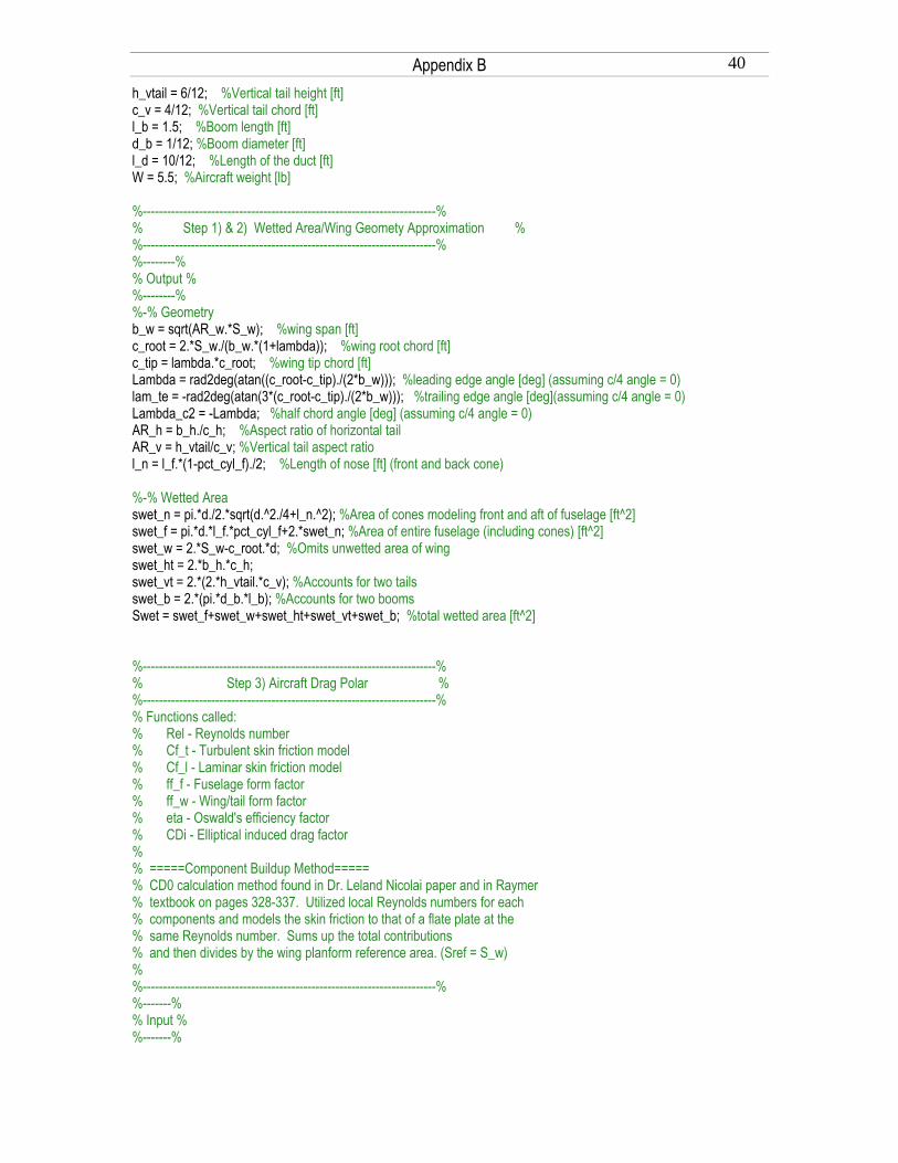
Appendix B 40 h_vtail = 6/12; %Vertical tail height [ft] c_v = 4/12; %Vertical tail chord [ft] l_b = 1.5; %Boom length [ft] d_b = 1/12; %Boom diameter [ft] l_d = 10/12; %Length of the duct [ft] W = 5.5; %Aircraft weight [lb] %-------------------------------------------------------------------------% % Step 1) & 2) Wetted Area/Wing Geomety Approximation % %-------------------------------------------------------------------------% %--------% % Output % %--------% %-% Geometry b_w = sqrt(AR_w.*S_w); %wing span [ft] c_root = 2.*S_w./(b_w.*(1+lambda)); %wing root chord [ft] c_tip = lambda.*c_root; %wing tip chord [ft] Lambda = rad2deg(atan((c_root-c_tip)./(2*b_w))); %leading edge angle [deg] (assuming c/4 angle = 0) lam_te = -rad2deg(atan(3*(c_root-c_tip)./(2*b_w))); %trailing edge angle [deg](assuming c/4 angle = 0) Lambda_c2 = -Lambda; %half chord angle [deg] (assuming c/4 angle = 0) AR_h = b_h./c_h; %Aspect ratio of horizontal tail AR_v = h_vtail/c_v; %Vertical tail aspect ratio l_n = l_f.*(1-pct_cyl_f)./2; %Length of nose [ft] (front and back cone) %-% Wetted Area swet_n = pi.*d./2.*sqrt(d.^2./4+l_n.^2); %Area of cones modeling front and aft of fuselage [ft^2] swet_f = pi.*d.*l_f.*pct_cyl_f+2.*swet_n; %Area of entire fuselage (including cones) [ft^2] swet_w = 2.*S_w-c_root.*d; %Omits unwetted area of wing swet_ht = 2.*b_h.*c_h; swet_vt = 2.*(2.*h_vtail.*c_v); %Accounts for two tails swet_b = 2.*(pi.*d_b.*l_b); %Accounts for two booms Swet = swet_f+swet_w+swet_ht+swet_vt+swet_b; %total wetted area [ft^2] %-------------------------------------------------------------------------% % Step 3) Aircraft Drag Polar % %-------------------------------------------------------------------------% % Functions called: % Rel - Reynolds number % Cf_t - Turbulent skin friction model % Cf_l - Laminar skin friction model % ff_f - Fuselage form factor % ff_w - Wing/tail form factor % eta - Oswald's efficiency factor % CDi - Elliptical induced drag factor % % =====Component Buildup Method===== % CD0 calculation method found in Dr. Leland Nicolai paper and in Raymer % textbook on pages 328-337. Utilized local Reynolds numbers for each % components and models the skin friction to that of a flate plate at the % same Reynolds number. Sums up the total contributions % and then divides by the wing planform reference area. (Sref = S_w) % %-------------------------------------------------------------------------% %-------% % Input % %-------%

Appendix B 41 rho = .00237; %Air density (rho) [slugs/ft^3] Vinf = 103; %Flight speed (Vinf) [ft/sec] a = 1116.43; %Speed of sound [ft/sec] mu = 3.62e-7; %Coefficient of viscosity (mu) [slugs/ft-sec] tc_w = 0.08; %Maximum wing thickness in percent chord tc_h = 0.08; %Maximum horizontal tail thickness in percent chord tc_vtail = 0.06; %Maximum vertical tail thickness in percent chord xc_m_w = 0.4; %x/c location of maximum thickness for wing xc_m_htail = 0.3; %x/c location of maximum thickness for horizontal tail xc_m_vtail = 0.4; %x/c location of maximum thickness for vertical tail lamda_m_w = deg2rad(0); %Sweep of maximum thickness line for wing lamda_m_htail = deg2rad(0); %Sweep of maximum thickness line for horizontal tail lamda_m_vtail = deg2rad(0); %Sweep of maximum thickness line for vertical tail FFfudge_f = 1.20; % The fuselage is not perfectly round ? FFfudge_w = 1.05; % Accounts for gap in front of flaperons over half the span FFfudge_vtail = 1.05; % Accounts for gap in front of rudder on one tail FFfudge_htail = 1.10; % Accounts for gap in front of elevator FFfudge_b = 1.00; % None as the boom is a perfect cylinder Q_htail = 1.08; % Interference drag coefficient (from vertical tails) Q_vtail = 1.08; % Interference from horizontal tail Q_w = 1.10; % Interference from fuselage Q_b = 1.00; % No interference on booms Q_d = 1.20; % Interference with fuselage %--------% % Output % %--------% %-% Fuselage Re_f = Rel(rho,Vinf,l_f,mu); %local reynolds number Cf_f = Cf_t(Re_f); %loal skin fricition coefficient FF = FFfudge_f.*ff_f(l_f,d); %Form factor CDmin_f = FF.*Cf_f.*(swet_f)./S_w; %component parisite drag %-% Wing Re_w = Rel(rho,Vinf,S_w./b_w,mu); %local reynolds number Cf_w = Cf_t(Re_w); %loal skin fricition coefficient M = Vinf./a; %Mach number FF = FFfudge_w.*ff_w(M,lamda_m_w,tc_w,xc_m_w); %Form factor CDmin_w = FF.*Q_w.*Cf_w.*swet_w./S_w; %component parisite drag %-% Horizontal Tail Re_htail = Rel(rho,Vinf,c_h,mu); %local reynolds number Cf_htail = Cf_t(Re_htail); %loal skin fricition coefficient FF = FFfudge_htail.*ff_w(M,lamda_m_htail,tc_h,xc_m_htail); %Form factor CDmin_htail = FF.*Q_htail.*Cf_htail.*swet_ht./S_w; %component parisite drag %-% Vertical Tail Re_vtail = Rel(rho,Vinf,c_v,mu); %local reynolds number Cf_vtail = Cf_t(Re_vtail); %loal skin fricition coefficient FF = FFfudge_vtail.*ff_w(M,lamda_m_vtail,tc_vtail,xc_m_vtail); %Form factor CDmin_vtail = FF.*Q_vtail.*Cf_vtail.*swet_vt./S_w; %component parisite drag %-% Tail Boom Re_b = Rel(rho,Vinf,l_b+c_root,mu); %local reynolds number

Appendix B 42 Cf_b = Cf_t(Re_b); %loal skin fricition coefficient FF = FFfudge_b.*ff_f(l_b,d_b); %Form factor CDmin_b = FF.*Q_b.*Cf_b.*swet_b./S_w; %component parisite drag %-% CD0 total C_bar_D_o = CDmin_f+CDmin_w+CDmin_htail+CDmin_vtail+CDmin_b; %Total parisite drag Cf_tot = C_bar_D_o .* S_w ./ Swet; %Total skin friction coefficient e = eta(AR_w); %Oswalds span efficiency factor k = 1./(pi*AR_w.*e) + 0.0167; %Induced drag coefficient from Nicolai white paper Clmin = 0.1428; %wing section lift coefficient at minimum section drag coefficient CLmin = Clmin; %Assume 2D is approximately equal to 3D minimum section lift coefficient. Cd_0 = C_bar_D_o+k*CLmin^2; %CD at CL=0 ==> CD = CD0 + k(CL-CLmin)^2 %-------------------------------------------------------------------------- % Step 4) Wing body lift Coefficient (Roskam Eq 3.17) % %-------------------------------------------------------------------------- % Functions called: % CLa_wf - Wing fuselage lift curve slope (Raymer Eq. 12.6) % % =====Roskam wing-fuselage lift coefficient===== % Uses Roskam text Eq 3.16 to break the the total CL into different % components. Eq 3.17 is the wing-fuselage lift coefficient component. % %-------------------------------------------------------------------------% Cl_alpha_w = 5.543; %2-D wing lift curve slope [1/rad] Beta2 = 1-(Vinf./a).^2; %Prandtl Glauret correction factor squared F = 1.07.*(1+d./b_w).^2; %Fuselage lift factor (Raymer Eq 12.9) CLawf = CLa_wf(AR_w,Cl_alpha_w,Beta2,swet_w,S_w,F); %Wing fuselage lift curve slope Cl0w = .1439; %2-D wing lift coefficient at zero a.o.a. CL0wf = 0.9*Cl0w; %3-D wing lift coefficient at zero a.o.a. (90% rule) alfa = 0; %Aircraft a.o.a [deg] i_w = 0; %Wing incidence angle [deg] alfaw = alfa + i_w; %Wing angle of attack CL_wb = CL0wf + CLawf.*deg2rad(alfaw); %Wing/body lift coefficient at alfa %-------------------------------------------------------------------------- % Step 5) Horizontal tail and body lift Coefficient (Roskam Eq 3.19) % %-------------------------------------------------------------------------- % =====Roskam Horizontal tail and body lift coefficient===== % Uses Roskam text Eq 3.16 to break the the total CL into different % components. Eq 3.19 is the wing-fuselage lift coefficient component. % %-------------------------------------------------------------------------% Cl_alpha_h = 5.451; %2-D horizontal tail lift curve slope [1/rad] CLah = Cl_alpha_h; %3-D horizontal tail lift curve slope [1/rad] (assume infinite wing) deda = 0.4667; %Downwash gradient eta_h = 0.9; %Dynamic pressure ratio for horizontal tail eta0 = 0.00001; %###### ASSUME VERY SMALL NUMBER FOR NOW ##### toue = 0.5; %Elevator angle of attack effectiveness (Roskam Fig 2.23) dele = 0; %Elevator deflection angle, positive trailing edge down [deg] i_h = 0; %Elevator incidence angle [deg] alfah = alfa+i_h-(eta0+deda.*alfa); %Horizontal tail angle of attack [deg] CL_hb = CLah.*deg2rad(alfah)+CLah.*toue.*deg2rad(dele); %horizontal tail lift coefficient at alfa CL_hb = round(CL_hb);

Appendix B 43 %-------------------------------------------------------------------------- % Step 6) Gather aerodynamic center distances of aircraft (Roskam 3.38) % %-------------------------------------------------------------------------- % Functions called: % Xac_A - Aerodynamic Center of aircraft (Roskam 3.38) % % =====Roskam wing-fuselage lift coefficient===== % Uses Roskam text Eq 3.38 to find the aerodynamic center of the aircraft. % %-------------------------------------------------------------------------% c_w= (c_root+c_tip)/2; Xach = c_root+l_b+c_h/4-(c_root-c_w)/4; %Distance from LE of MAC to ac of horizontal tail [ft] Xacwb = c_w/4; %Distance from LE of MAC to ac of wing and body [ft] (assume: body generatis no lift) Xacw = c_w/4; %Distance from LE of MAC to ac of wing ALONE [ft] %-------------------------------------------------------------------------- % Step 7) ADDITIONAL BASIC CONSTANTS % %-------------------------------------------------------------------------- % Basic Constants defined in tabulated output below %-------------------------------------------------------------------------- alpha_0 = deg2rad(-1.05); CL = W/(.5*rho*Vinf^2); Cl_alpha_v = 2*pi; dihedral_h = 0; epsilon_t = 0; epsilon_0_h = eta0; Lambda_c4 = 0; Lambda_c2_h = 0; Lambda_c4_h = 0; lambda_h = 1; l_f = l_f+l_b; S_h = swet_ht/2; S_v = swet_vt/2; theta = 0; theta_h = 0; if length(AR_w)>1 %-------------------------------------------------------------------------- % Step 8) Aspect ratio trade study % %-------------------------------------------------------------------------- CL = linspace(0,1.4,100); AR_ws = length(AR_w); CLs = length(CL); for i = 1:AR_ws CL_matrix(i,:) = CL; end for i = 1:CLs AR_w_matrix(:,i) = AR_w; end for i = 1:CLs C_bar_D_o_matrix(:,i) = C_bar_D_o; end AR_w = AR_w_matrix; CL = CL_matrix; C_bar_D_o = C_bar_D_o_matrix; e = eta(AR_w); CD_ind = CDi(CL,e,AR_w);

Appendix B 44 CD = CD_ind + C_bar_D_o; lines = [.0255 .026 .0265 .027 .0275 .028 .029 .030 .035 .04 .05 .06 .08 .10 .12]; [c,h] = contour(AR_w,CL,CD,lines); title('Lines of constant C_D (An AR trade study)') xlabel('AR') ylabel('C_L') clabel(c,h,'manual') grid off else %-------------------------------------------------------------------------- % Step 9) Tabulated Output % %-------------------------------------------------------------------------- form = '%-9s %.2f %7.0f %.5f %.4f\n'; fprintf('\n\n') fprintf('Component Area Re Cf CD0\n') fprintf(' (ft^2) (local)\n') fprintf('========= ======== ========= ========= ========\n') fprintf(form,'Wing',swet_w,Re_w,Cf_w,CDmin_w) fprintf(form,'Fuse/Duct',swet_f,Re_f,Cf_f,CDmin_f) fprintf(form,'V_tails',swet_vt,Re_vtail,Cf_vtail,2*CDmin_vtail) fprintf(form,'H_tail',swet_ht,Re_htail,Cf_htail,CDmin_htail) fprintf(form,'Booms',swet_b,Re_b,Cf_b,CDmin_b) fprintf('--------- -------- --------- --------- --------\n') fprintf('%-12s %-22.2f %-8.5f %-.4f\n', 'Totals:', Swet, Cf_tot, C_bar_D_o) fprintf(' (Normalized Results)') fprintf('\n\n') fprintf('--------------------- ------------------------------------------------\n') fprintf(' Basic Constants Definition \n') fprintf('===================== ================================================\n') form = '%-12s %.3f %s\n'; fprintf(form,'alpha_0',alpha_0,'Airfoil zero-lift AOA [rad]') fprintf(form,'AR_h',AR_h,'Aspect ratio of the horizontal tail') fprintf(form,'AR_w',AR_w,'Aspect ratio of the wing') fprintf(form,'b_h',b_h,'Span of the horizontal tail [ft]') fprintf(form,'b_w',b_w,'Span of the wing [ft]') fprintf(form,'C_bar_D_o',C_bar_D_o,'Parasite drag') fprintf(form,'Cd_0',Cd_0,'Drag coefficient at zero lift(parasite drag)') fprintf(form,'c_h',c_h,'MAC of the horizontal tail [ft]') fprintf(form,'CL',CL,'Lift coefficient (3-D) CL=W/(1/2*rho*U^2) (U=max flight speed)') fprintf(form,'CL_hb',CL_hb,'Lift coefficient of the horizontal tail/body') fprintf(form,'CL_wb',CL_wb,'Lift coefficient of the wing/body - assuming iw=0') fprintf(form,'Cl_alpha_h',Cl_alpha_h,'2-D lift curve slope of horizontal tail [1/rad]') fprintf(form,'Cl_alpha_v',Cl_alpha_v,'2-D lift curve slope of vertical tail [1/rad]') fprintf(form,'Cl_alpha_w',Cl_alpha_w,'2-D lift curve slope of wing [1/rad]') fprintf(form,'c_w',c_w,'MAC of the wing [ft]') fprintf(form,'c_v',c_v,'MAC of the vertical tail [ft]') fprintf(form,'d',d,'Average diameter of the fuselage [ft]') fprintf(form,'dihedral_h',dihedral_h,'Geometric dihedral angle of the horizontal tail [rad]') fprintf(form,'epsilon_t',epsilon_t,'Horizontal tail twist angle [rad]') fprintf(form,'epsilon_0_h',epsilon_0_h,'Downwash angle at the horizontal tail [rad] (see Note in Ref(3) under section 8.1.5.2)') fprintf(form,'eta_h',eta_h,'Ratio of dynamic pressure at the horizontal tail to that of the freestream') fprintf(form,'i_h',i_h,'Incidence angle of horizontal tail [rad]') fprintf(form,'i_w',i_w,'Incidence angle of the wing [rad]') fprintf(form,'k',k,'k of drag polar, generally=1/(pi*AR*e)') fprintf(form,'Lambda',deg2rad(Lambda),'Sweep angle of wing [rad] (l.e.)') fprintf(form,'Lambda_c2',deg2rad(Lambda_c2),'Sweep angle at the c/2 of the wing [rad]')

Appendix B 45 fprintf(form,'Lambda_c4',Lambda_c4,'Sweep angle at the c/4 of the wing [rad]') fprintf(form,'Lambda_c2_h',Lambda_c2_h,'Sweep angle at the c/2 of the horizontal tail [rad]') fprintf(form,'Lambda_c4_h',Lambda_c4_h,'Sweep angle at the c/4 of the horizontal tail [rad]') fprintf(form,'lambda',lambda,'Taper ratio of wing') fprintf(form,'lambda_h',lambda_h,'Taper ratio of horizontal tail') fprintf(form,'l_f',l_f,'Horizontal length of fuselage and boom [ft]') fprintf(form,'S_h',S_h,'Aera of horizontal tail [ft^2]') fprintf(form,'S_w',S_w,'Surface area of wing [ft^2]') fprintf(form,'S_v',S_v,'Surface area of vertical tail [ft^2]') fprintf(form,'tc_w',tc_w,'Thickness to chord ratio of wing') fprintf(form,'tc_h',tc_h,'Thickness to chord ratio of horizontal tail') fprintf(form,'theta',theta,'Wing twist - negative for washout [rad]') fprintf(form,'theta_h',theta_h,'Horizontal tail twist [rad] (-) for washout') fprintf(form,'Xach',Xach,'Distance from LE of wing MAC to AC of the Horizontal tail [ft]') fprintf(form,'Xacwb',Xacwb,'Distance from LE of wing MAC to AC of wing/body [ft] (assume: body has no lift)') fprintf(form,'Xacw',Xacw,'Distance from LE of wing MAC to AC of wing ALONE [ft]') fprintf('--------------------- ------------------------------------------------\n') end

Appendix C 46

Appendix C

Appendix C 47

Appendix of Tables

Diameter Weight Max RPM Cost Manufacturer Model [ in ] [ lbs ] [ RPM ] [ $ ]

Wemotec Midi Fan 3.5 0.231 35,000 $74.95 Wemotec Mini Fan 480 2.72 0.132 45,000 $53.90 Great Planes Hyperflow 2.23 0.081 49,000 $30.00 VASA VasaFan 65 2.6 0.077 45,000 $60.00

Table 3.1: Ducted Fan Candidates

Voltage Avg. Weight Avg. Cost Type Abbreviation [ V ] [ lbf ] [ $ ]

Nickel Metal Hydride NiMH 1.20 per Cell 0.09 per Cell $3.00 per Cell Nickel Cadium NiCd 1.20 per Cell 0.13 per Cell $2.70 per Cell

Lithium Polymer LiPo 3.70 per Cell 0.13 per Cell $25.00 per Cell Table 3.2: Available Hobby Batteries

A123 Systems' Lithium Ion Cells

Voltage per Cell 3.6 V Max Continous Current 70 Amps

Max Surge Current 120 Amps Capacity 2300 mAh

Weight per Cell 0.16 lbf Cost per Cell $11.50

Table 3.3: A123 Systems’ Lithium Ion Batteries

RPM Kv Voltage Req. Current Req. Efficiency Fan [RPM] [ RPM / Volt ] [ Volts ] [ Amps ] [ % 0f 100]

WeMoTec Midi 35,000 2800 17.5 120 70% WeMotTec Mini 480 45,000 2500 17.8 42 86%

Table 3.4: Results from Iterative Process to Find Fan Systems with 5 Li-Ion Cells

Motor HET Typhoon 2W-20 EDF

Kv 2980 Max Voltage 17 V



Table 3.5: HET Typhoon 2W-20 EDF Brushless Motor

Appendix C 48

Motor Ammo 36-50-2300

Kv 2300 Max Voltage 18



Table 3.6: Electrifly Ammo 36-50-2300 Brushless Motor

Propulsion System at High Speed Operation Conditions Fan Battery Motor

WeMoTec Midi Fan A123 Systems' Lithium Ion Cells Ammo 36-50-2300

Operating RPM 30,000 RPM Aircraft Velocity 107 ft/s

Endurance 2.1 min

Max Continous Current 70 A Max Continous Current 60 A Current Required 73.5 A Max Surge Current ** 120 A Max Surge Current ** 100 A

Voltage Required 16 V Max Voltage 18 V Max Voltage 18.5 V Weight 0.23 lbf 0.78 lbf 0.35 lbf Price $47.00 $58.00 $79.99

Totals

Weight 1.36 lbf Price $184.99 ** - Surge is 10 seconds

Table 3.7: Final Propulsion High Speed Specs

Propulsion System at Max Enduranc Operation Conditions Fan Battery Motor

WeMoTec Midi Fan A123 Systems' Lithium Ion Cells Ammo 36-50-2300

Operating RPM 15,000 RPM Aircraft Velocity 47 ft/s

Endurance 10.2 min

Max Continous Current 70 A Max Continous Current 60 A Current Required 19 A Max Surge Current ** 120 A Max Surge Current ** 100 A

Voltage Required 7.4 V Max Voltage 18 V Max Voltage 18.5 V Weight 0.23 lbf 0.78 lbf 0.35 lbf Price $47.00 $58.00 $79.99

Totals

Weight 1.36 lbf Price $184.99 ** - Surge is 10 seconds

Table 3.8: Final Propulsion Max Endurance Specs

Appendix C 49

Appendix of Figures Exhaust Velocity vs. Rev/sec

y = 0.2591xR2 = 0.9928

0

50

100

150

200

250

0 100 200 300 400 500 600 700 800

Rev/Sec

Exha

ust V

eloc

ity [

ft/s

]

y = 0.3314xR2 = 0.9969 WeMoTec Midi WeMoTec Mini 480 Fan

Figure 3.1: Relationship between Exhaust Velocity and Revolutions

Thrust vs. Exhaust Velocity

y = 1.426E-04xR2 = 1.000E+00

y = 7.24205E-05xR2 = 1.00000E+00

0.00

1.00

2.00

3.00

4.00

5.00

0 5000 10000 15000 20000 25000 30000 35000 40000

Efflux2 [ ft2/s2

Thru

st [

lbf ]

]

WeMoTec Midi Fan WeMoTec Mini 480 Fan

Figure 3.2: Relationship between Thrust and Exhaust Velocity Squared

Appendix C 50

Figure 3.3: WeMoTec Midi Fan Thrust Curve

Figure 3.4: WeMoTec Mini 480 Fan Thrust Curve

Appendix C 51

Figure 3.5: Final Propulsion System Thrust Curve

Appendix C 52

List of Symbols

Symbols DescriptionTa Thrust available m Mass flow Ve Exhaust velocity V∞ Freestream velocity ρ Density of free stream S Wetted area Cd Drag coefficient TR Thrust required

Appendix C 53


( )∞−= VVmT ea Equation 3.1: Thrust Available (Momentum)

22

21

dR SCVT ∞= ρ

Equation 3.2: Thrust Required

Appendix C 54

Appendix of Code Code 1:TestDesignAircraft.m % Script to design an end-to-end propulsion system for an % electric-powered propeller-driven aircraft. % Given: % drag polar, % aircraft weight, air density, % pitch to diameter ratio of the prop and prop data, % motor constants for a particular motor. % % Find: % speed for maximum endurance, % propeller diameter, % gear ratio, % voltage at which to operate the motor, % battery sizes to achieve the desired battery voltage, % endurance for single strand and dual strand batteries, % for an aircraft flying straight and level. Clear close all clc fprintf('>>>>---- Start ----<<<<') %--------------------------- Design Requirements -------------------------% V_stall_REQ = 30; % Stall Speed [ft/sec] Dash_distance_REQ = 1320; Endurance_REQ = 7; % min %----------------------- PHASE 1: AIRCRAFT SUBSYSTEM ---------------------% % >>>>>>>>>>>>>>>>>>>>>>>>>>>>> Variables <<<<<<<<<<<<<<<<<<<<<<<<<<<<<<<<% CD0=0.02; % drag coefficient when CL=0. CL0=0.09; % Zero Angle of Attack lift. A=5; % aspect ratio span squared divided by reference area e=0.89; % Oswalds efficiency factor V=[10:.01:170]; % velocity in ft/sec rho=0.002377; % air density in slugs/ft^3 S= 4.95; % wing area [ft^2] R = 100; % Turning Radius [ft] W = 6; % lbf, Weight of Aircraft %>>>>>>>>>>>>>>>>>>>>>>>>>>>>>>>>>>>><<<<<<<<<<<<<<<<<<<<<<<<<<<<<<<<<<<<<% %Generate Power Required Curve [Pr,Pre,Ve]=Power_Required(W,rho,S,CD0,A,e,V,CL0); %----------------------- PHASE 2: Propulsion System ----------------------% %%% FAN SPECS %%% % fan_name = ['WeMoTec Mini 480 Fan']; % Dia_fan = 2.72; % [in] % Dia_hub = 1.3; % [in] % RPMmax=45000; % Ct=0.8293; %

Appendix C 55 % Cp=0.8; % Tve=7.242e-5; %relation between thrust and eflux squared % Venrel=0.2696; %relation between Efflux and Rev/sec of fan fan_name = ['WeMoTec Midi Fan']; Dia_fan = 3.5; % [in] Dia_hub = 1.7; % [in] RPMmax=30000; %Design RPM Value Ct=0.9112; %coefficient of Thrust for Prop Cp=1.1; %relation between power and rpm, coefficient of power for Prop Tve=1.426e-4; %relation between thrust and eflux squared Venrel=0.3314; %relation between Efflux and Rev/sec of fan FSA = pi*((Dia_fan/24)^2-(Dia_hub/24)^2); % [ft^2] Fan Swept Area D=Dia_fan/12; % Fan Diameter in inches nmax=RPMmax/60; % Revolutions per second Vemax=nmax*Venrel % Max Exhaust Velocity Tstamax=Tve*Vemax^2 %Max Static Thrust Pre=rho*nmax^3*D^5*Cp; %Power Input Required in ft-lbf/sec Prewatts=Pre*1.356 %Convert Power Input Required to Watts RPMprop=RPMmax; %Adapter to Existing Code Tavail=(Tstamax/Vemax)*(Vemax-V); %Thrust Available Curve T_req=Pr./V; %Thrust Required Curve delta=Tavail-T_req; %Difference between thrust available and required Vmax=interp1(delta,V,0) %Find Max Speed Tneed=interp1(V,T_req,Vmax) %Find Thrust Required for Max speed %Plot Thrust Curves figure(4) hold on grid on H(1) = plot(V,Tavail,'LineWidth',3) H(3) = plot(linspace(V_stall_REQ,V_stall_REQ,5),[0:4],'k--','LineWidth',3); H(2) = plot(V,T_req,'k','LineWidth',3); title(['Thrust vs Velocity (' fan_name '@' num2str(RPMmax) 'RPM)']) xlabel('Velocity [ft/s]') ylabel('Thrust [lbf]') H(4) = plot(Vmax,Tneed,'rp','LineWidth',3) legend(H,[{'Thrust Available'} {'Thrust Required'} {['Stall Speed = ' num2str(V_stall_REQ) 'ft/s']} {['Max Velocity = ' num2str(Vmax) ' ft/s']}]) axis([0 170 0 3]) Pout=rho*nmax^2*D^4*Ct*Vmax; %Power out of Fan EtaProp=Pout/Pre %Efficiency of Fan % %----------------------- Motor Analysis -------------------------% % Motor Info in format % Motor Model/Name % Motor Constants % Ammo 28-45-2700

Appendix C 56 % Kv=2700; % RPM/volt % Kt=1355/Kv; % inch-ounce per ampere % R= .37; % Ohms % Io=1.5; % amperes % Mega AC 22/20/2 % Kv=2875; % RPM/volt % Kt=1355/Kv; % inch-ounce per ampere % R= .012; % Ohms % Io=3.37; % amperes % Mega AC 16/25/2 % Kv=2650; % RPM/volt % Kt=1355/Kv; % inch-ounce per ampere % R= .012; % Ohms % Io=2.3; % amperes % HET RC Typhoon EDF 2W-20 % Kv=3450; % RPM/volt % Kt=1355/Kv; % inch-ounce per ampere % R= .02; % Ohms % Io=3; % amperes % HET RC Typhoon EDF 2W-18 % Kv=3700; % RPM/volt % Kt=1355/Kv; % inch-ounce per ampere % R= .02; % Ohms % Io=3; % amperes % Electrifly Ammo 36/50/2300 Kv = 2300; Kt = 1355/Kv; R = 0.041; Io = 2; % Electrifly Ammo 36/50/1800 % Kv = 1800; % Kt = 1355/Kv; % R = 0.041; % Io = 1.9; % Fun 600-13 % Kv=1300; % Kt=1355/Kv; % R=0.0339; % Io=0.89; % MEGA 16/25/1 % Kv = 4800; % Kt=1355/Kv; % R = 0.012; % Io = 7; [Vinstar,Iinstar,Pinwattsstar,RPMstar,PoutHP,EtaMotorMax,ifig]=MotorMaxEff(Prewatts,Kv,Kt,R,Io,4); % Find Max Efficiency Point of Motor disp(' '); disp('PRELIMINARY MOTOR ANALYSIS');

Appendix C 57 string21=[' For maximum motor efficiency this motor must be provided with ',num2str(Vinstar),' input volts.']; string22=[' Under these conditions, the input current will be ',num2str(Iinstar),' amperes']; string23=[' and the input power will be ',num2str(Pinwattsstar),' watts.']; string24=[' The motor shaft will be spinning at ',num2str(RPMstar),' RPM.']; string25=[' The motor efficiency will be ',num2str(EtaMotorMax),'.']; disp(string21); disp(string22); disp(string23); disp(string24); disp(string25); disp(' '); RPMactual= RPMprop; % Compute for specified gear ratio string20b=['At this point the motor RPM and output power of the motor are specified, so motor inputs can be found.']; string20c=[' Motor RPM= ',num2str(RPMactual),' RPM and motor output power= ',num2str(Prewatts),' watts']; disp(string20b); disp(string20c); % compute motor input properties disp(' '); [Vinactual,Iinactual,Pinwattsactual,PoutHP,EtaMotoractual,ifig]=MotorInputs(Prewatts,RPMactual,Kv,Kt,R,Io,ifig); %Find Operating point of motor string30a=['MOTOR DESIGN SUMMARY']; string30= [' The output power of this motor is ',num2str(Prewatts),' watts or ',num2str(PoutHP),' Hp.']; string31= [' The motor input voltage is ',num2str(Vinactual),' volts.']; string32= [' The motor input current is ',num2str(Iinactual),' amperes.']; string33= [' and the motor input power is ',num2str(Pinwattsactual),' watts.']; string34= [' The electric motor shaft is spinning at ',num2str(RPMactual),' RPM.']; string36= [' The motor efficiency is ',num2str(EtaMotoractual),'.']; disp(string30a); disp(string30); disp(string31); disp(string32); disp(string33); disp(string34); disp(string36); % BATTERY SUBSYSTEM % disp(' '); disp('BATTERY SUBSYSTEM'); disp(' The battery pack will be made up of individual cells with the following properties:') VoltsPerCell=3.3; % volts per cell mAmpsHoursPerCell=2300; % milliamps hours per cell gramspercell=70; %grams per cell slugspercell=(gramspercell/1000)/14.5939; lbfpercell=32.17*slugspercell; string54=[' ',num2str(VoltsPerCell),' volts per cell, and ',num2str(mAmpsHoursPerCell),' milliamp hours per cell, and ',num2str(gramspercell),' grams per cell.']; disp(string54); disp(' '); disp(' A single string battery pack designed for the above conditions will have the following properties.') nCells1=ceil(Vinactual/VoltsPerCell); nVolts=nCells1*VoltsPerCell; weight1=nCells1*lbfpercell; BatteryEnergy1Joule=(mAmpsHoursPerCell*3600/1000)*nVolts; % Joules=watt*sec=ampere*volt*sec ActualEnduranceMin1=(1/60)*(BatteryEnergy1Joule/Pinwattsactual); % predicted endurance for single strand battery, minutes string50=[' ',num2str(nCells1),' total cells, arranged in a 1x',num2str(nCells1),' array.']; string51=[' producing ',num2str(nVolts),' volts, and giving a predicted endurance of ',num2str(ActualEnduranceMin1),' minutes,']; string54=[' and weighing ',num2str(weight1),' lbf.']; disp(string50); disp(string51); disp(string54); figure(4)

Appendix C 58 Code 2: Power_Required.m function [Pr,Pre,Ve]=Power_Required(W,rho,S,CD0,A,e,V,CL0) % function [Pre,Ve]=Power_Required(W,rho,S,CD0,A,e,V) % OUPUTS % Pop is operating power of the aircraft (ft-lbf/sec) % Vop is the operating velocity of the aircraft (ft/sec) % Pre is the minimum power required (ft-lbf/sec) % Ve is the velocity of the aircraft for minimum power required (ft/sec) % % INPUTS % CD0= drag coefficient when CL=0. % A= aspect ratio span squared divided by reference area % e= Oswalds efficiency factor % V= velocity vector in ft/sec % rho= air density in slugs/ft^3 % W= aircraft weight in pounds (lbf) % S= wing area % ifig is the figure number of the plot %--------------------------- Drag Calculations ---------------------------% k=1/(pi*A*e); % k from the drag polar CD=CD0+k*CL^2 kvisc=0.0167; kvisclow=0.0243; marker=interp1(V,[1:length(V)],45); CL=2*W./(rho*S*V.*V); % Lift cofficient as a function of velocity CD(1:marker)=CD0+(k+kvisclow)*(CL(1:marker)-CL0).^2; %Cd for low speed (<45ft/s) CD((marker+1):length(V))=CD0+(k+kvisc)*(CL((marker+1):length(V))-CL0).^2; %Cd for high speed (>45ft/s) % CD=CD0+k*CL.*CL % Drag coefficient as a function of velocity Pr=.5*rho*S*V.^3.*CD; % Power required ft/lbf/sec CLe=sqrt(3*CD0/k); % Lift coefficient for maximum endurance (minimum power required) CDe=4*CD0; % Drag coefficient for maximum endurance (minimum power required) Ve= sqrt(2*W/(rho*S*CLe)); % Speed for maximum endurance (minimum power required) Pre=interp1(V,Pr,Ve); % YI = INTERP1(X,Y,XI) % minimum power required %---------------------------- Output Settings ----------------------------% figure(1) hold on grid on plot(V,Pr/550,'LineWidth',2) xlabel('Velocity [ft/sec]') ylabel('Power required [hp]') title('Aircraft Power Required vs Speed') % plot(Ve,min(Pre)/550,'rp') fprintf('\nMinimum power of %.2f [ft-lbf/sec] is achieved at a speed of %.2f [ft/sec]',Pre,Ve);

Appendix C 59 Code 3: MotorMaxEff.m function [Vinstar,Iinstar,Pinwattsstar,RPMstar,PoutHP,EtaMotorMax,ifig]=MotorMaxEff(Poutwatts,Kv,Kt,R,Io,ifig) % function [Vinstar,Iinstar,Pinwattsstar,RPMstar,PoutHP,EtaMotorMax,ifig]=MotorMaxEff(Poutwatts,Kv,Kt,R,Io,ifig) % Computes Vinstar(volts), Iinstar(amps) from Poutwatts(watts) assuming that the % motor is running at the conditions for maximum efficiency. % Iin=sqrt(Io*Vin/R) % % Requires motor constants Kv,Kt,R,Io. % Kv= RPM/volt % Kt= inch-ounce per ampere % R= Ohms % Io= amperes % % Additional outputs include % Pinwattsstar =input power (watts) % RPMstar =RPM for motor running at most efficient conditions. % PoutHP =output power in HP % EtaMotorMax =maximum motor efficiency (non-dimensional) % % ifig in the current figure number and is updated if a figure is plotted. Vinmat=1:.1:20; % lets vary voltage over this range (volt) Iinmat=sqrt(Io*Vinmat/R); % current for max efficiency at Vinmat (amp) Poutmat=(Iinmat-Io).*(Vinmat-Iinmat*R); % power at max efficiency conditions (watts) % ifig=ifig+1; figure(ifig) % plot(Poutmat,Vinmat) % hold on; plot(Poutmat2,Vinmat,':'); hold off % xlabel('Power output (watts)') % ylabel('Input voltage (volts)') % title('Motor performance for maxmum efficiency') % YI = INTERP1(X,Y,XI,'spline') Vinstar=interp1(Poutmat,Vinmat,Poutwatts,'spline'); % finds voltage for appropriate amount of power (volts) % The above solution technique solves for Vinstar using a graphical % technique (table lookup). Poutwatts2=interp1(Vinmat,Poutmat,Vinstar,'spline'); % double check (watts) % hold on % plot([Poutwatts,Poutwatts],[0,Vinstar],'r:',[0,Poutwatts],[Vinstar,Vinstar],':') % hold off Iinstar=sqrt(Io*Vinstar/R); % Input current in amperes Pinwattsstar=Iinstar*Vinstar; % Input power in watts Poutwatts3=(Iinstar-Io)*(Vinstar-Iinstar*R); % triple check (watts) PoutHP=Poutwatts/745.7; % hp EtaMotorMax=((Iinstar-Io)/Iinstar)^2; % non-dimensional RPMstar=Kv*(Vinstar-Iinstar*R); % RPM

Appendix C 60 Code 4: MotorInputs.m function [Vin,Iin,PinWatts,PoutHP,EtaMotor,ifig]=MotorInputs(PoutWatts,RPM,Kv,Kt,R,Io,ifig) %function [Vin,Iin,PinWatts,PoutHP,EtaMotor,ifig]=MotorInputs(PoutWatts,RPM,Kv,Kt,R,Io,ifig) % Computes Vin(volts), Iin(amperes) from PoutWatts(watts), RPM(rpm). % Requires motor constants Kv,Kt,R,Io. % Kv= RPM/volt % Kt= inch-ounce per ampere % R= Ohms % Io= amperes % % ifig in the current figure number and is not used in this function. Kt=KvKt/Kv; % Doing this improves accuracy KvKt=12*16*60/(2*pi*1.355818); % This is by definition Kt=KvKt/Kv; % Doing this improves accuracy Poutftlbfsec=PoutWatts/1.355818; % ft-lbf/sec Omegarps=RPM*2*pi/60; % radians per sec Torqueftlbf=Poutftlbfsec/Omegarps; % ft-lbf Torqueozin=Torqueftlbf*12*16; % oz-in Iin=Torqueozin/Kt+Io; % amps Vin=RPM/Kv+Iin*R; % volts PinWatts=Iin*Vin; % watts PoutHP=PoutWatts/745.7; % Convert output power from watts to hp EtaMotor=PoutWatts/PinWatts; % non-dimensional end

Appendix D 61

Appendix D

Appendix D 62

List of Symbols (In order of Appearance) Symbol DescriptionSHT or Sh Horizontal Tail Area cHT Horizontal Tail Volume Coefficient CW or cavg Wing Mean Aerodynamic Chord (MAC) SW or S Wing Area LHT or lh Length Wing MAC to Horizontal Tail MAC SVT or Sv Vertical Tail Area cVT Vertical Tail Volume Coefficient bW or b Wing Span LVT or lv Length Wing MAC to Vertical Tail MAC

acAX Aircraft Aerodynamic Center

acwfX Wing-Fuselage Aerodynamic Center

CLαH Lift Coefficient per Angle of Attack of Horizontal Tail

αε

dd h

Downwash Effect

achX Horizontal Tail Aerodynamic Center

CLαwf Lift Coefficient per Angle of Attack of Wing-Fuselage AR Aspect Ratio λ Taper Ratio zh Distance Wing Centerline to Horizontal Tail Centerline ch Horizontal Tail Chord

βnC Weathercock Stability (Yawing Moment Coefficient with Sideslip Angle)

wnC β Yawing Moment Coefficient with Sideslip Angle of Wing

fnC β Yawing Moment Coefficient with Sideslip Angle of Fuselage

VnC β Yawing Moment Coefficient with Sideslip Angle of Vertical Tail

KN Empirical Factor for Body and Body+Wing Effects KRl Reynold’s Number Factor for Fuselage SBs Side Body Area lBB Fuselage Length

VyC β Side Force Coefficient with Sideslip Angle of Vertical Tail

α Angle of Attack CL Lift Coefficient CL0 Zero-Lift Coefficient CLα Lift-Coefficient with Angle of Attack CLih Lift Coefficient with Horizontal Tail Incidence ih Incidence Angle of Horizontal Tail CLδe Lift Coefficient with Elevator Deflection δe Elevator Deflection

0mC Pitching Moment Coefficient for Zero Lift

L

m

dCdC

Static Margin

mihC Pitching Moment Coefficient with Horizontal Tail Incidence Angle

emC δ Pitching Moment Coefficient with Elevator Deflection

Appendix D 63

cgx Center of Gravity Location as Fraction of MAC

stalltail−α Stall Angle of Attack of Horizontal Tail

M Moment Generated F Force d Distance L Lift Cl 2-D Lift Coefficient ρ Density V Velocity A Area

)()(

srsR

δ

Aircraft Yaw Rate Transfer Function

Appendix D 64

D&C 4.1 Tail Sizing Class I: Tail Sizing Volume Coefficient Method

Two equations were used to find the preliminary tail areas, they are as follows:

HT

WWHTHT L

SCcS = Equation 4.1

VT

WWVTVT L

SbcS = Equation 4.2

The lengths found in the denominator of each equation is an estimation of the length from the quarter-chord of the wing to the quarter-chord of the vertical and horizontal tails was made. This length was estimated at 3 feet and was based on the preliminary length of the aircraft to be approximately 4.5 feet long. The aerodynamics team members provided the remaining values for the variables in the two equations (wing span, wing mean chord, and wing area).

cHT 0.50 horizontal tail volume coefficient cVT 0.04 vertical tail volume coefficient bW 4.97 ft wing span SW 4.95 ft2 wing area LHT 3 ft length c/4 wing to c/4 horizontal tail LVT 3 ft length c/4 wing to c/4 vertical tails CW 1.041 ft wing mean chord SHT 0.3300 ft horizontal tail area SVT 0.8159 ft2 vertical tail area

Table 4.1: Table of Values for Estimating Tail Areas Class II: Tail Sizing X-plot Method

The first X-plot made was for the static longitudinal stability, which sizes the horizontal tail area. This X-plot is based on the aircrafts aerodynamic center and the non-dimensional location of the center of gravity. Roskam suggests that the center of gravity leg of the plot be represented as a function of the horizontal tail area. However, the center of gravity was decided to be placed at the quarter-chord of the aircraft wing for simplicity. The next step was to find the aerodynamic center of the aircraft as a function of the horizontal tail area. The equation for a tail-aft airplane for the aerodynamic center of the aircraft is as follows:

FC

XSS

ddC

XXwf

H

L

achhh

L

acwfacA

⎥⎥⎥⎥

⎦

⎤

⎢⎢⎢⎢

⎣

⎡⎭⎬⎫

⎩⎨⎧

⎟⎠⎞⎜

⎝⎛⎟⎠⎞⎜

⎝⎛ −

+=α

α αε1

Equation 4.3

Where,

Appendix D 65

wfh Lhh

L CSS

ddCF

αα αε

⎭⎬⎫

⎩⎨⎧

⎟⎠⎞⎜

⎝⎛⎟⎠⎞⎜

⎝⎛ −+= 11 Equation 4.4

For each instance in the equations, the horizontal tail area (Sh) the area was varied over a range. This range varied from 0 to 1 ft2. The values for the coefficients and the aerodynamic center of the wing-fuselage in these two equations were also provided by the aerodynamics group. The computations made while producing the longitudinal X-plot were critical to the design of the aircraft. This is because several values for the dimensions of the aircraft had to be defined. A very important parameter was the length of the dual booms being used to support the twin vertical tail configuration. This length was set at 1.5 feet. Also the placement of the horizontal tail between with the two vertical tails was decided. This was placed at the top of the two vertical tails. This is because of the propulsion system placement. If the horizontal tail was placed mid-span, the engine exhaust would directly hit the horizontal tail. The high horizontal tail would reduce the amount of exhaust hitting the surface. The effect of horizontal tail placement was considered while computing the downwash ratio at the horizontal tail ( αε dd h ). For the computation of this variable, Ref. 4 was utilized.

⎟⎠⎞

⎜⎝⎛ −⎟⎠⎞

⎜⎝⎛ −⎟⎟⎠

⎞⎜⎜⎝

⎛=

bz

lc

ARC

dd h

h

avgLh 17

31021725.0

λαε α Equation 4.5

The downwash effect also took into account the changing horizontal tail area because the length from the aerodynamic center of the wing to the aerodynamic center of the horizontal tail was changing as the chord of the tail varied. The chord of the tail was based on the fixed horizontal span of 1.5 feet and then computed as the tail area varied. This change in chord was crucial for the horizontal aerodynamic center location computation. The aerodynamic center of the horizontal tail was assumed to be at the quarter-chord of the tail.

Taking all of these parameters and the effect of varying the horizontal tail area led to the X-plot. The design point chosen was based on the desire to have a static margin greater than 15%. Research proved that a static margin greater than 15% would give a longitudinal stable aircraft. The design point was chosen as a horizontal tail area with an area of 0.625 ft2. This resulted in a corresponding chord length of 0.41667 feet (5 inches). This gives the horizontal tail aspect ratio as 3.6. The static margin was computed as 18.1% by taking difference between the aerodynamic center and the center of gravity.

bH 1.5 feet horizontal tail span Xacwf 0.249 feet aerodynamic center of wing-fuselage from leading edge CLαh 5.451 rad-1 lift coefficient per angle of attack for horizontal tail CLαwf 5.545 rad-1 lift coefficient per angle of attack for wing-fuselage AR 5 aspect ratio λ 0.45 wing taper ratio zh 0.5 feet distance from wing centerline to horizontal tail centerline

Table 4.2: Fixed Parameters for Longitudinal X-plot

Appendix D 66

SH 0.625 ft2 horizontal tail area cH 0.4167 ft chord of horizontal tail

αε

dd h 0.127 rad-1 Downwash effect

achX 2.115 Distance leading edge to aerodynamic center of horizontal tail

acAX 0.4314 Distance leading edge to aircraft aerodynamic center Table 4.3: Design Point Parameters of Horizontal Tail

In addition to the horizontal tail sizing, the longitudinal static stability (Cmα) can be

computed. This value is -0.79132 rad-1 (as computed by Flat Earth Code Ref. 5). This is another check of the static margin which was computed previously by the longitudinal X-plot to be 18.1%. The next step was to design the vertical tail area. This was done by following the method Roskam recommends to make a directional X-plot based on the equation for the variation of yawing moment coefficient with sideslip angle (weathercock stability). The tail area is found to be sufficient by ensuring that the weathercock stability is met. The stability criterion is found by relating the yawing moment coefficient with sideslip for the wing, fuselage, and the vertical tail seen in the following equation (rad-1):

Vnfnwnn CCCC ββββ ++= rad-1 Equation 4.6 For this equation the wing contribution (Cnβw) is neglected as recommended by Roskam (Ref. 3). For the fuselage the contribution is based on the following equation (rad-1):

bl

SS

KKC BBsRlNfn 3.57−=β rad-1 Equation 4.7

This value was computed to be -0.1334 rad-1 based on the parameters that were used (shown in Table 4). It was at this point that the vertical tail span was chosen as 0.5 feet (6 inches). This was based on observing similar aircraft that have boom mounted tail. In each instance it was seen that the vertical tail span was only slightly larger than the maximum height of the fuselage. The span of 0.5 feet was chosen because it is only slightly larger than the fuselage.

KN 0.002 empirical factor for body and body + wing effects KRl 1.2 Reynold’s Number factor for fuselage SBs 0.914 ft2 side body area S 4.97 ft2 wing area lB 2.52 ft2 fuselage length b 0.5 ft vertical tail span

Table 4.4: Parameters for Computation of Cnβf

The next step in the calculation of the yawing moment coefficient with sideslip angle was to

observe the effects of the vertical tail. In order to do this Roskam Ref. 3 was again used.

⎟⎠⎞

⎜⎝⎛ +

−=b

zlCC VV

VyVnαα

ββsincos rad-1 Equation 4.8

For this equation the second term in the numerator can be neglected because the angle of attack (α) is assumed to be zero. The distance from the center of gravity to the aerodynamic center of the vertical tail (lV) is also varied with the vertical tail area. The complication of this equation occurs with the variation of side force coefficient with sideslip angle (CyβV). This is because it is at this instant that the vertical tail contributions can be accounted for. In order to compute this value

Appendix D 67

Equation 9 is needed. With the use of figures provided in Ref. 3 values are obtained in order to complete the calculation. It is at this stage that the variation in the vertical tail area is considered.

SS

CC

CC V

VeffyVeffy

WBFVyVy β

β

ββ

⎪⎭

⎪⎬⎫

⎪⎩

⎪⎨⎧

−= )(2 rad-1 Equation 4.9

b 4.97 ft Wing span

Veffy

WBFVyC

Cβ

β )( 1 Found through use of Figure 7.10 (Ref. 3)

CyβVeff 2.8 Found through use of Figure 7.9 (Ref. 3) S 4.95 ft2 wing area

Table 4.5: Parameters for Compuation of CnβV

At this point the directional X-plot can be found. Roskam recommends that the value of

the weathercock stability be at least 0.06 rad-1. The Flat Earth Code (Ref. 5) used throughout this course advises that the range of Cnβ be from 0.06 to 0.12 rad-1. The chosen area for each vertical tail was 0.203 ft2 (30 in2). This tail area allowed for weathercock stability of 0.102 rad-1, which is within the values suggested by the Flat Earth Code. This was chosen because with this area the corresponding vertical tail chord was 5 inches. This is the same length of the horizontal tail chord and was thought that this would help to ease construction. The aspect ratio of each vertical tail is 1.2.

Appendix D 68

D&C 4.3 Static Stability Derivatives In order to compute the static stability derivatives found in 4.3, Flat Earth Code provided by

Prof. Andrisani was used. Flat Earth Code references Roskam’s Methods for Estimating Stability and Control Derivatives of Conventional Subsonic Airplanes, unless otherwise noted in the script. It should be noted that the weathercock stability Cnβ was found previously for the twin-tail configuration during tail sizing (4.1). D&C 4.4 Trim Diagram Equations and MATLAB® Code Equations 4.10-4.13 ( ) ( )

deg2.7

0 0

0

=

−=−−=−=−=

+++=

+++=

−stalltail

cgacaccg

L

m

L

m

emmihLL

mm

eLLihLLL

xxxxC

%Tara Trafton %AAE 451 - Trim diagram %Equations below from 4.2.2 - 'The Airplane Trim Diagram' of Raymer - % Stability and Control During Steady State Flight clear all close all clc color = ('bcgymkr'); %changes color with for loop iterations %------------Contants-------------- %From Basic/Make Constants and Aero team CM0 = 0.029; %zero lift pitching moment CL0 = .074581; %CL at alpha = 0 CLih = 0; %1/rad CMih = -5.5; %1/rad CLa = 5.543; %1/rad CMa = .60178; %1/rad CLde = .2022; %1/rad CMde = -1.28; %1/rad ahstall = deg2rad(7.2); %stall angle horiz. tail (rad) dedalfa = deg2rad(40); %downwash angle (rad) eps0 = 0; %initial downwash CLmax = 1.042; %CL for stall condition %------User Defined Variables------- alfa = [0:deg2rad(.5):deg2rad(10)]; %angle of attack (rad) ih = 0; %h-tail stab. incidence (rad) gam = 0; %flight path angle (rad) de = deg2rad([8 5 2 -1]); %elevator deflection (rad) deA = deg2rad([-8:.1:16]); %array of de to plot alfa max j = length(de); %constant used for counter aoa = deg2rad([-1:4:7]); %AoA to plot alfa max

CdCdC

SM

eCihCCdCdCC

eCihCCCC

α

δ

α δ

α

δ

δα

α

Appendix D 69

CLt = [0:.01:CLmax]; %Trim CL for plotting CMCLm = [.29:-.001:-.29]; %x range to show CLmax %------From CATIA Model-------------------- c = 1.352; %wing chord [ft] LE = 13/12; %distance of LE from nose xCGa = 20/12; %aft center of gravity [ft] xCGf = 16.902/12; %forward center of gravity [ft] xCG = 18.06/12; %quarter chord of wing [ft] xCGap = (xCGa - LE)/c; %aft CG percent chord xCGfp = (xCGf - LE)/c; %forward CG percent chord xCGp = (xCG - LE)/c; %nominal CG percent chord CG = [xCGfp xCGp xCGap]; %CG vector to get V of trim CG locations %-----------Trim Diagram----------- figure() %---CL vs. ALPHA PLOT---- subplot(121) %subplot gives conventional layout of trim diagram %Loop iterates for all values of deflection for i = [1:1:j] CL = (CL0 + CLa.*alfa +CLih*ih + CLde*de(i)); %Raymer 4.61a plot(rad2deg(alfa),CL, color(i),'LineWidth',2) hold on i = i+1; end xlabel('\alpha [deg]') ylabel('C_L') grid on legend('\delta_e = 8ô', '\delta_e = 5ô','\delta_e = 2ô','\delta_e = -1ô') title('Coefficient of Lift vs. Angle of Attack') %----TRIM TRIANGLE------ subplot(122) grid off %plotting CLmax on trim diagram... horizontal line at top plot(CMCLm,CLmax, 'r.', 'LineWidth',1) % xlabel('C_{m_{0.25c}}') % ylabel('C_L') hold all %plotting aoa for c = 1:length(deA) for d = 1:length(aoa) CMA(d,c) = CM0 + CMa*aoa(d) + CMih*ih + CMde*deA(c); CLA(d,c) = CL0 + CLa*aoa(d) +CLih*ih + CLde*deA(c); CMt(d,c) = CMA(d,c) - CLA(d,c)*(.25 - xCGfp); end plot(CMt(:,c),CLA(:,c), 'm.','LineWidth',2) hold on end

Appendix D 70

%plotting deflection angles on trim diagram for k = [1:1:j] CM = -(CM0 + CMa.*alfa +CMih*ih + CMde*de(k)); %Raymer 4.61b plot(CM,CL, color(k),'LineWidth',3) hold on; set(gca,'xdir','reverse') k = k+1; end %plotting CG positions on trim diagram... getting the 'V' for a = [1:1:length(CG)] SM = -1*(CG(a) - xCGp); %Raymer 4.61b CMt = 1*SM.*CLt; %Raymer plot(CMt,CLt, 'k','LineWidth',3) hold on a = a+1; end title('Trim Diagram C_L vs C_M_c_g for varying \delta_e') xlabel('C_M_c_g') ylabel('C_L') hold off

Figure 4.1: Trim Diagram Analysis for TFM-2

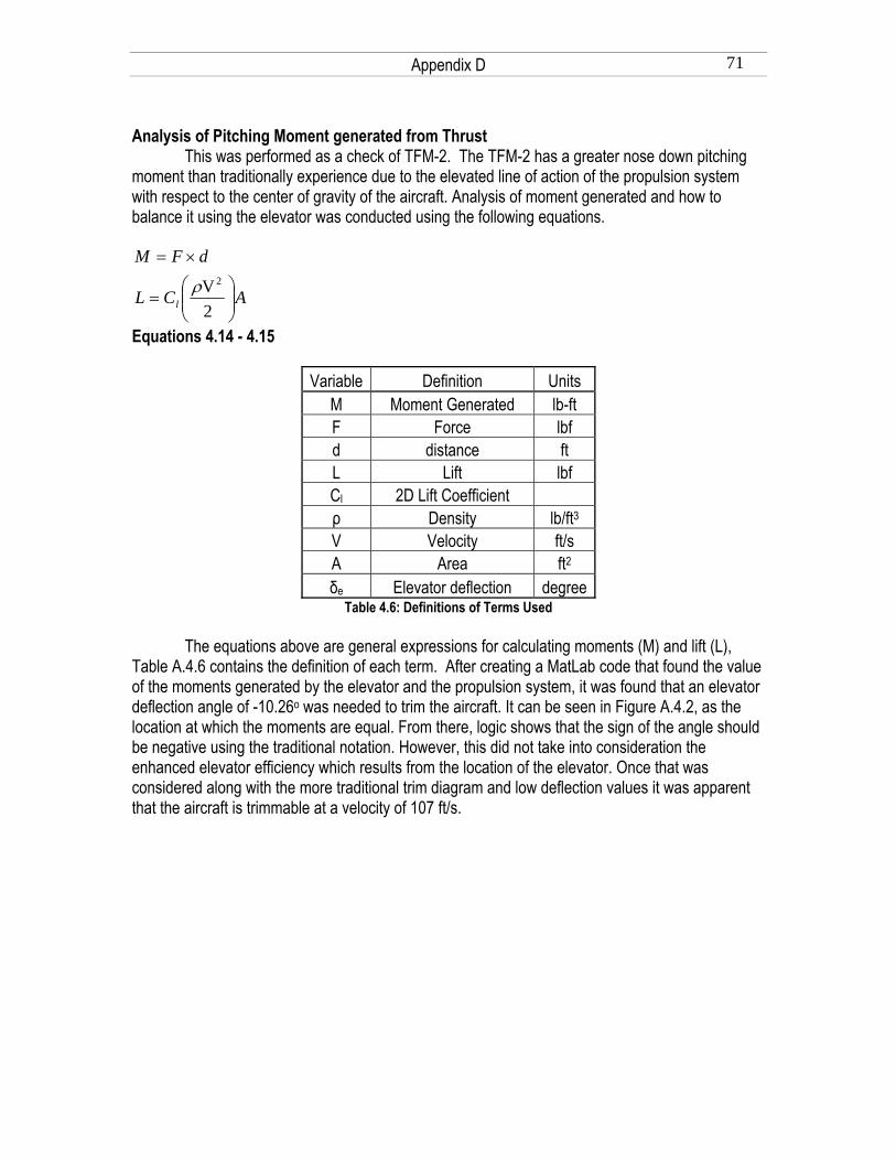
Appendix D 71

Analysis of Pitching Moment generated from Thrust

This was performed as a check of TFM-2. The TFM-2 has a greater nose down pitching moment than traditionally experience due to the elevated line of action of the propulsion system with respect to the center of gravity of the aircraft. Analysis of moment generated and how to balance it using the elevator was conducted using the following equations.

ACL

dFM

l ⎟⎟⎠

⎞⎜⎜⎝

⎛=

×=

2V2ρ

Equations 4.14 - 4.15

Variable Definition Units M Moment Generated lb-ft F Force lbf d distance ft L Lift lbf Cl 2D Lift Coefficient ρ Density lb/ft3V Velocity ft/s A Area ft2δe Elevator deflection degree

Table 4.6: Definitions of Terms Used

The equations above are general expressions for calculating moments (M) and lift (L), Table A.4.6 contains the definition of each term. After creating a MatLab code that found the value of the moments generated by the elevator and the propulsion system, it was found that an elevator deflection angle of -10.26o was needed to trim the aircraft. It can be seen in Figure A.4.2, as the location at which the moments are equal. From there, logic shows that the sign of the angle should be negative using the traditional notation. However, this did not take into consideration the enhanced elevator efficiency which results from the location of the elevator. Once that was considered along with the more traditional trim diagram and low deflection values it was apparent that the aircraft is trimmable at a velocity of 107 ft/s.

Appendix D 72

-15 -10 -5 00

0.5

1

1.5

2

2.5

3

3.5

4

δe [deg]

Mom

ent [

lb-ft

]

ElevatorThrust

Figure 4.2: Moment versus Elevator Deflection

Appendix D 73

D&C 4.5 Feedback Control System Without Feedback Control System % Ashley Brawner % Finding the damping of the open-loop yaw rate transfer function % A&AE 451 damp(RperDr) Eigenvalue Damping Freq. (rad/s) 0.00e+000 -1.00e+000 0.00e+000 1.69e-001 -1.00e+000 1.69e-001 -7.68e-001 + 4.03e+000i 1.87e-001 4.10e+000 -7.68e-001 - 4.03e+000i 1.87e-001 4.10e+000 -6.75e+000 1.00e+000 6.75e+000

Figure 4.3: Root Locus of Open-Loop Yaw Rate Transfer Function

Appendix D 74

Feedback Control System Root Locus:

Figure 4.4: Root Locus of Feedback Control System

Closed Loop Poles of Control System (Yaw Rate Feedback) % Ashley Brawner % Finding the damping of the Feedback Control System % A&AE 451 sys=feedback(Servo*RperDr,-0.4); damp(sys) Eigenvalue Damping Freq. (rad/s) 0.00e+000 -1.00e+000 0.00e+000 2.33e-001 -1.00e+000 2.33e-001 -5.38e+000 1.00e+000 5.38e+000 -4.66e+000 + 3.21e+000i 8.23e-001 5.66e+000 -4.66e+000 - 3.21e+000i 8.23e-001 5.66e+000 -1.68e+001 + 2.13e+001i 6.21e-001 2.71e+001 -1.68e+001 - 2.13e+001i 6.21e-001 2.71e+001

Appendix D 75

Appendix of Code BasicConstants.m Basic Constants.m is a MATLAB file which was used for running Prof. Andrisani’s Flat Earth code. This code was used to determine many constants which were needed for analysis, in addition it also evaluated the longitudinal and lateral stability of the TFM-2 aircraft after the equations of motion were linearized. % ********************************************* % BasicConstants_TFM2 Version 2.0 10/30/06 % This version requires Xcg and low_wing to be defined here. % % OBJECTIVE: Collect into one location all the vehicle specific constants (a.k.a. basic constants). % From these basic constants all the stability and control derivatives % can be determined. % INPUTS: None % OUTPUTS: Many basic constants defined in the Matlab workspace. % % This version is the first for team “Balsa to the Wall” % Arbitrary reference point is the quarter chord of the wing % Moment reference point is the quarter chord of the wing % Trim velocity assumed to be 107 ft/s % % ********************************************* % BasicConstants - Identifies, describes, and assigns all of the % the most basic variables for analyzing the control % and stability of a generic aircraft. % ********************************************* % % A&AE 451 Fall 2006 - Purdue University % % Note: This code is provided for a first order approximation of the dynamic % analysis of an airplane and is not intended for final designs. % % Equations/Figures can be found in : % % (Ref.1) Roskam, Jan. "Airplane Flight Dynamics and Automatic Flight % Controls" % Published by DARcorporation % 120 E. Ninth St., Suite 2 % Lawrence, KS 66044 % Third Printing, 2001. % % (Ref.2) Roskam, Jan. "Methods for Estimating Stability and % Control Derivatives of Conventional Subsonic Airplanes" % Published by the Author % 519 Boulder % Lawrence, Kansas 66044 % Third Printing, 1997. % % (Ref.3) Roskam, Jan. "Airplane Design: Part IV: Preliminary Calculation % of Aerodynamic, Thrust and Power Characteristics" % Published by Roskam Aviation and Engineering Corporation

Appendix D 76

% Rt4, Box 274 % Ottawa, Kansas 66067 % Second Printing, 1990. disp(' '); disp('Starting BasicConstants'); disp(' ') aircraft='TFM2'; adelf = 0; % Two dimensional lift effectiveness parameter Ref.(2),Equ(8.7) alpha = 0*pi/180; % Trim Angle of attack [rad]. This should be zero since our % equations of motion are body axis system rather then the stability axis system. alpha_0 = -0.018; % Airfoil zero-lift AOA [rad] altitude= 620; % Trim altitude [ft] [We fly at 20 feet plus West Lafayette’s sea level altitude] disp(['Trim altitude= ',num2str(altitude),' ft']) AR_h = 3.6585; % Aspect ratio of the horizontal tail AR_w = 5; % Aspect ratio of the wing b_f =3.47; % Span of the flap [ft] (Alieron total span)**** b_h = 1.5; % Span of the horizontal tail [ft] b_h_oe =6/12; % Elevator outboard position [ft] b_h_ie = 0; % Elevator inboard position [ft] b_w = 4.97; % Span of the wing [ft] b_v = 6/12; % Vertical tail span measured from fuselage centerline[ft] b_v_or = 5.5/12; % Outboard position of rudder [ft] b_v_ir = 0; % Inboard position of rudder [ft] c_a = 0.1825; % Chord of aileron [ft] C_bar_D_o = 0.018; % Parasite drag Cd_0 = 0.019; % Drag coefficient at zero lift (parasite drag) c_e = 1.25/12; % Elevator chord [ft] cf = 0.1825; % Chord of the wing flap [ft] c_h = 5/12; % Mean aerodynamic chord of the horizontal tail [ft] CL = 0.598; % Lift coefficient (3-D) CL=W/(1/2*rho*U^2) CL_hb = 0; % Lift coefficient of the horzontal tail/body CL_wb= 0.130; % Lift coefficient of the wing/body - assuming iw=0 Cl_alpha_h = 5.451; % 2-D Lift curve slope of horizontal tail Cl_alpha_v = 6.283; % 2-D Lift curve slope of vertical tail Cl_alpha = 6.032; % Two-dimensional lift curve slope of whole aircraft Cl_alpha_w = 5.543; % Two-dimensional lift curve slope of wing Cm_0_r = -0.029; % Zero lift pitching moment coefficient of the wing root Cm_o_t = -0.029; % Zero lift pitching moment coefficient of the wing tip **Cm_0_r = Cm_o_t because wing has % No twist c_r = 4.5/12; % MEAN Chord of the rudder [ft] c_w = 1.041; % Mean aerodynamic chord of the wing [ft] c_v = 5/12; % Mean aerodynamic chord of the vertical tail [ft] D_p = 10/12; % Diameter of propeller [ft] d = 0.417; % Average diameter of the fuselage [ft] delf = 0; % Streamwise flap deflection [rad] NO FLAPS delta_e = 0; % Elevator deflection [rad] delta_r = 0; % Rudder deflection [rad] dihedral = 0*pi/180; % Geometric dihedral angle of the wing [rad], positive for % dihedral (wing tips up), negative for % anhedral(tips down) [rad] ***EST dihedral_h = 0*pi/180; % Geometric dihedral angle of the horizontal tail [rad] e = 0.9; % Oswald's efficiency factor epsilon_t = 0; % Horizontal tail twist angle [rad] epsilon_0_h = 0*pi/180; % Downwash angle at the horizontal tail (see Note in % Ref.(3) under section 8.1.5.2) [rad] ***EST eta_h = 1; % Ratio of dynamic pressure at the horizontal tail to that of the freestream ***EST

Appendix D 77

eta_ia = 0.3; % Percent semi-span position of inboard edge of aileron eta_oa = 1; % Percent semi-span position of outboard edge of aileron eta_p = 0.8; % Propeller Efficiency ***EST eta_v = 1.0; % Ratio of the dynamic pressure at the vertical tail % to that of the freestream h1_fuse =4/12; % Height of the fuselage at 1/4 of the its length h2_fuse = 3/12; % Height of the fuselage at 3/4 of the its length h_h = 6/12; % Height from chord plane of wing to chord plane of % horizontal tail [ft] - Fig 3.7, Ref. 2 hmax_fuse = 4.2/12; % Maximum height of the fuselage [ft] Ixx = .444312; % Airplane moment of inertia about x-axis [slug-ft^2] *** With 4 lb load Iyy = .530488; % Airplane moment of inertia about y-axis [slug-ft^2] Izz = .960872; % Airplane moment of inertia about z-axis [slug-ft^2] Ixz = .007557; % Airplane product of inertia [slug-ft^2] i_h = 0*pi/180; % Incidence angle of horizontal tail [rad] This has applications from Trim Diagrams. i_w = 0*pi/180; % Incidence angle of wing [rad] k = 0.087; % k of the drag polar, generally= 1/(pi*AR*e) Lambda = .076; % Sweep angle of wing [rad] Lambda_c2 =-0.076; % Sweep angle at the c/2 of the wing [rad] Lambda_c4 = 0*pi/180; % Sweep angle at the c/4 of the wing [rad] Lambda_c2_v = 0*pi/180; % Sweep angle at the c/2 of the vertical tail [rad] Lambda_c4_v = 0*pi/180; % Sweep angle at the c/4 of the vertical tail [rad] Lambda_c2_h = 0*pi/180; % Sweep angle at the c/2 of the horizontal tail [rad] Lambda_c4_h = 0*pi/180; % Sweep angle at the c/4 of the horizontal tail [rad] lambda = .45; % Taper ratio of wing lambda_h = 1; % Taper ratio of horizontal tail lambda_v = 1.0; % Taper ratio of vertical tail l_f = 45/12; % Horizontal length of fuselage [ft] l_v = 31.43/12; % Horizontal distance from aircraft arbitrary reference point to vertical tail AC [ft] %Ref fig 2.1 in thesis for l_v, ref pt is c/4 low_wing=1; % low_wing=-1 if the wing is high % low_wing=1 if the wing is low % low_wing=0 if the wing is mid % Trim Airspeed u = 107; % ft/sec M = u/1221; % Mach number S_b_s = 131.035/144; % Body side area [ft^2] S_h = .625; % Area of horizontal tail [ft^2] S_h_slip = 100/144; % Area of horizontal tail that is covered in % prop-wash [ft^2] - See Fig.(8.64) - Ref.(3) ***EST % [Estimation] S_o = 15/144; % Fuselage x-sectional area at Xo [ft^2] - % See Fig.(7.2) - Ref.(2) % Xo is determined by plugging X1/l_b into: % 0.378 + 0.527 * (X1/l_b) = (Xo/l_b) [Estimation at this point] S_w = 4.95; % Surface area of wing [ft^2] S_v = 60/144; % Surface area of vertical tail [ft^2] tc_w = .08; % Thickness to chord ratio of wing tc_h = .08; % Thickness to chord ratio of horizontal tail theta = 0*pi/180; % Wing twist - negative for washout [rad] theta_h = 0*pi/180; % Horizontal tail twist between the root and tip % stations,negative for washout [rad] two_r_one = 0/12; % Fuselage depth in region of vertical tail [ft] Ref.(2),Figure 7.5 U = u/1.7; % knots % Free Stream Velocity (Trim velocity) [KNOTS true] disp(['Trim airspeed= ',num2str(U),' knots'])

Appendix D 78

W = 5.45242; % Weight of Airplane [lbf] wingloc = 0; % If the aircraft is a highwing: (wingloc=1), low-wing:(wingloc=0) wmax_fuse =3.6/12; % Maximum fuselage width [ft] X1 = (14+3)/12; % Distance from the front of the fuselage where the % x-sectional area decrease (dS_x/dx) % is greatest (most negative) [ft] - Ref.(2),Fig. 7.2 x_m = 15.875/12; % Distance from nose of aircraft to arbitrary reference point [ft] % measured positive aftward. Reference point will be MAC. x_over_c_v = .25 % PARAMETER ACCOUNTING FOR THE RELATIVE POSITIONS OF THE HORIZONTAL AND VERTICAL TAILS % defined as the fore-and-aft distance from leading edge of vertical fin to the % aerodynamic center of the horizontal tail divided by the chord of the vertical tail % [nondimensional] - See Fig 7.6 of Ref. 2 Xach = 2.882; % Distance from the leading edge of the wing mean aerodynamic chord % to the aerodynamic center of the horizontal tail (positive aftward) [ft] Xacwb = 0.249; % Distance from the leading edge of the wing mean aerodynamic chord % to the aerodynamic center of the wing and body. % Measured as positive aft, starting from the leading edge of the mean aero. chord. [ft] Xacw = 0.249; % Distance from the leading edge of the wing mean aerodynamic chord % to the aerodynamic center of the wing ALONE. % Measured as positive aft, starting from the leading edge of the mean aero. chord. [ft] Xref = 2.92/12; % Distance from the leading edge of the wing mean aerodynamic chord % to the arbitrary moment reference point. The equivalent force system % for the aerodynamic force system is given about this point. % Measured as positive aft, starting from the leading edge of the mean aero. chord. [ft] Xcg = 0.15*c_w; % Distance from the leading edge of the wing mean aerodynamic chord % to the center of gravity. % Measured as positive aft, starting from the leading edge of the mean aero. chord. [ft] % % Xcg is ignored until Step 2. It an be changed later in Step 2. % Z_h = -6/12; % Negative of the VERTICAL distance from the fuselage % centerline to the horizontal tail aero center % (Z_h is a negative number FOR TAILS ABOVE THE CENTERLINE) % - Ref.(2), Fig.7.6 % ***This produces a bunch of interpolation errors because % Roskam doesn't have data for horizontal tails below the % centerline of the fuselage Z_v = 3/12; % Vertical distance from the aircraft arbirary reference point to the vertical % tail aero center (positive up) - Ref.(2), Fig. 7.18 Z_w = -1.5/12; % This is the vertical distance from the wing root c/4 [ft] % to the fuselage centerline, % positive downward - Ref.(2), Equ(7.5) Z_w1 = -1.5/12; % Distance from body centerline to c/4 of wing root % chord,positive for c/4 point % below body centerline (ft) - Ref.(2), Fig. 7.1

Appendix E 79

Appendix E

Appendix E 80


IMy

bending =σ

Equation 5.3.1: Bending stress

EIFL3

3

=δ

Equation 5.3.2: Elastic deflection

cSCVT m2

21 ρ=

Equation 5.3.3: Torque due to aerodynamic loading

GJTL

=φ

Equation 5.3.4: Twist angle due to torsion

Appendix E 81

Appendix of Figures 14

Figure 5.2.1: Load factor at maximum lift vs. velocity

Figure 5.2.2: Load factor in level turn vs. bank angle

0 10 20 30 40 50 60 70 80 900

2

4

6

8

10

12Load Factor vs. Bank Angle

Bank Angle [deg]

n turn

10 20 30 40 50 60 70 80 90 1000

2

4

6

8

10

12

Load Factor vs. Velocity

Velocity [ft/sec]

n max

Appendix E 82

0

50

100

150

0

50

100

1500

2

4

6

8

10

n pull u

p

Load Factor vs. Velocity and Vertical Turn Radius

Velocity [ft/sec]Vertical Turn Radius [ft]

Figure 5.2.3: Load factor in climb vs. vertical turn radius and velocity

Load Factor vs. Turn Radius for Different Velocities

0

5

10

15

20

25

30

35

0 10 20 30 40 50 60

Ve r t i c a l Tur n Ra di us [ f t ]

30 [ f t / s]

35 [ f t / s]

40 [ f t / s]

45 [ f t / s]

50 [ f t / s]

55 [ f t / s]

60 [ f t / s]

65 [ f t / s]

70 [ f t / s]

75 [ f t / s]

80 [ f t / s]

85 [ f t / s]

90 [ f t / s]

95 [ f t / s]

100 [ f t / s]

Figure 5.2.4: Load factor in climb vs. vertical turn radius for range of velocities

Appendix E 83

00.5

11.5

22.5

-0.50

0.51

-0.8

-0.6

-0.4

-0.2

0

0.2

0.4

0.6

0.8

Chord [ft]

Exact Wing Geometry

Span [ft]

Thic

knes

s [ft

]

Figure 5.3.1: Discretization of the Wing Structure

0 0.5 1 1.5 2 2.50

2

4

6

8

10

12Elliptic Lift Distribution and Discretized Approximation

Distance from Root [ft]

Lift

[lbf]

Figure 5.3.2: Elliptic Lift Distribution

Appendix E 84

0 0.5 1 1.5 2 2.50

5

10

15

20

25Bending Moment vs. Span


Ben

ding

Mom

ent [

ft-lb

]

Figure 5.3.3: Bending Moment vs. Span

0 0.5 1 1.5 2 2.5-6

-5

-4

-3

-2

-1

0Torque vs. Distance from Root


Torq

ue [f

t-lbf

]

Figure 5.3.4: Torque vs. Span

Appendix E 85

0 0.5 1 1.5 2 2.5-30

-25

-20

-15

-10

-5

0Torque vs. Distance from Root


Torq

ue [f

t-lbf

]

Figure 5.3.5: Total Resultant Torque including Boom Load

Fiberglass Thickness vs. Cloth Weight

y = 0.0015xR2 = 0.9851

0

0.002

0.004

0.006

0.008

0.01

0.012

0 2 4 6Fiberglass Cloth Weight [oz]

Fibe

rgla

ss C

loth

Thi

ckne

ss [i

n]

8

Figure 5.3.6: Total Fiberglass Thickness vs. Cloth Weight

Appendix E 86

0 0.1 0.2 0.3 0.4 0.5 0.6 0.7 0.8 0.9 1

-0.3

-0.2

-0.1

0

0.1

0.2

0.3

0.4NACA 1408 Normalized Airfoil and Centroid Location

x/c

y/c

Figure 5.3.7: Normalized Airfoil and Centroid Location

0 0.1 0.2 0.3 0.4 0.5 0.6 0.7 0.8 0.9 1

-0.3

-0.2

-0.1

0

0.1

0.2

0.3

NACA 1408 Normalized Airfoil and Elliptic Approximation

x/c

y/c

Figure 5.3.7: Normalized Airfoil and Elliptic Approximation

Appendix E 87

Appendix E: V-n Diagram Walk-through

The design variables which were used in V-n diagram analysis are summarized in Table 5.2.1 below.

Design Variables Velocity V

Bank Angle φ Vertical Turn Radius r

Table 5.2.1: Load factor parameters.

Velocity and bank angle will be relatively easy to control. The vertical turn radius is more arbitrary, but can still be physically attained within reason.

The entire structure scales with load factor; therefore, the lower the load factor is, the lighter the aircraft structure can be made. As the intended mission is high speed, light weight becomes even more critical than in the case of more general purpose aircraft.

Three separate flight conditions were examined to determine the appropriate load factor. The first condition was level-flight at maximum lift, where CLmax was given by the aerodynamics team as 1.06. The second condition was a level-flight turn. The third condition was the climb.

2

2max VW

SCn L ρ=

Load factor at CL,max

φcos1

=n

Load factor in level-flight turn

12

+=grVn

Load factor in climb as a function of vertical turn radius These equations yield the instantaneous load factors for the given flight conditions and

required input parameters. Graphical representations of the above equations are presented in figures 5.2.1 through 5.2.4.

Appendix E 88

Appendix E: Comparison of Exact Airfoil Structural Properties with Elliptic Approximation

For simplification of analysis, the bending moments of inertia and polar moments of inertia

were initially approximated using an ellipse with thickness and chord corresponding to that of the local station airfoil. This was later compared with the exact airfoil structural properties obtained using XFOIL. The trade study evaluating this approximation was conducted with a uniform wing skin of 4 oz E-glass/epoxy having a thickness of 0.0059 in.

The bending moments of inertia and polar moments of inertia were calculated for the area and for the skin at each of the ten discretized stations. The errors presented in table 5.3.1 are the errors averaged over the ten stations. The comparison of tip vertical deflection and tip twist is shown in table 5.3.2 below. While providing an approximate initial first guess for structural design, the elliptic approximation proved to be a poor analysis approximation when precise results were desired.

I_xx_area_avg_error 22.70% I_xx_skin_avg_error 6.79%

J_area_avg_error 23.81% J_skin_avg_error 27.30%

Table 5.3.1: Average errors in structural properties in elliptic approximation

Airfoil Tip Vertical Deflection 1.386e-4 [ft] Ellipse Tip Vertical Deflection 1.298e-4 [ft]

Airfoil Tip Twist -1.045 [deg] Ellipse Tip Twist -0.8199 [deg]

Table 5.3.2: Comparison of exact airfoil calculations with elliptic approximation

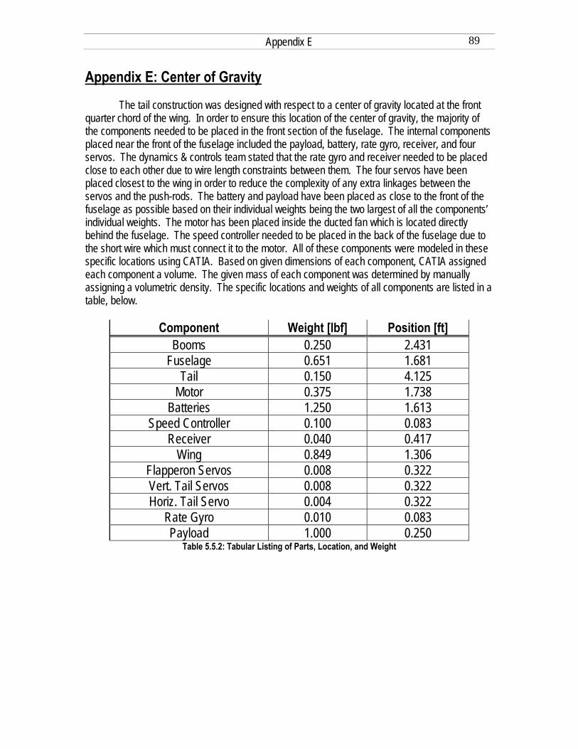
Appendix E 89

Appendix E: Center of Gravity

The tail construction was designed with respect to a center of gravity located at the front quarter chord of the wing. In order to ensure this location of the center of gravity, the majority of the components needed to be placed in the front section of the fuselage. The internal components placed near the front of the fuselage included the payload, battery, rate gyro, receiver, and four servos. The dynamics & controls team stated that the rate gyro and receiver needed to be placed close to each other due to wire length constraints between them. The four servos have been placed closest to the wing in order to reduce the complexity of any extra linkages between the servos and the push-rods. The battery and payload have been placed as close to the front of the fuselage as possible based on their individual weights being the two largest of all the components’ individual weights. The motor has been placed inside the ducted fan which is located directly behind the fuselage. The speed controller needed to be placed in the back of the fuselage due to the short wire which must connect it to the motor. All of these components were modeled in these specific locations using CATIA. Based on given dimensions of each component, CATIA assigned each component a volume. The given mass of each component was determined by manually assigning a volumetric density. The specific locations and weights of all components are listed in a table, below.

Component Weight [lbf] Position [ft] Booms 0.250 2.431

Fuselage 0.651 1.681 Tail 0.150 4.125

Motor 0.375 1.738 Batteries 1.250 1.613

Speed Controller 0.100 0.083 Receiver 0.040 0.417

Wing 0.849 1.306 Flapperon Servos 0.008 0.322 Vert. Tail Servos 0.008 0.322 Horiz. Tail Servo 0.004 0.322

Rate Gyro 0.010 0.083 Payload 1.000 0.250

Table 5.5.2: Tabular Listing of Parts, Location, and Weight

Appendix E 90

Appendix of Tables

[0/90] Woven Cloth E_1 [Msi] 3.5 E_2 [Msi] 3.5

G_12 [Msi] 0.68 Table 5.3.3: Woven E-glass Epoxy Material Properties

2 Ply Laminate [0/45]

E_x [Msi] 2.87 E_y [Msi] 2.87

G_xy [Msi] 1.13 Table 5.3.4: Woven E-glass Epoxy Material Properties, 2-ply equivalent moduli

3 Ply Laminate [-45/0/45]

E_x [Msi] 2.62 E_y [Msi] 2.62

G_xy [Msi] 1.28 Table 5.3.5: Woven E-glass Epoxy Material Properties, 3-ply equivalent moduli

Appendix E 91

Internal Layout of TFM-2

Figure 5.5.1: Internal Layout of TFM-2

Appendix E 92

Appendix of Code Wing Bending Analysis % Wing Bending Analysis close all clear all clc; % Updated 12 October 2006 % Assumes Elliptic Lift Distribution W = 5.5; % weight Span = 5; n = 5; SF = 1.5; g = 32.174; L = n*SF*W; a = Span/2; A = L/2; b = 4*A/(pi*a); n = 11; x = linspace(0,a,n); y = sqrt(b^2*(1-x.^2/a^2)); % Lift for i = 1:length(x)-1 x_avg(i) = (x(i)+x(i+1))/2; y_avg(i) = (y(i)+y(i+1))/2; end dx = x(2); dl = x(2)/2; n_dl = [1 3 5 7 9 11 13 15 17 19]; for j = 1:length(x_avg) L_local(j) = dx*y_avg(j); end for k = 1:length(L_local) M_local = L_local(k:length(L_local)).*(dl*n_dl(1:length(L_local)+1-k)); M_station(k) = sum(M_local); end

Appendix E 93

M = L/2*4*a/(3*pi) M_approx = M_station(1) Half_Lift = A Half_Lift_approx = sum(dx*y_avg) plot(x,y,'o-') hold on bar(x_avg,y_avg) title('Elliptic Lift Distribution and Discretized Approximation') xlabel('Distance from Root [ft]') ylabel('Lift [lbf]') figure plot(x(1:n-1),M_station,'o-') grid on title('Bending Moment vs. Span') xlabel('Distance from Root [ft]') ylabel('Bending Moment [ft-lb]')

Appendix E 94

NACA 1408 Wing Analysis % NACA 1408 Wing Analysis close all clear all clc; % Updated 25 October 2006 % Station Properties % [ A, Xc, Yc, Iyy, Iyy/t, Ixx, Ixx/t, J, J/t ] fprintf('[ A Xc Yc Iyy Iyy/t Ixx Ixx/t J J/t ]') Properties = [0.1003652, 0.5689842, 1.0439277e-2, 1.0145793e-2, 0.4540932, 6.8701578e-5, 4.4289734e-3, 2.7061885e-4, 1.4723400e-2; 0.089689165, 0.5378717, 9.8684337e-3, 8.1021124e-3, 0.3836002, 5.4863063e-5, 3.7414338e-3, 2.1610824e-4, 1.2437802e-2; 0.079600058, 0.5067170, 9.2968261e-3, 6.3818241e-3, 0.3207298, 4.3214237e-5, 3.1282266e-3, 1.7022298e-4, 1.03992991e-2; 0.070112742, 0.4755621, 8.7252399e-3, 4.9512368e-3, 0.2651335, 3.3526972e-5, 2.5859731e-3, 1.3206442e-4, 8.5966438e-3; 0.061227284, 0.4444072, 8.1536258e-3, 3.7758080e-3, 0.2163654, 2.5567635e-5, 2.1103078e-3, 1.0071212e-4, 7.0153750e-3; 0.052943632, 0.4132523, 7.5820335e-3, 2.8232406e-3, 0.1739763, 1.9117340e-5, 1.6968708e-3, 7.5304190e-5, 5.6409743e-3; 0.045261785, 0.3820978, 7.0104208e-3, 2.0634034e-3, 0.1375204, 1.3972162e-5, 1.3412997e-3, 5.5037035e-5, 4.4589327e-3; 0.038181752, 0.3509431, 6.4388211e-3, 1.4683584e-3, 0.1065501, 9.9428771e-6, 1.0392308e-3, 3.9165472e-5, 3.4547555e-3; 0.031711873, 0.3198301, 5.8679874e-3, 1.0128941e-3, 0.0806497, 6.8587369e-6, 7.8661321e-4, 2.7016893e-5, 2.6149678e-3; 0.025834661, 0.2886758, 5.2963835e-3, 6.7223917e-4, 0.0593026, 4.5520369e-6, 5.7840504e-4, 1.7930692e-5, 1.9228162e-3; 0.020559255, 0.2575209, 4.7247875e-3, 4.2572958e-4, 0.0420998, 2.8828013e-6, 4.1061913e-4, 1.1355497e-5, 1.3650381e-3] %%%%%%%%%%%%%%%%%%%%%%%%%%%%%%%%%%%%%%%%%%%%%%%%%%%%%%%%%%%%%%%%%%%%%%%%%%% % Wing Geometry Parameters Span = 5; c_root = 16.24/12; c_tip = 7.35/12; % NACA 1408 Airfoil Parameters t = 0.08; p = 0.4; m = 0.01; % Stations and chord a = Span/2;

Appendix E 95

n = 11; Station_loc = linspace(0,a,n); chord = (c_tip-c_root)/a.*Station_loc + c_root; %%%%%%%%%%%%%%%%%%%%%%%%%%%%%%%%%%%%%%%%%%%%%%%%%%%%%%%%%%%%%%%%%%%%%%%%%%% % Defines x-coordinates for discretized airfoil coordinates x_1 = [0,0.00025,0.001,0.002,0.003,0.006,0.01,0.015,0.025,0.04]; x_2 = linspace(0.06,0.15,4); x_3 = [0.2,0.25]; x_4 = [0.3:0.1:1]; x_disc = [x_1,x_2,x_3,x_4]; %%%%%%%%%%%%%%%%%%%%%%%%%%%%%%%%%%%%%%%%%%%%%%%%%%%%%%%%%%%%%%%%%%%%%%%%%%% % Finds discretized normalized airfoil coordinates for output to Catia model for i = 1:length(x_disc) X = x_disc(i); y_t = t/0.2*(0.2969*sqrt(X) - 0.1260*X - 0.3516*X^2 + 0.2843*X^3 - 0.1015*X^4); if X < p y_c = m/p^2*(2*p*X - X^2); else y_c = m/(1-p)^2*((1-2*p) + 2*p*X - X^2); end x_pos(i) = X; y_upper(i) = (y_t + y_c); y_lower(i) = (-y_t + y_c); end %%%%%%%%%%%%%%%%%%%%%%%%%%%%%%%%%%%%%%%%%%%%%%%%%%%%%%%%%%%%%%%%%%%%%%%%%%% % Fixing Numerical Error at TE in discretized airfoil q = length(x_pos); y_upper(q) = 0; y_lower(q) = 0; %%%%%%%%%%%%%%%%%%%%%%%%%%%%%%%%%%%%%%%%%%%%%%%%%%%%%%%%%%%%%%%%%%%%%%%%%%% % Finds exact and elliptic approximation normalized airfoil geometry dx = 0.0001; x = [0:dx:1]; for i = 1:length(x) X = x(i);

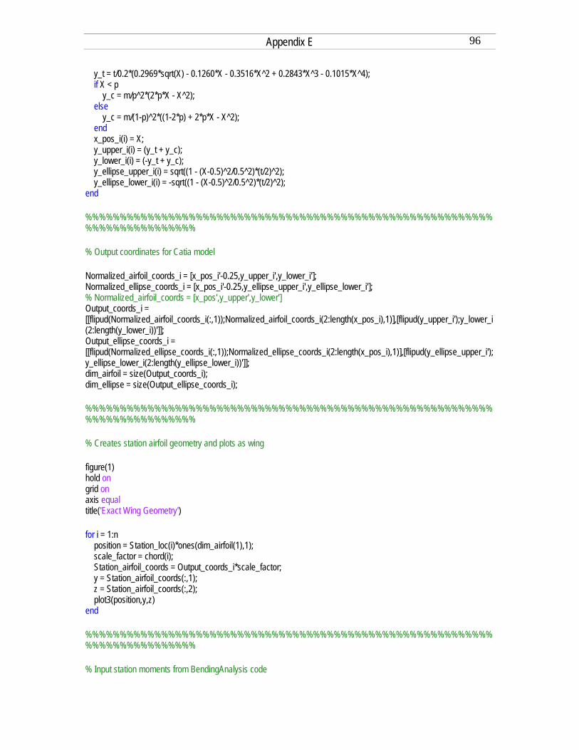
Appendix E 96

y_t = t/0.2*(0.2969*sqrt(X) - 0.1260*X - 0.3516*X^2 + 0.2843*X^3 - 0.1015*X^4); if X < p y_c = m/p^2*(2*p*X - X^2); else y_c = m/(1-p)^2*((1-2*p) + 2*p*X - X^2); end x_pos_i(i) = X; y_upper_i(i) = (y_t + y_c); y_lower_i(i) = (-y_t + y_c); y_ellipse_upper_i(i) = sqrt((1 - (X-0.5)^2/0.5^2)*(t/2)^2); y_ellipse_lower_i(i) = -sqrt((1 - (X-0.5)^2/0.5^2)*(t/2)^2); end %%%%%%%%%%%%%%%%%%%%%%%%%%%%%%%%%%%%%%%%%%%%%%%%%%%%%%%%%%%%%%%%%%%%%%%%%%% % Output coordinates for Catia model Normalized_airfoil_coords_i = [x_pos_i'-0.25,y_upper_i',y_lower_i']; Normalized_ellipse_coords_i = [x_pos_i'-0.25,y_ellipse_upper_i',y_ellipse_lower_i']; % Normalized_airfoil_coords = [x_pos',y_upper',y_lower'] Output_coords_i = [[flipud(Normalized_airfoil_coords_i(:,1));Normalized_airfoil_coords_i(2:length(x_pos_i),1)],[flipud(y_upper_i');y_lower_i(2:length(y_lower_i))']]; Output_ellipse_coords_i = [[flipud(Normalized_ellipse_coords_i(:,1));Normalized_ellipse_coords_i(2:length(x_pos_i),1)],[flipud(y_ellipse_upper_i');y_ellipse_lower_i(2:length(y_ellipse_lower_i))']]; dim_airfoil = size(Output_coords_i); dim_ellipse = size(Output_ellipse_coords_i); %%%%%%%%%%%%%%%%%%%%%%%%%%%%%%%%%%%%%%%%%%%%%%%%%%%%%%%%%%%%%%%%%%%%%%%%%%% % Creates station airfoil geometry and plots as wing figure(1) hold on grid on axis equal title('Exact Wing Geometry') for i = 1:n position = Station_loc(i)*ones(dim_airfoil(1),1); scale_factor = chord(i); Station_airfoil_coords = Output_coords_i*scale_factor; y = Station_airfoil_coords(:,1); z = Station_airfoil_coords(:,2); plot3(position,y,z) end %%%%%%%%%%%%%%%%%%%%%%%%%%%%%%%%%%%%%%%%%%%%%%%%%%%%%%%%%%%%%%%%%%%%%%%%%%% % Input station moments from BendingAnalysis code

Appendix E 97

M_station = [21.3922 16.6243 12.5079 9.0330 6.1824 3.9314 2.2465 1.0835 0.3846 0.0715 0.0000001]; L_local = [2.6195 2.5929 2.5390 2.4560 2.3405 2.1875 1.9881 1.7255 1.3602 0.5723 0.0000001]; %%%%%%%%%%%%%%%%%%%%%%%%%%%%%%%%%%%%%%%%%%%%%%%%%%%%%%%%%%%%%%%%%%%%%%%%%%% % Elliptic airfoil approximation wing geometry and analysis figure(2) hold on grid on axis equal title('Elliptic Approximation Wing Geometry') skin_t = 0.0059/12; for i = 1:n position = Station_loc(i)*ones(dim_ellipse(1),1); scale_factor = chord(i); Station_ellipse_coords = Output_ellipse_coords_i*scale_factor; y = Station_ellipse_coords(:,1); z = Station_ellipse_coords(:,2); plot3(position,y,z) b(i) = t*chord(i)/2; a(i) = chord(i)/2; h(i) = (a(i)-b(i))^2/(a(i)+b(i))^2; circumference(i) = pi*(a(i)+b(i))*[1 + 3*h(i)/(10+(4-3*h(i))^(1/2))]; skin_thick = 0.0059/12; sigma(i) = M_station(i)*a(i)/(pi/4*(a(i)*b(i)^3 - ((a(i)-skin_thick)*(b(i)-skin_thick)^3))); L = Station_loc(2); I_ellipse_area(i) = (pi/4*(a(i)*b(i)^3)); % I(i) = (pi/4*(a(i)*b(i)^3 - ((a(i)-skin_thick)*(b(i)-skin_thick)^3))); I_ellipse(i) = pi/4*(a(i)*b(i)^3 - ((a(i)-skin_thick)*(b(i)-skin_thick)^3)); I(i) = Properties(i,7)*skin_t; % d(i) = L_local(i)*L^3/(3*6e6*12^2*(pi/4*(a(i)*b(i)^3 - ((a(i)-skin_thick)*(b(i)-skin_thick)^3)))); d(i) = L_local(i)*L^3/(3*6e6*12^2*(I(i))); d_ellipse(i) = L_local(i)*L^3/(3*6e6*12^2*(I_ellipse(i))); % while sigma(i) > 165e3*12^2 % E-glass/Epoxy longitudinal tensile strength % skin_thick = skin_thick + 0.00000001; % sigma(i) = M_station(i)*a(i)/(pi/4*(a(i)*b(i)^3 - ((a(i)-skin_thick)*(b(i)-skin_thick)^3))); % end % % skin_thickness(i) = skin_thick; end deflection = sum(d) deflection_ellipse = sum(d_ellipse) %%%%%%%%%%%%%%%%%%%%%%%%%%%%%%%%%%%%%%%%%%%%%%%%%%%%%%%%%%%%%%%%%%%%%%%%%%% % Numerical integration airfoil function

Appendix E 98

for i = 1:length(x_pos_i) dA_upper(i) = y_upper_i(i)*dx; dA_lower(i) = abs(y_lower_i(i))*dx; x_num_upper(i) = x_pos_i(i)*dA_upper(i); x_num_lower(i) = x_pos_i(i)*dA_lower(i); y_num_upper(i) = y_upper_i(i)*dA_upper(i); y_num_lower(i) = y_lower_i(i)*dA_lower(i); end A_upper = sum(dA_upper); A_lower = sum(dA_lower); x_bar_upper = sum(x_num_upper)/A_upper; x_bar_lower = sum(x_num_lower)/A_lower; y_bar_upper = sum(y_num_upper)/A_upper; y_bar_lower = sum(y_num_lower)/A_lower; A = A_upper + A_lower; x_bar = (sum(x_num_upper) + sum(x_num_lower))/A; y_bar = (sum(y_num_upper) + sum(y_num_lower))/A; %%%%%%%%%%%%%%%%%%%%%%%%%%%%%%%%%%%%%%%%%%%%%%%%%%%%%%%%%%%%%%%%%%%%%%%%%%% % Plots Normalized Airfoil and Centroid figure plot(x_pos,y_upper,'r*-') hold on plot(x_pos,y_lower,'r*-') plot(x_pos_i,y_upper_i) plot(x_pos_i,y_lower_i) % plot(x_bar_upper-0.25,y_bar_upper,'o') % plot(x_bar_lower-0.25,y_bar_lower,'o') plot(x_bar,y_bar,'*') grid on axis equal title('NACA 1408 Normalized Airfoil and Centroid Location')%,'FontSize',20) xlabel('x/c')%,'FontSize',18) ylabel('y/c')%,'FontSize',18) %%%%%%%%%%%%%%%%%%%%%%%%%%%%%%%%%%%%%%%%%%%%%%%%%%%%%%%%%%%%%%%%%%%%%%%%%%% % Plots Normalized Airfoil and Elliptic Approximation figure plot(x_pos_i,y_upper_i) hold on plot(x_pos_i,y_lower_i) plot(x_pos_i,y_ellipse_upper_i,'k')

Appendix E 99

plot(x_pos_i,y_ellipse_lower_i,'k') grid on axis equal title('NACA 1408 Normalized Airfoil and Elliptic Approximation')%,'FontSize',20) xlabel('x/c')%,'FontSize',18) ylabel('y/c')%,'FontSize',18) % % Normalized_airfoil_coords = [x_pos'-0.25,y_upper',y_lower'] Normalized_airfoil_coords = [x_pos',y_upper',y_lower'] Output_coords = [[flipud(Normalized_airfoil_coords(:,1));Normalized_airfoil_coords(2:length(x_pos),1)],[flipud(y_upper');y_lower(2:length(y_lower))']] % figure % plot(Output_coords(:,1),Output_coords(:,2)) % axis equal % x_bar % y_bar Num_stations = n; Cm = -0.2; % Alpha = 0 g = 32.2; % ft/s^2 rho = 0.00237; % slug/ft^3 V = 100; % ft/s % G = 0.62e6*12^2; % lbf/ft^2 % HT with elevator x/c = 0.2 , del_e = 30 deg Chord_ht = 5/12; Span_ht = 1.5; C_L_ht = 1.22; S_ht = Chord_ht*Span_ht; L_ht = C_L_ht*0.5*rho*V^2*S_ht Station_chord = linspace(c_root,c_tip,Num_stations); Station_A_bar = Properties(:,1); l_boom = 1.5; % TE of wing to LE of HT T_ht = -L_ht*(l_boom+Chord_ht/4+3/4*Station_chord(4)); for k = 1:length(Station_chord)-1 Station_S(k) = Span/2/(Num_stations-1)*(Station_chord(k)+Station_chord(k+1))/2; T_local(k) = 0.5*rho*V^2*Station_S(k)*(Station_chord(k)+Station_chord(k+1))/2*Cm;%-L_local(k)*Station_chord(k)/4; % if k == 4 % T_local(k) = T_local(k) + T_ht; % end end T_local(3) = T_local(3)+T_ht; Thickness_opts = [0.00075, 0.00087, 0.001095, 0.0021, 0.003, 0.00345, 0.0046, 0.0059, 0.0093, 0.0107]/12; % for m = 1:length(Thickness_opts) skin_t_1 = 0.009/12;

Appendix E 100

G_1 = 1.277e6*12^2; E_1 = 2.62e6*12^2; % For Section 1 for k = 1:3 T_stat = sum(T_local(k:10)); % q(k) = T_station(k)/(2*(Station_A_bar(k)+Station_A_bar(k+1))/2); % J_ellipse(k) = pi*((a(k)^3*b(k)^3/(a(k)^2+b(k)^2))-((a(k)-skin_t)^3*(b(k)-skin_t)^3/((a(k)-skin_t)^2+(b(k)-skin_t)^2))); % J_area_ellipse(k) = pi*((a(k)^3*b(k)^3/(a(k)^2+b(k)^2))); J(k) = Properties(k,9)*skin_t_1; phi_station(k) = T_stat*Station_loc(2)/(G_1*J(k))*180/pi; % phi_station_ellipse(k) = T_stat*Station_loc(2)/(G*J_ellipse(k))*180/pi; % f(k) = 1; % while abs(phi_station) > .1 % f(k) = f(k) + 1 % % if f(k) > 113 % % break % % end % skin_t = skin_t + 0.00005/12 % J = Properties(k,9)*skin_t; % phi_station = T_stat*Station_loc(2)/(G*J)*180/pi; % end % t_torsion(k) = abs(q(k)*circumference(k)*(1/Span/2*pi/180)/(2*Station_A_bar(k)*G)); T_station(k) = T_stat; % end % Torsion_thickness(k) = skin_t*12; % Polar_Moment(k) = J; % Station_Twist(m) = sum(phi_station); I(k) = Properties(k,7)*skin_t_1; % d(i) = L_local(i)*L^3/(3*6e6*12^2*(pi/4*(a(i)*b(i)^3 - ((a(i)-skin_thick)*(b(i)-skin_thick)^3)))); d(k) = L_local(k)*L^3/(3*E_1*(I(k))); end skin_t_2 = 0.006/12; G_2 = 1.1283e6*12^2; E_2 = 2.87e6*12^2; for k = 4:10 T_stat = sum(T_local(k:10)); J(k) = Properties(k,9)*skin_t_2; phi_station(k) = T_stat*Station_loc(2)/(G_2*J(k))*180/pi; T_station(k) = T_stat; I(k) = Properties(k,7)*skin_t_2; d(k) = L_local(k)*L^3/(3*E_2*(I(k))); end phi_deg = sum(phi_station)' deflection = sum(d) figure plot(Station_loc(1:length(Station_loc)-1),T_station)

Appendix E 101

title('Torque vs. Distance from Root') xlabel('Distance from Root [ft]') ylabel('Torque [ft-lbf]') grid on

Appendix E 102

2-ply Composite Analysis % Matt Negilski % AAE 451 close all clear all clc % Woven Glass/Epoxy (M10E/3783) % 2-ply Analysis % Given material properties E_1 = 3.5e6; % psi E_2 = 3.5e6; G_12 = 0.68e6; Nu_12 = 0.11; Nu_21 = E_2*Nu_12/E_1; X = 62.8e3; X_pr = -54.6e3; Y = 55.9e3; Y_pr = -48.6e3; S = 12.2e3; t_k_1 = 0.003; % in t_k_2 = 0.003; h = t_k_1 + t_k_2; z_bar_1 = -(t_k_1/2); z_bar_2 = (t_k_1/2); % Q matrix for given material Q_11 = E_1/(1-Nu_12*Nu_21); Q_12 = Nu_12*E_2/(1-Nu_12*Nu_21); Q_21 = Nu_12*E_2/(1-Nu_12*Nu_21); Q_22 = E_2/(1-Nu_12*Nu_21); Q_66 = G_12; % +45 deg ply theta = 45; Q_bar_45 = zeros(3,3); Q_bar_45(1,1) = Q_11.*cos(theta*pi/180).^4+2.*(Q_12+2.*Q_66).*sin(theta*pi/180).^2.*cos(theta*pi/180).^2+Q_22.*sin(theta*pi/180).^4; Q_bar_45(1,2) = (Q_11+Q_22-4*Q_66).*sin(theta*pi/180).^2.*cos(theta*pi/180).^2+Q_12.*(sin(theta*pi/180).^4+cos(theta*pi/180).^4); Q_bar_45(1,3) = (Q_11-Q_12-2*Q_66).*sin(theta*pi/180).*cos(theta*pi/180).^3+(Q_12-Q_22+2*Q_66).*sin(theta*pi/180).^3.*cos(theta*pi/180); Q_bar_45(2,1) = (Q_11+Q_22-4*Q_66).*sin(theta*pi/180).^2.*cos(theta*pi/180).^2+Q_12.*(sin(theta*pi/180).^4+cos(theta*pi/180).^4);

Appendix E 103

Q_bar_45(2,2) = Q_11.*sin(theta*pi/180).^4+2.*(Q_12+2.*Q_66).*sin(theta*pi/180).^2.*cos(theta*pi/180).^2+Q_22.*cos(theta*pi/180).^4; Q_bar_45(2,3) = (Q_11-Q_12-2*Q_66).*cos(theta*pi/180).*sin(theta*pi/180).^3+(Q_12-Q_22+2*Q_66).*cos(theta*pi/180).^3.*sin(theta*pi/180); Q_bar_45(3,1) = (Q_11-Q_12-2*Q_66).*sin(theta*pi/180).*cos(theta*pi/180).^3+(Q_12-Q_22+2*Q_66).*sin(theta*pi/180).^3.*cos(theta*pi/180); Q_bar_45(3,2) = (Q_11-Q_12-2*Q_66).*cos(theta*pi/180).*sin(theta*pi/180).^3+(Q_12-Q_22+2*Q_66).*cos(theta*pi/180).^3.*sin(theta*pi/180); Q_bar_45(3,3) = (Q_11+Q_22-2*Q_12-2*Q_66).*sin(theta*pi/180).^2.*cos(theta*pi/180).^2+Q_66.*(sin(theta*pi/180).^4+cos(theta*pi/180).^4); T_sigma_45 = [cos(theta*pi/180)^2,sin(theta*pi/180)^2,2*sin(theta*pi/180)*cos(theta*pi/180);sin(theta*pi/180)^2,cos(theta*pi/180)^2,-2*sin(theta*pi/180)*cos(theta*pi/180);-sin(theta*pi/180)*cos(theta*pi/180),sin(theta*pi/180)*cos(theta*pi/180),cos(theta*pi/180)^2-sin(theta*pi/180)^2]; % 0 deg ply theta = 0; Q_bar_0 = zeros(3,3); Q_bar_0(1,1) = Q_11.*cos(theta*pi/180).^4+2.*(Q_12+2.*Q_66).*sin(theta*pi/180).^2.*cos(theta*pi/180).^2+Q_22.*sin(theta*pi/180).^4; Q_bar_0(1,2) = (Q_11+Q_22-4*Q_66).*sin(theta*pi/180).^2.*cos(theta*pi/180).^2+Q_12.*(sin(theta*pi/180).^4+cos(theta*pi/180).^4); Q_bar_0(1,3) = (Q_11-Q_12-2*Q_66).*sin(theta*pi/180).*cos(theta*pi/180).^3+(Q_12-Q_22+2*Q_66).*sin(theta*pi/180).^3.*cos(theta*pi/180); Q_bar_0(2,1) = (Q_11+Q_22-4*Q_66).*sin(theta*pi/180).^2.*cos(theta*pi/180).^2+Q_12.*(sin(theta*pi/180).^4+cos(theta*pi/180).^4); Q_bar_0(2,2) = Q_11.*sin(theta*pi/180).^4+2.*(Q_12+2.*Q_66).*sin(theta*pi/180).^2.*cos(theta*pi/180).^2+Q_22.*cos(theta*pi/180).^4; Q_bar_0(2,3) = (Q_11-Q_12-2*Q_66).*cos(theta*pi/180).*sin(theta*pi/180).^3+(Q_12-Q_22+2*Q_66).*cos(theta*pi/180).^3.*sin(theta*pi/180); Q_bar_0(3,1) = (Q_11-Q_12-2*Q_66).*sin(theta*pi/180).*cos(theta*pi/180).^3+(Q_12-Q_22+2*Q_66).*sin(theta*pi/180).^3.*cos(theta*pi/180); Q_bar_0(3,2) = (Q_11-Q_12-2*Q_66).*cos(theta*pi/180).*sin(theta*pi/180).^3+(Q_12-Q_22+2*Q_66).*cos(theta*pi/180).^3.*sin(theta*pi/180); Q_bar_0(3,3) = (Q_11+Q_22-2*Q_12-2*Q_66).*sin(theta*pi/180).^2.*cos(theta*pi/180).^2+Q_66.*(sin(theta*pi/180).^4+cos(theta*pi/180).^4); T_sigma_0 = [cos(theta*pi/180)^2,sin(theta*pi/180)^2,2*sin(theta*pi/180)*cos(theta*pi/180);sin(theta*pi/180)^2,cos(theta*pi/180)^2,-2*sin(theta*pi/180)*cos(theta*pi/180);-sin(theta*pi/180)*cos(theta*pi/180),sin(theta*pi/180)*cos(theta*pi/180),cos(theta*pi/180)^2-sin(theta*pi/180)^2]; % Case a: [+-45]s fprintf('For [45,0,45] Layup, \n') A = t_k_1*Q_bar_45 + t_k_2*Q_bar_0 B = t_k_1*z_bar_1*Q_bar_45 + t_k_2*z_bar_2*Q_bar_0 D = (t_k_1*z_bar_1^2+t_k_1^3/12)*Q_bar_45 + (t_k_2*z_bar_2^2+t_k_2^3/12)*Q_bar_0 E_x = (A(1,1)*A(2,2)-(A(1,2)^2))/(h*A(2,2)) E_y = (A(1,1)*A(2,2)-(A(1,2)^2))/(h*A(1,1)) Nu_xy = A(1,2)/A(2,2) Nu_yx = A(1,2)/A(1,1) G_xy = A(3,3)/h

Appendix E 104

epsilon_o = inv(A)*[1;0;0]; sigma_x_45 = Q_bar_45*epsilon_o; sigma_1_45 = T_sigma_45*sigma_x_45; sigma_x_0 = Q_bar_0*epsilon_o; sigma_1_0 = T_sigma_0*sigma_x_0; fprintf('FIRST PLY FAILURE: \n\n') fprintf('For fiber breakage, \n') N_x_45 = X/sigma_1_45(1) N_x_0 = X/sigma_1_0(1)

Appendix E 105

3-ply Composite Analysis % Matt Negilski % AAE 451 close all clear all clc % Woven Glass/Epoxy (M10E/3783) % 3-ply Analysis % Given material properties E_1 = 3.5e6; % psi E_2 = 3.5e6; G_12 = 0.68e6; Nu_12 = 0.11; Nu_21 = E_2*Nu_12/E_1; X = 62.8e3; X_pr = -54.6e3; Y = 55.9e3; Y_pr = -48.6e3; S = 12.2e3; t_k_1 = 0.003; % in t_k_2 = 0.003; t_k_3 = 0.003; h = 0.009; z_bar_1 = -(t_k_3/2); z_bar_2 = 0; z_bar_3 = (t_k_1/2); % Q matrix for given material Q_11 = E_1/(1-Nu_12*Nu_21); Q_12 = Nu_12*E_2/(1-Nu_12*Nu_21); Q_21 = Nu_12*E_2/(1-Nu_12*Nu_21); Q_22 = E_2/(1-Nu_12*Nu_21); Q_66 = G_12; % +45 deg ply theta = 45; Q_bar_45 = zeros(3,3); Q_bar_45(1,1) = Q_11.*cos(theta*pi/180).^4+2.*(Q_12+2.*Q_66).*sin(theta*pi/180).^2.*cos(theta*pi/180).^2+Q_22.*sin(theta*pi/180).^4; Q_bar_45(1,2) = (Q_11+Q_22-4*Q_66).*sin(theta*pi/180).^2.*cos(theta*pi/180).^2+Q_12.*(sin(theta*pi/180).^4+cos(theta*pi/180).^4); Q_bar_45(1,3) = (Q_11-Q_12-2*Q_66).*sin(theta*pi/180).*cos(theta*pi/180).^3+(Q_12-Q_22+2*Q_66).*sin(theta*pi/180).^3.*cos(theta*pi/180);

Appendix E 106

Q_bar_45(2,1) = (Q_11+Q_22-4*Q_66).*sin(theta*pi/180).^2.*cos(theta*pi/180).^2+Q_12.*(sin(theta*pi/180).^4+cos(theta*pi/180).^4); Q_bar_45(2,2) = Q_11.*sin(theta*pi/180).^4+2.*(Q_12+2.*Q_66).*sin(theta*pi/180).^2.*cos(theta*pi/180).^2+Q_22.*cos(theta*pi/180).^4; Q_bar_45(2,3) = (Q_11-Q_12-2*Q_66).*cos(theta*pi/180).*sin(theta*pi/180).^3+(Q_12-Q_22+2*Q_66).*cos(theta*pi/180).^3.*sin(theta*pi/180); Q_bar_45(3,1) = (Q_11-Q_12-2*Q_66).*sin(theta*pi/180).*cos(theta*pi/180).^3+(Q_12-Q_22+2*Q_66).*sin(theta*pi/180).^3.*cos(theta*pi/180); Q_bar_45(3,2) = (Q_11-Q_12-2*Q_66).*cos(theta*pi/180).*sin(theta*pi/180).^3+(Q_12-Q_22+2*Q_66).*cos(theta*pi/180).^3.*sin(theta*pi/180); Q_bar_45(3,3) = (Q_11+Q_22-2*Q_12-2*Q_66).*sin(theta*pi/180).^2.*cos(theta*pi/180).^2+Q_66.*(sin(theta*pi/180).^4+cos(theta*pi/180).^4); T_sigma_45 = [cos(theta*pi/180)^2,sin(theta*pi/180)^2,2*sin(theta*pi/180)*cos(theta*pi/180);sin(theta*pi/180)^2,cos(theta*pi/180)^2,-2*sin(theta*pi/180)*cos(theta*pi/180);-sin(theta*pi/180)*cos(theta*pi/180),sin(theta*pi/180)*cos(theta*pi/180),cos(theta*pi/180)^2-sin(theta*pi/180)^2]; % 0 deg ply theta = 0; Q_bar_0 = zeros(3,3); Q_bar_0(1,1) = Q_11.*cos(theta*pi/180).^4+2.*(Q_12+2.*Q_66).*sin(theta*pi/180).^2.*cos(theta*pi/180).^2+Q_22.*sin(theta*pi/180).^4; Q_bar_0(1,2) = (Q_11+Q_22-4*Q_66).*sin(theta*pi/180).^2.*cos(theta*pi/180).^2+Q_12.*(sin(theta*pi/180).^4+cos(theta*pi/180).^4); Q_bar_0(1,3) = (Q_11-Q_12-2*Q_66).*sin(theta*pi/180).*cos(theta*pi/180).^3+(Q_12-Q_22+2*Q_66).*sin(theta*pi/180).^3.*cos(theta*pi/180); Q_bar_0(2,1) = (Q_11+Q_22-4*Q_66).*sin(theta*pi/180).^2.*cos(theta*pi/180).^2+Q_12.*(sin(theta*pi/180).^4+cos(theta*pi/180).^4); Q_bar_0(2,2) = Q_11.*sin(theta*pi/180).^4+2.*(Q_12+2.*Q_66).*sin(theta*pi/180).^2.*cos(theta*pi/180).^2+Q_22.*cos(theta*pi/180).^4; Q_bar_0(2,3) = (Q_11-Q_12-2*Q_66).*cos(theta*pi/180).*sin(theta*pi/180).^3+(Q_12-Q_22+2*Q_66).*cos(theta*pi/180).^3.*sin(theta*pi/180); Q_bar_0(3,1) = (Q_11-Q_12-2*Q_66).*sin(theta*pi/180).*cos(theta*pi/180).^3+(Q_12-Q_22+2*Q_66).*sin(theta*pi/180).^3.*cos(theta*pi/180); Q_bar_0(3,2) = (Q_11-Q_12-2*Q_66).*cos(theta*pi/180).*sin(theta*pi/180).^3+(Q_12-Q_22+2*Q_66).*cos(theta*pi/180).^3.*sin(theta*pi/180); Q_bar_0(3,3) = (Q_11+Q_22-2*Q_12-2*Q_66).*sin(theta*pi/180).^2.*cos(theta*pi/180).^2+Q_66.*(sin(theta*pi/180).^4+cos(theta*pi/180).^4); T_sigma_0 = [cos(theta*pi/180)^2,sin(theta*pi/180)^2,2*sin(theta*pi/180)*cos(theta*pi/180);sin(theta*pi/180)^2,cos(theta*pi/180)^2,-2*sin(theta*pi/180)*cos(theta*pi/180);-sin(theta*pi/180)*cos(theta*pi/180),sin(theta*pi/180)*cos(theta*pi/180),cos(theta*pi/180)^2-sin(theta*pi/180)^2]; % Case a: [+-45]s fprintf('For [45,0,45] Layup, \n') A = t_k_1*Q_bar_45 + t_k_2*Q_bar_0 + t_k_3*Q_bar_45 B = t_k_1*z_bar_1*Q_bar_45 + t_k_2*z_bar_2*Q_bar_0 + t_k_3*z_bar_3*Q_bar_45 D = (t_k_1*z_bar_1^2+t_k_1^3/12)*Q_bar_45 + (t_k_2*z_bar_2^2+t_k_2^3/12)*Q_bar_0 + (t_k_3*z_bar_3^2+t_k_3^3/12)*Q_bar_45 E_x = (A(1,1)*A(2,2)-(A(1,2)^2))/(h*A(2,2)) E_y = (A(1,1)*A(2,2)-(A(1,2)^2))/(h*A(1,1)) Nu_xy = A(1,2)/A(2,2)

Appendix E 107

Nu_yx = A(1,2)/A(1,1) G_xy = A(3,3)/h epsilon_o = inv(A)*[1;0;0]; sigma_x_45 = Q_bar_45*epsilon_o; sigma_1_45 = T_sigma_45*sigma_x_45; sigma_x_0 = Q_bar_0*epsilon_o; sigma_1_0 = T_sigma_0*sigma_x_0; fprintf('FIRST PLY FAILURE: \n\n') fprintf('For fiber breakage, \n') N_x_45 = X/sigma_1_45(1) N_x_0 = X/sigma_1_0(1)

PURDUE UNIVERSITY - College of Engineering · purdue university aae451 thiokol final design report...

Documents

Transcript of PURDUE UNIVERSITY - College of Engineering · purdue university aae451 thiokol final design report...