Economic Research Southern Africa (ERSA) is a research programme funded by the National

Treasury of South Africa. The views expressed are those of the author(s) and do not necessarily represent those of the funder, ERSA or the author’s affiliated

institution(s). ERSA shall not be liable to any person for inaccurate information or opinions contained herein.

Public-private sector wage differentials and

household poverty among Black South

Africans

Malikah Jacobs

ERSA working paper 711

September 2017

Public-private sector wage differentials and household poverty

among Black South Africans

Malikah Jacobs∗

May 22, 2017

Abstract

This paper examines the extent and implications of the public-private sector wage differential prevalent

amongst the Black South African populace. In this paper we quantify the public sector wage premium,

examine the impact of the wage premium on the incidence of household poverty, and perform a robustness

analysis to determine whether the poverty effect of the wage premium varies by household type. Our

results suggest that a public sector wage premium of approximately 30% exists for Black formal-sector

employees, that the wage premium dampens the incidence of household poverty among Black South

Africans, and that Black females are more handsomely rewarded as state employees than Black males

are.

Keywords: Black South Africans, public sector, private sector, wage differential, wage premium,

poverty

1 Introduction

The wide-spread incidence of material poverty across Africa is not surprising given the unfavourable historical

context of the continent. Dating back to the global slave trade, and most recently the HIV/AIDS pandemic,

major regions of the continent face poverty issues more severe than those of even 20 years ago (Barrett et al.,

2006). In particular, there has been a dramatic rise in total poverty (number of people considered poor) as

well as poverty at the margin (the fraction of the population considered poor) in sub-Saharan Africa (World

Bank, 2013). While the extremely poor in Sub-Saharan Africa represented only 11% of the global total in

1981, by 2010 they accounted for more than a third of the worlds extreme poor (The World Bank, 2013).

Within a South Africa context, poverty is considered one of the countrys triple threats, with unemployment

and inequality as the other two (Nicolson, 2015).

Despite South Africa being classified as an upper-middle-income country in per capita terms, the majority

of South African households live in conditions akin to poverty or are at risk of falling into poverty. Between

2006 and 2011, there has, however, been a significant decline in the proportion of poor households in the

country – the decline in the proportion of households living below the upper-bound poverty line is from

42.2% of all households in 2006 to 32.9% in 2011 (Statistics South Africa, 2014). Despite this reduction, the

findings of Census 2011 indicate that this still translates into an approximate 4.75 million households in the

∗Master of Economic Science, School of Economic and Business Sciences, University of the Witwatersrand, Johannesburg,South Africa

1

country living below the upper-bound poverty line. Poverty alleviation and a reduction in inequality form the

fundamental twin objectives of the National Development Plan (NDP) and Vision for 2030 and direct current

development initiatives. The success of the plan will be judged against the sustainable transformation of

the opportunities of the poorest residents of South Africa, most of whom are black (Statistics South Africa,

2014).

Given the severity of household poverty in South Africa and the fact that the labour market plays a

non-trivial role in fuelling the problem, extant literature has investigated the role of wage dispersion factors

such as the violation of minimum wages and human capital on household poverty (for example, Bhorat

et al., 2015; Oosthuizen, 2013; Mutasa, 2012). This paper seeks to extend the literature by investigating

whether the governments wage distortion through the public-private sector wage premium plays a role in

household poverty. This research thrust is crucial given that the themes of poverty and public-private sector

wage differentials have been investigated separately in a South African context. Yet, an intricate link can be

drawn between the two – If the public-private sector premium accrues to individuals whose households would

fall below the poverty line in its absence, then the government aids in poverty alleviation. However, if the

premium is disproportionately paid to individuals whose households would remain above the poverty line in

its absence, then the government has a negligible effect on household poverty. An understanding of this link

is crucial in the context of South Africa as the public sector is the single largest employer, employing about

20% of the total workforce (Woolard, 2002). Hence, its wage setting practices are bound to have significant

effects on sectoral wage differentials and household welfare in South Africa.

In light of this, this research has three intertwined objectives: firstly, to investigate the extent of the

public-private sector wage differential among Black South Africans; secondly, to investigate whether the

public-private sector wage differential fuels or dampens the incidence of household poverty among Black

South Africans; and, finally, to determine whether the poverty effect of the public-private sector wage

differential varies by household type i.e. female headed vs. male headed households; households with single

vs. multiple public servants.

Attaining these objectives sheds light on yet unexplored sources of household poverty in South Africa.

This enhances our understanding of the problem and, hopefully, the findings will aid further research and

initiatives geared towards reducing the incidence. As it stands, poverty alleviation and eventual eradication

is considered the worlds greatest challenge and forms an indispensable focus of sustainable development,

listed at number 1 of the 17 sustainable goals (Statistics South Africa, 2015).

The structure of this paper is as follows. Section 2 presents a review of extant literature; the data sources

are presented in section 3; section 4 presents the study’s methodological techniques and estimation models;

section 5 reports and analyses the empirical output; and, finally, section 6 concludes the study.

2 A review of extant literature

2.1 Poverty in South Africa

The alleviation of poverty and the eradication of the inequalities created during the apartheid era are central

to policy formulation in post-apartheid South Africa (Statistics South Africa, 2008). The Reconstruction and

Development Program of 1994 addresses poverty at a multi-dimensional level, identifying those experiencing

conditions of poverty as vulnerable to deprivation in multiple dimensions. To this end, poverty lines provide

a means of reporting poverty levels and patterns as well as establishing a foundation for poverty-alleviation

2

schemes relevant to any population (Statistics South Africa, 2015). The measure provided by a poverty line

establishes statistical standards and a systematic manner through which monetary poverty indicators may

be reported (Statistics South Africa, 2008).

Statistics South Africa was officially tasked in 2007 by government to conceptualise, consult widely and

develop a national poverty line to be used in the statistical reporting of poverty rates in the country (Statistics

South Africa, 2014). The development of the poverty line followed the internationally-recognised approach of

cost-of-basic-needs, linking welfare to the consumption of food and non-food items (that is, the consumption

of goods and services).

In 2012, a set of three national poverty lines was published by Statistics South Africa as a means of

measuring the incidence of poverty in the country – the upper-bound poverty line (UBPL), the lower-

bound poverty line (LBPL), and the food poverty line (FPL) (Statistics South Africa, 2014). Individuals

falling below the rand value corresponding to the FPL earn incomes preventing them from purchasing and

consuming food items supplying them with the minimum per-capita-per-day energy level of approximately

2 100 kilocalories for good health (Statistics South Africa, 2015). The LBPL and UBPL include non-food

items in addition to the food items of the FPL, the difference between the two being that individuals at the

LBPL are required to sacrifice food items in order to obtain the essential non-food items, while those at the

UBPL cut-off are able to consume adequate quantities of both food and non-food items (Statistics South

Africa, 2014). The published FPL, LBPL and UBPL for 2014 were at R400, R544 and R753 per capita per

month respectively.

On the basis of the UBPL, South African households experienced an overall decline in household poverty

from 42.2% in 2006 to 32.9% in 2011 (Statistics South Africa, 2014). The picture, however, varies across

population groups; in 2006, 51.2% of black-headed households were living below the poverty line, whereas

the statistics for coloured-, Indian/Asian- and white-headed households were 33.3%, 9.1% and 0.5% respec-

tively. By 2011, 40.3% of black-headed households were in poverty (a reduction of 21%); the proportions

of coloured- and Indian/Asian-headed households in poverty decreased by 33% and 77% respectively. Un-

surprisingly, black-headed households comprise the majority of poor households; 93.2% in 2006 and 93.9%

in 2011 (Statistics South Africa, 2014). Among this populace, some disparities in the incidence of poverty

across demographic groups are also evident. For instance Posel and Rogan (2009) uncovered some engendered

trends in income poverty over the period 1997-2006. Female-headed households faced a relatively higher risk

of poverty than their male-headed counterparts. The latter also experienced a larger decline in household

poverty than the former. Hence, the proposed study will focus on the effect of the public-private sector

wage premium on household poverty among black South Africans, with some sensitivity to the gender divide

in household headship. By facing the brunt of household poverty, this group in general and female headed

households in particular requires relatively more attention than others. Given that, as far as is evident, there

is currently no South African study which enmeshes poverty and the public-private sector wage premium,

the discussion below focuses on the latter.

2.2 The public-private sector wage differential

2.2.1 Background on public-private sector wage differentials

The public sector (the government) is the largest single employer in terms of the South African labour force,

employing approximately 1.1 million people in 2001, 1.6 million of the 8.6 million formal-sector employees

in 2006, and 2.2 million people in 2014 (Woolard, 2002; Bosch, 2006; Statistics South Africa, 2014 ). The

3

South African Reserve Bank’s June 2006 Quarterly Bulletin reports that public-sector employment grew in

the region of 4% over a five-year period spanning February 2001 to February 2006.

Given the sheer size of the public sector as an employer, the disparity between the worker-specific charac-

teristics of public servants and the worker-specific characteristics of private sector employees, and the impact

thereof on worker compensation, demands attention (Woolard, 2002). Wage equations (mincerian earnings

functions) are traditionally adopted as the tool for analysing the impact of worker specific characteristics on

the distribution of the earnings of workers. Woolard (2002) employs wage equations separately for public and

private employees in order to assess the relative importance of the different worker-specific characteristics in

determining the earnings of public vs. private employees. Characteristics upon which earnings depend are

characteristics that are unchangeable (such as gender) while other factors are determined by the operation

of the economy and the labour market (Bosch, 2006). Given the presence of imperfect information and

imperfect markets, all inequalities cannot be resolved by the functioning of the labour market. However,

the state is able to address sources of inequality not resolved by the labour market as it is compelled by the

Constitution to ensure equity and wage fairness (Bosch, 2006). Thus, the inequality existing in the public

sector is significantly less than that prevailing in the private sector, resulting in a wage differential between

the earnings of comparable public and private employees.

The theoretical literature on the existence of a public sector wage premium may be briefly summarized in

three parts: (i) lags may exist in the adjustment of labour markets and their related sub-markets in response

to labour shocks; (ii) the employees of the two sectors may be considered non-competitive groups up to a

certain point; (iii) the public sector is not constrained by the pressures that the private sector is subjected

to, particularly pressures relating to competition and its inability to generate a degree of uniformity in the

wage rates offered to private sector employees (Preston, 1986). However, the existence of such competition

may persuade the state to do one of two things: firstly, the state may set wage rates above the competitive

rate and reduce the size of its work force; secondly, the state may set wage rates below the competitive rate

and accept the forthcoming consequences such as a labour force of lower quality.

2.2.2 A review of extant literature on public-private sector wage differentials

A vast body of literature investigates the public-private sector wage differential for some developed and

developing countries (for example Smith (1976) and Borjas (2002) for the United States; Dutsmann and Van

Soest (1997) for Germany; Panizza and Qiang (2005) for Latin American countries; Anghel et al. (2011) for

OECD countries; De Castro et al. (2013) for European countries; Lassibille (1998) and Garcia-Perez and

Jimeno (2007) for Spain; Nielsen and Rosholm (2001) for Zambia; Samarrai and Reilly (2005) for Tanzania;

and Woolard (2002), Bosch (2006), Kerr and Teal (2012) for South Africa). A meticulous analysis of the

literature exhibits a lack of consensus that the public sector generally pays more than the private sector. Some

studies (for example, Lindauer and Sabot (1983), Skyt-Neilsen and Rosholm (2001), Boudarbat (2004), and

Hyder and Reilly (2005)) conclude that public sector workers earn an array of premiums over their private

sector counterparts, while the opposite applies to Corbo and Stelcner (1983) and van der Gaag et al. (1989)

for example. Furthermore, studies such as Mohan (1986) and Al-Samarrai and Reilly (2005) find no evidence

of a significant earnings differential between public and private earnings. Despite the lack of consensus, many

studies find that: (i) the public sector wage premium is positive for low-skilled male workers, but negative

for highly skilled male workers when observable characteristics have been controlled for; (ii) the public

sector wage premium is positive for females with and without controls for observable characteristics; (iii)

the distribution of earnings in the public sector is more compressed than that of the private sector – the

4

premium is largest at the lower end of the wage distribution and lowest in the higher quantiles. (iv) sectoral

differences in worker characteristics and returns thereof partly explain the public sector premium.

The literature on public-private sector wage differentials has witnessed some methodological advance-

ment over time, from mean-based OLS regressions to endogenous switching regressions, distributive analysis

and matching techniques. The orthodox pooled public-private sector OLS Mincerian wage regressions which

include a dummy for public sector workers has been criticised for assuming that returns to worker character-

istics are similar for public and private sector workers (see Giordano et al. (2011) and Depalo et al. (2013)).

This has been corrected by endogenous switching regressions which allow the pay scales for public and pri-

vate sectors to differ and also controls for worker selection into the public vs. private sector (see Hartog and

Oosterbeck (1993); Dustman and van Soest (1998); Zweimuller and Winter-Ebmer (1994); Adamchick and

Bedi (2000); Christopoulou and Monastiriotis (2013)). To circumvent the problem of selection bias in cross

sections, a number of studies utilise longitudinal databases which employ fixed effects to control for the time

invariant worker characteristics and allow researchers to select a subsample of workers who switch sectors

(Ramos et al., 2014). The general finding of such studies is a reduction in the public sector wage premium in

comparison to the magnitude of the premium identified using cross-sectional data, with the premium being

obliterated entirely in certain instances (see Bargain and Melly (2008); Campos and Centeno (2012)). How-

ever, these mean based approaches assume that the magnitude of the public-private sector wage premium

is constant across the length of the wage distribution, which is not always the case. This prompted recent

studies to employ distributive analyses which can be complemented by matching techniques to analyse the

gap among comparable public and private sector workers across quantiles of the wage distribution (Woolard,

2002; Falaris, 2008). Nonetheless, the number of completely comparable individuals between the sectors is

sometimes found to be rather small (Ramoni-Perazzi and Bellante, 2006; Mizala et al., 2011).

Among the South African studies, of greatest relevance to the proposed study is Woolard (2002) who em-

ployed both mean-based and distributive methods to analyse the sectoral wage gap. The study investigates

the public-private sector wage differential using multivariate regression analysis and data from Statistics

South Africa’s Labour Force Survey for 2000. Among the key findings are that the government has distribu-

tive effects on wages. There is a public sector wage premium which tends to be largest in the middle of

the South African formal sector’s wage distribution (Woolard, 2002). On average, public-servants earn 18%

more than their private-sector counterparts. Among population groups, the premium is most substantial

for blacks (with a 32% premium compared to their private sector counterparts) but insignificant for whites.

Women also accrue a higher premium than men; women in the public sector earned 21% more than they

would in the private sector. This finding is particularly significant for black women who earn a 36% premium

over their private-sector counterparts. These findings are similar to those of Bosch (2006). The latter finds

a public-sector wage premium of 35%, with black and white employees of the public sector earning 32% and

28% higher than they would in the private sector.

Within a multivariate framework, the public-private sector wage differential can be rationalised by human

capital theory. This posits that the public sector employs more skilled workers than the private sector does.

For instance, in a South African context, Woolard (2002) discovered that the human capital distribution of

public sector workers lays to the right of their private sector counterparts. This is partly due to the South

African government’s quest to improve the quality of its service delivery, which hinges on skilled labour.

The higher level of productivity associated with more skilled workers affords public sector workers higher

remuneration than their private sector counterparts (Becker, 1964). In light of this paradigm, Lassibille

(1998), Christofides and Pashardes (2002), and Woolard (2002) discovered that the positive wage premium

5

earned by employees of the public sector is (largely) explained by their larger skills-base. An alternative

explanation for the wage gap is related to theories of labour market segmentation, such as the dual labour

market theory propounded by Dickens and Lang (1985). This posits that the labour market is segmented

into the primary (public) and secondary (private) sectors. Workers are assigned to these sectors and mobility

is restricted between the sectors. The primary sector is relatively more efficient and has good job attributes

e.g. wages increase with the level of education, there is no discrimination, and there are non-wage benefits,

while the secondary sector presents the opposite. Thus, wages are dependent on the operation of the segment

of the labour market to which one belongs. It can be inferred that wages of workers in the secondary sector

remain low irrespective of workers’ human capital and other labour market related endowments. Accordingly,

Bender and Elliot (2002) find that job-specific attributes exert a significant effect on wage differentials.

The consensus of extant theoretical literature may be summarized through a quote by Professor Morley

Gunderson (2000) of the University of Toronto (a leading academic researcher in the field of public vs private

sector pay):

“In summary, while the evidence clearly shows that government employers pay a wage premium relative

to private employers, that premium must be judged in light of the more egalitarian pay practices that seem

to prevail in the public sector, especially with respect to women and less skilled workers where the premiums

are usually largest.”

3 Data

For the proposed study, data at both the individual and the household levels is required. While we are aware

of more recent datasets, such as the 2008-2013 waves of the National Income Dynamics Study (NIDS) that

probe into an individual’s labour market characteristics as well as household income, the publicly available

data does not have a variable identifying public vs private employment. Given that this is a requirement,

this study makes use of a merged dataset of the Labour Force Survey of September 2000 (LFS 2000:2)

and the Income and Expenditure Survey of 2000 (IES 2000). The selection criteria owes to the fact that

a number of studies on various aspects of the South African labour market and household welfare (for

example, Development Policy Research Unit, 2008) employ this merged dataset. Although the latest wave of

the IES was published in 2011, it presents a poor merge with the Quarterly Labour Force surveys for 2011,

a potential merge which is yet to be improved upon and applied in extant literature. The LFS 2000:2-IES

2000 merge is justifiable in that, given the scope of this study, the analysis of poverty at the household

level should account for income sources that are not related to wages - information not captured in the LFS

2000:2. This information is instead found in the IES 2000. The IES, conducted by Statistics South Africa

every five years for the primary purpose of determining weights for the South African Consumer Price Index

(CPI), details the income and expenditure patterns and capacity of South African households; that is, it

provides data at the household level (Elsenburg, 2005). The sample population forming the base for the IES

is the same sample interviewed bi-annually for the Labour Force Survey (LFS). The LFS comprises more

detailed information regarding the employment activities of individual household members. Given that the

LFS 2000:2 and the IES 2000 were conducted at similar times, Statistics South Africa suggests merging

these data for typical analyses (Elsenburg, 2005). The merged dataset will combine detailed and nationally

representative household income and expenditure data (contained in the IES 2000) and employment data

(contained in the LFS 2000:2).

The merging criterion used for this study follows Elsenburg (2005). Slightly more than 98% of observations

6

are elements of both datasets. There are 416 data points contained in the IES 2000 that are not contained in

the LFS 2000:2, and 1 626 observations unique to the LFS 2000:2. For the 416 data points unique to the IES

2000, demographic information regarding those individuals is extracted from the IES, while demographic

data pertaining to all other sample members is extracted from the LFS 2000:2. This circumvents the need

to drop a substantial number of data points. In order to avoid a mismatch between age, gender and race

variables of individuals within households when merging the two datasets, the LFS 2000:2 is the main source

of demographic data while the IES 2000 is (solely) used to source household income and expenditure data

(with the exclusion of wage/salary income data). Data-weighting is performed on the basis of the 1996

population Census, ensuring that the data is reflective of the population. LFS person weights are used when

working with individual-level data, while IES household weights are used when working with household-level

income and expenditure data (Elsenburg, 2005).

The sub-sample extracted from the merged LFS/IES 2000 dataset and utilised for the purposes of this

study is confined to Black South Africans. The great merit of the LFS 2000:2 data, and of particular

importance to this study, is the detailed information provided regarding the type of employer, making

possible the delineation of employees into the public and private sectors (Woolard, 2002). For analysing the

public-private sector wage premium, Mincerian earnings functions will be employed. These will pertain to

black South Africans aged 15-65 (that is, those of working-age) employed in the formal sector. This selection

is made possible by the fact that the LFS 2000:2 specifically establishes whether persons are employed in the

formal or informal sectors. With regards to wage information, the LFS 2000:2 provides information regarding

total salary/pay (and whether this figure is a weekly, monthly or annual amount) and the number of hours

of work ordinarily performed per week by the individual. Where individuals refuse to provide specific figures

regarding total salary/pay, an income category is selected. In line with most studies (for example, Ntuli

and Kwenda, 2014), the midpoints of these income categories are used for the purposes of analysis. It is

also notable that IES data does not show how household income is distributed among constituent members.

Hence, we adopt the assumption that household income is equally distributed among members.

4 Methodology

This study flows through three stages in attaining the desired objectives. The first stage estimates the

proportion of black South African households classified as “poor” and living in conditions of “poverty”.

We then quantify the existing public-private sector wage premium and define a counterfactual household

income distribution (net the premium). Given the counterfactual income distribution, we then estimate the

incidence of household poverty based on this adjusted income distribution. Finally, a comparison between

the findings of the first and third stages is drawn in order to determine the effect of the public sector wage

premium on the household poverty rates of the Black South African populace. The econometric equations

and models adopted within the three stages are presented below.

4.1 First Stage

The first stage estimates the prevailing household poverty rate for black South Africans using an unadjusted

per capita monthly household income distribution (of which the public-sector wage premium will be a

portion) from the IES for 2000. This study will utilise the FPL (R141/capita), LBPL (R209/capita), and

UBPL (R308/capita) for 2000 as published by Statistics South Africa (2014).

7

Note that the poverty estimates detailed here are estimated at the individual rather than the household

level, as poverty is an individual status. To this end, we make the critical assumption that each individual

household member experiences an equivalent level of well-being, and, furthermore, that an individuals welfare

status reflects that of his household. This assumption does not hold in the face of intra-household inequality.

Such inequality should not be ignored in the construction of poverty-reduction strategies. For the purposes

of this study, where our focus is not on poverty-eradication measures, we assume that this assumption holds

and proceed with a poverty analysis.

In quantifying the prevailing poverty rate for our population comprising Black South Africans, we employ

the following three measures at each of the three poverty lines: the headcount poverty index, the poverty gap

(depth) index, and the poverty severity index. Each measure has its respective advantages and disadvantages,

and the reporting of the three measures simultaneously allows a sufficient overview of the status of our

population.

The headcount poverty index, the poverty gap measure and the poverty severity measure belong to the

Foster-Greer-Thorbecke (FGT) class of measures (Foster et al, 2010). The headcount poverty index measures

the proportion of the population whose income/consumption falls below a specified poverty line. The poverty

gap index may be defined as the mean shortfall in income/consumption of the entire population from the

chosen poverty line expressed as a percentage of that poverty line. This measure may be interpreted as the

cost of eliminating poverty (relative to the poverty line chosen) as it computes the rand value that the poor

would require to raise their incomes/expenditures up to the poverty line (as a proportion of the poverty

line) (Haughton and Khandker, 2005). The poverty severity index measures the intensity of poverty. The

poverty severity index is simply the poverty gap squared. This measure accounts for both the distance of the

poor from the poverty line as well as the inequality existing amongst the poor. When utilising the poverty

severity index, the poverty gap is weighted by itself, giving more weight to the “poorer” individuals.

The Distributive Analysis Stata Package (DASP), which is the chosen poverty estimation tool in this

study, calculates the three FGT measures as:

Pα =1

N

N∑i=1

(Gnz

)α (1)

In equation (1), N =∑Hh=1 ni (where h = 1,...,H identifies individual households) is the total sample

population. The poverty gap Gn is the difference between the poverty line z and the per capita household

income of “poor” households (Haughton and Khandker, 2005). The non-poor households will have a zero

poverty gap. The variable z represents the respective poverty line.

The parameter α in equation (1) is a non-negative poverty aversion parameter which indicates the degree

of sensitivity of the respective poverty measure to the inequality existing amongst the poor (Foster et al.,

2010). The larger the value of α, the greater the emphasis placed on the extremely poor (Foster et al, 1984;

Namara et al., 2008). The aversion parameter can take on the values 0, 1 and 2. In the case where α = 0,

we obtain the poverty headcount index; when α = 1, we obtain a measure of the depth of poverty; finally,

when α = 2, the result is the squared poverty gap measure (Foster et al., 1984; Bacha et al., 2011).

4.2 Second Stage

The second stage estimates the public-private sector wage premium using an OLS Mincerian earnings func-

tion, as in Bosch (2006), and Woolard (2002) inter alia. This takes the form of equation (2), where Ln(W)

8

is the logarithm of hourly wages for Black South Africans and ε is an error term (Woolard, 2002).

Further detail regarding the regressors may be found in table 1.

Ln(W ) = β0 + β1(gender) + β2(union) + β3(age) + β4(age)2 + β5(region) + β6(education)

+ β7(occupation) + β8(industry) + β9(public sector) + β10(tenure) + ε (2)

The particular focus is on the coefficientβ9, where a positive and statistically significant coefficient indi-

cates the existence of a public sector wage premium (Coppola and Calvo-Gonzalez, 2011).

In order to quantify the actual percentage value of the premium awarded to public servants, we rely

on the method suggested by Halvorsen and Palmquist (1980) in computing the percent effect of a dummy

variable on a dependent variable that is expressed in log terms:

percent premium = [(eβ9 − 1)100] (3)

Note that this premium will be expressed as an hourly percent value. The majority of studies whose

primary objective is investigating the magnitude of the public sector wage premium estimate the wage

premium as a monthly figure (for examples see Smith (1976) and Borjas, (2002) for the United States;

Dutsmann and Van Soest (1997) for Germany; Panizza and Qiang (2005) for Latin American countries;

Anghrl et al., (2011) for OECD countries; De Castro et al. (2013) for European countries; Lassibille (1998),

Garcia-Perez and Jimeno, (2007) for Spain; Nielsen and Rosholm (2001) for Zambia; Samarrai and Reilly

(2005) for Tanzania; and Woolard (2002), Bosch (2006), Kerr and Teal (2012) for South Africa). Our study

has the primary objective of investigating the impact of the wage premium on the household poverty rate

of Black South Africans. As such, the accuracy of the measure of the premium is of vital importance. In

general, our sample of employees work different hours per week, and thus a more precise estimate of the

premium is identified using the log of hourly wages as the dependent variable in our mincerian wage function.

The premium identified is then translated into a weekly premium figure and, finally, into a monthly premium

figure which is the primary input to the poverty calculations.

4.2.1 Sample selection bias

At this stage, the issue of potential sample selection bias requires attention. Selection bias exists if workers

are not randomly distributed across the two sectors (public and private). This is plausible in the case

where a wage differential between the two sectors exists (Coppola and Calvo-Gonzalez, 2011). Selection bias

is then an issue as the OLS estimates obtained in equation (2) are biased in the case that unobservable

characteristics affecting wages are correlated with characteristics influencing the probability of working in

a particular sector. Coppola and Calvo-Gonzalez (2011) thus point to the fact that the selection process

should be modelled and the consequences of the non-random selection of workers into the private and public

sectors should be underlined. In order to address potential selection bias, we require factors that influence

an individuals probability of being employed in the public/private sector without influencing the ensuing

wage regime. As properly documented in Casale and Posel (2011) and Bhorat and Gogga (2013), present

South African datasets lack the proper instruments to control for sample selection bias. Hence, issues of

sample selection bias are beyond the scope of this study due to data constraints. In this case, the findings of

the proposed study will only provide an indication of whether, in the pursuit of equity or fairness in wages,

the government actually fuels/dampens household poverty, not the actual magnitude of the effect.

9

4.3 Third Stage

In this stage, we investigate the relation between the public-private sector wage differential and household

poverty among black South Africans. As such, a counterfactual household income distribution replacing

public-sector earnings with those that would prevail if the public sector wage premium were removed is

required. The household poverty rate consistent with this counterfactual distribution of wages is then

calculated. In comparing poverty levels obtained using the (actual) prevailing income distribution and

counterfactual distribution, a measure of the effect of the premium on household poverty may be identified.

The impact of this premium on poverty (either fuelling or dampening it) is dependent on where in the

households’ income distribution the public-sector workers are inserted (that is, in the poorest or richest

households) and on the particular measure of the premium awarded to the public-sector workers (Gradin et

al., 2010).

The procedure adopted in estimating a counterfactual household income distribution follows that of

Gradin et al., (2010), who investigate the role of gender wage discrimination on household poverty rates

for several EU countries. In constructing the counterfactual household income distribution, the individ-

ual premium for every public servant in a household (estimated in stage two) is subtracted from his/her

actual/prevailing wage, resulting in a premium-free per capita household income distribution.

Letting x = (x1, ..., xh, ..., xH) be the vector of prevailing (observed) per capita monthly household

incomes, where h = 1, ...,H identifies individual households, and letting the subscript i represent a particular

individual belonging to household h, household h’s (prevailing) total monthly income, xh, is represented as:

xh =∑i∈h

Wi + λi (4)

where Wi is the monthly wage of individual i (equivalent to zero if individual i is unemployed) and λi is

individual i ’s income from sources other than wages (Gradin et al., 2010).

In the absence of the premium, let the counterfactual monthly distribution of household incomes be

x∗ = (x∗1, ..., x∗h, ..., x∗H), computed by replacing each public-sector employee’s wage, Wi, by the wage that

employee would earn if the (public-sector) premium were removed, W ∗i . Then:

x∗h =∑i∈h

(W ∗i + λi) =∑i∈h

(Wi − Pi + λi) = xh − Ph (5)

with

Ph =∑i∈h

Pi (6)

where Pi is the monthly public-sector premium faced by employee i (equivalent to zero for private sector

employees) (Gradin et al., 2010).

Thus, Ph is the hypothesised premium to be subtracted from each households income distribution (per

number of public servants) in constructing its counterfactual monthly income. The vector of premiums,

P = (P 1, ..., PH), is the difference between the prevailing income vector x and its counterfactual x∗; that is,

x∗ = x− P .

Empirically, the hourly percentage premium obtained from equation (3) is multiplied by the vector of

hourly wages for our sample of public sector employees, generating an hourly rand value for the wage

premium. The hourly public sector wage premium is then multiplied by the vector of hours worked per

week by public servants. This produces a weekly rand premium. Finally, to generate a monthly premium

10

rand value, we multiply the weekly rand premium by four. In this manner, we obtain a monthly premium

figure for each individual public servant. Note that the premium for private sector employees is taken to

be zero. Where a household comprises one public servant, the household premium is simply equal to the

individual public servant’s premium. In the instances where a household comprises more than one public

servant, the total household benefit (household premium) is computed by summing the individual benefits

of public servants (that is, the monthly wage premium). The household premium is then subtracted from

the existing vector of monthly household incomes, generating a counterfactual household income distribution

where the household income of households comprising zero public servants remains unchanged.

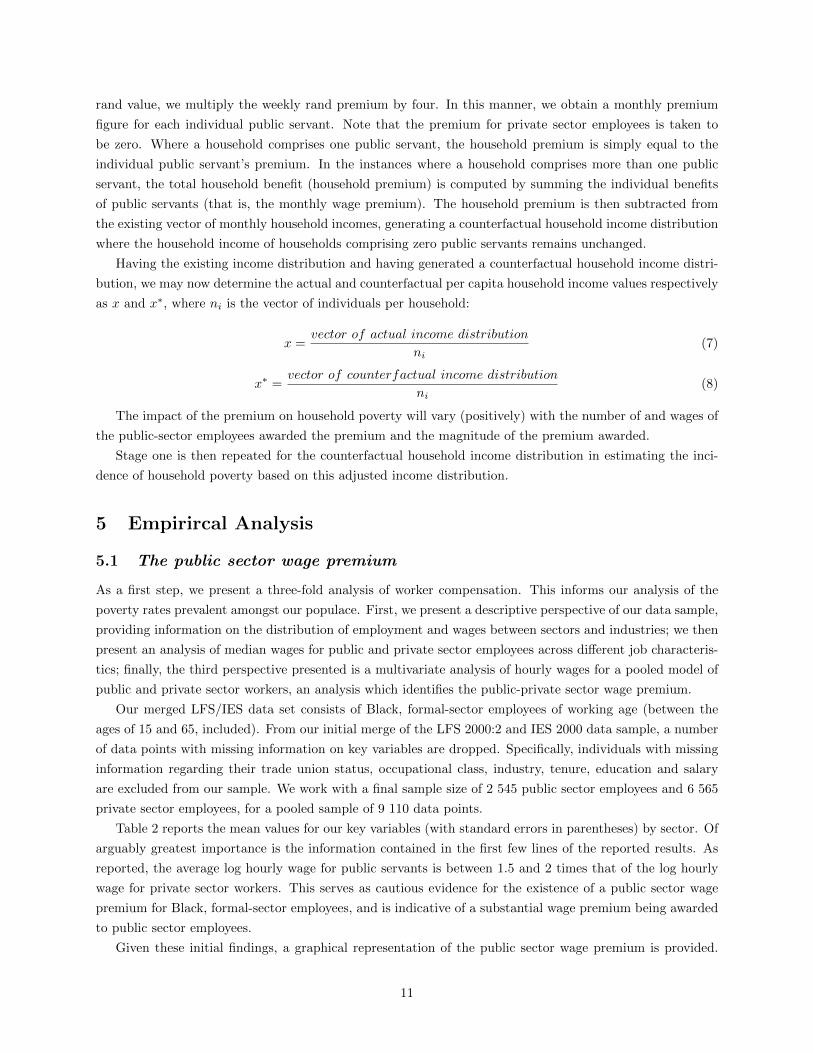
Having the existing income distribution and having generated a counterfactual household income distri-

bution, we may now determine the actual and counterfactual per capita household income values respectively

as x and x∗, where ni is the vector of individuals per household:

x =vector of actual income distribution

ni(7)

x∗ =vector of counterfactual income distribution

ni(8)

The impact of the premium on household poverty will vary (positively) with the number of and wages of

the public-sector employees awarded the premium and the magnitude of the premium awarded.

Stage one is then repeated for the counterfactual household income distribution in estimating the inci-

dence of household poverty based on this adjusted income distribution.

5 Empirircal Analysis

5.1 The public sector wage premium

As a first step, we present a three-fold analysis of worker compensation. This informs our analysis of the

poverty rates prevalent amongst our populace. First, we present a descriptive perspective of our data sample,

providing information on the distribution of employment and wages between sectors and industries; we then

present an analysis of median wages for public and private sector employees across different job characteris-

tics; finally, the third perspective presented is a multivariate analysis of hourly wages for a pooled model of

public and private sector workers, an analysis which identifies the public-private sector wage premium.

Our merged LFS/IES data set consists of Black, formal-sector employees of working age (between the

ages of 15 and 65, included). From our initial merge of the LFS 2000:2 and IES 2000 data sample, a number

of data points with missing information on key variables are dropped. Specifically, individuals with missing

information regarding their trade union status, occupational class, industry, tenure, education and salary

are excluded from our sample. We work with a final sample size of 2 545 public sector employees and 6 565

private sector employees, for a pooled sample of 9 110 data points.

Table 2 reports the mean values for our key variables (with standard errors in parentheses) by sector. Of

arguably greatest importance is the information contained in the first few lines of the reported results. As

reported, the average log hourly wage for public servants is between 1.5 and 2 times that of the log hourly

wage for private sector workers. This serves as cautious evidence for the existence of a public sector wage

premium for Black, formal-sector employees, and is indicative of a substantial wage premium being awarded

to public sector employees.

Given these initial findings, a graphical representation of the public sector wage premium is provided.

11

The use of a kernel density function allows the differences in the distribution of worker attributes across

the two sectors to be graphically exposed. The first density graph (figure 1) pertains to our total merged

LFS-IES data sample. As is evident, the log hourly wage for the public sector is right-shifted relative to

the analogous wage distribution of the private sector. This suggests that public sector workers earn more

than their private sector counterparts across quantiles of the wage distribution. As a further analysis, and

in striving for a robust graphical analysis, similar density graphs are reported for two subgroups of our

sample - a male sub-sample, and a female sub-sample. As the kernel density graphs indicate (figures 2 and

3), the female portion of the public sector has a larger degree of variation in log hourly wages. The male

sub-sample has a relatively normal distribution statistically. Thus, an analysis at the aggregate level (our

total sample) may appear distorted given that the male and female subgroups of our sample exhibit different

distributions of worker attributes; that is, while both subgroups reveal that there are proportionally more

workers possessing a higher level of human capital in the public sector when compared to the private sector,

the female subsample has a larger proportion of employees possessing a higher level of human capital in both

the public and private sectors (the graph for females has a higher degree of horizontal variation).

In light of this finding, the analysis of the public sector premium is extended and results are analysed

separately for households with a male vs. female head in order to ensure the robustness of the results of this

research paper.

As in Woolard (2002), a median comparison of public versus private wages in relation to a number

of variables is performed as an exploratory step. Median rather than mean wages are reported in that

comparisons may then be drawn between the wages of average workers rather than drawing a comparison of

average wages (which may be skewed by substantial outliers) (Woolard, 2002). Table 3 reports the results

of a median analysis. Note that all values are in rand terms. It is evident that public servants are earning

higher median wages than the comparable private workers with respect to all of our key variables. This

indicates that the wage distribution of the public sector remains right shifted (in comparisons drawn with

private sector wage distributions) across all categories when decomposed against worker characteristics. This

provides further evidence for human capital theory models postulating that the public sector employs workers

possessing a higher level of human capital when compared to the private sector; that is, core results remain

unchanged when wages are analysed in terms of worker-specific characteristics.

Having undertaken initial analyses, table 4 presents the results of the OLS mincerian regression function

detailed in stage two of the methodology section. Coefficients on all key variables are reported, with standard

errors and significance levels recorded. Of prime importance is the coefficient on the public sector dummy -

as noted previously, a positive and statistically significant coefficient indicates the existence of a public sector

wage premium. As reported in table 4, the coefficient of 0.259 is positive and significant at the 1% level.

This indicates that, after controlling for demographic, location and industry-occupation factors, public-sector

employees earn a wage premium over their private-sector counterparts. In order to identify the percentage

value of this premium, we adopt the statistic provided by Halvorsen and Palmquist (1980):

percent premium = [(eβ9 − 1)100] = [(e0.2587242 − 1)100] = 29.52995744% (9)

where β9 is the coefficient on the public sector dummy variable (see equation (2)).

This premium of 29.53% is quite substantial - the average Black public sector employee is earning up to

(approximately) 30% more than his/her private sector counterpart (after controlling for individual-specific

and job-specific characteristics).

Our regression equation produces an R-squared value of 55.5%. This implies that 55.5% of the variation

12

in wages is explained by the regressors of our OLS regression equation. The power of our regression analysis

and thus the magnitude of the public sector wage premium identified could be improved upon by running

a quantile regression analysis which would account for the presence of differing variances in the wage distri-

butions of the public and private sectors (as in Woolard, 2002). This is beyond the scope of this paper and

not deemed a necessary extrapolation as our premium result of 30% is almost identical to Woolards (2002)

statistic of 32% for Black South Africans.

Having obtained the actual percentage premium awarded to public sector employees, we obtained a

counterfactual income distribution, as detailed in the methodology section of this report, and perform the

poverty analysis presented below.

5.2 Poverty Analysis

In order to assess poverty at the household level for Black South Africans, we make use of three measures

of poverty at each of the three poverty lines (food, lower bound and upper bound) - the headcount poverty

index, the poverty gap measure, and the poverty severity measure, as discussed in methodology section. In

this analysis, the income levels referred to are the three poverty lines: the food poverty line, the lower bound

poverty line and the upper bound poverty line at R141 p.m., R209 p.m., and R308 p.m. respectively. The

discussion below refers to results presented in table 5.

In our analysis of the headcount poverty index, we look at the headcount poverty index at each of the three

poverty lines for the existing income distribution and compare these to the measures for the counterfactual

income distribution. We find that the proportion of the population considered “poor” sees a marginal

increase in the absence of a public sector wage premium. Specifically, the proportions of the population that

may be labelled “poor” relative to the food poverty line are 7.48% and 8.42% respectively for the actual and

counterfactual income distributions respectively; in terms of the LBPL, these proportions stand at 14.79%

and 16.48% respectively; finally, in relation to the upper bound poverty line these proportions stand at

25.64% and 27.60%, respectively. That is, the jump in the headcount index evident when the public sector

wage premium is removed from the wages of public sector employees varies between 0.94% for the FPL,

1.69% for the LBPL and 1.96% for the UBPL. Thus, in this instance, there is a positive effect on poverty

in the absence of the premium, indicating that the awarding of premiums by the state to public servants

reduces the incidence of poverty and improves the welfare of our household population (if only marginally).

Turning to the poverty gap measures at each of the three poverty lines for the actual versus counterfactual

income distributions, we see that, in relation to the FPL, the average percentage shortfalls in income for the

population stand at 2.50% and 2.83% respectively for the actual and counterfactual income distributions;

in terms of the LBPL, these percentages stand at 5.27% and 5.88% respectively; and finally, in relation

to the UBPL, these percentages stand at 10.01% and 10.99% respectively. It is therefore evident that the

netting out of the public sector wage premium is associated with a slight increase in the poverty gap for the

population in relation to all three of the poverty lines. In simple terms and in relation to the FPL, on average,

the poor have an expenditure shortfall of 2.50% of the poverty line when the existing income distribution is

utilised; additionally, when the counterfactual income distribution is utilised, on average, the poor have an

expenditure shortfall of 2.83% of the poverty line. Similar statements may be made in relation to the LBPL

and UBPL. Turning to the per capita cost of eliminating poverty (where “per capita” refers to an individual

household), we simply multiply each of our gap measures by the poverty line rand value - that is, the per

capita cost of eliminating poverty at the FPL in terms of the existing actual income distribution is R3.53,

and the corresponding figure in terms of the counterfactual income distribution is R3.99. It will therefore

13

cost more per capita to eliminate poverty in the absence of the public sector wage premium. Similarly, the

actual and counterfactual per capita costs of eliminating poverty in relation to the LBPL are R11.01 and

R12.29 respectively; and the actual and counterfactual per capita costs of eliminating poverty in relation to

the UBPL are R20.92 and R22.97 respectively.

Our findings thus indicate that in relation to each of our three poverty lines, the per capita cost of

eliminating poverty is lower when public servants are awarded a wage premium over their private sector

counterparts. Eliminating poverty in per capita terms at the food poverty line is cheaper by R0.46 when

public servants earn a wage premium, cheaper by R1.28 at the LBPL, and cheaper by R2.05 at the UBPL.

As is evident, there is a greater gap between the costs of eliminating poverty in relation to the actual versus

counterfactual income distributions the higher the poverty line being considered is.

Finally, we look at the poverty severity measures reported. The poverty severity index attaches a greater

weight to the “poorest among the poor”, where poorer individuals having larger poverty gaps contribute more

to this measure (Vecchi, 2007). This measure is not easily interpreted and is not widely used. The poverty

severity index is reported as a complement to the poverty gap measure, and both the poverty severity index

and the poverty gap measure are reported in order to provide an insight into poverty beyond the headcount

index. Generally, the finding for poverty severity is consistent with findings for the poverty head count and

poverty gap measures - that is, in the absence of a public sector wage premium, poverty severity increases.

5.3 Robustness Analysis

A final analysis is carried out in identifying whether the poverty effect of the public-sector wage premium

varies by household type (female vs. male headed households; households with single vs. multiple public

servants). Specifically, the three stages detailed in the methodology section of this paper are repeated for

these sub-samples of the household population.

5.3.1 Female-headed vs. Male-headed households

We first conduct two pieces of analysis distinguished by the gender of the household head of each of the

households comprising our sample. Results are reported in tables 6 and 7 for the male- and female-headed

sub-samples respectively.

When considering solely households whose household head is a male, the Mincerian regression equation

(2) yields a public sector wage premium of 26.34%, a premium somewhat smaller in magnitude than that

obtained for the entire data sample. When considering solely households whose household head is a female,

the Mincerian regression equation (2) yields a public sector wage premium of 36.64%, a premium somewhat

larger than that obtained for the entire data sample. This implies that separating households by household

head type will indeed impact upon the poverty results obtained. The relative magnitudes of the premiums

imply that females are more handsomely rewarded as state employees than males are.

In a comparison with our previous poverty results of table 5, we would expect a larger negative effect

on household poverty for the female-headed subsample, and a smaller negative effect on household poverty

for male-headed households. Comparing tables 6 and 7 to table 5, we see that results are as expected given

the magnitudes of the public sector wage premiums obtained. For the sample of households comprising

a male head, when analysing poverty based on the existing income distribution, the poverty measures are

between 4 and 0.05 percentage points lower than those obtained in table 5 for the headcount measure at

the UPL and the poverty gap measure at the FPL, respectively. With regards to the counterfactual income

14

distribution, the poverty measures are between 4.43 and 0.65 percentage points lower than those obtained

in table 5 for the headcount measure at the UPL and the poverty gap measure at the FPL, respectively. For

the sample of households comprising a female head, with regards to the existing income distribution, the

poverty measures are between 10.61 and 0.74 percentage points higher than those obtained in table 5 for the

headcount measure at the UPL and the poverty severity measure at the FPL, respectively. With regards to

the counterfactual income distribution, the poverty measures are between 11.97 and 0.87 percentage points

higher than those obtained in table 5 for the headcount measure at the UPL and the poverty severity measure

at the FPL, respectively. As is evident, the results are most different for the female headed households, ,

indicating that the poverty rates prevailing in the absence of the premium would be most severely felt by

households comprising a female head.

As is also expected, the poverty results pertaining to the counterfactual income distribution cast the

population as a “poorer” population when compared to the results pertaining to the existing income distri-

bution.

5.3.2 Households with one public servant vs. households with multiple public servants

We now conduct an analysis that incorporates data regarding the number of public servants comprising our

households. Specifically, an analysis is performed separately on a subsample of our households comprising

multiple public servants, and on a subsample of our households comprising a single public servant. Note

that households comprising no public servants are omitted in this analysis. Results are reported in tables 8

and 9.

When considering solely households comprising multiple public servants, the Mincerian regression equa-

tion (2) yields a public sector wage premium of 32.64%, a premium somewhat larger in magnitude than that

obtained when utilising the entire data sample. When considering solely households comprising only a single

public servant, the Mincerian regression equation (2) yields a public sector wage premium of 30.13%, again

a premium somewhat larger than that obtained when utilising the entire data sample. This implies that

separating households by the number of public servants comprising the household has an impact upon the

poverty results obtained.

In a comparison with our previous poverty results (table 5), we would expect a larger negative effect

on household poverty for both the subsamples of households comprising multiple public servants and those

comprising only a single public servant, with the negative effect relatively larger for households comprising

multiple public servants. Comparing tables 8 and 9 to table 5, we see that results are as expected. For the

sample of households comprising multiple public servants, with regards to the existing income distribution,

the poverty measures are between 3.67 and 0.28 percentage points higher than those obtained in table 5 for

the headcount measure at the UPL and the poverty severity measure at the FPL respectively. With regards

to the counterfactual income distribution, the poverty measures are between 4.43 and 0.65 percentage points

higher than those obtained in table 5 for the headcount measure at the UPL and the poverty gap measure at

the FPL respectively. For the sample of households comprising a single public servant, with regards to the

existing income distribution, the poverty measures are between 0.71 and 0.04 percentage points higher than

those obtained in table 5 for the headcount measure at the UPL and the poverty severity measure at the

FPL respectively. With regards to the counterfactual income distribution, the poverty measures are between

0.58 and zero percentage points higher than those obtained in table 5 for the headcount measure at the UPL

and the poverty severity measure at the FPL respectively. As is evident, the results are not significantly

different to those obtained when the entire sample is utilised as is.

15

As is expected, the poverty results pertaining to the counterfactual income distribution cast the popula-

tion as a “poorer” population when compared to the results pertaining to the existing income distribution

(the results for both distributions are, however, only marginally different).

We therefore find that an analysis that incorporates the type of household head may extend our findings

in a meaningful way, while an analysis in terms of number of public servants comprising a household holds

no econometric value in this instance.

Having performed a robustness analysis, we present a conclusion of our results in the context of the

objectives of this study.

6 Concluding Remarks

There are three core objectives to the analysis carried out in this research. The first involves an investigation

into the extent of the public-private sector wage differential pertaining to Black South Africans. The second

centres on identifying whether the public-private sector wage differential fuels or dampens the incidence of

household poverty among Black South Africans. The final objective is to provide a view on the robustness of

the findings of this study through investigating whether the poverty effect of the public-private sector wage

differential varies by household type.

With regards to our first objective, we find that a public sector wage premium of approximately 30% is

evident amongst the Black populace of South Africa. This result is in accord with our primary source of

reference, Woolard (2002) who conducts a similar analysis using solely Labour Force Survey 2000:2 data.

The premium identified is through a Mincerian earnings function controlling for worker-specific and job-

specific attributes, allowing us to net out the unexplained variation in earnings between public and private

employees, which is accrued by public servants as a wage premium.

When a counterfactual distribution of household income is constructed, we find that the awarding of

premiums by the state dampens the incidence, extent and severity of household poverty among Black South

Africans; that is, in the absence of the wage premium, the poverty indices cast the populace in poorer shape

than in the presence of the wage premium. This leads us to hesitantly accept the necessity of the state’s role

in the labour market.

Finally, looking to our third objective, we find that the poverty effect of the public-private sector wage

differential does vary by household type (female headed vs. male headed households), where female-headed

households are worse off. However, the poverty effect of the public-private sector wage differential does not

vary significantly between households with single vs. multiple public servants. We therefore find that an

analysis that incorporates the type of household head may extend our findings in a meaningful way, while

an analysis in terms of number of public servants comprising a household holds no econometric value in this

instance.

The results presented in this study suggest that the public sector wage premium enjoyed by state employ-

ees is awarded to those employees who would otherwise be at the lower end of the income distribution. This

is evident in that the inclusion of the premium in the analysis of poverty lowers the household poverty rate

for Black South Africans that would prevail in its absence. These results hold when an analysis is conducted

on subsamples of the household population, suggesting the robustness of the results here obtained. Our

results imply that the state plays a somewhat important role in poverty alleviation solely by awarding a

public sector wage premium, regardless of their reasons for so doing.

There are a number of limitations pertaining to this research study. The first and most notable limitation

16

of the methodology adopted in identifying and attaching a magnitude to the public sector wage premium is

that sample selection bias is not accounted for. Selection bias exists if workers are not randomly distributed

across the public and private sectors. This is plausible in the case that there exists a wage differential

between the two sectors. Selection bias is a potential issue in the OLS estimates obtained in this study.

Thus, our premium results and the poverty effects are only suggestive of whether the state dampens or fuels

the household poverty rate among Black South Africans, but does not identify the exact magnitude of this

effect. Future research may identify instruments to address the problem of sample selection bias in the wage

functions.

A further concern is the lack of an appropriate counterfactual for the absence of a public-sector wage

premium; that is to say, if a public-sector wage premium was not accrued to the employees comprising the

public service of South African, could the resources that would otherwise have provided the premium be

used to greater effect in combatting poverty in the country? This is forefront in research of this slant as

it contributes answers towards the impact of the premium on household poverty. This leads to questions

around the productivity of the public sector, and a concern arises around whether the reduction in poverty

would be greater if the resources paying for a public-sector premium were instead a contributor to a private-

sector wage subsidy. Although a forecast of the path of general equilibrium in the labour market in the

absence of the premium is almost impossible, there is reason to postulate that a reduction/elimination of

the public-sector wage premium would result in a lower incidence of poverty in the country. On the other

hand, it is ultimately probable that the public-sector wage premium is transmitted in such a way through

the economy that this so-called fiscal stimulus may be reducing poverty in households across South Africa,

even for those households without a member belonging to the public sector.

A final limitation of this research study is that the merged data set analysed comprises only 9 110 sample

points. Perhaps, a merge of more recent/current LFS and IES data sets will produce a larger sample size

and thus ensure robustness in terms of the representation of the entire Black South African populace. Future

research may employ the latest published waves of the Labour Force Survey and the Income and Expenditure

Survey and yield more relevant and informative results.

17

References[1] Adamchick, V.; Bedi, A. (2000), Wage differentials between the public and the private sectors: evidence

from an economy in transition, Labour Economics, 7, pp. 203-224.

[2] Aminue, A. (2011). ”Government Wage Review Policy and Public-Private Sector Wage Differential in

Nigeria.”AERC Research Paper 223, African Economic Research Consortium, Nairobi.

[3] Anghel, B., S. de la Rica, and J. Dolado (2011) .The Eect of Public Sector Employment on Women’s

Labour Martket Outcomes., FEDEA Working Paper No. 2011-08.

[4] Bargain, O.; Melly, B. (2008), Public Sector Pay Gap in France: New Evidence using Panel Data, IZA,

DP 3427, April.

[5] Barrett, C.B., Carter, M.R., and Ikegmai, M. (2006). Threshold-targeted Social Protection to Overcome

Poverty Traps and Aid Traps, University of Wisconsin.

[6] Becker, G. (1964), Human Capital, Princeton University Press: Princeton, NJ.

[7] Bender, K. and Elliot, R. (2002). The role of job attributes in understanding the public-private wage

differential. Industrial Relations 41, 407-421.

[8] Bender, K.A. (2003). ”Examining Equality Between Public and Private Sector Wage Distributions.”

Economic Inquiry, 41(1), 62-79.

[9] Bhorat, H., Kanbur, K., and Stanwix, B. (2015). Minimum Wages in Sub-Saharan Africa: A Primer.

Development Policy Research Unit, WP 201503.

[10] Borjas, G. (2002) .The Wage Structure and the Sorting of Workers into the Public Sector., NBER

Working Paper No. 9313.

[11] Bosch, A. (2006). Determinants of public and private-sector wages in South Africa. Research Depart-

ment, South African Reserve Bank.

[12] Boudarbat, B. 2004. Employment sector choice in a developing labour market. Mimeo. Department of

Economics, University of British Columbia.

[13] Campos, M.; Centeno, M. (2012), Public-private Wage Gaps in the Period Prior to the Adoption of the

Euro: An Aplication Based on Longitudinal Data, Banco de Portugal, WP 1/2012, January.

[14] Casale, D. & Posel, D. (2011). Unions and the Gender Wage Gap in South Africa, Journal of African

Economies, first published online August 3, 2010.

[15] Christofides, L., and Pashardes, P. (2002). Self/paid-employment, public/private sector selection, and

wage differentials. Labour Economics 9, 737-762.

[16] Christopoulou, R.; Monastiriotis, V. (2013), The Greek Public Sector Wage Premium before the Cri-

sis: Size, Selecction and Relative Valuation of Characteristics, British Journal of Industrial Relations,

doi: 10.1111/bjir.12023.

[17] Coppola, A., and Calvo-Gonzalez, O. (2011). Higher wages, lower pay: Public vs. private sector

compensation in Peru. The World Bank, Policy Research Working Paper 5858.

[18] Corbo, Vittorio, and Morton Stelcner. 1983. ”Earnings Determination and Labour Markets: Gran

18

Santiago, 1978.” Journal of Development Economics 12, no. 3: 251-66.

[19] Cousineau, J.M. and R. Lacroix. 1977. Wage Determination in Major Collective Agreements in the

Private and Public Sectors. Ottawa: Economic Council of Canada.

[20] De Castro, F., M. Salto, and H. Steiner (2013) .The gap between public and private wages: new evidence

for the EU., European Economy. Economic Papers 508.

[21] Depalo, D., Giordano, R.; Papapetrou, E. (2013), Public-private wage differentials in euro rea countries:

evidence from quantile decomposition analysis, Banca dItalia, Working paper 907.

[22] Dickens, W., Lang, K., (1985), ”A Test of Dual Labour Market Theory”, American Economic Review,

75, p. 792-805.

[23] Dustmann, C. and A. Van Soest (1997) .Wage Structures in the Private and Public Sectors in West

Germany., Fiscal Studies, vol. 18, pp. 225-247.

[24] Dustman, C.; van Soest, C. (1998), Public and private sector wages of male workers in Germany.

European Economic Review, 42, pgs.14171441.

[25] Elsenburg. (2005). Creating a 2000 IES-LFS Database in Stata. The Provincial Decision-making En-

abling Project, Technical Paper 2005: 1.

[26] E. M. (2008), A Quantile Regression Analysis of Wages in Panama. Review of Development Economics,

12: 498514. doi: 10.1111/j.1467-9361

[27] Esanov, A. (2006). The Growth-Poverty Nexus: Evidence From Kazakhstan (Asian Development Bank

(ADB) Institute Discussion Paper. No. 51). ADB: Tokyo.

[28] Foster, J.E., Gree, J., and Thorbecke, E. (2010). ”The Foster-Greer-Thorbecke (FGT) Poverty Measures:

Twenty-Fiver Years Later.” Institute for International Economic Policy, 2010:14.

[29] Garca-Prez, I. and J. Jimeno (2007) .Public Sector Wage Gaps in Spanish Regions., The Manchester

School, vol. 75, pp 501-531.

[30] Geary, J., and Murphy, A, (2011). ”The Reform of Public Sector Pay in Ireland under Social Pacts.”

[31] Giordano, R. et al. (2011), The Public Sector Pay Gap in a Selection of Euro Area Countries, ECB,

Working Papers Series n.1406/December 2011.

[32] Gradin, C., del Rio, C., and Canto, O. (2010). Gender wage discrimination and poverty in the EU.

Feminist Economics, 16: 2, 73 109.

[33] Gunderson, M. (1979). ”Earning differentials between the public and private sectors.” Canadian Journal

of Economics, XII(2): 228-42.

[34] Hartog, J.; Oosterbeck, H. (1993), Public and private sector wages in the Netherlands, European Eco-

nomic Review, 37, pp. 97-114.

[35] Haughton, J., and Khandker, S.R. (2005). ”Handbook on Poverty and Inequality.” Washington, DC:

World Bank.

[36] Hyder, A. and B. Reilly. 2005. The public sector pay gap in Pakistan: A quantile regressionanalysis.

PRUS Working Paper No. 33. Poverty Research Unit at Sussex, University of Sussex,Brighton.

19

[37] Kerr, A., Teal, F. (2012). Determinants of wage inequalities: Panel data evidence from South Africa.

Institute for the Study of Labour, IZA Discussion Paper No. 6534.

[38] Lassibille, G. (1998). Wage gaps between the public and private sector in Spain. Economics of Education

Review, 17(1), pp. 83-92.

[39] Lindauer, D.L. and R.H. Sabot. 1983. The publicprivate wage differential in a poor urban economy.

Journal of Development Economics, 12(3): 13752.

[40] Maczulskij, t. (2013). Economics of wage differentials and public sector labour markets. Jyvaskyla

Studies in Business and Economics 125.

[41] May, J. (2011). Smoke and mirrors: The science of poverty measurement and its application.

[42] Melly, B. (2003). Public-private sector wage differentials in Germany: evidence from quantile regression.

Swiss Institute for International Economics and Applied Economic Research (SIAW).

[43] Melly, B. (2005). Public-private sector wage differentials in Germany: Evidence from quantile regression.

Empirical Economics, 30:505-520.

[44] Mizala, A.; Romaguera, P.; Gallegos, S. (2011): ”Public-private wage gap in Latin America (1992-2007):

A matching approach”, Labour Economics 18 (S1), pp. S115-S131.

[45] Mohan, Rakesh. 1986. Work, Wages, and Welfare in a Developing Metropolis: Consequences of Growth

in Bogota, Colombia. New York: Oxford University Press.

[46] Morduch, J. (2006). Poverty Measures. Handbook on Poverty Statistics: Concepts, Methods and Policy

Use. Chapter III. UNSD.

[47] Mutasa, G. (2012). Disability Grant and Individual Labour Force Participation: The Case of South

Africa. Development Policy Research Unit, WP12/156.

[48] Nicolson, G. (2015). South Africa: Where 12 million live in extreme poverty. Daily Maverick.

[49] Nielsen, H.S., Rosholm, M. (2001). The public-private sector wage gap in Zambia in the 1990s: A

quantile regression approach. Empirical Economics 26: 169-182.

[50] Ntuli, M., and Kwenda, P. (2014). Private Returns to Education, Migration and Development Policies:

The Case of Zimbabwe. African Development Review, Volume 26, Issue 4, pages 535-548.

[51] Oosthuizen, M. (2013). ”Inflation Inequality in South Africa.” Development Policy Research Unit,

WP13/158.

[52] Panizza, U. and C. Qiang (2005) .Public.private wage dierential and gender gap in Latin America:

Spoiled bureaucrats and exploited women?. , The Journal of Socio-Economics, vol. 34, pp. 810-833.

[53] Posel D. & Rogan M. (2009). Women, Income and Poverty: Gendered Access to Resources in PostApartheid

South Africa. Agenda 23 (81): 2534.

[54] [7] Preston, M.H. 1986. The elementary macroeconomic consequences of differing public and private

sector wages. Public Finance, XXXXI(2): 17381.

[55] Ramoni, J., and Bellante, D. (2004). The relative pay of public employees in the U.S.: An assessment

of Empirical Research. International Business and Economics Research Journal, Volume 3, Number 11.

20

[56] Ramoni-Perazzi, J.; Bellante, D. (2006), Wage Differentials Between The Public And The Private Sector:

How Comparable Are The Workers?, Journal of Business & Economics Research, 4 (5),May, pp. 43-56.

[57] Ramos, R., Sanroma, E., Simon, H. (2014). ”Public-Private Sector Wage Differentials by Type of

Contract: Evidence from Spain.” IZA Discussion Paper No. 8158.

[58] Ravallion, M. 2009. Why Dont We See Poverty Convergence? Policy Research Working Paper No. 4974,

World Bank, Washington, DC.

[59] Samer Al-Samarrai & Barry Reilly, 2005. ”Education, Employment and Earnings of Secondary School-

Leavers in Tanzania: Evidence from a Tracer Study,” PRUS Working Papers 31, Poverty Research Unit

at Sussex, University of Sussex.

[60] Skyt-Neilsen, H. and M. Rosholm. 2001. The public sector wage gap in Zambia in the 1990s: Aquantile

regression approach. Empirical Economics, 26: 16982

[61] Smith, S. (1976) .Pay differentials between federal government and private sectors workers., Industrial

and Labour Relations Review, vol. 29, pp. 233.257.

[62] Statistics South Africa. (2008). Measuring poverty in South Africa: Methodological report on the

development of the poverty lines for statistical reporting. Technical Report D0300.

[63] Statistics South Africa. (2014). Poverty trends in South Africa: An examination of absolute poverty

between 2006 and 2011. Report No. 03-10-06.

[64] Statistics South Africa. (2015). Methodological report on rebasing of national poverty lines and devel-

opment on pilot provincial poverty lines. Technical Report No. 03-10-11.

[65] Van der Gaag, Jacques, and W. P. M. Vijverberg. 1988. ”A Switching Regression Model for Wage

Determinants in the Public and Private Sectors of a Developing Country.” Review of Economics and

Statistics 70, no. 2: 244-52.

[66] Woolard, I. (2002). A comparison of wage levels and wage inequality in the public and private sectors,

1995 and 2000. Development Policy Research Unit, Working paper 02/62.

[67] World Bank. (2013). The State of the Poor.

[68] Zweimuller, J.; Winter-Ebmer, R. (1994), Gender wage differentials in private and public sector jobs,Journal

of Population Economics, 7 (1994), pp. 271-285

21

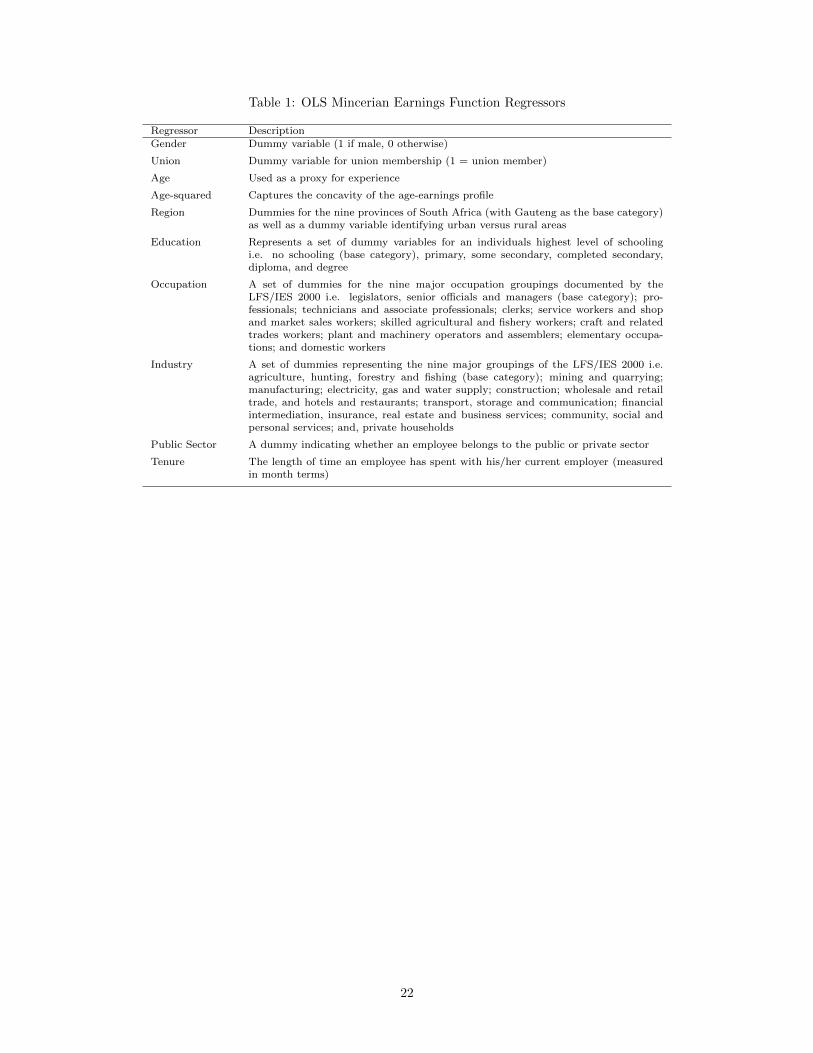
Table 1: OLS Mincerian Earnings Function Regressors

Regressor DescriptionGender Dummy variable (1 if male, 0 otherwise)

Union Dummy variable for union membership (1 = union member)

Age Used as a proxy for experience

Age-squared Captures the concavity of the age-earnings profile

Region Dummies for the nine provinces of South Africa (with Gauteng as the base category)as well as a dummy variable identifying urban versus rural areas

Education Represents a set of dummy variables for an individuals highest level of schoolingi.e. no schooling (base category), primary, some secondary, completed secondary,diploma, and degree

Occupation A set of dummies for the nine major occupation groupings documented by theLFS/IES 2000 i.e. legislators, senior officials and managers (base category); pro-fessionals; technicians and associate professionals; clerks; service workers and shopand market sales workers; skilled agricultural and fishery workers; craft and relatedtrades workers; plant and machinery operators and assemblers; elementary occupa-tions; and domestic workers

Industry A set of dummies representing the nine major groupings of the LFS/IES 2000 i.e.agriculture, hunting, forestry and fishing (base category); mining and quarrying;manufacturing; electricity, gas and water supply; construction; wholesale and retailtrade, and hotels and restaurants; transport, storage and communication; financialintermediation, insurance, real estate and business services; community, social andpersonal services; and, private households

Public Sector A dummy indicating whether an employee belongs to the public or private sector

Tenure The length of time an employee has spent with his/her current employer (measuredin month terms)

22

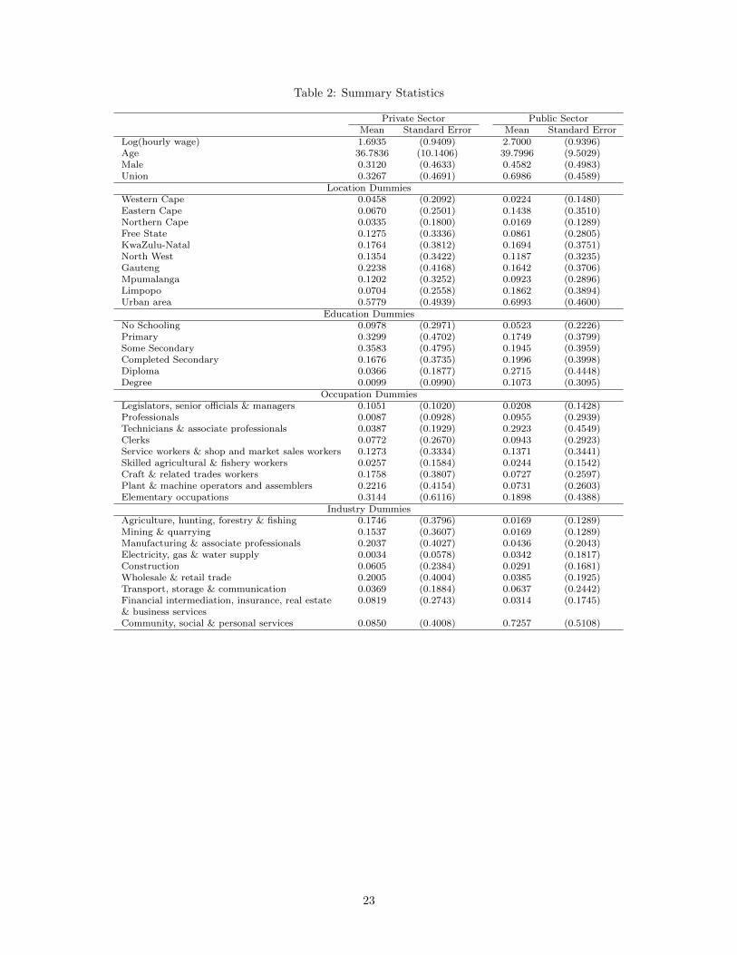
Table 2: Summary Statistics

Private Sector Public SectorMean Standard Error Mean Standard Error

Log(hourly wage) 1.6935 (0.9409) 2.7000 (0.9396)Age 36.7836 (10.1406) 39.7996 (9.5029)Male 0.3120 (0.4633) 0.4582 (0.4983)Union 0.3267 (0.4691) 0.6986 (0.4589)

Location DummiesWestern Cape 0.0458 (0.2092) 0.0224 (0.1480)Eastern Cape 0.0670 (0.2501) 0.1438 (0.3510)Northern Cape 0.0335 (0.1800) 0.0169 (0.1289)Free State 0.1275 (0.3336) 0.0861 (0.2805)KwaZulu-Natal 0.1764 (0.3812) 0.1694 (0.3751)North West 0.1354 (0.3422) 0.1187 (0.3235)Gauteng 0.2238 (0.4168) 0.1642 (0.3706)Mpumalanga 0.1202 (0.3252) 0.0923 (0.2896)Limpopo 0.0704 (0.2558) 0.1862 (0.3894)Urban area 0.5779 (0.4939) 0.6993 (0.4600)

Education DummiesNo Schooling 0.0978 (0.2971) 0.0523 (0.2226)Primary 0.3299 (0.4702) 0.1749 (0.3799)Some Secondary 0.3583 (0.4795) 0.1945 (0.3959)Completed Secondary 0.1676 (0.3735) 0.1996 (0.3998)Diploma 0.0366 (0.1877) 0.2715 (0.4448)Degree 0.0099 (0.0990) 0.1073 (0.3095)

Occupation DummiesLegislators, senior officials & managers 0.1051 (0.1020) 0.0208 (0.1428)Professionals 0.0087 (0.0928) 0.0955 (0.2939)Technicians & associate professionals 0.0387 (0.1929) 0.2923 (0.4549)Clerks 0.0772 (0.2670) 0.0943 (0.2923)Service workers & shop and market sales workers 0.1273 (0.3334) 0.1371 (0.3441)Skilled agricultural & fishery workers 0.0257 (0.1584) 0.0244 (0.1542)Craft & related trades workers 0.1758 (0.3807) 0.0727 (0.2597)Plant & machine operators and assemblers 0.2216 (0.4154) 0.0731 (0.2603)Elementary occupations 0.3144 (0.6116) 0.1898 (0.4388)

Industry DummiesAgriculture, hunting, forestry & fishing 0.1746 (0.3796) 0.0169 (0.1289)Mining & quarrying 0.1537 (0.3607) 0.0169 (0.1289)Manufacturing & associate professionals 0.2037 (0.4027) 0.0436 (0.2043)Electricity, gas & water supply 0.0034 (0.0578) 0.0342 (0.1817)Construction 0.0605 (0.2384) 0.0291 (0.1681)Wholesale & retail trade 0.2005 (0.4004) 0.0385 (0.1925)Transport, storage & communication 0.0369 (0.1884) 0.0637 (0.2442)Financial intermediation, insurance, real estate 0.0819 (0.2743) 0.0314 (0.1745)& business servicesCommunity, social & personal services 0.0850 (0.4008) 0.7257 (0.5108)

23

Table 3: A median analysis of our data sample by sector

Median Hourly WagePublic Sector Private Sector

GenderMale 14.02 6.67Female 17.86 4.17

Trade Union MembershipMembers 18.66 8.93Non-members 8.93 4.31

AreaUrban 16.67 7.14Rural 12.86 3.65

Occupational ClassLegislators, senior officials & managers 43.75 16.72Professionals 35.00 25.00Technicians & associate professionals 25.41 10.23Clerks 15.63 9.38Service workers & shop & market sales workers 13.89 5.42Skilled agricultural & fishery workers 8.95 3.00Craft & related trades workers 10.99 7.00Plant & machine operators & assemblers 10.73 7.50Elementary occupations 8.33 3.57

IndustryAgriculture, hunting, forestry & fishing 4.44 2.04Mining & quarrying 11.12 9.38Manufacturing 8.62 7.29Electricity, gas & water supply 12.14 10.00Construction 8.23 5.00Wholesale & retail trade 7.32 5.71Transport, storage & communication 12.50 7.18Financial intermediation, insurance, real estate & business services 8.84 7.00Community, social & personal services 18.89 6.25Other 5.44 2.22

Educational AttainmentNo schooling 8.50 3.00Primary 8.75 4.76Some secondary 11.25 6.25Completed secondary 14.66 7.50Diploma 27.66 13.75Degree 35.71 26.04

ProvinceWestern Cape 12.50 5.06Eastern Cape 21.50 4.45Northern Cape 16.07 3.89Free State 15.63 4.17Kwa-Zulu Natal 12.50 4.53North-West 15.63 7.50Gauteng 15.09 8.33Mpumalanga 12.31 5.20Limpopo 17.85 3.26

24

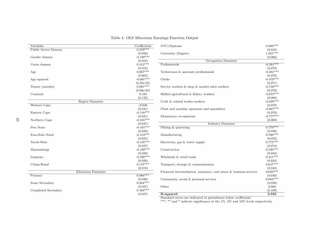
Table 4: OLS Mincerian Earnings Function Output

Variables Coefficients NTC/Diploma 0.898***Public Sector Dummy 0.259*** (0.045)

(0.026) University (Degree) 1.021***Gender dummy -0.198*** (0.066)

(0.018) Occupation DummiesUnion dummy 0.312*** Professionals -0.284***

(0.018) (0.079)Age 0.067*** Technicians & associate professionals -0.401***

(0.005) (0.070)Age squared -0.001*** Clerks -0.470***

(6.35e-05) (0.071)Tenure (months) 0.001*** Service workers & shop & market sales workers -0.738***

(9.68e-05) (0.070)Constant 0.182 Skilled agricultural & fishery workers -0.675***

(0.125) (0.086)Region Dummies Craft & related trades workers -0.629***

Western Cape -0.040 (0.070)(0.041) Plant and machine operators and assemblers -0.667***

Eastern Cape -0.148*** (0.070)(0.031) Elementary occupations -0.777***

Northern Cape -0.165*** (0.069)(0.047) Industry Dummies

Free State -0.435*** Mining & quarrying 0.776***(0.029) (0.036)

Kwa-Zulu Natal -0.154*** Manufacturing 0.590***(0.025) (0.033)

North-West -0.135*** Electricity, gas & water supply 0.775***(0.027) (0.074)

Mpumalanga -0.199*** Construction 0.536***(0.029) (0.043)

Limpopo -0.290*** Wholesale & retail trade 0.451***(0.030) (0.033)

Urban-Rural 0.147*** Transport, storage & communication 0.647***(0.019) (0.045)

Education Dummies Financial intermediation, insurance, real estate & business services 0.650***Primary 0.086*** (0.040)

(0.030) Community, social & personal services 0.684***Some Secondary 0.264*** (0.038)

(0.031) Other 0.068Completed Secondary 0.483*** (0.109)

(0.037) R-squared 0.555Standard errors are indicated in parentheses below coefficients***, ** and * indicate significance at the 1%, 5% and 10% levels respectively

25

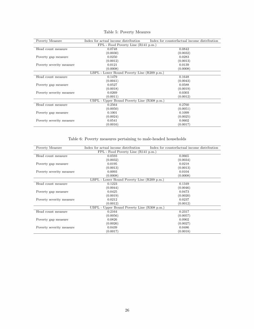
Table 5: Poverty Meaures

Poverty Measure Index for actual income distribution Index for counterfactual income distributionFPL - Food Poverty Line (R141 p.m.)

Head count measure 0.0748 0.0842(0.0030) (0.0032)

Poverty gap measure 0.0250 0.0283(0.0012) (0.0013)

Poverty severity measure 0.0121 0.0139(0.0008) (0.0008)

LBPL - Lower Bound Poverty Line (R209 p.m.)Head count measure 0.1479 0.1648

(0.0041) (0.0043)Poverty gap measure 0.0527 0.0588

(0.0018) (0.0019)Poverty severity measure 0.0269 0.0303

(0.0011) (0.0012)UBPL - Upper Bound Poverty Line (R308 p.m.)

Head count measure 0.2564 0.2760(0.0050) (0.0051)

Poverty gap measure 0.1001 0.1099(0.0024) (0.0025)

Poverty severity measure 0.0541 0.0602(0.0016) (0.0017)

Table 6: Poverty measures pertaining to male-headed households

Poverty Measure Index for actual income distribution Index for counterfactual income distributionFPL - Food Poverty Line (R141 p.m.)

Head count measure 0.0593 0.0665(0.0032) (0.0034)

Poverty gap measure 0.0195 0.0218(0.0013) (0.0013)

Poverty severity measure 0.0093 0.0104(0.0008) (0.0008)

LBPL - Lower Bound Poverty Line (R209 p.m.)Head count measure 0.1223 0.1349

(0.0044) (0.0046)Poverty gap measure 0.0425 0.0473

(0.0019) (0.0020)Poverty severity measure 0.0212 0.0237

(0.0012) (0.0012)UBPL - Upper Bound Poverty Line (R308 p.m.)

Head count measure 0.2164 0.2317(0.0056) (0.0057)

Poverty gap measure 0.0826 0.0902(0.0026) (0.0027)

Poverty severity measure 0.0439 0.0486(0.0017) (0.0018)

26

Table 7: Poverty measures pertaining to female-headed households

Poverty Measure Index for actual income distribution Index for counterfactual income distributionFPL - Food Poverty Line (R141 p.m.)

Head count measure 0.1158 0.1274(0.0070) (0.0073)

Poverty gap measure 0.0398 0.0448(0.0029) (0.0032)

Poverty severity measure 0.0195 0.0226(0.0018) (0.0020)

LBPL - Lower Bound Poverty Line (R209 p.m.)Head count measure 0.2157 0.2413

(0.0090) (0.0094)Poverty gap measure 0.0796 0.0890

(0.0041) (0.0043)Poverty severity measure 0.0418 0.0471

(0.0027) (0.0029)UBPL - Upper Bound Poverty Line (R308 p.m.)

Head count measure 0.3625 0.3957(0.0106) (0.0107)

Poverty gap measure 0.1464 0.1624(0.0054) (0.0056)

Poverty severity measure 0.0811 0.0906(0.0037) (0.0039)

Table 8: Poverty measures pertaining to households with multiple public servants

Poverty Measure Index for actual income distribution Index for counterfactual income distributionFPL - Food Poverty Line (R141 p.m.)

Head count measure 0.0899 0.0913(0.0038) (0.0038)

Poverty gap measure 0.0305 0.0309(0.0016) (0.0016)

Poverty severity measure 0.0149 0.0151(0.0010) (0.0010)

LBPL - Lower Bound Poverty Line (R209 p.m.)Head count measure 0.1729 0.1755

(0.0050) (0.0051)Poverty gap measure 0.0628 0.0638

(0.0022) (0.0023)Poverty severity measure 0.0324 0.0329

(0.0014) (0.0015)UBPL - Upper Bound Poverty Line (R308 p.m.)

Head count measure 0.2931 0.2954(0.0060) (0.0061)

Poverty gap measure 0.1167 0.1182(0.0030) (0.0030)

Poverty severity measure 0.0641 0.0650(0.0020) (0.0021)

27

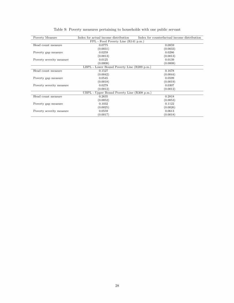
Table 9: Poverty measures pertaining to households with one public servant

Poverty Measure Index for actual income distribution Index for counterfactual income distributionFPL - Food Poverty Line (R141 p.m.)

Head count measure 0.0775 0.0859(0.0031) (0.0033)

Poverty gap measure 0.0259 0.0286(0.0013) (0.0013)

Poverty severity measure 0.0125 0.0139(0.0008) (0.0008)

LBPL - Lower Bound Poverty Line (R209 p.m.)Head count measure 0.1527 0.1678

(0.0042) (0.0044)Poverty gap measure 0.0545 0.0599

(0.0018) (0.0019)Poverty severity measure 0.0278 0.0307

(0.0012) (0.0012)UBPL - Upper Bound Poverty Line (R308 p.m.)

Head count measure 0.2635 0.2818(0.0052) (0.0053)

Poverty gap measure 0.1032 0.1122(0.0025) (0.0026)

Poverty severity measure 0.0559 0.0613(0.0017) (0.0018)

28

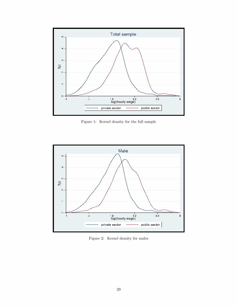
Figure 1: Kernel density for the full sample

Figure 2: Kernel density for males

29

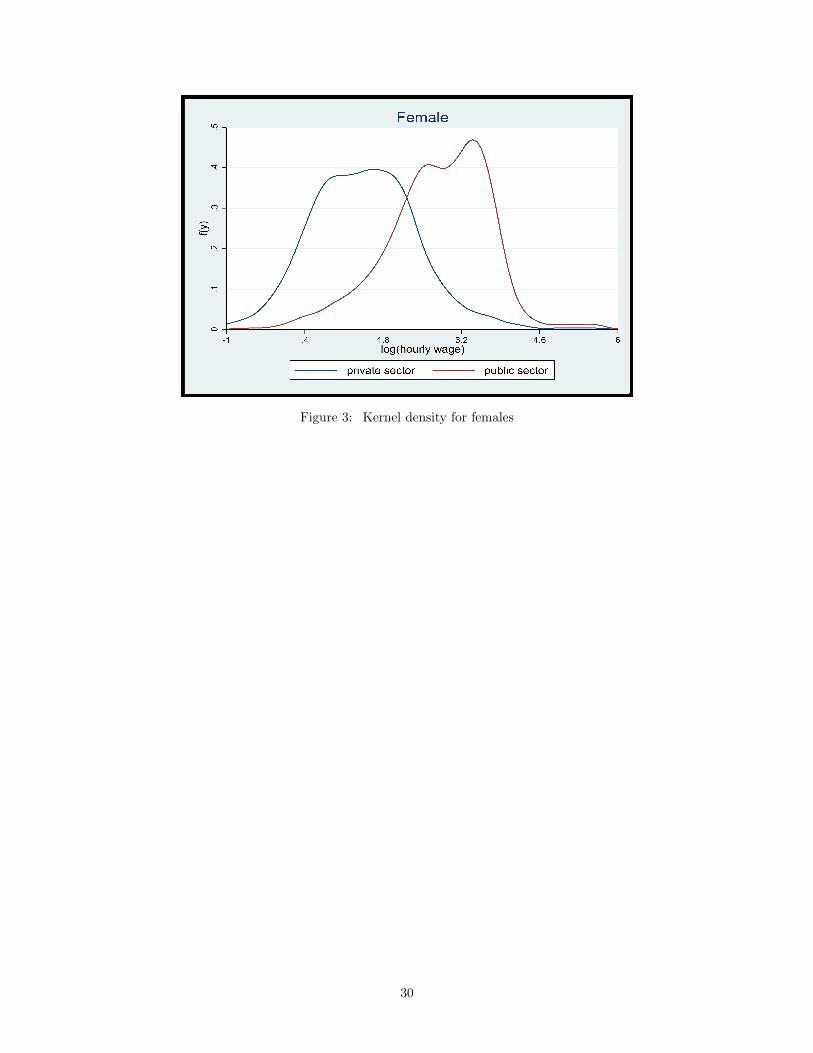
Figure 3: Kernel density for females

30