ORNL/TM-2013/26

Phenylnaphthalene as a Heat Transfer Fluid for Concentrating Solar Power: Loop Tests and Final Report

February 2013 Prepared by J. McFarlane J.R. Bell D.K. Felde R.A. Joseph III A.L. Qualls S.P. Weaver

DOCUMENT AVAILABILITY Reports produced after January 1, 1996, are generally available free via the U.S. Department of Energy (DOE) Information Bridge. Web site http://www.osti.gov/bridge Reports produced before January 1, 1996, may be purchased by members of the public from the following source. National Technical Information Service 5285 Port Royal Road Springfield, VA 22161 Telephone 703-605-6000 (1-800-553-6847) TDD 703-487-4639 Fax 703-605-6900 E-mail info@ntis.gov Web site http://www.ntis.gov/support/ordernowabout.htm Reports are available to DOE employees, DOE contractors, Energy Technology Data Exchange (ETDE) representatives, and International Nuclear Information System (INIS) representatives from the following source. Office of Scientific and Technical Information P.O. Box 62 Oak Ridge, TN 37831 Telephone 865-576-8401 Fax 865-576-5728 E-mail reports@osti.gov Web site http://www.osti.gov/contact.html

This report was prepared as an account of work sponsored by an agency of the United States Government. Neither the United States Government nor any agency thereof, nor any of their employees, makes any warranty, express or implied, or assumes any legal liability or responsibility for the accuracy, completeness, or usefulness of any information, apparatus, product, or process disclosed, or represents that its use would not infringe privately owned rights. Reference herein to any specific commercial product, process, or service by trade name, trademark, manufacturer, or otherwise, does not necessarily constitute or imply its endorsement, recommendation, or favoring by the United States Government or any agency thereof. The views and opinions of authors expressed herein do not necessarily state or reflect those of the United States Government or any agency thereof.

ORNL/TM-2013/26

Energy and Transportation Science Division

PHENYLNAPHTHALENE AS A HEAT TRANSER FLUID FOR CONCENTRATING SOLAR POWER: LOOP TESTS AND FINAL REPORT

J. McFarlane J.R. Bell

D.K. Felde R.A. Joseph, III

A.L. Qualls S.P. Weaver

February 2013

Prepared by OAK RIDGE NATIONAL LABORATORY

Oak Ridge, Tennessee 37831-6181 managed by

UT-BATTELLE, LLC for the

U.S. DEPARTMENT OF ENERGY under contract DE-AC05-00OR22725

iii

CONTENTS

Page LIST OF FIGURES ................................................................................................................................ v LIST OF TABLES ............................................................................................................................... vii ACRONYMS ........................................................................................................................................ ix ACKNOWLEDMENTS ........................................................................................................................ xi EXECUTIVE SUMMARY ................................................................................................................. xiii ABSTRACT ........................................................................................................................................... 1 1. INTRODUCTION ........................................................................................................................... 1 2. ALTERNATIVE SYNTHETIC PATHWAYS OF 1-PHENYLNAPHTHALENE ........................ 3 3. THERMODYNAMIC DATA AND STATIC TESTS .................................................................... 7 4. LOOP TESTING ........................................................................................................................... 11

4.1 APPARATUS ...................................................................................................................... 11 4.2 HEATING TESTS ............................................................................................................... 13 4.3 ANALYSIS AND RESULTS .............................................................................................. 14

5. POWER CYCLE ANALYSIS IN A PILOT-SCALE SOLAR LOOP .......................................... 17 5.1 PHASE 1 – LEVELIZED COST OF ENERGY ANALYSIS ............................................. 17 5.2 PHASE 2 – PILOT-SCALE SOLAR COLLECTION AND STIRLING POWER

CYCLE ................................................................................................................................. 18 5.3 PHASE 3 – COUPLED STIRLING ENGINE POWER GENERATION ........................... 19

6. DISCUSSION AND CONCLUSIONS ......................................................................................... 21 7. REFERENCES .............................................................................................................................. 23 Appendix A: FINAL REPORT COOL ENERGY INC ..................................................................... A-1

v

LIST OF FIGURES

Figure Page 1 Suzuki-Miyaura coupling scheme for production of 1-phenylnaphthalene ........................ 3 2 Scaled up apparatus showing production in a 3L flask ....................................................... 4 3 Phosphine ligand choices .................................................................................................... 5 4 Arrhenius plot of vapor pressure as a function of reciprocal temperature .......................... 7 5 Effect of temperatures on fluid heated for 1 week .............................................................. 8 6 Details of temperature increase after start of heating and temperature decrease ................ 9 7 Analysis of samples heated for varying lengths of time ..................................................... 9 8 Fe3O4 nanoparticles reduce turbidity and light scattering ................................................. 10 9 Components of high-temperature loop ...................................................................................... 12 10 Engineering drawing of 2400 kW heater in high-temperature loop ..................................... 13 11 Graphics of loop components from programmable logic control software ......................... 14 12 Loop temperature profiles ................................................................................................. 14 13 Chemical changes in fluid from loop testing. ................................................................... 16 14 Cool-Energy Pilot-Scale Solar Thermal Field .................................................................. 19 14 Gibbs energy of conversion from 1- to 2-phenylnaphthalene .......................................... 21

vii

LIST OF TABLES Table Page 1 Cost analysis for Suzuki-coupling synthesis of 1-phenylnaphthalene ................................ 5 2 Estimated cost of Kumada Coupling Synthesis for 1 L of 1-phenylnaphthalene ............... 6 3 Results from cycling 1-phenylnaphthalene ....................................................................... 10 4 Heating loop tests .............................................................................................................. 13 5 Gas chromatography methods ........................................................................................... 15 6 Samples taken for chemical analysis after loop testing .................................................... 15 7 Performance enhancement metrics from the use of higher-temperature heat transfer

fluids ................................................................................................................................. 18

ix

ACRONYMS CSP Concentrating solar power DI Deionized water FID Flame ionization detector GC Gas chromatograph HCE Heat collection element HTF Heat transfer fluid ID Inner diameter MSD Mass selective detector NMR Nuclear magnetic resonance NREL National Renewable Energy Laboratory ORNL Oak Ridge National Laboratory PID Proportional-integral-derivative SAM Solar advisory model SCA Solar collector array TES Thermal energy storage UHP Ultra high purity USDOE United States Department of Energy

xi

ACKNOWLEDGMENTS

The authors would like to thank Jason Braden, Bob Sitterson, and Andy Christopher for the fabrication work they did for this project. Sam Lewis performed the pyrolysis GC-MSD. Michael Hu assisted with the scoping experiments involving the Fe3O4 nanoparticles.

This research was sponsored by the US Department of Energy Office of Efficiency and Renewable Energy, with funding from the American Recovery and Reinvestment Act. Oak Ridge National Laboratory (ORNL) is managed by UT-Battelle, LLC for the U.S. Department of Energy under contract DE-AC05-00OR22725.

xiii

EXECUTIVE SUMMARY

Greater thermodynamic efficiency is needed to improve the feasibility of concentrating solar power (CSP) devices, and will depend on equipment and fluids that can operate at higher temperatures than current power plants – or up to at least 500°C. The fluids need to have good thermophysical characteristics, show stability when in contact with solar loop materials, and should have a projected economical pathway to manufacture. Substituted polyaromatic hydrocarbons were considered as heat transfer fluids for solar power because of their projected thermal stability to high temperatures and expected supply as by-products from the refining of clean diesel. Specifically low vapor pressure and resistance to thermal decomposition may make phenylnaphthalenes and similar polyaromatic hydrocarbons suitable as the heat transfer fluid in parabolic solar collectors. Substituted polyaromatic naphthalenes were thought to have an advantage over high temperature inorganic salts, being liquids at room temperature; however, the long term thermal stability above 530°C had not been previously been tested. Hence, the project focused on evaluating the chemistry of the proposed heat transfer fluids at high temperatures. This project was planned to progress through a staged approach from bench-scale testing and calculation of properties of an optimized organic heat transfer fluid through to testing of the fluid performance in an industrial pilot-scale loop for solar power generation. Tasks documented in an interim report included the batch synthesis of 1-phenylnaphthalene, data on thermodynamic and physical properties, and tests of thermal stability under static conditions. In this, the second phase of the project, candidate fluids were tested in an instrumented pressurized loop at ORNL. The facility is a bench-scale heat transfer testing facility that provides electrical heating of fluids in small to moderately-sized components to test performance at elevated temperatures and pressures. The completion of the high temperature testing has shown the importance of chemical kinetics and slow reactions in predicting performance of a heat transfer fluid at high temperatures. Slow degradation can lead to changes in physical properties that deleteriously affect phase separation and pumping. These studies have shown that high-temperature loop demonstration is required beyond thermophysical property measurement, to test the performance of a heat transfer fluid at expected operating temperatures. Further work on how to inhibit chemical changes in heat transfer fluids is recommended. In the third phase of the project, fluids that successfully complete elevated temperature were to have been tested in a pilot-scale thermal storage and power conversion system. However, the observed slow degradation of the fluids over time at high temperatures prompted ORNL and partner company Cool Energy, Inc. to propose a new scope of work focusing on improvements to the heat-to-energy conversion through the use of coupled Stirling engines in the solar test loop at Cool Energy. Hence, Cool Energy tested and modeled power conversion from a moderate-temperature solar loop using coupled Stirling engines. Cool Energy analyzed data collected on the third and fourth generation SolarHeart Stirling engines operating on a rooftop solar field with a lower temperature (Marlotherm) heat transfer fluid. The operating efficiencies of the Stirling engines were determined at multiple, typical solar conditions, based on data from actual cycle operation. Results highlighted the advantages of inherent thermal energy storage in the power conversion system. This successful Stirling engine testing should encourage development of a high temperature solar collector in the next generation of concentrating solar energy systems, making CSP more cost competitive with other routes of unconventional power generation.

xiv

In summary, this report discusses the feasibility of using 1-phenylnaphthalene as a representative polyaromatic hydrocarbon as a high temperature heat transfer fluid for trough-type CSP. Physical property measurements and calculations have been used to establish conditions for static heating tests that were documented in an earlier ORNL report. This report discusses results of heat transfer fluid performance in follow-on high temperature loop tests and presents the results of a power cycle analysis with Stirling engines, experimentally tested in a pilot-scale loop at temperatures to 300°C and modeled based on operation to 500°C.

1

ABSTRACT ORNL and subcontractor Cool Energy completed an investigation of higher-temperature, organic thermal fluids for solar thermal applications. Although static thermal tests showed promising results for 1-phenylnaphthalene, loop testing at temperatures to 450°C showed that the material isomerized at a slow rate. In a loop with a temperature high enough to drive the isomerization, the higher melting point byproducts tended to condense onto cooler surfaces. So, as experienced in loop operation, eventually the internal channels of cooler components such as the waste heat rejection exchanger may become coated or clogged and loop performance will decrease. Thus, pure 1-phenylnaphthalene does not appear to be a fluid that would have a sufficiently long lifetime (years to decades) to be used in a loop at the increased temperatures of interest. Hence a decision was made not to test the ORNL fluid in the loop at Cool Energy Inc. Instead, Cool Energy tested and modeled power conversion from a moderate-temperature solar loop using coupled Stirling engines. Cool Energy analyzed data collected on third and fourth generation SolarHeart Stirling engines operating on a rooftop solar field with a lower temperature (Marlotherm) heat transfer fluid. The operating efficiencies of the Stirling engines were determined at multiple, typical solar conditions, based on data from actual cycle operation. Results highlighted the advantages of inherent thermal energy storage in the power conversion system.

1. INTRODUCTION The thermal performance of concentrating solar power (CSP) trough plants is limited by several factors: the properties of the heat transfer fluid (HTF) choices available, the thermal performance of the solar receiver, and the operating properties of a medium-temperature steam cycle. Currently-used thermal oils are limited to maximum operating temperatures below approximately 400°C, which is less than ideal for most modern power-generation steam turbines [1]. High-temperature organic Rankine cycles use alkanes [2, 3], aromatics, and linear siloxanes to extract heat from thermal systems up to 350°C . Molten salt HTF can operate as high as 550°C, which is similar to modern gas or coal-fired steam cycles [4]. However, molten salts have a very high freezing temperature [5], making them unsuitable for use in CSP trough applications except as a thermal storage medium. Fluids enhanced by entrained nanoparticles are being studied at a conceptual and lab-scale level, but performance data have not yet been obtained [6, 7]. If a suitable alternative HTF can be developed, there is the possibility of reducing the levelized cost of energy (LCOE) of CSP plants by increasing the system temperature, and, thus, power cycle efficiency. Hence, this project addresses the need for heat transfer fluids for solar power generation that are stable to temperatures approaching 600°C, have good thermal characteristics, and that do not react with the vessels in which they are contained. The organic fluids considered here are expected to have thermophysical properties and stabilities up to at least 500°C [8], and should be readily available as the byproducts of clean-diesel refining [9]. The fluids were evaluated by: (1) optimizing the chemistry and thermophysical properties of candidate heat transfer fluids for repetitive cycling to high temperatures; (2) testing the performance of the heat transfer fluids in an instrumented flow loop; and (3) testing of performance in a pilot-scale concentrating solar loop at Cool Energy if suitable. If successful, the primary benefit of using the phenylnaphthalenes would have been the ability to operate thermal storage systems and small scale power conversion equipment at higher temperatures than the current

2

400°C maximum, which will increase thermodynamic conversion efficiency. Higher temperature operation; however, often occurs at the expense of higher capital costs and shorter operational lifetimes. None-the-less, these HTF candidates were considered because they could potentially allow higher temperature operation at acceptable pressures without accelerated material interactions or fluid degradation; and, thus, provide an option for parabolic and Fresnel solar collectors for power generation at temperatures above 500°C. This document is the final report in the testing of substituted naphthalenes for high-temperature CSP heat transfer. An earlier report [10] discusses a series of static cell tests that were performed on 1 mL sized samples of 1-phenylnapthalene at temperatures to 525°C. Some degradation was observed at the highest temperatures reached, but if temperatures were maintained below 500°C the 1-phenylnaphthalene synthetic oil appeared to be stable over at least a 2 week heating cycle. This report discusses a month long test to assess the approach to an equilibrium state at high temperatures. At temperatures lower than 500°C, the thermal stability of the fluid appeared to warrant further loop testing. A high-temperature loop was constructed at ORNL, charged with several hundred mL of fluid, and these dynamic tests are reported here. Scale-up synthesis methods are also outlined. In the loop, the fluid conversion to a 2-phenylnaphthalene isomer was less than in comparable static tests, but had a deleterious impact on fluid flow. Hence, planned testing of the fluid in a pilot-scale plant was not carried out. Pilot scale tests have been carried out with Marlotherm fluid at Cool Energy Inc. The performance of the coupled Stirling engines driven by the solar heated fluid was measured and calculations of efficiency were performed assuming possible thermal energy storage configurations. These, and other aspects of using Stirling technology for CSP power generation, are discussed in this report, and in more detail in Appendix A.

3

2. ALTERNATIVE SYNTHETIC PATHWAYS FOR 1-PHENYLNAPHTHALENE Although 1-phenylnaphthalene may be isolated during the refining of petroleum, direct synthesis may allow better quality control. A review of the synthetic methods for the preparation of 1-phenylnaphthalene was conducted. Until the discovery of the Suzuki coupling, the most commonly used method to produce the aryl-substituted naphthalene involved the use of sulfur in a high temperature reaction with previously prepared 1-phenyldialin, a procedure that is hazardous, has low yields with multistep complexity, and would be difficult to scale to commercial production [11, 12]. The Suzuki-Miyaura palladium cross-coupling reaction was discovered in the late 1970s [13], and developed to become industrially important by 2000. The reaction couples an aryl or alkenyl halide with an organometallic precursor to form a conjugated aryl or alkenyl organic over a palladium catalyst. This process was selected for the synthesis of the 1-phenylnaphthalene oil being tested as a heat transfer fluid, Fig. 1. Details of the synthesis have been described previously [10]. There were some modifications to the coupling procedure published in the literature. It was found that the Pd(II) acetate was more stable than Pd(0) towards deactivation and so served as a more effective catalyst. In addition, literature syntheses suggested the use of acetone. N-propanol was used instead as the acetone was found not to give a quantitative yield.

Fig. 1. Suzuki-Miyaura coupling scheme for production of 1-phenylnaphthalene

The synthesis has a number of advantageous attributes. The reaction completes within 2 h without heating to give a quantitative 95% yield of 1-phenylnaphthalene. After purification by filtration to remove the palladium and distillation, the sample purity could reach 99% as determined by nuclear magnetic resonance (NMR) and gas chromatography-mass selective detection (GC-MSD), with the main impurity being the 2-phenylnaphthalene isomer. The reaction was successfully scaled up to produce close to 200 mL of product at a time in a 3 L round bottomed flask, Fig. 2. The larger amount of oil, 1 L, was required for the loop testing, to be discussed later. The estimated cost of producing the synthetic oil by the Suzuki coupling mechanism is roughly $1200 L-1, Table 1. This is close to a rough estimate of $700·kg-1 based on the commodity cost of cumene, a comparable molecule. For a concentrating solar power array that may require 4000 L or more of fluid, and this is just for a pilot-scale plant, the cost of using this synthetic method becomes prohibitive. Hence, ways of reducing the cost were considered. The noble metal catalyst is a particularly important contributor to the cost. Catalyst costs can be reduced by reusing the platinum catalyst and by reducing the catalyst loading to a minimum level. A recyclable catalyst may eliminate the use of a phosphine carrier, although the degradation of the catalyst would have to be monitored. Less expensive starting materials could be selected, for instance using an iodo- or chloro-naphthalene rather than the brominated chemical. The use of solvent could be minimized. The coupling reaction was successfully carried out at ORNL when concentrated by a factor of 4 over standard conditions.

4

Any further concentration, though, could lead to precipitation of the reagents. A continuous flow reactor may reduce byproduct and waste formation, leading to a more efficient synthesis route. There are a number of aspects that can be optimized to reduce cost.

Fig. 2. Scaled up apparatus showing production in a 3L flask.

Table 1. Cost analysis for Suzuki-coupling synthesis of 1-phenylnaphthalene

Reagent Amount used

(g) Cost $/gram Percent

of total Comments

1-bromonaphthalene 1221 0.378 38.6 Commercial Suppliers – $0.244/gram

Phenylboronic acid 750 0.35 22

Pd(II)acetate 4.14 50 17.3 Polymer support, recyclable catalyst Reduce catalyst loading

Tri-o-tolylphosphine 16.3 8.32 11.3

Potassium carbonate 975 0.05 4.1

n-propanol 5 L 16 (per Liter) 6.7 Recycle solvent (azeotropes w/ water)

Total $1200/Liter

However, there are always trade-offs to be made when considering the use of less expensive materials in a synthesis. A specific example of how the choice of reagent will affect cost and processing is given in Fig. 3, where a comparison is made between tri-o-tolylphosphine and triphenylphosphine, the former costing almost 2 orders of magnitude more. From the traces in Fig. 8, the main 1-

5

phenylnaphthalene product elutes at 9.5 min, with the 2-phenyl isomer at 10.40 min. The lower molecular weight phenanthrene elutes earlier at 7.4 min. The ortho-substituted methyl group reduces side reactions in the coupling synthesis, giving a product that has a greater purity than the less expensive reagent. Thus, a cost analysis will have to include details of purification steps and the purity level required for the particular end use.

Fig. 3. Phosphine ligand choices. Triphenyl phosphine on the left versus tri o-tolylphosphine on the right, with corresponding GC-MS traces and prices per gram underneath.

An alternative synthesis approach is to make 1-phenylnaphthalene through a Kumada coupling process [14]. Savings come primarly from less expensive reagents. The catalyst used for this process is Ni(II) based rather than Pd(II). The 1-chloronaphthalene is used rather than the bromonaphthalene and the Grignard reagent phenyl-MgBr replaces phenylboronic acid. Hence, the estimated cost for 1 L of synthetic oil is half that expected for the Suzuki coupling, Table 2. Other coupling methods have been considered. The Wurtz synthesis reacts chloronaphthalene and a halobenzene in contact with sodium metal [15]. The advantages of this method are that the starting materials are low cost and easy to produce. However, the mechanism was not chosen for the synthesis of 1-phenylnaphthalene because it is not selective for asymmetric couplings, and will produce large amounts of biphenyl and binaphthyl byproducts. Elemental sodium will introduce hazards. The Gomberg-Bachmann process reacts naphthylamine and NaNO2 and HCl in benzene [16]. The process to form 1-phenylnaphthalene progresses through a diazo salt intermediate, which is explosive and cannot be isolated or allowed to crystallize, yet the reaction temperature must be kept below 50°C at all times. Besides the safety aspects, this process was rejected because of the low yields, typically less than 40%. In summary, the Suzuki coupling mechanism was chosen because it offers a simple process that can be carried out in the laboratory under mild conditions. A large literature offers options that can be

6

used to optimize the process, giving high yields and purity [17-21]. However, the Suzuki synthesis suffers from a low atom economy and is not economical on a large scale. The Kumada coupling alternative has better atom economy and lower cost starting materials than the Suzuki process, but uses more hazardous reagents. It has not been as well vetted in the literature, and so the issue of possible side reactions leading to a less pure product cannot be predicted or quantified. This would be an area for further investigation.

Table 2. Estimated cost of Kumada Coupling Synthesis for 1 L of 1-phenylnaphthalene

Reagent Amount used (g)

Cost $/gram

Percent of total

Comments

1-chloronaphthalene (tech grade 85%, remainder 2- isomer)

1128 0.19 37

Phenylmagnesium Bromide 1115 0.153 30 Based on 18L semibulk at Sigma-Aldrich (3.0 M in diethyl ether) Could be generated in situ from bromobenzene and Mg (EXOTHERMIC!)

Bis(triphenylphosphine)Ni(II)chloride

4.0 2.2 1.5

Diethyl ether 5L 36/L 31 Can be recovered and recycled.

Total $574/L

Effective synthetic routes exist for the preparation of 1-phenylnaphthalene as a synthetic oil at high yields. The processes are expensive, although reagent substitutions can be made to lower cost, such as by using chloronaphthalene as opposed to bromonaphthalene. The estimates of cost given in this section do not credit savings when purchasing chemicals on a bulk or industrial scale, although prices reflect the largest quantity lab scale, or semi-bulk, from large chemical suppliers. All of the processes would benefit from significant reduction in cost by using an immobilized metal catalyst in a continuous flow reactor, reducing labor and reaction time in comparison with batch production.

7

3. THERMODYNAMIC DATA AND STATIC TESTS From laboratory measurements and calculations of thermophysical properties, it was thought that substituted phenylnaphthalenes may have a combination of sufficiently high thermal stability and sufficiently low fusion temperatures to be suitable for concentrating solar power (CSP) loop operation at temperatures up to and above 500°C [9]. In particular, the high critical temperatures and low vapor pressures of 1-phenylnaphthalene appeared to be advantageous relative to other polyaromatic hydrocarbons, Fig. 4. Laboratory scale experiments were carried out by heating small amounts of synthetic oil in sealed stainless steel sample vessels for a predetermined period of time. The heating under an inert condition – the vessels were filled in an argon atmosphere – was done to test the fluid stability as predicted from property measurements.

Fig. 4. Arrhenius plot of vapor pressure as a function of reciprocal temperature. Symbols on the

plot refer to experimental data (1-phenylnapthalene, ©, 2-phenylnaphthalene, Ñ, and fluoranthene, ò. The solid lines are Wagner fits to these data.

The apparatus and results from static heating tests have been described in detail in an earlier publication [10], but are summarized here to give context to the later loop tests. Small amounts of synthesized 1-phenylnaphthalene, on the order of 1 mL, were subjected to heating in 7 mL stainless steel vessels from 400 to 500°C, usually over a period of one week. Coupons representing structural materials that may be found in the trough-type collectors of a CSP plant were introduced in some of the tests, including carbon steel, stainless steel, and brass. One series of tests involved thermally cycling the samples of synthetic oil between 290 and 450°C, typical of the thermal cycle in a CSP operation. Temperature data were taken throughout the heating experiments, and the fluids in the sample cells were analyzed by gas chromatography (GC) after heating to determine if breakdown products were present. The results of GC analysis, Fig. 5, indicated that the synthetic substituted naphthalene oils did not show any chemical change up to 400°C. At steady heating for 1 week at 450°C, some isomerization to 2-phenylnaphthalene was observed, but this was not accompanied by breakdown products. There was

8

evidence of sample conversion to fluoranthene and other products at 500°C; however, the rate of conversion was slow and the system did not appear to have reached thermodynamic equilibrium. After this first series of experiments, tests were planned to carry out the heating for a month to determine if equilibrium could be reached.

Fig. 5. Effect of temperature on fluid heated for 1 week.

For the month long heating tests, new sample vessels were constructed with flare fittings to be able to withstand the temperature and pressure conditions better than the compression fittings. The vessels were slightly smaller than in the past, with the interior volume measured gravimetrically after filling with deionized water at 23°C, and were each calculated to be 4.82±0.01 mL. The samples were sealed in an argon filled glove box before being mounted in the heating block. Details of the resistive heater and controller have been given earlier. The temperature of the vessels during the month long heating was very stable, controlled with a proportional-integral-derivative (PID) controller to within ±0.5°C. The ramp-up and cool-down temperature traces are given in Fig. 6, and represent the average temperature across the heating block. The first irregularity in the temperature trace at 425°C (18 min) shows where manual control of the heating rate was turned over to the PID controller. The second irregularity at 367 min shows where the temperature set point was adjusted to ensure the fluid was heated above 450°C. The results of the longer term tests are plotted in Fig. 7 along with the results from the shorter term tests. The results of heating indicate that the 1-phenylnaphthalene first isomerizes to 2-phenylnaphthalene and fluoranthene, which peak in concentration after about 1 week. After that point, the fluid slowly continues to disproportionate either to higher molecular weight polymers or to lower molecular weight fragments and stable aromatics and the 1-phenylnaphthalene concentration stabilizes at

9

21±2%. The process appears to be accelerated at 500°C (Fig.5) in comparison with 450°C (Fig.7), but the chemical mechanism is similar.

Fig. 6. Details of temperature increase after start of heating and temperature decrease at the conclusion of heating for the month long static test.

Fig. 7. Analysis of samples heated for varying lengths of time at 450°C.

Thermal cycle was undertaken on 1-phenylnaphthalene samples, sealed in argon, but with the sample chamber positioned in a housing filled with helium. The high thermal conductivity cover gas was chosen to increase the cool-down rate of the sample to allow a greater number of cycles per day. With the helium, 24 cycles between 290 and 450°C were possible in one day of heating. The cycling experiment was repeated twice. The results are given in Table 3. In each set of tests, to one of the samples was added a small amount of Fe3O4, to serve as a radical scavenger and, thus, to inhibit decomposition of the 1-phenylnaphthalene. The addition of Fe3O4 had no significant effect on the stability of the 1-phenylnaphthalene as can be seen in the results of the analysis of the fluid before and after heating. The synthesized 1-phenylnaphthalene had a small fraction of 2-phenylnaphthalene that was not removed during the purification process, but this is less than the impurity level in commercially available chemical feedstock.

10

Table 3. Results from cycling 1-phenylnaphthalene

Sample Mole fraction 1-phenylnaphthalene

Mole fraction 2-phenylnaphthalene

I-1 0.960 0.040 I-2 (with Fe3O4) 0.978 0.022 I-1 0.979 0.021 II-1 0.979 0.021 II-2 (with Fe3O4) 0.982 0.018 Average thermally cycled 0.976±0.009 0.024±0.009 Unheated 0.986 0.014 Although the samples appeared to be fairly stable under thermal cycling, visual inspection indicated a qualitative difference between the samples with and without the addition of Fe3O4 nanoparticles, Fig. 8. Fluids without the particles appeared to be turbid and indicated some carbonization, whereas the fluids with the particles were clear. Such sediment formation would not be apparent in the results of the GC-MS, but the visual darkening indicates the formation of larger molecular weight carbon molecules, likely arising from the recombination of aromatic radicals and precipitation of quadriphenyls and larger species. These species are non-volatile in the GC-MSD, but there is evidence of terphenyl formation at longer times and higher temperatures, Figs. 5 and 7.

Fig. 8. Fe3O4 nanoparticles reduce turbidity and light scattering (right hand vial).

In these tests, analysis of the head space was not possible, although gas release was apparent when some of the sample vessels were opened after a heating cycle. Hence, 1-phenylnaphthalene was subjected to pyrolysis GC, to determine if gaseous breakdown products could be identified. In this technique the sample is ramped very quickly to a high temperature, in this case 600°C, with online analysis using GC-MSD. However, as in the case of earlier thermophysical property measurements, the decomposition of 1-phenylnaphthalene was found to be a relatively slow process, and the pyrolysis GC-MS simply demonstrated the volatility of the synthetic oil as a function of temperature. Although the temperature range of stability was not as high as expected from the thermodynamic data on small samples, from these tests it appeared as if 1-phenylnaphthalene may be a candidate heat transfer fluid up to 450°C, if not above, and could be used to increase the thermodynamic efficiency of a high temperature solar collector for CSP applications. Thus, bench-scale tests were continued on samples of several hundred mL in an electrically heated loop.

11

4. LOOP TESTING To test performance of the 1-phenylnaphthalene under flowing conditions and realistic temperature gradients, small scale loop experiments were performed. The apparatus was heated electrically, decoupling investigation of fluid pumpability from solar collection efficiency. If the fluid had performed well in this test, larger amounts were to have been tested in a pilot-scale solar field at Cool Energy LLC, located in Boulder CO. 4.1 APPARATUS The loop was designed and constructed at ORNL specifically for the testing of the high temperature thermal energy storage fluids stability under thermal cycling conditions. The fluid volume was 600mL to just fill the loop, not including a reservoir for additional volume, Fig 9a. The apparatus was typically run with 700 mL of fluid. The temperature range of the fluid in the cycle was designed to reach a maximum at 500°C, with cooling to 70°C. A pneumatically powered, positive displacement, reciprocating injection pump was used to provide stable circulating flow. The pump was rated for 0.19 to 21.3 L·h-1, but was typically operated at the bottom of the range to achieve sufficient heating. The heated section, Fig. 9b and 10, used four symmetrically placed cartridge heaters of 600 W power. The heater was insulated with several layers of fiberglass insulation to minimize heat loss to the environment, Fig 9c. An accumulator with a sight tube provided a visual indication of the liquid level in the system. At temperature, the system was operated at an argon overpressure of 8 bar to suppress bulk boiling of the fluid. Because the loop was to contain high pressure organic fluid, for safety it was contained in an argon filled glove box that was sealed when in operation, Fig 9d. The online argon could also be used to flush the interior of the loop before operation, and when solvents or other gases needed to be removed during cleaning or after a heating test. The system had interlocks on the heater power in the event of high temperatures, pressures, or oxygen level in the glove box. Safety was also derived from having a primary system relief valve at 14 bar, a supply tank relief at 1.7 bar, and an argon gas relief valve set at 8.6 bar. Before operation, the system was hydro-tested 15 bar. The heated section weldment was hydrotested to 28 bar. The flow rate of fluid through the loop was calibrated using deionized (DI) water.

12

Fig. 9a. Fluid reservoir in sump.

Fig. 9b. 2.4 kW heater before insulating.

Fig. 9c. Complete loop showing insulation on the heater and the sight glass on the accumulator.

Fig. 9d. Loop in argon filled dry box.

13

Fig. 10. Engineering drawing of 2400 kW heater body in high-temperature loop.

4.2 HEATING TESTS The loop heating tests are summarized in Table 4. Control of the heating tests was achieved remotely, through programmable logic control, Fig. 11a. A graphic of the heated section is shown separately, Fig 11b. Both graphics were generated from the control display software. The temperature, pressure and heater power were monitored and recorded continuously by the system throughout the tests, which ran for up to 1 week.

Table 4. Heating tests using high-temperature loop

Fluid Fluid temperatures (min-max) °C

Duration (h) Flow Rate (mL·min-1)

Notes

Therminol 66 17 - 310 200 196 1-phenylnaphthalene 18 - 401 200 182 1-phenylnaphthalene 18 - 475

(set at 450) 38 147 plugged at cold

leg 1-phenylnaphthalene 435

(set at 420) 156 147 water heater

added to increase cold leg temperature

The temperature data for the Therminol 66 test and the 400°C 1-phenylnaphthalene test are given in Fig. 12a and b respectively. The bulk fluid temperature is the red line, considerably lower than the thermocouple reading in the heater. The pump inlet represents the lowest temperature of the system, after passing through the heat exchanger. The system pressure was monitored close to the pump discharge, and remained at about 7 bar during a run, unless a blockage occurred. The second 1-phenylnaphthalene test ended early because the system became plugged on the cold leg and the temperature rose to 475°C, beyond the set point at 450°C, and shut down on the high temperature trip point. The third test shut down in the same manner, with an excursion in temperature from 433 to 460°C in 1 second, with a maximum temperature of 514°C reached 40 s later. However, in this case, the pump also tripped on a low pressure, indicating a blockage.

14

After the first blockage incident, it was realized that with the cold leg operating at 18°C and well below the freezing point of 2-phenylnaphthalene, any conversion product would precipitate at the entrance to the pump, where flow is restricted. Hence a 9 kW heater was installed on the chilled cooling water, to increase the temperature to 45-46°C from the 4-5°C on previous tests. This modification allowed the final test to run for almost the prescribed period of time, but eventually, that one shut down as well.

Fig. 11a. Schematic of loop

Fig. 11b. Schematic of heater

Fig. 12a. Therminol 66 temperature profile in loop Fig. 12b. 1-phenylnaphthalene temperature

profile in loop

4.3 ANALYSIS AND RESULTS GC analysis was performed on fluids from the loop tests. The methods for the GC flame ionization detection (FID) and the GC MSD are given in Table 5. The GCs were run using DB5 capillary columns with ultrahigh purity (UHP) Helium as a carrier gas (99.9999%). Retention times were assigned based on the use of calibration runs and by assignment using the ion fragmentation pattern from the GC-MSD. Polyaromatic hydrocarbons do not fragment in the mass spectrometer and have a

15

large molecular ion, M+, thus making them easy to identify. The uncertainty on quantification of the analysis is about ±10%, but is less for the FID than the MSD.

Table 5. Gas Chromatography Methods

GC MSD GC FID Injector 250°C 150°C splitless splitless Oven Temperature Program 150-270°C @ 15°·min-1 150-270°C @ 15°·min-1 hold at 270°C for 3 min Hold at 270°C for 3 min Detector 340°C 340°C Column 30 m, 0.320 mm ID, 0.25µm 30 m, 0.530 mm ID, 0.5µm Carrier gas UHP helium @ 44 psig UHP helium @ 40 psig Solvent toluene toluene Solvent Delay 2.2 min Not applicable Samples were taken of the loop fluids after heating, Table 6, and analyzed using GC-MS, Fig. 13. Although some discoloration was noted from the test at 400°C, the fluid was found to be largely unaltered by GC-MSD analysis. The fluid was reused for the test at 450°C without purification. Following the test at 450°C, however, the heat transfer fluid was redistilled to remove impurities before the test at 420°C, reducing the amount of 2-phenylnaphthalene to 6%.

Table 6. Samples taken for chemical analysis after loop testing

Sample ID Comments 400-1 400°C, slight discoloration after heating

450-1 450-2 450-3 450-4 450-5

450°C, sample from clogged filter, semi-solid 450°C, fluid in reservoir 450°C, fluid in drain leg 450°C, fluid in drain leg 450°C, sample from heat exchanger, semi-solid

420-1 420-2 420-3 420-4

redistilled sample, before heating 420°C, fluid upstream of pump 420°C, sample from cold side of heat exchanger 420°C, sludge from heat exchanger, semi-solid

Results from the tests at 450 and 425°C, Fig.13, indicate that the sampling location had a significant bearing on the results of the analysis. The most highly altered fluid was found in sludges from the cold leg and filter, where the samples taken were yellow solid precipitates. Fluids from the reservoir or drain leg showed much less conversion. In all of these samples, the observed conversions were less than for fluids held continuously at 450°C, Fig. 7, where levels of 1-phenylnaphthalene dropped to 17%. This suggested that the kinetics of transformation were slowed during the thermal cycling. However, the flow system could not tolerate even modest amounts of 2-phenylnaphthalene before blockages formed.

16

Fig. 13. Chemical changes in fluid from loop testing. Labels are explained in Table 6.

17

5. POWER CYCLE ANALYSIS IN A PILOT-SCALE SOLAR LOOP In the third phase of the project, the synthetic oil was to have been demonstrated in an industrial solar pilot plant. ORNL partnered with Cool Energy, Inc., a domestic sustainable energy company that specializes in solar heating and electricity generation, to test the performance of the organic fluid in industrial pilot-scale loops. This phase of the work was to have demonstrated that the new fluids can perform in existing equipment and offer the possibility of improving overall efficiency. The work to be performed on this subcontract originally had 3 main components:

1) Evaluation of the technical performance and economic impacts of a 500°C heat transfer fluid used in a parabolic trough solar thermal generation facility.

2) Construction of a medium-temperature solar thermal field to test the fluid developed by ORNL in a solar heat transfer application.

3) Performance of the operational testing of the heat transfer fluid in the solar thermal field.

However, after completion of the small-scale high-temperature loop testing, Section 4, ORNL and Cool Energy renegotiated the final task to be more generally useful to the development of CSP generation and thermal energy storage. The reason for this was that although static thermal tests showed promising results, loop testing at temperatures to 450°C demonstrated that the chosen polyaromatic oil isomerized at a slow rate. In a loop with a temperature high enough to drive the isomerization, the higher freezing temperature byproduct tended to condense onto cooler surfaces. So, as experienced in loop operation, eventually the internal surfaces on cooler components, such as the waste heat rejection heat exchanger, became coated or clogged and loop performance decreased dramatically. The polyaromatic fluid, in its current form, does not appear to fulfill the requirements of a long operating window (years to decades) in an operating loop at temperatures above 400°C. 5.1 PHASE 1 – LEVELIZED COST OF ENERGY ANALYSIS Cool Energy, Inc. used the Solar Advisory Model (SAM) tool from the National Renewable Energy Laboratory (NREL) to evaluate the levelized cost of energy (LCOE) in various solar power plant operations, using projected costs and operating conditions for the Oak Ridge National Laboratory (ORNL) heat transfer fluids. The economic analysis depended on an estimate of heat transfer fluid costs, either up front, or a predetermined frequency of replacement in order to proceed. Energy storage systems were also evaluated using descriptions of the ORNL heat transfer fluid or using molten salt storage. The increase in operating temperature will also require performance improvements to other system components, particularly the absorber tubes. However, these improvements are also expected to benefit the LCOE. Specifically, the analysis carried out using the SAM tool undertook to quantify the performance enhancement gained by using higher-temperature heat transfer fluids with the metrics given in Table 7. Modeling indicates that the optimum temperature for generation efficiency should be near 500°C, but is dependent on the solar collection efficiency of the heat collection element (HCE) used in the field, which decreases with temperature, as well as on the increasing thermal efficiency of the power block equipment. SAM results indicate that for a system with no thermal energy storage (TES), the optimum system temperature with currently-available absorber tube technology is 475°C, reducing non-incentivized real LCOE from 19.14¢/kWh at a system temperature of 350°C to 18.5¢/kWh at 475°C. When TES is added, the optimum temperature drops somewhat, to 400°C, but the LCOE is also reduced. For a system using 6 hours TES, the non-incentivized real LCOE reduces from 16.43¢/kWh at 350°C to 16.02¢/kWh at 400°C. The difference is primarily due to the reduction in

18

solar field size by some 6.5%, while power output drops by only 2.6%.

Table 7. Performance enhancement metrics from the use of higher-temperature heat transfer fluids

Generation efficiency LCOE with current CSP plant equipment (i.e., concentrating parabolic trough collectors, turbines)

with current CSP plant equipment

with advanced CSP plant equipment (i.e., improved concentrating parabolic trough collectors, higher-temperature turbines)

with advanced CSP plant equipment

When a proposed high-temperature HCE was simulated, the results were more dramatic: the solar field size decreases for a given temperature due to higher HCE performance, and the LCOE is reduced by 9% to 14.97¢/kWh at an operating average temperature of 450°C, with 12 hours of thermal storage. This temperature is nearly 100°C above the operating temperatures of current solar fields, and is a conservative estimate of improved performance. Additional improvements may be possible to system economics if the power block can operate at wider temperature ranges, starting at lower field temperatures than the current models support. Another benefit of the higher temperatures and larger TES systems is the ability to operate much more of the year, at nearly 60% capacity factors. This reduces the impacts of intermittency, and allows operation deeper into the night hours, improving the value of the intermediate solar generation. Details of this task are documented in a report from Cool Energy. It is attached to the final report, Appendix A. 5.2 PHASE 2 – PILOT-SCALE SOLAR COLLECTOR AND STIRLING POWER CYCLE Cool Energy Inc. designed and built a pilot-scale industrial loop for the testing and evaluation of fluid performance under realistic solar heating conditions, Fig. 14. The original intention was that ORNL would provide specifications for the fluid. The tasks incorporated into this phase included the design of a roof-top mounted tubular solar collector at an industrial site in Boulder CO. The parts for the solar collector and power system were purchased, and the unit was built and commissioned with Marlotherm fluid. Although the test array was not expected to reach the temperatures of the ORNL loop tests, performance data would allow efficiency analysis up above 250°C. The results of these tests are documented in the final subcontract report, Appendix A.

19

Fig. 14a. Operating Stirling engine in laboratory. Fig. 14.b. Solar roof vacuum tubes

Fig. 14c. Solar thermal project components

Fig. 14d. Solar storage tank and thermal expansion tank before installation.

5.3 PHASE 3 – COUPLED STIRLING ENGINE POWER GENERATION In the support of the subcontract with ORNL, Cool Energy performed the first two tasks; however, it was not possible to complete the milestone related to fluid field testing in the Cool Energy solar thermal system due to the isomerization of the test fluids observed in the benchtop-scale loop at ORNL. Hence, Cool Energy significantly expanded the scope of the final report to include an analysis of the data collected on the third and fourth generation SolarHeart Stirling engines operating on the solar field constructed as part of the subcontract. The extended final report summarized the operating efficiencies of the engines at multiple, typical solar conditions, as well as explain the operating details of the unique solar thermal energy storage system with a lower temperature (Marlotherm) heat transfer fluid. The original scope of the report was intended to be much narrower, focusing primarily on the performance impacts of the ORNL heat transfer fluid. As part of the subcontract, several changes were implemented in the operational modes of the power system to yield better performance with higher temperature fluids, and these have been documented in detail in the final report. Such information will be extremely valuable when stable higher temperature thermal fluids are identified.

20

In its report to ORNL, Cool Energy detailed the steps taken to design, build and test a medium non-tracking solar thermal power generation system comprised of ten evacuated tube solar thermal collectors, a medium-temperature Stirling engine generator, and auxiliary equipment. The report also discusses thermal storage in the form of sensible heat of the Marlotherm heat transfer fluid. Thermal to electric efficiencies as high as 22.3% can be achieved with a Stirling engine operating at 275°C, which is close to 50% of the Carnot cycle efficiency. An analysis was assembled to allow comparison of CSP plants and their relative merits. While steam turbines are the incumbent technology for CSP plants, the potential advantages to Stirling cycle engines have been discussed in the Cool Energy report. Because one of the difficulties with implementing Stirling engines for practical applications has been reliability, Cool Energy focused on component reliability testing early in the development process. Such data on measurements and uncertainties are necessary to address the value of extrapolating performance data beyond a particular pilot plant and HTF [22, 23]. The final report also includes a description of a model of small, modular CSP towers driving Stirling engines. Each heliostat field generates 1 MW of power, using twenty-five 40 kW Stirling engines and hot oil thermal storage. The final report from Cool Energy Inc. is attached as Appendix A.

21

6. DISCUSSION AND CONCLUSIONS Experimental data from the loop tests suggested that even small amounts of 2-phenylnaphthalene could cause serious blockages in the heat transfer loop. Fouling by deposition of impurities has an additive effect because film formation will inhibit heat transfer in the heater and in the heat exchange units [24]. Gibbs energies were calculated for the conversion of 1-to 2-phenylnaphthalene, Fig. 15. As can be seen in the figure, the numbers are negative (although not greatly so) throughout the temperature range of interest, meaning that the 2-phenylnaphthalene is thermodynamically favored. Although the thermodynamics become less favorable at higher temperature, the results of these experiments suggest that the rate of conversion increases with increasing temperature. Hence, there may be a way to exert kinetic control over the conversion process, for instance by incorporating a radical scavenger or destabilizer into the fluid. Without such an additive though, loops running on 1-phenylnaphthalene will eventually be converted to 2-phenylnaphthalene as a major component. 2-phenylnaphthalene has a higher melting point than 1-phenylnaphthalene, but a lower vapor pressure. If the loop can be maintained at a higher minimum temperature, condensation may be prevented. However, the goal of this research was to identify a fluid that would be a liquid at temperatures as low as 20°C, or even lower, to simplify CSP collector loops by not requiring trace heating under cold conditions. Thus, the synthetic oil that was tested was not ideal for a CSP application. These experiments have illustrated the need for actual loop testing of a fluid under a dynamic set of conditions before scale-up to a pilot plant. Fluids that appear to have desirable thermophysical properties and stability in short term measurements can yet exhibit conversion and phase separation under longer term testing.

Fig.15. Gibbs energy of conversion from 1- to 2-phenylnaphthalene

22

In addition to the experiments, the NREL Solar Advisory model was used to simulate the financial and performance impacts of the operation of a CSP plant consisting of parabolic trough collectors, high-temperature HTF, and a steam turbine power block. The intention of this analysis was to quantify how much a higher operating temperature would improve the economics of such a plant. The projected LCOE reductions arising from increasing system temperature were projected to be rather small, on the order of 2.6%, which may not justify significant technical risks. The analysis showed that the primary benefit of increased system temperature with existing HCE choices is reduced capital costs for equipment and a slightly smaller plant footprint for the same power output. As noted by Kolb and Diver [25] and Kennedy, et al. [26], the primary opportunity for reducing the LCOE from CSP trough plants lies in increasing the performance of the solar collector array (SCA) and HCE, thus reducing the cost of the solar collection equipment since it represents nearly 50% of the installed cost of CSP trough plants. The use of a high-performance HCE would allow the use of molten salt HTF directly in the field; however, the problem of HTF freezing at night has not yet been solved. Given that O&M costs of the solar field are one of the primary expenses of CSP trough plants [26, 27], the use of a molten salt HTF may still be prohibitive from a cost and risk perspective. If a non-freezing HTF capable of operating at 400-500°C can be developed, there will be a greater incentive to undertake the development of higher-performance HCE surfaces, which will in turn result in smaller collector fields, which are the real drivers of the price of electricity delivered by CSP trough systems.

23

7. REFERENCES 1. W.F. Seifert and L.L. Jackson, "Organic Fluids for High-Temperature Heat-Transfer

Systems". Chemical Engineering, 1972. 79(24): p. 96-&. 2. L.O. Oyekunle and A.A. Susu, "High Temperature Thermal Stability Investigation of

Paraffinic Oil". Petroleum Science and Technology, 2005. 23. 3. L.O. Oyekunle and A.A. Susu, "Characteristic Properties of a Locally Produced Paraffinic

Oil and Its Suitability as a Heat-Transfer Fluid". Petroleum Science and Technology, 2005. 23(11-12): p. 1499-1509.

4. G. Angelino and C. Invernizzi, "Binary Conversion Cycles for Concentrating Solar Power Technology". Solar Energy, 2008. 82(7): p. 637-647.

5. R.W. Bradshaw, N.P. Siegel, and Asme, Molten Nitrate Salt Development for Thermal Energy Storage in Parabolic Trough Solar Power Systems. Es2008: Proceedings of the 2nd International Conference on Energy Sustainability, Vol 2. 2009. 631-637.

6. D. Shin, B. Jo, H.E. Kwak, D. Banerjee, and Asme, Investigation of High Temperature Nanofluids for Solar Thermal Power Conversion and Storage Applications. Proceedings of the Asme International Heat Transfer Conference - 2010, Vol 7: Natural Convection, Natural/Mixed Convection, Nuclear, Phase Change Materials, Solar. 2010. 583-591.

7. P. Keblinski, S. Merabia, J.L. Barrat, S. Shenogin, D.G. Cahil, and Asme, Nanoscale Heat Transfer and Phase Transformation Surrounding Intensely Heated Nanoparticles. Imece2009: Proceedings of the Asme International Mechanical Engineering Congress and Exposition, Vol 13. 2010. 141-145.

8. L. Moens, D.M. Blake, D.L. Rudnicki, and M.J. Hale, "Advanced Thermal Storage Fluids for Solar Parabolic Trough Systems". Journal of Solar Energy Engineering-Transactions of the Asme, 2003. 125(1): p. 112-116.

9. J. McFarlane, H. Luo, M. Garland, and W.V. Steele, "Evaluation of Phenylnaphthalenes as Heat Transfer Fluids for High Temperature Energy Applications". Separation Science and Technology, 2010. 45: p. 1908-1920.

10. J.R. Bell, R.A.I. Joseph, J. McFarlane, and A.L. Qualls, Phenylnaphthalene as a Heat Transfer Fluid for Concentrating Solar Power: High-Temperature Static Experiments 2012, Oak Ridge National Laboratory: Oak Ridge, TN.

11. R. Weiss, "1-Phenylnaphthalene". Organic Syntheses Collection, 1955. 3: p. 729. 12. R. Weiss and K. Woidich, "1-Phenylnaphthalene and Its Derivatives". Monatsh. Chem.,

1926. 46(Copyright (C) 2012 American Chemical Society (ACS). All Rights Reserved.): p. 453-8.

13. M. Miyaura, K. Yamada, and A. Suzuki, "A New Stereospecific Cross-Coupling by the Palladium-Catalyzed Reaction of 1-Alkenylboranes with 1-Alkenyl or 1-Alkynyl Halides". Tet. Lett., 1979. 20(36): p. 3437-3440.

14. I. Colon and D.R. Kelsey, "Coupling of Aryl Chlorides by Nickel and Reducing Metals". J Organic Chemistry, 1986. 51: p. 2627-2637.

15. D. Seyferth, "Alkyl and Aryl Derivatives of the Alkali Metals: Useful Synthetic Reagents as Strong Bases and Potent Nucleophiles. 1. Conversion of Organic Halides to Organoalkali-Metal Compounds ". Organometallics, 2006. 25(1): p. 2-24.

16. C. Ruchardt and E. Merz, "Der Mechanismus Der Bachmann-Gomberg Reaktion". Tet. Lett., 1964. 35-6: p. 2431-2436.

17. H. Eguchi, M. Nishiyama, S. Ishikawa, S. Soga, and Y. Koie, "Development and Industrialization of Efficient Cross-Coupling Reactions". Journal of Synthetic Organic Chemistry Japan, 2012. 70(9): p. 937-946.

18. R. Franzen and Y.J. Xu, "Review on Green Chemistry - Suzuki Cross Coupling in Aqueous

24

Media". Canadian Journal of Chemistry-Revue Canadienne De Chimie, 2005. 83(3): p. 266-272.

19. R. Narayanan, "Recent Advances in Noble Metal Nanocatalysts for Suzuki and Heck Cross-Coupling Reactions". Molecules, 2010. 15(4): p. 2124-2138.

20. V. Polshettiwar, A. Decottignies, C. Len, and A. Fihri, "Suzuki-Miyaura Cross-Coupling Reactions in Aqueous Media: Green and Sustainable Syntheses of Biaryls". Chemsuschem, 2010. 3(5): p. 502-522.

21. C. Seechurn, M.O. Kitching, T.J. Colacot, and V. Snieckus, "Palladium-Catalyzed Cross-Coupling: A Historical Contextual Perspective to the 2010 Nobel Prize". Angewandte Chemie-International Edition, 2012. 51(21): p. 5062-5085.

22. N. Janotte, E. Lupfert, R. Pitz-Paal, K. Pottler, M. Eck, E. Zarza, and K.J. Riffelmann, "Influence of Measurement Equipment on the Uncertainty of Performance Data from Test Loops for Concentrating Solar Collectors". Journal of Solar Energy Engineering-Transactions of the Asme, 2010. 132(3).

23. B. Bullington and Asme, Process Control and Design Issues in a Concentrated Solar Power Trough Plant with Thermal Storage. Asme Power Conference, 2010. 2010. 691-697.

24. A. Adili, C. Kerkeni, and S. Ben Nasralla, "Estimation of Thermophysical Properties of Fouling Using Inverse Problem and Its Impact on Heat Transfer Efficiency". Solar Energy, 2009. 83(9): p. 1619-1628.

25. G.J. Kolb and R.B. Diver, Conceptual Design of an Advanced Trough Utilizing a Molten Salt Working Fluid, in SolarPACES Symposium. 2008, Sandia National Laboratories, Albuquerque, NM: Las Vegas, NV.

26. C.E. Kennedy and H. Price, Progress in Development of High-Temperature Solar-Selective Coating, in ISEC. 2005, National Renewable Energy Laboratory: Golden, CO

27. C.E. Kennedy, Review of Mid-to-High-Temperature Solar Selective Absorber Materials. 2002, National Renewable Energy Laboratory: Golden, CO

Appendix A

FINAL REPORT ON COOL ENERGY, INC. SUBCONTRACT

Final Report on Cool Energy, Inc. Subcontract Project to Test Novel Heat

Transfer Fluid in Concentrating, Non-Tracking Solar Thermal Collector

System Including Stirling Engine Electricity Generation

Subcontract Report – ORNL Subcontract 40-91452

ORNL Technical Monitor: Joanna McFarlane

November 30, 2012

Samuel P. Weaver

Lee S. Smith

Kevin I. McWilliams

Cool Energy, Inc.

5541 Central Avenue

Boulder, CO 80301

Report Table of Contents

I. Program Introduction & Overview

II. Design and Installation of Low-Concentration Evacuated Tube Solar Field

for HTF Testing and for Solar-Stirling Power System

III. Low-Temperature Power Conversion Theory & Background

A. Review of Low-to-Medium Temperature Power Cycles

B. Comparison of Stirling Machines to Other Options

IV. Stirling Engine Design, Test, and Results

V. Extended Reliability Testing on Stirling Engine Components

VI. Concentrating Solar Power Economics

VII. Initial Analysis of Low-Cost Power-Tower Stirling Engine Approach for

Near-Baseload Power Generation

VIII. Conclusions

IX. Bibliography

X. Appendix A - Analysis of the Levelized Cost of Electricity from

Concentrating Solar Power Tracking Trough Plants Using High-

Temperature Heat Transfer Fluids, Subcontract Report – ORNL

Subcontract 40-91452

Acronym definitions

ASME American Society of Mechanical Engineers

CEI Cool Energy, Inc.

CSP Concentrating Solar Power

DoE Department of Energy

HCE Heat Collection Element

HTF Heat Transfer Fluid

IR Infrared Radiation

ITC Investment Tax Credit

kWe Kilowatt (electrical)

LCOE Levelized Cost of Electricity

MWe Megawatt (electrical)

NREL National Renewable Energy Lab

SAM Solar Advisor Model

SCA Solar Collector Array

SEGS Solar Electric Generation Station

SNL Sandia National Lab

SOW Statement of Work

TES Thermal Energy Storage

Program Introduction & Overview

Beginning in April of 2010, Cool Energy, Inc. began performance on a subcontract to ORNL to complete

the design and assembly of a 250 °C solar thermal power generation system, including solar thermal field,

attendant pumps, sensors, and data collection system, as well as the novel Cool Energy 2 kW SolarHeart®

Stirling engine. System design for the solar power system was completed in August of 2010, and

commissioning of the test field was completed in December of 2010. One of the main purposes of this test

field was to perform initial operational assessment on a novel high-temperature heat transfer fluid (HTF)

being synthesized by researchers at ORNL. In additional support of the research into high-temperature heat

transfer fluids for use in concentrating solar power (CSP) applications, Cool Energy engineers modeled the

economic and technical impacts of CSP plants at these higher temperatures (up to 500 °C), and made

determinations of expected performance and economic impacts on these CSP plants. The Solar Advisory

Model from NREL was used to explore what types of additional impacts would arise from the high-

temperature operations, and a report on this subject was delivered in October of 2010.

Throughout 2011, Cool Energy’s 2 kW engine was operated on the solar field in order to establish a

performance baseline in anticipation of the delivery of the ORNL test fluid. In parallel, three 4th-generation

3 kW prototype Stirling engines were assembled for testing at the Cool Energy solar field, as well as for

delivery to testing partners. These engines were each completed at the end of 2011, and the beginning of

2012, and were tested on the solar field, at times supplemented with electrical heaters for test purposes.

In mid-2012, the testing results from the ORNL high-temperature testing on the 1-phenylnaphthalenes had

shown that thermal decomposition began at lower temperatures than had been expected. After repeating the

testing, the researchers at ORNL decided that it did not make sense to circulate an un-promising alternative

HTF in the Cool Energy solar thermal loop. Instead, an alternative was proposed to have Cool Energy

assemble an overview report of the use of its Stirling engines in non-tracking and tracking CSP systems,

including a recap of some previous and on-going government-funded research, as well as an overview of its

privately funded research steps. This alternative use of project funds and time was approved by ORNL

program managers, and this final report will include work funded by the ORNL subcontract, as well as a

great deal of work that was funded by private funds during the development of the core Stirling engine

technology, as well as technical and market applications of this technology.

I. Design and Installation of Low-Concentration Evacuated Tube Solar

Field for HTF Testing and for Solar-Stirling Power System

The objective of this project was to provide a real-world demonstration of the low-temperature Stirling-

engine power generation technology developed by Cool Energy, Inc. (CEI) when powered by a solar

thermal energy source, and to perform as a solar test-bed for examining the long-term behavior of a new

heat transfer fluid (HTF) being developed by Oak Ridge National Laboratory (ORNL).

The system was originally intended to be installed on the roof of the Integrated Teaching and Learning Lab

building on the Boulder campus of the University of Colorado, shown in Figure 1.

Figure 1) Integrated Teaching and Learning Lab (south side), University of Colorado, Boulder.

Due to approval delays as well as unresolved liability and cost sharing concerns, the project was not

installed at the CU campus, but was instead located on a commercial building with good solar access leased

by CEI at 2840 Wilderness Place, Suite E, Boulder, Colorado.

In spite of these plan adjustments, by the summer of 2010 CEI had completed construction of a medium-

temperature, high performance solar collector field on the leased commercial building. Even higher

temperatures were able to be achieved with the simple addition of a supplemental electrical heat source to

increase the temperature developed by the solar collector field.

As reported above, the heat transfer fluid being investigated by ORNL did not succeed at the high-

temperature performance and endurance expected or in the ability to be produced in significant quantity. At

the time that this result was communicated to CEI, construction and operation of the solar collector field

system was complete, and electricity generation with the SolarHeart Stirling engines had been demonstrated

under many different solar conditions.

CEI extensively surveyed currently available commercial heat transfer fluids to find an inexpensive

alternative usable at temperatures up to 250 °C. Choices are limited – water has a very high vapor pressure,

while hydrocarbon and silicone oils have low heat capacities, low thermal conductivity, and, at low

temperatures, high viscosity, making them difficult to pump. Ionic fluids are corrosive, and molten salts

freeze at temperatures much higher than terrestrial ambient temperatures, requiring freeze protection and

reheating strategies throughout any system. CEI uses oil-based HTF’s in a cold-seal pot system exposed to

atmospheric conditions. Because the HTF had not been the focus of previous testing, it was not

quantitatively monitored. Darkening of the fluid, however, along with fine black particulates in the filter

catch areas, indicated slow, on-going chemical changes due to oxidation. Because the performance of the

HTF is crucial to the safety, operation, and longevity of the entire system, these problems have motivated

CEI to seek better HTF compositions, such as promised by ORNL’s experimental fluid.

In order to properly monitor the performance of the ORNL-developed heat transfer fluid, the fluid was to be

sampled regularly, and its pH checked for formation of acids due to thermal breakdown. Also, testing was

to be carried out to characterize and locate the source any contaminants appearing in the fluid.

Contaminants other than water will either appear as solids in the filter catch or discolor the fluid in a

specific fashion. Unstabilized mineral oils exposed to copper at high temperature, for example, will

catalyze and darken, causing further cracking of the oil and forming carbon deposits that can be caught in

the filter. Water can be found using the Karl Fischer water test. The fluid monitoring was to be carried out,

at a minimum, once monthly at Cool Energy. Typical industry practice is once yearly.

Any changes in the thermo-physical properties of the fluid would have been observable via performance

monitoring of the solar collector field. If the fluid viscosity increases due to thermal breakdown, for

example, this will become visible with increased pumping power for the same temperature and flow-rate, as

well as from carbon particles accumulating in the filtration system. Similarly, should the thermal capacity

or heat transfer properties be significantly altered, the solar collector field thermal performance would have

changed in a measureable way. The fluid would then be returned to ORNL for detailed analysis to identify

the specific property changes.

In addition to the performance evaluation of the heat transfer fluid, the seals and gear elements of the pumps

are periodically examined for damage or excessive wear. Some types of heat transfer fluids can evolve

solid, crystalline products which rapidly abrade the close-fitting moving parts in such pumps. To date no

such issues have been observed when operating either the solar field on Marlotherm HTF, nor in the high-

temperature engine testing loop which uses Duratherm HF as its heat transfer medium.

To evaluate the potential benefits and system operational changes that would be required by higher-

temperature operation of a utility-scale trough CSP power generation system, CEI employed NREL’s Solar

Advisor Model (now called the System Advisor Model) to model some reference power plants. CEI

simulated the technical and economic impacts of using heat transfer fluids having high-temperature

characteristics proposed by ORNL in concentrating solar power (CSP) generation facilities. After

successfully reconstructing a published test case (to confirm proper understanding and operation of the

simulation tools), models of advanced, higher-temperature CSP components were entered into the program,

and their performance simulated by allowing the HTF to approach a maximum temperature of 550 °C,

which is substantially above what currently available, oil-based products can withstand. In anticipation of

the higher-temperature capability of the HTF from ORNL, opportunities for decreasing the levelized cost of

electricity were then identified. See the attached report1 in Appendix A for details.

Solar Field Description

The solar collector field is composed of ten Ritter Solar GmbH CPC-18 INOX evacuated tube, low-

concentrating solar collector arrays. The collectors are designed specifically for solar process heating, and

are certified by SRCC in the US and Solar Keymark in the EU. Under good solar conditions (30 °C or

higher ambient temperature, 1000 W/m2 solar irradiance), they are capable of attaining a stagnation

temperature of 280 °C, according to testing carried out at the Swiss SPF solar testing lab. Because of the

high temperature and the types of oil used in the system, stainless steel plumbing is used throughout. See

Table 1 for size and material details.

Table 1 Ritter Solar Collector Information (outlined column).

CEI also previously tested and operated a similar evacuated tube collector of the same manufacturing

technology, the Linuo-Paradigma CPC-12, at temperatures of up to 215 °C, with an observed thermal

collection efficiency of around 30%. Both of these collector types have a low-concentration non-imaging

reflective concentrator behind each evacuated tube. The purpose of using this additional reflective

concentrator is to allow the tubes to remain small in diameter, reducing their thermal losses, while still

collecting nearly all of the sunlight incident on the collector aperture. Testing of the Linuo Paradigma unit

to qualify the performance of this approach was performed in a single-collector test stand, shown in Figure

2. The measured results corresponded quite well with the third-party test values.

Figure 2) Linuo-Paradigma CPC-12 (12 tubes) in test stand at CEI.

The contractor selected to install the solar collector field was Custom Solar, located at 4435 Darley Ave.

Boulder, Colorado. Figure 3 shows a CAD model representation of the solar collector field, which faces

due south, superposed on a view of the roof of the commercial building.

Figure 3) View of 2840 Wilderness Place roof with CAD model of solar collector field.

The ideal configuration for the collectors would be to mount them at a tilt angle equal to the site latitude,

which is 40°, but racks at a tilt angle of 45° are more easily available, and were used instead. In this

configuration, the collectors rise just over 48” above the roof. In order to assure that the array is secure in

Boulder’s windy climate, the arrays were clamped to the roof joists below the rubber membrane and steel

decking.

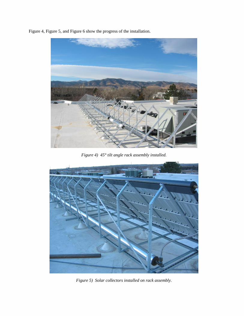
Figure 4, Figure 5, and Figure 6 show the progress of the installation.

Figure 4) 45° tilt angle rack assembly installed.

Figure 5) Solar collectors installed on rack assembly.

Figure 6) Completed solar collector field.

In order to prevent excessive pressure drop through the collector array, the collectors are arranged into two

strings of five units each, plumbed in parallel as shown schematically in Figure 7.

Figure 7) CEI demo system plumbing schematic.

Figure 8) CEI demo field modified for ORNL HTF testing.

Before testing the ORNL HTF, it had been planned to separate the solar collector field fluid circulation loop

from the main storage fluid circulation loop via a heat exchanger on the roof, along with a separate pump,

which would have allowed a much smaller volume of experimental HTF to be used for testing. The

schematic for the planned modifications to the field is shown in Figure 8.

The fluid lines to and from the solar collector field are brought into the building via penetrations in the roof

above the bay, as shown in Figure 9.

Figure 9) Insulated fluid line penetrations.

All lines are insulated with jacketed fiberglass, except near any fitting, valve, or joint, where closed-cell

foamed glass is used to prevent fluid accumulating in the insulation due to leaks at plumbing joints.

Plumbing and Mechanical Overview

The balance-of-system components not required to be placed on the roof reside in the bay below. There are

two main components: The first is an equipment skid, constructed by CEI, which carries the tanks, pumps,

and valves required for operation of the solar collector field, Stirling engine, and coolant system. The

second is the Stirling engine itself.

Mounted on the equipment skid are ASME-rated 120-gallon primary and 60-gallon fluid expansion tanks,

which contain a non-toxic HTF. Two internal gear pumps each pump HTF through the solar collector field

and the Stirling engine respectively, and a single hydronic pump circulates a water-antifreeze mixture

between the cold, heat rejection side of the Stirling engine and either a chiller or a fin-and-tube radiator.

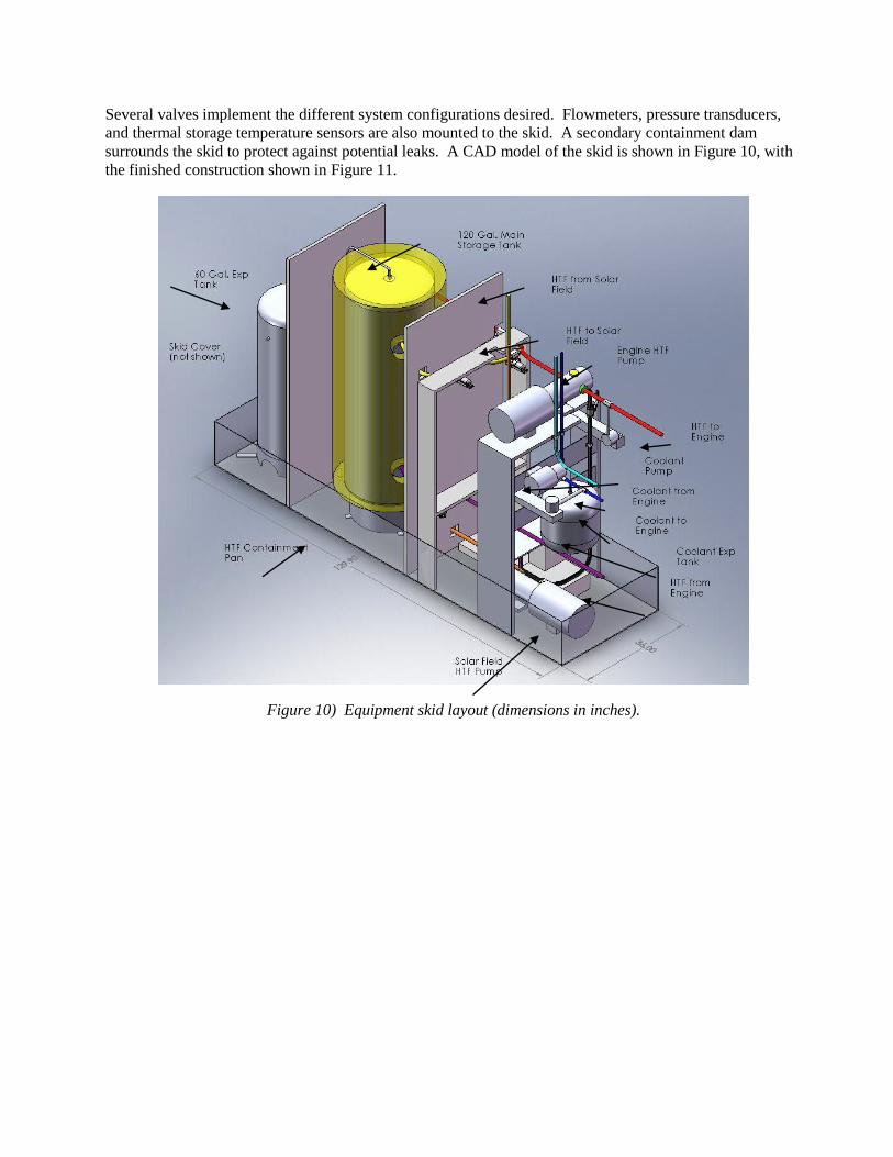
Several valves implement the different system configurations desired. Flowmeters, pressure transducers,

and thermal storage temperature sensors are also mounted to the skid. A secondary containment dam

surrounds the skid to protect against potential leaks. A CAD model of the skid is shown in Figure 10, with

the finished construction shown in Figure 11.

Figure 10) Equipment skid layout (dimensions in inches).

Figure 11) Finished equipment skid with secondary containment dam.

Of the several HTF compositions investigated, CEI has operated with three. The solar collector field

operates with Marlotherm N, and the Stirling engines operate with Duratherm HF and Duratherm 600, the

latter two being refined, non-toxic white mineral oils. Considered “Class III combustible liquids” under

NFPA/IBC codes, all are synthetic- or paraffinitic-hydrocarbon-based liquids having low vapor pressures,

low oxidation and decomposition rates, low corrosivity, and high flash point temperatures.

Installation Timeline

The evacuated tube solar collectors were installed during November, 2010, and the initial field

commissioning was completed by the end of 2010. P2 engine installation at the demo location began in the

first week of March, 2011, and was completed within a few days.

Expected System Performance

The system, as designed, was expected to produce approximately 2,200 kWh per year of electric energy,

given the observed performance of the P2 engine. This output is net of pumping, warm-up, and cool-down

costs, and assumes the engine will operate each day that it is able to, based on historical solar irradiation

and climate data for Boulder. Plots of the predicted system temperature and cumulative electric energy

production are given in Figure 12 and Figure 13.

Thermal Storage Temperature

200.00

250.00

300.00

350.00

400.00

450.00

0 100 200 300 400

Day of Year

Te

mp

era

ture

, K

Tank Temperature, K

Ambient Temperature

120 per. Mov. Avg.

(Tank Temperature, K)

Figure 12) Simulated thermal storage temperature vs. day of year.

Generated kWh

0

500

1000

1500

2000

2500

0 100 200 300 400

Day of Year

kW

h Generated kWh

Figure 13) Simulated cumulative electrical output vs. day of year.

Solar Collector Field Performance to Date

The initial results from the installed solar field were quite promising. The fluid returning to the storage tank

from the solar field was measured at temperatures in excess of 180 °C on sunny days in January. As more

insulation was added to the tank and system, by early March of 2011, the no-load storage temperatures

measured climbed to well above 200 °C. The first step of insulating the tank is shown in Figure 14.

Figure 14) Equipment skid with tank insulation operating on solar thermal energy from solar field.

The solar field and engine rapidly proved to work quite well together. Since the constructed solar array is

only 40-50% of the full design collection area for a combined heat-and-power system initially conceived,

the maximum temperatures and power levels were somewhat lower than initially modeled, but very

satisfactory nonetheless. The engine was able to operate for hours at a time with only solar input, shown in

operation in Figure 15, demonstrating consistent electrical power outputs and thermal-to-electric efficiency.

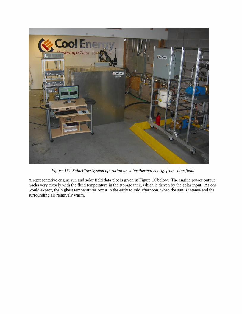
Figure 15) SolarFlow System operating on solar thermal energy from solar field.

A representative engine run and solar field data plot is given in Figure 16 below. The engine power output

tracks very closely with the fluid temperature in the storage tank, which is driven by the solar input. As one

would expect, the highest temperatures occur in the early to mid afternoon, when the sun is intense and the

surrounding air relatively warm.

Demo System Operation, April 22 2011

20

40

60

80

100

120

140

160

180

200

7:12:00 AM 9:36:00 AM 12:00:00 PM 2:24:00 PM 4:48:00 PM

Time of Day

Tem

pera

ture

(C

)

0

200

400

600

800

1000

Ele

ctr

ical

Watt

s

Tank Temperature

@ inlet from SF

Tank Temperature

@ outlet to SF

HTF Temperature

@ inlet to P2

Engine

HTF Temperature

@ P2 outlet

Engine Output

Watts

Figure 16) Chart of SolarFlow System operation demonstrating tank temperatures and engine operation

for a full day (April 22, 2011).

The P2 Stirling engine was operated very frequently on the solar field from March through June of 2011,

until it had to be removed to make room for testing of the fourth-generation P3 SolarHeart Engines.

III. Low-Temperature Power Conversion Theory & Background

A. Review of Low-to-Medium Temperature Power Cycles

Technical advantages of the Stirling engine: Rankine and other cycles that have been used to generate

electric power from low-temperature heat sources over the last 30 years have some significant

disadvantages. They are described below, to differentiate CEI’s Stirling engine especially in smaller

distributed generation applications and where the electric power generated is needed on site.

Rankine and Kalina Cycles: Rankine cycle systems, primarily using steam and designed to run full time

providing baseline electric power, have been optimized for huge outputs, as large as 1000 MWe from a

single generator. Although organic fluids as well as steam have been used as the working fluid in smaller

systems, only organic fluids have found application in practical systems generating less than 500 kWe,

which typically operate at hot temperatures below 350 °C. Below 50 kWe output, use of a turbine expander

becomes increasingly infeasible, because of the high cost of the turbine and the difficulty in making a

turbine small without compromising its isentropic efficiency. Freepower’s 6 kWe turbine-based WHR

systems, for example, must receive 70 kW of thermal power, resulting in a thermal efficiency of 8.6%. This

is only 34% of what is theoretically possible from the waste heat stream at the specified temperatures used

to power this system. Varying the power output of a turbine expander to track a varying thermal input

power or a varying electric load can be done efficiently only by changing the pressure of the high-pressure

side of the cycle, called “pressure sliding,” and not by varying the speed of the turbine. A sophisticated

control system is needed to do this, which must also balance the heat flows, condensate mass flow, and

vapor mass flows through the turbines. Some smaller Rankine cycle systems therefore use a positive-

displacement expander, such as the Lysholm screw expander used by Electratherm, or the trochoidal gear

expander used by Ener-G-Rotors. While less expensive than turbines, and capable of running at variable

speed, these expanders suffer from low isentropic efficiency due to leakage and thermal cycling of the metal

surfaces exposed to the working fluid, and thus compound the efficiency penalty of the Rankine cycle itself.

Although neither Electratherm nor Ener-G-Rotors currently publish thermal efficiency data, isentropic

efficiencies of a Lysholm two-phase expander have been measured at around 70%2. Compared to large

turbines having isentropic efficiencies of 85% to 90%, losses in this screw expander are thus two to three

times greater.

Rankine cycle engines all suffer from a maximum theoretical thermal efficiency that is inherently less than

the Carnot efficiency, because the heat addition and heat rejection processes do not take place at only the

highest and lowest temperature limits, respectively, achieved by the thermodynamic cycle, even if the heat

source and heat sink are ideal, infinite reservoirs. Much of the complexity of fossil-fuel fired steam

Rankine cycle plants is due to the addition, at strategic locations, of thermal circuits that remove heat from

one part of the system and return it to another part, mostly to overcome this inherent deficit in the structure

of the cycle, and only incidentally to reduce the temperature difference between the hot combustion gas and

the steam during the heat addition process. Pressurizing the high-pressure side of the cycle above the

critical pressure of water (making it a “supercritical” cycle), so that the water progresses through the boiler

in only a single phase while gaining temperature, does help make the difference between the hot

combustion gas and the water more uniform as the combustion gas flows counterflow to the flow of the

water, and therefore lets heat from the combustion gas be added to the working fluid across a more uniform

and smaller temperature difference throughout the boiler, thus reducing the amount of entropy generated.

But the purpose of this, however, is actually to increase the small temperature difference between the

combustion gas and the water that otherwise occurs in a non-supercritical cycle at the point in the boiler

where the water begins to boil and therefore is already quite hot, but which is also where the combustion

gas has already been cooled a great amount. Called the “pinch point,” this region of small temperature

difference ties up a large amount of boiler surface area for the comparatively small amount of heat

transferred into the water there.

Illustrating the complexity required to improve the thermal efficiency, Figure 17 shows a GateCycle

diagram of an only moderately complex, 50 MWe steam Rankine system used in a concentrating solar

power plant3. Only the thermal components and their connections are shown, and not the instrumentation

and control circuits. Except for the water loop to the cooling tower, the piping contains either high pressure

or near vacuum conditions. The boiler, steam turbines, and condenser, all complex components

individually, are connected in a sophisticated circuit including steam reheating and several stages of

regenerative feedwater heating. The feedwater has to be treated, requiring a chemical measuring and

dispensing system. Operating and maintaining a system of even this size requires a specialized labor force,

which has to be provided for in the O&M budget.

Figure 17) GateCycle Diagram for a 50 MWe Rankine Cycle Model

An organic Rankine cycle may use a zeotropic working fluid, composed of two or more chlorofluorocarbon

or hydrocarbon refrigerants, having a low specific heat but having the property that, as the working fluid

boils, the boiling temperature of the remaining liquid increases as it progresses through the boiler.

Alternatively, the cycle may use a working fluid that has a high specific heat and a low heat of vaporization,

which progresses through much of the boiler as a liquid while gaining temperature. A zero heat of

vaporization may be effected simply by pressurizing the high-pressure side of the cycle above the working

fluid’s critical pressure, as with a supercritical steam cycle, in which case the fluid progresses through the

boiler in only a single phase while gaining temperature. Called “temperature glide,” all of these techniques

increase the temperature of the working fluid as it progresses through the boiler, and thus allow the

temperature of a heat supply stream having a limited heat capacity rate to decrease significantly as it flows

counterflow to the working fluid. This enables more heat to be extracted from the heat supply stream and

thus increases the potential work output of the cycle, while adding this heat to the working fluid across a

more uniform and smaller temperature difference throughout the boiler and thus reducing the amount of

entropy generated. The advantage provided by these working fluids, however, is offset by a concomitant

disadvantage, that when the working fluid vapor is condensed and cooled after leaving the expander, the

temperature of the working fluid must decrease significantly as it progresses through the condenser or

subcooler, requiring that the working fluid leave the expander at a temperature high enough to allow for

this. To avoid rejecting this still useful heat to the heat sink and wasting it, a recuperation circuit,

sometimes called a regenerator, is added to recycle some of this heat into the condensed working fluid just

before it re-enters the boiler.

Organic Rankine cycles are typically operated so that the pressure of the working fluid in the condenser is

above atmospheric pressure, so that the risk of air leaking in and oxidizing or even exploding a flammable

gaseous working fluid is minimized. This is possible because such working fluids have saturation pressures

higher than that of water at the same temperature. (Merely a nuisance and not a hazard in a steam Rankine

cycle, air leaking in due to the necessarily very low pressure used in the condenser is removed by

separators. A steam Rankine cycle operated with a condenser pressure above atmospheric pressure would

have a heat rejection temperature above the boiling temperature of water at atmospheric pressure, or 100 °C

at sea level, and a concomitantly low thermal efficiency.) Even at higher saturation pressures, organic

Rankine cycle working fluids still condense at some fixed temperature higher than the highest temperature

expected of the heat rejection environment, often higher than those used in steam Rankine cycles, and thus

cannot track and take advantage of low temperatures of the heat rejection environment, as occur at night

and in winter, for increasing the thermal efficiency.

The Kalina cycle is a Rankine cycle using a zeotropic mixture of water and ammonia as the working fluid,

with additional components for managing the concentration of the ammonia in the water in order to

influence its concentration in the vapor exhausted from the expander. Because the mixture can be adjusted

to condense without freezing, heat may be rejected from the cycle at only a little above the terrestrial

ambient temperature (which may be below the freezing temperature of water), thus increasing the thermal

efficiency. The additional components add complexity, but enable the Kalina cycle to adapt to changing

temperature conditions better than the Rankine cycle, although only slowly and typically only on a seasonal

basis. The cycle otherwise has the same advantages and disadvantages described above for the organic

Rankine cycle, and thus requires a recuperation circuit. In spite of the thermodynamic advantages, practical

realizations of the cycle suffer sensitivities in the tradeoffs among power, efficiency, scale, and cost similar

to those in the Rankine cycle. Although the water-ammonia mixture is much less expensive than organic

fluids, and does not decompose at high temperatures, ammonia is toxic, and provision must be made to

handle leaks in the complex system.

For these and other enhancements to be effective at even partially overcoming the Rankine cycle’s

otherwise inherent irreversiblities, the operating temperatures of the cycle must be held within tight limits,

which are tied to phase-change, critical point, and other thermal properties of the particular working fluid,

regardless of the actual temperatures of the heat source and heat sink. Rankine cycle engines are therefore

not able to adapt to rapidly changing temperatures in the heat source or heat sink, as when an industrial

process, used as the heat source, changes its temperature significantly in response to process demands, or as

when the ambient air, used as the rejection sink, plunges to very cold temperatures overnight in winter.

All practical Rankine cycle realizations require numerous, large heat exchangers, the condenser being

particularly large because the density of the expanded working fluid is so low. Of all the limitations facing

Rankine cycle technology, however, the most serious is that it is so mature that significant improvements in

either cost or thermal efficiency are unlikely.

Closed Brayton cycle The closed Brayton cycle consists of the steps of isentropically compressing cool gas

to raise its pressure and temperature, isobarically adding heat to the compressed gas to further raise its

temperature, isentropically expanding the gas to reduce its pressure and temperature, and isobarically

removing heat from the expanded gas to further reduce its temperature. The four steps occur in four

separate components of the engine. The compression and expansion steps are performed by two separate

turbines. The heat addition and heat removal steps are performed by two separate heat exchangers. The

hot, heat-addition heat exchanger receives heat from a heat supply, and the cold, heat-removal heat

exchanger rejects heat to a heat sink. Because heat is added over a temperature range as the gas heats up at

constant pressure, the cycle could advantageously receive heat from heat streams having a finite heat

capacity rate. But heat is also rejected over a temperature range as the gas cools at constant pressure,

making rejection impossible at constant temperature into an infinite heat sink, such as the terrestrial ambient

atmosphere approximates. The working fluid is typically helium or a mixture of gases consisting of mostly

helium, to decrease the ratio of the thermal conductivity to the speed of sound in the mixture.

Although closed Brayton cycle engines are attractive because of their simplicity and reliability, a particular

disadvantage is that that two highly efficient and expensive turbines are required, both of which have to

spin at speeds as high as 200,000 rpm in a small system. Another disadvantage is that the only efficient

way to vary the torque input to the generator is by pressure sliding, requiring an additional system to

remove, store, and return the pressurized helium mixture to the system as required. As in the Rankine

cycle, and for the same reasons, the maximum theoretical thermal efficiency is inherently less than the

Carnot efficiency, even if the engine is operated between a heat source and a heat sink that are ideal, infinite

reservoirs.

Stirling cycle The Stirling cycle is traditionally described as consisting of the steps of isothermally

compressing cool gas to raise its pressure while removing heat, isochorically adding heat to the compressed

gas to raise its temperature and pressure, isothermally expanding the gas to reduce its pressure while still

adding heat, and isochorically removing heat from the expanded gas to reduce its temperature and pressure.

If the heat removed isochorically from the expanded gas is recycled across an infinitesimal temperature

difference to become the heat added isochorically to the compressed gas, then the only other heat added to

the gas is added isothermally at the highest temperature reached by the gas, and the only other heat removed

from the gas is removed isothermally at the lowest temperature reached by the gas. Because the heat

addition and heat removal processes both take place at constant temperatures, and because all heat transfer

processes occur across infinitesimal temperature differences, the theoretical thermal efficiency is the Carnot

efficiency.

The difficulty with this description is that the gas does not follow the same thermodynamic path at different

locations in a real engine, let alone the thermodynamic path described above. This has made both

understanding and analyzing the actual cycle difficult. Although the thermodynamic states of the gas may

be modeled as functions of time and a single spatial variable spanning the hot and cold extremes of the gas

circuit, as done, for example, in the Stirling engine analysis software program SAGE, even this

representation cannot be cast into the form of the traditional description, because the gas at every point in

the spatial dimension undergoes a unique thermodynamic cycle.

The cycle is typically realized by pistons reciprocating in cylinders, not only for changing the working

volume of the gas trapped therein, but also for moving the gas through compact heat exchangers that add or

remove heat at the appropriate times. Modern Stirling engines drive an electric generator integrated with

the internal mechanism, forming a self-contained package, and thus eliminating mechanical shaft seals,

which throughout the history of the Stirling engine have been inadequate and unreliable for sealing in the

high pressure gaseous working fluids. Electric power produced by the generator is passed through the

pressure vessel wall via electrical feedthroughs, which are not difficult to seal. Piping connections to the

engine are few and do not hold high-pressure fluids. The thermodynamic cycle imposed on the gaseous

working fluid is completely defined by the motion of the pistons, thereby eliminating all cycling valves,

valve train components, timing belts, chains, and gears, allowing the engine to operate quietly. Most of the

few remaining moving parts operate at ambient temperature, enhancing system reliability. Because the

working fluid remains gaseous throughout the cycle and everywhere within the engine, operating

temperatures can be widely varied without impairing functionality, to match thermal conditions external to

the engine, or to optimize performance. In particular, the heat rejection temperature may track that of the

ambient air, which the colder it is, the greater the thermal efficiency.

Both the speed and torque of the Stirling engine may be varied, to match power output with heat

availability, to adhere to a power production schedule, or to maximize power produced. Speed, the more

easily controlled output, can be changed quickly, and is best regulated by load management, whereby the

torque presented to the engine by the electric generator is varied electrically to let the engine speed up or

slow down as needed. The penalty to thermal efficiency from speed variation is nowhere near that of

turbine engines. Torque produced by the engine can be varied, but only by changing the operating

temperatures or the gas charge pressure.

A limitation in the mass flow rate of the heat stream might make it advantageous for the Stirling engine to

be composed of multiple, thermally independent units, each a complete Stirling engine, arranged to form a

compound engine, where the heat stream flows sequentially from unit to unit as its temperature cascades

downward to a low final temperature, thereby allowing more of the waste heat to be extracted. This, along

with a theoretical extension of the thermodynamic concept, is discussed in the next section.

B. Comparison of Stirling Machines to Other Power Conversion Options

Because the closed Brayton cycle has dim prospects (as the cost of a minimum of two turbines will always

be more than the cost of one turbine in a Rankine cycle system), the Stirling cycle will be compared only to

Rankine cycle systems.

The losses in a real Stirling engine, such as pressure drop, friction, adiabatic mixing, and non-isothermal

heat addition and rejection, are of a practical origin and are not fundamentally thermodynamic. If these

real-world losses are allowed to approach zero in a thermodynamic analysis, the thermal efficiency

converges to the Carnot efficiency. Compared to Rankine cycle engines operating between the

temperatures considered herein and whose practical losses are also allowed to approach zero, the Stirling

cycle starts out with a theoretical thermal efficiency that is inherently 20% to 25% higher.

The Stirling engine has a much simpler thermal system than does any Rankine cycle realization. The

working fluid is contained entirely within the Stirling engine, and is not circulated outside of the engine.

Always gaseous, the working fluid operates well above its critical temperature and pressure and thus does

not undergo any phase change, and hence does not constrain the engine to operate in a narrow range of

temperatures that would be dictated by a phase change or other behavior near the critical point.

The Stirling engine also possesses the flexibility of receiving and rejecting heat from many different types

of heat source or heat sink, by several methods, all external to the high pressure gas envelope containing the

engine itself. Such heat sources include direct irradiance from solar energy, heat from a nuclear

radioisotope, industrial waste heat, heat from combustion engine exhaust gas, geothermal heat, and heat

from direct combustion. Methods for admitting heat to and removing heat from the Stirling engine include

pumped loops containing liquid HTF, heat pipes, direct thermal contact, and pumped loops containing

phase-change fluids. Such phase-change fluids could be condensing steam for the heat addition fluid, or

boiling liquid natural gas for the heat rejection fluid. None of these methods is burdened with having to

withstand the high pressure within the engine.

The mechanical system for effecting the reciprocating piston motion and the electric generator itself are

entirely within the engine pressure envelope, and do not hold the high-pressure gas against atmospheric

pressure, in contrast to the many high-pressure pumps and valves used throughout a Rankine cycle system.

Power is delivered out of the engine’s pressure envelope electrically, not mechanically, which would

require a rotating shaft seal.

The system to control the Stirling engine is comparatively simple, and needs to manage only the hot and

cold heat supply circuits (powered by as few as one low-pressure pump each), and an engine starting and

stopping function. External off-the-shelf DC-AC inverters or AC-AC switchgear are used to regulate

engine speed, and perform electric power conditioning and grid tie functions. The system is fully automatic

and does not require attention of operational staff.

Although designing any heat engine to use a low-temperature heat source can be difficult to justify

economically because of the inherently low Carnot efficiency, the low temperature provides an opportunity

to offset this disadvantage by allowing the engine to be made out of less expensive or better performing

materials unencumbered by the risk of structural failure or degradation from exposure to high temperatures.

This wider range of options in turn permits a greater number of concepts to be considered in the design and

optimization of the engine, including economic optimization. Of all the heat engines in the current state of

the art that could potentially generate power from low-temperature heat sources, however, the Stirling

engine is the most adaptable for incorporating such materials while retaining its inherent simplicity,

scalability, and high thermal efficiency, and therefore has the most promising pathway to

commercialization.

Table 2 captures the engineering tradeoffs between various heat recovery approaches.

Table 2) Engineering tradeoffs (qualitative) between candidate heat recovery engines.

Thermodynamic advantages and flexibility of the Stirling engine currently unexploited

Typically, the thermodynamic cycle internal to the Stirling engine is supplied with heat at nearly a constant

temperature, regardless of how much heat is drawn from the heat source. Such a heat source is

characterized as an “infinite reservoir,” for the purpose of conveniently describing a hypothetical method

for assuring that the temperature of the heat supplied to the engine does not change if more or less heat is

drawn by the engine, particularly at different stages of the thermodynamic cycle. Although characterizing

the heat source this way is adequate for certain heat sources, such as solar and nuclear energy and most

high-temperature combustion sources, it is not realistic for characterizing a heat supply stream that

necessarily has a finite mass flow rate of the heat-bearing medium, as would be found in a geothermal or

waste heat stream. The temperature of such a heat supply stream as it progresses through the heat recovery

system must drop, perhaps significantly, for a useful amount of heat to be extracted and supplied to a heat

engine for conversion into work.

Three system topologies, described below, have been examined by CEI as potentially effective for dealing

with a heat supply stream having a finite capacity rate, using technology based on the Stirling cycle. The

second and third topologies are not currently being exploited in low-temperature, heat-to-power conversion

systems, thus motivating investigation into their potential. The analysis below reveals and quantifies the

opportunities presented by these two topologies compared to the first topology.

Each topology or configuration contains a particular, theoretical type of ideal, reversible heat engine, for

explaining how the impact of the finite capacity rate on the power and efficiency of the power conversion

system may be mitigated. It is anticipated that at least the first two configurations described would be

further analyzed for quick adaptation of CEI’s Stirling engine technology to applications with heat supply

streams having a finite capacity rate.

In the first configuration, referred to herein as “Single Stage,” the heat supply stream passes through an

ideal heat exchanger having unity effectiveness, which transfers some of the heat into an intermediary fluid,

which in turn supplies heat to an ideal, reversible heat engine. The heat capacity rate of this intermediary

fluid is assumed to be much greater than the heat capacity rate of the heat supply stream, so that the change

in temperature of the intermediary fluid as it circulates between the heat exchanger and the engine is

insignificant. The temperature of the working fluid internal to the engine during heat addition is constant,

and is equal to the temperature of the intermediary fluid. The temperature of the working fluid during heat

Conversion

device Initial cost

Minimum

output

Conversion

efficiency

System

complexity

System

weight

Part load

flexibility

Temperature

flexibility

Brayton

(turbine) High 50 kWe Mid Mid Mid Low Mid

Rankine

(turbine)

Low to

Mid 100 kWe Mid to High High High Low Low

Kalina

(turbine) Mid 100 kWe Mid High High Mid Mid

Stirling

(piston) Mid 1 kWe Mid to High Mid Mid High High

rejection is also constant, and is equal to the temperature of the heat sink. Maximizing the thermal

efficiency of the engine by operating it at the maximum temperature presented by the heat supply stream is

not a useful objective, however, because such a maximally efficient engine would draw only an infintesimal

amount of heat from the heat supply stream, and would therefore produce only an infintesimal amount of

power. A much more useful objective is to find the optimum temperature the heat supply stream should be

pulled down to that maximizes the power output of the engine, which balances the reduction in thermal

efficiency against the increase in the amount of heat drawn from the heat supply stream and made available

to the engine. The engine would be sized and operated so that the amount of heat it draws pulls the

temperature of the heat supply stream down to this optimum. This optimum temperature is given by

hopt ghs minT T T , where (1)

Thopt = Optimum hot temperature, K,

Tghs = Temperature of heat supply stream as supplied, K, and

Tmin = Heat rejection temperature, K

The maximum power produced is thus given by

m p ghs ghs min minP mC T 2 T T T , where (2)

Pm = Mechanical power, W,

m = Mass flow rate of heat supply stream, kg/s,

Cp = Heat capacity of heat supply stream, J/kg-K,and

The thermal efficiency of the engine is hence

min1

ghs

Tμ 1

T , where (3)

μ1 = Thermal efficiency.

μ1 is recognized as the Chambadal-Novikov or Curzon-Ahlborn efficiency.

In the second configuration, referred to as “Dual Stage,” the heat supply stream passes sequentially through

two ideal heat exchangers, each having unity effectiveness, which transfers some of the heat into two,

separate intermediary fluid streams. The temperature of the intermediary fluid in the heat exchanger though

which the heat supply stream first passes is thus higher than the temperature of the intermediary fluid in the

heat exchanger through which the heat supply stream subsequently passes. The intermediary fluid streams

in turn supply heat to two ideal, reversible heat engines, which necessarily operate at different hot

temperatures. The heat capacity rates of the intermediary fluids are assumed to be much greater than the

heat capacity rate of the heat supply stream, so that the change in temperature of either intermediary fluid as

it circulates between its corresponding heat exchanger and engine is insignificant. The temperature of the

working fluid internal to each engine during heat addition is constant, and is equal to the temperature of its

corresponding intermediary fluid. The temperature of the working fluid internal to each engine during heat

rejection is also constant, and is equal to the temperature of a single heat sink that serves both engines.

Each engine would be sized and operated so that the amount of heat it draws pulls the temperature of its

corresponding intermediary fluid down to its optimum. These optimum temperatures are given by

23hopt1 ghs minT T T and (4)

23hopt2 ghs minT T T , where (5)

Thopt 1 = Optimum hot temperature of first engine, K, and

Thopt 2 = Optimum hot temperature of second engine, K.

The maximum power produced is thus given by

23mt p ghs ghs min minP mC T 3 T T 2T , where (6)

Pmt = Total mechanical power from both engines, W.

The thermal efficiency of the combined engine system is hence

23ghs min min

1223

ghs ghs min

T T T1 2

T T T

, where (7)

μ12 = Thermal efficiency of combined system.

Based on simulations performed by CEI for waste heat recovery applications, the power produced by this

strategy can be over 30% greater than that of the Single Stage system supplied with the same mass flow rate

of the heat supply stream. Even though μ12 is typically close to μ1, the resulting power output is greater

because more of the heat in the heat supply stream is be utilized.

The premise of the Dual Stage configuration could be extended to any number of heat exchangers arranged

in series with the heat supply stream, with each heat exchanger extracting heat at a progressively lower

temperature and supplying it to a heat engine dedicated to that heat exchanger. The larger the number of

engines, the smaller each one would be. Of more interest, however, is to mathematically extend the idea to

an infinite number of infinitesimally small heat exchangers, each supplying an infinitesimal amount of heat

to an infinitesimally small, ideal reversible heat engine. The combination of all the infinitesimal heat

exchangers would manifest as a single, counterflow heat exchanger, and the intermediary fluid would

circulate at the same heat capacity rate as the heat supply stream, thus having a finite temperature drop

through the engine and an equal temperature gain through the counterflow heat exchanger (and hence not

having some fixed, optimum temperature). The intermediary fluid would supply heat to a special type of

heat engine wherein the thermodynamic working fluid receives heat from the intermediary fluid as it cools

throughout its transit through the engine such that everywhere the two fluids are in thermal contact, the

temperature difference between them is insignificant, thereby minimizing the production of entropy. This

process forms the third system topology.

The conceptual design of such a heat engine is a topic of current research by CEI, the goal of which is not

without precedent in the design of steam and organic Rankine cycles. In these approaches, the temperature

difference between a heat supply stream having a finite heat capacity rate (such as waste or geothermal

heat) and the working fluid in the boiler is minimized by choosing a working fluid that either takes a great

deal of heat to bring to the boiling temperature but comparatively little heat to boil, or takes little heat to

bring to the boiling temperature but boils at a progressively higher temperature as the composition of the

remaining liquid changes as it flows through the boiler, or is pressurized above the critical pressure so that it

does not exist as separate gas and liquid phases and simply gains temperature as it progresses through the

boiler. Because this process is called “temperature glide” in the power generation industry, the third

configuration is analogously referred to herein as the “Temperature Glide” configuration. The thermal

efficiency of this engine is given by the elegant, Carnot-like result

clmtg

hlm

T1

Tm = - , where (8)

μtg = Thermal efficiency of Temperature Glide engine,

Tclm = Log-mean-temperature difference of heat rejection stream, K, and

Thlm = Log-mean-temperature difference of heat supply stream, K.

The log-mean-temperature difference of the heat rejection stream is provided for the general case that its

heat capacity rate may also finite, and is given by

cexit minclm

cexit

min

T TT

Tln

T

-= , where (9)

Tcexit = Temperature the heat rejection stream leaves engine, K.

The log-mean-temperature difference of the heat supply stream is given by

ghs hexit

hlmghs

hexit

T TT

Tln

T

-= , where (10)

Thexit = Temperature the heat supply stream leaves engine, K.

The power produced is given by

( )ghs

mtg P hlm clm

hexit

TP mC T T ln

T= -& , where (11)

Pmtg = Mechanical power from Temperature Glide engine, W

The power from the Temperature Glide engine is maximized if both Tclm and Thexit are minimized so that

they equal Tmin, which requires that the heat rejection stream have an infinite capacity rate. The maximum

power produced is thus given by

ghs

mtgmax p ghs min

min

TP mC T T 1 ln

T

, where (12)

Pmtg max = Maximum mechanical power from Temperature Glide engine, W

The power produced by this strategy can be over 60% greater than that of the Single Stage system supplied

with the same mass flow rate of the heat supply stream. Even though μtg is likewise typically close to μ1,

even more power is produced because more (theoretically all) of the available heat in the heat supply stream

is utilized, by releasing the heat supply stream back into the environment at the temperature of the

environment Tmin.

A more detailed analysis has been made by CEI which includes less-than-unity effectiveness of the heat

exchangers and realistic engine thermal efficiencies derived from computed engine maps, but is lengthy and

not reproduced here. One consequence of the less-than-unity effectiveness of the heat exchangers is that

maximum power output of the third topology is obtained for some Thexit > Tmin instead of the criterion

Thexit = Tmin.

Based on CEI’s analysis of waste heat recovery applications, the Dual Stage configuration currently seems

to be the best candidate for heat recovery systems that would require either a large Stirling engine or a

system of a few smaller ones, because the Dual Stage system always produces significantly more

mechanical power than the Single Stage system, and the 300 °C (573 K) maximum temperature limit of

CEI’s engines does not have as much of an adverse effect on the mechanical power output of the Dual Stage

system as it does on that of the Temperature Glide system. On a large system built with several engines,

however, more than two stages could also be considered.

IV. Stirling Engine Design, Testing, and Results at Cool Energy, Inc.

Since 2006, CEI has designed, fabricated and tested four generations of low-temperature (100 °C to 300 °C)

Stirling engines. Over 3 kWe electric power output at over 22% thermal-to-electrical conversion efficiency

has been demonstrated, with a heat input temperature of 300 °C and a heat rejection temperature of 10 °C.

Initial pilot units have been shipped to development partners for further testing and validation. 20 kWe and

larger engines have been conceptually designed and shown to be feasible, with one 20 kWe concept

producing nearly seven times the power output of CEI’s current 3 kWe P3 unit, but at only 2.5 times the

estimated fabrication cost. Originally intended for waste heat recovery (WHR) applications, these engines

are easily adaptable to solar and geothermal heat sources, as the heat supply temperatures are similar. A

larger conceptual design producing 40 kWe is attractive as a bottoming cycle in large combustion engine

exhaust gas waste heat recovery applications and in utility-scale geothermal and solar applications.

CEI’s design philosophy

The SolarHeart engine is designed to be powered by low- to medium-temperature heat, specifically in the

range of 100 °C to 300 °C, from high-performance residential solar-thermal collectors, medium-

performance solar tracking trough collectors such as those offered by Sopogy or Abengoa Solar,

combustion and industrial waste heat sources, and geothermal heat sources. Designed for temperatures well

below typical combustion temperatures of 500 to 1000 °C, the SolarHeart engine platform is based on

inexpensive and mass-produced materials that minimize thermal losses and reduce weight and cost relative

to typical Stirling engines, which have been traditionally designed to operate at high temperatures. Having

a wide choice of materials has led to such novel approaches as self-lubricating, low-wear-rate materials at

sliding interfaces, non-metallic regenerators, and high-performance, compact heat exchangers mass

producible in common materials such as aluminum and carbon steel.

The SolarHeart Engine is a kinematic engine, having pistons connected to a mechanical drive linkage

turning an electric generator, and using compressed nitrogen as the working fluid. Hot fluid is sent from the

solar collector field, storage tank, or other heat source to hot-side heat exchangers within the engine, to

supply heat at a high temperature to the hot part of the Stirling thermodynamic cycle. Cold fluid is sent

from a radiator (or mechanical refrigeration chiller for testing purposes) to cold-side heat exchangers within

the engine, to remove heat at a low temperature from the cold part of the Stirling thermodynamic cycle.

Electric power produced by the generator is passed through the pressure vessel wall via electrical

feedthroughs. Because mechanical power does not leave the pressure envelope, there are no mechanical

shaft seals. During CEI’s testing, the electric power is sent to a programmable active resistive load, but will

eventually be sent through an inverter and onto the electric utility power grid.

The engine requires a hot heat transfer fluid (HTF) heat supply circuit and a cold HTF heat rejection circuit,

powered by as few as one pump each. The HTF in either circuit remains everywhere liquid, and is brought

directly to heat exchangers within the engine. None of the systems that handle the HTF have to withstand

the high pressures within the engine.

Because the few piping connections to the engine do not circulate high-pressure fluids, adding a complete,

Stirling-engine-based power conversion system requires only minimally invasive changes to an existing

heat source, primarily interposing a heat exchanger to capture the heat and transfer it to the HTF that brings

it into the Stirling engine. The simplicity of the SolarHeart Engine design enables simplicity in its

operation and control. It has an engine load management system to regulate engine speed and for electric

power conditioning, and an engine starting and stopping function, usually built into the engine electrical

load management system. Other than receiving high-level permission for the system to operate, it can be

fully automatic and will not require attention or intervention from system operators.

The left half of Figure 18 below shows an example of the type of heat exchanger used in the SolarHeart

Engines. These are modular assemblies that can be scaled up or down in heat transfer capacity. Shown in

the right half of Figure 18 is a patterned foil regenerator that can be non-metallic because of the lower hot

temperatures. There is no circulating lubricant in the SolarHeart Engine, so maintenance is minimized.

Figure 18) Left - high-performance heat exchanger; right - regenerator in CEI P3 engines.

A nearly completed P3 engine, in process of being insulated, is shown in Figure 19 below.

Figure 19) P3 internal assembly ready to receive thermal insulation.

The left half of Figure 20 below shows a demonstration of solar-heated oil being used to power the P2, a 3rd

generation, 2 kWe SolarHeart Engine, operating at 20 bar nitrogen gas charge pressure, in Boulder,

Colorado. The right half of Figure 20 shows one of the P3, 4th generation, 3 kWe engines, operating at

50 bar nitrogen gas charge pressure, ready for thermal testing on the same test setup. One of these engines

has been assembled and shipped to Schneider Electric in Grenoble, France where it is currently on test.

Figure 20) Left - CEI P2 (3rd

generation) SolarHeart Engine connected to solar test field; right - P3 (4th

generation) SolarHeart Engine ready for thermal testing.

Figure 22 below shows the development timeline of the four generations of Stirling engines assembled at

CEI.

Figure 21) Development timeline of four generations of low-temperature Stirling engines at CEI.

Future generations will include more powerful engines, starting with a proposed 20 kW design shown in

Figure 22.

Figure 22) CAD rendering of 20 kW SolarHeart engine currently under design.

Figure 23 shows recently measured versus predicted work loop plots for the P2 SolarHeart Engine

prototype. Figure 24 shows recently measured versus predicted work loop plots for the P3 SolarHeart

Engine prototype.

Figure 23) Expansion, compression, and net work loops, measured (solid lines) versus predicted (dashed

lines), for 214 °C hot temperature, 17 °C cold temperature, 300 psig charge pressure, and 550 rpm (P2

with non-metallic regenerator). Measured indicated efficiency was 20.7%, predicted indicated efficiency

was 28.6%, work per cycle was 93 J, indicated power output was 2514 W, and electrical power output was

1832 W. Thermal to electrical conversion efficiency was 15.08%.

Figure 24) Expansion, compression, and net work loops, measured (solid lines) versus predicted (dashed

lines), for 300 °C hot temperature, 7 °C cold temperature, 410 psig charge pressure, and 646 rpm (P3 with

non-metallic regenerator). Measured indicated efficiency was 27.5%, predicted indicated efficiency was

37.7%, work per cycle was 81 J, indicated power output was 2601 W, and electrical power output was

2039 W. Thermal to electrical conversion efficiency was 21.56%.

V. Extended Reliability Testing on Stirling Engine Components

The SolarHeart engine has a design lifetime of 70,000 operating hours with no servicing of the internal

mechanism components. In order to achieve such a high lifetime, the piston/cylinder materials will have to

maintain low wears rates and high lubricity, and the bearing greases will have to be stable at the operating

temperatures in the engine.

Coefficient of friction and wear rate testing of piston / cylinder material

combinations

Efforts to date have been focused on the piston/cylinder materials, resulting in completion of a preliminary

test plan by the tribology testing contractor NANOVEA, an affiliate of Micro Photonics, Inc.

The following material combinations were chosen:

1) Company #1 Carbon Material #1 pins on ceramic wear disk

2) Company #1 Carbon Material #2 pins on ceramic wear disk

3) Company #2 Carbon Material #3 pins on ceramic wear disk

4) Company #3 Carbon Material #4 pins on ceramic wear disk

5) Company #3 Carbon Material #4 pins on metallic wear disk

Test plan

Although NANOVEA’s linear motion test machine produces an oscillating motion characteristic close to

that of the sliding interfaces within the Stirling engine, it could not be used because the maximum velocity

attainable was too low. CEI therefore calculated the alternative test conditions of a constant contact

pressure and constant sliding velocity, attainable in a rotary, pin-on-disk tester, so that the pressure-velocity

product was the same as the time-averaged oscillating pressure-velocity product calculated from CEI’s

piston ring dynamic analysis, and so that the constant pressure and constant velocity were approximately

equal to the rms values of the oscillating pressure and velocity, respectively, likewise calculated from CEI’s

piston ring dynamic analysis. This resulted in the following, constant parameters for the rotary testing

machine:

Test apparatus: NANOVEA Tribometer TRB, a rotary pin-on-disk machine

Test protocol: ASTM G133

Test conditions:

Disk rotational speed: 500 rpm

Radius on disk of pin contact: 35 mm

Diameter of pin: 3 mm

Force on pin: 2 N

Calculated contact pressure-velocity product: 0.52 MPa-m/s

The combinations in items 1) and 2) above were tested first. Time-averaged coefficients of friction (labeled

as “Average COF”), wear rates of the ceramic countersurface, and wear rates of the carbon material pins

reported by NANOVEA are shown in Table 3.

Table 3) Test data summary

A representative plot of the raw coefficient-of-friction data, shown as instantaneous coefficient as a function

of time, is shown in Figure 25.

Carbon #1

Carbon #1

Carbon #2

Carbon #2

Of Ceramic Of Test Pin

Figure 25) First sample, Company #1 Carbon Material #1 pins on ceramic wear disk.

In Figure 25, what appears as noise superimposed on an underlying, smooth curve is actually a sinusoidal

waveform, and is due to the upper surface of ceramic wear disk that is in contact with the pin not being

exactly perpendicular to the axis of rotation, thereby causing a slight raising and lowering of both the pin

and the weight on the pin that produces the 2 N of force, for every rotation of the disk. The sinusoidal

variation is the force necessary to accelerate and decelerate the mass of this weight, and is within estimates

based on the face-to-face parallelism specification for the ceramic wear disk.

A representative cross section of the wear tracks in the ceramic disks is shown in Figure 26. “Area of the

hole” is the red area presumably worn away. The surfaces of the ceramic disks had not been characterized

for smoothness or flatness before the test, however, so it is not known how much of the red areas would

have been measured initially, and therefore should not have been included in the amount calculated as

having been worn off.

Figure 26 First sample, Company #1 Carbon Material #2 pins on ceramic wear disk.

In the calculation of the ceramic wear rates, the circumference of the track on the ceramic countersurface

times the total number of revolutions was used as the distance traveled in sliding, not the distance the

ceramic travelled while actually under the pin. Thus, the wear rates reported for the ceramic should be

increased by the ratio of the circumference of the track to the diameter of the pin, which is

2*π*35 mm / 3 mm = 73.3. Reported wear rates of the pins, however, were not credible, because the

method used to calculate the wear rate was not valid for CEI’s test pins, whose tip geometry was different

from that normally used in the pin-on-disk test. The standard method used by NANOVEA for calculating

wear on a pin is based on the tip originally having been a hemisphere the same diameter as the pin. After

the wear test, the typically small diameter of the flat spot worn on the hemisphere is measured, and the

volume of material worn off the hemisphere then calculated. The tips of CEI’s pins, however, were

machined already completely flat and perpendicular to the pin axes. The NANOVEA technician had

entered the diameter of the flat (which was the full diameter of the pin) into the model, which then

calculated the amount worn off as the volume of an entire hemisphere the same diameter as the pin.

Negotiations were started to find some other way to measure the small amount of mass worn off a pin

during the 24 hour wear test, which could be as small as 3 μg.

Because NANOVEA was not able to devise a way to measure what had been clearly demonstrated from

testing the previous materials to be miniscule amounts of material worn off of the test pins, the renegotiated

test plan eliminated the 24 hour wear test. This is a most encouraging result, however, in that the purpose

of the 24 hour wear test was to identify material combinations that, if they showed measurable wear in such

a short time, would clearly have to be eliminated from further consideration. The remaining test activities

were thus restricted to measuring only the dynamic coefficient of friction of the material combinations not

tested before the renegotiation, with risk that their wear rates might actually be measurable with the 24 hour

wear test. Because of the similarity of the carbon material from Company #2 to the previously tested

materials, and because the samples from Company #3 were being tested well below the limiting contact

pressure-velocity product specified by Company #3, it was decided that these material combinations would

be eliminated at this stage only if they showed visible wear or disintegration during the tests for coefficient

of friction, which none did.

The combinations in items 3), 4), and 5) above were tested next. Time-averaged coefficients of friction

(labeled as “Average Coefficient of Friction”) are shown for the ceramic wear disk and metallic wear disk

countersurfaces in Table 4 and Table 5 respectively.

Table 4) Test data summary, ceramic wear disk countersurface.

Company #2

Sample #2

Company #3

Sample #2

Company #3

Sample #1

Company #2

Sample #1

Table 5) Test data summary, metal wear disk countersurface

A representative plot of the raw coefficient-of-friction data, shown as a 20-point moving average of the

coefficient as a function of time, is shown in Figure 27 for the first material combination listed in Table 4.

Figure 27) First sample, Company #2 Carbon Material #3 pins on ceramic wear disk 20-point moving

average.

A representative plot of the raw coefficient-of-friction data, shown as instantaneous coefficient as a function

of time, is shown in Figure 28 for the first material combination listed in Table 5.

Company #3, Sample #1

Company #3, Sample #2

Figure 28) First sample, Hycomp “Fibrecomp” pins on stainless steel disk

In Figure 28, what appears as noise superimposed on an underlying, smooth curve is actually a sinusoidal

waveform, and has the same cause as that appearing in the curve in Figure 25. The large scale sinusoidal

variation of about three cycles was not explained by NANOVEA.

Extended reliability testing of piston and cylinder components

In-situ wear testing of pistons and piston rings:

Piston ring wear was measured after a teardown of the P2 engine. Measureable wear was found on the hot

piston rings, likely due to severe contamination from oil leaked from the hot heat exchangers and grease

flung up from the crankshaft and connecting rod bearings. Virtually no measurable wear was found on the

cold piston rings, however, which had less of this contamination. During the 150 hours of operation, the

rings wore the amounts shown in Table 6 below.

P2 Ring Position Average Wear, Inches

Cycle 1, cold nil

Cycle 2, cold 0.0002

Cycle 3, cold nil

Cycle 1, hot 0.0076

Cycle 2, hot 0.0012

Cycle 3, hot 0.0032

Table 6) Ring wear in P2 after 4.5 million cycles of operation

The engine was reassembled with the worst worn hot piston ring and its corresponding cold piston ring

replaced with new, Company #3, Carbon Material #4 rings.

When new, the shape of both of these rings deviated significantly from the desired profile, which is

specified so that the piston ring will contact the inside of the cylinder everywhere with a small but uniform

contact pressure, even in the absence of a difference in gas pressure across the piston. Neither ring

conformed to the inside surface of the ceramic cylinders, leaving gaps. After 200 hours of operation, the

engine was partially disassembled, whereupon it was observed that while the hot Carbon Material #4 ring

had become more conforming to the inside surface of its ceramic cylinder (as evidenced by the edge in

contact with the cylinder having a lapped appearance over its entirety), it also left fine microscratches on

the inside surface of the cylinder. The cold Carbon Material #4 ring, however, had not made full contact

with its cylinder cylinder (as evidenced by the edge in contact with the cylinder having a lapped appearance

in only isolated spots, between which the machine tool cutter marks from manufacture could still be seen),

and had not left any microscratches on the inside of the cylinder. It is believed that the higher temperature

in the hot cylinder caused the Carbon Material #4 polymer to plastically deform, thereby allowing the

sealing surfaces to come into better contact. Once good sealing was obtained, gas pressure was able to push

the ring outward against the cylinder surface, increasing the contact pressure between the edge of the ring

and the inside of the cylinder, and driving an abrasive component in the Carbon Material #4 into forcible

contact with the cylinders. The concentration of the microscratches, appearing as cloudiness on the ceramic

surfaces, tends to be high where the difference in gas pressure across the ring is high.

In the next stage of reliability characterization of the piston rings, the fourth-generation P3 Stirling engines

were set up to run 24/7 under automated safety shutdown computer control. Three designs of rings made of

Company #1 Carbon Material #1 were installed in a P3 prototype, indicated in the footnotes to Table 7

below. After 30 million revolutions, the amount of ring wear was measured, the results shown also in Table

7.

P3 Ring Position Average Wear, Inches

Cycle 1, cold1 0.0021

Cycle 2, cold1 0.0031

Cycle 3, cold1 0.0011

Cycle 1, hot2 0.0279

Cycle 2, hot1 0.0442

Cycle 3, hot3 0.0416

1 Ramsbottom (expanding split ring)

2 Two-piece

3 One-piece (no split and non-expanding)

Table 7) Ring wear in P3 cycles after 850 hours of operation

In-situ wear testing of rolling mechanical components in P3 crossheads:

Work to date has been to monitor the condition of the surfaces at the rolling interface of the crosshead

components in the P3 Stirling engines. Although it is believed that the degradation of the surfaces currently

observed is due to problems with alignment and loading forces, the solutions being explored include surface

analysis, to learn whether the damage is from sliding wear or fatigue, and surface hardening treatments.

Figure 29 below shows a crosshead rail (the straight part) and the wheel that rolls on it from the P3 engine,

after 30 million revolutions of the engine. This is the worst example of damage from the 24 surfaces in

each of two engines being observed for this behavior.

Figure 29) P3 crosshead rail and wheel, after 30 million revolutions of the engine.

Selection and test of alternative condensable vapors in the SolarHeart Engine

The sliding interface between the pistons and cylinders in the SolarHeart engines maintains a self-

lubricating effect in part because of water vapor trapped in the pressure vessel. Removal of this water

vapor, as would occur after purging the pressure vessel several times with dry nitrogen, or even just a

reduction in its vapor pressure, as would occur at cold operating temperatures, can degrade the friction and

wear properties of the piston/cylinder sliding interfaces. Degradation may also occur at high temperatures,

which drive the water vapor out of the materials. The scientific literature catalogues other, “condensable

vapors” that function similarly to water vapor in mediating lubricity in the piston/cylinder sets. Some of

these vapors are low to medium chain length hydrocarbons, methanol, and families of glycols. The

literature was thoroughly reviewed, and several candidate condensable vapors identified. One is currently

being tested in the engines running continuously to see if its presence reduces the wear rate of the materials

used in the hot part of the engine.

After purchasing a vacuum pump, CEI developed an ambient temperature, vacuum bakeout process

combined with a nitrogen purge cycle, to remove oxygen and excess water vapor. Previously uncontrolled,

water vapor in the terrestrial atmosphere initially present and trapped in the pressure vessel upon closure

condensed on cold sections during engine operation. To assure that the necessary amount of water vapor is

present to make what contribution it can for maintaining the lubricity of the sliding interfaces, but does not

condense at the coldest operating temperature, the nitrogen purge cycle is conducted so that an appropriate

mass fraction of water vapor is retained.

VI. Concentrating Solar Power Economics

In 2003, NREL published an analysis

6 by Sargent & Lundy LLC Consulting Group of cost and performance

forecasts for parabolic trough and power tower solar energy conversion technologies. Even at that time,

Sargent & Lundy considered parabolic trough technology to be mature and low risk, with higher risk falling

on the power tower concept because fewer had been built. Little had been done then or since with either

parabolic trough or power tower projects to improve the efficiency of their power blocks, which are always

Rankine cycle systems that usually run steam but sometimes run an organic working fluid. All of the

limitations of the Rankine cycle described above are present in these projects, including compromised

thermal efficiency, system complexity, and lack of flexibility to operate at different temperatures and heat

input rates.

The series of parabolic trough projects SEGS (Solar Electric Generating Station) I through IX, developed

by Luz in the Mojave Desert of the U.S. and shown in Figure 30, began operation in years ranging from

1984 to 1990, and as of 2009, were all still operating. Methodology developed by SunLab, a consortium of

researchers from Sandia National Laboratories and the National Renewable Energy Laboratory, was used

by Sargent & Lundy to develop the information presented in Figure 31 and Figure 32, and is considered

“best case” by Sargent & Lundy.

The Spanish project Solar Tres, now called Gemasolar and shown in Figure 33, has been operational since

May, 2011. The methodology developed by SunLab was again used by Sargent & Lundy to develop

performance projections and the information presented in Figure 33 and Figure 34, and is also considered

“best case” by Sargent & Lundy.

What Figure 31 and Figure 34 show is that for both parabolic trough and power tower solar energy

collection methods, the cost of collecting and storing the solar energy is a significant multiple of the cost of

the power block. The thermal efficiency of the power block thus has high economic leverage, as it can be

seen that the cost to achieve some fractional increase in thermal efficiency of the power block is offset

almost the same fractional decrease in the cost of the entire solar collection and storage system, which is

smaller by the same fraction. A more efficient Stirling engine generator power block can reduce the size of

a project at which it becomes economically feasible, by removing the financial pressure resulting from

having to generate electricity inefficiently at a scale too small to be well served by Rankine cycle heat

engines. For a given power output of a proposed project, the more efficient Stirling engine system will

produce the immediate benefit that the expensive solar energy collection and storage system can be

designed smaller.

Figure 32 and Figure 35 show that even without improvements to the power block, the levelized cost of

electricity (called Levelized Energy Cost, or LEC in the figures), declines significantly with time, as it is

expected that accumulated construction experience, volume production quantities, and further research and

development will continue to lower this cost metric.

Figure 30) SEGS III through VII projects, Kramer Junction, California

Figure 31) Apportionment of major cost categories for parabolic trough solar thermal power systems, from

Sargent & Lundy.

Figure 32) Projected reduction in levelized cost of electricity as influenced by scale of project (“Scale-

up”), further research and development (“R&D”), and cumulative experience with production (“Volume

Production”), for parabolic trough solar thermal power systems, from Sargent & Lundy.

Figure 33) The Gemasolar power tower project at Fuentes de Andalucía, Spain, in operation.

Figure 34) Apportionment of major cost categories for power tower solar thermal power systems, from

Sargent & Lundy.

Figure 35) Projected reduction in levelized cost of electricity as influenced by further research and

development (“Technical”), scale of project (“Scaling”), and cumulative experience with production

(“Volume Production”), for power tower solar thermal power systems, from Sargent & Lundy.

VII. Initial Analysis of Low-Cost Solar Power-Tower Stirling Engine

Approach for Near-Baseload Power Generation

With a development partner, Cool Energy has conceptualized an alternative approach for solar power

production that is a thermal power production technology that uses lower temperatures than current

concentrating solar power (CSP) approaches. These lower temperatures reduce the cost of the mirrors used

to concentrate the sunlight, as well as reducing the cost of the central receiver and the thermal storage

system. In addition to cost reductions, a system of this type can have a significant amount of storage, which

increases the dependability of the system, and increases the amount of energy delivered by the system for a

fixed power generation capacity.

The 3 kW scale of SolarHeart Engine has a significant market in distributed generation applications for

waste heat recovery, but does not address the higher-capacity needs of larger installations and central-

station power generation. Towards that end, Cool Energy has developed a conceptual design for larger

engines, including a 20 kW and a 40 kW Stirling engine. It is the intention of Cool Energy to apply its

experience and intellectual property portfolio (6 issued patents, 3 pending) to the production of larger

engines based on the same design principles in use on the 3 kW engines. Design-space costing studies have

indicated that a 40 kW size captures most of the economies of scale for increasing the capacity of the

engine. When developing the conceptual design for the concentrating solar power application, 40 kW is the

core engine size considered.

Application Study Example: Lancaster, CA USA 10 MW Power-Tower Stirling System

When considering how to size and scale a system for Lancaster, CA, the first step is to assess the electrical

load requirements for the location. Assuming that the location’s power grid could accept 10 MW of solar

power generation, the next step is to assess the solar resource for the location. That hourly irradiance and

ambient temperature data was acquired from

http://rredc.nrel.gov/solar/old_data/nsrdb/1991-2005/tmy3/by_state_and_city.html

For a CSP system, only the direct normal irradiance (DNI) can be steered by the mirrors onto the central

receiver, so that is the only irradiance considered in the hourly modeling of the solar power system. A

nominal system was designed for this location consisting of ten 1 MW power blocks. Each 1 MW power

block consists of:

1. 25 40 kWe SolarHeart engines mounted at the base of a solar receiver tower

2. 26,050 0.7 m2 heliostat mirrors with proprietary tracking and layout, occupying 3.6 hectares

3. 387,000 liter thermal energy storage tank containing Duratherm HF heat transfer fluid (HTF)

4. Solar Receiver with 40 m2 solar receiver and oil heat exchanger

5. Circulation pumps and plumbing for HTF

This system operates by focusing the sunlight onto the central receiver, where it heats the HTF up to a

temperature of 300 °C maximum. Any time the tower is receiving more thermal energy than it is losing to

the surrounding environment, pumps circulate the HTF from its storage tank through the solar receiver,

heating the oil and raising the temperature of the storage tank. When the temperature of the oil in the tank

is above a set limit (in this case modeled as 190 °C), the HTF is circulated to the bank of Stirling engines,

and the engines are allowed to run, producing electricity. This electricity, produced at 600 rpm, is 80 Hz

3-phase AC, and is immediately rectified to DC power which is delivered to a central inverter for the bank

of engines. The inverter converts the DC current to 60 Hz AC (or whatever frequency is supplied by the

local grid) and pushes the current out onto the grid mains. The inverter performs several control functions,

maintaining the engines’ operating speed at 600 rpm, and disconnecting the solar power plant from the grid

if required by an outage.

Lancaster, CA 10 MW Power-Tower Stirling System Production and Costs

This system will be located in an area with the following solar resource characteristics:

Average Daily Direct Normal Irradiance (DNI) 7.25 kWh/m2-day

This 10 MW system will have the following estimated production characteristics:

Total DNI Radiation Collected Annually 482,496 MWh

Total Thermal Energy Delivered to Storage

Annually 295,948 MWh-th

Total Thermal Energy Delivered to Engines

Annually 289,387 MWh-th

Total Gross Electrical Power Produced Annually 73,182 MWh-e

Total Hours of Operation Annually 7597 h

Capacity Factor 83.54%

This 10 MW system will have the following estimated economic characteristics:

Solar Field Costs $31.9 M

Receiver Tower Costs $5 M

Storage Tank Costs $11.6 M

Engine Costs $20 M

Installation Costs $5 M

Total System Costs $73.5 M

Annual Revenues (@ $0.11/kWh) $8.04 M

Annual O&M Costs $0.5 M

The economics of this early-stage solar power-tower Stirling engine system are about 35% better than the

economics of a photovoltaic (PV) plant at this point in time, assuming a $4/watt installed cost for the

tracking PV plant. The main difference between the two solar approaches is that the solar-Stirling approach

operates many more hours of the year than the PV system, and provides storage to continue producing

power in the evenings of each day. This can be a significant advantage, since no electrical batteries are

required. Figure 36 and Figure 37 below show the expected performance of this system.

400

450

500

550

600

650

700

750

0 100 200 300 400

Ta

nk

Te

mp

, K

Day of Year

Tank Temp vs. DoY

Tank Temp vs. DoY

Figure 36) Chart illustrating the storage tank temperature (in degrees Kelvin) for each day of the year for

the proposed solar Stirling system.

0

2,000

4,000

6,000

8,000

10,000

12,000

0 200 400

Gro

ss

Ele

ctr

ica

l Ou

tpu

t (k

W)

Day of Year

Power Production vs. Day of Year

Kilowatts produced vs. Day of Year"

84 per. Mov. Avg. (Kilowatts produced vs.

Day of Year")

Figure 37) Chart illustrating electrical power production (blue) for each day of the year for the proposed

solar Stirling system. Overlaid in pink is a moving average to enable easier viewing of the seasonal power

production trends.

Some of the advantages of a system like the one described above compared to current power tower

approaches are:

1. The central receiver tower of each power block need not project so high

2. The heliostat field around each tower is smaller, so that several fields can be more easily arranged

to fit an irregularly shaped land parcel

3. Losses from atmospheric and dust scattering and absorption are lower, and quality of flux density is

less stringent, because light is concentrated over smaller distances

4. Power block power output is smaller, promoting the use of Stirling engines

5. Pointing accuracy of the heliostats is less stringent

6. Fewer heliostats per tower allow faster and more flexible scheduling of aiming individual

heliostats, done sequentially to prevent concentrated beams from extending beyond the plant

boundary or other safety envelope

7. Higher coverage of land area with heliostats is possible if those heliostats farthest from the tower

can still aim toward the tower at a high angle of elevation

8. The Stirling engine is far more flexible regarding its temperatures of operation and rate of heat

input than Rankine cycle engines

9. The Stirling engine can start and stop more rapidly, allowing faster response to electric demand or

dispatch orders

VIII. Conclusions

Cool Energy has executed its subcontract with the Oak Ridge National Laboratory through the execution of

four of the five original statement of work items in the subcontract. The sub-contracted work items are

1) Complete and deliver detailed design of high-performance medium-temperature solar collector array

to be installed at a designated test site. (See Chapter II of this report).

2) Demonstrate initial operation of solar collector array. (See Chapter II of this report).

3) Deliver report on performance simulations and economic impacts of improvements in HTF

performance on concentrating solar generation facilities. (See appendix A of this report).

4) Place ORNL-provided HTF in solar test loop and initiate test plan. (All required planning had been

performed at Cool Energy to execute this step, including design of the test plan and test hardware.

Unfortunately, the HTF development was discontinued at ORNL late in the project, requiring

adjustment to the 5th SOW milestone).

5) Deliver final project report to the Company, including HTF performance analysis and final economic

impact analysis given measured performance. (After the situation with the delivery and test of the HTF

from ORNL became clear, this work item was adjusted to incorporate a final report that included not

only the work directly funded by the subcontract, but also privately and publicly funded results of

Stirling engine development and test for solar applications. In addition to the originally planned

reporting subjects of Chapter II and Appendix A, the subjects in Chapters III – VII were added to this

final work item.

This report has detailed the steps taken to design, build and test a medium temperature non-tracking solar

thermal power generation system comprised of ten evacuated tube solar thermal collectors, a medium-

temperature Stirling engine generator, thermal storage in the sensible heat of the Marlotherm heat transfer

fluid, and the pumps, plumbing, and controls required to deliver the heat to the Stirling engine.

In addition, the Solar Advisory Model was used to simulate the financial and performance impacts of the

operation of a concentrating solar power plant consisting of parabolic trough collectors, high-temperature

HTF, and a steam turbine power block. The intention of this analysis was to quantify how much a higher

operating temperature would improve the economics of a CSP plant. The primary conclusion of this

analysis was that for improved LCOE from a higher-temperature CSP plant, the heat-collecting elements of

the parabolic troughs would also have to improve their performance in order to reduce the thermal losses to

the atmosphere.

A comparison was also assembled and extended between various power cycles which could be used for

CSP plants and their relative merits. While it is clear that steam turbines are the incumbent technology for

CSP plants, several arguments were advanced detailing potential advantages to Stirling cycle machines in

these applications.

This report also detailed the most important aspects of the development of medium-temperature Stirling

engines at Cool Energy from 2006 to the present. The areas covered include design approach, simulation,

and testing results. During this development, it has been demonstrated that thermal to electric efficiencies

as high as 22.3% can be achieved with a Stirling engine operating at 275 °C, which is very close to 50% of

the Carnot efficiency at the given test points. Each of the third and fourth generation of these engines has

been operated on the evacuated tube solar collector field.

Because one of the difficulties with implementing Stirling engines for many practical applications has been

reliability, Cool Energy has focused on beginning component reliability testing early in the development

process, and some of those efforts have also been detailed in this report. Both component and assembly

testing have been completed and reported.

Finally, a model was developed and reported which uses small, modular CSP power towers to drive these

lower-temperature Stirling engines at scales of 1MW blocks each comprised of a heliostat field, 25 40kW

Stirling engines, and including hot oil thermal storage. These simulation analyses were also delivered in

this report.

Acknowledgments The authors would like to acknowledge all of the employees of Cool Energy, who have each contributed

results that have been reported here. In addition, Cool Energy would like to thanks all of its private

investors for providing funding that has allowed the technology development to advance to this point. Cool

Energy would like to also express its gratitude to the Department of Energy for the funding to complete this

project, as well as additional government support from the NSF, the EPA, and the State of Colorado. Cool

Energy would finally like to thank the researchers at Oak Ridge National Labs who administered this sub-

contract, including Joanna McFarlane and Lou Qualls.

IX. Bibliography

1 Analysis of the Levelized Cost of Electricity from Concentrating Solar Power Tracking Trough Plants Using High-

Temperature Heat Transfer Fluids, Subcontract Report – ORNL Subcontract 40-91452 2 Smith, Ian K.; Stosic, Nikola; Kovacevic, Ahmed; “Power Recovery from Low Cost Two-Phase Expanders,” Centre

for Positive Displacement Compressor Technology, City University, Northampton Square, London EC1V 0HB,

England, 2008 3 Kelly, B., Nexant Parabolic Trough Solar Power Plant Systems Analysis Task 1:Preferred Plant Size, NREL

Subcontractor Report SR-550-40162, Nexant, Inc., July 2006 4 Huttrer, G.W., 2001. The status of world geothermal power generation 1995-2000. Geothermics, 30, 7-27

5 National Renewable Energy Laboratory, http://www.nrel.gov/gis/geothermal.html

6 Assessment of Parabolic Trough and Power Tower Solar Technology Cost and Performance Forecasts, NREL

Subcontract Report SR-550-34440, Sargent & Lundy LLC Consulting Group Chicago, Illinois, October 2003

X. Appendix A - Analysis of the Levelized Cost of Electricity from

Concentrating Solar Power Tracking Trough Plants Using High-

Temperature Heat Transfer Fluids, Subcontract Report – ORNL

Subcontract 40-91452

Analysis of the Levelized Cost of Electricity from

Concentrating Solar Power Tracking Trough Plants Using

High-Temperature Heat Transfer Fluids

Subcontract Report – ORNL Subcontract 40-91452

ORNL Technical Monitor: Joanna McFarlane

11 October 2010 – original 21 April 2011 - updated

Kevin I. McWilliams Samuel P. Weaver

Cool Energy, Inc. 5541 Central Avenue Boulder, CO 80301

Report Table of Contents

I. Introduction & Overview

II. Theory & Background

a. Collector Efficiency Model

b. Power Block Efficiency Model

c. Heat Transfer Liquid Property Model

d. Trough Power Plant System Model

e. Theoretical Summary

III. Solar Advisor Model Results

a. Model Setup

b. Fixed Solar Multiple Collector Area Results

c. Optimal Solar Multiple Collector Area Results

d. Improved Heat Collection Element (NREL #6A) Results

IV. Conclusions

Acronym definitions

CSP Concentrating Solar Power

DoE Department of Energy

HCE Heat Collection Element

HTF Heat Transfer Fluid

IR Infrared Radiation

ITC Investment Tax Credit

KWe Kilowatt (electrical)

LCOE Levelized Cost of Electricity

MWe Megawatt (electrical)

NREL National Renewable Energy Lab

SAM Solar Advisor Model

SCA Solar Collector Array

SEGS Solar Electric Generation Station

SNL Sandia National Lab

TES Thermal Energy Storage

Acknowledgements The authors would like to thank everyone who generously assisted with the writing

of this report: Lee Smith, of Cool Energy, Inc. and Michael Wagner, Craig Turchi,

Chuck Kutscher, and Paul Gilman of NREL. This work would not have been

possible without them.

I. Introduction/overview Increasing the sunlight-to-electricity conversion efficiency and improving the economic

performance of solar thermal power plants is a topic of ever-increasing interest, given the

economic and environmental challenges arising from the current fossil-fueled economy. There are

three major types of solar thermal power plants in operation today: trough and central receiver

collection fields which each power a traditional steam turbine power block; and concentrating dish

systems that directly power distributed energy conversion devices, such as Stirling engines.

Concentrating dish systems can offer higher efficiencies than the other types of solar power plants,

but will not be covered here as they do not employ a heat transfer fluid for power conversion.

A tracking parabolic trough concentrating solar power (CSP) plant operates by circulating a heat

transfer fluid (HTF) through a field of parabolic trough solar collectors. The collectors are made

up of a parabolic reflector with a receiver tube located at the focal line of the parabolic reflector.

The receiver tube is typically a steel tube with a low-emissivity coating, contained within an

evacuated glass envelope, which limits convective losses. HTF circulates through each receiver

tube in the field. The collectors are aimed such that the aperture plane of the collector is as close

to normal to the direction of solar radiation as is possible. Existing examples of this technology

are the Solar Electric Generation System (SEGS) plants which have operated successfully from

1984 to the present day, producing up to 80 MWe from an individual solar field, as well as the

Acciona Solar One plant, near Boulder City, NV, which is a 75MW facility. Power plants of this

type have also been deployed in Spain and Israel with good results.

Figure 1) Solar Trough Plant, located in Beersheba, Israel

The other major type of solar thermal power plant in use which can employ HTF is the central

receiver type, in which a field of mirrors is arrayed around a central tower that has a solar receiver

mounted at the top. The plant operates by aiming the mirrors such that each casts its reflection

onto the tower receiver, which has HTF or steam circulating through it. These plants have been

operated successfully, producing up to 10MW in the 1980s and 90s in the desert near Dagget, CA

(Solar One/Two), at the PS10/20 facility in Spain (producing 20MW), and at smaller installations

in Israel and Germany. Central receiver plants have far less plumbing than do trough plants.

Figure 2) Solar One/Two Power Tower Facility, near Dagget, CA

In actual practice, there are two major limitations on the solar-to-electric conversion efficiency of

solar-thermal power plants. The first is the efficiency of the solar receiver at converting sunlight

into thermal energy contained in the circulating HTF. This collection efficiency decreases with

increasing temperature difference between the circulating HTF and the ambient temperature due to

increasing thermal losses arising from radiation, conduction, and convection. The second

efficiency limitation is the efficiency of the thermal-to-electric power conversion device, which

increases with increasing HTF temperature for a given rejection temperature. It is a simple matter

to show that the maximum plant operating efficiency for any irradiance level and ambient

temperature is at the temperature where the product of the solar collection and thermal conversion

device efficiency curves is maximized.

However, this problem is further complicated by the limitations of the HTF used in the solar field.

Trough plants are commonly operated with an organic petro-chemical based HTF, which can only

be operated up to about 400°C maximum temperature due to the inconvenient property that the

HTF begins to chemically decompose above these levels. The HTF decomposition has three

significant negative system impacts: the heat transfer and pumping properties of the fluid are

degraded, the pressure in the fluid plumbing increases as vapors are driven from the fluid, and the

hydrogen in the vapors leaks into the evacuated space in the receiver tubes. The HTF operating

temperature is rather low for modern steam-driven turbines, and the relatively wet steam which is

produced limits their efficiency and can be damaging to turbine blades. Power tower plants

operate at higher temperatures, generally 550°C, but utilize an inorganic molten salt as HTF or use

direct steam conversion of water. Molten salt does not suffer from the temperature limitations of

organic HTFs, but freezes at very high temperatures (100-200°C), which is highly problematic

when it must be circulated through miles of plumbing in a solar trough plant, and kept above

freeze temperature during the night. Also, molten salt is difficult to handle in plumbing systems

which require many dynamic seals, such as those in solar trough plants.

Therefore, in order to effectively increase the operating temperature, and thus efficiency of the

solar trough plant, a new HTF choice is needed, one which remains a liquid at low temperature,

but can be operated at elevated temperatures above 400°C. In addition, the solar receiver

performance must be considered and potentially modified, since if the efficiency drops too rapidly

at temperature, there will be no benefit to developing an HTF with higher-temperature limits. The

Solar Advisor Model (SAM, version 3.31.10), a solar design and simulation utility created by the

National Renewable Energy Laboratory (NREL), Sandia National Laboratory (SNL), and the

Department of Energy (DoE), has been used to perform an initial study of the engineering trade

space involving the trough receivers, the turbine performance, and the HTF properties. SAM is

based on TRNSYS, a thermal systems simulation program that is in wide use throughout academia

and industry. SAM allows rapid and detailed evaluation of exemplar solar trough and power tower

plants over a range of desired loop temperatures, power block efficiencies, and with different

trough heat collection element (HCE) properties.

II. Theory/Background There are two main elements to any thermal-to-electric power plant: the thermal energy

generation or collection system, and the power block which converts the thermal energy into

electrical energy. Both systems derive their baseline efficiency from the temperature at which they

are operated.

a) Collector Efficiency Model

In the case of a solar trough field, the net collection efficiency is determined by the energy balance

between solar thermal energy absorbed by the receiver surface and energy lost due to reflection,

radiation, convection, and conduction into the surrounding environment. The conversion

efficiency of the HCE across varying ambient temperature and solar irradiance conditions can be

characterized by determining the dynamic heat loss from the receiver and subtracting it from the

received radiation at the receiver tube. The following receiver heat loss relationship was

developed by NREL scientists for use with their Exelergy model, which is used in SAM[1]

, for the

empirical model. The result gives the heat loss in Watts per meter of receiver tube.

ambHTFwHTFbHTFHTFambHTF TTAAVTKIATATATTAAHL 65

2

4

3

3

2

210 cos

Eq. (1)

Where: THTF is the temperature of the HTF, in Celsius

Tamb is the temperature of the ambient air around the receiver, in Celsius

Ib is the direct-beam solar radiation, in W/m2

K is the incident angle modifier due to image spread from non-normal beam

radiation entering the reflector aperture plane

θ is the angle of incidence of beam radiation on the reflector aperture plane

Vw is the wind velocity, in m/s

A1,5,6 are parameters due to the temperature difference between the HTF and

ambient conditions

A2,3 are due to the heat losses from the HTF temperature

A4 is due to the heating of the receiver tube from incident solar radiation

NOTE: The loss terms A1-6 are determined empirically for a given receiver

The receiver heat loss, in W/m, is found in Eq. (1) and is subtracted from the solar radiation input,

which is given by[1]

:

KAIQ optpbinput cos Eq. (2)

Where: Ap is the aperture area of the collector reflector, in m2

ηopt is the optical efficiency of the reflector at normal incidence

Finally, the incident angle modifier, K, is given as[1]

:

20000537.0000884.0cos,1min K Eq. (3)

Ultimately, the energy output by the trough collector system is given as:

HLQQ inputnet Eq. (4)

And so the collector overall efficiency turns out to be:

net

input

Q

Q Eq. (5)

b) Power Block Efficiency Model

The power block, which converts the solar-thermal energy collected by the trough field into

electricity, is a heat engine and operates from the temperature differential between a heat source

(the solar field) and the heat sink (a cooling tower or ambient radiator system). The efficiency

with which the heat engine converts thermal energy into electricity is dependent on the magnitude

of the temperature difference between the hot and cold sources, with increasing temperature

differential producing higher thermal efficiency. The classical theoretical limit for this efficiency

is known as the Carnot limit, and is defined as:

H

C

CarnotT

T1 Eq. (6)

Where: TH, C is the temperature of the hot source or rejection sink, in Kelvin

The Carnot efficiency limit is for an idealized machine that has no entropy generation or

irreversible processes within the thermodynamic cycle. Clearly, no real machine can achieve this,

as losses due to friction, heat transfer entropy generation, etc., are inevitable. In the case of a large

hot side temperature drop through the power block turbine, the average steam temperature in the

turbine is used for TH. Further work in the field of finite-time thermodynamics leads to the

efficiency relation of Curzon and Ahlborn[2]

, which gives the efficiency of an endo-reversible heat

engine operating at maximum work output:

H

CAC T

T 1 Eq. (7)

However, the efficiency given at the point of maximum work output is not the maximum

efficiency of the heat engine, and in some cases, it is more economical to operate at the maximum

efficiency point. This is typically the case with nuclear and solar-thermal power plants, which

operate at efficiencies above the Curzon-Ahlborn limit. To find the point of optimum efficiency,

one must multiply the work function by the efficiency function[2]

. The relationship for this is given

below:

H

C

H

C

H

CW T

TT

TT

T825.01

2

Eq. (8)

The efficiency arising from the operating temperatures of the power block has a profound impact

on the required thermal input from the solar field or storage system, as can be seen below for an

110MWe power block operating at the optimum efficiency point given in Eq. (8). The rejection

temperature is assumed to be 30°C. The required thermal input is a direct driver for the size of

most expensive portion of a solar thermal power plant – the solar collector field. In the case of the

SAM physical power block model, a single reference design conversion efficiency is input, which

is then combined with a regression model to accurately predict turbine performance when operated

away from the design point (mass flow, HTF temperature, condenser pressure/temperature)[9]

.

MWth to Pwr Blk

200

220

240

260

280

300

320

340

360

380

200 300 400 500 600

Field Temperature, C

MW

th R

eq

uir

ed

fo

r 110M

We

MWth to Pwr Blk

Figure 3) Theoretical power block thermal input vs. average hot input temperature to produce

110MWe output – from equation 8.

c) Heat Transfer Fluid Property Models

Since thermal energy collected at the solar field must be transported from the field to the power

block and/or Thermal Energy Storage (TES) system, the HTF is a crucial component of any solar

thermal power plant. The thermal properties of any real fluid vary to some extent with

temperature. Density will always decrease with temperature for any practical HTF; however, the

heat capacity of the fluid can either increase (as with organic liquids) or decrease (as with

inorganic liquids) with temperature. Any HTF media will react with various agents in the system,

depending on its chemical structure and the operation temperature. Also, any liquid will begin to

evolve gases at temperature as various constituents begin to boil off.

Organic liquids suffer from high vapor pressure and are vulnerable to oxidation damage at high

temperatures (greater than 300°C), and are generally flammable. Inorganic molten salts are

chemically stable and have low vapor pressures at temperatures up to 450°C, making them more

attractive as a TES material at elevated temperature. Salts, however, suffer from very high freeze

temperatures, making them problematic for use in a large solar field as an HTF.

An examination of the thermal properties of the HTF choices currently in use is helpful to

understand the engineering tradeoffs made to date. The property of real interest is the volumetric

heat capacity, which will determine the required storage volume for a given thermal capacity, the

amount of time that energy is drawn from storage, and the temperature at which the storage fluid is

maintained. The following relationship gives the volumetric heat capacity of a fluid at a given

temperature:

TTCC pp * Eq. (9)

Where: Cp is the heat capacity at a given temperature, in J/kg-K

ρ is the density at a given temperature, in kg/m3

In order to explore the effect on TES size with varying HTF properties, the volumetric heat

capacities of several HTF choices currently in use are plotted below. Clearly, there is an optimum

temperature range at which to operate a given HTF selection, at least for the organic fluids.

Operating at the optimum temperature allows lower flow rates to be used, reducing parasitic

pumping losses and required HTF volume, which reduces costs. It is fairly obvious that molten

salts (Hitec, Hitec XL) are superior choices as far as volumetric heat capacity, making them a

natural choice for a TES material, and as the temperature differential across the TES grows, the

required storage volume shrinks dramatically (see Figure 7).

HTF Volumetric Energy Capacity vs. Solar Field Temperature

1400000

1900000

2400000

2900000

3400000

0 50 100 150 200 250 300 350 400 450 500

Temperature, C

J/m

^3

-K

Therminol VP-1

Dowtherm Q

Caloria

Hitec

Hitec XL

Figure 4) Volumetric Heat Capacity vs. Temperature for existing HTF choices, properties

extracted from SAM

d) Trough Power Plant System Modeling Though the SAM models are used to generate the variation of levelized cost of electricity (LCOE)

vs. temperature, it is helpful to examine the system behavior from a theoretical standpoint, to help

understand the SAM model behavior. SAM outputs do not directly show the combined efficiency

of the solar field and power block, for instance. They furthermore do not directly represent the

drivers of the solar field size or TES capacity as temperature is changed.

The first item of real interest is to determine where the theoretical optimum operation temperature

point lies, based on the collector and power block efficiency models. The two efficiency curves

are multiplied together to see where the increased performance of the power block due to higher

temperatures is offset by declining solar field efficiency. The results are shown below, in Figure 5,

and indicate that, in theory, the best average solar field operation temperature is between 500 and

525°C, where combined solar-to-electric efficiency is 30.1%. The power block is assumed to

operate at the optimum efficiency point given in Eq. (8). It is assumed that the collector field uses

the Schott PTR70 2008 receiver.

It is worth emphasizing that this optimum operation temperature represents an upper bound

average field temperature for the system, since it is derived from the peak reference irradiance

condition. In the simulations that come in later sections, the effect of lower irradiance and real-

world practical system losses will indicate a lower optimal operating temperature than 500°C.

System Efficiency Curves

0.2

0.3

0.4

0.5

0.6

0.7

225 425 625

HTF Temp, C

Eff

icie

nc

y

Collector Efficiency

Power Block Efficiency

Combined Efficiency

Figure 5) Solar Field, Power Block, and combined system efficiency curve vs. system temperature

An operating temperature increase also affects the required solar field and TES sizing, since the

power block requires less thermal input as efficiency increases. For a solar multiple of 1.0 (solar

multiple is the solar field size required to deliver the solar multiple of the rated power to the power

block at reference conditions – IE a solar multiple of 2.0 means the field is able, at reference

conditions, to deliver twice the rated thermal power required by the power block), the required

field size for 950W/m2 solar input at 30°C ambient temperature (standard reference conditions

used in SAM) into an 110MWe power block is given in Figure 6. It is unsurprising that the

smallest solar field size corresponds exactly with the maximum efficiency average solar field

temperature, 500 – 525°C.

The required TES volume for 4 hours of power production at 110MWe and a 100°C temperature

drop in the TES heat exchanger is given in Figure 7. Again, it is not surprising that the molten salt

candidates require considerably less volume, given the results in Figure 4. What is a bit counter-

intuitive is that the storage size actually drops for the molten salt cases because the thermal

capacity of the TES grows rapidly with increasing temperature differences, as well as due to the

reduced thermal requirements of a more efficient power block operating at higher temperatures.

Field Size vs. Loop Temperature,

Schott PTR70 2008, Solar Multiple = 2.0

350000

370000

390000

410000

430000

450000

470000

490000

510000

530000

550000

200 300 400 500 600

Field Temperature, C

Fie

ld S

ize, m

^2

Field Size

Figure 6) Required Solar Field for 110MWe output at Solar Multiple = 1.0

TES Volume for 4Hrs of 110MWe output

5000

7000

9000

11000

13000

15000

17000

19000

21000

23000

25000

375 425 475 525 575

Avg. Field Temperature, C

TE

S C

ub

ic M

ete

rs Therminol VP-1

Dowtherm Q

Caloria

Hitec

Hitec XL

Figure 7) Required TES volume for 4hrs of 110MWe output

e) Summary of Theoretical Analysis Based on the equations and figures previously presented, it is reasonable to believe that one can

lower the cost of electricity by increasing the operation temperature of a solar trough plant, if an

HTF choice suitable for doing so can be developed. It is further reasonable to state that with

currently-existing solar receiver technology, the optimum average solar field operation point is just

above 500°C. Since the theoretical work presented above does not take into account thermal

losses in plumbing, and also does not account for the intermittency of solar radiation, the actual

optimum temperature should be somewhat less.

However, given a constant 300°C field inlet temperature, attaining an average temperature of

525°C requires a field outlet temperature of 750°C. No HTF currently known other than high-

pressure steam or liquid metals (sodium, etc.) can be operated at such temperatures, so the

maximum field outlet temperature in this study is limited to 550°C, for an average field

temperature of 425°C.

III. Solar Advisor Model Results

a) Model Setup The SAM program has two methods for simulating CSP trough power plants. The physical model

is based on theoretical relationships between the operating temperature and component

performance, while the empirical model is based on curve fits of data taken from operational,

existing CSP trough plants, the most recent of which is nearly 20 years old. The empirical model

can be argued to be more accurate, since it is based on actual measured plant performance;

however, there is a caveat, which is that the empirical models tend to break down when used to

simulate performance in conditions that are not similar to those present when the data on which the

model is based was taken. For this reason, the physical model was chosen for this analysis. The

outputs from recent work by NREL scientists[3]

were used to verify correct operation of the base

case model.

To begin, the template CSP trough systems available in SAM were used as a starting point. These

systems are not necessarily meant to represent any given existing CSP trough plant, but are rather

meant to be realistic aggregates of those plants that have been built. The simulation was set to use

the Solargenix SG-1 collector with Schott PTR70 and PTR70 2008 receivers (in separate runs to

look at the effect of varying receiver performance), and a 100MWe power block based on the

SEGS power blocks. The system base case uses zero to six hours of molten-salt (Hitec XL) two-

tank TES, as TES systems designed around molten salt have been operated and shown to work

reliably at several solar power plants, and to offer the best combination of cost and system

utilization of the concepts tested so far[5]

. The plant is also assumed to operate an organic HTF (in

this case Therminol VP-1®) between 300° and 400°C, which are typical values for existing CSP

trough plants. The solar field is assumed to have a constant solar multiple of 2.0 for 950W/m2

design irradiance level (the solar multiple is the thermal output of the field at design irradiance

divided by the power block thermal input at rated power).

The location selected (i.e., climate data set used) was Dagget, CA, which hosts some of the ten

SEGS CSP trough plants. The financial inputs were set to mirror those used in previous economic

studies by Turchi[3]

, which showed that the real LCOE for new 100MWe CSP installations with 6

hours of energy storage should be about 14.6¢/kWh, given a 30% Federal Investment Tax Credit

(ITC) and installed costs around $494,000,000. Furthermore, Turchi stated that the capacity factor

should be around 40% for the given inputs. The financial inputs used are given below, in Figure 8.

Figure 8) Installed and O&M Costs for 100MW CSP plant with 6 Hrs. Energy Storage (Physical

model inputs)

Given the financial inputs above, the results from previous work and those obtained in SAM gave

good agreement for establishing a baseline real LCOE. The results from the baseline models are

given in Table 1. Both models matched each other to within 1%. This gave good confidence that

a realistic baseline case had been established for the given cost inputs. These financial inputs were

then modified slightly using the more representative values for wet-cooled CSP plants reported by

Turchi[3]

for going forward with examination of the effect of varying field temperatures and power

block efficiencies on the real LCOE produced by CSP trough plants. The power block efficiency

was as defined by Eq. (8), using the average field temperature as the hot temperature, as given in

Table 2, below. The initial field and TES temperature were set to the average temperature between

the field inlet and outlet temperatures for all cases, in order to avoid a potential problem when

using SAM where the system drops below the minimum run temperature in the first few days of

the simulation due to a low starting temperature and cannot recover. The effect of starting

temperatures is largely gone after a few days of the simulation.

Table 1) Baseline SAM Model Results for 100MW CSP plant with 6 Hrs. Energy Storage

Data Source SAM 3.31.10 Turchi[10]

Annual kWh 416,640,048 414,500,000

LCOE (nom) (¢/kWh) 18.41 18.4

LCOE (real) (¢/kWh) 14.56 14.6

IRR (%) 15 15

Min. DSCR 1.4 1.4

PPA escalation (%) 1.2 1.2

Debt Fraction (%) 40 40

Table 2: System Temperature and Power Block Efficiency Inputs Used

Case

#

Field Inlet/Pwr Blk

Outlet Temp, C

Field Outlet/Pwr Blk

Inlet Temp, C Avg Temp, C

Pwr Blk

Efficiency

1 300 400 350 0.3791

2 300 425 362.5 0.3927

3 300 450 375 0.3994

4 300 475 387.5 0.4065

5 300 500 400 0.4128

6 300 525 412.5 0.4195

7 300 550 425 0.4255

The effect of increasing temperature on the receiver performance also must be considered. The

physical model in SAM includes a term for HCE heat loss per unit length of the receiver surface,

and is represented by Eq. (1). Since the coefficients for this term are determined empirically, there

is some uncertainty as to their validity at conditions that vary widely from previous design points

(IE 300-400°C). The loss terms at temperature used for each receiver surface are given below, in

Table 3. The terms for the PTR70 original and 2008 version were extracted from the SAM

Empirical Model. Those for the NREL #6A were determined by multiplying the W/m2 losses

given in Figure 16 by an assumed collector aperture of 5m (used for all simulation runs).

Table 3: HCE Heat Losses vs. System Temperature

Field Outlet Temp, C

Avg. Field Temp, C

PTR70 W/m Loss

PTR70 2008 W/m Loss

NREL #6A W/m Loss

400 350 285.17 169.09 97.62

425 362.5 319.65 189.47 109.07

450 375 357.63 212.05 121.86

475 387.5 399.31 236.97 136.15

500 400 444.88 264.35 152.11

525 412.5 494.53 294.33 169.95

550 425 548.45 327.05 189.88

b) SAM Model Results – Solar Fields with Fixed Solar Multiple Given the inputs listed in Figure 8 and Tables 2 & 3, a trend of continuous, though slow, reduction

in LCOE (real, 0 incentives) is found with increasing system temperature, with the lowest LCOE

for a 2.0 Solar Multiple field occurring with 4 hours TES when using Schott PTR70 2008 heat

collection elements (HCE) at a field outlet temperature of 550°C. The increased field temperature

has the effect of reducing the non-incentivized real LCOE from 24.8¢/kWh to 23.4¢/kWh, as

shown in Figure 9. The original Schott PTR70 HCE performs best at 425 to 475°C field

temperatures, which is still somewhat above the temperatures currently used in the SEGS plants.

If no TES is utilized, the LCOE reduces with system temperature in the same fashion, but is

always approximately 1.5 ¢/kWh more than systems with TES. This result demonstrates that

utilizing TES is a major factor in bringing down LCOE for any currently available HCE choice

with a field solar multiple of 2.0.

LCOE (Real, no incentive) vs. Field Outlet Temperature,

Solar Multiple = 2.0

23

24

25

26

27

28

29

30

375 425 475 525 575

Field Outlet Temp, C

LC

OE

, c

/kW

h

Schott PTR70, 0 Hrs TES

Schott PTR70, 2 Hrs TES

PTR70, 4 Hrs TES

PTR70, 6 Hrs TES

PTR70 2008, 0 Hrs TES

PTR70 2008, 2 Hrs TES

PTR70 2008, 4 Hrs TES

PTR70 2008, 6 Hrs TES

Figure 9) Non-Incentivized Real LCOE vs. Design Temperature for Schott PTR70 and PTR70

2008 HCE

In order to better understand the drivers for LCOE, the kWh production, solar capacity factor, and

solar field/TES costs were examined for each design temperature point. The results show that

HCE thermal losses have a dramatic effect on production vs. system temperature. When using the

Schott PTR70 2008 HCE, the net kWh and capacity factors are actually better between system

outlet temperatures of 425° and 500°C than for the 400°C outlet baseline. However, when the

original Schott PTR70 HCE is selected, there is very little to no improvement at 425°C outlet vs.

the 400°C outlet, (except for with 0Hrs TES), and further reductions in kWh production and

capacity factor are seen at higher system outlet temperatures.

A system using Schott PTR70 2008 HCE and 4 Hrs. TES shows an increase from 41.1% capacity

factor at 400°C outlet design temperature to 41.2% capacity factor at an outlet temperature of

500°C (see Figure 10), while the capacity factor at 550°C outlet is 40.9%. The power output is

increased from 393,125,000 kWh/yr to 394,184,000 kWh/yr at 500 °C and reduced only slightly to

391,083,000 kWh/yr at 550°C. Increasing system temperature allows the plant to maintain

relatively constant performance with a continuous decrease in required solar collection area and

TES volume, creating a reduction in LCOE.

Solar Capacity % vs. Field Outlet Temperature, Solar

Multiple = 2.0

27

29

31

33

35

37

39

41

43

45

375 425 475 525 575

Field Outlet Temp, C

So

lar

Ca

pa

cit

y %

PTR70, 0 Hrs TES

PTR70, 2 Hrs TES

PTR70, 4 Hrs TES

PTR70, 6 Hrs TES

PTR70 2008, 0 Hrs TES

PTR70 2008, 2 Hrs TES

PTR70 2008, 4 Hrs TES

PTR70 2008, 6 Hrs TES

Figure 10) Solar Capacity Factor vs. System Design Temperature for Schott PTR70 and PTR70

2008 HCE

kWh/yr Produced vs. Field Outlet Temperature, Solar

Multiple = 2.0

250,000,000

270,000,000

290,000,000

310,000,000

330,000,000

350,000,000

370,000,000

390,000,000

410,000,000

430,000,000

375 425 475 525 575

Field Outlet Temp, C

kW

h/y

r P

rod

uc

ed

PTR70, 0 Hrs TES

PTR70, 2 Hrs TES

PTR70, 4 Hrs TES

PTR70, 6 Hrs TES

PTR70 2008, 0 Hrs TES

PTR70 2008, 2 Hrs TES

PTR70 2008, 4 Hrs TES

PTR70 2008, 6 Hrs TES

Figure 11) Plant kWh/yr Production vs. Design Temperature for Schott PTR70 and PTR70 2008

HCE

The primary driver for the LCOE performance of a CSP trough plant is the capital cost of the solar

collection and thermal storage equipment. The required collection area varies directly as a

function of the power block efficiency, as does the TES volume. As shown previously in Figures

5, 6, and 7, the major effect of increasing power block efficiency due to higher operating

temperature is to reduce the required collection area and TES volume. However, at some point,

the decrease in solar collection efficiency, coupled with limited solar resources will reduce plant

output enough to outweigh the lower capital costs associated with a smaller solar field and TES

system. The effect of increasing system temperature while component costs are held fixed is

shown in Figure 12. For a 100MWe CSP trough plant the installed cost of the solar field is reduced

from $271,927,000 to $250,839,000 by increasing the design outlet temperature from 400 to

550°C. Similarly, the TES cost for 4 hours of storage is reduced from $101,304,000 to

$89,851,900, a total savings of $32,540,100. Given a field cost of $295.00/m2, a reduction in cost

of $21,088,000 corresponds to a reduction in field size of 71,484m2.

Component Installed Cost vs. Solar Field Outlet

Temperature w/ PTR70 2008 HCE, Solar Multiple = 2.0

40,000,000

90,000,000

140,000,000

190,000,000

240,000,000

290,000,000

375 425 475 525 575

Field Outlet Temp, C

Ins

talle

d C

os

t, U

S $

Solar Field

2 Hrs TES

4 Hrs TES

6 Hrs TES

Figure 12) Installed Solar Field and TES Cost vs. Design Temperature for Schott PTR70 2008

HCE

Since the use of a different HTF at a higher temperature may increase the capital costs associated

with the HTF plumbing, the cost of the plumbing was varied, and the effect on LCOE studied. If,

for a CSP trough plant with 2 Hrs. TES and optimized solar multiple, the cost of the HTF

plumbing is increased by 50%, the LCOE can still be reduced from 24.1¢/kWh ($90/m2, 400°C

outlet temperature) by operating at outlet temperatures above 450°C. However, if the cost of the

HTF system increases much beyond this, it becomes very difficult to decrease LCOE by increasing

system temperature. This is shown in Figure 13, below.

LCOE (real, no incentives) vs. HTF system cost and Solar

Field Outlet Temperature (2 Hrs TES, Opt. Solar Multiple)

22

23

24

25

26

27

28

375 425 475 525 575

Field Outlet Temp, C

c/k

Wh

PTR70 2008,

$90.00/sq. meter

PTR70 2008,

$135.00/sq. meter

PTR70 2008,

$180.00/sq. meter

PTR70, $90.00/sq.

meter

Figure 13) LCOE vs. Field Temperature and cost of HTF system, Schott PTR70 2008 HCE

Given that thermal losses could have a major effect on the economic performance of a solar power

plant, an effort was made to vary this parameter, as well. If the thermal loss coefficients are

doubled from 0.45W/m2-K for the plumbing and 0.4W/m

2-K for the TES system (original SAM

values), the minimum LCOE increased by 0.08¢/kWh, to 23.18¢/kWh for a plant with 2Hrs TES

and optimized solar multiple. Given this minimal impact on economic performance and the fact

that the cost of additional insulation is not immediately known, the thermal loss coefficients were

simply set to the original SAM values for all subsequent simulations.

c) SAM Model Results – Optimal Solar Multiple Field Area At this point, it is clear that the relationship of the solar collection area to the thermal draw of the

power block and capacity of the TES system is a primary driver for economic performance of a

CSP plant. Several simulation runs were performed in SAM to determine what the optimum field

size is for a given TES capacity and field operation temperature. As can be seen in Figure 15

below, the optimal solar multiple increases with increasing operating temperature and TES

capacity. Doing this also has the effect of making LCOE continuously decrease down to as low as

23.1 ¢/kWh as field outlet temperature increases up to 500°C (See Figure 13, above) for the

PTR70 2008.

PTR70 2008 Optimum Solar Multiple vs. Solar Field Outlet

Temperature

1

1.25

1.5

1.75

2

2.25

2.5

375 425 475 525 575

Field Outlet Temp, C

Op

tim

um

So

lar

Mu

ltip

le

0 Hrs TES

2 Hrs TES

4 Hrs TES

6 Hrs TES

Figure 14) Optimal Solar Multiple vs. Field Temperature with Schott PTR70 2008 HCE

d) Improved Heat Collection Element (NREL #6A) Results

The performance of the HCE is a primary driver for the overall performance of any CSP trough

plant, and it is rather clear that currently-available HCE designs are well-suited for currently-used

solar field operating temperatures (around 350°C), and perform somewhat better at higher

temperatures. The major loss from HCE with a proper vacuum space around the HCE is due to re-

radiation of solar energy in the IR spectrum. According to Kennedy, et al, a well-designed HCE

absorbs all energy in the visible wavelength while emitting none in the IR wavelengths[7,8]

.

Naturally, this is not possible, but through the use of layered coatings (such as the multi-layer

Cermet used in Schott HCE), one can begin to approach this condition (see Figures 15 and 16,

below). The absorptance and emissivity properties of the original and updated Schott PTR70

receiver surfaces, as well as for the UVAC receiver surface, are compared to the properties of the

proposed NREL #6A receiver surface[7]

in Figure 17. Clearly, the new-generation Schott PTR70

receivers are much superior to the original Schott design, and to black chrome (not modeled).

However, no currently-available HCE surface is close to the low emission of the NREL#6A.

Whether the #6A surface can actually be manufactured and will survive the environment of a CSP

trough plant is still un-tested, but that will be set aside for the purposes of this study.

Figure 15) Ideal HCE Radiative Performance vs. Wavelength

[8]

Figure 16) Thermal Losses of Existing and Proposed Solar-Selective Coatings

[7]

HCE Thermal Loss vs. HTF Temp

0

100

200

300

400

500

600

325 375 425

Avg. Field Temp, C

W/m

Lo

ss

PTR70 2008 SAM

Emp. HCE loss

PTR70 SAM Emp.

HCE loss

NREL #6A Est. HCE

loss

Figure 17) HCE Thermal Loss (W/m) vs. Surface Temperature

The emissive properties for the NREL #6A receiver surface were input to SAM, and the estimated

design heat loss vs. field temperature, based on data from Figure 16, and given in Table 3 was

used. The solar field area was allowed to optimize by solar multiple, and TES systems with 2, 4,

6, and 12 hours of capacity were examined. The effect of using a higher-performing receiver is

clear. The optimum operation temperature with the NREL #6A HCE increased in all cases, though

for 0 or 2 hours of TES, the minimum LCOE occurs at a system outlet temperature of 525°C (see

Figure 18), but for 4, 6, and 12 hours of TES, the optimum exists beyond the 550°C, and could

lead to lower LCOE than the observed minimum with 2 hours TES.

The minimum LCOE observed exists for a NREL #6A system operating at 525°C with 2 hours of

TES and a solar multiple of 1.6. This gives a real (without incentives) LCOE of 22.18¢/kWh, a

reduction of almost 8% from 24.1¢/kWh (based on a PTR70 2008 system with TES), close to the

DOE goal of a 10% reduction in LCOE[7.8]

from the current value. The other major effect of

optimizing across both temperature and solar multiple (field size) is that relatively high solar

fractions are possible. For the optimum case of 550°C field temperature, 12 hours TES, and a

solar multiple of 2.8, the solar capacity factor is 61.85% with real no-incentive LCOE of

23.3¢/kWh, far superior to the current performance of SEGS-type CSP plants (see Figure 19). The

variations in solar capacity % seen in Figure 19 are due to the increasing optimal field solar

multiple that comes with increasing temperature or TES capacity.

NREL#6A HCE LCOE (Real, no Incentive) c/kWh, Opt.

Solar Multiple

22

22.5

23

23.5

24

24.5

25

25.5

26

375 425 475 525 575

Field Outlet Temp, C

c/k

Wh

NREL #6A, 0 Hrs TES

NREL #6A, 2 Hrs TES

NREL#6A, 4 Hrs TES

NREL#6A, 6 Hrs TES

NREL #6A, 12 Hrs

TES

Figure 18) LCOE (real, no incentives) vs. System Temperature for NREL #6A HCE

NREL#6A HCE Capacity Factor vs. Field Outlet Temp.,

Opt. Solar Multiple

25

30

35

40

45

50

55

60

65

375 425 475 525 575

Field Outlet Temp, C

So

lar

Ca

pa

cit

y F

ac

tor

%

0 Hrs TES

2 Hrs TES

4 Hrs TES

6 Hrs TES

12 Hrs TES

Figure 19) Solar Capacity % vs. System Temperature for NREL #6A HCE

IV. Conclusions The thermal performance of CSP trough plants is limited by several factors, among them the

properties of the HTF choices available, and the thermal performance of the solar receiver surface.

Currently-used thermal oils are limited to operating temperatures below approximately 400°C,

which is less than ideal for most modern power-generation steam turbines. Molten salt HTF can

operate as high as 550°C, which is similar to modern gas or coal-fired steam cycles. However,

molten salt has a very high freeze temperature, making it unsuitable for use in CSP trough

applications except as a thermal storage media. If a suitable alternative HTF can be developed,

there is the possibility of reducing the LCOE produced by solar plants by increasing the system

temperature, and thus, power cycle efficiency.

First-principles modeling indicates that the optimum average system temperature should exist

somewhere around 500°C for a system using PTR70 2008 HCE, but this is expected to be reduced

by the addition of thermal losses in plumbing and TES systems, as well as a limited and variable

solar resource. This is dependent on the solar collection efficiency of the HCE used in the field,

which decreases with temperature, as well as on the increasing thermal efficiency of the power

block equipment. SAM results indicate that for a system with no TES, the optimum average

system temperature with currently-available absorber tube technology is 387.5°C (field outlet of

475°C), reducing non-incentivized real LCOE from 23.7¢/kWh at a system temperature of 350°C

to 23.1¢/kWh at 387.5°C. When TES is added, the optimum temperature increases somewhat, to

400°C, but the minimum LCOE stays the same. For a system using 6 Hrs. TES, the non-

incentivized real LCOE reduces from 25.17¢/kWh at 350°C to 23.61¢/kWh at 412.5°C system

temperature (field outlet at 525°C). The reductions in LCOE are primarily due to the reduced size

of the solar collection and TES systems, while the output remains relatively constant.

However, it is worth noting the projected LCOE reductions due to simply increasing system

temperature are rather small, on the order of 4%, which may not justify significant technical risks.

The primary benefit of increased system temperature with existing HCE choices is reduced capital

costs for equipment and a slightly smaller plant footprint for the same power output of 100MWe.

As noted by Kolb and Diver[6]

and Kennedy, et al[7]

, the primary opportunity for reducing the

LCOE from CSP trough plants lies in increasing the performance of the solar collector array

(SCA) and HCE, and in reducing the cost of the solar collection equipment, since it represents

nearly 50% of the installed cost of CSP trough plants.

When a proposed high-temperature HCE was simulated with a higher-temperature HTF, the results

were more promising: the required field size decreases for a given temperature due to higher HCE

performance, and also the realizable LCOE can be reduced from 24.1¢/kWh for systems with TES

to 22.18¢/kWh (8% reduction) vs. the 4% reduction seen with existing HCE systems. The use of a

high-performance HCE would in principle allow the use of molten salt HTF directly in the field,

however the problem of HTF freezing at night is not solved. Given that O&M costs of the solar

field are one of the primary expenses of CSP trough plants[7,8]

, the use of molten salt HTF may still

be prohibitive from a cost and risk perspective. If a non-freezing HTF capable of operating at 400-

500°C can be developed, there will be far greater incentives to undertake the development of

higher-performance HCE surfaces and cheaper SCA systems, which are the real drivers of the

price of electricity delivered by CSP trough systems. Also the possibility of achieving competitive

economic performance with high capacity factors and dispatchability is dramatically enhanced by

increased system temperatures when coupled with higher-performing HCE surfaces and/or less-

costly solar collection equipment.

References

1. Burkholder, F., and Kutscher, C., May 2009, “Heat Loss Testing of Schott’s 2008 PTR70

Parabolic Trough Receiver,” NREL/TP-550-46533, National Renewable Energy

Laboratory, Golden, CO

2. Organization for Economic Cooperation and Development, 2005, Projected Costs of

Generating Electricity, OECD Publishing

3. Turchi, C., July 2010, “Parabolic Trough Reference Plant for Cost Modeling with Solar

Advisor Model (SAM),” NREL/TP-550-47605, National Renewable Energy Laboratory,

Golden, CO

4. US Dept. of Energy, February 2007, “Assessment of Potential Impact of Concentrating

Solar Power for Energy Generation,” DOE/GO-12007-2400, US Department of Energy

5. Pilkington Solar International GmbH, September 2000, “Survey of Thermal Storage for

Parabolic Trough Power Plants,” NREL/SR-550-27925, National Renewable Energy

Laboratory, Golden, CO

6. Kolb, G.J., and Diver, R.B., “Conceptual Design of an Advanced Trough Utilizing a

Molten Salt Working Fluid,” Sandia National Laboratories, Albuquerque, NM

7. Kennedy, C.E., and Price, H., 2005, “Progress in Development of High-Temperature Solar-

Selective Coating,” ISEC2005-76039, NREL/CP-520-36997, National Renewable Energy

Laboratory, Golden, CO

8. Kennedy, C.E, 2002, “Review of Mid-to-High-Temperature Solar Selective Absorber

Materials,” NREL/TP-520-31267, National Renewable Energy Laboratory, Golden, CO

9. Wagner, M.J., 2010, “Methodology for Constructing Reduced-Order Power Block

Performance Models for CSP Applications,” Solar PACES 2010, National Renewable

Energy Laboratory, Golden, CO

ORNL/TM-2013/26

INTERNAL DISTRIBUTION

1. D. Felde 6. ORNL Office of Technical Information 2. R.A. Joseph, III and Classification 3. T. King 4. J. McFarlane 5. A.L. Qualls

EXTERNAL DISTRIBUTION

7. L. Aaron, Department of Energy, Solar Energy Technology Program, 950 L’Enfant Plaza SW, Washington, DC, 20585

8. J. Bell, jbell1120@gmail.com 9. R. Pichumani, Department of Energy, Solar Energy Technology Program, 950 L’Enfant

Plaza SW, Washington, DC, 20585 10. J. Stekli, Department of Energy, Solar Energy Technology Program, 950 L’Enfant Plaza

SW, Washington, DC, 20585 11. S.P. Weaver, Cool Energy Inc., 5541 Central Avenue #172, Boulder, CO, 80301.