Protein sizing by light scattering, molecular weight and ... · Protein sizing by light scattering,...
62
Protein sizing by light scattering, molecular weight and polydispersity Ulf Nobbmann <[email protected]> Malvern Instruments Malvern, Worcestershire WR14 1XZ
Transcript of Protein sizing by light scattering, molecular weight and ... · Protein sizing by light scattering,...

Protein sizing by light scattering, molecular weight and polydispersity
Ulf Nobbmann <[email protected]>Malvern InstrumentsMalvern, Worcestershire WR14 1XZ

Outline
Why light scattering?Crystallization…
TheoryStatic light scattering (SLS) → molecular weightDynamic light scattering (DLS) → polydispersityElectrophoretic light scattering (ELS) → zeta potential
Application examplesMolecular weightSizingPolydispersity
Malvern Instruments & the Zetasizer Nano

Why Light Scattering?
The scattering intensity is a function of the molecular weight and concentration.Non-invasive technique, giving information on the size, mass, and charge of a protein sample.Light scattering is extremely sensitive to the presence of small amounts of aggregates.The velocity of a particle under an applied electric field is proportional to the charge.
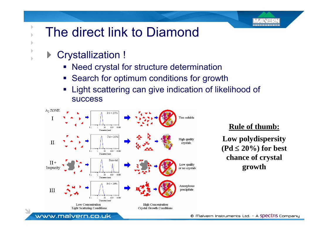
The direct link to Diamond Crystallization !
Need crystal for structure determinationSearch for optimum conditions for growthLight scattering can give indication of likelihood of success
Rule of thumb:Low polydispersity (Pd ≤ 20%) for best
chance of crystal growth

Light - Matter Interactions
As light is sent through material there are several potential interactions:
TransmissionAbsorptionFluorescence
Scattering !

Light - Matter Interactions:ScatteringThe incident photon induces an oscillating dipole in the electron cloud. As the dipole changes, energy is radiated or scattered in all directions.

Light Scattering
The scattering signal may be analysed by several methods:
Average signal strength: static, ‘classic’
Fluctuations of signal: dynamic, quasi-elastic
Shift of the signal: electrophoretic

Static Light Scattering
Molecular Weight Measurements

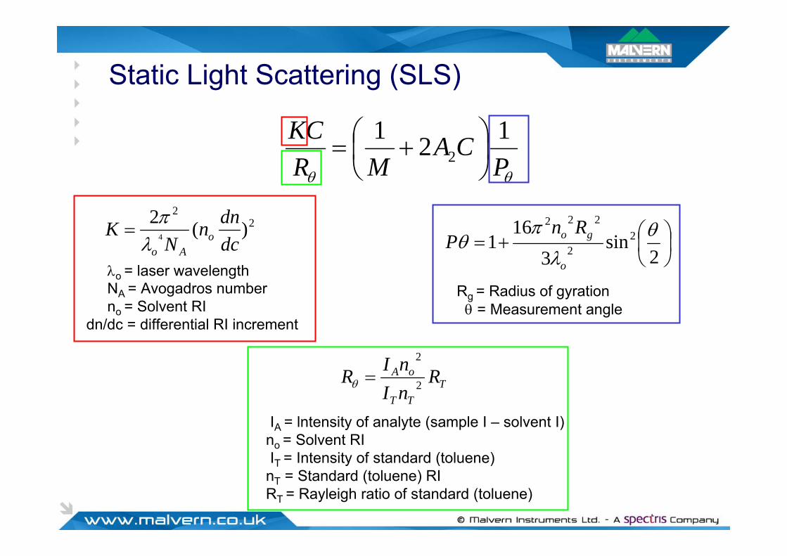
Static Light Scattering (SLS)Average scattering intensity is a function of the (particle) molecular weight and the 2nd virial coefficient.
)(121
2 θθ PCA
MRKC
⎟⎠⎞
⎜⎝⎛ +=
K = Optical constant C = ConcentrationM = Molecular weight Rθ = Rayleigh ratioA2 = 2nd Virial coefficient P(θ) = Shape (or form) factor
Rayleigh Equation
Static Light Scattering (SLS)
θθ PCA
MRKC 121
2 ⎟⎠⎞
⎜⎝⎛ +=
λo = laser wavelengthNA = Avogadros numberno = Solvent RI
dn/dc = differential RI increment
22
)(24 dc
dnnN
K oAoλ
π=
TTT
oA RnInIR 2
2
=θ
IA = lntensity of analyte (sample I – solvent I)no = Solvent RIIT = Intensity of standard (toluene)
nT = Standard (toluene) RI RT = Rayleigh ratio of standard (toluene)
⎟⎠⎞
⎜⎝⎛+=
2sin
316
1 22
222 θλ
πθ
o
go RnP
Rg = Radius of gyrationθ = Measurement angle

Static light scattering (SLS)
The intensity of scattered light that a macromolecule produces is proportional to the product of the weight-average molecular weight and the concentration of the macromolecule (I α (MW)(C))For molecules which show no angular dependence in their scattering intensity, accurate molecular weight determinations can be made at a single angle (Rayleigh scatterers, isotropic scattering)This is called a Debye plot and allows for the determination of
Absolute Molecular Weight2nd Virial Coefficient (A2)
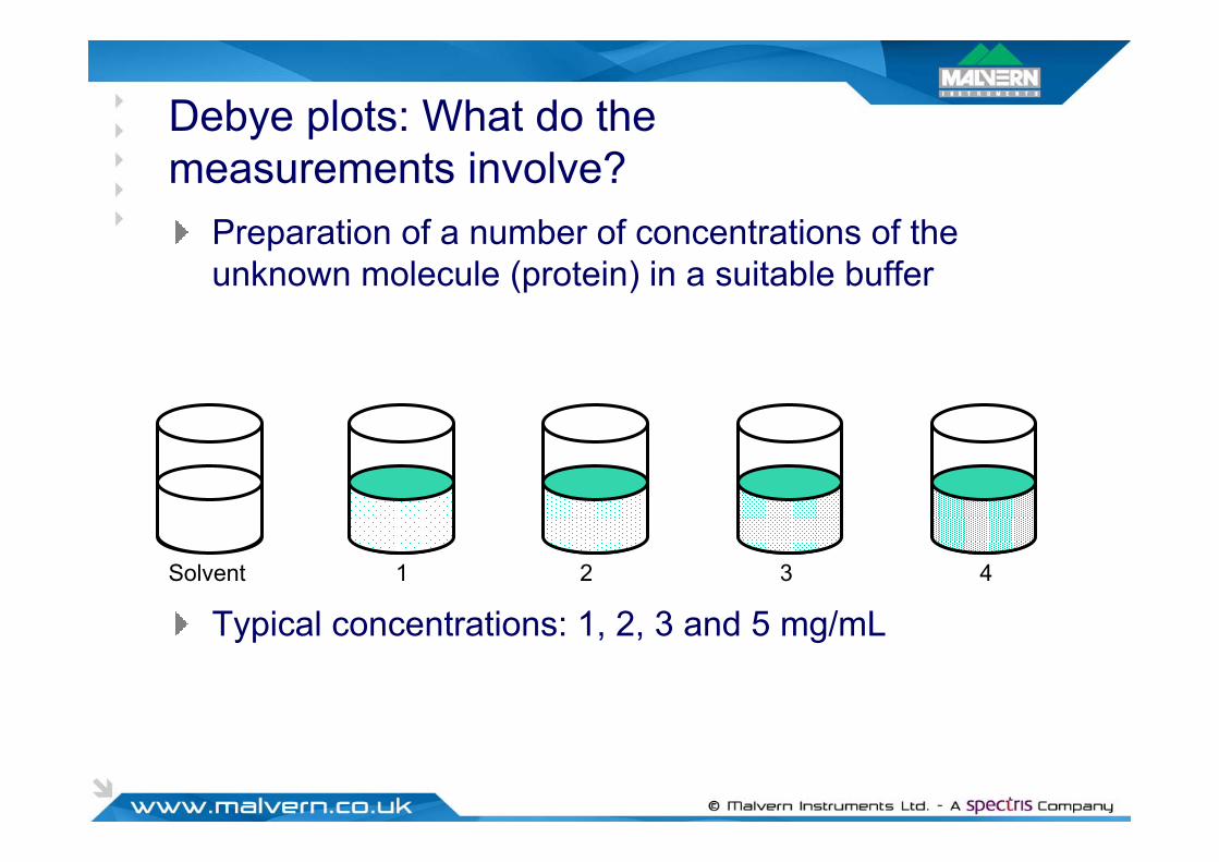
Debye plots: What do the measurements involve?
Preparation of a number of concentrations of the unknown molecule (protein) in a suitable buffer
Typical concentrations: 1, 2, 3 and 5 mg/mL1 2 3 4Solvent

Static Light Scattering (SLS)
For Rayleigh scatterers, P(θ) = 1 and the equation is simplified to
θθ PCA
MRKC 121
2 ⎟⎠⎞
⎜⎝⎛ +=
⎟⎠⎞
⎜⎝⎛ += CA
MRKC
221
θ
Therefore a plot of KC/Rθ versus C should give a straight line whose intercept at zero concentration will be 1/M and whose
gradient will be A2
(y = b + mx)

Molecular Weight Example (Lysozyme in PBS)
Itol = 192630 (counts/sec)Isol = 21870 (counts/sec)
)/(185.0 gmLdcdn
=
6.7743 x 10⁻⁵
6.6682 x 10⁻⁵
6.4765 x 10⁻⁵
6.1994 x 10⁻⁵
KC/Rθ
(1/Da)
720,700742,57010.059
344,900366,7705.029
201,030222,9003.018
65,96087,8301.006
Intensity of Analyte
(counts/sec)
Measured Intensity (counts/sec)
Lysozyme Concentration
(mg/mL)

Molecular Weight Example (Lysozyme in PBS)
1/Intercept = 14.6KDa
Slope = -3.23 x 10⁻⁴

2nd virial coefficient
A thermodynamic property describing the interaction strength between the molecule and the solventFor samples where A2 > 0, the molecules tend to stay in solution (protein molecules prefer contact with buffer)
When A2 = 0, the molecule-solvent interaction strength is equivalent to the molecule-molecule interaction strength – the solvent is described as being a theta solvent (protein doesn’t mind buffer)
When A2<0, the molecule will tend to fall out of solution or aggregate (protein doesn’t like buffer)

Dynamic Light Scattering
Molecular Size Measurements

Dynamic Light Scattering
Dynamic light scattering is a technique for measuring the size of molecules and nanoparticles
DLS measures the time dependent fluctuations in the scattering intensity to determine the translational diffusion coefficient (DT), and subsequently the hydrodynamic radius (RH)

Dynamic Light Scattering
Inte
nsity
Time (seconds)
The rate of intensity fluctuation is dependent upon the size of the particle/molecule
Dynamic light scattering is a technique for measuring the size of molecules and nanoparticles
DLS measures the time dependent fluctuations in the scattering intensity to determine the translational diffusion coefficient (D), and subsequently the hydrodynamic size

Dynamic Light Scattering (DLS)Fluctuations are a result of Brownian motion and can be correlated with the particle diffusion coefficient and size.
q = Scattering vector D = Diffusion coefficientRH = Radius k = Boltzmann constantT = Temperature η = Solvent viscosity
D6kTRH πη
=
Stokes-Einstein

Brownian Motion
Random movement of particles due to the bombardment by the solvent molecules that surround them

Brownian Motion
Temperature must be accurately known (viscosity)stable (otherwise convection present)
The larger the particle the more slowly the Brownian motion will beThe higher the temperature the more rapid the Brownian motion will be‘Velocity’ of the Brownian motion is defined by the translational diffusion coefficient (DT)

Physical Constraints
The non-randomness of the intensity trace is a consequence of the physical confinement of the particles to be in locations very near to their initial locations across very short time intervals.

Dynamic Light Scattering (DLS)Fluctuations are a result of Brownian motion and can be correlated with the particle diffusion coefficient and size.
q = Scattering vector D = Diffusion coefficientRH = Radius k = Boltzmann constantT = Temperature η = Solvent viscosity
D6kTRH πη
=
Stokes-Einstein
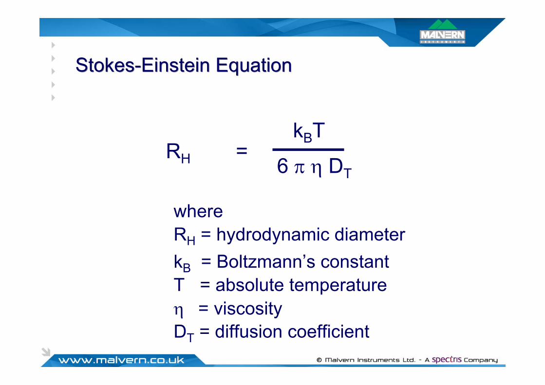
Stokes-Einstein EquationStokes-Einstein Equation
RH =6 π η DT
kBT
DT = diffusion coefficient
RH = hydrodynamic diameterkB = Boltzmann’s constantT = absolute temperatureη = viscosity
where

Comparative Protein RH Values
5 nm
LysozymeMW=14.5 kDa
RH=1.9 nm
Insulin - pH 7MW=34.2 kDa
RH=2.7 nm
Immunoglobulin GMW=160 kDaRH=7.1 nm Thyroglobulin
MW=650 kDaRH=10.1 nm

Correlogram Interpretation
Small Molecules
LargeParticles
Correlogram Interpretation

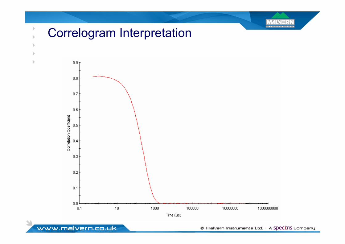
The time at which the correlation of the signal starts to decay gives
information about the mean diameter
Correlogram Interpretation

The time at which the correlation of the signal starts to decay gives
information about the mean diameter
The angle of decay gives information about the
polydispersity of the
distribution
θ
Correlogram Interpretation

The time at which the correlation of the signal starts to decay gives
information about the mean diameter
The angle of decay gives information about the
polydispersity of the
distribution
The baseline gives information about
the presence of large particles/aggregates
θ
Correlogram Interpretation

Distributions By DLS
Comparison of Z average (Cumulants) size to multi-modal distribution results.
Multimodal distribution fit
Z average: 12.4nm
(Single species assumption)

Intensity, Volume And Number Distributions
NUMBER43
VOLUME= πr3
INTENSITY= r 6
radius (nm)
Rel
ativ
e %
in c
lass
5 10 10050
1 1
radius (nm)
Rel
ativ
e %
in c
lass
5 10 10050
1
1000
radius (nm)R
elat
ive
% in
cla
ss
5 10 10050
1
1,000,000
Mixture containing equal numbers of 5 and 50nm spherical particles

Benefits Of Sizing By DLS
Non-invasiveHigh sensitivity (< 0.1 mg/mL for typical proteins)Low volume (12 µL)Scattering intensity is proportional to the square of the protein molecular weight, making the technique ideal for identifying the presence of trace amounts of aggregate.
Electrophoretic Light Scattering
Molecular Charge Measurements

Electrophoretic Light Scattering (ELS)Measured parameter is the frequency shift (Δν) of the light scattered from a moving particle.
⎟⎠⎞
⎜⎝⎛ υΔ
=μE
K
μ is the electrophoretic mobility, E is the electric field strength, and K is a constant.
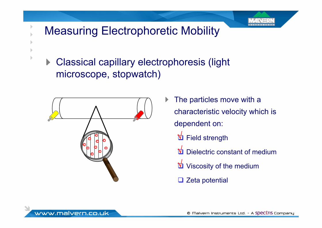
Measuring Electrophoretic Mobility
Classical capillary electrophoresis (light microscope, stopwatch)
+-The particles move with a characteristic velocity which is dependent on:
Field strength
Dielectric constant of medium
Viscosity of the medium
Zeta potential
√
√
√

Electrophoresis
Electrophoresis is the movement of a charged particle relative to the liquid it is suspended in under the influence of an applied electric fieldThe electrophoretic mobility of a colloidal dispersion can be used to determine the zeta potentialZeta potential is the charge a particle acquires in a particular mediumZeta potential measurements can be used to predict dispersion stabilityInfluenced by: pH, salts, concentration, additives,…

Electroosmosis
Electrophoresis in a
Closed Capillary Cell
Electroosmosis is the movement of liquid relative to a stationary charged surface under the influence of an applied field
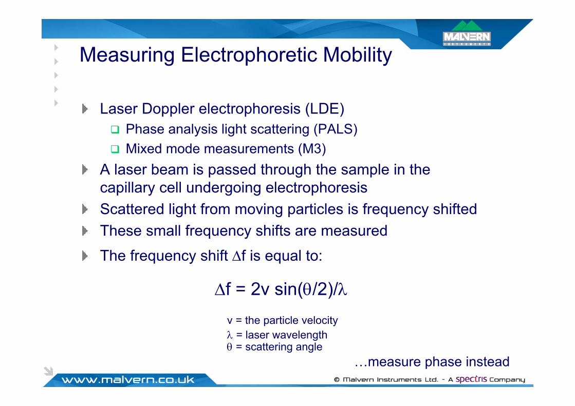
Measuring Electrophoretic Mobility
Laser Doppler electrophoresis (LDE) Phase analysis light scattering (PALS)Mixed mode measurements (M3)
A laser beam is passed through the sample in the capillary cell undergoing electrophoresisScattered light from moving particles is frequency shiftedThese small frequency shifts are measuredThe frequency shift Δf is equal to:
v = the particle velocityλ = laser wavelengthθ = scattering angle
Δf = 2v sin(θ/2)/λ
…measure phase instead

Mixed Mode Measurement (M3)
Mixed mode measurement (M3) is a patented method that allows measurement at any point in a capillary cell
It eliminates electroosmosis by reversing the applied field at a high frequency
Malvern have combined M3 with PALS to improve the measurement sensitivity and accuracy (M3-PALS)
Phase Analysis Light Scattering
Phase Difference Demonstration

Phase Plot From General Purpose
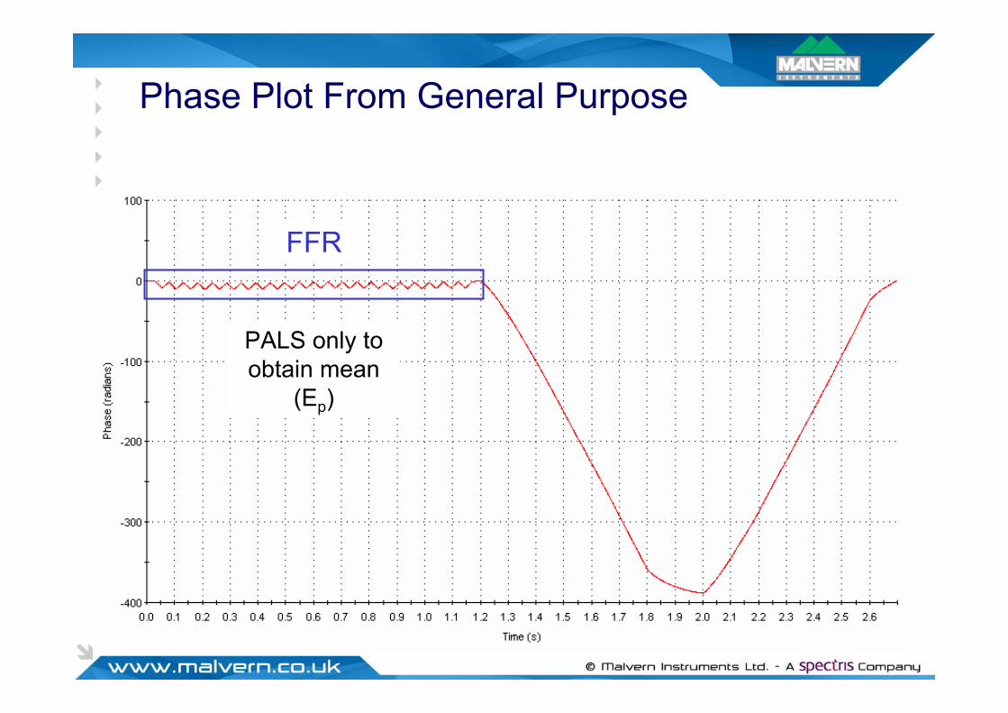
Phase Plot From General Purpose
FFR
PALS only to obtain mean
(Ep)

Phase Plot From General Purpose
FFR
PALS only to obtain mean
(Ep)
SFR
PALS to obtain mean (Eo+ Ep)+ FT to obtain
distribution (width)

Zetapotential Distribution Plot General Purpose
0
200000
400000
600000
800000
1000000
1200000
-200 -100 0 100 200
Inte
nsity
(kcp
s)
Zeta Potential (mV)
Zeta Potential Distribution
Record 1: dts50

Light Scattering Return
Hydrodynamic RadiusDistribution & PolydispersitySolution CompositionMolecular Weight2nd Virial CoefficientConformationShape EstimatesZeta PotentialpI & Charge EstimatesFormulation Stability
Application Example
Molecular Weight Measurements

Absolute Protein Molecular Weight
Jones, Mattison “Automated dynamic and static light scattering measurements”, BioPharm 2001, 14(8): 56.

A2 Crystallization Window
*George, A; Wilson, W.W. “Predicting protein crystallization from a dilute solution property”, Acta Crystallogr 1994, D50, 361-365.
Crystallization Window: -0.8 > A2 > –8 (x 10-4 mol mL / g2)*
CA2M1
RKC
2+=θ
Rayleigh Equation

Application Example
Molecular Size Measurements
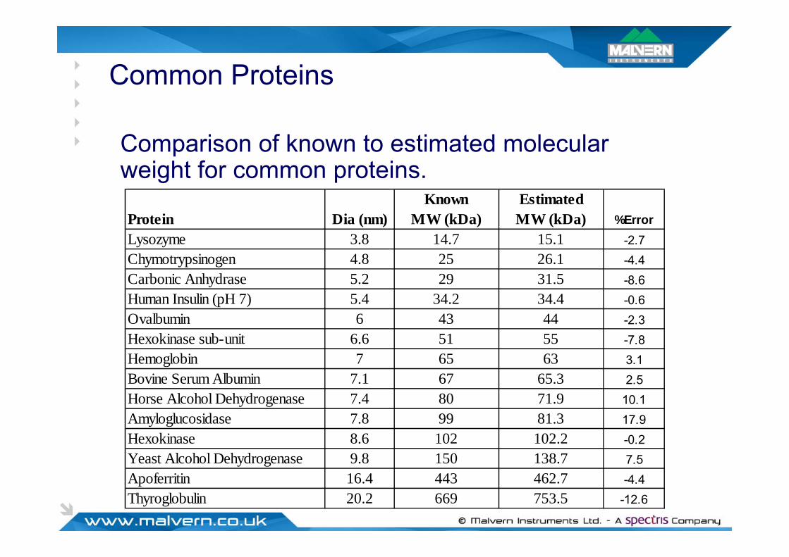
Common Proteins
Comparison of known to estimated molecular weight for common proteins.
Protein Dia (nm)Known
MW (kDa)EstimatedMW (kDa) %Error
Lysozyme 3.8 14.7 15.1 -2.7Chymotrypsinogen 4.8 25 26.1 -4.4Carbonic Anhydrase 5.2 29 31.5 -8.6Human Insulin (pH 7) 5.4 34.2 34.4 -0.6Ovalbumin 6 43 44 -2.3Hexokinase sub-unit 6.6 51 55 -7.8Hemoglobin 7 65 63 3.1Bovine Serum Albumin 7.1 67 65.3 2.5Horse Alcohol Dehydrogenase 7.4 80 71.9 10.1Amyloglucosidase 7.8 99 81.3 17.9Hexokinase 8.6 102 102.2 -0.2Yeast Alcohol Dehydrogenase 9.8 150 138.7 7.5Apoferritin 16.4 443 462.7 -4.4Thyroglobulin 20.2 669 753.5 -12.6

Identifying Quaternary Structure
DLS results indicate an insulin structure that is dimeric at pH 2 and hexameric at pH 7, consistent with crystallographic data.
Human Insulin - pH 2RH = 1.73Est MW = 12.1 kDaAct MW = 11.4 kDaDimer
Human Insulin - pH 7RH = 2.69Est MW = 34.1 kDaAct MW = 34.2 kDaHexamer

Application Example
Polydispersity Measurements

Polydispersity (Pd) From DLS
Pd is representative of the particle size distribution width.
Monodisperse Polydisperse
60 second measurement

Crystal Screening Using DLS

Monoclonal Antibody FragmentSize, zeta potential and molecular weight
Mean diameter = 5.1nm
Mean zeta potential = -7.6mV
MW = 20.7KDaA2 = - 0.0049 ml mol/g2

Malvern Instruments
& the Zetasizer Nano

Zetasizer Nano
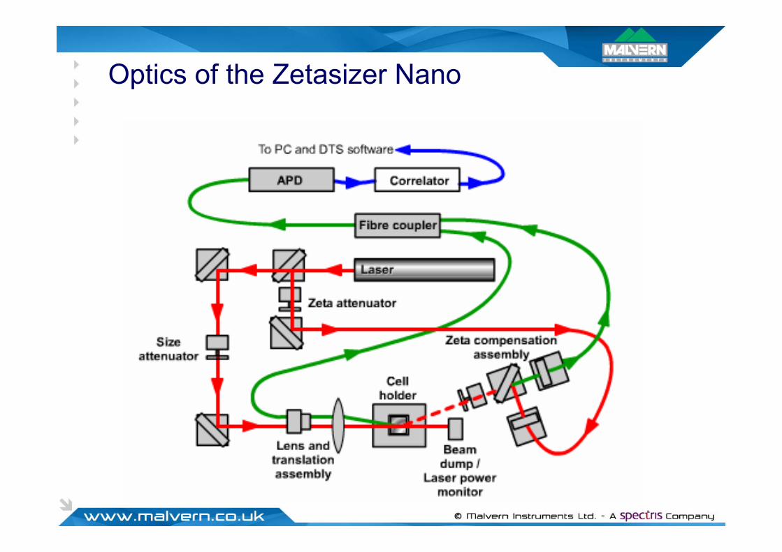
Optics of the Zetasizer Nano

Zetasizer Technical Specifications
Crystal screeningProtein & polymer characterizationCMC measurementsDrug delivery systems
Formulation stabilityBiological assembliesVirus & vaccine characterizationMacromolecular critical points
Parameter ValueSizing range 0.6 nm to 6 μm DiamConcentration range 0.1 mg/mL Lys to 30w%Min sizing sample volume 12 μLMin zeta sample volume 0.75 mLTemperature control 2 to 90 oCConductivity range 0 to 200 mS/cmLaser 3 mW 633 nm HeNeDetector APD

More information
Application notesMultimedia presentationsBrochuresDetailed specifications
www.malvern.co.uk/proteins