Propulsion Systems for Hybrid Vehicles
473
-
Upload
jackie-dong -
Category
Documents
-
view
1.227 -
download
6
Transcript of Propulsion Systems for Hybrid Vehicles
IET PowEr and EnErgy sErIEs 45
Series Editors: Professor A.T. Johns Professor D.F. Warne
Propulsion Systems for Hybrid Vehicles

Other volumes in this series:
Volume 1 Power circuit breaker theory and design C.H. Flurscheim (Editor)Volume 4 Industrial microwave heating A.C. Metaxas and R.J. MeredithVolume 7 Insulators for high voltages J.S.T. LoomsVolume 8 Variable frequency AC-motor drive systems D. FinneyVolume 10 SF6 switchgear H.M. Ryan and G.R. JonesVolume 11 Conduction and induction heating E.J. DaviesVolume 13 Statistical techniques for high voltage engineering W. Hauschild and
W. MoschVolume 14 Uninterruptable power supplies J. Platts and J.D. St Aubyn (Editors)Volume 15 Digital protection for power systems A.T. Johns and S.K. SalmanVolume 16 Electricity economics and planning T.W. BerrieVolume 18 Vacuum switchgear A. GreenwoodVolume 19 Electrical safety: a guide to causes and prevention of hazards
J. Maxwell AdamsVolume 21 Electricity distribution network design, 2nd edition E. Lakervi and
E.J. HolmesVolume 22 Artificial intelligence techniques in power systems K. Warwick, A.O. Ekwue
and R. Aggarwal (Editors)Volume 24 Power system commissioning and maintenance practice K. HarkerVolume 25 Engineers’ handbook of industrial microwave heating R.J. MeredithVolume 26 Small electric motors H. Moczala et al.Volume 27 AC-DC power system analysis J. Arrill and B.C. SmithVolume 29 High voltage direct current transmission, 2nd edition J. ArrillagaVolume 30 Flexible AC Transmission Systems (FACTS) Y-H. Song (Editor)Volume 31 Embedded generation N. Jenkins et al.Volume 32 High voltage engineering and testing, 2nd edition H.M. Ryan (Editor)Volume 33 Overvoltage protection of low-voltage systems, revised edition P. HasseVolume 34 The lightning flash V. CoorayVolume 35 Control techniques drives and controls handbook W. Drury (Editor)Volume 36 Voltage quality in electrical power systems J. Schlabbach et al.Volume 37 Electrical steels for rotating machines P. BeckleyVolume 38 The electric car: development and future of battery, hybrid and fuel-cell
cars M. WestbrookVolume 39 Power systems electromagnetic transients simulation J. Arrillaga and
N. WatsonVolume 40 Advances in high voltage engineering M. Haddad and D. WarneVolume 41 Electrical operation of electrostatic precipitators K. ParkerVolume 43 Thermal power plant simulation and control D. FlynnVolume 44 Economic evaluation of projects in the electricity supply industry H. KhatibVolume 45 Propulsion systems for hybrid vehicles J. MillerVolume 46 Distribution switchgear S. StewartVolume 47 Protection of electricity distribution networks, 2nd edition J. Gers and
E. HolmesVolume 48 Wood pole overhead lines B. WareingVolume 49 Electric fuses, 3rd edition A. Wright and G. NewberyVolume 50 Wind power integration: connection and system operational aspects B. Fox
et al.Volume 51 Short circuit currents J. SchlabbachVolume 52 Nuclear power J. WoodVolume 53 Condition assessment of high voltage insulation in power system
equipment R.E. James and Q. SuVolume 905 Power system protection, 4 volumes
Propulsion Systems for Hybrid Vehicles
John M. Miller
The Institution of Engineering and Technology
Published by The Institution of Engineering and Technology, London, United Kingdom
First edition © 2004 The Institution of Electrical Engineers Paperback edition © 2008 The Institution of Engineering and Technology
First published 2004 (978-0-86341-336-0) Reprinted with new cover 2006 Paperback edition 2008 (978-086341-915-7)
This publication is copyright under the Berne Convention and the Universal Copyright Convention. All rights reserved. Apart from any fair dealing for the purposes of research or private study, or criticism or review, as permitted under the Copyright, Designs and Patents Act, 1988, this publication may be reproduced, stored or transmitted, in any form or by any means, only with the prior permission in writing of the publishers, or in the case of reprographic reproduction in accordance with the terms of licences issued by the Copyright Licensing Agency. Inquiries concerning reproduction outside those terms should be sent to the publishers at the undermentioned address:
The Institution of Engineering and Technology Michael Faraday House Six Hills Way, Stevenage Herts, SG1 2AY, United Kingdom
www.theiet.org
While the author and the publishers believe that the information and guidance given in this work are correct, all parties must rely upon their own skill and judgement when making use of them. Neither the author nor the publishers assume any liability to anyone for any loss or damage caused by any error or omission in the work, whether such error or omission is the result of negligence or any other cause. Any and all such liability is disclaimed.
The moral rights of the author to be identified as author of this work have been asserted by him in accordance with the Copyright, Designs and Patents Act 1988.
British Library Cataloguing in Publication DataMiller, John
Propulsion systems for hybrid vehicles 1. Hybrid electric vehicles I. Title II. Institution of Electrical Engineers 629 . 2293
ISBN 978-0-86341-915-7
Typeset in India by Newgen Imaging Systems (P) Ltd, Chennai Printed in the UK by Lightning Source UK Ltd, Milton Keynes

For JoAnn and for Nathan

Contents
Preface xiii
1 Hybrid vehicles 1
1.1 Performance characteristics of road vehicles 111.1.1 Partnership for new generation of vehicle goals 111.1.2 Engine downsizing 121.1.3 Drive cycle characteristics 141.1.4 Hybrid vehicle performance targets 191.1.5 Basic vehicle dynamics 19
1.2 Calculation of road load 231.2.1 Components of road load 241.2.2 Friction and wheel slip 30
1.3 Predicting fuel economy 331.3.1 Emissions 331.3.2 Brake specific fuel consumption (BSFC) 331.3.3 Fuel economy and consumption conversions 35
1.4 Internal combustion engines: a primer 361.4.1 What is brake mean effective pressure (BMEP)? 381.4.2 BSFC sensitivity to BMEP 401.4.3 ICE basics: fuel consumption mapping 42
1.5 Grid connected hybrids 441.5.1 The connected car, V2G 441.5.2 Grid connected HEV20 and HEV60 461.5.3 Charge sustaining 49
1.6 References 50
2 Hybrid architectures 53
2.1 Series configurations 562.1.1 Locomotive drives 572.1.2 Series–parallel switching 58
Admin
下划线
Admin
下划线
本页已使用福昕阅读器进行编辑。 福昕软件(C)2005-2009,版权所有, 仅供试用。ഀ
viii Contents
2.1.3 Load tracking architecture 612.2 Pre-transmission parallel configurations 62
2.2.1 Mild hybrid 622.2.2 Power assist 652.2.3 Dual mode 66
2.3 Pre-transmission combined configurations 672.3.1 Power split 692.3.2 Power split with shift 732.3.3 Continuously variable transmission (CVT) derived 742.3.4 Integrated hybrid assist transmission 75
2.4 Post-transmission parallel configurations 782.4.1 Post-transmission hybrid 792.4.2 Wheel motors 81
2.5 Hydraulic post-transmission hybrid 812.5.1 Launch assist 822.5.2 Hydraulic–electric post-transmission 832.5.3 Very high voltage electric drives 84
2.6 Flywheel systems 842.6.1 Texas A&M University transmotor 842.6.2 Petrol electric drivetrain (PEDT) 852.6.3 Swiss Federal Institute flywheel concept 86
2.7 Electric four wheel drive 872.7.1 Production Estima Van example 88
2.8 References 89
3 Hybrid power plant specifications 91
3.1 Grade and cruise targets 953.1.1 Gradeability 983.1.2 Wide open throttle 98
3.2 Launch and boosting 983.2.1 First two seconds 983.2.2 Lane change 98
3.3 Braking and energy recuperation 993.3.1 Series RBS 1003.3.2 Parallel RBS 1013.3.3 RBS interaction with ABS 1023.3.4 RBS interaction with IVD/VSC/ESP 102
3.4 Drive cycle implications 1033.4.1 Types of drive cycles 1033.4.2 Average speed and impact on fuel economy 1033.4.3 Dynamics of acceleration/deceleration 1043.4.4 Wide open throttle (WOT) launch 105
Contents ix
3.5 Electric fraction 1053.5.1 Engine downsizing 1053.5.2 Range and performance 106
3.6 Usage requirements 1063.6.1 Customer usage 1073.6.2 Electrical burden 1073.6.3 Grade holding and creep 1073.6.4 Neutral idle 108
3.7 References 108
4 Sizing the drive system 109
4.1 Matching the electric drive and ICE 1094.1.1 Transmission selection 1104.1.2 Gear step selection 1124.1.3 Automatic transmission architectures 113
4.2 Sizing the propulsion motor 1184.2.1 Torque and power 1194.2.2 Constant power speed ratio (CPSR) 1224.2.3 Machine sizing 124
4.3 Sizing the power electronics 1284.3.1 Switch technology selection 1304.3.2 kVA/kW and power factor 1304.3.3 Ripple capacitor design 1324.3.4 Switching frequency and PWM 137
4.4 Selecting the energy storage technology 1394.4.1 Lead–acid technology 1474.4.2 Nickel metal hydride 1484.4.3 Lithium ion 1494.4.4 Fuel cell 1504.4.5 Ultra-capacitor 1564.4.6 Flywheels 159
4.5 Electrical overlay harness 1594.5.1 Cable requirements 1604.5.2 Inverter busbars 1644.5.3 High voltage disconnect 1664.5.4 Power distribution centres 167
4.6 Communications 1674.6.1 Communication protocol: CAN 1704.6.2 Power and data networks 1704.6.3 Future communications: TTCAN 1724.6.4 Future communications: Flexray 1744.6.5 Competing future communications protocols 1774.6.6 DTC diagnostic test codes 178
x Contents
4.7 Supporting subsystems 1794.7.1 Steering systems 1794.7.2 Braking systems 1794.7.3 Cabin climate control 1804.7.4 Thermal management 1814.7.5 Human–machine interface 184
4.8 Cost and weight budgeting 1854.8.1 Cost analysis 1854.8.2 Weight tally 186
4.9 References 188
5 Electric drive system technologies 191
5.1 Brushless machines 1915.1.1 Brushless dc 1955.1.2 Brushless ac 1995.1.3 Design essentials of the SPM 2035.1.4 Dual mode inverter 212
5.2 Interior permanent magnet 2145.2.1 Buried magnet 2155.2.2 Flux squeeze 2185.2.3 Mechanical field weakening 2235.2.4 Multilayer designs 225
5.3 Asynchronous machines 2255.3.1 Classical induction 2265.3.2 Winding reconfiguration 2295.3.3 Pole changing 230
5.4 Variable reluctance machine 2425.4.1 Switched reluctance 2445.4.2 Synchronous reluctance 2465.4.3 Radial laminated structures 249
5.5 Relative merits of electric machine technologies 2495.5.1 Comparisons for electric vehicles 2505.5.2 Comparisons for hybrid vehicles 251
5.6 References 254
6 Power electronics for ac drives 257
6.1 Essentials of pulse width modulation 2596.2 Resonant pulse modulation 2646.3 Space-vector PWM 2666.4 Comparison of PWM techniques 2746.5 Thermal design 2786.6 Reliability considerations 283
Contents xi
6.7 Sensors for current regulators 2866.8 Interleaved PWM for minimum ripple 2886.9 References 290
7 Drive system control 291
7.1 Essentials of field oriented control 2927.2 Dynamics of field oriented control 2977.3 Sensorless control 3047.4 Efficiency optimisation 3087.5 Direct torque control 3127.6 References 315
8 Drive system efficiency 319
8.1 Traction motor 3198.1.1 Core losses 3218.1.2 Copper losses and skin effects 327
8.2 Inverter 3308.2.1 Conduction 3308.2.2 Switching 3318.2.3 Reverse recovery 333
8.3 Distribution system 3348.4 Energy storage system 3358.5 Efficiency mapping 3368.6 References 340
9 Hybrid vehicle characterisation 343
9.1 City cycle 3509.2 Highway cycle 3519.3 Combined cycle 3519.4 European NEDC 3539.5 Japan 10-15 mode 3559.6 Regulated cycle for hybrids 3559.7 References 357
10 Energy storage technologies 359
10.1 Battery systems 35910.1.1 Lead–acid 36510.1.2 Nickel metal hydride 36610.1.3 Lithium ion 369
xii Contents
10.2 Capacitor systems 37310.2.1 Symmetrical ultra-capacitors 37610.2.2 Asymmetrical ultra-capacitors 37810.2.3 Ultra-capacitors combined with batteries 37910.2.4 Ultra-capacitor cell balancing 38710.2.5 Electro-chemical double layer capacitor
specification and test 39210.3 Hydrogen storage 397
10.3.1 Metal hydride 39910.3.2 High pressure gas 399
10.4 Flywheel systems 40010.5 Pneumatic systems 40210.6 Storage system modelling 402
10.6.1 Battery model 40310.6.2 Fuel cell model 40710.6.3 Ultra-capacitor model 410
10.7 References 419
11 Hybrid vehicle test and validation 423
11.1 Vehicle coast down procedure 42411.2 Sport utility vehicle test 42711.3 Sport utility vehicle plus trailer test 42911.4 Class 8 tractor test 43211.5 Class 8 tractor plus trailer test 43411.6 References 439
Index 441
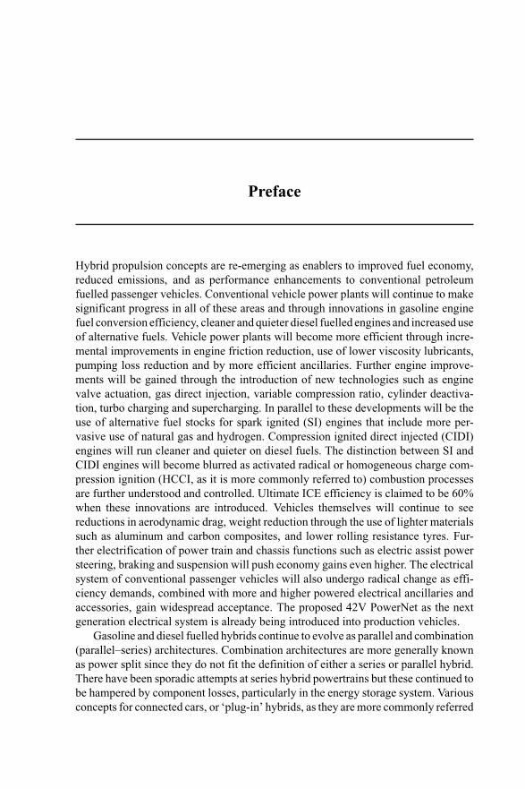
Preface
Hybrid propulsion concepts are re-emerging as enablers to improved fuel economy,reduced emissions, and as performance enhancements to conventional petroleumfuelled passenger vehicles. Conventional vehicle power plants will continue to makesignificant progress in all of these areas and through innovations in gasoline enginefuel conversion efficiency, cleaner and quieter diesel fuelled engines and increased useof alternative fuels. Vehicle power plants will become more efficient through incre-mental improvements in engine friction reduction, use of lower viscosity lubricants,pumping loss reduction and by more efficient ancillaries. Further engine improve-ments will be gained through the introduction of new technologies such as enginevalve actuation, gas direct injection, variable compression ratio, cylinder deactiva-tion, turbo charging and supercharging. In parallel to these developments will be theuse of alternative fuel stocks for spark ignited (SI) engines that include more per-vasive use of natural gas and hydrogen. Compression ignited direct injected (CIDI)engines will run cleaner and quieter on diesel fuels. The distinction between SI andCIDI engines will become blurred as activated radical or homogeneous charge com-pression ignition (HCCI, as it is more commonly referred to) combustion processesare further understood and controlled. Ultimate ICE efficiency is claimed to be 60%when these innovations are introduced. Vehicles themselves will continue to seereductions in aerodynamic drag, weight reduction through the use of lighter materialssuch as aluminum and carbon composites, and lower rolling resistance tyres. Fur-ther electrification of power train and chassis functions such as electric assist powersteering, braking and suspension will push economy gains even higher. The electricalsystem of conventional passenger vehicles will also undergo radical change as effi-ciency demands, combined with more and higher powered electrical ancillaries andaccessories, gain widespread acceptance. The proposed 42V PowerNet as the nextgeneration electrical system is already being introduced into production vehicles.
Gasoline and diesel fuelled hybrids continue to evolve as parallel and combination(parallel–series) architectures. Combination architectures are more generally knownas power split since they do not fit the definition of either a series or parallel hybrid.There have been sporadic attempts at series hybrid powertrains but these continued tobe hampered by component losses, particularly in the energy storage system. Variousconcepts for connected cars, or ‘plug-in’ hybrids, as they are more commonly referred
xiv Preface
to, continue to make progress and are being advocated as highly distributed micro-generation sources during utility grid peak loading hours. All electric hybrids todayare pre-transmission configurations wherein the electric torque source is summed tothe heat engine torque output at the transmission input shaft. A post-transmissionhybrid involves summing the electric torque to engine torque at the output shaft ofthe transmission. This effectively puts the electric drive motor at a fixed gear ratiorelative to the wheels so that some form of disconnect device is needed to avoid over-revving, on the one hand, or incurring excessive spin losses during inactive periods onthe other. Post-transmission hybrids have been investigated using electric drives butthese have not gained much favour from manufacturers. Post-transmission hydraulichybrid architectures, however, have found favor with automotive manufacturers andare being pursued for heavy-duty truck and commercial vehicle fleet applications,mainly as launch assist devices. A new branch has been added to the pre-transmissionand post-transmission hybrid configuration taxonomy with the introduction of electricfour wheel drive. In this architecture the electric drive system is standalone and con-nected to the normally undriven axle. Typically, an on-demand system – E-4, as onemanufacturer refers to it – consists of a single traction motor/generator geared to theaxle through a small transmission and differential. Very effective on low mu surfacesand grades, E-4 is finding widespread interest among manufacturers as another meansto introduce entry level hybridization without extensive vehicle chassis and power-train modifications. It also provides vehicle longitudinal stability control advantagesover conventional hybrid architectures. With E-4, power delivered to both axles canbe manipulated by the powertrain controller and separately by the E-4 controller.This requires a fast communication bus in the vehicle control architecture so that avehicle system controller containing some form of electronic stability program maycoordinate both systems.
In this book, attention is focused on hybrid technologies that are combined withgasoline internal combustion engines. Hybrid CIDI engines operating on diesel fuelhave been demonstrated, but the efficiency gained by adding electric fraction willbe modest since the diesel is already a very efficient energy converter. Wells-to-wheels energy analysis show that the process of delivering 100 units of gasolineenergy to the vehicle’s fuel tank is 88% efficient for both conventional and hybridtechnologies. Conventional gasoline ICEs are approximately 25% efficient, and ifthe overall driveline is 65% efficient that leaves 14 units of energy delivered to thewheels for propulsion. For a battery electric vehicle this rises to 20 units at the wheelseven though the well-to-tank (well to utility grid to vehicle battery) efficiency is only26% efficient. Tank (battery) to wheel efficiency in an EV is approximately 80% . Fora gasoline hybrid 26.4 units of energy are delivered to the wheels or 88% more thanwith a conventional vehicle driveline. This is because the gasoline-electric hybridpowertrain operates at 40% rather than 25% efficiency. CIDI engines running ondiesel fuel already operate at 40% efficiency so the gains to be realised by adding ahybrid system will be marginal for the cost invested. As fuel cell hybrids enter themarketplace the well-to-wheels efficiency is expected to better than match gasolineelectric hybrids by delivering 28 to 30 units of energy to the wheels.
Preface xv
This book assumes a working knowledge of automotive systems and electricmachines, power electronics and drives. It consists of 11 chapters organised in atop-down fashion. Chapters 1 and 2 are an overview and describe what is meantby hybridization, how the vehicle system targets are established and what the archi-tectural choices are. Chapter 3 goes into more detail on the vehicle system targetsand hybrid function definition as well as supporting subsystems necessary to supportthe hybrid powertrain. In Chapter 4 the reader is taken into more detail on sizingthe electric system components, selecting the energy storage system technology, andsummarising how to make a business case for a hybrid by exploring the developmentof the value equation based on benefit and system cost.
Chapters 5–7 contain the real fundamentals of electric drive systems, includingelectric machine design fundamentals, power electronics device and power processingfundamentals plus its controller and various modulation schemes. These three chap-ters may be used as part of a senior undergraduate, or as a supplement to graduate,level courses on machines, power electronics, modulation theory, and ac drives.
Chapter 8 puts all of the preceding material together into a vehicle system andexplores the impact that component and system losses have on system efficiency.The hypothesis that the most efficient system does not necessarily require optimumefficiency of all its component parts is examined. Chapter 9 introduces a samplingof internationally used standard drive cycles used to both quantify average drivingmodes and customer usage profiles and how these impact fuel economy. This chapteralso describes how certified testing laboratories utilise the various drive cycles toperform fuel economy tests.
Chapter 10 is meant to stand alone as an overall summary of energy storagesystems. It is designed to provide a deeper understanding of the most common energystorage systems and to expand on the introductory topics discussed in Chapter 4.Chapter 10 contains considerable detail on the advantages and weaknesses of energystorage technologies with the inclusion of some novel and less known techniques. Thischapter may be used as a complement to undergraduate courses in vehicle systemsengineering and mechatronics courses.
Chapters 11 concludes this book and is offered as an example of real world vehicletesting to show how the results of some simple coast down trials can be used to gleansome significant insights into not only vehicle propulsion power needs, but how thisneed is modified when towing a trailer. Trailer towing is a topic often neglectedbecause of the diversity of towed objects used in the after market. A covered trailerexample is presented to illustrate that intuition and experience based insights cannot berelied on to ascertain the performance of any vehicle when its aerodynamic characterhas been altered by pulling a trailer. The discussion then turns to railroad experienceand that of multi-vehicle trains and passenger car ‘platooning’ to illustrate the impactof closely spaced vehicles on propulsion power due to aerodynamic drag. Lastly, aclass 8 semi-tractor trailer is investigated to further illustrate this procedure and toshow why aerodynamic styling, fairings and side skirts are so important to maintainthe air streamlines over and around the tractor to trailer gap.
There will soon be a sport utility hybrid on the streets when the Ford Motor Co.introduces the hybrid Escape with a Job1 slated for late 2004. This vehicle is equipped

xvi Preface
for towing and the results presented in this chapter will hopefully show the importanceof carefully considering the type and style of trailer to those anticipating a need to dotowing with a hybrid vehicle. Trailer frontal area, shape and hitch length are crucial.
The material in this book is recommended primarily for practicing engineers inindustrial, commercial, academic and government settings. It can be used to comple-ment existing texts for a graduate or senior level undergraduate course on automotiveelectronics and transportation systems. Depending on the background of the practisingengineers or university students, the material contained in this book may be selectedto suit specific applications or interests. In more formal settings, and in particularwhere different disciplines such as electrical and mechanical engineering studentsare combined, course instructors are encouraged to focus on material presented inChapters 2–4. Instructors also have the flexibility to choose the material in any orderfor their lectures. A good deal of material in this book has been developed by theauthor during active projects and presentations at conferences, symposia, workshopsand invited lectures to various universities.
The author wishes to acknowledge his parents, John and Margarete, who first sethim out on this path of curiosity about the world. Many individuals have guided mealong the path to an engineering career and I wish to acknowledge those who haveinfluenced me the most. First, in appreciation to all the mentoring that Mr WilliamBolton afforded me during those formative early high school years and for thosememorable trips to two international science fairs. Later, to my undergraduate advisor,Prof. Dwight Mix, at the University of Arkansas-Fayetteville, for his imparting suchkeen insights into engineering; yes, that trek into discrete mathematics was worththe trip. Most of all, I wish to acknowledge Prof. Jerry Park, my PhD thesis advisor,for many fond memories of scientific exploration and discovery. What a confidenceboost to file for patents in the process of dissertation writing. He is a fine engineer,outstanding educator, and genuine friend whom I treasure having the good fortuneof knowing. On a personal note I wish to acknowledge Uncle Werner and to say tohim, that yes, it was time to retire and move on to different endeavors and give theyounger engineers room to grow. In remembrance of Doreen (my deceased first wife)for her insistence on higher education, and to my wife JoAnn for all her patience andsupport, without which this book would not have been possible. Last, but not least,the author wishes to acknowledge the efforts and assistance of Ms Wendy Hiles andthe editorial staff at the IEE.
John M. Miller2003
Chapter 1
Hybrid vehicles
At the time of writing, the automotive industry is awakening to the fact that indeed,hybrid electric vehicles are one answer to the world’s need for lower polluting andmore fuel efficient personal transportation. Studies have been done that show if gaso-line electric hybrids were introduced into the market starting today and reaching fullpenetration in ten years, and estimating that 40% of the oil consumption is used fortransportation, then it would be equivalent to doubling the annual rate of new oil fieldsbrought on line.1 In North America transportation is 97% dependent on petroleum,primarily gasoline and diesel fuels and even more to the point, transportation con-sumer 67% of total petroleum usage. There are now only 130 000 gasoline–electrichybrids on the streets that are being used for personal transportation. All the majorautomotive manufacturers have announced plans to introduce hybrid propulsion sys-tems into their products. Some manufacturers see hybrid vehicles as supplementaryactions or ‘bridging actions’ leading to an eventual fuel cell and hydrogen driveneconomy. More visionary companies see hybrid vehicles as viable long term environ-mental solutions during the period when internal-combustion engines (ICEs) evolve tocleaner and more efficient power plants. Today, Toyota Motor Company is a memberof the visionary camp and clearly the leader in hybrid technology. Toyota Motor Co.has announced that by CY2005 they will have an annual production rate of 300 000hybrids per year. Of the approximately 55M vehicles sold each year globally, this isa small, but significant, fraction of sales. In this book the global distribution of auto-mobiles will be assumed to be split as 18M in each of the three major geographicalregions: The Americas, Europe, and Asia-Pacific.
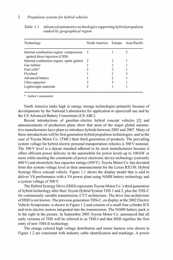
Technology leadership in hybrid technology belongs to the Japanese. Accordingto the US National Research Council [1], North America ranks nearly last in allareas of hybrid propulsion and its supporting technologies. Table 1.1, extracted fromReference 1, is a condensed summary of their rankings.
1 Professor M. Ehsani, Presentation to 2003 Global Powertrain Conference, Ann Arbor, M.I.
2 Propulsion systems for hybrid vehicles
Table 1.1 Advanced automotive technologies supporting hybrid propulsionranked by geographical region
Technology North America Europe Asia-Pacific
Internal combustion engine: compression 3 1 2ignited direct injection (CIDI)
Internal combustion engine: spark ignited 2 2 1Gas turbine 1 1 1Fuel cells* 2 2 1Flywheel 1 1 3Advanced battery 1 2 1Ultra-capacitor 3 3 1Lightweight materials 2 1 1
* Author’s assessment
North America ranks high in energy storage technologies primarily because ofdevelopments by the National Laboratories for application to spacecraft use and bythe US Advanced Battery Consortium (US ABC).
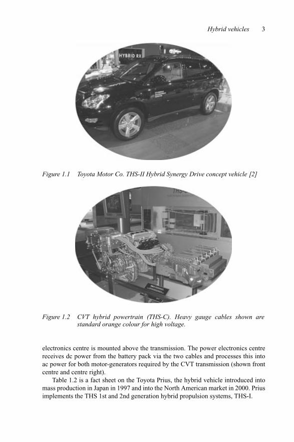
Recent introductions of gasoline–electric hybrid concept vehicles [2] andannouncements of production plans show that most of the major global automo-tive manufacturers have plans to introduce hybrids between 2003 and 2007. Many ofthese introductions will be first generation hybrid propulsion technologies, and in thecase of Toyota Motor Co. (TMC) their third generation of products. The prevailingsystem voltage for hybrid electric personal transportation vehicles is 300 V nominal.The 300 V level is a dejour standard adhered to by most manufacturers because itoffers efficient power delivery in the automobile for power levels up to 100 kW ormore while meeting the constraints of power electronic device technology (currently600 V) and electrolytic bus capacitor ratings (450 V). Toyota Motor Co. has deviatedfrom this system voltage level in their announcement for the Lexus RX330, HybridSynergy Drive concept vehicle. Figure 1.1 shows the display model that is said todeliver V8 performance with a V6 power plant using NiMH battery technology anda system voltage of 500 V.
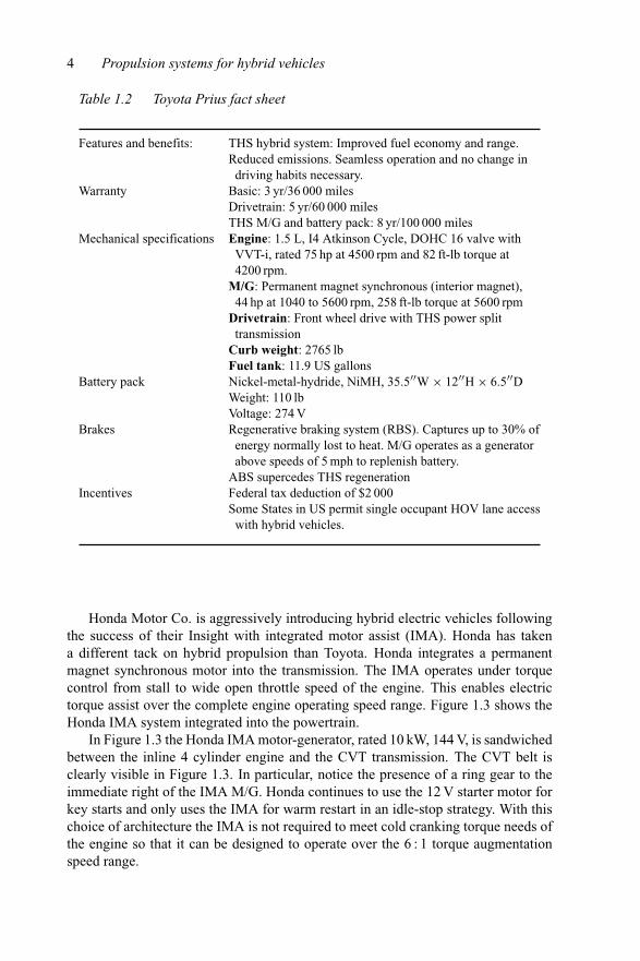
The Hybrid Synergy Drive (HSD) represents Toyota Motor Co.’s third generationof hybrid technology after their Toyota Hybrid System THS 1 and 2, plus the THS-Cfor continuously variable transmission, CVT architecture. The drive line architectureof HSD is not known. The previous generation THS-C, on display at the 2002 ElectricVehicle Symposium, is shown in Figure 1.2 and consists of a small four cylinder ICEand twin electric motors integrated into the transmission. The NiMH battery pack isto the right in the picture. In September 2003 Toyota Motor Co. announced that allearly versions of THS will be referred to as THS-I and that HSD signifies the firstentry of new THS-II technology.
The orange colored high voltage distribution and motor harness wire shown inFigure 1.2 are consistent with industry cable identification and markings. A power
Hybrid vehicles 3
Figure 1.1 Toyota Motor Co. THS-II Hybrid Synergy Drive concept vehicle [2]
Figure 1.2 CVT hybrid powertrain (THS-C). Heavy gauge cables shown arestandard orange colour for high voltage.
electronics centre is mounted above the transmission. The power electronics centrereceives dc power from the battery pack via the two cables and processes this intoac power for both motor-generators required by the CVT transmission (shown frontcentre and centre right).
Table 1.2 is a fact sheet on the Toyota Prius, the hybrid vehicle introduced intomass production in Japan in 1997 and into the North American market in 2000. Priusimplements the THS 1st and 2nd generation hybrid propulsion systems, THS-I.
4 Propulsion systems for hybrid vehicles
Table 1.2 Toyota Prius fact sheet
Features and benefits: THS hybrid system: Improved fuel economy and range.Reduced emissions. Seamless operation and no change in
driving habits necessary.Warranty Basic: 3 yr/36 000 miles
Drivetrain: 5 yr/60 000 milesTHS M/G and battery pack: 8 yr/100 000 miles
Mechanical specifications Engine: 1.5 L, I4 Atkinson Cycle, DOHC 16 valve withVVT-i, rated 75 hp at 4500 rpm and 82 ft-lb torque at4200 rpm.
M/G: Permanent magnet synchronous (interior magnet),44 hp at 1040 to 5600 rpm, 258 ft-lb torque at 5600 rpm
Drivetrain: Front wheel drive with THS power splittransmission
Curb weight: 2765 lbFuel tank: 11.9 US gallons
Battery pack Nickel-metal-hydride, NiMH, 35.5′′W × 12′′H × 6.5′′DWeight: 110 lbVoltage: 274 V
Brakes Regenerative braking system (RBS). Captures up to 30% ofenergy normally lost to heat. M/G operates as a generatorabove speeds of 5 mph to replenish battery.
ABS supercedes THS regenerationIncentives Federal tax deduction of $2 000
Some States in US permit single occupant HOV lane accesswith hybrid vehicles.
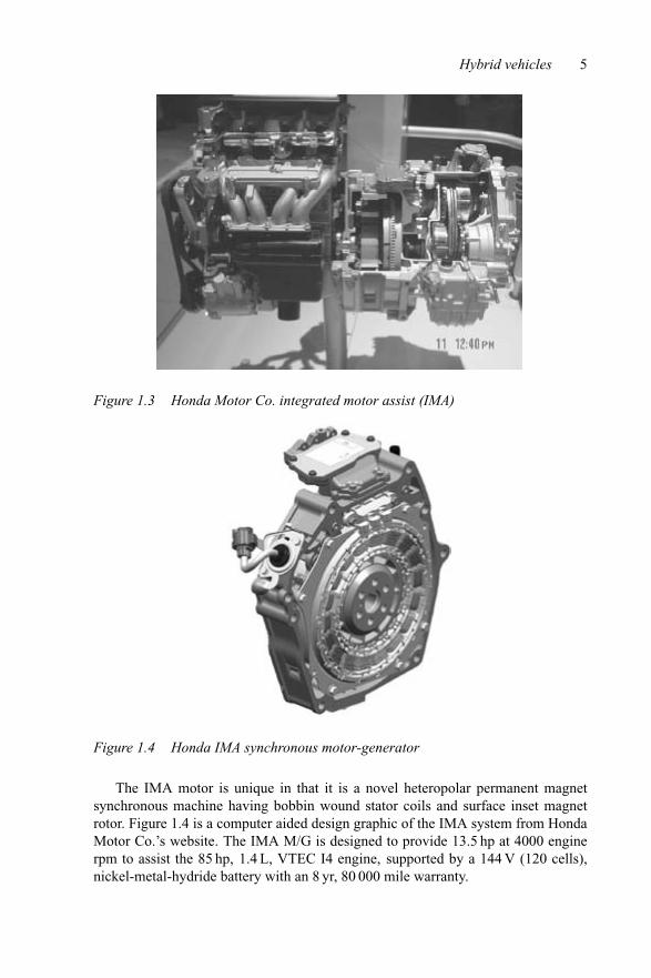
Honda Motor Co. is aggressively introducing hybrid electric vehicles followingthe success of their Insight with integrated motor assist (IMA). Honda has takena different tack on hybrid propulsion than Toyota. Honda integrates a permanentmagnet synchronous motor into the transmission. The IMA operates under torquecontrol from stall to wide open throttle speed of the engine. This enables electrictorque assist over the complete engine operating speed range. Figure 1.3 shows theHonda IMA system integrated into the powertrain.
In Figure 1.3 the Honda IMA motor-generator, rated 10 kW, 144 V, is sandwichedbetween the inline 4 cylinder engine and the CVT transmission. The CVT belt isclearly visible in Figure 1.3. In particular, notice the presence of a ring gear to theimmediate right of the IMA M/G. Honda continues to use the 12 V starter motor forkey starts and only uses the IMA for warm restart in an idle-stop strategy. With thischoice of architecture the IMA is not required to meet cold cranking torque needs ofthe engine so that it can be designed to operate over the 6 : 1 torque augmentationspeed range.
Hybrid vehicles 5
Figure 1.3 Honda Motor Co. integrated motor assist (IMA)
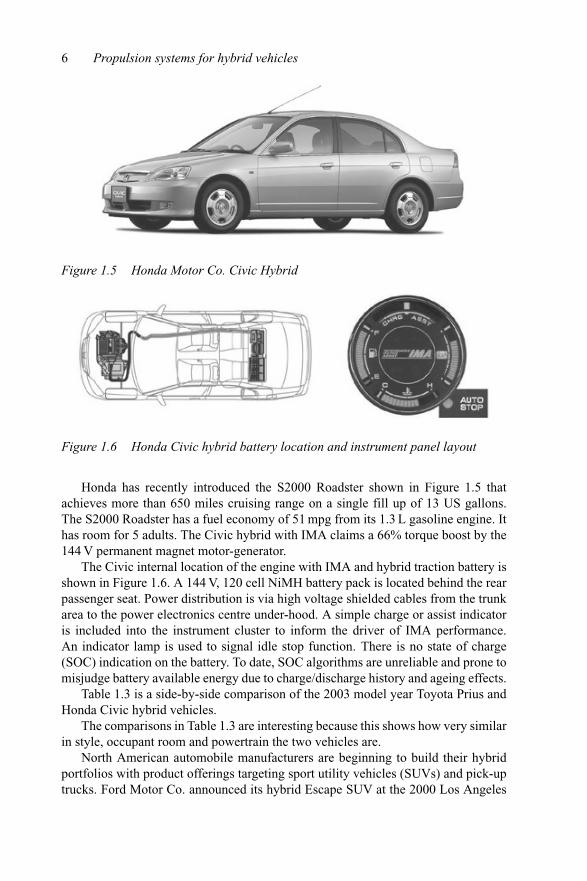
Figure 1.4 Honda IMA synchronous motor-generator
The IMA motor is unique in that it is a novel heteropolar permanent magnetsynchronous machine having bobbin wound stator coils and surface inset magnetrotor. Figure 1.4 is a computer aided design graphic of the IMA system from HondaMotor Co.’s website. The IMA M/G is designed to provide 13.5 hp at 4000 enginerpm to assist the 85 hp, 1.4 L, VTEC I4 engine, supported by a 144 V (120 cells),nickel-metal-hydride battery with an 8 yr, 80 000 mile warranty.
6 Propulsion systems for hybrid vehicles
Figure 1.5 Honda Motor Co. Civic Hybrid
Figure 1.6 Honda Civic hybrid battery location and instrument panel layout
Honda has recently introduced the S2000 Roadster shown in Figure 1.5 thatachieves more than 650 miles cruising range on a single fill up of 13 US gallons.The S2000 Roadster has a fuel economy of 51 mpg from its 1.3 L gasoline engine. Ithas room for 5 adults. The Civic hybrid with IMA claims a 66% torque boost by the144 V permanent magnet motor-generator.
The Civic internal location of the engine with IMA and hybrid traction battery isshown in Figure 1.6. A 144 V, 120 cell NiMH battery pack is located behind the rearpassenger seat. Power distribution is via high voltage shielded cables from the trunkarea to the power electronics centre under-hood. A simple charge or assist indicatoris included into the instrument cluster to inform the driver of IMA performance.An indicator lamp is used to signal idle stop function. There is no state of charge(SOC) indication on the battery. To date, SOC algorithms are unreliable and prone tomisjudge battery available energy due to charge/discharge history and ageing effects.
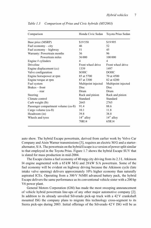
Table 1.3 is a side-by-side comparison of the 2003 model year Toyota Prius andHonda Civic hybrid vehicles.
The comparisons in Table 1.3 are interesting because this shows how very similarin style, occupant room and powertrain the two vehicles are.
North American automobile manufacturers are beginning to build their hybridportfolios with product offerings targeting sport utility vehicles (SUVs) and pick-uptrucks. Ford Motor Co. announced its hybrid Escape SUV at the 2000 Los Angeles
Hybrid vehicles 7
Table 1.3 Comparison of Prius and Civic hybrids (MY2003)
Comparison Honda Civic Sedan Toyota Prius Sedan
Base price (MSRP) $19 550 $19 995Fuel economy – city 46 52Fuel economy – highway 51 45Warranty: Powertrain months 36 96
Powertrain miles 36 000 100 000Engine # cylinders 4 4Driveline Front wheel drive Front wheel driveEngine displacement (cc) 1339 1497Valve configuration SOHC DOHCEngine horsepower at rpm 85 at 5700 70 at 4500Engine torque at rpm 87 at 3300 82 at 4200Fuel system Multipoint injected Multipoint injectedBrakes – front Disc Disc
– rear Drum DrumSteering Rack and pinion Rack and pinionClimate control Standard StandardCurb weight (lb) 2643 2765Passenger compartment volume (cu-ft) 91.4 88.6Cargo volume (cu-ft) 10.1 11.8Headroom (in) 39.8 38.8Wheels and tyres 14′′ alloy 14′′ alloy
70R14 65R14
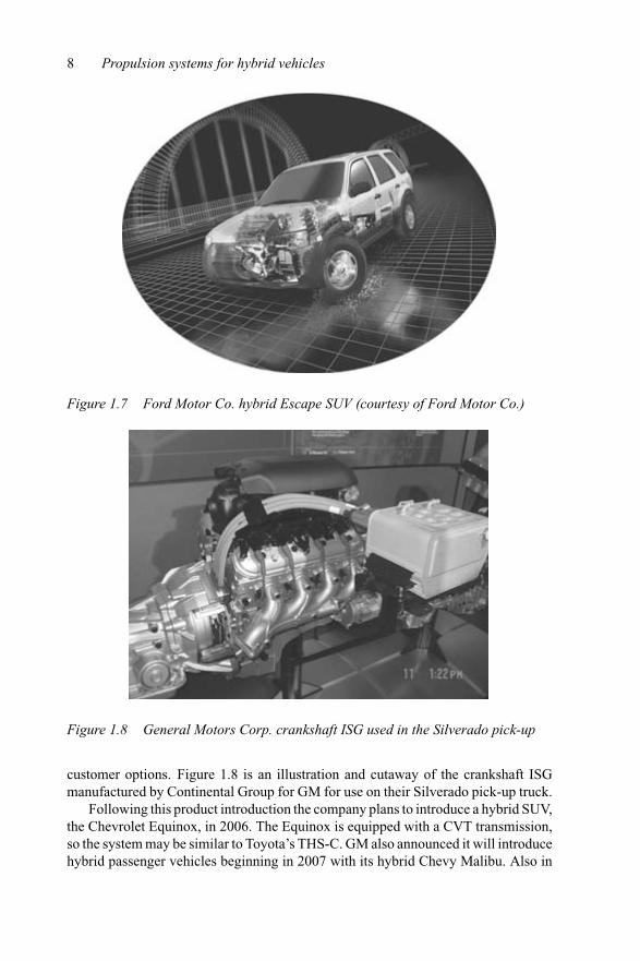
auto show. The hybrid Escape powertrain, derived from earlier work by Volvo CarCompany and Aisin Warner transmissions [3], requires an electric M/G and a starter-alternator, S/A. The powertrain on the hybrid Escape is a version of power split similarto that employed in the Toyota Prius. Figure 1.7 shows the hybrid Escape SUV thatis slated for mass production in mid-2004.
The Escape claims a fuel economy of 40 mpg city driving from its 2.3 L AtkinsonI4 engine augmented with a 65 kW M/G and 28 kW S/A powertrain. Some of thefuel economy will be evident on highway driving because the Atkinson cycle (lateintake valve opening) delivers approximately 10% higher economy than naturallyaspirated ICEs. Operating from a 300 V NiMH advanced battery pack, the hybridEscape delivers the same performance as its conventional vehicle sister with a 200 hpV6 power plant.
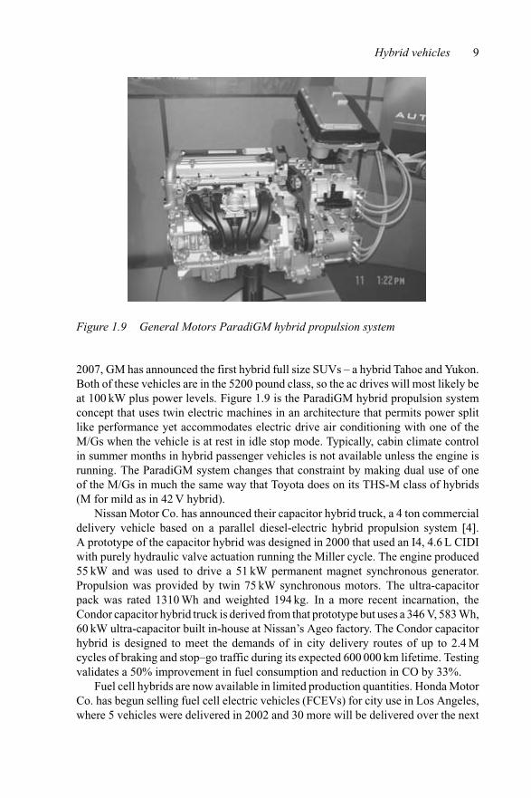
General Motors Corporation (GM) has made the most sweeping announcementof vehicle hybrid powertrain line-ups of any other major automotive company [2].In addition to its already unveiled Silverado pick-up truck with a 42 V crankshaftmounted ISG the company plans to migrate this technology cross-segment to itsSierra pick-ups during 2003. Initial offerings of the Silverado 42 V ISG will be as
8 Propulsion systems for hybrid vehicles
Figure 1.7 Ford Motor Co. hybrid Escape SUV (courtesy of Ford Motor Co.)
Figure 1.8 General Motors Corp. crankshaft ISG used in the Silverado pick-up
customer options. Figure 1.8 is an illustration and cutaway of the crankshaft ISGmanufactured by Continental Group for GM for use on their Silverado pick-up truck.
Following this product introduction the company plans to introduce a hybrid SUV,the Chevrolet Equinox, in 2006. The Equinox is equipped with a CVT transmission,so the system may be similar to Toyota’s THS-C. GM also announced it will introducehybrid passenger vehicles beginning in 2007 with its hybrid Chevy Malibu. Also in
Hybrid vehicles 9
Figure 1.9 General Motors ParadiGM hybrid propulsion system
2007, GM has announced the first hybrid full size SUVs – a hybrid Tahoe and Yukon.Both of these vehicles are in the 5200 pound class, so the ac drives will most likely beat 100 kW plus power levels. Figure 1.9 is the ParadiGM hybrid propulsion systemconcept that uses twin electric machines in an architecture that permits power splitlike performance yet accommodates electric drive air conditioning with one of theM/Gs when the vehicle is at rest in idle stop mode. Typically, cabin climate controlin summer months in hybrid passenger vehicles is not available unless the engine isrunning. The ParadiGM system changes that constraint by making dual use of oneof the M/Gs in much the same way that Toyota does on its THS-M class of hybrids(M for mild as in 42 V hybrid).
Nissan Motor Co. has announced their capacitor hybrid truck, a 4 ton commercialdelivery vehicle based on a parallel diesel-electric hybrid propulsion system [4].A prototype of the capacitor hybrid was designed in 2000 that used an I4, 4.6 L CIDIwith purely hydraulic valve actuation running the Miller cycle. The engine produced55 kW and was used to drive a 51 kW permanent magnet synchronous generator.Propulsion was provided by twin 75 kW synchronous motors. The ultra-capacitorpack was rated 1310 Wh and weighted 194 kg. In a more recent incarnation, theCondor capacitor hybrid truck is derived from that prototype but uses a 346 V, 583 Wh,60 kW ultra-capacitor built in-house at Nissan’s Ageo factory. The Condor capacitorhybrid is designed to meet the demands of in city delivery routes of up to 2.4 Mcycles of braking and stop–go traffic during its expected 600 000 km lifetime. Testingvalidates a 50% improvement in fuel consumption and reduction in CO by 33%.
Fuel cell hybrids are now available in limited production quantities. Honda MotorCo. has begun selling fuel cell electric vehicles (FCEVs) for city use in Los Angeles,where 5 vehicles were delivered in 2002 and 30 more will be delivered over the next
10 Propulsion systems for hybrid vehicles
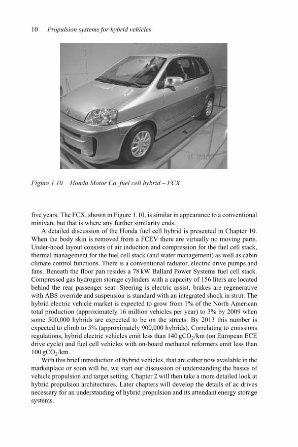
Figure 1.10 Honda Motor Co. fuel cell hybrid – FCX
five years. The FCX, shown in Figure 1.10, is similar in appearance to a conventionalminivan, but that is where any further similarity ends.
A detailed discussion of the Honda fuel cell hybrid is presented in Chapter 10.When the body skin is removed from a FCEV there are virtually no moving parts.Under-hood layout consists of air induction and compression for the fuel cell stack,thermal management for the fuel cell stack (and water management) as well as cabinclimate control functions. There is a conventional radiator, electric drive pumps andfans. Beneath the floor pan resides a 78 kW Ballard Power Systems fuel cell stack.Compressed gas hydrogen storage cylinders with a capacity of 156 liters are locatedbehind the rear passenger seat. Steering is electric assist, brakes are regenerativewith ABS override and suspension is standard with an integrated shock in strut. Thehybrid electric vehicle market is expected to grow from 1% of the North Americantotal production (approximately 16 million vehicles per year) to 3% by 2009 whensome 500,000 hybrids are expected to be on the streets. By 2013 this number isexpected to climb to 5% (approximately 900,000 hybrids). Correlating to emissionsregulations, hybrid electric vehicles emit less than 140 gCO2/km (on European ECEdrive cycle) and fuel cell vehicles with on-board methanol reformers emit less than100 gCO2/km.
With this brief introduction of hybrid vehicles, that are either now available in themarketplace or soon will be, we start our discussion of understanding the basics ofvehicle propulsion and target setting. Chapter 2 will then take a more detailed look athybrid propulsion architectures. Later chapters will develop the details of ac drivesnecessary for an understanding of hybrid propulsion and its attendant energy storagesystems.
Hybrid vehicles 11
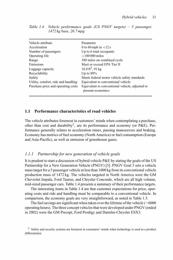
Table 1.4 Vehicle performance goals (US PNGV targets) – 5 passenger,1472 kg base, 26.7 mpg
Vehicle attribute ParameterAcceleration 0 to 60 mph in <12 sNumber of passengers Up to 6 total occupantsOperating life >100 000 milesRange 380 miles on combined cycleEmissions Meet or exceed EPA Tier IILuggage capacity 16.8 ft3, 91 kgRecyclability Up to 80%Safety Meets federal motor vehicle safety standardsUtility, comfort, ride and handling Equivalent to conventional vehiclePurchase price and operating costs Equivalent to conventional vehicle, adjusted to
present economics
1.1 Performance characteristics of road vehicles
The vehicle attributes foremost in customers’ minds when contemplating a purchase,other than cost and durability2, are its performance and economy (or P&E). Per-formance generally relates to acceleration times, passing manoeuvres and braking.Economy has metrics of fuel economy (North America) or fuel consumption (Europeand Asia-Pacific), as well as emission of greenhouse gases.
1.1.1 Partnership for new generation of vehicle goals
It is prudent to start a discussion of hybrid vehicle P&E by stating the goals of the USPartnership for a New Generation Vehicle (PNGV) [5]. PNGV Goal 3 sets a vehiclemass target for a 5 passenger vehicle at less than 1000 kg from its conventional vehicleproduction mass of 1472 kg. The vehicles targeted in North America were the GMChevrolet Impala, Ford Taurus, and Chrysler Concorde, which are all high volume,mid-sized passenger cars. Table 1.4 presents a summary of their performance targets.
The interesting items in Table 1.4 are that customer expectations for price, oper-ating costs and ride and handling must be comparable to a conventional vehicle. Incomparison, the economy goals are very straightforward, as noted in Table 1.5.
The fuel savings are significant when taken over the lifetime of the vehicle (∼6000operating hours). The three concept vehicles that were developed under PNGV (endedin 2002) were the GM Precept, Ford Prodigy and Daimler-Chrysler ESX3.
2 Safety and security systems are foremost in consumers’ minds when technology is used as a productdifferentiator.
12 Propulsion systems for hybrid vehicles
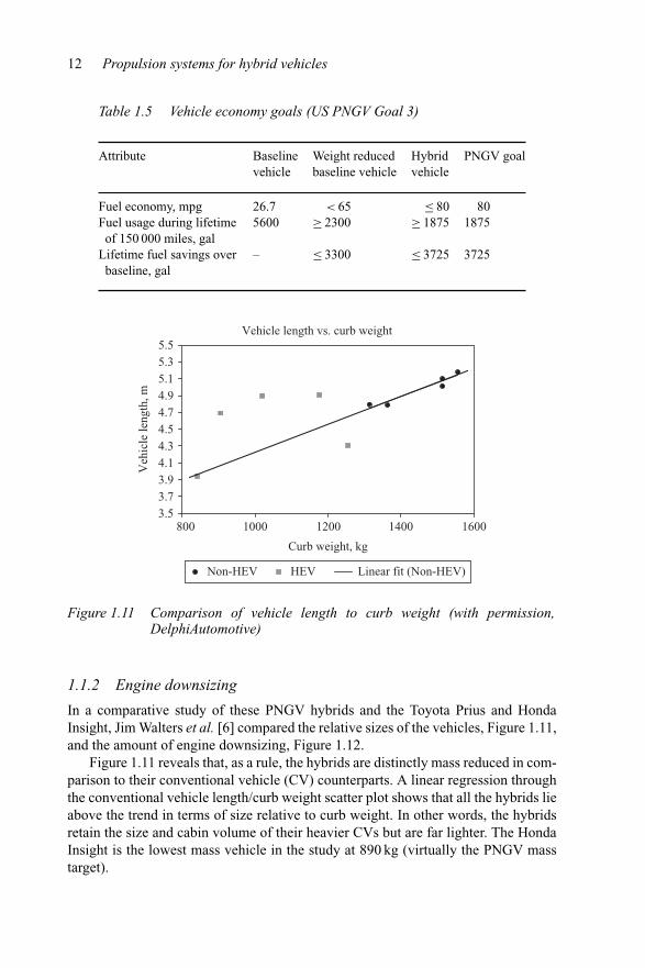
Table 1.5 Vehicle economy goals (US PNGV Goal 3)
Attribute Baseline Weight reduced Hybrid PNGV goalvehicle baseline vehicle vehicle
Fuel economy, mpg 26.7 < 65 ≤ 80 80Fuel usage during lifetime
of 150 000 miles, gal5600 ≥ 2300 ≥ 1875 1875
Lifetime fuel savings overbaseline, gal
– ≤ 3300 ≤ 3725 3725
Vehicle length vs. curb weight
3.53.73.94.14.34.54.74.95.15.35.5
800 1000 1200 1400 1600
Curb weight, kg
Veh
icle
leng
th, m
Non-HEV HEV Linear fit (Non-HEV)
Figure 1.11 Comparison of vehicle length to curb weight (with permission,DelphiAutomotive)
1.1.2 Engine downsizing
In a comparative study of these PNGV hybrids and the Toyota Prius and HondaInsight, Jim Walters et al. [6] compared the relative sizes of the vehicles, Figure 1.11,and the amount of engine downsizing, Figure 1.12.
Figure 1.11 reveals that, as a rule, the hybrids are distinctly mass reduced in com-parison to their conventional vehicle (CV) counterparts. A linear regression throughthe conventional vehicle length/curb weight scatter plot shows that all the hybrids lieabove the trend in terms of size relative to curb weight. In other words, the hybridsretain the size and cabin volume of their heavier CVs but are far lighter. The HondaInsight is the lowest mass vehicle in the study at 890 kg (virtually the PNGV masstarget).
Hybrid vehicles 13
Peak power-to-weight ratio
0
1
2
3
4
5
6
7
8
9
10
800 900 1000 1100 1200 1300 1400 1500 1600
Vehicle weight, kg
Rat
io, k
W/1
00kg
HEV
Non-HEV
MediumMild
Avg. = 6.74
Avg. = 8.1
Peak engine + electric ratio Engine only ratio Non-HEV engine only
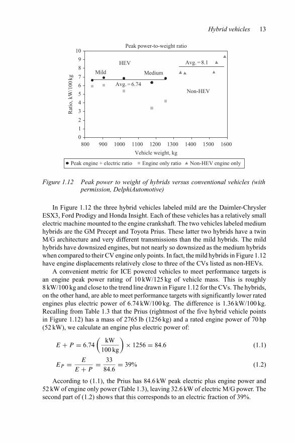
Figure 1.12 Peak power to weight of hybrids versus conventional vehicles (withpermission, DelphiAutomotive)
In Figure 1.12 the three hybrid vehicles labeled mild are the Daimler-ChryslerESX3, Ford Prodigy and Honda Insight. Each of these vehicles has a relatively smallelectric machine mounted to the engine crankshaft. The two vehicles labeled mediumhybrids are the GM Precept and Toyota Prius. These latter two hybrids have a twinM/G architecture and very different transmissions than the mild hybrids. The mildhybrids have downsized engines, but not nearly so downsized as the medium hybridswhen compared to their CV engine only points. In fact, the mild hybrids in Figure 1.12have engine displacements relatively close to three of the CVs listed as non-HEVs.
A convenient metric for ICE powered vehicles to meet performance targets isan engine peak power rating of 10 kW/125 kg of vehicle mass. This is roughly8 kW/100 kg and close to the trend line drawn in Figure 1.12 for the CVs. The hybrids,on the other hand, are able to meet performance targets with significantly lower ratedengines plus electric power of 6.74 kW/100 kg. The difference is 1.36 kW/100 kg.Recalling from Table 1.3 that the Prius (rightmost of the five hybrid vehicle pointsin Figure 1.12) has a mass of 2765 lb (1256 kg) and a rated engine power of 70 hp(52 kW), we calculate an engine plus electric power of:
E + P = 6.74(
kW
100 kg
)× 1256 = 84.6 (1.1)
EP = E
E + P= 33
84.6= 39% (1.2)
According to (1.1), the Prius has 84.6 kW peak electric plus engine power and52 kW of engine only power (Table 1.3), leaving 32.6 kW of electric M/G power. Thesecond part of (1.2) shows that this corresponds to an electric fraction of 39%.
14 Propulsion systems for hybrid vehicles
50
40
30
20
10
0
Power plant thermal efficiency, %
Veh
icle
mas
s re
duct
ion,
%
X
X CIDI
FCEV
30 40 50 60
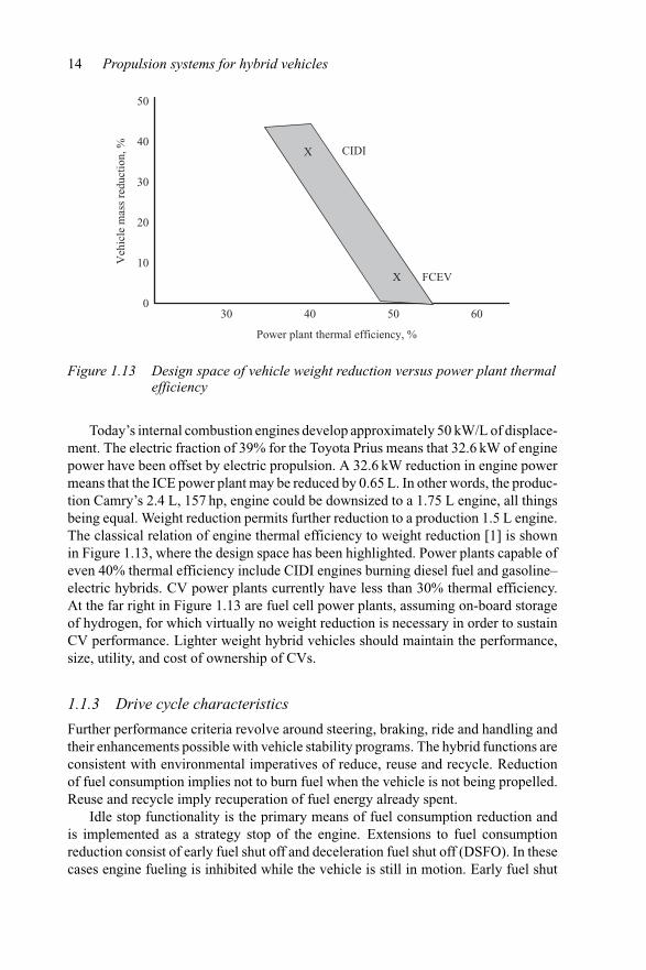
Figure 1.13 Design space of vehicle weight reduction versus power plant thermalefficiency
Today’s internal combustion engines develop approximately 50 kW/L of displace-ment. The electric fraction of 39% for the Toyota Prius means that 32.6 kW of enginepower have been offset by electric propulsion. A 32.6 kW reduction in engine powermeans that the ICE power plant may be reduced by 0.65 L. In other words, the produc-tion Camry’s 2.4 L, 157 hp, engine could be downsized to a 1.75 L engine, all thingsbeing equal. Weight reduction permits further reduction to a production 1.5 L engine.The classical relation of engine thermal efficiency to weight reduction [1] is shownin Figure 1.13, where the design space has been highlighted. Power plants capable ofeven 40% thermal efficiency include CIDI engines burning diesel fuel and gasoline–electric hybrids. CV power plants currently have less than 30% thermal efficiency.At the far right in Figure 1.13 are fuel cell power plants, assuming on-board storageof hydrogen, for which virtually no weight reduction is necessary in order to sustainCV performance. Lighter weight hybrid vehicles should maintain the performance,size, utility, and cost of ownership of CVs.
1.1.3 Drive cycle characteristics
Further performance criteria revolve around steering, braking, ride and handling andtheir enhancements possible with vehicle stability programs. The hybrid functions areconsistent with environmental imperatives of reduce, reuse and recycle. Reductionof fuel consumption implies not to burn fuel when the vehicle is not being propelled.Reuse and recycle imply recuperation of fuel energy already spent.
Idle stop functionality is the primary means of fuel consumption reduction andis implemented as a strategy stop of the engine. Extensions to fuel consumptionreduction consist of early fuel shut off and deceleration fuel shut off (DSFO). In thesecases engine fueling is inhibited while the vehicle is still in motion. Early fuel shut
Hybrid vehicles 15
Table 1.6 Standard drive cycles and statistics
Region Cycle Timeidling (%)
Max.speed (kph)
Averagespeed (kph)
Maximumaccl. (m/s2)
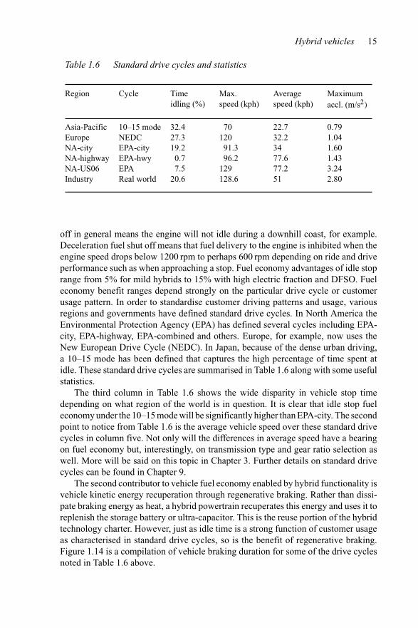
Asia-Pacific 10–15 mode 32.4 70 22.7 0.79Europe NEDC 27.3 120 32.2 1.04NA-city EPA-city 19.2 91.3 34 1.60NA-highway EPA-hwy 0.7 96.2 77.6 1.43NA-US06 EPA 7.5 129 77.2 3.24Industry Real world 20.6 128.6 51 2.80
off in general means the engine will not idle during a downhill coast, for example.Deceleration fuel shut off means that fuel delivery to the engine is inhibited when theengine speed drops below 1200 rpm to perhaps 600 rpm depending on ride and driveperformance such as when approaching a stop. Fuel economy advantages of idle stoprange from 5% for mild hybrids to 15% with high electric fraction and DFSO. Fueleconomy benefit ranges depend strongly on the particular drive cycle or customerusage pattern. In order to standardise customer driving patterns and usage, variousregions and governments have defined standard drive cycles. In North America theEnvironmental Protection Agency (EPA) has defined several cycles including EPA-city, EPA-highway, EPA-combined and others. Europe, for example, now uses theNew European Drive Cycle (NEDC). In Japan, because of the dense urban driving,a 10–15 mode has been defined that captures the high percentage of time spent atidle. These standard drive cycles are summarised in Table 1.6 along with some usefulstatistics.
The third column in Table 1.6 shows the wide disparity in vehicle stop timedepending on what region of the world is in question. It is clear that idle stop fueleconomy under the 10–15 mode will be significantly higher than EPA-city. The secondpoint to notice from Table 1.6 is the average vehicle speed over these standard drivecycles in column five. Not only will the differences in average speed have a bearingon fuel economy but, interestingly, on transmission type and gear ratio selection aswell. More will be said on this topic in Chapter 3. Further details on standard drivecycles can be found in Chapter 9.
The second contributor to vehicle fuel economy enabled by hybrid functionality isvehicle kinetic energy recuperation through regenerative braking. Rather than dissi-pate braking energy as heat, a hybrid powertrain recuperates this energy and uses it toreplenish the storage battery or ultra-capacitor. This is the reuse portion of the hybridtechnology charter. However, just as idle time is a strong function of customer usageas characterised in standard drive cycles, so is the benefit of regenerative braking.Figure 1.14 is a compilation of vehicle braking duration for some of the drive cyclesnoted in Table 1.6 above.
16 Propulsion systems for hybrid vehicles
Regen. duration for 50V < V_batt < 55V
0
5
10
15
20
0 10 20 30 40Time, s
Num
ber
of e
vent
s
EPA-cityEPA-hwyATDSUS06
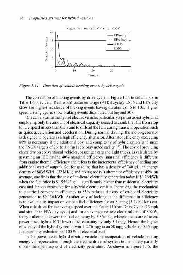
Figure 1.14 Duration of vehicle braking events by drive cycle
The correlation of braking events by drive cycle in Figure 1.14 to column six inTable 1.6 is evident. Real world customer usage (ATDS cycle), US06 and EPA-cityshow the highest incidence of braking events having durations of 5 to 10 s. Higherspeed driving cycles show braking events distributed out beyond 30 s.
One can visualise the hybrid electric vehicle, particularly a power assist hybrid, asemploying only the amount of electrical capacity needed to crank the ICE from stopto idle speed in less than 0.3 s and to offload the ICE during transient operation suchas quick acceleration and deceleration. During normal driving, the motor-generatoris designed to operate as a high efficiency alternator. Alternator efficiency exceeding80% is necessary if the additional cost and complexity of hybridization is to meetthe PNGV targets of 2× to 3× fuel economy noted earlier [7]. The cost of providingelectricity on conventional vehicles, passenger cars and light trucks, is calculated byassuming an ICE having 40% marginal efficiency (marginal efficiency is differentfrom engine thermal efficiency and refers to the incremental efficiency of adding oneadditional watt of output). So, for gasoline that has a density of 740 g/L, an energydensity of 8835 Wh/L (32 MJ/L) and taking today’s alternator efficiency at 45% onaverage, one finds that the cost of on-board electricity generation today is $0.26/kWhwhen the fuel price is $1.55/US gal – significantly higher than residential electricitycost and far too expensive for a hybrid electric vehicle. Increasing the mechanicalto electrical conversion efficiency to 85% reduces the cost of on-board electricitygeneration to $0.136/kWh. Another way of looking at the difference in efficiencyis to evaluate its impact on vehicle fuel efficiency for an 80 mpg (3 L/100 km) car.When calculated for the average speed over the Federal Urban Drive Cycle (23 mphand similar to EPA-city cycle) and for an average vehicle electrical load of 800 W,today’s alternator lowers the fuel economy by 5.86 mpg, whereas the more efficientpower assist hybrid M/G lowers fuel economy by only 3.1 mpg. Hence, the higherefficiency of the hybrid system is worth 2.76 mpg in an 80 mpg vehicle, or 0.35 mpgfuel economy reduction per 100 W of electrical load.
In the power assist hybrid electric vehicle the recuperation of vehicle brakingenergy via regeneration through the electric drive subsystem to the battery partiallyoffsets the operating cost of electricity generation. As shown in Figure 1.15, the
Hybrid vehicles 17
Time, s
kW
Average regenerationinverter power: –1 kW
35 kW
0 200 400 600 800 1000 1200 1400
20 kW
Average drivinginverter power: 11 kW
35
25
15
5
–5
–15
–25
Figure 1.15 Power assist hybrid propulsion and regeneration energy
Percent timespent atpower level
Percent energyat power level
Power, kW
–20 –10 0 10 20 30
60
50
40
30
20
10
–10
–20
0
Figure 1.16 Distribution of power and energy in a drive cycle
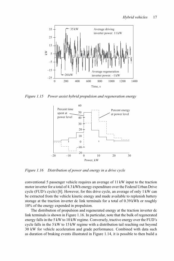
conventional 5 passenger vehicle requires an average of 11 kW input to the tractionmotor inverter for a total of 4.3 kWh energy expenditure over the Federal Urban Drivecycle (FUD’s cycle) [8]. However, for this drive cycle, an average of only 1 kW canbe extracted from the vehicle kinetic energy and made available to replenish batterystorage at the traction inverter dc link terminals for a total of 0.39 kWh or roughly10% of the energy expended in propulsion.
The distribution of propulsion and regenerated energy at the traction inverter dclink terminals is shown in Figure 1.16. In particular, note that the bulk of regeneratedenergy falls in the 5 kW to 10 kW regime. Conversely, tractive energy over the FUD’scycle falls in the 5 kW to 15 kW regime with a distribution tail reaching out beyond30 kW for vehicle acceleration and grade performance. Combined with data suchas duration of braking events illustrated in Figure 1.14, it is possible to then build a
18 Propulsion systems for hybrid vehicles
histogram of hybrid propulsion and braking energy. The energy distribution over thesame FUD’s drive cycle has been included in Figure 1.16.
Two things should now be clear from Figure 1.16: (i) a 20 kW regeneration capa-bility captures virtually all of the available kinetic energy of a mid-sized passengervehicle, assuming of course that the hybrid M/G is on the front axle, and (ii) vehi-cle tractive effort is supplied with a motoring power level of 30 kW. This seems toindicate that hybrid traction power plants in excess of 30 kW are necessary primarilyto deliver the acceleration performance customers expect. More will be said of thispower plant sizing in later chapters. One example of the mild hybrid discussed here,the Ford Motor Co. P2000 low storage requirement (LSR) vehicle, is described inmore depth in Reference 7. The P2000 is a 2000 kg, 5 passenger mid-sized sedanwith a 1.8 L CIDI engine and an 8 kW S/A rated at 300 Nm of peak cranking torquefrom a 300 V NiMH battery pack. The vehicle is low storage because the battery packenergy is less than 1 kWh.
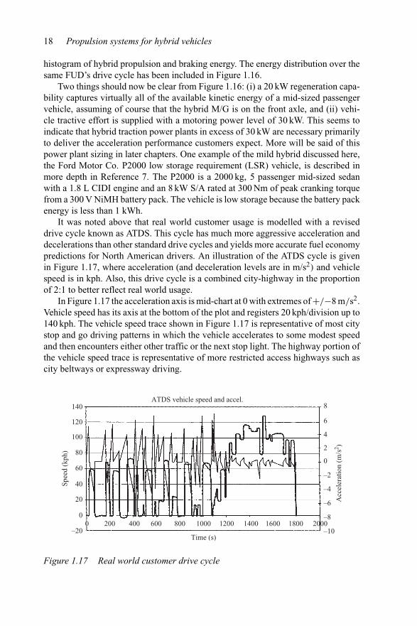
It was noted above that real world customer usage is modelled with a reviseddrive cycle known as ATDS. This cycle has much more aggressive acceleration anddecelerations than other standard drive cycles and yields more accurate fuel economypredictions for North American drivers. An illustration of the ATDS cycle is givenin Figure 1.17, where acceleration (and deceleration levels are in m/s2) and vehiclespeed is in kph. Also, this drive cycle is a combined city-highway in the proportionof 2:1 to better reflect real world usage.
In Figure 1.17 the acceleration axis is mid-chart at 0 with extremes of +/−8 m/s2.Vehicle speed has its axis at the bottom of the plot and registers 20 kph/division up to140 kph. The vehicle speed trace shown in Figure 1.17 is representative of most citystop and go driving patterns in which the vehicle accelerates to some modest speedand then encounters either other traffic or the next stop light. The highway portion ofthe vehicle speed trace is representative of more restricted access highways such ascity beltways or expressway driving.
140
120
100
80
60
40Spee
d (k
ph)
20
0
–200 400 600 800 1000
Time (s)
1200 1600 1800 2000–10
Acc
eler
atio
n(m
/s2 )
–8
–6
–4
–2
0
2
4
6
8
1400200
ATDS vehicle speed and accel.
Figure 1.17 Real world customer drive cycle
Hybrid vehicles 19
10s 106371 147.7h20s 32019 133.4h30s 35580 247.1h45s 19418 202.3h60s 8382 122.2h
120s 8436 210.9h240s 2571 128.6h480s 1127 112.7h720s 293 48.9htotal 214198 1353.9h
average eventtime
22.8s
0 000
10 000
20 000
30 000
40 000
50 000
60 000
70 000
0–1
0s
10–2
0s
20–3
0s
30–4
5s
45–
60s
1–2
min
2–4
min
4–8
min
8–1
2m
in
cycl
es
0
2
4
6
8
10
12
14
Dis
char
ge p
er c
ycle
, Ahcycles per 91k miles
discharge per event
(a) Event duration/number/cumulative time Histogram of tabulated data (b)
Figure 1.18 Tabulation of driving habits
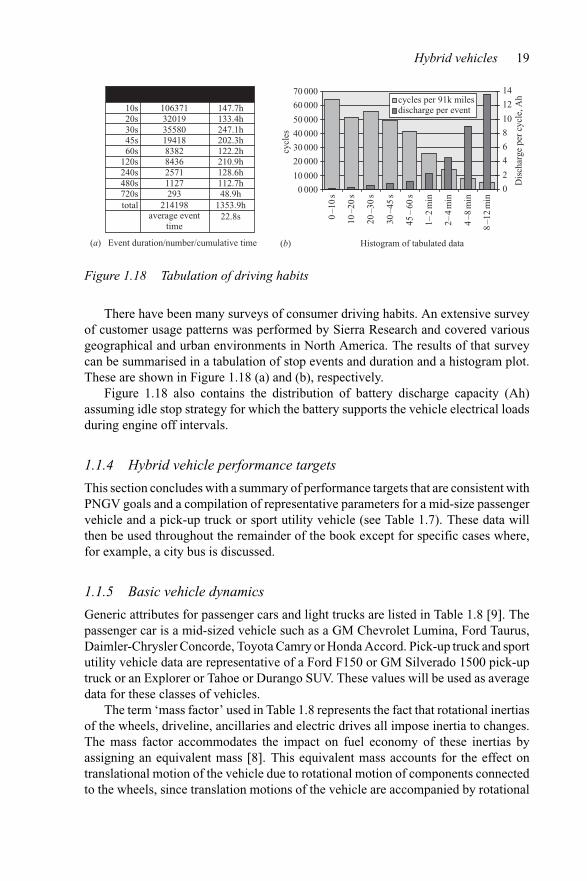
There have been many surveys of consumer driving habits. An extensive surveyof customer usage patterns was performed by Sierra Research and covered variousgeographical and urban environments in North America. The results of that surveycan be summarised in a tabulation of stop events and duration and a histogram plot.These are shown in Figure 1.18 (a) and (b), respectively.
Figure 1.18 also contains the distribution of battery discharge capacity (Ah)assuming idle stop strategy for which the battery supports the vehicle electrical loadsduring engine off intervals.
1.1.4 Hybrid vehicle performance targets
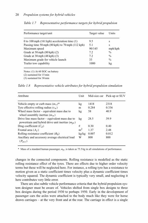
This section concludes with a summary of performance targets that are consistent withPNGV goals and a compilation of representative parameters for a mid-size passengervehicle and a pick-up truck or sport utility vehicle (see Table 1.7). These data willthen be used throughout the remainder of the book except for specific cases where,for example, a city bus is discussed.
1.1.5 Basic vehicle dynamics
Generic attributes for passenger cars and light trucks are listed in Table 1.8 [9]. Thepassenger car is a mid-sized vehicle such as a GM Chevrolet Lumina, Ford Taurus,Daimler-Chrysler Concorde, Toyota Camry or Honda Accord. Pick-up truck and sportutility vehicle data are representative of a Ford F150 or GM Silverado 1500 pick-uptruck or an Explorer or Tahoe or Durango SUV. These values will be used as averagedata for these classes of vehicles.
The term ‘mass factor’ used in Table 1.8 represents the fact that rotational inertiasof the wheels, driveline, ancillaries and electric drives all impose inertia to changes.The mass factor accommodates the impact on fuel economy of these inertias byassigning an equivalent mass [8]. This equivalent mass accounts for the effect ontranslational motion of the vehicle due to rotational motion of components connectedto the wheels, since translation motions of the vehicle are accompanied by rotational
20 Propulsion systems for hybrid vehicles
Table 1.7 Representative performance targets for hybrid propulsion
Performance target/unit Target value Units
0 to 100 mph (161 kph) acceleration time (1) 9.5 sPassing time 50 mph (80 kph) to 70 mph (112 kph) 5.1 sMaximum speed 90/145 mph/kphGrade at 50 mph (80 kph) (2) 7.2 %Grade at 30 mph (48 kph) (3) 7.2 %Maximum grade for vehicle launch 33 %Trailer tow capability 1000 kg
Notes: (1) At 60 SOC on battery(2) sustained for 15 min(3) sustained for 30 min
Table 1.8 Representative vehicle attributes for hybrid propulsion simulation
Attribute Unit Mid-size car Pick-up or SUV
Vehicle empty or curb mass (mv)* kg 1418 2318Tyre effective rolling radius (rw) m 0.284 0.336Wheel mass factor – equivalent mass due to
wheel assembly inertias (mw)
kg 58 40.9
Drive line mass factor – equivalent mass due topowertrain and hybrid drive unit inertias (mpt )
kg 28.5 39.9
Drag coefficient (Cd) # 0.30 0.40Frontal area (Af ) m2 1.37 2.48Rolling resistance coefficient (R0) kg/kg 0.007 0.012Ancillary and accessory average electrical load(Pacc)
W 800 800
* Mass of a standard human passenger, mp , is taken as 75.5 kg in all simulations of performance.
changes in the connected components. Rolling resistance is modelled as the staticrolling resistance effect of the tyres. There are effects due to higher order velocityterms but these will be neglected here. For instance, a rolling tyre has a resistance tomotion given as a static coefficient times velocity plus a dynamic coefficient timesvelocity squared. The dynamic coefficient is typically very small, and neglecting ithere contributes very little error.
There are also subtle vehicle performance criteria that the hybrid propulsion sys-tem designer must be aware of. Vehicles shifted from single box designs to threebox designs during the period 1930 to perhaps 1950. Early in the development ofpassenger cars the axles were attached to the body much like they were for horsedrawn carriages – at the very front and at the rear. The carriage in effect is a single
Hybrid vehicles 21
box design with axles at the front and rear. This in effect is a single body simply sup-ported at the ends, so bending moments due to road roughness contribute to vibrationin the body known as ‘beaming’. Beaming is the first bending mode of the simplysupported vehicle body. It was not as pronounced so as to be objectionable until bodystructures began to shed weight. Beaming is still an issue in over the road truckswhere the driver cabin becomes subject to to-and-fro longitudinal motion in responseto vertical vibrations coupled into the chassis from the road. To alleviate this tendencyto beaming, vehicle designers shifted a portion of the vehicle’s mass forward of thefront axle and rearward, behind the rear axle. This action lowered first mode beamingbut demanded in turn better structural design. The resulting body structure took on adistinct three box character with under-hood, cabin and trunk compartments separatedby bulkheads. Total package space became more of a concern as provision had to bemade for crush space front and rear, cabin volume for passengers and cargo spacein the trunk. All of these factors influence ride and handling. Well designed bodystructures that have high rigidity shift the first beaming mode to beyond 25 Hz. Con-vertibles when first introduced were a real design challenge because they lacked theA and C-pillar rigidity via the roof. The GM Covair, for example, required dynamicabsorbers to contain wheel hop.
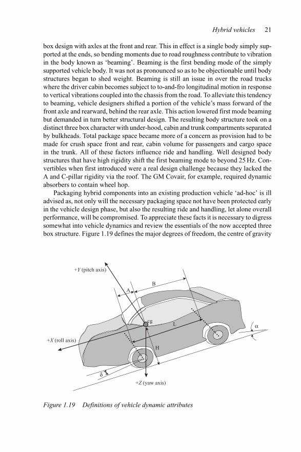
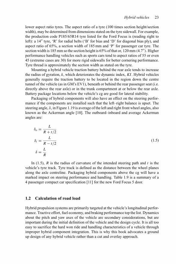
Packaging hybrid components into an existing production vehicle ‘ad-hoc’ is illadvised as, not only will the necessary packaging space not have been protected earlyin the vehicle design phase, but also the resulting ride and handling, let alone overallperformance, will be compromised. To appreciate these facts it is necessary to digresssomewhat into vehicle dynamics and review the essentials of the now accepted threebox structure. Figure 1.19 defines the major degrees of freedom, the centre of gravity
+X (roll axis)
+Y (pitch axis)
+Z (yaw axis)
cg
H
L
AB
δ
α
Figure 1.19 Definitions of vehicle dynamic attributes
22 Propulsion systems for hybrid vehicles
of the vehicle and axle locations relative to the centre of gravity defining the threebox structure.
In a passenger vehicle the centre of gravity, cg, lies about 18′′ above the floor panalong the vehicle’s centre line at approximately the location of the shift knob on a floormounted shift lever. The roll axis (X-axis) is along the centre of the vehicle protrudingthrough the front grill at the height of the cg. In Figure 1.19 the cg is located a distanceH above the road surface. The pitch axis (Y -axis) extends from the vehicle cg outthrough the passenger side door. Likewise, the yaw axis (Z-axis) extends from the cgalong the gravity line through the vehicle’s floor pan to the road. Vehicle wheel base,L, is the distance between the centres of the front and rear axles. It is not the distancebetween the front and rear tyre patches because suspension geometry changes thepositioning of the tyre patches according to loading and vehicle maneuvering. Thelongitudinal distances between the cg and front and rear axle centrelines are definedas A and B, respectively. Road grade is labeled ‘α’ and steering angle (of the wheelswithout induced roll coupling nor side slip) is labeled ‘δ’.
For good ride performance the metric dynamic index, KI , is defined that relatesthe radius of gyration, K , of front and rear equivalent sprung masses to the productof the two longitudinal distances from the cg, A and B. For good ride performance,the dynamic index, KI ∼ 1:
KI = k2
AB≈ 1 (1.3)
Sprung mass is that fraction of total vehicle mass supported by the suspension,including portions of the suspension members that move. Unsprung mass is theremaining fraction of vehicle mass carried directly by the tyres, excluding the sprungmass portion, and considered to move with the tyres.
The distribution of total sprung mass between the front and rear axles can bedefined using the relations in (1.4). The total sprung mass, ma , is split front torear as:
maf = B
Lma
mar = A
Lma
(1.4)
Generally, the front to rear static mass split is 60 : 40 or less. Dynamic effectsof braking cause a dynamic mass shift (pitch motion resulting in dive) so that frontaxle braking may be 70% or more of the total braking force. Hybrid M/Gs that arepackaged under-hood or integrated into the vehicle’s transmission will alter the massdistribution somewhat, but not as significantly as when a heavy battery is packagedaft of the rear axle. Automobile design rules of thumb in the past assigned a ratio ofsprung to unsprung mass of approximately 10 : 1. In recent years this ratio has drifteddown to an average of only 7 : 1 to 5 : 1 (range due to number of occupants). Thisis due to more pervasive application of front wheel drive, disc brakes in which theentire caliper assembly becomes unsprung mass, and the trend to larger diameter but
Hybrid vehicles 23
lower aspect ratio tyres. The aspect ratio of a tyre (100 times section height/sectionwidth), may be determined from dimensions stated on the tyre sidewall. For example,the production code P185/65R14 tyre listed for the Ford Focus is (reading right toleft): a 14′′ tyre, ‘R’ for radial belts (‘B’ for bias and ‘D’ for diagonal bias ply), andaspect ratio of 65%, a section width of 185 mm and ‘P’ for passenger car tyre. Thesection width is 185 mm so the section height is 65% of that or, 120 mm (4.7′′). Higherperformance handling vehicles such as sports cars tend to aspect ratios of 55 or even45 (extreme cases are 30) for more rigid sidewalls for better cornering performance.Tyre thread is approximately the section width as stated on the tyre.
Mounting a hybrid vehicle traction battery behind the rear axle tends to increasethe radius of gyration, k, which deteriorates the dynamic index, KI . Hybrid vehiclesgenerally require the traction battery to be located in the region down the centretunnel of the vehicle (as in GM’s EV1), beneath or behind the rear passenger seat (i.e.directly above the rear axle) or in the trunk compartment at or below the rear axle.Battery package locations below the vehicle’s cg are good for lateral stability.
Packaging of hybrid components will also have an effect on the steering perfor-mance if the components are installed such that the left–right balance is upset. Thesteering angle, δ, in Figure 1.19 is average of the left and right front wheel angles, alsoknown as the Ackerman angle [10]. The outboard–inboard and average Ackermanangles are:
δo = L
R + t/2
δi = L
R − t/2
δ = L
R
(1.5)
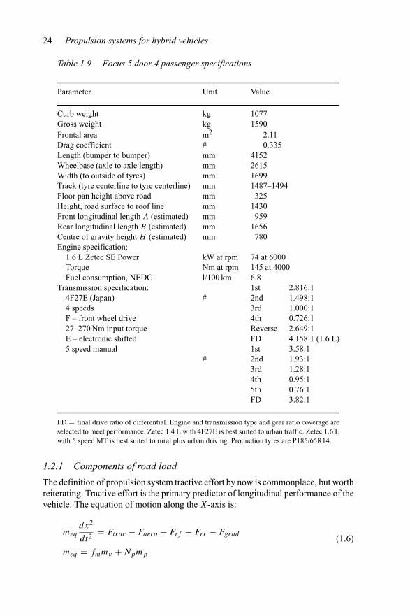
In (1.5), R is the radius of curvature of the intended steering path and t is thevehicle’s tyre track. Tyre track is defined as the distance between the wheel planesalong the axle centreline. Packaging hybrid components above the cg will have amarked impact on steering performance and handling. Table 1.9 is a summary of a4 passenger compact car specification [11] for the new Ford Focus 5 door.
1.2 Calculation of road load
Hybrid propulsion systems are primarily targeted at the vehicle’s longitudinal perfor-mance. Tractive effort, fuel economy, and braking performance top the list. Dynamicsabout the pitch and yaw axes of the vehicle are secondary considerations, but areimportant during the initial definition of the vehicle and the design cycle. It is all tooeasy to sacrifice the hard won ride and handling characteristics of a vehicle throughimproper hybrid component integration. This is why this book advocates a groundup design of any hybrid vehicle rather than a cut and overlay approach.
24 Propulsion systems for hybrid vehicles
Table 1.9 Focus 5 door 4 passenger specifications
Parameter Unit Value
Curb weight kg 1077Gross weight kg 1590Frontal area m2 2.11Drag coefficient # 0.335Length (bumper to bumper) mm 4152Wheelbase (axle to axle length) mm 2615Width (to outside of tyres) mm 1699Track (tyre centerline to tyre centerline) mm 1487–1494Floor pan height above road mm 325Height, road surface to roof line mm 1430Front longitudinal length A (estimated) mm 959Rear longitudinal length B (estimated) mm 1656Centre of gravity height H (estimated) mm 780Engine specification:
1.6 L Zetec SE Power kW at rpm 74 at 6000Torque Nm at rpm 145 at 4000Fuel consumption, NEDC l/100 km 6.8
Transmission specification: 1st 2.816:14F27E (Japan) # 2nd 1.498:14 speeds 3rd 1.000:1F – front wheel drive 4th 0.726:127–270 Nm input torque Reverse 2.649:1E – electronic shifted FD 4.158:1 (1.6 L)5 speed manual 1st 3.58:1
# 2nd 1.93:13rd 1.28:14th 0.95:15th 0.76:1FD 3.82:1
FD = final drive ratio of differential. Engine and transmission type and gear ratio coverage areselected to meet performance. Zetec 1.4 L with 4F27E is best suited to urban traffic. Zetec 1.6 Lwith 5 speed MT is best suited to rural plus urban driving. Production tyres are P185/65R14.
1.2.1 Components of road load
The definition of propulsion system tractive effort by now is commonplace, but worthreiterating. Tractive effort is the primary predictor of longitudinal performance of thevehicle. The equation of motion along the X-axis is:
meq
dx2
dt2 = Ftrac − Faero − Frf − Frr − Fgrad
meq = fmmv + Npmp
(1.6)
Hybrid vehicles 25
An equivalent mass, meq , has been defined in (1.6) that accounts for passengerloading and all rotating inertia effects. Passenger loading is determined by taking thenumber of passengers, Np, including the driver, times the standard human passengermass, mp of 75.5 kg. The mass factor, fm, accounts for all wheel, driveline, enginewith ancillaries, and hybrid M/G component inertias that rotate with the wheels. Theremaining terms on the right-hand side of (1.6) account for tractive force, Ftrac,aerodynamic force, Faero, front rolling resistance, Frf , rear rolling resistance, Frr ,and road grade. Rolling resistance is split front and rear to account for their differentcontributions to overall resistance due to the vehicle’s mass distribution and tyrerolling resistance coefficients. There may be some minor differences in coefficientof rolling resistance front to rear axle due to different specifications on tyre pressure,but these second order effects will be ignored. The mass factor, fm, is now definedas the translational equivalent of all rotating inertias reflected to the wheel axle:
fm = 1 + 4Jw
mvr2w
+ Jengζ2i ζ 2
FD
mvr2w
+ Jacζ2i ζ 2
FD
mvr2w
(1.7)
Mass factor is derived from equating rotational energy to its equivalent trans-lational energy and solving for the equivalent translating mass. In (1.7), rw is thewheel dynamic rolling radius (approximately equal to standing height minus one-third deflection), mv is the vehicle curb mass, and the Jxs are the respective inertias.The factors ζ 2
i and ζ 2FD are the transmission ratios in the ith gear and final drive ratio,
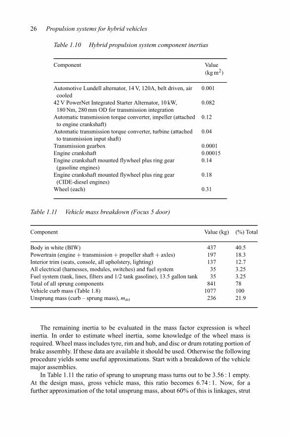
respectively. The appropriate gear ratios, ζI and ζFD are listed in Table 1.9. Beforethe mass factor can be calculated the component inertias must be known. Noticealso that in (1.7) the right-hand terms are mass ratios, i.e. a component’s equivalentmass divided by vehicle’s curb mass. Inertias are generally not available without verydetailed specifications for the components. Table 1.10 lists some representative iner-tia values. These values are generic in nature, but some approximations will attest totheir validity. The inertia values listed, and their counterpart equivalent masses willbe sufficient for the purposes of simulations in this book. To begin, recall that inertiaof a rotating, symmetric object such as a disc or rod is defined as
J0 = π
2< ρ > hr4
0 (kg m2) (1.8)
In (1.8), h is the disc thickness or rod length and r0 its radius. An average massdensity <ρ> has been assigned. For electric machines such as claw pole Lundell alter-nators with rotating copper wound field bobbins, or smooth rotor, cast aluminum cagetype induction starter-alternators, estimates for average mass density that prove usefulin approximations are 5500 kg/m3 and 2500 kg/m3, respectively. Some examples willreinforce this assertion. A typical 120 A Lundell alternator has a rotor thickness of∼40 mm and a diameter of 100 mm. When these values are substituted into (1.8) theapproximate polar moment of inertia comes out to J0 = 0.00098 kg m2. Without lossof applicability use 0.001 kg m2. As another example, a crankshaft mounted induc-tion starter-alternator designed for 42 V applications has a rotor thickness of 50 mm,a rotor diameter of 235 mm, and the approximation for average mass density notedabove. In this case the polar moment of inertia becomes J0 = 0.082 kg m2.
26 Propulsion systems for hybrid vehicles
Table 1.10 Hybrid propulsion system component inertias
Component Value(kg m2)
Automotive Lundell alternator, 14 V, 120A, belt driven, aircooled
0.001
42 V PowerNet Integrated Starter Alternator, 10 kW,180 Nm, 280 mm OD for transmission integration
0.082
Automatic transmission torque converter, impeller (attachedto engine crankshaft)
0.12
Automatic transmission torque converter, turbine (attachedto transmission input shaft)
0.04
Transmission gearbox 0.0001Engine crankshaft 0.00015Engine crankshaft mounted flywheel plus ring gear
(gasoline engines)0.14
Engine crankshaft mounted flywheel plus ring gear(CIDE-diesel engines)
0.18
Wheel (each) 0.31
Table 1.11 Vehicle mass breakdown (Focus 5 door)
Component Value (kg) (%) Total
Body in white (BIW) 437 40.5Powertrain (engine + transmission + propeller shaft + axles) 197 18.3Interior trim (seats, console, all upholstery, lighting) 137 12.7All electrical (harnesses, modules, switches) and fuel system 35 3.25Fuel system (tank, lines, filters and 1/2 tank gasoline), 13.5 gallon tank 35 3.25Total of all sprung components 841 78Vehicle curb mass (Table 1.8) 1077 100Unsprung mass (curb – sprung mass), mus 236 21.9
The remaining inertia to be evaluated in the mass factor expression is wheelinertia. In order to estimate wheel inertia, some knowledge of the wheel mass isrequired. Wheel mass includes tyre, rim and hub, and disc or drum rotating portion ofbrake assembly. If these data are available it should be used. Otherwise the followingprocedure yields some useful approximations. Start with a breakdown of the vehiclemajor assemblies.
In Table 1.11 the ratio of sprung to unsprung mass turns out to be 3.56 : 1 empty.At the design mass, gross vehicle mass, this ratio becomes 6.74 : 1. Now, for afurther approximation of the total unsprung mass, about 60% of this is linkages, strut
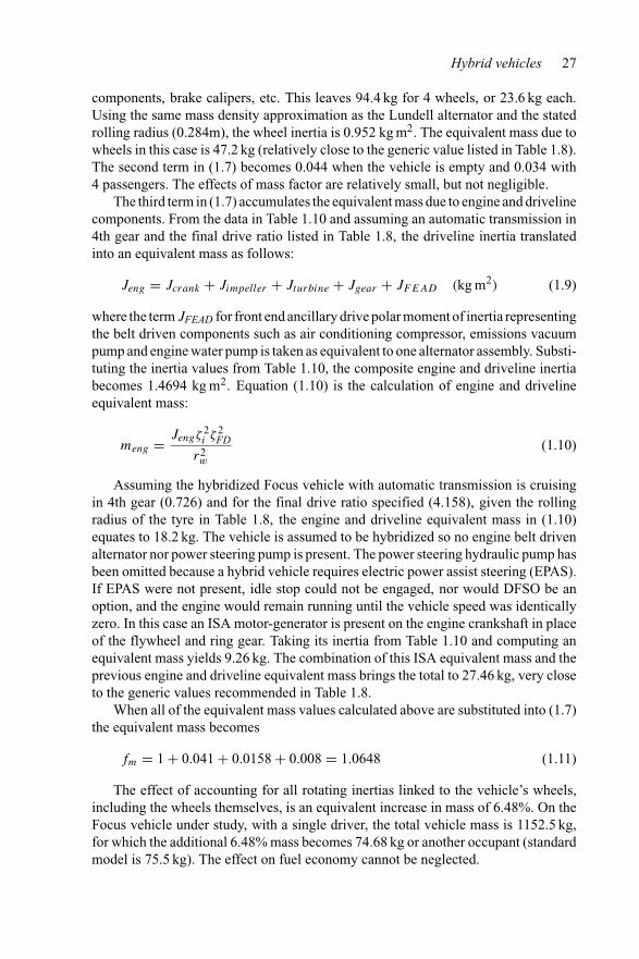
Hybrid vehicles 27
components, brake calipers, etc. This leaves 94.4 kg for 4 wheels, or 23.6 kg each.Using the same mass density approximation as the Lundell alternator and the statedrolling radius (0.284m), the wheel inertia is 0.952 kg m2. The equivalent mass due towheels in this case is 47.2 kg (relatively close to the generic value listed in Table 1.8).The second term in (1.7) becomes 0.044 when the vehicle is empty and 0.034 with4 passengers. The effects of mass factor are relatively small, but not negligible.
The third term in (1.7) accumulates the equivalent mass due to engine and drivelinecomponents. From the data in Table 1.10 and assuming an automatic transmission in4th gear and the final drive ratio listed in Table 1.8, the driveline inertia translatedinto an equivalent mass as follows:
Jeng = Jcrank + Jimpeller + Jturbine + Jgear + JFEAD (kg m2) (1.9)
where the termJFEAD for front end ancillary drive polar moment of inertia representingthe belt driven components such as air conditioning compressor, emissions vacuumpump and engine water pump is taken as equivalent to one alternator assembly. Substi-tuting the inertia values from Table 1.10, the composite engine and driveline inertiabecomes 1.4694 kg m2. Equation (1.10) is the calculation of engine and drivelineequivalent mass:
meng = Jengζ2i ζ 2
FD
r2w
(1.10)
Assuming the hybridized Focus vehicle with automatic transmission is cruisingin 4th gear (0.726) and for the final drive ratio specified (4.158), given the rollingradius of the tyre in Table 1.8, the engine and driveline equivalent mass in (1.10)equates to 18.2 kg. The vehicle is assumed to be hybridized so no engine belt drivenalternator nor power steering pump is present. The power steering hydraulic pump hasbeen omitted because a hybrid vehicle requires electric power assist steering (EPAS).If EPAS were not present, idle stop could not be engaged, nor would DFSO be anoption, and the engine would remain running until the vehicle speed was identicallyzero. In this case an ISA motor-generator is present on the engine crankshaft in placeof the flywheel and ring gear. Taking its inertia from Table 1.10 and computing anequivalent mass yields 9.26 kg. The combination of this ISA equivalent mass and theprevious engine and driveline equivalent mass brings the total to 27.46 kg, very closeto the generic values recommended in Table 1.8.
When all of the equivalent mass values calculated above are substituted into (1.7)the equivalent mass becomes
fm = 1 + 0.041 + 0.0158 + 0.008 = 1.0648 (1.11)
The effect of accounting for all rotating inertias linked to the vehicle’s wheels,including the wheels themselves, is an equivalent increase in mass of 6.48%. On theFocus vehicle under study, with a single driver, the total vehicle mass is 1152.5 kg,for which the additional 6.48% mass becomes 74.68 kg or another occupant (standardmodel is 75.5 kg). The effect on fuel economy cannot be neglected.
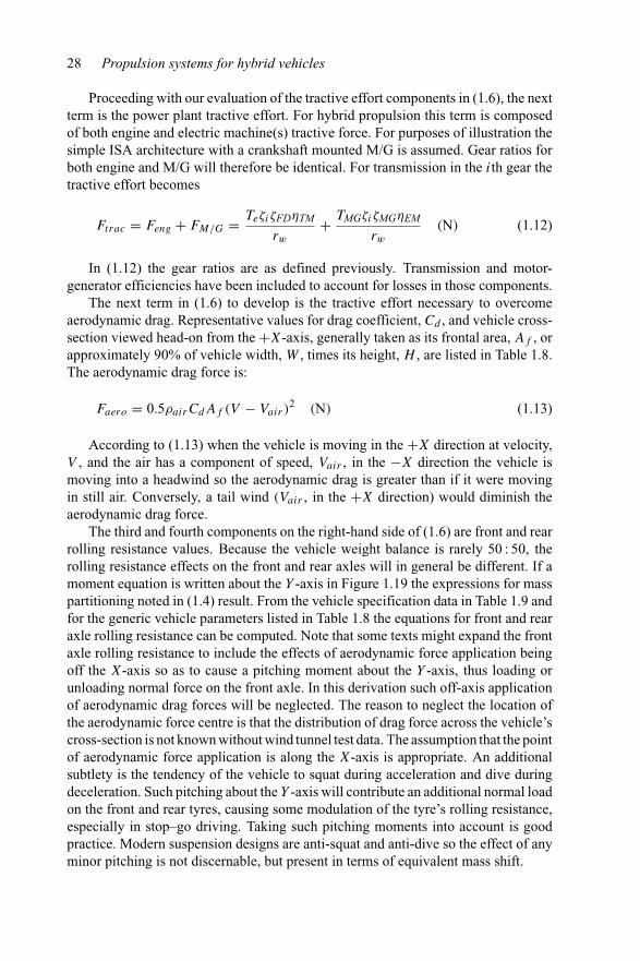
28 Propulsion systems for hybrid vehicles
Proceeding with our evaluation of the tractive effort components in (1.6), the nextterm is the power plant tractive effort. For hybrid propulsion this term is composedof both engine and electric machine(s) tractive force. For purposes of illustration thesimple ISA architecture with a crankshaft mounted M/G is assumed. Gear ratios forboth engine and M/G will therefore be identical. For transmission in the ith gear thetractive effort becomes
Ftrac = Feng + FM/G = TeζiζFDηTM
rw+ TMGζiζMGηEM
rw(N) (1.12)
In (1.12) the gear ratios are as defined previously. Transmission and motor-generator efficiencies have been included to account for losses in those components.
The next term in (1.6) to develop is the tractive effort necessary to overcomeaerodynamic drag. Representative values for drag coefficient, Cd , and vehicle cross-section viewed head-on from the +X-axis, generally taken as its frontal area, Af , orapproximately 90% of vehicle width, W , times its height, H , are listed in Table 1.8.The aerodynamic drag force is:
Faero = 0.5ρairCdAf (V − Vair )2 (N) (1.13)
According to (1.13) when the vehicle is moving in the +X direction at velocity,V , and the air has a component of speed, Vair , in the −X direction the vehicle ismoving into a headwind so the aerodynamic drag is greater than if it were movingin still air. Conversely, a tail wind (Vair , in the +X direction) would diminish theaerodynamic drag force.
The third and fourth components on the right-hand side of (1.6) are front and rearrolling resistance values. Because the vehicle weight balance is rarely 50 : 50, therolling resistance effects on the front and rear axles will in general be different. If amoment equation is written about the Y -axis in Figure 1.19 the expressions for masspartitioning noted in (1.4) result. From the vehicle specification data in Table 1.9 andfor the generic vehicle parameters listed in Table 1.8 the equations for front and rearaxle rolling resistance can be computed. Note that some texts might expand the frontaxle rolling resistance to include the effects of aerodynamic force application beingoff the X-axis so as to cause a pitching moment about the Y -axis, thus loading orunloading normal force on the front axle. In this derivation such off-axis applicationof aerodynamic drag forces will be neglected. The reason to neglect the location ofthe aerodynamic force centre is that the distribution of drag force across the vehicle’scross-section is not known without wind tunnel test data. The assumption that the pointof aerodynamic force application is along the X-axis is appropriate. An additionalsubtlety is the tendency of the vehicle to squat during acceleration and dive duringdeceleration. Such pitching about the Y -axis will contribute an additional normal loadon the front and rear tyres, causing some modulation of the tyre’s rolling resistance,especially in stop–go driving. Taking such pitching moments into account is goodpractice. Modern suspension designs are anti-squat and anti-dive so the effect of anyminor pitching is not discernable, but present in terms of equivalent mass shift.
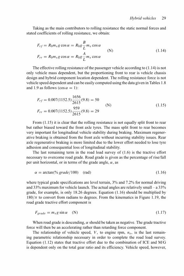
Hybrid vehicles 29
Taking as the main contributors to rolling resistance the static normal forces andstated coefficients of rolling resistance, we obtain:
Frf = R0mvg cos α = R0gB
Lmv cos α
Frr = R0mvg cos α = R0gA
Lmv cos α
(N) (1.14)
The effective rolling resistance of the passenger vehicle according to (1.14) is notonly vehicle mass dependent, but the proportioning front to rear is vehicle chassisdesign and hybrid component location dependent. The rolling resistance force is notvehicle speed dependent and can be easily computed using the data given in Tables 1.8and 1.9 as follows (cos α = 1):
Frf = 0.007(1152.5)1656
2615(9.8) = 50
Frr = 0.007(1152.5)959
2615(9.8) = 29
(N) (1.15)
From (1.15) it is clear that the rolling resistance is not equally split front to rearbut rather biased toward the front axle tyres. The mass split front to rear becomesvery important for longitudinal vehicle stability during braking. Maximum regener-ative braking is obtained from the front axle without incurring stability issues. Rearaxle regenerative braking is more limited due to the lower effort needed to lose tyreadhesion and consequential loss of longitudinal stability.
The last remaining term in the road load survey of (1.6) is the tractive effortnecessary to overcome road grade. Road grade is given as the percentage of rise/fallper unit horizontal, or in terms of the grade angle, α, as
α = arctan(% grade/100) (rad) (1.16)
where typical grade specifications are level terrain, 3% and 7.2% for normal drivingand 33% maximum for vehicle launch. The actual angles are relatively small – a 33%grade, for example, is only 18.26 degrees. Equation (1.16) should be multiplied by180/π to convert from radians to degrees. From the kinematics in Figure 1.19, theroad grade tractive effort component is
Fgrade = mvg sin α (N) (1.17)
When road grade is descending, α should be taken as negative. The grade tractiveforce will then be an accelerating rather than retarding force component.
The relationship of vehicle speed, V , to engine rpm, ne, is the last remain-ing parametric relationship necessary in order to complete the road load survey.Equation (1.12) states that tractive effort due to the combination of ICE and M/Gis dependent only on the total gear ratio and its efficiency. Vehicle speed, however,
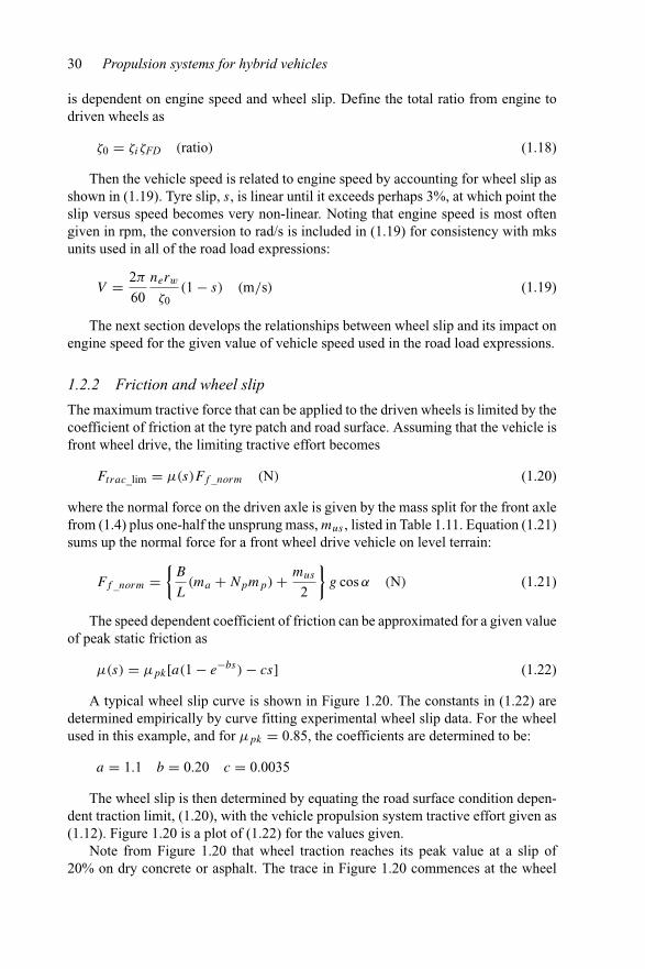
30 Propulsion systems for hybrid vehicles
is dependent on engine speed and wheel slip. Define the total ratio from engine todriven wheels as
ζ0 = ζiζFD (ratio) (1.18)
Then the vehicle speed is related to engine speed by accounting for wheel slip asshown in (1.19). Tyre slip, s, is linear until it exceeds perhaps 3%, at which point theslip versus speed becomes very non-linear. Noting that engine speed is most oftengiven in rpm, the conversion to rad/s is included in (1.19) for consistency with mksunits used in all of the road load expressions:
V = 2π
60
nerw
ζ0(1 − s) (m/s) (1.19)
The next section develops the relationships between wheel slip and its impact onengine speed for the given value of vehicle speed used in the road load expressions.
1.2.2 Friction and wheel slip
The maximum tractive force that can be applied to the driven wheels is limited by thecoefficient of friction at the tyre patch and road surface. Assuming that the vehicle isfront wheel drive, the limiting tractive effort becomes
Ftrac_lim = μ(s)Ff _norm (N) (1.20)
where the normal force on the driven axle is given by the mass split for the front axlefrom (1.4) plus one-half the unsprung mass, mus , listed in Table 1.11. Equation (1.21)sums up the normal force for a front wheel drive vehicle on level terrain:
Ff _norm ={
B
L(ma + Npmp) + mus
2
}g cos α (N) (1.21)
The speed dependent coefficient of friction can be approximated for a given valueof peak static friction as
μ(s) = μpk[a(1 − e−bs) − cs] (1.22)
A typical wheel slip curve is shown in Figure 1.20. The constants in (1.22) aredetermined empirically by curve fitting experimental wheel slip data. For the wheelused in this example, and for μpk = 0.85, the coefficients are determined to be:
a = 1.1 b = 0.20 c = 0.0035
The wheel slip is then determined by equating the road surface condition depen-dent traction limit, (1.20), with the vehicle propulsion system tractive effort given as(1.12). Figure 1.20 is a plot of (1.22) for the values given.
Note from Figure 1.20 that wheel traction reaches its peak value at a slip of20% on dry concrete or asphalt. The trace in Figure 1.20 commences at the wheel
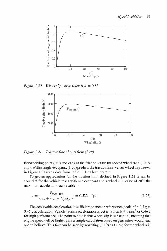
Hybrid vehicles 31
μ(i)
s(i)0 20 40 60 80 100
0
0.2
0.4
0.6
0.8
1
Wheel slip, %
Coe
ffic
ient
of
long
itudi
nal f
rict
ion
Figure 1.20 Wheel slip curve when μpk = 0.85
s(i)0 20 40 60 80 100
0
2000
4000
6000
8000
Wheel slip, %
Tra
ctiv
e ef
fort
lim
it, N
Ftrac_lim(i)
Figure 1.21 Tractive force limits from (1.20)
freewheeling point (0,0) and ends at the friction value for locked wheel skid (100%slip). With a single occupant, (1.20) predicts the traction limit versus wheel slip shownin Figure 1.21 using data from Table 1.11 on level terrain.
To get an appreciation for the traction limit defined in Figure 1.21 it can beseen that for the vehicle mass with one occupant and a wheel slip value of 20% themaximum acceleration achievable is
a = Ftrac_ lim
(ma + mus + Npmp)g= 0.522 (g) (1.23)
The achievable acceleration is sufficient to meet performance goals of ∼0.3 g to0.46 g acceleration. Vehicle launch acceleration target is typically 4.5 m/s2 or 0.46 gfor high performance. The point to note is that wheel slip is substantial, meaning thatengine speed will be higher than a simple calculation based on gear ratios would leadone to believe. This fact can be seen by rewriting (1.19) as (1.24) for the wheel slip
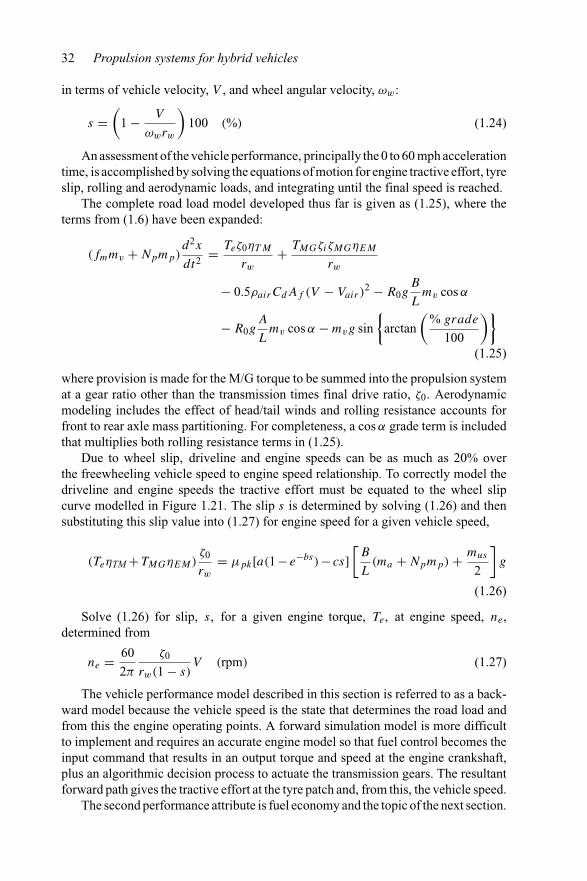
32 Propulsion systems for hybrid vehicles
in terms of vehicle velocity, V , and wheel angular velocity, ωw:
s =(
1 − V
ωwrw
)100 (%) (1.24)
An assessment of the vehicle performance, principally the 0 to 60 mph accelerationtime, is accomplished by solving the equations of motion for engine tractive effort, tyreslip, rolling and aerodynamic loads, and integrating until the final speed is reached.
The complete road load model developed thus far is given as (1.25), where theterms from (1.6) have been expanded:
(fmmv + Npmp)d2x
dt2 = Teζ0ηT M
rw+ TMGζiζMGηEM
rw
− 0.5ρairCdAf (V − Vair )2 − R0g
B
Lmv cos α
− R0gA
Lmv cos α − mvg sin
{arctan
(% grade
100
)}(1.25)
where provision is made for the M/G torque to be summed into the propulsion systemat a gear ratio other than the transmission times final drive ratio, ζ0. Aerodynamicmodeling includes the effect of head/tail winds and rolling resistance accounts forfront to rear axle mass partitioning. For completeness, a cos α grade term is includedthat multiplies both rolling resistance terms in (1.25).
Due to wheel slip, driveline and engine speeds can be as much as 20% overthe freewheeling vehicle speed to engine speed relationship. To correctly model thedriveline and engine speeds the tractive effort must be equated to the wheel slipcurve modelled in Figure 1.21. The slip s is determined by solving (1.26) and thensubstituting this slip value into (1.27) for engine speed for a given vehicle speed,
(TeηTM +TMGηEM)ζ0
rw= μpk[a(1− e−bs)− cs]
[B
L(ma + Npmp) + mus
2
]g
(1.26)
Solve (1.26) for slip, s, for a given engine torque, Te, at engine speed, ne,determined from
ne = 60
2π
ζ0
rw(1 − s)V (rpm) (1.27)
The vehicle performance model described in this section is referred to as a back-ward model because the vehicle speed is the state that determines the road load andfrom this the engine operating points. A forward simulation model is more difficultto implement and requires an accurate engine model so that fuel control becomes theinput command that results in an output torque and speed at the engine crankshaft,plus an algorithmic decision process to actuate the transmission gears. The resultantforward path gives the tractive effort at the tyre patch and, from this, the vehicle speed.
The second performance attribute is fuel economy and the topic of the next section.
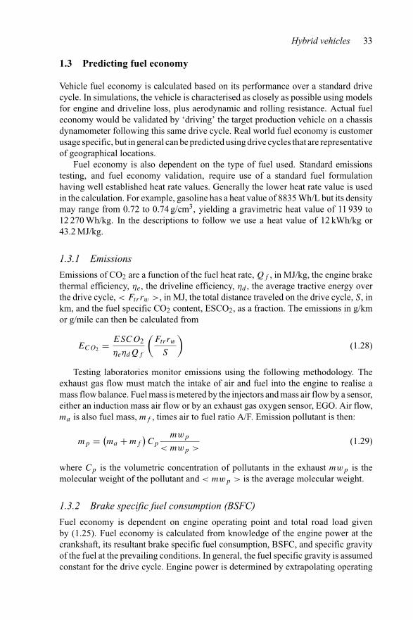
Hybrid vehicles 33
1.3 Predicting fuel economy
Vehicle fuel economy is calculated based on its performance over a standard drivecycle. In simulations, the vehicle is characterised as closely as possible using modelsfor engine and driveline loss, plus aerodynamic and rolling resistance. Actual fueleconomy would be validated by ‘driving’ the target production vehicle on a chassisdynamometer following this same drive cycle. Real world fuel economy is customerusage specific, but in general can be predicted using drive cycles that are representativeof geographical locations.
Fuel economy is also dependent on the type of fuel used. Standard emissionstesting, and fuel economy validation, require use of a standard fuel formulationhaving well established heat rate values. Generally the lower heat rate value is usedin the calculation. For example, gasoline has a heat value of 8835 Wh/L but its densitymay range from 0.72 to 0.74 g/cm3, yielding a gravimetric heat value of 11 939 to12 270 Wh/kg. In the descriptions to follow we use a heat value of 12 kWh/kg or43.2 MJ/kg.
1.3.1 Emissions
Emissions of CO2 are a function of the fuel heat rate, Qf , in MJ/kg, the engine brakethermal efficiency, ηe, the driveline efficiency, ηd , the average tractive energy overthe drive cycle, < Ftrrw >, in MJ, the total distance traveled on the drive cycle, S, inkm, and the fuel specific CO2 content, ESCO2, as a fraction. The emissions in g/kmor g/mile can then be calculated from
ECO2 = ESCO2
ηeηdQf
(Ftrrw
S
)(1.28)
Testing laboratories monitor emissions using the following methodology. Theexhaust gas flow must match the intake of air and fuel into the engine to realise amass flow balance. Fuel mass is metered by the injectors and mass air flow by a sensor,either an induction mass air flow or by an exhaust gas oxygen sensor, EGO. Air flow,ma is also fuel mass, mf , times air to fuel ratio A/F. Emission pollutant is then:
mp = (ma + mf
)Cp
mwp
< mwp >(1.29)
where Cp is the volumetric concentration of pollutants in the exhaust mwp is themolecular weight of the pollutant and < mwp > is the average molecular weight.
1.3.2 Brake specific fuel consumption (BSFC)
Fuel economy is dependent on engine operating point and total road load givenby (1.25). Fuel economy is calculated from knowledge of the engine power at thecrankshaft, its resultant brake specific fuel consumption, BSFC, and specific gravityof the fuel at the prevailing conditions. In general, the fuel specific gravity is assumedconstant for the drive cycle. Engine power is determined by extrapolating operating
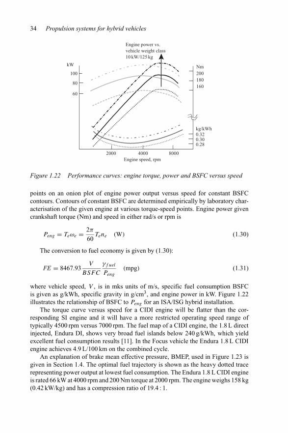
34 Propulsion systems for hybrid vehicles
100
80
60
kW
2000 4000 8000Engine speed, rpm
kg/kWh0.320.300.28
Nm200180160
Engine power vs.vehicle weight class10 kW/125 kg
Figure 1.22 Performance curves: engine torque, power and BSFC versus speed
points on an onion plot of engine power output versus speed for constant BSFCcontours. Contours of constant BSFC are determined empirically by laboratory char-acterisation of the given engine at various torque-speed points. Engine power givencrankshaft torque (Nm) and speed in either rad/s or rpm is
Peng = Teωe = 2π
60Tene (W) (1.30)
The conversion to fuel economy is given by (1.30):
FE = 8467.93V
BSFC
γf uel
Peng
(mpg) (1.31)
where vehicle speed, V , is in mks units of m/s, specific fuel consumption BSFCis given as g/kWh, specific gravity in g/cm3, and engine power in kW. Figure 1.22illustrates the relationship of BSFC to Peng for an ISA/ISG hybrid installation.
The torque curve versus speed for a CIDI engine will be flatter than the cor-responding SI engine and it will have a more restricted operating speed range oftypically 4500 rpm versus 7000 rpm. The fuel map of a CIDI engine, the 1.8 L directinjected, Endura DI, shows very broad fuel islands below 240 g/kWh, which yieldexcellent fuel consumption results [11]. In the Focus vehicle the Endura 1.8 L CIDIengine achieves 4.9 L/100 km on the combined cycle.
An explanation of brake mean effective pressure, BMEP, used in Figure 1.23 isgiven in Section 1.4. The optimal fuel trajectory is shown as the heavy dotted tracerepresenting power output at lowest fuel consumption. The Endura 1.8 L CIDI engineis rated 66 kW at 4000 rpm and 200 Nm torque at 2000 rpm. The engine weighs 158 kg(0.42 kW/kg) and has a compression ratio of 19.4 : 1.
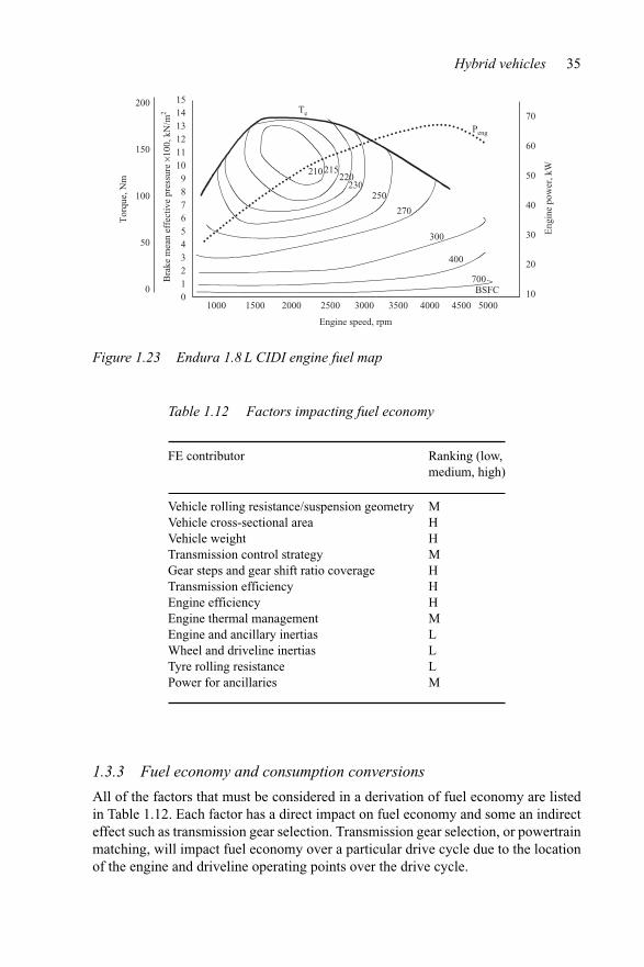
Hybrid vehicles 35
1514131211109876543210
1000 1500 2000 2500 3000 3500 4000 4500 5000
Engine speed, rpm
215220
230250
270
300
400
700BSFC
Bra
ke m
ean
effe
ctiv
e pr
essu
re ×
100,
kN
/m2 Te
Peng
70
60
50
40
30
20
10
Eng
ine
pow
er, k
W
200
150
100
50
0
Tor
que,
Nm
210
Figure 1.23 Endura 1.8 L CIDI engine fuel map
Table 1.12 Factors impacting fuel economy
FE contributor Ranking (low,medium, high)
Vehicle rolling resistance/suspension geometry MVehicle cross-sectional area HVehicle weight HTransmission control strategy MGear steps and gear shift ratio coverage HTransmission efficiency HEngine efficiency HEngine thermal management MEngine and ancillary inertias LWheel and driveline inertias LTyre rolling resistance LPower for ancillaries M
1.3.3 Fuel economy and consumption conversions
All of the factors that must be considered in a derivation of fuel economy are listedin Table 1.12. Each factor has a direct impact on fuel economy and some an indirecteffect such as transmission gear selection. Transmission gear selection, or powertrainmatching, will impact fuel economy over a particular drive cycle due to the locationof the engine and driveline operating points over the drive cycle.
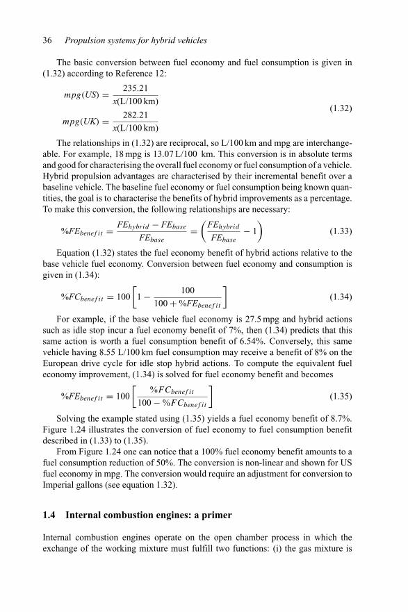
36 Propulsion systems for hybrid vehicles
The basic conversion between fuel economy and fuel consumption is given in(1.32) according to Reference 12:
mpg(US) = 235.21
x(L/100 km)
mpg(UK) = 282.21
x(L/100 km)
(1.32)
The relationships in (1.32) are reciprocal, so L/100 km and mpg are interchange-able. For example, 18 mpg is 13.07 L/100 km. This conversion is in absolute termsand good for characterising the overall fuel economy or fuel consumption of a vehicle.Hybrid propulsion advantages are characterised by their incremental benefit over abaseline vehicle. The baseline fuel economy or fuel consumption being known quan-tities, the goal is to characterise the benefits of hybrid improvements as a percentage.To make this conversion, the following relationships are necessary:
%FEbenef it = FEhybrid − FEbase
FEbase
=(
FEhybrid
FEbase
− 1)
(1.33)
Equation (1.32) states the fuel economy benefit of hybrid actions relative to thebase vehicle fuel economy. Conversion between fuel economy and consumption isgiven in (1.34):
%FCbenef it = 100[
1 − 100
100 + %FEbenef it
](1.34)
For example, if the base vehicle fuel economy is 27.5 mpg and hybrid actionssuch as idle stop incur a fuel economy benefit of 7%, then (1.34) predicts that thissame action is worth a fuel consumption benefit of 6.54%. Conversely, this samevehicle having 8.55 L/100 km fuel consumption may receive a benefit of 8% on theEuropean drive cycle for idle stop hybrid actions. To compute the equivalent fueleconomy improvement, (1.34) is solved for fuel economy benefit and becomes
%FEbenef it = 100[
%FCbenef it
100 − %FCbenef it
](1.35)
Solving the example stated using (1.35) yields a fuel economy benefit of 8.7%.Figure 1.24 illustrates the conversion of fuel economy to fuel consumption benefitdescribed in (1.33) to (1.35).
From Figure 1.24 one can notice that a 100% fuel economy benefit amounts to afuel consumption reduction of 50%. The conversion is non-linear and shown for USfuel economy in mpg. The conversion would require an adjustment for conversion toImperial gallons (see equation 1.32).
1.4 Internal combustion engines: a primer
Internal combustion engines operate on the open chamber process in which theexchange of the working mixture must fulfill two functions: (i) the gas mixture is
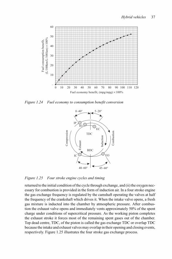
Hybrid vehicles 37
–
10
20
30
40
50
60
0 10 20 30 40 50 60 70 80 90 100 110 120
Fuel economy benefit, (mpg/mpg) × 100%
Fuel
con
sum
ptio
n be
nefi
t,(L
/100
km/L
/100
km)
×10
0%
Figure 1.24 Fuel economy to consumption benefit conversion
BDC
TDC
45–60°40–60°
5–20°0–40°
Indu
ctio
n
Exh
aust
IPIO
EC
EOIC
Com
bust
ion
Com
pres
sion
Figure 1.25 Four stroke engine cycles and timing
returned to the initial condition of the cycle through exchange, and (ii) the oxygen nec-essary for combustion is provided in the form of induction air. In a four stroke enginethe gas exchange frequency is regulated by the camshaft operating the valves at halfthe frequency of the crankshaft which drives it. When the intake valve opens, a freshgas mixture is inducted into the chamber by atmospheric pressure. After combus-tion the exhaust valve opens and immediately vents approximately 50% of the spentcharge under conditions of supercritical pressure. As the working piston completesthe exhaust stroke it forces most of the remaining spent gases out of the chamber.Top dead centre, TDC, of the piston is called the gas exchange TDC or overlap TDCbecause the intake and exhaust valves may overlap in their opening and closing events,respectively. Figure 1.25 illustrates the four stroke gas exchange process.
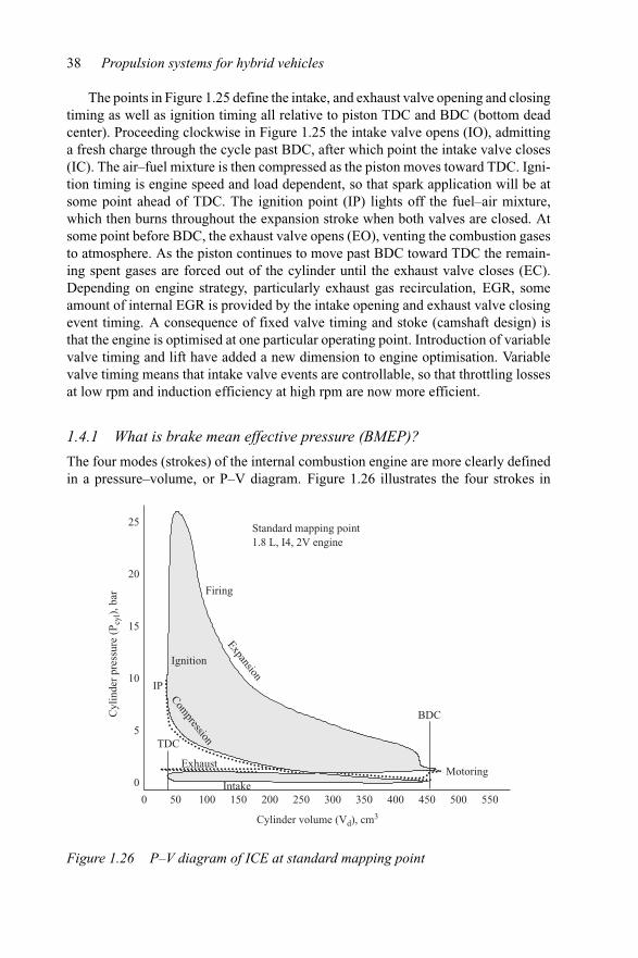
38 Propulsion systems for hybrid vehicles
The points in Figure 1.25 define the intake, and exhaust valve opening and closingtiming as well as ignition timing all relative to piston TDC and BDC (bottom deadcenter). Proceeding clockwise in Figure 1.25 the intake valve opens (IO), admittinga fresh charge through the cycle past BDC, after which point the intake valve closes(IC). The air–fuel mixture is then compressed as the piston moves toward TDC. Igni-tion timing is engine speed and load dependent, so that spark application will be atsome point ahead of TDC. The ignition point (IP) lights off the fuel–air mixture,which then burns throughout the expansion stroke when both valves are closed. Atsome point before BDC, the exhaust valve opens (EO), venting the combustion gasesto atmosphere. As the piston continues to move past BDC toward TDC the remain-ing spent gases are forced out of the cylinder until the exhaust valve closes (EC).Depending on engine strategy, particularly exhaust gas recirculation, EGR, someamount of internal EGR is provided by the intake opening and exhaust valve closingevent timing. A consequence of fixed valve timing and stoke (camshaft design) isthat the engine is optimised at one particular operating point. Introduction of variablevalve timing and lift have added a new dimension to engine optimisation. Variablevalve timing means that intake valve events are controllable, so that throttling lossesat low rpm and induction efficiency at high rpm are now more efficient.
1.4.1 What is brake mean effective pressure (BMEP)?
The four modes (strokes) of the internal combustion engine are more clearly definedin a pressure–volume, or P–V diagram. Figure 1.26 illustrates the four strokes in
Cylinder volume (Vd), cm3
25
20
15
10
5
0
Cyl
inde
r pr
essu
re (
P cyl
), b
ar
Standard mapping point1.8 L, I4, 2V engine
Motoring
Firing
IP
BDC
TDC
Intake
Exhaust
Compression
Expansion
Ignition
0 50 100 150 200 250 300 350 400 450 500 550
Figure 1.26 P–V diagram of ICE at standard mapping point
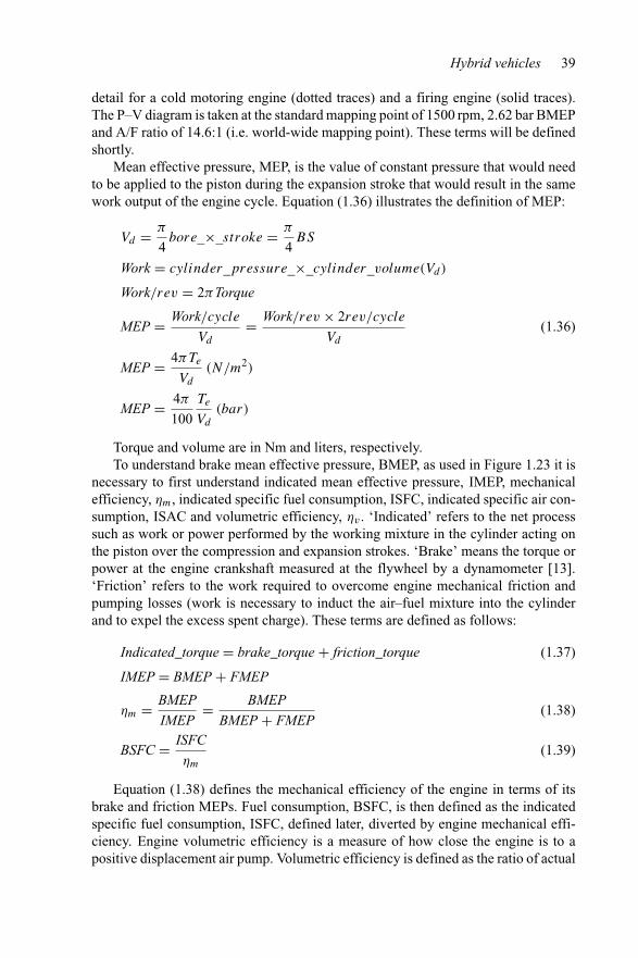
Hybrid vehicles 39
detail for a cold motoring engine (dotted traces) and a firing engine (solid traces).The P–V diagram is taken at the standard mapping point of 1500 rpm, 2.62 bar BMEPand A/F ratio of 14.6:1 (i.e. world-wide mapping point). These terms will be definedshortly.
Mean effective pressure, MEP, is the value of constant pressure that would needto be applied to the piston during the expansion stroke that would result in the samework output of the engine cycle. Equation (1.36) illustrates the definition of MEP:
Vd = π
4bore_×_stroke = π
4BS
Work = cylinder_pressure_×_cylinder_volume(Vd)
Work/rev = 2πTorque
MEP = Work/cycle
Vd
= Work/rev × 2rev/cycle
Vd
(1.36)
MEP = 4πTe
Vd
(N/m2)
MEP = 4π
100
Te
Vd
(bar)
Torque and volume are in Nm and liters, respectively.To understand brake mean effective pressure, BMEP, as used in Figure 1.23 it is
necessary to first understand indicated mean effective pressure, IMEP, mechanicalefficiency, ηm, indicated specific fuel consumption, ISFC, indicated specific air con-sumption, ISAC and volumetric efficiency, ηv . ‘Indicated’ refers to the net processsuch as work or power performed by the working mixture in the cylinder acting onthe piston over the compression and expansion strokes. ‘Brake’ means the torque orpower at the engine crankshaft measured at the flywheel by a dynamometer [13].‘Friction’ refers to the work required to overcome engine mechanical friction andpumping losses (work is necessary to induct the air–fuel mixture into the cylinderand to expel the excess spent charge). These terms are defined as follows:
Indicated_torque = brake_torque + friction_torque (1.37)
IMEP = BMEP + FMEP
ηm = BMEP
IMEP= BMEP
BMEP + FMEP(1.38)
BSFC = ISFC
ηm
(1.39)
Equation (1.38) defines the mechanical efficiency of the engine in terms of itsbrake and friction MEPs. Fuel consumption, BSFC, is then defined as the indicatedspecific fuel consumption, ISFC, defined later, diverted by engine mechanical effi-ciency. Engine volumetric efficiency is a measure of how close the engine is to apositive displacement air pump. Volumetric efficiency is defined as the ratio of actual
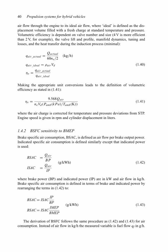
40 Propulsion systems for hybrid vehicles
air flow through the engine to its ideal air flow, where ‘ideal’ is defined as the dis-placement volume filled with a fresh charge at standard temperature and pressure.Volumetric efficiency is dependent on valve number and size (4 V is more efficientthan 2 V, for example), the valve lift and profile, manifold dynamics, tuning andlosses, and the heat transfer during the induction process (minimal):
qair_actual = Qactual
60ne/2(kg/h)
qair_ideal = ρairVd
ηv = qair_actual
qair_ideal
(1.40)
Making the appropriate unit conversions leads to the definition of volumetricefficiency as stated in (1.41):
ηv = 9.568Qair
neVd(Pamb(kPa)/Tamb(K))(1.41)
where the air charge is corrected for temperature and pressure deviations from STP.Engine speed is given in rpm and cylinder displacement in liters.
1.4.2 BSFC sensitivity to BMEP
Brake specific air consumption, BSAC, is defined as air flow per brake output power.Indicated specific air consumption is defined similarly except that indicated poweris used:
BSAC = Qair
BP
ISAC = Qair
IP
(g/kWh) (1.42)
where brake power (BP) and indicated power (IP) are in kW and air flow in kg/h.Brake specific air consumption is defined in terms of brake and indicated power byrearranging the terms in (1.42) to:
BSAC = ISACIP
BP
BSAC = ISACIMEP
BMEP
(g/kWh) (1.43)
The derivation of BSFC follows the same procedure as (1.42) and (1.43) for airconsumption. Instead of air flow in kg/h the measured variable is fuel flow qf in g/h.
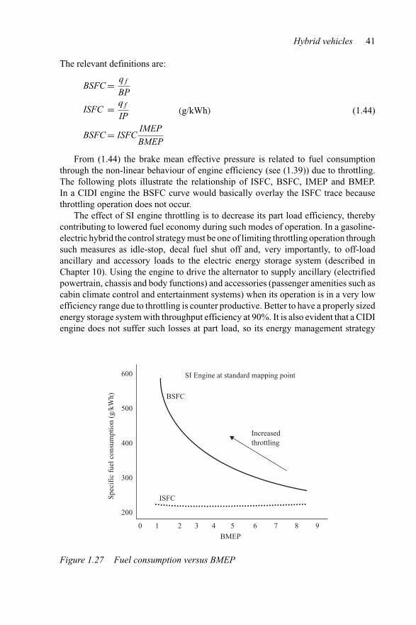
Hybrid vehicles 41
The relevant definitions are:
BSFC = qf
BP
ISFC = qf
IP
BSFC = ISFCIMEP
BMEP
(g/kWh) (1.44)
From (1.44) the brake mean effective pressure is related to fuel consumptionthrough the non-linear behaviour of engine efficiency (see (1.39)) due to throttling.The following plots illustrate the relationship of ISFC, BSFC, IMEP and BMEP.In a CIDI engine the BSFC curve would basically overlay the ISFC trace becausethrottling operation does not occur.
The effect of SI engine throttling is to decrease its part load efficiency, therebycontributing to lowered fuel economy during such modes of operation. In a gasoline-electric hybrid the control strategy must be one of limiting throttling operation throughsuch measures as idle-stop, decal fuel shut off and, very importantly, to off-loadancillary and accessory loads to the electric energy storage system (described inChapter 10). Using the engine to drive the alternator to supply ancillary (electrifiedpowertrain, chassis and body functions) and accessories (passenger amenities such ascabin climate control and entertainment systems) when its operation is in a very lowefficiency range due to throttling is counter productive. Better to have a properly sizedenergy storage system with throughput efficiency at 90%. It is also evident that a CIDIengine does not suffer such losses at part load, so its energy management strategy
0 1 2 3 4 5 6 7 8 9BMEP
Spec
ific
fue
l con
sum
ptio
n (g
/kW
h)
600
500
400
300
200
BSFC
ISFC
SI Engine at standard mapping point
Increasedthrottling
Figure 1.27 Fuel consumption versus BMEP
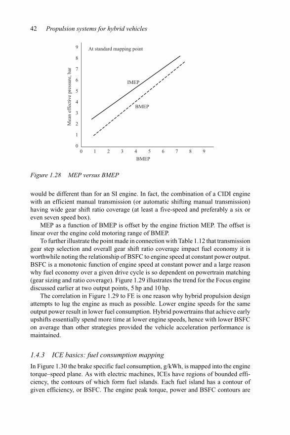
42 Propulsion systems for hybrid vehicles
BMEP
Mea
n ef
fect
ive
pres
sure
, bar
At standard mapping point9
8
7
6
5
4
3
2
1
0
BMEP
IMEP
0 1 2 3 4 5 6 7 8 9
Figure 1.28 MEP versus BMEP
would be different than for an SI engine. In fact, the combination of a CIDI enginewith an efficient manual transmission (or automatic shifting manual transmission)having wide gear shift ratio coverage (at least a five-speed and preferably a six oreven seven speed box).
MEP as a function of BMEP is offset by the engine friction MEP. The offset islinear over the engine cold motoring range of BMEP.
To further illustrate the point made in connection with Table 1.12 that transmissiongear step selection and overall gear shift ratio coverage impact fuel economy it isworthwhile noting the relationship of BSFC to engine speed at constant power output.BSFC is a monotonic function of engine speed at constant power and a large reasonwhy fuel economy over a given drive cycle is so dependent on powertrain matching(gear sizing and ratio coverage). Figure 1.29 illustrates the trend for the Focus enginediscussed earlier at two output points, 5 hp and 10 hp.
The correlation in Figure 1.29 to FE is one reason why hybrid propulsion designattempts to lug the engine as much as possible. Lower engine speeds for the sameoutput power result in lower fuel consumption. Hybrid powertrains that achieve earlyupshifts essentially spend more time at lower engine speeds, hence with lower BSFCon average than other strategies provided the vehicle acceleration performance ismaintained.
1.4.3 ICE basics: fuel consumption mapping
In Figure 1.30 the brake specific fuel consumption, g/kWh, is mapped into the enginetorque–speed plane. As with electric machines, ICEs have regions of bounded effi-ciency, the contours of which form fuel islands. Each fuel island has a contour ofgiven efficiency, or BSFC. The engine peak torque, power and BSFC contours are
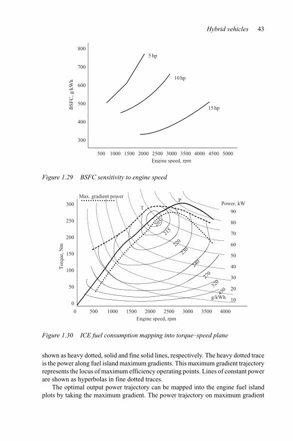
Hybrid vehicles 43
800
700
600
500
400
300
BSF
C, g
/kW
h
5 hp
10 hp
15 hp
Engine speed, rpm500 1000 1500 2000 2500 3000 3500 4000 4500 5000
Figure 1.29 BSFC sensitivity to engine speed
90
80
70
60
50
40
30
20
10
300
250
200
150
100
50
0
Engine speed, rpm
Tor
que,
Nm
205
215
220
230
240
270
320
450
Power, kW
g/kWh
T
PMax. gradient power
0 500 1000 1500 2000 2500 3000 3500 4000
Figure 1.30 ICE fuel consumption mapping into torque–speed plane
shown as heavy dotted, solid and fine solid lines, respectively. The heavy dotted traceis the power along fuel island maximum gradients. This maximum gradient trajectoryrepresents the locus of maximum efficiency operating points. Lines of constant powerare shown as hyperbolas in fine dotted traces.
The optimal output power trajectory can be mapped into the engine fuel islandplots by taking the maximum gradient. The power trajectory on maximum gradient
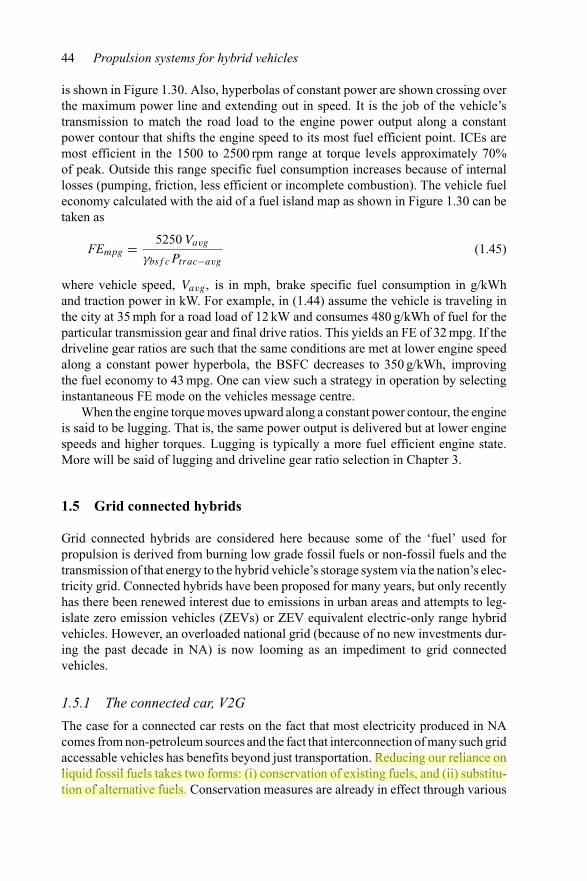
44 Propulsion systems for hybrid vehicles
is shown in Figure 1.30. Also, hyperbolas of constant power are shown crossing overthe maximum power line and extending out in speed. It is the job of the vehicle’stransmission to match the road load to the engine power output along a constantpower contour that shifts the engine speed to its most fuel efficient point. ICEs aremost efficient in the 1500 to 2500 rpm range at torque levels approximately 70%of peak. Outside this range specific fuel consumption increases because of internallosses (pumping, friction, less efficient or incomplete combustion). The vehicle fueleconomy calculated with the aid of a fuel island map as shown in Figure 1.30 can betaken as
FEmpg = 5250 Vavg
γbsf cPtrac−avg
(1.45)
where vehicle speed, Vavg , is in mph, brake specific fuel consumption in g/kWhand traction power in kW. For example, in (1.44) assume the vehicle is traveling inthe city at 35 mph for a road load of 12 kW and consumes 480 g/kWh of fuel for theparticular transmission gear and final drive ratios. This yields an FE of 32 mpg. If thedriveline gear ratios are such that the same conditions are met at lower engine speedalong a constant power hyperbola, the BSFC decreases to 350 g/kWh, improvingthe fuel economy to 43 mpg. One can view such a strategy in operation by selectinginstantaneous FE mode on the vehicles message centre.
When the engine torque moves upward along a constant power contour, the engineis said to be lugging. That is, the same power output is delivered but at lower enginespeeds and higher torques. Lugging is typically a more fuel efficient engine state.More will be said of lugging and driveline gear ratio selection in Chapter 3.
1.5 Grid connected hybrids
Grid connected hybrids are considered here because some of the ‘fuel’ used forpropulsion is derived from burning low grade fossil fuels or non-fossil fuels and thetransmission of that energy to the hybrid vehicle’s storage system via the nation’s elec-tricity grid. Connected hybrids have been proposed for many years, but only recentlyhas there been renewed interest due to emissions in urban areas and attempts to leg-islate zero emission vehicles (ZEVs) or ZEV equivalent electric-only range hybridvehicles. However, an overloaded national grid (because of no new investments dur-ing the past decade in NA) is now looming as an impediment to grid connectedvehicles.
1.5.1 The connected car, V2G
The case for a connected car rests on the fact that most electricity produced in NAcomes from non-petroleum sources and the fact that interconnection of many such gridaccessable vehicles has benefits beyond just transportation. Reducing our reliance onliquid fossil fuels takes two forms: (i) conservation of existing fuels, and (ii) substitu-tion of alternative fuels. Conservation measures are already in effect through various
Admin
线条
Admin
线条
Admin
下划线
Admin
下划线
Admin
高亮
Admin
波浪线
Admin
打字机
开源节流:broaden sources of income and reduce expenditure
本页已使用福昕阅读器进行编辑。 福昕软件(C)2005-2009,版权所有, 仅供试用。ഀ
Hybrid vehicles 45
legislated means to regulate transportation use fuel economy, non-transportation effi-ciency improvements such as building lighting (e.g. initiatives such as dark-skiesbuilding and electrical codes) and industrial motor efficiency programs (US energyconservation act). Substitution of alternative fuels means a transition away from liq-uid fossil fuels to natural gas, hydrogen, or non-conventional energy generation suchas solar and wind power. According to Tom Gage of AC Propulsion [14], any vehiclethat plugs into the electric power grid and draws some or all of its energy from thegrid will achieve both conservation and substitution.
The basic premise of the connected car is that a large portion of its commute rangecan be on energy stored on board that was delivered by the electric grid. This offsettingof petroleum consumption could be significant, according to Mr Gage. For example,a 40 mpg hybrid with 30 miles of electric only range could use grid electricity fortwo-thirds of its operation, yielding a petroleum fuel economy equivalent of 120 mpg.The second benefit of connected cars is that these parked vehicles represent a highlydistributed source of generation, or vehicle to grid, V2G infrastructure. This conceptof using on-board power assets for off-board consumption is not new. Other companieshave developed hybrids that use either the engine driven M/G as a power source foroff-board portable power such as power tools (the GM contractor special) or fuel cellpowered vehicles as an electricity source for home power.
These V2G vehicles offering off-board benefit would be classified under SAEJ1772 as level 1 through level 3:
Level 1: 110 V ac at 1.5 kW
Level 2: 240 V ac at 7.6 kW
Level 3: 240 V ac and >7 kW
One manufacturer has designed a level 3 V2G car capable of 40 kW power trans-fer. This is more than competitive with standby power generation using natural gasfired ICEs for powering homes, commercial establishments or apartments. In testsconducted for AC Propulsion by the California Air Resources Board (CARB) ElMonte emissions lab, it was found that non-methane hydrocarbons, NMHC, and COof the hybrid vehicle (Prius) were well below the emissions of a Capstone microtur-bine standby power unit or a combined cycle utility power plant. Table 1.13 illustratesthe resulting emissions from this V2G mock-up. Table 1.14 states the Euro 3 and Euro4 emission limits for both diesel and gasoline fuelled vehicles.
Table 1.13 V2G emissions (from Reference 14, Table 1)
Source NMHC (g/kWh) CO (g/kWh)
Prius hybrid on chassis rolls at 10 kW continuous 0.039 0.639Combined cycle power plant 0.050 0.077Capstone microturbine 0.077 0.603
Admin
波浪线
Admin
波浪线
Admin
波浪线
Admin
波浪线
Admin
下划线
Admin
下划线
Admin
下划线
Admin
高亮
Admin
高亮
Admin
下划线
Admin
下划线
本页已使用福昕阅读器进行编辑。 福昕软件(C)2005-2009,版权所有, 仅供试用。ഀ
46 Propulsion systems for hybrid vehicles
Table 1.14 Euro 3 (CY 2000) and Euro 4 (CY2005) emission limits
Regulation Euro 3 (g/km) Euro 4 (g/km)
diesel gasoline diesel gasolineCO 0.64 2.30 0.50 1.00HC – 0.20 – 0.10HC + NOx 0.56 – 0.30 –NOx 0.50 0.15 0.25 0.08PM 0.05 – 0.025 –
*PM = Particulate Matter.
CARB, along with the South Coast Air Quality Management District, andDOE/NREL are funding the construction of a V2G prototype by AC Propulsion.The V2G prototype will be a compact 4 door sedan augmented with 9 kWh Pb-Acidbattery pack, 30 kW dc auxiliary power unit, a 1.4 L SI engine and custom designedalternator auxiliary power unit. The vehicle engine will be modified to run off nat-ural gas when parked and gasoline when driving. The battery will provide 35 miles(56 km) of electric only range. This in effect will be an H60 hybrid. Performance willbe consistent with PNGV targets and the auxiliary power supply will provide level 3outlets.
1.5.2 Grid connected HEV20 and HEV60
The Electric Power Research Institute (EPRI) performed a customer survey to deter-mine the thresholds of desirable hybrid performance and costs [15]. Figure 1.31 is aneducational slide used by EPRI, to inform the survey participants of the distinctionbetween a conventional vehicle and a electric vehicle.
Survey participants were asked about the necessity of plugging in their vehiclesversus filling station visits to pump gasoline. By and large the respondents wereamenable to plugging in their vehicles rather than seeking out a filling station. Therewas concern, however, by apartment and condominium dwellers over the availabilityof a charging outlet, plus a caveat to remember to plug the vehicle in. The EPRIsurvey then introduced a charge sustaining hybrid, H0, and plug-in hybrid, H20 toH60, to test the waters on hybrid vehicles with and without the electric only range.Figure 1.32 is the slide used to educate the respondents to charge sustaining andelectric range capable hybrids.
An interesting finding from the survey was that a charge sustaining hybrid waspreferred over the conventional vehicle and that each successive increment in theelectric only range of the plug-in hybrid was preferred over its predecessor vehicle,i.e. H0 over CV, H20 over H0, H60 over H40, etc. The distinction appears to be in theflexibility to drive off electricity only versus gasoline in a charge sustaining mode.The H0 vehicle, or power assist hybrid, will be the principal focus of this book. Dual
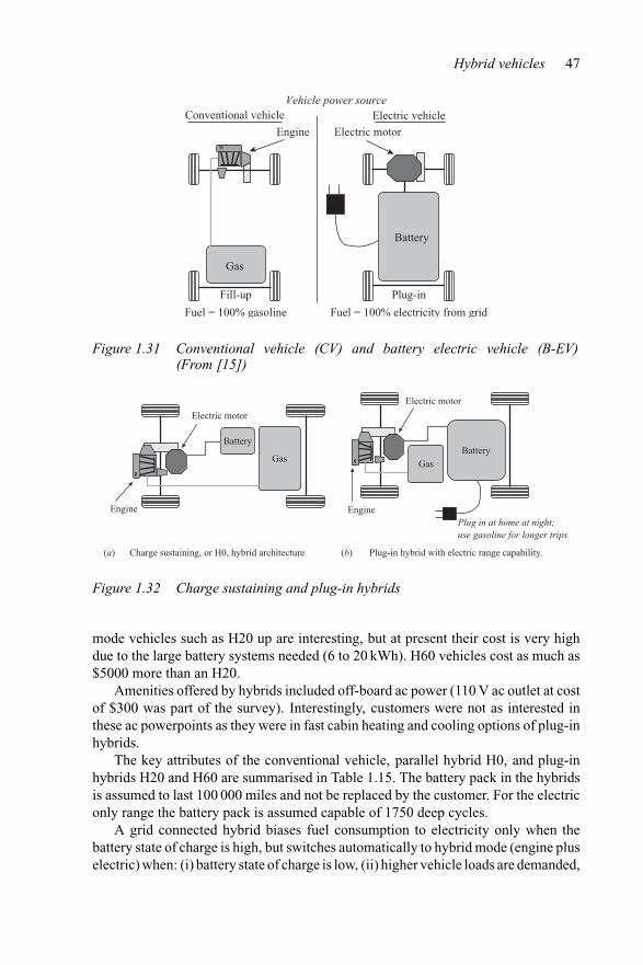
Hybrid vehicles 47
Vehicle power sourceConventional vehicle
Fill-up Plug-in
Battery
Gas
EngineElectric vehicle
Electric motor
Fuel = 100% gasoline Fuel = 100% electricity from grid
Figure 1.31 Conventional vehicle (CV) and battery electric vehicle (B-EV)(From [15])
Electric motor
Battery
Gas
Engine
Electric motor
Plug in at home at night;use gasoline for longer trips
Engine
BatteryGas
(a) Charge sustaining, or H0, hybrid architecture Plug-in hybrid with electric range capability.(b)
Figure 1.32 Charge sustaining and plug-in hybrids
mode vehicles such as H20 up are interesting, but at present their cost is very highdue to the large battery systems needed (6 to 20 kWh). H60 vehicles cost as much as$5000 more than an H20.
Amenities offered by hybrids included off-board ac power (110 V ac outlet at costof $300 was part of the survey). Interestingly, customers were not as interested inthese ac powerpoints as they were in fast cabin heating and cooling options of plug-inhybrids.
The key attributes of the conventional vehicle, parallel hybrid H0, and plug-inhybrids H20 and H60 are summarised in Table 1.15. The battery pack in the hybridsis assumed to last 100 000 miles and not be replaced by the customer. For the electriconly range the battery pack is assumed capable of 1750 deep cycles.
A grid connected hybrid biases fuel consumption to electricity only when thebattery state of charge is high, but switches automatically to hybrid mode (engine pluselectric) when: (i) battery state of charge is low, (ii) higher vehicle loads are demanded,
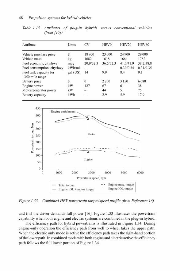
48 Propulsion systems for hybrid vehicles
Table 1.15 Attributes of plug-in hybrids versus conventional vehicles(from [15])
Attribute Units CV HEV0 HEV20 HEV60
Vehicle purchase price $ 18 900 23 000 24 900 29 000Vehicle mass kg 1682 1618 1664 1782Fuel economy, city/hwy mpg 20.9/32.3 36.5/32.3 41.7/41.9 38.2/38.8Fuel consumption, city/hwy kWh/mi – – 0.30/0.34 0.31/0.35Fuel tank capacity for
350 mile rangegal (US) 14 9.9 8.4 9.1
Battery price $ 0 2 200 3 150 6 680Engine power kW 127 67 61 38Motor/generator power kW – 44 51 75Battery capacity kWh – 2.9 5.9 17.9
450Engine enrichment
Motor
Engine
400
350
300
250
200
150
100
0 1000 2000 3000
Powertrain speed, rpm
Pow
ertr
ain
torq
ue, N
m
4000 5000 6000
50
0
Total torqueEngine IOL + motor torque
Engine max. torqueEngine IOL torque
Figure 1.33 Combined HEV powertrain torque/speed profile (from Reference 16)
and (iii) the driver demands full power [16]. Figure 1.33 illustrates the powertraincapability when both engine and electric systems are combined in the plug-in hybrid.
The efficiency path for hybrid powertrains is illustrated in Figure 1.34. Duringengine-only operation the efficiency path from well to wheel takes the upper path.When the electric only mode is active the efficiency path takes the right-hand portionof the lower path. In combined mode with both engine and electric active the efficiencypath follows the full lower portion of Figure 1.34.
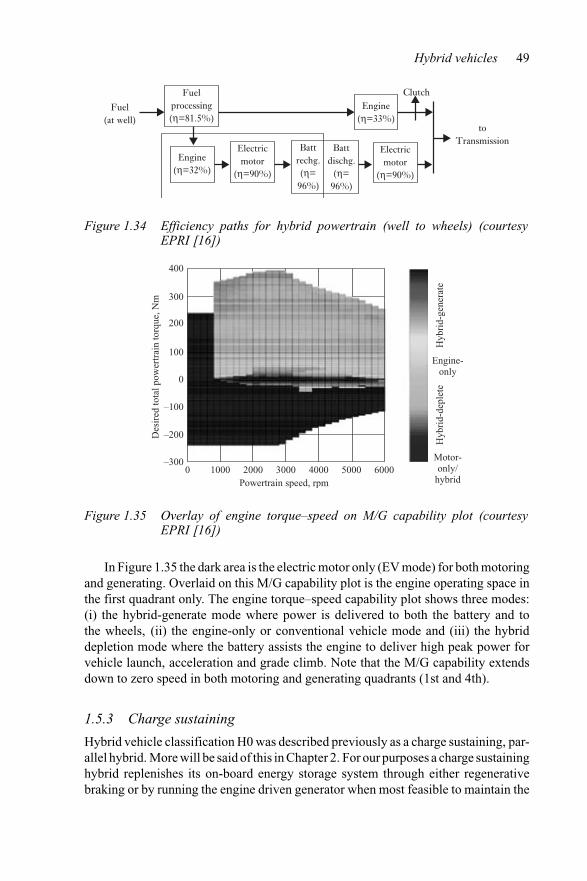
Hybrid vehicles 49
Fuel
processing
(η=81.5%)Fuel
(at well)
Clutch
Engine
(η=33%)
Engine
(η=32%)
Electric
motor
(η=90%)
Electric
motor
(η=90%)
Batt
rechg.
(η=
96%)
Batt
dischg.
(η=
96%)
to
Transmission
Figure 1.34 Efficiency paths for hybrid powertrain (well to wheels) (courtesyEPRI [16])
Des
ired
tota
l pow
ertr
ain
torq
ue, N
m
400
300
200
100
0
–100
–200
–3000 1000 2000 3000
Powertrain speed, rpm4000 5000 6000
Motor-only/
hybrid
Hyb
rid-
depl
ete
Hyb
rid-
gene
rate
Engine-only
Figure 1.35 Overlay of engine torque–speed on M/G capability plot (courtesyEPRI [16])
In Figure 1.35 the dark area is the electric motor only (EV mode) for both motoringand generating. Overlaid on this M/G capability plot is the engine operating space inthe first quadrant only. The engine torque–speed capability plot shows three modes:(i) the hybrid-generate mode where power is delivered to both the battery and tothe wheels, (ii) the engine-only or conventional vehicle mode and (iii) the hybriddepletion mode where the battery assists the engine to deliver high peak power forvehicle launch, acceleration and grade climb. Note that the M/G capability extendsdown to zero speed in both motoring and generating quadrants (1st and 4th).
1.5.3 Charge sustaining
Hybrid vehicle classification H0 was described previously as a charge sustaining, par-allel hybrid. More will be said of this in Chapter 2. For our purposes a charge sustaininghybrid replenishes its on-board energy storage system through either regenerativebraking or by running the engine driven generator when most feasible to maintain the
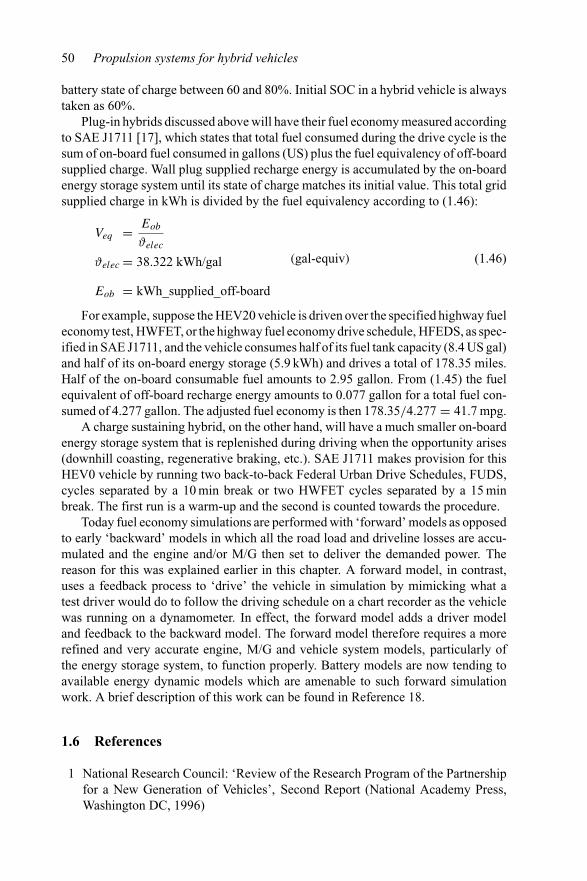
50 Propulsion systems for hybrid vehicles
battery state of charge between 60 and 80%. Initial SOC in a hybrid vehicle is alwaystaken as 60%.
Plug-in hybrids discussed above will have their fuel economy measured accordingto SAE J1711 [17], which states that total fuel consumed during the drive cycle is thesum of on-board fuel consumed in gallons (US) plus the fuel equivalency of off-boardsupplied charge. Wall plug supplied recharge energy is accumulated by the on-boardenergy storage system until its state of charge matches its initial value. This total gridsupplied charge in kWh is divided by the fuel equivalency according to (1.46):
Veq = Eob
ϑelec
ϑelec = 38.322 kWh/gal
Eob = kWh_supplied_off-board
(gal-equiv) (1.46)
For example, suppose the HEV20 vehicle is driven over the specified highway fueleconomy test, HWFET, or the highway fuel economy drive schedule, HFEDS, as spec-ified in SAE J1711, and the vehicle consumes half of its fuel tank capacity (8.4 US gal)and half of its on-board energy storage (5.9 kWh) and drives a total of 178.35 miles.Half of the on-board consumable fuel amounts to 2.95 gallon. From (1.45) the fuelequivalent of off-board recharge energy amounts to 0.077 gallon for a total fuel con-sumed of 4.277 gallon. The adjusted fuel economy is then 178.35/4.277 = 41.7 mpg.
A charge sustaining hybrid, on the other hand, will have a much smaller on-boardenergy storage system that is replenished during driving when the opportunity arises(downhill coasting, regenerative braking, etc.). SAE J1711 makes provision for thisHEV0 vehicle by running two back-to-back Federal Urban Drive Schedules, FUDS,cycles separated by a 10 min break or two HWFET cycles separated by a 15 minbreak. The first run is a warm-up and the second is counted towards the procedure.
Today fuel economy simulations are performed with ‘forward’ models as opposedto early ‘backward’ models in which all the road load and driveline losses are accu-mulated and the engine and/or M/G then set to deliver the demanded power. Thereason for this was explained earlier in this chapter. A forward model, in contrast,uses a feedback process to ‘drive’ the vehicle in simulation by mimicking what atest driver would do to follow the driving schedule on a chart recorder as the vehiclewas running on a dynamometer. In effect, the forward model adds a driver modeland feedback to the backward model. The forward model therefore requires a morerefined and very accurate engine, M/G and vehicle system models, particularly ofthe energy storage system, to function properly. Battery models are now tending toavailable energy dynamic models which are amenable to such forward simulationwork. A brief description of this work can be found in Reference 18.
1.6 References
1 National Research Council: ‘Review of the Research Program of the Partnershipfor a New Generation of Vehicles’, Second Report (National Academy Press,Washington DC, 1996)
Hybrid vehicles 51
2 North American International Auto Show, Cobo Center, Detroit, MI, 11–20January 2003. Author’s notes and photos
3 Information available on website: www.hybridford.com4 Automotive Engineering International: ‘Global vehicles’, December 2002,
pp. 14–15. Also see: www.sae.org/aei/5 National Research Council: ‘Review of the Research Program of the Partnership
for a New Generation of Vehicles’, Fourth Report (National Academy Press,Washington DC, 1998)
6 WALTERS, J., HUSTED, H. and RAJASHEKARA, K.: ‘Comparative studyof hybrid powertrain strategies’. Society of Automotive Engineers, SAE paper2001-01-2501
7 MILLER, J. M., GALE, A. R. and SANKARAN, V. A.: ‘Electric drive subsystemfor a low-storage requirement hybrid electric vehicle’, IEEE Trans. Veh. Technol.,1999, 48(6), pp. 34–48
8 SONG, D. and EL-SAYED, M.: ‘Multi-objective optimisation for automotiveperformance’, Int. J. Veh. Des., 2002, 30(4), pp. 291–308
9 CONLON, B.: ‘A Comparison of induction, permanent magnet, and switchedreluctance electric drive performance in automotive traction applications’,Powertrain Int., 2001, 4(4), pp. 34–48, www.powertrain-intl.com
10 GILLESPIE, T. D.: ‘Fundamentals of vehicle dynamics’ Society of AutomotiveEngineers, Inc., 400 Commonwealth Drive, Warrendale, PA, 15096-0001, 2001
11 Automobiltechnische Zeitschrift & Motortechnische Zeitschrift: The New FordFocus, Special Edition, 1999 www.atz-mtz.de
12 ‘Bosch automotive handbook’ (Robert Bosch GmbH, 1993 Postfach 30 02 20,D-70442) Stuttgart, Automotive Equipment Business Sector, Department forTechnical Information (KH/VDT), 3rd edn
13 DAVIS, R. I.: Nonlinear IC engine modeling for dynamic output torque observa-tion and control using a flywheel mounted electric motor’. PhD Thesis, Dept ofMechanical Engineering, University of Wisconsin-Madison, 1999
14 GAGE, T. and BROOKS, A.: ‘The case for the connected car’, Powertrain Int.,2002, 5(3), pp. 34–48, www.powertrain-intl.com
15 GRAHAM, R.: ‘Comparing the benefits and impacts of hybrid electric vehicleoptions’. EPRI Final Report 1000349, July 2001
16 MILLER, J., NAGEL, N., SCHULZ, S., CONLON, B., DUVALL, M., andKANKAM, D.: ‘Adjustable speed drives transportation industry needs, Part I:Automotive industry’. IEEE 39th Industry Applications Conference and AnnualMeeting, Grand American Hotel, Salt Lake City, Utah, 12–16 October 2003
17 SAE J1711 Recommended Practice for Measuring the Exhaust Emissions andFuel Economy of Hybrid-Electric Vehicles, 26 February 1997.
18 GEBBY, B. P.: ‘The validation of a hybrid powertrain model’. Society ofAutomotive Engineers, paper 98-SP-EV-07, 1998

Chapter 2
Hybrid architectures
It appears very unlikely that a specific powertrain architecture would be suitable forall vehicles in all markets. Today series and series–parallel switching architectures areeither in production or under prototype development for city buses, commercial trucksand other heavy vehicles. Pre-transmission parallel and power split architectureshave found their principal application in passenger vehicles in the compact and mid-size segments. Sub-compact and compact vehicles, including minivans, are beingconverted to CVT hybrids, where the continuously variable transmission, generallyof the belt type, has integrated into it the traction M/G. Because of the high actuationforces necessary in a CVT, an ancillary electric drive for the oil pump is necessary,generally in the 2 to 2.5 kW power rating. Higher rated power split and series–parallelswitching configurations are being introduced in small sport utility and larger vehicles.Fuel cell powered vehicles are strictly series hybrids because electric propulsion isthe only option.
All the major automotive companies have developed, or are developing, fuelcell powered vehicles. Daimler-Chrysler Corp., for example, began their develop-ments with the NECAR3 followed by NECAR4 and NECAR5. DCX also convertsproduction vehicles to fuel cell powered alternative drive concepts such as theirJeep Commander 2, and Chrysler Town and Country minivan, the Natrium. HondaMotor Co. is a clear front runner in fuel cell powered vehicles since they have goneinto limited production of the FCX1 minivan in 2002. The FCX is developed arounda Ballard Power Systems 78 kW PEM fuel cell supported by a 156 L compressedhydrogen gas storage tank and an ultra-capacitor bank for transient energy storage.
The prevailing rationale for introducing hybrid propulsion systems into massmarket personal transportation vehicles is to reduce the emissions of greenhousegases by curtailing their consumption rate. Other measures such as raising fuel pricesthrough additional taxes would reduce the consumption rate by pricing it out ofreach of a good portion of the public. Today, North America consumes 42% of the
1 FCX-V3 was introduced in CY2000, followed by FCX-V4 in CY2001.
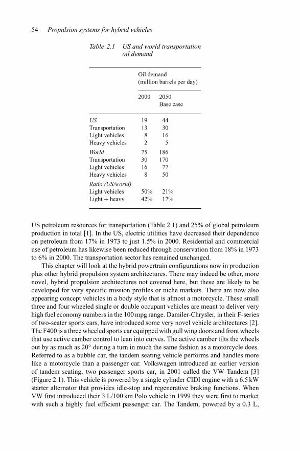
54 Propulsion systems for hybrid vehicles
Table 2.1 US and world transportationoil demand
Oil demand(million barrels per day)
2000 2050Base case
US 19 44Transportation 13 30Light vehicles 8 16Heavy vehicles 2 5
World 75 186Transportation 30 170Light vehicles 16 77Heavy vehicles 8 50
Ratio (US/world)Light vehicles 50% 21%Light + heavy 42% 17%
US petroleum resources for transportation (Table 2.1) and 25% of global petroleumproduction in total [1]. In the US, electric utilities have decreased their dependenceon petroleum from 17% in 1973 to just 1.5% in 2000. Residential and commercialuse of petroleum has likewise been reduced through conservation from 18% in 1973to 6% in 2000. The transportation sector has remained unchanged.
This chapter will look at the hybrid powertrain configurations now in productionplus other hybrid propulsion system architectures. There may indeed be other, morenovel, hybrid propulsion architectures not covered here, but these are likely to bedeveloped for very specific mission profiles or niche markets. There are now alsoappearing concept vehicles in a body style that is almost a motorcycle. These smallthree and four wheeled single or double occupant vehicles are meant to deliver veryhigh fuel economy numbers in the 100 mpg range. Damiler-Chrysler, in their F-seriesof two-seater sports cars, have introduced some very novel vehicle architectures [2].The F400 is a three wheeled sports car equipped with gull wing doors and front wheelsthat use active camber control to lean into curves. The active camber tilts the wheelsout by as much as 20◦ during a turn in much the same fashion as a motorcycle does.Referred to as a bubble car, the tandem seating vehicle performs and handles morelike a motorcycle than a passenger car. Volkswagen introduced an earlier versionof tandem seating, two passenger sports car, in 2001 called the VW Tandem [3](Figure 2.1). This vehicle is powered by a single cylinder CIDI engine with a 6.5 kWstarter alternator that provides idle-stop and regenerative braking functions. WhenVW first introduced their 3 L/100 km Polo vehicle in 1999 they were first to marketwith such a highly fuel efficient passenger car. The Tandem, powered by a 0.3 L,
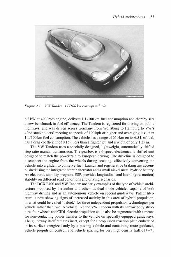
Hybrid architectures 55
Figure 2.1 VW Tandem 1 L/100 km concept vehicle
6.3 kW at 4000rpm engine, delivers 1 L/100 km fuel consumption and thereby setsa new benchmark in fuel efficiency. The Tandem is registered for driving on publichighways, and was driven across Germany from Wolfsburg to Hamburg to VW’s42nd stockholders’ meeting at speeds of 100 kph or higher and averaging less than1 L/100 km fuel consumption. The vehicle has a range of 650 km on its 6.5 L of fuel,has a drag coefficient of 0.159, less than a fighter jet, and a width of only 1.25 m.
The VW Tandem uses a specially designed, lightweight, automatically shiftedstep ratio manual transmission. The gearbox is a 6-speed electronically shifted unitdesigned to match the powertrain to European driving. The driveline is designed todisconnect the engine from the wheels during coasting, effectively converting thevehicle into a glider, to conserve fuel. Launch and regenerative braking are accom-plished using the integrated starter alternator and a small nickel metal hydride battery.An electronic stability program, ESP, provides longitudinal and lateral (yaw motion)stability on different road conditions and driving scenarios.
The DCX F400 and VW Tandem are early examples of the type of vehicle archi-tecture proposed by the author and others as dual mode vehicles capable of bothhighway driving and as an autonomous vehicle on special guideways. Patent liter-ature is now showing signs of increased activity in this area of hybrid propulsion,in what could be called ‘tribrid,’ for three independent propulsion technologies pervehicle rather than two. A vehicle like the VW Tandem with its narrow body struc-ture, four wheels and CIDI-electric propulsion could also be augmented with a meansfor non-contacting power transfer to the vehicle on specially equipped guideways.The guideway itself remains inert, except for a propulsion reaction plate embeddedin its surface energized only by a passing vehicle and containing route guidance,vehicle propulsion control, and vehicle spacing for very high density traffic [4 –7].
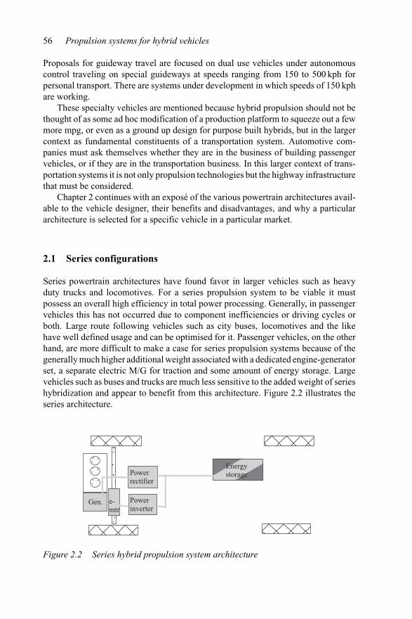
56 Propulsion systems for hybrid vehicles
Proposals for guideway travel are focused on dual use vehicles under autonomouscontrol traveling on special guideways at speeds ranging from 150 to 500 kph forpersonal transport. There are systems under development in which speeds of 150 kphare working.
These specialty vehicles are mentioned because hybrid propulsion should not bethought of as some ad hoc modification of a production platform to squeeze out a fewmore mpg, or even as a ground up design for purpose built hybrids, but in the largercontext as fundamental constituents of a transportation system. Automotive com-panies must ask themselves whether they are in the business of building passengervehicles, or if they are in the transportation business. In this larger context of trans-portation systems it is not only propulsion technologies but the highway infrastructurethat must be considered.
Chapter 2 continues with an exposé of the various powertrain architectures avail-able to the vehicle designer, their benefits and disadvantages, and why a particulararchitecture is selected for a specific vehicle in a particular market.
2.1 Series configurations
Series powertrain architectures have found favor in larger vehicles such as heavyduty trucks and locomotives. For a series propulsion system to be viable it mustpossess an overall high efficiency in total power processing. Generally, in passengervehicles this has not occurred due to component inefficiencies or driving cycles orboth. Large route following vehicles such as city buses, locomotives and the likehave well defined usage and can be optimised for it. Passenger vehicles, on the otherhand, are more difficult to make a case for series propulsion systems because of thegenerally much higher additional weight associated with a dedicated engine-generatorset, a separate electric M/G for traction and some amount of energy storage. Largevehicles such as buses and trucks are much less sensitive to the added weight of serieshybridization and appear to benefit from this architecture. Figure 2.2 illustrates theseries architecture.
Energystorage
Gen. e-mtr
Powerinverter
Powerrectifier
Figure 2.2 Series hybrid propulsion system architecture
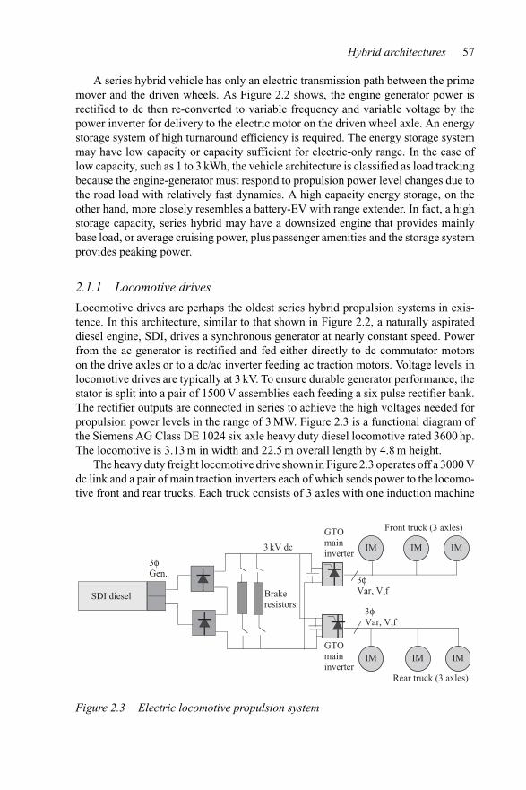
Hybrid architectures 57
A series hybrid vehicle has only an electric transmission path between the primemover and the driven wheels. As Figure 2.2 shows, the engine generator power isrectified to dc then re-converted to variable frequency and variable voltage by thepower inverter for delivery to the electric motor on the driven wheel axle. An energystorage system of high turnaround efficiency is required. The energy storage systemmay have low capacity or capacity sufficient for electric-only range. In the case oflow capacity, such as 1 to 3 kWh, the vehicle architecture is classified as load trackingbecause the engine-generator must respond to propulsion power level changes due tothe road load with relatively fast dynamics. A high capacity energy storage, on theother hand, more closely resembles a battery-EV with range extender. In fact, a highstorage capacity, series hybrid may have a downsized engine that provides mainlybase load, or average cruising power, plus passenger amenities and the storage systemprovides peaking power.
2.1.1 Locomotive drives
Locomotive drives are perhaps the oldest series hybrid propulsion systems in exis-tence. In this architecture, similar to that shown in Figure 2.2, a naturally aspirateddiesel engine, SDI, drives a synchronous generator at nearly constant speed. Powerfrom the ac generator is rectified and fed either directly to dc commutator motorson the drive axles or to a dc/ac inverter feeding ac traction motors. Voltage levels inlocomotive drives are typically at 3 kV. To ensure durable generator performance, thestator is split into a pair of 1500 V assemblies each feeding a six pulse rectifier bank.The rectifier outputs are connected in series to achieve the high voltages needed forpropulsion power levels in the range of 3 MW. Figure 2.3 is a functional diagram ofthe Siemens AG Class DE 1024 six axle heavy duty diesel locomotive rated 3600 hp.The locomotive is 3.13 m in width and 22.5 m overall length by 4.8 m height.
The heavy duty freight locomotive drive shown in Figure 2.3 operates off a 3000 Vdc link and a pair of main traction inverters each of which sends power to the locomo-tive front and rear trucks. Each truck consists of 3 axles with one induction machine
SDI diesel
3φ Gen.
Brakeresistors
3φ Var, V,f
3φ Var, V,f
Rear truck (3 axles)
Front truck (3 axles)
GTOmaininverter
GTOmaininverter
3 kV dc
IM IM IM
IM IM IM
Figure 2.3 Electric locomotive propulsion system
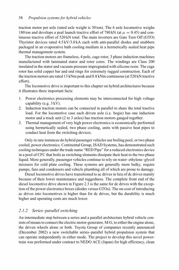
58 Propulsion systems for hybrid vehicles
traction motor per axle (rated axle weight is 30 ton). The 6 axle locomotive weighs180 ton and develops a peal launch tractive effort of 780 kN (at μ = 0.45) and con-tinuous tractive effort of 520 kN total. The main inverters are Gate Turn Off (GTO)Thyristor devices rated 4.5 kV/3.0 kA each with anti-parallel diodes and snubberspackaged in an evaporative bath cooling medium in a hermetically sealed heat pipethermal management system.
The traction motors are frameless, 4 pole, cage rotor, 3 phase induction machinesmanufactured with laminated stator and rotor cores. The windings are Class 200insulated in the stator and vacuum-pressure impregnated with silicone resin. The cagerotor has solid copper bar and end rings for extremely rugged construction. Each ofthe traction motors are rated 13 kNm peak and 8.8 kNm continuous (at 520 kN tractiveeffort).
The locomotive drive is important to this chapter on hybrid architectures becauseit illustrates three important facts:
1. Power electronics processing elements may be interconnected for high voltagecapability (e.g. 3 kV).
2. Induction traction motors can be connected in parallel to share the total tractiveload. For the locomotive case each driven axle (i.e. bogie) has one inductionmotor and a truck unit (2 to 3 axles) has traction motors ganged together.
3. Thermal management of very high power electronics is economically performedusing hermetically sealed, two phase cooling, units with passive heat pipes toconduct heat from the switching devices.
Only in rare instances do hybrid passenger vehicles use boiling pool, or two phasecooled, power electronics. Continental Group, ISAD Systems, has demonstrated suchcooling techniques under the trade name “RED Pipe” for a reduced electronics devicein a pool of CFC that boils as switching elements dissipate their heat to the two phaseliquid. More generally, passenger vehicles continue to rely on water–ethylene–glycolmixtures for cold plate cooling. These systems are generally more bulky, requirepumps, fans and condensers and vehicle plumbing all of which are prone to damage.
Diesel locomotive drives have transitioned to ac drives in lieu of dc drives mainlybecause of their lower maintenance and ruggedness. The complete front end of thediesel locomotive drive shown in Figure 2.3 is the same for dc drives with the excep-tion of the power electronics boxes (diodes versus GTOs). The on-cost of introducingac drives into locomotives is higher than for dc drives, but the durability is muchhigher and operating costs are much lower.
2.1.2 Series–parallel switching
An intermediate step between a series and a parallel architecture hybrid vehicle con-sists of means to connect the electric motor-generator, M/G, to either the engine alone,the driven wheels alone or both. Toyota Group of companies recently announced(December 2002) a new switchable series–parallel hybrid propulsion system thatcan operate independently in either mode. The project to develop this novel power-train was performed under contract to NEDO ACE (Japan) for high efficiency, clean
Hybrid architectures 59
Batterypack
e-mtr
ICE FDXM
ωf ωr
3
E-steer
C2C1
Figure 2.4 Switchable series–parallel hybrid architecture
urban public transportation system. Figure 2.4 depicts the switchable series–parallelarchitecture.
The switchable series–parallel hybrid powertrain consists of a diesel engine, per-manent magnet electric M/G, a conventional transmission and final drive, but withtwo key exceptions – the addition of a pair of clutches into the driveline. Clutch C1 is adisconnect clutch that is actuated when the engine load is not desirable, such as duringelectric-only propulsion and during regenerative braking when engine compressionbraking is not needed. Clutch C2 is the main drive clutch, designed for smoothengagement/disengagement and having mechanical damper mechanisms integral tothe clutch disc. Clutch C2 is actuated during engine and electric motor assisted launchand acceleration, grade climbing and descent, and for prolonged cruise.
Energy storage in the switchable series–parallel hybrid is shown as a battery pack,but this could be an advanced battery for high cycle life, an ultra-capacitor alone suchas used in the Nissan Condor Super-Capacitor truck, or in combination. The ToyotaGroup switchable series–parallel hybrid uses an ultra-capacitor for transient energystorage. The rationale for ultra-capacitor storage is that energy is stored in the sameform that it is being used. That is, the same electricity that propels the vehicle isstored as accumulated charge in the unit’s double layer capacitance. There is noelectrochemical conversion to rob turnaround efficiency. Electro-statically storedcharge is released during electric-only launch and replenished during regenerativebraking.
The Hino company now has 300 such urban route buses equipped with the switch-able series–parallel hybrid propulsion system and claims a fuel economy improvementof 80% over a conventional diesel bus.
Toyota Motor Company has developed an experimental low fuel consumptionvehicle dubbed the ES3 [8] (Figure 2.5). The Toyota ES3 achieved a fuel consumptionof 2.13 L/100 km on the Japan 10–15 mode. The ES3 propulsion system is derivedfrom its sister vehicle, the European Yaris, that employs a 1.4 L, I4, TDI engine.Equipped with common rail injection, variable ratio turbo, and a compact CVT. TheES3 is seen as a pioneering vehicle in low fuel consumption clean diesel technology.The key to low fuel consumption is the energy regenerator hybrid technology depictedin Figure 2.4. The ES3 powertrain is conventional in all respects except for the electric
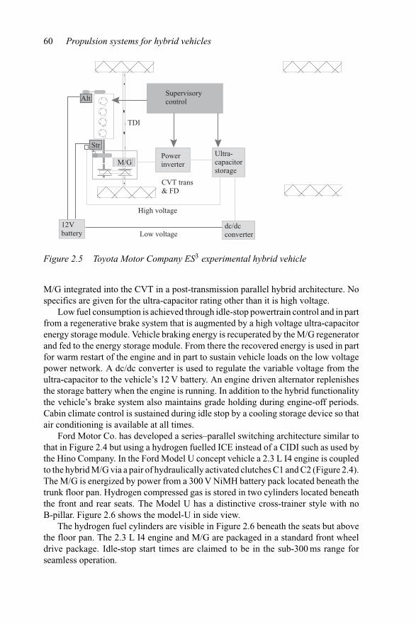
60 Propulsion systems for hybrid vehicles
Powerinverter
CVT trans& FD
Supervisorycontrol
Str
TDI
Ultra-capacitorstorage
M/G
High voltage
Low voltagedc/dcconverter
12Vbattery
Alt
Figure 2.5 Toyota Motor Company ES3 experimental hybrid vehicle
M/G integrated into the CVT in a post-transmission parallel hybrid architecture. Nospecifics are given for the ultra-capacitor rating other than it is high voltage.
Low fuel consumption is achieved through idle-stop powertrain control and in partfrom a regenerative brake system that is augmented by a high voltage ultra-capacitorenergy storage module. Vehicle braking energy is recuperated by the M/G regeneratorand fed to the energy storage module. From there the recovered energy is used in partfor warm restart of the engine and in part to sustain vehicle loads on the low voltagepower network. A dc/dc converter is used to regulate the variable voltage from theultra-capacitor to the vehicle’s 12 V battery. An engine driven alternator replenishesthe storage battery when the engine is running. In addition to the hybrid functionalitythe vehicle’s brake system also maintains grade holding during engine-off periods.Cabin climate control is sustained during idle stop by a cooling storage device so thatair conditioning is available at all times.
Ford Motor Co. has developed a series–parallel switching architecture similar tothat in Figure 2.4 but using a hydrogen fuelled ICE instead of a CIDI such as used bythe Hino Company. In the Ford Model U concept vehicle a 2.3 L I4 engine is coupledto the hybrid M/G via a pair of hydraulically activated clutches C1 and C2 (Figure 2.4).The M/G is energized by power from a 300 V NiMH battery pack located beneath thetrunk floor pan. Hydrogen compressed gas is stored in two cylinders located beneaththe front and rear seats. The Model U has a distinctive cross-trainer style with noB-pillar. Figure 2.6 shows the model-U in side view.
The hydrogen fuel cylinders are visible in Figure 2.6 beneath the seats but abovethe floor pan. The 2.3 L I4 engine and M/G are packaged in a standard front wheeldrive package. Idle-stop start times are claimed to be in the sub-300 ms range forseamless operation.
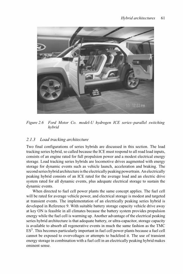
Hybrid architectures 61
Figure 2.6 Ford Motor Co. model-U hydrogen ICE series–parallel switchinghybrid
2.1.3 Load tracking architecture
Two final configurations of series hybrids are discussed in this section. The loadtracking series hybrid, so called because the ICE must respond to all road load inputs,consists of an engine rated for full propulsion power and a modest electrical energystorage. Load tracking series hybrids are locomotive drives augmented with energystorage for dynamic events such as vehicle launch, acceleration and braking. Thesecond series hybrid architecture is the electrically peaking powertrain. An electricallypeaking hybrid consists of an ICE rated for the average load and an electric drivesystem rated for all dynamic events, plus adequate electrical storage to sustain thedynamic events.
When directed to fuel cell power plants the same concept applies. The fuel cellwill be rated for average vehicle power, and electrical storage is modest and targetedat transient events. The implementation of an electrically peaking series hybrid isdeveloped in Reference 9. With suitable battery storage capacity vehicle drive awayat key ON is feasible in all climates because the battery system provides propulsionenergy while the fuel cell is warming up. Another advantage of the electrical peakingseries hybrid architecture is that adequate battery, or ultra-capacitor, storage capacityis available to absorb all regenerative events in much the same fashion as the TMCES3. This becomes particularly important in fuel cell power plants because a fuel cellcannot be exposed to overvoltages or attempts to backfeed it. The use of transientenergy storage in combination with a fuel cell in an electrically peaking hybrid makeseminent sense.
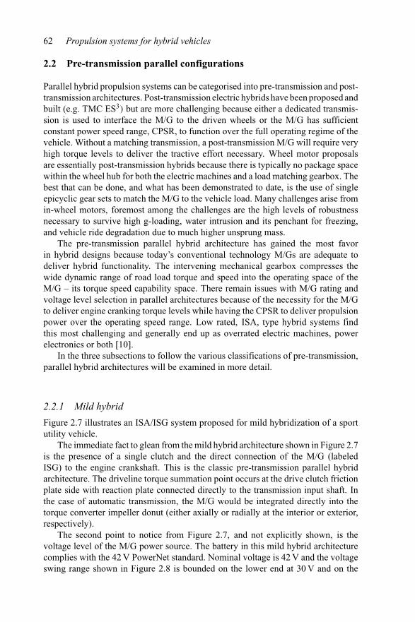
62 Propulsion systems for hybrid vehicles
2.2 Pre-transmission parallel configurations
Parallel hybrid propulsion systems can be categorised into pre-transmission and post-transmission architectures. Post-transmission electric hybrids have been proposed andbuilt (e.g. TMC ES3) but are more challenging because either a dedicated transmis-sion is used to interface the M/G to the driven wheels or the M/G has sufficientconstant power speed range, CPSR, to function over the full operating regime of thevehicle. Without a matching transmission, a post-transmission M/G will require veryhigh torque levels to deliver the tractive effort necessary. Wheel motor proposalsare essentially post-transmission hybrids because there is typically no package spacewithin the wheel hub for both the electric machines and a load matching gearbox. Thebest that can be done, and what has been demonstrated to date, is the use of singleepicyclic gear sets to match the M/G to the vehicle load. Many challenges arise fromin-wheel motors, foremost among the challenges are the high levels of robustnessnecessary to survive high g-loading, water intrusion and its penchant for freezing,and vehicle ride degradation due to much higher unsprung mass.
The pre-transmission parallel hybrid architecture has gained the most favorin hybrid designs because today’s conventional technology M/Gs are adequate todeliver hybrid functionality. The intervening mechanical gearbox compresses thewide dynamic range of road load torque and speed into the operating space of theM/G – its torque speed capability space. There remain issues with M/G rating andvoltage level selection in parallel architectures because of the necessity for the M/Gto deliver engine cranking torque levels while having the CPSR to deliver propulsionpower over the operating speed range. Low rated, ISA, type hybrid systems findthis most challenging and generally end up as overrated electric machines, powerelectronics or both [10].
In the three subsections to follow the various classifications of pre-transmission,parallel hybrid architectures will be examined in more detail.
2.2.1 Mild hybrid
Figure 2.7 illustrates an ISA/ISG system proposed for mild hybridization of a sportutility vehicle.
The immediate fact to glean from the mild hybrid architecture shown in Figure 2.7is the presence of a single clutch and the direct connection of the M/G (labeledISG) to the engine crankshaft. This is the classic pre-transmission parallel hybridarchitecture. The driveline torque summation point occurs at the drive clutch frictionplate side with reaction plate connected directly to the transmission input shaft. Inthe case of automatic transmission, the M/G would be integrated directly into thetorque converter impeller donut (either axially or radially at the interior or exterior,respectively).
The second point to notice from Figure 2.7, and not explicitly shown, is thevoltage level of the M/G power source. The battery in this mild hybrid architecturecomplies with the 42 V PowerNet standard. Nominal voltage is 42 V and the voltageswing range shown in Figure 2.8 is bounded on the lower end at 30 V and on the
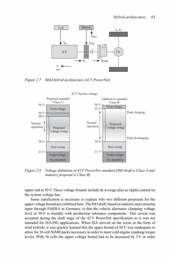
Hybrid architectures 63
FD
GR
rt, Fr
Pacc
Fuel Battery
Te Tisg
Umv
ICEISG
TpropTe
Figure 2.7 Mild hybrid architecture (42 V PowerNet)
42 V System voltage
Proposed standard‘Class A’
58 V
48 V
30 V
21 V
Overvoltage
Undervoltage
No operation
Proposedvoltage swing
50 V
Start swing
Normaloperation
58 V55 V
30 V
21 V
Overvoltage
Proposedvoltage swing
Addition to standard‘Class B’
Undervoltage
No operation
Start swing
Normaloperation
Peak charging
Peak discharging
Figure 2.8 Voltage definition of 42 V PowerNet standard (ISO draft is Class A andindustry proposal is Class B)
upper end at 50 V. These voltage bounds include dc average plus ac ripple content onthe system voltage bus.
Some clarification is necessary to explain why two different proposals for theupper voltage bound are exhibited here. The ISO draft, based on industry and consortiainput through FAKRA in Germany, is that the vehicle alternator clamping voltagelevel at 50 V is feasible with production tolerance components. This caveat wasaccepted during the draft stage of the 42 V PowerNet specification as it was notintended for ISA/ISG applications. When ISA arrived on the scene in the form ofmild hybrids, it was quickly learned that the upper bound of 50 V was inadequate toallow for 36 cell NiMH packs necessary in order to meet cold engine cranking torquelevels. With 36 cells the upper voltage bound had to be increased by 5 V in order
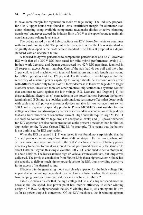
64 Propulsion systems for hybrid vehicles
to have some margin for regeneration mode voltage swing. The industry proposalfor a 55 V upper bound was found to leave insufficient margin for alternator loaddump clamping using available components (avalanche diodes or active clampingtransistors) and never exceed the industry limit of 60 V as the upper bound to maintainnon-hazardous voltage level status.
The debate raised by mild hybrid actions on 42 V PowerNet vehicles continueswith no resolution in sight. The point to be made here is that the Class A standard asoriginally developed is the draft defacto standard. The Class B proposal is a dejurestandard with an uncertain future.
A focused study was performed to compare the performance of a 42 V PowerNetISG with that of a 300 V ISG both rated for mild hybrid performance levels [11].In their work Leonardi and Degner constructed two 42 V ISG machines, identical inall respects, except for turn number. One of the pair had 4t per coil and the other5t per coil. A third machine, with identical laminations and stack length was woundfor 300 V operation and had 12t per coil. On the surface it would appear that thesensitivity of machine power capability to voltage should be a second order effectwith differences due only to the slot fill factor decrease at lower voltage due to largerdiameter wires. However, there are other practical implications in a systems contextthat continue to work against the low voltage ISG. Leonardi and Degner [11] listthese additional factors as: (i) connections in the power harness between the batteryterminals and ISG stator are not ideal and contribute resistance effects that do not scalewith cable size; (ii) power electronics devices suitable for low voltage must switch700 A and are generally specialty products. Power MOSFETs most suitable for lowvoltage operation are also majority carrier devices and have conduction voltage dropsthat are a linear function of conduction current. High currents require large MOSFETdie areas to contain the voltage drops to acceptable levels; and (iii) power batteriesfor 42 V operation are also not in production at the present time other than for limitedapplication on the Toyota Crown THS-M, for example. This means that the batteryis not optimised for ISG application.
When the ISG discussed in [11] was tested it was found, not surprisingly, that the5t stator produced more torque/amp than its 4t counterpart. Furthermore, when bothof these machines were compared to the 300 V machine in terms of battery powernecessary to deliver torque it was found that all performed essentially the same up toabout 150 Nm. Beyond this torque level the 300 V ISG continued to deliver torque upto about 180 Nm. The losses at these high drive levels were exorbitant, but torque wasdelivered. The obvious conclusion from Figure 2.9 is that a higher system voltage hasthe capacity to deliver much higher power levels to the ISG, thus providing overdrivefar in excess of its thermal rating.
Efficiency in the generating mode was clearly superior for the high voltage ISGin part due to the voltage dependent loss mechanisms listed earlier. To illustrate this,two mapping points are summarised for each machine in Table 2.2.
Table 2.2 makes it clear that the high voltage ISG is also a higher speed machinebecause the low speed, low power point has inferior efficiency to either windingdesign 42 V ISG. At higher speeds the 300 V winding ISG is just coming into its ownas far as power output is concerned. Of the 42 V machines, the 4t winding appears
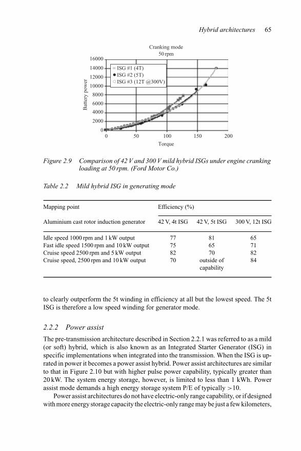
Hybrid architectures 65
Cranking mode50 rpm
Torque
16000
14000
12000
10000
8000
6000
4000
2000
00 50
Bat
tery
pow
er
100 150 200
ISG #1 (4T)ISG #2 (5T)ISG #3 (12T @300V)
Figure 2.9 Comparison of 42 V and 300 V mild hybrid ISGs under engine crankingloading at 50 rpm. (Ford Motor Co.)
Table 2.2 Mild hybrid ISG in generating mode
Mapping point Efficiency (%)
Aluminium cast rotor induction generator 42 V, 4t ISG 42 V, 5t ISG 300 V, 12t ISG
Idle speed 1000 rpm and 1 kW output 77 81 65Fast idle speed 1500 rpm and 10 kW output 75 65 71Cruise speed 2500 rpm and 5 kW output 82 70 82Cruise speed, 2500 rpm and 10 kW output 70 outside of 84
capability
to clearly outperform the 5t winding in efficiency at all but the lowest speed. The 5tISG is therefore a low speed winding for generator mode.
2.2.2 Power assist
The pre-transmission architecture described in Section 2.2.1 was referred to as a mild(or soft) hybrid, which is also known as an Integrated Starter Generator (ISG) inspecific implementations when integrated into the transmission. When the ISG is up-rated in power it becomes a power assist hybrid. Power assist architectures are similarto that in Figure 2.10 but with higher pulse power capability, typically greater than20 kW. The system energy storage, however, is limited to less than 1 kWh. Powerassist mode demands a high energy storage system P/E of typically >10.
Power assist architectures do not have electric-only range capability, or if designedwith more energy storage capacity the electric-only range may be just a few kilometers,
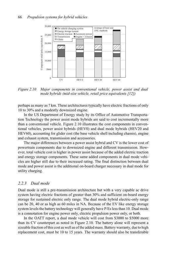
66 Propulsion systems for hybrid vehicles
30,000
25,000
20,000C
ompo
nent
ret
ail p
rice
equ
ival
ent,
$
15,000
10,000
5000
0CV HEV 0 HEV 20 HEV 60
Average of base andANL methods
On vehicle charging systemEnergy storage systemElectric traction Accessory powerTransmission Engine + exhaustGlider
Figure 2.10 Major components in conventional vehicle, power assist and dualmode hybrids (mid-size vehicle, retail price equivalents [12])
perhaps as many as 7 km. These architectures typically have electric fractions of only10 to 30% and a modestly downsized engine.
In the US Department of Energy study by its Office of Automotive Transporta-tion Technology the power assist mode hybrids are said to cost incrementally morethan a conventional vehicle. Figure 2.10 illustrates the cost components in conven-tional vehicles, power assist hybrids (HEV0) and dual mode hybrids (HEV20 andHEV60), accounting for glider cost (the base vehicle shell including chassis), engineand exhaust system, transmission and accessories.
The major differences between a power assist hybrid and CV is the lower cost ofpowertrain components due to downsized engine and different transmission. How-ever, total vehicle cost is higher in power assist because of the added electric tractionand energy storage components. These same added components in dual mode vehi-cles are higher still due to their increased rating. The final distinction between dualmode and power assist is the additional on-board charger necessary in dual mode forutility charging.
2.2.3 Dual mode
Dual mode is still a pre-transmission architecture but with a very capable ac drivesystem having electric fractions of greater than 30% and sufficient on-board energystorage for sustained electric only range. The dual mode hybrid electric-only rangecan be 20, 40 or as high as 60 miles in NA. Because of the EV like energy storagesystem levels the battery technology will generally have P/Es less than 10. Dual modeis a connotation for engine power only, electric propulsion power only, or both.
In the OATT report, a dual mode vehicle will cost from $3000 to $5000 morethan its CV counterpart as noted in Figure 2.10. The battery alone will represent asizeable fraction of this cost as well as of the added mass. Battery warranty, due to highreplacement cost, must be 10 to 15 years. The warranty should also be transferable
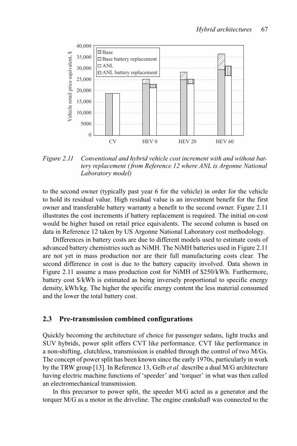
Hybrid architectures 67
CV HEV 0 HEV 20 HEV 60
Veh
icle
ret
ail p
rice
equ
ival
ent,
$
40,000
35,000
30,000
25,000
20,000
15,000
10,000
5000
0
BaseBase battery replacementANLANL battery replacement
Figure 2.11 Conventional and hybrid vehicle cost increment with and without bat-tery replacement ( from Reference 12 where ANL is Argonne NationalLaboratory model)
to the second owner (typically past year 6 for the vehicle) in order for the vehicleto hold its residual value. High residual value is an investment benefit for the firstowner and transferable battery warranty a benefit to the second owner. Figure 2.11illustrates the cost increments if battery replacement is required. The initial on-costwould be higher based on retail price equivalents. The second column is based ondata in Reference 12 taken by US Argonne National Laboratory cost methodology.
Differences in battery costs are due to different models used to estimate costs ofadvanced battery chemistries such as NiMH. The NiMH batteries used in Figure 2.11are not yet in mass production nor are their full manufacturing costs clear. Thesecond difference in cost is due to the battery capacity involved. Data shown inFigure 2.11 assume a mass production cost for NiMH of $250/kWh. Furthermore,battery cost $/kWh is estimated as being inversely proportional to specific energydensity, kWh/kg. The higher the specific energy content the less material consumedand the lower the total battery cost.
2.3 Pre-transmission combined configurations
Quickly becoming the architecture of choice for passenger sedans, light trucks andSUV hybrids, power split offers CVT like performance. CVT like performance ina non-shifting, clutchless, transmission is enabled through the control of two M/Gs.The concept of power split has been known since the early 1970s, particularly in workby the TRW group [13]. In Reference 13, Gelb et al. describe a dual M/G architecturehaving electric machine functions of ‘speeder’ and ‘torquer’ in what was then calledan electromechanical transmission.
In this precursor to power split, the speeder M/G acted as a generator and thetorquer M/G as a motor in the driveline. The engine crankshaft was connected to the
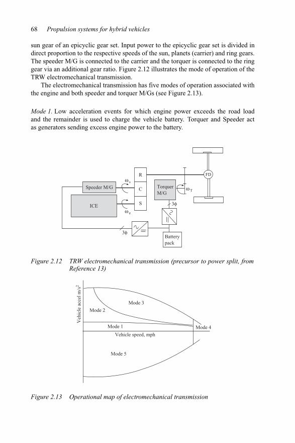
68 Propulsion systems for hybrid vehicles
sun gear of an epicyclic gear set. Input power to the epicyclic gear set is divided indirect proportion to the respective speeds of the sun, planets (carrier) and ring gears.The speeder M/G is connected to the carrier and the torquer is connected to the ringgear via an additional gear ratio. Figure 2.12 illustrates the mode of operation of theTRW electromechanical transmission.
The electromechanical transmission has five modes of operation associated withthe engine and both speeder and torquer M/Gs (see Figure 2.13).
Mode 1. Low acceleration events for which engine power exceeds the road loadand the remainder is used to charge the vehicle battery. Torquer and Speeder actas generators sending excess engine power to the battery.
FD
Speeder M/G
ICE
R
C ω T
ω e
ω s
S
TorquerM/G
Batterypack
3φ
3φ
Figure 2.12 TRW electromechanical transmission (precursor to power split, fromReference 13)
Vehicle speed, mph
Mode 1
Mode 2
Mode 3
Mode 4
Mode 5
Veh
icle
acc
el m
/s2
Figure 2.13 Operational map of electromechanical transmission
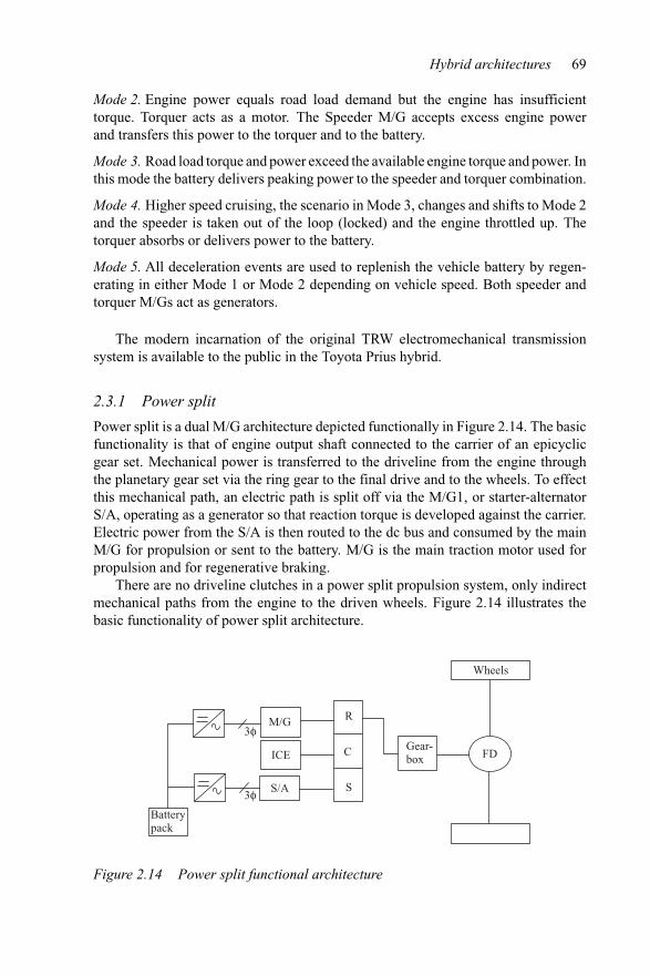
Hybrid architectures 69
Mode 2. Engine power equals road load demand but the engine has insufficienttorque. Torquer acts as a motor. The Speeder M/G accepts excess engine powerand transfers this power to the torquer and to the battery.
Mode 3. Road load torque and power exceed the available engine torque and power. Inthis mode the battery delivers peaking power to the speeder and torquer combination.
Mode 4. Higher speed cruising, the scenario in Mode 3, changes and shifts to Mode 2and the speeder is taken out of the loop (locked) and the engine throttled up. Thetorquer absorbs or delivers power to the battery.
Mode 5. All deceleration events are used to replenish the vehicle battery by regen-erating in either Mode 1 or Mode 2 depending on vehicle speed. Both speeder andtorquer M/Gs act as generators.
The modern incarnation of the original TRW electromechanical transmissionsystem is available to the public in the Toyota Prius hybrid.
2.3.1 Power split
Power split is a dual M/G architecture depicted functionally in Figure 2.14. The basicfunctionality is that of engine output shaft connected to the carrier of an epicyclicgear set. Mechanical power is transferred to the driveline from the engine throughthe planetary gear set via the ring gear to the final drive and to the wheels. To effectthis mechanical path, an electric path is split off via the M/G1, or starter-alternatorS/A, operating as a generator so that reaction torque is developed against the carrier.Electric power from the S/A is then routed to the dc bus and consumed by the mainM/G for propulsion or sent to the battery. M/G is the main traction motor used forpropulsion and for regenerative braking.
There are no driveline clutches in a power split propulsion system, only indirectmechanical paths from the engine to the driven wheels. Figure 2.14 illustrates thebasic functionality of power split architecture.
R
C
S
M/G
ICE
S/A
Gear-box FD
Wheels
Batterypack
3φ
3φ
Figure 2.14 Power split functional architecture
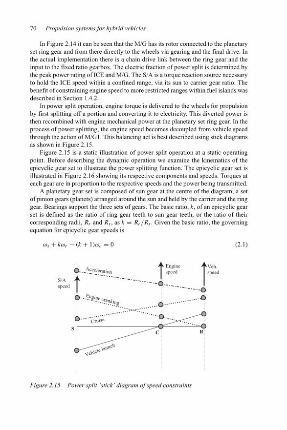
70 Propulsion systems for hybrid vehicles
In Figure 2.14 it can be seen that the M/G has its rotor connected to the planetaryset ring gear and from there directly to the wheels via gearing and the final drive. Inthe actual implementation there is a chain drive link between the ring gear and theinput to the fixed ratio gearbox. The electric fraction of power split is determined bythe peak power rating of ICE and M/G. The S/A is a torque reaction source necessaryto hold the ICE speed within a confined range, via its sun to carrier gear ratio. Thebenefit of constraining engine speed to more restricted ranges within fuel islands wasdescribed in Section 1.4.2.
In power split operation, engine torque is delivered to the wheels for propulsionby first splitting off a portion and converting it to electricity. This diverted power isthen recombined with engine mechanical power at the planetary set ring gear. In theprocess of power splitting, the engine speed becomes decoupled from vehicle speedthrough the action of M/G1. This balancing act is best described using stick diagramsas shown in Figure 2.15.
Figure 2.15 is a static illustration of power split operation at a static operatingpoint. Before describing the dynamic operation we examine the kinematics of theepicyclic gear set to illustrate the power splitting function. The epicyclic gear set isillustrated in Figure 2.16 showing its respective components and speeds. Torques ateach gear are in proportion to the respective speeds and the power being transmitted.
A planetary gear set is composed of sun gear at the centre of the diagram, a setof pinion gears (planets) arranged around the sun and held by the carrier and the ringgear. Bearings support the three sets of gears. The basic ratio, k, of an epicyclic gearset is defined as the ratio of ring gear teeth to sun gear teeth, or the ratio of theircorresponding radii, Rr and Rs , as k = Rr/Rs . Given the basic ratio, the governingequation for epicyclic gear speeds is
ωs + kωr − (k + 1)ωc = 0 (2.1)
RCS
Vehicle launch
Cruise
Engine cranking
AccelerationVeh.speed
Enginespeed
S/Aspeed
Figure 2.15 Power split ‘stick’ diagram of speed constraints
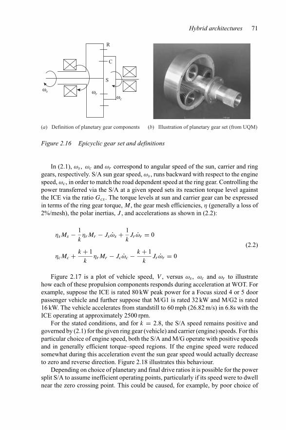
Hybrid architectures 71
R
S
C
ωs ωrωc
(a) Definition of planetary gear components (b) Illustration of planetary gear set (from UQM)
Figure 2.16 Epicyclic gear set and definitions
In (2.1), ωs , ωc and ωr correspond to angular speed of the sun, carrier and ringgears, respectively. S/A sun gear speed, ωs , runs backward with respect to the enginespeed, ωc, in order to match the road dependent speed at the ring gear. Controlling thepower transferred via the S/A at a given speed sets its reaction torque level againstthe ICE via the ratio Gcs . The torque levels at sun and carrier gear can be expressedin terms of the ring gear torque, M , the gear mesh efficiencies, η (generally a loss of2%/mesh), the polar inertias, J , and accelerations as shown in (2.2):
ηsMs − 1
kηrMr − Jsω̇s + 1
kJr ω̇r = 0
ηcMc + k + 1
kηrMr − Jcω̇c − k + 1
kJr ω̇r = 0
(2.2)
Figure 2.17 is a plot of vehicle speed, V , versus ωs , ωc and ωr to illustratehow each of these propulsion components responds during acceleration at WOT. Forexample, suppose the ICE is rated 80 kW peak power for a Focus sized 4 or 5 doorpassenger vehicle and further suppose that M/G1 is rated 32 kW and M/G2 is rated16 kW. The vehicle accelerates from standstill to 60 mph (26.82 m/s) in 6.8s with theICE operating at approximately 2500 rpm.
For the stated conditions, and for k = 2.8, the S/A speed remains positive andgoverned by (2.1) for the given ring gear (vehicle) and carrier (engine) speeds. For thisparticular choice of engine speed, both the S/A and M/G operate with positive speedsand in generally efficient torque–speed regions. If the engine speed were reducedsomewhat during this acceleration event the sun gear speed would actually decreaseto zero and reverse direction. Figure 2.18 illustrates this behaviour.
Depending on choice of planetary and final drive ratios it is possible for the powersplit S/A to assume inefficient operating points, particularly if its speed were to dwellnear the zero crossing point. This could be caused, for example, by poor choice of
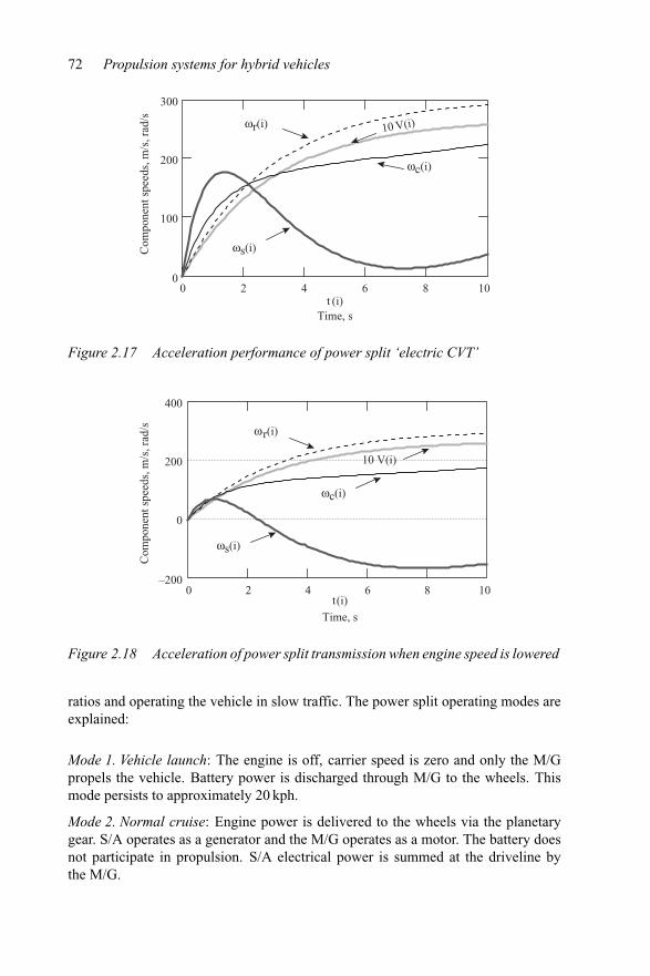
72 Propulsion systems for hybrid vehicles
10 V(i)
t (i)0 2 4 6 8 10
0
100
200
300
Time, s
Com
pone
nt s
peed
s, m
/s, r
ad/s
ωs(i)
ωr(i)
ωc(i)
Figure 2.17 Acceleration performance of power split ‘electric CVT’
t(i)Time, s
ωs(i)
0 2 4 6 8 10–200
0
200
400
Com
pone
nt s
peed
s, m
/s, r
ad/s
ωc(i)
ωr(i)
10 V(i)
Figure 2.18 Acceleration of power split transmission when engine speed is lowered
ratios and operating the vehicle in slow traffic. The power split operating modes areexplained:
Mode 1. Vehicle launch: The engine is off, carrier speed is zero and only the M/Gpropels the vehicle. Battery power is discharged through M/G to the wheels. Thismode persists to approximately 20 kph.
Mode 2. Normal cruise: Engine power is delivered to the wheels via the planetarygear. S/A operates as a generator and the M/G operates as a motor. The battery doesnot participate in propulsion. S/A electrical power is summed at the driveline bythe M/G.
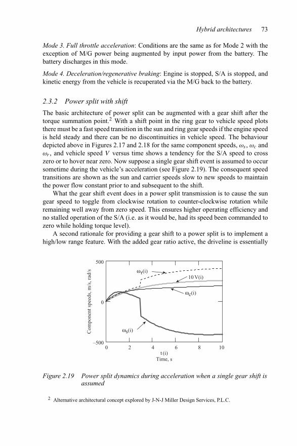
Hybrid architectures 73
Mode 3. Full throttle acceleration: Conditions are the same as for Mode 2 with theexception of M/G power being augmented by input power from the battery. Thebattery discharges in this mode.
Mode 4. Deceleration/regenerative braking: Engine is stopped, S/A is stopped, andkinetic energy from the vehicle is recuperated via the M/G back to the battery.
2.3.2 Power split with shift
The basic architecture of power split can be augmented with a gear shift after thetorque summation point.2 With a shift point in the ring gear to vehicle speed plotsthere must be a fast speed transition in the sun and ring gear speeds if the engine speedis held steady and there can be no discontinuities in vehicle speed. The behaviourdepicted above in Figures 2.17 and 2.18 for the same component speeds, ωs , ωc andωr , and vehicle speed V versus time shows a tendency for the S/A speed to crosszero or to hover near zero. Now suppose a single gear shift event is assumed to occursometime during the vehicle’s acceleration (see Figure 2.19). The consequent speedtransitions are shown as the sun and carrier speeds slow to new speeds to maintainthe power flow constant prior to and subsequent to the shift.
What the gear shift event does in a power split transmission is to cause the sungear speed to toggle from clockwise rotation to counter-clockwise rotation whileremaining well away from zero speed. This ensures higher operating efficiency andno stalled operation of the S/A (i.e. as it would be, had its speed been commanded tozero while holding torque level).
A second rationale for providing a gear shift to a power split is to implement ahigh/low range feature. With the added gear ratio active, the driveline is essentially
t (i)Time, s
ωs(i)
ωc(i)
ωr(i)10 V(i)
0 2 4 6 8 10–500
0
500
Com
pone
nt s
peed
s, m
/s, r
ad/s
Figure 2.19 Power split dynamics during acceleration when a single gear shift isassumed
2 Alternative architectural concept explored by J-N-J Miller Design Services, P.L.C.
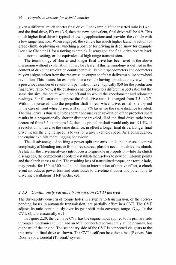
74 Propulsion systems for hybrid vehicles
given a different, much shorter final drive. For example, if the inserted ratio is 1.4 : 1and the final drive, FD was 3.5, then the new, equivalent, final drive will be 4.9. Thismuch higher final drive is typical of towing applications and provides the vehicle witha low range function. When engaged, the vehicle has much higher launch traction forgrade climb, deploying or launching a boat, or for driving in deep snow for example(see also Chapter 11 for a towing example). Disengaged, the final drive reverts backto its normal setting, or the equivalent of high range transmission.
The terminology of shorter and longer final drive has been used in the abovediscussion without explanation. It may be clearer if this terminology is defined in thecontext of driveline revolution counts per mile. Vehicle speedometers and odometersrely on a signal taken from the transmission output shaft that delivers a pulse per wheelrevolution. This means, for example, that a vehicle having a production tyre will turna prescribed number of revolutions per mile of travel, typically 850 for the productionfinal drive ratio. Now, if the customer changed tyres to a different aspect ratio, but thesame rim size, the count would be off and so would the speedometer and odometerreadings. For illustration, suppose the final drive ratio is changed from 3.5 to 3.7.With this increased ratio the propeller shaft to rear wheel drive, or half-shaft speedin the case of front wheel drive, will spin 5.7% faster for the same distance traveled.The final drive is thus said to be shorter because each revolution of the propeller shaftresults in a proportionally shorter distance traveled. Had the final drive ratio beendecreased from 3.5 to perhaps 3.2, then the propeller shaft would only turn 91.4% ofa revolution to traverse the same distance, in effect a longer final drive. Longer finaldrive means the engine speed is lower for a given vehicle speed. As a consequence,the engine exhibits more lugging behaviour.
The disadvantage of shifting a power split transmission is the increased controlcomplexity of blending torque from three sources plus the need for a driveline clutch.A clutch in the driveline always introduces a torque hole in propulsion while the clutchdisengages, the component speeds re-establish themselves to new equilibrium pointsand the clutch ceases to slip. The resulting loss of transmitted torque, or a torque hole,may persist for 150 to 300 ms. In addition to interruption of tractive effort, a clutchevent introduces power loss and contributes to driveline shudder and potentially todriveline oscillations if left unchecked.
2.3.3 Continuously variable transmission (CVT) derived
The driveability concern of torque holes in a step ratio transmission, or the corres-ponding losses in automatic transmission, are partially offset in a CVT. The CVTadjusts its ratio continuously over its gear shift ratio coverage range, Gsrc. In theCVT, Gsrc is maximally 6 : 1.
In Figure 2.20, the belt type CVT has the engine input applied to its primary sidethrough a mechanical clutch and an M/G connected permanently at the primary, butoutboard of the engine. The secondary side of the CVT is connected via gears to thetransmission final drive as shown. The CVT itself can be either a belt (Reeves, VanDoorne) or a toroidal (Torotrak) system.
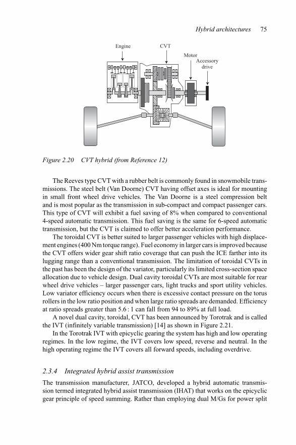
Hybrid architectures 75
Engine CVT
MotorAccessory
drive
Figure 2.20 CVT hybrid (from Reference 12)
The Reeves type CVT with a rubber belt is commonly found in snowmobile trans-missions. The steel belt (Van Doorne) CVT having offset axes is ideal for mountingin small front wheel drive vehicles. The Van Doorne is a steel compression beltand is most popular as the transmission in sub-compact and compact passenger cars.This type of CVT will exhibit a fuel saving of 8% when compared to conventional4-speed automatic transmission. This fuel saving is the same for 6-speed automatictransmission, but the CVT is claimed to offer better acceleration performance.
The toroidal CVT is better suited to larger passenger vehicles with high displace-ment engines (400 Nm torque range). Fuel economy in larger cars is improved becausethe CVT offers wider gear shift ratio coverage that can push the ICE farther into itslugging range than a conventional transmission. The limitation of toroidal CVTs inthe past has been the design of the variator, particularly its limited cross-section spaceallocation due to vehicle design. Dual cavity toroidal CVTs are most suitable for rearwheel drive vehicles – larger passenger cars, light trucks and sport utility vehicles.Low variator efficiency occurs when there is excessive contact pressure on the torusrollers in the low ratio position and when large ratio spreads are demanded. Efficiencyat ratio spreads greater than 5.6 : 1 can fall from 94 to 89% at full load.
A novel dual cavity, toroidal, CVT has been announced by Torotrak and is calledthe IVT (infinitely variable transmission) [14] as shown in Figure 2.21.
In the Torotrak IVT with epicyclic gearing the system has high and low operatingregimes. In the low regime, the IVT covers low speed, reverse and neutral. In thehigh operating regime the IVT covers all forward speeds, including overdrive.
2.3.4 Integrated hybrid assist transmission
The transmission manufacturer, JATCO, developed a hybrid automatic transmis-sion termed integrated hybrid assist transmission (IHAT) that works on the epicyclicgear principle of speed summing. Rather than employing dual M/Gs for power split
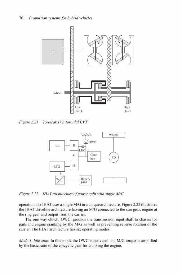
76 Propulsion systems for hybrid vehicles
ICE
Wheel
Lowclutch
Highclutch
Figure 2.21 Torotrak IVT, toroidal CVT
R
C
S
ICE
M/G
Gear-box FD
Wheels
OWC
LUC
Batterypack
3
Figure 2.22 IHAT architecture of power split with single M/G
operation, the IHAT uses a single M/G in a unique architecture. Figure 2.22 illustratesthe IHAT driveline architecture having an M/G connected to the sun gear, engine atthe ring gear and output from the carrier.
The one way clutch, OWC, grounds the transmission input shaft to chassis forpark and engine cranking by the M/G as well as preventing reverse rotation of thecarrier. The IHAT architecture has six operating modes:
Mode 1. Idle-stop: In this mode the OWC is activated and M/G torque is amplifiedby the basic ratio of the epicyclic gear for cranking the engine.
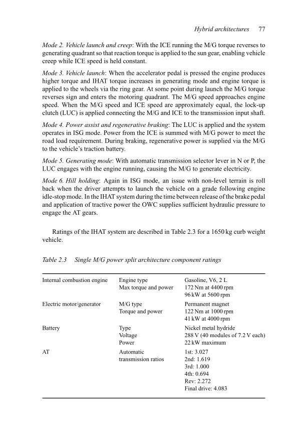
Hybrid architectures 77
Mode 2. Vehicle launch and creep: With the ICE running the M/G torque reverses togenerating quadrant so that reaction torque is applied to the sun gear, enabling vehiclecreep while ICE speed is held constant.
Mode 3. Vehicle launch: When the accelerator pedal is pressed the engine produceshigher torque and IHAT torque increases in generating mode and engine torque isapplied to the wheels via the ring gear. At some point during launch the M/G torquereverses sign and enters the motoring quadrant. The M/G speed approaches enginespeed. When the M/G speed and ICE speed are approximately equal, the lock-upclutch (LUC) is applied connecting the M/G and ICE to the transmission input shaft.
Mode 4. Power assist and regenerative braking: The LUC is applied and the systemoperates in ISG mode. Power from the ICE is summed with M/G power to meet theroad load requirement. During braking, regenerative power is supplied via the M/Gto the vehicle’s traction battery.
Mode 5. Generating mode: With automatic transmission selector lever in N or P, theLUC engages with the engine running, causing the M/G to generate electricity.
Mode 6. Hill holding: Again in ISG mode, an issue with non-level terrain is rollback when the driver attempts to launch the vehicle on a grade following engineidle-stop mode. In the IHAT system during the time between release of the brake pedaland application of tractive power the OWC supplies sufficient hydraulic pressure toengage the AT gears.
Ratings of the IHAT system are described in Table 2.3 for a 1650 kg curb weightvehicle.
Table 2.3 Single M/G power split architecture component ratings
Internal combustion engine Engine type Gasoline, V6, 2 LMax torque and power 172 Nm at 4400 rpm
96 kW at 5600 rpm
Electric motor/generator M/G type Permanent magnetTorque and power 122 Nm at 1000 rpm
41 kW at 4000 rpm
Battery Type Nickel metal hydrideVoltage 288 V (40 modules of 7.2 V each)Power 22 kW maximum
AT Automatic 1st: 3.027transmission ratios 2nd: 1.619
3rd: 1.0004th: 0.694Rev: 2.272Final drive: 4.083
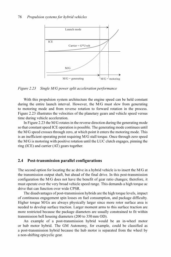
78 Propulsion systems for hybrid vehicles
Launch mode
M/G = generating M/G = motoring
ICECarrier = G*Uveh
M/G
Figure 2.23 Single M/G power split acceleration performance
With this propulsion system architecture the engine speed can be held constantduring the entire launch interval. However, the M/G must slew from generatingto motoring mode and from reverse rotation to forward rotation in the process.Figure 2.23 illustrates the velocities of the planetary gears and vehicle speed versustime during vehicle acceleration.
In Figure 2.23 the M/G rotates in the reverse direction during the generating modeso that constant speed ICE operation is possible. The generating mode continues untilthe M/G speed crosses through zero, at which point it enters the motoring mode. Thisis an inefficient operating point requiring M/G stall torque. Once through zero speedthe M/G is motoring with positive rotation until the LUC clutch engages, pinning thering (ICE) and carrier (AT) gears together.
2.4 Post-transmission parallel configurations
The second option for locating the ac drive in a hybrid vehicle is to insert the M/G atthe transmission output shaft, but ahead of the final drive. In this post-transmissionconfiguration the M/G does not have the benefit of gear ratio changes; therefore, itmust operate over the very broad vehicle speed range. This demands a high torque acdrive that can function over wide CPSR.
The disadvantages of post-transmission hybrids are the high torque levels, impactof continuous engagement spin losses on fuel consumption, and package difficulty.Higher torque M/Gs are always physically larger since more rotor surface area isneeded to develop surface traction. Larger moment arms to this surface traction aremore restricted because the package diameters are usually constrained to fit withintransmission bell housing diameters (200 to 350 mm OD).
An example of a post-transmission hybrid would be an in-wheel motoror hub motor hybrid. The GM Autonomy, for example, could be classified asa post-transmission hybrid because the hub motor is separated from the wheel bya non-shifting epicyclic gear.
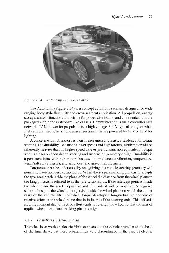
Hybrid architectures 79
Figure 2.24 Autonomy with in-hub M/G
The Autonomy (Figure 2.24) is a concept automotive chassis designed for wideranging body style flexibility and cross-segment application. All propulsion, energystorage, chassis functions and wiring for power distribution and communications arepackaged within the skateboard like chassis. Communication is via a controller areanetwork, CAN. Power for propulsion is at high voltage, 300 V typical or higher whenfuel cells are used. Chassis and passenger amenities are powered by 42 V or 12 V forlighting.
A concern with hub motors is their higher unsprung mass, a tendency for torquesteering, and durability. Because of lower speeds and high torques, a hub motor will beinherently heavier than its higher speed axle or pre-transmission equivalent. Torquesteer is a phenomenon due to steering and suspension geometry design. Durability isa persistent issue with hub motors because of simultaneous vibration, temperature,water/salt spray ingress, and sand, dust and gravel impingement.
Torque steer can be understood by recognizing that vehicle steering geometry willgenerally have non-zero scrub radius. When the suspension king pin axis interceptsthe tyre-road patch inside the plane of the wheel the distance from the wheel plane tothe king pin axis is referred to as the tyre scrub radius. If the intercept point is insidethe wheel plane the scrub is positive and if outside it will be negative. A negativescrub radius puts the wheel turning axis outside the wheel plane on which the cornermass of the vehicle sits. The wheel torque develops a longitudinal component oftractive effort at the wheel plane that is in board of the steering axis. This off axissteering moment due to tractive effort tends to re-align the wheel so that the axis ofapplied wheel torque and the king pin axis align.
2.4.1 Post-transmission hybrid
There has been work on electric M/Gs connected to the vehicle propeller shaft aheadof the final drive, but these programmes were discontinued in the case of electric
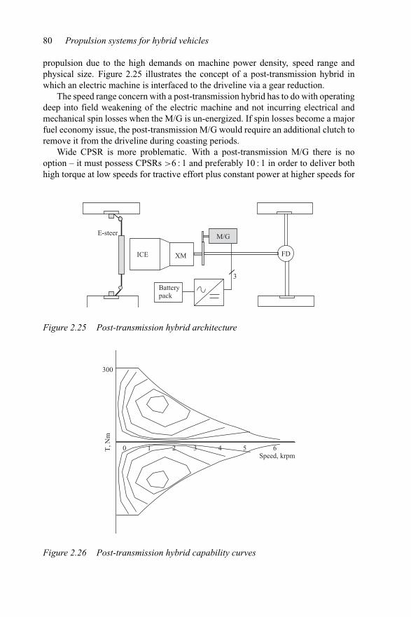
80 Propulsion systems for hybrid vehicles
propulsion due to the high demands on machine power density, speed range andphysical size. Figure 2.25 illustrates the concept of a post-transmission hybrid inwhich an electric machine is interfaced to the driveline via a gear reduction.
The speed range concern with a post-transmission hybrid has to do with operatingdeep into field weakening of the electric machine and not incurring electrical andmechanical spin losses when the M/G is un-energized. If spin losses become a majorfuel economy issue, the post-transmission M/G would require an additional clutch toremove it from the driveline during coasting periods.
Wide CPSR is more problematic. With a post-transmission M/G there is nooption – it must possess CPSRs >6 : 1 and preferably 10 : 1 in order to deliver bothhigh torque at low speeds for tractive effort plus constant power at higher speeds for
Batterypack
ICE XM
3
E-steer M/G
FD
Figure 2.25 Post-transmission hybrid architecture
T, N
m
300
Speed, krpm0 1 2 3 4 5 6
Figure 2.26 Post-transmission hybrid capability curves
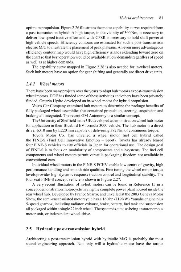
Hybrid architectures 81
optimum propulsion. Figure 2.26 illustrates the motor capability curves required froma post-transmission hybrid. A high torque, in the vicinity of 300 Nm, is necessary todeliver low speed tractive effort and wide CPSR is necessary to hold shaft power athigh vehicle speeds. Efficiency contours are estimated for such a post-transmissionelectric M/G to illustrate the placement of peak plateaus. An even more advantageousefficiency contour map would have high efficiency islands extending toward zero onthe chart so that best operation would be available at low demands regardless of speedas well as at higher demands.
The capability curve mapped in Figure 2.26 is also needed for in-wheel motors.Such hub motors have no option for gear shifting and generally are direct drive units.
2.4.2 Wheel motors
There have been many projects over the years to adapt hub motors as post-transmissionwheel motors. DOE has funded some of these activities and others have been privatelyfunded. Ontario Hydro developed an in-wheel motor for hybrid propulsion.
Volvo Car Company examined hub motors to determine the package benefits offully packaged wheel assemblies that contained propulsion, steering, suspension andbraking all integrated. The recent GM Autonomy is a similar concept.
The University of Sheffield in the UK developed a demonstration wheel hub motorfor application in their Bluebird EV formula 3000 vehicle. The hub motor is a directdrive, φ310 mm by L220 mm capable of delivering 382 Nm of continuous torque.
Toyota Motor Co. has unveiled a wheel motor fuel cell hybrid calledthe FINE-S (Fuel Cell Innovative Emotion – Sport). Toyota has already leasedfour FINE-S vehicles to city officials in Japan for operational use. The design goalof FINE-S is to focus on modularity of components and subsystems. The fuel cellcomponents and wheel motors permit versatile packaging freedom not available inconventional cars.
Individual wheel motors in the FINE-S FCHV enable low centre of gravity, highperformance handling and smooth ride qualities. Fine tuning the wheel motor torquelevels provides high dynamic response traction control and longitudinal stability. Thefour seat FINE-S concept vehicle is shown in Figure 2.27.
A very recent illustration of in-hub motors can be found in Reference 15 in aconcept demonstration motorcycle having the complete power plant housed inside therear wheel hub. Developed by Franco Sbarro, and unveiled at the 2003 Geneva MotorShow, the semi-encapsulated motorcycle has a 160 hp (119 kW) Yamaha engine plus5-speed gearbox, including radiator, exhaust, brake, battery, fuel tank and suspensionall packaged within a single 22 inch wheel. The system is cited as being an autonomousmotor unit, or independent wheel-drive.
2.5 Hydraulic post-transmission hybrid
Architecting a post-transmission hybrid with hydraulic M/G is probably the mostsound engineering approach. Not only will a hydraulic motor have the torque
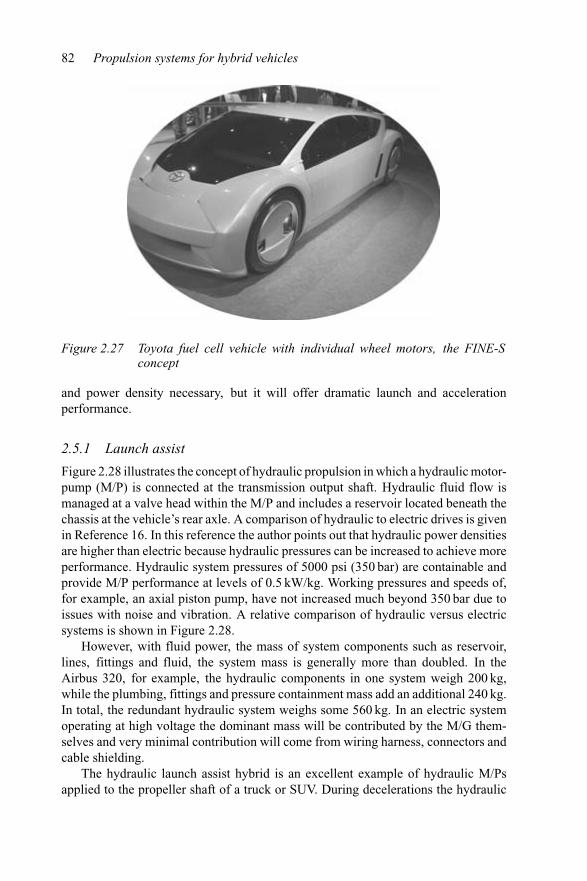
82 Propulsion systems for hybrid vehicles
Figure 2.27 Toyota fuel cell vehicle with individual wheel motors, the FINE-Sconcept
and power density necessary, but it will offer dramatic launch and accelerationperformance.
2.5.1 Launch assist
Figure 2.28 illustrates the concept of hydraulic propulsion in which a hydraulic motor-pump (M/P) is connected at the transmission output shaft. Hydraulic fluid flow ismanaged at a valve head within the M/P and includes a reservoir located beneath thechassis at the vehicle’s rear axle. A comparison of hydraulic to electric drives is givenin Reference 16. In this reference the author points out that hydraulic power densitiesare higher than electric because hydraulic pressures can be increased to achieve moreperformance. Hydraulic system pressures of 5000 psi (350 bar) are containable andprovide M/P performance at levels of 0.5 kW/kg. Working pressures and speeds of,for example, an axial piston pump, have not increased much beyond 350 bar due toissues with noise and vibration. A relative comparison of hydraulic versus electricsystems is shown in Figure 2.28.
However, with fluid power, the mass of system components such as reservoir,lines, fittings and fluid, the system mass is generally more than doubled. In theAirbus 320, for example, the hydraulic components in one system weigh 200 kg,while the plumbing, fittings and pressure containment mass add an additional 240 kg.In total, the redundant hydraulic system weighs some 560 kg. In an electric systemoperating at high voltage the dominant mass will be contributed by the M/G them-selves and very minimal contribution will come from wiring harness, connectors andcable shielding.
The hydraulic launch assist hybrid is an excellent example of hydraulic M/Psapplied to the propeller shaft of a truck or SUV. During decelerations the hydraulic
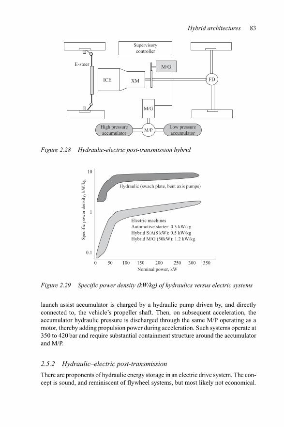
Hybrid architectures 83
M/PLow pressureaccumulator
M/G
ICE XM
E-steer M/G
FD
High pressureaccumulator
Supervisorycontroller
Figure 2.28 Hydraulic-electric post-transmission hybrid
Nominal power, kW0 50 100 150 200 250 300 350
Spec
ific
pow
er d
ensi
ty, k
W/k
g
10
1
0.1
Hydraulic (swach plate, bent axis pumps)
Electric machinesAutomotive starter: 0.3 kW/kgHybrid S/A(8 kW): 0.5 kW/kgHybrid M/G (50kW): 1.2 kW/kg
Figure 2.29 Specific power density (kW/kg) of hydraulics versus electric systems
launch assist accumulator is charged by a hydraulic pump driven by, and directlyconnected to, the vehicle’s propeller shaft. Then, on subsequent acceleration, theaccumulator hydraulic pressure is discharged through the same M/P operating as amotor, thereby adding propulsion power during acceleration. Such systems operate at350 to 420 bar and require substantial containment structure around the accumulatorand M/P.
2.5.2 Hydraulic–electric post-transmission
There are proponents of hydraulic energy storage in an electric drive system. The con-cept is sound, and reminiscent of flywheel systems, but most likely not economical.
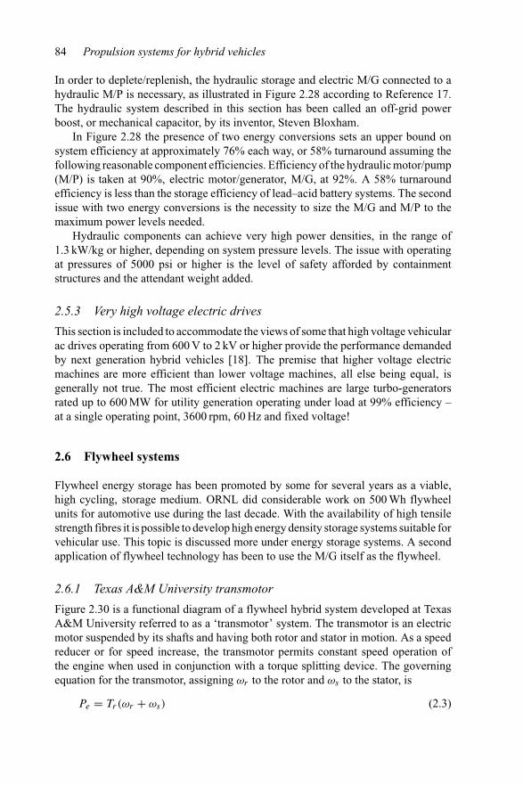
84 Propulsion systems for hybrid vehicles
In order to deplete/replenish, the hydraulic storage and electric M/G connected to ahydraulic M/P is necessary, as illustrated in Figure 2.28 according to Reference 17.The hydraulic system described in this section has been called an off-grid powerboost, or mechanical capacitor, by its inventor, Steven Bloxham.
In Figure 2.28 the presence of two energy conversions sets an upper bound onsystem efficiency at approximately 76% each way, or 58% turnaround assuming thefollowing reasonable component efficiencies. Efficiency of the hydraulic motor/pump(M/P) is taken at 90%, electric motor/generator, M/G, at 92%. A 58% turnaroundefficiency is less than the storage efficiency of lead–acid battery systems. The secondissue with two energy conversions is the necessity to size the M/G and M/P to themaximum power levels needed.
Hydraulic components can achieve very high power densities, in the range of1.3 kW/kg or higher, depending on system pressure levels. The issue with operatingat pressures of 5000 psi or higher is the level of safety afforded by containmentstructures and the attendant weight added.
2.5.3 Very high voltage electric drives
This section is included to accommodate the views of some that high voltage vehicularac drives operating from 600 V to 2 kV or higher provide the performance demandedby next generation hybrid vehicles [18]. The premise that higher voltage electricmachines are more efficient than lower voltage machines, all else being equal, isgenerally not true. The most efficient electric machines are large turbo-generatorsrated up to 600 MW for utility generation operating under load at 99% efficiency –at a single operating point, 3600 rpm, 60 Hz and fixed voltage!
2.6 Flywheel systems
Flywheel energy storage has been promoted by some for several years as a viable,high cycling, storage medium. ORNL did considerable work on 500 Wh flywheelunits for automotive use during the last decade. With the availability of high tensilestrength fibres it is possible to develop high energy density storage systems suitable forvehicular use. This topic is discussed more under energy storage systems. A secondapplication of flywheel technology has been to use the M/G itself as the flywheel.
2.6.1 Texas A&M University transmotor
Figure 2.30 is a functional diagram of a flywheel hybrid system developed at TexasA&M University referred to as a ‘transmotor’ system. The transmotor is an electricmotor suspended by its shafts and having both rotor and stator in motion. As a speedreducer or for speed increase, the transmotor permits constant speed operation ofthe engine when used in conjunction with a torque splitting device. The governingequation for the transmotor, assigning ωr to the rotor and ωs to the stator, is
Pe = Tr(ωr + ωs) (2.3)
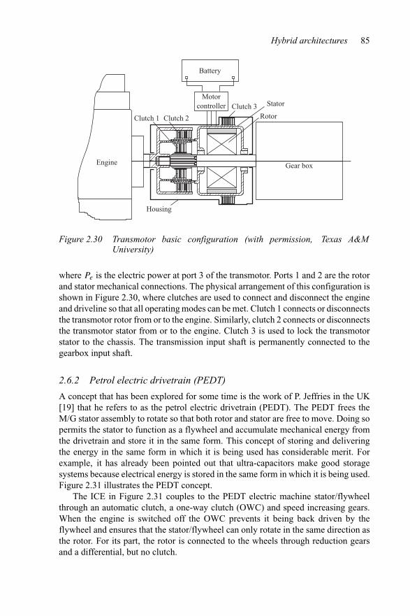
Hybrid architectures 85
Gear box
Battery
Motorcontroller
Clutch 1
Housing
Clutch 2
Clutch 3 Stator
Rotor
Engine
Figure 2.30 Transmotor basic configuration (with permission, Texas A&MUniversity)
where Pe is the electric power at port 3 of the transmotor. Ports 1 and 2 are the rotorand stator mechanical connections. The physical arrangement of this configuration isshown in Figure 2.30, where clutches are used to connect and disconnect the engineand driveline so that all operating modes can be met. Clutch 1 connects or disconnectsthe transmotor rotor from or to the engine. Similarly, clutch 2 connects or disconnectsthe transmotor stator from or to the engine. Clutch 3 is used to lock the transmotorstator to the chassis. The transmission input shaft is permanently connected to thegearbox input shaft.
2.6.2 Petrol electric drivetrain (PEDT)
A concept that has been explored for some time is the work of P. Jeffries in the UK[19] that he refers to as the petrol electric drivetrain (PEDT). The PEDT frees theM/G stator assembly to rotate so that both rotor and stator are free to move. Doing sopermits the stator to function as a flywheel and accumulate mechanical energy fromthe drivetrain and store it in the same form. This concept of storing and deliveringthe energy in the same form in which it is being used has considerable merit. Forexample, it has already been pointed out that ultra-capacitors make good storagesystems because electrical energy is stored in the same form in which it is being used.Figure 2.31 illustrates the PEDT concept.
The ICE in Figure 2.31 couples to the PEDT electric machine stator/flywheelthrough an automatic clutch, a one-way clutch (OWC) and speed increasing gears.When the engine is switched off the OWC prevents it being back driven by theflywheel and ensures that the stator/flywheel can only rotate in the same direction asthe rotor. For its part, the rotor is connected to the wheels through reduction gearsand a differential, but no clutch.
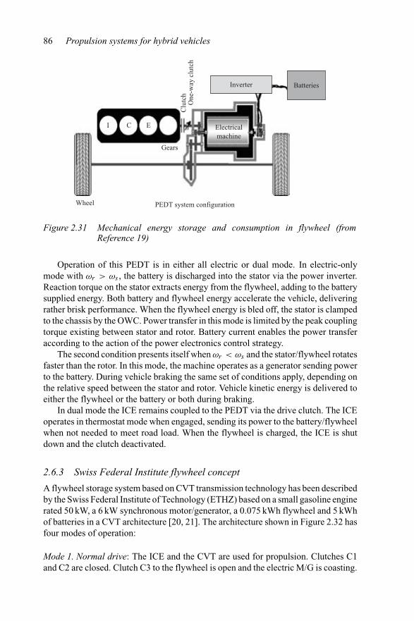
86 Propulsion systems for hybrid vehicles
Clu
tch
One
-way
clu
tch
Wheel
Gears
PEDT system configuration
Electricalmachine
Inverter Batteries
I C E
Figure 2.31 Mechanical energy storage and consumption in flywheel (fromReference 19)
Operation of this PEDT is in either all electric or dual mode. In electric-onlymode with ωr > ωs , the battery is discharged into the stator via the power inverter.Reaction torque on the stator extracts energy from the flywheel, adding to the batterysupplied energy. Both battery and flywheel energy accelerate the vehicle, deliveringrather brisk performance. When the flywheel energy is bled off, the stator is clampedto the chassis by the OWC. Power transfer in this mode is limited by the peak couplingtorque existing between stator and rotor. Battery current enables the power transferaccording to the action of the power electronics control strategy.
The second condition presents itself when ωr < ωs and the stator/flywheel rotatesfaster than the rotor. In this mode, the machine operates as a generator sending powerto the battery. During vehicle braking the same set of conditions apply, depending onthe relative speed between the stator and rotor. Vehicle kinetic energy is delivered toeither the flywheel or the battery or both during braking.
In dual mode the ICE remains coupled to the PEDT via the drive clutch. The ICEoperates in thermostat mode when engaged, sending its power to the battery/flywheelwhen not needed to meet road load. When the flywheel is charged, the ICE is shutdown and the clutch deactivated.
2.6.3 Swiss Federal Institute flywheel concept
A flywheel storage system based on CVT transmission technology has been describedby the Swiss Federal Institute of Technology (ETHZ) based on a small gasoline enginerated 50 kW, a 6 kW synchronous motor/generator, a 0.075 kWh flywheel and 5 kWhof batteries in a CVT architecture [20, 21]. The architecture shown in Figure 2.32 hasfour modes of operation:
Mode 1. Normal drive: The ICE and the CVT are used for propulsion. Clutches C1and C2 are closed. Clutch C3 to the flywheel is open and the electric M/G is coasting.
Hybrid architectures 87
e-mtr Powerinverter
Energystorage
CVT Trans.& FD
Flywheel
C1
C2
C3
Supervisorycontrol
Figure 2.32 Swiss Federal Institute of Technology flywheel CVT hybrid
Mode 2. Flywheel assist: Clutches C2 and C3 remain closed so that the flywheeland CVT maintain propulsion. When the flywheel speed drops below 1800 rpm theengine is started and C1 engaged to spin up the flywheel to 3800 rpm and to deliverpropulsion power to the wheels. When the flywheel speed exceeds 3800 rpm theengine is cut off and clutch C1 opened.
Mode 3. Electric machine and f lywheel assist: This is the zero emissions operatingmode. Power is delivered to the wheels by the M/G, augmented by decelerating theflywheel if necessary.
Mode 4. M/G and CVT only: This is the zero emission operating mode of a conven-tional EV. Because of limited rating of the M/G and battery, vehicle accelerationperformance is limited. Without a higher rated M/G this mode will be used only forlow speed operation.
The supervisory controller operates the ICE, CVT, M/G and clutches for properoperation in the four hybrid modes. The controller also monitors the energy storagesystem, power inverter and ICE for state of charge (available energy), invertermodulation settings and engine power.
2.7 Electric four wheel drive
A hybrid propulsion architecture that physically decouples the ICE propulsion andelectric propulsion systems is an electric four wheel drive, or all wheel drive, system.In the E4 architecture the existing ICE driveline remains unchanged, except perhapsfor up-rated electrical generation. The electric drive system is then implemented onthe non-driven axle as illustrated in Figure 2.33, where the M/G is connected to theaxle through a gear ratio and differential. Depending on design, a clutch at the gearboxinput may be necessary to mitigate the effects of M/G spin losses.
It is also interesting to investigate the range of options in an E4 system. Not onlyare the axle power levels variable in the range from 10 to 25 kW, but the amount of
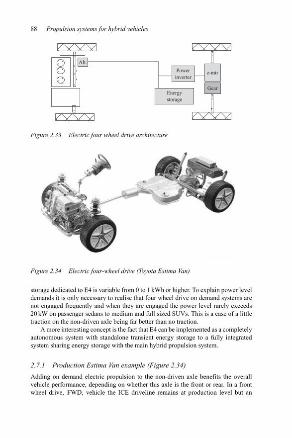
88 Propulsion systems for hybrid vehicles
Powerinverter
Energystorage
Alt.
e-mtr
Gear
Figure 2.33 Electric four wheel drive architecture
Figure 2.34 Electric four-wheel drive (Toyota Estima Van)
storage dedicated to E4 is variable from 0 to 1 kWh or higher. To explain power leveldemands it is only necessary to realise that four wheel drive on demand systems arenot engaged frequently and when they are engaged the power level rarely exceeds20 kW on passenger sedans to medium and full sized SUVs. This is a case of a littletraction on the non-driven axle being far better than no traction.
A more interesting concept is the fact that E4 can be implemented as a completelyautonomous system with standalone transient energy storage to a fully integratedsystem sharing energy storage with the main hybrid propulsion system.
2.7.1 Production Estima Van example (Figure 2.34)
Adding on demand electric propulsion to the non-driven axle benefits the overallvehicle performance, depending on whether this axle is the front or rear. In a frontwheel drive, FWD, vehicle the ICE driveline remains at production level but an
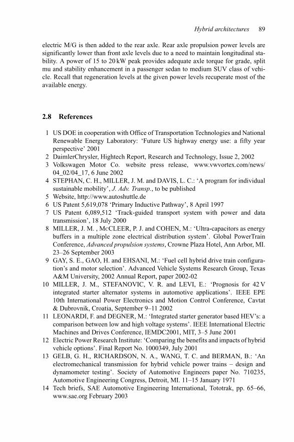
Hybrid architectures 89
electric M/G is then added to the rear axle. Rear axle propulsion power levels aresignificantly lower than front axle levels due to a need to maintain longitudinal sta-bility. A power of 15 to 20 kW peak provides adequate axle torque for grade, splitmu and stability enhancement in a passenger sedan to medium SUV class of vehi-cle. Recall that regeneration levels at the given power levels recuperate most of theavailable energy.
2.8 References
1 US DOE in cooperation with Office of Transportation Technologies and NationalRenewable Energy Laboratory: ‘Future US highway energy use: a fifty yearperspective’ 2001
2 DaimlerChrysler, Hightech Report, Research and Technology, Issue 2, 20023 Volkswagen Motor Co. website press release, www.vwvortex.com/news/
04_02/04_17, 6 June 20024 STEPHAN, C. H., MILLER, J. M. and DAVIS, L. C.: ‘A program for individual
sustainable mobility’, J. Adv. Transp., to be published5 Website, http://www.autoshuttle.de6 US Patent 5,619,078 ‘Primary Inductive Pathway’, 8 April 19977 US Patent 6,089,512 ‘Track-guided transport system with power and data
transmission’, 18 July 20008 MILLER, J. M. , McCLEER, P. J. and COHEN, M.: ‘Ultra-capacitors as energy
buffers in a multiple zone electrical distribution system’. Global PowerTrainConference, Advanced propulsion systems, Crowne Plaza Hotel, Ann Arbor, MI.23–26 September 2003
9 GAY, S. E., GAO, H. and EHSANI, M.: ‘Fuel cell hybrid drive train configura-tion’s and motor selection’. Advanced Vehicle Systems Research Group, TexasA&M University, 2002 Annual Report, paper 2002-02
10 MILLER, J. M., STEFANOVIC, V. R. and LEVI, E.: ‘Prognosis for 42 Vintegrated starter alternator systems in automotive applications’. IEEE EPE10th International Power Electronics and Motion Control Conference, Cavtat& Dubrovnik, Croatia, September 9–11 2002
11 LEONARDI, F. and DEGNER, M.: ‘Integrated starter generator based HEV’s: acomparison between low and high voltage systems’. IEEE International ElectricMachines and Drives Conference, IEMDC2001, MIT, 3–5 June 2001
12 Electric Power Research Institute: ‘Comparing the benefits and impacts of hybridvehicle options’. Final Report No. 1000349, July 2001
13 GELB, G. H., RICHARDSON, N. A., WANG, T. C. and BERMAN, B.: ‘Anelectromechanical transmission for hybrid vehicle power trains – design anddynamometer testing’. Society of Automotive Engineers paper No. 710235,Automotive Engineering Congress, Detroit, MI. 11–15 January 1971
14 Tech briefs, SAE Automotive Engineering International, Tototrak, pp. 65–66,www.sae.org February 2003
90 Propulsion systems for hybrid vehicles
15 Tech briefs, SAE Automotive Engineering International, pp. 10–11, www.sae.orgMay 2003
16 BRACKE, W.: ‘The Present and Future of Fluid Power’, Proc. Inst. Mech. Eng. I,J. Syst. Control Eng., 1993, 207, pp. 193–212
17 BLOXHAM, S. R.: “Off-grid electro-link power boost system’. Personalconversations with Mr Steve R. Bloxham in July 2002
18 LOUCHES, T.: ‘PaiceSM HyperdriveTM, its role in the future of powertrains’.Global PowerTrain Conference, Advanced Propulsion Systems, Sheraton Inn,Ann Arbor, MI. 24–26 September 2002, pp. 86–94
19 MILLER, J. M.: personal conversations with Peter Jeffries on PEDT, 1999–200020 SHAFAI, E. and GEERING, H. P.: ‘Control issues in a fuel-optimal hybrid
car’. International Federation of Automatic Control, IFAC 13th Triennial WorldCongress, San Francisco, CA, 1996
21 GUZZELLA, L., WITTMER, Ch. and ENDER, M.: ‘Optimal operation of drivetrains with SI-engines and flywheels’. International Federation of AutomaticControl, IFAC 13th Triennial World Congress, San Francisco, CA, 1996
Chapter 3
Hybrid power plant specifications
The vehicle power plant is designed to deliver sufficient propulsion power to thedriven wheels to meet performance targets that are consistent with vehicle brandimage. The previous two chapters described how conventional engines and electricdrive systems are matched to meet performance and economy targets. In this chapterwe continue to evaluate the matching criteria between combustion engines and acdrives for targeted road load conditions. The reader is no doubt aware of the variouspowertrain configurations available in the market place from small in-line three andfour cylinder engines with ISA type ac drives matched to the driveline by 5, and nowa 6 speed and in one instance a 7 speed, manual or automatic transmissions or evenwith continuously variable transmissions. Larger engines such as V6s and V8s withinherently higher torque are typically matched to the driveline with 3 and 4 speedtransmissions. At the high end, V10, V12 and even V16 engines with their availabletorque ranging from 350 to nearly 1400 Nm explain why such drivelines can pull ‘tall’gear ratios. To give some examples of this, the DaimlerChrysler V10 Viper engineis an aluminum block 8.3 L, overhead valve (OHV), 10 cylinder power plant rated373 kW (500 PS) and 712 Nm torque. The Jaguar XJ-S V12 is a 5.3 L, 12 cylinderpower plant rated 208 kW (284 PS) with 415 Nm torque at 2800 rpm. General MotorsCorp. in January 2003 introduced its Cadillac Sixteen with a V16 aluminum blockengine. The 13.6 L, OHV, V16 delivers 746 kW (1000 PS) and 1356 Nm of torque atjust 2000 rpm. The XV16 Cadillac engine has a mass of 315 kg and is designed tooperate with cylinder deactivation. Cylinder deactivation means the V16 engine canrun on 8 or as few as 4 cylinders, delivering an impressive 20 mpg fuel economy inthe 2270 kg GM flagship vehicle.
In the following sections the various trade-offs between power plant torque andpower rating are illustrated with regard to transmission selection and vehicle perfor-mance. To further illustrate the process suppose the power plants described above areplaced into passenger vehicles of size and weight recommended by the manufactur-ers. Table 3.1 shows the specifics of the vehicle and propulsion system. Furthermore,and because of lack of transmission data, the driveline gearing in low gear is takenas the tyre to road adhesion limit. The axle torque breakpoint shown in Figure 3.1 is
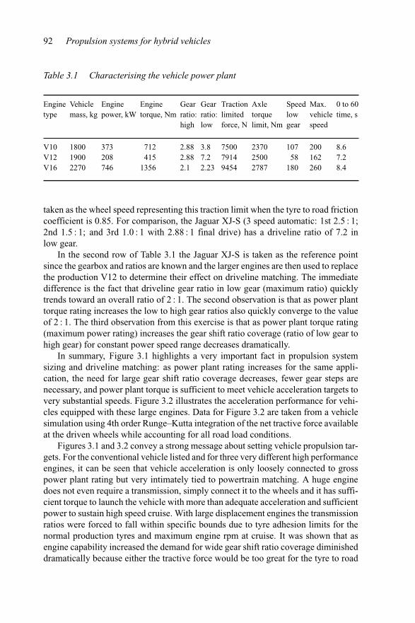
92 Propulsion systems for hybrid vehicles
Table 3.1 Characterising the vehicle power plant
Enginetype
Vehiclemass, kg
Enginepower, kW
Enginetorque, Nm
Gearratio:high
Gearratio:low
Tractionlimitedforce, N
Axletorquelimit, Nm
Speedlowgear
Max.vehiclespeed
0 to 60time, s
V10 1800 373 712 2.88 3.8 7500 2370 107 200 8.6V12 1900 208 415 2.88 7.2 7914 2500 58 162 7.2V16 2270 746 1356 2.1 2.23 9454 2787 180 260 8.4
taken as the wheel speed representing this traction limit when the tyre to road frictioncoefficient is 0.85. For comparison, the Jaguar XJ-S (3 speed automatic: 1st 2.5 : 1;2nd 1.5 : 1; and 3rd 1.0 : 1 with 2.88 : 1 final drive) has a driveline ratio of 7.2 inlow gear.
In the second row of Table 3.1 the Jaguar XJ-S is taken as the reference pointsince the gearbox and ratios are known and the larger engines are then used to replacethe production V12 to determine their effect on driveline matching. The immediatedifference is the fact that driveline gear ratio in low gear (maximum ratio) quicklytrends toward an overall ratio of 2 : 1. The second observation is that as power planttorque rating increases the low to high gear ratios also quickly converge to the valueof 2 : 1. The third observation from this exercise is that as power plant torque rating(maximum power rating) increases the gear shift ratio coverage (ratio of low gear tohigh gear) for constant power speed range decreases dramatically.
In summary, Figure 3.1 highlights a very important fact in propulsion systemsizing and driveline matching: as power plant rating increases for the same appli-cation, the need for large gear shift ratio coverage decreases, fewer gear steps arenecessary, and power plant torque is sufficient to meet vehicle acceleration targets tovery substantial speeds. Figure 3.2 illustrates the acceleration performance for vehi-cles equipped with these large engines. Data for Figure 3.2 are taken from a vehiclesimulation using 4th order Runge–Kutta integration of the net tractive force availableat the driven wheels while accounting for all road load conditions.
Figures 3.1 and 3.2 convey a strong message about setting vehicle propulsion tar-gets. For the conventional vehicle listed and for three very different high performanceengines, it can be seen that vehicle acceleration is only loosely connected to grosspower plant rating but very intimately tied to powertrain matching. A huge enginedoes not even require a transmission, simply connect it to the wheels and it has suffi-cient torque to launch the vehicle with more than adequate acceleration and sufficientpower to sustain high speed cruise. With large displacement engines the transmissionratios were forced to fall within specific bounds due to tyre adhesion limits for thenormal production tyres and maximum engine rpm at cruise. It was shown that asengine capability increased the demand for wide gear shift ratio coverage diminisheddramatically because either the tractive force would be too great for the tyre to road
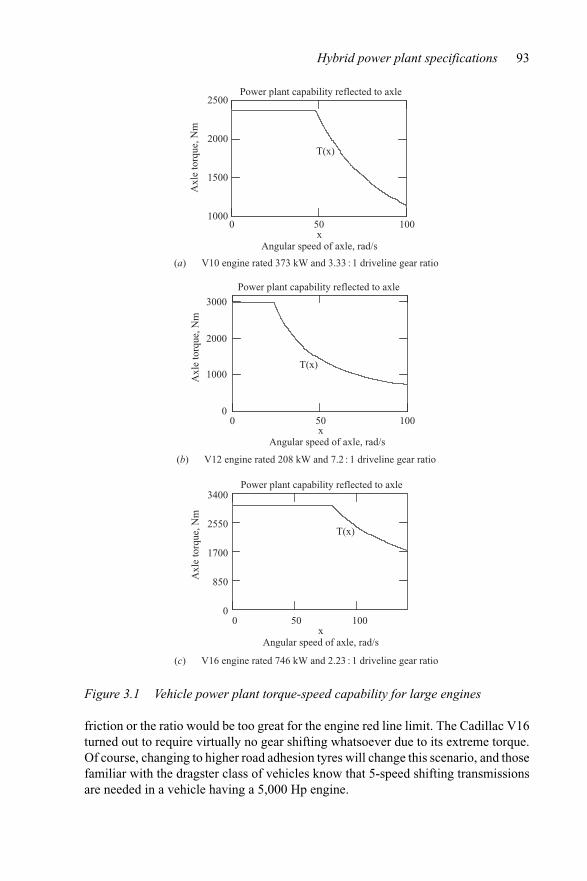
Hybrid power plant specifications 93
0 50 100
Power plant capability reflected to axle
Axl
e to
rque
, Nm
T(x)
T(x)
T(x)
1000
1500
2000
2500
xAngular speed of axle, rad/s
0 100
Power plant capability reflected to axle
Axl
e to
rque
, Nm
Axl
e to
rque
, Nm
0
1000
2000
3000
x50
Angular speed of axle, rad/s
xAngular speed of axle, rad/s
0 50 100
Power plant capability reflected to axle
0
850
1700
2550
3400
(a) V10 engine rated 373 kW and 3.33 : 1 driveline gear ratio
(b) V12 engine rated 208 kW and 7.2 : 1 driveline gear ratio
(c) V16 engine rated 746 kW and 2.23 : 1 driveline gear ratio
Figure 3.1 Vehicle power plant torque-speed capability for large engines
friction or the ratio would be too great for the engine red line limit. The Cadillac V16turned out to require virtually no gear shifting whatsoever due to its extreme torque.Of course, changing to higher road adhesion tyres will change this scenario, and thosefamiliar with the dragster class of vehicles know that 5-speed shifting transmissionsare needed in a vehicle having a 5,000 Hp engine.
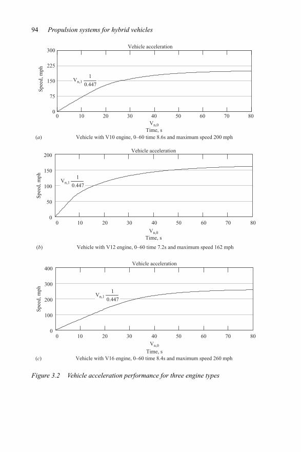
94 Propulsion systems for hybrid vehicles
Vehicle acceleration
Vn,11
0.447
0
75
150
225
300
0 10 20 30 50 60 70 80
Time, s
40Vn,0
0 10 20 30 40 50 60 70 800
50
100
150
200Vehicle acceleration
Spee
d, m
ph
Time, sVn,0
Vn,11
0.447
Spee
d, m
ph
Time, s
Vn,0
0 10 20 30 40 50 60 70 800
100
200
300
400Vehicle acceleration
Vn,11
0.447
Spee
d, m
ph
(b) Vehicle with V12 engine, 0–60 time 7.2s and maximum speed 162 mph
(a) Vehicle with V10 engine, 0–60 time 8.6s and maximum speed 200 mph
(c) Vehicle with V16 engine, 0–60 time 8.4s and maximum speed 260 mph
Figure 3.2 Vehicle acceleration performance for three engine types
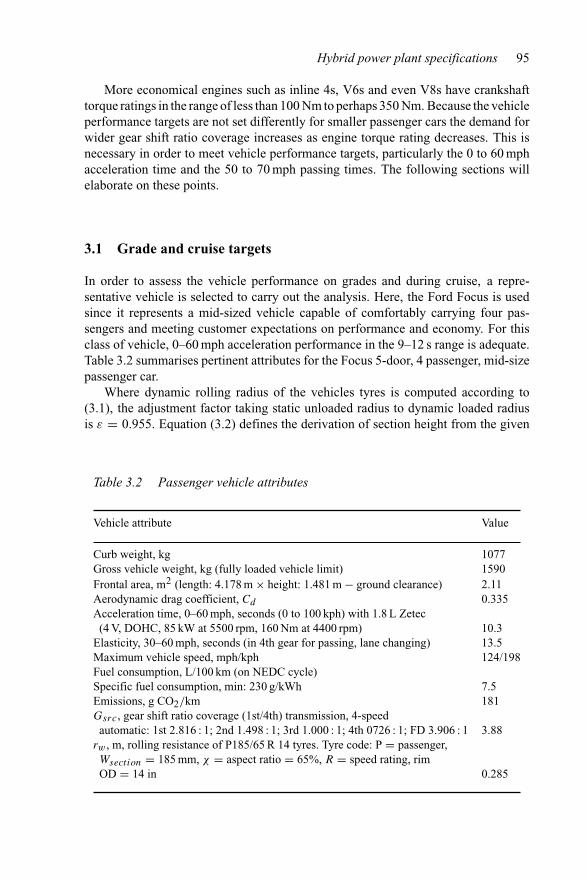
Hybrid power plant specifications 95
More economical engines such as inline 4s, V6s and even V8s have crankshafttorque ratings in the range of less than 100 Nm to perhaps 350 Nm. Because the vehicleperformance targets are not set differently for smaller passenger cars the demand forwider gear shift ratio coverage increases as engine torque rating decreases. This isnecessary in order to meet vehicle performance targets, particularly the 0 to 60 mphacceleration time and the 50 to 70 mph passing times. The following sections willelaborate on these points.
3.1 Grade and cruise targets
In order to assess the vehicle performance on grades and during cruise, a repre-sentative vehicle is selected to carry out the analysis. Here, the Ford Focus is usedsince it represents a mid-sized vehicle capable of comfortably carrying four pas-sengers and meeting customer expectations on performance and economy. For thisclass of vehicle, 0–60 mph acceleration performance in the 9–12 s range is adequate.Table 3.2 summarises pertinent attributes for the Focus 5-door, 4 passenger, mid-sizepassenger car.
Where dynamic rolling radius of the vehicles tyres is computed according to(3.1), the adjustment factor taking static unloaded radius to dynamic loaded radiusis ε = 0.955. Equation (3.2) defines the derivation of section height from the given
Table 3.2 Passenger vehicle attributes
Vehicle attribute Value
Curb weight, kg 1077Gross vehicle weight, kg (fully loaded vehicle limit) 1590Frontal area, m2 (length: 4.178 m × height: 1.481 m − ground clearance) 2.11Aerodynamic drag coefficient, Cd 0.335Acceleration time, 0–60 mph, seconds (0 to 100 kph) with 1.8 L Zetec
(4 V, DOHC, 85 kW at 5500 rpm, 160 Nm at 4400 rpm) 10.3Elasticity, 30–60 mph, seconds (in 4th gear for passing, lane changing) 13.5Maximum vehicle speed, mph/kph 124/198Fuel consumption, L/100 km (on NEDC cycle)Specific fuel consumption, min: 230 g/kWh 7.5Emissions, g CO2/km 181Gsrc, gear shift ratio coverage (1st/4th) transmission, 4-speedautomatic: 1st 2.816 : 1; 2nd 1.498 : 1; 3rd 1.000 : 1; 4th 0726 : 1; FD 3.906 : 1 3.88
rw , m, rolling resistance of P185/65 R 14 tyres. Tyre code: P = passenger,Wsection = 185 mm, χ = aspect ratio = 65%, R = speed rating, rimOD = 14 in 0.285
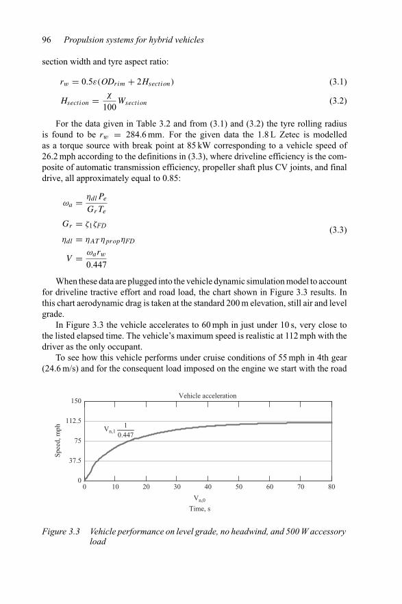
96 Propulsion systems for hybrid vehicles
section width and tyre aspect ratio:
rw = 0.5ε(ODrim + 2Hsection) (3.1)
Hsection = χ
100Wsection (3.2)
For the data given in Table 3.2 and from (3.1) and (3.2) the tyre rolling radiusis found to be rw = 284.6 mm. For the given data the 1.8 L Zetec is modelledas a torque source with break point at 85 kW corresponding to a vehicle speed of26.2 mph according to the definitions in (3.3), where driveline efficiency is the com-posite of automatic transmission efficiency, propeller shaft plus CV joints, and finaldrive, all approximately equal to 0.85:
ωa = ηdlPe
GrTe
Gr = ζ1ζFD
ηdl = ηAT ηpropηFD
V = ωarw
0.447
(3.3)
When these data are plugged into the vehicle dynamic simulation model to accountfor driveline tractive effort and road load, the chart shown in Figure 3.3 results. Inthis chart aerodynamic drag is taken at the standard 200 m elevation, still air and levelgrade.
In Figure 3.3 the vehicle accelerates to 60 mph in just under 10 s, very close tothe listed elapsed time. The vehicle’s maximum speed is realistic at 112 mph with thedriver as the only occupant.
To see how this vehicle performs under cruise conditions of 55 mph in 4th gear(24.6 m/s) and for the consequent load imposed on the engine we start with the road
Vn,1
Vehicle acceleration
Time, s
Spee
d, m
ph 10.447
0
37.5
75
112.5
150
0 10 20 30 40 50 60 70 80
Vn,0
Figure 3.3 Vehicle performance on level grade, no headwind, and 500 W accessoryload
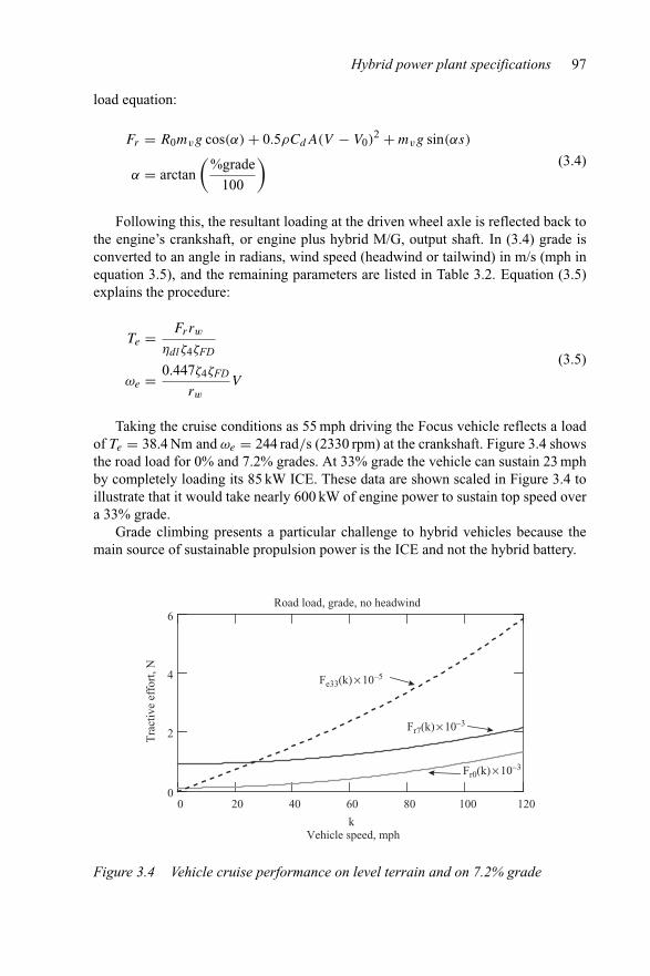
Hybrid power plant specifications 97
load equation:
Fr = R0mvg cos(α) + 0.5ρCdA(V − V0)2 + mvg sin(αs)
α = arctan(
%grade
100
) (3.4)
Following this, the resultant loading at the driven wheel axle is reflected back tothe engine’s crankshaft, or engine plus hybrid M/G, output shaft. In (3.4) grade isconverted to an angle in radians, wind speed (headwind or tailwind) in m/s (mph inequation 3.5), and the remaining parameters are listed in Table 3.2. Equation (3.5)explains the procedure:
Te = Frrw
ηdlζ4ζFD
ωe = 0.447ζ4ζFD
rwV
(3.5)
Taking the cruise conditions as 55 mph driving the Focus vehicle reflects a loadof Te = 38.4 Nm and ωe = 244 rad/s (2330 rpm) at the crankshaft. Figure 3.4 showsthe road load for 0% and 7.2% grades. At 33% grade the vehicle can sustain 23 mphby completely loading its 85 kW ICE. These data are shown scaled in Figure 3.4 toillustrate that it would take nearly 600 kW of engine power to sustain top speed overa 33% grade.
Grade climbing presents a particular challenge to hybrid vehicles because themain source of sustainable propulsion power is the ICE and not the hybrid battery.
k
0 20 40 60 80 100 1200
2
4
6Road load, grade, no headwind
Vehicle speed, mph
Tra
ctiv
e ef
fort
, N
Fr0(k) × 10–3
Fr7(k) × 10–3
Fe33(k) × 10–5
Figure 3.4 Vehicle cruise performance on level terrain and on 7.2% grade
98 Propulsion systems for hybrid vehicles
3.1.1 Gradeability
Hybrid power plants must have their heat engines sized to meet sustained performanceon a grade. As we saw above for the Focus vehicle, a 33% grade consumes itsentire engine output in order to sustain 23 mph. If there was some headwind or morevehicle occupants this would not be possible in high gear. The conclusions above havetaken into account that the driveline will downshift as appropriate to move the fullengine power to these lower speeds.
3.1.2 Wide open throttle
Analysis of vehicle propulsion under wide open throttle conditions is generally theapproach taken to illustrate the best vehicle performance in acceleration times andpassing. When the vehicle’s accelerator pedal is pressed completely to the floor,the engine controller senses the demand for full performance and autonomouslydeclutches the vehicle’s air conditioner compressor by de-energizing its electromag-netic clutch. In vehicles with controllable fans and water pumps there may be somefurther gains by restraining the power consumed by these ancillaries.
3.2 Launch and boosting
Virtually the complete impression of vehicle performance is gleaned during the firstcouple of seconds of a brisk take-off and acceleration. How smoothly the vehicleaccelerates, whether or not shift events are noticeable and if any driveline shudder orvibration is present contribute to the overall impression. Beyond the initial launch,and particularly when the automatic transmission torque converter is transitioningout of torque multiplication, the benefit of hybrid boosting becomes noticeable.
In the ISG type of direct drive systems having power levels less than 10 kW theboost impact is not noticeable above 3000 engine rpm. But up to that speed, boost-ing by the electric M/G is noticeable and does benefit vehicle acceleration becauseengine output torque is augmented. We saw in the introduction to this chapter howdramatically adding engine torque to the driveline improved the total vehicle capa-bility provided the correct matching is employed. If the transmission and final drivegear ratios are too ‘tall’, then the acceleration will not be as brisk, even with torqueaugmentation.
3.2.1 First two seconds
The most noticeable launch feel occurs during the first two seconds when the auto-matic transmission torque converter is delivering double the engine torque to thedriveline.
3.2.2 Lane change
Another measure of vehicle performance is lane change for passing and the attendantneed for acceleration from either 30 to 60 mph or from 50 to 70 mph depending
Hybrid power plant specifications 99
Table 3.3 Vehicle lane change and passing manoeuvres
Manoeuvre 30 to 60 mphtimes (s)
50 to 70 mphtimes (s)
Case 1: 0% grade, 1 occupant 6.1 5.9Case 2: 3% grade, 1 occupant 11.6 21.0Case 3: 0% grade, 4 occupants 7.0 7.2
on geographical location and driving habits. To illustrate the vehicle’s performanceduring passing manoeuvres we take the same Focus 5 door and compare its wide openthrottle performance in terms of time to accelerate for both of the speed intervals noted.Table 3.3 summarises the findings of running the simulation for three cases: Case (1)0% grade and single occupant; case (2) at 7% grade and with a single occupant; andcase (3) again the 0% grade but with four occupants.
Table 3.3 presents some interesting data. Again, performance on grade is muchmore demanding than adding occupants, as can be seen from the passing manoeuvretimes. The change from one to four occupants for the same manoeuvre makes onlya 17% increase in acceleration times, but climbing just a 3% grade results in a verynoticeable 90% and 256% increase in times.
3.3 Braking and energy recuperation
The performance of vehicle hybrid propulsion systems is strongly dependent on thetype of brake system used. The energy recuperation component of fuel economygain depends to a first order on the hybrid M/G rating and secondly to the types ofregenerative brake systems employed.
It is far more important to implement active brake controls on rear wheel driveversus front wheel drive hybrid vehicles when regenerative braking is employed.Vehicle rear brakes tend to lock and skid far easier than front wheels due to normalweight balance allocation and dynamic weight shifting during braking. Once the rearwheels lock up, the vehicle anti-lock braking system, ABS, will engage and startto modulate the brake line pressure at approximately 15 Hz. Engagement of ABSpre-empts regenerative brakes in a hybrid vehicle regardless of architecture.
There are several versions of regenerative brakes available depending on the levelof energy recuperation anticipated. Series regenerative braking systems, RBS, as thename implies, engage the electric M/G in generating mode first. Then, if the brakepedal is depressed further, and/or faster, the brake controller adds in the vehicle’sservice brakes to gain a more rapid deceleration. Lastly, if the brake pedal is depressedhard the ABS controller engages and controls braking using the service brakes only.
Parallel RBS is the system most commonly employed in mild hybrids. ParallelRBS does not require electro-hydraulic or electromechanical braking systems, but
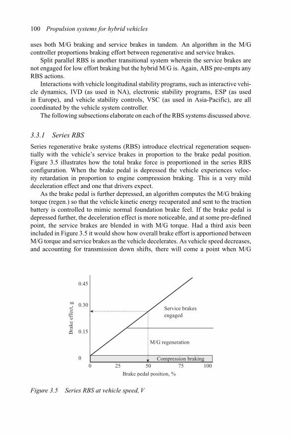
100 Propulsion systems for hybrid vehicles
uses both M/G braking and service brakes in tandem. An algorithm in the M/Gcontroller proportions braking effort between regenerative and service brakes.
Split parallel RBS is another transitional system wherein the service brakes arenot engaged for low effort braking but the hybrid M/G is. Again, ABS pre-empts anyRBS actions.
Interactions with vehicle longitudinal stability programs, such as interactive vehi-cle dynamics, IVD (as used in NA), electronic stability programs, ESP (as usedin Europe), and vehicle stability controls, VSC (as used in Asia-Pacific), are allcoordinated by the vehicle system controller.
The following subsections elaborate on each of the RBS systems discussed above.
3.3.1 Series RBS
Series regenerative brake systems (RBS) introduce electrical regeneration sequen-tially with the vehicle’s service brakes in proportion to the brake pedal position.Figure 3.5 illustrates how the total brake force is proportioned in the series RBSconfiguration. When the brake pedal is depressed the vehicle experiences veloc-ity retardation in proportion to engine compression braking. This is a very milddeceleration effect and one that drivers expect.
As the brake pedal is further depressed, an algorithm computes the M/G brakingtorque (regen.) so that the vehicle kinetic energy recuperated and sent to the tractionbattery is controlled to mimic normal foundation brake feel. If the brake pedal isdepressed further, the deceleration effect is more noticeable, and at some pre-definedpoint, the service brakes are blended in with M/G torque. Had a third axis beenincluded in Figure 3.5 it would show how overall brake effort is apportioned betweenM/G torque and service brakes as the vehicle decelerates. As vehicle speed decreases,and accounting for transmission down shifts, there will come a point when M/G
Compression braking
Brake pedal position, %
0 25 50 75 100
Bra
ke e
ffec
t, g
M/G regeneration
Service brakes engaged
0.45
0.30
0.15
0
Figure 3.5 Series RBS at vehicle speed, V
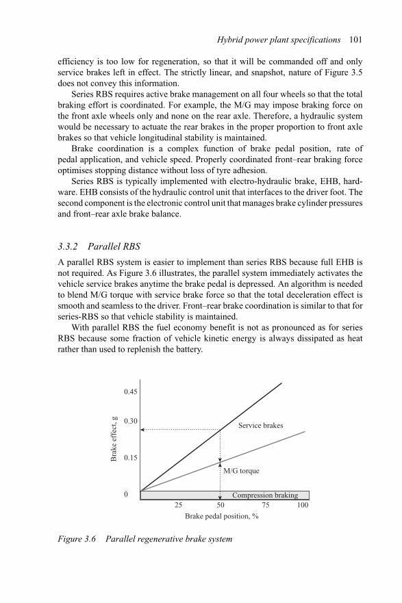
Hybrid power plant specifications 101
efficiency is too low for regeneration, so that it will be commanded off and onlyservice brakes left in effect. The strictly linear, and snapshot, nature of Figure 3.5does not convey this information.
Series RBS requires active brake management on all four wheels so that the totalbraking effort is coordinated. For example, the M/G may impose braking force onthe front axle wheels only and none on the rear axle. Therefore, a hydraulic systemwould be necessary to actuate the rear brakes in the proper proportion to front axlebrakes so that vehicle longitudinal stability is maintained.
Brake coordination is a complex function of brake pedal position, rate ofpedal application, and vehicle speed. Properly coordinated front–rear braking forceoptimises stopping distance without loss of tyre adhesion.
Series RBS is typically implemented with electro-hydraulic brake, EHB, hard-ware. EHB consists of the hydraulic control unit that interfaces to the driver foot. Thesecond component is the electronic control unit that manages brake cylinder pressuresand front–rear axle brake balance.
3.3.2 Parallel RBS
A parallel RBS system is easier to implement than series RBS because full EHB isnot required. As Figure 3.6 illustrates, the parallel system immediately activates thevehicle service brakes anytime the brake pedal is depressed. An algorithm is neededto blend M/G torque with service brake force so that the total deceleration effect issmooth and seamless to the driver. Front–rear brake coordination is similar to that forseries-RBS so that vehicle stability is maintained.
With parallel RBS the fuel economy benefit is not as pronounced as for seriesRBS because some fraction of vehicle kinetic energy is always dissipated as heatrather than used to replenish the battery.
Compression braking
Brake pedal position, %
25 50 75 100
Bra
ke e
ffec
t, g
M/G torque
Service brakes
0.45
0.30
0.15
0
Figure 3.6 Parallel regenerative brake system
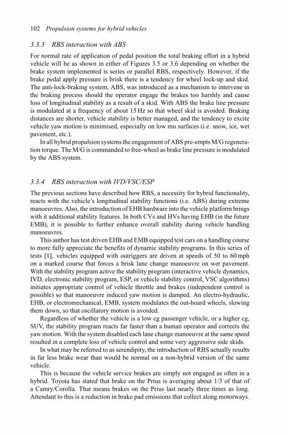
102 Propulsion systems for hybrid vehicles
3.3.3 RBS interaction with ABS
For normal rate of application of pedal position the total braking effort in a hybridvehicle will be as shown in either of Figures 3.5 or 3.6 depending on whether thebrake system implemented is series or parallel RBS, respectively. However, if thebrake pedal apply pressure is brisk there is a tendency for wheel lock-up and skid.The anti-lock-braking system, ABS, was introduced as a mechanism to intervene inthe braking process should the operator engage the brakes too harshly and causeloss of longitudinal stability as a result of a skid. With ABS the brake line pressureis modulated at a frequency of about 15 Hz so that wheel skid is avoided. Brakingdistances are shorter, vehicle stability is better managed, and the tendency to excitevehicle yaw motion is minimised, especially on low mu surfaces (i.e. snow, ice, wetpavement, etc.).
In all hybrid propulsion systems the engagement of ABS pre-empts M/G regenera-tion torque. The M/G is commanded to free-wheel as brake line pressure is modulatedby the ABS system.
3.3.4 RBS interaction with IVD/VSC/ESP
The previous sections have described how RBS, a necessity for hybrid functionality,reacts with the vehicle’s longitudinal stability functions (i.e. ABS) during extrememanoeuvres. Also, the introduction of EHB hardware into the vehicle platform bringswith it additional stability features. In both CVs and HVs having EHB (in the futureEMB), it is possible to further enhance overall stability during vehicle handlingmanoeuvres.
This author has test driven EHB and EMB equipped test cars on a handling courseto more fully appreciate the benefits of dynamic stability programs. In this series oftests [1], vehicles equipped with outriggers are driven at speeds of 50 to 60 mphon a marked course that forces a brisk lane change manoeuvre on wet pavement.With the stability program active the stability program (interactive vehicle dynamics,IVD, electronic stability program, ESP, or vehicle stability control, VSC algorithms)initiates appropriate control of vehicle throttle and brakes (independent control ispossible) so that manoeuvre induced yaw motion is damped. An electro-hydraulic,EHB, or electromechanical, EMB, system modulates the out-board wheels, slowingthem down, so that oscillatory motion is avoided.
Regardless of whether the vehicle is a low cg passenger vehicle, or a higher cg,SUV, the stability program reacts far faster than a human operator and corrects theyaw motion. With the system disabled each lane change manoeuvre at the same speedresulted in a complete loss of vehicle control and some very aggressive side skids.
In what may be referred to as serendipity, the introduction of RBS actually resultsin far less brake wear than would be normal on a non-hybrid version of the samevehicle.
This is because the vehicle service brakes are simply not engaged as often in ahybrid. Toyota has stated that brake on the Prius is averaging about 1/3 of that ofa Camry/Corolla. That means brakes on the Prius last nearly three times as long.Attendant to this is a reduction in brake pad emissions that collect along motorways.
Hybrid power plant specifications 103
700
600
Spee
d, r
ad/s 500
400
300
200
100
00 68 13
820
427
234
040
847
654
461
268
074
881
688
495
210
2010
8811
5612
2412
9213
60
FUDS cycle
Time, s
Figure 3.7 FUD’s standard drive cycle used for battery-EV development (wheelspeed)
3.4 Drive cycle implications
The US Federal Urban Drive Cycle was created during the early years of batteryelectric vehicle development to model urban driving conditions (Figure 3.7).
The FUD cycle is the first 1369 s of the Federal Test Procedure, FTP75. FUD’scycle represents an urban drive of 7.45 miles at an average speed of 19.59 mph.
3.4.1 Types of drive cycles
A great number of drive cycles have been developed to mock-up the driving habits oflarge populations of drivers in particular geographical areas. The main drive cyclesof interest to hybrid propulsion designers are the Environmental Protection Agency,EPA, city and highway cycles used in North America. In Europe the New EuropeanDrive Cycle (NEDC) is used extensively. In Asia–Pacific, and particularly Japan,the 10–15 mode is used almost always. There are other related, but revised for someparticular attribute, drive cycles – for example, US-06 or HWFET (highway fueleconomy test). There are cycles that exaggerate the vehicle’s acceleration demandsand are known as real world drive cycles.
The drive cycles listed in Table 3.4 show distinct geographical character. The firstthree rows for example, define the maximum and average speeds of how large groupsof the population are assumed to drive their vehicles. Notice that maximum speedsincrease going from Japan, through North America to Europe.
3.4.2 Average speed and impact on fuel economy
The fact that standard drive cycles have considerable variation in their average andmaximum speeds means that fuel economy and performance attributes for each cyclewill have a different impact on driveline design. For example, Figure 3.8 illustrateshow fuel economy varies by drive cycle as the transmission used to match the engineto the driven wheels has its gear shift ratio coverage varied. For each geographical
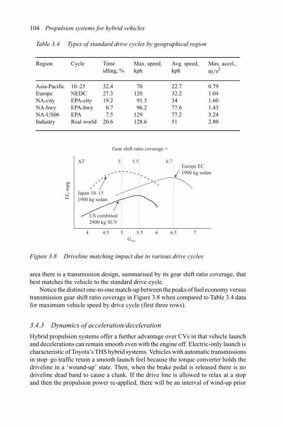
104 Propulsion systems for hybrid vehicles
Table 3.4 Types of standard drive cycles by geographical region
Region Cycle Timeidling, %
Max. speed,kph
Avg. speed,kph
Max. accel.,m/s2
Asia-Pacific 10–25 32.4 70 22.7 0.79Europe NEDC 27.3 120 32.2 1.04NA-city EPA-city 19.2 91.3 34 1.60NA-hwy EPA-hwy 0.7 96.2 77.6 1.43NA-US06 EPA 7.5 129 77.2 3.24Industry Real world 20.6 128.6 51 2.80
Gsrc
AT
Gear shift ratio coverage =
Japan 10–151900 kg sedan
Europe EC 1900 kg sedan
US combined 2900 kg SUV
FE, m
pg
4 4.5 5 5.5 6 6.5 7
5 5.5 6.7
Figure 3.8 Driveline matching impact due to various drive cycles
area there is a transmission design, summarised by its gear shift ratio coverage, thatbest matches the vehicle to the standard drive cycle.
Notice the distinct one-to-one match-up between the peaks of fuel economy versustransmission gear shift ratio coverage in Figure 3.8 when compared to Table 3.4 datafor maximum vehicle speed by drive cycle (first three rows).
3.4.3 Dynamics of acceleration/deceleration
Hybrid propulsion systems offer a further advantage over CVs in that vehicle launchand decelerations can remain smooth even with the engine off. Electric-only launch ischaracteristic of Toyota’s THS hybrid systems. Vehicles with automatic transmissionsin stop–go traffic retain a smooth launch feel because the torque converter holds thedriveline in a ‘wound-up’ state. Then, when the brake pedal is released there is nodriveline dead band to cause a clunk. If the drive line is allowed to relax at a stopand then the propulsion power re-applied, there will be an interval of wind-up prior
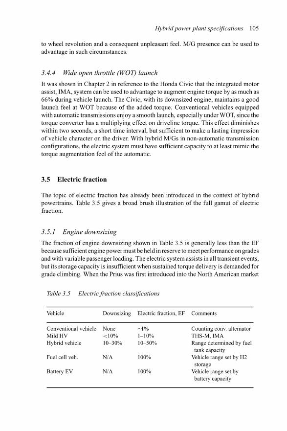
Hybrid power plant specifications 105
to wheel revolution and a consequent unpleasant feel. M/G presence can be used toadvantage in such circumstances.
3.4.4 Wide open throttle (WOT) launch
It was shown in Chapter 2 in reference to the Honda Civic that the integrated motorassist, IMA, system can be used to advantage to augment engine torque by as much as66% during vehicle launch. The Civic, with its downsized engine, maintains a goodlaunch feel at WOT because of the added torque. Conventional vehicles equippedwith automatic transmissions enjoy a smooth launch, especially under WOT, since thetorque converter has a multiplying effect on driveline torque. This effect diminisheswithin two seconds, a short time interval, but sufficient to make a lasting impressionof vehicle character on the driver. With hybrid M/Gs in non-automatic transmissionconfigurations, the electric system must have sufficient capacity to at least mimic thetorque augmentation feel of the automatic.
3.5 Electric fraction
The topic of electric fraction has already been introduced in the context of hybridpowertrains. Table 3.5 gives a broad brush illustration of the full gamut of electricfraction.
3.5.1 Engine downsizing
The fraction of engine downsizing shown in Table 3.5 is generally less than the EFbecause sufficient engine power must be held in reserve to meet performance on gradesand with variable passenger loading. The electric system assists in all transient events,but its storage capacity is insufficient when sustained torque delivery is demanded forgrade climbing. When the Prius was first introduced into the North American market
Table 3.5 Electric fraction classifications
Vehicle Downsizing Electric fraction, EF Comments
Conventional vehicle None ∼1% Counting conv. alternatorMild HV <10% 1–10% THS-M, IMAHybrid vehicle 10–30% 10–50% Range determined by fuel
tank capacityFuel cell veh. N/A 100% Vehicle range set by H2
storageBattery EV N/A 100% Vehicle range set by
battery capacity
106 Propulsion systems for hybrid vehicles
in CY2000 the major complaint was its lack of performance on grades. This wasin fact partly due to an engine downsized from approximately 2.2 L to 1.5 L (33%)and in part due to operating the engine on the Atkinson cycle (i.e. late intake valveopening).
Smaller displacement engines mean less pumping loss and higher efficiency, allelse being equal. In many instances an I4 can be used in lieu of a V6, or a V6 in lieuof a V8. The TMC hybrid synergy drive, for example, claims V8 performance witha small V6. The hybrid synergy drive represents TMC’s initial launch of their newhybrid family, THS-II. THS II relies on the same 274 V NiMH battery as THS-I, butwith a de/dc convertor to boost the link voltage to 500 V.
3.5.2 Range and performance
Hybrid vehicles must deliver performance comparable to conventional vehiclesregardless of the desire to downsize the engine, reduce overall vehicle mass, includ-ing fuel tank capacity, and use longer final drives. In North America an acceptablerange has settled to about 300 miles regardless of vehicle mass or overall economy(target range is 380 miles). The fuel tank is sized to match the range goal.
The Prius, for example, has a 10.9 US gal. fuel tank and will average 400 miles perfill-up (without having the low fuel indicator on). Low fuel annunciation is promptedwhen the fuel tank content falls below 2 gallons.
Performance cannot be compromised. A hybrid vehicle must deliver acceleration,handling and ride comparable to or exceeding that of its non-hybridized counter-part. The powertrain is augmented with sufficient electric torque to compensatea downsized engine. In addition to an advanced battery technology, many manu-facturers today are turning to ultra-capacitors for high pulse power delivery for briskaccelerations and handling, plus for benefits on energy recovery.
3.6 Usage requirements
Vehicle usage statistics are compiled through drive surveys that target diverse geo-graphical and metropolitan areas. Performance data are obtained from data acquisitionsystems installed on the vehicle. Data collected on the vehicle are sent via telemetryto a central facility where they are analyzed [2]. Such data are essential in order toassess HV performance at remote locations, or if fleets of vehicles are being tested.The system consists of self-powered telematics instrumentation that transmits vehi-cle data over a secure data channel to the programme engineers. In such monitoringsystems, GPS time, latitude and longitude, altitude and other information is collectedand transmitted along with vehicle systems performance. Putting a time tag on datapermits the usage patterns of the monitored vehicles to be assessed by location andlocal conditions.
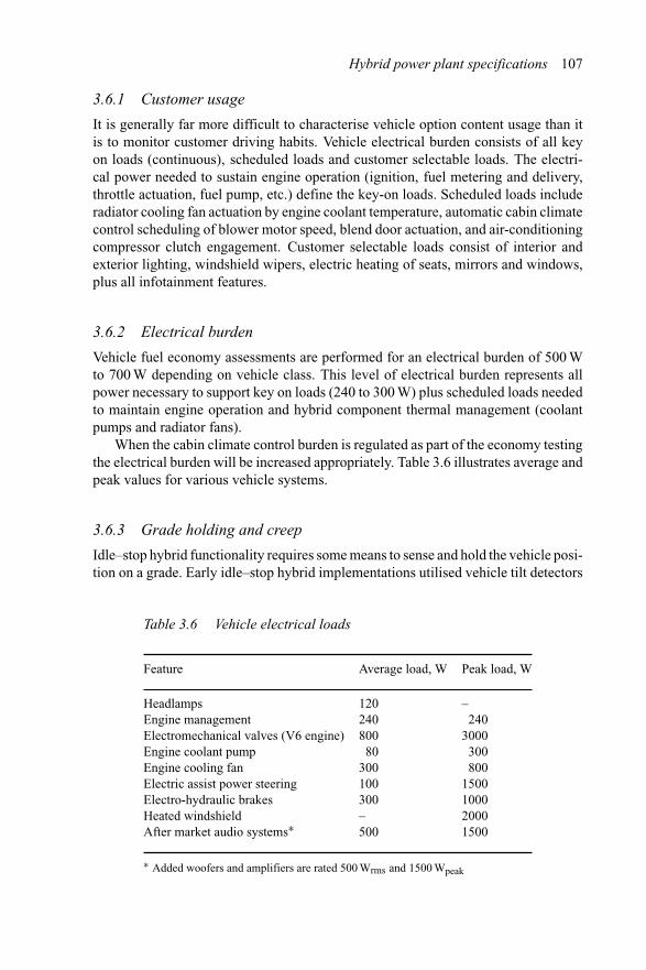
Hybrid power plant specifications 107
3.6.1 Customer usage
It is generally far more difficult to characterise vehicle option content usage than itis to monitor customer driving habits. Vehicle electrical burden consists of all keyon loads (continuous), scheduled loads and customer selectable loads. The electri-cal power needed to sustain engine operation (ignition, fuel metering and delivery,throttle actuation, fuel pump, etc.) define the key-on loads. Scheduled loads includeradiator cooling fan actuation by engine coolant temperature, automatic cabin climatecontrol scheduling of blower motor speed, blend door actuation, and air-conditioningcompressor clutch engagement. Customer selectable loads consist of interior andexterior lighting, windshield wipers, electric heating of seats, mirrors and windows,plus all infotainment features.
3.6.2 Electrical burden
Vehicle fuel economy assessments are performed for an electrical burden of 500 Wto 700 W depending on vehicle class. This level of electrical burden represents allpower necessary to support key on loads (240 to 300 W) plus scheduled loads neededto maintain engine operation and hybrid component thermal management (coolantpumps and radiator fans).
When the cabin climate control burden is regulated as part of the economy testingthe electrical burden will be increased appropriately. Table 3.6 illustrates average andpeak values for various vehicle systems.
3.6.3 Grade holding and creep
Idle–stop hybrid functionality requires some means to sense and hold the vehicle posi-tion on a grade. Early idle–stop hybrid implementations utilised vehicle tilt detectors
Table 3.6 Vehicle electrical loads
Feature Average load, W Peak load, W
Headlamps 120 –Engine management 240 240Electromechanical valves (V6 engine) 800 3000Engine coolant pump 80 300Engine cooling fan 300 800Electric assist power steering 100 1500Electro-hydraulic brakes 300 1000Heated windshield – 2000After market audio systems∗ 500 1500
∗ Added woofers and amplifiers are rated 500 Wrms and 1500 Wpeak
108 Propulsion systems for hybrid vehicles
to sense a grade and apply brakes. Others such as the Aisin–Warner Navimatic trans-mission use global positioning satellite elevation information to sense grades andengage the neutral idle grade holding function. All automatic transmissions providecreep function so that the vehicle does not roll-back when stopped on a grade.
Power split hybrid propulsion systems use a brake on the planetary gear set ringgear to hold a grade. A CVT transmission, for example, would also use a brake tolock the driveline when stopped.
3.6.4 Neutral idle
In a conventional automatic transmission the engine must work against the torqueconverter when the vehicle is stopped. This is a high slip condition on the torqueconverter that consumes fuel during vehicle stopped events. In a hybrid vehicle withautomatic transmission a separate, electrically driven oil pump is necessary to pres-surise the torque converter when the engine is off so that immediately followinga warm restart the vehicle is ready to launch. If the torque converter is not properlyconditioned upon restart and launch there will be a lag as the engine input power fillsand pressurises the torque converter. In a neutral idle transmission the input clutch iscontrolled in slip mode so that the engine does not work against the torque converter.Moreover, the fact that the input clutch is allowed to slip in a controlled mannermeans that normal automatic transmission creep is maintained and driveability doesnot suffer.
Transmissions designed for neutral idle function can gain as much as 2 pointsin overall efficiency by not having a slipping torque converter. Neutral idle is alsoemployed during vehicle braking so that the engine is now working against a partiallystalled transmission. The input clutch is the first clutch on the transmission inputshaft that is tied directly to the torque converter turbine in the Wilson and Lepelletierarchitectures. There is more discussion of the various transmission configurations inChapter 4.
3.7 References
1 Continental Group technology demonstration days, Pontiac Silverdome, Pontiac,MI, Sept. 2001
2 COURTRIGHT, G. ‘Case study of the applicability of applying real-time dataacquisition and monitoring of hybridized powertrains’. Global Powertrain Con-ference, Advanced Propulsion Systems, Sheraton Inn Hotel, Ann Arbor, MI,23–26 September 2002
Chapter 4
Sizing the drive system
The vehicle power plant must be sized for the target vehicle mass, load requirementsand performance goals. Vehicle propulsion system traction is set by the vehicle designmass and acceleration performance according to Newton’s law, F = ma. Acceptableacceleration levels are 0.15 to 0.3 g, which for a 1500 kg vehicle requires an accel-erating force F of 2205 to 4410 N. Aggressive acceleration levels are ∼0.6 g, whichamounts to a tractive wheel force of 8820 N or higher. The limit to tractive force isset by the vehicle mass in terms of normal force at the tyre patches in contact with theroad surface. The typical rubber tyre to asphalt road surface coefficient of friction isμ=0.85; surface coefficient of friction is generally lower than these values due to airconditions, presence of dirt and oil films, etc. Tractive force limits at a tyre patch aregiven as μFNqc, where the normal force is that due to quarter car mass. Tractive forceat the tyre patch in excess of the traction limit results in wheel slip and a dramaticdrop in tyre to road adhesion.
Passenger car propulsion power plants require peak power to vehicle mass ratiosof 10 kW/125 kg for acceptable acceleration performance. Sports and luxury cars tendto raise this metric to over 13 kW/125 kg, whereas compact and sub-compact vehiclestend to ratios somewhat less than 10 kW/125 kg.
In this chapter essential guidelines to propulsion power plant sizing are discussed,including the major hybrid components of M/G, power electronics, and energy storagesystem.
4.1 Matching the electric drive and ICE
One of the most common matching elements used in hybrid electric passenger vehiclesis the epicyclic, or planetary, gear set. Continuously variable transmissions of thecompression belt and toroidal variator variety are gaining popularity in compactvehicles and passenger vans because of seamless transitions in ratio. For larger CVTsthe issues of torque rating and efficiency at high ratio continue to be developmentalareas.
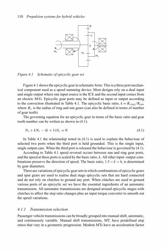
110 Propulsion systems for hybrid vehicles
R
S
C
ωs ωrωc
Figure 4.1 Schematic of epicyclic gear set
Figure 4.1 shows the epicyclic gear in schematic form. This is a three port mechan-ical component used as a speed summing device. Most designs rely on a dual inputand single output where one input source is the ICE and the second input comes froman electric M/G. Epicyclic gear ports may be defined as input or output accordingto the convection illustrated in Table 4.1. The epicyclic basic ratio, k = Rring/Rsun
where Rx is the radius of ring and sun gears (can also be defined in terms of numberof gear teeth).
The governing equation for an epicyclic gear in terms of the basic ratio and geartooth number can be written as shown in (4.1):
Ns + kNr − (k + 1)Nc = 0 (4.1)
In Table 4.1 the relationship noted in (4.1) is used to explain the behaviour ofselected two ports when the third port is held grounded. This is the single input,single output case. When the third port is released the behaviour is governed by (4.1).
According to Table 4.1 speed reversal occurs between sun and ring gear ports,and the speed at these ports is scaled by the basic ratio, k. All other input–output com-binations preserve the direction of speed. The basic ratio, 1.5 < k < 4, is determinedby gear diameters.
There are variations of epicyclic gear sets in which combinations of epicyclic gearsand spur gears are used to realise dual stage epicyclic sets that are hard connectedand do not rely on clutches to ground any port. When clutches are used to groundvarious ports of an epicyclic set we have the essential ingredients of an automatictransmission. All automatic transmissions are designed around epicyclic stages withclutches to affect the step ratio changes plus an input torque converter to smooth outthe speed variations.
4.1.1 Transmission selection
Passenger vehicle transmissions can be broadly grouped into manual shift, automatic,and continuously variable. Manual shift transmissions, MT, have predefined stepratios that vary in a geometric progression. Modern MTs have an acceleration factor
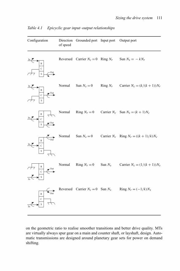
Sizing the drive system 111
Table 4.1 Epicyclic gear input–output relationships
Configuration Directionof speed
Grounded port Input port Output port
R
C
S
In
Out
Reversed Carrier Nc = 0 Ring Nr Sun Ns = − kNr
R
C
S
In
Out
Normal Sun Ns = 0 Ring Nr Carrier Nc = (k/(k + 1))Nr
R
C
S
In
Out
Normal Ring Nr = 0 Carrier Nc Sun Ns = (k + 1)Nc
R
C
S
In
OutNormal Sun Ns = 0 Carrier Nc Ring Nr = ((k + 1)/k)Nc
R
C
SIn
Out
Normal Ring Nr = 0 Sun Ns Carrier Nc = (1/(k + 1))Ns
R
C
SIn
Out
Reversed Carrier Nc = 0 Sun Ns Ring Nr = (−1/k)Ns
on the geometric ratio to realise smoother transitions and better drive quality. MTsare virtually always spur gear on a main and counter shaft, or layshaft, design. Auto-matic transmissions are designed around planetary gear sets for power on demandshifting.
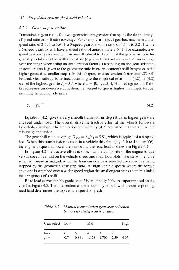
112 Propulsion systems for hybrid vehicles
4.1.2 Gear step selection
Transmission gear ratios follow a geometric progression that spans the desired rangeof speed ratio or shift ratio coverage. For example, a 4-speed gearbox may have a totalspeed ratio of 3.6 : 1 to 3.9 : 1, a 5-speed gearbox with a ratio of 4.3 : 1 to 5.2 : 1 whilea 6-speed gearbox will have a speed ratio of approximately 6 : 1. For example, a 6-speed gearbox is assumed with an overall ratio of 6 : 1 such that the geometric ratio forgear step is taken as the sixth root of six (e.g. r = 1.348 but <r> = 1.23 on averageover the range when using an acceleration factor). Depending on the gear selected,an acceleration is given to the geometric ratio in order to smooth shift busyness in thehigher gears (i.e. smaller steps). In this chapter, an acceleration factor, a=1.33 willbe used. Gear ratio ζx is defined according to the empirical relation in (4.2). In (4.2)we set the highest gear to ζ0=0.7, where x = {0, 1, 2, 3, 4, 5} in retrogression. Ratioζ0 represents an overdrive condition, i.e. output torque is higher than input torque,meaning the engine is lugging:
ζx = ζ0rxa
(4.2)
Equation (4.2) gives a very smooth transition in step ratios as higher gears areengaged under load. The overall driveline tractive effort at the wheels follows ahyperbola envelope. The step ratios predicted by (4.2) are listed in Table 4.2, wherex is the gear number.
The gear shift ratio coverage Gsrc = ζ6/ζ1 = 5.81, which is typical of a 6-speedbox. When this transmission is used in a vehicle driveline (e.g. 3.0 to 4.0 liter V6),the engine torque and power are mapped to the road load as shown in Figure 4.2.
In Figure 4.2 the tractive effort is shown as the composite of the engine torqueversus speed overlaid on the vehicle speed and road load plots. The steps in enginesupplied torque as magnified by the transmission gear selected are shown as beingstepped by the geometric gear step ratio. At high vehicle speeds where the torqueenvelope is stretched over a wider speed region the smaller gear steps act to minimisethe abruptness of a shift.
Road load curves for 0% grade up to 7% and finally 30% are superimposed on thechart in Figure 4.2. The intersection of the traction hyperbola with the correspondingroad load determines the top vehicle speed on grade.
Table 4.2 Manual transmission gear step selectionby accelerated geometric ratio
Gear select Low Mid High
6−x= 6 5 4 3 2 1ζx= 0.7 0.861 1.178 1.709 2.59 4.07
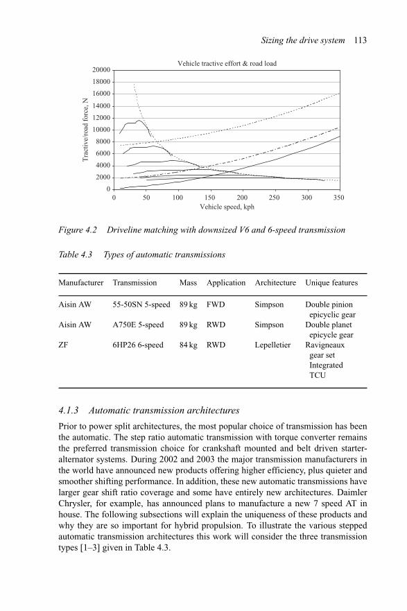
Sizing the drive system 113
Vehicle tractive effort & road load
0
2000
4000
6000
8000
10000
12000
14000
16000
18000
20000
0 50 100 150 200 250 300 350Vehicle speed, kph
Tra
ctiv
e/ro
ad f
orce
, N
Figure 4.2 Driveline matching with downsized V6 and 6-speed transmission
Table 4.3 Types of automatic transmissions
Manufacturer Transmission Mass Application Architecture Unique features
Aisin AW 55-50SN 5-speed 89 kg FWD Simpson Double pinionepicyclic gear
Aisin AW A750E 5-speed 89 kg RWD Simpson Double planetepicycle gear
ZF 6HP26 6-speed 84 kg RWD Lepelletier Ravigneauxgear setIntegratedTCU
4.1.3 Automatic transmission architectures
Prior to power split architectures, the most popular choice of transmission has beenthe automatic. The step ratio automatic transmission with torque converter remainsthe preferred transmission choice for crankshaft mounted and belt driven starter-alternator systems. During 2002 and 2003 the major transmission manufacturers inthe world have announced new products offering higher efficiency, plus quieter andsmoother shifting performance. In addition, these new automatic transmissions havelarger gear shift ratio coverage and some have entirely new architectures. DaimlerChrysler, for example, has announced plans to manufacture a new 7 speed AT inhouse. The following subsections will explain the uniqueness of these products andwhy they are so important for hybrid propulsion. To illustrate the various steppedautomatic transmission architectures this work will consider the three transmissiontypes [1–3] given in Table 4.3.
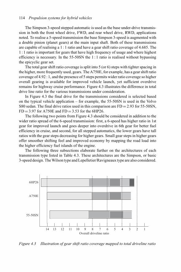
114 Propulsion systems for hybrid vehicles
The Simpson 3-speed stepped automatic is used as the base under-drive transmis-sion in both the front wheel drive, FWD, and rear wheel drive, RWD, applicationsnoted. To realise a 5-speed transmission the base Simpson 3-speed is augmented witha double pinion (planet gears) at the main input shaft. Both of these transmissionsare capable of realising a 1 : 1 ratio and have a gear shift ratio coverage of 4.685. The1 : 1 ratio is important for gears that have high frequency of usage and where highestefficiency is necessary. In the 55-50SN the 1 : 1 ratio is realised without bypassingthe epicyclic gear set.
The total gear shift ratio coverage is split into 5 (or 6) steps with tighter spacing inthe higher, more frequently used, gears. The A750E, for example, has a gear shift ratiocoverage of 4.92 : 1, and the presence of 5 steps permits wider ratio coverage so higheroverall gearing is available for improved vehicle launch, yet sufficient overdriveremains for highway cruise performance. Figure 4.3 illustrates the difference in totaldrive line ratio for the various transmissions under consideration.
In Figure 4.3 the final drive for the transmissions considered is selected basedon the typical vehicle application – for example, the 55-50SN is used in the VolvoS80 sedan. The final drive ratios used in this comparison are FD = 2.93 for 55-50SN,FD = 3.97 for A750E and FD = 3.53 for the 6HP26.
The following two points from Figure 4.3 should be considered in addition to thewider ratio spread of the 6-speed transmission: first, a 6-speed has higher ratio in 1stgear for improved launch and goes deeper into overdrive in 6th gear for better fuelefficiency in cruise, and second, for all stepped automatics, the lower gears have tallratios with the gear steps decreasing for higher gears. Small gear steps in higher gearsoffer smoother shifting feel and improved economy by mapping the road load intothe higher efficiency fuel islands of the engine.
The following three subsections elaborate further on the architectures of eachtransmission type listed in Table 4.3. These architectures are the Simpson, or basic3-speed design. The Wilson type and Lepelletier/Ravigneaux type are also considered.
Overall driveline ratio
6HP26
A750E
55-50SN
1234567891011121314
Figure 4.3 Illustration of gear shift ratio coverage mapped to total driveline ratio
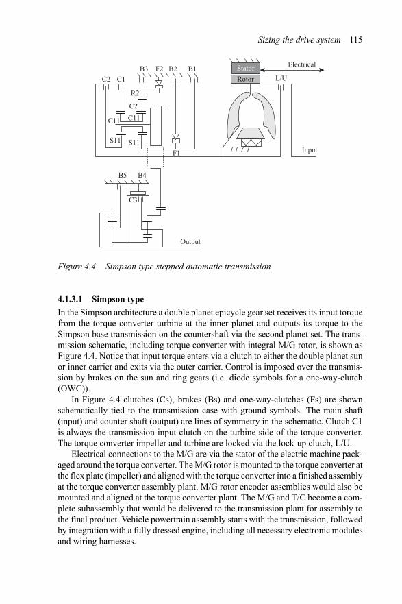
Sizing the drive system 115
Rotor
Stator
C1C2
B3 F2 B2 B1
F1
L/U
Input
C11
S11
R2
C2
C11
S11
Electrical
B5 B4
C3
Output
Figure 4.4 Simpson type stepped automatic transmission
4.1.3.1 Simpson type
In the Simpson architecture a double planet epicycle gear set receives its input torquefrom the torque converter turbine at the inner planet and outputs its torque to theSimpson base transmission on the countershaft via the second planet set. The trans-mission schematic, including torque converter with integral M/G rotor, is shown asFigure 4.4. Notice that input torque enters via a clutch to either the double planet sunor inner carrier and exits via the outer carrier. Control is imposed over the transmis-sion by brakes on the sun and ring gears (i.e. diode symbols for a one-way-clutch(OWC)).
In Figure 4.4 clutches (Cs), brakes (Bs) and one-way-clutches (Fs) are shownschematically tied to the transmission case with ground symbols. The main shaft(input) and counter shaft (output) are lines of symmetry in the schematic. Clutch C1is always the transmission input clutch on the turbine side of the torque converter.The torque converter impeller and turbine are locked via the lock-up clutch, L/U.
Electrical connections to the M/G are via the stator of the electric machine pack-aged around the torque converter. The M/G rotor is mounted to the torque converter atthe flex plate (impeller) and aligned with the torque converter into a finished assemblyat the torque converter assembly plant. M/G rotor encoder assemblies would also bemounted and aligned at the torque converter plant. The M/G and T/C become a com-plete subassembly that would be delivered to the transmission plant for assembly tothe final product. Vehicle powertrain assembly starts with the transmission, followedby integration with a fully dressed engine, including all necessary electronic modulesand wiring harnesses.
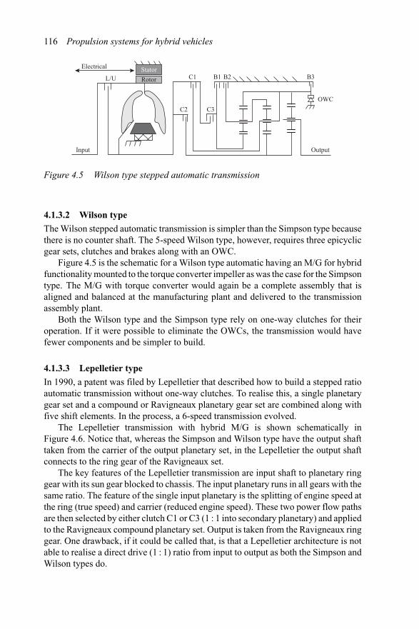
116 Propulsion systems for hybrid vehicles
C1 B1 B2 B3
OWC
L/U
Input
C2 C3
Electrical
Output
Rotor
Stator
Figure 4.5 Wilson type stepped automatic transmission
4.1.3.2 Wilson type
The Wilson stepped automatic transmission is simpler than the Simpson type becausethere is no counter shaft. The 5-speed Wilson type, however, requires three epicyclicgear sets, clutches and brakes along with an OWC.
Figure 4.5 is the schematic for a Wilson type automatic having an M/G for hybridfunctionality mounted to the torque converter impeller as was the case for the Simpsontype. The M/G with torque converter would again be a complete assembly that isaligned and balanced at the manufacturing plant and delivered to the transmissionassembly plant.
Both the Wilson type and the Simpson type rely on one-way clutches for theiroperation. If it were possible to eliminate the OWCs, the transmission would havefewer components and be simpler to build.
4.1.3.3 Lepelletier type
In 1990, a patent was filed by Lepelletier that described how to build a stepped ratioautomatic transmission without one-way clutches. To realise this, a single planetarygear set and a compound or Ravigneaux planetary gear set are combined along withfive shift elements. In the process, a 6-speed transmission evolved.
The Lepelletier transmission with hybrid M/G is shown schematically inFigure 4.6. Notice that, whereas the Simpson and Wilson type have the output shafttaken from the carrier of the output planetary set, in the Lepelletier the output shaftconnects to the ring gear of the Ravigneaux set.
The key features of the Lepelletier transmission are input shaft to planetary ringgear with its sun gear blocked to chassis. The input planetary runs in all gears with thesame ratio. The feature of the single input planetary is the splitting of engine speed atthe ring (true speed) and carrier (reduced engine speed). These two power flow pathsare then selected by either clutch C1 or C3 (1 : 1 into secondary planetary) and appliedto the Ravigneaux compound planetary set. Output is taken from the Ravigneaux ringgear. One drawback, if it could be called that, is that a Lepelletier architecture is notable to realise a direct drive (1 : 1) ratio from input to output as both the Simpson andWilson types do.
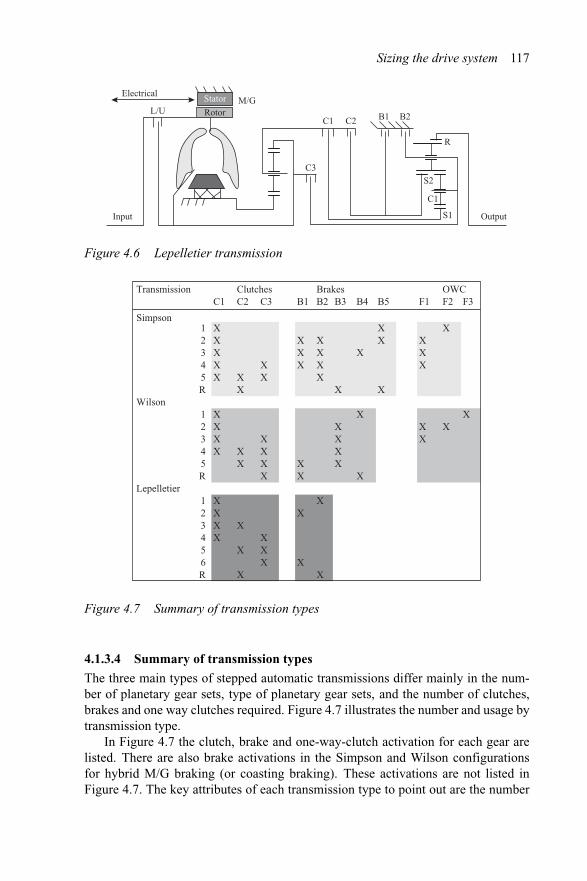
Sizing the drive system 117
M/GL/U
Input
Electrical
Rotor
Stator
Output
C1 C2 B1 B2
C3
S1
C1
S2
R
Figure 4.6 Lepelletier transmission
Transmission Clutches Brakes OWCC1 C2 C3 B1 B2 B3 B4 B5 F1 F2 F3
Simpson1 X X X2 X X X X X3 X X X X X4 X X X X X5 X X X XR X X X
Wilson1 X X X2 X X X X3 X X X X4 X X X X5 X X X XR X X X
Lepelletier1 X X2 X X3 X X4 X X5 X X6 X XR X X
Figure 4.7 Summary of transmission types
4.1.3.4 Summary of transmission types
The three main types of stepped automatic transmissions differ mainly in the num-ber of planetary gear sets, type of planetary gear sets, and the number of clutches,brakes and one way clutches required. Figure 4.7 illustrates the number and usage bytransmission type.
In Figure 4.7 the clutch, brake and one-way-clutch activation for each gear arelisted. There are also brake activations in the Simpson and Wilson configurationsfor hybrid M/G braking (or coasting braking). These activations are not listed inFigure 4.7. The key attributes of each transmission type to point out are the number
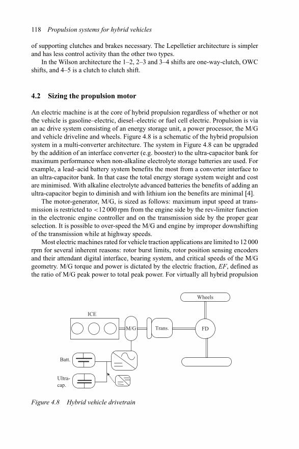
118 Propulsion systems for hybrid vehicles
of supporting clutches and brakes necessary. The Lepelletier architecture is simplerand has less control activity than the other two types.
In the Wilson architecture the 1–2, 2–3 and 3–4 shifts are one-way-clutch, OWCshifts, and 4–5 is a clutch to clutch shift.
4.2 Sizing the propulsion motor
An electric machine is at the core of hybrid propulsion regardless of whether or notthe vehicle is gasoline–electric, diesel–electric or fuel cell electric. Propulsion is viaan ac drive system consisting of an energy storage unit, a power processor, the M/Gand vehicle driveline and wheels. Figure 4.8 is a schematic of the hybrid propulsionsystem in a multi-converter architecture. The system in Figure 4.8 can be upgradedby the addition of an interface converter (e.g. booster) to the ultra-capacitor bank formaximum performance when non-alkaline electrolyte storage batteries are used. Forexample, a lead–acid battery system benefits the most from a converter interface toan ultra-capacitor bank. In that case the total energy storage system weight and costare minimised. With alkaline electrolyte advanced batteries the benefits of adding anultra-capacitor begin to diminish and with lithium ion the benefits are minimal [4].
The motor-generator, M/G, is sized as follows: maximum input speed at trans-mission is restricted to <12 000 rpm from the engine side by the rev-limiter functionin the electronic engine controller and on the transmission side by the proper gearselection. It is possible to over-speed the M/G and engine by improper downshiftingof the transmission while at highway speeds.
Most electric machines rated for vehicle traction applications are limited to 12 000rpm for several inherent reasons: rotor burst limits, rotor position sensing encodersand their attendant digital interface, bearing system, and critical speeds of the M/Ggeometry. M/G torque and power is dictated by the electric fraction, EF, defined asthe ratio of M/G peak power to total peak power. For virtually all hybrid propulsion
M/G
ICE
Trans. FD
Wheels
Batt.
Ultra-cap.
Figure 4.8 Hybrid vehicle drivetrain
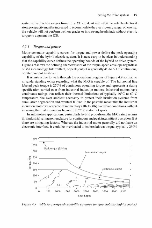
Sizing the drive system 119
systems this fraction ranges from 0.1 < EF < 0.4. At EF > 0.4 the vehicle electricalstorage capacity must be increased to accommodate the electric-only range, otherwise,the vehicle will not perform well on grades or into strong headwinds without electrictorque to augment the ICE.
4.2.1 Torque and power
Motor-generator capability curves for torque and power define the peak operatingcapability of the hybrid electric system. It is necessary to be clear in understandingthat the capability curve defines the operating bounds of the hybrid ac drive system.Figure 4.9 shows the defining characteristics of the torque-speed envelope regardlessof M/G technology. Intermittent, or peak, output is generally 4/3 to 5/3 of continuous,or rated, output as shown.
It is instructive to walk through the operational regions of Figure 4.9 so that nomisunderstanding exists regarding what the M/G is capable of. The horizontal linelabeled peak torque is 250% of continuous operating torque and represents a sizingspecification carried over from industrial induction motors. Industrial motors havecontinuous ratings that reflect their thermal limitations of typically 40◦C to 60◦Ctemperature rise over ambient necessary to protect their insulation systems fromcumulative degradation and eventual failure. In the past this meant that the industrialinduction motor was capable of momentary (10s to 30s) overdrive conditions withoutincurring thermal excursions beyond 180◦C at stator hot spots.
In automotive applications, particularly hybrid propulsion, the M/G rating retainsthis industrial rating nomenclature for continuous and peak intermittent operation. Butthere are mitigating factors. Whereas the industrial motor generally did not have anelectronic interface, it could be overloaded to its breakdown torque, typically 250%
Peak torque (38Nm)Intermittent output
Continuous outputTor
que,
Nm
400
350
300
250
200
150
100
50
00 500 1000 1500 2000 2500
Speed, rpm
3000 3500 4000 4500
80
85 9090
6565
Figure 4.9 M/G torque-speed capability envelope (unique-mobility hightor motor)
120 Propulsion systems for hybrid vehicles
of the thermal limited torque in class-B designs, for short durations. The regionbounded by the speed axis, the torque axis, the flat line representing constant torque,and a vertical to trapezoidal boundary back to the speed axis represents the constanttorque operating region. In the constant torque operating region the power electronicsinverter has sufficient voltage from the dc bus (battery or ultra-capacitor or generatoror some combination) to synthesise currents for injection into the electric machine.When the machine speed increases to the corner point speed defining the break pointbetween constant torque and constant power the inverter has essentially run out ofvoltage, the modulator that regulates current synthesis begins pulse dropping, andthe process ends with the inverter entering six step mode (also called block mode).Constant power is the region of field weakening bounded by the already mentionedconstant torque region plus the hyperbola that defines the continuous or intermittentpower envelope, and the speed axis. Useful operation ceases when the machine enterssecond breakdown. This last bit of terminology may not be as widespread as firstbreakdown (i.e. corner point or base speed) is for the region where constant torquetransitions into constant power.
In the second breakdown region different processes begin to dominate the electricmachine’s ability to produce torque, and these processes are technology dependent.We saw that first breakdown is dependent on ac drive system power supply andmachine design in that its corner point is defined as that speed at which the machine’sinternal voltage approximates the input dc supply voltage. During field weakeningthis internal voltage effect is mitigated so that current can continue to be injected intothe machine at rated value – hence constant power. Now, when the electric machinereaches the final limits of holding constant power the power begins to break down.In an asynchronous machine second breakdown is reached when the slip parame-ter increases from rated slip to breakdown slip. Torque is at its breakdown limit(∼V 2
s /ωLleakage, where the parameters are supply voltage and leakage inductance)and the machine slip is held constant at its breakdown value (again, typically 250%of rated). Beyond this second breakdown speed the current drops reciprocally withspeed so power also drops with the reciprocal of speed and torque is dropping as1/speed2.
In a permanent magnet synchronous machine of any variety the second break-down speed occurs when the injected current can no longer be held constant whilefield weakening is in progress. This occurs in a surface magnet machine or to someextent in an inset magnet machine when the angle control of the injected currentsexceeds about 30◦. For an interior magnet machine the second breakdown pointis much further out in field weakening and occurs when the d-axis, or magnet axiscurrent, is no longer able to hold the machine internal voltage constant because ithas reached the rated value of input current, i.e. there is no longer any componentof input current left to develop torque. When this condition occurs the machine iscompletely out of torque. In a variable reluctance, or switched reluctance, machinethe conditions of second breakdown are somewhat similar to the permanent mag-net machine. During constant torque operation of the variable reluctance machinethe current dwell angle is controlled while operating at fixed advance angle. Dur-ing constant power operation the dwell is fixed as the advance angle of current is
Sizing the drive system 121
progressively shifted ahead in time. When the advance angle is no longer capable ofbeing advanced the machine enters second breakdown and power drops reciprocallywith speed.
We can say that operating at peak torque on the capability curve is not the casein hybrid propulsion M/G design practice. True, the electric machine retains someoverdrive capacity, but in general the electric machine is designed for operation atnear its maximum capability during intermittent use (10s to 30s). It is the limitationof the power electronics that determines the envelope of the M/G capability. Thesemiconductor power driver stage has no provision for overdrive conditions. Thesemiconductor devices have thermal time constants of milliseconds so that a 10soverdrive condition in reality is steady state for power electronics. Therefore, theintermittent operation envelope shown in Figure 4.9 represents the limit of the powerelectronics more so than for the machine. The following definitions are made toemphasize the limitations of such capability curves:
• Continuous rating: The ac drive can be operated within its continuous rated regionindefinitely provided: (1) the motor thermal management system is operated at orbelow its cooling medium maximum inlet temperature conditions for the coolantused (air or liquid); (2) the power inverter thermal management system is within itsmaximum inlet temperature of coolant (air or liquid); and (3) the power electronicselectrical parameters are within nominal stress levels of 50% . For example, theoperating voltage of power switching devices should be at 50% of the device ratedbreakdown voltage.
• Intermittent overload operation is permitted for short durations (<30s) to containlow energy transients such as responding to fast gear changes or clutch actuationintervals when the M/G may be called upon to furnish additional torque and power.
• Peak overload operation is within the capability of the electric machine but outsidethe capability of the power electronics. There have been attempts to redefinethis peak condition to contain fast transients having low energy but very highpower – for example, an ISA mild hybrid in which engine cranking is desiredunder cold conditions. Some specifications may call for peak overdrive torquefor <50 ms in order to overcome engine crankshaft striction. The applicationof a very high torque impulse is necessary to breakaway the engine and permitsustained cranking at the ac drive system intermittent rating. At issue here isthe need for the power electronics to sustain overcurrents at the peak overdrivecondition. Such requirements generally do not pan out because the electronicsmust still be sized for the peak operating envelope.
• Thermal management systems for passenger car hybrids consist of auxiliarycoolant reservoirs, pumps and fans, along with a small radiator. The M/G willhave a separate coolant supply from either the vehicle’s engine coolant (<115◦C)
or transmission oil cooler (<120◦C). The power electronics coolant is restrictedto glycol–water mixtures having a maximum inlet temperature of 65◦C. Withthis thermal boundary condition on the power electronics internal cold plate thetemperature fluctuations at the semiconductor junctions can be held to <40◦Ctemperature rise and thereby achieve high durability (>6000 h life).
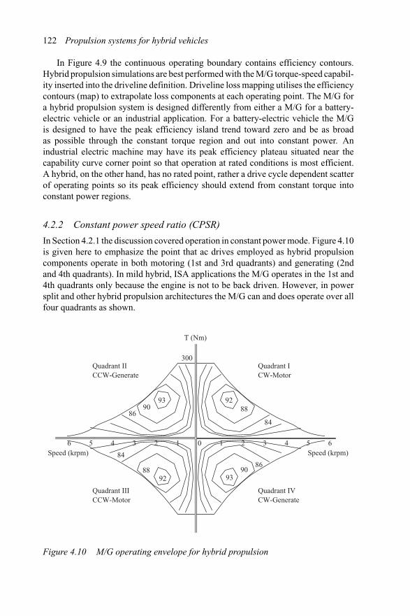
122 Propulsion systems for hybrid vehicles
In Figure 4.9 the continuous operating boundary contains efficiency contours.Hybrid propulsion simulations are best performed with the M/G torque-speed capabil-ity inserted into the driveline definition. Driveline loss mapping utilises the efficiencycontours (map) to extrapolate loss components at each operating point. The M/G fora hybrid propulsion system is designed differently from either a M/G for a battery-electric vehicle or an industrial application. For a battery-electric vehicle the M/Gis designed to have the peak efficiency island trend toward zero and be as broadas possible through the constant torque region and out into constant power. Anindustrial electric machine may have its peak efficiency plateau situated near thecapability curve corner point so that operation at rated conditions is most efficient.A hybrid, on the other hand, has no rated point, rather a drive cycle dependent scatterof operating points so its peak efficiency should extend from constant torque intoconstant power regions.
4.2.2 Constant power speed ratio (CPSR)
In Section 4.2.1 the discussion covered operation in constant power mode. Figure 4.10is given here to emphasize the point that ac drives employed as hybrid propulsioncomponents operate in both motoring (1st and 3rd quadrants) and generating (2ndand 4th quadrants). In mild hybrid, ISA applications the M/G operates in the 1st and4th quadrants only because the engine is not to be back driven. However, in powersplit and other hybrid propulsion architectures the M/G can and does operate over allfour quadrants as shown.
T (Nm)
300
8690
93 9288
84
8690
939288
84Speed (krpm) Speed (krpm)
Quadrant IICCW-Generate
Quadrant ICW-Motor
Quadrant IIICCW-Motor
Quadrant IVCW-Generate
6 5 4 3 2 1 10 2 3 4 5 6
Figure 4.10 M/G operating envelope for hybrid propulsion
Sizing the drive system 123
Motoring operation of the M/G occurs for positive torque and positive (CCW)speed or for negative torque and negative (CW) speed. When the sign of either torqueor speed are reversed the M/G is in generating mode. With modern power electroniccontrollers the machine is capable of operating anywhere within the confines of itstorque–speed envelope shown in Figure 4.10. For example, a transition from motoringat 2.5 krpm and 100 Nm of torque to generating at 2.5 krpm and −100 Nm of torqueis simply a sign change in the power electronics controller. The speed and hencemachine voltages remain constant, or perhaps the voltage gets boosted somewhat bycharging demands, but the machine currents slew at their electrical time constant toresume operation as a generator with phase currents in phase opposition to phasevoltages (generally sinusoidal variables). Since the machine transient electrical timeconstants are easily 10s if not 100s of times faster than the mechanical system, thetorque change is viewed as occurring nearly instantaneously.
Now, if the machine were operating in motoring mode at 2.5 krpm and +100 Nmof torque, which is basically in boosting mode for, say, passing, and the driver abortsthe manoeuvre and slows to re-enter traffic, the M/G may be commanded to switchto generating at −100 Nm of torque, for example, but at a lower speed, say 1.5 krpm.Since the M/G was operating well into field weakening (according to the chart inFigure 4.10) initially and the new operating point is basically on the constant torqueboundary (full field), the controller must boost the field to maintain the commandedgenerating level. This process is slower than simply changing the torque at constantspeed. The flux in the machine must be readjusted to its new and higher level, andthis occurs at the electrical time constant of field control in the machine (depends onmachine size/rating and ranges from 30 ms to >100 ms for hybrid traction motors).Whereas torque control was responding in sub-millisecond times, field control takesmuch longer. However, this is still about 10 times faster than the mechanical sys-tem. The same process occurs going from CCW motoring to CW generating exceptthat the speed is now determined by the mechanical system at its much slower timeconstant. The M/G power controller easily tracks the speed changes of normal oper-ation. We will see later that some manoeuvres can be more demanding on the M/Gresponse.
The four major classes of electric machines suitable for hybrid propulsion appli-cations are highlighted in the taxonomy of electric machines in Figure 4.11. Thereare only two major classes of electric machines, those that are synchronous withapplied excitation and those that are asynchronous to it. When excitation of the elec-tric machine rotor is direct current, dc, via field windings or permanent magnets, themachine is a synchronous type. When excitation of the electric machine rotor is ac,then operation is asynchronous. The definition gets vague when inside out motors areused, such as brushed dc motors with stationary permanent magnets. However, thedistinction persists in how the machine excitation is applied, be it dc or ac.
The acronyms defined in Figure 4.11 will be used throughout this book. Theseare IM for induction machine of cage rotor (cast aluminium) or wound rotor (i.e.slip rings), IPM for interior magnet designs, SPM for surface permanent magnet andVRM for variable reluctance, doubly salient designs. There are many variants ofthese electric machines such as drum versus axial, normal versus inside out, rotary
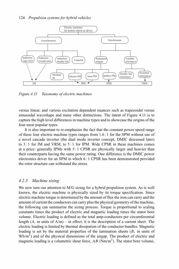
124 Propulsion systems for hybrid vehicles
Electric machinesfor hybrid vehicle ac drives
Asynchronous Synchronous
Inductioncage rotor
Inductionwound rotor
Inductiondoubly fed Unipolar
Permanentmagnet
Variablereluctance
Switchedreluctance
Doubly fedreluctanceSurface PMInset PMInterior PM
Brusheddc
IM IPM SPM VRM
Figure 4.11 Taxonomy of electric machines
versus linear, and various excitation dependent nuances such as trapezoidal versussinusoidal waveshape and many other distinctions. The intent of Figure 4.11 is tocapture the high level differences in machine types and to showcase the origins of thefour most popular types.
It is also important to re-emphasize the fact that the constant power speed rangeof these four electric machine types ranges from 1.6 : 1 for the SPM without use ofa novel cascade inverter (the dual mode inverter concept, DMIC discussed later)to 3 : 1 for IM and VRM, to 5 : 1 for IPM. Wide CPSR in these machines comesat a price: generally IPMs with 5 : 1 CPSR are physically larger and heavier thantheir counterparts having the same power rating. One difference is the DMIC powerelectronics driver for an SPM in which 6 : 1 CPSR has been demonstrated providedthe rotor structure can withstand the stress.
4.2.3 Machine sizing
We now turn our attention to M/G sizing for a hybrid propulsion system. As is wellknown, the electric machine is physically sized by its torque specification. Sinceelectric machine torque is determined by the amount of flux the iron can carry and theamount of current the conductors can carry plus the physical geometry of the machine,the following can summarise the sizing process. Torque is proportional to scalingconstants times the product of electric and magnetic loading times the stator borevolume. Electric loading is defined as the total amp-conductors per circumferentiallength (A, in units of A/m) – in effect, it is the description of a current sheet. Theelectric loading is limited by thermal dissipation of the conductor bundles. Magneticloading is set by the material properties of the lamination sheets (B, in units ofWb/m2) and of the physical dimensions of the airgap. The product of electric andmagnetic loading is a volumetric shear force, AB (Nm/m3). The stator bore volume,
Sizing the drive system 125
D2L, defines the airgap surface area (πDL) times the torque lever arm (D) of therotor on which the volumetric shear force acts. The scaling constants and coefficientsare absorbed into the proportionality constant for M/G torque in terms of its designloading and geometry. For electric machines of interest to hybrid propulsion thevolumetric shear force ranges from 25 000 to 80 000 Nm/m3. The relationship formachine torque is
T = kABD2L (4.3)
where k is a constant that includes geometry variables, and excitation waveshapevariables for voltage and currents. The bore diameter D, or more accurately the rotorOD, is the main sizing variable in electric machine design. Sizing is constrainedby four fundamental limits. Two of the fundamental sizing constraints have beendiscussed thus far: electric and magnetic loading. To further explain these sizingconstraints it is important to understand the limitations on current carrying capacityof copper (aluminium for induction machines). Current carrying capacity of copperwire is limited by its thermal dissipation, which in turn sets bounds on current density,Jcu. In electric machine design practice these bounds are
Jcu =⎧⎨⎩
2620
⎫⎬⎭ ←→
A/mm2@
⎧⎨⎩
Cont.3 min30s
⎫⎬⎭ (4.4)
Equation (4.4) has contained in it the thermal constraints of the machine sizingdesign. Higher current densities, up to 2 × 10⁸ A/m2 for copper, define its fusingcurrent limit.
Conductors are placed in slots in the stator iron. The tooth surface to tooth-slotpitch must maintain sufficient surface area in order to support the magnetic loadingfor the materials used and the particular choice of machine technology. Table 4.4summarises magnetic loading for the four major classes of electric machines.
The electric loading, A, for the various machine technologies listed in Table 4.4,is determined by using the current density limitations (4.4), from which the bounds
Table 4.4 Electric machine sizing: magnetic loading
Type Symbol Airgap mm B Wb/m2
Surface permanent magnet machine SPM <1.5 ∼0.82Interior/inset permanent magnet machine IPM ∼1.0 0.7Asynchronous, induction machine (also sync. rel.) IM ∼0.6 0.7Variable/switched reluctance machine VRM <0.5 0.8*
*Highly localized in gap between surfaces of opposing double saliencies.
126 Propulsion systems for hybrid vehicles
on electric loading can be found as:
A =
⎧⎪⎪⎨⎪⎪⎩
3 − min Techno log y 30s6 × 104 SPM 8 × 10⁴
3 × 10⁴ IPM 4.5 × 10⁴
3 × 10⁴ IM/VRM 4.5 × 10⁴
⎫⎪⎪⎬⎪⎪⎭ (Arms/m) (4.5)
Notice that the electric loading definitions in (4.5) are in Amps-rms per meter,not in peak amps. This is well defined for sinusoidal machines, but somewhat limitedfor non-sinusoidal machines such as the VRM.
The machine sizing procedure using (4.3), and supported by the definitions ofelectric and magnetic loading, permits the first approximation to machine sizingto be accomplished without resorting to finite element or detailed computer designsince the lamination design has not been fixed at this point, only the major packagingdimensions. The process of working with electromagnetic surface traction as justdescribed is akin to having a detailed lamination design, imposing the electric loading,and then using a magnetics finite element solver to find the flux and from this usinga post-processing calculation of the Maxwell shear force at the rotor surface (afteraveraging over the pole pair area).
The machine design is further constrained by a mechanical limit – the rotor burstcondition. For this constraint it is common design practice to limit the machine rotortangential velocity to <200 m/s. Surface speeds in excess of this lead to retentionissues of various sorts, windings, magnets, etc. It is interesting that the mechani-cal limit is linear with angular velocity and not quadratic as application of materialstress analysis would reveal. The following summary of large electric machinesin which rotor diameter, power rating and surface tangential speed is listed sup-ports the engineering practice of limiting rotor speeds according to a linear velocityconstraint [5].
Table 4.5 supports the engineering practice of limiting electric machine rotortangential speeds to less than 200 m/s. At higher speeds the issues of critical speedflexing, rotor retention and eccentricity become major concerns.
Table 4.5 Mechanical constraint: large electric machines
Machine rating, MW Cooling method Rotor diameter, m Rotor surface speed, m/s
25 Air 0.75 141120 Air 0.95 179150 H2 1.1 207320 Water 1.15 217757 Water 1.06 199932 Water 1.25 235
Note: H2 means hydrogen cooling. All machines are 2 pole.
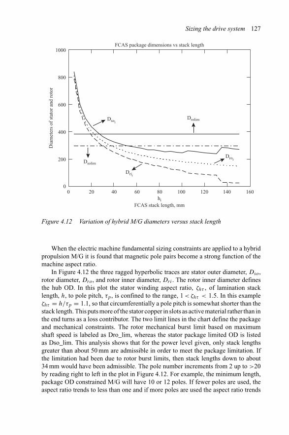
Sizing the drive system 127
0 20 40 60 80 100 120 140 1600
200
400
600
800
1000FCAS package dimensions vs stack length
FCAS stack length, mm
Dia
met
ers
of s
tato
r an
d ro
tor
Dsoi
Droi
Drii
Dsolim
Drolim
hi
Figure 4.12 Variation of hybrid M/G diameters versus stack length
When the electric machine fundamental sizing constraints are applied to a hybridpropulsion M/G it is found that magnetic pole pairs become a strong function of themachine aspect ratio.
In Figure 4.12 the three ragged hyperbolic traces are stator outer diameter, Dso,rotor diameter, Dro, and rotor inner diameter, Dri . The rotor inner diameter definesthe hub OD. In this plot the stator winding aspect ratio, ζhτ , of lamination stacklength, h, to pole pitch, τp, is confined to the range, 1 < ζhτ < 1.5. In this exampleζhτ = h/τp = 1.1, so that circumferentially a pole pitch is somewhat shorter than thestack length. This puts more of the stator copper in slots as active material rather than inthe end turns as a loss contributor. The two limit lines in the chart define the packageand mechanical constraints. The rotor mechanical burst limit based on maximumshaft speed is labeled as Dro_lim, whereas the stator package limited OD is listedas Dso_lim. This analysis shows that for the power level given, only stack lengthsgreater than about 50 mm are admissible in order to meet the package limitation. Ifthe limitation had been due to rotor burst limits, then stack lengths down to about34 mm would have been admissible. The pole number increments from 2 up to >20by reading right to left in the plot in Figure 4.12. For example, the minimum length,package OD constrained M/G will have 10 or 12 poles. If fewer poles are used, theaspect ratio trends to less than one and if more poles are used the aspect ratio trends
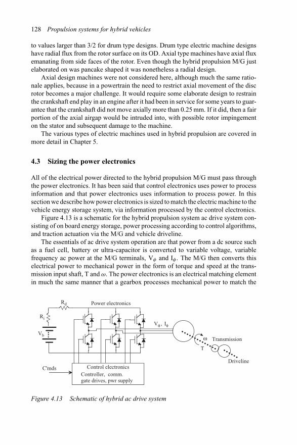
128 Propulsion systems for hybrid vehicles
to values larger than 3/2 for drum type designs. Drum type electric machine designshave radial flux from the rotor surface on its OD. Axial type machines have axial fluxemanating from side faces of the rotor. Even though the hybrid propulsion M/G justelaborated on was pancake shaped it was nonetheless a radial design.
Axial design machines were not considered here, although much the same ratio-nale applies, because in a powertrain the need to restrict axial movement of the discrotor becomes a major challenge. It would require some elaborate design to restrainthe crankshaft end play in an engine after it had been in service for some years to guar-antee that the crankshaft did not move axially more than 0.25 mm. If it did, then a fairportion of the axial airgap would be intruded into, with possible rotor impingementon the stator and subsequent damage to the machine.
The various types of electric machines used in hybrid propulsion are covered inmore detail in Chapter 5.
4.3 Sizing the power electronics
All of the electrical power directed to the hybrid propulsion M/G must pass throughthe power electronics. It has been said that control electronics uses power to processinformation and that power electronics uses information to process power. In thissection we describe how power electronics is sized to match the electric machine to thevehicle energy storage system, via information processed by the control electronics.
Figure 4.13 is a schematic for the hybrid propulsion system ac drive system con-sisting of on board energy storage, power processing according to control algorithms,and traction actuation via the M/G and vehicle driveline.
The essentials of ac drive system operation are that power from a dc source suchas a fuel cell, battery or ultra-capacitor is converted to variable voltage, variablefrequency ac power at the M/G terminals, Vφ and Iφ . The M/G then converts thiselectrical power to mechanical power in the form of torque and speed at the trans-mission input shaft, T and ω. The power electronics is an electrical matching elementin much the same manner that a gearbox processes mechanical power to match the
Vb
Ri
Rd
Vφ , Iφ
T
ω
Controller, comm.gate drives, pwr supply
C'mds
Power electronics
Control electronics
Transmission
Driveline
Figure 4.13 Schematic of hybrid ac drive system
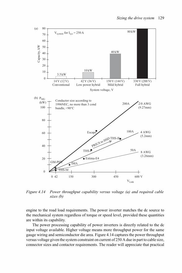
Sizing the drive system 129
Vsystem for Isys = 250 A
3.5 kW10 kW
40 kW
0
10
20
30
40
50
60
70
80
14 V (12 V)Conventional
42 V (36 V)Low power hybrid
150 V (144 V)Mild hybrid
330 V (288 V)Full hybrid
System voltage, V
Cap
acity
, kW
80 kW
0 42 150 300 450 600 VVLink
PMG
(kW)
50A
100A
200A 2/0 AWG (9.27mm)
4 AWG (5.2mm)
8 AWG (3.26mm)
Conductor size according to 1996NEC, no more than 3 cond bundle, <90°C
GM-PHT
THS-M
IMA
Estima-E4
THS-I
THS-II
Escape
PRIUS to HSD
80
60
40
20
0
100
(a)
(b)
Figure 4.14 Power throughput capability versus voltage (a) and required cablesizes (b)
engine to the road load requirements. The power inverter matches the dc source tothe mechanical system regardless of torque or speed level, provided these quantitiesare within its capability.
The power processing capability of power inverters is directly related to the dcinput voltage available. Higher voltage means more throughput power for the samegauge wiring and semiconductor die area. Figure 4.14 captures the power throughputversus voltage given the system constraint on current of 250 A due in part to cable size,connector sizes and contactor requirements. The reader will appreciate that practical
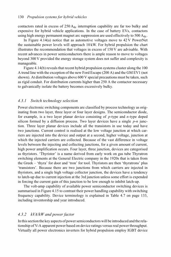
130 Propulsion systems for hybrid vehicles
contactors rated in excess of 250 Adc interruption capability are far too bulky andexpensive for hybrid vehicle applications. In the case of battery EVs, contactorsusing high energy permanent magnet arc suppression are used effectively to 500 Adc.
In Figure 4.14(a) notice that as automotive voltages move to 42 V PowerNetthe sustainable power levels will approach 10 kW. For hybrid propulsion the chartillustrates the recommendation that voltages in excess of 150 V are advisable. Withrecent advances in power semiconductors there is ample reason to move to voltagesbeyond 300 V provided the energy storage system does not suffer and complexity ismanageable.
Figure 4.14(b) reveals that recent hybrid propulsion systems cluster along the 100A trend line with the exception of the new Ford Escape (200 A) and the GM EV1 (notshown). At distribution voltages above 600 V special precautions must be taken, suchas rigid conduit. For distribution currents higher than 250 A the contactor necessaryto galvanically isolate the battery becomes excessively bulky.
4.3.1 Switch technology selection
Power electronic switching components are classified by process technology as orig-inating from two layer, three layer or four layer designs. The semiconductor diode,for example, is a two layer planar device consisting of p-type and n-type dopedsilicon formed by a diffusion process. Two layer devices have a single p-n junc-tion. Three layer planar devices include all the transistors in use today and havetwo junctions. Current control is realised at the low voltage junction at which car-riers are injected into the device and output at a second, higher voltage, junction atwhich the injected carriers are collected. Because of the vast difference in voltagelevels between the injecting and collecting junctions, for a given amount of current,high power amplification occurs. Four layer, three junction, devices are categorisedas thyristors. ‘Thyristor’ is a name derived from early work on gas tube Thyratronswitching elements at the General Electric company in the 1920s that is taken fromthe Greek – ‘thyra’ for door and ‘tron’ for tool. Thyristors are then ‘thyratrons’ plus‘transistors’. Because there are two junctions from which carriers are injected inthyristors, and a single high voltage collector junction, the devices have a tendencyto latch-up due to current injection at the 3rd junction unless some effort is expendedin forcing the current gain of this junction to be low enough to inhibit latch-up.
The volt-amp capability of available power semiconductor switching devices issummarised in Figure 4.15 to contrast their power handling capability with switchingfrequency capability. Device terminology is explained in Table 4.7 on page 133,including inventorship and year introduced.
4.3.2 kVA/kW and power factor
In this section the key aspects of power semiconductors will be introduced and the rela-tionship of V-A apparent power based on device ratings versus real power throughput.Virtually all power electronics inverters for hybrid propulsion employ IGBT device
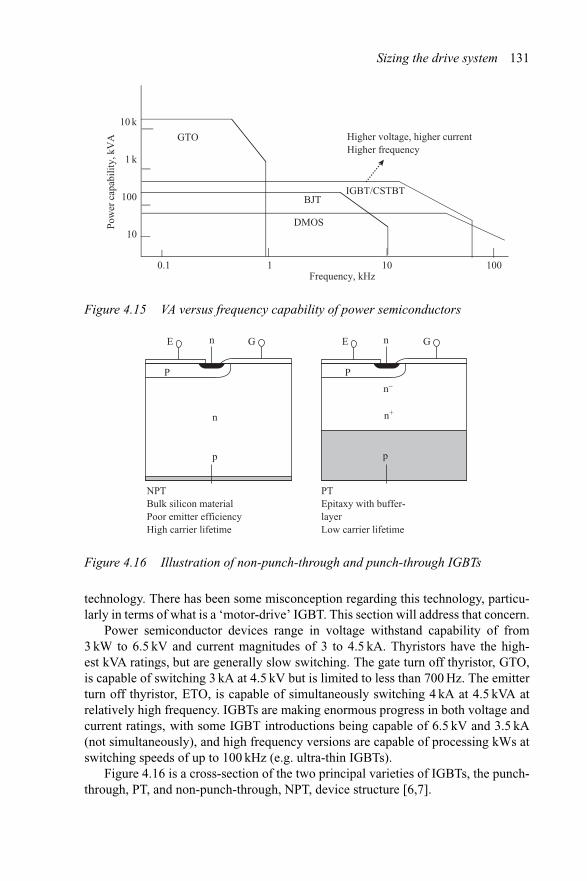
Sizing the drive system 131
Pow
er c
apab
ility
, kV
A
Frequency, kHz
10 k
1 k
100
10
GTO
DMOS
BJTIGBT/CSTBT
Higher voltage, higher currentHigher frequency
0.1 1 10 100
Figure 4.15 VA versus frequency capability of power semiconductors
E
NPTBulk silicon materialPoor emitter efficiencyHigh carrier lifetime
PTEpitaxy with buffer-layerLow carrier lifetime
Gn
n
p
E Gn
n+
n–
p
PP
Figure 4.16 Illustration of non-punch-through and punch-through IGBTs
technology. There has been some misconception regarding this technology, particu-larly in terms of what is a ‘motor-drive’ IGBT. This section will address that concern.
Power semiconductor devices range in voltage withstand capability of from3 kW to 6.5 kV and current magnitudes of 3 to 4.5 kA. Thyristors have the high-est kVA ratings, but are generally slow switching. The gate turn off thyristor, GTO,is capable of switching 3 kA at 4.5 kV but is limited to less than 700 Hz. The emitterturn off thyristor, ETO, is capable of simultaneously switching 4 kA at 4.5 kVA atrelatively high frequency. IGBTs are making enormous progress in both voltage andcurrent ratings, with some IGBT introductions being capable of 6.5 kV and 3.5 kA(not simultaneously), and high frequency versions are capable of processing kWs atswitching speeds of up to 100 kHz (e.g. ultra-thin IGBTs).
Figure 4.16 is a cross-section of the two principal varieties of IGBTs, the punch-through, PT, and non-punch-through, NPT, device structure [6,7].
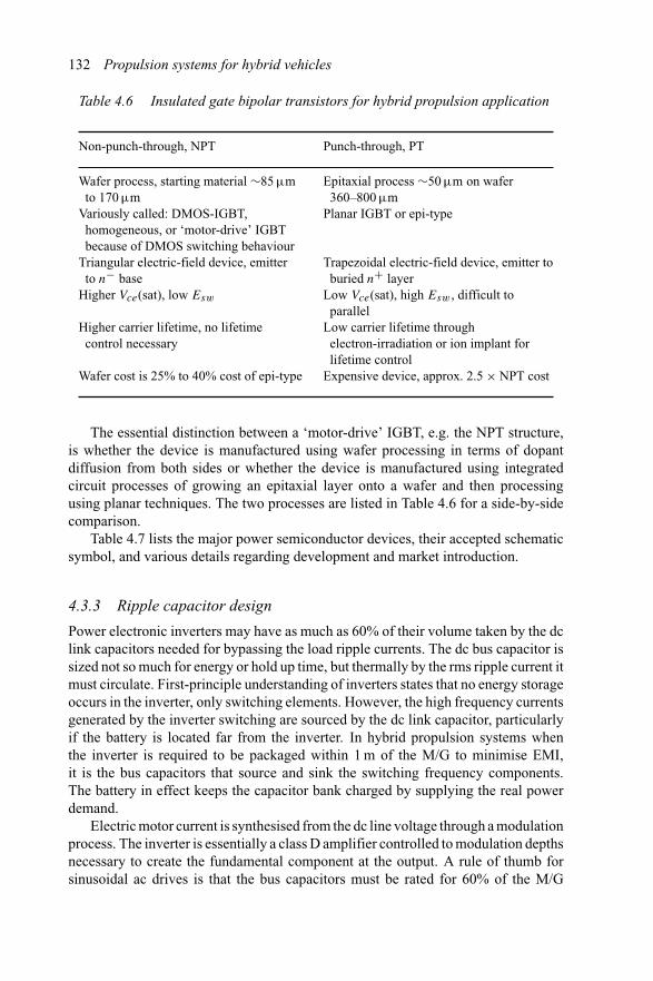
132 Propulsion systems for hybrid vehicles
Table 4.6 Insulated gate bipolar transistors for hybrid propulsion application
Non-punch-through, NPT Punch-through, PT
Wafer process, starting material ∼85 μmto 170 μm
Epitaxial process ∼50 μm on wafer360–800 μm
Variously called: DMOS-IGBT,homogeneous, or ‘motor-drive’ IGBTbecause of DMOS switching behaviour
Planar IGBT or epi-type
Triangular electric-field device, emitterto n− base
Trapezoidal electric-field device, emitter toburied n+ layer
Higher Vce(sat), low Esw Low Vce(sat), high Esw , difficult toparallel
Higher carrier lifetime, no lifetimecontrol necessary
Low carrier lifetime throughelectron-irradiation or ion implant forlifetime control
Wafer cost is 25% to 40% cost of epi-type Expensive device, approx. 2.5 × NPT cost
The essential distinction between a ‘motor-drive’ IGBT, e.g. the NPT structure,is whether the device is manufactured using wafer processing in terms of dopantdiffusion from both sides or whether the device is manufactured using integratedcircuit processes of growing an epitaxial layer onto a wafer and then processingusing planar techniques. The two processes are listed in Table 4.6 for a side-by-sidecomparison.
Table 4.7 lists the major power semiconductor devices, their accepted schematicsymbol, and various details regarding development and market introduction.
4.3.3 Ripple capacitor design
Power electronic inverters may have as much as 60% of their volume taken by the dclink capacitors needed for bypassing the load ripple currents. The dc bus capacitor issized not so much for energy or hold up time, but thermally by the rms ripple current itmust circulate. First-principle understanding of inverters states that no energy storageoccurs in the inverter, only switching elements. However, the high frequency currentsgenerated by the inverter switching are sourced by the dc link capacitor, particularlyif the battery is located far from the inverter. In hybrid propulsion systems whenthe inverter is required to be packaged within 1 m of the M/G to minimise EMI,it is the bus capacitors that source and sink the switching frequency components.The battery in effect keeps the capacitor bank charged by supplying the real powerdemand.
Electric motor current is synthesised from the dc line voltage through a modulationprocess. The inverter is essentially a class D amplifier controlled to modulation depthsnecessary to create the fundamental component at the output. A rule of thumb forsinusoidal ac drives is that the bus capacitors must be rated for 60% of the M/G
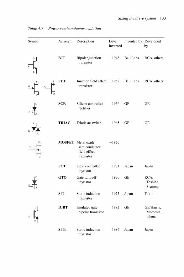
Sizing the drive system 133
Table 4.7 Power semiconductor evolution
Symbol Acronym Description Dateinvented
Invented by Developedby
E
C
B
BJT Bipolar junctiontransistor
1948 Bell Labs RCA, others
G G
S S
D D
FET Junction field effecttransistor
1952 Bell Labs RCA, others
A
K
G
SCR Silicon controlledrectifier
1956 GE GE
A
K
G
TRIAC Triode ac switch 1965 GE GE
S
D
G
MOSFET Metal oxidesemiconductorfield effecttransistor
∼1970
FCT Field controlledthyristor
1971 Japan Japan
A
K
G
GTO Gate turn-offthyristor
1970 GE RCA,Toshiba,Siemens
SIT Static inductiontransistor
1975 Japan Tokin
G
E
C IGBT Insulated gatebipolar transistor
1982 GE GE/Harris,Motorola,others
SITh Static inductionthyristor
1986 Japan Japan
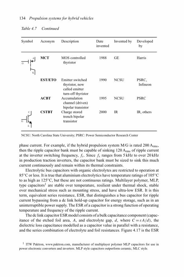
134 Propulsion systems for hybrid vehicles
Table 4.7 Continued
Symbol Acronym Description Dateinvented
Invented by Developedby
G
A
K
MCT MOS controlledthyristor
1988 GE Harris
EST/ETO Emitter switchedthyristor, nowcalled emitterturn-off thyristor
1990 NCSU PSRC,Infineon
ACBT Accumulationchannel (driven)bipolar transistor
1995 NCSU PSRC
G
E
C CSTBT Charge storedtrench bipolartransistor
2000 IR IR, others
NCSU: North Carolina State University; PSRC: Power Semiconductor Research Center
phase current. For example, if the hybrid propulsion system M/G is rated 200 Arms,then the ripple capacitor bank must be capable of sinking 120 Arms of ripple currentat the inverter switching frequency, fs . Since fs ranges from 5 kHz to over 20 kHzin production traction inverters, the capacitor bank must be sized to sink this muchcurrent continuously and remain within its thermal constraints.
Electrolytic bus capacitors with organic electrolytes are restricted to operation at85◦C or less. It is true that aluminium electrolytics have temperature ratings of 105◦Cto as high as 125◦C, but these are not continuous ratings. Multilayer polymer, MLP,type capacitors1 are stable over temperature, resilient under thermal shock, stableover mechanical stress such as mounting stress, and have ultra-low ESR. It is thisterm, equivalent series resistance, ESR, that distinguishes a bus capacitor for ripplecurrent bypassing from a dc link hold-up capacitor for energy storage, such as in anuninterruptible power supply. The ESR of a capacitor is a strong function of operatingtemperature and frequency of the ripple current.
The dc link capacitor ESR model consists of a bulk capacitance component (capac-itance of the etched foil area, A, and electrolyte gap, d, where C = εA/d), thedielectric loss capacitance modelled as a capacitor value in parallel with a resistance,and the series combination of electrolyte and foil resistances. Figure 4.17 is the ESR
1 ITW Paktron, www.paktron.com, manufacturer of multiplayer polymer MLP capacitors for use inpower electronic converters and inverters. MLP style capacitors outperform ceramic, MLC style.
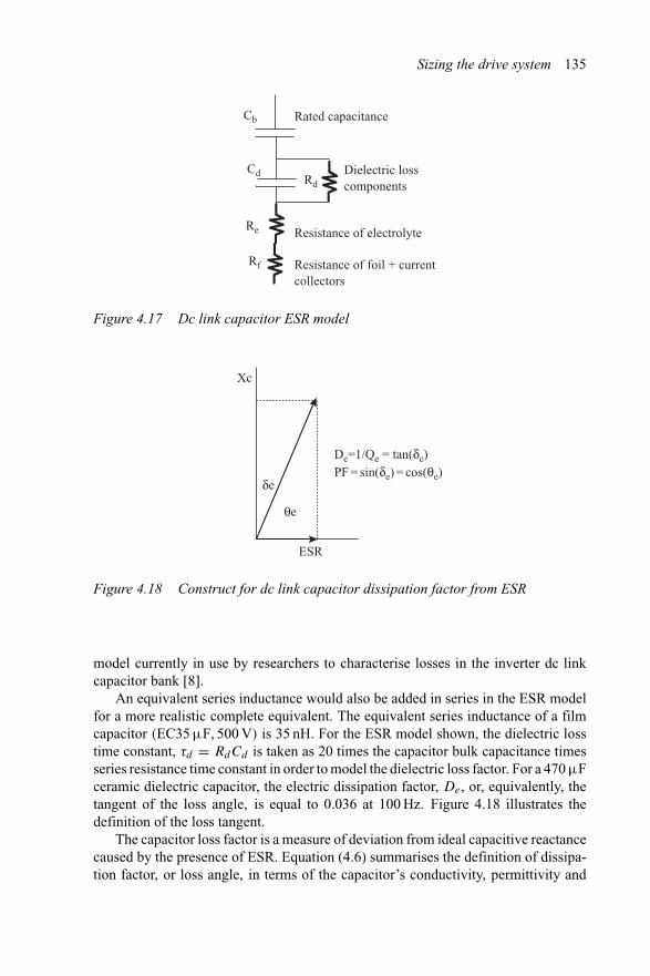
Sizing the drive system 135
Cb
CdRd
Re
Rf
Rated capacitance
Dielectric losscomponents
Resistance of electrolyte
Resistance of foil + currentcollectors
Figure 4.17 Dc link capacitor ESR model
ESR
Xc
δe
θe
De=1/Qe = tan(δe)PF = sin(δe) = cos(θe)
Figure 4.18 Construct for dc link capacitor dissipation factor from ESR
model currently in use by researchers to characterise losses in the inverter dc linkcapacitor bank [8].
An equivalent series inductance would also be added in series in the ESR modelfor a more realistic complete equivalent. The equivalent series inductance of a filmcapacitor (EC35 μF, 500 V) is 35 nH. For the ESR model shown, the dielectric losstime constant, τd = RdCd is taken as 20 times the capacitor bulk capacitance timesseries resistance time constant in order to model the dielectric loss factor. For a 470 μFceramic dielectric capacitor, the electric dissipation factor, De, or, equivalently, thetangent of the loss angle, is equal to 0.036 at 100 Hz. Figure 4.18 illustrates thedefinition of the loss tangent.
The capacitor loss factor is a measure of deviation from ideal capacitive reactancecaused by the presence of ESR. Equation (4.6) summarises the definition of dissipa-tion factor, or loss angle, in terms of the capacitor’s conductivity, permittivity and
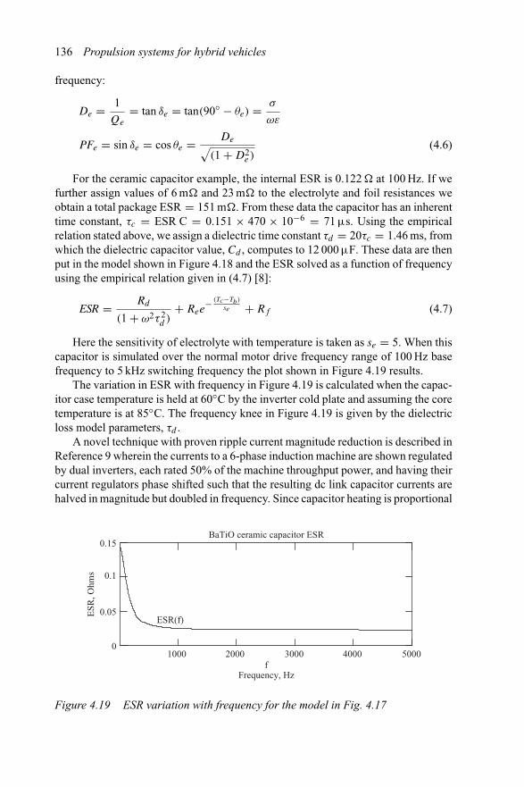
136 Propulsion systems for hybrid vehicles
frequency:
De = 1
Qe
= tan δe = tan(90◦ − θe) = σ
ωε
PFe = sin δe = cos θe = De√(1 + D2
e )(4.6)
For the ceramic capacitor example, the internal ESR is 0.122 � at 100 Hz. If wefurther assign values of 6 m� and 23 m� to the electrolyte and foil resistances weobtain a total package ESR = 151 m�. From these data the capacitor has an inherenttime constant, τc = ESR C = 0.151 × 470 × 10−6 = 71 μs. Using the empiricalrelation stated above, we assign a dielectric time constant τd = 20τc = 1.46 ms, fromwhich the dielectric capacitor value, Cd , computes to 12 000 μF. These data are thenput in the model shown in Figure 4.18 and the ESR solved as a function of frequencyusing the empirical relation given in (4.7) [8]:
ESR = Rd
(1 + ω2τ 2d )
+ Ree− (Tc−Tb)
se + Rf (4.7)
Here the sensitivity of electrolyte with temperature is taken as se = 5. When thiscapacitor is simulated over the normal motor drive frequency range of 100 Hz basefrequency to 5 kHz switching frequency the plot shown in Figure 4.19 results.
The variation in ESR with frequency in Figure 4.19 is calculated when the capac-itor case temperature is held at 60◦C by the inverter cold plate and assuming the coretemperature is at 85◦C. The frequency knee in Figure 4.19 is given by the dielectricloss model parameters, τd .
A novel technique with proven ripple current magnitude reduction is described inReference 9 wherein the currents to a 6-phase induction machine are shown regulatedby dual inverters, each rated 50% of the machine throughput power, and having theircurrent regulators phase shifted such that the resulting dc link capacitor currents arehalved in magnitude but doubled in frequency. Since capacitor heating is proportional
ESR(f)
f1000 2000 3000 4000 5000
0
0.05
0.1
0.15
Frequency, Hz
BaTiO ceramic capacitor ESR
ESR
, Ohm
s
Figure 4.19 ESR variation with frequency for the model in Fig. 4.17
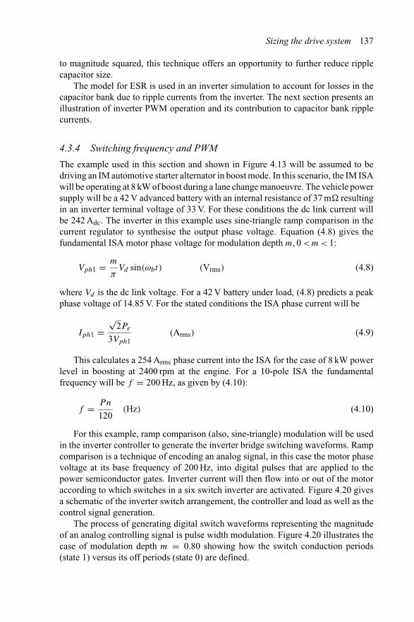
Sizing the drive system 137
to magnitude squared, this technique offers an opportunity to further reduce ripplecapacitor size.
The model for ESR is used in an inverter simulation to account for losses in thecapacitor bank due to ripple currents from the inverter. The next section presents anillustration of inverter PWM operation and its contribution to capacitor bank ripplecurrents.
4.3.4 Switching frequency and PWM
The example used in this section and shown in Figure 4.13 will be assumed to bedriving an IM automotive starter alternator in boost mode. In this scenario, the IM ISAwill be operating at 8 kW of boost during a lane change manoeuvre. The vehicle powersupply will be a 42 V advanced battery with an internal resistance of 37 m� resultingin an inverter terminal voltage of 33 V. For these conditions the dc link current willbe 242 Adc. The inverter in this example uses sine-triangle ramp comparison in thecurrent regulator to synthesise the output phase voltage. Equation (4.8) gives thefundamental ISA motor phase voltage for modulation depth m, 0 < m < 1:
Vph1 = m
πVd sin(ωbt) (Vrms) (4.8)
where Vd is the dc link voltage. For a 42 V battery under load, (4.8) predicts a peakphase voltage of 14.85 V. For the stated conditions the ISA phase current will be
Iph1 =√
2Pe
3Vph1(Arms) (4.9)
This calculates a 254 Arms phase current into the ISA for the case of 8 kW powerlevel in boosting at 2400 rpm at the engine. For a 10-pole ISA the fundamentalfrequency will be f = 200 Hz, as given by (4.10):
f = Pn
120(Hz) (4.10)
For this example, ramp comparison (also, sine-triangle) modulation will be usedin the inverter controller to generate the inverter bridge switching waveforms. Rampcomparison is a technique of encoding an analog signal, in this case the motor phasevoltage at its base frequency of 200 Hz, into digital pulses that are applied to thepower semiconductor gates. Inverter current will then flow into or out of the motoraccording to which switches in a six switch inverter are activated. Figure 4.20 givesa schematic of the inverter switch arrangement, the controller and load as well as thecontrol signal generation.
The process of generating digital switch waveforms representing the magnitudeof an analog controlling signal is pulse width modulation. Figure 4.20 illustrates thecase of modulation depth m = 0.80 showing how the switch conduction periods(state 1) versus its off periods (state 0) are defined.
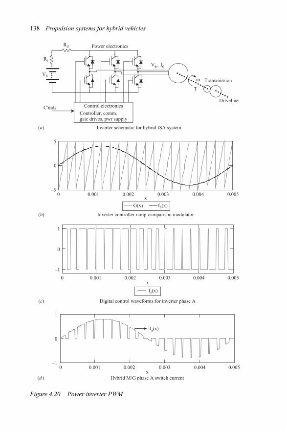
138 Propulsion systems for hybrid vehicles
Vb
Ri
Rd
Controller, comm.gate drives, pwr supply
C'mds
Power electronics
Control electronics
Vφ , Iφ
Inverter schematic for hybrid ISA system(a)
Inverter controller ramp-camparison modulator(b)
x0 0.001 0.002 0.003 0.004 0.005
–5
0
5
G(x) fb(x)
x0 0.001 0.002 0.003 0.004 0.005
–1
0
1
Digital control waveforms for inverter phase A(c)
fs(x)
Hybrid M/G phase A switch current(d )
Ia(x)
x0 0.001 0.002 0.003 0.004 0.005
–1
0
1
T
ω Transmission
Driveline
Figure 4.20 Power inverter PWM
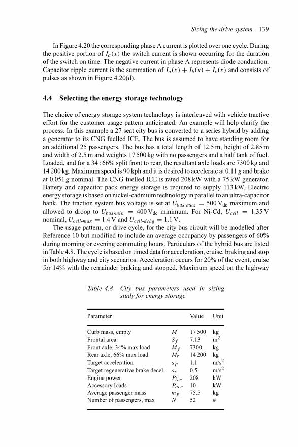
Sizing the drive system 139
In Figure 4.20 the corresponding phase A current is plotted over one cycle. Duringthe positive portion of Ia(x) the switch current is shown occurring for the durationof the switch on time. The negative current in phase A represents diode conduction.Capacitor ripple current is the summation of Ia(x) + Ib(x) + Ic(x) and consists ofpulses as shown in Figure 4.20(d).
4.4 Selecting the energy storage technology
The choice of energy storage system technology is interleaved with vehicle tractiveeffort for the customer usage pattern anticipated. An example will help clarify theprocess. In this example a 27 seat city bus is converted to a series hybrid by addinga generator to its CNG fuelled ICE. The bus is assumed to have standing room foran additional 25 passengers. The bus has a total length of 12.5 m, height of 2.85 mand width of 2.5 m and weights 17 500 kg with no passengers and a half tank of fuel.Loaded, and for a 34 : 66% split front to rear, the resultant axle loads are 7300 kg and14 200 kg. Maximum speed is 90 kph and it is desired to accelerate at 0.11 g and brakeat 0.051 g nominal. The CNG fuelled ICE is rated 208 kW with a 75 kW generator.Battery and capacitor pack energy storage is required to supply 113 kW. Electricenergy storage is based on nickel-cadmium technology in parallel to an ultra-capacitorbank. The traction system bus voltage is set at Ubus-max = 500 Vdc maximum andallowed to droop to Ubus-min = 400 Vdc minimum. For Ni-Cd, Ucell = 1.35 Vnominal, Ucell-max = 1.4 V and Ucell-dchg = 1.1 V.
The usage pattern, or drive cycle, for the city bus circuit will be modelled afterReference 10 but modified to include an average occupancy by passengers of 60%during morning or evening commuting hours. Particulars of the hybrid bus are listedin Table 4.8. The cycle is based on timed data for acceleration, cruise, braking and stopin both highway and city scenarios. Acceleration occurs for 20% of the event, cruisefor 14% with the remainder braking and stopped. Maximum speed on the highway
Table 4.8 City bus parameters used in sizingstudy for energy storage
Parameter Value Unit
Curb mass, empty M 17 500 kgFrontal area Sf 7.13 m2
Front axle, 34% max load Mf 7300 kgRear axle, 66% max load Mr 14 200 kgTarget acceleration ap 1.1 m/s2
Target regenerative brake decel. ar 0.5 m/s2
Engine power Pice 208 kWAccessory loads Pacc 10 kWAverage passenger mass mp 75.5 kgNumber of passengers, max N 52 #
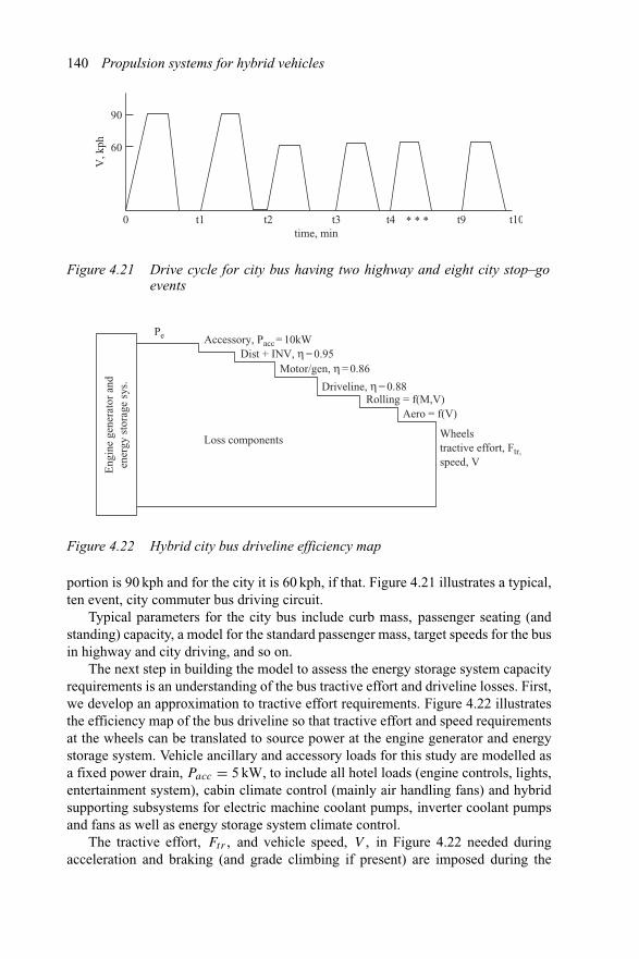
140 Propulsion systems for hybrid vehicles
V, k
ph
90
60
time, min0 t1 t2 t3 t4 * * * t9 t10
Figure 4.21 Drive cycle for city bus having two highway and eight city stop–goevents
Wheelstractive effort, Ftr,speed, V
Aero = f(V)Rolling = f(M,V)
Driveline, η = 0.88
Motor/gen, η = 0.86Dist + INV, η = 0.95
Accessory, Pacc = 10kWPe
Eng
ine
gene
rato
r an
den
ergy
sto
rage
sys
.
Loss components
Figure 4.22 Hybrid city bus driveline efficiency map
portion is 90 kph and for the city it is 60 kph, if that. Figure 4.21 illustrates a typical,ten event, city commuter bus driving circuit.
Typical parameters for the city bus include curb mass, passenger seating (andstanding) capacity, a model for the standard passenger mass, target speeds for the busin highway and city driving, and so on.
The next step in building the model to assess the energy storage system capacityrequirements is an understanding of the bus tractive effort and driveline losses. First,we develop an approximation to tractive effort requirements. Figure 4.22 illustratesthe efficiency map of the bus driveline so that tractive effort and speed requirementsat the wheels can be translated to source power at the engine generator and energystorage system. Vehicle ancillary and accessory loads for this study are modelled asa fixed power drain, Pacc = 5 kW, to include all hotel loads (engine controls, lights,entertainment system), cabin climate control (mainly air handling fans) and hybridsupporting subsystems for electric machine coolant pumps, inverter coolant pumpsand fans as well as energy storage system climate control.
The tractive effort, Ftr , and vehicle speed, V , in Figure 4.22 needed duringacceleration and braking (and grade climbing if present) are imposed during the
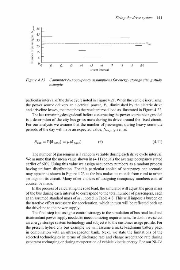
Sizing the drive system 141
Num
ber
of p
asse
nger
s, N
pass
0 t1 t2 t3 t4 t5 t6 t7 t8 t9 t10Event interval
55
45
35
25
15
5
0
Nexp
Figure 4.23 Commuter bus occupancy assumptions for energy storage sizing studyexample
particular interval of the drive cycle noted in Figure 4.21. When the vehicle is cruising,the power source delivers an electrical power, Pe, diminished by the electric driveand driveline losses, that matches the resultant road load as illustrated in Figure 4.22.
The last remaining design detail before constructing the power source sizing modelis a description of the city bus gross mass during its drive around the fixed circuit.For our analysis we assume that the number of passengers during heavy commuteperiods of the day will have an expected value, Nexp, given as
Nexp = E{n̄pass} = μ(n̄pass) (#) (4.11)
The number of passengers is a random variable during each drive cycle interval.We assume that the mean value shown in (4.11) equals the average occupancy statedearlier of 60%. Using this value we assign occupancy numbers as a random processhaving uniform distribution. For this particular choice of occupancy one scenariomay appear as shown in Figure 4.23 as the bus makes its rounds from rural to urbansettings on its circuit. Many other choices of assigning occupancy numbers can, ofcourse, be made.
In the process of calculating the road load, the simulator will adjust the gross massof the bus during each interval to correspond to the total number of passengers, eachat an assumed standard mass of mp, noted in Table 4.8. This will impose a burden onthe tractive effort necessary for acceleration, which in turn will be reflected back upthe driveline to the power supply.
The final step is to assign a control strategy to the simulation of bus road load andits attendant power supply needed to meet our sizing requirements. To do this we selectan energy storage system technology and subject it to the customer usage profile. Forthe present hybrid city bus example we will assume a nickel-cadmium battery packin combination with an ultra-capacitor bank. Next, we state the limitations of theselected technologies in terms of discharge rate and charge acceptance rate duringgenerator recharging or during recuperation of vehicle kinetic energy. For our Ni-Cd
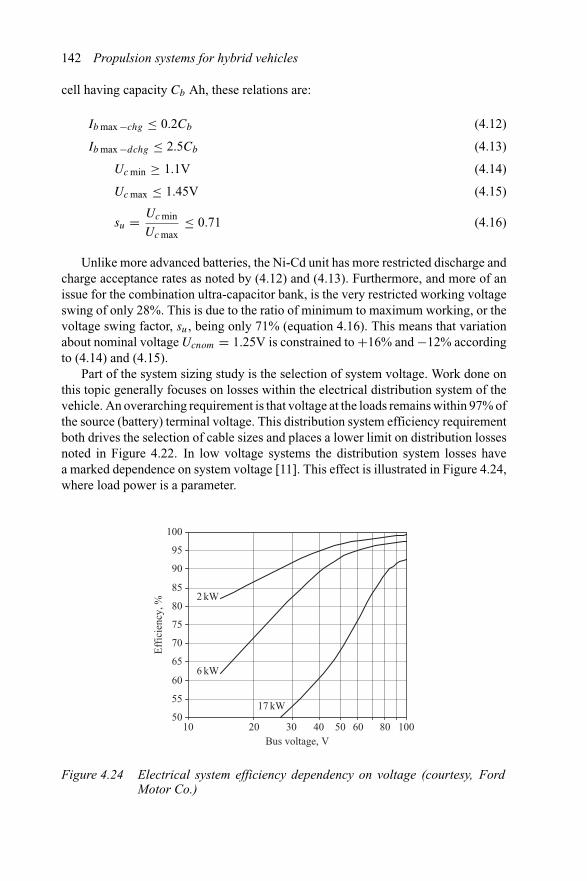
142 Propulsion systems for hybrid vehicles
cell having capacity Cb Ah, these relations are:
Ib max −chg ≤ 0.2Cb (4.12)
Ib max −dchg ≤ 2.5Cb (4.13)
Uc min ≥ 1.1V (4.14)
Uc max ≤ 1.45V (4.15)
su = Uc min
Uc max≤ 0.71 (4.16)
Unlike more advanced batteries, the Ni-Cd unit has more restricted discharge andcharge acceptance rates as noted by (4.12) and (4.13). Furthermore, and more of anissue for the combination ultra-capacitor bank, is the very restricted working voltageswing of only 28%. This is due to the ratio of minimum to maximum working, or thevoltage swing factor, su, being only 71% (equation 4.16). This means that variationabout nominal voltage Ucnom = 1.25V is constrained to +16% and −12% accordingto (4.14) and (4.15).
Part of the system sizing study is the selection of system voltage. Work done onthis topic generally focuses on losses within the electrical distribution system of thevehicle. An overarching requirement is that voltage at the loads remains within 97% ofthe source (battery) terminal voltage. This distribution system efficiency requirementboth drives the selection of cable sizes and places a lower limit on distribution lossesnoted in Figure 4.22. In low voltage systems the distribution system losses havea marked dependence on system voltage [11]. This effect is illustrated in Figure 4.24,where load power is a parameter.
50
55
60
65
70
75
80
85
90
95
100
10 20 30 40 50 60 80 100Bus voltage, V
Eff
icie
ncy,
%
2 kW
6 kW
17 kW
Figure 4.24 Electrical system efficiency dependency on voltage (courtesy, FordMotor Co.)
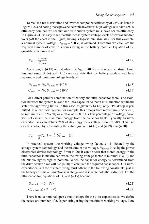
Sizing the drive system 143
To realise a net distribution and inverter component efficiency of 95%, as listed inFigure 4.22 and noting that a power electronic inverter at high voltage will have >97%efficiency nominal, we see that our distribution system must have >97% efficiency.In Figure 4.24 it is easy to see that this means system voltage levels of several hundredvolts (off the chart in the Figure, having a logarithmic abscissa). For this example,a nominal system voltage, Ubnom = 500 V, is assumed. From this we calculate therequired number of cells in a series string in the battery module. Equation (4.17)quantifies the procedure:
Nbc = Ubnom
Ucnom
(4.17)
According to (4.17) we calculate that Nbc = 400 cells in series per string. Fromthis and using (4.14) and (4.15) we can state that the battery module will havemaximum and minimum voltage levels of:
Ub min = NbcUc min = 440 V (4.18)
Ub max = NbcUc max = 580 V (4.19)
For a direct parallel combination of battery and ultra-capacitor there is no isola-tion between the system bus and the ultra-capacitor so that it must function within thestated voltage swing limits. In this case, as given by (4.16), only 71% droop is per-mitted. In a lead–acid system, for example, this droops from maximum (2.56 V/cell)to minimum (1.75 V/cell) or a ratio of 0.68. This low percentage of voltage droopwill not extract the maximum energy from the capacitor bank. Typically an ultra-capacitor bank can deliver 75% of its energy for a voltage droop of 50%. This factcan be verified by substituting the values given in (4.16) and (4.19) into (4.20):
Euc = 1
2Cuc(1 − s2
u)U2b max (J) (4.20)
In practical systems the working voltage swing factor, su, is dictated by thestorage system technology, and the maximum bus voltage, Ubmax , is set by the powerelectronics device technology. From (4.20) it can be seen that stored energy in theultra-capacitor is maximized when the swing voltage factor is minimal (i.e. 0) andthe bus voltage is high as possible. When the capacitor energy is determined fromthe drive scenario we will use (4.20) to calculate the required capacitance. Our ultra-capacitor cells in the resultant string must adhere to the following constraints, just asthe battery cells have limitations on charge and discharge potential extremes. For theultra-capacitor, equations (4.14) and (4.15) become:
Uucc min ≥ 0 (V) (4.21)
Uucc max ≤ 2.7 (V) (4.22)
There is not a nominal open circuit voltage for the ultra-capacitors, so we definethe necessary number of cells per string using the maximum working voltage. Note
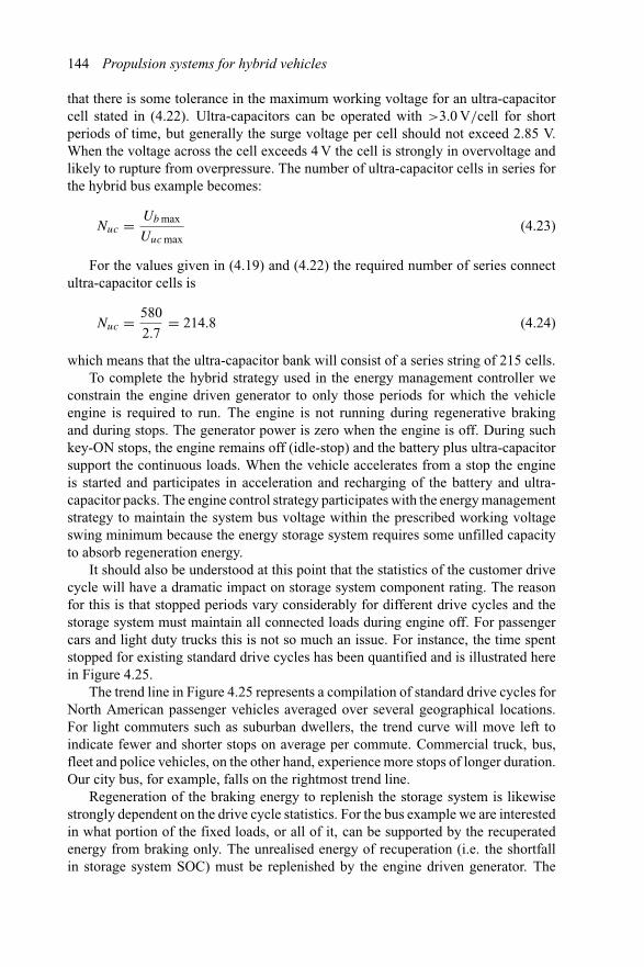
144 Propulsion systems for hybrid vehicles
that there is some tolerance in the maximum working voltage for an ultra-capacitorcell stated in (4.22). Ultra-capacitors can be operated with >3.0 V/cell for shortperiods of time, but generally the surge voltage per cell should not exceed 2.85 V.When the voltage across the cell exceeds 4 V the cell is strongly in overvoltage andlikely to rupture from overpressure. The number of ultra-capacitor cells in series forthe hybrid bus example becomes:
Nuc = Ub max
Uuc max(4.23)
For the values given in (4.19) and (4.22) the required number of series connectultra-capacitor cells is
Nuc = 580
2.7= 214.8 (4.24)
which means that the ultra-capacitor bank will consist of a series string of 215 cells.To complete the hybrid strategy used in the energy management controller we
constrain the engine driven generator to only those periods for which the vehicleengine is required to run. The engine is not running during regenerative brakingand during stops. The generator power is zero when the engine is off. During suchkey-ON stops, the engine remains off (idle-stop) and the battery plus ultra-capacitorsupport the continuous loads. When the vehicle accelerates from a stop the engineis started and participates in acceleration and recharging of the battery and ultra-capacitor packs. The engine control strategy participates with the energy managementstrategy to maintain the system bus voltage within the prescribed working voltageswing minimum because the energy storage system requires some unfilled capacityto absorb regeneration energy.
It should also be understood at this point that the statistics of the customer drivecycle will have a dramatic impact on storage system component rating. The reasonfor this is that stopped periods vary considerably for different drive cycles and thestorage system must maintain all connected loads during engine off. For passengercars and light duty trucks this is not so much an issue. For instance, the time spentstopped for existing standard drive cycles has been quantified and is illustrated herein Figure 4.25.
The trend line in Figure 4.25 represents a compilation of standard drive cycles forNorth American passenger vehicles averaged over several geographical locations.For light commuters such as suburban dwellers, the trend curve will move left toindicate fewer and shorter stops on average per commute. Commercial truck, bus,fleet and police vehicles, on the other hand, experience more stops of longer duration.Our city bus, for example, falls on the rightmost trend line.
Regeneration of the braking energy to replenish the storage system is likewisestrongly dependent on the drive cycle statistics. For the bus example we are interestedin what portion of the fixed loads, or all of it, can be supported by the recuperatedenergy from braking only. The unrealised energy of recuperation (i.e. the shortfallin storage system SOC) must be replenished by the engine driven generator. The
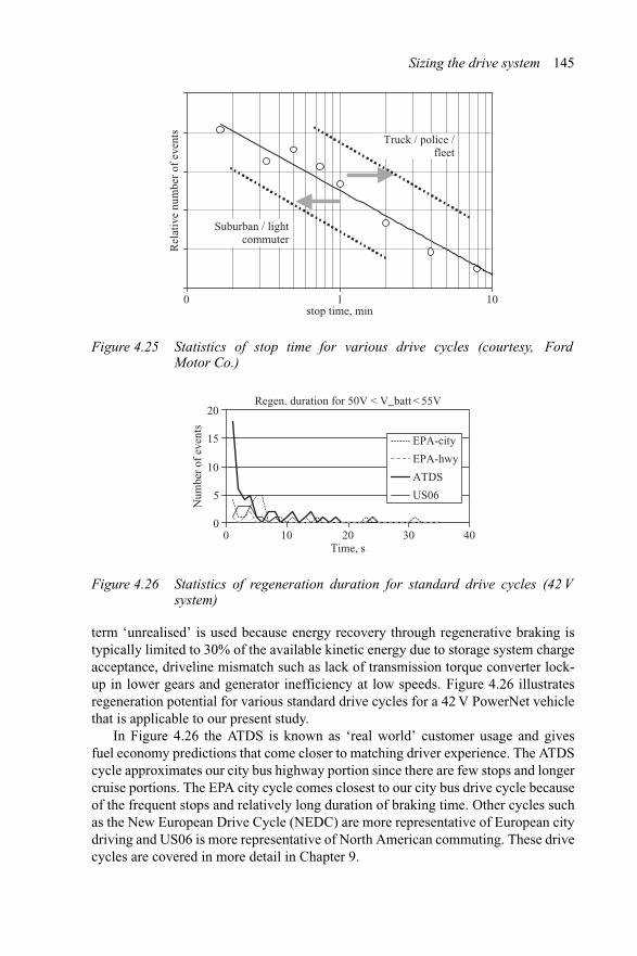
Sizing the drive system 145
0 1 10stop time, min
Suburban / lightcommuter
Truck / police /fleet
Rel
ativ
e nu
mbe
r of
eve
nts
Figure 4.25 Statistics of stop time for various drive cycles (courtesy, FordMotor Co.)
Regen. duration for 50V < V_batt < 55V
0
5
10
15
20
0 10 20 30 40Time, s
Num
ber
of e
vent
s
EPA-city
EPA-hwy
ATDS
US06
Figure 4.26 Statistics of regeneration duration for standard drive cycles (42 Vsystem)
term ‘unrealised’ is used because energy recovery through regenerative braking istypically limited to 30% of the available kinetic energy due to storage system chargeacceptance, driveline mismatch such as lack of transmission torque converter lock-up in lower gears and generator inefficiency at low speeds. Figure 4.26 illustratesregeneration potential for various standard drive cycles for a 42 V PowerNet vehiclethat is applicable to our present study.
In Figure 4.26 the ATDS is known as ‘real world’ customer usage and givesfuel economy predictions that come closer to matching driver experience. The ATDScycle approximates our city bus highway portion since there are few stops and longercruise portions. The EPA city cycle comes closest to our city bus drive cycle becauseof the frequent stops and relatively long duration of braking time. Other cycles suchas the New European Drive Cycle (NEDC) are more representative of European citydriving and US06 is more representative of North American commuting. These drivecycles are covered in more detail in Chapter 9.
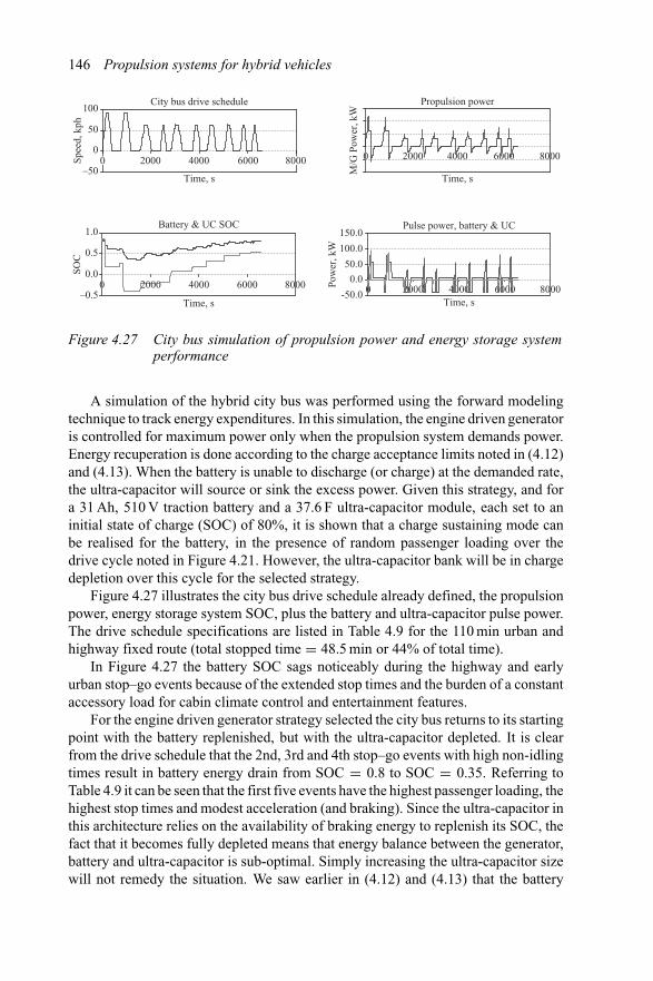
146 Propulsion systems for hybrid vehicles
City bus drive schedule
–50
0
50
100
2000 4000 6000 8000
Time, s
Spee
d, k
ph
0
Propulsion power
Time, s
0 2000 4000 6000 8000
M/G
Pow
er, k
W
0 2000 4000 6000 8000
Battery & UC SOC
–0.5
0.0
0.5
1.0
Time, s
SOC
0 2000 4000 6000 80000 2000 4000 6000 8000
Pulse power, battery & UC
-50.0
0.0
50.0
100.0
150.0
Time, s
Pow
er, k
W
0 2000 4000 6000 80000 2000 4000 6000 8000
Figure 4.27 City bus simulation of propulsion power and energy storage systemperformance
A simulation of the hybrid city bus was performed using the forward modelingtechnique to track energy expenditures. In this simulation, the engine driven generatoris controlled for maximum power only when the propulsion system demands power.Energy recuperation is done according to the charge acceptance limits noted in (4.12)and (4.13). When the battery is unable to discharge (or charge) at the demanded rate,the ultra-capacitor will source or sink the excess power. Given this strategy, and fora 31 Ah, 510 V traction battery and a 37.6 F ultra-capacitor module, each set to aninitial state of charge (SOC) of 80%, it is shown that a charge sustaining mode canbe realised for the battery, in the presence of random passenger loading over thedrive cycle noted in Figure 4.21. However, the ultra-capacitor bank will be in chargedepletion over this cycle for the selected strategy.
Figure 4.27 illustrates the city bus drive schedule already defined, the propulsionpower, energy storage system SOC, plus the battery and ultra-capacitor pulse power.The drive schedule specifications are listed in Table 4.9 for the 110 min urban andhighway fixed route (total stopped time = 48.5 min or 44% of total time).
In Figure 4.27 the battery SOC sags noticeably during the highway and earlyurban stop–go events because of the extended stop times and the burden of a constantaccessory load for cabin climate control and entertainment features.
For the engine driven generator strategy selected the city bus returns to its startingpoint with the battery replenished, but with the ultra-capacitor depleted. It is clearfrom the drive schedule that the 2nd, 3rd and 4th stop–go events with high non-idlingtimes result in battery energy drain from SOC = 0.8 to SOC = 0.35. Referring toTable 4.9 it can be seen that the first five events have the highest passenger loading, thehighest stop times and modest acceleration (and braking). Since the ultra-capacitor inthis architecture relies on the availability of braking energy to replenish its SOC, thefact that it becomes fully depleted means that energy balance between the generator,battery and ultra-capacitor is sub-optimal. Simply increasing the ultra-capacitor sizewill not remedy the situation. We saw earlier in (4.12) and (4.13) that the battery
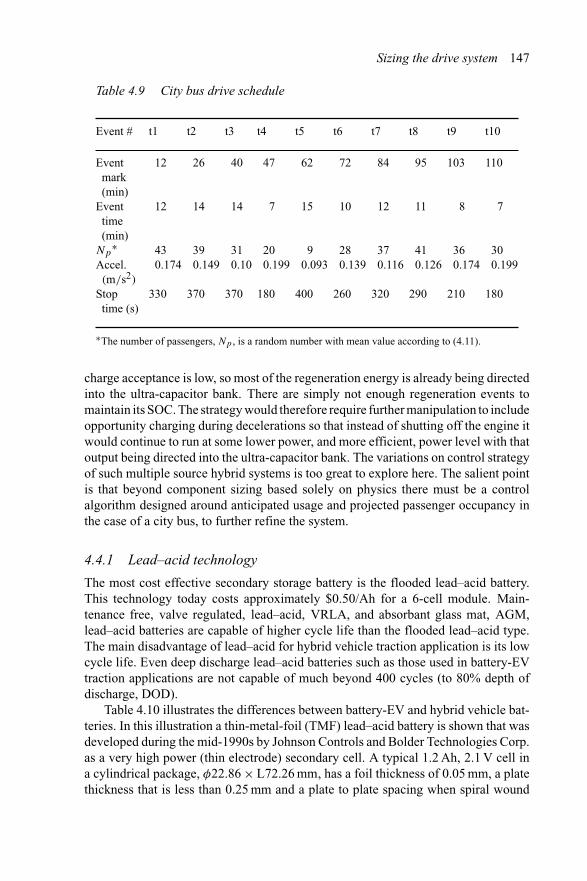
Sizing the drive system 147
Table 4.9 City bus drive schedule
Event # t1 t2 t3 t4 t5 t6 t7 t8 t9 t10
Eventmark(min)
12 26 40 47 62 72 84 95 103 110
Eventtime(min)
12 14 14 7 15 10 12 11 8 7
Np∗ 43 39 31 20 9 28 37 41 36 30
Accel.(m/s2)
0.174 0.149 0.10 0.199 0.093 0.139 0.116 0.126 0.174 0.199
Stoptime (s)
330 370 370 180 400 260 320 290 210 180
∗The number of passengers, Np , is a random number with mean value according to (4.11).
charge acceptance is low, so most of the regeneration energy is already being directedinto the ultra-capacitor bank. There are simply not enough regeneration events tomaintain its SOC. The strategy would therefore require further manipulation to includeopportunity charging during decelerations so that instead of shutting off the engine itwould continue to run at some lower power, and more efficient, power level with thatoutput being directed into the ultra-capacitor bank. The variations on control strategyof such multiple source hybrid systems is too great to explore here. The salient pointis that beyond component sizing based solely on physics there must be a controlalgorithm designed around anticipated usage and projected passenger occupancy inthe case of a city bus, to further refine the system.
4.4.1 Lead–acid technology
The most cost effective secondary storage battery is the flooded lead–acid battery.This technology today costs approximately $0.50/Ah for a 6-cell module. Main-tenance free, valve regulated, lead–acid, VRLA, and absorbant glass mat, AGM,lead–acid batteries are capable of higher cycle life than the flooded lead–acid type.The main disadvantage of lead–acid for hybrid vehicle traction application is its lowcycle life. Even deep discharge lead–acid batteries such as those used in battery-EVtraction applications are not capable of much beyond 400 cycles (to 80% depth ofdischarge, DOD).
Table 4.10 illustrates the differences between battery-EV and hybrid vehicle bat-teries. In this illustration a thin-metal-foil (TMF) lead–acid battery is shown that wasdeveloped during the mid-1990s by Johnson Controls and Bolder Technologies Corp.as a very high power (thin electrode) secondary cell. A typical 1.2 Ah, 2.1 V cell ina cylindrical package, φ22.86 × L72.26 mm, has a foil thickness of 0.05 mm, a platethickness that is less than 0.25 mm and a plate to plate spacing when spiral wound
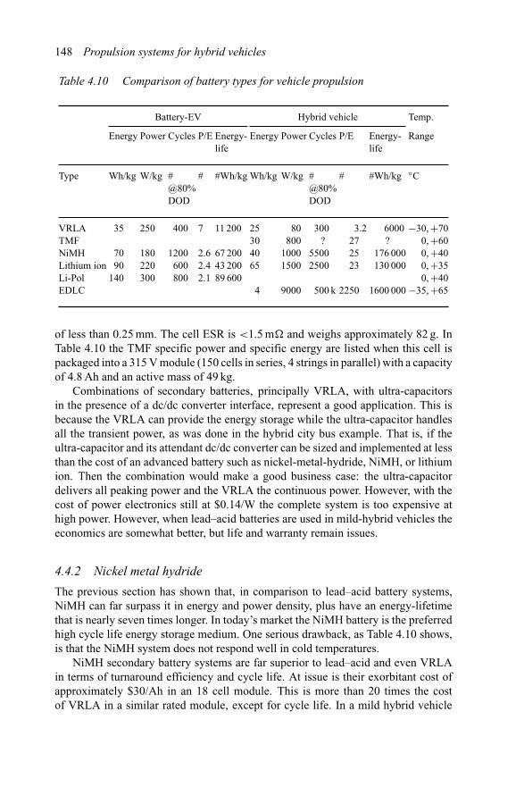
148 Propulsion systems for hybrid vehicles
Table 4.10 Comparison of battery types for vehicle propulsion
Battery-EV Hybrid vehicle Temp.
Energy Power Cycles P/E Energy-life
Energy Power Cycles P/E Energy-life
Range
Type Wh/kg W/kg #@80%DOD
# #Wh/kg Wh/kg W/kg #@80%DOD
# #Wh/kg ◦C
VRLA 35 250 400 7 11 200 25 80 300 3.2 6000 −30, +70TMF 30 800 ? 27 ? 0, +60NiMH 70 180 1200 2.6 67 200 40 1000 5500 25 176 000 0, +40Lithium ion 90 220 600 2.4 43 200 65 1500 2500 23 130 000 0, +35Li-Pol 140 300 800 2.1 89 600 0, +40EDLC 4 9000 500 k 2250 1600 000 −35, +65
of less than 0.25 mm. The cell ESR is <1.5 m� and weighs approximately 82 g. InTable 4.10 the TMF specific power and specific energy are listed when this cell ispackaged into a 315 V module (150 cells in series, 4 strings in parallel) with a capacityof 4.8 Ah and an active mass of 49 kg.
Combinations of secondary batteries, principally VRLA, with ultra-capacitorsin the presence of a dc/dc converter interface, represent a good application. This isbecause the VRLA can provide the energy storage while the ultra-capacitor handlesall the transient power, as was done in the hybrid city bus example. That is, if theultra-capacitor and its attendant dc/dc converter can be sized and implemented at lessthan the cost of an advanced battery such as nickel-metal-hydride, NiMH, or lithiumion. Then the combination would make a good business case: the ultra-capacitordelivers all peaking power and the VRLA the continuous power. However, with thecost of power electronics still at $0.14/W the complete system is too expensive athigh power. However, when lead–acid batteries are used in mild-hybrid vehicles theeconomics are somewhat better, but life and warranty remain issues.
4.4.2 Nickel metal hydride
The previous section has shown that, in comparison to lead–acid battery systems,NiMH can far surpass it in energy and power density, plus have an energy-lifetimethat is nearly seven times longer. In today’s market the NiMH battery is the preferredhigh cycle life energy storage medium. One serious drawback, as Table 4.10 shows,is that the NiMH system does not respond well in cold temperatures.
NiMH secondary battery systems are far superior to lead–acid and even VRLAin terms of turnaround efficiency and cycle life. At issue is their exorbitant cost ofapproximately $30/Ah in an 18 cell module. This is more than 20 times the costof VRLA in a similar rated module, except for cycle life. In a mild hybrid vehicle
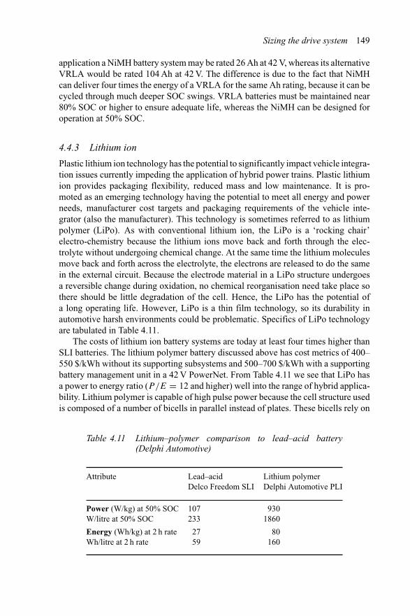
Sizing the drive system 149
application a NiMH battery system may be rated 26 Ah at 42 V, whereas its alternativeVRLA would be rated 104 Ah at 42 V. The difference is due to the fact that NiMHcan deliver four times the energy of a VRLA for the same Ah rating, because it can becycled through much deeper SOC swings. VRLA batteries must be maintained near80% SOC or higher to ensure adequate life, whereas the NiMH can be designed foroperation at 50% SOC.
4.4.3 Lithium ion
Plastic lithium ion technology has the potential to significantly impact vehicle integra-tion issues currently impeding the application of hybrid power trains. Plastic lithiumion provides packaging flexibility, reduced mass and low maintenance. It is pro-moted as an emerging technology having the potential to meet all energy and powerneeds, manufacturer cost targets and packaging requirements of the vehicle inte-grator (also the manufacturer). This technology is sometimes referred to as lithiumpolymer (LiPo). As with conventional lithium ion, the LiPo is a ‘rocking chair’electro-chemistry because the lithium ions move back and forth through the elec-trolyte without undergoing chemical change. At the same time the lithium moleculesmove back and forth across the electrolyte, the electrons are released to do the samein the external circuit. Because the electrode material in a LiPo structure undergoesa reversible change during oxidation, no chemical reorganisation need take place sothere should be little degradation of the cell. Hence, the LiPo has the potential ofa long operating life. However, LiPo is a thin film technology, so its durability inautomotive harsh environments could be problematic. Specifics of LiPo technologyare tabulated in Table 4.11.
The costs of lithium ion battery systems are today at least four times higher thanSLI batteries. The lithium polymer battery discussed above has cost metrics of 400–550 $/kWh without its supporting subsystems and 500–700 $/kWh with a supportingbattery management unit in a 42 V PowerNet. From Table 4.11 we see that LiPo hasa power to energy ratio (P/E = 12 and higher) well into the range of hybrid applica-bility. Lithium polymer is capable of high pulse power because the cell structure usedis composed of a number of bicells in parallel instead of plates. These bicells rely on
Table 4.11 Lithium–polymer comparison to lead–acid battery(Delphi Automotive)
Attribute Lead–acidDelco Freedom SLI
Lithium polymerDelphi Automotive PLI
Power (W/kg) at 50% SOC 107 930W/litre at 50% SOC 233 1860
Energy (Wh/kg) at 2 h rate 27 80Wh/litre at 2 h rate 59 160
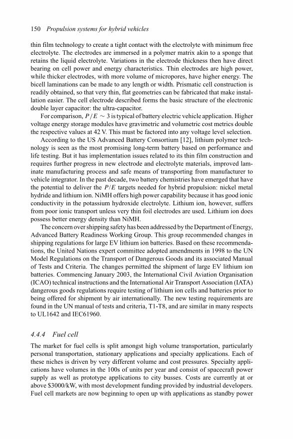
150 Propulsion systems for hybrid vehicles
thin film technology to create a tight contact with the electrolyte with minimum freeelectrolyte. The electrodes are immersed in a polymer matrix akin to a sponge thatretains the liquid electrolyte. Variations in the electrode thickness then have directbearing on cell power and energy characteristics. Thin electrodes are high power,while thicker electrodes, with more volume of micropores, have higher energy. Thebicell laminations can be made to any length or width. Prismatic cell construction isreadily obtained, so that very thin, flat geometries can be fabricated that make instal-lation easier. The cell electrode described forms the basic structure of the electronicdouble layer capacitor: the ultra-capacitor.
For comparison, P/E ∼ 3 is typical of battery electric vehicle application. Highervoltage energy storage modules have gravimetric and volumetric cost metrics doublethe respective values at 42 V. This must be factored into any voltage level selection.
According to the US Advanced Battery Consortium [12], lithium polymer tech-nology is seen as the most promising long-term battery based on performance andlife testing. But it has implementation issues related to its thin film construction andrequires further progress in new electrode and electrolyte materials, improved lam-inate manufacturing process and safe means of transporting from manufacturer tovehicle integrator. In the past decade, two battery chemistries have emerged that havethe potential to deliver the P /E targets needed for hybrid propulsion: nickel metalhydride and lithium ion. NiMH offers high power capability because it has good ionicconductivity in the potassium hydroxide electrolyte. Lithium ion, however, suffersfrom poor ionic transport unless very thin foil electrodes are used. Lithium ion doespossess better energy density than NiMH.
The concern over shipping safety has been addressed by the Department of Energy,Advanced Battery Readiness Working Group. This group recommended changes inshipping regulations for large EV lithium ion batteries. Based on these recommenda-tions, the United Nations expert committee adopted amendments in 1998 to the UNModel Regulations on the Transport of Dangerous Goods and its associated Manualof Tests and Criteria. The changes permitted the shipment of large EV lithium ionbatteries. Commencing January 2003, the International Civil Aviation Organisation(ICAO) technical instructions and the International Air Transport Association (IATA)dangerous goods regulations require testing of lithium ion cells and batteries prior tobeing offered for shipment by air internationally. The new testing requirements arefound in the UN manual of tests and criteria, T1-T8, and are similar in many respectsto UL1642 and IEC61960.
4.4.4 Fuel cell
The market for fuel cells is split amongst high volume transportation, particularlypersonal transportation, stationary applications and specialty applications. Each ofthese niches is driven by very different volume and cost pressures. Specialty appli-cations have volumes in the 100s of units per year and consist of spacecraft powersupply as well as prototype applications to city busses. Costs are currently at orabove $3000/kW, with most development funding provided by industrial developers.Fuel cell markets are now beginning to open up with applications as standby power
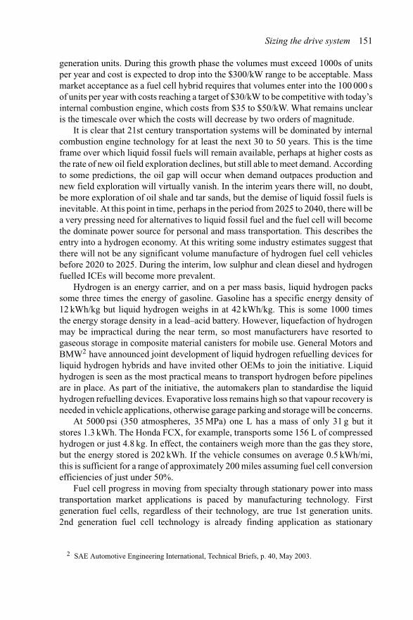
Sizing the drive system 151
generation units. During this growth phase the volumes must exceed 1000s of unitsper year and cost is expected to drop into the $300/kW range to be acceptable. Massmarket acceptance as a fuel cell hybrid requires that volumes enter into the 100 000 sof units per year with costs reaching a target of $30/kW to be competitive with today’sinternal combustion engine, which costs from $35 to $50/kW. What remains unclearis the timescale over which the costs will decrease by two orders of magnitude.
It is clear that 21st century transportation systems will be dominated by internalcombustion engine technology for at least the next 30 to 50 years. This is the timeframe over which liquid fossil fuels will remain available, perhaps at higher costs asthe rate of new oil field exploration declines, but still able to meet demand. Accordingto some predictions, the oil gap will occur when demand outpaces production andnew field exploration will virtually vanish. In the interim years there will, no doubt,be more exploration of oil shale and tar sands, but the demise of liquid fossil fuels isinevitable. At this point in time, perhaps in the period from 2025 to 2040, there will bea very pressing need for alternatives to liquid fossil fuel and the fuel cell will becomethe dominate power source for personal and mass transportation. This describes theentry into a hydrogen economy. At this writing some industry estimates suggest thatthere will not be any significant volume manufacture of hydrogen fuel cell vehiclesbefore 2020 to 2025. During the interim, low sulphur and clean diesel and hydrogenfuelled ICEs will become more prevalent.
Hydrogen is an energy carrier, and on a per mass basis, liquid hydrogen packssome three times the energy of gasoline. Gasoline has a specific energy density of12 kWh/kg but liquid hydrogen weighs in at 42 kWh/kg. This is some 1000 timesthe energy storage density in a lead–acid battery. However, liquefaction of hydrogenmay be impractical during the near term, so most manufacturers have resorted togaseous storage in composite material canisters for mobile use. General Motors andBMW2 have announced joint development of liquid hydrogen refuelling devices forliquid hydrogen hybrids and have invited other OEMs to join the initiative. Liquidhydrogen is seen as the most practical means to transport hydrogen before pipelinesare in place. As part of the initiative, the automakers plan to standardise the liquidhydrogen refuelling devices. Evaporative loss remains high so that vapour recovery isneeded in vehicle applications, otherwise garage parking and storage will be concerns.
At 5000 psi (350 atmospheres, 35 MPa) one L has a mass of only 31 g but itstores 1.3 kWh. The Honda FCX, for example, transports some 156 L of compressedhydrogen or just 4.8 kg. In effect, the containers weigh more than the gas they store,but the energy stored is 202 kWh. If the vehicle consumes on average 0.5 kWh/mi,this is sufficient for a range of approximately 200 miles assuming fuel cell conversionefficiencies of just under 50%.
Fuel cell progress in moving from specialty through stationary power into masstransportation market applications is paced by manufacturing technology. Firstgeneration fuel cells, regardless of their technology, are true 1st generation units.2nd generation fuel cell technology is already finding application as stationary
2 SAE Automotive Engineering International, Technical Briefs, p. 40, May 2003.
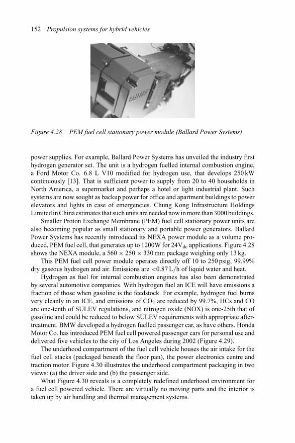
152 Propulsion systems for hybrid vehicles
Figure 4.28 PEM fuel cell stationary power module (Ballard Power Systems)
power supplies. For example, Ballard Power Systems has unveiled the industry firsthydrogen generator set. The unit is a hydrogen fuelled internal combustion engine,a Ford Motor Co. 6.8 L V10 modified for hydrogen use, that develops 250 kWcontinuously [13]. That is sufficient power to supply from 20 to 40 households inNorth America, a supermarket and perhaps a hotel or light industrial plant. Suchsystems are now sought as backup power for office and apartment buildings to powerelevators and lights in case of emergencies. Chung Kong Infrastructure HoldingsLimited in China estimates that such units are needed now in more than 3000 buildings.
Smaller Proton Exchange Membrane (PEM) fuel cell stationary power units arealso becoming popular as small stationary and portable power generators. BallardPower Systems has recently introduced its NEXA power module as a volume pro-duced, PEM fuel cell, that generates up to 1200W for 24Vdc applications. Figure 4.28shows the NEXA module, a 560 × 250 × 330 mm package weighing only 13 kg.
This PEM fuel cell power module operates directly off 10 to 250 psig, 99.99%dry gaseous hydrogen and air. Emissions are <0.87 L/h of liquid water and heat.
Hydrogen as fuel for internal combustion engines has also been demonstratedby several automotive companies. With hydrogen fuel an ICE will have emissions afraction of those when gasoline is the feedstock. For example, hydrogen fuel burnsvery cleanly in an ICE, and emissions of CO2 are reduced by 99.7%, HCs and COare one-tenth of SULEV regulations, and nitrogen oxide (NOX) is one-25th that ofgasoline and could be reduced to below SULEV requirements with appropriate after-treatment. BMW developed a hydrogen fuelled passenger car, as have others. HondaMotor Co. has introduced PEM fuel cell powered passenger cars for personal use anddelivered five vehicles to the city of Los Angeles during 2002 (Figure 4.29).
The underhood compartment of the fuel cell vehicle houses the air intake for thefuel cell stacks (packaged beneath the floor pan), the power electronics centre andtraction motor. Figure 4.30 illustrates the underhood compartment packaging in twoviews: (a) the driver side and (b) the passenger side.
What Figure 4.30 reveals is a completely redefined underhood environment fora fuel cell powered vehicle. There are virtually no moving parts and the interior istaken up by air handling and thermal management systems.
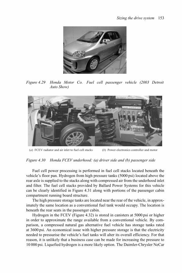
Sizing the drive system 153
Figure 4.29 Honda Motor Co. Fuel cell passenger vehicle (2003 DetroitAuto Show)
(a) FCEV radiator and air inlet to fuel cell stacks (b) Power electronics controller and motor
Figure 4.30 Honda FCEV underhood: (a) driver side and (b) passenger side
Fuel cell power processing is performed in fuel cell stacks located beneath thevehicle’s floor pan. Hydrogen from high pressure tanks (5000 psi) located above therear axle is supplied to the stacks along with compressed air from the underhood inletand filter. The fuel cell stacks provided by Ballard Power Systems for this vehiclecan be clearly identified in Figure 4.31 along with portions of the passenger cabincompartment running board structure.
The high pressure storage tanks are located near the rear of the vehicle, in approx-imately the same location as a conventional fuel tank would occupy. The location isbeneath the rear seats in the passenger cabin.
Hydrogen in the FCEV (Figure 4.32) is stored in canisters at 5000 psi or higherin order to approximate the range available from a conventional vehicle. By com-parison, a compressed natural gas alternative fuel vehicle has storage tanks ratedat 3600 psi. An economical issue with higher pressure storage is that the electricityneeded to pressurise the vehicle’s fuel tanks will alter its overall efficiency. For thatreason, it is unlikely that a business case can be made for increasing the pressure to10 000 psi. Liquefied hydrogen is a more likely option. The Daimler-Chrysler NeCar
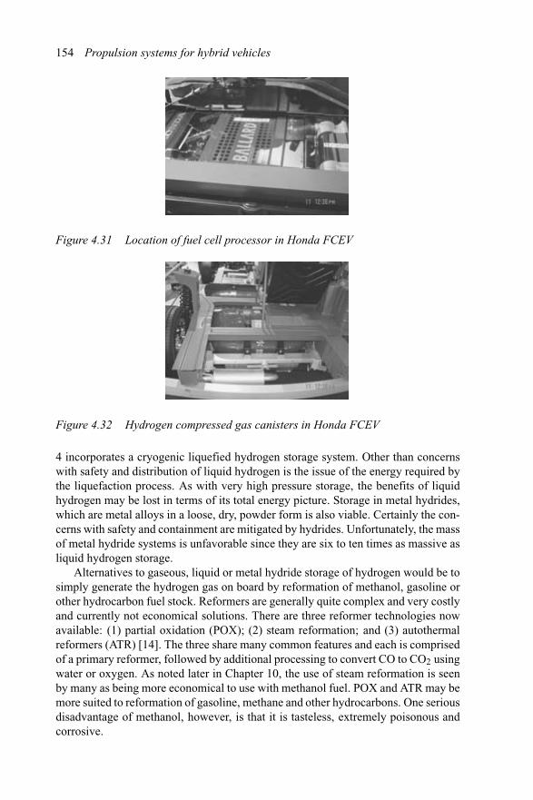
154 Propulsion systems for hybrid vehicles
Figure 4.31 Location of fuel cell processor in Honda FCEV
Figure 4.32 Hydrogen compressed gas canisters in Honda FCEV
4 incorporates a cryogenic liquefied hydrogen storage system. Other than concernswith safety and distribution of liquid hydrogen is the issue of the energy required bythe liquefaction process. As with very high pressure storage, the benefits of liquidhydrogen may be lost in terms of its total energy picture. Storage in metal hydrides,which are metal alloys in a loose, dry, powder form is also viable. Certainly the con-cerns with safety and containment are mitigated by hydrides. Unfortunately, the massof metal hydride systems is unfavorable since they are six to ten times as massive asliquid hydrogen storage.
Alternatives to gaseous, liquid or metal hydride storage of hydrogen would be tosimply generate the hydrogen gas on board by reformation of methanol, gasoline orother hydrocarbon fuel stock. Reformers are generally quite complex and very costlyand currently not economical solutions. There are three reformer technologies nowavailable: (1) partial oxidation (POX); (2) steam reformation; and (3) autothermalreformers (ATR) [14]. The three share many common features and each is comprisedof a primary reformer, followed by additional processing to convert CO to CO2 usingwater or oxygen. As noted later in Chapter 10, the use of steam reformation is seenby many as being more economical to use with methanol fuel. POX and ATR may bemore suited to reformation of gasoline, methane and other hydrocarbons. One seriousdisadvantage of methanol, however, is that it is tasteless, extremely poisonous andcorrosive.
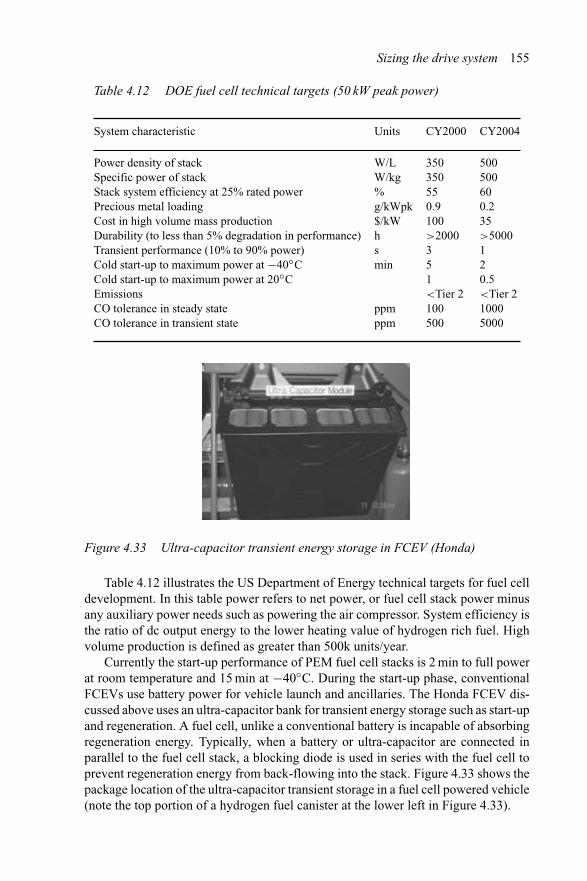
Sizing the drive system 155
Table 4.12 DOE fuel cell technical targets (50 kW peak power)
System characteristic Units CY2000 CY2004
Power density of stack W/L 350 500Specific power of stack W/kg 350 500Stack system efficiency at 25% rated power % 55 60Precious metal loading g/kWpk 0.9 0.2Cost in high volume mass production $/kW 100 35Durability (to less than 5% degradation in performance) h >2000 >5000Transient performance (10% to 90% power) s 3 1Cold start-up to maximum power at −40◦C min 5 2Cold start-up to maximum power at 20◦C 1 0.5Emissions <Tier 2 <Tier 2CO tolerance in steady state ppm 100 1000CO tolerance in transient state ppm 500 5000
Figure 4.33 Ultra-capacitor transient energy storage in FCEV (Honda)
Table 4.12 illustrates the US Department of Energy technical targets for fuel celldevelopment. In this table power refers to net power, or fuel cell stack power minusany auxiliary power needs such as powering the air compressor. System efficiency isthe ratio of dc output energy to the lower heating value of hydrogen rich fuel. Highvolume production is defined as greater than 500k units/year.
Currently the start-up performance of PEM fuel cell stacks is 2 min to full powerat room temperature and 15 min at −40◦C. During the start-up phase, conventionalFCEVs use battery power for vehicle launch and ancillaries. The Honda FCEV dis-cussed above uses an ultra-capacitor bank for transient energy storage such as start-upand regeneration. A fuel cell, unlike a conventional battery is incapable of absorbingregeneration energy. Typically, when a battery or ultra-capacitor are connected inparallel to the fuel cell stack, a blocking diode is used in series with the fuel cell toprevent regeneration energy from back-flowing into the stack. Figure 4.33 shows thepackage location of the ultra-capacitor transient storage in a fuel cell powered vehicle(note the top portion of a hydrogen fuel canister at the lower left in Figure 4.33).
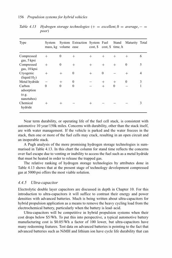
156 Propulsion systems for hybrid vehicles
Table 4.13 Hydrogen storage technologies (+ = excellent, 0 = average, − =poor)
Type Systemmass, kg
Systemvolume
Extractionease
Systemcost, $
Fuelcost, $
Standtime, h
Maturity Total
Compressedgas, 5 kpsi
+ 0 + + + + + 6
Compressedgas, 10 kpsi
+ 0 + + + + 0 5
Cryogenic(liquid H2)
+ + 0 + 0 − + 4
Metal hydride − + 0 − + + 0 3Carbon
adsorption(e.g.nanotubes)
0 0 0 − + 0 − 1
Chemicalhydride
+ + − + − − − 3
Near term durability, or operating life of the fuel cell stack, is consistent withautomotive 10 year/150k miles. Concerns with durability, other than the stack itself,are with water management. If the vehicle is parked and the water freezes in thestack, then one or more of the fuel cells may crack, resulting in an open circuit andan inoperable stack.
A Pugh analysis of the more promising hydrogen storage technologies is sum-marised in Table 4.13. In this chart the column for stand time reflects the concernsover fuel escape due to venting or inability to access the fuel such as a metal hydridethat must be heated in order to release the trapped gas.
The relative ranking of hydrogen storage technologies by attributes done inTable 4.13 shows that at the present stage of technology development compressedgas at 5000 psi offers the most viable solution.
4.4.5 Ultra-capacitor
Electrolytic double layer capacitors are discussed in depth in Chapter 10. For thisintroduction to ultra-capacitors it will suffice to contrast their energy and powerdensities with advanced batteries. Much is being written about ultra-capacitors forhybrid propulsion application as a means to remove the heavy cycling load from theelectrochemical battery, particularly when the battery is lead–acid.
Ultra-capacitors will be competitive in hybrid propulsion systems when theircost drops below $5/Wh. To put this into perspective, a typical automotive batterymanufacturing cost is $0.05/Wh a factor of 100 lower, but ultra-capacitors havemany redeeming features. Test data on advanced batteries is pointing to the fact thatadvanced batteries such as NiMH and lithium ion have cycle life durability that can
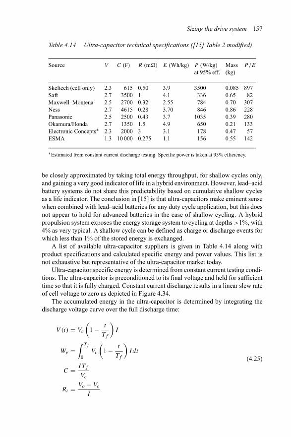
Sizing the drive system 157
Table 4.14 Ultra-capacitor technical specifications ([15] Table 2 modified)
Source V C (F) R (m�) E (Wh/kg) P (W/kg)at 95% eff.
Mass(kg)
P/E
Skeltech (cell only) 2.3 615 0.50 3.9 3500 0.085 897Saft 2.7 3500 1 4.1 336 0.65 82Maxwell–Montena 2.5 2700 0.32 2.55 784 0.70 307Ness 2.7 4615 0.28 3.70 846 0.86 228Panasonic 2.5 2500 0.43 3.7 1035 0.39 280Okamura/Honda 2.7 1350 1.5 4.9 650 0.21 133Electronic Concepts∗ 2.3 2000 3 3.1 178 0.47 57ESMA 1.3 10 000 0.275 1.1 156 0.55 142
∗Estimated from constant current discharge testing. Specific power is taken at 95% efficiency.
be closely approximated by taking total energy throughput, for shallow cycles only,and gaining a very good indicator of life in a hybrid environment. However, lead–acidbattery systems do not share this predictability based on cumulative shallow cyclesas a life indicator. The conclusion in [15] is that ultra-capacitors make eminent sensewhen combined with lead–acid batteries for any duty cycle application, but this doesnot appear to hold for advanced batteries in the case of shallow cycling. A hybridpropulsion system exposes the energy storage system to cycling at depths >1%, with4% as very typical. A shallow cycle can be defined as charge or discharge events forwhich less than 1% of the stored energy is exchanged.
A list of available ultra-capacitor suppliers is given in Table 4.14 along withproduct specifications and calculated specific energy and power values. This list isnot exhaustive but representative of the ultra-capacitor market today.
Ultra-capacitor specific energy is determined from constant current testing condi-tions. The ultra-capacitor is preconditioned to its final voltage and held for sufficienttime so that it is fully charged. Constant current discharge results in a linear slew rateof cell voltage to zero as depicted in Figure 4.34.
The accumulated energy in the ultra-capacitor is determined by integrating thedischarge voltage curve over the full discharge time:
V (t) = Vc
(1 − t
Tf
)I
We =∫ Tf
0Vc
(1 − t
Tf
)Idt
C = ITf
Vc
Ri = Vo − Vc
I
(4.25)
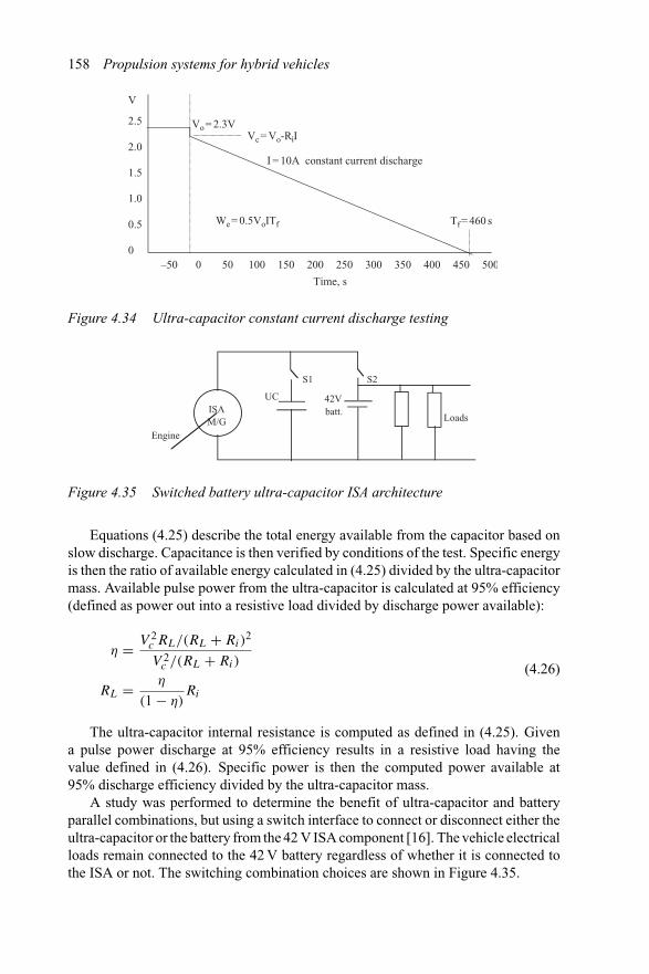
158 Propulsion systems for hybrid vehicles
I = 10A constant current discharge
Vo = 2.3V
Time, s
Vc = Vo-RiI
–50 0 50 100 150 200 250 300 350 400 450 500
2.0
1.5
1.0
0.5
0
Tf = 460 sWe = 0.5VoITf
V
2.5
Figure 4.34 Ultra-capacitor constant current discharge testing
Engine
UC 42Vbatt.
Loads
S1 S2
ISAM/G
Figure 4.35 Switched battery ultra-capacitor ISA architecture
Equations (4.25) describe the total energy available from the capacitor based onslow discharge. Capacitance is then verified by conditions of the test. Specific energyis then the ratio of available energy calculated in (4.25) divided by the ultra-capacitormass. Available pulse power from the ultra-capacitor is calculated at 95% efficiency(defined as power out into a resistive load divided by discharge power available):
η = V 2c RL/(RL + Ri)
2
V 2c /(RL + Ri)
RL = η
(1 − η)Ri
(4.26)
The ultra-capacitor internal resistance is computed as defined in (4.25). Givena pulse power discharge at 95% efficiency results in a resistive load having thevalue defined in (4.26). Specific power is then the computed power available at95% discharge efficiency divided by the ultra-capacitor mass.
A study was performed to determine the benefit of ultra-capacitor and batteryparallel combinations, but using a switch interface to connect or disconnect either theultra-capacitor or the battery from the 42 V ISA component [16]. The vehicle electricalloads remain connected to the 42 V battery regardless of whether it is connected tothe ISA or not. The switching combination choices are shown in Figure 4.35.
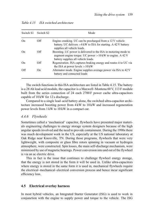
Sizing the drive system 159
Table 4.15 ISA switched architecture
Switch S1 Switch S2 Mode
On Off Engine cranking. UC can be precharged from a 12 V vehiclebattery. UC delivers >6 kW to ISA for starting. A 42 V batterysupplies all vehicle loads.
On Off Boosting. UC power is delivered to the ISA in motoring mode toaugment engine torque. UC power >10 kW to engine. A 42 Vbattery supplies all vehicle loads.
On Off Regeneration. ISA captures braking energy and routes it to UC viathe ISA at power levels >10 kW
Off On Alternator mode. Engine supplies average power via ISA to 42 Vbattery and connected loads
The switch functions in this ISA architecture are listed in Table 4.15. The batteryis a 28 Ah lead acid module, the capacitor is a Maxwell–Montena 60 V, 113 F modulebuilt from the series connection of 24 each 2700 F power cache ultra-capacitorscapable of 10 kW for 12 s discharge.
Compared to a single lead–acid battery alone, the switched ultra-capacitor archi-tecture increased boosting power from 4 kW to 10 kW and increased regenerationpower levels from 1 kW to 10 kW in a compact car.
4.4.6 Flywheels
Sometimes called a ‘mechanical’ capacitor, flywheels have presented major materi-als engineering challenges to energy storage system designers because of the highangular speeds involved and the need to provide containment. During the 1990s therewas much development work in the US, especially at the US national laboratory atOak Ridge near Knoxville, TN. During those programs, flywheels that were verylightweight, with composite or glass fibre rotors spinning in vacuum or hydrogenatmosphere, were constructed. Spin losses, the main self-discharge mechanism, wereminimised by use of magnetic bearings. Power conversion into and out of the flywheelis via an ac electric drive.
This in fact is the issue that continues to challenge flywheel energy storage,that the energy is not stored in the form it will be used in. Unlike ultra-capacitorswhere energy is stored in the same form it is used in, mechanical flywheels requirethe electrical–mechanical–electrical conversion process and hence incur significantefficiency loss.
4.5 Electrical overlay harness
In most hybrid vehicles, an Integrated Starter Generator (ISG) is used to work inconjunction with the engine to supply power and torque to the vehicle. The ISG
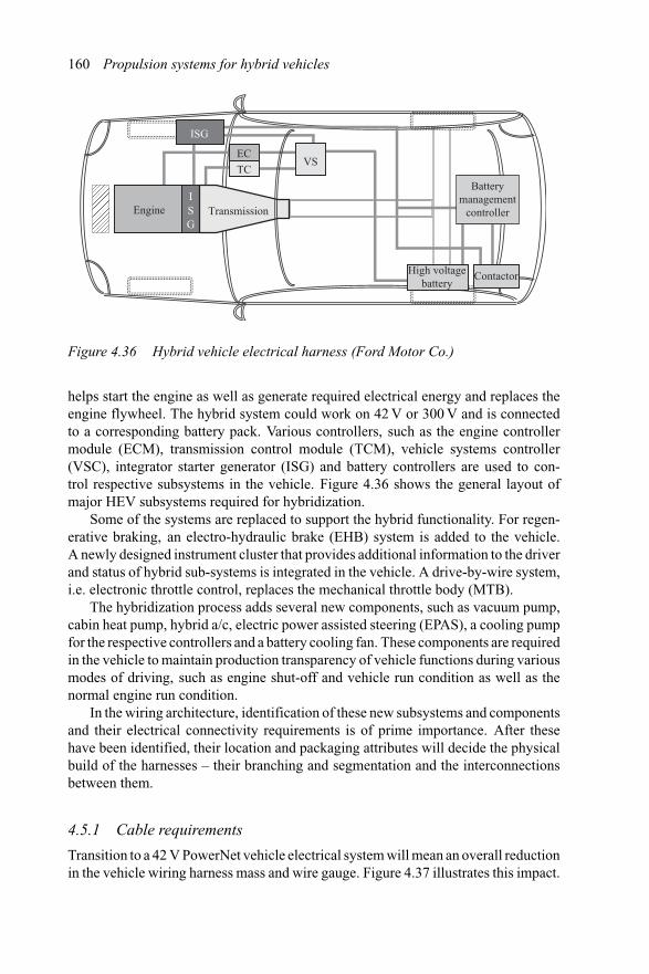
160 Propulsion systems for hybrid vehicles
ISG
Engine
ISG
VS
Contactor
Batterymanagement
controller
High voltagebattery
EC
TC
Transmission
Figure 4.36 Hybrid vehicle electrical harness (Ford Motor Co.)
helps start the engine as well as generate required electrical energy and replaces theengine flywheel. The hybrid system could work on 42 V or 300 V and is connectedto a corresponding battery pack. Various controllers, such as the engine controllermodule (ECM), transmission control module (TCM), vehicle systems controller(VSC), integrator starter generator (ISG) and battery controllers are used to con-trol respective subsystems in the vehicle. Figure 4.36 shows the general layout ofmajor HEV subsystems required for hybridization.
Some of the systems are replaced to support the hybrid functionality. For regen-erative braking, an electro-hydraulic brake (EHB) system is added to the vehicle.A newly designed instrument cluster that provides additional information to the driverand status of hybrid sub-systems is integrated in the vehicle. A drive-by-wire system,i.e. electronic throttle control, replaces the mechanical throttle body (MTB).
The hybridization process adds several new components, such as vacuum pump,cabin heat pump, hybrid a/c, electric power assisted steering (EPAS), a cooling pumpfor the respective controllers and a battery cooling fan. These components are requiredin the vehicle to maintain production transparency of vehicle functions during variousmodes of driving, such as engine shut-off and vehicle run condition as well as thenormal engine run condition.
In the wiring architecture, identification of these new subsystems and componentsand their electrical connectivity requirements is of prime importance. After thesehave been identified, their location and packaging attributes will decide the physicalbuild of the harnesses – their branching and segmentation and the interconnectionsbetween them.
4.5.1 Cable requirements
Transition to a 42 V PowerNet vehicle electrical system will mean an overall reductionin the vehicle wiring harness mass and wire gauge. Figure 4.37 illustrates this impact.
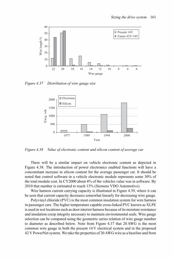
Sizing the drive system 161
0
10
20
30
40
50
60
Wire gauge
Wir
e le
ngth
%
Present 14VFuture 42V/14V
22 20 18 16 14 12 10 8 6 4
Figure 4.37 Distribution of wire gauge size
1977 1989 1994 2000Year
$/av
g. v
eh.
Electronic
Silicon
0
500
1000
1500
2000
Figure 4.38 Value of electronic content and silicon content of average car
There will be a similar impact on vehicle electronic content as depicted inFigure 4.38. The introduction of power electronics enabled functions will have aconcomitant increase in silicon content for the average passenger car. It should benoted that control software in a vehicle electronic module represents some 30% ofthe total module cost. In CY2000 about 4% of the vehicles value was in software. By2010 that number is estimated to reach 13% (Siemens VDO Automotive).
Wire harness current carrying capacity is illustrated in Figure 4.39, where it canbe seen that current capacity decreases somewhat linearly for decreasing wire gauge.
Polyvinyl chloride (PVC) is the most common insulation system for wire harnessin passenger cars. The higher temperature capable cross-linked PVC known as XLPEis used in wet locations such as door interior harness because of its moisture resistanceand insulation creep integrity necessary to maintain environmental seals. Wire gaugeselection can be computed using the geometric series relation of wire gauge numberto diameter as described below. Note from Figure 4.37 that 20 AWG is the mostcommon wire gauge in both the present 14 V electrical system and in the proposed42 V PowerNet system. We take the properties of 20 AWG wire as a baseline and from
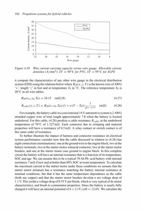
162 Propulsion systems for hybrid vehicles
20 18 16 14 12 10
PVCXLPE
0
5
10
15
20
25
30
35
40
22 8
Wire gauge
Cur
rent
den
sity
, A/m
m2
Figure 4.39 Wire current carrying capacity versus wire gauge. Allowable currentdensities (A/mm2): δT = 50◦C for PVC, δT = 95◦C for XLPE
it compute the characteristics of any other wire gauge in the electrical distributionsystem (EDS) using the relations below where R20(x, z, T ) is the known wire of AWG‘x’, length ‘z’ in feet and at temperature T0 in ◦C. The reference temperature T0 is20◦C in all wire tables:
R20(xo, z0, T0) = 10.15 (m�/ft) (4.27)
Rcable(y, z, T ) = R20(x, z0, T0)z(1 + γ (T − T0))1
2(x−y)/3(m�) (4.28)
For example, the battery cable in a conventional 14 V automotive system is 2 AWGstranded copper wire of total length approximately 7 ft when the battery is locatedunderhood. For this cable, (4.28) predicts a cable resistance Rcable at the underhoodtemperature of 70◦C of 1.327 m�. Each connector due to crimping and materialproperties will have a resistance of 0.5 m�. A relay contact or switch contact is ofthis same order of resistance.
To further illustrate the impact of harness and connector resistance on electricalsystem performance consider now that the cable discussed in relation to (4.28) haseight connections (terminations): one at the ground wire to the engine block; two at thebattery terminals; two at the starter motor solenoid contactor; two at the starter motorbrushes; and one at the starter motor case ground to engine block. In this completecircuit the battery will have an internal resistance that is a function of its temperature,SOC and age. We can assume this to be a typical 70 Ah Pb–acid battery with internalresistance 7 m� if new and at better than 80% SOC at room temperature. To calculatethe maximum current to the starter motor under these conditions we assume that thestarter motor armature has a resistance matching the battery internal resistance atnominal conditions, but that it has the same temperature dependence as the cable(both use copper) and that the starter motor brushes develop a net voltage drop of1.1 V. This yields a voltage drop of 0.55 V per brush, which is very typical of dc motorcharacteristics, and brush to commutator properties. Since the battery is nearly fullycharged it will have an internal potential of 6 × 2.1V/cell = 12.6V. We calculate the
Sizing the drive system 163
maximum current delivered to the starter motor as
Istarter = (Vbatt − 2Vbrush) × 103
Rcable(y, z, T ) + NcRconn + Rint + Rarm
(A) (4.29)
For the conditions noted above and where Nc = number of interconnects wefind that the starter motor current is 556 A maximum. In today’s automobile thestarter motor is internally geared with a planetary set having a ratio Ggr = 3.6:1 andexternally geared at the pinion to ring gear at the crankshaft of Grg = 14:1 or slightlyhigher, depending on the engine. In fact, the same starter motor is used for severaldifferent engine displacements by changing the ring gear number of teeth (gear ratio).Now using the fact that this starter motor has a torque constant, kt = 0.011 Nm/A,we can calculate the torque delivered to the engine crankshaft as
Tcrank = NgrNrgkt Istarter (Nm) (4.30)
For the conditions given, and for the approximations made, we find that thispermanent magnet, geared, starter motor is capable of delivering 308 Nm of torqueto the engine crankshaft. If we now assume the temperature is at −30◦C, we canrecalculate the starter motor maximum current by first noting that although the cable,termination and starter motor armature resistances will decrease in proportion totemperature, the battery internal resistance will actually increase due to slower iontransport dynamics and increased polarization. We will make the approximation thatcable and armature resistance, since these are copper wire based, will have the sameresistance change. Terminations, on the other hand, will be assumed to have negligiblechange. The battery internal resistance for this example is approximated accordingto the following expression (α = 0.0003, β = 2):
Rint(T ) = Rint(T0)(1 + α(T − T0)β) (�) (4.31)
With this modification to (4.2) the starter motor current at −30◦C actually drops to504 A, yielding a cranking torque of 280 Nm. In reality the starter motor brush voltagedrop will also increase, further reducing the available torque. Typically, starter motortorque capability, when at cold temperature, is in excess of the torque necessary tobreakover and crank a cold engine. Cranking speeds at cold temperature are alsoslower due to higher friction in the engine so that crank speeds of 100 rpm or less aretypical.
One further point to make regarding brushed dc motors and cold conditions isthat, if improperly designed, the cold inrush current, assuming a fresh battery, maybe higher than the room temperature design point, resulting in demagnetization ofthe ceramic magnets. Unlike rare earth magnets used in starter-alternator and otherhigh performance electric machines, a starter motor and most dc motors in the carwill rely on ceramic 7 or ceramic 8 magnets, which have less coercive force at coldtemperatures and so could conceivably be partially demagnetized.
164 Propulsion systems for hybrid vehicles
4.5.2 Inverter busbars
An important and easily overlooked component of the hybrid propulsion system make-up is the busbar structure present in all power electronic converters and inverters. Thepower electronics component resides in the main electric power flow path betweenthe energy storage system and the M/G and driveline. In the power electronics, dccurrent from the energy storage system is converted to variable frequency and voltageac currents for injection into the M/G through the process of high frequency switching.In order to process kW of electric power and not overstress the internal componentsit is necessary that parasitic inductances and stray lead inductances, all of whichcause voltage steps on their associated switching devices and all connected devices,be absolutely minimised. The voltage step occurring when currents are switched atinverter switching speeds can be very high. For example, suppose a typical currenttransition having a slew rate of 260 A/μs at the switch must flow through 100 nHof stray inductance, including inductance of the power module itself, the busbar andfinally the link capacitor. This current transition will result in a voltage step on thesilicon metalization of
Vstep = Lstray
di(t)
dt(4.32)
which computes out to 26.7 V of additional voltage stress. In a 42 V system with 80 Vrated semiconductor switches this amount of voltage overshoot could not be tolerated.The solution is low inductance busbars [17,18]. Table 4.16 lists the common types ofbusbars and the inductance of individual conductors.
For example, a laminar busbar system consists of positive and negative bars thatare 6 in wide, 0.125 in thick, and separated by Nomex sheets having a thicknessof 0.125 in. The complete busbar system is approximately 28 in in length. Insertingthese dimensions into the expression for inductance, the value returned is 209 nH.The conductor area, Wt , is estimated for the rated current, I , in amps dc, based onthe empirical expression given as (4.33):
Wt = 0.0645πI(1 + 0.5(N − 1)) (mm2) (4.33)
where N is the number of conductors in the busbar assembly, in this case N = 2.In the earlier example where the dc link current was 242 Adc, the required busbararea would be 49 mm2 with an aspect ratio W/t ∼ 48:1. Therefore the end itembusbar would be approximately 1 mm thick each conductor and 49 mm wide. Therated current density in the conductors would be 4.9 A/mm2.
Because of the skin effect in the busbar conductors there will be a significantac resistance component to the busbar so that current flows at the surface and doesnot penetrate the full bar depth. This has required the calculation of an equivalentdc current from which the busbar is re-sized. For the example cited, the nominal dccurrent of 242 A must be increased in proportion to the known frequency componentsof current. High frequency ac currents flow on only one side of each busbar conductor,the side facing the dielectric, and from this side only one skin depth into the bar.
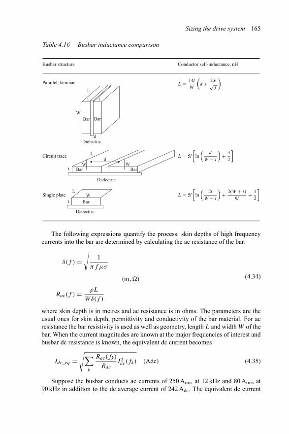
Sizing the drive system 165
Table 4.16 Busbar inductance comparison
Busbar structure Conductor self-inductance, nH
Parallel, laminar
Dielectric
Bar Bar
L
W
t t
d
L = 14l
W
(d + 2.6√
f
)
Circuit trace
Bar Bar
Dielectric
W Wt
dL
L = 5l
[ln(
d
W + t
)+ 3
2
]
Single plate
Dielectric
t
L
BarW L = 5l
[ln(
2l
W + t
)+ 2(W + t)
9l+ 1
2
]
The following expressions quantify the process: skin depths of high frequencycurrents into the bar are determined by calculating the ac resistance of the bar:
δ(f ) =√
1
πf μσ
(m, �)
Rac(f ) = ρL
Wδ(f )
(4.34)
where skin depth is in metres and ac resistance is in ohms. The parameters are theusual ones for skin depth, permittivity and conductivity of the bar material. For acresistance the bar resistivity is used as well as geometry, length L and width W of thebar. When the current magnitudes are known at the major frequencies of interest andbusbar dc resistance is known, the equivalent dc current becomes
Idc_eq =√∑
k
Rac(fk)
Rdc
I 2ac(fk) (Adc) (4.35)
Suppose the busbar conducts ac currents of 250 Arms at 12 kHz and 80 Arms at90 kHz in addition to the dc average current of 242 Adc. The equivalent dc current
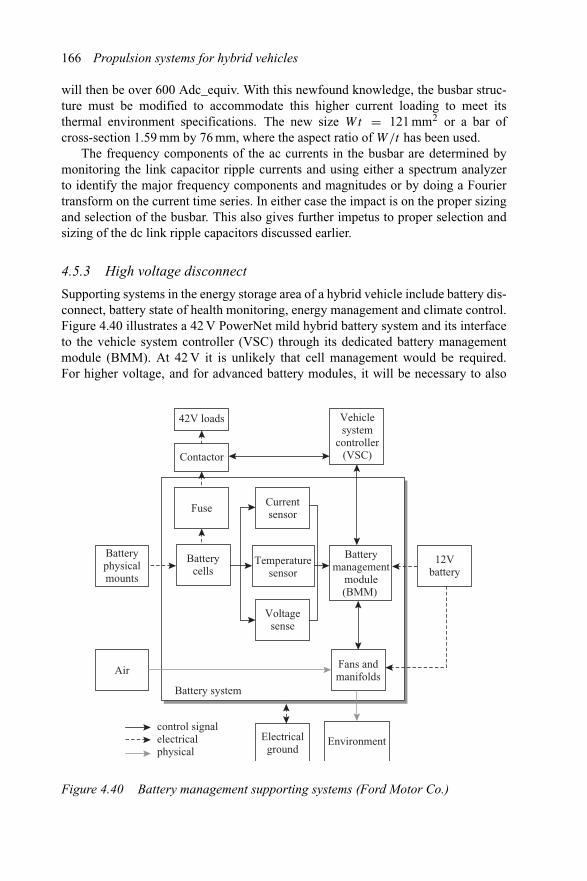
166 Propulsion systems for hybrid vehicles
will then be over 600 Adc_equiv. With this newfound knowledge, the busbar struc-ture must be modified to accommodate this higher current loading to meet itsthermal environment specifications. The new size Wt = 121 mm2 or a bar ofcross-section 1.59 mm by 76 mm, where the aspect ratio of W/t has been used.
The frequency components of the ac currents in the busbar are determined bymonitoring the link capacitor ripple currents and using either a spectrum analyzerto identify the major frequency components and magnitudes or by doing a Fouriertransform on the current time series. In either case the impact is on the proper sizingand selection of the busbar. This also gives further impetus to proper selection andsizing of the dc link ripple capacitors discussed earlier.
4.5.3 High voltage disconnect
Supporting systems in the energy storage area of a hybrid vehicle include battery dis-connect, battery state of health monitoring, energy management and climate control.Figure 4.40 illustrates a 42 V PowerNet mild hybrid battery system and its interfaceto the vehicle system controller (VSC) through its dedicated battery managementmodule (BMM). At 42 V it is unlikely that cell management would be required.For higher voltage, and for advanced battery modules, it will be necessary to also
Batteryphysicalmounts
Electricalground
Air
Vehiclesystem
controller(VSC)
Batterycells
Currentsensor
42V loads
Batterymanagement
module(BMM)
Fans andmanifolds
Environment
Voltagesense
Battery system
12Vbattery
Contactor
Fuse
control signalelectricalphysical
Temperaturesensor
Figure 4.40 Battery management supporting systems (Ford Motor Co.)
Sizing the drive system 167
include a cell management system consisting of some means to stabilize individualcell charge. Forms of cell management include charge transfer devices or resistivedividers. In practice, high voltage NiMH batteries will have a cell management unitfor strings of six to ten cells. In lithium ion it may be necessary to have cell man-agement for every three to five cells. Electrical protection is provided by fuse andcontactor arrangements. For high voltage batteries it is also necessary to interlockthe internal cell stack(s) from the case terminals or connector. Generally a plug isused that opens the cell pack from the terminals and disengages the contactor in theprocess (disconnect before break).
4.5.4 Power distribution centres
Modern automobiles, and luxury brands in particular, have evolved to multi-zone elec-trical distribution centers. In this zonal architecture the local branch circuits are fedfrom power distribution centres in much the same manner that apartment complexeshave a single service entrance but distribution panels for each individual apartment.The Jaguar XK8, for example, uses three zone power distribution, underhood, passen-ger compartment and trunk (boot). The trunk power distribution centre is importantin high end vehicles because so much electronic content is being pushed into thepackage tray area just behind the rear seat back and beneath the rear window. Con-tent includes anti-theft, radio head, entertainment amplifiers, multi-CDROM drivesand more. When interior and exterior lighting is included the load at the trunk areademands a separate zonal distribution centre.
In hybrid vehicles the same package locations become filled with traction batter-ies, or battery climate control hardware in addition to all the pre-existing electroniccontent. Power distribution centres today are still relay boxes having busbar inter-connects and some introduction of smart power semiconductors. The semiconductorcontent is expected to increase significantly with hybrid vehicles and as morepowerful controller area networks are incorporated such as Flexray.
4.6 Communications
In vehicle and outside of the vehicle communications are fast growing technol-ogy areas in automotive applications. Automotive communications networks havetypically used LANs (local area networks) of the controller area network (CAN)variety. The GM Hywire concept vehicle, for example, is advertized as a completelyx-by-wire architecture, but CAN networks are converting over to protocols that aremore fault tolerant and have guaranteed communications times and no issues withmessage latency as has been common for multiple access collision detection (MA/CD)protocols in the past. Time triggered protocols (TTP) have been proposed for manyyears and are now beginning to enter the automotive arena as a new protocol derivedfrom a TTP/C basis known as Flexray.
To understand automotive communications it is important to understand the basicsof networked communications. In 1983 the Open Systems Interconnection (OSI)
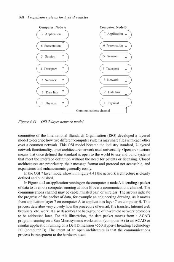
168 Propulsion systems for hybrid vehicles
7 Application
6 Presentation
5 Session
4 Transport
3 Network
2 Data link
1 Physical
7 Application
6 Presentation
5 Session
4 Transport
3 Network
2 Data link
1 Physical
Communications channel
Computer: Node A Computer: Node B
Figure 4.41 OSI 7-layer network model
committee of the International Standards Organisation (ISO) developed a layeredmodel to describe how two different computer systems may share files with each otherover a common network. This OSI model became the industry standard, 7-layerednetwork functionality, open architecture network used universally. Open architecturemeans that once defined the standard is open to the world to use and build systemsthat meet the interface definition without the need for patents or licensing. Closedarchitectures are proprietary, their message format and protocol not accessible, andexpansions and enhancements generally costly.
In the OSI 7 layer model shown in Figure 4.41 the network architecture is clearlydefined and published.
In Figure 4.41 an application running on the computer at node A is sending a packetof data to a remote computer running at node B over a communications channel. Thecommunications channel may be cable, twisted pair, or wireless. The arrows indicatethe progress of the packet of data, for example an engineering drawing, as it movesfrom application layer 7 on computer A to applications layer 7 on computer B. Thisprocess describes very closely how the procedure of e-mail, file transfer, Internet webbrowsers, etc. work. It also describes the background of in-vehicle network protocolsto be addressed later. For this illustration, the data packet moves from a ACADprogram running on a Sun Microsystems workstation (computer A) to an ACAD orsimilar application running on a Dell Dimension 4550 Hyper-Threading TechnologyPC (computer B). The intent of an open architecture is that the communicationsprocess is transparent to the hardware used.
Sizing the drive system 169
The OSI 7 layers are defined as:
1. Physical. The modem and wire or other channel connecting to nodes. The channelmay be coaxial cable, twisted pair copper wire, fibre-optic cable, radio or infraredlinks, etc.
2. Data link. Describes how the nodes of the network obtain access and share thephysical connections to the channel. The physical address of a node, or its mediaaccess control, is defined at layer 2. For example, internet service provider pointto point control for dial up access is defined at this data link layer.
3. Network. This layer takes care of routing data packets to nodes that may not evenbe on the same LAN as computer A, for instance. The network layer contains log-ical rather than physical addresses and the routing mechanisms needed to accessremote LANs or wide area networks, WANs. This is where internet protocol (IP),for example, resides.
4. Transport. The layer that acknowledges message transmission across the networkand validating that transmission has occurred without loss of data. If a data packetis lost, this layer is responsible for resending the data packet and confirming itwas received and placed back into the correct sequence. This layer is called TCP(transmission control protocol).
5. Session. The session layer maintains an open communications channel betweentwo separate nodes during transmission. An initial packet is transmitted to estab-lish the connection, after which subsequent packets are sent. The session layerensures that the context of all packets is preserved.
6. Presentation. This is the application isolation layer. Layer 6 reconciles differencesbetween application data encryption/decryption techniques. For example, theapplication on computer A may use EBCDIC for character code conversion, whilecomputer B may be using ASCII to encrypt character data. The presentation layerisolates the application layer from the particulars of the environment in whichthe application on node B, for example, resides.
7. Application. This is where executable applications such as auto CAD, orMicrosoft Word, or any other application resides. This layer is the human–machine interface (HMI).
To continue the communications process described in Figure 4.41 we follow thearrows from layer 7 on computer A to layer 7 on the remote computer B. Node Ahands off the data packet (file transfer, FTP to remote computer B) to its presentationlayer 6, which isolates the application from node B’s application. Layer 6 does itsprocessing, adds headers and trailers to the packet and passes it down to layer 5, whichdoes the same, adding its headers and trailers, and so on down to the physical layer.The physical layer modem sends its 1s and 0s across the communications channel tonode B. Layer 1 on node B collects up all the 1s and 0s, packs them up and beginsthe hand-off to its layer 2. At layer 2 on node B it strips off its headers and trailerinformation, does the requisite processing and passes the data packet on to layer 3,and so on up to layer 7. As a result of all this processing the original ACAD drawingsent by computer A arrives at the application running on computer B.
170 Propulsion systems for hybrid vehicles
The point of this example was to illustrate that the FTP server on the Microsystemsworkstation running the Solaris operating system is not required to even know that theDell Hyper-Threading PC at node B is running Microsoft Windows 2000 Professional.The file is transferred flawlessly. This same need for flawless and fault tolerantcommunications is present in the automobile networks, but the consequence of a‘lost’ data packet is far more serious when the data packet was sent from the vehiclesystem controller to the hybrid M/G to command generating mode at torque levelTx to slow the engine speed down while simultaneously having commanded theengine electronic throttle control to reduce air flow and commanding an upshift tothe automatic transmission during vehicle acceleration.
Communications architecture in the future automobile will be an open system sothat any supplier can build modules that connect to the published network standardand its function will execute flawlessly. Vehicle power train controls today follow theOSEK operating system (Offene Systeme und deren Schnittstellen fur die Elektronikim Kraftfahrzeug). Engine controllers have progressed from 8-bit cores having 128 kBof ROM, through 16-bit 256 kB engines, on to today’s 32-bit chips supported by512 kB to 1 MB of ROM.
4.6.1 Communication protocol: CAN
During most of the early years of electronic engine control and for hybrid propulsiontechnologies some form of CAN communications between the various subsystemshas been in use. Early SAE standards categorised in-vehicle networks according todata handling speed. Setting a standard based on data handling speed in effect deter-mined the types of devices that could be served and the types of data communicationprotocols that could be applied. Early hybrid propulsion communications architec-tures relied on class B and some provision was made for class C, CAN, where veryfast data exchange was necessary, such as in the powertrain controller. Class A isa low speed protocol used primarily for in-vehicle body electrical functions such aspower seat and power window controls. Protocols on class A networks include localinterconnect network (LIN) and time triggered protocol/A (TTP/A).
Class B networks are designed for data sharing between devices in the hopeof minimising if not eliminating redundant sensors – for example, instrumentation,speed-control functions, emissions systems and others. Class B network protocolsinclude ISO 9141-2 and SAE J1850.
CAN class C network protocol was developed for real time control applications,hence the reference to powertrain control functions. Also included in class C protocolis vehicle dynamics control. Protocols listed under class C are CAN and J1039.
The various in-vehicle network classes are described in Table 4.17 along withtypical in-vehicle applications served.
4.6.2 Power and data networks
Modern vehicles, and particularly hybrid vehicles, are evolving to a four layer powerand data communications architecture. The four layer model is based on broad classes
Sizing the drive system 171
Table 4.17 In-vehicle communications networks
Network class Speed Application
Class ALIN, TTP/A
<10 kbps Customer amenities: power seats,windows, mirrors, trunk release, etc.
Class BJ1850, ISO 9141-2
10 kbps → 125 kbps Information transfer: cabin climatecontrol, dash-board instrumentation,convenience features, etc.
Class CCAN, J1039
125 kbps → 12 Mbps Real time control: powertrain andvehicle dynamics
Class D MOST,Flexray
>1 Mbps Multimedia and safety criticalapplications: x-by-wire, digital TV,Internet
Vehicle systemcontroller
ISG subsystembelt or crankshaft
Engine Transmission
Other 42Vloads
Brake actuators
ETC, fan, water pump
ISGtorque
Gear sel, L/U clutchoil pump
SOC, SOH,Vsys Continuous,scheduled,selectable
Brakesregen. brake sys.
Steeringelectric assist
Steering actuator
UC UCUC
ECU
MtrRac
k ECU
HCU
ECU
Mtr Throttlebody
Steeringwheel
Brakepedal
Accel.pedal
Power and communications (PDA)
42V batteryprimary storage
Figure 4.42 Hierarchical power and data architecture
of functionality, data transmission speed and data protocols associated with broadclasses of speeds.
The four layer model includes: power distribution in an open architecture senseof generation, storage and distribution systems; safety and mobility including air bagdeployment control to powertrain and x-by-wire controls; body layer including inte-rior and exterior lighting, customer amenities and instrumentation; and infotainmentlayer including high end audio products, TV, wireless phone, voice actuated systems,navigation aides, and other additions in a scaleable and flexible architecture.
In-vehicle architectures, besides being open, are hierarchical by design. A hierar-chical architecture adheres to strict protocols of top-down command flow and upwardflow of data. Lateral data flow is allowed, but lateral command flow is prohibited.This is the architecture of choice for hybrid propulsion in which a high level vehiclesystem controller is coordinating its various subsystems as shown in Figure 4.42.
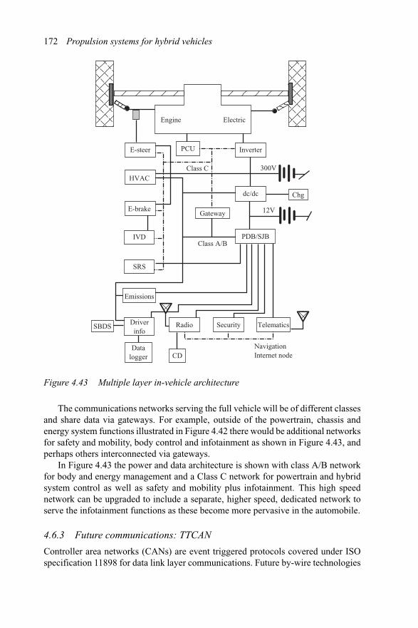
172 Propulsion systems for hybrid vehicles
PDB/SJB
12V
300V
Class A/B
NavigationInternet node
Engine Electric
InverterPCU
Class CHVAC
E-brake
IVD
SRS
E-steer
dc/dc
Emissions
SBDS
CDData
logger
Driverinfo
Radio Security Telematics
Chg
Gateway
Figure 4.43 Multiple layer in-vehicle architecture
The communications networks serving the full vehicle will be of different classesand share data via gateways. For example, outside of the powertrain, chassis andenergy system functions illustrated in Figure 4.42 there would be additional networksfor safety and mobility, body control and infotainment as shown in Figure 4.43, andperhaps others interconnected via gateways.
In Figure 4.43 the power and data architecture is shown with class A/B networkfor body and energy management and a Class C network for powertrain and hybridsystem control as well as safety and mobility plus infotainment. This high speednetwork can be upgraded to include a separate, higher speed, dedicated network toserve the infotainment functions as these become more pervasive in the automobile.
4.6.3 Future communications: TTCAN
Controller area networks (CANs) are event triggered protocols covered under ISOspecification 11898 for data link layer communications. Future by-wire technologies
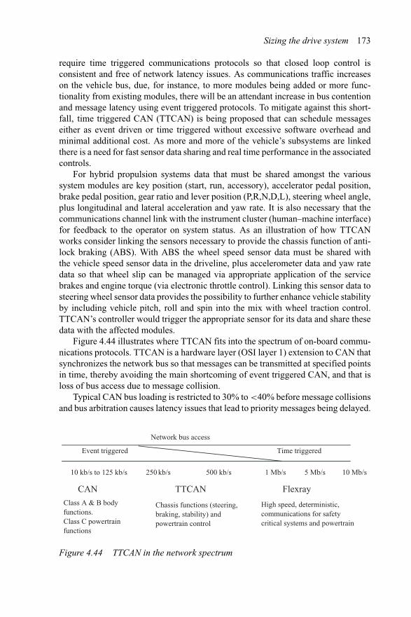
Sizing the drive system 173
require time triggered communications protocols so that closed loop control isconsistent and free of network latency issues. As communications traffic increaseson the vehicle bus, due, for instance, to more modules being added or more func-tionality from existing modules, there will be an attendant increase in bus contentionand message latency using event triggered protocols. To mitigate against this short-fall, time triggered CAN (TTCAN) is being proposed that can schedule messageseither as event driven or time triggered without excessive software overhead andminimal additional cost. As more and more of the vehicle’s subsystems are linkedthere is a need for fast sensor data sharing and real time performance in the associatedcontrols.
For hybrid propulsion systems data that must be shared amongst the varioussystem modules are key position (start, run, accessory), accelerator pedal position,brake pedal position, gear ratio and lever position (P,R,N,D,L), steering wheel angle,plus longitudinal and lateral acceleration and yaw rate. It is also necessary that thecommunications channel link with the instrument cluster (human–machine interface)for feedback to the operator on system status. As an illustration of how TTCANworks consider linking the sensors necessary to provide the chassis function of anti-lock braking (ABS). With ABS the wheel speed sensor data must be shared withthe vehicle speed sensor data in the driveline, plus accelerometer data and yaw ratedata so that wheel slip can be managed via appropriate application of the servicebrakes and engine torque (via electronic throttle control). Linking this sensor data tosteering wheel sensor data provides the possibility to further enhance vehicle stabilityby including vehicle pitch, roll and spin into the mix with wheel traction control.TTCAN’s controller would trigger the appropriate sensor for its data and share thesedata with the affected modules.
Figure 4.44 illustrates where TTCAN fits into the spectrum of on-board commu-nications protocols. TTCAN is a hardware layer (OSI layer 1) extension to CAN thatsynchronizes the network bus so that messages can be transmitted at specified pointsin time, thereby avoiding the main shortcoming of event triggered CAN, and that isloss of bus access due to message collision.
Typical CAN bus loading is restricted to 30% to <40% before message collisionsand bus arbitration causes latency issues that lead to priority messages being delayed.
Event triggered Time triggered
Network bus access
CAN TTCAN Flexray
Class A & B body functions.Class C powertrain functions
Chassis functions (steering, braking, stability) andpowertrain control
High speed, deterministic, communications for safety critical systems and powertrain
10 kb/s to 125 kb/s 250 kb/s 500 kb/s 1 Mb/s 5 Mb/s 10 Mb/s
Figure 4.44 TTCAN in the network spectrum
174 Propulsion systems for hybrid vehicles
With TTCAN, bus synchronization and time triggering boost bus availability to about90% of capability. This is because with only a single message on the bus loss ofarbitration is prevented and channel latency becomes entirely predictable. In the caseof using a CAN physical layer with TTCAN this puts an upper limit of approximately1 Mb/s on bus loading.
Because of the flexible event and time triggering options, TTCAN has been calledMultiCAN by some manufacturers. The benefit of TTCAN lies in the fact that existingnetwork physical medium and channels remain intact and the time triggering alongwith synchronization of the bus and all connected modules shifting from local to globaltime without the need for expensive hardware or replacement of the network medium.The protocol is at the proposal stage and will be offered as part of manufacturers’32-bit microcontrollers [19].
4.6.4 Future communications: Flexray
With all of the new x-by-wire technologies now on the horizon the automotive indus-try must respond with a single, reliable, high speed communications standard forin-vehicle networking [20]. Drive-by-wire technologies include steering, braking,suspension and traction control via engine throttle control and hybrid system M/Gcontrol, and more, will replace every hydraulic and mechanical system now in place.These safety critical and propulsion control subsystems require deterministic commu-nications for which the protocol demanded is time triggered versus the event triggeredCAN protocols. The Flexray protocol is now in the process of being validated as thetechnology of choice that will provide the high speed, deterministic, fault tolerant,level of communications bandwidth needed for data transmission in chassis control,hybrid powertrain and energy management system functions.
An industry wide Flexray consortium of global automotive manufacturers andsuppliers has formed to drive the adoption of an open standard for high speed databus communications to meet the future demands of x-by-wire. The consortium formedin September 2000 and has since grown to include the major automotive OEMs (GM,Ford, DCX, BMW) and suppliers (Motorola, Philips, Bosch, Mitsubishi Electric &Electronics, and others). The Flexray consortium is an alliance of automotive OEMsand semiconductor manufacturers.
The Safe-by-Wire Consortium sister to the Flexray Consortium will developindustry standard automotive safety bus for use in safety restraint systems (SRSincluding air bag, knee bolster airbags, side air bags, weight sensors and occupantsensors).
The Flexray protocol targets future in-vehicle applications that require, and ben-efit from, higher data rates, deterministic behaviour and fault tolerance. Flexray isthe communications protocol that is scalable and incorporates the benefits of familiarsynchronous and asynchronous protocols. Flexray protocol supports fault-tolerantclock synchronization via a global time base, has collision free bus access, providesguaranteed message latency, has message oriented addressing identifiers, and a scal-able fault tolerance over single or dual channels. The physical layer (OSI layer 1)
Sizing the drive system 175
includes an independent bus guardian for error containment while supporting busspeeds up to 10 Mbps. The basic features of Flexray are:
• scalable synchronous and asynchronous data transmission• high net data rate of 5 Mbps with a gross data rate of up to 10 Mbps• deterministic data transmission, guaranteed message latency and jitter• fault tolerant and time triggered services in hardware versus software• fast error detection and signaling, supports redundant channels• fault tolerant, synchronous, global time base• bus guardian error containment at the physical layer (electronic or optical)• arbitration free transmission• it supports all popular network configurations (bus, star, multiple star).
Flexray is not TTP/C, but it has some features of TTP/C such as a time divisionmultiple access (TDMA) bus access scheme. The message format of Flexray consistsof a static header plus 246 byte dynamic frame lengths containing membership andacknowledgement fields.
Flexray is one of many in-vehicle protocols either in use or proposed for datacommunications. Table 4.18 provides a listing of some of the more popular and opensystem protocols. There are other, proprietary protocols in existence, but only openarchitectures are of future interest.
Bus loading on conventional vehicles will continue to increase. In hybrid propul-sion systems the demand for more functionality automatically increases the networktraffic since more torque sources must be managed in addition to the internal com-bustion engine and transmission. With CAN protocols network access is on demandand becomes a real issue when several modules contend for the bus, each with highpriority messages. Once agreement is reached to regulate the placement of messagesand to plan for present and future content a deterministic communications channel isrealised. Flexray is one such solution to the contention issues of event based protocols
Table 4.18 In-vehicle network data protocols
Data protocol Applications Media Data rate, max
Bluetooth Control Wireless 750 kbpsCAN Control Twisted-pair 1 MbpsD2B Audio/video Fibre-optic 12 MbpsDSI Sensor multiplexing 2 wire 5 kbpsFlexray Safety and mobility 2 wire 10 MbpsIEEE-1394 Multimedia 6 wire twisted pairs 200 MbpsJ1850 PWM Control 2 wire 41.6 kbpsJ1939 Control Twisted-pair 1 MbpsLIN Control Single wire 20 kbpsMOST Multimedia Fibre-optic 25 MbpsTTP Real time control 2 channel 5 Mbps (10 Mbps optical)
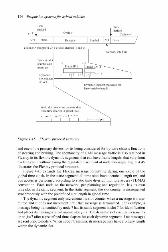
176 Propulsion systems for hybrid vehicles
y – 1 Cycle yCycle y + 1
Timederived
Timederived
Static Dynamic Symbol NIT StaticNIT
Channel A (single) or Ch 1 of dual channel (1 and 2)
j j + 1 j + 2 j + 3 * * * Dynamicslot counter if no Tx
m m + 1 m + 2 m + 3 * * *
Static slot counter increments after fixed time interval in global time.
Frame ID j Frame ID j+1J J+1
Dynamic slot counter with messages
Dynamic segment messages can have variable length
Network idle time
Figure 4.45 Flexray protocol structure
and one of the primary drivers for its being considered for by-wire chassis functionsof steering and braking. The spontaneity of CAN message traffic is also retained inFlexray in its flexible dynamic segments that can have frame lengths that vary fromcycle to cycle without losing the regulated placement of node messages. Figure 4.45illustrates the Flexray protocol structure.
Figure 4.45 expands the Flexray message formatting during one cycle of theglobal time clock. In the static segment, all time slots have identical length (m) andbus access is performed according to static time division multiple access (TDMA)convention. Each node on the network, per planning and regulation, has its owntime slot in the static segment. In the static segment, the slot counter is incrementedsynchronously with the predefined slot length in global time.
The dynamic segment only increments its slot counter when a message is trans-mitted and it does not increment until that message is terminated. For example, amessage being transmitted by node 7 has its static segment in slot 7 for identificationand places its messages into dynamic slot j=7. The dynamic slot counter incrementsup to j=7 after a predefined time elapses for each dynamic segment if no messagesare sent prior to node 7. When node 7 transmits, its message may have arbitrary lengthwithin the dynamic slot.
Sizing the drive system 177
Because of the predefined positioning of node messages with time slots it ispossible to determine if a particular node is responding properly. If for some reasonnode 7 sends its message out of its assigned slot then an error is detected. Thisfunctionality is that of a bus guardian and in Flexray the bus guardian controls accessto the physical bus. The bus guardian receives the predefined schedule from thebus host during initialization and from that point on the bus guardian activates its buswatchdog which contains an independent time reference. Bus drivers and bus guardiancollaborate and support each other in the identification of faults. Diagnostics of busfaults are then passed on to the bus host.
4.6.5 Competing future communications protocols
It is clear that modern personal transportation vehicles, hybrid vehicles in particular,will rely on multiple communications buses per vehicle. This is because the needfor communications varies according to systems supported and the speed at whichinformation must be shared. Body modules for powered seats, windows, mirrors andthe like are slow functions and low speed communications suffices (class A). Withthe introduction of x-by-wire functionality there is a pressing demand for real timecontrol in chassis, powertrain and safety related systems.
In some circles there is a belief that as many as eight different communicationsnetworks will be required in the future vehicle [21]. These networks include class-A, -B and -C, as already defined plus a dedicated network for diagnostics, airbagdeployment within the safety restraint system (SRS), mobile media, x-by-wire andwireless. Since each of these categories would require their own protocol, there canbe multiple protocols in use per vehicle. These protocols are now defined:
• Class A networks are for general purpose communications. Many proprietaryschemes have been devised but those are disappearing, as are all such closedarchitecture and OEM specific protocols. For class A the leading contender isLIN, the smart connector protocol. A LIN consortium is now developing.
• Class B networks cover the majority of non-critical system communicationssuch as battery monitoring, transmission shifting, etc. Network traffic is eventdriven with some periodic traffic (time stamped data). For class B the standardremains CAN.
• Class C networks are reserved for faster, higher bandwidth functions such asengine management, timing signals, fuel injection and so on. Message speedis 125 kb/s to 500 kb/s over predominantly twisted pair copper wire. ISO 11898is the leading CAN protocol for class C networks.
• Emissions diagnostics now use ISO 14230 standard on the data link connectorbetween the engine controller and the external diagnostic connector (used for scantesting). High speed CAN is being phased in as the diagnostics protocol, and by2007 this will be the only legally acceptable protocol for on-board diagnostics(OBD II and soon OBD III).
• Mobile media or ‘PC-on-wheels’ for the mobile office will continue to rely on dualnetworks, one for low speed (250 kb/s) and one for high speed (>100 Mb/s). Thelow speed channel is for telematics, navigation aides and information services
178 Propulsion systems for hybrid vehicles
such as audio. High speed channels for real time audio and video will likelyrequire fibre-optic media at 10 Mb/s, 25 Mb/s and possibly 50 Mb/s rates. Theleading protocols are AutoPC for information and telematics. D2B is alreadybeing used and MOST is the top contender in this area. The integrated databus (IDB) consortium continues to favour firewire as part of their IDB-1394initiative.
• Wireless protocols are necessary for cell phone and palm pilots (PDAs) but couldeventually include cameras and pagers. By far the leading protocol is Bluetooth,but here again, IEEE 802.11 appears a strong contender. The new protocol on theblock is ultra-wide band (UWB) communications that has been approved in theUS by the Federal Communications Commission in February 2002. Essentially a‘white noise’ communications scheme, UWB transmits information using a largenumber of frequencies simultaneously, each at very low power.
• A safety bus is used for airbag deployment where multiple safety restraint systemsare employed in the same vehicle and must be coordinated. The safety bus containsinformation on vehicle acceleration and jerk along with occupant sensing, seatbelt pretensioners (such as pyrotechnic types) and other sensors. The leadingcontenders are Delphi’s Safe-by-Wire and the Bosch-Siemens BST protocol.
• Drive-by-Wire is a protocol proposed for drive (electronic throttle control), steerand brake by wire functions. These are high speed, real time, control functionsthat demand deterministic message transmission over a communications channel.The leading contenders are TTCAN (1-2 Mb/s) and Flexray (10 Mb/s). The mostimportant concern in x-by-wire systems is fault tolerance. Generally, dual busarchitecture for redundancy is required along with dual microprocessors, buswatchdog and proven reliability.
4.6.6 DTC diagnostic test codes
Vehicle emission legislation has led to a requirement to identify and archive emis-sions system related faults in the vehicle’s powertrain controller for later retrieval.Diagnostic test codes (DTC) are standardised codes available on the vehicle datalink connector and accessible using any of the available scan tools developed forthis purpose. For example, the most common mistake made by drivers that resultsin setting a DTC, and the attendant latching of the instrument malfunction indicatorlamp (MIL) ON, is leaving the fuel tank cap off while driving. The resulting loss ofpressure in the fuel tank vapour recovery system (purge canister) shows up as a vapourrecovery system gross leak. To correct the problem a scan tool with personality cardfor the particular make and model of vehicle is needed so that the DTC can be reset.
Other conditions are not so benign. For example, in hybrid vehicles the tractionbattery is classified as an emissions related component. This means that its abilityto continue functioning must be continuously monitored and checked. When thebattery, or other energy storage system, component loses 20% of its capacity it willbe considered worn out. For an advanced battery, wear out usually means upwardsof 200 000 charge–discharge cycles. In a hybrid propulsion system this number ofevents should be sufficient for 10 years and 150 000 mile warranty interval.
Sizing the drive system 179
There are currently efforts under way to extend the warranty interval to 15 yearsand 150 000 miles for hybrid batteries. This means that the battery, as an emissionssystem regulated component, must sustain its capability over the given warrantyperiod or be replaced by the manufacturer if it wears out sooner. Detection of wear outrequires accurate and reliable monitoring. This has led to various suppliers workingon battery life models and other means to detect battery wear out. The most notable ofthese activities has been the effort lead by Johnson Controls Inc., in cooperation withthe MIT-Industry Consortium on Advanced Automotive Electrical and ElectronicSystems and Components and its member companies, to develop a battery availableenergy monitor. This model has been shown to give accurate and repeatable resultsfor lead–acid battery systems, but it remains unproven for long term monitoring.
4.7 Supporting subsystems
It should be understood that hybrid vehicles require electrically augmented steering,braking and climate control systems. The vehicle steering system must be full electricassist, or electric over hydraulic, as a minimum to ensure that steering boost is avail-able even with the engine off, regardless of the vehicle at rest or in motion, and simi-larly for the brakes since engine vacuum is not available during idle-off mode. In fact,some mild hybrid implementations use separate electrically driven vacuum pumpsfor the brakes during engine off periods. Cabin climate control is the most energyintensive engine off load. The following subsections elaborate on each of these topics.
4.7.1 Steering systems
As a general rule of thumb, when a vehicle steering mechanism rack load exceedsabout 8 kN, a low voltage, dc brush motor, electric assist may be inadequate foracceptable steering boost performance. The range of rack loads from 8 kN to roughly12 kN defines a transition during which 14 V electric assist must give way to 42 VPowerNet systems. The low voltage 14 V power supply is not adequate to source theinstantaneous power demanded by steering systems having high rack loading. Above12 kN of rack load, regardless of vehicle type, the electric assist steering is best servedfrom a 42 V PowerNet vehicle power supply.
Battery EVs will generally operate their electric assist steering from the tractionbattery. However, this requires attention to high voltage cabling and proper circuitprotection. For distribution voltages greater than 60 V, it is accepted practice to containhigh voltage cabling within orange jacketed sleeves or to use orange colored cableinsulation.
4.7.2 Braking systems
A hybridized vehicle does not inherently require electric assist (electro-hydraulic orelectromechanical) brake gear. Vehicle operation can be maintained in hybrid modewith conventional foundation brakes, but energy recuperation will fall significantly
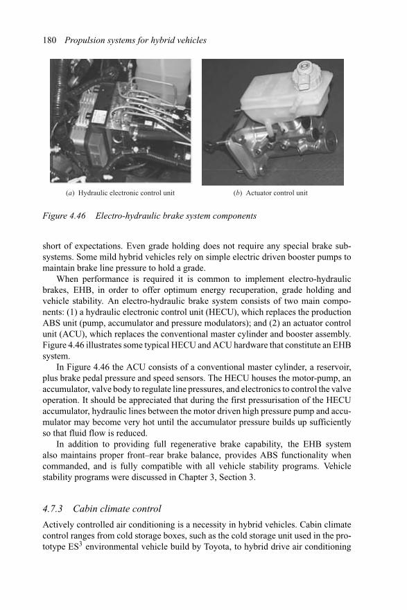
180 Propulsion systems for hybrid vehicles
(a) Hydraulic electronic control unit (b) Actuator control unit
Figure 4.46 Electro-hydraulic brake system components
short of expectations. Even grade holding does not require any special brake sub-systems. Some mild hybrid vehicles rely on simple electric driven booster pumps tomaintain brake line pressure to hold a grade.
When performance is required it is common to implement electro-hydraulicbrakes, EHB, in order to offer optimum energy recuperation, grade holding andvehicle stability. An electro-hydraulic brake system consists of two main compo-nents: (1) a hydraulic electronic control unit (HECU), which replaces the productionABS unit (pump, accumulator and pressure modulators); and (2) an actuator controlunit (ACU), which replaces the conventional master cylinder and booster assembly.Figure 4.46 illustrates some typical HECU and ACU hardware that constitute an EHBsystem.
In Figure 4.46 the ACU consists of a conventional master cylinder, a reservoir,plus brake pedal pressure and speed sensors. The HECU houses the motor-pump, anaccumulator, valve body to regulate line pressures, and electronics to control the valveoperation. It should be appreciated that during the first pressurisation of the HECUaccumulator, hydraulic lines between the motor driven high pressure pump and accu-mulator may become very hot until the accumulator pressure builds up sufficientlyso that fluid flow is reduced.
In addition to providing full regenerative brake capability, the EHB systemalso maintains proper front–rear brake balance, provides ABS functionality whencommanded, and is fully compatible with all vehicle stability programs. Vehiclestability programs were discussed in Chapter 3, Section 3.
4.7.3 Cabin climate control
Actively controlled air conditioning is a necessity in hybrid vehicles. Cabin climatecontrol ranges from cold storage boxes, such as the cold storage unit used in the pro-totype ES3 environmental vehicle build by Toyota, to hybrid drive air conditioning
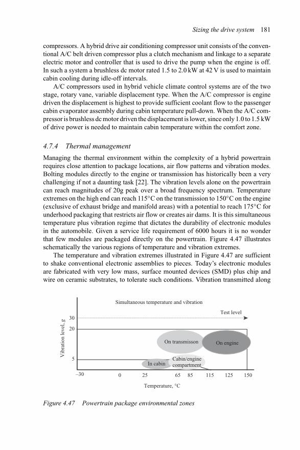
Sizing the drive system 181
compressors. A hybrid drive air conditioning compressor unit consists of the conven-tional A/C belt driven compressor plus a clutch mechanism and linkage to a separateelectric motor and controller that is used to drive the pump when the engine is off.In such a system a brushless dc motor rated 1.5 to 2.0 kW at 42 V is used to maintaincabin cooling during idle-off intervals.
A/C compressors used in hybrid vehicle climate control systems are of the twostage, rotary vane, variable displacement type. When the A/C compressor is enginedriven the displacement is highest to provide sufficient coolant flow to the passengercabin evaporator assembly during cabin temperature pull-down. When the A/C com-pressor is brushless dc motor driven the displacement is lower, since only 1.0 to 1.5 kWof drive power is needed to maintain cabin temperature within the comfort zone.
4.7.4 Thermal management
Managing the thermal environment within the complexity of a hybrid powertrainrequires close attention to package locations, air flow patterns and vibration modes.Bolting modules directly to the engine or transmission has historically been a verychallenging if not a daunting task [22]. The vibration levels alone on the powertraincan reach magnitudes of 20g peak over a broad frequency spectrum. Temperatureextremes on the high end can reach 115◦C on the transmission to 150◦C on the engine(exclusive of exhaust bridge and manifold areas) with a potential to reach 175◦C forunderhood packaging that restricts air flow or creates air dams. It is this simultaneoustemperature plus vibration regime that dictates the durability of electronic modulesin the automobile. Given a service life requirement of 6000 hours it is no wonderthat few modules are packaged directly on the powertrain. Figure 4.47 illustratesschematically the various regions of temperature and vibration extremes.
The temperature and vibration extremes illustrated in Figure 4.47 are sufficientto shake conventional electronic assemblies to pieces. Today’s electronic modulesare fabricated with very low mass, surface mounted devices (SMD) plus chip andwire on ceramic substrates, to tolerate such conditions. Vibration transmitted along
Temperature, °C
Simultaneous temperature and vibration
Test level
In cabin
On transmisson On engine
Vib
ratio
n le
vel,
g 30
20
5
–30 0 25 65 85 115 125 150
Cabin/enginecompartment
Figure 4.47 Powertrain package environmental zones
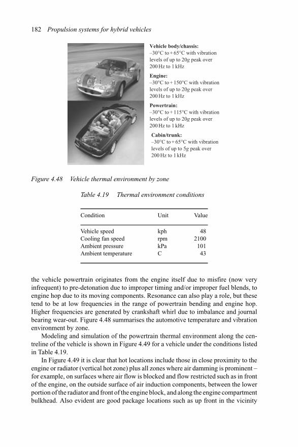
182 Propulsion systems for hybrid vehicles
Vehicle body/chassis: –30°C to + 65°C with vibrationlevels of up to 20g peak over200 Hz to 1 kHz
Engine:–30°C to + 150°C with vibration levels of up to 20g peak over200 Hz to 1 kHz
Powertrain:–30°C to + 115°C with vibration levels of up to 20g peak over200 Hz to 1 kHz
Cabin/trunk:–30°C to + 65°C with vibrationlevels of up to 5g peak over200 Hz to 1 kHz
Figure 4.48 Vehicle thermal environment by zone
Table 4.19 Thermal environment conditions
Condition Unit Value
Vehicle speed kph 48Cooling fan speed rpm 2100Ambient pressure kPa 101Ambient temperature C 43
the vehicle powertrain originates from the engine itself due to misfire (now veryinfrequent) to pre-detonation due to improper timing and/or improper fuel blends, toengine hop due to its moving components. Resonance can also play a role, but thesetend to be at low frequencies in the range of powertrain bending and engine hop.Higher frequencies are generated by crankshaft whirl due to imbalance and journalbearing wear-out. Figure 4.48 summarises the automotive temperature and vibrationenvironment by zone.
Modeling and simulation of the powertrain thermal environment along the cen-treline of the vehicle is shown in Figure 4.49 for a vehicle under the conditions listedin Table 4.19.
In Figure 4.49 it is clear that hot locations include those in close proximity to theengine or radiator (vertical hot zone) plus all zones where air damming is prominent –for example, on surfaces where air flow is blocked and flow restricted such as in frontof the engine, on the outside surface of air induction components, between the lowerportion of the radiator and front of the engine block, and along the engine compartmentbulkhead. Also evident are good package locations such as up front in the vicinity
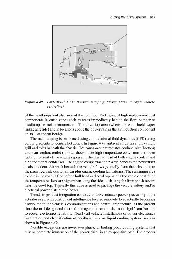
Sizing the drive system 183
80°C
67°C
67°C
43°C
92°C
Figure 4.49 Underhood CFD thermal mapping (along plane through vehiclecentreline)
of the headlamps and also around the cowl top. Packaging of high replacement costcomponents in crush zones such as areas immediately behind the front bumper orheadlamps is not recommended. The cowl top area (where the windshield wiperlinkages reside) and in locations above the powertrain in the air induction componentareas also appear benign.
Thermal mapping is performed using computational fluid dynamics (CFD) usingcolour gradients to identify hot zones. In Figure 4.49 ambient air enters at the vehiclegrill and exits beneath the chassis. Hot zones occur at radiator coolant inlet (bottom)and near coolant outlet (top) as shown. The high temperature zone from the lowerradiator to front of the engine represents the thermal load of both engine coolant andair conditioner condenser. The engine compartment air wash beneath the powertrainis also evident. Air wash beneath the vehicle flows generally from the driver side tothe passenger side due to ram air plus engine cooling fan patterns. The remaining areato note is the zone in front of the bulkhead and cowl top. Along the vehicle centrelinethe temperatures here are higher than along the sides such as by the front shock towersnear the cowl top. Typically this zone is used to package the vehicle battery and/orelectrical power distribution boxes.
Trends in product integration continue to drive actuator power processing to theactuator itself with control and intelligence located remotely to eventually becomingdistributed in the vehicle’s communications and control architecture. At the presenttime thermal design and thermal management remain the most significant barriersto power electronics reliability. Nearly all vehicle installations of power electronicsfor traction and electrification of ancillaries rely on liquid cooling systems such asshown in Figure 4.50.
Notable exceptions are novel two phase, or boiling pool, cooling systems thatrely on complete immersion of the power chips in an evaporative bath. The process
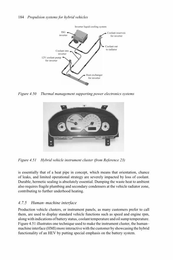
184 Propulsion systems for hybrid vehicles
Coolant intoinverter
Inverter liquid cooling system
Coolant reservoirfor inverter
Coolant outto radiator
ISGinverter
12V coolant pumpfor inverter
Heat exchangerfor inverter
Figure 4.50 Thermal management supporting power electronics systems
Figure 4.51 Hybrid vehicle instrument cluster (from Reference 23)
is essentially that of a heat pipe in concept, which means that orientation, chanceof leaks, and limited operational strategy are severely impacted by loss of coolant.Durable, hermetic sealing is absolutely essential. Dumping the waste heat to ambientalso requires fragile plumbing and secondary condensers at the vehicle radiator zone,contributing to further underhood heating.
4.7.5 Human–machine interface
Production vehicle clusters, or instrument panels, as many customers prefer to callthem, are used to display standard vehicle functions such as speed and engine rpm,along with indications of battery status, coolant temperature and oil sump temperature.Figure 4.51 illustrates one technique used to make the instrument cluster, the human–machine interface (HMI) more interactive with the customer by showcasing the hybridfunctionality of an HEV by putting special emphasis on the battery system.
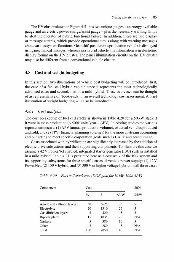
Sizing the drive system 185
The HV cluster shown in Figure 4.51 has two unique gauges – an energy availablegauge and an electric power charge/assist gauge – plus the necessary warning lampsto alert the operator of hybrid functional failure. In addition, there are two displayor message centres, which provide operational status along with warning messagesabout various system functions. Gear shift position in a production vehicle is displayedusing mechanical linkages, whereas in a hybrid vehicle this information is in electronicdisplay format on the HV cluster. The panel illumination circuits on the HV clustermay also be different from a conventional vehicle cluster.
4.8 Cost and weight budgeting
In this section, two illustrations of vehicle cost budgeting will be introduced: first,the case of a fuel cell hybrid vehicle since it represents the most technologicallyadvanced case; and second, that of a mild hybrid. These two cases can be thoughtof as representative of ‘book-ends’ in an overall technology cost assessment. A briefillustration of weight budgeting will also be introduced.
4.8.1 Cost analysis
The cost breakdown of fuel cell stacks is shown in Table 4.20 for a 50 kW stack ifit were in mass production (>500k units/year – APV). In costing studies the variousrepresentations are: (1) APV (annual production volume), or actual vehicles producedand sold; and (2) FPV (financial planning volumes) for the more upstream accountingand budgeting to meet specific corporation goals such as CAFÉ and brand image.
Costs associated with hybridization are significantly increased by the addition ofelectric drive subsystems and their supporting components. To illustrate this case weassume a 42 V PowerNet enabled, integrated starter generator (ISG) system installedin a mild hybrid. Table 4.21 is presented here as a cost walk of the ISG system andits supporting subsystems for three specific cases of vehicle power supply: (1) 42 VPowerNet; (2) 150 V hybrid; and (3) 300 V or higher voltage hybrid. In all three cases
Table 4.20 Fuel cell stack cost (DOE goal for 50 kW, 500k APV)
Component Cost 2004
% $ $/kW $/kW
Anode and cathode layers 50 3625 75 5Electrolyte 20 1310 25 5Gas diffusion layers 5 420 5 5Bipolar plates 15 1035 20 N/AGaskets 5 380 10 5Other 5 280 5 N/ATotal 100 7050 140 N/A
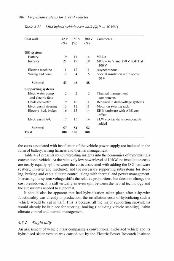
186 Propulsion systems for hybrid vehicles
Table 4.21 Mild hybrid vehicle cost walk (@P = 10 kW)
Cost walk 42 V 150 V 300 V Comments(%) (%) (%)
ISG systemBattery 9 11 14 VRLAInverter 21 19 18 MOS – 42 V and 150 V, IGBT at
300 VElectric machine 11 12 11 AsynchronousWiring and conn. 2 4 5 Special insulation req’d above
60 VSubtotal 43 46 48
Supporting systemsElect. water pump 2 2 2 Thermal management
componentsand electric fansDc/dc converter 9 10 11 Required in dual-voltage systemsElect. assist steering 13 12 11 Motor on steering rackElectric–hyd. brakes 16 15 14 EHB hardware with ABS cost
offsetElect. assist A/C 17 15 14 2 kW electric drive components
addedSubtotal 57 54 52
Total 100 100 100
the costs associated with installation of the vehicle power supply are included in theform of battery, wiring harness and thermal management.
Table 4.21 presents some interesting insights into the economics of hybridizing aconventional vehicle. At the relatively low power level of 10 kW the installation costsare nearly equally split between the costs associated with adding the ISG hardware(battery, inverter and machine), and the necessary supporting subsystems for steer-ing, braking and cabin climate control, along with thermal and power management.Increasing the system voltage shifts the relative proportions, but does not change thecost breakdown; it is still virtually an even split between the hybrid technology andthe subsystems needed to support it.
It should also be apparent that had hybridization taken place after x-by-wirefunctionality was already in production, the installation costs of hybridizing such avehicle would be cut in half. This is because all the major supporting subsystemswould already be in place for steering, braking (including vehicle stability), cabinclimate control and thermal management.
4.8.2 Weight tally
An assessment of vehicle mass comparing a conventional mid-sized vehicle and itshybridized sister version was carried out by the Electric Power Research Institute
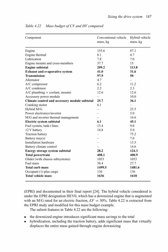
Sizing the drive system 187
Table 4.22 Mass budget of CV and HV compared
Component Conventional vehiclemass, kg
Hybrid vehiclemass, kg
Engine 155.6 87.1Engine thermal 8.1 4.7Lubrication 7.8 7.0Engine mounts and cross-members 37.7 15Engine subtotal 209.2 113.8Exhaust and evaporative system 41.0 31.6Transmission 97.9 50Alternator 4.7 –A/C compressor 6.2 11.2A/C condensor 2.2 2.3A/C plumbing + coolant, mounts 12.6 12.6Accessory power module – 10.0Climate control and accessory module subtotal 25.7 36.1Cranking motor 6.1 –Hybrid M/G – 23.5Power electronics/inverter – 5.0M/G and inverter thermal management – 16.6Electric system subtotal 6.1 45.1Fuel system, tank+lines 13.4 9.012 V battery 14.8 5.0Traction battery – 75.2Battery tray(s) – 7.0Installation hardware – 13.5Battery climate control – 14.6Energy storage system subtotal 28.2 124.3Total powertrain 408.1 400.9Glider (with chassis subsystems) 1053 1053Fuel mass 38.4 27.7Total curb mass 1499.5 1481.6Occupant (1) plus cargo 136 136Total vehicle mass 1636 1618
(EPRI) and documented in their final report [24]. The hybrid vehicle considered isunder the EPRI designation HEV0, which has a downsized engine that is augmentedwith an M/G rated for an electric fraction, EF = 30%. Table 4.22 is extracted fromthe EPRI study and modified for this mass budget example.
The salient features in Table 4.22 are the following:
• the downsized engine introduces significant mass savings to the total• hybridization, including the traction battery, adds significant mass that virtually
displaces the entire mass gained through engine downsizing
188 Propulsion systems for hybrid vehicles
• fuel tank and conventional vehicle accessory battery (SLI) both represent masssavings in the hybridized vehicle
• gross vehicle weight is only slightly less for the hybrid vehicle.
The bottom line is that hybridizing a conventional vehicle can easily consume allweight reduction actions taken before the hybrid components are installed. Ratherthan retrofit and modify a conventional vehicle it would be more appropriate todesign a hybrid vehicle (fuel cell vehicle, for that matter) from the ground up.
4.9 References
1 SCHERER, H.: ‘ZF 6-speed automatic transmission for passenger cars’. SAEtechnical paper 2003-01-0596, Society of Automotive Engineers 2003 WorldCongress, Detroit, MI, 3–6 March 2003
2 NOZAKI, K., KASHIHARA, Y., TAKAHASHI, N., HOSHINO, A., MORI, A.and TSUKAMOTO, H.: ‘Toyota’s new five-speed automatic transmissionA750E/A750F for RWD Vehicles’. Society of Automotive Engineers 2003 WorldCongress, Detroit, MI, 3–6 March 2003
3 YAMAMOTO, Y., NISHIDA, M., SUZUKI, K. and KOZAKI, S.: ‘New five-speed automatic transmission for FWD vehicles’. SAE technical paper 2001-01-0871, Society of Automotive Engineers 2001 World Congress, Detroit, MI, 5–8March 2001
4 BURKE, A.: ‘Cost-effective combinations of ultra-capacitors and batteriesfor vehicle applications’. Proceedings of the Second International AdvancedAutomotive Battery Conference, Las Vegas, NV, February 2002
5 OSTOVIC, V. personal discussion by author, 19 February 20026 LORENZ, L. and MITLEHNER, H.: ‘Key power semiconductor device concepts
for the next decade’. IEEE Industry Applications Society 37th Annual Meeting,William Penn Omni Hotel, Pittsburg, PA, 13–18 October 2002
7 FRANCIS, R. and SOLDANO, M.: ‘A new SMPS non punch through IGBTreplaces MOSFET in SMPS high frequency applications’. IEEE Applied PowerElectronics Conference and Exposition, APEC03, Fountainbleau Hotel, Miami,FL, 9–13 February 2003
8 KIEFERNDORF, R.: ‘Active rectifier controlled variable DC link PWM drive’.Wisconsin Electric Machines and Drives Consortium, WEMPEC, Annual ReviewMeeting, Madison, WI, 22–23 May 2002
9 HUANG, H., MILLER, J. M. and DEGNER, M. W.: ‘Method and circuitfor reducing battery ripple current is a multiple inverter system of an electricmachine’. US Patent #6,392,905, Issued 21 May 2002
10 TARABA, G. M., CEBREIRO, J. P. and TACCA, H. E.: ‘Batteries and hyper-capacitors selection criteria for a series hybrid bus’. IEEE Workshop on PowerElectronics in Transportation, No. 02TH8625, Auburn Hills, MI, 24–25 October2002, pp. 17–23
11 BROST, R. D.: ‘42V battery requirements from an automaker’s perspective’.Ninth Asian Battery Conference, Indonesia, 10–13 September 2001
Sizing the drive system 189
12 SUTULA, R., HEITNER, K., ROGERS, S. A. and DUONG, T. Q.: ‘Electric andhybrid vehicle energy storage R&D programs of the US Department of Energy’.Electric Vehicle Symposium, EVS16, September 1999
13 Ballard Power Systems website: www.ballard.com14 SMITH, B. C. and Next Energy Initiative: ‘Positioning the State of Michigan
as a leading candidate for fuel cell and alternative powertrain manufacturing’.Report by the Michigan Economic Development Corporation and the MichiganAutomotive Partnership, August 2001
15 BURKE, A.: ‘Cost-effective combinations of ultra-capacitors and batteries forvehicle applications’. Proceedings of the 2nd Advanced Automotive BatteryConference, Las Vegas, NV, February 2002
16 LUGERT, G., KNORR, R. and GRAF, H-M.: ‘14V/42V PowerNet and ISG – asolution for high dynamic energy supply suitable for mass market’. Proceedingsof the 2nd Advanced Automotive Battery Conference, Las Vegas, NV, February2002
17 ELDRE Corporation, www.busbar.com18 DIMINO, C. A., DODBALLAPUR, R. and POMES, J. A.: ‘A low inductance,
simplified snubber, power inverter implementation’. Proceedings of the HighFrequency Power Converter HFPC Conference, 1994, pp. 502–509
19 LETEINTURIER, P., KELLING, N. A. and KELLING, U.: ‘TTCAN from appli-cations to products in automotive systems’. SAE technical paper 2003-01-0114,SAE world congress, Detroit, MI, 3–6 March 2003
20 FUEHRER, T., HUGEL, R., HARTWICH, F. and WEILER, H.: ‘FlexRay – thecommunications system for future control systems in vehicles’. SAE technicalpaper 2003-01-0110, SAE world congress, Detroit, MI, 3–6 March 2003
21 LUPINI, C. A.: ‘Multiplex Bus Progression 2003’. SAE technical paper 2003-01-0111, SAE world congress, Detroit, MI, 3–6 March 2003
22 MILLER, J. M.: ‘Barriers and opportunity for power train integrated power elec-tronics’. Centre for Power Electronic Systems, CPES, Invited Paper, VirginiaTechnological and State University seminar, Blacksburg, VA, 16 April 2002
23 JAURA, A. K. and MILLER, J. M.: ‘HEV’s – vehicles that go the extra mileand are fun to drive’. SAE Convergence on Transportation Electronics, PaperNo. 202-21-0040, Cobo Exposition and Conference Center, Detroit, MI, 21–23October 2002
24 GRAHAM, R.: ‘Comparing the benefits and impacts of hybrid electric vehicleoptions’. EPRI Final Report #1000349, www.epri.com

Chapter 5
Electric drive system technologies
This chapter explores the four classes of electric machines having the most bearingon hybrid propulsion systems: the brushless permanent magnet machine in its surfacepermanent magnet (SPM) configuration; the interior permanent magnet (IPM) syn-chronous machine in either inset or buried magnet configuration; the asynchronousor cage rotor induction machine (IM); and the variable reluctance or doubly salientmachine (VRM).
There exists a mountain of books, papers and training workshops dedicated tothe design and study of these four classes of machines. The purpose of this chapteris to present a design perspective of these electric machines in the context of hybridvehicle propulsion. This is a topic that is still not as well defined, for example, asthe design of industrial electric machines. In this chapter we focus attention on thedesign characteristics of the four classes of electric machines of most interest forhybrid propulsion. To amplify the reasons for these choices consider the followingproducts now available in the market:
SPM (Honda Insight and Civic mild hybrids, FCX-V3 FCEV; Mannesman-SachsISA)
IPM (Toyota Prius, Estima and Ford Motor Co. hybrid Escape)IM (GM Silverado ISG, Continental ISAD, Delphi-Automotive ISG, Valeo ISA)VRM (Dana ISA).
These machines in current use are all of the drum design – that is, rotor flux isradial across a cylindrical airgap, versus axial designs that have a distinct pancakeappearance with axial flux across an airgap that separates the disc shaped stator(s)and rotor(s). A plural connotation is used on axial machines because most will havea single stator and twin rotor discs or vice versa.
5.1 Brushless machines
The electromagnetic interaction responsible for torque production is the Lorenz forcedefined with the help of Figure 5.1. In this illustration a pair of magnets force magnetic
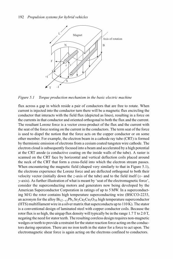
192 Propulsion systems for hybrid vehicles
MagnetL
F
N B
Axis of rotation
+I
T –I
S
rx
Figure 5.1 Torque production mechanism in the basic electric machine
flux across a gap in which reside a pair of conductors that are free to rotate. Whencurrent is injected into the conductor turn there will be a magnetic flux encircling theconductor that interacts with the field flux (depicted as lines), resulting in a force onthe currents in that conductor and oriented orthogonal to both the flux and the current.The resultant Lorenz force is a vector cross-product of the flux and the current withthe seat of the force resting on the current in the conductors. The term seat of the forceis used to dispel the notion that the force acts on the copper conductor or on someother member. For example, the electron beam in a cathode ray tube (CRT) is formedby thermionic emission of electrons from a cesium coated tungsten wire cathode. Theelectron cloud is subsequently focused into a beam and accelerated by a high potentialat the CRT anode (a conductive coating on the inside walls of the tube). A raster isscanned on the CRT face by horizontal and vertical deflection coils placed aroundthe neck of the CRT that form a cross-field into which the electron stream passes.When encountering the magnetic field (shaped very similarly to that in Figure 5.1),the electrons experience the Lorenz force and are deflected orthogonal to both theirvelocity vector (initially down the z-axis of the tube) and to the field itself (x- andy-axis). As further illustration of what is meant by ‘seat of the electromagnetic force’,consider the superconducting motors and generators now being developed by theAmerican Superconductor Corporation in ratings of up to 5 MW. In a superconduct-ing M/G the rotor contains high temperature superconducting wire (BSCCO-2233,an acronym for the alloy Bi(2−x)PbxSr2Ca2Cu3O10 high temperature superconductor(HTS) multifilament wire in a silver matrix that superconducts up to 110 K). The statoris a conventional design of laminated steel with copper conductor coils. Because therotor flux is so high, the airgap flux density will typically be in the range 1.7 T to 2.0 T,negating the need for stator teeth. The resulting coreless design requires non-magneticwedges or teeth to provide a restraint for the stator reaction force acting on the conduc-tors during operation. There are no iron teeth in the stator for a force to act upon. Theelectromagnetic shear force is again acting on the electrons confined to conductors.
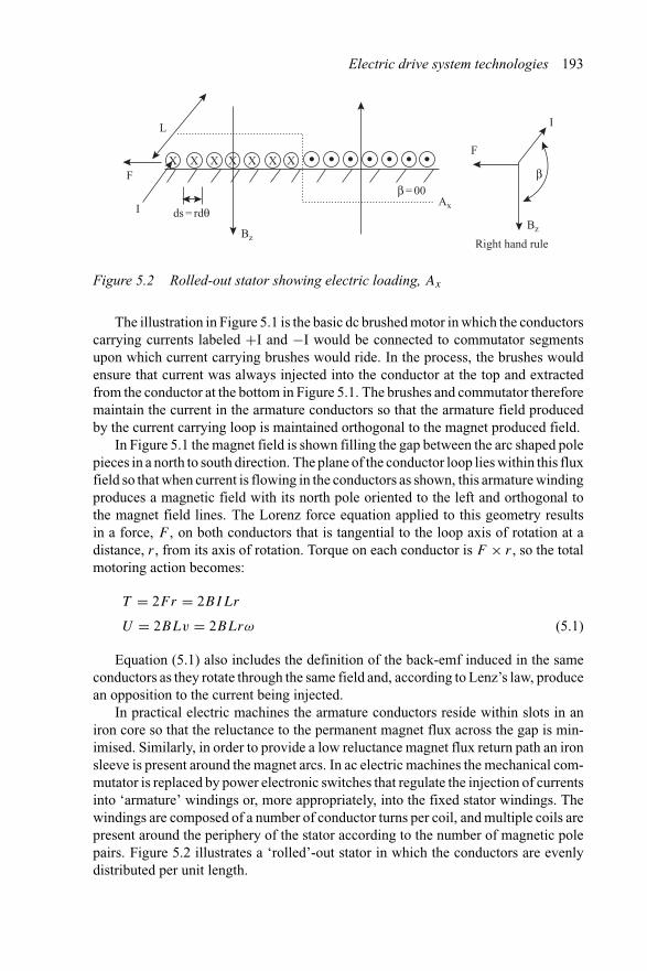
Electric drive system technologies 193
X X X X X X X
L
F
I ds = rdθ
BzBz
Right hand rule
Ax
F
I
ββ = 00
Figure 5.2 Rolled-out stator showing electric loading, Ax
The illustration in Figure 5.1 is the basic dc brushed motor in which the conductorscarrying currents labeled +I and −I would be connected to commutator segmentsupon which current carrying brushes would ride. In the process, the brushes wouldensure that current was always injected into the conductor at the top and extractedfrom the conductor at the bottom in Figure 5.1. The brushes and commutator thereforemaintain the current in the armature conductors so that the armature field producedby the current carrying loop is maintained orthogonal to the magnet produced field.
In Figure 5.1 the magnet field is shown filling the gap between the arc shaped polepieces in a north to south direction. The plane of the conductor loop lies within this fluxfield so that when current is flowing in the conductors as shown, this armature windingproduces a magnetic field with its north pole oriented to the left and orthogonal tothe magnet field lines. The Lorenz force equation applied to this geometry resultsin a force, F , on both conductors that is tangential to the loop axis of rotation at adistance, r , from its axis of rotation. Torque on each conductor is F × r , so the totalmotoring action becomes:
T = 2Fr = 2BILr
U = 2BLv = 2BLrω (5.1)
Equation (5.1) also includes the definition of the back-emf induced in the sameconductors as they rotate through the same field and, according to Lenz’s law, producean opposition to the current being injected.
In practical electric machines the armature conductors reside within slots in aniron core so that the reluctance to the permanent magnet flux across the gap is min-imised. Similarly, in order to provide a low reluctance magnet flux return path an ironsleeve is present around the magnet arcs. In ac electric machines the mechanical com-mutator is replaced by power electronic switches that regulate the injection of currentsinto ‘armature’ windings or, more appropriately, into the fixed stator windings. Thewindings are composed of a number of conductor turns per coil, and multiple coils arepresent around the periphery of the stator according to the number of magnetic polepairs. Figure 5.2 illustrates a ‘rolled’-out stator in which the conductors are evenlydistributed per unit length.
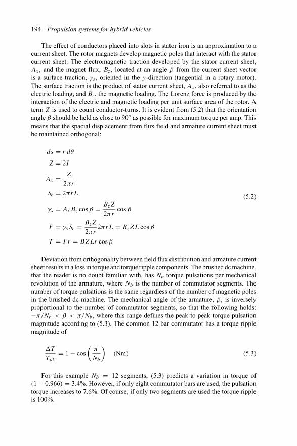
194 Propulsion systems for hybrid vehicles
The effect of conductors placed into slots in stator iron is an approximation to acurrent sheet. The rotor magnets develop magnetic poles that interact with the statorcurrent sheet. The electromagnetic traction developed by the stator current sheet,Ax , and the magnet flux, Bz, located at an angle β from the current sheet vectoris a surface traction, γs , oriented in the y-direction (tangential in a rotary motor).The surface traction is the product of stator current sheet, Ax , also referred to as theelectric loading, and Bz, the magnetic loading. The Lorenz force is produced by theinteraction of the electric and magnetic loading per unit surface area of the rotor. Aterm Z is used to count conductor-turns. It is evident from (5.2) that the orientationangle β should be held as close to 90◦ as possible for maximum torque per amp. Thismeans that the spacial displacement from flux field and armature current sheet mustbe maintained orthogonal:
ds = r dθ
Z = 2I
Ax = Z
2πr
Sr = 2πrL
γs = AxBz cos β = BzZ
2πrcos β
F = γsSr = BzZ
2πr2πrL = BzZL cos β
T = Fr = BZLr cos β
(5.2)
Deviation from orthogonality between field flux distribution and armature currentsheet results in a loss in torque and torque ripple components. The brushed dc machine,that the reader is no doubt familiar with, has Nb torque pulsations per mechanicalrevolution of the armature, where Nb is the number of commutator segments. Thenumber of torque pulsations is the same regardless of the number of magnetic polesin the brushed dc machine. The mechanical angle of the armature, β, is inverselyproportional to the number of commutator segments, so that the following holds:−π/Nb < β < π/Nb, where this range defines the peak to peak torque pulsationmagnitude according to (5.3). The common 12 bar commutator has a torque ripplemagnitude of
�T
Tpk
= 1 − cos(
π
Nb
)(Nm) (5.3)
For this example Nb = 12 segments, (5.3) predicts a variation in torque of(1 − 0.966) = 3.4%. However, if only eight commutator bars are used, the pulsationtorque increases to 7.6%. Of course, if only two segments are used the torque rippleis 100%.
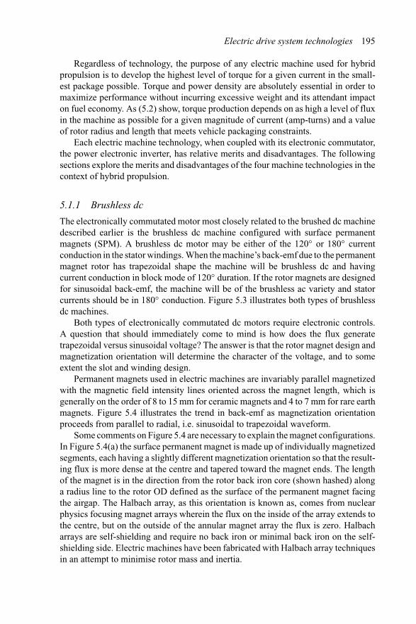
Electric drive system technologies 195
Regardless of technology, the purpose of any electric machine used for hybridpropulsion is to develop the highest level of torque for a given current in the small-est package possible. Torque and power density are absolutely essential in order tomaximize performance without incurring excessive weight and its attendant impacton fuel economy. As (5.2) show, torque production depends on as high a level of fluxin the machine as possible for a given magnitude of current (amp-turns) and a valueof rotor radius and length that meets vehicle packaging constraints.
Each electric machine technology, when coupled with its electronic commutator,the power electronic inverter, has relative merits and disadvantages. The followingsections explore the merits and disadvantages of the four machine technologies in thecontext of hybrid propulsion.
5.1.1 Brushless dc
The electronically commutated motor most closely related to the brushed dc machinedescribed earlier is the brushless dc machine configured with surface permanentmagnets (SPM). A brushless dc motor may be either of the 120◦ or 180◦ currentconduction in the stator windings. When the machine’s back-emf due to the permanentmagnet rotor has trapezoidal shape the machine will be brushless dc and havingcurrent conduction in block mode of 120◦ duration. If the rotor magnets are designedfor sinusoidal back-emf, the machine will be of the brushless ac variety and statorcurrents should be in 180◦ conduction. Figure 5.3 illustrates both types of brushlessdc machines.
Both types of electronically commutated dc motors require electronic controls.A question that should immediately come to mind is how does the flux generatetrapezoidal versus sinusoidal voltage? The answer is that the rotor magnet design andmagnetization orientation will determine the character of the voltage, and to someextent the slot and winding design.
Permanent magnets used in electric machines are invariably parallel magnetizedwith the magnetic field intensity lines oriented across the magnet length, which isgenerally on the order of 8 to 15 mm for ceramic magnets and 4 to 7 mm for rare earthmagnets. Figure 5.4 illustrates the trend in back-emf as magnetization orientationproceeds from parallel to radial, i.e. sinusoidal to trapezoidal waveform.
Some comments on Figure 5.4 are necessary to explain the magnet configurations.In Figure 5.4(a) the surface permanent magnet is made up of individually magnetizedsegments, each having a slightly different magnetization orientation so that the result-ing flux is more dense at the centre and tapered toward the magnet ends. The lengthof the magnet is in the direction from the rotor back iron core (shown hashed) alonga radius line to the rotor OD defined as the surface of the permanent magnet facingthe airgap. The Halbach array, as this orientation is known as, comes from nuclearphysics focusing magnet arrays wherein the flux on the inside of the array extends tothe centre, but on the outside of the annular magnet array the flux is zero. Halbacharrays are self-shielding and require no back iron or minimal back iron on the self-shielding side. Electric machines have been fabricated with Halbach array techniquesin an attempt to minimise rotor mass and inertia.
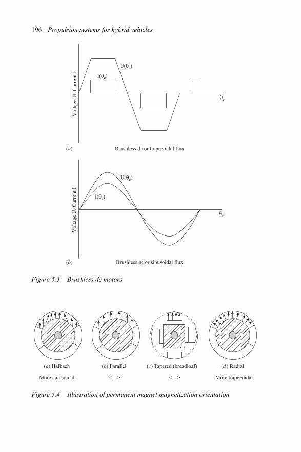
196 Propulsion systems for hybrid vehicles
Vol
tage
U, C
urre
nt I
Vol
tage
U, C
urre
nt I
I(θe)
I(θe)
Brushless ac or sinusoidal flux
U(θe)
U(θe)
θe
θe
(b)
Brushless dc or trapezoidal flux(a)
Figure 5.3 Brushless dc motors
(a) Halbach
More sinusoidal More trapezoidal<---><--->
(b) Parallel (c) Tapered (breadloaf) (d ) Radial
Figure 5.4 Illustration of permanent magnet magnetization orientation
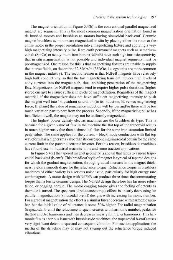
Electric drive system technologies 197
The magnet orientation in Figure 5.4(b) is the conventional parallel magnetizedmagnet arc segment. This is the most common magnetization orientation found indc brushed motors and brushless ac motors having sinusoidal back-emf. Ceramicmagnet brushless ac motors are magnetized in situ by placing either the rotor or theentire motor in the proper orientation into a magnetizing fixture and applying a veryhigh magnetizing intensity pulse. Rare earth permanent magnets such as samarium-cobalt (SmCo) or neodyimum-iron-boron (NdFeB) have such high intrinsic coercivitythat in situ magnetization is not possible and individual magnet segments must bepre-magnetized. One reason for this is that magnetizing fixtures are unable to supplythe intense fields, on the order of 2.8 MA/m (35 kOe, i.e. cgs units are more commonin the magnet industry). The second reason is that NdFeB magnets have relativelyhigh bulk conductivity, so that the fast magnetizing transient induces high levels ofeddy currents into the magnet slab, thus inhibiting penetration of the magnetizingflux. Magnetizers for NdFeB magnets tend to require higher pulse durations (higherstored energy) to ensure sufficient levels of magnetization. Regardless of the magnetmaterial, if the magnetizer does not have sufficient magnetizing intensity to pushthe magnet well into 1st quadrant saturation (in its induction, B, versus magnetizingforce, H, plane) the value of remanence induction will be low and/or there will be toomuch variation part to part from the process. Secondly, if the magnetizing pulse hasinsufficient dwell, the magnet may not be uniformly magnetized.
The highest power density electric machines are the brushless dc type. This isbecause for a given value of flux in the machine the flat top of the trapezoid resultsin much higher rms value than a sinusoidal flux for the same iron saturation limitedpeak value. The same applies for the current – block mode conduction with flat topwaveform has a higher rms value than its corresponding sinusoidal cousin for the samecurrent limit in the power electronic inverter. For this reason, brushless dc machineshave found use in industrial machine tools and some traction applications.
In Figure 5.4(c) the tapered magnet geometry is shown that tends to a more trape-zoidal back-emf (b-emf). This breadloaf style of magnet is typical of tapered designsfor which the gradual magnetization, through gradual increase in the magnet thick-ness, yields a smooth shape for the reluctance torque. Reluctance torque in brushlessmachines of either variety is a serious noise issue, particularly for high energy rareearth magnets. A motor design with NdFeB can produce three times the commutatingtorque than a ferrite ceramic design. The NdFeB design therefore has far more reluc-tance, or cogging, torque. The motor cogging torque gives the feeling of detents asthe rotor is turned. The spectrum of reluctance torque effects is linearly decreasing forparallel magnetization (sinusoidal b-emf) designs with increasing harmonic number.For a gradual magnetization the effect is a similar linear decrease with harmonic num-ber, but the initial value of reluctance is some 30% higher. For radial magnetization(trapezoidal b-emf) the reluctance torque increases with harmonic number, peaks forthe 2nd and 3rd harmonics and then decreases linearly for higher harmonics. This har-monic flux is a serious issue with brushless dc machines: the trapezoidal b-emf causesvery significant detent torque and consequent vibration. For traction applications theinertia of the driveline may or may not swamp out the reluctance torque inducedvibrations.
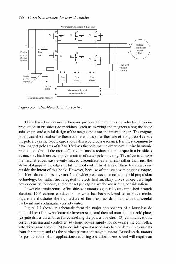
198 Propulsion systems for hybrid vehicles
Power electronics stage & heat sink
Vehicleenergystoragesystem
dclinkcap.
+
GD
S
GD
S
GD
S
GD
S
GD
S
GD
S
Back-emfvoltagesensing
Surfacepermanentmagnet(SPM)
Gatedriver
Gatedriver
Microcontroller andcommunications
Gatedriver
Currentsense
Communications network
Logicpowersupply
Figure 5.5 Brushless dc motor control
There have been many techniques proposed for minimising reluctance torqueproduction in brushless dc machines, such as skewing the magnets along the rotoraxis length, and careful design of the magnet pole arc and interpolar gap. The magnetpole arc can be visualised as the circumferential span of the magnet in Figure 5.4 versusthe pole arc (in the 1-pole case shown this would be π -radians). It is most common tohave magnet pole arcs of 0.7 to 0.8 times the pole span in order to minimise harmonicproduction. One of the more effective means to reduce detent torque in a brushlessdc machine has been the implementation of stator pole notching. The effect is to havethe magnet edges pass evenly spaced discontinuities in airgap rather than just thestator slot gaps at the edges of full pitched coils. The details of these techniques areoutside the intent of this book. However, because of the issue with cogging torque,brushless dc machines have not found widespread acceptance as a hybrid propulsiontechnology, but rather are relegated to electrified ancillary drives where very highpower density, low cost, and compact packaging are the overriding considerations.
Power electronic control of brushless dc motors is generally accomplished throughclassical 120◦ current conduction, or what has been referred to as block mode.Figure 5.5 illustrates the architecture of the brushless dc motor with trapezoidalback-emf and rectangular current control.
Figure 5.5 shows in schematic form the major components of a brushless dcmotor drive: (1) power electronic inverter stage and thermal management cold plate;(2) gate driver assemblies for controlling the power switches; (3) communications,current sensing and controller; (4) logic power supply for powering the controller,gate drivers and sensors; (5) the dc link capacitor necessary to circulate ripple currentsfrom the motor; and (6) the surface permanent magnet motor. Brushless dc motorsfor position control and applications requiring operation at zero speed will require an
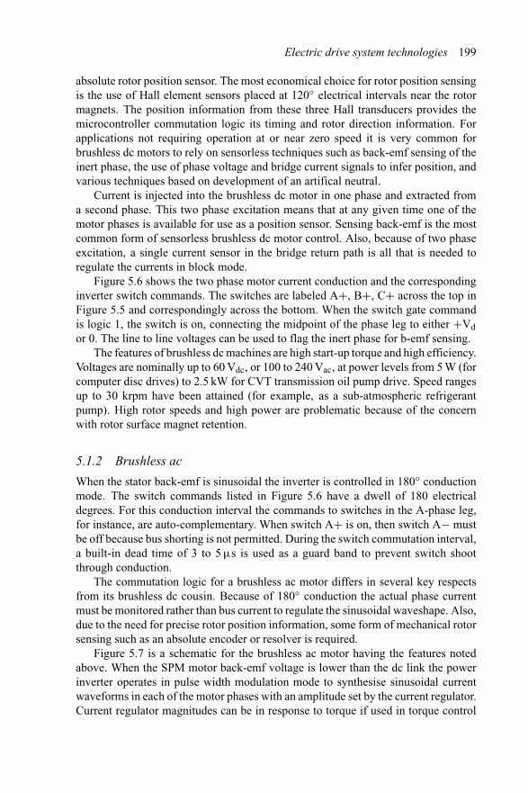
Electric drive system technologies 199
absolute rotor position sensor. The most economical choice for rotor position sensingis the use of Hall element sensors placed at 120◦ electrical intervals near the rotormagnets. The position information from these three Hall transducers provides themicrocontroller commutation logic its timing and rotor direction information. Forapplications not requiring operation at or near zero speed it is very common forbrushless dc motors to rely on sensorless techniques such as back-emf sensing of theinert phase, the use of phase voltage and bridge current signals to infer position, andvarious techniques based on development of an artifical neutral.
Current is injected into the brushless dc motor in one phase and extracted froma second phase. This two phase excitation means that at any given time one of themotor phases is available for use as a position sensor. Sensing back-emf is the mostcommon form of sensorless brushless dc motor control. Also, because of two phaseexcitation, a single current sensor in the bridge return path is all that is needed toregulate the currents in block mode.
Figure 5.6 shows the two phase motor current conduction and the correspondinginverter switch commands. The switches are labeled A+, B+, C+ across the top inFigure 5.5 and correspondingly across the bottom. When the switch gate commandis logic 1, the switch is on, connecting the midpoint of the phase leg to either +Vdor 0. The line to line voltages can be used to flag the inert phase for b-emf sensing.
The features of brushless dc machines are high start-up torque and high efficiency.Voltages are nominally up to 60 Vdc, or 100 to 240 Vac, at power levels from 5 W (forcomputer disc drives) to 2.5 kW for CVT transmission oil pump drive. Speed rangesup to 30 krpm have been attained (for example, as a sub-atmospheric refrigerantpump). High rotor speeds and high power are problematic because of the concernwith rotor surface magnet retention.
5.1.2 Brushless ac
When the stator back-emf is sinusoidal the inverter is controlled in 180◦ conductionmode. The switch commands listed in Figure 5.6 have a dwell of 180 electricaldegrees. For this conduction interval the commands to switches in the A-phase leg,for instance, are auto-complementary. When switch A+ is on, then switch A− mustbe off because bus shorting is not permitted. During the switch commutation interval,a built-in dead time of 3 to 5 μs is used as a guard band to prevent switch shootthrough conduction.
The commutation logic for a brushless ac motor differs in several key respectsfrom its brushless dc cousin. Because of 180◦ conduction the actual phase currentmust be monitored rather than bus current to regulate the sinusoidal waveshape. Also,due to the need for precise rotor position information, some form of mechanical rotorsensing such as an absolute encoder or resolver is required.
Figure 5.7 is a schematic for the brushless ac motor having the features notedabove. When the SPM motor back-emf voltage is lower than the dc link the powerinverter operates in pulse width modulation mode to synthesise sinusoidal currentwaveforms in each of the motor phases with an amplitude set by the current regulator.Current regulator magnitudes can be in response to torque if used in torque control
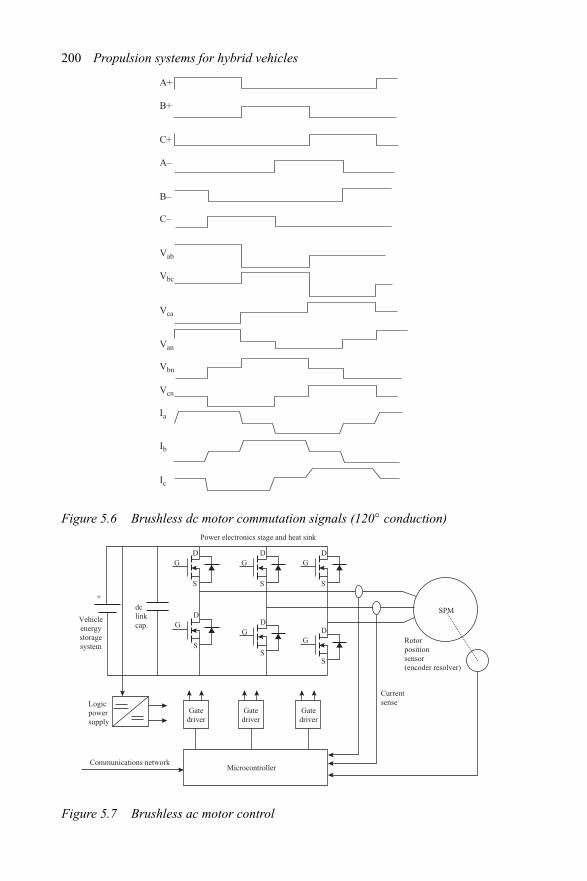
200 Propulsion systems for hybrid vehicles
A+
B+
C+
A–
B–
C–
Vab
Vbc
Vca
Van
Vbn
Vcn
Ia
Ib
Ic
Figure 5.6 Brushless dc motor commutation signals (120◦ conduction)Power electronics stage and heat sink
Vehicleenergystoragesystem
dclinkcap.
+
GD
S
GD
S
GD
S
GD
S
GD
S
GD
S
SPM
Gatedriver
Currentsense
Rotorpositionsensor(encoder resolver)
Gatedriver
Microcontroller
Gatedriver
Communications network
Logicpowersupply
Figure 5.7 Brushless ac motor control
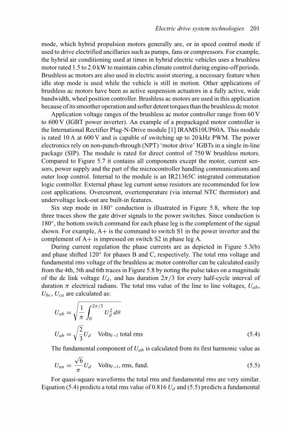
Electric drive system technologies 201
mode, which hybrid propulsion motors generally are, or in speed control mode ifused to drive electrified ancillaries such as pumps, fans or compressors. For example,the hybrid air conditioning used at times in hybrid electric vehicles uses a brushlessmotor rated 1.5 to 2.0 kW to maintain cabin climate control during engine-off periods.Brushless ac motors are also used in electric assist steering, a necessary feature whenidle stop mode is used while the vehicle is still in motion. Other applications ofbrushless ac motors have been as active suspension actuators in a fully active, widebandwidth, wheel position controller. Brushless ac motors are used in this applicationbecause of its smoother operation and softer detent torques than the brushless dc motor.
Application voltage ranges of the brushless ac motor controller range from 60 Vto 600 V (IGBT power inverter). An example of a prepackaged motor controller isthe International Rectifier Plug-N-Drive module [1] IRAMS10UP60A. This moduleis rated 10 A at 600 V and is capable of switching up to 20 kHz PWM. The powerelectronics rely on non-punch-through (NPT) ‘motor drive’ IGBTs in a single in-linepackage (SIP). The module is rated for direct control of 750 W brushless motors.Compared to Figure 5.7 it contains all components except the motor, current sen-sors, power supply and the part of the microcontroller handling communications andouter loop control. Internal to the module is an IR21365C integrated commutationlogic controller. External phase leg current sense resistors are recommended for lowcost applications. Overcurrent, overtemperature (via internal NTC thermistor) andundervoltage lock-out are built-in features.
Six step mode in 180◦ conduction is illustrated in Figure 5.8, where the topthree traces show the gate driver signals to the power switches. Since conduction is180◦, the bottom switch command for each phase leg is the complement of the signalshown. For example, A+ is the command to switch S1 in the power inverter and thecomplement of A+ is impressed on switch S2 in phase leg A.
During current regulation the phase currents are as depicted in Figure 5.3(b)and phase shifted 120◦ for phases B and C, respectively. The total rms voltage andfundamental rms voltage of the brushless ac motor controller can be calculated easilyfrom the 4th, 5th and 6th traces in Figure 5.8 by noting the pulse takes on a magnitudeof the dc link voltage Ud , and has duration 2π/3 for every half-cycle interval ofduration π electrical radians. The total rms value of the line to line voltages, Uab,Ubc, Uca are calculated as:
Uab =√
1
π
∫ 2π/3
0U2
d dθ
Uab =√
2
3Ud Voltsl−l total rms (5.4)
The fundamental component of Uab is calculated from its first harmonic value as
Uan =√
6
πUd Voltsl−l , rms, fund. (5.5)
For quasi-square waveforms the total rms and fundamental rms are very similar.Equation (5.4) predicts a total rms value of 0.816 Ud and (5.5) predicts a fundamental
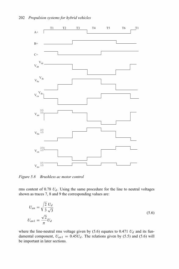
202 Propulsion systems for hybrid vehicles
T1A+
B+
C+
Vdc
Vdc
Vdc
Van
Vca
Vbc
Vab
T2 T3 T4 T5 T6 T1
2/31/3
Vbn
2/31/3
Vcn
2/31/3
Vno
2/31/3
Figure 5.8 Brushless ac motor control
rms content of 0.78 Ud . Using the same procedure for the line to neutral voltagesshown as traces 7, 8 and 9 the corresponding values are:
Uan =√
2
3
Ud√3
Uan1 =√
2
πUd
(5.6)
where the line-neutral rms voltage given by (5.6) equates to 0.471 Ud and its fun-damental component, Uan1 = 0.45Ud . The relations given by (5.5) and (5.6) willbe important in later sections.
Electric drive system technologies 203
5.1.3 Design essentials of the SPM
In this section the surface permanent magnet machine will be treated from a hybriddesign vantage point. The objective is to design an SPM as an M/G for a mild hybridvehicle. The design process will illustrate the important features of machine targetsetting, electromagnetic design and modeling.
First, a brief review of the types of electric machines available for the hybridpropulsion M/G set. Figure 5.9 illustrates six types of electric machines that shouldbe considered for this application. The machine types are as follows:
(A) Surface permanent magnet (SPM). This is the most basic of permanent magnetelectric machine designs. PMs are bonded to the surface of the solid iron rotorback iron, which is in turn fitted to the high carbon steel (4150 or equivalentsteel) shaft. Rotor back iron is necessary as a flux return path, and this core maybe either solid or laminated, depending on application.
(B) Interior permanent magnet or buried magnet design (IPM). A single layer buriedmagnet, tangential orientation, design IPM was the original design of the buriedPM concept when it was first conceived1 about 24 years ago. The buried magnetsprovide magnetization of the stator and minimise the reactive power needed.This design has been used for line-start appliance adjustable speed applicationsbecause of its high power factor and good torque performance.
(C) Asynchronous or induction machine design (IM) – the industrial workhorseelectric. The induction design dates to 1888, when Nikola Tesla first conceivedof what he termed his ‘current lag’ motor [2]. Trapped in his fourth floor room atthe Gerlach Hotel in New York City during the blizzard of 1888 – the location ofhis newly formed Tesla Electric Company funded by venture capitalists when heresigned from the Edison Electric Company just three days earlier – he sketchedout the design of the world’s first asynchronous electric machine. His design wasthat of an alternating current, three phase asynchronous machine – the inductionmachine.
(D) Interior permanent magnet – flux squeeze design with radial PMs. Rather thanburying the rotor permanents beneath a soft iron pole shoe, the magnets caneither be inset into the surface with the interpolar gap filled with soft iron, orthey can be sandwiched between larger soft iron wedges as shown in (D). Thisdesign is particularly attractive for ceramic magnet machines because of theflux squeezing effect at the airgap of flux collected from the larger surface ofthe magnets and then focused out the rotor surface.
(E) Synchronous reluctance (synchrel) design. By simply swapping out the cageor wound rotor of an induction machine and inserting a rotor of laminatedsaliencies, one obtains the synchronous reluctance design. These ‘rain-gutter’style laminations have low reluctance to stator flux in the direct-axis, but highreluctance to flux in its quadrature axis. The synchrel machine has received
1 US Patent 4,139,790 by C.R. Steen, ‘Direct axis aiding permanent magnets for a laminatedsynchronous motor rotor,’ Issued 13 February 1979.
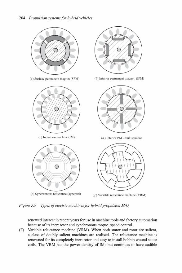
204 Propulsion systems for hybrid vehicles
(b) Interior permanent magnet (IPM)
(e) Synchronous reluctance (synchrel) ( f ) Variable reluctance machine (VRM)
(a) Surface permanent magnet (SPM)
(c) Induction machine (IM) (d ) Interior PM – flux squeeze
Figure 5.9 Types of electric machines for hybrid propulsion M/G
renewed interest in recent years for use in machine tools and factory automationbecause of its inert rotor and synchronous torque–speed control.
(F) Variable reluctance machine (VRM). When both stator and rotor are salient,a class of doubly salient machines are realised. The reluctance machine isrenowned for its completely inert rotor and easy to install bobbin wound statorcoils. The VRM has the power density of IMs but continues to have audible
Electric drive system technologies 205
noise problems unless the stator back iron is reinforced, for example, by beingexcessively thick, or includes bosses or other structural enhancements.
Electric machines with smooth stators, i.e. slotted designs with distributed wind-ings, can be either ‘copper-dominated’ or ‘iron-dominated’. When the iron fraction,or ratio of stator tooth width to stator tooth pitch, β = Wt/τs > 0.55, the machinecan be called iron dominated. For the most part, hybrid propulsion machines are irondominated in order to operate at magnetic loading values >0.7 tesla (T). This trendresults from the fact that hybrid propulsion M/Gs have high peak to continuous usage,so that putting more iron into the design permits operation at high flux levels for effi-cient inverter and battery operation. When high torque is demanded, the machinecurrents are driven to high values, but generally for short durations such as 10 to 30s,and to somewhat lower values for up to 3 min. The fact that hybrid M/Gs are generallyliquid cooled (use of engine coolant and/or transmission oil) completely supports thistrend. Generally speaking, liquid cooling boosts the torque production, so that theoutput of liquid cooled machines is four times that of air cooled machines, all elsebeing equal. The fundamental purpose of any electric machine is to deliver torque.If the machine package volume is constrained, then a metric of torque per L is valid,but this is not as universally applicable as the more specific torque per unit mass,Nm/kg. High torque to mass implies high power density and also high accelerationcapability.
Some comments about the application choice of the electric machine types listed inFigure 5.9 are in order before proceeding with a more detailed design of the SPM. TheSPM design may be sinusoidal or trapezoidal b-emf. Sinusoidal, brushless ac designs,tend to require higher inverter rating than the trapezoidal, brushless dc designs. Bothbrushless dc SPM and the IPM designs tend to have high torque ripple. The inductionmachine has the lowest torque ripple of any other type, but it requires a supply ofmagnetization current from its inverter, thus increasing the inverter kVA rating. IMsfor hybrid propulsion require that a rather large fraction of input VAs be dedicated tomagnetizing the machine. IMs of several hundred to thousands of horsepower have amuch smaller fraction of input VAs dedicated to magnetizing the machine. This canbe better appreciated by recognising that the ratio of air gap to machine dimensionbecomes a smaller fraction as motor size increases. The doubly salient machineshave many desirable features for hybrid propulsion and are beginning to be looked atmore seriously. The VRM has had hybrid propulsion advocates for many years, butstructural design to maintain the tight airgaps necessary, and controller algorithmscapable of real time current waveshape control based on rotor position have beenproblematic. The VRM is capable of the wide CPSR, as is the IPM, and so shouldfind application to power split and other hybrid propulsion architectures.
To summarise the comparisons of the various electric machine technologies forapplication to hybrid propulsion it is necessary to comment on their torque-producingmechanisms (see Table 5.1). Later, the comparisons will close with summaries oftorque ripple components of average torque.
The specific torque density of the electric machines shown in Figure 5.9 is themost important metric of general applicability to hybrid propulsion. With the aide of
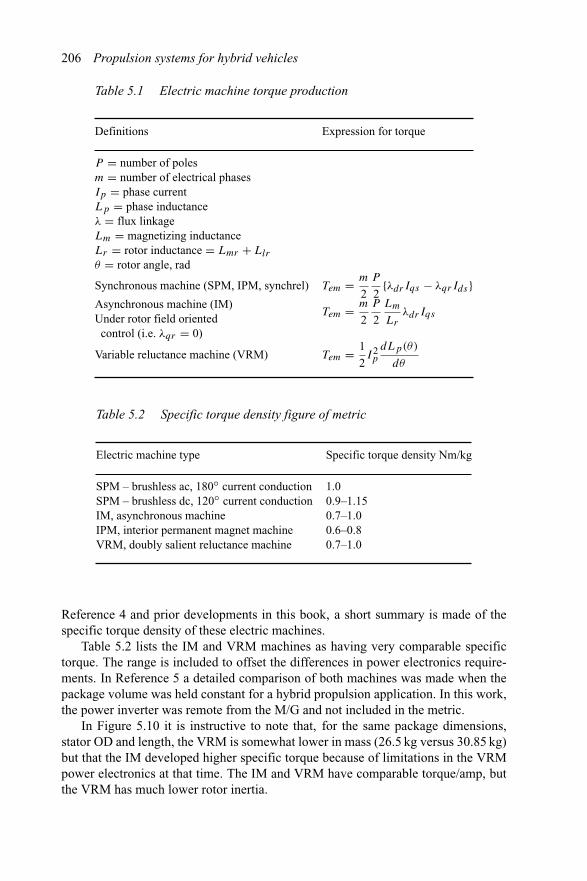
206 Propulsion systems for hybrid vehicles
Table 5.1 Electric machine torque production
Definitions Expression for torque
P = number of polesm = number of electrical phasesIp = phase currentLp = phase inductanceλ = flux linkageLm = magnetizing inductanceLr = rotor inductance = Lmr + Llr
θ = rotor angle, rad
Synchronous machine (SPM, IPM, synchrel) Tem = m
2
P
2{λdrIqs − λqrIds}
Asynchronous machine (IM)Under rotor field oriented
Tem = m
2
P
2
Lm
Lrλdr Iqs
control (i.e. λqr = 0)
Variable reluctance machine (VRM) Tem = 1
2I2p
dLp(θ)
dθ
Table 5.2 Specific torque density figure of metric
Electric machine type Specific torque density Nm/kg
SPM – brushless ac, 180◦ current conduction 1.0SPM – brushless dc, 120◦ current conduction 0.9–1.15IM, asynchronous machine 0.7–1.0IPM, interior permanent magnet machine 0.6–0.8VRM, doubly salient reluctance machine 0.7–1.0
Reference 4 and prior developments in this book, a short summary is made of thespecific torque density of these electric machines.
Table 5.2 lists the IM and VRM machines as having very comparable specifictorque. The range is included to offset the differences in power electronics require-ments. In Reference 5 a detailed comparison of both machines was made when thepackage volume was held constant for a hybrid propulsion application. In this work,the power inverter was remote from the M/G and not included in the metric.
In Figure 5.10 it is instructive to note that, for the same package dimensions,stator OD and length, the VRM is somewhat lower in mass (26.5 kg versus 30.85 kg)but that the IM developed higher specific torque because of limitations in the VRMpower electronics at that time. The IM and VRM have comparable torque/amp, butthe VRM has much lower rotor inertia.
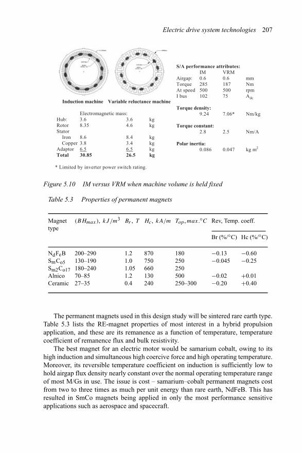
Electric drive system technologies 207
Induction machine Variable reluctance machine
Electromagnetic mass:
* Limited by inverter power switch rating.
Hub: 3.6 3.6 kgRotor 8.35 4.6 kgStator Iron 8.6 8.4 kg
Copper 3.8 3.4 kgAdaptor 6.5 6.5 kgTotal 30.85 26.5 kg
S/A performance attributes:IM VRM
Airgap: 0.6 0.6 mmTorque 285 187 NmAt speed 500 500 rpmI bus 102 75 Adc
Torque density:9.24 7.06* Nm/kg
Torque constant:2.8 2.5 Nm/A
Polar inertia:0.086 0.047 kg m2
Figure 5.10 IM versus VRM when machine volume is held fixed
Table 5.3 Properties of permanent magnets
Magnet (BHmax), kJ/m3 Br , T Hc, kA/m Top , max.◦C Rev, Temp. coeff.type
Br (%/◦C) Hc (%/◦C)
NdFeB 200–290 1.2 870 180 −0.13 −0.60SmCo5 130–190 1.0 750 250 −0.045 −0.25Sm2Co17 180–240 1.05 660 250Alnico 70–85 1.2 130 500 −0.02 +0.01Ceramic 27–35 0.4 240 250–300 −0.20 +0.40
The permanent magnets used in this design study will be sintered rare earth type.Table 5.3 lists the RE-magnet properties of most interest in a hybrid propulsionapplication, and these are its remanence as a function of temperature, temperaturecoefficient of remanence flux and bulk resistivity.
The best magnet for an electric motor would be samarium cobalt, owing to itshigh induction and simultaneous high coercive force and high operating temperature.Moreover, its reversible temperature coefficient on induction is sufficiently low tohold airgap flux density nearly constant over the normal operating temperature rangeof most M/Gs in use. The issue is cost – samarium–cobalt permanent magnets costfrom two to three times as much per unit energy than rare earth, NdFeB. This hasresulted in SmCo magnets being applied in only the most performance sensitiveapplications such as aerospace and spacecraft.
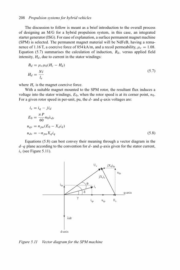
208 Propulsion systems for hybrid vehicles
The discussion to follow is meant as a brief introduction to the overall processof designing an M/G for a hybrid propulsion system, in this case, an integratedstarter generator (ISG). For ease of explanation, a surface permanent magnet machine(SPM) is selected. The permanent magnet material will be NdFeB, having a rema-nence of 1.16 T, a coercive force of 854 kA/m, and a recoil permeability, μr = 1.08.Equation (5.7) summarises the calculation of induction, Bd , versus applied fieldintensity, Hd , due to current in the stator windings:
Bd = μrμ0(Hc − Hd)
Hd = Ni
le
(5.7)
where Hc is the magnet coercive force.With a suitable magnet mounted to the SPM rotor, the resultant flux induces a
voltage into the stator windings, E0, when the rotor speed is at its corner point, n0.For a given rotor speed in per-unit, pu, the d- and q-axis voltages are:
is = iq − jid
E0 = πP
60n0λdr
uqs = npu(E0 − Xdid)
uds = −npuXqiq (5.8)
Equations (5.8) can best convey their meaning through a vector diagram in thed–q plane according to the convention for d- and q-axis given for the stator current,is (see Figure 5.11).
Us
uds
ids
jXdids
jXsis
uqsiqs
is
Es
q-axis
d-axis
λdr
γ
δ
θ
Figure 5.11 Vector diagram for the SPM machine
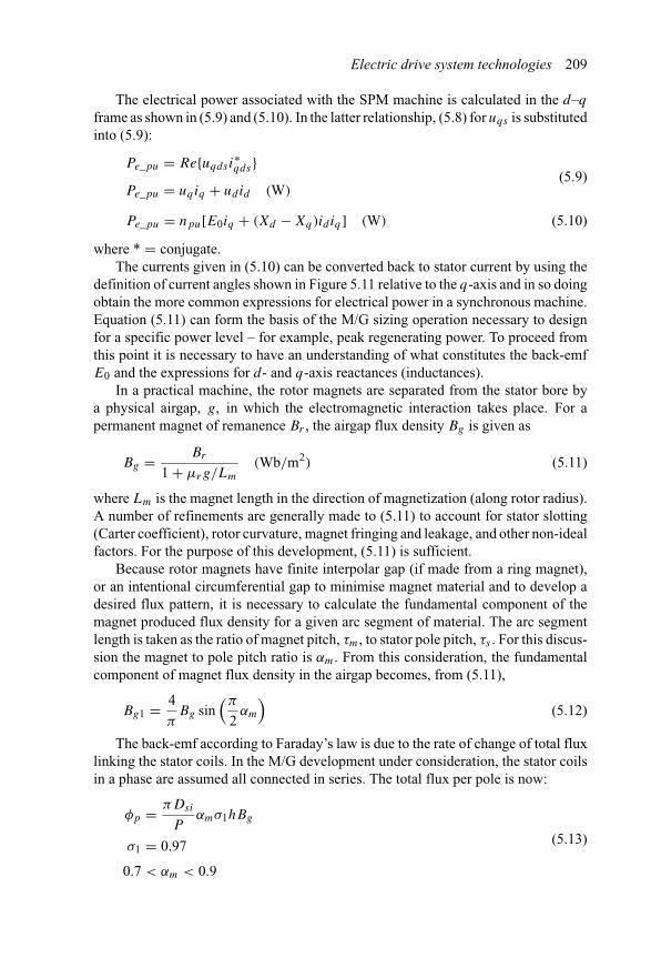
Electric drive system technologies 209
The electrical power associated with the SPM machine is calculated in the d–q
frame as shown in (5.9) and (5.10). In the latter relationship, (5.8) for uqs is substitutedinto (5.9):
Pe_pu = Re{uqdsi∗qds}
Pe_pu = uqiq + udid (W)(5.9)
Pe_pu = npu[E0iq + (Xd − Xq)id iq ] (W) (5.10)
where * = conjugate.The currents given in (5.10) can be converted back to stator current by using the
definition of current angles shown in Figure 5.11 relative to the q-axis and in so doingobtain the more common expressions for electrical power in a synchronous machine.Equation (5.11) can form the basis of the M/G sizing operation necessary to designfor a specific power level – for example, peak regenerating power. To proceed fromthis point it is necessary to have an understanding of what constitutes the back-emfE0 and the expressions for d- and q-axis reactances (inductances).
In a practical machine, the rotor magnets are separated from the stator bore bya physical airgap, g, in which the electromagnetic interaction takes place. For apermanent magnet of remanence Br , the airgap flux density Bg is given as
Bg = Br
1 + μrg/Lm
(Wb/m2) (5.11)
where Lm is the magnet length in the direction of magnetization (along rotor radius).A number of refinements are generally made to (5.11) to account for stator slotting(Carter coefficient), rotor curvature, magnet fringing and leakage, and other non-idealfactors. For the purpose of this development, (5.11) is sufficient.
Because rotor magnets have finite interpolar gap (if made from a ring magnet),or an intentional circumferential gap to minimise magnet material and to develop adesired flux pattern, it is necessary to calculate the fundamental component of themagnet produced flux density for a given arc segment of material. The arc segmentlength is taken as the ratio of magnet pitch, τm, to stator pole pitch, τs . For this discus-sion the magnet to pole pitch ratio is αm. From this consideration, the fundamentalcomponent of magnet flux density in the airgap becomes, from (5.11),
Bg1 = 4
πBg sin
(π
2αm
)(5.12)
The back-emf according to Faraday’s law is due to the rate of change of total fluxlinking the stator coils. In the M/G development under consideration, the stator coilsin a phase are assumed all connected in series. The total flux per pole is now:
φp = πDsi
Pαmσ1hBg
σ1 = 0.97
0.7 < αm < 0.9
(5.13)
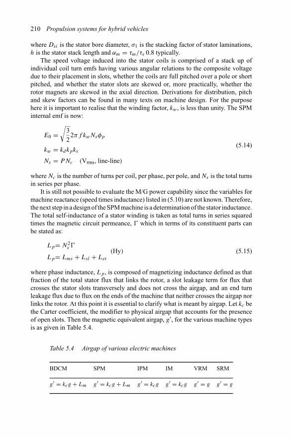
210 Propulsion systems for hybrid vehicles
where Dsi is the stator bore diameter, σ1 is the stacking factor of stator laminations,h is the stator stack length and αm = τm/τs 0.8 typically.
The speed voltage induced into the stator coils is comprised of a stack up ofindividual coil turn emfs having various angular relations to the composite voltagedue to their placement in slots, whether the coils are full pitched over a pole or shortpitched, and whether the stator slots are skewed or, more practically, whether therotor magnets are skewed in the axial direction. Derivations for distribution, pitchand skew factors can be found in many texts on machine design. For the purposehere it is important to realise that the winding factor, kw, is less than unity. The SPMinternal emf is now:
E0 =√
3
22πf kwNsφp
kw = kdkpks
Ns = PNc (Vrms, line-line)
(5.14)
where Nc is the number of turns per coil, per phase, per pole, and Ns is the total turnsin series per phase.
It is still not possible to evaluate the M/G power capability since the variables formachine reactance (speed times inductance) listed in (5.10) are not known. Therefore,the next step in a design of the SPM machine is a determination of the stator inductance.The total self-inductance of a stator winding is taken as total turns in series squaredtimes the magnetic circuit permeance, � which in terms of its constituent parts canbe stated as:
Lp= N2s �
Lp= Lms + Lsl + Let
(Hy) (5.15)
where phase inductance, Lp, is composed of magnetizing inductance defined as thatfraction of the total stator flux that links the rotor, a slot leakage term for flux thatcrosses the stator slots transversely and does not cross the airgap, and an end turnleakage flux due to flux on the ends of the machine that neither crosses the airgap norlinks the rotor. At this point it is essential to clarify what is meant by airgap. Let kc bethe Carter coefficient, the modifier to physical airgap that accounts for the presenceof open slots. Then the magnetic equivalent airgap, g′, for the various machine typesis as given in Table 5.4.
Table 5.4 Airgap of various electric machines
BDCM SPM IPM IM VRM SRM
g′ = kcg + Lm g′ = kcg + Lm g′ = kcg g′ = kcg g′ = g g′ = g
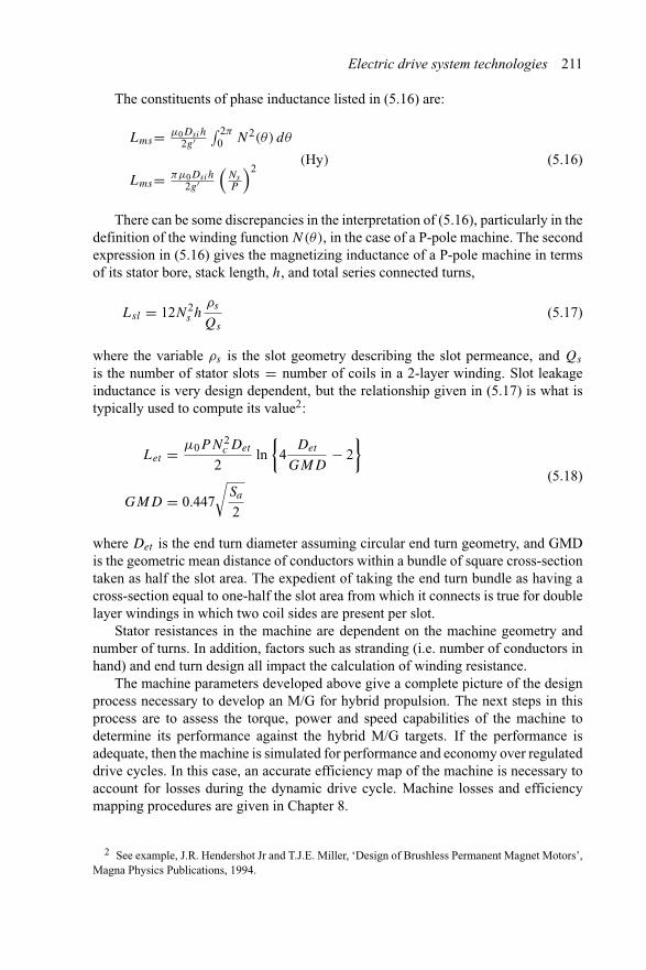
Electric drive system technologies 211
The constituents of phase inductance listed in (5.16) are:
Lms= μ0Dsih2g′
∫ 2π
0 N2(θ) dθ
Lms= πμ0Dsih2g′
(Ns
P
)2(Hy) (5.16)
There can be some discrepancies in the interpretation of (5.16), particularly in thedefinition of the winding function N(θ), in the case of a P-pole machine. The secondexpression in (5.16) gives the magnetizing inductance of a P-pole machine in termsof its stator bore, stack length, h, and total series connected turns,
Lsl = 12N2s h
ρs
Qs
(5.17)
where the variable ρs is the slot geometry describing the slot permeance, and Qs
is the number of stator slots = number of coils in a 2-layer winding. Slot leakageinductance is very design dependent, but the relationship given in (5.17) is what istypically used to compute its value2:
Let = μ0PN2c Det
2ln{
4Det
GMD− 2
}
GMD = 0.447
√Sa
2
(5.18)
where Det is the end turn diameter assuming circular end turn geometry, and GMDis the geometric mean distance of conductors within a bundle of square cross-sectiontaken as half the slot area. The expedient of taking the end turn bundle as having across-section equal to one-half the slot area from which it connects is true for doublelayer windings in which two coil sides are present per slot.
Stator resistances in the machine are dependent on the machine geometry andnumber of turns. In addition, factors such as stranding (i.e. number of conductors inhand) and end turn design all impact the calculation of winding resistance.
The machine parameters developed above give a complete picture of the designprocess necessary to develop an M/G for hybrid propulsion. The next steps in thisprocess are to assess the torque, power and speed capabilities of the machine todetermine its performance against the hybrid M/G targets. If the performance isadequate, then the machine is simulated for performance and economy over regulateddrive cycles. In this case, an accurate efficiency map of the machine is necessary toaccount for losses during the dynamic drive cycle. Machine losses and efficiencymapping procedures are given in Chapter 8.
2 See example, J.R. Hendershot Jr and T.J.E. Miller, ‘Design of Brushless Permanent Magnet Motors’,Magna Physics Publications, 1994.
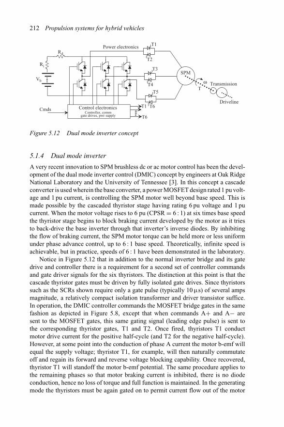
212 Propulsion systems for hybrid vehicles
Vb
Ri
Rd
ωT
Controller, commgate drives, pwr supply
Cmds
Power electronics
Control electronics
Transmission
Driveline
T1
T2
T3
T4
T5
T6T1
T6
SPM
Figure 5.12 Dual mode inverter concept
5.1.4 Dual mode inverter
A very recent innovation to SPM brushless dc or ac motor control has been the devel-opment of the dual mode inverter control (DMIC) concept by engineers at Oak RidgeNational Laboratory and the University of Tennessee [3]. In this concept a cascadeconverter is used wherein the base converter, a power MOSFET design rated 1 pu volt-age and 1 pu current, is controlling the SPM motor well beyond base speed. This ismade possible by the cascaded thyristor stage having rating 6 pu voltage and 1 pucurrent. When the motor voltage rises to 6 pu (CPSR = 6 : 1) at six times base speedthe thyristor stage begins to block braking current developed by the motor as it triesto back-drive the base inverter through that inverter’s inverse diodes. By inhibitingthe flow of braking current, the SPM motor torque can be held more or less uniformunder phase advance control, up to 6 : 1 base speed. Theoretically, infinite speed isachievable, but in practice, speeds of 6 : 1 have been demonstrated in the laboratory.
Notice in Figure 5.12 that in addition to the normal inverter bridge and its gatedrive and controller there is a requirement for a second set of controller commandsand gate driver signals for the six thyristors. The distinction at this point is that thecascade thyristor gates must be driven by fully isolated gate drives. Since thyristorssuch as the SCRs shown require only a gate pulse (typically 10 μs) of several ampsmagnitude, a relatively compact isolation transformer and driver transistor suffice.In operation, the DMIC controller commands the MOSFET bridge gates in the samefashion as depicted in Figure 5.8, except that when commands A+ and A− aresent to the MOSFET gates, this same gating signal (leading edge pulse) is sent tothe corresponding thyristor gates, T1 and T2. Once fired, thyristors T1 conductmotor drive current for the positive half-cycle (and T2 for the negative half-cycle).However, at some point into the conduction of phase A current the motor b-emf willequal the supply voltage; thyristor T1, for example, will then naturally commutateoff and regain its forward and reverse voltage blocking capability. Once recovered,thyristor T1 will standoff the motor b-emf potential. The same procedure applies tothe remaining phases so that motor braking current is inhibited, there is no diodeconduction, hence no loss of torque and full function is maintained. In the generatingmode the thyristors must be again gated on to permit current flow out of the motor
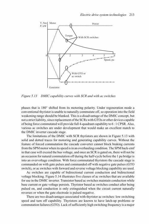
Electric drive system technologies 213
0 1 2 3 4 5 6
Speed, pu
Power
Torque
Motor
Generator
T, NmP, kW
With GTO or ac switch
With SCR switches
Figure 5.13 DMIC capability curves with SCR and with ac switches
phases that is 180◦ shifted from its motoring polarity. Under regeneration mode aconventional thyristor is unable to naturally commutate off, so operation into the fieldweakening range should be blanked. This is a disadvantage of the DMIC concept, butnot a strict liability, since replacement of the SCRs with GTOs or other devices capableof being force commutated will provide full 4-quadrant capability to 6 : 1 CPSR. Also,various ac switches are under development that would make an excellent match tothe DMIC inverter cascade stage.
The limitations of the DMIC with SCR thyristors are shown in Figure 5.13 withsolid and dotted traces for motoring and generating capability curves. Without thefeature of forced commutation the cascade converter cannot block braking currentsfrom the SPM motor when its speed is in an overhauling condition. The SPM back-emfin that case will exceed the bus voltage, and once an SCR is gated on, there will not bean occasion for natural commutation off during the half-cycle before the 1 pu bridge isinto an overvoltage condition. With force commutated thyristors the cascade stage iscommanded on with gate pulses and commanded off with negative gate pulses (GTOswitch), or ac switches with forward and reverse voltage blocking capability are used.
Ac switches are capable of bidirectional current conduction and bidirectionalvoltage blocking. Figure 5.14 illustrates five classes of ac switches that are availablefor use in the DMIC inverter. Transistor based ac switches maintain conduction whilebase current or gate voltage persists. Thyristor based ac switches conduct after beingpulsed on, and conduction is only extinguished when the circuit current naturallyreverses or when the gate electrode is pulsed negative.
There are two disadvantages associated with thyristor ac switches: low switchingspeed and turn off capability. Thyristors are known to have latch-up problems orcommutation failures (GTO). Lack of sufficiently high switching frequency is a major
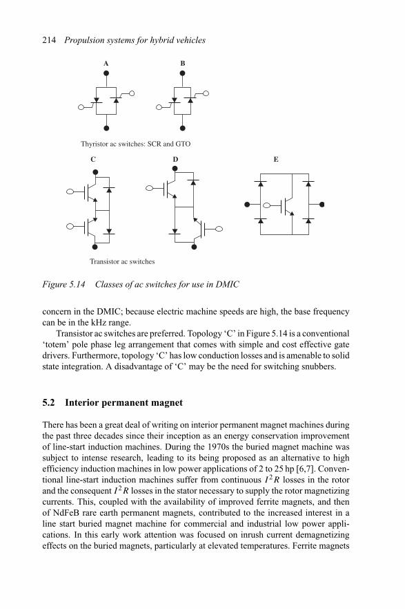
214 Propulsion systems for hybrid vehicles
Thyristor ac switches: SCR and GTO
Transistor ac switches
A B
C D E
Figure 5.14 Classes of ac switches for use in DMIC
concern in the DMIC; because electric machine speeds are high, the base frequencycan be in the kHz range.
Transistor ac switches are preferred. Topology ‘C’ in Figure 5.14 is a conventional‘totem’ pole phase leg arrangement that comes with simple and cost effective gatedrivers. Furthermore, topology ‘C’ has low conduction losses and is amenable to solidstate integration. A disadvantage of ‘C’ may be the need for switching snubbers.
5.2 Interior permanent magnet
There has been a great deal of writing on interior permanent magnet machines duringthe past three decades since their inception as an energy conservation improvementof line-start induction machines. During the 1970s the buried magnet machine wassubject to intense research, leading to its being proposed as an alternative to highefficiency induction machines in low power applications of 2 to 25 hp [6,7]. Conven-tional line-start induction machines suffer from continuous I 2R losses in the rotorand the consequent I 2R losses in the stator necessary to supply the rotor magnetizingcurrents. This, coupled with the availability of improved ferrite magnets, and thenof NdFeB rare earth permanent magnets, contributed to the increased interest in aline start buried magnet machine for commercial and industrial low power appli-cations. In this early work attention was focused on inrush current demagnetizingeffects on the buried magnets, particularly at elevated temperatures. Ferrite magnets
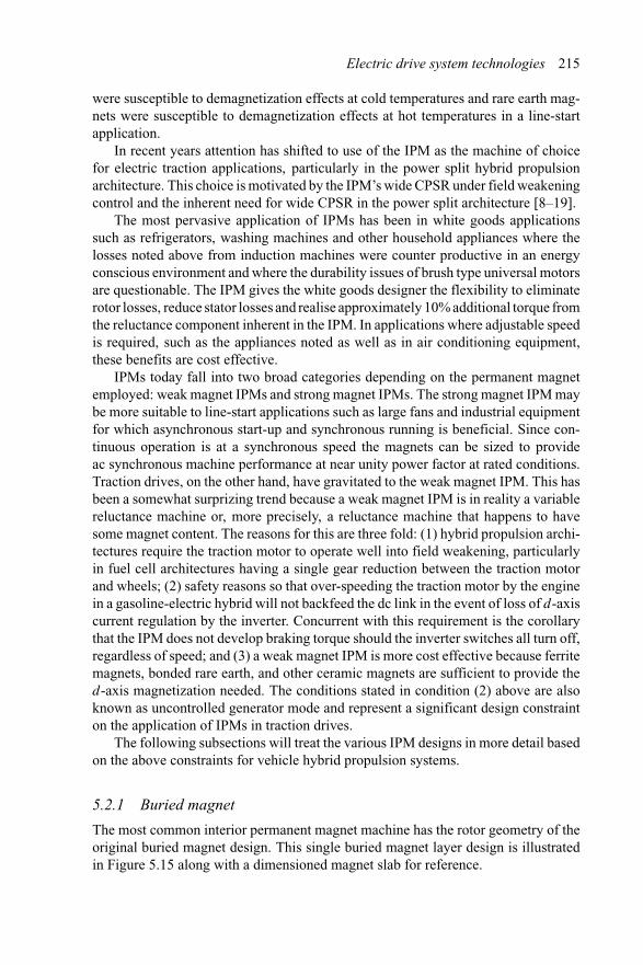
Electric drive system technologies 215
were susceptible to demagnetization effects at cold temperatures and rare earth mag-nets were susceptible to demagnetization effects at hot temperatures in a line-startapplication.
In recent years attention has shifted to use of the IPM as the machine of choicefor electric traction applications, particularly in the power split hybrid propulsionarchitecture. This choice is motivated by the IPM’s wide CPSR under field weakeningcontrol and the inherent need for wide CPSR in the power split architecture [8–19].
The most pervasive application of IPMs has been in white goods applicationssuch as refrigerators, washing machines and other household appliances where thelosses noted above from induction machines were counter productive in an energyconscious environment and where the durability issues of brush type universal motorsare questionable. The IPM gives the white goods designer the flexibility to eliminaterotor losses, reduce stator losses and realise approximately 10% additional torque fromthe reluctance component inherent in the IPM. In applications where adjustable speedis required, such as the appliances noted as well as in air conditioning equipment,these benefits are cost effective.
IPMs today fall into two broad categories depending on the permanent magnetemployed: weak magnet IPMs and strong magnet IPMs. The strong magnet IPM maybe more suitable to line-start applications such as large fans and industrial equipmentfor which asynchronous start-up and synchronous running is beneficial. Since con-tinuous operation is at a synchronous speed the magnets can be sized to provideac synchronous machine performance at near unity power factor at rated conditions.Traction drives, on the other hand, have gravitated to the weak magnet IPM. This hasbeen a somewhat surprizing trend because a weak magnet IPM is in reality a variablereluctance machine or, more precisely, a reluctance machine that happens to havesome magnet content. The reasons for this are three fold: (1) hybrid propulsion archi-tectures require the traction motor to operate well into field weakening, particularlyin fuel cell architectures having a single gear reduction between the traction motorand wheels; (2) safety reasons so that over-speeding the traction motor by the enginein a gasoline-electric hybrid will not backfeed the dc link in the event of loss of d-axiscurrent regulation by the inverter. Concurrent with this requirement is the corollarythat the IPM does not develop braking torque should the inverter switches all turn off,regardless of speed; and (3) a weak magnet IPM is more cost effective because ferritemagnets, bonded rare earth, and other ceramic magnets are sufficient to provide thed-axis magnetization needed. The conditions stated in condition (2) above are alsoknown as uncontrolled generator mode and represent a significant design constrainton the application of IPMs in traction drives.
The following subsections will treat the various IPM designs in more detail basedon the above constraints for vehicle hybrid propulsion systems.
5.2.1 Buried magnet
The most common interior permanent magnet machine has the rotor geometry of theoriginal buried magnet design. This single buried magnet layer design is illustratedin Figure 5.15 along with a dimensioned magnet slab for reference.
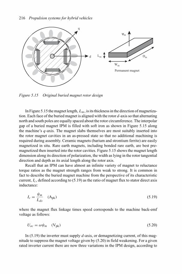
216 Propulsion systems for hybrid vehicles
Lm
Wm
Dmd
q
ψm
Permanent magnet
Figure 5.15 Original buried magnet rotor design
In Figure 5.15 the magnet length, Lm, is its thickness in the direction of magnetiza-tion. Each face of the buried magnet is aligned with the rotor d-axis so that alternatingnorth and south poles are equally spaced about the rotor circumference. The interpolargap of a buried magnet IPM is filled with soft iron as shown in Figure 5.15 alongthe machine’s q-axis. The magnet slabs themselves are most suitably inserted intothe rotor magnet cavities in an as-pressed state so that no additional machining isrequired during assembly. Ceramic magnets (barium and strontium ferrite) are easilymagnetized in situ. Rare earth magnets, including bonded rare earth, are best pre-magnetized then inserted into the rotor cavities. Figure 5.15 shows the magnet lengthdimension along its direction of polarization, the width as lying in the rotor tangentialdirection and depth as its axial length along the rotor axis.
Recall that an IPM can have almost an infinite variety of magnet to reluctancetorque ratios as the magnet strength ranges from weak to strong. It is common infact to describe the buried magnet machine from the perspective of its characteristiccurrent, Ic, defined according to (5.19) as the ratio of magnet flux to stator direct axisinductance:
Ic = ψm
Lds
(Apk) (5.19)
where the magnet flux linkage times speed corresponds to the machine back-emfvoltage as follows:
Uoc = ωψm (Vpk) (5.20)
In (5.19) the inverter must supply d-axis, or demagnetizing current, of this mag-nitude to suppress the magnet voltage given by (5.20) in field weakening. For a givenrated inverter current there are now three variations in the IPM design, according to
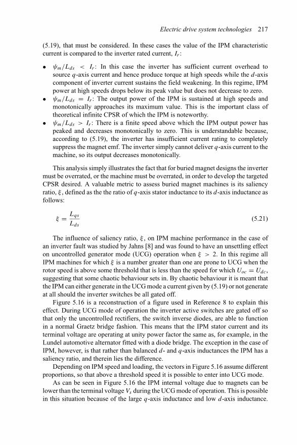
Electric drive system technologies 217
(5.19), that must be considered. In these cases the value of the IPM characteristiccurrent is compared to the inverter rated current, Ir :
• ψm/Lds < Ir : In this case the inverter has sufficient current overhead tosource q-axis current and hence produce torque at high speeds while the d-axiscomponent of inverter current sustains the field weakening. In this regime, IPMpower at high speeds drops below its peak value but does not decrease to zero.
• ψm/Lds = Ir : The output power of the IPM is sustained at high speeds andmonotonically approaches its maximum value. This is the important class oftheoretical infinite CPSR of which the IPM is noteworthy.
• ψm/Lds > Ir : There is a finite speed above which the IPM output power haspeaked and decreases monotonically to zero. This is understandable because,according to (5.19), the inverter has insufficient current rating to completelysuppress the magnet emf. The inverter simply cannot deliver q-axis current to themachine, so its output decreases monotonically.
This analysis simply illustrates the fact that for buried magnet designs the invertermust be overrated, or the machine must be overrated, in order to develop the targetedCPSR desired. A valuable metric to assess buried magnet machines is its saliencyratio, ξ , defined as the the ratio of q-axis stator inductance to its d-axis inductance asfollows:
ξ = Lqs
Lds
(5.21)
The influence of saliency ratio, ξ , on IPM machine performance in the case ofan inverter fault was studied by Jahns [8] and was found to have an unsettling effecton uncontrolled generator mode (UCG) operation when ξ > 2. In this regime allIPM machines for which ξ is a number greater than one are prone to UCG when therotor speed is above some threshold that is less than the speed for which Uoc = Udc,suggesting that some chaotic behaviour sets in. By chaotic behaviour it is meant thatthe IPM can either generate in the UCG mode a current given by (5.19) or not generateat all should the inverter switches be all gated off.
Figure 5.16 is a reconstruction of a figure used in Reference 8 to explain thiseffect. During UCG mode of operation the inverter active switches are gated off sothat only the uncontrolled rectifiers, the switch inverse diodes, are able to functionin a normal Graetz bridge fashion. This means that the IPM stator current and itsterminal voltage are operating at unity power factor the same as, for example, in theLundel automotive alternator fitted with a diode bridge. The exception in the case ofIPM, however, is that rather than balanced d- and q-axis inductances the IPM has asaliency ratio, and therein lies the difference.
Depending on IPM speed and loading, the vectors in Figure 5.16 assume differentproportions, so that above a threshold speed it is possible to enter into UCG mode.
As can be seen in Figure 5.16 the IPM internal voltage due to magnets can belower than the terminal voltage Vs during the UCG mode of operation. This is possiblein this situation because of the large q-axis inductance and low d-axis inductance.
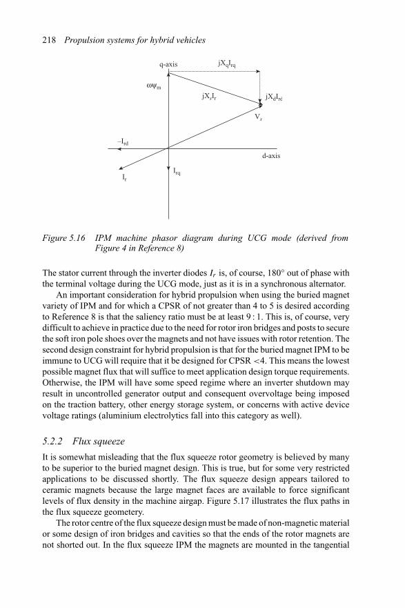
218 Propulsion systems for hybrid vehicles
q-axis jXqIrq
jXsIr jXdIrd
d-axis
Irq
–Ird
Ir
Vs
ωψm
Figure 5.16 IPM machine phasor diagram during UCG mode (derived fromFigure 4 in Reference 8)
The stator current through the inverter diodes Ir is, of course, 180◦ out of phase withthe terminal voltage during the UCG mode, just as it is in a synchronous alternator.
An important consideration for hybrid propulsion when using the buried magnetvariety of IPM and for which a CPSR of not greater than 4 to 5 is desired accordingto Reference 8 is that the saliency ratio must be at least 9 : 1. This is, of course, verydifficult to achieve in practice due to the need for rotor iron bridges and posts to securethe soft iron pole shoes over the magnets and not have issues with rotor retention. Thesecond design constraint for hybrid propulsion is that for the buried magnet IPM to beimmune to UCG will require that it be designed for CPSR <4. This means the lowestpossible magnet flux that will suffice to meet application design torque requirements.Otherwise, the IPM will have some speed regime where an inverter shutdown mayresult in uncontrolled generator output and consequent overvoltage being imposedon the traction battery, other energy storage system, or concerns with active devicevoltage ratings (aluminium electrolytics fall into this category as well).
5.2.2 Flux squeeze
It is somewhat misleading that the flux squeeze rotor geometry is believed by manyto be superior to the buried magnet design. This is true, but for some very restrictedapplications to be discussed shortly. The flux squeeze design appears tailored toceramic magnets because the large magnet faces are available to force significantlevels of flux density in the machine airgap. Figure 5.17 illustrates the flux paths inthe flux squeeze geometery.
The rotor centre of the flux squeeze design must be made of non-magnetic materialor some design of iron bridges and cavities so that the ends of the rotor magnets arenot shorted out. In the flux squeeze IPM the magnets are mounted in the tangential
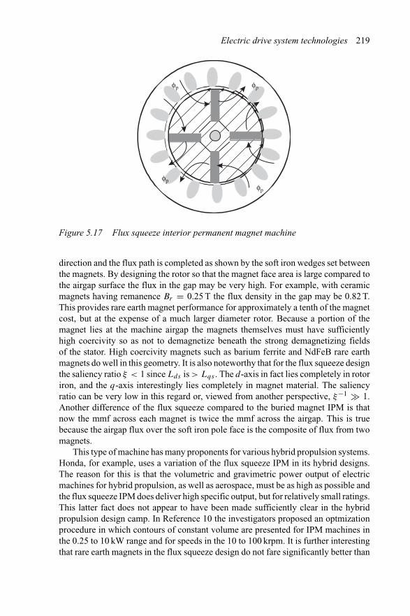
Electric drive system technologies 219
φp
φpφp
φp
Figure 5.17 Flux squeeze interior permanent magnet machine
direction and the flux path is completed as shown by the soft iron wedges set betweenthe magnets. By designing the rotor so that the magnet face area is large compared tothe airgap surface the flux in the gap may be very high. For example, with ceramicmagnets having remanence Br = 0.25 T the flux density in the gap may be 0.82 T.This provides rare earth magnet performance for approximately a tenth of the magnetcost, but at the expense of a much larger diameter rotor. Because a portion of themagnet lies at the machine airgap the magnets themselves must have sufficientlyhigh coercivity so as not to demagnetize beneath the strong demagnetizing fieldsof the stator. High coercivity magnets such as barium ferrite and NdFeB rare earthmagnets do well in this geometry. It is also noteworthy that for the flux squeeze designthe saliency ratio ξ < 1 since Lds is > Lqs . The d-axis in fact lies completely in rotoriron, and the q-axis interestingly lies completely in magnet material. The saliencyratio can be very low in this regard or, viewed from another perspective, ξ−1 � 1.Another difference of the flux squeeze compared to the buried magnet IPM is thatnow the mmf across each magnet is twice the mmf across the airgap. This is truebecause the airgap flux over the soft iron pole face is the composite of flux from twomagnets.
This type of machine has many proponents for various hybrid propulsion systems.Honda, for example, uses a variation of the flux squeeze IPM in its hybrid designs.The reason for this is that the volumetric and gravimetric power output of electricmachines for hybrid propulsion, as well as aerospace, must be as high as possible andthe flux squeeze IPM does deliver high specific output, but for relatively small ratings.This latter fact does not appear to have been made sufficiently clear in the hybridpropulsion design camp. In Reference 10 the investigators proposed an optmizationprocedure in which contours of constant volume are presented for IPM machines inthe 0.25 to 10 kW range and for speeds in the 10 to 100 krpm. It is further interestingthat rare earth magnets in the flux squeeze design do not fare significantly better than
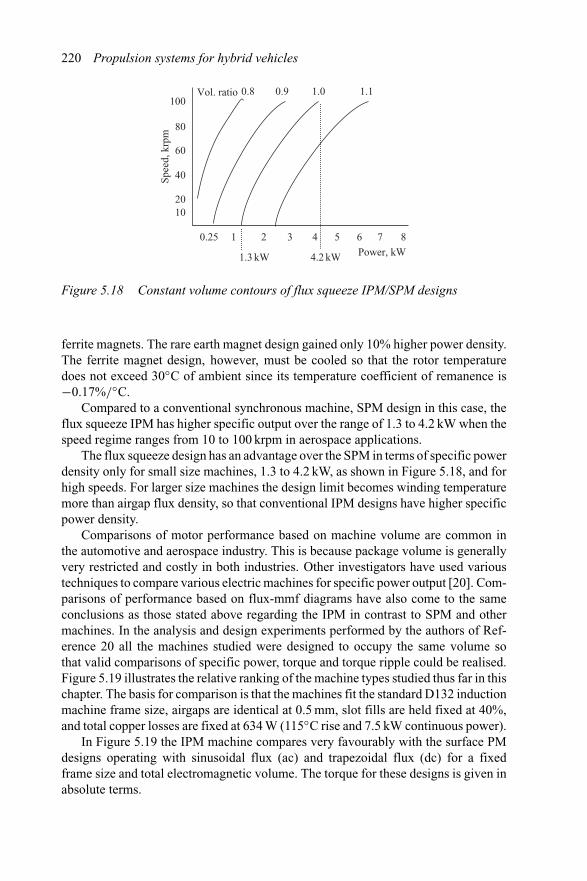
220 Propulsion systems for hybrid vehicles
0.25
0.8 0.9 1.0 1.1Vol. ratio
1
1.3 kW 4.2 kW Power, kW
1020
40
60
80
100
2 3 4 5 6 7 8
Spee
d, k
rpm
Figure 5.18 Constant volume contours of flux squeeze IPM/SPM designs
ferrite magnets. The rare earth magnet design gained only 10% higher power density.The ferrite magnet design, however, must be cooled so that the rotor temperaturedoes not exceed 30◦C of ambient since its temperature coefficient of remanence is−0.17%/◦C.
Compared to a conventional synchronous machine, SPM design in this case, theflux squeeze IPM has higher specific output over the range of 1.3 to 4.2 kW when thespeed regime ranges from 10 to 100 krpm in aerospace applications.
The flux squeeze design has an advantage over the SPM in terms of specific powerdensity only for small size machines, 1.3 to 4.2 kW, as shown in Figure 5.18, and forhigh speeds. For larger size machines the design limit becomes winding temperaturemore than airgap flux density, so that conventional IPM designs have higher specificpower density.
Comparisons of motor performance based on machine volume are common inthe automotive and aerospace industry. This is because package volume is generallyvery restricted and costly in both industries. Other investigators have used varioustechniques to compare various electric machines for specific power output [20]. Com-parisons of performance based on flux-mmf diagrams have also come to the sameconclusions as those stated above regarding the IPM in contrast to SPM and othermachines. In the analysis and design experiments performed by the authors of Ref-erence 20 all the machines studied were designed to occupy the same volume sothat valid comparisons of specific power, torque and torque ripple could be realised.Figure 5.19 illustrates the relative ranking of the machine types studied thus far in thischapter. The basis for comparison is that the machines fit the standard D132 inductionmachine frame size, airgaps are identical at 0.5 mm, slot fills are held fixed at 40%,and total copper losses are fixed at 634 W (115◦C rise and 7.5 kW continuous power).
In Figure 5.19 the IPM machine compares very favourably with the surface PMdesigns operating with sinusoidal flux (ac) and trapezoidal flux (dc) for a fixedframe size and total electromagnetic volume. The torque for these designs is given inabsolute terms.
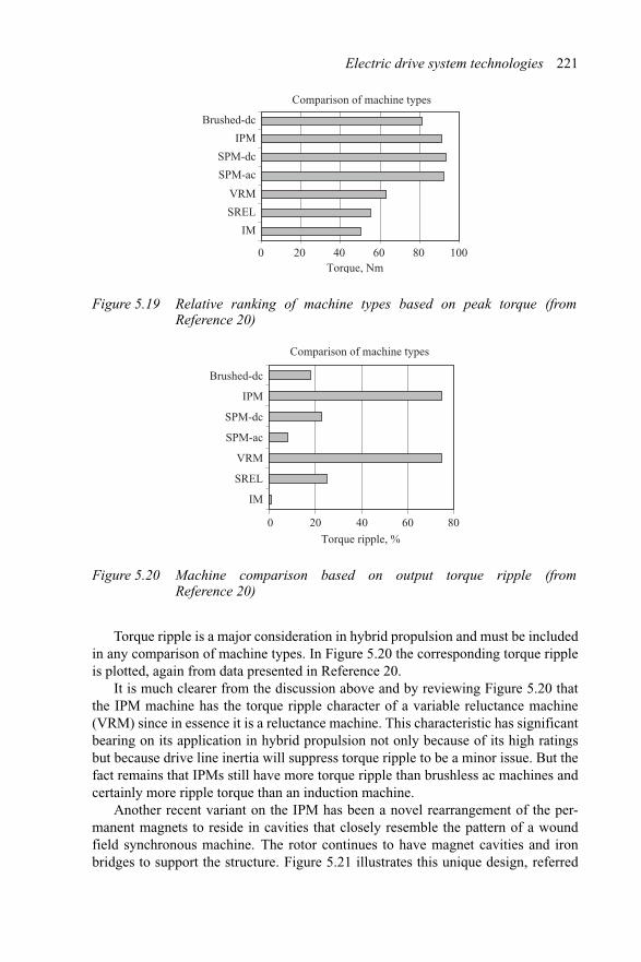
Electric drive system technologies 221
Comparison of machine types
Torque, Nm0 20 40 60 80 100
IM
SREL
VRM
SPM-ac
SPM-dc
IPM
Brushed-dc
Figure 5.19 Relative ranking of machine types based on peak torque (fromReference 20)
Comparison of machine types
0 20 40 60 80
Torque ripple, %
IM
SREL
VRM
SPM-ac
SPM-dc
IPM
Brushed-dc
Figure 5.20 Machine comparison based on output torque ripple (fromReference 20)
Torque ripple is a major consideration in hybrid propulsion and must be includedin any comparison of machine types. In Figure 5.20 the corresponding torque rippleis plotted, again from data presented in Reference 20.
It is much clearer from the discussion above and by reviewing Figure 5.20 thatthe IPM machine has the torque ripple character of a variable reluctance machine(VRM) since in essence it is a reluctance machine. This characteristic has significantbearing on its application in hybrid propulsion not only because of its high ratingsbut because drive line inertia will suppress torque ripple to be a minor issue. But thefact remains that IPMs still have more torque ripple than brushless ac machines andcertainly more ripple torque than an induction machine.
Another recent variant on the IPM has been a novel rearrangement of the per-manent magnets to reside in cavities that closely resemble the pattern of a woundfield synchronous machine. The rotor continues to have magnet cavities and ironbridges to support the structure. Figure 5.21 illustrates this unique design, referred
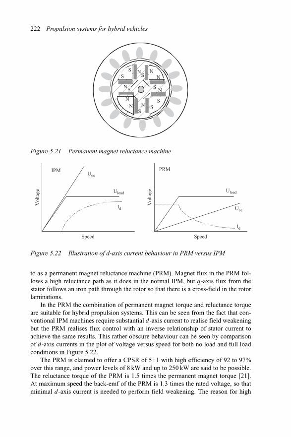
222 Propulsion systems for hybrid vehicles
N
N
N
N
S
S
S
S
SS
NN
SSN
N
Figure 5.21 Permanent magnet reluctance machine
IPM
Speed Speed
Vol
tage
Vol
tage
PRMUoc
UocId
Id
Uload Uload
Figure 5.22 Illustration of d-axis current behaviour in PRM versus IPM
to as a permanent magnet reluctance machine (PRM). Magnet flux in the PRM fol-lows a high reluctance path as it does in the normal IPM, but q-axis flux from thestator follows an iron path through the rotor so that there is a cross-field in the rotorlaminations.
In the PRM the combination of permanent magnet torque and reluctance torqueare suitable for hybrid propulsion systems. This can be seen from the fact that con-ventional IPM machines require substantial d-axis current to realise field weakeningbut the PRM realises flux control with an inverse relationship of stator current toachieve the same results. This rather obscure behaviour can be seen by comparisonof d-axis currents in the plot of voltage versus speed for both no load and full loadconditions in Figure 5.22.
The PRM is claimed to offer a CPSR of 5 : 1 with high efficiency of 92 to 97%over this range, and power levels of 8 kW and up to 250 kW are said to be possible.The reluctance torque of the PRM is 1.5 times the permanent magnet torque [21].At maximum speed the back-emf of the PRM is 1.3 times the rated voltage, so thatminimal d-axis current is needed to perform field weakening. The reason for high
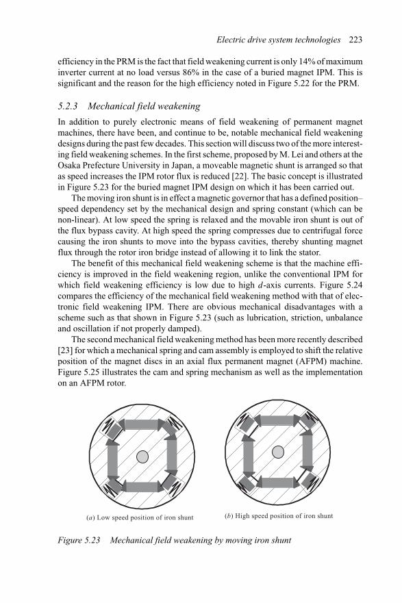
Electric drive system technologies 223
efficiency in the PRM is the fact that field weakening current is only 14% of maximuminverter current at no load versus 86% in the case of a buried magnet IPM. This issignificant and the reason for the high efficiency noted in Figure 5.22 for the PRM.
5.2.3 Mechanical field weakening
In addition to purely electronic means of field weakening of permanent magnetmachines, there have been, and continue to be, notable mechanical field weakeningdesigns during the past few decades. This section will discuss two of the more interest-ing field weakening schemes. In the first scheme, proposed by M. Lei and others at theOsaka Prefecture University in Japan, a moveable magnetic shunt is arranged so thatas speed increases the IPM rotor flux is reduced [22]. The basic concept is illustratedin Figure 5.23 for the buried magnet IPM design on which it has been carried out.
The moving iron shunt is in effect a magnetic governor that has a defined position–speed dependency set by the mechanical design and spring constant (which can benon-linear). At low speed the spring is relaxed and the movable iron shunt is out ofthe flux bypass cavity. At high speed the spring compresses due to centrifugal forcecausing the iron shunts to move into the bypass cavities, thereby shunting magnetflux through the rotor iron bridge instead of allowing it to link the stator.
The benefit of this mechanical field weakening scheme is that the machine effi-ciency is improved in the field weakening region, unlike the conventional IPM forwhich field weakening efficiency is low due to high d-axis currents. Figure 5.24compares the efficiency of the mechanical field weakening method with that of elec-tronic field weakening IPM. There are obvious mechanical disadvantages with ascheme such as that shown in Figure 5.23 (such as lubrication, striction, unbalanceand oscillation if not properly damped).
The second mechanical field weakening method has been more recently described[23] for which a mechanical spring and cam assembly is employed to shift the relativeposition of the magnet discs in an axial flux permanent magnet (AFPM) machine.Figure 5.25 illustrates the cam and spring mechanism as well as the implementationon an AFPM rotor.
(a) Low speed position of iron shunt (b) High speed position of iron shunt
Figure 5.23 Mechanical field weakening by moving iron shunt
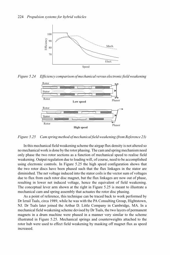
224 Propulsion systems for hybrid vehicles
Speed
Eff
icie
ncy
Mech.
Elect.
100
90
80
70
Figure 5.24 Efficiency comparison of mechanical versus electronic field weakening
Stator
Rotor
Rotor Phasor
Stator
Rotor
Rotor Phasor
Low speed
High speed
Figure 5.25 Cam spring method of mechanical field weakening (from Reference 23)
In this mechanical field weakening scheme the airgap flux density is not altered sono mechanical work is done by the rotor phasing. The cam and spring mechanism needonly phase the two rotor sections as a function of mechanical speed to realise fieldweakening. Output regulation due to loading will, of course, need to be accomplishedusing electronic controls. In Figure 5.25 the high speed configuration shows thatthe two rotor discs have been phased such that the flux linkages in the stator arediminished. The net voltage induced into the stator coils is the vector sum of voltagesdue to flux from each rotor disc magnet, but the flux linkages are now out of phase,resulting in lower net induced voltage, hence the equivalent of field weakening.The conceptual lever arm shown at the right in Figure 5.25 is meant to illustrate amechanical cam and spring assembly that actuates the rotor disc phasing.
As a point of reference, this technique can be traced back to work performed byDr Izrail Tsals, circa 1989, while he was with the PA Consulting Group, Hightstown,NJ. Dr Tsals later joined the Arthur D. Little Company in Cambridge, MA. In amechanical field weakening scheme devised by Dr Tsals, the two layers of permanentmagnets in a drum machine were phased in a manner very similar to the schemeillustrated in Figure 5.25. Mechanical springs and counterweights attached to therotor hub were used to effect field weakening by masking off magnet flux as speedincreased.
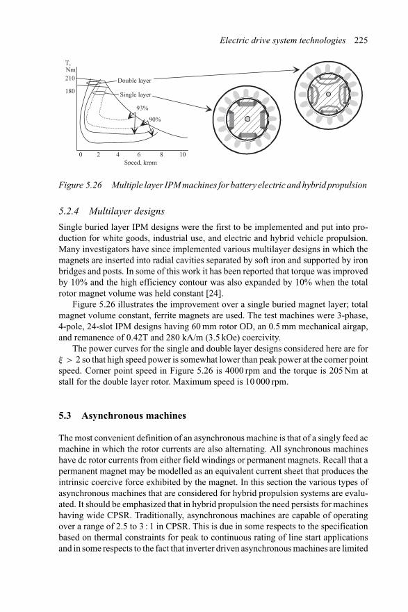
Electric drive system technologies 225
93%
90%
Double layer
Single layer
0 2 4 6 8 10Speed, krpm
T,Nm
210
180
Figure 5.26 Multiple layer IPM machines for battery electric and hybrid propulsion
5.2.4 Multilayer designs
Single buried layer IPM designs were the first to be implemented and put into pro-duction for white goods, industrial use, and electric and hybrid vehicle propulsion.Many investigators have since implemented various multilayer designs in which themagnets are inserted into radial cavities separated by soft iron and supported by ironbridges and posts. In some of this work it has been reported that torque was improvedby 10% and the high efficiency contour was also expanded by 10% when the totalrotor magnet volume was held constant [24].
Figure 5.26 illustrates the improvement over a single buried magnet layer; totalmagnet volume constant, ferrite magnets are used. The test machines were 3-phase,4-pole, 24-slot IPM designs having 60 mm rotor OD, an 0.5 mm mechanical airgap,and remanence of 0.42T and 280 kA/m (3.5 kOe) coercivity.
The power curves for the single and double layer designs considered here are forξ > 2 so that high speed power is somewhat lower than peak power at the corner pointspeed. Corner point speed in Figure 5.26 is 4000 rpm and the torque is 205 Nm atstall for the double layer rotor. Maximum speed is 10 000 rpm.
5.3 Asynchronous machines
The most convenient definition of an asynchronous machine is that of a singly feed acmachine in which the rotor currents are also alternating. All synchronous machineshave dc rotor currents from either field windings or permanent magnets. Recall that apermanent magnet may be modelled as an equivalent current sheet that produces theintrinsic coercive force exhibited by the magnet. In this section the various types ofasynchronous machines that are considered for hybrid propulsion systems are evalu-ated. It should be emphasized that in hybrid propulsion the need persists for machineshaving wide CPSR. Traditionally, asynchronous machines are capable of operatingover a range of 2.5 to 3 : 1 in CPSR. This is due in some respects to the specificationbased on thermal constraints for peak to continuous rating of line start applicationsand in some respects to the fact that inverter driven asynchronous machines are limited
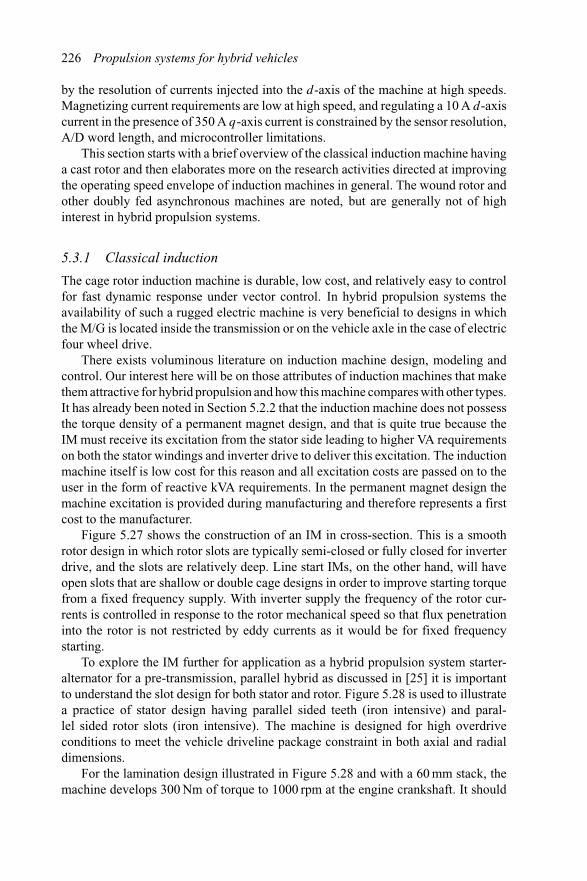
226 Propulsion systems for hybrid vehicles
by the resolution of currents injected into the d-axis of the machine at high speeds.Magnetizing current requirements are low at high speed, and regulating a 10 A d-axiscurrent in the presence of 350 A q-axis current is constrained by the sensor resolution,A/D word length, and microcontroller limitations.
This section starts with a brief overview of the classical induction machine havinga cast rotor and then elaborates more on the research activities directed at improvingthe operating speed envelope of induction machines in general. The wound rotor andother doubly fed asynchronous machines are noted, but are generally not of highinterest in hybrid propulsion systems.
5.3.1 Classical induction
The cage rotor induction machine is durable, low cost, and relatively easy to controlfor fast dynamic response under vector control. In hybrid propulsion systems theavailability of such a rugged electric machine is very beneficial to designs in whichthe M/G is located inside the transmission or on the vehicle axle in the case of electricfour wheel drive.
There exists voluminous literature on induction machine design, modeling andcontrol. Our interest here will be on those attributes of induction machines that makethem attractive for hybrid propulsion and how this machine compares with other types.It has already been noted in Section 5.2.2 that the induction machine does not possessthe torque density of a permanent magnet design, and that is quite true because theIM must receive its excitation from the stator side leading to higher VA requirementson both the stator windings and inverter drive to deliver this excitation. The inductionmachine itself is low cost for this reason and all excitation costs are passed on to theuser in the form of reactive kVA requirements. In the permanent magnet design themachine excitation is provided during manufacturing and therefore represents a firstcost to the manufacturer.
Figure 5.27 shows the construction of an IM in cross-section. This is a smoothrotor design in which rotor slots are typically semi-closed or fully closed for inverterdrive, and the slots are relatively deep. Line start IMs, on the other hand, will haveopen slots that are shallow or double cage designs in order to improve starting torquefrom a fixed frequency supply. With inverter supply the frequency of the rotor cur-rents is controlled in response to the rotor mechanical speed so that flux penetrationinto the rotor is not restricted by eddy currents as it would be for fixed frequencystarting.
To explore the IM further for application as a hybrid propulsion system starter-alternator for a pre-transmission, parallel hybrid as discussed in [25] it is importantto understand the slot design for both stator and rotor. Figure 5.28 is used to illustratea practice of stator design having parallel sided teeth (iron intensive) and paral-lel sided rotor slots (iron intensive). The machine is designed for high overdriveconditions to meet the vehicle driveline package constraint in both axial and radialdimensions.
For the lamination design illustrated in Figure 5.28 and with a 60 mm stack, themachine develops 300 Nm of torque to 1000 rpm at the engine crankshaft. It should
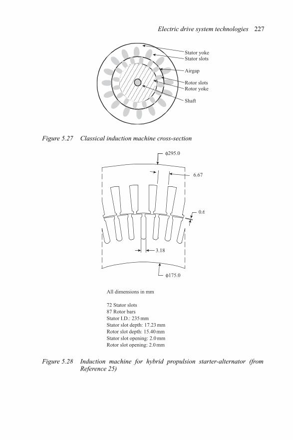
Electric drive system technologies 227
Stator yokeStator slots
Airgap
Rotor slotsRotor yoke
Shaft
Figure 5.27 Classical induction machine cross-section
All dimensions in mm
72 Stator slots87 Rotor barsStator I.D.: 235 mmStator slot depth: 17.23 mmRotor slot depth: 15.40 mmStator slot opening: 2.0 mmRotor slot opening: 2.0 mm
φ175.0
3.18
0.6
6.67
φ295.0
Figure 5.28 Induction machine for hybrid propulsion starter-alternator (fromReference 25)
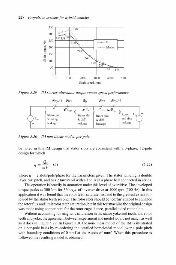
228 Propulsion systems for hybrid vehicles
0
50
100
150
200
250
300
350
0 1000 2000 3000 4000 5000
Shaft speed, rpm
Shaf
t tor
que,
Nm Exp.
Model
348358
380
360
306
248
248
269233
163 175
Figure 5.29 IM starter-alternator torque versus speed performance
Fsm
Rotorend ring leakage
Rotor slot & diff. leakage
Stator slot & diff. leakage
Stator endwindingleakage
Φm ΦrmFrm
Φsm
Figure 5.30 IM non-linear model, per pole
be noted in this IM design that stator slots are consistent with a 3-phase, 12-poledesign for which
q = Qs
mP(#) (5.22)
where q = 2 slots/pole/phase for the parameters given. The stator winding is doublelayer, 5/6 pitch, and has 2 turns/coil with all coils in a phase belt connected in series.
The operation is heavily in saturation under this level of overdrive. The developedtorque peaks at 300 Nm for 360 Apk of inverter drive at 1000 rpm (100 Hz). In thisapplication it was found that the rotor teeth saturate first and to the greatest extent fol-lowed by the stator teeth second. The rotor slots should be ‘coffin’ shaped to enhancethe rotor flux and limit rotor teeth saturation, but in this test machine the original designwas made using copper bars for the rotor cage, hence, parallel sided rotor slots.
Without accounting for magnetic saturation in the stator yoke and teeth, and rotorteeth and yoke, the agreement between experiment and model would not match as wellas it does in Figure 5.29. In Figure 5.30 the non-linear model of the IM is illustratedon a per-pole basis by re-ordering the detailed homeloidal model over a pole pitchwith boundary conditions of 0 mmf at the q-axis of mmf. When this procedure isfollowed the resulting model is obtained.
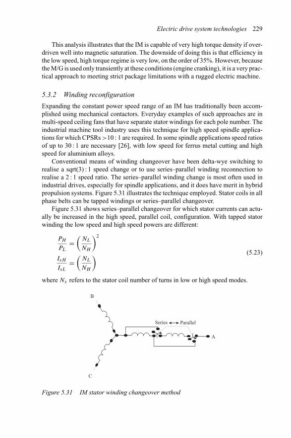
Electric drive system technologies 229
This analysis illustrates that the IM is capable of very high torque density if over-driven well into magnetic saturation. The downside of doing this is that efficiency inthe low speed, high torque regime is very low, on the order of 35%. However, becausethe M/G is used only transiently at these conditions (engine cranking), it is a very prac-tical approach to meeting strict package limitations with a rugged electric machine.
5.3.2 Winding reconfiguration
Expanding the constant power speed range of an IM has traditionally been accom-plished using mechanical contactors. Everyday examples of such approaches are inmulti-speed ceiling fans that have separate stator windings for each pole number. Theindustrial machine tool industry uses this technique for high speed spindle applica-tions for which CPSRs >10 : 1 are required. In some spindle applications speed ratiosof up to 30 : 1 are necessary [26], with low speed for ferrus metal cutting and highspeed for aluminium alloys.
Conventional means of winding changeover have been delta-wye switching torealise a sqrt(3) : 1 speed change or to use series–parallel winding reconnection torealise a 2 : 1 speed ratio. The series–parallel winding change is most often used inindustrial drives, especially for spindle applications, and it does have merit in hybridpropulsion systems. Figure 5.31 illustrates the technique employed. Stator coils in allphase belts can be tapped windings or series–parallel changeover.
Figure 5.31 shows series–parallel changeover for which stator currents can actu-ally be increased in the high speed, parallel coil, configuration. With tapped statorwinding the low speed and high speed powers are different:
PH
PL
=(
NL
NH
)2
IsH
IsL
=(
NL
NH
) (5.23)
where Nx refers to the stator coil number of turns in low or high speed modes.
B
C
A
Series Parallel
Figure 5.31 IM stator winding changeover method
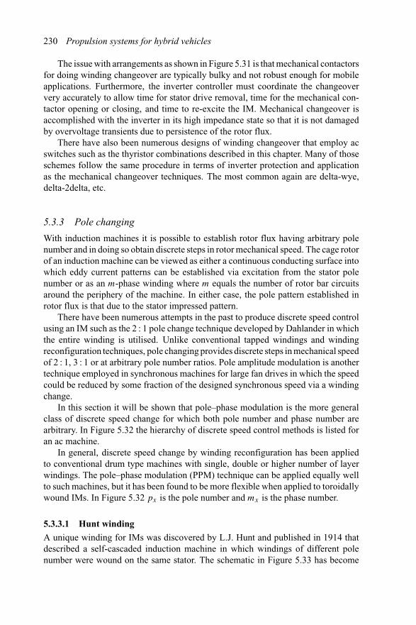
230 Propulsion systems for hybrid vehicles
The issue with arrangements as shown in Figure 5.31 is that mechanical contactorsfor doing winding changeover are typically bulky and not robust enough for mobileapplications. Furthermore, the inverter controller must coordinate the changeoververy accurately to allow time for stator drive removal, time for the mechanical con-tactor opening or closing, and time to re-excite the IM. Mechanical changeover isaccomplished with the inverter in its high impedance state so that it is not damagedby overvoltage transients due to persistence of the rotor flux.
There have also been numerous designs of winding changeover that employ acswitches such as the thyristor combinations described in this chapter. Many of thoseschemes follow the same procedure in terms of inverter protection and applicationas the mechanical changeover techniques. The most common again are delta-wye,delta-2delta, etc.
5.3.3 Pole changing
With induction machines it is possible to establish rotor flux having arbitrary polenumber and in doing so obtain discrete steps in rotor mechanical speed. The cage rotorof an induction machine can be viewed as either a continuous conducting surface intowhich eddy current patterns can be established via excitation from the stator polenumber or as an m-phase winding where m equals the number of rotor bar circuitsaround the periphery of the machine. In either case, the pole pattern established inrotor flux is that due to the stator impressed pattern.
There have been numerous attempts in the past to produce discrete speed controlusing an IM such as the 2 : 1 pole change technique developed by Dahlander in whichthe entire winding is utilised. Unlike conventional tapped windings and windingreconfiguration techniques, pole changing provides discrete steps in mechanical speedof 2 : 1, 3 : 1 or at arbitrary pole number ratios. Pole amplitude modulation is anothertechnique employed in synchronous machines for large fan drives in which the speedcould be reduced by some fraction of the designed synchronous speed via a windingchange.
In this section it will be shown that pole–phase modulation is the more generalclass of discrete speed change for which both pole number and phase number arearbitrary. In Figure 5.32 the hierarchy of discrete speed control methods is listed foran ac machine.
In general, discrete speed change by winding reconfiguration has been appliedto conventional drum type machines with single, double or higher number of layerwindings. The pole–phase modulation (PPM) technique can be applied equally wellto such machines, but it has been found to be more flexible when applied to toroidallywound IMs. In Figure 5.32 px is the pole number and mx is the phase number.
5.3.3.1 Hunt winding
A unique winding for IMs was discovered by L.J. Hunt and published in 1914 thatdescribed a self-cascaded induction machine in which windings of different polenumber were wound on the same stator. The schematic in Figure 5.33 has become
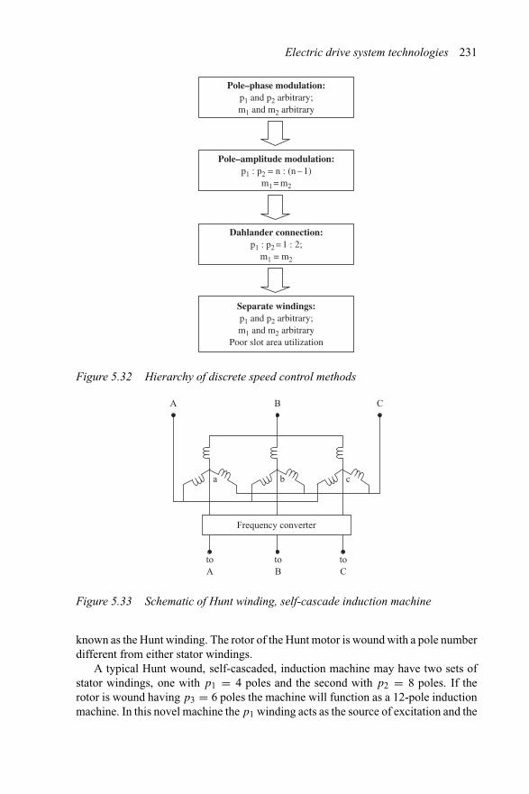
Electric drive system technologies 231
Separate windings:p1 and p2 arbitrary;m1 and m2 arbitrary
Poor slot area utilization
Dahlander connection:p1 : p2 = 1 : 2;
m1 = m2
Pole–amplitude modulation:p1 : p2 = n : (n – 1)
m1 = m2
Pole–phase modulation:p1 and p2 arbitrary;m1 and m2 arbitrary
Figure 5.32 Hierarchy of discrete speed control methods
A B C
toA
toB
Frequency converter
toC
a b c
Figure 5.33 Schematic of Hunt winding, self-cascade induction machine
known as the Hunt winding. The rotor of the Hunt motor is wound with a pole numberdifferent from either stator windings.
A typical Hunt wound, self-cascaded, induction machine may have two sets ofstator windings, one with p1 = 4 poles and the second with p2 = 8 poles. If therotor is wound having p3 = 6 poles the machine will function as a 12-pole inductionmachine. In this novel machine the p1 winding acts as the source of excitation and the
232 Propulsion systems for hybrid vehicles
second stator winding behaves as if it were a rotor winding. The rotor p3 winding itselfinterprets the stator p1 and p2 fields and develops a torque corresponding to p1 +p2.The original Hunt winding was a very early attempt at induction machine speedcontrol for low speed applications from a fixed frequency supply. With resistanceloading on the wound rotor it was possible to realise high starting torque and lowspeed operation.
Subsequent applications of the Hunt winding have led to numerous develop-ments of a class of doubly fed induction and most recently, doubly excited reluctancemachines [27–29]. The interested reader is referred to those references.
5.3.3.2 Electronic pole change
The concept of electronic pole changing has been described by various authors sincethe early 1970s after the availability of bipolar electronic switches. The fact that manyindustrial applications require operation over vastly different speed regimes had beenthe early motivation for such research. More recently, and especially after the earlyyears of research and development on battery electric vehicles, it became importantto extend the limited CPSR of induction machines to enable high torque for vehiclelaunch and grades, yet maintain sustainable power at relatively high speeds. Thework by Osama and Lipo in the mid-1990s was one such example of electronic polechanging in which contactorless changeover was realised by purely electronic controlof machine currents [30].
In their work, Osama and Lipo described a contactorless pole changing techniquethat was capable of extending the field weakening range of a 4-pole IM. The machineitself was wound with six coil groups (e.g. phases) with two sets of three phases eachconnected to their respective power electronic inverters as shown schematically inFigure 5.34.
The machine described in Figure 5.34 must be designed to sustain the stator androtor flux of its lowest pole number operating mode. For example, if the motor is aconventional 4-pole IM, and 2-pole operation is required, the injected currents mustconform with the values given in Table 5.5 below. In this table a minus sign signifiespolarity reversal at the inverter group leg associated with that coil group. If a singledc supply is used as is shown in the figure, then the neutrals of the two 3-phase groupsmust remain isolated. That means that neutrals in group (1,3,5) must be isolated fromthe group (2,4,6). Furthermore, the rotor of the IM used for 2 : 1 pole change mustbe somewhat larger than a 4-pole rotor in order to remain unsaturated under 2-poleoperation.
Electronic pole changing of an existing IM design often leads to oversaturationof the machine’s stator yoke (back-iron) or rotor yoke. This is the case because a highpole number machine is often reconfigured electronically to a lower pole numbermachine, – in the case of the electronic pole changing scheme covered here, by afactor of 2 : 1. In order to realise a pole change of 3 : 1 or in fact arbitrary pole numberchanging, the techniques of pole–phase modulation must be employed, as will beseen in the next section.
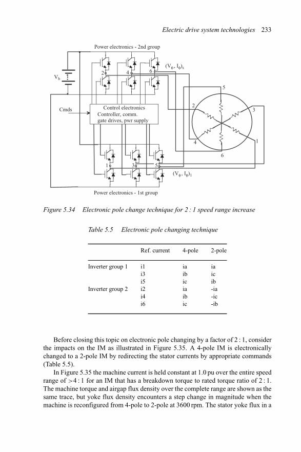
Electric drive system technologies 233
Vb
Cmds
Power electronics - 2nd group
Power electronics - 1st group
1
1
2
2
3
3
4
4
5
6
6
(Vφ , Iφ)s
(Vφ , Iφ)1
Controller, comm.gate drives, pwr supply
Control electronics
5
Figure 5.34 Electronic pole change technique for 2 : 1 speed range increase
Table 5.5 Electronic pole changing technique
Ref. current 4-pole 2-pole
Inverter group 1 i1 ia iai3 ib ici5 ic ib
Inverter group 2 i2 ia -iai4 ib -ici6 ic -ib
Before closing this topic on electronic pole changing by a factor of 2 : 1, considerthe impacts on the IM as illustrated in Figure 5.35. A 4-pole IM is electronicallychanged to a 2-pole IM by redirecting the stator currents by appropriate commands(Table 5.5).
In Figure 5.35 the machine current is held constant at 1.0 pu over the entire speedrange of >4 : 1 for an IM that has a breakdown torque to rated torque ratio of 2 : 1.The machine torque and airgap flux density over the complete range are shown as thesame trace, but yoke flux density encounters a step change in magnitude when themachine is reconfigured from 4-pole to 2-pole at 3600 rpm. The stator yoke flux in a
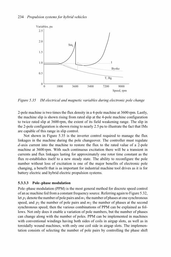
234 Propulsion systems for hybrid vehicles
00 1800 3600 5400 7200 9000
Speed, rpm
T, Bg
Byoke
I
Sωe
0.5
1.0
1.5
2.0
2.5Variables, pu
Figure 5.35 IM electrical and magnetic variables during electronic pole change
2-pole machine is two times the flux density in a 4-pole machine at 3600 rpm. Lastly,the machine slip is shown rising from rated slip at the 4-pole machine configurationto twice rated slip at 3600 rpm, the extent of its field weakening range. The slip inthe 2-pole configuration is shown rising to nearly 2.5 pu to illustrate the fact that IMsare capable of this range in slip control.
Not shown in Figure 5.35 is the inverter control required to manage the fluxlinkages in the machine during the pole changeover. The controller must regulated-axis current into the machine to restore the flux to the rated value of a 2-polemachine at 3600 rpm. With such continuous excitation there will be a transient incurrents and flux linkages lasting for approximately one rotor time constant as theflux re-establishes itself to a new steady state. The ability to reconfigure the polenumber without loss of excitation is one of the major benefits of electronic polechanging, a benefit that is as important for industrial machine tool drives as it is forbattery electric and hybrid electric propulsion systems.
5.3.3.3 Pole–phase modulation
Pole–phase modulation (PPM) is the most general method for discrete speed controlof an ac machine fed from a constant frequency source. Referring again to Figure 5.32,let p1 denote the number of pole pairs and m1 the number of phases at one synchronousspeed, and p2 the number of pole pairs and m2 the number of phases at the secondsynchronous speed; then the various combinations of PPM can be explained as fol-lows. Not only does it enable a variation of pole numbers, but the number of phasescan change along with the number of poles. PPM can be implemented in machineswith conventional windings having both sides of coils in airgap slots, as well as intoroidally wound machines, with only one coil side in airgap slots. The implemen-tation consists of selecting the number of pole pairs by controlling the phase shift
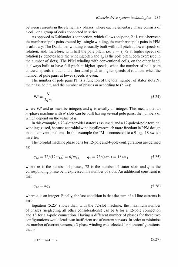
Electric drive system technologies 235
between currents in the elementary phases, where each elementary phase consists ofa coil, or a group of coils connected in series.
As opposed to Dahlander’s connection, which allows only one, 2 : 1, ratio betweenthe number of pole pairs created by a single winding, the number of pole pairs in PPMis arbitrary. The Dahlander winding is usually built with full pitch at lower speeds ofrotation, and, therefore, with half the pole pitch, i.e. y = τp/2 at higher speeds ofrotation (y denotes here the winding pitch and τp is the pole pitch, both expressed inthe number of slots). The PPM winding with conventional coils, on the other hand,is always built to have full pitch at higher speeds, when the number of pole pairsat lower speeds is odd, and a shortened pitch at higher speeds of rotation, when thenumber of pole pairs at lower speeds is even.
The number of pole pairs PP is a function of the total number of stator slots N ,the phase belt q, and the number of phases m according to (5.24):
PP = N
2qm(5.24)
where PP and m must be integers and q is usually an integer. This means that anm-phase machine with N slots can be built having several pole pairs, the numbers ofwhich depend on the value of q.
In this example, a 72-slot toroidal stator is assumed, and a 12-pole/4-pole toroidalwinding is used, because a toroidal winding allows much more freedom in PPM designthan a conventional one. In this example the IM is connected to a 9-leg, 18-switchinverter.
The toroidal machine phase belts for 12-pole and 4-pole configurations are definedas:
q12 = 72/(12m12) = 6/m12 q4 = 72/(4m4) = 18/m4 (5.25)
where m is the number of phases, 72 is the number of stator slots and q is thecorresponding phase belt, expressed in a number of slots. An additional constraint isthat
q12 = nq4 (5.26)
where n is an integer. Finally, the last condition is that the sum of all line currents iszero.
Equation (5.25) shows that, with the 72-slot machine, the maximum numberof phases (neglecting all other considerations) can be 6 for a 12-pole connectionand 18 for a 4-pole connection. Having a different number of phases for these twoconfigurations would lead to an inefficient use of current sensors. In order to minimisethe number of current sensors, a 3-phase winding was selected for both configurations,that is
m12 = m4 = 3 (5.27)
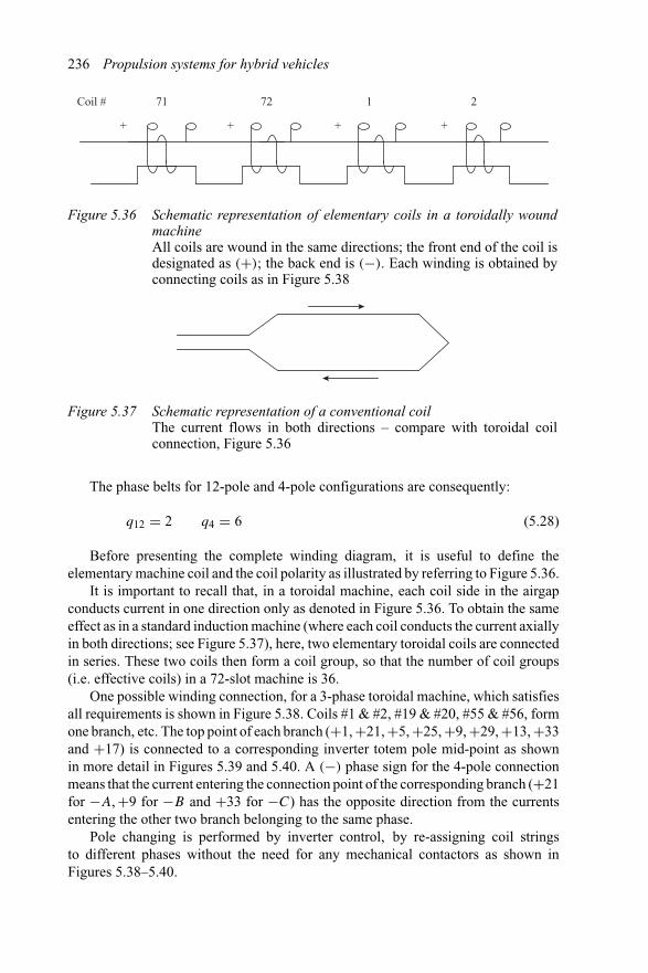
236 Propulsion systems for hybrid vehicles
Coil # 72 1 271
+ ++ +
Figure 5.36 Schematic representation of elementary coils in a toroidally woundmachineAll coils are wound in the same directions; the front end of the coil isdesignated as (+); the back end is (−). Each winding is obtained byconnecting coils as in Figure 5.38
Figure 5.37 Schematic representation of a conventional coilThe current flows in both directions – compare with toroidal coilconnection, Figure 5.36
The phase belts for 12-pole and 4-pole configurations are consequently:
q12 = 2 q4 = 6 (5.28)
Before presenting the complete winding diagram, it is useful to define theelementary machine coil and the coil polarity as illustrated by referring to Figure 5.36.
It is important to recall that, in a toroidal machine, each coil side in the airgapconducts current in one direction only as denoted in Figure 5.36. To obtain the sameeffect as in a standard induction machine (where each coil conducts the current axiallyin both directions; see Figure 5.37), here, two elementary toroidal coils are connectedin series. These two coils then form a coil group, so that the number of coil groups(i.e. effective coils) in a 72-slot machine is 36.
One possible winding connection, for a 3-phase toroidal machine, which satisfiesall requirements is shown in Figure 5.38. Coils #1 & #2, #19 & #20, #55 & #56, formone branch, etc. The top point of each branch (+1, +21, +5, +25, +9, +29, +13, +33and +17) is connected to a corresponding inverter totem pole mid-point as shownin more detail in Figures 5.39 and 5.40. A (−) phase sign for the 4-pole connectionmeans that the current entering the connection point of the corresponding branch (+21for −A, +9 for −B and +33 for −C) has the opposite direction from the currentsentering the other two branch belonging to the same phase.
Pole changing is performed by inverter control, by re-assigning coil stringsto different phases without the need for any mechanical contactors as shown inFigures 5.38–5.40.
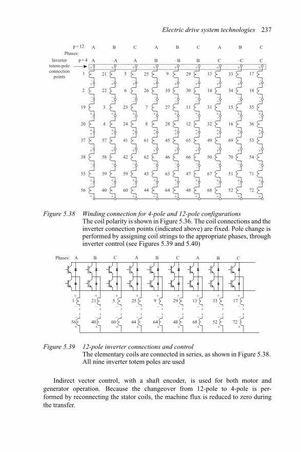
Electric drive system technologies 237
Phases:
B –BA –A A B C –C C
A BA B C C A B Cp = 12
p = 4Invertertotem-poleconnection
points
3
4
57
58
39
40
22
21
23
24
41
42
59
60
7
8
61
62
43
44
26
255
6
27
28
45
46
63
64
11
12
65
66
47
48
30
299
10
31
32
49
50
67
68
15
16
69
70
51
52
34
3313
14
35
36
53
54
71
72
17
18
19
20
37
38
55
56
1
2
+
+
+
+
+
+
–
–
––
–
–
––
+
+
+
+
+
+
+
+
–
–
––
–
–
––
+
+
+
+
+
+
+
+
–
–
––
–
–
––
+
+
+
+
+
+
+
+
–
–
––
–
–
––
+
+
+
+
+
+
+
+
–
–
––
–
–
––
+
+
+
+
+
+
+
+
–
–
––
–
–
––
+
+
+
+
+
+
+
+
–
–
––
–
–
––
+
+
+
+
+
+
+
+
–
–
––
–
–
––
+
+
+
+
+
+
+
+
–
–
––
–
–
––
+
+
Figure 5.38 Winding connection for 4-pole and 12-pole configurationsThe coil polarity is shown in Figure 5.36. The coil connections and theinverter connection points (indicated above) are fixed. Pole change isperformed by assigning coil strings to the appropriate phases, throughinverter control (see Figures 5.39 and 5.40)
1
56
21
40
5
60
25
44
9
64
29
48
13
68
33
52
17
72
A B C A B C A B CPhases:
+
–
–
+
+
–
–
+
+
–
–
+
+
–
–
+
+
–
–
+
+
–
–
+
+
–
–
+
+
–
–
+
+
–
–
+
Figure 5.39 12-pole inverter connections and controlThe elementary coils are connected in series, as shown in Figure 5.38.All nine inverter totem poles are used
Indirect vector control, with a shaft encoder, is used for both motor andgenerator operation. Because the changeover from 12-pole to 4-pole is per-formed by reconnecting the stator coils, the machine flux is reduced to zero duringthe transfer.
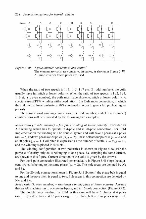
238 Propulsion systems for hybrid vehicles
1
56
21
40
5
60
25
44
9
64
29
48
13
68
33
52
17
72
A – A A B – B B C – C CPhases:
+
–
–
+
+
–
–
+
+
–
–
+
+
–
–
+
+
–
–
+
+
–
–
+
+
–
–
+
+
–
–
+
+
–
–
+
Figure 5.40 4-pole inverter connections and controlThe elementary coils are connected in series, as shown in Figure 5.38.All nine inverter totem poles are used
When the ratio of two speeds is 1 : 3, 1 : 5, 1 : 7 etc. (1: odd number), the coilsusually have full pitch at lower polarity. When the ratio of two speeds is 1 : 2, 1 : 4,1 : 6 etc. (1: even number), the coils must have shortened pitch at lower polarity. Aspecial case of PPM winding with speed ratio 1 : 2 is Dahlander connection, in whichthe coil pitch at lower polarity is 50% shortened in order to give a full pitch at higherpolarity.
The conventional winding connections for (1: odd number) and (1: even number)combinations will be illustrated by the following two examples.
Speed ratio (1: odd number) – full pitch winding at lower polarity: Consider anAC winding which has to operate in 4-pole and in 20-pole connection. For PPMimplementation the winding will be double layered and will have 5 phases at 4 poles(m4 = 5) and two phases at 20 poles (m20 = 2). Phase belt at four poles is q4 = 2, andat 20 poles q20 = 1. Coil pitch is expressed as the number of teeth, y = τp,4 = 10,and the winding is placed in 40 slots.
The winding configuration at two polarities is shown in Figure 5.38. For thepurpose of clarity only coils belonging to one phase, i.e. carrying the same current,are shown in this figure. Current direction in the coils is given by the arrows.
For the 4-pole connection illustrated schematically in Figure 5.41 (top) the adja-cent two coils belong to the same phase (q4 = 2). The pole areas are denoted by N4and S4.
For the 20-pole connection shown in Figure 5.41 (bottom) the phase belt is equalto one and the pole pitch is equal to two. Pole areas in this connection are denoted byN20 and S20.Speed ratio (1: even number) – shortened winding pitch at lower polarity: Assumethat an AC machine has to operate in 4-pole, and in 16-pole connection (Figure 5.42).
The double layer winding for PPM in this case will have 6 phases at 4 poles(m4 = 6) and 3 phases at 16 poles (m16 = 3). Phase belt at four poles is q4 = 2,
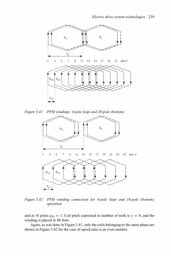
Electric drive system technologies 239
1 3 5 7 9 11 13 15 17 19 21 slot #
τp,
τp,2
N4S4
N20 S20
Figure 5.41 PPM windings: 4-pole (top) and 20-pole (bottom)
N4
1 3 5 7 9 11 13 15 17 19 21 slot #23 25
S4
N16 S16
τp,
τp,1
Figure 5.42 PPM winding connection for 4-pole (top) and 16-pole (bottom)operation
and at 16 poles q16 = 1. Coil pitch expressed in number of teeth is y = 9, and thewinding is placed in 48 slots.
Again, as was done in Figure 5.41, only the coils belonging to the same phase areshown in Figure 5.42 for the case of speed ratio is an even number.
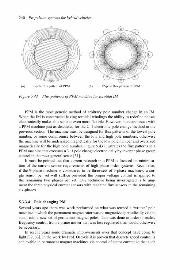
240 Propulsion systems for hybrid vehicles
(a) (b) 12-pole flux pattern of PPM2-pole flux pattern of PPM
Figure 5.43 Flux patterns of PPM machine for toroidal IM
PPM is the most generic method of arbitrary pole number change in an IM.When the IM is constructed having toroidal windings the ability to redefine phaseselectronically makes this scheme even more flexible. However, there are issues witha PPM machine just as discussed for the 2 : 1 electronic pole change method in theprevious section. The machine must be designed for flux patterns of the lowest polenumber, or some compromise between the low and high pole numbers, otherwisethe machine will be undersized magnetically for the low pole number and oversizedmagnetically for the high pole number. Figure 5.43 illustrates the flux patterns in aPPM machine that executes a 3 : 1 pole change electronically by inverter phase groupcontrol in the most general sense [31].
It must be pointed out that current research into PPM is focused on minimisa-tion of the current sensor requirements of high phase order systems. Recall that,if the 9-phase machine is considered to be three-sets of 3-phase machines, a sin-gle sensor per set will suffice provided the proper voltage control is applied tothe remaining two phases per set. One technique being investigated is to aug-ment the three physical current sensors with machine flux sensors in the remainingsix-phases.
5.3.3.4 Pole changing PM
Several years ago there was work performed on what was termed a ‘written’ polemachine in which the permanent magnet rotor was re-magnetized periodically via thestator into a new set of permanent magnet poles. This was done in order to realisefrequency control from a prime mover that was less regulated than would otherwisebe necessary.
In recent years some dramatic improvements over that concept have come tolight [32, 33]. In the work by Prof. Ostovic it is proven that discrete speed control isachievable in permanent magnet machines via control of stator current so that such
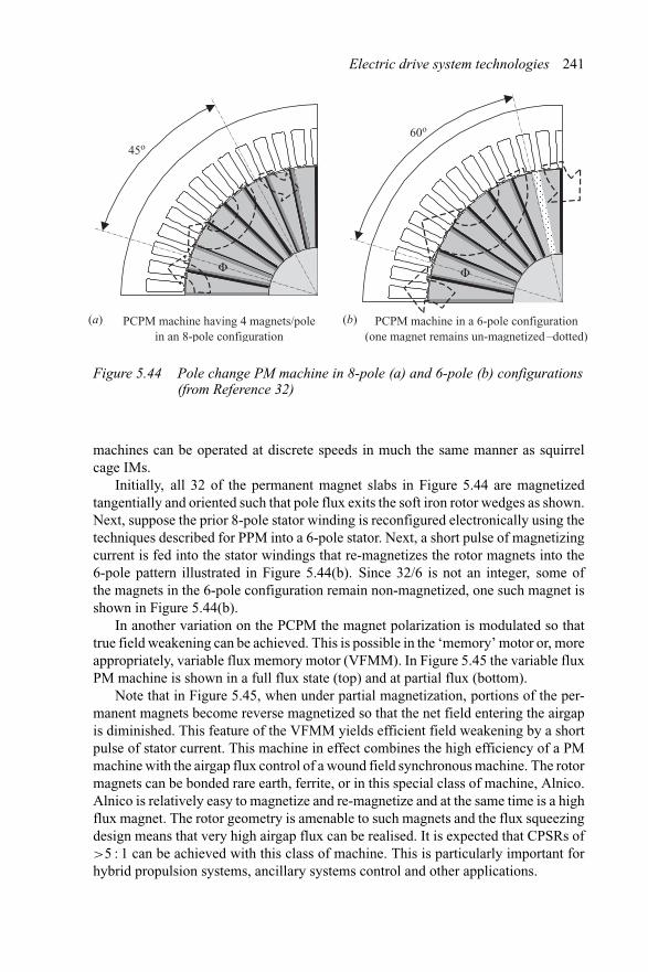
Electric drive system technologies 241
45o
60o
(a) (b) PCPM machine in a 6-pole configuration(one magnet remains un-magnetized –dotted)
PCPM machine having 4 magnets/polein an 8-pole configuration
Φ Φ
Figure 5.44 Pole change PM machine in 8-pole (a) and 6-pole (b) configurations(from Reference 32)
machines can be operated at discrete speeds in much the same manner as squirrelcage IMs.
Initially, all 32 of the permanent magnet slabs in Figure 5.44 are magnetizedtangentially and oriented such that pole flux exits the soft iron rotor wedges as shown.Next, suppose the prior 8-pole stator winding is reconfigured electronically using thetechniques described for PPM into a 6-pole stator. Next, a short pulse of magnetizingcurrent is fed into the stator windings that re-magnetizes the rotor magnets into the6-pole pattern illustrated in Figure 5.44(b). Since 32/6 is not an integer, some ofthe magnets in the 6-pole configuration remain non-magnetized, one such magnet isshown in Figure 5.44(b).
In another variation on the PCPM the magnet polarization is modulated so thattrue field weakening can be achieved. This is possible in the ‘memory’ motor or, moreappropriately, variable flux memory motor (VFMM). In Figure 5.45 the variable fluxPM machine is shown in a full flux state (top) and at partial flux (bottom).
Note that in Figure 5.45, when under partial magnetization, portions of the per-manent magnets become reverse magnetized so that the net field entering the airgapis diminished. This feature of the VFMM yields efficient field weakening by a shortpulse of stator current. This machine in effect combines the high efficiency of a PMmachine with the airgap flux control of a wound field synchronous machine. The rotormagnets can be bonded rare earth, ferrite, or in this special class of machine, Alnico.Alnico is relatively easy to magnetize and re-magnetize and at the same time is a highflux magnet. The rotor geometry is amenable to such magnets and the flux squeezingdesign means that very high airgap flux can be realised. It is expected that CPSRs of>5 : 1 can be achieved with this class of machine. This is particularly important forhybrid propulsion systems, ancillary systems control and other applications.
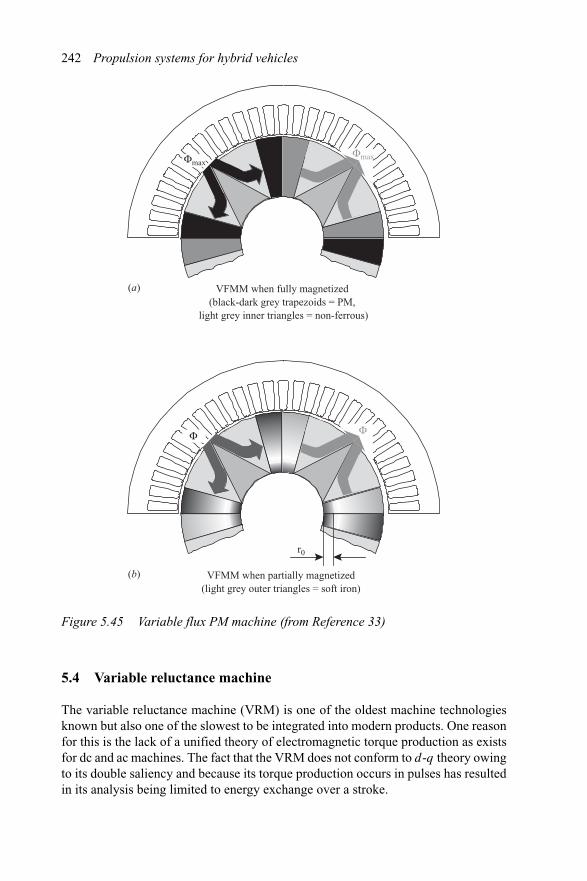
242 Propulsion systems for hybrid vehicles
(a) VFMM when fully magnetized (black-dark grey trapezoids = PM,
light grey inner triangles = non-ferrous)
ΦmaxΦmax
ΦΦ
(b) VFMM when partially magnetized(light grey outer triangles = soft iron)
r0
Figure 5.45 Variable flux PM machine (from Reference 33)
5.4 Variable reluctance machine
The variable reluctance machine (VRM) is one of the oldest machine technologiesknown but also one of the slowest to be integrated into modern products. One reasonfor this is the lack of a unified theory of electromagnetic torque production as existsfor dc and ac machines. The fact that the VRM does not conform to d-q theory owingto its double saliency and because its torque production occurs in pulses has resultedin its analysis being limited to energy exchange over a stroke.
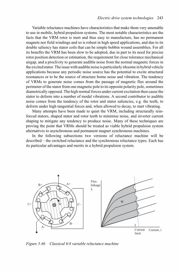
Electric drive system technologies 243
Variable reluctance machines have characteristics that make them very amenableto use in mobile, hybrid propulsion systems. The most notable characteristics are thefacts that the VRM rotor is inert and thus easy to manufacture, has no permanentmagnets nor field windings and so is robust in high speed applications, and due to itsdouble saliency has stator coils that can be simple bobbin wound assemblies. For allits benefits the VRM has been slow to be adopted, due in part to its need for preciserotor position detection or estimation, the requirement for close tolerance mechanicalairgap, and a proclivity to generate audible noise from the normal magnetic forces inthe excited stator. The issue with audible noise is particularly irksome in hybrid vehicleapplications because any periodic noise source has the potential to excite structuralresonances or to be the source of structure borne noise and vibration. The tendencyof VRMs to generate noise comes from the passage of magnetic flux around theperimeter of the stator from one magnetic pole to its opposite polarity pole, sometimesdiametrically opposed. The high normal forces under current excitation then cause thestator to deform into a number of modal vibrations. A second contributor to audiblenoise comes from the tendency of the rotor and stator saliencies, e.g. the teeth, todeform under high tangential forces and, when allowed to decay, to start vibrating.
Many attempts have been made to quiet the VRM, including structurally rein-forced stators, shaped stator and rotor teeth to minimise noise, and inverter currentshaping to mitigate any tendency to produce noise. Many of these techniques areproving the point that VRMs should be treated as viable hybrid propulsion systemalternatives to asynchronous and permanent magnet synchronous machines.
In the following subsections two versions of reluctance machine will bedescribed – the switched reluctance and the synchronous reluctance types. Each hasits particular advantages and merits in a hybrid propulsion system.
A–
A+B+
B–
C+ C–
Fluxlinkageλ
Current, i
W
ICurrentlimit
Ω
Figure 5.46 Classical 6/4 variable reluctance machine
244 Propulsion systems for hybrid vehicles
5.4.1 Switched reluctance
The switched reluctance machine is now the common terminology for the conven-tional double salient VRM. Figure 5.46 illustrates this structure in a 6/4 geometry.Because of the industrial acceptability of 3- and 4-phase systems it is natural forVRMs to exist in 6/4 and 8/6 geometries. The numerator Ns in the expression Ns/Nr
is the number of stator teeth, where Ns = 2m, and the denominator is simply thenumber of rotor teeth. A machine of this construction will have mNr pulses perrevolution – hence the descriptive term, a 12-pulse VRM or a 24-pulse VRM.
In Figure 5.46 the energy enclosed by the shaded area represents the co-energyas a rotor tooth moves from un-aligned position as shown by the position of the rotorin the figure as phase A is energized. Current is injected into the phase A windingin this unaligned position. The inductance is low, so the rise time of the current isvery rapid until the current amplitude reaches the inverter current limit, I . At thispoint the inverter current regulator begins to PWM the current, so that it remainsat its commanded value while the rotor moves from unaligned to aligned position.After sufficient dwell, the current is switched off and allowed to decay along the fluxlinkage–current trajectory for fully aligned position back to the origin. The counter-clockwise motion about the λ-I diagram encloses an area, W , representing the netenergy exchanged to mechanical energy at the shaft. The area beneath the unalignedposition line represents phase A leakage inductance. The area from the fully alignedcurve to the λ-axis represents energy stored in the winding and returned to the supply –the reactive kVA, in other words. The spacing between the λ-I curves in Figure 5.46is a function of rotor angle, θ . Bear in mind that, as the inverter sequences betweenthe phases in the order A-B-C, the rotor indexes clockwise as noted by �.
Torque production in the VRM is given by (5.29) for average and instantaneousvalues:
Tavg = mNrW
2π(Nm) (5.29)
T = ∂W(i, θ)
∂θ
where W is the energy converted per working stroke of the machine – the energyconverted per phase excitation. It requires excitation of all m phases to move therotor by one rotor tooth pitch – hence, the quantity in the numerator for averagetorque of the number of ‘working’ strokes per revolution times the work performedper stroke. The flux linkage in the VRM is given by (5.30) and the expression forinduced voltage. The variable L(θ) is the inductance variation with rotor position:
λ = L(θ)i
E = dλ
dt= L
di
dt+ i
dL
dθ
dθ
dt(5.30)
dθ
dt= ω
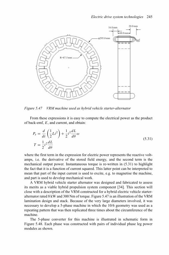
Electric drive system technologies 245
R=87.5 mm
ϕ295.0 mm
16.0 mm 20.0 mm
60.0 mm
+
Figure 5.47 VRM machine used as hybrid vehicle starter-alternator
From these expressions it is easy to compute the electrical power as the productof back-emf, E, and current, and obtain:
Pe = d
dt
(1
2Li2
)+ 1
2i2 dL
dθω
T = 1
2i2 dL
dθ
(5.31)
where the first term in the expression for electric power represents the reactive volt-amps, i.e. the derivative of the stored field energy, and the second term is themechanical output power. Instantaneous torque is re-written in (5.31) to highlightthe fact that it is a function of current squared. This latter point can be interpreted tomean that part of the input current is used to excite, e.g. to magnetise the machine,and part is used to develop mechanical work.
A VRM hybrid vehicle starter alternator was designed and fabricated to assessits merits as a viable hybrid propulsion system component [34]. This section willclose with a description of the VRM constructed for a hybrid electric vehicle starter-alternator rated 8 kW and 300 Nm of torque. Figure 5.47 is an illustration of the VRMlamination design and stack. Because of the very large diameters involved, it wasnecessary to develop a 5-phase machine in which the 10/6 geometry was used as arepeating pattern that was then replicated three times about the circumference of themachine.
The 5-phase converter for this machine is illustrated in schematic form inFigure 5.48. Each phase was constructed with pairs of individual phase leg powermodules as shown.
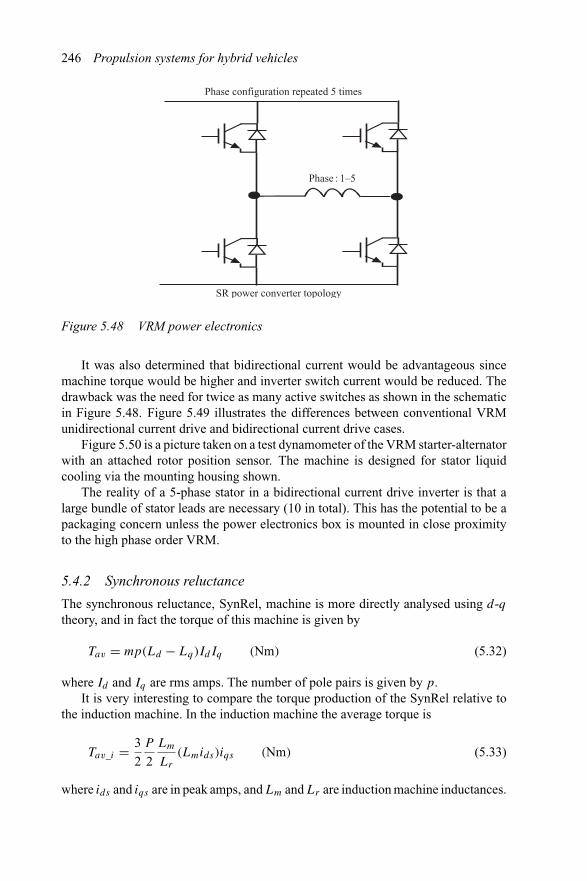
246 Propulsion systems for hybrid vehicles
Phase configuration repeated 5 times
SR power converter topology
Phase : 1–5
Figure 5.48 VRM power electronics
It was also determined that bidirectional current would be advantageous sincemachine torque would be higher and inverter switch current would be reduced. Thedrawback was the need for twice as many active switches as shown in the schematicin Figure 5.48. Figure 5.49 illustrates the differences between conventional VRMunidirectional current drive and bidirectional current drive cases.
Figure 5.50 is a picture taken on a test dynamometer of the VRM starter-alternatorwith an attached rotor position sensor. The machine is designed for stator liquidcooling via the mounting housing shown.
The reality of a 5-phase stator in a bidirectional current drive inverter is that alarge bundle of stator leads are necessary (10 in total). This has the potential to be apackaging concern unless the power electronics box is mounted in close proximityto the high phase order VRM.
5.4.2 Synchronous reluctance
The synchronous reluctance, SynRel, machine is more directly analysed using d-qtheory, and in fact the torque of this machine is given by
Tav = mp(Ld − Lq)IdIq (Nm) (5.32)
where Id and Iq are rms amps. The number of pole pairs is given by p.It is very interesting to compare the torque production of the SynRel relative to
the induction machine. In the induction machine the average torque is
Tav_i = 3
2
P
2
Lm
Lr
(Lmids)iqs (Nm) (5.33)
where ids and iqs are in peak amps, and Lm and Lr are induction machine inductances.
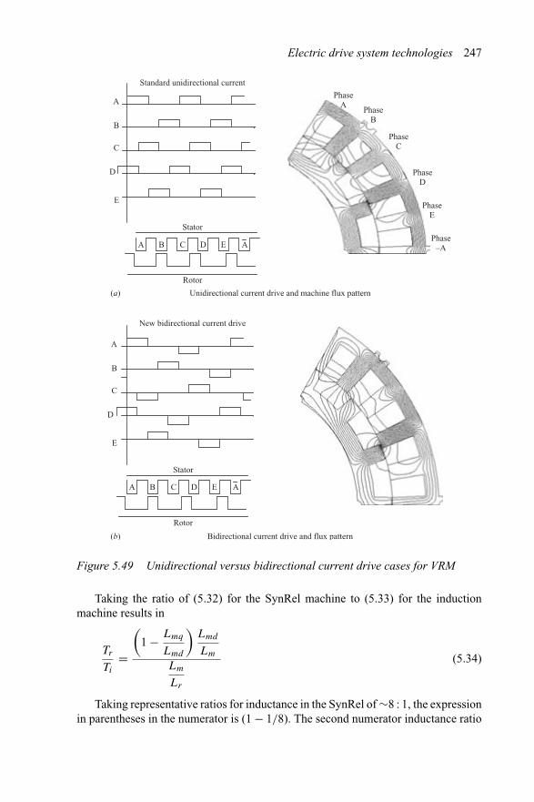
Electric drive system technologies 247
Unidirectional current drive and machine flux pattern(a)
PhaseA
PhaseB
Stator
Standard unidirectional current
E
E
D
D
C
C
B
B
A
AA
Rotor
PhaseC
PhaseD
PhaseE
Phase–A
Bidirectional current drive and flux pattern(b)
New bidirectional current drive
E
D
C
B
A
Stator
Rotor
EDCB AA
Figure 5.49 Unidirectional versus bidirectional current drive cases for VRM
Taking the ratio of (5.32) for the SynRel machine to (5.33) for the inductionmachine results in
Tr
Ti
=
(1 − Lmq
Lmd
)Lmd
Lm
Lm
Lr
(5.34)
Taking representative ratios for inductance in the SynRel of ∼8 : 1, the expressionin parentheses in the numerator is (1 − 1/8). The second numerator inductance ratio
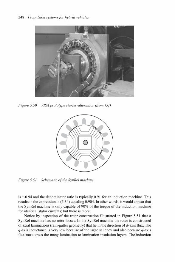
248 Propulsion systems for hybrid vehicles
Figure 5.50 VRM prototype starter-alternator (from [5])
Figure 5.51 Schematic of the SynRel machine
is ∼0.94 and the denominator ratio is typically 0.91 for an induction machine. Thisresults in the expression in (5.34) equaling 0.904. In other words, it would appear thatthe SynRel machine is only capable of 90% of the torque of the induction machinefor identical stator currents; but there is more.
Notice by inspection of the rotor construction illustrated in Figure 5.51 that aSynRel machine has no rotor losses. In the SynRel machine the rotor is constructedof axial laminations (rain-gutter geometry) that lie in the direction of d-axis flux. Theq-axis inductance is very low because of the large saliency and also because q-axisflux must cross the many lamination to lamination insulation layers. The induction
Electric drive system technologies 249
machine rotor losses are
Pr = 3
2i2r Rr (W) (5.35)
This means that, unlike the induction machine, the SynRel has no rotor losses tocontend with, so only stator copper losses must be accounted for. The IM stator currentconsists of both magnetizing and load current components, for which magnetizingcurrent is approximately 15% of the total. Taking this into account results in theSynRel machine having only 63% of the losses of the induction machine. So now, ifthe ratio in (5.34) is again computed but for equal losses, the result is
Tr
Ti
= 1.26 (5.36)
This is a completely different picture of the SynRel in comparison to the IM, butit does not account for the fact yet that inverter losses in the SynRel are higher thatfor an IM because the power factor is lower in the SynRel. Typical power factors forIMs are 0.85, whereas for the SynRel it is 0.80.
The advantage of the SynRel machine over the IM diminishes as the rating incr-eases. For larger machines, generally>20 hp, the magnetizing reactance of the SynRelincreases, thereby diminishing the efficiency advantage it held over the inductionmachine. This means that for machine ratings suitable for hybrid propulsion systemsthe SynRel really has no efficiency advantage even given its inert rotor. The otherdrawback of the machine technology is the fact that its axial laminated rotor structurehas real issues at higher speeds, where rotor retention becomes a major concern.
5.4.3 Radial laminated structures
Radial laminated SynRel machines are generally not as widely used as axial laminateddesigns because with multiple flux barriers the mechanical constraints on ribs andposts to support the soft iron pole shoes above and in between the flux barriers becomemajor design challenges. It has been shown that for the same total losses a SynRelmachine can have 20% more torque than a corresponding IM. However, losses inthe SynRel machine increase substantially with increasing pole number, so thesemachines are restricted to pole numbers of less than four.
There is strong interest in SynRel for machine tool applications because it candeliver overload torque ratings of >3 : 1. It is also recommended to drive the radiallaminated designs with current controlled inverters and to avoid delta connected statorwindings.
In general, this design has not found much favour with hybrid propulsion designsbecause it cannot compete with its cousin the IPM.
5.5 Relative merits of electric machine technologies
This chapter has reviewed a great many electric machine technologies and severalmethods of controlling such machines. It is now important that this vast amount of
250 Propulsion systems for hybrid vehicles
material on electric machines be summarised into a more cohesive framework fromwhich hybrid propulsion system designers can choose. For this summary two sem-inal papers will be cited that give clear insights into machine comparisons for thetwo important categories of ac drives: battery electric vehicles and hybrid propulsionsystems.
The next two subsections will summarise the material in this chapter in the contextof machine technology comparisons of the leading three major categories: inductionmachine (IM), interior permanent magnet machine (IPM) and variable reluctancemachine (VRM). Furthermore, each of these machine types was compared basedon a representative vehicle and performance specifications. The interested reader isreferred to the appropriate reference at the end of this chapter.
5.5.1 Comparisons for electric vehicles
It is well known that the choice of ac drive system for European and North Americanbattery electric vehicle traction systems is the ac induction machine drive. For Asia-Pacific the choice is and continues to be the ac permanent magnet drive system. Thissection looks at the reasons for this particular choice of ac drive system. The variablereluctance drive system is and continues to receive favourable reviews but as yetremains on the sidelines in vehicle propulsion areas.
In the comparisons to follow the relative rankings are based on the availability ofa 400 Apk and 400 Vdc inverter as the power driver. The battery is sized for 250 Vdc.Inverter control is based on field orientation principles for fast dynamic responseand efficient use of the power silicon. The vehicle itself is assumed to have a massof 1500 kg, a drag coefficient of 0.32 with a frontal area of 2.3 m2 and an overalltransmission gear ratio of from 8 : 1 to 12 : 1. The vehicle performance targets are>30% grade and 135 kph max speed.
Table 5.6 lists the key machine parameters needed to determine the machinecontinuous torque rating. Based on thermal limitations the continuous torque is setby the dissipation limits on conductor current density, which for battery electricvehicles is restricted to 5 A/mm2 except for the IPM machine, where it is 6.5 A/mm2.Peak torque is typically 2.5 to 3 times this value, and in general <20 A/mm2.
The continuous torque for these prototype machines has been calculated usingthe airgap shear force on the rotor surface for the values of electric and magneticloading listed in Table 5.6. The torque equations used in Reference 35 are listed herefor reference:
TIM = TIPM = 2p√
2σ1Ac
1
2Bmax
Di
2h
(Nm) (5.37)TVRM = 2p
√3σ1Ac
1
2Bmax
Di
2h
All the machines listed in Table 5.6 have corner point speeds of 3000 rpm and peaktorque values that are twice the continuous torque. All the machines in the Table 5.6are liquid cooled. Using the calculations from this section and the data in Table 5.6results in the comparison data given in Table 5.7 for the three ac drive systems.
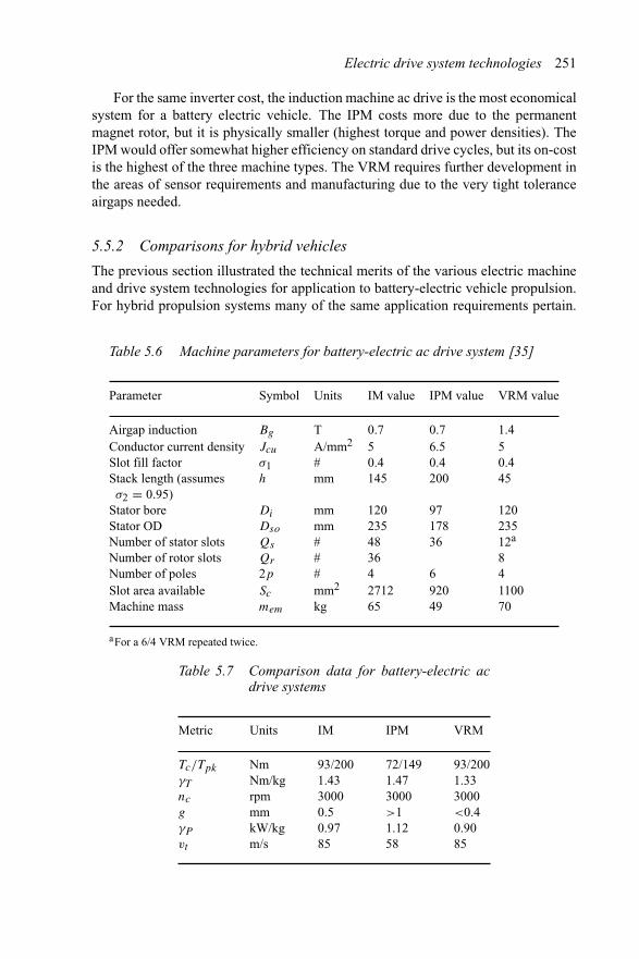
Electric drive system technologies 251
For the same inverter cost, the induction machine ac drive is the most economicalsystem for a battery electric vehicle. The IPM costs more due to the permanentmagnet rotor, but it is physically smaller (highest torque and power densities). TheIPM would offer somewhat higher efficiency on standard drive cycles, but its on-costis the highest of the three machine types. The VRM requires further development inthe areas of sensor requirements and manufacturing due to the very tight toleranceairgaps needed.
5.5.2 Comparisons for hybrid vehicles
The previous section illustrated the technical merits of the various electric machineand drive system technologies for application to battery-electric vehicle propulsion.For hybrid propulsion systems many of the same application requirements pertain.
Table 5.6 Machine parameters for battery-electric ac drive system [35]
Parameter Symbol Units IM value IPM value VRM value
Airgap induction Bg T 0.7 0.7 1.4Conductor current density Jcu A/mm2 5 6.5 5Slot fill factor σ1 # 0.4 0.4 0.4Stack length (assumes h mm 145 200 45σ2 = 0.95)
Stator bore Di mm 120 97 120Stator OD Dso mm 235 178 235Number of stator slots Qs # 48 36 12a
Number of rotor slots Qr # 36 8Number of poles 2p # 4 6 4Slot area available Sc mm2 2712 920 1100Machine mass mem kg 65 49 70
aFor a 6/4 VRM repeated twice.
Table 5.7 Comparison data for battery-electric acdrive systems
Metric Units IM IPM VRM
Tc/Tpk Nm 93/200 72/149 93/200γT Nm/kg 1.43 1.47 1.33nc rpm 3000 3000 3000g mm 0.5 >1 <0.4γP kW/kg 0.97 1.12 0.90vt m/s 85 58 85
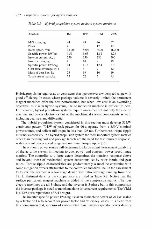
252 Propulsion systems for hybrid vehicles
Table 5.8 Hybrid propulsion system ac drive system attributes
Attribute IM IPM SPM VRM
M/G mass, kg 44 43 46 57Poles 4 8 12 12Rated speed, rpm 13 000 8200 8500 16 200Specific power, kW/kg 1.59 1.63 1.52 1.23Inverter current, Arms 350 350 280 500Inverter mass, kg 8 10 9 19Specific power, kVA/kg 14 11.2 12.4 5.9Gear ratio coverage, x : 1 11 6 7 12Mass of gear box, kg 25 19 16 19Total system mass, kg 77 72 71 95
Hybrid propulsion requires ac drive systems that operate over a wide speed range withgood efficiency. In cases where package volume is severely limited the permanentmagnet machines offer the best performance, but when low cost is an overridingobjective, as it is in hybrid systems, the ac induction machine is difficult to beat.Furthermore, hybrid propulsion systems require assessment of not only the electricmachine and power electronics but of the mechanical system components as well,including gear sets and differential.
The hybrid propulsion system considered in this section must develop 35 kWcontinuous power, 70 kW of peak power for 90 s, operate from a 350 V nominalpower source, and deliver full torque in less than 125 ms. Furthermore, torque ripplemust not exceed 5%. In a hybrid propulsion system the most important system metricsother than meeting cost and package targets are the need for fast transient response,wide constant power speed range and minimum torque ripple [36].
The on-board power source will determine to a large extent the transient capabilityof the ac drive system in meeting torque, power and constant power speed rangemetrics. The controller to a large extent determines the transient response aboveand beyond those of mechanical system constraints set by rotor inertia and gearratios. Torque ripple characteristics are predominantly a machine constraint withsome mitigation effects attributable to the controller and driveline. In the assessmentto follow, the gearbox is a two stage design with ratio coverage ranging from 6 to12 : 1. Pertinent data for the comparisons are listed in Table 5.8. Notice that thesurface permanent magnet machine is added to the comparison matrix. The fourelectric machines are all 3-phase and the inverter is 3-phase but in this comparisonthe inverter package is sized to match machine drive current requirements. The VRMis a 12/8 (two repetitions of 6/4 design).
The inverter specific power, kVA/kg, is taken as machine power of 70 kW scaledby a factor of 1.6 to account for power factor and efficiency losses. It is clear fromthis comparison that, in terms of system total mass, inverter specific power density
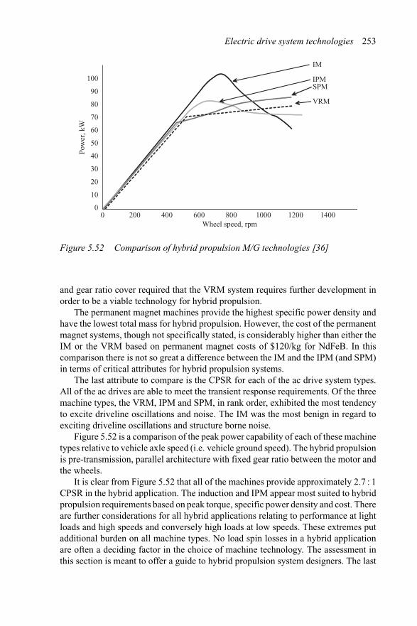
Electric drive system technologies 253
Wheel speed, rpm
Pow
er, k
W100
90
80
70
60
50
40
30
20
10
0
IM
IPMSPM
VRM
0 200 400 600 800 1000 1200 1400
Figure 5.52 Comparison of hybrid propulsion M/G technologies [36]
and gear ratio cover required that the VRM system requires further development inorder to be a viable technology for hybrid propulsion.
The permanent magnet machines provide the highest specific power density andhave the lowest total mass for hybrid propulsion. However, the cost of the permanentmagnet systems, though not specifically stated, is considerably higher than either theIM or the VRM based on permanent magnet costs of $120/kg for NdFeB. In thiscomparison there is not so great a difference between the IM and the IPM (and SPM)in terms of critical attributes for hybrid propulsion systems.
The last attribute to compare is the CPSR for each of the ac drive system types.All of the ac drives are able to meet the transient response requirements. Of the threemachine types, the VRM, IPM and SPM, in rank order, exhibited the most tendencyto excite driveline oscillations and noise. The IM was the most benign in regard toexciting driveline oscillations and structure borne noise.
Figure 5.52 is a comparison of the peak power capability of each of these machinetypes relative to vehicle axle speed (i.e. vehicle ground speed). The hybrid propulsionis pre-transmission, parallel architecture with fixed gear ratio between the motor andthe wheels.
It is clear from Figure 5.52 that all of the machines provide approximately 2.7 : 1CPSR in the hybrid application. The induction and IPM appear most suited to hybridpropulsion requirements based on peak torque, specific power density and cost. Thereare further considerations for all hybrid applications relating to performance at lightloads and high speeds and conversely high loads at low speeds. These extremes putadditional burden on all machine types. No load spin losses in a hybrid applicationare often a deciding factor in the choice of machine technology. The assessment inthis section is meant to offer a guide to hybrid propulsion system designers. The last
254 Propulsion systems for hybrid vehicles
point to make on Figure 5.52 is that the theoretical CPSR range of >5 : 1 for IPMs isoften not observed in practical systems, and in this figure it was as limited as the IM.
5.6 References
1 WOOD, P., BATTELLO, M., KESKAR, N. and GUERRA, A.: ‘Plug-N-DriveTMfamily applications overview’. IR Application Note, AN-1044, February 2003.Also see, www.irf.com
2 WISE, T.: ‘Tesla – a biographical novel of the world’s greatest inventor’ (TurnerPublishing, Inc., Atlanta, 1994)
3 LAWLER, J. S., BAILEY, J. M. and MCKEEVER, J. W.: ‘Theoretical verificationof the infinite constant power speed range of the brushless DC motor drivenby dual mode inverter control’. IEEE 7th Workshop on Power Electronics inTransportation, WPET2002, DaimlerChrysler Technical Center, Auburn Hills,MI, 24–25 October 2002
4 EPRI TR-101264, Project 3087-01, ‘Assessment of electric motor technology:present status, future trends and R&D needs’. McCleer Power Inc., Jackson, MI,December 1992
5 MILLER, J. M., GALE, A. R., MCCLEER, P. J., LEONARDI, F. andLANG, J. H.: ‘Starter-alternator for hybrid electric vehicle: comparison of induc-tion and variable reluctance machines and drives’. IEEE Industry ApplicationsSociety Annual Meeting, Adams Mark Hotel, Saint Louis, MO, 11–15 October1998
6 SCHIFERL, R. and LIPO, T. A.: ‘Core loss in buried magnet permanent magnetsynchronous motors’. Proceedings of IEEE Power Engineering Society SummerMeeting, July 1988
7 HONSINGER, V.: ‘The fields and parameters of interior type AC permanentmagnet machines’, IEEE Trans. Power Appar. Syst., 1982, 101(4), pp. 867–876
8 JAHNS, T. M.: ‘Component rating requirements for wide constant poweroperation of interior PM synchronous machine drives’. 2000 IEEE IndustryApplications Society Annual Meeting, Rome, Italy, 8–12 October 2000
9 JAHNS, T.: ‘Uncontrolled generator operation of interior PM synchronousmachines following high-speed inverter shutdown’, IEEE Industry ApplicationsSociety Annual Meeting, Adams Mark Hotel, Saint Louis, MO, 12–15 October1998.
10 AMARATUNGA, G. A. J., ACARNLEY, P. P. and MCLAREN, P. G.: ‘Optimummagnetic circuit configurations for permanent magnet aerospace generators’,IEEE Trans. Aerosp. Electron. Syst., 1985, 21(2), pp. 230–255
11 KUME, T., IWAKANE, T., SAWA, T. and YOSHIDA, T.: ‘A wide constant powerrange vector-controlled ac motor drive using winding changeover technique’,IEEE Trans. Ind. Appl., 1991, 27(5), pp. 934–939
12 SAKI, K., HATTORI, T., TAKAHASHI, N., ARATA, M. and Tajima, T.: ‘Highefficiency and high performance motor for energy saving in systems’. IEEE PowerEngineering Society Winter Meeting, 2001, pp. 1413–1418
Electric drive system technologies 255
13 OSAMA, M. and LIPO, T. A.: ‘Modeling and analysis of a wide-speed-rangeinduction motor drive based on electronic pole changing’, IEEE Trans. Ind. Appl.,1997, 33(5), pp. 1177–1184
14 MILLER, J. M., STEFANOVIC, V. R., OSTOVIC, V. and KELLY, J.: ‘Designconsiderations for an automotive integrated starter-generator with pole-phase-modulation’. IEEE Industry Applications Society Annual Meeting, Chicago, IL,30 September–4 October 2001
15 WAI, J. and JAHNS, T. M.: ‘A new control technique for achieving wide constantpowerspeed operation with an interior PM alternator machine’. IEEE IndustryApplications Society Annual Meeting, Chicago, IL, 30 September–4 October2001
16 OSTOVIC, V.: ‘Memory motors – a new class of controllable flux pm machinesfor a true wide speed operation’. IEEE Industry Applications Society AnnualMeeting, Chicago, IL, 30 September–4 October 2001
17 OSTOVIC, V.: ‘Pole-changing permanent magnet machines’. IEEE IndustryApplications Society Annual Meeting, Chicago, IL, 30 September–4 October2001
18 CARICCHI, F., CRESCIMBINI, F., GIULII CAPPONI, F. and SOLERO, L.:‘Permanent-magnet, direct-drive, starter-alternator machine with weakened fluxlinkage for constant power operation over extremely wide speed range’. IEEEIndustry Applications Society Annual Meeting, Chicago, IL, 30 September–4October 2001
19 TAPIA, J. A., LIPO, T. A. and LEONARDI, F.: ‘CPPM: a synchronous perma-nent magnet machine with field weakening’. IEEE Industry Applications SocietyAnnual Meeting, Chicago, IL, 30 September–4 October 2001
20 STATON, D. A., DEODHAR, R. P., SOONG, W. L. and MILLER, T. J. E.:‘Torque prediction using the flux-MMF diagram in AC, DC and reluctancemotors’, IEEE Trans. Ind. Appl., 1996, 32 (1), pp. 180–188
21 SAKAI, K., HATTORI, T., TAKAHASHI, N., ARATA, M. and TAJIMA, T.:‘High efficiency and high performance motor for energy saving in systems’.IEEE Power Engineering Society Winter Meeting, 2001
22 LEI, M., SANADA, M., MORIMOTO, S. and TAKEDA, Y.: ‘Basic study offlux weakening for interior permanent magnet synchronous motor with movingiron piece’, Trans. IEEE Jpn., 1998, 118-D(12) (Translated from Japanese by DrSamuel Shinozaki for the author)
23 CARICCHI, F., CRESCIMBINI, F., GIULII CAPPONI, F. and SOLERO, L.:‘Permanent magnet, direct-drive, starter/alternator machine with weakened fluxlinkage for constant-power operation over extremely wide speed range’. IEEEIndustry Applications Society Annual Meeting, Hyatt-Regency-Miracle Mile,Chicago, IL, 30 September–4 October 2001
24 HONDA, Y., NAKAMURA, T., HIGAKI, T. and TAKEDA, Y.: ‘Motor designconsiderations and test results of an interior permanent magnet synchronous motorfor electric vehicles’. IEEE Industry Applications Society Annual Meeting, NewOrleans, LA, 5–9 October 1997
25 MCCLEER, P. J., MILLER, J. M., GALE, A. R., DEGNER, M. W. andLEONARDI, F.: ‘Non-linear model and momentary performance capability of a
256 Propulsion systems for hybrid vehicles
cage rotor induction machine used as an automotive combined starter-alternator’.IEEE Industry Applications Society Annual Meeting, Phoenix, AZ, 3–7 October1999
26 KUME, T., IWAKANE, T., SAWA, T. and YOSHIDA, T.: ‘A wide constant powerrange vector-controlled ac motor drive using winding changeover technique’,IEEE Trans. Ind. Appl., 1991, 27(5), pp. 934–939
27 XU, L., LIANG, F. and LIPO, T.A.: ‘Transient model of a doubly excited reluc-tance motor’. Wisconsin Electric Machines and Power Electronics Consortium,WEMPEC, Research Report 89-29. University of Wisconsin-Madison, ECEDept., 1415 Johnson Drive, Madison, WI, 53706.
28 LIANG, F., XU, L. and LIPO, T. A.: ‘d-q analysis of a variable speed doubly acexcited reluctance motor’. WEMPEC, Research report 90-16
29 LAO, X. and LIPO, T. A.: ‘A synchronous/permanent magnet hybrid ac machine’.WEMPEC Research Report 97-14
30 OSAMA, M. and LIPO, T. A.: ‘Modeling and analysis of a wide-speed rangeinduction motor drive based on electronic pole changing’, IEEE Trans. Ind. Appl.,1997, 33, (5), pp. 1177–1184
31 MILLER, J. M., STEFANOVIC, V. R., OSTOVIC, V. and KELLY, J.: ‘Designconsiderations for an automotive integrated starter-generator with pole-phase-modulation’. IEEE Industry Applications Society Annual Meeting, Hyatt-Regency-Miracle Mile, Chicago, IL, 30 September–4 October 2001
32 OSTOVIC, V.: ‘Pole-changing permanent magnet machines’. IEEE IndustryApplications Society Annual Meeting, Hyatt-Regency-Miracle Mile, Chicago,IL, 30 September–4 October 2001
33 OSTOVIC, V.: ‘Memory motors – a new class of controllable flux PM machinesfor a true wide speed operation’. IEEE Industry Applications Society AnnualMeeting, Hyatt-Regency-Miracle Mile, Chicago, IL, 30 September–4 October2001
34 MILLER, J. M., GALE, A. R., MCCLEER, P. J., LEONARDI, F. andLANG, J. H.: ‘Starter-alternator for hybrid electric vehicle: comparison of induc-tion and variable reluctance machines and drives’. IEEE Industry ApplicationsSociety Annual Meeting, Adams Mark Hotel, Saint Louis, MO, 12–15 October1998
35 WINTER, U.: ‘Comparison of different drive system technologies for elec-tric vehicles’. Proceedings of Electric Vehicle Symposium, EVS15, Brussels,Belgium, 30 September–2 October 1998
36 CONLON, B.: ‘A comparison of induction, permanent magnet, and switchedreluctance electric drive performance in automotive traction applications’,PowerTrain Int., 2001, 4(4), pp. 34–48 www.powertrain-intl.com
Chapter 6
Power electronics for ac drives
Power electronics and its control fall within what is known as ‘inner-loop’ control ofthe hybrid ac drive system. Starting with solid state, or brushless, commutators, forpermanent magnet electric machines in the 1970s the techniques of solid state motorcontrol have been applied to industrial induction machines in the form of adjustablespeed drives (nearly 90% of all electric machines produced and sold are induc-tion machines) and recently to interior permanent magnet and reluctance machinesfor hybrid propulsion. Without the advancements and miniaturization efforts of thesemiconductor community, the hybrid vehicle would not be market ready.
As the highest cost component of the hybrid propulsion system, with the possibleexception of the vehicle battery, the power electronics represents one of the mostcomplex power processing elements in the vehicle. In this chapter the various typesof semiconductor devices are summarised along with their applicability for use asin-vehicle power control. The assessment of power electronics for ac drive systemsthen continues with discussion of various modulation techniques, thermal design andreliability considerations. Modulation techniques are important for many reasons.Most of the present modulation methods are capable of synthesising a clean sinusoidalac waveform from the vehicle’s on-board energy storage system but not all do so withequal efficiency, noise emissions or dc voltage utilisation.
Integration of power electronics systems today is at the stage where a single inte-grated power module consisting of a full active bridge of power semiconductors,integrated gate drivers, and fault detection and reporting logic are available off theshelf. At higher powers (>50 kW) the power electronics may consist of individualphase leg modules. At low powers, (<1.5 kW) the complete power electronics stageand microcontroller are all integrated into a single smart power brick. The Interna-tional Rectifier, Plug-N-Drive series (IRAMS10UP60A), is a 10 A, 600 V, 3-phasemotor controller all fully integrated into an SIPI and capable of 20 kHz PWM mod-ulation [1]. The Plug-N-Drive component is an example of an intelligent powerelectronic module (IPEM). The IR IPEM is chip and wire fabricated on insulatedmetal substrate technology (IMST) with 600 V non-punch-through (NPT) insulated
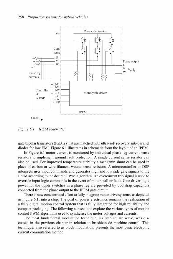
258 Propulsion systems for hybrid vehicles
Vφ, Iφ
Cmds
Power electronicsV+
Curr.sense
UVW
Monolythic driver
Phase outputUVW
IPEM
ControlleruCor DSP
Phase leg currents
H-UH-VH-WL-UL-VL-WI-trip
Figure 6.1 IPEM schematic
gate bipolar transistors (IGBTs) that are matched with ultra-soft recovery anti-paralleldiodes for low EMI. Figure 6.1 illustrates in schematic form the layout of an IPEM.
In Figure 6.1 motor current is monitored by individual phase leg current senseresistors to implement ground fault protection. A single current sense resistor canalso be used. For improved temperature stability a manganin shunt can be used inplace of carbon or wire filament wound sense resistors. A microcontroller or DSPinterprets user input commands and generates high and low side gate signals to theIPEM according to the desired PWM algorithm. An overcurrent trip signal is used tooverride input logic commands in the event of motor stall or fault. Gate driver logicpower for the upper switches in a phase leg are provided by bootstrap capacitorsconnected from the phase output to the IPEM gate circuit.
There is now concentrated effort to fully integrate motor drive systems, as depictedin Figure 6.1, into a chip. The goal of power electronics remains the realization ofa fully digital motion control system that is fully integrated for high reliability andcompact packaging. The following subsections explore the various types of motioncontrol PWM algorithms used to synthesise the motor voltages and currents.
The most fundamental modulation technique, six step square wave, was dis-cussed in the previous chapter in relation to brushless dc machine control. Thistechnique, also referred to as block modulation, presents the most basic electroniccurrent commutation method.
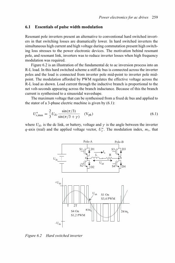
Power electronics for ac drives 259
6.1 Essentials of pulse width modulation
Resonant pole inverters present an alternative to conventional hard switched invert-ers in that switching losses are dramatically lower. In hard switched inverters thesimultaneous high current and high voltage during commutation present high switch-ing loss stresses to the power electronic devices. The motivation behind resonantpole, and resonant link, inverters was to reduce inverter losses when high frequencymodulation was required.
Figure 6.2 is an illustration of the fundamental dc to ac inversion process into anR-L load. In this hard switched scheme a stiff dc bus is connected across the inverterpoles and the load is connected from inverter pole mid-point to inverter pole mid-point. The modulation afforded by PWM regulates the effective voltage across theR-L load as shown. Load current through the inductive branch is proportional to thenet volt-seconds appearing across the branch inductance. Because of this the branchcurrent is synthesised to a sinusoidal waveshape.
The maximum voltage that can be synthesised from a fixed dc bus and applied tothe stator of a 3-phase electric machine is given by (6.1):
U∗s,max = 2
3Udc
sin(π/3)
sin(π/3 + γ )(Vpk) (6.1)
where Udc is the dc link, or battery, voltage and γ is the angle between the inverterq-axis (real) and the applied voltage vector, U∗
s . The modulation index, mi , that
Udc
S1 D1
S2 D2
S3 D3
S4 D4
Pole-A Pole-B
L RIa
Uab
a b
Uab
S4 On S1,2 PWM
S1 On S3,4 PWM
T 2T
+Udc
–Udc
π/ωa 2π/ωa
Figure 6.2 Hard switched inverter
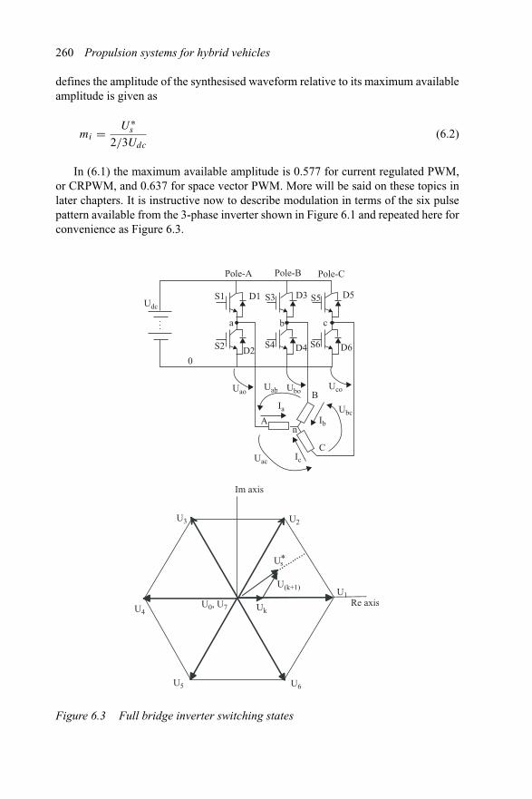
260 Propulsion systems for hybrid vehicles
defines the amplitude of the synthesised waveform relative to its maximum availableamplitude is given as
mi = U∗s
2/3Udc
(6.2)
In (6.1) the maximum available amplitude is 0.577 for current regulated PWM,or CRPWM, and 0.637 for space vector PWM. More will be said on these topics inlater chapters. It is instructive now to describe modulation in terms of the six pulsepattern available from the 3-phase inverter shown in Figure 6.1 and repeated here forconvenience as Figure 6.3.
UdcS1 D1
S2 D2
S3 D3
S4 D4
Pole-A Pole-B
Ia
Pole-C
S5 D5
S6 D60
a b c
nA
B
C
Ib
Ic
Uao Ubo Uco
Uac
Ubc
Uab
U1
U2U3
U4
U5 U6
U0, U7 Uk
Us*
U(k+1)
Re axis
Im axis
Figure 6.3 Full bridge inverter switching states
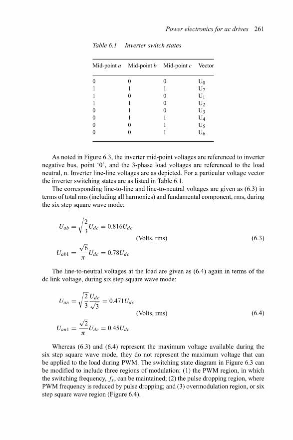
Power electronics for ac drives 261
Table 6.1 Inverter switch states
Mid-point a Mid-point b Mid-point c Vector
0 0 0 U01 1 1 U71 0 0 U11 1 0 U20 1 0 U30 1 1 U40 0 1 U50 0 1 U6
As noted in Figure 6.3, the inverter mid-point voltages are referenced to inverternegative bus, point ‘0’, and the 3-phase load voltages are referenced to the loadneutral, n. Inverter line-line voltages are as depicted. For a particular voltage vectorthe inverter switching states are as listed in Table 6.1.
The corresponding line-to-line and line-to-neutral voltages are given as (6.3) interms of total rms (including all harmonics) and fundamental component, rms, duringthe six step square wave mode:
Uab =√
2
3Udc = 0.816Udc
Uab1 =√
6
πUdc = 0.78Udc
(Volts, rms) (6.3)
The line-to-neutral voltages at the load are given as (6.4) again in terms of thedc link voltage, during six step square wave mode:
Uan =√
2
3
Udc√3
= 0.471Udc
Uan1 =√
2
πUdc = 0.45Udc
(Volts, rms) (6.4)
Whereas (6.3) and (6.4) represent the maximum voltage available during thesix step square wave mode, they do not represent the maximum voltage that canbe applied to the load during PWM. The switching state diagram in Figure 6.3 canbe modified to include three regions of modulation: (1) the PWM region, in whichthe switching frequency, fs , can be maintained; (2) the pulse dropping region, wherePWM frequency is reduced by pulse dropping; and (3) overmodulation region, or sixstep square wave region (Figure 6.4).
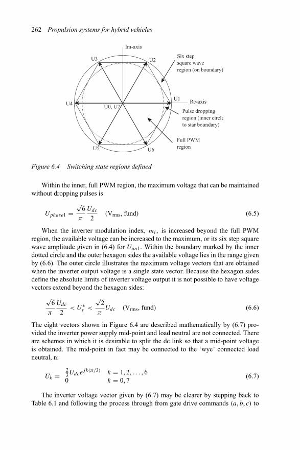
262 Propulsion systems for hybrid vehicles
Re-axis
Im-axis
U1
U2U3
U4
U5 U6
U0, U7
Full PWM region
Pulse dropping region (inner circleto star boundary)
Six step square wave region (on boundary)
Figure 6.4 Switching state regions defined
Within the inner, full PWM region, the maximum voltage that can be maintainedwithout dropping pulses is
Uphase1 =√
6
π
Udc
2(Vrms, fund) (6.5)
When the inverter modulation index, mi , is increased beyond the full PWMregion, the available voltage can be increased to the maximum, or its six step squarewave amplitude given in (6.4) for Uan1. Within the boundary marked by the innerdotted circle and the outer hexagon sides the available voltage lies in the range givenby (6.6). The outer circle illustrates the maximum voltage vectors that are obtainedwhen the inverter output voltage is a single state vector. Because the hexagon sidesdefine the absolute limits of inverter voltage output it is not possible to have voltagevectors extend beyond the hexagon sides:
√6
π
Udc
2< U∗
s <
√2
πUdc (Vrms, fund) (6.6)
The eight vectors shown in Figure 6.4 are described mathematically by (6.7) pro-vided the inverter power supply mid-point and load neutral are not connected. Thereare schemes in which it is desirable to split the dc link so that a mid-point voltageis obtained. The mid-point in fact may be connected to the ‘wye’ connected loadneutral, n:
Uk =23Udce
jk(π/3) k = 1, 2, . . . , 60 k = 0, 7
(6.7)
The inverter voltage vector given by (6.7) may be clearer by stepping back toTable 6.1 and following the process through from gate drive commands (a, b, c) to
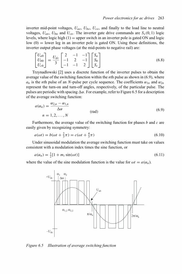
Power electronics for ac drives 263
inverter mid-point voltages, Uao, Ubo, Uco, and finally to the load line to neutralvoltages, Uan, Ubn and Ucn. The inverter gate drive commands are Sx(0, 1) logiclevels, where logic high (1) = upper switch in an inverter pole is gated ON and logiclow (0) = lower leg in an inverter pole is gated ON. Using these definitions, theinverter output phase voltages (at the mid-points to negative rail) are:⎡
⎣Ua0Ub0Uc0
⎤⎦ = Udc
3
⎡⎣ 2 −1 −1
−1 2 −1−1 −1 2
⎤⎦⎡⎣Sa
Sb
Sc
⎤⎦ (6.8)
Trzynadlowski [2] uses a discrete function of the inverter pulses to obtain theaverage value of the switching function within the nth pulse as shown in (6.9), wherean is the nth pulse of an N -pulse per cycle sequence. The coefficients α1n and α2n
represent the turn-on and turn-off angles, respectively, of the particular pulse. Thepulses are periodic with spacing �α. For example, refer to Figure 6.5 for a descriptionof the average switching function:
a(αn) = α2,n − α1,n
�α(rad)
n = 1, 2, . . . , N(6.9)
Furthermore, the average value of the switching function for phases b and c areeasily given by recognizing symmetry:
a(ωt) = b(ωt + 23π) = c(ωt + 4
3π) (6.10)
Under sinusoidal modulation the average switching function must take on valuesconsistent with a modulation index times the sine function, or
a(αn) = 12 [1 + mi sin(ωt)] (6.11)
where the value of the sine modulation function is the value for ωt = a(αn).
+Udc
–Udc
Uab
α1 α2Δα
α1,2 α2,2
π/ωa 2π/ωa
Figure 6.5 Illustration of average switching function
264 Propulsion systems for hybrid vehicles
The line-to-line voltage at the load can be found for phase A to phase B as follows:
Uab(an) = Udc[a(αn) − b(αn)]Uab(an) = Udc
{12 [1 + mi sin(ωt)] − 1
2
[1 + mi sin
(ωt + 2
3π)]}
Uab(an) =√
3
2miUdc sin
(αn + π
6
) (6.12)
The load line-to-line, and hence line-to-neutral voltage, are completely definedby (6.12) for the stated dc link voltage, modulation index and modulating functionwaveform. Other investigators – Kaura and Blasko, for example [3] – have workedto extend the linearity of sinusoidal PWM into the pulse dropping region depictedin Figure 6.4 by adding a square wave to the modulating function discussed above.With this scheme the modulator maintains linearity from full PWM through the pulsedropping region and up to a six step square wave mode. The interested reader isreferred to that reference.
The pulse dropping region defines the zones about the vertices of the hexagonwhere the velocity of the voltage vector must increase with increasing modulationdepth. In the limit, as the voltage vector reaches the limit of the outer circle thatinscribes the hexagon, it exists only at the vertex points and has infinite velocityalong the sides of the hexagon as the voltage vector steps from one inverter voltagestate to the next. This is the six step square wave mode.
6.2 Resonant pulse modulation
That a vast number of inverter topologies exist that are potentially better suited tomatching the performance levels of classical PWM voltage source inverters was thecontention posed by Prof. Divan [4]. Indeed, all power converters can be classifiedinto hard switched or soft (i.e. resonant) switching. Soft switching inverters havesignificantly reduced device stresses and can be found in topologies ranging fromresonant converters, resonant link converters and resonant pole inverters. The mostpopular appear to be topologies that employ a high frequency resonant LC circuitin the main power transfer path. There have been numerous attempts over the yearsto incorporate series resonant and parallel resonant elements into the power transferpath. This section will discuss the more popular high frequency resonant dc linkconverter.
Figure 6.6 is the schematic of the power stage and representative waveforms ofthe resonant dc link inverter. In this circuit, the resonant dc bus is implemented bythe addition of a small inductor and capacitor along with one additional semicon-ductor switch at the input of a conventional six switch voltage source inverter (VSI).When the dc link switch is gated ON, current from the supply charges the inductorlinearly. When the link converter switch is gated OFF, the inductor discharges intothe capacitor, forming a resonant pulse at the VSI inverter input. The main switches
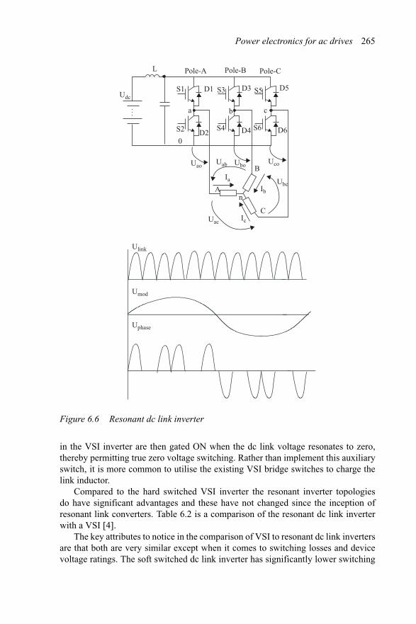
Power electronics for ac drives 265
UdcS1 D1
S2 D2
S3 D3
S4 D4
Pole-AL Pole-B
Ia
Pole-C
S5 D5
S6 D60
a b c
nA
B
C
Ib
Ic
Uao Ubo Uco
Uac
Ubc
Uab
Ulink
Umod
Uphase
Figure 6.6 Resonant dc link inverter
in the VSI inverter are then gated ON when the dc link voltage resonates to zero,thereby permitting true zero voltage switching. Rather than implement this auxiliaryswitch, it is more common to utilise the existing VSI bridge switches to charge thelink inductor.
Compared to the hard switched VSI inverter the resonant inverter topologiesdo have significant advantages and these have not changed since the inception ofresonant link converters. Table 6.2 is a comparison of the resonant dc link inverterwith a VSI [4].
The key attributes to notice in the comparison of VSI to resonant dc link invertersare that both are very similar except when it comes to switching losses and devicevoltage ratings. The soft switched dc link inverter has significantly lower switching
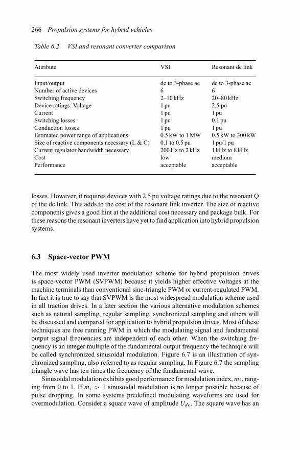
266 Propulsion systems for hybrid vehicles
Table 6.2 VSI and resonant converter comparison
Attribute VSI Resonant dc link
Input/output dc to 3-phase ac dc to 3-phase acNumber of active devices 6 6Switching frequency 2–10 kHz 20–80 kHzDevice ratings: Voltage 1 pu 2.5 puCurrent 1 pu 1 puSwitching losses 1 pu 0.1 puConduction losses 1 pu 1 puEstimated power range of applications 0.5 kW to 1 MW 0.5 kW to 300 kWSize of reactive components necessary (L & C) 0.1 to 0.5 pu 1 pu/1 puCurrent regulator bandwidth necessary 200 Hz to 2 kHz 1 kHz to 8 kHzCost low mediumPerformance acceptable acceptable
losses. However, it requires devices with 2.5 pu voltage ratings due to the resonant Qof the dc link. This adds to the cost of the resonant link inverter. The size of reactivecomponents gives a good hint at the additional cost necessary and package bulk. Forthese reasons the resonant inverters have yet to find application into hybrid propulsionsystems.
6.3 Space-vector PWM
The most widely used inverter modulation scheme for hybrid propulsion drivesis space-vector PWM (SVPWM) because it yields higher effective voltages at themachine terminals than conventional sine-triangle PWM or current-regulated PWM.In fact it is true to say that SVPWM is the most widespread modulation scheme usedin all traction drives. In a later section the various alternative modulation schemessuch as natural sampling, regular sampling, synchronized sampling and others willbe discussed and compared for application to hybrid propulsion drives. Most of thesetechniques are free running PWM in which the modulating signal and fundamentaloutput signal frequencies are independent of each other. When the switching fre-quency is an integer multiple of the fundamental output frequency the technique willbe called synchronized sinusoidal modulation. Figure 6.7 is an illustration of syn-chronized sampling, also referred to as regular sampling. In Figure 6.7 the samplingtriangle wave has ten times the frequency of the fundamental wave.
Sinusoidal modulation exhibits good performance for modulation index, mi , rang-ing from 0 to 1. If mi > 1 sinusoidal modulation is no longer possible because ofpulse dropping. In some systems predefined modulating waveforms are used forovermodulation. Consider a square wave of amplitude Udc. The square wave has an
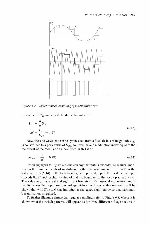
Power electronics for ac drives 267
Us*
Ush*
UΔ
Ua
Figure 6.7 Synchronized sampling of modulating wave
rms value of Udc and a peak fundamental value of:
Us1 = 4
πUdc
m′ = Us1
Udc
= 1.27(6.13)
Now, the sine wave that can be synthesised from a fixed dc bus of magnitude Udc
is constrained to a peak value of Udc, so it will have a modulation index equal to thereciprocal of the modulation index listed in (6.13) or
mmax = 1
m′ = 0.787 (6.14)
Referring again to Figure 6.4 one can say that with sinusoidal, or regular, mod-ulation the limit on depth of modulation within the zone marked full PWM is thevalue given by (6.14). In the transition region of pulse dropping the modulation depthexceeds 0.787 and reaches a value of 1 at the boundary of the six step square wave.The value mmax is a real and significant limitation of sinusoidal modulation and itresults in less than optimum bus voltage utilisation. Later in this section it will beshown that with SVPWM this limitation is increased significantly so that maximumbus utilisation is realised.
To further illustrate sinusoidal, regular sampling, refer to Figure 6.8, where it isshown what the switch patterns will appear as for three different voltage vectors in
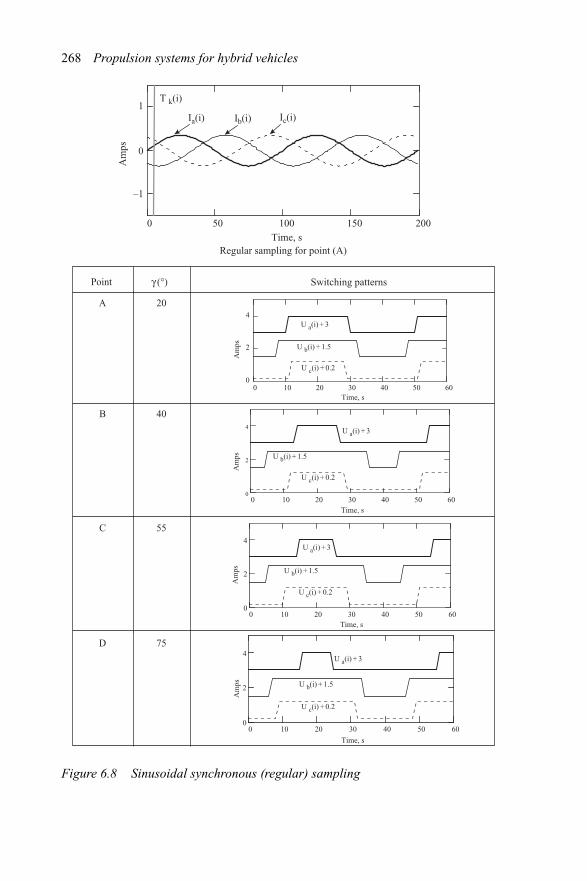
268 Propulsion systems for hybrid vehicles
0 50 100Time, s
150 200
Regular sampling for point (A)
Ia(i) Ib(i) Ic(i)
T k(i)
0
1
–1
Am
ps
Time, s0 10 20 30 40 50 60
Am
ps
U a(i) + 3
U b(i) + 1.5
U c(i) + 0.2
0
2
4
Point γ (°)
A 20
B 40
C 55
D 75
Time, s0 10 20 30 40 50 60
0
2
4
Am
ps
U a(i) + 3
U b(i) + 1.5
U c(i) + 0.2
Time, s0 10 20 30 40 50 60
0
2
4
Am
ps
U a(i) + 3
U b(i) + 1.5
U c(i) + 0.2
Time, s
0 10 20 30 40 50 600
2
4
Am
ps
U a(i) + 3
U b(i) + 1.5
U c(i) + 0.2
Switching patterns
Figure 6.8 Sinusoidal synchronous (regular) sampling
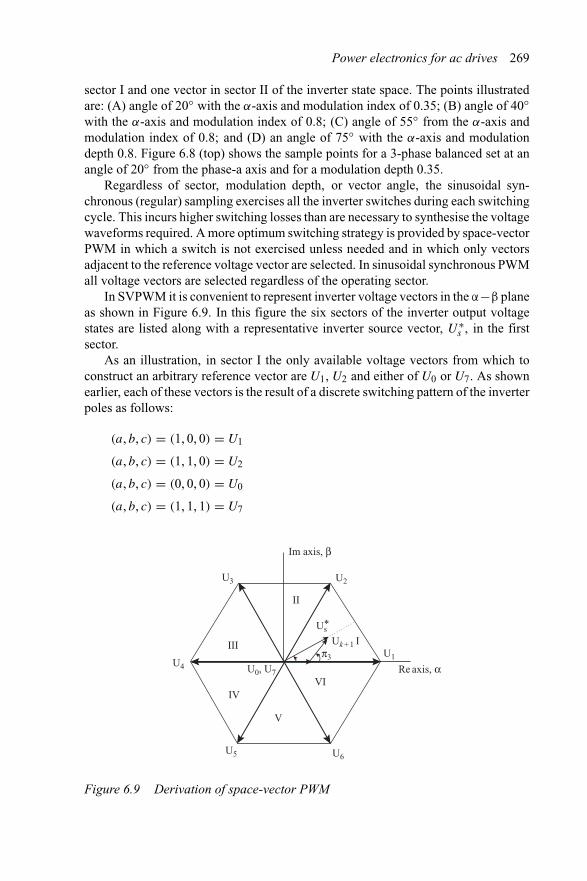
Power electronics for ac drives 269
sector I and one vector in sector II of the inverter state space. The points illustratedare: (A) angle of 20◦ with the α-axis and modulation index of 0.35; (B) angle of 40◦with the α-axis and modulation index of 0.8; (C) angle of 55◦ from the α-axis andmodulation index of 0.8; and (D) an angle of 75◦ with the α-axis and modulationdepth 0.8. Figure 6.8 (top) shows the sample points for a 3-phase balanced set at anangle of 20◦ from the phase-a axis and for a modulation depth 0.35.
Regardless of sector, modulation depth, or vector angle, the sinusoidal syn-chronous (regular) sampling exercises all the inverter switches during each switchingcycle. This incurs higher switching losses than are necessary to synthesise the voltagewaveforms required. A more optimum switching strategy is provided by space-vectorPWM in which a switch is not exercised unless needed and in which only vectorsadjacent to the reference voltage vector are selected. In sinusoidal synchronous PWMall voltage vectors are selected regardless of the operating sector.
In SVPWM it is convenient to represent inverter voltage vectors in the α−β planeas shown in Figure 6.9. In this figure the six sectors of the inverter output voltagestates are listed along with a representative inverter source vector, U∗
s , in the firstsector.
As an illustration, in sector I the only available voltage vectors from which toconstruct an arbitrary reference vector are U1, U2 and either of U0 or U7. As shownearlier, each of these vectors is the result of a discrete switching pattern of the inverterpoles as follows:
(a, b, c) = (1, 0, 0) = U1
(a, b, c) = (1, 1, 0) = U2
(a, b, c) = (0, 0, 0) = U0
(a, b, c) = (1, 1, 1) = U7
Re axis, α
Im axis, β
U1π3
Uk + 1 I
U2
Us
U3
U4
U5 U6
U0, U7
III
IV
V
VI
II
*
Figure 6.9 Derivation of space-vector PWM
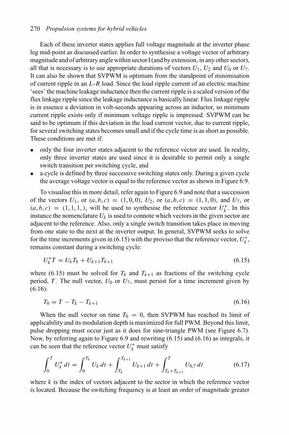
270 Propulsion systems for hybrid vehicles
Each of these inverter states applies full voltage magnitude at the inverter phaseleg mid-point as discussed earlier. In order to synthesise a voltage vector of arbitrarymagnitude and of arbitrary angle within sector I (and by extension, in any other sector),all that is necessary is to use appropriate durations of vectors U1, U2 and U0 or U7.It can also be shown that SVPWM is optimum from the standpoint of minimisationof current ripple in an L-R load. Since the load ripple current of an electric machine‘sees’ the machine leakage inductance then the current ripple is a scaled version of theflux linkage ripple since the leakage inductance is basically linear. Flux linkage rippleis in essence a deviation in volt-seconds appearing across an inductor, so minimumcurrent ripple exists only if minimum voltage ripple is impressed. SVPWM can besaid to be optimum if this deviation in the load current vector, due to current ripple,for several switching states becomes small and if the cycle time is as short as possible.These conditions are met if:
• only the four inverter states adjacent to the reference vector are used. In reality,only three inverter states are used since it is desirable to permit only a singleswitch transition per switching cycle, and
• a cycle is defined by three successive switching states only. During a given cyclethe average voltage vector is equal to the reference vector as shown in Figure 6.9.
To visualise this in more detail, refer again to Figure 6.9 and note that a successionof the vectors U1, or (a, b, c) = (1, 0, 0), U2, or (a, b, c) = (1, 1, 0), and U7, or(a, b, c) = (1, 1, 1, ), will be used to synthesise the reference vector U∗
k . In thisinstance the nomenclature Uk is used to connote which vectors in the given sector areadjacent to the reference. Also, only a single switch transition takes place in movingfrom one state to the next at the inverter output. In general, SVPWM seeks to solvefor the time increments given in (6.15) with the proviso that the reference vector, U∗
k ,remains constant during a switching cycle:
U∗k T = UkTk + Uk+1Tk+1 (6.15)
where (6.15) must be solved for Tk and Tk+1 as fractions of the switching cycleperiod, T . The null vector, U0 or U7, must persist for a time increment given by(6.16):
T0 = T − Tk − Tk+1 (6.16)
When the null vector on time T0 = 0, then SVPWM has reached its limit ofapplicability and its modulation depth is maximized for full PWM. Beyond this limit,pulse dropping must occur just as it does for sine-triangle PWM (see Figure 6.7).Now, by referring again to Figure 6.9 and rewriting (6.15) and (6.16) as integrals, itcan be seen that the reference vector U∗
k must satisfy∫ T
0U∗
k dt =∫ Tk
0Uk dt +
∫ Tk+1
Tk
Uk+1 dt +∫ T
Tk+Tk+1
U0,7 dt (6.17)
where k is the index of vectors adjacent to the sector in which the reference vectoris located. Because the switching frequency is at least an order of magnitude greater
Power electronics for ac drives 271
than the fundamental frequency, the transitions between states in (6.17) will occurfor essentially quasi-static behaviour of the commanded reference.
We refer again to Figure 6.9 and note the angle that the vectors Uk , Uk+1 and U∗k
make with the a-axis and then rewrite (6.15) as (6.18) in terms of actual magnitudes:
32miUdc[cos 0 + j sin 0]Tk + 3
2miUdc[cos(π/3) + j sin(π/3)]= 3
2miUdc[cos γ + j sin γ ] (6.18)
where the modulation index has been defined previously as the ratio of the maxi-mum sinusoidal synthesised wave amplitude to that of an equivalent square wavemagnitude, and γ = ωt . Therefore, solving (6.18) results in expressions for Tk andTk+1 as:
Tk = miTsin(π/3 − γ )
sin(π/3)
Tk+1 = miTsin(γ )
sin(π/3)
T0 = T − Tk − Tk+1
(6.19)
Equation (6.19) summarises the calculations leading to SVPWM. It is also evidentthat with a fast digital processor these calculations can be processed on line and quicklysince half the coefficients are constants or easily obtained from look-up tables as thereference vector moves from sector to sector in the inverter state diagram. It is alsoclear from (6.19) how the modulation depth impacts the time intervals. Higher levelsof modulation index result in a larger fraction of the total switching period beingdevoted to adjacent state vectors and a diminishing amount of time for the null vector.
Next, it is instructive to illustrate the particular switching pattern characteristic ofSVPWM during one switching cycle. It is also important to recognize that in SVPWMthe inverter gating frequency is one-half the state clock frequency. For example, ifthe clock frequency is fclk then the inverter switching frequency fs = fclk/2.
The average values over a switching cycle of inverter phase to negative busvoltages U1, U2 and U3 are calculated with the aid of Figure 6.10. To clarify, thevoltages given by (6.20) are from the inverter phase leg to negative bus, wheresubscripts 1, 2 and 3 are used in lieu of a, b and c phases for convenience:
U1 = Udc
T
[−T0
2+ T1 + T2 + T0
2
]
U2 = Udc
T
[−T0
2− T1 + T2 + T0
2
]
U3 = Udc
T
[−T0
2− T1 − T2 + T0
2
]= −U1
(6.20)
272 Propulsion systems for hybrid vehicles
U1
U2
U3
t
Tk Tk + 1T0/2 T0/2
2TT
Figure 6.10 Switching pattern of SVPWM
When the relations given in (6.19) are substituted into (6.20) with appropriatesubscript change, the inverter to negative rail voltages are:
U1 = 2√3miUdc sin(γ + π/3)
U2 = miUdc sin(γ − π/6)
U3 = − 2√3miUdc sin(γ + π/3)
(6.21)
Knowing the inverter phase leg voltages it is a straightforward calculation toarrive at the line-to-line voltages at the inverter output. These are the voltages thatwill be applied to the electric machine as a load:
Uab = 4√3miUdc sin(ωt + π/6)
Ubc = 4√3miUdc sin(ωt − π/2)
Uca = 4√3miUdc sin(ωt − 7π/6)
(6.22)
The line-to-line voltages are sinusoidal but the modulating function that willproduce these output voltages is not sinusoidal. First, to clarify the amplitudes of theline-to-line, Ul−l , phase to negative bus, U1, and peak of the modulating function, Um,
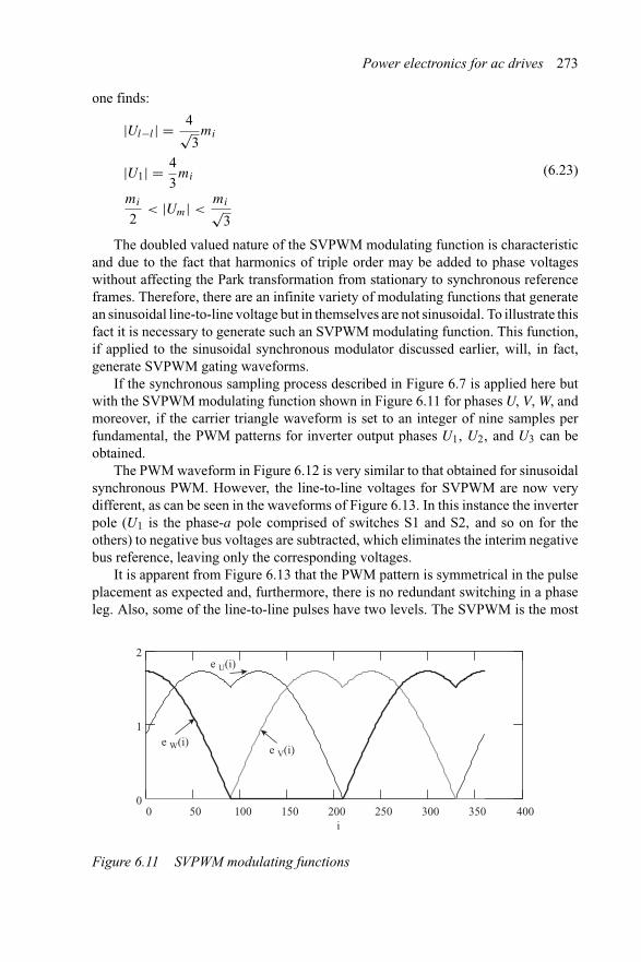
Power electronics for ac drives 273
one finds:
|Ul−l | = 4√3mi
|U1| = 4
3mi
mi
2< |Um| <
mi√3
(6.23)
The doubled valued nature of the SVPWM modulating function is characteristicand due to the fact that harmonics of triple order may be added to phase voltageswithout affecting the Park transformation from stationary to synchronous referenceframes. Therefore, there are an infinite variety of modulating functions that generatean sinusoidal line-to-line voltage but in themselves are not sinusoidal. To illustrate thisfact it is necessary to generate such an SVPWM modulating function. This function,if applied to the sinusoidal synchronous modulator discussed earlier, will, in fact,generate SVPWM gating waveforms.
If the synchronous sampling process described in Figure 6.7 is applied here butwith the SVPWM modulating function shown in Figure 6.11 for phases U, V, W, andmoreover, if the carrier triangle waveform is set to an integer of nine samples perfundamental, the PWM patterns for inverter output phases U1, U2, and U3 can beobtained.
The PWM waveform in Figure 6.12 is very similar to that obtained for sinusoidalsynchronous PWM. However, the line-to-line voltages for SVPWM are now verydifferent, as can be seen in the waveforms of Figure 6.13. In this instance the inverterpole (U1 is the phase-a pole comprised of switches S1 and S2, and so on for theothers) to negative bus voltages are subtracted, which eliminates the interim negativebus reference, leaving only the corresponding voltages.
It is apparent from Figure 6.13 that the PWM pattern is symmetrical in the pulseplacement as expected and, furthermore, there is no redundant switching in a phaseleg. Also, some of the line-to-line pulses have two levels. The SVPWM is the most
i0 50 100 150 200 250 300 350 400
0
1
2e U(i)
e W(i)e V(i)
Figure 6.11 SVPWM modulating functions
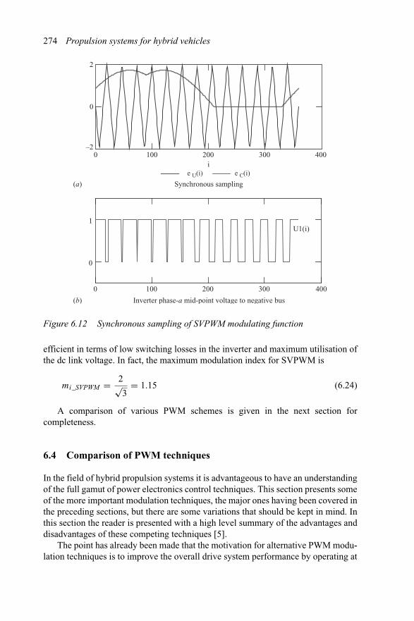
274 Propulsion systems for hybrid vehicles
e U(i) e C(i)i
0 100 200 300 400
0
2
–2
0 100 200 300 400
U1(i)
0
1
(b)
(a) Synchronous sampling
Inverter phase-a mid-point voltage to negative bus
Figure 6.12 Synchronous sampling of SVPWM modulating function
efficient in terms of low switching losses in the inverter and maximum utilisation ofthe dc link voltage. In fact, the maximum modulation index for SVPWM is
mi_SVPWM = 2√3
= 1.15 (6.24)
A comparison of various PWM schemes is given in the next section forcompleteness.
6.4 Comparison of PWM techniques
In the field of hybrid propulsion systems it is advantageous to have an understandingof the full gamut of power electronics control techniques. This section presents someof the more important modulation techniques, the major ones having been covered inthe preceding sections, but there are some variations that should be kept in mind. Inthis section the reader is presented with a high level summary of the advantages anddisadvantages of these competing techniques [5].
The point has already been made that the motivation for alternative PWM modu-lation techniques is to improve the overall drive system performance by operating at
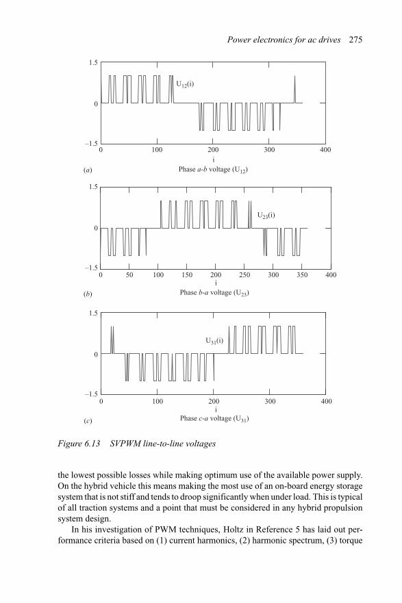
Power electronics for ac drives 275
iPhase a-b voltage (U12)
i
i
Phase b-a voltage (U23)
Phase c-a voltage (U31)
1.5
–1.5
0
1.5
–1.5
0
1.5
–1.5
0
U12(i)
(a)
(b)
(c)
0 50 100 150 200 250 300 350 400
0 100 200 300 400
U23(i)
U31(i)
0 100 200 300 400
Figure 6.13 SVPWM line-to-line voltages
the lowest possible losses while making optimum use of the available power supply.On the hybrid vehicle this means making the most use of an on-board energy storagesystem that is not stiff and tends to droop significantly when under load. This is typicalof all traction systems and a point that must be considered in any hybrid propulsionsystem design.
In his investigation of PWM techniques, Holtz in Reference 5 has laid out per-formance criteria based on (1) current harmonics, (2) harmonic spectrum, (3) torque
276 Propulsion systems for hybrid vehicles
harmonics, (4) switching frequency, (5) polarity consistency rule and (6) dynamicperformance. All of these criteria can be seen to be very important for the hybridpropulsion system designer. Current harmonics give rise to additional iron and cop-per losses in the machine and power inverter, particularly in the dc link capacitors,and the harmonic spectrum that may be sparse or dense with frequency components atvarious relative amplitudes. Holtz goes on to propose a figure of merit for modulationtechniques based on the product of spectral amplitudes and switching frequency asa means of comparison. Torque harmonics are already obvious to the hybrid propul-sion system designer and typically a strong function of the electric machine topology,but also dependent on inverter current harmonic injection. Switching frequency isimportant because the fidelity of the load currents increases linearly with switchingfrequency because the current ripple is reduced. However, switching frequency isstrongly dependent on available semiconductor device technology. IGBTs today inthe form of ultra-thin wafer processing (∼ 85 μm to even 65 μm in the laboratoryand rated at 600 V) are capable of switching rated current at up to 80 kHz. This isfar too high for motor drives, but the capability is there. Higher voltage and highercurrent power electronic devices such as GTOs for very high power (e.g. MW) arecapable of switching at 500 Hz to, perhaps, 700 Hz. Switching frequency also givesrise to electromagnetic interference (EMI) concerns if not properly treated. Inverterpackages with low inductance busbars, or laminated busbar and output phase termina-tions, provide the lowest EMI structures. Additional filtering for common mode andtransverse mode noise are possible with filters in the output lines. A polarity consis-tency rule is useful for grading those PWM techniques that select voltage vectors thatdo not have the same polarity as the reference voltage. Recall that the sine-trianglePWM was able to select voltage vectors that were not in the same sector as the refer-ence. SVPWM is the best because no more than two active and two null vectors areused at any one time. Dynamic performance is a metric for inner loop performanceor current regulator bandwidth. Dynamic performance is set by inverter switchingfrequency, controller loop execution times, current or voltage sensor bandwidth andall associated lag times.
Recall that the inverter modulation index, mi , is defined as the ratio of the refer-ence vector to the maximum value of a square wave fundamental wave. The limitingvalues of the modulation index for sine-triangle PWM and SVPWM are listed in(6.25) for convenience, where the scaling is relative to a square wave:
mi_PWM =√
32 = 0.787
mi_SVPWM = 2√3
= 1.15 (6.25)
mi_Squarewave = 1
Table 6.3 summarises the salient aspects of the various PWM techniques used asalgorithms to control power electronic inverters. It can be seen from the commentsin the table that space vector modulators provide the best overall performance. Incertain applications the alternative modulators prove very useful. Hysteresis current
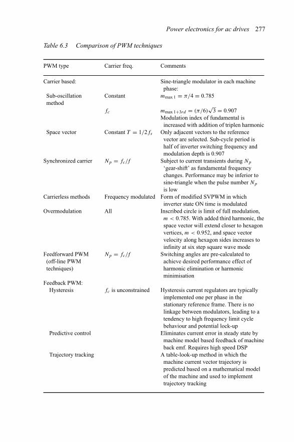
Power electronics for ac drives 277
Table 6.3 Comparison of PWM techniques
PWM type Carrier freq. Comments
Carrier based: Sine-triangle modulator in each machinephase:
Sub-oscillationmethod
Constant mmax 1 = π/4 = 0.785
fc mmax 1+3rd = (π/6)√
3 = 0.907Modulation index of fundamental isincreased with addition of triplen harmonic
Space vector Constant T = 1/2fs Only adjacent vectors to the referencevector are selected. Sub-cycle period ishalf of inverter switching frequency andmodulation depth is 0.907
Synchronized carrier Np = fc/f Subject to current transients during Np
‘gear-shift’ as fundamental frequencychanges. Performance may be inferior tosine-triangle when the pulse number Np
is lowCarrierless methods Frequency modulated Form of modified SVPWM in which
inverter state ON time is modulatedOvermodulation All Inscribed circle is limit of full modulation,
m < 0.785. With added third harmonic, thespace vector will extend closer to hexagonvertices, m < 0.952, and space vectorvelocity along hexagon sides increases toinfinity at six step square wave mode
Feedforward PWM(off-line PWMtechniques)
Np = fc/f Switching angles are pre-calculated toachieve desired performance effect ofharmonic elimination or harmonicminimisation
Feedback PWM:Hysteresis fc is unconstrained Hysteresis current regulators are typically
implemented one per phase in thestationary reference frame. There is nolinkage between modulators, leading to atendency to high frequency limit cyclebehaviour and potential lock-up
Predictive control Eliminates current error in steady state bymachine model based feedback of machineback emf. Requires high speed DSP
Trajectory tracking A table-look-up method in which themachine current vector trajectory ispredicted based on a mathematical modelof the machine and used to implementtrajectory tracking
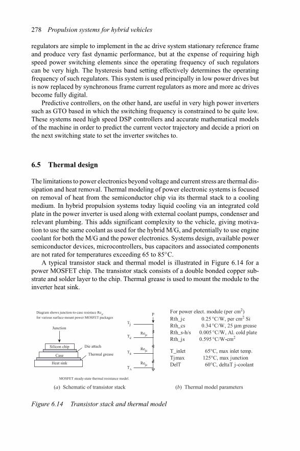
278 Propulsion systems for hybrid vehicles
regulators are simple to implement in the ac drive system stationary reference frameand produce very fast dynamic performance, but at the expense of requiring highspeed power switching elements since the operating frequency of such regulatorscan be very high. The hysteresis band setting effectively determines the operatingfrequency of such regulators. This system is used principally in low power drives butis now replaced by synchronous frame current regulators as more and more ac drivesbecome fully digital.
Predictive controllers, on the other hand, are useful in very high power inverterssuch as GTO based in which the switching frequency is constrained to be quite low.These systems need high speed DSP controllers and accurate mathematical modelsof the machine in order to predict the current vector trajectory and decide a priori onthe next switching state to set the inverter switches to.
6.5 Thermal design
The limitations to power electronics beyond voltage and current stress are thermal dis-sipation and heat removal. Thermal modeling of power electronic systems is focusedon removal of heat from the semiconductor chip via its thermal stack to a coolingmedium. In hybrid propulsion systems today liquid cooling via an integrated coldplate in the power inverter is used along with external coolant pumps, condenser andrelevant plumbing. This adds significant complexity to the vehicle, giving motiva-tion to use the same coolant as used for the hybrid M/G, and potentially to use enginecoolant for both the M/G and the power electronics. Systems design, available powersemiconductor devices, microcontrollers, bus capacitors and associated componentsare not rated for temperatures exceeding 65 to 85◦C.
A typical transistor stack and thermal model is illustrated in Figure 6.14 for apower MOSFET chip. The transistor stack consists of a double bonded copper sub-strate and solder layer to the chip. Thermal grease is used to mount the module to theinverter heat sink.
For power elect. module (per cm2)Rth_jcRth_csRth_s-h/sRth_js
T_inlet 65°C, max inlet temp.Tjmax 125°C, max junctionDelT 60°C, deltaT j-coolant
Silicon chip
Case
Heat sink
Die attach
Junction
Diagram shows junction-to-case resistace ReJC
for various surface-mount power MOSFET packages
Thermal grease
0.25 °C/W, per cm2 Si0.34 °C/W, 25 μm grease
0.005 °C/W, Al. cold plate0.595 °C/W-cm2
Tj
P
Tc
Ts
TA
Rejc
Rejc
Rejc
MOSFET steady-state thermal resistance model.
(a) Schematic of transistor stack (b) Thermal model parameters
Figure 6.14 Transistor stack and thermal model
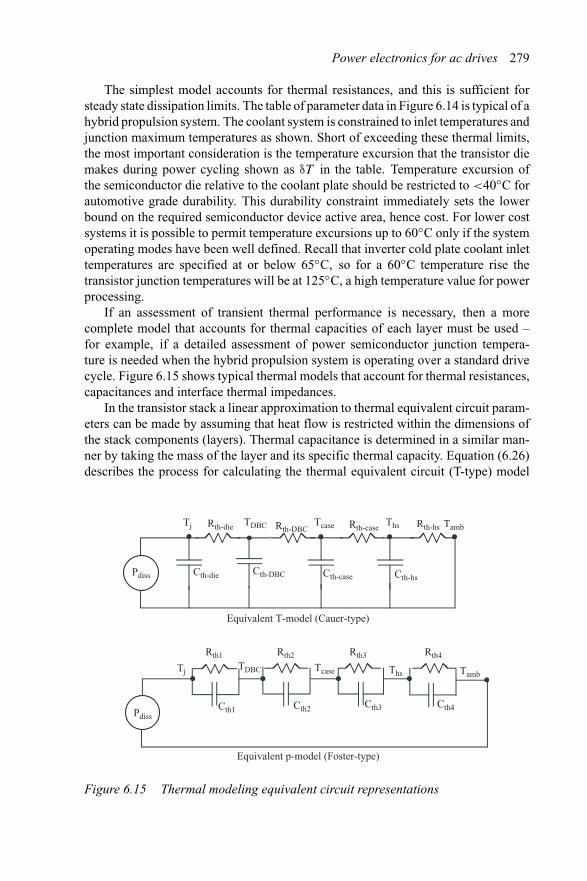
Power electronics for ac drives 279
The simplest model accounts for thermal resistances, and this is sufficient forsteady state dissipation limits. The table of parameter data in Figure 6.14 is typical of ahybrid propulsion system. The coolant system is constrained to inlet temperatures andjunction maximum temperatures as shown. Short of exceeding these thermal limits,the most important consideration is the temperature excursion that the transistor diemakes during power cycling shown as δT in the table. Temperature excursion ofthe semiconductor die relative to the coolant plate should be restricted to <40◦C forautomotive grade durability. This durability constraint immediately sets the lowerbound on the required semiconductor device active area, hence cost. For lower costsystems it is possible to permit temperature excursions up to 60◦C only if the systemoperating modes have been well defined. Recall that inverter cold plate coolant inlettemperatures are specified at or below 65◦C, so for a 60◦C temperature rise thetransistor junction temperatures will be at 125◦C, a high temperature value for powerprocessing.
If an assessment of transient thermal performance is necessary, then a morecomplete model that accounts for thermal capacities of each layer must be used –for example, if a detailed assessment of power semiconductor junction tempera-ture is needed when the hybrid propulsion system is operating over a standard drivecycle. Figure 6.15 shows typical thermal models that account for thermal resistances,capacitances and interface thermal impedances.
In the transistor stack a linear approximation to thermal equivalent circuit param-eters can be made by assuming that heat flow is restricted within the dimensions ofthe stack components (layers). Thermal capacitance is determined in a similar man-ner by taking the mass of the layer and its specific thermal capacity. Equation (6.26)describes the process for calculating the thermal equivalent circuit (T-type) model
Rth-die Rth-DBC Rth-case
Cth-die Cth-DBC Cth-case Cth-hs
TDBC Tcase Ths
Equivalent T-model (Cauer-type)
TjTDBC Tcase Ths Tamb
Rth1 Rth2 Rth3 Rth4
Cth1 Cth2 Cth3 Cth4
Equivalent p-model (Foster-type)
Pdiss
Rth-hs TambTj
Pdiss
Figure 6.15 Thermal modeling equivalent circuit representations
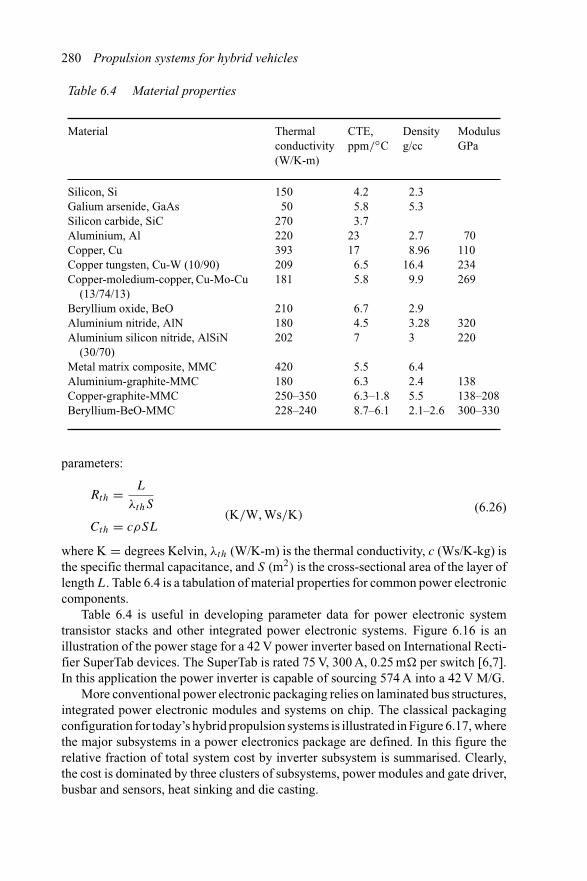
280 Propulsion systems for hybrid vehicles
Table 6.4 Material properties
Material Thermalconductivity(W/K-m)
CTE,ppm/◦C
Densityg/cc
ModulusGPa
Silicon, Si 150 4.2 2.3Galium arsenide, GaAs 50 5.8 5.3Silicon carbide, SiC 270 3.7Aluminium, Al 220 23 2.7 70Copper, Cu 393 17 8.96 110Copper tungsten, Cu-W (10/90) 209 6.5 16.4 234Copper-moledium-copper, Cu-Mo-Cu
(13/74/13)181 5.8 9.9 269
Beryllium oxide, BeO 210 6.7 2.9Aluminium nitride, AlN 180 4.5 3.28 320Aluminium silicon nitride, AlSiN
(30/70)202 7 3 220
Metal matrix composite, MMC 420 5.5 6.4Aluminium-graphite-MMC 180 6.3 2.4 138Copper-graphite-MMC 250–350 6.3–1.8 5.5 138–208Beryllium-BeO-MMC 228–240 8.7–6.1 2.1–2.6 300–330
parameters:
Rth = L
λthS(K/W, Ws/K)
Cth = cρSL
(6.26)
where K = degrees Kelvin, λth (W/K-m) is the thermal conductivity, c (Ws/K-kg) isthe specific thermal capacitance, and S (m2) is the cross-sectional area of the layer oflength L. Table 6.4 is a tabulation of material properties for common power electroniccomponents.
Table 6.4 is useful in developing parameter data for power electronic systemtransistor stacks and other integrated power electronic systems. Figure 6.16 is anillustration of the power stage for a 42 V power inverter based on International Recti-fier SuperTab devices. The SuperTab is rated 75 V, 300 A, 0.25 m� per switch [6,7].In this application the power inverter is capable of sourcing 574 A into a 42 V M/G.
More conventional power electronic packaging relies on laminated bus structures,integrated power electronic modules and systems on chip. The classical packagingconfiguration for today’s hybrid propulsion systems is illustrated in Figure 6.17, wherethe major subsystems in a power electronics package are defined. In this figure therelative fraction of total system cost by inverter subsystem is summarised. Clearly,the cost is dominated by three clusters of subsystems, power modules and gate driver,busbar and sensors, heat sinking and die casting.
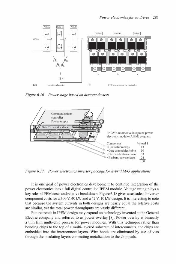
Power electronics for ac drives 281
R
R
L
R
LL
40Vdc
Pole A
a b c
Pole B Pole C
Pole A
a b c
Pole B Pole C
(a) Inverter schematic (b) FET arrangement on heatsinks
Figure 6.16 Power stage based on discrete devices
Gate Driver & cables
CommunicationsControllerPower supply
heatsink
Gate Driver & cables
CommunicationscontrollerPower supply
heatsink
PNGV’s automotive integrated power electronic module (AIPM) program:
Component % total $• Control/comm/ps 13• Gate dr/modules/cable 30• Die cast/heatsink conn 33• Busbars/ curr sen/caps 24
100
Figure 6.17 Power electronics inverter package for hybrid M/G applications
It is one goal of power electronics development to continue integration of thepower electronics into a full digital controlled IPEM module. Voltage rating plays akey role in IPEM costs and relative breakdown. Figure 6.18 gives a cascade of invertercomponent costs for a 300 V, 40 kW and a 42 V, 10 kW design. It is interesting to notethat because the system currents in both designs are nearly equal the relative costsare similar, yet the total power throughputs are vastly different.
Future trends in IPEM design may expand on technology invented at the GeneralElectric company and referred to as power overlay [8]. Power overlay is basicallya thin film multi-chip process for power modules. With this technique rather thanbonding chips to the top of a multi-layered substrate of interconnects, the chips areembedded into the interconnect layers. Wire bonds are eliminated by use of viasthrough the insulating layers connecting metalization to the chip pads.
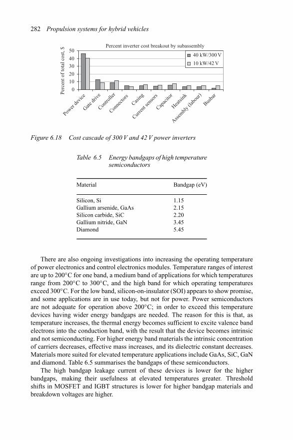
282 Propulsion systems for hybrid vehicles
Percent inverter cost breakout by subassembly
0
10
20
30
40
50
Power
devic
e
Gate dr
ive
Contro
ller
Conne
ctors
Casing
Curren
t sen
sors
Capac
itor
Heatsi
nk
Assembly
(lab
our)
Busba
rPerc
ent o
f to
tal c
ost,
$ 40 kW/300 V
10 kW/42 V
Figure 6.18 Cost cascade of 300 V and 42 V power inverters
Table 6.5 Energy bandgaps of high temperaturesemiconductors
Material Bandgap (eV)
Silicon, Si 1.15Gallium arsenide, GaAs 2.15Silicon carbide, SiC 2.20Gallium nitride, GaN 3.45Diamond 5.45
There are also ongoing investigations into increasing the operating temperatureof power electronics and control electronics modules. Temperature ranges of interestare up to 200◦C for one band, a medium band of applications for which temperaturesrange from 200◦C to 300◦C, and the high band for which operating temperaturesexceed 300◦C. For the low band, silicon-on-insulator (SOI) appears to show promise,and some applications are in use today, but not for power. Power semiconductorsare not adequate for operation above 200◦C; in order to exceed this temperaturedevices having wider energy bandgaps are needed. The reason for this is that, astemperature increases, the thermal energy becomes sufficient to excite valence bandelectrons into the conduction band, with the result that the device becomes intrinsicand not semiconducting. For higher energy band materials the intrinsic concentrationof carriers decreases, effective mass increases, and its dielectric constant decreases.Materials more suited for elevated temperature applications include GaAs, SiC, GaNand diamond. Table 6.5 summarises the bandgaps of these semiconductors.
The high bandgap leakage current of these devices is lower for the higherbandgaps, making their usefulness at elevated temperatures greater. Thresholdshifts in MOSFET and IGBT structures is lower for higher bandgap materials andbreakdown voltages are higher.
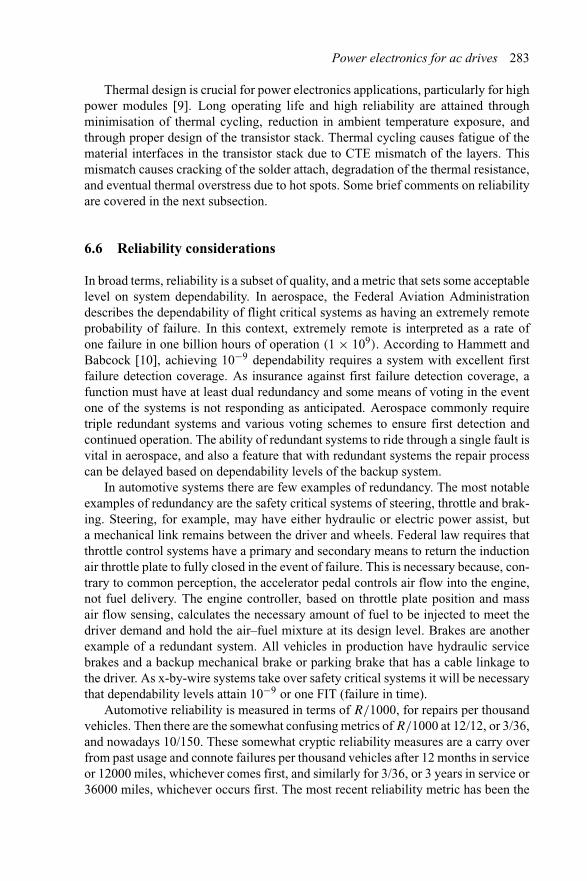
Power electronics for ac drives 283
Thermal design is crucial for power electronics applications, particularly for highpower modules [9]. Long operating life and high reliability are attained throughminimisation of thermal cycling, reduction in ambient temperature exposure, andthrough proper design of the transistor stack. Thermal cycling causes fatigue of thematerial interfaces in the transistor stack due to CTE mismatch of the layers. Thismismatch causes cracking of the solder attach, degradation of the thermal resistance,and eventual thermal overstress due to hot spots. Some brief comments on reliabilityare covered in the next subsection.
6.6 Reliability considerations
In broad terms, reliability is a subset of quality, and a metric that sets some acceptablelevel on system dependability. In aerospace, the Federal Aviation Administrationdescribes the dependability of flight critical systems as having an extremely remoteprobability of failure. In this context, extremely remote is interpreted as a rate ofone failure in one billion hours of operation (1 × 10⁹). According to Hammett andBabcock [10], achieving 10−9 dependability requires a system with excellent firstfailure detection coverage. As insurance against first failure detection coverage, afunction must have at least dual redundancy and some means of voting in the eventone of the systems is not responding as anticipated. Aerospace commonly requiretriple redundant systems and various voting schemes to ensure first detection andcontinued operation. The ability of redundant systems to ride through a single fault isvital in aerospace, and also a feature that with redundant systems the repair processcan be delayed based on dependability levels of the backup system.
In automotive systems there are few examples of redundancy. The most notableexamples of redundancy are the safety critical systems of steering, throttle and brak-ing. Steering, for example, may have either hydraulic or electric power assist, buta mechanical link remains between the driver and wheels. Federal law requires thatthrottle control systems have a primary and secondary means to return the inductionair throttle plate to fully closed in the event of failure. This is necessary because, con-trary to common perception, the accelerator pedal controls air flow into the engine,not fuel delivery. The engine controller, based on throttle plate position and massair flow sensing, calculates the necessary amount of fuel to be injected to meet thedriver demand and hold the air–fuel mixture at its design level. Brakes are anotherexample of a redundant system. All vehicles in production have hydraulic servicebrakes and a backup mechanical brake or parking brake that has a cable linkage tothe driver. As x-by-wire systems take over safety critical systems it will be necessarythat dependability levels attain 10−9 or one FIT (failure in time).
Automotive reliability is measured in terms of R/1000, for repairs per thousandvehicles. Then there are the somewhat confusing metrics of R/1000 at 12/12, or 3/36,and nowadays 10/150. These somewhat cryptic reliability measures are a carry overfrom past usage and connote failures per thousand vehicles after 12 months in serviceor 12000 miles, whichever comes first, and similarly for 3/36, or 3 years in service or36000 miles, whichever occurs first. The most recent reliability metric has been the
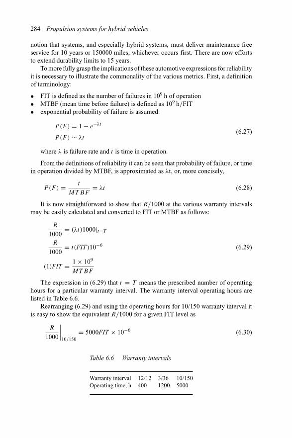
284 Propulsion systems for hybrid vehicles
notion that systems, and especially hybrid systems, must deliver maintenance freeservice for 10 years or 150000 miles, whichever occurs first. There are now effortsto extend durability limits to 15 years.
To more fully grasp the implications of these automotive expressions for reliabilityit is necessary to illustrate the commonality of the various metrics. First, a definitionof terminology:
• FIT is defined as the number of failures in 109 h of operation• MTBF (mean time before failure) is defined as 109 h/FIT• exponential probability of failure is assumed:
P(F) = 1 − e−λt
P (F ) ∼ λt(6.27)
where λ is failure rate and t is time in operation.
From the definitions of reliability it can be seen that probability of failure, or timein operation divided by MTBF, is approximated as λt, or, more concisely,
P(F) = t
MT BF= λt (6.28)
It is now straightforward to show that R/1000 at the various warranty intervalsmay be easily calculated and converted to FIT or MTBF as follows:
R
1000= (λt)1000|t=T
R
1000= t(FIT )10−6 (6.29)
(1)FIT = 1 × 10⁹
MT BF
The expression in (6.29) that t = T means the prescribed number of operatinghours for a particular warranty interval. The warranty interval operating hours arelisted in Table 6.6.
Rearranging (6.29) and using the operating hours for 10/150 warranty interval itis easy to show the equivalent R/1000 for a given FIT level as
R
1000
∣∣∣∣10/150
= 5000FIT × 10−6 (6.30)
Table 6.6 Warranty intervals
Warranty interval 12/12 3/36 10/150Operating time, h 400 1200 5000
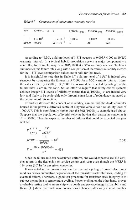
Power electronics for ac drives 285
Table 6.7 Comparison of automotive warranty metrics
FIT MTBF = 1/λ λ R/1000|12/12 R/1000|3/36 R/1000|10/150
1 1 × 10⁹ 1 × 10⁻⁹ 0.0004 0.0012 0.00525000 40000 25 × 10−6 10 30 125
According to (6.30), a failure level of 1-FIT equates to 0.005R/1000 at 10/150warranty interval. In a typical hybrid propulsion system a major component – acontroller, for example, may have 30R/1000 at a 3/36 warranty interval. Table 6.7summarises this failure rate along with a comparison of the various reliability metricsfor the 1-FIT level (comparison values are in bold for that row).
It is insightful to note that in Table 6.7 a failure level of 1 FIT is indeed verystringent by comparing the failures in R/1000 for a 3/36 warranty interval. Here,the values differ by 25000 (= 30/0.0012), as would be expected by noting that thefailure rates λ are in this ratio. So, an effort to require that safety critical systemsachieve integer FIT levels of reliability means that R/1000|10/150 are indeed verylow, and likely to be achievable only through some form of redundancy, as stated atthe beginning of this section.
To further illustrate the concept of reliability, assume that the dc/dc converterhoused in the power electronics centre of a hybrid vehicle has a reliability level of1000 FIT. This is significantly higher than the 30R/1000|3/36 example used above.Suppose that the population of hybrid vehicles having this particular converter isP = 50000. Then the expected number of failures that could be expected per yearwill be:
F
(#
yr
)= PT
MTBF
MTBF = 109
103FIT= 106 (6.31)
F = 50 × 103(8760)
106 = 438
Since the failure rate can be assumed uniform, one would expect to see 438 vehi-cles return to the dealership or service centre each year even though the MTBF is114 years (106 h) for any given converter.
It was noted in the previous section that thermal cycling of power electronicsmodules causes cumulative degradation of the transistor stack interfaces, leading toeventual failure. Therefore, a good test procedure for transistor stack integrity is tosubject the module to temperature cycling. Power cycling, on the other hand, provesa valuable testing tool to assess chip wire bonds and package integrity. Lambilly andKeser [11] show that thick wire connections debonded after only a small number
286 Propulsion systems for hybrid vehicles
of power cycles because of mechanical, rather than electrical, strain. Furthermore,because of the different CTEs of the various materials in the package, the substratedeformed due to these bimetallic effects, leading to its lifting off the heatsink andfurther exacerbating thermal stress. In some cases the substrates, ceramic in mostinstances, of the power modules cracked, but in most cases became delaminated fromthe heatsink due to voiding at solder contact surfaces.
6.7 Sensors for current regulators
Current sensing is one of the most important aspects of power electronics control.Without accurate and reliable current sensing it is not possible to maintain the integrityof the ac drive system current regulators. With respect to hybrid propulsion systemsthe most important attributes of current sensors and their interface to the hybridM/G controller are offset, gain imbalance, delay and quantization [12]. The impactof such behaviours is important for the distortion caused to the hybrid M/G con-troller direct and quadrature current commands. The following description coversa 3-phase SPM electric machine used as the suspension system actuator for eachwheel in an active suspension vehicle. Currents ia and ib having one or more defectsadded are compared with commanded currents in the stationary reference frame inmuch the same manner as a hysteresis current regulator, but in open loop. Referencedqo current commands are generated and fed through an dqo ↔ abc transforma-tion to the stationary reference frame for comparison. The ‘sensed’ currents thathave been corrupted in specific ways are transformed to a dqo synchronous referenceframe and compared to the reference commands. The comparison in the synchronousreference frame is used to illustrate the manner in which specific sensor corrup-tion affects the synchronous frame current regulator. These effects are discussedbelow:
• Offset error: To introduce offset imbalance, a constant (e.g. 1 A) is added to theoutput of the sensor to simulate deviation from normal balanced conditions of a+/− 5 V range with 0 V as 0-current (or, in the case of single ended supplies,deviation from 2.500 V). The stationary sensed currents now contain a dc offsetof one of the sinusoidal waveforms. In the synchronous frame rather than steadyidqs references both ids and iqs are corrupted by an ac component. If this were aclosed loop ac drive, the corrupted reference signals would cause the controllerto issue sinusoidal commands 180◦ out of phase to cancel the disturbances, thusfurther propagating the error.
• Balanced offset: If each of two current sensors in a 3-phase system has offsetintroduced, but with opposite polarity (e.g. +1A and −1A), then the effectsnoted above are compounded.
• Gain error: To study the effect of gain error (linearity not affected), one of thecurrent sensors is given a scale factor 50% higher than its complementary sensor.Now the feedback signals iqds contain frequency components at twice the excita-tion frequency. Not only is there a double frequency component associated with
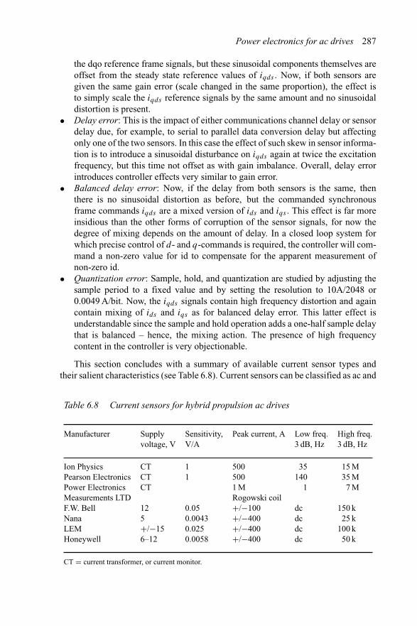
Power electronics for ac drives 287
the dqo reference frame signals, but these sinusoidal components themselves areoffset from the steady state reference values of iqds . Now, if both sensors aregiven the same gain error (scale changed in the same proportion), the effect isto simply scale the iqds reference signals by the same amount and no sinusoidaldistortion is present.
• Delay error: This is the impact of either communications channel delay or sensordelay due, for example, to serial to parallel data conversion delay but affectingonly one of the two sensors. In this case the effect of such skew in sensor informa-tion is to introduce a sinusoidal disturbance on iqds again at twice the excitationfrequency, but this time not offset as with gain imbalance. Overall, delay errorintroduces controller effects very similar to gain error.
• Balanced delay error: Now, if the delay from both sensors is the same, thenthere is no sinusoidal distortion as before, but the commanded synchronousframe commands iqds are a mixed version of ids and iqs . This effect is far moreinsidious than the other forms of corruption of the sensor signals, for now thedegree of mixing depends on the amount of delay. In a closed loop system forwhich precise control of d- and q-commands is required, the controller will com-mand a non-zero value for id to compensate for the apparent measurement ofnon-zero id.
• Quantization error: Sample, hold, and quantization are studied by adjusting thesample period to a fixed value and by setting the resolution to 10A/2048 or0.0049 A/bit. Now, the iqds signals contain high frequency distortion and againcontain mixing of ids and iqs as for balanced delay error. This latter effect isunderstandable since the sample and hold operation adds a one-half sample delaythat is balanced – hence, the mixing action. The presence of high frequencycontent in the controller is very objectionable.
This section concludes with a summary of available current sensor types andtheir salient characteristics (see Table 6.8). Current sensors can be classified as ac and
Table 6.8 Current sensors for hybrid propulsion ac drives
Manufacturer Supplyvoltage, V
Sensitivity,V/A
Peak current, A Low freq.3 dB, Hz
High freq.3 dB, Hz
Ion Physics CT 1 500 35 15 MPearson Electronics CT 1 500 140 35 MPower Electronics CT 1 M 1 7 MMeasurements LTD Rogowski coilF.W. Bell 12 0.05 +/−100 dc 150 kNana 5 0.0043 +/−400 dc 25 kLEM +/−15 0.025 +/−400 dc 100 kHoneywell 6–12 0.0058 +/−400 dc 50 k
CT = current transformer, or current monitor.
288 Propulsion systems for hybrid vehicles
dc sensors. Dc types can be further classified as double ended or single ended, depend-ing on whether or not a balanced power source is required. All current sensors operateat 5 V or 10 V logic levels.
Current sensors are vital components in power electronic systems. The Hall effect,control current types available from F.W. Bell, Nana Electronics, LEM, Honeywelland others, are the primary types in use because sensing to dc is afforded. Somemanufacturers are investigating magneto-resistive current sensors for improved tem-perature performance, but these are still not on the market. Other manufacturers havedeveloped a prototype, digital, high accuracy current sensor, based on a temperaturestable manganin shunt and all digital signal conditioning and impedance correctionfor dc to 100 kHz bandwitdh [13]. As the quest for fully digital ac traction drivesprogresses, the approach given in [13] may find renewed interest.
6.8 Interleaved PWM for minimum ripple
There have been periodic attempts to use various power electronic systems to min-imise the rms current ripple in the dc link capacitor of a hard switched inverter. Boseand Kastha [14] describe the use of active filters to eliminate the dc link capacitor bycontrolling an auxiliary converter loaded with an inductor to entirely eliminate theelectrolytic. Since electrolytic capacitors are deemed the most unreliable componentin power electronic systems this approach does have merit. However, the added costof 4 additional power semiconductors needed for the auxiliary H-bridge converterinterface to the inductor make this somewhat impractical. But an interesting prospectnonetheless.
It is also possible to minimise the dc link capacitance through a means of inter-leaving the inverter pulse currents. Huang et al. [15] show that a phase displacedinverter system in which a pair of 0.5 pu rated inverter modules drive a dual wind-ing IM from a common dc bus is capable of significantly reducing capacitor ripplecontent. In this system the electric machine is a quasi-6-phase machine having dual3-phase windings that are phase shifted and controlled via independent inverters.By interleaving the PWM control signals to the dual inverters the effective dc linkcurrent that must be circulated within the link capacitors is halved in magnitude anddoubled in frequency. Because losses are proportional to I 2R, this technique effec-tively reduces the total capacitor dissipation to one-half its nominal value. Figure 6.19illustrates the concept of interleaved PWM for dc link capacitor ripple currentminimisation.
In a conventional ac drive system the dc link capacitor and battery experiencehigh discharge pulse magnitudes and dwell times. In the interleaved system shown inFigure 6.19 the battery current and the link capacitor are diminished in magnitude butdoubled in frequency of occurrence. Figure 6.20 illustrates the current waveforms tobe expected from interleaved PWM control.
It is recommended that the topic of dc link capacitor minimisation or eliminationbe encouraged as it has great potential to further reduce inverter package volume,promote system-on-a-chip initiatives, and foster improved systems reliability.
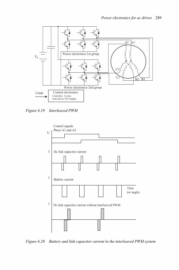
Power electronics for ac drives 289
Vb
Cmds
Power electronics-2nd group
Control electronics
Power electronics-1st group
A2 A1
B2 B1
C2
C1
Controller, Comm. Gate drives, Pwr Supply
Figure 6.19 Interleaved PWM
Control signals Phase A1 and A2
Dc link capacitor current
Battery current
Dc link capacitor current without interleaved PWM
Time(or angle)
U
I
I
I
Figure 6.20 Battery and link capacitor current in the interleaved PWM system
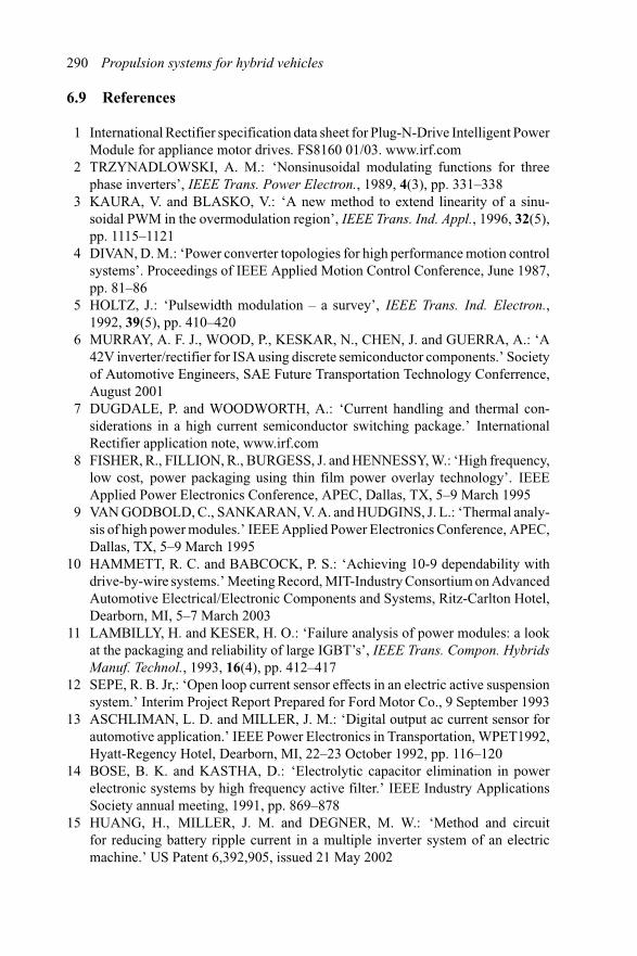
290 Propulsion systems for hybrid vehicles
6.9 References
1 International Rectifier specification data sheet for Plug-N-Drive Intelligent PowerModule for appliance motor drives. FS8160 01/03. www.irf.com
2 TRZYNADLOWSKI, A. M.: ‘Nonsinusoidal modulating functions for threephase inverters’, IEEE Trans. Power Electron., 1989, 4(3), pp. 331–338
3 KAURA, V. and BLASKO, V.: ‘A new method to extend linearity of a sinu-soidal PWM in the overmodulation region’, IEEE Trans. Ind. Appl., 1996, 32(5),pp. 1115–1121
4 DIVAN, D. M.: ‘Power converter topologies for high performance motion controlsystems’. Proceedings of IEEE Applied Motion Control Conference, June 1987,pp. 81–86
5 HOLTZ, J.: ‘Pulsewidth modulation – a survey’, IEEE Trans. Ind. Electron.,1992, 39(5), pp. 410–420
6 MURRAY, A. F. J., WOOD, P., KESKAR, N., CHEN, J. and GUERRA, A.: ‘A42V inverter/rectifier for ISA using discrete semiconductor components.’ Societyof Automotive Engineers, SAE Future Transportation Technology Conferrence,August 2001
7 DUGDALE, P. and WOODWORTH, A.: ‘Current handling and thermal con-siderations in a high current semiconductor switching package.’ InternationalRectifier application note, www.irf.com
8 FISHER, R., FILLION, R., BURGESS, J. and HENNESSY, W.: ‘High frequency,low cost, power packaging using thin film power overlay technology’. IEEEApplied Power Electronics Conference, APEC, Dallas, TX, 5–9 March 1995
9 VAN GODBOLD, C., SANKARAN, V. A. and HUDGINS, J. L.: ‘Thermal analy-sis of high power modules.’ IEEE Applied Power Electronics Conference, APEC,Dallas, TX, 5–9 March 1995
10 HAMMETT, R. C. and BABCOCK, P. S.: ‘Achieving 10-9 dependability withdrive-by-wire systems.’ Meeting Record, MIT-Industry Consortium on AdvancedAutomotive Electrical/Electronic Components and Systems, Ritz-Carlton Hotel,Dearborn, MI, 5–7 March 2003
11 LAMBILLY, H. and KESER, H. O.: ‘Failure analysis of power modules: a lookat the packaging and reliability of large IGBT’s’, IEEE Trans. Compon. HybridsManuf. Technol., 1993, 16(4), pp. 412–417
12 SEPE, R. B. Jr,: ‘Open loop current sensor effects in an electric active suspensionsystem.’ Interim Project Report Prepared for Ford Motor Co., 9 September 1993
13 ASCHLIMAN, L. D. and MILLER, J. M.: ‘Digital output ac current sensor forautomotive application.’ IEEE Power Electronics in Transportation, WPET1992,Hyatt-Regency Hotel, Dearborn, MI, 22–23 October 1992, pp. 116–120
14 BOSE, B. K. and KASTHA, D.: ‘Electrolytic capacitor elimination in powerelectronic systems by high frequency active filter.’ IEEE Industry ApplicationsSociety annual meeting, 1991, pp. 869–878
15 HUANG, H., MILLER, J. M. and DEGNER, M. W.: ‘Method and circuitfor reducing battery ripple current in a multiple inverter system of an electricmachine.’ US Patent 6,392,905, issued 21 May 2002
Chapter 7
Drive system control
Use of the appropriate control technology cannot be overstated with regard to hybridpropulsion systems. The traction and ancillary electric machines are pushed to theirabsolute limits in terms of fundamental constraints on electric, magnetic, thermal,mechanical and packaging. Without the proper control techniques many of the bene-fits gained through innovative design can be washed away. Asynchronous machines,for example, work just fine under volts/hertz control, but this would not be an appro-priate strategy in a hybrid propulsion system because its torque/amp and transientperformance would be far inferior to field oriented control. All the scalar controlmethods noted fall short of the transient performance afforded by vector controlapproaches.
This chapter gives an assessment of the most popular and relevant control tech-niques for hybrid propulsion systems. Generally confined to the traction system ‘outerloop’, the techniques to be described determine how torque is regulated and speedcontrolled. Because of the presence of multiple torque sources in the hybrid drivetrainit is necessary to employ torque control of all the sources, including engine, hybridM/G(s), and any other source of motive power (flywheels).
Sensorless control is gaining more acceptance, especially for brushless dcand induction machines. This chapter looks at some promising sensorless controltechniques and gives an assessment of where this technology is going.
Fault management, diagnostics and prognostics are important aspects of hybridpowertrain development. How are faults sensed, what the consequences of a faulteddriveline component, particularly the electric M/G are, and how fault recovery ismanaged are topics that face the hybrid propulsion control system designer.
Hybrid propulsion system M/G control is nearly universally implemented withfield orientation techniques, regardless of the electric machine type. It is the mainfocus of this chapter to present field oriented control principles in an uncomplicatedmanner with the essential principle of field oriented control as the enabler for anyelectric machine to deliver the same performance and response as if it were a dcarmature controlled machine. Figure 7.1 illustrates this principle and the physics offield orientation in the case of a brushed dc machine.
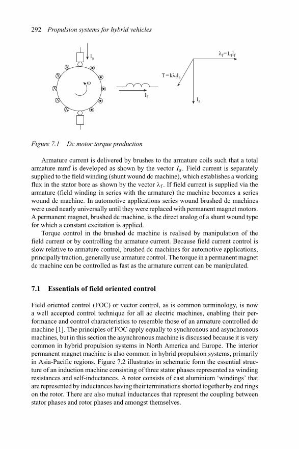
292 Propulsion systems for hybrid vehicles
X
Ia
If
T = kλfIa
λf = LfIf
Ia
ωX
X
X
X
Figure 7.1 Dc motor torque production
Armature current is delivered by brushes to the armature coils such that a totalarmature mmf is developed as shown by the vector Ia . Field current is separatelysupplied to the field winding (shunt wound dc machine), which establishes a workingflux in the stator bore as shown by the vector λf . If field current is supplied via thearmature (field winding in series with the armature) the machine becomes a serieswound dc machine. In automotive applications series wound brushed dc machineswere used nearly universally until they were replaced with permanent magnet motors.A permanent magnet, brushed dc machine, is the direct analog of a shunt wound typefor which a constant excitation is applied.
Torque control in the brushed dc machine is realised by manipulation of thefield current or by controlling the armature current. Because field current control isslow relative to armature control, brushed dc machines for automotive applications,principally traction, generally use armature control. The torque in a permanent magnetdc machine can be controlled as fast as the armature current can be manipulated.
7.1 Essentials of field oriented control
Field oriented control (FOC) or vector control, as is common terminology, is nowa well accepted control technique for all ac electric machines, enabling their per-formance and control characteristics to resemble those of an armature controlled dcmachine [1]. The principles of FOC apply equally to synchronous and asynchronousmachines, but in this section the asynchronous machine is discussed because it is verycommon in hybrid propulsion systems in North America and Europe. The interiorpermanent magnet machine is also common in hybrid propulsion systems, primarilyin Asia-Pacific regions. Figure 7.2 illustrates in schematic form the essential struc-ture of an induction machine consisting of three stator phases represented as windingresistances and self-inductances. A rotor consists of cast aluminium ‘windings’ thatare represented by inductances having their terminations shorted together by end ringson the rotor. There are also mutual inductances that represent the coupling betweenstator phases and rotor phases and amongst themselves.
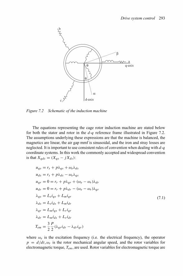
Drive system control 293
a
b
q-axis
d-axisc
β
α
θ
θ
Figure 7.2 Schematic of the induction machine
The equations representing the cage rotor induction machine are stated belowfor both the stator and rotor in the d-q reference frame illustrated in Figure 7.2.The assumptions underlying these expressions are that the machine is balanced, themagnetics are linear, the air gap mmf is sinusoidal, and the iron and stray losses areneglected. It is important to use consistent rules of convention when dealing with d-qcoordinate systems. In this work the commonly accepted and widespread conventionis that Xqds = (Xqs − jXds):
uqs = rs + pλqs + ωeλds
uds = rs + pλds − ωeλqs
uqr = 0 = rr + pλqr + (ωe − ωr)λdr
udr = 0 = rr + pλdr − (ωe − ωr)λqr
λqs = Lsiqs + Lmiqr
λds = Lsids + Lmidr
λqr = Lmiqs + Lriqr
λdr = Lmids + Lridr
Tem = 3
2
P
2(λqr idr − λdr iqr )
(7.1)
where ωe is the excitation frequency (i.e. the electrical frequency), the operatorp = d/dt , ωr is the rotor mechanical angular speed, and the rotor variables forelectromagnetic torque, Tem, are used. Rotor variables for electromagnetic torque are
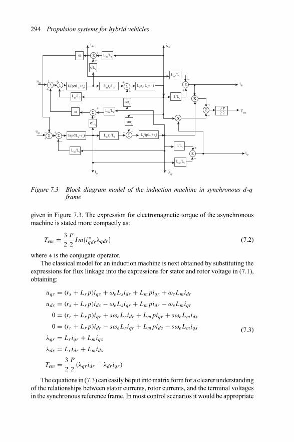
294 Propulsion systems for hybrid vehicles
ΣΣ
Σ
Σ
Σ
Σ
Σ Σ
Σ Σ
Σω
ω
Lm/Lr
1/Lr
1/Lr
Lr/(pLr+ rr)1/(pσLs+rs)
σLs
σLs
Lmrr/Lr
X
X
λqr
ids
uds
uqs
iqs
idr
Tem
iqr
+
+
+
+ +
+
+
+
+
+
+
+
+
+
+
+
–
–
–
–
–
–
3 P2 2
Lm/Lr
Lm/Lr
sωe
Lm/Lr
Lmrr /LrLr/(pLr+rr)1/(pσLs+rs)
Lm/Lr
Lm/Lr
λdr
sωe
Figure 7.3 Block diagram model of the induction machine in synchronous d-qframe
given in Figure 7.3. The expression for electromagnetic torque of the asynchronousmachine is stated more compactly as:
Tem = 3
2
P
2Im{i∗qdrλqdr} (7.2)
where ∗ is the conjugate operator.The classical model for an induction machine is next obtained by substituting the
expressions for flux linkage into the expressions for stator and rotor voltage in (7.1),obtaining:
uqs = (rs + Lsp)iqs + ωeLsids + Lmpiqr + ωeLmidr
uds = (rs + Lsp)ids − ωeLsiqs + Lmpidr − ωeLmiqr
0 = (rr + Lrp)iqr + sωeLr idr + Lmpiqr + sωeLmids
0 = (rr + Lrp)idr − sωeLr iqr + Lmpids − sωeLmiqs
λqr = Lriqr + Lmiqs
λdr = Lridr + Lmids
Tem = 3
2
P
2(λqr idr − λdr iqr )
(7.3)
The equations in (7.3) can easily be put into matrix form for a clearer understandingof the relationships between stator currents, rotor currents, and the terminal voltagesin the synchronous reference frame. In most control scenarios it would be appropriate
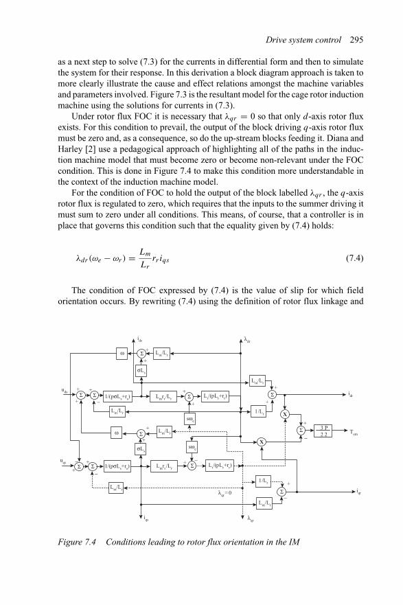
Drive system control 295
as a next step to solve (7.3) for the currents in differential form and then to simulatethe system for their response. In this derivation a block diagram approach is taken tomore clearly illustrate the cause and effect relations amongst the machine variablesand parameters involved. Figure 7.3 is the resultant model for the cage rotor inductionmachine using the solutions for currents in (7.3).
Under rotor flux FOC it is necessary that λqr = 0 so that only d-axis rotor fluxexists. For this condition to prevail, the output of the block driving q-axis rotor fluxmust be zero and, as a consequence, so do the up-stream blocks feeding it. Diana andHarley [2] use a pedagogical approach of highlighting all of the paths in the induc-tion machine model that must become zero or become non-relevant under the FOCcondition. This is done in Figure 7.4 to make this condition more understandable inthe context of the induction machine model.
For the condition of FOC to hold the output of the block labelled λqr , the q-axisrotor flux is regulated to zero, which requires that the inputs to the summer driving itmust sum to zero under all conditions. This means, of course, that a controller is inplace that governs this condition such that the equality given by (7.4) holds:
λdr(ωe − ωr) = Lm
Lr
rr iqs (7.4)
The condition of FOC expressed by (7.4) is the value of slip for which fieldorientation occurs. By rewriting (7.4) using the definition of rotor flux linkage and
ΣΣ
Σ
Σ
Σ
Σ
Σ Σ
Σ Σ
Σω
ω
Lm/Lr
1/Lr
1/Lr
Lr/(pLr+rr)1/(pσLs+rs)
σLs
σLs
Lmrr /Lr
X
X
λqr
λqr= 0
ids
uds
uqs
iqs
idr
Tem
iqr
+
+
+
+ +
+
+
+
+
+
+
+
+
+
+
+
–
–
–
–
–
–
3 P2 2
Lm/Lr
Lm/Lr
sωe
Lm/Lr
Lmrr /LrLr/(pLr+rr)1/(pσLs+rs)
Lm/Lr
Lm/Lr
λdr
sωe
Figure 7.4 Conditions leading to rotor flux orientation in the IM
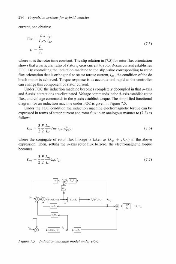
296 Propulsion systems for hybrid vehicles
current, one obtains:
sωe = Lm
Lrτr
iqs
idr
τr = Lr
rr
(7.5)
where τr is the rotor time constant. The slip relation in (7.5) for rotor flux orientationshows that a particular ratio of stator q-axis current to rotor d-axis current establishesFOC. By controlling the induction machine to the slip value corresponding to rotorflux orientation that is orthogonal to stator torque current, iqs , the condition of the dcbrush motor is achieved. Torque response is as accurate and rapid as the controllercan change this component of stator current.
Under FOC the induction machine becomes completely decoupled in that q-axisand d-axis interactions are eliminated. Voltage commands in the d-axis establish rotorflux, and voltage commands in the q-axis establish torque. The simplified functionaldiagram for an induction machine under FOC is given in Figure 7.5.
Under the FOC condition the induction machine electromagnetic torque can beexpressed in terms of stator current and rotor flux in an analogous manner to (7.2) asfollows.
Tem = 3
2
P
2
Lm
Lr
Im{iqdsλ∗qdr} (7.6)
where the conjugate of rotor flux linkage is taken as (λqr + jλdr ) in the aboveexpression. Then, setting the q-axis rotor flux to zero, the electromagnetic torquebecomes
Tem = 3
2
P
2
Lm
Lr
λdr iqs (7.7)
X
Σ
Σ
Σ
Σω Lm/Lr
Lr /(pLr+ rr)1/(pσLs+rs)
σLs
iqs
ids
λdrLmrr /Lr
uds
uqs
Tem
+
+
+
+ +
+
–
–
3 P2 2
Lm/Lr
ωeσLs
Lm/Lr1/(pσLs+rs)
Figure 7.5 Induction machine model under FOC
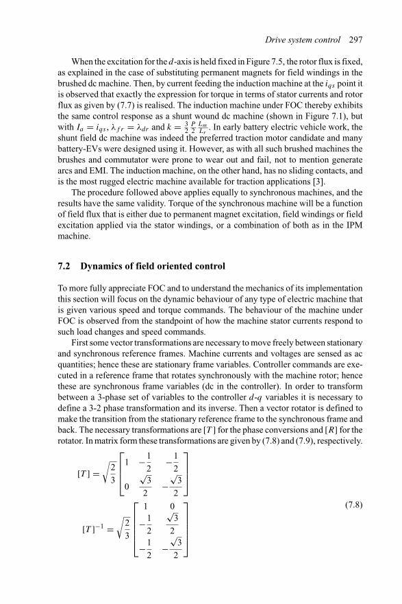
Drive system control 297
When the excitation for the d-axis is held fixed in Figure 7.5, the rotor flux is fixed,as explained in the case of substituting permanent magnets for field windings in thebrushed dc machine. Then, by current feeding the induction machine at the iqs point itis observed that exactly the expression for torque in terms of stator currents and rotorflux as given by (7.7) is realised. The induction machine under FOC thereby exhibitsthe same control response as a shunt wound dc machine (shown in Figure 7.1), butwith Ia = iqs , λf r = λdr and k = 3
2P2
Lm
Lr. In early battery electric vehicle work, the
shunt field dc machine was indeed the preferred traction motor candidate and manybattery-EVs were designed using it. However, as with all such brushed machines thebrushes and commutator were prone to wear out and fail, not to mention generatearcs and EMI. The induction machine, on the other hand, has no sliding contacts, andis the most rugged electric machine available for traction applications [3].
The procedure followed above applies equally to synchronous machines, and theresults have the same validity. Torque of the synchronous machine will be a functionof field flux that is either due to permanent magnet excitation, field windings or fieldexcitation applied via the stator windings, or a combination of both as in the IPMmachine.
7.2 Dynamics of field oriented control
To more fully appreciate FOC and to understand the mechanics of its implementationthis section will focus on the dynamic behaviour of any type of electric machine thatis given various speed and torque commands. The behaviour of the machine underFOC is observed from the standpoint of how the machine stator currents respond tosuch load changes and speed commands.
First some vector transformations are necessary to move freely between stationaryand synchronous reference frames. Machine currents and voltages are sensed as acquantities; hence these are stationary frame variables. Controller commands are exe-cuted in a reference frame that rotates synchronously with the machine rotor; hencethese are synchronous frame variables (dc in the controller). In order to transformbetween a 3-phase set of variables to the controller d-q variables it is necessary todefine a 3-2 phase transformation and its inverse. Then a vector rotator is defined tomake the transition from the stationary reference frame to the synchronous frame andback. The necessary transformations are [T ] for the phase conversions and [R] for therotator. In matrix form these transformations are given by (7.8) and (7.9), respectively.
[T ] =√
2
3
⎡⎢⎢⎣
1 −1
2−1
2
0
√3
2−
√3
2
⎤⎥⎥⎦
[T ]−1 =√
2
3
⎡⎢⎢⎢⎢⎣
1 0
−1
2
√3
2
−1
2−
√3
2
⎤⎥⎥⎥⎥⎦
(7.8)
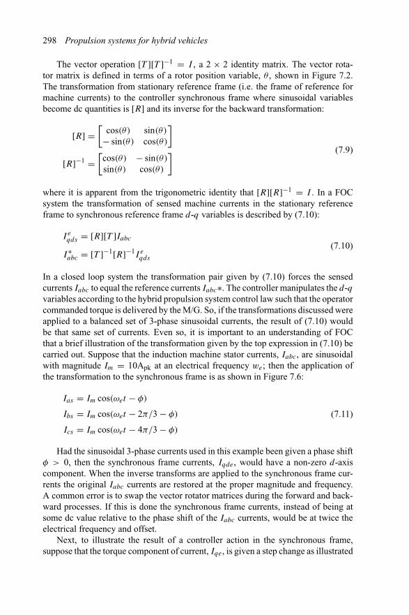
298 Propulsion systems for hybrid vehicles
The vector operation [T ][T ]−1 = I , a 2 × 2 identity matrix. The vector rota-tor matrix is defined in terms of a rotor position variable, θ , shown in Figure 7.2.The transformation from stationary reference frame (i.e. the frame of reference formachine currents) to the controller synchronous frame where sinusoidal variablesbecome dc quantities is [R] and its inverse for the backward transformation:
[R] =[
cos(θ) sin(θ)
− sin(θ) cos(θ)
]
[R]−1 =[
cos(θ) − sin(θ)
sin(θ) cos(θ)
] (7.9)
where it is apparent from the trigonometric identity that [R][R]−1 = I . In a FOCsystem the transformation of sensed machine currents in the stationary referenceframe to synchronous reference frame d-q variables is described by (7.10):
I eqds = [R][T ]Iabc
I ∗abc = [T ]−1[R]−1I e
qds
(7.10)
In a closed loop system the transformation pair given by (7.10) forces the sensedcurrents Iabc to equal the reference currents Iabc∗. The controller manipulates the d-qvariables according to the hybrid propulsion system control law such that the operatorcommanded torque is delivered by the M/G. So, if the transformations discussed wereapplied to a balanced set of 3-phase sinusoidal currents, the result of (7.10) wouldbe that same set of currents. Even so, it is important to an understanding of FOCthat a brief illustration of the transformation given by the top expression in (7.10) becarried out. Suppose that the induction machine stator currents, Iabc, are sinusoidalwith magnitude Im = 10Apk at an electrical frequency we; then the application ofthe transformation to the synchronous frame is as shown in Figure 7.6:
Ias = Im cos(ωet − φ)
Ibs = Im cos(ωet − 2π/3 − φ)
Ics = Im cos(ωet − 4π/3 − φ)
(7.11)
Had the sinusoidal 3-phase currents used in this example been given a phase shiftφ > 0, then the synchronous frame currents, Iqde, would have a non-zero d-axiscomponent. When the inverse transforms are applied to the synchronous frame cur-rents the original Iabc currents are restored at the proper magnitude and frequency.A common error is to swap the vector rotator matrices during the forward and back-ward processes. If this is done the synchronous frame currents, instead of being atsome dc value relative to the phase shift of the Iabc currents, would be at twice theelectrical frequency and offset.
Next, to illustrate the result of a controller action in the synchronous frame,suppose that the torque component of current, Iqe, is given a step change as illustrated
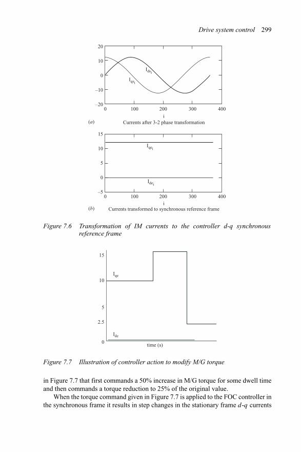
Drive system control 299
20
10
Iqsi
Iqei
Idsi
Idei
0
0 100 200 300 400
–10
–20
15
10
5
0 100 200 300 400
0
–5
Currents after 3-2 phase transformation
Currents transformed to synchronous reference frame
(a)
(b)i
i
Figure 7.6 Transformation of IM currents to the controller d-q synchronousreference frame
15
10
5
2.5
0time (s)
Ide
Iqe
Figure 7.7 Illustration of controller action to modify M/G torque
in Figure 7.7 that first commands a 50% increase in M/G torque for some dwell timeand then commands a torque reduction to 25% of the original value.
When the torque command given in Figure 7.7 is applied to the FOC controller inthe synchronous frame it results in step changes in the stationary frame d-q currents
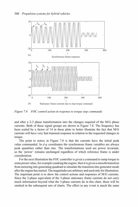
300 Propulsion systems for hybrid vehicles
20
0
0 100 200i
300 400–20
Iqsi Idsi
IaiIbi Ici
i0 100 200 300 400
–20
–10
0
10
20
Synchronous frame response
Stationary frame currents due to step torque command
(a)
(b)
Figure 7.8 FOC control action in response to torque step commands
and after a 2-3 phase transformation into the changes required of the M/G phasecurrents. Both of these signal groups are shown in Figure 7.8. The frequency hasbeen scaled by a factor of 14 in these plots to better illustrate the fact that M/Gcurrents will have very fast transient response in relation to the requested changes intorque.
The point to notice in Figure 7.8 is that the currents have the initial peakvalue commanded. In d-q coordinates the synchronous frame variables are alwayspeak quantities rather than rms. The transformations used are power invariant,so the ‘power’ remains unchanged regardless of which reference frame is underconsideration.
For the next illustration the FOC controller is given a command to ramp torque tosome preset value, for example cranking the engine; then it is given a smooth transitionfrom motoring into generating quadrant to simulate the transition into generator modeafter the engine has started. The magnitudes are arbitrary and used only for illustration.The important point is to show the control actions and responses of M/G currents.Since the 2-phase equivalent of the 3-phase stationary frame currents do not carrymuch information beyond what the 3-phase currents do in this chart, these will beomitted in the subsequent sets of charts. The effect in any event is much the same
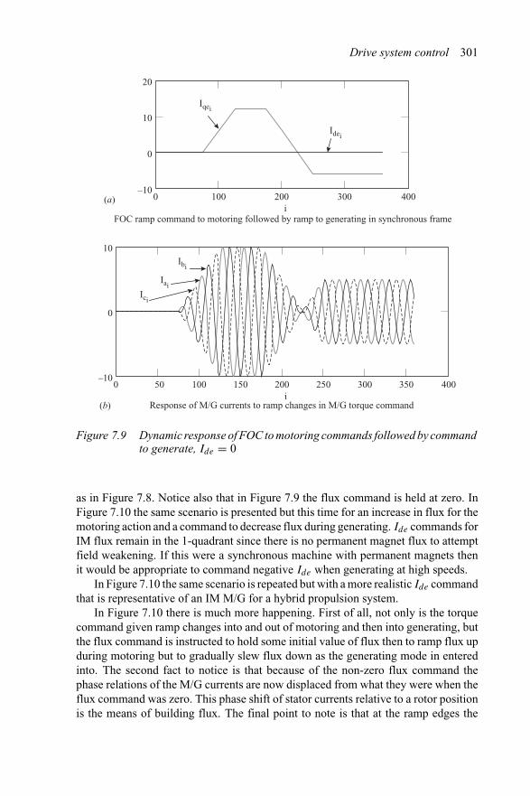
Drive system control 301
Iqei
Iai
Ibi
Ici
Idei
i
i
–10
0
10
20
0 100 200
FOC ramp command to motoring followed by ramp to generating in synchronous frame
Response of M/G currents to ramp changes in M/G torque command
300 400
–10
0
10
0 50 100 150 200 250 300 350 400
(a)
(b)
Figure 7.9 Dynamic response of FOC to motoring commands followed by commandto generate, Ide = 0
as in Figure 7.8. Notice also that in Figure 7.9 the flux command is held at zero. InFigure 7.10 the same scenario is presented but this time for an increase in flux for themotoring action and a command to decrease flux during generating. Ide commands forIM flux remain in the 1-quadrant since there is no permanent magnet flux to attemptfield weakening. If this were a synchronous machine with permanent magnets thenit would be appropriate to command negative Ide when generating at high speeds.
In Figure 7.10 the same scenario is repeated but with a more realistic Ide commandthat is representative of an IM M/G for a hybrid propulsion system.
In Figure 7.10 there is much more happening. First of all, not only is the torquecommand given ramp changes into and out of motoring and then into generating, butthe flux command is instructed to hold some initial value of flux then to ramp flux upduring motoring but to gradually slew flux down as the generating mode in enteredinto. The second fact to notice is that because of the non-zero flux command thephase relations of the M/G currents are now displaced from what they were when theflux command was zero. This phase shift of stator currents relative to a rotor positionis the means of building flux. The final point to note is that at the ramp edges the
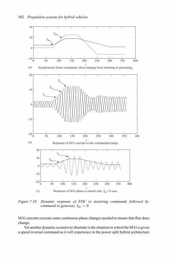
302 Propulsion systems for hybrid vehicles
i
i
i
–10
0
10
20
0 50 100 150 200 250 300 350 400
–20
–10
0
10
20
0 50 100 150 200 250 300 350 400
–20
–10
0
10
20
0 50 100 150 200 250 300 350 400
Iqei
Iai
Ibi
Ici
Idei
Iai
Idei
Synchronous frame commands when ramping from motoring to generating
Response of M/G currents to the commanded ramps
Response of M/G phase-a current only, Ide > 0 case
(a)
(b)
(c)
Figure 7.10 Dynamic response of FOC to motoring commands followed bycommand to generate, Ide > 0
M/G currents execute some continuous phase changes needed to ensure that flux doeschange.
Yet another dynamic scenario to illustrate is the situation in which the M/G is givena speed reversal command as it will experience in the power split hybrid architecture
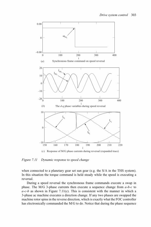
Drive system control 303
iSynchronous frame command on speed reversal
The d-q phase variables during speed reversal
Response of M/G phase currents during reversal (expanded trace)i
0.08
–0.08
0
0 100 200 300 400
i0 100 200 300 400
–20
–10
0
10
20
–10
0
10
150 160 170 180 190 200 210 220
ωesi
Iqsi
Iai
Ibi
Ici
Idsi
(a)
(b)
(c)
Figure 7.11 Dynamic response to speed change
when connected to a planetary gear set sun gear (e.g. the S/A in the THS system).In this situation the torque command is held steady while the speed is executing areversal.
During a speed reversal the synchronous frame commands execute a swap inphase. The M/G 3-phase currents then execute a sequence change from a-b-c toa-c-b as shown in Figure 7.11(c). This is consistent with the manner in which a3-phase ac machine executes a direction change. If any two phases are swapped themachine rotor spins in the reverse direction, which is exactly what the FOC controllerhas electronically commanded the M/G to do. Notice that during the phase sequence
304 Propulsion systems for hybrid vehicles
change one of the phase currents is completely undisturbed while the remaining twophases slew very rapidly to their new sequence.
7.3 Sensorless control
The topic of position sensorless control of ac drive systems is particularly relevantto hybrid propulsion systems. Not only are mechanical position sensors difficult tointegrate into and package within the vehicle driveline, but they are fragile and suscep-tible to EMI and signal distortion. It would be a great advantage to minimise positionsensor requirements or to eliminate the need entirely if adequate software algorithmswere available to perform the function of tracking the M/G rotor position accurately.Not only is rotor position sensor degradation an issue in maintaining smooth controlof the hybrid M/G system, but corruption of the position signal introduces distur-bances into the voltage and current controllers that have a tendency to unbalancethe machine excitation and cause noise and vibration. An intermittent sensor is evenmore insidious because the effect may come and go from just driving over a potholeor other road disturbance.
Many investigators have tackled the problem of sensor elimination for the var-ious types of electric machines. Before noting what has been done to eliminateposition sensors, it should be noted that different machines require fundamentallydifferent types of rotor position sensing. Synchronous machines, such as perma-nent magnet types, require a very accurate indication of where the rotor magnetis so that armature current can be maintained in quadrature to the rotor flux. Thisrequires an absolute position sensor that resolves shaft position to typically <0.2◦mechanical. In higher pole count electric machines the mechanical resolution ofposition is even higher. To resolve to an angle of 0.176◦ mechanical requires an11 bit encoder or resolver. Another complication is that not only is an 11 bit wordlength required to resolve position, but bit rate is very high in the case of M/Gsrated for 13 000 rpm. Then high bandwidth resolvers are necessary that have suffi-cient bit rate to deliver accurate position information to the controller at very fastupdate rates.
Variable and switched reluctance machines can have even more stringent positionsensing requirements than the permanent magnet machines. Many hybrid architec-tures of the ISG variety use VRM designs that are based on 6/4 saliency patternrepeated two, three or more times about the periphery of the machine. To suchmachines, 0.1◦ resolution or higher are necessary for proper timing of the signals.Such position sensors are more likely laboratory grade and, sometimes of precisioninstrument quality, not the rugged sensor demanded in an automotive environment.
Rajashekara et al. [4] provide a comprehensive summary of position sensor-less techniques employed on the five major electric machine types. In Table 7.1 asummary of the common types of sensorless methods investigated, or under investi-gation, are given referenced by ac machine type. In all position sensorless techniquesthere is strong reliance on accurate measurement of machine currents, voltages andtemperature environment.
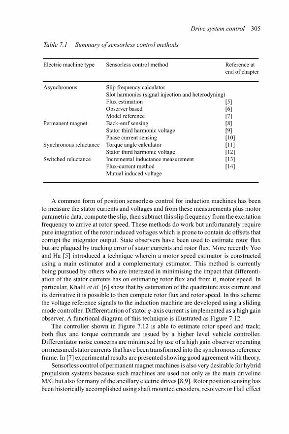
Drive system control 305
Table 7.1 Summary of sensorless control methods
Electric machine type Sensorless control method Reference atend of chapter
Asynchronous Slip frequency calculatorSlot harmonics (signal injection and heterodyning)Flux estimation [5]Observer based [6]Model reference [7]
Permanent magnet Back-emf sensing [8]Stator third harmonic voltage [9]Phase current sensing [10]
Synchronous reluctance Torque angle calculator [11]Stator third harmonic voltage [12]
Switched reluctance Incremental inductance measurement [13]Flux-current method [14]Mutual induced voltage
A common form of position sensorless control for induction machines has beento measure the stator currents and voltages and from these measurements plus motorparametric data, compute the slip, then subtract this slip frequency from the excitationfrequency to arrive at rotor speed. These methods do work but unfortunately requirepure integration of the rotor induced voltages which is prone to contain dc offsets thatcorrupt the integrator output. State observers have been used to estimate rotor fluxbut are plagued by tracking error of stator currents and rotor flux. More recently Yooand Ha [5] introduced a technique wherein a motor speed estimator is constructedusing a main estimator and a complementary estimator. This method is currentlybeing pursued by others who are interested in minimising the impact that differenti-ation of the stator currents has on estimating rotor flux and from it, motor speed. Inparticular, Khalil et al. [6] show that by estimation of the quadrature axis current andits derivative it is possible to then compute rotor flux and rotor speed. In this schemethe voltage reference signals to the induction machine are developed using a slidingmode controller. Differentiation of stator q-axis current is implemented as a high gainobserver. A functional diagram of this technique is illustrated as Figure 7.12.
The controller shown in Figure 7.12 is able to estimate rotor speed and track;both flux and torque commands are issued by a higher level vehicle controller.Differentiator noise concerns are minimised by use of a high gain observer operatingon measured stator currents that have been transformed into the synchronous referenceframe. In [7] experimental results are presented showing good agreement with theory.
Sensorless control of permanent magnet machines is also very desirable for hybridpropulsion systems because such machines are used not only as the main drivelineM/G but also for many of the ancillary electric drives [8,9]. Rotor position sensing hasbeen historically accomplished using shaft mounted encoders, resolvers or Hall effect
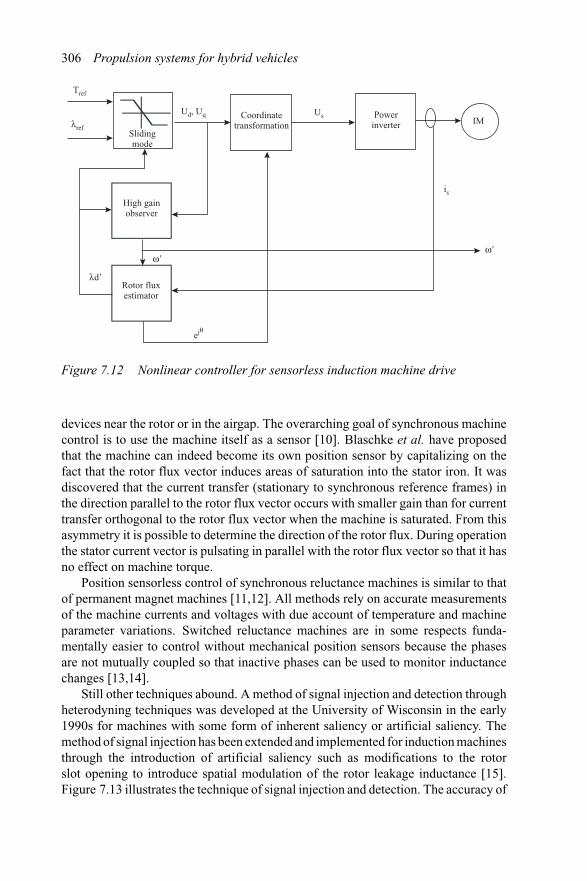
306 Propulsion systems for hybrid vehicles
Tref
λref
Ud, Uq Us
is
ejθ
λd�
ω�ω�
Slidingmode
Coordinatetransformation
Powerinverter
High gainobserver
Rotor fluxestimator
IM
Figure 7.12 Nonlinear controller for sensorless induction machine drive
devices near the rotor or in the airgap. The overarching goal of synchronous machinecontrol is to use the machine itself as a sensor [10]. Blaschke et al. have proposedthat the machine can indeed become its own position sensor by capitalizing on thefact that the rotor flux vector induces areas of saturation into the stator iron. It wasdiscovered that the current transfer (stationary to synchronous reference frames) inthe direction parallel to the rotor flux vector occurs with smaller gain than for currenttransfer orthogonal to the rotor flux vector when the machine is saturated. From thisasymmetry it is possible to determine the direction of the rotor flux. During operationthe stator current vector is pulsating in parallel with the rotor flux vector so that it hasno effect on machine torque.
Position sensorless control of synchronous reluctance machines is similar to thatof permanent magnet machines [11,12]. All methods rely on accurate measurementsof the machine currents and voltages with due account of temperature and machineparameter variations. Switched reluctance machines are in some respects funda-mentally easier to control without mechanical position sensors because the phasesare not mutually coupled so that inactive phases can be used to monitor inductancechanges [13,14].
Still other techniques abound. A method of signal injection and detection throughheterodyning techniques was developed at the University of Wisconsin in the early1990s for machines with some form of inherent saliency or artificial saliency. Themethod of signal injection has been extended and implemented for induction machinesthrough the introduction of artificial saliency such as modifications to the rotorslot opening to introduce spatial modulation of the rotor leakage inductance [15].Figure 7.13 illustrates the technique of signal injection and detection. The accuracy of
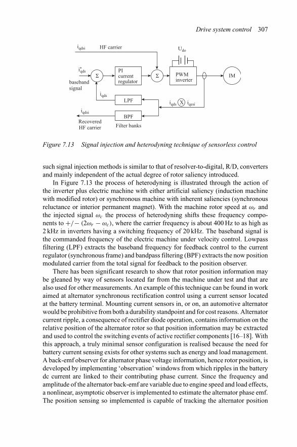
Drive system control 307
iqdsi
i*qds
iqds
iqdsi
iqds
Udo
iqesi
HF carrier
basebandsignal
PIcurrentregulator
PWMinverter
RecoveredHF carrier Filter banks
IM
XLPF
BPF
Σ Σ
Figure 7.13 Signal injection and heterodyning technique of sensorless control
such signal injection methods is similar to that of resolver-to-digital, R/D, convertersand mainly independent of the actual degree of rotor saliency introduced.
In Figure 7.13 the process of heterodyning is illustrated through the action ofthe inverter plus electric machine with either artificial saliency (induction machinewith modified rotor) or synchronous machine with inherent saliencies (synchronousreluctance or interior permanent magnet). With the machine rotor speed at ωr andthe injected signal ωc the process of heterodyning shifts these frequency compo-nents to +/− (2ωr − ωc), where the carrier frequency is about 400 Hz to as high as2 kHz in inverters having a switching frequency of 20 kHz. The baseband signal isthe commanded frequency of the electric machine under velocity control. Lowpassfiltering (LPF) extracts the baseband frequency for feedback control to the currentregulator (synchronous frame) and bandpass filtering (BPF) extracts the now positionmodulated carrier from the total signal for feedback to the position observer.
There has been significant research to show that rotor position information maybe gleaned by way of sensors located far from the machine under test and that arealso used for other measurements. An example of this technique can be found in workaimed at alternator synchronous rectification control using a current sensor locatedat the battery terminal. Mounting current sensors in, or on, an automotive alternatorwould be prohibitive from both a durability standpoint and for cost reasons. Alternatorcurrent ripple, a consequence of rectifier diode operation, contains information on therelative position of the alternator rotor so that position information may be extractedand used to control the switching events of active rectifier components [16–18]. Withthis approach, a truly minimal sensor configuration is realised because the need forbattery current sensing exists for other systems such as energy and load management.A back-emf observer for alternator phase voltage information, hence rotor position, isdeveloped by implementing ‘observation’ windows from which ripples in the batterydc current are linked to their contributing phase current. Since the frequency andamplitude of the alternator back-emf are variable due to engine speed and load effects,a nonlinear, asymptotic observer is implemented to estimate the alternator phase emf.The position sensing so implemented is capable of tracking the alternator position
308 Propulsion systems for hybrid vehicles
to within a constant offset, and has dynamic capability to track speed changes of+/−1000 Hz/s.
Flux linkage based techniques are gaining popularity for permanent magnetmachine sensorless position control. Historically, permanent magnet machine sensor-less techniques have included back-emf sensing directly from the inert phase in 120◦conduction drives, from flux-linkage methods based on machine voltage and currentsusing integration, and even by monitoring the conduction times of the inverter free-wheeling diodes. Kim et al. [19] have recently introduced a new flux-linkage-derived,but speed-independent, method. In this method pairs of line-to-line speed-dependentfunctions containing voltage and current measurements along with derivatives ofcurrent are divided. The resultant function contains the rotor angle information, butis speed-independent, and hence capable of estimating rotor position to very lowspeed. In an experimental setup the method was found to control a 4-pole brushlessdc machine to 20 rpm in the laboratory.
The literature on mechanical position transducerless motion control systems isextensive and new techniques are reported each year. However, to date there havebeen no reliable means of detecting rotor position of synchronous machines to zerospeed other than the method of heterodyning.
7.4 Efficiency optimisation
Optimisation of the drive system in a hybrid vehicle is crucial to its overall energymanagement strategy. In the induction machine, for example, there is a conflictover which flux setting to use, flux for maximum torque, or flux for maximumefficiency. When prioritized as flux for optimum efficiency it generally turns outthat torque/ampere suffers, especially when not corrected for battery voltage changes[20]. Figure 7.14 illustrates a technique whereby machine flux can be adjusted toapproach maximum torque/ampere or to deliver optimum efficiency depending ondriver demand.
In Figure 7.14 there are two command signals, two monitor signals and twooutput signals necessary to realise efficiency optimisation and flux programming.Commands are issued for M/G torque T ∗
e and stator flux level λ∗s . Flux programming
is generally in the upstream controller where it can be either a table look up based ontorque and M/G speed, or it can be programmed as a function of those variables. A fluxprogram is required in any M/G controller that enters field weakening. In the caseof IM and IPM machines, in particular, the flux program must hold machine fluxconstant during the voltage ramp up phase of control (i.e. during constant torqueoperation), then decrease flux command inversely with speed during field weakeningoperation. The flux command during field weakening should also be adjusted so thatefficiency is optimised as high flux levels in an M/G at high speed tend to exact highercore losses.
To ensure that the M/G controller hold its commands for flux in a range appro-priate for the system limitations and speed regime two signals are monitored: M/Gstator resistance Rs and the energy storage system dc link voltage Udc. It has been
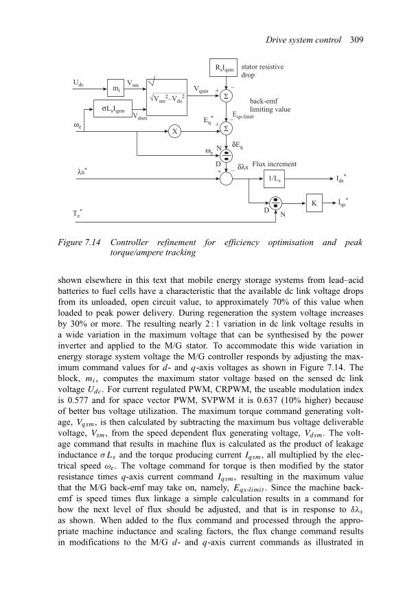
Drive system control 309
Udc
δEq
Eq*
Ids*
Iqs*
Eqs-limit
Vsm
Vdsm
1/Ls
σLsIqsm
RsIqsm
√Vsm2–Vds
2
mi Vqsm
ωe
ωe
Te*
λs* δλs
X Σ
Σ
N
N
K
D
D
+
+
+
–
–
–
stator resistivedrop
back-emflimiting value
Flux increment
Figure 7.14 Controller refinement for efficiency optimisation and peaktorque/ampere tracking
shown elsewhere in this text that mobile energy storage systems from lead–acidbatteries to fuel cells have a characteristic that the available dc link voltage dropsfrom its unloaded, open circuit value, to approximately 70% of this value whenloaded to peak power delivery. During regeneration the system voltage increasesby 30% or more. The resulting nearly 2 : 1 variation in dc link voltage results ina wide variation in the maximum voltage that can be synthesised by the powerinverter and applied to the M/G stator. To accommodate this wide variation inenergy storage system voltage the M/G controller responds by adjusting the max-imum command values for d- and q-axis voltages as shown in Figure 7.14. Theblock, mi , computes the maximum stator voltage based on the sensed dc linkvoltage Udc. For current regulated PWM, CRPWM, the useable modulation indexis 0.577 and for space vector PWM, SVPWM it is 0.637 (10% higher) becauseof better bus voltage utilization. The maximum torque command generating volt-age, Vqsm, is then calculated by subtracting the maximum bus voltage deliverablevoltage, Vsm, from the speed dependent flux generating voltage, Vdsm. The volt-age command that results in machine flux is calculated as the product of leakageinductance σLs and the torque producing current Iqsm, all multiplied by the elec-trical speed ωe. The voltage command for torque is then modified by the statorresistance times q-axis current command Iqsm, resulting in the maximum valuethat the M/G back-emf may take on, namely, Eqs-limit . Since the machine back-emf is speed times flux linkage a simple calculation results in a command forhow the next level of flux should be adjusted, and that is in response to δλs
as shown. When added to the flux command and processed through the appro-priate machine inductance and scaling factors, the flux change command resultsin modifications to the M/G d- and q-axis current commands as illustrated in
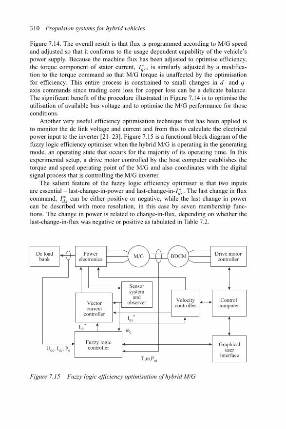
310 Propulsion systems for hybrid vehicles
Figure 7.14. The overall result is that flux is programmed according to M/G speedand adjusted so that it conforms to the usage dependent capability of the vehicle’spower supply. Because the machine flux has been adjusted to optimise efficiency,the torque component of stator current, I ∗
qs , is similarly adjusted by a modifica-tion to the torque command so that M/G torque is unaffected by the optimisationfor efficiency. This entire process is constrained to small changes in d- and q-axis commands since trading core loss for copper loss can be a delicate balance.The significant benefit of the procedure illustrated in Figure 7.14 is to optimise theutilisation of available bus voltage and to optimise the M/G performance for thoseconditions.
Another very useful efficiency optimisation technique that has been applied isto monitor the dc link voltage and current and from this to calculate the electricalpower input to the inverter [21–23]. Figure 7.15 is a functional block diagram of thefuzzy logic efficiency optimiser when the hybrid M/G is operating in the generatingmode, an operating state that occurs for the majority of its operating time. In thisexperimental setup, a drive motor controlled by the host computer establishes thetorque and speed operating point of the M/G and also coordinates with the digitalsignal process that is controlling the M/G inverter.
The salient feature of the fuzzy logic efficiency optimiser is that two inputsare essential – last-change-in-power and last-change-in-I ∗
ds . The last change in fluxcommand, I ∗
ds can be either positive or negative, while the last change in powercan be described with more resolution, in this case by seven membership func-tions. The change in power is related to change-in-flux, depending on whether thelast-change-in-flux was negative or positive as tabulated in Table 7.2.
Dc loadbank
Drive motorcontroller
Controlcomputer
Graphicaluser
interface
VelocitycontrollerVector
currentcontroller
Sensorsystem
andobserver
Fuzzy logiccontroller
Powerelectronics M/G BDCM
Ids*
Iqs*
Udc, Idc, Pe
T,ω,Pm
ωe
Figure 7.15 Fuzzy logic efficiency optimisation of hybrid M/G
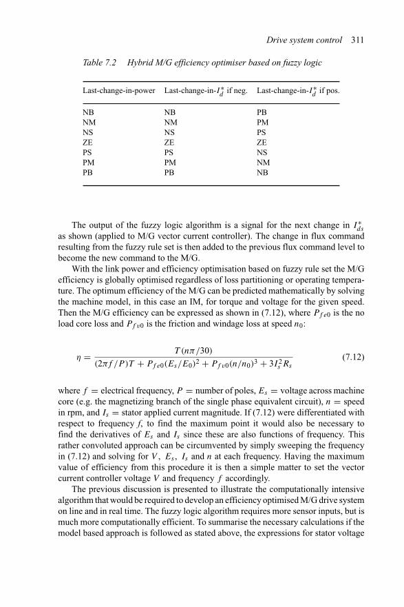
Drive system control 311
Table 7.2 Hybrid M/G efficiency optimiser based on fuzzy logic
Last-change-in-power Last-change-in-I∗d
if neg. Last-change-in-I∗d
if pos.
NB NB PBNM NM PMNS NS PSZE ZE ZEPS PS NSPM PM NMPB PB NB
The output of the fuzzy logic algorithm is a signal for the next change in I ∗ds
as shown (applied to M/G vector current controller). The change in flux commandresulting from the fuzzy rule set is then added to the previous flux command level tobecome the new command to the M/G.
With the link power and efficiency optimisation based on fuzzy rule set the M/Gefficiency is globally optimised regardless of loss partitioning or operating tempera-ture. The optimum efficiency of the M/G can be predicted mathematically by solvingthe machine model, in this case an IM, for torque and voltage for the given speed.Then the M/G efficiency can be expressed as shown in (7.12), where Pf e0 is the noload core loss and Pf v0 is the friction and windage loss at speed n0:
η = T (nπ/30)
(2πf /P )T + Pf e0(Es/E0)2 + Pf v0(n/n0)3 + 3I 2s Rs
(7.12)
where f = electrical frequency, P = number of poles, Es = voltage across machinecore (e.g. the magnetizing branch of the single phase equivalent circuit), n = speedin rpm, and Is = stator applied current magnitude. If (7.12) were differentiated withrespect to frequency f, to find the maximum point it would also be necessary tofind the derivatives of Es and Is since these are also functions of frequency. Thisrather convoluted approach can be circumvented by simply sweeping the frequencyin (7.12) and solving for V , Es , Is and n at each frequency. Having the maximumvalue of efficiency from this procedure it is then a simple matter to set the vectorcurrent controller voltage V and frequency f accordingly.
The previous discussion is presented to illustrate the computationally intensivealgorithm that would be required to develop an efficiency optimised M/G drive systemon line and in real time. The fuzzy logic algorithm requires more sensor inputs, but ismuch more computationally efficient. To summarise the necessary calculations if themodel based approach is followed as stated above, the expressions for stator voltage
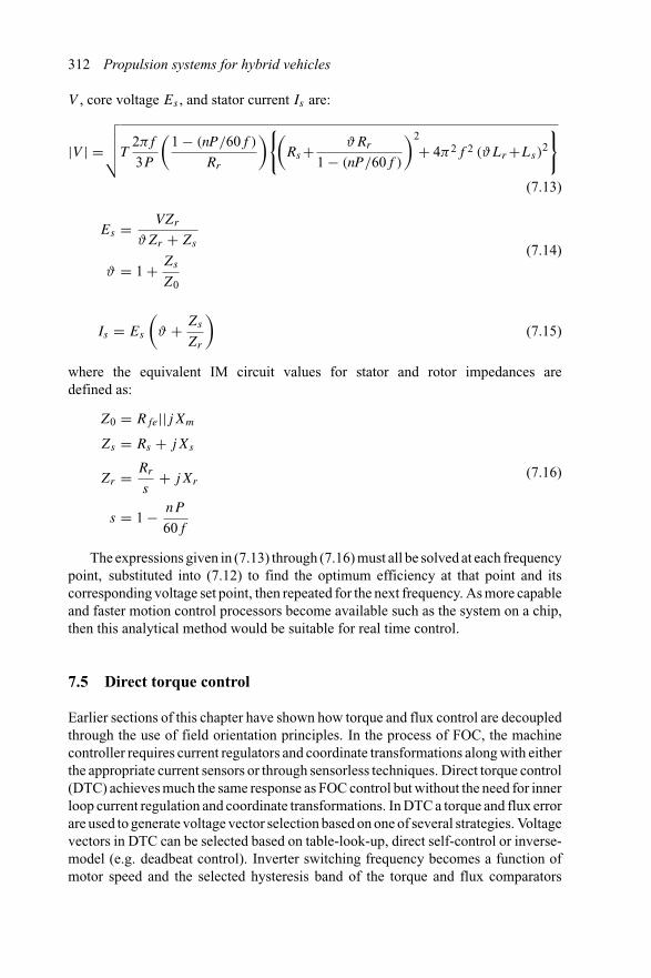
312 Propulsion systems for hybrid vehicles
V , core voltage Es , and stator current Is are:
|V | =√√√√T
2πf
3P
(1 − (nP/60f )
Rr
){(Rs + ϑRr
1 − (nP/60f )
)2
+ 4π2f 2 (ϑLr +Ls)2
}
(7.13)
Es = VZr
ϑZr + Zs
ϑ = 1 + Zs
Z0
(7.14)
Is = Es
(ϑ + Zs
Zr
)(7.15)
where the equivalent IM circuit values for stator and rotor impedances aredefined as:
Z0 = Rfe||jXm
Zs = Rs + jXs
Zr = Rr
s+ jXr
s = 1 − nP
60f
(7.16)
The expressions given in (7.13) through (7.16) must all be solved at each frequencypoint, substituted into (7.12) to find the optimum efficiency at that point and itscorresponding voltage set point, then repeated for the next frequency. As more capableand faster motion control processors become available such as the system on a chip,then this analytical method would be suitable for real time control.
7.5 Direct torque control
Earlier sections of this chapter have shown how torque and flux control are decoupledthrough the use of field orientation principles. In the process of FOC, the machinecontroller requires current regulators and coordinate transformations along with eitherthe appropriate current sensors or through sensorless techniques. Direct torque control(DTC) achieves much the same response as FOC control but without the need for innerloop current regulation and coordinate transformations. In DTC a torque and flux errorare used to generate voltage vector selection based on one of several strategies. Voltagevectors in DTC can be selected based on table-look-up, direct self-control or inverse-model (e.g. deadbeat control). Inverter switching frequency becomes a function ofmotor speed and the selected hysteresis band of the torque and flux comparators
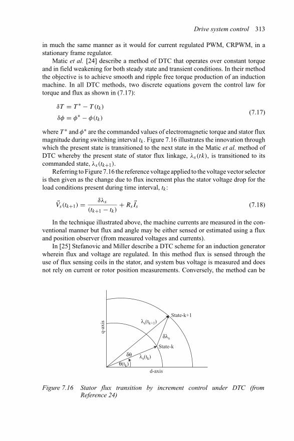
Drive system control 313
in much the same manner as it would for current regulated PWM, CRPWM, in astationary frame regulator.
Matic et al. [24] describe a method of DTC that operates over constant torqueand in field weakening for both steady state and transient conditions. In their methodthe objective is to achieve smooth and ripple free torque production of an inductionmachine. In all DTC methods, two discrete equations govern the control law fortorque and flux as shown in (7.17):
δT = T ∗ − T (tk)
δφ = φ∗ − φ(tk)(7.17)
where T ∗ and φ∗ are the commanded values of electromagnetic torque and stator fluxmagnitude during switching interval tk . Figure 7.16 illustrates the innovation throughwhich the present state is transitioned to the next state in the Matic et al. method ofDTC whereby the present state of stator flux linkage, λs(tk), is transitioned to itscommanded state, λs(tk+1).
Referring to Figure 7.16 the reference voltage applied to the voltage vector selectoris then given as the change due to flux increment plus the stator voltage drop for theload conditions present during time interval, tk:
�Vs(tk+1) = δλs
(tk+1 − tk)+ Rs
�Is (7.18)
In the technique illustrated above, the machine currents are measured in the con-ventional manner but flux and angle may be either sensed or estimated using a fluxand position observer (from measured voltages and currents).
In [25] Stefanovic and Miller describe a DTC scheme for an induction generatorwherein flux and voltage are regulated. In this method flux is sensed through theuse of flux sensing coils in the stator, and system bus voltage is measured and doesnot rely on current or rotor position measurements. Conversely, the method can be
q-ax
is
d-axis
State-k
State-k+1
θ(tk)λs(tk)
δλs
δθ
λs(tk+1)
Figure 7.16 Stator flux transition by increment control under DTC (fromReference 24)
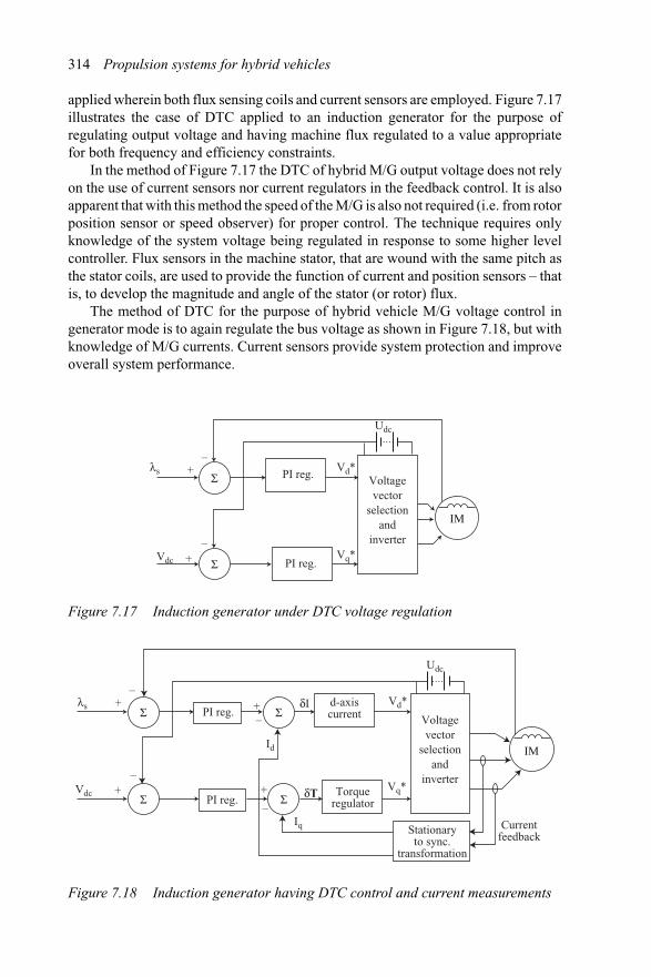
314 Propulsion systems for hybrid vehicles
applied wherein both flux sensing coils and current sensors are employed. Figure 7.17illustrates the case of DTC applied to an induction generator for the purpose ofregulating output voltage and having machine flux regulated to a value appropriatefor both frequency and efficiency constraints.
In the method of Figure 7.17 the DTC of hybrid M/G output voltage does not relyon the use of current sensors nor current regulators in the feedback control. It is alsoapparent that with this method the speed of the M/G is also not required (i.e. from rotorposition sensor or speed observer) for proper control. The technique requires onlyknowledge of the system voltage being regulated in response to some higher levelcontroller. Flux sensors in the machine stator, that are wound with the same pitch asthe stator coils, are used to provide the function of current and position sensors – thatis, to develop the magnitude and angle of the stator (or rotor) flux.
The method of DTC for the purpose of hybrid vehicle M/G voltage control ingenerator mode is to again regulate the bus voltage as shown in Figure 7.18, but withknowledge of M/G currents. Current sensors provide system protection and improveoverall system performance.
PI reg.
PI reg.
Vq*
Vd*
Udc
Vdc +–
+–
λsΣ
Σ
ΙΜ
Voltagevector
selectionand
inverter
Figure 7.17 Induction generator under DTC voltage regulation
d-axiscurrent
Torqueregulator
Currentfeedback
Stationaryto sync.
transformation
PI reg.
PI reg.Vq*
Vd*
Iq
Id
Vdc +–
+ +
+
–
–
–
λs δI
δT
ΙΜ
ΣΣ
ΣΣ
Voltagevector
selectionand
inverter
Udc
Figure 7.18 Induction generator having DTC control and current measurements
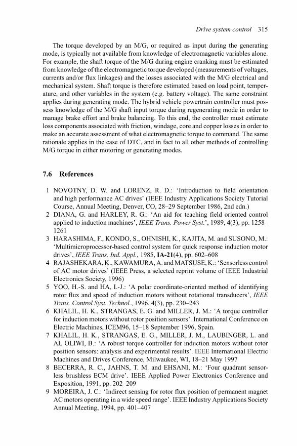
Drive system control 315
The torque developed by an M/G, or required as input during the generatingmode, is typically not available from knowledge of electromagnetic variables alone.For example, the shaft torque of the M/G during engine cranking must be estimatedfrom knowledge of the electromagnetic torque developed (measurements of voltages,currents and/or flux linkages) and the losses associated with the M/G electrical andmechanical system. Shaft torque is therefore estimated based on load point, temper-ature, and other variables in the system (e.g. battery voltage). The same constraintapplies during generating mode. The hybrid vehicle powertrain controller must pos-sess knowledge of the M/G shaft input torque during regenerating mode in order tomanage brake effort and brake balancing. To this end, the controller must estimateloss components associated with friction, windage, core and copper losses in order tomake an accurate assessment of what electromagnetic torque to command. The samerationale applies in the case of DTC, and in fact to all other methods of controllingM/G torque in either motoring or generating modes.
7.6 References
1 NOVOTNY, D. W. and LORENZ, R. D.: ‘Introduction to field orientationand high performance AC drives’ (IEEE Industry Applications Society TutorialCourse, Annual Meeting, Denver, CO, 28–29 September 1986, 2nd edn.)
2 DIANA, G. and HARLEY, R. G.: ‘An aid for teaching field oriented controlapplied to induction machines’, IEEE Trans. Power Syst.’, 1989, 4(3), pp. 1258–1261
3 HARASHIMA, F., KONDO, S., OHNISHI, K., KAJITA, M. and SUSONO, M.:‘Multimicroprocessor-based control system for quick response induction motordrives’, IEEE Trans. Ind. Appl., 1985, IA-21(4), pp. 602–608
4 RAJASHEKARA, K., KAWAMURA, A. and MATSUSE, K.: ‘Sensorless controlof AC motor drives’ (IEEE Press, a selected reprint volume of IEEE IndustrialElectronics Society, 1996)
5 YOO, H.-S. and HA, I.-J.: ‘A polar coordinate-oriented method of identifyingrotor flux and speed of induction motors without rotational transducers’, IEEETrans. Control Syst. Technol., 1996, 4(3), pp. 230–243
6 KHALIL, H. K., STRANGAS, E. G. and MILLER, J. M.: ‘A torque controllerfor induction motors without rotor position sensors’. International Conference onElectric Machines, ICEM96, 15–18 September 1996, Spain.
7 KHALIL, H. K., STRANGAS, E. G., MILLER, J. M., LAUBINGER, L. andAL OLIWI, B.: ‘A robust torque controller for induction motors without rotorposition sensors: analysis and experimental results’. IEEE International ElectricMachines and Drives Conference, Milwaukee, WI, 18–21 May 1997
8 BECERRA, R. C., JAHNS, T. M. and EHSANI, M.: ‘Four quadrant sensor-less brushless ECM drive’. IEEE Applied Power Electronics Conference andExposition, 1991, pp. 202–209
9 MOREIRA, J. C.: ‘Indirect sensing for rotor flux position of permanent magnetAC motors operating in a wide speed range’. IEEE Industry Applications SocietyAnnual Meeting, 1994, pp. 401–407
316 Propulsion systems for hybrid vehicles
10 BLASCHKE, F., BURGT, J. V.-D. and VANDENPUT, A.: ‘Sensorless directfield orientation at zero flux frequency’. Conference Record IEEE 31st IndustryApplications Society Annual Meeting, Hotel Del Coronado, San Diego, CA, 6–10October 1996
11 AREFEEN, M. S., EHSANI, M. and LIPO, T. A.: ‘Elimination of discrete posi-tion sensor for synchronous reluctance motor’. Conference Record IEEE PowerElectronics Specialists Conference, 1993, pp. 440–445
12 XU, L., NOVOTNY, D. W., LIPO, T. A. and XU, X.: ‘Vector control of a syn-chronous reluctance motor including saturation and iron losses’. Proceedings ofthe IEEE Industry Applications Society Annual Meeting, 1990, pp. 359–364.
13 BASS, J. T., EHSANI, M. and MILLER, T. J. E.: ‘Robust torque control ofswitched reluctance motor without a shaft position sensor’, IEEE Trans. on Ind.Electron., 1986, IE-33(3), pp. 212–216
14 HUSAIN, I. and EHSANI, M.: ‘Rotor position sensing in switched reluctancemotor drives by measuring mutually induced voltages’, IEEE Trans. Ind. Appl.,1994, 30, pp. 665–672
15 JANSEN, P. L. and LORENZ, R. D.: ‘Transducerless position and velocityestimation in induction and salient AC machines’. IEEE Industry ApplicationsSociety Annual Meeting, 1994
16 UTKIN, V. I., CHEN, D.-S., ZAREI, S. and MILLER, J. M.: ‘Synchronous rec-tification of the automotive alternator using sliding mode observer’. Proceedingsof the American Controls Conference, Albuquerque, NM, 4–6 June 1997
17 DRAKUNOV, S., UTKIN, V., ZAREI, S. and MILLER, J. M.: ‘Sliding modeobservers for automotive applications’. Proceedings of the 1996 IEEE Interna-tional Conference on Control Applications, Dearborn, MI, 15–18 September1996.
18 UTKIN, V. I., CHEN, D.-S., ZAREI, S. and MILLER, J. M.: ‘Discrete timesliding mode observer for automotive alternator’. Proceedings of the EuropeanControls Conference, ECC97, Brussels, Belgium, July 1997
19 KIM, T.-H., LEE, B.-K. and EHSANI, M.: ‘Sensorless control of the BLDCmotors from near zero to high speed’. IEEE Applied Power Electronics Confer-ence and Exposition, Fontainbleau Hotel, Miami Beach, FL, 9–13 February 2003
20 DENG, D. and XU, X.: US Patent 5,739,664 ‘Induction motor drive controller’,issued 14 April 1998
21 SEPE, R., Jr. and MILLER, J. M.: ‘Intelligent efficiency mapping of a hybrid elec-tric vehicle starter/alternator using fuzzy logic’. 18th Digital Avionics SystemsConference, St. Louis, MO, 24–29 October 1999.
22 SEPE, R.B., Jr. and MILLER, J. M.: ‘Real-time collaborative experimenta-tion via the internet: fuzzy efficiency optimisation of a hybrid electric vehiclestarter/alternator’, Int. J. Veh. Des., IJVD-SPE-CAE2002, November 2002.
23 SEPE, R. B., Jr., MORRISON, C., MILLER, J. M. and GALE, A.: ‘High effi-ciency operation of a hybrid electric vehicle starter/generator over road profiles’.IEEE Industry Applications Society Annual Meeting, Industrial Automation &Controls Committee, Hyatt-Regency Hotel, Miracle Mile, Chicago, IL, October2001

Drive system control 317
24 MATIC, P., BLANUSA, B. and VUKOSAVIC, S.: ‘A novel direct torque andflux control algorithm for the induction motor drive’. IEEE International ElectricMachines and Drives Conference, Monona Terrace Conference Center, Madison,WI, 1–4 June 2003, pp. 965–970
25 STEFANOVIC, V. R. and MILLER, J. M.: ‘Method of controlling an inductiongenerator’. US Patent 6,417,650 issued 9 July 2002.

Chapter 8
Drive system efficiency
It should not be surprising that the most important attribute of today’s hybrid propul-sion system is that total driveline efficiency exceed 80%. When vehicle fuel economyis in excess of 40 mpg, a 100 W power loss due to core heating in the traction motoror its attendant power inverter represents a significant impact. Weight is another veryimportant attribute, but its impact is not as noticeable until performance on gradesis required. This chapter provides an assessment of the complete hybrid drive sys-tem and where the prominent loss mechanisms reside. Particular attention is paidto the traction M/G core and copper losses and the inverter conduction and switch-ing losses. Mechanical friction contributions are noted, particularly with regard tonon-conventional designs due to adding the hybrid components.
An illustration of a non-conventional contributor to friction would be the need fora large diameter bearing to support the otherwise cantilevered mass of a crankshaftmounted starter-alternator. In single clutch, or M/G to transmission torque converterarrangements, there is a tendency to have large shifts in M/G rotor centre of gravityfrom the crankshaft main journal bearing and the potential to have this rotor executelarge deviations in whirl as the unsupported end has no means to resist crankshaftbounce and whirl. An auxiliary large diameter bearing is then incorporated on theoutboard rotor side for support.
8.1 Traction motor
By and large the most significant contributor to hybrid propulsion system efficiencyis the electric machine. M/G losses are comprised of iron (core) losses, copper ( jouleheating), mechanical friction (bearing system), windage and stray losses. CharlesProteus Steinmetz completed his doctoral work at the University of Breslau, Germany,and in 1889 immigrated to the US and later joined the General Electric Company inSchenectady, NY. In the early 1890s Steinmetz developed and published one of themost seminal works on the theory of magnetic hysteresis, the phenomena in whichthe magnetization in a metal can have two values depending on whether the field
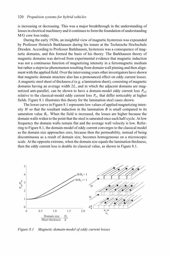
320 Propulsion systems for hybrid vehicles
is increasing or decreasing. This was a major breakthrough in the understanding oflosses in electrical machinery and it continues to form the foundation of understandingM/G core loss today.
During the early 1920s, an insightful view of magnetic hysteresis was expoundedby Professor Heinrich Barkhausen during his tenure at the Technische HochschuleDresden. According to Professor Barkhausen, hysteresis was a consequence of mag-netic domains, and this formed the basis of his theory. The Barkhausen theory ofmagnetic domains was derived from experimental evidence that magnetic inductionwas not a continuous function of magnetizing intensity in a ferromagnetic mediumbut rather a stepwise phenomenon resulting from domain wall pinning and then align-ment with the applied field. Over the intervening years other investigators have shownthat magnetic domain structure also has a pronounced effect on eddy current losses.A magnetic steel sheet of thickness d (e.g. a lamination sheet), consisting of magneticdomains having an average width 2L, and in which the adjacent domains are mag-netized anti-parallel, can be shown to have a domain-model eddy current loss Ped
relative to the classical-model eddy current loss Pec that differ noticeably at higherfields. Figure 8.1 illustrates this theory for the lamination steel cases shown.
The lower curve in Figure 8.1 represents low values of applied magnetizing inten-sity H so that the resultant induction in the lamination B is small compared to itssaturation value Bs . When the field is increased, the losses are higher because thedomain walls widen to the point that the steel is saturated once each half-cycle. At lowfrequency the domain walls remain flat and the average wall velocity is low. Refer-ring to Figure 8.1, the domain-model of eddy current converges to the classical modelas the domain size approaches zero, because then the permeability, instead of beingdiscontinuous as a result of domain size, becomes homogeneous on a microscopicscale. At the opposite extreme, when the domain size equals the lamination thickness,then the eddy current loss is double its classical value, as shown in Figure 8.1.
P ed/
P ec B/Bs << 1
B/Bs = 1
Domain size 2LSheet thickness d
2L
d
H
H
5
4
3
2
1
00 0.5 1.0 1.5 2.0
Figure 8.1 Magnetic domain-model of eddy current losses
Drive system efficiency 321
The underlying theory of domain-model eddy current loss is that the spatialinhomogeneity of permeability due to domain size leads to higher eddy current lossesthan what would otherwise be calculated using the classical Steinmetz model. Inferromagnetic material the eddy currents are localized to the moving domain walls,where it can reach high values. Because of this localized eddy current flow the lossesare higher than if the currents were more evenly distributed in the lamination. There-fore, the larger the domain size in the magnetic steel, the fewer are the domain walls,and the faster they must move in response to a given flux change at a given frequency.
The components of core loss can be summarised as [1]:
• Classical eddy current losses that result from circulating currents in the bulk ironmaterial are produced by changing magnetic fields. For example, an M/G that isdesigned for 5 V/turn will have 5 V/macro circulating path in the iron laminations.This induced voltage gives rise to circulating currents that dissipate power as Jouleheating in the iron. Bulk circulating currents can be minimised by increasing thematerial resistivity (e.g. add silicon, aluminum, phosphorous, manganese, etc.)or by decreasing the lamination thickness. However, lower thickness flat rolledsteels can have issues with surface texture, surface treatment and coatings.
• Anomalous eddy current losses are generated by circulating currents as a resultof flux changes due to uniform domain wall motion. In typical magnetic steelshaving grain sizes of 100 μm there may be two magnetic domains per grain. Theempirical relation for anomalous eddy current loss due to domain wall motion is
Pe_wm = Gs
√Hwmσf 3B
where Hwm is the hysteresis dependency on grain size Gs . Small grain size resultsin lower domain wall velocity and high hysteresis, whereas large grain size resultsin low hysteresis component. In other words, there is an optimal grain size foreach specific frequency of operation. Decreasing the material conductivity willlower the loss.
• Hysteresis loss is caused by alternating currents induced by erratic domain wallmotion. Domain walls are pinned at precipitates, so minimisation calls for lowsilicon, carbon and nitrogen content. The presence of inclusions resulting frominsufficient time to float out slag, plus lattice defects due to re-crystallization, andtendencies to relatively large grain size will all increase hysteresis loss. Further-more, magnetoelastic effects due to lattice strain and surface strain are reducedthrough annealing and surface coating.
Net core losses in the hybrid propulsion traction motor can be substantial andaccountable for some integral percentage of overall fuel economy loss. The next twosections cover the classical loss model and some extensions that are applicable tocalculating core losses in hybrid M/G.
8.1.1 Core losses
Iron losses in soft ferromagnetic materials are classically separated into hysteresis andeddy current components, Ph and Pe [2]. It can be said that hysteresis loss is caused by
322 Propulsion systems for hybrid vehicles
localized irreversible changes as magnetizing intensity is cycled within the confinesof the materials saturation level of induction. When there are no minor hysteresisloops to contend with, the classical Steinmetz equation for core loss applies:
Pcore = Ph + Pe
Pcore = khmcorefBα + kemcore(fB)2 (8.1)
where the coefficients kh and ke are in W/kg and core mass is in kg. The hysteresiscomponent exponent on induction is in the range 1.6 < α < 2.2. Some authors also addan additional term to (8.1) to account for high frequency harmonic losses to accountfor inverter drive switching frequency components in M/G voltage. Others prefer tocondense the entire expression given by (8.1) into a single term with a coefficienteasily extracted from manufacturer data sheets on the particular sheet steel used.Equation (8.2) illustrates this format.
Pcore = kcore
(B
Bs
)α (ω
ω0
)β
α = 1.9
β = 1.6
(8.2)
where kcore is the data sheet value for core loss at the normalized induction B0 andexcitation frequency ω0. For a typical good quality steel used in hybrid M/G, such asTempel M19, the value of the loss coefficient kcore is 1.5 × 10⁻⁵ W/kg at B0 = 1 T,and ω0 = 2π(400).
In hybrid propulsion systems the switching converter does introduce voltage (andcurrent) harmonics that contribute additional core losses through the excitation ofminor hysteresis loops in the magnetic steels employed in the designs. This effect canbe accounted for if the component loss coefficients given in (8.1) are made functionsof the induction. This augmented coefficient, K(B), has the property of adding anadditional excitation loss component to the total core loss expression:
Ph = khmcorefBαK(B)
K(B) = 1 + ch
B
n∑i
δB (8.3)
Ph = Phc + Ph_exc
where δB is the incremental induction change due to an excursion about a minorhysteresis loop. Figure 8.2 illustrates the major and minor hysteresis loops used inthe context of this discussion.
Classical eddy current losses are calculated based on the lamination steel electricalconductivity, geometry and magnetic characteristics. Equation (8.4) illustrates theclassical case and a more recent modification where the earlier sinusoidal time varying
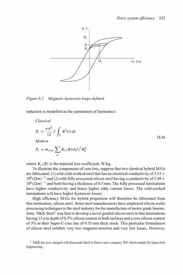
Drive system efficiency 323
H, A/m
B, T
Bs
Br
Ha
B
Figure 8.2 Magnetic hysteresis loops defined
induction is modelled as the summation of harmonics:
Classical
Pe = σd2
12f
∫T
B2(t) dt
Modern
Pe = mcore
∑k
Ke(B)(kf )2B2k
(8.4)
where Ke(B) is the material loss coefficient, W/kg.To illustrate the components of core loss, suppose that two identical hybrid M/Gs
are fabricated: (1) with cold-worked steel that has an electrical conductivity of 3.33×10⁶(�m)−1 and (2) with fully processed silicon steel having a conductivity of 5.88×10⁶(�m)−1 and both having a thickness of 0.5 mm. The fully processed laminationshave higher conductivity and hence higher eddy current losses. The cold-workedlaminations will have higher hysteresis losses.
High efficiency M/Gs for hybrid propulsion will therefore be fabricated fromthin lamination, silicon steel. Some steel manufacturers have employed silicon waferprocessing techniques to the steel industry for the manufacture of motor grade lamina-tions. NKK Steel1 was first to develop a novel graded silicon steel in thin laminationshaving 15 μm depth of 6.5% silicon content at both surfaces and a core silicon contentof 3% in their Super-E core line of 0.35 mm thick stock. This particular formulationof silicon steel exhibits very low magneto-striction and very low losses. However,
1 NKK has now merged with Kawasaki Steel to form a new company JFE which stands for Japan IronEngineering.
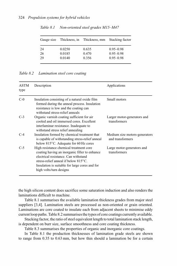
324 Propulsion systems for hybrid vehicles
Table 8.1 Non-oriented steel grades M15–M47
Gauge size Thickness, in Thickness, mm Stacking factor
24 0.0250 0.635 0.95–0.9826 0.0185 0.470 0.95–0.9829 0.0140 0.356 0.95–0.98
Table 8.2 Lamination steel core coating
ASTM Description Applicationstype
C-0 Insulation consisting of a natural oxide filmformed during the anneal process. Insulationresistance is low and the coating canwithstand stress-relief anneals
Small motors
C-3 Organic varnish coating sufficient for aircooled and oil immersed cores. Excellentinterlaminar resistance. Inadequate towithstand stress relief annealing
Larger motor-generators andtransformers
C-4 Insulation formed by chemical treatment thatis capable of withstanding stress-relief annealbelow 815◦C. Adequate for 60 Hz cores
Medium size motors-generatorsand transformers
C-5 High resistance chemical treatment corecoating having an inorganic filler to enhanceelectrical resistance. Can withstandstress-relief anneal if below 815◦C.Insulation is suitable for large cores and forhigh volts/turn designs
Large motor-generators andtransformers
the high silicon content does sacrifice some saturation induction and also renders thelaminations difficult to machine.
Table 8.1 summarises the available lamination thickness grades from major steelsuppliers [3,4]. Lamination steels are processed as non-oriented or grain oriented.Laminations are core coated to insulate each from adjacent sheets to minimise eddycurrent loop paths. Table 8.2 summarises the types of core coatings currently available.
Stacking factor, the ratio of steel equivalent length to total lamination stack length,is dependent on burr size, surface smoothness and core coating thickness.
Table 8.3 summarises the properties of organic and inorganic core coatings.In Table 8.1 the production thicknesses of lamination grade steels are shown
to range from 0.35 to 0.63 mm, but how thin should a lamination be for a certain
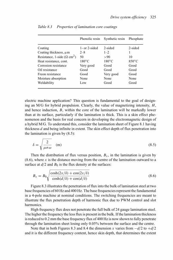
Drive system efficiency 325
Table 8.3 Properties of lamination core coatings
Phenolic resin Synthetic resin Phosphate
Coating 1- or 2-sided 2-sided 2-sidedCoating thickness, μm 2–8 1–2 1Resistance, 1-side (� cm2) 50 >90 10Heat resistance, cont. 180◦C 180◦C 850◦CCorrosion resistance Very good Good GoodOil resistance Good Good GoodFreon resistance Good Very good GoodMoisture absorption None None NoneWeldability Low Good Good
electric machine application? This question is fundamental to the goal of design-ing an M/G for hybrid propulsion. Clearly, the value of magnetizing intensity, H ,and hence induction, B, within the core of the lamination will be markedly lowerthan at its surface, particularly if the lamination is thick. This is a skin effect phe-nomenon and the basis for real concern in developing the electromagnetic design ofa hybrid M/G. To understand this, consider the lamination sheet of Figure 8.1 havingthickness d and being infinite in extent. The skin effect depth of flux penetration intothe lamination is given by (8.5):
δ =√
2
μσω(m) (8.5)
Then the distribution of flux versus position, Bx , in the lamination is given by(8.6), where x is the distance moving from the centre of the lamination outward to asurface at d/2 and B0 is the flux density at the surfaces:
Bx = B0
√cosh(2x/δ) + cos(2x/δ)
cosh(d/δ) + cos(d/δ)(8.6)
Figure 8.3 illustrates the penetration of flux into the bulk of lamination steel at twobase frequencies of 60 Hz and 400 Hz. The base frequencies represent the fundamentalin a 4-pole machine at nominal conditions. The switching frequencies are meant toillustrate the flux penetration depth of harmonic flux due to PWM control and slotharmonics.
High frequency flux does not penetrate the full bulk of 24 gauge lamination steel.The higher the frequency the less flux is present in the bulk. If the lamination thicknessis reduced to 0.2 mm the base frequency flux of 400 Hz is now shown to fully penetratethrough the lamination sheet losing only 0.05% between the surface and the centre.
Note that in both Figures 8.3 and 8.4 the dimension x varies from −d/2 to +d/2and it is the different frequency content, hence skin depth, that determines the extent
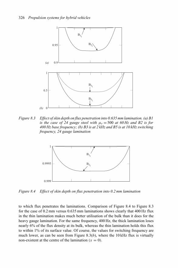
326 Propulsion systems for hybrid vehicles
1
0.95
B1i
B2i
B3i
B5i
0.9
1
0.5
0
(a)
(b)
Figure 8.3 Effect of skin depth on flux penetration into 0.635 mm lamination. (a) B1is the case of 24 gauge steel with μr = 500 at 60 Hz and B2 is for400 Hz base frequency; (b) B3 is at 2 kHz and B5 is at 10 kHz switchingfrequency, 24 gauge lamination
B1i
B2i
1
0.9995
0.999
Figure 8.4 Effect of skin depth on flux penetration into 0.2 mm lamination
to which flux penetrates the laminations. Comparison of Figure 8.4 to Figure 8.3for the case of 0.2 mm versus 0.635 mm laminations shows clearly that 400 Hz fluxin the thin lamination makes much better utilisation of the bulk than it does for theheavy gauge lamination. For the same frequency, 400 Hz, the thick lamination losesnearly 6% of the flux density at its bulk, whereas the thin lamination holds this fluxto within 1% of its surface value. Of course, the values for switching frequency aremuch lower, as can be seen from Figure 8.3(b), where the 10 kHz flux is virtuallynon-existent at the centre of the lamination (x = 0).
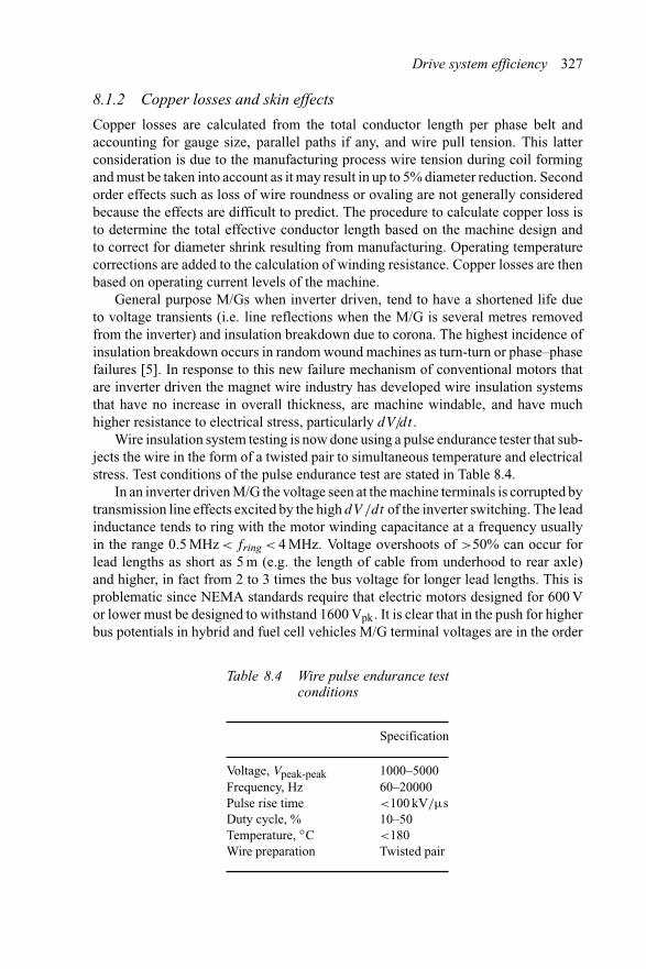
Drive system efficiency 327
8.1.2 Copper losses and skin effects
Copper losses are calculated from the total conductor length per phase belt andaccounting for gauge size, parallel paths if any, and wire pull tension. This latterconsideration is due to the manufacturing process wire tension during coil formingand must be taken into account as it may result in up to 5% diameter reduction. Secondorder effects such as loss of wire roundness or ovaling are not generally consideredbecause the effects are difficult to predict. The procedure to calculate copper loss isto determine the total effective conductor length based on the machine design andto correct for diameter shrink resulting from manufacturing. Operating temperaturecorrections are added to the calculation of winding resistance. Copper losses are thenbased on operating current levels of the machine.
General purpose M/Gs when inverter driven, tend to have a shortened life dueto voltage transients (i.e. line reflections when the M/G is several metres removedfrom the inverter) and insulation breakdown due to corona. The highest incidence ofinsulation breakdown occurs in random wound machines as turn-turn or phase–phasefailures [5]. In response to this new failure mechanism of conventional motors thatare inverter driven the magnet wire industry has developed wire insulation systemsthat have no increase in overall thickness, are machine windable, and have muchhigher resistance to electrical stress, particularly dV/dt .
Wire insulation system testing is now done using a pulse endurance tester that sub-jects the wire in the form of a twisted pair to simultaneous temperature and electricalstress. Test conditions of the pulse endurance test are stated in Table 8.4.
In an inverter driven M/G the voltage seen at the machine terminals is corrupted bytransmission line effects excited by the high dV /dt of the inverter switching. The leadinductance tends to ring with the motor winding capacitance at a frequency usuallyin the range 0.5 MHz < fring < 4 MHz. Voltage overshoots of >50% can occur forlead lengths as short as 5 m (e.g. the length of cable from underhood to rear axle)and higher, in fact from 2 to 3 times the bus voltage for longer lead lengths. This isproblematic since NEMA standards require that electric motors designed for 600 Vor lower must be designed to withstand 1600 Vpk. It is clear that in the push for higherbus potentials in hybrid and fuel cell vehicles M/G terminal voltages are in the order
Table 8.4 Wire pulse endurance testconditions
Specification
Voltage, Vpeak-peak 1000–5000Frequency, Hz 60–20000Pulse rise time <100 kV/μsDuty cycle, % 10–50Temperature, ◦C <180Wire preparation Twisted pair
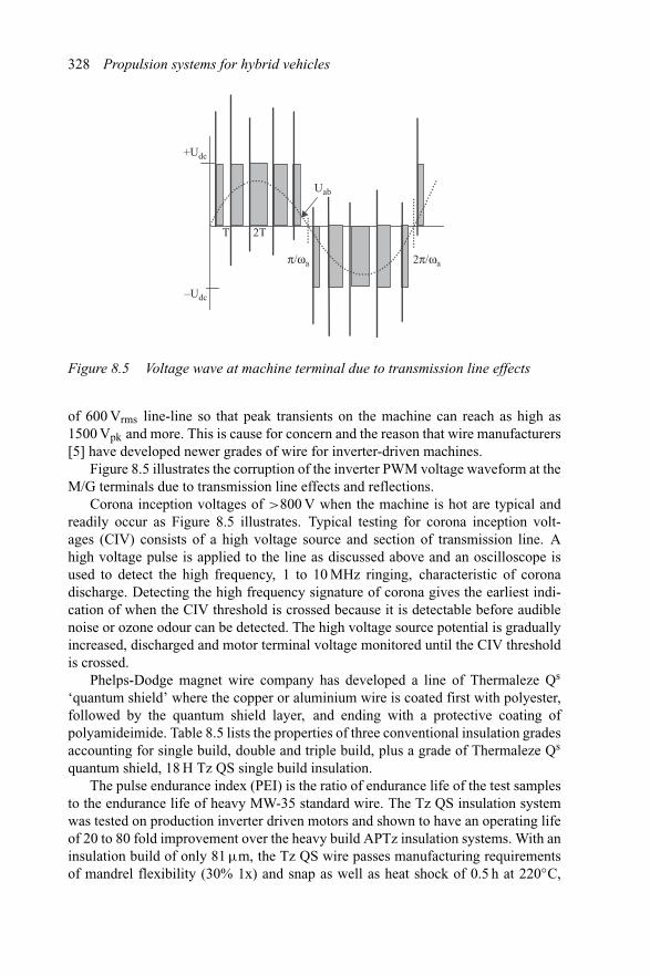
328 Propulsion systems for hybrid vehicles
+Udc
–Udc
Uab
T 2T
π/ωa 2π/ωa
Figure 8.5 Voltage wave at machine terminal due to transmission line effects
of 600 Vrms line-line so that peak transients on the machine can reach as high as1500 Vpk and more. This is cause for concern and the reason that wire manufacturers[5] have developed newer grades of wire for inverter-driven machines.
Figure 8.5 illustrates the corruption of the inverter PWM voltage waveform at theM/G terminals due to transmission line effects and reflections.
Corona inception voltages of >800 V when the machine is hot are typical andreadily occur as Figure 8.5 illustrates. Typical testing for corona inception volt-ages (CIV) consists of a high voltage source and section of transmission line. Ahigh voltage pulse is applied to the line as discussed above and an oscilloscope isused to detect the high frequency, 1 to 10 MHz ringing, characteristic of coronadischarge. Detecting the high frequency signature of corona gives the earliest indi-cation of when the CIV threshold is crossed because it is detectable before audiblenoise or ozone odour can be detected. The high voltage source potential is graduallyincreased, discharged and motor terminal voltage monitored until the CIV thresholdis crossed.
Phelps-Dodge magnet wire company has developed a line of Thermaleze Qs
‘quantum shield’ where the copper or aluminium wire is coated first with polyester,followed by the quantum shield layer, and ending with a protective coating ofpolyamideimide. Table 8.5 lists the properties of three conventional insulation gradesaccounting for single build, double and triple build, plus a grade of Thermaleze Qs
quantum shield, 18 H Tz QS single build insulation.The pulse endurance index (PEI) is the ratio of endurance life of the test samples
to the endurance life of heavy MW-35 standard wire. The Tz QS insulation systemwas tested on production inverter driven motors and shown to have an operating lifeof 20 to 80 fold improvement over the heavy build APTz insulation systems. With aninsulation build of only 81 μm, the Tz QS wire passes manufacturing requirementsof mandrel flexibility (30% 1x) and snap as well as heat shock of 0.5 h at 220◦C,
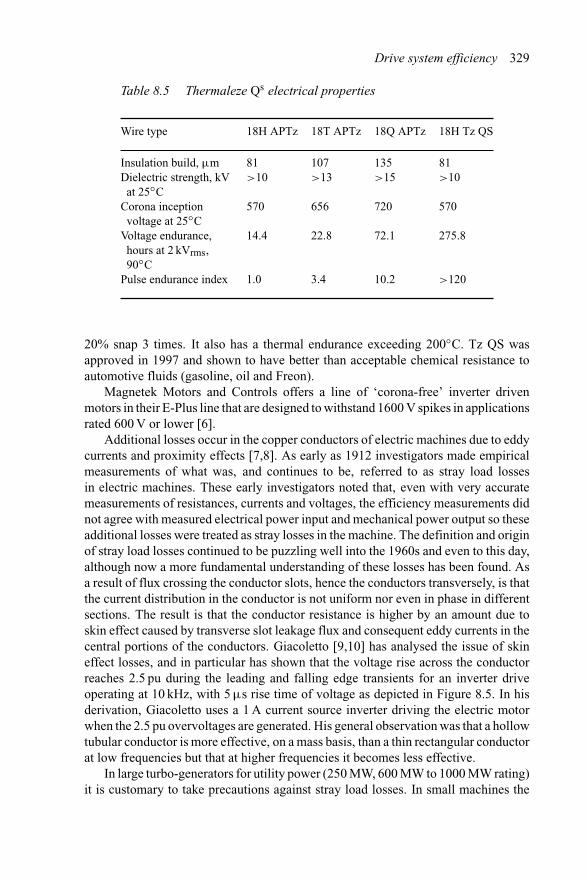
Drive system efficiency 329
Table 8.5 Thermaleze Qs electrical properties
Wire type 18H APTz 18T APTz 18Q APTz 18H Tz QS
Insulation build, μm 81 107 135 81Dielectric strength, kV
at 25◦C>10 >13 >15 >10
Corona inceptionvoltage at 25◦C
570 656 720 570
Voltage endurance,hours at 2 kVrms,90◦C
14.4 22.8 72.1 275.8
Pulse endurance index 1.0 3.4 10.2 >120
20% snap 3 times. It also has a thermal endurance exceeding 200◦C. Tz QS wasapproved in 1997 and shown to have better than acceptable chemical resistance toautomotive fluids (gasoline, oil and Freon).
Magnetek Motors and Controls offers a line of ‘corona-free’ inverter drivenmotors in their E-Plus line that are designed to withstand 1600 V spikes in applicationsrated 600 V or lower [6].
Additional losses occur in the copper conductors of electric machines due to eddycurrents and proximity effects [7,8]. As early as 1912 investigators made empiricalmeasurements of what was, and continues to be, referred to as stray load lossesin electric machines. These early investigators noted that, even with very accuratemeasurements of resistances, currents and voltages, the efficiency measurements didnot agree with measured electrical power input and mechanical power output so theseadditional losses were treated as stray losses in the machine. The definition and originof stray load losses continued to be puzzling well into the 1960s and even to this day,although now a more fundamental understanding of these losses has been found. Asa result of flux crossing the conductor slots, hence the conductors transversely, is thatthe current distribution in the conductor is not uniform nor even in phase in differentsections. The result is that the conductor resistance is higher by an amount due toskin effect caused by transverse slot leakage flux and consequent eddy currents in thecentral portions of the conductors. Giacoletto [9,10] has analysed the issue of skineffect losses, and in particular has shown that the voltage rise across the conductorreaches 2.5 pu during the leading and falling edge transients for an inverter driveoperating at 10 kHz, with 5 μs rise time of voltage as depicted in Figure 8.5. In hisderivation, Giacoletto uses a 1 A current source inverter driving the electric motorwhen the 2.5 pu overvoltages are generated. His general observation was that a hollowtubular conductor is more effective, on a mass basis, than a thin rectangular conductorat low frequencies but that at higher frequencies it becomes less effective.
In large turbo-generators for utility power (250 MW, 600 MW to 1000 MW rating)it is customary to take precautions against stray load losses. In small machines the
330 Propulsion systems for hybrid vehicles
stray load losses are noticeable and to some degree negligible. In very large machinesthe second and third order effects contributing to stray load losses become significantthermal design considerations. Armature winding stray load losses in large generatorsconsist of circulating current and eddy current loss originating from cross-slot leakageflux. A remedy has been to transpose the armature bars along the length of the statorso that their position changes from the top of the slot at one end, to the middleof the slot in the central section of the stator, and on to the bottom of the slot atthe opposite end. The typical armature bar transposition is 540◦, so that end turncoupling is also minimised. Even with such transposition of a conductor in verylarge machines it is common to still have a 20◦C temperature difference betweenconductors at the bottom of a slot and those at the top of a slot. The reason is thatcross-slot leakage is higher at the top coils so that higher eddy current losses areexperienced.
8.2 Inverter
Losses in the electronic power processor can be grouped into active component (semi-conductor) losses and passive component losses. Passive components experiencinglosses related to power throughput are the link capacitors, device snubbers if used,and current shunts if used. Active device losses are decomposed into conduction,switching and reverse recovery losses.
This section will give a brief introduction to inverter losses and some of thetraditional methods used to quantify inverter losses.
8.2.1 Conduction
Conduction loss in a power electronic inverter is due to the power dissipated in thesemiconductor chip by the simultaneous current and voltage stress. During ON-stateconduction a majority carrier device such as a MOSFET will experience a voltagedrop that is linearly proportional to the current through the device and the resistanceof the device. In the OFF-state the resistance increases by six orders of magnitude ormore. Minority carrier devices, on the other hand, experience conductivity modulationduring the ON-state and have a voltage drop across the device terminals that is alogarithmic function of the current through the device. IGBTs are representative ofminority carrier devices, as are diodes, bipolar transistors and thyristors.
The simplest device, the bipolar diode, has a voltage–current characteristic givenby the ideal diode equation (8.7), where k = 1.38 × 10⁻²³ J/◦K (i.e. the Boltzmannconstant), q = 1.602 × 10⁻¹⁹ coulomb is the electronic charge, T = 298 is thenominal temperature in Kelvin (◦K), and I0 is the diode saturation current ∼10−14A.At room temperature the diode voltage coefficient is 0.026 and at a forward current of10 A the diode voltage is 0.9 V. Power diodes at higher currents will have a differentvalue of saturation current:
VD = kT
qln(
I
I0
)(V) (8.7)
Drive system efficiency 331
In addition to the voltage polarization, the diode also has bulk resistance andtransport phenomena that can be modelled according to (8.8) for a more accurateassessment of diode conduction losses [11]:
PD = 0.026(
T + 273
300
){ln |i| + c1i} + c2i
2 (8.8)
where representative values for the constants c1 and c2 are 37 and 0.003. For thepower MOSFET transistor the conduction loss can be modelled as:
PMOS = i2Rds(T )
PMOS = i2{Rds(T = 20)[1 + γ (T − 20)]} (8.9)
Rds(T ) = 1
(Z/L)μe(T )C′g(Ugs − Ugs(TH)(T ))
where the temperature coefficient of resistance (i.e. the second term in the Fourierexpansion) for a majority carrier device, γ = 0.0073. Rds(T ) is shown to be a functionof the device active source perimeter, Z, and channel length, L, with multipliers ofcarrier mobility (m2/Vs), gate oxide capacitance per unit area (F/m2) and effectivevoltage at the gate [12].
The ON-state losses for an IGBT device can be developed from (8.8) since itsbehaviour is similar to that of a diode consisting of minority carrier injection, bulkresistivity and contact resistance. Power loss of the IGBT device is given in (8.10),where the dynamic resistance accounts for the MOS channel and contacts:
PIGBT = Uce(SAT )i + i2Rd (8.10)
In reality, the IGBT is more closely approximated using (8.11) in which theexponent on device current is approximately 1.7 or less. The first term is the collector–emitter saturation voltage and the last term the dynamic resistance. At a junctiontemperature of 100◦C the loss equation for an IGBT can be written as:
PIGBT = Uce(SAT )i + Rdiη
Uce(SAT ) = 0.6
Rd = 0.135
η = 1.645
(8.11)
The parameters in (8.11) are for a 130 A IGBT, or the parallel combination ofIGBTs necessary to sustain that current when hot.
8.2.2 Switching
In power electronic systems the switching loss accounts for a significant fraction ofinverter dissipation. For the power MOSFET and IGBT the turn-ON and turn-OFF
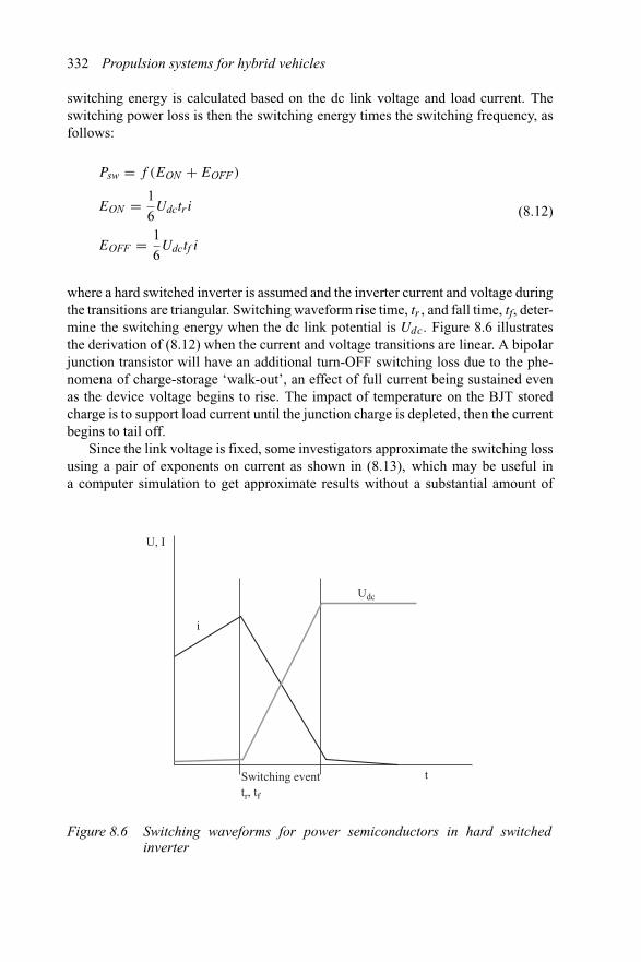
332 Propulsion systems for hybrid vehicles
switching energy is calculated based on the dc link voltage and load current. Theswitching power loss is then the switching energy times the switching frequency, asfollows:
Psw = f (EON + EOFF )
EON = 1
6Udctr i
EOFF = 1
6Udctf i
(8.12)
where a hard switched inverter is assumed and the inverter current and voltage duringthe transitions are triangular. Switching waveform rise time, tr , and fall time, tf, deter-mine the switching energy when the dc link potential is Udc. Figure 8.6 illustratesthe derivation of (8.12) when the current and voltage transitions are linear. A bipolarjunction transistor will have an additional turn-OFF switching loss due to the phe-nomena of charge-storage ‘walk-out’, an effect of full current being sustained evenas the device voltage begins to rise. The impact of temperature on the BJT storedcharge is to support load current until the junction charge is depleted, then the currentbegins to tail off.
Since the link voltage is fixed, some investigators approximate the switching lossusing a pair of exponents on current as shown in (8.13), which may be useful ina computer simulation to get approximate results without a substantial amount of
U, I
i
Udc
Switching event tr, tf
t
Figure 8.6 Switching waveforms for power semiconductors in hard switchedinverter
Drive system efficiency 333
device characterisation:
Psw = f (c1iυ1 + c2i
υ2)
c1 = 0.012c2 = 0.0042υ1 = 1.25υ2 = 1.3
(Hz, mJ/cycle) (8.13)
For the case of 100◦C junction temperature and a fixed link voltage, c1 and ν1 areturn_ON and c2, ν2 are for turn-OFF. For different link voltages or different tempera-ture the coefficients will need to be recomputed based on some device characterisation.A similar procedure will work for MOSFET devices [13].
8.2.3 Reverse recovery
In a hard switched converter with reactive current flow there will be diode conductionwhen the transistor opposite the conducting diode is gated ON. Circuit current willswitch to the transistor gated ON, but an additional component of current will flowthrough the switch in a shoot-through fashion until the diode is commutated off.The diode current is quickly reversed, but persists, for a duration of time necessaryto sweep all the stored charge from the p−n junction. The time to accomplish thisis the reverse recovery time during which an amount of charge Qrr is cleared. Aswith the active devices, the power dissipation in the diode during reverse recovery iscalculated as:
Prr = fErr
Err = 1
6
3Udc
2trri (8.14)
In many power electronic circuits, particularly those built with thyristors, it isnecessary to add snubbers across the active device to limit dU/dt , dI/dt , or somecombination. In the MOS-controlled thyristor (MCT), it is necessary to add dI/dt
snubbing in series with the anode to limit the rate of rise of current to prevent devicedamage. Gate-turn-off thyrsitors (GTOs) also require dU/dt snubbers to limit therate of rise of voltage during forward recovery to allow the device sufficient time tointernally stabilize. If a snubber capacitor is used, its switching power dissipation iscalculated as shown in (8.15). If a non-dissipative snubber is used, this energy willbe recuperated, but circuit complexity would be higher.
Psnub = fEsnub
Esnub = 1
2C
(3Udc
2
)2 (8.15)
334 Propulsion systems for hybrid vehicles
Other elements in the switching circuit may be analysed in a similar manneras done in the above three subsections. Link capacitors, for example, have lossesequal to the circulating current and capacitor equivalent series resistance, ESR, ori2ESR.
8.3 Distribution system
Losses in the power distribution system are comprised of harness and cable resistivelosses, connector losses, and fuse or contactor or other protective device loss. Fusesare sized to protect the downstream wiring from damage due to wire shorts to ground,or to other circuits, or faults at the load. In a fuse itself a ‘weak-link’ or seriesof ‘weak-links’ are regions of the ribbon element that are narrower than the fusestock. At sufficient current, joule heating proportional to I 2t causes the weak-linkto begin to melt, at which point two unstable phenomena contribute to very rapidfuse link metal vaporization. First, the weak-link itself begins to melt. Melting isfollowed by a surface tension effect in which the molten portion tends to form intodroplets that are still joined. At the napes of this series of droplets, or unduloids, thecross-sectional area becomes constricted below that of the original fuse, thus furtheraccelerating fuse vaporization. The second phenomenon that accelerates fuse clearingis the pinch effect, whereby current flow through a liquid conductor reacts with itsown magnetic field, further constricting the conductor material into an even smallercross-section [14]. The constricting pressure at the unduloid is proportional to thesquare of the current flowing in the cross-section and inversely proportional to thediameter squared of the effective cross-section. The effect is that of an Ampereanforce (as opposed to a Lorentz force) that tends to separate the liquid conductorinto individual balls. Fuse elements are made of low melting point materials such assilver or its alloys. Semiconductor protection fuses such as those used in each poleof a thyristor inverter – GTO, for example – are made of pure silver to achieve thefastest clearing time. McCleer [14] develops a concise theory of the fuse from bothan electrical and thermal model perspective.
Electrical contacts are also analysed by McCleer [14], where he shows that contactresistance of a relay or contactor can be modelled as a constriction resistance due toa large number of asperities, N , having an average radius ra , at the points of contact.The contact resistance is calculated as shown in (8.16), where ρr is the contact materialresistivity:
Rc = ρr
2∑N
k ak
(8.16)
Contact voltage drop is nearly self-regulating at 0.1 to 0.2 V per interface, withmost instances of contact voltage drop in automotive circuits being in the vicinity of0.025 V.
Vehicle harness cables are sized to conform with allowable temperature rise inconfined spaces and because of this tend to follow the industrial practice of 3 to 5%
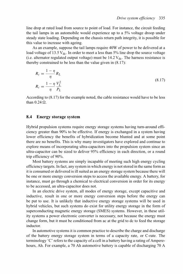
Drive system efficiency 335
line drop at rated load from source to point of load. For instance, the circuit feedingthe tail lamps in an automobile would experience up to a 5% voltage droop understeady state loading. Depending on the chassis return path integrity, it is possible forthis value to increase with ageing.
As an example, suppose the tail lamps require 40W of power to be delivered at aload voltage of 13.5 Vdc. In order to meet a less than 5% line drop the source voltage(i.e. alternator regulated output voltage) must be 14.2 Vdc. The harness resistance isthereby constrained to be less than the value given in (8.17):
Rc = 1 − η
ηRL
Rc = 1 − η
η
V 2L
PL
(8.17)
According to (8.17) for the example noted, the cable resistance would have to be lessthan 0.24 �.
8.4 Energy storage system
Hybrid propulsion systems require energy storage systems having turn-around effi-ciency greater than 90% to be effective. If energy is exchanged in a system havinglower efficiency the benefits of hybridization become blunted and at some pointthere are no benefits. This is why many investigators have explored and continue toexplore means of incorporating ultra-capacitors into the propulsion system since anultra-capacitor can be sized to deliver 95% efficiency in each direction, or a roundtrip efficiency of 90%.
Most battery systems are simply incapable of meeting such high energy cyclingefficiency targets. In fact, any system in which energy is not stored in the same form asit is consumed or delivered is ill suited as an energy storage system because there willbe one or more energy conversion steps to access the available energy. A battery, forinstance, must go through a chemical to electrical conversion in order for its energyto be accessed, an ultra-capacitor does not.
In an electric drive system, all modes of energy storage, except capacitive andinductive, result in one or more energy conversion steps before the energy canbe put to use. It is unlikely that inductive energy storage systems will be used inhybrid vehicles, but such systems do exist for utility energy storage in the form ofsuperconducting magnetic energy storage (SMES) systems. However, in these util-ity systems a power electronic converter is necessary, not because the energy mustchange form, but it must be conditioned from ac at the grid to dc to feed the storageinductor.
In automotive systems it is common practice to describe the charge and dischargeof the battery energy storage system in terms of a capacity rate, or C-rate. Theterminology ‘C’ refers to the capacity of a cell in a battery having a rating of Ampere-hours, Ah. For example, a 70 Ah automotive battery is capable of discharging 70 A
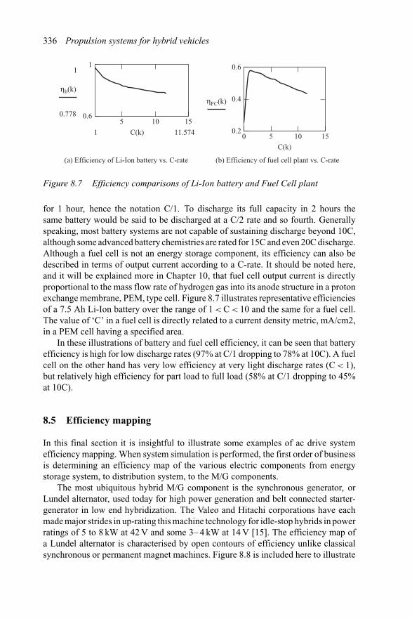
336 Propulsion systems for hybrid vehicles
1
0.65 10
0.6
0.4
0.25 10 150
15
1
1
C(k)
C(k)
11.574
0.778
ηb(k)
ηFC(k)
(a) Efficiency of Li-Ion battery vs. C-rate (b) Efficiency of fuel cell plant vs. C-rate
Figure 8.7 Efficiency comparisons of Li-Ion battery and Fuel Cell plant
for 1 hour, hence the notation C/1. To discharge its full capacity in 2 hours thesame battery would be said to be discharged at a C/2 rate and so fourth. Generallyspeaking, most battery systems are not capable of sustaining discharge beyond 10C,although some advanced battery chemistries are rated for 15C and even 20C discharge.Although a fuel cell is not an energy storage component, its efficiency can also bedescribed in terms of output current according to a C-rate. It should be noted here,and it will be explained more in Chapter 10, that fuel cell output current is directlyproportional to the mass flow rate of hydrogen gas into its anode structure in a protonexchange membrane, PEM, type cell. Figure 8.7 illustrates representative efficienciesof a 7.5 Ah Li-Ion battery over the range of 1 < C < 10 and the same for a fuel cell.The value of ‘C’ in a fuel cell is directly related to a current density metric, mA/cm2,in a PEM cell having a specified area.
In these illustrations of battery and fuel cell efficiency, it can be seen that batteryefficiency is high for low discharge rates (97% at C/1 dropping to 78% at 10C). A fuelcell on the other hand has very low efficiency at very light discharge rates (C < 1),but relatively high efficiency for part load to full load (58% at C/1 dropping to 45%at 10C).
8.5 Efficiency mapping
In this final section it is insightful to illustrate some examples of ac drive systemefficiency mapping. When system simulation is performed, the first order of businessis determining an efficiency map of the various electric components from energystorage system, to distribution system, to the M/G components.
The most ubiquitous hybrid M/G component is the synchronous generator, orLundel alternator, used today for high power generation and belt connected starter-generator in low end hybridization. The Valeo and Hitachi corporations have eachmade major strides in up-rating this machine technology for idle-stop hybrids in powerratings of 5 to 8 kW at 42 V and some 3– 4 kW at 14 V [15]. The efficiency map ofa Lundel alternator is characterised by open contours of efficiency unlike classicalsynchronous or permanent magnet machines. Figure 8.8 is included here to illustrate
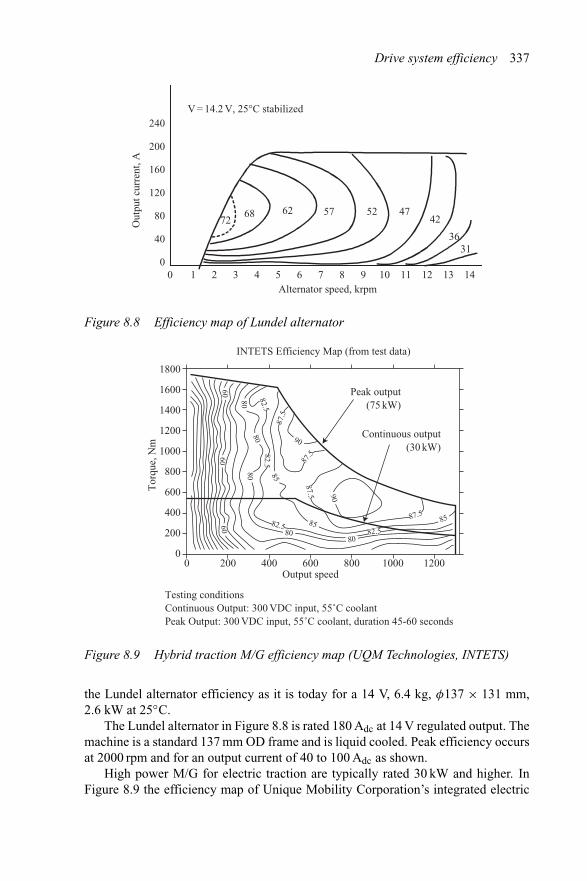
Drive system efficiency 337
Out
put c
urre
nt, A
Alternator speed, krpm
V = 14.2 V, 25°C stabilized
7268 62 57 52 47
42
3631
240
200
160
120
80
40
00 1 2 3 4 5 6 7 8 9 10 11 12 13 14
Figure 8.8 Efficiency map of Lundel alternator
Peak output(75 kW)
Continuous output(30 kW)
00
200
400
600
800
1000
Tor
que,
Nm
1200
1400
1600
1800
200 400 600Output speed
800 1000 1200
6060
60
80
8080
80
8082.5
82.5
82.582.5
85
90
90
85
85
87.5
87.5
87.5
87.5
INTETS Efficiency Map (from test data)
Testing conditionsContinuous Output: 300 VDC input, 55˚C coolantPeak Output: 300 VDC input, 55˚C coolant, duration 45-60 seconds
Figure 8.9 Hybrid traction M/G efficiency map (UQM Technologies, INTETS)
the Lundel alternator efficiency as it is today for a 14 V, 6.4 kg, φ137 × 131 mm,2.6 kW at 25◦C.
The Lundel alternator in Figure 8.8 is rated 180 Adc at 14 V regulated output. Themachine is a standard 137 mm OD frame and is liquid cooled. Peak efficiency occursat 2000 rpm and for an output current of 40 to 100 Adc as shown.
High power M/G for electric traction are typically rated 30 kW and higher. InFigure 8.9 the efficiency map of Unique Mobility Corporation’s integrated electric
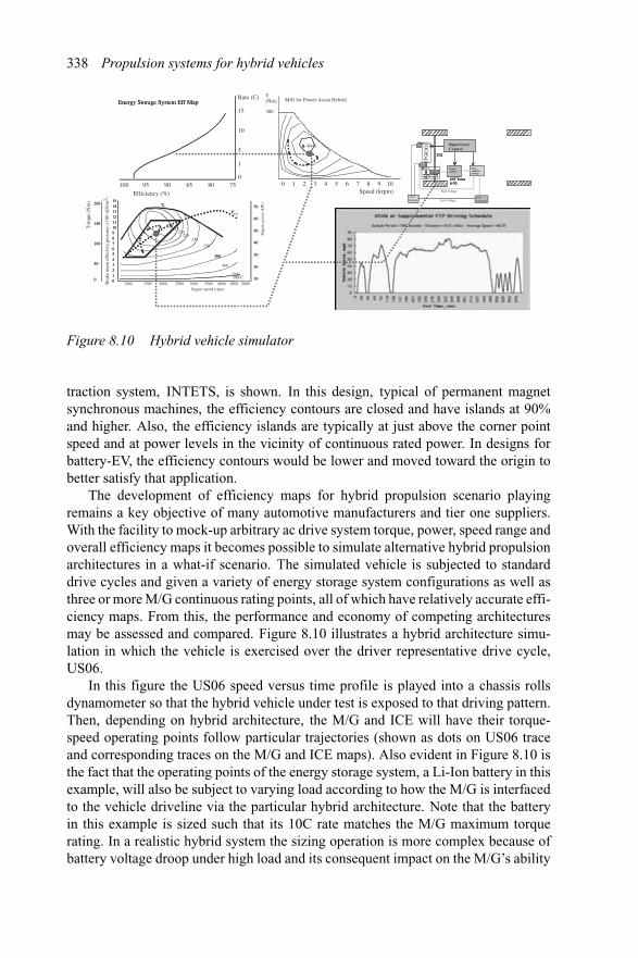
338 Propulsion systems for hybrid vehicles
1000 1500 2000 2500 3000 3500 4000 4500 5000
210215220
230250
270
300
400
700BSFC
Te
Peng
70
60
50
40
30
20
10
200
150
100
50
0
T(Nm)
300
Speed (krpm)
η~94%
Energy Storage System Eff MapRate (C)
15
10
5
1
0
PowerInverter
Ultra-capacitorstorage
CVT Trans & FD
SupervisoryControl
Str
TDI
Alt
M/G
dc/dc
210
300
Te
P70
60
50
40
30
20
10
200
150
100
50
0
η
Energy Storage System Eff Map
PowerInverter
Ultra-capacitorstorage
CVT Trans & FD
SupervisoryControl
Str
TDI
Alt
12Vbattery
M/G
dc/dc converter
Bra
ke m
ean
effe
ctiv
e pr
essu
re ×
100
(kN
/m2 )
Tor
que
(Nm
)
Eng
ine
pow
er (
kW)
Engine speed (rpm)
1514131211109876543210
1514131211109876543210
Efficiency (%)100 95 90 85 80 75 0 1 2 3 4 5 6 7 9 108
M/G for Power Assist Hybrid
Low Voltage
High Voltage
Figure 8.10 Hybrid vehicle simulator
traction system, INTETS, is shown. In this design, typical of permanent magnetsynchronous machines, the efficiency contours are closed and have islands at 90%and higher. Also, the efficiency islands are typically at just above the corner pointspeed and at power levels in the vicinity of continuous rated power. In designs forbattery-EV, the efficiency contours would be lower and moved toward the origin tobetter satisfy that application.
The development of efficiency maps for hybrid propulsion scenario playingremains a key objective of many automotive manufacturers and tier one suppliers.With the facility to mock-up arbitrary ac drive system torque, power, speed range andoverall efficiency maps it becomes possible to simulate alternative hybrid propulsionarchitectures in a what-if scenario. The simulated vehicle is subjected to standarddrive cycles and given a variety of energy storage system configurations as well asthree or more M/G continuous rating points, all of which have relatively accurate effi-ciency maps. From this, the performance and economy of competing architecturesmay be assessed and compared. Figure 8.10 illustrates a hybrid architecture simu-lation in which the vehicle is exercised over the driver representative drive cycle,US06.
In this figure the US06 speed versus time profile is played into a chassis rollsdynamometer so that the hybrid vehicle under test is exposed to that driving pattern.Then, depending on hybrid architecture, the M/G and ICE will have their torque-speed operating points follow particular trajectories (shown as dots on US06 traceand corresponding traces on the M/G and ICE maps). Also evident in Figure 8.10 isthe fact that the operating points of the energy storage system, a Li-Ion battery in thisexample, will also be subject to varying load according to how the M/G is interfacedto the vehicle driveline via the particular hybrid architecture. Note that the batteryin this example is sized such that its 10C rate matches the M/G maximum torquerating. In a realistic hybrid system the sizing operation is more complex because ofbattery voltage droop under high load and its consequent impact on the M/G’s ability
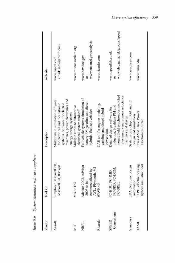
Drive system efficiency 339
Tabl
e8.
6Sy
stem
sim
ulat
orso
ftwar
esu
pplie
rs
Ven
dor
Tool
kit
Des
crip
tion
Web
site
Ans
oft
Sim
plor
er,M
axw
ell2
D,
Max
wel
l3D
,RM
xprt
Mul
tidom
ain
sim
ulat
ion
soft
war
efo
rel
ectr
ical
and
mec
hatr
onic
syst
ems.
Soft
war
efo
rel
ectr
icm
achi
nes,
pow
erel
ectr
onic
san
den
ergy
stor
age
syst
ems
ww
w.a
nsof
t.com
emai
l:in
fo@
anso
ft.c
om
MIT
MA
EST
rOM
ultip
leat
trib
ute
auto
mot
ive
elec
tric
alsy
stem
trad
eoff
ww
w.m
itcon
sort
ium
.org
NR
EL
Adv
isor
2002
.Adv
isor
2003
tobe
com
mer
cial
ized
byA
VL
,Ply
mou
th,M
I
Full
vehi
cle
syst
ems
sim
ulat
ion
ofba
ttery
EV
,gas
olin
ean
ddi
esel
hybr
ids,
fuel
cell
vehi
cles
ww
w.h
ev.d
oe.g
ovor w
ww
.ctts
.nre
l.gov
/ana
lysi
s
Ric
ardo
WA
VE
v5C
AE
tool
for
engi
nem
odel
ing,
gaso
line
and
dies
elhy
brid
pow
ertr
ains
ww
w.r
icar
do.c
om
SPE
ED
Con
sort
ium
PC-B
DC
,PC
-IM
D,
PC-S
RD
,PC
-DC
M,
PC-S
RE
L
Det
aile
dde
sign
soft
war
efo
rin
duct
ion,
brus
hles
sPM
and
wou
ndfi
eld
sync
hron
ous,
switc
hed
relu
ctan
ce,s
ynch
rono
usre
luct
ance
mac
hine
san
ddr
ives
ww
w.s
peed
lab.
co.u
kor w
ww
.ele
c.ga
l.ac.
uk/g
roup
s/sp
eed
Syno
psys
ED
Ael
ectr
onic
desi
gnau
tom
atio
nSy
stem
son
ach
ip,F
PGA
and
ICde
sign
and
sim
ulat
ion
ww
w.s
ynop
sys.
com
TAM
UE
LPH
,ele
ctri
cpe
akin
ghy
brid
sim
ulat
ion
tool
Texa
sA
&M
Uni
v.Po
wer
Ele
ctro
nics
Cen
tre
ww
w.ta
mu.
edu
340 Propulsion systems for hybrid vehicles
to actually deliver full rated torque. For these reasons the battery capacity may beincreased somewhat.
The conclusion from Figure 8.10 is that the most efficient propulsion system isnot necessarily the one having all of the most efficient components. Rather, the cycleaverage efficiency, hence fuel economy, is more dependent on how much time isspent at each efficiency of M/G, ICE, battery, and of course the transmission.
Note also in Figure 8.10 that hybrid propulsion strategy attempts, to hold theengine in a more confined operating space as shown. This space limits WOT operationto minimize emissions, restricts engine speed swing and restricts inefficient part loadoperation.
Developing efficiency maps for ac drive systems today requires up-front designand modeling of the proposed M/G rating and package constraints. As system simu-lation tools become more advanced it is now possible to simulate in a timely mannera number of competing designs. Other than industry proprietary software tools, thoseshown in Table 8.6 are seen as pre-eminent system simulators for assessment ofbattery EV and hybrid propulsion systems. The list is in alphabetical order withoutpreference to any one system simulator toolbox.
There are, of course, many other software tools and design services available forthe design of vehicle systems, powertrain architectures, energy storage systems andelectric drive components. The list in Table 8.6 is meant only to illustrate the breadthof services available.
8.6 References
1 ALLEN, J. W.: Armco Inc. Research, personal discussions on specialty flat-rolledsteels, November 1997
2 ATALLAH, K., ZHU, Z. Q. and HOWE, D.: ‘An improved method for predictingiron losses in brushless permanent magnet dc drives,’ IEEE Trans. Mag., 1992,28(5), pp. 2997–2999
3 ‘Armco non-oriented electrical steel catalog’, Armco Steel, 19974 ‘Tempel electrical steel catalog’ (Tempel Steel, 5215 Old Orchard Road, Skokie,
IL 60077, USA), 19955 WEHRLE, J. T. and BARTA, D. J.: Phelps Dodge magnet wire company personal
discussions, November 19776 LANGHORST, P. and HANCOCK, C.: ‘The simple truth about motor-drive com-
patibility’, Magnetek Advanced Technology Center, 1145 Corporate Lake Drive,St Louis, MO 63132, USA
7 JIMOH, A. A., FINDLAY, R. D. and POLOUJADOFF, M.: ‘Stray losses ininduction machines. Part I: Definition, origin and measurement’, IEEE Trans.Power Appar. Syst., 1985, PAS-104(6), pp. 1500–1505
8 JIMOH, A. A., FINDLAY, R. D. and POLOUJADOFF, M.: ‘Stray losses ininduction machines. Part II: Calculation and reduction’, IEEE Trans. Power App.Syst., 1985, PAS-104(6), pp. 1506–1512
Drive system efficiency 341
9 GIACOLETTO, L. J.: ‘Frequency- and time-domain analysis of skin effects’,IEEE Trans. Magn., 1996, 32(1), pp. 220–229
10 GIACOLETTO, L. J.: ‘Pulse operation of transmission lines including skin-effectresistance’, Technical Note, Microw. J., 2000, 43(2), pp. 150–155
11 SEPE, R. B. Jr,: ‘Quasi-behavioural model of a voltage fed inverter suitable forcontroller development’. IEEE Applied Power Electronics Conference, APEC95,Dallas, TX, 1995
12 HUDGINS, J. L., MENHART, S., PORTNOY, W. M. and SANKARAN, V. A.:‘Temperature variation effects on the switching characteristics of MOS gateddevices’, Proceedings of the European Power Electronics annual meeting,Firenze, Italy, 1991
13 REES, F. L. and MILLER, J. M.: ‘50–100V dc inverters for vehicular actuatorsystems: the use of MOSFET’s and IGBT’s compared’. IEEE Workshop on PowerElectronics in Transportation, WPET, 23–23 October 1992. IEEE CatalogueNo. 92TH0451–5
14 MCCLEER, P. J.: ‘The theory and practice of overcurrent protection’ (Mechan-ical Products, Inc., 1987)
15 AKEMAKOU, A.: ‘High power electrical generation’. MIT Industry Consor-tium on Advanced Automotive Electrical/Electronic Components and Systems,Program Review Meeting, Centre de Congres – Pierre Baudis, Toulouse, France

Chapter 9
Hybrid vehicle characterisation
This chapter will describe how passenger vehicles are characterised first as to drag androlling resistance coefficients and second according to fuel economy over standarddrive cycles. Vehicle data necessary to compute rolling resistance and aerodynamicdrag coefficients are taken from coast down tests. This procedure is further describedin Chapter 11 along with some actual test data about how this applies to character-ising the hybrid propulsion system. In this chapter the various standard drive cyclesemployed in various geographical and demographic areas are compared and rationalegiven for their selection.
Coast down testing is a procedure long in existence to extract the vehicle tyreand body aerodynamic drag characteristics. A coast down test procedure consists ofaccelerating the vehicle to a prescribed speed on a straight and level road course,holding a set speed and then, with the vehicle in neutral allowing it to coast downnaturally. The test is then repeated in the same manner from the opposite direction toaverage out any inconsistencies due to relative wind velocity and road grade.
It is important to understand the need to accurately characterise a vehicle in termsof fuel economy and emissions by also understanding how efficiently the fuel isdelivered to the vehicle’s fuel tank in the first place and the type of fuel being used.A recent US House of Representatives bill on hybrid incentives has not renewed exist-ing incentives on gasoline-hybrid, but has introduced new incentives for CIDI-hybrid[1]. The new incentive allows up to $3000 on diesel fuelled hybrids to encouragefurther development of this technology. In addition to the base incentive a $500 ‘life-time fuel savings’ increment has been issued to further encourage development andrefinement of CIDI fuels, engine technology and hybridization.
There remains a clear need for cleaner vehicles, particularly larger passengervehicles, sport utility vehicles and heavy trucks, including line haul and over theroad (OTR) trucks. There are now some 200 M passenger vehicles licensed in NorthAmerica that are fuelled by gasoline. Add to this another 270k propane, LPG, fuelledvehicles, and many others operating on E85 ethanol, compressed natural gas, CNG,and other alternatives. As of August 2003 there were only 147k hybrid vehicles inoperation globally.
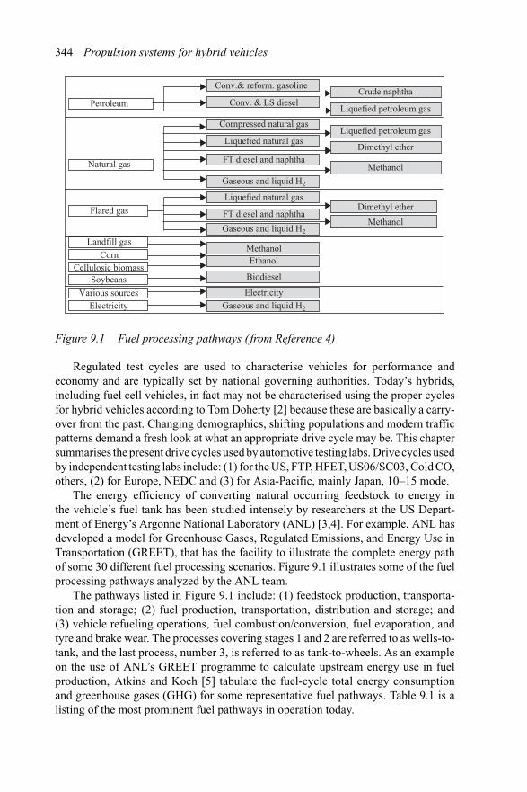
344 Propulsion systems for hybrid vehicles
Conv.& reform. gasoline
Petroleum
Natural gas
Flared gas
Landfill gas
CornCellulosic biomass
Soybeans
Various sourcesElectricity
Cornpressed natural gas
Conv. & LS diesel
Liquefied natural gas
FT diesel and naphtha
Crude naphtha
Liquefied petroleum gas
Liquefied petroleum gas
Dimethyl ether
Methanol
Dimethyl ether
Methanol
MethanolEthanol
Biodiesel
ElectricityGaseous and liquid H2
Liquefied natural gas
FT diesel and naphtha
Gaseous and liquid H2
Gaseous and liquid H2
Figure 9.1 Fuel processing pathways ( from Reference 4)
Regulated test cycles are used to characterise vehicles for performance andeconomy and are typically set by national governing authorities. Today’s hybrids,including fuel cell vehicles, in fact may not be characterised using the proper cyclesfor hybrid vehicles according to Tom Doherty [2] because these are basically a carry-over from the past. Changing demographics, shifting populations and modern trafficpatterns demand a fresh look at what an appropriate drive cycle may be. This chaptersummarises the present drive cycles used by automotive testing labs. Drive cycles usedby independent testing labs include: (1) for the US, FTP, HFET, US06/SC03, Cold CO,others, (2) for Europe, NEDC and (3) for Asia-Pacific, mainly Japan, 10–15 mode.
The energy efficiency of converting natural occurring feedstock to energy inthe vehicle’s fuel tank has been studied intensely by researchers at the US Depart-ment of Energy’s Argonne National Laboratory (ANL) [3,4]. For example, ANL hasdeveloped a model for Greenhouse Gases, Regulated Emissions, and Energy Use inTransportation (GREET), that has the facility to illustrate the complete energy pathof some 30 different fuel processing scenarios. Figure 9.1 illustrates some of the fuelprocessing pathways analyzed by the ANL team.
The pathways listed in Figure 9.1 include: (1) feedstock production, transporta-tion and storage; (2) fuel production, transportation, distribution and storage; and(3) vehicle refueling operations, fuel combustion/conversion, fuel evaporation, andtyre and brake wear. The processes covering stages 1 and 2 are referred to as wells-to-tank, and the last process, number 3, is referred to as tank-to-wheels. As an exampleon the use of ANL’s GREET programme to calculate upstream energy use in fuelproduction, Atkins and Koch [5] tabulate the fuel-cycle total energy consumptionand greenhouse gases (GHG) for some representative fuel pathways. Table 9.1 is alisting of the most prominent fuel pathways in operation today.
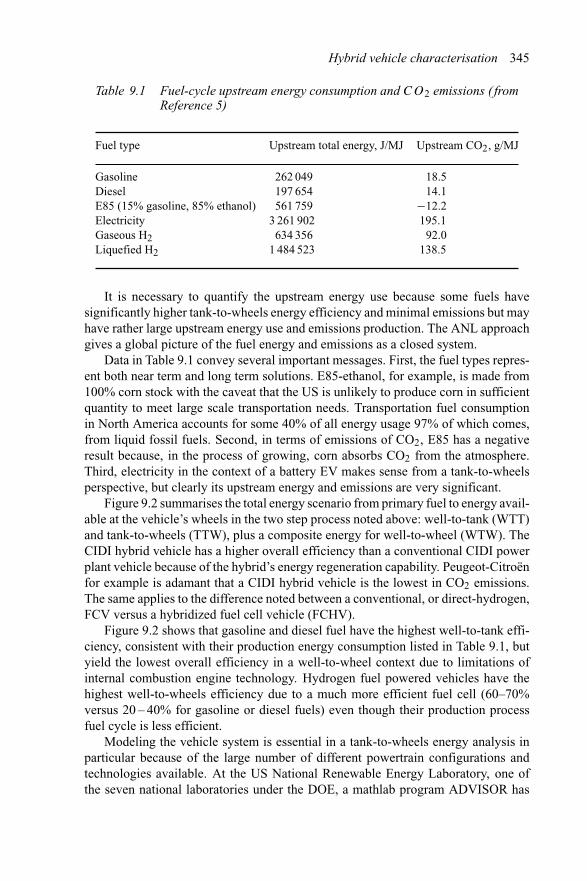
Hybrid vehicle characterisation 345
Table 9.1 Fuel-cycle upstream energy consumption and CO2 emissions ( fromReference 5)
Fuel type Upstream total energy, J/MJ Upstream CO2, g/MJ
Gasoline 262 049 18.5Diesel 197 654 14.1E85 (15% gasoline, 85% ethanol) 561 759 −12.2Electricity 3 261 902 195.1Gaseous H2 634 356 92.0Liquefied H2 1 484 523 138.5
It is necessary to quantify the upstream energy use because some fuels havesignificantly higher tank-to-wheels energy efficiency and minimal emissions but mayhave rather large upstream energy use and emissions production. The ANL approachgives a global picture of the fuel energy and emissions as a closed system.
Data in Table 9.1 convey several important messages. First, the fuel types repres-ent both near term and long term solutions. E85-ethanol, for example, is made from100% corn stock with the caveat that the US is unlikely to produce corn in sufficientquantity to meet large scale transportation needs. Transportation fuel consumptionin North America accounts for some 40% of all energy usage 97% of which comes,from liquid fossil fuels. Second, in terms of emissions of CO2, E85 has a negativeresult because, in the process of growing, corn absorbs CO2 from the atmosphere.Third, electricity in the context of a battery EV makes sense from a tank-to-wheelsperspective, but clearly its upstream energy and emissions are very significant.
Figure 9.2 summarises the total energy scenario from primary fuel to energy avail-able at the vehicle’s wheels in the two step process noted above: well-to-tank (WTT)and tank-to-wheels (TTW), plus a composite energy for well-to-wheel (WTW). TheCIDI hybrid vehicle has a higher overall efficiency than a conventional CIDI powerplant vehicle because of the hybrid’s energy regeneration capability. Peugeot-Citroënfor example is adamant that a CIDI hybrid vehicle is the lowest in CO2 emissions.The same applies to the difference noted between a conventional, or direct-hydrogen,FCV versus a hybridized fuel cell vehicle (FCHV).
Figure 9.2 shows that gasoline and diesel fuel have the highest well-to-tank effi-ciency, consistent with their production energy consumption listed in Table 9.1, butyield the lowest overall efficiency in a well-to-wheel context due to limitations ofinternal combustion engine technology. Hydrogen fuel powered vehicles have thehighest well-to-wheels efficiency due to a much more efficient fuel cell (60–70%versus 20 – 40% for gasoline or diesel fuels) even though their production processfuel cycle is less efficient.
Modeling the vehicle system is essential in a tank-to-wheels energy analysis inparticular because of the large number of different powertrain configurations andtechnologies available. At the US National Renewable Energy Laboratory, one ofthe seven national laboratories under the DOE, a mathlab program ADVISOR has
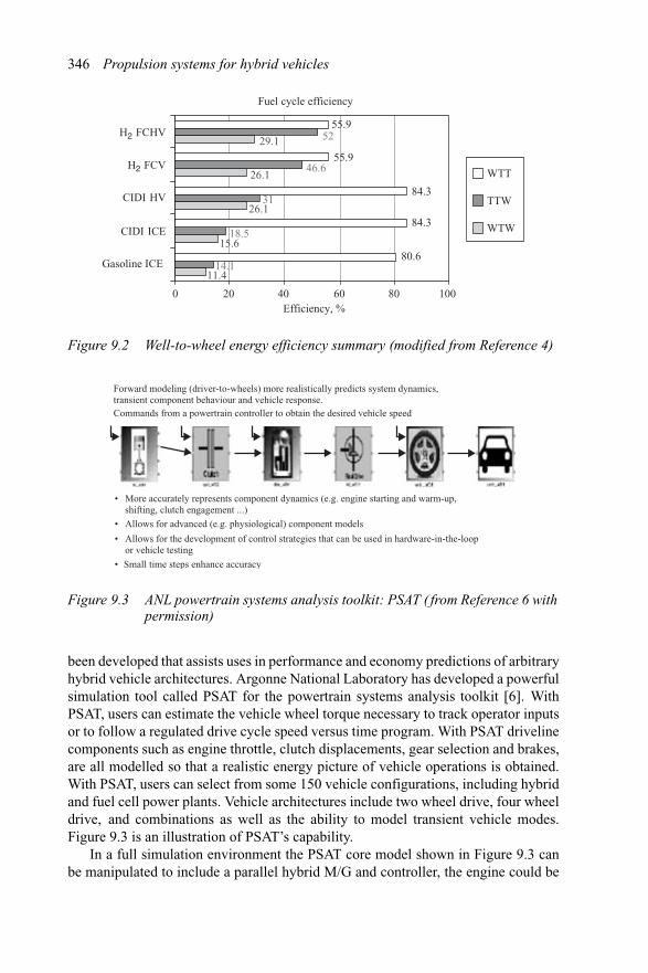
346 Propulsion systems for hybrid vehicles
Fuel cycle efficiency
11.4
15.6
26.1
26.1
29.1
14.1
18.5
31
46.6
52
80.6
84.3
84.3
55.9
55.9
0 20 40 60 80 100
Gasoline ICE
CIDI ICE
CIDI HV
H2 FCV
H2 FCHV
Efficiency, %
WTT
TTW
WTW
Figure 9.2 Well-to-wheel energy efficiency summary (modified from Reference 4)
Forward modeling (driver-to-wheels) more realistically predicts system dynamics,transient component behaviour and vehicle response.Commands from a powertrain controller to obtain the desired vehicle speed
• More accurately represents component dynamics (e.g. engine starting and warm-up, shifting, clutch engagement ...)
• Allows for the development of control strategies that can be used in hardware-in-the-loop or vehicle testing
• Allows for advanced (e.g. physiological) component models
• Small time steps enhance accuracy
Figure 9.3 ANL powertrain systems analysis toolkit: PSAT ( from Reference 6 withpermission)
been developed that assists uses in performance and economy predictions of arbitraryhybrid vehicle architectures. Argonne National Laboratory has developed a powerfulsimulation tool called PSAT for the powertrain systems analysis toolkit [6]. WithPSAT, users can estimate the vehicle wheel torque necessary to track operator inputsor to follow a regulated drive cycle speed versus time program. With PSAT drivelinecomponents such as engine throttle, clutch displacements, gear selection and brakes,are all modelled so that a realistic energy picture of vehicle operations is obtained.With PSAT, users can select from some 150 vehicle configurations, including hybridand fuel cell power plants. Vehicle architectures include two wheel drive, four wheeldrive, and combinations as well as the ability to model transient vehicle modes.Figure 9.3 is an illustration of PSAT’s capability.
In a full simulation environment the PSAT core model shown in Figure 9.3 canbe manipulated to include a parallel hybrid M/G and controller, the engine could be
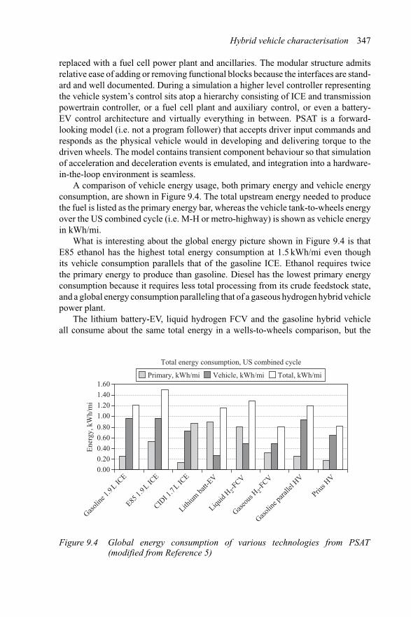
Hybrid vehicle characterisation 347
replaced with a fuel cell power plant and ancillaries. The modular structure admitsrelative ease of adding or removing functional blocks because the interfaces are stand-ard and well documented. During a simulation a higher level controller representingthe vehicle system’s control sits atop a hierarchy consisting of ICE and transmissionpowertrain controller, or a fuel cell plant and auxiliary control, or even a battery-EV control architecture and virtually everything in between. PSAT is a forward-looking model (i.e. not a program follower) that accepts driver input commands andresponds as the physical vehicle would in developing and delivering torque to thedriven wheels. The model contains transient component behaviour so that simulationof acceleration and deceleration events is emulated, and integration into a hardware-in-the-loop environment is seamless.
A comparison of vehicle energy usage, both primary energy and vehicle energyconsumption, are shown in Figure 9.4. The total upstream energy needed to producethe fuel is listed as the primary energy bar, whereas the vehicle tank-to-wheels energyover the US combined cycle (i.e. M-H or metro-highway) is shown as vehicle energyin kWh/mi.
What is interesting about the global energy picture shown in Figure 9.4 is thatE85 ethanol has the highest total energy consumption at 1.5 kWh/mi even thoughits vehicle consumption parallels that of the gasoline ICE. Ethanol requires twicethe primary energy to produce than gasoline. Diesel has the lowest primary energyconsumption because it requires less total processing from its crude feedstock state,and a global energy consumption paralleling that of a gaseous hydrogen hybrid vehiclepower plant.
The lithium battery-EV, liquid hydrogen FCV and the gasoline hybrid vehicleall consume about the same total energy in a wells-to-wheels comparison, but the
Total energy consumption, US combined cycle
0.00
0.20
0.40
0.60
0.80
1.00
1.20
1.40
1.60
Gasoli
ne 1.
9L ICE
E85 1.
9L ICE
CIDI 1
.7L IC
E
Lithium
batt-
EV
Liquid
H 2-F
CV
Gaseo
us H 2
-FCV
Gasoli
ne pa
rallel
HV
Prius H
V
Ene
rgy,
kW
h/m
i
Primary, kWh/mi Vehicle, kWh/mi Total, kWh/mi
Figure 9.4 Global energy consumption of various technologies from PSAT(modified from Reference 5)
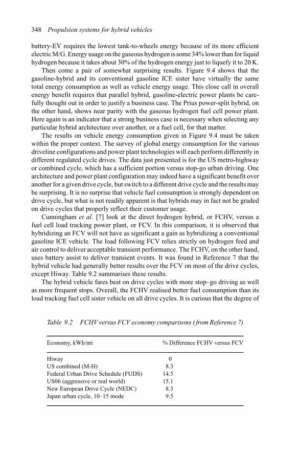
348 Propulsion systems for hybrid vehicles
battery-EV requires the lowest tank-to-wheels energy because of its more efficientelectric M/G. Energy usage on the gaseous hydrogen is some 34% lower than for liquidhydrogen because it takes about 30% of the hydrogen energy just to liquefy it to 20 K.
Then come a pair of somewhat surprising results. Figure 9.4 shows that thegasoline-hybrid and its conventional gasoline ICE sister have virtually the sametotal energy consumption as well as vehicle energy usage. This close call in overallenergy benefit requires that parallel hybrid, gasoline-electric power plants be care-fully thought out in order to justify a business case. The Prius power-split hybrid, onthe other hand, shows near parity with the gaseous hydrogen fuel cell power plant.Here again is an indicator that a strong business case is necessary when selecting anyparticular hybrid architecture over another, or a fuel cell, for that matter.
The results on vehicle energy consumption given in Figure 9.4 must be takenwithin the proper context. The survey of global energy consumption for the variousdriveline configurations and power plant technologies will each perform differently indifferent regulated cycle drives. The data just presented is for the US metro-highwayor combined cycle, which has a sufficient portion versus stop-go urban driving. Onearchitecture and power plant configuration may indeed have a significant benefit overanother for a given drive cycle, but switch to a different drive cycle and the results maybe surprising. It is no surprise that vehicle fuel consumption is strongly dependent ondrive cycle, but what is not readily apparent is that hybrids may in fact not be gradedon drive cycles that properly reflect their customer usage.
Cunningham et al. [7] look at the direct hydrogen hybrid, or FCHV, versus afuel cell load tracking power plant, or FCV. In this comparison, it is observed thathybridizing an FCV will not have as significant a gain as hybridizing a conventionalgasoline ICE vehicle. The load following FCV relies strictly on hydrogen feed andair control to deliver acceptable transient performance. The FCHV, on the other hand,uses battery assist to deliver transient events. It was found in Reference 7 that thehybrid vehicle had generally better results over the FCV on most of the drive cycles,except Hiway. Table 9.2 summarises these results.
The hybrid vehicle fares best on drive cycles with more stop–go driving as wellas more frequent stops. Overall, the FCHV realised better fuel consumption than itsload tracking fuel cell sister vehicle on all drive cycles. It is curious that the degree of
Table 9.2 FCHV versus FCV economy comparisons ( from Reference 7)
Economy, kWh/mi % Difference FCHV versus FCV
Hiway 0US combined (M-H) 8.3Federal Urban Drive Schedule (FUDS) 14.5US06 (aggressive or real world) 15.1New European Drive Cycle (NEDC) 8.3Japan urban cycle, 10–15 mode 9.5
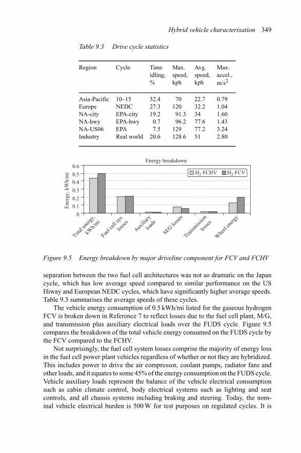
Hybrid vehicle characterisation 349
Table 9.3 Drive cycle statistics
Region Cycle Timeidling,%
Max.speed,kph
Avg.speed,kph
Max.accel.,m/s2
Asia-Pacific 10–15 32.4 70 22.7 0.79Europe NEDC 27.3 120 32.2 1.04NA-city EPA-city 19.2 91.3 34 1.60NA-hwy EPA-hwy 0.7 96.2 77.6 1.43NA-US06 EPA 7.5 129 77.2 3.24Industry Real world 20.6 128.6 51 2.80
Energy breakdown
0
0.10.2
0.3
0.40.5
0.6
Total e
nerg
y,
kWh/m
i
Fuel c
ell sy
s.
losse
s
Auxili
ary
loads
M/G
losse
s
Transm
ission
losse
s
Whe
el en
ergy
Ene
rgy,
kW
h/m
i H2 FCHV H2 FCV
Figure 9.5 Energy breakdown by major driveline component for FCV and FCHV
separation between the two fuel cell architectures was not so dramatic on the Japancycle, which has low average speed compared to similar performance on the USHiway and European NEDC cycles, which have significantly higher average speeds.Table 9.3 summarises the average speeds of these cycles.
The vehicle energy consumption of 0.5 kWh/mi listed for the gaseous hydrogenFCV is broken down in Reference 7 to reflect losses due to the fuel cell plant, M/G,and transmission plus auxiliary electrical loads over the FUDS cycle. Figure 9.5compares the breakdown of the total vehicle energy consumed on the FUDS cycle bythe FCV compared to the FCHV.
Not surprisingly, the fuel cell system losses comprise the majority of energy lossin the fuel cell power plant vehicles regardless of whether or not they are hybridized.This includes power to drive the air compressor, coolant pumps, radiator fans andother loads, and it equates to some 45% of the energy consumption on the FUDS cycle.Vehicle auxiliary loads represent the balance of the vehicle electrical consumptionsuch as cabin climate control, body electrical systems such as lighting and seatcontrols, and all chassis systems including braking and steering. Today, the nom-inal vehicle electrical burden is 500 W for test purposes on regulated cycles. It is
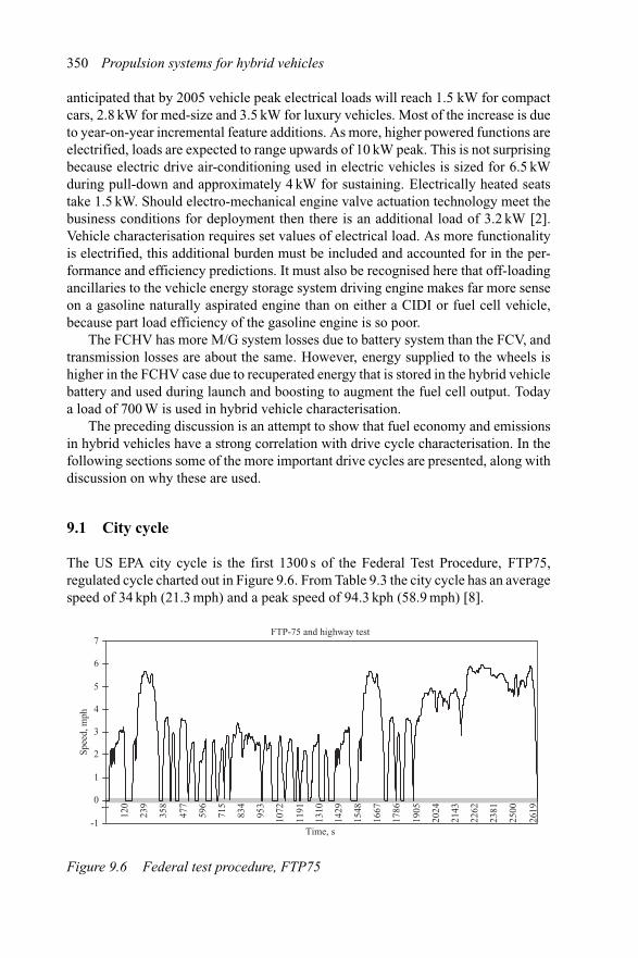
350 Propulsion systems for hybrid vehicles
anticipated that by 2005 vehicle peak electrical loads will reach 1.5 kW for compactcars, 2.8 kW for med-size and 3.5 kW for luxury vehicles. Most of the increase is dueto year-on-year incremental feature additions. As more, higher powered functions areelectrified, loads are expected to range upwards of 10 kW peak. This is not surprisingbecause electric drive air-conditioning used in electric vehicles is sized for 6.5 kWduring pull-down and approximately 4 kW for sustaining. Electrically heated seatstake 1.5 kW. Should electro-mechanical engine valve actuation technology meet thebusiness conditions for deployment then there is an additional load of 3.2 kW [2].Vehicle characterisation requires set values of electrical load. As more functionalityis electrified, this additional burden must be included and accounted for in the per-formance and efficiency predictions. It must also be recognised here that off-loadingancillaries to the vehicle energy storage system driving engine makes far more senseon a gasoline naturally aspirated engine than on either a CIDI or fuel cell vehicle,because part load efficiency of the gasoline engine is so poor.
The FCHV has more M/G system losses due to battery system than the FCV, andtransmission losses are about the same. However, energy supplied to the wheels ishigher in the FCHV case due to recuperated energy that is stored in the hybrid vehiclebattery and used during launch and boosting to augment the fuel cell output. Todaya load of 700 W is used in hybrid vehicle characterisation.
The preceding discussion is an attempt to show that fuel economy and emissionsin hybrid vehicles have a strong correlation with drive cycle characterisation. In thefollowing sections some of the more important drive cycles are presented, along withdiscussion on why these are used.
9.1 City cycle
The US EPA city cycle is the first 1300 s of the Federal Test Procedure, FTP75,regulated cycle charted out in Figure 9.6. From Table 9.3 the city cycle has an averagespeed of 34 kph (21.3 mph) and a peak speed of 94.3 kph (58.9 mph) [8].
FTP-75 and highway test
-1
0
1
2
3
4
5
6
7
Time, s
Spee
d, m
ph
1
120
239
358
477
596
715
834
953
1072
1191
1310
1429
1548
1667
1786
1905
2024
2143
2262
2381
2500
2619
Figure 9.6 Federal test procedure, FTP75
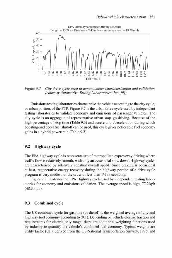
Hybrid vehicle characterisation 351
60
50
40
30
20
10
Test time, s
Veh
icle
spe
ed, m
ph
0 52 104
156
208
260
312
364
416
468
520
572
624
676
728
780
832
884
936
988
1040
1092
1144
1196
1248
1300
1352
0
EPA urban dynamometer driving scheduleLength = 1369 s – Distance = 7.45 miles – Average speed = 19.59 mph
Figure 9.7 City drive cycle used in dynamometer characterisation and validation(courtesy Automotive Testing Laboratories, Inc. [9])
Emissions testing laboratories characterise the vehicle according to the city cycle,or urban portion, of the FTP. Figure 9.7 is the urban drive cycle used by independenttesting laboratories to validate economy and emissions of passenger vehicles. Thecity cycle is an aggregate of representative urban stop–go driving. Because of thehigh percentage of stop time (Table 9.3) and acceleration/deceleration during whichboosting/and decel fuel shutoff can be used, this cycle gives noticeable fuel economygains in a hybrid powertrain (Table 9.2).
9.2 Highway cycle
The EPA highway cycle is representative of metropolitan expressway driving wheretraffic flow is relatively smooth, with only an occasional slow down. Highway cyclesare characterised by relatively constant overall speed. Since braking is occasionalat best, regenerative energy recovery during the highway portion of a drive cycleprogram is very modest, of the order of less than 1% in economy.
Figure 9.8 illustrates the EPA Highway cycle used by independent testing labor-atories for economy and emissions validation. The average speed is high, 77.2 kph(48.3 mph).
9.3 Combined cycle
The US-combined cycle for gasoline (or diesel) is the weighted average of city andhighway fuel economy according to (9.1). Depending on vehicle electric fraction andrequirements for electric only range, there are additional weighting functions usedby industry to quantify the vehicle’s combined fuel economy. Typical weights areutility factor (UF), derived from the US National Transportation Survery, 1995, and
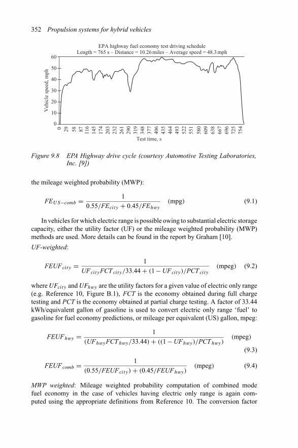
352 Propulsion systems for hybrid vehicles
60
50
40
30
20
10
Test time, s
Veh
icle
spe
ed, m
ph
0 29 58 87 116
145
174
203
232
261
290
319
348
377
406
435
464
493
522
551
580
609
638
667
696
725
754
0
EPA highway fuel economy test driving scheduleLength = 765 s – Distance = 10.26 miles – Average speed = 48.3 mph
Figure 9.8 EPA Highway drive cycle (courtesy Automotive Testing Laboratories,Inc. [9])
the mileage weighted probability (MWP):
FEUS−comb = 1
0.55/FEcity + 0.45/FEhwy
(mpg) (9.1)
In vehicles for which electric range is possible owing to substantial electric storagecapacity, either the utility factor (UF) or the mileage weighted probability (MWP)methods are used. More details can be found in the report by Graham [10].
UF-weighted:
FEUFcity = 1
UFcityFCT city/33.44 + (1 − UFcity)/PCT city
(mpeg) (9.2)
where UFcity and UFhwy are the utility factors for a given value of electric only range(e.g. Reference 10, Figure B.1), FCT is the economy obtained during full chargetesting and PCT is the economy obtained at partial charge testing. A factor of 33.44kWh/equivalent gallon of gasoline is used to convert electric only range ‘fuel’ togasoline for fuel economy predictions, or mileage per equivalent (US) gallon, mpeg:
FEUFhwy = 1
(UFhwyFCThwy/33.44) + ((1 − UFhwy)/PCThwy)(mpeg)
(9.3)
FEUFcomb = 1
(0.55/FEUFcity) + (0.45/FEUFhwy)(mpeg) (9.4)
MWP weighted: Mileage weighted probability computation of combined modefuel economy in the case of vehicles having electric only range is again com-puted using the appropriate definitions from Reference 10. The conversion factor
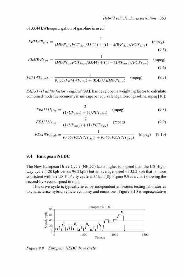
Hybrid vehicle characterisation 353
of 33.44 kWh/equiv. gallon of gasoline is used:
FEMWPcity = 1
(MWPcityFCT city/33.44) + ((1 − MWPcity)/PCT city)(mpeg)
(9.5)
FEMWPhwy = 1
(MWPhwyFCThwy/33.44) + ((1 − MWPhwy)/PCThwy)(mpeg)
(9.6)
FEMWPcomb = 1
(0.55/FEMWPcity) + (0.45/FEMWPhwy)(mpeg) (9.7)
SAE J1711 utility factor weighted: SAE has developed a weighting factor to calculatecombined mode fuel economy in mileage per equivalent gallon of gasoline, mpeg [10]:
FEJ1711city = 2
(1/UFcity) + (1/PCT city)(mpeg) (9.8)
FEJ1711hwy = 2
(1/UFhwy) + (1/PCThwy)(mpeg) (9.9)
FEMWPcomb = 1
(0.55/FEJ1711city) + (0.45/FEJ1711hwy)(mpeg) (9.10)
9.4 European NEDC
The New European Drive Cycle (NEDC) has a higher top speed than the US High-way cycle (120 kph versus 96.2 kph) but an average speed of 32.2 kph that is moreconsistent with the US FTP city cycle at 34 kph [8]. Figure 9.9 is a chart showing thesecond-by-second speed in mph.
This drive cycle is typically used by independent emissions testing laboratoriesto characterise hybrid vehicle economy and emissions. Figure 9.10 is representative
European NEDC
0
20
40
60
80
0 500 1000 1500Time, s
Spee
d, m
ph
Figure 9.9 European NEDC drive cycle
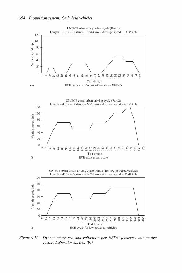
354 Propulsion systems for hybrid vehicles
120
100
80
60
40
20
Test time, s
Veh
icle
spe
ed, k
ph
0 8 16 24 32 40 48 56 64 72 80 88 96 104
112
120
128
136
144
152
160
168
176
184
1920
UN/ECE elementary urban cycle (Part 1)Length = 195 s – Distance = 0.944 km – Average speed = 18.35 kph
ECE cycle (i.e. first set of events on NEDC)(a)
120
100
80
60
40
20
Test time, s
Veh
icle
spe
ed, k
ph
0 16 32 48 64 80 96 112
128
144
160
176
192
208
224
240
256
272
288
304
320
336
352
368
384
4000
UN/ECE extra-urban driving cycle (Part 2)Length = 400 s – Distance = 6.955 km – Average speed = 62.59 kph
ECE extra urban cycle(b)
120
100
80
60
40
20
Test time, s
Veh
icle
spe
ed, k
ph
0 16 32 48 64 80 96 112
128
144
160
176
192
208
224
240
256
272
288
304
320
336
352
368
384
4000
UN/ECE extra-urban driving cycle (Part 2) for low-powered vehiclesLength = 400 s – Distance = 6.609 km – Average speed = 59.48 kph
ECE cycle for low powered vehicles(c)
Figure 9.10 Dynamometer test and validation per NEDC (courtesy AutomotiveTesting Laboratories, Inc. [9])
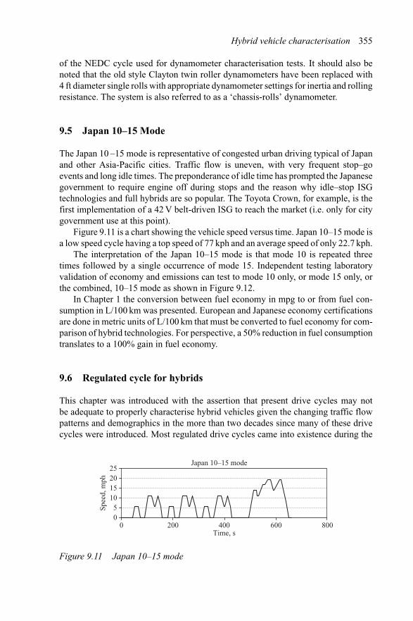
Hybrid vehicle characterisation 355
of the NEDC cycle used for dynamometer characterisation tests. It should also benoted that the old style Clayton twin roller dynamometers have been replaced with4 ft diameter single rolls with appropriate dynamometer settings for inertia and rollingresistance. The system is also referred to as a ‘chassis-rolls’ dynamometer.
9.5 Japan 10–15 Mode
The Japan 10 –15 mode is representative of congested urban driving typical of Japanand other Asia-Pacific cities. Traffic flow is uneven, with very frequent stop–goevents and long idle times. The preponderance of idle time has prompted the Japanesegovernment to require engine off during stops and the reason why idle–stop ISGtechnologies and full hybrids are so popular. The Toyota Crown, for example, is thefirst implementation of a 42 V belt-driven ISG to reach the market (i.e. only for citygovernment use at this point).
Figure 9.11 is a chart showing the vehicle speed versus time. Japan 10–15 mode isa low speed cycle having a top speed of 77 kph and an average speed of only 22.7 kph.
The interpretation of the Japan 10–15 mode is that mode 10 is repeated threetimes followed by a single occurrence of mode 15. Independent testing laboratoryvalidation of economy and emissions can test to mode 10 only, or mode 15 only, orthe combined, 10–15 mode as shown in Figure 9.12.
In Chapter 1 the conversion between fuel economy in mpg to or from fuel con-sumption in L/100 km was presented. European and Japanese economy certificationsare done in metric units of L/100 km that must be converted to fuel economy for com-parison of hybrid technologies. For perspective, a 50% reduction in fuel consumptiontranslates to a 100% gain in fuel economy.
9.6 Regulated cycle for hybrids
This chapter was introduced with the assertion that present drive cycles may notbe adequate to properly characterise hybrid vehicles given the changing traffic flowpatterns and demographics in the more than two decades since many of these drivecycles were introduced. Most regulated drive cycles came into existence during the
Japan 10–15 mode
05
10152025
0 200 400 600 800Time, s
Spee
d, m
ph
Figure 9.11 Japan 10–15 mode
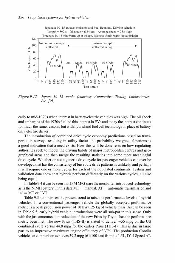
356 Propulsion systems for hybrid vehicles
120
100
80
60
40
20
Test time, s
Veh
icle
spe
ed, k
ph
0 35 70 105
140
175
210
14 25 60 95 130
30 65 100
135
35 70 105 5 40 75 110
145
180
2150
No emission samplecollected
Japanese 10–15 exhaust emission and Fuel Economy Driving scheduleLength = 892 s – Distance = 6.34 km – Average speed = 25.61 kph
(Preceded by 15 min warm-up at 60 kph, idle test, 5 min warm-up at 60 kph)
Emission samplecollected in bag
15 Mode 15 ModeIdle 10 Mode 10 Mode 10 Mode
Figure 9.12 Japan 10–15 mode (courtesy Automotive Testing Laboratories,Inc. [9])
early to mid-1970s when interest in battery-electric vehicles was high. The oil shockand embargos of the 1970s fuelled this interest in EVs and today the interest continuesfor much the same reasons, but with hybrid and fuel cell technology in place of batteryonly electric drives.
The introduction of combined drive cycle economy predictions based on trans-portation surveys resulting in utility factor and probability weighted functions isa good indication that a need exists. How this will be done rests on how regulatingauthorities seek to model the driving habits of major metropolitan centres and geo-graphical areas and then merge the resulting statistics into some more meaningfuldrive cycle. Whether or not a generic drive cycle for passenger vehicles can ever bedeveloped that has the consistency of bus route drive patterns is unlikely, and perhapsit will require one or more cycles for each of the populated continents. Testing andvalidation data show that hybrids perform differently on the various cycles, all elsebeing equal.
In Table 9.4 it can be seen that IPM M/G’s are the most often introduced technologyas is the NiMH battery. In this data MT = manual, AT = automatic transmission and‘∗’ = MT or CVT.
Table 9.5 summarises the present trend to raise the performance levels of hybridvehicles. In a conventional passenger vehicle the globally accepted performancemetric is a peak propulsion power of 10 kW/125 kg of vehicle mass. As can be seenin Table 9.5, early hybrid vehicle introductions were all sub-par in this sense. Onlywith the just announced introduction of the new Prius by Toyota has the performancemetric been met. The new Prius (THS-II) is slated to deliver ∼55 mpg on the UScombined cycle versus 44.8 mpg for the earlier Prius (THS-I). This is due in largepart to an impressive maximum engine efficiency of 37%. The production Corollavehicle for comparison achieves 39.2 mpg (61/100 km) from its 1.5L, IY, 4 Speed AT.
Hybrid vehicle characterisation 357
Table 9.4 Summary of current hybrid vehicles in the market or planned forintroduction
OEM Model Arch BattVoltage(V)
Batttype
Battcapacity(Ah)
Enginedisp.(L)
Enginepower(kW)
M/Gpower(kW)
M/Gtype
Transtype
Toyota Crown THS-M 42 VRLA 20 3.0 3.5 Lund AT-5GM Silverad PHT 42 VRLA 5.3 4.8 IM AT-4Suzuki K-Twin IMA 192 VRLA 0.6 32 5 MT-3Honda Insight IMA 144 NiMH 6.5 1.0 10 SPM MT-5∗Honda Civic IMA 144 NiMH 1.3 63 10 SPM MT-5∗Toyota Prius-I THS-I 274 NiMH 6.5 1.5 53 33/10 IPM PSToyota Prius-II THS-II 500 NiMH 6.5 1.5 57 50/10 IPM PSFord Escape PS 314 NiMH 5.5 2.3 80 65/28 IPM PSNissan Tino 345 Li-Ion 17/13 IPM CVTToyota Estima THS-I 216 NiMH 2.4 13/3.5; IPM PS
E4 18
Table 9.5 Trends in hybrid vehicle electric fraction
Vehicle Curb mass Enginepower
M/Gpower
Electricfraction
Peakspecificpower
(kg) (kW) (kW) (%) (kW/125 kg)Civic 1242 63 10 14 7.35Prius 1254 53 33/10 38 8.6Escape 2053 80 65/28 45 8.8HSD 1295 57 50/10 47 10.3
Hybrid Synergy Drive, HSD, goal is to match V6 performance with an I4through ‘electric supercharging’
The Toyota Hybrid Synergy Drive (THS-II) will deliver 2.8L/100km on the Japan 10–15 mode (84 mpg); 4.3L/100 km on the US M-H cycle (54.7 mpg): and 4.3L/100 kmon the ECE cycle (54.7 mpg).
9.7 References
1 ‘US House gives CIDI hybrid electric vehicle incentives’. US House of Repres-entatives House Bill, passed April 2003, http://www.hev.doe.gov
2 KAUFMAN, E.: ‘Electrical shock: fuel crisis or not, 42-volt systems are closerthan you think’. After Market Business web site, www.aftermarketbusiness.com
358 Propulsion systems for hybrid vehicles
3 ROUSSEAU, A., AHLUWAHLIA, R., DEVILLE, B. and ZHANG, Q.: ‘Well-to-wheels analysis of advanced SUV fuel cell vehicles’. Society of Automotive Engi-neers, Technical Publication 2003-01-0415, also published in SAE Internationalpublication, SP-1741
4 WANG, M. Q.: ‘Development and use of GREET 1.6 fuel-cycle modelfor transportation fuels and vehicle technologies’. US DOE-ANL Trans-portation Technology R&D Centre Report ANL/ESD/TM-163, June 2001.www.transportation.anl.gov/ttrdc/greet
5 ATKINS, M. J. and KOCH, C. R.: ‘A well-to-wheel comparison of sev-eral powertrain technologies’. SAE Technical Publication 2003-01-0081, SAEInternational Publication SP-1750
6 HARDY, K. and ROUSSEAU, A.: ‘PSAT: Argonne’s vehicle systemmodeling tool’. US DOE-ANL Transportation Technology R&D Center,www.transportation.anl.gov/ttrdc/greet
7 CUNNINGHAM, J., MOORE, R. and RAMASWAMY, S.: ‘A comparison ofenergy use for a direct-hydrogen hybrid versus a direct-hydrogen load follow-ing fuel cell vehicle’. SAE International Technical Paper 2003-01-0416, CoboConference Center, Detroit, MI, 3–6 March 2003
8 ROUSSEAU, A.: Argonne National Laboratory, Personal collaboration9 BARTON, G.: Automotive Testing Laboratory, Inc., 263 S. Mulberry Street,
Mesa, AZ 85202, www.atl-az.com. Personal collaboration on vehicle testingusing regulated cycles
10 GRAHAM, R.: ‘Comparing the benefits and impacts of hybrid vehicle options’.Electric Power Research Institute, EPRI, Report 1000349, July 2001
Chapter 10
Energy storage technologies
Energy storage systems are tailored to the type of fuel being used or to the mechani-cal, chemical, thermal or electrical form of energy directly stored. Liquid fossil fuelsthat will be used as feedstock for the engine include gasoline, liquefied petroleumgas (LPG), natural gas (NG) or hydrogen. Mechanical storage systems include fly-wheels, plus pneumatic (hydraulic) and elastic mediums to store energy in its kineticand potential energy forms, respectively. Hydraulic storage systems generally usepneumatic means such as a nitrogen bladder as the actual storage medium with thehydraulics as the actuation system.
A taxomomy of energy storage systems has been done that shows the relativeenergy density of the various media [1]. Table 10.1 is a summary of these fundamentalenergy storage systems.
Fundamental energy storage systems in the ideal case can be differentiated bythe medium of storing energy whether it is nuclear bond, covalent bond or molecularbond. Storage in nuclear bonds (fusion and fission) has energy storage densities somesix to seven orders of magnitude higher than storage in covalent bonds (gasoline),which in turn has energy storage density some three orders of magnitude greater thanelectro-chemical, mechanical or electro-magnetic systems (molecular bonds). Theremainder of this chapter will be devoted to understanding energy storage systems ofa practical nature that are suited to hybrid propulsion.
10.1 Battery systems
The world battery market is approximately a $30B business, 30% of which is devotedto motive power applications in the form of starting-lighting-ignition (SLI) batteries($3B market) and the remainder to primary cells and sealed rechargeable cells.
A battery is a collection of electro-chemical cells that convert chemical energydirectly to electrical energy via an isothermal process having a fixed supply of reac-tants. The battery is self-contained and generally has constant energy density forthe particular choice of active materials. We can view the battery as illustrated in
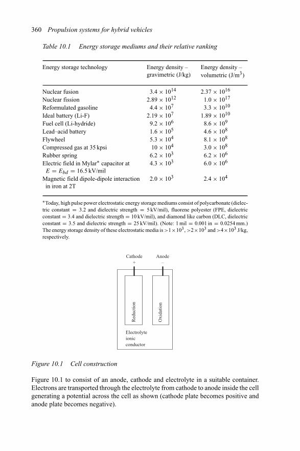
360 Propulsion systems for hybrid vehicles
Table 10.1 Energy storage mediums and their relative ranking
Energy storage technology Energy density –gravimetric (J/kg)
Energy density –volumetric (J/m3)
Nuclear fusion 3.4 × 10¹⁴ 2.37 × 10¹⁶
Nuclear fission 2.89 × 10¹² 1.0 × 10¹⁷
Reformulated gasoline 4.4 × 10⁷ 3.3 × 10¹⁰
Ideal battery (Li-F) 2.19 × 10⁷ 1.89 × 10¹⁰
Fuel cell (Li-hydride) 9.2 × 10⁶ 8.6 × 10⁹
Lead–acid battery 1.6 × 10⁵ 4.6 × 10⁸
Flywheel 5.3 × 10⁴ 8.1 × 10⁸
Compressed gas at 35 kpsi 10 × 104 3.0 × 10⁸
Rubber spring 6.2 × 10³ 6.2 × 10⁶
Electric field in Mylar∗ capacitor atE = Ebd = 16.5 kV/mil
4.3 × 10³ 6.0 × 10⁶
Magnetic field dipole-dipole interactionin iron at 2T
2.0 × 10³ 2.4 × 10⁴
∗Today, high pulse power electrostatic energy storage mediums consist of polycarbonate (dielec-tric constant = 3.2 and dielectric strength = 5 kV/mil), fluorene polyester (FPE, dielectricconstant = 3.4 and dielectric strength = 10 kV/mil), and diamond like carbon (DLC, dielectricconstant = 3.5 and dielectric strength = 25 kV/mil). (Note: 1 mil = 0.001 in = 0.0254 mm.)The energy storage density of these electrostatic media is >1×10³, >2×10³ and >4×10³ J/kg,respectively.
Oxi
datio
n
Red
uctio
n
Electrolyteionicconductor
Cathode+
Anode–
Figure 10.1 Cell construction
Figure 10.1 to consist of an anode, cathode and electrolyte in a suitable container.Electrons are transported through the electrolyte from cathode to anode inside the cellgenerating a potential across the cell as shown (cathode plate becomes positive andanode plate becomes negative).
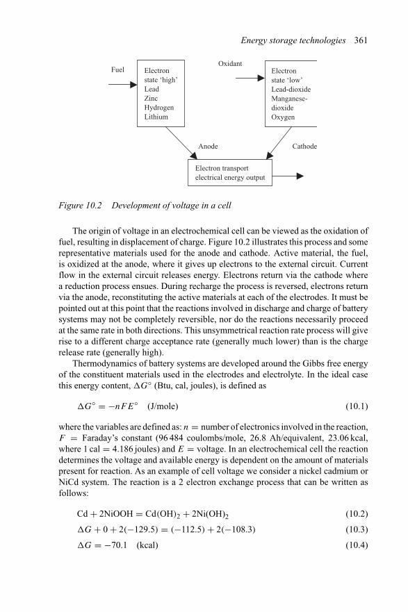
Energy storage technologies 361
Electronstate ‘high’LeadZincHydrogenLithium
Electronstate ‘low’Lead-dioxideManganese-dioxideOxygen
Electron transportelectrical energy output
Anode Cathode
FuelOxidant
Figure 10.2 Development of voltage in a cell
The origin of voltage in an electrochemical cell can be viewed as the oxidation offuel, resulting in displacement of charge. Figure 10.2 illustrates this process and somerepresentative materials used for the anode and cathode. Active material, the fuel,is oxidized at the anode, where it gives up electrons to the external circuit. Currentflow in the external circuit releases energy. Electrons return via the cathode wherea reduction process ensues. During recharge the process is reversed, electrons returnvia the anode, reconstituting the active materials at each of the electrodes. It must bepointed out at this point that the reactions involved in discharge and charge of batterysystems may not be completely reversible, nor do the reactions necessarily proceedat the same rate in both directions. This unsymmetrical reaction rate process will giverise to a different charge acceptance rate (generally much lower) than is the chargerelease rate (generally high).
Thermodynamics of battery systems are developed around the Gibbs free energyof the constituent materials used in the electrodes and electrolyte. In the ideal casethis energy content, �G◦ (Btu, cal, joules), is defined as
�G◦ = −nFE◦ (J/mole) (10.1)
where the variables are defined as: n = number of electronics involved in the reaction,F = Faraday’s constant (96 484 coulombs/mole, 26.8 Ah/equivalent, 23.06 kcal,where 1 cal = 4.186 joules) and E = voltage. In an electrochemical cell the reactiondetermines the voltage and available energy is dependent on the amount of materialspresent for reaction. As an example of cell voltage we consider a nickel cadmium orNiCd system. The reaction is a 2 electron exchange process that can be written asfollows:
Cd + 2NiOOH = Cd(OH)2 + 2Ni(OH)2 (10.2)
�G + 0 + 2(−129.5) = (−112.5) + 2(−108.3) (10.3)
�G = −70.1 (kcal) (10.4)
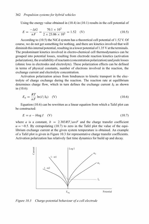
362 Propulsion systems for hybrid vehicles
Using the energy value obtained in (10.4) in (10.1) results in the cell potential of
E = −�G
nF= 70.1 × 10³
2 × 23.06 × 103 = 1.52 (V) (10.5)
According to (10.5) the NiCd system has a theoretical cell potential of 1.52 V. Ofcourse, we do not get something for nothing, and there are kinetics involved that willdiminish this internal potential, resulting in a lower potential of 1.35 V at the terminals.The predominant kinetics involved in electro-chemical cell thermodynamics can begrouped into potential losses, resulting from electrode reaction kinetics (activationpolarization), the availability of reactants (concentration polarization) and joule losses(ohmic loss in electrodes and electrolyte). These polarization effects can be definedin terms of physical constants, number of electrons involved in the reaction, theexchange current and electrolyte concentration.
Activation polarization arises from hindrances to kinetic transport in the elec-trolyte of charge exchange during the reaction. The reaction rate at equilibriumdetermines charge flow, which in turn defines the exchange current I0 as shownin (10.6):
Ea = RT
nFln(I/I0) (V) (10.6)
Equation (10.6) can be rewritten as a linear equation from which a Tafel plot canbe constructed:
E = a − blog I (V) (10.7)
where a is a constant, b = 2.303RT /αnF and the charge transfer coefficientα = ∼0.5. By extrapolating (10.7) to zero in the Tafel plot the value of the equi-librium exchange current at the given system temperature is obtained. An exampleof a Tafel plot is given in Figure 10.3 for representative charge transfer coefficients.Activation polarization has relatively fast time dynamics for build up and decay.
Io
Log I
Eeq. Potential
1 – α1
1 – α2
α2
α1
Cur
rent
Figure 10.3 Charge-potential behaviour of a cell electrode
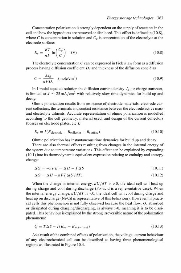
Energy storage technologies 363
Concentration polarization is strongly dependent on the supply of reactants in thecell and how the byproducts are removed or displaced. This effect is defined in (10.8),where C is concentration in solution and Ce is concentration of the electrolyte at theelectrode surface:
Ec = RT
nFln(
Ce
C
)(V) (10.8)
The electrolyte concentration C can be expressed in Fick’s law form as a diffusionprocess having diffusion coefficient De and thickness of the diffusion zone δ as
C = δJd
nFDe
(mole/cm3) (10.9)
In 1 molal aqueous solution the diffusion current density Jd , or charge transport,is limited to J ∼ 25 mA/cm2 with relatively slow time dynamics for build up anddecay.
Ohmic polarization results from resistance of electrode materials, electrode cur-rent collectors, the terminals and contact resistance between the electrode active massand electrolyte diluents. Accurate representation of ohmic polarization is modelledaccording to the cell geometry, material used, and design of the current collectors(bosses on electrode plates, etc.):
Er = I (Relectrode + Rcollector + Rsurface) (10.10)
Ohmic polarization has instantaneous time dynamics for build up and decay.There are also thermal effects resulting from changes in the internal energy of
the system due to temperature variations. This effect can be explained by expanding(10.1) into its thermodynamic equivalent expression relating to enthalpy and entropychange:
�G = −nFE = �H − T �S (10.11)
�G = �H − nFT (dU/dT ) (10.12)
When the change in internal energy, dU/dT is >0, the ideal cell will heat upduring charge and cool during discharge (Pb–acid is a representative case). Whenthe internal energy change, dU/dT is <0, the ideal cell will cool during charge andheat up on discharge (Ni-Cd is representative of this behaviour). However, in practi-cal cells this phenomenon is not fully observed because the heat flow, Q, absorbedor dissipated during charging/discharging, is always >0, meaning it is to be dissi-pated. This behaviour is explained by the strong irreversible nature of the polarizationphenomena:
Q = T �S − I (Eoc − Epol−total) (10.13)
As a result of the combined effects of polarization, the voltage–current behaviourof any electrochemical cell can be described as having three phenomenologicalregions as illustrated in Figure 10.4.
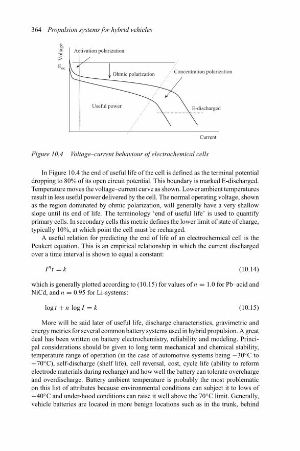
364 Propulsion systems for hybrid vehicles
Current
Vol
tage
Eoc
E-discharged
Activation polarization
Concentration polarizationOhmic polarization
Useful power
Figure 10.4 Voltage–current behaviour of electrochemical cells
In Figure 10.4 the end of useful life of the cell is defined as the terminal potentialdropping to 80% of its open circuit potential. This boundary is marked E-discharged.Temperature moves the voltage–current curve as shown. Lower ambient temperaturesresult in less useful power delivered by the cell. The normal operating voltage, shownas the region dominated by ohmic polarization, will generally have a very shallowslope until its end of life. The terminology ‘end of useful life’ is used to quantifyprimary cells. In secondary cells this metric defines the lower limit of state of charge,typically 10%, at which point the cell must be recharged.
A useful relation for predicting the end of life of an electrochemical cell is thePeukert equation. This is an empirical relationship in which the current dischargedover a time interval is shown to equal a constant:
Int = k (10.14)
which is generally plotted according to (10.15) for values of n = 1.0 for Pb–acid andNiCd, and n = 0.95 for Li-systems:
log t + n log I = k (10.15)
More will be said later of useful life, discharge characteristics, gravimetric andenergy metrics for several common battery systems used in hybrid propulsion. A greatdeal has been written on battery electrochemistry, reliability and modeling. Princi-pal considerations should be given to long term mechanical and chemical stability,temperature range of operation (in the case of automotive systems being −30◦C to+70◦C), self-discharge (shelf life), cell reversal, cost, cycle life (ability to reformelectrode materials during recharge) and how well the battery can tolerate overchargeand overdischarge. Battery ambient temperature is probably the most problematicon this list of attributes because environmental conditions can subject it to lows of−40◦C and under-hood conditions can raise it well above the 70◦C limit. Generally,vehicle batteries are located in more benign locations such as in the trunk, behind
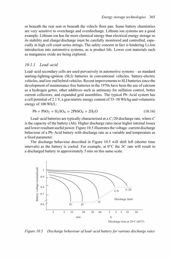
Energy storage technologies 365
or beneath the rear seat or beneath the vehicle floor pan. Some battery chemistriesare very sensitive to overcharge and overdischarge. Lithium ion systems are a goodexample. Lithium ion has far more chemical energy than electrical energy storage soits stability and charge/discharge must be carefully monitored and controlled, espe-cially in high cell count series strings. The safety concern in fact is hindering Li-Ionintroduction into automotive systems, as is product life. Lower cost materials suchas manganese oxide are being explored.
10.1.1 Lead–acid
Lead–acid secondary cells are used pervasively in automotive systems – as standardstarting-lighting-ignition (SLI) batteries in conventional vehicles, battery-electricvehicles, and low end hybrid vehicles. Recent improvements to SLI batteries since thedevelopment of maintenance free batteries in the 1970s have been the use of calciumas a hydrogen getter, other additives such as antimony for sulfation control, bettercurrent collectors, and expanded grid assemblies. The typical Pb–Acid system hasa cell potential of 2.1 V, a gravimetric energy content of 35–50 Wh/kg and volumetricenergy of 100 Wh/L:
Pb + PbO2 + H2SO4 = 2PbSO4 + 2H2O (10.16)
Lead–acid batteries are typically characterised at a C/20 discharge rate, where C
is the capacity of the battery (Ah). Higher discharge rates incur higher internal lossesand lower resultant useful power. Figure 10.5 illustrates the voltage–current dischargebehaviour of a Pb–Acid battery with discharge rate as a variable and temperature asa fixed parameter.
The discharge behaviour described in Figure 10.5 will shift left (shorter timeintervals) as the battery is cooled. For example, at 0◦C the 3C rate will result ina discharged battery in approximately 5 min on this same scale.
Bat
tery
vol
tage
(no
rmal
ized
)
1
0.9
0.8
0.7
0.6
Discharge time at 20˚C (68˚F)
C/20C/8
1C2C3C
Discharge limit
2 5 10 20 30 60 2 3 5 10 20
min h
Figure 10.5 Discharge behaviour of lead–acid battery for various discharge rates
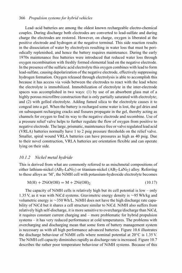
366 Propulsion systems for hybrid vehicles
Lead–acid batteries are among the oldest known rechargeable electro-chemicalcouples. During discharge both electrodes are converted to lead-sulfate and duringcharge the electrodes are restored. However, on charge, oxygen is liberated at thepositive electrode and hydrogen at the negative terminal. This side reaction resultsin the dissociation of water by electrolysis resulting in water loss that must be peri-odically replenished, and hence the battery requires maintenance. During the early1970s maintenance free batteries were introduced that reduced water loss throughoxygen recombination with freshly formed elemental lead on the negative electrode.In the presence of the sulfuric acid electrolyte this oxygen combines with lead to formlead-sulfate, causing depolarization of the negative electrode, effectively suppressinghydrogen formation. Oxygen released through electrolysis is able to accomplish thisbecause it has access via voids between the electrodes to react with the lead wherethe electrolyte is immobilized. Immobilization of electrolyte in the inter-electrodespaces was accomplished in two ways: (1) by use of an absorbent glass mat of ahighly porous microfibre construction that is only partially saturated with electrolyte;and (2) with gelled electrolyte. Adding fumed silica to the electrolyte causes it tocongeal into a gel. When the battery is recharged some water is lost, the gel dries andon subsequent recharging cracks and fissures propagate in the gel, thereby acting aschannels for oxygen to find its way to the negative electrode and recombine. Use ofa pressure relief valve helps to further regulate the flow of oxygen from positive tonegative electrode. The large, prismatic, maintenance free or valve regulated lead acid(VRLA) batteries normally have 1 to 2 psig pressure thresholds on the relief valve.Smaller, spiral wound VRLA batteries can have pressures as high as 40 psig. Dueto their novel construction, VRLA batteries are orientation flexible and can operatelying on their side.
10.1.2 Nickel metal hydride
This is derived from what are commonly referred to as mischmetal compositions ofeither lathium-nickel (AB5-LaNi5) or titanium-nickel (AB2-LaNi2) alloy. Referringto these alloys as ‘M’, the NiMH cell with potassium-hydroxide electrolyte becomes
M(H) + 2NiO(OH) = M + 2Ni(OH)2 (10.17)
The capacity of NiMH cells is relatively high but its cell potential is low – only1.35 V, as it was with NiCd systems. Gravimetric energy density is ∼95 Wh/kg andvolumetric energy is ∼350 Wh/L. NiMH does not have the high discharge rate capa-bility of NiCd but it shares a cell structure similar to NiCd. NiMH also suffers fromrelatively high self-discharge, it is more sensitive to overcharge/discharge than NiCd,it requires constant current charging and – more problematic for hybrid propulsionsystems – it has very reduced performance at cold temperatures. The problems withovercharging and discharging mean that some form of battery management systemis necessary as with all high performance advanced batteries. Figure 10.6 illustratesthe discharge behaviour of NiMH cells where nominal potential at 20◦C is 1.35 V.The NiMH cell capacity diminishes rapidly as discharge rate is increased. Figure 10.7describes the rather poor temperature behaviour of NiMH systems. Because of this
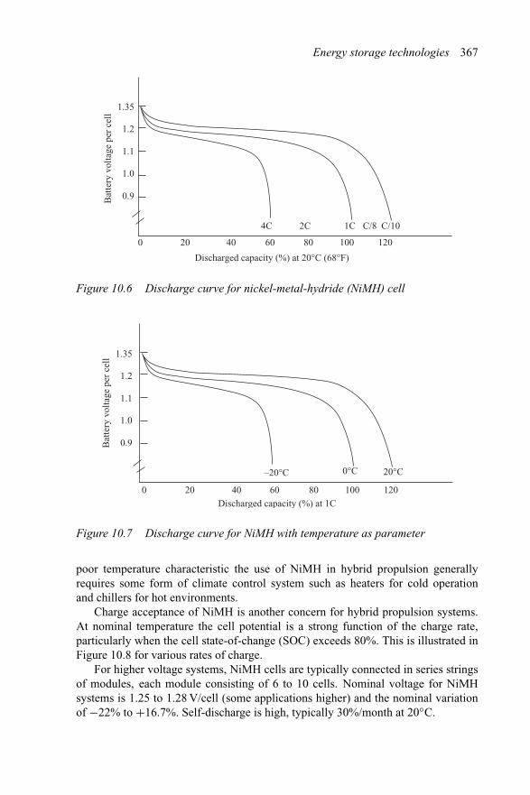
Energy storage technologies 367
Bat
tery
vol
tage
per
cel
l1.35
1.2
1.1
1.0
0.9
Discharged capacity (%) at 20°C (68°F)
C/10C/81C2C4C
0 20 40 60 80 100 120
Figure 10.6 Discharge curve for nickel-metal-hydride (NiMH) cell
Bat
tery
vol
tage
per
cel
l 1.35
1.2
1.1
1.0
0.9
Discharged capacity (%) at 1C
0°C 20°C–20°C
0 20 40 60 80 100 120
Figure 10.7 Discharge curve for NiMH with temperature as parameter
poor temperature characteristic the use of NiMH in hybrid propulsion generallyrequires some form of climate control system such as heaters for cold operationand chillers for hot environments.
Charge acceptance of NiMH is another concern for hybrid propulsion systems.At nominal temperature the cell potential is a strong function of the charge rate,particularly when the cell state-of-change (SOC) exceeds 80%. This is illustrated inFigure 10.8 for various rates of charge.
For higher voltage systems, NiMH cells are typically connected in series stringsof modules, each module consisting of 6 to 10 cells. Nominal voltage for NiMHsystems is 1.25 to 1.28 V/cell (some applications higher) and the nominal variationof −22% to +16.7%. Self-discharge is high, typically 30%/month at 20◦C.
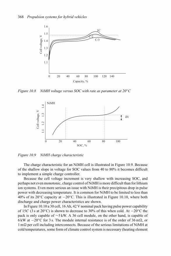
368 Propulsion systems for hybrid vehicles
1C1.5
1.4
1.3
1.2
C/2C/3
20 40 60 80 100 120 140
Capacity, %
0
1.6
1.1
Cel
l vol
tage
, V
Figure 10.8 NiMH voltage versus SOC with rate as parameter at 20◦C
Cel
l vol
tage
, V
1.1
1.2
1.3
1.4
δV
NiMH
0 20 40 60SOC, %
80 100
Figure 10.9 NiMH charge characteristic
The charge characteristic for an NiMH cell is illustrated in Figure 10.9. Becauseof the shallow slope in voltage for SOC values from 40 to 80% it becomes difficultto implement a simple charge controller.
Because the cell voltage increment is very shallow with increasing SOC, andperhaps not even monotonic, charge control of NiMH is more difficult than for lithiumion systems. Even more serious an issue with NiMH is their precipitous drop in pulsepower with decreasing temperature. It is common for NiMH to be limited to less than40% of its 20◦C capacity at −20◦C. This is illustrated in Figure 10.10, where bothdischarge and charge power characteristics are shown.
In Figure 10.10 a 30 cell, 16 Ah, 42 V nominal pack having pulse power capabilityof 15C (3 s at 20◦C) is shown to decrease to 30% of this when cold. At −20◦C thepack is only capable of ∼5 kW. A 36 cell module, on the other hand, is capable of6 kW at −20◦C for 3 s. The module internal resistance is of the order of 36 m�, or1 m� per cell including interconnects. Because of the serious limitations of NiMH atcold temperatures, some form of climate control system is necessary (heating element
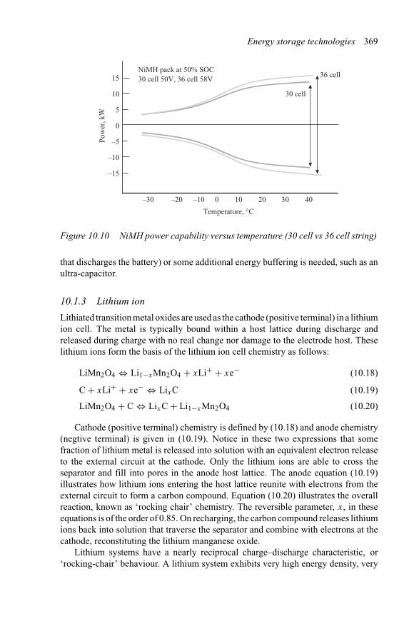
Energy storage technologies 369
Temperature, °C
30 cell
36 cellNiMH pack at 50% SOC30 cell 50V, 36 cell 58V
–30 –20 –10 0 10 20 30 40
15
10
5
0
–5
–10
–15
Pow
er, k
W
Figure 10.10 NiMH power capability versus temperature (30 cell vs 36 cell string)
that discharges the battery) or some additional energy buffering is needed, such as anultra-capacitor.
10.1.3 Lithium ion
Lithiated transition metal oxides are used as the cathode (positive terminal) in a lithiumion cell. The metal is typically bound within a host lattice during discharge andreleased during charge with no real change nor damage to the electrode host. Theselithium ions form the basis of the lithium ion cell chemistry as follows:
LiMn2O4 ⇔ Li1−xMn2O4 + xLi+ + xe− (10.18)
C + xLi+ + xe− ⇔ LixC (10.19)
LiMn2O4 + C ⇔ LixC + Li1−xMn2O4 (10.20)
Cathode (positive terminal) chemistry is defined by (10.18) and anode chemistry(negtive terminal) is given in (10.19). Notice in these two expressions that somefraction of lithium metal is released into solution with an equivalent electron releaseto the external circuit at the cathode. Only the lithium ions are able to cross theseparator and fill into pores in the anode host lattice. The anode equation (10.19)illustrates how lithium ions entering the host lattice reunite with electrons from theexternal circuit to form a carbon compound. Equation (10.20) illustrates the overallreaction, known as ‘rocking chair’ chemistry. The reversible parameter, x, in theseequations is of the order of 0.85. On recharging, the carbon compound releases lithiumions back into solution that traverse the separator and combine with electrons at thecathode, reconstituting the lithium manganese oxide.
Lithium systems have a nearly reciprocal charge–discharge characteristic, or‘rocking-chair’ behaviour. A lithium system exhibits very high energy density, very
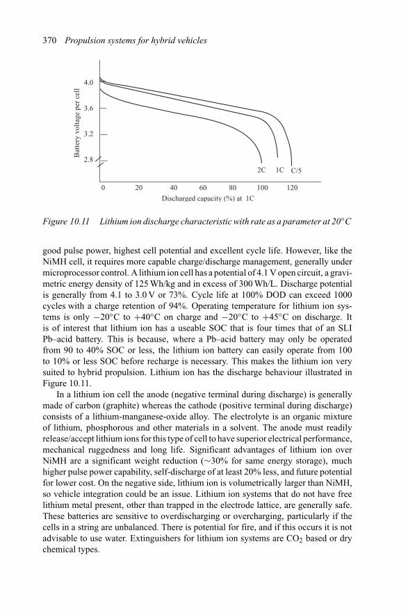
370 Propulsion systems for hybrid vehicles
Bat
tery
vol
tage
per
cel
l4.0
3.6
3.2
2.8
Discharged capacity (%) at 1C
0 20 40 60 80 100 120
C/51C2C
Figure 10.11 Lithium ion discharge characteristic with rate as a parameter at 20◦C
good pulse power, highest cell potential and excellent cycle life. However, like theNiMH cell, it requires more capable charge/discharge management, generally undermicroprocessor control. A lithium ion cell has a potential of 4.1 V open circuit, a gravi-metric energy density of 125 Wh/kg and in excess of 300 Wh/L. Discharge potentialis generally from 4.1 to 3.0 V or 73%. Cycle life at 100% DOD can exceed 1000cycles with a charge retention of 94%. Operating temperature for lithium ion sys-tems is only −20◦C to +40◦C on charge and −20◦C to +45◦C on discharge. Itis of interest that lithium ion has a useable SOC that is four times that of an SLIPb–acid battery. This is because, where a Pb–acid battery may only be operatedfrom 90 to 40% SOC or less, the lithium ion battery can easily operate from 100to 10% or less SOC before recharge is necessary. This makes the lithium ion verysuited to hybrid propulsion. Lithium ion has the discharge behaviour illustrated inFigure 10.11.
In a lithium ion cell the anode (negative terminal during discharge) is generallymade of carbon (graphite) whereas the cathode (positive terminal during discharge)consists of a lithium-manganese-oxide alloy. The electrolyte is an organic mixtureof lithium, phosphorous and other materials in a solvent. The anode must readilyrelease/accept lithium ions for this type of cell to have superior electrical performance,mechanical ruggedness and long life. Significant advantages of lithium ion overNiMH are a significant weight reduction (∼30% for same energy storage), muchhigher pulse power capability, self-discharge of at least 20% less, and future potentialfor lower cost. On the negative side, lithium ion is volumetrically larger than NiMH,so vehicle integration could be an issue. Lithium ion systems that do not have freelithium metal present, other than trapped in the electrode lattice, are generally safe.These batteries are sensitive to overdischarging or overcharging, particularly if thecells in a string are unbalanced. There is potential for fire, and if this occurs it is notadvisable to use water. Extinguishers for lithium ion systems are CO2 based or drychemical types.
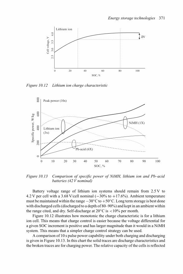
Energy storage technologies 371
SOC, %
Cel
l vol
tage
, V
2.5
3.0
3.5
4.0
Lithium ion
δV
0 20 40 60 80 100
Figure 10.12 Lithium ion charge characteristic
Spec
ific
pow
er, W
/kg
020
040
060
080
0
Peak power (10s)
Pb-acid (6X)
NiMH (1X)
Lithium ion(3x)
0 10 20 30 40 50 60 70 80 90
SOC, %
100
Figure 10.13 Comparison of specific power of NiMH, lithium ion and Pb–acidbatteries (42 V nominal)
Battery voltage range of lithium ion systems should remain from 2.5 V to4.2 V per cell with a 3.68 V/cell nominal (−30% to +17.6%). Ambient temperaturemust be maintained within the range −30◦C to +50◦C. Long term storage is best donewith discharged cells (discharged to a depth of 80–90%) and kept in an ambient withinthe range cited, and dry. Self-discharge at 20◦C is <10% per month.
Figure 10.12 illustrates how monotonic the charge characteristic is for a lithiumion cell. This means that charge control is easier because the voltage differential fora given SOC increment is positive and has larger magnitude than it would in a NiMHsystem. This means that a simpler charge control strategy can be used.
A comparison of 10 s pulse power capability under both charging and dischargingis given in Figure 10.13. In this chart the solid traces are discharge characteristics andthe broken traces are for charging power. The relative capacity of the cells is reflected
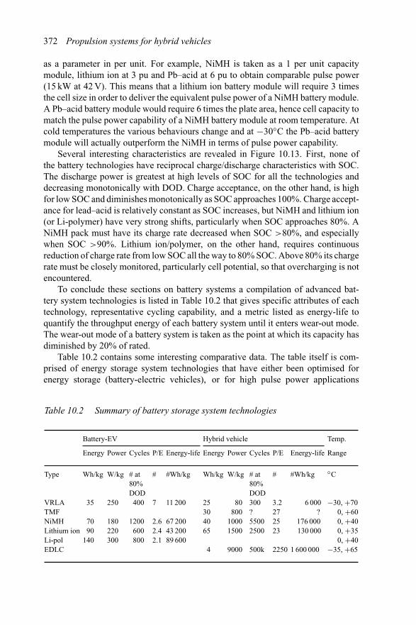
372 Propulsion systems for hybrid vehicles
as a parameter in per unit. For example, NiMH is taken as a 1 per unit capacitymodule, lithium ion at 3 pu and Pb–acid at 6 pu to obtain comparable pulse power(15 kW at 42 V). This means that a lithium ion battery module will require 3 timesthe cell size in order to deliver the equivalent pulse power of a NiMH battery module.A Pb–acid battery module would require 6 times the plate area, hence cell capacity tomatch the pulse power capability of a NiMH battery module at room temperature. Atcold temperatures the various behaviours change and at −30◦C the Pb–acid batterymodule will actually outperform the NiMH in terms of pulse power capability.
Several interesting characteristics are revealed in Figure 10.13. First, none ofthe battery technologies have reciprocal charge/discharge characteristics with SOC.The discharge power is greatest at high levels of SOC for all the technologies anddecreasing monotonically with DOD. Charge acceptance, on the other hand, is highfor low SOC and diminishes monotonically as SOC approaches 100%. Charge accept-ance for lead–acid is relatively constant as SOC increases, but NiMH and lithium ion(or Li-polymer) have very strong shifts, particularly when SOC approaches 80%. ANiMH pack must have its charge rate decreased when SOC >80%, and especiallywhen SOC >90%. Lithium ion/polymer, on the other hand, requires continuousreduction of charge rate from low SOC all the way to 80% SOC. Above 80% its chargerate must be closely monitored, particularly cell potential, so that overcharging is notencountered.
To conclude these sections on battery systems a compilation of advanced bat-tery system technologies is listed in Table 10.2 that gives specific attributes of eachtechnology, representative cycling capability, and a metric listed as energy-life toquantify the throughput energy of each battery system until it enters wear-out mode.The wear-out mode of a battery system is taken as the point at which its capacity hasdiminished by 20% of rated.
Table 10.2 contains some interesting comparative data. The table itself is com-prised of energy storage system technologies that have either been optimised forenergy storage (battery-electric vehicles), or for high pulse power applications
Table 10.2 Summary of battery storage system technologies
Battery-EV Hybrid vehicle Temp.
Energy Power Cycles P/E Energy-life Energy Power Cycles P/E Energy-life Range
Type Wh/kg W/kg # at # #Wh/kg Wh/kg W/kg # at # #Wh/kg ◦C80% 80%DOD DOD
VRLA 35 250 400 7 11 200 25 80 300 3.2 6 000 −30, +70TMF 30 800 ? 27 ? 0, +60NiMH 70 180 1200 2.6 67 200 40 1000 5500 25 176 000 0, +40Lithium ion 90 220 600 2.4 43 200 65 1500 2500 23 130 000 0, +35Li-pol 140 300 800 2.1 89 600 0, +40EDLC 4 9000 500k 2250 1 600 000 −35, +65
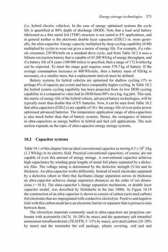
Energy storage technologies 373
(i.e. hybrid electric vehicles). In the case of energy optimised systems the cyclelife is quantified at 80% depth of discharge (DOD). Note that a lead–acid batteryfabricated as a thin metal foil (TMF) structure is not suited to EV applications, andin general neither is the electronic double layer capacitor (EDLC) or, more gener-ally, the ultra-capacitor. Energy capacity multiplied by deep cycling capability (0.80)multiplied by cycles to wear out gives a metric of energy life. For example, if a vehi-cle consumes 250 Wh/mile on a standard drive cycle, and from Table 10.2 it uses alithium ion traction battery that is capable of 43 200 Wh/kg of energy throughput, andif a battery life of 8 years (100 000 miles) is specified, then a range of 172.8 miles/kgcan be expected. To meet the range goal requires some 578.7 kg of battery. If theaverage consumption increases to 400 Wh/mile, then a battery mass of 926 kg isnecessary, or a smaller mass, but a replacement interval must be defined.
Battery systems for hybrid vehicles are optimised for shallow cycling (1% toperhaps 4% of capacity per event) and have comparably higher cycling. In Table 10.2the hybrid system cycling capability has been projected from its low DOD cyclingcapability to a comparative value had its DOD been 80% on a log–log plot. This said,the metric of energy-life of the hybrid vehicle, advanced battery technologies, will betypically more than double that of EV batteries. Now, it can be seen from Table 10.2that ultra-capacitors (EDLCs) are capable of 10× the energy-life of even pulse poweroptimised advanced batteries. The temperature application range of ultra-capacitorsis also much better than that of battery systems. Hence, the resurgence of interestin ultra-capacitors as energy buffers in hybrid and fuel cell applications. The nextsection expands on the topic of ultra-capacitor energy storage systems.
10.2 Capacitor systems
Table 10.1 of this chapter lists an ideal conventional capacitor as storing 4.3×10³ J/kg(1.2 Wh/kg) in its electric field. Practical conventional capacitors, of course, are notcapable of even this amount of energy storage. A conventional capacitor achieveshigh capacitance by winding great lengths of metal foil plates separated by a dielec-tric film. The voltage rating is determined by the dielectric strength (V/m) and itsthickness. An ultra-capacitor works differently. Instead of metal electrodes separatedby a dielectric (sheet or film) that facilitates charge separation across its thicknessan ultra-capacitor achieves charge separation distances on the order of ion dimen-sions (∼10 Å). The ultra-capacitor’s charge separation mechanism, or double layercapacitor model, was described by Helmholtz in the late 1800s. In Figure 10.14the construction of an ultra-capacitor is shown to consist of carbon (activated carbon)foil electrodes that are impregnated with conductive electrolyte. Positive and negativefoils with this carbon mush have an electronic barrier or separator that is porous to ionsbetween them.
The electrolyte materials commonly used in ultra-capacitors are propylene car-bonate with acetonitrile (ACN, 10–20% by mass) and the quaternary salt tetraethylammonium tetrafluoroborate (TEATFB, 5–15% by mass), activated carbon (10–20%by mass) and the remainder the cell package, plastic covering, end seal and
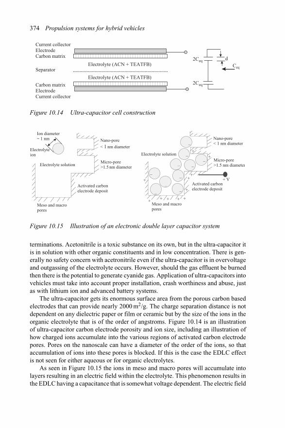
374 Propulsion systems for hybrid vehicles
Current collectorElectrodeCarbon matrix
Separator
Carbon matrixElectrodeCurrent collector
Electrolyte (ACN + TEATFB)
Electrolyte (ACN + TEATFB)
Ceq
2Ceq
2Ceq
d
Figure 10.14 Ultra-capacitor cell construction
Electrolyteion
Ion diameter~ 1 nm Nano-pore
< 1 nm diameter
Micro-pore>1.5 nm diameter
Meso and macropores
Activated carbonelectrode deposit
Electrolyte solution
Nano-pore< 1 nm diameter
Micro-pore>1.5 nm diameter
Meso and macropores
Activated carbonelectrode deposit
Electrolyte solution
+ V
–
––
––
––
–
––
+
+ + +
++
++
+
+ +
Figure 10.15 Illustration of an electronic double layer capacitor system
terminations. Acetonitrile is a toxic substance on its own, but in the ultra-capacitor itis in solution with other organic constituents and in low concentration. There is gen-erally no safety concern with acetronitrile even if the ultra-capacitor is in overvoltageand outgassing of the electrolyte occurs. However, should the gas effluent be burnedthen there is the potential to generate cyanide gas. Application of ultra-capacitors intovehicles must take into account proper installation, crash worthiness and abuse, justas with lithium ion and advanced battery systems.
The ultra-capacitor gets its enormous surface area from the porous carbon basedelectrodes that can provide nearly 2000 m2/g. The charge separation distance is notdependent on any dielectric paper or film or ceramic but by the size of the ions in theorganic electrolyte that is of the order of angstroms. Figure 10.14 is an illustrationof ultra-capacitor carbon electrode porosity and ion size, including an illustration ofhow charged ions accumulate into the various regions of activated carbon electrodepores. Pores on the nanoscale can have a diameter of the order of the ions, so thataccumulation of ions into these pores is blocked. If this is the case the EDLC effectis not seen for either aqueous or for organic electrolytes.
As seen in Figure 10.15 the ions in meso and macro pores will accumulate intolayers resulting in an electric field within the electrolyte. This phenomenon results inthe EDLC having a capacitance that is somewhat voltage dependent. The electric field
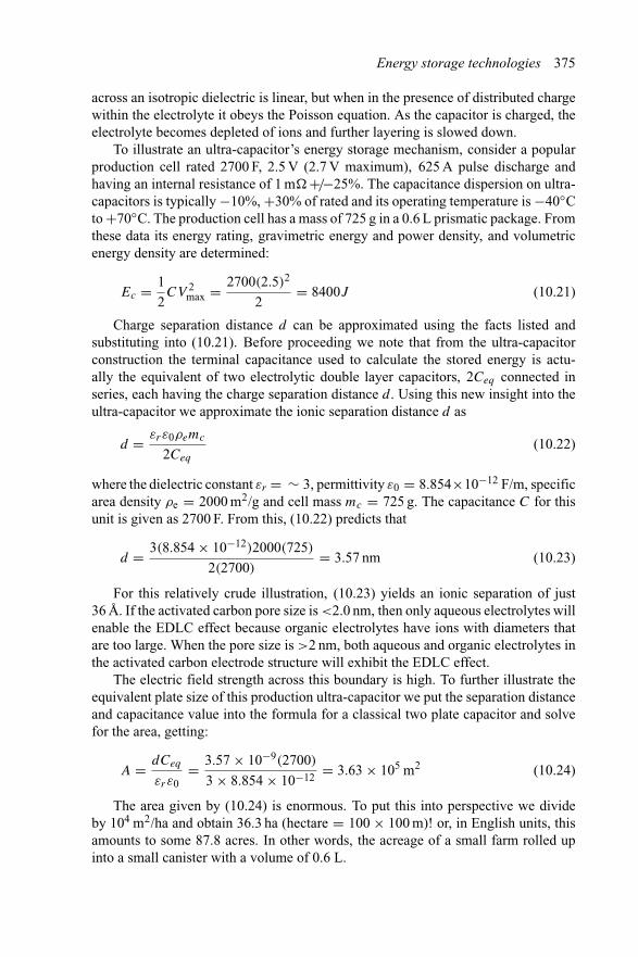
Energy storage technologies 375
across an isotropic dielectric is linear, but when in the presence of distributed chargewithin the electrolyte it obeys the Poisson equation. As the capacitor is charged, theelectrolyte becomes depleted of ions and further layering is slowed down.
To illustrate an ultra-capacitor’s energy storage mechanism, consider a popularproduction cell rated 2700 F, 2.5 V (2.7 V maximum), 625 A pulse discharge andhaving an internal resistance of 1 m� +/−25%. The capacitance dispersion on ultra-capacitors is typically −10%, +30% of rated and its operating temperature is −40◦Cto +70◦C. The production cell has a mass of 725 g in a 0.6 L prismatic package. Fromthese data its energy rating, gravimetric energy and power density, and volumetricenergy density are determined:
Ec = 1
2CV 2
max = 2700(2.5)2
2= 8400J (10.21)
Charge separation distance d can be approximated using the facts listed andsubstituting into (10.21). Before proceeding we note that from the ultra-capacitorconstruction the terminal capacitance used to calculate the stored energy is actu-ally the equivalent of two electrolytic double layer capacitors, 2Ceq connected inseries, each having the charge separation distance d. Using this new insight into theultra-capacitor we approximate the ionic separation distance d as
d = εrε0ρemc
2Ceq
(10.22)
where the dielectric constant εr = ∼ 3, permittivity ε0 = 8.854×10⁻¹² F/m, specificarea density ρe = 2000 m2/g and cell mass mc = 725 g. The capacitance C for thisunit is given as 2700 F. From this, (10.22) predicts that
d = 3(8.854 × 10⁻¹²)2000(725)
2(2700)= 3.57 nm (10.23)
For this relatively crude illustration, (10.23) yields an ionic separation of just36 Å. If the activated carbon pore size is <2.0 nm, then only aqueous electrolytes willenable the EDLC effect because organic electrolytes have ions with diameters thatare too large. When the pore size is >2 nm, both aqueous and organic electrolytes inthe activated carbon electrode structure will exhibit the EDLC effect.
The electric field strength across this boundary is high. To further illustrate theequivalent plate size of this production ultra-capacitor we put the separation distanceand capacitance value into the formula for a classical two plate capacitor and solvefor the area, getting:
A = dCeq
εrε0= 3.57 × 10⁻⁹(2700)
3 × 8.854 × 10−12 = 3.63 × 10⁵ m2 (10.24)
The area given by (10.24) is enormous. To put this into perspective we divideby 104 m2/ha and obtain 36.3 ha (hectare = 100 × 100 m)! or, in English units, thisamounts to some 87.8 acres. In other words, the acreage of a small farm rolled upinto a small canister with a volume of 0.6 L.
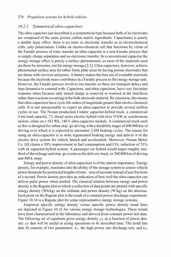
376 Propulsion systems for hybrid vehicles
10.2.1 Symmetrical ultra-capacitors
The ultra-capacitor just described is a symmetrical type because both of its electrodesare composed of the same porous carbon matrix ingredients. Capacitance is purelya double layer effect, there is no ionic or electronic transfer as in electrochemicalcells, only polarization. Unlike an electro-chemical cell that functions by virtue ofthe Faradic process of ionic transfer an ultra-capacitor is a non-Faradic process thatis simply charge separation and no electronic transfer. In a conventional capacitor theenergy storage effect is purely a surface phenomenon, so most of the materials usedare there for structure, not for energy storage [2,3]. Ultra-capacitors, however, achievephenomenal surface area for rather finite plate areas by having porous electrodes thatare dense with crevices and pores. A battery makes the best use of available materialsbecause the electrode mass contributes in a Faradic process to the energy storage task.However, the Faradic process involves ion transfer so there are transport delays andtime dynamics to contend with. Capacitors, and ultra-capacitors, have very fast pulseresponse times because only stored charge is removed or restored at the interfacesrather than reactions occurring in the bulk electrode material. By extension, this meansthat ultra-capacitors have cycle life orders of magnitude greater than electro-chemicalcells. It is not unreasonable to expect an ultra-capacitor to provide several millioncycles in use. The Nissan production Condor capacitor-hybrid truck, a commercial4 ton load capacity, 7 L diesel series electric hybrid with twin 55 kW ac synchronousmotors, relies on a 583 Wh, 346 V ultra-capacitor module. A commercial truck suchas this is designed for urban stop–go driving with a durability target of 600 000 km ofdriving over which it is expected to encounter 2.4M braking cycles. The reason forusing an ultra-capacitor is to store regenerated braking energy and deliver it to theelectric drive system for vehicle launch and acceleration. Moreover, Nissan MotorCo. [4] claims a 50% improvement in fuel consumption and CO2 reduction of 33%with its capacitor-hybrid system. A passenger car hybrid would target roughly one-third of the mileage and stop–go events as the delivery truck, or 200 000 km of drivingand 800 k stops.
Energy and power density of ultra-capacitors is of the utmost importance. Energydensity, for example, translates into the ability of the storage system to source vehiclepower demands for protracted lengths of time – tens of seconds instead of just fractionsof a second. Power density provides an indication of how well the ultra-capacitor candeliver pulse power when needed. The classical relation between energy and powerdensity is the Ragone plot in which a collection of data points are plotted with specificenergy density (Wh/kg) on the ordinate and power density (W/kg) on the abscissa.Each point on the Ragone plot is the result of a constant power discharge experiment.Figure 10.16 is a Ragone plot for some representative energy storage systems.
Empirical specific energy density versus specific power density trend linesare depicted in Figure 10.16 for various energy storage technologies. These trendshave been characterised in the laboratory and derived from constant power test data.The following set of equations gives energy density γE as a function of power den-sity γP that will be useful in sizing operations to be described later. The trend linedata fit consists of two parameters: k1, the high power rate discharge test, and k2,
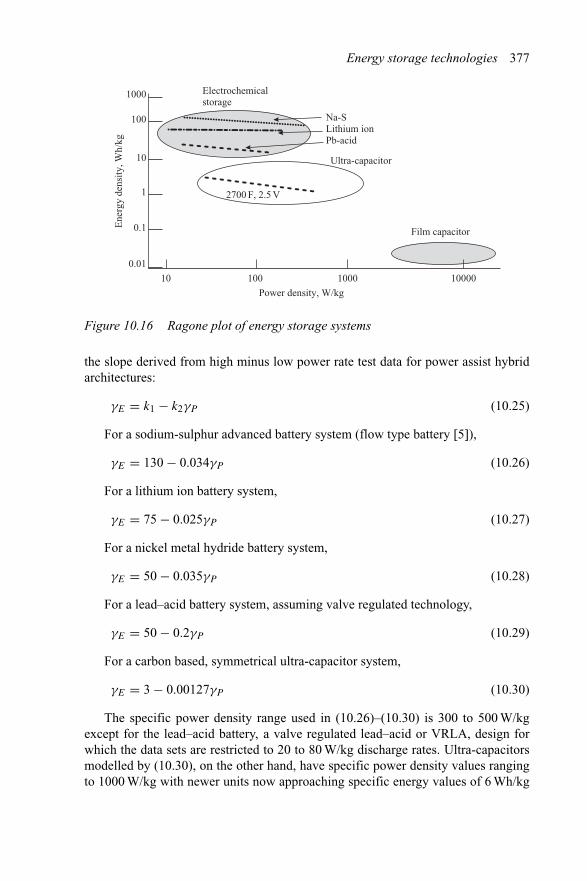
Energy storage technologies 377
Electrochemicalstorage
Ultra-capacitor
Film capacitor
2700 F, 2.5 V
Na-SLithium ionPb-acid
Ene
rgy
dens
ity, W
h/kg
Power density, W/kg
10
0.01
0.1
1
10
100
1000
100 1000 10000
Figure 10.16 Ragone plot of energy storage systems
the slope derived from high minus low power rate test data for power assist hybridarchitectures:
γE = k1 − k2γP (10.25)
For a sodium-sulphur advanced battery system (flow type battery [5]),
γE = 130 − 0.034γP (10.26)
For a lithium ion battery system,
γE = 75 − 0.025γP (10.27)
For a nickel metal hydride battery system,
γE = 50 − 0.035γP (10.28)
For a lead–acid battery system, assuming valve regulated technology,
γE = 50 − 0.2γP (10.29)
For a carbon based, symmetrical ultra-capacitor system,
γE = 3 − 0.00127γP (10.30)
The specific power density range used in (10.26)–(10.30) is 300 to 500 W/kgexcept for the lead–acid battery, a valve regulated lead–acid or VRLA, design forwhich the data sets are restricted to 20 to 80 W/kg discharge rates. Ultra-capacitorsmodelled by (10.30), on the other hand, have specific power density values rangingto 1000 W/kg with newer units now approaching specific energy values of 6 Wh/kg
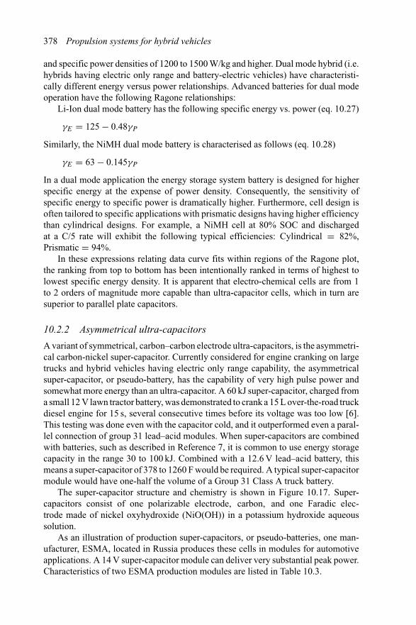
378 Propulsion systems for hybrid vehicles
and specific power densities of 1200 to 1500 W/kg and higher. Dual mode hybrid (i.e.hybrids having electric only range and battery-electric vehicles) have characteristi-cally different energy versus power relationships. Advanced batteries for dual modeoperation have the following Ragone relationships:
Li-Ion dual mode battery has the following specific energy vs. power (eq. 10.27)
γE = 125 − 0.48γP
Similarly, the NiMH dual mode battery is characterised as follows (eq. 10.28)
γE = 63 − 0.145γP
In a dual mode application the energy storage system battery is designed for higherspecific energy at the expense of power density. Consequently, the sensitivity ofspecific energy to specific power is dramatically higher. Furthermore, cell design isoften tailored to specific applications with prismatic designs having higher efficiencythan cylindrical designs. For example, a NiMH cell at 80% SOC and dischargedat a C/5 rate will exhibit the following typical efficiencies: Cylindrical = 82%,Prismatic = 94%.
In these expressions relating data curve fits within regions of the Ragone plot,the ranking from top to bottom has been intentionally ranked in terms of highest tolowest specific energy density. It is apparent that electro-chemical cells are from 1to 2 orders of magnitude more capable than ultra-capacitor cells, which in turn aresuperior to parallel plate capacitors.
10.2.2 Asymmetrical ultra-capacitors
A variant of symmetrical, carbon–carbon electrode ultra-capacitors, is the asymmetri-cal carbon-nickel super-capacitor. Currently considered for engine cranking on largetrucks and hybrid vehicles having electric only range capability, the asymmetricalsuper-capacitor, or pseudo-battery, has the capability of very high pulse power andsomewhat more energy than an ultra-capacitor. A 60 kJ super-capacitor, charged froma small 12 V lawn tractor battery, was demonstrated to crank a 15 L over-the-road truckdiesel engine for 15 s, several consecutive times before its voltage was too low [6].This testing was done even with the capacitor cold, and it outperformed even a paral-lel connection of group 31 lead–acid modules. When super-capacitors are combinedwith batteries, such as described in Reference 7, it is common to use energy storagecapacity in the range 30 to 100 kJ. Combined with a 12.6 V lead–acid battery, thismeans a super-capacitor of 378 to 1260 F would be required. A typical super-capacitormodule would have one-half the volume of a Group 31 Class A truck battery.
The super-capacitor structure and chemistry is shown in Figure 10.17. Super-capacitors consist of one polarizable electrode, carbon, and one Faradic elec-trode made of nickel oxyhydroxide (NiO(OH)) in a potassium hydroxide aqueoussolution.
As an illustration of production super-capacitors, or pseudo-batteries, one man-ufacturer, ESMA, located in Russia produces these cells in modules for automotiveapplications. A 14 V super-capacitor module can deliver very substantial peak power.Characteristics of two ESMA production modules are listed in Table 10.3.
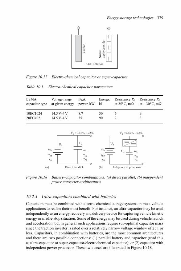
Energy storage technologies 379
KOH solution
Car
bon
Nic
kel
oxyh
ydro
xide
Figure 10.17 Electro-chemical capacitor or super-capacitor
Table 10.3 Electro-chemical capacitor parameters
ESMAcapacitor type
Voltage rangeat given energy
Peakpower, kW
Energy,kJ
Resistance Ri
at 25◦C, m�
Resistance Ri
at −30◦C, m�
10EC1024 14.5 V–4 V 8.7 30 6 920EC402 14.5 V–4 V 35 90 2 3
mc
γEcγPc
mc
γEcγPc
Vd +0.16%, –22% Vd +0.16%, –22%
mb
γEb
γPb
mb
γEb
γPb
UbUbUc
Uc
(a) (b)Direct parallel Independent processor
Figure 10.18 Battery–capacitor combinations: (a) direct parallel; (b) independentpower converter architectures
10.2.3 Ultra-capacitors combined with batteries
Capacitors must be combined with electro-chemical storage systems in most vehicleapplications to realise their most benefit. For instance, an ultra-capacitor may be usedindependently as an energy recovery and delivery device for capturing vehicle kineticenergy in an idle-stop situation. Some of the energy may be used during vehicle launchand acceleration, but in general such applications require sub-optimal capacitor masssince the traction inverter is rated over a relatively narrow voltage window of 2 : 1 orless. Capacitors, in combination with batteries, are the most common architecturesand there are two possible connections: (1) parallel battery and capacitor (read thisas ultra-capacitor or super-capacitor/electrochemical capacitor); or (2) capacitor withindependent power processor. These two cases are illustrated in Figure 10.18.
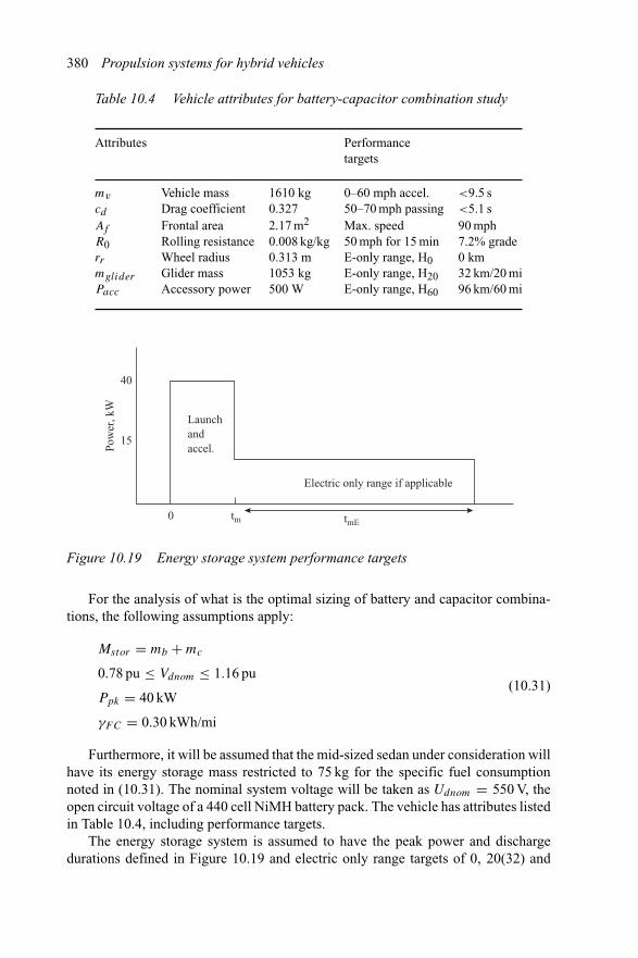
380 Propulsion systems for hybrid vehicles
Table 10.4 Vehicle attributes for battery-capacitor combination study
Attributes Performancetargets
mv Vehicle mass 1610 kg 0–60 mph accel. <9.5 scd Drag coefficient 0.327 50–70 mph passing <5.1 sAf Frontal area 2.17 m2 Max. speed 90 mphR0 Rolling resistance 0.008 kg/kg 50 mph for 15 min 7.2% graderr Wheel radius 0.313 m E-only range, H0 0 kmmglider Glider mass 1053 kg E-only range, H20 32 km/20 miPacc Accessory power 500 W E-only range, H60 96 km/60 mi
Launchandaccel.
Electric only range if applicable
Pow
er, k
W
40
15
0 tm tmE
Figure 10.19 Energy storage system performance targets
For the analysis of what is the optimal sizing of battery and capacitor combina-tions, the following assumptions apply:
Mstor = mb + mc
0.78 pu ≤ Vdnom ≤ 1.16 pu
Ppk = 40 kW
γFC = 0.30 kWh/mi
(10.31)
Furthermore, it will be assumed that the mid-sized sedan under consideration willhave its energy storage mass restricted to 75 kg for the specific fuel consumptionnoted in (10.31). The nominal system voltage will be taken as Udnom = 550 V, theopen circuit voltage of a 440 cell NiMH battery pack. The vehicle has attributes listedin Table 10.4, including performance targets.
The energy storage system is assumed to have the peak power and dischargedurations defined in Figure 10.19 and electric only range targets of 0, 20(32) and
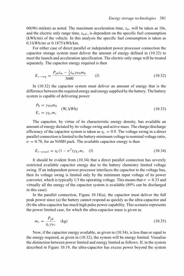
Energy storage technologies 381
60(96) mi(km) as noted. The maximum acceleration time, tm, will be taken as 10s,and the electric only range time, tmE , is dependent on the specific fuel consumption(kWh/mi) of the vehicle. In this analysis the specific fuel consumption is taken as0.3 kWh/mi or 0.1875 kWh/km.
For either case of direct parallel or independent power processor connection thecapacitor storage system must deliver the amount of energy defined in (10.32) tomeet the launch and acceleration specification. The electric only range will be treatedseparately. The capacitor energy required is then
Ec−req = Ppktm − 12 tmγPbmb
3600(J) (10.32)
In (10.32) the capacitor system must deliver an amount of energy that is thedifference between the required energy and energy supplied by the battery. The batterysystem is capable of delivering power:
Pb = γPbmb(W, kWh)
Ec = γEcmc
(10.33)
The capacitor, by virtue of its characteristic energy density, has available anamount of energy dictated by its voltage swing and active mass. The charge/dischargeefficiency of the capacitor system is taken as ηc = 0.9. The voltage swing in a directparallel connection is limited to the battery minimum voltage to nominal voltage ratio,σ = 0.78, for an NiMH pack. The available capacitor energy is then
Ec−avail = ηc(1 − σ 2)γEcmc (J) (10.34)
It should be evident from (10.34) that a direct parallel connection has severelyrestricted available capacitor energy due to the battery chemistry limited voltageswing. If an independent power processor interfaces the capacitor to the voltage bus,then its voltage swing is limited only by the minimum input voltage of its powerconverter, which is typically 1/3 the operating voltage. This means that σ = 0.33 andvirtually all the energy of the capacitor system is available (89% can be dischargedin this case).
In the parallel connection, Figure 10.18(a), the capacitor must deliver the fullpeak power since (a) the battery cannot respond as quickly as the ultra-capacitor and(b) the ultra-capacitor has much high pulse power capability. This scenario representsthe power limited case, for which the ultra-capacitor mass is given as
mc = Ppk
ηcγPc
(kg) (10.35)
Now, if the capacitor energy available, as given in (10.34), is less than or equal tothe energy required, as given in (10.32), the system will be energy limited. Visualisethe distinction between power limited and energy limited as follows. If, in the systemdescribed in Figure 10.19, the ultra-capacitor has excess power beyond the system
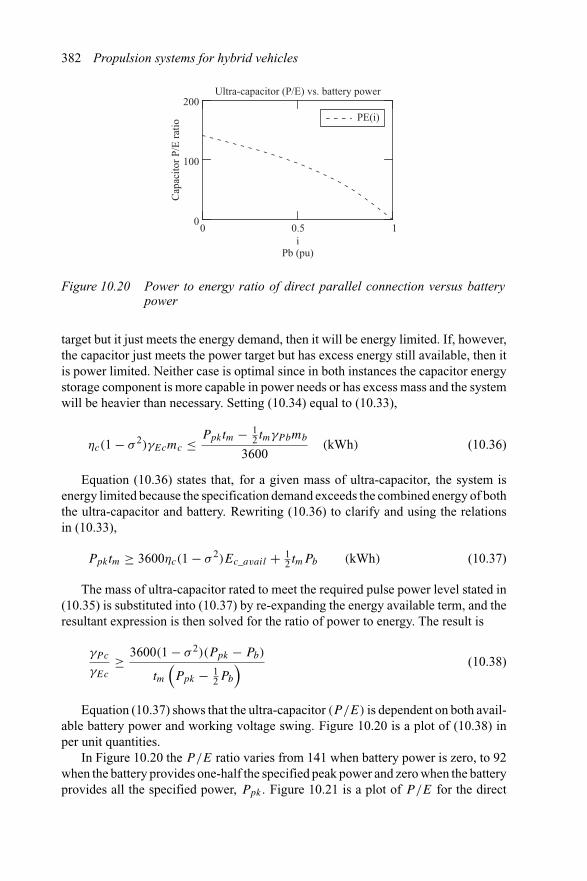
382 Propulsion systems for hybrid vehicles
PE(i)
i0 0.5 1
0
100
200Ultra-capacitor (P/E) vs. battery power
Pb (pu)
Cap
acito
r P/
E r
atio
Figure 10.20 Power to energy ratio of direct parallel connection versus batterypower
target but it just meets the energy demand, then it will be energy limited. If, however,the capacitor just meets the power target but has excess energy still available, then itis power limited. Neither case is optimal since in both instances the capacitor energystorage component is more capable in power needs or has excess mass and the systemwill be heavier than necessary. Setting (10.34) equal to (10.33),
ηc(1 − σ 2)γEcmc ≤ Ppktm − 12 tmγPbmb
3600(kWh) (10.36)
Equation (10.36) states that, for a given mass of ultra-capacitor, the system isenergy limited because the specification demand exceeds the combined energy of boththe ultra-capacitor and battery. Rewriting (10.36) to clarify and using the relationsin (10.33),
Ppktm ≥ 3600ηc(1 − σ 2)Ec_avail + 12 tmPb (kWh) (10.37)
The mass of ultra-capacitor rated to meet the required pulse power level stated in(10.35) is substituted into (10.37) by re-expanding the energy available term, and theresultant expression is then solved for the ratio of power to energy. The result is
γPc
γEc
≥ 3600(1 − σ 2)(Ppk − Pb)
tm
(Ppk − 1
2Pb
) (10.38)
Equation (10.37) shows that the ultra-capacitor (P /E) is dependent on both avail-able battery power and working voltage swing. Figure 10.20 is a plot of (10.38) inper unit quantities.
In Figure 10.20 the P/E ratio varies from 141 when battery power is zero, to 92when the battery provides one-half the specified peak power and zero when the batteryprovides all the specified power, Ppk . Figure 10.21 is a plot of P/E for the direct
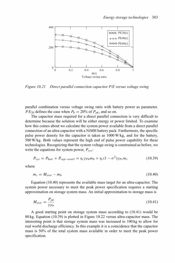
Energy storage technologies 383
σ(i)0 0.2 0.4 0.6 0.8 1
0
200
400
Voltage swing ratio
PE20(i)
PE40(i)
PE60(i)
Figure 10.21 Direct parallel connection capacitor P/E versus voltage swing
parallel combination versus voltage swing ratio with battery power as parameter.PE20 defines the case when Pb = 20% of Ppk , and so on.
The capacitor mass required for a direct parallel connection is very difficult todetermine because the solution will be either energy or power limited. To examinehow this comes about we calculate the system power available from a direct parallelconnection of an ultra-capacitor with a NiMH battery pack. Furthermore, the specificpulse power density for the capacitor is taken as 1000 W/kg, and for the battery,500 W/kg. Both values represent the high end of pulse power capability for thesetechnologies. Recognizing that the system voltage swing is constrained as before, wewrite the equations for system power, Psys :
Psys = Pbatt + Pcap−avail = ηcγPbmb + ηc(1 − σ 2)γPcmc (10.39)
where
mc = Mstor − mb (10.40)
Equation (10.40) represents the available mass target for an ultra-capacitor. Thesystem power necessary to meet the peak power specification requires a startingapproximation on storage system mass. An initial approximation to storage mass is
Mstor = Ppk
γPb
(10.41)
A good starting point on storage system mass according to (10.41) would be80 kg. Equation (10.39) is plotted in Figure 10.22 versus ultra-capacitor mass. Theinteresting point is that storage system mass was increased to 100 kg to allow forreal world discharge efficiency. In this example it is a coincidence that the capacitormass is 50% of the total system mass available in order to meet the peak powerspecification.
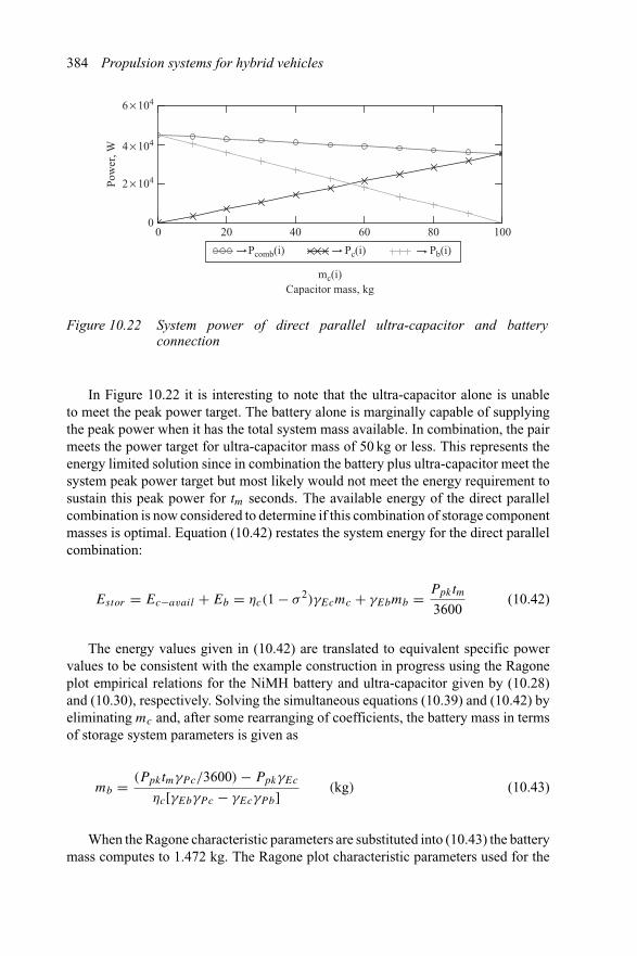
384 Propulsion systems for hybrid vehicles
0 20 40 60 80 100
Capacitor mass, kgmc(i)
Pow
er, W
6 × 10⁴
4 × 10⁴
2 × 10⁴
0
Pcomb(i) Pc(i) Pb(i)
Figure 10.22 System power of direct parallel ultra-capacitor and batteryconnection
In Figure 10.22 it is interesting to note that the ultra-capacitor alone is unableto meet the peak power target. The battery alone is marginally capable of supplyingthe peak power when it has the total system mass available. In combination, the pairmeets the power target for ultra-capacitor mass of 50 kg or less. This represents theenergy limited solution since in combination the battery plus ultra-capacitor meet thesystem peak power target but most likely would not meet the energy requirement tosustain this peak power for tm seconds. The available energy of the direct parallelcombination is now considered to determine if this combination of storage componentmasses is optimal. Equation (10.42) restates the system energy for the direct parallelcombination:
Estor = Ec−avail + Eb = ηc(1 − σ 2)γEcmc + γEbmb = Ppktm
3600(10.42)
The energy values given in (10.42) are translated to equivalent specific powervalues to be consistent with the example construction in progress using the Ragoneplot empirical relations for the NiMH battery and ultra-capacitor given by (10.28)and (10.30), respectively. Solving the simultaneous equations (10.39) and (10.42) byeliminating mc and, after some rearranging of coefficients, the battery mass in termsof storage system parameters is given as
mb = (PpktmγPc/3600) − PpkγEc
ηc[γEbγPc − γEcγPb] (kg) (10.43)
When the Ragone characteristic parameters are substituted into (10.43) the batterymass computes to 1.472 kg. The Ragone plot characteristic parameters used for the
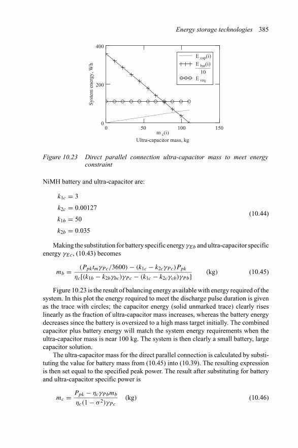
Energy storage technologies 385
m c(i)0 50 100 150
0
200
400
E cap(i)
Ultra-capacitor mass, kg
Syst
em e
nerg
y, W
h
10
E bat(i)
E req
Figure 10.23 Direct parallel connection ultra-capacitor mass to meet energyconstraint
NiMH battery and ultra-capacitor are:
k1c = 3
k2c = 0.00127
k1b = 50
k2b = 0.035
(10.44)
Making the substitution for battery specific energyγEb and ultra-capacitor specificenergy γEc, (10.43) becomes
mb = (PpktmγPc/3600) − (k1c − k2cγPc)Ppk
ηc[(k1b − k2bγbc)γPc − (k1c − k2cγcb)γPb] (kg) (10.45)
Figure 10.23 is the result of balancing energy available with energy required of thesystem. In this plot the energy required to meet the discharge pulse duration is givenas the trace with circles; the capacitor energy (solid unmarked trace) clearly riseslinearly as the fraction of ultra-capacitor mass increases, whereas the battery energydecreases since the battery is oversized to a high mass target initially. The combinedcapacitor plus battery energy will match the system energy requirements when theultra-capacitor mass is near 100 kg. The system is then clearly a small battery, largecapacitor solution.
The ultra-capacitor mass for the direct parallel connection is calculated by substi-tuting the value for battery mass from (10.45) into (10.39). The resulting expressionis then set equal to the specified peak power. The result after substituting for batteryand ultra-capacitor specific power is
mc = Ppk − ηcγPbmb
ηc(1 − σ 2)γPc
(kg) (10.46)
386 Propulsion systems for hybrid vehicles
The total system mass is given by (10.40) after rearranging for Mstor . In thisconfiguration the ultra-capacitor mass computes to 109.7 kg and the total systemmass becomes 111.2 kg.
A more realistic configuration is the independent power converter interface tothe ultra-capacitor shown in Figure 10.18(b). In this connection the battery systembus voltage constraint remains but the ultra-capacitor voltage is permitted to droopsubstantially lower. This means that more energy is available from the ultra-capacitorso its mass can be reduced well below that obtained for the direct parallel connection.In fact, if the voltage ratio used in (10.40) can be set to 0.33 from its value of 0.78,yielding a substantial increase in capacitor available energy. This configuration isnow explored in more detail.
There is a rather interesting relationship for P/E of an independent processorultra-capacitor connection. To describe this, the mass of the ultra-capacitor is taken asits available power (i.e. the ratio of system peak power demand minus battery power)divided by the capacitor’s rated discharge rate. This is expressed mathematicallyin (10.47):
mc = Ppk − γPbmb
ηcγPc
(kg) (10.47)
Next, expressing the energy available from the ultra-capacitor as greater than orequal to the required energy to meet the specification leaves
ηc(1 − σ 2)γEcmc ≥ 1
3600[Ppktm − tmγPbmb] (Wh) (10.48)
Then substituting for ultra-capacitor mass mc in (10.48) from (10.47) yields anexpression that can be used to find the relationship of specific power to specificenergy for the ultra-capacitor or its P/E limit. Making the necessary substitutionsand solving reduces (10.48) to
γPc
γEc
≤ 3600(1 − σ 2)
tm(h−1) (10.49)
Representative values for specific energy of an ultra-capacitor range from 2 to6 Wh/kg and specific power values can be in the range of 1000 W/kg. For theserepresentative values (10.49) predicts that ultra-capacitor P/E for an independentpower processor architecture will be in the range of 167 to 500. These are entirelyreasonable values for an ultra-capacitor.
When an independent power processor is used to buffer the ultra-capacitor incombination with a battery, the capacitor voltage swing can now be more extreme,leading to extraction of most of its energy. The resulting question is this: Can thecombined mass of the ultra-capacitor plus its power processor be less than the batterymass saved so that a net mass and perhaps cost benefit accrues? The voltage swingratio σ is set equal to 0.3, and all remaining parameters in (10.45) for battery massand (10.46) for ultra-capacitor mass are left unchanged. This means that the target
Energy storage technologies 387
pulse power remains at 40 kW given a pulse duration of 10 s. When these expressionsare solved, the following results are obtained
mb = 1.472mc = 49.05mI = 12.868Mstor = 63.39
(kg) (10.50)
Equation (10.50) introduces a new component, the power processor. Power elec-tronics for automotive applications today reveals that these units have a typicalspecific power density γPI of about 5 kW/kg. The relation used to obtain the valuein (10.50) for the magnitude of capacitor pulse power, assuming a power invariant orhousekeeping logic mass, mIo, of 5 kg is
mI = Pcap
γPI
+ mIo (kg) (10.51)
The total system mass then becomes the combination of (10.46), (10.47) and(10.51) which, after some rearranging becomes
Mstor =[
1 + ηc(1 − σ 2)
{γPc
γPI
}]mc + mb + mIo (kg) (10.52)
Equation (10.52) for total storage system mass is intriguing because it illustratesthe significant role that the added power processor plays. In (10.52) the second termmultiplying capacitor mass is actually derived from (10.51) for power processor massand shows that as voltage swing increases the converter mass increases in propor-tion, which adds more mass to the total storage system. Countering this trend withincreasing voltage swing, and hence higher energy extraction, is the power processorspecific power density. As technology improves, the converter power density willimprove and further reduce the additional mass to this configuration. In any event,the resulting mass contributions are as given in (10.50).
Summarising the component masses for a direct parallel and independent powerconverter configuration yields the results noted in Table 10.5.
Table 10.5 shows that with an independent power processor not only is the ultra-capacitor mass minimised, but the total system mass is reduced by 43%. If theadditional cost of the power processor does not offset the savings obtained fromthe energy components, in that case the independent power processor architecturewould be the correct approach.
10.2.4 Ultra-capacitor cell balancing
In order to store the maximum amount of energy in an ultra-capacitor its voltage mustbe near, or at, maximum tolerable levels. Ultra-capacitors having organic electrolytesare typically confined to voltage stress levels less than 2.7 V across any given cell ina series string. The accepted surge voltage of an ultra-capacitor is 2.85 V. When thevoltage exceeds 3 V the cell will gas and when the voltage is raised above 4 V the cell
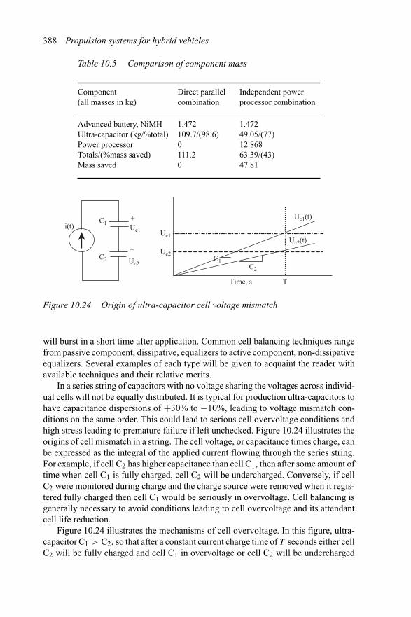
388 Propulsion systems for hybrid vehicles
Table 10.5 Comparison of component mass
Component(all masses in kg)
Direct parallelcombination
Independent powerprocessor combination
Advanced battery, NiMH 1.472 1.472Ultra-capacitor (kg/%total) 109.7/(98.6) 49.05/(77)Power processor 0 12.868Totals/(%mass saved) 111.2 63.39/(43)Mass saved 0 47.81
+Uc1
+
Uc2
C1
C2
i(t)Uc1
Uc2
TTime, s
C2
Uc1(t)
Uc2(t)
C1
Figure 10.24 Origin of ultra-capacitor cell voltage mismatch
will burst in a short time after application. Common cell balancing techniques rangefrom passive component, dissipative, equalizers to active component, non-dissipativeequalizers. Several examples of each type will be given to acquaint the reader withavailable techniques and their relative merits.
In a series string of capacitors with no voltage sharing the voltages across individ-ual cells will not be equally distributed. It is typical for production ultra-capacitors tohave capacitance dispersions of +30% to −10%, leading to voltage mismatch con-ditions on the same order. This could lead to serious cell overvoltage conditions andhigh stress leading to premature failure if left unchecked. Figure 10.24 illustrates theorigins of cell mismatch in a string. The cell voltage, or capacitance times charge, canbe expressed as the integral of the applied current flowing through the series string.For example, if cell C2 has higher capacitance than cell C1, then after some amount oftime when cell C1 is fully charged, cell C2 will be undercharged. Conversely, if cellC2 were monitored during charge and the charge source were removed when it regis-tered fully charged then cell C1 would be seriously in overvoltage. Cell balancing isgenerally necessary to avoid conditions leading to cell overvoltage and its attendantcell life reduction.
Figure 10.24 illustrates the mechanisms of cell overvoltage. In this figure, ultra-capacitor C1 > C2, so that after a constant current charge time of T seconds either cellC2 will be fully charged and cell C1 in overvoltage or cell C2 will be undercharged
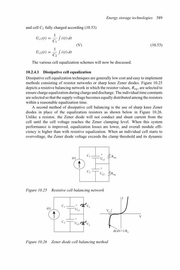
Energy storage technologies 389
and cell C1 fully charged according (10.53)
Uc1(t) = 1
C1
∫i(t) dt
Uc2(t) = 1
C2
∫i(t) dt
(V) (10.53)
The various cell equalization schemes will now be discussed.
10.2.4.1 Dissipative cell equalization
Dissipative cell equalization techniques are generally low cost and easy to implementmethods consisting of resistor networks or sharp knee Zener diodes. Figure 10.25depicts a resistive balancing network in which the resistor values, Req , are selected toensure charge equalization during charge and discharge. The individual time constantsare selected so that the supply voltage becomes equally distributed among the resistorswithin a reasonable equalization time.
A second method of dissipative cell balancing is the use of sharp knee Zenerdiodes in place of the equalization resistors as shown below in Figure 10.26.Unlike a resistor, the Zener diode will not conduct and shunt current from thecell until the cell voltage reaches the Zener clamping level. When this systemperformance is improved, equalization losses are lower, and overall module effi-ciency is higher than with resistive equalization. When an individual cell starts toovervoltage, the Zener diode voltage exceeds the clamp threshold and its dynamic
Req
Req
+Uc1
+
Uc2
C1
C2
i(t)
Figure 10.25 Resistive cell balancing network
+Uc1
+Uc2
C1
C2
i(t)Vz
Vz
I
V
Vz
dI/dV=1/Rz
Figure 10.26 Zener diode cell balancing method
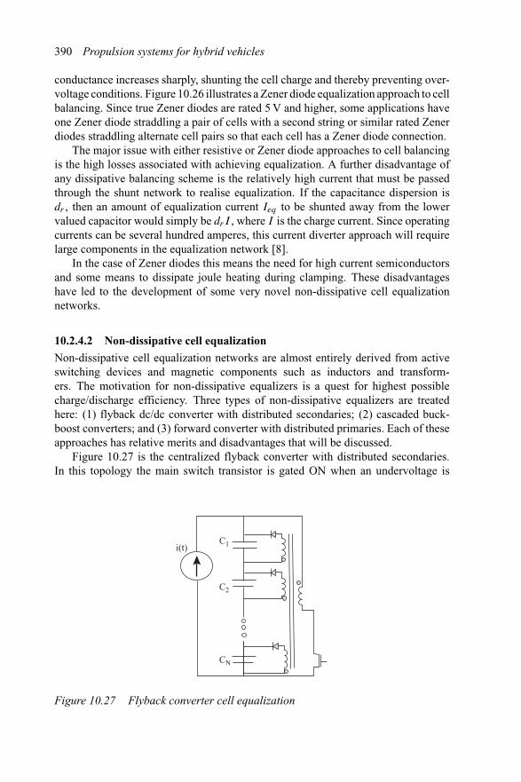
390 Propulsion systems for hybrid vehicles
conductance increases sharply, shunting the cell charge and thereby preventing over-voltage conditions. Figure 10.26 illustrates a Zener diode equalization approach to cellbalancing. Since true Zener diodes are rated 5 V and higher, some applications haveone Zener diode straddling a pair of cells with a second string or similar rated Zenerdiodes straddling alternate cell pairs so that each cell has a Zener diode connection.
The major issue with either resistive or Zener diode approaches to cell balancingis the high losses associated with achieving equalization. A further disadvantage ofany dissipative balancing scheme is the relatively high current that must be passedthrough the shunt network to realise equalization. If the capacitance dispersion isdr , then an amount of equalization current Ieq to be shunted away from the lowervalued capacitor would simply be drI , where I is the charge current. Since operatingcurrents can be several hundred amperes, this current diverter approach will requirelarge components in the equalization network [8].
In the case of Zener diodes this means the need for high current semiconductorsand some means to dissipate joule heating during clamping. These disadvantageshave led to the development of some very novel non-dissipative cell equalizationnetworks.
10.2.4.2 Non-dissipative cell equalization
Non-dissipative cell equalization networks are almost entirely derived from activeswitching devices and magnetic components such as inductors and transform-ers. The motivation for non-dissipative equalizers is a quest for highest possiblecharge/discharge efficiency. Three types of non-dissipative equalizers are treatedhere: (1) flyback dc/dc converter with distributed secondaries; (2) cascaded buck-boost converters; and (3) forward converter with distributed primaries. Each of theseapproaches has relative merits and disadvantages that will be discussed.
Figure 10.27 is the centralized flyback converter with distributed secondaries.In this topology the main switch transistor is gated ON when an undervoltage is
C1
C2
CN
i(t)
Figure 10.27 Flyback converter cell equalization
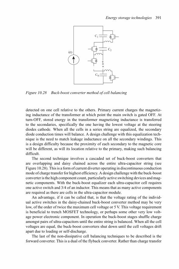
Energy storage technologies 391
C1
C2
CN
i(t)
Figure 10.28 Buck-boost converter method of cell balancing
detected on one cell relative to the others. Primary current charges the magnetiz-ing inductance of the transformer at which point the main switch is gated OFF. Atturn-OFF, stored energy in the transformer magnetizing inductance is transferredto the secondaries, specifically the one having the lowest voltage at the steeringdiodes cathode. When all the cells in a series string are equalized, the secondarydiode conduction times will balance. A design challenge with this equalization tech-nique is the need to match leakage inductance on all the secondary windings. Thisis a design difficulty because the proximity of each secondary to the magnetic corewill be different, as will its location relative to the primary, making such balancingdifficult.
The second technique involves a cascaded set of buck-boost converters thatare overlapping and daisy chained across the entire ultra-capacitor string (seeFigure 10.28). This is a form of current diverter operating in discontinuous conductionmode of charge transfer for highest efficiency. A design challenge with the buck-boostconverter is the high component count, particularly active switching devices and mag-netic components. With the buck-boost equalizer each ultra-capacitor cell requiresone active switch and 3/4 of an inductor. This means that as many active componentsare required as there are cells in the ultra-capacitor module.
An advantage, if it can be called that, is that the voltage rating of the individ-ual active switches in the daisy-chained buck-boost converter method may be verylow, of the order of twice the maximum cell voltage or 5 V. This voltage requirementis beneficial to trench MOSFET technology, or perhaps some other very low volt-age power electronic component. In operation the buck-boost stages shuffle chargeamongst pairs of ultra-capacitors until the entire string is balanced. When all the cellvoltages are equal, the buck-boost converters shut down until the cell voltages driftapart due to loading or self-discharge.
The last of the non-dissipative cell balancing techniques to be described is theforward converter. This is a dual of the flyback converter. Rather than charge transfer
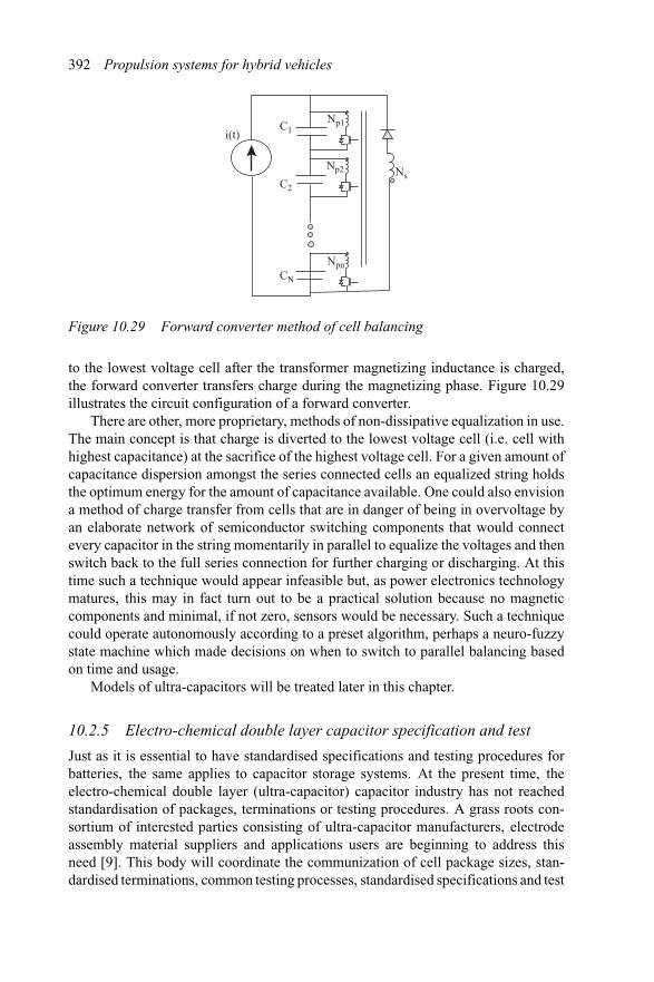
392 Propulsion systems for hybrid vehicles
Ns
Np1
Np2
Npn
C1
C2
CN
i(t)
Figure 10.29 Forward converter method of cell balancing
to the lowest voltage cell after the transformer magnetizing inductance is charged,the forward converter transfers charge during the magnetizing phase. Figure 10.29illustrates the circuit configuration of a forward converter.
There are other, more proprietary, methods of non-dissipative equalization in use.The main concept is that charge is diverted to the lowest voltage cell (i.e. cell withhighest capacitance) at the sacrifice of the highest voltage cell. For a given amount ofcapacitance dispersion amongst the series connected cells an equalized string holdsthe optimum energy for the amount of capacitance available. One could also envisiona method of charge transfer from cells that are in danger of being in overvoltage byan elaborate network of semiconductor switching components that would connectevery capacitor in the string momentarily in parallel to equalize the voltages and thenswitch back to the full series connection for further charging or discharging. At thistime such a technique would appear infeasible but, as power electronics technologymatures, this may in fact turn out to be a practical solution because no magneticcomponents and minimal, if not zero, sensors would be necessary. Such a techniquecould operate autonomously according to a preset algorithm, perhaps a neuro-fuzzystate machine which made decisions on when to switch to parallel balancing basedon time and usage.
Models of ultra-capacitors will be treated later in this chapter.
10.2.5 Electro-chemical double layer capacitor specification and test
Just as it is essential to have standardised specifications and testing procedures forbatteries, the same applies to capacitor storage systems. At the present time, theelectro-chemical double layer (ultra-capacitor) capacitor industry has not reachedstandardisation of packages, terminations or testing procedures. A grass roots con-sortium of interested parties consisting of ultra-capacitor manufacturers, electrodeassembly material suppliers and applications users are beginning to address thisneed [9]. This body will coordinate the communization of cell package sizes, stan-dardised terminations, common testing processes, standardised specifications and test
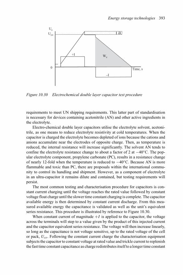
Energy storage technologies 393
Uc
Time, s
+I
–I
δU
We
0
Uco
Figure 10.30 Electrochemical double layer capacitor test procedure
requirements to meet UN shipping requirements. This latter part of standardisationis necessary for devices containing acetonitrile (AN) and other active ingredients inthe electrolyte.
Electro-chemical double layer capacitors utilise the electrolyte solvent, acetoni-trile, as one means to reduce electrolyte resistivity at cold temperatures. When thecapacitor is charged the electrolyte becomes depleted of ions because the cations andanions accumulate near the electrodes of opposite charge. Then, as temperature isreduced, the internal resistance will increase significantly. The solvent AN tends toconfine the electrolyte resistance change to about a factor of 2 at −40◦C. The pop-ular electrolyte component, propylene carbonate (PC), results in a resistance changeof nearly 12-fold when the temperature is reduced to −40◦C. Because AN is moreflammable and toxic than PC, there are proposals within the international commu-nity to control its handling and shipment. However, as a component of electrolytein an ultra-capacitor it remains dilute and contained, but testing requirements willpersist.
The most common testing and characterisation procedure for capacitors is con-stant current charging until the voltage reaches the rated value followed by constantvoltage float charge until the slower time constant charging is complete. The capacitoravailable energy is then determined by constant current discharge. From this mea-sured available energy the capacitance is validated as well as the unit’s equivalentseries resistance. This procedure is illustrated by reference to Figure 10.30.
When constant current of magnitude +I is applied to the capacitor, the voltageacross the terminals will step to a value given by the product of this injected currentand the capacitor equivalent series resistance. The voltage will then increase linearly,so long as the capacitance is not voltage sensitive, up to the rated voltage of the cellor pack, Uco. Following the constant current charge the characterisation equipmentsubjects the capacitor to constant voltage at rated value and trickle current to replenishthe fast time constant capacitance as charge redistributes itself to a longer time constant
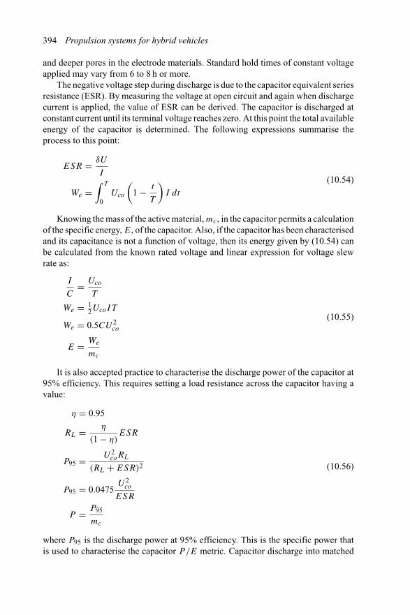
394 Propulsion systems for hybrid vehicles
and deeper pores in the electrode materials. Standard hold times of constant voltageapplied may vary from 6 to 8 h or more.
The negative voltage step during discharge is due to the capacitor equivalent seriesresistance (ESR). By measuring the voltage at open circuit and again when dischargecurrent is applied, the value of ESR can be derived. The capacitor is discharged atconstant current until its terminal voltage reaches zero. At this point the total availableenergy of the capacitor is determined. The following expressions summarise theprocess to this point:
ESR = δU
I
We =∫ T
0Uco
(1 − t
T
)I dt
(10.54)
Knowing the mass of the active material, mc, in the capacitor permits a calculationof the specific energy, E, of the capacitor. Also, if the capacitor has been characterisedand its capacitance is not a function of voltage, then its energy given by (10.54) canbe calculated from the known rated voltage and linear expression for voltage slewrate as:
I
C= Uco
T
We = 12UcoIT
We = 0.5CU2co
E = We
mc
(10.55)
It is also accepted practice to characterise the discharge power of the capacitor at95% efficiency. This requires setting a load resistance across the capacitor having avalue:
η = 0.95
RL = η
(1 − η)ESR
P95 = U2coRL
(RL + ESR)2
P95 = 0.0475U2
co
ESR
P = P95
mc
(10.56)
where P95 is the discharge power at 95% efficiency. This is the specific power thatis used to characterise the capacitor P/E metric. Capacitor discharge into matched
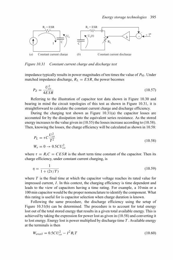
Energy storage technologies 395
I
Ri = ESR
C
Uc Uc(t)
C
Ri = ESR
RL
kI*
–+ +
(a) (b)Constant current charge Constant current discharge
Figure 10.31 Constant current charge and discharge test
impedance typically results in power magnitudes of ten times the value of P95. Undermatched impedance discharge, RL = ESR, the power becomes
PZ = U2co
4ESR(10.57)
Referring to the illustration of capacitor test data shown in Figure 10.30 andbearing in mind the circuit topologies of this test as shown in Figure 10.31, it isstraightforward to calculate the constant current charge and discharge efficiency.
During the charging test shown as Figure 10.31(a) the capacitor losses areaccounted for by the dissipation into the equivalent series resistance. As the storedenergy increases to the value given in (10.55) the losses increase according to (10.58).Then, knowing the losses, the charge efficiency will be calculated as shown in 10.58:
PL = τCU2
co
T 2
We = 0 → 0.5CU2co
(10.58)
where τ = RiC = CESR is the short term time constant of the capacitor. Then itscharge efficiency, under constant current charging, is
η = 1
1 + (2τ/T )(10.59)
where T is the final time at which the capacitor voltage reaches its rated value forimpressed current, I . In this context, the charging efficiency is time dependent andleads to the view of capacitors having a time rating. For example, a 10 min or a100 min capacitor would be the proper nomenclature to identify the component. Whatthis rating is useful for is capacitor selection when charge duration is known.
Following the same procedure, the discharge efficiency using the setup ofFigure 10.31(b) can be determined. The procedure is to account for total energylost out of the total stored energy that results in a given total available energy. This isachieved by taking the expression for power lost as given in (10.58) and converting itto lost energy. Energy lost is power multiplied by discharge time T . Available energyat the terminals is then
Wavail = 0.5CU2co − I 2RiT (10.60)
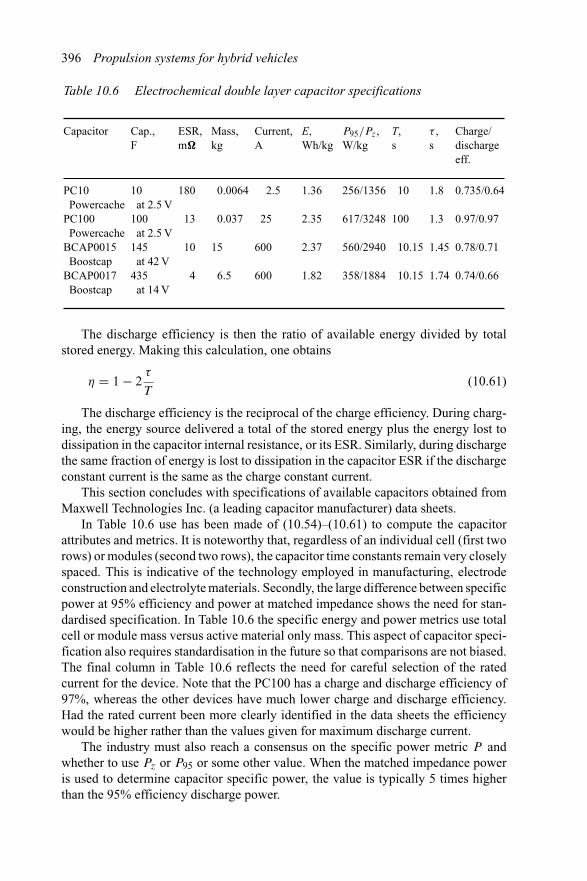
396 Propulsion systems for hybrid vehicles
Table 10.6 Electrochemical double layer capacitor specifications
Capacitor Cap.,F
ESR,m�
Mass,kg
Current,A
E,Wh/kg
P95/Pz,W/kg
T,s
τ ,s
Charge/dischargeeff.
PC10 10 180 0.0064 2.5 1.36 256/1356 10 1.8 0.735/0.64Powercache at 2.5 V
PC100 100 13 0.037 25 2.35 617/3248 100 1.3 0.97/0.97Powercache at 2.5 V
BCAP0015 145 10 15 600 2.37 560/2940 10.15 1.45 0.78/0.71Boostcap at 42 V
BCAP0017 435 4 6.5 600 1.82 358/1884 10.15 1.74 0.74/0.66Boostcap at 14 V
The discharge efficiency is then the ratio of available energy divided by totalstored energy. Making this calculation, one obtains
η = 1 − 2τ
T(10.61)
The discharge efficiency is the reciprocal of the charge efficiency. During charg-ing, the energy source delivered a total of the stored energy plus the energy lost todissipation in the capacitor internal resistance, or its ESR. Similarly, during dischargethe same fraction of energy is lost to dissipation in the capacitor ESR if the dischargeconstant current is the same as the charge constant current.
This section concludes with specifications of available capacitors obtained fromMaxwell Technologies Inc. (a leading capacitor manufacturer) data sheets.
In Table 10.6 use has been made of (10.54)–(10.61) to compute the capacitorattributes and metrics. It is noteworthy that, regardless of an individual cell (first tworows) or modules (second two rows), the capacitor time constants remain very closelyspaced. This is indicative of the technology employed in manufacturing, electrodeconstruction and electrolyte materials. Secondly, the large difference between specificpower at 95% efficiency and power at matched impedance shows the need for stan-dardised specification. In Table 10.6 the specific energy and power metrics use totalcell or module mass versus active material only mass. This aspect of capacitor speci-fication also requires standardisation in the future so that comparisons are not biased.The final column in Table 10.6 reflects the need for careful selection of the ratedcurrent for the device. Note that the PC100 has a charge and discharge efficiency of97%, whereas the other devices have much lower charge and discharge efficiency.Had the rated current been more clearly identified in the data sheets the efficiencywould be higher rather than the values given for maximum discharge current.
The industry must also reach a consensus on the specific power metric P andwhether to use Pz or P95 or some other value. When the matched impedance poweris used to determine capacitor specific power, the value is typically 5 times higherthan the 95% efficiency discharge power.
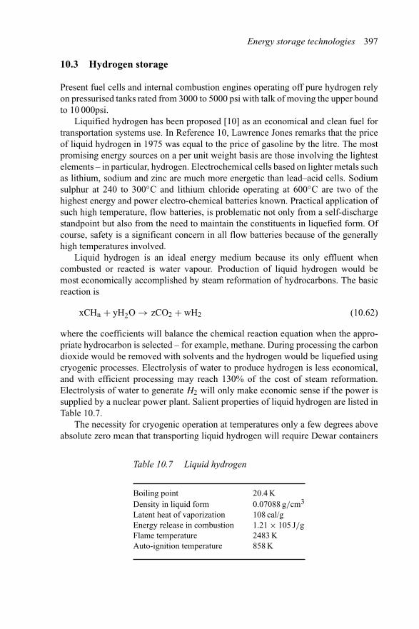
Energy storage technologies 397
10.3 Hydrogen storage
Present fuel cells and internal combustion engines operating off pure hydrogen relyon pressurised tanks rated from 3000 to 5000 psi with talk of moving the upper boundto 10 000psi.
Liquified hydrogen has been proposed [10] as an economical and clean fuel fortransportation systems use. In Reference 10, Lawrence Jones remarks that the priceof liquid hydrogen in 1975 was equal to the price of gasoline by the litre. The mostpromising energy sources on a per unit weight basis are those involving the lightestelements – in particular, hydrogen. Electrochemical cells based on lighter metals suchas lithium, sodium and zinc are much more energetic than lead–acid cells. Sodiumsulphur at 240 to 300◦C and lithium chloride operating at 600◦C are two of thehighest energy and power electro-chemical batteries known. Practical application ofsuch high temperature, flow batteries, is problematic not only from a self-dischargestandpoint but also from the need to maintain the constituents in liquefied form. Ofcourse, safety is a significant concern in all flow batteries because of the generallyhigh temperatures involved.
Liquid hydrogen is an ideal energy medium because its only effluent whencombusted or reacted is water vapour. Production of liquid hydrogen would bemost economically accomplished by steam reformation of hydrocarbons. The basicreaction is
xCHn + yH2O → zCO2 + wH2 (10.62)
where the coefficients will balance the chemical reaction equation when the appro-priate hydrocarbon is selected – for example, methane. During processing the carbondioxide would be removed with solvents and the hydrogen would be liquefied usingcryogenic processes. Electrolysis of water to produce hydrogen is less economical,and with efficient processing may reach 130% of the cost of steam reformation.Electrolysis of water to generate H2 will only make economic sense if the power issupplied by a nuclear power plant. Salient properties of liquid hydrogen are listed inTable 10.7.
The necessity for cryogenic operation at temperatures only a few degrees aboveabsolute zero mean that transporting liquid hydrogen will require Dewar containers
Table 10.7 Liquid hydrogen
Boiling point 20.4 KDensity in liquid form 0.07088 g/cm3
Latent heat of vaporization 108 cal/gEnergy release in combustion 1.21 × 10⁵ J/gFlame temperature 2483 KAuto-ignition temperature 858 K
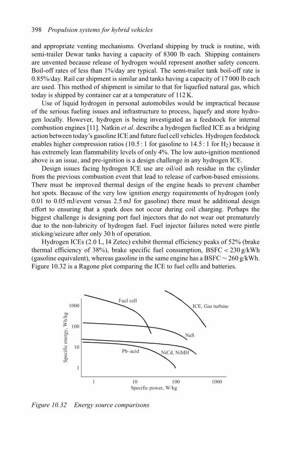
398 Propulsion systems for hybrid vehicles
and appropriate venting mechanisms. Overland shipping by truck is routine, withsemi-trailer Dewar tanks having a capacity of 8300 lb each. Shipping containersare unvented because release of hydrogen would represent another safety concern.Boil-off rates of less than 1%/day are typical. The semi-trailer tank boil-off rate is0.85%/day. Rail car shipment is similar and tanks having a capacity of 17 000 lb eachare used. This method of shipment is similar to that for liquefied natural gas, whichtoday is shipped by container car at a temperature of 112 K.
Use of liquid hydrogen in personal automobiles would be impractical becauseof the serious fueling issues and infrastructure to process, liquefy and store hydro-gen locally. However, hydrogen is being investigated as a feedstock for internalcombustion engines [11]. Natkin et al. describe a hydrogen fuelled ICE as a bridgingaction between today’s gasoline ICE and future fuel cell vehicles. Hydrogen feedstockenables higher compression ratios (10.5 : 1 for gasoline to 14.5 : 1 for H2) because ithas extremely lean flammability levels of only 4%. The low auto-ignition mentionedabove is an issue, and pre-ignition is a design challenge in any hydrogen ICE.
Design issues facing hydrogen ICE use are oil/oil ash residue in the cylinderfrom the previous combustion event that lead to release of carbon-based emissions.There must be improved thermal design of the engine heads to prevent chamberhot spots. Because of the very low ignition energy requirements of hydrogen (only0.01 to 0.05 mJ/event versus 2.5 mJ for gasoline) there must be additional designeffort to ensuring that a spark does not occur during coil charging. Perhaps thebiggest challenge is designing port fuel injectors that do not wear out prematurelydue to the non-lubricity of hydrogen fuel. Fuel injector failures noted were pintlesticking/seizure after only 30 h of operation.
Hydrogen ICEs (2.0 L, I4 Zetec) exhibit thermal efficiency peaks of 52% (brakethermal efficiency of 38%), brake specific fuel consumption, BSFC < 230 g/kWh(gasoline equivalent), whereas gasoline in the same engine has a BSFC ∼ 260 g/kWh.Figure 10.32 is a Ragone plot comparing the ICE to fuel cells and batteries.
Spec
ific
ene
rgy,
Wh/
kg
1000
100
10
1
1 10 100 1000Specific power, W/kg
Pb–acid NiCd, NiMH
NaS
Fuel cellICE, Gas turbine
Figure 10.32 Energy source comparisons
Energy storage technologies 399
Pressurised hydrogen for personal automobile use is the most practical, eventhough the ICE will have 30% less power. View this another way; in a naturallyaspirated ICE the hydrogen gas displaces 30% of the induction air so power outputsimilarly reduced. To obtain equal power to gasoline the ICE will need higher dis-placement because a stoichiometric mixture consists of 2 parts hydrogen to 1 partoxygen (or 5 parts air). A gasoline–air mixture consists of 1 part heptane vapour to11 parts of oxygen (55 parts air). Because the hydrocarbon molecules are so muchlarger than hydrogen, the combustion chamber for hydrogen will need to be larger.Performance is also not as good as gasoline.
10.3.1 Metal hydride
An alternative to high pressure hydrogen storage, or liquefied hydrogen, is to store itin a metal hydride. Compounds such as Mg2Cu, Mg2Ni and Mg will combine withhydrogen and bind it as Mg2NiH4 and MgH2 so that as much hydrogen is stored perunit volume as liquid hydrogen. Metal hydrides are stable at normal temperatures andpressure but dissociate to hydrogen gas and metal above 260◦C. A storage tank ofsintered magnesium could be charged with hydrogen and heat from the ICE exhaustused to liberate it from the metal hydride.
The hydrogen economy, if this comes about, relies on the fact that hydrogen hasa specific energy density (119.6 MJ/kg or 33.22 kWh/kg) three times higher thangasoline (43.2 MJ/kg or 12 kWh/kg) or any other hydrocarbon fuel.
10.3.2 High pressure gas
The most common form of high pressure gas energy storage is CNG (compressednatural gas), and sometimes, liquefied natural gas (LNG) is used. Extracted fromunderground reservoirs, natural gas is a fossil fuel composed mainly of methanealong with other hydrocarbons such as propane, butane and inert gases (carbon diox-ide, helium and nitrogen, among others). Natural gas is used today as feedstock foralternative fuel vehicles, where it is stored on-board in pressure cylinders rated 3000to 5000 psi. Discussion of raising the storage pressure to 10 000 psi is under investi-gation. LNG is more difficult because it requires cryogenic temperatures of −259 ◦Fin order to be liquid. LNG must be stored in Dewar canisters (thermos bottles).
ICEs modified for CNG use typically have upgraded fuel delivery systems, heatedpressure reduction valves and carburetion systems. CNG provides quicker cold startsbecause it vaporizes readily and burns with lower emissions. It also has a higheroctane number than gasoline so its less prone to knocking. The fill time for a CNGvehicle is from 2 to 5 min. On the down side, CNG does not have the energy densityof gasoline, so the vehicle range is substantially less. Natural gas is one of the fuelsin the US that is subject to the 1988 Alternative Motor Fuels Act (AFMA), publiclaw 100-494 meant to encourage more widespread use of alcohol and natural gas astransportation fuels.
Propane, or liquefied petroleum gas (LPG), is available today as a by-productof NG processing and from crude oil refining. The only grade of LPG available for
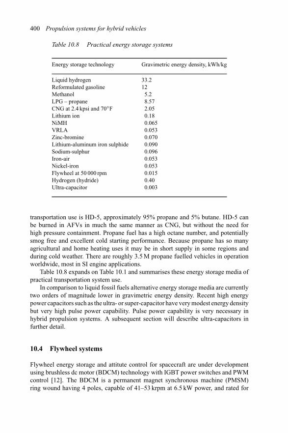
400 Propulsion systems for hybrid vehicles
Table 10.8 Practical energy storage systems
Energy storage technology Gravimetric energy density, kWh/kg
Liquid hydrogen 33.2Reformulated gasoline 12Methanol 5.2LPG – propane 8.57CNG at 2.4 kpsi and 70◦F 2.05Lithium ion 0.18NiMH 0.065VRLA 0.053Zinc-bromine 0.070Lithium-aluminum iron sulphide 0.090Sodium-sulphur 0.096Iron-air 0.053Nickel-iron 0.053Flywheel at 50 000 rpm 0.015Hydrogen (hydride) 0.40Ultra-capacitor 0.003
transportation use is HD-5, approximately 95% propane and 5% butane. HD-5 canbe burned in AFVs in much the same manner as CNG, but without the need forhigh pressure containment. Propane fuel has a high octane number, and potentiallysmog free and excellent cold starting performance. Because propane has so manyagricultural and home heating uses it may be in short supply in some regions andduring cold weather. There are roughly 3.5 M propane fuelled vehicles in operationworldwide, most in SI engine applications.
Table 10.8 expands on Table 10.1 and summarises these energy storage media ofpractical transportation system use.
In comparison to liquid fossil fuels alternative energy storage media are currentlytwo orders of magnitude lower in gravimetric energy density. Recent high energypower capacitors such as the ultra- or super-capacitor have very modest energy densitybut very high pulse power capability. Pulse power capability is very necessary inhybrid propulsion systems. A subsequent section will describe ultra-capacitors infurther detail.
10.4 Flywheel systems
Flywheel energy storage and attitute control for spacecraft are under developmentusing brushless dc motor (BDCM) technology with IGBT power switches and PWMcontrol [12]. The BDCM is a permanent magnet synchronous machine (PMSM)ring wound having 4 poles, capable of 41–53 krpm at 6.5 kW power, and rated for
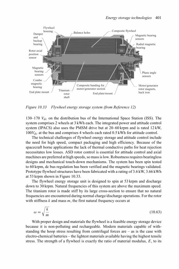
Energy storage technologies 401
Flywheelhousing Composite flywheel
Balance holesMagnetic bearingsensors
Radial magneticbearing
Composite banding formotor/generator section
Motor/generatorrotor magnets,back iron End plate/mount
Damperandbackupbearing
Magneticbearingsensors
Combomagnetic
bearing
End plate mount Titaniumrotorshaft
Phase anglesensors
Rotor axialpositionsensor
Figure 10.33 Flywheel energy storage system (from Reference 12)
130–170 Vdc on the distribution bus of the International Space Station (ISS). Thesystem comprises 2 wheels at 3 kWh each. The integrated power and attitude controlsystem (IPACS) also uses the PMSM drive but at 20–60 krpm and is rated 12 kW,100Vdc at the bus and comprises 4 wheels each rated 0.5 kWh for attitude control.
The technical challenges of flywheel energy storage and attitude control includethe need for high speed, compact packaging and high efficiency. Because of thespacecraft borne applications the lack of thermal conductive paths for heat rejectionnecessitates low losses. ASD rotor control is essential for attitude control and axialmachines are preferred at high speeds, so mass is low. Robustness requires bearinglessdesigns and mechanical touch-down mechanisms. The system has been spin testedto 60 krpm, dc bus regulation has been verified and the magnetic bearings validated.Prototype flywheel structures have been fabricated with a rating of 3.6 kW, 3.66 kWhat 53 krpm shown in Figure 10.33.
The flywheel energy storage unit is designed to spin at 53 krpm and dischargedown to 30 krpm. Natural frequencies of this system are above the maximum speed.The titanium rotor is made stiff by its large cross-section to ensure that no naturalfrequencies are encountered during normal charge/discharge operations. For the rotorwith stiffness k and mass m, the first natural frequency occurs at
ω =√
k
m(10.63)
With proper design and materials the flywheel is a feasible energy storage devicebecause it is non-polluting and rechargeable. Modern materials capable of with-standing the hoop stress resulting from centrifugal forces are – as is the case withelectro-chemical batteries – the lightest materials available having the highest tensilestress. The strength of a flywheel is exactly the ratio of material modulus, E, to its
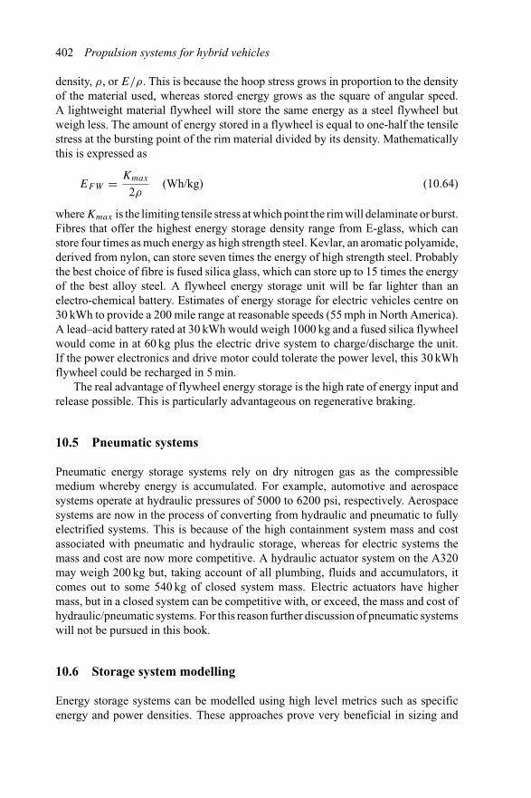
402 Propulsion systems for hybrid vehicles
density, ρ, or E/ρ. This is because the hoop stress grows in proportion to the densityof the material used, whereas stored energy grows as the square of angular speed.A lightweight material flywheel will store the same energy as a steel flywheel butweigh less. The amount of energy stored in a flywheel is equal to one-half the tensilestress at the bursting point of the rim material divided by its density. Mathematicallythis is expressed as
EFW = Kmax
2ρ(Wh/kg) (10.64)
whereKmax is the limiting tensile stress at which point the rim will delaminate or burst.Fibres that offer the highest energy storage density range from E-glass, which canstore four times as much energy as high strength steel. Kevlar, an aromatic polyamide,derived from nylon, can store seven times the energy of high strength steel. Probablythe best choice of fibre is fused silica glass, which can store up to 15 times the energyof the best alloy steel. A flywheel energy storage unit will be far lighter than anelectro-chemical battery. Estimates of energy storage for electric vehicles centre on30 kWh to provide a 200 mile range at reasonable speeds (55 mph in North America).A lead–acid battery rated at 30 kWh would weigh 1000 kg and a fused silica flywheelwould come in at 60 kg plus the electric drive system to charge/discharge the unit.If the power electronics and drive motor could tolerate the power level, this 30 kWhflywheel could be recharged in 5 min.
The real advantage of flywheel energy storage is the high rate of energy input andrelease possible. This is particularly advantageous on regenerative braking.
10.5 Pneumatic systems
Pneumatic energy storage systems rely on dry nitrogen gas as the compressiblemedium whereby energy is accumulated. For example, automotive and aerospacesystems operate at hydraulic pressures of 5000 to 6200 psi, respectively. Aerospacesystems are now in the process of converting from hydraulic and pneumatic to fullyelectrified systems. This is because of the high containment system mass and costassociated with pneumatic and hydraulic storage, whereas for electric systems themass and cost are now more competitive. A hydraulic actuator system on the A320may weigh 200 kg but, taking account of all plumbing, fluids and accumulators, itcomes out to some 540 kg of closed system mass. Electric actuators have highermass, but in a closed system can be competitive with, or exceed, the mass and cost ofhydraulic/pneumatic systems. For this reason further discussion of pneumatic systemswill not be pursued in this book.
10.6 Storage system modelling
Energy storage systems can be modelled using high level metrics such as specificenergy and power densities. These approaches prove very beneficial in sizing and
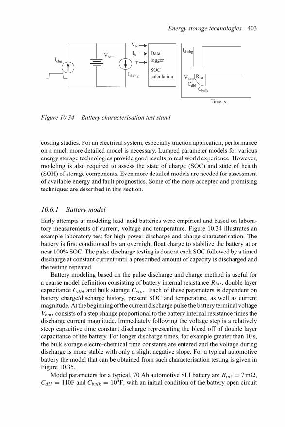
Energy storage technologies 403
Ichg
Idschg
+ VbattDatalogger
SOCcalculation
Vb
Ib
T
Vbatt
Time, s
Idschg
Rint
CdblCbulk
Figure 10.34 Battery characterisation test stand
costing studies. For an electrical system, especially traction application, performanceon a much more detailed model is necessary. Lumped parameter models for variousenergy storage technologies provide good results to real world experience. However,modeling is also required to assess the state of charge (SOC) and state of health(SOH) of storage components. Even more detailed models are needed for assessmentof available energy and fault prognostics. Some of the more accepted and promisingtechniques are described in this section.
10.6.1 Battery model
Early attempts at modeling lead–acid batteries were empirical and based on labora-tory measurements of current, voltage and temperature. Figure 10.34 illustrates anexample laboratory test for high power discharge and charge characterisation. Thebattery is first conditioned by an overnight float charge to stabilize the battery at ornear 100% SOC. The pulse discharge testing is done at each SOC followed by a timeddischarge at constant current until a prescribed amount of capacity is discharged andthe testing repeated.
Battery modeling based on the pulse discharge and charge method is useful fora coarse model definition consisting of battery internal resistance Rint , double layercapacitance Cdbl and bulk storage Cstor . Each of these parameters is dependent onbattery charge/discharge history, present SOC and temperature, as well as currentmagnitude. At the beginning of the current discharge pulse the battery terminal voltageVbatt consists of a step change proportional to the battery internal resistance times thedischarge current magnitude. Immediately following the voltage step is a relativelysteep capacitive time constant discharge representing the bleed off of double layercapacitance of the battery. For longer discharge times, for example greater than 10 s,the bulk storage electro-chemical time constants are entered and the voltage duringdischarge is more stable with only a slight negative slope. For a typical automotivebattery the model that can be obtained from such characterisation testing is given inFigure 10.35.
Model parameters for a typical, 70 Ah automotive SLI battery are Rint = 7 m�,Cdbl = 110F and Cbulk = 106F, with an initial condition of the battery open circuit
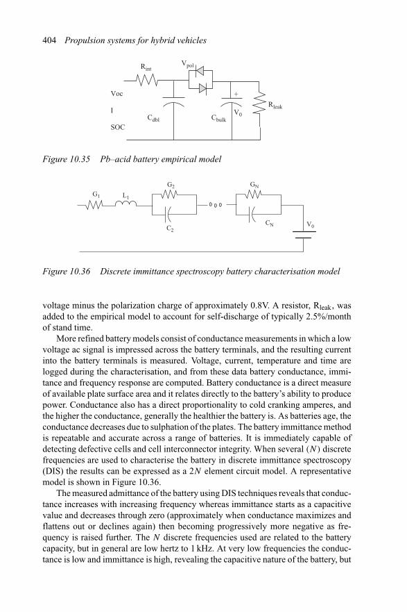
404 Propulsion systems for hybrid vehicles
Voc
I
SOC
RintVpol
Cdbl Cbulk
+
V0
Rleak
Figure 10.35 Pb–acid battery empirical model
G1
G2
C2
GN
CN V0
L1
Figure 10.36 Discrete immittance spectroscopy battery characterisation model
voltage minus the polarization charge of approximately 0.8V. A resistor, Rleak, wasadded to the empirical model to account for self-discharge of typically 2.5%/monthof stand time.
More refined battery models consist of conductance measurements in which a lowvoltage ac signal is impressed across the battery terminals, and the resulting currentinto the battery terminals is measured. Voltage, current, temperature and time arelogged during the characterisation, and from these data battery conductance, immi-tance and frequency response are computed. Battery conductance is a direct measureof available plate surface area and it relates directly to the battery’s ability to producepower. Conductance also has a direct proportionality to cold cranking amperes, andthe higher the conductance, generally the healthier the battery is. As batteries age, theconductance decreases due to sulphation of the plates. The battery immittance methodis repeatable and accurate across a range of batteries. It is immediately capable ofdetecting defective cells and cell interconnector integrity. When several (N) discretefrequencies are used to characterise the battery in discrete immittance spectroscopy(DIS) the results can be expressed as a 2N element circuit model. A representativemodel is shown in Figure 10.36.
The measured admittance of the battery using DIS techniques reveals that conduc-tance increases with increasing frequency whereas immittance starts as a capacitivevalue and decreases through zero (approximately when conductance maximizes andflattens out or declines again) then becoming progressively more negative as fre-quency is raised further. The N discrete frequencies used are related to the batterycapacity, but in general are low hertz to 1 kHz. At very low frequencies the conduc-tance is low and immittance is high, revealing the capacitive nature of the battery, but
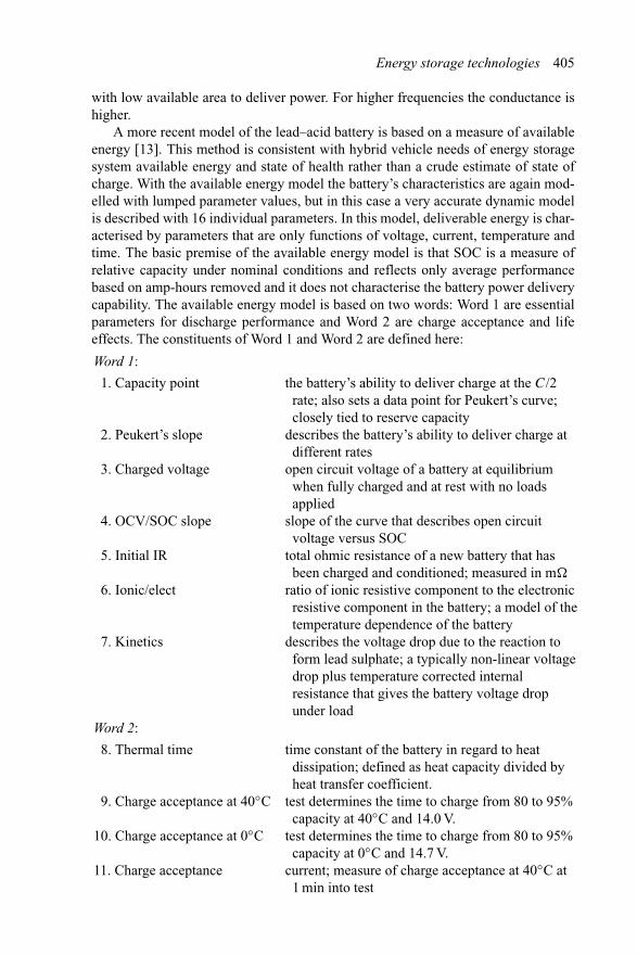
Energy storage technologies 405
with low available area to deliver power. For higher frequencies the conductance ishigher.
A more recent model of the lead–acid battery is based on a measure of availableenergy [13]. This method is consistent with hybrid vehicle needs of energy storagesystem available energy and state of health rather than a crude estimate of state ofcharge. With the available energy model the battery’s characteristics are again mod-elled with lumped parameter values, but in this case a very accurate dynamic modelis described with 16 individual parameters. In this model, deliverable energy is char-acterised by parameters that are only functions of voltage, current, temperature andtime. The basic premise of the available energy model is that SOC is a measure ofrelative capacity under nominal conditions and reflects only average performancebased on amp-hours removed and it does not characterise the battery power deliverycapability. The available energy model is based on two words: Word 1 are essentialparameters for discharge performance and Word 2 are charge acceptance and lifeeffects. The constituents of Word 1 and Word 2 are defined here:
Word 1:
1. Capacity point the battery’s ability to deliver charge at the C/2rate; also sets a data point for Peukert’s curve;closely tied to reserve capacity
2. Peukert’s slope describes the battery’s ability to deliver charge atdifferent rates
3. Charged voltage open circuit voltage of a battery at equilibriumwhen fully charged and at rest with no loadsapplied
4. OCV/SOC slope slope of the curve that describes open circuitvoltage versus SOC
5. Initial IR total ohmic resistance of a new battery that hasbeen charged and conditioned; measured in m�
6. Ionic/elect ratio of ionic resistive component to the electronicresistive component in the battery; a model of thetemperature dependence of the battery
7. Kinetics describes the voltage drop due to the reaction toform lead sulphate; a typically non-linear voltagedrop plus temperature corrected internalresistance that gives the battery voltage dropunder load
Word 2:
8. Thermal time time constant of the battery in regard to heatdissipation; defined as heat capacity divided byheat transfer coefficient.
9. Charge acceptance at 40◦C test determines the time to charge from 80 to 95%capacity at 40◦C and 14.0 V.
10. Charge acceptance at 0◦C test determines the time to charge from 80 to 95%capacity at 0◦C and 14.7 V.
11. Charge acceptance current; measure of charge acceptance at 40◦C at1 min into test
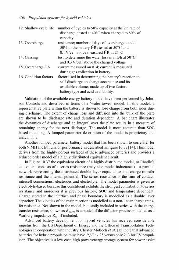
406 Propulsion systems for hybrid vehicles
12. Shallow cycle life number of cycles to 50% capacity at the 2 h rate ofdischarge, tested at 40◦C when charged to 80% ofcapacity
13. Overcharge resistance; number of days of overcharge to add50% to the battery I2R; tested at 50◦C and0.1 V/cell above measured I2R at 25◦C
14. Gassing test to determine the water loss in mL/h at 50◦Cand 0.3 V/cell above the charged voltage
15. Overcharge CA current measured on #14; current is measuredduring gas collection in battery
16. Condition factors factor used in determining the battery’s reaction toself-discharge on charge acceptance and itsavailable volume; made up of two factors –battery type and acid availability.
Validation of the available energy battery model have been performed by John-son Controls and described in terms of a ‘water tower’ model. In this model, arepresentative plate within the battery is shown to lose charge from both sides dur-ing discharge. The extent of charge loss and diffusion into the bulk of the plateare shown to be discharge rate and duration dependent. A bar chart illustratesthe dynamics of discharge and an integral over the plate results in a measure ofremaining energy for the next discharge. The model is more accurate than SOCbased modeling. A lumped parameter description of the model is proprietary andunavailable.
Another lumped parameter battery model that has been shown to correlate, forboth NiMH and lithium ion performance, is described in Figure 10.37 [14]. This modelderives from the highly porous surfaces of these advanced batteries and provides areduced order model of a highly distributed equivalent circuit.
In Figure 10.37 the equivalent circuit of a highly distributed model, or Randle’sequivalent, consists of a series resistance (may also model inductance) – a parallelnetwork representing the distributed double layer capacitance and charge transferresistance and the internal potential. The series resistance is the sum of contact,intercell connections, electrodes and electrolyte. The model parameter is given aselectrolyte-based because this constituent exhibits the strongest contribution to seriesresistance and moreover it is previous history, SOC and temperature dependent.Charge stored in the interface and phase boundary is modelled as a double layercapacitor. The kinetics of the main reaction is modelled as a non-linear charge trans-fer resistance. Not shown in the model, but easily included in series with the chargetransfer resistance, shown as Rdist , is a model of the diffusion process modelled as aWarburg impedance Zw, if included.
Advanced battery development for hybrid vehicles has received considerableimpetus from the US Department of Energy and the Office of Transportation Tech-nologies in cooperation with industry. Chester Motloch et al. [15] note that advancedbatteries for hybrid propulsion must have P/E > 25 versus only 2–3 for EV propul-sion. The objective is a low cost, high power/energy storage system for power assist
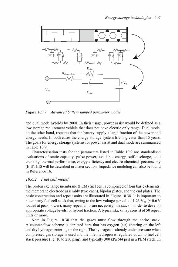
Energy storage technologies 407
+ V0
Rdist
Cdist
Relectrolyte
Voc
Figure 10.37 Advanced battery lumped parameter model
and dual mode hybrids by 2008. In their usage, power assist would be defined as alow storage requirement vehicle that does not have electric only range. Dual mode,on the other hand, requires that the battery supply a large fraction of the power andenergy needs. In both cases the energy storage system life is greater than 15 years.The goals for energy storage systems for power assist and dual mode are summarisedin Table 10.9.
Characterisation tests for the parameters listed in Table 10.9 are standardisedevaluations of static capacity, pulse power, available energy, self-discharge, coldcranking, thermal performance, energy efficiency and electro-chemical spectroscopy(EIS). EIS will be described in a later section. Impedance modeling can also be foundin Reference 16.
10.6.2 Fuel cell model
The proton exchange membrane (PEM) fuel cell is comprised of four basic elements:the membrane electrode assembly (two each), bipolar plates, and the end plates. Thebasic construction and repeat units are illustrated in Figure 10.38. It is important tonote in any fuel cell stack that, owing to the low voltage per cell of 1.23 Voc (∼0.6 Vloaded at peak power), many repeat units are necessary in a stack in order to developappropriate voltage levels for hybrid traction. A typical stack may consist of 50 repeatunits or more.
Note in Figure 10.38 that the gases must flow through the entire stack.A counter-flow scheme is depicted here that has oxygen (air) entering on the leftand dry hydrogen entering on the right. The hydrogen is already under pressure whencompressed gas storage is used and the inlet hydrogen is regulated down to fuel cellstack pressure (i.e. 10 to 250 psig), and typically 300 kPa (44 psi) in a PEM stack. In
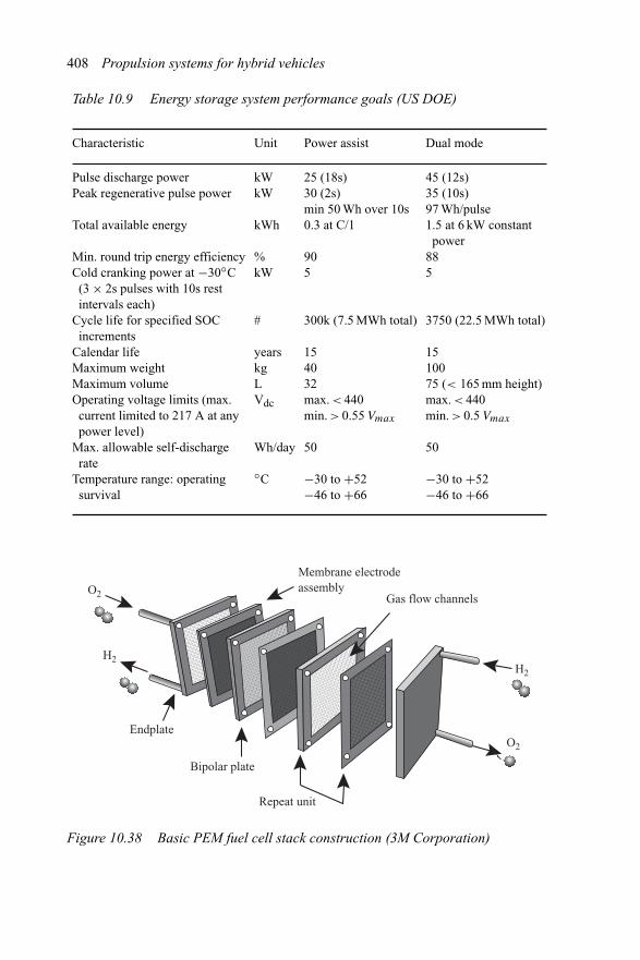
408 Propulsion systems for hybrid vehicles
Table 10.9 Energy storage system performance goals (US DOE)
Characteristic Unit Power assist Dual mode
Pulse discharge power kW 25 (18s) 45 (12s)Peak regenerative pulse power kW 30 (2s) 35 (10s)
min 50 Wh over 10s 97 Wh/pulseTotal available energy kWh 0.3 at C/1 1.5 at 6 kW constant
powerMin. round trip energy efficiency % 90 88Cold cranking power at −30◦C
(3 × 2s pulses with 10s restintervals each)
kW 5 5
Cycle life for specified SOCincrements
# 300k (7.5 MWh total) 3750 (22.5 MWh total)
Calendar life years 15 15Maximum weight kg 40 100Maximum volume L 32 75 (< 165 mm height)Operating voltage limits (max.
current limited to 217 A at anypower level)
Vdc max. < 440 max. < 440min. > 0.55 Vmax min. > 0.5 Vmax
Max. allowable self-dischargerate
Wh/day 50 50
Temperature range: operatingsurvival
◦C −30 to +52 −30 to +52−46 to +66 −46 to +66
Membrane electrodeassembly
Gas flow channels
Endplate
Bipolar plate
Repeat unit
H2
O2
H2
O2
Figure 10.38 Basic PEM fuel cell stack construction (3M Corporation)
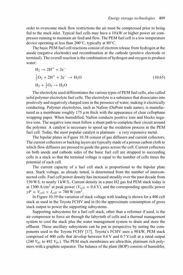
Energy storage technologies 409
order to overcome stack flow restrictions the air must be compressed prior to beingfed to the stack inlet. Typical fuel cells may have a 10 kW or higher power air com-pressor running to maintain air feed and flow. The PEM fuel cell is a low temperaturedevice operating at less than 200◦C, typically at 80◦C.
The basic PEM fuel cell reactions consist of electron release from hydrogen at theanode (negative electrode) and recombination at the cathode (positive electrode orterminal). The overall reaction is the combination of hydrogen and oxygen to producewater:
H2 → 2H+ + 2e−
12 O2 + 2H+ + 2e− → H2O
H2 + 12 O2 → H2O
(10.65)
The electrolyte used differentiates the various types of PEM fuel cells, also calledsolid polymer electrolyte fuel cells. The electrolyte is a substance that dissociates intopositively and negatively charged ions in the presence of water, making it electricallyconducting. Polymer electrolytes, such as Nafion (DuPont trade name), is manufac-tured as a membrane roughly 175 μm thick with the appearance of clear cellophanewrapping paper. When humidified, Nafion conducts positive ions and blocks nega-tive ions. The negative ions must follow a shunt path to complete their circuit aroundthe polymer. A catalyst is necessary to speed up the oxidation process in the PEMfuel cell. Today, the most popular catalyst is platinum – a very expensive metal.
The bipolar plates in Figure 10.38 consist of gas diffusers and current collectors.The current collectors or backing layers are typically made of a porous carbon cloth towhich flow diffusers are pressed to guide the gases across the cell. Current collectorson both anode and cathode sides of the basic fuel cell are strapped to succeedingcells in a stack so that the terminal voltage is equal to the number of cells times thepotential of each cell.
The current capacity of a fuel cell stack is proportional to the bipolar platearea. Stack voltage, as already noted, is determined from the number of intercon-nected cells. Fuel cell power density has increased steadily over the past decade from150 W/L to nearly 1 kW/L. Current density in a pure H2 gas fed PEM stack today isat 1300 A/cm2 at peak power (Vcell = 0.6 V), and the corresponding specific powerγP = Vcell × Jcell = 780 W/cm2.
In Figure 10.39 the variation of stack voltage with loading is shown for a 400 cellstack as used in the Toyota FCHV and in (b) the approximate consumption of grossstack output to power the supporting subsystems.
Supporting subsystems for a fuel cell stack, other than a reformer if used, is theair compressor to force air through the labyrinth of cells and a thermal managementsystem to cool the stack plus the water management system to drain and store theeffluent. These ancillary subsystems can be put in perspective by noting the com-ponents used in the Toyota FCHV [17]. Toyota’s FCHV uses a 90 kW, PEM stackcomprised of 400 cells that develop between 0.6 V and 0.7 V/cell at a rated output(240 Vdc to 492 Vdc). The PEM stack membranes are ultra-thin, platinum rich poly-mers with a graphite separator. The balance of the plant (BOP) consists of humidifer,
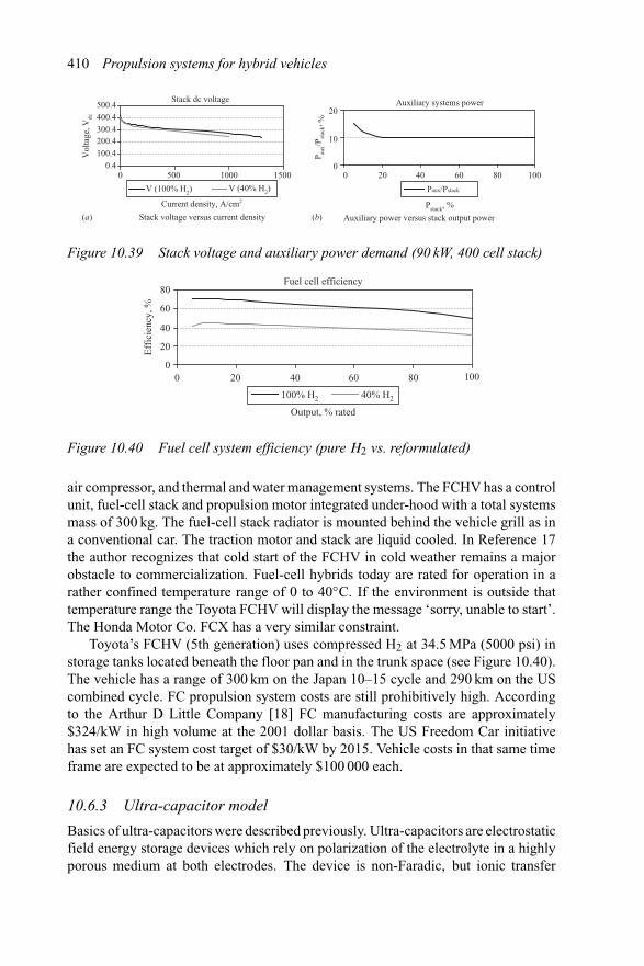
410 Propulsion systems for hybrid vehicles
Stack dc voltage
0.4100.4200.4300.4400.4500.4
0 500 1000 1500
Current density, A/cm2
Vol
tage
, Vdc
Auxiliary systems power
0
10
20
0 20 40 60 80 100
Pstack, %
P aux/
P stac
k, %
Paux/PstackV (100% H2) V (40% H2)
Stack voltage versus current density Auxiliary power versus stack output power(a) (b)
Figure 10.39 Stack voltage and auxiliary power demand (90 kW, 400 cell stack)
Fuel cell efficiency
0
20
40
60
80
0 20 40 60 80 100
Output, % rated
Eff
icie
ncy,
%
100% H2 40% H2
Figure 10.40 Fuel cell system efficiency (pure H2 vs. reformulated)
air compressor, and thermal and water management systems. The FCHV has a controlunit, fuel-cell stack and propulsion motor integrated under-hood with a total systemsmass of 300 kg. The fuel-cell stack radiator is mounted behind the vehicle grill as ina conventional car. The traction motor and stack are liquid cooled. In Reference 17the author recognizes that cold start of the FCHV in cold weather remains a majorobstacle to commercialization. Fuel-cell hybrids today are rated for operation in arather confined temperature range of 0 to 40◦C. If the environment is outside thattemperature range the Toyota FCHV will display the message ‘sorry, unable to start’.The Honda Motor Co. FCX has a very similar constraint.
Toyota’s FCHV (5th generation) uses compressed H2 at 34.5 MPa (5000 psi) instorage tanks located beneath the floor pan and in the trunk space (see Figure 10.40).The vehicle has a range of 300 km on the Japan 10–15 cycle and 290 km on the UScombined cycle. FC propulsion system costs are still prohibitively high. Accordingto the Arthur D Little Company [18] FC manufacturing costs are approximately$324/kW in high volume at the 2001 dollar basis. The US Freedom Car initiativehas set an FC system cost target of $30/kW by 2015. Vehicle costs in that same timeframe are expected to be at approximately $100 000 each.
10.6.3 Ultra-capacitor model
Basics of ultra-capacitors were described previously. Ultra-capacitors are electrostaticfield energy storage devices which rely on polarization of the electrolyte in a highlyporous medium at both electrodes. The device is non-Faradic, but ionic transfer
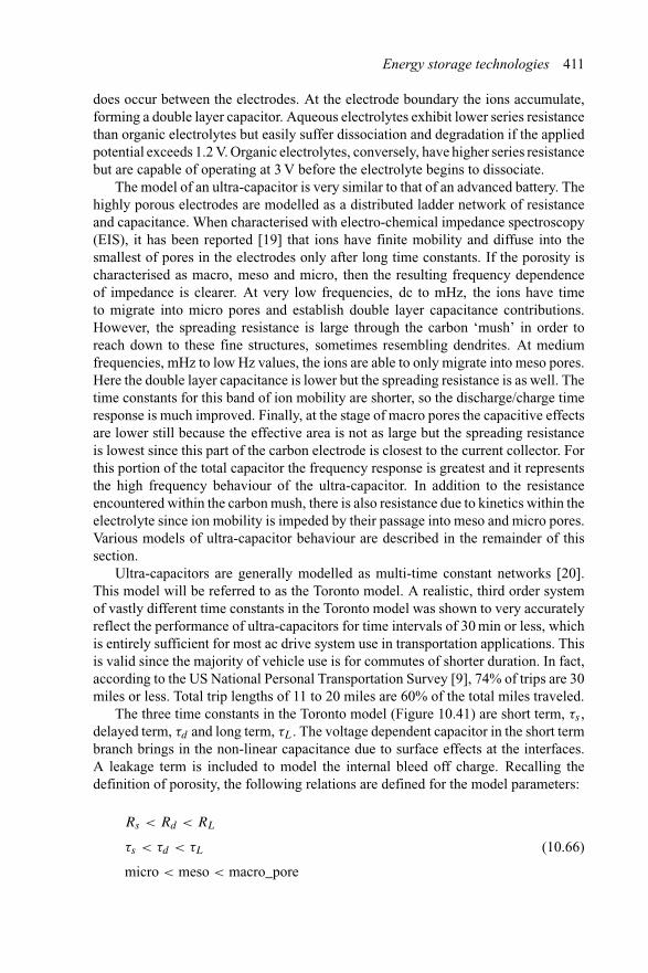
Energy storage technologies 411
does occur between the electrodes. At the electrode boundary the ions accumulate,forming a double layer capacitor. Aqueous electrolytes exhibit lower series resistancethan organic electrolytes but easily suffer dissociation and degradation if the appliedpotential exceeds 1.2 V. Organic electrolytes, conversely, have higher series resistancebut are capable of operating at 3 V before the electrolyte begins to dissociate.
The model of an ultra-capacitor is very similar to that of an advanced battery. Thehighly porous electrodes are modelled as a distributed ladder network of resistanceand capacitance. When characterised with electro-chemical impedance spectroscopy(EIS), it has been reported [19] that ions have finite mobility and diffuse into thesmallest of pores in the electrodes only after long time constants. If the porosity ischaracterised as macro, meso and micro, then the resulting frequency dependenceof impedance is clearer. At very low frequencies, dc to mHz, the ions have timeto migrate into micro pores and establish double layer capacitance contributions.However, the spreading resistance is large through the carbon ‘mush’ in order toreach down to these fine structures, sometimes resembling dendrites. At mediumfrequencies, mHz to low Hz values, the ions are able to only migrate into meso pores.Here the double layer capacitance is lower but the spreading resistance is as well. Thetime constants for this band of ion mobility are shorter, so the discharge/charge timeresponse is much improved. Finally, at the stage of macro pores the capacitive effectsare lower still because the effective area is not as large but the spreading resistanceis lowest since this part of the carbon electrode is closest to the current collector. Forthis portion of the total capacitor the frequency response is greatest and it representsthe high frequency behaviour of the ultra-capacitor. In addition to the resistanceencountered within the carbon mush, there is also resistance due to kinetics within theelectrolyte since ion mobility is impeded by their passage into meso and micro pores.Various models of ultra-capacitor behaviour are described in the remainder of thissection.
Ultra-capacitors are generally modelled as multi-time constant networks [20].This model will be referred to as the Toronto model. A realistic, third order systemof vastly different time constants in the Toronto model was shown to very accuratelyreflect the performance of ultra-capacitors for time intervals of 30 min or less, whichis entirely sufficient for most ac drive system use in transportation applications. Thisis valid since the majority of vehicle use is for commutes of shorter duration. In fact,according to the US National Personal Transportation Survey [9], 74% of trips are 30miles or less. Total trip lengths of 11 to 20 miles are 60% of the total miles traveled.
The three time constants in the Toronto model (Figure 10.41) are short term, τs ,delayed term, τd and long term, τL. The voltage dependent capacitor in the short termbranch brings in the non-linear capacitance due to surface effects at the interfaces.A leakage term is included to model the internal bleed off charge. Recalling thedefinition of porosity, the following relations are defined for the model parameters:
Rs < Rd < RL
τs < τd < τL
micro < meso < macro_pore
(10.66)
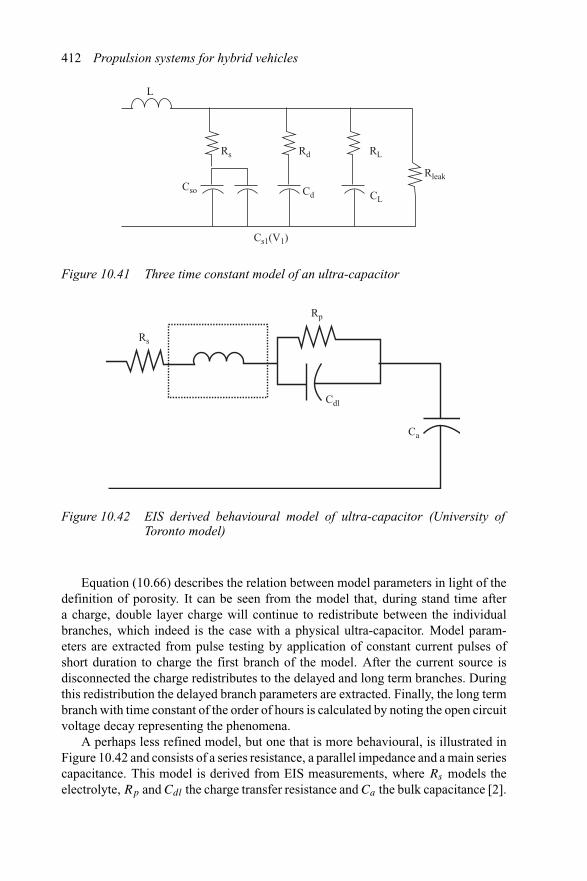
412 Propulsion systems for hybrid vehicles
L
Rs Rd RL
RleakCso
Cs1(V1)
Cd CL
Figure 10.41 Three time constant model of an ultra-capacitor
Rp
Rs
Cdl
Ca
Figure 10.42 EIS derived behavioural model of ultra-capacitor (University ofToronto model)
Equation (10.66) describes the relation between model parameters in light of thedefinition of porosity. It can be seen from the model that, during stand time aftera charge, double layer charge will continue to redistribute between the individualbranches, which indeed is the case with a physical ultra-capacitor. Model param-eters are extracted from pulse testing by application of constant current pulses ofshort duration to charge the first branch of the model. After the current source isdisconnected the charge redistributes to the delayed and long term branches. Duringthis redistribution the delayed branch parameters are extracted. Finally, the long termbranch with time constant of the order of hours is calculated by noting the open circuitvoltage decay representing the phenomena.
A perhaps less refined model, but one that is more behavioural, is illustrated inFigure 10.42 and consists of a series resistance, a parallel impedance and a main seriescapacitance. This model is derived from EIS measurements, where Rs models theelectrolyte, Rp and Cdl the charge transfer resistance and Ca the bulk capacitance [2].
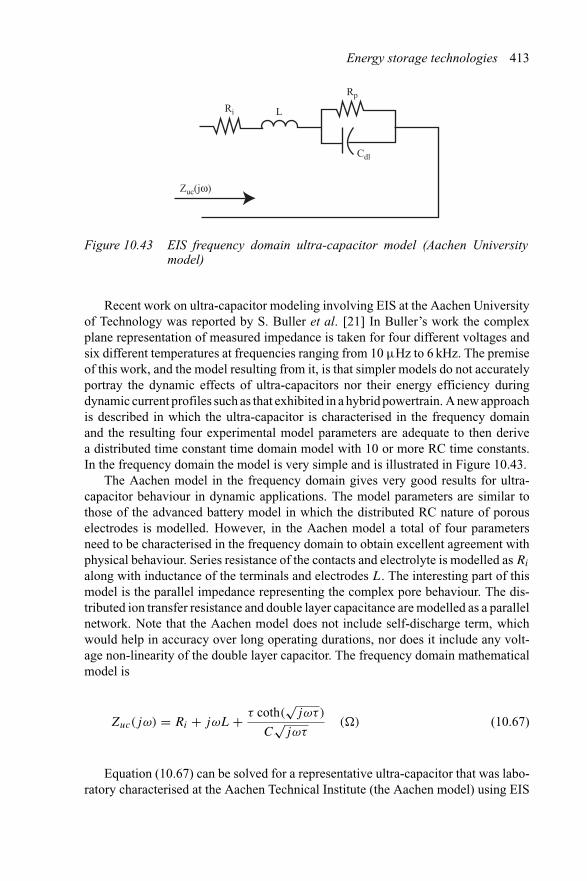
Energy storage technologies 413
Ri
Rp
Cdl
L
Zuc(jω)
Figure 10.43 EIS frequency domain ultra-capacitor model (Aachen Universitymodel)
Recent work on ultra-capacitor modeling involving EIS at the Aachen Universityof Technology was reported by S. Buller et al. [21] In Buller’s work the complexplane representation of measured impedance is taken for four different voltages andsix different temperatures at frequencies ranging from 10 μHz to 6 kHz. The premiseof this work, and the model resulting from it, is that simpler models do not accuratelyportray the dynamic effects of ultra-capacitors nor their energy efficiency duringdynamic current profiles such as that exhibited in a hybrid powertrain. A new approachis described in which the ultra-capacitor is characterised in the frequency domainand the resulting four experimental model parameters are adequate to then derivea distributed time constant time domain model with 10 or more RC time constants.In the frequency domain the model is very simple and is illustrated in Figure 10.43.
The Aachen model in the frequency domain gives very good results for ultra-capacitor behaviour in dynamic applications. The model parameters are similar tothose of the advanced battery model in which the distributed RC nature of porouselectrodes is modelled. However, in the Aachen model a total of four parametersneed to be characterised in the frequency domain to obtain excellent agreement withphysical behaviour. Series resistance of the contacts and electrolyte is modelled as Ri
along with inductance of the terminals and electrodes L. The interesting part of thismodel is the parallel impedance representing the complex pore behaviour. The dis-tributed ion transfer resistance and double layer capacitance are modelled as a parallelnetwork. Note that the Aachen model does not include self-discharge term, whichwould help in accuracy over long operating durations, nor does it include any volt-age non-linearity of the double layer capacitor. The frequency domain mathematicalmodel is
Zuc(jω) = Ri + jωL + τ coth(√
jωτ)
C√
jωτ(�) (10.67)
Equation (10.67) can be solved for a representative ultra-capacitor that was labo-ratory characterised at the Aachen Technical Institute (the Aachen model) using EIS
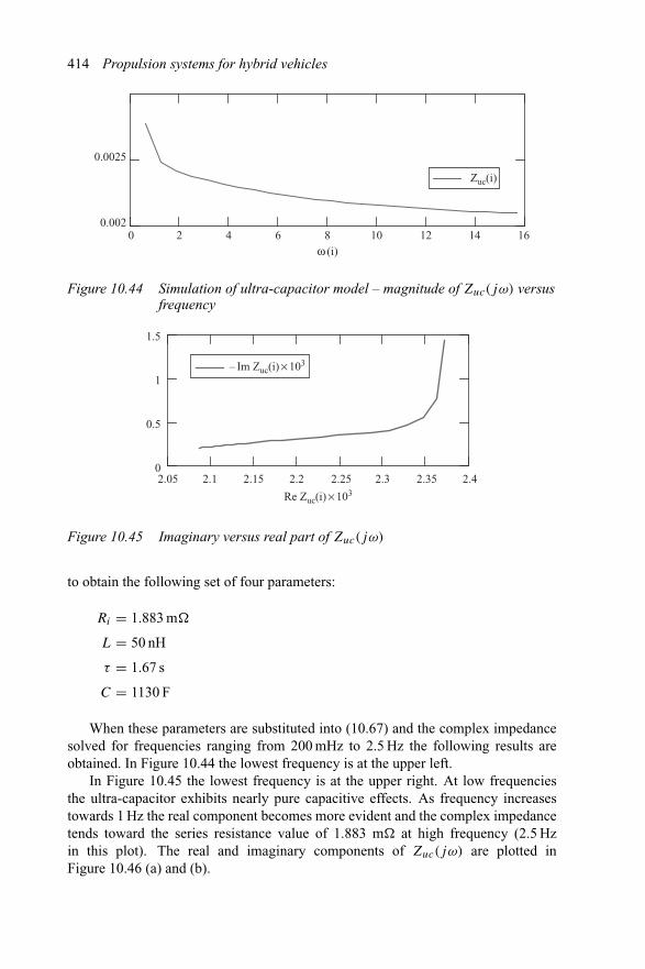
414 Propulsion systems for hybrid vehicles
ω (i)0 2 4 6 8 10 12 14 16
0.002
0.0025
Zuc(i)
Figure 10.44 Simulation of ultra-capacitor model – magnitude of Zuc(jω) versusfrequency
2.05 2.1 2.15 2.2 2.25 2.3 2.35 2.40
0.5
1
1.5
– Im Zuc(i) × 103
Re Zuc(i) × 103
Figure 10.45 Imaginary versus real part of Zuc(jω)
to obtain the following set of four parameters:
Ri = 1.883 m�
L = 50 nH
τ = 1.67 s
C = 1130 F
When these parameters are substituted into (10.67) and the complex impedancesolved for frequencies ranging from 200 mHz to 2.5 Hz the following results areobtained. In Figure 10.44 the lowest frequency is at the upper left.
In Figure 10.45 the lowest frequency is at the upper right. At low frequenciesthe ultra-capacitor exhibits nearly pure capacitive effects. As frequency increasestowards 1 Hz the real component becomes more evident and the complex impedancetends toward the series resistance value of 1.883 m� at high frequency (2.5 Hzin this plot). The real and imaginary components of Zuc(jω) are plotted inFigure 10.46 (a) and (b).
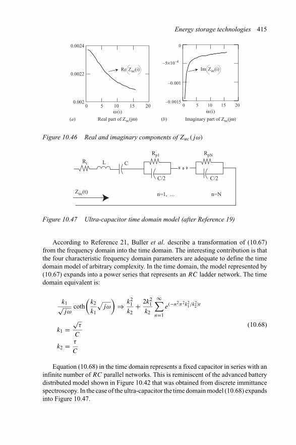
Energy storage technologies 415
Re Zuc(i)
0 5 10 15 200.002
0.0022
0.0024
ω (i) ω (i)
Im Zuc(i)
0 5 10 15 20–0.0015
–0.001
–5×10⁻⁴
0
(a) (b)Real part of Zuc(jω) Imaginary part of Zuc(jω)
Figure 10.46 Real and imaginary components of Zuc(jω)
Rp1
C/2
CLRi
n=Nn=1, ...
C/2
RpN
Zuc(t)
Figure 10.47 Ultra-capacitor time domain model (after Reference 19)
According to Reference 21, Buller et al. describe a transformation of (10.67)from the frequency domain into the time domain. The interesting contribution is thatthe four characteristic frequency domain parameters are adequate to define the timedomain model of arbitrary complexity. In the time domain, the model represented by(10.67) expands into a power series that represents an RC ladder network. The timedomain equivalent is:
k1√jω
coth(
k2
k1
√jω
)⇒ k2
1
k2+ 2k2
1
k2
∞∑n=1
e(−n2π2k21/k2
2)t
k1 =√
τ
C
k2 = τ
C
(10.68)
Equation (10.68) in the time domain represents a fixed capacitor in series with aninfinite number of RC parallel networks. This is reminiscent of the advanced batterydistributed model shown in Figure 10.42 that was obtained from discrete immittancespectroscopy. In the case of the ultra-capacitor the time domain model (10.68) expandsinto Figure 10.47.
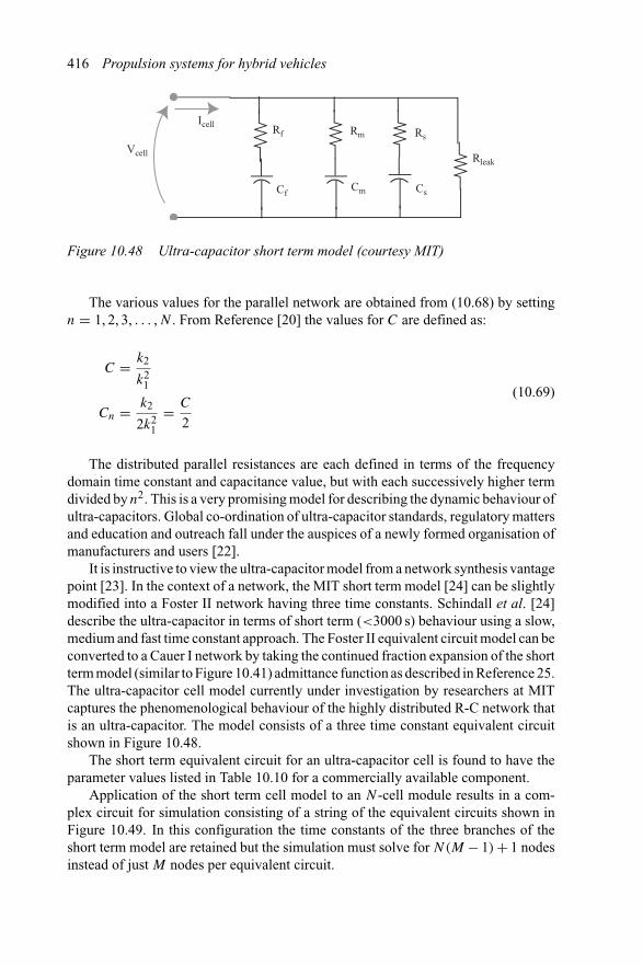
416 Propulsion systems for hybrid vehicles
Rf Rm Rs
Rleak
CfCm Cs
Vcell
Icell
Figure 10.48 Ultra-capacitor short term model (courtesy MIT)
The various values for the parallel network are obtained from (10.68) by settingn = 1, 2, 3, . . . , N . From Reference [20] the values for C are defined as:
C = k2
k21
Cn = k2
2k21
= C
2
(10.69)
The distributed parallel resistances are each defined in terms of the frequencydomain time constant and capacitance value, but with each successively higher termdivided by n2. This is a very promising model for describing the dynamic behaviour ofultra-capacitors. Global co-ordination of ultra-capacitor standards, regulatory mattersand education and outreach fall under the auspices of a newly formed organisation ofmanufacturers and users [22].
It is instructive to view the ultra-capacitor model from a network synthesis vantagepoint [23]. In the context of a network, the MIT short term model [24] can be slightlymodified into a Foster II network having three time constants. Schindall et al. [24]describe the ultra-capacitor in terms of short term (<3000 s) behaviour using a slow,medium and fast time constant approach. The Foster II equivalent circuit model can beconverted to a Cauer I network by taking the continued fraction expansion of the shortterm model (similar to Figure 10.41) admittance function as described in Reference 25.The ultra-capacitor cell model currently under investigation by researchers at MITcaptures the phenomenological behaviour of the highly distributed R-C network thatis an ultra-capacitor. The model consists of a three time constant equivalent circuitshown in Figure 10.48.
The short term equivalent circuit for an ultra-capacitor cell is found to have theparameter values listed in Table 10.10 for a commercially available component.
Application of the short term cell model to an N -cell module results in a com-plex circuit for simulation consisting of a string of the equivalent circuits shown inFigure 10.49. In this configuration the time constants of the three branches of theshort term model are retained but the simulation must solve for N(M − 1) + 1 nodesinstead of just M nodes per equivalent circuit.
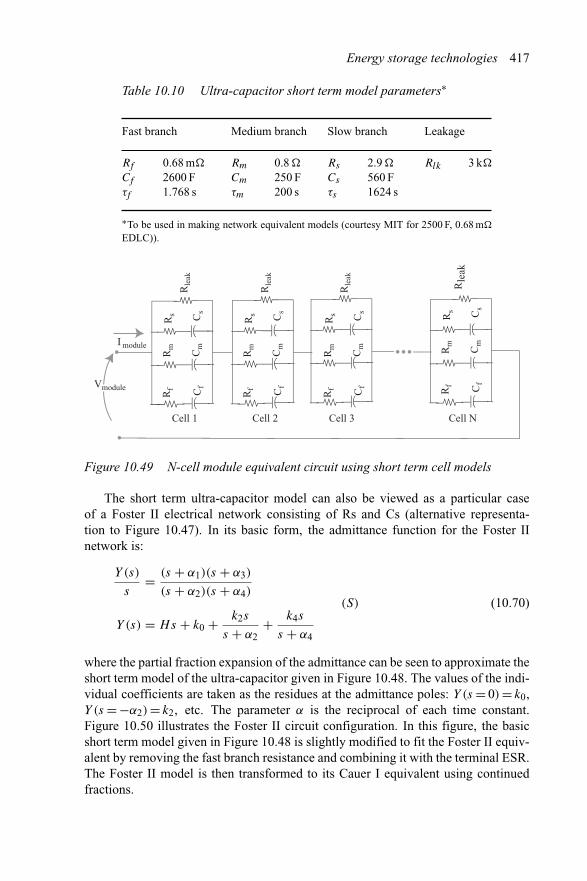
Energy storage technologies 417
Table 10.10 Ultra-capacitor short term model parameters∗
Fast branch Medium branch Slow branch Leakage
Rf 0.68 m� Rm 0.8 � Rs 2.9 � Rlk 3 k�
Cf 2600 F Cm 250 F Cs 560 Fτf 1.768 s τm 200 s τs 1624 s
∗To be used in making network equivalent models (courtesy MIT for 2500 F, 0.68 m�
EDLC)).
I module
Rf
Rm
Rs
Rle
ak
Rle
ak
Rle
ak
Cf
Cm
Cs
Rf
Rm
Rs
Cf
Cm
Cs
Rf
Rm
Rs
Cf
Cm
Cs
Rf
Rm
Rs
Cf
Cm
Cs
Rle
ak
Vmodule
Cell 1 Cell 2 Cell 3 Cell N
Figure 10.49 N-cell module equivalent circuit using short term cell models
The short term ultra-capacitor model can also be viewed as a particular caseof a Foster II electrical network consisting of Rs and Cs (alternative representa-tion to Figure 10.47). In its basic form, the admittance function for the Foster IInetwork is:
Y (s)
s= (s + α1)(s + α3)
(s + α2)(s + α4)
Y (s) = Hs + k0 + k2s
s + α2+ k4s
s + α4
(S) (10.70)
where the partial fraction expansion of the admittance can be seen to approximate theshort term model of the ultra-capacitor given in Figure 10.48. The values of the indi-vidual coefficients are taken as the residues at the admittance poles: Y (s = 0) = k0,Y (s = −α2) = k2, etc. The parameter α is the reciprocal of each time constant.Figure 10.50 illustrates the Foster II circuit configuration. In this figure, the basicshort term model given in Figure 10.48 is slightly modified to fit the Foster II equiv-alent by removing the fast branch resistance and combining it with the terminal ESR.The Foster II model is then transformed to its Cauer I equivalent using continuedfractions.
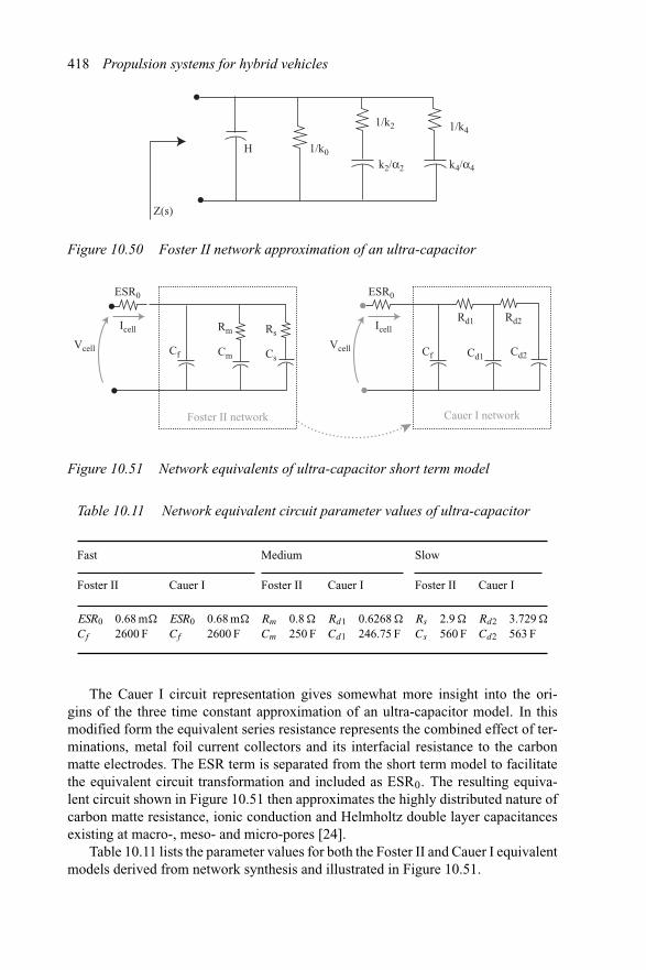
418 Propulsion systems for hybrid vehicles
H 1/k0
1/k2
k2/α2 k4/α4
1/k4
Z(s)
Figure 10.50 Foster II network approximation of an ultra-capacitor
Rd1Rm Rs
Cf Cm CsVcell
Icell
ESR0 ESR0
Foster II network
Rd2
Cf Cd1 Cd2
Cauer I network
Vcell
Icell
Figure 10.51 Network equivalents of ultra-capacitor short term model
Table 10.11 Network equivalent circuit parameter values of ultra-capacitor
Fast Medium Slow
Foster II Cauer I Foster II Cauer I Foster II Cauer I
ESR0 0.68 m� ESR0 0.68 m� Rm 0.8 � Rd1 0.6268 � Rs 2.9 � Rd2 3.729 �
Cf 2600 F Cf 2600 F Cm 250 F Cd1 246.75 F Cs 560 F Cd2 563 F
The Cauer I circuit representation gives somewhat more insight into the ori-gins of the three time constant approximation of an ultra-capacitor model. In thismodified form the equivalent series resistance represents the combined effect of ter-minations, metal foil current collectors and its interfacial resistance to the carbonmatte electrodes. The ESR term is separated from the short term model to facilitatethe equivalent circuit transformation and included as ESR0. The resulting equiva-lent circuit shown in Figure 10.51 then approximates the highly distributed nature ofcarbon matte resistance, ionic conduction and Helmholtz double layer capacitancesexisting at macro-, meso- and micro-pores [24].
Table 10.11 lists the parameter values for both the Foster II and Cauer I equivalentmodels derived from network synthesis and illustrated in Figure 10.51.

Energy storage technologies 419
It is intriguing to find that the parameter values found by moving from a Foster IInetwork model to its Cauer I equivalent model are very similar. Although the Cauer Imodel structure is more insightful of ultra-capacitor distributed resistance and capac-itance, the Foster II model appears to be more suitable for laboratory characterisationof behaviour. The model parameters in the Cauer I network representation are foundaccording to (10.71) written in terms of the Foster II model parameters as derivedfrom the MIT short term model:
Y (s) = Cf s3 + [(αm + αs)Cf + 1/Rm + 1/Rs ]s2 + (αmαsCf + αs/Rm + αm/Rs)s
s2 + (αm + αs)s + αmαs
Y (s) = 2600s3 + 16.197s2 + 1.0502 × 10⁻²s
s2 + 5.616 × 10⁻³s + 3.08 × 10⁻⁶
Y (s) = 2600s + 1
0.6268 + 1
246.75s + 1
3.729 + 1
563s
(10.71)
In (10.71) the Cauer I resistive elements in the ladder network are the coeffi-cients of s0 in the continued fraction expansion, and the shunt branch elements arecoefficients of s1 as admittances (i.e. a capacitor).
10.7 References
1 GIACOLETTO, L. J.: ‘Energy storage and conversion’, IEEE Spectrum, 1965,2(2), pp. 95–102
2 CHU, A., BRAATZ, P. and SOUKIAZIAN, S.: ‘Supercapacitors and batteries forhybrid electric vehicle applications: a primer’. Proceedings of the 2002 GlobalPowerTrain Congress, Advanced Propulsion Systems, 24–26 September 2002,Ann Arbor, MI
3 COHEN, M. and SMITH, R.: ‘Application of distributed power modules on42 V systems’. Proceedings of the 2002 Global PowerTrain Congress, AdvancedPropulsion Systems, 24–26 September 2002, Ann Arbor, MI
4 Automotive Engineering, Society of Automotive Engineers, Warrendale, PA.,December 2002 issue, pp. 14–15
5 HASKINS, H. J. and DZIECIUCH, M. A.: ‘Power capacitor requirements forelectric vehicles’. International Seminar on Electric Vehicles, December 1991
6 ONG, W. and JOHNSTON, R. H.: ‘Electrochemical capacitors and their poten-tial application to heavy duty vehicles’. SAE technical paper # 2000-01-3495,Electronics for trucks and buses 2000, SP-1568, Truck and Buss Meeting andExposition, Portland, Oregon, 4–6 December 2000
7 GRAHAM, R.: ‘Comparing the benefits and impacts of hybrid electric vehicleoptions’. Electric Power Research Institute, Report # 1000349, July 2001
420 Propulsion systems for hybrid vehicles
8 BARRADE, P.: ‘Series connection of supercapacitors: comparative study ofsolutions for the active equalization of the voltages’. Electrimacs 2002, 7th Inter-national Conference on modeling and simulation of electric machines, convertersand systems, 18–21 August 2002, Ecole De Technologie Superieure (ETS),Montreal, Canada
9 1990 National Personal Transportation Survey Databook, Vol.1, US Departmentof Transportation, Federal Highway Administration
10 JONES, L. W.: ‘Liquid hydrogen as a fuel for the future’, in ‘Energy and man:technical and social aspects of energy’ (IEEE Press, 1975)
11 NATKIN, R., STOCKHAUSEN, W., TANG, X., KABAT, D., REAMS, L.,HASHEMI, S. and SZWABOWSKI, S.: ‘Ford hydrogen internal combustionengine design and vehicle development program’. Global PowerTrain Congress2002, Proceedings of Advanced Propulsion Systems, Sheraton Inn, Ann Arbor,MI, 24–26 September 2002
12 MILLER, J. M., NAGEL, N., SCHULZ, S., CONLON, B., DUVALL, M.,KANKAM, D.: ‘Adjustable speed drives transportation industry needs. Part II:Utility and aeropropulsion’. IEEE 39th Industry Applications Conference andAnnual Meeting, Grand American Hotel, Salt Lake City, Utah, 12–16 October2003
13 DOUGHERTY, T. and ZAGRODNIK, J.: ‘Proposed new electrical parameters forbattery simulation and monitoring’. MIT Industry Consortium on advanced auto-motive electrical/electronic components and systems, Program Review Meeting,Ritz Carlton Marina del Rey Hotel, Los Angeles, CA, 30 January–1 February2002
14 VERBRUGGE, M., CONELL, R., TARNOWSKY, S. and YING, R.: ‘Per-spectives on 42 V high-power battery systems’. 2nd International AdvancedAutomotive Battery Conference, AABC2002, Las Vegas, NV, February 2002
15 MOTLOCH, C. G., MURPHY, T. C., SUTULA, R. A. and MILLER, T. J.:‘Overview of PNGV battery development and test program’. 2nd Interna-tional Advanced Automotive Battery Conference, AABC2002, Las Vegas, NV,February 2002
16 BULLER, S., WALTER, J., KARDEN, E. and De DONCKER, R.W.:‘Impedance-based monitoring of automotive batteries’. 2nd InternationalAdvanced Automotive Battery Conference, AABC2002, Las Vegas, NV, Febru-ary 2002
17 YAMAGUCHI, J.: ‘Leading the way: fuel-cell vehicles from Toyota and Hondaare hitting the streets for customer use in both Japan and the USA’. SAEAutomotive Engineering International, March 2003, pp. 54–58
18 WEISS, M., HEYWOOD, J. B., SCHAFER, A. and NATARAJAN, V. K.:‘Comparative assessment of fuel cell cars’. MIT LFEE 2003-001 RP, February2003, available from LFEE Publications, MIT, Room E40-473, 77 MassachusettsAvenue, Cambridge, MA 02139–4307
19 NEW, D. and KASSAKIAN, J.: ‘Automotive applications of ultra-capacitors’.MIT Industry Consortium on Advanced Automotive Electrical/Electronic Com-ponents and Systems, Consortium Project Report RU13, September 2002
Energy storage technologies 421
20 ZUBIETA, L. and BONERT, R.: ‘Characterisation of double-layer capacitors forpower electronics applications’, IEEE Trans. Ind. Appl., 2000, 36, pp. 199–205
21 BULLER, S., KARDEN, E., KOK, D. and De DONCKER, R.W.: ‘Modelingthe dynamic behaviour of supercapacitors using impedance spectroscopy’, IEEETrans. Ind. Appl., 2002, 38(6), pp. 1622–1626
22 Kilofarad International, an affiliate of The Electronic Components, Assembliesand Materials Association (ECA). 2500 Wilson Blvd, Arlington, VA. 22201–3834
23 BUDAK, A.: ‘Passive and active network analysis and synthesis’ (HoughtonMifflin Company, Boston 1974)
24 SCHINDALL, J., KASSAKIAN, J., PERREAULT, D. and NEW, D.: ‘Automo-tive applications of ultra-capacitors: characterisation, modeling and utilisation’.MIT-Industry Consortium on Advanced Automotive Electrical/Electronic Com-ponents and Systems, Spring meeting, Ritz-Carlton Hotel, Dearborn, MI, 5–6March 2003
25 MILLER, J. M., McCLEER, P. J. and COHEN, M.: ‘Ultra-capacitors as energybuffers in a multiple zone electrical distribution system’. Global PowerTrainCongress 2003, Proceedings of Advanced Propulsion Systems, Crowne PlazaHotel, Ann Arbor, MI, 23–25 September 2003

Chapter 11
Hybrid vehicle test and validation
Development of hybrid propulsion systems requires knowledge of the vehicleattributes in terms of mass, frontal area, tyre rolling radius and rolling resistance,plus its aerodynamic drag coefficient. The accepted procedure for obtaining thesedata comes from vehicle coast down testing. This chapter illustrates the coast downprocess on two very different vehicles seen often on highways in North America andEurope: the sport utility vehicle and tractor-trailors (semis).
Before engaging in coast down testing it is necessary to know the vehicle mass,frontal area and tyre rolling radius. The procedure to obtain these data, if not knownfrom manufacturers’ specifications, is to weigh the vehicle, and calculate the frontalarea and tyre rolling radius according to (11.1):
A = caHW
rw = 1609
2πNw
(m2, m) (11.1)
where the vehicle track, W , and height from ground to roof, H , are used to approxi-mate the frontal area. The factor ca (∼0.9) is a coefficient in (11.1) to make provisionfor nominal ground clearance and aerodynamic styling (body contours). The tyrerolling radius is best obtained by noting the number of revolutions made per set dis-tance, such as a kilometer or mile. In (11.1) the number of tyre revolutions per mile isused to compute the dynamic rolling radius on the road surface for which the vehicleattributes are being evaluated. The static rolling radius has been described earlier inthis book, and will be compared here to dynamic rolling radius to validate the fac-tor of 0.95 to 0.99 used in that discussion. The procedure for the derivation of tyredynamic rolling radius from the tyre manufacturer code is repeated here for clarity.For example, the P235/70 R16 tyre manufactured by Continental Group has a sectionwidth of 235 mm, an aspect ratio (section height as percentage of section width of70%, and a rim diameter of 16 in (406.4 mm). Using these data the dynamic rolling
424 Propulsion systems for hybrid vehicles
resistance is calculated using (11.2):
rw = cr(drim + 2(70/100)ws)
2(11.2)
where drim is the rim diameter (convert in to mm), ws is the tyre section width inmm, and cr is a coefficient to down adjust static rolling radius, to dynamic rollingradius, and is typically 0.95 to 0.99. For the given passenger vehicle tyre the staticrolling radius determined from (11.2) when cr = 1.0 is 367 mm.
For the sport utility test vehicle, a 2002 Ford Motor Co. Escape 4 × 4, the frontalarea and dynamic rolling radius predicted from (11.1), comes out to:
A = 0.9(1.551)(1.774) = 2.476
rw = 100
2π(43.9)= 0.363
m2, m (11.3)
The value for dynamic rolling radius calculated from (11.3) is 99% of the valuecalculated from the tyre code when the coefficient is set equal to unity. This meansthat a value of cr = 0.99 will adjust the static rolling radius to a dynamic rollingradius with good accuracy. The hybrid Escape (when it comes out) will have lowerrolling resistance tyres manufactured by Yokahama and are specified as P255/55 R18105 V, so its rolling radius will be 0.369 m or virtually the same as (11.3).
Atmospheric conditions of temperature (◦C) and barometric pressure (Hg) areused to correct the sea level air density to that of the testing location accordingto (11.4):
ρ = ρSTP
(Pr
29.92
)(288.16
273.16 + Tamb
)
ρSTP = 1.225
(kg/m3) (11.4)
where air density at standard temperature and pressure (STP) is given for a barometerof 29.92 in Hg (101.325 bar) and a temperature of 15◦C.
11.1 Vehicle coast down procedure
The coast down test procedure is now explained. Vehicle attributes of mass, frontalarea, and tyre dynamic rolling radius have been explained in the previous section.Vehicle test mass must be adjusted for occupant and cargo. In the coast down testingreported below there are two occupants – a driver and a time keeper. Coast downtesting is necessary in order to extract the vehicle’s aerodynamic drag coefficient andtyre rolling resistance. By taking measurements of elapsed time between two closelyspaced speeds when the vehicle is rolling fast and again when the vehicle has nearlystopped rolling it is possible to determine these two coefficients with fair accuracy.Higher resolution could be obtained by wind tunnel testing, for example, but coastdown testing is a very accepted method.
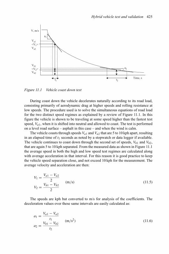
Hybrid vehicle test and validation 425
Time, st2t1
a1
a2
V, m/s
Va1<V1>Va2
Vb1<V2>Vb2
Figure 11.1 Vehicle coast down test
During coast down the vehicle decelerates naturally according to its road load,consisting primarily of aerodynamic drag at higher speeds and rolling resistance atlow speeds. The procedure used is to solve the simultaneous equations of road loadfor the two distinct speed regimes as explained by a review of Figure 11.1. In thisfigure the vehicle is shown to be traveling at some speed higher than the fastest testspeed, Va1, when it is shifted into neutral and allowed to coast. The test is performedon a level road surface – asphalt in this case – and when the wind is calm.
The vehicle coasts through speeds Va1 and Va2 that are 5 to 10 kph apart, resultingin an elapsed time of t1 seconds as noted by a stopwatch or data logger if available.The vehicle continues to coast down through the second set of speeds, Vb1 and Vb2,that are again 5 to 10 kph separated. From the measured data as shown in Figure 11.1the average speed in both the high and low speed test regimes are calculated alongwith average acceleration in that interval. For this reason it is good practice to keepthe vehicle speed separation close, and not exceed 10 kph for the measurement. Theaverage velocity and acceleration are then:
V1 = Va1 − Va2
2
V2 = Vb1 − Vb2
2
(m/s) (11.5)
The speeds are kph but converted to m/s for analysis of the coefficients. Thedeceleration values over these same intervals are easily calculated as:
a1 = Va1 − Va2
t1
a2 = Vb1 − Vb2
t2
(m/s2) (11.6)
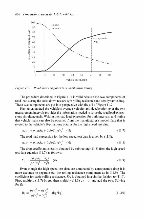
426 Propulsion systems for hybrid vehicles
Vehicle speed, mph
Perc
enta
ge o
f to
tal r
oad
load
Rollingresistance
Aerodynamicdrag
100
90
80
70
60
50
40
30
20
10
00 10 20 30 40 50 60 70 80
Figure 11.2 Road load components in coast down testing
The procedure described in Figure 11.1 is valid because the two components ofroad load during the coast down test are tyre rolling resistance and aerodynamic drag.These two components are put into perspective with the aid of Figure 11.2.
Having calculated the vehicle’s average velocity and deceleration over the twomeasurement intervals provides the information needed to solve the road load expres-sions simultaneously. Writing the road load expression for both intervals, and notingthat vehicle mass can also be obtained from the manufacturer’s model plate that isriveted to the vehicle’s B-pillar, one obtains for the high speed test data,
mva1 = mvgR0 + 0.5ρCdAV 21 (N) (11.7)
The road load expression for the low speed test data is given by (11.8),
mva2 = mvgR0 + 0.5ρCdAV 22 (N) (11.8)
The drag coefficient is easily obtained by subtracting (11.8) from the high speedtest data equation (11.7) as follows:
Cd = 2mv(a1 − a2)
ρA(V 21 − V 2
2 )(#) (11.9)
Even though the high speed test data are dominated by aerodynamic drag it ismore accurate to separate out the rolling resistance component as in (11.9). Thecoefficient for static rolling resistance, R0, is obtained in a similar fashion to (11.9).First, multiply (11.7) by a2, then multiply (11.8) by −a1 and add the two. Solvingfor R0,
R0 = a2V21 − a1V
22
g(V 21 − V 2
2 )(kg/kg) (11.10)
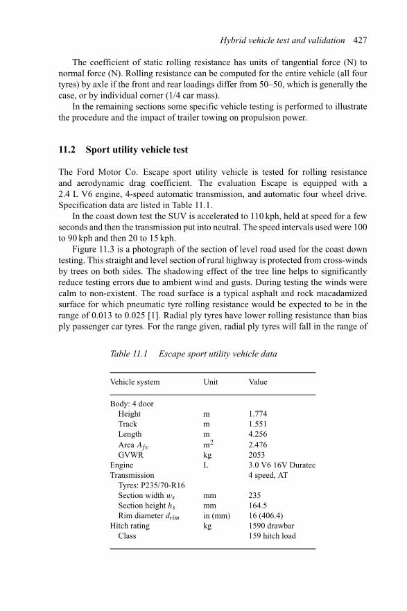
Hybrid vehicle test and validation 427
The coefficient of static rolling resistance has units of tangential force (N) tonormal force (N). Rolling resistance can be computed for the entire vehicle (all fourtyres) by axle if the front and rear loadings differ from 50–50, which is generally thecase, or by individual corner (1/4 car mass).
In the remaining sections some specific vehicle testing is performed to illustratethe procedure and the impact of trailer towing on propulsion power.
11.2 Sport utility vehicle test
The Ford Motor Co. Escape sport utility vehicle is tested for rolling resistanceand aerodynamic drag coefficient. The evaluation Escape is equipped with a2.4 L V6 engine, 4-speed automatic transmission, and automatic four wheel drive.Specification data are listed in Table 11.1.
In the coast down test the SUV is accelerated to 110 kph, held at speed for a fewseconds and then the transmission put into neutral. The speed intervals used were 100to 90 kph and then 20 to 15 kph.
Figure 11.3 is a photograph of the section of level road used for the coast downtesting. This straight and level section of rural highway is protected from cross-windsby trees on both sides. The shadowing effect of the tree line helps to significantlyreduce testing errors due to ambient wind and gusts. During testing the winds werecalm to non-existent. The road surface is a typical asphalt and rock macadamizedsurface for which pneumatic tyre rolling resistance would be expected to be in therange of 0.013 to 0.025 [1]. Radial ply tyres have lower rolling resistance than biasply passenger car tyres. For the range given, radial ply tyres will fall in the range of
Table 11.1 Escape sport utility vehicle data
Vehicle system Unit Value
Body: 4 doorHeight m 1.774Track m 1.551Length m 4.256Area Afv m2 2.476GVWR kg 2053
Engine L 3.0 V6 16V DuratecTransmission 4 speed, AT
Tyres: P235/70-R16Section width ws mm 235Section height hs mm 164.5Rim diameter drim in (mm) 16 (406.4)
Hitch rating kg 1590 drawbarClass 159 hitch load
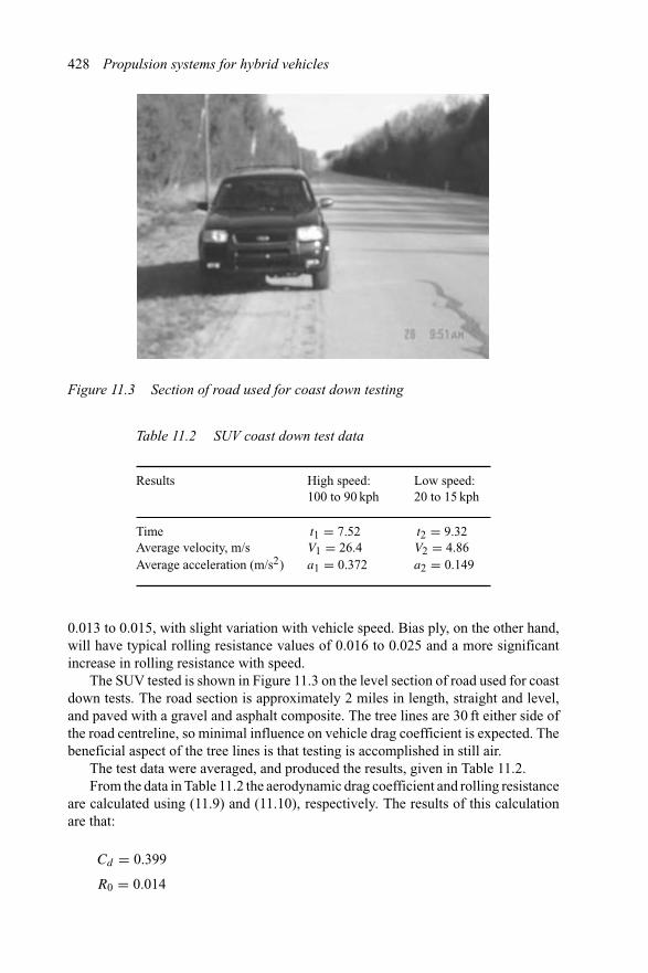
428 Propulsion systems for hybrid vehicles
Figure 11.3 Section of road used for coast down testing
Table 11.2 SUV coast down test data
Results High speed:100 to 90 kph
Low speed:20 to 15 kph
Time t1 = 7.52 t2 = 9.32Average velocity, m/s V1 = 26.4 V2 = 4.86Average acceleration (m/s2) a1 = 0.372 a2 = 0.149
0.013 to 0.015, with slight variation with vehicle speed. Bias ply, on the other hand,will have typical rolling resistance values of 0.016 to 0.025 and a more significantincrease in rolling resistance with speed.
The SUV tested is shown in Figure 11.3 on the level section of road used for coastdown tests. The road section is approximately 2 miles in length, straight and level,and paved with a gravel and asphalt composite. The tree lines are 30 ft either side ofthe road centreline, so minimal influence on vehicle drag coefficient is expected. Thebeneficial aspect of the tree lines is that testing is accomplished in still air.
The test data were averaged, and produced the results, given in Table 11.2.From the data in Table 11.2 the aerodynamic drag coefficient and rolling resistance
are calculated using (11.9) and (11.10), respectively. The results of this calculationare that:
Cd = 0.399
R0 = 0.014
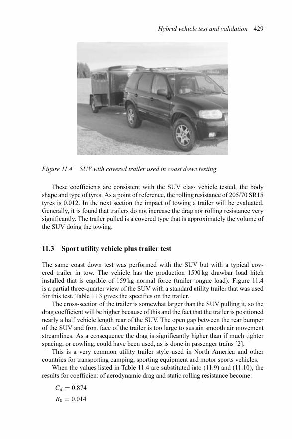
Hybrid vehicle test and validation 429
Figure 11.4 SUV with covered trailer used in coast down testing
These coefficients are consistent with the SUV class vehicle tested, the bodyshape and type of tyres. As a point of reference, the rolling resistance of 205/70 SR15tyres is 0.012. In the next section the impact of towing a trailer will be evaluated.Generally, it is found that trailers do not increase the drag nor rolling resistance verysignificantly. The trailer pulled is a covered type that is approximately the volume ofthe SUV doing the towing.
11.3 Sport utility vehicle plus trailer test
The same coast down test was performed with the SUV but with a typical cov-ered trailer in tow. The vehicle has the production 1590 kg drawbar load hitchinstalled that is capable of 159 kg normal force (trailer tongue load). Figure 11.4is a partial three-quarter view of the SUV with a standard utility trailer that was usedfor this test. Table 11.3 gives the specifics on the trailer.
The cross-section of the trailer is somewhat larger than the SUV pulling it, so thedrag coefficient will be higher because of this and the fact that the trailer is positionednearly a half vehicle length rear of the SUV. The open gap between the rear bumperof the SUV and front face of the trailer is too large to sustain smooth air movementstreamlines. As a consequence the drag is significantly higher than if much tighterspacing, or cowling, could have been used, as is done in passenger trains [2].
This is a very common utility trailer style used in North America and othercountries for transporting camping, sporting equipment and motor sports vehicles.
When the values listed in Table 11.4 are substituted into (11.9) and (11.10), theresults for coefficient of aerodynamic drag and static rolling resistance become:
Cd = 0.874
R0 = 0.014
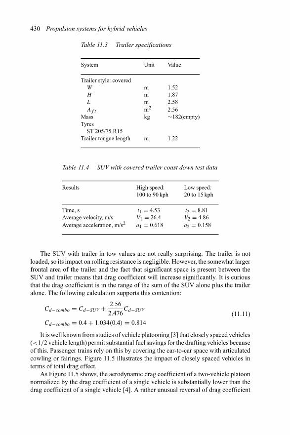
430 Propulsion systems for hybrid vehicles
Table 11.3 Trailer specifications
System Unit Value
Trailer style: coveredW m 1.52H m 1.87L m 2.58Af t m2 2.56
Mass kg ∼182(empty)Tyres
ST 205/75 R15Trailer tongue length m 1.22
Table 11.4 SUV with covered trailer coast down test data
Results High speed:100 to 90 kph
Low speed:20 to 15 kph
Time, s t1 = 4.53 t2 = 8.81Average velocity, m/s V1 = 26.4 V2 = 4.86Average acceleration, m/s2 a1 = 0.618 a2 = 0.158
The SUV with trailer in tow values are not really surprising. The trailer is notloaded, so its impact on rolling resistance is negligible. However, the somewhat largerfrontal area of the trailer and the fact that significant space is present between theSUV and trailer means that drag coefficient will increase significantly. It is curiousthat the drag coefficient is in the range of the sum of the SUV alone plus the traileralone. The following calculation supports this contention:
Cd−combo = Cd−SUV + 2.56
2.476Cd−SUV
Cd−combo = 0.4 + 1.034(0.4) = 0.814(11.11)
It is well known from studies of vehicle platooning [3] that closely spaced vehicles(<1/2 vehicle length) permit substantial fuel savings for the drafting vehicles becauseof this. Passenger trains rely on this by covering the car-to-car space with articulatedcowling or fairings. Figure 11.5 illustrates the impact of closely spaced vehicles interms of total drag effect.
As Figure 11.5 shows, the aerodynamic drag coefficient of a two-vehicle platoonnormalized by the drag coefficient of a single vehicle is substantially lower than thedrag coefficient of a single vehicle [4]. A rather unusual reversal of drag coefficient
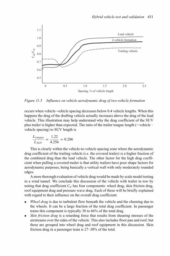
Hybrid vehicle test and validation 431
Cd2
/Cd1
Spacing, % of vehicle length
Lead vehicle
Trailing vehicle
2-vehicle formation
1.1
1.0
0.9
0.8
0.7
0.6
0.5
0 0.5 1.0 1.5 2.0 2.5
Figure 11.5 Influence on vehicle aerodynamic drag of two-vehicle formation
occurs when vehicle–vehicle spacing decreases below 0.4 vehicle lengths. When thishappens the drag of the drafting vehicle actually increases above the drag of the leadvehicle. This illustration may help understand why the drag coefficient of the SUVplus trailer is higher than expected. The ratio of the trailer tongue length (∼vehicle –vehicle spacing) to SUV length is
Ltongue
LSUV= 1.22
4.256= 0.286
This is clearly within the vehicle-to-vehicle spacing zone where the aerodynamicdrag coefficient of the trailing vehicle (i.e. the covered trailer) is a higher fraction ofthe combined drag than the lead vehicle. The other factor for the high drag coeffi-cient when pulling a covered trailer is that utility trailers have poor shape factors foraerodynamic purposes, being basically a vertical wall with only moderately roundededges.
A more thorough evaluation of vehicle drag would be made by scale model testingin a wind tunnel. We conclude this discussion of the vehicle with trailer in tow bynoting that drag coefficient Cd has four components: wheel drag, skin friction drag,roof equipment drag and pressure wave drag. Each of these will be briefly explainedwith regard to their influence on the overall drag coefficient:
• Wheel drag is due to turbulent flow beneath the vehicle and the churning due tothe wheels. It can be a large fraction of the total drag coefficient. In passengertrains this component is typically 38 to 66% of the total drag.
• Skin friction drag is a retarding force that results from shearing stresses of theairstreams over the sides of the vehicle. This also includes floor pan and roof, butthese are grouped into wheel drag and roof equipment in this discussion. Skinfriction drag in a passenger train is 27–30% of the total.
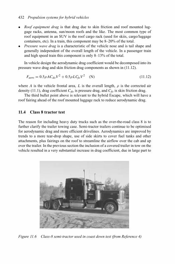
432 Propulsion systems for hybrid vehicles
• Roof equipment drag is that drag due to skin friction and roof mounted lug-gage racks, antenna, sun/moon roofs and the like. The most common type ofroof equipment in an SUV is the roof cargo rack (used for skiis, cargo/luggagecontainers, etc). In a train, this component may be 8–20% of the total.
• Pressure wave drag is a characteristic of the vehicle nose and is tail shape andgenerally independent of the overall length of the vehicle. In a passenger trainand high speed train this component is only 8–13% of the total.
In vehicle design the aerodynamic drag coefficient would be decomposed into itspressure wave drag and skin friction drag components as shown in (11.12).
Faero = 0.5ρACdoV2 + 0.5ρLCfoV
2 (N) (11.12)
where A is the vehicle frontal area, L is the overall length, ρ is the corrected airdensity (11.1), drag coefficient Cdo is pressure drag, and Cfo is skin friction drag.
The third bullet point above is relevant to the hybrid Escape, which will have aroof fairing ahead of the roof mounted luggage rack to reduce aerodynamic drag.
11.4 Class 8 tractor test
The reason for including heavy duty trucks such as the over-the-road class 8 is tofurther clarify the trailer towing case. Semi-tractor trailers continue to be optimisedfor aerodynamic drag and more efficient drivelines. Aerodynamics are improved bytrends to a more tear-drop shape, use of side skirts to cover fuel tanks and otherattachments, plus fairings on the roof to streamline the airflow over the cab and upover the trailer. In the previous section the inclusion of a covered trailer in tow on thevehicle resulted in a very substantial increase in drag coefficient, due in large part to
Figure 11.6 Class-8 semi-tractor used in coast down test (from Reference 4)
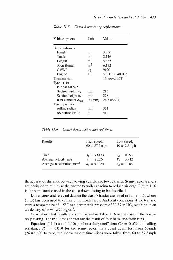
Hybrid vehicle test and validation 433
Table 11.5 Class-8 tractor specifications
Vehicle system Unit Value
Body: cab-overHeight m 3.200Track m 2.146Length m 5.385Area-frontal m2 6.182GVWR kg 9020Engine L V8, CIDI 400 Hp
Transmission 18 speed, MTTyres: (10)
P285/80-R24.5Section width ws mm 285Section height hs mm 228Rim diameter drim in (mm) 24.5 (622.3)
Tyre dynamics:rolling radius mm 531revolutions/mile # 480
Table 11.6 Coast down test measured times
Results High speed:60 to 57.5 mph
Low speed:10 to 7.5 mph
Time t1 = 3.613 s t2 = 10.56 sAverage velocity, m/s V1 = 26.26 V2 = 3.912Average acceleration, m/s2 a1 = 0.3086 a2 = 0.106
the separation distance between towing vehicle and towed trailer. Semi-tractor trailersare designed to minimise the tractor to trailer spacing to reduce air drag. Figure 11.6is the semi-tractor used in the coast down testing to be described.
Dimensions and relevant data on the class-8 tractor are listed in Table 11.5, where(11.3) has been used to estimate the frontal area. Ambient conditions at the test sitewere a temperature of −5◦C and barometric pressure of 30.37 in HG, resulting in anair density of ρ = 1.331 kg/m3.
Coast down test results are summarised in Table 11.6 in the case of the tractoronly testing. The trial times shown are the result of four back-and-forth runs.
Equations (11.9) and (11.10) predict a drag coefficient Cd = 0.659 and rollingresistance R0 = 0.010 for the semi-tractor. In a coast down test from 60 mph(26.82 m/s) to zero, the measurement time slices were taken from 60 to 57.5 mph
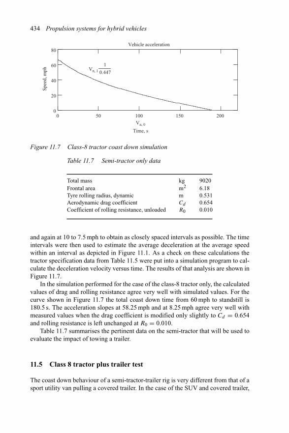
434 Propulsion systems for hybrid vehicles
1
0.447
0
20
40
60
80Vehicle acceleration
Time, s
Spee
d, m
ph Vn, 1
Vn, 0
0 50 100 150 200
Figure 11.7 Class-8 tractor coast down simulation
Table 11.7 Semi-tractor only data
Total mass kg 9020Frontal area m2 6.18Tyre rolling radius, dynamic m 0.531Aerodynamic drag coefficient Cd 0.654Coefficient of rolling resistance, unloaded R0 0.010
and again at 10 to 7.5 mph to obtain as closely spaced intervals as possible. The timeintervals were then used to estimate the average deceleration at the average speedwithin an interval as depicted in Figure 11.1. As a check on these calculations thetractor specification data from Table 11.5 were put into a simulation program to cal-culate the deceleration velocity versus time. The results of that analysis are shown inFigure 11.7.
In the simulation performed for the case of the class-8 tractor only, the calculatedvalues of drag and rolling resistance agree very well with simulated values. For thecurve shown in Figure 11.7 the total coast down time from 60 mph to standstill is180.5 s. The acceleration slopes at 58.25 mph and at 8.25 mph agree very well withmeasured values when the drag coefficient is modified only slightly to Cd = 0.654and rolling resistance is left unchanged at R0 = 0.010.
Table 11.7 summarises the pertinent data on the semi-tractor that will be used toevaluate the impact of towing a trailer.
11.5 Class 8 tractor plus trailer test
The coast down behaviour of a semi-tractor-trailer rig is very different from that of asport utility van pulling a covered trailer. In the case of the SUV and covered trailer,
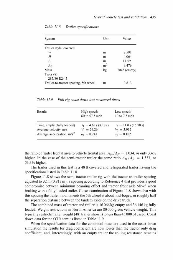
Hybrid vehicle test and validation 435
Table 11.8 Trailer specifications
System Unit Value
Trailer style: coveredW m 2.591H m 4.064L m 14.59Aft m2 9.476
Mass kg 7045 (empty)Tyres (8)
285/80 R24.5Trailer-to-tractor spacing, 5th wheel m 0.813
Table 11.9 Full rig coast down test measured times
Results High speed:60 to 57.5 mph
Low speed:10 to 7.5 mph
Time, empty (fully loaded) t1 = 4.63 s (8.18 s) t2 = 11.0 s (15.78 s)Average velocity, m/s V1 = 26.26 V2 = 3.912Average acceleration, m/s2 a1 = 0.241 a2 = 0.102
the ratio of trailer frontal area to vehicle frontal area, Afv/Aft = 1.034, or only 3.4%higher. In the case of the semi-tractor trailer the same ratio Afv/Aft = 1.533, or53.3% higher.
The trailer used in this test is a 48 ft covered and refrigerated trailer having thespecifications listed in Table 11.8.
Figure 11.8 shows the semi-tractor-trailer rig with the tractor-to-trailer spacingadjusted to 32 in (0.813 m), a spacing according to Reference 4 that provides a goodcompromise between minimum beaming effect and tractor front axle ‘dive’ whenbraking with a fully loaded trailer. Close examination of Figure 11.8 shows that withthis spacing the trailer mount meets the 5th wheel at about mid-bogey, or roughly halfthe separation distance between the tandem axles on the drive truck.
The combined mass of tractor and trailer is 16 066 kg empty and 36 146 kg fullyloaded. Weight restrictions in North America are 80 000 gross vehicle weight. Thistypically restricts trailer weight (48’ trailer shown) to less than 45 000 of cargo. Coastdown data for the OTR semi is listed in Table 11.9.
When the specification data for the combined mass are used in the coast downsimulation the results for drag coefficient are now lower than the tractor only dragcoefficient, and, interestingly, with an empty trailer the rolling resistance remains
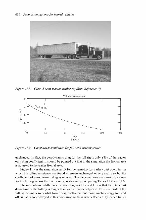
436 Propulsion systems for hybrid vehicles
Figure 11.8 Class-8 semi-tractor-trailer rig (from Reference 4)
Vn, 1
1
0.447
0
20
40
60
80Vehicle acceleration
Spee
d, m
ph
0 50 150 200 250
Time, s
100Vn, 0
Figure 11.9 Coast down simulation for full semi-tractor-trailer
unchanged. In fact, the aerodynamic drag for the full rig is only 88% of the tractoronly drag coefficient. It should be pointed out that in the simulation the frontal areais adjusted to the trailer frontal area.
Figure 11.9 is the simulation result for the semi-tractor-trailer coast down test inwhich the rolling resistance was found to remain unchanged, or very nearly so, but thecoefficient of aerodynamic drag is reduced. The decelerations are curiously slowerfor the full rig versus the tractor only, as shown by comparing Tables 11.9 and 11.6.
The most obvious difference between Figures 11.9 and 11.7 is that the total coastdown time of the full rig is longer than for the tractor only case. This is a result of thefull rig having a somewhat lower drag coefficient but more kinetic energy to bleedoff. What is not conveyed in this discussion so far is what effect a fully loaded trailer
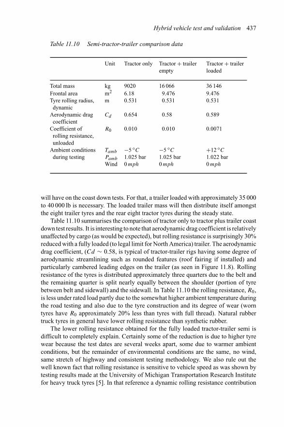
Hybrid vehicle test and validation 437
Table 11.10 Semi-tractor-trailer comparison data
Unit Tractor only Tractor + trailerempty
Tractor + trailerloaded
Total mass kg 9020 16 066 36 146Frontal area m2 6.18 9.476 9.476Tyre rolling radius,
dynamicm 0.531 0.531 0.531
Aerodynamic dragcoefficient
Cd 0.654 0.58 0.589
Coefficient ofrolling resistance,unloaded
R0 0.010 0.010 0.0071
Ambient conditions Tamb −5 ◦C −5 ◦C +12 ◦Cduring testing Pamb 1.025 bar 1.025 bar 1.022 bar
Wind 0 mph 0 mph 0 mph
will have on the coast down tests. For that, a trailer loaded with approximately 35 000to 40 000 lb is necessary. The loaded trailer mass will then distribute itself amongstthe eight trailer tyres and the rear eight tractor tyres during the steady state.
Table 11.10 summarises the comparison of tractor only to tractor plus trailer coastdown test results. It is interesting to note that aerodynamic drag coefficient is relativelyunaffected by cargo (as would be expected), but rolling resistance is surprisingly 30%reduced with a fully loaded (to legal limit for North America) trailer. The aerodynamicdrag coefficient, (Cd ∼ 0.58, is typical of tractor-trailer rigs having some degree ofaerodynamic streamlining such as rounded features (roof fairing if installed) andparticularly cambered leading edges on the trailer (as seen in Figure 11.8). Rollingresistance of the tyres is distributed approximately three quarters due to the belt andthe remaining quarter is split nearly equally between the shoulder (portion of tyrebetween belt and sidewall) and the sidewall. In Table 11.10 the rolling resistance, R0,is less under rated load partly due to the somewhat higher ambient temperature duringthe road testing and also due to the tyre construction and its degree of wear (worntyres have R0 approximately 20% less than tyres with full thread). Natural rubbertruck tyres in general have lower rolling resistance than synthetic rubber.
The lower rolling resistance obtained for the fully loaded tractor-trailer semi isdifficult to completely explain. Certainly some of the reduction is due to higher tyrewear because the test dates are several weeks apart, some due to warmer ambientconditions, but the remainder of environmental conditions are the same, no wind,same stretch of highway and consistent testing methodology. We also rule out thewell known fact that rolling resistance is sensitive to vehicle speed as was shown bytesting results made at the University of Michigan Transportation Research Institutefor heavy truck tyres [5]. In that reference a dynamic rolling resistance contribution
438 Propulsion systems for hybrid vehicles
is characterised as follows:
Ftyre = chwy(R0 + R1V )
Fbias−ply = chwy(R0b + R1bV ) (N) (11.13)
Fradial = chwy(R0r + R1rV )
where, chwy = {1.0 smooth concrete, 1.2 worn concrete, 1.5 hot asphalt} and thestatic and dynamic rolling resistance coefficients are: R0b = 0.004, R0r =0.007, R1b = 0.004 and R1r = 0.000046. From this characterisation we would notexpect to shift in coast down test because the testing procedure is performed on thesame road and at the same speeds. The conclusion here is that tyre wear apparentlyhas caused the shift in static rolling resistance to a somewhat lower value. The effectis compounded by warmer ambient temperatures.
Regulations pertaining to OTR trucking are now changing with some states requir-ing non-idling at rest stops and elsewhere. Infrastructure changes include installationof shore power at rest stops and terminals. Some installations of shore power require-ments are already in place and non-idling may soon be regulated. Military line haul andcommercial OTR trucks are also being targeted for dedicated auxiliary power units forproviding power for all accessories during engine-off periods. Various technologiesfrom fuel cells to free piston engines are being evaluated as electric power cells ratedat 5 kW for powering cabin climate control and accessories during overnight parking.In Reference 5, Algrain et al. describe a programme to electrify a class-8 tractorthrough inclusion of a crankshaft mounted starter-alternator that supports an electricdriven water pump, oil pump, air compressor for brakes, and modular air condition-ing module for cabin climate control. In addition, the electrification effort includesan on board APU rated 8 kW at 340 Vdc. The APU is driven by a small, 2 cylinder,0.5 L CIDI engine rated 14 Hp at 3600 rpm. A shore power module supplies dc busvoltage from a 120V/240V, 60 Hz, input. The truck 12 V battery(s) are maintainedduring non-idling load periods through a dc/dc converter having input power deliv-ered from either the shore power connection or from the APU. The starter-alternatorfor a large displacement (15 L CIDI) engine is a package, φ360 × L125 mm, that israted 1200 Nm cranking torque and generates 15 kW at 600 rpm idle and 28 kW at1200 rpm. The fuel economy gained through use of the non-idling electrification isprojected at 7.5% (plus an additional 4.5% from the APU) and a potential for 1%additional through electrified accessories. Considering that the North American pop-ulation of class-8 rigs is 458 000, it can be seen that the fuel savings amount to some550 M gal/yr, which equates to $825 M/yr given diesel fuel at $1.50/US gal. Fuelsavings alone translate to an annual savings per semi of $1800.
Trailer towing for hybrid passenger vehicles remains a challenge, as demonstratedin this chapter. Attaching the added load of a covered trailer, loaded or not,significantly changes the aerodynamics to the point that fuel economy will be loweredand vehicle power plant, if the engine is downsized too much, may be insufficient tonegotiate long grades at traffic speeds.
Hybrid vehicle test and validation 439
11.6 References
1 WONG, J. Y.: ‘Theory of ground vehicles’ (John Wiley & Sons, 1993, 2nd edn.),Fig. 1.3
2 CAI, Y. and CHEN, S. S.: ‘A review of dynamic characteristics of magneticallylevitated vehicle systems’. Argonne National Laboratory, Report # ANL-95/38for US DOE under contract W-31-109-Eng-38, November 1995
3 ZABAT, M. A., STABILE, N. S. and BROWAND, F. K.: ‘Estimates of fuel savingsfrom platooning’. Proceedings of the 1995 Annual Meeting of ITS America,Intelligent Transportation Systems, Vol. 2, 15–17 March 1995, Washington, DC
4 Miller, R. M.: Victoria Creek Conveyance, Cedar, MI. Personal discussions,April 2003
5 GILLESPIE, T. D. ‘Fundamentals of vehicle dynamics’, SAE ISBN 1-56091-199-9, Sixth Printing 1992
6 ALGRAIN, M. C., LANE, W. H. and ORR, D. C.: ‘A case study in the elec-trification of class 8 trucks,’ IEEE International Electric Machines and DrivesConference, IEMDC2003, Monona Terrace Convention Center, Madison, WI.June 1–4, 2003.

Index
Aachen University of Technology 412–13ABS (anti-lock braking system) 99, 100,
102, 173, 180absorbers 20ac drives 9–10, 159
ISA type 91power electronics for 257–90
AC Propulsion 45–6acceleration 31–2, 42, 71, 75, 77, 96, 98,
138–9brisk 98burden on tractive effort necessary for
139dramatic 82dynamics of 104–5full/wide open throttle 73, 98high capability 205hybrid vehicle must deliver 106low 68maximum time 374MT 110–11quick 16smooth 98straight and level 343test 425, 434upshift of automatic transmission 170velocities versus time 78
acceptance rate 361, 372, 405accumulators 83, 180, 402acetonitrile 373, 374, 392Ackerman angles 23actuators 180, 183
hydraulic 402ACU (actuator control unit) 180Advanced Automotive Electrical and
Electronic Systems and Components179
Advanced Battery Readiness WorkingGroup 150
aerodynamic drag 96, 343, 423–5, 428,429–31, 436
drag semi-tractor trailers optimised for432
aerospace 207, 220, 283AFMA (Alternative Motor Fuels Act, US
1988) 399AFPM (axial flux permanent magnet)
machines 125, 223air conditioning 98, 180–1, 183, 201, 215,
437electric drive 9, 350
air consumption see BSAC; ISACair damming 182air density 424, 433Airbus 324, 82airgaps 209, 210, 219, 233, 234
axial 125shear force 254sinusoidal 293very tight tolerance 255
Aisin-Warner Navimatic transmission 107alcohol 399Algrain, M. C. 437alloys 229, 366, 370Alnico 241alternators 25, 60, 63, 64
current ripple 307Lundell 25–7, 217, 336see also ISA; starter-alternators
aluminium 229, 292, 321American Superconductor Corporation 192Amperean force 334amplitude 260–2, 266, 271angstroms 374

442 Index
ANL (Argonne National Laboratory) 67,344, 346
anodes 360, 361, 369antimony 365applications 169APTz insulation systems 328APU (auxiliary power unit) 437APV (annual production volume) 185architectures 53–90, 337, 379, 387
brushless dc motor 198communications 170, 183dual bus 178fuel cell 215hierarchical 171ISA 27multi-converter 116open 168, 171power split 113, 215, 302–3wiring 160
area networks see CANs; LANs; WANsarmature current 292, 304aromatic polyamide 401ASCII (American Standard Code for
Information Interchange) 169Asia-Pacific 103, 254, 292, 344
see also Japanasynchronous machines 225–42AT gears 77, 78ATDS cycle 16, 18, 145Atkins, M. J. 344Atkinson cycle 4, 7, 106atmospheric conditions 424ATRs (autothermal reformers) 154automatic transmission 26, 74, 75, 96, 98,
106, 107, 115, 427designed around planetary gear sets for
power on demand shifting 111essential ingredients of 110Lepelletier type 108, 114–15Ravigneaux type 114Simpson type 113–15upshift during acceleration 170Wilson type 108, 114, 115–16, 117
automotive harsh environments 149AutoPC 178AWG (American wire gauge) 161–2axial flux 125, 223
Babcock, P. S. 283balanced offset 286Ballard Power Systems 10, 53, 151–2bandgap materials 282bandwidth 276, 288, 304
barium 216Barkhausen, Heinrich 320battery systems 359–73
warranties 66–7, 178–9see also charge; discharge; energy
storage; lead-acid; nickel; SLI; TMFbeaming 21Bell (F. W.) 288bimetallic effects 286BJT (bipolar junction transistor) stored
charge 332Blaschke, F. 306Blasko, V. 264block mode 120Bluebird EV formula 3000 vehicle 81Bluetooth 178BMEP (brake mean effective pressure) 34,
38–42BMM (battery management module) 166BMW 151, 152, 174Bolder Technologies Corp. 147Boltzmann constant 330BOP (balance of the plant) 409Bose, B. K. 288boundary conditions 228BP (brake power) 40BPF (bandpass filtering) 307braking 11, 86, 138, 139, 179–80, 376
dynamic effects of 22energy recuperation and 15, 99–102performance 23see also ABS; BP; BSAC; BSFC; BMEP;
EHB; EMB; RBSbrand image 185brushless machines 191–214, 258, 308, 399BSAC (brake specific air consumption)
40–2BSFC (brake specific fuel consumption)
33–5, 398sensitivity to BMEP 40–2
BST (Bosch-Siemens) protocol 178buck-boost converters 390, 391bulk storage 402, 403Buller, S. 412, 414buried magnets 214, 215–18, 223bus synchronisation 174busbars 164–6, 276, 280butane 399bypass cavities 223
cabin climate control 9, 60, 139, 180–1,186, 349, 437
cable requirements 160–3
Index 443
CAFÉ 185calcium 365CANs (controller area networks) 79, 167,
170, 175, 176, 177see also TTCANs
capacitor systems 379–87see also double layer capacitors; super-
capacitors; ultra-capacitorsCapstone microturbine standby power unit
45CARB (California Air Resources Board) 45carbon 370, 373–5, 377, 408, 410carbon dioxide 152, 154, 345, 376, 399Carter coefficient 209, 210cathodes 192, 360, 361, 369, 370, 408
steering diodes 390Cauer I network 415, 417–18cell equalisation
dissipative 388–9non-dissipative 389–92
ceramic magnets 163, 216, 218, 219CFC (chlorofluorocarbon) 58CFD (computational fluid dynamics) 183character code conversion 169characterisation 333, 343–57, 403charge 390
constant current 388separation distances 373–5stored 332sustaining 49–50test 393–4, 395see also SOC
chassis 76, 79, 82, 116, 174, 335, 350by-wire functions 175–6real time control in 177
Chung Kong Infrastructure HoldingsLimited 152
CIDI (compression-ignition direct-injection)engines 14, 34, 54, 55, 343, 345,437
city buses 138–47, 150CIVs (corona inception voltages) 328Clayton twin roller dynamometers 355climate control systems 367
see also cabin climate controlclutches 59, 60, 74, 87, 110
automatic 85see also LUCs; OWCs
CNG (compressed natural gas) 343, 399coast down procedure 343, 423, 424–7, 429,
432–3, 434, 437coaxial cable 169coercive force 208, 219
combined cycle 351–2commercialisation 409communications 167–79, 258commutators 193, 194, 297comparisons 250–1, 274–8
ramp 134compressed gas storage 10, 60, 407compressors 181condition factors 405conductance 403–4conduction 138, 199, 201, 330–1
diode 333, 390conductivity 135, 150, 321, 323
high bulk 197thermal 280
conductors 125, 192, 193–4busbar 164GMD of 211temperature differences between 330
configurations 56–61combined: pre-transmission 67–78parallel: post-transmission 78–81;
pre-transmission 62–7conservation 43, 44constant current 388, 393constant offset 308constant power 119–20, 121, 122, 256
see also CPSRconsumer driving habits 19containment structures 82, 83, 84Continental Group 8, 58, 191, 423continuous rating 124cooling 58, 124, 160, 183–4, 278, 279
stator liquid 254torque and 205
copper losses 220, 319and skin effects 326–30
copper wire 162core losses 320, 321–6cornering 23corona discharge 328corrosion 154costs 185–8, 280, 281, 409–10
replacement components 183coupling 292, 330CPSR (constant power speed range) 62, 78,
120–2, 205, 212, 215, 217, 218, 222,232, 241, 253
wide 80–1, 225crankshaft striction 121creep 77, 107–8critical speed flexing 126
444 Index
CRPWM (current regulatedpulse-width-modulation) 260, 309,313
CRT (cathode ray tube) 192cruise conditions 95–8, 116, 138, 139, 145
normal 72crush zones 183cryogenic processes 397, 399CTEs (coefficients of thermal expansion)
283, 286Cunningham, J. 348current collectors 408current sensors 287–8CV (conventional vehicle) characteristics 8,
12–14, 66, 96, 105CVT (continuously variable transmission)
2–3, 4, 8, 53, 60, 67, 74–5, 87, 108larger, torque rating and efficiency 109flywheel system based on 86
cyanide gas 374
Dahlander connections 230, 235DaimlerChrysler 115
Concorde 11, 19ESX3 11, 13F-series sports cars 54, 55Jeep Commander 53Natrium 53NECAR 53, 153V10 Viper engine 91
Dana 191data
link 169packets 169, 170transmission speed 171
dc 126, 165–6, 265brushed 194, 197, 292brushless 195–9, 258, 308bus capacitors 132–4link capacitors 130, 131, 133, 288output energy 155
DCX 174decay 362, 363deceleration 18, 69, 73, 82–3, 425, 434, 436
flywheel 87Degner, M. 64delay error 287Dell Dimension 4550 Hyper-Threading
Technology PC 168, 170Delphi 178, 191demagnetisation effects 215, 216, 219Department of Energy (US) 65, 81, 150,
154–5, 406
see also ANL; National RenewableEnergy Laboratory
dependability 283Dewar tanks/canisters 397, 399DFSO (deceleration fuel shut off) 14diagnostics 291diamond 282dielectric constant 133, 282, 375dielectrics 373, 374, 375diesel 151, 343, 345, 347, 376, 437
naturally aspirated engine 57diffusion 363, 405, 406
dopant 132DIS (discrete immittance spectroscopy)
403–4, 415disc brakes 22discharge 159, 363, 365, 369, 371, 372, 376,
377, 404capacity 19constant current 393depth of 147, 372, 373dynamics of 405efficiency 378, 390, 394, 395, 396matched impedance 394potential 143, 370self 364, 366, 367, 370, 396, 407voltage curve 157
displacement 13, 39, 75, 106, 163, 181, 194,437
Divan, D. M. 264DMIC (dual mode inverter control) 122,
211–14Doherty, Tom 344dopant diffusion 127, 129double layer capacitors 373–5, 392–6, 406,
410downsizing 57, 66, 105–6, 187, 438drag 434
pressure wave 432roof equipment 432skin friction 431wheel 431see also aerodynamic drag
dragster class 93drive-by-wire technologies 174, 178drive cycles 15, 18, 144, 145
implications 102–5see also NEDC
drive systemscontrol 291–317efficiency 319–39sizing 109–89
Index 445
DSP (digital signal processor) controllers258, 278
DTC (direct torque control) 312–15DTCs (diagnostic test codes) 178–9dual mode 55, 56, 66–7, 406DuPont 408durability 79, 119, 156, 215, 279, 307, 376dynamometers 355
EBCDIC (extended binary-coded decimalinterchange code) 169
eccentricity 124ECM (engine controller module) 160eddy currents 197, 226, 230, 320, 324
anomalous 321EDLCs (electrochemical double layer
capacitors) 373, 374, 375, 392–6EDS (electrical distribution system) 162EF (electric fraction) 13–15, 116
engine downsizing 105–6range and performance 106
efficiency 109, 350, 400, 412charge 390, 395discharge 378, 390, 394–6drive system 319–39thermal 14, 398volumetric 39WTW 345
efficiency mapping 211, 336–8efficiency optimisation 308–12EGR (exhaust gas recirculation) 38EHB (electro-hydraulic brake) system 103,
160, 180EIS (electrochemical spectroscopy) 407,
410, 412, 413electric drives 61, 335, 337, 376, 401
ac 159battery only 356matching 109–15technologies 191–252very high voltage 84
electric fields 374–5electric loading 122, 123electric power 13, 69, 72, 107, 253, 437Electric Vehicle Symposium (2002) 2electrical overlay harness 159–167electrical protection 167electrification effort 437electrochemical cells/batteries 396, 401electrolysis 366, 397electrolytes 149, 150, 360, 362, 363, 370,
392, 412, 413aqueous 374, 375
conductive 373depleted of ions 375immobilisation of 366organic 374, 375, 387, 410outgassing of 374polymer 408
electronic pole change 232–4electronic throttle control 170, 173electrons 149, 192, 361EMB (electromechanical brake) 102EMI (electromagnetic interference) 258,
276, 304emissions 10, 33, 53, 152, 177, 178, 397
minimal 345testing 355thermionic 192zero 87see also ZEVs
encryption 169energy recovery 106energy storage 10, 57, 59, 60, 65, 66, 84, 87,
128, 218, 308mobile systems 309modest 61standalone transient 88superconducting magnetic 335technologies 139–59, 359–420
engine power 68–9, 96engine speed 71, 77, 116, 307enthalpy 363entropy 363EPA (US Environment Protection Agency)
15, 16, 103, 145city cycle 350–1, 353
EPAS (electric power assist steering) 27,160
epicyclic gears 68, 70, 76, 78, 110, 111double planet 114, 115
EPRI (Electric Power Research Institute)45–6, 186–7
error detection 177ESMA capacitors 378–9ESP (electronic stability program) 55, 100,
102ESR (equivalent series resistance) 131–4,
334, 393–5, 417ethanol 343, 345, 347excitation 231, 234, 244, 253, 255, 293,
305, 322constant 292permanent magnetic 297two phase 199
exhaust valves 37
446 Index
failure detection 283see also FIT; MTBF
FAKRA 63Faraday 209, 361, 376, 378fatigue 283fault management 291FCEVs (fuel cell electric vehicles) 9, 44, 53,
81, 153, 155, 344FCHVs (hybridized fuel cell vehicles) 345,
348–50FCT (full charge testing) 352FD (final drive) 74Federal Aviation Administration 283Federal Communications Commission 178Federal Test Procedure 103, 350feedback control 307, 314ferrite magnets 214–15, 216, 220, 225,
241ferromagnetic material 321FEUF (fuel economy utility factors) 352Fick’s law 363FIT (failure in time) 283, 284–5fixed ratio gearbox 70Flexray 167, 174–7, 178flux density 233, 234, 326flux linkage 308flux squeeze 218–23flyback converters 390, 391flywheel systems 84–7, 159, 291, 399–401FOC (field oriented control) 292–304, 312Ford Motor Co. 27, 174
Endura DI 34Escape SUV 6–7, 191, 424, 427–32F150 19Focus 34, 42, 95, 97, 98, 99L V10 151Model U concept 60P2000 LSR vehicle 18Prodigy 11, 13Taurus 11, 19
forward converters 390, 391Foster II equivalent circuit model 415,
416–18Fourier transform/expansion 166, 331friction 39, 92, 93, 109, 431
non-conventional contributor to 319wheel slip and 30–2
FTP (file transfer protocol) 169, 170FUD (Federal Urban Drive) cycle 17, 18,
49, 102–3, 349fuel cells 61, 79, 150–6, 215, 347, 407–10
cost breakdown 185see also FCEVs
fuel consumption 11, 14, 44, 48, 348, 355brake specific 33–5, 398low 59mapping, ICEs 43–4percentage of all energy usage 345specific 33–5, 39, 40
fuel economy 6, 11, 15, 23, 27, 44, 195,319, 343, 438
average speed and impact on 103–5combined mode 352predicting 33–6, 145, 352testing 355utility factors 352see also HFEDS; HWFET
fuel injector failures 398fuel savings 430, 437fumed silica 366fuses 334fuzzy logic 310, 311FWDs (four wheel drives) 87–91
Gage, Tom 43–4gain error 286–7gasoline 151, 152, 154, 343, 345, 347, 348,
352, 353performance 398price of 396
gassing 405gear step selection 42, 112
see also epicyclic gears; planetary gearset
Gelb, G. H. 67General Electric company 129, 281, 319generating mode 77Geneva Motor Show (2003) 81Germany 63
see also BMW; Siemens; Volkswagengetters 365GHGs (greenhouse gases) 344Giacoletto, L. J. 329Gibbs free energy 361GM (General Motors) Corporation 45, 151,
174Autonomy 78–9, 81Cadillac V16 91, 93Covair 21Durango 19EV1 23Explorer 19Hywire concept vehicle 167Precept 11, 13Sierra 7Silverado 7, 19, 191
Index 447
Tahoe 9, 19Yukon 9
GM Chevrolet 11, 19Equinox 8Impala 11Lumina 19
GM Chevy Malibu 8grade and cruise targets 95–8Graetz bridge 217Graham, R. 352graphite 370gravimetric energy 364, 365, 366, 375, 399GREET (Greenhouse Gases, Regulated
Emissions, and Energy Use inTransportation) model 344
grid connected hybrids 44–50GTOs (gate-turn-off ) thyristors 58, 213,
278, 333, 334
Ha, I.-J. 305Halbach array techniques 195Hall effect 288, 305–6Hall transducers 199Hammett, R. C. 283handling 104harmonics 261, 273, 275–6, 322HECU (hydraulic electronic control unit)
180helium 399Helmholtz, H. L. F. von 373, 417hermetic sealing 184heterodyning techniques 306, 307, 308HFEDS (highway fuel economy drive
schedule) 48–9high pressure gas storage 399high voltage disconnect 166–7Highway cycle (US) 349, 351, 352hill holding 77Hino company 59Hitachi corporation 336HMI (human-machine interface) 169, 173,
184–5Holtz, J. 276Honda Motor Co. 4, 152, 219
Accord 19Civic 6–7, 105, 191FCX 151, 191, 409Insight 12, 13, 191S2000 Roadster 6
Honeywell 288hot spots 283HSD (Hybrid Synergy Drive) 2HTS (high temperature superconductor) 192
hub motors 81Hunt, L. J. 230HWFET (highway fuel economy test) 50,
103hydraulic post-transmission hybrid 81–4hydraulic pressure 77, 83, 402hydraulic storage 84, 402hydrocarbons 397, 398, 399
non-methane 45hydrogen 152, 345, 359, 408
liquid 151, 153–4, 347, 348, 396–8hydrogen storage 154, 156, 396–9
compressed gas 10, 60hysteresis 312, 319–20, 321, 322
current regulators 276–8
IATA (International Air TransportAssociation) 150
ICAO (International Civil AviationOrganization) 150
ICEs (internal-combustion engines) 1, 2, 13,42–4, 61, 71, 77, 85, 87, 88, 97, 347
clean diesel 151CNG fuelled city bus, generator added to
138combination of M/G and 29constant speed operation 78electrical capacity needed to crank 15–16fuel cell hybrid competitiveness with 151fuel consumption mapping 42–4hydrogen fuelled 151, 152, 397, 398limitations of technology 345matching electric drive and 109–18modified for CNG 399natural gas fired 45naturally aspirated 7
IDB (integrated data bus) 178idle stop 76, 77, 107, 355
functionality 14idle times 15, 355
stop-start 60IEEE (Institute of Electrical and Electronic
Engineers) 178IGBT (insulated gate bipolar transistor)
device technology 128, 201, 257–8,276, 282, 330, 331, 399
IHAT (integrated hybrid assist transmission)75–8
IMA (integrated motor assist) 4–6, 105IMEP (indicated mean effective pressure)
39, 40impedance 394, 406, 412, 414
448 Index
IMST (insulated metal substrate technology)257
indicated power 40inductance 210, 216, 217–18, 242–3, 327,
390leakage 256, 270, 306, 309phase 211self 292stray lead 164
induction machines 191, 203–6, 220, 232,256, 292, 308
air 182cage rotor 293classical 226–9current feeding 297FOC and 296line-start 214remanence 197self-cascaded 230, 231sensorless control 305squirrel cage 241stator current 256, 298torque 242, 253, 255traction motor 58
inertias 355driveline 26, 27, 221rotational 19, 25rotor 195, 206, 256
infotainment 107, 172instrument panels 184intake valves 37interconnections 160, 163, 281International Rectifier
Plug-N-Drive module 201, 257SuperTab devices 280
International Space Station 399INTETS (integrated electric traction system)
336inverter busbars 164–6inverters 58, 130–5, 215, 216–17
corona-free 329current controlled 253dual 136field orientation control 254losses 253, 330–4power 276power electronic 143, 164, 201, 232, 261resonant pole 259, 264, 266traction 373very high power 278voltage source 264–6see also DMIC
ions 410see also lithium ion technology
IP (internet protocol) 169IPACS (integrated power and attitude
control system) 400IPEM (intelligent power electronic module)
257–8, 281IPMs (interior permanent magnets) 124,
191, 203, 205, 214–25, 253, 254,255, 308
iron 319, 321ISA (integrated starter alternator) systems
27, 62, 63, 91, 122, 158IM 134Mannesman-Sachs 191
ISA/ISG hybrid 34, 62, 63ISAC (indicated specific air consumption)
39ISAD Systems 58, 191ISFC (indicated specific fuel consumption)
39, 41ISG (integrated starter generator) 7, 8, 65,
77, 98, 159–60, 191, 208, 304cost of 185, 186high-voltage 64idle stop technologies 355see also ISA/ISG
ISO (International Standards Organization)63, 170, 172, 177
OSI (Open Systems Interconnection)167–8, 169, 173, 174
isothermal process 359IVD (interactive vehicle dynamics) 100, 102IVT (infinitely variable transmission) 75
JaguarXJ-S 91, 92XK8 167
Japan 103, 22310–15 mode 15, 355see also Hitachi; Honda; Nissan; Toyota;
YamahaJATCO 75Jeffries, P. 85Johnson Controls Inc. 147, 179, 405Jones, Lawrence 396Joule heating 319, 321, 389
Kastha, D. 288Kaura, V. 264Keser, H. O. 285–6Kevlar 401Khalil, H. K. 305
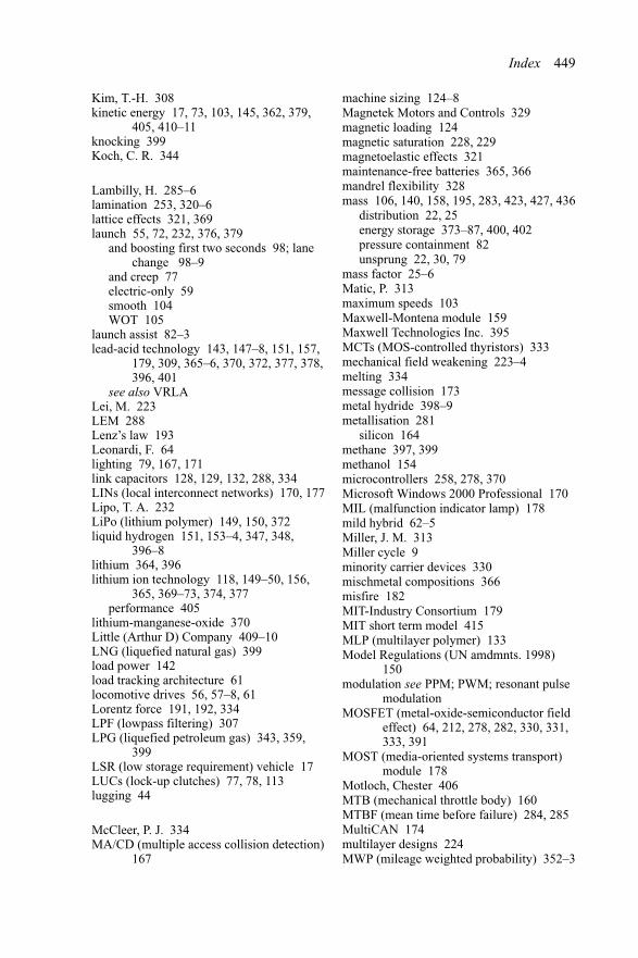
Index 449
Kim, T.-H. 308kinetic energy 17, 73, 103, 145, 362, 379,
405, 410–11knocking 399Koch, C. R. 344
Lambilly, H. 285–6lamination 253, 320–6lattice effects 321, 369launch 55, 72, 232, 376, 379
and boosting first two seconds 98; lanechange 98–9
and creep 77electric-only 59smooth 104WOT 105
launch assist 82–3lead-acid technology 143, 147–8, 151, 157,
179, 309, 365–6, 370, 372, 377, 378,396, 401
see also VRLALei, M. 223LEM 288Lenz’s law 193Leonardi, F. 64lighting 79, 167, 171link capacitors 128, 129, 132, 288, 334LINs (local interconnect networks) 170, 177Lipo, T. A. 232LiPo (lithium polymer) 149, 150, 372liquid hydrogen 151, 153–4, 347, 348,
396–8lithium 364, 396lithium ion technology 118, 149–50, 156,
365, 369–73, 374, 377performance 405
lithium-manganese-oxide 370Little (Arthur D) Company 409–10LNG (liquefied natural gas) 399load power 142load tracking architecture 61locomotive drives 56, 57–8, 61Lorentz force 191, 192, 334LPF (lowpass filtering) 307LPG (liquefied petroleum gas) 343, 359,
399LSR (low storage requirement) vehicle 17LUCs (lock-up clutches) 77, 78, 113lugging 44
McCleer, P. J. 334MA/CD (multiple access collision detection)
167
machine sizing 124–8Magnetek Motors and Controls 329magnetic loading 124magnetic saturation 228, 229magnetoelastic effects 321maintenance-free batteries 365, 366mandrel flexibility 328mass 106, 140, 158, 195, 283, 423, 427, 436
distribution 22, 25energy storage 373–87, 400, 402pressure containment 82unsprung 22, 30, 79
mass factor 25–6Matic, P. 313maximum speeds 103Maxwell-Montena module 159Maxwell Technologies Inc. 395MCTs (MOS-controlled thyristors) 333mechanical field weakening 223–4melting 334message collision 173metal hydride 398–9metallisation 281
silicon 164methane 397, 399methanol 154microcontrollers 258, 278, 370Microsoft Windows 2000 Professional 170MIL (malfunction indicator lamp) 178mild hybrid 62–5Miller, J. M. 313Miller cycle 9minority carrier devices 330mischmetal compositions 366misfire 182MIT-Industry Consortium 179MIT short term model 415MLP (multilayer polymer) 133Model Regulations (UN amdmnts. 1998)
150modulation see PPM; PWM; resonant pulse
modulationMOSFET (metal-oxide-semiconductor field
effect) 64, 212, 278, 282, 330, 331,333, 391
MOST (media-oriented systems transport)module 178
Motloch, Chester 406MTB (mechanical throttle body) 160MTBF (mean time before failure) 284, 285MultiCAN 174multilayer designs 224MWP (mileage weighted probability) 352–3
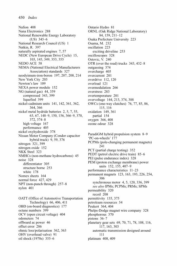
450 Index
Nafion 408Nana Electronics 288National Renewable Energy Laboratory
(US) 345–6National Research Council (US) 1Natkin, R. 397naturally aspirated engines 7, 57NEDC (New European Drive Cycle) 15,
103, 145, 349, 353, 355NEDO ACE 58NEMA (National Electrical Manufacturers
Association) standards 327neodyimum-iron-boron 197, 207, 208, 214New York City 203Newton’s law 109NEXA power module 152NG (natural gas) 44, 359
compressed 343, 399liquefied 399
nickel-cadmium units 141, 142, 361, 362,364, 366
nickel metal hydride batteries 2, 5, 7, 55,63, 67, 148–9, 150, 156, 366–9, 370,372, 374–8
high voltage 167performance 405
nickel oxyhydroxide 378Nissan Motor Company (Condor capacitor
hybrid truck) 9, 59, 376nitrogen 321, 399nitrogen oxide 152NKK Steel 323NMHCs (non-methane hydrocarbons) 45noise 328
differentiator 305structure borne 253white 178
Nomex sheets 164normal force 427, 429NPT (non-punch through) 257–8nylon 401
OATT (Office of Automotive TransportationTechnology) 66, 406, 411
OBD (on-board diagnostics) 177octane numbers 399OCV (open circuit voltage) 404odometers 74offboard ac power 46offset error 286ohmic loss/polarisation 362, 363OHV (overhead valve) 91oil shock (1970s) 355–6
Ontario Hydro 81ORNL (Oak Ridge National Laboratory)
84, 159, 211–12Osaka Prefecture University 223Osama, M. 232oscillation 223
exciting driveline 253oscilloscopes 328Ostovic, V. 240OTR (over the road) trucks 343, 432–8outgassing 374overcharge 405overcurrent 201overdrive 112, 120overload 121overmodulation 266overstress 283overtemperature 201overvoltage 144, 213, 374, 388OWCs (one-way clutches) 76, 77, 85, 86,
115, 116oxidation 149, 361
partial 154oxygen 366, 408ozone odour 328
ParadiGM hybrid propulsion system 8–9‘PC-on-wheels’ 177PCPMs (pole-changing permanent magnets)
241PCT (partial charge testing) 352PEDT (petrol electric drive train) 85–6PEI (pulse endurance index) 328PEM (proton exchange membrane) power
units 152, 155, 407–9performance characteristics 11–23permanent magnets 123, 163, 193, 226, 254,
306synchronous motor 4, 5, 120, 336, 399see also IPMs; PCPMs; PRMs; SPMs
permeability 320recoil 208
permittivity 135, 375petroleum resources 54Peukert 364, 404Phelps-Dodge magnet wire company 328phosphorous 370pistons 36–7planetary gear sets 69, 70, 71, 78, 108, 116,
117, 163, 303automatic transmission designed around
111platinum 408, 409
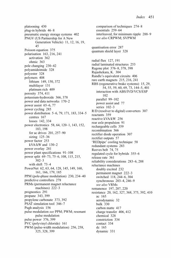
Index 451
platooning 430plug-in hybrids 46–8pneumatic energy storage systems 402PNGV (US Partnership for A New
Generation Vehicle) 11, 12, 16, 19,45
Poisson equation 375polarisation 163, 216, 241
activation 362ohmic 363
pole changing 230–42polyamideimide 328polyester 328polymers 408
lithium 149, 150, 372multilayer 131platinum rich 409
porosity 374, 411potassium-hydroxide 366, 378power and data networks 170–2power assist 65–6, 77power cycling 285power distribution 5–6, 79, 171, 183, 334–5
centres 167losses 142, 334
power electronics 58, 64, 120–1, 143, 152,183, 198
for ac drives 201, 257–90sizing 125–36
power factor 253kVA/kW and 130–2
power overlay 281power plant specifications 91–108power split 69–73, 75–6, 108, 115, 215,
302–3with shift 73–4
PowerNet 62, 63, 64, 128, 145, 149, 160,161, 166, 179, 185
PPM (pole-phase modulation) 230, 234–40predictive controllers 278PRMs (permanent magnet reluctance
machines) 222–3prognostics 291propane 343, 399propylene carbonate 373, 392PSAT simulation tool 346–7Pugh analysis 156pulse modulation see PPM; PWM; resonant
pulse modulationpulse power 376, 399PVC (polyvinyl chloride) 161PWM (pulse-width modulation) 256, 258,
325, 328, 399
comparison of techniques 274–8essentials 259–64interleaved, for minimum ripple 288–9see also CRPWM; SVPWM
quantisation error 287quantum shield layer 328
radial flux 127, 191radial laminated structures 253Ragone plot 376–8, 378, 398Rajashekara, K. 304Randle’s equivalent circuits 406rare earth magnets 215, 216, 241RBS (regenerative brake systems) 15, 29,
54, 55, 59, 60, 69, 73, 144–5, 401interaction with ABS/IVD/VCS/ESP
102parallel 99–102power assist and 77series 102–3
R/D (resolver to digital) converters 307reactants 359reactive kVA/kW 256rear axle propulsion 91rechargeable cells 359recombination 366rectifier diode operation 307rectifier outputs 57‘REDpipe’ cooling technique 58redundant systems 283Reeves belt 74, 75regulated cycle for hybrids 355–6release rate 361reliability considerations 283–6, 288reluctance machines
doubly excited 232permanent magnet 222–3switched 118, 244–6, 304synchronous 203–4, 246–9see also VRMs
remanence 197, 207, 220resistance 20, 162, 327, 368, 375, 392, 410
ac 165aerodynamic 32bulk 330carbon matte 417charge transfer 406, 412chemical 328constriction 334contact 334dc 165dynamic 331
452 Index
resistance (contd.)fast branch 417harness 335ion transfer 413load 394ohmic 405rolling 23–4, 28–9, 32, 355, 423–30,
434, 436series 406, 410, 413stator 308, 309thermal 279ultra-capacitor internal 158winding 211, 292see also ESR
resonance 182resonant pulse modulation 264–6reuse and recycle 13–14reverse recovery 333–4ripple capacitor design 128–34road load 96, 97, 425
calculation 23–32torque 62
‘rocking chair’ chemistry 369rolling resistance 23–4, 28–9, 32, 355,
423–30, 434, 436rotor flux 296, 297, 305, 306rotors 85, 115, 123, 124, 126, 127, 159, 191,
198–9, 208, 219, 224, 241, 254AFPM 223ASD control 400axial laminated structure 253coupling between stator phases and 292inert 253parallel sided slots 226, 228reducing losses 215tendency to deform 255tooth movement 256
Runge-Kutta integration 92Russia 378
Safe-by-Wire Consortium 174, 178samarium-cobalt 197, 207Sbarro, Franco 81Schindall, J. 415semiconductors 120, 121, 128, 130–1, 164,
167, 276, 278, 279operating temperatures 282protection fuses 334
sensorless control 291, 304–8, 312sensors for current regulators 286–8separation distances 374, 375, 379, 432,
435shear force 124, 254
Sheffield, University of 81shielded cables 82
high voltage 6shipping containers 397shore power equipment 437shorting 199side skids 102Siemens 57, 161, 178Sierra Research 18signal distortion 304signal injection 306–7silica glass 401silicon 164, 323sinusoidal modulation 266, 267SIP (single in-line package) 201six step square wave mode 264sizing machine 124–8SLI (starting-lighting-ignition) batteries
149, 359, 365, 370SMDs (surface mounted devices) 181SMES (superconducting magnetic energy
storage) 335snubbers 58, 214, 333SOC (state of charge) 6, 144, 146, 147, 149,
367, 368, 372, 402, 405, 406OCV versus 404
sodium-sulphur 377, 396software 161, 304, 337SOH (state of health) 402solar power 45solder contact surfaces 286solid polymer electrolyte fuel cells 408solvents 370South Coast Air Quality Management
District 46spacecraft 150, 207, 400spacing 429–30, 432, 435specific energy 67, 376, 378specific power 377, 378, 395–6, 409spectroscopy
discrete immittance 403–4, 415electrochemical 407, 410–13
speeders 68, 69speedometers 74spin losses 80, 253SPMs (surface permanent magnets) 124,
191, 195, 220, 253, 286design essentials 203–11
sprung mass 22SRS (safety restraint systems) 174, 177stability programs 180
see also ESPstandardisation 392, 396
Index 453
starter-alternators 69, 115, 226, 253crankshaft mounted 319, 437
starter motors 162–5stator current 296, 305, 306, 310stators 84, 85, 86, 126, 191, 192, 194, 198,
199, 206, 216, 219, 253coupling between rotor phases and 292parallel sided teeth 228reducing losses 217rolled-out 193slotting 209, 210, 211smooth 205tendency to deform 255toroidal 235
steam reformation 154, 397steel 320, 321, 325
good quality 322steering systems
axis 79electric assist 10, 179performance 23see also EPAS
Stefanovic, V. R. 313Steinmetz, Charles Proteus 319, 321stiction 223stop time 15storage system modelling 402–18STP (standard temperature and pressure)
424stress 122, 283
tensile 401thermal 286
strontium 216SULEV (Super Ultra Low Emissions
Vehicles) regulations 152sulphation control 365sulphuric acid 366Sun Microsystems 168super-capacitors 378, 399surface tension 334suspension geometry 79SUVs (sport utility vehicles) 6–7, 67, 82,
88, 91tests 423, 427–32, 434–5
SVPWM (space-vector pulse-widthmodulation) 266–74, 276, 309
Swiss Federal Institute flywheel concept86–7
switching 158–9, 307, 331–3, 390power electronics 129, 261, 269, 270resonant 264series-parallel 58–61
switching frequency 164, 259, 326, 332and PWM 134–6
synchronous motor 86permanent magnet 4, 5, 118
synchronous reluctance 246–9, 255design 203–4
SynRel 246–9
Tafel plot 362TCM (transmission controller module) 160TCP (transmission control protocol) 169TDMA (time division multiple access) 175,
176TEATFB (tetraethylammonium
tetrafluoroborate) 379telematics 177, 178
instrumentation 106Tempel M19 322Tennes see, University of 212terminations 162, 163Tesla, Nikola 203testing 344, 403
coast down 343, 423, 424–7, 429,432–3, 434, 437
electrochemical double layer capacitor392–6
full charge 352partial charge 352validation and 355, 356, 423–30
Texas A&M University transmotor 84–5thermal cycling 283thermal design 278–83, 398thermal excursions 119thermal management 58, 121, 152, 181–4,
198, 409thermal mapping 183thermal time 405Thermaleze Qs 328thermistors 201thermodynamics 361, 363thin film multi-chip process 281THS (Toyota Hybrid System) 2, 7, 9, 104,
106, 303thyristors 129, 130, 212
gate-turn-off 58, 213, 278, 333, 334MOS-controlled 333
time constants 410, 411, 412titanium 400titanium-nickel 366TMF (thin-metal-foil) battery 147toroidal CVTs 74, 75, 109Toronto (ultra-capacitor) model 411
454 Index
torque 4, 6, 31, 32, 38, 64, 70, 73, 74, 81–2,84, 96, 121, 193, 233, 298–300, 309,310
applied wheel 79braking 215constant 313crankshaft 33, 163, 437direct control 312–15driveline 105electromagnetic 293–4, 296, 313, 315engine 42, 95, 98, 112good performance 203high 78, 79, 80, 91, 195, 205, 206, 229,
232, 255IHAT 77IM 242, 253, 255improved 225instantaneous 253M/G 102, 124output higher than input 112peak 18, 42, 194, 228, 253, 254, 255permanent magnet 222power and 119–22reaction 69, 71, 86reluctance 197, 198, 216, 222road load 62stall 225synchronous machine 297
torque converters 104, 108, 110, 115, 145,319
torque ripple 220, 221, 256, 313torquers 68, 69towing applications 74Toyota Group 58, 59Toyota Motor Company 1, 59
Camry 14, 19Crown 64, 355ES3 vehicle 59–60, 61, 62, 180Estima 88–91, 191FINE-S FCHV 81, 409Lexus RX330 2Prius 2, 4, 6, 11, 13, 44, 69, 105–6, 191,
348see also THS
traction drives 215traction motor 319–30tractive effort 23, 29–30, 31, 32–3, 58, 96,
138high torque at low speeds for 80
tractive force 109tractor (class-8) test 432–8trailers 429–32, 434–8transformations 297–8, 300
transistor stack 283, 285transmission 15, 42, 57, 85, 91, 93, 118, 254
electromechanical 67, 68manual shift 110–11step ratio manual 55see also automatic transmission; CVT;
gear step selection; IHAT; IVT;power split
transmotor 84–5TRW electromechanical transmission 68Trzynadlowski, A. M. 263Tsals, Izrail 224TTCANs (time triggered control area
networks) 172–4, 178TTPs (time triggered protocols) 167, 170,
175TTW (tank-to-wheels) 345, 347, 348turbo-generators 329–30tyres 343, 436
radial ply 427–8rolling radius 96scrub radius 79
UGM (uncontrolled generator mode) 215,217
ultra-capacitors 9, 53, 59, 60, 61, 118, 143,144, 146–8, 150, 155, 156–9, 335,374, 410–18
asymmetrical 378–87buck-boost converter and 391capacitance dispersion 375, 388cell balancing 387–92combined with batteries 379–87storage systems 85symmetrical 376–8workings 379
UN (United Nations) 150, 392undervoltage 201, 390Unique Mobility Corporation 336United Kingdom 81, 85unsprung mass 22, 30, 79US ABC (US Advanced Battery
Consortium) 1, 150US Freedom Car initiative 410usage requirements 106
electrical burden 107grade holding and creep 107–9neutral idle 108
UWB (ultra-wide band) 178
V2G vehicles 44–6Valeo corporation 191, 336
Index 455
Van Doorne belt 74, 75vapour recovery 178vector control approaches 291
see also FOCvelocity 78, 425, 426
deceleration 434VFMM (variable flux memory motor) 241vibration 79, 98, 181–2, 197
modal 239Volkswagen
Polo 54Tandem 54–5
volumetric energy 39, 365, 366, 375Volvo Car Company 6, 81
S80 sedan 114VRLA (valve-regulated lead-acid) batteries
147, 148, 149, 366, 377VRMs (variable reluctance machines) 120,
124, 125, 191, 204–5, 206, 215, 221,242–9, 253, 256, 304
VSC (vehicle systems controller) 160, 166VSIs (voltage source inverters) 264–6
‘walk-out’ 332Walters, Jim 12WANs (wide area networks) 169Warburg impedance 406waveforms 195, 199, 260, 266, 269, 328,
332quasi-square 201SVPWM gating 273switching 332
‘weak-links’ 334weight tally 186–8wheel motors 81white noise 178wind power 43windings 58, 64–5, 123, 288, 292, 297
armature 193, 329–30Hunt 230–2PPM 235, 241reconfiguration of 229–30stator 193, 195, 208, 210, 211, 228, 229,
232tapped 229toroidal 235, 256
Wisconsin, University of 306Word 1/2 parameters 404–5WOT (wide open throttle) 98, 105WTT (well-to-tank) 345WTW (well-to-wheels) 345, 347
x-by-wire technologies 174, 177, 178XLPE (cross-linked PVC) 161
Yamaha 81Yoo, H.-S. 305
Zener diodes (sharp knee) 388, 389Zetec 96ZEVs (zero emission vehicles) 44zinc 396