Abstract

This work extends the spatial voting model to include variable voter turnout. I con-sider two alternative assumptions. First, I look at voter indifference, when the probabilityof a voter turning out depends on the difference in utility from the election of her mostpreferred and second most preferred candidate. The second assumption is voter alien-ation, when the probability of turning out depends on the utility from the election of hermost preferred candidate. For a deterministic model, I show that in an equilibrium, thepositions of the candidates do not necessarily converge to the median voter. I then studyhow the positions of the candidates, their relative shares of winning, and turnout dependon the distribution on voter preferences and on nonspatial candidate characteristics. In aprobabilistic voting model, indifference is shown to reduce the stability of the convergentequilibrium.

1 Introduction

A spatial model of elections involves candidates who propose policy platforms and voters whochoose which candidate to support based on the proximity of the candidate’s platform to thevoter’s most preferred policy. The early and best-known result (Downs, 1957) was that ifthere are two vote-maximizing candidates, the policy space is one-dimensional, and the voterpreferences are single-peaked, then both candidates should choose the same policy platform,identical to the median most preferred policy of the voters. If the policy space was more thanone-dimensional, there was no stable outcome (Plott, 1967, McKelvey, 1976).

This contradicts the empirical evidence, as the observed policy positions of candidates andparties are relatively stable, and they do not usually converge. This observed disparity was themotivation behind a large body of theoretical work, analyzing such concepts as probabilisticvoting (Hinich, Ledyard, and Ordeshook, 1972a, Enelow and Hinich, 1982), office-motivatedcandidates (Wittman, 1977), or valence (Groseclose, 2001).

One possible explanation for policy divergence is that the political platforms of candidatesor parties affect the decisions of individual voters whether or not to vote. Turnout consequencesare almost certainly taken into account when political platforms are announced. Losing thesupport of the base voters is one the main reasons that keeps politicians from trying to “stealthe political clothes” of their opponents and converge to the median voter1.

Explaining positive turnout in the framework of the rational choice theory is a major the-oretical challenge. There is a large and growing body of literature on the topic2, but there isno consensus on what kind of behavior makes individuals participate in large elections.

The “paradox of the rational voter” is a consequence of the fact that each single vote isunlikely to be decisive if the overall number of voters is large (Riker and Ordeshook, 1968,Davis, Hinich, and Ordeshook, 1970, Chamberlain and Rotschild, 1982, Myerson, 2000). Thus,if there are positive costs of participating in the elections (like travel expenses, time, gatheringinformation, etc.), then the voter is better off not voting.

This paradox was first remarked upon by Anthony Downs (1957) in his well-known work.He did not address the issue directly, attributing widespread voting to extra-theoretic (andirrational) factors.

The game-theoretic models with strategic voters did not produce conclusive results (Led-yard, 1984, Palfrey and Rosenthal, 1983, 1985). The basic argument of such models can be

1Turnout is one of several mechanisms that can result in policy divergence. For a review of literature on thistopic see Zakharov (2006).

2Other literature reviews include, among others, Aldrich (1993), Lijphart (1997), and Feddersen (2004).

1

formulated as follows. If no one is voting, then the outcome of the elections will depend on thechoice of any single voter who decides to vote. Other voters will become active as long as thebenefit of voting exceeds the cost. Thus it is possible to have an equilibrium where all votersare rational and some level of voting activity is present. In such an equilibrium, every activevoter’s expected benefit of voting will be no less than the cost. Nevertheless, this argument isinsufficient, since the participation rate in large electorates will be very small.

Different models of voter behavior were suggested. Ferejohn and Fiorina (1974) looked atvoters as regret minimizers. A more recent strand of literature views abstention as a result ofrational behavior of voters who are not perfectly informed about their benefit from the electionof a particular candidate. It was argued that if voters are not perfectly informed about theirpreferences, some voters might abstain even if the cost of voting is zero. It was argued thatthe less informed voters may abstain in order to allow the more informed voters to decide theoutcome (Feddersen and Pesendorfer, 1996, Feddersen, 2004).

The evidential decision model of Grafstein (1991) treats every voter as thinking that heraction will influence the actions of all other voters. In this setting both the perceived probabilityof being pivotal and turnout are higher. In a model by Kanazawa (1998), backward-lookingvoters similarly associate their past voting behavior with the outcome of the previous elections.

Eldin, Gelman, and Kaplan (2005) considered voters who care not only for her own utility,but also for the utility of every other individual in the society. Similar approach is followed byHarsanyi (1980), Feddersen and Sandroni (2002), and Coate and Conlin (2005).

Other theoretical arguments involve a third type of agent — the group leader, who mayreward individual voters for their participation and support of a particular candidate (Morton,1991, Uhlaner, 1989).

There are several hypotheses relevant to the spatial theory that can be tested empirically.The best-studied prediction is that turnout depends on the closeness of the election, as in acloser election the probability of casting the decisive vote is higher (Geys, 2006, contains areview of relevant literature). Most tests support the hypothesis, although the evidence issometimes contradictory, such as in Kirchgassner and Zu Himmern (1997) study of GermanGeneral Elections for 1983–1994.

The so-called “mobilization hypothesis” provides an alternative explanation to the (possible)positive relationship between turnout and election closeness. It can be argued that if theelections are more closely contested, then the competing candidates are mobilized to procureadditional turnout (see, for example, a study by Cox and Munger, 1989, linking campaignspending and election closeness).

2 Spatial voting models under indifference and alien-

ation hypotheses.

The results of spatial models with variable turnout and strategic voters are mixed and incon-clusive, especially when one is interested in the effect that turnout has on the positions of thecandidates. One proposed solution is to simplify the model by assuming that the voters decidewhether to vote or to abstain according to some fised rule.

The two well-known conjectures linking the likelihood of turnout and the policy positionsof the candidates are known as indifference and alienation hypotheses. Under the indifferencehypothesis, a voter casts her ballot if and only if there is sufficient difference between payoffsthat the candidates offer to the voter. Hence, a voter who is indifferent between the candidateswill abstain. Under the alienation hypothesis, a voter will abstain if she is sufficiently dissatisfiedwith the policies promised by either of the candidates.

2

Until recently, there were relatively few works investigating indifference and alienation hy-pothesis. The in the earliest work on the subject (Brody and Page, 1973) the authors analyzedsurvey data collected after 1968 U.S. Presidential elections. It was found that the likelihood ofthe respondent having voted was greater if her evaluation of her most preferred candidate wasmore favorable. A similar relationship supporting the indifference hypothesis was also found.Later works by Zipp (1985) and Plane and Gershtenson (2004) also found support for bothindifference and alienation hypotheses using survey-level data.

In a recent paper, Adams, Dow, and Merrill (2006) used a conditional logit model to estimatethe alienation and indifference components of abstention. The authors found that for the 1980-1992 Presidential elections both factors contributed to depressed turnout, with no substantialpartisan differences in their effects.

A plausible way to introduce indifference and alienation in a spatial model is to assume thatthe probability of voting is a function of the positions of the candidates and the policy preferenceof the voter. Under the indifference hypothesis, one would assume that the probability of votingdeclines with the policy distance between the candidates; under the alienation hypothesis,the probability of voting would decline with the distance between the voter and the nearestcandidate.

In the original work by Downs (1957) it was noted that voter alienation may result in thedivergence of candidate platforms from the median voter If we assume that alienated votersabstain, then a candidate who decides to move her platform closer to the median voter’ blisspoint faces a tradeoff: on one hand, she gains some votes closer to the center of the politicalspectrum (the “moderate” voters), but on the other hand she may be bound to lose some voteson the far left (those of the “extreme” voters).

More formal analysis, starting with Davis, Hinich, and Ordeshook (1970), Hinich, Ledyard,and Ordeshook (1972a,b), and McKelvey (1975), suggested that voter indifference by itselfshould not be sufficient to dislodge a median voter equilibrium. Voter alienation is more likelyto lead to the divergence of policy positions, as a candidate who decides to move her platformcloser to the median voter’ bliss point faces a tradeoff: on one hand, she gains some votes closerto the center of the political spectrum (the “moderate” voters), but on the other hand she maybe bound to lose some votes on the far left (those of the “extreme” voters). If the distributionis unimodal, and the voter density at the peak of the distribution is sufficiently high, then bothcandidates converging to the mode is a local equilibrium. If the distribution is symmetric andthe median and the mean coincide with the mode, then the equilibrium is a global one.3

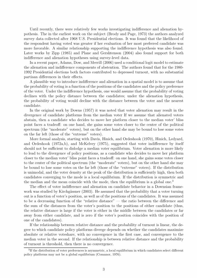
The effect of voter indifference and alienation on candidate behavior in a Downsian frame-work was studied by Kirchgassner (2003). He assumed that the probability that a voter turningout is a function of voter’s position, as well as of the positions of the candidates. It was assumedto be a decreasing function of the “relative distance” — the ratio between the difference andthe sum of the distances from the voter’s position to the positions of either candidate (thus,the relative distance is large if the voter is either in the middle between the candidates or faraway from either candidate, and is zero if the voter’s position coincides with the position ofone of the candidates).

If the relationship between relative distance and the probability of turnout is linear, the de-gree to which candidate policy platforms diverge depends on whether the candidates maximizeabsolute or relative voteshare, with no convergence in the first case, and convergence to themedian voter in the second. If the relationship is between relative distance and the probabilityof turnout is threshold, then there is no convergence.

3If the distribution of voter preferences is asymmetric, a local equilibrium in which candidates select differentpolicy platforms may not be a global equilibrium (Comanor, 1976).

3

The model presented in this work is similar in spirit to that of Kirchgasser (2003). However,there are two important differences. First, the authors consider the voters with policy prefer-ences distributed over a single-dimensional policy space according to a general-form continuousdistribution (it was taken to be uniform in the latter work).

The second feature of the model studied in this work is that we use the concept of candi-date valence (notion of candidate valence is attributed to Stokes, 1963). This term refers tocandidate characteristics such as popularity, name recognition, experience4, and other factorsthat contribute to a voter’s satisfaction with the candidate regardless of that candidate’s policyposition.

Different candidate valence has several implications for spatial models of voting. First, thereis no equilibrium in the standard voter5. Any position of the low valence candidate can bematched by her rival, who will obtain all the votes as a result. Second, changes in the politicalplatforms of the candidates have asymmetric effects on the position of the indifferent voter ifthe voters are risk-averse. A change in the policy position of the candidate with the greatervalence will have a greater impact on the indifferent voter’s position than an equal change inthe position of her rival.

3 Model assumptions.

There is a continuum of voters with policy ideal policies distributed on a convex compact setX ⊂ Rn with a continuous density f(·).

There are K ≥ 2 candidates with policy positions y1, · · · , yK .If candidate j is elected, a voter with the ideal policy v ∈ [0, 1] receives a utility of

uj(v) = ǫj − φ(‖yj − v‖). (3.1)

Here, yj is the policy position of Candidate j, ej is the valence of Candidate j, and φ(·) is atwice-differentiable function with φ′(·) > 0, φ′(·) > 0, φ′(0) = 0, and φ(d) = φ(−d) for all d > 0.This function reflects the voter’s disutility from the difference between the realized policy andthe voter’s preferred policy v.

The voters are assumed to be sincere. The choice of a voter with the ideal policy v dependson the utilities uj(v) for j = 1, · · · , K and is described by the function t : RK → ∆K+1, wheretK+1 denotes the probability of abstention.

Under the regular sincere voting hypothesis, a voter supports a candidate who delivers thehighest utility, or fairly randomizes if there are several such voters.

Sincere voting (SV)

tj(u1(v), · · · , uK(v)) =

{

1#{i|ui(v)=maxk uk(v)} , uj(v) = maxk uk(v)

0 , uj(v) 6= maxk uk(v).(3.2)

For K = 2, the sincere voting hypothesis is consistent with the behavior of a rational voterwhose voting costs are zero.

Under the indifference hypothesis, a voter supports a candidate only if the utility that thecandidate delivers to the voter is significantly bigger than the next highest utility.

4The implications of endogenous valence were analyzed by Zakharov (2005).5One can either analyze the mixed equilibrium, as Aragones and Palfrey (2002), assume that the candidates

are policy-motivated, as was done by Groseclose (2001), or look at the conditions for the existence of anequilibrium in several dimensions, as in Ansolabehere and Snyder (2000).

4

Indifference (IH).

tj(u1(v), · · · , uK(v)) =

{

1, uj(v) − c ≥ maxk 6=j uk(v)0, uj(v) − c < maxk 6=j uk(v).

(3.3)

The indifference assumption is consistent with the behavior of a rational voter who hasvoting costs of C, believes that her vote will be pivotal with the exogenous probability p = C

c,

and believes that when her vote is pivotal, the alternative is the election of the next-bestcandidate.

Alienation (AH).

tj(u1(v), · · · , uK(v)) =

{

1, uj(v) ≥ max{d,maxk 6=j uk(v)}0, uj(v) < max{d,maxk 6=j uk(v)}.

(3.4)

The alienation hypothesis is consistent with the behavior of a rational voter who has votingcosts C, believes that her vote will be pivotal with the exogenous probability p = C

d, and

believes that when her vote is pivotal, the alternative is the implementation of a status quopolicy which delivers zero utility to the voter.

A more conventional interpretation of the alienation hypothesis is that a voter is simplyreluctant to support a candidate who delivers a low level of utility, with the psychologicalbenefit of abstaining exceeding the possible value of being pivotal against the candidates whoare even less acceptable to the voter.

Next we must define the payoffs of the candidates. The voteshare of candidate j is equal to

Vj =∫

tjdF (v). (3.5)

There are potentially two sources of candidate motivation. The classical Downsian viewis that candidates are motivated solely by winning the elections. The probability of winningoffice is an increasing function of either the share of vote obtained by the candidate, or of thedifference between the candidate’s voteshare and the largest voteshare among the opposingcandidates (the candidate’s plurality). This distinction is irrelevant for a two-candidate modelwith perfect turnout, but may become important if the voteshares of the candidates do not addup to one6.

Office-motivated candidates (OMC). The utility of Candidate j is

Uj = (1 − λ)Vj + λ(Vj − maxk 6=j

Vk). (3.6)

The parameter 0 ≤ λ ≤ 1 is the weight of plurality versus voteshare in determining thecandidate’s chances of winning.

6In a work by Hinich, Ledyard, and Ordeshook (1972), the probability P1(y1, y2, v) of a voter with policypreference v supporting candidate 1 was a continuously differentiable functions with the following properties:P1 = 0 if φ(|v−y1|) > φ(|v−y2|), P1 is decreasing in φ(|v−y1|)−φ(|v−y2|) and in φ(|v−y1|) if φ(|v−y1|) < φ(|v−y2|), and P1(y1, y2, v) = P2(y2, y1, v). A one-shot game between two plurality-maximizing candidates producedpolicy convergence. Crucially, their result depended on the candidate objective functions being symmetric iny1 and y2. This is not the case if the candidates have different valence.

5

An alternative hypothesis is that a candidate is interested in having a certain policy objectiverealized after the elections.7

Policy-motivated candidates (PMC). The utility of Candidate i is

Ui = −ψ(|y − yi|). (3.7)

The value yi is the ideal policy of Candidate i, while ψ(·) is the disutility function of thecandidate.8 The value y is the policy that the candidate expects will be realized after theelections.

4 Indifference and alienation in the deterministic model.

In this section I look at a one-dimensional, two-candidate deterministic voting model. Theadvantage of using a deterministic model is the the possibility of doing a comparative staticsanalysis at the equilibrium. One can derive the conditions that describe the positions of thecandidates in an equilibrium, and see how the positions change with the changes in the modelparameters — cost of voting, valence of the candidates, and the distribution of voters.

The voter with policy preference y is the indifferent voter if

ǫ− φ(y1 − y) = −φ(y2 − y), (4.8)

where ǫ = ǫ1 − ǫ2. Provided that y1 < y2, all voters with y < y receive higher utility underCandidate 1, while the rest of the voters receive higher utility under Candidate 2.

Under IH, the indifferent voter will abstain, as well as the voters in his neighborhood.Denote by y1, y2 the leftmost and rightmost abstaining voter. We have

ǫ− φ(y1 − y1) − c+ φ(y2 − y1) = 0 (4.9)

andǫ− φ(y2 − y1) + c+ φ(y2 − y2) = 0. (4.10)

The following result is straightforward.

Proposition 4.1 Let n = 1, K = 2. Under IH and OMC,

1. No pure-strategy equilibria exists if ǫ1 6= ǫ2.

2. If ǫ1 = ǫ2, an equilibrium exists, with y2 − y1 = φ−1(c) and f(y1) = f(y2).

If one of the candidates shifts her policy position toward that of her opponent, her votesharemay change for two reasons. First, the position of the indifferent voter will change; second, theturnout will be affected. Since we assumed that voter disutility is concave in policy distance,the turnout will decrease by a greater amount if the positions of the two candidates are closer.At some point, the marginal voteshare effect of a change in a candidate’s position will be zero.

7This idea was first exploited in the works of Donald Wittman (1983) and Randall Calvert (1985).8A work of Timothy Groseclose (2001) explores a two-candidate game with the candidates maximizing a

weighted average of (3) for λ = 0 and (3). His work did include candidates with different valence, but did notconsider the possibility of voters abstaining. For tractability’s sake we restrict our attention to one of the twocases.

6

If the two candidates have equal valence, then the changes in the positions of the candidateswill have symmetric effects on their voteshare, so an equilibrium is possible. If the valence isasymmetric, so is the effect of a candidate’s position on her voteshare. Thus if y1 is candidate1’s best response y2, then y2 is not a best response to y1.

Example. Let φ(x) = x2 and ǫ1 − ǫ2 = ǫ ≥ 0. Then from (6.73) and (6.74) we have

y1 =y1 + y2

2+

ǫ− c

2(y2 − y1)(4.11)

and

y2 =y1 + y2

2+

ǫ+ c

2(y2 − y1). (4.12)

The utilities of the candidates (6.73), (6.74) will be given by

U1 = (1 + λ)y1 + y2

2+

1

2(y2 − y1)((1 + λ)ǫ− (1 − λ)c) (4.13)

and

U2 = 1 − (1 + λ)y1 + y2

2− 1

2(y2 − y1)((1 + λ)ǫ+ (1 − λ)c). (4.14)

The best responses of the two candidates are given by

y1(y2) =

{

y2 +√

2 (1−λ)c−(1+λ)ǫ1+λ

, (1 − λ)c > (1 + λ)ǫ

y2, (1 − λ)c < (1 + λ)ǫ.(4.15)

and

y2(y1) = y1 +

√

2(1 − λ)c+ (1 + λ)ǫ

1 + λ. (4.16)

I now consider the effects of the alienation hypothesis. The alienation hypothesis claimsthat a voter will abstains if the positions of both candidates are sufficiently different from herown ideal position. Thus a candidate who decides to move her position closer to her opponent’sfaces a dilemma. On one hand, the candidate will capture additional votes from her opponent.On the other hand, the candidate will lose votes on the far end of the political spectrum. Theeffects of voter density and candidate valence on policy positions in such an equilibrium arenontrivial and demand investigation.

Under an alienation hypothesis, a voter votes only if her distance from the nearest candidateis sufficiently small. Denote by

di = φ−1

(

ǫi −c′

p

)

(4.17)

the distance between the the position of candidate i and the position of the voter who preferscandidate i to the other candidate and is on the verge of abstaining because of alienation.

We call the voters who are on the threshold of abstaining ambivalent voters.There are potentially two cases (see Fig. 1). In the first case, with

y2 − y2 > d1 + d2, (4.18)

there are alienated voters with positions between y1 and y2. In the opposite case, with

y2 − y1 ≤ d1 + d, (4.19)

all voters with positions between y2 and y1 participate.The equilibrium conditions and comparative statics are different in for case. For the first

case, the following result holds:

7

y1 − d1 y1 y1 + d2 y2 − d2 y2 y2 + d2

(a) Case 1: y2 − y1 > d1 + d2

y1 − d1 y1 y y2 y2 + d2

(b) Case 2: y2 − y1 ≤ d1 + d2

Figure 1: Voter choice depending on candidate location

Proposition 4.2 Let y1, y2 be a LNE under OMC and AH, such that y2 − y1 ≥ 2d. Thenwe have:

f(y1 + d1) = f(y1 − d1), f ′(y1 + d1) − f ′(y1 − d1) < 0f(y2 + d2) = f(y2 − d2), f ′(y2 + d2) − f ′(y2 − d2) < 0.

(4.20)

If the candidates are so far apart that there are alienated voters with intermediate positions,then changes in the position of one candidate have no effect on the voteshare of the othercandidate.

The comparative statics in this equilibrium are straightforward:

Corollary 4.1 Let y1, y2 be a LNE under OMC and AH, such that y2 − y1 ≥ 2d. Then wehave

∂y1

∂d1

≥ 0 (4.21)

if and only if f ′(y1 − d1) + f ′(y1 + d1) ≥ 0.

The effect of both a reduction of the voting cost and the increase in candidate valence isidentical, as both the distance between the ambivalent voters 2d1 and the candidate’s share ofvote increases.

The second case is more interesting. The equilibrium is described as follows:

Proposition 4.3 Let y1, y2 be a LNE under OMC and AH, such that y2 − y1 > d1 + d2. Letf ′(y) 6= 0 and f ′(y1 − d1) = f ′(y2 + d2) = 0. Then, the following holds:

f(y)φ′(y − y1)

φ′(y − y1) + φ′(y2 − y)= (1 − λ)f(y1 − d1), (4.22)

f(y)φ′(y2 − y)

φ′(y − y1) + φ′(y2 − y)= (1 − λ)f(y2 + d2), (4.23)

ǫ− φ(y − y1) = −φ(y2 − y), (4.24)

and

f ′(y)

f(y)<

1

φ′(y − y1) + φ′(y2 − y)min

{

φ′(y − y1)φ′′(y2 − y)

φ′(y2 − y),φ′(y2 − y)φ′′(y − y1)

φ′(y − y1)

}

. (4.25)

In an equilibrium, each candidate loses and gains an equal amount of votes by moving herposition. Since the candidate with the valence advantage gains more votes than her opponentif she moves her position toward the indifferent voter, it follows that the density of voters isgreater in the neighborhood of the voter who is ambivalent between voting for the advantagedcandidate and abstaining, than in the neighborhood of the other ambivalent voter.

The first corollary is an immediate consequence of the fact that the voters are risk-averse:

Corollary 4.2 Let ǫ1 > ǫ2. Then f(y1 − d1) > f(y2 + d2).

8

Since a voter with a higher valence gains more voteshare if she moves toward the indifferentvoter, in an equilibrium she must also be bound to lose more voter due to alienation.

We want to know how the equilibrium positions of the candidates and the position of theindifferent voter are affected by changes in the valence advantage of the first candidate, bychanges in voter densities in the neighborhood of the indifferent voter and the ambivalentvoters, and by cost of voting c′.

We have to make several assumptions. First, we assume that the third derivative of thedisutility function φ(·) is negative. This assumption has the following interpretation. Supposethat a voter with the ideal policy v has to choose between two options: policy y > v anda lottery where policies y − a and y + a are realized with probability 1

2each. If the third

derivative of the disutility function is negative, then the difference in utility from these twopotions declines with the policy distance y − v.

The third derivative assumption is inherently consistent with the alienation hypothesis. Asthe distance between the candidates and the voter increases, the voter is willing to pay less inorder to insure herself against a lottery on the candidate’s positions, and thus is less likely tovote.

The second assumption that we make is that the voter density is constant in the neighbor-hood of the ambivalent voters.

Corollary 4.3 Let y1 < y2 be equilibrium positions of the candidates, and let y be the positionof the indifferent voter. Let f ′(y1 − d1) = f ′(y2 + d2) = 0 and f ′(y) 6= 0. Then, the followingholds:

∂y1

∂d= 0,

∂y2

∂d= 0,

∂y

∂d= 0,

∂(y2 − y1)

∂f(y)= 0,

∂(y2 − y1)

∂λ= 0,

∂y

∂ǫ= 0. (4.26)

Each of the following holds if and only if f ′(y) > 0:

∂(y2 − y1)

∂f(y1 − d1)< 09,

∂(y2 − y1)

∂f(y2 + d2)< 0,

∂y

∂f(y1 − d1)> 0,

∂y

∂f(y2 + d2)< 0, (4.27)

∂y1

∂f(y)< 0,

∂y2

∂f(y)< 0,

∂y

∂f(y)< 0,

∂y1

∂λ< 0,

∂y2

∂λ< 0,

∂y

∂λ< 0.

Suppose that, in addition, we have φ′′′(·) < 0. Then each of the following holds if and only ifǫ1 > ǫ2:

∂y1

∂ǫ< 0,

∂y2

∂ǫ> 0,

∂(y2 − y1)

∂ǫ> 0. (4.28)

Let φ′′′(·) < 0 and ǫ1 > ǫ2. Then the following is true if f ′(y) > 0:

∂y1

∂f(y1 − d1)< 0,

∂y2

∂f(y2 + d2)> 0. (4.29)

Let φ′′′(·) < 0 and ǫ1 > ǫ2. Then the following is true if f ′(y) < 0:

∂y1

∂f(y2 + d2)< 0,

∂y2

∂f(y1 − d1)> 0. (4.30)

We find that the cost of voting C and the perceived probability of being decisive p do notaffect the equilibrium positions of the candidates and of the indifferent voter. This is because

9We assume that f(y) uniformly increases in some neighborhood of y.

9

of our assumption of uniform voter density in the neighborhood of the ambivalent voters. Anincrease in d = C

pwill reduce the voteshare of both candidates, but the marginal effect of a

change in a candidate’s position on the voteshare of the candidate will remain unaffected. Forthe same reason, an equal change in the valence of both candidates will not affect their policypositions, although it will change their absolute and, likely, their relative voteshares.

An increase in the valence advantage of one of the candidates will lead to a divergence ofcandidate positions, with the positions of both candidates moving away from the indifferentvoter. This, in turn, should lead to a higher turnout.

The effect of an increase in the voter density in the neighborhood of the indifferent voterdepends on an additional factor. If f ′(y) > 0, that is, the indifferent voter lies to the leftof a local maximum in the density of voters, then an increase in f(y) will lead to a leftwardshift in the positions of both candidates and of the indifferent voter. In the new equilibrium,f(y), y − y1 and y2 − y will remain the same, as we have assumed constant density around theambivalent voters. An increase of the role of plurality in a candidate’s objective function hasthe same effect as an increase in the voter density near the indifferent voter. When the weightof plurality increases, so does the value of capturing the indifferent voter, as the candidate notonly gains votes, but also decreases the voteshare of her opponent.

Note that the policy distance y2 − y1 is unaffected by both the changes in f(y) and λ. Thusincreases of these parameters should result in an increase in turnout if and only if the leftcandidate has higher valence.

Finally, I consider the case when the voter of each type votes with a certain probability(perhaps due to different costs of voting). The probability of voting is taken to depend on thepolicy difference between the candidates10.

Uniform effect of policy distance on turnout (UEH). A voter votes with probabilityψ(|y2 − y1|), where ψ(·) is a twice differentiable function.

The payoffs to the candidates are

U1 = ψ(y2 − y1)F (y) (4.31)

andU2 = ψ(y2 − y1)(1 − F (y)). (4.32)

The following equilibrium result has been obtained:

Proposition 4.4 Under UEH, y1, y2 are a LNE if

f(y)ψ(y2 − y1) − ψ′(y2 − y1) = 0, (4.33)

10This approach is similar to that of Kirchgasser (2003), where the probability of voting function is defineddirectly and does not follow from any rational behavior. The function proposed there is consistent with bothalienation and indifference hypotheses:

P (v, y1, y2) =

y2−y1y1+y2−2v , v < y1y1+y2−2vy2−y1

, y1 ≤ v ≤ y1+y22

2v−y1−y2y2−y1

, y1+y22 ≤ v ≤ y2

y2−y12v−y1+y2

, y2 ≤ v.

Here participation is a continuous function of v with limv→−∞ P = 0, limv→∞ P = 0, P (y1+y22 , y1, y2) = 0, andP (y1, y1, y2) = P (y2, y1, y2) = 1. However, this function is not used here for two reasons. First, it is appropriateonly if both candidates have identical valence. Second, in order to calculate candidate voteshares one has tointegrate voting probabilities over all voters to the left and to the right of the indifferent voter y1+y2

2 . Hence,voter preferences must be distributed uniformly in order for the results to be tractable.

10

F (y) =φ′(y − y1)

φ′(y − y1) + φ′(y2 − y), (4.34)

andǫ− φ(y1 − y) = −φ(y2 − y).

First, her voteshare relative to her opponent will increase. Second, the overall votesharemay decrease since turnout may increase with smaller policy distance. In an equilibrium, theturnout increases with the policy distance. Otherwise, each candidate (or at least the candidatewith the valence advantage) will benefit from moving in the direction of her opponent. Thusthe conditions of the indifference hypothesis are satisfied in automatically.

One of our goals is to examine the comparative statics of the model. We want to knowhow will the positions and the voteshares of the candidates shift if the valence of one of thecandidates or the voter density in the neighborhood of the indifferent voter changes. There isthe following result:

Corollary 4.4 Let y1, y2 be a local Nash equilibrium in the election game with payoffs (4.31),(4.32), and let ψ′′(y) > 0 and f ′(y) > 0. Then, we have

∂y

∂ǫ> 0, (4.35)

∂(y2 − y1)

∂ǫ< 0, (4.36)

and∂(y2 − y)

∂ǫ< 0. (4.37)

An increase in the valence advantage the first candidate has several competing effects onthe position of the indifferent voter and on the policy distance. The candidate who has thevalence advantage can now obtain greater voteshare by moving her position toward that of heropponent, and will be better off given the position of her opponent. At the same time, theopponent will be better off moving away from the candidate. Thus the overall effect on thepositions of the candidates is not clear. However, the effects on the position of the indifferentvoter and on the policy distance are more certain.

5 Indifference and alienation in the probabilistic model.

In the second part of the work, I study the implications that the indifference and alienationassumptions will have on the probabilistic voting model.

The principal assumption of a spatial probabilistic voting model is that the candidates arenot fully aware of the effect of their policies on the utility of a voter. Thus, from a candidate’sperspective, a voter’s action is a random variable conditional on the ideal policy of the voter,the platforms of all candidates, and other observable factors.

This uncertainty can arise for several reasons. Voters with identical attitudes toward policymay have different perception of candidates’ personal qualities, such as her competence or

11

honesty11. Uncertainty can also be a result of idiosyncratic random events affecting anindividual’s voting decision.

The equilibrium in a probabilistic voting model is common, as the expected votesharesof the candidates depend continuously on their policy positions. However, virtually all worksinvestigate the existence of an equilibrium where all candidates select identical policy platforms.

Hinich, Ledyard, and Ordeshook (1972) proved that an equilibrium in a two-candidatepositioning game exists as long as the probability that a voter supports a candidate is concavein the voter’s utility from the election of that candidate, and convex in the utility the voterreceives if the opponent is elected. The equilibrium is a convergent one if the probability of avoter supporting a candidate is a function of the difference in utilities that the voter derivesfrom the election of each candidate. The well-known result is that both candidates choose themean voter’s ideal policy if the voter utility is the negative squared Eucledian distance betweenthe policies of the candidates. Lin, Enelow, and Dorussen (1999) obtained the conditions for aconvergent equilibrium for a multi-candidate game for some other distance metrics.

A sufficient condition for the existence of an equilibrium is the concavity of probabilitiesof voting in candidate locations. This assumption is a very strong one and has been criticizedin several works, most recently by Kirchgasser (2000). If the domain of candidate positions isunrestricted, then the probability that a voter supports a candidate cannot be concave in thecandidate’s position. Thus the existence of the equilibrium cannot be guaranteed.

The analysis of a probabilistic voting model typically addresses this question in one of thethree ways.

First, one may try to answer whether the concavity conditions for a convergent equilibriumare satisfied locally. The most recent work here is Schofield (2006), who derived the localequilibrium conditions for several candidates with different valence. The second question (anda more difficult one to answer) is whether the local convergent equilibrium is also a global one.This issue was addressed in many works, starting with Hinich (1978) and Enelow and Hinich(1982). The general result have been that the convergent equilibrium will unravel if votingis close to being deterministic, or if the variance of the voter ideal policies is large. Finally,one may try to find nonconvergent equilibria. This is the most difficult problem of all, andit has not been solved analytically. Numeric solutions were proposed in several works, suchas Schofield, Sened, and Nixon (1998), Lin, Enelow, and Dorussen (1999), or Schofield (2006).The nonconvergent equilibria were found to be local. Moreover, the degree of in local Nashequilibria, simulated with the use of real survey data to estimate voter ideal points, was greaterthan the degree of convergence of estimated candidate positions in the same elections.

In this work, I will address the first two questions and obtain local and global conditions fora convergent equilibrium for voters with squared Eucledian disutility, under the assumption ofvoter indifference.

5.1 The probabilistic voting model

I consider N voters of equal mass with the ideal policies vi ∈ Rn, and K candidates.The utility of voter i if candidate j wins is given by

uij = ej − β‖vi − yj‖2 + ǫij , (5.38)

there vi is the ideal policy of voter i, yj and ej are the policy position and valence of candidatej, and ǫij is zero-mean random variable, IID with the distribution F (·). We take β = 1 for

11A candidate is said to have a higher valence if she has, on average, a higher perceived ability (Stokes,1963). Deterministic models incorporating valence include Groseclose (2001) that assumes the candidates to bepartially motivated by policy, and Aragones and Palfrey (2002) that looks at a mixed-strategy equilibrium.

12

a general functional form of F (·) and e1 ≤ · · · ≤ eK . Without the loss of generality we let∑

i vi = 0.This specification follows Hinich (1977) and the majority of other works. Under an alter-

native specification, such as in Coughlin and Nitzan (1981), the value ǫij has a multiplicativeeffect on voter utility.

The indifference and alienation assumptions for a multi-candidate model probabilistic modelcan be formulated as follows:

Indifference (IH). Voter i votes for candidate j if and only if uij − c ≥ maxk 6=j uik for somec ≥ 0.

Alienation (AH). Voter i votes for candidate j if and only if uij ≥ maxk 6=j uik uij ≥ d forsome d.

If the random variable ǫij is continuous with unrestricted domain, then the probability thatuij = uik is equal to zero for k 6= j.

Denote by Pij the probability that voter i supports candidate j. Then the expected voteshareof candidate j is

Vj =N∑

i=1

Pij . (5.39)

5.2 Local conditions for K = 2, n = 1, and the general form of F (·).We first look at the probabilistic voting model under the indifference hypothesis. Without lossof generality, assume that ei1 − ei2 are identically distributed with the distribution functionG(·).

The probabilities that voter i abstains or votes for one of the candidates are given by

Pi1 = 1 −G((vi − y1)2 − (vi − y2)

2 + c), (5.40)

Pi2 = G((vi − y1)2 − (vi − y2)

2 − c), (5.41)

and

P (Voter i abstains) = 1−Pi1−Pi2 = G((vi−y1)2−(vi−y2)

2 +c)−G((vi−y1)2−(vi−y2)

2−c).(5.42)

The expected voteshares of the candidates are

V1 =N∑

i=1

(1 −G((vi − y1)2 − (vi − y2)

2 + c)) (5.43)

V2 =N∑

i=1

G((vi − y1)2 − (vi − y2)

2 − c). (5.44)

I assume that the candidates maximize a weighted sum of plurality and voteshare:

Ui = λVi + (1 − λ)(Vi − V−i) = Vi − λV−i. (5.45)

The conditions for a convergent local Nash equilibrium in a game with are similar to thosefor the case of perfect turnout.

13

Proposition 5.1 Let the utility of the candidates be given by (5.43), (5.44), and (5.45). Sup-pose that G(·) has a differentiable density g(·). Denote by v and σ2

v the mean and variance ofvi. Then, y1 = y2 = v is a local Nash equilibrium if and only if

g(−c) + λg(c) − 2σ2v(g

′(−c) + λg′(c)) > 0,

g(c) + λg(−c) + 2σ2v(g

′(c) + λg′(−c)) > 0 (5.46)

The expected utility of the two candidates in the convergent equilibrium would be

U∗1 = 1 −G(c) − λG(−c), (5.47)

U∗2 = G(−c) − λ(1 −G(c)). (5.48)

The intuition of behind this result is as follows. Since the voter’s disutility from policydistance is concave, the marginal effect a candidate’s position on the voter’s utility is increasingin policy distance. But so is the effect of a change in a candidate’s position on the voter’sprobability of supporting that candidate — so the policy choice of each candidate is weightedin favor of more distant voters. If the disutility is linear, then these weights are linear in policydistance.

It is worth comparing the second-order conditions for this model and the case with perfectturnout. For c = 0, the condition (5.46) becomes

σ2v <

f(0)

2|f ′(0)| . (5.49)

Thus the electoral mean is a local equilibrium if a change in a candidate’s position has asignificant impact on her probability of winning (high f(0), low σ2

v). The concavity conditionis also satisfied if the density of ǫ is sufficiently close to constant. Conditions similar to (5.46)were obtained by Hinich (1978), Enelow (1989), Lin, Enelow, and Dorussen (1999), Schofield(2006), and by a number of other works.

If there is a possibility of voter abstention due to indifference, a slightly different conditionis required.

Corollary 5.1 Suppose that g(·) is symmetric around zero mean. Then the following is true.

1. If g′(c) ≥ 0, then y1 = y2 = v is a local equilibrium.

2. If g′(c) < 0 and

λ >g(c) − 2σ2

vg′(c)

g(c) + 2σ2vg

′(c), (5.50)

or

σ2v <

g(c)(1 + λ)

−2g′(c)(1 − λ), (5.51)

then y1 = y2 = v is a local equilibrium.

The equilibrium is more likely to exists if the density of ǫ is multimodal, with the voters withthe realizations of ǫ at the modes of the distribution not abstaining. Thus a local equilibriumbecomes less likely if c is large. Finally, the local convergent equilibrium exists if the varianceof voter ideal policies is small or the candidates are plurality maximizers.

14

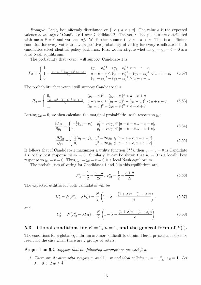
Example. Let ǫi be uniformly distributed on [−e + a, e + a]. The value a is the expectedvalence advantage of Candidate 1 over Candidate 2. The voter ideal policies are distributedwith mean v = 0 and variance σ2

v . We further assume that e − a > c. This is a sufficientcondition for every voter to have a positive probability of voting for every candidate if bothcandidates select identical policy platforms. First we investigate whether y1 = y2 = v = 0 is alocal Nash equilibrium.

The probability that voter i will support Candidate 1 is

Pi1 =

1, (y1 − vi)2 − (y2 − vi)

2 < a− e− c,

1 − (y1−vi)2−(y2−vi)2+c−a+e

2e, a− e− c ≤ (y1 − vi)

2 − (y2 − vi)2 < a+ e− c,

0, (y1 − vi)2 − (y2 − vi)

2 ≥ a + e− c.

(5.52)

The probability that voter i will support Candidate 2 is

Pi2 =

0, (y1 − vi)2 − (y2 − vi)

2 < a− e+ c,(y1−vi)2−(y2−vi)2−c−a+e

2e, a− e+ c ≤ (y1 − vi)

2 − (y2 − vi)2 < a+ e+ c,

1, (y1 − vi)2 − (y2 − vi)

2 ≥ a+ e+ c.

(5.53)

Letting y2 = 0, we then calculate the marginal probabilities with respect to y1:

∂Pi1

∂y1

=

{

−1e(y1 − vi), y2

1 − 2viy1 ∈ [a− e− c, a+ e− c],0, y2

1 − 2viy1 /∈ [a− e− c, a+ e+ c],(5.54)

∂Pi2

∂y1

=

{

1e(y1 − vi), y2

1 − 2viy1 ∈ [a− e+ c, a− e+ c],0, y2

1 − 2viy1 /∈ [a− e+ c, a+ e+ c],(5.55)

It follows that if Candidate 1 maximizes a utility function (??), then y1 = v = 0 is Candidate1’s locally best response to y2 = 0. Similarly, it can be shown that y2 = 0 is a locally bestresponse to y1 = v = 0. Thus, y1 = y2 = v = 0 is a local Nash equilibrium.

The probabilities of voting for Candidates 1 and 2 in this equilibrium are

P ∗i1 =

1

2− c− a

2e, P ∗

i2 =1

2− c+ a

2e. (5.56)

The expected utilities for both candidates will be

U∗1 = N(P ∗

i1 − λPi2) =N

2

(

1 − λ− (1 + λ)c− (1 − λ)a

e

)

, (5.57)

and

U∗2 = N(P ∗

i2 − λPi1) =N

2

(

1 − λ− (1 + λ)c+ (1 − λ)a

e

)

(5.58)

5.3 Global conditions for K = 2, n = 1, and the general form of F (·).The conditions for a global equilibrium are more difficult to obtain. Here I present an existenceresult for the case when there are 2 groups of voters.

Proposition 5.2 Suppose that the following assumptions are satisfied:

1. There are 2 voters with weights w and 1 − w and ideal policies v1 = − w1−w

, v2 = 1. Let

λ = 0 and w ≥ 12.

15

2. The value ǫi be distributed on [a−e, a+e], e−a > c, according to a nonzero differentiabledensity f(·).

3. For i = 1, 2, we have

2g′((vi − y1)2 + c)(vi − y1)

2 > −g((vi − y1)2 + c) (5.59)

for all y1 such that |vi − y1| ≤√a+ e− c and

2g′((vi − y2)2 − c)(vi − y2)

2 > −g((vi − y2)2 − c) (5.60)

for all y2 such that |vi − y2| ≤√a+ e+ c.

Then, y1 = 0 is Candidate 1’s globally best response to y2 = 0 if one of the following threeconditions is satisfied:

1. c > a− e+ w2

(1−w)2and 1 −G(c) ≥ w(1 −G(c− w2

(1−w)2)),

2. c ∈ [a− e+ 1, a− e+ w2

(1−w)2], G(c) ≤ min{1 − w, 1 − (1 − w)(1 −G(c− 1))},

3. c < a− e+ 1, G(c) ≤ 1 − w.

Similarly, y2 = 0 is a globally best response to y1 = 0 if one of the following three conditions issatisfied:

1. c > w2

(1−w)2− a− e and G(−c) ≥ wG( w2

(1−w)2− c),

2. c ∈ [1 − a− e, w2

(1−w)2− a− e] and G(−c) ≥ max{w, (1 − w)G(1 − c)},

3. c < 1 − e− a and G(−c) ≥ w.

We assume λ = 0 for simplicity’s sake. The condition e − a > c is sufficient for bothgroups of voters to have a positive probability of voting for each candidate at the convergentequilibrium. Equation (5.59) is sufficient to ensure that if the maximum of V1 for y2 = 0 isattained at y1 6= 0, then it is reached at the maximum of either P11 or P12. Equation (5.60) isthe similar condition for the maximum of V2.

The first inequality corresponds to the case when maxy P12(y, 0) < 1 and maxy P11(y, 0) < 1,second — when maxy P12(y, 0) < 1 and maxy P22(y, 0) = 1, third — when maxy P12(y, 0) =maxy P11(y, 0) = 1.

The first special case to consider is the one with a symmetric distribution of ǫ1. In thatcase, y1 = 0 is the best response for y2 = 0 if and only if y2 = 0 is the best response for y2 = 0.

Suppose that the third inequality is satisfied. In this case, Candidate 1 can deviate fromy1 = 0 to ensure that Voter 1 supports him with probability 1. Since the utility of Candidate 1at y1 = y2 = 0 is decreasing in c, the equilibrium is more likely to be a global one if c is smaller.Moreover, if e < 1, then for every w there exists a c small enough such that y1 = y2 = 0 is aglobal equilibrium.

Next consider conditions 2 and 3. It follows that for every c there exists w large enough sothat the voter mean is not a global equilibrium.

Example. Suppose that ǫi are distributed as in the example above, and that there arethree voters with positions v1 = −2b, v2 = v3 = b for some b > 0. Let λ = 0. DenoteP12 = maxy>0 P12. Denote by y1 the largest y1 > 0 such that P11(y1, 0) = 0. Since thesecond-order condition is satisfied for y ≤ y1, V1(0, 0) ≥ V1(y, 0) for all y > 0 if and only if2P12 ≤ V1(0, 0). There are two cases.

16

1. P12 < 1 or b2 < e− a + c. Then the condition 2P12 ≤ V1(0, 0) is b2 < e−c+a2

.

2. P12 = 1 or b2 ≥ e− a+ c. Then the condition is V1(0, 0) ≥ 2 is e+ 3c− 3a < 0.

Similar conditions for the second candidate are

1. P21 < 1 or b2 < e+ a+ c. Then the condition 2P21 ≤ V2(0, 0) is b2 < e−c+5a2

.

2. P12 = 1 or b2 ≥ e+ a+ c. Then the condition V2(0, 0) ≥ 2 is e+ 3c+ 3a ≤ 0 that is neversatisfied.

For a = 0, the sole condition for the global equilibrium is b2 < e−c2

.

5.4 Alienation

Under the alienation hypothesis the analysis becomes much less tractable, since for every i, thevoting decision is affected by the realizations of ǫi1, ǫi2, and ǫi1−ǫi2. The probabilities of votingand abstaining are given by

P (Voter i supports candidate 1) = (1 − F ((vi − y1)2 + d))F ((vi − y2)

2 + d) +

+∫ ∞

(vi−y1)2+d

∫ e1

(vi−y2)2+df(e1)f(e2)de2de1, (5.61)

P (Voter i supports candidate 2) = F ((vi − y1)2 + d)(1 − F ((vi − y2)

2 + d)) +

+∫ ∞

(vi−y1)2+d

∫ ∞

e1

f(e1)f(e2)de2de1, (5.62)

andP (Voter i abstains) = F ((vi − y1)

2 + d)F ((vi − y2)2 + d), (5.63)

where d < 0. The choice of the voter is illustrated on Figure 2.

Figure 2: Voter choice depending on the realization of ǫi1 and ǫi2.

The first-order conditions for voteshare maximization are

∂V1

∂y1= −2

N∑

i=1

(vi − y1)(

f((vi − y1)2 + d)F ((vi − y2)

2 + d) +

+∫ ∞

0f((vi − y1)

2 + d+ h)f((vi − y2)2 + d+ h)dh

)

= 0 (5.64)

and

∂V2

∂y2

= −2N∑

i=1

(vi − y2)(

f((vi − y2)2 + d)F ((vi − y1)

2 + d) +

+∫ ∞

0f((vi − y1)

2 + d+ h)f((vi − y2)2 + d+ h)dh

)

= 0. (5.65)

17

If the density f(·) is constant, a variant of the electoral mean is a convergent equilibrium.Let ǫi be uniformly distributed on [−a, a]. The conditions (5.64), (5.65) become

∂V1

∂y1= −1

a

∑

i:(vi−y1)2+d<a

(vi − y1) (5.66)

and∂V2

∂y2= −1

a

∑

i:(vi−y2)2+d<a

(vi − y2). (5.67)

It follows that in a convergent equilibrium, we have12

y∗ =∑

|vi−y∗|<√

a−d

vi. (5.68)

At least one such y∗ exists, but there can be multiple equilibria. At each such equilibrium,both candidates select the mean ideal policy of the voters who do not abstain with probabilityone.

Example. There are 6 voters with positions v1 = 0,v2 = 1, v3 = 2, v4 = 8, v5 = 9, andv6 = 10. If 5 ≤

√a− d ≤ 6, there are 3 local equilibria satisfying (5.68): y∗ = 1, y∗ = 5, and

y∗ = 9.

5.5 Local conditions for K ≥ 2, n ≥ 1, and a specific form of F (·).In order to obtain tractable second-order conditions for a model with more than two candidatesand a multi-dimensional policy space, one must assume some specific functional form for F (·).Here I modify the model of Schofield (2006) to account for voter indifference. I take

F (x) = e−e−x

. (5.69)

Under this assumption, the probabilities of voting are given by

Pij =exp(ei − c− β‖yj − vi‖2)∑K

k=1 exp(ek − β‖yk − vi‖2). (5.70)

For y1 = · · · = yK = 0, we must have

Pij = Pj =1

1 +∑

k 6=j exp(ek − ej + c). (5.71)

The candidates are assumed to maximize their expected voteshare. Denote ∇ by the n × ncovariance matrix of vi. The main existence result is identical to that of Schofield (2006):

Proposition 5.3 In a game with candidate payoffs Vj, the joint origin y1 = · · · yK is a localNash equilibrium only if every eigenvalue of the characteristic matrix

Ci = 2β(1 − 2P1)∇− I (5.72)

is negative.

It follows that a convergent equilibrium is less likely given a higher c.A more interesting issue is the effect that voter indifference and alienation may have on the

existence and location of nonconvergent equilibria. Empirical literature suggests that there isan inconsistency between measured candidate positions in multi-party elections and simulatedNash equilibria for the same elections. The observed candidate positions are significantly lessconvergent than the predicted positions. It may be that voter indifference and alienation canaccount for at least some part of this difference.

12The second-order condition is always satisfied.

18

6 Conclusion

This work formalizes a two-candidate Downsian election game where voters may choose toabstain. There are two hypotheses regarding voter’s behavior. First, a voter may abstain ifthe difference between the candidates (from that voter’s point of view) is insignificant. Thisassumption is known as the indifference hypothesis. Under the second, alienation hypothesis avoter abstains if the utility from the election of either candidates is below a certain thresholdvalue. The candidates are assumed to maximize a weighted sum of absolute voteshare andplurality.

The first observation is that the equilibrium fails to exist under the first assumption, asthe candidates continue to converge to the median voter. Under the second assumption, anequilibrium is likely to exist. The key observation is that the equilibrium is unaffected by smallchanges in the threshold utility.

Separately, the author considers the case when the probability of voting for each voteris defined as a function of the policy distance between candidates. It was shown that in anequilibrium, the probability of voting declines with policy distance.

The hypotheses are analyzed under both deterministic and probabilistic voting. If the votingis probabilistic and the disutility of the voters is quadratic in policy distance, then the positionsof the candidates can converge to the mean of the distribution of voter preferences only underthe indifference assumption.

There are potentially several ways to expand this paper’s analysis. It would be interestingto explore the implications of the candidates being motivated by policy instead of office.

19

Appendix

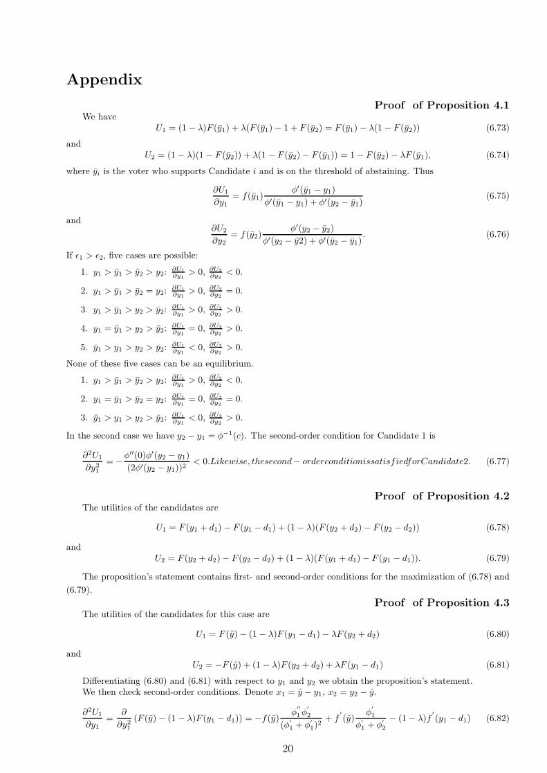
Proof of Proposition 4.1We have

U1 = (1 − λ)F (y1) + λ(F (y1) − 1 + F (y2) = F (y1) − λ(1 − F (y2)) (6.73)

andU2 = (1 − λ)(1 − F (y2)) + λ(1 − F (y2) − F (y1)) = 1 − F (y2) − λF (y1), (6.74)

where yi is the voter who supports Candidate i and is on the threshold of abstaining. Thus

∂U1

∂y1= f(y1)

φ′(y1 − y1)

φ′(y1 − y1) + φ′(y2 − y1)(6.75)

and∂U2

∂y2= f(y2)

φ′(y2 − y2)

φ′(y2 − y2) + φ′(y2 − y1). (6.76)

If ǫ1 > ǫ2, five cases are possible:

1. y1 > y1 > y2 > y2:∂U1

∂y1> 0, ∂U2

∂y2< 0.

2. y1 > y1 > y2 = y2:∂U1

∂y1> 0, ∂U2

∂y2= 0.

3. y1 > y1 > y2 > y2:∂U1

∂y1> 0, ∂U2

∂y2> 0.

4. y1 = y1 > y2 > y2:∂U1

∂y1= 0, ∂U2

∂y2> 0.

5. y1 > y1 > y2 > y2:∂U1

∂y1< 0, ∂U2

∂y2> 0.

None of these five cases can be an equilibrium.

1. y1 > y1 > y2 > y2:∂U1

∂y1> 0, ∂U2

∂y2< 0.

2. y1 = y1 > y2 = y2:∂U1

∂y1= 0, ∂U2

∂y2= 0.

3. y1 > y1 > y2 > y2:∂U1

∂y1< 0, ∂U2

∂y2> 0.

In the second case we have y2 − y1 = φ−1(c). The second-order condition for Candidate 1 is

∂2U1

∂y21

= −φ′′(0)φ′(y2 − y1)

(2φ′(y2 − y1))2< 0.Likewise, thesecond− orderconditionissatisfiedforCandidate2. (6.77)

Proof of Proposition 4.2The utilities of the candidates are

U1 = F (y1 + d1) − F (y1 − d1) + (1 − λ)(F (y2 + d2) − F (y2 − d2)) (6.78)

andU2 = F (y2 + d2) − F (y2 − d2) + (1 − λ)(F (y1 + d1) − F (y1 − d1)). (6.79)

The proposition’s statement contains first- and second-order conditions for the maximization of (6.78) and

(6.79).

Proof of Proposition 4.3The utilities of the candidates for this case are

U1 = F (y) − (1 − λ)F (y1 − d1) − λF (y2 + d2) (6.80)

andU2 = −F (y) + (1 − λ)F (y2 + d2) + λF (y1 − d1) (6.81)

Differentiating (6.80) and (6.81) with respect to y1 and y2 we obtain the proposition’s statement.We then check second-order conditions. Denote x1 = y − y1, x2 = y2 − y.

∂2U1

∂y1=

∂

∂y21

(F (y) − (1 − λ)F (y1 − d1)) = −f(y)φ

′′

1φ′

2

(φ′

1 + φ′

1)2

+ f′

(y)φ

′

1

φ′

1 + φ′

2

− (1 − λ)f′

(y1 − d1) (6.82)

20

and

∂2U2

∂y2=

∂

∂y22

((1 − λ)F (y2 + d2) − F (y)) = −f(y)φ

′′

2φ′

1

(φ′

1 + φ′

2)2

+ f′

(y)φ

′

2

φ′

1 + φ′

2

+ (1 − λ)f′

(y2 + d2). (6.83)

If the second set of equilibrium conditions are satisfied, then the second derivatives are negative.

Proof of Corollary 4.3Let

G =

f(y) φ′(y−y1)φ′(y−y1)+φ′(y2−y)

− f(y1 − d)

f(y) φ′(y2−y)φ′(y−y1)+φ′(y2−y)

− f(y2 + d)

ǫ− φ(y − y1) + φ(y2 − y)

. (6.84)

Denote f = f(y), f ′ = f ′(y), f1 = f(y1), f2 = f(y2), φ1 = φ(y − y1), φ2 = φ(y2 − y),

V = ( y1 y2 y ) (6.85)

andP = ( f1 f2 f ǫ d λ ) . (6.86)

If the equilibrium conditions (4.22), (4.23), and (4.24) are satisfied, then we have

G(V, P ) =

000

. (6.87)

According to the implicit function theorem, we must have

∂V

∂P= −

(

∂G

∂V

)−1∂G

∂P. (6.88)

We have:

∂G

∂V=

− fφ′′

1φ′

2

(φ′

1+φ

′

2)2

− fφ′

1φ′′

2

(φ′

1+φ

′

2)2

f′

φ′

1

φ′

1+φ

′

2

+f(φ′

1φ′′

2+φ′

2φ′′

1)

(φ′

1+φ

′

2)2

fφ′′

1φ′

2

(φ′

1+φ

′

2)2

fφ′

1φ′′

2

(φ′

1+φ

′

2)2

f′

φ′

2

φ′

1+φ

′

2

− f(φ′

1φ′′

2+φ′

2φ′′

1)

(φ′

1+φ

′

2)2

φ′

1 φ′

2 −(φ′

1 + φ′

2)

, (6.89)

∂G

∂P=

−(1 − λ) 0φ′

1

φ′

1+φ

′

2

0 0 f1

0 −(1 − λ)φ′

2

φ′

1+φ

′

2

0 0 f2

0 0 0 1 0 0

, (6.90)

(

∂G

∂V

)−1

=

fL−f ′φ′2

2(φ′

1+φ′

2)

f f ′L

fL−f ′φ′

1φ′

2(φ′

1+φ′

2)

f f ′L−φ′

1φ′

2

L

fL+f ′φ′

1φ′

2(φ′

1+φ′

2)

f f ′L

fL−f ′φ′2

2(φ′

1+φ′

2)

f f ′L

φ′

1φ′

2

L

1f ′

1f ′

0

, (6.91)

whereL = φ′′1φ

′22 − φ′′2φ

′21 . (6.92)

According to the implicit function theorem, we must have

∂V

∂P= −

(

∂G

∂V

)

∂G

∂P(6.93)

at V that is the solution to the equilibrium conditions (4.22), (4.23), (4.24). This gives us

∂y1

∂f1= −1 − λ

f ′+

(1 − λ)φ′22 (φ′1 + φ′2)

fL, (6.94)

∂y2

∂f1= −1 − λ

f ′− (1 − λ)φ′1φ

′2(φ

′1 + φ′2)

fL, (6.95)

∂(y2 − y1)

∂f1=

−(1 − λ)φ′2(φ′1 + φ′2)

2

fL, (6.96)

21

∂y

∂f1= −1 − λ

f ′, (6.97)

∂y1

∂f2=

1 − λ

f ′+

(1 − λ)φ′1φ′2(φ

′1 + φ′2)

fL, (6.98)

∂y2

∂f2= +

1 − λ

f ′− (1 − λ)φ′21 (φ′1 + φ′2)

fL, (6.99)

∂(y2 − y1)

∂f2= − (1 − λ)φ′1(φ

′1 + φ′2)

2

fL, (6.100)

∂y

∂f2=

1 − λ

f ′, (6.101)

∂y1

∂f= − 1

f ′, (6.102)

∂y2

∂f= − 1

f ′, (6.103)

∂(y2 − y1)

∂f= 0, (6.104)

∂y

∂f= − 1

f ′, (6.105)

∂y1

∂ǫ=φ′1φ

′2

L, (6.106)

∂y2

∂ǫ= −φ

′1φ

′2

L, (6.107)

∂(y2 − y1)

∂ǫ= −2

φ′1φ′2

L, (6.108)

∂y

∂ǫ= 0, (6.109)

∂y1

∂d= 0, (6.110)

∂y2

∂d= 0, (6.111)

∂(y2 − y1)

∂d= 0, (6.112)

∂y

∂d= 0, (6.113)

∂y1

∂λ= − f1 + f2

f ′, (6.114)

∂y2

∂λ= − f1 + f2

f ′, (6.115)

∂(y2 − y1)

∂λ= 0, (6.116)

∂y

∂λ= − f1 + f2

f ′. (6.117)

Proof of Proposition 4.4If the local Nash equilibrium we must have

∂U1

∂y1= f(y)

∂y

∂y1ψ(y2 − y1) − F (y)ψ′(y2 − y1) = 0 (6.118)

22

and∂U2

∂y2= −f(y)

∂y

∂y2ψ(y2 − y1) + (1 − F (y))ψ′(y2 − y1) = 0. (6.119)

Subtracting the two equations we obtain

f(y)ψ(y2 − y1)

(

∂y

∂y1+

∂y

∂y2

)

− ψ′(y2 − y1) = 0. (6.120)

We have∂y

∂y1=

φ′(y − y1)

φ′(y − y1) + φ′(y2 − y)(6.121)

and∂y

∂y2=

φ′(y2 − y)

φ′(y − y1) + φ′(y2 − y), (6.122)

so ∂y∂y1

+ ∂y∂y2

= 1 and

f(y)ψ(y2 − y1) − ψ′(y2 − y1) = 0. (6.123)

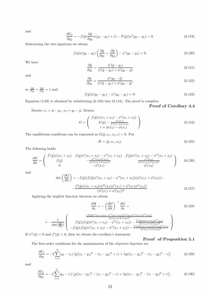
Equation (4.33) is obtained by substituting (6.123) into (6.118). The proof is complete.

Proof of Corollary 4.4Denote x1 = y − y1, x2 = y2 − y. Denote

G =

f(y)ψ(x1 + x2) − ψ′(x1 + x2)

F (y) − φ′(x1)φ′(x1)+φ′(x2)

ǫ+ φ(x2) − φ(x1)

(6.124)

The equilibrium conditions can be expressed as G(y, x1, x2, ǫ) = 0. Put

H = (y, x1, x2). (6.125)

The following holds:

∂G

∂h=

f ′(y)ψ(x1 + x2) f(y)ψ′(x1 + x2) − ψ′′(x1 + x2) f(y)ψ′(x1 + x2) − ψ′′(x1 + x2)

f(y) − φ′′(x1)φ′(x2)

(φ′(x1)+φ′(x2))2φ′′(x2)

(φ′(x1)+φ′(x2))2

0 −φ′(x1) φ′(x2)

(6.126)

and

det

(

∂G

∂h

)

= −f(y)(f(y)ψ′(x1 + x2) − ψ′′(x1 + x2))(φ′(x1) + φ′(x2))−

−f′(y)ψ(x1 + x2)(φ

′2(x2)φ′′(x1) + φ′(x1)φ

′′(x2))

(φ′(x1) + φ′(x2))2. (6.127)

Applying the implicit function theorem we obtain

∂H

∂ǫ= −

(

∂G

∂h

)−1∂G

∂ǫ= (6.128)

= − 1

det(∂G∂h

)

(f(y)ψ′(x1+x2)−ψ′′(x1+x2))(φ

′(x2)φ′′(x1)+φ

′′(x2))(φ′(x1)+φ′(x2))2

f(y)(f(y)ψ′(x1 + x2) − ψ′′(x1 + x2)) − f ′(y)ψ(x1+x2)φ′′(x2)

(φ′(x1)+φ′(x2))2

−f(y)(f(y)ψ′(x1 + x2) − ψ′′(x1 + x2)) − f ′(y)ψ(x1+x2)φ′(x2)φ

′′(x1)(φ′(x1)+φ′(x2))2

.

If ψ′′(y) < 0 and f ′(y) > 0, then we obtain the corollary’s statement.

Proof of Proposition 5.1The first-order conditions for the maximization of the objective function are

∂U1

∂y1= −2

N∑

i=1

(y1 − vi)[

g((vi − y1)2 − (vi − y2)

2 + c) + λg((vi − y1)2 − (vi − y2)

2 − c)]

(6.129)

and

∂U2

∂y2= −2

N∑

i=1

(y2 − vi)[

g((vi − y1)2 − (vi − y2)

2 − c) + λg((vi − y1)2 − (vi − y2)

2 + c)]

. (6.130)

23

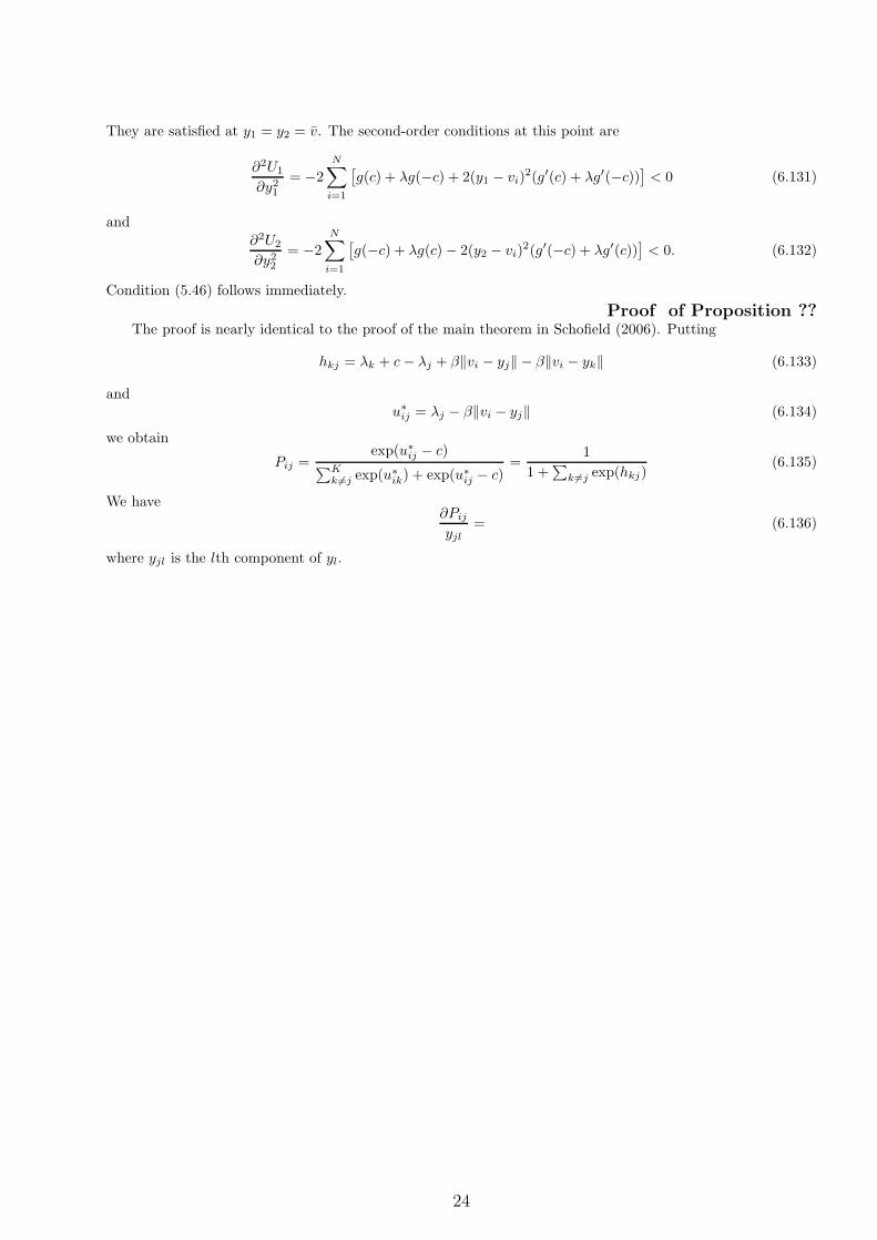
They are satisfied at y1 = y2 = v. The second-order conditions at this point are

∂2U1

∂y21

= −2

N∑

i=1

[

g(c) + λg(−c) + 2(y1 − vi)2(g′(c) + λg′(−c))

]

< 0 (6.131)

and

∂2U2

∂y22

= −2

N∑

i=1

[

g(−c) + λg(c) − 2(y2 − vi)2(g′(−c) + λg′(c))

]

< 0. (6.132)

Condition (5.46) follows immediately.

Proof of Proposition ??The proof is nearly identical to the proof of the main theorem in Schofield (2006). Putting

hkj = λk + c− λj + β‖vi − yj‖ − β‖vi − yk‖ (6.133)

andu∗ij = λj − β‖vi − yj‖ (6.134)

we obtain

Pij =exp(u∗ij − c)

∑Kk 6=j exp(u∗ik) + exp(u∗ij − c)

=1

1 +∑

k 6=j exp(hkj)(6.135)

We have∂Pij

yjl= (6.136)

where yjl is the lth component of yl.

24

References

[1] Adams, James, Jay Dow, and Samuel Merrill III. 2006. “The Political Consequences ofAlienation-Based and Indifference-Based Voter Abstention: Applications to PresidentialElections.” Political Behavior 28(1): 65–86

[2] Aldrich, John. 1993. “Rational Choice and Turnout.” American Journal of Political Science37(1): 246–278

[3] Ansolabehere, Stephen, and James M. Snyder, Jr. 2000. “Valence Politics and Equilibriumin Spatial Elections Model.” Public Choice 103: 327–336

[4] Aragones, Enriqueta, and Thomas R. Palfrey. 2002. Mixed Equilibrium in a Downsian Modelwith a Favored Candidate. Journal of Economic Theory, 103(1): 131-161

[5] Brody, Richard A., and Benjamin J. Page. 1973. “Indifference, Alienation, and RationalDecisions: The Effects of Candidate Evaluations on Turnout and Vote.” Public Choice 15:1–17

[6] Calvert, R. (1985) Robustness of multidimensional voting model: Candidate motivations,uncertainty and convergence. American Journal of Political Science 29: 69–95

[7] Chamberlain, Gary, and Michael Rotschild. 1981. “A Note on the Probability of Casting aDecisive Vote.” Journal of Economic Theory 25: 152–162

[8] Coate, Steven, and Michael Conlin. 2004. “A Group Rule-Utilitarian Approach to VoterTurnout: Theory and Evidence.” The American Economic Review 94(5): 1476–1504

[9] Cox, Gary W., and Michael C. Munger. 1989. “Closeness, Expenditures, and Turnout inthe 1982 U.S. House Elections.” American Political Science Review 83(1): 217–231

[10] Downs, A. (1957) An economic theory of democracy. Hew York: Harper & Row

[11] Eldin, Aaron, Andrew Gelman, and Noah Kaplan. 2005. “Voting as a Rational Choice:The Effect of Preferences Regarding the Well-Being of Others.” Unpublished manuscript.

[12] Enelow, J. and Hinich, M. 1982. “Nonspatial candidate characteristics and electoral com-petition.” Journal of Politics 44: 115–130

[13] Enelow, J. and Hinich, M. 1984. “Probabilistic Voting and the Importance of CentristIdeologies in Democratic Elections.” Journal of Politics 459–478

[14] Feddersen, Timothy. 2004. “Rational Choice THeory and the Paradox of Not Voting.”Journal of Economic Perspectives 18(1): 99–112

[15] Feddersen, Timothy. 1992. “A Voting Model Implying Duverger’s Law and PositiveTurnout.” American Journal of Political Science 36(4): 938–962

[16] Feddersen, Timothy, and Wolfgang Pesendorfer. 1996. “The Swing Voter’s Curse.” Amer-ican Economic Review 86(3): 408–424

[17] Feddersen, Timothy, and Wolfgang Pesendorfer. 1999. “Abstention in Elections with Asym-metric Information and Diverse Preferences. ” The American Political Science Review 93(2):381–398

25

[18] Feddersen, Timothy J. and Alvaro Sandroni. 2002. “A Theory of Participation in Elec-tions.” Unpublished manuscript.

[19] Ferejohn, John A. and Fiorina, Morris P. 1974. “The Paradox of not Voting: A DecisionTheoretic Analysis” The American Political Science Review 68: 525–536

[20] Gelman, A. and King, G. 1990 “Estimating incumbency advantage without bias.” Ameri-can Journal of Political Science 34: 1142–1164

[21] Geys, Benny. 2006. “Explaining Voter Turnout: A Review of Aggregate-Level Research.”Unpublished manuscript.

[22] Grafstein, Rodert. 1990. “An Evidential Decision Theory of Turnout.” Americn Journalof Political Science 35(4): 989–1010

[23] Groceclose, T. (2001) A model of candidate location when one candidate has a valenceadvantage. Americn Journal of Political Science 45(5): 862–886

[24] Harsanui, John D. 1980. “Rule Utilitarianism, Rights, Obligations and the Theory ofRational Behavior.” Theory and Decision 12(1), 115–133

[25] Hinich, M., Ledyard, J., and Ordeshook, P. (1972a) Nonvoting and the existence of equi-librium under majority rule. Journal of Economic Theory 4: 144–153

[26] Kanasawa, Satoshi. 1998. “A Possible Solution to the Paradox of Voter Turnout.” Journalof Politics 60(4): 974–995

[27] Kirchgassner, Gebhard. 2000. “Probabilistic Voting and Equilibrium: An ImpossibilityResult.” Public Choice 103: 35–48

[28] Kirchgassner, Gebhard. 2003. Abstention Because of Indifference and Alienation, and ItsConsequences for Party Competition: A Simple Psychological Model. University of St. GallenDepartment of Economics working paper series 2003 2003-12, Department of Economics,University of St. Gallen.

[29] Kirchgasser, Gebhard, and Anne M. Zu Himmern. 1997. “Expected Closeness and Turnout:An Empirical Analysis for the Genman General Elections, 1983–1994. Public Choice 91: 3–25

[30] Lijphart, Arend. 1997. “Unequal Participation: Democracy’s Unresolved Dilemma.” TheAmerican Political Science Review 91(1), 1–14

[31] Ledyard, John. 1984. “The Pure Theory of Large Two-Candidate Elections.” Public Choice44: 7–41

[32] Leighley, Jan. 1996. “Group Membership and the Mobilization of Political Participation.”Jounal of Politics 58: 447–463

[33] Morton, Rebecca B. 1991. ”Groups in Rational Turnout Models.” Americn Journal ofPolitical Science 35(3): 758–776

[34] Mueller, Dennis. 2003. Public Choice III. Cambridge: Cambridge University Press.

[35] Myerson, Roger. 2000. “Large Poisson Games.” Journal of Economic Theory 94(1): 7–45

26

[36] Palfrey, Thomas R., and Howard Rosenthal. 1983. “A Strategic Calculus of Voting”. PublicChoice 41: 7–53

[37] Palfrey, Thomas R., and Howard Rosenthal. 1985. “Voter Participation and StrategicUncertainty”. The American Political Science Review 79: 62–78

[38] Plane, Dennis L., and Joseph Gershtenson. 2004. “Candidate’s ideological locations, ab-stention, and turnout in US midterm Senate elections” Political Behavior 26: 69–93

[39] Riker, William H., and Peter C. Ordeshook. 1968. “A Theory of the Calculus of Voting”.American Political Schence Review 62: 25–42

[40] Stokes, D. (1963) Spatial models of party competition. American Political Science Review57: 368-77

[41] Thurder, Paul W., and Eymann, A. 2000. “Policy-Specific Alienation and Indifference inthe Calculus of Voting: A Simultaneous Model of Party Choice and Abstention”. PublicChoice 102: 51–77

[42] Uhlaner, Carole J. 1989. “Rational Turnout: The Neglected Role of Groups.” AmericnJournal of Political Science 33(2): 390–422

[43] Zakharov, Alexei V. 2005. “Candidate Location and Endogenous Valence.” EERC No.05/17

[44] Zakharov, Alexei V. 2006. “Policy divergence in spatial voting models.” Unpublishedmanuscript.

[45] Zipp, John F. 1985. “Perceived Representativeness and Voting: An Assessment of theImpact of “Choices” vs. “Echoes”. American Political Science Review 79: 50–61

27