Propagating annular modes - Oceans at MIT
17
Propagating annular modes Aditi Sheshadri (Columbia University) R. Alan Plumb (MIT)
Transcript of Propagating annular modes - Oceans at MIT

Propagating annular modes
Aditi Sheshadri (Columbia University)
R. Alan Plumb (MIT)
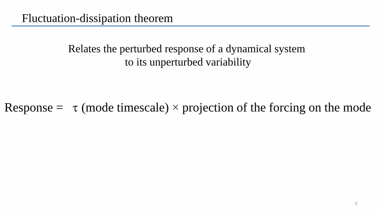
Fluctuation-dissipation theorem
Relates the perturbed response of a dynamical system
to its unperturbed variability
2
Response = (mode timescale) × projection of the forcing on the mode

Dynamical climate responses and the fluctuation-dissipation theorem
Kushner (2010)
GHG
Kushner et al. 2001
Ozone hole
Thompson and Solomon 2002

Model setup
• Dry, hydrostatic, global primitive equation model (based onPolvani and Kushner, 2002), T42, 40 levels
• Replaces radiation and convection schemes with relaxationto a zonally symmetric Teq, that is similar to Held Suarez inthe troposphere
• In the stratosphere (above 200 hPa), equilibriumtemperature set to U. S. Standard atmosphere, except overthe winter pole, where a cold anomaly provides arepresentation of the polar vortex
• Simple seasonal cycle in equilibrium temperature that isconfined to the stratosphere
4
Latitude
Pre
ssu
re
-50 0 50
1
3
10
32
100
320 150
200
250
300
Teq at NH winter solstice

Polar stratospheric cooling
2
2
0
2
2
0
2
2
00
22
ln7000ln7000
2exp,,
t
ttqtQ
Similar to Butler et al. 2010 and Sun et al. 2014, but with
dayKq /5.00 2/0 28.0 05.00
4000 t0= October 2020t
5
(We’ll vary this)
Temperature difference averaged over the polar cap (65-90S)
Month
Pre
ssure
S O N D J F M
10
32
100
320
925-15
-10
-5
0
5
Months
Pre
ssu
re
J F M A M J J A S O N D
1
3
10
32
100
320
925 -1
-0.8
-0.6
-0.4
-0.2
0
Month
La
titu
de
J F M A M J J A S O N D
-80
-60
-40
-20
-1
-0.8
-0.6
-0.4
-0.2
0
50 hPa
Averaged 65-90S

Tropospheric circulation changes
6
Month
Pre
ssu
re
S O N D J F M
10
32
100
320
925 -800
-600
-400
-200
0Geopotential height difference averaged over the polar cap (65-90S)
Month
La
titu
de
J F M A M J J A S O N D
-80
-60
-40
-20
-4
-2
0
2
4
850 hPa [u] response
-2 0 2-90
-80
-70
-60
-50
-40
-30
-20
-10
0Dec
Lati
tude
-2 0 2-90
-80
-70
-60
-50
-40
-30
-20
-10
0Jan
-2 0 2-90
-80
-70
-60
-50
-40
-30
-20
-10
0Feb
-2 0 2-90
-80
-70
-60
-50
-40
-30
-20
-10
0Mar
850 hPa [u] response doesn’t always match the
first annular mode!
EOF1
Response

7
Surface responses to all year cooling – involves 2 EOFs
• Large dipole response early in the year
• Minimum, poleward shifted response in
SON
-5 0 5-90
-80
-70
-60
-50
-40
-30
-20
-10
0JFMAM
-5 0 5-90
-80
-70
-60
-50
-40
-30
-20
-10
0JAS
Almost all the response explained
by sum of contributions from 2
EOFs
Month
La
titu
de
J A S O N D J F M A M J
-80
-60
-40
-20
-4
-2
0
2
4
EOF1
EOF2
Response
EOF1+2

8
Seasonal cycle of annular mode timescales
• Seasonality in tropospheric (in the control
run) induced by lower stratospheric
seasonality
• If the projection of the forcing on the
modes does not change through the year,
the response in mode 2, relative to 1 would
change by a factor of 2 over the year
J A S O N D J F M A M J5
10
15
20
25
30
35
Month
in
da
ys
Month
La
titu
de
J A S O N D J F M A M J
-80
-60
-40
-20
-4
-2
0
2
4
(EOF1)
(EOF2)

Summary – tropospheric response to ozone depletion
• Stratospheric seasonal cycle leads to seasonal changes in the persistence
of the tropospheric mid-latitude jet and storm tracks
• The response of the atmosphere to external forcing cannot be described
by a single “annular mode”!
(cf. Black and McDaniel 2007a,b)
J A S O N D J F M A M J5
10
15
20
25
30
35
Month
in
da
ys
-5 0 5-90
-80
-70
-60
-50
-40
-30
-20
-10
0JFMAM
-5 0 5-90
-80
-70
-60
-50
-40
-30
-20
-10
0JAS
Sheshadri and Plumb 2016a 9

• Principal Oscillation Patterns (POPs) are the true modes
e.g. Von Storch (1988), Penland (1989)
they contain dynamical information, and can be used to extract both spatial patterns and timescales. If EOFs were all independent, POPs would look like EOFs.
• Let’s simplify the problem, and look at a perpetual winter situation
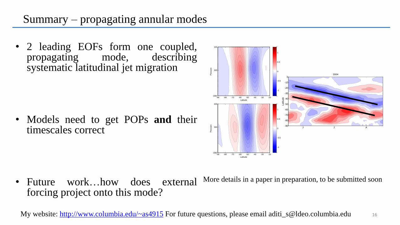
Are the model’s two leading EOFs actually one mode describing systematic latitudinal migrations of the jet?
Two leading EOFs actually one propagating mode?
10
1
0
CCG
TWVG

11
PCs of two leading EOFs show lagged cross-correlation
2 leading EOFs explain 40% and 29% of
variance, with = 19 and 13 days
Pre
ssure
Latitude
-80 -70 -60 -50 -40 -30
100
320
925
-1
-0.5
0
0.5
1
Pre
ssure
Latitude
-80 -70 -60 -50 -40 -30
100
320
925
-1
-0.5
0
0.5
1
-60 -40 -20 0 20 40 60-0.2
0
0.2
0.4
0.6
0.8
1
1.2
Lags
-60 -40 -20 0 20 40 60-0.4
-0.3
-0.2
-0.1
0
0.1
0.2
0.3
Lags

Complex conjugate eigenvalues/eigenvectors imply propagation
POP, (Re/Im) Γ=0.3574±0.4818i
12
2 leading EOFs explain 40% and 29% of
variance, with = 19 and 13 days
Pre
ssure
Latitude
-80 -70 -60 -50 -40 -30
100
320
925
-1
-0.5
0
0.5
1
Pre
ssure
Latitude
-80 -70 -60 -50 -40 -30
100
320
925
-1
-0.5
0
0.5
1
Pre
ssure
Latitude
-80 -70 -60 -50 -40 -30
100
320
925
-1
-0.5
0
0.5
1
Pre
ssure
Latitude
-80 -70 -60 -50 -40 -30
100
320
925
-1
-0.5
0
0.5
1
Gives a decay time of 39 days, and a period of
134.8 days (recovers the lag at which cross-
correlation maximizes)

Poleward propagation of wind anomalies
Days
La
titu
de
100 200 300 400 500 600 700 800 900 1000
-80
-60
-40
-20
Days
La
titu
de
100 200 300 400 500 600 700 800 900 1000
-80
-60
-40
-20
[u] anomalies integrated through the
troposphere show consistent poleward
propagation.. (cf. Feldstein 1998)
and are well captured by the first 2 EOFs
13

-60 -40 -20 0 20 40 60-0.2
-0.15
-0.1
-0.05
0
0.05
0.1
0.15
0.2
Lags
14
ERA-I consistent with this picture
2 leading EOFs explain 37% and 19% of
variance, with = 11 and 8 days
La
titu
de
2004
J J A-90
-80
-70
-60
-50
-40
-30
-20
-10
0
PCs are not
independent
Poleward propagation of
[u] anomalies
Pre
ssure
Latitude
-90 -80 -70 -60 -50 -40 -30 -20
100
300
1000
-1
-0.5
0
0.5
1
Pre
ssure
Latitude
-90 -80 -70 -60 -50 -40 -30 -20
100
300
1000
-1
-0.5
0
0.5
1
Pre
ssure
Latitude
-90 -80 -70 -60 -50 -40 -30 -20
100
300
1000
-1
-0.5
0
0.5
1
Pre
ssure
Latitude
-90 -80 -70 -60 -50 -40 -30 -20
100
300
1000
-1
-0.5
0
0.5
1

POPs are independent of pressure weighting
Pre
ssure
Latitude
-80 -70 -60 -50 -40 -30
1
3
10
32
100
320
925
-1
-0.5
0
0.5
1
Pre
ssure
Latitude
-80 -70 -60 -50 -40 -30
1
3
10
32
100
320
925
-1
-0.5
0
0.5
1
EOF1 weighted
EOF2 weighted
Pre
ssure
Latitude
-80 -70 -60 -50 -40 -30
1
3
10
32
100
320
925
-0.25
-0.2
-0.15
-0.1
-0.05
0
0.05
0.1
0.15
0.2
0.25
Pre
ssure
Latitude
-80 -70 -60 -50 -40 -30
1
3
10
32
100
320
925
-0.25
-0.2
-0.15
-0.1
-0.05
0
0.05
0.1
0.15
0.2
0.25
EOF1 unweighted
EOF2 unweighted
Pre
ssure
Latitude
-80 -70 -60 -50 -40 -30
1
3
10
32
100
320
925
-1
-0.5
0
0.5
1
Pre
ssure
Latitude
-80 -70 -60 -50 -40 -30
1
3
10
32
100
320
925
-1
-0.5
0
0.5
1
Re (POP) weighted/unweighted
Im (POP) weighted/unweighted
15
16
Summary – propagating annular modes
• 2 leading EOFs form one coupled,propagating mode, describingsystematic latitudinal jet migration
• Models need to get POPs and theirtimescales correct
• Future work…how does externalforcing project onto this mode?
La
titu
de
2004
J J A-90
-80
-70
-60
-50
-40
-30
-20
-10
0
More details in a paper in preparation, to be submitted soon
My website: http://www.columbia.edu/~as4915 For future questions, please email [email protected]
ressure
Latitude
-90 -80 -70 -60 -50 -40 -30 -20
100
300
1000
-1
-0.5
0
0.5
1
Pre
ssure
Latitude
-90 -80 -70 -60 -50 -40 -30 -20
100
300
1000
-1
-0.5
0
0.5
1

Pre
ssure
Latitude
-80 -60 -40 -20
200
400
600
800
925 -4
-2
0
2
4
Pre
ssure
Latitude
-80 -60 -40 -20
200
400
600
800
925 -4
-2
0
2
4
Pre
ssure
Latitude
-80 -60 -40 -20
200
400
600
800
925 -4
-2
0
2
4
Frequency-dependent barotropic/baroclinic modes
Regressions of heat flux on..
(cf. Thompson and Woodworth, Thompson and Barnes)
EOF 1 [u] EOF 1 LP [u] EOF 1 HP [u]
Sheshadri and Plumb 2016b (in review at J. Atmos. Sci.)
My website: http://www.columbia.edu/~as4915 For future questions, please email [email protected] 17