ProMAX VSP User Training Manualread.pudn.com/downloads272/sourcecode/math/1240848/VSP... ·...
304
ProMAX VSP User Training Manual copyright © 1999-2004 by Landmark Graphics Corporation Part No. 625321 Rev. B May 2004
Transcript of ProMAX VSP User Training Manualread.pudn.com/downloads272/sourcecode/math/1240848/VSP... ·...

ProMAX VSPUser Training Manual
copyright © 1999-2004 by Landmark Graphics Corporation
Part No. 625321 Rev. B May 2004

© 1999- 2004 Landmark Graphics CorporationAll Rights Reserved Worldwide
This publication has been provided pursuant to an agreement containing restrictions on its use. The publication is also protected by Federal copyright law. No part of this publication may be copied or distributed, transmitted, transcribed, stored in a retrieval system, or translated into any human or computer language, in any form or by any means, electronic, magnetic, manual, or otherwise, or
disclosed to third parties without the express written permission of:
Landmark Graphics CorporationBuilding 1, Suite 200, 2101 CityWest, Houston, Texas 77042, USA
P.O. Box 42806, Houston, Texas 77242, USAPhone:713-839-2000
Help desk: 713-839-2200FAX: 713-839-2401
Internet: www.lgc.com
Trademark Notice
3DFS, 3D Drill View, 3D Drill View KM, 3DView, 3D Surveillance, Active Field Surveillance, Active Reservoir Surveillance, ADC, Advanced Data Transfer, ARIES, Asset Development Center, Asset Development Centre, Asset Performance, AssetView, Atomic Meshing, BLITZ, BLITZPAK, CasingSeat, COMPASS, Corporate Data Archiver, Corporate Data Store, Data Manager,
DataStar, DBPlot, Decision Suite, Decisionarium, DecisionSpace, DecisionSpace AssetPlanner, DecisionSpace AssetView, DecisionSpace Atomic Meshing, DecisionSpace Decision Management Systems(DMS), DecisionSpace PowerGrid, DecisionSpace PowerModel, DecisionSpace PrecisionTarget, DecisionSpace Reservoir, DecisionSpace TracPlanner, DecisionSpace Well Seismic
Fusion, DepthTeam, DepthTeam Explorer, DepthTeam Express, DepthTeam Express3, DepthTeam Extreme, DepthTeam Interpreter, Desktop Navigator, DESKTOP-PVT, DESKTOP-VIP, DEX, DFW, DIMS, Discovery, Discovery Asset, Drill-to-the-
Earth Model, Drillability Suite, Drilling Desktop, DrillModel, DSS, Dynamic Reservoir Management, Dynamic Surveillance System, EarthCube, EDM, eLandmark, Engineer’s Data Model, Engineer's Desktop, Engineer’s Link, EOS-PAK, Executive Assistant, ezFault, ezSurface, ezTracker, FastTrack, FieldWorks, FZAP!, GeoDataLoad, GeoGraphix (stylized), GeoGraphix
Exploration System, GeoLink, GeoProbe, GeoProbe GF DataServer, GeoProbe Integrated, GES, GESXplorer, GMAplus, GRIDGENR, Handheld Field Operator, I2 Enterprise, iDIMS, IsoMap, Landmark, Landmark and Design, Landmark logo and Design, Landmark Decision Center, LandScape, Lattix, LeaseMap, LMK Resources, LogEdit, LogM, LogPrep, Magic Earth,
MagicDesk, MagicStation, MagicVision, Make Great Decisions, MathPack, MIRA, Model Builder, MyLandmark, OpenBooks, OpenExplorer, OpenJournal, OpenSGM, OpenVision, OpenWells, OpenWire, OpenWorks, OpenWorks Well File, PAL, Parallel-VIP, PetroBank, PetroWorks, PlotView, Point Gridding Plus, Pointing Dispatcher, PostStack, PostStack ESP, PowerCalculator, PowerExplorer, PowerHub, Power Interpretation, PowerJournal, PowerModel, PowerSection, PowerView, PRIZM, PROFILE, ProMAGIC, ProMAX, ProMAX 2D, ProMAX 3D, ProMAX 3DPSDM, ProMAX MVA, ProMAX VSP, pSTAx, QUICKDIF,
QUIKCDP, QUIKDIG, QUIKRAY, QUIKSHOT, QUIKVSP, RAVE, RAYMAP, RTOC, Real Freedom, Real-Time Asset Management Center, Real-Time Asset Management Centre, Real Time Knowledge Company, Real-Time Operations Center, Real Time Production Surveillance, Real Time Surveillance, RESev, ResMap, RMS, SafeStart, SCAN, SeisCube, SeisMap, SeisModel,
SeisSpace, SeisVision, SeisWell, SeisWorks, SeisXchange, Sierra, Sierra (design), SigmaView, SimResults, SIVA, Spatializer, SpecDecomp, StrataAmp, StrataMap, Stratamodel, StrataSim, StratWorks, StressCheck, STRUCT, Surf & Connect, SynTool,
System Start for Servers, SystemStart, SystemStart for Clients, SystemStart for Storage, T2B, TDQ, Team Workspace, TERAS, Total Drilling Performance, TOW/cs, TOW/cs The Oilfield Workstation, TracPlanner, Trend Form Gridding, Turbo Synthetics,
VIP, VIP-COMP, VIP-CORE, VIP-DUAL, VIP-ENCORE, VIP-EXECUTIVE, VIP-Local Grid Refinement, VIP-THERM, WavX, Web Editor, Web OpenWorks, Well Seismic Fusion, Wellbase, Wellbore Planner, Wellbore Planner Connect, WELLCAT,
WELLPLAN, WellXchange, WOW, Xsection, You're in Control. Experience the difference, ZAP!, and Z-MAP Plus are trademarks, registered trademarks or service marks of Landmark Graphics Corporation or Magic Earth, Inc.
All other trademarks are the property of their respective owners.
Note
The information contained in this document is subject to change without notice and should not be construed as a commitment by Landmark Graphics Corporation. Landmark Graphics Corporation assumes no responsibility for any error that may appear in this manual. Some states or jurisdictions do not allow disclaimer of expressed or implied warranties in certain transactions; therefore,
this statement may not apply to you.

Contents
Agenda . . . . . . . . . . . . . . . . . . . . . . . . . . . . . . . . . . . . . . . . . . . . . . . . . . . . . . . . . . . . . . . . . . xi
Agenda - Day 1. . . . . . . . . . . . . . . . . . . . . . . . . . . . . . . . . . . . . . . . . . . . . . . . . . . . . . . xi
Agenda Day 2 . . . . . . . . . . . . . . . . . . . . . . . . . . . . . . . . . . . . . . . . . . . . . . . . . . . . . . . xiii
Agenda Day 3 . . . . . . . . . . . . . . . . . . . . . . . . . . . . . . . . . . . . . . . . . . . . . . . . . . . . . . . xiv
Preface . . . . . . . . . . . . . . . . . . . . . . . . . . . . . . . . . . . . . . . . . . . . . . . . . . . . . . . . . . . . . . . . . . xv
About The Manual . . . . . . . . . . . . . . . . . . . . . . . . . . . . . . . . . . . . . . . . . . . . . . . . . . . . xv
Conventions. . . . . . . . . . . . . . . . . . . . . . . . . . . . . . . . . . . . . . . . . . . . . . . . . . . . . . . . . xvi
ProMAX User Interface . . . . . . . . . . . . . . . . . . . . . . . . . . . . . . . . . . . . . . . . . . . . . 1-1
Topics covered in this chapter: . . . . . . . . . . . . . . . . . . . . . . . . . . . . . . . . . . . . . . . . 1-1
ProMAX Menu Map . . . . . . . . . . . . . . . . . . . . . . . . . . . . . . . . . . . . . . . . . . . . . . . . . 1-2
Getting Started . . . . . . . . . . . . . . . . . . . . . . . . . . . . . . . . . . . . . . . . . . . . . . . . . . . . . . 1-3
Flow Building and Execution . . . . . . . . . . . . . . . . . . . . . . . . . . . . . . . . . . . . . . . . . 1-8
Sorting. . . . . . . . . . . . . . . . . . . . . . . . . . . . . . . . . . . . . . . . . . . . . . . . . . . . . . . . . . . . . 1-14
Interactivity of Trace Display . . . . . . . . . . . . . . . . . . . . . . . . . . . . . . . . . . . . . . 2-1
Topics to be covered in this chapter:. . . . . . . . . . . . . . . . . . . . . . . . . . . . . . . . . . . 2-1
Trace Display Window. . . . . . . . . . . . . . . . . . . . . . . . . . . . . . . . . . . . . . . . . . . . . . . 2-2
Icon Bar . . . . . . . . . . . . . . . . . . . . . . . . . . . . . . . . . . . . . . . . . . . . . . . . . . . . . . . . . . . . 2-4
Using Icons . . . . . . . . . . . . . . . . . . . . . . . . . . . . . . . . . . . . . . . . . . . . . . . . . . . . . . . . . 2-6
Interactive Data Access . . . . . . . . . . . . . . . . . . . . . . . . . . . . . . . . . . . . . . . . . . . . . 2-14
Landmark ProMAX VSP User Training Manual i
Contents
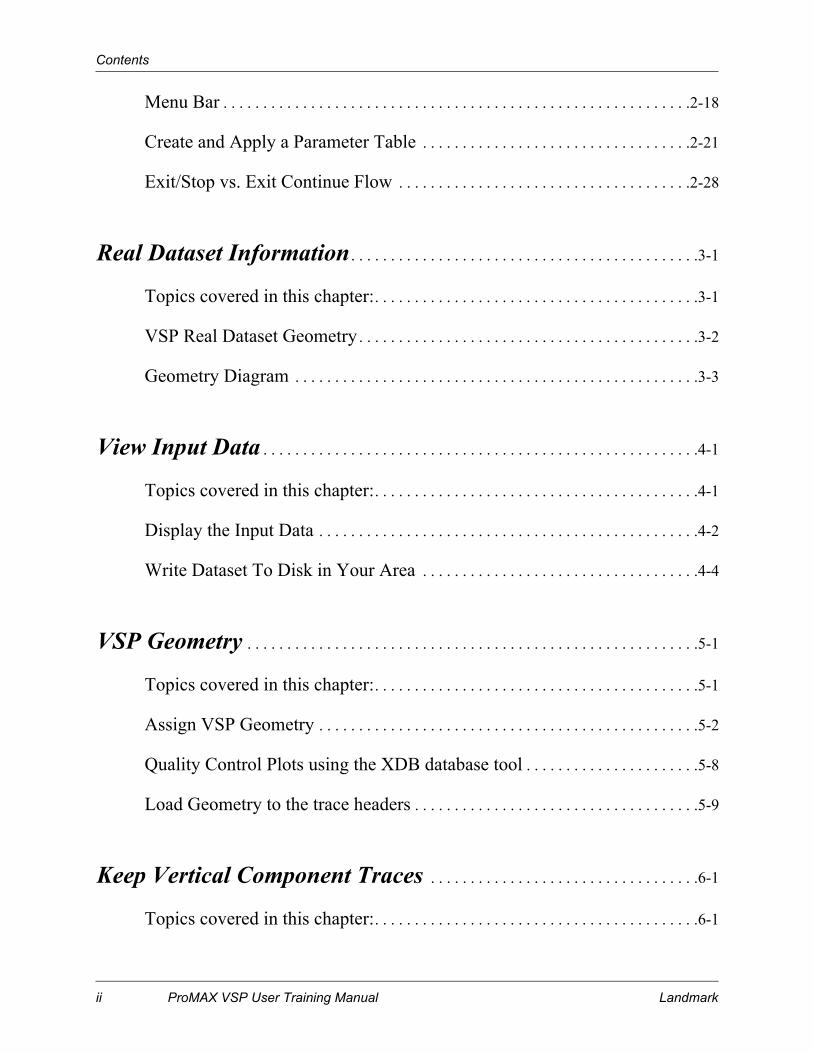
Menu Bar . . . . . . . . . . . . . . . . . . . . . . . . . . . . . . . . . . . . . . . . . . . . . . . . . . . . . . . . . . .2-18
Create and Apply a Parameter Table . . . . . . . . . . . . . . . . . . . . . . . . . . . . . . . . . .2-21
Exit/Stop vs. Exit Continue Flow . . . . . . . . . . . . . . . . . . . . . . . . . . . . . . . . . . . . .2-28
Real Dataset Information . . . . . . . . . . . . . . . . . . . . . . . . . . . . . . . . . . . . . . . . . . . .3-1
Topics covered in this chapter:. . . . . . . . . . . . . . . . . . . . . . . . . . . . . . . . . . . . . . . . .3-1
VSP Real Dataset Geometry . . . . . . . . . . . . . . . . . . . . . . . . . . . . . . . . . . . . . . . . . . .3-2
Geometry Diagram . . . . . . . . . . . . . . . . . . . . . . . . . . . . . . . . . . . . . . . . . . . . . . . . . . .3-3
View Input Data . . . . . . . . . . . . . . . . . . . . . . . . . . . . . . . . . . . . . . . . . . . . . . . . . . . . . . .4-1
Topics covered in this chapter:. . . . . . . . . . . . . . . . . . . . . . . . . . . . . . . . . . . . . . . . .4-1
Display the Input Data . . . . . . . . . . . . . . . . . . . . . . . . . . . . . . . . . . . . . . . . . . . . . . . .4-2
Write Dataset To Disk in Your Area . . . . . . . . . . . . . . . . . . . . . . . . . . . . . . . . . . .4-4
VSP Geometry . . . . . . . . . . . . . . . . . . . . . . . . . . . . . . . . . . . . . . . . . . . . . . . . . . . . . . . . .5-1
Topics covered in this chapter:. . . . . . . . . . . . . . . . . . . . . . . . . . . . . . . . . . . . . . . . .5-1
Assign VSP Geometry . . . . . . . . . . . . . . . . . . . . . . . . . . . . . . . . . . . . . . . . . . . . . . . .5-2
Quality Control Plots using the XDB database tool . . . . . . . . . . . . . . . . . . . . . .5-8
Load Geometry to the trace headers . . . . . . . . . . . . . . . . . . . . . . . . . . . . . . . . . . . .5-9
Keep Vertical Component Traces . . . . . . . . . . . . . . . . . . . . . . . . . . . . . . . . . .6-1
Topics covered in this chapter:. . . . . . . . . . . . . . . . . . . . . . . . . . . . . . . . . . . . . . . . .6-1
ii ProMAX VSP User Training Manual Landmark

Contents
Trap Vertical Traces . . . . . . . . . . . . . . . . . . . . . . . . . . . . . . . . . . . . . . . . . . . . . . . . . 6-2
Output a file with vertical traces only. . . . . . . . . . . . . . . . . . . . . . . . . . . . . . . . . . 6-4
First Break Picks on Vertical Traces . . . . . . . . . . . . . . . . . . . . . . . . . . . . . 7-1
Topics covered in this chapter: . . . . . . . . . . . . . . . . . . . . . . . . . . . . . . . . . . . . . . . . 7-1
Pick First Breaks . . . . . . . . . . . . . . . . . . . . . . . . . . . . . . . . . . . . . . . . . . . . . . . . . . . . 7-2
QC the First Breaks in the Database using XDB . . . . . . . . . . . . . . . . . . . . . . . . 7-4
VSP Velocity Functions . . . . . . . . . . . . . . . . . . . . . . . . . . . . . . . . . . . . . . . . . . . . . 8-1
Topics covered in this chapter: . . . . . . . . . . . . . . . . . . . . . . . . . . . . . . . . . . . . . . . . 8-1
Generate Average Velocity vs. Depth and Smooth. . . . . . . . . . . . . . . . . . . . . . 8-2
Compute an RMS Velocity Function . . . . . . . . . . . . . . . . . . . . . . . . . . . . . . . . . . 8-5
VSP True Amplitude Recovery. . . . . . . . . . . . . . . . . . . . . . . . . . . . . . . . . . . . . 9-1
Topics covered in this chapter: . . . . . . . . . . . . . . . . . . . . . . . . . . . . . . . . . . . . . . . . 9-1
True Amplitude Recovery Tests . . . . . . . . . . . . . . . . . . . . . . . . . . . . . . . . . . . . . . 9-2
Apply True Amplitude Recovery. . . . . . . . . . . . . . . . . . . . . . . . . . . . . . . . . . . . . . 9-5
VSP Wave Field Separation . . . . . . . . . . . . . . . . . . . . . . . . . . . . . . . . . . . . . . . 10-1
Topics covered in this chapter: . . . . . . . . . . . . . . . . . . . . . . . . . . . . . . . . . . . . . . . 10-1
Flatten the Downgoing with F-B Picks . . . . . . . . . . . . . . . . . . . . . . . . . . . . . . . 10-2
Flatten with F-B Picks and Event Alignment . . . . . . . . . . . . . . . . . . . . . . . . . . 10-4
Landmark ProMAX VSP User Training Manual iii

Contents
Compare Flattening Iterations . . . . . . . . . . . . . . . . . . . . . . . . . . . . . . . . . . . . . . . .10-8
Wavefield Separation with Median Filter . . . . . . . . . . . . . . . . . . . . . . . . . . . . .10-10
F-K Analysis . . . . . . . . . . . . . . . . . . . . . . . . . . . . . . . . . . . . . . . . . . . . . . . . . . . . . . .10-14
Wavefield Separation with F-K Filter . . . . . . . . . . . . . . . . . . . . . . . . . . . . . . . .10-17
Wavefield Separation with Eigenvector (K-L) Filter . . . . . . . . . . . . . . . . . . .10-20
Wavefield Separation Comparison Test . . . . . . . . . . . . . . . . . . . . . . . . . . . . . .10-24
Save the Upgoing Energy . . . . . . . . . . . . . . . . . . . . . . . . . . . . . . . . . . . . . . . . . . .10-26
Wavefield Separation to Keep Downgoing. . . . . . . . . . . . . . . . . . . . . . . . . . . .10-28
Save the Downgoing Energy . . . . . . . . . . . . . . . . . . . . . . . . . . . . . . . . . . . . . . . .10-31
QC plot of Separated Data. . . . . . . . . . . . . . . . . . . . . . . . . . . . . . . . . . . . . . . . . . .10-33
VSP Deconvolution . . . . . . . . . . . . . . . . . . . . . . . . . . . . . . . . . . . . . . . . . . . . . . . . . .11-1
Topics covered in this chapter:. . . . . . . . . . . . . . . . . . . . . . . . . . . . . . . . . . . . . . . .11-1
Picking the Decon Design Gate . . . . . . . . . . . . . . . . . . . . . . . . . . . . . . . . . . . . . . .11-2
Apply the mute for QC. . . . . . . . . . . . . . . . . . . . . . . . . . . . . . . . . . . . . . . . . . . . . . .11-3
Deconvolution Filter Design. . . . . . . . . . . . . . . . . . . . . . . . . . . . . . . . . . . . . . . . . .11-4
Deconvolution Filter QC . . . . . . . . . . . . . . . . . . . . . . . . . . . . . . . . . . . . . . . . . . . . .11-6
Deconvolution - Application to UpGoing . . . . . . . . . . . . . . . . . . . . . . . . . . . . . .11-7
Spectral Analysis Before and After Decon . . . . . . . . . . . . . . . . . . . . . . . . . . . . .11-9
VSP Corridor Stack . . . . . . . . . . . . . . . . . . . . . . . . . . . . . . . . . . . . . . . . . . . . . . . . . .12-1
Topics covered in this chapter:. . . . . . . . . . . . . . . . . . . . . . . . . . . . . . . . . . . . . . . .12-1
iv ProMAX VSP User Training Manual Landmark

Contents
One Way Normal Moveout Correction . . . . . . . . . . . . . . . . . . . . . . . . . . . . . . . 12-2
Picking Corridor Mutes . . . . . . . . . . . . . . . . . . . . . . . . . . . . . . . . . . . . . . . . . . . . . 12-4
Apply the Corridor Mutes for QC . . . . . . . . . . . . . . . . . . . . . . . . . . . . . . . . . . . . 12-5
Produce the Corridor Stack . . . . . . . . . . . . . . . . . . . . . . . . . . . . . . . . . . . . . . . . . . 12-7
Splice the Corridor Stack into a Surface Stack. . . . . . . . . . . . . . . . . . . . . . . . 12-10
Generate Intv-Dpth Velocity Function . . . . . . . . . . . . . . . . . . . . . . . . . . 13-1
Topics covered in this chapter: . . . . . . . . . . . . . . . . . . . . . . . . . . . . . . . . . . . . . . . 13-1
Compute Interval Velocity vs. Depth . . . . . . . . . . . . . . . . . . . . . . . . . . . . . . . . . 13-2
VSP CDP Transform . . . . . . . . . . . . . . . . . . . . . . . . . . . . . . . . . . . . . . . . . . . . . . . 14-1
Topics covered in this chapter: . . . . . . . . . . . . . . . . . . . . . . . . . . . . . . . . . . . . . . . 14-1
VSP CDP Transform. . . . . . . . . . . . . . . . . . . . . . . . . . . . . . . . . . . . . . . . . . . . . . . . 14-2
VSP Migration . . . . . . . . . . . . . . . . . . . . . . . . . . . . . . . . . . . . . . . . . . . . . . . . . . . . . . . 15-1
Topics covered in this chapter: . . . . . . . . . . . . . . . . . . . . . . . . . . . . . . . . . . . . . . . 15-1
VSP Migration . . . . . . . . . . . . . . . . . . . . . . . . . . . . . . . . . . . . . . . . . . . . . . . . . . . . . 15-2
Display the VSP Migration . . . . . . . . . . . . . . . . . . . . . . . . . . . . . . . . . . . . . . . . . . 15-3
VSP Report Generation . . . . . . . . . . . . . . . . . . . . . . . . . . . . . . . . . . . . . . . . . . . . 16-1
Topics covered in this chapter: . . . . . . . . . . . . . . . . . . . . . . . . . . . . . . . . . . . . . . . 16-1
VSP Report Generation . . . . . . . . . . . . . . . . . . . . . . . . . . . . . . . . . . . . . . . . . . . . . 16-2
Landmark ProMAX VSP User Training Manual v

Contents
VSP Corkscrew Geometry . . . . . . . . . . . . . . . . . . . . . . . . . . . . . . . . . . . . . . . . . .17-1
Topics covered in this chapter:. . . . . . . . . . . . . . . . . . . . . . . . . . . . . . . . . . . . . . . .17-1
Assign VSP Geometry . . . . . . . . . . . . . . . . . . . . . . . . . . . . . . . . . . . . . . . . . . . . . . .17-2
Quality Control Plots from the database . . . . . . . . . . . . . . . . . . . . . . . . . . . . . . .17-8
Pre Vertical Stack Dataset Information . . . . . . . . . . . . . . . . . . . . . . . . . .18-1
Topics covered in this chapter:. . . . . . . . . . . . . . . . . . . . . . . . . . . . . . . . . . . . . . . .18-1
VSP Prevertical Stack Dataset Geometry . . . . . . . . . . . . . . . . . . . . . . . . . . . . . .18-2
VSP Level Statics and Vertical Stack . . . . . . . . . . . . . . . . . . . . . . . . . . . . . . . . . . . . . . . . . . . . . . . . . . . . . . . . .19-1
Topics covered in this chapter:. . . . . . . . . . . . . . . . . . . . . . . . . . . . . . . . . . . . . . . .19-1
Plot the Traces . . . . . . . . . . . . . . . . . . . . . . . . . . . . . . . . . . . . . . . . . . . . . . . . . . . . . .19-2
Create Headers and QC Sorting . . . . . . . . . . . . . . . . . . . . . . . . . . . . . . . . . . . . . . .19-4
VSP Level Statics . . . . . . . . . . . . . . . . . . . . . . . . . . . . . . . . . . . . . . . . . . . . . . . . . . .19-6
Apply and QC the Level Statics. . . . . . . . . . . . . . . . . . . . . . . . . . . . . . . . . . . . . . .19-8
Vertically Stack Shots by Common Levels. . . . . . . . . . . . . . . . . . . . . . . . . . . . .19-9
3-Component Transform and First Break Picking . . . . . . . . . . . . . . . . . . . . . . . . . . . . . . . . . . . . . . . . . . . . . . . . . .20-1
Topics covered in this chapter:. . . . . . . . . . . . . . . . . . . . . . . . . . . . . . . . . . . . . . . .20-1
3-Component Transform and First Arrival Picking . . . . . . . . . . . . . . . . . . . . .20-2
Copying Picks from one Trace to the Others . . . . . . . . . . . . . . . . . . . . . . . . . . .20-5
vi ProMAX VSP User Training Manual Landmark

Contents
QC the Copied Picks . . . . . . . . . . . . . . . . . . . . . . . . . . . . . . . . . . . . . . . . . . . . . . . . 20-7
VSP 3-Component Orientation . . . . . . . . . . . . . . . . . . . . . . . . . . . . . . . . . . . 21-1
Topics covered in this chapter: . . . . . . . . . . . . . . . . . . . . . . . . . . . . . . . . . . . . . . . 21-1
3 Component Hodogram Analysis. . . . . . . . . . . . . . . . . . . . . . . . . . . . . . . . . . . . 21-2
Example Hodogram Analysis Plot. . . . . . . . . . . . . . . . . . . . . . . . . . . . . . . . . . . . 21-4
Example of Hodogram Output Trace Data . . . . . . . . . . . . . . . . . . . . . . . . . . . . 21-7
Salt Dome Synthetic VSP . . . . . . . . . . . . . . . . . . . . . . . . . . . . . . . . . . . . . . . . . . 22-1
Topics covered in this chapter: . . . . . . . . . . . . . . . . . . . . . . . . . . . . . . . . . . . . . . . 22-1
View the Model . . . . . . . . . . . . . . . . . . . . . . . . . . . . . . . . . . . . . . . . . . . . . . . . . . . . 22-2
Finite Difference Modeling for VSP. . . . . . . . . . . . . . . . . . . . . . . . . . . . . . . . . . 22-4
Geometry Spreadsheet . . . . . . . . . . . . . . . . . . . . . . . . . . . . . . . . . . . . . . . . . . . . . . 22-6
Load Geometry . . . . . . . . . . . . . . . . . . . . . . . . . . . . . . . . . . . . . . . . . . . . . . . . . . . . . 22-7
Isolate the Upgoing Data . . . . . . . . . . . . . . . . . . . . . . . . . . . . . . . . . . . . . . . . . . . . 22-8
Corridor Stack. . . . . . . . . . . . . . . . . . . . . . . . . . . . . . . . . . . . . . . . . . . . . . . . . . . . . 22-10
VSP-CDP Transform . . . . . . . . . . . . . . . . . . . . . . . . . . . . . . . . . . . . . . . . . . . . . . 22-11
VSP Migration . . . . . . . . . . . . . . . . . . . . . . . . . . . . . . . . . . . . . . . . . . . . . . . . . . . . 22-12
Add Well Location to VSP Data . . . . . . . . . . . . . . . . . . . . . . . . . . . . . . . . . . . . 22-14
Velocity Model with Migrated VSP Data . . . . . . . . . . . . . . . . . . . . . . . . . . . . 22-16
Finite Difference Model of 2D Seismic . . . . . . . . . . . . . . . . . . . . . . . . . . . . . . 22-17
Corridor Stack Spliced into 2D Stack. . . . . . . . . . . . . . . . . . . . . . . . . . . . . . . . 22-19
Landmark ProMAX VSP User Training Manual vii

Contents
VSP-CDP Transform Spliced into 2D Stack . . . . . . . . . . . . . . . . . . . . . . . . . .22-21
Appendix 1: ProMAX VSP System and Database Parameters23-
1
Topics covered in this chapter:. . . . . . . . . . . . . . . . . . . . . . . . . . . . . . . . . . . . . . . .23-1
Directory Structure . . . . . . . . . . . . . . . . . . . . . . . . . . . . . . . . . . . . . . . . . . . . . . . . . .23-2
ProMAX Data Directories . . . . . . . . . . . . . . . . . . . . . . . . . . . . . . . . . . . . . . . . . . . .23-7
Program Execution . . . . . . . . . . . . . . . . . . . . . . . . . . . . . . . . . . . . . . . . . . . . . . . . . .23-8
Ordered Parameter Files. . . . . . . . . . . . . . . . . . . . . . . . . . . . . . . . . . . . . . . . . . . . .23-15
Parameter Tables . . . . . . . . . . . . . . . . . . . . . . . . . . . . . . . . . . . . . . . . . . . . . . . . . . .23-20
Disk Datasets . . . . . . . . . . . . . . . . . . . . . . . . . . . . . . . . . . . . . . . . . . . . . . . . . . . . . .23-24
Tape Datasets . . . . . . . . . . . . . . . . . . . . . . . . . . . . . . . . . . . . . . . . . . . . . . . . . . . . . .23-28
Appendix 2: Archival Methods . . . . . . . . . . . . . . . . . . . . . . . . . . . . . . . . . . . .24-1
Topics covered in this chapter:. . . . . . . . . . . . . . . . . . . . . . . . . . . . . . . . . . . . . . . .24-1
SEG-Y Output . . . . . . . . . . . . . . . . . . . . . . . . . . . . . . . . . . . . . . . . . . . . . . . . . . . . . .24-2
Tape Data Ouput . . . . . . . . . . . . . . . . . . . . . . . . . . . . . . . . . . . . . . . . . . . . . . . . . . . .24-5
Archive to Tape . . . . . . . . . . . . . . . . . . . . . . . . . . . . . . . . . . . . . . . . . . . . . . . . . . . . .24-6
Appendix 3: Prepare Input Data . . . . . . . . . . . . . . . . . . . . . . . . . . . . . . . . . .25-1
Topics covered in this chapter:. . . . . . . . . . . . . . . . . . . . . . . . . . . . . . . . . . . . . . . .25-1
Preparing the Input Data . . . . . . . . . . . . . . . . . . . . . . . . . . . . . . . . . . . . . . . . . . . . .25-2
viii ProMAX VSP User Training Manual Landmark

Contents
Appendix 4: UNIX Workstation Basics . . . . . . . . . . . . . . . . . . . . . . . . . 26-1
Topics covered in this chapter: . . . . . . . . . . . . . . . . . . . . . . . . . . . . . . . . . . . . . . . 26-1
Text Editors in ProMAX . . . . . . . . . . . . . . . . . . . . . . . . . . . . . . . . . . . . . . . . . . . . 26-2
UNIX Commands . . . . . . . . . . . . . . . . . . . . . . . . . . . . . . . . . . . . . . . . . . . . . . . . . . 26-5
Examples of UNIX Commands . . . . . . . . . . . . . . . . . . . . . . . . . . . . . . . . . . . . . 26-15
Landmark ProMAX VSP User Training Manual ix

Contents
x ProMAX VSP User Training Manual Landmark

Agenda
Agenda - Day 1
Introductions, Course Agenda
ProMAX User Interface Overview
Trace Display Functionality
• Exercises to familiarize ourselves with Trace Display
System Overview Discussion
• Discussion of the ProMAX system architecture
Review of VSP Method and Our Main Dataset
SEGY Input and Display
Geometry
• Building the geometry database for VSP data
Landmark ProMAX VSP User Training Manual xi

Loading the Trace Headers
Keep Vertical Component Traces
First Break Picking
Velocity Function Generation
Velocity Function Manipulation
True Amplitude Recovery Testing
True Amplitude Recovery
Wavefield Separation Testing
• Flatten on direct arrivals
• Median Filter - FK Filter - Eigen Vector Filters
Agenda-xii ProMAX VSP User Training Manual Landmark

Agenda Day 2
Isolate the Upgoing Energy
• After choosing the desired wavefield separation technique we will iso-late the upgoing energy
Isolate the Downgoing Energy
• After choosing the desired wavefield separation technique we will iso-late the downgoing energy
Deconvolution
• Source signature removal filter design and application
Corridor Stack
Splicing the Corridor Stack into a Surface Stack
Generate Interval Velocity in Depth Function
VSP-CDP Transform
VSP Migration
VSP Report Generation
VSP Corkscrew Geometry
Look at Data for Level Statics and Level Summing
Level Statics
Level Summing (vertical stack)
Landmark ProMAX VSP User Training Manual xiii
Agenda Day 3
3-Component Transforms and First Break Picking
3-Component Hodogram Analysis
Synthetic VSP on Salt Dome Model with Full VSP Sequence
Cross Well Tomography Demonstration
Archive Methods
Agenda-xiv ProMAX VSP User Training Manual Landmark

Preface
About The Manual
This two volume manual is intended to accompany the instruction given during the standard ProMAX Seismic Processing and Analysis course. Because of the power and flexibility of ProMAX, it is unreasonable to attempt to cover all possible features and applications in this manual. Instead, we try to provide key examples and descriptions, using exercises which are directed toward common uses of the system.
The amount of material in the manuals exceeds what can be covered in a typical training course. This is intentional as it allows the instructor to tailor each class to the needs of the students by selecting the appropriate material.
After the class, you will find the manuals useful as a supplement to the online user manual.
How To Use The Manual
This manual is divided into chapters that discuss the key aspects of the ProMAX system. In general, chapters conform to the following outline:
• Introduction: A brief discussion of the important points of the topic and exercise(s) contained within the topic.
• Topics Covered in Chapter: Brief list of skills or processes in the order that they are covered in the exercise.
• Topic Description: More detail about the individual skills or processes covered in the chapter.
• Exercise: Details pertaining to each skill in an exercise, along with diagrams and explanations. Examples and diagrams will assist you during the course by minimizing note taking requirements and providing guidance through specific exercises.
Landmark ProMAX VSP User training Manual xv

Preface
This format allows you to glance at the topic description to either quickly reference an implementation or simply as a means of refreshing your memory on a previously covered topic. If you need more information, see the Exercise sections of each topic.
Conventions
Mouse Button Help
This manual does not refer to using mouse buttons unless they are specific to an operation. MB1 is used for most selections. The mouse buttons are numbered from left to right so:
MB1 refers to an operation using the left mouse button. MB2 is the middle mouse button. MB3 is the right mouse button.
Actions that can be applied to any mouse button include:
• Click: Briefly depress the mouse button.
• Double Click: Quickly depress the mouse button twice.
• Shift-Click: Hold the shift key while depressing the mouse button.
• Drag: Hold down the mouse button while moving the mouse.
Mouse buttons will not work properly if either Caps Lock or Nums Lock are on.
Exercise Organization
Each exercise consists of a series of steps that will build a flow, help with parameter selection, execute the flow, and analyze the results. Many of the steps give a detailed explanation of how to correctly pick parameters or use the functionality of interactive processes.
The editing flow examples list key parameters for each process of the exercise. As you progress through the exercises, familiar parameters will not always be listed in the flow example.
xvi ProMAX VSP User training Manual Landmark

Preface
The exercises are organized such that your dataset is used throughout the training session. Carefully follow the instructor’s direction when assigning geometry and checking the results of your flow. An improperly generated dataset or database may cause a subsequent exercise to fail.
Landmark ProMAX VSP User training Manual xvii

Preface
xviii ProMAX VSP User training Manual Landmark

Chapter 1
ProMAX User InterfaceThis chapter will get you started processing with ProMAX. You will learn how to set up a work space with the ProMAX User Interface, and then build and execute data processing flows.
Topics covered in this chapter:
o ProMAX Menu Map
o Getting Started
o Building a Workspace
o Flow Building and Execution
o Data Sorting
Landmark ProMAX VSP User Training Manual 1-1

Chapter 1: ProMAX User Interface
1-2 ProMAX VSP User Training Manual Landmark
ProMAX Menu Map

Chapter 1: ProMAX User Interface
Getting Started
ProMAX is built upon a three level organizational model referred to as Area/Line/Flow. When entering ProMAX for the first time, you will build your own Area/Line/Flow workspace. As you add your own Area, you may want to name it with reference to a geographic area that indicates where the data were collected, such as “Onshore Texas”, or use your name, such as “daves area”. Line is a subdirectory of Area which contains a list of 2D lines from an area, or the name of a 3D survey.
After choosing a line from the Line menu or adding a new line, the Flow window will appear. Name your flows according to the processing taking place, such as “brute stack”. For this course, we will also use a number, for example "01: Display shots".
Look at the Menu Map figure on the previous page. This figure refers to the menus we have just discussed, as well as other menus you will use to access your datasets, database, and parameter tables.
Building a Workspace
In this exercise, you will build a workspace and look at some of the functionality available within the user interface.
Initiating a ProMAX session is done in a variety of ways. Typically your system administrator will create a start-up script or make a UNIX alias, and set certain variables within your shell start-up script to make this easy. Starting ProMAX will not be discussed in this Essentials class. You will use a start-up script that has already been built.
1. Type promax
A product name window appears, followed by the Area menu that displays a list of all available Areas. Along the top of this window you will find the version number of the User Interface, the machine identification code, hostname, and license ID. The Areas are described by a user specified name, and a UNIX name. The UNIX name is a parsed version of the name you selected for the area. Capital letters, most punctuation, and spaces are removed in the parsing routine. This parsed name is the name of the actual UNIX directory. Other information is also listed, such as owner, date and the number of lines in each Area.
Landmark ProMAX VSP User Training Manual 1-3

Chapter 1: ProMAX User Interface
Area Menu
The black horizontal band below the menu displays mouse button help. Mouse button help describes the possible actions at the current location of the cursor, and gives brief parameter information during the flow building process.
Below the mouse button help line are options to Exit ProMAX, configure the queues and user interface, as well as check on the status of jobs.
• Config: Brings up settings which control how lists of Areas, Lines, Flows, Datasets, Parameter tables and Headers are sorted. Also controls nice values for running flows, the number of copies of flow output, where ProMAX UI restarts after exit and
Configuration OptionsJob Notificationand Control
Mouse Button Help Processing QueuesWindow
Area Menu
Global OptionsActive CommandAvailable areas
Exit Promax
1-4 ProMAX VSP User Training Manual Landmark

Chapter 1: ProMAX User Interface
popup behavior. Lastly, it allows you to specify the attributes dsplayed for Areas and Lines.
• Option: Brings up settings for debugging, compression, use of dataset headers for sorting, and locations of data, scratch space and the configuration file.
• Queue: Allows user to control batch processing queues.
• Exit: Will exit the User Interface, prompts to save if there is an unsaved flow.
• Notification: Gives information about jobs, and allows user to check job status.
The list of options running across the top of this menu: Select, Add, Delete, Rename, and Permission are called global options. To use these, you must first select the command, then select the Area name that you want the command to apply to. The Copy command works differently by providing popup menus to choose an Area to copy from.
2. Select Add from the Area Menu with MB1.
At this point you are building your work space. Adding an Area creates a UNIX directory.
3. Before moving the mouse, enter an Area name
Use your name for the area name. For example, “Mary’s area”.
4. Press return, or move the mouse to register your selection.
You can control whether moving the mouse registers the selection, or if you need to press return in the Config popup. Set the Popups remain after mouse leaves option to yes or no.
The Line Menu appears with the same global options to choose from as the Area Menu.
Landmark ProMAX VSP User Training Manual 1-5

Chapter 1: ProMAX User Interface
5. Add a Line using the same steps as you did for adding an Area. Name the line “Intro Line”
Line Menu
Global Options
Line Menu
Area Name
Available Seismic Lines
1-6 ProMAX VSP User Training Manual Landmark

Chapter 1: ProMAX User Interface
The Flow window appears with the following new global options:
• Datasets: Lists all your datasets for that particular line.
• Database: Allows you to view your Ordered Parameter Files.
• Tables: Allows you to view various Parameter Table Menus.
• Product: Changes from ProMAX 2D to ProMAX 3D or VSP.
6. Add a Flow and name it “01: Display Shots”.
Flow Menu
ChangeAccess
Available Flows
Flows Menu
AccessParameterTables
Database ProductsAccessDatasets
Landmark ProMAX VSP User Training Manual 1-7

Chapter 1: ProMAX User Interface
Flow Building and Execution
Now it is time to build a flow, and process data. In order to perform this you will need to tell ProMAX which processes you want to invoke, as well as provide specific details for each of these steps. Finally, there are different options available for executing a flow.
Build a Flow
Upon completion of the previous exercise, you are in the ProMAX flow building menu (see below). From here, you will construct flows by choosing processes and selecting the necessary parameter information. Once the flow is ready, you will execute it and view the results.
1. Look at the flow building menu.
Edit Flow Menu
Available Processes
Parameter Specification
Editable Flow
1-8 ProMAX VSP User Training Manual Landmark

Chapter 1: ProMAX User Interface
The screen is split into two sides: a list of processes on the right and a blank tablet below the global options on the left. To build a flow, you will select from the processes on the right and add them to the blank tablet on the left.
2. Move your cursor into different areas of the display, such as into the processes list, the blank tablet and the global options. Notice that the mouse button help is sensitive to the current cursor location.
3. Global Options for flow editing:
• Add: This is the default. When highlighted in blue, a process can be selected from the list of processes and added to the flow.
• Delete: When selected with MB1, the highlighted process is removed from the flow. This process is actually stored in a new kill buffer. Selecting Delete with MB2 appends a newly deleted process to the existing kill buffer. MB3 is used to insert (paste) the contents of this buffer into the current flow. The memory of the buffer is maintained even after exiting a flow menu, so the contents may be cut and pasted from one flow to another.
• Execute: When selected, the job is executed.
• There are two methods available to execute a flow using the Trace Display process:
MB1 and MB2 will execute the flow interactively. The mouse button help explaining the difference between MB1 and 2 does not apply to the Trace Display process. Either button will allow the display to immediately take over the monitor for display.
MB3 indicates Execute via Queue. This option enables the use of the two types of batch queues. When using MB3, a new menu pops up allowing the use of either the general batch queues or the small job batch queues. In order for this option to work, your system administrator must enable the queues whenProMAX 2D was installed.
• View: Accesses the view (job.output) file. This file includes important job information such as error statements.
• Exit: Leaves the edit flow menu, and returns you to the flow listing menu.
Landmark ProMAX VSP User Training Manual 1-9
Chapter 1: ProMAX User Interface
4. Move your cursor into the Data Input/Output portion of the processes list, and select the process “Disk Data Input” with MB1.
You have just added your first process to a flow.
The list of available processes is very long. It is ordered from top to bottom in a general processing sequence with I/O processes at the top and poststack migration tools further down on the list. There is a scroll bar to help you view the list.
There are also options available to hide processes in the secondary, or More list. By doing this, you can customize the list to only display the processes you use most often.
5. In the Data Input / Output category, click MB1 on the word “MORE”. Notice that a popup appears containing a list of secondary processes.
6. Move the “SS Phoenix Output” process to the secondary list, and make sure the procedure worked correctly by viewing the secondary list again.
To move a processes to the secondary list, click MB3 on the process name (notice the mouse button help). You can move a process from the secondary to primary list with the same procedure.
There is also a text search to help you find specific processes.
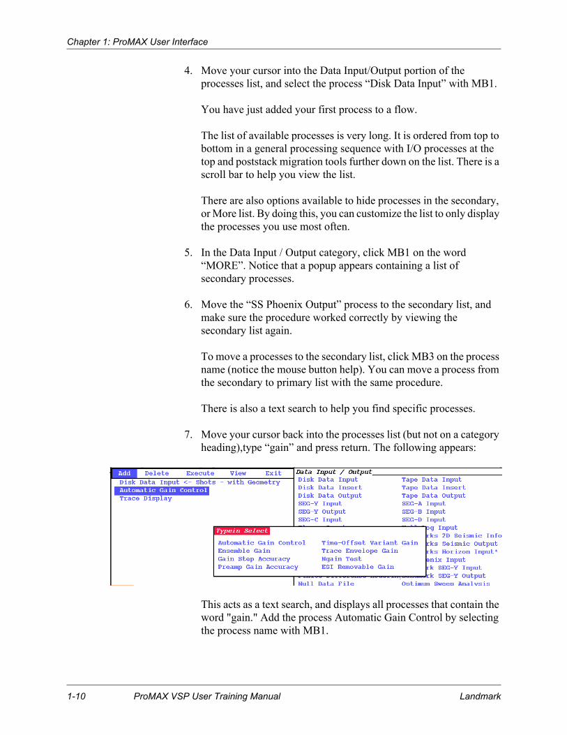
7. Move your cursor back into the processes list (but not on a category heading),type “gain” and press return. The following appears:
This acts as a text search, and displays all processes that contain the word "gain." Add the process Automatic Gain Control by selecting the process name with MB1.
1-10 ProMAX VSP User Training Manual Landmark

Chapter 1: ProMAX User Interface
8. Finish building the following flow by adding the “Trace Display” process to your flow.
9. Select Disk Data Input parameters.
Select Disk Data Input with MB2 to bring up the parameter selection window. To view the helpfile for a process, select the red highlighted question mark.
10. Select Yes for the “Read data from other lines/surveys?” parameter.
For the introductory lessons we will read data from the tutorial line.
11. Select Invalid for the “Select dataset” parameter.
Follow the instructor’s directions for the exact path to the dataset. After you select the dataset you will be returned to the flow editing menu.
Editing Flow: 01: Display Shots
Add Delete Execute View Exit
Disk Data InputRead data from other lines/surveys?: -----------------------------YesSelect dataset: --------------------------------------Area: 2d-tutorials----------------------------------Line: Wave Equation Multiple Reject --------------------------------------------Dataset: Shots-w/ geometryTrace Read Option: ---------------------------------------------Get AllRead the data multiple times?: ------------------------------------NoProcess trace headers only?: --------------------------------------NoOverride input data’s sample interval?: ------------------------No
Automatic Gain ControlApplication mode: ------------------------------------------------ApplyType of AGC scalar: --------------------------------------------MEANAGC operator length: --------------------------------------------1500BASIS for scalar application: ------------------------------CenteredExclude hard zeroes?: ----------------------------------------------YesRobust Scaling?: -----------------------------------------------------No
Trace Display----Default all parameters for this process----
Landmark ProMAX VSP User Training Manual 1-11

Chapter 1: ProMAX User Interface
Default the rest of the parameters in this menu.
12. Select Automatic Gain Control with MB2.
You can now modify parameters for AGC. Select Apply for the Application mode.
By clicking on the parameter, a popup menu appears for making a selection from the menu. Help text appears for each of the associated choices in the popup menu. Move your mouse out of the popup window to retain the default.
13. Set the AGC operator length to 1500ms.
To change this value simply place your cursor on the old value, and type in the number 1500.
This example is called a Type-In parameter. Type in a value to replace the defaulted or existing value. The mouse help will always read, “MB1 Enter, MB2 Edit”. Clicking MB1 will clear the default and let you enter the new parameter. Clicking MB2 will let you edit the existing default value.
14. Select Trace Display parameters.
For now, do not change any of the values. We will discuss many of these options in the next chapter. At that point, you will have the opportunity to test and explore the various options.
1-12 ProMAX VSP User Training Manual Landmark

Chapter 1: ProMAX User Interface
15. Run the flow by clicking on the global command Execute with MB1 or MB2.
A new Trace Display window appears on the screen. Ten icons appear in a column to the left of the traces, and pulldown menus appear above the traces. There is a detailed discussion of these in the next chapter.
16. Select the Next Screen icon with MB1.
This takes you to the next shot. Repeat 2-3 times.
17. Select File Exit/Stop Flow.
This interrupts the job and brings you back to the flow editing menu.
NextScreenIcon
Landmark ProMAX VSP User Training Manual 1-13

Chapter 1: ProMAX User Interface
Sorting
Your first look at the data was the first shot with all channels. After clicking the Next Ensemble icon, you saw the next shot. What if you wanted to look at every other shot? What if you only wanted to look at channels 1 through 60? What if you wanted to sort the data to CDP and then display. All these options and more are available in Disk Data Input.
Sort data by source number
1. Edit your flow named “01: Display Shots”.
2. Open the Disk Data Input Menu and click where the menu reads Get All for Trace Read Option.
Editing Flow: 01: Display Shots
Add Delete Execute View Exit
Disk Data InputRead data from other lines/surveys?-------------------------------YesSelect dataset: --------------------------------------Area: 2d-tutorials ---------------------------------Line: Wave Equation Multiple Reject
---------------------------------Dataset: Shots-w/ geometryTrace Read Option--------------------------------------------------SortInteractive Data Access?: ------------------------------------------NoSelect primary trace header entry------------------------SOURCESelect secondary trace header entry ----------------------- NONESort order for dataset ----------------------------------------------1,3/Presort in memory or on disk?: ----------------------------MemoryRead the data multiple times?: ------------------------------------NoProcess trace headers only?: --------------------------------------NoOverride input data’s sample interval?: ------------------------No
Automatic Gain Control----Use the same parameters as before----
Trace Display----Default all parameters for this process----
1-14 ProMAX VSP User Training Manual Landmark

Chapter 1: ProMAX User Interface
This toggles the read option to Sort, and the menu will automatically add several new options:
• Select Primary trace header entry: Allows you to specify a group of ensembles or traces to read, or sort the data to a different order. Virtually all sorting within ProMAX is done on input. This allows a user to easily change domains without running a separate, time consuming flow. An ensemble in ProMAX is any logical grouping of traces, such as a shot record, or a CDP gather.
• Select Secondary trace header entry: Allows you to re-order, and choose which traces you want to read within each ensemble.
• Sort order for dataset: Allows you to specify an order, or restrict the amount of data brought read.
• Interactive Data Access: Allows you to move forward and backward throught the data after it is displayed, as well as change the values for primary and secondary sort order to jump to a new location. Also allows you to select an ensemble to display from the database.
3. Select SOURCE for the primary sort order, this will read in shot ordered ensembles.
4. Leave the secondary sort set to NONE, this means that no sorting of traces within ensembles will be performed.
5. Select Sort order for dataset.
An Emacs Widget Window appears for specifying input traces. A format and example are given at the bottom of this window.
6. In the Widget Window delete the default values, and type 1, 3/.
This specifies that only SOURCE numbers 1 and 3 will be read into the flow.
7. Move your cursor out of the Widget Window.
8. Select Execute.
The first shot displayed is Live Source Number 1.
Landmark ProMAX VSP User Training Manual 1-15
Chapter 1: ProMAX User Interface
9. Select the Next Screen icon.
This will be Live Source Number 3.
When the last source is displayed, the Next Screen icon becomes inactive. To exit this display, select File Exit/Stop Flow.
Sort data by source and channel number
Lets make the exercise slightly more complicated, and display every tenth shot, limiting the number of channels to 1-60.
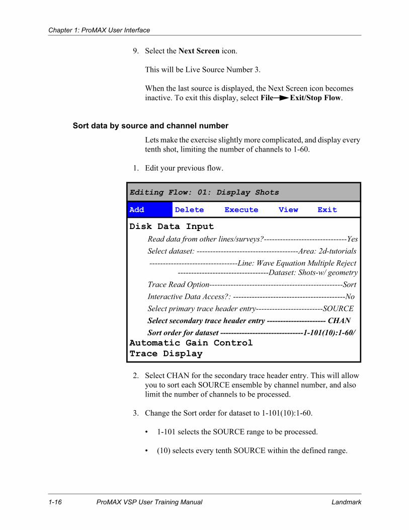
1. Edit your previous flow.
2. Select CHAN for the secondary trace header entry. This will allow you to sort each SOURCE ensemble by channel number, and also limit the number of channels to be processed.
3. Change the Sort order for dataset to 1-101(10):1-60.
• 1-101 selects the SOURCE range to be processed.
• (10) selects every tenth SOURCE within the defined range.
Editing Flow: 01: Display Shots
Add Delete Execute View Exit
Disk Data InputRead data from other lines/surveys?-------------------------------YesSelect dataset: --------------------------------------Area: 2d-tutorials ---------------------------------Line: Wave Equation Multiple Reject
----------------------------------Dataset: Shots-w/ geometryTrace Read Option--------------------------------------------------SortInteractive Data Access?: ------------------------------------------NoSelect primary trace header entry-------------------------SOURCESelect secondary trace header entry ---------------------- CHANSort order for dataset -------------------------------1-101(10):1-60/
Automatic Gain ControlTrace Display
1-16 ProMAX VSP User Training Manual Landmark

Chapter 1: ProMAX User Interface
• : separates the primary sort order from the secondary sort order.
• 1-60 selects the first 60 CHAN (channels) within each SOURCE.
4. Execute the flow.
You will see the first shot and all subsequent shots display with only the first 60 channels.
5. Select the Next Screen icon to see additional shots.
6. Move your cursor into the trace display area. Notice that the mouse button help gives a listing of the current CHAN and SOURCE. Trace Display will always give you a listing of the values for the current Secondary and Primary sort keys.
7. Select File Exit/Stop Flow when finished.
Sort data by CDP number
The dataset that we have been reading, is stored on disk in shot order. Both of the previous exercises maintained the shot ordering, and specified the shot gathers to be displayed. In this exercise you will actually read in the data as CDP gathers. This uses the other side of sorting, which is to actually change the type of ensemble being processed.
Recall that the primary trace header entry specifies the type of ensemble to build, and also the range of that ensemble to read. The secondary sort key allows you to sort and select the traces within each ensemble.
Note
If you only select a primary sort key, then only one range of values is allowed in the sort order for dataset. If you select both a primary and a secondary sort key, then two ranges of values, separated by a colon, are necessary in the sort order. This is a common area for new ProMAX users to make mistakes.
Landmark ProMAX VSP User Training Manual 1-17

Chapter 1: ProMAX User Interface
1. Edit your previous flow.
2. Select CDP for the Primary trace header entry. This tells the program to build CDP gathers from the input dataset.
3. Select OFFSET for the secondary trace header entry. This tells the program to order the traces within each CDP gather by the OFFSET header.
4. Set the sort order for dataset to 500-600(25):*/.
• 500-600(25) This select every 25th CDP between 500, and 600.
• * This is a wildcard that tells the program to read in all OFFSET ranges.
5. Execute the flow.
6. Notice that we have now displayed a CDP gather, even though the input dataset is stored on disk as shot gathers.
7. Move your cursor into the trace display area, and confirm that the displayed gather has Primary and Secondary sorts of CDP and OFFSET.
8. Select File Exit/Stop Flow when finished
Editing Flow: 01: Display Shots
Add Delete Execute View Exit
Disk Data InputRead data from other lines/surveys?-------------------------------YesSelect dataset: --------------------------------------Area: 2d-tutorials ---------------------------------Line: Wave Equation Multiple Reject
---------------------------------Dataset: Shots-w/ geometryTrace Read Option--------------------------------------------------SortInteractive Data Access?: -------------------------------------------NoSelect primary trace header entry-------------------------------CDPSelect secondary trace header entry ----------------------OFFSETSort order for dataset ---------------------------------500-600(25):*/
Automatic Gain ControlTrace Display
1-18 ProMAX VSP User Training Manual Landmark

Chapter 1: ProMAX User Interface
Display near offset section
Using the sorting capabilities within Disk Data Input, you can easily display a near offset section by selecting the first channel on each shot. A near offset section will give you a broader overview of what the geology for your line looks like.
1. Edit your previous flow.
2. Change the primary trace header entry to CHAN (which is roughly equivalent to offset).
3. Set the secondary trace header entry to SOURCE.
4. Set the sort order for dataset to *:*/. This will select all channels for all shots starting with channel number 1.
5. Select File Exit/Stop Flow when finished.
Editing Flow: 01: Display Shots
Add Delete Execute View Exit
Disk Data InputRead data from other lines/surveys?-------------------------------YesSelect dataset: --------------------------------------Area: 2d-tutorials ---------------------------------Line: Wave Equation Multiple Reject
----------------------------------Dataset: Shots-w/ geometryTrace Read Option--------------------------------------------------SortInteractive Data Access?: -------------------------------------------NoSelect primary trace header entry-----------------------------CHANSelect secondary trace header entry ----------------------SOURCESort order for dataset ----------------------------------------------*:*/
Automatic Gain ControlTrace Display
Landmark ProMAX VSP User Training Manual 1-19

Chapter 1: ProMAX User Interface
1-20 ProMAX VSP User Training Manual Landmark

Chapter 2
Interactivity of Trace DisplayTrace Display provides general trace display and analysis capabilities. In addition, it allows for interactive definition of parameter tables. Interaction with the data is accomplished using a series of icons and pulldown menus presented upon execution of a flow with Trace Display. Icon or menu choices allow you the ability to:
• Obtain information about the traces in the display window. • Modify the presentation. • Define processing parameter information.
Topics to be covered in this chapter:
o Trace Display Window
o Icon Bar
o Details of how to use the Icons
o Interactive Data Access
o Menu Bar
o Create and Apply a Parameter Table
Landmark ProMAX VSP User Training Manual 2-1
Chapter 2: Interactivity of Trace Display
Trace Display Window
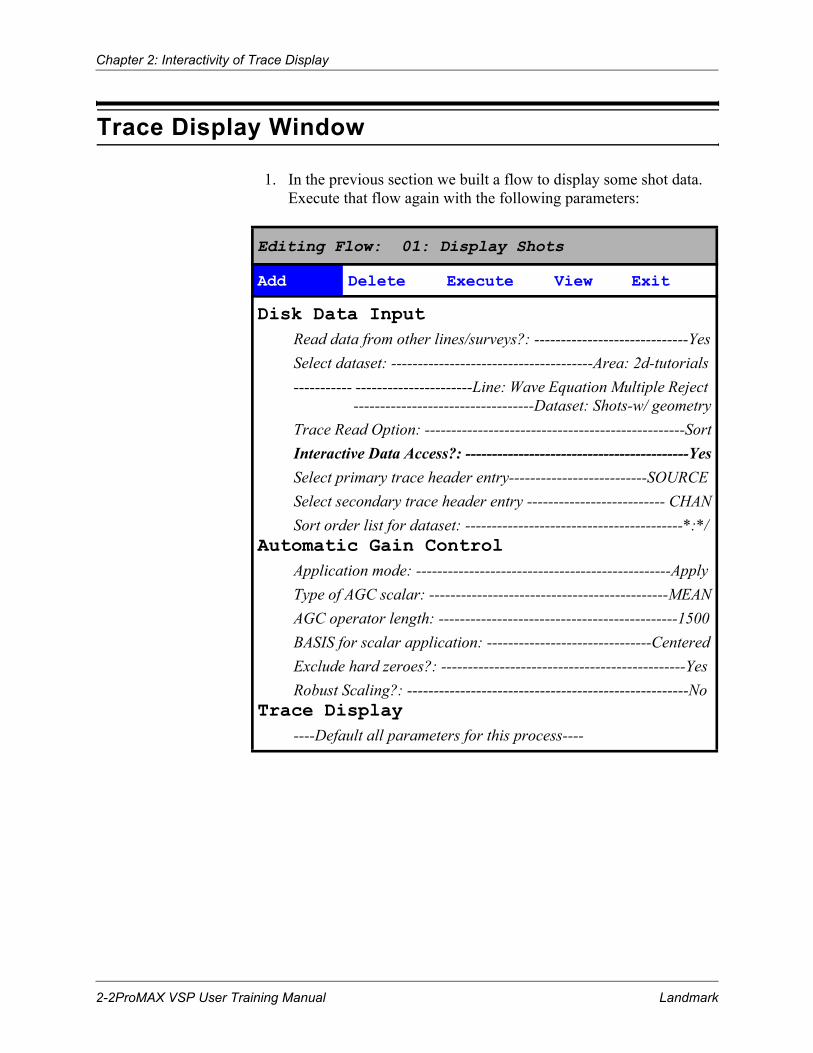
1. In the previous section we built a flow to display some shot data. Execute that flow again with the following parameters:
Editing Flow: 01: Display Shots
Add Delete Execute View Exit
Disk Data InputRead data from other lines/surveys?: -----------------------------YesSelect dataset: --------------------------------------Area: 2d-tutorials----------- ----------------------Line: Wave Equation Multiple Reject
----------------------------------Dataset: Shots-w/ geometryTrace Read Option: -------------------------------------------------SortInteractive Data Access?: ------------------------------------------YesSelect primary trace header entry--------------------------SOURCESelect secondary trace header entry -------------------------- CHANSort order list for dataset: -----------------------------------------*:*/
Automatic Gain ControlApplication mode: ------------------------------------------------ApplyType of AGC scalar: ---------------------------------------------MEANAGC operator length: ---------------------------------------------1500BASIS for scalar application: -------------------------------CenteredExclude hard zeroes?: ----------------------------------------------YesRobust Scaling?: -----------------------------------------------------No
Trace Display----Default all parameters for this process----
2-2ProMAX VSP User Training Manual Landmark

Chapter 2: Interactivity of Trace Display
You will get the following display:
Menu BarIcon Bar
Mouse help Data display
InteractiveData Access
Landmark ProMAX VSP User Training Manual 2-3
Chapter 2: Interactivity of Trace Display
Icon Bar
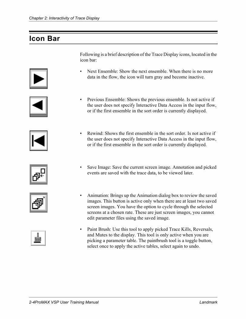
Following is a brief description of the Trace Display icons, located in the icon bar:
• Next Ensemble: Show the next ensemble. When there is no more data in the flow, the icon will turn gray and become inactive.
• Previous Ensemble: Shows the previous ensemble. Is not active if the user does not specify Interactive Data Access in the input flow, or if the first ensemble in the sort order is currently displayed.
• Rewind: Shows the first ensemble in the sort order. Is not active if the user does not specify Interactive Data Access in the input flow, or if the first ensemble in the sort order is currently displayed.
• Save Image: Save the current screen image. Annotation and picked events are saved with the trace data, to be viewed later.
• Animation: Brings up the Animation dialog box to review the saved images. This button is active only when there are at least two saved screen images. You have the option to cycle through the selected screens at a chosen rate. These are just screen images, you cannot edit parameter files using the saved image.
• Paint Brush: Use this tool to apply picked Trace Kills, Reversals, and Mutes to the display. This tool is only active when you are picking a parameter table. The paintbrush tool is a toggle button, select once to apply the active tables, select again to undo.
2-4ProMAX VSP User Training Manual Landmark

Chapter 2: Interactivity of Trace Display
• Zoom Tool: Click and drag using MB1 to select an area to zoom. If you release MB1 outside the window, the zoom operation is canceled. If you just click MB1 without dragging, this tool will unzoom. You can use the zoom tool in the horizontal or vertical axis area to zoom in one direction only
• Annotation Tool: When active, you can add, change, and delete text annotation in the trace and header plot areas. For adding text, activate the icon, then click MB1 where you want the text to appear. For changing text, the pointer changes to a circle when it is over existing text annotation, move by dragging the text with MB1, delete by clicking MB2, and edit the text or annotation color with MB3.
• Velocity Tool: Displays linear or hyperbolic velocities. For a linear velocity, click MB1 at one end of a waveform and drag the red vector out along the event. A velocity is displayed at the bottom of the screen. Use MB2 to display a hyperbolic velocity by anchoring the cursor at the approximate zero offset position of the displayed shot or CDP. Position the red line along the event and read the velocity at the bottom. New events can be measured with either velocity option by reclicking the mouse on a new reflector to re-anchor the starting point. Velocities can be labeled by using MB3 on the current velocity. Geometry must be assigned to successfully use this icon.
• Header Tool: Displays detailed information about trace headers and their values for each individual trace. Activate the icon, and click MB1 on any trace to call up the header template. If the header template is in the way of the traces being viewed, you can move the template by dragging the window. To remove the template deactivate the header icon, or activate any other icon.
Landmark ProMAX VSP User Training Manual 2-5

Chapter 2: Interactivity of Trace Display
Using Icons
In this section we will review the functionality of the Icons in Trace Display
Zoom
There are three ways to zoom in Trace Display
1. Select a rectangular area.
2. A single MB1 click will unzoom the display.
Press and hold MB1 to define the first corner of the zoom window.Continue to hold the button and drag the cursor to the other corner.Release the Mouse button and the display will zoom
2-6ProMAX VSP User Training Manual Landmark
Chapter 2: Interactivity of Trace Display
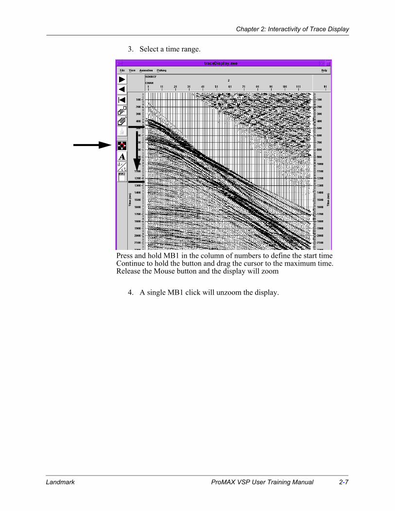
3. Select a time range.
4. A single MB1 click will unzoom the display.
Press and hold MB1 in the column of numbers to define the start timeContinue to hold the button and drag the cursor to the maximum time.Release the Mouse button and the display will zoom
Landmark ProMAX VSP User Training Manual 2-7

Chapter 2: Interactivity of Trace Display
5. Select a range of traces.
6. A single MB1 click will unzoom the display
Press and hold MB1 in the row of numbers to define the start traceContinue to hold the button and drag the cursor to the maximum trace.Release the Mouse button and the display will zoom
2-8ProMAX VSP User Training Manual Landmark

Chapter 2: Interactivity of Trace Display
Add Annotation
Text annotation can be added anywhere on the display, a useful feature for screen dumps to help identify specific features present on the display.
Text may be added, moved (in position on the display), and/or edited using the appropriate mouse button as described at the bottom of the display in the mouse button help area.
Click MB1 anywhere on the screen and the "Edit Text" window appears.Type in some text and press the OK button.The text will appear on the display where you clicked.
You may move, delete or edit this text by placing the cursor on the text.You may add another text label by clicking somewhere else on the display.
The size of the text can be controlled as an X-resource by editing the appropriated X-resources file.
Landmark ProMAX VSP User Training Manual 2-9

Chapter 2: Interactivity of Trace Display
Velocity Measurement
With the dx/dt analysis feature you can measure the apparent velocity of linear or hyperbolic events that appear on the display. This feature will only work if the trace offset values in the headers exist and are accurate.
Click MB1 on a linear event of interest.Move the mouse away from the point where you clickedA red line should appear with velocity tracking at the bottom of the
Press MB3 at the end of the line and the velocity will be annotated nearthe line.
Hyperbolic events can be measured by using MB2 to initiate the lineinstead of MB1
display.
2-10ProMAX VSP User Training Manual Landmark

Chapter 2: Interactivity of Trace Display
Trace Header Dump
You can get a listing of all of the existing trace headers and their values for any given trace by using this icon.
Select any trace with MB1 and the trace header listing willappear in a separate window.
You can continue by selecting a different trace.
You can remove the window by clicking on the icon again.You may also find resizing and moving the windows to be useful.
Landmark ProMAX VSP User Training Manual 2-11

Chapter 2: Interactivity of Trace Display
Save Screen
This icon saves the current screen image as an XWD file in memory. These screens can be recalled from memory and then can be reviewed in different sequences.
By default, a screen is saved every time a different ensemble is displayed. If you change the display of a current ensemble and want to save an image you must press the Save Screen icon.
Save three or four screens by either displaying a different ensemble, or by changing the display (zoom, annotation, etc.) and manually saving the screen.
2-12ProMAX VSP User Training Manual Landmark

Chapter 2: Interactivity of Trace Display
Animate Screens
After you save at least two screens, the Animation Icon becomes active.
With the Animation window active you can review the saved screens.You may elect to view them circularly, one at time in sequence, or comparetwo of the saved screens.
The speed of the circulation can also be controlled by the Speed Slide bar.The speed can be changed as the screens are swapping.
Landmark ProMAX VSP User Training Manual 2-13
Chapter 2: Interactivity of Trace Display
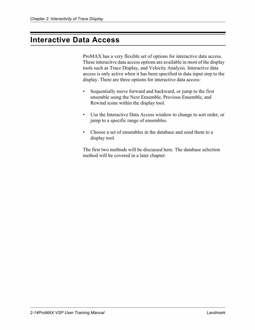
Interactive Data Access
ProMAX has a very flexible set of options for interactive data access. These interacitve data access options are available in most of the display tools such as Trace Display, and Velocity Analysis. Interactive data access is only active when it has been specified in data input step to the display. There are three options for interactive data access:
• Sequentially move forward and backward, or jump to the first ensemble using the Next Ensemble, Previous Ensemble, and Rewind icons within the display tool.
• Use the Interactive Data Access window to change to sort order, or jump to a specific range of ensembles.
• Choose a set of ensembles in the database and send them to a display tool.
The first two methods will be discussed here. The database selection method will be covered in a later chapter.
2-14ProMAX VSP User Training Manual Landmark

Chapter 2: Interactivity of Trace Display
1. Sequentially move forward and backward several times using the Next Ensemble and Previous Ensemble icons.
Next
Previous
Landmark ProMAX VSP User Training Manual 2-15

Chapter 2: Interactivity of Trace Display
2. Jump back to the first ensemble using the rewind icon.
Rewind toFirstEnsemble
2-16ProMAX VSP User Training Manual Landmark

Chapter 2: Interactivity of Trace Display
3. Type a range of ensembles to display in the box supplied, and press the Send Sort Order List button.
4. Notice that the Primary, Secondary, and Tertiary sorts are displayed for reference only, you cannot change to sort order here.
Also notice that you can select a previous sort list from the middle box, or select a previously saved sort list from the file menu.
Landmark ProMAX VSP User Training Manual 2-17

Chapter 2: Interactivity of Trace Display
Menu Bar
File Pulldown Menu
File has seven options available in a pulldown menu. You can save your picks, make a hardcopy plot, move to next screen, previous screen or rewind, or exit Trace Display. You have two choices when you exit. You can exit and stop the flow, or you can exit and let the flow continue without Trace Display.
View Pulldown Menu
View has six options in a pulldown menu. You can control the trace display, the trace scaling, and trace annotation parameters. You can also choose to plot a trace header above the trace data, edit the color map used for color displays or toggle the color bar on and off.
Common changes would be to change the Amplitude Scaling Factor from 1 to other values, and to change the display mode from WT/VAR to Variable Density using a greyscale.
Adding Header plots of various header words is also commonly done. For pre-stack data you may elect to plot the offset above the traces and for stack data you may want to plot the stack fold above the section.
You may also elect to change the numbers plotted above the traces. For example you may want to look at the FFID numbers and the offsets.
The best way to learn these features is to play with them and see what happens.
Note:
Use caution when using the stop option. For example, assume that you have a flow that contains Disk Data Input to read in ten ensembles followed by Disk Data Output and Trace Display. If you execute this flow and use the Exit/Stop Flow option after viewing the first five ensembles, then only the five ensembles that you viewed will be stored in the output dataset as opposed to writing out ten ensembles. If you use the Exit/Continue Flow option instead, then all ten ensembles will be written out.
2-18ProMAX VSP User Training Manual Landmark

Chapter 2: Interactivity of Trace Display
Watch the difference between the Apply and OK buttons. The Apply button will make the changes but the selection window will remain. The OK button will make the changes and dismiss the window.
Animation Pull Down Menu
The Animation menu allows you to save screens, or display previously saved screens in any order and at different swap speeds. The animation tool pictured below, is used to display previously saved screens. This is identical to the functionality provided by the Save Screens and Animate Screens icons.
Landmark ProMAX VSP User Training Manual 2-19

Chapter 2: Interactivity of Trace Display
Picking Pull Down Menu
Picking allows you to interactively open and add information to one or more parameter tables.
These parameter tables allow you to save information about which picked traces you’d like to kill or reverse. Also, you can pick any kind of mute, horizons, gates, or autostatics horizons. Other options allow you to edit database or header values.
We will look at this option in the next section.
Once you have selected a parameter table for your picks, a new icon will appear in the icon bar.
2-20ProMAX VSP User Training Manual Landmark

Chapter 2: Interactivity of Trace Display
Create and Apply a Parameter Table
Parameter tables are generated when you interactively define lists or tables of information. These files are stored in binary format and are intended for use in subsequent processing flows. The interactivity of Trace Display allows you to generate these tables, while viewing the data. You may also QC the interpolation of values from one shot, or CDP to another for space variant parameter tables such as mute functions.
Pick Parameter Tables
In this exercise, you will pick a top mute and some example trace edits. Other parameter tables may be picked in a similar fashion.
1. Edit your flow named “01: Display Shots”.
2. Select to read the first, last, and middle shot gathers on the line (Sources 1,88,176).
Editing Flow: 01: Display shots
Add Delete Execute View Exit
Disk Data InputRead data from other lines/surveys?-------------------------------YesSelect dataset---------------------------------------Shots- w/ geometryTrace Read Option--------------------------------------------------SortInteractive Data Access?: -------------------------------------------NoSelect primary trace header entry--------------------------SOURCESelect secondary trace header entry -------------------------- NONESort order for dataset ----------------------------------------1,88,176/----Default the remaining parameters-----
Automatic Gain Control----Use same parameters as before----
Trace DisplayNumber of ENSEMBLES (line segments) / screen -----------------3----Default all remaining parameters for this process---
Landmark ProMAX VSP User Training Manual 2-21
Chapter 2: Interactivity of Trace Display
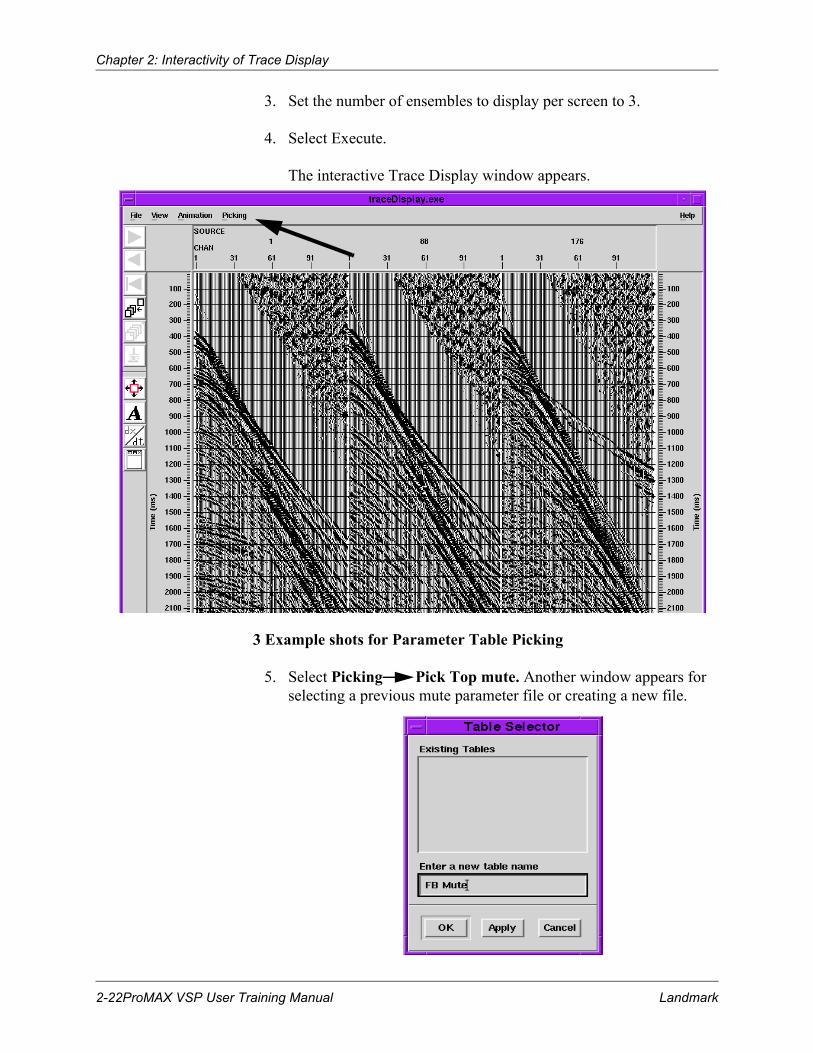
3. Set the number of ensembles to display per screen to 3.
4. Select Execute.
The interactive Trace Display window appears.
3 Example shots for Parameter Table Picking
5. Select Picking Pick Top mute. Another window appears for selecting a previous mute parameter file or creating a new file.
2-22ProMAX VSP User Training Manual Landmark

Chapter 2: Interactivity of Trace Display
When you create a new file, another window appears listing trace headers to choose the secondary key from.
In this case, an appropriate key for Muting traces would be AOFFSET, allowing selection of the mute within each shot record based on Times that are interpolated as a function of absolute value of offset. Depending upon the parameter table you are picking, the most appropriate secondary header should appear at the top of the list.
The “Picking” icon
• This appears when one or more pick objects from the Picking menu are selected. A small window with the file name will appear on the right hand side of the screen. This means the table is open and ready to be edited. When active, click with MB1 to pick a point on a trace or click and drag to pick a range of traces. When the mouse is over a picked point, the pointer shape changes into a circle. Click and drag using MB1 to move a picked point. Use MB2 to select a single point to delete, or click and drag over a range of points to delete them. To select traces from the next shot, use the Next Ensemble icon. The created table remains open, and waits for more picks to be added to the file.
Some parameters require a top and a bottom pick, such as a surgical mute. Once you have picked the top of the mute zone, depress MB3 anywhere inside the trace portion of Trace Display. A new menu appears allowing you to pick an associated layer (New Layer). Some of the other options allow you to snap your pick to the nearest amplitude peak, trough or zero crossing.
Landmark ProMAX VSP User Training Manual 2-23

Chapter 2: Interactivity of Trace Display
6. Pick a mute.
Pick a few points (3 to 6) on the first shot to define a top mute to remove the refraction energy. Selected points will be connected and interpolated as well as extrapolated.
Your mute should look similar the following:
Picking a Mute
7. Click MB3 in the display field and choose Project from the popup menu to display the projection of your picks on all offsets and to the other shots in the display.
2-24ProMAX VSP User Training Manual Landmark

Chapter 2: Interactivity of Trace Display
8. Pick a different mute on the last shot and project again. Watch how the projected mute on the center shot is interpolated based on the first and last shots.
The “Paint Brush” Icon
The Paint Brush can be used to visually show the effect of applying the mute.
9. Select the Paint Brush icon.
You can toggle the mute on and off with the Paint Brush Icon. Edit the mute if you are not happy. Remember you can only edit picks when the picking icon is highlighted.
Picking Traces to be Killed
10. Select Picking Kill Traces.
You will be prompted to enter a descriptive name for this list of traces to be killed followed by a secondary header selection. Use a name similar to “Traces to be killed” sorted by Channel number.
A second parameter table is now listed in the Parameter table selection window.
11. Using MB1 select some traces to be killed (use your imagination).
MB2 can be used to remove previously selected traces from the list. The traces to be killed will be marked with at Red line.
12. Select File Exit/Stop Flow. When you choose to exit, you are prompted to save the picks you have just made. The picks are saved in parameter tables which can be used later in processing.
Landmark ProMAX VSP User Training Manual 2-25

Chapter 2: Interactivity of Trace Display
Apply the Mute and Trace Edits
1. Edit your previous flow by inserting Trace Muting and a Trace Kill/Reverse.
2. In the Trace Muting menu click on Invalid to choose the mute parameter file (FB Mute).
In ProMAX, each type of parameter table has its own separate menu, such as mute tables, kill trace tables, velocity tables. When selecting the mute parameter file, you are taken to a menu of parameter files for Mutes.
3. In the Trace Kill/Reverse menu select the list of traces to be killed.
4. Execute the flow.
Editing Flow: 01: Display Shots
Add Delete Execute View Exit
Disk Data Input----Use same parameters as before----
Trace MutingRe-apply previous mutes: -------------------------------------------NoMute time reference: --------------------------------------------Time 0Type of Mute: --------------------------------------------------------TopStarting ramp: ---------------------------------------------------------30EXTRAPOLATE mute times?: -------------------------------------YesGet mute file from the DATABASE?: ------------------------------YesSelect Mute Parameter File: ---------------------------------FB Mute
Trace Kill/ReverseTrace editing MODE ------------------------------------------------KillGet edits from the DATABASE? ----------------------------------- YesSELECT trace Kill parameter file --------------- Traces to be killed
Automatic Gain Control----Use same parameters as before----
Trace DisplayNumber of ENSEMBLES (line segments) / screen -----------------3----Default all remaining parameters for this process-----
2-26ProMAX VSP User Training Manual Landmark
Chapter 2: Interactivity of Trace Display
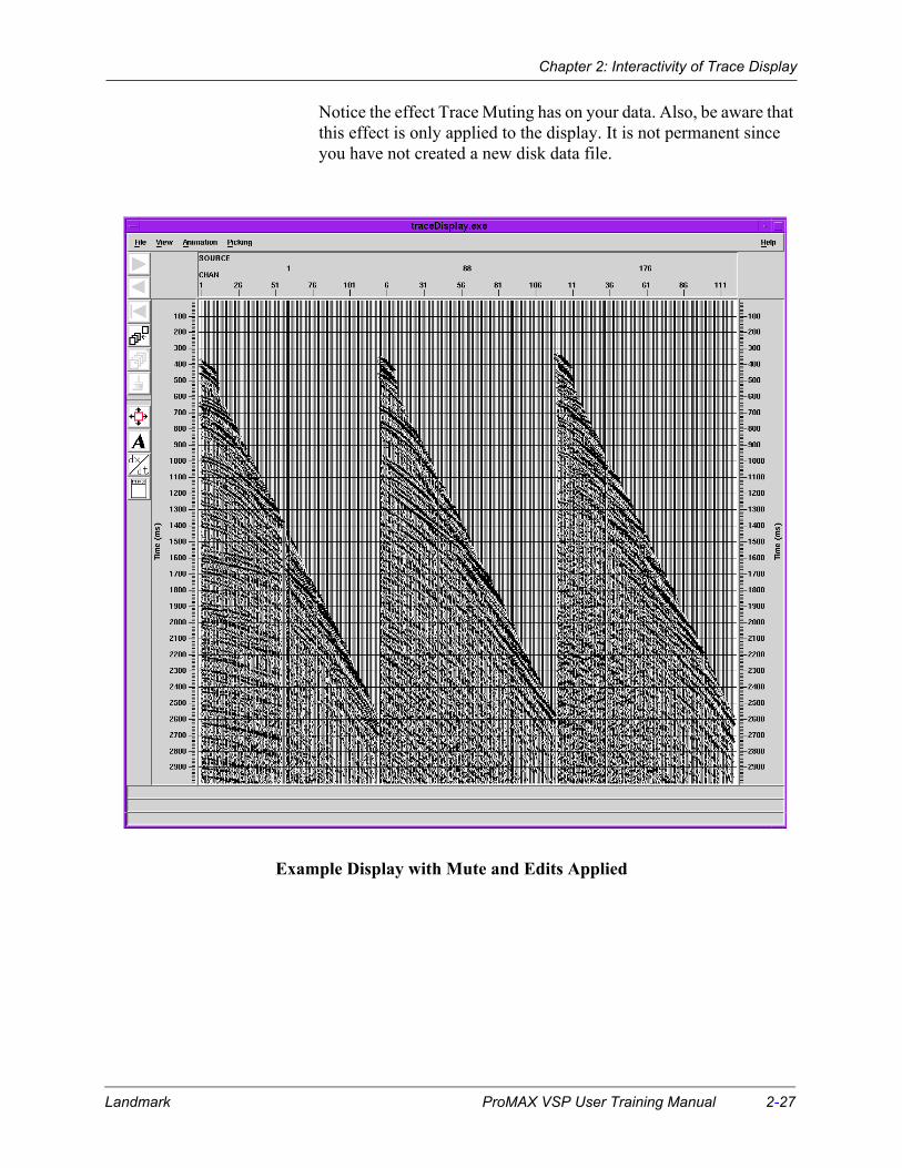
Notice the effect Trace Muting has on your data. Also, be aware that this effect is only applied to the display. It is not permanent since you have not created a new disk data file.
Example Display with Mute and Edits Applied
Landmark ProMAX VSP User Training Manual 2-27

Chapter 2: Interactivity of Trace Display
Exit/Stop vs. Exit Continue FlowThere are two Exit options in Trace Display. One will terminate the Trace Display and the entire flow, the other will Terminate the Trace Display and allow the remaining processes in the flow to continue running. In this exercise we will look at the difference.
1. Using the same flow, change the input to read the first 20 shots and add a Disk Data Output at the end of the flow.
Editing Flow: 01: Display Shots
Add Delete Execute View Exit
Disk Data InputRead data from other lines/surveys?-------------------------------YesSelect dataset---------------------------------------Shots- w/ geometryTrace Read Option--------------------------------------------------SortSelect primary trace header entry--------------------------SOURCESelect secondary trace header entry ------------------------ NONESort order for dataset ---------------------------------------------1-20/----Default the remaining parameters----
Trace Muting----Use same parameters as before----
Trace Kill/Reverse----Use same parameters as before----
Automatic Gain Control----Use same parameters as before----
Trace DisplayNumber of ENSEMBLES (line segments) / screen -----------------3----Default all remaining parameters for this process----
Disk Data OutputOutput dataset Filename: -----------------------------------------tempNew or Existing File? ----------------------------------------------NewRecord length to output: ----------------------------------------------0.Trace sample format: ---------------------------------------------16 bitSkip primary disk storage?: -----------------------------------------No
2-28ProMAX VSP User Training Manual Landmark

Chapter 2: Interactivity of Trace Display
The "0." setting for the Record length to output parameter means output the entire trace, however long it may be.
2. Execute the flow.
3. The first display will have the first three shots.
4. Use the File Exit/Stop Flow pull down menu to stop the flow.
5. Exit from the flow and go the DATASETS list.
6. Click MB2 on the dataset named “temp” to get the expanded dataset information.
Notice that this file contains only the first three shots that were displayed. Since the Flow was halted, no additional shots were processed.
7. Execute the flow again.
8. Use the File Exit/Continue Flow pull down menu to stop the Trace Display but allow the flow to continue.
MB2
Landmark ProMAX VSP User Training Manual 2-29

Chapter 2: Interactivity of Trace Display
9. Notice that the flow continues to run.
10. Exit from the flow and go the DATASETS list.
11. With MB2 get the expanded dataset information of the file named “temp.”
Notice that the file now contains all 20 shots.
12. Delete the file named temp from disk.
MB2
2-30ProMAX VSP User Training Manual Landmark

Chapter 3
Real Dataset InformationMost of the exercises in this manual will use a real dataset. This dataset has already been vertically stacked so that there is only 1 shot for each depth position. The following information provides you with the needed information to build the geometry spreadsheet and database, and prepare the job flows in the exercises.
Topics covered in this chapter:
o VSP Real Dataset Geometry
Landmark ProMAX VSP User Training Manual 3-1
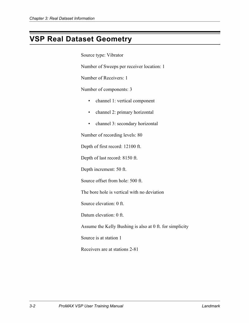
Chapter 3: Real Dataset Information
VSP Real Dataset Geometry
Source type: Vibrator
Number of Sweeps per receiver location: 1
Number of Receivers: 1
Number of components: 3
• channel 1: vertical component
• channel 2: primary horizontal
• channel 3: secondary horizontal
Number of recording levels: 80
Depth of first record: 12100 ft.
Depth of last record: 8150 ft.
Depth increment: 50 ft.
Source offset from hole: 500 ft.
The bore hole is vertical with no deviation
Source elevation: 0 ft.
Datum elevation: 0 ft.
Assume the Kelly Bushing is also at 0 ft. for simplicity
Source is at station 1
Receivers are at stations 2-81
3-2 ProMAX VSP User Training Manual Landmark
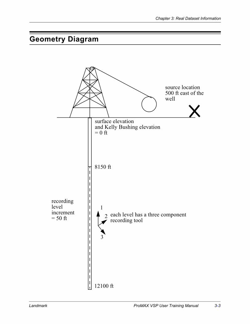
Chapter 3: Real Dataset Information
Geometry Diagram
12100 ft
8150 ft
recordinglevelincrement= 50 ft
surface elevationand Kelly Bushing elevation= 0 ft
source location500 ft east of thewell
each level has a three componentrecording tool
12
3
Landmark ProMAX VSP User Training Manual 3-3

Chapter 3: Real Dataset Information
3-4 ProMAX VSP User Training Manual Landmark

Chapter 4
View Input DataThis is our first look at the input data. There are 80 FFIDs, each consisting of 3 channels. Channel 1 is the vertical trace, channels 2 and 3 are the two horizontal traces situated orthogonal to one another. The traces are approximately 3400 ms in length.
Topics covered in this chapter:
o Display the SEG-Y Input data
o Write Dataset To Disk in Your Area
Landmark ProMAX VSP User Training Manual 4-1

Chapter 4: View Input Data
Display the Input Data
ExerciseIn this exercise we will simply view the traces and look at the trace headers to familiarize ourselves with the data.
1. First, add a new Line or a new Area and Line. Choose names that will not conflict with other users in this training session.
2. Build the following flow to look at the input data and trace headers:
3. Your instructor will give you the exact name of the SEGY file that you will input.
Read all available traces. There are 3 traces per shot ensemble and 80 ensembles.
4. Apply an AGC scaler for cosmetics.
5. Display the data and view the trace headers.
Set the Trace Display to plot 80 ensembles and annotate each FFID and channel.
Editing Flow: 10 read SEGY data
Add Delete Execute View Exit
SEGY InputType of storage to use: ----------------------------- Disk ImageEnter DISK file path name: ---------------------------------------------
--------------------------/misc_files/vsp/vsp_segyMAX traces per ensemble: ----------------------------------------3Remap SEGY header values -----------------------------------No
Automatic Gain ControlTrace Display
Number of ENSEMBLES /screen -----------------------------80Primary trace LABELING ------------------------------------ FFIDSecondary trace LABELING ------------------------------- Chan
4-2 ProMAX VSP User Training Manual Landmark

Chapter 4: View Input Data
Select the “header” icon and click on a trace.
Which trace headers have values that look meaningful?
Landmark ProMAX VSP User Training Manual 4-3

Chapter 4: View Input Data
Write Dataset To Disk in Your Area
Exercise1. Expand the previous flow to write the dataset to disk in your own
area for future processing.
2. Write the file to disk in your own area.
3. Make sure you toggle the AGC and the Trace Display inactive.
4. After the flow is complete go to the datasets list and press MB2 on the dataset name that you just created.
It should have 80 ensembles and a total of 240 traces.
Editing Flow: 10 read SEGY data
Add Delete Execute View Exit
SEGY InputType of storage to use: ----------------------------- Disk ImageEnter DISK file path name: ---------------------------------------------
--------------------------/misc_files/vsp/vsp_segyMAX traces per ensemble: ----------------------------------------3
Remap SEGY header values -----------------------------------No>Automatic Gain Control<>Trace Display<Disk Data Output
Output Dataset -------------------------------shots - input data
4-4 ProMAX VSP User Training Manual Landmark

Chapter 5
VSP GeometryVSP Geometry Assignment takes advantage of the simplicity of the spatial relationship between the source and receiver positions in VSP data. This helps to minimize the input required to describe the geometry.
Some VSP data is very complex and incorporates a lot of varied information to describe the geometry. Some holes are deviated (crooked) and you may have inclination and azimuth information at all recorded depth levels. In these cases you may also have two sets of depth information: log depth and vertical depth. The Spreadsheets have been written to handle all such information.
Our case is very simple, using a non-deviated hole.
Topics covered in this chapter:
o Assign VSP Geometry
o Quality Control Plots from the database
o Load Geometry to the trace headers
Landmark ProMAX VSP User Training Manual 5-1
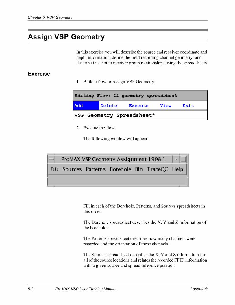
Chapter 5: VSP Geometry
Assign VSP Geometry
In this exercise you will describe the source and receiver coordinate and depth information, define the field recording channel geometry, and describe the shot to receiver group relationships using the spreadsheets.
Exercise1. Build a flow to Assign VSP Geometry.
2. Execute the flow.
The following window will appear:
Fill in each of the Borehole, Patterns, and Sources spreadsheets in this order.
The Borehole spreadsheet describes the X, Y and Z information of the borehole.
The Patterns spreadsheet describes how many channels were recorded and the orientation of these channels.
The Sources spreadsheet describes the X, Y and Z information for all of the source locations and relates the recorded FFID information with a given source and spread reference position.
Editing Flow: 11 geometry spreadsheet
Add Delete Execute View Exit
VSP Geometry Spreadsheet*
5-2 ProMAX VSP User Training Manual Landmark

Chapter 5: VSP Geometry
3. Open the Borehole spreadsheet by clicking on “Borehole” on the main menu.
In this case we have a straight, vertical borehole. The log depths are the same as the elevations, except that they are all positive numbers. All x,y values will be defined at 0.0 and 0.0.
4. Define the borehole with two sets of X,Y, and Z coordinates.
5. Exit from the Borehole Spreadsheet.
6. Open the Patterns Spreadsheet by clicking on “Patterns” on the main menu.
There is only one pattern for this geometry.
The Grp Int column specifies the separation between the specified recording channels in the borehole.
The Offset column specifies a shift to apply to the “chan from” channel relative to the depth listed in the sources spreadsheet.
In this case we have three channels all at the same depth. You will define the exact depth for the receivers for each shot.
7. Exit from the Patterns Spreadsheet.
Landmark ProMAX VSP User Training Manual 5-3

Chapter 5: VSP Geometry
8. Open the Sources Spreadsheet by clicking on “Sources” on the main window.
9. We have a total of 80 shots in this VSP, so the first thing to do is expand the sources spreadsheet to 80 rows.
In the “mark block” column, click MB3 to highlight all rows in the spreadsheet. Alternatively, you could use MB1 to select the first row of a block and MB2 to select the last row of a block. Now use the edit pull down to insert additional rows so that you have a total of 80.
10. Fill the Source and FFID columns starting at 1 and incrementing by 1. Use MB3 on the leftmost column to select all rows of the spreadsheet. Now, click MB2 on the column header FFID, and fill values starting with 1 and incrementing by 1. Repeat this for the Sources column.
11. All shots are at shot station number 1 and at an elevation of 0.0 ft.
12. X,Y values are defined at 500.0 and 0.0 respectively.
13. All shots use the same pattern (1) and have 3 channels.
14. The pattern reference depths start at 12100 and decrement by 50 ft. for each shot.
NOTE:
For documentation purposes, the columns have been re-ordered slightly. All additional columns are filled with 0.0
5-4 ProMAX VSP User Training Manual Landmark
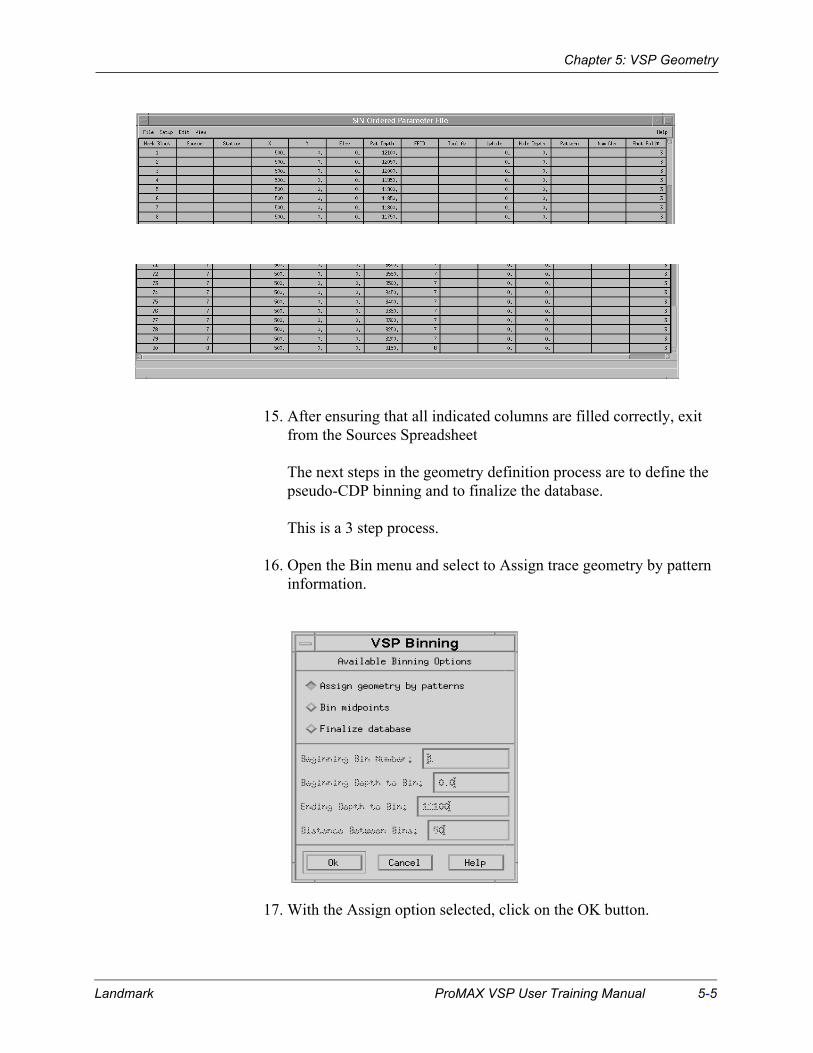
Chapter 5: VSP Geometry
15. After ensuring that all indicated columns are filled correctly, exit from the Sources Spreadsheet
The next steps in the geometry definition process are to define the pseudo-CDP binning and to finalize the database.
This is a 3 step process.
16. Open the Bin menu and select to Assign trace geometry by pattern information.
17. With the Assign option selected, click on the OK button.
Landmark ProMAX VSP User Training Manual 5-5

Chapter 5: VSP Geometry
You should see several windows related to Assigning VSP geometry based on patterns flash by fairly quickly. The last window will say that the geometry has been successfully assigned.
18. Dismiss the Status window by clicking on OK.
19. Select Bin Midpoints in order to compute the (pseudo) Common Depth points.
Bin starting at CDP 1, starting at 0.0 ft. and ending at 12100 ft. incrementing by 50 ft. per bin.
20. Click on the OK button.
Again you should see several windows flash by ending with a window indicating that the binning was completed successfully.
21. Dismiss this window by clicking on the OK button.
22. Select the Finalize Database option and click on the OK button.
NOTE:
The CDP domain has no relevance for ProMAX VSP processing. CDP numbers are only created to satisfy the requirement of many ordinary ProMAX modules that CDP values exist. By convention, you should set the distance between bins equal to the typical receiver spacing in the borehole. Most CDP attributes simply mimic the receiver attribute information.
5-6 ProMAX VSP User Training Manual Landmark

Chapter 5: VSP Geometry
This step completes building the look up tables and other database finalization functions
You should see a window indicating that the VSP geometry finalization has completed successfully.
23. Dismiss the Status window by clicking on OK.
24. Click on the Cancel button in the binning dialog box to dismiss this window.
25. Click on File / Exit to end the geometry spreadsheet flow.
Landmark ProMAX VSP User Training Manual 5-7

Chapter 5: VSP Geometry
Quality Control Plots using the XDB database tool
Access DBTools by selecting “Database” in the flow menu. From the resulting DBTools dialog, click on the Database pulldown and select XDB Database Display.
2D plot of TRC vs. Receiver elevation and log depth
• used to check depth assigned to each trace
2D plot of SRF vs. elevation
• used to check depth assigned to each receiver station
2D plot of TRC vs. various other values
• used to check additional information for each trace
5-8 ProMAX VSP User Training Manual Landmark

Chapter 5: VSP Geometry
Load Geometry to the trace headers
Exercise1. Build the following flow to install the Geometry information into the
trace headers:
2. Input the file that we previously wrote to your own areas after reading the SEGY data.
3. Select VSP Inline Geom Header Load parameters.
Since you did not use the Extract Database Files process your data does not currently have valid trace numbers. You must assign the geometry to the trace headers by referencing the FFID and automatic default of recording channel.
Editing Flow: 12 load geometry to headers
Add Delete Execute View Exit
Disk Data InputSelect dataset----------------------------------shots - input dataTrace Read Option--------------------------------------------Get All
VSP Inline Geom Header LoadPrimary header to match database --------------------- FFIDSecondary header to match database ---------------- NoneMatch by valid trace number?---------------------------------NoVerbose Diagnostics?----------------------------------------------No
Trace Header MathSelect Mode ------------------------------- Fixed equation modeDefine trace header equation ------------- geo_comp=chan
Disk Data OutputOutput Dataset Filename-------------- “shots - with geom”New, or Existing, File?------------------------------------------NewRecord length to output--------------------------------------------0.Trace sample format------------------------------------------16 bitSkip primary disk Storage?-------------------------------------No
Landmark ProMAX VSP User Training Manual 5-9
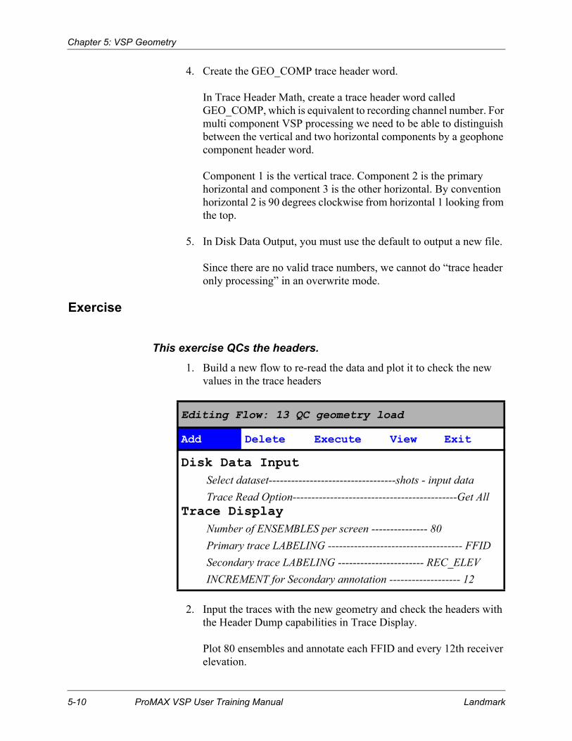
Chapter 5: VSP Geometry
4. Create the GEO_COMP trace header word.
In Trace Header Math, create a trace header word called GEO_COMP, which is equivalent to recording channel number. For multi component VSP processing we need to be able to distinguish between the vertical and two horizontal components by a geophone component header word.
Component 1 is the vertical trace. Component 2 is the primary horizontal and component 3 is the other horizontal. By convention horizontal 2 is 90 degrees clockwise from horizontal 1 looking from the top.
5. In Disk Data Output, you must use the default to output a new file.
Since there are no valid trace numbers, we cannot do “trace header only processing” in an overwrite mode.
Exercise
This exercise QCs the headers.1. Build a new flow to re-read the data and plot it to check the new
values in the trace headers
2. Input the traces with the new geometry and check the headers with the Header Dump capabilities in Trace Display.
Plot 80 ensembles and annotate each FFID and every 12th receiver elevation.
Editing Flow: 13 QC geometry load
Add Delete Execute View Exit
Disk Data InputSelect dataset----------------------------------shots - input dataTrace Read Option--------------------------------------------Get All
Trace DisplayNumber of ENSEMBLES per screen --------------- 80Primary trace LABELING ------------------------------------ FFIDSecondary trace LABELING ----------------------- REC_ELEVINCREMENT for Secondary annotation ------------------- 12
5-10 ProMAX VSP User Training Manual Landmark

Chapter 5: VSP Geometry
You should see the correct shot X value, and receiver elevation values.
.
NOTE:
For VSP processing, the receiver depths are placed in the attribute name REC_ELEV, and use negative values to indicate depth below mean sea level.
The ProMAX attribute REC_DEP is used in marine processing dto indicate the depth of a towed streamer below the the water surface.
Landmark ProMAX VSP User Training Manual 5-11

Chapter 5: VSP Geometry
5-12 ProMAX VSP User Training Manual Landmark

Chapter 6
Keep Vertical Component TracesAlthough most VSPs are recorded using multi-component instruments, often only the vertical component traces are actually used. In order to simplify data handling, we want to isolate only those traces that we are going to process. In this exercise we will run a job that will keep only the vertical component traces for further processing.
We will keep the original data (with all 3 components) for some other exercises later in the class.
A good question to ask here is:
“What is the best sort order to build the most efficient ensemble for future processing?”
Topics covered in this chapter:
o Create Vertical Component Dataset
Landmark ProMAX VSP User Training Manual 6-1

Chapter 6: Keep Vertical Component Traces
Trap Vertical Traces
Exercise1. Build the following flow to keep only the vertical traces.
Sort the input data on CHAN/FFID and only keep channel 1 for all of the shots.
If we make an ensemble of only channel 1, then we can always default the Trace Display to plot all traces in 1 ensemble instead of having to change it to 80 and worry about ensemble gaps and display label issues.
2. In Trace Length, limit the amount of data to be processed to 2000 ms.
3. Display the resulting dataset and if satisfied, write the output to disk.
Editing Flow: 14 trap vertical traces
Add Delete Execute View Exit
Disk Data InputSelect dataset----------------------------------shots - with geomTrace Read Option-------------------------------------------- SORTInteractive Data Access ----------------------------------------- NoSelect primary trace header ----------------------------- CHANSelect secondary trace header ---------------------------- FFIDSelect tertiary trace header ------------------------------ NONESort order list for dataset ------------------------------------ 1:*/Presort in memory or on disk? ------------------------ Memory
Trace LengthNew trace length ----------------------------------------------- 2000
>Disk Data Output<Trace Display
Number of ENSEMBLES per screen -------------------------- 1Primary trace LABELING ---------------------------------- CHANSecondary trace LABELING ----------------------- REC_ELEV
6-2 ProMAX VSP User Training Manual Landmark
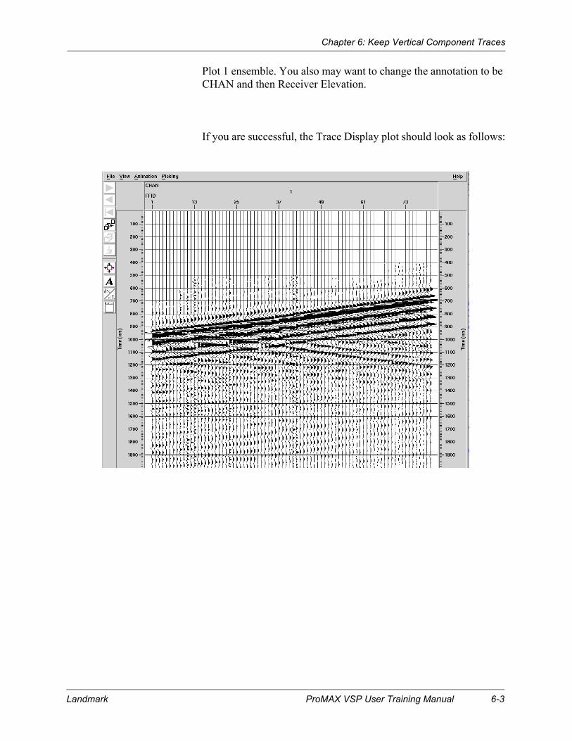
Chapter 6: Keep Vertical Component Traces
Plot 1 ensemble. You also may want to change the annotation to be CHAN and then Receiver Elevation.
If you are successful, the Trace Display plot should look as follows:
Landmark ProMAX VSP User Training Manual 6-3

Chapter 6: Keep Vertical Component Traces
Output a file with vertical traces only
1. Modify the flow to output a file that contains only the vertical traces.
Editing Flow: 14 trap vertical traces
Add Delete Execute View Exit
Disk Data InputSelect dataset----------------------------------shots - with geomTrace Read Option-------------------------------------------- SORTInteractive Data Access ----------------------------------------- NoSelect primary trace header ----------------------------- CHANSelect secondary trace header ---------------------------- FFIDSelect tertiary trace header ------------------------------ NONESort order list for dataset ------------------------------------ 1:*/Presort in memory or on disk? ------------------------ Memory
Trace LengthNew trace length ----------------------------------------------- 2000
Disk Data OutputOutput Dataset Filename------------ “vertical traces only”New, or Existing, File?------------------------------------------NewRecord length to output--------------------------------------------0.Trace sample format------------------------------------------16 bitSkip primary disk Storage?-------------------------------------No
>Trace Display<
6-4 ProMAX VSP User Training Manual Landmark

Chapter 7
First Break Picks on Vertical TracesFirst Break times are an integral part of the processing of VSP data. In this exercise we will pick the first arrival times on the vertical component traces for use in future processing steps.
In the processing of VSP data, first arrival times are used for a variety of different purposes. These times are used to compute velocity functions which are then used by other processes. The first arrival times are also used as flattening statics for wavefield separation. They are also used to convert the VSP data to two way travel time in preparation for Corridor Stack. With all of these uses in mind, it is apparent that the first arrivals must be accurate.
Topics covered in this chapter:
o Pick First Breaks
Landmark ProMAX VSP User Training Manual 7-1
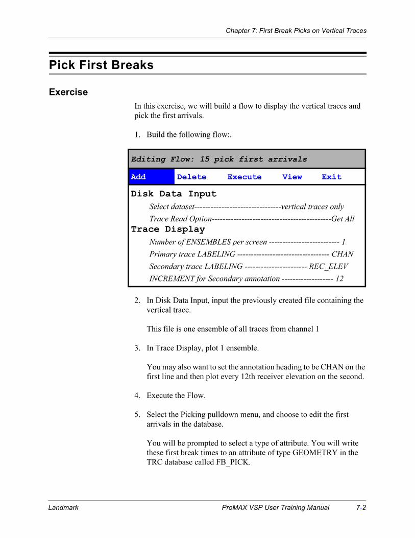
Chapter 7: First Break Picks on Vertical Traces
Pick First Breaks
ExerciseIn this exercise, we will build a flow to display the vertical traces and pick the first arrivals.
1. Build the following flow:.
2. In Disk Data Input, input the previously created file containing the vertical trace.
This file is one ensemble of all traces from channel 1
3. In Trace Display, plot 1 ensemble.
You may also want to set the annotation heading to be CHAN on the first line and then plot every 12th receiver elevation on the second.
4. Execute the Flow.
5. Select the Picking pulldown menu, and choose to edit the first arrivals in the database.
You will be prompted to select a type of attribute. You will write these first break times to an attribute of type GEOMETRY in the TRC database called FB_PICK.
Editing Flow: 15 pick first arrivals
Add Delete Execute View Exit
Disk Data InputSelect dataset--------------------------------vertical traces onlyTrace Read Option--------------------------------------------Get All
Trace DisplayNumber of ENSEMBLES per screen -------------------------- 1Primary trace LABELING ---------------------------------- CHANSecondary trace LABELING ----------------------- REC_ELEVINCREMENT for Secondary annotation ------------------- 12
Landmark ProMAX VSP User Training Manual 7-2

Chapter 7: First Break Picks on Vertical Traces
6. The Pick editing icon on the left side of the plot will automatically be selected for you.
7. Pick the arrivals with the rubber-band and then snap to the desired phase with MB3.
It is suggested to pick the first strong, continuous peak.
8. Edit any picks as you see fit.
9. Exit the program to save the picks to the database.
7-3 ProMAX VSP User Training Manual Landmark

Chapter 7: First Break Picks on Vertical Traces
QC the First Breaks in the Database using XDB
1. Click on Database in the flow menu. From the resulting DBTools dialog, click on the Database pulldown and select XDB Database Display. Plot the first arrival times from the TRC database and edit any bad picks.
Reposition any picks that appear out of line and then save the edited picks back to the database. This is accomplished using the Database/Save buttons.
Be sure not to move the pick off of the selected trace.
2. If you want, you can re-execute the pick job and then replot the edited picks on the traces for further QC.
7-4 ProMAX VSP User Training Manual Landmark

Chapter 8
VSP Velocity FunctionsVSP datasets can provide additional velocity information to aid in the processing of surface seismic data and provide comparisons with well log information. Additionally, some processes that can be applied to VSP data require some velocity information. VSP data provides a direct measurement of average velocity as a function of depth.
The Velocity Manipulation process allows you to generate other types of velocity fields from this average velocity function which in turn permits you to generate VSP-CDP transforms and/or migrations of the VSP data.
Topics covered in this chapter:
o Generate Average Velocity vs. Depth
o QC using Velocity Viewer/Point Editor
o Velocity function manipulation
o Velocity function smoothing
o Compute an RMS Velocity Function
Landmark ProMAX VSP User Training Manual 8-1

Chapter 8: VSP Velocity Functions
Generate Average Velocity vs. Depth and Smooth
The first arrival times are a direct measure of travel time as a function of source to receiver distance. This gives a direct measurement of the average velocity between the source and receiver.
Exercise1. Build the following flow to compute the average velocity:
2. Parameterize Vel Table From VSP.
Editing Flow: 16 generate avg vel function
Add Delete Execute View Exit
Vel Table From VSP*Specify a datum elevation---------------------------------------- 0Limit source-receiver horizontal offsets ------------------- NoLimit source elevations ------------------------------------------ NoLimit receiver elevations ---------------------------------------- NoLimit vertical source-receiver separation----------------------NoSelect output AVERAGE velocity file --------------------------------------------------------------- from raw first break pick timesTable overwrite options ---------- Overwrite existing tableTime pick Parameter ---------- TRC GEOMETRY FB_PICK
Velocity Viewer / Point Editor*Select the type of field you wish to edit ----------------------------------------------------------- Average Velocity in DepthDo you wish to edit an existing table --------------------- YesSelect the input velocity database entry --------- ----------------------------------------------- from raw first break pick timesSelect output velocity database entry -------------------------------------------------------------------------- smoothed versionMinimum depth (or time) of velocity field ------------------- 0Maximum depth (or time) of velocity field ------------------ 0
8-2 ProMAX VSP User Training Manual Landmark

Chapter 8: VSP Velocity Functions
Using a reference datum of 0 ft., generate an average velocity vs. depth velocity table. Do not impose any limits. Input the set of first breaks that was picked from the vertical traces and then edited from the database.
3. View the output function using Velocity Viewer/ Point Editor.
Select parameters to input the average velocity vs. depth table created from the first arrivals, and output to a new velocity table that you will smooth interactively.
When the display appears, click on Modify / Smooth Velocity Field. Set the interactive smoothing parameters to output a function every 1000 CDPs to ensure that only one function is output. Also set the depth sampling interval to 50 ft. to match the original input sampling interval. The CDP smoothing value can be defaulted and set the depth smoothing level to 250 ft.
After applying the smoothing, click on the velocity function edit icon, then move the cursor into the data field to make it update with the newly smoothed function.
The following diagram shows the difference between the original, or raw average velocity vs. the smoothed version.
Landmark ProMAX VSP User Training Manual 8-3

Chapter 8: VSP Velocity Functions
Exit and save the smoothed velocity function table.
8-4 ProMAX VSP User Training Manual Landmark

Chapter 8: VSP Velocity Functions
Compute an RMS Velocity Function
1. Build the following flow.
2. Input the average velocity function that was computed from the
Editing Flow: 17 compute VRMS from VAVG
Add Delete Execute View Exit
Velocity Manipulation*Type of velocity table to input ----- Average Vel in DepthGet velocity table from database entry ------------------ YesSelect input velocity database entry -----------------------------------
----------------from raw first break pick timesCombine a second velocity table ---------------------------- NoResample the input velocity table? ------------------------- NoShift or stretch the input velocity table ---------------------- NoType of parameter table to output -------------------------------------
---------------------------- Stacking (RMS) VelocitySelect output velocity database entry ----------------------------------
---------------------------------- from raw averageSpatially resample the velocity table ---------------------- NoOutput a single average velocity table -------------------- NoSmooth velocity field --------------------------------------------- NoVertically resample the output velocity table ----------- NoAdjust Output velocity by percentage --------------------- No
Velocity Viewer / Point Editor*Select the type of field you wish to edit -------------------------------------------------------------- Stacking (RMS) VelocityDo you wish to edit an existing table --------------------- YesSelect the input velocity database entry --------- ------------------------------------------------------------------ from raw averageSelect output velocity database entry ---------------------------------------------------------------------------from raw averageMinimum depth (or time) of velocity field ------------------- 0Maximum depth (or time) of velocity field ------------------ 0
Landmark ProMAX VSP User Training Manual 8-5

Chapter 8: VSP Velocity Functions
first arrival times before smoothing and convert it to an RMS function. You might want to name the output table “from raw average”.
3. Display the output function using the point editor.
4. Rerun the same flow using the smoothed average function that you created earlier. Convert it to an RMS function using the option: from smoothed average.
5. Compare the results and look at the values of the RMS function in the Velocity table editor.
Editing Flow: 17 compute VRMS from VAVG
Add Delete Execute View Exit
Velocity Manipulation*Select input velocity database entry -----------------------------------
-----------------------------------smoothed versionSelect output velocity database entry ----------------------------------
-------------------------- from smoothed averageVelocity Viewer / Point Editor*
Select the input velocity database entry --------- ---------------------------------------------------------- from smoothed averageSelect output velocity database entry ------------------------------------------------------------------from smoothed average
8-6 ProMAX VSP User Training Manual Landmark
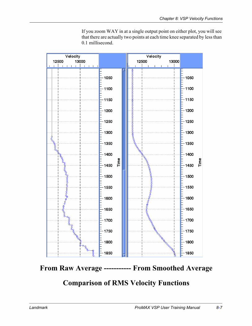
Chapter 8: VSP Velocity Functions
If you zoom WAY in at a single output point on either plot, you will see that there are actually two points at each time knee separated by less than 0.1 millisecond.
From Raw Average ----------- From Smoothed Average
Comparison of RMS Velocity Functions
Landmark ProMAX VSP User Training Manual 8-7
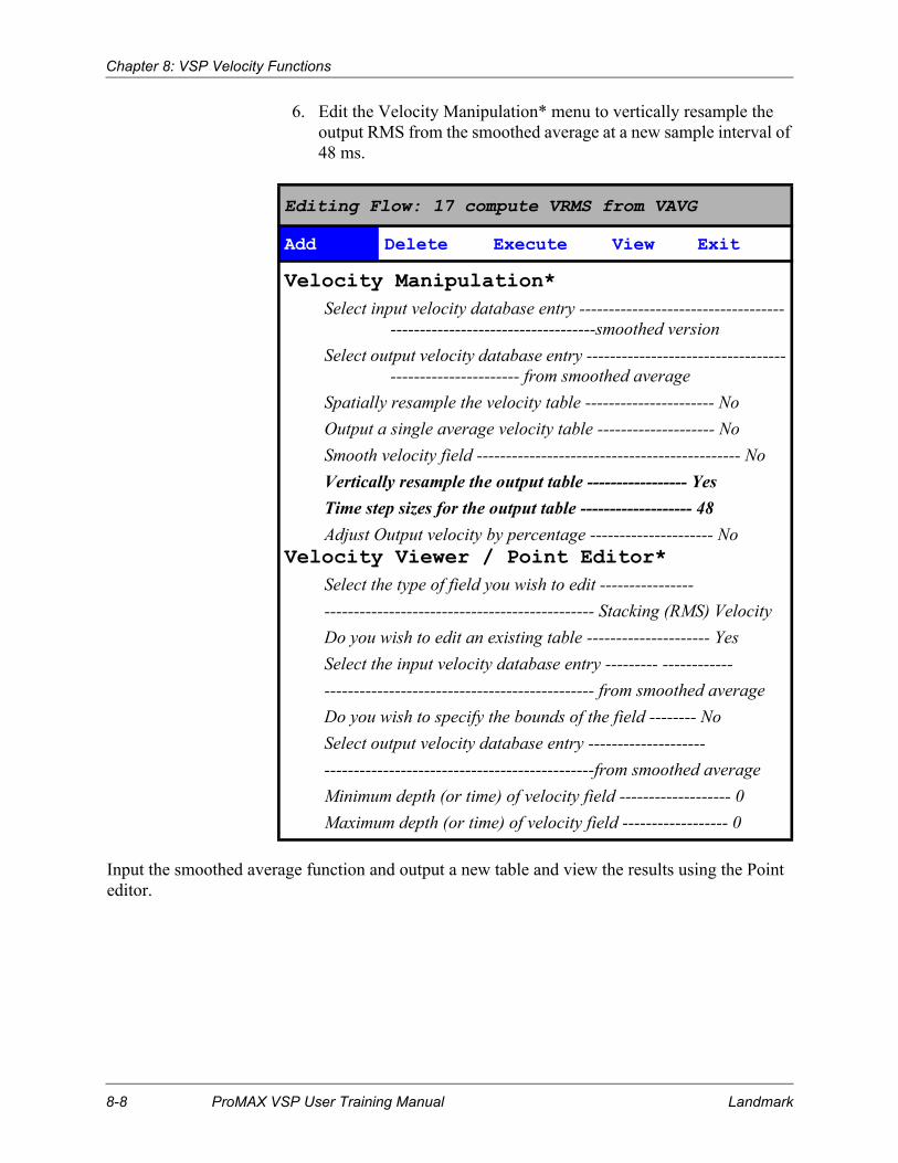
Chapter 8: VSP Velocity Functions
6. Edit the Velocity Manipulation* menu to vertically resample the output RMS from the smoothed average at a new sample interval of 48 ms.
Input the smoothed average function and output a new table and view the results using the Point editor.
Editing Flow: 17 compute VRMS from VAVG
Add Delete Execute View Exit
Velocity Manipulation*Select input velocity database entry -----------------------------------
-----------------------------------smoothed versionSelect output velocity database entry ----------------------------------
---------------------- from smoothed averageSpatially resample the velocity table ---------------------- NoOutput a single average velocity table -------------------- NoSmooth velocity field --------------------------------------------- NoVertically resample the output table ----------------- YesTime step sizes for the output table ------------------- 48Adjust Output velocity by percentage --------------------- No
Velocity Viewer / Point Editor*Select the type of field you wish to edit -------------------------------------------------------------- Stacking (RMS) VelocityDo you wish to edit an existing table --------------------- YesSelect the input velocity database entry --------- ---------------------------------------------------------- from smoothed averageDo you wish to specify the bounds of the field -------- NoSelect output velocity database entry ------------------------------------------------------------------from smoothed averageMinimum depth (or time) of velocity field ------------------- 0Maximum depth (or time) of velocity field ------------------ 0
8-8 ProMAX VSP User Training Manual Landmark

Chapter 9
VSP True Amplitude RecoveryVSP data is similar to surface seismic data in that it also suffers from amplitude loss due to spherical divergence and inelastic attenuation. However, one difference is that VSP data generally only travels half of the distance relative to surface data because the data we are interested in is recorded in the borehole directly above the reflecting horizon. This difference is compensated for in the VSP True Amplitude Recovery process. Spherical divergence requires accurate first arrival times in the header and both the spherical divergence and inelastic attenuation corrections require a velocity function. Therefore, TAR cannot be applied until after the first arrivals have been picked, loaded to the trace headers, and an RMS velocity function has been generated.
As an alternative to spherical divergence and dB/sec gain recovery, you may elect to test various time power curves.
In this chapter, you will test the VSP True Amplitude Recovery process for an appropriate dB/sec correction combined with spherical divergence. The spherical divergence correction requires a velocity function which was generated in the previous chapter by converting your average velocity function into an RMS function.
Topics covered in this chapter:
o True Amplitude Recovery Tests
o Apply True Amplitude Recovery Correction.
Landmark ProMAX VSP User Training Manual 9-1

Chapter 9: VSP True Amplitude Recovery
True Amplitude Recovery Tests
In this exercise, you will test the VSP True Amplitude Recovery process for an appropriate dB/sec correction combined with spherical divergence. The spherical divergence correction uses the velocity function that was generated by converting your average velocity function into an RMS function.
9-2 ProMAX VSP User Training Manual Landmark

Chapter 9: VSP True Amplitude Recovery
1. Build a flow to test various dB/Sec corrections combined with spherical divergence.
2. Input the file with only the vertical traces and process all traces.
3. Transfer the first break times to the trace headers.
Editing Flow: 18 VSP true amp recovery
Add Delete Execute View Exit
Disk Data InputSelect dataset--------------------------------vertical traces onlyTrace Read Option--------------------------------------------Get All
Database/Header TransferDirection of transfer -- Load TO trace headers FROM dbNumber of parameters -------------------------------------------- 1First database parameter --- TRC GEOMETRY FB_PICKFirst header entry --------(FB_PICK) First break pick time
Parameter TestEnter parameter VALUES ----------------- 10|8|6|4|2|0Trace grouping to reproduce ---------------------- Ensembles
VSP True Amplitude RecoveryApply spherical divergence corrections ---------------- YESBasis for spherical divergence -------------------------- 1/distApply inelastic attenuation correction --------------------- NoGet TAR velocity from database ---------------------------- YesShould the vel be treated as space variable ------------ NoSelect the velocity parameter table ------------------------------------
--------------------------- from smoothed averageApply dB/sec correction --------------------------------------- YesdB/sec correction constant ------------------------------ 99999Apply time raised to a power correction ------------------ NoAPPLY or REMOVE ------------------------------------------- ApplyMaximum application time --------------------------------- 2000
Trace DisplayNumber of ENSEMBLES per screen -------------------------- 7Trace scaling option ------------------------ Entire screen
Landmark ProMAX VSP User Training Manual 9-3

Chapter 9: VSP True Amplitude Recovery
4. Produce a comparison of 10, 8, 6, 4, 2 and 0 dB/Sec combined with a 1/dist spherical divergence correction. Notice the reverse order of parameters values. This is chosen because the “no TAR” reference record is the last panel, and it makes more sense to have this panel next to the smallest value tested. Notice also that the 0 dB/sec record still has spherical divergence applied.
Use the RMS velocity function that you generated from the smoothed average and then resampled to every 48 ms.
5. Parameterize Trace Display for the test panels.
We are generating 6 panels plus the control panel, so we will have a total of 7 ensembles.
We may also elect to set the minimum time of the display to 500 msec instead of 0 for the comparison to avoid a lot of dead samples at the top of the display.
Since we are looking for relative amplitude on these traces, we may find that using entire screen scaling will be a better choice than individual trace scaling.
6. Produce a second set of test panels varying the time power value from 1.4 to 2.2 by 0.2 and turning off the SPHDIV and dB/sec corrections.
You must reset the dB/sec correction back to a number other than 99999. Even though this parameter value is “hidden” when you turn off the dB/sec option, the value is still seen by the menu interpreter on execution. If you leave it as 99999, it will assume you intend to use Parameter Test, and the job will fail.
Don’t forget to reset the number of ensembles to display in Trace Display if you are using this option.
9-4 ProMAX VSP User Training Manual Landmark

Chapter 9: VSP True Amplitude Recovery
Apply True Amplitude Recovery
After selecting a set of TAR parameters (suggested SPHDIV and 6 dB/sec to 2000 ms), process the traces and output a new data file with TAR applied.
Editing Flow: 18 VSP true amp recovery
Add Delete Execute View Exit
Disk Data InputSelect dataset--------------------------------vertical traces onlyTrace Read Option--------------------------------------------Get All
Database/Header TransferDirection of transfer -- Load TO trace headers FROM dbNumber of parameters -------------------------------------------- 1First database parameter --- TRC GEOMETRY FB_PICKFirst header entry --------(FB_PICK) First break pick time
>Parameter Test<VSP True Amplitude Recovery
Final Selected ParametersTrace Display Label
Trace Label --------------------------- vertical traces with TARDisk Data Output
Output Dataset Filename-------- vertical traces with TARNew, or Existing, File?------------------------------------------NewRecord length to output--------------------------------------------0.Trace sample format------------------------------------------16 bitSkip primary disk Storage?-------------------------------------No
Landmark ProMAX VSP User Training Manual 9-5

Chapter 9: VSP True Amplitude Recovery
9-6 ProMAX VSP User Training Manual Landmark

Chapter 10
VSP Wave Field SeparationCorridor Stacks, VSP-CDP transforms and/or migrations are the final products from most VSP processing exercises. These products usually consist of only upgoing reflected energy. The downgoing energy must be removed from the total wavefield to uncover the reflected energy. It is also necessary to isolate the downgoing energy to aid in the deconvolution process. There are three basic techniques available to separate the downgoing and upgoing wavefields from the total wave field. These are Median, FK and Eigenvector Filters.
Topics covered in this chapter:
o Flattening the downgoing using the first arrivals
o Wavefield Separation using a Median Filter
o Wavefield Separation using an F-K filter
o Wavefield Separation using an EigenVector Filter.
o Wavefield Separation Test Comparisons
o Saving the Upgoing to Disk
o Saving the Downgoing to Disk
Landmark ProMAX VSP User Training Manual 10-1

Chapter 10: VSP Wave Field Separation
Flatten the Downgoing with F-B Picks
Wavefield separation requires flattening on the downgoing energy. This is accomplished by applying first arrival times as static values followed by some trim statics. Therefore, as a prerequisite to wavefield separation, first arrival times must be in the database and in the trace headers.
Exercise1. Build the following flow to apply the first break pick times as a static
to flatten the down going energy.
2. Input the file containing only the vertical component traces after tar has been applied and process all traces.
Remember that we transferred the first arrival times from the database to the headers prior to applying True Amplitude Recovery.
3. Select Header Statics parameters.
Apply a positive 100 ms Bulk Shift to all the traces and Subtract the first arrival time from the trace header as a static.
Editing Flow: 19 flatten downgoing arrivals
Add Delete Execute View Exit
Disk Data InputSelect dataset-------------------------vertical traces with TARTrace Read Option--------------------------------------------Get All
Header StaticsBulk shift Static -------------------------------------------------- 100What about previous statics ---- Add to previous staticsApply how many static header entries --------------------- 1First header word to apply --------------------------- FB_PICKHow to apply header statics ------------------------- Subtract
Apply Fractional StaticsTrace Display
10-2 ProMAX VSP User Training Manual Landmark

Chapter 10: VSP Wave Field Separation
4. In Apply Fractional Statics, apply the non-sample period portion of the static.
5. Plot the output traces on the screen and check to see that the first arrivals are approximately flat at about 100 ms.
Set the maximum time of the display to 500 msec.
Landmark ProMAX VSP User Training Manual 10-3

Chapter 10: VSP Wave Field Separation
Flatten with F-B Picks and Event Alignment
Because the first arrival pick times can be somewhat contaminated by noise, we can estimate trim statics via a cross correlation technique and apply them for additional flattening.
10-4 ProMAX VSP User Training Manual Landmark

Chapter 10: VSP Wave Field Separation
1. Expand the previous flow to add one iteration of event alignment.
2. Select Event Alignment in a Window parameters.
Use a 55 trace Selective Stack model, ignoring end of ensemble markers in order to estimate static shifts up to 10 ms. Specify a window 100 ms wide centered on the first breaks [1:50-150/]. Use a primary header word of FFID with no secondary header.
Editing Flow: 19 flatten downgoing arrivals
Add Delete Execute View Exit
Disk Data InputHeader StaticsApply Fractional Statics------------Event Alignment in Window
Maximum allowable static shift ----------------------------- 10Allowable percentage of hard zeros ------------------------ 15Number of traces in window----------------------------------55Method of building model trace ------------ Selective StackIgnore end of ensembles? ------------------------------------- YesSeek and report reversed traces ---------------------------- NoAccumulate statics in TOT_ALIN ---------------------------- NoGet analysis window parms from Database? --------- NoSELECT Primary header word ---------------------------- FFIDSELECT secondary header word ---------------------- NONESPECIFY window analysis parameters ------ 1:50-150/
Header StaticsBulk shift Static ------------------------------------------------------ 0What about previous statics ---- Add to previous staticsApply how many static header entries --------------------- 1First header word to apply ------------------------------alinstatHow to apply header statics -------------------------------- Add
Apply Fractional Statics------------Trace Display
Landmark ProMAX VSP User Training Manual 10-5

Chapter 10: VSP Wave Field Separation
3. Read the Event Alignment helpfile to find the name of the attribute to apply in Header Statics and also how to set the yes/no switch for Accumulate Statics in TOT_ALIN.
Set to No for this flow.
4. In Header Statics, ADD a user defined attribute called ALINSTAT to any previous statics and apply any remaining fractional statics.
5. Plot the output traces on the screen and check to see that the first arrivals are flatter than those from the previous exercise.
6. Expand the previous flow to add in a second iteration of event alignment.
7. In Event Alignment in Window, use a 30 trace Selective Stack model, again Ignoring end of ensemble issues.
Editing Flow: 19 flatten downgoing arrivals
Add Delete Execute View Exit
Disk Data InputHeader StaticsApply Fractional StaticsEvent Alignment in WindowHeader StaticsApply Fractional Statics--------------Event Alignment in Window
Number of traces in window --------------------------------- 30Accumulate statics in TOT_ALIN ----------------------------Yes
Header StaticsBulk shift Static ------------------------------------------------------ 0What about previous statics ---- Add to previous staticsApply how many static header entries --------------------- 1First header word to apply ------------------------------alinstatHow to apply header statics -------------------------------- Add
Apply Fractional Statics--------------Trace Display
10-6 ProMAX VSP User Training Manual Landmark

Chapter 10: VSP Wave Field Separation
Use the same gate as the previous execution.
Make sure you properly set the yes/no switch for Accumulate Statics in TOT_ALIN. Yes in this case.
8. Add the new ALINSTAT statics to any previous statics and apply any fractional remainder.
9. Plot the output traces on the screen and check to see that the first arrivals are even flatter than those from the previous exercise.
Landmark ProMAX VSP User Training Manual 10-7

Chapter 10: VSP Wave Field Separation
Compare Flattening Iterations
1. COPY the previous flow to a new flow to compare all three datasets.
2. Using flow editing techniques, rearrange and expand the existing flow to generate the comparison displays of:
• First Arrivals only
• 1 loop of Event Alignment
• 2 loops of Event Alignment
Editing Flow: 20 compare flattening
Add Delete Execute View Exit
Disk Data InputHeader StaticsApply Fractional StaticsReproduce Traces IF <REPEAT=1>
Trace Display LabelELSEIF <REPEAT=2>
Event Alignment in WindowHeader StaticsApply Fractional StaticsTrace Display Label
ELSEIF <REPEAT=3>Event Alignment in WindowHeader StaticsApply Fractional StaticEvent Alignment in WindowHeader StaticsApply Fractional StaticsTrace Display Label
ENDIFTrace Display
Specify Display END time ------------------------------------ 500
10-8 ProMAX VSP User Training Manual Landmark
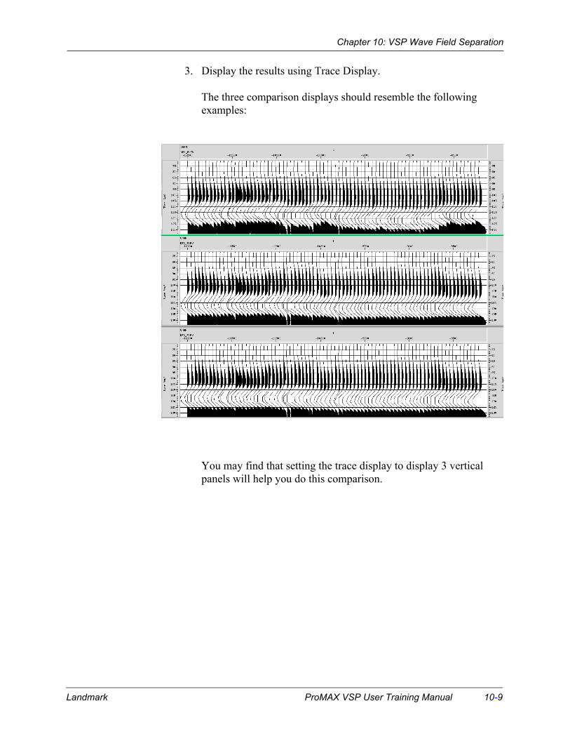
Chapter 10: VSP Wave Field Separation
3. Display the results using Trace Display.
The three comparison displays should resemble the following examples:
You may find that setting the trace display to display 3 vertical panels will help you do this comparison.
Landmark ProMAX VSP User Training Manual 10-9

Chapter 10: VSP Wave Field Separation
Wavefield Separation with Median Filter
The median filter has proven to be a very effective means of estimating the flattened event amplitudes by computing the median amplitude over a series of traces at constant time samples. If the input data is well flattened and the waveforms are stable, then the median filter should perform well. Typically, the amplitudes of consistent events are estimated and then this component is subtracted from the input.
10-10 ProMAX VSP User Training Manual Landmark

Chapter 10: VSP Wave Field Separation
Exercise1. COPY the flow “19 flatten downgoing arrivals” and edit the flow to
run parameter test of 2D spatial filtering to estimate and subtract the downgoing energy.
Editing Flow: 21 wavefield separation
Add Delete Execute View Exit
Disk Data InputHeader StaticsApply Fractional StaticsEvent Alignment in WindowHeader StaticsApply Fractional StaticsEvent Alignment in WindowHeader StaticsApply Fractional Statics---------------Parameter Test
Enter parameter VALUES --------- 19|15|13|11|9|7|5|3Trace grouping to reproduce ---------------------- Ensembles
2-D Spatial FilteringType of 2-D filter --------------------------- Simple 2-D MedianNumber of SAMPLES for 2-D filter ---------------------------- 1Number of TRACES for 2-D Filter ---------------------- 99999Type of trace edge taper --------------------- Fold edge backApplication mode for 2-D filter ------------------ SubtractionMinimum number of traces for subtraction ---------------- 3Steer filters along a velocity dip? ---------------------------- NoRe-apply mutes after filtering ------------------------------- Yes
Bandpass FilterDefault all parameters EXCEPTOrmsby filter frequency values ------------- 8-12-100-125
>Trace Display Label<---------------Trace Display
Number of ENSEMBLES per screen ------------------------ 10Trace scaling option --------------------------- Entire Screen
Landmark ProMAX VSP User Training Manual 10-11

Chapter 10: VSP Wave Field Separation
2. In Parameter Test, test a series of different length median filters.
Test values of 19 | 15 | 13 | 11 | 9 | 7 | 5 | 3 for the number of traces in the filter.
3. In 2D Spatial Filtering, apply a Single Sample, Simple 2D Median Filter to Subtract the downgoing energy from the total flattened wavefield.
In the Minimum Number of traces for Subtraction parameter, use a minimum of 3 traces in the filter and fold live traces back over the edge to make sure that there are always enough traces for the filter.
4. Apply a fairly wide open zero phase Ormsby Band Pass filter to suppress any adverse side effects of the median filter.
For this data at a 4 ms sample rate, apply a filter of 8-12-100-125.
5. Display the results using Trace Display.
You may find that setting the maximum time to display to 700 ms prior to display may save you some time in the zooming process.
You may also find that setting the display to plot 5 horizontal panels will be helpful.
You may also want to reset the Trace Display to do one vertical panel with 1 ensemble per screen and use the screen swapping capabilities within Trace Display to compare the different results.
6. After selecting the length of filter that works best, rerun the flow to QC the output section.
Toggle the Parameter Test inactive and input the proper filter length (11) in the 2D Spatial Filter process instead of the 99999 for the parm test.
10-12 ProMAX VSP User Training Manual Landmark

Chapter 10: VSP Wave Field Separation
7. Add a Trace Display Label after the Median Filter to annotate these data for future reference.
Upgoing Energy Separated by Median Filter
Landmark ProMAX VSP User Training Manual 10-13

Chapter 10: VSP Wave Field Separation
F-K Analysis
Using an F-K filter to separate the input data into various dip components is another very effective means of separating the flattened downgoing energy from the dipping upgoing energy, thus separating the upgoing from the downgoing. We can plot the flattened data in the F-K plane and estimate various fan filters and/or polygonal filters to isolate one of the dip components.
Using the Interactive F-K Analysis process, you can interactively test various reject and accept F-K polygons to keep the upgoing and downgoing.
10-14 ProMAX VSP User Training Manual Landmark
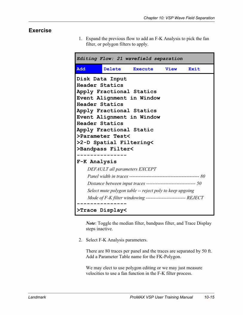
Chapter 10: VSP Wave Field Separation
Exercise1. Expand the previous flow to add an F-K Analysis to pick the fan
filter, or polygon filters to apply.
Note: Toggle the median filter, bandpass filter, and Trace Display steps inactive.
2. Select F-K Analysis parameters.
There are 80 traces per panel and the traces are separated by 50 ft. Add a Parameter Table name for the FK-Polygon.
We may elect to use polygon editing or we may just measure velocities to use a fan function in the F-K filter process.
Editing Flow: 21 wavefield separation
Add Delete Execute View Exit
Disk Data InputHeader StaticsApply Fractional StaticsEvent Alignment in WindowHeader StaticsApply Fractional StaticsEvent Alignment in WindowHeader StaticsApply Fractional Static>Parameter Test<>2-D Spatial Filtering<>Bandpass Filter<---------------F-K Analysis
DEFAULT all parameters EXCEPTPanel width in traces -------------------------------------------- 80Distance between input traces ------------------------------- 50Select mute polygon table -- reject poly to keep upgoingMode of F-K filter windowing ------------------------- REJECT
--------------->Trace Display<
Landmark ProMAX VSP User Training Manual 10-15

Chapter 10: VSP Wave Field Separation
3. Use the dx/dt tool to measure the apparent velocity of the up-going energy in flattened space on the F-K Analysis section.
The velocity should be about 6700 ft./sec.
4. Pick a positive and negative velocity cut to apply as a fan filter in F-K Filter.
Numbers like -4000 and + 20000 are good choices for a reject filter to keep the upgoing.
You may choose numbers like -20000 and +20000 as an accept filter to keep the downgoing.
Note: If you are working with polygons, be careful about how you set the Accept and Reject options.
5. Generate the Filtered Output panel to QC the polygon and parameters.
10-16 ProMAX VSP User Training Manual Landmark

Chapter 10: VSP Wave Field Separation
Wavefield Separation with F-K Filter
Experiment with different accept and reject fan filters and polygons looking at the output in F-K Analysis and Trace Display.
1. Expand the previous flow to add an F-K Filter to estimate and reject the downgoing energy.
2. You may have to include Inline Sort module because F-K Filter does not tolerate “chan” as the primary sort key. Include Inline Sort and Ensemble Redefine before F-K Filter. Include another Inline Sort after the F-K Filter in order to return the data to its original sort order.
This could be done by changing the sort order in Disk Data Input. However, for making comparisons with the other wavefield separation methods in this flow, it is simpler to modify the flow
Landmark ProMAX VSP User Training Manual 10-17

Chapter 10: VSP Wave Field Separation
using Inline Sort. The Ensemble Redefine ensures that all traces go into the F-K transform, rather than one FFID (one trace) at a time.
3. Input your velocities as a fan filter and/or try any picked polygons to Reject the downgoing and keep only the upgoing. Use the defaults for padding and tapering.
Editing Flow: 21 wavefield separation
Add Delete Execute View Exit
Disk Data InputHeader StaticsApply Fractional StaticsEvent Alignment in WindowHeader StaticsApply Fractional StaticsEvent Alignment in WindowHeader StaticsApply Fractional Static>Parameter Test<>2-D Spatial Filtering<>Bandpass Filter<---------------Inline Sort
Primary sort key ------------------------------------ FFIDEnsemble Redefine
Mode of application ------------------------------------ EntireF-K Filter
Type of F-K filter ----------------------------- Arbitrary PolygonDistance between input traces ------------------------------- 50Panel Width on Traces ------------------------------------------ 80Select mute parameter file - reject poly to keep upgoingMode of F-K filter operation --------------------------- REJECT
Inline SortPrimary sort key ------------------------------------ Chan
>F-K Analysis<--------------->Trace Length<>Trace Display<
10-18 ProMAX VSP User Training Manual Landmark

Chapter 10: VSP Wave Field Separation
Suggested parameters are to use a fan filter of -4000 and + 20000 ft./sec in reject mode. With this velocity the K-space wrap parameter should be set to No. QC the output with F-K analysis.
Landmark ProMAX VSP User Training Manual 10-19

Chapter 10: VSP Wave Field Separation
Wavefield Separation with Eigenvector (K-L) Filter
An Eigenvector Filter essentially decomposes a group of traces into dip components where the number of dip components is related to the number of traces in the transform. These dip components are accessed by selecting eigenvector percentages from 0 to 100 percent where the low percentages are the flatter components. The option exists to either keep the selected percentage or to subtract the selected percentage from the input.
Three sets of times are required depending on what options are selected:
• a design gate from which the dip component matrix weights are computed
• an application time gate
• an optional subtraction time gate.
In general the application and subtraction gates are the entire time range of the data. The design gates should be restricted to a good data zone. For VSP data, this is the area near the first arrivals.
When operating on data that has been flattened on the first arrivals, the low percentage eigenvectors are the flattened downgoing energy and the high percentages are the dipping upgoing. In this exercise you will design the eigenvectors over a time window around the first arrivals using a fairly short spatial window and then subtract the low percentage values from the input to extract the upgoing energy.
10-20 ProMAX VSP User Training Manual Landmark
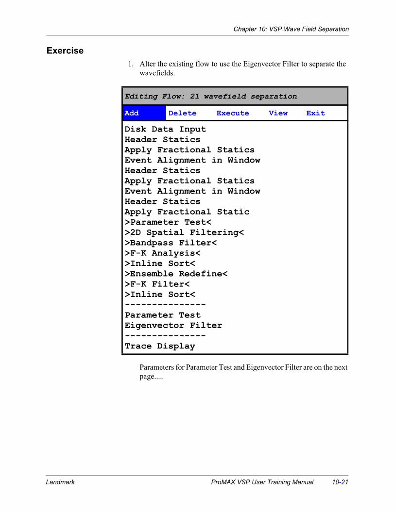
Chapter 10: VSP Wave Field Separation
Exercise1. Alter the existing flow to use the Eigenvector Filter to separate the
wavefields.
Parameters for Parameter Test and Eigenvector Filter are on the next page.....
Editing Flow: 21 wavefield separation
Add Delete Execute View Exit
Disk Data InputHeader StaticsApply Fractional StaticsEvent Alignment in WindowHeader StaticsApply Fractional StaticsEvent Alignment in WindowHeader StaticsApply Fractional Static>Parameter Test<>2D Spatial Filtering<>Bandpass Filter<>F-K Analysis<>Inline Sort<>Ensemble Redefine<>F-K Filter<>Inline Sort<---------------Parameter TestEigenvector Filter---------------Trace Display
Landmark ProMAX VSP User Training Manual 10-21

Chapter 10: VSP Wave Field Separation
.
Note: Toggle the F-K filter and F-K Analysis inactive in the flow
1. Design a test of the Eigenvector filter over the first arrivals
Use a constant design window for all FFID’s from 0-500 ms and apply a filter over the entire time range (0-2000 ms). Also, subtract over the entire time range from 0-2000 ms. Test values of 3, 7, 11, 15, and 19 for the trace window width and subtract the first 10 percent of the Eigen images.
Editing Flow: 21 wavefield separation
Add Delete Execute View Exit
---------------Parameter Test
Enter parameter VALUES ------------------- 3|7|11|15|19Trace grouping to reproduce ---------------------- Ensembles
Eigenvector FilterMode ----------------------------- Subtract Eigenimage of ZoneGet matrix design gates from DATABASE --------------- NoSELECT Primary header word ---------------------------- FFIDSPECIFY design time gate ---------------------------- 1:0-500/Get application gates from DATABASE ------------------- NoSELECT Primary header word ---------------------------- FFIDSPECIFY application gate -------------------------- 1:0-2000/Get Subtraction gate from DATABASE -------------------- NoSELECT Primary header word ---------------------------- FFIDSPECIFY subtraction gate -------------------------- 1:0-2000/Type of Computation ------------------------------------------ RealHorizontal window width -------------------------------- 99999Start percent of eigenimage range ---------------------------- 0End percent of eigen image range -------------------------- 10Re-apply trace mutes after filter --------------------------- Yes
---------------Trace Display
10-22 ProMAX VSP User Training Manual Landmark

Chapter 10: VSP Wave Field Separation
2. You may want to test various panel widths, design gates, and Eigen image percentage ranges.
Note that you cannot use the “Parameter Test” sequence to test the percentage ranges.
3. Try various Trace Display configurations:
1) Each output ensemble individually and then swap the screens.
2) All ensembles on the same screen.
Note that the Eigen Filter is very difficult to test because the percentage to keep range varies as a function of the length of the filter.
Landmark ProMAX VSP User Training Manual 10-23

Chapter 10: VSP Wave Field Separation
Wavefield Separation Comparison Test
Exercise1. Expand the previous flow to reproduce the traces and add IF -
ELSEIF - ENDIF statements around the various separation programs.
Editing Flow: 21 wavefield separation
Add Delete Execute View Exit
Disk Data InputHeader StaticsApply Fractional StaticsEvent Alignment in WindowHeader StaticsApply Fractional StaticsEvent Alignment in WindowHeader StaticsApply Fractional Statics>Parameter Test<Inline SortEnsemble RedefineReproduce TracesIF
2D Spatial FilteringTrace Display LabelBandpass Filter
ELSEIFF-K Filter>F-K Analysis<Trace Display label
ELSEIFEigenvector FilterTrace Display Label
ENDIF>Trace Length<Trace Display
Number of ensembles per screen ------------------------------- 80
10-24 ProMAX VSP User Training Manual Landmark

Chapter 10: VSP Wave Field Separation
2. Notice that the Inline Sort and Ensemble Redefine needed for the F-K Filter has been included here before any wavefield separation method is applied. This modification to the flow does not effect the other methods of wavefield separation becuase the physical sequence of the traces is not changed. This is NOT to be trusted as an ordinary way to handle processing. Modifying ensemble boundaries and sort order definintions will usually cause a very different result or may cause job failure.
3. Based on the value of the Repeat header word, apply all three types of separation possibilities and compare the results using Trace Display.
4. If desired, an AGC or other type of gain function may be applied.
5. Experiment with various display options to compare the results from the different separation techniques.
• Display each method (each group of 80 traces) on the screen independently and scroll through them.
• Display all three 80 trace groups on the screen at the same time.
• Display all three 80 trace groups on the screen in 3 vertical and then 3 horizontal display panels.
6. Select the method that produces the best results.
Landmark ProMAX VSP User Training Manual 10-25

Chapter 10: VSP Wave Field Separation
Save the Upgoing Energy
Exercise1. Select the method that best isolates the upgoing and then remove the
flattening statics, and trim statics and save the upgoing data. Copy the testing flow and delete modules that you do not need
2. Suppose that the F-K Filter was selected as the best option to isolate the upgoing energy.
Editing Flow: 22 save upgoing energy
Add Delete Execute View Exit
Disk Data InputHeader StaticsApply Fractional StaticsEvent Alignment in WindowHeader StaticsApply Fractional StaticsEvent Alignment in WindowHeader StaticsApply Fractional Statics>2D Spatial Filtering<>Trace Display Label<>Bandpass Filter<Inline SortEnsemble RedefineF-K FilterInline Sort<Trace Display label>Eigenvector Filter<>Trace Display Label<--------------Header StaticsDisk Data Output-------------->Trace Display<
10-26 ProMAX VSP User Training Manual Landmark
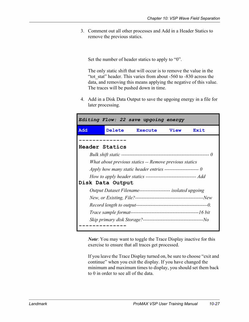
Chapter 10: VSP Wave Field Separation
3. Comment out all other processes and Add in a Header Statics to remove the previous statics.
Set the number of header statics to apply to “0”.
The only static shift that will occur is to remove the value in the “tot_stat” header. This varies from about -560 to -830 across the data, and removing this means applying the negative of this value. The traces will be pushed down in time.
4. Add in a Disk Data Output to save the upgoing energy in a file for later processing.
Note: You may want to toggle the Trace Display inactive for this exercise to ensure that all traces get processed.
If you leave the Trace Display turned on, be sure to choose “exit and continue” when you exit the display. If you have changed the minimum and maximum times to display, you should set them back to 0 in order to see all of the data.
Editing Flow: 22 save upgoing energy
Add Delete Execute View Exit
--------------Header Statics
Bulk shift static ------------------------------------------------------ 0What about previous statics -- Remove previous staticsApply how many static header entries --------------------- 0How to apply header statics ------------------------------- Add
Disk Data OutputOutput Dataset Filename------------------- isolated upgoingNew, or Existing, File?------------------------------------------NewRecord length to output--------------------------------------------0.Trace sample format------------------------------------------16 bitSkip primary disk Storage?-------------------------------------No
--------------
Landmark ProMAX VSP User Training Manual 10-27

Chapter 10: VSP Wave Field Separation
Wavefield Separation to Keep Downgoing
Exercise1. Copy flow “21 wavefield separation” in order to test for the best
approach to use for isolating the downgoing energy only. The downgoing energy is used to design deconvolution operators.
2. This flow will use the same method of inline sort to accomodate the
10-28 ProMAX VSP User Training Manual Landmark

Chapter 10: VSP Wave Field Separation
requirements of F-K Filter..
3. In 2D Spatial Filtering, select to run in Normal mode, the Eigenvector Filter to Output the eigenvector filtered zone, and the F-K filter to run in an Accept mode.
Editing Flow: 23 test and save downgoing
Add Delete Execute View Exit
Disk Data InputHeader StaticsApply Fractional StaticsEvent Alignment in WindowHeader StaticsApply Fractional StaticsEvent Alignment in WindowHeader StaticsApply Fractional StaticsInline Sort
Primary sort key ---------------------------------------------FFIDEnsemble Redefine
Mode of application ------------------------------------- EntireReproduce Traces>Parameter Test<IF
2D Spatial FilteringTrace Display LabelBandpass Filter
ELSEIFF-K Filter>F-K Analysis<Trace Display label
ELSEIFEigenvector FilterTrace Display Label
ENDIFInline Sort
sort keys -------------------------------- Repeat, Chan, FFID>Disk Data Output<Trace Display
Landmark ProMAX VSP User Training Manual 10-29

Chapter 10: VSP Wave Field Separation
When isolating the upgoing energy, we modeled the downgoing and subtracted it from the original record. We will use the same methods here, but we will output the modeled downgoing data.
Note: You may want to change the fan filter velocities for this exercise. Values of -20000 to 20000 ft./sec in an accept mode are reasonable.
4. Repeat the various comparison displays and select the method which gives the desired results.
• Display 3 vertical panels limiting the time on each panel to 1100 ms.
• Display 3 ensembles on one screen to 2000 ms.
10-30 ProMAX VSP User Training Manual Landmark

Chapter 10: VSP Wave Field Separation
Save the Downgoing Energy
Exercise1. Select one of the separation techniques and leave the flattening
statics applied. Save the downgoing data to disk.
2. Comment out all other processes. If you choose F-K Filter, you will need to include Inline Sort and Ensemble Redefine. The other
Editing Flow: 23 test and save downgoing
Add Delete Execute View Exit
Disk Data InputHeader StaticsApply Fractional StaticsEvent Alignment in WindowHeader StaticsApply Fractional StaticsEvent Alignment in WindowHeader StaticsApply Fractional Statics>Reproduce Traces<>IF<>2-D Spatial Filtering<>Trace Display Label<>Bandpass Filter<>ELSEIF<>F-K Analysis<>F-K Filter<>Trace Display label<>ELSEIF<Eigenvector FilterTrace Display Label>ENDIF<Disk Data Output
Output Dataset Filename------------------- isolated downgoing-------------->Trace Display<
Landmark ProMAX VSP User Training Manual 10-31

Chapter 10: VSP Wave Field Separation
methods do not require the sort.
3. Change the dataset name in Disk Data Output to save the down going energy for later processing.
4. In this case, also make sure that you do NOT apply Header Statics before outputting the data. The final Header Statics module should be removed or toggled inactive.
Why do we leave the statics applied to the downgoing data?
10-32 ProMAX VSP User Training Manual Landmark
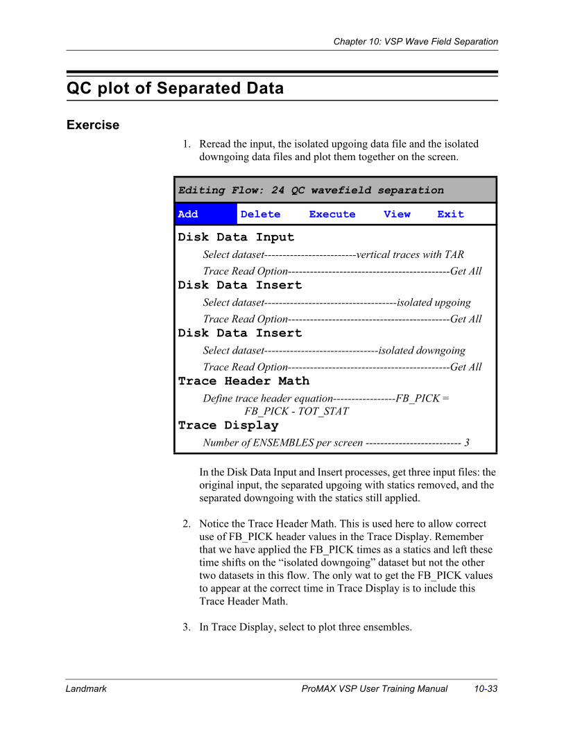
Chapter 10: VSP Wave Field Separation
QC plot of Separated Data
Exercise1. Reread the input, the isolated upgoing data file and the isolated
downgoing data files and plot them together on the screen.
In the Disk Data Input and Insert processes, get three input files: the original input, the separated upgoing with statics removed, and the separated downgoing with the statics still applied.
2. Notice the Trace Header Math. This is used here to allow correct use of FB_PICK header values in the Trace Display. Remember that we have applied the FB_PICK times as a statics and left these time shifts on the “isolated downgoing” dataset but not the other two datasets in this flow. The only wat to get the FB_PICK values to appear at the correct time in Trace Display is to include this Trace Header Math.
3. In Trace Display, select to plot three ensembles.
Editing Flow: 24 QC wavefield separation
Add Delete Execute View Exit
Disk Data InputSelect dataset-------------------------vertical traces with TARTrace Read Option--------------------------------------------Get All
Disk Data InsertSelect dataset------------------------------------isolated upgoingTrace Read Option--------------------------------------------Get All
Disk Data InsertSelect dataset-------------------------------isolated downgoingTrace Read Option--------------------------------------------Get All
Trace Header MathDefine trace header equation-----------------FB_PICK =
FB_PICK - TOT_STATTrace Display
Number of ENSEMBLES per screen -------------------------- 3
Landmark ProMAX VSP User Training Manual 10-33

Chapter 10: VSP Wave Field Separation
4. On the Trace Display interface, click on Picking and select first break picks from the database.
They should plot at about the start of the reflection data on the upgoing.
This is for QC only. Do not change or save the picks.
Note: The first arrival pick times are meaningless on the flattened downgoing data.
10-34 ProMAX VSP User Training Manual Landmark

Chapter 11
VSP DeconvolutionDeconvolution of VSP data involves the generation of an inverse filter designed to compress an input wavelet to a zero phase wavelet. The input wavelet is commonly extracted from the separated downgoing energy. A filter is designed to compress this energy into a zero-phase wavelet centered on the first arrival time. This filter is then applied to the upgoing data to remove the source signature from the reflection energy and output a zero phase wavelet at the actual time of the reflection generation interface.
Some design gate determination is commonly performed to isolate the wavelet from which the inverse filter is designed. This design gate generally starts at zero time, envelopes the first arrivals and progresses in time for a couple of hundred milliseconds. The maximum time of the gate typically comes immediately after the last consistent reverberation of the first arrival.
Topics covered in this chapter:
o Picking a design gate
o Designing the inverse filter on the downgoing data
o Applying the filter to the down-going for Quality Control
o Applying the filter to the upgoing data
Landmark ProMAX VSP User Training Manual 11-1

Chapter 11: VSP Deconvolution
Picking the Decon Design Gate
Exercise1. Build a flow to plot the downgoing data and pick a design gate.
2. Input the separated, flattened downgoing data.
3. All of the Trace Display parameters may be defaulted.
4. Using the Pick pulldown menu, select to pick a Bottom Mute to be applied prior to inverse filter design.
When prompted for a header entry to use for the mute function, select FFID as the header entry over which to vary the mute start times. Set the bottom mute to start at about 400 ms.
5. Exit the program to save the mute parameter table.
Editing Flow: 25 VSP deconvolution
Add Delete Execute View Exit
Disk Data InputSelect dataset-------------------------------isolated downgoingTrace Read Option--------------------------------------------Get All
Trace Display
11-2 ProMAX VSP User Training Manual Landmark

Chapter 11: VSP Deconvolution
Apply the mute for QC
Exercise1. Expand the previous flow to apply the mute for QC.
2. Apply the mute that was just picked as a Bottom Mute.
3. Display the result.
Editing Flow: 25 VSP deconvolution
Add Delete Execute View Exit
Disk Data InputSelect dataset-------------------------------isolated downgoingTrace Read Option--------------------------------------------Get All
Trace MutingReapply previous mutes --------------------------------------- NOMute time reference ---------------------------------------- Time 0Type of mute -------------------------------------------------- bottomending ramp --------------------------------------------------------- 30EXTRAPOLATE mute times --------------------------------- YESget mute file from the database ---------------------------- YesSelect mute parameter file -- decon design bottom mute
Trace Display
Landmark ProMAX VSP User Training Manual 11-3

Chapter 11: VSP Deconvolution
Deconvolution Filter Design
Exercise1. Build a flow to design the decon filter traces.
2. Input the separated, flattened downgoing data and apply the bottom mute to limit the design gate.
3. Select Filter Generation parameters.
After applying a Hanning Window taper over 100% of the input wavelets (zero percent flat), design and output to disk 1000 ms inverse filters where time zero on the input trace is 100 ms and use 3% white noise.
4. Plot the output from Filter Generation in Trace Display. You may wish to change the trace gain level after you see the display.
Editing Flow: 25 VSP deconvolution
Add Delete Execute View Exit
Disk Data InputTrace MutingFilter Generation
Filter type ------------------------------------------------------ InverseType of operator ------------------------------------ Time DomainPercent additive noise factor ------------------------------------ 3Trace length for the filter trace --------------------------- 1000Time on input trace representing time zero ----------- 100Apply taper to input wavelet AND output -------------- YesTaper type --------------------------------------------------- HanningPercent flat for time window ramping ----------------------- 0Output filter or filtered wavelet -------------------------- FilterNormalize output filters ----------------------------------------yesSpectral plot --------------------------------------------------------- NoWrite filter trace to disk ---------------------------------------- YesOutput dataset name ------------------------------ decon filters
Trace Display
11-4 ProMAX VSP User Training Manual Landmark

Chapter 11: VSP Deconvolution
The plotted traces are the actual filters to be applied.
5. In Filter Generation, output the filter traces to a disk file.
Why did we specify 100 ms as the “time on input representing time zero” in the filter generation menu?
Landmark ProMAX VSP User Training Manual 11-5

Chapter 11: VSP Deconvolution
Deconvolution Filter QC
Exercise1. Expand the previous flow to apply the filters and QC the results on
the down going data.
2. Input the separated, flattened downgoing data.
3. Select VSP Deconvolution parameters.
Apply filters that have been mixed over 5 FFIDs and exclude 1 filter trace on each end. Make sure that the zero reference time of the filter is correct. This should be set to 500 ms. which is the center time of the filter traces.
4. Add a label for display
What is the apparent phase of the wavelets in the display? Is the peak of the zero phase wavelet at the correct time? What are we demonstrating with this QC?
Editing Flow: 25 VSP deconvolution
Add Delete Execute View Exit
Disk Data Input>Trace Muting<>Filter Generation<VSP Deconvolution
Dataset where filters are stored -------------- decon filtersMode of mixing filters -------------------------------------- MixingSelect header on which to match traces -------------- FFIDBin Radius ------------------------------------------------------------- 5Exclude filters at edge of image ----------------------------- NoTime of input filter that represents zero time --------- 500Reapply mutes after deconvolution ----------------------- Yes
Trace Display LabelTrace Label ----------------------------- downgoing - decon QC
Trace Display
11-6 ProMAX VSP User Training Manual Landmark
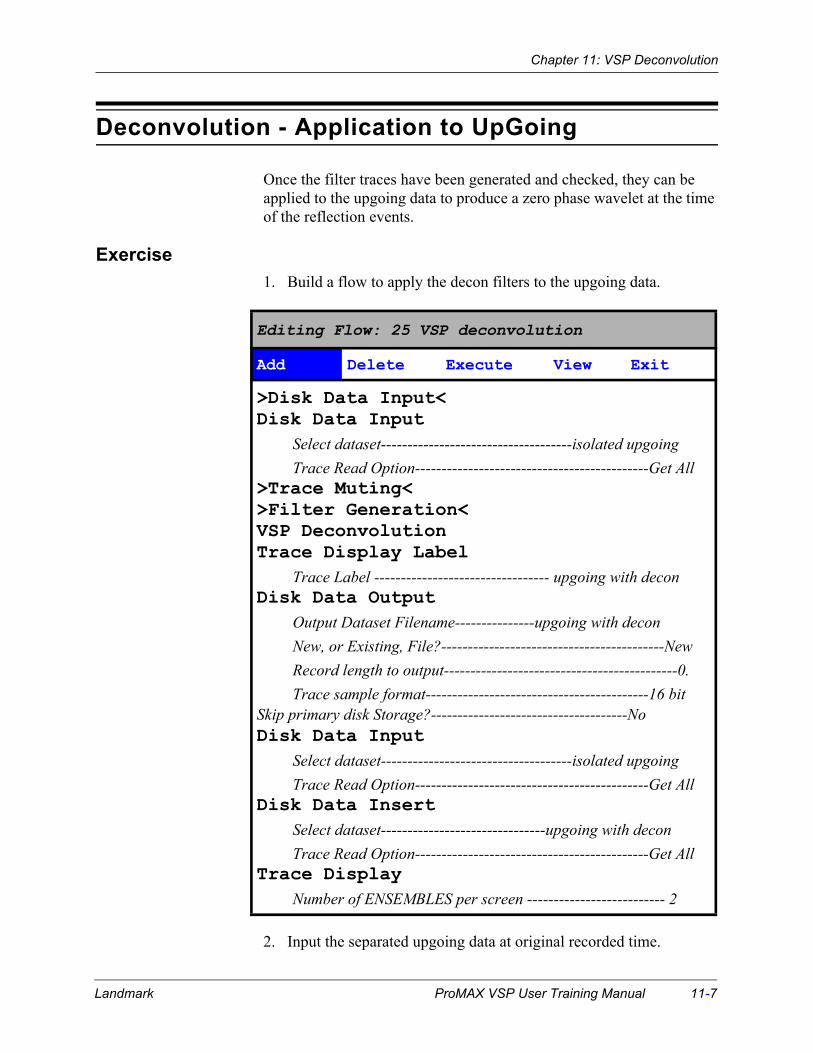
Chapter 11: VSP Deconvolution
Deconvolution - Application to UpGoing
Once the filter traces have been generated and checked, they can be applied to the upgoing data to produce a zero phase wavelet at the time of the reflection events.
Exercise1. Build a flow to apply the decon filters to the upgoing data.
2. Input the separated upgoing data at original recorded time.
Editing Flow: 25 VSP deconvolution
Add Delete Execute View Exit
>Disk Data Input<Disk Data Input
Select dataset------------------------------------isolated upgoingTrace Read Option--------------------------------------------Get All
>Trace Muting<>Filter Generation<VSP DeconvolutionTrace Display Label
Trace Label --------------------------------- upgoing with deconDisk Data Output
Output Dataset Filename---------------upgoing with deconNew, or Existing, File?------------------------------------------NewRecord length to output--------------------------------------------0.Trace sample format------------------------------------------16 bit
Skip primary disk Storage?-------------------------------------NoDisk Data Input
Select dataset------------------------------------isolated upgoingTrace Read Option--------------------------------------------Get All
Disk Data InsertSelect dataset-------------------------------upgoing with deconTrace Read Option--------------------------------------------Get All
Trace DisplayNumber of ENSEMBLES per screen -------------------------- 2
Landmark ProMAX VSP User Training Manual 11-7

Chapter 11: VSP Deconvolution
3. In VSP Deconvolution, apply the filters that were previously generated.
Mix the filters over 5 FFIDs and exclude 1 filter trace on each end. Make sure that the zero reference time of the filter is correct. This should be set to 500 ms or the center of the filter traces.
4. In Trace Display Label, label this data as being upgoing energy with decon applied.
5. In Disk Data Output, write the deconvolved data to disk.
6. Read the before and after decon files in a Disk Data Input and compare them with Trace Display.
11-8 ProMAX VSP User Training Manual Landmark

Chapter 11: VSP Deconvolution
Spectral Analysis Before and After Decon
Once the deconvolution has been applied we can generate a comparison spectral analysis of the data before and after decon.
Exercise1. Expand the previous flow to read two files from disk and then do a
spectral analysis on each.
Run a Multiple Subset analysis on one ensemble at a time. Use Recording Channel and FFID as the primary and secondary annotation levels.
Editing Flow: 26 spectral analysis
Add Delete Execute View Exit
Disk Data InputSelect dataset------------------------------------isolated upgoingTrace Read Option--------------------------------------------Get All
Disk Data InsertSelect dataset-------------------------------upgoing with deconTrace Read Option--------------------------------------------Get All
Interactive Spectral AnalysisData Selection method ---------------------- Multiple subsetsFreeze the selected subset ----------------------------------- YesDisplay data by traces or ensembles --------- EnsemblesNumber of ensembles per analysis location -------------- 1Number of ensembles between analysis locs ------------ 1Primary header for sorting and label ----------------- CHANSecondary header for sorting and label ----- REC_ELEVDefault all remaining parameters--------------------------------
Landmark ProMAX VSP User Training Manual 11-9

Chapter 11: VSP Deconvolution
11-10 ProMAX VSP User Training Manual Landmark

Chapter 12
VSP Corridor StackThe Corridor stack is one of the common final products from VSP data processing for zero (or near) offset surveys. This stack can be tied to surface seismic stack sections to help the processors and interpreters identify key geologic horizons at known depths to events seen on the seismic section. The corridor stack can also be used to help the drillers predict what is coming up deeper in the borehole by what is called “looking ahead of the bit”.
There is scope for discussion about how the processing sequence for the corridor stack is put together. We will first present the sequence using the prepared ProMAX macros for simplicity and then we can discuss variations on the processing sequence.
Topics covered in this chapter:
o One Way Normal Moveout Correction
o Picking Corridor Mutes
o Apply the Corridor Mutes for QC
o Produce the Corridor Stack
o Splice the Corridor Stack into a Surface Stack
Landmark ProMAX VSP User Training Manual 12-1

Chapter 12: VSP Corridor Stack
One Way Normal Moveout Correction
Normal moveout correction is applied to correct travel times for the horizonal offset between the source location and the receivers in the borehole. This is exactly the same effect as for conventional surface seismic recording except that the times are corrected for one-way travel from source to the receiver, rather than the two-way time of source to reflector to receiver in conventional seismic.
Exercise1. Build a flow to pick the top and bottom mute to define the corridor
to stack.
2. In Disk Data Input, input the deconvolved upgoing data file.
3. Apply the One Way NMO correction using the RMS velocity function that was generated earlier for the Spherical Divergence Correction.
Use the resampled RMS from the smoothed average.
4. Use Trace Display to plot the traces.
Editing Flow: 27 corridor stack
Add Delete Execute View Exit
Disk Data InputSelect dataset--------------------------- upgoing with deconTrace read option---------------------------------------------Get All
One Way Normal Moveout CorrectionCDP number for velocity----------------------------------------- 1Direction for NMO application--------------------- FORWARDStretch mute percentage---------------------------- 0.0Apply any remaining static during NMO?--------------- YesGet velocities from the database?-------------------------- YesSelect velocity parameter file----from smoothed average
Trace DisplayNumber of ensembles per screen -------------------------------- 80
12-2 ProMAX VSP User Training Manual Landmark

Chapter 12: VSP Corridor Stack
The one-way NMO correction for this dataset is very small. The source to borehole offset is 500 feet while the first receiver is more than 8000 feet down the hole.
You may think that nothing has happened to the data. You can modify the flow to reproduce the data and use IF/ENDIF logic to compare the data with and without the one-way NMO correction.
Note: If you wish to investigate the One Way NMO Correction module, beware that it uses the header attributes SOU_X, SOU_Y, REC_X and REC_Y to calculate the offset distance for this correction. It does not use the OFFSET header value.
Landmark ProMAX VSP User Training Manual 12-3

Chapter 12: VSP Corridor Stack
Picking Corridor Mutes
Two mutes are required to define the top and bottom of the corridor.
Exercise1. Execute the flow to have Trace Display on screen.
2. From the picking pulldown menu, select to define a top mute.
Define the mute to set the Top of the corridor.
Give the mute table a name that clearly indicates its purpose as a top mute for corridor stack. All mute tables are saved in one list and the names should tell you exactly how each mute table is intended to be used.
When prompted, select FFID as the header entry over which to vary the mute start times.
Note: This mute should be about the same time as the first arrivals.
3. From the picking pulldown menu, select to define a bottom mute.
Define the mute to set the Bottom of the corridor. It is normal to make the corridor about 100 ms wide.
4. Use the paintbrush icon to check the mutes, then save and exit the tool.
Editing Flow: 27 corridor stack
Add Delete Execute View Exit
Disk Data InputOne Way Normal Moveout CorrectionTrace Display
12-4 ProMAX VSP User Training Manual Landmark

Chapter 12: VSP Corridor Stack
Apply the Corridor Mutes for QC
As a second check of the mutes, apply the mutes to the data and display the result.
Exercise1. Expand the existing flow to add in two Trace Muting processes.
2. In Disk Data Input, input the deconvolved upgoing data file.
Editing Flow: 27 corridor stack
Add Delete Execute View Exit
Disk Data InputOne Way Normal Moveout Correction---------Trace Muting
Re-apply previous mutes-----------------------------------------NoMute time reference------------------------------------------Time 0TYPE of mute--------------------------------------------------------TopStarting ramp--------------------------------------------30.EXTRAPOLATE mute times?----------------------------------YesGet mute file from the DATABASE?-------------------------YesSELECT mute parameter file-----corridor stack top mute
Trace MutingRe-apply previous mutes-----------------------------------------NoMute time reference------------------------------------------Time 0TYPE of mute---------------------------------------------------BottomStarting ramp--------------------------------------------30.EXTRAPOLATE mute times?-----------------------YesGet mute file from the DATABASE?-------------------------YesSELECT mute parameter file-------------------------------------------
--------------------------corridor stack bottom mute
---------Trace Display
Landmark ProMAX VSP User Training Manual 12-5

Chapter 12: VSP Corridor Stack
3. In Trace Muting, apply the Top and Bottom mutes.
Do not forget that one is a Top mute and the other is a Bottom mute.
4. Display the result with Trace Display.
12-6 ProMAX VSP User Training Manual Landmark

Chapter 12: VSP Corridor Stack
Produce the Corridor Stack
In this exercise you will use the VSP Corridor Stack macro to apply the mutes and the first arrival times as a positive static. This will shift the data to two way time. You will then stack the traces. This stack trace will be copied a number of times to produce the final Corridor Stack dataset.
Exercise1. Expand the existing flow to add in the processes associated with
VSP Corridor Stack and optional enhancement programs.
Parameters for VSP Corridor Stack are on the next page.
Editing Flow: 27 corridor stack
Add Delete Execute View Exit
Disk Data Input <GET ALL>One Way Normal Moveout Correction--------->Trace Muting<>Trace Muting<>Trace Display<---------VSP Corridor Stack
Trace Display LabelDisk Data OutputAutomatic Gain ControlBandpass FilterTrace Display
Landmark ProMAX VSP User Training Manual 12-7

Chapter 12: VSP Corridor Stack
.
2. Comment out the two trace mutes since they are applied in the Corridor Stack Macro. Also comment out the Trace Display.
MB3 will toggle the processes inactive.
3. In VSP Corridor Stack, apply the Top and Bottom mutes and add the first arrival times from the header as a static.
Make 5 copies of a mean stack trace. For display purposes, apply a bulk shift static correction of -980 ms.
Note: The -980 shift is specific for the dataset in this class. In typical data, you may apply a small static or no static at this point.
4. Write the Corridor Stack traces to a disk dataset.
Editing Flow: 27 corridor stack
Add Delete Execute View Exit
VSP Corridor StackRamp time for top mute (ms)-----------------------------------30.EXTRAPOLATE top mute times?-----------------------------YesGet top mute file from the DATABASE---------------------YesSelect top mute parameter file---corridor stack top muteRamp time for bottom mute (ms)-----------------------------30.EXTRAPOLATE bottom mute times?-----------------------YesGet bottom mute file from the DATABASE?--------------YesSelect bottom mute parameter file--------------------------------------
------------------------corridor stack bottom muteBulk shift static-------------------------------------------------- -980What about previous statics?----Add to previous staticsApply how many static header entries?---------------------1First header word to apply-----------First break pick timeHeader statics application mode---------------------------AddMethod for trace summing----------------------------------MeanRoot power scalar for stack normalization---------------0.5Number of copies------------------------------------------------------5
12-8 ProMAX VSP User Training Manual Landmark

Chapter 12: VSP Corridor Stack
5. If desired, add in the AGC and/or Bandpass Filter before and/or after stack to help with the cosmetic appearance of the stack traces.
6. Add a new Trace Display to plot the corridor stack.
Note: The value for the output CDP attribute is set to the CDP value of the last trace input to the process. Remember that CDP number has no real significance in out VSP processing.
Landmark ProMAX VSP User Training Manual 12-9
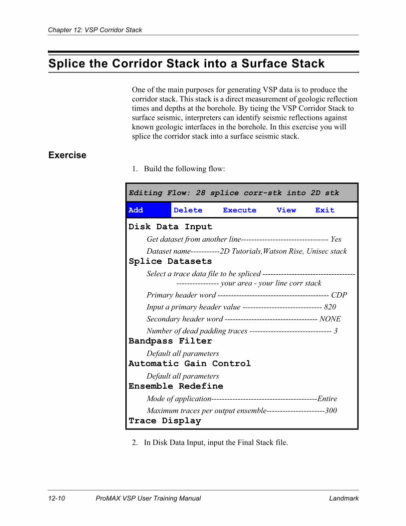
Chapter 12: VSP Corridor Stack
Splice the Corridor Stack into a Surface Stack
One of the main purposes for generating VSP data is to produce the corridor stack. This stack is a direct measurement of geologic reflection times and depths at the borehole. By tieing the VSP Corridor Stack to surface seismic, interpreters can identify seismic reflections against known geologic interfaces in the borehole. In this exercise you will splice the corridor stack into a surface seismic stack.
Exercise1. Build the following flow:
2. In Disk Data Input, input the Final Stack file.
Editing Flow: 28 splice corr-stk into 2D stk
Add Delete Execute View Exit
Disk Data InputGet dataset from another line--------------------------------- YesDataset name-----------2D Tutorials,Watson Rise, Unisec stack
Splice DatasetsSelect a trace data file to be spliced -----------------------------------
---------------- your area - your line corr stackPrimary header word ------------------------------------------ CDPInput a primary header value ------------------------------ 820Secondary header word ----------------------------------- NONENumber of dead padding traces ------------------------------- 3
Bandpass FilterDefault all parameters
Automatic Gain ControlDefault all parameters
Ensemble RedefineMode of application----------------------------------------EntireMaximum traces per output ensemble----------------------300
Trace Display
12-10 ProMAX VSP User Training Manual Landmark

Chapter 12: VSP Corridor Stack
3. In Splice Datasets, splice in the Corridor Stack at CDP Bin Number 820 of the 2D stack, and pad with 3 dead traces. Remember that the CDP numbers of our VSP data have no real meaning.
4. Apply a bandpass filter and AGC for cosmetic purposes.
5. Use Ensemble Redefine to ensure that the entire set of traces is brought into Trace Display together.
6. Plot the combined display with Trace Display
Note: This stack and VSP data are from completely different areas.
When the corridor stack was generated, a -980 time shift was applied so that it approximately ties the conventional stack data.
Landmark ProMAX VSP User Training Manual 12-11

Chapter 12: VSP Corridor Stack
12-12 ProMAX VSP User Training Manual Landmark

Chapter 13
Generate Intv-Dpth VelocityFunctionTwo products from VSP data processing require an Interval Velocity vs. Depth velocity function. These are the VSP-CDP transform and the VSP Migration.
In this exercise, we will build INTV-DPTH velocity fields from the average velocity functions that we derived from the first arrival times before and after smoothing. Some additional editing will be required to ensure that the velocity field spans the entire desired depth image area for the VSP migration.
Topics covered in this chapter:
o Compute Interval Velocity vs. Depth
o QC of the function using the Velocity Viewer/Point Editor
Landmark ProMAX VSP User Training Manual 13-1

Chapter 13: Generate Intv-Dpth Velocity Function
Compute Interval Velocity vs. Depth
The average velocity vs. depth function in itself is not very useful but we can convert this function to an interval velocity vs. depth function for future processing. As you will see, typically some smoothing must occur while generating the interval velocity function.
13-2 ProMAX VSP User Training Manual Landmark

Chapter 13: Generate Intv-Dpth Velocity Function
1. Build the following flow:
2. Input the average velocity function computed from the first arrival
Editing Flow: 29 generate intv-dpth function
Add Delete Execute View Exit
Velocity Manipulation*Type of velocity table to input ----- Average Vel in DepthGet velocity table from database entry ------------------ YesSelect input velocity database entry -----------------------------------
----------------from raw first break pick timesCombine a second velocity table ---------------------------- NoResample the input velocity table? ------------------------- NoShift or stretch the input velocity table -------------------- NoType of parameter table to output -------------------------------------
--------------------------------- Interval Vel in DepthSelect output velocity database entry ----------------------------------
---------------------------------- from raw averageSpatially resample the velocity table ---------------------- NoOutput a single average velocity table -------------------- NoSmooth velocity field --------------------------------------------- NoVertically resample the output velocity table ----------- NoAdjust Output velocity by percentage --------------------- NoClip output velocities?-----------------------------------------No
Velocity Viewer / Point Editor*Select the type of field you wish to edit -------------------------------------------------------------Interval Vel in DepthDo you wish to edit an existing table --------------------- YesSelect the input velocity database entry --------- ------------------------------------------------------------------ from raw averageMinimum CDP coordinate in viewing box---------------------1Maximum CDP coordinate in viewing box ----------------244Select output velocity database entry ---------------------------------------------------------------------------from raw averageMinimum depth (or time) of velocity field ------------------- 0Maximum depth (or time) of velocity field ------------------ 0
Landmark ProMAX VSP User Training Manual 13-3

Chapter 13: Generate Intv-Dpth Velocity Function
times and output an interval velocity vs. depth function.
3. View the output intv-dpth function.
Click on the velocity scale icon and the function edit icon.
We will not do any editing, so you can output to the same table as you are reading from.
Are there any problems with this interval velocity function?
Exercise1. Expand the flow to generate a new interval velocity vs. depth
function from the smoothed average velocity vs. depth function.
2. Input the smoothed average velocity function computed from the first arrival times and output a new intv-depth table.
3. View the output table for QC.
Editing Flow: 29 generate intv-depth function
Add Delete Execute View Exit
>Velocity Manipulation*<>Velocity Viewer/Point Editor*<Velocity Manipulation*
Select input velocity database entry ----------------------------------------------------------------------smoothed version
Select output velocity database entry ------------------------------------------------------------ from smoothed average
Vertically resample the output table ----------------- YesTime step sizes for the output table ------------------- 48
Velocity Viewer / Point Editor*Select the input velocity database entry --------- ---------------------------------------------------------- from smoothed averageSelect output velocity database entry ------------------------------------------------------------------ from smoothed average
13-4 ProMAX VSP User Training Manual Landmark

Chapter 13: Generate Intv-Dpth Velocity Function
You may elect to run each of these simultaneously for comparison.
------- from raw avg ------- from smoothed avg -----
Note: There are two points very close together on both functions so you can elect to resample the function in Velocity Manipulation prior to output.
Landmark ProMAX VSP User Training Manual 13-5

Chapter 13: Generate Intv-Dpth Velocity Function
ExerciseOne of the requirements for the VSP migration is that the velocity field span the entire range of the output image area. Since we may want to image events recorded below the bottom of the well, we must expand the velocity field in depth to cover the proposed image area. We will also resample the output intv-depth function to the original sample period of 50 ft.
1. Edit the existing flow.
2. Input the smoothed average velocity function computed from the first arrival times and output a new intv-depth table.
3. In Velocity Manipulation, resample the output function to a depth increment of 50 ft.
4. View the output table for QC.
Specify an output maximum depth of 15000 ft.
Editing Flow: 29 generate intv-depth function
Add Delete Execute View Exit
>Velocity Manipulation*<>Velocity Viewer/Point Editor*<Velocity Manipulation*
Select input velocity database entry ----------------------------------------------------------------------smoothed version
Select output velocity database entry ------------------------------------------------------------ from smoothed average
Vertically resample the output table ----------------- YesTime step sizes for the output table ------------------- 50
Velocity Viewer / Point Editor*Select the input velocity database entry --------- ---------------------------------------------------------- from smoothed averageSelect output velocity database entry ------------------------------------------------------------------ from smoothed averageMinimum depth (or time) of vel field -------------------------- 0Maximum depth (or time) of vel field ----------------- 15000
13-6 ProMAX VSP User Training Manual Landmark

Chapter 13: Generate Intv-Dpth Velocity Function
5. Remember to go into edit mode and you may elect to edit the velocity function in preparation for migration.
6. In the smoothing parameter window, set the CDP sampling interval to a number greater than the range of CDPs in the display. This way you get only a single function output.
Edit the smoothed version and output a Velocity Function for VSP-CDP transform and Migration.
7. Be sure to click on “update” above the function edit window, or reselect the velocity location in order to see the result of your smoothing/editing.
Landmark ProMAX VSP User Training Manual 13-7

Chapter 13: Generate Intv-Dpth Velocity Function
13-8 ProMAX VSP User Training Manual Landmark
Chapter 14
VSP CDP TransformFor VSP surveys where the source is offset from the well location, a standard final product is the VSP to CDP transform. The VSP to CDP transform is a high spatial and temporal resolution seismic section that allows you to image reflection events near the borehole in the direction toward the shot location. This may help identify faults and/or the attitude of dipping reflected events.
Topics covered in this chapter:
o Generation of the VSP CDP transform
Landmark ProMAX VSP User Training Manual 14-1

Chapter 14: VSP CDP Transform
VSP CDP Transform
Exercise1. Build a flow to generate the VSP-CDP transform.
2. In Disk Data Input, input the upgoing data with decon applied.
3. Select the VSP/CDP Transform parameters.
Editing Flow: 30 VSP-CDP transform
Add Delete Execute View Exit
Disk Data InputSelect dataset-------------------------------upgoing with deconTrace Read Option--------------------------------------------Get All
VSP/CDP TransformHorizontal binning interval -------------------------------------- 5CDP at which to extract vel function --------------------- 100Specify trace length of output trace in msec -------- 3000Select how velocity is to be specified ------------ DatabaseSelect a velocity file ---------------- from smoothed averageRay trace interval ------------------------------------------------- 20Datum elevation ----------------------------------------------------- 0Allowable percentage of moveout stretch ---------------- 50
Trace Display LabelTrace Label --------------------------------- VSP-CDP transform
Disk Data OutputOutput Dataset Filename-------------VSP - CDP transformNew, or Existing, File?------------------------------------------NewRecord length to output--------------------------------------------0.Trace sample format------------------------------------------16 bitSkip primary disk Storage?-------------------------------------No
Trace DisplayPrimary trace LABELING header ----------------------- NONESecondary trace LABELING header ---------------- RBIN_X
14-2 ProMAX VSP User Training Manual Landmark
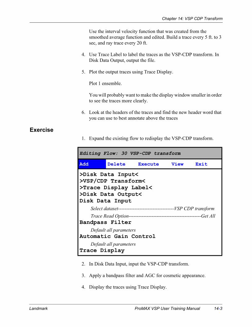
Chapter 14: VSP CDP Transform
Use the interval velocity function that was created from the smoothed average function and edited. Build a trace every 5 ft. to 3 sec, and ray trace every 20 ft.
4. Use Trace Label to label the traces as the VSP-CDP transform. In Disk Data Output, output the file.
5. Plot the output traces using Trace Display.
Plot 1 ensemble.
You will probably want to make the display window smaller in order to see the traces more clearly.
6. Look at the headers of the traces and find the new header word that you can use to best annotate above the traces
Exercise1. Expand the existing flow to redisplay the VSP-CDP transform.
2. In Disk Data Input, input the VSP-CDP transform.
3. Apply a bandpass filter and AGC for cosmetic appearance.
4. Display the traces using Trace Display.
Editing Flow: 30 VSP-CDP transform
Add Delete Execute View Exit
>Disk Data Input<>VSP/CDP Transform<>Trace Display Label<>Disk Data Output<Disk Data Input
Select dataset----------------------------------VSP CDP transformTrace Read Option--------------------------------------------Get All
Bandpass FilterDefault all parameters
Automatic Gain ControlDefault all parameters
Trace Display
Landmark ProMAX VSP User Training Manual 14-3

Chapter 14: VSP CDP Transform
Plot the traces by annotating the RBIN_X header word above the traces. This will plot a value representing the distance from the borehole above the traces.
Note: You must type-in RBIN_X as a user-defined attribute.
You may want to enhance the appearance of the transform by applying a trace mix and/or adjusting the scaling and/or bandpass filter parameters.
OPTIONAL EXERCISE: Change Disk Data Input to “sort” by FFID. Toggle off the Disk Data Output. Execute thte job. Step through the output data in Trace Display. This should give you a clear sense of what the process is doing.
Note: Be careful of assuming any meaning to CDP number in the trace headers. CDP values are equal to RBIN_X values.
14-4 ProMAX VSP User Training Manual Landmark

Chapter 15
VSP MigrationFor VSP surveys where the source is offset from the well location, it is possible to migrate the recorded data. The migration produces a high spatial resolution seismic section that allows you to image reflection events in the vicinity of the bore-hole looking in the plane defined by the well bore and the shot location. Unlike the VSP-CDP transform, the migration can look on the opposite side of the borehole. This may help identify faults and/or the attitude of dipping reflected events.
The migration differs from the VSP-CDP transform in that the transform is a simple mapping function that takes a point on a shot to receiver trace and maps that point to a single reflection point in the subsurface. The migration operation is similar to that for surface seismic data, where it attempts to place a data point at all locations from which it could have originated.
Topics covered in this chapter:
o VSP Migration
Landmark ProMAX VSP User Training Manual 15-1

Chapter 15: VSP Migration
VSP Migration
Exercise1. Build the following flow to migrate the VSP data:
2. In Disk Data Input, input the upgoing data with decon applied.
3. Select the following VSP Kirchhoff Mig. parameters, with the exception of inputting 30 for “Dip range to keep...”:
4. In Trace Label, label the traces as the migration. In Disk Data Output, output the file to disk.
Editing Flow: 31 VSP migration
Add Delete Execute View Exit
Disk Data Input <GET ALL>VSP Kirchhoff MigrationTrace Display LabelDisk Data Output
30
15-2 ProMAX VSP User Training Manual Landmark

Chapter 15: VSP Migration
Display the VSP Migration
Exercise1. Expand the flow to reread the migrated data and add an AGC prior
to display.
2. In Disk Data Input, input the migration file.
3. Scale the data to improve its cosmetic appearance.
Use a value of about 2000 for the AGC gate length.
4. In Trace Display, plot the migrated data and annotate CDP number above the traces.
Editing Flow: 31 VSP migration
Add Delete Execute View Exit
>Disk Data Input< <GET ALL>>Trace Header Math<>VSP Kirchhoff Migration<>Trace Display Label<>Disk Data Output<-------------------Disk Data InputAutomatic Gain Control-------------------Trace Display
Landmark ProMAX VSP User Training Manual 15-3

Chapter 15: VSP Migration
15-4 ProMAX VSP User Training Manual Landmark

Chapter 16
VSP Report GenerationA final report for VSP processing typically includes a listing of first arrival information for each source-receiver pair, the depth of each receiver, or velocity information derived from the VSP data. The module VSP Report combines selected data in the ProMAX database (velocity tables as well as OPF database) into one ASCII file to use in a VSP report. Multiple ASCII files can be created to ensure convenient formatting and organization for inclusion in documents.
Topics covered in this chapter:
o VSP Report
Landmark ProMAX VSP User Training Manual 16-1

Chapter 16: VSP Report Generation
VSP Report Generation
Exercise1. Build the following flow, making your own selection of parameter
values to send to the output file.
The input sort order has been chosen such that the information start at the shallowest receiver depths and increase down the hole. You can chose the sort order such that the information in the report starts from the bottom of the hole.
If we make an ensemble of only channel 1, then we can always default the Trace Display to plot all traces in 1 ensemble instead of having to change it to 80 and worry about ensemble gaps and display label issues.
2. The report file name can be an explicit pathname for the location of the file. When only a file name is given, the report file will be created under the flow directory underneath $PROMAX_DATA_HOME.
Editing Flow: 31 VSP report generation
Add Delete Execute View Exit
Disk Data InputSelect dataset ----------------------------------shots - with geomTrace Read Option-------------------------------------------- SORTInteractive Data Access ----------------------------------------- NoSelect primary trace header ----------------------- REC_ELEVSort order list for dataset ------------------------------------- *Presort in memory or on disk? ------------------------ Memory
VSP ReportFull path of output file ------------- VSPreportFile.txt<choose among numerous parameter options>
UNIX CommandsType in command? ------------------------------- YesSpecify command -------------------- cat VSPreportFile.txt
16-2 ProMAX VSP User Training Manual Landmark

Chapter 16: VSP Report Generation
3. UNIX Commands is optional. It is chosen so that the “report” can be viewed with the job.output viewer, instead of going to the Unix directory.
Be sure to include interval velocity information in your report. Notice that interval velocity values are shown on a line between the receiver depth locations, ensuring no ambiguity about which interval they belong to.
Landmark ProMAX VSP User Training Manual 16-3

Chapter 16: VSP Report Generation
16-4 ProMAX VSP User Training Manual Landmark

Chapter 17
VSP Corkscrew GeometryVSP Geometry can as simple as a straight borehole or it may become more complex when working with deviated boreholes. In this exercise we will look at a synthetic VSP which was recorded in a borehole that resembles a corkscrew.
Topics covered in this chapter:
o Assign VSP Geometry
o Quality Control Plots from the database
Landmark ProMAX VSP User Training Manual 17-1

Chapter 17: VSP Corkscrew Geometry
Assign VSP Geometry
In this exercise you will describe the source and receiver coordinate and depth information, define the field recording channel geometry, and describe the shot to receiver group relationships using the spreadsheets.
Exercise1. Add a new ProMAX line called VSP Corkscrew Geometry.
2. Build a flow to Assign VSP Geometry.
3. Execute the flow.
The following window will appear:
Fill in each of the Borehole, Patterns, and Sources spreadsheets in this order.
The Borehole spreadsheet describes the X, Y and Z information of the borehole.
The Patterns spreadsheet describes how many channels were recorded and the orientation of these channels.
The Sources spreadsheet describes the X, Y and Z information for all of the source locations and relates the recorded FFID information with a given source and spread reference position.
Editing Flow: Spreadsheet / Geometry
Add Delete Execute View Exit
VSP Geometry Spreadsheet*
17-2 ProMAX VSP User Training Manual Landmark

Chapter 17: VSP Corkscrew Geometry
Synthetic Corkscrew VSP Geometry Diagram
1000 1100 1170.71
929.
92
929.92
1000
1100
1170
.71
X-Coordinate
Y-C
oord
inat
e100
1050,1050
100 on the surface
1000log depthdifference
995truevertical depthdifference
1-3
4-6
7-9
10-12
13-15
50
maximum log depth of 7000 ft
ft
50ft50ft50ft
Landmark ProMAX VSP User Training Manual 17-3

Chapter 17: VSP Corkscrew Geometry
4. Open the Borehole spreadsheet by clicking on “Borehole” on the main menu.
In this case we have a curved borehole. We have 8 control points. The log depths differ from the elevations.
5. Define the borehole with the following sets of X,Y, and Z coordinates. Notice the difference in Elev and Log Depth.
6. Exit from the Borehole Spreadsheet.
7. Open the Patterns Spreadsheet by clicking on “Patterns” on the main menu.
There is only one pattern for this geometry.
The Grp Int column specifies the separation between the specified recording channels in the borehole.
The Offset column specifies a shift to apply to the “chan from” channel relative to the depth listed in the sources spreadsheet.
In this case we have fifteen channels with a set of three at the same depth. We will simulate a 5 level multi-component tool where the individual levels are 50 apart. You will define the exact depth for the first receiver for each shot.
The Offset column specifies the location of the channel number specified in the Min Chan column on the pattern card relative to the Pat Depth value specified in the Sources Spreadsheet for a particular shot. Subsequent channels in the record are positioned by adding the Grp Int entry for each channel up to and including the channel in the Max/Gap Chan column. Positive Offset and GrpInt values add depth
17-4 ProMAX VSP User Training Manual Landmark

Chapter 17: VSP Corkscrew Geometry
to the specified channels relative to the depth specified for a shot in the Sources Spreadsheet.
8. Exit from the Patterns Spreadsheet.
9. Open the Sources Spreadsheet by clicking on “Sources” on the main window.
10. We have a total of 28 shots in this VSP, so the first thing to do is expand the sources spreadsheet to 28 rows.
Mark the last card as a block with MB1 and MB2 and then use the edit pull down to insert the required number of cards.
11. Number the Sources and FFIDs starting at 1 and incrementing by 1.
12. All shots are at shot station number 1 and at an elevation of 0.0 ft.
13. X,Y values are defined at 1050.0 and 1050.0 respectively.
14. All shots use the same pattern (1) and each has 15 channels.
15. The pattern reference depths start at 6800 and decrement by 250 ft. for each shot.
Note: For documentation purposes, the columns have been re-ordered slightly. All additional columns are filled with 0.0.
Landmark ProMAX VSP User Training Manual 17-5

Chapter 17: VSP Corkscrew Geometry
16. Exit from the Sources Spreadsheet
The next steps in the geometry definition process are to define the pseudo CDP binning and to finalize the database.
This is a 3 step process.
17. Open the Bin menu and select to Assign trace geometry by pattern information.
18. With the Assign option selected, click on the OK button.
You should see several windows related to Assigning VSP geometry based on patterns flash by fairly quickly. The last window will say that the geometry has been successfully assigned.
19. Dismiss the Status window by clicking on OK.
20. Select Bin Midpoints in order to compute the (pseudo) Common Depth points.
17-6 ProMAX VSP User Training Manual Landmark

Chapter 17: VSP Corkscrew Geometry
Bin starting at CDP 1, starting at 0.0 ft. and ending at 12100 ft. incrementing by 50 ft. per bin.
21. Click on the OK button.
Again you should see several windows flash by ending with a window indicating that the binning was completed successfully.
22. Dismiss this window by clicking on the OK button.
23. Select the Finalize Database option and click on the OK button.
This step completes building the look up tables and other database finalization functions. You should see a window indicating that the VSP geometry finalization has completed successfully.
24. Dismiss the Status window by clicking on OK.
25. Click on the Cancel button in the binning dialog box to dismiss this window.
26. Click on File / Exit to end the geometry spreadsheet flow.
NOTE:
The CDP domain has no relevance for ProMAX VSP processing. CDP numbers are only created to satisfy the requirement of many ordinary ProMAX modules that CDP values exist. By convention, you should set the distance between bins equal to the typical receiver spacing in the borehole. Most CDP attributes simply mimic the receiver attribute information.
Landmark ProMAX VSP User Training Manual 17-7
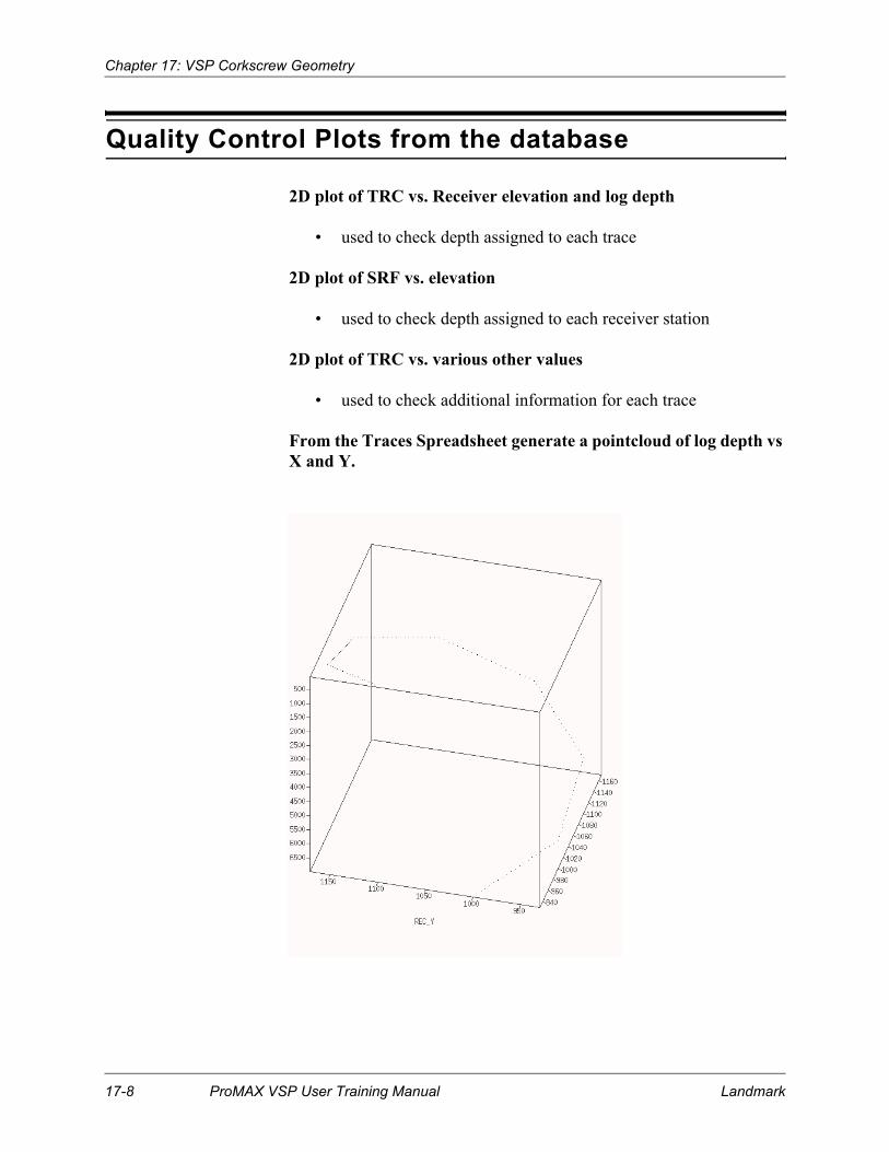
Chapter 17: VSP Corkscrew Geometry
Quality Control Plots from the database
2D plot of TRC vs. Receiver elevation and log depth
• used to check depth assigned to each trace
2D plot of SRF vs. elevation
• used to check depth assigned to each receiver station
2D plot of TRC vs. various other values
• used to check additional information for each trace
From the Traces Spreadsheet generate a pointcloud of log depth vs X and Y.
17-8 ProMAX VSP User Training Manual Landmark

Chapter 18
Pre Vertical Stack DatasetInformationA dataset was generated to illustrate some of the capabilities of ProMAX VSP. This dataset will be used for an exercise to demonstrate vertically stacking multiple shots where the receiver(s) were at common depth positions. This could be the case of recording single-sweep vibroseis records.
For this example we replicated our dataset 5 times, added some random noise and statics shifts to each set of traces. Essentially, we made simulated a recording configuration using 10 recording levels. Each recording level had 8 receivers and was recorded using 5 sweeps at each level.
Topics covered in this chapter:
o VSP Pre Vertical Stack Dataset Geometry
Landmark ProMAX VSP User Training Manual 18-1

Chapter 18: Pre Vertical Stack Dataset Information
VSP Prevertical Stack Dataset Geometry
Source type: surface
Number of Sweeps per receiver location: 5
Number of Receivers / receiver string: 8
Number of components: 1
• Channel 1: vertical component first receiver
Number of recording levels: 10
Depth of first record: 12100 ft.
Depth of last record: 8150 ft.
Depth increment: 50
Source offset from hole: N/A
The bore hole is vertical with no deviation
Source elevation: 0 ft.
Datum elevation: 0 ft.
Assume the Kelly Bushing is also at 0 ft. for simplicity
Source is at station 1
Receivers are at stations 2-81
18-2 ProMAX VSP User Training Manual Landmark

Chapter 19
VSP Level Statics andVertical StackWhen collecting VSP data, it is common to acquire multiple records with the sources and receivers at the same location. This helps attenuate random noise and builds up the signal to noise ratio of the data. Each time the source and recording system are activated, there can be small time differences in the records relative to one another. In order to optimize the vertical stack of these records, these time differences can be measured, normalized and applied prior to vertically stacking the records.
There are some fairly complex issues associated with these processes such as:
• What information is available in the incoming trace headers?
• What information do I have on observers notes?
• What are the best primary and secondary sort orders for picking analysis time gates?
• Do I need to do some trace header manipulation to build special ensembles?
• How many traces and recording levels per shot do I have per shot record?
Topics covered in this chapter:
o Plot the traces and evaluate sorting options
o Create header values and QC sorting
o VSP Level Statics parameterization and calculation
o Apply and QC the level statics
o Vertically stack shots by common levels
Landmark ProMAX VSP User Training Manual 19-1

Chapter 19: VSP Level Statics and Vertical Stack
Plot the Traces
In this exercise you will plot the data to familiarize yourself with the geometry and organization and trace headers.
Exercise1. Add a new line with a name like “Level statics and vertical stk”.
2. Build a flow to plot the input data, which will be read from another line.
3. In Disk Data Input, input the prevertical stack traces file from the VSP Training area Level statics - vertical stack line.
4. Use Trace Display to plot 400 ensembles, just to make sure all traces show up in one screen.
There are 10 levels, with 8 receivers and 5 sweeps per level.
The traces are in ensembles of 8 traces; each ensemble is for one vibroseis sweep. Each 5 consecutive ensembles belong to the same shooting level.
5. Look at the trace headers and see what values exist and are common for all traces at the same depth level.
We need to find or create header words so the data can be sorted appropriately for calculating statics for the shots belonging to the same level.
Editing Flow: 01 display raw traces
Add Delete Execute View Exit
Disk Data InputRead data from other lines/survey ------------------------- YesSelect dataset ---- VSP Training ; Level statics vertical stack ;
PRE VERTICAL STACK TRACESTrace read option ----------------------------------- Get all
Trace DisplayNumber of ensembles per screen ----------------------- 400
19-2ProMAX VSP User Training Manual Landmark

Chapter 19: VSP Level Statics and Vertical Stack
6. FFID 1-5 belong to the first level, FFID 6-10 belong to the second level, and so on until we end with FFID 46-50 for level 10. We can use a Trace Header Math to compute values for an attribute we will call STRNGLVL:
STRNGLVL = 1 + ( int ( ( ffid - 1 ) / 5 ) ) )
This formula says: subtract one from the ffid, then divide the value by five. Take the integer of that result and add one.
For FFID 1-5, the result is 1, for 6-10 the result is 2, and so on. FFID 46-50 give a result of 10.
7. We will also create a header word SHTR_GRP, indicating “shot-receiver group”, using the following formula:
SHTR_GRP = strnglvl * 8 + ( chan - 8 )
This value gives 80 sets of 5 traces -- the 5 traces that will be vertically stacked. We will sort on this attribute in order to do the vertical stack.
Depending on available header values and the shooting geometry, there may be other ways to create headers attributes for sorting the data for calculating level statics and level summing.
Landmark ProMAX VSP User Training Manual 19-3

Chapter 19: VSP Level Statics and Vertical Stack
Create Headers and QC Sorting
In this exercise we create the headers we need for doing level statics and summation, and QC sorting on those headers to make sure we have it correct.
Exercise1. Copy the previous flow and call it 02 display sorted data:
2. Using the parameters shown above, your display should show 80 ensembles with 5 traces each. The traces within each of these ensembles will be vertically stacked after we calculate and apply level statics.
Do you believe the traces are properly sorted for vertical stack?
Editing Flow: 02 display sorted data
Add Delete Execute View Exit
Disk Data InputRead data from other lines/survey ------------------------- YesSelect dataset ---- VSP Training ; Level statics vertical stack ;
PRE VERTICAL STACK TRACESTrace read option ----------------------------------- Get all
Trace Header MathDefine trace header equation -------------------- STRNGLVL = 1 +
( int ( ( ffid-1 ) / 5 ) ) )Trace Header Math
Define trace header equation ------------------- SHTR_GRP = STRNGLVL *8 + ( chan -8 )
Inline SortPrimary sort key -------------------------------------- SHTR_GRPSecondary sort key ----------------------------------- FFID
Disk Data OutputOutput dataset filename --------- Re-ordered pre-vertical stack
Trace DisplayNumber of ensembles per screen ----------------------- 400
19-4ProMAX VSP User Training Manual Landmark
Chapter 19: VSP Level Statics and Vertical Stack
3. We need to pick will be a miscellaneous time gate to define the data window for the VSP Level Statics module to estimate statics.
We want a table that has constant values for all traces with the same receiver elevation, but varies linearly between receivers. We will pick a miscellaneous time gate where we will pick times and interpolate the times as a function of receiver elevation.
There are several ways we could sort the data to achieve this, but we will see that the data in the Trace Display is sorted the way we need for picking this time gate.
4. Pick a miscellaneous time gate with a secondary key of “FFID” and select times on the first trace and last trace about 50 ms before the first arrivals.
5. Using MB3, Project the pick times to all of the other traces.
You should see that all traces recorded at the same receiver elevation have the same time.
6. Add a New Layer using MB3 to this table.
Pick the bottom time of the correlation gate about 100-200 ms below the top time.
7. Use MB3 to Project the times to the other traces.
Use “Exit and Continue Flow” to exit the Trace Display program so that it will properly write all the data to the output file. Be sure to save the table as well.
8. Turn off the Disk Data Output and re-run the flow changing the primary sort key in Inline Sort to “strnglvl”, secondary key “ffid” and tertiary key “chan”.
You should get 10 ensembles of 40 traces each.
Each of these ensembles is the group of traces that will be evaluated for common shot statics within the recording level.
There is nothing more you need to do with this data, except feel comfortable that you understand the organization. It may help to understand the organization if you plot various headers values on top of Trace Display.
Landmark ProMAX VSP User Training Manual 19-5

Chapter 19: VSP Level Statics and Vertical Stack
VSP Level Statics
In this exercise we will estimate and apply the differential statics between shots recorded for constant receiver levels.
Exercise1. Add a new flow as follows:
2. Shots will be identified by their FFIDs, that is all traces with the same FFID belong to the same shot and will get the same static.
Editing Flow: 03 level statics
Add Delete Execute View Exit
Disk Data InputSelect dataset ------------------- Re-ordered pre-vertical stackTrace read option --------------------------------------- Get all
VSP Level StaticsShot header name --------------------------------------- FFIDHow will shot groups be identified --------------- HeaderShot grouping header name ------------------------- STRNGLVLMaximum number of shots in a group --------------------- 5Maximum separation between header values ------------ 0.1Header name for analysis receivers ------------------- ChanAnalysis receivers -------------------------------------------- 1Maximum static shift ---------------------------------------10.0Basis for analysis window ---------------------------- DatabaseSelect analysis window parameter file --- “level static window”
Header StaticsWhat about previous statics ------------ Add to previous staticsFirst header word to apply --------------------- LVL_SHFT
Apply Fractional StaticsDisk Data Output
Output dataset filename -------------- Level statics appliedTrace Display
Number of ensembles per screen ---------------------- 80
19-6ProMAX VSP User Training Manual Landmark

Chapter 19: VSP Level Statics and Vertical Stack
We created the header word STRNGLVL to associate all of the traces that belong to a given receiver tool level and the shots recorded into it.
For this dataset there are 5 shots in each STRNGLVL group.
3. The STRNGLVL values increment by 1, and we must set the maximum separation to a value less than 1. This is based on the number scheme we have created.
4. Analyze statics based on all 8 channels for all shots. You should find that using any combination of channel numbers should provide nearly identical results (about 0.1 msec variation). It is good practice to use all the data, unless test results indicate otherwise.
5. You can expect a maximum static shift of about 10 ms on this dataset.
6. Select to use the analysis window picked in the previous exercise.
7. The Trace Display is optional. Be sure to use “exit and continue” to make sure the output dataset is properly filled.
Landmark ProMAX VSP User Training Manual 19-7
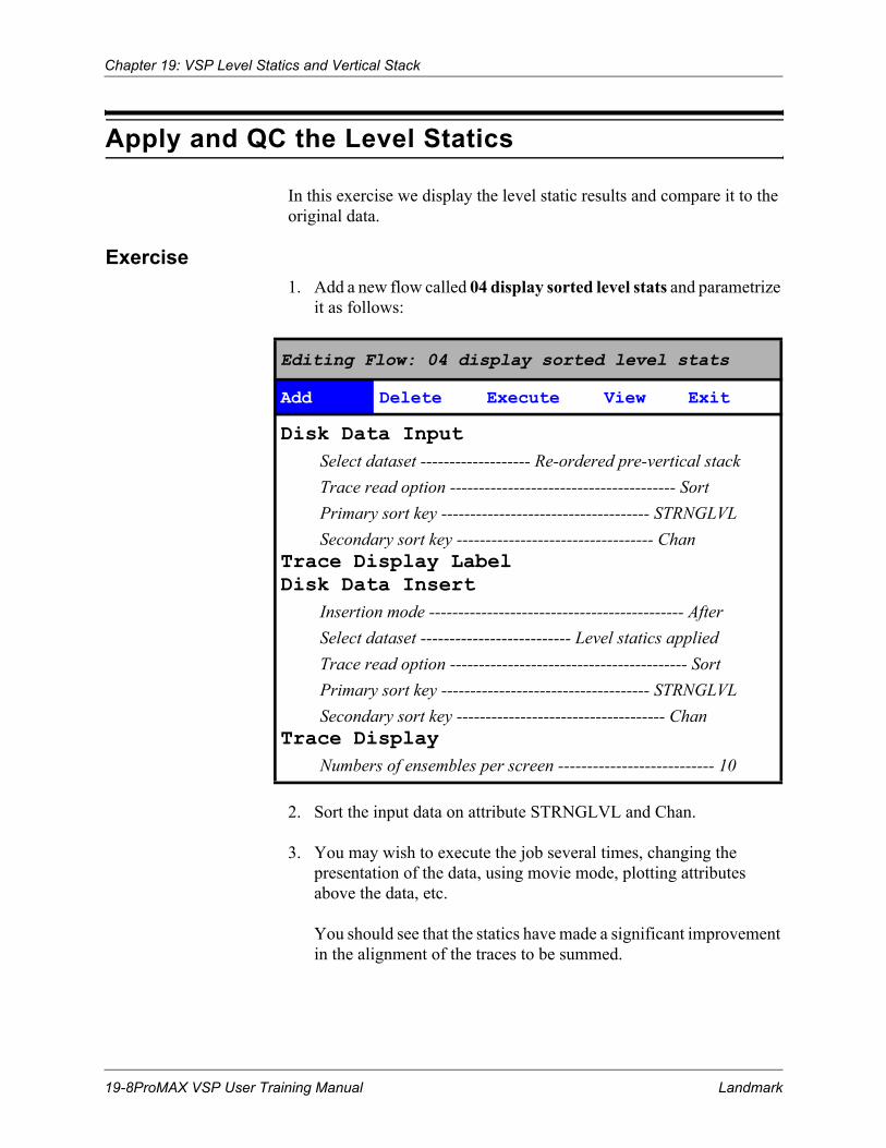
Chapter 19: VSP Level Statics and Vertical Stack
Apply and QC the Level Statics
In this exercise we display the level static results and compare it to the original data.
Exercise1. Add a new flow called 04 display sorted level stats and parametrize
it as follows:
2. Sort the input data on attribute STRNGLVL and Chan.
3. You may wish to execute the job several times, changing the presentation of the data, using movie mode, plotting attributes above the data, etc.
You should see that the statics have made a significant improvement in the alignment of the traces to be summed.
Editing Flow: 04 display sorted level stats
Add Delete Execute View Exit
Disk Data InputSelect dataset ------------------- Re-ordered pre-vertical stackTrace read option --------------------------------------- SortPrimary sort key ------------------------------------ STRNGLVLSecondary sort key ---------------------------------- Chan
Trace Display LabelDisk Data Insert
Insertion mode -------------------------------------------- AfterSelect dataset -------------------------- Level statics appliedTrace read option ----------------------------------------- SortPrimary sort key ------------------------------------ STRNGLVLSecondary sort key ------------------------------------ Chan
Trace DisplayNumbers of ensembles per screen --------------------------- 10
19-8ProMAX VSP User Training Manual Landmark

Chapter 19: VSP Level Statics and Vertical Stack
Vertically Stack Shots by Common Levels
This flow re-calculates the level statics because it is inexpensive and the structure of this flow is simpler for comparing data with and without the level statics applied before summing.
Exercise1. Add a new flow 05 sum leveled shots parameterized as follows:
2. Reproduce “all data” to make 2 copies.
Editing Flow: 05 sum leveled shots
Add Delete Execute View Exit
Disk Data InputSelect dataset ------------------- Re-ordered pre-vertical stack
Reproduce TracesTrace grouping to reproduce --------------------- All Data
IFVSP Level StaticsHeader StaticsApply Fractional StaticsVSP Level Summing
Shot header name --------------------------------------- FFIDHeader name for secondary key ---------------------- ChanHow will shot groups be indentified -------------- HeaderShot grouping header name ---------------------- SHTR_GRPMaximum number of shots in a group ------------------- 5How will shot groups be stacked ------------ Median Stack
Trace Display LabelELSEIFVSP Level SummingTrace Display LabelENDIFIn-line Sort
Sort keys ---------------------------- Repeat, FFID, ChanTrace Display
Landmark ProMAX VSP User Training Manual 19-9
Chapter 19: VSP Level Statics and Vertical Stack
3. Level statics are calculated and applied exactly as in previous flow.
4. FFID the primary key that identifies sets of traces belonging to one record that will be part of summation. Chan is the secondary key for summation. SHTR_GRP indentifies the set of FFIDs that will be collected for summation. There are 5 FFIDs whithin each shot-receiver group. Common channel numbers withing the set of FFIDs in a single SHTR_GRP will be summed.
5. Median stack seems to produce a very slightly better result than mean stack.
6. Use the same parameters for the second VSP Level Summing module.
7. Run the flow several times, changing the display organization and method.
8. You may wish to use Interactive Spectral Analysis to compare the frequency content of the results with and without level statics.
The output of this process would be used as input to the flow number 12 in the “Main VSP” line. The value in this sequence of level statics and summation is two-fold: imporved signal to noise ratio by stacking multiple common source point records and improved resolution by optimizing data alignment before summation.
19-10ProMAX VSP User Training Manual Landmark

Chapter 20
3-Component Transform andFirst Break PickingIn some cases it may be advantageous to generate a trace that represents the total power of all three component traces in order to help in the first break picking process. Here we will generate a trace that is the RMS amplitude of the three component traces and look at a couple of different techniques for picking the first arrivals.
This method is more valuable with longer offset VSP data or when signal to noise ratio is low, making first arrival picking to be difficult. The primary purpose is to allow better first break picking. The resultant trace data is used only for first break picking.
Topics covered in this chapter:
o 3 Component Transform to generate an RMS amplitude trace and First arrival picking
o Setting the first arrival times identical on all three components
o QC the copied picks
Landmark ProMAX VSP User Training Manual 20-1

Chapter 20: 3-Component Transform and First Break Picking
3-Component Transform and First Arrival Picking
In this exercise you will input the three component traces and recompute new traces based on the amplitudes of all three inputs.
Create these flows in your “Main VSP” line.
Exercise1. Build a flow named 41 3-component transform to construct an
RMS trace and display the results.
2. In Disk Data Input, read the real data with the correct geometry in the headers.
Editing Flow: 41 3-Component transform
Add Delete Execute View Exit
Disk Data Input Select input dataset filename ------------- shots with geomTrace read option ----------------------------------------- Get All
3-Component TransformsHeader word for selecting replacement trace ----- Geophone
component (x,y,z)Value of replacement trace header ---------------------------2Select 3-component transform to apply --- Sum Squares StackMaximum time to calculate transform (ms) ---------- 1500
In Line SortSelect new PRIMARY sort key -------------------- Geophone
component (x,y,z)Select new SECONDARY sort key:------------------------FFIDMaximum traces per output ensemble:--------------------80Number of traces in buffer:----------------------------240
Trace DisplayNumber of ENSEMBLES (line segments)/screen:---------1Number of display panels:--------------------------------3Trace Orientation:---------------------------------------Horizontal
20-2 ProMAX VSP User Training Manual Landmark

Chapter 20: 3-Component Transform and First Break Picking
This file still has 3 traces per shot and has a primary sort order of FFID.
3. Select 3-Component Transform parameters.
Replace header entry geophone component (x,y,z) number 2 and process to 1500 ms using a sum squares stack.
4. Sort the data with a primary sort of Geophone Component (x,y,z) and secondary of FFID.
There are 80 traces per ensemble and a total of 240 traces in the sort buffer.
5. In Trace Display, display the three component traces.
Use 1 ensemble per screen and 3 horizontal panels.
You may also want to try 3 vertical panels.
6. Identify the first arrivals on the display of the RMS trace. These RMS traces have replaced the original channel 2 (horizontal phone) traces in the output dataset. The RMS traces are easily identified because all sample values are “rectified” (i.e., they are all positive values).
7. Create a new First Break entry of the type GEOMETRY in the database using the Picking pulldown menu.
Select to edit database values (first breaks) and give these FB Picks a name that describes them as being picks from the RMS trace.
8. After “rubber-banding” the first arrivals on one of the panels, snap them to the nearest peak. Some care may be needed to stay on the same peak event because all values are positive on the RMS traces.
Notice that each panel is picked completely independently from the others. In this case only pick the one panel that contains the RMS traces.
9. Compare the picks by plotting them from the database.
We should have two sets of first break picks in the TRC database. The picks from the vertical traces are all “channel 1” traces that we picked earlier, and the new picks from the RMS traces are all “channel 2” traces.
Landmark ProMAX VSP User Training Manual 20-3

Chapter 20: 3-Component Transform and First Break Picking
You should notice that the line described by the pick times for the RMS traces is smoother (less noisy) than for the vertical traces. This might be a better result for creating a velocity function or for flattening data for further processing.
20-4 ProMAX VSP User Training Manual Landmark
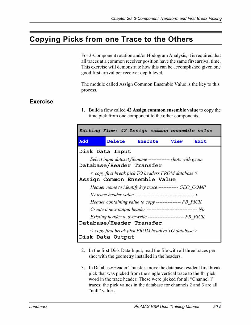
Chapter 20: 3-Component Transform and First Break Picking
Copying Picks from one Trace to the Others
For 3-Component rotation and/or Hodogram Analysis, it is required that all traces at a common receiver position have the same first arrival time. This exercise will demonstrate how this can be accomplished given one good first arrival per receiver depth level.
The module called Assign Common Ensemble Value is the key to this process.
Exercise1. Build a flow called 42 Assign common ensemble value to copy the
time pick from one component to the other components.
2. In the first Disk Data Input, read the file with all three traces per shot with the geometry installed in the headers.
3. In Database/Header Transfer, move the database resident first break pick that was picked from the single vertical trace to the fb_pick word in the trace header. These were picked for all “Channel 1” traces; the pick values in the database for channels 2 and 3 are all “null” values.
Editing Flow: 42 Assign common ensemble value
Add Delete Execute View Exit
Disk Data InputSelect input dataset filename ------------- shots with geom
Database/Header Transfer< copy first break pick TO headers FROM database >
Assign Common Ensemble ValueHeader name to identify key trace ------------ GEO_COMPID trace header value ------------------------------------ 1Header containing value to copy --------------- FB_PICKCreate a new output header ------------------------------- NoExisting header to overwrite ---------------------- FB_PICK
Database/Header Transfer< copy first break pick FROM headers TO database >
Disk Data Output
Landmark ProMAX VSP User Training Manual 20-5

Chapter 20: 3-Component Transform and First Break Picking
4. In Assign Common Ensemble Value, copy the first break pick time from channel 1 to the other channels of each ensemble.
5. Transfer the copied first break times from the trace header back to the database.
Each trace has a meaningful first arrival time in the trace header, but the values in the database for all channels 2 and 3 are still “null”. For future reference it is advisable to copy all these values out to the database.
6. Write the output data to a new file.
The module Assign Common Ensemble Value can be useful in other situations, and is not limited to use in VSP processing.
20-6 ProMAX VSP User Training Manual Landmark

Chapter 20: 3-Component Transform and First Break Picking
QC the Copied Picks
As a final QC of the copied picks, plot them over the traces to see if all three traces at each receiver depth level are constant.
Exercise1. Display the picks in the database.
Exit from the flow. Click on the global Database button.
Use the Database display tool to graph the various picks and compare the results.
2. Expand the flow to reread the new data file and plot the first breaks.
3. Toggle all of the previous processes inactive.
4. In Disk Data Input, read in the file that was written in the previous exercise that has the copied picks in the header.
5. In Trace Display, plot the traces on one screen by displaying all 80 ensembles.
6. Execute the flow.
7. Overlay the picks from the headers and/or the database on the traces.
Editing Flow: copy first break picks
Add Delete Execute View Exit
>Disk Data Input<>Database/Header Transfer<>Assign Common Ensemble Value<>Database/Header Transfer<>Disk Data Output<----------------------Disk Data InputTrace Display
Landmark ProMAX VSP User Training Manual 20-7

Chapter 20: 3-Component Transform and First Break Picking
Use the Picking pulldown menu to select the first breaks from the trace headers, or the database.
All three traces of each FFID should have the same pick time. Check the values by using the header dump facility.
20-8 ProMAX VSP User Training Manual Landmark

Chapter 21
VSP 3-Component OrientationMost modern down-hole seismic recording tools consist of one or more sets of geophones in a string. Each of these sets is typically a group of three geophones, (occasionally you may find four component tools). For the three component tool there will be one vertical geophone and two horizontal geophones which are oriented perpendicular to one another. Sometimes, in processing, the energy recorded on the horizontal phones is of interest. This data may contain a lot of shear wave energy which can yield valuable information if this is the goal. Quite often, this horizontally recorded energy is ignored and only the vertical traces are used in processing.
In this chapter we will look at the interactive Hodogram Analysis 3-component orientation process which can be used to build new horizontal traces from the recorded traces that represent what are called transverse and radial components. These correspond to the traces that would have been recorded had the horizontal phones been perpendicular and parallel, to the line defined by the shot and receiver positions on the surface. Additionally, given the vertical and oriented (radial) horizontal traces, two new traces can be built representing the maximum and medium traces where the maximum trace is that which would have been recorded had one geophone been aligned pointing directly toward the source position.
Once the geophone orientation is known, additional processing of the oriented horizontal traces is possible for both p-wave and shear wave energy.
Topics covered in this chapter:
o 3 Component Hodogram Analysis
Landmark ProMAX VSP User Training Manual 21-1

Chapter 21: VSP 3-Component Orientation
3 Component Hodogram Analysis
ExerciseThis exercise is done in your “Main VSP” line.
In this exercise we will work with the two horizontal traces and build two new horizontal traces: one Radial and one Transverse. Watch the polarity of the output (watch the vertical orientation plot as well) in order to get the output traces all the correct polarity.
The program identifies the highest absolute amplitude in the analysis gate should be a positive value. If the highest amplitude is negative, the program reverses the polarity of the trace.
Be aware that there are 5 traces whose output polarity is reversed. These can be identified and corrected with careful review in the tool. Alternatively, reversed polarity output traces can be picked using Trace Display and corrected in a subsequent flow.
1. Build a flow to compute the radial and transverse traces from two horizontally recorded input traces of unknown orientation.
2. In Disk Data Input, read the traces with constant first arrival times for each trace at each receiver level in the headers.
3. Apply a bandpass filter.
Default values are ok. This is only done to make things easier to see in this class. This workflow might be done in two passes -- once with bandpass filter to confirm data behavior, then a second time without
Editing Flow: 3 comp hodogram analysis
Add Delete Execute View Exit
Disk Data Input < input dataset with FB_PICK valid in all traces >
Bandpass FilterHodogram Analysis
< see parameters on next page >Disk Data Output
21-2 ProMAX VSP User Training Manual Landmark

Chapter 21: VSP 3-Component Orientation
bandpass filter. In general you would not want to apply any trace by trace amplitude corrections for this process.
4. Select Hodogram Analysis parameters.
Be sure that the channel numbers associated with the vertical and horizontal-1 and horizontal-2 traces are correct. In this case, these are channels 1, 2 and 3, respectively. Use the first arrival pick times as a basis for the analysis window. Do not output the analysis window to a time gate file. Write the orientation values to the trace headers.
5. Select an output dataset name.
6. Execute the Flow.
You should see a display similar to the following after zooming in around the first arrivals.
Landmark ProMAX VSP User Training Manual 21-3

Chapter 21: VSP 3-Component Orientation
Example Hodogram Analysis Plot
The Hodogram plot has three basic sections:
• the trace data area
• the horizontal hodogram
• the vertical hodogram
Example Hodogram Analysis Product Display
OriginalVertical andTwoHorizontal
OriginalVertical andRadial and TransverseHorizontalTraces
Traces
OrientedVertical,Transverse VerticalandTransverse HorizontalTraces
Hodogram of Two HorizontalTraces
Hodogramof OrientedHorizontal and OriginalVertical
21-4 ProMAX VSP User Training Manual Landmark

Chapter 21: VSP 3-Component Orientation
1. Click on the Hodogram editing icon.
This enables us to alter the orientation angle that the program computed automatically if desired. Normally we will only want to watch the polarity of the oriented traces and we may need to rotate the trace by 180 degrees to get the proper polarity.
2. Look at the second and third trace of the middle trace display.
The second trace should be maximized at the same polarity as the first trace and the third trace should be minimized.
3. Press MB2 in the top hodogram window to rotate the oriented traces by 180 degrees to change it’s polarity.
Change it back again with another MB2 Click. This trace has the correct polarity.
4. Press MB2 in the bottom hodogram window to rotate the oriented vertical trace by 180 degrees.
After rotation this trace now has the proper orientation.
5. Fine tune the orientation to minimize the third trace on the second set of traces and the second trace on the third set of traces by using MB1 and rotating the orientation axes.
In general you will find that the fine tuning is not required.
6. Press the Next Screen icon to go to the next set of three traces for the next depth level.
Repeat the orientation procedures where the goal is to:
• 1) maximize the second trace on the second panel of traces at the same polarity as the original vertical trace
• 2) maximize the first trace on the third panel of traces at the same polarity as the original vertical trace.
7. Continue until all 80 levels have been oriented.
Landmark ProMAX VSP User Training Manual 21-5

Chapter 21: VSP 3-Component Orientation
8. Expand the flow to display the output data.
9. Read the file that was just created.
You will want to sort the input with a primary ensemble sort order of hodo_typ and sort the traces within these ensembles to increase by FFID.
10. You may want to experiment with different display options.
A best first guess would be to use Trace Display and plot 5 ensembles.
You may also want to try 1 ensemble per screen and 5 horizontal panels.
Editing Flow: 3 comp hodogram analysis
Add Delete Execute View Exit
>Disk Data Input<>Bandpass Filter<>Hodogram Analysis<>Disk Data Output<Disk Data Input <hodo_typ,ffid>
Select primary trace header entry------------------hodo_typSelect secondary trace header entry---------------------FFID
Trace Display
21-6 ProMAX VSP User Training Manual Landmark
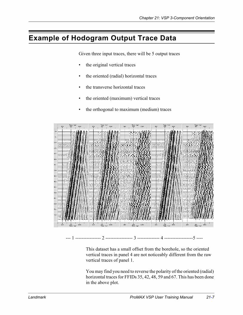
Chapter 21: VSP 3-Component Orientation
Example of Hodogram Output Trace Data
Given three input traces, there will be 5 output traces
• the original vertical traces
• the oriented (radial) horizontal traces
• the transverse horizontal traces
• the oriented (maximum) vertical traces
• the orthogonal to maximum (medium) traces
--- 1 ---------------- 2 ----------------- 3 -------------- 4 ------------------5 ----
This dataset has a small offset from the borehole, so the oriented vertical traces in panel 4 are not noticeably different from the raw vertical traces of panel 1.
You may find you need to reverse the polarity of the oriented (radial) horizontal traces for FFIDs 35, 42, 48, 59 and 67. This has been done in the above plot.
Landmark ProMAX VSP User Training Manual 21-7

Chapter 21: VSP 3-Component Orientation
21-8 ProMAX VSP User Training Manual Landmark

Chapter 22
Salt Dome Synthetic VSPThis exercise begins with a velocity model of a salt dome, then uses Finite Difference Modeling to create a synthetic VSP trace dataset with the borehole near the salt dome vertical face. This dataset is taken through a VSP processing sequence in order to review concepts and to introduce the user to use of modules in a more complex geologic regime.
Finite difference modeling is used to create a 2D dataset. The corridor stack and VSP-CDP transform data are spliced into this 2D line.
Most if this chapter repeats information that has been covered in previous chapters. Explanations and flow parameter details are focused on new concepts and issues of interest.
Topics covered in this chapter:
o View the Model
o Finite Difference Modeling for VSP
o Geometry Spreadsheet
o Load Geometry
o Isolate the Upgoing Data
o Corridor Stack
o VSP-CDP Transform
o VSP Migration
o Add Well Location to VSP Data
o Velocity Model with Migrated VSP Data
o Finite Difference Model of 2D Seismic
o Corridor Stack Spliced into 2D Stack
o VSP-CDP Transform Spliced into 2D Stack
Landmark ProMAX VSP User Training Manual 22-1

Chapter 22: Salt Dome Synthetic VSP
View the Model
1. Copy the line “Synthetic VSP from Salt Dome” from area “VSP Training” to your own area.
2. Execute the flow “01 View Velocity Model”
The velocity model was created manually using the module Volume Viewer Editor. It has the following characteristics:
Spatial range: 0-10000 feet horizontally, 0-10000 feet vertically
CDP range: 1-200 at 25 feet sampling
Datum elevation: 0 ft.
Velocity range: 8000-12400 fps in sediments,15000 fps in salt.
Model CDP 1 is at spatial coordinate 0.0, CDP 200 is at spatial coordinate 5000.0. Beware of the ProMAX convention within tables for VSP and 2D lines that X-coordinate is equal to the CDP number. Details and special considerations will be explained as you work through the processing sequence.
22-2 ProMAX VSP User Training Manual Landmark

Chapter 22: Salt Dome Synthetic VSP
The well location is at CDP 100. The source for the synthetic VSP will be at CDP 50.
A stack dataset was input to Volume Viewer Editor and the display type was changed to “variable area”. The trace dataset was specially created to illustrate the shot and well locations.
Landmark ProMAX VSP User Training Manual 22-3

Chapter 22: Salt Dome Synthetic VSP
Finite Difference Modeling for VSP
The velocity model was input to Finite Difference Modeling in order to produce a VSP dataset using the following flow:
Editing Flow: 02 FD model the VSP data
Add Delete Execute View Exit
Finite Difference ModelingVelocity field ------------------------------------------------ salt modelDo you want to input a density field?---------------------------- NoGenerate synthetic data or movie snapshots?------- Synthetic dataIs this a point source or an exploding reflector run? ---------------
-------------------------------- Normal point sourceDepth of field for modeling --------------------------------- 10000.0Length of time (ms) to run modeling per shot ------------- 2000.0Approximate peak frequency to be modeled -------------------- 25Type of source wavelet ------------------------- Zero phase RickerGrid adjustment factor --------------------------------------------- 1.0CDP spacing in feet or meters ---------------------------------- 50.0Number of CDPs to buffer the edges for the modeling field --- 40Reflecting or absorbing boundary at the surface ------- AbsorbingTake geometry from the headers of an input dataset” ------- NoNumber of shots ------------------------------------------------------- 1CDP of the first shot ------------------------------------------------ 50Depth of the first shot ---------------------------------------------- 0.0Number of receiver stations -------------------------------------- 140Receiver X locations absolute or relative to the shot? --- RelativeDistance (in CDPs) between shot and first group ------------- 50Receiver location increment (in CDPs) ------------------------- 0.0Is the modeling for VSP/cross-hole data? ---------------------- YesReceiver depths absolute or relative to the shot? ------ AbsoluteDepth of first receiver in feet or meters -------------------- 1000.0Receiver depth increment in feet or meters ------------------- 50.0
< more modules next page>
22-4 ProMAX VSP User Training Manual Landmark

Chapter 22: Salt Dome Synthetic VSP
Flow parameterization continued:
Review of the parameters for Finite Difference Modeling on the previous page shows that we are generating VSP data with the source at CDP 50, the borehole at CDP 100 and 140 receiver levels at 50 feet increments. We define an absorbing surface so that multiples are not included, which makes it easier to see events of interest.
The Trace Header Math’s are used to simplify the geometry description in the spreadsheet loading this to the trace headers.
Editing Flow: 02 FD model the VSP data
Add Delete Execute View Exit
Finite Difference ModelingTrace Header Math
Select mode ------------------------------------ Fixed equation modeDEFINE trace header equation ----------------------- ffid = chan
Trace Header Math Select mode ------------------------------------ Fixed equation modeDEFINE trace header equation ------------------- source = chan
Trace Header Math Select mode ------------------------------------ Fixed equation modeDEFINE trace header equation -------------------------- chan = 1
Disk Data OutputOutput dataset filename ------------------------------ Synthetic VSP
Trace Display
Landmark ProMAX VSP User Training Manual 22-5

Chapter 22: Salt Dome Synthetic VSP
Geometry Spreadsheet
Flow 03 Geometry spreadsheet uses the following key parameters:
Sources spreadsheet
Borehole spreadsheet
Pattern spreadsheet
Pseudo-CDP binning and database finalization are applied after entering the above data to the spreadsheets.
22-6 ProMAX VSP User Training Manual Landmark
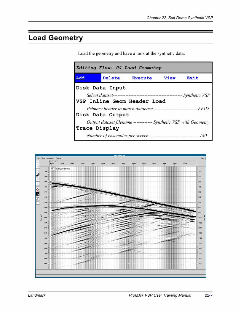
Chapter 22: Salt Dome Synthetic VSP
Load Geometry
Load the geometry and have a look at the synthetic data:
Editing Flow: 04 Load Geometry
Add Delete Execute View Exit
Disk Data InputSelect dataset-------------------------------------------- Synthetic VSP
VSP Inline Geom Header Load Primary header to match database---------------------------- FFID
Disk Data OutputOutput dataset filename ------------ Synthetic VSP with Geometry
Trace DisplayNumber of ensembles per screen ------------------------------- 140
Landmark ProMAX VSP User Training Manual 22-7

Chapter 22: Salt Dome Synthetic VSP
Isolate the Upgoing Data
Flow 05 Isolate upgoing data includes the following key steps:
1. Use Trace display to pick the direct arrivals as FB_PICK via the database.
2. Run the module Vel Table From VSP* to create an average velocity function in depth from the first break picks, then display the function and smooth it if needed.
3. Transfer the first break picks back to the headers and apply them as a negative static. Ensure the direct arrival event is flattened and make all traces into a single ensemble of 140 traces. Apply 2D
Editing Flow: 05 Isolate upgoing data
Add Delete Execute View Exit
Disk Data InputTrace Display--------------Vel Table From VSP*Velocity Viewer/Point Editor--------------Disk Data InputDatabase/Header Transfer
< move FB_PICK from database to headers >Header Statics
< bulk shift 100, subtract FB_PICK >Apply Fractional StaticEvent Alignment in WindowEnsemble Redefine2D Spatial Filtering
< simple 2D median filter using 51 points >Header StaticsApply Fractional StaticDisk Data Output
Output dataset filename ------------ Synthetic VSP - upgoing onlyTrace Display
22-8 ProMAX VSP User Training Manual Landmark

Chapter 22: Salt Dome Synthetic VSP
Spatial Filtering to attenuate the direct arrival using a 51 point filter. A long filter is chosen in order avoid attenuating the reflection event from the salt face. On the traces recorded deeper in the borehole, this reflection event is nearly parallel to the flattened direct arrival. With a shorter filter this event gets attenuated. With a longer filter the direct arrival is not very well attenuated for the traces shallower in the borehole.
The residual direct arrival energy on the left side of the display can be removed with a top mute.
Landmark ProMAX VSP User Training Manual 22-9

Chapter 22: Salt Dome Synthetic VSP
Corridor Stack
Flow 06 Corridor stack flow is executed in three stages using the following steps:
1. Convert the average velocity in depth table to RMS velocity to be used for one-way NMO correction.
2. Apply one-way NMO and pick a top mute and a bottom mute to bound the data in the corridor.
3. Produce the corridor stack data using the picked mutes.
Editing Flow: 06 Corridor stack
Add Delete Execute View Exit
Velocity Manipulation*< input average vel in depth >< output RMS velocity >
--------------Disk Data Input
< sort on CHAN, FFID >One Way Normal Moveout CorrectionTrace Display---------------Disk Data InputOne Way Normal Moveout CorrectionVSP Corridor StackDisk Data Output
Output dataset filename ------------------------ VSP corridor stackTrace Display
22-10 ProMAX VSP User Training Manual Landmark

Chapter 22: Salt Dome Synthetic VSP
VSP-CDP Transform
Flow 07 VSP-CDP transform uses 50 feet for the output spatial sampling in order to match the spatial sampling of the 2D seismic data the is generated in flow 11. The velocity for the transform is taken from CDP 75, midway between the source and the borehole location. The ray tracing interval is set to a small value to ensure a well-sampled transform and a smooth output dataset.
The transform outputs 25 traces numbered as CDP 1-25. Trace header math is used to shift these CDP numbers to the range 76-100 so they can be spliced into the 2D dataset and have correct header values.
Bandpass filter can be used (optionally) to attenuate relatively low frequency energy reflected from the salt face, but which is incorrectly mapped through the transform.
Editing Flow: 07 VSP-CDP Transform
Add Delete Execute View Exit
Disk Data InputEnsemble RedefineVSP-CDP Transform
Horizontal binning interval ------------------------------------- 50.0CDP at which to extract velocity function ---------------------- 75Specify length of output trace in ms ------------------------ 2000.0Select how velocity is to be specified -------------------- DatabaseSelect a velocity model ------------------------------------ salt modelRay trace interval ------------------------------------------------- 10.0Datum elevation ---------------------------------------------------- 0.0Allowable percentage of moveout stretch ------------------ 100.0
Trace Header MathDefine trace header equation -------------------- cdp = cdp + 75
<Bandpass Filter>Disk Data Output
Output dataset filename ----------------------- VSP-CDP transformTrace Display
Landmark ProMAX VSP User Training Manual 22-11

Chapter 22: Salt Dome Synthetic VSP
VSP Migration
Flow 08 VSP Migration uses the following key parameters:
Editing Flow: 08 VSP Migration
Add Delete Execute View Exit
Disk Data InputVSP Kirchhoff Migration
Minimum output depth for migrated image ----------------------- 0.Maximum output depth for migrated image --------------- 10000.Depth sample rate for output migrated image ------------------ 20.Minimum output X-coordinate for migrated image ------------- 0.Maximum output X-coordinate for migrated image ------ 10000.Output trace spacing for migrated image ----------------------- 50.Output CDP number corresponding to minimum X-coordinate - 1Minimum X-coordinate for input velocity field ----------------- 0.0Maximum X-coordinate for input velocity field ----------- 10000.0Offset sampling of velocity field to use -------------------------- 50.Depth sampling of velocity field to use ------------------------ 100.Length of smoothing for velocities ------------------------------ 100.Maximum frequency to migrate (in Hz) ------------------------- 90.Dip of primary events of interest (degrees) ---------------------- 0.Dip range to keep around events of interest ------------------ 90.Is this a two-component migration? ------------------------------ NoApply raypath amplitude corrections? -------------------------- NoApply receiver directionality corrections? --------------------- NoWill tow velocity fields be used? --------------------------------- NoShould each source/receiver image be output? --------------- NoGet velocities from the database? ------------------------------- YesSelect source velocity parameter file ------------------- salt modelSave ray path files? ------------------------------------------------ No
Disk Data OutputOutput dataset filename ----------------------------- VSP Migration
Trace Display
22-12 ProMAX VSP User Training Manual Landmark

Chapter 22: Salt Dome Synthetic VSP
The migration parameters are set so that the spatial sampling and CDP numbering of the output image match those of the velocity model. The parameters that control ray-tracing are set relatively small to ensure accuracy over consideration of faster run-time. The range of dips to keep is left wide-open in order to capture both the low-dip sediments and the nearly vertical salt interface.
Landmark ProMAX VSP User Training Manual 22-13

Chapter 22: Salt Dome Synthetic VSP
Add Well Location to VSP Data
Flow 09 Add well to VSP migration combines two datasets by summing correspondent CDP traces. The migrated VSP data is summed with a special trace dataset that was created to highlight the source and wellbore positions.
The special dataset is input first, then resampled to match the sample rate of the migrated VSP data.
The sort order causes common CDP traces from the datasets to be adjacent, and the Trace Math sums these adjacent trace pairs.
Editing Flow: 09 Add well to VSP migration
Add Delete Execute View Exit
Disk Data InputSelect dataset ------------------------------ Well and shot locationsTrace read option ------------------------------------------------ SortSelect primary trace header entry ------------- CDP bin number
Resample / DesampleOutput sample rate ----------------------------------------------- 20.0
Disk Data InsertInsertion mode ------------------------------------------------ MergedMaximum traces per output ensemble ----------------------------- 2Select dataset ------------------------------------------ VSP MigrationTrace read option ------------------------------------------------- SortSelect primary trace header entry -------------- CDP bin number
Trace MathMode of operation --------------------------------------- Trace/TraceType of trace/trace operation --------------------------- Add Traces
Ensemble RedefineMode of application -------------------------------------------- EntireMaximum traces per output ensemble -------------------------- 201
Disk Data OutputOutput dataset filename ------------------ VSP migration plus Well
Trace Display
22-14 ProMAX VSP User Training Manual Landmark

Chapter 22: Salt Dome Synthetic VSP
Above is migrated VSP data with well position at CDP 100 shown as a trace with constant high positive amplitude.
The low-dip sediments pierced by the wellbore are quite evident, as is the reflection from the salt face. The majority of energy in this image is artifacts from the migration process, which is a natural consequence of the limited spatial extent of conventional VSP recording.
Landmark ProMAX VSP User Training Manual 22-15

Chapter 22: Salt Dome Synthetic VSP
Velocity Model with Migrated VSP Data
Flow 10 Model with migrated VSP data displays the Salt Model with a seismic data underlay of the migrated VSP with the well location flagged with a high amplitude trace at CDP 100.
Change the trace display parameters to variable area with bias -10. The reflection from the salt maps nicely onto the salt face between 2200-7500 feet, and sediment reflectors show clearly at the wellbore location.
Editing Flow: 10 Model with migrated VSP data
Add Delete Execute View Exit
Volume/Viewer Editor*Work in time or depth ------------------------------------------ DepthInput volume ------------------------------------------------ salt modelDisplay poststack seismic data? --------------------------------- YesSelect poststack data file --------------- VSP migration plus Well
22-16 ProMAX VSP User Training Manual Landmark

Chapter 22: Salt Dome Synthetic VSP
Finite Difference Model of 2D Seismic
Flow 11 FD model 2D synthetic uses finite difference modeling to create the traces corresponding to a 2D section across the salt model.
Editing Flow: 11 FD model 2D synthetic
Add Delete Execute View Exit
Finite Difference ModelingVelocity field ------------------------------------------------- salt modelDo you want to input a density field?----------------------------- NoGenerate synthetic data or movie snapshots?----- Synthetic dataIs this a point source or an exploding reflector run? ---------------
------------------------------------------ Exploding reflectorDepth of field for modeling --------------------------------- 10000.0Length of time (ms) to run modeling per shot -------------- 2000.0Approximate peak frequency to be modeled -------------------- 25Grid adjustment factor --------------------------------------------- 1.0CDP spacing in feet or meters ---------------------------------- 50.0Reflecting or absorbing boundary at the surface ----- AbsorbingCDP of left edge of modeling field ---------------------------------- 1CDP of right edge of modeling field ----------------------------- 201
Disk Data OutputOutput dataset filename ---------------------- Synthetic 2D seismic
Trace Display
Landmark ProMAX VSP User Training Manual 22-17

Chapter 22: Salt Dome Synthetic VSP
Synthetic 2D data across the salt model.
22-18 ProMAX VSP User Training Manual Landmark
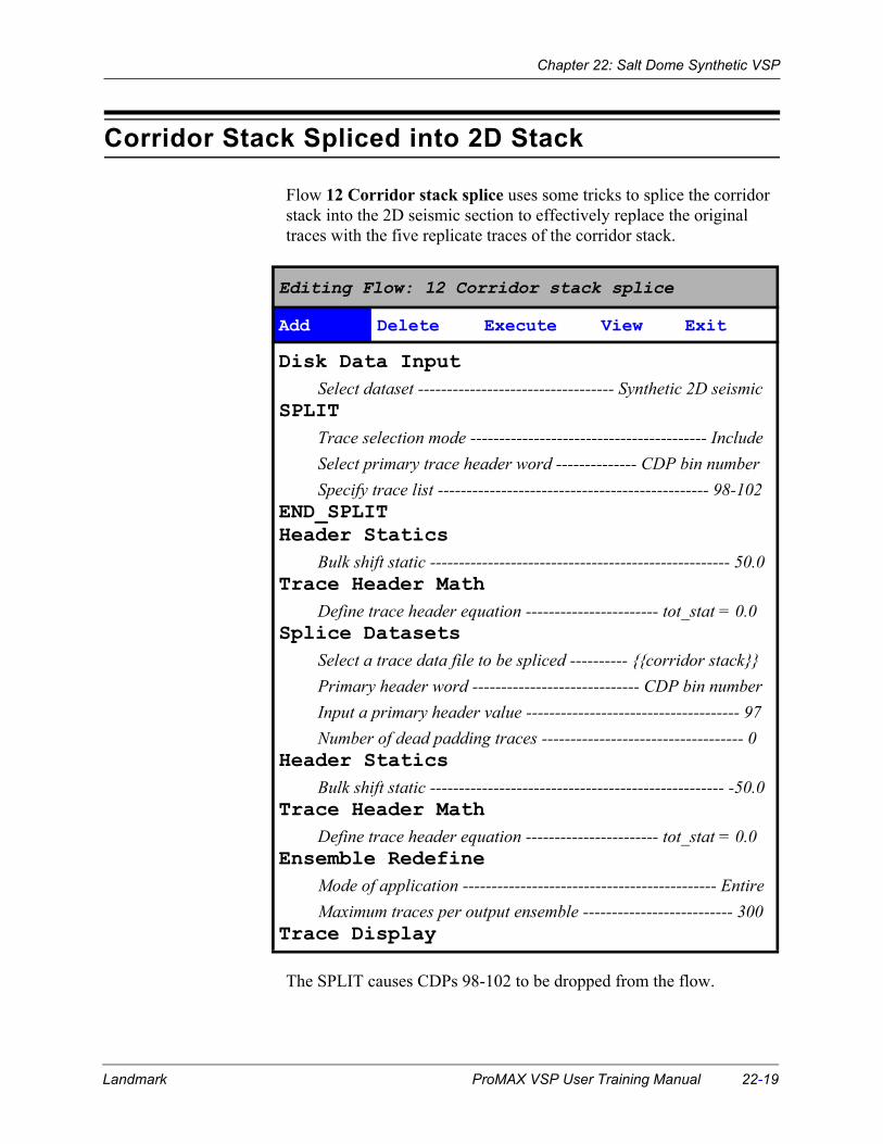
Chapter 22: Salt Dome Synthetic VSP
Corridor Stack Spliced into 2D Stack
Flow 12 Corridor stack splice uses some tricks to splice the corridor stack into the 2D seismic section to effectively replace the original traces with the five replicate traces of the corridor stack.
The SPLIT causes CDPs 98-102 to be dropped from the flow.
Editing Flow: 12 Corridor stack splice
Add Delete Execute View Exit
Disk Data InputSelect dataset ---------------------------------- Synthetic 2D seismic
SPLITTrace selection mode ----------------------------------------- IncludeSelect primary trace header word -------------- CDP bin numberSpecify trace list ----------------------------------------------- 98-102
END_SPLITHeader Statics
Bulk shift static ---------------------------------------------------- 50.0Trace Header Math
Define trace header equation ----------------------- tot_stat = 0.0Splice Datasets
Select a trace data file to be spliced ---------- {{corridor stack}}Primary header word ----------------------------- CDP bin numberInput a primary header value ------------------------------------- 97Number of dead padding traces ----------------------------------- 0
Header StaticsBulk shift static --------------------------------------------------- -50.0
Trace Header MathDefine trace header equation ----------------------- tot_stat = 0.0
Ensemble RedefineMode of application -------------------------------------------- EntireMaximum traces per output ensemble -------------------------- 300
Trace Display
Landmark ProMAX VSP User Training Manual 22-19

Chapter 22: Salt Dome Synthetic VSP
After examining the corridor stack, a shift of 50 milliseconds allowed a better overall match of the corridor stack and the 2D seismic. This static was effected by shifting the 2D data by +50, resetting the tot_stat attribute to 0.0, splicing, then shifting everything back by -50 ms. This has net effect of shifting only the corridor stack by -50 ms.
The corridor stack is inserted after CDP 97. Exactly 5 CDPs were omitted via SPLIT, and 5 corridor stack trace inserted, effectively replacing CDPs 98-102.
There is a noticeable time-variant mistie between the corridor stack and the 2D data, with the mistie increasing for shallower events. There are several possible contributors to this problem. The corridor stack method assumes a small horizontal offset of source to borehole. The one-way NMO corrections can vary according to the method of generating the Vrms function. A better result (but still mistied) is achieved with a function converted directly from the depth interval velocity model than with an average function derived via first arrival times (and converted to Vrms). The method also assumes a flat layered velocity field.
22-20 ProMAX VSP User Training Manual Landmark

Chapter 22: Salt Dome Synthetic VSP
VSP-CDP Transform Spliced into 2D Stack
Flow 13 VSP-CDP transform splice inserts the transform data into the 2D section, replacing the corresponding CDPs.
The SPLIT causes CDPs 85-109 to be dropped from the flow.
The 25 traces of the transformed data are inserted after CDP 84. Exactly 25 CDPs were omitted via SPLIT, and 25 transform traces inserted, effectively replacing CDPs 85-109.
The Trace Header Math ensures the CDP numbers of all traces are correct. This is not a requirement, but does allow correct annotation in the display, and could be useful if additional processing was needed.
Editing Flow: 13 VSP-CDP transform splice
Add Delete Execute View Exit
Disk Data InputSelect dataset ----------------------------------- Synthetic 2D seismic
SPLITTrace selection mode ------------------------------------------ IncludeSelect primary trace header word -------------- CDP bin numberSpecify trace list ----------------------------------------------- 85-109
END_SPLITSplice Datasets
Select a trace data file to be spliced ----- {{VSP-CDP transform}}Primary header word ------------------------------ CDP bin numberInput a primary header value ------------------------------------- 84Number of dead padding traces ----------------------------------- 0
Ensemble RedefineMode of application -------------------------------------------- EntireMaximum traces per output ensemble -------------------------- 300
Trace Header MathDefine trace header equation ------------------------- cdp = seqno
Trace Display
Landmark ProMAX VSP User Training Manual 22-21

Chapter 22: Salt Dome Synthetic VSP
Steeply dipping curvi-linear events are obvious on the transform data. A bandpass filter helps somewhat to remove this. Another option is picking a surgical mute in Trace Display. This energy is misplaced steeply dipping reflection and diffraction energy, due to the method presuming a flat layered 1D velocity model.
In general, the match between the transform data and the stack is very good. However, the transform data is presumed to be midway between the source and borehole, which would be approximately CDPs 63-87. A better fit is found be splicing the transform into the stack 22 CDPs updip.
22-22 ProMAX VSP User Training Manual Landmark

Chapter 23
Appendix 1: ProMAX VSP Systemand Database ParametersIn this chapter we discuss some of the behind-the-scenes program operation, as well as basic ProMAX framework. Understanding the ProMAX framework and its relationship to the UNIX directory structure can be useful. The ability to manipulate the various components of the line database, such as ordered parameter files, from the User Interface is critical to smooth operation of the software.
Topics covered in this chapter:
o Directory Structure
o Program Execution
o Ordered Parameter Files
o Parameter Tables
o Disk Datasets
o Tape Datasets
Landmark ProMAX VSP User Training Manual 23-1

Chapter 23: Appendix 1: ProMAX VSP System and Database Parameters
Directory Structure
/advance (or $PROMAX_HOME)
The directory structure begins at a subdirectory set by the $PROMAX_HOME environmental variable. This variable defaults to /advance, and is used in all the following examples. Set the $PROMAX_HOME environment variable to /my_disk/my_world/advance to have your Advance directory tree begin below the /my_disk/my_world subdirectory.
/advance/sys
/advance/sys is actually a symbolic link to subdirectories unique to a given hardware platform, such as:
/advance/rs6000 for IBM RS6000 workstations,
/advance/sparc for Sun Microsystems Sparcstations running SunOS,
/advance/sgimips for Silicon Graphics Indigo workstations using the 32 bit operating system and
/advance/sgimips4 for Silicon Graphics Indigo and Power Challenge workstations using the 64 bit operating system.
This link facilitates a single file server containing executable programs and libraries for all machine types owned by a client. Machine specific executables are invoked from the UNIX command line, located in /advance/sys/bin.
Operating System specific executables and libraries, called from ProMAX, are located under /advance/sys/exe. These machine-dependent directories are named after machine type, not manufacturer, to permit accommodation of different architectures from the same vendor. Accommodating future hardware architectures will simply involve addition of new subdirectories. Unlike menus, help and miscellaneous files, a single set of executables is capable of running all Advance products, provided the proper product specific license identification number is in place.
23-2 ProMAX VSP User Training Manual Landmark
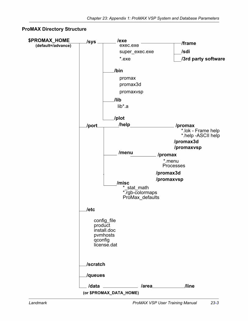
Landmark ProMAX VSP User Training Manual 23-3
Chapter 23: Appendix 1: ProMAX VSP System and Database Parameters ProMAX Directory Structure
/sys
/port
/etc
/scratch
/queues
config_fileproductinstall.docpvmhostsqconfiglicense.dat
/data
/help
/menu
/misc
/plot
/lib
/bin
/exe
/promax3d
lib*.a
/promax
*.menuProcesses
/frame/sdi/3rd party software
super_exec.exe*.exe
exec.exe
*.lok - Frame help*.help -ASCII help
*_stat_math*.rgb-colormapsProMax_defaults
$PROMAX_HOME
/area /line(or $PROMAX_DATA_HOME)
(default=/advance)
/promax3d
/promax
/promaxvsp
/promaxvsp
promaxpromax3dpromaxvsp

Chapter 23: Appendix 1: ProMAX VSP System and Database Parameters
Third party software distributed by Advance will now be distributed in a subdirectory of /advance/sys/exe using the company’s name, thus avoiding conflicts where two vendors use identical file names. For example, SDI’s CGM Viewer software would be in /advance/sys/exe/sdi and Frame Technology’s FrameViewer would be in /advance/sys/exe/frame.
23-4 ProMAX VSP User Training Manual Landmark

Chapter 23: Appendix 1: ProMAX VSP System and Database Parameters
ProMAX Directory Structure
/sys
/port
/etc
/scratch
/queues
config_fileproductinstall.docpvmhostsqconfiglicense.dat
/data
/help
/menu
/misc
/plot
/lib
/bin
/exe
/promax3d
lib*.a
/promax
*.menuProcesses
/frame/sdi/3rd party
super_exec.exe*.exe
exec.exe
*.lok - Frame help*.help -ASCII help
*_stat_math*.rgb-colormapsProMax_defaults
$PROMAX_HOME
/area /line(or $PROMAX_DATA_HOME)
(default=/advance)
/promax3d
/promax
/promaxvsp
/promaxvsp
promaxpromax3dpromaxvsp
software
Landmark ProMAX VSP User Training Manual 23-5

Chapter 23: Appendix 1: ProMAX VSP System and Database Parameters
/advance/port
Software that is portable across all platforms is grouped under a single subdirectory /advance/port. This includes menus and Processes (/advance/port/menu), helpfiles(/advance/port/help), miscellaneous files (/advance/port/misc). Under the menu and help subdirectories are additional subdirectories for each ProMAX software product. For instance, under /advance/port/menu, you will find subdirectories for ProMAX 2D (promax), ProMAX 3D (promax3d), and ProMAX VSP (promaxvsp). Menus for additional products are added as new subdirectories under /advance/port/menu.
/advance/etc
Files unique to a particular machine are located in the /advance/etc subdirectory. Examples of such files are the config_file, which contains peripheral setup information for all products running on a particular machine, and the product file, which assigns unique pathnames for various products located on the machine.
/advance/scratch
The scratch area defaults to /advance/scratch. This location can be overridden with the environmental variable, PROMAX_SCRATCH_HOME.
All ProMAX development tools are included within the following subdirectories: /advance/sys/lib, /advance/sys/obj, /advance/port/src, /advance/port/bin, /advance/port/include and /advance/port/man.
/advance/data (or $PROMAX_DATA_HOME)
The primary data partition defaults to /advance/data, with new areas being added as subdirectories beneath this subdirectory. This default location is specified using the entry:
— primary disk storage partition: /advance/data 20
in the /advance/etc/config_file. This location can also be set with the environmental variable $PROMAX_DATA_HOME.
23-6 ProMAX VSP User Training Manual Landmark

Chapter 23: Appendix 1: ProMAX VSP System and Database Parameters
ProMAX Data Directories
Each region identifies a collection of files and directories which can be summarized as the Area, Line, Parameter Tables, Flow, Trace Headers, and Ordered Parameter Files database.
/Data
/AreaDescNameProject
/LineDescName17968042TVEL31790267TGAT36247238TMUT12345678CIND12345678CMAP
/12345678HDR1HDR2TRC1
/Flow1
TRC2
DescName
job.output
/OPF.SINOPF60_SIN.GEOMETRY.ELEV
/OPF.SRF
A Flow subdirectoryTypeName
packet.job
and its files
Parameter Table files
Index and Map Dataset files
Dataset subdirectoryand Header and TraceDataset files
PROMAX_DATA_HOME
or
#s0_OPF60_SRF.GEOMETRY.ELEV
/OPF.SIN Databasesubdirectory anda non-spanned file
/OPF.SRF Databasesubdirectory and aspan file
Area subdirectory and its files
Landmark ProMAX VSP User Training Manual 23-7

Chapter 23: Appendix 1: ProMAX VSP System and Database Parameters
Program Execution
User Interface ($PROMAX_HOME/sys/bin/promax)
Interaction with ProMAX is handled through the User Interface. As you categorize your data into Areas and Lines, the User Interface automatically creates the necessary UNIX subdirectories and provides an easy means of traversing this data structure.
However, the primary function of the User Interface is to create, modify, and execute processing flows. A flow is a sequence of processes that you perform on seismic data. Flows are built by selecting processes from a list, and then selecting parameters for each process. A typical flow contains an input process, one or more data manipulation processes, and a display and/or output process. All information, needed to execute a flow, is held within a Packet File (packet.job) within each Flow subdirectory. This Packet File provides the primary means of communication between the User Interface and the Super Executive program. See next section, Super Executive Program.
In addition, the User Interface provides utility functions for copying, deleting and archiving Areas, Lines, Flows, and seismic datasets; accessing and manipulating ordered database files and parameter tables; displaying processing histories for your flows; and providing information about currently running jobs. The User Interface is
23-8 ProMAX VSP User Training Manual Landmark

Chapter 23: Appendix 1: ProMAX VSP System and Database Parameters
primarily mouse-driven and provides point-and-click access to the functions.
Program Execution
Super Executive Program (super_exec.exe)
Execution of a flow is handled by the Super Executive, which is launched as a separate task by the User Interface. The Super Executive is a high level driver program that examines processes in your flow by reading packet.job and determines which executables to use. The majority of the processes are subroutines linked together to form the Executive. Since this is the processing kernel for ProMAX, many of your processing flows, although they contain several processes, are handled by a single execution of the Executive. Several of the processes
Landmark ProMAX VSP User Training Manual 23-9

Chapter 23: Appendix 1: ProMAX VSP System and Database Parameters
are stand-alone programs. These processes cannot operate under the control of the Executive, and handle their own data input and output by directly accessing external datasets. In these instances, the Super Executive is responsible for invoking the stand-alone programs and, if necessary, multiple calls to the Executive in the proper sequence.
The Packet File, packet.job, defines the processes and their type for execution. The Super Executive concerns itself with only two types of processes:
• Executive processes
• Stand-alone processes
Executive processes are actually subroutines operating in a pipeline, meaning they accept input data and write output data at the driver level. However, stand-alone processes cannot be executed within a pipeline, but rather must obtain input and/or produce output by directly accessing external datasets.
The Super Executive sequentially gathers all Executive-type processes until a stand-alone is encountered. At that point, the Packet File information for the Executive processes is passed to the Executive routine (exec.exe) for processing. Once this is completed, the Super Executive invokes the stand-alone program for processing, and then another group of Executive processes, or another stand-alone process. This continues until all processes in the flow have been completed.
Executive Program (exec.exe)
The Executive program is the primary processing executable for ProMAX. The majority of the processes available under ProMAX are contained in this one executable program.
The Executive features a pipeline architecture that allows multiple seismic processes to operate on the data before it is displayed or written to a dataset. Special processes, known as input and output tools, handle the tasks of reading and writing the seismic data, removing this burdensome task from the individual processes. This results in processes that are easier to develop and maintain.
23-10 ProMAX VSP User Training Manual Landmark

Chapter 23: Appendix 1: ProMAX VSP System and Database Parameters
The basic flow of data through the Executive pipeline is shown below:
Each individual process will not operate until it has accumulated the necessary traces. Single trace processes will run on each trace as the traces come down the pipe. Multi channel processes will wait until an entire ensemble is available. For example in the example flow the FK
Landmark ProMAX VSP User Training Manual 23-11

Chapter 23: Appendix 1: ProMAX VSP System and Database Parameters
filter will not run until one ensemble of traces has passed through the DDI and AGC. If we specify for the Trace Display to display 2 ensembles, it will not make a display until two shots have been processed through the DDI, AGC and FK filter. No additional traces will be processed until Trace Display is instructed to release the traces that it has displayed and is holding in memory by clicking on the traffic light icon or terminating its execution (but continuing the flow).
Note: All the processes shown are Executive processes and thus operate in the pipeline. An intermediate dataset and an additional input tool process is needed if a stand-alone process were included in this flow.
A pipeline process must accept seismic traces from the Executive, process them, and return the processed data to the Executive. The table below describes the four types of processes defined for use in the Executive.
23-12 ProMAX VSP User Training Manual Landmark
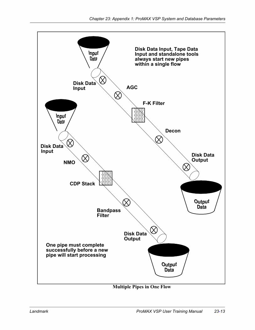
Chapter 23: Appendix 1: ProMAX VSP System and Database Parameters
AGC
F-K Filter
Decon
Disk DataInput
Disk Data
Disk Data Input, Tape DataInput and standalone tools always start new pipeswithin a single flow
One pipe must completesuccessfully before a newpipe will start processing
NMO
CDP Stack
Bandpass
Disk DataInput
Disk Data
Filter
Output
Output
Multiple Pipes in One Flow
Landmark ProMAX VSP User Training Manual 23-13

Chapter 23: Appendix 1: ProMAX VSP System and Database Parameters
Types of Executive Processes
The table below describes the four types of processes defined for use in the Executive.
Stand-Alone Processes and Socket Tools
Some seismic processing tools are not well suited to a pipeline architecture. Typically, these are tools making multiple passes through the data or requiring self-directed input. These tools can be run inline in a ProMAX job flow and appear as ordinary tools, but in reality are launched as separate processes. The current version of ProMAX does not provide the ability to output datasets from a stand-alone process. Socket tools start a new process and then communicates with the Executive via UNIX interprocess communications. Socket tools have the singular advantage of being able to accept and output traces in an asynchronous manner.
Table 1: ProMAX Executive Process Types
Process Type Description
simple tools Accepts and returns a single seismic trace.
ensemble tools Accepts and returns a gather of seismic traces
complex tools Accepts and returns a variable number of seismic traces such as, stack. This type of process actually controls the flow of seismic data.
panel tools Accepts and returns overlapping panels of traces to accommodate a group of traces too large to fit into memory. Overlapping panels are processed and then merged along their seams.
23-14 ProMAX VSP User Training Manual Landmark
Chapter 23: Appendix 1: ProMAX VSP System and Database Parameters
Ordered Parameter Files
Click to jump to the sectionThis section discusses the following issues relating to the Ordered Parameter Files database:
• Organization
• Database Structure
• File Naming Conventions
The Ordered Parameter Files database serves as a central repository of information that you or the various tools can rapidly access. Collectively, the ordered database files store large classes of data, including acquisition parameters, geometry, statics and other surface consistent information, and pointers between the source, receiver and CDP domains. The design of the Orders is tailored for seismic data, and provides a compact format without duplication of information.
The Ordered Parameter Files database is primarily used to obtain a list of traces to process, such as traces for a shot or CDP. This list of traces is then used to locate the index to actual trace data and headers in the MAP file of the dataset. Once determined, the index is used to extract the trace and trace header data from their files.
Organization
The Ordered Parameter Files contain information applying to a line and its datasets. For this reason, there can be many datasets for a single set of Ordered Database Files.
Ordered Parameter Files, unique to a line, reside in the Area/Line subdirectory. The Ordered Parameter Files database stores information in structured categories, known as Orders, representing unique sets of information. In each Order, there are N slots available for storage of information, where N is the number of elements in the order, such as the number of sources, number of surface locations, or number of CDPs. Each slot contains various attributes in various formats for one
Landmark ProMAX VSP User Training Manual 23-15
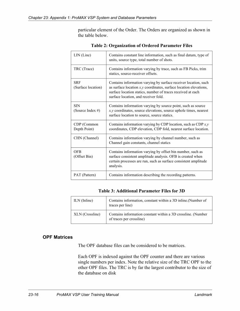
Chapter 23: Appendix 1: ProMAX VSP System and Database Parameters
particular element of the Order. The Orders are organized as shown in the table below.
OPF Matrices
The OPF database files can be considered to be matrices.
Each OPF is indexed against the OPF counter and there are various single numbers per index. Note the relative size of the TRC OPF to the other OPF files. The TRC is by far the largest contributor to the size of the database on disk
Table 2: Organization of Ordered Parameter Files
LIN (Line) Contains constant line information, such as final datum, type of units, source type, total number of shots.
TRC (Trace) Contains information varying by trace, such as FB Picks, trim statics, source-receiver offsets.
SRF (Surface location)
Contains information varying by surface receiver location, such as surface location x,y coordinates, surface location elevations, surface location statics, number of traces received at each surface location, and receiver fold.
SIN (Source Index #)
Contains information varying by source point, such as source x,y coordinates, source elevations, source uphole times, nearest surface location to source, source statics.
CDP (Common Depth Point)
Contains information varying by CDP location, such as CDP x,y coordinates, CDP elevation, CDP fold, nearest surface location.
CHN (Channel) Contains information varying by channel number, such as Channel gain constants, channel statics
OFB (Offset Bin)
Contains information varying by offset bin number, such as surface consistent amplitude analysis. OFB is created when certain processes are run, such as surface consistent amplitude analysis.
PAT (Pattern) Contains information describing the recording patterns.
Table 3: Additional Parameter Files for 3D
ILN (Inline) Contains information, constant within a 3D inline.(Number of traces per line)
XLN (Crossline) Contains information constant within a 3D crossline. (Number of traces per crossline)
23-16 ProMAX VSP User Training Manual Landmark

Chapter 23: Appendix 1: ProMAX VSP System and Database Parameters
OPF Maftrices
SIN (Sources) Database
SRF (Receivers) Database
Landmark ProMAX VSP User Training Manual 23-17

Chapter 23: Appendix 1: ProMAX VSP System and Database Parameters
Database Structure
The ProMAX database was restructured for the 6.0 release to handle large 3D land and marine surveys. The features of the new database structure are listed below:
Each order is contained within a subdirectory under Area and Line. For example, the TRC is in the subdirectory OPF.TRC.
There are two types of files contained in the OPF subdirectories:
• Parameter: Contain attribute values. There may be any number of attribute files associated with an OPF.
• Index: Holds the list of parameters and their formats. There is only one index file in each OPF subdirectory. The exception to this is the LIN OPF. The LIN information is managed by just two files, one index and one parameter, named LIN.NDX and LIN.REC.
OPF files are of two types:
• Span: These files are denoted by the prefix, #s. Non-span files lack this prefix. The TRC, CDP, SIN, and SRF OPF parameters are span files. The first span for each parameter is always written to primary storage. Span files are created in the secondary storage partitions listed in the config_file as denoted with the OPF keyword. Span files may be moved to any disk partition within the secondary storage list for read purposes. Newly created spans are written in the OPF denoted secondary storage partitions. All subsequent spans are written to the secondary storage partitions denoted by the OPF keyword in a round robin fashion until the secondary storage is full. Then, subsequent spans are created in primary storage. Span file size is currently fixed at 10 megabytes, or approximately 2.5 million 4 byte values per span file.
• Non-span: All other OPFs are non-span.
Given the fact that each parameter is managed by a file, it may be necessary to increase the “maximum number of files open” limit on some systems, specifically, SUN, Solaris and SGI. From the csh, the following command increases the file limit to 255 files open, “limit de 255”.
The geometry spreadsheet is a ProMAX database editor. Modifying information within a spreadsheet editor and saving the changes will automatically update the database.
23-18 ProMAX VSP User Training Manual Landmark

Chapter 23: Appendix 1: ProMAX VSP System and Database Parameters
There is no longer an import or export from the geometry database to the ProMAX database files as was required prior to the 6.0 release.
Database append is allowed. Data can be added to the database via the OPF Extract tool or the geometry spreadsheet. This allows for the database to be constructed incrementally as the data arrives.
There is improved network access to the database. Database I/O across the network is optimized to an NFS default packet size of 4K. All database reads and writes are in 4K pages.
Existing and restored 5.X databases are automatically converted to the 6.0 (and later) database format.
File Naming Conventions
Parameter file names consist of information type and parameter name, preceded by a prefix denoting the Order of the parameter.
For example, the x coordinate for a shot in the SIN has the following name: #s0_OPF60_SIN.GEOMETRY.X_COORD. Where #s0_OPF60 indicates a first span file for the parameter, _SIN denotes the Order, GEOMETRY describes the information type of the parameter, and X_COORD is the parameter name.
4. Index file names contain the three letter Order name. For example, the index file for the TRC is called OPF60_TRC.
Within each Order, there are often multiple attributes, with each attribute being given a unique name.
NOTE:
The index file for each Order must remain in the primary storage partition. Span parameter files may be moved and distributed anywhere within primary and secondary storage.
Landmark ProMAX VSP User Training Manual 23-19
Chapter 23: Appendix 1: ProMAX VSP System and Database Parameters
Parameter Tables
Parameter Tables are files used to store lists of information in a very generalized structure. To increase access speed and reduce storage requirements, parameter tables are stored in binary format. They are stored in the Area/Line subdirectory along with seismic datasets, the Ordered Parameter Files database files (those not in separate directories), and Flow subdirectories.
Parameter Tables are often referred to as part of the database. Parameter tables differ from the OPF database in OPF files contain many attributes that are 1 number per something. Parameter tables contain more than one number per something. For example a velocity function contains multiple velocity-time pairs at 1 CDP.
Creating a Parameter Table
Parameter tables are typically created in three ways:
• Processes store parameters to a table for later use by other processes.
• Parameter tables can be imported from ASCII files that were created by other software packages or hand-edited by you.
• Parameter tables can be created by hand using the Parameter Table Editor which is opened by the Create option on the parameter table list screen.
An example is the interactive picking of time gates within the Trace Display process. After seismic data is displayed on the screen, you pull down the Picking Menu and choose the type of table to create. The end result of your work is a parameter table. If you were to pick a top mute, you would generate a parameter table ending in TMUT. If you were picking a time horizon, you would generate a table ending in THOR. These picks are stored in tabular format, where they can be edited, used by other processes in later processing, or exported to ASCII files for use by other software packages.
Remember, you name and store the parameter tables in their specific Area/Line subdirectory. Therefore, you can inadvertently overwrite an existing parameter table by editing a parameter table in a different processing flow.
23-20 ProMAX VSP User Training Manual Landmark

Chapter 23: Appendix 1: ProMAX VSP System and Database Parameters
ASCII File Export to Parameter Table Editor
Export writes either ASCII or EBCDIC formatted files with fixed columnar data from a spreadsheet editor. In the following exercise, a velocity table is exported to an ASCII file.
Exercise1. In a flow-building window, add the Access Parameter Tables
process to a flow and view the parameter menu with MB2.
Find the line: VEL: RMS (stacking) velocity and click on Invalid. The list of parameter tables for RMS Velocity appear.
2. Click on Edit and select the name of the file to export.
A Parameter Table spreadsheet appears with CDP, TIME, and SEMB_VEL columns.
3. Click on File and select Export.
An ASCII File Export window appears with export information for quality control before actually creating the ASCII file.
4. Click on File.
A new window appears with the path to your working directory.
5. Enter a filename after the last / and click OK.
The window disappears and a dashed line appears in the ASCII File Export window.
6. Click on Format.
An Export Definition Selection window appears.
7. Type in a selection name and click on OK.
The Column Export Definition window appears.
8. Fill the Column Export Definition with starting and ending column numbers, then click on Save.
When you fill in the start and end columns for a particular column definition, the contents of the column appear in the ASCII File
Landmark ProMAX VSP User Training Manual 23-21

Chapter 23: Appendix 1: ProMAX VSP System and Database Parameters
Export window. Be sure the column definitions are wide enough to accommodate all the significant figures, as well as complete column titles. If they are not, edit the Column Export Definition window until the information is correct.
9. When the ASCII File Export window is correct, click on Apply.
An Apply Export window appears. You may choose to overwrite or append new information to the ASCII file. You may also add a single line description of your work that will be internal to the file.
10. Click on OK.
This creates the ASCII file in the directory you specified. You may now Quit the Column Export Definition window, Cancel the ASCII file Export Window, and pull down the File menu in the Parameter Table window and exit this window and continue working.
ASCII File Import to a Parameter Table
File Import reads either ASCII or EBCDIC formatted files with fixed columnar data into the spreadsheet editor.
Exercise1. In a flow-building window, add the Access Parameter Tables
process and view the parameter menu with MB2.
Find the line: VEL: RMS (stacking) velocity and click on Invalid. The list of Parameter Files(tables) for RMS velocity appear.
2. Click on Create.
The cursor will move to the top of the table name column, enter a new velocity file name. After typing a name, press Return. A Parameter Table spreadsheet appears with CDP, TIME, and VEL_RMS columns.
3. Click on File and choose Import.
Two new windows appear: ASCII/EBCDIC File Import and File Import Selection. In the File Import Selection window, choose the path to the file containing velocity information to import and click on OK. The import information appears in the ASCII/EBCDIC File Import window.
23-22 ProMAX VSP User Training Manual Landmark

Chapter 23: Appendix 1: ProMAX VSP System and Database Parameters
4. Click on Format in the ASCII/EBCDIC File Import window.
The Import Definition Selection window appears.
5. Type in a selection name and click on OK.
The Column Import Definition window appears.
6. Blank rows that will not be imported into the new velocity file.
To blank the rows, click MB1 in the first row to ignore and click MB2 in the last row to ignore. Press Ctrl-d, the rows to ignore are labeled Ignore Record for Import.
7. Fill the Column Import Definition window.
Begin filling the Column Import Definition window by choosing a definition parameter by clicking on the parameter name. The parameter box will be highlighted in white. Next, move the cursor into the ASCII/EBCDIC File Import window to the values defining the definition parameter. Hold down MB1 as you drag it from left to right across the import parameter values. The chosen columns should highlight in black in the ASCII/EBCDIC File Import window and the Start Col and End Col boxes in the Column Import Definition window should contain the appropriate column numbers. Repeat this process with the other two parameters and save the definition.
8. When the Column Import Definition window is correct, click on Apply in the ASCII/EBCDIC File Import window.
The Apply Import window appears. You may choose to overwrite or append new information to the spreadsheet.
9. Click OK.
This fills in the spreadsheet with selected numbers. Also, the Import windows disappear from the screen. You may now continue working and apply these velocities to your data.
Landmark ProMAX VSP User Training Manual 23-23

Chapter 23: Appendix 1: ProMAX VSP System and Database Parameters
Disk Datasets
ProMAX uses a proprietary disk dataset format that is tailored for interactive processing and random disk access. Disk dataset files can span multiple filesystems, allowing for unlimited filesize datasets.
A typical set of files might look like this:
— /advance/data/usertutorials/landexample/12345678CIND /advance/data/usertutorials/landexample/12345678CMAP /advance/data/usertutorials/landexample/12345678/TRC1 /advance/data/usertutorials/landexample/12345678/HDR1
These files are described in more detail in the table below.
Table 4: Composition of a Seismic Dataset
File Name Contents
Trace (...TRCx)
File containing actual sample values for data trace.
Trace Header (....HDRx)
File containing trace header entries corresponding to data samples for traces in the trace file. This file may vary in length, growing as new header entries are added. Keep trace headers in a separate file so trace headers can be sorted without needing to skip past the seismic data samples.
Map (....CMAP)
File keeps track of trace locations. Given a particular trace number, it will find the sequential trace number within the dataset. This rapidly accesses traces during processing. The map file is a separate file, as it may grow during processing.
Index (....CIND)
File has free-form format information relating to the entire dataset, including sample interval, number of samples per trace, processing history, and names of trace header entries. This file may grow during processing.
23-24 ProMAX VSP User Training Manual Landmark

Chapter 23: Appendix 1: ProMAX VSP System and Database Parameters
Disk Dataset Components - Relative Sizes
Secondary Storage
In a default ProMAX configuration, all seismic dataset files reside on a single disk partition. The location of this disk partition is set in the $PROMAX_HOME/etc/config_file with the entry:
— primary disk storage partition: /advance/promax/data 20
In addition to the actual trace data files, the primary storage partition will always contain your flow subdirectories, parameter tables, ordered parameter files, and various miscellaneous files. The ...CIND and ...CMAP files which comprise an integral part of any seismic dataset are always written to primary storage.
Since the primary storage file system is of finite size, ProMAX provides the capability to have some of the disk datasets, such as the ...TRCx and ...HDRx files, and some of the ordered parameter files span multiple disk partitions. Disk partitions other than the primary disk storage partition are referred to as secondary storage.
All secondary storage disk partitions must be declared in the appropriate $PROMAX_HOME/etc/config_file. Samples entries are:
CIND
CMAP
HDRx
TRCx
Landmark ProMAX VSP User Training Manual 23-25

Chapter 23: Appendix 1: ProMAX VSP System and Database Parameters
secondary disk storage partition: /advance/promax/data2 20 TRC OPF secondary disk storage partition: /advance/promax/data3 20 TRC secondary disk storage partition: /advance/promax/data4 20 OPF secondary disk storage partition: /advance/promax/data5 20
Refer to the ProMAX System Administration guide for a complete description of the config_file entries for primary and secondary disk storage.
Under the default configuration, the initial TRC1 and HDR1 files are written to the primary storage partition. It is possible to override this behavior by setting the appropriate parameter in Disk Data Output. If the parameter Skip primary disk partition? is set to Yes, then no TRC or HDR files will be written to the primary disk partition. This can be useful as a means of maintaining space on the primary storage partition. (To make this the default situation for all users, have your ProMAX system administrator edit the diskwrite.menu file, setting the value for Alstore to ‘t’ instead of ‘nil’).
A typical set of data files might look like this:
— /advance/data/usertutorials/landexample/12345678CIND /advance/data/usertutorials/landexample/12345678CMAP /advance/data/usertutorials/landexample/12345678/TRC1 /advance/data/usertutorials/landexample/12345678/HDR1 /advance/data/usertutorials/landexample/12345678/TRC4 /advance/data/usertutorials/landexample/12345678/HDR4 /advance/data/usertutorials/landexample/12345678/TRC7 /advance/data/usertutorials/landexample/12345678/HDR7 /advance/data2/usertutorials/landexample/12345678/TRC2 /advance/data2/usertutorials/landexample/12345678/HDR2 /advance/data2/usertutorials/landexample/12345678/TRC5 /advance/data2/usertutorials/landexample/12345678/HDR5 /advance/data2/usertutorials/landexample/12345678/TRC8 /advance/data2/usertutorials/landexample/12345678/HDR8 /advance/data3/usertutorials/landexample/12345678/TRC3 /advance/data3/usertutorials/landexample/12345678/HDR3 /advance/data3/usertutorials/landexample/12345678/TRC6 /advance/data3/usertutorials/landexample/12345678/HDR6
23-26 ProMAX VSP User Training Manual Landmark

Chapter 23: Appendix 1: ProMAX VSP System and Database Parameters
Secondary storage is used in a “as listed and available” fashion. As an attempt to minimize data loss due to disk hardware failure, ProMAX tries to write a dataset to as few physical disks as possible. If the primary storage partition is skipped by setting the appropriate parameter in Disk Data Output, the CIND and CMAP files are still written to the primary storage partition, but the TRCx or HDRx files will not be found there.
Landmark ProMAX VSP User Training Manual 23-27
Chapter 23: Appendix 1: ProMAX VSP System and Database Parameters
Tape Datasets
Tape datasets are stored in a proprietary format, similar to the disk dataset format, but incorporating required structures for tape input and output. Tape input/output operates either in conjunction with a tape catalog system, or without reference to the tape catalog. The tape devices used for the Tape Data Input, Tape Data Insert, and Tape Data Output processes are declared in the ProMAX device configuration window. This allows access to tape drives anywhere on a network. The machines that the tape drives are attached to do not need to be licensed for ProMAX, but the fclient.exe program must be installed.
Tape Trace Datasets
A ProMAX tape dataset is similar to a disk dataset in that the index file (...CIND) and map file (...CMAP) still reside on disk in the Line/survey database. Refer to the documentation in the Disk Datasets portion of this helpfile for a discussion of these files. Having the index and map files available on disk provides you with immediate access to information about the dataset, without needing to access any tapes. It also provides all the information necessary to access traces in a non-sequential manner.
Although the index and map files still reside on disk, copies of them are also placed on tape(s), so that the tape(s) can serve as a self-contained unit(s). If the index and map files are removed from disk, or never existed, as in the case where a dataset is shipped to another site, the tapes can be read without them. However, access to datasets through the index and map files residing solely on tape must be purely sequential.
Tape datasets are written by the Tape Data Output process, and can be read using the Tape Data Input or Tape Data Insert processes. These input processes include the capability to input tapes by reel, ensemble number, or trace number. Refer to the relevant helpfile for a complete description of the parameters used in these processes.
The use or non-use of the tape catalog in conjunction with the tape I/O processes is determined by the tape catalog type entry in the appropriate $PROMAX_HOME/etc/config_file. Setting this variable to full activates catalog access, while an entry of none deactivates catalog access. An entry of external is used to indicate that an external tape catalog, such as the Cray Reel Librarian, will be used. You can override the setting provided in the config_file by setting the environment
23-28 ProMAX VSP User Training Manual Landmark

Chapter 24
Appendix 2: Archival MethodsArchiving your data protects your work from system failure and may allow you to bring data into other software packages. It is also useful for freeing up disk space and preserving flows. In this chapter, we will discuss the archiving methods that can be run from inside the ProMAX User Interface.
Topics covered in this chapter:
o SEG-Y Output
o Tape Data Output
o Archive to Tape
Landmark ProMAX VSP User Training Manual 24-1

Chapter 24: Appendix 2: Archival Methods
SEG-Y Output
ProMAX offers a variety of industry standard and individual company output formats. Of these, SEG-Y is the most commonly used. This process can write out industry standard SEG-Y tapes as well as frequently requested non-standard variations of SEG-Y and IEEE format. SEG-Y Output is a good choice for archiving a dataset that will later be loaded to a third party software package. This process will successfully archive data spanning over multiple disks. One downfall to this archival method is that it will not automatically map all the ProMAX trace headers. However, SEG-Y Output provides you the capability of manually mapping these non-standard trace headers.
In this exercise, you will write a SEG-Y formatted tape, mapping some of the non-standard SEG-Y headers. We will check to make sure the headers were mapped correctly by using SEG-Y Input and Trace Display.
24-2 ProMAX VSP User Training Manual Landmark

Chapter 24: Appendix 2: Archival Methods
1. Build the following flow in your 2D Land line or in the 2d-tutorials/tutor2d-watson rise area and line:
2. Select Disk Data Input parameters.
Select to read the first two shots from your "raw shots with extract" dataset.
We are limiting the dataset size for efficiency.
3. Select SEG-Y Output parameters.
Select Disk for type of storage--we will be using a Disk file instead of Tape. Enter the DISK file path name according to your instructor’s directions. Select Yes to Remap SEG-Y headers. Use the default remapping values to map the header values for sou_sloc and srf_sloc.
Editing Flow: SEG-Y Output
Add Delete Execute View Exit
Disk Data InputSelect dataset: ------------------------------------raw shots w/ extractTrace read option: --------------------------------------------------SortInteractive Data Access?: -------------------------------------------NoSelect primary trace header entry: --------------------------------SINSelect secondary trace header entry: ---------------------------NoneSort order for dataset: ----------------------------------------------1,2/
SEG-Y OutputType of SEG-Y: ------------------------------------------------StandardType of storage to use: -------------------------------------Disk ImageEnter DISK file path name----------------per instructor’s directionsRemap SEGY header values?: -------------------------------------YESOutput/override trace header entries: ---------------------------------
----sou_sloc,4I,,181/srf_sloc,4I,,185/----Default remaining parameters----
>SEG-Y Input<>Trace Display<
Landmark ProMAX VSP User Training Manual 24-3

Chapter 24: Appendix 2: Archival Methods
The SEG-Y format reserves bytes 181-240 for optional use. The *_sloc trace headers are important to ProMAX so we typically write them to the extended headers. These header values must be present in order to automatically rebuild the database files with the Extract Database Files process. (See chapter 2D Land 1).
4. Execute the flow.
5. Once the job is complete, build the following flow to QC the traces and headers written to tape.
6. Select SEG-Y Input parameters.
Select Disk for type of storage and the same path and filename you used for SEG-Y Output. Choose to remap headers, and use the defaults for sou_sloc and srf_sloc.
7. Execute the flow.
8. Use the Header tool icon in Trace Display to QC the headers.
The extended header values should be preserved (sou_sloc and srf_sloc).
Editing Flow: SEG-Y Output
Add Delete Execute View Exit
>Disk Data Input<>SEG-Y Output<SEG-Y Input
Type of SEG-Y: ------------------------------------------------StandardType of storage to use: -------------------------------------Disk ImageEnter DISK file path name----------------per instructor’s directionsRemap SEGY header values?: -------------------------------------YESInput/override trace header entries: ------------------------------
---------sou_sloc,4I,,181/srf_sloc,4I,,185/----Default remaining parameters----
Trace Display----Default remaining parameters----
24-4 ProMAX VSP User Training Manual Landmark

Chapter 24: Appendix 2: Archival Methods
Tape Data Ouput
Tape Data Output writes seismic traces to tape in ProMAX format. This process is ideal for archiving a dataset to be used later in ProMAX since it automatically preserves all trace headers, the CIND, and CMAP files. Like SEG-Y Output, Tape Data Output will archive datasets spanning multiple disks.
While we will not complete an exercise using Tape Data Output, you should be aware of its benefits for archiving data.
Landmark ProMAX VSP User Training Manual 24-5

Chapter 24: Appendix 2: Archival Methods
Archive to Tape
The SEG output formats and ProMAX Tape Output only operate on seismic trace files. ProMAX offers a process called Archive to Tape which writes entire Areas or Lines to tape. The associated read process is List/Restore from Tape. Archive to Tape and List/Restore from Tape offer the ability to span tape volumes and utilizes ProMAX’s secondary storage system.
List/Restore from Tape also checks for available disk space before writing files. Both processes offer the option to skip trace data files. In this case, only the TRC and HDR files will be processed.
Once the Area or Area/Line has been archived, you have the option of automatically removing the area or line after it is written to tape.
The following flows demonstrate the use of Archive to Tape and List Restore from Tape. Follow your instructor’s directions on which areas or lines can be archived and which tape device to use.
The Archive to Tape and List/Restore from Tape processes must be run from an area and line named "archive." Typically this area and line is expected to be shared by all users of the system so it should have permissions set to 775 or 777. Each user can maintain separate flows for individual archives. This approach improves the audit trail and eliminates the possibility of running a flow that removes itself if its Area/Line is deleted.
24-6 ProMAX VSP User Training Manual Landmark
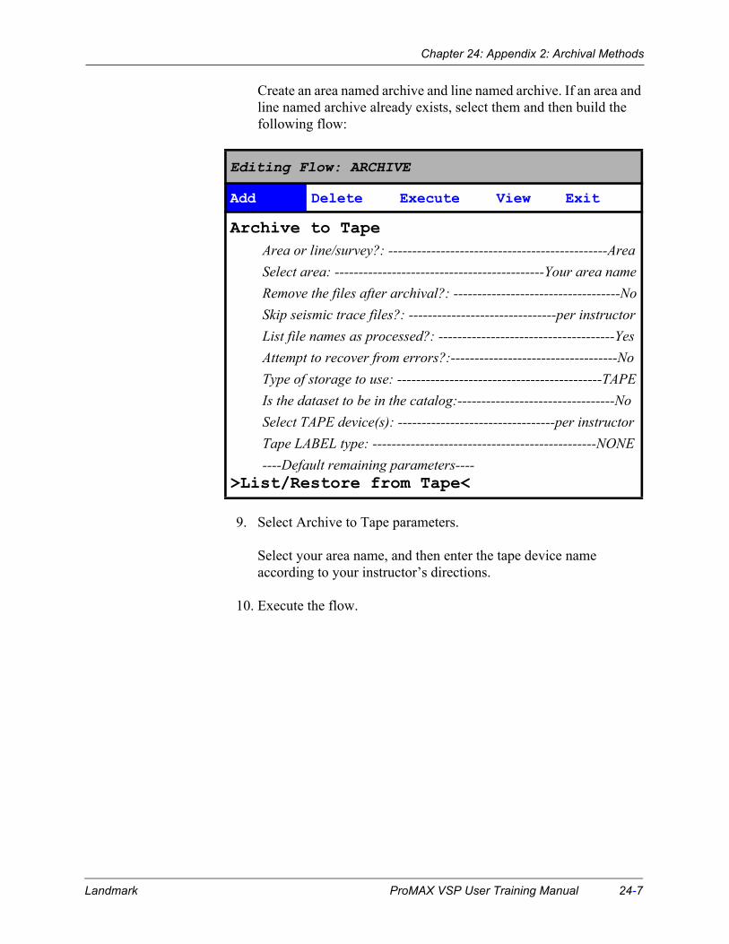
Chapter 24: Appendix 2: Archival Methods
Create an area named archive and line named archive. If an area and line named archive already exists, select them and then build the following flow:
9. Select Archive to Tape parameters.
Select your area name, and then enter the tape device name according to your instructor’s directions.
10. Execute the flow.
Editing Flow: ARCHIVE
Add Delete Execute View Exit
Archive to TapeArea or line/survey?: ----------------------------------------------AreaSelect area: --------------------------------------------Your area nameRemove the files after archival?: -----------------------------------NoSkip seismic trace files?: -------------------------------per instructorList file names as processed?: -------------------------------------YesAttempt to recover from errors?:-----------------------------------NoType of storage to use: -------------------------------------------TAPEIs the dataset to be in the catalog:---------------------------------NoSelect TAPE device(s): ---------------------------------per instructorTape LABEL type: -----------------------------------------------NONE----Default remaining parameters----
>List/Restore from Tape<
Landmark ProMAX VSP User Training Manual 24-7

Chapter 24: Appendix 2: Archival Methods
11. When the Archive to Tape process completes, build the following flow to check the contents of the tape:
12. Select List/Restore from Tape parameters.
Select Simple List for Type of operation.
Select a tape drive device name according to your instructor’s directions.
13. Execute the flow.
Verify that your Area exists on the archive tape by looking at your job.output file.
When you are ready to restore the archive, build a similar flow changing Simple list to Restore.
Editing Flow: ARCHIVE
Add Delete Execute View Exit
>Archive to Tape<List/Restore from Tape
Type of operation: -------------------------------------------Simple listSkip seismic trace files?: -------------------------------Per instructorType of storage to use: -------------------------------------------TAPEIs the dataset in the catalog:-----------------------------------------NoSelect TAPE devices:------------------------------------Per instructorTape LABEL type: -----------------------------------------------NONE----Default remaining parameters----
24-8 ProMAX VSP User Training Manual Landmark

Chapter 25
Appendix 3: Prepare Input DataThere was a minor limitation with the tutorial dataset whereby in the original file, all of the shot records had the same FFID and the geophone component header word was not set. In order to process these data, we had to assign different FFID numbers to each record and set the geophone component value.
Additional header words were also zeroed so that you could follow the header updates as the processing progressed.
Topics covered in this chapter:
o Preparing the Input Data
Landmark ProMAX VSP User Training Manual 25-1

Chapter 25: Appendix 3: Prepare Input Data
Preparing the Input Data
This is an exercise in trace header manipulation. There may be cases where you may want to alter trace headers before starting to process a dataset. Here is one example.
Exercise1. Build a flow to look at the trace headers.
2. In Disk Data Input, read a file from another area.
This dataset can be found in:
• Area: VSP tutorials
• Line: VSP tutorials
• Data File: Wtexas_VSP
3. In Trace Display, plot the data and view the trace headers to identify the header values that may need to be altered prior to the start of processing.
Since we have no idea how this data is organized, use all defaults for Trace Display except specify to plot 100 ensembles. This will help you identify what an ensemble is and then how to deal with the data.
4. Derive an equation to use to assign the FFIDs from 1 to 80. Also note that the Geophone (x,y,z) header word does not exist and must be set equal to the channel number.
Editing Flow: prepare input data
Add Delete Execute View Exit
Disk Data Input <Get All>Trace Display
25-2 ProMAX VSP User Training Manual Landmark

Chapter 25: Appendix 3: Prepare Input Data
Exercise1. Expand the previous flow to rebuild the trace headers and write the
file to your own line directory.
2. In the first Trace Header Math, compute FFID=(12100-CDP)/50+1.
3. In the second Trace Header Math, compute GEO_COMP=chan.
4. In the remaining Trace Header Math processes, set SOU_X=0.0, REC_ELEV=0.0, CDP=0, TR_FOLD=0.0, and LINE_NO=0 one at a time.
Note: Some are integer others are floating point.
5. Sort the data back to FFID/CHAN.
There are 3 traces per FFID ensemble and a total of 240 traces in the dataset.
6. Check the output headers using Trace display.
7. In Disk Data Output, write the data to disk when satisfied that the data is OK.
Editing Flow:
Add Delete Execute View Exit
Disk Data Input <Get All>Trace Header MathTrace Header MathTrace Header MathTrace Header MathTrace Header MathTrace Header MathTrace Header MathIn-line Sort>Disk Data Output<Trace Display
Landmark ProMAX VSP User Training Manual 25-3

Chapter 25: Appendix 3: Prepare Input Data
25-4 ProMAX VSP User Training Manual Landmark

Chapter 26
Appendix 4: UNIX WorkstationBasicsThis chapter serves as a quick reference to you for some basic workstation operations.
Topics covered in this chapter:
o Text Editors in ProMAX
o UNIX Commands
o Examples of UNIX Commands
Landmark ProMAX VSP User Training Manual 26-1

Chapter 26: Appendix 4: UNIX Workstation Basics
Text Editors in ProMAX
There are three text editors used with ProMAX:
• Emacs Editor
• Emacs Editor Widget
• Emacs View Widget
The Emacs Editor is a general-purpose, full-function editor. It can be operated outside of ProMAX or in the processes: Config File Edit and the Emacs Editor process. To start the Emacs editor outside of ProMAX, exit ProMAX and type emacs filename at the UNIX prompt.
The Emacs Editor Widget is a subset of the full-function editor and is used within ProMAX when a single line editor is insufficient but a full-function editor is unnecessary. It supports cursor movement commands and a small set of editing commands.
The Emacs View Widget is similar to Emacs Widget in cursor movement, but does not allow any modification of text. The Emacs View Widget only displays text. It is used by ProMAX to view help files and the flow execution output listings (view job.output).
Since all the editors listed above are variations on the Emacs Editor, they operate similarly. Of course, the View Widget, which does not actually modify text, has no need for editing commands. Since the Editor Widget is a subset of the full Emacs Editor, it does not have all the commands in the Emacs Editor (Search and Replace, for example).
Note: The implementation of the editors is slightly different for each of the ProMAX supported hardware platforms. One reason for the differences is the fact that the keyboards are not the same on each platform. The main difference is the designation of the Meta key. This is the diamond key on either side of the space bar on the keyboard of SUN SPARCstations, Compose Character key on DECstations and the Alt key on IBM RS/6000 workstations. In the following instructions, replace the Meta key with the equivalent key stroke depending on your platform.
26-2 ProMAX VSP User Training Manual Landmark

Chapter 26: Appendix 4: UNIX Workstation Basics
Cursor movement:Use the 4 cursor arrow keys
Point the mouse cursor and click button 1
Ctrl-A Move the cursor to the beginning of the current line
Ctrl-E Move the cursor to the end of the current line
Ctrl-V Scroll the screen forward (down) one screen
”Meta”-V Scroll the screen backward (up) one screen
“Meta”-Shift-<Jump to the beginning of the file
“Meta”-Shift-> Jump to the end of the file
Ctrl-S Search forward for a string; (start entering ‘string’)
Ctrl-R Search backward for a string; (start entering ‘string’)
Editing:All keyboard entry is in insert mode
Delete key Delete one character to the left of the cursor (“Backspace” for DEC)
Ctrl-D Delete one character to the right of the cursor
Ctrl-K Kill to the end of the line (from the cursor)
Ctrl-Y Yank back the contents of the kill buffer (created by Ctrl-K or Ctrl-W); “cut and paste”; (can move the cursor first)
“Meta”-X, then type “repl s” Search and replace; (follow prompts)
Ctrl-X, Ctrl-W Write new Emacs file; (enter path & filename)
Ctrl-X, Ctrl-S Save current Emacs file
Ctrl-X, Ctrl-F Find another Emacs file
Ctrl-X, I Insert a file at current cursor location
Ctrl-X, Ctrl-C Exit Emacs
Landmark ProMAX VSP User Training Manual 26-3

Chapter 26: Appendix 4: UNIX Workstation Basics
Exiting Emacs:Ctrl-X, Ctrl-C; (then respond Y or N to saving)
26-4 ProMAX VSP User Training Manual Landmark
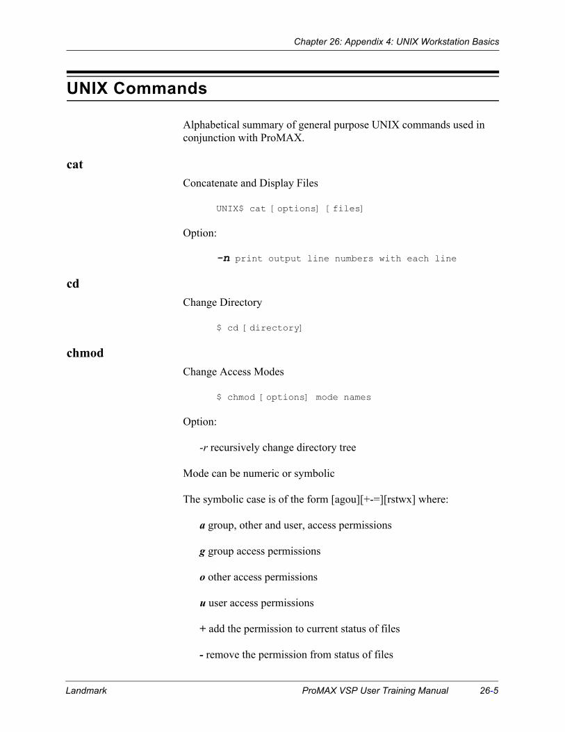
Chapter 26: Appendix 4: UNIX Workstation Basics
UNIX Commands
Alphabetical summary of general purpose UNIX commands used in conjunction with ProMAX.
cat Concatenate and Display Files
UNIX$ cat [options] [files]
Option:
-n print output line numbers with each line
cdChange Directory
$ cd [directory]
chmodChange Access Modes
$ chmod [options] mode names
Option:
-r recursively change directory tree
Mode can be numeric or symbolic
The symbolic case is of the form [agou][+-=][rstwx] where:
a group, other and user, access permissions
g group access permissions
o other access permissions
u user access permissions
+ add the permission to current status of files
- remove the permission from status of files
Landmark ProMAX VSP User Training Manual 26-5

Chapter 26: Appendix 4: UNIX Workstation Basics
= set the permission of files to specified value
r read permission
s set owner -ID or group -ID on execution (usable only with g or u)
t save text mode
w write permission
x execute permission
cpcopy files
$ cp [options] file 1 file 2
make a copy of file 1 named file 2
$ cp [options] files directory
make copies of specified files in directory
Options:
-i prompt user before overwriting file
-p copies have same modification times and modes as source files
-r recursive copy of directory (with subdirectories)
dfReport Free Block Count
$ df [options][filesys][file]
Options:
-i print number of modes free and in use
files df reports on file system containing files
filesys is a list of device names or mounted directory names to report (default = all mounted)
26-6 ProMAX VSP User Training Manual Landmark

Chapter 26: Appendix 4: UNIX Workstation Basics
duSummarize Disk Usage
$ du [options][names]
Options:
-a generate entry for each file
-s only display a grand total summary (default is entry for each directory)
names directory names or filenames
grepSearch File for Pattern
$ grep [options]expr [files]
stdin read if no files specified
Options:
-b precede line with block number
-c print count of matching lines only
-e expr useful if the expr start with a -
-i ignore case of letters in search
-l print only names of files with matching lines
-n print line numbers
-s print error messages only
-v print non-matching lines
-w search for expression as a word
expr expression or pattern
Landmark ProMAX VSP User Training Manual 26-7

Chapter 26: Appendix 4: UNIX Workstation Basics
killTerminate Process
$ kill -l
list signal names
$ kill [signal]process-ids
Options:
signal send signal instead of terminate
0 for process-id implies all processes resulting from current login
lnMake Links to File
$ ln [option] file1 file2
make a link to file1 named file2
$ ln [option] files directory
make links of specified files in directory
$ ln [option] pathname
make link with same name in current directory
Option:
-s make symbolic link (hard link default)
loginSign On to System
$ login [option][user]
login as user, logout if no user specified
lsList Contents of Directories
$ ls [options][names]
26-8 ProMAX VSP User Training Manual Landmark

Chapter 26: Appendix 4: UNIX Workstation Basics
names can be files of directories
current working directory used if no name specified
Options:
-1 print listing of one entry per line
-a list all entries (including ones starting with.)
-d list only name (not contents) of directory
-l long list (mode, links, owner, size, mod. time)
-r reverse sort order
-R recursively print subdirectories
-s print file size in kilobytes
manPrint Manual Entries
$ man -k keywords
print 1 line synopsis for each section containing keywords
$ man -f files
print 1 line synopsis for sections related to files
$ man [options][section] cmds
print manual sections for each cmd specified
Options:
- pipe output through more (default on terminals)
-M path to search for entries (/usr/man/default)
-t troff output to raster device
path list of directories to search, separated by colons section Arabic section number, followed by optional letter signifying type of command
Landmark ProMAX VSP User Training Manual 26-9

Chapter 26: Appendix 4: UNIX Workstation Basics
dirCreate Specified Directories
$ mkdir directories
moreView file by Screenful or by Line
$ more [options][files]
Options:
-c redraw page one line at a time
-d prompt after each screenful
-f count by newlines instead of screen lines
-l treat formfeed (L) as ordinary character
-n window size (default set with stty)
+n start viewing file at line n
-s reduce multiple blank lines to one
-u suppress terminal underlining or enhancing
+/pat start two lines before line containing pat
Enter h when more pauses for interactive options
mvMove Files (See CP)
$ mv [options] file1 file2
rename (or move) file1 file2
$ mv [options] files directory
rename (or move) specified files to directory
26-10 ProMAX VSP User Training Manual Landmark

Chapter 26: Appendix 4: UNIX Workstation Basics
Options:
- following arguments are filenames
-f force overwriting of existing files
-i interactive mode
psReport Process Status
$ ps [keys][-t list][process-id]
Keys:
a print all processes involving terminals
c print internally stored command name
e print both environment and arguments
g print all processes
k use/vmcore in place of /dev/kmem and /dev/mem for debugging l long listing
n process number (must be last key)
s add size of kernel stack of process to output
tn list processes associated with terminals; n is terminal number (must be last key)
u include fields of interest to user
U update namelist database (for speed)
v print virtual memory statistics
w 132 column output format
ww arbitrarily wide output
x include processes with no terminal
Landmark ProMAX VSP User Training Manual 26-11

Chapter 26: Appendix 4: UNIX Workstation Basics
pwdPrint Working Directory Name
$ pwd
rcpCopy Files Between Machines
$ rcp [option] file1 file2
copy file1 file2
$ [options] files directory
copy files to specified directory
Options:
-p copies have same modification times and modes as source files
-r recursive copy of directories
rloginLogin on Remote Terminal
$ [rlogin] remote [options]
Options:
-8 allow 8 bit data path
-ec specify new escape character c
-l user user is login name on remote system
-L run remote session in litout mode
remote remote host system
rlogin is optional if /usr/hosts in search path
rmRemove Files
$ rm [options] files
26-12 ProMAX VSP User Training Manual Landmark

Chapter 26: Appendix 4: UNIX Workstation Basics
Options:
- treat all following arguments as filenames
-i ask for confirmation before each delete
-r recursively delete directories
rmdir Remove Empty Directories (See RM)
$ rmdir directories
suBecome Another User (Set User)
$ su [options][user]
user defaults to root
Options:
- act like full login
-f if csh, don’t execute .cshrc
tarTape file Archiver
$ tar [key][option][files]
stdin read if no files specified
Keys: format: letter [modifiers]
Function Letters:
c create new tape and record files
t tell when files found, all entries if no files
x extract files, entire tape if no files
Landmark ProMAX VSP User Training Manual 26-13

Chapter 26: Appendix 4: UNIX Workstation Basics
Function Modifiers:
0...9 specify which tape drive to use (0 default)
b next arg is blocking factor (20 default, 20 max)
B force I/O blocking at 20 blocks per record
f arch arch is the file to be used for input/output to archives (if-then stdin read)
h follow symbolic links
l complain if all file links not found
m update file modification times
v verbose mode
w wait for confirmation after reporting filename (y causes action to be performed)
Option:
-C dir change directory to dir
whoWho is on the System
$ who [file][am i]
Arguments:
file read instead of /etc/utmp for login information
am i output who you are logged in as
whoamiPrint Effective User-Id
$ whoami
works even if you have become another user with su.
26-14 ProMAX VSP User Training Manual Landmark

Chapter 26: Appendix 4: UNIX Workstation Basics
Examples of UNIX Commands
Most of the following commands apply to Berkeley UNIX. Some of the commands will be different or even unavailable, depending on which shell you are using. The following examples refer to the C shell, and do not necessarily work with the Bourne or Korn shells.
alias promax /advance/sys/bin/promax&
The alias command is used to substitute a short, convenient command in place of a longer command. In this case, promax is the new (alias) command. From this point on, typing promax will be equivalent to typing the full /advance/sys/bin/promax&.
Note: This alias will only be effective until you log out. If you want it to be available each time you log in, place this line in your .cshrc file. This is a C shell command.
cp -r /advance/data/offshore .
cp is the copy command. The -r tells the system that you want to copy recursively (useful for copying directories trees). The directory from which you are copying in this case is /advance/data/offshore. Note the final ., which denotes the target directory. The single . means the current directory. Be careful about how you specify the target directory. If you told the system to copy the files to a directory offshore and this directory already exists, then the files will end up in offshore/offshore.
df
df shows the amount of free space on all the currently mounted file systems, including remotely mounted file systems. The listing will show you which of the file systems are remotely mounted. It is possible to specify one file system and see the amount of free space in only that file system. If you do not specify a file system, then df will default to showing all the mounted file systems. There are many other options for df which you may find useful.
du -s offshore
The du command summarizes disk usage. It can show disk usage file by file. When the -s option is given, only a grand total summary of disk
Landmark ProMAX VSP User Training Manual 26-15

Chapter 26: Appendix 4: UNIX Workstation Basics
usage is produced. Specifying offshore requests a disk usage report for that directory.
grep -i STAT elev_stat_math | grep -i CDP
grep is the search command. This command will search for the lines within the file elev_stat_math which contain the string STAT. The -i causes the search to ignore upper or lower case differences. Without this option, it would look for STAT exactly, in upper case. The | or pipe redirects the output from the search into another grep command. This again performs a case-insensitive search for CDP. Because the output from the first search contains only lines with the string STAT, the result of the piped search will contain only lines with both STAT and CDP.
grep STAT header.list static_hdrs
This grep will search the file header.list for lines containing the string source in upper case letters only, and then will direct the output of the search to a file called static_hdrs.
kill -9 2367
The kill command will stop a current process by sending a signal. The process number in this case is number 2367, which was found by using the ps command. There are many modifiers for this command, but one which you should know is the -9. This makes it impossible for the process to ignore the signal.
You might use this when a process is locked up and there is no other way to stop it.
ln -s /advance/data2/oswork offshore
The ln command means link. The -s denotes a symbolic link. This can be used to link files on different file systems. A normal link, sometimes known as a hard link, specified as ln without the -s, cannot link between file systems.
This symbolic link will cause the directory /advance/data2/oswork to appear in the current directory under the name offshore. It is not a new directory, or a copy of the oswork directory in /advance/data2. When you access a file in your directory called offshore, you are actually accessing the original file in the directory /advance/data2/oswork.
26-16 ProMAX VSP User Training Manual Landmark

Chapter 26: Appendix 4: UNIX Workstation Basics
Therefore any changes made in offshore will be made to in /advance/data2/os work.
You should be aware that certain commands act differently when applied to a linked file. For example, if you delete the linked file using rm applied to the linked file in your directory, only the link is removed. The original file is intact. But if you copy the linked file with cp applied to the file in your directory, the system will make a copy of the original file.
ps -ax
The ps (process status) command shows all of the processes currently running on the system. The -a tells the system to display all processes except process group leaders and processes not started from terminals. The x shows processes without control terminals. If you do not specify the x, then you may not see the process for which you are looking. The -ax on Berkeley UNIX changes to -elf on System V UNIX. The l provides a long form of the listing, -f provides a full listing of the processes, and -e asks for every process on the system.
rcp -r neptune:/usr/disk2/offshore .
rcp is the remote copy command. The -r, as with the cp command, is the recursive form of copy. It will copy the /usr/disk2/offshore directory and its subdirectories from the named server. The destination directory is ., the current working directory.
rmdir offshore
The rmdir command removes directories. In this example the rmdir command will remove the directory offshore. rmdir will only remove an empty directory. If you still have entries in the directory, this command will fail. You can check the contents of the directory, to see if it contains files you meant to keep. Or you can use the rm -r command, at your own risk.
tar c /advance/data/offshore
The tar command (tape archive) is used for moving files to or from tape. The c means create, so a new tape will be created. The directory to be copied to tape is /advance/data/offshore. To copy more directories to tape, just list them after the first directory, separated by spaces. x in place of the c will extract files from the tape and copy them to the disk.
Landmark ProMAX VSP User Training Manual 26-17

Chapter 26: Appendix 4: UNIX Workstation Basics
tar x with no files listed will read everything off the tape. tar x followed by a file name, directory or path will only read the data if it exists on the tape. This is a safe way to get back a specific dataset from the tape. The v option is verbose, so that you can see what the process is doing. Otherwise, like most UNIX processes, it is silent. You may wish to investigate cpio as a more versatile alternative to tar.
tar c ./offshore
This tar command copies to tape the directory offshore and the files which belong to the directory offshore. The ./ preceding ‘offshore’ indicates that offshore is a subdirectory of the current working directory. It is generally best to use relative path names (rather than full path names) when you are using tar.
26-18 ProMAX VSP User Training Manual Landmark