NOAA SPACE WEATHER PREDICTION CENTER

Geoelectric Field Maps: Progress on NOAA’s operational near real-time Geoelectric Field

Estimation Capability

Christopher Balch – NOAA/SWPC Anna Kelbert – USGS/Geomagnetism E.J. Rigler – USGS/Geomagnetism Space Weather Workshop 17-20 April 2018

Acknowledgements

• Collaborators:

Antti Pulkkinen – NASA/CCMC

David Boteler – NRCAN

Greg Lucas - USGS

• Data providers: USGS & NRCAN

• Interpolation Algorithm: SECS from FMI

• Conductivity model upgrade:

NSF’s Earthscope USArray project

NOAA SPACE WEATHER PREDICTION CENTER

Motivation & Milestones for E-field Maps

• Goal is to provide something better than the Kp index/G-scale or local K-indices to indicate geomagnetic activity level for systems affected by geomagnetically induced currents (GIC)

• Geoelectric Field – identified as the key space weather parameter needed by the electrical power industry

– Space Weather Workshop 2011:

’…the best, most useful environment parameter…’

– Referenced by industry standards groups (NERC/FERC)

Used to describe the benchmark geomagnetic storm event and

vulnerability assessment requirements

– National Space Weather Action Plan (SWAP) (OSTP 2015) highlights the

Geoelectric field in Goal 1.1 (Benchmarks) & Goal 5.5 (Enhance

Understanding)

• Local-regional activity can differ from globally averaged activity levels

• The geoelectric field is a direct indicator of induction hazard

NOAA SPACE WEATHER PREDICTION CENTER

How will the information will be used?

• The geoelectric field enables calculation geomagnetically induced currents

• The GIC calculation requires realistic system modeling

– Users are developing realistic models of their systems (a standards requirement)

• Calculated GIC can be compared to measured GIC for validation

• Assessment of GIC impacts on the system:

– System stability when GIC is present (i.e. voltage stability)

– Transformer behavior under GIC-caused saturation conditions

– Impact of GIC-caused harmonics on other system components

• System planning or after-the-fact analysis:

– Simulations can locate problem spots and focus mitigation efforts

– Analysis can inform real-time response procedures to E-field nowcast/forecast

• The industry is developing tools to help with these assessments

• With more accurate and appropriately targeted information, the industry can make a more informed and appropriate decision in response to storm events, resulting in more efficient operations and cost savings

E-field maps – current capability

USGS observatories (7)

B-field time series Detrending Algorithm

NRCAN observatories (5)

B-field time series

Interpolation Algorithm

B-field on 2°x2° grid

E-field calculation:

2°x2° grid, 1D conductivities

B-field experimental products:

-results in database

-graphical maps (on request)

-gridded data files (on request)

E-field experimental products:

-results in database

-graphical maps (public release Oct ‘17)

-gridded data files (available on request)

Station Latencies (typical):

BOU, BSL, FRD, FRN, NEW ~1.6 min

SJG, TUC ~2.8 min

MEA, OTT ~2-4 min

VIC, BRD, STJ ~4-8 min

B-field Interpolation Map

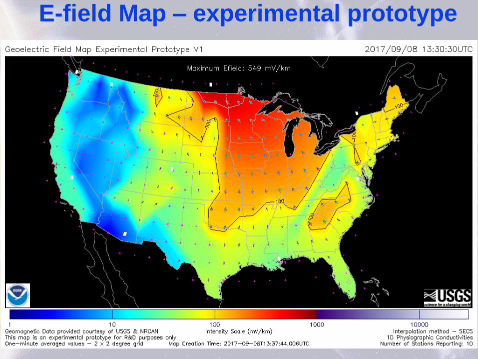
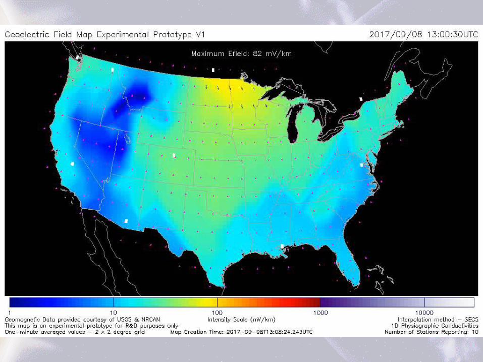
E-field Map – experimental prototype

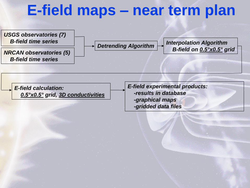
E-field maps – near term plan

USGS observatories (7)

B-field time series Detrending Algorithm

NRCAN observatories (5)

B-field time series

Interpolation Algorithm

B-field on 0.5°x0.5° grid

E-field calculation:

0.5°x0.5° grid, 3D conductivities

E-field experimental products:

-results in database

-graphical maps

-gridded data files

Near Term Plan for Data Dissemination: GeoJSON

• About GeoJSON • Adheres to a standard (RFC 7946): https://tools.ietf.org/html/rfc7946

• Can be read by web and desktop GIS clients

• Can be parsed as json, or by geojson libraries in a variety of languages

• Could be returned by a geospatial data service (e.g. ESRI ArcGIS Online)

• ASCII for human readability, compresses well when served with gzip enabled

• Sample data available from the September 2017 storm

• SWPC will be producing GeoJSON gridded data files soon

NOAA SPACE WEATHER PREDICTION CENTER

Geoelectric Field Calculation • Input – Geomagnetic Field (B-field) time series

• Earth conductivity acts like a frequency dependent filter:

– The effect on input amplitude and phase depends on the frequency

• High frequency fields have relatively shallow penetration (top-most layers), lower frequency

fields have relatively deeper penetration (lower layers with different conductivity properties)

• Methods to determine the filter:

– One-dimensional multi-layer models (conductivity varies with depth) allow the

filter to be calculated numerically (but typically with limited accuracy)

(EPRI-Fernberg models - 2012)

– A magnetotelluric site survey (measures B-field and E-field together) allows the

filter to be constructed empirically which incorporates all the effects of the 3D

Earth conductivity (not available in all locations) (Earthscope-based models)

– Earthscope MT data used with ModEM MT inversion code (Kelbert et al 2014)

to generate high resolution 3D electrical conductivity model. (Enables

interpolation between survey sites and also filters out near surface ‘noise’)

NOAA SPACE WEATHER PREDICTION CENTER

NOAA SPACE WEATHER PREDICTION CENTER

Geoelectric Field Calculation: Frequency Domain

• The Local Magnetotelluric (MT) transfer function relates the horizontal components of the geomagnetic field to the horizontal components of the geoelectric field in frequency domain:

𝐸 𝑥 𝑓𝑘𝐸 𝑦 𝑓𝑘

=𝑍 𝑥𝑥 𝑓𝑘 𝑍 𝑥𝑦 𝑓𝑘

𝑍 𝑦𝑥 𝑓𝑘 𝑍 𝑦𝑦 𝑓𝑘

𝐵 𝑥 𝑓𝑘𝐵 𝑦 𝑓𝑘

• The components are complex-valued

• For an idealized, multi-layer one-dimensional conductivity (e.g. Fernberg models), the MT response tensor reduces to a simplified form:

𝐸 𝑥 𝑓𝑘𝐸 𝑦 𝑓𝑘

=0 𝑍 𝑓𝑘

−𝑍 𝑓𝑘 0

𝐵 𝑥 𝑓𝑘𝐵 𝑦 𝑓𝑘

• For a uniform Earth (constant conductivity σ):

𝑍 𝑓𝑘 =𝑖𝜔

𝜇𝜎, i.e. scales with 𝜔1/2

How should we use the MT site surveys?

• Surveys are on a nominal (irregular) 70 km grid

• What E-field do we use for the power lines?

• Should the site-based transfer functions be spatially averaged to represent regional (vs local) conductivity?

• The validation efforts will help answer these questions

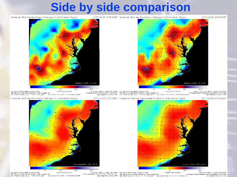
Side by side comparison

Sample validation plot (preliminary)

NOAA SPACE WEATHER PREDICTION CENTER

Conductivity Upgrade using inversion models

• 3D model(s) constrained by MT survey data (Kelbert et al. – in press - 2018/TBD)

• Enables calculation of transfer functions at 0.1 degree resolution

• We smooth to 0.5 degree grid with 50 km averaging radius as an initial hypothesis on the appropriate regional scaling for GIC applications

• We run E-field calculations using this model for the September 2017 storm

Sample high resolution grid

0.1 degree resolution model from MT inversion (USGS) together with ½ degree grid

½ degree grid with 50 km averaging radius – sample E-field calculation

NOAA SPACE WEATHER PREDICTION CENTER

Challenges • Observatory delays, drop-outs, varying latency

• We could generate maps using a smaller number of observatories, trading accuracy for timeliness

• Should SWPC generate ‘preliminary’ maps with incomplete (but more timely data), which are later updated as slower data arrives?

• Sparseness of the observatory network is a concern

• Very important to add more observatories to the network

• Interpolation model accuracy needs to be determined

• Ongoing work on spatial averaging of the transfer functions

• More end-user participation in validation is needed

NOAA SPACE WEATHER PREDICTION CENTER

Next Steps • Initial upgrade to conductivity using 3D model provided by USGS

• This will include an upgrade from 2 degree to ½ degree spatial resolution

• Ongoing collaboration with industry for validation

• Increase cadence from one minute to one second

• Investigate summary measure or indicator

• Investigate forecast capabilities using Geospace model

NOAA SPACE WEATHER PREDICTION CENTER

Questions?

NOAA SPACE WEATHER PREDICTION CENTER

NOAA SPACE WEATHER PREDICTION CENTER

NOAA SPACE WEATHER PREDICTION CENTER

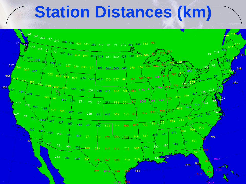
Station Distances (km)

Addressing the Spatial Resolution Question

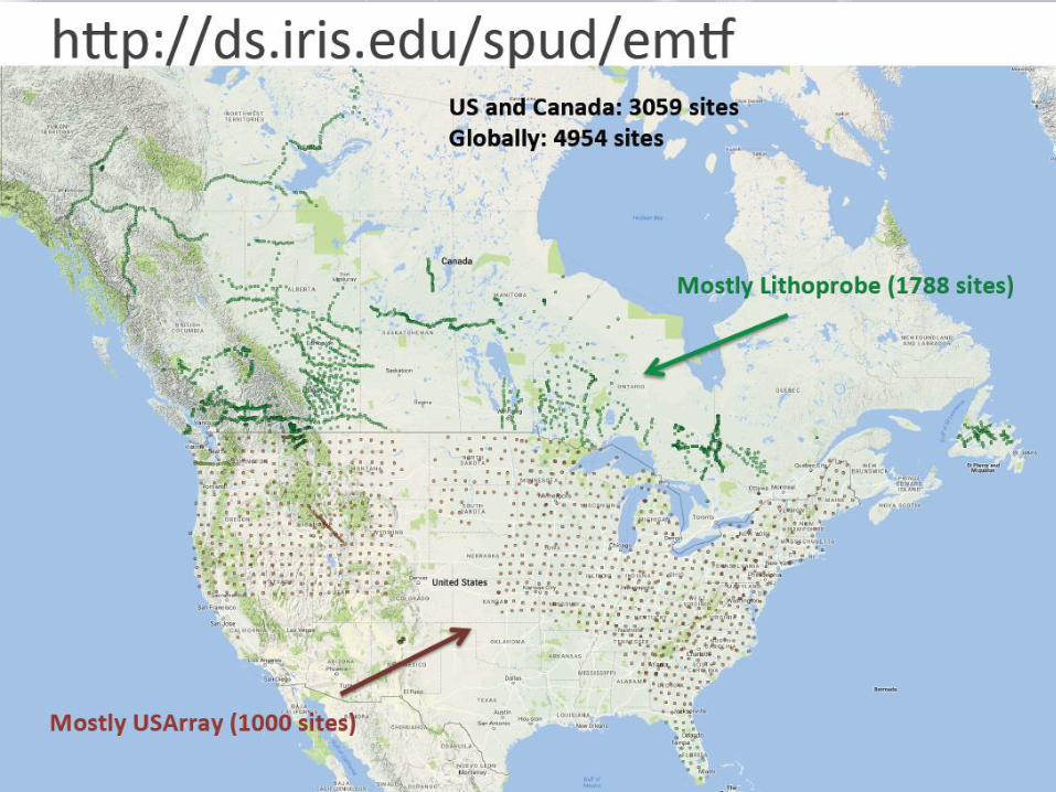
• A high-resolution 3D electrical conductivity model was obtained from a subset of the EarthScope magnetotelluric (MT) data using ModEM MT inversion code (Kelbert et al, 2014)

• Higher resolution may be achieved with a model than could be obtained by using measured impedances alone

• Modeled 3D impedances were generated for each cell of the high resolution conductivity model (20 km). Here, we focus on an area of 500 km radius around Minneapolis. For lower resolution variants, modeled impedances are averaged over a wider area, as shown

Spatial Resolution Tests • We expect some of the 3D variability to be averaged out because the

calculation of GIC integrates over the length of a power line

• We carry out E-field calculations integrated over an actual transmission line for different spatial resolution conductivity models, using the 20 km x 20 km model as the basis

• We derive two spatially averaged conductivity models:

– 1 degree x 1 degree with 100 km averaging

– ½ degree x ½ degree with 50 km averaging

E(t) =E(t )×dlådlå

=Ex(t )dx+E

y(t )dyå

L

Line-averaged E-field calculation:

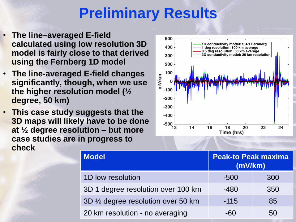
Preliminary Results

• The line–averaged E-field calculated using low resolution 3D model is fairly close to that derived using the Fernberg 1D model

• The line-averaged E-field changes significantly, though, when we use the higher resolution model (½ degree, 50 km)

• This case study suggests that the 3D maps will likely have to be done at ½ degree resolution – but more case studies are in progress to check

Model Peak-to Peak maxima

(mV/km)

1D low resolution -500 300

3D 1 degree resolution over 100 km -480 350

3D ½ degree resolution over 50 km -115 85

20 km resolution - no averaging -60 50

Implications

• The increase of resolution from 2° x 2° to ½° x ½° increases the number of grid points by a factor 16

• Current maps have 283 points so it appears that the 3D maps will have something like 4528 points

• Current cadence is one-minute, but development is far along to use one-second data (one-second data is flowing into SWPC today already) to generate 10 second cadence E-field results

• Model calculations at 10 second cadence implies about 27,168 points per minute

• Important to use a standardized, agreed upon protocol for disseminating the data – are there existing protocols or standards that would be appropriate for us to develop to ?