PRODUCTIVITY IMPROVEMENT AND COST OPTIMIZATION OF …

PRODUCTIVITY IMPROVEMENT AND COST OPTIMIZATION OF SMALL AND

MEDIUM SCALE ENTERPRISES

by

UNMESH VISHWAS TAMHANKAR

Presented to the Faculty of the Graduate School of

The University of Texas at Arlington in Partial Fulfillment

of the Requirements

for the Degree of

MASTER OF SCIENCE IN INDUSTRIAL ENGINEERING

THE UNIVERSITY OF TEXAS AT ARLINGTON

MAY 2017

ii

Copyright © by Unmesh Vishwas Tamhankar 2017

All Rights Reserved

iii

Acknowledgements

I would like to thank Dr. Aera LeBoulluec for her constant support and motivation

during the last 12 months. Originally, I did not plan on pursuing the Thesis option for my

graduate coursework. It was in a meeting with Dr. LeBoulluec in the summer of 2016,

while discussing my doctoral prospective, that she encouraged me to pursue the thesis

option and generously agreed to be my faculty advisor for the thesis. Since then, she has

been instrumental in improving my understanding of the field.

She has always given me the freedom to pursue my ideas and had mentored me

so that I could be able to develop them in a structured manner. She has provided me with

all the necessary resources to facilitate a smooth progress. She has taught me, through

her own actions, professionalism and punctuality, which I will imbibe into my persona.

With her support, guidance and mentorship, I am a better engineer now than I was a year

ago.

Finally, I would like to thank my parents for being with me despite being half the

world away. They have believed in me regardless of the circumstance and they have

given me all the resources at their disposal so that I can have the future they always

wanted for me.

APRIL 19, 2017

iv

ABSTRACT

PRODUCTIVITY IMROVEMENT AND COST OPTIMIZATION OF SMALL AND MEDIUM

SCALE ENTERPRISES

Unmesh Vishwas Tamhankar, MS

The University of Texas at Arlington, 2017

Supervising Professor: Aera LeBoulluec

Productivity improvement and cost optimization have been a topic of discussion

for at least a century. The publication of Fredrick Taylor’s book ‘The Principles of

Scientific Management’ in 1911 can be considered as the beginning of the Efficiency

movement. Surprisingly, the awareness about the principles of Industrial Engineering is

relatively low in many family-owned Small and Medium Scale Enterprises (SMEs).

According to a World Bank report, formal SMEs make up 45% of total employment and

contribute 33% of GDP in emerging markets. In the USA, SMEs make up for more than

95% of all firms and employ 50% of private sector employees. Therefore, it is self-evident

that improvement in the productivity of this sector will have a sizable impact on the

economy.

Productivity increase and cost optimization are critical tasks for SMEs. In a

competitive environment, increasing productivity without installing additional capacity

enables the SMEs to avoid heavy investment and maximize their profitability. In

comparison with large-scale industries, the SMEs have less cash to spend, and skilled

professionals who can implement productivity improvement strategies such as Lean, Six

Sigma, Total Quality Management, etc. are not readily available most of the time. Thus,

productivity improvement can become a costly and difficult exercise. Therefore, there is a

need of a fast and cost effective solution to the problem of productivity improvement.

v

This work offers a time saving productivity improvement and cost optimization

solution for an SME through the implementation of lean methodology and the use of

modern simulation packages (Simio). The implementation of lean methodologies

supports elimination of waste and makes available resources that were incorrectly

allocated, resulting in an increment in productivity. The simulation packages serve as a

visual aid to understand the interrelation between various components of the enterprise.

Additionally, they serve as a tool for the what-if analysis in case of any changes being

made in the existing setup. Most importantly, the use of simulation eliminates the

necessity of multiple trial and error cycles, which in turn saves time and reduces the

overall cost of the improvement effort undertaken by the company. Finally, this research

aims to establish this method of implementation of productivity improvement solution as a

standard for similar SMEs to achieve quick results with minimum cost incurred.

vi

Table of Contents

Acknowledgements .............................................................................................................iii

List of Illustrations .............................................................................................................. ix

List of Tables ....................................................................................................................... x

Chapter 1 Literature review ................................................................................................. 1

Chapter 2 COMPANY AND PRODUCT INFORMATION ................................................... 5

2.1 Company Information ........................................................................................ 5

2.2 Product Information ........................................................................................... 5

Chapter 3 RESEARCH METHODOLOGY .......................................................................... 6

Chapter 4 DIRECT TIME STUDY ....................................................................................... 9

4.1 Data ................................................................................................................... 9

4.2 Analyst’s Notes ................................................................................................ 11

4.3 Calculations ..................................................................................................... 12

4.4 Result ............................................................................................................... 14

Chapter 5 Value Stream Mapping ..................................................................................... 17

5.1 Introduction ...................................................................................................... 17

5.2 Components of VSM ....................................................................................... 18

5.3 Observations .................................................................................................... 21

Chapter 6 Simulation ......................................................................................................... 22

6.1 Problem Definition – ........................................................................................ 22

6.2 Project Planning............................................................................................... 23

6.3 System Definition ............................................................................................. 25

6.4 Conceptual Model ............................................................................................ 28

6.5 Preliminary Design........................................................................................... 32

6.6 Input Data Preparation .................................................................................... 32

6.6.1 Data fitting and test for normality. ............................................................... 33

vii

6.7 Model Translation ............................................................................................ 36

6.8 Verification ....................................................................................................... 37

6.8.1 Machine Utilization ...................................................................................... 38

6.8.2 Operator Utilization ...................................................................................... 39

6.9 Model with Variation ........................................................................................ 40

6.9.1 Machine Utilization ...................................................................................... 41

6.9.2 Operator Utilization ...................................................................................... 42

6.10 Experimentation ............................................................................................... 44

6.10.1 Experiment 1 ........................................................................................... 44

6.10.1.1 Machine Utilization .............................................................................. 45

6.10.1.2 Operator Utilization ............................................................................. 46

6.10.2 Experiment 2 ........................................................................................... 47



6.10.3 Experiment 3 ........................................................................................... 51



6.11 Analysis and Interpretation .............................................................................. 54

Chapter 7 Conclusion ........................................................................................................ 56

Chapter 8 Future Scope .................................................................................................... 58

8.1 Scope for Improvement ................................................................................... 58

8.2 Scope for Implementation ................................................................................ 59

Appendix A Direct Time Study – Pilot Study ..................................................................... 60

Appendix B Direct Time Study - Sample Observations .................................................... 66

Appendix C Data Fitting - Sample Calculation .................................................................. 69

Appendix D Simio Model Layout ....................................................................................... 72

viii

Biographical Information ................................................................................................... 81

ix

List of Illustrations

Figure 4.1 Pilot Time Study ............................................................................................... 13

Figure 4.2 Direct Time Study – Recorded Data ................................................................ 15

Figure 5.1 Present State Value Stream Map .................................................................... 20

Figure 6.1 Gantt Chart (a) ................................................................................................. 24

Figure 6.2 Gantt Chart (b) ................................................................................................. 24

Figure 6.3 Picture of the facility. ........................................................................................ 28

Figure 6.4 Conceptual Model ............................................................................................ 30

Figure 6.5 Geometric Layout (Courtesy – Autoparts, Inc.) ............................................... 31

Figure 6.6 Model layout- Experiment 2 (Part A) ............................................................... 48

Figure 6.7 Model layout – Experiment 2 (Part B) .............................................................. 48

Figure 6.8 Summary of Throughput .................................................................................. 54

x

List of Tables

Table 4.1 Operation Sequence ......................................................................................... 10

Table 4.2 Allowances for Direct Time Study ..................................................................... 13

Table 4.3 Time Check ....................................................................................................... 16

Table 6.1 Worker allocation in the current system ............................................................ 27

Table 6.2 Conceptual Model ............................................................................................. 29

Table 6.3 Machine Utilization-Deterministic Model ........................................................... 38

Table 6.4 Operator Utilization-Deterministic Model .......................................................... 39

Table 6.5 Stochastic Model Throughput Summary ........................................................... 40

Table 6.6 Machine Utilization – Stochastic Model ............................................................ 41

Table 6.7 Operator Utilization – Stochastic Model ............................................................ 42

Table 6.8 Machine Utilization-Experiment 1 ..................................................................... 45

Table 6.9 Operator Utilization-Experiment 1 ..................................................................... 46

Table 6.10 Machine Utilization-Experiment 2 ................................................................... 49

Table 6.11 Operator Utilization-Experiment 2 ................................................................... 50

Table 6.12 Machine Utilization-Experiment 3 ................................................................... 52

Table 6.13 Operator Utilization-Experiment 3 ................................................................... 53

Table 6.14 Expenses Involved .......................................................................................... 55

1

Chapter 1

LITERATURE REVIEW

According to Prime Faraday Technology Watch, in the UK, SMEs in the

manufacturing sector make up 99% of the firms and provide employment for roughly 50%

of the workforce [10]. However, productivity improvement initiatives have not been very

popular with the manufacturing sector of the economy. Although it has been around for

decades, the lean methodology—and the tools and techniques it offers—are not widely

accepted by the SMEs [1]. Pachanga, Shehab, Roy and Nelder (2006) consider this

reluctance to be the result of the uncertainty that surrounds the cost of implementation

and the potential benefits of the same. Since it is not always possible to foresee the

tangible results of lean implementation, it becomes difficult for the leadership to put their

faith in lean methodologies over conventional methods. Conclusively, the authors state

that a committed leadership is essential for a successful implementation [1].

The paper by Hawkins (2001) highlights the most important tools that SMEs of

this day need in order to maintain their competitiveness and in general, their operational

well being. They include lean manufacturing and supply chain responsiveness, among

other things [10]. To incorporate both attributes, it is imperative to improve the existing

processes. There are multiple barriers that can potentially deter SMEs from implementing

improvements. The barriers include employees that are resistant to change, unavailability

of additional manpower for additional tasks, lack of highly trained specialists, and lack of

standardization [10]. To tackle those barriers, the right question to ask is whether the

SMEs can afford not to improve productivity [10]. Additionally, the right outlook about

productivity improvement is to look at short-term cost (of productivity improvement

initiatives) as long-term investments [10].

2

Many ideas now termed as ‘lean’ stem from the Toyota Production System

(TPS). TPS percolated to Toyota’s suppliers and subsequently entered Japanese

mainstream industry [10]. Value stream mapping (VSM), an important technique offered

by lean methodology, is used for classifying the activities, identifying non-value adding

activities, and eliminating the same for a leaner system performance. Heines and Rich

offer seven tools of VSM which include two new tools, Quality Filter Mapping and

Physical Structure Mapping [11]. Heines and Rich offer a six-step method of VSM

deployment which begins with interviewing the internal stakeholders of the organization,

and the final step being the decision, about which of the seven tools described before are

appropriate for use in a given situation [11]. This novel approach offers a unique way of

implementation of VSM that requires participation from all important stakeholders at all

levels, thereby increasing chances of successful implementation of improvement

initiatives. This method can theoretically be implemented in any industry / facility [11].

Many practitioners have successfully implemented productivity improvement and

waste reduction techniques in the similar niche (i.e. small and medium enterprises).

Gupta and Brannan (1995) implemented Just – In – Time (JIT) in a small manufacturing

company where preliminary analysis identified various problems in the existing setup

[16]. They achieved reduced material movement, reduced lead times, reduced inventory

levels, and a smooth flow of materials [16]. Gunasekaran and Lyu implemented JIT in a

small automotive parts manufacturing facility and observed a continuous annual growth

of 5% to 10% for 3 consecutive years [13]. They noted that improvement in productivity

helps bring the quality defects to surface, in both product and production, which were

invisible prior to the implementation of JIT [13]. Karlsson and Ahlstrom theoretically

implemented the lean principles in an SME manufacturing electronic office supplies and

3

found that the successful implementation of lean is contingent upon lean distribution, lean

procurement, and involvement of partners [14].

A committed leadership with a strong belief in methodologies such as lean, still

needs quantifiable evidence or data to believe in the profitability of the whole exercise of

lean implementation [15]. According to Abdulmalek and Rajgopal, providing quantifiable

evidence in advance can be a difficult task because of the sheer complexity of the

systems [15]. It is nearly impossible to predict the behavior of all the elements in a facility

and about all the Key Performance Indicators (KPIs) because of the dynamic nature and

the vast number of variables involved in a facility [2]. In order to generate belief within the

leadership, the obvious tool to be used is simulation. Simulation offers a capability of

predicting system behavior with preset assumptions. As a result, the combination of lean

and simulation provides a tangible and quantifiable effect analysis of the changes and

improvements proposed at the beginning of the process [2].

In the early phases of process improvement, a variety of opportunities can be

recognized. The prioritization of what opportunities to focus on primarily depends on the

policy set forth by the leadership. Based on the amount of resources available, such as

manpower, funds, and time, the management may choose to tackle a small group of

problems first. In such a case, the combination of lean and simulation tools can be

effective for the impact assessment of the prioritized solutions. Basan, Coccola, and

Mendez (2014) employed a similar strategy while tackling design optimization problems

for a beer packaging line. Various avenues of improvement were identified and

subsequently modeled, and it was up to the leadership to choose which improvements

out of the proposed set of improvements were to be implemented [7].

Simulation can be considered as a proven and reliable tool to check the

requirement, or the lack thereof, of a specific part of the facility. Brown and Sturrock

4

(2009), for a major HVAC manufacturer, deployed the simulation tool (SIMIO) to check

the necessity to structure the assembly line as a belt conveyor, which implies that all the

material movement happens at the same time and at the same pace. They found,

through the simulation results, that there is no absolute necessity for the material

movement to occur as if it was occurring on a belt conveyor and as a result the client

facility plans to remove the belt conveyor and install roller conveyors. This result supports

the utility of simulation tools in driving ‘lean thinking’ as it provides a tangible result that is

essentially what the leadership needs to make a decision [8].

Out of the plethora of simulation tools available in the market, it is necessary to

find the one that best suits the requirements. In broad terms, the objective of this project

was to establish the combination of lean, simulation, and process improvement

techniques as a time-saving, cost-saving way to identify and analyze the changes

necessary for productivity improvement. Accordingly, the simulation tool must possess

the qualities like flexibility, ease of use, ability to perform experiments, etc. C.D. Pegden,

outlines the advantages of SIMIO and observes that it is a graphical, object-oriented tool

which requires comparatively less programming [9]. The software is domain neutral, i.e. it

is designed so that the objects can be configured to act as elements in virtually all

facilities. It also allows creation of new objects if the predefined objects are unable to

meet the requirements of simulation [9]. SIMIO can be used in different paradigms and to

support event, object, process and agent view, and the occurrence of probabilistic events

such as breakdowns, failures, variable lead times, etc. [9]. As it requires less

programming and coding, it does not necessarily require a specifically trained

professional [9]. As it is domain neutral, it can be deployed at any SME without one

having to worry about its applicability [9]. These advantages certainly make SIMIO the

tool of interest for this project [9].

5

Chapter 2

COMPANY AND PRODUCT INFORMATION

2.1 Company Information

To protect the anonymity of the company, this facility is called ‘Autoparts Inc.’ for

the purpose of this project. Autoparts Inc. is a leader in manufacturing sheet metal press

components in Maharashtra, India. Established in 1967 with small and limited facilities,

the company now possesses diverse production facilities to meet varying customer

needs and schedules.

Autoparts Inc. has nurtured development, production, and marketing functions to

ensure desired quality, reliability, reasonable price, and timely delivery to create values

for customer businesses. The group supplies sheet metal press components to Indian

and overseas OEMs with consistent growth in intricacy, range, and values. Their

business philosophy is to create customer end values for continuous, sustained, and

mutual growth.

2.2 Product Information

This research focuses on Autoparts Inc., specifically one division of their

manufacturing known as unit 3. The products manufactured by Autoparts Inc. industries

at Unit 3 are the sheet metal discs required to cover the brake shoes of TATA ace and

Piaggio Vehicle Pvt. Ltd. To manufacture the product, multistage forming processes are

carried out. The processes consist of shearing, blanking, forming, vertical drilling, inclined

drilling, deburring and visual inspection. The processes are carried out on various

presses and other machines on the shop floor. The presses are equipped with the

required dies for the forming and drilling operations.

6

Chapter 3

RESEARCH METHODOLOGY

The first step of the project was data collection. For successful implementation of

the methodology, a large amount of data is needed to ensure high accuracy of the

results. This data was acquired from an automobile spare parts manufacturing facility in

India. The data to be collected was primarily the work measurement data, along with

geometric layouts, production statistics, operator details, actual demand, demand

forecast, etc. A sample dataset was collected at first. Based on the sample dataset, the

number of readings required for the required confidence level and accuracy was

calculated.

After data collection was complete and the required number of data points were

obtained, the next step was to perform a time study. A time study is a method of

calculating the standard time of production for an average component, produced in a

predefined environment. Time study considers the worker performance rating and the

PFD (Personal, Fatigue, Delays) allowances. As a result, a standard time for the product

was obtained which is indicative of the ideal time it takes to manufacture one component.

After the time study was complete, we moved forward to the next stage (i.e.

application of lean). In this stage, firstly Value Stream Mapping (VSM) was deployed.

This tool is useful in identifying value adding, non-value adding, and necessary non-value

adding activities. Secondly, the necessity and possibility of application of 5-S was

checked. The inventory levels and transporter routing logic was assessed to identify the

waste of unnecessary inventory and waste of transportation and excess motion.

After the opportunities of waste reduction were identified, the next step was to

understand and learn the simulation package chosen for use during this project. The

package chosen was SIMIO as it offers several considerable advantages. This package

7

requires less coding and programming as compared to other packages available off the

shelf. It is graphical and can process large amounts of data with relative ease. These

characteristics make it lucrative, as the objective of this project is to establish this method

of productivity improvement and cost optimization as a standard for manufacturing

oriented SMEs. The target audience in the industry may not have an adequate amount of

specially trained workforce available thus; the ease of use offered by SIMIO was a key

factor in its selection.

After necessary prowess was achieved in the use of SIMIO, the modeling phase

commenced. In the first phase of modeling, the factory floor was modeled using the

deterministic / average values. This model should ideally produce results closer to the

average performance of the factory. A certain level of error is permitted as a deterministic

model is bound to be subject to some approximation. The acceptable rate of error is set

at 5%. This means that the model with calculated throughput within +/- 5% of the actual

value will be accepted. Successful completion of this phase indicates that the data and

the modeling assumptions are representative of the real-world situation.

In the next stage, the complexity of the model was increased. The model was

now required to possess probability distributions such as those observed in the obtained

dataset in stage 2. This model should ideally give different throughput numbers every

run, since the probabilistic approach is now incorporated in the model. However, the

average throughput over several production runs should be similar to that of the actual

production of the facility. The acceptable rate of error at this phase is set at 3%.

The next step was to brainstorm the opportunities for improvement. Possible

improvements can be the solutions to the individual problems identified in the fourth

stage or some combination of them. These solutions will then be incorporated into the

model and the effect of the changes on KPIs such as throughput levels, inventory levels,

8

worker utilization will be observed. The selection of the best solution depends on the

priorities set forth by the company leadership.

The next and final stage was to document and record the findings and

observations of this project that can serve as a template for future use by manufacturing

oriented SMEs. The advantages of following this method of productivity improvement, as

described in the project, was emphasized upon so that the other SMEs can implement

this method for their benefit.

9

Chapter 4

DIRECT TIME STUDY

4.1 Data

To complete the direct time study, a large amount of data was needed. The data

was collected at the factory.

In this time study analysis, the following method of data collection was followed.

Firstly, measurable work elements were defined. Then, the time taken by the workers to

complete these work elements was observed. Subsequently, worker’s performance rating

was assigned. The measurable work elements found were as follows.

• Shearing Operation – Setup Time

• Shearing Operation – Process Time

• Blanking Operation – Setup Time

• Blanking Operation – Process Time

• First Forming Operation – Setup Time

• First Forming Operation – Process Time

• Second Forming Operation – Setup Time

• Second Forming Operation – Process Time

• Stamping Operation – Setup Time

• Stamping Operation – Process Time

• Cutting and Bending Operation – Setup Time

• Cutting and Bending Operation – Process Time

• Hole Pressing Operation – Setup Time

• Hole Pressing Operation – Process Time

• Tube Hole Operation – Setup Time

10

• Tube Hole Operation – Process Time

• Contouring Operation – Setup Time

• Contouring Operation – Process Time

• Grinding Operation

• Packing Operation

Time taken to accomplish each of these activities was recorded using the

standard time study procedures. The method of recording used was the Snapback

Method. The rating was generally assumed at 90%.

The operation sequence is shown in the table below.

Table 4.1 Operation Sequence

Workstation No Machine Present Process Present Operational

sequence

1 Press Blanking 2

2 Press

3 Press 2nd forming/ drawing 4

4 Press 1st forming/ drawing 3

5 Press Cutting/ Bending 6

6 Drill Drill Vertical 7

7 Drill Drill Inclined 8

8 Deburring Deburring 9

9 Inspection Table Inspection 10

10 Press

11 Press

11

Table 4.1 – Continued

12 Press

13 Press

14 Press Stamping 5

15 Press

16 Shearing M/c Shearing 1

17 Hand Grinders Grinding 11

18 Packing area Packing 12

4.2 Analyst’s Notes

The number of occurrence for every work element was not the same. One cycle

of blanking operation created an equivalent 4 parts for the process. Therefore, the

number of occurrence was set at 0.25. One cycle of shearing operation created

equivalent of 40 parts. Therefore, the number of occurrence was set at 0.025. One cycle

of packing operation processed 25 parts at the same time. Therefore, the number of

occurrence was set at 0.04. Since the observations were recorded over a period of

several days, the TEBS and TEAF don’t have a single value. Alternatively, a cumulative

value is provided. The start time and the end time don’t have a single value but the total

elapsed time was noted carefully. Observations, wherein the time taken was

disproportionately large due to some failure in the machinery, were carefully noted and

discarded. There are some outliers in the time study. These can be attributed mostly to

mishandling of the equipment and the jobs. For example, there were cases when the job

would slide out of the operator’s grasp and the operator would have to pick it up.

12

4.3 Calculations

Number of cycles required –

The formula used to calculate the number of cycles (Nc) required is as follows.

Nc = ((tα/2 * s)/(k*μ))^2

Where,

tα/2 = t value for (α = 0.05) i.e. confidence interval of 95%

s = Standard deviation of the sample observations

K = Accuracy or proportion of interval (accuracy = +/- 5% of the actual)

μ = sample mean

Per this formula, a sample of 15 readings was taken for each process element.

The sample calculations of the number of readings required per the dispersion of values

can be found in the table below. The full spreadsheet of work measurement data

recorded can be found is Appendix A.

13

Figure 4.1 Pilot Time Study

After calculating the number of observations required for required accuracy and

confidence interval, the highest number was found out to be 147 for Contouring – Setup

time. Hence the required number of observations was selected as 150. Standard

procedure for calculations was used with allowance shown in the table below.

Table 4.2 Allowances for Direct Time Study

Category Value

Personal 5%

Basic Fatigue 4%

Variable Allowance – Abnormal Position

Allowance

2%

Variable Allowance – Use of Force 1%

14


Variable Allowance – Noise Level 2%

Variable Allowance - Monotony 1%

Total 15%

According to the International Labor Organization rules, the allowances can be

explained as follows [17]. A personal allowance of 5% is necessary for all operations

along with a basic fatigue allowance of 4%. Additionally, an abnormal position allowance

of 2% is awarded since the working positions are slightly awkward requiring long periods

of bending. A 1% allowance is awarded for use of force since the job involves lifting up to

10 lbs. Noise level allowance of 2% is awarded because of the presence of intermittent

noises and 1% allowance is given for monotony. Cumulatively, a total of 15% allowance

is awarded.

The recorded work measurement data can be found in Figure 4.2, shown below.

4.4 Result

After Using the formula,

Standard Time = Normal Time * (1+ Allowances), the standard time, after all due

consideration, was found out to be 1.15 minutes.

The input required to calculate error is the total recorded time and the

unaccounted time, the values of which were 204.27 and 3.08 minutes respectively. The

error after calculations was found out to be 1.48% that is within the acceptable limit (0%

to 2%).

15

Figure 4.2 Direct Time Study – Recorded Data

16

The time check can be shown as follows.

Table 4.3 Time Check

Time Check

Finishing Time (minutes)

Starting Time (minutes)

Elapsed Time (minutes) 714.5

TEBS (minutes) 0.48

TEAF (minutes) 0.13

Total Check time (minutes) 0.61

Effective Time (minutes) 703.35

Ineffective Time (minutes) 0

Total Recorded Time (minutes) 703.956

Unaccounted Time (minutes) 10.54405

Recording Error 1.48%

17

Chapter 5

Value Stream Mapping

5.1 Introduction

Value Stream Mapping (VSM) is the conventional method of charting the process

under observation into distinguishable parts. These processes can be categorized into

three distinct types: Value - adding processes, Non - value adding processes, Necessary

non - value adding processes. An explanation of what these categories entail, along with

some examples can be found below.

• Value - adding processes – These processes involve operations where work is

being done on the component / product through direct or indirect manual labor,

with or without the use of machines [11]. The typical examples of value – adding

processes include cutting, drilling, assembly, forging, etc.

• Non - value adding processes – These processes involve operations or actions

that are entirely unnecessary and should be eliminated to the highest extent

possible. These processes are the most likely causes of waste in the system

[11]. The typical examples include waiting time, stacking, work in process (WIP)

inventory, etc.

• Necessary non – value adding processes, as the name suggests, these

processes do not typically add value to the product but are necessary under

current manufacturing / operating environment [11]. To eliminate the waste

introduced in the system due to these processes, a redesign of the

manufacturing / operating environment is necessary. The examples include

material movement, packing and unpacking tools, worker movements, etc.

18

5.2 Components of VSM

While preparing the current state value stream map for Autoparts Inc., the

following components of the manufacturing environment were taken into consideration.

• Supplier - This entity supplies the main raw material to the facility. The main raw

material is sheet metal that is supplied on a fixed daily basis. The transport is

facilitated through trucks.

• Customer - Finished parts are shipped to this entity after packaging. The

transport is facilitated through trucks.

• Process control - This entity is the representation of the management of the

facility. This entity provides inputs in form of orders to the supplier and receives

inputs in form of orders from the customers. This entity also provides inputs to

the first station in the process regarding the quantity and the commencement of

processing. It receives input from the final station regarding the completion of

process.

• Workstation - This entity represents any active workstation in the process where

an operation takes place on the component. A workstation may have a specific

number of operators assigned to it.

• Operator – This entity represents the operators working on the shop floor. Some

operators are assigned to specific workstations whereas others are shared

between multiple workstations or processes.

• Inventory – This entity represents the inventory between two workstations. On

the shop floor, material movement is carried out in stacks of 40, thereby

accumulating an inventory of 80 parts in between workstations.

19

• Timeline – Timeline is used to denote the time it takes to complete a specific

activity. The crest part of the timeline denotes a Non-Value adding activity

whereas a trough part denotes a Value- adding activity.

• Activity ratio – The activity ratio is calculated by dividing the value-added time by

the production lead time. The value-added time is the sum of times during which

value is added, whereas the production lead time is the sum of non-value added

time.

• Information flow – Different types of arrows are used to show the direction and

the mode of the flow of information. A straight arrow means manual / handwritten

flow of information whereas the lightening arrow means electronic flow of

information.

The resulting VSM diagram can be found in below.

20

Figure 5.1 Present State Value Stream Map

21

5.3 Observations

Following observations can be made based on the value stream map.

• There is a high inventory level in between workstations.

• The activity ratio is very poor, i.e. 1%.

• The Non-value adding activities can be reduced to a great extent.

22

Chapter 6

Simulation

After completion of value stream mapping, the next step in this project is

simulation. For a structured effort and standardization, simulation projects are conducted

in these sequential steps. They are as follows.

6.1 Problem Definition –

Setting a problem definition involves defining the areas or the aspects of the

plant that the project seeks to improve. It also intends to answer the ‘why’ of the project.

Having a clear problem definition will help to have a clear set of objectives and a minimal

obscurity in the project goals. In this study, we shall try to tackle an industrial situation

where, a managerial team must take decisions about expansion of their sheet metal

pressing plant. We have collected the data for current manufacturing conditions at this

plant. We have studied their charts to know the manufacturing process and its

constraints. Their current production ranges somewhere between 1800 - 1850

components per shift. They have an increase in demand that requires them to increase

their production almost immediately. It is predicted that this increase in demand is not a

momentary flair, but will continue to rise. It will require a significant capacity increase. It is

also mandatory that the suggested changes should not require a substantial capital

investment and that the changes should not increase the rigidity of the process. The

management thinks that the plant needs to have flexibility in the products manufactured.

Currently, the manufacturing line at Autoparts Inc. is an imbalanced system in terms of

operator utilization and machine utilization. Also, the overall output is far below the

system potential according to the management. Therefore, our goal is to balance the

system and to increase the system output at minimum possible expense. We want to

23

provide a turn-key solution for the productivity improvement problem which can be used

and reused by moderately skilled professionals in a similar environment, any time in the

future.

Problems faced by the company –

Currently, the plant is struggling to match the demand. Problems that the company is

facing now are,

• Production output is currently below market demand.

• The machines and operators are underutilized.

• The plant is not efficient in terms of resource utilization.

The constraints under which the analysts are required to operate are as follows.

• Avoid large investments in presses.

• Maximize the utilization of the available resources.

• Avoid layoffs as much as possible.

• Provide a long-term solution for flexibility.

6.2 Project Planning

This step involves planning and managing the resources necessary for the

duration of the project.

• Time – The management of the time required for each step can be found in the

Gantt Chart shown in Figure 6.1 and Figure 6.2. Postscript ‘I’ in the Gantt Chart

refers to the first of a month and postscript ‘II’ refers to the second half.

• Manpower – This task will be performed by the analyst with the help and

guidance of the Supervising Professor.

24

• Equipment – The equipment required for this project is a stopwatch and a

personal computer to operate the DES tool Simio.

• Software – We have chosen Simio as the discrete event simulation tool. The

reasons for choosing simio are as follows.

▪ Less programming required as compared to other simulation tools.

▪ Excellent Graphical User Interface (GUI).

▪ Domain Neutral nature.

Figure 6.1 Gantt Chart (a)

Figure 6.2 Gantt Chart (b)

25

6.3 System Definition

To achieve the objectives of the project, it is highly important to define the system

that we intend to work on. The system definition phase required us to understand the

system that we wish to simulate during the project. The system can be described as

follows.

• The main raw material that is purchased from the vendors is steel sheets, which

arrives in stacks of 80 sheets per day. The sheets are first cut in 10 parts of

rectangular shape using the shearing machine, which needs two operators.

• These rectangular cut parts are stacked in the output buffer of the shearing

machine. A helper transports these parts with the help of a trolley at the rate of

40 cut pieces per trip to the blanking machine, which is the subsequent

operation.

• The parts are stacked up in the input buffer of the blanking machine. The

blanking machine, which needs one operator, cuts these parts into circular discs.

It cuts 4 circular discs from each rectangular cut piece. Thus, each sheet

effectively gives 40 discs.

• The circular discs are stacked up in the output buffer of the blanking machine.

From this buffer, the parts are transported to the input buffer of Press 3 where 1st

forming/drawing is done. This machine requires one operator for processes and

one operator for material movement.

• After press 3 performs its functions, the parts are stacked up in the output buffer

from where they are transported to the input buffer of Press 2. Press 2 performs

2nd drawing and the parts are again stacked up in its output buffer. This machine

requires one operator.

26

• From the output buffer of Press 2, the parts go to the input buffer of Press 7

where stamping is done. This machine requires one operator to process the

components and one operator to simply transport the materials to and from this

machine.

• After Press 7, parts are brought to the input buffer of Press 4, for the cutting and

bending operation. Press 4 also requires one operator.

• After the cutting and bending operation, the parts are stacked up in the output

buffer. From here, they are taken to the input buffer of the Hole Pressing

operation, which requires one operator.

• After Hole Pressing is done, the parts, after being stacked up in the output buffer.

They are then transported to the input buffer of the Tube Hole Operation, which

requires one operator.

• After the Tube Hole operation is carried out, the parts are stored in the output

buffer, ready to be transported to the Deburring machine. Deburring machine

needs one operator.

• After deburring is done, these parts are stacked up in the output buffer. From

here, they will be taken to the grinding section.

• The input buffer of the grinding section serves as a buffer for the grinding

operation part input. There are currently 3 operators who perform this operation

using hand held grinders.

• The subsequent operation is packaging operation which requires 2 operators.

Here, the finished parts are bundled in batches of 25 and packed for shipment.

The worker allocation is shown in table below.

27

Table 6.1 Worker allocation in the current system

Workstation No of Operators

Shearing 2

Blanking 1

First forming 1

Second forming 1

Stamping 1

Cutting & Bending 1

Hole pressing 1

Tube Hole 1

Contouring 1

Grinding (3 Workstations) 3

Packaging 2

Helpers 4

Total 19

Additionally, there is a supervisor and a plant engineer present during the shift.

The actual system is shown in figure below.

28

Figure 6.3 Picture of the facility.

6.4 Conceptual Model

The conceptual model can be termed as a model that reflects all the vital process

parameters as they appear on the actual factory floor. In the case of this project, the

conceptual model should contain the following elements.

• Machines

• Workers

• Material handling

• Source of materials

• Flow of material

29

These elements that are present on the factory floor were suitably termed as per the

convenience of the software. Below is the list of the conventional terms and their

respective software specific translation.

Table 6.2 Conceptual Model

Conventional Terms Software Specific Translations

Presses Workstations

Operator Worker

Material handling Vehicle

Source of materials Source

Stacks Queue

Shearing Machine Separator

Packaging Combiner

The geometric layout of the factory is shown in the figure below. It contains two parallel

rows of machines placed at a distance from each other. In between the two rows is the

storage place where earlier setup items are stored. The middle row also contains the

shearing setup. The material receipt and dispatch is accomplished through the door at

the eastern side of the plant. The entry and exit of the personnel is facilitated through the

door at the southern side of the plant. The actual layout was provided by the company,

but the remaining details, however trivial, were measured later to achieve maximum

accuracy of the geometric layout.

30

Figure 6.4 Conceptual Model

31

Figure 6.5 Geometric Layout (Courtesy – Autoparts, Inc.)

32

6.5 Preliminary Design

After the conceptual model is ready, the system performance measures should

be selected. The performance measures indicate the factors that are important or

decisive in the net performance of the company. Having the detailed plan at this early

stage facilitates better understanding of the system and the system variables.

The process variables that we have chosen to vary are as follows.

• System throughput – System throughput is of the prime concern and the project

will focus on maximizing the system output.

• Machine utilization – It is imperative that the machines stay in the processing

mode for an optimum amount of time. The ideal machine utilization should be

between 60% to 80%.

• Operator utilization – The operators should be busy for an optimum amount of

time.

• Material movement – Material movement should not be a reason for the

sluggishness in the production. We will focus on improvising the existing modes

of material movement. We will try to decrease the amount of material movement

by adding some new equipment, if necessary.

6.6 Input Data Preparation

For this project, the data recorded during the direct time study was used.

Additional data analysis was performed to identify the probability distributions in the data.

The work measurement observations can be found in Appendix A and Appendix B.

33

6.6.1 Data fitting and test for normality.

After recording the work measurement data, it is necessary to identify the

probability distributions of the recorded data to understand the patterns. Usually, the most

common distribution observed in natural events is the normal distribution, and hence it

will be a priority to check for normality in the datasets. If normality can’t be confirmed

using the statistical analysis tools, we move on to the next possible common data

distributions e.g. exponential, lognormal, gamma, beta, etc. If the data does not

accurately conform to the requirements of the probability distributions listed, we can

assume a triangular distribution, which can be arbitrarily observed in the data. The DES

tool chosen for this project (Simio) supports most probability distributions. By

incorporating the behaviors of these probability distributions, the simulation model can

mimic the real-world situation more accurately.

The stepwise method employed for data fitting of a particular dataset is as

follows. This process is performed on each dataset recorded during the direct time study.

• For a dataset, generate a QQ plot using R and a Histogram using MS-Excel. QQ

plots and histograms are fairly accurate tools to check for normality in the

dataset.

• Conduct the Shapiro -Wilk test using R. Comparing the p-value obtained from the

results of the Shapiro-Wilk test with the predetermined level (0.05) we can judge

whether there is a confirmed normality in a given dataset.

• If both these steps lead us to a result of normality not being observed in the

dataset, we move on to the next step i.e. Chi Square test for goodness of fit. This

test is explained below.

• The Chi-Square test is used to test if a sample of data belongs to a population

that has a behavior resembling that of a specific probability distribution. This test

34

can be used for discrete data that is divided in classes. It also requires a

significant number of samples for it to be effective and valid. Since, both these

conditions are satisfied by the data that we have, the Chi-Square test can be

used here. The hypothesis for this test is as follows

H0: The data follows a specific distribution.

H1: The data does not follow a specific distribution.

Test condition: Reject H0 if χ 2 > χ 2 (1-α, k-c)

Where,

α = Significance level (0.05)

k = Number of classes/bins (15)

c = Number of estimated parameters for a specific distribution +1

Examples,

▪ Normal distribution –

For the normal distribution, two parameters (mean and standard deviation)

are required. Hence, c=2+1=3

Therefore,

The hypotheses are

H0: The data follows a Normal distribution.

H1: The data does not follow Normal distribution.

Test condition: Reject H0 if χ 2 > χ 2 (1-0.05, 15-3)

Similarly,

▪ Exponential distribution –

H0: The data follows Exponential distribution.

35

H1: The data does not follow Exponential distribution.


▪ Poisson distribution

H0: The data follows a Poisson distribution.

H1: The data does not follow Poisson distribution.


▪ Gamma distribution

H0: The data follows a Gamma distribution.

H1: The data does not follow Gamma distribution.


▪ Lognormal

H0: The data follows a Lognormal distribution.

H1: The data does not follow Lognormal distribution.


According to the Chi-Square distribution table, for the same level of

significance, a smaller Chi-Square value is associated with lesser degrees of

freedom. Hence, in order to avoid unnecessary calculation, we will test the

hypothesis at c=4. If in any case, we fail to reject the hypothesis, we can go

into the additional analysis necessary to identify which distribution the data

conforms with.

The sample results of data analysis can be found in Appendix C.

36

6.7 Model Translation

The actual operations being carried out on the floor need to be converted into

equivalent and suitable objects so that they can be used in the software i.e. Simio. Thus,

we need to translate the model into a suitable format.

The translation of the model can be explained as below.

▪ Shearing machine - Shearing machine, as the name suggests, cuts a sheet into

10 equal rectangular pieces of the designed dimensions. As the machine

separates one part into several parts, it is equivalent to a separator according to

the Simio logic.

▪ Blanking machine - The blanking machine chiefly serves the purpose of punching

the cut sheets, to produce 4 circular discs from each of the pieces. As it

separates one component into several components, it can be termed as a

separator.

▪ Presses – The presses used in the plant are required to carry out the various

functions. They can be termed as workstations. The workstations under this

category are

▪ First Forming

▪ Second Forming

▪ Stamping

▪ Cutting and bending

▪ Hole Pressing

▪ Tube Hole

▪ Contouring

37

▪ Grinding Machines – The grinding machines in this facility are simple hand held

grinders. There is no setup time associated with this operation and hence for the

ease of programming, we use server objects to imitate the 3 grinding machines.

▪ Packaging – At the Packaging station, finished parts are packed in stacks of 25.

To resemble this operation, combiners are used.

▪ Queues – Queues primarily achieve the objective of storing the materials. A

queue is required to imitate input buffers, output buffers, and processing buffers.

▪ Operators – Operators employed at their respective stations perform their

respective tasks. Additionally, there are helpers which help in various tasks and

assist in material movement. The worker is a versatile resource. It can be used

as a secondary resource or a vehicle class object in Simio.

6.8 Verification

To Verify the validity of the translated model, we build a deterministic model

which considers only the average/ standard time of every process. Here, no variation is

considered whatsoever.

After running the model, we find that the throughput of the simulated process for

one shift of 8 hours is 1750 finished components ready for dispatch. This is very close to

the real-world system. The error in this model is 3%. Therefore, it can be said that the

model generated so far is representative of the actual system and ready for further

modifications. The layout of the model is shown in Appendix D.

The assumptions are as follows,

• The skill expertise of the operators is same for all operations.

• Machine failures are not considered.

• Buffer capacity is infinite.

38

• Movement speed of the vehicle and operator is same for all tasks

• The sheets arrive at once, every day.

The KPIs observed in this model are as follows.

6.8.1 Machine Utilization

Table 6.3 Machine Utilization-Deterministic Model

Machine Utilization (%)

Shearing 8.32

Blanking 25.39

First Forming 62.82

Second Forming 87.85

Stamping 39.40

Cutting and bending 71.73

Hole Pressing 73.06

Tube Hole 58.15

Contouring 47.14

Grinder 1 9.78

Grinder 2 10.88

39


Grinder 3 13.81

Packaging 22.63

6.8.2 Operator Utilization

Table 6.4 Operator Utilization-Deterministic Model

Operator Utilization (%)

OP_SH_1 22

OP_SH_2 22

OP_BL_1 25.39

OP_FF_1 62.82

OP_FF_2 14.31

OP_SF_1 87.85

OP_ST_1 39.4

OP_ST_TRANSPORT 18.52

OP_CB_1 71.73

OP_HP_1 73.06

OP_TH_1 58.15

OP_CT_1 47.14

40


OP_GR_1 9.78

OP_GR_2 10.88

OP_GR_3 13.81

OP_PK_1 22.6

OP_PK_2 22.6

VEHICLE1 90

VEHICLE2 2

6.9 Model with Variation

To impart variability into the model, which is always present in the real-world

system, we use the probability distributions that we identified in the input data preparation

step. The addition of probability distribution means that the time required for each

operation will now be randomly selected from the assigned probability distribution tables.

Resulting system output will vary each time, like that of the real-world production system.

After 20 simulated runs of the model, the throughput was as follows

Table 6.5 Stochastic Model Throughput Summary

Run Throughput Run Throughput Run Throughput Run Throughput

1 1850 6 1857 11 1800 16 1846

41


2 1828 7 1820 12 1840 17 1848

3 1825 8 1827 13 1844 18 1835

4 1833 9 1852 14 1831 19 1846

5 1830 10 1838 15 1835 20 1839

The average throughput of the 20 runs was found out to be 1840

This throughput is close to the actual throughput with an error of less than 1%. Some of

the key observations are listed here.

1. The flow of material is very complex

2. The amount of time for which the machines and operators are utilized is shown in

the tables below.

6.9.1 Machine Utilization

Table 6.6 Machine Utilization – Stochastic Model


Shearing 8.79

Blanking 27.5

First Forming 65

Second Forming 75

Stamping 45

42


Cutting and bending 80

Hole Pressing 70

Tube Hole 55

Contouring 55.21

Grinder 1 10.5

Grinder 2 10.5

Grinder 3 8.75

Packaging 27.5

6.9.2 Operator Utilization

Table 6.7 Operator Utilization – Stochastic Model


OP_SH_1 23

OP_SH_2 23

OP_BL_1 27.5

OP_FF_1 65

OP_FF_2 14.31

OP_SF_1 75

43


OP_ST_1 45

OP_ST_TRANSPORT 18

OP_CB_1 80

OP_HP_1 70

OP_TH_1 55

OP_CT_1 55.21

OP_GR_1 10.5

OP_GR_2 10.5

OP_GR_3 8.75

OP_PK_1 27.5

OP_PK_2 27.5

VEHICLE1 90.42

VEHICLE2 2

It can be seen that the packaging machine’s operators are idle for most of the

time. They could be used further down the line. Shearing and blanking machines are also

starved for parts.

44

6.10 Experimentation

Now that we have accurately modeled the existing setup of Autoparts Inc., we

can try to implement various changes to the simulated model to understand their impact

on the system behavior. We use the waste identification and reduction techniques

outlined in the lean methodology. According to the lean methodology, there are seven

types of waste that can exist in a system. They are:

• Transport – Waste of transport

• Inventory – Waste of components in the inventory that are not being processed

• Motion – Waste of unnecessary motion that the objects or the operators make

• Waiting – Waste of objects waiting for the subsequent operation

• Overproduction – Waste of excess production

• Overprocessing – Waste of excess processing resulting from poor setup

• Defects – waste of identifying or reworking on defects.

We shall try to find the presence of these defects and try to minimize them as

much as possible.

6.10.1 Experiment 1

In this experiment, we shall strive to minimize and simplify the material

movement on the shop floor. The material from blanking goes to press 3, then comes

back to Press 2, then across the shop floor to Press 7 and then back to Press 4. This is

adding a massive bottleneck due to the material movement necessary. We propose that,

the dies and punches should be rearranged to regulate the material flow in a straight line.

This way, the operators will spend more time in processing and less time in travelling to

and from a workstation. The modified layout can be shown as below. Additionally, the

45

quantity of the batch of materials, which is currently set at 40, should be reduced to 30.

This way there will be less WIP inventory in the system.

After making the necessary changes and running the model for 20 simulated

runs, the average throughput is 2000 components in one shift. The improvement in

throughput is 9%.

The KPIs are found to be as follows

6.10.1.1 Machine Utilization

Table 6.8 Machine Utilization-Experiment 1


Shearing 8.35

Blanking 25.44

First Forming 54.56


Stamping 34.56


Hole Pressing 64.15

Tube Hole 55.32

Contouring 47.96

Grinder 1 16.95

46


Grinder 2 12

Grinder 3 9

Packaging 28

6.10.1.2 Operator Utilization

Table 6.9 Operator Utilization-Experiment 1


OP_SH_1 24

OP_SH_2 24

OP_BL_1 25.44

OP_FF_1 54.56

OP_FF_2 15.58

OP_SF_1 77.3

OP_ST_1 34.56


OP_CB_1 62.55

OP_HP_1 64.15

OP_TH_1 55.32

47


OP_CT_1 47.96

OP_GR_1 17

OP_GR_2 13

OP_GR_3 9

OP_PK_1 28

OP_PK_2 28

VEHICLE1 93

VEHICLE2 3

The Key Observations here is that the transporter object is busy for 93% of the time.

6.10.2 Experiment 2

The transporter being busy for 93% of the time is a serious cause of concern. To

alleviate this bottleneck, we introduce a conveyor system for the material movement

between the two sets of workstations that have the highest distances between them.

They are:

• From Shearing Machine to Blanking Machine – 6m.

• From Contouring Machine to the Grinders – 7m.

After making the necessary change, the layout is as follows.

48

Figure 6.6 Model layout- Experiment 2 (Part A)

Figure 6.7 Model layout – Experiment 2 (Part B)

49

After making the changes and running the model, we find that the average

throughput of the model is 2250. This goes to prove that the material movement was a

bottleneck in the system. The KPIs are as follows.




Shearing 8.65

Blanking 26.35

First Forming 62.43


Stamping 39.67


Hole Pressing 73.03

Tube Hole 63.32

Contouring 53.48

Grinder 1 13.43

Grinder 2 15.36

Grinder 3 13.65

Packaging 29.21

50




OP_SH_1 25

OP_SH_2 25

OP_BL_1 26.35

OP_FF_1 62.43

OP_FF_2 17.92

OP_SF_1 86.91

OP_ST_1 39.67


OP_CB_1 71.38

OP_HP_1 73.03

OP_TH_1 63.32

OP_CT_1 53.48

OP_GR_1 13.43

OP_GR_2 15.36

OP_GR_3 13.65

51


OP_PK_1 29.21

OP_PK_2 29.21

VEHICLE1 85

VEHICLE2 3

6.10.3 Experiment 3

We can observe from the results of experiment 2 that the grinding machines are

busy only for 12% to 13% of the times. Additionally, due to the simplified material

movement, the stamping machine transport operator is busy only for 22% of the time.

Also, the number of entities exiting the grinding stations was 2353 but only 2250 of them

were packaged subsequently. Based on these observations, we propose the following

changes.

1. Remove Grinder 3 – The operator will be available for other assignments.

2. Allocate the stamping machine transportation to another shared transporter –

The stamping machine transport operator will be available for other assignments.

We allocate these operators to an additional packaging station. In this facility, the

task of packaging is done simply by making stacks of 25 finished components and

securing them together. Making these changes to the model and running it, we get an

average throughput of 2375 finished components per shift. The increment in productivity

is 5.5%. The KPIs are as follows.

52




Shearing 8.47

Blanking 26.44

First Forming 62.66


Stamping 39.46


Hole Pressing 72.82

Tube Hole 63.70

Contouring 54.85

Grinder 1 21.56

Grinder 2 21.86

Packaging 1 15.25

Packaging 2 15.65

53




OP_SH_1 25

OP_SH_2 25

OP_BL_1 26.44

OP_FF_1 62.66

OP_FF_2 17.82

OP_SF_1 88.56

OP_ST_1 39.46


OP_CB_1 71.35

OP_HP_1 72.87

OP_TH_1 63.7

OP_CT_1 54.85

OP_GR_1 21.56

OP_GR_2 21.86

OP_GR_3 (at packaging 2) 15.65

54


OP_PK_1 15.25

OP_PK_2 29.21

VEHICLE1 91

VEHICLE2 3

6.11 Analysis and Interpretation

The simulation initiative has been successful in identifying the opportunities of

improvement and studying the impact various changes on the overall system behavior.

The summary of results of the various stages of simulation can be shown in a bar chart

as follows.

Figure 6.8 Summary of Throughput

55

As per the goals set at the initial stage, we have taken the system through the

entire simulation process to increase the productivity of the system at minimum

expenditure. The total improvement in productivity earned over these experimentations

can be given by,

Total Increase in Productivity = 𝐹𝑖𝑛𝑎𝑙 𝑇ℎ𝑟𝑜𝑢𝑔ℎ𝑝𝑢𝑡−𝑂𝑟𝑖𝑔𝑖𝑛𝑎𝑙 𝑇ℎ𝑟𝑜𝑔ℎ𝑔𝑝𝑢𝑡

𝑂𝑟𝑖𝑔𝑖𝑛𝑎𝑙 𝑇ℎ𝑟𝑜𝑢𝑔ℎ𝑝𝑢𝑡

= (2375 - 1800) / (1800)

= 31%

The expenses that will be incurred are shown below. This report will be submitted

to the industry for perusal. It will be their decision whether to opt for these modifications.

Table 6.14 Expenses Involved

Experiment Additional Investment Required

Experiment 1 No investment required

Experiment 2 Conveyor

36’ @ INR10000/running foot

= INR360000 ($5200)

Experiment 3 No investment required

As we can see, the proposed changes require minimal capital investments. The

expenses involved in rearranging the dies and installation of conveyors will be assessed

and taken care of by the management, if they choose to implement the changes.

56

Chapter 7

Conclusion

It is motivating to understand that this method has positive results. We set out

with some constraints that we were supposed to operate under. These constraints were

set forth by the management of the facility. Comparison of the final result with the original

constraints and problem statement will help us assess the effectiveness of the proposed

changes.

The first constraint dictated that investments in presses were to be avoided. This

was partly because of the fact that there were additional presses present with the facility

and they can be repurposed to carry out any pressing operation with changes in dies and

fixtures. This constraint is strictly followed throughout the course of the project. None of

the experiments require the purchase of a press. Experiment 1 however requires the

press 2 to be returned to working conditions from its current nonfunctioning state. This

will require minimal investment and no purchases whatsoever.

The second constraint required us to maximize the utilization of the resources

already present. The resources such as the machines and the operators have had an

increase in average utilization. If the results of the deterministic model and the results of

experiment 3 are compared, it can be observed that the machines and the operator

utilization numbers have increased by 10% on average. This is indicative of an optimized

cost structure. The ideal utilization levels for machines and operators may be considered

as 60% - 80%. Excessive utilization of the machine resources may cause excessive wear

and tear and thus higher rate of rejection. Similarly, excessive utilization of the operator

resource may cause fatigue and may introduce defects.

The third constraint was avoiding layoff as much as possible. This constraint can

be attributed to the management’s reluctance to lay off the operators as most of the

57

operators have been working there for a number of years. This constraint was strictly

adhered to. This can be witnessed in the third experiment. In this experiment, the

operators that were busy for a small amount of time were allocated to other tasks. Care

was taken that the workstations where the underutilized operators were originally

allocated do not suffer losses in productivity. Additionally, the new assignments were

designed as to increase the overall productivity of the operation.

This method of productivity improvement is a viable solution for flexibility.

Hypothetically, if the facility needs to make any changes to the facility, either because of

increased demand or because of changes in the product, the facility can implement this

same approach to find the optimized system performance.

Conclusively, we can say that we have fared well with the problem statement that

we were presented with and with the constraints we were supposed to follow. The results

produced through this project, if implemented, can increase the productivity of the facility

by more than 30%. The increase in productivity has little cost associated to it. The cost

burden shared per component is negligible considering the lifespan of the purchased

items, such as conveyors, and the volume of production during that span.

58

Chapter 8

Future Scope

8.1 Scope for Improvement

In this project, the inventory between two stations was reduced from 80 parts to

60 parts. This reduction in inventory levels boosted the production. In future, we will try to

reduce the inventory levels even further. However, there is a possibility that with

increased throughput levels, the material movement system will be overburdened. This

brings us to the second improvement possible. If the material movement system is

overburdened because of the increased throughput, an end-to-end conveyor system

could be installed. This will eliminate the need for manual material movement entirely.

Additionally, we can try to implement a Constant Work In Progress (CONWIP)

system. To successfully implement a CONWIP system, it is necessary that the process is

fairly balanced, with the processing times of each cells being similar. We can observe

from the time study that the process times for the processes vary greatly. Hence, to

successfully facilitate the CONWIP system, we will have to perform extensive line

balancing. One way to achieve this level of line balancing is to introduce automation for

the repetitive processes. Operations from first forming to contouring are repetitive, which

require no special skills from the operator. If these operations are automated, the process

and setup times can be greatly regulated.

The improvements such as end-to-end conveyors and automation require

extensive capital investments. This is not in line with the constraints set forth by the

management for this study. If the constraints were to be relieved, the options such as

conveyors and automation can be explored for an added increase in the productivity.

59

8.2 Scope for Implementation

This project is a turn-key solution for productivity improvement and system

simulation. The resources necessary to commit to and to complete this project are easily

accessible. The data is supposed to be available with the professional working in the

facility. It would require a DES tool that can be purchased online. The technical

knowledge required does not necessarily require years of training. With the

understanding of some of the key concepts of industrial engineering, tasks like the time

study can be successfully performed. The DES tool may need some getting used to but

for an experienced professional, it will not take more than a week. As a result, this project

can be used as a template in any industry similar in size, scope, and operating in similar

market situations.

60

Appendix A

Direct Time Study – Pilot Study

66

Appendix B

Direct Time Study - Sample Observations

69

Appendix C

Data Fitting - Sample Calculation

70

Data fitting and test for normality 1) Shearing setup time

Shapiro-Wilk normality test -

data: x1$Shearing_setup W = 0.96219, p-value = 0.0005338 Pearson chi-square normality test - data: x1$Shearing_setup P = 90.792, p-value = 3.469e-14 Critical Chi Sq. Value = 19.67514 Normal Distribution Parameters - Mean = 0.9802 Standard Deviation = 0.0336 Result = Normality not confirmed.

71

R Core Team (2016). R: A language and environment for statistical computing. R Foundation for Statistical Computing, Vienna, Austria. URL https://www.R-project.org/. Shapiro Wilk Test - Reference Slawomir Jarek (2012). mvnormtest: Normality test for multivariate variables. R package version 0.1-9. https://CRAN.R-project.org/package=mvnormtest #Normality testing of shearing(Setup_time) x1 <- read.csv(file.choose(),header=T) qqnorm(x1$Shearing_setup,main = "Normal Q-Q Plot: Shearing_setup") qqline(x1$Shearing_setup) shapiro.test(x1$Shearing_setup) z1=pearson.test(x1$Shearing_setup) z1 qchisq(0.05,z1$n.classes-4,lower.tail=FALSE)

https://www.r-project.org/

https://cran.r-project.org/package=mvnormtest

72

Appendix D

Simio Model Layout

73

1. Shearing Machine

2. Blanking

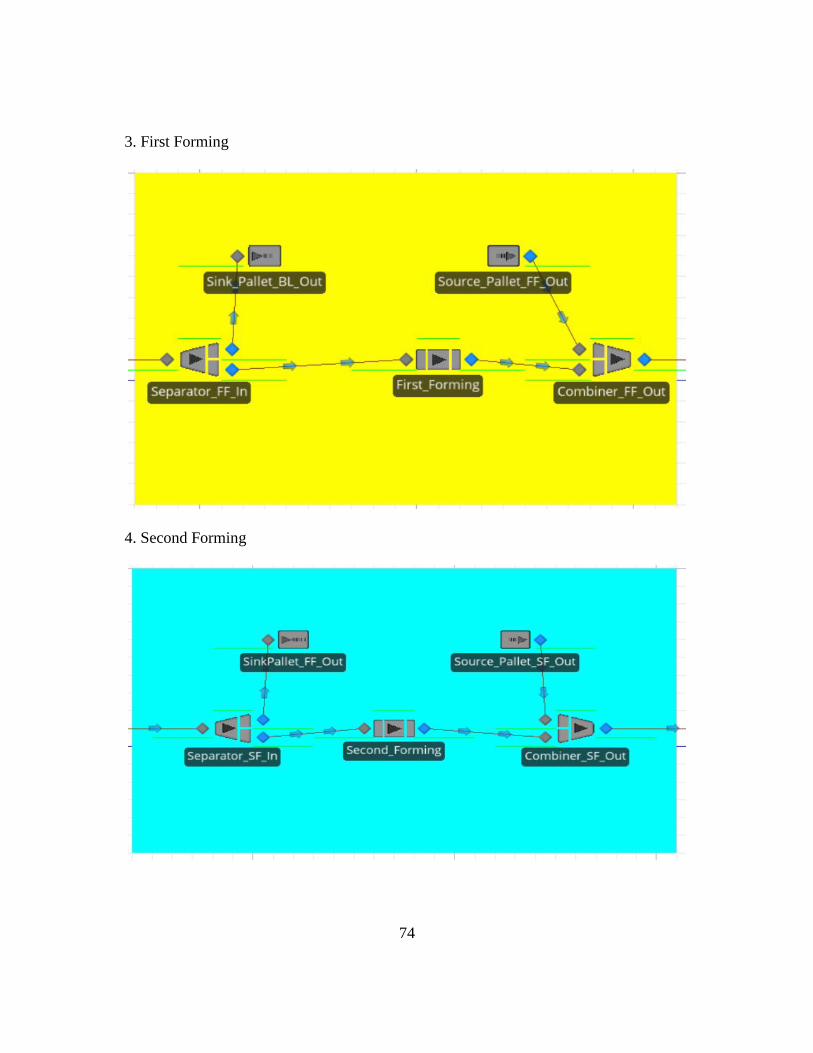
74

3. First Forming

4. Second Forming

75

5. Stamping

6. Cutting and Bending

76

7. Hole Pressing

8. Tube hole

77

9. Contouring

10. Grinding

78

11. Packing

79

Value Stream Map

References

[1] Pius Achanga, Esam Shehab, Rajkumar Roy, Geoff Nelder, (2006),"Critical

success factors for lean implementation within SMEs", Journal of Manufacturing

Technology Management, Vol. 17 Iss 4 pp. 460 – 471

[2] Fawaz A. Abdulmalek, Jayant Rajgopal,” Analyzing the benefits of lean

manufacturing and value stream mapping via simulation: A process sector case

study”, Int. J. Production Economics 107 (2007) 223–236

[3] Taho Yang, Yiyo Kuo, Chao-Ton Su, Chia-Lin Hou,” Lean production system

design for fishing net manufacturing using lean principles and simulation

optimization”, Journal of Manufacturing Systems 34 (2015) 66–73

[4] Adam Graunke, Michael Christian, George Thiers, Timothy Sprock, Leon

McGinnis,”AUTOMATED PRODUCTION SYSTEM SIMULATIONS USING

COMMERCIAL OFF-THE-SHELF SIMULATION TOOLS” , Proceedings of the

2016 Winter Simulation Conference.

[5] David J. Meade, Sameer Kumar, Abdolazim Houshyar,” Financial Analysis of a

Theoretical Lean Manufacturing Implementation Using Hybrid Simulation

Modeling”, Journal of Manufacturing Systems Vol 25/No. 2

[6] Pavel Vik, Luis Dias, Ricardo Abreu,” USING SIMIO FOR THE

SPECIFICATION OF AN INTEGRATED AUTOMATED WEIGHING SOLUTION

IN A CEMENT PLANT” Proceedings of the 2010 Winter Simulation Conference

[7] Natalia P. Basán Mariana E. Cóccola Carlos A. Méndez,” OPTIMIZING THE

DESIGN AND OPERATION OF A BEER PACKAGING LINE THROUGH AN

80

ADVANCED SIMIO-BASED DES TOOL” Proceedings of the 2014 Winter

Simulation Conference

[8] J. Ethan Brown, David Sturrock,” Identifying cost reduction and performance

improvement opportunities through simulation”, Proceedings of 2009 winter

simulation conference

[9] C. Dennis Pegden,” Simio: A new simulation system based on intelligent

objects”, Proceedings of 2007 winter simulation conference

[10] Lisa Hawkins,(2001)”Fundamental Productivity Improvement Tools and

Techniques for SME” ISBN 1-84402-001-0

[11] Peter Hines Nick Rich, (1997),"The seven value stream mapping tools",

International Journal of Operations & Production Management, Vol. 17 Iss 1 pp.

46 – 64

[12] Anand Gurumurthy Rambabu Kodali, (2011),"Design of lean manufacturing

systems using value stream mapping with simulation - A case study", Journal of

Manufacturing Technology Management, Vol. 22 Iss 4 pp. 444 – 473

[13] A. Gunasekaran & J. Lyu (1997) Implementation of just-in-time in a small

company: A case study, Production Planning & Control, 8:4, 406-412,

DOI:10.1080/095372897235217

[14] Christer Karlsson Pär Åhlström, (1997),"A lean and global smaller firm?",

International Journal of Operations & Production Management, Vol. 17 Iss 10 pp.

940 – 952

[15] Richard B. Detty & Jon C. Yingling (2000) Quantifying benefits of conversion to

lean manufacturing with discrete event simulation: A case study, International

Journal of Production Research, 38:2, 429-445

81

[16] Surendra M. Gupta & Louis Brennan,” Implementation of just-in-time

methodology in a small company” Production planning and control, Vol.6 1995

[17] http://nptel.ac.in/courses/112107142/part1/table9_1.htm

Biographical Information

Unmesh Vishwas Tamhankar currently lives in Arlington, TX. He is originally from

Karad, India. He has earned his B.E. in Mechanical Engineering from Shivaji University,

India before earning his Master’s Degree (M.S.) in Industrial Engineering from The

University of Texas at Arlington in 2017. Unmesh was the president of the APICS Student

chapter at UTA and was associated with APICS, SWE, NSBE, CSCMP during his time at

the University of Texas at Arlington.

http://nptel.ac.in/courses/112107142/part1/table9_1.htm

PRODUCTIVITY IMPROVEMENT AND COST OPTIMIZATION OF …

Documents

Transcript of PRODUCTIVITY IMPROVEMENT AND COST OPTIMIZATION OF …