PRODUCTION SYSTEMS ENGINEERINGwell. 3-9 . 2. Structural ... Calculation of uptime pdf’s: ......
105
PRODUCTION SYSTEMS ENGINEERING Chapter 3: Mathematical Modeling of Production Systems Instructors: J. Li, S.M. Meerkov, and L. Zhang Copyright © 2008-2012 J. Li, S.M. Meerkov, and L Zhang
Transcript of PRODUCTION SYSTEMS ENGINEERINGwell. 3-9 . 2. Structural ... Calculation of uptime pdf’s: ......

PRODUCTION SYSTEMS ENGINEERING
Chapter 3: Mathematical Modeling of Production Systems
Instructors: J. Li, S.M. Meerkov, and L. Zhang
Copyright © 2008-2012 J. Li, S.M. Meerkov, and L Zhang

3-2
Motivation All methods of PSE are model-based. No two production systems are identical. It is possible, however, to reduce “any” production
systems to one of the small set of standard models. These standard models and the process of reduction are
the topics of this chapter.

OUTLINE
1. Types of Production Systems 2. Structural Modeling 3. Parametric Modeling: Mathematical Models of Machines 4. Parametric Modeling: Mathematical Models of Buffers 5. Modeling Interactions between Machines and Buffers 6. Performance Measures 7. Model Validation 8. Steps of Modeling, Analysis, Continuous Improvement, and Design 9. Simplification: Transforming Exponential Models into Bernoulli Ones 10. Case Studies 12. Summary
3-3

1. Types of Production Systems
1.1 Serial Lines 1.1.1 Basic structure Consists of processing units and MHD arranged serially:
Processing unit: machine, manufacturing cell, shop in a plant, or a plant
Material handling device: boxes, kanban cards, conveyors, AGVs, trucks, trains… The main feature: storing capacity.
3-4

1.1.2 Serial lines with FGB and carriers
Serial lines with FGB:
Closed serial lines:
3-5

1.1.3 Serial lines with quality issues
Serial lines with inspection machines:
Serial lines with rework:
3-6

1.1.4 Re-entrant lines (for semiconductor manufacturing)
Serial line is a work horse of manufacturing: every production system contains a serial line.
Large part of PSE is devoted to these systems.
3-7

1.2 Assembly Systems
1.2.1 Basic structure Two or more serial lines (component line) and one or more
merge operations plus additional processing machines.
3-8

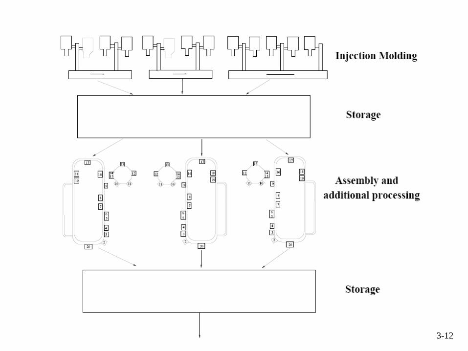
1.2.2 Assembly systems with multiple component lines and merge operations
All variations in structure are possible for assembly systems as well.
3-9

2. Structural Modeling
Structural modeling – the process of reduction of a production system to one of the standard types.
Example: Serial lines with parallel or synchronous dependent machine.
3-10

3-11
3-12

3-13

3-14

3. Parametric Modeling: Mathematical Models of Machines
3.1 Timing Issues 3.1.1 Machine cycle time and capacity
Cycle time (τ) – time necessary to process a part by a machine. τ may be constant, variable or random. In large volume manufacturing it is mostly constant.
Machine capacity (c) – number of parts produced per unit of time.
3-15
3.1.2 Slotted vs. unslotted time
Slotted time: time is slotted with slot duration τ; all transitions occur at the beginning or the end of a slot. Systems satisfying this property are called synchronous.
Unslotted or continuous time: the above mentioned changes may occur at any time moment. If the cycle times of all machines are identical, such a system is
still referred to as synchronous. If the cycle times are not identical, the system is called
asynchronous.
3-16

3.1.3 Discrete event vs. flow systems
Discrete event systems: only a complete job is transferred into or taken from a buffer.
Flow systems: infinitesimal part of a job is transferred to or taken from a buffer.
In the unslotted time case, flow systems are easier for analysis.
3-17

3.2 Machine Reliability Models
Machine reliability model – pmf or pdf of up- and downtime
3.2.1 Reliability models for slotted time case: Bernoulli (B)
(static, no state)
Applicable to operations where downtime is comparable with cycle time.
3-18

Geometric (Geo)
Machine states: Transition probabilities:
3-19
3.2.1 Reliability models for slotted time case (cont.)

Resulting pmf’s of up- and downtime:
Memoryless pmf. Applicable when the downtime is much longer than the cycle time
(e.g., some machining operations) 3-20
3.2.1 Reliability models for slotted time case (cont.)

Moments of slotted time reliability models
3-21
3.2.1 Reliability models for slotted time case (cont.)

3.2.2 Reliability models for continuous time case
Machines with a constant breakdown and repair rates
3-22

Assume . Then, by the total probability formula
3-23
3.2.2 Reliability models for continuous time case (cont.)
Calculation of uptime pdf’s:

For δt → 0,
3-24
3.2.2 Reliability models for continuous time case (cont)
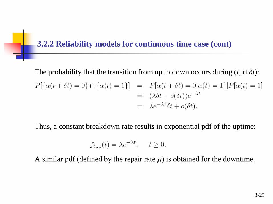
The probability that the transition from up to down occurs during (t, t+δt): Thus, a constant breakdown rate results in exponential pdf of the uptime: A similar pdf (defined by the repair rate µ) is obtained for the downtime.
3-25
3.2.2 Reliability models for continuous time case (cont)

Applicable to machining operations with a very small “most- probable” uptime and downtimes.
3-26
3.2.2 Reliability models for continuous time case (cont)

3.2.2 Reliability models for continuous time case (cont)
Machines with linearly increasing breakdown and repair rates.
Using the same approach, we derive
which is the Rayleigh pdf.
3-27
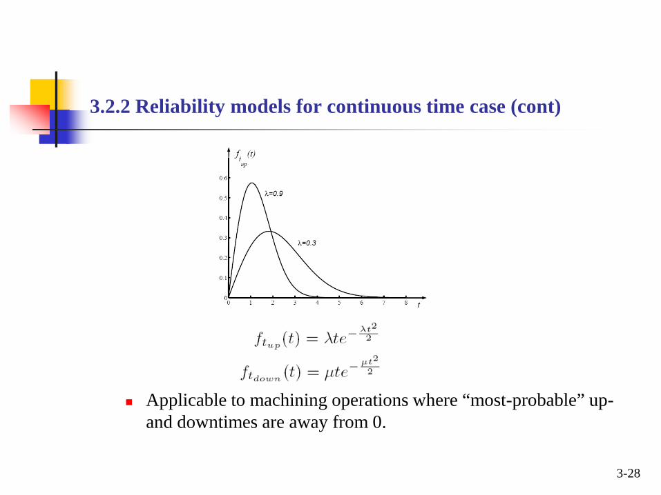
Applicable to machining operations where “most-probable” up- and downtimes are away from 0.
3-28
3.2.2 Reliability models for continuous time case (cont)

Machines with decreasing breakdown and repair rates
3-29
long tail
3.2.2 Reliability models for continuous time case (cont)

Weibull reliability model
3-30
3.2.2 Reliability models for continuous time case (cont)

Gamma reliability model
3-31
3.2.2 Reliability models for continuous time case (cont)

Log-normal reliability model Consider , where X is a Gaussian random variable.
Then, tup has the log-normal pdf:
3-32
3.2.2 Reliability models for continuous time case (cont)

3.2.2 Reliability models for continuous time case (cont)
Mixed reliability model (M): up- and downtime are distributed differently with pdf’s from the set {exp, Ra, W, ga, LN}.
General reliability model (G): up- and downtime have arbitrary distribution.
3-33

Moments of continuous time reliability models
3-34
3.2.2 Reliability models for continuous time case (cont)

For any reliability model, machine efficiency (e) is the probability to produce a part during a cycle time.
Efficiency of machines with various reliability models are
as follows:
Bernoulli: e = p
3-35
3.2.3 Efficiency of the machines

Geometric
3-36
3.2.3 Efficiency of the machines (cont)
Markov balance equations:
Steady state probabilities:
Since

Exponential
3-37
3.2.3 Efficiency of the machines (cont)
Markov balance equations:
Steady state probabilities:
Since

General
3-38
3.2.3 Efficiency of the machines (cont)
Let tup and tdown be random up- and downtime distributed arbitrarily with expected values Tup and Tdown. Assume that tup and tdown are measured in units of cycle time.
Let
Then

3-39
3.2.3 Efficiency of the machines (cont)
According to the strong law of large numbers, the following takes place with probability 1:
Thus,
. .1
.w p
up
up down
Te
T T=
+

3.2.4 Coefficients of variations for up- and downtime of manufacturing equipment
Manufacturing equipment on the factory floor often has coefficients of variation of up- and downtime less than 1.
The explanation of this phenomenon is as follows:
Theorem: If the breakdown (respectively, repair) rate is increasing in time, the resulting uptime (respectively, downtime) distribution has the coefficient of variation less than 1. If the breakdown (respectively, repair) rate is decreasing in time, the coefficient of variation is greater than 1.
3-40

Time-dependent failures – machine breakdown can occur even the machine is blocked or starved.
Operation-dependent failures – machine breakdown occur only when machine is not blocked or starved.
Both are practical. The difference in performance is small.
In this course, we use time-dependent failures (easier to analyze).
3-41
3.2.5 Time dependent vs. operation-dependent failures

3.3 Notations
Machines:
belong to {exp, Ra, W, ga, LN, G}
Synchronous serial line:
Asynchronous serial line:
3-42

3.4 Machine Model Identification
Goal: Determine
τ: use “stop watch” (include loading/unloading time)
and are practically impossible to identify.
3-43

3.4.1 What is possible (and necessary!) to identify
3-44
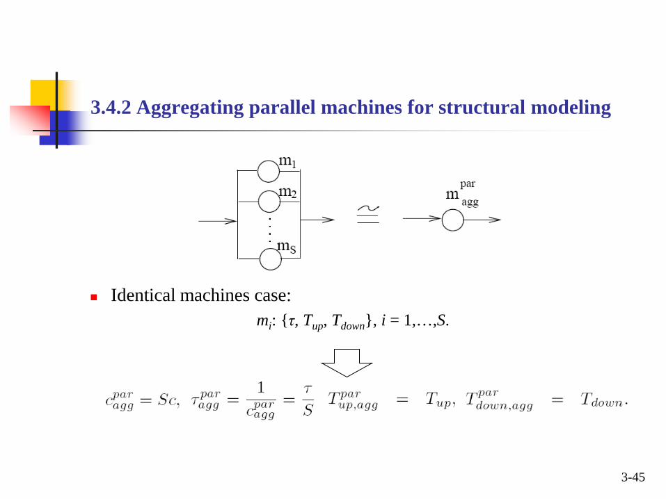
3.4.2 Aggregating parallel machines for structural modeling
Identical machines case: mi: {τ, Tup, Tdown}, i = 1,…,S.
3-45

3.4.2 Aggregating parallel machines for structural modeling (cont)
Non-identical machines case: mi: {τi, Tup,i, Tdown,i}, i = 1,…,S.
3-46

Example
Original system
3-47
3.4.2 Aggregating parallel machines for structural modeling (cont)
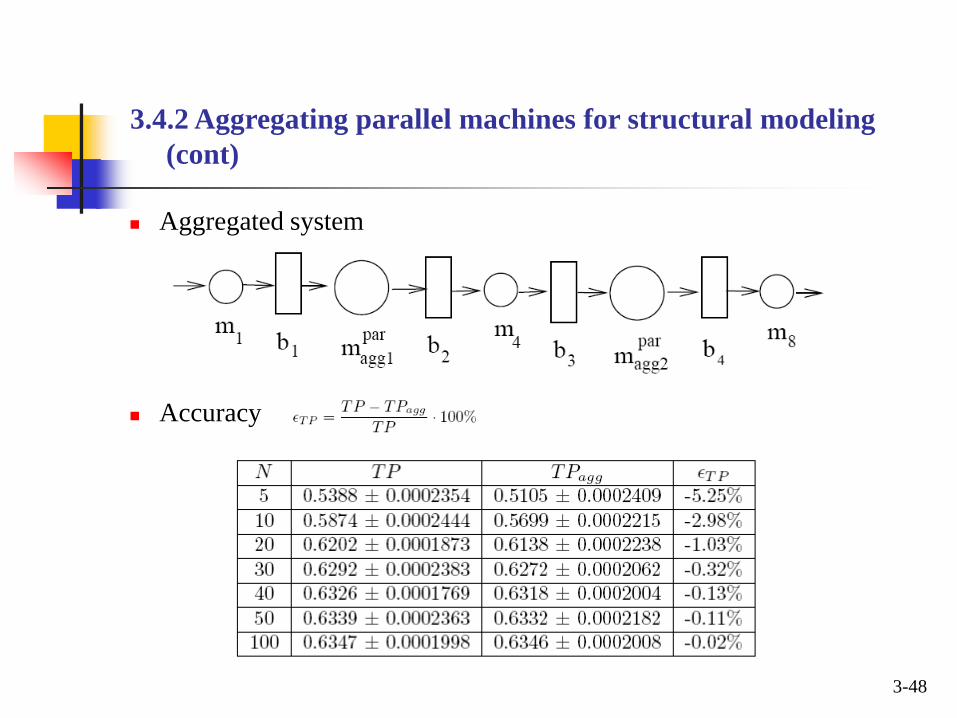
Aggregated system
Accuracy
3-48
3.4.2 Aggregating parallel machines for structural modeling (cont)
3-49
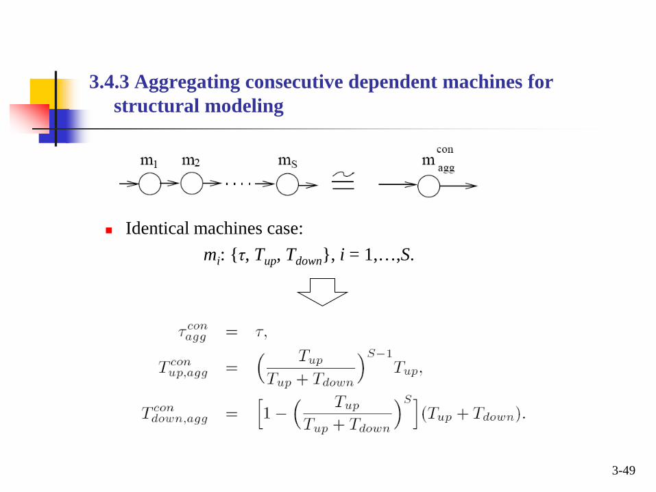
3.4.3 Aggregating consecutive dependent machines for structural modeling
Identical machines case: mi: {τ, Tup, Tdown}, i = 1,…,S.

3-50
3.4.3 Aggregating consecutive dependent machines for structural modeling(cont.)
Non-identical machines case: mi: {τ, Tup, Tdown}, i = 1,…,S.

3-51
3.4.4 PSE Toolbox

3-52
Modeling function and tools
3.4.4 PSE Toolbox (cont.)

3-53
Aggregation of parallel machines
3.4.4 PSE Toolbox (cont.)

3-54
Aggregation of consecutive dependent machines
3.4.4 PSE Toolbox (cont.)

3.5 Machine Quality Models
Machine quality model – pmf or pdf of time intervals when defectives are produced. Bernoulli quality model
Exponential model
General
3-55
g

4. Parametric Modeling: Mathematical Models of Buffers
MHD identification: identification of {τ, Tup, Tdown} of the machines part and identification of N.
Often, mechanical part may be omitted.
3-56
4.1 Structural Model

Number of parts to sustain continuous operation
Buffer capacity
3-57
4.2 Modeling Conveyors
Ki – number of parts that fit into the conveyor

5. Modeling Interaction between Machines and Buffers
5.1 Slotted Time Case
5.1.1 State changing conventions
Machine state is determined at the beginning of each time slot.
Buffer state is determined at the end of each time slot.
3-58

Blocked before service (BBS) – a machine cannot operate if it is up, the downstream buffer is full and the downstream machine does not take a part from this buffer → The part in the machine is viewed as if it is in the buffer.
Blocked after service (BAS) – if up and not starved, the machine operates even if the downstream buffer is full.
This implies that
Starvation – a machine is starved if it is up and the upstream buffer is empty.
3-59
5.1.2 Blocking and starvation conventions

6. Performance Measures
6.1 Production Rate and Throughput Production rate (PR) – average number of parts produced by the
last machine per cycle time in the steady state. Appropriate for synchronous systems.
Throughput (TP) – average number of parts produced by the last machine per unit of time in the steady state.
Appropriate for both synchronous and asynchronous systems.
3-60

Functional dependence of PR:
For a Bernoulli line:
For a synchronous exponential line:
For an asynchronous exponential line:
For a synchronous line with Weibull machines:
For a closed Bernoulli line:
3-61
6.1 Production Rate and Throughput (cont)

For a Bernoulli assembly system:
For a line with Bernoulli quality and reliability model:
None of these function can be evaluated in closed form for M > 2. For Bernoulli and exponential reliability models, these function
can be evaluated analytically using recursive procedures. For other cases, empirical formulas can be derived.
3-62
6.1 Production Rate and Throughput (cont)

6.2 Work-in-process and Finished Goods Inventories
WIPi – average number of parts, i.e., i-th buffer, in the steady state.
Finished goods inventory (FGI) – average number of parts in FGB in steady state.
For Bernoulli lines:
For exponential lines:
3-63

6.3 Probabilities of Blockages and Starvations
Blockage of mi (BLi) – steady state probability that mi is up, bi is full and mi+1 does not take a part from bi.
Starvation of mi (STi)– steady state probability that mi is up and bi-1 is empty.
For slotted time case:
3-64

For continuous time case:
For exponential lines:
Closed form expressions are available only for Markovian systems with M = 2.
For M > 2, recursive procedures are derived
3-65
6.3 Probabilities of Blockages and Starvations (cont)

6.4 Due-time Performance
DTP – the steady state probability to ship to the customer the desired number of parts, D, during a given shipping period, T:
For exponential line
Analytical expression is available only for M = 1.
For M > 1, lower bound is available.
3-66

6.5 Transient Characteristics
Transient characteristics – a group of performance measures that describe how PR and WIP reach their steady states: tsPR – settling time for PR tsWIP – settling time for WIP
All are characterized by the second largest eigenvalues of the transition matrix and pre-exponential coefficients.
Solution are available for Markovian cases.
3-67

6.6 Residence Time
3-68

6.7 Measuring Performance Characteristics of the Factory Floor
PR and TP are typically monitored.
WIPi and RT less often.
BLi and STi very seldom – although, as we will see later, they are most important for system “diagnostics” and continuous improvement.
3-69
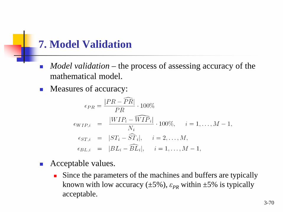
7. Model Validation
Model validation – the process of assessing accuracy of the mathematical model.
Measures of accuracy:
Acceptable values. Since the parameters of the machines and buffers are typically
known with low accuracy (±5%), εPR within ±5% is typically acceptable.
3-70

8. Steps of Modeling, Analysis, Continuous Improvement, and Design
8.1 Modeling Layout investigation
Structural modeling
Parametric modeling Machine parameter identification
Buffer parameter identification
Model validation
3-71

8.2 Analysis, Continuous Improvement, and Design
Using the mathematical model of a production system, the following problem can be solved:
Evaluation of PR, TP, WIP, BL, ST, etc.
Investigation of “what if” scenarios
Direction for improvement and design of continuous improvement projects with predictable results
3-72

9. Simplification: Transforming Exponential Models into Bernoulli Ones
9.1 Scenario Motivation: Bernoulli models are easier to deal with. exp-B transformation
B-exp transformation
3-73

9.2 Exp-B Transformation
Expressions
3-74
where

3-75
Accuracy
M = 3, λ = 0.01, μ = 0.1

9.3 B-exp Transformation
Expressions
Accuracy – the same as exp-B. 3-76

9.3 PSE Toolbox
Exp-B transformation
3-77

3-78
9.3 PSE Toolbox
Exp-B-Exp transformation:
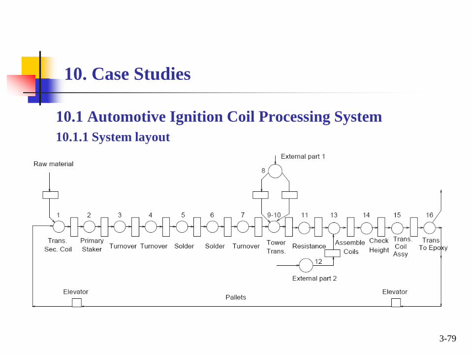
10. Case Studies
10.1 Automotive Ignition Coil Processing System 10.1.1 System layout
3-79

3-80
10.1.2 System performance

3-81
10.1.3 Structural modeling

Exponential assumption 3-82
10.1.4 Modeling and identification of the machines

3-83
10.1.5 Modeling and identification of the buffers

Exponential
3-84
10.1.6 Overall system model

Bernoulli
3-85
10.1.6 Overall system model (cont)

10.2 Automotive Paint Shop Production System
10.2.1 System layout
3-86

3-87
10.2.2 System performance

3-88
10.2.3 Structural modeling

3-89
10.2.4 Modeling and identification of the machines
Average production losses (jobs/hour)

Bernoulli assumption
3-90
10.2.4 Modeling and identification of the machines (cont)

3-91
10.2.5 Modeling and identification of the buffers
3-92
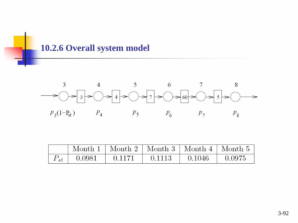
10.2.6 Overall system model

10.3 Automotive Ignition Module Assembly System
10.3.1 System layout
3-93

Numerical throughput 600 part/hour. Losses ≈ 40%.
3-94
10.3.2 System performance

3-95
10.3.3 Structural modeling

Exponential assumption τi ≈ 6 sec/part
3-96
10.3.3 Structural modeling (cont.)

3-97
10.3.4 Modeling and identification of the buffers

3-98
10.3.5 Average frequency of starvations and blockages by carriers

Exponential
3-99
10.3.6 Overall system model

Bernoulli
3-100
10.3.6 Overall system model (cont)

11. Summary
11.1 Steps of Mathematical Modeling Layout Structural modeling Parametric modeling
Machine identification Buffer identification
Model validation
3-101

11.2 Machine Model
Cycle time pmf or pdf of uptime pmf or pdf of downtime pmf or pdf of parts quality
3-102

11.3 Reliability Models
Bernoulli Geometric Exponential Rayleigh Weibull Gamma Log-normal General
3-103
11.4 Modeling Conventions
Slotted or unslotted time Time-dependent or operation-dependent Synchronous or asynchronous Discrete event or flow model Blocked before or blocked after service
3-104

11.5 Performance Measures
Production rate or throughput Work-in-process Finished goods inventory Probability of blockages and starvations Customer demand satisfaction Transient properties
3-105