Processing Acoustic Doppler Current Profiler Data for Score 1

Operational Oceanography and Meteorology

OC 3570 LT Cristal Armijo

Sept 14, 2007

2

I. Introduction and Background The Acoustic Doppler current profiler (ADCP) is an instrument that uses an

acoustic signal and the Doppler shift principle to measure current velocities to produce a

“current profile” of the water column. ADCP’s are employed around the world for a

variety purposes such as measuring coastal to deep water currents, streamline and

sediment flow in rivers and estuaries. Teledyne RD Instruments (RDI) manufactures a

wide range of ADCP’s, there are BroadBand and NarrowBand that are set operate from

38-2400 kHz and measure currents ranging from <1 to approximately 1000 meters.

ADCP’s have many configurations such as: hull-mounted, direct reading, self contained

and remote head. The Naval Postgraduate School (NPS) Oceanography Department

employs a self-contained BroadBand (BB) Workhorse Sentinel 300kHz ADCP from RD

I. The BB Workhorse ADCP is versatile because it can be hull-mounted or moored

(upward or downward- looking), it provides precision data due to the BB signal

processing which generates low-noise, high resolution data with minimal power

consumption.

On January 28, 2006 the Operational Oceanography cruise conducted on board of

the Research Vessel Point Sur assembled and deployed the SCORE 1 (SC1) mooring

(Figure 1) with a BB Workhorse Sentinel self-contained 300kHz ADCP off the west

coast of San Clemente Island located in Southern California Bight region, position:

Latitude 32° 55.726°N and Longitude 118° 36.503°W (Figure 2). The SC1 mooring

was recovered during the summer Operational Oceanography cruise on July 10, 2006.

This project encompasses the steps it took to deploy the ADCP at SC1. The purpose is to

gain a basic understanding of how the ADCP operates, samples and processes data. Next

3

step is look at what post-processing was performed to produce plots that illustrate the

current variation around San Clemente Island (SC1).

II. Acoustic Doppler Current Profiler (ADCP)

The ADCP sends out an acoustic signal “ping” and then uses Doppler shift

principle to measure current velocity to produce a “current profile” of the water column.

The ping is sent out at a fixed frequency of 307.2 kHz, the transducers listen for the

return echo from the backscatters in the water. Backscatters are considered suspended

particles in the water for example, plankton and very small fish. The ADCP uses the

Doppler shift to calculate the current velocities at different depths, equation (1) accounts

for the transmitted and received signals and for radial motion.

(1) Fd = 2 Fs(V/C) cos(A) (Gordon, 1996)

Fd = Doppler shift frequency, Fs = frequency of sound (standing still),

V = relative velocity (between source and receiver), C = sound speed (m/s)

A = angle between acoustic beam and scatter velocity (shown below)

Figure from (Gordon, 1996 p.8)

The Workhorse ADCP uses a four-beam transducer head with a 20 degree beam angle. In

order to calculate the current velocities using a multiple beam solution the ADCP

assumes the currents are homogeneous throughout the water column. It then uses

4

trigonometric relations between the beams to calculate three-dimensional current velocity

vectors that represent the u, v, and w components. The fourth beam is a redundant beam

used to calculate the error velocity and to back up the assumption of horizontal

homogeneity. Error velocity is the difference between a velocity measured by one set of

three beams versus a velocity measure by the other set of three beams during the same

time frame (Simpson, 2001). This difference could be due to a non-homogenous

environment or corrupt data caused by a large fish or obstruction blocking the

transmission of the signal.

III. Deploying the ADCP

Prior to deploying an ADCP it is important to perform a compass calibration to

correct any distortions caused by the batteries magnetic signature. A compass calibration

was conducted on the ADCP used in the SC1 mooring. The calibration was completed at

NPS by the Oceanography Department, in a magnetic free environment prior to taking

the ADCP onboard the RV Pt. Sur. The calibration procedure is performed using

Windows 2000/XP PC in conjunction with RDI ‘s program WinSC. The ADCP has an

automated built- in test that measures how well the compass is calibrated known as the

compass calibration verification. Prior to calibration the total error on the ADCP read

3.0° and after calibration the error read 1.2°. The new calibration matrix was recorded to

nonvolatile memory. Next step used RDI’s program PlanADCP to set up the deployment

file by inputting Control System, Environmental, Water Profiling and Timing commands

specific for this deployment. Appendix A includes all the codes inputted into the

PlanADCP program. An important environmental command to discuss is EB - heading

bias. EB inputs the value of the magnetic declination (variance) for this deployment

5

equals the heading angle 13.33° E. The EB counteracts the effects of magnetic variance

at deployment site (SC1). (All other values and codes are explained in the WorkHorse

Commands and Output Data Format, RD Instruments). Calibration reduces the error on

the direction of the current. Based on the set parameters inputted into the PlanADCP, the

program calculates the standard deviation of current velocity within the ADCP. It

calculates the value by taking square root of the maximum standard deviation of 3 cm/s

for 4m depth cell size (RDI) and divides by the total number of pings per ensemble set at

40 to get the minimum standard deviation which is ~0.43 cm/s. After all inputs are

entered into the PlanADCP, the ADCP was ready to deploy. The mooring was assembled

onboard the RV Pt. Sur and deployed on January 28, 2006 to the depth 124 m. (The

maximum standard deviation for a 300kHz Workhorse Sentinel ADCP can be found RDI

website.)

IV. Data Collection (Sampling)

The ADCP used at the SC1 mooring collected data for 165 days, recording

15,633 ensembles. It was configured to be an upward- looking ADCP, set to burst

sample. The burst sample sends out 40 * 1 sec pings within the first 40 seconds of the

ensemble interval of 15 minutes. The advantage of using a burst sample is to prevent

aliasing surface wave velocities. Sampling within the first 40 seconds enables the ADCP

to capture the entire surface wave/swell cycle, then by taking the average of the cycle

which equals ~zero allows the ADCP to capture the true velocity current without the

surface interference.

Each ensemble includes 26 bins of information and each bin corresponds to a

specific depth cell. The depth of each bin is uniformly spaced at 4 m and the ADCP

6

measures the average velocity over the depth range of each depth cell to produce the

current velocity profile. Averaging over the range of each depth cell reduces the affects

of spatial aliasing (Gordon, 1996). The profiles are generated by range-gating the echo

signal (Gordon, 1996). Because shorter ranges return the echo signal faster than longer

ranges, range gating was developed to break the received signal into successive segments

for independent processing (Gordon, 1996).

The BB ADCP produces four data types: velocity, echo intensity, correlation and

percent good. For the SC1 mooring velocity data was set to record in earth coordinates,

meaning that velocity is converted into north, south and up components. Echo intensity

data is outputted in decibels, it is a measure of signal strength. For an upward- looking

ADCP echo intensity is important. Echo intensity decreases with range, if the there is a

spike in the intensity it is a good assumption that echo signal is seeing the surface. The

side lobes reflect an increased intensity signal back to the ADCP, this used to determine

if the bins near the surface are good or bad data. Correlation is measure of data quality.

Percent good data uses a variety of criteria such as correlation, error velocity, and fish

detection to determine what percent of the data is good.

V. ADCP Data Processing

Ensemble averaging is used reduce the measurement uncertainty. Uncertainty

introduces two errors: random error and bias. Random error is uncorrelated from ping to

ping, averaging reduces the standard deviation of velocity error by the square root of the

number of pings (Gordon, 1996). Bias is the velocity error difference that does not go

away with averaging. Setting the ADCP to average inside, in the data acquisition system

allows the instrument to compute true vector averages, minimizes bias associated with

7

the conversion of beam to earth coordinates, and reduces the time required to for data

transmission (Gordon, 1996). The processing cycle within the ADCP is dependent on

the ping rate, a single ping has five phases: overhead, transmit pulse, blank period,

processing, and sleep. After all the pings complete, the ADCP computes an ensemble

average and then transmits the data to the internal recorder.

The ADCP at SC1 was recovered on July 10, 2006, once brought onboard it

hooked up to a computer to compare the internal clock to actual time (GMT), to check

the clock drift. ADCP clock is listed as (YY/MM/DD HH:MM:SS). The ADCP at SC1:

Actual Time (GMT): 06/07/10 15:05:00 and ADCP Time (GMT): 06/0710 15:05:07

The ADCP internal clock drift was 7 seconds fast. The purpose of this check to ensure

that data recorded was sampled at the correct time. If the clock drift was greater than the

ensemble time interval a time correction would have to be made to the data series. All

the data collected by the ADCP is stored in a binary file and can be retrieved by

removing the flash card and downloaded to a PC.

The binary data file from SCORE 1 (SC1) was uploaded into WinADCP.

WinADCP was used to export a mat file that included all data collected from the ADCP.

VI. Post-Processing using MATLAB

First step in post-processing is to determine the good data from the bad data. A

matlab program, Workhorsepro1 loads the data set. Workhorsepro1 uses the function

uvflags to flag bad data. This function flags bad data based on the correlation magnitude

(cm) and the percent good values at pg3 and pg4. If the cm is less than 64 counts in any

of the 4 beams then data is flagged bad. If the combined percentages for pg3 and pg4 are

less than 25% the data is flagged bad. Workhorsepro1 linear interpolates the bad data,

8

uses a despiker to remove any u and v components with a standard deviation value of 2.5

or greater and then creates a new saved file. Workhorsepro2 loads the new file created in

workhorsepro1, and then uses a matlab program prinax to rotate the principal axis to a

new coordinate system. Rotating the axis allows the maximum (minimum) variance to be

associated with major (minor) axis (figures 3 & 4). Workhorsepro2 uses a ‘lowpass’ 4th

order Butterworth filter to remove the tides with a cutoff frequency set at .01 and then

uses a math2true program to change from math to geographic (true) coordinates.

Workhorsepro2, generates several plots representing the entire smoothed data series.

VII. Data Results

The alongshore (v-flow) is the dominant flow, the current flow is moving faster to

north than the cross-shore flow (u-flow). (Figure 5). There is a significant flow reversal

in the alongshore component, ~ the second week in May 2006 the flow shifts to south.

The contour plot (Figure 6) correlates with this flow reversal, the southward flow

decreases with depth, near surface flow is ~20 cm/s and decreases to ~5 cm/s at 100 ft.

At about the third week in May 2006 the flow is reversed back to the north, there is a

significant spike in the current velocity flow. The Progressive Vector Diagram (PVD)

integrates velocity to produce the trajectory flow for the entire data series. The PVD

(figure 8), shows a consistent northward flow, it also shows the flow reversal followed by

the strong pulse of northward flow.

Empirical Orthogonal Functions (EOFs) analysis provides a compact description

of spatial and temporal variability of data series in terms of statistical modes (Emery and

Thomson, 2001). EOFs is a good method for removing unwanted scales of variability,

and less energetic variance from the data series. An EOF analysis (Figure 8) on the un-

9

filtered v-component shows modes 1-3 account for 80% of the variance in the data series:

mode 1 – 55%, mode 2 – 17%, and mode 3 – 8%. These three modes can be used to

reconstruct a new data field capturing the significant variance, more energetic current

velocities. Figure 8 also shows a very energetic tidal structure.

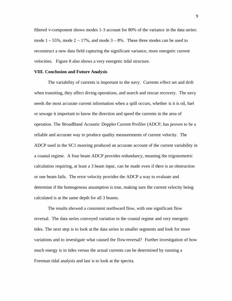
VIII. Conclusion and Future Analysis

The variability of currents is important to the navy. Currents effect set and drift

when transiting, they affect diving operations, and search and rescue recovery. The navy

needs the most accurate current information when a spill occurs, whether is it is oil, fuel

or sewage it important to know the direction and speed the currents in the area of

operation. The BroadBand Acoustic Doppler Current Profiler (ADCP, has proven to be a

reliable and accurate way to produce quality measurements of current velocity. The

ADCP used in the SC1 mooring produced an accurate account of the current variability in

a coastal regime. A four beam ADCP provides redundancy, meaning the trigonometric

calculation requiring, at least a 3 beam input, can be made even if there is an obstruction

or one beam fails. The error velocity provides the ADCP a way to evaluate and

determine if the homogenous assumption is true, making sure the current velocity being

calculated is at the same depth for all 3 beams.

The results showed a consistent northward flow, with one significant flow

reversal. The data series conveyed variation in the coastal regime and very energetic

tides. The next step is to look at the data series in smaller segments and look for more

variations and to investigate what caused the flow reversal? Further investigation of how

much energy is in tides versus the actual currents can be determined by running a

Foreman tidal analysis and last is to look at the spectra.

10

Figure 1 SCORE 1 Mooring

Figure 2 SC1 Mooring Postion

11

Appendix A

;This is the set-up for SCORE 1 Jan 2006 ;To be deployed for six months, WHS S/N: 6742 ; CR1 CF11101 EA0 EB01333 EC1500 ED1200 ES35 EX11111 EZ1111111 WA50 WB0 WD111100000 WF176 WN36 WP40 WS400 WV125 TE00:15:00.00 TP00:01.00 TF06/01/26 00:15:00 CK CS ; ;Instrument = Workhorse Sentinel ;Frequency = 307200 ;Water Profile = YES ;Bottom Track = NO ;High Res. Modes = NO ;High Rate Pinging = NO ;Shallow Bottom Mode= NO ;Wave Gauge = NO ;Lowered ADCP = NO ;Beam angle = 20 ;Temperature = 8.00 ;Deployment hours = 4800.00 ;Battery packs = 1 ;Automatic TP = NO ;Memory size [MB] = 1021 ;Saved Screen = 2 ; ;Consequences generated by PlanADCP version 2.02: ;First cell range = 6.12 m ;Last cell range = 146.12 m ;Max range = 110.80 m ;Standard deviation = 0.43 cm/s ;Ensemble size = 868 bytes ;Storage required = 15.89 MB (16665600 bytes) ;Power usage = 387.35 Wh ;Battery usage = 0.9 ;EB Value is Magnetic Declination= 13.33 deg East for 2006 ;from Chart 18749 Edition #: 38

12

Figure 3 ScatterPlots of the U & V Velocities (unrotated) and (rotated)

Figure 4 Vertically Averaged Flow - Alongshore is the dominant flow. Note the flow reversal in May.

13

Figure 5 Contour Plots, velocity is in cm/s

14

Figure 6 Empirical Orthogonal Functions for the V component (unfiltered and rotated), Top left: Mode 1-3, Top right: Time series including tidal data, Bottom left: Mean flow, Bottom right: Standard Deviation

15

References

Emery, W.J. and Thomson, R.E., 2001, Data Analysis Methods in Physical Oceanography, Elsevier, p. 319-343.

Gordon, Lee, 1996, Acoustic Doppler current profiler – Principles of operation: A practical primer: RD Instruments, San Diego, CA.

Simpson, Michael, R., 2001, Discharge Measurements Using a Broad-Band Acoustic Doppler Current Profiler, United States Geological Survey, Sacramento, CA. WorkHorse-Maintenance Guide, RD Instruments, January 2001. (P/N 957-6153-00)

WorkHorse-Commands and Output Data Format, RD Instruments, August 2001. (P/N 957-6156-00) www.rdinstruments.com (This site was used to look specific information about the Sentinel ADCP and to find maximum standard deviation for speed.)