Process Parameter Optimization with Numerical modelling ...
89
Minnesota State University, Mankato Minnesota State University, Mankato Cornerstone: A Collection of Scholarly Cornerstone: A Collection of Scholarly and Creative Works for Minnesota and Creative Works for Minnesota State University, Mankato State University, Mankato All Graduate Theses, Dissertations, and Other Capstone Projects Graduate Theses, Dissertations, and Other Capstone Projects 2017 Process Parameter Optimization with Numerical modelling and Process Parameter Optimization with Numerical modelling and Experimentation design of Binder Jet Additive Manufacturing Experimentation design of Binder Jet Additive Manufacturing Sairam Vangapally Minnesota State University, Mankato Follow this and additional works at: https://cornerstone.lib.mnsu.edu/etds Part of the Mechanical Engineering Commons Recommended Citation Recommended Citation Vangapally, S. (2017). Process Parameter Optimization with Numerical modelling and Experimentation design of Binder Jet Additive Manufacturing [Master’s thesis, Minnesota State University, Mankato]. Cornerstone: A Collection of Scholarly and Creative Works for Minnesota State University, Mankato. https://cornerstone.lib.mnsu.edu/etds/739/ This Thesis is brought to you for free and open access by the Graduate Theses, Dissertations, and Other Capstone Projects at Cornerstone: A Collection of Scholarly and Creative Works for Minnesota State University, Mankato. It has been accepted for inclusion in All Graduate Theses, Dissertations, and Other Capstone Projects by an authorized administrator of Cornerstone: A Collection of Scholarly and Creative Works for Minnesota State University, Mankato.
Transcript of Process Parameter Optimization with Numerical modelling ...
Minnesota State University, Mankato Minnesota State University, Mankato
Cornerstone: A Collection of Scholarly Cornerstone: A Collection of Scholarly
and Creative Works for Minnesota and Creative Works for Minnesota
State University, Mankato State University, Mankato
All Graduate Theses, Dissertations, and Other Capstone Projects
Graduate Theses, Dissertations, and Other Capstone Projects
2017
Process Parameter Optimization with Numerical modelling and Process Parameter Optimization with Numerical modelling and
Experimentation design of Binder Jet Additive Manufacturing Experimentation design of Binder Jet Additive Manufacturing
Sairam Vangapally Minnesota State University, Mankato
Follow this and additional works at: https://cornerstone.lib.mnsu.edu/etds
Part of the Mechanical Engineering Commons
Recommended Citation Recommended Citation Vangapally, S. (2017). Process Parameter Optimization with Numerical modelling and Experimentation design of Binder Jet Additive Manufacturing [Master’s thesis, Minnesota State University, Mankato]. Cornerstone: A Collection of Scholarly and Creative Works for Minnesota State University, Mankato. https://cornerstone.lib.mnsu.edu/etds/739/
This Thesis is brought to you for free and open access by the Graduate Theses, Dissertations, and Other Capstone Projects at Cornerstone: A Collection of Scholarly and Creative Works for Minnesota State University, Mankato. It has been accepted for inclusion in All Graduate Theses, Dissertations, and Other Capstone Projects by an authorized administrator of Cornerstone: A Collection of Scholarly and Creative Works for Minnesota State University, Mankato.
PROCESS PARAMETER OPTIMIZATION WITH NUMERICAL
MODELLING AND EXPERIMENTATION DESIGN OF BINDER
JET ADDITIVE MANUFACTURING
A Thesis Submitted in Partial Fulfillment of the Requirements
for the Degree of Master of Science in
Mechanical Engineering
By
Sairam Vangapally
MINNESOTA STATE UNIVERSITY, MANKATO
October 2017
i
The thesis of Sairam Vangapally is approved on 10/13/2017:
_________________________________ _______________
Dr. Shaobiao Cai, PE-Assistant Professor Date
__________________________________ ________________
Dr. Jin Y. Park, Professor Date
_________________________________ ________________
Dr. Kuldeep Agarwal, Assistant Professor Date
Minnesota State University, Mankato

ii
© 2017
Sairam Vangapally
ALL RIGHTS RESERVED
iii
ABSTRACT
Binder jetting technology is an additive manufacturing technology in which powder materials are
binded together layer by layer forming the product from input CAD model. The process involves
printing the product layer by layer, curing and sintering. The mechanical properties of 3D printed
samples varies based on process parameters, hence there is a need to tune the process parameters
for optimal characteristics. Three main parameters namely layer thickness, sintering time and
sintering temperature were identified and the study focuses on the effect of parameters on
dimensional accuracy and compressive strength of the samples. Full factorial experimenta l
approach was used to conduct the experiments and analysis of variance was performed to
determine the significance of parameters. Along with parameters optimization, feed forward back
propagation artificial neural network model is developed to quantify the relationship between three
parameters and compressive strength, the model is developed based on experimental data and
validated with known data.
Also, Compressive behavior of four lattice designs considered in the study were simulated by finite
element analysis and numerical results were compared with experimental data in order to validate
the finite element model. FE models of different lattice designs were developed from experimenta l
test data using ANSYS and the simulated compressive behavior is compared to that experimenta l
compression test results.

iv
Dedicated to my parents, advisor and friends, I couldn’t have done this without you. Thank you
for all your support along the way.

v
ACKNOWLEDGMENTS
Firstly, I would like to thank my advisor, Dr. Shaobiao Cai for providing me the opportunity to
work on this project. I am grateful to him for his patience and guidance throughout the thesis work.
I would like to express my sincere gratitude to Dr. Jin Y Park for his suggestions and support
during my graduate study. Special thanks to Dr. Kuldeep Agarwal for his suggestions and guidance
during the experimentation work. I would like to thank all the three committee members for their
continuous support and encouragement throughout my graduate study. I would like to thank Mr.
Kevin Schull for providing a great environment for accompanying research in the laboratory.
Lastly, I would like to thank my parents and friends for their continued support for helping me to
achieve my objectives.
vi
TABLE OF CONTENTS
CHAPTER 1 .................................................................................................................................. 1
1.0 Introduction ........................................................................................................................ 1
1.1 Research Objectives and Scope ...................................................................................... 11
CHAPTER 2 ................................................................................................................................ 13
2.0 Process and Approaches .................................................................................................. 13
2.1 Experimental Method and Design .................................................................................. 13
2.1.1 Full Factorial Design of Experiments ......................................................................... 15
2.1.2 Sample Preparation...................................................................................................... 17
2.1.3 Compression Testing.................................................................................................... 17
2.1.4 Main and Interaction Effect plots ............................................................................... 18
2.1.5 Analysis of Variance..................................................................................................... 18
2.2 Neural Network Model .................................................................................................... 21
2.3 Finite Element Modelling ................................................................................................ 26
2.3.1 Designs ........................................................................................................................... 26
2.3.2 Material Properties ...................................................................................................... 27
CHAPTER 3 ................................................................................................................................ 29
3.0 Results and Discussion..................................................................................................... 29
3.1 Experimental Analysis: Effect of Build Parameters ..................................................... 29
3.1.1 Solid Structure .............................................................................................................. 30
3.1.2 Circular Lattice Structure ........................................................................................... 38
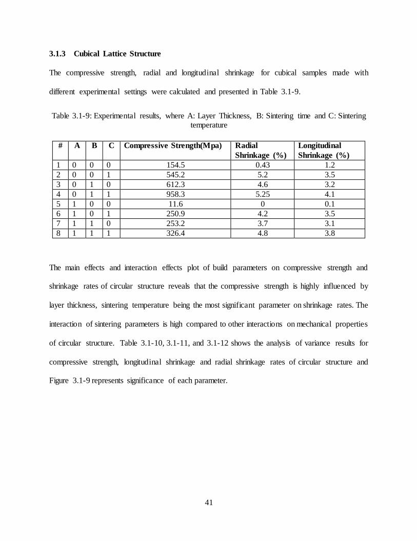
3.1.3 Cubical Lattice Structure ............................................................................................ 41
3.1.4 Discussion ...................................................................................................................... 44
3.2 Neural Network Results .................................................................................................. 47
vii
3.2.1 Solid Structure .............................................................................................................. 47
3.2.2 Circular Lattice Structure ........................................................................................... 50
3.2.3 Cubical Lattice Structure ............................................................................................ 52
3.2.4 Model Validation .......................................................................................................... 56
3.3 Finite Element Analysis ................................................................................................... 58
3.3.1 Finite element simulation of solid ............................................................................... 59
3.3.2 Finite element simulation of four lattice structures .................................................. 60
3.4 Applications ...................................................................................................................... 64
3.5 Conclusion and Suggestion for Future work ................................................................. 66
4 BIBLIOGRAPHY ................................................................................................................ 68
viii
LIST OF FIGURES
Figure 1.0-1: Schematic representation of binder jetting process [21] ........................................... 4
Figure 1.0-2: Fishbone diagram representing various parameters involved in the process ............ 5
Figure 1.0-3: Neural Network Schematic representation ............................................................... 8
Figure 2.1-1: Flow Diagram of Experimental Methodology ........................................................ 13
Figure 2.1-2: (a) ExOne M-lab machine, (b) Radial shrinkage and longitudinal shrinkage
directions ............................................................................................................... 15
Figure 2.1-3: Binder jet additive manufactured solid cylindrical sample ..................................... 17
Figure 2.1-4: Sample in between compression platens of MTS Machine .................................... 18
Figure 2.2-1: Neural Network Schematic representation, Where A-Layer thickness, B-Sintering
time, C-Sintering temperature, O-Compressive Strength, Σ represents summation
& F(x) is activation function, b1 & b2 are bias .................................................... 22
Figure 2.2-2: Flow chart showing the entire training process and the parameters involved. ....... 25
Figure 2.3-1: Finite element Analysis Methodology .................................................................... 26
Figure 2.3-2:(a) Cubical unit cell (b) Circular unit cell (c) Circular 1 (d) Cubical 1 (e) Circular 2
(f) Cubical 2 .......................................................................................................... 27
Figure 2.3-3: Binder jetting fabricated samples of various lattice structures ............................... 28
Figure 3.1-1: Main effects plot of process parameters on compressive strength, A-Layer
thickness (low- 50 µm, high- 100 µm), B-Sintering time (low- 2hours, high- 4
hours), C-Sintering temperature (low- 1120 oC, high- 1180oC) ........................... 31
Figure 3.1-2: Interaction effects plot of process parameters on compressive strength, A*B refers
interaction between Layer thickness and Sintering time, A*C refers interaction
ix
between Layer thickness and Sintering temperature, B*C refers interaction
between Sintering temperature and Sintering time ............................................... 32
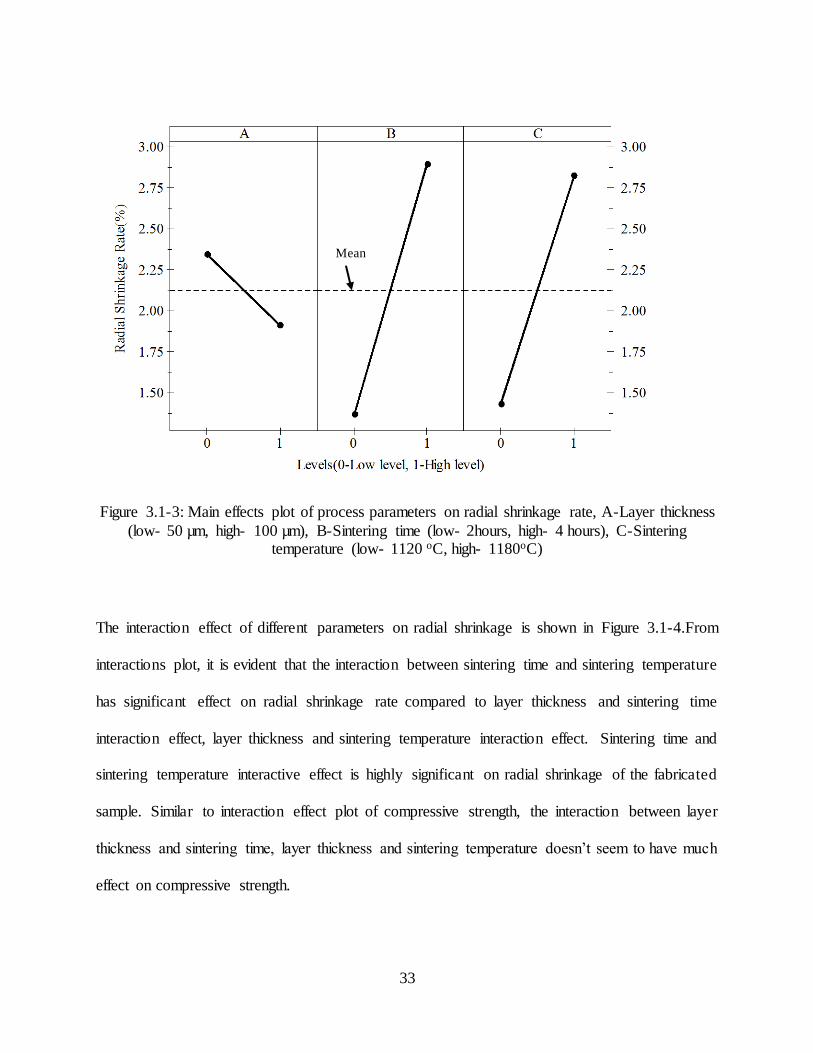
Figure 3.1-3: Main effects plot of process parameters on radial shrinkage rate, A-Layer thickness
(low- 50 µm, high- 100 µm), B-Sintering time (low- 2hours, high- 4 hours), C-
Sintering temperature (low- 1120 oC, high- 1180oC) ........................................... 33
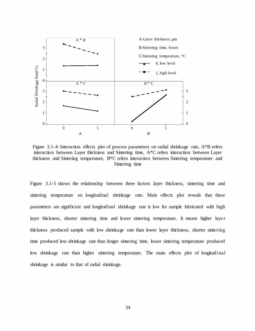
Figure 3.1-4: Interaction effects plot of process parameters on radial shrinkage rate, A*B refers
interaction between Layer thickness and Sintering time, A*C refers interaction
between Layer thickness and Sintering temperature, B*C refers interaction
between Sintering temperature and Sintering time ............................................... 34
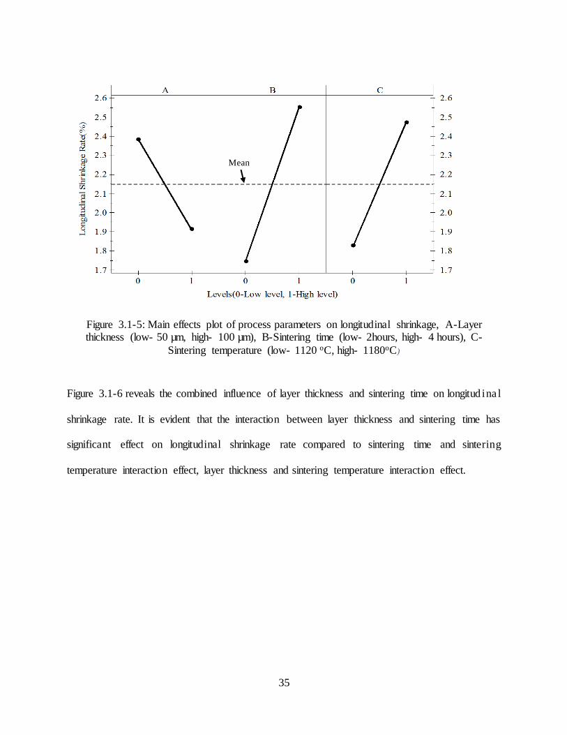
Figure 3.1-5: Main effects plot of process parameters on longitudinal shrinkage, A-Layer
thickness (low- 50 µm, high- 100 µm), B-Sintering time (low- 2hours, high- 4
hours), C-Sintering temperature (low- 1120 oC, high- 1180oC) ........................... 35
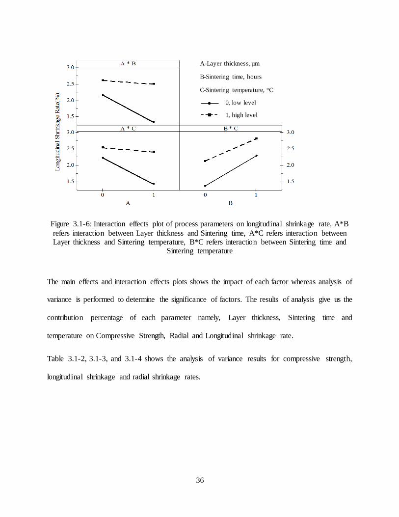
Figure 3.1-6: Interaction effects plot of process parameters on longitudinal shrinkage rate, A*B
refers interaction between Layer thickness and Sintering time, A*C refers
interaction between Layer thickness and Sintering temperature, B*C refers
interaction between Sintering time and Sintering temperature ............................. 36
Figure 3.1-7: Percentage contributions on (a) Compressive Strength (b) Radial shrinkage rate (c)
Longitudinal shrinkage rate. A-Layer thickness, B-Sintering time and C-Sintering
temperature............................................................................................................ 38
Figure 3.1-8: Percentage contributions on (a) Compressive Strength (b) Radial shrinkage rate (c)
Longitudinal shrinkage rate. A-Layer thickness, B-Sintering time and C-Sintering
temperature............................................................................................................ 40
x
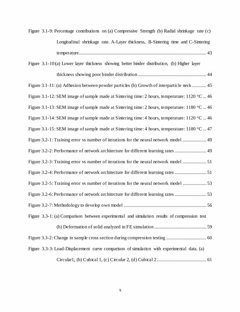
Figure 3.1-9: Percentage contributions on (a) Compressive Strength (b) Radial shrinkage rate (c)
Longitudinal shrinkage rate. A-Layer thickness, B-Sintering time and C-Sintering
temperature............................................................................................................ 43
Figure 3.1-10:(a) Lower layer thickness showing better binder distribution, (b) Higher layer
thickness showing poor binder distribution .......................................................... 44
Figure 3.1-11: (a) Adhesion between powder particles (b) Growth of interparticle neck ............ 45
Figure 3.1-12: SEM image of sample made at Sintering time: 2 hours, temperature: 1120 oC ... 46
Figure 3.1-13: SEM image of sample made at Sintering time: 2 hours, temperature: 1180 oC ... 46
Figure 3.1-14: SEM image of sample made at Sintering time: 4 hours, temperature: 1120 oC ... 46
Figure 3.1-15: SEM image of sample made at Sintering time: 4 hours, temperature: 1180 oC ... 47
Figure 3.2-1: Training error vs number of iterations for the neural network model .................... 49
Figure 3.2-2: Performance of network architecture for different learning rates ........................... 49
Figure 3.2-3: Training error vs number of iterations for the neural network model .................... 51
Figure 3.2-4: Performance of network architecture for different learning rates ........................... 51
Figure 3.2-5: Training error vs number of iterations for the neural network model .................... 53
Figure 3.2-6: Performance of network architecture for different learning rates ........................... 53
Figure 3.2-7: Methodology to develop own model ...................................................................... 56
Figure 3.3-1: (a) Comparison between experimental and simulation results of compression test
(b) Deformation of solid analyzed in FE simulation ............................................ 59
Figure 3.3-2: Change in sample cross section during compression testing .................................. 60
Figure 3.3-3: Load-Displacement curve comparison of simulation with experimental data. (a)
Circular1, (b) Cubical 1, (c) Circular 2, (d) Cubical 2 .......................................... 61
xi
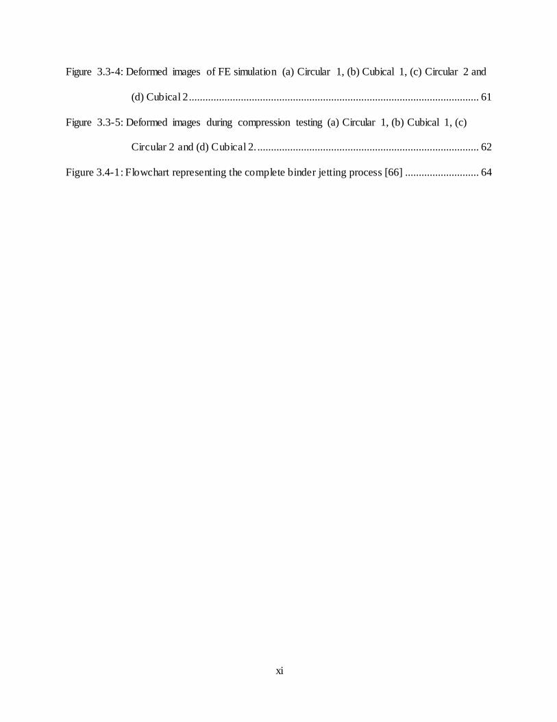
Figure 3.3-4: Deformed images of FE simulation (a) Circular 1, (b) Cubical 1, (c) Circular 2 and
(d) Cubical 2.......................................................................................................... 61
Figure 3.3-5: Deformed images during compression testing (a) Circular 1, (b) Cubical 1, (c)
Circular 2 and (d) Cubical 2. ................................................................................. 62
Figure 3.4-1: Flowchart representing the complete binder jetting process [66] ........................... 64
xii
LIST OF TABLES
Table 1.0-1: Additive manufacturing methods, materials, their advantages and disadvantages .... 3
Table 2.1-1: Process Parameters and Levels................................................................................. 14
Table 2.1-2: Full Factorial Experimental Plan, Low-level is represented as 0 and High level is
represented as 1. A (low- 50 µm, high- 100 µm), B (low- 2hours, high- 4 hours), C
(low- 1120 oC, high- 1180oC) ............................................................................... 16
Table 2.1-3: Chemical composition of SS31 (wt%) ..................................................................... 16
Table 2.1-4: Formulae for Degree of freedom, Sum of squares ................................................... 19
Table 2.3-1: Lattice Parameters for different designs................................................................... 27
Table 3.1-1: Experimental results, where A: Layer Thickness, B: Sintering time and C: Sintering
temperature............................................................................................................ 30
Table 3.1-2: Results of Analysis of variance of compressive strength ......................................... 37
Table 3.1-3: Results of Analysis of variance of radial shrinkage rate .......................................... 37
Table 3.1-4: Results of Analysis of variance of longitudinal shrinkage rate ................................ 37
Table 3.1-5: Experimental results, where A: Layer Thickness, B: Sintering time and C: Sintering
temperature............................................................................................................ 39
Table 3.1-6: Results of Analysis of variance for compressive strength ....................................... 39
Table 3.1-7: Results of Analysis of variance for radial shrinkage rate ......................................... 40
Table 3.1-8: Results of Analysis of variance for longitudinal shrinkage rate .............................. 40
Table 3.1-9: Experimental results, where A: Layer Thickness, B: Sintering time and C: Sintering
temperature............................................................................................................ 41
Table 3.1-10: Results of Analysis of variance for compressive strength ..................................... 42
Table 3.1-11: Results of Analysis of variance for radial shrinkage rate ....................................... 42
xiii
Table 3.1-12: Results of Analysis of variance for longitudinal shrinkage rate ............................ 42
Table 3.1-13: Optimized parameters............................................................................................. 43
Table 3.2-1: Inputs A (Layer thickness), B (Sintering time), C (Sintering temperature) along with
normalized output of compressive strength in the range of 0 to 1. ....................... 48
Table 3.2-2: Normalized inputs and output values of circular structure ....................................... 50
Table 3.2-3: Normalized inputs and output values of cubical structure ....................................... 52
Table 3.2-4: Neural network results for different structures......................................................... 54
Table 3.2-5: Data from experimentation found in literature ......................................................... 57
Table 3.2-6: Validation of neural network model......................................................................... 57
Table 3.3-1: Material properties used for finite element analysis. ............................................... 58
Table 3.3-2: Experimental and FE results..................................................................................... 62
xiv
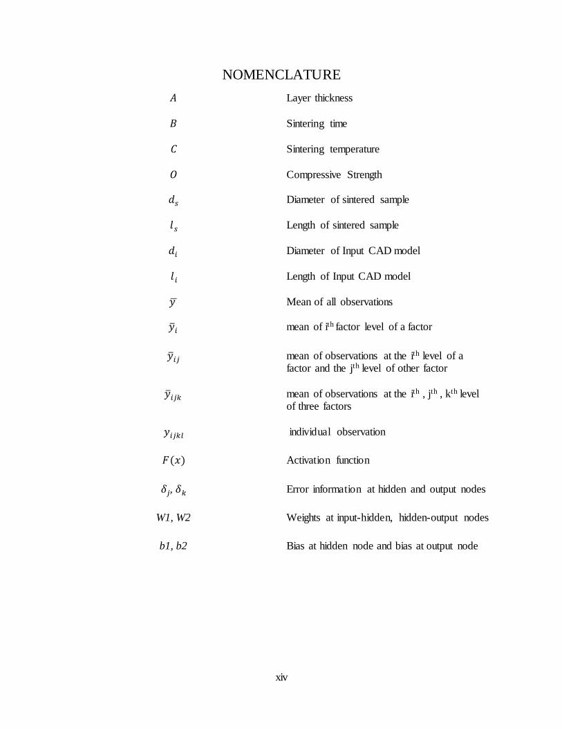
NOMENCLATURE
𝐴 Layer thickness
𝐵 Sintering time
𝐶 Sintering temperature
𝑂 Compressive Strength
𝑑𝑠 Diameter of sintered sample
𝑙𝑠 Length of sintered sample
𝑑𝑖 Diameter of Input CAD model
𝑙𝑖 Length of Input CAD model
𝑦 ̅ Mean of all observations
�̅�𝑖 mean of ith factor level of a factor
�̅�𝑖𝑗 mean of observations at the ith level of a factor and the jth level of other factor
�̅�𝑖𝑗𝑘 mean of observations at the ith , jth , kth level of three factors
𝑦𝑖𝑗𝑘𝑙 individual observation
𝐹(𝑥) Activation function
𝛿𝑗, 𝛿𝑘 Error information at hidden and output nodes
W1, W2 Weights at input-hidden, hidden-output nodes
b1, b2 Bias at hidden node and bias at output node
1
CHAPTER 1
1.0 INTRODUCTION
Additive manufacturing makes the product layer by layer according to sliced input CAD model,
with very less material waste compared to conventional manufacturing. Additive manufactur ing
has wide range of applications which includes biomedical, automotive and aerospace industries. It
has been gaining significance recently because of its ability to manufacture complex shaped
geometries and low material waste compared to conventional manufacturing processes [1, 2]. The
combination of additive manufacturing with topology optimization is highly desirable in many
applications, one such important application is bone tissue engineering where artificial bone
scaffolds are used for bone tissue regeneration. Bone scaffolds are generally made using
conventional manufacturing techniques like gas foaming, solvent casting, electrospinning, freeze
drying, melt molding are used for making bone scaffolds [3]. The major problem with conventiona l
manufacturing techniques used for porous scaffolds are the control on pore sizes and
interconnected pore networks. Additive manufacturing is capable of producing structures with
complex internal architecture like bone scaffolds with controlled porosity, pore geometry and
interconnected pore network [4]. Therefore, there is a great deal of attention to additive
manufacturing technologies where three-dimensional products are made layer by layer additive ly
according to data obtained from CAD file.
Additive manufacturing is a process of joining materials to make objects from 3D model data,
usually layer upon layer, as opposed to subtractive manufacturing technology [5]. Fused deposition
modeling, Selective laser sintering, Material jetting, Binder jetting, Selective laser melting are
different technologies available in the market. There are many studies available in literature
2
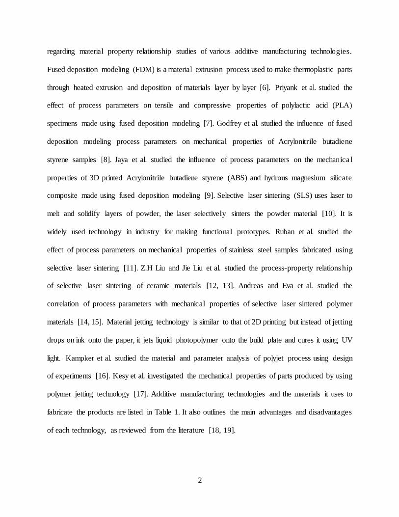
regarding material property relationship studies of various additive manufacturing technologies.
Fused deposition modeling (FDM) is a material extrusion process used to make thermoplastic parts
through heated extrusion and deposition of materials layer by layer [6]. Priyank et al. studied the
effect of process parameters on tensile and compressive properties of polylactic acid (PLA)
specimens made using fused deposition modeling [7]. Godfrey et al. studied the influence of fused
deposition modeling process parameters on mechanical properties of Acrylonitrile butadiene
styrene samples [8]. Jaya et al. studied the influence of process parameters on the mechanica l
properties of 3D printed Acrylonitrile butadiene styrene (ABS) and hydrous magnesium silicate
composite made using fused deposition modeling [9]. Selective laser sintering (SLS) uses laser to
melt and solidify layers of powder, the laser selectively sinters the powder material [10]. It is
widely used technology in industry for making functional prototypes. Ruban et al. studied the
effect of process parameters on mechanical properties of stainless steel samples fabricated using
selective laser sintering [11]. Z.H Liu and Jie Liu et al. studied the process-property relationship
of selective laser sintering of ceramic materials [12, 13]. Andreas and Eva et al. studied the
correlation of process parameters with mechanical properties of selective laser sintered polymer
materials [14, 15]. Material jetting technology is similar to that of 2D printing but instead of jetting
drops on ink onto the paper, it jets liquid photopolymer onto the build plate and cures it using UV
light. Kampker et al. studied the material and parameter analysis of polyjet process using design
of experiments [16]. Kesy et al. investigated the mechanical properties of parts produced by using
polymer jetting technology [17]. Additive manufacturing technologies and the materials it uses to
fabricate the products are listed in Table 1. It also outlines the main advantages and disadvantages
of each technology, as reviewed from the literature [18, 19].
3
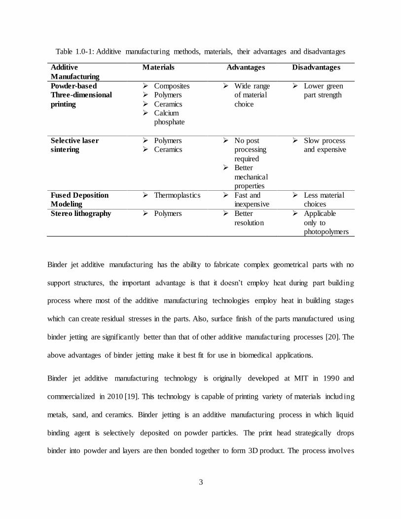
Table 1.0-1: Additive manufacturing methods, materials, their advantages and disadvantages
Additive
Manufacturing
Materials Advantages Disadvantages
Powder-based
Three-dimensional
printing
Composites Polymers
Ceramics Calcium
phosphate
Wide range of material
choice
Lower green part strength
Selective laser
sintering
Polymers Ceramics
No post processing
required Better
mechanical properties
Slow process and expensive
Fused Deposition
Modeling
Thermoplastics Fast and inexpensive
Less material choices
Stereo lithography Polymers Better
resolution
Applicable
only to photopolymers
Binder jet additive manufacturing has the ability to fabricate complex geometrical parts with no
support structures, the important advantage is that it doesn’t employ heat during part building
process where most of the additive manufacturing technologies employ heat in building stages
which can create residual stresses in the parts. Also, surface finish of the parts manufactured using
binder jetting are significantly better than that of other additive manufacturing processes [20]. The
above advantages of binder jetting make it best fit for use in biomedical applications.
Binder jet additive manufacturing technology is originally developed at MIT in 1990 and
commercialized in 2010 [19]. This technology is capable of printing variety of materials includ ing
metals, sand, and ceramics. Binder jetting is an additive manufacturing process in which liquid
binding agent is selectively deposited on powder particles. The print head strategically drops
binder into powder and layers are then bonded together to form 3D product. The process involves
4
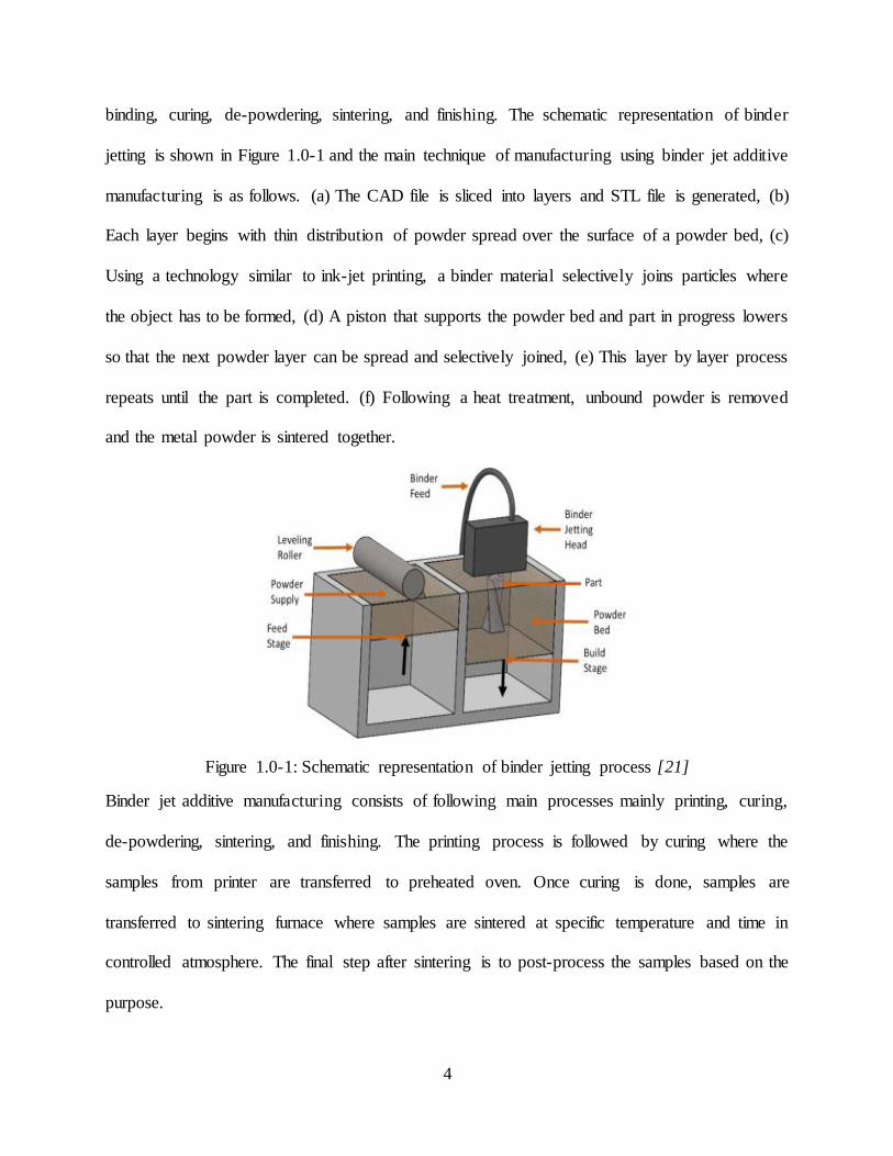
binding, curing, de-powdering, sintering, and finishing. The schematic representation of binder
jetting is shown in Figure 1.0-1 and the main technique of manufacturing using binder jet additive
manufacturing is as follows. (a) The CAD file is sliced into layers and STL file is generated, (b)
Each layer begins with thin distribution of powder spread over the surface of a powder bed, (c)
Using a technology similar to ink-jet printing, a binder material selectively joins particles where
the object has to be formed, (d) A piston that supports the powder bed and part in progress lowers
so that the next powder layer can be spread and selectively joined, (e) This layer by layer process
repeats until the part is completed. (f) Following a heat treatment, unbound powder is removed
and the metal powder is sintered together.
Figure 1.0-1: Schematic representation of binder jetting process [21]
Binder jet additive manufacturing consists of following main processes mainly printing, curing,
de-powdering, sintering, and finishing. The printing process is followed by curing where the
samples from printer are transferred to preheated oven. Once curing is done, samples are
transferred to sintering furnace where samples are sintered at specific temperature and time in
controlled atmosphere. The final step after sintering is to post-process the samples based on the
purpose.

5
The process parameters which effects the output characteristics of samples are represented in fish-
bone diagram as shown in Figure 1.0-2. The parameters include powder size, layer thickness
during binding, part orientation in the bed, drying time during binding, heater power, roller speed,
curing temperature, curing time, sintering time, sintering temperature and sintering atmosphere.
Any variation in the above-mentioned parameter changes the output properties. Similar to
conventional manufacturing, there are many process parameters to be set before manufactur ing.
Binder jetting involves lot of processes involved which makes the relationship between input
process parameters and output properties very complicated. Hence there is a need to tune the
process parameters to achieve controlled and stable process.
Figure 1.0-2: Fishbone diagram representing various parameters involved in the process
Few researchers studied the relationship between process parameters and output characterist ics
obtained using binder jet additive manufacturing technology. Yao et al. investigated the process
parameters including binder setting saturation value, layer thickness, location of made up parts for
ZCorp 3D printing system with plaster powder and identified the process parameters to reduce the
building time [22]. Vaezi et al. studied the influence of binder saturation and layer thickness on
mechanical strength, surface quality of plaster-based powder and found that the uniform layer
thickness and increase in binder saturation resulted in increased tensile and flexural strength with
MACHINE
HEATING
CONDITION
S
PROCESS
POWDER
Output
Characteristic Sintering time
Sintering temperature
Curing temperature
Curing time
Cleaning cycle
Heating Power
Heating time
Binder washing
time
Heating
time
Layer
thickness
Heating
time
Feed-to-
powder
ratio
Heating
time
Binder
Saturation
Heating
time
Roll
Speed
Heating
time Shape
Composition
Size
Agglomeration
Flowability
6
low dimensional accuracy [23]. Hsu et al. studied the influence of layer thickness, binder
saturation, location of green parts, powder type and optimized the parameters for ZCorp 3D
printing improving dimensional accuracy, less fabrication time and less binder consumption [24].
Shresta et al. studied the effect of binder saturation, layer thickness, roll speed, feed-to-powder
ratio on transverse rupture strength and found that binder saturation and feed-to-powder ratio are
most critical factors influencing mechanical properties [25]. Suwanprateeb et al. studied the
influence of layer thickness and binder saturation on transformation efficiency of 3D printed
plaster of paris and found that low layer thickness, saturation yielded high transformation
efficiency [26]. Chen et al. studied the influence of layer thickness, drying time, binder saturat ion
on dimensional accuracy and surface finish of SS420 sample and found that layer thickness, binder
saturation influenced surface finish whereas dimensional accuracy is influenced by drying time
[27]. Tang et al. study was focused on mechanical properties of SS316 samples made by binder
jetting with default process parameters [28]. Bai et al. studied the effect of powder size and
sintering atmospheric control on part density, shrinkage and found that controlled sintering
atmosphere in with presence of hydrogen improves the sintered density of copper samples [29].
Doyle et al. studied the effect of layer thickness and orientation on mechanical behavior of stainless
steel bronze parts made using binder jetting and found that layer thickness as larger influence than
orientation on tensile mechanical properties of bronze infiltra ted stainless steel samples [30].
Most of the researchers studied the binder jetting of polymer materials and there are very few
studies on the optimization of process parameters for binder jet additive manufacturing of metal
parts. Also, most of the studies considered printing setup parameters like powder size, binder
saturation, layer thickness, and drying time leaving behind the heat treatment parameters effect.
Hence, there is a need to carry out optimization studies involving metal manufacturing and the
7
current research is carried out to study the effect of printing setup parameter layer thickness in
combination with sintering parameters, temperature and time. Output characteristics considered
are compressive strength, radial, and longitudinal shrinkage rates, these are chosen from the binder
jetting application perspective in bone scaffold engineering, as the complex bone structure
produced should be dimensionally accurate with compressive strength.
Apart from studying the process property relationship, it is very important to establish quantitat ive
relationship between process parameters and properties, as it cuts down the cost of experiments.
Physics-based modelling is almost impossible for 3D printing, as it involves powder-binder
reaction, curing and sintering. Hence numerical models can be effective in finding the appropriate
parameters with respect to desired output characteristics. Artificial neural network is the well-
known method to serve as a numerical model based on experimental data, hence a numerical model
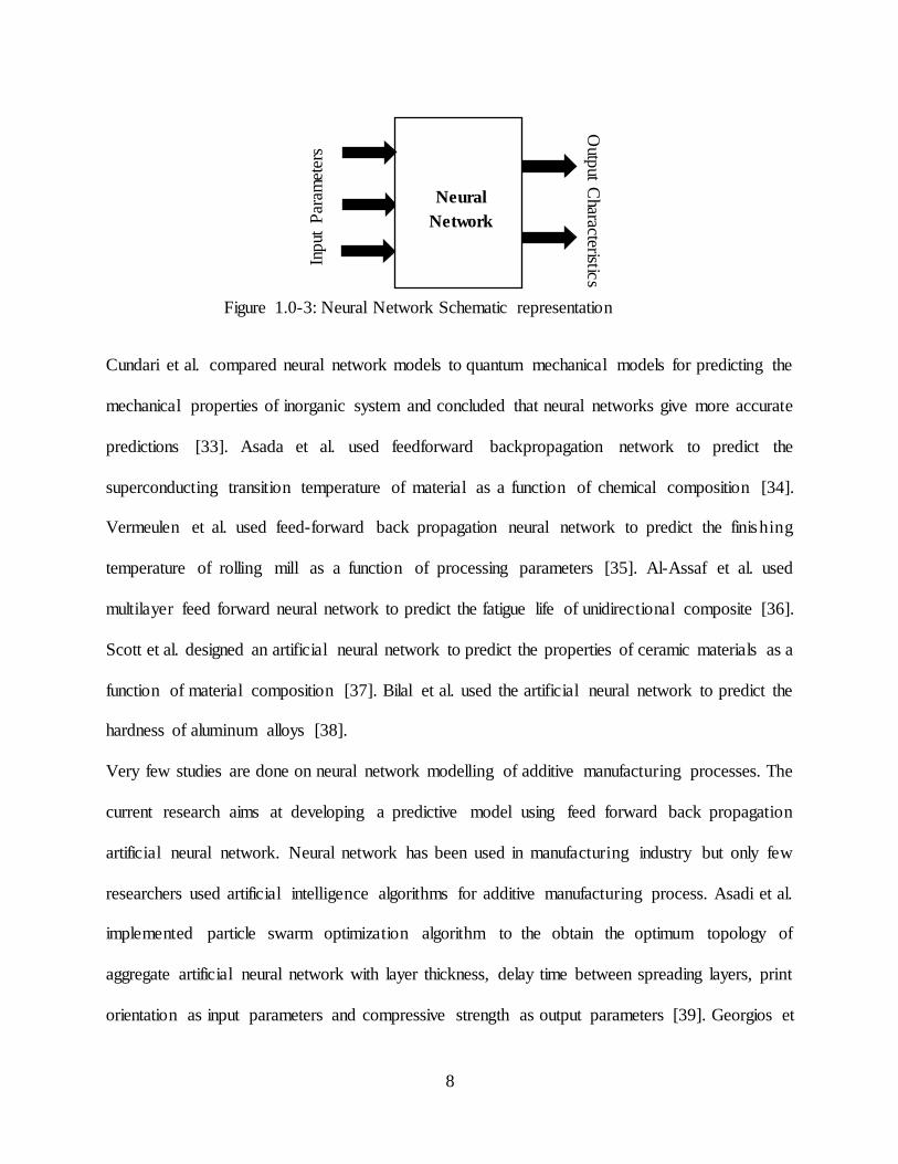
can be developed for the 3D printing process using artificial neural network. Figure 1.0-3 shows
the schematic representation of neural network generating output values based on fed input
parameters. Applications of artificial neural network include thin films & superconductors,
materials, machining & processing, thermal and mechanical fields [31]. Neural networks are found
to be best in constructing complex map between inputs and output of a system. It is a system of
mathematical equations working on data approximating the human brain. Neural network consists
of neurons connecting each other with respective weights and passing the information. Awodele
et al. defined artificial neural network as brain in aspect that knowledge is gained through learning
and weights are used to store the knowledge [32].
8
Cundari et al. compared neural network models to quantum mechanical models for predicting the
mechanical properties of inorganic system and concluded that neural networks give more accurate
predictions [33]. Asada et al. used feedforward backpropagation network to predict the
superconducting transition temperature of material as a function of chemical composition [34].
Vermeulen et al. used feed-forward back propagation neural network to predict the finishing
temperature of rolling mill as a function of processing parameters [35]. Al-Assaf et al. used
multilayer feed forward neural network to predict the fatigue life of unidirectional composite [36].
Scott et al. designed an artificial neural network to predict the properties of ceramic materials as a
function of material composition [37]. Bilal et al. used the artificial neural network to predict the
hardness of aluminum alloys [38].
Very few studies are done on neural network modelling of additive manufacturing processes. The
current research aims at developing a predictive model using feed forward back propagation
artificial neural network. Neural network has been used in manufacturing industry but only few
researchers used artificial intelligence algorithms for additive manufacturing process. Asadi et al.
implemented particle swarm optimization algorithm to the obtain the optimum topology of
aggregate artificial neural network with layer thickness, delay time between spreading layers, print
orientation as input parameters and compressive strength as output parameters [39]. Georgios et
Input
Par
amet
ers
Outp
ut Characteristic
s
Neural
Network
Figure 1.0-3: Neural Network Schematic representation
9
al. used the neural network models to assess the quality characteristics of printed electronic
products caused by dimensional deviations [40].
Additive Manufacturing can process more complex structures compared to conventiona l
manufacturing, a good example is lattice structures. Even with the numerous applications of lattice
structures, there is still a manufacturing complexity. Casting, brazing, metal forming are the
manufacturing techniques used for making simple lattice structures, the structures made by these
techniques has limited design freedom. Additive Manufacturing can be used to make cellular
structures of complex designs, it is found to be promising technology to produce lattice structures
with controlled porosity and pore size. Metal cellular structures exhibit a combination of high-
performance characteristics as high strength, low mass, good energy absorption and thermal
properties [41, 42]. Cellular structures can be classified based on the topology of the pore and cell
size. Metal stochastic cellular structures and periodic lattice cellular structures are two types of
cellular structures. Metal stochastic cellular structures typically have a random distribution of open
or closed voids and metal periodic cellular lattice structures have uniform structures that are
generated by repeating a unit cell. Periodic lattice structures have superior mechanical properties
than that of stochastic metal structures, structural performance of lattice strut structures with less
than 5% density was proven to be up to three times higher than that of stochastic foams [43, 44].
Hence metal lattice structures are of greater interest to study and the most relevant applications of
lattice structures are found in the fields of biomedical, aerospace, chemical and automotive
industries.
Lot of research has been conducted regarding the application of additive manufacturing in making
cellular structures. Osman et al. studied the compressive properties of cellular lattice structures
manufactured using fused deposition modeling [45]. Mullen et al. developed an approach based
10
on a defined regular unit cell to design and produced structures using selective laser sintering with
a large range of both physical and mechanical properties [46]. Chunze et al. studied the
performance of stainless steel lattice cellular structure fabricated via selective laser sintering
technique [47]. Contuzzi et al. investigated compressive property of Ti6Al4V pillar textile unit
cell made by selective laser melting [48]. Seyed et al. studied the mechanical properties of porous
biomaterials made from six different space-filling units are studied [49]. Farzadi et al. studied the
compressive properties of lattice structure made using powder-based inkjet 3D printing [50].
Recep et al. studied design, optimization, and evaluation of periodic lattice-based cellular
structures fabricated by additive manufacturing [51]. Christiane et al. conducted the experimenta l
analysis of additive manufactured parts with diverse unit cell structures in compression and
flexural tests [52]. Mechanical testing shows that the additively made produced material is highly
anisotropic and that the material has many advantages compared to the traditionally manufactured
[53].
Large amount of research is dedicated on manufacturing of lattice structures using additive
manufacturing and very few studies deals with finite element simulation of lattice structures
fabricated using additive manufacturing. Jie et al. performed finite element analysis to evaluate the
mechanical properties of cellular structures [54]. Mark et al. validated the finite element simula t ion
of cellular structures with empirical data obtained from compression testing of samples made using
selective laser sintering [55]. Uzoma et al. developed the finite element model to simulate the
compressive behavior and compared it with experimental results [56]. Clayto et al. simulated the
diamond lattice structures of different unit sizes and compared it with experimentation results [57].
Kolan et al. performed finite element analysis to predict the compressive behavior of five different
porous structures made using selective laser sintering [58]. Langranda et al. investigated the
11
influence of element type and numerical scheme on structural response of cellular materials under
compressive load [59]. There is a need to develop the finite element models of binder jet additive ly
manufactured lattice structures as it eliminates the need for experiments cutting down the
experimentation cost and time. The current study also explores the compressive behavior of lattice
structures by simulating the finite element model developed from experimental compression data
of solid cylinder along with performing process-parameter optimization.
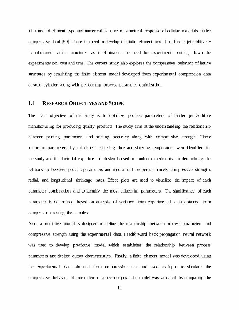
1.1 RESEARCH OBJECTIVES AND SCOPE
The main objective of the study is to optimize process parameters of binder jet additive
manufacturing for producing quality products. The study aims at the understanding the relationship
between printing parameters and printing accuracy along with compressive strength. Three
important parameters layer thickness, sintering time and sintering temperature were identified for
the study and full factorial experimental design is used to conduct experiments for determining the
relationship between process parameters and mechanical properties namely compressive strength,
radial, and longitudinal shrinkage rates. Effect plots are used to visualize the impact of each
parameter combination and to identify the most influential parameters. The significance of each
parameter is determined based on analysis of variance from experimental data obtained from
compression testing the samples.
Also, a predictive model is designed to define the relationship between process parameters and
compressive strength using the experimental data. Feedforward back propagation neural network
was used to develop predictive model which establishes the relationship between process
parameters and desired output characteristics. Finally, a finite element model was developed using
the experimental data obtained from compression test and used as input to simulate the
compressive behavior of four different lattice designs. The model was validated by comparing the

12
FE simulation results with that of experimental compression test results of different lattice
structures.
13
CHAPTER 2
2.0 PROCESS AND APPROACHES
The current study is divided into two different parts, first of all experimentation is performed to
study the effect of process parameters on compressive strength, shrinkage rate and secondly,
numerical modelling is done using artificial intelligence approach to develop a prediction model
and also finite element modelling is carried out using the experimental data.
2.1 EXPERIMENTAL METHOD AND DESIGN
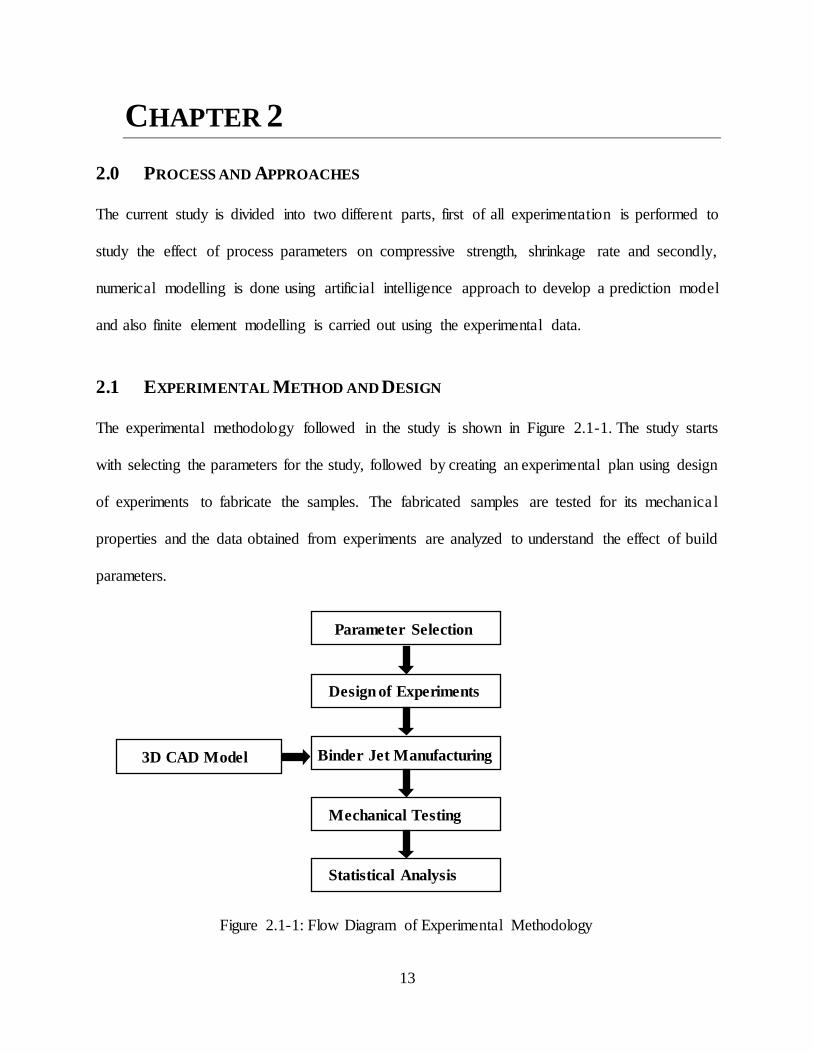
The experimental methodology followed in the study is shown in Figure 2.1-1. The study starts
with selecting the parameters for the study, followed by creating an experimental plan using design
of experiments to fabricate the samples. The fabricated samples are tested for its mechanica l
properties and the data obtained from experiments are analyzed to understand the effect of build
parameters.
Parameter Selection
Design of Experiments
Binder Jet Manufacturing
Statistical Analysis
3D CAD Model
Mechanical Testing
Figure 2.1-1: Flow Diagram of Experimental Methodology
14
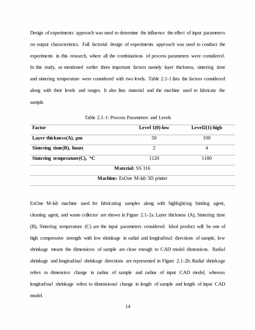
Design of experiments approach was used to determine the influence the effect of input parameters
on output characteristics. Full factorial design of experiments approach was used to conduct the
experiments in this research, where all the combinations of process parameters were considered.
In this study, as mentioned earlier three important factors namely layer thickness, sintering time
and sintering temperature were considered with two levels. Table 2.1-1 lists the factors considered
along with their levels and ranges. It also lists material and the machine used to fabricate the
sample.
Table 2.1-1: Process Parameters and Levels
Factor Level 1(0)-low Level2(1)-high
Layer thickness(A), µm 50 100
Sintering time(B), hours 2 4
Sintering temperature(C), oC 1120 1180
Material: SS 316
Machine: ExOne M-lab 3D printer
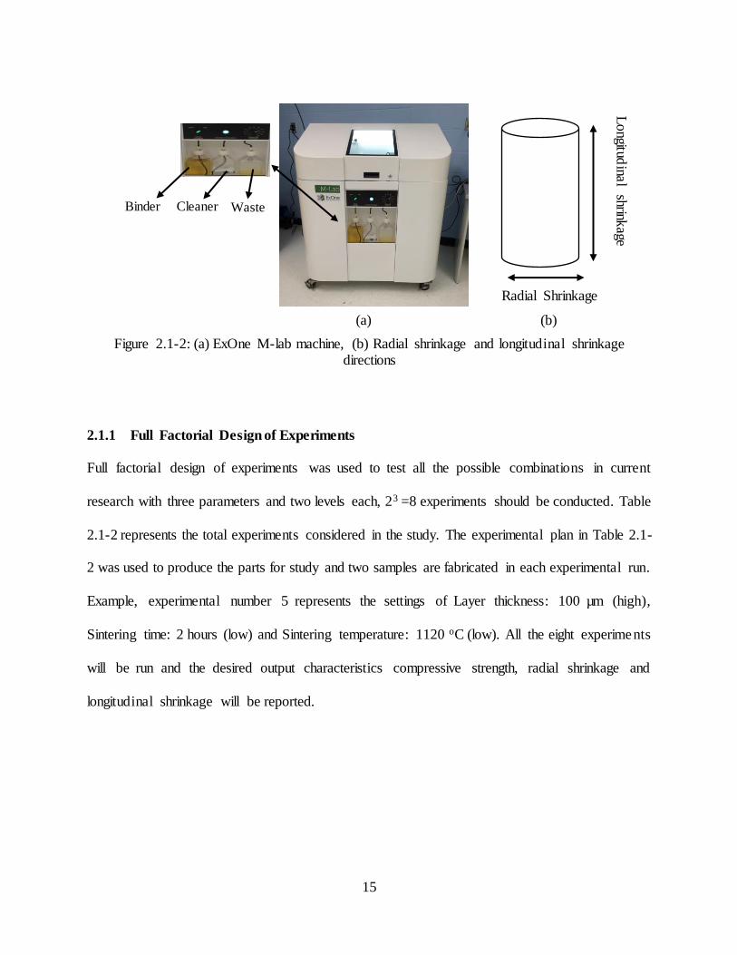
ExOne M-lab machine used for fabricating samples along with highlighting binding agent,
cleaning agent, and waste collector are shown in Figure 2.1-2a. Layer thickness (A), Sintering time
(B), Sintering temperature (C) are the input parameters considered. Ideal product will be one of
high compressive strength with low shrinkage in radial and longitudinal directions of sample, low
shrinkage means the dimensions of sample are close enough to CAD model dimensions. Radial
shrinkage and longitudinal shrinkage directions are represented in Figure 2.1-2b. Radial shrinkage
refers to dimension change in radius of sample and radius of input CAD model, whereas
longitudinal shrinkage refers to dimensional change in length of sample and length of input CAD
model.
15
Figure 2.1-2: (a) ExOne M-lab machine, (b) Radial shrinkage and longitudinal shrinkage directions
2.1.1 Full Factorial Design of Experiments
Full factorial design of experiments was used to test all the possible combinations in current
research with three parameters and two levels each, 23 =8 experiments should be conducted. Table
2.1-2 represents the total experiments considered in the study. The experimental plan in Table 2.1-
2 was used to produce the parts for study and two samples are fabricated in each experimental run.
Example, experimental number 5 represents the settings of Layer thickness: 100 µm (high),
Sintering time: 2 hours (low) and Sintering temperature: 1120 oC (low). All the eight experiments
will be run and the desired output characteristics compressive strength, radial shrinkage and
longitudinal shrinkage will be reported.
Longitud
inal
shrinkage
Radial Shrinkage
(a) (b)
Binder Cleaner Waste

16
Table 2.1-2: Full Factorial Experimental Plan, Low-level is represented as 0 and High level is represented as 1. A (low- 50 µm, high- 100 µm), B (low- 2hours, high- 4 hours), C (low- 1120
oC, high- 1180oC)
Experiment Layer Thickness(A) Sintering Time(B) Sintering Temperature(C)
1 0 0 0
2 0 0 1
3 0 1 0
4 0 1 1
5 1 0 0
6 1 0 1
7 1 1 0
8 1 1 1
2.1.1.1 Material
The powder material used is Stainless steel 316 powder with particle size of 30 µm, the material
is obtained from Ex-One and used with no further treatment. The chemical composition of
stainless steel powder is showed in the Table 2.1-3.
Table 2.1-3: Chemical composition of SS31 (wt%)
C Mn P S Si Cr
0.08 max 2.00 max 0.045 max 0.03 max 0.75 max 16.00-18.00

17
2.1.2 Sample Preparation
The sample used in the study are cylindrical structures with dimensions 25mm length and 10 mm
diameter, the CAD model is designed in Creo 3.0. Then the CAD model is sliced to layers and the
generated STL model is input to system for printing. The 3D printing process starts with loading
the powder material into the bed. Along with powder material, the STL file has to be uploaded
into the system and the sample fabricated is shown in Figure 2.1-3.
Figure 2.1-3: Binder jet additive manufactured solid cylindrical sample
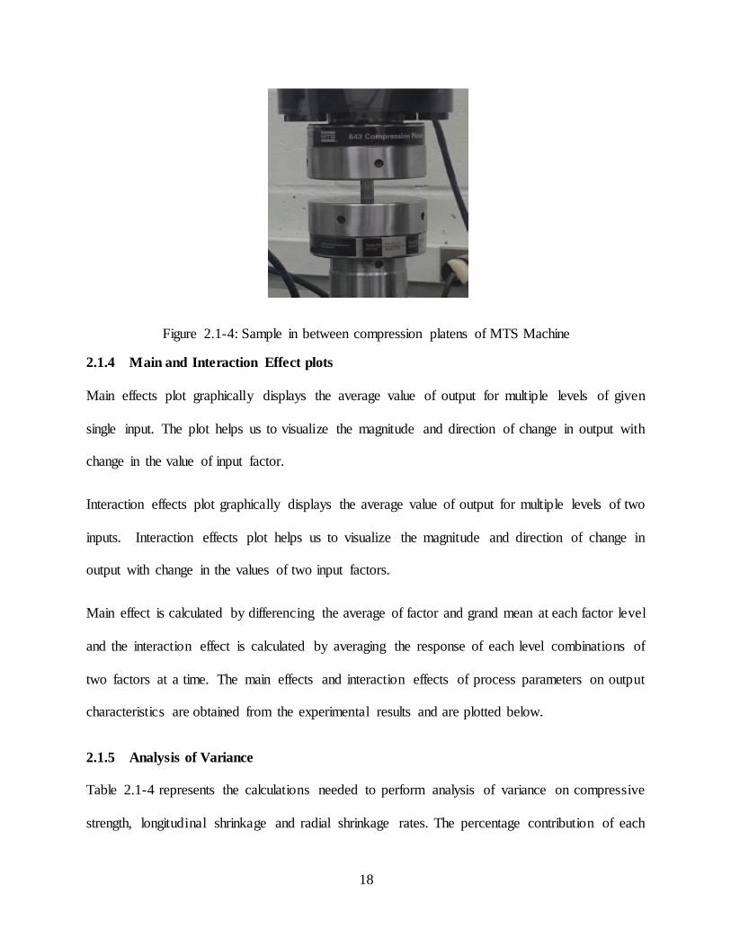
2.1.3 Compression Testing
Compression testing was carried out on samples according to ASTM E9 standards for metallic
materials [60]. MTS 810 material testing system with a 1 KN load cell at a constant crosshead
speed of 0.1 in/ min was used and the data recorded for every 0.05 seconds, shown in Figure 2.1-
4. The stress-strain curves were derived from the load-displacement data obtained during
experiments. Figure 2.1-4 shows the sample in between the compression platens of MTS machine
during the testing.
18
Figure 2.1-4: Sample in between compression platens of MTS Machine
2.1.4 Main and Interaction Effect plots
Main effects plot graphically displays the average value of output for multiple levels of given
single input. The plot helps us to visualize the magnitude and direction of change in output with
change in the value of input factor.
Interaction effects plot graphically displays the average value of output for multiple levels of two
inputs. Interaction effects plot helps us to visualize the magnitude and direction of change in
output with change in the values of two input factors.
Main effect is calculated by differencing the average of factor and grand mean at each factor level
and the interaction effect is calculated by averaging the response of each level combinations of
two factors at a time. The main effects and interaction effects of process parameters on output
characteristics are obtained from the experimental results and are plotted below.
2.1.5 Analysis of Variance
Table 2.1-4 represents the calculations needed to perform analysis of variance on compressive
strength, longitudinal shrinkage and radial shrinkage rates. The percentage contribution of each
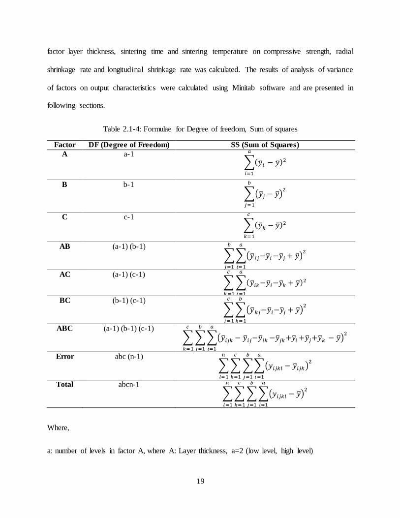
19
factor layer thickness, sintering time and sintering temperature on compressive strength, radial
shrinkage rate and longitudinal shrinkage rate was calculated. The results of analysis of variance
of factors on output characteristics were calculated using Minitab software and are presented in
following sections.
Table 2.1-4: Formulae for Degree of freedom, Sum of squares
Factor DF (Degree of Freedom) SS (Sum of Squares)
A a-1 ∑(�̅�𝑖 − �̅�)2
𝑎
𝑖=1
B b-1
∑(�̅�𝑗 − �̅�)2
𝑏
𝑗=1
C c-1 ∑(�̅�𝑘 − �̅�)2
𝑐
𝑘=1
AB (a-1) (b-1)
∑ ∑(�̅�𝑖𝑗−�̅�𝑖 −�̅�𝑗 + �̅�)2
𝑎
𝑖=1
𝑏
𝑗=1
AC (a-1) (c-1) ∑ ∑(�̅�𝑖𝑘−�̅�𝑖−�̅�𝑘 + �̅�)2
𝑎
𝑖=1
𝑐
𝑘 =1
BC (b-1) (c-1)
∑ ∑(�̅�𝑘𝑗−�̅�𝑖−�̅�𝑗 + �̅�)2
𝑏
𝑘=1
𝑐
𝑗=1
ABC (a-1) (b-1) (c-1)
∑ ∑ ∑(�̅�𝑖𝑗𝑘 − �̅�𝑖𝑗−�̅�𝑖𝑘 −�̅�𝑗𝑘+�̅�𝑖 +�̅�𝑗+�̅�𝑘 − �̅�)2
𝑎
𝑖=1
𝑏
𝑗=1
𝑐
𝑘=1
Error abc (n-1)
∑ ∑ ∑ ∑(𝑦𝑖𝑗𝑘𝑙 − �̅�𝑖𝑗𝑘)2
𝑎
𝑖=1
𝑏
𝑗=1
𝑐
𝑘=1
𝑛
𝑙=1
Total abcn-1
∑ ∑ ∑ ∑(𝑦𝑖𝑗𝑘𝑙 − �̅�)2
𝑎
𝑖=1
𝑏
𝑗=1
𝑐
𝑘=1
𝑛
𝑙=1
Where,
a: number of levels in factor A, where A: Layer thickness, a=2 (low level, high level)
20
b: number of levels in factor B, where B: Sintering time, b=2 (low level, high level)
c: number of levels in factor C, where C: Sintering temperature, c=2 (low level, high level)
n: number of observations
𝑦 ̅: mean of all observations
�̅�𝑖 : mean of ith factor level of factor A
�̅�𝑗 ∶ mean of jth factor level of factor A
�̅�𝑘 ∶ mean of kth factor level of factor A
�̅�𝑖𝑗 ∶ mean of observations at the ith level of factor A and the jth level of factor B
�̅�𝑖𝑘 : mean of observations at the ith level of factor A and the kth level of factor C
�̅�𝑘𝑗 : mean of observations at the kth level of factor C and the jth level of factor B
�̅�𝑖𝑗𝑘 : mean of observations at the ith level of factor A, jth level of factor B and kth level of factor C
𝑦𝑖𝑗𝑘𝑙 ∶ individual observation
MS (Mean Squares) = SS (Sum of Squares)/DF (Degree of freedom)
F-Value= MS of Factor/MS of Error
21
2.2 NEURAL NETWORK MODEL
Artificial neural networks are best tools compared to other available data modelling tools, as it is
capable of mapping complex non-linear relationship between input factors and output
characteristics. After training the neural network with known data, it is capable of providing
approximate output results with unseen data which makes the technique useful for predictive
applications. Feedforward back propagation neural network is the simplest ANN in use and found
its applications in developing predictive experimental models. Feed forward back propagation
neural network with sigmoid activation function was considered for designing the experimenta l
model. There are three different layers in neural network.
Input layer: The leftmost layer, input parameters are feed into neural network through this layer.
Hidden layer: The layer connecting the input and output layer is hidden layer, it is called hidden
as its values are not observed in the training set.
Output layer: The rightmost layer, where all the hidden neurons produce output.
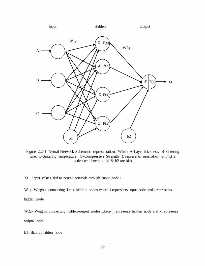
Figure 2.2-1 represents the architecture of neural network used in the study. In feed forward,
neurons in input layer are connected to neurons in hidden layer, whereas neurons in hidden layer
are connected to output layer. Backpropagation is a training method in which neurons adjust their
weight to achieve the target output. The network contains three layers with a total of 8 nodes, 4
being hidden nodes, 3 input nodes and 1 output node.
22
Xi – Input values fed to neural network through input node i
W1ij- Weights connecting input-hidden nodes where i represents input node and j represents
hidden node
W2jk- Weights connecting hidden-output nodes where j represents hidden node and k represents
output node
b1- Bias at hidden node
A
A
C
W1ij
W2jk
𝛴 F(x)
𝛴 F(x)
𝛴 F(x)
𝛴 F(x)
B
Sintering temperature
A
Sintering temperature
C
Sintering temperature
A A b1
b2
O 𝛴 F(x)
Input Hidden Output
Figure 2.2-1: Neural Network Schematic representation, Where A-Layer thickness, B-Sintering
time, C-Sintering temperature, O-Compressive Strength, Σ represents summation & F(x) is activation function, b1 & b2 are bias
23
b2-Bias at output node
F(x) - Activation function
δk-Error information at output node
δj-Error information at hidden node
ΔW1- Delta weights at input-hidden layer
ΔW2- Delta weights at hidden-output layer
Zj – Hidden node, Yk– Output node
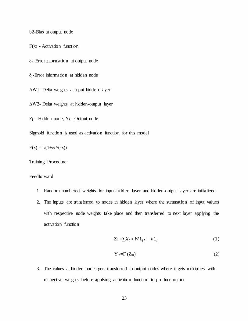
Sigmoid function is used as activation function for this model
F(x) =1/(1+ⅇ ^(-x))
Training Procedure:
Feedforward
1. Random numbered weights for input-hidden layer and hidden-output layer are initialized
2. The inputs are transferred to nodes in hidden layer where the summation of input values
with respective node weights take place and then transferred to next layer applying the
activation function
Zin=∑𝑋𝑖 ∗ 𝑊1𝑖𝑗 + 𝑏1𝑖 (1)
Yin=F (Zin) (2)
3. The values at hidden nodes gets transferred to output nodes where it gets multiplies with
respective weights before applying activation function to produce output
24
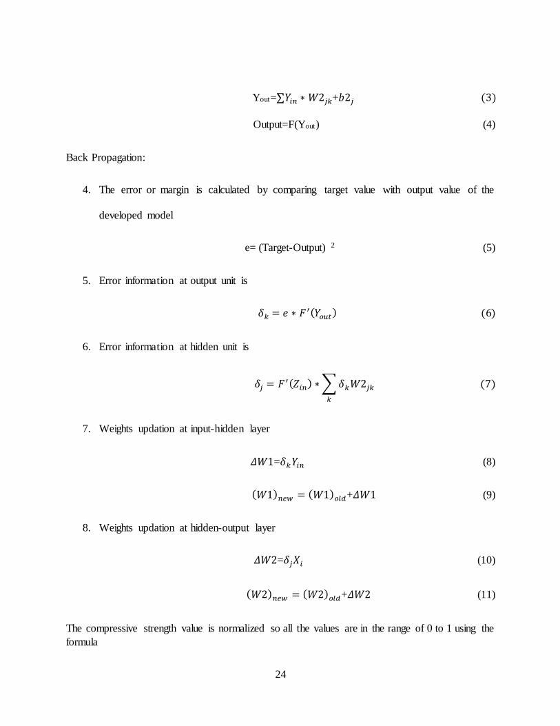
Yout=∑𝑌𝑖𝑛 ∗ 𝑊2𝑗𝑘+𝑏2𝑗 (3)
Output=F(Yout) (4)
Back Propagation:
4. The error or margin is calculated by comparing target value with output value of the
developed model
e= (Target-Output) 2 (5)
5. Error information at output unit is
𝛿𝑘 = ⅇ ∗ 𝐹 ′(𝑌𝑜𝑢𝑡) (6)
6. Error information at hidden unit is
𝛿𝑗 = 𝐹 ′(𝑍𝑖𝑛) ∗ ∑ 𝛿𝑘𝑊2𝑗𝑘
𝑘
(7)
7. Weights updation at input-hidden layer
𝛥𝑊1=𝛿𝑘𝑌𝑖𝑛 (8)
(𝑊1)𝑛𝑒𝑤 = (𝑊1)𝑜𝑙𝑑+𝛥𝑊1 (9)
8. Weights updation at hidden-output layer
𝛥𝑊2=𝛿𝑗𝑋𝑖 (10)
(𝑊2)𝑛𝑒𝑤 = (𝑊2)𝑜𝑙𝑑+𝛥𝑊2 (11)
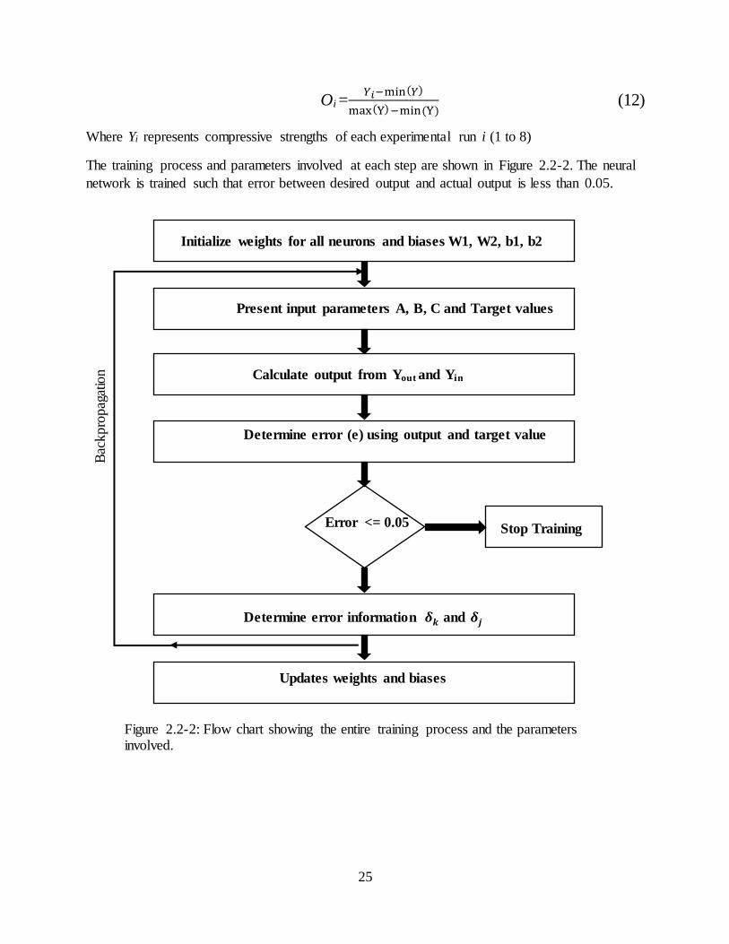
The compressive strength value is normalized so all the values are in the range of 0 to 1 using the
formula
25
Oi =𝑌𝑖−min(𝑌)
max(Y) −min(Y) (12)
Where Yi represents compressive strengths of each experimental run i (1 to 8)
The training process and parameters involved at each step are shown in Figure 2.2-2. The neural
network is trained such that error between desired output and actual output is less than 0.05.
Initialize weights for all neurons and biases W1, W2, b1, b2
Present input parameters A, B, C and Target values
Calculate output from Yout and Yin
Determine error (e) using output and target value
Error <= 0.05
Determine error information 𝜹𝒌 and 𝜹𝒋
Updates weights and biases
Stop Training
Figure 2.2-2: Flow chart showing the entire training process and the parameters involved.
Bac
kpro
pag
atio
n
26
After successful training, the network is tested with new data sets for its performance. Then the
value obtained using the network is denormalized to find the difference between the predicted
value and actual value.
𝑌𝑝𝑟𝑒𝑑𝑖𝑐𝑡𝑒𝑑 = [𝑌𝑛𝑒𝑡𝑤𝑜𝑟𝑘 𝑣𝑎𝑙𝑢𝑒 ∗ (max(𝑌) − min(𝑌))] + min(𝑌) (13)
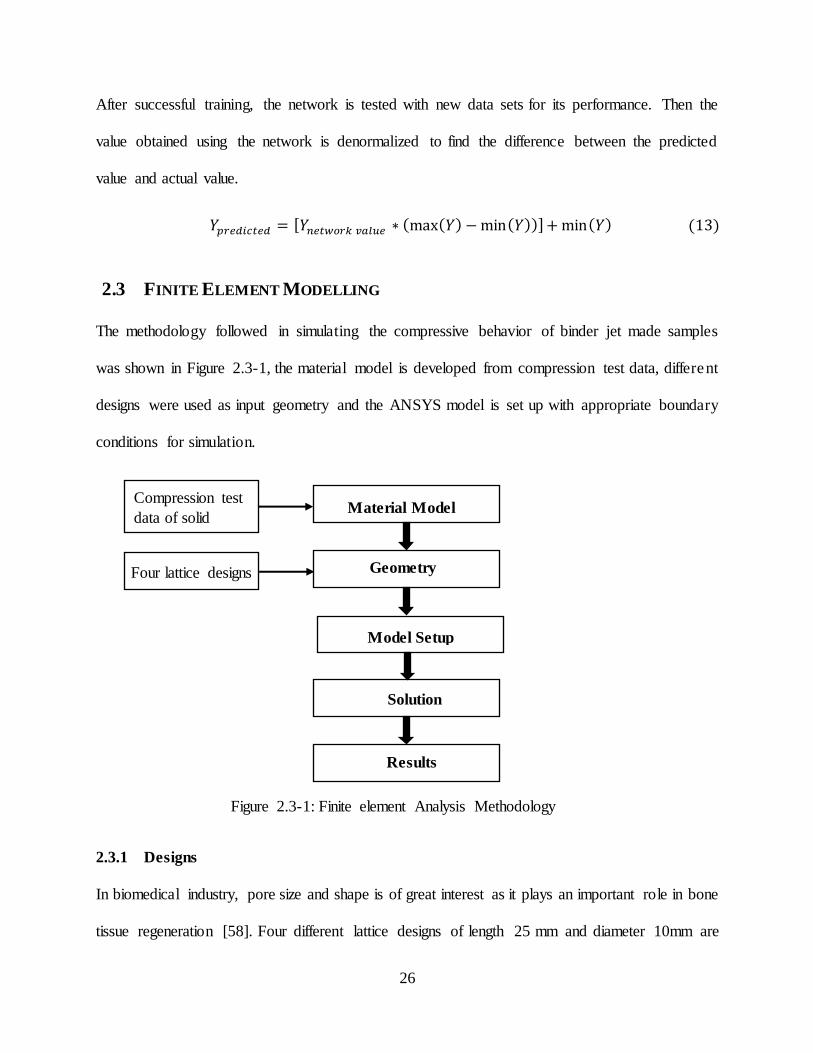
2.3 FINITE ELEMENT MODELLING
The methodology followed in simulating the compressive behavior of binder jet made samples
was shown in Figure 2.3-1, the material model is developed from compression test data, different
designs were used as input geometry and the ANSYS model is set up with appropriate boundary
conditions for simulation.
2.3.1 Designs
In biomedical industry, pore size and shape is of great interest as it plays an important role in bone
tissue regeneration [58]. Four different lattice designs of length 25 mm and diameter 10mm are
Material Model
Geometry
Model Setup
Solution
Results
Compression test
data of solid
Four lattice designs
Figure 2.3-1: Finite element Analysis Methodology
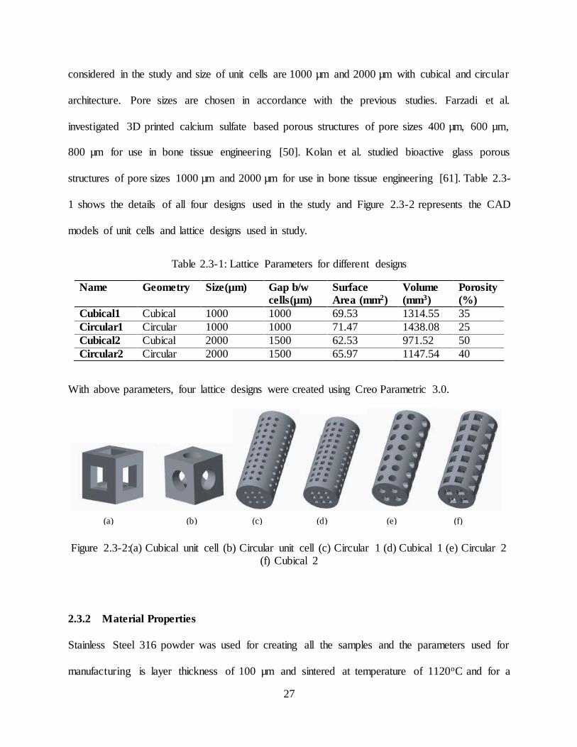
27
considered in the study and size of unit cells are 1000 µm and 2000 µm with cubical and circular
architecture. Pore sizes are chosen in accordance with the previous studies. Farzadi et al.
investigated 3D printed calcium sulfate based porous structures of pore sizes 400 µm, 600 µm,
800 µm for use in bone tissue engineering [50]. Kolan et al. studied bioactive glass porous
structures of pore sizes 1000 µm and 2000 µm for use in bone tissue engineering [61]. Table 2.3-
1 shows the details of all four designs used in the study and Figure 2.3-2 represents the CAD
models of unit cells and lattice designs used in study.
Table 2.3-1: Lattice Parameters for different designs
Name Geometry Size(µm) Gap b/w
cells(µm)
Surface
Area (mm2)
Volume
(mm3)
Porosity
(%)
Cubical1 Cubical 1000 1000 69.53 1314.55 35
Circular1 Circular 1000 1000 71.47 1438.08 25
Cubical2 Cubical 2000 1500 62.53 971.52 50
Circular2 Circular 2000 1500 65.97 1147.54 40
With above parameters, four lattice designs were created using Creo Parametric 3.0.
Figure 2.3-2:(a) Cubical unit cell (b) Circular unit cell (c) Circular 1 (d) Cubical 1 (e) Circular 2 (f) Cubical 2
2.3.2 Material Properties
Stainless Steel 316 powder was used for creating all the samples and the parameters used for
manufacturing is layer thickness of 100 µm and sintered at temperature of 1120oC and for a
(a) (b) (c) (d) (e) (f)

28
duration of 2 hours. Various lattice structures fabricated are shown in Figure 2.3-3. MTS testing
machine was used to carry out compression testing on four designs at same compression rate, 0.1
in/min and same conditions according to ASTM E9-09 standards.
Figure 2.3-3: Binder jetting fabricated samples of various lattice structures
Finite element analysis is done for compression test of four lattice configurations, the material
properties of stainless steel were assigned in ANSYS according to experimental data obtained from
compression testing of solid cylinder at same experimental conditions.
The material properties were derived from the physical testing of solid stainless-steel cylinder, the
samples were compressed and experimental stress-strain curve was used as input to create the
material model. A linear elastic along with multilinear isotropic plasticity model were assigned to
the model with the Young's modulus of 2508.4 Mpa and Poisson’s ratio of 0.3. The ultimate
compressive stress value assigned is 743.3 Mpa at a plastic strain of 0.36 which is obtained from
the experimental stress-strain curve. The lower surface of the lattice designs is fixed and the
displacement rate is applied on opposite surface to imitate the experimental setup. The simula t ion
was carried out for all the designs with same material model, same boundary conditions and the
results are presented in following sections.
29
CHAPTER 3
3.0 RESULTS AND DISCUSSION
Experimental analysis was performed to determine the effect and significance of layer thickness,
sintering time and sintering temperature on compressive strength, shrinkage rates. The same
experimental data was used to develop the model predicting compressive strength given the inputs
of layer thickness, sintering time and temperature. Finally, finite element simulation results were
compared with that of actual experimental results for four lattice structures considered in the study.
3.1 EXPERIMENTAL ANALYSIS: EFFECT OF BUILD PARAMETERS
Experiments were conducted according to full factorial design of experiments plan as discussed in
the last chapter. The length and diameter of each sample was recorded after sintering to get
shrinkage rate in radial and longitudinal directions and are calculated as below.
𝑅𝑎𝑑𝑖𝑎𝑙 𝑆ℎ𝑟𝑖𝑛𝑘𝑎𝑔ⅇ(%) = 𝑑𝑠 − 𝑑𝑖
𝑑𝑢
∗ 100
𝐿𝑜𝑛𝑔𝑖𝑡𝑢𝑑𝑖𝑛𝑎𝑙 𝑆ℎ𝑟𝑖𝑛𝑘𝑎𝑔ⅇ(%) = 𝑙𝑠 − 𝑙𝑖
𝑙𝑢
∗ 100
Where ds, di are diameters of sintered sample and input CAD model
ls, li are diameters of sintered sample and input CAD model
Along with shrinkage rates, ultimate compressive strength is also the output characteristic to be
studied. The load-displacement data from compression test were converted to stress-strain values,
the ultimate compressive strength is then obtained from stress-strain data.
30
𝐶𝑜𝑚𝑝𝑟ⅇ𝑠𝑠𝑖𝑣ⅇ 𝑆𝑡𝑟ⅇ𝑛𝑔𝑡ℎ(𝑀𝑝𝑎) = 𝐶𝑜𝑚𝑝𝑟ⅇ𝑠𝑠𝑖𝑣ⅇ 𝐿𝑜𝑎𝑑
𝐶𝑟𝑜𝑠𝑠 𝑠ⅇ𝑐𝑡𝑖𝑜𝑛𝑎𝑙 𝐴𝑟ⅇ𝑎
3.1.1 Solid Structure
The compressive strength, radial and longitudinal shrinkage for solid samples made with different
experimental settings were calculated and tabulated below. The experimental results from Table
3.1-1 were analyzed to find the effects of build parameters.
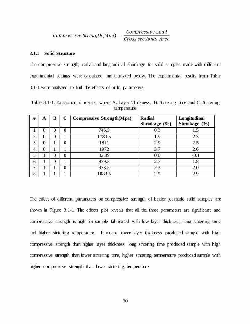
Table 3.1-1: Experimental results, where A: Layer Thickness, B: Sintering time and C: Sintering temperature
# A B C Compressive Strength(Mpa) Radial
Shrinkage (%)
Longitudinal
Shrinkage (%)
1 0 0 0 745.5 0.3 1.5
2 0 0 1 1780.5 1.9 2.3
3 0 1 0 1811 2.9 2.5
4 0 1 1 1972 3.7 2.6
5 1 0 0 82.89 0.0 -0.1
6 1 0 1 879.5 2.7 1.8
7 1 1 0 978.5 2.3 2.0
8 1 1 1 1083.5 2.5 2.9
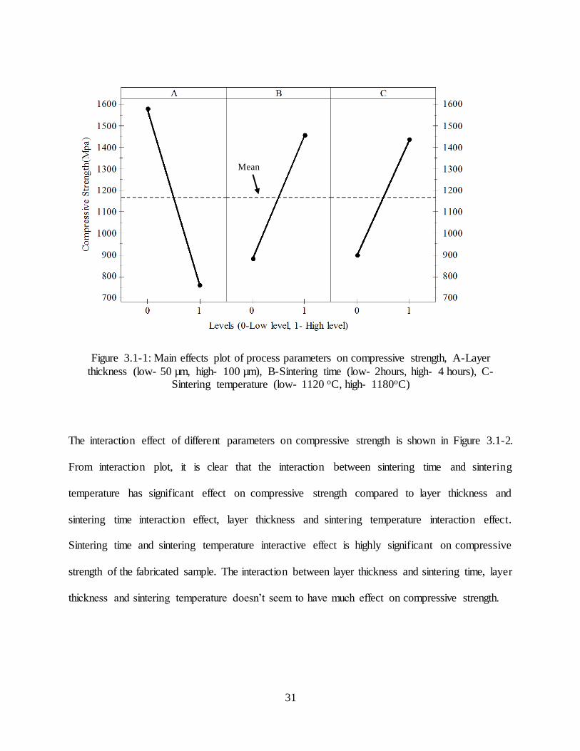
The effect of different parameters on compressive strength of binder jet made solid samples are
shown in Figure 3.1-1. The effects plot reveals that all the three parameters are significant and
compressive strength is high for sample fabricated with low layer thickness, long sintering time
and higher sintering temperature. It means lower layer thickness produced sample with high
compressive strength than higher layer thickness, long sintering time produced sample with high
compressive strength than lower sintering time, higher sintering temperature produced sample with
higher compressive strength than lower sintering temperature.
31
Figure 3.1-1: Main effects plot of process parameters on compressive strength, A-Layer
thickness (low- 50 µm, high- 100 µm), B-Sintering time (low- 2hours, high- 4 hours), C-Sintering temperature (low- 1120 oC, high- 1180oC)
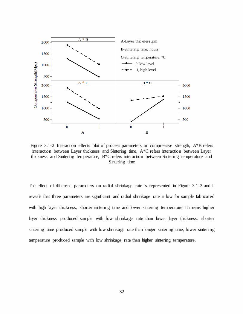
The interaction effect of different parameters on compressive strength is shown in Figure 3.1-2.
From interaction plot, it is clear that the interaction between sintering time and sintering
temperature has significant effect on compressive strength compared to layer thickness and
sintering time interaction effect, layer thickness and sintering temperature interaction effect.
Sintering time and sintering temperature interactive effect is highly significant on compressive
strength of the fabricated sample. The interaction between layer thickness and sintering time, layer
thickness and sintering temperature doesn’t seem to have much effect on compressive strength.
Mean
32
Figure 3.1-2: Interaction effects plot of process parameters on compressive strength, A*B refers
interaction between Layer thickness and Sintering time, A*C refers interaction between Layer thickness and Sintering temperature, B*C refers interaction between Sintering temperature and
Sintering time
The effect of different parameters on radial shrinkage rate is represented in Figure 3.1-3 and it
reveals that three parameters are significant and radial shrinkage rate is low for sample fabricated
with high layer thickness, shorter sintering time and lower sintering temperature It means higher
layer thickness produced sample with low shrinkage rate than lower layer thickness, shorter
sintering time produced sample with low shrinkage rate than longer sintering time, lower sintering
temperature produced sample with low shrinkage rate than higher sintering temperature.
A-Layer thickness, µm
B-Sintering time, hours
C-Sintering temperature, oC
0, low level
1, high level
33
Figure 3.1-3: Main effects plot of process parameters on radial shrinkage rate, A-Layer thickness
(low- 50 µm, high- 100 µm), B-Sintering time (low- 2hours, high- 4 hours), C-Sintering temperature (low- 1120 oC, high- 1180oC)
The interaction effect of different parameters on radial shrinkage is shown in Figure 3.1-4.From
interactions plot, it is evident that the interaction between sintering time and sintering temperature
has significant effect on radial shrinkage rate compared to layer thickness and sintering time
interaction effect, layer thickness and sintering temperature interaction effect. Sintering time and
sintering temperature interactive effect is highly significant on radial shrinkage of the fabricated
sample. Similar to interaction effect plot of compressive strength, the interaction between layer
thickness and sintering time, layer thickness and sintering temperature doesn’t seem to have much
effect on compressive strength.
Mean
34
Figure 3.1-4: Interaction effects plot of process parameters on radial shrinkage rate, A*B refers interaction between Layer thickness and Sintering time, A*C refers interaction between Layer
thickness and Sintering temperature, B*C refers interaction between Sintering temperature and Sintering time
Figure 3.1-5 shows the relationship between three factors layer thickness, sintering time and
sintering temperature on longitudinal shrinkage rate. Main effects plot reveals that three
parameters are significant and longitudinal shrinkage rate is low for sample fabricated with high
layer thickness, shorter sintering time and lower sintering temperature. It means higher laye r
thickness produced sample with low shrinkage rate than lower layer thickness, shorter sintering
time produced less shrinkage rate than longer sintering time, lower sintering temperature produced
low shrinkage rate than higher sintering temperature. The main effects plot of longitud ina l
shrinkage is similar to that of radial shrinkage.
A-Layer thickness, µm
B-Sintering time, hours
C-Sintering temperature, oC
0, low level
1, high level
35
Figure 3.1-5: Main effects plot of process parameters on longitudinal shrinkage, A-Layer thickness (low- 50 µm, high- 100 µm), B-Sintering time (low- 2hours, high- 4 hours), C-
Sintering temperature (low- 1120 oC, high- 1180oC)
Figure 3.1-6 reveals the combined influence of layer thickness and sintering time on longitud ina l
shrinkage rate. It is evident that the interaction between layer thickness and sintering time has
significant effect on longitudinal shrinkage rate compared to sintering time and sintering
temperature interaction effect, layer thickness and sintering temperature interaction effect.
Mean
36
Figure 3.1-6: Interaction effects plot of process parameters on longitudinal shrinkage rate, A*B
refers interaction between Layer thickness and Sintering time, A*C refers interaction between Layer thickness and Sintering temperature, B*C refers interaction between Sintering time and
Sintering temperature
The main effects and interaction effects plots shows the impact of each factor whereas analysis of
variance is performed to determine the significance of factors. The results of analysis give us the
contribution percentage of each parameter namely, Layer thickness, Sintering time and
temperature on Compressive Strength, Radial and Longitudinal shrinkage rate.
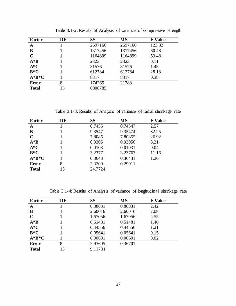
Table 3.1-2, 3.1-3, and 3.1-4 shows the analysis of variance results for compressive strength,
longitudinal shrinkage and radial shrinkage rates.
A-Layer thickness, µm
B-Sintering time, hours
C-Sintering temperature, oC
0, low level
1, high level
37
Table 3.1-2: Results of Analysis of variance of compressive strength
Factor DF SS MS F-Value
A 1 2697166 2697166 123.82
B 1 1317456 1317456 60.48 C 1 1164899 1164899 53.48
A*B 1 2323 2323 0.11 A*C 1 31576 31576 1.45 B*C 1 612784 612784 28.13
A*B*C 1 8317 8317 0.38
Error 8 174265 21783 Total 15 6008785
Table 3.1-3: Results of Analysis of variance of radial shrinkage rate
Factor DF SS MS F-Value
A 1 0.7455 0.74547 2.57
B 1 9.3547 9.35474 32.25 C 1 7.8086 7.80855 26.92 A*B 1 0.9305 0.93050 3.21
A*C 1 0.0103 0.01031 0.04 B*C 1 3.2377 3.23767 11.16
A*B*C 1 0.3643 0.36431 1.26
Error 8 2.3209 0.29011 Total 15 24.7724
Table 3.1-4: Results of Analysis of variance of longitudinal shrinkage rate
Factor DF SS MS F-Value
A 1 0.88831 0.88831 2.42 B 1 2.60016 2.60016 7.08 C 1 1.67056 1.67056 4.55
A*B 1 0.51481 0.51481 1.40 A*C 1 0.44556 0.44556 1.21
B*C 1 0.05641 0.05641 0.15 A*B*C 1 0.00601 0.00601 0.02
Error 8 2.93605 0.36701
Total 15 9.11784
38
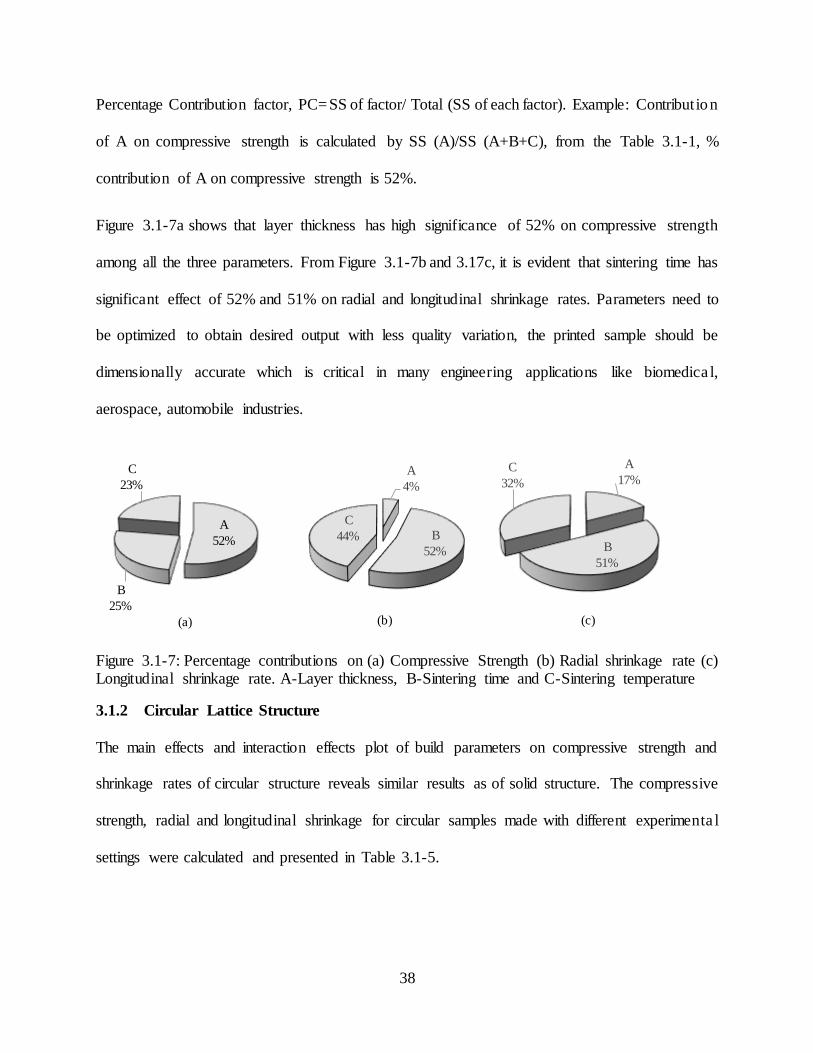
Percentage Contribution factor, PC= SS of factor/ Total (SS of each factor). Example: Contribution
of A on compressive strength is calculated by SS (A)/SS (A+B+C), from the Table 3.1-1, %
contribution of A on compressive strength is 52%.
Figure 3.1-7a shows that layer thickness has high significance of 52% on compressive strength
among all the three parameters. From Figure 3.1-7b and 3.17c, it is evident that sintering time has
significant effect of 52% and 51% on radial and longitudinal shrinkage rates. Parameters need to
be optimized to obtain desired output with less quality variation, the printed sample should be
dimensionally accurate which is critical in many engineering applications like biomedica l,
aerospace, automobile industries.
Figure 3.1-7: Percentage contributions on (a) Compressive Strength (b) Radial shrinkage rate (c) Longitudinal shrinkage rate. A-Layer thickness, B-Sintering time and C-Sintering temperature
3.1.2 Circular Lattice Structure
The main effects and interaction effects plot of build parameters on compressive strength and
shrinkage rates of circular structure reveals similar results as of solid structure. The compressive
strength, radial and longitudinal shrinkage for circular samples made with different experimenta l
settings were calculated and presented in Table 3.1-5.
A
52%
B
25%
C
23%
(a)
A
4%
B
52%
C
44%
(b)
A
17%
B
51%
C
32%
(c)
39
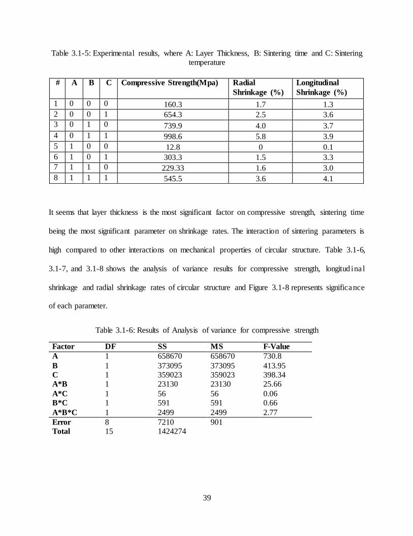
Table 3.1-5: Experimental results, where A: Layer Thickness, B: Sintering time and C: Sintering temperature
It seems that layer thickness is the most significant factor on compressive strength, sintering time
being the most significant parameter on shrinkage rates. The interaction of sintering parameters is
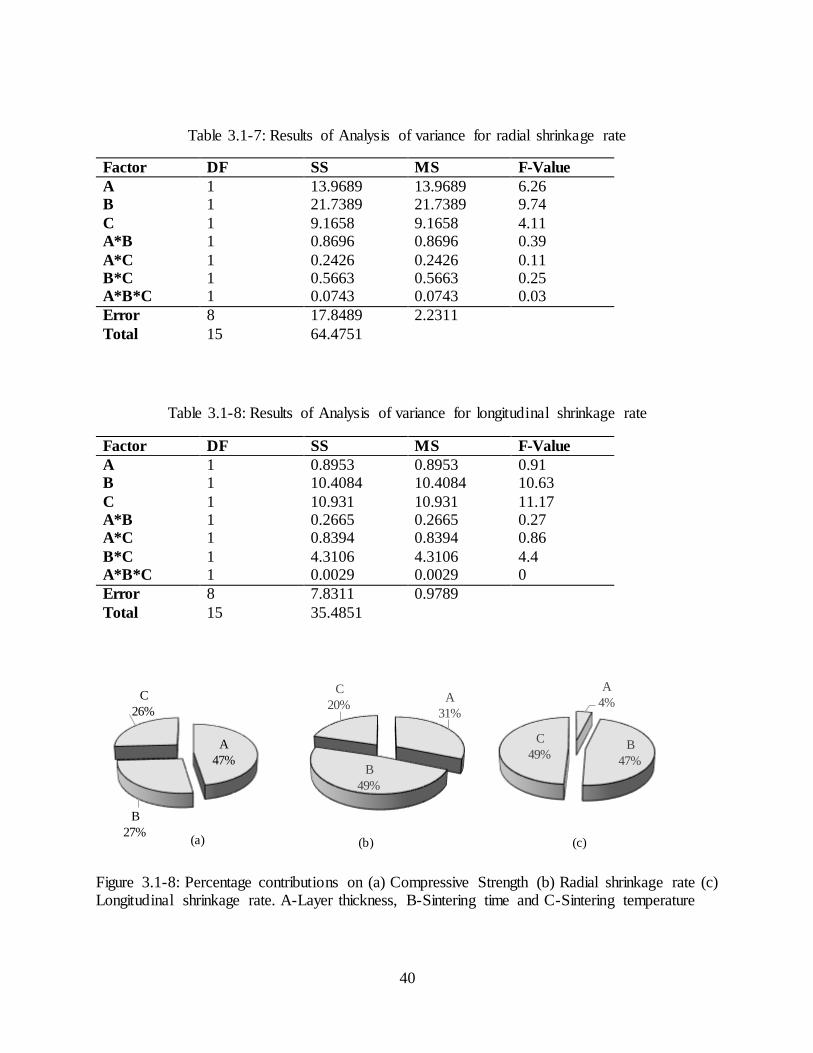
high compared to other interactions on mechanical properties of circular structure. Table 3.1-6,
3.1-7, and 3.1-8 shows the analysis of variance results for compressive strength, longitud ina l
shrinkage and radial shrinkage rates of circular structure and Figure 3.1-8 represents significance
of each parameter.
Table 3.1-6: Results of Analysis of variance for compressive strength
Factor DF SS MS F-Value
A 1 658670 658670 730.8
B 1 373095 373095 413.95 C 1 359023 359023 398.34 A*B 1 23130 23130 25.66
A*C 1 56 56 0.06 B*C 1 591 591 0.66
A*B*C 1 2499 2499 2.77
Error 8 7210 901 Total 15 1424274
# A B C Compressive Strength(Mpa) Radial
Shrinkage (%)
Longitudinal
Shrinkage (%)
1 0 0 0 160.3 1.7 1.3
2 0 0 1 654.3 2.5 3.6
3 0 1 0 739.9 4.0 3.7
4 0 1 1 998.6 5.8 3.9
5 1 0 0 12.8 0 0.1
6 1 0 1 303.3 1.5 3.3
7 1 1 0 229.33 1.6 3.0
8 1 1 1 545.5 3.6 4.1
40
Table 3.1-7: Results of Analysis of variance for radial shrinkage rate
Factor DF SS MS F-Value
A 1 13.9689 13.9689 6.26 B 1 21.7389 21.7389 9.74
C 1 9.1658 9.1658 4.11 A*B 1 0.8696 0.8696 0.39
A*C 1 0.2426 0.2426 0.11 B*C 1 0.5663 0.5663 0.25 A*B*C 1 0.0743 0.0743 0.03
Error 8 17.8489 2.2311
Total 15 64.4751
Table 3.1-8: Results of Analysis of variance for longitudinal shrinkage rate
Factor DF SS MS F-Value
A 1 0.8953 0.8953 0.91 B 1 10.4084 10.4084 10.63
C 1 10.931 10.931 11.17 A*B 1 0.2665 0.2665 0.27 A*C 1 0.8394 0.8394 0.86
B*C 1 4.3106 4.3106 4.4 A*B*C 1 0.0029 0.0029 0
Error 8 7.8311 0.9789
Total 15 35.4851
Figure 3.1-8: Percentage contributions on (a) Compressive Strength (b) Radial shrinkage rate (c) Longitudinal shrinkage rate. A-Layer thickness, B-Sintering time and C-Sintering temperature
A
47%
B
27%
C
26%
(a)
A
31%
B
49%
C
20%
(b)
A
4%
B
47%
C
49%
(c)
41
3.1.3 Cubical Lattice Structure
The compressive strength, radial and longitudinal shrinkage for cubical samples made with
different experimental settings were calculated and presented in Table 3.1-9.
Table 3.1-9: Experimental results, where A: Layer Thickness, B: Sintering time and C: Sintering temperature
The main effects and interaction effects plot of build parameters on compressive strength and
shrinkage rates of circular structure reveals that the compressive strength is highly influenced by
layer thickness, sintering temperature being the most significant parameter on shrinkage rates. The
interaction of sintering parameters is high compared to other interactions on mechanical properties
of circular structure. Table 3.1-10, 3.1-11, and 3.1-12 shows the analysis of variance results for
compressive strength, longitudinal shrinkage and radial shrinkage rates of circular structure and
Figure 3.1-9 represents significance of each parameter.
# A B C Compressive Strength(Mpa) Radial
Shrinkage (%)
Longitudinal
Shrinkage (%)
1 0 0 0 154.5 0.43 1.2
2 0 0 1 545.2 5.2 3.5
3 0 1 0 612.3 4.6 3.2
4 0 1 1 958.3 5.25 4.1
5 1 0 0 11.6 0 0.1
6 1 0 1 250.9 4.2 3.5
7 1 1 0 253.2 3.7 3.1
8 1 1 1 326.4 4.8 3.8

42
Table 3.1-10: Results of Analysis of variance for compressive strength
Factor DF SS MS F-Value
A 1 509939 509939 1943.83
B 1 352836 352836 1344.97 C 1 275205 275205 1049.05
A*B 1 76674 76674 292.27 A*C 1 44986 44986 171.48 B*C 1 11109 11109 42.35
A*B*C 1 3684 3684 14.04
Error 8 2099 262 Total 15 1276532
Table 3.1-11: Results of Analysis of variance for radial shrinkage rate
Factor DF SS MS F-Value
A 1 1.7556 1.7556 22.25
B 1 18.5761 18.5761 235.48 C 1 28.5156 28.5156 361.47 A*B 1 0.0081 0.0081 0.1
A*C 1 0.0064 0.0064 0.08 B*C 1 13.286 13.286 168.42
A*B*C 1 0.2256 0.2256 2.86
Error 8 0.6311 0.0789 Total 15 63.0046
Table 3.1-12: Results of Analysis of variance for longitudinal shrinkage rate
Factor DF SS MS F-Value
A 1 0.4692 0.4692 1.51 B 1 8.5849 8.5849 27.6
C 1 13.7641 13.7641 44.25 A*B 1 0.1521 0.1521 0.49
A*C 1 0.1681 0.1681 0.54 B*C 1 4.3056 4.3056 13.84 A*B*C 1 0.3782 0.3782 1.22
Error 8 2.4887 0.3111
Total 15 30.311
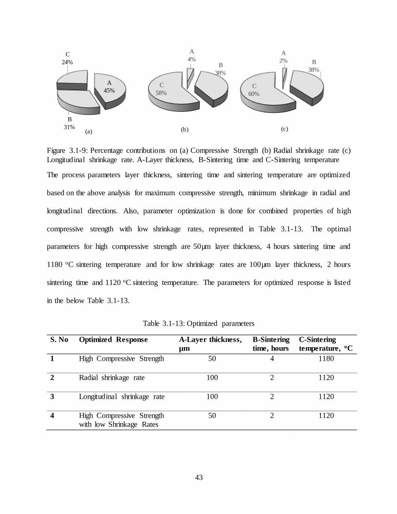
43
Figure 3.1-9: Percentage contributions on (a) Compressive Strength (b) Radial shrinkage rate (c)
Longitudinal shrinkage rate. A-Layer thickness, B-Sintering time and C-Sintering temperature
The process parameters layer thickness, sintering time and sintering temperature are optimized
based on the above analysis for maximum compressive strength, minimum shrinkage in radial and
longitudinal directions. Also, parameter optimization is done for combined properties of high
compressive strength with low shrinkage rates, represented in Table 3.1-13. The optimal
parameters for high compressive strength are 50µm layer thickness, 4 hours sintering time and
1180 oC sintering temperature and for low shrinkage rates are 100µm layer thickness, 2 hours
sintering time and 1120 oC sintering temperature. The parameters for optimized response is listed
in the below Table 3.1-13.
Table 3.1-13: Optimized parameters
S. No Optimized Response A-Layer thickness,
µm
B-Sintering
time, hours
C-Sintering
temperature, oC
1 High Compressive Strength 50 4 1180
2 Radial shrinkage rate 100 2 1120
3 Longitudinal shrinkage rate 100 2 1120
4 High Compressive Strength with low Shrinkage Rates
50 2 1120
A
45%
B
31%
C
24%
(a)
A
4%B
38%
C
58%
(b)
A
2% B
38%
C
60%
(c)
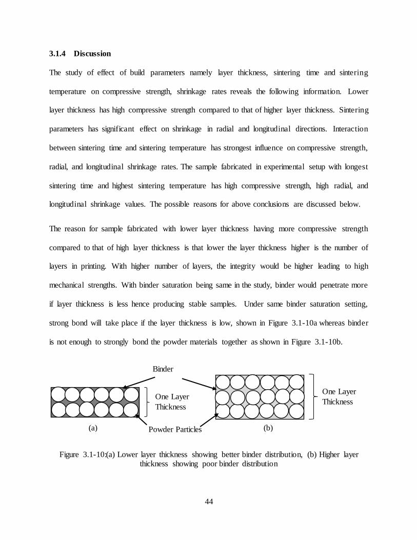
44
3.1.4 Discussion
The study of effect of build parameters namely layer thickness, sintering time and sintering
temperature on compressive strength, shrinkage rates reveals the following information. Lower
layer thickness has high compressive strength compared to that of higher layer thickness. Sintering
parameters has significant effect on shrinkage in radial and longitudinal directions. Interaction
between sintering time and sintering temperature has strongest influence on compressive strength,
radial, and longitudinal shrinkage rates. The sample fabricated in experimental setup with longest
sintering time and highest sintering temperature has high compressive strength, high radial, and
longitudinal shrinkage values. The possible reasons for above conclusions are discussed below.
The reason for sample fabricated with lower layer thickness having more compressive strength
compared to that of high layer thickness is that lower the layer thickness higher is the number of
layers in printing. With higher number of layers, the integrity would be higher leading to high
mechanical strengths. With binder saturation being same in the study, binder would penetrate more
if layer thickness is less hence producing stable samples. Under same binder saturation setting,
strong bond will take place if the layer thickness is low, shown in Figure 3.1-10a whereas binder
is not enough to strongly bond the powder materials together as shown in Figure 3.1-10b.
Figure 3.1-10:(a) Lower layer thickness showing better binder distribution, (b) Higher layer thickness showing poor binder distribution
(a) (b)
One Layer
Thickness
One Layer
Thickness
Binder
Powder Particles
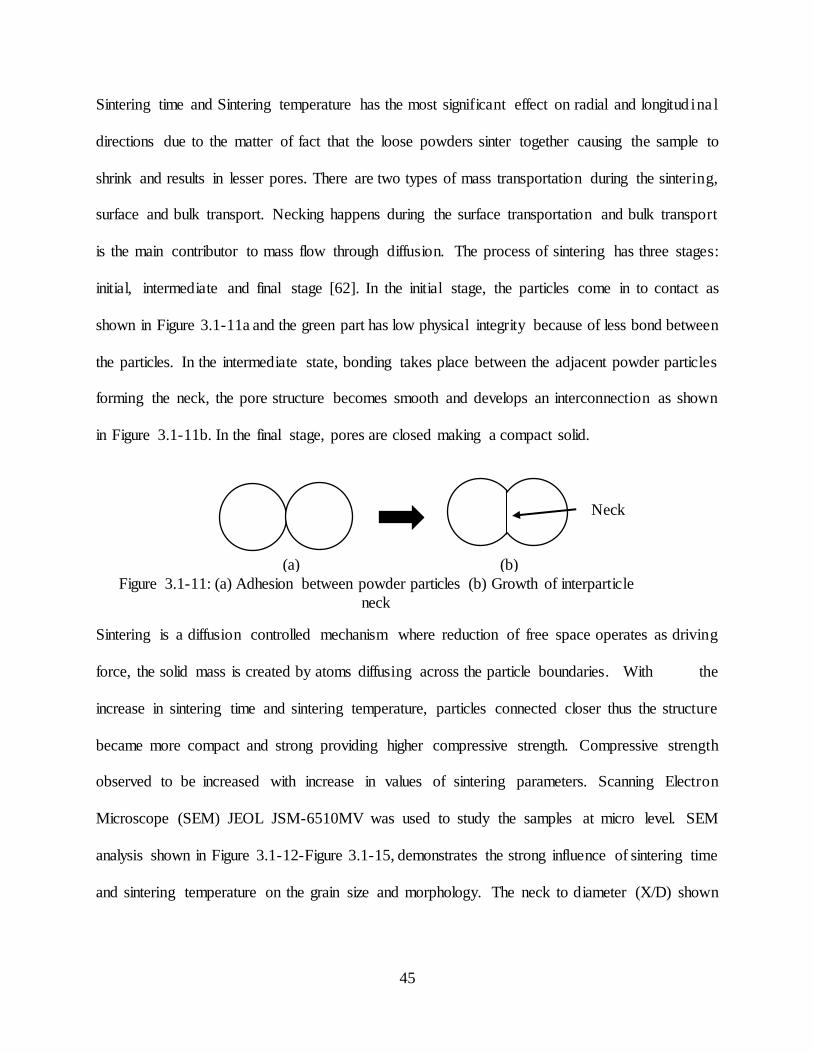
45
Sintering time and Sintering temperature has the most significant effect on radial and longitud ina l
directions due to the matter of fact that the loose powders sinter together causing the sample to
shrink and results in lesser pores. There are two types of mass transportation during the sintering,
surface and bulk transport. Necking happens during the surface transportation and bulk transport
is the main contributor to mass flow through diffusion. The process of sintering has three stages:
initial, intermediate and final stage [62]. In the initial stage, the particles come in to contact as
shown in Figure 3.1-11a and the green part has low physical integrity because of less bond between
the particles. In the intermediate state, bonding takes place between the adjacent powder particles
forming the neck, the pore structure becomes smooth and develops an interconnection as shown
in Figure 3.1-11b. In the final stage, pores are closed making a compact solid.
Sintering is a diffusion controlled mechanism where reduction of free space operates as driving
force, the solid mass is created by atoms diffusing across the particle boundaries. With the
increase in sintering time and sintering temperature, particles connected closer thus the structure
became more compact and strong providing higher compressive strength. Compressive strength
observed to be increased with increase in values of sintering parameters. Scanning Electron
Microscope (SEM) JEOL JSM-6510MV was used to study the samples at micro level. SEM
analysis shown in Figure 3.1-12-Figure 3.1-15, demonstrates the strong influence of sintering time
and sintering temperature on the grain size and morphology. The neck to diameter (X/D) shown
Figure 3.1-11: (a) Adhesion between powder particles (b) Growth of interparticle
neck
Neck
(a) (b)
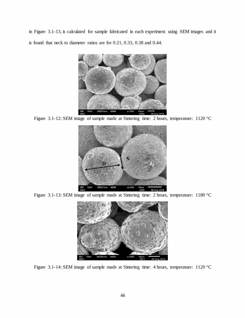
46
in Figure 3.1-13, is calculated for sample fabricated in each experiment using SEM images and it
is found that neck to diameter ratios are for 0.21, 0.33, 0.38 and 0.44.
Figure 3.1-12: SEM image of sample made at Sintering time: 2 hours, temperature: 1120 oC
Figure 3.1-13: SEM image of sample made at Sintering time: 2 hours, temperature: 1180 oC
Figure 3.1-14: SEM image of sample made at Sintering time: 4 hours, temperature: 1120 oC

47
Figure 3.1-15: SEM image of sample made at Sintering time: 4 hours, temperature: 1180 oC
The necking is high for experiment with long sintering time and sintering temperature and it is
understandable that compressive strength is maximum for sample with high sintering time and
sintering temperature because of strong bonding between the particles at micro level. Therefore,
controlling sintering time and sintering temperature at lower layer thickness will produce a sample
with high compressive strengths and less shrinkage rates.
3.2 NEURAL NETWORK RESULTS
1. First case: The data used for testing is from compression testing of solid structure.
2. Second case: The data used for testing is from compression testing of circular structure.
3. Third case: The data used for testing from compression testing of cubical structure.
3.2.1 Solid Structure
With the normalized data in Table 3.2-1, the feedforward backpropagation network was trained
with seven datasets leaving behind the one data set of experiment 7 for testing the network
performance.
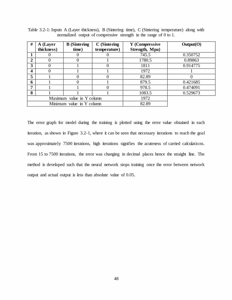
48
Table 3.2-1: Inputs A (Layer thickness), B (Sintering time), C (Sintering temperature) along with normalized output of compressive strength in the range of 0 to 1.
# A (Layer
thickness)
B (Sintering
time)
C (Sintering
temperature)
Y (Compressive
Strength, Mpa)
Output(O)
1 0 0 0 745.5 0.350752
2 0 0 1 1780.5 0.89863
3 0 1 0 1811 0.914775
4 0 1 1 1972 1
5 1 0 0 82.89 0
6 1 0 1 879.5 0.421685
7 1 1 0 978.5 0.474091
8 1 1 1 1083.5 0.529673
Maximum value in Y column 1972
Minimum value in Y column 82.89
The error graph for model during the training is plotted using the error value obtained in each
iteration, as shown in Figure 3.2-1, where it can be seen that necessary iterations to reach the goal
was approximately 7500 iterations, high iterations signifies the acuteness of carried calculations.
From 15 to 7500 iterations, the error was changing in decimal places hence the straight line. The
method is developed such that the neural network stops training once the error between network
output and actual output is less than absolute value of 0.05.
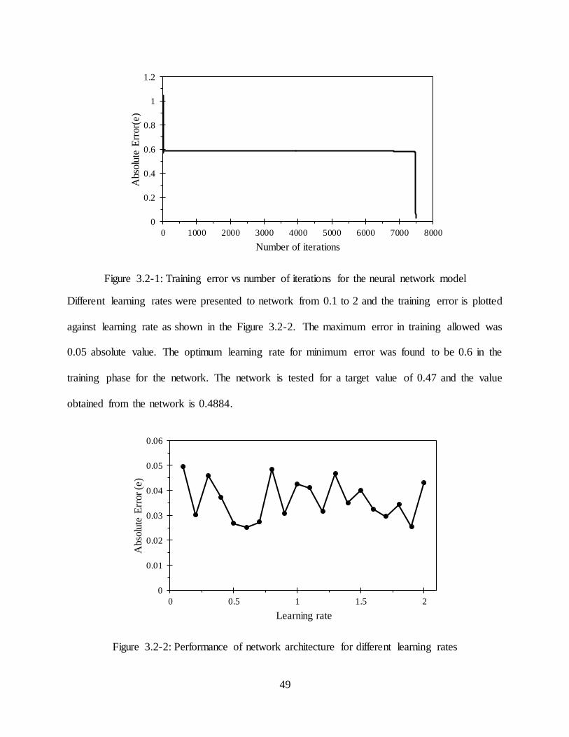
49
Figure 3.2-1: Training error vs number of iterations for the neural network model
Different learning rates were presented to network from 0.1 to 2 and the training error is plotted
against learning rate as shown in the Figure 3.2-2. The maximum error in training allowed was
0.05 absolute value. The optimum learning rate for minimum error was found to be 0.6 in the
training phase for the network. The network is tested for a target value of 0.47 and the value
obtained from the network is 0.4884.
Figure 3.2-2: Performance of network architecture for different learning rates
0
0.2
0.4
0.6
0.8
1
1.2
0 1000 2000 3000 4000 5000 6000 7000 8000
Abso
lute
Err
or(
e)
Number of iterations
0
0.01
0.02
0.03
0.04
0.05
0.06
0 0.5 1 1.5 2
Abso
lute
Err
or
(e)
Learning rate
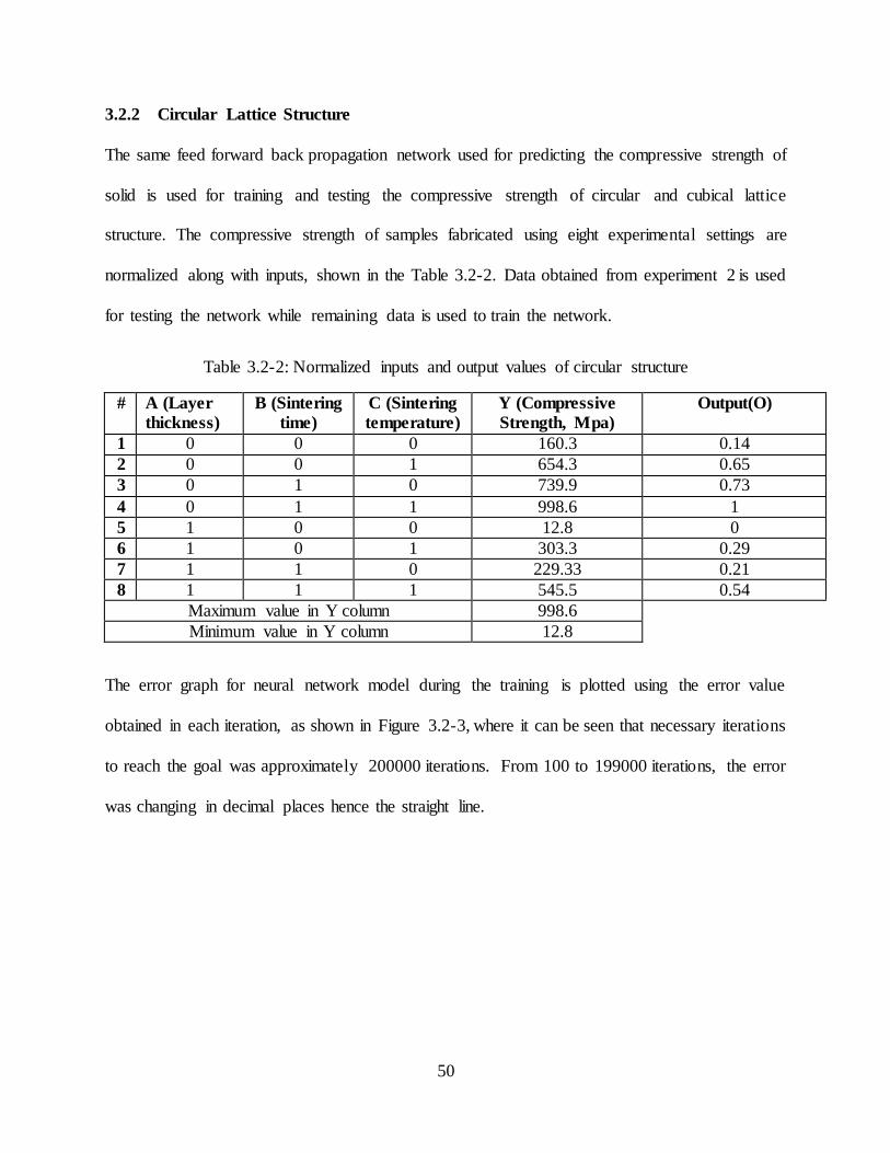
50
3.2.2 Circular Lattice Structure
The same feed forward back propagation network used for predicting the compressive strength of
solid is used for training and testing the compressive strength of circular and cubical lattice
structure. The compressive strength of samples fabricated using eight experimental settings are
normalized along with inputs, shown in the Table 3.2-2. Data obtained from experiment 2 is used
for testing the network while remaining data is used to train the network.
Table 3.2-2: Normalized inputs and output values of circular structure
# A (Layer
thickness)
B (Sintering
time)
C (Sintering
temperature)
Y (Compressive
Strength, Mpa)
Output(O)
1 0 0 0 160.3 0.14
2 0 0 1 654.3 0.65
3 0 1 0 739.9 0.73
4 0 1 1 998.6 1
5 1 0 0 12.8 0
6 1 0 1 303.3 0.29
7 1 1 0 229.33 0.21
8 1 1 1 545.5 0.54
Maximum value in Y column 998.6
Minimum value in Y column 12.8
The error graph for neural network model during the training is plotted using the error value
obtained in each iteration, as shown in Figure 3.2-3, where it can be seen that necessary iterations
to reach the goal was approximately 200000 iterations. From 100 to 199000 iterations, the error
was changing in decimal places hence the straight line.
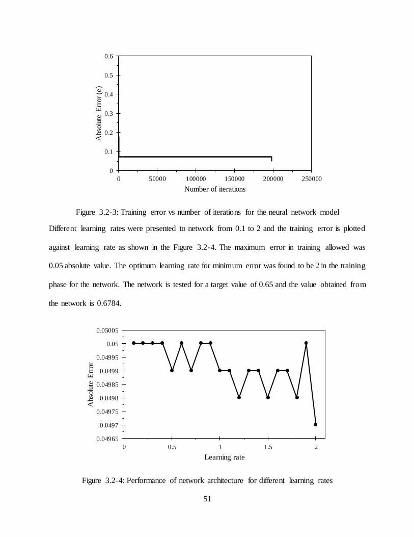
51
Figure 3.2-3: Training error vs number of iterations for the neural network model
Different learning rates were presented to network from 0.1 to 2 and the training error is plotted
against learning rate as shown in the Figure 3.2-4. The maximum error in training allowed was
0.05 absolute value. The optimum learning rate for minimum error was found to be 2 in the training
phase for the network. The network is tested for a target value of 0.65 and the value obtained from
the network is 0.6784.
Figure 3.2-4: Performance of network architecture for different learning rates
0
0.1
0.2
0.3
0.4
0.5
0.6
0 50000 100000 150000 200000 250000
Abso
lute
Err
or
(e)
Number of iterations
0.04965
0.0497
0.04975
0.0498
0.04985
0.0499
0.04995
0.05
0.05005
0 0.5 1 1.5 2
Abso
lute
Err
or
Learning rate

52
3.2.3 Cubical Lattice Structure
The compressive strength of cubical samples fabricated using eight experimental settings are
normalized along with inputs, shown in the Table 3.2-3. Data obtained from experiment 6 is used
for testing the network while remaining data is used to train the network.
Table 3.2-3: Normalized inputs and output values of cubical structure
# A (Layer
thickness)
B (Sintering
time)
C (Sintering
temperature)
Y (Compressive
Strength, Mpa)
Output(O)
1 0 0 0 154.5 0.15
2 0 0 1 545.2 0.56
3 0 1 0 612.3 0.63
4 0 1 1 958.3 1
5 1 0 0 11.6 0
6 1 0 1 250.9 0.25
7 1 1 0 253.2 0.26
8 1 1 1 326.4 0.33
Maximum value in Y column 958.3
Minimum value in Y column 11.6
The error graph for neural network model during the training is plotted using the error value
obtained in each iteration, as shown in Figure 3.2-5, where it can be seen that necessary iterations
to reach the goal was approximately 7500 iterations. From 75 to 7500 iterations, the error was
changing in decimal places hence the straight line.

53
Figure 3.2-5: Training error vs number of iterations for the neural network model
Different learning rates were presented to network from 0.1 to 2 and the training error is plotted
against learning rate as shown in the Figure 3.2-6. The maximum error in training allowed was
0.05 absolute value. The optimum learning rate for minimum error was found to be 2 in the trainin g
phase for the network. The network is tested for a target value of 0.25 and the value obtained from
the network is 0.2759.
Figure 3.2-6: Performance of network architecture for different learning rates
0
0.2
0.4
0.6
0.8
1
1.2
0 1000 2000 3000 4000 5000 6000 7000 8000
Abso
lute
Err
or(
e)
Iterations
0.0488
0.049
0.0492
0.0494
0.0496
0.0498
0.05
0.0502
0 0.5 1 1.5 2
Abso
lute
Err
or(
e)
Learning rate
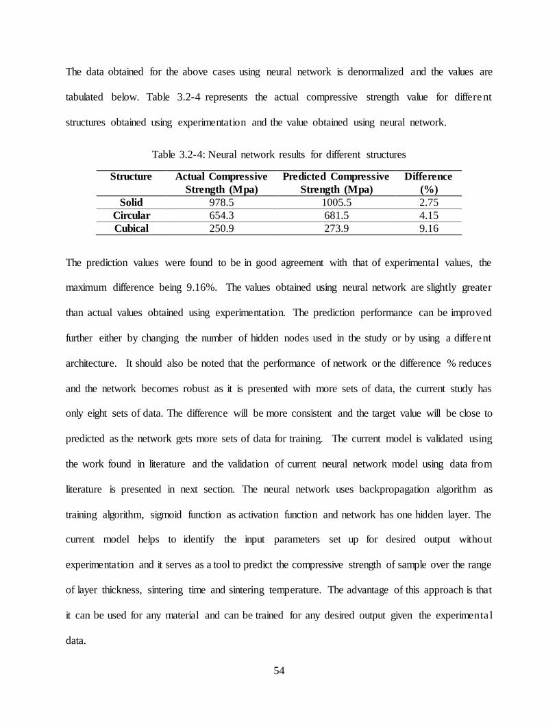
54
The data obtained for the above cases using neural network is denormalized and the values are
tabulated below. Table 3.2-4 represents the actual compressive strength value for different
structures obtained using experimentation and the value obtained using neural network.
Table 3.2-4: Neural network results for different structures
Structure Actual Compressive
Strength (Mpa)
Predicted Compressive
Strength (Mpa)
Difference
(%)
Solid 978.5 1005.5 2.75
Circular 654.3 681.5 4.15
Cubical 250.9 273.9 9.16
The prediction values were found to be in good agreement with that of experimental values, the
maximum difference being 9.16%. The values obtained using neural network are slightly greater
than actual values obtained using experimentation. The prediction performance can be improved
further either by changing the number of hidden nodes used in the study or by using a different
architecture. It should also be noted that the performance of network or the difference % reduces
and the network becomes robust as it is presented with more sets of data, the current study has
only eight sets of data. The difference will be more consistent and the target value will be close to
predicted as the network gets more sets of data for training. The current model is validated using
the work found in literature and the validation of current neural network model using data from
literature is presented in next section. The neural network uses backpropagation algorithm as
training algorithm, sigmoid function as activation function and network has one hidden layer. The
current model helps to identify the input parameters set up for desired output without
experimentation and it serves as a tool to predict the compressive strength of sample over the range
of layer thickness, sintering time and sintering temperature. The advantage of this approach is that
it can be used for any material and can be trained for any desired output given the experimenta l
data.
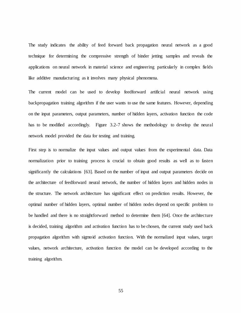
55
The study indicates the ability of feed forward back propagation neural network as a good
technique for determining the compressive strength of binder jetting samples and reveals the
applications on neural network in material science and engineering particularly in complex fields
like additive manufacturing as it involves many physical phenomena.
The current model can be used to develop feedforward artificial neural network using
backpropagation training algorithm if the user wants to use the same features. However, depending
on the input parameters, output parameters, number of hidden layers, activation function the code
has to be modified accordingly. Figure 3.2-7 shows the methodology to develop the neural
network model provided the data for testing and training.
First step is to normalize the input values and output values from the experimental data. Data
normalization prior to training process is crucial to obtain good results as well as to fasten
significantly the calculations [63]. Based on the number of input and output parameters decide on
the architecture of feedforward neural network, the number of hidden layers and hidden nodes in
the structure. The network architecture has significant effect on prediction results. However, the
optimal number of hidden layers, optimal number of hidden nodes depend on specific problem to
be handled and there is no straightforward method to determine them [64]. Once the architecture
is decided, training algorithm and activation function has to be chosen, the current study used back
propagation algorithm with sigmoid activation function. With the normalized input values, target
values, network architecture, activation function the model can be developed according to the
training algorithm.
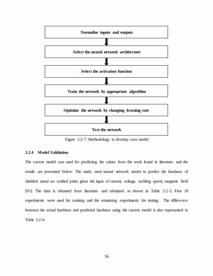
56
3.2.4 Model Validation
The current model was used for predicting the values from the work found in literature and the
results are presented below. The study used neural network model to predict the hardness of
shielded metal arc welded joints given the input of current, voltage, welding speed, magnetic field
[65]. The data is obtained from literature and tabulated as shown in Table 3.2-5. First 18
experiments were used for training and the remaining experiments for testing. The difference
between the actual hardness and predicted hardness using the current model is also represented in
Table 3.2-6.
Normalize inputs and outputs
Select the neural network architecture
Select the activation function
Train the network by appropriate algorithm
Optimize the network by changing learning rate
Test the network
Figure 3.2-7: Methodology to develop own model
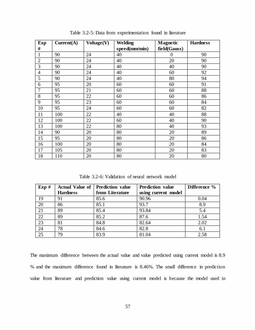
57
Table 3.2-5: Data from experimentation found in literature
Exp
#
Current(A) Voltage(V) Welding
speed(mm/min)
Magnetic
field(Gauss)
Hardness
1 90 24 40 0 90
2 90 24 40 20 90
3 90 24 40 40 90
4 90 24 40 60 92
5 90 24 40 80 94
6 95 20 60 60 91
7 95 21 60 60 88
8 95 22 60 60 86
9 95 23 60 60 84
10 95 24 60 60 82
11 100 22 40 40 88
12 100 22 60 40 90
13 100 22 80 40 93
14 90 20 80 20 89
15 95 20 80 20 86
16 100 20 80 20 84
17 105 20 80 20 83
18 110 20 80 20 80
Table 3.2-6: Validation of neural network model
Exp # Actual Value of
Hardness
Prediction value
from Literature
Prediction value
using current model
Difference %
19 91 85.6 90.96 0.04
20 86 85.1 93.7 8.9
21 89 85.4 93.84 5.4
22 89 85.2 87.6 1.54
23 81 84.8 82.64 2.02
24 78 84.6 82.8 6.1
25 79 83.9 81.04 2.58
The maximum difference between the actual value and value predicted using current model is 8.9
% and the maximum difference found in literature is 8.46%. The small difference in prediction
value from literature and prediction value using current model is because the model used in
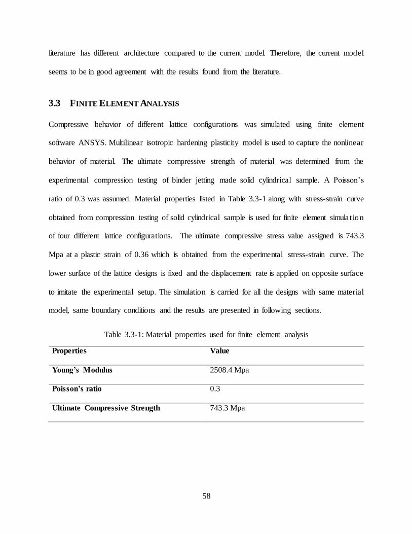
58
literature has different architecture compared to the current model. Therefore, the current model
seems to be in good agreement with the results found from the literature.
3.3 FINITE ELEMENT ANALYSIS
Compressive behavior of different lattice configurations was simulated using finite element
software ANSYS. Multilinear isotropic hardening plasticity model is used to capture the nonlinear
behavior of material. The ultimate compressive strength of material was determined from the
experimental compression testing of binder jetting made solid cylindrical sample. A Poisson’s
ratio of 0.3 was assumed. Material properties listed in Table 3.3-1 along with stress-strain curve
obtained from compression testing of solid cylindrical sample is used for finite element simula t ion
of four different lattice configurations. The ultimate compressive stress value assigned is 743.3
Mpa at a plastic strain of 0.36 which is obtained from the experimental stress-strain curve. The
lower surface of the lattice designs is fixed and the displacement rate is applied on opposite surface
to imitate the experimental setup. The simulation is carried for all the designs with same material
model, same boundary conditions and the results are presented in following sections.
Table 3.3-1: Material properties used for finite element analysis
Properties Value
Young’s Modulus 2508.4 Mpa
Poisson’s ratio 0.3
Ultimate Compressive Strength 743.3 Mpa
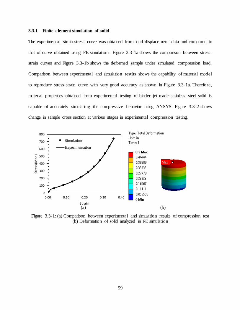
59
3.3.1 Finite element simulation of solid
The experimental strain-stress curve was obtained from load-displacement data and compared to
that of curve obtained using FE simulation. Figure 3.3-1a shows the comparison between stress-
strain curves and Figure 3.3-1b shows the deformed sample under simulated compression load.
Comparison between experimental and simulation results shows the capability of material model
to reproduce stress-strain curve with very good accuracy as shown in Figure 3.3-1a. Therefore,
material properties obtained from experimental testing of binder jet made stainless steel solid is
capable of accurately simulating the compressive behavior using ANSYS. Figure 3.3-2 shows
change in sample cross section at various stages in experimental compression testing.
Figure 3.3-1: (a) Comparison between experimental and simulation results of compression test (b) Deformation of solid analyzed in FE simulation
0
100
200
300
400
500
600
700
800
0.00 0.10 0.20 0.30 0.40
Stre
ss(M
pa
)
Strain
Simulation
Experimentation
(a) (b)
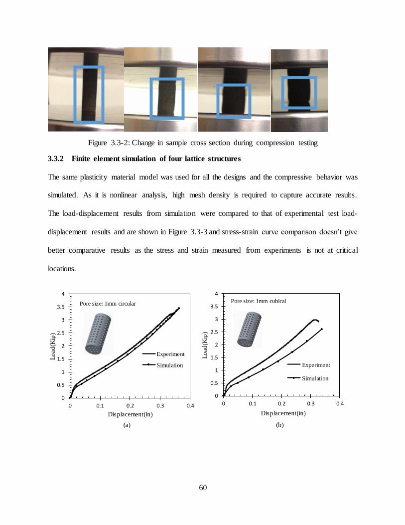
60
Figure 3.3-2: Change in sample cross section during compression testing
3.3.2 Finite element simulation of four lattice structures
The same plasticity material model was used for all the designs and the compressive behavior was
simulated. As it is nonlinear analysis, high mesh density is required to capture accurate results.
The load-displacement results from simulation were compared to that of experimental test load-
displacement results and are shown in Figure 3.3-3 and stress-strain curve comparison doesn’t give
better comparative results as the stress and strain measured from experiments is not at critical
locations.
0
0.5
1
1.5
2
2.5
3
3.5
4
0 0.1 0.2 0.3 0.4
Lo
ad
(Kip
)
Displacement(in)
Experiment
Simulation
0
0.5
1
1.5
2
2.5
3
3.5
4
0 0.1 0.2 0.3 0.4
Lo
ad
(Kip
)
Displacement(in)
Experiment
Simulation
(a) (b)
Pore size: 1mm circular Pore size: 1mm cubical

61
Figure 3.3-3: Load-Displacement curve comparison of simulation with experimental data. (a) Circular1, (b) Cubical 1, (c) Circular 2, (d) Cubical 2
Deformed images of samples during FE simulation and experimental testing is shown in Figure
3.3-4 and Figure 3.3-5 respectively. The displacements induced in experimentation and Finite
element simulation are similar and all the lattice structures shown the maximum displacement at
the surface where load applied and the lowest at supporting surface.
Figure 3.3-4: Deformed images of FE simulation (a) Circular 1, (b) Cubical 1, (c) Circular 2 and
(d) Cubical 2
0
0.5
1
1.5
2
2.5
0 0.1 0.2 0.3 0.4
Lo
ad
(Kip
)
Displacement(in)
Experiment
Simulation
0
0.5
1
1.5
2
2.5
0 0.1 0.2 0.3 0.4
Lo
ad
(Kip
)
Displacement(in)
Experiment
Simulation
(a) (b) (c) (d)
(c) (d)
Pore size: 2mm circular Pore size: 2mm cubical
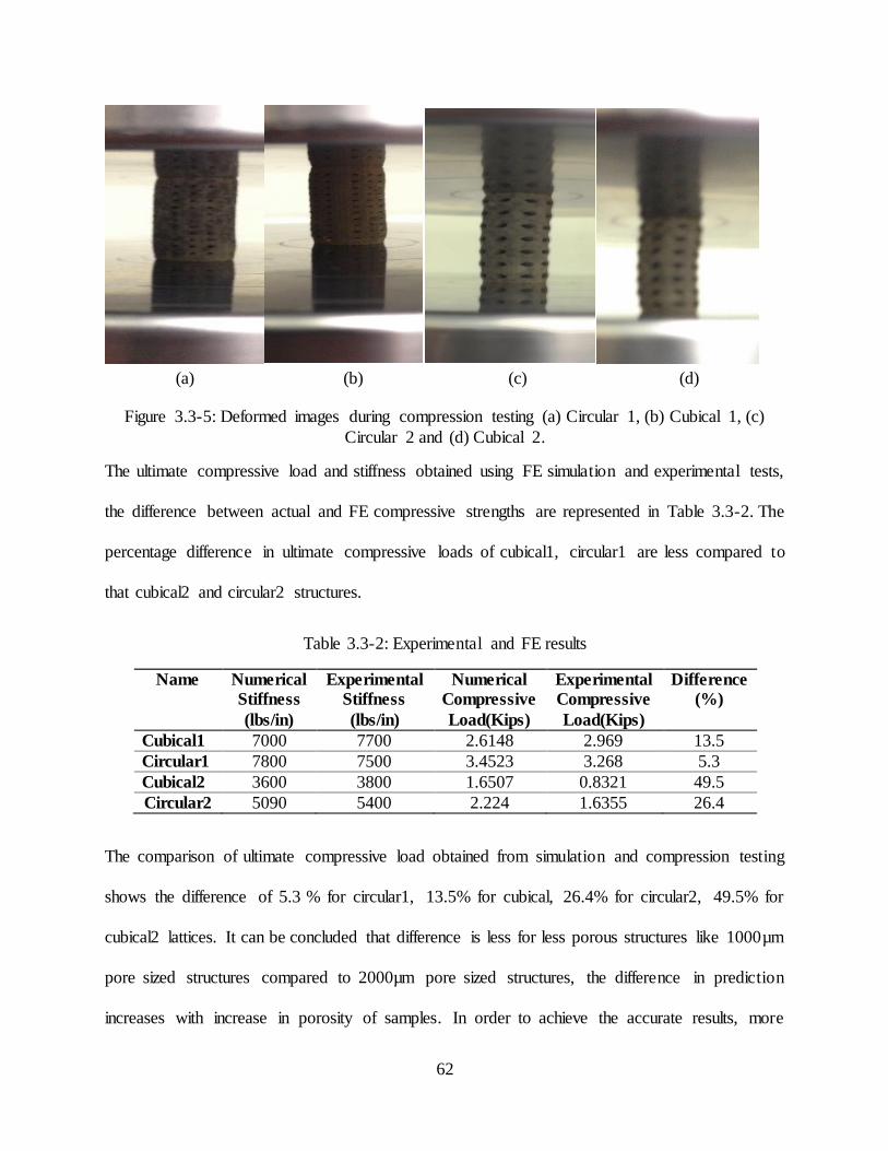
62
Figure 3.3-5: Deformed images during compression testing (a) Circular 1, (b) Cubical 1, (c)
Circular 2 and (d) Cubical 2.
The ultimate compressive load and stiffness obtained using FE simulation and experimental tests,
the difference between actual and FE compressive strengths are represented in Table 3.3-2. The
percentage difference in ultimate compressive loads of cubical1, circular1 are less compared to
that cubical2 and circular2 structures.
Table 3.3-2: Experimental and FE results
Name Numerical
Stiffness
(lbs/in)
Experimental
Stiffness
(lbs/in)
Numerical
Compressive
Load(Kips)
Experimental
Compressive
Load(Kips)
Difference
(%)
Cubical1 7000 7700 2.6148 2.969 13.5
Circular1 7800 7500 3.4523 3.268 5.3
Cubical2 3600 3800 1.6507 0.8321 49.5
Circular2 5090 5400 2.224 1.6355 26.4
The comparison of ultimate compressive load obtained from simulation and compression testing
shows the difference of 5.3 % for circular1, 13.5% for cubical, 26.4% for circular2, 49.5% for
cubical2 lattices. It can be concluded that difference is less for less porous structures like 1000µm
pore sized structures compared to 2000µm pore sized structures, the difference in prediction
increases with increase in porosity of samples. In order to achieve the accurate results, more
(a) (b) (c) (d)
63
mechanical tests along with thermal examination has to be performed on solid cylinder to make
the material model account for the real material behavior. The nonlinear analysis involving plastic
deformation needs high mesh density to capture the results more accurately and also the reason of
error could be from the fact that the finite element solvers doesn’t account for porosity, the sample
is assumed to be made from conventional manufacturing or subtractive manufacturing and also the
solver assumes there is no force in directions other than the one in which loading takes place. The
material model is still preliminary model, it can be improved and the difference would have been
less if the material accounts for overall failure.

64
3.4 APPLICATIONS
Binder jet additive manufacturing is still in its preliminary research stage compared to other metal
additive manufacturing technologies like selective laser melting, direct metal laser sintering,
especially in order to transit the binder jet additive manufacturing from prototyping to real
production lot of research has to be established. The current study of process-parameter
optimization serves as guideline to adjust the printing parameters for fabrication of variety of
materials for different applications and it also helps to better understand the machine for fabricating
quality products. Process-property optimization study suggests the set of process parameters to
achieve desired compressive strength with low shrinkage rates, reducing the experimentation cost.
The entire binder jetting process is shown in Figure 3.4-1. It can be seen there are lot of phenomena
which effects the overall characteristics of final product.
Figure 3.4-1: Flowchart representing the complete binder jetting process [66]
65
Physical modelling of binder jet additive manufacturing is almost impossible as it involves lot of
phenomena like CAD to STL conversion, binder powder reaction, heat treatment, information
exchange, powder chemistry. There has to be data-driven model which serves as a guide to
quantify the relationship between input and output parameters. The current neural network model
helps to identify the set of parameters to achieve desired compressive strength eliminating the need
of experimentation.
It is also important to have finite element models of binder jet made samples so that the technology
can be deployed for specific application, one such important application is bone scaffold
engineering. Finite element models are useful for stress-strain analysis, determination of
mechanical properties and helps in design optimization of scaffolds/implants. The current FE study
serves as starting point for more research on finite element modelling of binder jet made samples
using experimentation.
66
3.5 CONCLUSION AND SUGGESTION FOR FUTURE WORK
Stainless steel cylindrical samples were fabricated for each run of experimental plan with different
process parameters. Layer thickness, sintering time and sintering temperature were analyzed to the
study its effect on compressive strength and shrinkage rates. The optimized response considered
in the study are high compressive strength, low radial and longitudinal shrinkage rates.
Visualization plots shows that layer thickness has most influence on compressive strength whereas
sintering time has higher influence on radial and longitudinal shrinkage rates. The optimal
parameters for high compressive strength are 50µm layer thickness, 4 hours sintering time and
1180 oC sintering temperature and for low shrinkage rates are 100µm layer thickness, 2 hours
sintering time and 1120 oC sintering temperature. The identified optimal parameters might not be
same for different material, but the study serves as guidelines to adjust printing parameters for
different materials. Along with parameter optimization, the study also investigated the application
of artificial neural network for property prediction and a numerical model was developed using
feed forward back propagation neural network shows the predictive capability of 2.75%, 4.15%
and 9.16% for three different test cases and the predictive capability gets better with repeated
training and the model validation was done with data from the literature. The developed model
predicts the compressive strength given the input parameters and it serves as framework to set the
process parameters to achieve desired output characteristics, thus saving experimental costs.
Finite element models of different designs were developed using the material data obtained from
compression testing of solid cylinder, the compressive behavior of different designs was simulated
using Finite element software package ANSYS. The comparison of load-displacement curves
obtained from simulation and compression testing shows accurate results for solid and are in good
agreement for 1000 µm pore sized lattice structure with difference being less than 13.5%,

67
compared to that of 2000 µm pore sized lattice structures. The material model needs to be made
accountable by conducting several mechanical tests like tensile test, volumetric compression test,
and shear test. The study serves as starting point for simulating the binder jetting made sample
using experimental data.
In the current study, only three important parameters were considered to study their effect on
mechanical properties. Furthermore, three more process parameters like powder characterist ics,
binder saturation, printing orientation can be considered for the studying their effect on output
characteristics. Also, the same work can be extended for other materials for different applications
using binder jet additive manufacturing.
As more parameters are explored, more input and output parameters can be included in the neural
model making the model prediction become accurate. More experiments should be conducted to
collect more data, training the network with more data improves the prediction accuracy. Also,
more mechanical tests as to be performed to make the finite element material model accountable
for overall mechanical behavior.
Once the material model is established, it will be of interest to carry out structure optimization of
binder jet made samples. In the current study with lattice structures of two shapes and unit cells,
shape and topology optimization studies would be of greater interest as the optimization of lattice
structures using additive manufacturing has numerous applications in aerospace, automotive and
biomedical industries.
68
4 BIBLIOGRAPHY
[1] A. Butscher, M. Bohner, S. Hofmann, S. Gauckler and R. Müller, "Structural and materia l
approaches to bone tissue engineering in powder-based three-dimensional printing, "
ActaBiomaterialia, p. 907–920, 2011.
[2] A. Butscher, M. Bohner, C. Roth, A. Ernstberger and R. Heuberger, "Printability of calcium
phosphate powders for three-dimensional printing of tissue engineering scaffolds, "
ActaBiomaterialia, pp. 373-385, 2012.
[3] S. Bose, S. Vahabzadeh and A. Bandyopadhyay, "Bone tissue engineering using 3D
printing," Materialstoday, vol. 16, no. 12, pp. 496-504, 2013.
[4] M. Barak and A. Black, "Using 3D-Printing to Evaluate Trabecular Bone Mechanica l
Properties," The FASEB Journal, vol. 31.
[5] "Standard terminology for additive manufacturing technologies," ASTM-F2792-12a, 2013.
[6] O. Mohamed, S. Masood and J. Bhowmik, "Optimization of Fused Deposition Modeling
Process Parameters:A Review of Current Research and Future Prospects," Advanced
Manufacturing, vol. 3, pp. 42-53, 2015.
[7] P. Patel, J. Patel and K. Maniya, "Evaluation of FDM Process Parameter for PLA Material
by Using MOORA-TOPSIS Metho," International Journal of Mechanical and Industrial
Technology, vol. 3, no. 1, pp. 84-93, 2015.
[8] G. Onwubolu and F. Rayegani, "Characterization and Optimization of Mechanical Properties
of ABS Parts Manufactured by the Fused Deposition Modeling Process," International
Journal of Manufacturing Engineering Volume, 2014.
[9] K. Christiyana, U. Chandrasekhar and K. Venkateswarlu, "A study on the influence of
process parameters on the Mechanical Properties of 3D printed ABS composite," Material
Science Engineering.
[10] K. Bakshi and A. Mulay, "A Review on Selective Laser Sintering: A Rapid Prototyping
Technology," IOSR Journal of Mechanical & Civil Engineering (IOSRJMCE), pp. 53-57.
[11] W. Ruban, V. VijayaKumar, P. Dhanabal and T. Pridhar, "Effective Process Parameters in
Selective laser sintering," International journal of Rapid Manufacturing, vol. 4, no. 2-4.
[12] Z. Liu, J. Nolte, J. Packard, G. Hilmas, F. Dogan and M. Leu, "Selective Laser Sintering of
High density Alumina Ceramic Parts," in 35th International MATADOR Conference.
69
[13] J. Liu, B. Zhang, C. Yan and Y. Shi, "The effect of processing parameters on characterist ic s
of selective laser sintering dental glass‐ceramic powder," Rapid Prototyping Journal, vol.
16, no. 2, pp. 138-145, 2010.
[14] A. Wegner and G. Witt, "Correlation of process parameters and part properties in laser
sintering using response surface modelling," Physics Procedia , vol. 39, pp. 480-490, 2012.
[15] E. Hofland, I. Baran and D. Wismeijer, "Correlation of Process Parameters with Mechanica l
Properties of Laser Sintered PA12 Parts," Advances in Materials Science and Engineering
Volume , 2017.
[16] A. Kampker, K. Kreisköther and C. Reinders, "Material and Parameter Analysis of the
PolyJet Process for Mold Making Using Design of Experiments," International Journal of
Chemical, Molecular, Nuclear, Materials and Metallurgical Engineering, vol. 11, no. 3.
[17] A. Kesy and J. Kotlinski, "Mechanical properties of parts produced by using polymer jetting
technology," Archives of Civil and Mechanical Engineering, vol. 10, no. 3, 2010.
[18] K. Wong and A. Hernandez, "A Review of Additive Manufacturing," ISRN Mechanical
Engineering, 2012.
[19] Gibson, D. Rosen and B. Stucker, Additive manufacturing technologies, Springer, 2010.
[20] A. Jansson and O. Edholm, "Scale factor and shrinkage in additive manufacturing using
binder jetting," in Stockhol, Sverige, 2016.
[21] J. Gonzalez, J. Mireles, Y. Lin and R. Wicker, "Characterization of ceramic components
fabricated using binder jetting additive manufacturing technology," Ceramics International,
vol. 42, no. 9.
[22] A. Yao and Y. Tseng, "A robust process optimization for a powder type rapid prototyper,"
Rapid Prototyping Journal, vol. 8, pp. 180-189, 2002.
[23] V. Mohammad and C. Chua, "Effects of layer thickness and binder saturation level
parameters on 3D printing process," International Journal of Advanced Manufacturing
Technology, vol. 53, no. 1-4, pp. 275-284, 2010.
[24] T. Hsu and W. Lai, "Manufacturing parts optimization in the three‐dimensional printing
process by the Taguchi method," Journal of Chinese institute of Engineers, pp. 121-130,
2010.
[25] S. Shrestha and G. Manogharan, "Optimization of Binder Jetting Using Taguchi Method,"
JOM Additive Manufacturing, vol. 69, no. 3, pp. 491-497, 2017.

70
[26] J. Suwanprateeb, F. Thammarakcharoen, K. Wasoontararat and W. Suvannapruk, "Influence
of printing parameters on the transformation efficiency of 3D-printed plaster of paris to
hydroxyapatite and its properties," Rapid Prototyping Journal, vol. 18, p. 4, 2012.
[27] C. Han and F. Yaoyao, "Process parameters optimization for improving surface quality and
manufacturing accuracy of binder jetting additive manufacturing process," Rapid
Prototyping Journal, vol. 22, no. 3, pp. 527-538, 2016.
[28] Y. Tang, Y. Zhou, T. Hoff, M. Garon and Y. Zhao, "Elastic modulus of 316 stainless steel
lattice structure fabricated via binder jetting process," Material Science Technology, vol. 32,
p. 648, 2016.
[29] Y. Bai and C. Williams, "An exploration of binder jetting of copper," Design, Research, and
Education for Additive Manufacturing Systems Laboratory.
[30] M. Doyle, K. Agarwal, K. Sealy and K. Schull, "Effect of layer thickness and orientation on
mechanical behavior of binder jet stainless steel 420+ bronze parts," Procedia
Manufacturing, vol. 1, pp. 251-262, 2015.
[31] A. Ihom and A. Offiong, "Neural Networks in Material science and Engineering: A review
of sailent isssues," European journal of engineering and technology, vol. 3, 2015.
[32] O. Awodele and O. Jegede, "Neural Networks and Its Application in Engineering," in
Informing Science & IT Education Conference , 2009.
[33] T. Cundari and E. Moody, "A comparison of neural networks versus quantum mechanics for
inorganic systems," Journal of Chemical Information and Computer Sciences, vol. 37, no.
5, pp. 871-875, 1997.
[34] Y. Asada, E. Nakada, S. Matsumoto and H. Uesaka, "Prediction of t-c for yba2cu3oz doped
with ca using neural network," Journal of Superconductivity, vol. 10, no. 1, pp. 23-26, 1997.
[35] W. Vermeulen, P. Morris, A. deWeijer and S. VanderZwaag, "Prediction of martensite start
temperature using artificial neural networks," Ironmaking Steelmaking, vol. 23, no. 5, pp.
433-437, 1996.
[36] Y. Al-Assaf and H. Kadi, "Fatigue life prediction of unidirectional glass fiber/epoxy
composite laminae using neural networks," Composite Structures, vol. 53, no. 1, pp. 65-71,
2001.
[37] D. Scott, P. Coveney, J. Kilner, J. Rossiny and N. Alford, "Prediction of the functiona l
properties of ceramic materials from composition using artificial neural networks," Journal
of the European Ceramic Society, 2007.
71
[38] B. Zahran, "Using neural networks to predict the hardness of aluminum alloys," Engineering,
Technology & Applied Science Research, vol. 5, no. 1, pp. 757-759, 2015.
[39] M. Eydivanda, M. Hashjinb, A. Fathic, M. Padashic and N. Osmana, "Optimal Design of a
3D-printed Scaffold Using Intelligent Evolutionary Algorithms," Applied Soft Computing,
vol. 39, pp. 36-47, 2016.
[40] G. Tourloukis, S. Stoyanov and T. Tilford, "Predictive modelling for 3D inkjet printing
processes," in Electronics Technology(ISSE), 2016.
[41] N. H, "Fabrication, properties and application of porous metals with directional pores,"
Progress in Material Science, vol. 52, 2007.
[42] A. Evans, J. Hutchinson, N. Fleck, M. Ashby and H. Wadley, "The topological design of
multifunctional cellular metals," Progress in Material Science, vol. 46, 2001.
[43] O. Harrysson, O. Cansizoglu, C. D, H. West and T. Mahale, "Properties of Ti–6Al–4V non-
stochastic lattice structures fabricated via electron beam melting," Material Science
Engineering, 2008.
[44] H. Wadley, "Cellular metals manufacturing," Advance Engineering Materials, vol. 4, pp.
726-733, 2002.
[45] O. Iyibilgin, C. Yigit and M. Leu, " Experimental investigation of different cellular lattice
structures manufactured by fused deposition modeling," in Solid freeform fabrication, 2013.
[46] L. Mullen, R. Stamp, W. Brooks, E. Jones and C. Sutcliffe, "Selective laser melting: a regular
unit cell approach for the manufacture of porous, titanium, bone in-growth constructs,
suitable for orthopedic applications," Journal of Biomedical Research, vol. 89, 2009.
[47] C. Yan, L. Hao, A. Hussein, P. Young and D. Raymont, "Advanced lightweight 316L
stainless steel cellular lattice structures fabricated via selective laser melting," Materials and
Design, 2013.
[48] N. Contuzzi, S. Campanelli, C. Casavola and L. Lamberti, "Manufacturing and
Characterization of 18Ni Marage 300 Lattice Components by Selective Laser Melting, "
Materials, vol. 6, pp. 3451-3468, 2013.
[49] S. M. Ahmadi, S. Yavari, R. Wauthle, B. Pouran, J. Schrooten, H. Weinans and A. Zadpoor,
"Additively Manufactured Open-Cell Porous Biomaterials Made from Six Different Space-
Filling Unit Cells: The Mechanical and Morphological Properties," Materials, vol. 8, pp.
1871-1896, 2015.
72
[50] A. Farzadi, M. Hashjin, M. Eydivand and N. Osman, "Effect of Layer Thickness and Printing
Orientation on Mechanical Properties and Dimensional Accuracy of 3D Printed Porous
Samples for Bone Tissue Engineering," PLOS ONE, 2014.
[51] R. Gorguluarslan, U. Gandhi, R. Mandapati and K. Choi, "Design and fabrication of periodic
lattice-based cellular structures," Computer-Aided Design and Applications, vol. 13, no. 1,
2016.
[52] C. Beyer and D. Igueroa, "Design and Analysis of Lattice Structures for Additive
Manufacturing," Journal of Manufacturing Science and Technology, vol. 12, 2016.
[53] H. Brodin and J. Saarimäki, "Mechanical properties of lattice truss structures made of a
selective laser melted superalloy," in 13th International Conference on Fracture, Beijing,
2013.
[54] J. Niu, H. Choo and W. Sun, "Finite element analysis and experimental study of plastic lattice
structures manufactured by selective laser sintering," Journal of Materials: Design and
Applications.
[55] M. Helou, S. Vongbunyong and S. Kara, "Finite Element Analysis and Validation of Cellula r
Structures," ScienceDirect, Procedia , pp. 94-99, 2016.
[56] U. Ajoku, N. Hopkinson and M. Caine, "Experimental measurement and finite element
modeling of the compressive properties of laser sintered Nylon-12," Materials Science and
Engineering, pp. 211-216, 2006.
[57] C. Neff, N. Hopkinson and N. Crane, "Selective Laser Sintering of Diamond Lattice
Structures: Experimental Results and FEA Model Comparison," University of South Florida,
Tampa.
[58] K. Kolan, M. Leu, G. Hilmas and T. Comte, "Effect of Architecture and Porosity on
Mechanical Properties of Borate Glass Scaffolds Made by Selective Laser Sintering," in SFF
Syposium, 2013.
[59] B. Langranda, F. Casadeib, V. Marcadona, G. Portemonta and S. Krucha, "FE modeling of
cellular materials under compressive load," Procedia Engineering, p. 1951 – 1958, 2017.
[60] "Standard Test Methods of Compression Testing of Metallic Materials at Room
Temperature".ASTM International, Designation: E9-09.
[61] K. Kolan, M. Leu, G. Hilmas, R. Brown and M. Velez, "Fabrication of 13-93 bioactive glass
scaffolds for bone tissue engineering using indirect selective laser sintering," Biofabrication,
vol. 3, 2011.
[62] R. German, Sintering Theory and Practice, John Wiley & Sons Inc, 1996.
73
[63] J. Sola and J. Sevilla, "Importance of input data normalization for the application of neural
networks to complex industrial problems," IEEE Transactions on Nuclear Science, vol. 44,
no. 3, 1997.
[64] T. Nguyen, Y. Yang, K. Bae and S. Choi, "Prediction of deformation of steel plate by
artificial neural network in forming process with induction heating," Journal of Mechanical
Science and Technology, vol. 23, 2009.
[65] R. Singh, R. Gupta and S. Sarkar, "Application of artificial neural network for prediction of
hardness of shielded metal arc welded joints under the influence of external magnetic field, "
International Journal of Engineering Research and Development.
[66] C. Ingenthron, "The Effects of Layer Thickness on Dry-Sliding Wear of Binder Jet
Additively Manufactured Stainless Steel and Bronze Composite," Cornerstone:Minneso ta
State University, Mankato, 2015.