Proceedings of the rst International Workshop on...

Proceedings of the firstInternational Workshop on Deep

Learning and MusicDLM2017

Joint with the International Joint Conference onNeural Networks (IJCNN)

18-19 May, 2017Anchorage, Alaska

Dorien HerremansQueen Mary University of London

Ching-Hua ChuanUniversity of North Florida

Published on May 14th, 2017Editors: Dorien Herremans and Ching-Hua ChuanDOI: 10.13140/RG.2.2.22227.99364/1

Contents

Technical program 3

1 About the workshop 4Topic . . . . . . . . . . . . . . . . . . . . . . . . . . . . . . . . . . 41.1 Organizers . . . . . . . . . . . . . . . . . . . . . . . . . . . . . 51.2 Technical Committee . . . . . . . . . . . . . . . . . . . . . . . 5

I Invited Speakers 6Dr. Oriol Nieto – Long Tail Music Recommendation With Deep

Architectures . . . . . . . . . . . . . . . . . . . . . . . . . . . 7Dr. Kat Agres – The intersection of neural networks and music

cognition . . . . . . . . . . . . . . . . . . . . . . . . . . . . . 8Prof. Sageev Oore – Generative Models for Music . . . . . . . . . . 9

II Long talks 10Modeling Musical Context with Word2vec . . . . . . . . . . . . . . 11Chord Label Personalization through Deep Learning of Integrated

Harmonic Interval-based Representations . . . . . . . . . . . 19Music Signal Processing Using Vector Product Neural Networks . . 26Vision-based Detection of Acoustic Timed Events: a Case Study

on Clarinet Note Onsets . . . . . . . . . . . . . . . . . . . . . 31Audio spectrogram representations for processing with Convolu-

tional Neural Networks . . . . . . . . . . . . . . . . . . . . . . 37

III Short talks 42Talking Drums: Generating drum grooves with neural networks . . 43

1

Modifcation of Musical Signals Based on Genre Classification Con-volutional Neural Network . . . . . . . . . . . . . . . . . . . . 48

Machine listening intelligence . . . . . . . . . . . . . . . . . . . . . 50Toward Inverse Control of Physics-Based Sound Synthesis . . . . . 56

Participants 62

Proceedings of the First International Workshop on Deep Learning for Music,

Anchorage, US, 18-19 May, 2017

–2–

International Workshop on Deep learning and MusicTechnical program

Thursday May 18th

13:30 Long Tail Music Recommendation With Deep Architectures

O. Nieto (Pandora)

Modeling Musical Context Using Word2vec

C.H. Chuan, and D. Herremans

14:40 Break

14:50 Chord Label Personalization through Deep Learning of Integrated Harmonic

Interval-based Representations

H.V. Koops, W.B. de Haas, J. Bransen and A. Volk

Talking Drums: Generating Drum Grooves With Neural Networks

P. Hutchings

Transforming Musical Signals through a Genre Classifying Convolutional

Neural Network

S. Geng, G. Ren, and M. Ogihara

15:55 Break

16:10 The Intersection of Neural Networks and Music Cognition

K. Agres (A*STAR)

Music Signal Processing Using Vector Product Neural Networks

Z.C. Fan, T.S. Chan, Y.H. Yang, and J.S. R. Jang

17:20 Discussion

18:20 End

Friday May 19th

9:30 Machine listening intelligence

C.E. Cella

Toward Inverse Control of Physics-Based Sound Synthesis

A. Pfalz, and E. Berdahl

Vision-based Detection of Acoustic Timed Events: a Case Study on Clarinet

Note Onsets

A. Bazzica, J.C. van Gemert, C.C.S. Liem, and A. Hanjalic

10:25 Generative Models for Music

S. Oore (Google & St. Mary’s University, Halifax)

Audio Spectrogram Representations for Processing with Convolutional

Neural Networks

L. Wyse

11:50 End



–3–

Chapter 1

About the workshop

There has been tremendous interest in deep learning across many fields ofstudy. Recently, these techniques have gained popularity in the field ofmusic. Projects such as Magenta (Google’s Brain Team’s music generationproject), Jukedeck and others testify to their potential.

While humans can rely on their intuitive understanding of musical pat-terns and the relationships between them, it remains a challenging taskfor computers to capture and quantify musical structures. Recently, re-searchers have attempted to use deep learning models to learn features andrelationships that allow us to accomplish tasks in music transcription, audiofeature extraction, emotion recognition, music recommendation, and auto-mated music generation.

With this workshop we aim to advance the state-of-the-art in machineintelligence for music by bringing together researchers in the field of mu-sic and deep learning. This will enable us to critically review and discusscutting-edge-research so as to identify grand challenges, effective method-ologies, and potential new applications.

Papers and abstracts on the application of deep learning techniques onmusic were welcomed, including but not limited to:

• Deep learning applications for computational music research

• Modelling hierarchical and long term music structures using deep learn-ing

• Modelling ambiguity and preference in music

• Software frameworks and tools for deep learning in music

4

1.1 Organizers

D. Herremans, Queen Mary University of LondonC.H. Chuan, University of North Florida

1.2 Technical Committee

Dorien Herremans, Queen Mary University of London, UKChing-Hua Chuan, University of North Florida, USLouis Bigo, Universite Lille 3, FranceSebastian Stober, University of Potsdam, GermanyMaarten Grachten, Austrian Research Institute for Artificial Intelligence,Austria



–5–

Part I

Invited Speakers

6

Dr. Oriol Nieto, Pandora

Oriol Nieto, born in Barcelona in 1983, is a datascientist at Pandora. He obtained his Ph.D in Mu-sic Data Science from the Music and Audio Re-search Lab at NYU (New York, NY, USA) in 2015.He holds an M.A. in Music, Science and Technol-ogy from Stanford University (Stanford, CA, USA),an M.Sc in Information Technologies from PompeuFabra University (Barcelona, Spain), and a B.Sc.in Computer Science from Polytechnic University ofCatalonia (Barcelona, Spain). His research focuseson topics such as music information retrieval, large scale recommendationsystems, and machine learning with especial emphasis on deep architectures.He plays guitar, violin, and sings (and screams) in his spare time.

Long Tail Music Recommendation With Deep Architectures

In this work we focus on recommending music in the long tail: the subsetof a music collection composed by tracks and artists that are either novel orundiscovered. To do so, we make use of convolutional networks applied toaudio signals to approximate factors obtained by collaborative filtering andattributes of the Music Genome Project (a human labeled dataset that con-tains over 1.5 million annotated tracks, with approximately 400 attributesper track). The basics of collaborative filtering and machine listening arereviewed, framed under the music recommendation umbrella, and enhancedwith deep learning.



–7–

Dr. Kat Agres, A*STAR

Kat Agres received her PhD in Experimental Psy-chology from Cornell University in 2012. She alsoholds a bachelor’s degree in Cognitive Psychologyand Cello Performance from Carnegie Mellon Uni-versity, and has received numerous grants to sup-port her research, including a Fellowship from theNational Institute of Health. She recently finisheda postdoctoral research position at Queen Mary,University of London, where she was supportedby a European Commission FP7 grant on Com-putational Creativity. Her research explores a widerange of topics, including music cognition, compu-tational models of music perception, auditory learning and memory, andmusic technology for healthcare. She has presented her work at interna-tional workshops and conferences in over a dozen countries, and, in January2017, Kat joined the A*STAR Institute of High Performance Computing(Social & Cognitive Computing Department) in Singapore to start a pro-gram of research focused on music cognition.

The intersection of neural networks and musiccognition

One branch of my current research seeks to simulate perceptual and cognitiveprocesses in the domain of music through the use of both shallow and deepneural networks. My talk will present an overview of this work, discussinghow NNs may be employed to model how humans learn tonal structure inmusic, as well as octave equivalence and harmonic expectation. Focus will beplaced on how different representations, training corpora, and architecturesmay be used to simulate different populations of listeners (e.g., novices versusexpert musicians).



–8–

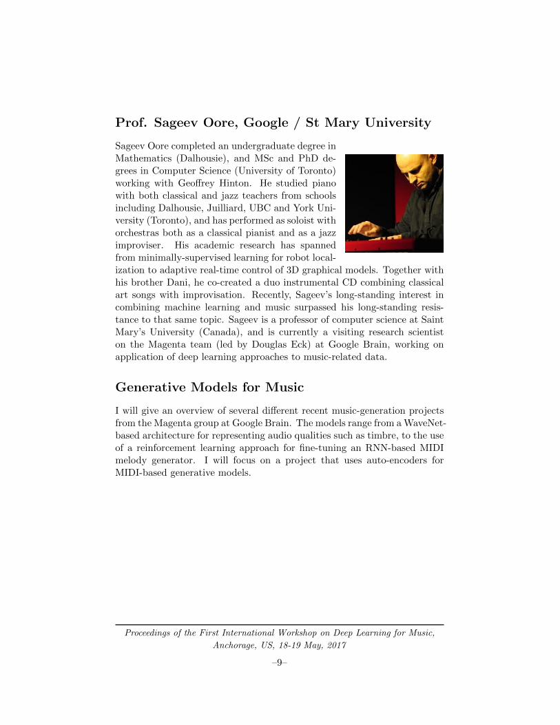
Prof. Sageev Oore, Google / St Mary University

Sageev Oore completed an undergraduate degree inMathematics (Dalhousie), and MSc and PhD de-grees in Computer Science (University of Toronto)working with Geoffrey Hinton. He studied pianowith both classical and jazz teachers from schoolsincluding Dalhousie, Juilliard, UBC and York Uni-versity (Toronto), and has performed as soloist withorchestras both as a classical pianist and as a jazzimproviser. His academic research has spannedfrom minimally-supervised learning for robot local-ization to adaptive real-time control of 3D graphical models. Together withhis brother Dani, he co-created a duo instrumental CD combining classicalart songs with improvisation. Recently, Sageev’s long-standing interest incombining machine learning and music surpassed his long-standing resis-tance to that same topic. Sageev is a professor of computer science at SaintMary’s University (Canada), and is currently a visiting research scientiston the Magenta team (led by Douglas Eck) at Google Brain, working onapplication of deep learning approaches to music-related data.

Generative Models for Music

I will give an overview of several different recent music-generation projectsfrom the Magenta group at Google Brain. The models range from a WaveNet-based architecture for representing audio qualities such as timbre, to the useof a reinforcement learning approach for fine-tuning an RNN-based MIDImelody generator. I will focus on a project that uses auto-encoders forMIDI-based generative models.



–9–

Part II

Long talks

10

Modeling Musical Context Using Word2vec

D. Herremans∗1 and C.-H. Chuan†2

1Queen Mary University of London, London, UK2University of North Florida, Jacksonville, USA

We present a semantic vector space model for capturing complex polyphonic mu-sical context. A word2vec model based on a skip-gram representation with negativesampling was used to model slices of music from a dataset of Beethoven’s pianosonatas. A visualization of the reduced vector space using t-distributed stochasticneighbor embedding shows that the resulting embedded vector space captures tonalrelationships, even without any explicit information about the musical contents ofthe slices. Secondly, an excerpt of the Moonlight Sonata from Beethoven was al-tered by replacing slices based on context similarity. The resulting music showsthat the selected slice based on similar word2vec context also has a relatively shorttonal distance from the original slice.

Keywords: music context, word2vec, music, neural networks, semantic vectorspace

1 Introduction

In this paper, we explore the semantic similarity that can be derived by looking solely atthe context in which a musical slice appears. In past research, music has often been mod-eled through Recursive Neural Networks (RNNs) combined with Restricted Bolzmann Ma-chines [Boulanger-Lewandowski et al., 2012], Long-Short Term RNN models [Eck and Schmid-huber, 2002, Sak et al., 2014], Markov models [Conklin and Witten, 1995] and other statisticalmodels, using a representation that incorporates musical information (i.e., pitch, pitch class,duration, intervals, etc.). In this research, we focus on modeling the context, over the content.

Vector space models [Rumelhart et al., 1988] are typically used in natural language processing(NLP) to represent (or embed) words in a continuous vector space [Turney and Pantel, 2010,McGregor et al., 2015, Agres et al., 2016, Liddy et al., 1999]. Within this space, semanticallysimilar words are represented geographically close to each other [Turney and Pantel, 2010]. Arecent very efficient approach to creating these vector spaces for natural language processingis word2vec [Mikolov et al., 2013c].

∗[email protected]†[email protected]



–11–

Although music is not the same as language, it possesses many of the same types of char-acteristics. Besson and Schon [2001] discuss the similarity of music and language in terms of,among others, structural aspects and the expectancy generated by both a word and a note.We can therefore use a model from NLP: word2vec. More specifically a skip-gram model withnegative sampling is used to create and train a model that captures musical context.

There have been only few attempts at modeling musical context with semantic vector spacemodels. For example, Huang et al. [2016] use word2vec to model chord sequences in orderto recommend chords other than the ‘ordinary’ to novice composers. In this paper, we aimto use word2vec for modeling musical context in a more generic way as opposed to a reducedrepresentation as chord sequences. We represent complex polyphonic music as a sequence ofequal-length slices without any additional processing for musical concepts such as beat, timesignature, chord tones and etc.

In the next sections we will first discuss the implemented word2vec model, followed by adiscussion of how music was represented. Finally, the resulting model is evaluated.

2 Word2vec

Word2vec refers to a group of models developed by Mikolov et al. [2013c]. They are used tocreate and train semantic vector spaces, often consisting of several hundred dimensions, basedon a corpus of text [Mikolov et al., 2013a]. In this vector space, each word from the corpus isrepresented as a vector. Words that share a context are geographically close to each other inthis space. The word2vec architecture can be based on two approaches: a continuous bag-of-words, or a continuous skip-gram model (CBOW). The former uses the context to predict thecurrent word, whereas the latter uses the current word to predict surrounding words [Mikolovet al., 2013b]. Both models have a low computational complexity, so they can easily handle acorpus with a size ranging in the billions of words in a matter of hours. While CBOW modelsare faster, it has been observed that skip-gram performs better on small datasets [Mikolovet al., 2013a]. We therefore opted to work with the latter model.

Skip-gram with negative sampling The architecture of a skip-gram model is represented inFigure 1. For each word wt in a corpus of size T at position t, the network tries to predict thesurrounding words in a window c (c = 2 in the figure). The training objective is thus definedas:

1

T

T∑

t=1

∑

−c≤i≤c,i 6=0

log p(wt+i|wt), (1)

whereby the term p(wt+i|wt) is calculated by a softmax function. Calculating the gradient ofthis term is, however, computationally very expensive. Alternatives to circumvent this probleminclude hierarchical softmax [Morin and Bengio, 2005] and noise contrastive estimation [Gut-mann and Hyvarinen, 2012]. The word2vec model used in this research implements a variantof the latter, namely negative sampling.

The idea behind negative sampling is that a well trained model should be able to distinguishbetween data and noise [Goldberg and Levy, 2014]. The original training objective is thusapproximated by a new, more efficient, formulation that implements a binary logistic regressionto classify between data and noise samples. When the model is able to assign high probabilities



–12–

Projection

n-dim.

Input Output

wt

wt+1

wt+2

wt−1

wt−2

Figure 1: A skip-gram model with n-dimensions for word wt at position t.

to real words and low probabilities to noise samples, the objective is optimized Mikolov et al.[2013c].

Cosine similarity was used as a similarity metric between two musical-slice vectors in ourvector space. For two non-zero vectors A and B in n dimensional space, with an angle θ, it isdefined as [Tan et al., 2005]:

Similarity(A, B) = cos(θ) =

∑ni=1Ai ×Bi√∑n

i=1A2i ×

√∑ni=1B

2i

(2)

In this research, we port the above discussed model and techniques to the field of music.We do this by replacing ‘words’ with ‘slices of polyphonic music’. The manner in which this isdone is discussed in the next section.

3 Musical slices as words

In order to study the extend to which word2vec can model musical context, polyphonic musicalpieces are represented with as little injected musical knowledge as possible. Each piece is simplysegmented into equal-length, non-overlapping slices. The duration of these slices is calculatedfor each piece based on the distribution of time between note onsets. The smallest amount oftime between consecutive onsets that occurs in more than 5% of all cases is selected as theslice-size. The slices capture all pitches that sound in a slice: those that have their onset in theslice, and those that are played and held over the slice. The slicing process does not dependon musical concepts such as beat or time signature; instead, it is completely data-driven. Ourvocabulary of words, will thus consist of a collection of musical slices.

In addition, we do not label pitches as chords. All sounding pitches, including chord tones,non-chord tones, and ornaments, are all recorded in the slice. We do not reduce pitches intopitch classes either, i.e., pitches C4 and C5 are considered different pitches. The only musicalknowledge we use is the global key, as we transpose all pieces to either C major or A minorbefore segmentation. This enables the functional role of pitches in tonality to stay the sameacross compositions, which in turn causes there to be more repeated slices over the datasetand allows the model to be better trained on less data. In the next section, the performanceof the resulting model is discussed.



–13–

4 Results

In order to evaluate how well the proposed model captures musical context, a few experimentswere performed on a dataset consisting of Beethoven’s piano sonatas. The resulting datasetconsists of 70,305 words, with a total of 14,315 unique occurrences. As discussed above,word2vec models are very efficient to train. Within minutes, the model was trained on theCPU of a MacBook Pro.

We trained the model a number of times, with a different number of dimensions of the vectorspace (see Figure 2a). The more dimensions there are, the more accurate the model becomes,however, the time to train the model also becomes longer. In the rest of the experiments, wedecided to use 128 dimensions. In a second experiment, we varied the size of the skip window,i.e., how many words to consider to the left and right of the current word in the skip-gram.The results are displayed in Figure 2b, and show that a skip window of 1 is most ideal for ourdataset.

(a) Results for varying the number of dimen-sions of the vector space.

(b) Results for varying the size of the skipwindow.

Figure 2: Evolution of the average loss during training. A step represents 2000 training win-dows.

4.1 Visualizing the semantic vector space

In order to better understand and evaluate the proposed model, we created visualizationsof selected musical slices in a dimensionally reduced space. We use t-Distributed StochasticNeighbor Embedding (t-SNE), a technique developed by Maaten and Hinton [2008] for visu-alizing high-dimensional data. t-SNE has previously been used in a music analysis context forvisualizing clusters of musical genres based on musical features [Hamel and Eck, 2010].

In this case, we identified the ‘chord’ to which each slice of the dataset belongs based on asimple template-matching method. We expect that tonally close chords occur together in thesemantic vector space. Figure 3 confirms this hypothesis. When examining slices that containC and G chords (a perfect fifth apart), the space looks very dispersed, as they often co-occur(see Figure 3c). The same occurs for the chord pair Eb and Bb in Figure 3d. On the other



–14–

hand, when looking at the tonally distant chord pair E and Eb (Figure 3a), we see that clustersappear in the reduced vector space. The same happens for the tonally distant chords Eb, Bb

and B in Figure 3b.

(a) E (green) and Eb (blue). (b) Eb (black), Db (green) and B (gray).

(c) C (green) and G (blue). (d) Eb (green) and Bb (blue).

Figure 3: Reduced vector space with t-SNE for different slices (labeled by the most close chord)

4.2 Content versus context

In order to further examine if word2vec captures semantic meaning in music via the modelingof context, we modify a piece by replacing some of its original slices with the most similar oneas captured by the cosine similarity in the vector space model. If word2vec is really able tocapture this, the modified piece should sound similar to the original. This allows us to evaluatethe effectiveness of using word2vec for modeling music.

Figure 4 shows the first 17 measures of Beethoven’s piano sonata Op. 27 No. 2 (Moonlight),



–15–

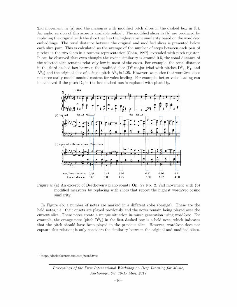
2nd movement in (a) and the measures with modified pitch slices in the dashed box in (b).An audio version of this score is available online1. The modified slices in (b) are produced byreplacing the original with the slice that has the highest cosine similarity based on the word2vecembeddings. The tonal distance between the original and modified slices is presented beloweach slice pair. This is calculated as the average of the number of steps between each pair ofpitches in the two slices in a tonnetz representation [Cohn, 1997], extended with pitch register.It can be observed that even thought the cosine similarity is around 0.5, the tonal distance ofthe selected slice remains relatively low in most of the cases. For example, the tonal distancein the third dashed box between the modified slice (Db major triad with pitches Db

4, F4, andAb

4) and the original slice of a single pitch Ab4 is 1.25. However, we notice that word2vec does

not necessarily model musical context for voice leading. For example, better voice leading canbe achieved if the pitch D4 in the last dashed box is replaced with pitch D5.

Figure 4: (a) An excerpt of Beethoven’s piano sonata Op. 27 No. 2, 2nd movement with (b)modified measures by replacing with slices that report the highest word2vec cosinesimilarity.

In Figure 4b, a number of notes are marked in a different color (orange). These are theheld notes, i.e., their onsets are played previously and the notes remain being played over thecurrent slice. These notes create a unique situation in music generation using word2vec. Forexample, the orange note (pitch Db

5) in the first dashed box is a held note, which indicatesthat the pitch should have been played in the previous slice. However, word2vec does notcapture this relation; it only considers the similarity between the original and modified slices.

1http://dorienherremans.com/word2vec



–16–

5 Conclusions

A skip-gram model with negative sampling was used to build a semantic vector space modelfor complex polyphonic music. By representing the resulting vector space in a reduced two-dimensional graph with t-SNE, we show that musical features such as a notion of tonal proxim-ity are captured by the model. Music generated by replacing slices based on word2vec contextsimilarity also presents close tonal distance compared to the original.

In the future, an embedded model that combines both word2vec with, for instance, a long-short term memory recurrent neural network based on musical features, would offer a morecomplete way to more completely model music. The TensorFlow code used in this research isavailable online2.

Acknowledgements

This project has received funding from the European Union’s Horizon 2020 research and in-novation programme under grant agreement No 658914.

References

Kat R Agres, Stephen McGregor, Karolina Rataj, Matthew Purver, and Geraint A Wiggins.Modeling metaphor perception with distributional semantics vector space models. In Work-shop on Computational Creativity, Concept Invention, and General Intelligence. Proceedingsof 5 th International Workshop, C3GI at ESSLI, pages 1–14, 2016.

Mireille Besson and Daniele Schon. Comparison between language and music. Annals of theNew York Academy of Sciences, 930(1):232–258, 2001.

Nicolas Boulanger-Lewandowski, Yoshua Bengio, and Pascal Vincent. Modeling temporal de-pendencies in high-dimensional sequences: Application to polyphonic music generation andtranscription. arXiv preprint arXiv:1206.6392, 2012.

Richard Cohn. Neo-riemannian operations, parsimonious trichords, and their” tonnetz” rep-resentations. Journal of Music Theory, 41(1):1–66, 1997.

Darrell Conklin and Ian H Witten. Multiple viewpoint systems for music prediction. Journalof New Music Research, 24(1):51–73, 1995.

Douglas Eck and Juergen Schmidhuber. Finding temporal structure in music: Blues impro-visation with lstm recurrent networks. In Neural Networks for Signal Processing, 2002.Proceedings of the 2002 12th IEEE Workshop on, pages 747–756. IEEE, 2002.

Yoav Goldberg and Omer Levy. word2vec explained: Deriving mikolov et al.’s negative-sampling word-embedding method. arXiv preprint arXiv:1402.3722, 2014.

Michael U Gutmann and Aapo Hyvarinen. Noise-contrastive estimation of unnormalized sta-tistical models, with applications to natural image statistics. Journal of Machine LearningResearch, 13(Feb):307–361, 2012.

2http://dorienherremans.com/word2vec



–17–

Philippe Hamel and Douglas Eck. Learning features from music audio with deep belief net-works. In ISMIR, volume 10, pages 339–344. Utrecht, The Netherlands, 2010.

Cheng-Zhi Anna Huang, David Duvenaud, and Krzysztof Z Gajos. Chordripple: Recommend-ing chords to help novice composers go beyond the ordinary. In Proceedings of the 21stInternational Conference on Intelligent User Interfaces, pages 241–250. ACM, 2016.

Elizabeth D Liddy, Woojin Paik, S Yu Edmund, and Ming Li. Multilingual document retrievalsystem and method using semantic vector matching, December 21 1999. US Patent 6,006,221.

Laurens van der Maaten and Geoffrey Hinton. Visualizing data using t-sne. Journal of MachineLearning Research, 9(Nov):2579–2605, 2008.

Stephen McGregor, Kat Agres, Matthew Purver, and Geraint A Wiggins. From distributionalsemantics to conceptual spaces: A novel computational method for concept creation. Journalof Artificial General Intelligence, 6(1):55–86, 2015.

Tomas Mikolov, Kai Chen, Greg Corrado, and Jeffrey Dean. Efficient estimation of wordrepresentations in vector space. arXiv preprint arXiv:1301.3781, 2013a.

Tomas Mikolov, Quoc V Le, and Ilya Sutskever. Exploiting similarities among languages formachine translation. arXiv preprint arXiv:1309.4168, 2013b.

Tomas Mikolov, Ilya Sutskever, Kai Chen, Greg S Corrado, and Jeff Dean. Distributed repre-sentations of words and phrases and their compositionality. In Advances in neural informa-tion processing systems, pages 3111–3119, 2013c.

Frederic Morin and Yoshua Bengio. Hierarchical probabilistic neural network language model.In Aistats, volume 5, pages 246–252. Citeseer, 2005.

David E Rumelhart, Geoffrey E Hinton, and Ronald J Williams. Learning representations byback-propagating errors. Cognitive modeling, 5(3):1, 1988.

Hasim Sak, Andrew W Senior, and Francoise Beaufays. Long short-term memory recurrentneural network architectures for large scale acoustic modeling. In Interspeech, pages 338–342,2014.

Pang-Ning Tan, Michael Steinbach, and Vipin Kumar. Introduction to Data Mining, (FirstEdition). Addison-Wesley Longman Publishing Co., Inc., Boston, MA, USA, 2005. ISBN0321321367.

Peter D Turney and Patrick Pantel. From frequency to meaning: Vector space models ofsemantics. Journal of artificial intelligence research, 37:141–188, 2010.



–18–

Chord Label Personalization through DeepLearning of Integrated HarmonicInterval-based Representations

Hendrik Vincent Koops∗1, W. Bas de Haas†2, Jeroen Bransen‡2, andAnja Volk§ 1

1Utrecht University, Utrecht, the Netherlands

2Chordify, Utrecht, the Netherlands

The increasing accuracy of automatic chord estimation systems, the availability ofvast amounts of heterogeneous reference annotations, and insights from annotatorsubjectivity research make chord label personalization increasingly important. Nev-ertheless, automatic chord estimation systems are historically exclusively trainedand evaluated on a single reference annotation. We introduce a first approachto automatic chord label personalization by modeling subjectivity through deeplearning of a harmonic interval-based chord label representation. After integratingthese representations from multiple annotators, we can accurately personalize chordlabels for individual annotators from a single model and the annotators’ chord la-bel vocabulary. Furthermore, we show that chord personalization using multiplereference annotations outperforms using a single reference annotation.

Keywords: Automatic Chord Estimation, Annotator Subjectivity, Deep Learning

1 Introduction

Annotator subjectivity makes it hard to derive one-size-fits-all chord labels. Annotators tran-scribing chords from a recording by ear can disagree because of personal preference, biastowards a particular instrument, and because harmony can be ambiguous perceptually as wellas theoretically by definition [Schoenberg, 1978, Meyer, 1957]. These reasons contributed toannotators creating large amounts of heterogeneous chord label reference annotations. Forexample, on-line repositories for popular songs often contain multiple, heterogeneous versions.

∗[email protected]†[email protected]‡[email protected]§[email protected]



–19–

One approach to the problem of finding the appropriate chord labels in a large number ofheterogeneous chord label sequences for the same song is data fusion. Data fusion researchshows that knowledge shared between sources can be integrated to produce a unified view thatcan outperform individual sources [Dong et al., 2009]. In a musical application, it was foundthat integrating the output of multiple Automatic Chord Estimation (ace) algorithms resultsin chord label sequences that outperform the individual sequences when compared to a singleground truth [Koops et al., 2016]. Nevertheless, this approach is built on the intuition that onesingle correct annotation exists that is best for everybody, on which ace systems are almostexclusively trained. Such reference annotation is either compiled by a single person [Mauchet al., 2009], or unified from multiple opinions [Burgoyne et al., 2011]. Although most of thecreators of these datasets warn for subjectivity and ambiguity, they are in practice used as thede facto ground truth in MIR chord research and tasks (e.g. mirex ace).

On the other hand, it can also be argued that there is no single best reference annotation,and that chord labels are correct with varying degrees of “goodness-of-fit” depending on thetarget audience [Ni et al., 2013]. In particular for richly orchestrated, harmonically complexmusic, different chord labels can be chosen for a part, depending on the instrument, voicing orthe annotators’ chord label vocabulary.

In this paper, we propose a solution to the problem of finding appropriate chord labelsin multiple, subjective heterogeneous reference annotations for the same song. We proposean automatic audio chord label estimation and personalization technique using the harmoniccontent shared between annotators. From deep learned shared harmonic interval profiles,we can create chord labels that match a particular annotator vocabulary, thereby providingan annotator with familiar, and personal chord labels. We test our approach on a 20-songdataset with multiple reference annotations, created by annotators who use different chordlabel vocabularies. We show that by taking into account annotator subjectivity while trainingour ace model, we can provide personalized chord labels for each annotator.

Contribution. The contribution of this paper is twofold. First, we introduce an approach toautomatic chord label personalization by taking into account annotator subjectivity. Throughthis end, we introduce a harmonic interval-based mid-level representation that captures har-monic intervals found in chord labels. Secondly, we show that after integrating these featuresfrom multiple annotators and deep learning, we can accurately personalize chord labels for indi-vidual annotators. Finally, we show that chord label personalization using integrated featuresoutperforms personalization from a commonly used reference annotation.

2 Deep Learning Harmonic Interval Subjectivity

For the goal of chord label personalization, we create an harmonic bird’s-eye view from differentreference annotations, by integrating their chord labels. More specifically, we introduce a newfeature that captures the shared harmonic interval profile of multiple chord labels, which wedeep learn from audio. First, we extract Constant Q (cqt) features from audio, then wecalculate Shared Harmonic Interval Profile (ship) representations from multiple chord labelreference annotations corresponding to the cqt frames. Finally, we train a deep neural networkto associate a context window of cqt to ship features.

From audio, we calculate a time-frequency representation where the frequency bins aregeometrically spaced and ratios of the center frequencies to bandwidths of all bins are equal,called a Constant Q (cqt) spectral transform [Schorkhuber and Klapuri, 2010]. We calculate



–20–

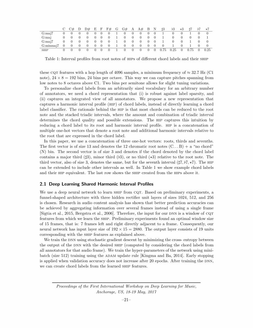
C C# D D# E F F# G G# A A# B N ]3 [3 ?3 ]7 [7 ?7G:maj7 0 0 0 0 0 0 0 1 0 0 0 0 0 1 0 0 1 0 0G:maj 0 0 0 0 0 0 0 1 0 0 0 0 0 1 0 0 0 0 1G:maj7 0 0 0 0 0 0 0 1 0 0 0 0 0 1 0 0 1 0 0G:minmaj7 0 0 0 0 0 0 0 1 0 0 0 0 0 0 1 0 1 0 0ship 0 0 0 0 0 0 0 1 0 0 0 0 0 0.75 0.25 0 0.75 0 0.25

Table 1: Interval profiles from root notes of hips of different chord labels and their ship

these cqt features with a hop length of 4096 samples, a minimum frequency of ≈ 32.7 Hz (C1note), 24× 8 = 192 bins, 24 bins per octave. This way we can capture pitches spanning fromlow notes to 8 octaves above C1. Two bins per semitone allows for slight tuning variations.

To personalize chord labels from an arbitrarily sized vocabulary for an arbitrary numberof annotators, we need a chord representation that (i) is robust against label sparsity, and(ii) captures an integrated view of all annotators. We propose a new representation thatcaptures a harmonic interval profile (hip) of chord labels, instead of directly learning a chordlabel classifier. The rationale behind the hip is that most chords can be reduced to the rootnote and the stacked triadic intervals, where the amount and combination of triadic intervaldetermines the chord quality and possible extensions. The hip captures this intuition byreducing a chord label to its root and harmonic interval profile. hip is a concatenation ofmultiple one-hot vectors that denote a root note and additional harmonic intervals relative tothe root that are expressed in the chord label.

In this paper, we use a concatenation of three one-hot vectors: roots, thirds and sevenths.The first vector is of size 13 and denotes the 12 chromatic root notes (C. . . B) + a “no chord”(N) bin. The second vector is of size 3 and denotes if the chord denoted by the chord labelcontains a major third (]3), minor third ([3), or no third (?3) relative to the root note. Thethird vector, also of size 3, denotes the same, but for the seventh interval (]7, [7, ?7). The hipcan be extended to include other intervals as well. In Table 1 we show example chord labelsand their hip equivalent. The last row shows the ship created from the hips above it.

2.1 Deep Learning Shared Harmonic Interval Profiles

We use a deep neural network to learn ship from cqt. Based on preliminary experiments, afunnel-shaped architecture with three hidden rectifier unit layers of sizes 1024, 512, and 256is chosen. Research in audio content analysis has shown that better prediction accuracies canbe achieved by aggregating information over several frames instead of using a single frame[Sigtia et al., 2015, Bergstra et al., 2006]. Therefore, the input for our dnn is a window of cqtfeatures from which we learn the ship. Preliminary experiments found an optimal window sizeof 15 frames, that is: 7 frames left and right directly adjacent to a frame. Consequently, ourneural network has input layer size of 192× 15 = 2880. The output layer consists of 19 unitscorresponding with the ship features as explained above.

We train the dnn using stochastic gradient descent by minimizing the cross- entropy betweenthe output of the dnn with the desired ship (computed by considering the chord labels fromall annotators for that audio frame). We train the hyper-parameters of the network using mini-batch (size 512) training using the adam update rule [Kingma and Ba, 2014]. Early stoppingis applied when validation accuracy does not increase after 20 epochs. After training the dnn,we can create chord labels from the learned ship features.



–21–

3 Annotator Vocabulary-based Chord Label Estimation

The ship features are used to associate probabilities to chord labels from a given vocabulary.For a chord label L the hip h contains exactly three ones, corresponding to the root, thirdsand sevenths of the label L. From the ship A of a particular audio frame, we project out threevalues for which h contains ones (h(A)). The product of these values is then interpreted asthe combined probability CP (= Π h(A)) of the intervals in L given A. Given a vocabularyof chord labels, we normalize the CPs to obtain a probability density function over all chordlabels in the vocabulary given A. The chord label with the highest probability is chosen asthe chord label for the audio frame associated to A.

For the chord label examples in Table 1, the products of the non-zero values of the point-wisemultiplications ≈ 0.56, 0.19, and 0.19 for G:maj7, G:maj, and G:minmaj7 respectively. If weconsider these chord labels to be a vocabulary, and normalize the values, we obtain probabilities≈ 0.6, 0.2, 0.2, respectively. Given extracted ship from multiple annotators providing referenceannotations and chord label vocabularies, we can now generate annotator specific chords labels.

4 Evaluation

ship models multiple (related) chords for a single frame, e.g., the ship in Table 1 modelsdifferent flavors of a G and a C chord. For the purpose of personalization, we want to presentthe annotator with only the chords they understand and prefer, thereby producing a high chordlabel accuracy for each annotator. For example, if an annotator does not know a G:maj7 butdoes know an G, and both are probable from an ship, we like to present the latter. In thispaper, we evaluate our dnn ace personalization approach, and the ship representation, foreach individual annotator and their vocabulary.

In an experiment we compare training of our chord label personalization system on multiplereference annotations with training on a commonly used single reference annotation. In thefirst case we train a dnn (dnnship) on ships derived from a dataset introduced by Ni et al.[2013] containing 20 popular songs annotated by five annotators with varying degrees of musicalproficiency. In the second case, we train a dnn (dnniso) on the hip of the Isophonics (iso) singlereference annotation [Mauch et al., 2009]. iso is a peer-reviewed, and de facto standard trainingreference annotation used in numerous ace systems. From the (s)hip the annotator chordlabels are derived and we evaluate the systems on every individual annotator. We hypothesizethat training a system on ship based on multiple reference annotations captures the annotatorsubjectivity of these annotations and leads to better personalization than training the samesystem on a single (iso) reference annotation.

It could be argued that the system trained on five reference annotations has more data tolearn from than a system trained on the single iso reference annotation. To eliminate thispossible training bias, we evaluate the annotators’ chord labels directly on the chord labelsfrom iso (ann|iso). This evaluation reveals the similarity between the ship and the iso andputs the results from dnniso in perspective. If dnnship is better at personalizing chords (i.e.provides chord labels with a higher accuracy per annotator) than dnniso while the annotator’sannotations and the iso are similar, then we can argue that using multiple reference annotationsand ship is better for chord label personalization than using just the iso. In a final baselineevaluation, we also test iso on dnniso to measure how well it models the iso.

Ignoring inversions, the complete dataset from Ni et al. [2013] contains 161 unique chord



–22–

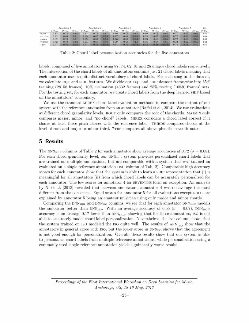
Annotator 1 Annotator 2 Annotator 3 Annotator 4 Annotator 5 isodnnship ann|iso dnniso dnnship ann|iso dnniso dnnship ann|iso dnniso dnnship ann|iso dnniso dnnship ann|iso dnniso dnniso

root 0.85 0.73 0.66 0.82 0.74 0.67 0.80 0.72 0.65 0.80 0.73 0.65 0.77 0.67 0.60 0.86majmin 0.82 0.69 0.61 0.69 0.67 0.53 0.67 0.69 0.53 0.73 0.67 0.55 0.72 0.61 0.55 0.69mirex 0.82 0.70 0.61 0.69 0.68 0.54 0.66 0.69 0.54 0.73 0.68 0.56 0.72 0.62 0.55 0.69thirds 0.82 0.70 0.62 0.75 0.67 0.59 0.79 0.69 0.62 0.76 0.68 0.61 0.72 0.62 0.55 0.837ths 0.77 0.56 0.50 0.64 0.53 0.42 0.64 0.56 0.43 0.53 0.48 0.40 0.72 0.53 0.55 0.65

Table 2: Chord label personalization accuracies for the five annotators

labels, comprised of five annotators using 87, 74, 62, 81 and 26 unique chord labels respectively.The intersection of the chord labels of all annotators contains just 21 chord labels meaning thateach annotator uses a quite distinct vocabulary of chord labels. For each song in the dataset,we calculate cqt and ship features. We divide our cqt and ship dataset frame-wise into 65%training (28158 frames), 10% evaluation (4332 frames) and 25% testing (10830 frames) sets.For the testing set, for each annotator, we create chord labels from the deep learned ship basedon the annotators’ vocabulary.

We use the standard mirex chord label evaluation methods to compare the output of oursystem with the reference annotation from an annotator [Raffel et al., 2014]. We use evaluationsat different chord granularity levels. root only compares the root of the chords. majmin onlycompares major, minor, and “no chord” labels. mirex considers a chord label correct if itshares at least three pitch classes with the reference label. thirds compares chords at thelevel of root and major or minor third. 7ths compares all above plus the seventh notes.

5 Results

The dnnship columns of Table 2 for each annotator show average accuracies of 0.72 (σ = 0.08).For each chord granularity level, our dnnship system provides personalized chord labels thatare trained on multiple annotations, but are comparable with a system that was trained anevaluated on a single reference annotation (iso column of Tab. 2). Comparable high accuracyscores for each annotator show that the system is able to learn a ship representation that (i) ismeaningful for all annotators (ii) from which chord labels can be accurately personalized foreach annotator. The low scores for annotator 4 for sevenths form an exception. An analysisby Ni et al. [2013] revealed that between annotators, annotator 4 was on average the mostdifferent from the consensus. Equal scores for annotator 5 for all evaluations except root areexplained by annotator 5 being an amateur musician using only major and minor chords.

Comparing the dnnship and dnniso columns, we see that for each annotator dnnship modelsthe annotator better than dnniso. With an average accuracy of 0.55 (σ = 0.07), dnniso’saccuracy is on average 0.17 lower than dnnship, showing that for these annotators, iso is notable to accurately model chord label personalization. Nevertheless, the last column shows thatthe system trained on iso modeled the iso quite well. The results of ann|iso show that theannotators in general agree with iso, but the lower score in dnniso shows that the agreementis not good enough for personalization. Overall, these results show that our system is ableto personalize chord labels from multiple reference annotations, while personalization using acommonly used single reference annotation yields significantly worse results.



–23–

6 Conclusions and Discussion

We presented a system that provides personalized chord labels from multiple reference anno-tations from audio, based on the annotators’ specific chord label vocabulary and an interval-based chord label representation that captures the shared subjectivity between annotators. Totest the scalability of our system, our experiment needs to be repeated on a larger dataset,with more songs and more annotators. Furthermore, a similar experiment on a dataset withinstrument/proficiency/cultural-specific annotations from different annotators would shed lighton whether our system generalizes to providing chord label annotations in different contexts.From the results presented in this paper, we believe chord label personalization is the nextstep in the evolution of ace systems.

Acknowledgments

We thank Y. Ni, M. McVicar, R. Santos-Rodriguez and T. De Bie for providing their dataset.

References

J. Bergstra, N. Casagrande, D. Erhan, D. Eck, and B. Kegl. Aggregate features and adaboostfor music classification. Machine learning, 65(2-3):473–484, 2006.

J.A. Burgoyne, J. Wild, and I. Fujinaga. An expert ground truth set for audio chord recog-nition and music analysis. In Proc. of the 12th International Society for Music InformationRetrieval Conference, ISMIR, volume 11, pages 633–638, 2011.

X.L. Dong, L. Berti-Equille, and D. Srivastava. Integrating conflicting data: the role of sourcedependence. Proc. of the VLDB Endowment, 2(1):550–561, 2009.

D.P. Kingma and J. Ba. Adam: A method for stochastic optimization. In Proc. of the 3rdInternational Conference on Learning Representations, ICLR, 2014.

H.V. Koops, W.B. de Haas, D. Bountouridis, and A. Volk. Integration and quality assessmentof heterogeneous chord sequences using data fusion. In Proc. of the 17th International Societyfor Music Information Retrieval Conference, ISMIR, New York, USA, pages 178–184, 2016.

M. Mauch, C. Cannam, M. Davies, S. Dixon, C. Harte, S. Kolozali, D. Tidhar, and M. Sandler.Omras2 metadata project 2009. In Late-breaking demo session at 10th International Societyfor Music Information Retrieval Conference, ISMIR, 2009.

L.B. Meyer. Meaning in music and information theory. The Journal of Aesthetics and ArtCriticism, 15(4):412–424, 1957.

Y. Ni, M. McVicar, R. Santos-Rodriguez, and T. De Bie. Understanding effects of subjectivityin measuring chord estimation accuracy. IEEE Transactions on Audio, Speech, and LanguageProcessing, 21(12):2607–2615, 2013.

C. Raffel, B. McFee, E.J. Humphrey, J. Salamon, O. Nieto, D. Liang, D.P.W. Ellis, andC. Raffel. mir eval: A transparent implementation of common mir metrics. In Proc. ofthe 15th International Society for Music Information Retrieval Conference, ISMIR, pages367–372, 2014.



–24–

A. Schoenberg. Theory of harmony. University of California Press, 1978.

C. Schorkhuber and A. Klapuri. Constant-q transform toolbox for music processing. In Proc.of the 7th Sound and Music Computing Conference, Barcelona, Spain, 2010.

S. Sigtia, N. Boulanger-Lewandowski, and S. Dixon. Audio chord recognition with a hybridrecurrent neural network. In Proc. of the 16th International Society for Music InformationRetrieval Conference, ISMIR, pages 127–133, 2015.



–25–

Music Signal Processing Using Vector ProductNeural Networks

Zhe-Cheng Fan∗1, Tak-Shing T. Chan†2, Yi-Hsuan Yang‡2, andJyh-Shing R. Jang§1

1Dept. of Computer Science and Information Engineering, National Taiwan University, Taiwan

2Research Center for Information Technology Innovation, Academia Sinica, Taiwan

We propose a novel neural network model for music signal processing using vec-tor product neurons and dimensionality transformations. Here, the inputs arefirst mapped from real values into three-dimensional vectors then fed into a three-dimensional vector product neural network where the inputs, outputs, and weightsare all three-dimensional values. Next, the final outputs are mapped back to the re-als. Two methods for dimensionality transformation are proposed, one via contextwindows and the other via spectral coloring. Experimental results on the iKaladataset for blind singing voice separation confirm the efficacy of our model.

Keywords: Deep learning, deep neural networks, vector product neural networks,dimensionality transformation, music source separation.

1 Introduction

In recent years, deep learning has become increasingly popular in the music information re-trieval (MIR) community. For MIR problems requiring clip-level predictions or frame-by-framepredictions, such as genre classification, music segmentation, onset detection, chord recogni-tion and vocal/non-vocal detection, many existing algorithms are based on convolutional neuralnetworks (CNN) and recurrent neural networks (RNN). For audio regression problems whichrequire an estimate for each time-frequency (t-f) unit over a spectrogram, such as source sep-aration [Zhang and Wang, 2016], more algorithms are based on deep neural networks (DNN).This is because for such problems both input and output are matrices of the same size andtherefore the neural network cannot involve operations that may reduce the spatial resolution.Existing DNN models for such problems usually consider each t-f unit as a real value and take

∗[email protected]†[email protected]‡[email protected]§[email protected]



–26–

that as input for the network [Huang et al., 2014, Roma et al., 2016]. The question we want toaddress in this paper is whether we can achieve better results by applying some transformationmethods to enrich the information for each t-f unit.

A widely used approach to enrich the information of each t-f unit is to add temporal context[Zhang and Wang, 2016]. For instance, in addition to the current frame, we add the previous-k and subsequent-k frames to compose a real-valued matrix and take it as the input of theneural network. But in this way, the interaction between different dimensions cannot be wellmodeled. To address this issue, we find it promising to consider a (2k+1)-dimensional neuralnetwork [Nitta, 2007]. As a first attempt, we implement this using vector product neuralnetwork (VPNN) [Nitta, 1993], a three-dimensional neural network that has only been testedon a simple XOR task in the literature. That is to say, k in this work is set to 1 (i.e. consideringonly the two neighboring frames). Each t-f unit is projected to a three-dimensional vector viathis dimensionality transformation method. In VPNN, the input, output, weight and bias ofeach neuron are all three-dimensional vectors. While the main operation in DNN is matrixmultiplication, it is the vector product in VPNN.

The goal of the paper is three-fold. First, we renovate VPNN with modern optimizationtechniques [Ruder, 2016] and test it on MIR problems instead of a simple XOR problem.Second, we test and compare the conventional context-enriched DNN structure using realvalues and the context-enriched VPNN structure for the specific task of blind singing voiceseparation from monaural recordings, which is a type of source separation problem. Third,we implement the idea of spectral coloring as another way to convert a real-valued matrixto a three-dimensional vector-valued matrix and evaluate this method again for blind singingvoice separation. Our experiments confirm the efficacy of VPNN and both dimensionalitytransformation methods.

2 Vector Product Neural Network

In VPNN, the input data, weights, and biases are all three-dimensional vectors. Suppose thereis an L-intermediate-layer VPNN, the input zli of activation function in each neuron at the l-thlayer is:

zli =

J∑

j=1

wlij × al−1

j + bli, (1)

where × denotes vector product, wlij stands for the weight connecting neurons j and i at l-th

layer, al−1j the input signal coming from neuron j at (l − 1)-th layer, bl

i the bias of neuroni at l-th layer. If x=[x1 x2 x3] and y=[y1 y2 y3], the result of vector product operation isx×y = [x2y3− x3y2, x3y1− x1y3, x1y2− x2y1]. As each element of the output vector receivescontributions from all other dimensions, the vector product can capture all possible interactionsamong the three dimensions. This is not possible with real-valued neural network models

Note that we need to compute a lot of vector products between the layers in VPNN. In orderto reduce training time, we propose to reformulate the vector product as matrix multiplication,which is more amenable to GPU acceleration. Suppose there are two vector-valued matrices,P and Q. Their vector-valued matrix product ⊗ can be equivalently written as:

P⊗Q = [p2q3 − p3q2,p3q1 − p1q3,p1q2 − p2q1], (2)



–27–

where p1, p2, p3 are the matrices making up P and q1, q2, q3 are the matrices making up Q.By applying Eq. (2), the output at hidden layer l can be defined as:

Al = φ(Wl ⊗Al−1 + Bl), (3)

and the output Y of the VPNN, which is a vector-valued matrix, can be defined as:

Y = φ(WL...φ(W2 ⊗ φ(W1 ⊗A0 + B1) + B2) + ...BL), (4)

where operator ⊗ denotes the vector-valued matrix product mentioned in Eq. (2). At the l-thlayer, Al is the hidden state, Wl is weight matrix, and Bl is bias matrix. All of them arevector-valued matrices. At the first layer, A0 is the input of the VPNN, consisting of vector-valued data from dimensionality transformation. The function φ is the sigmoid function. Inorder to achieve better performance, modern gradient optimization methods [Ruder, 2016] areimplemented in our VPNN. Due to space constraints, we only report our results using Adam,a method for stochastic gradient descent.

3 Dimensionality Transformation and Objective Function

In this section, we elaborate two ideas for dimensionality transformation. One is based onadding temporal context described in Section 1. The other one is based on a novel techniquecalled spectral coloring, which associates each t-f unit with a color in the RGB color space.Both ideas yield three-dimensional vectors as the input to VPNN.

3.1 Context-Windowed Transformation

To enrich the information for each t-f unit and improve the problem of interaction betweendifferent dimensions, we make current frame, previous and subsequent frames as a three-dimensional vector for each t-f unit. For ordinary NN, the input would be three real-valuedmatrices. For VPNN, the input is a three-dimensional matrix. In other words, the firstdimension consists of previous frames, second dimension for current frames and third dimensionfor subsequent frames. Here we call this model as context-Window Vector Product NeuralNetwork (WVPNN). After feeding the three-dimensional matrix into the VPNN, we get three-dimensional outputs and the second dimension is our predicted result.

3.2 Spectral Color Transformation

We can also map each t-f unit from a one-dimensional value into a three-dimensional vector,by using so-called spectral color transform, using for example the hot colormap in Matlabdirectly as a lookup table, where the forward and inverse maps are both computed by nearestneighbor searches. The hot colormap is associated with a resolution parameter which specifiesthe length of the colormap. As nearest neighbor interpolation will turn into piecewise linearinterpolation when n tends to infinity, we can imitate the hot colormap with infinite resolutionby the following piecewise linear functions instead:

v =

rgb

=

max(min(x/n, 1), 0)max(min((x− n)/n, 1), 0)

max(min((x− 2n)/(1− 2n), 1), 0)

, (5)



–28–

where v stands for the three-dimensional vector-valued vector, r, g and b the R, G, and Bvalues respectively, x the magnitude of each t-f unit, and n a scalar to bias the generation ofRGB values. We empirically set n to 0.0938 in this work. We call this model Colored VectorProduct Neural Network (CVPNN). After feeding the RGB values into VPNN, we get RGBvalues as outputs. Each RGB value is then inversed-mapped to a magnitude at each t-f unit.

3.3 Target Function and Masking

During the training process of singing voice separation, given the predicted vocal spectra Z1

and predicted music spectra Z2, together with the original sources Z1 and Z2, the objectivefunction J of the WVPNN and CVPNN can be defined as:

J = ‖Z1 − Z1‖2 + ‖Z2 − Z2‖2. (6)

After getting the output from WVPNN and CVPNN, we can obtain the predicted spectray1 and y2. We smooth the results with a time-frequency masking technique called that softtime-frequency mask [Huang et al., 2015], and the magnitude spectra of the input frame canbe transformed back to the time-domain by inverse STFT with the original phases.

4 Experiments

The proposed models are evaluated by singing voice separation experiments on the iKaladataset [Chan et al., 2015]. Only 252 song clips are released as a public set for evaluation.Due to the limitation of GPU memory, we partition the public set into 63 training clips and189 testing clips. To reduce computation, all clips are downsampled to 16000 Hz. For eachsong clip, we use STFT to yield magnitude spectra with a 1024-point window and a 256-pointhop size. The performance is measured in terms of source to distortion ratio (SDR), sourceto interferences ratio (SIR), and source to artifact ratio (SAR), as calculated by the blindsource separation (BSS) Eval toolbox v3.0 [Vincent et al., 2006]. The overall performance isreported via global NSDR (GNSDR), global SIR (GSIR), and global SAR (GSAR), which arethe weighted means of the measures over all clips with a weighting proportional to the lengthof the clips. Higher numbers mean better performances.

In order to compare the performance of ordinary DNN and CVPNN, we construct twonetworks that both consist of 3 hidden layers and 512 neurons in each hidden layer, denotedas CVPNN and DNN1, respectively, using Eq. (6) as the target function. The dimensionalityof each t-f unit is 1 for ordinary DNN and 3 for CVPNN. A network structure similiar tothis DNN1 was used in [Roma et al., 2016]. As shown in Table 1, CVPNN performs betterthan DNN1 in both GNSDR and GSIR. As CVPNN has three times of NN parameters (i.e.number of weights and bias) as compared with DNN1, for fair comparison we further constructan ordinary DNN comprising 3 hidden layers and 1536 neurons in each hidden layer, denotedas DNN2, so that both CVPNN and ordinary DNN have the same number of parameters.Table 1 shows that CVPNN still performs better. Besides, we also construct two architectureswhich have the same number of parameters and t-f units composed of context window size of 3frames, denoted as WVPNN and DNN3 respectively. Both of them are composed of 3 hiddenlayers. The number of neurons in each hidden layer is 512 for WVPNN, and 1536 for DNN.The difference of these two is the combination of input frames. The input frames is constructed



–29–

Table 1: Comparison of ordinary DNN, WVPNN and CVPNN.

Neural Networks. Arch. Context Window Size GNSDR GSIR GSAR

DNN1 512x3 1 8.16 11.88 12.11DNN2 1536x3 1 8.37 12.64 11.82

CVPNN 512x3 1 8.87 13.38 11.37

DNN3 1536x3 3 8.85 12.59 12.52WVPNN 512x3 3 9.01 13.82 11.97

as a three-dimensional vector-valued matrix for WVPNN and a two-dimensional valued matrixfor DNN3. Results in Table 1 show that WVPNN performs better than ordinary DNN3.

5 Conclusion and Future Work

In this paper, we propose WVPNN and CVPNN for monaural singing voice separation, usingtwo dimensionality transformation methods. We also propose modern gradient optimizationmethods on VPNN to attain better performance. Our evaluation shows that both proposedmodels are better than traditional DNN, with 0.16–0.85 dB GNSDR gain and 1.23–1.94 dBGSIR gain. Future work is to extend these models to CNN and RNN and apply them to otherMIR problems, such as genre classification and music segmentation.

References

Tak-Shing Chan et al. Vocal activity informed singing voice separation with the iKala dataset.In Proc. ICASSP, pages 718–722, 2015.

Po-Sen Huang et al. Singing-voice separation from monaural recordings using deep recurrentneural networks. In Proc. ISMIR, pages 477–482, 2014.

Po-Sen Huang et al. Joint optimization of masks and deep recurrent neural networks formonaural source separation. IEEE Trans. Audio, Speech and Language Processing, 23(12):2136–2147, 2015.

Tohru Nitta. A backpropagation algorithm for neural networks based an 3D vector product.In Proc. IJCNN, pages 589–592, 1993.

Tohru Nitta. N-dimensional vector neuron. In Proc. IJCAI, pages 2–7, 2007.

Gerard Roma et al. Singing voice separation using deep neural networks and f0 estimation. Inhttp://www.music-ir.org/mirex/abstracts/2016/RSGP1.pdf, 2016.

Sebastian Ruder. An overview of gradient descent optimization algorithms. arXiv preprintarXiv:1609.04747, 2016.

Emmanuel Vincent et al. Performance measurement in blind audio source separation. IEEETrans. Audio, Speech and Language Processing, 14(4):1462–1469, July 2006.

Xiao-Lei Zhang and DeLiang Wang. A deep ensemble learning method for monaural speechseparation. IEEE Trans. Audio, Speech and Language Processing, 24(5):967–977, 2016.



–30–

Vision-based Detection of Acoustic TimedEvents: a Case Study on Clarinet Note Onsets

A. Bazzica∗1, J.C. van Gemert2, C.C.S. Liem1, and A. Hanjalic1

1Multimedia Computing Group - Delft University of Technology, The Netherlands

2Vision Lab - Delft University of Technology, The Netherlands

Acoustic events often have a visual counterpart. Knowledge of visual informationcan aid the understanding of complex auditory scenes, even when only a stereo mix-down is available in the audio domain, e.g., identifying which musicians are playingin large musical ensembles. In this paper, we consider a vision-based approach tonote onset detection. As a case study we focus on challenging, real-world clarinetistvideos and carry out preliminary experiments on a 3D convolutional neural networkbased on multiple streams and purposely avoiding temporal pooling. We releasean audiovisual dataset with 4.5 hours of clarinetist videos together with cleanedannotations which include about 36,000 onsets and the coordinates for a numberof salient points and regions of interest. By performing several training trials onour dataset, we learned that the problem is challenging. We found that the CNNmodel is highly sensitive to the optimization algorithm and hyper-parameters, andthat treating the problem as binary classification may prevent the joint optimiza-tion of precision and recall. To encourage further research, we publicly share ourdataset, annotations and all models and detail which issues we came across duringour preliminary experiments.

Keywords: computer vision, cross-modal, audio onset detection, multiple-stream,event detection

1 Introduction

Acoustic timed events take place when persons or objects make sound, e.g., when someonespeaks or a musician plays a note. Frequently, such events also are visible: a speaker’s lipsmove, and a guitar cord is plucked. Using visual information we can link sounds to itemsor people and can distinguish between sources when multiple acoustic events have differentorigins. We then can also interpret our environment in smarter ways: e.g., identifying thecurrent speaker, and indicating which instruments are playing in an ensemble performance.

∗[email protected] (now at Google)



–31–

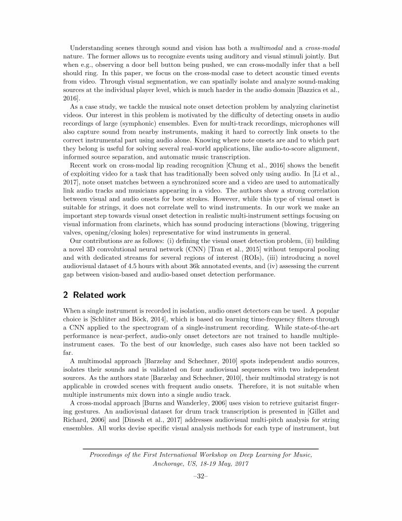
Understanding scenes through sound and vision has both a multimodal and a cross-modalnature. The former allows us to recognize events using auditory and visual stimuli jointly. Butwhen e.g., observing a door bell button being pushed, we can cross-modally infer that a bellshould ring. In this paper, we focus on the cross-modal case to detect acoustic timed eventsfrom video. Through visual segmentation, we can spatially isolate and analyze sound-makingsources at the individual player level, which is much harder in the audio domain [Bazzica et al.,2016].

As a case study, we tackle the musical note onset detection problem by analyzing clarinetistvideos. Our interest in this problem is motivated by the difficulty of detecting onsets in audiorecordings of large (symphonic) ensembles. Even for multi-track recordings, microphones willalso capture sound from nearby instruments, making it hard to correctly link onsets to thecorrect instrumental part using audio alone. Knowing where note onsets are and to which partthey belong is useful for solving several real-world applications, like audio-to-score alignment,informed source separation, and automatic music transcription.

Recent work on cross-modal lip reading recognition [Chung et al., 2016] shows the benefitof exploiting video for a task that has traditionally been solved only using audio. In [Li et al.,2017], note onset matches between a synchronized score and a video are used to automaticallylink audio tracks and musicians appearing in a video. The authors show a strong correlationbetween visual and audio onsets for bow strokes. However, while this type of visual onset issuitable for strings, it does not correlate well to wind instruments. In our work we make animportant step towards visual onset detection in realistic multi-instrument settings focusing onvisual information from clarinets, which has sound producing interactions (blowing, triggeringvalves, opening/closing holes) representative for wind instruments in general.

Our contributions are as follows: (i) defining the visual onset detection problem, (ii) buildinga novel 3D convolutional neural network (CNN) [Tran et al., 2015] without temporal poolingand with dedicated streams for several regions of interest (ROIs), (iii) introducing a novelaudiovisual dataset of 4.5 hours with about 36k annotated events, and (iv) assessing the currentgap between vision-based and audio-based onset detection performance.

2 Related work

When a single instrument is recorded in isolation, audio onset detectors can be used. A popularchoice is [Schluter and Bock, 2014], which is based on learning time-frequency filters througha CNN applied to the spectrogram of a single-instrument recording. While state-of-the-artperformance is near-perfect, audio-only onset detectors are not trained to handle multiple-instrument cases. To the best of our knowledge, such cases also have not been tackled sofar.

A multimodal approach [Barzelay and Schechner, 2010] spots independent audio sources,isolates their sounds and is validated on four audiovisual sequences with two independentsources. As the authors state [Barzelay and Schechner, 2010], their multimodal strategy is notapplicable in crowded scenes with frequent audio onsets. Therefore, it is not suitable whenmultiple instruments mix down into a single audio track.

A cross-modal approach [Burns and Wanderley, 2006] uses vision to retrieve guitarist finger-ing gestures. An audiovisual dataset for drum track transcription is presented in [Gillet andRichard, 2006] and [Dinesh et al., 2017] addresses audiovisual multi-pitch analysis for stringensembles. All works devise specific visual analysis methods for each type of instrument, but



–32–

do not consider transcription or onset detection for clarinets.Action recognition aims to understand events. Solutions based on 3D convolutions [Tran

et al., 2015] use frame sequences to learn spatio-temporal filters, whereas two-streams networks[Feichtenhofer et al., 2016] add a temporal optical flow stream. A recurrent network [Donahueet al., 2015] uses LSTM units on top of 2D convolutional networks. While action recognitionis similar to visual-based acoustic timed events detection, there is a fundamental difference:action recognition aims to detect the presence or absence of an action in a video. Instead, weare interested in the exact temporal location of the onset.

In action localization [Mettes et al., 2016] the task is to find what, when, and where an actionhappens. This is modeled with a “spatio-temporal tube”: a list of bounding-boxes over frames.Instead, we are not interested in the spatial location; we aim for the temporal location only,which due to the high-speed nature of onsets reverts to the extreme case of a single temporalpoint.

3 Proposed baseline method

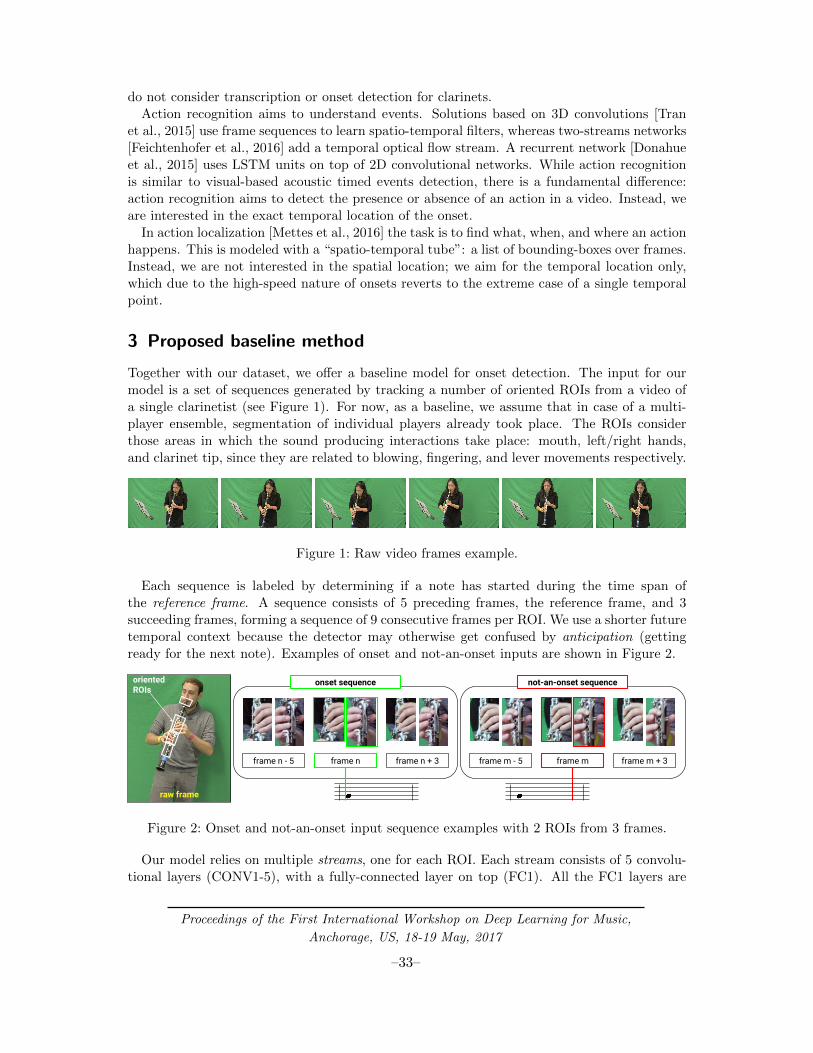
Together with our dataset, we offer a baseline model for onset detection. The input for ourmodel is a set of sequences generated by tracking a number of oriented ROIs from a video ofa single clarinetist (see Figure 1). For now, as a baseline, we assume that in case of a multi-player ensemble, segmentation of individual players already took place. The ROIs considerthose areas in which the sound producing interactions take place: mouth, left/right hands,and clarinet tip, since they are related to blowing, fingering, and lever movements respectively.

Figure 1: Raw video frames example.

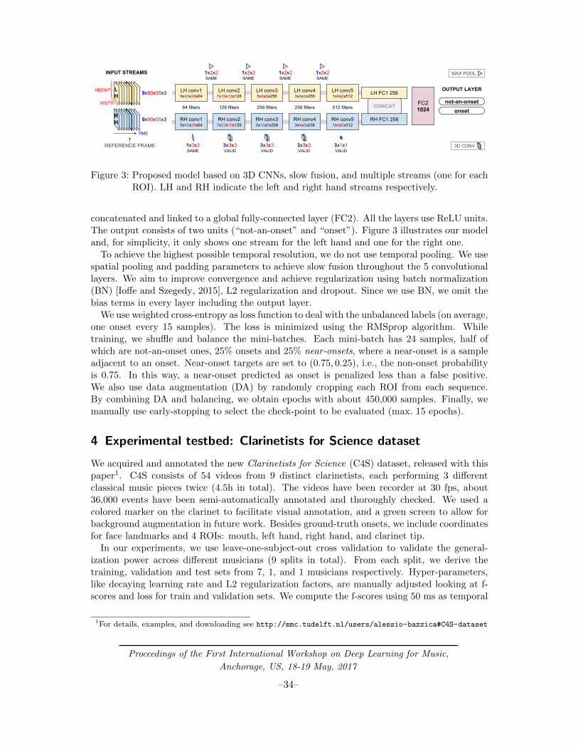
Each sequence is labeled by determining if a note has started during the time span ofthe reference frame. A sequence consists of 5 preceding frames, the reference frame, and 3succeeding frames, forming a sequence of 9 consecutive frames per ROI. We use a shorter futuretemporal context because the detector may otherwise get confused by anticipation (gettingready for the next note). Examples of onset and not-an-onset inputs are shown in Figure 2.

frame m - 5 frame m + 3frame mframe n - 5 frame n frame n + 3

onset sequence not-an-onset sequence

raw frame

orientedROIs

Figure 2: Onset and not-an-onset input sequence examples with 2 ROIs from 3 frames.

Our model relies on multiple streams, one for each ROI. Each stream consists of 5 convolu-tional layers (CONV1-5), with a fully-connected layer on top (FC1). All the FC1 layers are



–33–

9x90x55x3

9x80x55x3

FC21024 onset

not-an-onset

INPUT STREAMS

CONCAT

LH FC1 256

RH FC1 256

LH

RH

WIDTH

HEIGHT

TIME

REFERENCE FRAME

LH conv19x40x28x64

LH conv27x19x13x128

LH conv35x9x6x256

LH conv43x4x2x256

LH conv51x4x2x512

RH conv19x45x28x64

RH conv27x22x13x128

RH conv35x10x6x256

RH conv43x4x2x256

RH conv51x4x2x512

1x3x3SAME

3x3x3VALID

3x1x1VALID

3x3x3VALID

3x3x3VALID

1x2x2SAME

1x2x2SAME

1x2x2SAME

1x2x2SAME

OUTPUT LAYER

MAX POOL

3D CONV

64 filters 128 filters 256 filters 256 filters 512 filters

Figure 3: Proposed model based on 3D CNNs, slow fusion, and multiple streams (one for eachROI). LH and RH indicate the left and right hand streams respectively.

concatenated and linked to a global fully-connected layer (FC2). All the layers use ReLU units.The output consists of two units (“not-an-onset” and “onset”). Figure 3 illustrates our modeland, for simplicity, it only shows one stream for the left hand and one for the right one.

To achieve the highest possible temporal resolution, we do not use temporal pooling. We usespatial pooling and padding parameters to achieve slow fusion throughout the 5 convolutionallayers. We aim to improve convergence and achieve regularization using batch normalization(BN) [Ioffe and Szegedy, 2015], L2 regularization and dropout. Since we use BN, we omit thebias terms in every layer including the output layer.

We use weighted cross-entropy as loss function to deal with the unbalanced labels (on average,one onset every 15 samples). The loss is minimized using the RMSprop algorithm. Whiletraining, we shuffle and balance the mini-batches. Each mini-batch has 24 samples, half ofwhich are not-an-onset ones, 25% onsets and 25% near-onsets, where a near-onset is a sampleadjacent to an onset. Near-onset targets are set to (0.75, 0.25), i.e., the non-onset probabilityis 0.75. In this way, a near-onset predicted as onset is penalized less than a false positive.We also use data augmentation (DA) by randomly cropping each ROI from each sequence.By combining DA and balancing, we obtain epochs with about 450,000 samples. Finally, wemanually use early-stopping to select the check-point to be evaluated (max. 15 epochs).

4 Experimental testbed: Clarinetists for Science dataset

We acquired and annotated the new Clarinetists for Science (C4S) dataset, released with thispaper1. C4S consists of 54 videos from 9 distinct clarinetists, each performing 3 differentclassical music pieces twice (4.5h in total). The videos have been recorder at 30 fps, about36,000 events have been semi-automatically annotated and thoroughly checked. We used acolored marker on the clarinet to facilitate visual annotation, and a green screen to allow forbackground augmentation in future work. Besides ground-truth onsets, we include coordinatesfor face landmarks and 4 ROIs: mouth, left hand, right hand, and clarinet tip.

In our experiments, we use leave-one-subject-out cross validation to validate the general-ization power across different musicians (9 splits in total). From each split, we derive thetraining, validation and test sets from 7, 1, and 1 musicians respectively. Hyper-parameters,like decaying learning rate and L2 regularization factors, are manually adjusted looking at f-scores and loss for train and validation sets. We compute the f-scores using 50 ms as temporal

1For details, examples, and downloading see http://mmc.tudelft.nl/users/alessio-bazzica#C4S-dataset



–34–

tolerance to accept a predicted onset as true positive. We compare to a ground-truth informedrandom baseline (correct number of onsets known) and to two state-of-the-art audio-only onsetdetectors (namely, SuperFlux [Bock and Widmer, 2013] and CNN-based [Schluter and Bock,2014]).

5 Results and discussion

During our preliminary experiments, most of the training trials were used to select optimizationalgorithm and suitable hyper-parameters. Initially, gradients were vanishing, most of the neu-rons were inactive, and networks were only learning bias terms. After finding hyper-parametersovercoming the aforementioned issues, we trained our model on 2 splits.

method Split 1 Split 2 Average

informed random baseline 27.4 19.6 23.5

audio-only SuperFlux [Bock and Widmer, 2013] 82.8 81.3 82.1

audio-only CNN [Schluter and Bock, 2014] 94.3 92.1 93.2

visual-based (proposed) 26.3 25.0 25.7

Table 1: F-scores with a temporal tolerance of 50 ms.

By inspecting the f-scores in Table 1, we see that our method only performs slightly betterthan the baseline, and that the gap between audio-only and visual-based methods is large (60%on average). We investigated why and found that throughout the training, precision and recalloften oscillate with a negative correlation. This means that our model struggles with jointlyoptimizing those scores. This issue could be alleviated by different near-onsets options or byformulating a regression problem instead of a binary classification one.

When we train on other splits, we observe initial f-scores not changing throughout the epochs.We also observe different speeds at which the loss function converges. The different behaviorsacross the splits may indicate that alternative initialization strategies should be considered andthat the hyper-parameters are split-dependent.

6 Conclusions

We have presented a novel cross-modal way to solve note onset detection visually. In ourpreliminary experiments, we faced several challenges and learned that our model is highlysensitive to initialization, optimization algorithm and hyper-parameters. Also, using a binaryclassification approach may prevent the joint optimization of precision and recall. To allowfurther research, we release our novel fully-annotated C4S dataset. Beyond visual onset de-tection, C4S data will also be useful for clarinet tracking, body pose estimation, and ancillarymovement analysis.

Acknowledgments

We thank the C4S clarinetists, Bochen Li, Sara Cazzanelli, Marijke Schaap, Ruud de Jong,dr. Michael Riegler and the SURFsara Dutch National Cluster team for their support in en-abling the experiments of this paper.



–35–

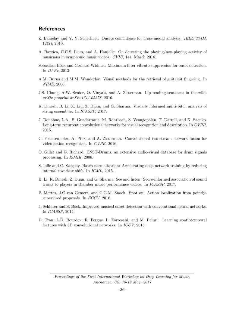
References

Z. Barzelay and Y. Y. Schechner. Onsets coincidence for cross-modal analysis. IEEE TMM,12(2), 2010.

A. Bazzica, C.C.S. Liem, and A. Hanjalic. On detecting the playing/non-playing activity ofmusicians in symphonic music videos. CVIU, 144, March 2016.

Sebastian Bock and Gerhard Widmer. Maximum filter vibrato suppression for onset detection.In DAFx, 2013.

A.M. Burns and M.M. Wanderley. Visual methods for the retrieval of guitarist fingering. InNIME, 2006.

J.S. Chung, A.W. Senior, O. Vinyals, and A. Zisserman. Lip reading sentences in the wild.arXiv preprint arXiv:1611.05358, 2016.

K. Dinesh, B. Li, X. Liu, Z. Duan, and G. Sharma. Visually informed multi-pitch analysis ofstring ensembles. In ICASSP, 2017.

J. Donahue, L.A., S. Guadarrama, M. Rohrbach, S. Venugopalan, T. Darrell, and K. Saenko.Long-term recurrent convolutional networks for visual recognition and description. In CVPR,2015.

C. Feichtenhofer, A. Pinz, and A. Zisserman. Convolutional two-stream network fusion forvideo action recognition. In CVPR, 2016.

O. Gillet and G. Richard. ENST-Drums: an extensive audio-visual database for drum signalsprocessing. In ISMIR, 2006.

S. Ioffe and C. Szegedy. Batch normalization: Accelerating deep network training by reducinginternal covariate shift. In ICML, 2015.

B. Li, K. Dinesh, Z. Duan, and G. Sharma. See and listen: Score-informed association of soundtracks to players in chamber music performance videos. In ICASSP, 2017.

P. Mettes, J.C van Gemert, and C.G.M. Snoek. Spot on: Action localization from pointly-supervised proposals. In ECCV, 2016.

J. Schluter and S. Bock. Improved musical onset detection with convolutional neural networks.In ICASSP, 2014.

D. Tran, L.D. Bourdev, R. Fergus, L. Torresani, and M. Paluri. Learning spatiotemporalfeatures with 3D convolutional networks. In ICCV, 2015.



–36–

Audio spectrogram representations forprocessing with Convolutional Neural Networks

Lonce Wyse∗1

1National University of Singapore

One of the decisions that arise when designing a neural network for any applica-tion is how the data should be represented in order to be presented to, and possiblygenerated by, a neural network. For audio, the choice is less obvious than it seemsto be for visual images, and a variety of representations have been used for differentapplications including the raw digitized sample stream, hand-crafted features, ma-chine discovered features, MFCCs and variants that include deltas, and a varietyof spectral representations. This paper reviews some of these representations andissues that arise, focusing particularly on spectrograms for generating audio usingneural networks for style transfer.

Keywords: spectrograms, data representation, style transfer, sound synthesis

1 Introduction

Audio can be represented in many ways, and which one is “best” depends on the applicationas well as the processing machinery. For many years, feature design and selection was a keycomponent of many audio analysis tasks and the list includes spectral centroid and higher-order statistics of spectral shape, zero crossing statistics, harmonicity, fundamental frequency,and temporal envelope descriptions. Today, the general wisdom is to let the network determinethe features it needs to accomplish its task.

For classification, particularly in speech, Mel Frequency Cepstral Coefficients (MFCCs)which describe the shape of a spectrum, have a long history. Although they are a lossyrepresentation, they are used for their classification and identification effectiveness even atvery reduced data rates compared to sampled audio. MFCC’s have also been used for environ-mental sound classification with convolutional neural networks [Piczak, 2015], although thereported 65% classification accuracy might be helped with a less lossy representation. Rawaudio samples have also been used for event classification, for example in SoundNet [Aytaret al., 2016].

∗[email protected]



–37–

2 Sound Representation for Generative Networks

For generative applications, a representation that can be used to synthesize high-quality soundis essential. This rules out “lossy” representations such as MFCCs and many hand-craftedfeature sets, but still leaves several options.

Raw audio samples are lossless and trivially convertible to audio. WaveNet [van den Oordet al., 2016], is a deep convolutional net (not recurrent) that uses raw audio samples as inputand is trained to predict the most likely next sample in a sequence. During the generative phase,each predicted sample is incorporated into the sequence used to predict the following sample.With “conditioning” information (such as which phoneme is being spoken) provided along withinput, interesting parametric control at synthesis time is possible. WaveNet implementationsrun as deep as 60 layers, and raw audio is typically sampled at rates ranging from 16K to 48Kper second, so synthesis is slow at many minutes of processing per second of audio.

Magnitude spectra can also be used for generative applications given techniques for derivingphase from properties of the magnitude spectra to reconstruct an audio signal. The most often-used phase reconstruction technique comes from Griffin and Lim [1984], which is implementedin the Librosa library [McFee et al., 2015]. However, it involves many iterations of forwardand inverse Short-time Fourier Transforms (STFTs), and is fundamentally not real time (thewhole temporal extent of the signal is used to reconstruct each point in time), and is plagued bylocal minima in the error surface that sometimes prevent high-quality reconstruction. Recentresearch has produced methods that are theoretically and in practice real time [Zhu et al.,2007] [Prusa and Søndergaard, 2016]; methods that can produce very convincing transients(temporally compact events) [Prusa, 2017]; and non-iterative methods of reasonable qualitythat are as fast to compute as a single STFT [Beauregard et al., 2015].

Spectrograms are 2D images representing sequences of spectra with time along one axis,frequency along the other, and brightness or color representing the strength of a frequencycomponent at each time frame. This representation is thus at least suggestive that some ofthe convolutional neural network architectures for images could be applied directly to sound.

Style transfer [Gatys et al., 2015] is a generative application that uses pre-trained networksto create new images combining the content of one image and the style of another. Becauseof the plethora of image networks available (e.g. VGG-19 [Simonyan and Zisserman, 2014]pre-trained on the 1.2M image database ImageNet [Deng et al., 2009]) and the dearth ofnetworks trained on audio data, the question naturally arises as to whether the image netswould be useful for audio style transfer representing audio spectrogram images. We ran someexperiments with the pre-trained VGG-19 network, with the goal of superimposing “style”or textural features from one spectrogram on the “content” or structural features of another.The features were defined as in [Gatys et al., 2015], so that content features were just theactivations in deeper layers of the network, and style features were defined as the Gram matrix,a second-order measure derived from activations on several shallower layers.

In order to use spectral data for this purpose, several issues had to be addressed. Becauseimage processing networks work on 3-channel RGB input, the single-channel magnitude valuesof the spectrograms must be duplicated across 3 channels to work with the pre-trained net-work. Since color channels are processed differently from each other in the neural network, thepost-processing synthesized color image must be converted back to a single channel based onluminosity to be meaningful as a spectrogram.

Although processing sonograms as images “works” in the sense that visual characteristicsare combined in interesting nonlinear ways, the resulting sounds are not nearly as compelling



–38–

as style transfer for visual images is. The issue is likely due to the difference between howsonic objects are represented in spectrograms compared to how visual objects are representedin 2D, and the way convolutional networks are designed to work with these images.

Convolutional neural networks designed for images use 2D convolution kernels that shareweights across both the x and the y dimensions. This is based in part on the notion oftranslational invariance, which means that an image feature or object is the same no matterwhere it is in the image. For sonic objects in the linear-frequency sonogram, this is truewhen objects are shifted in the x dimension (time), but not when they are shifted in the ydimension (frequency). Audio objects consist of energy across the frequency dimension, and asa sound is raised in pitch, its representation not only shifts up, but changes in spatial extent.A log frequency representation may go some way to addressing this issue, but the non-localdistribution of energy across frequency of an audio object might still be problematic for 2Dconvolution kernels. Sound images also present other challenges compared to visual images- for example, sound objects are “transparent” so that multiple objects can have energy atthe same frequency, where a given pixel in a visual image almost always corresponds to onlyone object. In addition, audio objects are non-locally distributed over a spectrogram whereasvisual objects tend to be comprised of neighboring pixels in an image.

Dmitry Ulyanov Ulyanov and Lebedev [2016] reports in a blog posting about using convo-lutional neural networks in a different way for audio style transfer. He uses spectrograms, butinstead of representing the frequency bins as the y dimension in an image, he considers thedifferent frequencies as existing at the same point in a 1D representation as stack of “channels”in the same way the 3 channels for red, green, and blue are stacked at each point in a 2D visualimage. As in image applications, the convolution kernel spans the entire channel dimension;there is no small shared-weight convolution kernel that shifts along the channel dimension asit does in the spatial dimensions. The number of audio channels, typically 256 or 512, is muchgreater than the 3 channels used for color images, and the vertical dimension is reduced to one.

There are two remarkable aspects to the network used by Ulyanov for style transfer thatdifferentiate it from the “classical” approach described by Gatys et al. [Gatys et al., 2015].First, the network uses only a single layer. The network activations driving content generationand those driving style generation come from one and the same set of weights. The differencebetween content and style thus comes not from the depth of the layers, but only from thedifference between first-order and second-order measures of activation. Secondly, the networkwas not pre-trained, but uses random weights. The blog post claims this unintuitive approachgenerated results as good as any other, and the sound examples posted are indeed compelling.

To further investigate the utility of spectrogram representations and the hypothesis thatweights are unimportant for style transfer, a network with two convolutional layers and twofully-connected layers was trained on the ESC-50 data set [Piczak, 2015] consisting of 20005-second sounds. Sounds were represented as spectrograms consisting of 856 frames with 257frequency bins, and the network was trained to recognize 50 classes. We then compared pre-trained and random weight values for style transfer1.

Sonograms generated with different weight and noise conditions are shown in Figure 1. Thecontent target is speech and the style target is a crowing rooster. This study shows a significant

1The network was trained with 2 convolutional layers of 2048 and 64 channels resp., used relu activationfunctions, and each was followed by max pooling of size 2 with strides of 2. A fully connected final layer had32 channels. A secondary classification was performed simultaneously (multi-task learning) as regularization,where sounds were divided into 16 balanced classes based on spectral centroid. Details and sound examplesat http://lonce.org/research/audioST



–39–

difference between random and pre-trained weights. Additionally, the network trained for audioclassification does not introduce the audible artifacts of the kind we found using an image-trained network. Although style transfer does work without regard to weights based only onthe first-order and second-order content and style matching strategy, a network trained foraudio classification appears to generate a more integrated synthesis of content and style.

Figure 1: a) With trained network weights and no added image noise, the result shows well-integrated features from both style and content. b) With random weights, styleinfluence is hard to detect and content sounds noisy. c) Adding noise to the initialimage results in sound that has the gross amplitude features of the content and anoisy timber barely identifiable with the style source d) Random weights and addedimage noise cause the loss of any sense of either content and style.

For the architecture we used, style suffers more than content from noise effects, whetheradded to the initial image, or in the form of random weights. Also, to compensate for thereduction of parameters in the network when arranging frequency bins as channels, it is neces-sary to dramatically increase the number of channels in the network layer(s) in order for longertimescale style features to appear in the synthesis. Ulyanov used 4096 channels, we used 2048in the first layer. This is both greater than the typical channel depth used in image processingnetworks, and greater than was necessary to pre-train the network on the classification task.

3 Summary

Spectral representations may have a role in applications that use neural networks for classifica-tion or regression. They retain more information than most hand-crafted features traditionallyused for audio analysis, and are of lower dimension than raw audio. The are particularly use-ful for generative applications due to available techniques for reconstructing high-quality audio



–40–

signals. Linear-frequency sonograms can not be treated in the same was as images are by 2Dconvolutional networks, but other approaches such as considering frequency bins as channelsare being explored and show promising results.

References

Yusuf Aytar, Carl Vondrick, and Antonio Torralba. Soundnet: Learning sound representationsfrom unlabeled video. In Advances in Neural Information Processing Systems, pages 892–900, 2016.

Gerry Beauregard, Mithila Harish, and Lonce Wyse. Single pass spectrogram inversion. InProceedings of the 2015 IEEE International Conference on Digital Signal Processing. IEEE,2015.

Jia Deng, Wei Dong, Richard Socher, Li jia Li, Kai Li, and Li Fei-fei. Imagenet: A large-scalehierarchical image database. In In CVPR, 2009.

Leon A. Gatys, Alexander S. Ecker, and Matthias Bethge. A neural algorithm of artistic style.In arXiv preprint arXiv:1508.06576, 2015.

D.W. Griffin and J.S. Lim. Signal estimation from modified shorttime fourier transform. InIEEE Trans. Audio Speech Lang. Process, volume ASSP-32, no. 2, pages 236–243. IEEE,1984.

Brian McFee, Colin Raffel, Dawen Liang, Daniel PW Ellis, Matt McVicar, Eric Battenberg,and Oriol Nieto. librosa: Audio and music signal analysis in python. In Proceedings of the14th python in science conference, 2015.

Karol J. Piczak. Environmental sound classification with convolutional neural networks. InMachine Learning for Signal Processing (MLSP), 2015 IEEE 25th International Workshopon. IEEE, 2015.

Zdenek Prusa. Towards high quality real-time signal reconstruction from stft magnitude. 2017.(accessed March10, 2017) http://ltfat.github.io/notes/ltfatnote048.pdf.

Zdenek Prusa and Peter L Søndergaard. Real-time spectrogram inversion using phase gradientheap integration. In Proc. Int. Conf. Digital Audio Effects (DAFx-16), 2016.

Karen Simonyan and Andrew Zisserman. Very deep convolutional networks for large-scaleimage recognition. CoRR, abs/1409.1556, 2014. URL http://arxiv.org/abs/1409.1556.

Dmitry Ulyanov and Vadim Lebedev. Audio texture synthesis and style trans-fer, 2016. (accessed March10, 2017) https://dmitryulyanov.github.io/

audio-texture-synthesis-and-style-transfer/.

Aaron van den Oord, Sander Dieleman, Heiga Zen, Karen Simonyan, Oriol Vinyals, AlexGraves, Nal Kalchbrenner, Andrew Senior, and Koray Kavukcuoglu. Wavenet: A generativemodel for raw audio. CoRR abs/1609.03499, 2016.

Xinglei Zhu, Gerry Beauregard, and Lonce Wyse. Real-time signal estimation from modifiedshort-time fourier transform magnitude spectra. In IEEE Trans. Audio Speech Lang. Process,volume 15, pages 1645–1653. IEEE, 2007.



–41–

Part III

Short talks

42

Talking Drums: Generating drum grooves withneural networks

P. Hutchings∗1

1Monash University, Melbourne, Australia

Presented is a method of generating a full drum kit part for a provided kick-drumsequence. A sequence to sequence neural network model used in natural languagetranslation was adopted to encode multiple musical styles and an online surveywas developed to test different techniques for sampling the output of the softmaxfunction. The strongest results were found using a sampling technique that drewfrom the three most probable outputs at each subdivision of the drum pattern butthe consistency of output was found to be heavily dependent on style.

Keywords: RNN, percussion, generative music, translation

1 Introduction

This research details the development of a percussion-role agent as part of a larger projectwhere virtual, self-rating agents with different musical roles work in a process of co-agency togenerate music compositions in real-time [Hutchings and McCormack, 2017]. The percussion-role agent was developed for generating multiple possible multi-instrument percussion parts toaccompany provided melodies and harmonies in real-time.

A neural network based agent was developed to incorporate a range of different music stylesfrom a large corpus of compositions and to utilise a softmax function as part of the self-ratingprocess. A network architecture used in natural language translation was adopted based onthe idea that a percussion score could be considered as containing multiple drums ‘speaking’different languages but saying the same thing at the same time. The network was trained on acollection of drum kit scores from over 250 pop, rock, funk and Afro-Cuban style compositionsand patterns from drum technique books. The output of the network was evaluated froman online survey and a physical interface was developed for feeding kick-drum parts into thenetwork.

∗[email protected]



–43–

1.1 Related work

Markov models [Hawryshkewich et al., 2010] [Tidemann and Demiris, 2008], generative gram-mars [Bell and Kippen, 1992] and neural network models Choi et al. [2016] have all been shownto be effective in the area of drum score generation. The approach shown in this paper is basedon the requirements of generating an agent for a multi-agent composition system. Research inthis area has demonstrated the need for agent models to match the needs of the overall system[Eigenfeldt and Pasquier, 2009].

The similarities and differences between music and natural language have been explored indetail [Patel, 2003] [Mithen, 2011]. While distinct differences exist in terms of cognitive pro-cessing, semantics and cultural function, there are similarities in the structure of phrases thathave lead to the use of natural language processing techniques in the analysis and generationof music.

1.2 Translation model

Generating a full drum kit score based on the rhythm of one or more individual instruments inthe kit is a problem with different challenges than natural language translation. All translationsare one to one in word count. Music is a non-semantic form of communication which allowsfor and values greater structural variation than spoken language so imperfect translations canstill be effective. Conversely because there is no perfect translation, there are many differentoutputs for a given input in the training data, decreasing convergence during training. Theproblem can also be viewed as one of data-expansion as a single instrument part is expandedto fill a full drum kit with multiple concurrent instruments being used. To take advantage ofthese strengths and diminish the weaknesses of a translation based neural network model anew syntax for expressing drum parts was developed.

2 Method

2.1 Data preprocessing

A collection of 250 drum kit scores in 4/4 were found on drum tablature websites and booksand parsed into a music-XML format. Tracks were selected based on the most viewed web-pages for rock, pop, funk and Afro-Cuban styles of music and were each checked for accuracyby comparing with the original recordings by ear. Pop, rock and funk styles were selecteddue to their global popularity and typical use of a standard drum kit. The Afro-Cuban stylewas added to this list to see if some of the stricter idiomatic structures of the style, such asthe ‘clave’ rhythmic pattern, could be preserved. Afro-Cuban and funk drum tablatures weremore difficult to find so the tablatures were augmented with patterns from drum techniqueinstruction books. For each genre a total of 7000-7500 bars were parsed.

Each bar was divided into 48 subdivisions, allowing all triplet and tuple divisions down tothe resolution of semiquaver triplets to be represented. Each division was given a word tokenthat represented the drums being hit on that subdivision and barlines were replaced with aword token describing the musical style which allowed multiple styles to be encoded in a singleRNN network.

The tokenised phrase in Equation 1 represents a kick-drum being kicked on each beat of a



–44–

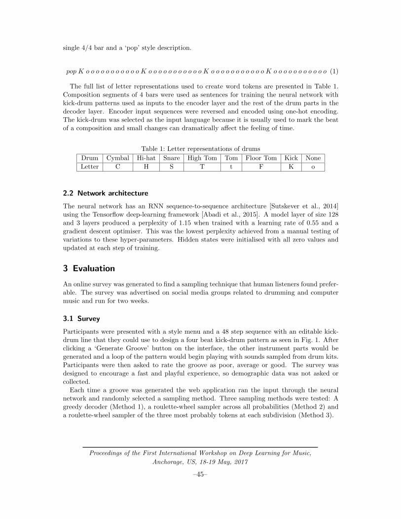
single 4/4 bar and a ‘pop’ style description.

pop K o o o o o o o o o o o K o o o o o o o o o o o K o o o o o o o o o o o K o o o o o o o o o o o (1)

The full list of letter representations used to create word tokens are presented in Table 1.Composition segments of 4 bars were used as sentences for training the neural network withkick-drum patterns used as inputs to the encoder layer and the rest of the drum parts in thedecoder layer. Encoder input sequences were reversed and encoded using one-hot encoding.The kick-drum was selected as the input language because it is usually used to mark the beatof a composition and small changes can dramatically affect the feeling of time.

Table 1: Letter representations of drums

Drum Cymbal Hi-hat Snare High Tom Tom Floor Tom Kick None

Letter C H S T t F K o

2.2 Network architecture

The neural network has an RNN sequence-to-sequence architecture [Sutskever et al., 2014]using the Tensorflow deep-learning framework [Abadi et al., 2015]. A model layer of size 128and 3 layers produced a perplexity of 1.15 when trained with a learning rate of 0.55 and agradient descent optimiser. This was the lowest perplexity achieved from a manual testing ofvariations to these hyper-parameters. Hidden states were initialised with all zero values andupdated at each step of training.

3 Evaluation

An online survey was generated to find a sampling technique that human listeners found prefer-able. The survey was advertised on social media groups related to drumming and computermusic and run for two weeks.

3.1 Survey

Participants were presented with a style menu and a 48 step sequence with an editable kick-drum line that they could use to design a four beat kick-drum pattern as seen in Fig. 1. Afterclicking a ‘Generate Groove’ button on the interface, the other instrument parts would begenerated and a loop of the pattern would begin playing with sounds sampled from drum kits.Participants were then asked to rate the groove as poor, average or good. The survey wasdesigned to encourage a fast and playful experience, so demographic data was not asked orcollected.

Each time a groove was generated the web application ran the input through the neuralnetwork and randomly selected a sampling method. Three sampling methods were tested: Agreedy decoder (Method 1), a roulette-wheel sampler across all probabilities (Method 2) anda roulette-wheel sampler of the three most probably tokens at each subdivision (Method 3).



–45–

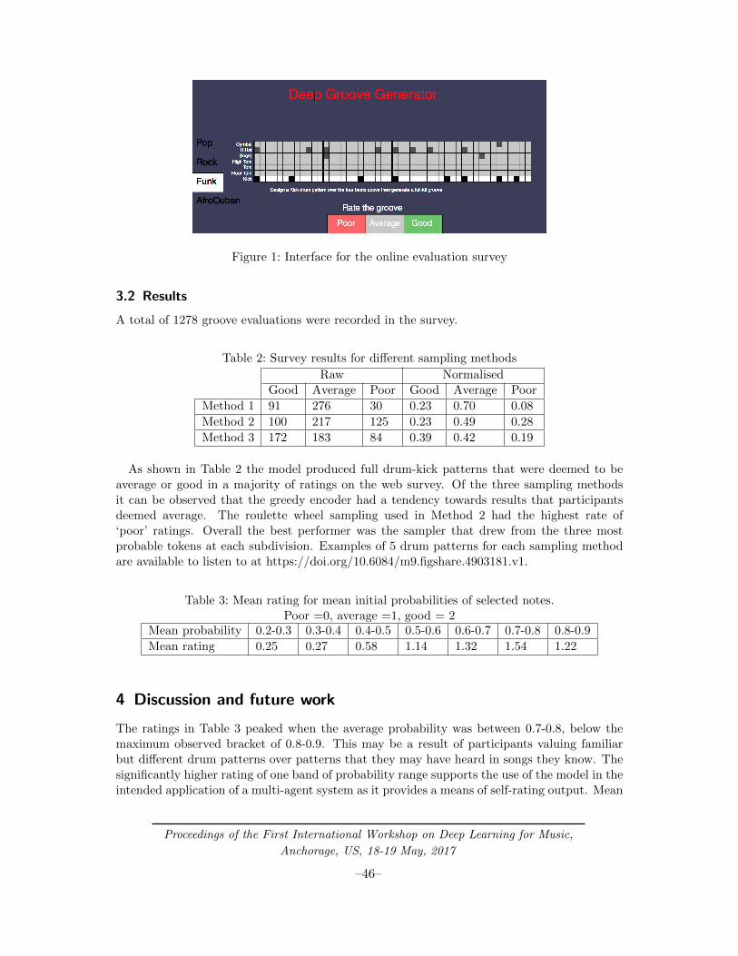
Figure 1: Interface for the online evaluation survey

3.2 Results

A total of 1278 groove evaluations were recorded in the survey.

Table 2: Survey results for different sampling methods

Raw NormalisedGood Average Poor Good Average Poor

Method 1 91 276 30 0.23 0.70 0.08

Method 2 100 217 125 0.23 0.49 0.28

Method 3 172 183 84 0.39 0.42 0.19

As shown in Table 2 the model produced full drum-kick patterns that were deemed to beaverage or good in a majority of ratings on the web survey. Of the three sampling methodsit can be observed that the greedy encoder had a tendency towards results that participantsdeemed average. The roulette wheel sampling used in Method 2 had the highest rate of‘poor’ ratings. Overall the best performer was the sampler that drew from the three mostprobable tokens at each subdivision. Examples of 5 drum patterns for each sampling methodare available to listen to at https://doi.org/10.6084/m9.figshare.4903181.v1.

Table 3: Mean rating for mean initial probabilities of selected notes.Poor =0, average =1, good = 2

Mean probability 0.2-0.3 0.3-0.4 0.4-0.5 0.5-0.6 0.6-0.7 0.7-0.8 0.8-0.9

Mean rating 0.25 0.27 0.58 1.14 1.32 1.54 1.22

4 Discussion and future work

The ratings in Table 3 peaked when the average probability was between 0.7-0.8, below themaximum observed bracket of 0.8-0.9. This may be a result of participants valuing familiarbut different drum patterns over patterns that they may have heard in songs they know. Thesignificantly higher rating of one band of probability range supports the use of the model in theintended application of a multi-agent system as it provides a means of self-rating output. Mean



–46–

ratings of Afro-Cuban style patterns were significantly lower (24% poor) than for other styles(16-18% poor) which may be the result of stylistic bias of the participants or could suggestimportant elements of the style are not represented in the model output.

A syntax for expressing desired accents is being developed as an encoder to expand the palletand may improve results in the Afro-Cuban and other styles. A physical drum-pedal interfacehas been developed to test the system with drummers in a natural playing position.

References

Martın Abadi, Ashish Agarwal, Paul Barham, Eugene Brevdo, Zhifeng Chen, Craig Citro,Greg S. Corrado, Andy Davis, Jeffrey Dean, Matthieu Devin, Sanjay Ghemawat, IanGoodfellow, Andrew Harp, Geoffrey Irving, Michael Isard, Yangqing Jia, Rafal Jozefow-icz, Lukasz Kaiser, Manjunath Kudlur, Josh Levenberg, Dan Mane, Rajat Monga, SherryMoore, Derek Murray, Chris Olah, Mike Schuster, Jonathon Shlens, Benoit Steiner, IlyaSutskever, Kunal Talwar, Paul Tucker, Vincent Vanhoucke, Vijay Vasudevan, FernandaViegas, Oriol Vinyals, Pete Warden, Martin Wattenberg, Martin Wicke, Yuan Yu, and Xi-aoqiang Zheng. TensorFlow: Large-scale machine learning on heterogeneous systems, 2015.URL http://tensorflow.org/. Software available from tensorflow.org.

Bernard Bell and Jim Kippen. Bol processor grammars, understanding music with ai: per-spectives on music cognition, 1992.

Keunwoo Choi, George Fazekas, and Mark B. Sandler. Text-based LSTM networks for au-tomatic music composition. CoRR, abs/1604.05358, 2016. URL http://arxiv.org/abs/

1604.05358.

Arne Eigenfeldt and Philippe Pasquier. A realtime generative music system using autonomousmelody, harmony, and rhythm agents. In XIII Internationale Conference on GenerativeArts, Milan, Italy, 2009.

Andrew Hawryshkewich, Philippe Pasquier, and Arne Eigenfeldt. Beatback: A real-time in-teractive percussion system for rhythmic practise and exploration. In NIME, pages 100–105,2010.

Patrick Hutchings and Jon McCormack. Using autonomous agents to improvise music compo-sitions in real-time. In International Conference on Evolutionary and Biologically InspiredMusic and Art, pages 114–127. Springer, 2017.

S. Mithen. The Singing Neanderthals: The Origins of Music, Language, Mind and Body. Orion,2011. ISBN 9781780222585. URL https://books.google.com.au/books?id=3aP0tkerd_

wC.

Aniruddh D Patel. Language, music, syntax and the brain. Nature neuroscience, 6(7):674–681,2003.

Ilya Sutskever, Oriol Vinyals, and Quoc V Le. Sequence to sequence learning with neuralnetworks. In Advances in neural information processing systems, pages 3104–3112, 2014.

Axel Tidemann and Yiannis Demiris. A drum machine that learns to groove. In AnnualConference on Artificial Intelligence, pages 144–151. Springer, 2008.



–47–

Transforming Musical Signals through a GenreClassifying Convolutional Neural Network

Shijia Geng∗1, Gang Ren†1, and Mitsunori Ogihara‡1, 2

1Center for Computational Science, University of Miami, Coral Gables, FL, USA

2Department of Computer Science, University of Miami, Coral Gables, FL, USA

Convolutional neural networks (CNNs) have been successfully applied on bothdiscriminative and generative modeling for music-related tasks. For a particulartask, the trained CNN contains information representing the decision making orthe abstracting process. One can hope to manipulate existing music based onthis “informed” network and create music with new features corresponding to theknowledge obtained by the network. In this paper, we propose a method to utilizethe stored information from a CNN trained on musical genre classification task.The network was composed of three convolutional layers, and was trained to classifyfive-second song clips into five different genres. After training, randomly selectedclips were modified by maximizing the sum of outputs from the network layers. Inaddition to the potential of such CNNs to produce interesting audio transformation,more information about the network and the original music could be obtained fromthe analysis of the generated features since these features indicate how the network“understands” the music.

Keywords: convolutional neural network, musical signal modification, musicalgenre classification

1 Introduction

Recent studies show that CNNs provide promising performance when applied to the music-related fields such as genre classification, instrument recognition, and music composing [Diele-man et al., 2011]. A CNN trained on a particular music-related task “learns” one type ofknowledge about music and it has the potential to be applied to reshaping music or audiorecording. It can be viewed as an audio counterpart of the deepdream project which adjustsimages to enhance patterns based on CNN trained on visual recognition tasks [Mordvintsevet al., 2015].

∗[email protected]†[email protected]‡[email protected]



–48–

2 Methods

In this study, a CNN with three convolutional layers was trained to classify music into fivegenres (alternative, electronica, pop, rap, and rock). The private datasets for training andtesting were prepared from 23,639 song files. The signals obtained from the audio files weredownsampled to 8,000Hz and separated into five-second (40,000 data point) clips. Eventually,a total of 139,500 audio clips were prepared.

The major components of the network include an input layer, three convolutional layers, andan output layer. The shapes of the input and output layers are 1×40, 000 and 1×5, respectively.The convolutional layers hold 16 filters each, having length 8, 32, and 128, respectively. Thestride length for each filter is 8. The activation function for each node in the convolutionallayers is the rectify function. In addition, batch normalization was applied on the intermediateresult generated by each convolutional layer.

The optimization approach used in the classification task was mini-batch gradient descent,which took a subset of data in each iteration and updated the parameters based on the gradientof the aggregated loss. The specific update method applied was based on Nesterov’s acceleratedgradient descent. During training, twenty epochs were applied and the training loss and trainingtime for each epoch were recorded.

The computational goal for the modification procedure was to modify the input clip in orderto maximize the objective function which is the sum of a particular convolutional layer or allconvolutional layers. The optimization method chosen to maximize the objective function wasgradient ascent. Each modified clip was normalized and saved as a 16-bit audio file in thelinear pulse-code modulation waveform audio file format.

3 Results and Discussion

The classification accuracies for the five genres, alternative, electronica, pop, rap and rockmusic, are respectively 27.6%, 45.3%, 34.2%, 84.3%, and 51.2%. The results indicate that theproposed CNN has better performances for the genres with outstanding characteristic suchas rap and rock. However, its ability to distinguish genres with uncertain features such asalternative and pop is weak. A more complicated network architecture may be required inorder to overcome the weakness.

The resulting audio files are available at [Mod, 2017]. The ones based on lower layers tend todevelop some attack-like features, while the ones based on higher layers have clear harmonicspattern. More constraints might be necessary to reduce the noises in the modification.

References

Modifications https://sites.google.com/site/modificationofmusicsignals/, 2017.

Sander Dieleman, Philemon Brakel, and Benjamin Schrauwen. Audio-based music classificationwith a pretrained convolutional network. In 12th International Society for Music InformationRetrieval Conference (ISMIR-2011), pages 669–674. University of Miami, 2011.

Alexander Mordvintsev, Christopher Olah, and Mike Tyka. Inceptionism: Going deeper intoneural networks. Google Research Blog. Retrieved June, 20:14, 2015.



–49–

Machine listening intelligence

Carmine-Emanuele Cella1

1Ircam, Paris, France

This manifesto paper will introduce machine listening intelligence, an integratedresearch framework for acoustic and musical signals modelling, based on signalprocessing, deep learning and computational musicology.

Keywords: deep unsupervised learning, computational musicology, representation theory.

1 Introduction

1.1 Motivation

The relation between signals and symbols is a central problem for acoustic signal processing.Among different kind of signals, musical signals are specific examples in which there is someinformation regarding the underlying symbolic structure. While an impressive amount ofresearch has been done in this domain in the past thirty years, the symbolic processing ofacoustic and musical signals is still only partially possible.

The aim of this paper, grounded on our previous work [Cella, 2009], is to propose a manifestofor a generalised approach for the representation of acoustic and musical signalscalled machine listening intelligence (MLI), by integrating cognitive musicology in-sights, hand-crafted signal processing and deep learning methods in a general mathematicalframework.

Among existing approaches that share similarities with ours, there are the multiple viewpointsystem [Conklin, 2013] and IDyOM [Pearce and Wiggins, 2013]. While comparing differencesand similiarities with these approaches could be interesting, we will not do this here and wemention them only for reference.

1.2 Scientific assessment

In the past twenty years, with the improvement of computers and the advancements in ma-chine learning techniques, a whole field called music information retrieval (MIR) developedmassively. This important domain of research brought impressive results and had been ableto tackle problems that appeared to be unsolvable, such as the classification of very com-plex signals. Nonetheless, tasks that are relatively easy for humans are still hard and thereare not general solutions. Apparently, these kind of tasks are often ill-defined or lack properinformation to be correctly represented.



–50–

More recently, the uprise of deep learning techniques in computer vision created a real revolu-tion in machine learning given the advancements they provided [Krizhevsky et al., 2012]. Deepconvolutional networks, for example, provide state of the art classifications and regressionsresults over many high-dimensional problems [Le Cun et al., 2015]. Their general architectureis based on a cascade of linear filter weights and non-linearities [Mallat, 2016]; the weightsare learned from massive training phases and generally outperform hand-crafted features. Theswitch to large scale problems that happened in the past few years in the computer visioncommunity, moreover, proved the fact that we need to address more general problems foracoustic signals, where the domain of research is not defined by a single sample but by a wholepopulation.

However, these complex programmable machines bring us to a very difficult and partiallyunknown mathematical world. We believe that representation theory is good candidate forsuch mathematical model. Signal representation methods can be thought as linear operatorsin vector space and representation theory studies abstract algebraic structures by representingtheir elements as linear transformations of vector spaces [Fulton and Harris, 2004].

Next sections will be as follows: section 2 will show some problems and applications thatwe would like to address with our approach. From section 3 we will go more into technicaldetails describing what are representations for signals and reviewing their properties both fromcognitive and mathematical standpoints. This will serve a background for section 4, that willpresent the general research approach for MLI.

2 Problems and outcomes

Among the large number of open problems in the field of signal processing, we would liketo present here some interesting examples that could be treated in the context of machinelistening intelligence. These problems refer particularly to music and creative applications,but we think that the developed methodology could be further used in different domains. Assuch, they must be considered just as examples of possible outcomes.

2.1 Semantic signal processing

A signal transformation is, in a general sense, any process that changes or alter a signalin a significant way. Transformations are closely related to representations: each action is,indeed, performed in a specific representation level. For example, an elongation performedin time domain gives inferior results (perceptually) to the same transformation performed infrequency domain, where you have access to phases. In the same way, a pitch shift operatedin frequency domain gives inferior results to the same operation performed using a spectralenvelope representation, where you have access to dominant regions in the signal. In the twocases discussed above we passed from a low-level representation (waveform) to a middle-levelrepresentation (spectral envelope). We could, ideally, iterate this process by increasing thelevel of abstraction in a representation thus giving access to specific properties of sound thatare perceptually relevant; by means of a powerful representation it could therefore be possibleto access a semantic level for transformations. We envision, therefore, the possibility in thefuture to have such kind of semantic transformations by accessing representations given bydeep learning models.



–51–

2.2 High-level acoustic features

One of the most impressive example of creative application of deep learning is, in our opinion,style transfer. In a paper published in 2016 [Gatys et al., 2016], for example, the authorsshowed how it is possible, using the latent space of a deep network, to transfer high levelfeatures from one image to another. It is interesting to remark that the transferred featuresare not simple effects but real traits of the style of the image.

Unfortunately, such an impressive process is not possible on acoustic signals for the moment.In 2013 we achieved the construction of an advanced hybridisation system for sounds [Cellaand Burred, 2013]. The basic idea of our approach was to represent sounds in term of classesof equivalences and probabilities, then mix the classes of one sound with the probabilitiesof another one. While the perceptual results were satisfying for us, the limitation of therepresentation method used, didn’t permit to access high-level acoustic features.

We believe that deep musical style transfer can be considered as a generalisation of hybridi-sation and we strongly believe that this kind of processing could be achieved by MLI.

3 Signal representations

Defining a representation for music and musical signals involves the establishment of essentialproperties that must be satisfied. Many years of research have been devoted to such a complextask in the field of cognitive musicology, a branch of cognitive sciences focused on the modellingof musical knowledge by means of computational methods [Laske and al., 1992].

Among important properties for musical representations found from the literature in thefield, there are milestones such as multiple abstraction levels, multi-scale and generativity.Interestingly enough, these properties are not only specific to music but can be applicable todifferent kind of acoustic signals, as we will see.

Usually, the description of acoustic signals select a particular degree of abstraction in thedomain of the representation. In general, low-level representations are generic and have veryhigh dimensionality. These representations evolve fast and the only transformations that arepossible at this level are geometric (translations, rotations, etc.) and are mostly defined oncontinuous (Lie) groups [Mallat, 2016]. In the middle, there are families of representations(often related to perceptual concepts) that have a medium level of abstraction and a not so hugedimensionality and allow for transformations on specific concept (variables), usually defined ondiscrete groups [Lostanlen and Cella, 2016]. On the other end, very abstract representationsare pretty much expressive and have a low dimensionality; in a sense, these representations dealwith almost-stationary entities such as musical ideas and unfortunately it is very difficult toknow which mathematical structure stays behind. As an example, we could think to low-levelrepresentations as signals (used by listeners), to middle-level as scores (used by performers)and to high-level as musical ideas (used by composers). Figure 1 depicts the outlined concepts.

Representations can be considered linear operators that need to be invariant to sources ofunimportant variability, while being able to capture discriminative information from signals.As such, they must respect four basic properties; being x a signal and Φx its representation:

• discriminability: Φx 6= Φy =⇒ x 6= y;

• stability: ‖Φx− Φy‖2 ≤ C‖x− y‖2;

• invariance (to group of transformations G): ∀g ∈ G,Φg.x = Φx;



–52–

ideas scores signals

composers performers + instruments listeners

fast

geometric transformations(translations, rotations, ...)

continuous (Lie) groupsdiscrete finite groups??

transformations on specific variables (known or discovered)

(symmetry in Z12)

unknown transformations

expressive generic

slowalmoststationary

high dimensionality,low abstraction

medium dimensionality,medium abstraction

low dimensionality,high abstraction

representations

Figure 1: Different abstraction degrees in representations.

• reconstruction: y = Φx ⇐⇒ x = Φ−1y.

Discriminability means that if the representations of two signals are different than the two sig-nals must be different. Stability means that a small modification of a signal should be reflectedin a small modification in the representation and vice-versa. Invariance to a group of transfor-mation G, means that if a member of the group is applied to a signal, than the representationmust not change; reconstruction, finally, is the possibility to go back to a signal that is equiv-alent to the original (in the sense of a group of transformations) from the representation. It ispossible to divide representations in two major categories: prior and learned.

3.1 Prior and learned representations

In prior representations, signals are decomposed using a basis that has been defined mathemat-ically, in order to respect (some of) the properties given above. The general model of a priorrepresentation is a decomposition of a signal x into a linear combination of expansion functions:x =

∑Kk=1 αkgk, where K is the dimensionality, the coefficients αk are weights derived from an

analysis stage an functions gk are fixed beforehand and are used during a synthesis stage. Thechoice of the decomposition functions is dependent on the particular type of application neededand the more compact (sparse) the representation is, the more the functions are correlated tothe signal.

In learned representations, the decomposition functions used to describe a signal are learnedby a training on some examples that belong to a specific problem. The training can be donein two different ways: supervised or unsupervised.

Supervised learning is a high-dimensional interpolation problem. We approximate a functionf(x) from q training samples {xi, f(xi)}i≤q, where x is a data vector of very high dimension d.A powerful example of supervised learned representation are convolutional neural networks.

In unsupervised training, on the other hand, there is not a target function to approximateand other mathematical constraints are applied, such as sparsity or variance reduction. Typical



–53–

examples of unsupervised representations are sparse coding and auto-encoders.

3.2 Importance of unsupervised learning

Recent advancements showed that supervised learning is able, if given the right conditions, tooutperform both unsupervised and prior representations. There are problems, however, wherethis family of representations cannot be applied and the only possible approach for learning arepresentation is using unsupervised methods:

• lack of labeled data: copyright issues can make impossible to deploy a database of labeledmusic of a significative size to be used a reference case for reproducible research;

• cost of data gathering : some real-life problems are related to contexts in which is impos-sible to gather large amount of data (such as biomedical recordings);

• conceptual disagreement : in some cases, it is very difficult or even impossible to assignlabels to acoustic signals given their inherent ambiguity (music is often such a case).

4 Research approach

The discussion given above outlines, in our opinion, the necessity of a general framework ableto integrate the different approaches to the representation of musical and acoustical signalsinto a common perspective.

Machine listening intelligence aims at being such a framework, by integrating cognitivemusicology insights, established signal processing techniques and more recent advancements indeep learning in the context of representation theory.

Prior representations are defined by mathematical models but fail to achieve the same ex-pressivity of learned representations. On the contrary, deep learning proved to be valuablein incredibly different domains and showed that some learning techniques are indeed general.One of the issues, in the case of acoustic and musical signals, is that there is not a commonand established mathematical model for this kind of methods. Moreover, supervised learningis not always possible for the reasons outlined in section 3.2. Therefore, we envision a researchapproach based on the following main factors:

• deep unsupervised learning methods: only with deep architectures it is possible tocreate multi-scale representations that have different abstraction levels; using unsuper-vised learning, it is possible to address difficult problems that lack labelled data;

• representation theory: by interpreting learning with linear operators, it is possible tocreate a common mathematical language to compare and study its properties;

• large scale problems: using large datasets (that usually embody difficult problems)will impose the research of scalable and general learning methods, that can be transferredto many different domains;

• multi-disciplinarity: putting together several sources of knowledge such as psychoa-coustics, cognitive musicology, computational neurobiology, signal processing and ma-chine learning is the key for future development of the so-called intelligent machines.



–54–

While prior representations formally define the level of abstraction, they cannot reach thesame level of aggregate information gathered by deep learning networks. These networks, onthe other hand, are not capable of explaining the concepts they discover. For such reasons,it is interesting to make a bridge between these two approaches by immersing both in a moregeneral framework that could be found in representation theory. Machine listening intelligenceaims at filling this gap.

References

C. E. Cella. Towards a symbolic approach to sound analysis. In proceedings of MCM. Yale,USA, 2009.

C. E. Cella and J. J. Burred. Advanced sound hybridization by means of the theory of sound-types. In proceedings of ICMC. Perth, Australia, 2013.

D. Conklin. Multiple viewpoint systems for music classification. In Journal of New MusicResearch, volume 42, no. 1, pages 19–26, 2013.

W. Fulton and J. Harris. Representation theory. In proceedings of MCM, volume 129. NY:Springer New York, 2004.

L. Gatys, A. Ecker, and M. Bethge. Style transfer using convolutional neural networks. Inproceedings of CVPR, 2016.

A. Krizhevsky, I. Sutskever, and G. Hinton. Imagenet classification with deep convolutionalneural networks. In proceedings of NIPS, pages 1090–1098, 2012.

O. Laske and al. Understanding music with a.i.: perspectives on music cognition. AAAI Press,1992.

Y. Le Cun, Y. Bengio, and G. Hinton. Deep learning. In Nature. 215, 2015.

V. Lostanlen and C. E. Cella. Deep convolutional networks on the pitch spiral for musicalinstrument recognition. In proceedings of ISMIR. New York, USA, 2016.

S. Mallat. Understanding deep convolutional networks. In Philosophical transactions A, 2016.

M. T. Pearce and G. A. Wiggins. Auditory expectation: The information dynamics of musicperception and cognition. In Topics in Cognitive Science, volume 4, no. 4, pages 625–652,2013.



–55–

Toward Inverse Control ofPhysics-Based Sound Synthesis

A. Pfalz1 and E. Berdahl1

1Louisiana State University

Long Short-Term Memory networks (LSTMs) can be trained to realize inversecontrol of physics-based sound synthesizers. Physics-based sound synthesizers sim-ulate the laws of physics to produce output sound according to input gesture signals.When a user’s gestures are measured in real time, she or he can use them to controlphysics-based sound synthesizers, thereby creating simulated virtual instruments.

An intriguing question is how to program a computer to learn to play suchphysics-based models. This work demonstrates that LSTMs can be trained toaccomplish this inverse control task with four physics-based sound synthesizers.

Keywords: LSTM, physics-based models, sound synthesis

1 Introduction

1.1 Sound Matching

Controlling the parameters of sound synthesizers in order to realize target sounds has been achallenge for decades. For instance, with the Frequency Modulation (FM) synthesis technique,the connection between the carrier frequencies, modulation frequencies, and modulation indices(particularly as these are automated) and the sound produced is complicated. Accordingly, re-searchers have applied various techniques for adapting FM parameters to achieve target soundssuch as Horner et al. [1993], Garcia [2001], Lai et al. [2006], and Tan and Lim [1996]. Similarwork as also been conducted for tuning the parameters of physics-based models; however, mostof these works have required very specific optimizations that apply only to certain models (seeSondhi and Resnick [1983] and Riionheimo and Valimaki [2002]).

1.2 Inverse Control

However, since humans are able to learn to play musical instruments, it seems very likelythat machine learning methods could help address the inverse control problem. For example,deep as well as shallow learning for audio and music generation has been investigated from anumber of different perspectives. One approach is generating sequences of notes using MIDIor symbolic notation (as in Waite [2016]). WaveNet is another very promising project amongothers (van den Oord et al. [2016]).



–56–

(a) Typical paradigm for physics-basedsound synthesis (forward control).

(b) Proposed paradigm (inverse control).

Figure 1: Paradigms for physics-based sound synthesis.

The advantage of this technique is that it allows the generation of sounds to be automated.If a complex sound is desired, the user needs to spend time practicing to execute a potentiallydifficult gesture to be able to produce the output audio.

2 Approach

2.1 Overview

Synth-A-Modeler is an open-source software project for building physics-based sound synthe-sizers (see Berdahl and Smith III [2012]). Figure 1a shows the typical paradigm for physics-based sound synthesis. In contrast, the present work proposes a new paradigm in which anLSTM learns to realize inverse control of a physics-based sound synthesizer. In other words,the LSTM uses a target sound to match the gesture that was used to create the target soundusing a physics-based sound synthesizer. Consequently, the predicted synthesized gesture canbe applied to a physics-based sound synthesizer to create a synthesized sound. Although notstudied directly in this introductory work, this paradigm has potential applications denoisingaudio recordings, toolkits for making foley, sound transformations and sound mappings.

2.2 Physics-Based Sound Synthesizers Used in the Project

Each physics-based sound synthesizer used in this work receives a gesture signal that could forexample represent the position of a musician’s hand in real-time, enabling her or him to playvirtual sound synthesizers. These gesture signals are in the range of −0.05 m to 0.05 m (seeFigure 2a for an example gesture) with an audio sampling rate of 44.1kHz. Depending on theparticular sound synthesizer type, the gesture excites the synthesizer in a different way.

For example, the sound synthesizer PluckAResonator.mdl incorporates a virtual pluckingmechanism that activates a single, virtually oscillating resonator. Accordingly, the sound istriggered when the plectrum is pushed beyond the 0 m point (see Figure 2).1

For example, as the gesture signal moves up from −0.05 m, there will at first be no soundsynthesized until the virtual plectrum moves close enough to interact with the virtual resonator(see Figure 2). Then, as the gesture continues moving up, the plectrum “plucks” the virtualresonator causing it to vibrate and produce sound (see Figure 2 near t = 16000 samples).Notice that the spikes in amplitude in the synthesized sound signal correspond approximatelyto zero crossings in the gesture signal.

1To model the dynamics of a plectrum more precisely, the sound is actually triggered when the plectrum ispushed a small distance d meters beyond the difference between the virtual gesture input signal and thecurrent position of the resonator, where d changes sign with each pluck. The details of how the soundsynthesizers work are beyond the scope of this paper. Their dynamical behaviors are complex, nonlinearand nuanced, as is appropriate for modern physics-based sound synthesis.



–57–

(a) Gesture signal. (b) Synthesized sound output.

Figure 2: Gesture signal input and corresponding synthesized sound output for a physics-basedmodel with a plucking excitation. (The horizontal axis is time in samples.)

Different nonlinear excitation mechanisms were employed in the models described below,to verify that the LSTMs could, just like human musicians, learn to produce a wide range ofgestures for this application. For example, the synthesizer TouchSeveralModalResn.mdl wascontrolled using a kind of “nonlinear contact link,” ScratchMassLinkChain.mdl incorporateda bowed-string kind of interaction, and PluckHarp10.mdl featured ten individually pluckablevirtual strings, each with its own distinct plucking point across the input gesture range.

2.3 An LSTM Network for Inverse Control

Long Short Term Memory (LSTM) networks are known for their sequence prediction abilities(see Hochreiter and Schmidhuber [1997]). In this work, it was decided to try using LSTMs forinverse control in order to see if an LSTM could learn to play music using physics-based soundsynthesizers.

LSTMs were implemented using the high level TensorFlow API contrib.rnn. The modelshad two or three layers each with 1024 units implemented with contrib.rnn.MultiRNNCell

wrapper with default settings except where indicated otherwise (Abadi et al. [2015]). The lossfunction used the mean-squared error to measure the similarity between a synthesized gesturey and a gesture y that was used to produce a target sound x. The Adam Optimizer was used.Figure 3 shows the process of generating the data and training an LSTM.

In order to capture the most data with a single input, the audio data in x was downsampledfrom 44100Hz to 2756Hz (a speech-quality sampling rate) before showing it to the LSTM.To obtain gesture signals, six-minute recordings were made with each physics-based soundsynthesizer of a human musician performing musical gestures using a single degree-of-freedomhaptic device (Berdahl and Kontogeorgakopoulos [2012]). This recording was then broken intosegments that were 1024 samples long. Batches of 98 inputs were used per training iteration.The models were trained over 64 epochs. The validation and testing datasets were each 10%of the original six-minute corpus.



–58–

Figure 3: Diagram of how loss is computed.

3 Results

Audio examples of results from these experiments are available at https://cct.lsu.edu/

~apfalz/inverse_control.html. In each of the files, the left channel is the synthesizedgesture y. The right channel is the target audio x. All the examples come from the test set.

Audio example 1 shows the simplest of the physics based models. The resultant audiomatches the target audio quite closely. There are slight differences in the amplitude and phaseon the audio. The authors found the differences are barely noticeable and only when listeningon headphones. Audio example 2 shows comparable results with the physics based model thatuses a virtual touch for its mode of interaction.

Audio example 3 shows the most impressive results from these experiments. In this example,the LSTM had to learn to consider the frequencies of the target audio it was trying to match.In some informal trials not shown here, the LSTM was shown to be able to predict comparablyaccurate gestures for simpler physics based models like the one shown in audio example 1 whenthe LSTM was shown only the RMS level of the target audio, rather than the raw audio itself.

Audio example 4 shows the worst performance. This was expected because the target audiois decidedly more complex than the other inputs. The LSTM was still able to predict a gesturethat closely matched the target audio. However, there the gesture contained some extraneousexcitations.

The normalized absolute error for the test set was calculated using equation 1.

NormalizedAbsoluteError =1N

∑Ni=1 |Yi − Yi|

1N

∑Ni=1 |Yi|

, (1)

where Y is the targets and Y is the prediction. The model was able to synthesize the targetgesture very accurately for TouchSeveralModalResn.mdl and PluckHarp10.mdl with 4.12%and 2.20% error respectively. TouchSeveralModalResn.mdl and ScratchMassLinkChain.mdl

performed worse with 22.37% and 16.84% error respectively. The audio that resulted fromthese gestures still matched the target audio closely though.

4 Conclusions and Future Work

The LSTM was able to synthesize gestures for inverse control of physics-based sound synthesis.The synthesized gestures could be used with physics-based models for re-synthesizing audiothat, at least in the opinion of the authors, subjectively resembled the target audio quite closely,the authors hope that readers will visit the project web page and listen to the sound examplesto judge for themselves. Moreover, the gestures synthesized by the LSTM matched the targetgestures. Applications of this technology could include denoising of audio recordings, toolkitsfor making foley, as well as new kinds of sound transformations and mappings, which can be



–59–

achieved by applying the synthesized gesture signals to a diverse range of physics-based soundsynthesizers.

More generality might come from training in such a way that the LSTM produces a synthe-sized gesture that would produce match the target audio but without matching the particulargesture that created the input to LSTM. Measuring the loss against the audio directly ratherthan against the gestures would remedy this. The physics based models are capable of awider range of sounds than are demonstrated in the audio inputs presented here. It should beinvestigated to what extent an LSTM could model both the input gesture and time-varyingparameters like fundamental frequency or amplitude. Also larger datasets can be generatedrandomly instead of only using input from a human.

References

Martın Abadi, Ashish Agarwal, Paul Barham, Eugene Brevdo, Zhifeng Chen, Craig Citro,Greg S. Corrado, Andy Davis, Jeffrey Dean, Matthieu Devin, Sanjay Ghemawat, IanGoodfellow, Andrew Harp, Geoffrey Irving, Michael Isard, Yangqing Jia, Rafal Jozefow-icz, Lukasz Kaiser, Manjunath Kudlur, Josh Levenberg, Dan Mane, Rajat Monga, SherryMoore, Derek Murray, Chris Olah, Mike Schuster, Jonathon Shlens, Benoit Steiner, IlyaSutskever, Kunal Talwar, Paul Tucker, Vincent Vanhoucke, Vijay Vasudevan, FernandaViegas, Oriol Vinyals, Pete Warden, Martin Wattenberg, Martin Wicke, Yuan Yu, and Xi-aoqiang Zheng. TensorFlow: Large-scale machine learning on heterogeneous systems, 2015.URL http://tensorflow.org/. Software available from tensorflow.org.

Edgar Berdahl and Alexandros Kontogeorgakopoulos. The firefader design: Simple, open-source, and reconfigurable haptics for musicians. In Proceedings of the 9th Sound and MusicComputing Conference, pages 90–98, 2012.

Edgar Berdahl and J Smith III. An introduction to the synth-a-modeler compiler: Modularand open-source sound synthesis using physical models. In Proceedings of the Linux AudioConference, 2012.

R Garcia. Growing sound synthesizers using evolutionary methods. In Proceedings ALMMA2001: Artificial Life Models for Musical Applications Workshop,(ECAL 2001), 2001.

Sepp Hochreiter and Jurgen Schmidhuber. Long short-term memory. Neural Comput., 9(8):1735–1780, November 1997. ISSN 0899-7667.

Andrew Horner, James Beauchamp, and Lippold Haken. Machine tongues XVI: Genetic al-gorithms and their application to FM matching synthesis. Computer Music Journal, 17(4):17–29, 1993.

Yuyo Lai, Shyh-Kang Jeng, Der-Tzung Liu, and Yo-Chung Liu. Automated optimization ofparameters for fm sound synthesis with genetic algorithms. In International Workshop onComputer Music and Audio Technology, page 205. Citeseer, 2006.

Janne Riionheimo and Vesa Valimaki. Parameter estimation of a plucked string synthesismodel with genetic algorithm. In ICMC, 2002.



–60–

Man Mohan Sondhi and JR Resnick. The inverse problem for the vocal tract: Numericalmethods, acoustical experiments, and speech synthesis. The Journal of the Acoustical Societyof America, 73(3):985–1002, 1983.

BTG Tan and SM Lim. Automated parameter optimization of double frequency modulationsynthesis using the genetic annealing algorithm. Journal of the audio Engineering Society,44(1/2):3–15, 1996.

Aaron van den Oord, Sander Dieleman, Heiga Zen, Karen Simonyan, Oriol Vinyals, AlexGraves, Nal Kalchbrenner, Andrew Senior, and Koray Kavukcuoglu. Wavenet: A generativemodel for raw audio. CoRR abs/1609.03499, 2016.

Elliot Waite. Generating long-term structure in songs and stories. https://magenta.

tensorflow.org/2016/07/15/lookback-rnn-attention-rnn/, 2016.



–61–

Participants

• Ashutosh Adhikari, Dhirubhai Ambani Institute of Information andCommunication Technology, Gandhinagar, Vadodara, India

• Kat Agres, Agency for Science, Technology and Research (A*STAR),Singapore, Singapore

• Juan Castro-Garcia, Michigan State University, East Lansing, UnitedStates

• Carmine-Emanuele Cella, Ircam, Paris, France

• Tak-Shing Thomas Chan, Academia Sinica, Taipei City, Taiwan

• Xi Chen, Tsinghua University, Beijing, China

• Ching-Yu Chiu, University of technology Sydney, Ultimo, Australia

• Minkyu Choi, KAIST, Daejeon, Korea, Republic of

• Ching-Hua Chuan, University of North Florida, Jacksonville, UnitedStates

• Brannon Dorsey, Branger Briz, Chicago, United States

• Dennis Forster, Carl-von-Ossietzky University of Oldenburg, Frank-furt, Germany

• Ashwinkumar Ganesan, University Of Maryland Baltimore County(UMBC), Baltimore, United States

• Shijia Geng, University of Miami, Miami, United States

• Christopher Henry, University of Winnipeg, Winnipeg, Canada

• Dorien Herremans, Queen Mary University of London, UK

• Alex Hocking, University of Hertfordshire, Hatfield, United Kingdom

• ZengGuang Hou, Institute of Automation, Chinese Academy of Sci-ences, Beijing, China

• Shuwei Huo, TianJin University, Tianjin University, China

• Ahmed Hussein, Robert Gordon University, Aberdeen, United King-dom

• Patrick Hutchings, Monash University, Caulfield East, Australia

• Nicolangelo Iannella, School of Mathematical Sciences, University ofNottingham, Nottingham, United Kingdom

• Johannes Jensen, NTNU, Trondheim, Norway



–62–

• Blair Kaneshiro, Stanford University, Palo Alto, United States

• Boris Knyazev, University of Luebeck and Bauman Moscow University,Moscow, Russian Federation

• Bojan Kolosnjaji, Technical University of Munich, Garching, Germany

• Hendrik Vincent Koops, Utrecht University, Utrecht, Netherlands

• Michael Kummer, University of FL CISE, Gainesville, United States

• Minwoo Lee, Colorado State University, Fort Collins, United States

• Seihyoung Lee, ETRI, Gwangju, Korea, Republic of

• Julien-Charles Levesque, Universite Laval, Gatineau, Canada

• Heng Liu, University of Arizona, Tucson, United States

• Marcus Liwicki, University of Fribourg, Fribourg, Switzerland

• Amir Madany Mamlouk, University of Luebeck, Luebeck, Germany

• Alexander Matyasko, Nanyang Technological University, Singapore,Singapore

• Oriol Nieto, Pandora, Oakland, United States

• Sageev Oore, St. Marie University and Google, Mountainview, USA

• Antonio Paiva, ExxonMobil Research and Engineering, Annandale,United States

• Na Pang, Institute of Information Engineering, Chinese Academy ofSciences, Beijing, China

• Jung-youl Park, An affiliated institute of ETRI, Daejeon, Korea, Re-public of

• Danilo Pereira, University of Pernambuco, Recife, Brazil

• Andrew Pfalz, Louisiana State university, US

• Mahardhika Pratama, La Trobe University, Melbourne, Australia

• Carlos Silla, Pontifical Catholic University of Parana (PUCPR), CU-RITIBA, Brazil

• Fouad Slimane, EPFL, Fribourg, Switzerland

• Yu Song, Institute of Computing Technology, Chinese Academy ofSciences, Shenzhen, China

• Jose Sotelo, U. Montral., Montreal, Canada



–63–

• Brij Mohan Lal Srivastava, International Institute of Information Tech-nology, Hyderabad, Hyderabad, India

• Lucas Stoffl, Technical University of Munich, Kumhausen, Germany

• Kanishka Tyagi, The University of Texas at Arlington, Arlington,United States

• Xiaoyu Wang, Tokyo Institute of Technology, Yokohama, Japan

• yong xu, university of surrey, guildford, United Kingdom

• Yonghua Yin, Imperial College London, London, United Kingdom

• Konrad Zolna, RTB House, 32-500, Poland



–64–

Acknowledgements

This workshop has received funding from the European Union’s Horizon2020 research and innovation programme under grant agreement No 658914.

65

Proceedings of the rst International Workshop on...

Documents

Transcript of Proceedings of the rst International Workshop on...