Proceedings of the 2007 International Conference on ...
436
Proceedings of the 2007 International Conference on Computational and Mathematical Methods in Science and Engineering Illinois Institute of Technology Chicago, Illinois, USA 20-23, June, 2007 Editor: Bruce A. Wade Associate Editors: Greg Fasshauer, Abdul Q.M. Khaliq, Jesús Vigo Aguiar
Transcript of Proceedings of the 2007 International Conference on ...

Proceedings of the 2007 International Conference on
Computational and Mathematical Methods in Science and Engineering
Illinois Institute of Technology Chicago, Illinois, USA
20-23, June, 2007
Editor: Bruce A. Wade
Associate Editors:
Greg Fasshauer, Abdul Q.M. Khaliq, Jesús Vigo Aguiar

Proceedings of the 2007 International Conference on
Computational and Mathematical Methods in Science and Engineering
Illinois Institute of Technology Chicago, Illinois, USA
20-23, June, 2007
G. Fasshauer, A.Q.M. Khaliq, J. Vigo Aguiar, B. A. Wade, eds. Preface We are honored to bring you this collection of articles and extended abstracts from the Seventh International Conference on Computational and Mathematical Methods in Science and Engineering (CMMSE 2007), held at the Illinois Institute of Technology, Chicago, Illinois, USA, June 20-23, 2007. The primary focus of CMMSE is on new ideas and interdisciplinary interaction in rapidly growing fields of computational mathematics, mathematical modeling, and applications. CMMSE 2007 special sessions represent advances in financial mathematics and engineering, industrial mathematics, computational spectral theory, multiscale modeling and high performance computing in mathematical biology, algorithms and computation for complex networks, and novel finite difference and hybrid methods for ordinary and partial differential equations. We would like to thank the plenary speakers for their excellent contributions in research and leadership in their respective fields. We express our gratitude to the special session organizers, who have been a very important part of the conference, and, of course, to all participants. Chicago, Illinois, USA, June 20, 2007 G. Fasshauer, A.Q.M.Khaliq, J. Vigo Aguiar, B.A. Wade
ii

Acknowledgements We are indebted to many people who have helped with the conference: CMMSE 2007 Plenary Speakers M. Anitescu, Argonne National Laboratory, USA H.T. Banks, North Carolina State University, USA E. Brändas, Uppsala Universitet, Uppsala, Sweden P. Forsyth, University of Waterloo, Canada Y. Jiang, Los Alamos National Laboratory, USA G. Papanicolaou, Stanford University, USA J. Pasciak, Texas A & M University, USA CMMSE 2007 Special Session Organizers H.T. Banks, North Carolina State University, USA R. Bawa, Punjabi University, India T. R. Bielecki, Illinois Institute of Technology, USA S. Boccaletti, Istituto Nazionale di Ottica Applicata, Italy J. Burns, Virginia Tech, USA B. Chanane, King Fahd University of Petroleum and Minerals, Saudi Arabia R. Criado, Universidad Rey Juan Carlos, Spain S. Damelin, Georgia Southern University, USA R.K. Dash, Medical College of Wisconsin, USA J. Davis, Baylor University, USA F. Hickernell, Illinois Institute of Technology, USA A.Q.M. Khaliq, Middle Tennessee State University, USA I. Lauko, University of Wisconsin-Milwaukee, USA J. Martín Vaquero, Universidad de Salamanca, Spain M. Siddique, Virginia Union University Z. Sinkala, Middle Tennessee State University, USA Q. Sheng, Baylor University, USA J. Vigo Aguiar, Universidad de Salamanca, Spain D. Xie, University of Wisconsin-Milwaukee, USA
ISBN 978-84-690-6887-8
iii

Contents
1. A theory of non-gaussian option pricing G. Adams, M. Nelly……………………………………………………….………………………….…1
2. Iterative refinement for neville elimination
P. Alonso, J. Delgado, R. Gallego & J. Manuel Peña………………………...……………….……….12 3. A Mathematical model of the static pantograph/catenary interaction E. Arias, A. Alberto, T. Rojo, F. Cuartero, & J. Benet…………………….…………….………….…16 4. Phenomenological to molecular modelling of hysteresis in viscoelastic polymers: elastomers to
biotissue H.T. Banks……………………………………………………………………………………….…….27
5. Functional quantization method using low discrepancy pints with application to option
pricing M.B. Bastrzyk, B.Niu and F.J. Hickernell……………………………………………..……………....37
6. Robust computational techniques for global solution and normalized flux singularly perturbed
reaction-diffusion problems R. Bawa……………………………………………………………………………….……..….…..…41 7. Second-order-uniform convergent scheme for singularly perturbed convection-diffusion problems
R.K. Bawa & S. Natesan………………………………………………………………………………42 8. Deadlock detection algorithm for grid resource management
S. Bawa & A. Sharma ………………………………………………………….……………………..52 9. Analysis of computational grid environments
S. Bawa…………………………….……….....................................................….……………….…..59
10. An optimization problem in deregulated electricity markets solved with the nonsmooth maximum principle L. Bayón, J.M. Grau1, M.M. Ruiz & P.M. Suárez……………………………………………....……70
11. Carr's randomization for American options in regime-switching models
S. Boyarchenko & S. Levendorskii……………………………………………………………..…….81 12. Analysis of the PML method applied to scattering problems and the computation of resonances in
open systems J. H. Bramble, J. E. Pasciak, & S. Kim…………..…………………………..…….…………..……..92
13. The Jordan Form and Its Use in Chemical Physics and Physical Chemistry
E. J. Brändas.……………………………………………………….………..….…………….………94
14. Valuation of guaranteed annuity options in affine term structure models C. C. Chu and Y. K. Kwok……………………………..……………………..………….…..……….99
iv
15. Non-linear analysis of cable networks by FEM and experimental validation
J. J. del Coz Díaz, P. J. García Nieto, D. Castro Fresno & E. Blanco Fernández………..…………..125
16. Optimal design of robust and efficient complex networks R. Criado, J.Pello, M. Romance and M.Vela-Pérez.............................................................................136
17. Energy and discrepancy as criteria for designs for numerical computation
S. B. Damelin & F. J. Hickernell…………………………………………….…….…………………143
18. Investigation about fractional calculus in financial markets S.A. David……………………………..………………………………………...………………..…..148
19. On the optimal approximation for the symmetric procrustes problems of the matrix equation AXB = C
Y. Deng & D. Boley……………………………………………………………...……………..…….159 20. A CFL-like constraint for the fast marching method in nonhomogeneous chemical kinetics
R. Escobedo……………………………………………………………..……………………………169 21. A Transshipment problem with random demands
S.N. Gupta…………………………………………….……………………..………………………..180 22. Third order analysis of efficiency and improvement for Barabási-Albert networks
B. Hernández-Bermejo, J. Marco-Blanco & M. Romance……………………….………….…...….190
23. A new data structure for multiplying a sparse matriz with a dense vector S. Hossain…………………………………………………………………..…….…….……………197
24. An asymptotic expansions for numerical solution of linear differential-algebraic equations
M. M. Hosseini and Y. Taherinasab …………………………………………………………………205
25. Linearly-Implicit methods applied to a chemotaxis model B. Janssen………………………………………………………………………………….…………212
26. Solving stiff second order initial value problems directly by backward differentiation formulas
S. N. Jator………………………………………………………….……………………….………...223
27. A uniformly convergent B-spline collocation technique on a non-uniform mesh for solving singularly perturbed turning point problem exhibiting two boundary layers
M. K. Kadalbajoo & V. Gupta……………………………………………….…….………….………233 28. Numerical simulation of turbulent shear flows over a third–order stokes wave
H. Khanal & S. Sajjadi……………………………………………………….………………….….…245 29. Sampling with prolates
T. Levitina & E. J. Brändas…………………………………………………..………………..….…..256
v

30. Quantitative diffusion tensor imaging tractography measures along geodesic distances in amnestic mild cognitive impairment X. Liang, N. Cao & J. Zhang …………………………………………….…………….…….……....260
31. High order compact finite difference Scheme for solving nonlinear Black-Scholes equation with
transaction costs W. Liao & A.Q. M. Khaliq…………………..…………………………………….……...………….261
32. Asian options as ultradiffusion processes
M. Marcozzi…………………………………..…………………….………...…………….….……..272 33. Undergraduate computational physics education: coming of age?
R. F. Martin, Jr…………………………………..……………..………..………………….…….…..279 34. Exponential fitted Runge-Kutta methods of collocation typebased on Gauss, Radau and Lobatto
traditional methods J. Martín Vaquero & J. Vigo-Aguiar............................................................................. .......................289
35. Functional support vector machines and generalizad linear models for glacier geomorphology
analysis J. M. Matías, C. Ordóñez, J. Taboada & T. Rivas………………………………..……..………….…304
36. On the numerical evaluation of option prices in the variance gamma model
A. Mayo……………………………………………………………….………………….……..…….312 37. Black-Scholes equation: Green's function solution for terminal-boundary value problems
M. Melnikov ……………..……..……………..………………………………… ..…….……..….....323
38. H-matrix preconditioners for invariant probability distribution in dynamical systems S. Oliveira & F. Yang…………………………………………………….…………………………..333
39. An alternative to FFT for the spectral análisis of short or discontinuous time series
S. Pytharouli, P. Psimoulis, E. Kokkinou & S. Stiros………………..…………………….………...341 40. Computing solutions of systems of nonlinear polynomial inequalities and equations
R. Sharma & O. P. Sha……………….………………….………...………..…………...…………..348
41. Balanced proper orthogonal decomposition for model reduction of infinite dimensional linear
systems J.R. Singler & B. A. Batten……………………………………………….……………………..……361
42. A model chemotaxis system and its numerical solution
M. W. Smiley…………………………………………………………………….............……..……372 43. Chaotic dynamics in a three species mutual interferente aquatic population model with Holling type
II functional response R. K. Upadhyay…….……………………………………………..…………………….….………..383
vi

44. An improved nonlinear algorithm appropriate for solving special initial-value problems of the form y’ = f(y) J. Vigo-Aguiar & H. Ramos……………..……………………………..……………………..……..397
45. SVD stabilized block diagonal preconditioner for large scale dense complex linear systems in
electromagnetics Y. Wang, J. Lee & J. Zhang……………………..….……………..…………………………………..407
46. New parallel symmetric SOR preconditioners by mult-type partitioning
D. Xie………………………………………….……………………...…..…………………..………418
47. A new quadrature using integration lattices X. Zeng, R.-X. Yue & F. J. Hickernell……………………………………………………………….429
vii

Proceedings of the International Conference on Computational and Mathematical Methods in Science and Engineering, CMMSE2007 Chicago, 20 - 23 June 2007
A Theory of Non-Gaussian Option Pricing
Gil Adams, Michael Kelly Illinois Institute of Technology, Stuart School of Business
emails : [email protected], [email protected]
AbstractThe Black - Scholes model has been the option pricing standard for three decades and continues to be even with its acknowledged deficiencies. One such deficiency is its dependence on Gaussian distributions. This article uses Mathematica's symbolic programming language to implement an alternative model, one similar in structure to Black - Scholes, but based upon a more realistic non - Gaussian distribution.
Key Words : Non - Gaussian, Black - Scholes, Options, Entropy, Tsallis, Borland
à 1. Introduction
In the literature of financial instruments and especially of option pricing, the Black-Scholesmodel [1] is recognized as the basis of the interlocking theory that ties together no-arbitrage risk-neutral pricing with stochastic calculus applied to risky assets and with the reduction of thepartial differential equation (PDE) for financial derivatives to the well known heat equation.This intersection of the established fields, mathematics and statistics, has given a well justifiedand prominent position to the Black-Scholes pricing of European options. However like allmodels, the Black-Scholes is based upon assumptions which represent idealizations that do notapply well to all the markets. The two most important of these assumptions are: first, theinvariance of the volatility Σ or annualized standard deviation of the returns of the underlyingequity. The second assumption is the stochastic component of the equity, often called theWiener process coefficient. There has therefore been a strong need for a new model capable ofbetter representing the observed values and higher option prices.
It has long been known [2] that the volatility is stochastic and that changes in its value cansignificantly alter pricing. In those markets where the volatility is especially high, such as theNasdaq 100 index [www.Nasdaq.com] and technology stocks, the Black-Scholes formula leadsto significant underpricing. One traditional method [3] of dealing with this has been to introduceanother stochastic equation for the volatility that involves further stochastic calculus difficulties.The method introduced here is to change the volatility coefficient or Wiener process Ω. Theassumption of lognormality in equity prices has led to the adoption of the Gaussian distributionN for the Wiener process. However the very fat tails at either extreme of the stock distributionsuggest non-Gaussian distributions. There have been many attempts at replacing the Gaussiandistribution with T distributions [4 & 5], stable distributions [6] and other fractal measures [7].Based upon earlier work in the application of maximum entropy [8] to financial evaluation, it isapparent that entropy can generate non-Gaussian distributions. Entropy is a measure of themissing information in the stochastic behavior of a market variable. The work described hereextends this notion by replacing the noise process with a generalized Wiener process governedby a non-Gaussian fat-tailed Tsallis distribution of index q>1 associated with the Tsallis non-extensive entropy.
For the purposes of exposition we utilize the same notation and functional definitions as occur inthe original work of Tsallis [9] and Borland [10]. For consistency we replicate these definitionsusing the Mathematica code. 1

For the purposes of exposition we utilize the same notation and functional definitions as occur inthe original work of Tsallis [9] and Borland [10]. For consistency we replicate these definitionsusing the Mathematica code.
à 2. Tsallis Entropy
In order to describe Tsallis or non-extensive entropy we first need to define extensivity. Giventwo independent systems A and B, for which the joint probability density satisfies
pHA,BL = pHAL pHBLthe Tsallis entropy of this system satisfies
(2.1)Hq IA, BM = Hq IAM + Hq IBM + H1 - qL Hq IAM Hq IBMFrom this result, it is evident that the parameter q is a measure of the departure from extensivity.For an extensive system we take the limit as q -> 1,
HHA, BL = HHAL + HHBL The Tsallis entropy HqHpL is a generalization of the standard Boltzmann-Gibbs entropy HHpL putforward by Constantino Tsallis in 1988 [9]. These different versions of entropy are defined as
(2.2)HHpL = -Ù pHxL â x
HqHpL =1-Ù pqHxL â xHq-1L
Where pHxL denotes the probability distribution of the underlying asset at maturity and q is thereal parameter associated with non-extensivity. In the limit as q -> 1, the normal Boltzmann-Gibbs entropy is recovered. In this paper q is shown to have a financial interpretation consistentwith different levels of volatility and different markets.
à 3. Borland Model
The purpose of this article is to expand upon and implement in Mathematica code the contentsof Borland's "A theory of non-Gaussian option pricing" [10]. What follows in this section is ashortened version of the original paper, emphasizing the Feynman-Kac perspective. Thestandard model for stock movement is
(3.1)â St = Μ St â t + Σ St â Ω, t r 0
St represents the value of a stock S at time t, its mean rate of drift by Μ and the returns' variance
by Σ2. The Ω represents a zero-mean Gaussian process with variance t, i.e. EAHâ ΩL2E = â t.When Μ and Σ are linear functions, the Feynman-Kac formula yields exact solutions forfunctions of St. Since Μ and Σ are constants here then the Feynman-Kac formula is applicable tooption pricing as demonstrated in the next section 4.The Borland model for stock movement is
â St = JΜ + Σ2
2Rq
1-q HWHtLL N St â t + Σ St â W
(3.2)â St = JΜ + Σ2
2Rq
1-q HWHtLL N St â t + Σ St Rq
1-q
2 HWHtLL â Ω
with the symbols as above. The driving noise W is a non-Gaussian statistical feedback process
â HWHtLL = R1- q
2 HWHtLL â Ω
2
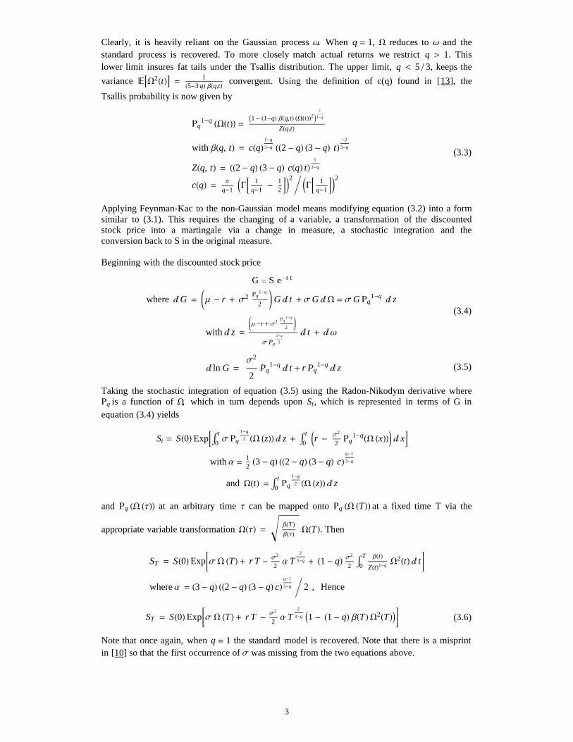
Clearly, it is heavily reliant on the Gaussian process Ω. When q = 1, W reduces to Ω and thestandard process is recovered. To more closely match actual returns we restrict q > 1. Thislower limit insures fat tails under the Tsallis distribution. The upper limit, q < 5 3, keeps the
variance EAW2HtLE = 1H5-3 qL ΒHq,tL convergent. Using the definition of c(q) found in [13], the
Tsallis probability is now given by
(3.3)
Rq1-q HWHtLL =
I1 - H1-qL ΒHq,tL HWHtLL2M 1
1-q
ZHq,tLwith ΒHq, tL = cHqL 1-q
3-q HH2 - qL H3 - qL tL -2
3-q
ZHq, tL = HH2 - qL H3 - qL cHqL tL 1
3-q
cHqL = Πq-1
JGB 1q-1
- 12
FN2 JGB 1q-1
FN2
Applying Feynman-Kac to the non-Gaussian model means modifying equation (3.2) into a formsimilar to (3.1). This requires the changing of a variable, a transformation of the discountedstock price into a martingale via a change in measure, a stochastic integration and theconversion back to S in the original measure.
Beginning with the discounted stock price
(3.4)
G = S ã-r t
where â G = KΜ - r + Σ2 Rq1-q
2O G â t + Σ G â W = Σ G Rq
1-q â z
with â z =Μ -r + Σ2 Rq
1-q
2
Σ Pq
1-q
2
â t + â Ω
(3.5)â ln G =Σ2
2Pq
1-q â t + r Pq1-q â z
Taking the stochastic integration of equation (3.5) using the Radon-Nikodym derivative whereRq is a function of W, which in turn depends upon St, which is represented in terms of G inequation (3.4) yields
St = SH0L ExpBÙ0
tΣ Rq
1-q
2 HW HzLL â z + Ù0
t Jr - Σ2
2Rq
1-qHW HxLLN â xFwith Α = 1
2 H3 - qL HH2 - qL H3 - qL cL q-1
3-q
and WHtL = Ù0
tRq
1-q
2 HW HzLL â z
and Rq HW HΤLL at an arbitrary time Τ can be mapped onto Rq HW HTLL at a fixed time T via the
appropriate variable transformation WHΤL =ΒHTLΒHΤL WHTL. Then
ST = SH0L ExpCΣ W HTL + r T - Σ2
2 Α T
2
3-q + H1 - qL Σ2
2 Ù0
T ΒHtLZHtL1-q
W2HtL â tGwhere Α = H3 - qL HH2 - qL H3 - qL cL q-1
3-q 2 , Hence
(3.6)ST = SH0L ExpCΣ W HTL + r T - Σ2
2 Α T
2
3-q I1 - H1 - qL ΒHTL W2HTLMGNote that once again, when q = 1 the standard model is recovered. Note that there is a misprintin [10] so that the first occurrence of Σ was missing from the two equations above.
3

à 4. Similarities Between the Black-Scholes and Borland Models
á Solutions to Stochastic Differential Equations
Feynman-Kac Solution to Black-Scholes
In the Black-Scholes version of equation (3.1) Μ can be replaced by the risk-neutral interest rater, so that we now have
(4.1)â St = Σ St â Ω + r St â t , t r 0
Here we implement Lyasoff's [11] version of the Feynman-Kac option pricing formula. TheEuropean option as a function of St described by equation (4.1) can be written as the integralrepresentation of
(4.2)OptionPrice@t, St, KD = EAã-rt Max@St - K, 0D É S0 = S H0LE, t ³ 0,
(4.3)where St = S0 ãJr-
1
2 Σ2N t + Σ Wt , t r 0
With St equal to the stock price and K equal to the strike price, then for a Black-ScholesEuropean call option on a non-dividend paying asset the payoff function is Max@St - K, 0D andusing equation (4.3) we can write this simply in Mathematica code as
BSCall@t_, s_, k_D :=
ã-r t
2 Π NIntegrateBMaxBs * ã
Jr-Σ2
2N t + Σ t y
- k, 0F * ã-y2
2 ,
8y, -¥, ¥< , Method ® GaussKronrod, MaxRecursion ® 15,
WorkingPrecision ® 20, PrecisionGoal ® 10 F;For the specific set of values below, the European Black-Scholes call on a non-dividend payingstock is
So = 50; K = 40; r = 6 100; T = 6 10;Σ = 3 10; BSCall@T, So, KD N
12.091
Feynman-Kac Solution to Borland
Since neither the call option nor Feynman-Kac place any restrictions on the stock price thatwould exclude the non-Gaussian model, we can apply equation (3.6) to equation (4.2).
BorCall1@t_, s_, k_D :=ã- r t
Z@q, tD
NIntegrateBMaxBs * ãΣ W + r t -
Σ2
2 Α t
2
3-q +H1-qL Α t2
3-q Β@q,tD Σ2
2 W2
- k, 0F *
I1 - H1 - qL Β@q, tD W2M 1
1-q , 8W, -¥, ¥<, Method ® GaussKronrod,
MaxRecursion ® 15, WorkingPrecision ® 20, PrecisionGoal ® 10F;
For the set of values below, with Α dependent on q, the European non-Gaussian call is:
So = 50; K = 40; r = 6 100; T = 6 10; Σ = 3 10;q = 1.15; Α = 1.06307; BorCall1@T, So, KD N
12.214
Interchanging the strike and the stock prices in the payoff functions will exchange the call for aput option: PayOff@St, KD = Max@K - St, 0D. However, for the purposes of simplicity in thisarticle, we choose to demonstrate only European call functions for underlying assets that pay nodividends as in [10]. For the Borland model, just as for the standard Gaussian one, modifyingthe results to include dividend-paying assets, with a dividend yield ∆, by replacing r with r - ∆is a simple matter.
It should be noted that when the q ® 1, equation (3.2) ® equation (4.1) and equation (3.6) ®equation (4.3). In other words as q ® 1, Tsallis distribution recovers normal distribution andBorland recovers the traditional Black-Scholes model. By example, for the specific set of valuesbelow, with Α dependent on q being very close to 1, the European Black-Scholes call and theEuropean Borland call are equal.
4

Interchanging the strike and the stock prices in the payoff functions will exchange the call for aput option: PayOff@St, KD = Max@K - St, 0D. However, for the purposes of simplicity in thisarticle, we choose to demonstrate only European call functions for underlying assets that pay nodividends as in [10]. For the Borland model, just as for the standard Gaussian one, modifyingthe results to include dividend-paying assets, with a dividend yield ∆, by replacing r with r - ∆is a simple matter.
It should be noted that when the q ® 1, equation (3.2) ® equation (4.1) and equation (3.6) ®equation (4.3). In other words as q ® 1, Tsallis distribution recovers normal distribution andBorland recovers the traditional Black-Scholes model. By example, for the specific set of valuesbelow, with Α dependent on q being very close to 1, the European Black-Scholes call and theEuropean Borland call are equal.
So = 50; K = 40; r = 6 100; T = 6 10;Σ = 3 10; q = 1.000001; Α = 1.0000;
TableForm@88"BorlandCall", "BlackScholesCall"<,8BorCall1@T, So, KD, BSCall@T, So, KD<<D N
BorlandCall BlackScholesCall
12.091 12.091
á Conversion to CDFs
Black-Scholes
The Gaussian and the non-Gaussian pricing models can also be expressed in the form of thedifference between CDFs of functions which correspond to the probabilities of the stock pricebeing in and out of the money. For example, the standard Black-Scholes format draws on twoubiquitous financial functions: "done" and "dtwo". The normal CDF of done is related to theprobability of the stock price being in the money. Shaw [12] codes the European Black-Scholesmodel for non-dividend paying assets very much like the following.
done@s_, Σ_, k_, t_, r_D :=
Hr * t + Log@s kDL HΣ * Sqrt@tDL + HΣ * Sqrt@tDL 2;dtwo@s_, Σ_, k_, t_, r_D := done@s, Σ, k, t, rD - HΣ * Sqrt@tDL;BlackScholesCall@s_, k_, Σ_, r_, t_D :=
s * Η@done@s, Σ, k, t, rDD - k * Exp@-r * tD * Η@dtwo@s, Σ, k, t, rDD;For the specific set of values below, the Black-Scholes European call on a non-dividend payingasset is
So = 50; K = 40; r = 6 100; T = 6 10;Σ = 3 10; BlackScholesCall@So, K, Σ, r, TD N
12.091
Borland
The non-Gaussian model for a non-dividend asset draws upon two functions: "NQ1" and "MQ".
NQ1@D1_, D2_, q_, t_D :=
NIntegrateBI1 - H1 - qL Β@q, tD x2M 1
1-q, 8x, D1, D2< F Z@q, tD;MQ@Α_, Σ_, D1_, D2_, q_, t_D := WithB8Β1 = Β@q, tD<,
NIntegrateBExpBΣ x -Σ2
2Α t
2
3-q I1 - H1 - qL Β1 x2MF
I1 - H1 - qL Β1 x2M 1
1-q, 8x, D1, D2< F Z@q, tDF;This is similar to Black-Scholes in concept and form.
5

BorCall3@s_, k_, Σ_, r_, t_, q_D :=
ModuleB8Α, s1, s2<, Α =H3 - qL
2HH2 - qL H3 - qL c@qDL q-1
3-q;
s1 = S1@Α, k, q, r, s, Σ, tD; s2 = S2@Α, k, q, r, s, Σ, tD;s MQ@Α, Σ, s1, s2, q, tD - ã-r t k NQ1@s1, s2, q, tD F;
For the specific set of values below, the non-Gaussian European call for a non-dividend payingasset is
So = 50; K = 40; r = 6 100; T = 6 10; Σ = 3 10;q = 1.15; BorCall3@So, K, Σ, r, T, qD N
12.214
We can reduce the NQ1 integral for better speed and more efficient execution. With D1 and D2
substituting as dummy values for the functions S1 and S2, the integral becomes
NQ1HD1, D2, q, tL = ã- r T KZHq,TL ÙD1
D2 I1 - H1 - qL ΒHq, tL Wt2M 1
1-q â Wt
Two assumptions must be met to achieve the desired results from the integration. The first is
that Β - Β q 's imaginary part is not zero (dropping some arguments for clarity). Since q is
always greater than 1, the first assumption is verified. The second assumption requires the upperlimit of integration to be larger than the lower limit, specifically D2 > D1. This assumption isalways satisfied when q is not equal to one and when the following parameters are not equal tozero: Α, Β, Σ, r or T. Therefore
IntegrateBI1 - H1 - qL B x2M 1
1-q, 8x, D1, D2<,Assumptions ® : D2 > D1 , ImB B - B q F ¹ 0>F
2 F1
1
2,
1
q - 1;
3
2; -B Hq - 1L D2
2 D2 - 2 F1
1
2,
1
q - 1;
3
2; -B Hq - 1L D1
2 D1
Using the Hypergeometric2F1 functions
NQ@D1_, D2_, q_, t_D := WithB8Β1 = Β@q, tD<,D2 * Hypergeometric2F1B1
2,
1
-1 + q,3
2, -D22 H-1 + qL Β1F - D1 *
Hypergeometric2F1B12,
1
-1 + q,3
2, -D12 H-1 + qL Β1F Z@q, tDF;
BorlandCall@s_, k_, Σ_, r_, t_, q_D :=
ModuleB8Α, s1, s2<, Α =H3 - qL
2HH2 - qL H3 - qL c@qDL q-1
3-q;
s1 = S1@Α, k, q, r, s, Σ, tD; s2 = S2@Α, k, q, r, s, Σ, tD;s MQ@Α, Σ, s1, s2, q, tD - ã-r t k NQ@s1, s2, q, tDF;
On average the hypergeometric version is faster:
So = 50; K = 40; r = 6 100; T = 6 10; Σ = 3 10; q = 1.01;
TableForm@88"Borland: Hypergeometric version", "Borland: NIntegrate version"<,Mean@Table@8Timing@BorlandCall@ððDD, Timing@ BorCall3@ððDD< &
8So, K, Σ, r, T, q<, 8500<DD<DBorland: Hypergeometric version Borland: NIntegrate version
0.00503 Second
12.0986
0.008502 Second
12.0986
à 5. The Option Greeks
6
à
5. The Option Greeks
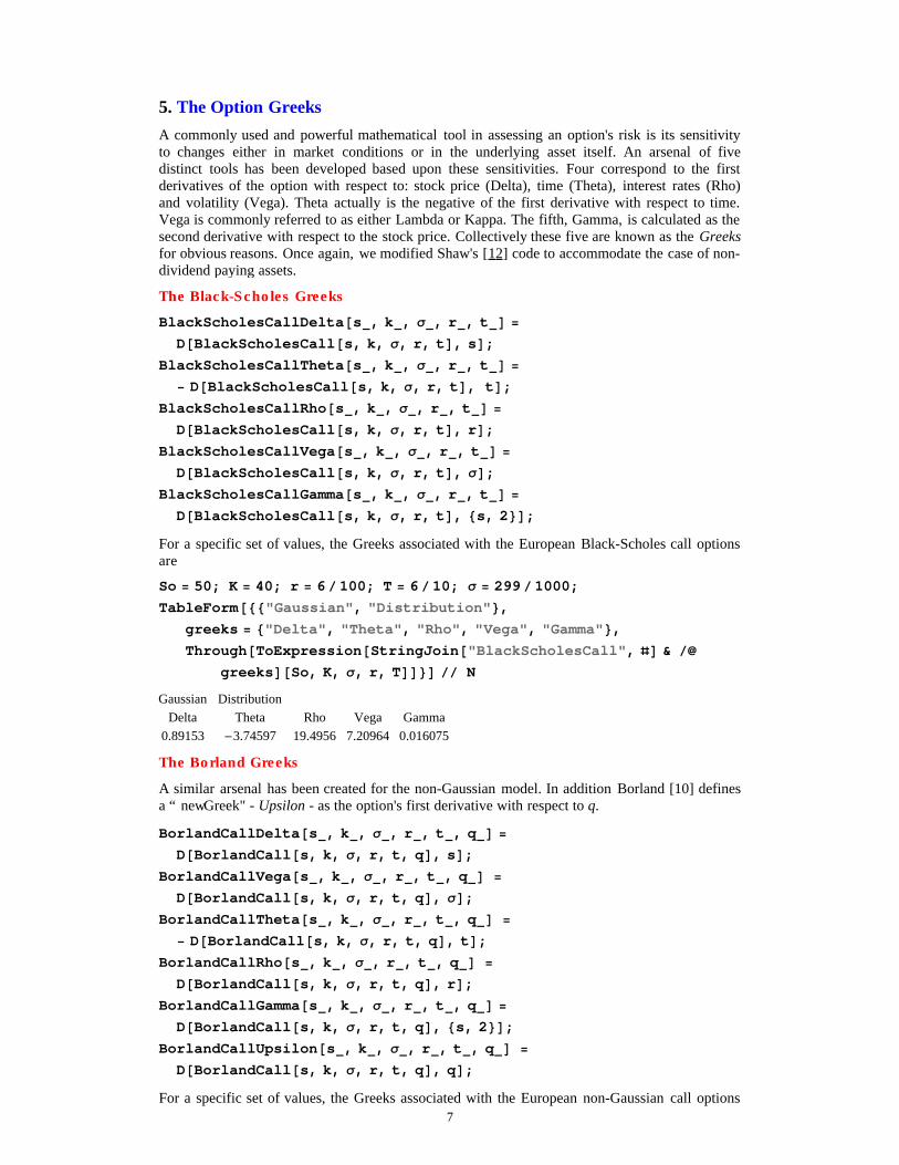
A commonly used and powerful mathematical tool in assessing an option's risk is its sensitivityto changes either in market conditions or in the underlying asset itself. An arsenal of fivedistinct tools has been developed based upon these sensitivities. Four correspond to the firstderivatives of the option with respect to: stock price (Delta), time (Theta), interest rates (Rho)and volatility (Vega). Theta actually is the negative of the first derivative with respect to time.Vega is commonly referred to as either Lambda or Kappa. The fifth, Gamma, is calculated as thesecond derivative with respect to the stock price. Collectively these five are known as the Greeksfor obvious reasons. Once again, we modified Shaw's [12] code to accommodate the case of non-dividend paying assets.
The Black-Scholes Greeks
BlackScholesCallDelta@s_, k_, Σ_, r_, t_D =
D@BlackScholesCall@s, k, Σ, r, tD, sD;BlackScholesCallTheta@s_, k_, Σ_, r_, t_D =
- D@BlackScholesCall@s, k, Σ, r, tD, tD;BlackScholesCallRho@s_, k_, Σ_, r_, t_D =
D@BlackScholesCall@s, k, Σ, r, tD, rD;BlackScholesCallVega@s_, k_, Σ_, r_, t_D =
D@BlackScholesCall@s, k, Σ, r, tD, ΣD;BlackScholesCallGamma@s_, k_, Σ_, r_, t_D =
D@BlackScholesCall@s, k, Σ, r, tD, 8s, 2<D;For a specific set of values, the Greeks associated with the European Black-Scholes call optionsare
So = 50; K = 40; r = 6 100; T = 6 10; Σ = 299 1000;TableForm@88"Gaussian", "Distribution"<,
greeks = 8"Delta", "Theta", "Rho", "Vega", "Gamma"<,Through@ToExpression@StringJoin@"BlackScholesCall", ðD &
greeksD@So, K, Σ, r, TDD<D N
Gaussian Distribution
Delta Theta Rho Vega Gamma
0.89153 -3.74597 19.4956 7.20964 0.016075
The Borland Greeks
A similar arsenal has been created for the non-Gaussian model. In addition Borland [10] definesa “ new Greek" - Upsilon - as the option's first derivative with respect to q.
BorlandCallDelta@s_, k_, Σ_, r_, t_, q_D =
D@BorlandCall@s, k, Σ, r, t, qD, sD;BorlandCallVega@s_, k_, Σ_, r_, t_, q_D =
D@BorlandCall@s, k, Σ, r, t, qD, ΣD;BorlandCallTheta@s_, k_, Σ_, r_, t_, q_D =
- D@BorlandCall@s, k, Σ, r, t, qD, tD;BorlandCallRho@s_, k_, Σ_, r_, t_, q_D =
D@BorlandCall@s, k, Σ, r, t, qD, rD;BorlandCallGamma@s_, k_, Σ_, r_, t_, q_D =
D@BorlandCall@s, k, Σ, r, t, qD, 8s, 2<D;BorlandCallUpsilon@s_, k_, Σ_, r_, t_, q_D =
D@BorlandCall@s, k, Σ, r, t, qD, qD;For a specific set of values, the Greeks associated with the European non-Gaussian call optionsare 7

For a specific set of values, the Greeks associated with the European non-Gaussian call optionsare
So = 50; K = 40; r = 6 100; T = 6 10; Σ = 299 1000; q = 1.01;
TableForm@88"Non-Gaussian", "Distribution"<,greeks = 8"Delta", "Theta", "Rho", "Vega", "Gamma", "Upsilon"<,Through@ToExpression@StringJoin@"BorlandCall", ðD & greeksD@So, K, Σ, r, T, qDD<D N
Non-Gaussian Distribution
Delta Theta Rho Vega Gamma Upsilon
0.891386 -3.76197 19.4868 7.24104 0.0160282 0.757974
à 6. Graphical Results - The Options and Their Greeks
The results in this article are visual and fall into two main categories. The first deals with theoptions themselves and their relationship to various parameters: strikes, expiration time,volatility and q, etc. The images in the first section generally compare the standard Gaussianmodel against the non-Gaussian model. The second category deals primarily with the traditionalfive Greeks and Upsilon as defined in section 5.
á The Options
20 30 40 50 60 70 80Strike
0
510
15
20
2530
ll
aC
Call Price
Figure 1 demonstrates two sets of Calls over a range of Strike Prices, one generated by Black-Scholes and one by the non-Gaussian model. S(0), abbreviated as S0, is set to 50, r = 0.06 andT = 0.6. For the B-S case (solid blue) q = 1 and Σ = 0.3. For the non-Gaussian case (dashed red)q = 1.5 and Σ = 0.299.
20 30 40 50 60 70 80Strike
-0.3-0.2-0.1
00.10.20.3
CHq=
5.1
L-C
Hq=1
L
Call Price Difference
Figure 2 demonstrates two sets of Call Price Differences over a range of Strike Prices: Borland -BlackScholes. S0 = 50, r = 0.06. The solid blue line represents time T = 0.6. Borland is calculatedusing q = 1.5 and Σ = 0.297; BS is calculated using Σ = 0.3. For the dashed red line, time T = 0.05,Borland using q = 1.5 and Σ = 0.41; BS using Σ = 0.3.
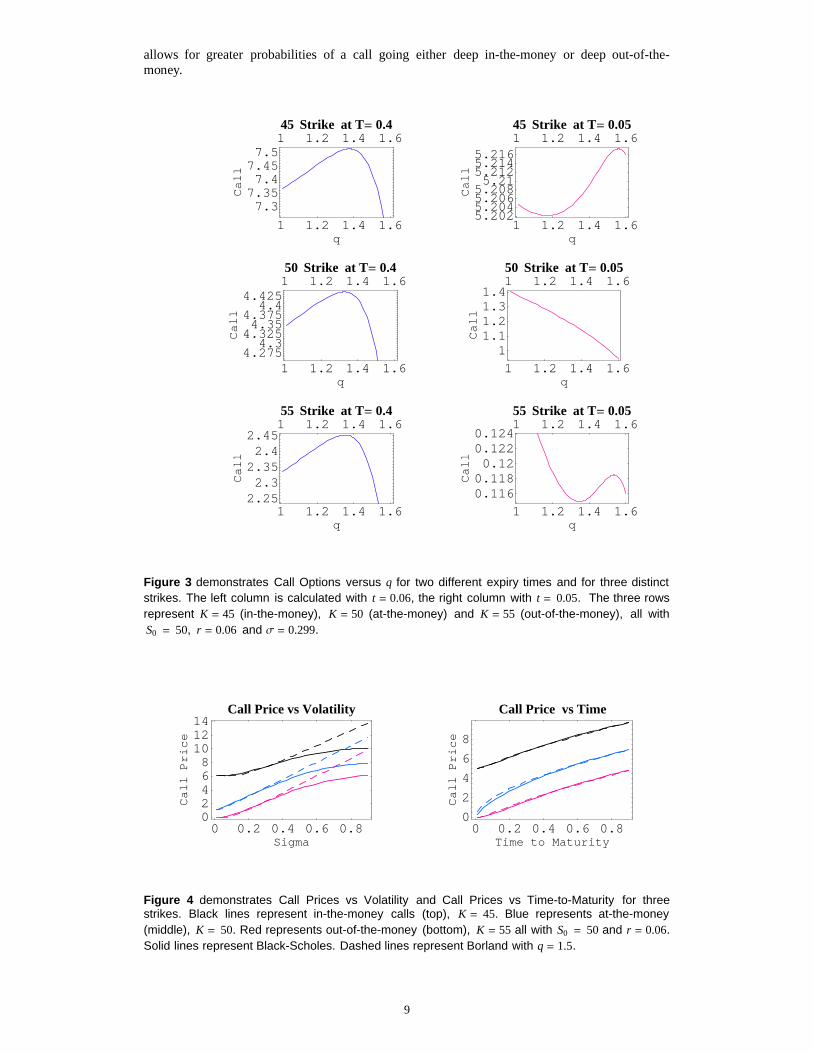
The image directly above demonstrates that the fatter tails of a Tsallis distribution (q = 1.5)allows for greater probabilities of a call going either deep in-the-money or deep out-of-the-money.
8
The image directly above demonstrates that the fatter tails of a Tsallis distribution (q = 1.5)allows for greater probabilities of a call going either deep in-the-money or deep out-of-the-money.
1 1.2 1.4 1.6q
2.252.32.352.42.45
ll
aC
1 1.2 1.4 1.655 Strike at T= 0.4
1 1.2 1.4 1.6q
0.1160.1180.120.1220.124
ll
aC
1 1.2 1.4 1.655 Strike at T= 0.05
1 1.2 1.4 1.6q
4.2754.3
4.3254.354.3754.4
4.425
ll
aC
1 1.2 1.4 1.650 Strike at T= 0.4
1 1.2 1.4 1.6q
11.11.21.31.4
ll
aC
1 1.2 1.4 1.650 Strike at T= 0.05
1 1.2 1.4 1.6q
7.37.357.47.457.5
ll
aC
1 1.2 1.4 1.645 Strike at T= 0.4
1 1.2 1.4 1.6q
5.2025.2045.2065.2085.215.2125.2145.216
ll
aC
1 1.2 1.4 1.645 Strike at T= 0.05
Figure 3 demonstrates Call Options versus q for two different expiry times and for three distinctstrikes. The left column is calculated with t = 0.06, the right column with t = 0.05. The three rowsrepresent K = 45 (in-the-money), K = 50 (at-the-money) and K = 55 (out-of-the-money), all withS0 = 50, r = 0.06 and Σ = 0.299.
0 0.2 0.4 0.6 0.8Sigma
02468101214
ll
aC
ec
ir
P
Call Price vs Volatility
0 0.2 0.4 0.6 0.8Time to Maturity
0
2
4
6
8
ll
aC
ec
ir
P
Call Price vs Time
Figure 4 demonstrates Call Prices vs Volatility and Call Prices vs Time-to-Maturity for threestrikes. Black lines represent in-the-money calls (top), K = 45. Blue represents at-the-money(middle), K = 50. Red represents out-of-the-money (bottom), K = 55 all with S0 = 50 and r = 0.06.Solid lines represent Black-Scholes. Dashed lines represent Borland with q = 1.5.
á The Greeks 9

á
The Greeks
30 40 50 60 70Stock Price
00.010.020.030.040.05
dD
Sd
Gamma
30 40 50 60 70Stock Price
-2-1.5-1
-0.50
0.5
Cd
qdUpsilon
30 40 50 60 70Stock Price
024681012
Cd
dΣVega
30 40 50 60 70Stock Price
0
5
10
15
Cd
rd
Rho
20 30 40 50 60 70 80Stock Price
00.20.40.60.81
Cd
Sd
Delta
30 40 50 60 70Stock Price
-7-6-5-4-3-2-10
-C
dTd
Theta
Figure 5 demonstrates the five traditional Greeks - Delta JD = ∆c
∆SN,Theta JΘ = - ∆c
∆TN, Vega
JV = ∆c
∆ΣN, Rho JΡ = ∆c
∆rN and Gamma JG = ∆D
∆SN. Solid blue lines represent Black-Scholes and
dashed red lines represent Borland with q = 1.5. For the "new" Greek Upsilon J¡ = ∆c
∆qN the
dashed line represents Borland with q = 1.1. The solid lines represent, in order, Borland withq = 1.3 (red), q = 1.4 (green), q = 1.45 (blue) and q = 1.5 (black). All are calculated over a range ofStock Prices with K = 50, r = 0.06, T = 0.4 and Σ = 0.300
à 7. Conclusion
It has long been observed that the Black-Scholes model, while adequate in describing stablemarkets, is no longer reliable for highly volatile markets and that it has become necessary tointroduce additional stochastic volatility models to account for this. Here we offer anothersolution that posits the observed variability as a function of the non-extensive parameter q. Thisadditional parameter allows an explanation of the moneyness bias in modern markets.Furthermore the need for proper hedging in volatile markets is often poorly modeled bytraditional measures of the greeks. Here we show that values of q ¹ 1 can accommodate theextreme sensitivity for option prices close to maturity and the strike value by providing greeksthat reflect this observed responsiveness. Lastly both the option prices and their greeks can bedetermined rapidly using Mathematica's Integrate[] function.
10

à References
[1] F. Black and M. Scholes, The Pricing of Options and Corporate Liabilities, Journal of Political Economy, 81,
1973 pp. 637– 659.
[2] J.C.Hull and A.White, The Pricing of Options on Assets with Stochastic Volatility, Journal of Finance, 42(
June), 1987 pp. 281-300.
[3] Alan L.Lewis, Option Valuation Under Stochastic Volatility with Mathematica Code, 2nd Edition, Finance
Press, California USA, 2005.
[4] K. Fergusson and E. Platen, On the Distributional Characterisation of Daily Log-Returns of a World Stock
Index, Applied Mathematical Finance, 13(1), 2006 pp. 19-38.
[5] S.Hurst,The characteristic function of the Student T distribution, Mathematical Sciences Institute, Financial
Mathematics Research Reports, FMRR95-006, 1995, http://wwwmaths.anu.edu.au/research.reports/fmrr/95/
[6] D. Edelman, Natural Generalisation of Black-Scholes in the Presence of Skewness, Using Stable
Distributions, Abacus, 31(1), 1995 pp. 113-119.
[7] R.J. Elliott and J. van der Hoek, A general Fractional White Noise Theory and Applications to Finance,
Mathematical Finance, 13, 2003 pp. 301-330.
[8] P.Buchen and M. Kelly, The Maximum Entropy Distribution of an Asset Inferred from Option prices, Journal
of Financial and Quantitative Analysis, 31(1), 1996 pp. 143-159.
[9] C. Tsallis, Nonextensive Statistics: Theoretical, Experimental and Computational Evidences and
Connections, Brazilian Journal of Physics, 29, 1, March 1999.
[10] L. Borland, A theory of non-Gaussian option pricing, Quantitative Finance, 2, 2002 pp. 415-431.
[11] A. Lyasoff, Path Integral Methods for Parabolic Partial Differential Equations with Examples from
Computational Finance, The Mathematica Journal, 9(2), 2004 pp. 399-422.
[12] W. T. Shaw, Modelling Financial Derivatives with Mathematica, Cambridge University Press, 1998.
11

Proceedings of the International Conferenceon Computational and Mathematical Methodsin Science and Engineering, CMMSE 2007Chicago, 20–23 June 2007.
Iterative Refinement for Neville Elimination
Pedro Alonso1, Jorge Delgado1, Rafael Gallego1 and Juan ManuelPena2
1 Department of Mathematics, University of Oviedo, Spain2 Department of Mathematics, University of Zaragoza, Spain
emails: [email protected], [email protected], [email protected],[email protected]
Abstract
We provide a sufficient condition for the convergence of iterative refinementusing Neville elimination.
Key words: Iterative refinement, Neville elimination, Total positivityMSC 2000: 65F05, 65F10
1 Introduction
Let us consider a linear system of equations Ax = b, with A ∈ Rn×n. Then, solving thissystem with some direct method, in floating point arithmetic, we get an approximationx(0) to the solution. Iterative refinement is a well established and studied technique toimprove the accuracy of the computed solution x(0) of the linear system Ax = b. Thisprocess can be summarized in the following algorithm
Algorithm Iterative refinement
Input A, b, nTol, xTol
Compute an approximation to the solution of Ax = b: x(0)
k = 0; x(−1) = ∞While k ≤ nTol and ‖x(k) − x(k−1)‖ ≥ xTol do
Compute the residual r(k) = b−Ax(k)
Solve the system A y(k) = r(k): y(k)
Update the solution x(k+1) = x(k) + y(k)
k = k + 1End-WhileOutput x(k)
12

It is necessary to compute the residual with extra precision to avoid the errorsproduced by cancellation of significant figures. For more details in this technique see,for example [12] and [7].
The usual method to solve a linear system of equations Ax = b is Gaussian elim-ination. So, in the literature it has been considered the study of iterative refinementusing Gaussian elimination from several points of view: convergence (see [7], [15], [18]and [19]), stability (see [17] and [12]) and error analysis (see [14] and [19]).
The main purpose of this work is to study the convergence of iterative refinementusing Neville elimination. This method is an alternative procedure to Gaussian elim-ination to transform a square matrix A into an upper triangular matrix U . Nevilleelimination makes zeros in a column of the matrix A by adding to each row a multi-ple of the previous one. Here we only give a brief description of this procedure (fora detailed and formal introduction of it we refer to [10]). If A ∈ Rn×n, the Nevilleelimination procedure consists of at most n− 1 steps:
A = A(1) → A(1) → A(2) → A(2) → · · · → A(n) = A(n) = U.
On one hand, A(t) is obtained from the matrix A(t) by moving to the bottom the rowswith a zero entry in column t, if necessary, to get that
a(t)it = 0, i ≥ t ⇒ a
(t)ht = 0, ∀h ≥ i.
On the other hand, A(t+1) is obtained from A(t) making zeros in the column t belowthe main diagonal by adding an adequate multiple of the ith row to the (i + 1)th fori = n − 1, n − 2, . . . , t. If A is nonsingular, the matrix A(t) has zeros below its maindiagonal in the first t− 1 columns. It has been proved that this process is very usefulwith totally positive matrices, sign-regular matrices and other related types of matrices(see [8] and [3]).
A real matrix is called totally positive if all its minors are nonnegative. Totallypositive matrices arise in a natural way in many areas of Mathematics, Statistics,Economics, etc. Specially, their application to approximation theory and ComputerAided Geometric Design (CAGD) is of great interest. For example, coefficient matricesof interpolation or least square problems with a lot of representations in CAGD (theBernstein basis, the B-spline basis, etc.) are totally positive. Some recent applicationsof such kind of matrices to CAGD can be found in [13], [5] and [16]. For applicationsof totally positive matrices to other fields see [8].
In [6], [11], [9] and [10] it has been proved that Neville elimination is a very usefulalternative to Gaussian elimination when working with totally positive matrices. Inaddition, there are some studies that prove the high performance computing of Nevilleelimination (see [2]).
Then, taking into account the convenience of using Neville elimination with totallypositive matrices and that, as far as we know, no study of the convergence of theiterative refinement through Neville elimination exists, the main goal of this work is toperform that task.
13
Let A be a n× n nonsingular matrix, in [1] it has been proved that the computedsolution x of Ax = b by Neville elimination satisfies
(A + H)x = b, (1)
with H verifying different bounds depending on the matrix A. Considering (1) and thesystem
(A + Hk)y(k) = r(k), (2)
we will study the convergence of the iterative refinement. We will prove that in thegeneral case the procedure converges if
‖Hk‖ ≤1
2‖A−1‖. (3)
In the case that A is a totally positive matrix and taking into account that it can beproved that
‖H‖ ≤ 6116
γn ‖A‖, (4)
with γn :=nu
1− nu, where u is the unit of roundoff, we deduce that the following condi-
tion on A ensures the convergence of the iterative refinement using Neville elimination:
6116
γn ‖A‖ ‖A−1‖ <12. (5)
We point out that (4) is of the same kind as the bounds obtained by de Boor andPinkus in [4] for Gaussian elimination.
The bound (5) depends on the condition number of the matrix A as every equivalentbound corresponding to Gaussian method. But, in contrast to most of the equivalentbounds for this method, our bound does not depend on the growth factor of the elimi-nation procedure.
Acknowledgements
This work has been partially supported by the Spanish Research Grant MTM2006-03388 and under MEC and FEDER Grant TIN2004-05920.
References
[1] P. Alonso, M. Gasca and J.M. Pena, Backward Error Analysis of NevilleElimination, Appl. Numer. Math. 23 (1997) 193–204.
[2] P. Alonso, R. Cortina, I. Dıaz and J. Ranilla, Neville Elimination: aStudy of the Efficiency Using Checkerboard Partitioning, Linear Algebra Appl.393 (2004) 3–14.
[3] T. Ando, Totally Positive Matrices, Linear Algebra Appl. 90 (1987) 165–219.
14

[4] C. de Boor and A. Pinkus, Backward Error Analysis for Totally Positive LinearSystems, Numer. Math. 23 (1997) 193–204.
[5] J. Delgado and J.M. Pena, Progressive Iterative Approximation and Baseswith the Fastest Convergence Rates, Comp. Aided Geom. D. 24 (2007) 10–18.
[6] J. Demmel and P. Koev, The Accurate and Efficient Solution of a TotallyPositive Generalized Vandermonde Linear System, SIAM J. Matrix Anal. Appl.27 (2005) 142–152.
[7] G.E. Forsythe and C.B. Moler, Computer Solutions of Linear AlgebraicSystems, Prentince-Hall, Englewood Cliffs, NJ, 1967.
[8] M. Gasca and and C.A. Micchelli, eds., Total Positivity and its Applications,Kluwer Academic Publishers, Boston, 1996.
[9] M. Gasca and J.M. Pena, Total positivity and Neville Elimination, LinearAlgebra Appl. 165 (1992) 25–44.
[10] M. Gasca and J.M. Pena, A Matricial Description of Neville Elimination withApplications to Total Positivity, Linear Algebra Appl. 202 (1994) 33–53.
[11] M. Gasso and J.R. Torregrosa, A Totally Positive Factorization of Rectan-gular Matrices by the Neville elimination, SIAM J. Matrix Anal. Appl. 25 (2004)986–994.
[12] N. J. Higham, Accuracy and Stability of Numerical Algorithms, SIAM, Philadel-phia, 1996.
[13] H. Lin, H. Bao and G. Wang, Totally positive bases and progressive iterationapproximation, Comput. Math. Appl. 50 (2005) 575–586.
[14] C.B. Moler, Iterative Refinement in Floating Point, J. Assoc. Comput. Mach.14 (1967), 316–321.
[15] J.M. Ortega, Numerical Analysis A Second Course, SIAM, Philadelphia, 1990.
[16] J.M. Pena, Shape preserving representations in Computer Aided-Geometric De-sign, Nova Science Publishers, Inc., New York, 1999.
[17] R.D Skeel, Iterative Refinement Implies Numerical Stability for Gaussian Elim-ination, Math. Comput. 35 (1980) 817–832.
[18] J.H. Wilkinson, Errors Analysis of Direct Methods of Matrix Inversion, J. Assoc.Comput. Mach. 8 (1961) 281-330.
[19] J.H. Wilkinson, Rounding Errors in Algebraic Processes, Notes on Applied Sci-ence 32 (Her Majesty’s Stationery Office, 1963).
15

Proceedings of the International Conferenceon Computational and Mathematical Methodsin Science and Engineering, CMMSE 2007Chicago, 20–23 June 2007.
A mathematical model of the static pantograph/catenaryinteraction
Enrique Arias1, Angelines Alberto2, Tomas Rojo1, FernandoCuartero1 and Jesus Benet1
1 Escuela Poliecnica Superior de Albacete, University of Castilla-La Mancha
2 Albacete Research Institute of Albacete, University of Castilla-La Mancha
emails: [email protected], [email protected], [email protected],[email protected], [email protected]
Abstract
In this paper, a mathematical model of the static pantograph/catenary inter-action for high speed railways. Also, a High Performance Computing Algorithmassociated to the model has been developed to obtain the solution of the staticequilibrium equation of the pantograph/catenary system after an exhaustive studyof the tradictionl mechanical approach based on a set of coupled strings. In orderto obtain an adequate behaviour in the pantograph/catenary system, it is nec-essary the existence of adequate conditions in the line, and this requires a veryprecise mechanical calculus. The resulting stiffness matrix has a high sparsity de-gree. This circumstance can be exploited into two senses: less memory storagerequeriments, and the use of suitable methods for solving the static equilibriumequation as projection methods.
Key words: high performance computing, interaction pantograph/catenary, staticequilibrium equation, sparse linear algebra libraries
1 Introduction
The evolution in the transport market resulting from the globalization of the econ-omy, the increasing deregulation of the markets, the competition on the base of acustomer service, the growing environmental concerns, and the need to ensure a longterm operational profitability consistent with prevailing economic reality are driving toa radical change (structural and cultural) in the railway sector, centered on innovativeapproaches to business and services, conducive to a future-oriented and market-drivenposture in the global transportation marketplace.
The survival in the ever evolving and highly competitive transport market, implies acontinuous search for the roots of excellence enabling railway operators and supplying
16

industry to achieve a world-class profile. This quest for excellence has to cover theentire range of business activities, beginning with market demand and ending withcustomer satisfaction. It will entail the need for an integrated development and timelydeployment of the adequate organizational, technological and skill infrastructures.
Thus, the fulfillment of this strategy needs new construction concepts, among them,the development of more performant coupled pantograph/ catenary systems and a wideutilization of new technologies.
Furthermore, the multitude of electrification systems currently in use throughoutEurope and subsequently the massive capital investment that would be necessary in or-der to implement any sort of European wide harmonised solution, preclude to envisageany major change in this field in the foreseeable future. A detailed study of electrifica-tion systems and catenary/pantograph technology considering economic aspects maybe found in [4].
During the recent last years, passengers transportation by railway has experienceda considerable increase in some European countries (Germany, France, Spain, ...). Forthat reason, reaching of higher velocities in railways has become a very importanttarget. In that scenario, the pantograph/catenary system, with its dynamic behaviour,becomes a crucial component (see [5, 2, 3]), because at high speed it is very difficult toguarantee the permanent contact of the pantograph head and contact the wire, moreover without the increasing of noise and wear.
In order to obtain an adequate behaviour in the pantograph/catenary system, itis necessary the existence of adequate conditions in the line, and this requires, amongother aspects, a very precise mechanical calculus. Recent investigations have focusedon dynamical behaviour by dynamical simulations in order to allow a better interactionof the pantograph and the catenary [3, 6]; in this paper we will follow a more traditionalapproach, focusing in the catenary, modeled, as usual, by a set of coupled strings.
The best conditions in which the pantograph would obtain electric energy from theline are when the contact wire is parallel to the ground, and then, an important problemis to determine the exact length of the droppers in order to allow the contact wire toacquire the correct shape. So, our objective is the development of a technique whichallows us to implement a high precision calculation algorithm, and thus to develop asoftware tool to design high quality catenaries.
In this work, a High Performance Computing (HPC) Algorithm has been developedfor solving the static equilibrium equation of the pantograph/catenary interaction inorder to obtain good performances.
This paper is structured as follows. In Section 2, the catenary model is described.Section 3 introduces some aspects on High Performance Computing. Section 4 presentsthe standard linear algebra libraries BLAS and SPARSKIT. In section 5 the experi-mental results are presented. Finally, some conclusions and future work guidelines areoutlined.
17

Support CarrierDropper
Contact wire
Compensation arm
Deflection
Support
Compensation arm
Figure 1: A span of catenary
2 The catenaty model
The conventional catenary electrification system is designed for heavy-traffic mainlineoperation and it is useful for train speeds well above 200 kph. For such high-speed op-eration an essentially constant contact force must be maintained between the overheadcontact-wire and the locomotive’s pantograph power-collecting apparatus.
As we have previously indicated, in this paper we will use a classical model ofthe catenary wire appearing in railways, so we consider the catenary composed froma reduced range of elements, such as carrier, droppers, contact wire and compensationarms (see Figure 1). The droppers are supporting the contact wire in order to obtain ahorizontal line. The interval between two compensation arms will be called the span.
In this section an introduction to the problems related to the study of railwayscatenaries is outlined. After that, the modelization of the carrier, the contact wire,the droppers and the compensation arm is carried out. Finally, the static problem isdefined.
2.1 Problems to consider in the mechanical study of railway catenar-ies
A span of catenary is composed by three types of cables (see Figure 1): the carrier, thedroppers and the contact wire. The carrier is fixed at the supports, while the contactwire is upheld by the compensation arm.
In the mechanical study of the catenary system, three differents problems can beconsidered:
• The calculation of the droppers length: This problem consists on the deter-mination of the droppers length for obtaining an adecuate position in the contactwire, as parallel to the ground, as parabolic shape, in order to compesate thedifference of stiffness between the supports and the center. This problem requiresa study of the static forces in the wires.
• The static problem: It consists on the determination of the static position ofthe catenary when a force is applied. This allows to know the variation of the
18

stiffness along the line.
• The dynamic problem: This allows to simulate the behaviour of the pantograph-catenary in time.
In the study of the last two problems, a discretization using FEM (Finite Element
Methods) must be used. In order to be able to deal with a great number of variables,some method for getting adecuate computational efficiency is required.
2.2 Modelization of the carrier and contact wire
The carrier and the contact wire can be considered as a pretensed beam. Under thisassumption, the following Euler-Bernouilli equation is used:
p
gy = −EIyIV + Txy′′ − p, (1)
Where p is the uniform load of the wire, Tx is the horizontal tension of the wire,E is the elastic module, g represents the gravity force and I the diametral moment ofinertia.
Equation 1 allows us to discretize the system using FEM in order to obtain thestiffness matrix and the static equation of an element of the wire with a length of l:
kq = r,
In this case, each node has two variables: the vertical position yi and the angle θi
k =EI
l3
12 6l −12 6l6l 4l2 −6l 2l2
−12 −6l 12 −6l6l 2l2 −6l 4l2
+Tx
30l
36 3l −36 3l3l 4l2 −3l −l2
−36 −3l 36 −3l3l −l2 −3l 4l2
, (2)
r =
−pl2
−pl2
l2
−pl2
pl2
l2
, (3)
q =
yi
θj
yi
θj
. (4)
In the case that we do not consider the bending stiffness (see Figure 2), the cablesare considered as a pretensed string, then each node has a variable, that is, the verticalposition yi. In this case, the system is represented as
k =Tx
l
[
1 −1−1 1
]
, r =
[
−pl2
−pl2
]
, q =
[
yi
yj
]
. (5)
19

Figure 2: String elements
2.3 Modelization of the droppers
The droppers can be considered as an elastic bar with a length of l, which are de-formated from an initial length l0 by an initial load F . The stiffness matrix, theindependent term and the vector variables are:
k =EA
l
[
1 −1−1 1
]
, r =
[
EAl0l
−EAl0
l− P
]
=
[
EA − F
−EA + F − P
]
, q =
[
yi
yj
]
, (6)
where P is the weight of the dropper and A the cross area. The initial load F isknown by the static analysis of the forces.
The droppers only can work in a traction mode. Their effect of the opposite caseis not considered.
2.4 Modelization of the campensation arm
The effect of the compensation arm can be considered as an spring with a vertical forcefbover the contact wire:
fb = r0 + (yh − yA)kb, (7)
being kb the apparent stiffness of the compensation arm, yA is the dynamic positionof the holding point, yh is the static position of the holding point, a known data, andro is the weight of the cable that supports the compensation arm.
2.5 The static problem
In the static problem the static position of the system is determined when we applya vertical force over the contact wire. So, it is necessary to configurate the stiffnessmatrix K and the independent term R of the system and then solving the lineal systemfor the position of the nodes Q of the cables:
20

Figure 3: Model of Catenary. Notation
KQ = R. (8)
Once the equilibrium position of the system is obtained, it is needed to check if alldroppers work in a traction mode. In an affirmative case the problem is solved, but inthe negative case, the stiffness matrix and the independent term must be reconfiguredin order to eliminate the terms of the droppers that do not work, obtaining the newposition and repeating this problem until all droppers work in a traction mode.
2.6 Discretization process
The carrier and the contact wires are discretized according to a finite element method(FEM), from left to right in a progressive way ([7, 8, 9, 10]. First, inner nodes of thecarrier are numbered obtaining s elements and np droppers (os1, os2, osnp). Making thesame numeration for the contact wire, s+h− 2 elements are obtained (the numerationof droppers for the contact wire is oh1, oh2, ..., ohnp) (see Figure 3).
Considering the conections between nodes (see Figure 4 and 5) the stiffness matrixK is conjugate.
From a general point of view, the stiffnes matrix has the following structure
(
K11 K12
K21 K22
)(
Y1
Y2
)
=
(
R1
R2
)
(9)
where K11 ∈ Rnl×nl, K12 ∈ Rnl×na, K21 ∈ Rna×nl and K22 ∈ Rna×na, being nl
the number of free nodes and na the number of nodes subjected to constrains. Y1
represents the unknows in this equation and Y2 are the boundary conditions.
Operating by blocks, the following pair of equations are obtained
21

Figure 4: Nodes linked by means of two string elements.
Figure 5: Nodes linked by means of two string elements and one elastic bar element.
K11Y1 + K12Y2 = R1, (10)
K21Y1 + K22Y2 = R2. (11)
From this pair of equations, only the first one has interest in order to calculate theunknows Y1. Actually, the final system of equations to be solved is
K11Y1 = R1 − K12Y2. (12)
In 12, all terms except Y1 are known.
One example of K11 matrix is shown in Figure 6. This matrix has a high degree ofsparsity. So, a good treatment of the storage space, and the application of a suitablemethod to solve sparse systems lead us to the High Performance Computing approach,aim of this paper.
3 High Performance Computing Approach
In order to solve a mathematical problem in a efficient way on a computer, the followingsteps are involved [13]
22

Figure 6: Example of stiffness matrix (test 4)
1. Making a mathematical model of the problem, translating the problem into amathematical language, eg. ordinary differential equations.
2. Finding or developing constructive methods for solving the mathematical model,that is, a literature search to find what methods are available for the problem.
3. Identifying the best method from a numerical point of view.
4. Implementing on the computer the numerically effective method identified in theprevious step.
In general, the developed software has to be a high-quality mathematical softwarewhich guarantees a good solution to the problem. This high quality mathematicalsoftware should have the following features: Power and flexibility, easily read andmodified, portability, robustness, efficient and economic in use of storage.
The two last points are specially important in the problem solved in this work.In particular, the sparsity and simmetry of the stiffness matrix has been exploted,improving the efficiency of the implementation and dramatically reducing the memorystorage requirements.
Finally, a High Performance Implementation (HPI) has to take into account thefeatures of current architectures like, for example, cache memory. These features areparticularly important when rebuilding the traditional algorithms to a block-orientedimplementations. Block-oriented algorithms reduce drastically the data flow betweenmain memory and secondary memory enhancing the performance of the final imple-mentation. These HPI have been carried out by using BLAS and SPARSKIT standardlinear algebra libraries.
The BLAS [11](Basic Linear Algebra Subroutines) library includes subroutines forcommon linear computations such as dot-products (BLAS-I), matrix-vector multipli-cation (BLAS-II), and matrix-matrix multiplication (BLAS-III).
Sparse matrices appear on a lot of current problems in science and engineering.Due to that fact, an intensive research is being carried out in this area producing lotof storage schemes and methods to deal with sparse matrices. SPARSKIT [12] is a
23

software packet which allows us to work with different storage schemes (COO, CSR,CSC, etc) and iterative methods for solving sparse systems of equations. This packetis divided into several modules for conversion of storage scheme (FORMAT module),basic linear algebra operations over sparse matrices (BLASSM and MATVEC module),system of equations solvers (ITSOL module), etc.
4 Experimental Results
In this section, the experimental results obtained with the new HPC implementationof the algorithm for solving the static equilibrium equation are presented.
The test battery used in the experiments is shown in Table 1
Test nv np nps nph lv
1 10 10 1 2 59
2 15 11 1 2 64
3 3 15 1 1 64
4 10 10 10 10 59
Table 1: Test Battery
Where nv is the number of sections, np is the number of droppers, nps representsthe number of elements between droppers in the carrier, nph is the number of elementsbetween droppers in the contact and lv is the length of the section.
The experiments have been carried out in a Pentium III-650MHz with Red HatLinux V. 7.2 operating system. The experimental platform has 385 MBytes of RAMmemory and a cache memory of 256 KBytes. BLAS and SPARSKIT libraries havebeen compiled in this machine in order to obtain better performances.
Test 1 to 3 are low dimension problems used to verify the results, and test 4 is amore realistic example (see Figure 6). Thanks to the sparse storage scheme used in thiswork, the amount of used memory has been considerably decreased. This reduction inthe storage space compared with the original algorithm is summarized in Table 2. InTable 2, N represents the number of nodes and nz the number of non-zero elements inthe stiffnes matrix.
Test N nz % Reduction of memory
1 332 1157 98,95
2 542 1902 99,35
3 98 366 96,20
4 2202 6767 99,86
Table 2: Reduction of memory requirements
The execution time has also been drastically reduced. Table 3 shows the execution
24

time for the different tests and the percentage of time reduction with respect to theoriginal implementation
Test Number of iterations Execution time (msecs) % Reduction of memory
1 27 6,379 98,94
2 15 20,124 99,67
3 24 1,389 99,04
4 57 228,58 *
Table 3: Reduction of execution time
The test 4 could not be executed by using the original implementation.
5 Conclusions and Future Work
In this work a High Performance Computing Algorithm has been developed for solvingthe static equilibrium equation of the pantograph/catenary system of High Speed Rail-ways. This new approach is based on the implementation philosophy of High QualitySotfware.
The experimental results show that the HPC resulting algorithm provides spectac-ular reduction in the memory requirements as well as in execution time.
By using BLAS and SPARSKIT standard linear algebra libraries, two secondaryobjectives, but not less important, are achieved, i.e., portability and efficiency.
This work is the initial point of a lot of computational efforts in order to applythe HPC philosophy to different algorithms developed by the authors [17] followingtradicional implementations. So, the future work could be outlined in the followingpoints:
• Consider the solution of the static equilibrium equation when the spans containsdifferent number of droppers and these are not equispaced.
• To extent this work considering the stitched catenary.
• To deal with the dynamical problem with guarantees.
• According to the results obtained for the dynamical problem, think about par-allel implementations on shared memory platforms based on threads [14] or ondistributed memory platforms based on MPI [15] and using the standard libraryPETSC [16].
The obtained algorithms will be used by RENFE, the Spanish Railway Company,in the design of high speed railways (AVE program).
6 Acknowledgments
We will thank Jesus Montesinos, engineer of RENFE, for its technical support andgood knowledge of the real problem beyond the simulation world.
25
References
[1] Poetsch G., J. Evans, R. Meisinger, W. Kortum, M. Baldauf, A. Veitl and J. Wal-laschek. “Pantograph/catenary dynamics and control”, Vehicle System Dynamics,28:159-195, 1997.
[2] Poetsch G. and J. Wallaschek. “Symulating the dynamic behaviour of electricallines for high-speed trains on parallel computers”, International Symposium onCable Dynamics, Lige, 1993.
[3] Simeon, B. and Arnold M. “The simulation of pantograph and catenary: a PDAEapproach”, Technical Report 1990, Fachbereich Mathematik Technische Universi-tat Darmstadt, 1998.
[4] Garfinkle, M. “Tracking pantograph for branchline electrification”, Technical Re-port -, School of Textiles and Materials Technology, University of Philadelphia,1998.
[5] Poetsch G., J. Evans, R. Meisinger, W. Kortum, M. Baldauf, A. Veitl, & J. Wal-laschek.“Pantograph/catenary dynamics and control”, Vehicle System Dynamics,28:159–195, 1997.
[6] Carsten, N. J. “Nonlinear systems with discrete and continuous elements”, PhDthesis, University of, 1997.
[7] K. J. Bathe. “Finite Element Procedures in Engineering Analysis”, Ed. Prentice-Hall, 1996.
[8] Thomas J. R. Hughes. “The Finite Element Method”, Ed. Prentice-Hall, 1987.[9] Zienkiewics, R. L. Taylor. “El Metodo de los Elementos Finitos”, Ed. McGraw
Hill, 1980.[10] Cook D. C., Malkus D. S., Plesha M. E. “Concepts and Applications of Finite
Element Analysis”, Ed. John Wiley and Sons, 1989.[11] J. J. Dongarra, J. Du Croz, I. S. Duff and S. Hammarling. “A set of Level 3 Basic
Linear Algebra Subprograms”, ACM Trans. Math. Soft, 1990.[12] Yousef Saad. “SPARSKIT: a basic tool kit for sparse matrix computations”, Uni-
versity of Illinois and NASA Ames Research Center, 1994.[13] B. Nath Datta, “Numerical Linear Algebra and Applications”, Broks/Cole Pub-
lishing Company, 1995.[14] Mueller, F. “Pthreads Library Interface”, Institut fur Informatik, March, 1999.[15] Gropp, W. and Lusk, E. and Skjellum, A. “Using MPI: Portable Parallel Program-
ming with the Message-Passing Interface”, MIT Press, 1994.[16] Batish Balay, William Group, Lois Curfman McInnes, B. Innes. “PETSC 2.0
User’s Manual”, Mathematic and Computer Science Division, 2000.[17] J. Benet, F. Cuartero and T. Rojo. “A tool to calculate catenaries in railways”,
Seventh International Conference on Computer in Railways, COMPRAIL-2000,2000.
26

Proceedings of the International Conferenceon Computational and Mathematical Methodsin Science and Engineering, CMMSE 2007Chicago, 20–23 June 2007.
Phenomenological to Molecular Modelling of Hysteresis inViscoelastic Polymers: Elastomers to Biotissue
H.T. BanksCenter for Research in Scientific Computation
North Carolina State UniversityRaleigh, NC 27695-8205
Extended Abstract
In control and systems theory, delay systems or systems with memory (hysteresis) haveplayed an important role for many years because of the early realizations by Minorsky andothers [34, 35, 36, 27, 28, 38] that feedback design based on dynamics wherein one ignoresany delays may fail catastrophically to stabilize or control a system in which delays orhysteresis are present in the dynamics. This is true whether the hysteresis is a fundamentalpart of the underlying dynamics or a part of the input or control operator. For the latterthere is a growing body of literature [5, 6, 7, 26, 33, 45] on the Preisach and related theoriesfor hysteretic control input such as arises in smart material systems [16, 18, 41]. Here weshall focus on the delays or hysteresis arising in the fundamental dynamics of the systemsto be stabilized or controlled. In particular we consider viscoelastic materials that arepolymeric in nature. This includes a wide range of materials of current importance such as(rubber or silicone based) filled elastomers and all types of biotissue (soft tissue, ligaments,cartilage, etc.).
The mathematical modelling of viscoelasticity (sometimes also loosely referred to ashysteresis) in materials using ideas from elasticity has attracted the attention of a largenumber of investigators over the past century. Among significant contributors (see themany references in [17, 19, 20, 22, 23, 32, 37, 39, 42, 44, 46, 47]) have been some of thetrue giants from the fields of engineering and material sciences. One of the most widelyused empirical models for viscoelasticity in materials is the Boltzmann convolution law[12, 20, 22, 23, 46], one form of which is given in equation (1)
σ(t) = ge(ε(t)) + CD ε(t) +∫ t
−∞Y (t− s)
d
dsgv (ε(s), ε(s)) ds, (1)
where ε is the infinitesimal strain, Y is the convolution memory kernel, and ge and gv arenonlinear functions accounting for the elastic and viscoelastic responses of the elastomers,respectively; for summaries and further references, see Chapter 2 of [23] as well as [12].This form of model, when incorporated into force balance laws, results in integro-partialdifferential equations which are most often phenomenological in nature as well as beingcomputationally challenging both in simulation and control design. This stress-strain lawimplies that the stress depends not only on the current strain and strain rate but also on thehistory of the strain and the strain-rate. It is very important to note that the stress-strainlaw (1) contains various standard internal strain or internal variable formulations as special
27

cases. The anelastic displacement field (ADF) models of Lesieutre [30, 31] for compositematerials exhibiting both elastic and anelastic displacement fields are formulated on theassumption that the host elastic material contains anelastic materials with internal strainsε1 which are elastic strain driven. That is, the constitutive laws have the form
σ(t) = Eε(t)− E1ε1(t), (2)
where the internal strain is given by
ε1(t) +1τε1(t) = c2ε(t), ε1(0) = 0, (3)
or equivalently,
ε1(t) =∫ t
0c2e
− t−sτ ε(s)ds.
Several generalizations of this formulation exist, e.g., Johnson, et al., [24, 25], suggest thatthe internal strain is strain rate driven, i.e.,
ε1(t) +1τε1(t) = c2ε(t). (4)
The Boltzmann-type law (1) (under appropriate assumptions on the past memory from −∞to 0) corresponds to an internal strain model of the form
ε1(t) +1τε1(t) =
d
dtgv(ε(t), ε(t)), ε1(0) = 0. (5)
This form is often chosen since one finds that neither (3) nor (4) provide laws that readilydescribe experimental data, especially in the cases of filled elastomers, biotissues and othermolecular polymers.
Fung, in his extensive efforts [23] with biomechanics and biotissue, develops and presentsthe quasi-linear viscoelastic constitutive equation
Sij(t) =∫ t
−∞Gijkl(t− τ)
∂S(e)kl [E(τ)]
∂τdτ, (6)
where Sij is the Kirchoff stress tensor, E is the Green’s strain tensor, Gijkl is a reducedrelaxation function, and S
(e)kl is the “elastic” stress tensor. For the scalar components Gijkl,
Fung proposes the reduced relaxation function G(t) given in the form
G(t) =
1 + C[E1(t
τ2)−E1(
t
τ1)]
[1 + c ln(
τ2
τ1)]−1. (7)
Here E1(z) =∫∞z
e−t
t dt, C represents the degree to which viscous effects are present, andτ1 and τ2 represent fast and slow viscous time phenomena. We note that the internal strainvariable formulation (2), (5) is equivalent to the constitutive relationship proposed by Fungif one considers an approximation of the relaxation function G by a sum of exponentialterms. Various internal strain variable models are investigated in [1] and a good agreementis demonstrated between a two internal strain variable model (e.g., of the form σ = Eε −E1ε1 − E2ε2) and undamped simulated data based on the Fung kernel G.
Since its introduction, this quasi-linear viscoelastic (QLV) theory of Fung has been ap-plied successfully in stress-strain experiments to several types of biological tissue. A benefit
28

to using (6) as a constitutive equation is that, unlike simpler models for viscoelasticity, itallows for the consideration of a continuous spectrum (e.g., see the discussions in [23]) ofrelaxation times and frequencies (this is also true of the probabilistic-based internal variableapproach developed in [13] and described below). (The need for a continuum of relaxationtimes in certain materials was observed many years ago [21, 40, 43, 47].) While Fung’stheory has been successfully employed for fitting hysteretic stress-strain curves, for controlapplications one is interested in using it in a full dynamical model. Unfortunately, the QLV,as presented by Fung, leads to exceedingly difficult computations within full dynamical par-tial differential equations, especially in estimation and control problems. This motivatedthe development of the internal variable approach described in [1, 13, 30] (which permitsdiscrete approximation to a continuum) in attempts to approximate well the correspond-ing dynamic responses even in cases where the stress-strain curves alone do not produceadequate approximations – see [23].
The probabilistic based internal variable alternative [13] to Fung’s kernel involves aparameter dependent kernel with a continuous distribution of parameters and internal vari-ables. In the case of a finite combination of Dirac δ distributions, one obtains a finitesummation of exponential functions as the approximation kernel (see the discussions be-low). This method can be extended to allow for consideration of a continuous spectrum ofrelaxation times and frequencies by utilizing absolutely continuous parameter distributionsin place of the δ distributions.
The internal variable approach to overcome both conceptual and computational chal-lenges is consistent with the belief that hysteresis is actually a manifestation of the presenceof multiple scales in a physical or biological material system that is frequently modelled(and masked) with a phenomenological representation such as an hysteresis integral for themacroscopic stress-strain constitutive law. The internal variable modelling leads to an ef-ficient computational alternative for the corresponding integro-partial differential equationmodels. In addition, it provides a “molecular” basis for the models (for a comparison ofmodels of viscoelastic damping via hysteretic integrals versus internal variable representa-tions, see [12] and the references therein).
Our own interest in viscoelasticity in polymeric materials has been motivated by projectsin our Industrial Applied Mathematics Program with at least two of our industrial partners:The Lord Corporation and Medacoustics, Inc. The collaborations with polymer scientistsand engineers at Lord involved the dynamic modelling of filled rubbers which experimen-tally exhibit both significant hysteresis and nonlinearity in tensile and shear deformationsas depicted in the sample stress-strain curves in Figure 1. The efforts with engineers atMedacoustics used some of the viscoelastic models we have investigated in attempts to un-derstand the propagation of arterial stenosis induced shear waves in composite biotissue ina sensor development and characterization project.
In some of our earlier efforts [14, 15], the models for hysteretic damping in elastomersemployed a phenomenological Boltzmann-type constitutive law of the form (1). As ex-plained in [11, 14], our nonlinear materials undergoing large deformations required the useof finite (as opposed to infinitesimal) strain theories [39]. However, since the nonlinearitybetween the stress and finite strain is an unknown to be estimated (using inverse problemalgorithms) and since the finite strain can be expressed in terms of known nonlinearitiesas a function of the infinitesimal strain (at least in the problems of interest here), one caneffectively formulate the problem as one of estimating the unknown nonlinearity betweenstress and infinitesimal strain (see [14]). Hence one can develop models for stress in terms ofinfinitesimal strain. Our previous efforts as summarized in [11] have shown, through com-
29

0 0.5 1 1.5 2 2.5 3 3.50
1
2
3
4
5
6
7
8
9
10
(3)
(2)
(1)
Figure 1: Experimental stress-strain curves for (1) unfilled, (2) lightly filled and (3) highlyfilled rubber in tensile deformations.
parison with experimental data, that the best fit to filled elastomer data occurs when ge
and gv are cubic, along with Y as a distribution of decaying exponentials. We subsequently[9, 10, 11] developed nonlinear models based on stick-slip “molecular” ideas of Johnsonand Stacer [24] and Doi and Edwards [19] which resulted in a form for ge, gv and Y in(1) that matched the empirical findings reported in [11, 14, 15]. These models allow formultiple relaxation times present in polymer strands of composite materials within a virtualcompartmental model of entangled chemically cross-linked/physically constrained system oflong chain “molecules”. While accounting for multiple relaxation parameters, these modelsdo not include physically or chemically based parameters in representations of the polymerstrands.
In the current review, we summarize the historical development of hysteresis laws out-lined above and briefly outline two recent advances: (i) a new constitutive model [4] that hasbeen developed which combines the virtual stick-slip continuum “molecular-based” ideas ofJohnson and Stacer [24] with the Rouse bead chain (see Figure 2) ideas as described inDoi and Edwards [19]; (ii) a two dimensional version [8, 29] of a model that accounts forstenosis driven shear wave propagation in biotissue.
Figure 2: Representation of vectors for a bead-spring polymer molecule.
The new molecular-based constitutive model, in which polymer chains are treated asRouse type strings of interconnected beads (a reasonable approximation for many materi-
30

als), permits the incorporation of many important physical parameters (such as tempera-ture, segment bond length, internal friction, and segment density) in the overall hystereticconstitutive relationship. Its form is similar to that developed in [11, 10] and does have thegeneral form (1) of Boltzmann type, even though the kernel is not of convolution type.
In the discussions of the biotissue efforts, we recount an internal variable formulation ofBoltzmann type hysteresis laws to investigate the propagation of stenosis generated waves inbiotissue where it has been demonstrated that a viscoelastic (as opposed to an elastic) for-mulation is important and that waves generated in a two-dimensional cylindrical geometrywith inner radius partial occlusions can be readily modelled and simulated.
The early models and the nonlinear extensions of the Boltzmann law did not provideinsight into the underlying mechanisms for tensile and/or shear deformations in filled rubberor biotissue. This is not unexpected since the approaches described above are based onpseudo-phenomenological formulations. We then ([10, 11]) turned to a different approachbased on molecular arguments which, as we shall see, lead precisely to the class of modelsbased on a Boltzmann hysteresis formulation. As usual, one begins with force and momentbalance and seeks constitutive laws for the viscoelastic stress term σvisco in
σ(t; τ) = σelast(ε, ε) + σvisco(ε1(·)),where ε = ∂u
∂x is the infinitesimal strain and ε1 is an “internal strain” variable on whichσvisco depends in an hysteretic manner. As described above, we found that a reasonabledescription of the data of interest could be given with the typical stress-strain relationship
σ(t) = ge(ε(t), ε(t)) +∫ t
0γe−
t−sτ
d
dsgv(ε(s), ε(s))ds,
where τ is a relaxation parameter, gv is defined with cubic polynomials and ge = ge(∂u∂x) +
CD∂2u∂t∂x . We have already observed that this expression is equivalent to
σ(t) = ge(ε(t), ε(t)) + γε1(t; τ), (8)
where, for a given “relaxation parameter” τ, the internal strain ε1(t; τ) satisfies (5). Infact, we found that highly filled rubbers required multiple relaxation times τ1, τ2 in anapproximation to (7) to obtain good model fits to the data. As one might expect, molecularbased formulations, where microscopic relaxation parameters vary across the population ofmolecules in the material, lead to internal dynamics of the form (5),(8) that involve multiplevalues of τ . When combined with a Prohorov metric framework (see [2, 3]) for uncertainty ininternal dynamics, these ideas lead to the computational models we have used. Indeed, themolecular based approach leads to a general class of models with uncertainty or randomnessin the stress
σ(t, x; P ) = ge(ε(t, x), ε(t, x)) + γ
∫
Tε1(t, x; τ)dP (τ), (9)
where P is a probability distribution over the set T of possible relaxation parameters, andε1(t; τ) satisfies, for each τ ∈ T ,
ε1(t, x; τ) +1τε1(t, x; τ) = ε(t, x)h(ε(t, x)).
For the reptation model derivation in [10], one begins with the Doi/Edwards [19]stick-slip molecular models as embodied in the continuous tube reptation models of John-son/Stacer [24] wherein polymer materials such as rubber are postulated to be composed of
31

two types of molecules. In tensile deformations, one denotes by L(t) the length of chemicallycross-linked or CC molecules, while `(t) denotes the length of physically constrained or PCmolecules. To use stick-slip models in continuum simulations of reptation in rubbers, oneconsiders networks of “cells” or boxes of parallel-sided CC boxes and PC boxes with sidesof length (principal stretches)
λc = 1 + ε = 1 +∂uc
∂x, λp = 1 + ε1 = 1 +
∂up
∂x,
respectively. Here uc denotes the deformations of the CC box and up denotes the defor-mations of the PC box. Using a linear stick-slip assumption as in [24], and strain energydensities based on experiments of Young and Danik (see [9, 11] for details), one obtains asa limit of PC response to step tensile deformations of the CC molecules, the ε, ε1 coupleddynamics
ε1 +1τε1 = ε
1 + ε1
1 + ε.
However, if one replaces the linear assumption of [9] by a nonlinear stick-slip hypothesis(which is the basis of the work in [10]), one obtains a more general nonlinear, dynamicalrelationship between ε and ε1 given by
ε1 +1τε1 = εf((1 + ε1)/(1 + ε)).
Expansion and truncation of higher order terms lead to equations of the form
ε1 +1τε1 = ε(α0 + α1ε + α2ε
2 + α3ε3), (10)
which are of the same form as the internal variable model (5),(8) with gv a cubic polynomial.For the corresponding contributions to σ from the strain energy densities of Young-Danik/Johnson-Stacer with the nonlinear stick-slip hypothesis, one obtains a contribution to therate independent strain gs
v (after expanding f in a Taylor series and dropping higher orderterms) of the form
gsv(ε, ε1) = gcubic(ε) + γ1ε1,
where ε1 is as before (i.e., the internal strain satisfying (10)). Thus, the total stress-strainrelationship can be written in the form (9). If the measure P of (9) has atoms at τ1 andτ2, (i.e., the measure is composed of Dirac measures concentrated at τ1 and τ2), then theconstitutive law leads precisely to the model
σ(t, x; P ) = ge(ε(t, x), ε(t, x)) + γ1ε1(t, x; τ1) + γ2ε2(t, x; τ2),
which was used in the data fits in [1, 11].SummaryIn the presentation we will expand the details of the history and results from ideas
ranging from Boltzmann to Doi-Edwards/Stacer-Johnson to Fung as outlined above. Wethen report on two recent efforts in the modelling of viscoelastic polymers. First, we outlinea new constitutive model which combines the “molecular-based” ideas of Johnson and Stacerwith the Rouse bead chain ideas and explain its relation to the Boltzmann phenomenologicalmodels. Second, we discuss a two-dimensional version of an internal variable model thataccounts for shear wave propagation in biotissue and the model’s relationship to the Fungkernel model. A brief summary of these two presentations is:
32

(i) A Stick-Slip/Rouse Hybrid Model:We give a brief outline of a new constitutive model; more details of the derivation can be
found in the report [4]. We model a polymer material undergoing directional deformationby assuming it is composed of two virtual compartments as depicted in Figure 3. One
Figure 3: PC molecule entrapped by the surrounding constraining tube.
compartment consists of a constraining tube which is a macroscopic compartment containingboth CC (chemically cross-linked) and PC (physically constrained) molecules. The othercompartment is microscopic in nature and consist of those PC molecules aligned with thedirection of the deformation. These molecules will at first “stick” to the constraining tubeand be carried along with its motion, but will very quickly “slip” and begin to “relax” backto a configuration of lower strain energy. In the model derivation to obtain the constitutivelaw one computes the contributions of both “compartments” to the overall stress of thispolymer material undergoing deformations.
(ii) Stenosis-Driven Shear Wave Propagation in Biotissue:In a second discussion, we turn to recent results on the viscoelastic models for prop-
agation of stenosis-driven biotissue waves mentioned above. Specifically we report on twodimensional models that employ an internal variable approach to model wave propagation.To motivate this, we recall [1] that coronary artery disease (CAD) is caused by atheroscle-rosis, the gradual accumulation of plaque along the walls of an artery. This buildup, knownas a stenosis, restricts the flow of blood, leading to a decrease in the oxygen supply to theheart muscle. It is well known that arterial stenoses produce sounds due to turbulent bloodflow in partially occluded arteries. In principle, turbulent normal wall forces exist at anddownstream from an arterial stenosis, exerting pressure on the wall of the artery whichthen causes a small displacement in the surrounding body tissue. The goal is to model thepropagation of the wave generated from the stenosis to the chest wall, and ultimately, tocreate an inverse problem methodology which can be utilized to determine the location ofan arterial stenosis. We also discuss comparison of the viscoelastic model to an elastic oneas well as present typical simulations for a biologically motivated example.
33

Acknowledgements
This research was supported in part by the US Air Force Office of Scientific Research undergrant AFOSR-FA9550-04-1-0220.
References
[1] H.T. Banks, J.H. Barnes, A. Eberhardt, H. Tran and S. Wynne, Modeling and com-putation of propagating waves from coronary stenoses, Computational and AppliedMathematics, 21 (2002), 767–788.
[2] H.T. Banks and K. Bihari, Modeling and estimating uncertainty in parameter estima-tion, CRSC-TR99-40, NCSU, December 1999; Inverse Problems, 17 (2001), 1–17.
[3] H.T. Banks, D. Bortz, G.A. Pinter and L.K. Potter, Modeling and imaging tech-niques with potential application in bioterrorism, CRSC-TR03-02, NCSU, January2003; Chapter 6 in Bioterrorism: Mathematical Modeling Applications in HomelandSecurity, (H.T. Banks and C. Castillo-Chavez, eds.), Frontiers in Applied Mathemat-ics, Vol.28, SIAM, Philadelphia, 2003, 129–154.
[4] H.T. Banks, J.B. Hood, N.G. Medhin and J.R. Samuels, A stick-slip/Rouse hy-brid model for viscoelasticity in polymers, Technical Report CRSC-TR06-26, NCSU,November, 2006; Nonlinear Analysis: Real World Applications, submitted.
[5] H.T. Banks and A.J. Kurdila, Hysteretic control influence operators representing smartmaterial actuators: Identification and approximation , CRSC-TR96-23, August, 1996;Proc. 35th IEEE Conf. on Decision and Control (Kobe, Japan), December, 1996, 3711–3716.
[6] H.T. Banks, A.J. Kurdila and G. Webb, Identification of hysteretic control influenceoperators representing smart actuators, Part I: Formulation , CRSC-TR96-14, April1996; Mathematical Problems in Engineering, 3 (1997), 287–328.
[7] H.T. Banks, A.J. Kurdila and G. Webb, Identification of hysteretic control influenceoperators representing smart actuators: Part II, Convergent approximations , CRSC-TR97-7, April, 1997; J. of Intelligent Material Systems and Structures, 8 (1997), 536–550.
[8] H.T. Banks and N.S. Luke, Simulations of propagating shear waves in biotissue em-ploying an internal variable approach to dissipation, Technical Report CRSC-TR06-28,NCSU, December, 2006; Communications in Computational Physics, submitted.
[9] H.T. Banks and N.G. Medhin, A molecular based dynamic model for viscoelasticresponses of rubber in tensile deformations, CRSC-TR00-27, NCSU, October, 2000;Communications on Applied Nonlinear Analysis, 8 (2001), 1–18 .
[10] H.T. Banks, N.G. Medhin and G.A. Pinter, Nonlinear reptation in molecular basedhysteresis models for polymers, Quarterly Applied Math., 62 (2004), 767–779.
[11] H.T. Banks, N.G. Medhin and G.A. Pinter, Multiscale considerations in modelingof nonlinear elastomers, Technical Report CRSC-TR03-42, NCSU, October, 2003; J.Comp. Meth. Engr. Sci. and Mech., 8 (2007), 1–10.
34

[12] H.T. Banks and G.A. Pinter, Damping: hysteretic damping and models, CRSC-TR99-36, NCSU, December, 1999; in Encyclopedia of Vibration, ( S.G. Braun, D. Ewins andS. Rao, eds.), Academic Press, London, 2001, pp. 658-664.
[13] H.T. Banks and G.A. Pinter, A probabilistic multiscale approach to hysteresis in shearwave propagation in biotissue, Multiscale Modeling and Simulation, 3 (2005), 395–412.
[14] H.T. Banks, G.A. Pinter, L.K. Potter, M.J. Gaitens and L.C. Yanyo, Modeling of quasi-static and dynamic load responses of filled viscoelastic materials, Technical ReportCRSC-TR98-48, NCSU, December, 1998; Chapter 11 in Mathematical Modeling: CaseStudies from Industry (E. Cumberbatch and A. Fitt, eds.), Cambridge University Press,2001, pp. 229–252.
[15] H.T. Banks, G.A. Pinter, L.K. Potter, B.C. Munoz and L.C. Yanyo, Estimation andcontrol related issues in smart material structures and fluids, Technical Report CRSC-TR98-02, NCSU, January, 1998; Optimization Techniques and Applications (L. Cac-cetta, et al., eds.), Curtain Univ. Press, July, 1998, pp. 19–34.
[16] M.Brokate and J. Sprekels, Hysteresis and Phase Transitions, Springer-Verlag, NewYork, 1996.
[17] M. Doi, Introduction to Polymer Physics, Clarendon Press, Oxford, 1996.
[18] M.V. Gandhi and B.S. Thompson, Smart Materials and Structures, Chapman and Hall,London, 1992.
[19] M. Doi and M. Edwards, The Theory of Polymer Dynamics, Oxford, New York, 1986.
[20] J.D. Ferry, Viscoelastic Properties of Polymers, John Wiley and Sons, Inc., New York,1961.
[21] J.D. Ferry, E.R. Fitzgerald, L.D. Grandine and M.L. Williams, Temperature depen-dence of dynamic properties of elastomers: relaxation distributions, Ind. Engr. Chem.,44 (1952), 703–706.
[22] Y.C. Fung, Foundations of Solid Mechanics, Prentice-Hall, Englewood Cliffs, NJ, 1965.
[23] Y.C. Fung, Biomechanics: Mechanical Properties of Living Tissues, Springer-Verlag,New York, 1993.
[24] A.R. Johnson and R.G. Stacer, Rubber viscoelasticity using the physically constrainedsystem’s stretches as internal variables, Rubber Chemistry and Technology, 66 (1993),567–577.
[25] A.R. Johnson, C.J. Quigley and J.L. Mead, Large strain viscoelastic constitutive mod-els for rubber, part I: Formulations, Rubber Chemistry Technology, 67 (1994), 904–917.
[26] M.A. Krasnosel’skii and A.V. Pokrovskii, Systems with Hysteresis, Nauka, Moscow,1983; translated, Springer-Verlag, Berlin, 1989.
[27] A. Halanay, Differential Equations, Academic Press, New York, 1966.
[28] J.K. Hale, Functional Differential Equations, Springer-Verlag, New York, 1971.
35

[29] N.S. Luke, Modeling Shear Wave Propagation in Biotissue: An Internal Variable Ap-proach to Dissipation, Ph.D. dissertation, NC State University, August, 2006.
[30] G.A. Lesieutre, Modeling frequency-dependent longitudinal dynamic behavior of linearviscoelastic long fiber components, J. Composite Materials, 28 (1994), 1770–1782.
[31] G.A. Lesieutre and K. Govindswamy, Finite element modeling of frequency-dependentand temperature-dependent dynamic behavior of viscoelastic materials in simple shear,Int. J. Solids Structures, 33 (1996), 419–432.
[32] J.E. Marsden and T.J.R. Hughes, Mathematical Foundations of Elasticity, Prentice-Hall, Englewood Cliffs, NJ, 1983.
[33] I.D. Mayergoyz, Mathematical Models of Hysteresis, Springer-Verlag, New York, 1991.
[34] N. Minorsky, Self-excited oscillations in dynamical systems possessing retatded actions,J. Applied Mechanics, 9 (1942), A65–A71.
[35] N. Minorsky, On non-linear phenomenon of self-rolling, Proc. National Academy ofSciences, 31 (1945), 346–349.
[36] N. Minorsky, Nonlinear Oscillations, Van Nostrand, New York, 1962.
[37] R.W. Ogden, Non-Linear Elastic Deformations, Ellis Horwood Limited, Chichester,1984.
[38] M.N. Oguztorelli, Time-Lag Control Systems, Academic Press, New York, 1966.
[39] R.S. Rivlin, Large elastic deformations of isotropic materials, I, II, III, Phil. Trans.Roy. Soc. A 240, (1948), 459–525.
[40] F. Schwarzl and A.J. Staverman, Higher approximation methods for the relaxationspectrum from static and dynamic measurements of viscoelastic materials, Appl. Sci.Res., A4 (1953), 127–141.
[41] R.C. Smith, Smart Material Systems: Model Development, Frontiers in Applied Math-ematics, Vol. FR32, SIAM, Philadelphia, 2005.
[42] J.K. Stille, Introduction to Polymer Chemistry, John Wiley and Sons, Inc., New York,1962.
[43] D. Ter Haar, A phenomenological theory of viscoelastic behavior, Physica, 16 (1950),839–850.
[44] L.R.G. Treloar, The Physics of Rubber Elasticity, Clarendon, Oxford 1975.
[45] A. Visitin, Differential Models of Hysteresis, Springer-Verlag, New York, 1994.
[46] I.M. Ward, Mechanical Properties of Solid Polymers, J. Wiley & Sons, New York, 1983.
[47] M.L. Williams and J.D. Ferry, Second approximation calculations of mechanical andelectrical relaxation and retardation distributions, J. Poly. Sci., 11 (1953), 169–175.
36

Proceedings of the International Conferenceon Computational and Mathematical Methodsin Science and Engineering, CMMSE 2007Chicago, 20–23 June 2007.
Functional quantization method using low discrepancy
points with application to option pricing
Marta B. Bastrzyk1, Ben Niu1 and Fred J. Hickernell2
1 Department of Applied Mathematics, Illinois Institute of Technology
2 Department of Applied Mathematics, Illinois Institute of Technology
emails: [email protected], [email protected], [email protected]
Abstract
We are interested in the use of functional quantization method with low discrep-ancy points. Two different sampling techniques with respect to Time DiscretizationMethod and Eigenfunction Expansion Truncation Method are discussed. We applyour new algorithm to price European and Asian style derivatives. Numerical re-sults from function quantization method with low discrepancy points are comparedto Monte Carlo simulation and Quasi-Monte Carlo simulation results.
Key words: Functional Quantization, low discrepancy points, Monte Carlo,Quasi Monte Carlo.
1 Introduction
Generally, there are two ways to approximate a stochastic process Xt, where Xt is as-sumed to be the Brownian motion because of our interest in derivative pricing. Thesetwo different ways are: time discretization method and eigenfunction expansion trunca-tion method. The discretization method is done by discretizing time interval [0, T ] intoequal subintervals. The idea behind the second method is Karhunen-Loeve expansionof Gaussian process. Specially speaking, Karhunen-Loeve eigenbasis and correspondingeigenvalues of Brownian motion admit a closed form. This particular method has beenextensively explored by Gilles Pages and Jacques Printems, they used product quan-tizers to numerically solve option pricing problems. Our goal is to use low discrepancypoints instead of product quantizers. We apply our new algorithm to Asian and Eu-ropean options, and we get competitive result compared to the method using productquantizers.
37

2 Time Discretization method
We discuss the time discretization techniques with respect to the application for Asianoptions. We consider continuous Asian call option defined on [0, T ] with initial assetprice S(0), strike price K, constant risk-free rate r and volatility σ. The asset pricecan be formulated as:
S(X(t)) = S(0) exp(r−σ2/2)t+σX(t) .
The payoff depends on the whole path of the asset price process, which is
f(X(·)) = max
(
1
T
∫ T
0
S(X(t))dt − K, 0
)
e−rT .
The price of Asian call option is computed as
I = E(f(X(·)))Here X(t) is a Brownian motion defined on [0, T ], then we discretize the time interval[0, T ] to s subintervals equally: tk = kT
s , k = 1, 2, . . . , s. After time discretization, wecan approximate X(t) at each discretized time by
X(tk) =
√
T
s(Z1 + . . . + Zk).
where Z1, . . . , Zs are i.i.d standard normal distributed random variables. For purposeof simulation, we can sample X(tk) by,
Xi(tk) =
√
T
s(zi,1 + zi,2 + · · · + zi,k). zi = (zi,1, . . . , zi,s).
Here the zini=1
can be any sequence of points in Rs. For example, zini=1
maybei.i.d standard normal random variables, the inverse of uniformly distributed low dis-crepancy sequence on [0, 1]s, e.g. Sobol’ sequence, Halton sequence, or centralizedVoronoi quantizers. i means the ith simulated path. The choice of a good sequence ofpoints is an activate research topic. For option pricing, this method will be suitable forEuropean call and put option since the payoff depends only on X(T ). However, for acontinuous Asian option where the payoff depends on the whole path of the asset priceprocess, there is significant discretization error.
We assume the payoff function fD,s : Rs → R, where fD,s means payoff functionfor discretization method with s discretized time intervals. Then, the Asian call optionpricing I is approximately computed as
I = E(f(X(·))) ≈ ID,s,n = E(fD,s(X(·))) =
n∑
i=1
fD,s (Xi(t1), . . . , Xi(ts)) wi.
where
fD,s(X(·)) = max
(
1
s
s∑
k=1
S(X(tk) − K, 0
)
e−rT .
38

In this equation, n means the number of asset paths and wi means the weight functionwhich can be chosen as wi = 1
n . We can see from above that fD,s is a s−dimensionalfunction. This method admits time discretization error.
3 Eigenfunction Expansion Truncation Method
In the above method the accuracy and convergence will be affected by discretizationerror. In the second method, which is called functional quantization method studiedby Professor Gilles Pages, we can ignore discretization error for one moment, however,we focus more on truncation error.
The basic principle under this idea is the Karhunen-Loeve expansion of Gaussianprocess, here, we consider about Brownian motion X(t) defined on [0, T ]. We expandX(t) based on its eigenfunction and eigenvalue got from Karhunen-Loeve expansion ofX(t), which is
X(t) =∞
∑
j=1
Zj
√
λjej(t), Zj ∼ i.i.d N(0, 1).
The above expansion has infinitely many eigenvalues and eigenfunctions, and fornumerical computation purpose, we have to truncate it at some level, say, truncate itas d dimensional expansion, which is
X(t) =
∞∑
j=1
Zj
√
λjej(t) ≈d
∑
j=1
Zj
√
λjej(t).
Specifically for Brownian motion on [0, T ], the Karhunen-Loeve eigenfunction andits eigenvalues admit a closed form given by
ej(t) =
√
2
Tsin
(
π
(
j − 1
2
)
t
T
)
, λj =
(
T
π(j − 1/2)
)
, j ≥ 1.
Having the above close form expansions, we can sample X(t) by choosing somestandard normal distributed random variable which can either be generated by simplerandom number generator or be transformed from some low discrepancy sequence bynormal inverse function. For i = 1, 2, · · · , N , we have
Xi(t) ≈d
∑
j=1
zij
√
λjej(t), zi = (zij) = (zi1, zi2, · · · , zid), zij ∼ i.i.d N(0, 1).
then, we can evaluate the Brownian motion X(t) at any time t by
Xi(tk) ≈d
∑
j=1
zij
√
λjej(tk), zi = (zij) = (zi1, zi2, · · · , zid), zij ∼ i.i.d N(0, 1).
Here we can use functional quantization based technique to simulate the stock path.With the above sampled Brownian motion path, we can solve the above Asian optionproblem. .
39

4 Numerical Experiments
We test the above algorithm on European style option and Asian style option. For Eu-ropean option, we do not need to use time discretization technique because the payoffof European option only depends on the state at expiration date. We use pseudo-random sequence, Vander Corput sequence and randomized Vander Corput sequencefor Monte Carlo and Quasi-Monte Carlo simulation, then we use the same sequence onfunctional quantization based method, our numerical test shows that functional quan-tization method using low discrepancy points is the fastest method to approach thetrue value. For Asian option, we use both of the time discretization method and func-tional quantization method. For time discretization techniques, we use middle pointrule and rectangular rule. Our numerical results show that functional quantizationmethod using low discrepancy points, and with middle point rule discretization tech-nique are the most efficient compared to Monte Carlo simulation using pseudo randomsequence, Quasi-Random sequence(Sobol’), and functional quantization method usingpseudo random sequence.
Acknowledgements
This work is jointly done by Professor Fred J. Hickernell, Ben Niu, Marta B. Bastrzyk.
References
[1] G.Pages, J. Printems, Functional Quantization for Pricing Derivatives, Re-search Report,CERMICS/ENPC, (2004), no 264
[2] Lapeyre B., Team E., Competitive Monte Carlo methods for the pricing of AsianOptions, Journal of Computational Finance. Geom. 5 (2001) 39-57.
[3] Glasserman, P., Monte Carlo Methods in Financial Eigneering, Springer (2003).
40

Proceedings of the International Conferenceon Computational and Mathematical Methodsin Science and Engineering, CMMSE 2007Chicago, 20–23 June 2007.
Robust Computational Techniques For Global Solutionand Normalized Flux of Singularly Perturbed
Reaction-Diffusion Problems
Rajesh K. Bawa1
1 Department of Computer Science, Punjabi University, Patiala, Punjab, INDIA147002
emails: rajesh k [email protected]
Abstract
In this talk, First, An ε-uniform computational technique will be presentedfor singularly perturbed two-point boundary-value (BVP) problems of reactiondiffusion type with natural boundary conditions. This technique combines a cubicspline scheme and classical difference scheme. In the inner region, we are usingcubic spline approximation for solution at mesh points, whereas in outer region,classical difference scheme is used. This variable mesh scheme is applied on well-known piecewise shishkin mesh. This hybrid scheme is generalized for problemshaving Robin type boundary conditions. Also, Techniques to find global solutionand normalized flux of the problems with natural boundary conditions will bepresented. Detailed error analysis is provided and various numerical example aretaken to show the efficiency of these techniques.
Key words: Singular perturbation problems (SPPs), reaction-Diffusion Prob-lems, Cubic spline, Global Solution, Normalized Flux.
41
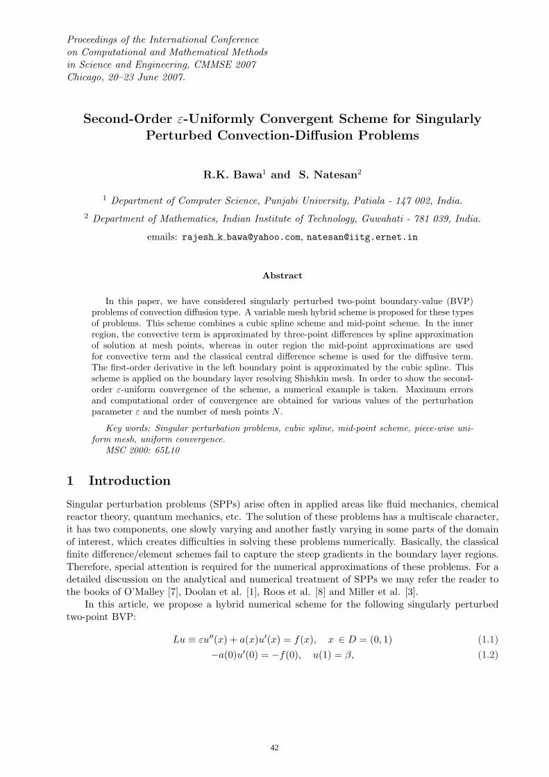
Proceedings of the International Conferenceon Computational and Mathematical Methodsin Science and Engineering, CMMSE 2007Chicago, 20–23 June 2007.
Second-Order ε-Uniformly Convergent Scheme for SingularlyPerturbed Convection-Diffusion Problems
R.K. Bawa1 and S. Natesan2
1 Department of Computer Science, Punjabi University, Patiala - 147 002, India.2 Department of Mathematics, Indian Institute of Technology, Guwahati - 781 039, India.
emails: rajesh k [email protected], [email protected]
Abstract
In this paper, we have considered singularly perturbed two-point boundary-value (BVP)problems of convection diffusion type. A variable mesh hybrid scheme is proposed for these typesof problems. This scheme combines a cubic spline scheme and mid-point scheme. In the innerregion, the convective term is approximated by three-point differences by spline approximationof solution at mesh points, whereas in outer region the mid-point approximations are usedfor convective term and the classical central difference scheme is used for the diffusive term.The first-order derivative in the left boundary point is approximated by the cubic spline. Thisscheme is applied on the boundary layer resolving Shishkin mesh. In order to show the second-order ε-uniform convergence of the scheme, a numerical example is taken. Maximum errorsand computational order of convergence are obtained for various values of the perturbationparameter ε and the number of mesh points N .
Key words: Singular perturbation problems, cubic spline, mid-point scheme, piece-wise uni-form mesh, uniform convergence.
MSC 2000: 65L10
1 Introduction
Singular perturbation problems (SPPs) arise often in applied areas like fluid mechanics, chemicalreactor theory, quantum mechanics, etc. The solution of these problems has a multiscale character,it has two components, one slowly varying and another fastly varying in some parts of the domainof interest, which creates difficulties in solving these problems numerically. Basically, the classicalfinite difference/element schemes fail to capture the steep gradients in the boundary layer regions.Therefore, special attention is required for the numerical approximations of these problems. For adetailed discussion on the analytical and numerical treatment of SPPs we may refer the reader tothe books of O’Malley [7], Doolan et al. [1], Roos et al. [8] and Miller et al. [3].
In this article, we propose a hybrid numerical scheme for the following singularly perturbedtwo-point BVP:
Lu ≡ εu′′(x) + a(x)u′(x) = f(x), x ∈ D = (0, 1) (1.1)−a(0)u′(0) = −f(0), u(1) = β, (1.2)
42

where ε > 0 is a small parameter, a and f are sufficiently smooth functions such that a(x) ≥α > 0, x ∈ D = [0, 1]. Under these assumptions, the BVP (1.1-1.2) has a unique solution u(x) ∈C2(D)
⋂C1(D) exhibiting a weak boundary layer at x = 0, see for example [8].
The application of second order cubic spline difference scheme on whole domain using Shishkinmesh may result in oscillations in the coarser region due to involvement of three-point approxima-tions of convective term in the scheme for smaller values of ε. Whereas, the use of midpoint schemein whole domain results in oscillation free scheme but with first order convergence rate. In order toretain the second order convergence of cubic spline scheme together with non-oscillating behaviorof mid-point scheme, we club these two schemes by taking cubic spline scheme in inner region andmid-point scheme in outer region. The value of the transition parameter σ0 is chosen in such a waythat the resultant hybrid scheme is second order ε-uniformly convergent through out the domain.More precisely, we take σ0 = 2/α.
The convection-diffusion BVP (1.1-1.2) has been studied earlier by Natesan et al. [5, 6, 9]. Inall these articles, the BVP is solved by using a domain decomposition method. The domain of thedifferential equation is divided into non-overlapping subdomains and the differential equation issolved on each subdomain with suitable conditions at the interfaces of the domain. These methodsare suitable for parallel computers, indeed, in [9], the numerical scheme is implemented in a parallelmachine. Bawa et al. have derived difference schemes for SPPs using cubic splines in [2].
In the following section K and C denote generic positive constants independent of nodal points,mesh size and the perturbation parameter ε.
2 The Continuous Problem
As the proposed scheme can be generalized easily for problems containing reactive terms, we studythe analytical behavior of the solution of the following BVP, which will be used to derive errorbounds for the derivatives of the solution.
Lu ≡ εu′′(x) + a(x)u′(x)− b(x)u(x) = g(x, ε), x ∈ Ω (2.1)
B0u(0) ≡ b(0)u(0)− a(0)u′(0) = −g(0, ε), B1u(1) ≡ u(1) = β. (2.2)
Definition 2.1 A function g(x, ε) is said to be of Class(K, j), if the derivatives of g with respectto x satisfy
| g(i)(x, ε) |≤ K[1 + ε−i exp(−αx/ε)], 0 ≤ i ≤ j, x ∈ Ω
Lemma 2.2 [3]. Let v be a smooth function satisfying B0v(0) ≥ 0, B1v(1) ≥ 0 and Lv(x) ≤0,∀x ∈ Ω. Then v(x) ≥ 0,∀x ∈ Ω.
Lemma 2.3 [3]. Let v be a smooth function. Then, we have the following uniform stability esti-mate
| v(x) |≤ C[| B0v(0) | + | B1v(1) | +maxy∈Ω
| Lv(y) |], ∀x ∈ Ω.
Lemma 2.4 Let g ∈ Class(K, 0). Then the solution y of (2.1-2.2) satisfies
| y(i)(x) |≤ C, i = 0, 1.
Proof. The proof can be seen in [6].
43

Lemma 2.5 [6] Let g ∈ Class(K, j). Then the solution y of (2.1-2.2) satisfies
| y′′(0) |≤ C and | y(i)(0) |≤ Cε−i+1, i = 3(1)j + 1.
Theorem 2.6 Let g be of Class(K, j). Then the solution y of (2.1-2.2) satisfies
| y(i)(x) |≤ C[1 + ε−i+1 exp(−αx/ε)], i = 2(1)j + 1, x ∈ Ω.
Proof. Refer [6] for the proof.
Corollary 2.7 If u(x) is the solution of (1.1-1.2) and a, b and f are in Cj(Ω), then u satisfies
| u(i)(x) |≤ C[1 + ε−i+1 exp(−αx/ε)], i = 1(1)j + 1, x ∈ Ω.
3 The Discrete Problem
In this section, first, we derive the cubic spline scheme on variable meshes, and then propose thehybrid scheme. Finally, we provide the piece-wise uniform Shishkin meshes for the SPP (1.1-1.2).
3.1 Cubic Spline Difference Scheme
Let the mesh points of Ω = [0, 1] be
x0 = 0, xi =i−1∑
k=0
hk, hk = xk+1 − xk, xN = 1, i = 1, 2, . . . , N − 1. (3.1)
We derive the difference scheme in the following.For given values u(x0), u(x1), · · · , u(xN ) of a function u(x) at the nodal points x0, x1, . . . , xN ,
there exists an interpolating cubic spline S(x) with following properties:
(i) S(x) coincides with a polynomial of degree three on each subinterval [xi, xi+1], i = 0, . . . , N−1;
(ii) S(x) ∈ C2[0, 1];
(iii) S(xi) = u(xi), i = 0, . . . , N .
The cubic spline can be given by
S(x) =(xi+1 − x)3
6hiMi +
(x− xi)3
6hiMi+1 +
(u(xi)− h2
i
6Mi
)(xi+1 − x
hi
)+
+(
u(xi+1)− h2i
6Mi+1
)(x− xi
hi
), xi ≤ x ≤ xi+1, i = 0, · · · , N − 1 (3.2)
where Mi = S′′(xi), i = 0, · · · , N .The first derivative of S(x) is given by
S′(x) = −Mi(xi+1 − x)2
2hi+ Mi+1
(x− xi)2
2hi+
u(xi+1)− u(xi)hi
− (Mi+1 −Mi)6
hi,
xi ≤ x ≤ xi+1, i = 0, · · · , N − 1. (3.3)
44

and the second derivative is
S′′(x) = Mi(xi+1 − x)
hi+ Mi+1
(x− xi)hi
. (3.4)
For the one sided limit of the first derivative, from (3.3), we have
S′(xi−) =hi−1
6Mi−1 +
hi−1
3Mi +
u(xi)− u(xi−1)hi−1
, (3.5)
andS′(xi+) = −hi
3Mi − hi
6Mi+1 +
u(xi+1)− u(xi)hi
. (3.6)
From (3.2) and (3.4), the functions S(x) and S′′(x) are continuous on Ω and for S′(x) to becontinuous at the interior nodes xi, we have from (3.5)-(3.6), the following well-known ’continuitycondition’:
hi−1
6Mi−1 +
(hi + hi−1
3
)Mi +
hi
6Mi+1 =
(ui+1 − ui
hi
)−
(ui − ui−1
hi−1
), i = 1, · · · , N − 1. (3.7)
This equation ensures the continuity of the first order derivative of the spline S(x) at the interiornodes.
For obtaining second order approximations of the first order derivatives at the nodal points interms of approximate values ui of u(x) at xi, we do the following.
Taking usual Taylor series expansion for y around xi, and neglecting the third and forth orderterms, we get the following approximations for ui+1 and ui−1
ui+1 ' ui + hiu′i +
h2i
2u′′i , (3.8)
ui−1 ' ui − hi−1u′i +
h2i−1
2u′′i . (3.9)
Multiplying (3.9) by h2i /h2
i−1 and subtracting from (3.8), we get the following approximation foru′i:
u′i '1
hihi−1(hi−1 + hi)[h2
i−1ui+1 + (h2i − h2
i−1)ui − h2i ui−1] (3.10)
Multiplying (3.9) by h2i /h2
i−1 and adding it to(3.8), we get the following approximation foru′′i :
u′′i '2
hihi−1(hi−1 + hi)[hi−1ui+1 − (hi−1 + hi)ui + hiui−1] (3.11)
Also, we have
u′i+1 ≈ u′i + hiu′′i , (3.12)
u′i−1 ' u′i − hi−1u′′i . (3.13)
Using the expressions for u′i and u′′i from (3.10) and (3.11)respectively, and putting them in (3.12),we get the following approximation for u′i+1:
u′i+1 '1
hihi−1(hi + hi−1)[(h2
i−1 + 2hihi−1)ui+1 − (hi−1 + hi)2ui + h2i ui−1] (3.14)
45
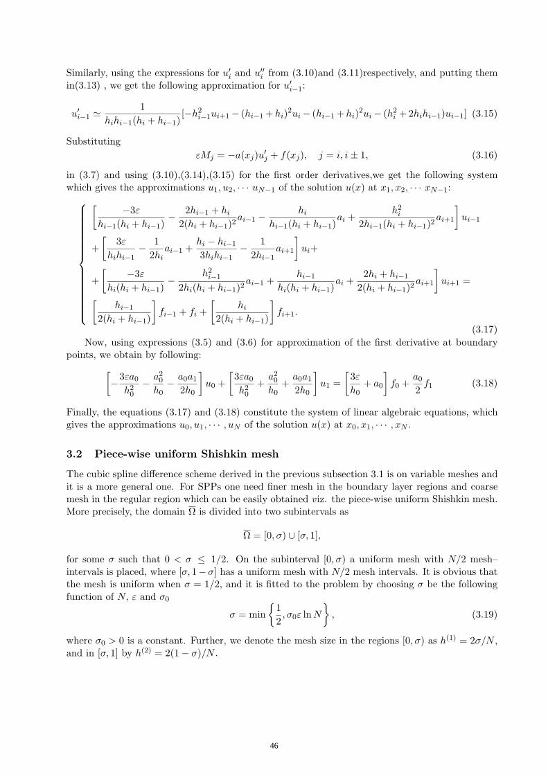
Similarly, using the expressions for u′i and u′′i from (3.10)and (3.11)respectively, and putting themin(3.13) , we get the following approximation for u′i−1:
u′i−1 '1
hihi−1(hi + hi−1)[−h2
i−1ui+1− (hi−1 +hi)2ui− (hi−1 +hi)2ui− (h2i +2hihi−1)ui−1] (3.15)
SubstitutingεMj = −a(xj)u′j + f(xj), j = i, i± 1, (3.16)
in (3.7) and using (3.10),(3.14),(3.15) for the first order derivatives,we get the following systemwhich gives the approximations u1, u2, · · · uN−1 of the solution u(x) at x1, x2, · · · xN−1:
[ −3ε
hi−1(hi + hi−1)− 2hi−1 + hi
2(hi + hi−1)2ai−1 − hi
hi−1(hi + hi−1)ai +
h2i
2hi−1(hi + hi−1)2ai+1
]ui−1
+[
3ε
hihi−1− 1
2hiai−1 +
hi − hi−1
3hihi−1− 1
2hi−1ai+1
]ui+
+[ −3ε
hi(hi + hi−1)− h2
i−1
2hi(hi + hi−1)2ai−1 +
hi−1
hi(hi + hi−1)ai +
2hi + hi−1
2(hi + hi−1)2ai+1
]ui+1 =
[hi−1
2(hi + hi−1)
]fi−1 + fi +
[hi
2(hi + hi−1)
]fi+1.
(3.17)Now, using expressions (3.5) and (3.6) for approximation of the first derivative at boundary
points, we obtain by following:[−3εa0
h20
− a20
h0− a0a1
2h0
]u0 +
[3εa0
h20
+a2
0
h0+
a0a1
2h0
]u1 =
[3ε
h0+ a0
]f0 +
a0
2f1 (3.18)
Finally, the equations (3.17) and (3.18) constitute the system of linear algebraic equations, whichgives the approximations u0, u1, · · · , uN of the solution u(x) at x0, x1, · · · , xN .
3.2 Piece-wise uniform Shishkin mesh
The cubic spline difference scheme derived in the previous subsection 3.1 is on variable meshes andit is a more general one. For SPPs one need finer mesh in the boundary layer regions and coarsemesh in the regular region which can be easily obtained v iz. the piece-wise uniform Shishkin mesh.More precisely, the domain Ω is divided into two subintervals as
Ω = [0, σ) ∪ [σ, 1],
for some σ such that 0 < σ ≤ 1/2. On the subinterval [0, σ) a uniform mesh with N/2 mesh–intervals is placed, where [σ, 1− σ] has a uniform mesh with N/2 mesh intervals. It is obvious thatthe mesh is uniform when σ = 1/2, and it is fitted to the problem by choosing σ be the followingfunction of N, ε and σ0
σ = min
12, σ0ε ln N
, (3.19)
where σ0 > 0 is a constant. Further, we denote the mesh size in the regions [0, σ) as h(1) = 2σ/N ,and in [σ, 1] by h(2) = 2(1− σ)/N .
46

3.3 The hybrid scheme
As the use of the second-order cubic spline scheme derived in Section 3.1 in the whole domain givessatisfactory results only when the values of ε and N are compatible, i.e., when N−1 ≤ ε, and it isdifficult to get uniform convergence. Therefore, taking advantage of its higher order convergenceand uniform convergence of the mid-point scheme, we propose the following hybrid scheme, wherecubic spline scheme is used only in the boundary layer region and mid-point scheme in the outerregion.
More precisely, the hybrid scheme is given as
LNui ≡ r−i ui−1 + rci ui + r+
i ui+1 = q−i fi−1 + qci fi + q+
i fi+1, i = 1, · · · , N/2− 1,
LNui ≡ r−i ui−1 + rci ui + r+
i ui+1 = fi+1/2, i = N/2, · · · , N − 1(3.20)
along with the following equations corresponding to the boundary points
BN0 ui ≡ rc
0u0 + r+0 u1 = qc
0f0 + q+0 f1,
BN1 ui ≡ uN = β,
(3.21)
for i = 1, · · · , N/2− 1
r−i =−3ε
hi−1(hi + hi−1)− 2hi−1 + hi
2(hi + hi−1)2ai−1 − hi
hi−1(hi + hi−1)ai +
h2i
2hi−1(hi + hi−1)2ai+1
rci =
3ε
hihi−1− 1
2hiai−1 +
hi − hi−1
3hihi−1− 1
2hi−1ai+1;
r+i =
−3ε
hi(hi + hi−1)− h2
i−1
2hi(hi + hi−1)2ai−1 +
hi−1
hi(hi + hi−1)ai +
2hi + hi−1
2(hi + hi−1)2ai+1;
q−i =hi−1
2(hi + hi−1); qc
i = 1; q+i =
hi
2(hi + hi−1),
(3.22)and for i = N/2, · · · , N − 1
r−i =2ε
hi−1(hi + hi−1); rc
i =−2ε
hi−1(hi + hi−1)− 2ε
hi(hi + hi−1)− ai+1/2
hi;
r+i =
2ε
hi(hi + hi−1)+
ai+1/2
hi;
(3.23)
and
rc0 = −3εa0
h20
− a20
h0− a0a1
2h0; r+
0 =3εa0
h20
+a2
0
h0+
a0a1
2h0;
qc0 =
3ε
h0+ a0; q+
0 =a0
2;
(3.24)
The tri-diagonal system of linear algebraic equations (3.20-3.21) can be solved by any existingcodes.
47

3.4 Truncation Error
Here, we derive the truncation error for the difference scheme proposed in Section 3.3. The discretestability analysis, and error estimates will be carried out in our forthcoming article [4].
For i = 1, · · · , N/2− 1, the truncation error of the hybrid scheme is given by
τi,u = [r−i u(xi−1) + rci u(xi) + r+
i u(xi+1)]− [q−i f(xi−1) + qci f(xi) + q+
i f(xi+1)]. (3.25)
Using the differential equation (1.1) for f in the above expression, we get
τi,u = [r−i u(xi−1) + rci u(xi) + r+
i u(xi+1)]− [q−i (εu′′(xi−1) + ai−1u′(xi−1)) +
+qci (εu
′′(xi) + aiu′(xi)) + q+
i (εu′′(xi+1) + ai+1u′(xi+1))]. (3.26)
Now, making use of the Taylor series expansion, we have
u(xi−1) = u(xi)− hi−1u′(xi) +
h2i−1
2!u′′(xi)−
h3i−1
3!u(iii)(xi) +
h4i−1
4!u(iv)(xi) + · · · ,
and
u(xi+1) = u(xi) + hiu′(xi) +
h2i
2!u′′(xi) +
h3i
3!u(iii)(xi) +
h4i
4!u(iv)(xi) + · · ·
Using the values of u(xi−1), u(xi+1) in (3.26), we have
τi,u = T0,iu(xi) + T1,iu′(xi) + T2,iu
′′(xi) + T3,iu(iii)(xi) + T4,iu
(iv)(xi) + h.o.t., (3.27)
where
T0,i = r−i + rci + r+
i ,
T1,i = −hi−1r−i + hir
+i − (q−i ai−1 + qc
i ai + q+i ai+1),
T2,i =h2
i−1
2!r−i +
h2i
2!r+i + ε(q−i + qc
i + q+i )− (
hi−1q−i ai−1 − hiq
+i ai+1
),
T3,i = −h3i−1
3!r−i +
h3i
3!r+i − ε(q−i hi−1 − q+
i hi) +(
h2i−1
2!q−i ai−1 +
h2i
2!q+i ai+1
),
T4,i =h4
i−1
4!r−i +
h4i
4!r+i + ε(q−i
h2i−1
2!+
h2i
2!q+i )−
(h3
i−1
3!q−i ai−1 − h4
i
4!q+i ai+1
).
It can be easily seen that
T0,i = T1,i = T2,i = T3,i = 0, T4,i = −3ε
(h3
i + h3i−1
hi + hi−1
)[14!− 1
2!6
].
Thus, we have
τi,u = −3ε
(h3
i + h3i−1
hi + hi−1
) [14!− 1
2!6
]u(iv)(xi) + O(N−3). (3.28)
For i = N/2, · · · , N − 1, we can proceed in similar manner to show that
τi,u = −ε
(hi − hi−1
3
)u(iii)(xi) +
2ε
4!
(h3
i + h3i−1
hi + hi−1
)u(iv)(xi) + O(N−3). (3.29)
48

The truncation error at the boundary point x0 is given by
τ0,u = rc0u(x0) + r+
0 u(x1)− qc0f0 − q+
0 f1 (3.30)
Again using (1.1), and the Taylor series expansion for u(x1), the truncation error at x0 can be givenas
τ0,u = −3εh20
(14!− 1
2!6
)u
(iv)0 (x0) + O(N−3). (3.31)
Using the bounds of the solution obtained in Section 2, one can prove the following proposition.
Proposition 3.1 Let u(x) and ui be respectively the solutions of (1.1-1.2) and (3.20-3.21). Then,the local truncation error satisfies the following bounds:
|τi,u| ≤ CN−2σ20 ln2 N, for 0 ≤ i < N/2,
|τi,u| ≤ C(N−2ε + N−ασ0), for N/2 ≤ i ≤ N − 1, and h(2) ≥ √ε,
|τi,u| ≤ C(N−1ε + N−ασ0), for N/2 ≤ i ≤ N − 1 and h(2) <√
ε.
4 Numerical Experiments
To show the accuracy of the present method, here we have implemented it on the following exam-ple. The results are presented in the form of tables with maximum point–wise errors and rate ofconvergent, and figures showing the maximum point-wise error in the loglog scale.
Example 4.1 Consider the following convection-diffusion Neumann BVP:
εu′′(x) + (1 + 2x)2u′(x) = −(x3 + exp(−x)), x ∈ (0, 1)−u′(0) = −1, u(1) = 0.
To calculate the maximum point-wise error and rate of convergence, we use the double meshprinciple. We calculate the numerical solution UN on ΩN and the numerical solution UN on themesh ΩN where the transition parameter is now given by
σ = min
12, σ0ε ln(N/2)
.
Define the double mesh differences to be
GNε = max
xj ∈ΩNε
|UN (xj)− U2N (xj)|, and GN = maxε
GNε ,
where UN (xj) and U2N (xj) respectively denote the numerical solutions obtained using N and 2Nmesh intervals. Further, we calculate the parameter-robust orders of convergence as
p = log2
(GN
ε
G2Nε
)and p
uni= log2
(GN
G2N
).
The numerical results for the present example are presented in Table 1. The maximum point-wiseerrors are plotted in Figure 1.
49

5 Discussion
In this paper, we proposed a hybrid scheme for the numerical solution of convection dominatedtwo-point boundary-value problems. This scheme consists of both the cubic spline and mid-pointschemes. This scheme is applied on a layer resolving Shishkin mesh. In the boundary layer region,where the mesh is fine, the cubic spline scheme is used. In the outer region, i.e., in the coarse meshregion, the mid-point scheme is used. Truncation errors are derived. The numerical results revealthe second-order ε-uniform convergence of the scheme throughout the domain.
Acknowledgements
This work is supported by the Department of Science and Technology, Government of India underresearch grant SR/S4/MS:318/06.
References
[1] E.P. Doolan, J.J.H. Miller, and W.H.A. Schildres, Uniform Numerical Methods forProblems with Initial and Boundary Layers, Boole Press, Dublin, 1980.
[2] M.K. Kadalbajoo and R.K. Bawa, Variable Mesh Difference Scheme Cubic for SingularlyPerturbed Boundary-Value Problems Using Splines, Jl. Optim. Theory. and Appl., 9 (1996)405–416.
[3] J.J.H. Miller, E. O’Riordan, and G.I. Shishkin, Fitted Numerical Methods for SingularPerturbation Problems, World Scientific, Singapore, 1996.
[4] S. Natesan and R.K. Bawa, Second-Order Parameter-Uniform Error Estimate for Convec-tion Dominated Two-Point Boundary-Value Problems, Working Paper, 2007.
[5] S. Natesan and N. Ramanujam, ’Shooting Method’ for the Solution of Singularly PerturbedTwo-Point Boundary-Value Problems Having Less Severe Boundary Layers, Appl. Math. Com-put., 133 (2002) 623–641.
[6] S. Natesan, J. Vigo-Aguiar, and N. Ramanujam, A Numerical Algorithm for SingularPerturbation Problems Exhibiting Weak Boundary Layers, Comput. Math. Appl. 45 (2003)469–479.
[7] R.E. O’Malley, Singular Perturbation Methods for Ordinary Differential Equations,Springer, New York, 1991.
[8] H.-G. Roos, M. Stynes, and L. Tobiska, Numerical Methods for Singularly PerturbedDifferential Equations, Springer, Berlin, 1996.
[9] J. Vigo-Aguiar and S. Natesan, A Parallel Boundary Value Technique for SingularlyPerturbed Two-Point Boundary Value Problems, The Journal of Supercomputing 27 (2004)195–206.
50

Table 1: Maximum point-wise errors ENε , rate of convergence p and ε uniform errors EN for
Example 4.1.
ε Number of mesh points N
16 32 64 128 256 512 1024 204810−0 2.4092e-3 1.1589e-3 5.6619e-4 2.7960e-4 1.3891e-4 6.9227e-5 3.4557e-5 1.7264e-5
1.0558 1.0334 1.0179 1.0093 1.0047 1.0024 1.001210−2 1.1338e-3 1.2896e-4 3.8017e-5 3.0810e-5 1.7304e-5 8.3840e-6 3.8425e-6 1.7205e-6
3.1362 1.7622 0.3032 0.8323 1.0454 1.1256 1.159310−4 2.6484e-3 6.8858e-4 1.7263e-4 4.2598e-5 1.0332e-5 2.4250e-6 5.2827e-7 9.3387e-8
1.9434 1.9959 2.0188 2.0437 2.0910 2.1986 2.500010−6 2.6687e-3 6.9728e-4 1.7630e-4 4.4196e-5 1.1054e-5 2.7623e-6 6.8981e-7 1.7206e-7
1.9363 1.9837 1.9961 1.9994 2.0006 2.0016 2.003310−8 2.6689e-3 6.9737e-4 1.7634e-4 4.4212e-5 1.1061e-5 2.7657e-6 6.9145e-7 1.7286e-7
1.9363 1.9836 1.9959 1.9990 1.9997 1.9999 2.000010−10 2.6689e-3 6.9737e-4 1.7634e-4 4.4212e-5 1.1061e-5 2.7657e-6 6.9146e-7 1.7288e-7
1.9363 1.9836 1.9959 1.9990 1.9997 1.9999 1.999910−12 2.6689e-3 6.9737e-4 1.7634e-4 4.4212e-5 1.1061e-5 2.7657e-6 6.9146e-7 1.7288e-7
1.9363 1.9836 1.9959 1.9990 1.9997 1.9999 1.9999EN 2.6689e-3 1.1589e-3 5.6619e-4 2.7960e-4 1.3891e-4 6.9227e-5 3.4557e-5 1.7264e-5puni 1.2035 1.0334 1.0179 1.0093 1.0047 1.0024 1.0012
101
102
103
10−7
10−6
10−5
10−4
10−3
10−2
N
Max
. Err
or
ε = 1ε = 1e−1ε = 1e−2ε = 1e−3ε = 1e−5
020
404 5 6 7 8 9 10 11
0
0.5
1
1.5
2
2.5
3
x 10−3
log2(1/ ε)log2(N)
Max
. Err
or
0.5
1
1.5
2
2.5
x 10−3
(a) N Vs. Maximum Error. (b) N , ε Vs. Maximum Error.
Figure 1: Plots of Maximum Point-wise Error for Example 4.1.
51

Deadlock Detection Algorithm for Grid Resource Management
Seema Bawa, Anju Sharma
Computer Science & Engineering Department Thapar University, Patiala Punjab- 147004, India
sbawa, anjusharma @tiet.ac.in
Abstract Distributed environments are touching newer heights; becoming more useful, popular and complex with the emergence of technologies like peer-to-peer computing, autonomic computing, pervasive computing and Grid computing. Grid computing is emerging as the new paradigm to provide collaborative and resource sharing environment over multiple geographically distributed environments. These technologies aim to enable large resource sharing. Due to the heterogeneous and dynamic nature of resources, we need to develop highly distributed and extensible framework for resource management. This paper presents an algorithm for Grid Resource Management based on deadlock detection mechanism used in operating systems. The proposed algorithm aims to achieve the major objectives like: fairness of resource distribution among nodes, scalability, flexibility and simplicity. A prototype implementation of the algorithm is also presented in the paper. Keyword: Distributed environments, Grid computing, Resource Management, Resource Allocation Graph (RAG)
1. Introduction Grid infrastructures and computing environments have progressed significantly in the past few years [1]. Grid is a distributed system involving heterogeneous resources located in different geographical domains that are potentially managed by different organizations. In Grid systems many users run their application at the same time and compete for the finite number of resources.
Figure 1. Schematic view of Resource Pool
R2
CPU
Memory
Disk Space
Printer
Monitor
Resource Pool
R1
R3
R4
R5
U1
U2
U3
U4
U5
Type of Resources Users
52

The key problem here is to find the node that offer the desired type and amount of resources like cpu, memory, disk space etc. – required by a user to start and complete the execution of its application. Owing to the heterogeneous environment of the Grid, it has large set of resources. These resources can be represented by resource pool as shown in the Figure 1. These resources are represented as R1, R2, R3, R4 and R5. Categorization may be done as CPU, Memory, Printer, Disk Space, and Monitor. A user may request as many resources as it requires to carry out its designated task. Apparently, the number of resources requested may not exceed the total number of resources available in the system. For example, a process can not request three printers if the system has only two. If a system has two CPUs, then the resource type CPU has two instances. If a user requests an instance of a resource type, the allocation of any instance of the type will satisfy the request. If it does not, then the instances are not identical, and the resource type classes have not been defined properly. For example, a system may have two printers; both may be defined to be in the same resource class, if no one cares which printer prints the output. However, if one printer is on the ninth floor and other is in the basement, then the people of ninth floor may not see both printers as equivalent, and separate resource classes may need to be defined for each printer. Deadlock is one of the most serious problems in multitasking concurrent programming systems [2]. Consider a simple case study of an organization: In an organization thousands of employees work for a shift and they need some resources for specific amount of time. Suppose a user U1 uses the memory for half a day and in between this half day user U4 need, the same memory. So, to use the memory user U4 has to wait or U1 and U4 may have to compete for the memory at the same time. Once they are competing a condition occurs which is known as deadlock. Deadlock can be described through a Resource Allocation Graph (RAG) [3]. It can be shown that, if the graph contains no cycles, then no process in the system is deadlock. If the graph does not contain a cycle, then a deadlock may exist. Suppose that process P3 requests an instance of resource type R2. Since no resource instance is currently available, a request edge P3→ P2 is added to the graph (Figure 2). At this point, two minimal cycles exist in the system: P1→R1→P2→R3→P3→R2→P1 and P2→R3→P3→R2→P2. Processes P1, P2, P3 are deadlocked.
Figure 2. Resource Allocation Graph (RAG) with Deadlock
•
• •
• • •
•
P2P1 P3
R1 R2
R3 R4
53

Deadlock is constant problem often offsetting the advantages of resource sharing [4]. A set of threads is deadlocked if each thread is waiting for an event that can only be generated by another thread in the set [5]. Detecting the deadlock is one of the major problems in Grid Computing [6]. When a deadlock is detected message is propagated to whole cycle of the deadlock as described in the Section 3.1. Some algorithms for deadlock detection are described in following sections.
2. Deadlock Detection Algorithms
2.1 Assessment Algorithm
This algorithm is used for finding out whether or not a system is in assessing state. It can be described as follows:
I. Initialize Start := Open and Finish [i] := False for i =1,2,…,n.
II. Let Start and Finish be vectors of length v and n, respectively. III. Find an i such that both
a. Finish[i] = False b. Requirei <= Start
If no such i exists, go to step IV IV. Start := Start + Allotment;
Finish[i] := True; Go to step II.
V. If Finish[i] = True for all i, then calculate that the system is in safe state.
This algorithm may require an order of v*n2 operations to decide whether the state is safe.
2.2 Demand Resource Algorithm
Let Requesti be the request vector for user Pi. If Requesti [j] = k, then user Pi wants k instances of resource type Rj. When a request for resources is made by user Pi, the following actions are taken:
a. If Requesti <= Requirei, go to step b. Otherwise, raise an error condition, since the user has exceeded its maximum.
b. If Requesti <= Requirei, go to step c. Otherwise Pi must wait, since resources are not available.
c. Have the system pretend to have allotment the request resources to user Pi by modifying the state as follows:
Open :=Open – Requesti; Allotment := Allotmenti + Requesti; Requirei := Requirei - Requesti;
If the resulting resource allocation state is safe, the transaction is completed and user Pi is allocated the resources. However, if the new state is not assess, then Pi must wait for Requesti and the old resource-allocation state is restored.
54

3. Proposed Approach and Data Structures for the Algorithm Based on the above algorithms the proposed approach and data structures for the algorithms are as follows. When a new user enters into the system, it must declare the maximum number of instances of each resource type that it may need. This number may not exceed the total number of resources in the system. When a user requests a set of resources, the system must determine whether the allotment of these resources will leave the system in assess state. If it will, the resources are allocated; otherwise, the user must wait until some other user releases enough resources. Several data structures must be maintained to implement the algorithm. These data structures encode the state of the resource-allocation system. Let n be the number of users in the system and v be the number of resource types. We need the following data structures.
• Open: A vector of length v indicates the number of available user of each type. If available [Resource j] = k, there are k instances of resource type Rj open.
• Max: An n*v matrix defines the maximum demand of each user. If Max [i, j] = k, then user Qi may request at most k instances of resource type Rj.
• Allotment: An n*v matrix defines the number of resources of each type currently allocated to each user. If Allocation [i,j] = k, then user Qi is currently allocated k instances of resource type Rj.
• Require: An n*v matrix indicates the remaining resource need of each user. If require [i,j] = k, then user Qi may need k more instances of resource type Rj to complete its task. Note that Require [i,j] = Max [i,j] – Allotment [i,j].
3.1 Type of messages • Inadequate number of resources: Once the user request for resources, if
resources are not available then popup message is generated “inadequate number of resources”.
• Over allocation of resources: If available resources are less then or equal to zero then ‘over allocation of resources’ message is popped up.
• Failed to satisfy the Customer: the message ‘failed to satisfy’ the customer is popped up when the requested resources are not available.
• Satisfy the Customer: If not failed to satisfy the customer then the message generated is “satisfy the customer”.
• State is Safe: Once the customer is satisfied the ‘state is safe’. • State is Unsafe: If the Customer is not satisfied the ‘state is unsafe’.
4. Implementation Details
We have considered the standard C library function, malloc. Initially implementation of this algorithm is done using ‘C’ programming language. Five cases are considered i.e. ‘failed to allocate the existing resources’, ‘failed to allocate the available resources’, ‘state is safe’, ‘state is unsafe’, and ‘overallocation of resource’. In order to do this we need to declare the argument count (argc) and the array of strings (argv). We have used two 1-dimensional arrays and two 2-dimensional arrays, as pointers, and use malloc call
55

later to make them into arrays with actual storage. The pseudocode of the proposed algorithm is given below.
4.1 The pseudocode for the proposed Deadlock Detection Algorithm
procedure Deadlock Detection Algorithm (nr, nc, argc, argv) Enter the number of resource ,number of customer for the computation, argc (argument count), argv (array of strings) var nr, nc, ii, jj, existing_resourrces, available_resources, current_allocation, requested_resources, done=0, trials=0, freed=0 begin Step 1: nr, nc; PLEASE SPECIFY THE NUMBER OF RESOURCES AND NUMBER OF CUSTOMERS
Step 2: if (! (existing_resources) || (! (available_resources) ||(! (current_allocation) || (! (requested_resources) then //if Resources are not present failure: “inadequate number of resources” //Message pop up
Step 3: for ii :=0 to< nr do how many of existing_resources exists?
available_resources [ ]= existing_resources [ ] Step 4: for ii:=0 to < nc
tell me about the resources for customers how many of resources are currently allocated to customer
available_resources[ ] -= current_allocation[ ] [ ] //available_resources = available_resources – current_allocation
if available_resources [ ] < 0 overallocation of resources exit (1) else how many maximum of resources would customer like to have? Requested_resource[ ] [ ] -= current_allocation [ ] [ ] //Requested_resources = Requested_resources-current_allocation
Step 5: while (!done) do trials =0; freed = 0; do begin for ii := 1 to <nc if requested_resources trials++; failed = 0; for jj := 1 to < nr if requested_resources [ ] [ ] > available_resources [ ] [ ] failed = 1 failed to satisfy the customer break;
Step 6: if (!failed) free++; for jj := to < nr available_resources [ ] += current_allocation [ ] [ ] //available_resources = available_resources + current_allocation free (requested_resources) ; requested_resources [ ] = NULL;
56
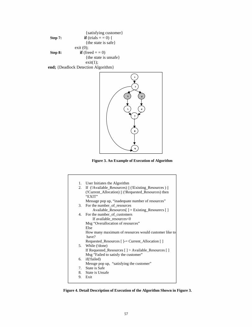
satisfying customer Step 7: if (trials = = 0)
the state is safe exit (0); Step 8: if (freed = = 0)
the state is unsafe exit(1);
end; Deadlock Detection Algorithm
1. User Initiates the Algorithm 2. If (!Available_Resources) || (!Existing_Resources ) ||
(!Current_Allocation) || (!Requested_Resources) then “EXIT” Message pop up, “inadequate number of resources”
3. For the number_of_resources Available_Resources[ ] = Existing_Resourecs [ ]
4. For the number_of_customers If available_resources<0
Msg “Overallocation of resources” Else How many maximum of resources would customer like to have? Requested_Resources [ ]-= Current_Allocation [ ]
5. While (!done) If Requested_Resources [ ] > Available_Resources [ ] Msg ”Failed to satisfy the customer”
6. if(!failed) Messge pop up, “satisfying the customer”
7. State is Safe 8. State is Unsafe 9. Exit
Figure 4. Detail Description of Execution of the Algorithm Shown in Figure 3.
1
2
65
3 4
8
7
9
Figure 3. An Example of Execution of Algorithm
57

5. Conclusion We have proposed a Deadlock Detection Algorithm, in Grids which is well suited for applications such as Resource Management in Grids. Deadlock Detection algorithm is capable of meeting the identified requirements and the approach is workable. By implementing the Algorithm proposed above in Grid Computing, we can establish a Fairness, Scalability, Flexibility and Simplicity in Resource Management. Figure 3. shows example of execution of the algorithm. Figure 4. Shows the detail description of the execution of the algorithm.
ACKNOWLEDGEMENT
The authors are deeply indebted to Thapar University, Patiala (India). Words are not sufficient to acknowledge our gratitude towards TU Grid Group actively working at the Centre of Excellence in Grid Computing (CoEGC) the Thapar Deemed University, Patiala for providing us motivation and base for carrying out this work. The free and open discussions and brainstorming sessions held during weekly meetings there had been extremely helpful in this endeavor.
References: [1] http://arxiv.org/pdf/cs.CE/0301018 [2] E. Knapp, “Deadlock Detection in Distributed Database Systems,” ACM Computing
Surveys, Vol. 19, No. 4, pp. 303-327, Dec. 1987. [3] Galvin Gagna. “Operating System Concepts”, Edition 7. [4] M. Singhal, “Deadlock Detection in Distributed Systems,” IEEE Computer, Vol. 22,
pp. 37–48, 1989. [5] Tanenbaum. “Modern Operating Systems”, Prentice Hall, 2001. [6] Nacer Farajzadeha, Mehdi Hashemzadeha, Morteza Mousakhania, Abolfazl T.
Haghighat,” An Efficient Generalized Deadlock Detection and Resolution Algorithm in Distributed Systems” Proceedings Fifth International Conference on Computer and Information Technology (CIT’05) 2005 IEEE.
58

Proceedings of the International Conference on Computational and Mathematical Methods in Science and Engineering, CMMSE2007 Chicago, 20-23 June 2007
Analysis of Computational Grid Environments
Seema Bawa
Department of Computer Science & Engineering Thapar University, Patiala
Abstract
The Grid is computing and data management infrastructure, which provides the electronic underpinning for a global society in business, government and research. To realize the global grid environment we need a standard architecture to cope up the heterogeneity and the interoperatability The middleware component is of extreme importance while building the Grid environment, as the majority of the Grid specific features are implemented using the Grid middleware. The grid middlewares act as glue between the grid resource components and the application components. The Globus, Condor, Nimrod/g, Alchemi are the popular middlewares. The comparative analysis of these middlewares let the grid community know the choices available. Keywords: Grid computing, Middleware, Globus, Nimrod/g, Alchemi, Condor 1. Introduction
Grids are becoming platforms for high-performance and distributed computing [7]. A Grid benefits users by permitting them to acces0s heterogeneous resources, such as machines, data, people and devices that are distributed geographically and organizationally. They allow users to execute compute intensive problems whose computational requirements cannot be satisfied by a single machine. Grid Computing has emerged as a new and important field and can be visualized as an enhanced form of Distributed Computing. With the advent of new technology, it has been realized that paralleling sequential applications could yield faster results and sometimes at a lower cost [2].
Grid computing is the next generation IT infrastructure that promises to transform the way organizations and individuals compute, communicate and collaborate [8][9]. It offers untapped processing cycles from networks of computers spanning vast geographical boundaries. Sharing in a Grid is not just a simple sharing of files but of hardware, software, data, and other resources [6]. Thus a complex yet secure sharing is at the heart of the Grid.
2. Grid Components The various components s that are necessary to form a Grid are as follows.
2.1 Grid Fabric
This consists of all the globally distributed resources that are accessible from anywhere on the Internet. These resources could be computers (such as PCs or Symmetric Multi-Processors) running a variety of operating systems (such as UNIX or Windows), storage devices, databases, and special scientific instruments such as a radio telescope or particular heat sensor [17].
59

2.2 Core Grid middleware This offers core services such as remote process management, co-allocation of resources,
storage access, information registration and discovery, security, and aspects of Quality of Service (QoS) such as resource reservation and trading. These services abstract the complexity and heterogeneity of the fabric level by providing a consistent method for accessing distributed resources.
2.3 User-level Grid middleware User level middleware utilizes the interfaces provided by the low-level middleware to provide
higher-level abstractions and services. This includes application development environments, programming tools, and resource brokers for managing resources and scheduling application tasks for execution on global resources.
Fig 2.2 Grid components [17]
2.4 Grid applications and Portal Grid applications are typically developed using Grid-enabled languages and utilities such as
HPC++ or MPI. An example application, such as parameter simulation or a grand-challenge problem, would require computational power, access to remote data sets, and may need to interact with scientific instruments. Grid portals offer Web-enabled application services, where users can submit and collect results for their jobs on remote resources through the Web [17].
3. Grid Middleware Grids have middleware stacks, which are a series of cooperating programs, protocols and agents
designed to help users access the resources of a Grid[28]. Grid Middleware refers to the security, resource management, data access, instrumentation, policy, accounting, and other services required for applications, users, and resource providers to operate effectively in a Grid environment. Middleware acts as a sort of 'glue' which binds these services together. Formally Grid middleware can be define [23] as:
60

“A mediator layer that provide a consistent and homogeneous access to resources managed locally with different syntax and access methods”
Till today several implementation of Grid middleware have been achieved. These implementations have well identified basic services. These middleware implementations are now moving their focus from proprietary/ adhoc solutions to standard based solutions. The brief overview of the some popular middleware’s Globus, Alchemi, and Condor is discussed in this section.
3.1 Globus The Globus [27] toolkit is designed to enable people to create computational Grids. It has been
developed over several years chiefly at the Argonne National Laboratory Illinois USA. As an open source project any person can download the software, examine it, install it and hopefully improve it. By this constant stream of comments and improvements, new versions of the software can be developed with increased functionality and reliability. In this way the Globus project itself will be on going with constant evolution of the toolkit [27].
3.1.1 Globus Pyramids Globus Toolkit has three pyramids of support built on top of a security infrastructure, as
illustrated. They are: • Resource management • Data management • Information services
All of these pyramids are built on top of the underlying Grid Security Infrastructure (GSI). This provides security functions, including single/mutual authentication, confidential communication, authorization, and delegation.
Fig3.1 Globus pyramids [24] Resource management
The resource management pyramid provides support for: • Resource allocation • Submitting jobs: Remotely running executable files and receiving results • Managing job status and progress
Information services
The information services pyramid provides support for collecting information in the Grid and for querying this information, based on the Lightweight Directory Access Protocol (LDAP). Data management
61

The data management pyramid provides support to transfer files among machines in the Grid and for the management of these transfers. [24]
3.1.2 Components of Globus Toolkit For each pyramid previously presented, Globus provides a component to implement resource management, data management, and information services. The various Components are: GRAM, MDS, GridFTP and GSI.
Fig 3.2 System overview of Globus [24]
3.1.2.1 Grid Security Infrastructure (GSI)
GSI provides elements for secure authentication and communication in a Grid. The infrastructure is based on the SSL protocol (Secure Socket Layer), public key encryption, and x.509 certificates. For a single sign-on, Globus add some extensions on GSI. It is based on the Generic Security Service API, which is a standard API promoted by the Internet Engineering Task Force (IETF). These are the main functions implemented by GSI are: Single/mutual authentication, Confidential communication, Authorization, Delegation 3.1.2.2 Grid Resource Allocation Manager (GRAM)
GRAM is the module that provides the remote execution and status management of the execution. When a client submits a job, the request is sent to the remote host and handled by the gatekeeper daemon located in the remote host. Then the gatekeeper creates a job manager to start and monitor the job. When the job is finished, the job manager sends the status information back to the client and terminates [24]. GRAM contains the following elements: globusrun command, Resource Specification Language (RSL), gatekeeper daemon, job manager, forked process, Global Access to Secondary Storage (GASS) 3.1.2.3 Monitoring and Discovery Service (MDS)
MDS provides access to static and dynamic information of resources. Basically, it contains the following components: Grid Resource Information Service (GRIS), Grid Index Information Service (GIIS), Information Provider, MDS client
3.1.2.4 GridFTP
GridFTP provides a secure and reliable data transfer among Grid nodes [24].
62

3.2 Alchemi Alchemi is an open-source .Net based Enterprise Grid computing framework developed by researchers at the GRIDS lab, in the Computer Science and Software Engineering Department at the University of Melbourne, Australia. It allows you to painlessly aggregate the computing power of networked machines into a virtual supercomputer and to develop applications to run on the grid with no additional investment and no discernible impact to users. It has been designed with the primary goal of being easy to use without sacrificing power and flexibility.
3.2.1 Architecture Alchemi follows the master-worker parallel programming paradigm [14] in which a central component dispatches independent units of parallel execution to workers and manages them. This smallest unit of parallel execution is a grid thread, which is conceptually and programmatically similar to a thread object (in object-oriented sense) that wraps a "normal" multitasking operating system thread.
3.2.2 Alchemi components Alchemi has the following components designed for the grid construction: • Manager • Executor • Owner • Cross Platform Manger
Fig. 4.4 Alchemi architecture [1]
3.2.2.1 Manger
The Manager manages the execution of grid applications and provides services associated with managing thread execution. The Executors register themselves with the Manager, which in turn keeps track of their availability. Threads received from the Owner are placed in a pool and scheduled to be executed on the various available Executors. Threads are scheduled on a Priority and First Come First Served (FCFS) basis, in that order. 3.2.2.2 Executor
The Executor accepts threads from the Manager and executes them. An Executor can be configured to be dedicated, meaning the resource is centrally managed by the Manager, or non-dedicated, meaning that the resource is managed on a volunteer basis via a screen saver or by the user. For non-dedicated execution, there is one-way communication between the Executor and the Manager. Thus, Alchemi’s execution model provides the dual benefit of: • Flexible resource management i.e. centralized management with dedicated execution vs.
decentralized management with non-dedicated execution; and
63

• Flexible deployment under network constraints i.e. the component can be deployment as non dedicated where two-way communication is not desired or not possible (e.g. when it is behind a firewall or NAT/proxy server).
Thus, dedicated execution is more suitable where the Manager and Executor are on the same Local Area Network while non-dedicated execution is more appropriate when the Manager and Executor are to be connected over the Internet. 3.2.2.3 Owner
Grid applications created using the Alchemi API are executed on the Owner component. The Owner provides an interface with respect to grid applications between the application developer and the grid. Hence it “owns” the application and provides services associated with the ownership of an application and its constituent threads. The Owner submits threads to the Manager and collects completed threads on behalf of the application developer via the Alchemi API [1]. 3.2.2.4 Cross-Platform Manager
The Cross-Platform Manager, an optional sub-component of the Manager, is a generic web services interface that exposes a portion of the functionality of the Manager in order to enable Alchemi to manage the execution of platform independent grid jobs (as opposed to grid applications utilizing the Alchemi grid thread model). Jobs submitted to the Cross-Platform Manager are translated into a form that is accepted by the Manager (i.e. grid threads), which are then scheduled and executed as normal in the fashion described above.
3.3 Condor Condor is a high-throughput distributed batch computing system. Condor is a sophisticate job
scheduler developed by the condor research project at the university of Wisconsin-Madison Department of Computer science. Users submit their serial or parallel jobs to Condor, Condor places them into a queue, chooses when and where to run the jobs based upon a policy, carefully monitors their progress, and ultimately informs the user upon completion [6].
3.3.1 Condor architecture Condor’s key activities - job-resource allocation, job startup and execution, and metadata
collection and display – are kept separate, allowing compartmentalization of Condor into clearly defined components, distributed amongst submission site, central manager and execution site, as illustrated in figure: [5] Central Manager: For every condor pool a single central manager is responsible for collecting resource characteristics and usage information (i.e. accounting)
Fig. 4.8 Condor Architecture [5]
64

from all machines in the pool and enforcing community policies [5]. It is based on this collected information, and on user priorities, that job execution requests can be matched to suitable resources for execution during a negotiation cycle. Submit Machine: This system client allows users to submit jobs to a local virtual ‘queue’ (scheduler - schedd). The scheduler will request resource allocations for its jobs from the central manager during a negotiation cycle [5]. Once a resource has been allocated to a job, the scheduler will spawn a shadow daemon responsible for managing the remote execution that job. Execute Machine: The execute machine, represented by the startd daemon, runs jobs on behalf of clients [5]. It advertises its capabilities and usage information - as well as requirements and preferences upon a match - to the central manager, and manages the local execution of the job (via a spawned starter daemon), whilst protecting resource owner policies (e.g. a job may be vacated if the user touches the keyboard).
3.3.2 Condor daemons A Condor workstation (machine) [21] runs two Condor daemons, the scheduler daemon Schedd
and the starter daemon Startd. One Condor machine is designated to run Central Manager (CM), which consists of two daemons, the Negotiator and the Collector. The Condor daemons cooperate with each other by exchanging messages. The tasks of the daemon are: • The Schedd [21][26] maintains a queue of jobs submitted on its machines, prioritizes them and
controls the remote startup of these jobs. The requirements of each job are stored in a job context.
• The Startd monitors [21][26] the state of its machines, advertises its resources towards the CM, handles the startup and monitors the execution of a job submitted at another machine.
• The Collector [21][26] gathers information of the machines in the pool. The information, which is sent by the Schedd (job queue information), the Startd (machine state and resources), and the Negotiator (machine properties), is stored in a machine context.
• The Negotiator [15][16] prioritizes the machines, and matches contexts of jobs and contexts of available machines.
3.4 Nimrod-G Nimrod-G is a tool for automated modeling and execution of parameter sweep applications
(parameter studies) over global computational Grids. It provides a simple declarative parametric modeling language for expressing parametric experiments. A domain expert can easily create a plan for a parametric experiment and use the Nimrod-G system to deploy jobs on distributed resources for execution [19]. It uses novel resource management and scheduling algorithms based on economic principles. Specifically, it supports user-defined deadline and budget constraints for schedule optimizations and manages supply and demand of resources in the Grid using a set of resource trading services
3.4.1 Architecture Nimrod-G has been developed as a Grid resource broker based on the GRACE framework. It
leverages services provided by Grid middleware systems such as Globus, Legion, and the GRACE trading mechanisms. The middleware systems provide a set of low-level protocols for secure and uniform access to remote resources; and services for accessing resources information and storage management. The modular and layered architecture of Nimrod-G is shown in Figure 4.2. The key components of Nimrod-G resource broker consist of: • Nimrod-G Clients, which can be:
o Tools for creating parameter sweep applications. o Steering and control monitors, and
65

o Customized end user applications (e.g., Active Sheets). • The Nimrod-G Resource Broker, that consists of:
o A Task Farming Engine (TFE), o A Scheduler that performs resource discovery, trading, and scheduling, o A Dispatcher and Actuator, and o Agents for managing the execution of jobs on resources.
The Nimrod-G broker architecture leverages services provided by lower-level different Grid middleware solutions to perform resource discovery, trading, and deployment of jobs on Grid resources [19].
3.5 Grid Middleware Characteristics The various characteristics, which the grid middleware’s should have, are: • Transparency: The grid middleware should provide the users an environment where they are
unaware of the underlying complexities like where the resources are located, who is the owner of that particular resource.
• Robustness: As the very nature of the grid, they need to operate in very dynamic environment. The virtual organizations are constructed dynamically at run time depending upon the requirement of a particular application. The chances of the failure of the grid nodes increase; the middleware should be able to deal with the faults. It should be able to dynamically relocate the load if a node becomes unavailable.
• Security: The grid spans over a large geographical area and multiple organizations, which dynamically collaborate at run time. Every organization has its own security policies, authentication mechanisms and security requirements. The middleware must take care of these security policies so that the integrity and the confidentiality of these organizations are maintained.
• Persistency: The middleware should be able to mange the states and keep track of them, so that the user can retrieve the desired information, like how much the job is completed, how long will it still take to finish the job etc, at any time.
• Scalability: the middleware should scale the grids in a very nice manner as the grids are the talk of the day, and they are expanding.
• Ease to use/ program: The middleware should provide the users an environment where they can write code very easily so that it can be run on grid environment. The programming environment should be easy to learn.
Fig4.9 Nimrod/G Layered Architecture [19]
66

4. Comparative analysis of Middlewares As discussed in the problem statement, the middlewares are compared on the basis of following
characteristics:
4.1 Category The category defines whether the middleware is user level or core middleware. The globus,
alchemi, condor are core middlewares where as the nimrod/G is a user level middleware. Nimrod/g requires a core middleware for it’s functioning. Here we use it with the globus.
4.2 Security Security is key to the grid environment. The globus has GSI pyramid for the security. It uses
Public Key infrastructure and X.509 certificates for the authentication purposes. The Alchemi has role-based security. The manager is configured to support anonymous or non-anonymous Executors. The Alchemi administrator configures user, group and permission. In Nimrod/G there is as such no security mechanisms. It uses the security provided by the low-level middleware services. Condor provides high support for authorization, authentication, encryption. When the condor is installed the default configuration setting include none of them. The administrator, through the use of macros, enables these features.
4.3 Architecture The globus follows the hourglass model, in which the core functionalities are in the center. It
has a layered and modular architecture. Each module and layer focuses on a particular aspect. The alchemi has hierarchal, master slave architecture. It has a centralized manager and the executors, which connect to this manager. Condor too has a hierarchal architecture. The nimrod/g has a component based layered architecture. These components interact with each other to deliver the functionality.
4.4 Scalability Scalability indicates the ability of a system to increase total throughput under an increased load
and when hardware or software resources are added. The globus is very close to the hardware. The scalability is direct result. It can scale till Internet. Alchemi has a centralized manger so the load on the manger increases if the grid is expanded to a large extent. Similarly in the condor the centralized architecture limits the scalability. Nimrod/G is extensible enough to use the underlying middleware services.
4.5 Programming environment Globus provides the replacement libraries for UNIX & C libraries, Special MPI library (MPICH
–G), CoG (Commodity Grid) kits in Java, Python, CORBA, Matlab, Java Server Pages, Perl and Web Services. The Alchemi uses the Grid multithreaded model for the execution of the applications. The condor has support for the C, Java, and MPI environment. The Nimrod provides a parametric language to describe the executable written in C or java.
4.6 Run Time Platform The run time platform for the globus is the unix like platforms and the windows. The Alchemi
run on the windows environment having .net framework installed. The Condor has support for both widows and unix platforms. The run time platform plays an important role. As if a user familiar with linux environment cannot use the alchemi.
67

4.7 Ease of use/Understand The globus is very close to hardware level. It uses the complex calls and the commands to run
the jobs and it operates on the command line interface. So it is not user friendly. The alchemi has a graphical interface and offers the simple API to use the environment. The condor too works only on command line interface and user need to learn commands to operate.
4.8 Scheduling policy Globus does not have its own scheduler it uses the above layer functionalities for the
scheduling. The Condor Scheduling policy is Performance centric i.e. it tries to maximize the throughput of overall system. The nimrod/g has market driven scheduling policy i.e. it uses the economical principles. Alchemi has system centric Scheduling policy
4.9 Type of applications The condor is used for high throughput computing applications. The nimrod/g is used for
scientific parametric sweep applications. The Globus and Alchemi are used for the applications requiring large computations.
4.10 Implementation Technologies These all are open source projects. The Globus has been implemented using C and java
technologies. The Alchemi has been implemented using the C#, perl. The Condor has been implemented using C and java. The above comparison is summarized in the table given next. 5. Conclusion
This paper provides the introduction to the grid computing. It emphasizes the importance of the middleware components, discusses the major grid middleware technologies At last, the comparative analysis between these middleware has been done on the basis of various factors. This paper provides, the in depth detail of the Grid Middleware that act as an interface between the resources and the applications. This paper provides the architectural and philosophical differences, between these middleware technologies and thus educates the grid community about the choices available.
References [1] Akshay Luther, Rajkumar Buyya, Rajiv Ranjan, and Srikumar Venugopal, “Alchemi: NET-
based Grid Computing Framework and its Integration into Global Grids” Technical Report, GRIDS-TR-2003-8, Grid Computing and Distributed Systems Laboratory, University of Melbourne, Australia, December 2003.
[2] B. Bansal, “Design and Development of Grid Portal”, thesis Submitted at Computer Science & Engineering Deptt., TIET Patiala, May 2005.
[3] Bart Jacob, “Grid computing: What are the key components?” . [4] Clovis Chapman1, Paul Wilson2, “Condor services for the Global Grid: Interoperability
between Condor and OGSA”, Proceedings of the 2004 UK e-Science All Hands Meeting, ISBN 1-904425-21-6, pages 870-877, Nottingham, UK, August 2004
[5] Douglas Thain, Todd Tannenbaum, and Miron Livny, "Distributed Computing in Practice: The Condor Experience" Concurrency and Computation: Practice and Experience, Vol. 17, No. 2-4, pages 323-356, April, 2005.
[6] Foster, I., Kesselman, C., Nick, J. and Tuecke, S..”The Anatomy of the Grid: Enabling Scalable Virtual Organizations” International J. Supercomputer Applications, 15(3), 2001.
68
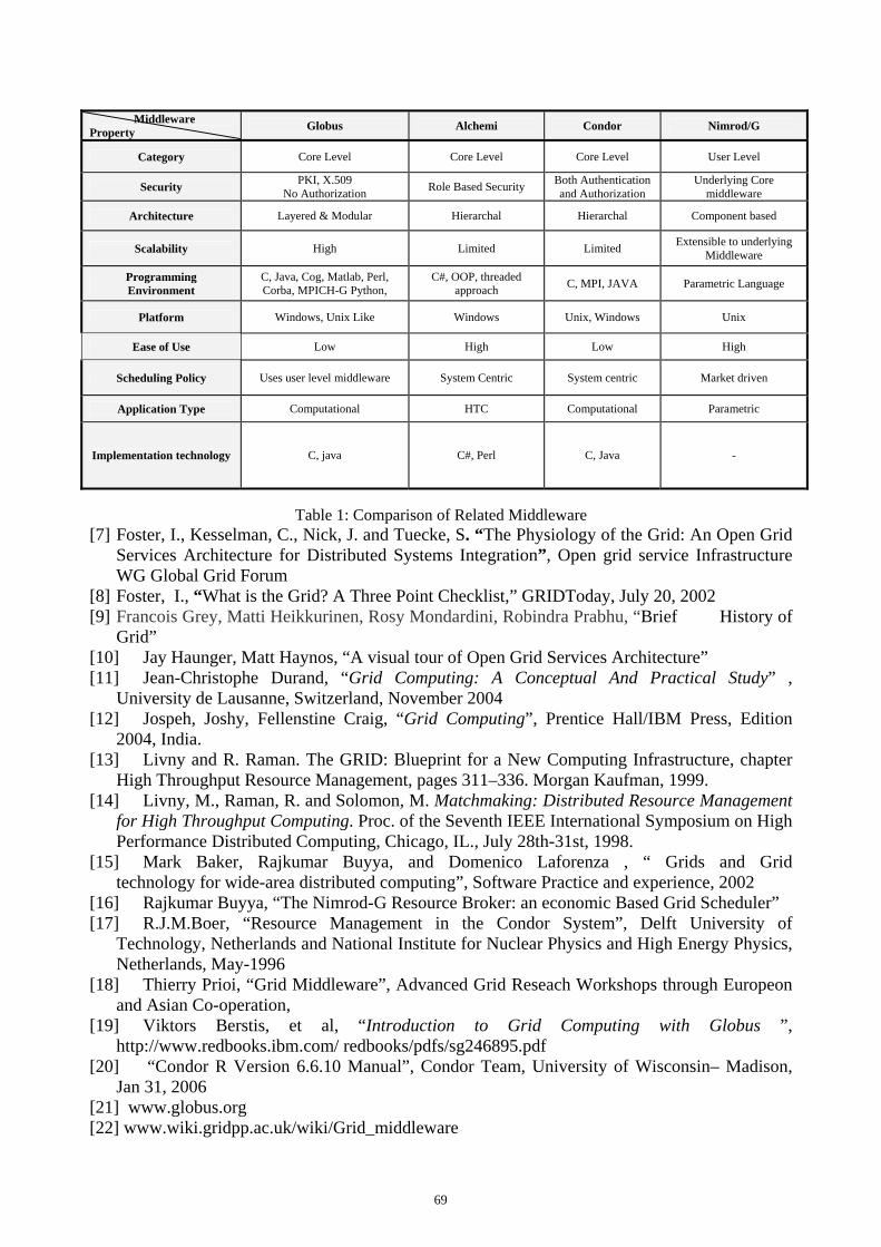
Middleware Property Globus Alchemi Condor Nimrod/G
Category Core Level Core Level Core Level User Level
Security PKI, X.509 No Authorization Role Based Security Both Authentication
and Authorization Underlying Core
middleware
Architecture Layered & Modular Hierarchal Hierarchal Component based
Scalability High Limited Limited Extensible to underlying Middleware
Programming Environment
C, Java, Cog, Matlab, Perl, Corba, MPICH-G Python,
C#, OOP, threaded approach C, MPI, JAVA Parametric Language
Platform Windows, Unix Like Windows Unix, Windows Unix
Ease of Use Low High Low High
Scheduling Policy Uses user level middleware System Centric System centric Market driven
Application Type Computational HTC Computational Parametric
Implementation technology C, java C#, Perl C, Java -
Table 1: Comparison of Related Middleware [7] Foster, I., Kesselman, C., Nick, J. and Tuecke, S. “The Physiology of the Grid: An Open Grid
Services Architecture for Distributed Systems Integration”, Open grid service Infrastructure WG Global Grid Forum
[8] Foster, I., “What is the Grid? A Three Point Checklist,” GRIDToday, July 20, 2002 [9] Francois Grey, Matti Heikkurinen, Rosy Mondardini, Robindra Prabhu, “Brief History of
Grid” [10] Jay Haunger, Matt Haynos, “A visual tour of Open Grid Services Architecture” [11] Jean-Christophe Durand, “Grid Computing: A Conceptual And Practical Study” ,
University de Lausanne, Switzerland, November 2004 [12] Jospeh, Joshy, Fellenstine Craig, “Grid Computing”, Prentice Hall/IBM Press, Edition
2004, India. [13] Livny and R. Raman. The GRID: Blueprint for a New Computing Infrastructure, chapter
High Throughput Resource Management, pages 311–336. Morgan Kaufman, 1999. [14] Livny, M., Raman, R. and Solomon, M. Matchmaking: Distributed Resource Management
for High Throughput Computing. Proc. of the Seventh IEEE International Symposium on High Performance Distributed Computing, Chicago, IL., July 28th-31st, 1998.
[15] Mark Baker, Rajkumar Buyya, and Domenico Laforenza , “ Grids and Grid technology for wide-area distributed computing”, Software Practice and experience, 2002
[16] Rajkumar Buyya, “The Nimrod-G Resource Broker: an economic Based Grid Scheduler” [17] R.J.M.Boer, “Resource Management in the Condor System”, Delft University of
Technology, Netherlands and National Institute for Nuclear Physics and High Energy Physics, Netherlands, May-1996
[18] Thierry Prioi, “Grid Middleware”, Advanced Grid Reseach Workshops through Europeon and Asian Co-operation,
[19] Viktors Berstis, et al, “Introduction to Grid Computing with Globus ”, http://www.redbooks.ibm.com/ redbooks/pdfs/sg246895.pdf
[20] “Condor R Version 6.6.10 Manual”, Condor Team, University of Wisconsin– Madison, Jan 31, 2006
[21] www.globus.org [22] www.wiki.gridpp.ac.uk/wiki/Grid_middleware
69

Proceedings of the International Conferenceon Computational and Mathematical Methodsin Science and Engineering, CMMSE 2007Chicago, 20–23 June 2007.
An Optimization Problem in Deregulated ElectricityMarkets solved with the Nonsmooth Maximum Principle
L. Bayon1, J.M. Grau1, M.M. Ruiz1 and P.M. Suarez1
1 Department of Mathematics, University of Oviedo, Spain
emails: [email protected], [email protected], [email protected], [email protected]
Abstract
In this paper, the new short-term problems that are faced by a generation com-pany in a deregulated electricity market are addressed and a optimization algorithmis proposed. Our model of the spot market explicitly represents the price of elec-tricity as an uncertain exogenous variable. We consider a very complex problemof hydrothermal optimization with pumped-storage plants, so the problem dealswith non-regular Lagrangian and non-holonomic inequality constraints. To obtaina necessary minimum condition, the problem was formulated within the frameworkof nonsmooth analysis using the generalized (or Clarke’s) gradient and the Nons-mooth Maximum Principle. The optimal control problem is solved by means of analgorithm implemented in the commercial software package Mathematica. Resultsof the application of the method to a numerical example are presented.
Key words: Nonsmooth Analysis, Control Problem, Electricity marketsMSC 2000: 49M20, 49J24, 91B24, 91B26
1 Introduction
Over the last decade, the electricity industry has experienced significant changes interms of deregulation and competition. In this paper, we focus on the problem that ageneration company faces when preparing its offers for the day-ahead market. Severalmethods have been proposed for simulating competitive generation markets. Most ofthese models [1] can be categorized into two major groups: models that represent all thegeneration companies and models that focus on a particular generation company. Twoapproaches can be adopted to represent spot market auctions when only one companyis considered: price modeled as an exogenous variable and price modeled as a functionof the demand supplied by the firm under study. In the former, the price of electricitydoes not depend on the company’s decisions. This can be acceptable if the company issmall enough. These models can again be classified into two sub-groups, depending onwhether they use a deterministic [2] or probabilistic [3] price representation.
70
In this paper, we only represent the operation of one company in detail, includ-ing each of the company’s generation units. Our model of the spot market explicitlyrepresents the price of electricity as an uncertain exogenous variable. We represent gen-eration units at a high level of detail and our model distinguishes individual generationunits and considers inter-temporal constraints such as hydro reserves. In addition, wealso consider pumped-storage hydro-plants.
The Spanish activity rules [4] have been used as a reference model for the market.The day-ahead market in the Spanish wholesale electricity market is organized as a setof twenty-four simultaneous hourly auctions. The simple bid format consists of a pairof (hourly) values: quantity q[MWh] and price p[euro/MWh]. The utility companythat inspires our paper, HC, controls approximately only 7% of all the electricity thatis generated. So, we consider our company as a price-taker, and under this assumption,the volatility of the spot market price of electricity is represented by a stochastic model.Price forecasting techniques in power systems are relatively recent procedures [5] [6].Although the problem of constructing the probability distribution exceeds the purposeof this paper, we suggest the following simplified approach based on [7]. The idea is tosearch for past spot market sessions that can be considered similar to the session thatthe company is about to face. To identify the days, we classify the entire collection ofsessions (using clustering techniques) according to the values of an explanatory variable.The most relevant information about the current session for our problem is the vectorof 24 prices that has resulted from the day-ahead market clearing. Once a groupof S similar days has been identified, the company can assume that the probabilitydistribution for the market session under study is completely defined by these pastS market sessions (probability distributions with finite support). If we now focus on aparticular auction, it is easy to understand that the S quantities and S prices decided bythe company for that hour constitute the offer curve (nondecreasing) that the companymust submit to that auction.
This paper addresses a very complex problem of hydrothermal optimization withpumped-storage plants. In this kind of problem (see the previous paper [8]), the La-grangian is piecewise continuous and we consider constraints for the admissible gen-erated power. Hence, this paper considers non-regular Lagrangian and non-holonomicinequality constraints (differential inclusions). To obtain a necessary minimum condi-tion, the problem is formulated within the framework of nonsmooth analysis [9] usingthe generalized (or Clarke’s) gradient and the Nonsmooth Maximum Principle. Thischaracteristic distinguishes our work from all the above.
2 Statement of the Problem
In this section the optimization problem of one company is described, the objectivefunction of which can be defined as its profit maximization. Let us assume that ourhydrothermal system accounts for n hydro-plants and m thermal plants: the (Hn−Tm)problem.
Let Ψi : Di ⊆ R+ −→ R+ (i = 1, . . . ,m) be the cost functions (euro/h) of the m
71

thermal plants. The most usual cost function of each generator can be represented asa quadratic function:
Ψi(Pi(t)) = αi + βiPi(t) + γiP2i (t); i = 1, ..., m
where Pi(MW ) is the power generated, and we consider the thermal plants to beconstrained by technical restrictions of the type
Pi min ≤ Pi(t) ≤ Pi max; i = 1, ..., m, ∀t ∈ [0, T ]
[0, T ] being the optimization interval. In prior studies [10], it was proven that theproblem with m thermal plants may be reduced to the study of a hydrothermal systemmade up of one single thermal plant, called the thermal equivalent : the (Hn − T1)problem. We shall denote as the equivalent minimizer of Ψim
1 , the function Ψ :D1 + · · ·+ Dm → R defined by
Ψ(P (t)) = minm∑
i=1
Ψi(Pi(t)); Pmin ≤ P (t) ≤ Pmax
with P (t) the power generated by said thermal equivalent.We assume that our system accounts for n hydro-plants that have a pumping
capacity. The mapping H : ΩH −→ R
H(t, z1(t), . . . , zi(t), . . . , zn(t), z1(t), . . . , zi(t), . . . , zn(t)) = H(t, z(t), z(t))
is called the function of effective hydraulic contribution and is the power contributedto the system at the instant t by the set of hydro-plants, zi(t) being the volume that isdischarged up to the instant t by the i-th hydro-plant, zi(t) the rate of water dischargeat the instant t by the i-th hydro-plant, and ΩH ⊂ [0, T ] × Rn × Rn the domain ofdefinition of H.
We say that z = (z1, . . . , zn) is admissible for H if zi belong to the class C1[0, T ](the set of piecewise C1 functions), and (t, z(t), z(t)) ∈ ΩH , ∀t ∈ [0, T ]. The volume bi
that must be discharged up to the instant T is called the admissible volume of the i-thhydro-plant. Let b = (b1, . . . , bn) ∈ Rn be the vector of admissible volumes. In a generalmodel, with hydraulic coupling between the n hydro-plants, we call Hi(t, zi(t), zi(t)) :ΩHi = [0, T ]×R×R −→ R the function of effective hydraulic contribution by the i-thhydro-plant, being
H(t, z(t), z(t)) =n∑
i=1
Hi(t, zi(t), zi(t))
Besides, we consider Hi(t, zi(t), zi(t)) to be bounded by technical constraints
Hi min ≤ Hi(t, zi(t), zi(t)) ≤ Hi max; i = 1, · · · , n, ∀t ∈ [0, T ]
Throughout the paper, no transmission losses will be considered; a crucial aspectwhen addressing the optimization problem from a centralized viewpoint. From theperspective of a generation company, and within the framework of the new electricity
72

market, said losses are not relevant, since the generators currently receive payment forall the energy they generate in power plant bars.
Let us assume that the cost function Ψ : R+ −→ R+ satisfies Ψ′(x) > 0, ∀x ∈ R+,i.e. it is strictly increasing. This constraint is absolutely natural: it reads more costto more generated power. Let us assume as well that Ψ′′(x) > 0, ∀x ∈ R+, i.e. it isstrictly convex. The models traditionally employed meet this constraint.
Let us assume that the function Hi is strictly increasing with respect to the rate ofwater discharge zi, i.e. ∂Hi/∂zi > 0 (more power to a higher rate of water discharge)and that [∂Hi/∂zi]zi=0 = 0. Let us also assume that ∂2Hi/∂z2
i < 0, i.e. Hi is concavewith respect to zi. The real models meet these three constraints. In addition, pumped-storage plants are considered, and in this kind of problem, the derivative of Hi withrespect to zi (∂Hi/∂zi) presents discontinuity at zi = 0, which is the border betweenthe power generation zone (positive values of zi) and the pumping zone (negative valuesof zi). In the real models, it is verified that H+
z ≤ H−z . In the (Hn − T1) problem, the
objective function is given by revenue minus cost during the optimization interval [0, T ]
F (P, z) =∫ T
0[p(t)(P (t) + H(t, z(t), z(t)))−Ψ(P (t))] dt
Revenue is obtained by multiplying the total production (thermal and hydraulic) of thecompany by the clearing price p(t) in each hour t. Cost is given by Ψ, the cost functionof the thermal equivalent, where P (t) is the power generated by said plant. With thisstatement, our objective functional in continuous time form is
maxP,z
F (P, z) = maxP,z
∫ T
0L(t, P (t), z(t), z(t))dt (2.1)
with L(t, P (t), z(t), z(t)) = p(t)(P (t) + H(t, z(t), z(t)))−Ψ(P (t)), on the set
Ω =
z ∈
(C1[0, T ]
)n|
zi(0) = 0, zi(T ) = bi
Hi min ≤ Hi(t, zi(t), zi(t)) ≤ Hi max, ∀t ∈ [0, T ]∀i = 1, . . . , n
(2.2)
3 The (H1 − T1) Problem
We begin the development in this section by presenting the simple problem with onepumped-storage hydro-plant (i = 1). In the (H1−T1) problem, we have z = z and ourobjective functional is
F (P, z) =∫ T
0L(t, P (t), z(t), z(t))dt
with L(t, P (t), z(t), z(t)) = p(t)(P (t) + H(t, z(t), z(t)))−Ψ(P (t)) on the set
Ω =
z ∈ C1[0, T ] | z(0) = 0, z(T ) = bHmin ≤ H(t, z(t), z(t)) ≤ Hmax, ∀t ∈ [0, T ]
73

where L(·, ·, ·, ·) and Lz(·, ·, ·, ·) are the class C0 and Lz(t, P, z, ·) is piecewise continuous(Lz(t, P, z, ·) is discontinuous in z = 0). The problem involves non-holonomic inequal-ity constraints (differential inclusions) and the previous assumptions guarantee that:Lzz(t, P, z, z) < 0; Lz(t, P, z, z) > 0. We also assume that
H(t, b, z(t)) ≤ H(t, z(t), z(t)) ≤ H(t, 0, z(t)), ∀z ∈ Ω
These suppositions are fulfilled in all real hydrothermal problems, and bearing in mindthe weak influence of z(t), (H(t, b, z) ' H(t, z, z) ' H(t, 0, z)), it is reasonable tosubstitute the restriction: Hmin ≤ H(t, z(t), z(t)) ≤ Hmax by others of the type: Hmin ≤H(t, b, z); H(t, 0, z) ≤ Hmax. Thus, it is reasonable to substitute Ω by
Ω∗ =
z ∈ C1[0, T ] | z(0) = 0, z(T ) = bHmin ≤ H(t, b, z); H(t, 0, z) ≤ Hmax, ∀t ∈ [0, T ]
The solution to the problem in Ω∗ will be very close to that obtained with the set Ω, theadvantage being that the mathematical treatment of sets of type Ω∗ is much simplerthan of those of type Ω. We shall focus in the present paper on the development ofthe applications of Optimal Control Theory (OCT) and nonsmooth analysis to thisproblem. Let us term as the coordination function of z ∈ Ω∗ the function in [0, T ],defined by:
Yz(t) = Lz(t, P (t), z(t), z(t))−∫ t
0Lz(s, P (s), z(s), z(s))ds
denoting by Y+z (t) and Y−z (t) the expressions obtained when considering the lateral
derivatives of L with respect to z. Let us now see the fundamental result, which is thebasis for elaborating the optimization algorithm. We present the problem consideringthe state variables to be z(t) and P (t) and the control variables u1(t) = z(t) andu2(t) = P (t). The optimal control problem is thus:
maxu1(t),u2(t)
∫ T
0L(t, P (t), z(t), u1(t))dt; with
z = u1; P = u2
z(0) = 0, z(T ) = b
u1(t) ∈ Θ = x | Hmin ≤ H(t, b, x);H(t, 0, x) ≤ Hmax ; u2(t) ∈ (−∞,∞)
We shall use the nonsmooth version of Pontryagin’s Minimum Principle (PMP) [9] asthe basis for proving this theorem.
Theorem 1 (Theorem of Coordination). If (z∗, P ∗) ∈ (C1, C1) is a solutionof our problem, then ∃K ∈ R+ such that:
i) If z∗(t) = 0 =⇒ Y+z∗(t) ≤ K ≤ Y−z∗(t)
ii) If z∗(t) 6= 0 =⇒ Yz∗(t) is
≥ K if H(t, b, z∗(t)) = Hmin
= K if Hmin < H(t, z∗(t), z∗(t)) < Hmax
≤ K if H(t, 0, z∗(t)) = Hmax
and Ψ (P ∗(t)) = p(t)
We shall call this relation
Lz(t, P (t), z(t), z(t))−∫ t
0Lz(s, P (s), z(s), z(s))ds = K ∈ R+, ∀t ∈ [0, T ] (3.1)
74

the coordination equation for z(t), and the positive constant K will be termed thecoordination constant of the extremal.
Note. It is very important to stress that the problem is thus easily broken downinto the two sub-problems: Thermal and Hydro. In the thermal sub-problem, the powerP (t) of the equivalent thermal plant is distributed (as we see in [10]) between the mthermal plants, and so is completely resolved. In the next section, we consider oncemore the general problem (Hn − T1) with n hydro-plants, which is the problem to besolved.
4 Generalization to the (Hn − T1) Problem.The Optimization Algorithm
In this section, we present an algorithm of the numerical resolution of the problem ofoptimization of a hydrothermal system that involves n hydro-plants. The associatedvariational problem is related to solving a boundary-value problem for a system ofdifferential equations. The algorithm uses a particular strategy related to the methodof cyclic coordinate descent (CCD). The CCD method minimizes a function cyclicallywith respect to the coordinate variables. With our method, a problem of the typeHn − T1 could be solved (under certain conditions) if we start out from the resolutionof a sequence of problems of the type H1−T1. The algorithm for the Hn−T1 problemcarries out several iterations and at each j-th iteration calculates n stages, one for eachhydro-plant. At each stage, it calculates the optimal functioning of a hydro-plant, whilethe behavior of the rest of the plants is assumed fixed. For every z = (z1, . . . , zn) ∈ Ω,we consider the functional F i
z defined by
F iz(P, vi) =
∫ T
0
[p(t)(P (t) + H i
z(t, vi(t), vi(t)))−Ψ(P (t))]dt
with H iz(t, vi, vi) = H(t, z1, . . . , zi−1, vi, zi+1, . . . , zn, z1, . . . , zi−1, vi, zi+1, . . . , zn)
where H iz represents the power generated by the hydraulic system as a function of
the rate of water discharge and the volume turbinated by the i-th plant, under theassumption that the rest of the plants behave in a definite way. We call the i-thminimizing mapping the mapping φi : Ω −→ Ω, defined in the following way: for everyz ∈ Ω
φi(P, z1, . . . , zi, . . . , zn) = (P ∗, z1, . . . , z∗i , . . . , zn)
where (P ∗, z∗i ) minimizes F iz. If we set Φ = (φn φn−1 · · · φ2 φ1) and
(P j , zj) = Φ(P j−1, zj−1)
beginning with some admissible (P 0, z0), we construct a sequence of (P j , zj) via suc-cessive applications of φin
i=1 and the algorithm will search
limj→∞
(P j , zj)
75

It is simple to justify the convergence of the algorithm in a finite number of steps,simply by considering the following solution set:
z | F (P, z)− F (Φ (P, z))< ε
Scenarios
l=1 l S=... ...
Hydro-plant 1
Hydro-plant i
Hydro-plant n
.
.
.
.
.
.
Converges?
Yes
No
j=1,.
..
Hydro-plant i
t=1
.
.
.
.
.
.
z T bK( )->
Yes
Solution H -T1 1
No
Sea
rch
ing
K t=t
t=24
Solution H -Tn 1
Converges?
Scenario l
F P z F P z( , )- ( ( , ))<F e
Fig. 1. The Optimization Algorithm.
The application of every φi involves solving a problem of the type (H1−T1). To obtainthe optimum operating conditions of the hydro-plant, we shall use the coordinationequation (3.1). To undertake the approximate calculation of the solution, expressed inTheorem 1, we use a similar numerical method to those used to solve differential equa-tions in combination with an appropriate adaptation of the classical shooting method.
Step 1) Approximate construction of zK (the adapted Euler method).The problem will consist in finding for each K the function zK that satisfies
zK(0) = 0, and the conditions of Theorem 1. From the computational point of view,the construction of zK can be performed with the use of a discretized version of Equa-tion (3.1). The approximate construction of each zK , which we shall call zK , is carriedout by means of polygonals (Euler’s method). In general, the construction of zK mustbe carried out by constructing and successively concatenating the extremal arcs andboundary arcs until completing the interval [0, T ].
Step 2) Construction of a sequence Kjj∈N such that zKj (T ) converges to b (theadapted shooting method).
76

Varying the coordination constant K, we would search for the extremal that fulfilsthe second boundary condition zK(T ) = b. The procedure is similar to the shootingmethod used to resolve a two-point boundary value problem (TPBVP). A number ofmethods exist for solving these problems, including shooting, collocation and finitedifference methods. Among the shooting methods, the Simple Shooting Method (SSM)and the Multiple Shooting Method (MSM) appear to be the most widely known andused methods. We implemented a SSM and obtained good results. Effectively, we mayconsider the function ϕ(K) := zK(T ) and calculate the root of ϕ(K) − b = 0, whichmay be realized approximately using elemental procedures. The secant method wasused in the present paper, and the algorithm shows a rapid convergence to the optimalsolution for a wide range of Kmin and Kmax.
5 Application to a Real Hydrothermal System
A computer program was written (using the Mathematica package) to apply the re-sults obtained in this paper to a real power system. As an example, we shall use thehydrothermal system that the electricity company HC has in Asturias (Spain), whichis made up of 2 classic thermal plants: Abono (with two groups of 360 and 543 ofpower (Mw) respectively) and Soto (with two groups of 254 and 350 of power (Mw)respectively) and 9 hydro-plants. For our optimization problem, we shall only use the 3variable-head (the generation is function of z and z) hydro-plants of the utility companyHC : Salime, Tanes (pumped-storage) and La Barca. We do not consider the remaininghydro-plants, because they are run-of-river type (without reservoir) and power gen-eration is not controllable. Let us see the models of different subsystems used in ourstudy. For the cost functions, we use a second-order polynomial
Ψi(Pi(t)) = αi + βiPi(t) + γiP2i (t)
The hydro-network has the three hydro-plants on different rivers, so the rate of dis-charge at the upstream plant does not affect the behaviour at the downstream plants:the hydraulic system has no hydraulic coupling. We use a variable head model and thei-th function of effective hydraulic generation Hi (for a conventional hydro-plant) isgiven by
Hi(t, zi(t), zi(t)) = Ai(t)zi(t)−Bizi(t)zi(t)− Ciz2i (t); zi(t) ≥ 0
where Ai(t), Bi and Ci are the coefficients
Ai(t) =1Gi
Byi(S0i + t · ii); Bi =Byi
Gi; Ci =
Bti
Gi
For the pumped-storage plant, Hi is defined piecewise, taking in the pumping zone(zi(t) < 0): M ·Hi(t, zi(t), zi(t)). The parameters that appear in this formula are: theefficiency G in (m4/h.Mw), the natural inflow i in (m3/h), the initial volume S0 in(106m3), and the coefficients By in (10−7m−2) and Bt in (10−5hm−2), parameters thatdepend on the geometry of the reservoir.
77

Let us consider the construction of the scenario structure for the day-ahead marketproblem faced by the company HC in the Spanish spot market. In particular, themarket session of February 15th 2006 is considered as the current session. The pastmarket sessions [4] that are considered relevant range from February 1st to February14th. Table I presents the results of the clustering analysis performed on this range ofdays. The classification provided by the S-means algorithm for S = 4 (four clusters) ispresented below.
Table I. Clustering Analysis.
Date 1 2 3 4 5 6 7 8 9 10 11 12 13 14 15Day W Th F Sa S M T W Th F Sa S M T W
Cluster 4 4 4 1 2 3 4 4 4 4 1 2 3 4 4
As can be seen, the four day types provided by the clustering analysis are quite rea-sonable: Cluster 1 and Cluster 2 corresponds to low-price days (Saturdays and Sun-days, respectively), Cluster 3 includes one type of weekday: Mondays, and Cluster 4comprises the other type of weekdays. This analysis suggests considering eight sce-narios (eight realizations) for the day-ahead market problem faced by the company onFebruary 15th. We consider short-term hydrothermal scheduling (24 hours) with anoptimization interval [0, 24] and we consider a discretization of 24 subintervals. Thetotal optimal hydro and thermal power generation for the company HC are shown inFigure 2-a and Figure 2-b respectively. The eight scenarios considered are presented inboth figures.
1 4 8 12 16 20 24
t (h)250
500
750
1000
1250
1500
P(Mw)
( )b
1 4 8 12 16 20 24
t (h)
- 50
50
100
150
200
250
P(Mw)
( )a
Fig. 2. (a) Optimal hydro-power. (b) Optimal thermal-power.
The solution yields the optimal offers that the company must submit to each of the day-ahead market auctions. Figure 3-a shows the offers corresponding to the 4th auctionfor the total optimal thermal-power, and for the eight possible realizations. The 8quantities and 8 prices for that hour constitute the offer curve (nondecreasing) that the
78

company must submit to that auction.
200 300 400 500 600
5.9
6.1
6.2
6.3
6.4
210 220 230 240
10.7
10.8
10.9
11.1
11.2
11.3
11.0
Energy (Mwh)
Price (€/Mwh)
6.0
( )a ( )b
Price (€/Mwh)
Energy (Mwh)
Fig. 3. (a) Thermal-offers. (b) Hydro-offers.
These results can be easily analyzed. Figure 3-a shows that the offer curve obtainedfor the 4th hourly auction is quite flat, thus making the company rather uncertainabout the amount of energy that it will finally sell. This is confirmed by Figure 2-b,in which the company’s eight possible levels of sales for the 4th hour are very different.However, it is not possible to construct an offer curve (nondecreasing) for the company’soptimal hydro-power. Figure 3-b shows the offers corresponding to the 12th auctionfor the total optimal hydro-power, and for the eight possible realizations. It is easy tounderstand that this behaviour is due to the inter-temporal constraints for the hydro-plants, besides the pumped-storage character of some of the hydro-plants (the optimalhydro-solution of one of the auctions influences the rest of the auctions). Therefore, wesuggest that the optimal offers that the company must submit, for the hydro-plants,must be a half value of the optimal hydro-power generation that we present in Figure2-a.
References
[1] M. Ventosa, A. Baıllo, M. Rivier and A. Ramos, Electricity Market Mod-eling Trends, Energy Policy 33(7) (2005) 897–913.
[2] G. Gross and D.J. Finlay, Optimal Bidding Strategies in Competitive Electric-ity Markets, Proc. 12th PSCC (1996) 815–823.
[3] J. Valenzuela and M. Mazumdar, Probabilistic Unit Commitment under aDeregulated Market, in: B. F. Hobbs, M. H. Rothkopf, R. P. O’Neill and H.-P.Chao, (Eds.), The Next Generation of Electric Power Unit Commitment Models,Kluwer Academic Publishers, Boston, (2001) 139–152.
[4] Companıa Operadora del Mercado Espanol de Electricidad, S.A. Electricity marketactivity rules. http://www.omel.es/es/pdfs/EMRules.pdf.
[5] A.J. Conejo, F.J. Nogales and J.M. Arroyo, Price-taker bidding strategyunder price uncertainty, IEEE Trans. Power Sys. 17(4) (2002) 1081–1088.
79

[6] A. Mateo, A. Munoz and J. Garcıa, Modeling and forecasting electricity priceswith input/output hidden Markov models, IEEE Trans. Power Sys. 20(1) (2005)13–24.
[7] A. Baıllo, M. Ventosa, A. Ramos and M. Rivier, Optimal offering strategiesfor generation companies operating in electricity spot markets, IEEE Trans. PowerSys. 19(2) (2004) 745–753.
[8] L. Bayon, J. Grau, M.M. Ruiz and P.M. Suarez, Nonsmooth Optimizationof Hydrothermal Problems, Journal of Computational and Applied Mathematics192(1) (2006) 11–19.
[9] F.H. Clarke, Optimization and Nonsmooth Analysis, SIAM, Philadelphia, 1990.
[10] L. Bayon, J. Grau, M.M. Ruiz and P.M. Suarez, New developments onequivalent thermal in hydrothermal optimization: an algorithm of approximation,Journal of Computational and Applied Mathematics 175(1) (2005) 63–75.
80

Proceedings of the International Conferenceon Computational and Mathematical Methodsin Science and Engineering, CMMSE 2007Chicago, 20–23 June 2007.
Carr’s randomization for American optionsin regime-switching models
Svetlana Boyarchenko1 and Sergei Levendorskii1
1 Department of Economics, The University of Texas at Austin
emails: [email protected], [email protected]
Abstract
In the paper, we solve the pricing problem for American options in Markov-modulated Levy models. The early exercise boundaries and prices are calculatedusing a generalization of Carr’s randomization for regime-switching models. An ef-ficient iteration pricing procedure is developed. The computational time is of orderm2, where m is the number of states, and of order m, if the parallel computationsare allowed. The payoffs, riskless rates and class of Levy processes may depend ona state. Special cases are stochastic volatility models and models with stochasticinterest rate; both must be modelled as finite-state Markov chains.
Key words: regime-switching, Levy processes, American options, stochastic in-terest rates, stochastic volatility
MSC 2000: AMS codes 60J75, 90 08, 91B28
1 Introduction
Different pricing problems in regime switching models were considered in a numberof papers. In the majority of publications, Markov-modulated (geometric) Brownianmotion models are studied. For closed form solutions for perpetual lookback options,see [11]. Perpetual American put in the geometric Brownian motion model coupledby a two-state Markov chain was studied in [13]. In [9], a pricing procedure for theAmerican put with finite time horizon was designed, for GBM modulated by a twostate chain, under assumption that the early exercise boundary in one state is belowthe early exercise boundary in the other state. For further references, see the op. cit.The results for switching models with jumps are scarce due to technical difficulties,although the literature on pricing of American options under processes with jumps isfairly extensive by now – see, e.g., [1]-[8], [14], [15] and the bibliography therein. In [2],the perpetual American put in regime-switching Levy models with phase-type jumps isstudied. The technique of the paper relies on the special elegant structure of this classof models and a simple explicit structure of the payoff function. It is not clear how to
81

generalize the technique of the cited paper for more general classes of payoff functionsand processes.
In [7], [8], closed form solutions for perpetual American and real options are ob-tained under uncertainty modelled as a monotone function of a process with i.i.d.increments. As an application of the technique, explicit recurrent formulas for Carr’srandomization under Levy processes are derived. These models of uncertainty exhibitmean-reverting and switching features, switches being endogenous in the sense thatthe characteristics of the price process change as the price arrives in another regionof the state space. In the paper, we extend the method of [5]-[8] coupling (monotonefunctions of) Levy processes by an exogenous finite-state Markov chain, and constructregime-switching models with both endogenous and exogenous switching. Note thatnot only the parameters of the process but the interest rate and payoff functions areallowed to depend on the state of the Markov chain. Thus, we allow for jumps in thepayoff, interest rate, volatility (and other parameters of the price process or the typeof the process), and jumps in the price process itself.
In the case of perpetual American options, the optimal exercise rules can be viewedas natural extensions of the record-setting news principles in [4] and universal bad newsprinciple in [8] to regime switching models; these principles are applied in each state ofthe Markov chain assuming that the value functions in all other states are given. Thenthe equation for the exercise boundary and explicit analytical expression for the valuefunction are as simple as in the no-regime-switching case. After that, we prove thatthe resulting system of equations for the exercise boundaries and option values in allstates can be easily solved using the iteration method. If the transition rates are small,iterations converge very fast. Finally, we prove that in the limit, the optimal exerciserule and option value obtain. In the case of American options with finite time horizon,we reduce to a sequence of perpetual American options. The solution of options in thesequence is similar to [5], [6], [7], [15] but simpler even for the non-switching case. Also,we improve the scheme in op.cit. allowing for time steps of varying sizes; in op.cit., thetime grid was equally spaced.
2 PRELIMINARIES
2.1 Levy processes and Expected Present Value operators
The moment generating function of a Levy process can be represented in the formE
[ezXt
]= etΨ(z); the function Ψ is called the Levy exponent. The latter naturally
appears when one calculates the action of the infinitesimal generator of Xt, denoted L,on exponential functions: Lezx = Ψ(z)ezx. As a basic example, we will use the processwhich appeared in [10] for the first time:
Ψ(z) =σ2
2z2 + bz +
c+z
λ+ − z+
c−z
λ− − z; (1)
the results are valid for Levy processes satisfying the (ACP)-property.
82

Let T ∼ Exp(q). Then
Ex[g(XT )] := qEx
[∫ +∞
0e−qtg(Xt)dt
].
Introduce the normalized resolvent or expected present value operator: EPV-operatorof a stochastic process X:
Eg(x) = qEx
[∫ +∞
0e−qtg(Xt)dt
].
This operator calculates the EPV of a stream qg(Xt). Applying E to g(x) = ezx andusing the equality E
[ezXt
]= etΨ(z), we obtain that E acts on exponential functions as
the multiplication operator by the number q(q−Ψ(z))−1. To ensure that the expectationis finite, it is necessary and sufficient that the real part of q − Ψ(z) is positive. Since(q − L)ezx = (q − Ψ(z))ezx, we conclude that q−1(q − L) and E are mutual inverses.To make this statement precise, we need to specify function spaces between whichq−1(q−L) and E act. We will also need the normalized EPV-operators of the supremumprocess Xt = sup0≤s≤t Xs and the infimum process Xt = inf0≤s≤t Xs. These EPV-operators act as follows:
E+g(x) := qEx
[∫ ∞
0e−qtg(Xt)dt
], E−g(x) := qEx
[∫ ∞
0e−qtg(Xt)dt
].
Evidently, E+g(x) = Ex[g(XT )] and E−g(x) = Ex[g(XT )], where T is the exponentialrandom variable introduced at the beginning of this subsection. It is straightforwardto check that E+ and E− also act on an exponential function ezx as multiplicationoperators by numbers, which we denote κ+(z) and κ−(z), respectively:
E+ezx = κ+(z)ezx, E−ezx = κ−(z)ezx. (2)
These numbers are κ+(z) = E[ezXT
], κ−(z) = E
[ezXT
]. Note that to simplify the
notation, we suppress the dependence of the EPV-operators E , E± and numbers κ±(z)on q (and on the process X).
2.2 Wiener-Hopf factorization
The Wiener-Hopf factorization formula reads:
E[ezXT ] = E[ezXT ]E[ezXT ], ∀ z ∈ iR.
Equivalently, ∀ z ∈ iRq/(q −Ψ(z)) = κ+(z)κ−(z). (3)
Applying E , E+ and E− to g(x) = ezx and using (2)-(3), we obtain the third version ofthe Wiener-Hopf factorization formula:
Eg(x) = E+E−g(x) = E−E+g(x). (4)
By linearity, (4) holds for linear combinations of exponents and integrals of exponents,hence for wide classes of functions. Equation (4) means that the normalized EPV-operator of a Levy process admits a factorization into a product of the normalizedEPV-operators of the supremum and infimum processes.
83
2.3 Example
For the Levy process with the characteristic exponent (1), the Wiener-Hopf factors are
κ+(z) =∏
l=1,2
β+l
β+l − z
, κ−(z) =∏
l=1,2
β−lβ−l − z
,
where β−2 < λ− < β−1 < 0 < β+1 < λ+ < β+
2 are the roots of the “characteristicequation” q −Ψ(β) = 0. EPV-operators acts as follows
E+u(x) =∑
l=1,2
a+l β+
l
∫ +∞
0e−β+
l yu(x + y)dy,
E−u(x) =∑
l=1,2
a−l (−β−l )∫ 0
−∞e−β−l yu(x + y)dy,
where a±1 , a±2 > 0 come from the decomposition of κ±(z) into the sum of simple frac-tions.
3 CARR’S RANDOMIZATION IN REGIME-SWITCHINGMODELS
Let λjk be the transition rate from state j to state k. The riskless rate in state j is qj .The infinitesimal generator of the driving Levy process X
(j)t in state j is denoted by
Lj , and the Levy exponent of the process X(j)t – by Ψj . We assume that a switch from
state j to state k and a jump of X(j)t do not happen simultaneously, a.s. However, we
may produce simultaneous switches and jumps playing with different payoff functionsin different states of the Markov chain.
Consider the American option with the payoff Gj(Xt) in state j and time horizon T .Here and below, we assume that an index j means that Xt evolves as X
(j)t−τj , where τ j is
the last moment of a switch to the state j, starting at the point, where switch happened.Assume that all functions Gj are continuous, non-increasing and change sign; then, atsufficiently low levels of the stochastic factor, in some states (possibly, not all), it maybe optimal to exercise the option. The standard example is Gj(x) = Kj −Bje
x, whereKj and Bj are positive. Kj can be interpreted as the strike price in state j, and Bk/Bj
as a jump factor in the stock price at a moment of a switch from state j to state k. Forsimplicity, we assume that if the discount rate q is sufficiently large, then each payoffGj(X
(j)j ) can be represented as the EPV of some stream:
Gj(x) = Exj
[∫ +∞
0e−qtgj(X
(j)t )dt
], (5)
where the function gj = gq,j is continuous, non-increasing, positive in a neighborhood of−∞, and changes sign. The subscript j in Ex
j means that the expectation is calculated
84

assuming that Xt will follow the Levy process X(j)t and there will be no switches. If
|Gj(x)| grows as x → ∞ then (5) imposes certain restrictions on the Levy exponentsΨj . For instance, if Gj and their derivatives G
(s)j , s ≤ 2, satisfy the bound
|g(x)| ≤ C(eσ−x + eσ+x), (6)
where σ− ≤ 0 ≤ σ+, then (5) can be satisfied with any q > maxΨj(σ−),Ψj(σ+)and gj = (q − Lj)Gj provided Ψj(z) are defined for z ∈ [σ−, σ+]. For each state j, theoption owner needs to find a stopping time τj ≤ T , which maximizes
Vj(t, x) = Ej,x
∫ τj
0e−(qj+Λj)t
∑
k 6=j
λjkVk(t,Xt)dt
+ Ej,x
[e−τj(qj+Λj)Gj(Xτj )+
].
to approximate the optimal stopping problem with finite time horizon by sequences ofoptimal stopping problems with infinite time horizon. A sequence of optimal stoppingproblems with infinite time horizon is determined by a partition 0 = t0 < t1 < · · · <tN = T of the interval [0, T ], and a “staircase” x = hs, ts < t ≤ ts+1, s = 0, 1, . . . , N−1,which approximates the early exercise boundary. In the regime-switching version, weneed to introduce a staircase for each state j: x = hs
j , ts < t ≤ ts+1, s = 0, 1, . . . , N − 1.In the case of put-like options, Gj are non-increasing functions, which change sign, andin Carr’s approximation, the option is exercised when the state j staircase is reachedor crossed from above, in state j; in the case of call-like options, Gj are non-decreasingfunctions, which change sign, and in Carr’s approximation, the option is exercised whenthe state j staircase is reached or crossed from below, in state j.
Let vsj (x) be the approximation to the option value Vj(ts, x) in state j, at time ts,
and set qsj = ∆−1
s + qj + Λj . Assume that the approximations vs+1i,∗ on the next time
step are known for all i, and, for a given j, the approximations vsk,∗, k 6= j, are known.
We assume that these functions are continuous and satisfy bound (6). For s = N ,vNj,∗(x) = Gj(x)+ are known and satisfy bound (6). We can interpret vs = (vs
j )mj=1 as
the value of the option to swap the stream (∆−1s vs+1
j,∗ (Xt))mj=1 for the instantaneous
payoff (Gj(Xt))mj=1; the value function, stream and payoff are functions on Rm, the
state space of the regime switching process Xt.For s = N − 1, N − 2, . . . , we need to choose a stopping time, τ s
j so that vsj (x) is
maximized, and we will show that τ sj is the hitting time of a semi-infinite interval of
the form (−∞, hsj ]. The corresponding free boundary problem is
(qsj − Lj)vs
j (x) = ∆−1s vs+1
j,∗ (x) +∑
k 6=j
λjkvsk,∗(x),
vsj (x) = Gj(x), (7)
for x > hsj and x ≤ hs
j , respectively. We replaced Gj(x)+ in (7) with Gj(x) becausethe stream ∆−1
s vs+1j,∗ (Xt) +
∑k 6=j λjkv
sk,∗(Xt) is non-negative, hence, it is non-optimal
to exercise the option unless Gj(Xτsj) > 0.
Note that we do not use a scheme which is implicit w.r.t. vsj but explicit w.r.t.
vsk, k 6= j, that is, the scheme with vs+1
k,∗ , k 6= j, in the RHS, because this scheme is less
85

accurate than the scheme which is implicit w.r.t. all vsj . However, the latter requires
more iterations. If the transition probabilities λjk are small, the number of iterationson each time step is small for both schemes.
3.1 Solution of the sequence of perpetual options
For each s = N − 1, N − 2, . . ., we find the set of optimal exercise boundaries hsjm
j=1
in three steps. First, we derive a system for the optimal exercise boundaries andoption values vs
jmj=1 assuming that the option values are sufficiently regular. Then
we construct an iteration procedure, which converges to a solution of this system. Weuse the procedure to prove that this solution is sufficiently regular, and that it givesoptimal exercise rules and option values. Finally, we prove that the solution is unique.
Introduce vsj = vs
j − Gj , vsk,∗ = vs
k,∗ − Gk, gj =∑
k 6=j λjkGk − (qj + Λj − Lj)Gj .Assume that functions Gj and their derivatives up to order 2 satisfy bound (6); thenfunctions gs
j = (qsj −Lj)Gj are well-defined. We choose ∆s sufficiently small so that qs
j
is sufficiently large in the sense that for j = 1, 2, . . . , m,
qsj −Ψj(σ) > 0, ∀ σ ∈ [σ−, σ+]. (8)
Using qsj and Lj in place of q and L, we define the EPV-operators Es
j , Es,−j , Es,+
j .
Theorem 3.1 Let the following conditions hold:
(i) ∆s and the Levy exponents Ψj satisfy (8);
(ii) gsj = (qs
j − Lj)Gj are non-decreasing functions that change sign, and Gj(+∞) =−∞;
(iii) gj are continuous non-decreasing functions, and gj(−∞) < 0;
(iv) for s = l + 1 and all k, functions vsk,∗ are known;
(v) for some j, functions vlk,∗ in states k 6= j are known.
Then for the same j and s = l,
a) function gsj =
∑k 6=j λjkv
sk,∗ + ∆−1
s vs+1j,∗ + gj is a non-decreasing continuous function
satisfying bound (6); in addition,
gsj (−∞) < 0 < gs
j (+∞) = +∞; (9)
b) function wsj := Es,+
j gsj is continuous. It increases and satisfies (9), therefore equation
wsj (h) = 0 has a unique solution, denote it hs
j,∗;
c) the hitting time of (−∞, hsj,∗], τ−(hs
j,∗), is a unique optimal stopping time;
d) Carr’s approximation to state-j option value is
vsj,∗ = (qs
j )−1Es,−
j 1(hsj,∗,+∞)w
sj + Gj ;
e) vsj,∗ = vs
j,∗ − Gj is a positive non-decreasing function that admits bound (6) andsatisfies vs
j,∗(+∞) = +∞; it vanishes below hsj,∗ and increases on [hs
j,∗,+∞).
86

3.2 Iteration procedure
For s = N , the state-j option value is known: vNj,∗(x) = Gj(x)+, and the state-j exercise
boundary hnj,∗ is a unique root of the equation Gj(h) = 0, j = 1, 2, . . . , m. In the
regime-switching version of Carr’s randomization procedure, we need to calculate the(approximations to the) exercise boundaries hs
j,∗ and option values vsj,∗, j = 1, 2, . . . , m,
for s = l < N , assuming that for l + 1 ≤ s ≤ N and j = 1, 2, . . . , m, hsj,∗ and vs
j,∗are known. In the non-switching case, we were able to derive explicit formulas for the(Carr’s approximations to the) exercise boundaries and option values on step s in termsof the option values on the previous step. Here, in the regime-switching case, we cannotderive explicit analytical formulas but we can design an efficient iteration procedureinstead. For each s = n − 1, n − 2, . . . and j = 1, 2, . . . , m, we construct sequenceshsn
j ∞n=0 and vsnj ∞n=0, such that the limits
hsj = lim
n→+∞hsnj , vs
j = limn→+∞ vsn
j (10)
are the optimal exercise boundary, hsj,∗, and option value, vs
j,∗ (in the switching analogof Carr’s randomization procedure, at time step s and in state j). Thus, for each s,we need to introduce an additional cycle in n; and inside the cycle in n, we will useadditional cycles in j = 1, 2, . . . , m.
Fix s < N . Below, we formulate the iteration procedure for wsj,∗, ws
j,∗, hsj,∗, vs
j,∗and vs
j,∗. Calculate
ws0j = −Es,+
j (qsj − Lj)Gj = qs
j (Es,−j )−1Gj ,
set vs0j = 0, hs0
j = +∞, j = 1, 2, . . . , m, and for n = 1, 2, . . . , define, step by step, in theinterior cycle in j = 1, 2, . . . , m,
(i) functions wsnj = wsn
j + ws0j , where
wsnj = Es,+
j
∑
k 6=j
λjkvs,n−1k + ∆−1
s vs+1j,∗
;
(ii) hsnj , a solution of the equation wsn
j (h) = 0;
(iii) functions
vsn0j = (qs
j )−1Es,−
j 1(−∞,hsnj ](−ws
j0),
vsn1j = (qs
j )−1Es,−
j 1(hsnj ,+∞)w
sij ,
vsnj = vsn
1j + vsn0j ,
vsnj = vsn
j −Gj .
Theorem 3.2 Let conditions (i)–(iii) of Theorem 3.1 hold. Then ∀ s = N − 1, N −2, . . ., j = 1, 2, . . . , m and n = 1, 2, . . .
87

Table 1: Parameters of the processes
m σ b c− λ− c+ λ+
1 0.25 -0.03 0.02 -5 0.015 102 0.15 -0.02 0.01 -4 0.01 123 0.2 -0.02 0.15 -4.5 0.1 13
a) wsnj is continuous increasing function that changes sign, hence, hsn
j is well-defined;
b) ws,n+1j > ws,n
j , hsnj < hs,n−1
j , and vsnj > vs,n−1
j on [hsnj , +∞);
c) vsnj (x) = 0, x ≤ hsn
j , and vsnj increases on [hsn
j , +∞);
d) sequences hskj +∞
k=1 and vskj +∞
k=1 are bounded from below and above, respectively;hence, there exist finite limits (10);
e) limits (10) are the optimal time-step-s-state-j exercise boundary, hsj,∗, and option
value, vsj,∗; the latter is positive;
f) function vsj,∗ = vs
j,∗−Gj is continuous; it satisfies (6), vanishes below hsj,∗, increases
on [hsj,∗,+∞), and vs
j,∗(+∞) = +∞.
3.3 Numerical example
The generator of the Markov chain is−0.03 0.01 0.020.015 −0.025 0.010.015 0.03 −0.045
.
In Table 1, we list parameters of processes in different states. Riskless rates: q1 =0.05, q2 = 0.055, q3 = 0.045; payoff functions: G1(x) = 2−ex, G2(x) = 2.5−2ex, G3(x) =3− 1.5ex. Numerical experiments demonstrate that the method is sufficiently accurateeven for a very long time interval τ = 50 with more than 150 time steps. In the examplebelow, we divided interval [0, 25] into 25 subintervals using the geometric progressionwith the first term 0.005, then we used the uniform spacing ∆s = ∆25 till t = 15, andafter that, the uniform spacing with ∆s = 2 ∗ ∆25 till t = 50.1186. Close to expiry,state-1 boundary seems lower than Figure 1 and Table 2 show because it drops downrather fast, and the part adjacent to 0 almost coincides with the vertical axis. hj,∗(0+)denote the limit of the early exercise boundary at expiry. The limits are calculatedusing the following theorem, which generalizes the result in [5], [15] for Levy processes.
Theorem 3.3 Let (j, x) be in the money region, that is, Gj(x) > 0, but
0 < (qj + Λj − Lj)(−Gj)(x) +∑
k 6=j
λjkGk(x)+
88

0 10 20 30 40 50
00.20.40.6
τ
h
(a) State−1 boundary
0 10 20 30 40 50−0.4
−0.2
0
0.2
τ
h
(b) State−2 boundary
0 10 20 30 40 500
0.20.40.6
τ
h
(c) State−3 boundary
Figure 1: Early exercise boundaries hj,∗(τ) for τ ≤ 50 to expiry. Parameters are inTable 1. Crosses: hj,∗(0). Dash-dotted lines: early exercise boundaries for the perpetualoption. Solid lines: early exercise boundaries.
+∫ +∞
−∞(−Gj(x + y))+Fj(dy). (11)
Then there exists τ0 = τ0(j, x) such that for each τ ∈ (0, τ0), it is not optimal to exercisethe option as XT−τ = (j, x).
Here Fj(dy) is the state-j Levy density. In our example, (11) has a unique solution, andit follows from Theorem 3.3, that this solution is not larger than the limit of the earlyexercise boundary at expiry. We cannot prove that it is the limit and not just an upperbound but the numerical results shown below support the claim that the solution isthe limit. In this example, hj,∗(0+) is strictly below hj,∗(0) for each j, which is causedby the interaction of three factors: the stock pays dividends because qj −Ψj(1) > 0 inthis example; each Levy process X
(j)t has the non-trivial positive jumps component; at
a moment of a jump, the payoff may jump up. We will analyze the interaction amongthese three factors in a separate publication.
89

4 Conclusion
In the paper, we derived the iteration procedure for the American put with finite thehorizon in Markov-modulated Levy models. The procedure does not use any aprioriassumption on the relative location of the early exercise boundaries in different states.The riskless rates, payoff functions and Levy processes depend on a state. Levy pro-cesses are assumed to satisfy the (ACP)-property, and payoff functions can be moregeneral than for the standard put and call options. The procedures are efficient if thetransition rates are not large w.r.t. the riskless rates. The CPU time is of order m2,where m is the number of states; if parallel computations are used, then the CPU timeis of order m. Numerical example show that the method is accurate for options ofdifferent maturities. Method can be applied to stochastic interest models and stochas-tic volatility models; both must be modelled as finite state Markov chains. Jumps atmoment of switching can be used to model a mean-reverting component of the priceprocess; this component may correlate with the stochastic interest rate and volatility.
The method of the paper admit extension in several directions: approximationof the standard stochastic interest rate/volatility models (with possible switching) bymodels constructed in the paper; credit risk models; optimal exercise with learning thecurrent state; real options, especially, with strategic interactions; and other.
Acknowledgements
This work has been partially supported by NSF grant #DMS-0631628.
References
[1] L. Alili and A. Kyprianou, Some remarks on first passage of Levy process,the American put and pasting principles, Annals of Applied Probability 15 (2005)2062–2080.
[2] S. Asmussen, F. Avram and M.R. Pistorius, Russian and American putoptions under exponential phase-type Levy models, Stochastic Processes and Ap-plications 109 (2004) 79–111.
[3] F. Avram, A. E. Kyprianou and M.R. Pistorius, Exit problems for spec-trally negative Levy processes and applications to (Canadized) Russian options,The Annals of Applied Probability 14 (2004) 215–238.
[4] S. I. Boyarchenko, Irreversible Decisions and Record-Setting News Principles,American Economic Review, 94 (2004) 557–568.
[5] S. I. Boyarchenko and S. Z. Levendorskii, Perpetual American Options un-der Levy Processes, SIAM Journal on Control and Optimization 40 (2002) 1663–1696.
90

[6] S. I. Boyarchenko and S. Z. Levendorskii, Non-Gaussian Merton-Black-Scholes theory, World Scientific, Singapore, 2002.
[7] S. I. Boyarchenko and S. Z. Levendorskii, American options: the EPV pric-ing model, Annals of Finance 1 (2005) 267–292.
[8] S. I. Boyarchenko and S. Z. Levendorskii, General Option Exercise Rules,with Applications to Embedded Options and Monopolistic Expansion, Contributionsto Theoretical Economics 6 (2006) Article 2
[9] J. Buffington and R.J. Elliott, American options with regime switching,International Journal of Theoretical and Applied Finance, 5 (2002) 497–514.
[10] D. Duffie, J. Pan and K. Singleton, Transform Analysis and Asset Pricingfor Affine Jump Diffusions, Econometrica 68 (2000) 1343–1376.
[11] X. Guo, An explicit solution to an optimal stopping problem with regime switch-ing, Journal of Applied Probability 38 (2001) 464–481.
[12] X. Guo, J. Miao and E. Morellec, Irreversible investment with regime shifts,Journal of Economic Theory 122 (2005) 37–59.
[13] X. Guo and Q. Zhang, Closed form solutions for perpetual American put optionswith regime switching, SIAM Journal of Applied Mathematics 64 (2004) 2034–2049.
[14] A.E. Kyprianou and M.R. Pistorius, Perpetual options and Canadizationthrough fluctuation theory, Annals of Applied Probability 13 (2003) 1077-1098.
[15] S. Z. Levendorskii, Pricing of the American put under Levy processes, Interna-tional Journal of Theoretical and Applied Finance 7 (2004) 303–336.
91

ANALYSIS OF THE PML METHOD APPLIED TO SCATTERING PROBLEMS ANDTHE COMPUTATION OF RESONANCES IN OPEN SYSTEMS.
JAMES H. BRAMBLE,JOSEPH E. PASCIAK, AND SEUNGIL KIM
Abstract: In this talk, I shall consider the application of the so-called perfectly matched layer(PML) to acoustic and electromagnetic scattering problems as well as discuss how PML can be usedto reformulate problems of computing resonances in open systems.
One of the main difficulty with the numerical approximation of scattering problems is that suchproblems are posed on unbounded domains with a boundary condition at infinity given by either theSommerfeld condition or, in the case of electromagnetics, the Silver-Muller condition. There arenumerous approaches for dealing with the boundary condition at infinity, e.g., truncating the domainand applying an approximate boundary condition, truncating the domain and using boundary inte-gral techniques, using infinite element techniques, or truncating the domain and using a ficticiousabsorbing boundary layer (PML). A discussion of these approaches can be found in [1, 2, 8, 9, 12]and the included references. Computational evidence suggests that the PML approach is competi-tive and effective. Moreover, it is simple to implement in any suitably general code developed forbounded domain computations.
For scattering problems, the PML method has a long history starting from papers by Berenger [1,2]. The original approach involed the introduction of additional variables so that the equations couldbe split in an appropriate way. Subsequently, PML formulations were developed which avoided thissplitting [6, 13]. Chew and Weedon [6] provided significant insight into the understanding of PMLby viewing the method as a complex coordinate shift.
One can view the PML process as two distinct steps. First, a PML problem is posed on the infi-nite domain whose solution coincides with that of the original problem on a finite domain (regionof interest) while decaying rapidly (exponentially) outside. It is this decay that allows one to trun-cate the problem to a bounded domain not much larger than the domain of interest and to applyany convenient boundary condition on the resulting ficticious boundary. Many authors have studiedapplications of PML showing the existence and uniqueness of solutions for the truncated problemand its exponential convergence to the infinite domain PML problem (on the region of interest)[5, 7, 10, 11]. However, existence and uniqueness results alone are not enough to guarantee stablenumerical approximation. In [4, 5], we show that under appropriate conditions on the PML param-eters, the PML method leads to continuous and discrete systems which satisfy inf-sup conditionswith uniform constants independent of the truncation domain size and mesh size. Such estimatesare necessary to conclude stable and convergent numerical approximation and will be presented inthis talk.
I will also consider the application of PML to the problem of computing resonances in opensystems, specifically, acoustic resonances. Resonances are related to improper eigenfunctions forthe Helmholtz operator satisfying an outgoing boundary condition. They are improper in the sensethat they grow exponentially at infinity. We shall see that the application of PML converts the reso-nance problem to a standard eigenvalue problem (still on an infinite domain). This new eigenvalue
1
92

2 JAMES H. BRAMBLE,JOSEPH E. PASCIAK, AND SEUNGIL KIM
problem involves an operator which resembles the original Helmholtz equation transformed by acomplex shift in coordinate system. Our goal will be to approximate the shifted operator first byreplacing the infinite domain by a finite (computational) domain with a convenient boundary con-dition and second by applying finite elements on the computational domain. I will give theoremswhich show that the first of these steps leads to eigenvalue convergence to the desired resonancevalues and are free from spirious computational eigenvalues provided that the size of computationaldomain is sufficiently large. The analysis of the second step is classical (see [3] and the includedreferences).
I will conclude the talk with numerical results for PML applied to scattering problems and theresonance problem. These results will show that PML leads to an effective solution technique forboth of these problems.
REFERENCES
[1] J.-P. Berenger. A perfectly matched layer for the absorption of electromagnetic waves.J. Comput. Phys.,114(2):185–200, 1994.
[2] J.-P. Berenger. Three-dimensional perfectly matched layer for the absorption of electromagnetic waves.J. Comput.Phys., 127(2):363–379, 1996.
[3] J. H. Bramble and J. E. Osborn. Rate of convergence estimates for nonselfadjoint eigenvalue approximations.Math.Comp., 27:525–549, 1973.
[4] J. H. Bramble and J. E. Pasciak. Analysis of a finite element PML approximation for the three dimensional time-harmonic Maxwell problem.Math. Comp. (to appear).
[5] J. H. Bramble and J. E. Pasciak. Analysis of a finite PML approximation for the three dimensional time-harmonicMaxwell and acoustic scattering problems.Math. Comp., 76(258):597–614, 2007.
[6] W. Chew and W. Weedon. A 3d perfectly matched medium for modified Maxwell’s equations with streched coordi-nates.Microwave Opt. Techno. Lett., 13(7):599–604, 1994.
[7] F. Collino and P. Monk. The perfectly matched layer in curvilinear coordinates.SIAM J. Sci. Comp., 19(6):2061–2090, 1998.
[8] M. Grote and J. Keller. Nonreflecting boundary conditions for Maxwell equations.J. Comput. Phys., 139:327–342,1998.
[9] F. Ihlenburg. Finite element analysis of acoustic scattering, volume 132 ofApplied Mathematical Sciences.Springer-Verlag, New York, 1998.
[10] M. Lassas and E. Somersalo. On the existence and convergence of the solution of PML equations.Computing,60(3):229–241, 1998.
[11] M. Lassas and E. Somersalo. Analysis of the PML equations in general convex geometry.Proc. Roy. Soc. EdinburghSect. A, 131(5):1183–1207, 2001.
[12] P. Monk. A finite element method for aproximating the time-harmonic Maxwell equations.Numer. Math., 63:243–261, 1992.
[13] Z. Sacks, D. Kingsland, R. Lee, and J. Lee. A perfectly matched anisotropic absorber for use as an absorbingboundary condition.IEEE Trans. Antennas Propagat., 43:1460–1464.
DEPARTMENT OFMATHEMATICS, TEXAS A&M U NIVERSITY, COLLEGE STATION , TX 77843-3368.E-mail address: [email protected]
DEPARTMENT OFMATHEMATICS, TEXAS A&M U NIVERSITY, COLLEGE STATION , TX 77843-3368.E-mail address: [email protected]
DEPARTMENT OFMATHEMATICS, TEXAS A&M U NIVERSITY, COLLEGE STATION , TX 77843-3368.E-mail address: sgkim @math.tamu.edu
93

Proceedings of the International Conference on Computational and Mathematical Methods in Science and Engineering, CMMSE2007 Chicago, 20-23 June 2007
The Jordan Form and Its Use in Chemical Physics and Physical Chemistry
Erkki J. Brändas
Department of Quantum Chemistry, Uppsala University, Uppsala, Sweden
email: [email protected]
Abstract
We derive and discuss a general complex symmetric form of the most general Jordan block representation and propose various examples in physics and chemistry where this extension appears necessary. Key words: complex symmetry, Jordan blocks, ODLRO off-diagonal long-range order, special- and general relativity MSC2000: 83-A05
1. Introduction The query whether Jordan blocks of Segrè characteristics larger than one should appear in normal Jordan form representations of extended quantum dynamical formulations has been perceived many times in the past decades, see e.g. [1,2] and references therein. The question has to be elucidated a bit further. Jordan block representations of nilpotent operators are of course commonly used in quantum mechanics e.g. step operators in angular momentum algebra as well as annihilation and creation operators in second quantization. Here we focus on a different theme. The Hamiltonian, or Liouvillian, of a dynamical system generally serves two purposes: they represent a measurable observable, the energy, and simultaneously they generate the time evolution of the system. In standard quantum mechanics the Hamiltonian-Liouvillian is by definition self-adjoint yielding real eigenvalues (with the Segrè characteristic equal to one) and unitary time evolution, see e.g. [3]. Within this framework it is clear that no Jordan blocks could or should come into view. However, original advances in non-selfadjoint extensions of Hamiltonian/Liouvillian dynamics, [4,5] calls for the immediate incorporation of general classical canonical forms of the Jordan type [1,6]. In these extended applications, the possible occurrence of degeneracies, with Segrè characteristics larger than one, would result in an unwanted
94

CMMSE 2007
computational breakdown - usually considered as a numerical accident brought forward by the self-orthogonality of the transformed vectors. In the next section we will take into account the form of a complex symmetric representation, which is commensurate with the non-self-adjoint extensions mentioned above. We will suggest some examples in chemistry and physics where the spectral map promotes Jordan block formations. In the final section the group theoretical structure of the transformations indicating further interesting organizations within a biological frame will be presented.
2. The complex symmetric form of the Jordan block Since complex symmetric representations are routine in the majority of non-selfadjoint quantum treatments, e.g. complex scaling applications [4], it is important to know that a complex symmetric matrix invokes no constraint on the general secular problem. Gantmacher [7] proved that every square matrix is similar to a symmetric matrix and that every symmetric matrix is orthogonally similar to an explicitly given normal form. The author has for many years considered situations in which particular complex symmetric forms have been employed, see e.g. Ref. [8]. Particular applications concern proton transfer processes and dynamics and quantum correlations in condensed matter systems, see e.g. Refs. [1,9]. The specific symmetric matrix of dimension m derived and used, see Refs. [1, 6] has a very simple and useful structure defined by
Q
Qkl = (δkl −1m
) ei πm
(k + l−2); k, l =1,2,..m (1)
In other words one can prove that Q = B−1JB (2) with J defined as
J =
0 1 0 . 00 0 1 . .. . . . 0. . . . 10 . . . 0
⎛
⎝
⎜ ⎜ ⎜ ⎜ ⎜ ⎜
⎞
⎠
⎟ ⎟ ⎟ ⎟ ⎟ ⎟
(3)
and where the unitary matrix that connects the standard Jordan form J with Q becomes
B
95

CMMSE 2007
B =1m
1 ω ω 2 . ω m−1
1 ω 3 ω 6 . ω 3(m−1)
. . . . .
. . . . .1 ω 2m−1 ω 2(2m−1) . ω (m−1)(2m−1)
⎛
⎝
⎜ ⎜ ⎜ ⎜ ⎜ ⎜
⎞
⎠
⎟ ⎟ ⎟ ⎟ ⎟ ⎟
; ω = eiπm (4)
The form can be generalized to various powers Qr, i.e.
Qklr = ωr (k+ l−2)[δkl − (Rr )kl ]; k,l = 1,2,..m (5)
(R r )kl =
1m
sin( πr(l−k )m )
sin( π (l−k )m )
k ≠ l
rm k = l
⎧
⎨ ⎪ ⎪
⎩ ⎪ ⎪
(6)
3. The group structure – an example To see how the transformation above lends itself to an interesting structure we consider again the transformation formula Eq. (1-4) above. Not only does the unitary transformation B show that a complex symmetric matrix is similar to a real matrix that display the standard Jordan form, but it does further exhibit interesting properties as a simple example will demonstrate. First we introduce a simple notation that will display the cyclic structure incorporated in B. Let us e.g. denote the simple column (ω, ω3, ω5, ····,ω2−1)† , for an arbitrary n, with the symbol (n)† where n≤m. Choosing m=12 we can write for √12 B the symbolic form
1( )1( )1( )1( )1( )1( )1( )1( )1( )1( )1( )1( )
12
⎛
⎝
⎜ ⎜ ⎜ ⎜ ⎜ ⎜ ⎜ ⎜ ⎜ ⎜ ⎜ ⎜ ⎜ ⎜ ⎜ ⎜
⎞
⎠
⎟ ⎟ ⎟ ⎟ ⎟ ⎟ ⎟ ⎟ ⎟ ⎟ ⎟ ⎟ ⎟ ⎟ ⎟ ⎟
6
⎛
⎝
⎜ ⎜ ⎜ ⎜ ⎜ ⎜ ⎜
⎞
⎠
⎟ ⎟ ⎟ ⎟ ⎟ ⎟ ⎟
6
⎛
⎝
⎜ ⎜ ⎜ ⎜ ⎜ ⎜ ⎜
⎞
⎠
⎟ ⎟ ⎟ ⎟ ⎟ ⎟ ⎟
4⎛
⎝
⎜ ⎜ ⎜ ⎜
⎞
⎠
⎟ ⎟ ⎟ ⎟
4⎛
⎝
⎜ ⎜ ⎜ ⎜
⎞
⎠
⎟ ⎟ ⎟ ⎟
4⎛
⎝
⎜ ⎜ ⎜ ⎜
⎞
⎠
⎟ ⎟ ⎟ ⎟
3⎛
⎝
⎜ ⎜ ⎜
⎞
⎠
⎟ ⎟ ⎟
3⎛
⎝
⎜ ⎜ ⎜
⎞
⎠
⎟ ⎟ ⎟
3⎛
⎝
⎜ ⎜ ⎜
⎞
⎠
⎟ ⎟ ⎟
3⎛
⎝
⎜ ⎜ ⎜
⎞
⎠
⎟ ⎟ ⎟
12
⎛
⎝
⎜ ⎜ ⎜ ⎜ ⎜ ⎜ ⎜ ⎜ ⎜ ⎜ ⎜ ⎜ ⎜ ⎜ ⎜ ⎜
⎞
⎠
⎟ ⎟ ⎟ ⎟ ⎟ ⎟ ⎟ ⎟ ⎟ ⎟ ⎟ ⎟ ⎟ ⎟ ⎟ ⎟
2⎛
⎝ ⎜
⎞
⎠ ⎟
2⎛
⎝ ⎜
⎞
⎠ ⎟
2⎛
⎝ ⎜
⎞
⎠ ⎟
2⎛
⎝ ⎜
⎞
⎠ ⎟
2⎛
⎝ ⎜
⎞
⎠ ⎟
2⎛
⎝ ⎜
⎞
⎠ ⎟
12
⎛
⎝
⎜ ⎜ ⎜ ⎜ ⎜ ⎜ ⎜ ⎜ ⎜ ⎜ ⎜ ⎜ ⎜ ⎜ ⎜ ⎜
⎞
⎠
⎟ ⎟ ⎟ ⎟ ⎟ ⎟ ⎟ ⎟ ⎟ ⎟ ⎟ ⎟ ⎟ ⎟ ⎟ ⎟
3⎛
⎝
⎜ ⎜ ⎜
⎞
⎠
⎟ ⎟ ⎟
3⎛
⎝
⎜ ⎜ ⎜
⎞
⎠
⎟ ⎟ ⎟
3⎛
⎝
⎜ ⎜ ⎜
⎞
⎠
⎟ ⎟ ⎟
3⎛
⎝
⎜ ⎜ ⎜
⎞
⎠
⎟ ⎟ ⎟
4⎛
⎝
⎜ ⎜ ⎜ ⎜
⎞
⎠
⎟ ⎟ ⎟ ⎟
4⎛
⎝
⎜ ⎜ ⎜ ⎜
⎞
⎠
⎟ ⎟ ⎟ ⎟
4⎛
⎝
⎜ ⎜ ⎜ ⎜
⎞
⎠
⎟ ⎟ ⎟ ⎟
6
⎛
⎝
⎜ ⎜ ⎜ ⎜ ⎜ ⎜ ⎜
⎞
⎠
⎟ ⎟ ⎟ ⎟ ⎟ ⎟ ⎟
6
⎛
⎝
⎜ ⎜ ⎜ ⎜ ⎜ ⎜ ⎜
⎞
⎠
⎟ ⎟ ⎟ ⎟ ⎟ ⎟ ⎟
12
⎛
⎝
⎜ ⎜ ⎜ ⎜ ⎜ ⎜ ⎜ ⎜ ⎜ ⎜ ⎜ ⎜ ⎜ ⎜ ⎜ ⎜
⎞
⎠
⎟ ⎟ ⎟ ⎟ ⎟ ⎟ ⎟ ⎟ ⎟ ⎟ ⎟ ⎟ ⎟ ⎟ ⎟ ⎟
(7)
96

CMMSE 2007
or simply
( )( )( )( )( )( )( )( )( )( )( )( )
⎛
⎝
⎜ ⎜ ⎜ ⎜ ⎜ ⎜ ⎜ ⎜ ⎜ ⎜ ⎜ ⎜ ⎜ ⎜ ⎜ ⎜
⎞
⎠
⎟ ⎟ ⎟ ⎟ ⎟ ⎟ ⎟ ⎟ ⎟ ⎟ ⎟ ⎟ ⎟ ⎟ ⎟ ⎟
⎛
⎝
⎜ ⎜ ⎜ ⎜ ⎜ ⎜ ⎜
⎞
⎠
⎟ ⎟ ⎟ ⎟ ⎟ ⎟ ⎟
⎛
⎝
⎜ ⎜ ⎜ ⎜ ⎜ ⎜ ⎜
⎞
⎠
⎟ ⎟ ⎟ ⎟ ⎟ ⎟ ⎟
⎛
⎝
⎜ ⎜ ⎜ ⎜
⎞
⎠
⎟ ⎟ ⎟ ⎟
⎛
⎝
⎜ ⎜ ⎜ ⎜
⎞
⎠
⎟ ⎟ ⎟ ⎟
⎛
⎝
⎜ ⎜ ⎜ ⎜
⎞
⎠
⎟ ⎟ ⎟ ⎟
⎛
⎝
⎜ ⎜ ⎜
⎞
⎠
⎟ ⎟ ⎟
⎛
⎝
⎜ ⎜ ⎜
⎞
⎠
⎟ ⎟ ⎟
⎛
⎝
⎜ ⎜ ⎜
⎞
⎠
⎟ ⎟ ⎟
⎛
⎝
⎜ ⎜ ⎜
⎞
⎠
⎟ ⎟ ⎟
⎛
⎝
⎜ ⎜ ⎜ ⎜ ⎜ ⎜ ⎜ ⎜ ⎜ ⎜ ⎜ ⎜ ⎜ ⎜ ⎜ ⎜
⎞
⎠
⎟ ⎟ ⎟ ⎟ ⎟ ⎟ ⎟ ⎟ ⎟ ⎟ ⎟ ⎟ ⎟ ⎟ ⎟ ⎟
⎛
⎝ ⎜
⎞
⎠ ⎟
⎛
⎝ ⎜
⎞
⎠ ⎟
⎛
⎝ ⎜
⎞
⎠ ⎟
⎛
⎝ ⎜
⎞
⎠ ⎟
⎛
⎝ ⎜
⎞
⎠ ⎟
⎛
⎝ ⎜
⎞
⎠ ⎟
⎛
⎝
⎜ ⎜ ⎜ ⎜ ⎜ ⎜ ⎜ ⎜ ⎜ ⎜ ⎜ ⎜ ⎜ ⎜ ⎜ ⎜
⎞
⎠
⎟ ⎟ ⎟ ⎟ ⎟ ⎟ ⎟ ⎟ ⎟ ⎟ ⎟ ⎟ ⎟ ⎟ ⎟ ⎟
⎛
⎝
⎜ ⎜ ⎜
⎞
⎠
⎟ ⎟ ⎟
⎛
⎝
⎜ ⎜ ⎜
⎞
⎠
⎟ ⎟ ⎟
⎛
⎝
⎜ ⎜ ⎜
⎞
⎠
⎟ ⎟ ⎟
⎛
⎝
⎜ ⎜ ⎜
⎞
⎠
⎟ ⎟ ⎟
⎛
⎝
⎜ ⎜ ⎜ ⎜
⎞
⎠
⎟ ⎟ ⎟ ⎟
⎛
⎝
⎜ ⎜ ⎜ ⎜
⎞
⎠
⎟ ⎟ ⎟ ⎟
⎛
⎝
⎜ ⎜ ⎜ ⎜
⎞
⎠
⎟ ⎟ ⎟ ⎟
⎛
⎝
⎜ ⎜ ⎜ ⎜ ⎜ ⎜ ⎜
⎞
⎠
⎟ ⎟ ⎟ ⎟ ⎟ ⎟ ⎟
⎛
⎝
⎜ ⎜ ⎜ ⎜ ⎜ ⎜ ⎜
⎞
⎠
⎟ ⎟ ⎟ ⎟ ⎟ ⎟ ⎟
⎛
⎝
⎜ ⎜ ⎜ ⎜ ⎜ ⎜ ⎜ ⎜ ⎜ ⎜ ⎜ ⎜ ⎜ ⎜ ⎜ ⎜
⎞
⎠
⎟ ⎟ ⎟ ⎟ ⎟ ⎟ ⎟ ⎟ ⎟ ⎟ ⎟ ⎟ ⎟ ⎟ ⎟ ⎟
(8)
Note that the columns (2, 12), (3, 11), (4, 10), (5,9), and (6.8) are related by the operation of multiplying the complex conjugate with a minus sign. The 2-cycle is here simply (i,-i). In general this relation is connected with the columns s, for 1<s≤n/2, and n+2-s. The 2-cycle is always (i,-i) if n is even. The rows have a similar symmetry, i.e. for m=12 the rows (1,12), (2,11), (3,9)…. (6,7) are complex conjugate of each other or generally row s, for 1<s≤n/2, and n+1-s are complex conjugate of each other. For m odd the middle cycle is (1,-1). One might speculate what would be the consequence for the appearance of a large prime number m=p occurring above, since the only “repetitive vector” would be in the middle containing sub-blocks of (1,-1). The present structure suggests tempting interpretations in the biological field, e.g. proton correlations in DNA, the origin of the screw like symmetry of the double helix and possible long term correlations of the smallest microscopic self-organizing units co-operating in vivo systems, see e.g. Ref. [10] for some more detailed suggestions and associated time evolutionary consequences. It is indeed an invigorating feature that Jordan blocks appear as fundamental units in an extended quantum description that also incorporates characteristics of the special and general theories of relativity [11].
Acknowledgements The author is indebted to Prof. Bruce Wade and Prof. Jésus Vigo-Aguiar for generous support and hospitality. Supported in part by the Swedish Foundation for Strategic Research.
References [1] E. BRÄNDAS, Resonances and Dilatation Analyticity in Liouville Space,
97
CMMSE 2007
Adv. Chem. Phys. 99 (1997) 211-244. [2] A. BOHM, M. GADELLA, M. LOEVE, S. MAXON, P. PATULEANU,
C. PUNTMANN, Gamow-Jordan Vectors and Nonreducible Density Operators from Higher Order S-Matrix Poles, J. Math. Phys. 38 (1997) 6072-6100.
[3] P. O. LÖWDIN, Linear Algebra for Quantum Theory, Wiley, New York, 1998. [4] E. BALSLEV, J. M. COMBES, Spectral properties of many-body Schrödinger operators with dilatation-analytic interactions, Commun. Math. Phys. 22 (1971) 280-294. [5] A. BOHM, M. GADELLA, Dirac Kets, Gamow vectors and Gel´fand Triplets, Springer Verlag, Berlin, 1989. [6] C.E. REID, E. BRÄNDAS, On a Theorem for Complex Symmetric Matrices and its Relevance in the Study of Decay Phenomena, Lecture Notes in Physics, 325 (1989) 476-483. [7] F. R. GANTMACHER, The theory of matrices, Vol II, Chelsea Publishing Company, New York, 1959. [8] E. BRÄNDAS, Relaxation Processes and Coherent Dissipative Structures,
in Dynamics during Spectroscopic Transitions. Eds E. Lippert and J. D. Macomber, Springer Verlag, (1995) 148-193.
[9] E. BRÄNDAS, Applications of CSM Theory, in Dynamics during Spectroscopic Transitions. Eds E. Lippert and J. D. Macomber, Springer Verlag, (1995) 194-241.
[10] E. BRÄNDAS, Dissipative Systems and Microscopic Selforganisation, Adv. Quant. Chem. 41 (2002) 121-138. [11] E. BRÄNDAS, Quantum Mechaanics and the Special- and General Theory of Relativity, Adv. Quant. Chem. 54 (2007) in press.
98

Valuation of guaranteed annuity optionsin affine term structure models
Chi Chiu Chu and Yue Kuen Kwok
Department of Mathematics, Hong Kong University of Science and TechnologyClear Water Bay, Hong Kong
Abstract
We propose three analytic approximation methods for numerical valuation of the guar-anteed annuity options in deferred annuity pension policies. The approximation methodsinclude stochastic duration approach, Edgeworth expansion and analytic approximationin affine diffusions. The payoff structure in the annuity policies is similar to a quanto calloption written on a coupon bearing bond. To circumvent the limitations of the one-factorinterest rate model, we model the interest rate dynamics by a two-factor affine interestrate term structure model. The numerical accuracy and computational efficiency of theseapproximation methods are analyzed. We also investigate the value sensitivity of theguaranteed annuity option with respect to different parameters in the pricing model.
JEL classification: G13; G23
Keywords: Guaranteed annuity option, affine term structure models, coupon-bond options,stochastic duration, Edgeworth approximation, affine approximation
1. IntroductionA guaranteed annuity option (GAO) provides the policyholder the right to either receiveat retirement an assured accumulated funds or a life annuity at a fixed rate. This is oneof the many examples of minimum return guarantees (embedded options) in life insurancepolicies. Pension-type policies with GAO’s were popular in UK retirement saving contractsin the 1970’s and 1980’s. Between 1975 and 1985, UK interest rates were at a high level(typically above 10%). It was then generally perceived that the GAO’s have insignificantvalue since these options are deeply out-of-the-money. However, for pension-type contractshaving a long term, which may last for 30 years or more, the change in financial and othervariables may cause the embedded GAO to become an uncontrollable liability. There area number of factors that contribute to the acute increase in the value of these GAO’s.First, the current UK interest rates stay at lower level so that the annuity value becomeshigher. Second, the accumulated equity value of these contracts may increase substantiallywith a strong return in the stock market. Third, the improvement of mortality compared
Corresponding author. Tel: 852-2358-7418; fax: 852-2358-1643. E-mail address:[email protected]
1
99

to the anticipated mortality assumption when these contracts were written. Due to thesignificant increase in liabilities in these pension-type contracts, Equitable Life (a leadingUK insurance firm) had to close for new business. Detailed accounts of the issues faced bythe issuance of GAO’s can be found in the review articles by O’Brien (2001) and Wilkieet al . (2004).
There have been numerous works on the pricing and hedging of GAO’s using theoption valuation approach. Boyle and Hardy (2003) provide an insightful review on theissues of pricing, reserving and hedging GAO’s under interest rate risk, equity risk andmortality risk. Pelsser (2003) shows how to construct a replicating portfolio of interest rateswaptions that replicates the GAO. The swaption is seen to mimick the type of interestrate exposure faced by the GAO issuer. However, his swaption replication technique stillfaces problems with the equity risk and mortality risk. When the equity return increases,the hedger has to acquire more swaptions for hedging.
The payoff structure of the GAO resembles a quanto call option written on a coupon-bearing bond. The “quanto” feature appears since the payoff is in units of “stock” (likeunits of foreign currency) rather than in cash. The moneyness of the option is entirelydependent on the interest rate risk. Ballotta and Haberman (2003a) apply the one-factorHo-Lee model and Vasicek model to price GAO in unit-linked deferred annuity contractsthat are purchased on the grant date by a single premium [with later extension to includestochastic mortality effects (Ballotta and Haberman (2003b))]. However, an one-factorinterest rate model would implicitly imply that all future interest rates are perfectly corre-lated. Since pension policies are long term contracts, it is generally known in the literaturethat a two-factor interest rate model performs much better in hedging long-term interestrate derivatives.
In this paper, we employ a two-factor interest rate model of the affine class (Dai andSingleton, 2000) to characterize the stochastic interest rate movement. Similar to Ballotta-Haberman framework (2003a), we do not incorporate the insurance company expenses,tax effects and pre-retirement death benefits into our model. Also, the mortality risk isassumed to be unsystematic and independent of the equity and interest rate risks. Underthe simplicity of the one-factor interest rate model, Ballotta and Haberman (2003a) are ableto apply the decomposition technique of Jamshidian (1989) on pricing options on coupon-bearing bonds, thanks to the observation that the annuity option payoff can be written asthe payoff generated by a portfolio of zero-coupon bond options with appropriate strikeprices. However, since the interest rates become correlated under the two-factor interestrate model, the Jamshidian decomposition technique cannot be applied.
There will be no closed form analytic price formula for the GAO when the interestrate dynamics is modeled by a two-factor interest rate model. However, several analyticapproximation methods are known in the literature for pricing bond options or swaptionsunder multi-factor affine interest rate models. One method uses a single zero-coupon bondas a proxy for the original coupon-bearing bond. The approximation error is minimized
2
100

by choosing the maturity of the zero-coupon bond equal to the stochastic duration (Coxet al ., 1979; Wei, 1997) of the coupon-bearing bond. Another method makes use of theEdgeworth approximation of the probability distribution of the value of the coupon-bearingbond (Collin-Dufresne and Goldstein, 2002). The third method approximates the condi-tional distributions of the risk factors in affine diffusions. The exercise probability of theannuity option is approximated through an approximation of the exercise region. This isachieved by the linearization of the exercise region, whose boundary is approximated bya hyperplane. One then compute the relevant probabilities needed for pricing options oncoupon-bearing bonds by the same numerical method used in the pricing of options onzero-coupon bonds (Singleton and Umantsev, 2002). We adopt and modify these analyticapproximation methods for numerical valuation of the GAO in deferred annuity pensionpolicies. The numerical accuracy and computational efficiency of these approximationschemes are compared, and the impact of different parameter values in the pricing modelon the GAO value are investigated.
The paper is organized as follows. In the next section, we present the model setupof the GAO and the formulation of the multi-factor affine interest rate model. Nice ana-lytic tractability of the affine term structure model for finding present values of annuitypayments are demonstrated. In Section 3, we discuss the method of minimum varianceduration. The GAO is priced under the measure associated with the numeraire that isrelated to the annuity payment paid at τ -period after retirement. A judicious analyticapproximation is made in the expectation calculations so that closed form formula can beobtained. The pricing error between the exact and approximate solutions is minimized bychoosing τ such that the variance of the value of the future stream of annuity paymentsnormalized by the price of the τ -maturity bond is minimized. In Section 4, we illustratehow to perform the Edgeworth expansion of the distribution of the annuity value at thematurity of the policy. Under the affine diffusion assumption, the bond prices are expo-nential affine functions of the risk factors. The moments of the annuity value are alsoexponential affine so that the coefficients can be solved through the solution of a systemof Ricatti equations. In Section 5, we apply the affine approximation approach to thevaluation of GAO. Section 6 reports the numerical experiments that were performed tocompare the numerical accuracy and computational efficiency of the minimum varianceduration approach, Edgeworth series approximation and affine approximation. Pricingbehaviors of the GAO are also examined. The last section summarizes and concludes themain results of the paper.
2. Model setup of the guaranteed annuity optionThe payoff structure of a guaranteed annuity option (GAO) is similar to a call option ona coupon bond, where the “coupons” are the future stream of annuity payments and the“maturity of the bond” is related to the mortality of the policyholder. Besides the interestrate risk as in usual options on a coupon bond, the GAO also has exposure in equity riskand mortality risk. The equity risk arises since the payoff is in units of stock rather than
3
101

in cash so that the payoff is essentially in the form of a quanto option (the equity riskin GAO resembles the exchange rate risk in quanto option). For the mortality risk, weassume that it is independent of the financial risk so that it is diversifiable. It is quiteacceptable to use deterministic mortality for valuing options dependent on death of thepolicyholder (Boyle and Hardy, 2003).
We consider a single premium equity-linked policy whose policy’s maturity date isT . The maturity date T coincides with the retirement age R of the policyholder. Thepremium is invested in equity whose value St is assumed to follow a Geometric Brownianprocess. We let aR(t) denote the market value at time t of a life annuity of one dollar perannum starting at age R. Let npR denote the probability that a person aged R survivesn years and DT+n(t) denote the market value of the unit par default free zero-couponbond at time t with maturity date T + n. Also, we let ω denote the maximum age in themortality table. By constructing a portfolio of default free bonds that match exactly withthe expected cash flows of the annuity, the value of annuity aR(T ) is given by
aR(T ) =ω−R−1∑
n=0
npRDT+n(T ) = 1 +ω−R−1∑
n=1
npRDT+n(T ), (2.1)
since 0pR = DT (T ) = 1. Provided that the policyholder survives to maturity T , he either
receives ST orST
gaR(T ) at T , whichever has a high value. Here, g is called the guaranteed
conversion rate (say, g = 9). When the policyholder exercises the GAO, the equity fundST is used to purchase an annuity of ST /g. The value of the GAO at maturity T is thengiven by
terminal value of GAO =ST
g(aR(T ) − g)+, (2.2)
where x+ = max(x, 0). By assuming deterministic mortality rates, the payoff of the form(aR(T )− g)+ resembles an option on a coupon bond with strike g and coupon payment ofamount npR at time T + n, n = 0, 1, · · ·. The factor ST /g behaves like the exchange ratefactor in a quanto option. The GAO has two types of financial risk exposure: interest raterisk and equity risk.
When the interest rate dynamics is modeled by an one-factor short rate model, it isrelatively straightforward to obtain closed form formula for the GAO using the Jamshidiandecomposition technique for coupon bearing bond (Boyle and Hardy, 2003; Ballotta andHaberman, 2003a). Unfortunately, the one-factor assumption of the short rate wouldimply full correlation of all future interest rates. Such feature invites criticism when theone-factor short rate model is employed to price long term interest rate derivatives. In thispaper, we use the multi-factor affine term structure framework to model the interest ratederivatives. The affine framework has become more popular due to its analytic tractability
4
102
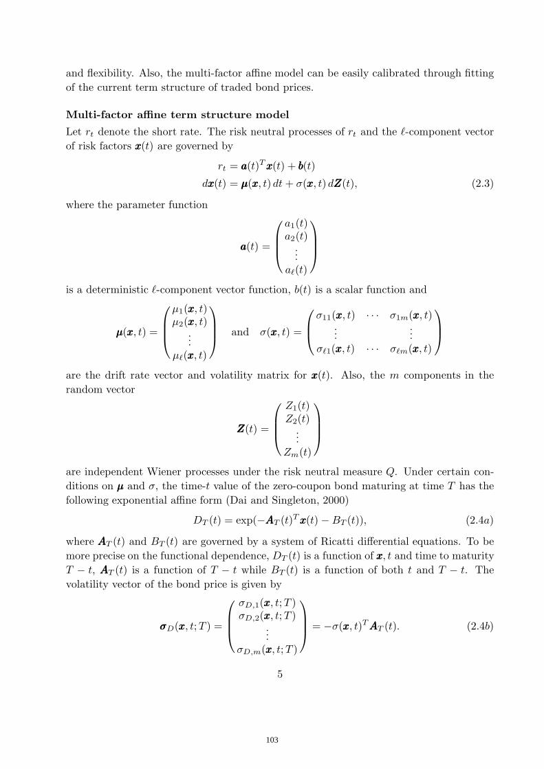
and flexibility. Also, the multi-factor affine model can be easily calibrated through fittingof the current term structure of traded bond prices.
Multi-factor affine term structure model
Let rt denote the short rate. The risk neutral processes of rt and the -component vectorof risk factors xxx(t) are governed by
rt = aaa(t)T xxx(t) + bbb(t)
dxxx(t) = µµµ(xxx, t)dt + σ(xxx, t)dZZZ(t), (2.3)
where the parameter function
aaa(t) =
⎛
⎜
⎜
⎝
a1(t)a2(t)
...a(t)
⎞
⎟
⎟
⎠
is a deterministic -component vector function, b(t) is a scalar function and
µµµ(xxx, t) =
⎛
⎜
⎜
⎝
µ1(xxx, t)µ2(xxx, t)
...µ(xxx, t)
⎞
⎟
⎟
⎠
and σ(xxx, t) =
⎛
⎜
⎝
σ11(xxx, t) · · · σ1m(xxx, t)...
...σ1(xxx, t) · · · σm(xxx, t)
⎞
⎟
⎠
are the drift rate vector and volatility matrix for xxx(t). Also, the m components in therandom vector
ZZZ(t) =
⎛
⎜
⎜
⎝
Z1(t)Z2(t)
...Zm(t)
⎞
⎟
⎟
⎠
are independent Wiener processes under the risk neutral measure Q. Under certain con-ditions on µµµ and σ, the time-t value of the zero-coupon bond maturing at time T has thefollowing exponential affine form (Dai and Singleton, 2000)
DT (t) = exp(−AAAT (t)T xxx(t) − BT (t)), (2.4a)
where AAAT (t) and BT (t) are governed by a system of Ricatti differential equations. To bemore precise on the functional dependence, DT (t) is a function of xxx, t and time to maturityT − t, AAAT (t) is a function of T − t while BT (t) is a function of both t and T − t. Thevolatility vector of the bond price is given by
σσσD(xxx, t;T ) =
⎛
⎜
⎜
⎝
σD,1(xxx, t;T )σD,2(xxx, t;T )
...σD,m(xxx, t;T )
⎞
⎟
⎟
⎠
= −σ(xxx, t)T AAAT (t). (2.4b)
5
103

For the equity fund, its time-t value under the risk neutral measure Q is modeled by
dSt
St= (r − q)dt + σσσS(t)T dZZZ, (2.5)
where q is the constant dividend yield and σσσS(t)T = (σS,1(t) σS,2(t) · · · σS,m(t)) is thevector of equity volatilities.
Risk neutral valuation of GAO value
Under the risk neutral measure Q, the time-t value V (S,xxx, t) of the GAO is given by therisk neutral expectation of the payoff at time T times the probability of survival of thepolicyholder over the next T − t years. The probability of survival is given by T−tpR−(T−t)
since the policyholder reaches age R in T − t years later. We assume that the companyhas well diversified the sale of annuity products so that the mortality risk can be taken tobe independent of the financial risk under the risk neutral measure Q. Given the terminalpayoff defined in Eq. (2.2), we then have
V (S,xxx, t) = T−tpR−(T−t)EQ
[
e−∫ T
tru du ST
g(aR(T ) − g)+
]
= T−tpR−(T−t)
EQ
[
e−∫ T
tru du ST
g
ω−R−1∑
n=1
npRDT+n(t)1aR(T )>g
]
−(
1 − 1g
)
EQ
[
e−∫
T
tru du
ST1aR(T )>g
]
. (2.6)
It will be illustrated that the above expectation calculations can be simplified by themethod of change of numeraire.
Let Fn(S,xxx, t) denote the time-t value of a security that pays ST DT+n(T ) at time T
so that Fn(S,xxx, t)/g gives the time-t value of the annuity payment at time T +n. By usingthe equity fund value St as the numeraire, we obtain
Fn(S,xxx, t) = EQ
[
e−∫
T
tru du
STDT+n(T )]
= Ste−q(T−t)EQS [DT+n(T )], (2.7)
where QS is the measure associated with the numeraire St. In a similar manner, theexpectation of the second term in Eq. (2.6) can be expressed as
EQ
[
e−∫ T
tru du
ST1aR(T )>g
]
= Ste−q(T−t)EQS
[
1aR(T )>g]
= Ste−q(T−t)PQS [aR(T ) > g], (2.8)
6
104

where PQS [A] denotes the probability of event A occurring under the measure QS . Tocompute the expectation of the first term in Eq. (2.6), it is more appropriate to chooseFn(S,xxx, t), n = 1, 2, · · · , ω − R, as the numeraire. Let QFn denote the measure associatedwith the numeraire Fn. We then have
EQ
[
e−∫
T
tru du ST
g
ω−R−1∑
n=1
npRDT+n(T )1aR(T )>g
]
=ω−R−1∑
n=1
npR
gFn(S,xxx, t)PQFn
[aR(T ) > g]. (2.9)
In our subsequent discussion, we limit the multi-factor affine term structure modelto the Gaussian type model, where the volatility matrix σ(xxx, t) defined in Eq. (2.3) is afunction of t only. For a Gaussian type model, the bond price volatility vector becomes
σσσD(t;T ) = −σ(t)T AAAT (t).
Stochastic differential equations
Under the risk neutral measure Q, the stochastic differential equation (SDE) of DT (t) isgiven by
dDT (t)DT (t)
= rt dt + σσσD(t;T )T dZZZ.
Using the Girsanov Theorem, the SDE of DT (t) under the measure QS is given by
dDT (t)DT (t)
= [rt + σσσD(t;T )T σσσS(t)] dt + σσσD(t;T )T dZZZQS , (2.10)
where ZZZQS is a vector of Brownian processes under QS . The SDE of Fn(S,xxx, t) under therisk neutral measure Q is given by
dFn
Fn= rt dt + [σσσS(t) + σσσD(t;T + n) − σσσD(t;T )]T dZZZ
= rt dt +
σσσS(t) + σ(t)T [AAAT (t) −AAAT+n(t)]T
dZZZ. (2.11)
Next, we would like to solve for Fn(S,xxx, t). We consider lnDT+n(t)DT (t)
, whose dynamics
under QS is given by
d
(
lnDT+n(t)DT (t)
)
7
105

=
σσσS(t)T [σσσD(t;T + n) − σσσD(t, T )] − 12(
‖σσσD(t;T + n)‖2 − ‖σσσD(t;T )‖2)
dt
+ [σσσD(t;T + n) − σσσD(t;T )]T dZZZQS
=
[σσσS(t) − σσσD(t;T )]T [σσσD(t;T + n) − σσσD(t;T )] − 12‖σσσD(t;T + n) − σσσD(t;T )‖2
dt
+ [σσσD(t;T + n) − σσσD(t;T )]T dZZZQS . (2.12)
The solution to Fn(S,xxx, t) is readily found to be
Fn(S,xxx, t) =DT+n(t)DT (t)
Ste−q(T−t)
exp
(
∫ T
t
[σσσS(u) − σσσD(u;T )]T [σσσD(u;T + n) − σσσD(u;T )] du
)
. (2.13)
Lastly, the SDE of xxx under QFn can be deduced to be
dxxx = µµµ(xxx, t) + σ(t) [σσσS(t) + σσσD(t;T + n) − σσσD(t;T )] dt + σ(t)dZZZQFn
=
µµµ(xxx, t) + σ(t)σσσS(t) + σ(t)σ(t)T [AAAT (t) −AAAT+n(t)]
dt + σ(t)dZZZQFn, (2.14)
where ZZZQFnis a vector of Brownian processes under the measure QFn .
Under the Gaussian type affine term structure model, the bond prices are lognormallydistributed [see Eq. (2.4a,b)]. Since the future annuity payment stream can be visualizedas a portfolio of discount bonds and the density of the sum of lognormal distributions hasno closed form representation, so there is no closed form analytic solution to the GAOvalue under the multi-factor affine term structure model. In the next three sections, weexplore three different analytic methods for finding approximate solution to V (S,xxx, t).
3. Method of minimum variance durationWe adopt the idea of minimum variance duration similar to that proposed by Munk (1999).The minimum variance duration approach has been shown to give highly accurate approx-imation solution to an option on coupon bearing bond under the multi-factor interest ratemodel. The minimum variance duration may be considered as an extension of the conceptof stochastic duration. Recall that the stochastic duration of a coupon bearing bond in amulti-factor diffusion model is defined to be the time to maturity of the zero-coupon bondwith the same relative volatility as that of the coupon bearing bond (Wei, 1997).
The solution of the GAO value may be sought by pricing under the measure associatedwith the numeraire corresponding to the security that pays ST aR(T ) at T . However,the pricing under such measure is not analytically tractable. Instead, we consider analternative numeraire that corresponds to the security that pays ST DT+τ (T ) at maturitytime T . Here, τ represents the time to maturity of the underlying bond at time T . Later,
8
106

we illustrate how to choose the parameter τ such that the error in the approximate solutionis minimized in some sense. Let Fτ (S,xxx, t) denote the time-t value of such security andQFτ denote the pricing measure when Fτ (S,xxx, t) is used as the numeraire. Under QFτ , thetime-t value of the GAO is given by [see Eqs. (2.6) and (2.9)]
V (S,xxx, t) = T−tpR−(T−t)EQ
[
e−∫ T
tru du
ST
(
aR(T )g
− 1)+]
= T−tpR−(T−t)Fτ (S,xxx, t)EQFτ
[
(
aR(T )gDT+τ(T )
− 1DT+τ(T )
)+]
. (3.1)
Nice analytic tractability can be achieved if we setaR(T )
gDT+τ (T )be some constant K. Here,
K is judiciously chosen to be the mean ofaR(T )
gDT+τ(T )under QFτ . The analytic approximate
solution to V (S,xxx, t) is taken to be
Va(S,xxx, t) = T−tpR−(T−t)Fτ (S,xxx, t)EQFτ
[
(
K − 1DT+τ (T )
)+]
, (3.2a)
where
K = EQFτ
[
aR(T )gDT+τ(T )
]
. (3.2b)
The remaining procedures include (i) the derivation of closed form analytic expression forVa(S,xxx, t), (ii) the determination of the parameter τ such that the pricing error |V (S,xxx, t)−Va(S,xxx, t)| is minimized based on the minimization of variance.
Approximate price formula
First, K can be readily found to be
K =1g
ω−R−1∑
n=0
npREQFτ
[
DT+n(T )DT+τ (T )
]
=1g
Ste−q(T−t)
Fτ (S,xxx, t)
ω−R−1∑
n=0
npREQS [DT+n(T )]
=1
gFτ (S,xxx, t)
ω−R−1∑
n=0
npRFn(S,xxx, t). (3.3)
Next, the expectation in Eq. (3.2a) is found to be
EQFτ
[
(
K − 1DT+τ (T )
)+]
= KPQFτ
[
DT+τ(T ) >1K
]
− Ste−q(T−t)
Fτ (S,xxx, t)PQS
[
DT+τ (T ) >1K
]
. (3.4)
9
107

By combining Eqs. (3.3) and (3.4) together, we obtain
Va(S,xxx, t) = T−tpR−(T−t)
ω−R−1∑
n=0
npRFn(S,xxx, t)g
PQFτ
[
DT+τ (T ) >1K
]
− Ste−q(T−t)PQS
[
DT+τ (T ) >1K
]
. (3.5)
Similar to Eq. (2.11), the dynamics of lnDT+τ (t)DT (t)
under QFτ is found to be
d
(
lnDT+τ (t)DT (t)
)
=
[σσσS(t) − σσσD(t;T )]T [σσσD(t;T + τ ) − σσσD(t;T )]
+12‖σσσD(t;T + τ )− σσσD(t;T )‖2
dt
+ [σσσD(t;T + τ ) − σσσD(t;T )]T dZZZQFτ. (3.6)
The mean of lnDT+τ(T ) under QFτ and QS are obtained as follows:
EQFτ[lnDT+τ (T )] = c(τ ) +
v2(τ )2
+ ln[
DT+τ (t)DT (t)
]
(3.7a)
EQS [ln DT+τ (T )] = c(τ ) − v2(τ )2
+ ln[
DT+τ(t)DT (t)
]
, (3.7b)
where
c(τ ) =∫ T
t
[σσσS(u) − σσσD(u;T )]T [σσσD(u;T + τ ) − σσσD(u;T )] du
v2(τ ) = var [lnDT+τ(T )] =∫ T
t
‖σσσD(u;T + τ ) − σσσD(u;T )‖2 du.
Also, we may express Fn(S,xxx, t) and K in the following forms:
Fn(S,xxx, t) =DT+n(t)St
DT (t)e−q(T−t)+c(n)
K =e−c(τ)
gDT+τ(t)
ω−R−1∑
n=0
npRDT+n(t)ec(n) =e−c(τ)
gDT+τ (t)aR(t).
Here, the quantity
aR(t) =ω−R−1∑
n=0
npRDT+n(t)ec(n)
10
108
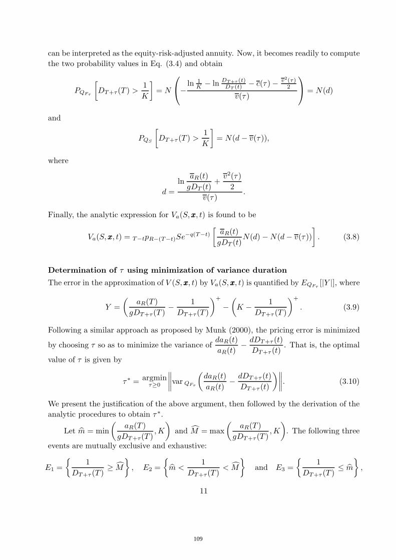
can be interpreted as the equity-risk-adjusted annuity. Now, it becomes readily to computethe two probability values in Eq. (3.4) and obtain
PQFτ
[
DT+τ(T ) >1K
]
= N
⎛
⎝−ln 1
K − ln DT+τ (t)DT (t) − c(τ ) − v2(τ)
2
v(τ )
⎞
⎠ = N(d)
and
PQS
[
DT+τ(T ) >1K
]
= N(d − v(τ )),
where
d =ln
aR(t)gDT (t)
+v2(τ )
2v(τ )
.
Finally, the analytic expression for Va(S,xxx, t) is found to be
Va(S,xxx, t) = T−tpR−(T−t)Se−q(T−t)
[
aR(t)gDT (t)
N(d) − N(d − v(τ ))]
. (3.8)
Determination of τ using minimization of variance duration
The error in the approximation of V (S,xxx, t) by Va(S,xxx, t) is quantified by EQFτ[|Y |], where
Y =(
aR(T )gDT+τ(T )
− 1DT+τ(T )
)+
−(
K − 1DT+τ (T )
)+
. (3.9)
Following a similar approach as proposed by Munk (2000), the pricing error is minimized
by choosing τ so as to minimize the variance ofdaR(t)aR(t)
− dDT+τ (t)DT+τ (t)
. That is, the optimal
value of τ is given by
τ ∗ = argminτ≥0
∥
∥
∥
∥
var QFτ
(
daR(t)aR(t)
− dDT+τ (t)DT+τ (t)
)∥
∥
∥
∥
. (3.10)
We present the justification of the above argument, then followed by the derivation of theanalytic procedures to obtain τ ∗.
Let m = min(
aR(T )gDT+τ(T )
,K
)
and M = max(
aR(T )gDT+τ(T )
,K
)
. The following three
events are mutually exclusive and exhaustive:
E1 =
1DT+τ (T )
≥ M
, E2 =
m <1
DT+τ(T )< M
and E3 =
1DT+τ (T )
≤ m
,
11
109

and from which we deduce that
EQFτ[|Y |] = EQFτ
[
|Y |1E1
]
+ EQFτ
[
|Y |1E2
]
+ EQFτ
[
|Y |1E3
]
.
Each of the above expectation calculations is analyzed below.
(i) EQFτ
[
|Y |1E1
]
= 0 since Y becomes zero when E1 occurs.
(ii) EQFτ
[
|Y |1E2
]
≤ EQFτ[|Y |]PQFτ
[E2]1/2 and PQFτ[E2] has a smaller value when
aR(T )gDT+τ(T )
stays closer to its mean K. This occurs when var QFτ
(
aR(T )gDT+τ(T )
)
is
minimized.
(iii)EQFτ
[
|Y |1E3
]
= EQFτ
[∣
∣
∣
∣
aR(T )gDT+τ(T )
− K
∣
∣
∣
∣
1E3
]
≤
EQFτ
[
(
aR(T )gDT+τ(T )
− K
)2]
PQFτ[E3]
1/2
=
var QFτ
(
aR(T )gDT+τ(T )
)
PQFτ[E3]1/2
.
Therefore, one can minimize the pricing error by minimizing var QFτ
(
aR(T )gDT+τ(T )
)
over
the choice of τ . However, the minimization procedure appears to be intractable dueto the complex expressions for aR(T ) and DT+τ(T ). Instead, we attempt to minimize
the relative change of value inaR(T )
DT+τ(T ), which can be measured by the variance of
daR(t)aR(t)
− dDT+τ (t)DT+τ (t)
.
Under the risk neutral measure Q, the dynamics of aR(t) and DT+τ (t) are given by
daR(t)aR(t)
= rt dt + σσσa(t;T )T dZZZ
dDT+τ(t)DT+τ(t)
= rt dt + σσσD(t;T + τ )T dZZZ,
where the volatility vector of annuity σσσa is given by
σσσa(t;T ) =ω−R−1∑
n=0
npRDT+n(t)aR(t)
σσσD(t;T + n).
For an one-factor interest rate model, it is readily seen that the solution to τ ∗ defined inEq. (3.10) is given by
σσσa(t;T ) = σσσD(t;T + τ ∗), (3.11)
12
110

which is just the stochastic duration of the annuity (Wei, 1997). For the general multi-
factor case, the minimization of var QFτ
(
daR(t)aR(t)
− dDT+τ (t)DT+τ (t)
)
leads to the following non-
linear algebraic equation for τ :
[σσσa(t;T ) − σσσD(t;T + τ )]T∂σσσD(t;T + τ )
∂τ= 0. (3.12)
Two-factor Gaussian model
We illustrate how to compute Va(S,xxx, t) using the two-factor Gaussian interest rate model(G2++) as an example. For the G2++ model, the interest rate rt is given by
rt = x1,t + x2,t + b(t) (3.13a)
where the dynamics of the risk factors are governed by
dx1 = −κ1x1 dt + σ1 dZ1
dx2 = −κ2x2 dt + σ2(ρ dZ1 +√
1 − ρ2 dZ2). (3.13b)
Here, b(t) is a function which is determined by fitting the current interest rate term struc-ture and ρ is the correlation coefficient between the risk factors. For Gaussian type models,one of the drawbacks is the possibility of negative interest rates. For the G2++ model,the corresponding solution of AAAT (t) and BT (t) as defined in Eq. (2.4a) are found to be
AAAT (t) =
(
1−e−κ1(T−t)
κ1
1−e−κ2(T−t)
κ2
)
, (3.14a)
and
BT (t) = − lnDT (0)Dt(0)
− σ21
κ1
(
1 − e−2κ1t
2κ1
)[
1 − e−2κ1(T−t)
2κ1
]
− σ22
κ2
(
1 − e−2κ2t
2κ2
)[
1 − e−2κ2(T−t)
2κ2
]
− ρσ1σ2
(
1κ1
+1κ2
)(
1 − e−(κ1+κ2)t
κ1 + κ2
)[
1 − e−(κ1+κ2)(T−t)
κ1 + κ2
]
+(
σ21
κ1+
ρσ1σ2
κ2
)(
1 − e−κ1t
κ1
)[
1 − e−κ1(T−t)
κ1
]
+(
ρσ1σ2
κ1+
σ22
κ2
)(
1 − e−κ2t
κ2
)[
1 − e−κ2(T−t)
κ2
]
. (3.14b)
13
111

Once AAAT (t) and BT (t) are known, the bond prices DT+n(t) and aR(t) can be determined.It remains to find c(τ ) and v2(τ ) for the G2++ model. The corresponding volatility vectorσσσD(t;T ) is given by
σσσD(t;T ) = −
⎛
⎜
⎝
σ1κ1
[1 − e−κ1(T−t)] + ρσ2κ2
[1− e−κ2(T−t)]σ2
√1−ρ2
κ2[1 − e−κ2(T−t)]
0
⎞
⎟
⎠. (3.14c)
Suppose the stochastic component of the equity fund value St under the risk neutralmeasure is σS dZS , where dZS dZ1 = ρS1 dt and dZS dZ2 = ρS2 dt, then
dSt
St= (r − q)dt + σσσT
S dZZZ, (3.15a)
where the volatility vector σσσS is given by
σσσTS =(
σSρS1 σSρS2 σS
√
1 − ρ2S1 − ρ2
S2
)
. (3.15b)
For the G2++ model, we obtain
c(τ ) =∫ T
t
[σσσS − σσσD(u;T )]T [σσσD(u;T + τ ) − σσσD(u;T )] du
=σ2
1
κ1
(
1 − e−κ1τ
κ1
)[
1 − e−2κ1(T−t)
2κ1
]
+σ2
2
κ2
(
1 − e−κ2τ
κ2
)[
1 − e−2κ2(T−t)
2κ2
]
+ ρσ1σ2
(
2 − e−κ1τ − e−κ2τ
κ1κ2
)[
1 − e−(κ1+κ2)(T−t)
κ1 + κ2
]
−(
σ21
κ1+
ρσ1σ2
κ2+ σ1σSρS1
)(
1 − e−κ1τ
κ1
)[
1 − e−κ1(T−t)
κ1
]
−[
σ22
κ2+
ρσ1σ2
κ1+ σ2σS(ρS1ρ + ρS2
√
1 − ρ2)](
1 − e−κ2τ
κ2
)[
1 − e−κ2(T−t)
κ2
]
, (3.16)
and
v2(τ ) =∫ T
t
‖σσσD(u, T + τ ) − σσσD(u, T )‖2 du
= σ21
(
1 − e−κ1τ
κ1
)2 [1 − e−2κ1(T−t)
2κ1
]
+ 2ρσ1σ2
(
1 − e−κ1τ
κ1
)(
1 − e−κ2τ
κ2
)
[
1 − e−(κ1+κ2)(T−t)
κ1 + κ2
]
+ σ22
(
1 − e−κ2τ
κ2
)2 [1 − e−2κ2(T−t)
2κ2
]
. (3.17)
14
112

4. Edgeworth expansionFrom Eq. (2.6), the calculation of the GAO value amounts to the determination ofPQFn
[aR(T ) > g], n = 0, 1, 2, · · · (note that QFn becomes QS when n = 0). Let π(n)(a) de-note the density function of aR(T ) under the measure QFn . We estimate PQFn
[aR(T ) > g]by performing a cumulant expansion of π(n)(a). The cumulants of a distribution are relatedto the moments of a distribution. The first two cumulants of a distribution are simply themean and variance of the distribution, and there exists an one-to-one relationship betweenmoments and cumulants. Let m
(n)j and c
(n)j denote the jth moment and jth cumulants of
π(n)(a). It is well known that (Collin-Dufresne and Goldstein, 2002)
c(n)1 = m
(n)1 , c
(n)2 = m
(n)2 − (m(n)
1 )2, c(n)3 = m
(n)3 − 3m
(n)1 m
(n)2 + 2(m(n)
1 )3, etc. (4.1)
We would like to approximate PQFn[aR(T ) > g] in terms of the first three cumulants. Also,
we illustrate how to find the first three moments by solving a system of Ricatti equations.By virtue of Eq. (2.6), we then obtain an approximate price formula of the GAO valuebased on the Edgeworth expansion of π(n)(a).
1. Approximation of PQFn[aR(T ) > g] in terms of cumulants
Let Π(n)(λ) denote the characteristic function of aR(T ) under QFn , where
Πn(λ) = EQFn[eiλaR(T )] =
∫ ∞
−∞eiλaπ(n)(a)da. (4.2)
The cumulants are defined as the coefficients of a Taylor series expansion of the loga-rithm of the characteristic function, where
ln Π(n)(λ) =∞∑
j=1
cj(iλ)j
j!. (4.3)
By taking the Fourier inversion of Π(n)(λ) and keeping cumulants only up to the thirdorder, we obtain
π(n)(a) =12π
∫ ∞
−∞e−iλaΠ(n)(λ)dλ
=12π
∫ ∞
−∞exp
(
−iλa + iλc(n)1 − c
(n)2
2λ2 − i
c(n)3
6λ3 + o(λ3)
)
dλ
≈ 12π
∫ ∞
−∞exp
(
−i(a − c(n)1 )λ − c
(n)2
2λ2
)(
1 − ic(n)3
6λ3
)
dλ.
After some tedious integration procedure, we obtain
π(n)(a) ≈
⎡
⎣
1√
c(n)2
− c(n)3 (a − c
(n)1 )
2(c(n)2 )5/2
+c(n)3 (a − c
(n)1 )3
6(c(n)2 )7/2
⎤
⎦n
⎛
⎝
a − c(n)1
√
c(n)2
⎞
⎠ , (4.4)
15
113

where n(x) =1√2π
e−x2/2. Furthermore, we deduce that
PQFn[a(T ) > g] =
∫ ∞
g
π(n)(a)da
≈ N(z1) +c(n)3
6(c(n)2 )3/2
(z21 − 1)n(z1), (4.5)
where
z1 =c(n)1 − g√
c(n)2
.
2. Determination of the moments of aR(T ) under the measure QFn
We would like to find the jth moment of aR(T ) under the measure QFn as defined by
m(n)j = EQFn
[a(T )j ]. (4.6)
Note that
a(T )j =
[
ω−R−1∑
n=0
npRDT+n(T )
]j
=ω−R∑
n1,n2,···,nj=0
(n1pR n2pR · · · njpR)[DT+n1(T )DT+n2(T ) · · ·DT+nj (T )]
so that
m(n)j =
ω−R−1∑
n1,n2,···,nj=0
(n1pR n2pR · · · njpR)
EQFn
[
exp
(
−j∑
k=1
[
AAAT+nk(T )T xxx(T ) + BT+nk(T )]
)]
. (4.7)
The moments are seen to have the exponential affine form. For nice analyticaltractability associated with the Gaussian type models, we assume that the drift termµµµ(xxx, t) takes the linear form
µµµ(xxx, t) = µµµ0(t) + µ1(t)xxx,
where µµµ0(t) is a -component vector and µ1(t) is a × matrix. The expectation termin Eq. (4.7) can be evaluated by solving a system of Ricatti equations.
16
114

By following the standard evaluation procedures in affine term structure models, weobtain
EQFn
[
exp
(
−j∑
k=1
AAAT+nk(T )T xxx(T ) − BT+nk(T )
)]
= exp(
−GGGT (t)T xxx(t) − G0T (t))
(4.8)
where GGGT (t) and G0T (t) have dependence on n1, n2, · · · , nj and n, and they satisfy the
following systems of Ricatti equations.
(i) dGGGT (t)dt
+ µ1(t)T GGGT (t) = 000
GGGT (T ) =j∑
k=1
AAAT+nk(T ); (4.9)
(ii) dG0T
dt+ GGGT (t)T
µµµ0(t) + σ(t)σS(t) + σ(t)σ(t)T [AAAT (t) −AAAT+n(t)]
=12GGGT (t)T σ(t)σ(t)T GGGT (t)
G0T (T ) =
j∑
k=1
BT+nk(T ). (4.10)
Let ΦT (t) be the solution to the following system of differential equations
dΦT (t)dt
= −µ1(t)T ΦT (t)
ΦT (T ) = I (4.11)
where ΦT (t) is a × matrix and I is the × identity matrix. It can be shown that
ΦT (t) = exp
(
∫ T
t
µ1(u)T du
)
. (4.12)
Now, the closed form solution to GGGT (t) and G0T (t) can be expressed in terms of ΦT (t) as
follows
GGGT (t) = ΦT (t)GGGT (T ) =j∑
k=1
exp
(
∫ T
t
µ1(u)T du
)
AAAT+nk(T ) (4.13a)
G0T (t) = G0
T (T ) +∫ T
t
GGGT (u)T
µµµ0(u) + σ(u)σσσS(u)
+ σ(u)σ(u)T
[
AAAT (u) −AAAT+n(u) − GGGT (u)2
]
du. (4.13b)
17
115

Two-factor Gaussian model
We illustrate how to compute GGGT (t) and G0T (t) using the two-factor Gaussian interest rate
model defined by Eqs. (3.13a,b) and the equity fund dynamics defined by Eqs. (3.15a,b).The volatility matrix σ(t) is given by
σ(t) =(
σ1 0 0σ2ρ σ2
√
1 − ρ2 0
)
so that
σ(t)σ(t)T =(
σ21 ρσ1σ2
ρσ1σ2 σ22
)
.
The solution to ΦT (t) is found to be
ΦT (t) =(
e−κ1(T−t) 00 e−κ2(T−t)
)
while AAAT (t) and BT (t) are given by Eqs. (3.14a,b).
Finally, the solution to GGGT (t) and G0T (t) are given by
GGGT (t) =(
GT,1(T )e−κ1(T−t)
GT,2(T )e−κ2(T−t)
)
where GT (T ) =(
GT,1(T )GT,2(T )
)
, (4.14a)
and
G0T (t) = G0
T (T ) + σ1σSρS1GT,1(T )(
1 − e−κ1(T−t)
κ1
)
+ σ2σS(ρS1ρ + ρS2
√
1 − ρ2)GT,2(T )(
1 − e−κ2(T−t)
κ2
)
− σ21GT,1(T )
[
1 − e−κ1n
κ1+
GT,1(T )2
](
1 − e−2κ1(T−t)
2κ1
)
− σ22GT,2(T )
[
1 − e−κ2n
κ2+
GT,2(T )2
](
1 − e−2κ2(T−t)
2κ2
)
− ρσ1σ2
[
GT,1(T )(
1 − e−κ2n
κ2
)
+ GT,2(T )(
1 − e−κ1n
κ1
)
+ GT,1(T )GT,2(T )] [
1 − e−(κ1+κ2)(T−t)
κ1 + κ2
]
. (4.14b)
5. Affine approximation approachUnlike the Edgeworth expansion approach, Singleton and Umantsev (2002) propose toapproximate the probability of exercising the option PQFn
[aR(xxx, T ) > g] through an ap-proximation of the exercise region itself. They show that if all the future cashflows are
18
116

positive, then the boundary of the in-the-money region aR(xxx, T ) > g is a concave surface.Their method involves the linearization of the exercise boundary by fitting a hyperplaneβββ
Txxx = 1 that approximates the exercise boundary aR(xxx, T ) = g. The probability of exer-
cising PQFn[aR(xxx, t) > g] is then approximated by either PQFn
[βββTxxx > 1] or PQFn
[βββTxxx < 1]
(whose choice depends on the location of the exercise region). For the Gaussian type mod-els, βββ
Txxx(T ) = β1x1(T ) + · · · + βx(T ) is normally distributed whose mean and variance
are given by βββTµµµxxx and βββ
Tσxxxβββ, where µµµxxx and σxxx are the conditional mean vector and
covariance matrix of xxx(T ) given xxx(t) under QFn .
Fitting algorithm
Consider a two-factor interest rate model with two risk factors, the fitting algorithm in-volves the following steps.
1. Choose a level of significance α (say, 1%), then find the two values x2,α/2 and x2,1−α/2
such that
PQFn[x2,α/2 < x2(T ) < x2,1−α/2] = 1 − α.
2. Once x2,α/2 and x2,1−α/2 are known, solve for x1,α/2 and x1,1−α/2 so that the twopoints (x1,α/2, x2,α/2) and (x1,1−α/2, x2,1−α/2) fall on the exercise boundary: a(xxx, T ) =g.
3. Fit a hyperplane (a line in the case of a two-factor interest rate model)
β1x1 + β2x2 = 1
to the two points determined in Step 2 by solving for the parameters β1 and β2 through
βββ =(
β1
β2
)
=(
x1,α/2 x2,α/2
x1,1−α/2 x2,1−α/2
)−1 ( 11
)
.
Choose the appropriate region βββTxxx > 1 or βββTxxx < 1 so as to approximate theexercise region aR(xxx, t) > g.
6. Numerical resultsIn this section, we present our numerical experiments that were performed to comparethe numerical accuracy and computational efficiency of the three analytic approximationmethods. Also, we explore how the GAO value depends on the guaranteed conversion rateg and various correlation coefficients in the pricing model.
In our numerical calculations, we use the following set of parameter values in thepricing model (unless otherwise specified).
19
117
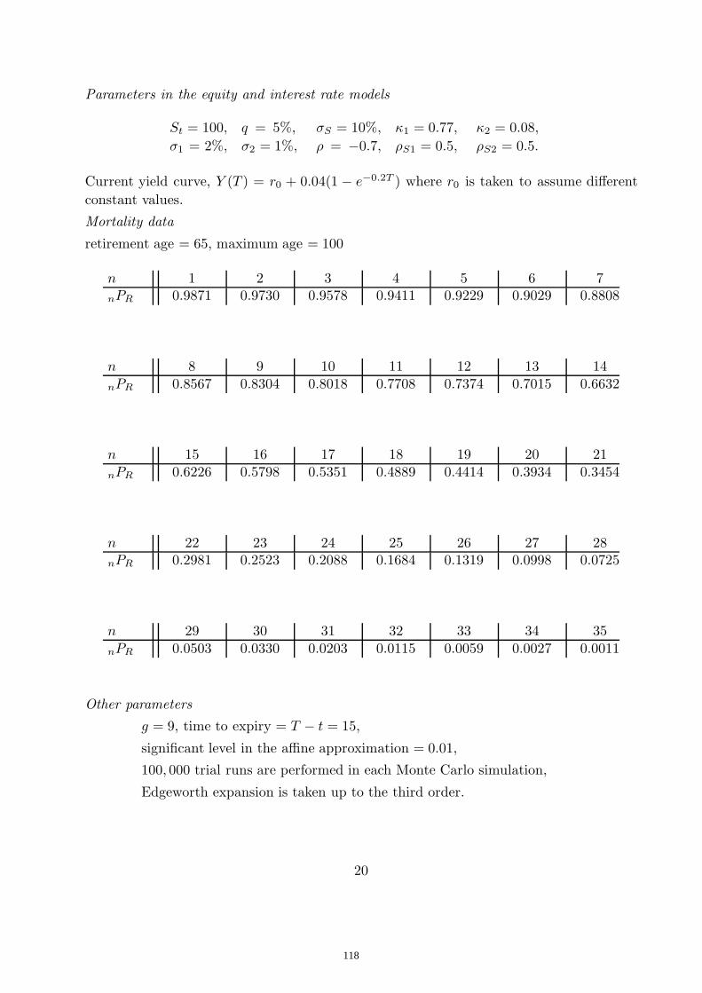
Parameters in the equity and interest rate models
St = 100, q = 5%, σS = 10%, κ1 = 0.77, κ2 = 0.08,
σ1 = 2%, σ2 = 1%, ρ = −0.7, ρS1 = 0.5, ρS2 = 0.5.
Current yield curve, Y (T ) = r0 + 0.04(1 − e−0.2T ) where r0 is taken to assume differentconstant values.
Mortality data
retirement age = 65, maximum age = 100
n 1 2 3 4 5 6 7nPR 0.9871 0.9730 0.9578 0.9411 0.9229 0.9029 0.8808
n 8 9 10 11 12 13 14nPR 0.8567 0.8304 0.8018 0.7708 0.7374 0.7015 0.6632
n 15 16 17 18 19 20 21nPR 0.6226 0.5798 0.5351 0.4889 0.4414 0.3934 0.3454
n 22 23 24 25 26 27 28nPR 0.2981 0.2523 0.2088 0.1684 0.1319 0.0998 0.0725
n 29 30 31 32 33 34 35nPR 0.0503 0.0330 0.0203 0.0115 0.0059 0.0027 0.0011
Other parameters
g = 9, time to expiry = T − t = 15,
significant level in the affine approximation = 0.01,
100, 000 trial runs are performed in each Monte Carlo simulation,
Edgeworth expansion is taken up to the third order.
20
118

Computational efficiency and numerical accuracy
In a typical run in the numerical calculations of the GAO value at a given value of r0,the following computer running times (in minutes) for various methods are recorded inTable 1. Since tedious iterative calculations are required to calculate the higher ordermoments in the Edgeworth expansion method, our experience shows that even only upto the third order expansion, the running time required by the Edgeworth expansion islonger than that of the Monte Carlo simulation with 100, 000 trials. Since closed formformulas are available in the minimum variance duration method, the required runningtime is significantly shorter than that of the other numerical methods.
method Monte Carlo simulation Edgeworth expansion affine approximaton min. var. duration
running time 0.4305 1.136 0.1812 0.0016
Table 1 Comparison of computer running time (in minutes) of various numerical methodsthat compute the GAO value.
In Table 2, we list the numerical results of GAO value obtained by various numericalmethods at different choices of r0 in the assumed functional form of the yield curve. Theagreement between the numerical values is quite well acceptable.
r0% Monte Carlo Simulation Edgeworth expansion affine approximation min. var. duration
0.5 11.7750 11.8161 11.7913 11.81001.0 9.7568 9.7502 9.7412 9.77141.5 7.8952 7.8479 7.8529 7.89582.0 6.1543 6.1293 6.1418 6.19462.5 4.6735 4.6199 4.6313 4.68603.0 3.3793 3.3408 3.3464 3.39113.5 2.3257 2.2999 2.3044 2.32734.0 1.5116 1.4897 1.5057 1.50084.5 0.9222 0.8942 0.9310 0.90085.0 0.5201 0.4922 0.5439 0.4984
Table 2 Comparison of numerical results of GAO value obtained by various numericalmethods.
We also explore the pricing errors of the three analytic approximation methods. Usingthe Monte Carlo results as the benchmark, we calculate the GAO value at 100 differentvalue of r0 (r0 = 0.1%, 0.2%, · · · , 10%) and compute the percentage error of each analytic
21
119

approximation method. The variation of the percentage error with respect toa
gDT (t)is
plotted in Fig. 1. The pricing error is typically less than 1% whena
gDT (t)> 1 (the annuity
option is currently in-the-money) while the accuracy deteriorates whena
gDT (t)falls below
1. Similar behaviors on numerical accuracy are exhibited in swaption calculations usingthe affine approximation method (Singleton and Umantsev, 2002) and minimum varianceduration method (Munk, 1999).
Pricing behaviors of the guaranteed annuity option
We investigate the pricing behaviors of the GAO with respect to various parameters in thepricing model. In Fig. 2, we plot the GAO value against g at varying values of T − t. Thecurves exhibit consistency with the intuition that the GAO value should be a decreasingfunction of g. The rate of decrease of GAO value is higher at a lower value of g. Also,the GAO has a higher value when the policyholder enters the contract closer to retirement(smaller value of T − t). This is related to the time value of money since smaller T − t
means shorter time horizon over which the annuity payments are discounted. This effectcounteracts the usual theta effect of option value, which implies that a longer-lived optionusually has a higher value.
Our GAO pricing model assumes that the interest rate dynamics is governed by tworisk factors (G2++ model). Therefore, there are 3 correlation coefficients in the model,namely, the correlation coefficient ρ between the interest rate risk factors, the correlationcoefficients ρS1 and ρS2 between the stock price process and the risk factors. In Fig.3, we plot the GAO value against ρ with different sets of values of ρS1 and ρS2. In theanalytic approximation price formula, the functional dependence of the GAO value on thesecorrelation coefficients appears to be so highly complicated that any theoretical analysis isintractable. From the plots in Fig. 3, it is quite disquieting to observe that the GAO valueis highly sensitive to the correlation coefficients. Similar phenomena of price sensitivity tothe correlation coefficient have also been reported by Ballotta and Haberman (2003).
7. ConclusionsSince there is no closed form analytic price formula for a guaranteed annuity option whenthe interest rate dynamics is modeled by a multi-factor short rate model, the numericalvaluation of the guarantee in deferred annuity pension policies is resorted to either MonteCarlo simulation or analytic approximation methods. In this paper, we construct threeanalytic approximation methods for effective valuation of the annuity option value whenthe interest rate dynamics is modeled by a multi-factor affine term structure model. Themethod of minimum variance duration starts with a judicious analytic approximation sothat closed form formula can be obtained. The pricing error is minimized by choosingthe period τ of a reference bond such that the variance of the value of the annuity pay-
22
120

ment normalized by the price of the (T + τ )-maturity bond is minimized. The Edgeworthexpansion method seeks the Edgeworth approximation of the probability distribution ofthe annuity value at option’s maturity. In the affine approximation, the exercise prob-ability of the annuity option is approximated through the approximation of the concaveexercise boundary by a hyperplane. When these three analytic approximation methodsare compared in terms of numerical accuracy and computational efficiency, the methodof minimum variance duration seems to have the best performance among them. Whenthe annuity option is in-the-money or slightly out-of-the-money, the pricing error of theseapproximation methods are within a few percentage points. Though the three-term Edge-worth expansion demonstrates sufficient accuracy, the computational time required is evenlonger than that of the Monte Carlo simulation method using 100, 000 simulation paths.
Our numerical studies showed that the value of the annuity option is highly dependenton the guaranteed conversion rate of the annuity and the correlation coefficients amongthe risk factors. As future works, one may use a more accurate model to characterizethe equity return process, like the use of stochastic volatility model or regime switchingmodel. Also, we may incorporate stochastic mortality effects and other market factors(tax, expenses, etc.) into the pricing model.
ReferencesBallotta, L., Haberman, S., 2003a. Valuation of guaranteed annuity conversion options.Insurance: Mathematics and Economics 33, 87-108.
Ballotta, L., Haberman, S. 2003b. The fair valuation problem of guaranteed annuityoptions: the stochastic mortality environment case. Working paper of City University,London.
Boyle, P., Hardy, M., 2003. Guaranteed annuity options. ASTIN Bulletin 33(2), 125-152.
Collin-Dufresne, P., Goldstein, R.S., 2002. Pricing swaptions within an affine framework.Journal of Derivatives, Fall issue, 1-18.
Cox, J.C., Ingersoll, J.E., Ross, S.A., 1979. Duration and the measurement of basis risk.Journal of Business 51(1), 51-61.
Dai, Q., Singleton, K.J., 2000. Specification analysis of affine term structure models.Journal of Finance 55, 1943-1978.
Heath, D., Jarrow, R., Morton, A., 1992. Bond pricing and term structure of interestrates: a new methodology for contingent claims valuation. Econometrica 60(1), 77-105.
Jamshidian, F., 1989. An exact bond option formula. Journal of Finance, 44(1), 205-209.
23
121

Munk, C., 1999. Stochastic duration and fast coupon bond option pricing in multi-factormodels. Reviews of Derivatives Research 3, 157-181.
O’Brien, C., 2001. Guaranteed annuity options: Five issues for resolution. Working paperof University of Nottingham.
Pelsser, A., 2003. Pricing and hedging guaranteed annuity options via static option repli-cation. Insurance: Mathematics and Economics 33(2), 283-296.
Singleton, K.J., Umantsev, L., 2002. Pricing coupon-bond options and swaptions in affineterm structure models. Mathematical Finance 12(4), 427-446.
Wei, J., 1997. A simple approach to bond option pricing. Journal of Futures Markets17(2), 131-160.
Wilkie, A.D., Waters, H.R., Kong, S., 2004. Reserving, pricing and hedging for policieswith guaranteed annuity options. British Actuarial Journal 9(2), 263-425.
24
122

0.95 1 1.05 1.1 1.15 1.2 1.25−4
−3
−2
−1
0
1
2
3
a/[gDT(t)]
prec
enta
ge e
rror
SimulationEdgeworthAffineMinimum variance duration
Fig. 1. Comparison of the pricing error (in percentage) of various analytic approximation
methods. Good numerical accuracy is revealed whena
gDT (t)> 1 (the annuity option is
currently in-the-money).
5 6 7 8 9 10 11 120
10
20
30
40
50
60
g
GA
O v
alue
T−t=10T−t=15T−t=20
Fig. 2. Plot of GAO value against guaranteed conversion rate g at varying values of timeto expiry T − t.
25
123

−1 −0.8 −0.6 −0.4 −0.2 0 0.2 0.4 0.6 0.8 12
2.5
3
3.5
4
4.5
ρ
GA
O v
alue
ρS1
=0.5, ρS2
=0.5ρ
S1=−0.5, ρ
S2=0.5
ρS1
=0.5, ρS2
=−0.5
Fig. 3. Price sensitivity of the GAO value to the correlation coefficients in the pricingmodel.
26
124

Proceedings of the International Conference on Computational and Mathematical Methods in Science and Engineering, CMMSE2007 Chicago, 20-23 June 2007
Non-linear analysis of cable networks by FEM and experimental validation
J. J. del Coz Díaz1, P. J. García Nieto2, D. Castro Fresno3 and E. Blanco Fernández3
1 Construction and Production Engineering Department, University of Oviedo, Viesques Department Building no. 7, 33204 Gijón (Spain)
2 Department of Mathematics, Faculty of Sciences, University of Oviedo, 33007 Oviedo (Spain)
3 Department of Construction, ETSIPCC, University of Cantabria, 39005 Santander (Spain)
emails: [email protected], [email protected],
[email protected], [email protected]
Abstract This work studies the analysis of the resistant capacity of cable nets for the stabilization of slopes. Two tests have been carried out, one with a distributed longitudinal load and the other with distributed transversal load, in order to simulate in situ the working conditions of these systems. Tensile tests were also carried out on the cable elements of the network in order to obtain the non-linear mechanical properties. On the one hand, the proposed numerical procedure uses the finite element method (FEM) and it takes into account the material and geometrical non-linearities due to the geometrical change in the cable net substructure. On the other hand, the cable network is modelled by one-dimensional beam elements with joints between them by means of multibody coupling. The laboratory tests only provide information about the strain and maximum resistance, but they do not establish a relationship between the values of stresses of each net element. These data have been obtained through the computational simulation by FEM. A reliable model of the interaction of the flexible contour beam with the cable network enables the achievement of more efficient solutions in the design analysis. Finally, we compare the structural behaviour of the numerical and experimental results by means of the equivalent elastic modulus and the equivalent Poisson’s ratio. Reasonable agreement between the predicted results by FEM and test observations was found. Key words: Finite element analysis; cable networks; Material and geometrical non-linearities; Soil stabilization; MSC2000: 74S05, 74C05, 35J60
125

CMMSE 2007
1. Introduction On gentle slopes, erosion blankets, both natural and man-made, or hydro-seeding can be employed to hold soil and seed in place until vegetation gets established. These lightweight products may not be enough to control erosion caused by high water velocities associated with steep slopes. Where steeper slopes and high water velocities prevail, a wire mesh and a cable net slope protection system may be used [1-2]. Wire mesh and cable net slope protection have been in use for more than 50 years along highways to control rockfall on actively eroding slopes. The present work studies these last flexible systems of slopes’ surface stabilization, the levelling of grounds and loose materials by the finite element method (FEM) as well as the analysis and a subsequent comparison with the experimental results. The cable network systems provide: (a) control of the erosion; (b) covering; (c) fastening of the ground and (d) surface stabilization. The system works like a lightly tightened continuous surface that receives from the ground the loads due to the earth pressure on the cable networks and it transmits them to the head of the anchorages, which at the same time transmit them to the stable area of the hillside or slope. Once the system object of the study has been described, the most important characteristics in the numerical simulation will be discussed. Next, we shall carry out an analysis of the obtained results and to conclude we shall do a comparison of numerical results with the experimental tests. Finally we shall analyse the causes of the possible discrepancies present between the experimental and numerical results.
2. Mathematical model The finite element method is used to model the cable network and the boundary structure. Approximation of the structure by a discrete number of finite size straight and curved elements, connected at nodes, is a quite natural simulation since the original cable network consists of turns made of elements and curves. According to stiffness properties the structural system is divided in several substructures (one per wire). Therefore, the resolution of this problem implies the simultaneous study of two non-linearities [3]: (1) material non-linearity (elastoplastic behaviour in this case), and (2) geometrical non-linearity or large displacements. The most straightforward way to create the mathematical model of a cable network with a flexural contour structure is to include the cable and the beam elements in a common system of equations in general matrix form. If load P is applied at the nodes of the original undeflected structure, an unbalanced resultant force is produced:
PFR −= (1)where F is the vector of internal forces at nodes and P is the vector of external forces at nodes. R is a non-linear function with respect to the displacements of the structure. In order to find the equilibrium state geometry, Eq. (1) has to be solved, using relevant numerical methods [4]. According to the Newton-Raphson method we calculate the correction of the solution at every iteration cycle:
( ) iii RKd 1−= (2)
126

CMMSE 2007
where iK is the stiffness matrix of the structure. The new geometry after cycle i is determined by the vector of nodal co-ordinates:
iii duu +=+1 (3)Nodal displacements produce elastoplastic elongation [3] of the cable elements and change of the tension and bending forces according to axial and flexural stiffness. Therefore stiffness matrix K and unbalanced force R have to be updated for every iteration cycle according to the current geometry. Convergence of the described method is usually rapid near the equilibrium state, but may be disturbed if elements of the stiffness matrix vary significantly or if the initial geometry is inappropriate. 2.1. Plasticity The plastic behaviour is characterized by irreversibility of stress paths and the development of permanent (i.e. non-recoverable) deformation (or strain), known as yielding (or plastic flow). A hardening plastic material model provides a refinement of the ideal plastic material model. In this model, it is assumed that the yield stress depends on some parameter κ (e.g. plastic strain pε ), called the hardening parameter. The general yield criterion is expressed in the form [5]:
( ) 0, =κσ ijF (4)After initial yielding, the stress level at which further plastic deformation occurs may be dependent on the current degree of plastic straining, known as strain hardening [5]. Thus, the yield surface will vary (i.e. expand) at each stage of plastic deformation. If the subsequent yield surfaces are a uniform expansion of the original yield surface, the hardening model is said to be isotropic. The behaviour is initially linear elastic with slope E (Young’s modulus) until onset of yielding at the uniaxial yield stress Yσ . Thereafter, the material response is elasto-plastic with the local tangent to the curve, TE , called the elasto-plastic tangent modulus, continually changing. At some stress level σ in the plastic range, if the load is increased to induce a stress of σd , it results in a corresponding strain εd . This increment of strain contains two
parts: elastic edε (recoverable) and plastic pdε (non-recoverable) [3,5]:
Tepe E
dd
Eddddd ==+=
εσσεεεε ,,
(5)
The strain-hardening parameter, H, is defined by [6-7]:
EE
E
dd
dd
ddH
T
Tep
−=
−==
11εεεσ
εσ
(6)
The element stiffness for the linear elastic portion is, say [ ]eK [6-7]:
[ ] [ ] [ ][ ]∫=b
a
x
x
eTe dxBDBK (7)
where [ ]eD is the linear elasticity matrix ( EDe = for the uniaxial case). When the element deforms plastically, [ ]eD reflects the decreased stiffness. This is computed, for
127

CMMSE 2007
uniaxial material behaviour, by the following procedure. The increment in load dF causes an incremental displacement du :
( ) pe
peexxe dHAdAdFddhdhdu εσεεε ==+== , (8)
where eh is the length and eA the area of cross-section of the element. The effective stiffness is:
( ) ( )⎥⎦⎤
⎢⎣
⎡+
−=+
==HE
EhAE
ddhdHA
dudFE
e
epe
e
peep 1
εεε
(9)
The element stiffness for the plastic range becomes [5-7],
[ ] [ ] [ ][ ]dxBDBKb
a
x
x
epTep ∫= (10)
where [ ]epD is the material stiffness in the plastic range. For the uniaxial case epep ED = . Eq. (7) is valid when Yσσ < and Eq. (10) is valid for Yσσ > . Note that
Yd σσσ −= when Yσσ > . 2.2. Large displacements Whether the displacements (or strains) are large or small, equilibrium conditions between internal and external ‘forces’ have to be satisfied. Thus, if the displacements are prescribed in the usual manner by a finite number of nodal parameters ar , we can obtain the necessary equilibrium equations using the virtual work principle [7]:
( ) ∫ =−=ΨV
T fdVBa 0rrr σ (11)
where Ψ once again represents the sum of external and internal generalized forces, and in which B is defined from the strain definition εr as:
adBd rr=ε (12)
The bar suffix has now been added for, if displacements are large, the strains depend non-linearly on displacement, and the matrix B is now dependent on ar . We see that it can be conveniently write:
( )aBBB Lr
+= 0 (13)
in which 0B is the same matrix as in linear infinitesimal strain analysis and only LB depends on the displacement. In general, LB will be found to be a linear function of such displacements. Clearly the solution of Eq. (11) will have to be approached iteratively. If, for instance, the Newton-Raphson process is to be adopted we have to find the relation between adr and Ψd . Thus taking appropriate variations of Eq. (11) with respect to adr we have [6]:
∫ ∫ =+=ΨV V
TTT adKdVdBdVBdd rrr σσ (14)
and using equation εσrr dDd = and Eq. (12) it is obtained:
adBDdDd rrr== εσ
128

CMMSE 2007
and taking into account the Eq. (13), it is verified that LdBBd = . Therefore,
∫ +=+=ΨV
TL adKadKadKdVdBd rrrr
σσ (15)
where
∫ +==V
LT KKdVBDBK 0
in which 0K represents the usual, small displacements stiffness matrix and the matrix LK is due to the large displacements, and are given by [7]:
∫=V
T dVBDBK 000 , ( )∫ ++=V
TLL
TLL
TL dVBDBBDBBDBK 00 (16)
To summarize, Eq. (15) can be expressed globally as: ( ) adKadKKKd TL
rr=++=Ψ σ0 (17)
where TK represents the total, tangential stiffness, matrix. Newton-type iteration can once more be applied precisely in order to solve the final non-linear problem. 2.3. Multibody coupling by joints One of the major areas of nonlinear analysis is the solution of problems in which separate bodies or structures may come in contact with each other. Several methods have been developed to handle such problems and, in this paper, the multibody coupling has been adopted [7-8]. Often it is desirable to have two (or more) rigid bodies connected in some specified manner. For example, in our case, each turn in the cable network is hooked to another. Both turns are treated as flexible non-linear bodies and it is necessary to consider coupling among them in order to obtain the global structural behavior of the network. This type of interconnection is commonly referred to as a joint. When generating our model, we define the relationships among different degrees of freedom by using elements to connect the nodes. In this work, we use a joint which is a linear connection where one body may freely move around the other but relative translation is prevented (see Fig. 1 below). Thus each turn may not translate relative to another in any direction. If a full translation constraint is imposed a simple relation may be introduced as [7]:
0( ) ( )a bjC x x= − =r rr r (18)
where a and b denote two rigid bodies.
3. Geometrical model Several geometrical models were analyzed in this work. In order to carry out a right numerical simulations, it is necessary to reproduce accurately both the geometrical and mechanical characteristics of the system object of study. In the present work, the characteristics of meshes are shown in Fig. 2.
129

CMMSE 2007
Fig.1. Couplings among turns of the cable network.
Fig. 2. Geometrical model of a cable network.
4. Finite element model and analysis Based on the geometrical model of a piece of cable network (see Fig.2) the finite element model was built, following a four-step process. Firstly, the definition of mechanical properties is based on real tests. Secondly, the selection of the element types, formulations and physical properties was made. Thirdly, the geometrical model was meshed. Finally, loads and boundary conditions were applied and the model was solved.
130

CMMSE 2007
4.1. Mechanical properties
The mechanical properties of the high strength steel such as its Young’s modulus, its yield stress and its ultimate stress have been obtained by means of the experimental results from direct tensile tests carried out to these wires. In this way, for the 3 mm diameter wire the mechanical characteristics obtained are shown in Table 1.
Table 1. Mechanical properties of the 3 mm diameter wire.
Stress [MPa] Strain Young’s Modulus [MPa]
0.000 0.0000 1,101.328 0.0056 196,906 1,482.037 0.0093 1,794.777 0.0139 1,826.427 0.0300
4.2. Element types and meshing
The element used in this study is a quadratic (3-node) beam element with six degrees of freedom at each node (include translations in the x, y, and z directions and rotations about the x, y, and z directions) and it includes stress stiffness terms [3,9], since for its characteristics is the most appropriate for the problem. This is an one-dimensional element well-suited for large rotation and large strain nonlinear applications as in this work. This element is based on Timoshenko beam theory and shear deformation effects are included. In this work a extremely fine mesh has been used in order to obtain a good accurateness. This mesh has an element size of 1 millimetre, giving rise to a mesh of approximately 70,000 elements (see Fig. 3).
Fig. 3. Finite element mesh and boundary conditions: (a) entire mesh for the direct tensile test (left), (b) entire mesh for the cross tensile test (middle) and (c) detail of a connection (right).
131

CMMSE 2007
4.3. Loads and boundary conditions
Two different boundary conditions have been applied in the numerical model:
• On the one hand, in order to simulate the direct tensile test, several boundary conditions have to be imposed in the finite element model (see Fig. 3(a)). Firstly, at the lower side of the mesh, displacements in directions x, y and z, are constrained. Secondly, at the left and right sides, displacements in directions x and z are constrained, in order to allow the displacement in vertical direction y. Finally, at the upper side, the displacement in z direction is constrained and it is imposed a displacement in y direction of 60 mm.
• On the other hand, the cross tensile test requires different boundary conditions (see Fig. 3(b)). In the first place, at the upper and lower sides, displacements in directions z and y are constrained, allowing the displacement in direction x. Secondly, at the left side, displacements in directions x and z are constrained. Finally, at the right side, a displacement in direction x of 60 mm is imposed.
5. Non-linear analysis of cable networks A non-linear analysis was performed taking into account the geometrical and material non-linearities: large displacements and plasticity. The solution controls were also adjusted to improve convergence. Thus the parameter time was set to the value of one, corresponding to the value of maximum displacement applied (60 mm), the geometrical non-linearity was activated, the inertial effects were not included, the number of equilibrium iterations was specified and the convergence tolerance values of displacements were delimited as well as the time step for the analysis. In this work, the total number of iterations in order to get convergence was about 160.
6. Analysis of results and discussion On the one hand, we show the von-Mises stresses obtained by FEM for the direct tensile test and the cross tensile test (see Fig. 4). On the other hand, we show the experimental patent device with the cable networks used in the Cantabria University laboratory in order to determine the experimental results (see Fig. 5). Graphs representing both the numerical and experimental results are shown in Fig. 6, in order to get the longitudinal and transversal equivalent elastic moduli by means of a linear fitting from data. The values obtained are:
1) From the direct tensile test (longitudinal equivalent elastic modulus): • Numerical simulation: 1,690.6 kN/m. • Experimental test: 1,886.3 kN/m.
2) From the cross tensile test (transversal equivalent elastic modulus): • Numerical simulation: 319.9 kN/m. • Experimental test: 222.47 kN/m.
132
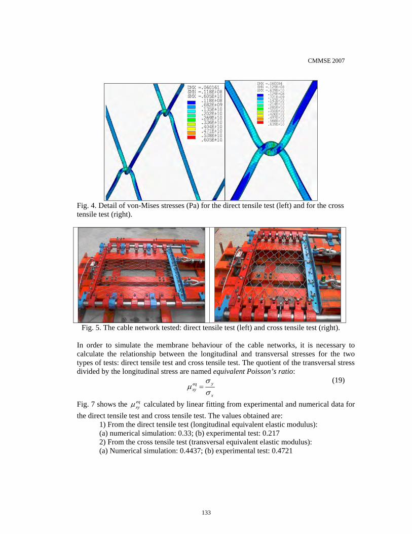
CMMSE 2007
Fig. 4. Detail of von-Mises stresses (Pa) for the direct tensile test (left) and for the cross tensile test (right).
Fig. 5. The cable network tested: direct tensile test (left) and cross tensile test (right). In order to simulate the membrane behaviour of the cable networks, it is necessary to calculate the relationship between the longitudinal and transversal stresses for the two types of tests: direct tensile test and cross tensile test. The quotient of the transversal stress divided by the longitudinal stress are named equivalent Poisson’s ratio:
yeqxy
x
σμ
σ=
(19)
Fig. 7 shows the eqxyμ calculated by linear fitting from experimental and numerical data for
the direct tensile test and cross tensile test. The values obtained are: 1) From the direct tensile test (longitudinal equivalent elastic modulus): (a) numerical simulation: 0.33; (b) experimental test: 0.217 2) From the cross tensile test (transversal equivalent elastic modulus): (a) Numerical simulation: 0.4437; (b) experimental test: 0.4721
133

CMMSE 2007
Fig. 6. Stress vs. strain curves obtained from the numerical simulation by FEM and from experimental test: (a) direct tensile test (left) and (b) cross tensile test (right).
Fig. 7. Equivalent Poisson´s ratio: (a) direct tensile test (left) and (b) cross tensile test (right).
7. Conclusions A method for modelling static behaviour of cable networks has been developed and verified here. The equilibrium equations of elasto-plastic network are derived in the incremental form. The procedure can serve as an alternative tool in order to avoid expensive physical tests in the laboratory of different configurations and geometries of cable networks. From the results obtained, the following conclusions can be drawn:
• In the first place, the finite element method (FEM) has been shown as suitable tool in the modelling and analysis of singular structures, such as the complex structural behaviour of cable networks with strong non-linearities.
• The definition of the cable network geometry is very cumbersome using a finite elements analysis program. For this reason, a three-dimensional parameter design program was used in order to design the turn appropriately as well as the entire assembly of the cable network.
134

CMMSE 2007
• We have compared the numerical results with the experimental ones. The following aspects are observed:
A good agreement between the longitudinal equivalent moduli for both techniques: numerical and experimental.
A small deviation in the value of the transversal equivalent moduli, due to the Bauschinger effect [5] in turns, residual stresses, etc.
A good performance is observed with respect to the equivalent Poisson’s ratios.
Finally, in view of the obtained results for both tests, it can be considered that a numerical simulation like this one can provide accurately results that will help us to understand the behaviour of these stabilization systems. In future works, it would be necessary to take into account other local phenomena in turns such as the effects due to residual stresses, the hysteresis of materials, etc. Acknowledgements We gratefully acknowledge the financial support provided by the Construction Technology Research Group (GITECO) at the University of Cantabria, Malla Talud Cantabria Ltd. (MTC) and SODERCAN. We thank the Construction and Production Engineering Department of the University of Oviedo for the computational support. References
[1] H.A. BUCHHOLDT, An introduction to cable roof structures, Thomas Telford, London, 1999.
[2] S. SHU, B. MUHUNTHAN, T.C. BADGER, R. GRANDORFF, Load testing of anchors for wire mesh and cable net rockfall slope protection systems, Engineering Geology 79 (2005) 162-176.
[3] K.J. BATHE, Finite element procedures, Prentice Hall, Englewood Cliffs, 1996.
[4] J. STOER, R. BULIRSCH, Introduction to numerical analysis, Springer-Verlag, New York, 2004.
[5] J.C. SIMO, T.J.R. HUGHES, Computational inelasticity, Springer-Verlag, New York, 1998.
[6] J.N. REDDY, An introduction to non-linear finite element analysis, Oxford University Press, New York, 2005.
[7] O.C. ZIENKIEWICZ, R.L TAYLOR, The finite element method: solid mechanics, Butterworth-Heinemann, Oxford, 2000.
[8] J.J. DEL COZ DIAZ, P.J. GARCIA NIETO, C. BETEGON BIEMPICA, G. FERNANDEZ ROUGEOT, Non-linear analysis of unbolted base plates by the FEM and experimental validation, Thin-walled Structures 44 (2006) 529-541.
[9] D. BRAESS, Finite elements: theory, fast solvers, and applications in solid mechanics, Cambridge University Press, Cambridge, 2001.
135
Proceedings of the International Conferenceon Computational and Mathematical Methodsin Science and Engineering, CMMSE 2007Chicago, 20–23 June 2007.
Optimal design of robust and efficient complex networks
R.Criado, J. Pello, M. Romance and M.Vela-Perez
Departamento de Matematica Aplicada, ESCET, Universidad Rey Juan Carlos,C/Tulipan s/n, 28933, Mostoles, Madrid, Spain
emails: [email protected], [email protected],[email protected], [email protected]
Abstract
A relevant problem in network design is how to construct or improve a complexnetwork in order to optimise some structural properties. In this work we studythis design problem when we deal with efficiency and vulnerability and we presentsome characterisation of the extremal networks and improvements. Finally weapply these result to the optimal improvement of the Spanish and German airportnetworks.
Key words: Optimal networks, robustness, efficiency, vulnerability, networktopology, network design.
MSC 2000: 05C75, 05C90, 94C15, 94C30
1 Introduction
In the last years, much progress has been made to describe the complex structure ofreal world networks [1, 2, 3, 9, 10]. Complex networks have applications in fields rang-ing from biology (which include issues such as metabolic pathways, genetic regulatorynetworks or protein folding) to the Internet or the World Wide Web and other techno-logical systems, as well as the study of social or economic relationships, to name a few.Hence a detailed analysis of the underlying network is central for the understanding ofthe modelled complex system [1, 9]. The investigation of such issues must necessarilyembrace a diversity of viewpoints that include different complementary aspects of thenetwork structure.
There are several mathematical parameters that give structural properties of thenetwork, but in this work we will consider the efficiency and vulnerability as mainanalysis tools. If G = (V, E) is a complex network with n nodes and m links, it isconsidered that the performance of G is a single function Φ(G) > 0 that measures thebehaviour of G. Some examples of the performance of a network G are the characteristic
136

path length of the network L(G), the mean flow-rate information over G, but we willuse the efficiency E+(G), defined (see [6, 7]) as
E+(G) =1
n(n− 1)
∑
i6=j∈V
1dij
, (1)
where dij stands for the shortest distance between the nodes i and j. This conceptplays the role of measuring its ability for the exchange of information and its responsefor the spread of perturbations in diverse applications [3, 4].
Another important parameter is the vulnerability (as the opposite concept to ro-bustness) which is related with the ability of a network to avoid malfunctioning whena fraction of its constituents is damaged due to random failures or intentional attacks[5, 7]. There are several different approaches in the literature to measure the vulnerabil-ity of a complex network [4, 5] but, in general, they can be divided in two types. On theone hand we find the static vulnerability which analyses the response of the structuralproperties of the networks when some of its nodes or links are removed, while, on theother hand, the dynamical vulnerability is considered to measure the redistribution offlow in the network when a failure or attack occurs.
In this paper we will consider static vulnerability related to structural properties ofthe complex network that allows us to spot its critical components in order to improvethe security. In [5], an axiomatic description of the robustness is presented and somecandidates for vulnerability functions are proposed based on the network regularity.Roughly speaking, a vulnerability function is a normalised function v(G) intrinsic tothe topology of G that increases if we remove some components of the network. In [5]it is considered that the vulnerability is related to the node regularity and the numberof alternative links that can balance a random or intentional attack. The basic ideais that the more similar the nodes are, the more robust the network is, assumed thatwe had fixed the number of links and nodes in the network. Hence, in addition to thenumber of nodes and links, also the dispersion of the degree distribution should play acentral role in the vulnerability of the network, and it was introduced the vulnerabilityfunction V1(G) of a network G = (V, E) with n nodes and m links as
V1(G) = exp(
M − a
n+ n−m− 2 +
2n
), (2)
where M = maxgr(vi); i ∈ V , a = mingr(i); i ∈ V and gr(vi) is the degree ofnode i ∈ V . This definition can be computed easily and gives a good estimation of therobustness of a complex network but the fact that only the nodes of extremal degreesare considered makes it not as sharp as desirable from a statistical point of view. Toavoid this problem, a sharper estimator of the regularity of the degree distribution mustbe considered, leading to the vulnerability function V2(G) given by
V2(G) = exp(
σ
n+ n−m− 2 +
2n
), (3)
137

where n is the number of nodes of G, m stands for the number of links and σ denotesthe standard deviation of the degree distribution, i.e.
σ =
(1n
∑
i∈V
(gr(vi)− 2m
n
)2)1/2
. (4)
Once that we have fixed some quantitative parameters for the properties of thenetwork, it is natural to ask how a network must be designed or improved to get thebest possible result, possibly with a given set of constrains. For example, if we had thechance to reinforce the airline network of a country by adding a new link between twoairports, it would be desirable to know which airports we should connect in order tooptimize the efficiency of the whole network.
In this work we present some results regarding the optimal design of networks withrespect to efficiency and vulnerability and also, how to improve a given network tooptimise those parameters. The approaches for optimising vulnerability and efficiencyare rather different since the problems have different nature. While we get a completecharacterisation of the extremal network for the vulnerability function, the case ofefficiency function is much deeper and we present some approximation algorithms thatwe apply to the optimal improvement of the Spanish and German airport networks.
2 Extreme networks for vulnerability and efficiency
In this section we consider the set of all connected networks G with n nodes and m linksand we find the extreme graphs for vulnerability and efficiency. That is, we find thosenetworks with maximal vulnerability, with minimal vulnerability and with maximalefficiency for a given number of nodes n and links m.
When dealing with a vulnerability function we work with definition V2(·), since fordefinition V1(·) the results are straightforward. On the other hand, for efficiency, weuse the additive definition E+(·) given by Latora and Marchiori (see [6, 7]), but notethat since there is a relationship between the different definitions for the efficiency, wecan transfer the results from one to the other.
Our first result is about vulnerability and its extreme values. We will use thefollowing inequality.
Proposition 2.1 Let G = (V, E) be a network with n > 1 nodes and m links and letgr = (gr(v1), ..., gr(vn)) its degree vector. Then
n∑
i=1
gr(vi)2 = ‖gr‖2 ≥ 4m2
n. (5)
Note that we have the equality in (5) for the K-regular graphs, simply by theequality case in Cauchy-Schwartz inequality. By using this result we can characterisethe minimal vulnerability networks with a given number of nodes and links, as thefollowing result shows.
138

Theorem 2.2 Let G = (V, E) be a network with n > 1 nodes and m links and letgr = (gr(v1), ..., gr(vn)) its degree vector. Then G has the minimum vulnerability ifits degree vector is the most parallel to the vector (1, . . . , 1), that is, G is the closestnetwork to the K-regular one with m links. Hence, the degree vector for G is of the
form (a, . . . , a, b), a, b ≤ n− 1, withn∑
i=1
gr(vi) = 2m.
Similarly, by using some geometric arguments in Rk, we have a result that charac-terises the network with maximum vulnerability.
Theorem 2.3 Let G = (V, E) be a network with n > 1 nodes and m links and let gr =(gr(v1), ..., gr(vn)) its degree vector. Then G has the maximum vulnerability if its degreevector is the most parallel to the vector (n−1, 1, . . . , 1), that is, G is the closest networkto the Star. Hence, the degree vector for G is of the form (n− 1, . . . , n− 1, a, 1, . . . , 1),
a ≤ n− 1, withn∑
i=1
gr(vi) = 2m.
When dealing with extremal networks for the efficiency function, a first analysisshould include the local structure of the graph. By using this approach the degree vectoris the natural tool and we show that for the networks having a node with maximumdegree there is a simple formula for the efficiency function:
Theorem 2.4 Let G be a simple network with n > 1 nodes and m links. If there existsa node with maximum degree (i.e. gr(vi) = n− 1) then
E+(G) =m
n(n− 1)+
12.
Note that last theorem shows that we have the upper equality in [4, theorem 2.2] forthe simple networks with a node with maximum degree. As a consequence we deducethat for a network G (with n > 1 nodes) to have maximum efficiency it is enough thatG has the n-Star as a subgraph or another K-complete bipartite subgraph.
We find also an inequality for efficiency in terms of the maximum degree of thenetwork (not necessarily equal to n− 1).
Proposition 2.5 Let G = (V,E) be a a network with n > 1 nodes and m links. Letvk ∈ V be the node with maximum degree in the network (not necessarily equal to n−1),gr(vk) = a. Then dij ≤ n−a+1 for every vi, vj ∈ V, where dij is the minimum distancebetween vi and vj. Furthermore,
E+(G) ≥ 2m(n− a)n(n− 1)(n + 1− a)
+1
n + 1− a.
139

3 Optimal improvement of complex network
A major problem in network design is spotting the critical element to be added to agiven (real-life) complex network that gets the best possible network for some parame-ters. By cost restrictions, the elements to be added to the network (nodes or links)are usually limited and hence the problem of finding the optimal improvement of thenetwork is related to a discrete and conditioned critical points problem which is hardto solve by direct methods. In this section we will consider such problems when wewant to get an optimal improvement of the network that maximises its robustness (i.e.minimises some vulnerability function) or maximises its performance (i.e. the efficiencyfunction) and we will give some computationally effective criteria to determine theseconditioned critical points.
If we consider a complex network G and we want to add a single link ` such thatwe get a network G′ = G∪` with minimal vulnerability or maximal efficiency, a firstnaive approach leads us to compute all possible improvements of type G∪` and spotthe optimal, but in real networks this can be computationally non-effective. Note, forexample, that if we want to locate the improvement of a complex network with n nodeswhich has maximal efficiency, an exhaustive analysis of all possible candidates uses analgorithm of computational complexity of order n7, which is far from being effectivewhen dealing with real networks with thousand (or million) of nodes. Therefore it isnecessary to develop new strategies of design that reduce the complexity of locatingthe critical component to be added in order to get effective tools for the networkoptimisation.
Locating the critical single link ` that gets the most robust improvement G∪` of anetwork G is related to the degree of the nodes to be linked. If we want to minimise thevulnerability function V1(G∪`), it is straightforward that the optimal design strategyis to decrease the range of the degree distribution of G by adding a link joining thenode of minimal degree with other node which has no maximal degree. If we considerthe vulnerability function V2(·), we could think that the same idea should work, butsince this vulnerability function uses the whole degree distribution, it can be checkedthat this is not the optimal strategy for network improvement. Despite this fact, theoptimal computationally effective strategy is also related to the minimal degree of thenodes involved as the following result shows.
Theorem 3.1 Let G = (V,E) be a graph and `0 = vi0 , vj0 such that vi0 , vj0 ∈ V and`0 /∈ E. Then the following assertions are equivalent:
(i) G′ = G ∪ `0 has minimal vulnerability V2(·) among all improvements G ∪ `.(ii) γ(vi0 , vj0) = min γ(vi, vj); vi, vj /∈ E, where γ(vi, vj) = gr(vi) + gr(vj).
Note that the computational complexity to find the minimum of γ(vi, vj) directlyis of order n4, while the exhaustive computation of the optimal improvement of typeG ∪ ` has complexity n5.
140

Locating the maximal efficiency improvement of type G ∪ ` is, by far, a muchmore complicated problem. In this case, it is clear that the addition of a single link `to a network G can produce deep changes in its geodesic structure. We could naivelyexpect that the optimal improvement occurs when we link the most distant nodes, butit is easy to find simple example where this idea fails. Actually, it seems that there isno other clear-enough criterium for locating the improvement of the network with max-imal efficiency. As an alternative approach, we propose to give other computationallyeffective method that gives an approximation of the optimal improvement. If we wantto get a near-optimal improvement of type G ∪ ` we have to mix two different facts:
(i) Nodes to be mixed have to be far in order to produce a significant increase in theefficiency.
(ii) The new link should produce the biggest change in the geodesic structure of thenetwork. Note that this geodesic sensitivity is related again to the degree of thenodes involved.
However, these conditions do not, by themselves, guarantee that a certain edge willprovide the greatest, or close to the greatest, efficiency increase. The following graphsshow the increase in efficiency in the Spanish and German airport networks when asingle link is added, against the sum of the degrees of the nodes connected. It canbe seen that linking nodes already close always has a small impact on efficiency, whilepicking distant nodes may have a larger effect, but it may as well not be the case.
0 5 10 15 20 25 30 350
1
2
3
4
5
6
7x 10
−3 Spanish airport network
degree sum
effic
ienc
y in
crem
ent
0 10 20 30 40 500
0.01
0.02
0.03
0.04
0.05
0.06German airport network
degree sum
effic
ienc
y in
crem
ent
So, while choosing the two most connected nodes does not always bring the highestefficiency, at least we know we have to take two of the most connected, and preferablydistant, nodes. There is a bound to how much the efficiency can increase when addinga single edge, based on their initial distance and their degrees. Therefore, a suitablecourse of action to find the best edge would be to sort the possible edges to be addedaccording to distance and node degree and run through them in decreasing order,testing the change in efficiency and stopping when the bound ensures that we havealready come across the best choice. The graphs above suggest that this best choicewill actually be one of the first pairs to be tested.
141

References
[1] R.Albert and A. L. Barabasi, “Statistical mechanics of complex networks”,Rev. Mod. Phys. 74 (2002), 47–97.
[2] Y.Bar-Yam, Dynamics of Complex Systems, Addison-Wesley, 1997.
[3] S. Boccaletti, V. Latora, Y. Moreno, M. Chavez, D.-U. Hwang, “Com-plex networks: Structure and dynamics”, Physics Reports 424 (2006), 175–308.
[4] R.Criado, A.Garcıa del Amo, B.Hernandez-Bermejo, M.Romance,“New results on computable efficiency and its stability for complex networks”,Journal of Computational and Applied Mathematics 192, 59 (2006).
[5] R.Criado, J. Flores, B.Hernandez-Bermejo, J. Pello, M.Romance,“Effective measurement of network vulnerability under random and intentionalattacks”, Journal of Mathematical Modelling and Algorithms Vol 4, No 3 (2005),307–316.
[6] V.Latora and M.Marchiori, “Efficient behaviour of small-world networks”,Phys. Rev. Lett. 87 (2001), art. no. 198701.
[7] V.Latora and M.Marchiori, “How the science of complex networks can helpdeveloping strategies against terrorism”, Chaos, Solitons and Fractals 20 (2004),69–75.
[8] V.Latora, M.Marchiori, “Vulnerability and protection of infrastructure net-works”, Phys. Rev. E71(2005), art. no. 015103
[9] M.E. J.Newman, “The structure and function of complex networks”, SIAM Re-view 45 (2003), 167–256.
[10] S.H. Strogatz, “Exploring complex networks”, Nature 410 (2001), 268–276.
142

Proceedings of the International Conferenceon Computational and Mathematical Methodsin Science and Engineering, CMMSE 2007Chicago, 20–23 June 2007.
Energy and Discrepancy as Criteria for Designs forNumerical Computation
Steven B. Damelin1 and Fred J. Hickernell2
1 Department of Mathematical Sciences, Georgia Southern University, Post OfficeBox 8093, Statesboro, GA 30460-8093
2 Department of Applied Mathematics, Illinois Institute of Technology, 10 W. 32ndStreet, E1-208, Chicago, IL 60616
emails: [email protected], [email protected]
Abstract
Criteria for optimally placing points on sets in Euclidean space for numericalcomputation is a difficult and old problem. Placing points to minimize energyprovides a physical model and intuition. Placing points to minimize discrepancyappeals to ideas from goodness-of-fit for distributions. This talk shows that energyand discrepancy are essentially the same concept. The relationship to of energyand discrepancy
Key words: capacity, cubature, discrepancy, distribution, energy, equilibriummeasure, inner product, kernels, invariance, minimizer, norm, numerical integra-tion, positive definite, potential field, Riesz kernel, reproducing Hilbert space, signedmeasure
1 Introduction
The problem of uniformly distributing points on some compact set in d ≥ 1 dimensionalEuclidean space with positive d dimensional Hausdorf measure, is an interesting anddifficult problem. A physically motivated solution is to treat the points as electrostaticcharges and place them so that an electrostatic energy is minimized. Another approachto spreading points uniformly, developed initially for the d-dimensional unit cube, isthe discrepancy defined by Weyl [15]. The discrepancy measures the sup-norm ofthe difference between the uniform distribution and the empirical distribution of thepoints, and is known in the statistics literature as a Kolmogorov-Smirnov statistic [1].Besides energy and discrepancy, other distance-based measures of even spread includethe fill distance (mesh norm, sphere covering radius) and the separation distance (spherepacking distance). See [6, 11, 14] and the references cited therein, for general discussionsof these concepts.
143

2 Energy and Discrepancy
Measures of quality placement of points arise from the numerical analysis andstatistics literatures, where this is known as the design problem. The JMP statisticalpackage [12] offers minimum energy, minimum discrepancy, and sphere packing designsamong its options for space-filling designs. In some cases, these quality measures canbe related to energy, discrepancy and the other measures of even spread. For example,it is known that certain minimum energy type points on the unit interval are goodfor polynomial interpolation, (see [2, 13] and the references cited therein) and thatdiscrepancy provides a tight upper bound on the numerical integration error [10].
The literature surrounding energy, discrepancy and other measures of even spreadhave developed mostly independently of each other. The purpose of this talk is to makethe connection between the two. Specifically, we show that energy and discrepancy areequivalent under rather broad conditions. This implies that numerical integration errorhas a tight bound in terms of energy.
The work presented here arose out of the authors’ work on different aspects ofenergy, discrepancy and numerical integration error [3, 4, 5, 7, 8, 9]. We have observedsimilar ideas arising in the energy and discrepancy literatures, often using differentterminology and notations, and we believe that having these connections made explicitwould facilitate a deeper understanding of these concepts and future research.
2 Summary of Results
The main points of this talk are summarized in Tables 1-2. These tables list keyconcepts, and their interpretations in the energy, discrepancy and numerical integrationerror literatures. In this article, we demonstrate connections between these concepts.
References
[1] R. B. D’Agostino, M. A. Stephens (eds.), Goodness-of-Fit Techniques, MarcelDekker, New York, 1986.
[2] S. B. Damelin, Marcinkiewicz-Zygmund inequalities and the numerical approxi-mation of singular integrals for exponential weights: methods,results and openproblems, some new, some old, J. Complexity 19 (2003) 406–415.
[3] S. B. Damelin, P. Grabner, Numerical integration, energy and asymptotic equidis-tributon on the sphere, J. Complexity 19 (231–246).
[4] S. B. Damelin, J. Levesley, X. Sun, Energies, group invariant kernels and numericalintegration on compact manifolds, submitted for publication (2006).
[5] S. B. Damelin, J. Levesley, X. Sun, Energy estimates and the Weyl criterion oncompact homogeneous manifolds, in: Algorithms and Approximation V, Springer-Verlag, 2007.
144

Steven
B.D
amelin
and
Fred
J.H
ickernell
3
Table 1: Outline of the Equivalence Between Energy, Discrepancy, and Numerical Integration ErrorX ∈ Rd belongs to a suitable (large) class of measurable sets
Concept Energy Discrepancy Numerical Integration Error
Symmetric, positive definitekernel function K defined onX
2
K(x,y) defines energy be-tween two unit charges locatedat x,y ∈ X
K(x,y) defines an inner prod-uct between two probabilitymeasures with unit probabili-ties at x and y respectively
K(x,y) is the reproducing ker-nel for a Hilbert space, H(K),of integrands, i.e., K(·,y) isthe representer for functionevaluation at y
Signed measure µ : X → R,Q(µ) =
∫
Xdµ(x); M(K) a
linear space of signed measures
µ represents a charge distribu-tion on X , Q(µ) is the totalcharge
〈µ, ν〉M(K)
=∫
X2 K(x,y) dµ(x)dν(y),
Q(µ) is the total measure ofthe domain X
∫
Xf(x) dµ(x) for f ∈ H(K) is
a continuous linear functionalon H(K)
Function fµ : X → R given byfµ =
∫
XK(·,y) dµ(y);
H(K) is a linear space of func-tions
fµ represents the potentialfield induced by µ
〈fµ, fν〉H(K)
=∫
X2 K(x,y) dµ(x)dν(y)
E(µ)=
∫
X2 K(x,y) dµ(x)dµ(y)
E(µ) represents the energy ofthe charge distribution µ
E(µ) = ‖µ‖2
M(K)E(µ) = ‖fµ‖
2
H(K)
D(ν;µ) =∫
X2 K(x,y)
× d(µ − ν)(x)d(µ − ν)(y)D(ν;µ) =
√
E(µ − ν) D(ν;µ) is the discrepancy ofthe measure ν compared to themeasure µ
D(ν;µ) = sup‖f‖
H(K)≤1
∣
∣
∫
Xf(x) dµ(x)
−
∫
Xf(x) dν(x)
∣
∣
145
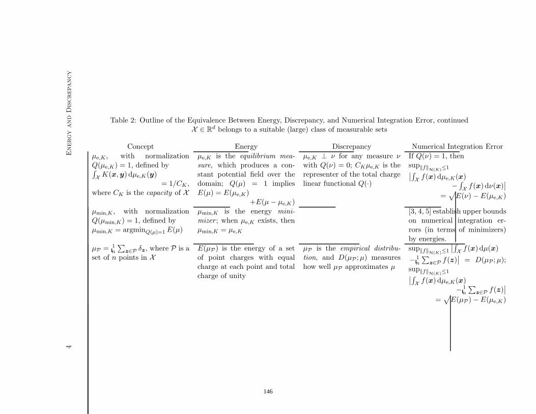
4Energy
and
Dis
crepa
ncy
Table 2: Outline of the Equivalence Between Energy, Discrepancy, and Numerical Integration Error, continuedX ∈ Rd belongs to a suitable (large) class of measurable sets
Concept Energy Discrepancy Numerical Integration Error
µe,K, with normalizationQ(µe,K) = 1, defined by∫
XK(x,y) dµe,K(y)
= 1/CK ,where CK is the capacity of X
µe,K is the equilibrium mea-sure, which produces a con-stant potential field over thedomain; Q(µ) = 1 impliesE(µ) = E(µe,K)
+E(µ − µe,K)
µe,K ⊥ ν for any measure ν
with Q(ν) = 0; CKµe,K is therepresenter of the total chargelinear functional Q(·)
If Q(ν) = 1, thensup
‖f‖H(K)
≤1∣
∣
∫
Xf(x) dµe,K(x)
−
∫
Xf(x) dν(x)
∣
∣
=√
E(ν) − E(µe,K)
µmin,K , with normalizationQ(µmin,K) = 1, defined byµmin,K = argminQ(µ)=1 E(µ)
µmin,K is the energy mini-mizer ; when µe,K exists, thenµmin,K = µe,K
[3, 4, 5] establish upper boundson numerical integration er-rors (in terms of minimizers)by energies.
µP = 1
n
∑
z∈Pδz, where P is a
set of n points in X
E(µP ) is the energy of a setof point charges with equalcharge at each point and totalcharge of unity
µP is the empirical distribu-tion, and D(µP ;µ) measureshow well µP approximates µ
sup‖f‖
H(K)≤1
∣
∣
∫
Xf(x) dµ(x)
−1
n
∑
z∈Pf(z)
∣
∣ = D(µP ;µ);sup
‖f‖H(K)
≤1∣
∣
∫
Xf(x) dµe,K(x)
−1
n
∑
z∈Pf(z)
∣
∣
=√
E(µP ) − E(µe,K)
146
Steven B. Damelin and Fred J. Hickernell 5
[6] Q. Du, V. Faber, M. Gunzburger, Centroidal Voronoi tessellations: applicationsand algorithms, SIAM Rev. 41 (4) (1999) 637–676.
[7] F. J. Hickernell, A generalized discrepancy and quadrature error bound, Math.Comp. 67 (1998) 299–322.
[8] F. J. Hickernell, Goodness-of-fit statistics, discrepancies and robust designs,Statist. Probab. Lett. 44 (1999) 73–78.
[9] F. J. Hickernell, What affects the accuracy of quasi-Monte Carlo quadrature?, in:H. Niederreiter, J. Spanier (eds.), Monte Carlo and Quasi-Monte Carlo Methods1998, Springer-Verlag, Berlin, 2000.
[10] H. Niederreiter, Random Number Generation and Quasi-Monte Carlo Methods,CBMS-NSF Regional Conference Series in Applied Mathematics, SIAM, Philadel-phia, 1992.
[11] T. J. Santner, B. J. Williams, W. I. Notz, The Design & Analysis of ComputerExperiments, Springer-Verlag, New York, 2003.
[12] SAS Institute, JMP 6.0 (2005).
[13] L. N. Trefethen, Spectral Methods in MATLAB, Software, Environments, Tools,SIAM, Philadelphia, 2000.
[14] H. Wendland, Scattered Data Approximation, No. 17 in Cambridge Monographson Applied and Computational Mathematics, Cambridge University Press, Cam-bridge, 2005.
[15] H. Weyl, Uber die Gleichverteilung der Zahlen mod Eins, Math. Ann. 77 (1916)313–352.
147
Proceedings of the International Conference on Computational and Mathematical Methods in Science and Engineering, CMMSE2007 Chicago, 20-23 June 2007
Investigation about Fractional Calculus in Financial Markets
Sergio Adriani David Faculty of Mathematics, Pontiff Catholic University of Campinas
São Paulo State - Brazil
email: [email protected]
Abstract In the last decade the progress in the areas of chaos and fractals revealed subtle relationships with the fractional calculus. Nonetheless, it is generally excluded from standard courses in mathematics, partly because many mathematicians are unfamiliar with its nature and its applications. One particular purpose of this paper is to discuss the usefulness of fractional-order calculus in financial markets. Even there is an increasing interest in the development of the new paradigm another purpose is to encourage the usage of this mathematical idea in other scientific areas by means of a historical apologia for development of the fractional calculus. Key words: Fractional Calculus, Finance
1. Introduction The theory of fractional calculus goes back to the beginning of the theory of differential calculus but its inherent complexity postponed the application of the associated concepts. In fact, fractional calculus is a natural extension of the classical mathematics. Since the beginning of the theory of differential and integral calculus, mathematicians such as Euler and Liouville investigated their ideas on the calculation of non-integer order derivatives and integrals. Perhaps, the subject would better be called integration and differentiation of arbitrary order. In spite of the work that has been done in the area, the application of fractional derivatives and integrals has been scarce until recently. However, in the last years, the advances in the theory of chaos revealed relations with fractional derivatives and integrals, motivating a renewed interest in this field. The basic aspects of the fractional calculus theory can be addressed in references [22]. In what concerns the application of the concepts can be mentioned research about damping [5,18] , chaos and fractals [19,21]. Regarding the adoption of this concept in other scientific areas I outline that several researchers has been inspired to paying attention to the new possibility.
148

CMMSE 2007
In special case of the applications involving financial markets only some researchers around the world has been interested by this tool [29]. Therefore, although this work is still giving its first steps and, consequently, many aspects remain to be investigated, I consider that it will be able possible a greater interest in this field. This paper is divided as follows. In section 2, I outline the origins of fractional calculus to doing permissible an historical apologia for the development. In the section 3 will be presented several approaches of mathematical formulation. Section 4 is devoted to the financial markets application possibility. Finally, in section 5 will be presented the conclusions and outlook
2. Origins and Historical Apologia
Leibniz when asked about what if n be ½ in n
n
xdyd said [28]: “Some day it would lead to
useful consequences”. In 1730 Euler mentioned interpolating between integral orders of a derivative. In 1812 Laplace defined a fractional derivative by means of an integral and in 1819 there appeared the first discussion of a derivative of fractional order in a calculus written by Lacroix. Lacroix expressed its nth derivative (for n ≤ m) in terms of Legrende’s symbol Г for the generalized factorial as follow:
nmnmn
nx
nmm
xnm
mxd
yd −−
+−Γ+Γ
=−
=)1(
)1(!)(
!
Thus, starting with the function y = xm replaced n with ½ and let m = 1, obtaining the derivative or order ½ of the function x :
xxxd
ydπ2
)2/3()2( 2/1
2/1
2/1=
ΓΓ
=
It was Liouville who made the first major study of fractional calculus. The Liouville’s first definition of a derivative of arbitrary order ν involved an infinite series. Here the series need to be convergent for some ν. The Liouville’s second definition was able to give a fractional derivative of x -a whenever both x and a are positive. Based on the definite integral related to the gamma integral of Euler can be to calculate the integral formula to x –a. Note that in the integral
∫∞
−−
0
1 dueu uxa
if we change the variables t = x u , then
149

CMMSE 2007
∫∫∫∫∞
−−−−
−−
−∞−− ==⎟
⎠⎞
⎜⎝⎛=
0
11
11
0
1 111 dtetx
dtx
exx
tdtx
extdueu ta
at
a
at
auxa
Thus,
∫∫∞
−−∞
−− =0
1
0
1 1 dtetx
dueu taa
uxa
But,
( ) ∫∞
−−=Γ0
1 dteta ta
Therefore, this yields the integral formula
( ) ∫∞
−−−
Γ=
0
11 dueua
x uxaa
Consequently, by analogy to equation (1),
( ) νννν
ν νν −−−−−
Γ+Γ
−=Γ
+Γ= aa
ax
aa
xa
axdxd
)()(
1)(
)(
The term in the last equation suggests the need to broaden the theory to include complex numbers.
( )ν1−
Indeed in terms of contemporary definitions, the modern theory of fractional calculus is intimately connected with the theory of operators. In classical calculus the symbol is often used fr the nth derivative operador ( for n ≥ 0) while, less commonly, is used for the antiderivative ( or integral ) operador.
nxD
1−xD
A convenient notation described by Davis [28] was the following: if υ is a positive real number, denotes differentiation of order υ of the function f along the x-axis. Similarly, the operator will denote integration of order υ of the function f along the x-axis.
)(xfDxcν
)(xfDxcν−
In fractional calculus there is no geometric interpretation of integration or differentiation of arbitrary order. Because this, the subscripts c and x are here called terminals of integration instead of limits of integration. This avoid unnecessary confusion. In 1884 Laurent published what is now recognized as the definitive paper in the foundation of fractional calculus. By means the Cauchy’s integral formula for complex valued analytic functions and a simple change of notation to employ a positive υ rather
150
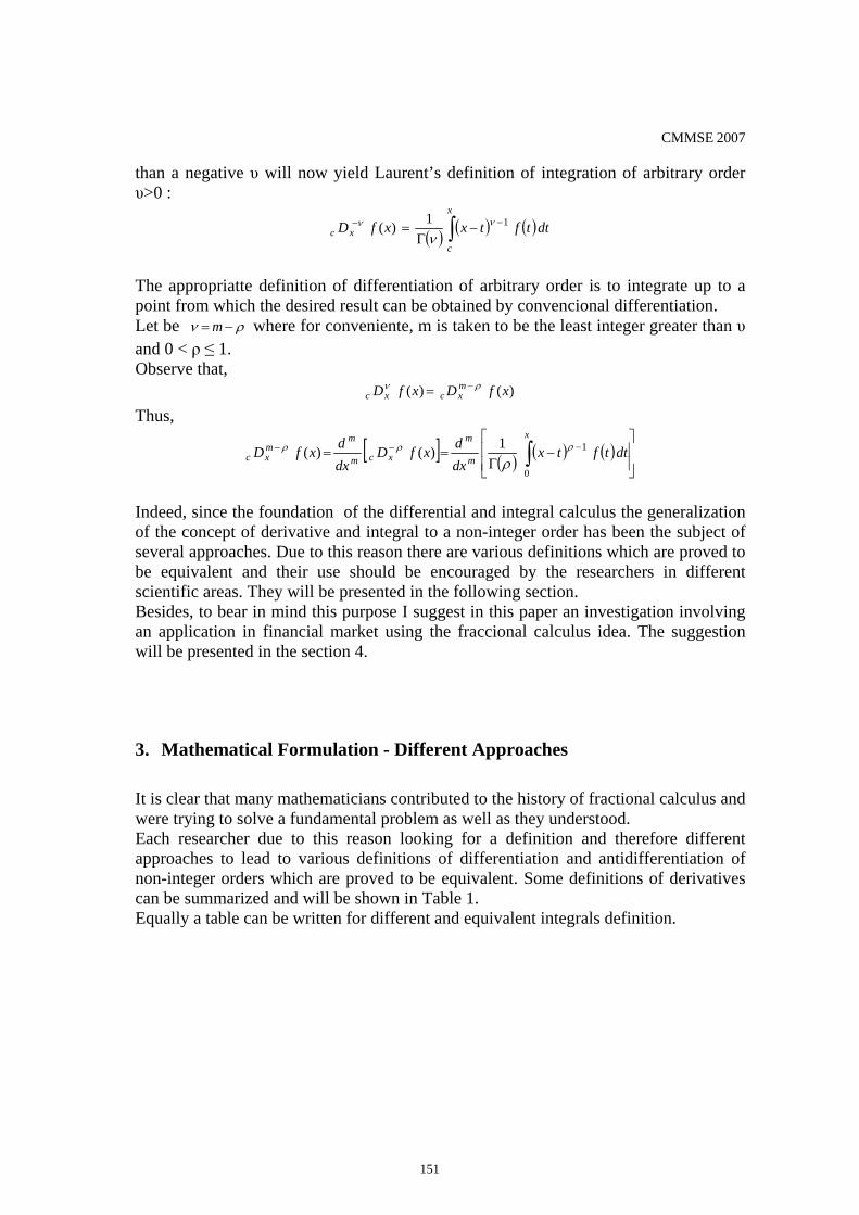
CMMSE 2007
than a negative υ will now yield Laurent’s definition of integration of arbitrary order υ>0 :
( ) ( ) ( )∫ −− −Γ
=x
cxc dttftxxfD 11)( νν
ν
The appropriatte definition of differentiation of arbitrary order is to integrate up to a point from which the desired result can be obtained by convencional differentiation. Let be ρν −=m where for conveniente, m is taken to be the least integer greater than υ and 0 < ρ ≤ 1. Observe that,
)()( xfDxfD mxcxc
ρν −= Thus,
[ ] ( ) ( ) ( )⎥⎥⎦
⎤
⎢⎢⎣
⎡−
Γ== ∫ −−−
x
m
m
xcm
mmxc dttftx
dxdxfD
dxdxfD
0
11)()( ρρρ
ρ
Indeed, since the foundation of the differential and integral calculus the generalization of the concept of derivative and integral to a non-integer order has been the subject of several approaches. Due to this reason there are various definitions which are proved to be equivalent and their use should be encouraged by the researchers in different scientific areas. They will be presented in the following section. Besides, to bear in mind this purpose I suggest in this paper an investigation involving an application in financial market using the fraccional calculus idea. The suggestion will be presented in the section 4.
3. Mathematical Formulation - Different Approaches It is clear that many mathematicians contributed to the history of fractional calculus and were trying to solve a fundamental problem as well as they understood. Each researcher due to this reason looking for a definition and therefore different approaches to lead to various definitions of differentiation and antidifferentiation of non-integer orders which are proved to be equivalent. Some definitions of derivatives can be summarized and will be shown in Table 1. Equally a table can be written for different and equivalent integrals definition.
151

CMMSE 2007
Table 1: Definition of derivatives of arbitrary order
Lacroix nmn
nx
nmm
xdyd −
+−Γ+Γ
=)1(
)1(
Liouville ( ) ννν
ν ν −−−
Γ+Γ
−= aa
xa
axdxd
)()(
1
Laurent ( ) ( ) ( )
⎥⎥⎦
⎤
⎢⎢⎣
⎡−
Γ== ∫ −−
x
m
mmxcxc dttftx
dxdxfDxfD
0
11)()( ρρν
ρ
Hadamard ( )
( ) ( )( )( ) ⎥
⎥⎦
⎤
⎢⎢⎣
⎡ −−Γ
= ∫ +
x
x dttxt
tfxfxfD0
1ln1)( ν
ν
νν
Chen ( ) ( ) ( )
⎥⎥⎦
⎤
⎢⎢⎣
⎡−
−Γ= ∫ −
x
m
m
x dttftxdxdxfD
011)( νν
ν
Marchaud
( )( ) ( )( ) ⎥
⎥
⎦
⎤
⎢⎢
⎣
⎡
−
−−Γ
= ∫∞−
+
x
x dttx
tfxfxfD νν
νν
11)(
Likewise other researchers have been important and contributed with owner approach and definition as well as Fourier, Laplace, Riemann, Grunwald-Letnikov. Although all this can be equivalent definitions , from the one specific point of view, that is to say for a specific application some definitions seem more attractive. The problem of to investigate an application in finance will be the matter of the next section.
4. Application in Finance The problem of estimating capital asset price volatility is good for risk management. The dynamics in financial markets demand full time complete and more accurate modelling. Although a good number of works has been published about financial markets, most of do not use the fractional calculus like tool. [1,3,4,6,7,14,15,16,32]. Nevertheless, some investigation in finance using fractional diffusion equation has been studied by Scalas et al [23]. In this section , I propose a simple model based on the following discussion: It is well- know that commonly occur a significant change in capital flow when the investors has at any moment a minimum risk perception changes. In this way it seems to me that is reasonable to imagine that the capital flow invested, denoted
dtd λ ,can be proportional to this risk perception changes denoted ( ). 0yy −
152

CMMSE 2007
Mathematically,
( )0
2
yydtd
−∝⎟⎠⎞
⎜⎝⎛ λ
Can be written,
( )0
2
yyCdtd
−−=⎟⎠⎞
⎜⎝⎛ λ
Note that the an increasing in the risk perception can to stimulate a reduction in the capital injection. This is the meaning of minus signal in above equation. Thus,
( )yyCdtd
−= 0λ
and
( )dtC
yyd
=−0
λ
Now, integrating both sides,
( )∫∫ −−=0
0
210
0
yT
dyydtC λ
or,
( )∫ −−=0
0
210
y
dyyK λ
where TCK = Here we can to observe that ( )yF=λ where λ is the amount of capital of return and y represent the risk perception. To bear in mind this fact, we can notice ( ) dyyFd '=λ If we change variables and to 0y y x and t, and replace 'F by the integral equation becomes
f
( ) ( )∫ −−=x
dttftxK0
21
From now the problem is to determine the function . This can be done multiplying the last equation by
f
( )211Γ in order to obtain
( ) ( ) ( ) ( ) ( )xfDdttftxKx
x21
00
21
211
21−− =−
Γ=
Γ ∫
153

CMMSE 2007
Consequently,
( )xfKDx π=210 (*)
I outline that of the general Laurent’s definition of derivative let us now consider the derivative of order 21 of the constant K . Using we can notice ρν −= mDD
( ) ( ) ( ) ( ) ( ) ( )ν
ρρρν
νρρρρρρ−
−−
−Γ=
Γ−=
⎥⎥⎦
⎤
⎢⎢⎣
⎡
Γ=
⎥⎥⎦
⎤
⎢⎢⎣
⎡−
Γ= ∫ xK
mxpKxK
dxddtKtx
dxdKD
m
m
mx
m
m
x 1!!1
0
10
In particular case where 21=ν we haven,
( )212121
0 21−− =
Γ= xKxKKDx
π(**)
Therefore, from (*) and (**) can be concluded
( )x
Kxfπ
=
This curious results show similarity with the solution to the tautochrone problem solved by Abel [28]. Of course , there are limitations to the model proposed. For instance, I am essentially considering the single asset in isolation. The estimation of other unknown parameters is not treated here Perhaps the quadratic order for
dtd λ could be better adjusted.
This work is still living its first steps and consequently, many aspects remain to be investigated.
5. Conclusions The recent progress in the area of chaos reveals promising aspects for future developments and application of the theory of fractional calculus in various scientific areas. In this paper the treatment of fractional calculus has been suggestive rather than rigorous in order to rescue the interest to the reader and at the same time to provide a hint of its potential in many scientific areas. In special case of the financial markets some preliminary works has been proposed. A simple model system involving risk and capital return based on the fractional order concepts are simple to implement and reveal a good alternative way of prediction in financial markets.
154

CMMSE 2007
Besides, in accordance to the nature of this conference this paper have also contributed to the interdisciplinary feature involving fractional calculus applied in finance systems by means of modeling, presentation and discussion about capital flow when the investors has at any moment a minimum risk perception changes.
References
[1] ] Akdeniz, L., Dechert, W. D., "Risk and Return in a Dynamic Asset Pricing Model", In Proc: Second International Conference on Computing in Economics and Finance. Geneva, Switzerland, 1996
[2] Anastasio, T. J. , “The Fractional-Order Dynamics of Brainstem Vestibulo-oculomotor Neurons”, Biological Cybernetics, vol. 72, pp. 69-79 , 1994. [3] Anderson, E. W., Hansen, L. P., "Perturbation Methods for Risk-Sensitive Economies", Second International Conference on Computing in Economics and Finance. Geneva, Switzerland, 1996.
[4 ] Arcoverde, G. Lins , "Uma nota sobre o procedimento de Mapeamentos em Vértices nos modelos de cálculo do VaR de instrumentos de renda fixa”, 1999. Artigo downloadable de : http://www.risktech.com.br/
[5] Bagley, R.L , Torvik, P.J. , “On the Fractional Calculus Model of Viscoelastic Behaviour” Journal of Rheology, vol. 3-, no. 1, pp. 133-135, 1986.
[6] Clark, P. K. , “A subordinated stochastic process model with finite variance for speculative prices”, Econometrica, vol 41, pp. 135-156, 1973. [7] Correia, M.M.R.L., “Memória longa, agrupamento de valores extremos e assimetria em séries financeiras”. Dissertação de mestrado. Universidade de São Paulo – USP – 1997. [8] Correia, M.M.R.L, Pereira, P.L.V. “Modelos não lineares em finanças: previsibilidade em mercados financeiros e aplicações à gestão de risco”. Annals of the XXI Brazilian Econometric Meeting, Vol 1, p. 240-59, Brazilian Econometric Society: Vitória, Espírito Santo. 1998.
[9] David, S.A., Rosário, J.M., Machado, J. “Chaotic Vibrations of a beam induced by magnetoelastic interactions”. VII International Conference on Computational Plasticity – Barcelona – Espanha ( 07/04/2003 a 10/04/2003).
155
CMMSE 2007
[10] David, S.A, Rosário, J. M., Machado, J.: “On Numerical Simulations of a Magnetoelastic Dynamical Systems”, Nonlinear Dynamics, Chaos, Control and their Applications to Engineering Sciences, Chapter 2: Nonlinear Dynamics, Vol 5. Chaos Control and Times Series, Published by ABCM, AAM, SBMAC and SIMAI, pp. 157-166,ISBN: 85-900351-5-8, (2002). [11] David, S.A., Rosário, J.M.: “Investigation about Nolinearities in a Robot with Elastic Members”, Computational Fluid and Solid Mechanics, Solids and Structures, vol.1, K.J.Bathe editor, pp. 137-139, Elsevier Science Ltd., England, ISBN 0-08-043944-6. (2001) [12] David, S.A., Rosário, J.M., Machado, J.: “Investigation about Chaos in a Magneto-elastic Dynamical System”, Computational Fluid and Solid Mechanics, Multi-Physics, vol.2, K.J.Bathe editor, pp. 1120-1123, Elsevier Science Ltd., England, ISBN 0-08-043944-6. (2001)
[13] David, S.A.; Rosário, J.M. (1999): “Modeling, Simulation and Control of Flexible Robots” Nonlinear Dynamics, Chaos, Control and Their Applications to Engineering Sciences, Chapter 3: Control, Robotics, Neural Networks and Optimization Engineering, vol. 1, Published by ABCM and AAM, pp. 353-358, ISBN: 85-900351-2-3, (1999). [14] Daykin, C. D. , "Practical Risk Theory for Actuaries", (1994).
[15] Garman, M. B., "Descomposición de los Elementos Componentes del VeR Dentro de una Cartera de Inversión", Financial Engineering Associates, Inc., (1997). [16] Garman, M. B., Klass, M. J. , “On the Estimation of Security Price Volatility from Historical Data”, Financial Engineering Associates, Inc., (2003). [17] Gaul, L. , Chen, C. M., “Modeling of Viscoelastic Elastomer Mounts in Multibody Systems”, Advanced Multibody System Dynamics, W. Schielen (ed.) , pp. 257-276, Kluwe Academic Publishers, (1993). [18] Koeller, R. C. , “Applications of Fractional Calculus to the Theory of Viscoelasticity”, ASME , Journal of Applied Mechanics”, vol. 51, pp. 299 – 307 , June (1984). [19] Liu, S. H. , “Fractal Model for the ac Response of a Rough Interface”, Physical Review Letters. Vol.55 no. 5, pp. 529-532, July (1985). [20] Machado, J. A. T. , “System Modeling and Control Trough Fractional-Order Algorithms”, Nonlinear Dynamics, Chaos, Control and Their Applications to Engineering Sciences, vol. 4, pp. 99-115, (2002).
156

CMMSE 2007
[21] Machado, J. A. T. , “Analysis and Design of Fractional-Order Digital Control systems”, SAMS – Journal Systems Analysis, Modelling, Simulation, vol. 27 , pp. 107-122, (1997). [22] Machado, J. A. T. , Azenha, A. “Position/Force Fractional Control of Mechanical Manipulators”, IEEE Int. Workshop on Advanced Motion Control, Coimbra, Portugal, (1998). [23] Mainardi, F. “ Fractional Relaxation-Oscillation and Fractional Diffusion –Wave Phenomena”. Chaos, Solitons & Fractals, vol. 7, no. 9, pp. 1461-1477, (1996).
[24] Mathieu, B., Lay, L. L. , Oustaloup, A. “Identifications of Non-Integer Order Systems in Time Domain”, IEEE-SMC/IMACS Symposium on Control, Optimization and Supervision, pp. 952-956, Lille, France, (1996). [25] Méhauté, A. L. , “From Dissipative and Non-Dissipative Processes in Fractal Geometry: The Janal”, New Journal of Chemistry, vpl.14, no. 3, pp. 207-215, (1990). [26] Oustaloup, A. ,”Fractional Order Sinusoidal Oscillators: Optimization and Their Use in Highly Linear FM Modulation”, IEEE Trans. On Cicuits and systems, vol. 28, no. 10, pp. 1007-1009, October (1981). [27] Ozaktas, H. M. , Arikan, O. , Kutay, M. A. , Bozdagi, G. , “Digital Computation of the Fractional Fourier Transform”, IEEE Trans. On signal Processing, vol. 44, no. 9, pp. 2141-2150, Sept. (1996). [28] Ross Bertram , “Fractional Calculus”, Mathematics Magazine, vol. 50, no. 3, pp. 115-122, Maio (1977). [29] Scalas, E. , Gorenflo, R. , Mainardi, F. , “Fractional Calculus and continuous time finance “, Physica A, vol. 284, pp. 376-384 , (2000). [30] Schor, A ; Bonomo, M & Valls Pereira, P. L. "Arbitrage Pricing Theory (APT) and Macroeconomics Variables: a comparative study for the brazilian stock market". Annals of the XXI Brazilian Econometric Meeting, vol 1, p. 181-200, Brazilian Econometric Society: Vitória, Espírito Santo, (1998).
[31] Souza, L.A.R. & Da Silva, M. E., "Teoria de Valores Extremos para Cálculo de VaR",(1999). Artigo downloadable de : http://www.risktech.com.br/
157

CMMSE 2007
[32] Ursini, E. L. Girolami, A. David, S.A “Optimal Dynamic Investment Path of the Firm: Planned Rate of Return, Prices (Tariffs) and Impairments due to Technological Obsolescence. In Proc: International Conference on Computational and Mathematical Methods in Science and Engineering - Alicante - Espanha - (20/09/2002 a 25/09/2002)
[33] Ziegelmann, F. A. , Pereira, P.L.V., “Modelos de Volatilidade estocástica com deformação temporal: um estudo empírico para o índice Bovespa”, Pesquisa e Planejamento Econômico, 27, 2, p.323-343. (1997).
158
Proceedings of the International Conferenceon Computational and Mathematical Methodsin Science and Engineering, CMMSE 2007Chicago, 20–23 June 2007.
On the optimal approximation for the symmetricProcrustes problems of the matrix equation AXB = C
Yuanbei Deng 1 and Daniel Boley2
1 College of Mathematics and Econometrics, Hunan University, Changsha,Hunan410082, P.R.China
2 Department of Computer Science and Engineering, University of Minnesota,Minneapolis, MN55455,U.S.A.
emails: [email protected], [email protected]
Abstract
The explicit analytical expressions of the optimal approximation solutions forthe symmetric Procrustes problems of the linear matrix equation AXB = C arederived, with the projection theorem in Hilbert space , the quotient singular valuedecomposition (QSVD) and the canonical correlation decomposition (CCD) beingused.
Key words: Linear matrix equation, least squares problem, optimal approxima-tion , QSVD , CCD
MSC 2000: 65F15,65F20
1 Introduction
The least-squares problems of linear matrix equations are called Procrustes problems(cf.Higham,1988 and Andersson and Elfving, 1997). The unconstrained and constrainedleast squares problems have been of interest for many applications, including particlephysics and geology , inverse Sturm-Liouville problem [11], inverse problems of vibra-tion theory [6], control theory, digital image and signal processing, photogrammetry,finite elements, and multidimensional approximation [8]. Penrose(cf. [2], [13] ) firstconsidered the linear matrix equation
AX = B (1.1)
and obtained its general solution and least-squares solution by making use of the Moore-Penrose generalized inverse, then Sun[14] obtained the least-squares solution and therelated optimal approximation solution of Eq. (1.1) when X is a real matrix. When X
159
is constrained to be a real symmetric matrix , the least-squares solution of (1.1) wasderived by Higham and Sun respectively in 1988([12] and [15]) , and Sun also obtainedthe related symmetric optimal approximation solution of Eq. (1.1) in [15].
In this paper , the following linear matrix equation
AXB = C (1.2)
are considered . Fausett and Fulton[8] and Zha[18] considered the unconstrained least-squares problems of Eq. (1.2), Eric Chu[4] and Dai Hua[5] obtained the general ex-pressions for the symmetric solution of Eq. (1.2) by using the general singular valuedecomposition of matrices (GSVD), and the symmetric and skew-symmetric least-squares solutions of Eq. (1.2) have been derived by Deng, Hu and Zhang[7]. Butit remains unsolved about the optimal approximation solutions for the symmetric andskew-symmetric Procrustes problems of this equation. Therefore in the following, wewill consider the optimal approximation solutions of the symmetric least squares prob-lems of Eq. (1.2). We always suppose that Rm×n is the set of all m× n real matrices,SRn×n and ORn×n are the sets of all symmetric and orthogonal matrices in Rn×n,respectively, A ∗ B represent the Hadamard product of A and B, and ‖Y ‖F denotesthe Frobenius norm of a real matrix Y , defined as
‖Y ‖2F =< Y, Y >=
∑
i,j
y2ij ,
here the inner product is given by < A, B >= trace(AT B), and Rm×n become a Hilbertspace with the inner product.
Problem I. Given matrices A ∈ Rm×n,B ∈ Rn×p,C ∈ Rm×p and Xf ∈ Rn×n, let
SE = X|X ∈ SRn×n, ‖AXB − C‖F = min. (1.3)
Then find Xe ∈ SE , such that
‖Xe −Xf‖F = minX∈SE
‖X −Xf‖F . (1.4)
We first introduce some results about the quotient singular value decomposition(QSVD) and the canonical correlation decomposition (CCD)of matrices , as soon asthe projection theorem on Hilbert space, which are essential tools for the Problem , see[3],[9], [10] and [16] for details.
The QSVD is a simple form of the GSVD. The QSVD of a pair of matrices (A,BT )is as follows.
QSVD Theorem. Let A ∈ Rm×n, B ∈ Rn×p. Then there exist orthogonalmatrices U ∈ ORm×m, V ∈ ORp×p and a nonsingular matrix Y ∈ Rn×n such that
A = UΣ1Y−1, BT = V Σ2Y
−1, (1.5)
where
Σ1 =
Ir′ 0 0 00 S 0 00 0 0 0
r′
s′
m− r′ − s′,
r′ s′ t′ n− k′(1.6)
160

Σ2 =
0 0 0 00 Is′ 0 00 0 It′ 0
p + r′ − k′
s′
t′,
r′ s′ t′ n− k′(1.7)
k′ = rank(AT , B), r′ = k′ − rank(B),
s′ = rank(A) + rank(B)− k′, S = diag(σ1, · · · , σs′),
σi > 0(i = 1, · · · , s′), t′ = k′ − r′ − s′.
When A and BT are of full column rank, i.e. r(B) = r(A) = n, then r′ = 0, s′ = n, k′ =n, and
Σ1 =(
S0
)n
m− n, Σ2 =
(0Is′
)p− n
n.
n n(1.8)
The canonical correlations decomposition of the matrix pair (AT , B) is given bythe following theorem.
CCD Theorem. LetA ∈ Rm×n, B ∈ Rn×p, and assume that g = rank(A), h =rank(B), g ≥ h. Then there exist a orthogonal matrix Q ∈ ORn×n and nonsingularmatrices XA ∈ Rm×m, XB ∈ Rp×p such that
AT = Q[ΣA, 0]X−1A , B = Q[ΣB, 0]X−1
B , (1.9)
where ΣA ∈ Rn×g and ΣB ∈ Rn×h are of the forms:
ΣA =
Ii 0 00 Λj 00 0 00 0 00 ∆j 00 0 It
, ΣB =(
Ih
0
), (1.10)
with the same row partitioning, and
Λj = diag(λi+1, . . . , λi+j), 1 > λi+1 ≥ . . . ≥ λi+j > 0,∆j = diag(δi+1, . . . , δi+j), 0 < δi+1 ≤ . . . ≤ δi+j < 1,λ2
i+1 + δ2i+1 = 1, . . . , λ2
i+j + δ2i+j = 1, i.e.,Λ2
j + ∆2j = I,
Here,i = rank(A) + rank(B)− rank[AT , B],j = rank[AT , B] + rank(AB)− rank(A)− rank(B),t = rank(A)− rank(AB), g = i + j + t.
Following is the projection theorem (cf. [16]).
Lemma 1.1 Let H be a Hilbert space, M be a subspace of H, andM⊥ be the orthogonalcomplement subspace of M. For a given H ∈ H, if there exists an M0 ∈ M such that‖H −M0‖ ≤ ‖H −M‖ holds for any M ∈ M, then M0 is unique and M0 ∈ M is theunique minimization vector in M if and only if (H −M0)⊥M, i.e.,(H −M0) ∈M⊥.
161

2 The main results
In this section, the explicit expression for the solution of Problem I is derived. Withoutloss of generality, we suppose that rank(A) ≥ rank(B).
Instead of considering the solution of Problem I, we will find a matrix C0, and thentransform Problem I to the following equivalent problem.
Problem I0. Given matrices A ∈ Rm×n,B ∈ Rn×p,C0 ∈ Rm×p and Xf ∈ Rn×n,let
SE0 = X|X ∈ SRn×n, AXB = C0. (2.11)
Then find Xe ∈ SE0 , such that
‖Xe −Xf‖F = minX∈SE0
‖X −Xf‖F . (2.12)
First we use the projection theorem on Rm×p.
Theorem 2.1 Given A ∈ Rm×n, B ∈ Rn×p, C ∈ Rm×p, let X0 be one of the symmetricleast-squares solutions of the matrix equation (1.2) and define
C0 = AX0B, (2.13)
then the matrix equation
AXB = C0, (2.14)
is consistent in SRn×n, and the symmetric solution set SE0 of the matrix equation(2.13) is the same as the symmetric least-squares solution set SE of the matrix equation(1.2).
Proof. Let
L = Z|Z = AXB, X ∈ SRn×n. (2.15)
Then L is obviously a linear subspace of Rm×p.Because X0 is the symmetric least-squares solutions of the matrix equation (1.2), from (2.13) we see that C0 ∈ L and
‖C0 − C‖F = ‖AX0B − C‖F
= minX∈SRn×n ‖AXB − C‖F
= minZ∈L ‖Z − C‖F .
Then by Lemma 1.1 we have
(C0 − C)⊥L or (C0 − C) ∈ L⊥.
162

Next for all X ∈ SRn×n, AXB − C0 ∈ L, it then follows that
‖AXB − C‖2F
= ‖(AXB − C0) + (C0 − C)‖2F
= ‖AXB − C0‖2F + ‖C0 − C‖2
F .
Hence, SE = SE0 , and the conclusion of the theorem is true. ¤Now suppose A ∈ Rm×n, B ∈ Rn×p and the matrix pair (A,BT ) has the QSVD
(1.5), and partition UT CV into the following blocks matrix.
UT CV =
C11 C12 C13
C21 C22 C23
C31 C32 C33
r′
s′
m− r′ − s′
p + r′ − k′ s′ t′, (2.16)
then the expression of C0 will be shown in the following theorem.
Theorem 2.2 Let A,B, C be given in Problem I, the matrix pair (A,BT ) have theQSVD (1.5), and UT CV be partitioned by (2.16), then for any symmetric least-squaressolution X0 of the matrix equation (1.2) the matrix C0 defined by (2.13) can be deter-mined by the following form.
C0 = UC∗V T , C∗ =
0 C12 C13
0 SX22 C23
0 0 0
r′
s′
m− r′ − s′
p + r′ − k′ s′ t′, (2.17)
where
X22 = φ ∗ (CT22S + SC22),
φ = (ϕkl) ∈ SRs′×s′ , ϕkl = 1σ2
k+σ2l, 1 ≤ k, l ≤ s′.
(2.18)
Proof. From Theorem 2.1 in [7] we know that the symmetric least-squares solutionof the matrix equation (1.2) can be obtained using of the QSVD of matrix pair (A,BT )and the general form of the solution is
X0 = Y
X ′11 C12 C13 X ′
14
CT12 X22 S−1C23 X ′
24
CT13 (S−1C23)T X ′
33 X ′34
X ′T14 X ′T
24 X ′T34 X ′
44
Y T , (2.19)
where X22 is given by (2.18) and X ′11 ∈ SRr′×r′ , X ′
33 ∈ SRt′×t′ , X ′44 ∈ SR(n−k′)×(n−k′),
163
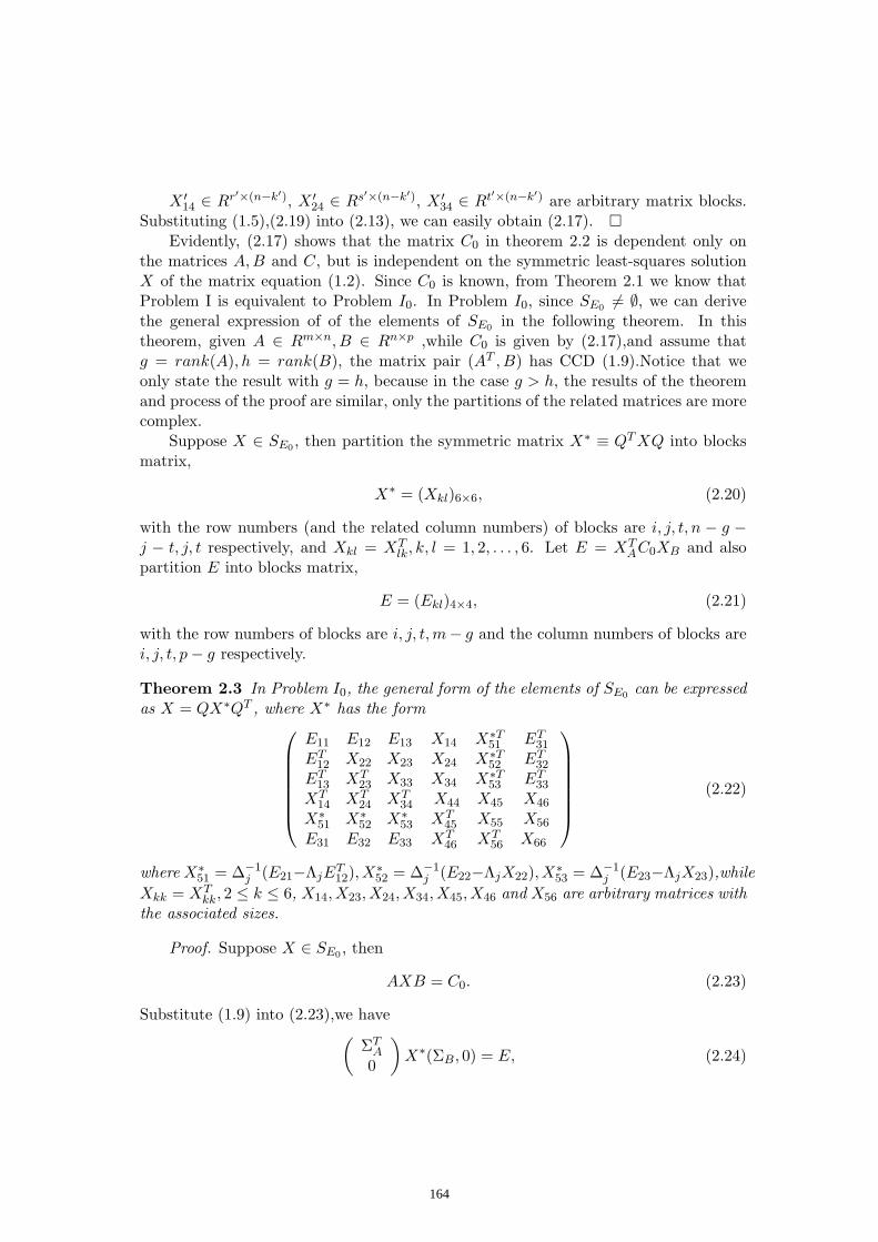
X ′14 ∈ Rr′×(n−k′), X ′
24 ∈ Rs′×(n−k′), X ′34 ∈ Rt′×(n−k′) are arbitrary matrix blocks.
Substituting (1.5),(2.19) into (2.13), we can easily obtain (2.17). ¤Evidently, (2.17) shows that the matrix C0 in theorem 2.2 is dependent only on
the matrices A,B and C, but is independent on the symmetric least-squares solutionX of the matrix equation (1.2). Since C0 is known, from Theorem 2.1 we know thatProblem I is equivalent to Problem I0. In Problem I0, since SE0 6= ∅, we can derivethe general expression of of the elements of SE0 in the following theorem. In thistheorem, given A ∈ Rm×n, B ∈ Rn×p ,while C0 is given by (2.17),and assume thatg = rank(A), h = rank(B), the matrix pair (AT , B) has CCD (1.9).Notice that weonly state the result with g = h, because in the case g > h, the results of the theoremand process of the proof are similar, only the partitions of the related matrices are morecomplex.
Suppose X ∈ SE0 , then partition the symmetric matrix X∗ ≡ QT XQ into blocksmatrix,
X∗ = (Xkl)6×6, (2.20)
with the row numbers (and the related column numbers) of blocks are i, j, t, n − g −j − t, j, t respectively, and Xkl = XT
lk, k, l = 1, 2, . . . , 6. Let E = XTAC0XB and also
partition E into blocks matrix,
E = (Ekl)4×4, (2.21)
with the row numbers of blocks are i, j, t,m− g and the column numbers of blocks arei, j, t, p− g respectively.
Theorem 2.3 In Problem I0, the general form of the elements of SE0 can be expressedas X = QX∗QT , where X∗ has the form
E11 E12 E13 X14 X∗T51 ET
31
ET12 X22 X23 X24 X∗T
52 ET32
ET13 XT
23 X33 X34 X∗T53 ET
33
XT14 XT
24 XT34 X44 X45 X46
X∗51 X∗
52 X∗53 XT
45 X55 X56
E31 E32 E33 XT46 XT
56 X66
(2.22)
where X∗51 = ∆−1
j (E21−ΛjET12), X
∗52 = ∆−1
j (E22−ΛjX22), X∗53 = ∆−1
j (E23−ΛjX23),whileXkk = XT
kk, 2 ≤ k ≤ 6, X14, X23, X24, X34, X45, X46 and X56 are arbitrary matrices withthe associated sizes.
Proof. Suppose X ∈ SE0 , then
AXB = C0. (2.23)
Substitute (1.9) into (2.23),we have(
ΣTA
0
)X∗(ΣB, 0) = E, (2.24)
164
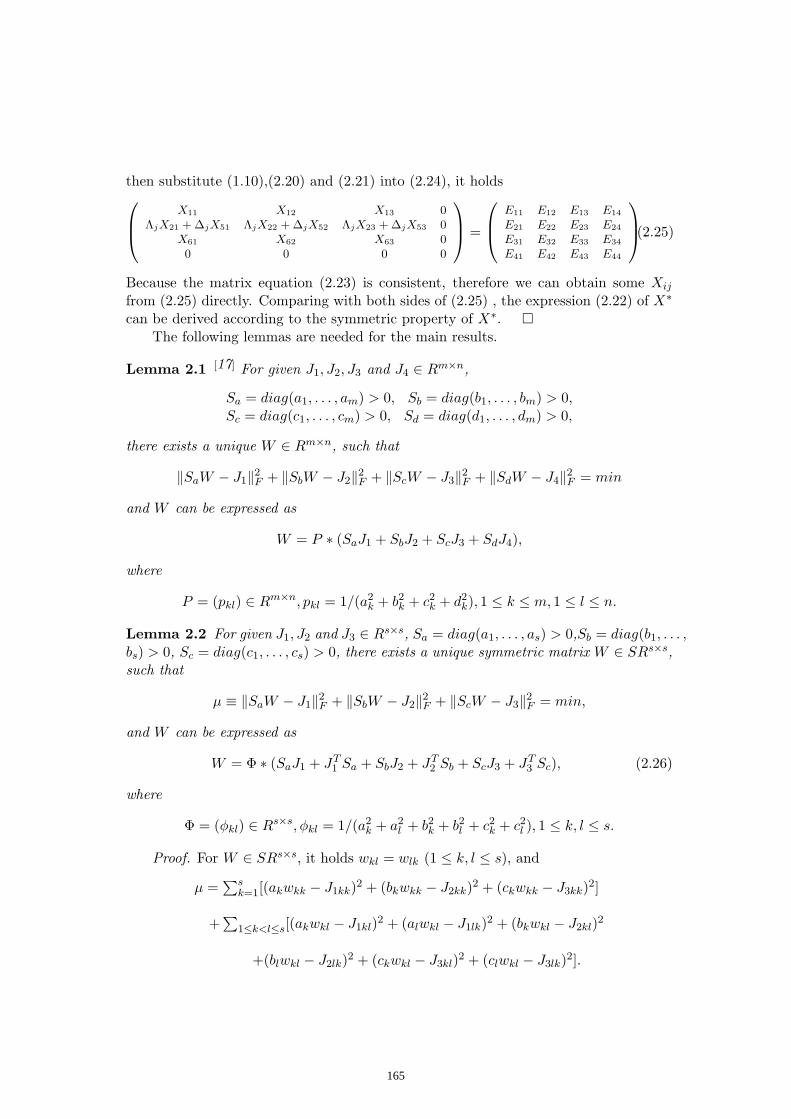
then substitute (1.10),(2.20) and (2.21) into (2.24), it holds
X11 X12 X13 0ΛjX21 + ∆jX51 ΛjX22 + ∆jX52 ΛjX23 + ∆jX53 0
X61 X62 X63 00 0 0 0
=
E11 E12 E13 E14
E21 E22 E23 E24
E31 E32 E33 E34
E41 E42 E43 E44
.(2.25)
Because the matrix equation (2.23) is consistent, therefore we can obtain some Xij
from (2.25) directly. Comparing with both sides of (2.25) , the expression (2.22) of X∗
can be derived according to the symmetric property of X∗. ¤The following lemmas are needed for the main results.
Lemma 2.1 [17] For given J1, J2, J3 and J4 ∈ Rm×n,
Sa = diag(a1, . . . , am) > 0, Sb = diag(b1, . . . , bm) > 0,Sc = diag(c1, . . . , cm) > 0, Sd = diag(d1, . . . , dm) > 0,
there exists a unique W ∈ Rm×n, such that
‖SaW − J1‖2F + ‖SbW − J2‖2
F + ‖ScW − J3‖2F + ‖SdW − J4‖2
F = min
and W can be expressed as
W = P ∗ (SaJ1 + SbJ2 + ScJ3 + SdJ4),
where
P = (pkl) ∈ Rm×n, pkl = 1/(a2k + b2
k + c2k + d2
k), 1 ≤ k ≤ m, 1 ≤ l ≤ n.
Lemma 2.2 For given J1, J2 and J3 ∈ Rs×s, Sa = diag(a1, . . . , as) > 0,Sb = diag(b1, . . . ,bs) > 0, Sc = diag(c1, . . . , cs) > 0, there exists a unique symmetric matrix W ∈ SRs×s,such that
µ ≡ ‖SaW − J1‖2F + ‖SbW − J2‖2
F + ‖ScW − J3‖2F = min,
and W can be expressed as
W = Φ ∗ (SaJ1 + JT1 Sa + SbJ2 + JT
2 Sb + ScJ3 + JT3 Sc), (2.26)
where
Φ = (φkl) ∈ Rs×s, φkl = 1/(a2k + a2
l + b2k + b2
l + c2k + c2
l ), 1 ≤ k, l ≤ s.
Proof. For W ∈ SRs×s, it holds wkl = wlk (1 ≤ k, l ≤ s), and
µ =∑s
k=1[(akwkk − J1kk)2 + (bkwkk − J2kk)2 + (ckwkk − J3kk)2]
+∑
1≤k<l≤s[(akwkl − J1kl)2 + (alwkl − J1lk)2 + (bkwkl − J2kl)2
+(blwkl − J2lk)2 + (ckwkl − J3kl)2 + (clwkl − J3lk)2].
165

Since the function µ is a continuous and differentiable function of 12s(s + 1) variables
wkl, hence µ obtains its minimum value at wkl when ∂µ∂wkl
= 0, i.e.,
wkl =akJ1kl + alJ1lk + bkJ2kl + blJ2lk + ckJ3kl + clJ3lk
a2k + a2
l + b2k + b2
l + c2k + c2
l
, 1 ≤ k ≤ l ≤ s.
Therefore W can be expressed by (2.26). ¤Finally we give the the optimal approximation solutions for the symmetric least-
squares problems of the linear matrix equation AXB = C, and we still suppose thatrank(A) = rank(B).
Theorem 2.4 Let matrices A,B, C and Xf be given in Problem I, suppose rank(A) =rank(B), partition the matrix QT XfQ into blocks matrix
QT XfQ = (X(f)kl )6×6, (2.27)
with the same row and column numbers as X∗ of (2.20). Then the unique solution Xe
of Problem I can be expressed as Xe = QX∗QT , and X∗ is equal to
E11 E12 E13 X(f)14 XT
51 ET31
ET12 X22 X23 X(f)
24 XT52 ET
32
ET13 XT
23 X(f)33 X(f)
34 XT53 ET
33
X(f)41 X(f)
42 X(f)43 X(f)
44 X(f)45 X(f)
46 X51 X52 X53 X(f)
54 X(f)55 X(f)
56 E31 E32 E33 X(f)
64 X(f)65 X(f)
66
(2.28)
where X51 = ∆−1j (E21 − ΛjE
T12), X52 = ∆−1
j (E22 − ΛjX22), X53 = ∆−1j (E23 − ΛjX23),
X(f)kl =
12(X(f)
kl + X(f)Tlk ) = X(f)
lk T ,
X22 = Ψ ∗ [X(f)22 + X
(f)T22 + ∆−1
j Λj(∆−1j E22 −X
(f)T25 ) + (∆−1
j E22 −X(f)T25 )T Λj∆−1
j
+∆−1j Λj(∆−1
j E22 −X(f)52 ) + (∆−1
j E22 −X(f)52 )T Λj∆−1
j ],
Ψ = (ψkl) ∈ Rj×j , ψkl =1
2(1 + ( δi+k
λi+k)2) + ( δi+l
λi+l)2)
, 1 ≤ k, l ≤ j.
and
X23 = G ∗ [X(f)23 + X
(f)T32 + ∆−1
j Λj(∆−1j E23 −X
(f)T35 ) + ∆−1
j Λj(∆−1j E23 −X
(f)53 ),
G = (gkl) ∈ Ri×t, gkl =12λi+k, 1 ≤ k,≤ i, 1 ≤ l ≤ t.
166
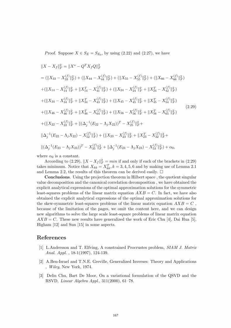
Proof. Suppose X ∈ SE = SE0 , by using (2.22) and (2.27), we have
‖X −Xf‖2F = ‖X∗ −QT XfQ‖2
F
= (‖X33 −X(f)33 ‖2
F ) + (‖X44 −X(f)44 ‖2
F ) + (‖X55 −X(f)55 ‖2
F ) + (‖X66 −X(f)66 ‖2
F )
+(‖X14 −X(f)14 ‖2
F + ‖XT14 −X
(f)41 ‖2
F ) + (‖X24 −X(f)24 ‖2
F + ‖XT24 −X
(f)42 ‖2
F )
+(‖X34 −X(f)34 ‖2
F + ‖XT34 −X
(f)43 ‖2
F ) + (‖X45 −X(f)45 ‖2
F + ‖XT45 −X
(f)54 ‖2
F )
+(‖X46 −X(f)46 ‖2
F + ‖XT46 −X
(f)64 ‖2
F ) + (‖X56 −X(f)56 ‖2
F + ‖XT56 −X
(f)65 ‖2
F )
+(‖X22 −X(f)22 ‖2
F + ‖(∆−1j (E22 − ΛjX22))T −X
(f)25 ‖2
F +
‖∆−1j (E22 − ΛjX22)−X
(f)52 ‖2
F ) + (‖X23 −X(f)23 ‖2
F + ‖XT23 −X
(f)32 ‖2
F +
‖(∆−1j (E23 − ΛjX23))T −X
(f)35 ‖2
F + ‖∆−1j (E23 − ΛjX23)−X
(f)53 ‖2
F ) + α0,
(2.29)
where α0 is a constant.According to (2.29), ‖X−Xf‖2
F = min if and only if each of the brackets in (2.29)takes minimum. Notice that Xkk = XT
kk, k = 3, 4, 5, 6 and by making use of Lemma 2.1and Lemma 2.2, the results of this theorem can be derived easily. ¤
Conclusions. Using the projection theorem in Hilbert space , the quotient singularvalue decomposition and the canonical correlation decomposition , we have obtained theexplicit analytical expressions of the optimal approximation solutions for the symmetricleast-squares problems of the linear matrix equation AXB = C. In fact, we have alsoobtained the explicit analytical expressions of the optimal approximation solutions forthe skew-symmetric least-squares problems of the linear matrix equation AXB = C ,because of the limitation of the pages, we omit the content here, and we can designnew algorithms to solve the large scale least-square problems of linear matrix equationAXB = C. These new results have generalized the work of Eric Chu [4], Dai Hua [5],Higham [12] and Sun [15] in some aspects.
References
[1] L.Andersson and T. Elfving, A constrained Procrustes problem, SIAM J. MatrixAnal. Appl. , 18-1(1997), 124-139.
[2] A.Ben-Israel and T.N.E. Greville, Generalized Inverses: Theory and Applications, Wiley, New York, 1974.
[3] Delin Chu, Bart De Moor, On a variational formulation of the QSVD and theRSVD, Linear Algebra Appl., 311(2000), 61–78.
167

[4] King-wah Eric Chu, Symmetric solutions of linear matrix equations by matrixdecompositions, Linear Algebra Appl., 119(1989), 35–50.
[5] Dai Hua, On the symmetric solutions of linear matrix equations, Linear AlgebraAppl. , 131(1990),1-7.
[6] Dai Hua,P.Lancaster, Linear matrix equations from an inverse problem of vibrationtheory, Linear Algebra Appl., 246(1996),31–47.
[7] Yuanbei Deng, Xiyan Hu and Lei Zhang, Least squares solution of BXA’=T oversymmetric, skew-symmetric and positive semi-definite X, SIAM J. Matrix Anal.Appl. , 25-2(2003),486-494.
[8] D.W.Fausett and C.T.Fulton,Large least squares problems involving Kroneckerproducts, SIAM J. Matrix Anal. Appl., 15(1994),219–227.
[9] G.H. Golub and C.F. Van Loan, Matrix Computations, 2nd Edition, Johns Hop-kins University Press, Baltimore, 1989.
[10] G. H. Golub and H. Zha, Perturbation analysis of the canonical correlations ofmatrix pairs, Linear Algebra Appl. , 210 (1994), 3-28.
[11] O.Hald, On discrete and numerical Sturm-Liouville problems, Ph.D. dissertation, Dept. Mathematics, New York Univ., New York,1972.
[12] N. J. Higham, The symmetric Procrustes problem, BIT , 28(1988), 133-143.
[13] R. A. Penrose, A generalized inverse for matrices, Proceedings of the CambridgePhilo- sophical Society, 51(1955), 406-13.
[14] Jiguang Sun, The least-squares solution of a kind of inverse eigenvalue problems,Math. Numer. Sinica, 2(1987), 206-216.(in Chinese)
[15] Jiguang Sun, Two kinds of inverse eigenvalue problems for real symmetric matrices,Math. Numer. Sinica, 3(1988), 282–290.(in Chinese)
[16] Rishuang Wang, Functional Analysis and Optimization Theory, Beijing Universityof Aeronautics and Astronautics Press , Beijing, 2003 . (in Chinese).
[17] Guiping Xu, Musheng Wei, Daosheng Zheng, On solutions of matrix equation ,Linear Algebra Appl. , 279(1998),93-109.
[18] Hongyuan Zha, Comments on large least squares problems involving Kroneckerproducts, SIAM J. Matrix Anal.Appl. , 16–4(1995),1172.
168
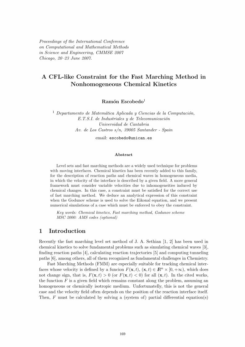
Proceedings of the International Conferenceon Computational and Mathematical Methodsin Science and Engineering, CMMSE 2007Chicago, 20–23 June 2007.
A CFL-like Constraint for the Fast Marching Method inNonhomogeneous Chemical Kinetics
Ramon Escobedo1
1 Departamento de Matematica Aplicada y Ciencias de la Computacion,E.T.S.I. de Industriales y de Telecomunicacion
Universidad de CantabriaAv. de Los Castros s/n, 39005 Santander - Spain
email: [email protected]
Abstract
Level sets and fast marching methods are a widely used technique for problemswith moving interfaces. Chemical kinetics has been recently added to this family,for the description of reaction paths and chemical waves in homogeneous media,in which the velocity of the interface is described by a given field. A more generalframework must consider variable velocities due to inhomogeneities induced bychemical changes. In this case, a constraint must be satisfied for the correct useof fast marching method. We deduce an analytical expression of this constraintwhen the Godunov scheme is used to solve the Eikonal equation, and we presentnumerical simulations of a case which must be enforced to obey the constraint.
Key words: Chemical kinetics, Fast marching method, Godunov schemeMSC 2000: AMS codes (optional)
1 Introduction
Recently the fast marching level set method of J. A. Sethian [1, 2] has been used inchemical kinetics to solve fundamental problems such as simulating chemical waves [3],finding reaction paths [4], calculating reaction trajectories [5] and computing tunnelingpaths [6], among others, all of them recognized as fundamental challenges in Chemistry.
Fast Marching Methods (FMM) are especially suitable for tracking chemical inter-faces whose velocity is defined by a funcion F (x, t), (x, t) ∈ IRn
× [0,+∞), which doesnot change sign, that is, F (x, t) > 0 (or F (x, t) < 0) for all (x, t). In the cited works,the function F is a given field which remains constant along the problem, assuming anhomogeneous or chemically isotropic medium. Unfortunatelly, this is not the generalcase and the velocity field often depends on the position of the reaction interface itself.Then, F must be calculated by solving a (system of) partial differential equation(s)
169

simultaneously with the interface evolution problem. In this more general framework,the FMM must be coupled to a static chemical problem which gives the instantaneousvelocity field and a CFL-like constraint for F must be taken into account.
In inhomogeneous or anisotropic chemical media, the mathematical model usuallyconsists in describing the evolution of a chemical magnitude u(x, y, t) in a 2D or 3Ddomain Ω. To do this, one must be able to calculate the magnitude u(x, y, t) for agiven position of the interface Γ at a given time tn, and the velocity of (at least) allthe points of Γ at time tn. Then the FMM can obtain the new position of the interfaceafter a short interval of time ∆t, and start again for tn+1 = tn + ∆t.
The algorithm consits of a chemical part, where the solution un and the velocityFn are calculated in Ωn (characterized by Γn, i.e. changing in time) and a geometricpart, where the geometry is changed by moving the interface to its new position Γn+1.
In inhomogeneous problems, the velocity is renewed after each interval of time ∆t
by solving the chemical problem with a fixed interface. The consistency of the algorithmis based on the assumption that ∆t is short enough to ensure that the velocity fieldremains almost constant during this interval of time.
Here, we derive an explicit expression which acts as a CFL contraint from therenewal of F and imposes a restriction for the FMM, concretely in the Godunov method,which is the one used in [4–6].
2 The Fast Marching Method
2.1 Setup of the algorithm
Let (xi, yj)Nx,Ny
i=1,j=1be a rectangular space discretization of a two-dimensional domain
Ω. At time tn, the chemical interface Γn is given by a set of Nnl nodes of Ω:
Γn = (xnl , yn
l )Nn
l
l=1. (1)
Assume that F ≥ 0 (recall that the velocity does not change sign). The idea of theFMM consists in describing the evolution of the interface –the front– by means of anarrival time function φ(x, y) defined as the time it takes to the interface to arrive tothe point (x, y) ∈ Ω. At time tn, the interface is given by the points such that
φn(x, y) = tn. (2)
Starting from these points, the FMM provides the arrival time for t ≥ tn. At the end ofthe FMM step, the arrival time is tn+1 and the position of the interface is given by thepoints such that φn(x, y) = tn+1. In principle, φn(x, y) can be constructed beyond tn+1,but its validity is subject to restrictions imposed by Fn, especially in inhomogeneousmedia; in this case, φn(x, y) must be often reconstructed after each ∆t.
Three sets can be defined using the classical notation: (we omit the index n)
A = (x, y) ∈ Ω/ φ(x, y) ≤ 0: the front is or has been here;
C = (x, y) ∈ Ω/ φ(x, y) > 0 and at least one of its neighbors is in A;
170
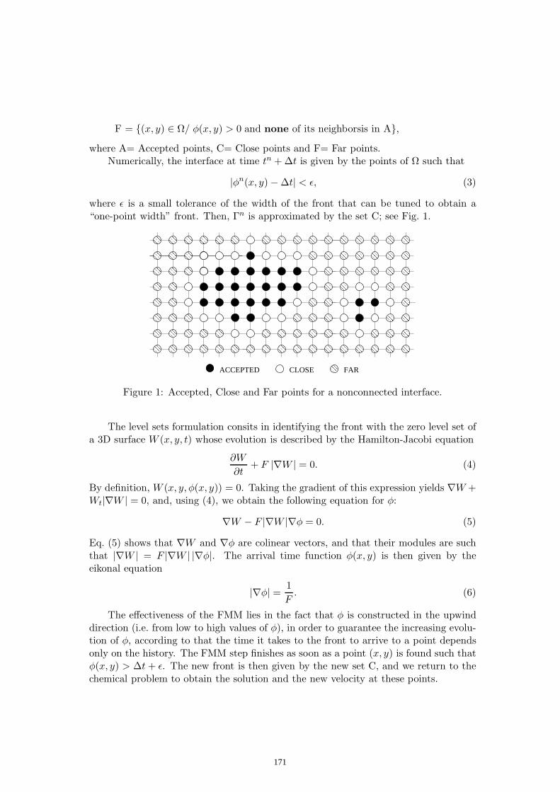
F = (x, y) ∈ Ω/ φ(x, y) > 0 and none of its neighborsis in A,
where A= Accepted points, C= Close points and F= Far points.Numerically, the interface at time tn + ∆t is given by the points of Ω such that
|φn(x, y) − ∆t| < ǫ, (3)
where ǫ is a small tolerance of the width of the front that can be tuned to obtain a“one-point width” front. Then, Γn is approximated by the set C; see Fig. 1.
ACCEPTED CLOSE FAR
Figure 1: Accepted, Close and Far points for a nonconnected interface.
The level sets formulation consits in identifying the front with the zero level set ofa 3D surface W (x, y, t) whose evolution is described by the Hamilton-Jacobi equation
∂W
∂t+ F |∇W | = 0. (4)
By definition, W (x, y, φ(x, y)) = 0. Taking the gradient of this expression yields ∇W +Wt|∇W | = 0, and, using (4), we obtain the following equation for φ:
∇W − F |∇W |∇φ = 0. (5)
Eq. (5) shows that ∇W and ∇φ are colinear vectors, and that their modules are suchthat |∇W | = F |∇W | |∇φ|. The arrival time function φ(x, y) is then given by theeikonal equation
|∇φ| =1
F. (6)
The effectiveness of the FMM lies in the fact that φ is constructed in the upwinddirection (i.e. from low to high values of φ), in order to guarantee the increasing evolu-tion of φ, according to that the time it takes to the front to arrive to a point dependsonly on the history. The FMM step finishes as soon as a point (x, y) is found such thatφ(x, y) > ∆t + ǫ. The new front is then given by the new set C, and we return to thechemical problem to obtain the solution and the new velocity at these points.
171

2.2 FMM step: from tn to t
n+1:
The FMM first initializes φ(x, y) and then corrects its values by solving (6) with an it-erative process. The initialization must be done at least for the first time step, and canbe omitted in successive time steps if no reinitialization of φ is needed. The constraintwe present here is in fact a test which can enforce this reinitialization.
FMM algorithm
1.1 At all points of A, set φ = 0.
1.2 At all points of C (the interface), assign to φ the value of the time obtained bydividing the distance from the point to the set A by the velocity of the interfaceat this point: φ = d/F (see later a better way to do this step).
1.3 At all points of F, assign to φ the value +∞. These points are far and they don’thave any influence in the correction of the points of C (upwind).
Once φ is initialized, the fast marching starts. The interface evolves point by point bycorrecting the initial estimation by means of the following iterative process:
2.1 Obtain the point TRIAL (xT , yT ) from set C which has the smallest value of φ:(xT , yT ) ∈ C and φ(x, y) ≥ φ(xT , yT ), ∀(x, y) ∈ C. See Fig. 2(a).
2.2 Test:
i. If φ(xT , yT ) > ∆t+ ǫ, φ has been constructed for all the points verifying (3).Then the FMM step is finished and we return to the chemical problem.
ii. If not, there still exists points at which the interface will arrive at a timelesser or equal to ∆t + ǫ and we have to continue.
2.3 Move (xT , yT ) to A (and delete it from C); its value is the definitive one becauseit cannot be improved with this algorithm. See Fig. 2(b).
2.4 Move to C the neighbors of (xT , yT ) that are in F, because these points have nowa neighbor in A. See Fig. 2(c).
2.5 Actualize the value of φ at all the neighbors of (xT , yT ) that are in C, by solvingEq. (6). See Fig. 3. This is the gordian knot of the FMM; see next section.
2.6 The interface has been moved one point; see Fig. 4. Goto 2.1.
172

j
i
(c)
(b)(a)
TRIAL
CLOSE
ACCEPTED
FAR
Figure 2: The interface is moved one point: (a) Find the point (xT , yT ). (b) Move(xT , yT ) to A. (c) Move the neighbors of (xT , yT ) from F to C.
1
2
1 2
i
j
(a)
j
i+1
j−1
i
(b) (c)
Figure 3: Actualization of φ with the Godunov scheme in the neighbors of (xT , yT ) thatare in C: (a) the two neighbors; (b) First neighbor of (xT , yT ) and its respective neigh-bors: the information comes only from the left. (c) Second neighbor: the informationcomes in both directions, from the left and from above.
2.3 Godunov’s method
A suitable way to solve the eikonal equation in the context of the fast marching algo-rtihm is the Godunov method [1], which is precisely the method used in [4–6]. TheGodunov method makes use of the following approximation of the gradient:
[
max (D−xi,j φ, −D+x
i,j φ, 0)2 + max (D−yi,j φ, −D
+yi,j φ, 0)2
]
1/2
=1
Fi,j, (7)
where D−xi,j φ = (φi,j − φi−1,j/∆x and D+x
i,j φ = (φi+1,j − φi,j)/∆x. The numericalresolution of Eq. (7) is not trivial because unknown values must be compared a priori.Typically, expensive iterative methods are used (Rouy-Tourin, 1992). Fortunately, wecan take advance from the upwind character of the Godunov approximation.
Before to explain the step 2.5 of the FMM algorithm, note that the step 1.2 isequivalent to solve (7) with φ = 0 in the points of A and φ = +∞ in the points of F.
173

Step 2.5: The actualization of φ at the neighbors of (xT , yT ) is done by solving Eq. (7)by assigning to φ the value +∞ at the neighbors [of the neighbor of (xT , yT ) which isbeing actualized] that are not in A. Once the calculation is done, the previous values ofφ at the neighbors of the neighbor of (xT , yT ) must by restituted. The neighbors thatare in A are used with their value and they remain unchanged.
(b)
(c)
(a)
Figure 4: Next FMM step: (a) new position of the interface and localization of the newpoint (xT , yT ); (b) and (c): steps 2.3 to 2.5 in this new situation.
How we do this? Assume a uniforme grid: h = ∆x = ∆y. Then Eq. (7) becomes
max (φi,j − φi−1,j, φi,j − φi+1,j , 0)2 + max (φi,j − φi,j−1, φi,j − φi,j+1, 0)2 =h2
F 2
i,j
. (8)
These maxima cannot be calculated without knowing φi,j , which is precisely the un-known of the equation. Let us replace maxima by minima,
max(φi,j − φi−1,j , φi,j − φi+1,j, 0) = φi,j − min(φi−1,j , φi,j, φi+1,j), (9)
max (φi,j − φi,j−1, φi,j − φi,j+1, 0) = φi,j − min(φi,j−1, φi,j, φi,j+1), (10)
and define the values
α1 = min(φi−1,j , φi+1,j) and α2 = min(φi,j−1, φi,j+1), (11)
which are known values, because they correspond to nodes of A or they have beenassigned to +∞ for this calculation. Then Eq. (7) is equivalent to
(φi,j − min(φi,j , α1))2 + (φi,j − min(φi,j , α2))
2 =h2
F 2
i,j
. (12)
174

As we are actualizing φi,j, at least one of the neighbors of (xi, yj) must be in A, thatis, the information comes from at least one direction x or y, or from both directions:
• If the information comes only from direction x (respectively y), then we cancalculate min(φi,j , α2) = φi,j, because (xi, yj−1) and (xi, yj+1) are not in A, so φ
must be at +∞ in these points. The equation to solve is simply
φi,j = α1 +h
Fi,j
(
Respectively, φi,j = α2 +h
Fi,j
)
. (13)
• If the information comes fromboth directions, then there exists at least one neigh-bor in each direction where the value of φ is lower than φi,j: α1,2 < +∞. This way,φi,j can be dropped from minima calculations in (12) and minima calculations areredundant. The Godunov equation becomes (φi,j −α1)
2 + (φi,j −α2)2 = h2/F 2
i,j .This can be rewritten as
φ2
i,j − (α1 + α2)φi,j +1
2
(
α2
1 + α2
2 −h2
F 2
i,j
)
= 0. (14)
Here ∆ = −(α1 − α2)2 + 2h2/F 2
i,j cannot be negative, so the velocity must be
such that |α1 − α2|Fi,j ≤
√
2h. This is called a “classically allowed point” in [3].When ∆ > 0, the higher root must be used to preserve the upwind.
1
2
3
1 2 3
(a)
j
i ii+1
j
i
j+1
(b)
j−1
(d)(c)
Figure 5: Actualization of the neighbors of the new point (xT , yT ). In this case thereare three neighbors to be actualized, each one with a different kind of neighborhood.
For the consistency of the FMM algorithm, a second upwind condition must beverified by Eq. (14), which is that φi,j must be greater or equal than α1 and α2:
φi,j =α1 + α2
2+
1
2
√
∆ > α1,2, i.e. ∆ > 4
[
α1,2 −α1 + α2
2
]
2
= (α1 − α2)2,
and then
Fi,j <h
|α1 − α2|. (15)
This condition is more restrictive than the one deduced for “classically allowed points”,and is consequently the one which must be used.
175

2.4 The Condition (15) is a constraint
By construction, the FMM is such that expression (15) is always verified during thegeometric part of the problem. Let us give a qualitative description of this fact.
P
P
2 P=
P
T
A
(b)(a)
1
i
1
2
j
α
αh
h
Figure 6: Numerical cell in the actualization of PA = (xi, yj).
Fig. 6 shows the numerical cell of a point PT = (xT , yT ) whose upper neighbor PA =(xi, yj) is being updated. Assume that information comes in both directions, from theleft from P1 = (xi−1, yj) and from below from P2 = (xi, yj−1). The value of φ at PA
will depend on φ(P1) and φ(P2). The trial point PT must be P1 or P2; assume PT = P2.
In this case, α1 = φi−1,j and α2 = φi,j−1. The value α2 − α1 (which is positive,because the front arrives first to P1) is the time elapsed between the arrivals of thefront to P1 and to P2: α2 − α1 is the time spent by the front in going from P1 to P2.Note that the interface can be a not connected set, in such a way that it can arrive toP2 from far from P1. For simplicity, assume that it is a connected set.
In terms of velocities, the value h/(α2 − α1) is the velocity at which the interfacecovers the distance between P1,2 and PA in a time α2 −α1. The restriction (15) meansthat Fi,j must be lower than this value. This, of course, makes sense, because Fi,j isthe value of the velocity of the interface at PA. Numerically, Fi,j is the value used toactualize φi,j , that is, the value of F in the numerical cell of PA. It is then necessaryto Fi,j to be lower than the velocity at which the interface goes from P1 to P2; if not,once in P1, the interface will arrive first to PA and then to P2, and this is not possible.
In terms of times, the time it takes to the interface to arrive to (xi, yj) coming fromits neighbors (located at a distance h) at a velocity Fi,j must be greater or equal thanthe time spent in going from one neighbor to the other, |α1 −α2|. If this is not so, theinterface will arrive first to the point that is being actualized than to a neighbor whichis being used for this actualization, and this is an absurdity.
As we have seen, the FMM preserves the upwind during the geometric part of thenumerical resolution. But, during the chemical part of the problem, the velocity isrenewed and the expression (15) can be no longer satisfied. Let us show how.
The function Fn is defined as the velocity at the points of Γn at time tn; nothingis said about the value of Fn outside the interface, and it may happen (especially ininhomogeneous problems) that a velocity does not make sense outside the interface.However, these values are used in the FMM, by extending Fn to a narrow band aroundΓn (several methods can be used [7], e.g. the velocity at the nearest point of Γn). Whenthe FMM step has been done, and before the renewal of Fn, the interface is given by
176

a new set of points
Γn+1 = (xn+1
l , yn+1
l )Nn+1
l
l=1.
The velocity at these points at time tn is called, actually, Fnext, an extention of Fn. The
condition (15) is still preserved for Fnext, but this can be false for the renewed velocity
Fn+1(Γn+1). In fact, the velocity at Γn+1 can be very different, depending on thesmoothness of the chemical processes: the velocity is not constant between time-stepsof size ∆t, and important changes may happen from one interval of time to the otherwhich can affect considerably the velocity:
Fn+1(Γn+1) 6= Fnext
(Γn+1).
From the chemical point of view, the velocity of the interface at a given point isunique (recall that F does not change sign), but the numerical resolution makes use oftwo values of the velocity at the points at which the arrival of the interface coincideswith the change of time-step: the extended value Fn
ext and the renewed value Fn+1.
The condition (15) can be not satisfied by Fn+1; there is no reason why Fn+1 couldbe enforced to verify (15). In the cited works it is mentioned that “nonclassical points”are simply deleted from the close or trial sets [4]. This may affect to the fidelity of thesimulation to the real chemical problem. Both the existence of real solutions of Eq. (7)and the upwind condition (15) must be ensured by the algorithm.
It is in this way that the condition (15) acts as a constraint for φ. In fact, inthe algorithm we have proposed here, this condition must be introduced as a test forthe validity of φ for the next FMM step. If the condition is not satisfied, then thereinitialization of φ is needed, or, in a more complicated way, an adaptive time-stepalgorithm must be implemented. The refinement of the spatial mesh makes thingssmoother, but it also contributes to render more demanding the condition (15).
3 A numerical example
We have considered a general situation in which achemical reaction takes place in a domain characterizedby the geometry described in the contiguous figure.
Assume that the chemical reactant interface ar-rives to a region in which the substrate is chemicallyinhomogeneous. Inhomogeneities can be due to differ-ent properties of the substrate, but also to dynamicaleffects induced by the reaction (electromagnetic effects,temperature. . . ). The reactant can then evolve witha different speed in different parts of the substrate.Assume that the channel (with two entrances, A andB) described by two nonreactive and noncatalytic obstacles, is a fast reactant region(Fch = 1), compared to the rest of the substrate (Fs = 0.1). This figure shows the(frequent) case in which the interface arrives first to one of the entrances (e.g., A).
177
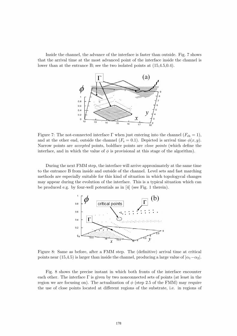
Inside the channel, the advance of the interface is faster than outside. Fig. 7 showsthat the arrival time at the most advanced point of the interface inside the channel islower than at the entrance B; see the two isolated points at (15,4.5,0.4).
Figure 7: The not-connected interface Γ when just entering into the channel (Fch = 1),and at the other end, outside the channel (Fs = 0.1). Depicted is arrival time φ(x, y).Narrow points are accepted points, boldface points are close points (which define theinterface, and in which the value of φ is provisional at this stage of the algorithm).
During the next FMM step, the interface will arrive approximately at the same timeto the entrance B from inside and outside of the channel. Level sets and fast marchingmethods are especially suitable for this kind of situation in which topologycal changesmay appear during the evolution of the interface. This is a typical situation which canbe produced e.g. by four-well potentials as in [4] (see Fig. 1 therein).
Figure 8: Same as before, after a FMM step. The (definitive) arrival time at criticalpoints near (15,4.5) is larger than inside the channel, producing a large value of |α1−α2|.
Fig. 8 shows the precise instant in which both fronts of the interface encountereach other. The interface Γ is given by two nonconnected sets of points (at least in theregion we are focusing on). The actualization of φ (step 2.5 of the FMM) may requirethe use of close points located at different regions of the substrate, i.e. in regions of
178

different velocities: outside the channel, the interface is just arriving (high arrival time),whereas inside the channel the interface has a low arrival time. Then |α1−α2| becomeslarge with respect to its typical value when points are all in the same region. Whenthe velocity is renewed, chemical processes can be such that F can adopt a large value;the combination of these two effects can lead to a violation of the constraint.
It is important to note that even if the constraint (15) can be seen as a CFL-likecondition, where the value of a parameter (F ) is restricted by a space over time fraction,it is not a CFL condition. Even if the space value is h (the space step), the time value|α1 − α2| is absolutely not related to the time step of the algorithm.
Conclusion
In conclusion, we have derived a constraint for the Godunov scheme when it is used tosolve the Eikonal equation during the FMM, when this later is coupled to a chemicalproblem in inhomogeneous media producing nonconstant velocity fields.
Acknowledgements
We thank F. Bernal for fruitful discussions. This work has been carried out under aRamon y Cajal contract at the University of Cantabria.
References
[1] J. A. Sethian, A fast marching level set method for monotonically advancingfronts, Proc. Natl. Sci. Sci. USA 93 (1996), 1591–1595.Fast Marching Methods, SIAM Review 41, No. 2 (1999), 199–235.
[2] D. L. Chopp, Some Improvements of the Fast Marching Method, SIAM J. Sci.Comput. 23, No. 1 (2001), 230–244.
[3] K. Kaly-Kullai, A fast method to simulate travelling waves in nonhomogeneouschemical or biological media, J. Math. Chem. 34 (2003), 163–176.
[4] B. K. Dey, M. R. Janicki, P. W. Ayers, Hamilton-Jacobi equation for theleast-action/least-time dynamical path based on fast marching method, J. Chem.Phys. 121 (2004), 6667–6679.
[5] B. K. Dey, S. Bothwell, P. W. Ayers, Fast marching method for calculatingreactive trajectories for chemical reactions, J. Math. Chem. 41 (2007), 1–25.
[6] B. K. Dey, P. W. Ayers, Computing tunneling paths with the Hamilton-Jacobiequation and the fast marching method, Molec. Phys. 105 (2007), 71–83.
[7] D. Adalsteinsson, J. A. Sethian, The Fast Construction of Extension Veloci-ties in Level Set Methods, J. Comput. Phys. 148, No. 2 (1998), 2–22.
179

Proceedings of the International Conference on Computational and Mathematical Methods in Science and Engineering, CMMSE2007 Chicago, 20-23 June 2007
A Transshipment Problem with Random Demands
Dr. S.N. Gupta
School of Computing, Information & Mathematical Sciences, University of the South Pacific,Laucala Campus,
Private Mail Bag, Suva, FIJI. Email: [email protected] ; [email protected]
Abstract
This paper presents a study of a stochastic transshipment problem with random demands. In our model the random demand has not been replaced by its expectation but the probabilistic nature of the problem has been built into the problem formulation itself so that the system has the opportunity to take maximum advantage of the probability distribution of demand. Deterministic equivalent of the problem is obtained and an algorithm is developed for solving the same. Keywords: transshipment, random demand, global optimum, basic feasible solution. 1. Introduction The standard transportation problem and its several variants including the stochastic transportation problems have been extensively studied and special methods developed for solving them. However, the transshipment problem with random demands seems to have remained unexplored so far. Interest in transshipment problem arises because transshipments are often required for effective supply chain management and better replenishment strategies [2,4,6]. Transshipments also occur in the military logistics where direct transportation of goods to destination may not be advisable for security reasons. Moreover, the demands in real life are usually uncertain and have to be treated as random variables. This creates considerable complications. The purpose of this paper is to study a stochastic transshipment problem in which the demands at various destinations are assumed to be independent discrete random variables with known probability distributions. In this study, the random demand has not been replaced by its expectation but, following the technique of Dantzig[1] the probabilistic nature of the problem has been built into the problem formulation itself so that the system has the opportunity to take maximum advantage of the probability distribution of demand. The stochastic transshipment problem is reduced to an equivalent deterministic transportation type linear programming problem and an algorithm is developed to solve the same.
180

CMMSE 2007
2. Problem Formulation Consider a transshipment problem with m sources numbered 1, 2, ........ .., m and n sinks numbered m+1, m+2,..., m+n. The sequential numbering of sources and sinks is found convenient because in a transshipment problem every source and sink acts both as a shipping point as well as a receiving point of goods. Let, ai = the quantity available at source i= 1,2,……..m, bj = the quantity demanded at sink j= m+1,m+2,………….,m+n, xij = the quantity shipped from station i to j (i, j= 1,2,……,m+n), cij = the per unit shipment cost from station i to j (i, j= 1,2,……,m+n),
ti = quantity transshipped at the station i (i= 1,2,……,m+n), li = per unit transshipment cost (including unloading, reloading, and storage etc.) at the station i (i= 1,2,……,m+n), sj = revenue received (sale proceeds minus the handling costs like seller’s commission etc.) per unit of demand satisfied at sink Dj
In the standard transshipment problem the objective is usually to minimize the total of transshipment and transportation costs. However, in our case we have no precise information concerning the demand bj, but that we know its probability distribution for each j. So, in order to take care of the randomness of demands, instead of minimizing the total cost, we take our objective as the maximization of the net expected revenue (i.e., total expected revenue minus the total costs of procurement, transshipment and transportation). This would cause a tug of war between maximizing the expected revenue and minimizing the costs of transportation and transshipment.
Mathematically, the problem may be stated as under:
Problem P1: Find xij so as to
maximize F = ∑∑ ∑∑+
=
+
=
+
=
+
+=
−−nm
iii
nm
i
nm
jijij
nm
mjjjj tlxcYsf
11 1
**
1),( …(2.1)
subject to ∑+
=
nm
jijx
1
* = ⎩⎨⎧
++==+
nm,...1mitm,.....,2,1ita
i
ii )2.2...()2.2...(
ba
…(2.2)
*
1
m n
iji
x+
=∑ =
⎪⎩
⎪⎨⎧
++=+
=
nm,...1mjtb
m,.....,2,1jt
jj
j
)3.2...()3.2...(
ba
…(2.3)
xij ≥ 0 … … …(2.4)
∑+
=
nm
1j
* indicates that the term j = i is excluded from the sum.
Here fj(sj, Yj) is a yet unknown function that describes the expected revenue from the destination j if a net total of Yj units are shipped to that destination. So the function F is a measure of the net expected revenue.
181
CMMSE 2007
Constraints (2.2a) imply that the total quantity that leaves the source i ( = 1, 2, …, m) is equal to the quantity available plus the quantity transshipped and (2.2b) imply that the total quantity that leaves the sink i ( = m+1, m+2, …, m+n) is equal to the quantity transshipped. Similarly Constraints (2.3a) imply that the total quantity that arrives at the source j ( = 1, 2, …, m) is equal to the quantity that source transships and (2.3b) imply that the total arriving at the sink j (= m+1, m+2, …, m+n) is equal to the demand at that sink plus the quantity that the sink transships. The transshipped quantities ti are unknown and generate -1 coefficients when brought over to left-hand side. So we impose an upper bound to (say) on the amount that can be transshipped at any point such that ti≤ to or ti = to – xii i = 1, 2, 3,….., m+n, …(2.5) where xii is a nonnegative slack. After substituting (2.5) in (2.1) to (2.3) and on simplifying the original transshipment problem P1 is reduced to the following genuine transportation type linear programming problem. Problem P2:
Maximize F = 1 1 1 1
( , )m n m n m n m n
j j j ij ij i oj m i j i
f s Y c x l t+ + + +
= + = = =
− −∑ ∑∑ ∑ …(2.6)
Subject to ∑+
=
nm
1jijx =
⎩⎨⎧
++==+
nm,...1mitm,.....,2,1ita
o
oi ...(2.7 )...(2.7 )
ab
…(2.7)
∑+
=
nm
iijx
1
= ⎩⎨⎧
++=+=
nmmjtbmjt
oj
o
,...1,.....,2,1
...(2.8 )...(2.8 )
ab
…(2.8)
xij ≥ 0 i, j = 1, 2, 3,….., m+n, …(2.9) where cii = -li and note that the * (asterisk) on the summations have disappeared due to the inclusion of xii. The upper bound to can be interpreted as the size of a fictitious stockpile at each of the sources and sinks which is large enough to take care of all transshipments. Obviously, to need not be larger than the total quantity required to be shipped. So,
we take to= ∑=
m
1iia which ensures that to is not limiting. The unused stockpile at
the station i=1, 2, ……..m+n, if any, will be absorbed in the slack xii.
182

CMMSE 2007
Thus, the m×n order transshipment problem P1 has been converted into a direct shipment transportation problem P2 of order (m+n)× (m+n) which can have no more than 2(m+n)-1 variables different from zero. However, (m+n) of these non-zero variables are the slack variables xii representing the unused stockpile and hence there are in fact no more than (m+n-1) variables of interest which are different from zero. As indicated earlier, the demands bj (j =m+1, m+2, …,m+n) are independently distributed discrete random variables. Let the probability distribution of bj be as below:
Demand bj b1j < b2j < ………< jH jb
Prob (bj=bhj) = phj Prob (bj≥ bhj) = π hj
p1j
π 1j=∑=
jH
1hhjp (= 1)
p2j
π 2j=∑=
jH
2hhjp
………… ………….
jH jp
jHjH jjp=π
However, the moment we treat bj as random variable, a new problem begins to rear its head. The constraints (2.8b) fail to make sense. To make the problem meaningful it has to be reformulated into an equivalent deterministic problem. 3. Equivalent Deterministic Problem In the function fj(sj, Yj), note that Yj, the net quantity shipped to sink j, can be any amount between the lowest value b1j and the highest value jH j
b in the probability distribution of the demand bj (j = m+1, m+ 2, …, m+n). If 0≤Yj ≤ b1j, then each of the Yj units shall be absorbed with probability j1π (= 1).
Hence, the expected revenue is = sj j1π Yj.
If b1j≤Yj ≤ b2j, then each unit upto b1j shall be absorbed with probability j1π and each of the additional units (Yj - b1j) shall be absorbed with probability j2π . Hence, the expected revenue is = sj j1π b1j + sj j2π (Yj - b1j). In general, if bhj≤Yj ≤ bh+1,j, then the expected revenue is = sj j1π b1j + j2π (b2j - b1j) + ……. j2π (bhj – bh-1,j) + jh ,1+π (Yj - bhj).
Let us now break Yj into incremental units yhj (h = 1, 2,…Hj) as: Yj = y1j + y2j + y3j + …. + yhj + .… jH j
y …(3.1)
183

CMMSE 2007
where
⎪⎪
⎭
⎪⎪
⎬
⎫
=−≤≤
=−≤≤
=≤≤
− jHjHjHjH
jjjj
jjj
jjjjRbby
Rbby
sayRby
,1
2122
111
0::::
0
)(0
…(3.2)
Relation (3.1) makes physical sense only if there exists some h = hj (say) such that all intervals below the hj
th interval are filled to capacity and all intervals above it are empty i.e.
⎪⎭
⎪⎬
⎫
+==
=≤
−==
),...,1(0
)(
)1,...,2,1(
jjhj
jhjhj
jhjhj
Hhhy
hhRy
hhRy
…(3.3)
Assuming for the time being that the conditions (3.3) hold, the total expected
revenue from sink j is: fj(sj, yj) = ∑=
jH
hhjhjj ys
1π
Substituting the value of fj(sj, yj) in (2.6), the net expected revenue is:
F = ∑∑∑∑ ∑+
=
+
=
+
=
+
+= =
−−nm
ioi
nm
i
nm
jijij
nm
mjhjhj
H
hj tlxcys
j
11 11 1π
The third term on the right hand side is a constant that can now be ignored but adjusted in the end. Since we have to maximize F (or minimize –F), so, ignoring the constant term and treating both xij and yhj as decision variables, the deterministic equivalent of the Problem P2 is:
Problem P3: Minimize Z =∑∑+
=
+
=
nm
1i
nm
1jijijxc +∑∑
+
= =
nm
i
H
hhjhj
j
yd1 1
…(3.4)
where dhj= -sj hjπ
Subject to ∑+
=
nm
1jijx =
⎩⎨⎧
++==+
nm,...1mitm,.....,2,1ita
o
oi ...(3.5 )...(3.5 )
ab
…(3.5)
∑+
=
nm
iijx
1 = to, j=1,2,…..,m … (3.6 )a
∑∑=
+
=
−jH
hhj
nm
iij yx
11= to, j= m+1,…, m+n … (3.6 )b …(3.6)
xij, yhj ≥ 0 )h,j,i(∀ …(3.7) yhj ≤ Rhj )j,h(∀ …(3.8)
184

CMMSE 2007
and subject to the additional stipulation that the constraints (3.3) are also satisfied. Fortunately, it turns out that (3.3) do not restrict our choice of optimum solution in any way. This we prove in the following theorem. Theorem 1 A feasible solution to Problem P3 can always be improved if it violates any of the constraints (3.3). Proof Let (x*
ij, y*hj) be a feasible solution to Problem P3 obtained on ignoring (3.3). The
value of Z at this solution is:
Z* = ∑∑+
=
+
=
nm
1i
nm
1j
*ijijxc + ∑ ∑
+
+= =
nm
mj
H
hhjhj
j
yd1 1
*
Suppose that there exists some h = ho & j = jo such that 0& *
,1* ><
+ oooooo jhjhjhyRy
It is clearly a violation of the constraints (3.3). Now, we increase *
jh ooy and decrease *j,1h ooy
+by equal amounts θ (> 0) such that
the feasibility of the solution is not disturbed. The new value of the objective function becomes: Zo = Z* + θ )( *
,1*
oooo jhjhdd
+−
But )( *,1
*oooo jhjh
dd+
− ≤ 0, as hjπ ≥ jh ,1+π for all h and j.
Hence it follows that Zo ≤ Z* . Q.E.D. This result shows that if an optimum solution to Problem P3 is obtained after ignoring (3.3), it shall suo moto satisfy (3.3). Thus, to solve problem P3, we may simply ignore the constraints (3.3). 4. Preliminaries to the Solution of Problem P3
1. It is assumed that the set of all feasible solutions of Problem P3 is regular (i.e. non-empty and bounded).
2. Problem P3 is a transportation type linear programming problem with upper bound restrictions on some variables. So, its global minimum exists at a basic feasible solution of its constraints.
3. We shall, hereinafter, call the constraints (3.5) through (3.7) as the original system and the constraints (3.5) through (3.8) as the bounded system. As none of the constraints in the original system is redundant, a basic feasible solution to the original system shall contain 2(m+n) basic variables. For the capacitated system also, a basic feasible solution shall contain 2(m+n) basic variables and the same may be found by working on the original system provided that some of the non basic variables are
185

CMMSE 2007
allowed to take their upper bound values[3]. 4. The special structure of Problem P3, permits us to arrange it into an array
as shown in table 1:
Table 1 x11
c11
…
x1m
c1m
x1 m+1
c1 m+1
…
x1 m+n
c1 m+n
a1+to
……. .……
… …
……. …….
……. …….
… …
……. …….
……. …….
xm1
cm1
…
xmm
cmm
xm,m+1 cm,m+1
…
xm m+n
cm m+n
am+to
xm+1,1
cm+1,1
…
xm+1m
cm+1m
xm+1,m+1
cm+1,m+1
…
xm+1 m+n cm+1 m+n
to
……. …….
… …
……. …….
……. …….
… …
……. …….
……. …….
xm+n,1
cm+n 1
…
xm+n,m
cm+n m
xm+n,m+1
cm+n m+1
…
xm+n m+n
cm+n m+n
to
to … to y1 m+1 R1 m+1
d1 m+1
…
y1,m+n R1,m+n
d1,m+n ……. … ……. ……. … …….
YH,m+1 RH,m+1
dH,m+1
…
YH,m+n RH,m+n
dH,m+n
to … to
In the above table, there are (m+n) rows in columns j=1,2,….m and (m+n+H) rows in columns j=m+1,m+2,….m+n. Here H = max Hj, so that there shall be some empty boxes near the bottom of the table in columns j=m+1,m+2,….m+n. These empty boxes shall be crossed out.
Absence of the row totals for yhj’s in the table indicates that there are no row equations for yhj variables. Besides, to obtain the column equations (3.6b), each yhj has to be multiplied by (-1). We have omitted (-1) from yhj boxes for convenience.
186

CMMSE 2007
5. Initial Basic Feasible Solution To start with, we fix the demands bj’s approximately equal to their expected
values such that ∑∑=
+
+=
=m
1ii
nm
1mjj ab and also such that for all j except j = j*, each bj
falls at the upper end of one of the intervals yhj into which the bj has been divided
i.e. bj ∑′
=
=jh
1hhjR for some jh′ ≤ Hj and for all j except j = j* (the bj can always be so
chosen that it is done). With these fixed demands the upper portion (above the double line) of the Table 1 resembles a (m+n)× (m+n) standard transportation problem for which an initial basic feasible solution with 2(m+n)-1 basic variables is obtained by any of the several available methods. Now, in each of the columns j=m+1,m+2,….m+n the values of the non basic yhj’s are entered at their upper bounds Rhj in turn h =1, 2,…. until we have entered enough non basic yhj’s so that their sum over h is equal to bj. Obviously, we shall never have to enter yhj below its upper bound except in column j = j*, where the last nonzero entry will be yhj*≤Rhj*. This last entry and the 2(m+n)-1 basic xij’s found earlier, constitute the required initial basic feasible solution with 2(m+n) basic variables. In case the last non zero entry in column j* is also at its upper bound, then we take the last yhj entry of any column as our 2(m+n)th basic variable.
6. Optimality criteria Let the simplex multipliers corresponding to the objective function Z (Problem P3) be ui and vj ),...,2,1,( nmji +=∀ . These are determined by solving the following equations.
⎪⎭
⎪⎬⎫
=−
=++
hj
ij
y basicfor 0
xbasicfor 0
jhj
jiij
vd
vuc …(6.1)
These are 2(m+n) linear equations in as many unknowns ui and vj and can be easily solved. Let the relative cost coefficients corresponding to the variables xij and yhj be ijδ and hjλ . These are determined by solving the following equations:
ij
hj
for non basic x
for non basic yij ij i j
hj hj j
c u v
d v
δ
λ
= + + ⎫⎪⎬= − ⎪⎭
…(6.2)
It can be easily shown that for a given basic feasible solution (xij, yhj) of the Problem P3, the value of the objective function Z is:
187

CMMSE 2007
Z= ( )1 1 1 1 1 1 1
jHm n m n m n m m n m n
ij ij hj hj i i o i o j oi j j m h i i m j
x y u a t u t v tδ λ+ + + + +
= = = + = = = + =
⎧ ⎫+ − + + +⎨ ⎬
⎩ ⎭∑ ∑ ∑ ∑ ∑ ∑ ∑
=1 1 1 1 1 1 1
( )jHm n m n m n m m n m n
ij ij hj hj i i o i ji j j m h i i m j
x y u a t u vδ λ+ + + + +
= = = + = = = + =
⎧ ⎫+ − + +⎨ ⎬
⎩ ⎭∑ ∑ ∑ ∑ ∑ ∑ ∑ …(6.3)
Here, ijδ = 0 for all basic xij and also the values of the non basic xij are zero. So, the first term on the r.h.s. of (6.3) vanishes. Similarly hjλ = 0 for the basic yhj, but as regards the values of non basic yhj’s - some are zero and the others are at their upper bounds. Hence,
Z = * *
1 1 1 1 1( )
jHm n m m n m n
hj hj i i o i jj m h i i m j
R u a t u vλ+ + +
= + = = = + =
⎧ ⎫− + +⎨ ⎬⎩ ⎭
∑ ∑ ∑ ∑ ∑ …(6.4)
Where ∑ * indicates the sum over those non basic yhj which are at their upper bounds. Now if the value of any one of the non basic variables xst or yrt is changed to:
stx = (xst +θ ) or rty = (yrt ± θ ),
with the other non basic variables remaining unaltered and the basic variables adjusted to maintain feasibility of the solution, then the improved value of Z shall be: Z = Z +θ ijδ or Z = Z ± θ hjλ , as the case may be. Note that we take plus sign if yrt = 0 and minus sign if yrt = Rrt. The objective function will improve iff Z - Z < 0 i.e.
(Z +θ ijδ ) - Z < 0 or (Z ± θ hjλ ) - Z < 0 ⇒ θ ijδ < 0 or ± θ hjλ < 0 ⇒ ijδ < 0 or ± hjλ < 0
(Since in non degenerate case θ > 0 and in degenerate case θ = 0 ⇒ Z = Z). Thus, the current solution is optimum iff
0 ( non basic x )
0 ( non basic y at zero level)
0 ( non basic y at upper bound)
ij ij
hj hj
hj hj
δ
λ
λ
⎫≥ ∀⎪
≥ ∀ ⎬⎪≤ ∀ ⎭
…(6.5)
If any of the optimality criteria (6.5) is violated, the current solution can be improved. The non basic variable which violates (6.5) most severely is selected
188

CMMSE 2007
to enter the basis. The values of the new basic variables are found by applying the usual θ -adjustments. It should, however, be kept in mind that the coefficient of each yhj in the column equations (3.7b) is (-1). The variable to leave the basis is the one that becomes either zero or equal to its upper bound. If two or more basic variables reach zero or their upper bounds simultaneously then only one of them becomes non basic. Should it happen that the entering variable itself attains upper or lower bound (zero) without simultaneously making any of the basic variables zero or equal to its upper bounds, the set of basic variables remains unaltered; only their values are changed to allow the so-called entering variable to be fixed at its upper or lower bound. Termination of the process The process is bound to terminate with a finite number of iterations as it involves movement from one basic feasible solution to another basic feasible solution, and the number of basic feasible solutions is always finite. The author has tested the algorithm on several numerical examples. Acknowledgement I am indebted to the authorities of the USP, Fiji for facilitating this research. References [1] Dantzig G.B. (1955), “Linear Programming under Uncertainty”, Management
Science 1, 197-206. [2] Garg, R. and Prakash, S. (1985), “Time minimizing Transshipment Problem”, Indian
J. of Pure Applied Mathematics 16, 449-460. [3] Garvin W.W. (1963), “Introduction to Linear Programming”, McGraw Hill Book
Company, New York. [4] Herer, Y.T. and Tzur, M. (2001), “The Dynamic Transshipment Problem”, Naval
Research Logistic Quarterly 48, 386-408. [5] Orden, A. (1956), “The Transshipment Problem” Management Science 2, 276-285. [6] Zhao, H., Despande, V. and Rayan, J.K. (2006), “Emergency transshipment in decentralized dealer network: when to send and accept transshipment requests” Naval Research Logistic Quarterly 53, 547-567.
189
Proceedings of the International Conferenceon Computational and Mathematical Methodsin Science and Engineering, CMMSE 2007Chicago, 20–23 June 2007.
Third Order Analysis of Efficiency and Improvement forBarabasi-Albert Networks
B.Hernandez-Bermejo1, J.Marco-Blanco1 and M.Romance1
1 Departamento de Matematica Aplicada,ESCET, Universidad Rey Juan Carlos,c/Tulipan s.n., 28933 Mostoles, Madrid, Spain
emails: [email protected], [email protected],[email protected]
Abstract
Third order analytical expressions for Barabasi-Albert networks efficiency areobtained. They are used to study the improvement of such kind of networks.
Key words: Network efficiency; Network vulnerability; Scale-free networks; Net-work topology; Network design
MSC 2000: 02.10
1 Introduction
Performance and stability are very important properties to characterise complex net-works which have been widely studied [2,8,9,10,11,12,13,14,15,16,17,18]. Magnitudesas efficiency [17], vulnerability [11] improvement [18] have been introduced and studiedin order to quantify these properties. Real networks, whose understanding is a primarygoal of the field of complex networks, may be formed for a huge number of nodes andconnections (of the order of hundred-thousand or even million)[3,5,19]. Therefore, cal-culations in the modelled networks necessary to measure these or other magnitudes maybe computationally very expensive. For this reason, we consider of a great importancethe development of alternative “cheaper” approximations which lead to the calculationestimation of relevant magnitudes. In this work we follow this guideline in networksconstructed following the Barabasi and Albert (BA) network model [1], some of whichproperties reproduce those of real networks. The special properties of the tree structureallow obtaining analytic estimates of the efficiency and the improvement of Barabasiand Albert Networks. These estimates are used to obtain important conclusions whichshow the advantages of the preferential attachment way of growth.
190

Third Order Analysis of Efficiency and Improvement for BA Networks
We focus on the study of efficiency and improvement in BA networks. Efficiencyquantifies the performance of the network. If G = (V,E) is a complex network, itsefficiency is defined [17] as
E(G) =1
n(n− 1)
∑i6=j∈G
1dij
, (1)
where di,j is the distance between the nodes i and j. Improvement measures the relativevariation of the efficiency of a network when a new element is added. It is defined [18]as:
I(G, G∗) =E(G∗)− E(G)
E(G), (2)
where G∗ is the network G with the addition of the new elements.First of all we shall briefly introduce the BA model, whose most important case
leads to tree structure networks. Then we present some general properties of this kindof networks, and making use of these results, we will finally obtain analytic expressionsfor efficiency and improvement.
2 Barabasi and Albert Model
Most real networks are created by successive addition of nodes. It is reasonable toconsider this addition to depend upon the network properties at the moment that anew connection is created. The Barabasi and Albert model (BA model) combines bothcharacteristics in the following way:
1. There is a periodic addition of nodes that are connected to the already presentones: we begin with a small graph of m0 nodes. In every time step a new nodewith m edges is introduced and connected.
2. The higher is the degree of an existing node, the higher is the probability of beingconnected to the new node: the probability that the new node is linked to theexisting node i is
Π(ki) =ki∑j kj
(3)
where ki is the degree of node i. After t time steps a network with n = m0 + tnodes and mt edges is obtained.
Networks constructed according to this model reproduce the aforementioned self-similarity present in many real-world networks: the degree distribution of the systemfollows a power law p(k) ∼ k−γ independently of the size of the network. Due tothis self-similar character, these networks are also called scale-free networks. The casem = 1, in which new nodes connect to the network with one edge is one of the mostcommon. The resulting networks constructed this way have a tree structure.
191

B.Hernandez-Bermejo, J.Marco-Blanco, M.Romance
3 Some properties of networks with tree structure
As mentioned, due to the way of construction, BA networks with m = 1 have a treestructure. In a connected network with such structure, there exist univocal relationsbetween the nodes degrees and the distances among them as it is explained. In figure1.a) it is represented the node i of a tree type graph. The distance among first neigh-bours of the same node is always 2 (it cannot be 1 because in that case there wouldbe a cycle and the network could not be a tree). Then, there are ki(ki − 1) length-twodistances which pass through node i. The sum over all nodes
∑ni=1 ki(ki − 1) gives the
total number of distances 2 in the network.
Figure 1: a)Node i with degree ki = 4 of a tree type network. 12 length 2 distances passthrough it. b) The distance among first neighbours of i and j is 3.
In figure 1.b) it can be seen that each first neighbour of i (except node j) isplaced at a distance of 3 from every first neighbour of j and vice versa. Then, thereare (ki − 1)(kj − 1) length 3 distances which pass through i and j. If we sum overall connected pair of nodes in the network, we obtain the total number of length 3distances.
But the efficiency of a network is precisely the weighted sum of the distances amongits nodes, then if we know the number of distances until i-th order, we may obtain ani-th order approximation of the efficiency. To make use of these properties we needinformation about the network nodes degree.
4 Mean Field Theory
Barabasi and Albert have also developed a method [4] that describes analytically theevolution of BA Networks. In the mean-field theory it is assumed that the degree ofeach node of the network evolves as a continuous variable with a rate of change
∂ki
∂t= mΠ(ki). (4)
With the initial condition that node i was introduced at time ti, we obtain an
192

Third Order Analysis of Efficiency and Improvement for BA Networks
analytical expression for the time dependence of the degree of node i given by
ki(t) = m
(t
ti
)0.5
, (5)
where k1, k2, ..., kn is termed degree sequence. With this information of the degreesequence and the mentioned tree structure properties we develop interesting results onBA networks efficiency and vulnerability.
5 Upper and lower bounds for efficiency in BA networks
Combining the degree sequence with the properties of the tree structure showed insection 2, third order lower and upper estimates for BA graphs are obtained. Theresults are compared with empirical values obtained by computer simulation of thesame networks. That is represented in figure 2.
Figure 2: Efficiency of BA networks with m=1 vs number of nodes, n (dots). Upperand lower estimates (lines)
BA networks with m = 1 with number of nodes ranging from 3 to 2300 are plotted.Ten realisations are made for each size of network. They are compared with the upperand lower analytic estimates (E+, E−) given by
E+(G) =1
n(n− 1)
[3∑
i=1
1idi − (n(n− 1)− d1 − d2 − d3)
14
], (6)
E−(G) =1
n(n− 1)
[3∑
i=1
1idi − (n(n− 1)− d1 − d2 − d3)
1D
], (7)
193

B.Hernandez-Bermejo, J.Marco-Blanco, M.Romance
where di is the number of length i distances in the graph and D the diameter of thegraph. With these estimates we may approximate the values for the efficiency for largernetworks, whose size may not allow direct calculations. But more important is the trendof the efficiency showed in the figure, which reveals new features of BA Networks.
6 Improvement on BA networks
In this section we study the improvement (2) of a network which growths followingthe BA model with m = 1. The empirical values of the improvement and the analyticones are compared. In figure 3 empirical values of I(G, G∗) are shown, where G∗ is thethe graph which results from adding G a new node with a new edge. In figure 4 it isrepresented the corresponding quantities ∂E+(G)
∂t and ∂E−(G)∂t .
We observe in figures 3 and 4 that for large numbers of nodes the preferentialattachment leads to a conservation of the efficiency. As in the degree distribution, thescale-free character arise.
Figure 3: Empirical improvement E(G∗)−E(G)E(G) against n (dots). Numerical fitting (line).
194

Third Order Analysis of Efficiency and Improvement for BA Networks
Figure 4: ∂E+(G)∂t (dashed line) and ∂E−(G)
∂t (continuous line) against n.
When a new node is added to a network, the highest increase of the efficiency wouldoccur if the new node connects to the most connected existing node. On the other hand,the network would become very vulnerable to a deliberate removal of that node, thatis, more sensible to an intentional attack. Therefore, the preferential attachment seemsto lead to a growth that balances the efficiency and the robustness against intentionalattacks to the network.
ACKNOWLEDGEMENTS: The authors acknowledge the grant from the SpanishMEC, Project Ref. MTM2006-10053.
References
[1] A. L. Barabasi and R. Albert, “Emergence of scaling in random networks”,Science 286 (1999)509.
[2] R. Albert, H. Jeong and A. L. Barabasi, “Error and attack tolerance ofcomplex networks”, Nature 406 (2000)378.
[3] R. Albert and A. L. Barabasi, “Statistical Mechanics of complex networks”,Rev. Mod. Phys. 74 (2002) 47–97.
[4] . L. Barabasi, R. Albert and H. Jeong, “Mean-field theory for scale-freerandom networks”, Physica A 272 (1999) 173-187.
[5] . L. Barabasi, R. Albert and H. Jeong, “Scale-free characteristics of randomnetworks: The topology of the World Wide Web”, Physica A 281 (2000) 69.
[6] S. Bocaletti, V. Latora, Y. Moreno, M. Chavez and D.-U. Hwang,“Complex Networks: Structure and dynamics”, Phys.Rep. 424 (2006) 175-308.
195
B.Hernandez-Bermejo, J.Marco-Blanco, M.Romance
[7] B. Bollobas and O. Riordan, “The diameter of a scale-free random graph”,Combinatorica 24 (2004) 5-34.
[8] R. Cohen, K. Erez, D. ben-Avraham and S. Havlin, “Resilience of theInternet to Random Breakdowns”, Phys Rev Lett 85 (2000) 4626.
[9] R. Cohen, K. Erez, D. ben-Avraham and S. Havlin, “Breakdown of theInternet under Intentional Attack”, Phys Rev Lett 86 (2001) 33682.
[10] R. Criado, B. Hernandez-Bermejo and M. .Romance, “On the correla-tions among efficiency, vulnerability and cost in random networks”, CMMSE-2005(2005) 1-8.
[11] R. Criado, J. Flores, B. Hernandez-Bermejo, J. Pello and M. Ro-mance, “Effective measurement of network vulnerability under random and in-tentional attacks”, Journal of Mathematical Modelling and Algorithms 4 (2005)307-316.
[12] R. Criado, A. Garcıa del Amo, B. Hernandez-Bermejo and M. Ro-mance, “New Results in computable efficiency and its stability for complex net-works”, J.Comput.Appl. Math. 196 (2006) 59-74.
[13] R. Criado, B. Hernandez-Bermejo, J. Marco-Blanco and M. Romance,“Asymptotic estimate for efficiency, vulnerability and cost for random networks”,to appear at Journal of Computational and Applied Mathematics.
[14] P. Crucitti, V. Latora, M. Marchiori and A. Rapisarda, “Efficiency ofscale-free networks: error and attack tolerance”, Physica A 320 (2003) 622–642.
[15] A. H. Dekker and B. D. Colbert, “Network robustness and graph theory”,Proceedings of ACSC04, the 27th Australasian Computer Science (2004) .
[16] P. Holme, B. Kim, C. Yoon and S. Han, “Attack vulnerability of complexnetworks”, Phys Rev E 65 (2003) 056109.
[17] V. Latora and M. Marchiori, “Efficient Behavior of Small-World Networks”,Phys Rev Lett 87 (2001) 198701.
[18] V. Latora and M. Marchiori, “Vulnerability and Protection of Network In-frastructures”, Phys. Rev. E 71 (2005) 015103(R).
[19] M. E. J. Newman, “The structure and function of complex networks”, SIAMreview 45 (2003) 167–256.
196

Proceedings of the International Conferenceon Computational and Mathematical Methodsin Science and Engineering, CMMSE 2007Chicago, 20–23 June 2007.
A New Data Structure for Multiplying a Sparse Matrixwith a Dense Vector
Shahadat Hossain1
1 Department of Mathematics and Computer Science, University of Lethbridge,Alberta, Canada
emails: [email protected]
Abstract
We propose an efficient storage scheme for sparse matrices with general sparsitypattern. The new storage scheme utilizes a compression procedure to improve thetemporal and spatial locality of the data for sparse linear algebra operations e.g.,matrix-vector product calculation. By accepting overhead for explicitly storing afew zero entries, indirect access to the dense input vector is avoided. Furthermore,it uses column reordering to minimize the auxiliary storage needed. Our proposalis suitable for vector- as well as modern cache-based super-scalar architectures.Preliminary numerical testing demonstrate the effectiveness of the new storagescheme.
Key words: column compression, structural orthogonality, consecutive elements
1 Introduction
Computations involving sparse matrices arise frequently in problems in scientific andengineering applications. For example, discretization of partial differential equationsusing finite-difference or finite-element schemes give rise to matrix problems that arelarge and a significant proportion of their entries are zero[5]. Solving such large-scaleproblems satisfactorily on even the most advanced present day computers poses manyalgorithmic and data management challenges. In this paper we focus on one of the fun-damental computational kernels of sparse linear algebra, namely computing the productof a sparse matrix A ∈ Rm×n with a dense vector x ∈ Rn. For example, sparse eigenvalue computation methods such as the Jacobi-Davidson algorithm [2] require repeatedcalculation of matrix-vector products (MVP). Efficient execution of MVP calculationdepends on the effective utilization of a priori known sparsity information by avoid-ing operations on zero entries. As such, only the nonzero entries of the sparse matrixare stored in contiguous locations of computer memory. The data storage schemes
197

for sparse matrices are quite varied and some of the more specialized ones are natu-rally derived from specific computational problems. A survey of more common storageschemes can be found in [1]. The data structures for sparse matrices with arbitrarysparsity pattern usually have two components – an array to store the nonzero datavalues and auxiliary arrays to identify the row and column indices of those data values.The Compressed Row Storage (CRS) is one of the popular storage schemes for repre-senting sparse matrices with no special structure (e.g. banded). The shorter lengthof the inner loop of MVP computation, however, causes performance degradation withthe CRS scheme on vector processors. Furthermore, most of these storage schemes alsoinvolve indirect access to data elements. The main contribution of this paper is a newproposal for storing sparse matrices. The important features of the new storage schemeare as follows:
1. it uses structural orthogonality to pack the nonzero entries from different matrixrows into a small number of dense vectors (that may store some zero) each ofdimension n,
2. there are no indirect access to the vector x in the calculation of the product Axand,
3. it uses column ordering to place the nonzero entries in each row of A into con-tiguous locations and thereby reducing the auxiliary storage.
The paper is organized in 4 sections. After a brief introduction to the CRS we describethe new storage scheme in Section 2. We provide algorithms for performing matrix-vector multiplication using the storage schemes discussed in this section. Section 3reports some preliminary experimental results for performing MVP calculation. Section4 concludes the paper with notes on further research.
2 Representing Sparse Matrices
Efficient sparse matrix computations critically rely on effective utilization of sparsityand other structural information. Known regularity of the sparsity pattern can be takenadvantage of when representing a sparse matrix on modern computers. Significantsavings in storage and computation can be realized, for example, for a banded sparsematrix by storing the dense diagonals as long vectors. However, matrices with irregularsparsity pattern need auxiliary storage to store the indices of the nonzero entries andnecessitate indirect access to the data. Indirect access implies additional data movementwhich is order of magnitude slower than floating point operations. Also the irregularaccess pattern to the elements often results in enough cache misses (in cache-basedmachines) such that the overall performance of the sparse matrix algorithms on suchmachines can become unacceptably low.
Throughout the paper we use the following example to illustrate the data structuresand algorithms for sparse matrix operations.
198

A =
a11 0 a13 a14 0 00 a22 0 0 0 a26
a31 0 a33 0 a35 00 a42 0 a44 0 0
a51 0 a53 0 a55 00 a62 0 a64 0 a66
Figure 1: Sparsity pattern of a 6× 6 sparse matrix.
2.1 Compressed Row Storage
The CRS scheme is one of the most popular data structures for representing matriceswhose sparsity pattern have no known regular structure. This storage scheme can beimplemented using three arrays: value to store the nonzero entries, colind that storesthe column indices of the nonzero entries row-by-row, and rowptr that contains theindex of the first nonzero element of each row of the sparse matrix stored in colindarray.
In the CRS storage scheme the sparse matrix is compressed by moving the nonzeroentries in each row to the left as shown below. The data structures to store the ex-
A =
a11 a13 a14 0 0 0a22 a26 0 0 0 0a31 a33 a35 0 0 0a42 a44 0 0 0 0a51 a53 a55 0 0 0a62 a64 a66 0 0 0
Figure 2: The sparse matrix after CRS compression.
ample matrix A under the CRS scheme is shown in Figure 2.1. It consists of 3 arraysas mentioned before. Array value stores the nonzero entries in each row contigu-ously, array colind stores the column indices of the nonzero entries of value, andarray rowptr indexes into colind array and stores the location of the first nonzeroentry in each row of A. For example, the nonzero entries in row i can be accessed byvalue(rowptr(i)) ... value(rowptr(i+1)-1). Note that the CRS scheme storesonly the nonzero entries of A. Let nnz(A) denote the number of nonzero entries inmatrix A. The storage requirement in the CRS scheme for A ∈ Rm×n is therefore
memoryCRS = 2nnz(A) + m + 1.
Access to the nonzero entries of A is provided row-wise.Computers that employ high-speed cache memory to improve the speed of data
access relies on reuse of data that are brought into the high-speed memory. Temporal
199

value a11 a13 a14 a22 a26 a31 a33 a35 a42 a44 a51 a53 a55 a62 a64 a66
colind 1 3 4 2 6 1 3 5 2 4 1 3 5 2 4 6
rowptr 1 4 6 9 11 14 17
Figure 3: Compressed Row Storage (CRS) data structure
1. for i=1:n2. for k=rowptr(i):rowptr(i+1)-1;3. j = colind(k);4. y(i) = y(i) + val(k)*x(j);5. end6. end
Figure 4: Matrix-vector multiplication y = Ax in CRS scheme.
locality is the property whereby a recently referenced data item is most likely to bereferenced again in the near future while spatial locality ensures that the data thatare stored close to each other in computer memory are most likely to be referencedtogether. Both of these locality properties imply reuse. The code for MVP with theCRS scheme as shown in Figure 4 depicts that the access to the elements of vector xcan be highly irregular resulting in poor spatial locality. A second difficulty for MVPcalculation using the CRS scheme is concerned with the need for indirect access to theelements of vector x. To address the problem with indirect access Pinar and Heath[4] propose column reordering to make the nonzero entries in each row contiguous.Then each such block of nonzero entries can be stored as a unit such that only oneindirect access is needed per block compared with one indirect access per nonzero inthe CRS scheme. However, reordering of columns for arranging the nonzero entries incontiguous location is NP-hard [4]. For our example matrix the permutation vector(
4 2 6 5 3 1)
rearranges the columns so that most of the nonzero entries ineach row become contiguous. The column reordered matrix is shown in Figure 5.
2.2 Compressed Column Block Storage (CCBS)
The blocking procedure described above, when implemented in conjunction with theCRS scheme, renders reduced indirect access. The implementation of this blockingscheme, however, requires an additional array (of length the number of blocks of con-secutive nonzero entries in the matrix) in addition to the auxiliary storage required inthe CRS scheme. The new storage scheme Compressed Column Block Storage (CCBS)
200

A =
a14 0 0 0 a13 a11
0 a22 a26 0 0 00 0 0a35 a33 a31
a44 a42 0 0 0 00 0 0 a55 a53 a51
9a64 a62 a66 0 0 0
.
Figure 5: Columns are permuted to align the nonzero entries in each row.
that we propose here for representing sparse matrices does not need to store columnindices. Instead it stores the row index of each block of contiguous nonzero entries.
Two vectors (or rows) are said to be structurally orthogonal if they do not bothcontain nonzero entries in the same column position. The central idea behind CCBSscheme is to partition the rows of the sparse matrix A into p groups such that the rowsin each group are structurally orthogonal. A group of structurally orthogonal rows canbe “packed” into one dense row. Ideally, we would like to have the dense rows fullypacked i.e., with no zero entries. However, in practice this is unlikely to happen so thatwe allow few zero entries explicitly stored. To illustrate this data structure we refer toour example matrix shown in Figure 5. A structurally orthogonal partition of the rowscan be obtained as
Pr(A) = 1, 2, 3, 4, 5, 6
where the numbers denote row indices. As can be easily verified the rows in each groupare structurally orthogonal and therefore can be packed into a dense row vector. Theresulting compressed matrix is shown in Figure 6 where matrix S represents the column
B = ST A =
a14 a22 a26 0 a13 a11
a44 a42 0 a35 a33 a31
a64 a62 a66 a55 a53 a51
where ST =
1 1 0 0 0 00 0 1 1 0 00 0 0 0 1 1
.
Figure 6: Matrix compressed via structurally orthogonal row partition.
compression defined by the row partition Pr(A). To represent the compressed matrixwe need two auxiliary arrays: one to store the row index of each block of contiguouselements and the other to index into array value for the stored elements of A. InFigure 7 value contains the actual elements of A, brind holds the row index of thefirst entry of each “element block”, and brptr holds the index of the first entry of the“element block” as located in value. Note that compressed matrix rows 1 and 2 containtwo zero entries which are explicitly stored in the data structure array value. Samplecode for computing the matrix-vector product in the new CCBS scheme is shown inFigure 8. Variable ncolr represents the number of row vectors in the compressedmatrix.
201

value a14 a22 a26 0 a13 a11 a44 a42 0 a35 a33 a31 a64 a62 a66 a55 a53 a51
brind 1 2 1 4 3 6 5
brptr 1 2 5 7 10 13 16 19
Figure 7: Compressed Column Block Storage (CCBS) data structure
1. blk = 1;2. for l=1:ncolr;3. j=1;4. while j <= n5. i=brind(blk);6. for k=bptr(blk):bptr(blk+1)-1;7. y(i) = y(i) + val(k)*x(j);8. j = j+1;9. end
10. blk = blk+1;11. end;12. end
Figure 8: Matrix-vector multiplication y = Ax in CCBS scheme.
The effectiveness of the CCBS storage scheme depends on the two preprocessingsteps: ordering of the columns so that the nonzero entries in each row are contiguousand compressing the columns by computing a structurally orthogonal row partition.For each block of elements in a compressed matrix row we need to store its row index.Therefore, it is important that the column reordering step minimizes the number ofblocks of contiguous nonzero entries. As noted earlier this is a computationally hardproblem. The goal of the column compression step is to partition the rows into struc-turally orthogonal groups that minimizes the number of zero entries in the rows of thecompressed matrix. Unfortunately, the general problem of structurally orthogonal par-titioning of rows is also NP-hard [3]. However, for both the preprocessing steps goodheuristics are available [3, 4].
202

3 Numerical Experiments
In this section we report very preliminary experimental results using the CCBS schemefor computing MVP. The experiments have been performed with MATLAB 7.0.X onApple PowerBook G4 running OS-X operating system.
In our numerical testing we have used square matrices of dimension 10000 withrandom sparsity pattern. The number of row groups in the structurally orthogonalpartition have been fixed at 10. The number of blocks per compressed row are variedbetween 500 to 8000. Table 1 displays timing results for the two storage schemes. Inthe table the column labeled “Blocks/Row” denotes the number of blocks of consecu-tive nonzero entries per compressed matrix row and the column labeled “CCBS/CRS”displays the ratio of the running times of CCBS and CRS schemes.
Table 1: Running Time For MVP calculation in CRS and CCBS Schemes.
Blocks/Row CCBS/CRS500 .711000 .623000 .665000 .828000 .81
The running times reported are the averages over 5 random sparsity patterns ateach block size. It is clear that the CCBS scheme outperforms the CRS scheme. Wealso emphasize that the CRS scheme used in the experiments are actually blockedCRS scheme. Therefore, CCBS is expected to be much more efficient compared withordinary CRS storage.
4 Concluding Remarks
We have presented a new storage scheme for sparse matrices that exploits the sparsityinformation to pre-compress the matrix before generating the data structure for storingthe nonzero entries and the sparsity pattern. Although experimental testing on prac-tical test problems has not been realized, the limited test results do indicate that thisstorage scheme is very promising. The CCBS scheme exhibits superior temporal andspatial locality and avoids indirect referencing of the vectors. However, more thoroughtheoretical analysis and extensive numerical testing are needed before full potential ofthis new sparse matrix representation can be appreciated. Furthermore, investigationinto appropriate column ordering and row partitioning heuristics suitable for problemsencountered in practice constitutes another important research direction. All of theabove mentioned research questions are currently being studied.
203

Acknowledgements
This research was partially supported by NSERC (discovery grant) and the Universityof Lethbridge.
References
[1] R. Barrett, M. Berry, T. F. Chan, J. Demmel, J. Donato, J. Dongarra, V. Eijkhout,R. Pozo, C. Romine, and H. V. der Vorst. Templates for the Solution of LinearSystems: Building Blocks for Iterative Methods, 2nd Edition. SIAM, Philadelphia,PA, 1994.
[2] P. N. Brown and Y. Saad. Hybrid Krylov methods for nonlinear systems of equa-tions. SIAM J. Sci. Stat. Comput., 11(3):450–481, 1990.
[3] T. F. Coleman and J. J. More. Estimation of sparse Jacobian matrices and graphcoloring problems. SIAM J. Numer. Anal., 20(1):187–209, 1983.
[4] Ali Pinar and Michael T. Heath. Improving performance of sparse matrix-vectormultiplication. Proceedings of the 1999 ACM/IEEE conference on Supercomputing(CDROM), 1999
[5] Y. Saad. Iterative Methods for Sparse Linear Systems, 2nd Edition. SIAM,Philadelphia, PA, 2003.
204

in Science and Engineering, CMMSE2007 Chicago, 20-23 June 2007
An asymptotic expansions for numerical solution of linear Differential-Algebraic
Equations
M. M. Hosseini and Y. Taherinasab
Department of Mathematics, Yazd University, Yazd, Iran. Emails: [email protected], [email protected]
Abstract Here, it is attempt to present an efficient analytical and numerical method for solving linear differential algebraic equations(DAEs). The modified form of asymptotic expansion is found to be fast and accurate. First we calculate matrix such that if for every integer
KD 0 det ≠KDK then we can achieve asymptotic expansion of linear DAEs, which gives an arbitrary
order for solving linear DAEs. The analysis is accompanied by numerical example. Keywords: Asymptotic expansions, Differential algebraic equations. 1. Introduction Consider the linear DAEs with variable matrix coefficients in theC space m
)()()()()( tftXtBtXtA =+& , (1)
with an initial condition
00)( XtXLim
t=
→ , (2) St∈
where 22 , t arg ,0 , 0 πβαπβα ≤≤≤−<<<<∈= ttCtS is a sector of variable in complex plane with a corner in zero ( -some positive constant ) and
and are functions of 0t
mmRB,A ×∈ mRf ∈ t . Suppose that and have the following asymptotic expansion on [5]
)t(B),t(A )(tfS
∑∞
=≈
0r
rr tf)t(f 0t → St∈ ,
205

∑∞
=≈
0r
rr tA)t(A 0t → St∈ , (3)
∑∞
=
≈0
)(r
rr tBtB 0t → St∈ ,
and holomorphic in sector . Let`s find the solution in the such form S
∑∞
=
=0
)(r
rr tXtX 0t → St∈ , (4)
where power series ∑ satisfied the equation formally. It means that the power
series in (3) after inserting instead of into equation (1) leads to the linear system of the algebraic equation
∞
=0r
rr tX
)(tX
KKK EXD = , (5)
where and are constant matrices ( KD KE 0 det ≠KD ) solving the equation of (5) repeating the above procedure for higher order terms ( L,3,2,1=K ). We can get the arbitrary order power series of the solution for (1). This method will be very efficient when the coefficient matrices be analytic. In this article, the focus of study is on problems that are analytic on . S 2. Analysis of the method Consider the linear DAEs of the form (1) that is singular ( ) and is arbitrary matrix. At first we rewrite such that all of the nonzero rows be up and zero rows be down such that
)(tA 0 det =A )(tB)(tA
0 det 1 ≠A ,
⎥
⎦
⎤⎢⎣
⎡=⎥
⎦
⎤⎢⎣
⎡⎥⎦
⎤⎢⎣
⎡+⎥
⎦
⎤⎢⎣
⎡⎥⎦
⎤⎢⎣
⎡− )(
)(00
2
1
2
1
43
21
2
121
tftf
XX
BBBB
XXAA
pmp
&
&. (6)
Here, if then by using elementary operators on , we can obtain such that .
0 det 1 =A )(tA)t(A1 0 det 1 ≠A
In (6), and are -matrices, and are 1A 1B pp × 2A 2B )( pmp −× -matrices, is -matrix, is
3Bppm ×− )( 4B )()( pmpm −×− -matrix, is )(1 tf 1×p -matrix and
is -matrix. Here from (6), we have )(2 tf
1)( ×− pm
122112211 fXBXBXAXA =+++ && (7.a)
22413 fXBXB =+ (7.b) and with substituting (3) and (4) into (7), we have
206

+⎟⎠
⎞⎜⎝
⎛⎟⎠
⎞⎜⎝
⎛+⎟
⎠
⎞⎜⎝
⎛⎟⎠
⎞⎜⎝
⎛ ∑∑∑∑∞
=
−∞
=
∞
=
−∞
= 1
12
02
1
11
01
r
rr
r
rr
r
rr
r
rr trXtAtrXtA
⎟⎠
⎞⎜⎝
⎛=⎟
⎠
⎞⎜⎝
⎛⎟⎠
⎞⎜⎝
⎛+⎟
⎠
⎞⎜⎝
⎛⎟⎠
⎞⎜⎝
⎛ ∑∑∑∑∑∞
=
∞
=
∞
=
∞
=
∞
= 01
02
02
01
01
r
rr
r
rr
r
rr
r
rr
r
rr tftXtBtrXtB (8.a)
and
⎟⎠
⎞⎜⎝
⎛=⎟
⎠
⎞⎜⎝
⎛⎟⎠
⎞⎜⎝
⎛+⎟
⎠
⎞⎜⎝
⎛⎟⎠
⎞⎜⎝
⎛ ∑∑∑∑∑∞
=
∞
=
∞
=
∞
=
∞
= 02
02
04
01
03
r
rr
r
rr
r
rr
r
rr
r
rr tftXtBtXtB . (8.b)
Because the coefficients of are equal in two side of equations (8.a) and (8.b), so,
K,,,1 2tt
102020101021201110 fXBXBXAXA =+++ .
1120212120101111102121222011111210 22 fXBXBXBXBXAXAXAXA =+++++++ .
12202221212220
101211111210212222212320111212111310 2323fXBXBXB
XBXBXBXAXAXAXAXAXA=+++
++++++++
. (9.a)
.
. and
2020401030 fXBXB =+ .
212041214010311130 fXBXBXBXB =+++ . (9.b)
22204221412240103211311230 fXBXBXBXBXBXB =+++++ . . . . Now we can obtain the coefficient in (8.a) as below 1−
Kt
)
Kt
[ ] ( ) )1(1)(22)(110
)1(22)1(11)1( −−−=
+−+− =++++−∑ KiKiiKi
K
iiKiiKi fXBXBXAXAiK . (10.a)
In the same way, from (8.b) the coefficient of is
( K
K
iiKiiKi fXBXB 2
0)(24)(13 =+∑
=−− (10.b)
We can write two equations (10.a) and (10.b) in the matrix form as below
207

1k,X
X
BB
BA)iK(BA)iK(
f
f
X
X
BB
KAKA
)iK(2
)iK(1K
1i i4i3
)1i(2i3)1i(1i1
K2
)1K(1
K2
K1
4030
2010
≥⎥⎥⎦
⎤
⎢⎢⎣
⎡
⎟⎟
⎠
⎞
⎜⎜
⎝
⎛ +−+−
−⎥⎥⎦
⎤
⎢⎢⎣
⎡=
⎥⎥⎦
⎤
⎢⎢⎣
⎡
⎥⎥⎦
⎤
⎢⎢⎣
⎡
−
−
=
−−
−
∑ (11)
Now consider the two matrices of the form
⎥⎦
⎤⎢⎣
⎡=
4030
2010
BBKAKA
DK
and
⎥⎦
⎤⎢⎣
⎡⎟⎟⎠
⎞⎜⎜⎝
⎛ +−+−−⎥
⎦
⎤⎢⎣
⎡=
−
−
=
−−− ∑)(2
)(1
1 43
)1(23)1(11
2
)1(1 )()(
iK
iKK
i ii
iiii
K
KK X
XBB
BAiKBAiKf
fE .
By considering (11), we have
KKK EXD = . (12) Here if be a nonsingular for every integer KD K then the Tylor series of is exist for every integer
KXK .
Example: Consider for , the DAEs of the form 1t0 ≤≤
⎟⎟⎟
⎠
⎞
⎜⎜⎜
⎝
⎛=
⎟⎟⎟
⎠
⎞
⎜⎜⎜
⎝
⎛
⎟⎟⎟
⎠
⎞
⎜⎜⎜
⎝
⎛
−−++−
+⎟⎟⎟
⎠
⎞
⎜⎜⎜
⎝
⎛
′′′
⎟⎟⎟
⎠
⎞
⎜⎜⎜
⎝
⎛
−−
)sin(00
1001102)1(1
00010
1
3
2
12
3
2
12
tvvv
xxxx
vvv
ttt
(13)
with initial condition
⎟⎟⎟
⎠
⎞
⎜⎜⎜
⎝
⎛=
011
)0(v . The exact solution is
)sin()()sin()(
)(
3
2
1
ttvttetv
teetvt
tt
=+=
+= −
(14)
By using the Taylor expansion of , and , we have )(A t )(tB )t(f
208

⎟⎟⎟⎟
⎠
⎞
⎜⎜⎜⎜
⎝
⎛
⎟⎟⎠
⎞⎜⎜⎝
⎛⎟⎟⎠
⎞⎜⎜⎝
⎛
00000
1001
2010 AA 876
, , (15)
⎟⎟⎟⎟
⎠
⎞
⎜⎜⎜⎜
⎝
⎛
⎟⎟⎠
⎞⎜⎜⎝
⎛−⎟⎟
⎠
⎞⎜⎜⎝
⎛ −
0001
00010
2111 AA 48476
⎟⎟⎟⎟
⎠
⎞
⎜⎜⎜⎜
⎝
⎛
⎟⎟⎠
⎞⎜⎜⎝
⎛⎟⎟⎠
⎞⎜⎜⎝
⎛
00001
0000
2212 AA 876
which for every , , 03≥i 01 =iA 2 =iA . In addition,
( ) ( ) ⎟⎟⎟⎟⎟
⎠
⎞
⎜⎜⎜⎜⎜
⎝
⎛
⎟⎟⎠
⎞⎜⎜⎝
⎛⎟⎟⎠
⎞⎜⎜⎝
⎛−−
4030
2010
10010
1011
BB
BB
321
48476
, , (16)
( ) ( ) ⎟⎟⎟⎟⎟
⎠
⎞
⎜⎜⎜⎜⎜
⎝
⎛
⎟⎟⎠
⎞⎜⎜⎝
⎛⎟⎟⎠
⎞⎜⎜⎝
⎛ −
4131
2111
00012
0010
BB
BB
321
48476
( ) ( ) ⎟⎟⎟⎟⎟
⎠
⎞
⎜⎜⎜⎜⎜
⎝
⎛
⎟⎟⎠
⎞⎜⎜⎝
⎛⎟⎟⎠
⎞⎜⎜⎝
⎛
4232
2212
10001
0000
BB
BB
321
876
which for every , ,3≥i 01 =iB 02 =iB , 03 =iB 04, =iB . In the same way for , )(tf
( ) ⎟⎟⎟⎟⎟
⎠
⎞
⎜⎜⎜⎜⎜
⎝
⎛
⎟⎟⎠
⎞⎜⎜⎝
⎛
20
10
000
f
f
, , ,
( ) ⎟⎟⎟⎟⎟
⎠
⎞
⎜⎜⎜⎜⎜
⎝
⎛
⎟⎟⎠
⎞⎜⎜⎝
⎛
21
11
100
f
f
( ) ⎟⎟⎟⎟⎟
⎠
⎞
⎜⎜⎜⎜⎜
⎝
⎛
⎟⎟⎠
⎞⎜⎜⎝
⎛
22
12
000
f
f
( )⎟⎟⎟⎟⎟
⎠
⎞
⎜⎜⎜⎜⎜
⎝
⎛
−
⎟⎟⎠
⎞⎜⎜⎝
⎛
32123
13
6100
f
f
, (17)
such that for every , , 04≥i 01 =if 2 =if . From (12),(15),(16) and (17) we have
⎟⎟⎟
⎠
⎞
⎜⎜⎜
⎝
⎛=
1000000
KK
DK for every 1≥K , such that 0 det ≠KD .
Now from (12) and for )0(v 1=K ,
⎟⎟⎟
⎠
⎞
⎜⎜⎜
⎝
⎛
⎟⎟⎟
⎠
⎞
⎜⎜⎜
⎝
⎛−−
−−
⎟⎟⎟
⎠
⎞
⎜⎜⎜
⎝
⎛=
⎟⎟⎟
⎠
⎞
⎜⎜⎜
⎝
⎛
⎟⎟⎟
⎠
⎞
⎜⎜⎜
⎝
⎛
011
000110
011
100
100010001
zyx
By Solving this equation, we obtain . ⎟⎟⎟
⎠
⎞
110
2
⎜⎜⎜
⎝
⎛=)1(v
By repeating above procedure for =K with , v , we have )0(v )1(
⎟⎟⎟
⎠
⎞
⎜⎜⎜
⎝
⎛
⎟⎟⎟
⎠
⎞
⎜⎜⎜
⎝
⎛ −−
⎟⎟⎟
⎠
⎞
⎜⎜⎜
⎝
⎛
⎟⎟⎟
⎠
⎞
⎜⎜⎜
⎝
⎛−−
−−
⎟⎟⎟
⎠
⎞
⎜⎜⎜
⎝
⎛=
⎟⎟⎟
⎠
⎞
⎜⎜⎜
⎝
⎛
⎟⎟⎟
⎠
⎞
⎜⎜⎜
⎝
⎛
011
000100210
110
000210
021
000
200020002
zyx
209

Therefore is achieved as )2(v⎟⎟⎟
⎠
⎞
⎜⎜⎜
⎝
⎛=
02323
)2(v . In the same way we obtain
⎟⎟⎟
⎠
⎞
⎜⎜⎜
⎝
⎛
−=
616131
)3(v .
K . It must be noted that we can calculate every power of series for every For instance with , we have 3K =
32
616131
02323
110
011
)( ttttV⎟⎟⎟
⎠
⎞
⎜⎜⎜
⎝
⎛
−+
⎟⎟⎟
⎠
⎞
⎜⎜⎜
⎝
⎛+
⎟⎟⎟
⎠
⎞
⎜⎜⎜
⎝
⎛+
⎟⎟⎟
⎠
⎞
⎜⎜⎜
⎝
⎛=
which it exactly is the first three term of Taylor series of solution. Remark: In this method if matrix is ill condition then the Taylor series may be not convergent to exact solution. In this case it is prefer to use partial or complete pivoting to get a better solution.
D
References 1. E. Babolian, M. M. Hosseini, A modified spectral method for numerical solution of ordinary differential equations with non-analytic solution, , J. Comput. Appl. Math. 137 ,2003, pp.151-160. 2. P. Henrici, Applied computational complex analysis, Vol. 1, Wiley, New York, 1974 (chapter 1). 3. H.Hirayama, Arbitrary order and A-stable numerical method for solving algebraic ordinary differential equation by power series, in: International Cofference on Mathemathics and Computers in Physics, Vouliagmeni, Athena, Greece, July 9-16, 2000. 4. Sergiy Nesenenko, Asymptotic expansions for solutions of Linear Differential-Algebraic Equations. 5. W. Wasow, Asymptotic expansions for Ordinary Differential Equations, J. Wiley and Sons, New York-London-Sidney, 1965, pp.462. 6. K. E. Brenan, S. L. Campbell, L. R. Petzold, Numerical solution of initial-value problem in differential-algebraic equations, North-Holland,Amsterdam,1989. 7. Ercan Celik, Mustafa Bayram, On the numerical solution of differential-algebraic equations by Pade series, J. Comput. Appl. Math. 137 ,2003, pp.151-160. 8. Y. E. Boyarintsev. Regular and singular of Linear Ordinary Differential Equations, Novosibirsk, 1980, (Russian).
210

9. G. Corliss, Y. F. Chang, Solving Ordinary Differential Equations using Taylor series, ACM Trans. Math. Soft. 8 ,1982, pp.114-144. 10. Yasutaka Sibuya, Some Global Properties of Matrices of Functions of one Variable, Math. Annalen 161, Hf. 1, 1965, pp. 67. 11. F. R. Gantmacher. The Theory of Matrices. Vol. II, Chelsea, New York, 1964.
211

Proceedings of the International Conferenceon Computational and Mathematical Methodsin Science and Engineering, CMMSE 2007Chicago, 20–23 June 2007.
Linearly-Implicit methods applied to a chemotaxis model
Britta Janssen1
1 Department of Mathematical Science, University of Wisconsin-Milwaukee,Milwaukee, WI, 53212, USA
emails: [email protected]
Abstract
We consider a mathematical model describing the bacterial growth of E. coliand S. typhiurium when abandoned to chemicals. These bacteria form very inter-esting patterns which can be simulated by using a system of three coupled differ-ential equations. This non-linear system of partial differential equations presentsa challenge to accurate computation due to the presence of advection and widelyvarying diffusion coefficients, as well as initial data with jumps.
We have used a straightforward idea, using in space finite differences and in timea linearly-implicit approach to solve the non-linear coupled system. The diffusionterm is considered implicitly, whereas the nonlinear hyperbolic and reaction partsare treated explicitly.
Key words: Linearly-Implicit – Bacterial growth – Chemotaxis – Pattern for-mation
1 Introduction
Many organisms (bacteria for example) show a random walk if a chemical is present.That is the density at each point changes slightly due to motion. This is called chemo-taxis. Often this movement results in interesting spatial patterns. To explore thesepatterns mathematical models of the biological process may be considered and inves-tigated through computational simulations. Chemotactic behavior is determined by adensity-dependent diffusion term and is highly nonlinear. Hence, realistic models aretoo difficult to be solved analytically, and we turn to numerical methods.
The models for this chemotaxis are time-dependent systems of partial differentialequations. Here we consider a system in two dimensions which contains three distinctprocesses:
• reaction terms (for example: growth and death of cells)
• diffusion terms (random movement under some physical influence)
212

• chemotaxis terms (directed motion in response to chemical concentration gradi-ent)
The reaction term models the interaction between different components, e.g. consump-tion of nutrients, growth or death of cells, release of chemoattractant, etc. The diffusionterm models a random walk each component performs. The chemotaxis term modelsthe directed motion of a component in response to the concentration gradient of anothercomponent.
Additionally the initial data may be nonsmooth. In particular, the initial datahas jump discontinuities. This causes problems for many numerical methods whichgenerate oscillations on points where the data is discontinuous [6, 11, 15, 17].
We consider a mathematical model of a bacterial growth process. Here the ini-tial data are discontinuous. Numerical schemes often develop inaccuracies for solv-ing parabolic partial differential equations with nonsmooth data, e.g. high frequencycomponents. A well known property of parabolic partial differential equations is thesmoothing property. That is, for any positive time their solution is infinitely differen-tiable even if the initial data is nonsmooth. Numerical methods are also expected tohave an analogous property. But numerical methods often develop inaccuracies whenthe initial data is discontinuous. For more details, refer to [7, 8, 9, 10].
2 Bacteria and Model
Escherichia coli (E. coli) and Salmonella typhimurium (S. typhiurium) are the bacteriaconsidered in this paper. E. coli can, for example, be found in the human intestineand S. typhimurium in poultry if it is incompletely cooked. Both physical mechanismsof movement are essentially the same, as was first studied by H.C. Berg in 1983 [3].These bacteria put themselves in motion by means of long hairlike appendages knownas flagella. If these appendages all rotate counter-clockwise, they join together, movingthe bacteria forward known as “run.” If the rotation is clockwise, instead of a forwardmovement it turns around irregularly in one spot known as “tumbling.”
If a chemical is present the motion of the bacteria may be directed preferentially to-wards lower or higher concentration of the chemical. If the bacteria moves preferentiallytowards the lower concentration of the chemical, the chemical is called a chemorepel-lent, otherwise a chemoattractant. The only difference between a chemoattractant anda chemorepellent is the direction of motion. Therefore, for simplicity, only the case ofchemoattractant is considered in this paper.
In 1966 J. Adler [1, 2] performed experiments with E. coli. In laboratories, both E.coli and S. typhimurium have been observed to form interesting one-dimensional andtwo-dimensional patterns.
In the two-dimensional experiment a petri dish was equally covered with the samechemoattracting “food.” The bacteria was set in the middle of the petri dish as a highdensity inoculum. Here the bacteria split into two parts, one which remained at thecenter of the petri dish and another one which moved outwards, forming an expandingring.
213

If there was more than one kind of food, all chemoattracting to the bacteria, thebacteria split into more than two parts. Here, one remained at the center of the petridish and the others formed expanding rings, each consuming one kind of food. Thenumber of rings matches the number of foods on the petri dish.
In 1991 Budrene and Berg [4] showed that a colony of E. coli or S. typhimuriumform interesting and regular patterns when abandoned to, or feeding on, intermediatesof the tricarboxylic acid (TCA) cycle. They discovered that succinate and fumaratehave the strongest effects. This substance we call the “stimulant” since it is the initiatorof the pattern. If the bacteria is exposed to or feeds on TCA it secretes aspartate, whichis a potent chemoattractant.
Budrene and Berg performed two different kinds of experiments, one where thebacteria were placed in a liquid medium and the other where the bacteria were placedon a semi-solid substrate (0.24% water agar/nutrient). Here we will only consider thepattern formed in the semi-solid experiments. In these experiments a high densityinoculum of bacteria was placed on a petri dish. The petri dish contained a uniformdistribution of the stimulant in 0.24% water agar. The stimulant is in this case alsothe main food for the bacteria. After a few days the bacteria had been through 25to 40 generations. During this time the bacteria spread out from the inoculum andcovered then the whole petri dish with a stationary pattern. This pattern consists ofhigh density aggregates with small regions of nearly zero cell density. The patternsformed by E. coli are more complex than the pattern of S. typhimurium which formsconcentric rings. These rings are either continuous or spotted. E. coli patterns includesunflower spirals, radial spots, radial stripes and chevrons.
For both experiments (E. coli and S. typhimurium), initially succinate is dis-tributed uniformly throughout the medium and an inoculum of bacteria is put at thecenter of the medium. For E. coli a very low density bacterial population forms, whichthen spreads outward from the initial inoculum. Within this bacterial population highdensity rings of bacteria are seen. For S. typhimurium a swarm ring (high density ringof energetically agile bacteria) forms and disperses outwards from the initial inoculum.The bacterial density in this swarm ring increases until a special point, when it becomesunstable and a percentage of the bacteria are left behind as aggregates which remainfull of energetically agile bacteria for a short period of time and then disband as thebacteria combines again with the swarm ring. A clump of bacteria is left behind in theaggregates original location; this is non-motile.
All patterns have the same building blocks of bacteria, aspartate, i.e. chemoat-tractant and succinate, i.e. stimulant. An important role have the following biologicalprocesses:
• diffusion of bacteria, aspartate and succinate
• proliferation of bacteria (includes reproduction and death of cells)
• secretion and uptake of aspartate by the bacteria
• consumption of succinate
214

• chemotaxis of the cells up gradients of aspartate
There is no actual death of cells, but some cells become non-motile and stop partici-pating in forming the pattern.
If we combine all these processes into a mathematical model, we derive a systemof three partial differential equations of the form
rate of changeof cell densityn
=diffusionof cells
+chemotaxisof cells toaspartate
+growth anddeath of cells
rate of changeof aspartateconcentration c
=diffusionofaspartate
+productionof aspartateby cells
−
uptake ofaspartate bycells
rate of changeof succinateconcentration s
=diffusionofsuccinate
−
uptake ofsuccinate bycells
Here n denotes the bacterial cell density, c the aspartate concentration and s the suc-cinate concentration.
Using functional forms for the box terms and expressions special for E. coli andS. typhimurium which were also determined by experiments, we arrive at the followingmathematical model
∂n
∂t= Dn∇
2n − α∇
[
n
(1 + c)2∇c
]
+ ρn
(
δs2
1 + s2− n
)
∂c
∂t= Dc∇
2c + βsn2
γ + n2− nc
∂s
∂t= Ds∇
2s − κns2
1 + s2(1)
where α, β, γ, δ, ρ and κ are experimentally determined parameters. The domain Ω isassumed to be compact. For more details, refer to [12, 14].
The initial condition is given as
n(x, y, 0) =
u0 if (x − x0)2 + (y − y0)
2≤ r
0 otherwise
c(x, y, 0) = 0
s(x, y, 0) = s0
where r denotes the width of the initial inoculum and (x0, y0) its center.The boundary conditions are assumed to be
n(x, y, t) = 0
c(x, y, t) = 0
s(x, y, t) = s0
215

on the boundary δΩ. The domain Ω is assumed to be large enough such that thebacteria never reaches the boundary.
3 Linearly-Implicit Approach
Mixed implicit-explicit methods are useful in applications as chemical reactions, pop-ulation dynamics, biological environments, and enzyme reactions. There exist alreadysoftware for Linearly-implicit one-step methods, e.g. RODAS with LU-decomposition[5] and ROWMAP [16], which uses Krylov-techniques for the solution of huge problemswhich arise from semi-discretization of parabolic equations.
Various numerical methods are available to solve reaction-diffusion systems. Onecould use, for instance, an implicit method that is unconditionally stable. This wouldallow us to choose a larger time step for solving the system compared to an explicitmethod. If one of the diffusion coefficients is very small or one of the reaction kinetics ishighly non-linear these methods may be very slow. If we use explicit methods and oneof the diffusion coefficients is huge, or one of the reaction parts is very stiff, this maylead to spurious solutions and we may have a severe restriction on the time step. Thatmeans we receive solutions which are dramatically different from the true solution andif we choose a time step which does not satisfy the restriction we even have an instablenumerical method. Another idea could be a predictor-corrector approach where thepredictor consists of an explicit method to get an initial guess for the corrector whichis an implicit method. But also this approach is in our case very slow.
Our model is given by (1)
∂n
∂t= Dn∇
2n − α∇
[
n
(1 + c)2∇c
]
+ ρn
(
δs2
1 + s2− n
)
∂c
∂t= Dc∇
2c + βsn2
γ + n2− nc
∂s
∂t= Ds∇
2s − κns2
1 + s2
with x ∈ (0, X), y ∈ (0, Y ) and t ≥ 0 where ∇2 represents the Laplacian in two
dimensions. The grid spacing in x- and y-direction will be denoted by ∆x and ∆y,respectively. We divide the length of the x-domain and y-domain into Nx and Ny
partitions, respectively, with X = Nx∆x and Y = Ny∆y. We denote the time by ∆t.
Discretizing this model with the approach of a linearly-implicit method results in
216

the following if we assume ∆x = ∆y and Nx = Ny, so also X = Y :
uk+1
i,j − uki,j
∆t= Dn
uk+1
i,j+1+ uk+1
i,j−1+ uk+1
i+1,j + uk+1
i−1,j − 4uk+1
i,j
∆x2
−α
∆x2
[(
uki,j+1
− uki,j
(1 + vki,j)
2− 2uk
i,j
vki,j+1
− vki,j
(1 + vki,j)
3
)
(
vki,j+1 − vk
i,j
)
+
(
uki+1,j − uk
i,j
(1 + vki,j)
2− 2uk
i,j
vki+1,j − vk
i,j
(1 + vki,j)
3
)
(
vki+1,j − vk
i,j
)
+uk
i,j
(1 + vki,j)
2
(
vki,j+1 + vk
i,j−1 + vki+1,j + vk
i−1,j − 4vki,j
)
]
+ρ uki,j
(
δ(wk
i,j)2
1 + (wki,j)
2− uk
i,j
)
vk+1
i,j − vki,j
∆t= Dc
vk+1
i,j+1+ vk+1
i,j−1+ vk+1
i+1,j + vk+1
i−1,j − 4vk+1
i,j
∆x2
+βwki,j
(uki,j)
2
γ + (uki,j)
2− uk
i,jvki,j
wi,jk + 1 − wki,j
∆t= Ds
wk+1
i,j+1+ wk+1
i,j−1+ wk+1
i+1,j + wk+1
i−1,j − 4wk+1
i,j
∆x2
−κuki,j
(wki,j)
2
1 + (wki,j)
2
where the linear diffusion terms are discretized implicitly and the non-linear hyperbolicpart as well as the non-linear reaction terms are discretized explicitly. Here uk
i,j , vki,j ,
and wki,j are numerical solutions of n, c, and s at x = i∆x, i = 1, . . . , Nx − 1, y =
j∆y, j = 1, . . . , Ny − 1 and t = k∆t, k > 0, respectively.
This can also be rewritten in the general form
(I − rlAl)vk+1 = vk + ∆tFl(tk, x, uk, vk) + ∆tb
with
r1 = Dn∆t
∆x2r2 = Dc
∆t
∆x2r3 = Ds
∆t
∆x2.
The matrix Al ∈ R(N−1)×(N−1) with N − 1 = (Nx − 1)(Ny − 1) and Nx = Ny ispentagonal
Al =
Dl −rlI
−rlI Dl −rlI. . .
. . .. . .
−rlI Dl −rlI
−rlI Dl
217

with Dl ∈ R(Nx−1)×(Ny−1) given as
Dl =
1 + 4rl −rl
−rl 1 + 4rl −rl
. . .. . .
. . .
−rl 1 + 4rl −rl
−rl 1 + 4rl
and I ∈ R(Nx−1)×(Ny−1) is the identity matrix.We do not have variations in a1,2 and aN+1,N since we have no derivative boundary
conditions. The vector b contains the boundary conditions.We get three independent systems. Since the matrices are not time dependent, we
can calculate the LU-decomposition of the matrices once and use the decomposition tosolve the linear system we get in each time step.
To calculate the LU-decomposition of our matrices we used the UMFPACK library(Version 2.2), which stands for “Unsymmetric-pattern MultiFrontal PACKage.” Thissoftware is freely available at the webpage
http://www.cise.ufl.edu/research/sparse/umfpack/
for educational and non-commercial purposes. It is a package for solving sparse linearsystems, Ax = b, where A is sparse and can be unsymmetric. It is written in ANSIFortran 77. There are options for choosing a good pivot order, factorizing a subsequentmatrix with the same pivot order and nonzero pattern as a previously factorized matrix,and solving systems of linear equations with the factors. Iterative refinement, withsparse backward error estimates, can also be performed. Single and double precision,complex, and complex double precision (complex*16) routines are available.
For using the routines only the non-zero elements of the matrix must be storedwhich is a huge difference than storing all values of the matrix. In our case, you onlyneed to store (4 + 3(Nx − 2)) for each matrix D ∈ R(Nx−1)×(Ny−1) and 2Nx(Nx − 1)for all identity-matrices, that is in total Nx(4 + 3(Nx − 2)) + 2Nx(Nx − 1) instead of(N − 1)2 = (Nx − 1)2(Ny − 1)2 elements.
4 Results
We did numerical simulations of the model (1). Once the simulations were done byusing a program written by Rebecca Tyson, who kind supplied the source code. Sheconsidered exactly the same model in her PhD-thesis [12]. She used the CLAWPACK-software which is freely available at the webpage
http://www.amath.washington.edu/˜rjl/clawpack.html .
Afterwards, we carried out the same simulations, on the same computational platform,with our program. The input parameters were exactly the same.
The bacteria is assumed to be in the middle of the petri dish. The coordinates(x0, y0) are given in the input file together with the length of the domain in x- and
218

y-direction. The length is given as 30 cm in both direction. The center for the bacteriawas given as (x0, y0) = (10, 10).
The cell density u was set to the initial concentration u0 = 2 within a radiusof width = 2 cm from the center. The concentration of the chemoattractant (thefood of the bacteria) v was set to zero and the succinate concentration w was set tow0 = 1. After some time there will be chemoattractant since the cells produce thechemoattractant. The experiment was simulated until the end time tend = 5s wasreached. The maximal time was taken not so large that the bacteria never reaches thedomain boundary. This has the advantage of allowing simple zero boundary conditionsin the program. Together with the initial data u, v, and w were printed into file eleventimes. The coefficient were set as seen in Table 1. We used the same coefficient asRebecca Tyson does in her paper [13].
diffusion coefficient for cells Du 0.25
diffusion coefficient for chemoattractant Dv 1.0
diffusion coefficient for succinate Dw 1.0
chemotaxis coefficient α 2.25
production of chemoattractant β 0.2
saturation of production of chemoattractant γ 1.0
carrying capacity or yield coefficient δ 20.0
consumption of food κ 0.0
growth rate for cells ρ 0.01
Table 1: Input parameters
Since no analytical solution is known, we ran Rebecca Tyson’s program on a veryfine grid and considered this as the exact solution. We ran her program as well as ourswith different values for ∆x and ∆t = 1
2∆x. Afterwards, we measured the errors in the
infinity-norm/L2-norm and calculated the rates as
r =ln ei
ei+1
ln hi
hi+1
where ei is the error in the ith iteration and hi the step is the chosen spatial step width∆x in the ith iteration.
In Table 2 we list the results from our program, and in Table 3 the results calculatedwith the Tyson program.
219
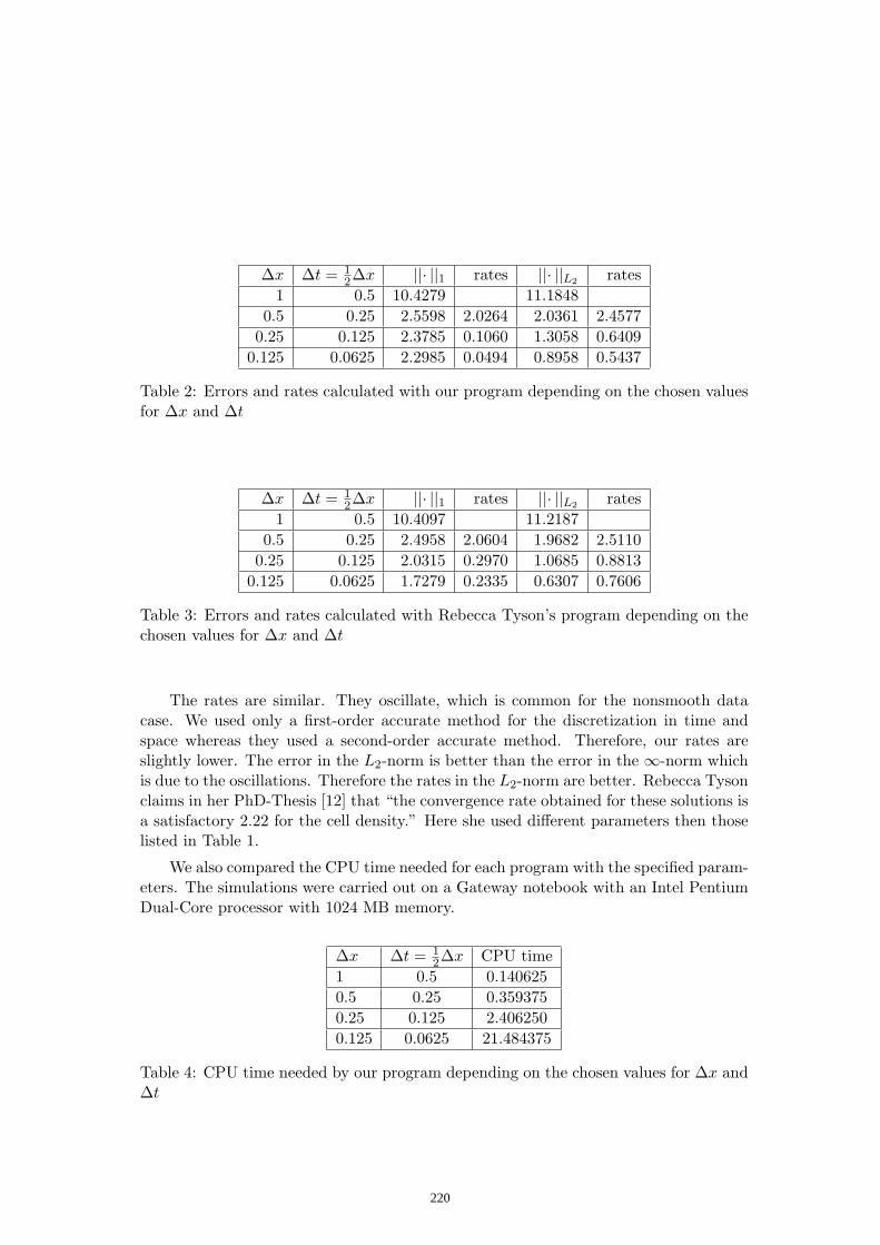
∆x ∆t = 1
2∆x ||· ||1 rates ||· ||L2
rates
1 0.5 10.4279 11.1848
0.5 0.25 2.5598 2.0264 2.0361 2.4577
0.25 0.125 2.3785 0.1060 1.3058 0.6409
0.125 0.0625 2.2985 0.0494 0.8958 0.5437
Table 2: Errors and rates calculated with our program depending on the chosen valuesfor ∆x and ∆t
∆x ∆t = 1
2∆x ||· ||1 rates ||· ||L2
rates
1 0.5 10.4097 11.2187
0.5 0.25 2.4958 2.0604 1.9682 2.5110
0.25 0.125 2.0315 0.2970 1.0685 0.8813
0.125 0.0625 1.7279 0.2335 0.6307 0.7606
Table 3: Errors and rates calculated with Rebecca Tyson’s program depending on thechosen values for ∆x and ∆t
The rates are similar. They oscillate, which is common for the nonsmooth datacase. We used only a first-order accurate method for the discretization in time andspace whereas they used a second-order accurate method. Therefore, our rates areslightly lower. The error in the L2-norm is better than the error in the ∞-norm whichis due to the oscillations. Therefore the rates in the L2-norm are better. Rebecca Tysonclaims in her PhD-Thesis [12] that “the convergence rate obtained for these solutions isa satisfactory 2.22 for the cell density.” Here she used different parameters then thoselisted in Table 1.
We also compared the CPU time needed for each program with the specified param-eters. The simulations were carried out on a Gateway notebook with an Intel PentiumDual-Core processor with 1024 MB memory.
∆x ∆t = 1
2∆x CPU time
1 0.5 0.140625
0.5 0.25 0.359375
0.25 0.125 2.406250
0.125 0.0625 21.484375
Table 4: CPU time needed by our program depending on the chosen values for ∆x and∆t
220
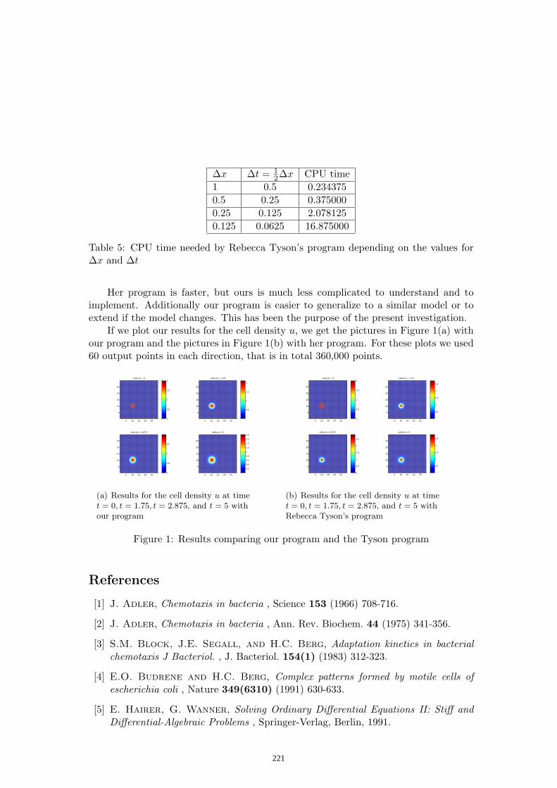
∆x ∆t = 1
2∆x CPU time
1 0.5 0.234375
0.5 0.25 0.375000
0.25 0.125 2.078125
0.125 0.0625 16.875000
Table 5: CPU time needed by Rebecca Tyson’s program depending on the values for∆x and ∆t
Her program is faster, but ours is much less complicated to understand and toimplement. Additionally our program is easier to generalize to a similar model or toextend if the model changes. This has been the purpose of the present investigation.
If we plot our results for the cell density u, we get the pictures in Figure 1(a) withour program and the pictures in Figure 1(b) with her program. For these plots we used60 output points in each direction, that is in total 360,000 points.
5 10 15 20 25
5
10
15
20
25
cells at t = 0
5 10 15 20 25
5
10
15
20
25
cells at t = 1.75
5 10 15 20 25
5
10
15
20
25
cells at t = 2.875
5 10 15 20 25
5
10
15
20
25
cells at t = 5
0
0.5
1
1.5
2
0.5
1
1.5
2
0
0.5
1
1.5
0.2
0.4
0.6
0.8
1
1.2
1.4
1.6
1.8
(a) Results for the cell density u at timet = 0, t = 1.75, t = 2.875, and t = 5 withour program
5 10 15 20 25
5
10
15
20
25
cells at t = 0
5 10 15 20 25
5
10
15
20
25
cells at t = 1.75
5 10 15 20 25
5
10
15
20
25
cells at t = 2.875
5 10 15 20 25
5
10
15
20
25
cells at t = 5
0
0.5
1
1.5
2
0.5
1
1.5
2
2.5
0
0.5
1
1.5
2
2.5
0.5
1
1.5
2
2.5
(b) Results for the cell density u at timet = 0, t = 1.75, t = 2.875, and t = 5 withRebecca Tyson’s program
Figure 1: Results comparing our program and the Tyson program
References
[1] J. Adler, Chemotaxis in bacteria , Science 153 (1966) 708-716.
[2] J. Adler, Chemotaxis in bacteria , Ann. Rev. Biochem. 44 (1975) 341-356.
[3] S.M. Block, J.E. Segall, and H.C. Berg, Adaptation kinetics in bacterialchemotaxis J Bacteriol. , J. Bacteriol. 154(1) (1983) 312-323.
[4] E.O. Budrene and H.C. Berg, Complex patterns formed by motile cells ofescherichia coli , Nature 349(6310) (1991) 630-633.
[5] E. Hairer, G. Wanner, Solving Ordinary Differential Equations II: Stiff andDifferential-Algebraic Problems , Springer-Verlag, Berlin, 1991.
221
[6] R.J. LeVeque, Wave propagation algorithms for multi-dimensional hyperbolicsystems , J. Comput. Phys. 131 (1997) 327–353.
[7] M. Luskin and R. Rannacher, On the Smoothing Property of the Crank-Nicholson Scheme , Appl. Anal. 14 (1982) 117–135.
[8] M. Luskin and R. Rannacher, On the Smoothing Property of the GalerkinMethod for Parabolic Equations , SIAM J. Numer. Anal. 19 (1982) 93–113.
[9] R. Rannacher, Finite Element Solution of Diffusion Problems with IrregularData , Numer. Math. 43 (1984) 309–327.
[10] R. Rannacher, Discretization of the Heat Equation with Singular Initial Data ,Zeit. Ang. Math. Meth. (ZAMM) 62 (1982) 346–348.
[11] G.D. Smith, Numerical Solution of Partial Differential Equations: Finite Differ-ence Methods , Oxford University Press, New York, 1985.
[12] R.C. Tyson, Pattern formation by E. coli - mathematical and numerical investi-gation of a biological phenomenon , PhD thesis, University of Washington, 1996.
[13] R.C. Tyson, L.G. Stern and R.J. LeVeque, Fractional step methods appliedto a chemotaxis model , J. Math. Biol. 41 (2000) 455–475.
[14] R.C. Tyson, S.R. Lubkin, and J.D. Murray, A minimal mechanis for bac-terial pattern formation , Proceedings of the Royal Society B: Biological Sciences266(1416) (1999) 299-304.
[15] B.A. Wade, A.Q.M. Khaliq, M. Siddique, and M. Yousuf, Smoothing withPositivety-Preserving Pade Schemes for Parabolic Problems with Nonsmooth dataNumerical Methods for Partial Differential Equations , Wiley Interscience 21(3)
(2005) 553-573.
[16] R. Weiner, B.A. Schmitt, H. Podhaisky, ROWMAP - a ROW-code withKrylov techniques for large stiff ODEs , Appl. Num. Math. 25 (1997) 303–319.
[17] M. Yousuf, Smoothing schemes for the inhomogeneous linear and semilinearparabolic problems with nonsmooth data , PhD thesis, University of Wisconsin- Milwaukee, 2005.
222

Solving stiff second order initial valueproblems directly by Backward
Differentiation Formulas
Samuel N. JatorDepartment of MathematicsAustin Peay State UniversityClarksville, TN 37044, U. S. A
Email: [email protected]
May 17, 2007
Abstract
In this paper, we propose a family of Backward Differentiation Formulas (BDFs)forthe direct solution of the general stiff second order initial value problems (IVPs)of the form y′′ = f(x, y, y′). The method is derived by the interpolation and collo-cation of the assumed approximate solution and its second derivative at x = xn+j
,j = 1, 2, ..., k − 1 and x = xn+k respectively, where k is the step number of themethod. The interpolation and collocation procedures lead to a system of (k+1)equations, which are solved to to determine the unknown coefficients. The result-ing coefficients are used to construct the approximate continuous solution fromwhich Multiple Finite Difference Methods (MFDMs) are obtained and simultane-ously applied to provide a direct solution to IVPs. Two specific methods for k = 2and k = 3 are used to illustrate the process. Numerical examples are given to showthe efficiency of the method.
AMS Subject Classification : 65L05, 65L06, 65L12
Key Words: Backward Differentiation Formulas, Collocation, Interpolation, SecondOrder, Initial Value Problem, Multiple Finite Difference Methods
223

1 Introduction
The general second-order ordinary differential equation of the form
y′′ = f(x, y, y′), (1)
y(a) = y0, y′(a) = δ0
is encountered in several areas of engineering and science such as circuit theory, con-trol theory, chemical kinetics, and biology. In practice, problem (1) is solved by firstreducing it to a system of first-order differential equations and then applying the variousmethods available for solving systems of first order IVPs. This approach is extensivelydiscussed in the literature and in this paper we cite just a few notable ones such asLambert[8], [9], Brugnano and Trigiante[2], Onumanyi et al [11], [10], Fatunla[4]. Inparticular, BDFs are well known for their effectiveness in solving stiff IVPs Gear[5] . Al-though there has been tremendous success with this approach, it has certain draw backs.For instance, computer programs associated with the methods are often complicated es-pecially when incorporating subroutines to supply the starting values for the methodsresulting in longer computer time and more human effort.
In the past decades, considerable attention has been devoted to solving (1) directlywithout first reducing it to a system of first order differential equations. In particular,the focus has mostly been concentrated on solving directly the special form of (1) givenby y′′ = f(x, y) since it occurs frequently in mechanical systems without dissipation. Inthis area, Twizell and Khaliq[13], proposed a class of p-stable two-step higher-derivativeformulas for the special second-order initial-value problems. Yusuph and Onumanyi[14]proposed two new LMMs of order 4 associated with the standard Numerov method whichwere applied to solve the special form of (1) directly. We also cite the works of Simos[12],Fatunla[4], and Lambert[8].
Several methods have also been proposed in the literature for solving the generalform (1) directly without first reducing it to an equivalent first-order system. For in-stance, Hairer and Wanner[6] proposed Nystrom type methods for (1) and stated orderconditions for determining the parameters of the methods. Other methods of the Runge-Kutta type considered in the literature for solving (1) are due to Chawla and Sharma[3]and Henrinci[7]. Awoyemi[1] considered multiderivative methods of the LMM type andstated that the direct application of those methods to non-stiff problems of the form (1)saves computer time and human effort. In Awoyemi[1] the methods were implementedas predictor - corrector methods and the Taylor Series algorithm was used to supplythe starting values. While the methods yielded good results, the disadvantage in thisapproach is that the Taylor series algorithm involves higher order partial derivatives thatare tedious to obtain.
224

In this paper, we propose a family of BDFs of steps k = 2 and k = 3 which areimplemented on stiff IVPs of the form (1) without the need for either predictors orstarting values from other methods.
The paper is organized as follows. In section two, we derive an approximation fory(x) which is continuous. Section three is devoted to the specification of the methods andhow the MFDMs are obtained and simultaneously applied to (1). Numerical examplesare given in section four to show the efficiency of the method. Finally, the conclusion ofthe paper is discussed in section five.
2 The derivation method
We seek an approximation of the form
y(x) ≈ y(x) =k∑
j=0
ιjΥj(x) (2)
where Υj(x) ’s are assumed polynomial basis functions and ιj ’s are unknown coeffi-cients to be determined by imposing the following conditions.
y (xn+j) = yn+j, j = 0, · · · , k − 1 (3)
y′′ (xn+k) = fn+k (4)
Hence, equations (3) and (4) lead to a system of (k+1) equations which is solved toobtain ιj ’s .Our k-step continuous BDF is constructed by substituting the the values ofιj ’s into equation (2). After some manipulation, our method is expressed in the form
y(x) =k−1∑j=0
αj(x)yn+j + h2βk(x)fn+k (5)
which is applied directly to provide the solution to (1). In particular, we seek asolution on
πN : a = x0 < x1 < x2 < ... < xn < xn+1 < ... < xN = b
225
h = xn+1 − xn , n = 0, 1, . . . N
where πN is a partition of [a, b] and h is the constant step-size of the partition of πN .
In the next section, we specify the methods.
3 Specification of the Methods
We obtain 2 methods for k = 2 and k = 3 with the following specifications:
Case: k=2
Υj(x) = xj , i = 0, · · · , 2.
We also express αj(x) and βj(x) as functions of t where t = (x − xn+1)/h in whatfollows:
α0(t) = −t ; α1(t) = (1 + t)
β2(t) = 12(t + t2)
The following 2-step BDF is obtained by evaluating (5) at x = xn+2
yn+2 − 2yn+1 + yn = h2fn+2
An additional Equation and derivatives are obtained by imposing that
y′(x) = δ(x) , y′(a) = δ0
In particular, to start the initial value problem for n = 0, we obtain the followingequation from y′(a) = δ0.
hδ0 = yn+1 − yn − h2
2fn+2
It is worth noting that the derivatives are provided by δ(xn+τ ), τ = 1, 2 as follows:
hδn+1 = −yn + yn+1 + h2
2fn+2
hδn+2 = −yn + yn+1 + 3h2
2fn+2
226

Case: k=3
Υj(x) = xj , i = 0, · · · , 3.
We also express αj(x) and βj(x) as functions of t where t = (x − xn+2)/h in whatfollows:
α0(t) = 112
(4t + 3t2 − t3) ; α1(t) = 16(−10t− 3t2 + t3)
α2(t) = 112
(12 + 16t + 3t2 − t3) ; β3(t) = h2
12(2t + 3t2 + t3)
The following 3-step BDF is obtained by evaluating (5) at x = xn+3
2yn+3 − 5yn+2 + 4yn+1 − yn = h2fn+3 (6)
Equation (6) can be used with the following additional methods:
−2yn + 5yn+1 − 4yn+2 + yn+3 = −h2fn
which is obtained from (5) by numbering the grid points from the right to the leftwith a negative step-size and
hδ0 = −53yn + 7
3yn+1 − 2
3yn+2 + h2
6fn+3
is obtained from y′(a) = δ0.
It is worth noting that the derivatives are provided by δ(xn+τ ), τ = 1, · · · , 3 as follows:
hδn+1 = − 512
yn − 16yn+1 + 7
12yn+2 − h2
12fn+2
hδn+2 = 13yn − 5
3yn+1 + 5
3yn+2 + h2
6fn+3
hδn+3 = 712
yn − 136yn+1 + 19
12yn+2 + 11h2
12fn+3
It is vital to note that the resulting specific case of y(x) evaluated at xn+k can beused as a continuous numerical integrator directly and singly in the conventional wayon overlapping sub-intervals. However, a better approach is to derive MFDMs from theevaluation of y(x) and the first derivative function δ(x) at specified points. The MFDMsobtained are applied to simultaneously provide values for y1, · · · , yk without looking forany other methods to provide the starting values. Hence, this is an improvement overthe use of (5) evaluated at xn+k singly for IVPs. We proceed by explicitly obtaining
227

initial conditions at xn+k, n = 0, k, · · · , N − k using the computed values y(xn+k) = yn+k
and δ(xn+k) = δn+k over sub-intervals [x0, xk], · · · , [xN−k, xN ] which do not overlap (see[14]). In addition to providing the starting values, the method also provides an accurateapproximation to y′(x) using δ(x).
4 Numerical examples
In this section, we give 2 examples to illustrate the efficiency of the methods. We findabsolute errors of the approximate solution in πN . The computations were carried outusing our written Mathematica code in Mathematica 5.2 (see tables 1 to 4) .
Example 4.1.y′′ + 1001y′ + 1000y = 0, y(0) = 1, y′(0) = −1
Exact : y(x) = e−x
Example 4.2.y′′ + 102y′ + 200y = 0, y(0) = 1, y′(0) = −2
Exact : y(x) = e−2x
x y y Error
0.0 1.0000000000 1.0000000000 0.0000000.1 0.904837418035959473 0.904543399638336964 2.94018× 10⁻⁴
0.2 0.818730753077981887 0.818173598553347147 5.57155× 10⁻⁴
0.3 0.740818220681717853 0.740066941293423763 7.51279× 10⁻⁴
0.4 0.670320046035639371 0.669399772406962778 9.20274× 10⁻⁴
0.5 0.606530659712633379 0.605501145850122934 10.29514× 10⁻⁴
0.6 0.5488116360940265 0.547685220660996208 11.26415× 10⁻⁴
0.7 0.496585303791409593 0.495405051428370057 11.80252× 10⁻⁴
0.8 0.449328964117221563 0.448101587862691275 12.27376× 10⁻⁴
0.9 0.406569659740599131 0.405327333668655853 12.42326× 10⁻⁴
1.0 0.367879441171442334 0.366624888659087 12.54553× 10⁻⁴
Table 1: Absolute Errors, ‖y − y‖, for Example 4.1, Case k = 2, where y(x) = e−x
228

x y y Error
0.0 1.0000000000 1.0000000000 0.0000000.1 0.818730753077981887 0.816535433070866112 2.19532× 10⁻³
0.2 0.670320046035639371 0.666141732283464538 4.17831× 10⁻³
0.3 0.5488116360940265 0.543474486948973822 5.33715× 10⁻³
0.4 0.449328964117221563 0.443189286378572688 6.13968× 10⁻³
0.5 0.367879441171442334 0.361550989243710718 6.32845× 10⁻³
0.6 0.301194211912202147 0.294824454215837548 6.36976× 10⁻³
0.7 0.246596963941606528 0.240514319493515893 6.08264× 10⁻³
0.8 0.201896517994655377 0.196125223275308577 5.77129× 10⁻³
0.9 0.165298888221586555 0.159996554702243365 5.30233× 10⁻³
1.0 0.135335283236612702 0.130467702915348038 4.86758× 10⁻³
Table 2: Absolute Errors, ‖y − y‖, for Example 4.2, Case k = 2, where y(x) = e−2x
x y y Error
0.0 1.0000000000 1.0000000000 0.0000000.1 0.904837418035959473 0.904848530444377274 1.11124× 10⁻⁵
0.2 0.818730753077981887 0.818788243555019512 5.74905× 10⁻⁵
0.3 0.740818220681717853 0.740910321998192245 9.21013× 10⁻⁵
0.4 0.670320046035639371 0.670360829978287053 4.07839× 10⁻⁵
0.5 0.606530659712633379 0.606505357852192261 2.53019× 10⁻⁵
0.6 0.5488116360940265 0.548764377514921797 4.72586× 10⁻⁵
0.7 0.496585303791409593 0.496566369066338086 1.89347× 10⁻⁵
0.8 0.449328964117221563 0.449371845425690263 4.28813× 10⁻⁵
0.9 0.406569659740599131 0.406649327717074182 7.96680× 10⁻⁵
1.0 0.367879441171442334 0.367908853058919316 2.94119 ×10⁻⁵
1.1 0.332871083698079539 0.332826522546983571 4.45612× 10⁻⁵
1.2 0.301194211912202147 0.301119953271358253 7.42586× 10⁻⁵
Table 3: Absolute Errors, ‖y − y‖, for Example 4.1, Case k = 3, where y(x) = e−x
229

x y y Error
0.0 1.0000000000 1.0000000000 0.0000000.1 0.818730753077981887 0.818894645941277943 1.63893× 10⁻⁴
0.2 0.670320046035639371 0.671157167530224008 8.37121× 10⁻⁴
0.3 0.5488116360940265 0.550155440414506724 13.43804× 10⁻⁴
0.4 0.449328964117221563 0.449968231809354257 6.39268× 10⁻⁴
0.5 0.367879441171442334 0.367517875200228694 3.61566× 10⁻⁴
0.6 0.301194211912202147 0.300437595640151045 7.56616× 10⁻⁴
0.7 0.246596963941606528 0.246312289173206311 2.84675× 10⁻⁴
0.8 0.201896517994655377 0.202533535807732123 6.37018× 10⁻⁴
0.9 0.165298888221586555 0.166444586543129613 11.45698× 10⁻⁴
1.0 0.135335283236612702 0.135829954803814967 4.94672× 10⁻⁴
1.1 0.110803158362333875 0.11023920371426179 5.63955× 10⁻⁴
1.2 0.0907179532894125273 0.0896631588239585397 10.54795× 10⁻⁴
Table 4: Absolute Errors, ‖y − y‖, for Example 4.2, Case k = 3, where y(x) = e−2x
230

5 Conclusions
We have proposed Two specific methods for k = 2 and k = 3 for solving stiff second-order IVPs directly without first adapting the second order IVP to an equivalent firstorder system. An essential ingredient in the method involves the way in which it isapplied. For instance, we proceed by explicitly obtaining initial conditions at xn+k, n =0, k, ..., N − k using the computed values y(xn+k) = yn+k and δ(xn+k) = δn+k oversub-intervals [x0, xk], · · · , [xN−k, xN ] which do not overlap. We have demonstrated theefficiency of the methods on two stiff problems and the results are given in tables 1 and2 (case k = 2) and tables 3 and 4 (case k = 3). Our future research will be focused onstudying the stability properties of these methods and applying them as Boundary valuemethods to solve both initial and boundary value problems.
231

References
[1] Awoyemi, D. O., 1999, A class of continuous methods for general second order initialvalue problems in ordinary differential equations,Inter. J. Compt. Maths, 72, 1-9,29-37.
[2] Brugnano L. and D. Trigiante, D., 1998, Solving Differential Problems by Multi-tep Initial and Boundary Value Methods, Gordon and Breach Science Publishers,Amsterdam, 1998, 280-299.
[3] Chawla, M. M. and Sharma S. R., 1985, Families of Three-Stage Third Order Runge-Kutta-Nystrom Methods for y′′ = f(x, y, y′) , Journal of the Australian MathematicalSociety 26, 375-386.
[4] Fatunla, S.O., 1988, Numerical Methods for InitialValue Problems in Ordinary Dif-ferential Equation (NewYork: Academic Press Inc.).
[5] Gear, C.W., (1971a) Algorithm 407, DIFSUB for solution of Ordinary DifferentialEquations. Comm. ACM., vol 14, pp. 185 190.
[6] Hairer E. and Wanner G., 1976, A Theory for Nystrom methods, Numerische Math-ematik 25, 383 - 400.
[7] Henrici, P.,1962, Discrete Variable Methods for ODEs, John Wiley, New York, USA.
[8] Lambert, J. D.,1991, Numerical methods for ordinary differential systems, John Wi-ley, New York.
[9] Lambert, J. D,1973 Computational methods in ordinary differential equations, JohnWiley, New York.
[10] Onumanyi, P., Sirisena, U. W. and Jator, S.N., 1999, Continuous finite differenceapproximations for solving differential equations,Inter. J. Compt. Maths. 72, 1, 15-27(80).
[11] Onumanyi,P., Awoyemi, D. O., Jator, S. N. and Sirisena,U. W., 1994, New linearmutlistep methods with continuous coefficients for first order initial value problems,J. Nig. Math. Soc. 13, 37-51(7).
[12] Simos, T. E., 2002, Dissipative Trigonometrically-Fitted Methods for Second OrderIVPs with oscillating Solution, Int. J. Mod. Phys. 13, (10), 1333-1345.
[13] Twizell, E.H. and Khaliq, A.Q.M., 1984, Multiderivative methods for periodic IVPs.SIAM Journal of Numerical Analysis, 21, 111121.
[14] Yusuph, Y. and Onumanyi, P., 2005, New Multiple FDMs through multistep col-location for y′′ = f(x, y), Proceedings of the conference organized by the NationalMathematical Center, Abuja Nigeria.
232

Proceedings of the International Conference
on Computational and Mathematical Methods
in Science and Engineering, CMMSE 2007
Chicago, 20–23 June 2007.
A uniformly convergent B-spline collocation technique on a
non-uniform mesh for solving singularly perturbed turning
point problem exhibiting two boundary layers
Mohan K. Kadalbajoo1 and Vikas Gupta1
1 Department of Mathematics & Statistics, Indian Institute of Technology Kanpur, India.
emails: [email protected], [email protected]
Abstract
A numerical method is devised for solving singularly perturbed turning point boundaryvalue problems having two boundary layers. The proposed method is composed of B-splinecollocation on piecewise uniform mesh of Shishkin type. Some theoretical bounds are givenfor the derivative of analytical solution. The method is shown to be unconditionally stableand accurate of order O(∆x)2. An extensive amount of analysis has been carried out to provethe uniform convergence with respect to singular perturbation parameter. Several numericalexperiments have been included to support the theoretical results and to demonstrate theefficiency of the method.
Key words: singular perturbation, turning point, B-spline collocation, Shishkin mesh,boundary layer, uniform convergence
MSC 2000: 65L10, 65L20
1 Introduction
Singularly perturbed problems arises in various field of Physics and Engineering such as fluid
flows at high Reynolds numbers, heat and mass transfer with high peclet numbers [10][12],
drift-diffusion equation of semiconductor device modeling [17] and magneto-hydrodynamics duct
problems at high Hartman numbers [9]. The solution of singular perturbation problems pos-
sesses steep gradients in narrow layer regions of the domain depending upon the nature of the
convection coefficient, as the singular perturbation parameter ε approaches zero. Therefore in
order to tackle such oscillations we need to derive a method using a class of special piecewise-
uniform mesh, called Shishkin mesh, where half the mesh points are concentrated in the layer
regions. For further discussions, reader may refer to Doolan et. al. [5] Farrell et. al. [6] Miller
233

et. al. [14] and Roos et al. [19].
In particular, singularly perturbed turning point problems received much attention in the lit-
erature due to the complexity involved in finding uniformly valid asymptotic expansions unlike
non-turning point problems. In this paper, we consider the following singularly perturbed two-
point boundary value problem with a turning point at x = 0:
Lu(x) ≡ εu′′(x) + a(x)u′(x)− b(x)u(x) = f(x), x ∈ Ω = (−1, 1), (1.1a)
u(−1) = A, u(1) = B, (1.1b)
where ε is a small perturbation parameter satisfying 0 < ε << 1, A and B are given constants,
a, b and f are sufficiently smooth functions. Moreover,
a(0) = 0, a′(0) ≤ 0. (1.2)
|a(x)| ≥ a0 > 0, 0 < |x| ≤ 1. (1.3)
b(x) ≥ 0, b(0) > 0. (1.4)
b(x) ≥ b0 > 0, x ∈ Ω = [−1, 1], (1.5)
|a′(x)| ≥∣∣∣∣a′(0)
2
∣∣∣∣ , x ∈ Ω = [−1, 1]. (1.6)
Under these assumptions (1.2)- (1.6), the turning point problem (1.1) possesses a unique
solution having twin boundary layers at x = −1 and x = 1 i.e., at both end points [2].
Abrahmsson [1] derived a priori estimates for solution of singular perturbation problems with a
turning point. Berger et. al.[2], Wasow [23] and O’Malley [16] studied qualitative aspects of these
problems. Farrell [7] gave the sufficient conditions for uniform convergence of a difference scheme
for these turning point problems. Sun and Stynes used Galerkin finite element methods on
various piecewise uniform meshes for such problems [20]. Clavero et. al. presented a uniformly
convergent finite difference method for such problems with turning points [3], whereas, Surla
and Uzelac [22] solved them by taking a linear combination of the two spline difference schemes.
Kadalbajoo and Patidar [11] proposed a numerical method based on cubic spline approximation
with nonuniform mesh for the singularly perturbed two-point boundary value problems having
a turning point. In this paper, we propose a B-spline collocation method to solve problems of
type (1.1) with piecewise uniform mesh of Shishkin type.
This paper is organized as follows. In Section 2 we present some analytical results for continuous
turning point problem (1.1). In Section 3 we use B-spline collocation method to solve the problem
with Shishkin mesh. The derivation of uniform convergence is given in Section 4. Some numerical
examples have been solved and the results are presented in Section 5. Finally, discussion and
conclusion is given at the end of the paper in Section 6. Throughout the paper we use C as a
generic positive constant independent of ε and mesh parameter.
234
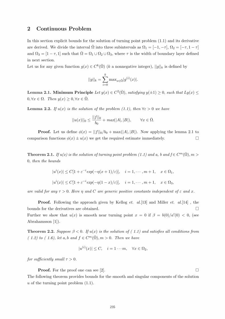
2 Continuous Problem
In this section explicit bounds for the solution of turning point problem (1.1) and its derivative
are derived. We divide the interval Ω into three subintervals as Ω1 = [−1,−τ ], Ω2 = [−τ, 1− τ ]
and Ω3 = [1− τ, 1] such that Ω = Ω1 ∪Ω2 ∪Ω3, where τ is the width of boundary layer defined
in next section.
Let us for any given function g(x) ∈ Ck(Ω) (k a nonnegative integer), ||g||k is defined by
||g||k =k∑
i=0
maxx∈Ω|g(i)(x)|.
Lemma 2.1. Minimum Principle Let y(x) ∈ C2(Ω), satisfying y(±1) ≥ 0, such that Ly(x) ≤0,∀x ∈ Ω. Then y(x) ≥ 0,∀x ∈ Ω.
Lemma 2.2. If u(x) is the solution of the problem (1.1), then ∀ε > 0 we have
||u(x)||0 ≤ ||f ||0b0
+ max(|A|, |B|), ∀x ∈ Ω.
Proof. Let us define φ(x) = ||f ||0/b0 + max(|A|, |B|). Now applying the lemma 2.1 to
comparison functions φ(x)± u(x) we get the required estimate immediately.
Theorem 2.1. If u(x) is the solution of turning point problem (1.1) and a, b and f ∈ Cm(Ω),m >
0, then the bounds
|ui(x)| ≤ C[1 + ε−iexp(−η(x + 1)/ε)], i = 1, · · · ,m + 1, x ∈ Ω1,
|ui(x)| ≤ C[1 + ε−iexp(−η(1− x)/ε)], i = 1, · · · ,m + 1, x ∈ Ω3,
are valid for any τ > 0. Here η and C are generic positive constants independent of ε and x.
Proof. Following the approach given by Kellog et. al.[13] and Miller et. al.[14] , the
bounds for the derivatives are obtained.
Further we show that u(x) is smooth near turning point x = 0 if β = b(0)/a′(0) < 0, (see
Abrahamsson [1]).
Theorem 2.2. Suppose β < 0. If u(x) is the solution of ( 1.1) and satisfies all conditions from
( 1.2) to ( 1.6), let a, b and f ∈ Cm(Ω),m > 0. Then we have
|u(i)(x)| ≤ C, i = 1 · · ·m, ∀x ∈ Ω2,
for sufficiently small τ > 0.
Proof. For the proof one can see [2].
The following theorem provides bounds for the smooth and singular components of the solution
u of the turning point problem (1.1).
235

Theorem 2.3. Suppose the solution u of the turning point problem (1.1) has the decomposition
u = v + w,
where, for all i, 0 ≤ i ≤ 3, the smooth component satisfies
|v(i)(x)| ≤ C[1 + ε−(i−2)(exp(−a0(1 + x)/ε) + exp(−a0(1− x)/ε))], ∀x ∈ Ω,
and the singular component satisfies
|w(i)(x)| ≤ Cε−i(exp(−a0(1 + x)/ε) + exp(−a0(1− x)/ε)), ∀x ∈ Ω.
Proof. The proof follows by approach as given in Miller et. al.[14]
3 Discrete Problem
In this section, third-degree B-splines are used to construct collocation method to turning point
problem (1.1) discussed in section 1 with nonuniform mesh ΩN of Shishkin type. Shishkin mesh
is defined as follows:
3.1 Shishkin Mesh
Consider N = 2m with m ≥ 3, be a positive integer and let τ be the width of boundary layer.
Therefore, for a given N and ε, the interval Ω = [−1, 1] be divided into three subintervals
Ω1 = [−1,−1 + τ ], Ω2 = [−1 + τ, 1− τ ] and Ω3 = [1− τ, 1] such that Ω = Ω1 ∪ Ω2 ∪ Ω3.
The transition parameter τ is given by
τ ≡ min14,Kε log N, K ≥ 1
mina0, b0 .
Thus transition parameter τ depends on both ε and N . The value of constant K depends on
the particular scheme being used. Define
h =
h1 = hi = 4τ/N, if i = 1, 2, · · ·N/4,
h2 = hi = 4(1− τ)/N, if i = N/4 + 1, · · · 3N/4,
h3 = hi = 4τ/N, if i = 3N/4 + 1, · · ·N .
(3.1)
where N is the no. of discretization points and the set of mesh points ΩN = xiNi=0 with
xi =
−1 + (4τ/N)i, if i = 0, 1, 2, · · ·N/4,
(−1 + τ) + (4(1− τ)/N)(i−N/4), if i = N/4 + 1, · · · 3N/4,
(1− τ) + (4τ/N)(i− 3N/4), if i = 3N/4 + 1, · · ·N ,
(3.2)
i.e. the finite interval [−1, 1] is partitioned into N finite elements by the partition π : −1 = x0 <
x1 < x2 < · · · < xN = 1, where h is the piecewise uniform mesh spacing.
236

3.2 Methodology of B-spline Collocation
We assume X is a linear subspace of L2(Ω), the space of all square integrable functions defined
on Ω. For i = −1, 0, . . . , N + 1, the cubic B-splines are defined by the following relation[18]
φi(x) =1h3
(x− xi−2)3, xi−2 ≤ x ≤ xi−1,
h3 + 3h2(x− xi−1) + 3h(x− xi−1)2 − 3(x− xi−1)3, xi−1 ≤ x ≤ xi,
h3 + 3h2(xi+1 − x) + 3h(xi+1 − x)2 − 3(xi+1 − x)3, xi ≤ x ≤ xi+1,
(xi+2 − x)3, xi+1 ≤ x ≤ xi+2,
0, otherwise.
(3.3)
Each φi(x) is a continuously differentiable, piecewise cubic on π and φi(x) ∈ X. Reader can find
detailed description of B-spline functions in [18], [15] and [21]. Now suppose the approximate
solution of Eq. (1.1) is given by
U(x) =N+1∑
i=−1
ciφi(x), (3.4)
where ci are unknown real coefficients. Here we have introduced two extra cubic B-splines, φ−1
and φN+1 to satisfy the boundary conditions. Therefore, we have
LU(xi) = f(xi), 0 ≤ i ≤ N , (3.5)
and
U(x0) = A, U(xN ) = B. (3.6)
On solving the collocation equations (3.5), and putting the values of B-spline functions φi and
of derivatives at mesh points ΩN , we obtain a system of (N + 1) linear equations in (N + 3)
unknowns
(6ε− 3aih− bih2)ci−1 + (−12ε− 4bih
2)ci
+ (6ε + 3aih− bih2)ci+1 = fih
2, 0 ≤ i ≤ N . (3.7)
The given boundary conditions become
c−1 + 4c0 + c1 = A, (3.8)
and
cN−1 + 4cN + cN+1 = B. (3.9)
Thus by the Eqs. (3.7), (3.8) and (3.9) we obtain a (N+3)×(N+3) system with (N+3) unknowns
c−1, c0, . . . , cN+1. Now eliminating c−1 from first equation of (3.7) and from equation (3.8),
we find
(−36ε + 12a0h)c0 + 6a0hc1 = f0h2 −A(6ε− 3a0h− b0h
2). (3.10)
Similarly, eliminating cN+1 from the last equation of (3.7) and from (3.9), we get
6aN hcN−1 + (−36ε + 12aN h)cN = fN h2 −B(6ε + 3aN h− bN h2). (3.11)
237

Thus we are lead to a system of (N + 1) linear equations in (N + 1) unknowns
TxN = dN . (3.12)
Where xN = (c0, c1, . . . , cN )T are the unknown real coefficients with right hand side dN =(f0h
2 −A(6ε− 3a0h− b0h2), f1h
2, . . . , fN−1h2, fN h2 −B(6ε + 3aN h− bN h2))T . The coefficient
matrix T is given by
2666666666666666664
−36ε + 12a0h 6a0h 0 0 . . . 0
6ε− 3a1h− b1h2 −12ε− 4b1h2 6ε + 3a1h− b1h2 0 . . . 0
..
....
..
.... . . .
..
.
0 0 6ε− 3aih− bih2 −12ε− 4bih
2 6ε + 3aih− bih2 0
.
.....
.
.....
.
.....
..
....
..
....
..
....
0 . . . 0 6ε− 3aN−1h− bN−1h2 −12ε− 4bN−1h2 6ε + 3aN−1h− bN−1h2
0 . . . 0 0 −6aN h −36ε− 12aN h
3777777777777777775
It is easily seen that collocation matrix T is strictly diagonally dominant and hence nonsingular.
Since T is nonsingular, we can solve (3.12) for c0, c1, . . . , cN and substitute into the boundary
conditions (3.8) and (3.9) to obtain c−1 and cN+1. Hence the method of collocation using a basis
of cubic B-splines applied to problem (1.1) has a unique solution U(x) given by (3.4).
4 Derivation for Uniform Convergence
In this section we deduce that the present collocation method has a uniform convergence of
order two with Shishkin mesh in maximum norm.
Theorem 4.1. Let u ∈ C4[−1, 1] be the solution of problem (1.1) and let U be the cubic B-
spline collocation approximate on the piecewise uniform mesh. Then for N sufficiently large
(independently of ε), we have
sup0<ε≤1
||U − u||Ω ≤ CN−2(lnN)2.
Proof. The solution U of the discrete problem is decomposed in an analogous manner as
that of the continuous solution u. Thus U = V +W , where V is the solution of the inhomogeneous
problem given by
LV = f, V (−1) = v(1), V (1) = v(1),
and W is the solution of the homogeneous problem
LW = 0, W (−1) = w(1), W (1) = w(1).
To show the proposed collocation method is ε-uniform, here we consider only the subinterval
[−1, 0]. In the same way, one can obtain similar estimate in the subinterval [0, 1]. Here we use
de Boor [4] and Hall [8] spline interpolation error estimates to derive ε-uniform error estimate.
238
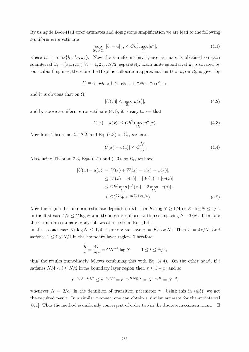
By using de Boor-Hall error estimates and doing some simplification we are lead to the following
ε-uniform error estimate
sup0<ε≤1
||U − u||Ω ≤ Ch2c max
Ω|u′′|, (4.1)
where hc = maxh1, h2, h3. Now the ε-uniform convergence estimate is obtained on each
subinterval Ωi = (xi−1, xi),∀i = 1, 2 . . . N/2, separately. Each finite subinterval Ωi is covered by
four cubic B-splines, therefore the B-spline collocation approximation U of u, on Ωi, is given by
U = ci−2φi−2 + ci−1φi−1 + ciφi + ci+1φi+1,
and it is obvious that on Ωi
|U(x)| ≤ maxΩi
|u(x)|, (4.2)
and by above ε-uniform error estimate (4.1), it is easy to see that
|U(x)− u(x)| ≤ Ch2 maxΩi
|u′′(x)|. (4.3)
Now from Theorems 2.1, 2.2, and Eq. (4.3) on Ωi, we have
|U(x)− u(x)| ≤ Ch2
ε2. (4.4)
Also, using Theorem 2.3, Eqs. (4.2) and (4.3), on Ωi, we have
|U(x)− u(x)| = |V (x) + W (x)− v(x)− w(x)|,≤ |V (x)− v(x)|+ |W (x)|+ |w(x)|≤ Ch2 max
Ωi
|v′′(x)|+ 2 maxΩi
|w(x)|,
≤ C(h2 + e−a0(1+xi)/ε). (4.5)
Now the required ε- uniform estimate depends on whether Kε log N ≥ 1/4 or Kε log N ≤ 1/4.
In the first case 1/ε ≤ C log N and the mesh is uniform with mesh spacing h = 2/N . Therefore
the ε- uniform estimate easily follows at once from Eq. (4.4).
In the second case Kε log N ≤ 1/4, therefore we have τ = Kε log N . Then h = 4τ/N for i
satisfies 1 ≤ i ≤ N/4 in the boundary layer region. Therefore
h
ε=
4τ
Nε= CN−1 log N, 1 ≤ i ≤ N/4,
thus the results immediately follows combining this with Eq. (4.4). On the other hand, if i
satisfies N/4 < i ≤ N/2 in no boundary layer region then τ ≤ 1 + xi and so
e−a0(1+xi)/ε ≤ e−a0τ/ε = e−a0K log N = N−a0K = N−2,
whenever K = 2/a0 in the definition of transition parameter τ . Using this in (4.5), we get
the required result. In a similar manner, one can obtain a similar estimate for the subinterval
[0, 1]. Thus the method is uniformly convergent of order two in the discrete maximum norm.
239
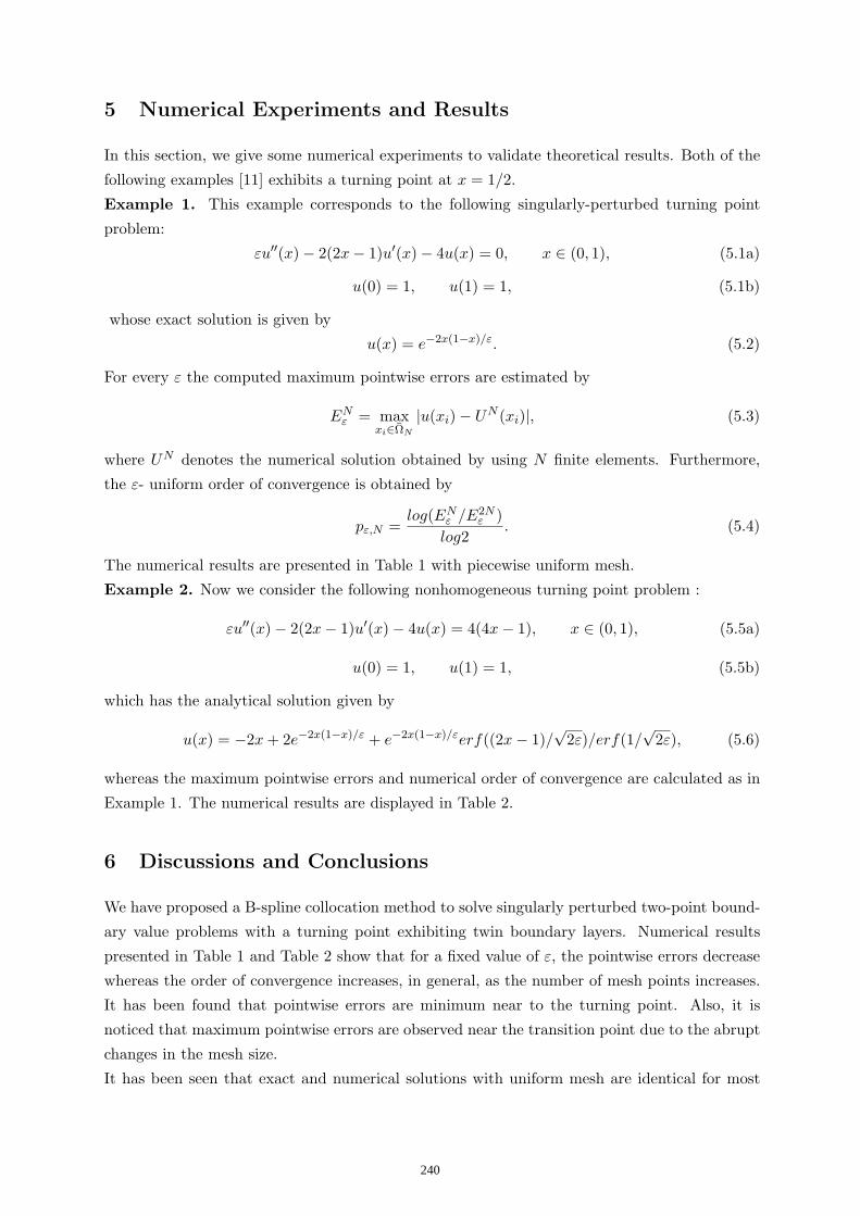
5 Numerical Experiments and Results
In this section, we give some numerical experiments to validate theoretical results. Both of the
following examples [11] exhibits a turning point at x = 1/2.
Example 1. This example corresponds to the following singularly-perturbed turning point
problem:
εu′′(x)− 2(2x− 1)u′(x)− 4u(x) = 0, x ∈ (0, 1), (5.1a)
u(0) = 1, u(1) = 1, (5.1b)
whose exact solution is given by
u(x) = e−2x(1−x)/ε. (5.2)
For every ε the computed maximum pointwise errors are estimated by
ENε = max
xi∈ΩN
|u(xi)− UN (xi)|, (5.3)
where UN denotes the numerical solution obtained by using N finite elements. Furthermore,
the ε- uniform order of convergence is obtained by
pε,N =log(EN
ε /E2Nε )
log2. (5.4)
The numerical results are presented in Table 1 with piecewise uniform mesh.
Example 2. Now we consider the following nonhomogeneous turning point problem :
εu′′(x)− 2(2x− 1)u′(x)− 4u(x) = 4(4x− 1), x ∈ (0, 1), (5.5a)
u(0) = 1, u(1) = 1, (5.5b)
which has the analytical solution given by
u(x) = −2x + 2e−2x(1−x)/ε + e−2x(1−x)/εerf((2x− 1)/√
2ε)/erf(1/√
2ε), (5.6)
whereas the maximum pointwise errors and numerical order of convergence are calculated as in
Example 1. The numerical results are displayed in Table 2.
6 Discussions and Conclusions
We have proposed a B-spline collocation method to solve singularly perturbed two-point bound-
ary value problems with a turning point exhibiting twin boundary layers. Numerical results
presented in Table 1 and Table 2 show that for a fixed value of ε, the pointwise errors decrease
whereas the order of convergence increases, in general, as the number of mesh points increases.
It has been found that pointwise errors are minimum near to the turning point. Also, it is
noticed that maximum pointwise errors are observed near the transition point due to the abrupt
changes in the mesh size.
It has been seen that exact and numerical solutions with uniform mesh are identical for most
240

of the region of the domain except in the boundary layer regions. Thus the present method is
second order accurate and numerical results support the theoretical estimates. This method is
shown to be uniformly convergent and independent of mesh parameters. The proposed method
gives more accurate results than many of other boundary layer resolving finite difference meth-
ods. Also this method produces the solution at any point in the domain, whereas the finite
difference methods gives the solution only at the chosen mesh points.
241
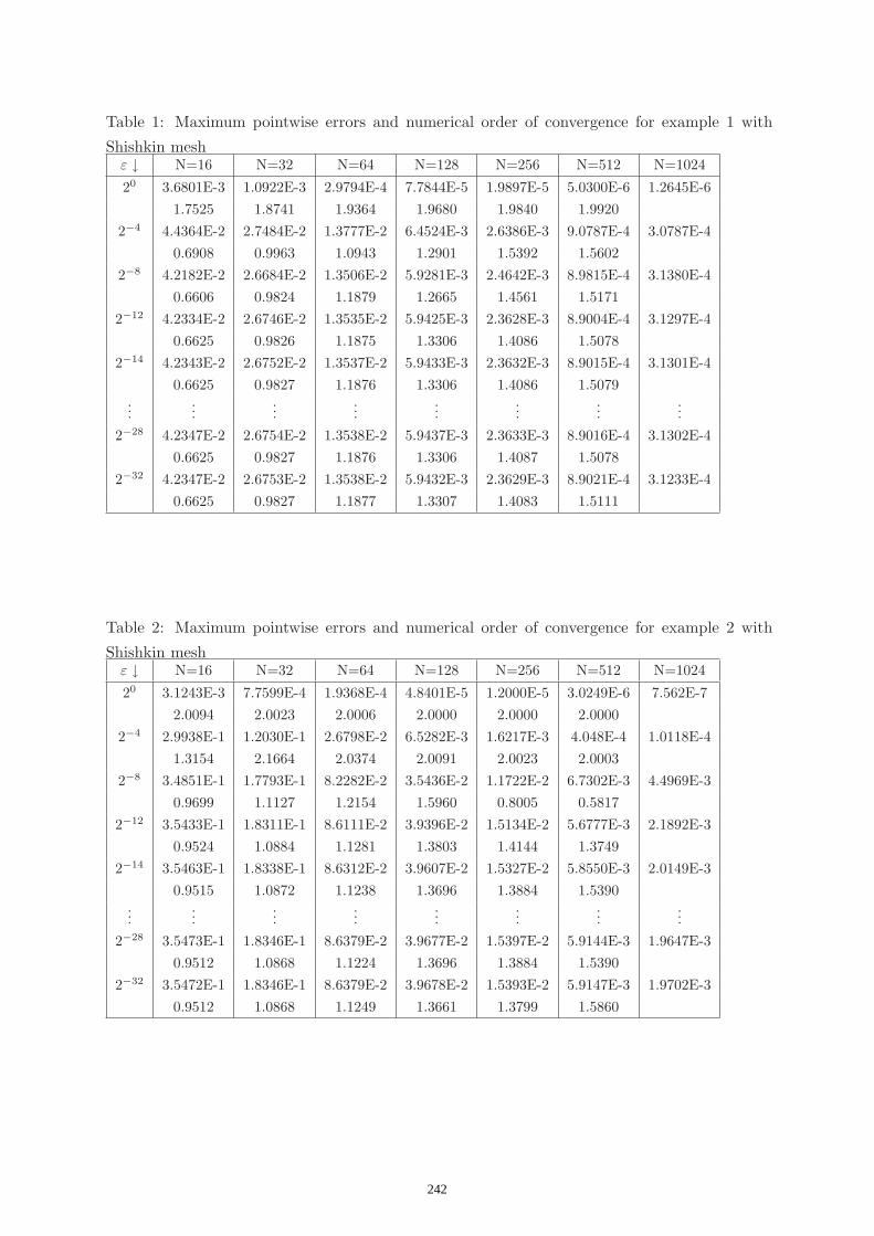
Table 1: Maximum pointwise errors and numerical order of convergence for example 1 with
Shishkin meshε ↓ N=16 N=32 N=64 N=128 N=256 N=512 N=1024
20 3.6801E-3 1.0922E-3 2.9794E-4 7.7844E-5 1.9897E-5 5.0300E-6 1.2645E-61.7525 1.8741 1.9364 1.9680 1.9840 1.9920
2−4 4.4364E-2 2.7484E-2 1.3777E-2 6.4524E-3 2.6386E-3 9.0787E-4 3.0787E-40.6908 0.9963 1.0943 1.2901 1.5392 1.5602
2−8 4.2182E-2 2.6684E-2 1.3506E-2 5.9281E-3 2.4642E-3 8.9815E-4 3.1380E-40.6606 0.9824 1.1879 1.2665 1.4561 1.5171
2−12 4.2334E-2 2.6746E-2 1.3535E-2 5.9425E-3 2.3628E-3 8.9004E-4 3.1297E-40.6625 0.9826 1.1875 1.3306 1.4086 1.5078
2−14 4.2343E-2 2.6752E-2 1.3537E-2 5.9433E-3 2.3632E-3 8.9015E-4 3.1301E-40.6625 0.9827 1.1876 1.3306 1.4086 1.5079
......
......
......
......
2−28 4.2347E-2 2.6754E-2 1.3538E-2 5.9437E-3 2.3633E-3 8.9016E-4 3.1302E-40.6625 0.9827 1.1876 1.3306 1.4087 1.5078
2−32 4.2347E-2 2.6753E-2 1.3538E-2 5.9432E-3 2.3629E-3 8.9021E-4 3.1233E-40.6625 0.9827 1.1877 1.3307 1.4083 1.5111
Table 2: Maximum pointwise errors and numerical order of convergence for example 2 with
Shishkin meshε ↓ N=16 N=32 N=64 N=128 N=256 N=512 N=1024
20 3.1243E-3 7.7599E-4 1.9368E-4 4.8401E-5 1.2000E-5 3.0249E-6 7.562E-72.0094 2.0023 2.0006 2.0000 2.0000 2.0000
2−4 2.9938E-1 1.2030E-1 2.6798E-2 6.5282E-3 1.6217E-3 4.048E-4 1.0118E-41.3154 2.1664 2.0374 2.0091 2.0023 2.0003
2−8 3.4851E-1 1.7793E-1 8.2282E-2 3.5436E-2 1.1722E-2 6.7302E-3 4.4969E-30.9699 1.1127 1.2154 1.5960 0.8005 0.5817
2−12 3.5433E-1 1.8311E-1 8.6111E-2 3.9396E-2 1.5134E-2 5.6777E-3 2.1892E-30.9524 1.0884 1.1281 1.3803 1.4144 1.3749
2−14 3.5463E-1 1.8338E-1 8.6312E-2 3.9607E-2 1.5327E-2 5.8550E-3 2.0149E-30.9515 1.0872 1.1238 1.3696 1.3884 1.5390
......
......
......
......
2−28 3.5473E-1 1.8346E-1 8.6379E-2 3.9677E-2 1.5397E-2 5.9144E-3 1.9647E-30.9512 1.0868 1.1224 1.3696 1.3884 1.5390
2−32 3.5472E-1 1.8346E-1 8.6379E-2 3.9678E-2 1.5393E-2 5.9147E-3 1.9702E-30.9512 1.0868 1.1249 1.3661 1.3799 1.5860
242

References
[1] L. Abrahamsson, A priori estimates for solutions of singular perturbations with a turning
point, Stud. Appl. Math. 56 (1977) 51–69.
[2] A. Berger, H. Han and R. Kellog, A priori estimates and analysis of a numerical
method for a turning point problem, Math. Comp. 42 (1984) 465–492.
[3] C. Clavero and F. Lisbona, Uniformly convergent finite difference methods for singularly
perturbed problems with turning points, Numer. Algo. 4 (1993) 339–359.
[4] C. de Boor, On the convergence of odd degree spline interpolation, J. Approx. Theory 1
(1968) 452–463.
[5] E.P. Doolan, J.J.H. Miller, and W.H.A. Schilders, Uniform Numerical Methods
for Problems with Initial and Boundary Layers, Boole Press, Dublin, 1980.
[6] P.A. Farrell, A.F. Hegarty, J.J.H. Miller, E. O’Riordan, and G.I. Shishkin,
Robust Computational Techniques for Boundary Layers, Chapman & hall, CRC Press, Boca
Raton, Florida, 2000.
[7] P.A. Farrell, Sufficient conditiond for the uniform convergence of a difference scheme
for a singularly perturbed turning point problem, SIAM J. Numer. Anal. 25 (1988) 618–643.
[8] C.A. Hall, On error bounds for spline interpolation, J. Approx. Theory 1 (1968) 209–218.
[9] J.C.R. Hunt and J.A. Shercliff, Magnetohydrodynamics at high Hartman number,
Ann. Rev. Fluid Mech. 3 (1971) 37-62.
[10] M. Jacob, Heat transfer., Wiley, New York, 1959.
[11] M.K. Kadalbajoo and K.C. Patidar, Variable mesh spline approximation method for
solving singularly perturbed turning point problems having boundary layer(s), Comp. Math.
Appl. 42 (2001) 1439–1453.
[12] H.O. Kreiss, T.A. Manteuffel, B. Schwartz, B. Wendroff, and A.B. White,
Supra-convergent schemes on irregular grids, Math. Comp. 47 (1986) 537-554.
[13] R.B. Kellog and A. Tsan, Analysis of some difference approximations for a singular
perturbation problem without turning points, Math. Comp. 32 (1978) 1025–1039.
[14] J.J.H. Miller, E. O’Riordan and G.I. Shishkin, Fitted Numerical Methods for Sin-
gular Perturbations Problems, World Scientific, Singapore, 1996.
[15] G. Micula, Handbook of Splines, Kluwer Academic Publishers, Dordrecht, The Nether-
lands, 1999.
[16] R. O’Malley, Introduction to Singular Perturbations, Academic Press, New York, 1974.
243

[17] S. Polak, C. Den Heiger, W.H. Schilders and P. Markowich, Semiconductor
device modelling from the numerical point of view , Int. J. Numer. Methods Eng. 24 (1987)
763-838.
[18] P.M. Prenter, Spline and Variational Methods, John Willey & Sons, New York, 1975.
[19] H.G. Roos, M. Stynes and L. Tobiska, Numerical Methods for Singularly Perturbed
Differential Equations, Springer, Berlin, 1996.
[20] G.-F. Sun and M. Stynes, Finite element methods on piecewise equidistant meshes for
interior turning point problems, Numer. Algo. 8 (1994) 111–129.
[21] L.L. Schumaker, Spline Functions: Basic Theory , Krieger Publishing Company, Florida,
1981.
[22] K. Surla and Z. Uzelac, A difference scheme for boundary value problems with turning
point, Univ. u Novom Sadu Zb. Rad. Prirod. -Mat. Fak. Ser. Mat. 25(1995) 67-73.
[23] W. Wasow, Linear turning point theory, Springer, New York, 1985.
244

Proceedings of the International Conferenceon Computational and Mathematical Methodsin Science and Engineering, CMMSE 2007Chicago, 20–23 June 2007.
Numerical Simulation of Turbulent Shear Flows Over aThird–Order Stokes Wave
Harihar Khanal1 and Shahrdad Sajjadi1
1 Center for Geophysics and Planetary Physics, Department of Mathematics,Embry-Riddle Aeronautical University, Daytona Beach, FL, U.S.A.
emails: [email protected], [email protected]
Abstract
The problem of water wave generation and attenuation by wind is proposed bynumerically calculating the turbulent air flow over a third order Stokes wave train.Most existing works Townsend [11], Gent & Taylor [4] uses a turbulent flow closermodel of one equation type and assumed the flow to be aerodynamically roughto avoid the difficulties arising from the viscous sublayer. However, air flows overwater waves are known to be aerodynamically transitional Snyder et al. [10]. Thus,in this investigation we shall adopt Sajjadi’s [9] roughness parameter to circumventthis difficulty.
The turbulence model adopted for this investigation is based on the two equa-tion closer scheme proposed by Saffman & Wilcox [7], and is used to simulateturbulent flow within and outside the viscous sublayer over steep nonlinear surfacewaves.
The linearized turbulent flow equations for small (yet finite) wave slope aresolved numerically up, and including, the third order in wave steepness, takinginto account the dynamical and kinematical boundary conditions at wave free sur-face. The resulting PDEs are first decomposed into a system of ODEs and solvednumerically using the Multiple Shooting Method as described in Ascher et al. [1].
The main aim of the present investigation is to calculate the vertical structureof wind field, the perturbation pressure as well as the fractional rate of energy inputfrom wind to nonlinear surface waves and hence calculate the energy transfer toa third-order Stokes wave as well as the growth rate due to turbulent shear flowflowing over it. The results show good agreement with computations of Conte &Miles [3] and also supports the recent theoretical investigation of Sajjadi [9].
Key words: Air-Sea Interactions, Turbulence Model, Third-Order Stokes Waves.
1 Introduction
Despite of the large amount of research conducted over the last sixty years, still themechanism by which ocean waves are generated by wind is not fully understood. For
245

example, when energy is transferred by wind to the ocean, it is still not known whatpercentage of energy and momentum go into waves and what percentage go into cur-rents.
Earlier theories Miles [6], in which the interaction of the atmospheric turbulenceand wave fields was neglected, have provided some explanation of the physics of theair flow over water waves. Recent works (Belcher & Hunt [2], Sajjadi [8, 9]) haveprovided a more detailed physical mechanism for this processes, in particular, theyhave shown that the surface pressure is extremely sensitive to the turbulence closureschemes adopted. However, the equations of motion which govern the turbulent airflow over water waves are not amenable to analytical solutions and therefore must besolved numerically.
In the present contribution, a numerical model is constructed for turbulent air flowover steep water waves. The water wave is represented by a third order Stokes waveand turbulence model adopted for the air flow over such waves is taken from the twoequation model originally proposed by Saffman & Wilcox [7].
Since the boundary layer above water waves is not large compared to the waveamplitude, the boundary conditions cannot be prescribed on the mean undisturbedsurface. Thus, orthogonal curvilinear coordinates are adopted and the equations ofmotion and the boundary conditions (BCs) are transformed into this coordinate system.The resulting equations and the BCs, in the new coordinates, are then expressed inperturbation expansions with respect to the wave slope, up to and including the thirdorder in wave steepness.
The perturbation equations consists of a set of coupled ordinary differential equa-tions, with respect to the vertical coordinate, which are solved numerically using themultiple shooting method as described by Ascher et al. [1].
2 Formulation of the Problem
We consider motion of an incompressible air flow over water waves, and refer the equa-tions to Cartesian coordinates (x, y, z) in which the y-axis is measured vertically up-wards from the undisturbed water surface.
If ui = (u, v, w) are the local components of flow velocity in Eulerian frame ofreference at a point in Cartesian coordinates (x, y, z), then the Navier-Stokes equationsmay be cast in the form
∂ui∂xj
= 0, ρ(
∂uj
∂t + uj∂ui∂xj
)= − ∂p
∂xi+ ∂
∂xj
µ
(∂ui∂xj
+ ∂uj
∂xi
), (1)
where ρ, p and µ are respectively the air density, the pressure and the dynamic viscosity.We will consider a fully developed turbulent flow of a third order Stokes wave
ys = a cos κx + 12a2κ cos 2κx + 3
8a3κ2 cos 3κx +O(a4κ3) (2)
in a frame of reference moving with the wave with a speed c in the positive x-direction,where κ = 2π/λ is the wave number, λ the wavelength and a the amplitude.
246

Decomposing the instantaneous velocity fields and the pressure into mean and fluctu-ating components according to ui = Ui + ui and p = P + p, then upon substitutioninto (1), followed by time averaging we obtain the Reynolds-averaged Navier-Stokesequations
∂Ui∂xi
= 0, ρUj∂Ui∂xj
= − ∂P∂xi
+ ∂∂xj
µ
(∂Ui∂xj
+ ∂Uj
∂xi
)− ρuiuj
(3)
In equation (3), ρuiuj are the unknown Reynolds stresses which must be providedthrough a closure scheme. Here, we follow the closure model suggested by Saffman &Wilcox [7] and express the Reynolds stresses as
−ρuiuj = 2ρεSij − 23ρEδij , Sij = 1
2
(∂Ui∂xj
+ ∂Uj
∂xi
), E = 1
2uiuj (4)
where ε is a scalar eddy viscosity, Sij is the mean rate of strain tensor, and E is thespecific turbulent kinetic energy.Hence, the two-dimensional governing equations for the turbulent flow over Stokes wavemay be cast in their final form as
∂Ui∂xi
= 0, Uj∂Ui∂xj
= − ∂P∂xi
+ ∂∂xj
2(ν + ε)Sij , P = 12P + 2
3E (5a)
where ν = µ/ρ represents the kinematic viscosity. The turbulent closure (kinetic energyE and pseudo-vorticity ω) equations are
Uj∂E∂xj
= E(b1
√2SijSij − b2ω
)+ ∂
∂xj
(ν + b3ε) ∂E
∂xj
(5b)
Uj∂ω2
∂xj= ω2
(b4
√∂Ui∂xj
∂Ui∂xj
− b5ω)
+ ∂∂xj
(ν + b3ε)∂ω2
∂xj
, (5c)
where ε = E/ω.
3 Equations in Curvilinear Coordinates
In the problem posed here, the boundary layer thickness is small compared with thewave amplitude. Thus, it is not satisfactory to apply the surface boundary conditionsat the mean water level (y = 0). Hence to circumvent this difficulty a reference frame,moving with the wave, is chosen and use is made of a system of orthogonal curvilinearcoordinates in which the wave surface is a coordinate line. Therefore, we define
x = ζ − Re[iae(iκ(ζ+iη))], y = η − Re[ae(iκ(ζ+iη))]
To third order in (aκ), the coordinate η = 0 corresponds to the free surface ys givenby (2). The Jacobian of the transformation may be expressed as
J = ∂(ζ,η)∂(x,y) =
1 + 2aκe−κη cos κζ + (aκ)2e−2κη + (aκ)3e−3κη
−1 (6)
correct to the third order.Non-dimensionalizing the governing equations, given in section §2, such that the veloc-ities are scaled with respect to the friction velocity U∗ and the length is scaled with
247

respect to ν/U∗. Thus the equations of motion can be written in (ζ, η) coordinatessystem as follows:Continuity:
J
∂∂ζ
(J−
12 u
)+ ∂
∂η
(J−
12 v
)= 0 (7)
where u and v are the mean mean velocities in the ζ and η directions, respectively.u-Momentum:
∂∂ζ
(J−1uu
)+ ∂
∂η
(J−1uv
)+ J−2 (u2+v2)
2∂J∂ζ + J−1 ∂p
∂ζ =∂∂ζ
J−1ε
[∂∂ζ
(J
12 u
)+ ∂
∂η
(J
12 v
)]− ∂
∂η
J−1ε
[∂∂η
(J
12 u
)− ∂
∂ζ
(J
12 v
)](8)
Here ν = µ/ρ is the kinematic viscosity, ε = E/ω is the turbulent viscosity and ε = ν+ε.v-Momentum:
∂∂ζ
(J−1uv
)+ ∂
∂η
(J−1vv
)+ J−2 (u2+v2)
2∂J∂ζ + J−1 ∂p
∂η =∂∂ζ
J−1ε
[∂∂ζ
(J
12 u
)+ ∂
∂η
(J
12 v
)]+ ∂
∂η
J−1ε
[∂∂ζ
(J
12 u
)− ∂
∂η
(J
12 v
)](9)
Turbulent Kinetic Energy:
J−12 u∂E
∂ζ + J−12 v ∂E
∂η − J−1Eb1
√2SijSij − b2ω
− ∂∂ζ
(ν + b3ε)∂E
∂ζ
− ∂
∂η
(ν + b3ε)∂E
∂η
= 0 (10)
Pseudo-vorticity Equation:
J−12 u∂ω2
∂η + J−12 v ∂ω2
∂ζ − J−1ω2b4
√Sω − b5ω
− ∂∂ζ
(1 + b6Eω−1)∂ω2
∂η
− ∂
∂η
(1 + b6Eω−1)∂ω2
∂η
= 0 (11)
The stress terms in (10) and (12a) are given by
2SijSij = R2t +R2
n =
∂∂ζ
(J
12 u
)− ∂
∂η
(J
12 v
)2+
∂∂η
(J
12 u
)+ ∂
∂ζ
(J
12 v
)2(12a)
where
εRt = −uv = ε
∂∂ζ
(J
12 u
)− ∂
∂η
(J
12 v
)(12b)
εRn = −u2 + 23E = v2 − 2
3E = ε
∂∂ζ
(J−
12 u
)− ∂
∂η
(J−
12 v
)(12c)
are the tangential (εRt) and the normal (εRn) components of Reynolds stresses in theorthogonal curvilinear coordinates, and
Sω = SijSij + 12J2
∂∂ζ
(J−
12 u
)− ∂
∂η
(J−
12 v
)2(12d)
248

The constants b1 to b6 in the transport equations (10) and (12a) are taken from Saffman& Wilcox [7] and their values are
b3 = b6 = 12 , b1 = 0.3, b2 = b2
1, b4 = b1
b5b2− 4b6
b1K2
, K = 0.41, and 5
3 < b5b2
< 2.
Boundary Conditions: At η = η∞, which we typically take to be 10m above the watersurface, the boundary conditions are
u = 1K ln(1 + η) + B − c, v = P = 0, E = 1
b1, ω = 1
Kb1η (13)
whilst on the water surface (η = 0) the boundary conditions are
u = −cJ−12 (0), v = E = 0, ω = Q
(U∗z0
ν
)J−1(0)/b1 (14)
The constant B in (14) depends on the nature of the surface. z0 is the the roughnesslength and U∗ is the friction velocity. Here, Q is the universal function defined by
Q(
U∗z0ν
)=
6.26
[ln(
U∗z0ν
)+ 2.38]2
(Smooth and transitional)
1.44[ln
(U∗z0
ν
)+ 0.68]2
(Rough)(15)
3.1 Linearized Perturbation Equations
We expand u, v, P, E, ω and J in order of wave steepness aκ as
u(ζ, η) = U0(η) + aκU1(η)eiKζ + (aκ)2U2e2iKζ + (aκ)3U3e
3iKζ +O(aκ)4
v(ζ, η) = aκV1(η)eiKζ + (aκ)2V2e2iKζ + (aκ)3V3e
3iKζ +O(aκ)4
P (ζ, η) = aκP1(η)eiKζ + (aκ)2P2e2iKζ + (aκ)3P3e
3iKζ +O(aκ)4
E(ζ, η) = E0(η) + aκE1(η)eiKζ + (aκ)2E2e2iKζ + (aκ)3E3e
3iKζ +O(aκ)4
ω(ζ, η) = Ω0(η) + aκΩ1(η)eiKζ + (aκ)2Ω2e2iKζ + (aκ)3Ω3e
3iKζ +O(aκ)4
J(ζ, η) = 1 + aκJ1(η)eiKζ + (aκ)2J2e2iKζ + (aκ)3J3e
3iKζ +O(aκ)4
Here λ is wave length, κ = 2πλ is the wave number, K = νκ
U∗, J1(η) = 2e−Kη, J2(η) =
2e−2Kη and J3(η) = 2e−3Kη. Substituting these expansions into the partial differentialequations (7) – (12a), and the boundary conditions and equating the coefficients ofO(1), O(aκ) and O(aκ)2 terms, we get the following system of ordinary differentialequations.To O(1) the equations of motion areu-Momentum:
(1 + E0Ω−10 )d2U0
dη2 +
ddη (1 + E0Ω−1
0 )
dU0dη = 0 (16a)
Turbulent Kinetic Energy:
(1 + b3E0Ω−10 )d2E0
dη2 +
ddη (1 + b3E0Ω−1
0 )
dE0dη +
(b3Ω0 − b1
dU0dη
)E0 = 0 (16b)
249

Pseudo-vorticity:
(1 + b6E0Ω−10 )d2Ω2
0dη2 +
ddη (1 + b6E0Ω−1
0 )
dΩ20
dη +(b5Ω0 − b4
dU0dη
)Ω2
0 = 0 (16c)
The boundary conditions are given by U0 = 1K ln(1+η∞)+B−c, E0 = 1
b1, Ω0 = 1
Kb1η∞
(typicallyfew meters above the wave) and U0 = −c, E0 = 0, Ω0 = Q(
U∗z0ν
)J−1
1 (0)/b1.on the water surface (η = 0).Similarly the O(aκ) equations are given byContinuity:
dV1dη + 2iK
(U1 − 1
2U0J1
)= 0 (17a)
u-Momentum:
(1 + E0Ω−10 )d2U1
dη2 +
ddη (1 + E0Ω−1
0 )
dU1dη −
K2(1 + E0Ω−1
0 ) + iKU0
U1
−iKP1 +
iK ddη (1 + E0Ω−1
0 )− dU0dη
V1 + d
dη
(E0Ω−1
0 − E0Ω−20 Ω1)dU0
dη
−1
2K2(1 + E0Ω−10 )U0J1 − 1
2J1ddη (1 + E0Ω−1
0 )dU0dη − 1
2J1(1 + E0Ω−10 )d2U0
dη2
+12U0(1 + E0Ω−1
0 )d2J1dη2 = 0 (17b)
v-Momentum:
(1 + E0Ω−10 )d2V1
dη2 + 2
ddη (1 + E0Ω−1
0 )
dV1dη −
K2(1 + E0Ω−1
0 ) + iKU0
V1
−dP1dη −
12U2
0dJ1dη + iK
(dU0dη
) (E1Ω−1
0 − E0Ω−20 Ω1
)−iKJ1
U0
ddη (1 + E0Ω−1
0 ) + (1 + E0Ω−10 )dU0
dη
= 0 (17c)
Turbulent Kinetic Energy:
(1 + b3E0Ω−10 )d2E1
dη2 +
ddη (1 + b3E0Ω−1
0 )
dE1dη
−
K2(1 + E0Ω−10 ) + iKU0 − b1
dU0dη + b2Ω0
E1
+b3(E1Ω−10 − E0Ω−2
0 Ω1))d2E0dη2 +
b3
ddη (E1Ω−1
0 − E0Ω−20 Ω1))− V1
dE0dη
+
b1dU1dη + 1
2b1U0dJ1dη −
12b1J1
dU0dη + b2Ω0J1 − b2Ω1 + iKV1
E0 = 0 (17d)
Pseudo-vorticity:
Ω0(1 + b6E0Ω−10 )d2Ω1
dη2 +
Ω0ddη (1 + b6E0Ω−1
0 )+
2(1 + b6E0Ω−10 )
dΩ0
dη
dΩ1
dη−
[K2(1 + b6E0Ω−1
0 )Ω0 + b4Ω0dU0
dη− 3
2b5Ω2
0
−iKU0Ω0 + ddη
(1 + b6E0Ω−1
0 )dΩ0dη
]Ω1 + b6E1Ω−1
0d2Ω2
0dη2 +
b4Ω20
dU0dη
dU1dη − V1
dΩ20
dη + b5Ω30J1 − 1
2b4Ω20J1
dU0dη = 0 (17e)
250

The respective boundary conditions at η = η∞ are U1 = V1 = P1 = E1 = Ω1 = 0 andand on η = 0, U1 = 1
2cJ1(0), V1 = E1 = 0 and Ω1 = Q(
U∗z0ν
)J1(0)/b1.
The O(aκ)2 and O(aκ)3 equations may be derived in the same way as the lower orderones. However, these equations are very lengthy and thus are not presented here.
3.2 Numerical Methods
We transform the independent variable η to ξ using the substitution ξ = ln(1 + η). Wethen seperate the real and imaginary parts and put the system in a normal form. Theresulting boundary value problem with a system of 54 first order nonlinear ordinarydifferential equations are solved numerically using the Multiple Shooting Method asdescribed by Ascher et al. [1].
4 Results
The wave-perturbation pressure p is proportional to the wave steepness aκ and may beexpressed as
p = ρwc2[
aκσ1
(α1 + iβ1) eiKζ + (aκ)2
σ2(α2 + iβ2) e2iKζ + (aκ)3
σ3(α3 + iβ3) e3iKζ
](18)
where c =√
gκ(1 + (aκ)2 is the wave phase velocity, σn (n = 1, 2, 3) are the frequencies
of the first, second and third harmonics and ρw is the water density. The total energytransfer parameter from the wind to the wave is given by
β = β0 + aκβ1 + (aκ)2β2 + (aκ)3β3 (19)
which is related to fractional growth of wave per radian ζa. The energy transfer pa-rameter, β, is related to the total energy of the water wave, E, by
(κcE)−1 ∂E∂t = sβ
(U1c
)2(20)
where s = ρa
ρw, ρa being the air density and U∗ the wind friction velocity, and U1 = U∗
K .The present turbulent closure model adopted here automatically produces a logarithmicmean velocity for the wind, which agrees exactly with the following analytical profile
U = U1 ln(
ηη0
), η η0 (21)
Thus, we adopt the following formulation for the energy transfer rate
β = −πw′′
c
w′3c
(∫ ∞
ηc
e−ww2 dη
)2
(22)
where w = U(η)/U1 and the suffix c indicates evaluation at the critical height at whichU = c. Hence, after calculating u(ζf , η) = U(η) at a fixed value of ζ, namely ζ = ζf ,we substitute the result in (22) and evaluate the integral numerically using Gauss-Laguerre quadrature. In (22), ηc is given by ηc = Ω
(U1c
)2ec/U1 , where Ω = gη0/U2
1
251

0
2
4
6
8
10
12
0 2 4 6 8 10 12
β
c/U1
Conte & Miles♦ ♦ ♦ ♦ ♦♦
♦
♦
♦
♦♦ ♦
♦Present Result
++++++++++++++++++++++++++++++++++++++++++++++++++
+
Figure 1: Variation of β with c/U1 for Ω = 3 × 10⁻³. –♦–, Computation of Conte &Miles [3]; +++, Present computation.
is the dimensionless Charnock’s constant, and g is the acceleration due to gravity.In comparing our results with the numerical simulations of Conte & Miles [3], wehave considered the transitional flow, for which U∗η0/ν = 0.25 for three values of Ω =3×10⁻³, 10−2 and 2×10⁻². Figure 1 shows the plot of β against c/U1 for Ω = 3×10⁻³.As can be seen from the figure the result of the present computation agrees well withConte & Miles in the narrow range 6 ≤ c/U1 ≤ 9 where Miles [6] formulation is expectedto become important Phillips [5, §4.3]. For c/U1 < 6 however, the present calculatedresult are smaller compared with Conte & Miles’ values. Similarly, for c/U1 > 9 theresult is larger than theirs. The reason for this may be attributed to the fact that Miles’critical layer is moving farter (for smaller values) and closer (for the larger values) to thewave surface as c/U1 decreases (for smaller values) and increases (for larger values) fromthe narrow range. Also, Conte & Miles’ model is an inviscid laminar model and hencedoes not account for the effect of turbulence, particularly as U1 increases and thus c/U1
decreases. In figure 2 we consider the transitional air flow for which Ω = 10−2. As canbe seen from this figure the agreement between the present computations and Conte &Miles’ is in excellent agreement for c/U1 ≤ 3 and also in a narrow region 6 ≤ c/U1 ≤ 7.However, for a fully rough flow, Ω = 2× 10⁻², where the effect of turbulence becomesmore important, we observe the result of the present computation is higher, over theentire range of c/U1, compared with that of Conte & Miles, as shown in figure 3. Thisis, of course, to be expected as Miles’ model neglects the interaction of turbulent airflow with waves. Finally, in figure 4 the fractional growth of the wave per unit radian,ζa/s, is plotted against U1/c for all values of Charnock’s constant considered. Also, forcomparison, the results of computation by Conte & Miles is also plotted. As can be
252

0123456789
10
0 2 4 6 8 10 12
β
c/U1
Conte & Miles♦
♦♦
♦
♦
♦
♦
♦♦ ♦ ♦ ♦
♦Present Result
++++++++++++++++++++++++++++++++++++++++++++++++++
+
Figure 2: Variation of β with c/U1 for Ω = 10−2. –♦–, Computation of Conte &Miles [3]; +++, Present computation.
0
2
4
6
8
10
12
0 2 4 6 8 10 12
β
c/U1
Conte & Miles♦ ♦ ♦
♦♦
♦
♦
♦
♦♦ ♦ ♦
♦Present Result++++++++++++++++++++++++++++++++++++++++++++++++++
+
Figure 3: Variation of β with c/U1 for Ω = 2 × 10⁻². –♦–, Computation of Conte &Miles [3]; +++, Present computation.
253

0.0001
0.01
1
100
10000
0.1 1
ζa/s
U1/c
♦♦♦♦♦♦♦♦
♦
♦
♦Ω = 2× 10⁻²
+++++++
++
+Ω = 3× 10⁻³
××××××××××××××××××××××××××××××××××××××××××××××××××
××××××××××××××××××××××××××××××××××××××××××××××××××
××××××××××××××××××××××××××××××××××××××××××××××××××
44444444444444444444444444444444444444444444444444
44444444444444444444444444444444444444444444444444
44444444444444444444444444444444444444444444444444
??????????????????????????????????????????????????
??????????????????????????????????????????????????
??????????????????????????????????????????????????
?
Figure 4: Variation of ζa/s with U1/c for Ω = 3 × 10⁻³,Ω = 10−2 and Ω = 2 × 10⁻².Symbols, Computation of Conte & Miles [3]; solid lines, Present computation.
seen from this figure these is a very good agreement between the present computationsand that of Conte & Miles [3]. We remark that the results indicate that there is verylittle sensitivity to the choice of Charnock’s constant, Ω, used, particularly in the regionwhere turbulence is dominant. This is because in the presence of turbulence, the criticallayer moves much closer to the surface and hence there will be insignificant contributionto the wave growth.
5 Conclusions
A numerical model for generation and growth of a third-order Stokes wave by a tur-bulent shear flow is proposed. The turbulence model adopted here is based on twoequation model proposed by Saffman & Wilcox [7]. The governing equations for tur-bulent flow over a third-order Stokes wave are solved numerically up and including thethird order in wave steepness.From the results of computation, the energy transfer parameter from wind to wave aswell as the wave growth per unit radian are calculated for a range of nondimensionalwind parameters. The present results are compared with the earlier computation ofConte & Miles [3] and favorable agreement is achieved.
ACKNOWLEDGEMENTS
This work was supported by the Office of Sponsored Program and Department ofMathematics, Embry-Riddle Aeronautical University.
254

References
[1] U.Ascher, R.Matheij and R.Russel, Numerical Solution of Boundary ValueProblems for Ordinary Differential Equations, SIAM, Philadelphia, PA, 1995.
[2] S.E. Belcher and J.C.R.Hunt, Turbulent shear flow over slowly moving waves,J. Fluid Mech. 251 (1993) 109–148.
[3] S.Conte and J.W. Miles, On the numerical investigation of the Orr-Sommerfeld equation, J. Soc. Indust. Appl. Math. 7 (1959) 361–366.
[4] P.R.Gent and P.A.Taylor, A Numerical Model of Flow above Water Waves,J. Fluid Mech. 77 (1976) 105–128.
[5] O.M.Phillips, The Dynamics of the Upper Ocean, Cambridge University Press,1977.
[6] J.W.Miles, On the generation of waves by shear flows, J. Fluid Mech. 3 (1957)185–204.
[7] P.G. Saffman and D.C.Wilcox, Turbulence model predictions for turbulentboundary layers, AIAA J. 12 (1974) 541–546.
[8] S.G. Sajjadi, On the growth of a fully non-linear Stokes wave by turbulent shearflow. Part 2. Rapid distortion theory, Math. Engng. Ind. 6 (1998) 247–260.
[9] S.G. Sajjadi, Interaction of Turbulence due to Tropical Cyclones with SurfaceWaves, Adv. Appl. Fluid Mech. (2007) In press.
[10] R.L. Snyder, F.W.Dobson, J.A. Elliot and R.B. Long, Array measurementof atmospheric pressure fluctuations above surface gravity waves, J. Fluid Mech.102 (1974) 1–59.
[11] A.A.Townsend, Flow in a deep turbulent boundary layer over a surface distrotedby water waves, J. Fluid Mech. 55 (1972) 719-735.
255

Proceedings of the International Conferenceon Computational and Mathematical Methodsin Science and Engineering, CMMSE 2007Chicago, 20–23 June 2007.
Sampling with prolates
Tatiana Levitina1 and Erkki J. Brandas2
1 Institut Computational Mathematics, TU Braunschweig, Braunschweig, Germany2 Department of Quantum Chemistry, Uppsala University, Uppsala, Sweden
emails: [email protected], [email protected]
Abstract
The Filter diagonalization technique using exact eigenfunctions of the finiteFourier transform is discussed and improved. A previously developed computa-tional method based on the Walter-Shen sampling formula is advanced and ex-tended.
Key words: Fourier transform, filter diagonalization, spectral analysis, prolates,sampling theorem.
MSC 2000: 94A20, 42A99, 44A20, 33C90, 33F05
1 Introduction
The present work continues a series of publications [1, 2, 3] on a modification of theFilter–diagonalization technique. Invented originally by Neuhauser and coworkers [4, 5,6], this technique was later significantly developed (see, e.g. [7, 8, 9, 10]) and nowadaysis one of the most popular and efficient tools for spectral analysis of complex quantumsystems.
2 Filter Diagonalization Technique
In spite of the enormous variety of modifications, the basic idea of the Filter Diago-nalization Technique remains unchanged. At first the auto–correlation function of thesystem is formed as C(t) =< Ψ(0)|H|Ψ(t) >, with Ψ(t) being a wave packet, thatevolves in accordance with the time–dependent Schrodinger equation:
∂ϕ
∂t(~x, t) = −iHϕ(~x, t), i.e. ϕ(~x, t) = e−iHtϕ(~x, 0);
above H stands for the system Hamiltonian.
256

The auto–correlation function is assumed to be a sum of sinusoids of unknownfrequencies — eigenvalues of the Hamiltonian. In order to detect and compute suchfrequencies located at a selected interval (ω∗−Ω, ω∗+ Ω), one filters C(t), suppressingthe contribution of harmonics that are situated outside this interval. Spectral estima-tion of the resulting filtered part of the auto–correlation function is then formulated asa linear algebra eigenvalue problem
U~bk = ωkW~bk, (1)
for a pair of small matrixes, which entries are expressed through the short–time (−T, T )segments of the auto–correlation function convolved with a filter. For the detailed andcomprehensive survey of the Filter Diagonalization technique we address the reader toreference [11].
3 Filtering with Prolates
The present modification differs from the others by the choice of filtering functions,namely the eigenfunctions of the Finite Fourier Transform, i.e. defined by the equation
√c∫
−√
c
exp(ix y)ψl(c, y) dy = µl(c)ψl(c, x) , x ∈ [−√c,√c].
These functions are in several aspects superior in comparison with all other filters (see[1, 2, 3] and the references therein). In what follows we shall also refer to them asprolates as is the practice among the signal processing community.
We first scale and squeeze prolates so that they may fit the time- and frequency-intervals of interest:
θl(ω) = ψl
(√T
Ωω
)ΞΩ, ΞΩ =
1, ω ∈ (−Ω,Ω),0, ω ∈ (−∞,−Ω) ∩ (Ω,∞),
Θl(t) = ψl
(√ΩTt
),
preserving ΩT = c.Convolved with the Fourier transform of the auto–correlation function, prolates
θl(ω) eliminate completely the contribution of the Hamiltonian H spectrum from out-side the interval (ω∗ − Ω, ω∗ + Ω), while for the spectrum located inside this intervalthe eigenvalue problem (1) arises, where matrix entrances have the appearance
Wsl = (−1)s+l Ωµsµl
4π2T
∞∫−∞
∞∫−∞
eiω∗(t−τ) C(t− τ) Θs(t) Θl(τ) dτ dt (2)
Usl = (−1)s+l Ωµsµl
4π2T
∞∫−∞
∞∫−∞
eiω∗(t−τ)C(t− τ) Θs(t)
ω∗Θl(τ)− i
dΘl (τ)dτ
dτ dt.
257

We transform the double integrals in infinite limits to the following expressions:
Wsl =(−1)l+s
4π2µl µs
ΩT
∫ ∞
−∞eiω
∗t c(t) Υsl(t) dt,
Usl =(−1)l+s
4π2µl µs
ΩT
∫ ∞
−∞eiω
∗t c(t) ζ sl(t) dt,
where functions Υsl(t) and ζ sl(t) are the convolutions of prolates:
Υsl(t) =∫ ∞
−∞Θs (t+ τ) Θl(τ) dτ ,
ζ sl(t) =∫ ∞
−∞Θs (t+ τ)
ω∗Θl(τ)− i
dΘl (τ)dτ
dτ ,
which allows us to convert the infinite integrals to the finite ones:
Υsl(t) = (−1)l 2π Tµs µl Ω
∫ Ω
−Ωei ω tθs (ω) θl(ω) dω,
ζ sl(t) = (−1)l 2π Tµs µl Ω
∫ Ω
−Ωei ω tθs (ω) θl(ω)[ω∗ − ω] dω,
4 Sampling for Integration of Matrix Entries
To avoid the necessity to recompute Υsl(t) and ζ sl(t) at a fine integration grid, we offerto interpolate these functions using special sampling formulas obtained recently byWalter and Shen [12], since both Υsl(t) and ζ sl(t) are Ω-band limited. In [3] we showedthat the sampling formula in Ref. [12] works for these functions perfectly inside theinterval (−T, T ), despite that they are (−2T, 2T )–time concentrated; besides only fewsamples of Υsl(t) and ζ sl(t) are required, see estimates in [3]. However our calculationsshow that at the points of [−2T,−T ]
⋃[T, 2T ] both functions Υsl(t) and ζ sl(t) differ
essentially from zero, which means that they can not be efficiently expressed here asa linear combination of squeezed ψl(c, y), as the latter are mostly concentrated onthe interval [−T, T ]. Yet one should not give up of sampling with prolates. Indeed,according to our estimates in [3], both Υsl(t) and ζ sl(t) are highly concentrated in[−2T, 2T ], which together with that they are Ω–band limited, makes these functions aperfect object for sampling via ψl(2c, y).
Preliminary calculations show the perfect correspondence between the samplingformula and the functions Υsl(t) and ζ sl(t) at the whole range [−2T, 2T ]. Since outsidethis interval both Υsl(t) and ζ sl(t) are practically zero, the outer integrals in the righthand side of (2) should be truncated to [−2T, 2T ]. The truncation error εtr does notexceed then
εtr ≤2 ‖C(t)‖∞
|µp|
[π√c
(1− |µp|2
2π
)]1/2
, p = minl, s,
that is an invisibly small value, provided l, s 2c/π.
258

Note that the number of required samples is 2 times larger than that for samplingon the interval [−T, T ]. The numerical procedure used to calculate the prolates aswell as all integrals of them has been described in detail in [13]. It allows calculationof prolates in a wide range of parameter ”c” variation and guaranties the prescribedaccuracy of all supplementary calculations.
Acknowledgements
This work is supported by the Royal Swedish Academy of Sciences, HPC2N/NSC/PDC,the Foundation of Strategic Research, project number 99232, and the Russian Founda-tion for Basic Research under Grant No. 05-01-00257.
References
[1] T.V. Levitina and E.J. Brandas, Int. J. Theor. Phys., Vol. 42(10), 2531 (2003)
[2] T.V. Levitina and E.J. Brandas, Journal of Mathematical Chemistry, 40(1),43 (2006).
[3] T.V. Levitina and E.J. Brandas, Int. J. of Comp. Math., (accepted for publishing).
[4] D. Neuhauser, J. Chem. Phys., Vol. 93, 2611 (1990).
[5] M.R. Wall and D. Neuhauser, J. Chem. Phys., Vol. 102, 8011 (1995).
[6] J.W. Pang and D. Neuhauser, Chem. Phys. Lett., Vol. 252, 173 (1996).
[7] V.A. Mandelshtam and H.S. Taylor, J. Chem. Phys., Vol. 107, 6756 (1997).
[8] J. Chen, V. A. Mandelstham and A. J. Shaka, J. Magn. Reson., Vol. 146, 368(2000).
[9] V. A. Mandelshtam, Prog. in Nucl. Magn. Reson. Spec, Vol. 38, 159 (2001).
[10] R. Santra, J. Breidbach, J. Zobeley, and L.S. Cederbaum, J. Chem. Phys.,Vol. 112 (21), 9243 (2000).
[11] V.A. Mandelshtam, Progress in Nuclear Magnetic Resonance Spectroscopy,Vol. 38, 159 (2001).
[12] G. G. Walter and X. Shen, Journal of Sampling Theory in Signal and ImageProcessing , Vol. 2, N. 1, 25 (2003).
[13] T.V. Levitina, E.J. Brandas, J.Comp.Meth.Sci. & Engrg. Vol. 1, N. 1, 287 (2001).
259

Proceedings of the International Conference on Computational and Mathematical Methods in Science and Engineering, CMMSE2007 Chicago, 20-23 June 2007
Quantitative Diffusion Tensor Imaging Tractography Measures along Geodesic Distances in Amnestic Mild Cognitive
Impairment
Xuwei Liang, Ning Cao and Jun Zhang Laboratory of Computational Medical Imaging & Data Analysis,
Department of Computer Science, University of Kentucky
emails: [email protected], [email protected], [email protected]
Abstract
Diffusion tensor imaging (DTI) based tractography enables selective reconstruction of specific white matter pathways in human brain. The various DTI techniques have been used to investigate white matter abnormalities and alternations in amnestic mild cognitive impairment (MCI) and Alzheimer’s disease (AD). Region-of-interest (ROI) and voxel based morphometric (VBM) analyses have been popular approaches so far although there are potential limitations with these methods. In this study, we estimated the white matter abnormalities of the cingulum in participants with MCI compared with age-matched controls using DTI tractography and statistical analysis of diffusivity measures, namely mean diffusivity (MD) and fractional anisotropy (FA) indices, mapped as geodesic pathways to establish the correspondence across individual subjects. The preliminary result illustrates localized micro structural whiter matter changes within the left posterior cingulum which is in agreement with previously proposed clinical studies. This demonstrates taht the proposed method is feasible and may be useful of early AD assessment. Key words: Mild cognitice impairment, diffusion tensor imaging, tractography, geodesic distances
References [1] Kang N, Zhang J, Carlson ES, Gembris D. White matter fiber tractography via
anisotropic diffusion simulation in the human brain. IEEE Trans. Med. Imag. 2005;24:1127–1137.
[2] Zhang J, Kang N, Rose SE. Approximating anatomical brain connectivity with diffusion tensor MRI using kernel-based diffusion simulations. In G. E. Christensen and M. Sonka, editors, Proc. of IPMI 2005, LNCS 3565, pages 64–75, 2005.
[3] Xu D, Mori S, Solaiyappan M, van Zijl PCM, and Davatzikos C, A framework for callosal fiber distribution analysis, NeuroImage 17, 1131–1143 (2002).
[4] Stephen E Rose, Katie L McMahon, Andrew L Janke, Brona O'Dowd, Greig de Zubicaray, Mark W Strudwick and Jonathan B Chalk. MRI diffusion indices and neuropsychological performance in amnestic mild cogntive impairment. J. Neurol. Neurosurg. Psychiatry published online 5 Jun. 2006.
260

Proceedings of the International Conferenceon Computational and Mathematical Methodsin Science and Engineering, CMMSE 2007Chicago, 20–23 June 2007.
High Order Compact Finite Difference Scheme for SolvingNonlinear Black-Scholes equation with Transaction Costs
Wenyuan Liao1 and Abdul Q. M. Khaliq2
1 Department of Mathematics and Statistics, McMaster University,Hamilton, Ontario, L8S 4K1, Canada
2 Department of Mathematical Sciences, Middle Tennessee State University,Murfreesboro, Tennessee 37132 , USA
emails: [email protected], [email protected]
Abstract
Recently several nonlinear Black-Scholes equations were widely used to modeloption price when transaction cost is considered. Due to the complicity the an-alytical solution to such model is seldom available, so numerical method is fairlyimportant and necessary. In this paper, an unconditionally stable high order com-pact finite difference scheme is proposed. The compact algorithm is fourth-orderaccurate in both the temporal and spatial dimensions. Except for price of option,the new algorithm also computes the hedging delta ∂V
∂Sas well. Two numerical
examples are presented to demonstrate the accuracy and efficiency of the proposedscheme.
Key words: High Order Compact, Black Scholes, Option Pricing, TransactionCost
1 Introduction
In the past several decades, stock option was one of the most popular financial deriva-tives which was widely and successfully used to hedge risk in financial world. Manytypes of options are available to buyers, to name a few, such as European Call(Put)option, American Call(Put) option, Exotic option, Bermuda option, etc, and those op-tions are currently traded throughout the world. However accurately pricing an optionwas not easy until in 1973, Black and Scholes published their famous Black-Scholesmodel in [3]. In an idealized financial market, the price of an European option canbe obtained by analytically solving the Black-Scholes equation. but this is not veryuseful in practice, as mentioned in [6] and [17] because the Black-Scholes model hadbeen derived under some very restrictive assumptions, such as frictionless, liquid and
261

complete market. In the real financial market, the traders actually work in a differentenvironment: transaction costs arising [1],[2],[4] and [5]; market is incomplete, etc. Le-land firstly noticed and proposed a modified nonlinear Black-Scholes model to deal withtransaction costs in [8]. In 1973 Boyle and Vorst modified the volatility in the original
Black-Scholes model with σ = σ0(1 + c µ
σ0
√
∆t)
1
2 in [4]. Some other modifications to σ
also had been proposed recently, such as in [12], Paras and Avellaneda replaced σ with
σ0(1 + Asign(VSS))1
2 .A more complicated model has been proposed by Barles and Soner in [2], which
will be discussed in more details in the next section.As one can see, analytical solution to nonlinear Black-Scholes equation is seldom
available. So we have to rely on numerical approaches such as binomial approxima-tions, Monter-Carlo methods, finite element method and finite difference method toget accurate option price. Our goal here is to obtain unconditionally stable high ordercompact finite difference scheme for solving nonlinear Black-Scholes equation.
The rest of the paper is organized as follows. In section 2 a nonlinear Black-Scholesequation is introduced and reformulated, and an explicit treatment for the nonlinearterm is introduced so finally a linear convection-diffusion equation is obtained. Someprevious high order compact methods for solving linear convection-diffusion equationare summarized in section 3, which is followed by the description of our compact highorder finite difference scheme in section 4. Two numerical examples are presentedto illustrate the high order and efficiency of the new algorithm in section 5. Someconclusion remarks and possible future works are discussed in the final section.
2 Mathematical model
In this section, we consider the model
Vτ +1
2σ(VSS)2S2VSS + ρSVS − ρV = 0 (1)
where the nonlinear volatility is defined as σ = σ0(1 + Φ(e(ρ(τ0−τ))a2S2VSS), ρ is therisk-free interest rate, τ0 is the maturity and a is a constant relating to transaction costs.Note that in (1) the function Φ is defined as the solution of the following initial-valueproblem:
Φ′(x) =Φ(x) + 1
2√
xΦ(x) − xfor x 6= 0. (2)
with initial condition Φ(0) = 0.The terminal condition for (1) is given by: V (S, τ0) = V0(S) for S ≥ 0, where τ0 is
the excise time, E is strike price. The boundary conditions for (1) are given as
V (0, τ) = 0, for 0 ≤ τ ≤ τ0
V (S, τ) ∼ S − Eeρ(τ−τ0), when S → ∞ (3)
To transform the problem (1) into a convection-diffusion problem and to avoidpossible degeneration at S = 0, a variable transformation is used [6]. Let x(S) = ln( S
E),
262

t(τ) = 1
2σ2
0(τ0 − τ), and u = e−x V
E, then (1) can be reformulated into
ut − (1 + Φ[e(Kt+x)a2E(uxx + ux)])(uxx + ux) − Kux = 0 (4)
where x ∈ (−∞,∞), 0 ≤ t ≤ T =σ2
0τ02
, K = 2ρ
σ2
0
. The reformulated problem is
associated with the following initial and boundary conditions:
u(x, 0) = u0(x) = max(1 − e−x, 0), (5)
u(x, t) = 0 (x → −∞), (6)
u(x, t) ∼ 1 (x → +∞). (7)
In the next two sections we will focus on the numerical methods for solving aconvection-diffusion equation in the form of (4). Once the numerical solution to (4) isobtained, we can do an inverse transformation to compute the option price.
3 Review of previous methods
Solving (4) involves the solution of (2), so any implicit algorithm is very complicatedand inefficient, since the function Φ is not explicitly defined. One widely used approachis to treat the term Φ explicitly then (4) becomes a convection-diffusion equation withconstant coefficients, which can be solved efficiently by some implicit algorithm. Nu-merical tests shown that the explicit treatment of the nonlinear term σ will not effectthe algorithm’s overall stability.
Thus, equivalently we can just focus on the numerical methods for solving thefollowing one dimensional time dependent convection-diffusion equation:
ut = βuxx + λux (8)
where β and λ are constants and some corresponding boundary and initial conditionsare given as well.
Several high order compact scheme had been developed to solve equation (8) inthe past several decades, such as [7], [16] and [18]. These schemes approximate spatialdifferential with high order accuracy and result in compact thus efficient computation,but failed to handle time derivative in an efficient and accurate way. So far the highestorder in temporal dimension is only third order. Further more, some stability issuesarise because the time derivative has not been carefully handled.
A family of fourth-order finite difference schemes for solving (8) has also beenproposed by Rigal in [13],[14] and [15] as well. These schemes are defined as follows:
(1 + C)Dtunj = (
1
2+ A1)βD+D−un
j + (1
2+ A2)βD+D−un+1
j
+λ(1
2+ B1)D0u
nj + λ(
1
2+ B2)D0u
n+1
j (9)
where Dt,D0,D+ and D− are some basic difference operators while Ai,Bi and C aresome parameters which will be chosen such that the highest order truncation error can
263

be eliminated thus the resulted scheme is fourth order accurate(basically to eliminatehighest order term in Taylor series) and compact. It is obvious that the resulted schemesare higher order and compact but one can also easily see, that the highest possible orderin temporal dimension is still third order, and the stable region is considerably smallas well.
4 Higher order compact scheme
To take advantage of Pade approximation and Richardson extrapolation, and achieveunconditional stability, a new scheme is proposed in this paper. In stead of solving asingle convection-diffusion equation, we convert the original problem (8) to a systemof two equations by introducing a new unknown function v(x, t) = ux(x, t), so ut =βuxx + λv. Now apply ∂
∂xto both sides of the new equation, we obtain uxt = βuxxx +
λuxx. Since uxt = vt and uxxx = vxx, the original convection-diffusion equation can beconverted to the following equivalent system:
ut = βuxx + λv (10)
vt = βvxx + λuxx (11)
If there is a reaction term f(u) in the original equation (8), we can modify (11)and still obtain a similar system
ut = βuxx + λv + f(u)
vt = βvxx + λuxx +∂f
∂uv (12)
To be complete, (11) and (12) have to be equipped with corresponding boundaryand initial conditions. For u(x, t), the initial and boundary conditions are already beengive as u(x, 0) = u0(x), u(0, t) = b0(t) and u(1, t) = b1(t) respectively. Assume thatthe u0(t) is smooth enough, one can derive the initial condition for v(x, t) by takingderivative of u(x, t) with respect to x then letting t → 0, so v(x, 0) = u0
′(x).Unlike the initial condition,, it is difficult to obtain an analytical expressions of the
boundary conditions for v(x, t). Here we propose a compact fourth order approximationto solve this issue.
Notice that usually we can not derive an analytical boundary conditions for v(x, t),so a compact fourth order numerical approximation is proposed here to approximatev(0, t) and v(1, t). Define the difference operator ∆x as ∆xui = ui+1−ui−1
2h. Assume
the grid is uniform, i.e., the interval [0, 1] is divided into N subintervals and h =1.0N
. As defined early, v(h, t) = ∂u∂x
(h, t) ≈u(2h,t)−u(0,t)
2h= ∆x
2hu(h, t) is a second order
approximation, which can be improved to fourth oder if ∆x is replaced by ∆x
1+1
6δ2x
.
Therefore, v(h, t) = ∆x
2h(1+1
6δ2x)
u(h, t), which implies that (1 + 1
6δ2x)v(h, t) = ∆x
2hu(h, t),
i.e. 1
6v(2h, t) + 2
3v(h, t) + 1
6v(0, t) = 1
2h(u(2h, t) − u(0, t)), from which we can obtain a
fourth order approximation: v(0, t) = 3
h(u(2h, t)−u(0, t))−4v(h, t)−v(2h, t). Similarly,
we can approximate boundary condition v(1, t) as v(1, t) = 3
h(u(1−h, t)−u(1−2h, t))−
4v(1 − h, t) − v(1 − 2h, t).
264
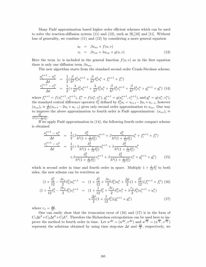
Many Pade approximation based higher order efficient schemes which can be usedto solve the reaction-diffusion system (11) and (12), such as [9],[10] and [11]. Withoutloss of generality, we combine (11) and (12) by considering a more general equation
ut = βuxx + f(u, v)
vt = βvxx + λuxx + g(u, v) (13)
Here the term λv is included in the general function f(u, v) so in the first equationthere is only one diffusion term βuxx.
The new algorithm starts from the standard second order Crank-Nicolson scheme,
un+1
i − uni
∆t=
1
2(
β
h2δ2
xun+1
i +β
h2δ2
xuni + fn+1
i + fni )
vn+1
i − vni
∆t=
1
2(+
λ
h2δ2
xun+1
i +λ
h2δ2
xuni +
β
h2δ2
xvn+1
i +β
h2δ2
xvni + gn+1
i + gni ) (14)
where fn+1
i = f(un+1
i , vn+1
i ), fni = f(un
i , vni ), gn+1
i = g(un+1
i , vn+1
i ), and gni = g(un
i , vni ),
the standard central difference operator δ2x defined by δ2
xui = ui+1−2ui+ui−1, however(uxx)i ≈
1
h2 (ui+1 − 2ui + ui−1) gives only second order approximation to uxx. One wayto improve the above approximation to fourth order is Pade approximation: (uxx)i ≈
δ2x
h2(1+1
12δ2x)
.
If we apply Pade approximation in (14), the following fourth order compact schemeis obtained
un+1
i − uni
∆t=
1
2(β
δ2x
h2(1 + 1
12δ2x)
un+1
i + βδ2x
h2(1 + 1
12δ2x)
uni + fn+1
i + fni )
vn+1
i − vni
∆t=
1
2(+λ
δ2x
h2(1 + 1
12δ2x)
un+1
i + λδ2x
h2(1 + 1
12δ2x)
uni
+βδ2x
h2(1 + 1
12δ2x)
vn+1
i + βδ2x
h2(1 + 1
12δ2x)
vni + gn+1
i + gni ) (15)
which is second order in time and fourth order in space. Multiply 1 + 1
12δ2x to both
sides, the new scheme can be rewritten as
(1 +δ2x
12−
βrx
2δ2
x)un+1
i = (1 +δ2x
12+
βrx
2δ2
x)uni +
∆t
2(1 +
δ2x
12)(fn+1
i + fni ) (16)
(1 +1
12δ2
x −βrx
2δ2
x)vn+1
i = (1 +1
12δ2
x +βrx
2δ2
x)vni + λ
rx
2δ2
x(un+1
i + uni )
+∆t
2(1 +
1
12δ2
x)(gn+1
i + gni ) (17)
where rx = ∆th2 .
One can easily show that the truncation error of (16) and (17) is in the form ofC1∆t2+C2∆t4+C3h
4. Therefore the Richardson extrapolation can be used here to im-
prove the method to fourth order in time. Let w∆t = (u∆t, v∆t) and w∆t
2 = (u∆t
2 , v∆t
2 )represent the solutions obtained by using time step-size ∆t and ∆t
2, respectively, we
265

can set the final solution as w = 4w∆t2 −w∆t
3to eliminate the term ∆t2, which is fourth
order accurate in both the temporal and spatial dimensions.Note that Eq.(16) and (17) contain both un+1
i and vn+1
i (explicitly or implicitly infn+1
i and gn+1
i ). It is not efficient if both equations are simply linearized and usingNewton’s method, so an efficient alternating direction iterative algorithm is proposedhere.
Denote the solutions to (16) and (17) after k iterations by un+1
i
(k)and vn+1
i
(k)
respectively. To get un+1
i
(k+1)and vn+1
i
(k+1), We first expand fn+1
i = f(un+1
i , vn+1
i ) by
f(un+1
i , vn+1
i ) = f(un+1
i
(k), vn+1
i
(k)) +
∂f
∂u(un+1
i
(k), vn+1
i
(k))(un+1
i − un+1
i
(k)) (18)
and insert it into (16), then solve the following (19) for un+1
i
(k+1)
(1 +1
12δ2
x −βrx
2δ2
x −∆t
2(1 +
1
12δ2
x)Jin+1
(k)
)un+1
i = (1 +1
12δ2
x +βrx
2δ2
x)uni
+∆t
2(1 +
1
12δ2
x)(f(un+1
i
(k), vn+1
i
(k)) − Jn+1
(k)
i un+1
i
(k)+ f(un
i , vni )) (19)
where Jn+1(k)
i = ∂f∂u
(un+1
i
(k), vn+1
i
(k)).
Once un+1
i
(k+1)is available, we proceed to expand gn+1
i = g(un+1
i , vn+1
i ) by
g(un+1
i , vn+1
i ) = g(un+1
i
(k+1), vn+1
i
(k)) +
∂g
∂v(un+1
i
(k+1), vn+1
i
(k))(vn+1
i − vn+1
i
(k)) (20)
then insert it into (17). We thus obtain the following equation
(1 +1
12δ2
x −βrx
2δ2
x −∆t
2(1 +
1
12δ2
x)Jn+1(k)
i )vn+1
i = (1 +1
12δ2
x +βrx
2δ2
x)uni
+∆t
2(1 +
1
12δ2
x)(f(un+1
i
(k), vn+1
i
(k)) − Jn+1
(k)
i un+1
i
(k)+ f(un
i , vni )). (21)
where Jn+1(k)
i = ∂g∂v
(un+1
i
(k+1), vn+1
i
(k)). Solve it we can get vn+1
i
(k+1). The two steps
are repeated alternatively till convergent.
5 Numerical results
5.1 Case 1: Linear Convection-Diffusion equation
We first test our new scheme by solving an 1D convection-diffusion equation. Our goalfor this numerical test case is to show that the new algorithm is fourth order accuratein both time and space. In this example, we consider the following equation
∂u
∂t=
1
2
∂2u
∂x2+
1
2
∂u
∂x, x ∈ (0, 1), t ∈ (0, 1]
u(x, 0) = ex, x ∈ [0, 1]
u(0, t) = et, u(1, t) = e1+t, t ∈ (0, 1] (22)
266

Table 1:
∆t 0.2 0.1 0.05 0.025 0.0125
e1 3.1458E-003 7.8855E-004 1.9723E-004 4.9313E-005 1.2329E-005
Logr(e1(∆t)
e1(∆t
2)) - 1.9961 1.9993 1.9999 2.0000
e2 7.2118E-006 3.8724E-007 2.3334E-008 1.4282E-009 8.7867E-011
Logr(e2(∆t)
e1(∆t
2)) - 4.2195 4.0527 4.0301 4.0228
Table 2:
h 0.1 0.05 0.025 0.0125 0.00625
e3 4.4151E-007 2.7251E-008 1.6907E-009 1.0831E-010 2.6539E-012
Logr(e3(h)
e3(h
2)) - 4.0181 4.0106 3.9644 5.3509
for which the exact solution is known as u(x, t) = et+x.First, let v(x, t) = ∂u
∂x, then the equivalent system of two reaction-diffusion equa-
tions is
ut =1
2uxx +
1
2v
vt =1
2vxx +
1
2uxx (23)
with the following initial and boundary conditions:
u(x, 0) = ex , v(x, 0) = ex for x ∈ (0, 1) (24)
u(0, t) = et, u(1, t) = e1+t, for t ∈ (0, 1). (25)
Note the boundary conditions for v(x, t) are derived in the previous section.The data in Table 1 shows the maximum errors between the calculated and exact
solutions at T = 1. e1 is the maximum error for a small and fixed h = 0.0001 while ∆t
is varying. It clearly shows that when ∆t is reduced by a factor of r, e1 is reduced bya factor about r2, i. e., the algorithm is second oder accurate in time. e2 is the sameas e1 except that Richardson extrapolation is used. One can easily see that when ∆t
is reduced by a factor of r, e2 is reduced by a factor about r4, i.e., the algorithm withRichardson’s extrapolation is fourth oder accurate in time.
The data in Table 2 shows the maximum errors between the calculated and exactsolutions at T = 1. e3 is the maximum error for a small and fixed ∆t = 0.0001 while h
is different. Again, the reason we use a very small value of ∆t is to make sure that thedominated error is from h. It clearly shows that when h is reduced by a factor of r, e3
is reduced by a factor about r4, i. e., the algorithm is fourth oder accurate in space.The data in Table 3 shows that the algorithm with Richardson’s extrapolation is
fourth order accurate in both time and space. e4 is the maximum error with ∆t = h
both been reduced by a factor of r, and we can see that e4 is reduced by a factor aboutr4.
267

Table 3:
∆t = h 0.1 0.05 0.025 0.0125 0.01
e4 3.1866E-007 1.9885E-008 1.2336E-009 7.6730E-011 3.1560E-011
Logr(e4(h)
e4(h
2)) - 4.0023 4.0107 4.0069 3.9814
5.2 Case 2: Nonlinear Black-Scholes equation
We solve the reformulated nonlinear Black-Scholes equation (4) with initial condition(5) and boundary conditions (6)-(7). The derivation and reformulation of the modelwere briefly discussed early in section 1 and section 2. The nonlinearity is treatedexplicitly, see [6]. The ODE (2) is solved for future use by high order numerical methodand the solution is plotted in Fig. (1). More details can be found in both [2] and [6].Note that the initial data for the nonlinear Black-Scholes equation (4) is continuousbut not differentiable at x = 0, so cubic spline interpolation was used to smooth theinitial data, and the original data and smoothed initial data are plotted in Fig. (2).
−40 −30 −20 −10 0 10 20 30 40−5
0
5
10
15
20
25
30
35
40
45
Figure 1: Numerical solution to the ODE (2)
Fig.(3) shows the influence of the transaction costs on the price of the EuropeanCall option. The nonlinear Black-Scholes equation (4) is solved by the proposed highorder compact scheme for different transaction costs: a = 0.0, 0.01, 0.02 and 0.03, whileother model parameters are fixed as: σ0 = 0.2, ρ = 0.1, E = 100 and T = 0.02.One can see that for the same pay-off function, when transaction costs a increase, thecorresponding option prices also increase. Not surprisingly, the lowest price curve isthe case when a = 0.0, .i.e, no transaction costs charged.
268
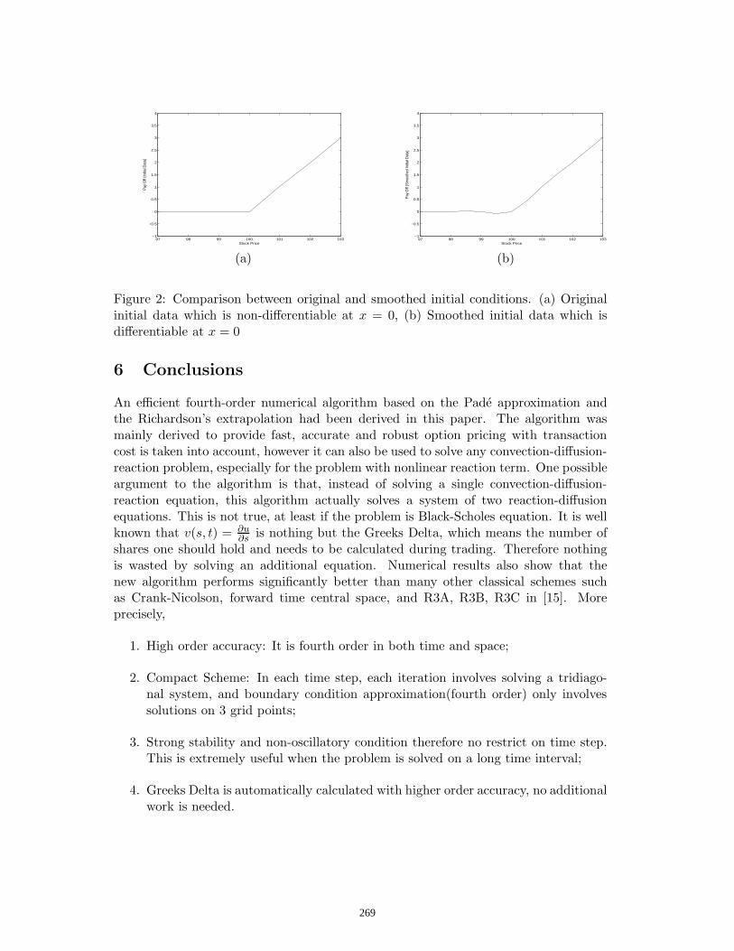
97 98 99 100 101 102 103−1
−0.5
0
0.5
1
1.5
2
2.5
3
3.5
4
Stock Price
Pay
Off
(Initi
al D
ata)
(a)
97 98 99 100 101 102 103−1
−0.5
0
0.5
1
1.5
2
2.5
3
3.5
4
Stock Price
Pay
Off
(Sm
ooth
ed In
itial
Dat
a)
(b)
Figure 2: Comparison between original and smoothed initial conditions. (a) Originalinitial data which is non-differentiable at x = 0, (b) Smoothed initial data which isdifferentiable at x = 0
6 Conclusions
An efficient fourth-order numerical algorithm based on the Pade approximation andthe Richardson’s extrapolation had been derived in this paper. The algorithm wasmainly derived to provide fast, accurate and robust option pricing with transactioncost is taken into account, however it can also be used to solve any convection-diffusion-reaction problem, especially for the problem with nonlinear reaction term. One possibleargument to the algorithm is that, instead of solving a single convection-diffusion-reaction equation, this algorithm actually solves a system of two reaction-diffusionequations. This is not true, at least if the problem is Black-Scholes equation. It is wellknown that v(s, t) = ∂u
∂sis nothing but the Greeks Delta, which means the number of
shares one should hold and needs to be calculated during trading. Therefore nothingis wasted by solving an additional equation. Numerical results also show that thenew algorithm performs significantly better than many other classical schemes suchas Crank-Nicolson, forward time central space, and R3A, R3B, R3C in [15]. Moreprecisely,
1. High order accuracy: It is fourth order in both time and space;
2. Compact Scheme: In each time step, each iteration involves solving a tridiago-nal system, and boundary condition approximation(fourth order) only involvessolutions on 3 grid points;
3. Strong stability and non-oscillatory condition therefore no restrict on time step.This is extremely useful when the problem is solved on a long time interval;
4. Greeks Delta is automatically calculated with higher order accuracy, no additionalwork is needed.
269
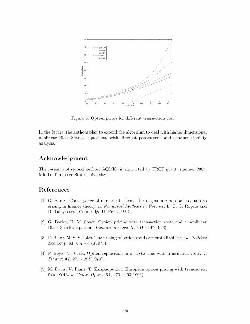
75 80 85 90 95 100 105 110 115 1200
10
20
30
40
50
60
70
80
Stock Price
Opt
ion
Pric
e
pay−off
a=0.00
a=0.01
a=0.02
a=0.03
Figure 3: Option prices for different transaction cost
In the future, the authors plan to extend the algorithm to deal with higher dimensionalnonlinear Black-Scholes equations, with different parameters, and conduct stabilityanalysis.
Acknowledgment
The research of second author( AQMK) is supported by FRCP grant, summer 2007,Middle Tennessee State University.
References
[1] G. Barles, Convergence of numerical schemes for degenerate parabolic equationsarising in finance theory, in Numerical Methods in Finance, L. C. G. Rogers andD. Talay, etds., Cambridge U. Press, 1997.
[2] G. Barles, H. M. Soner. Option pricing with transaction costs and a nonlinearBlack-Scholes equation. Finance Stochast. 2, 369 - 397(1998).
[3] F. Black, M. S. Scholes, The pricing of options and corporate liabilities, J. PoliticalEconomy, 81, 637 - 654(1973).
[4] P. Boyle, T. Vorst. Option replication in discrete time with transaction costs. J.Finance 47, 271 - 293(1973).
[5] M. Davis, V. Panis, T. Zariphopoulou. European option pricing with transactionfees. SIAM J. Contr. Optim. 31, 470 - 493(1993).
270

[6] B. During, M. Fournie and A. Jungel, High Order Compact Finite DifferenceSchemes for a Nonlinear Black-Scholes Equation,Intern. J. Theor. Appl. Finance6, 767 - 789(2003).
[7] R. S. Hirsh, Higher order accurate difference solution of fluid mechanics prob-lems by a compact difference technique. Journal of Computational Physics, 9:90 -109(1975).
[8] H. Leland, Option pricing and replication with Transaction Costs, Journal of Fi-nance, 5, 1283 - 1301(1985).
[9] W. Liao, J. Zhu, and A. Q. M. Khaliq, An efficient high order algorithm for solvingsystems of reaction-diffusion equations, Journal of Numerical Methods for PartialDifferential Equations, 18, 340 - 354 (2002).
[10] Y. Gu, W. Liao, and J. Zhu, An efficient high order algorithm for solving sys-tems of 3-D reaction-diffusion equations, Journal of Computational and AppliedMathematics, 155, 1 - 17 (2003).
[11] W. Liao, J. Zhu and A.Q.M. Khaliq, A fourth-Order Compact Algorithm for Non-linear Reaction-Diffusion Equations with Neumann Boundary Conditions, NumerMethods Partial Differential Equations , 22,600 - 616(2006).
[12] A. Paras, M. Avellaneda. Dynamic hedging portfolios for derivative securities inthe presence of large transaction costs. Appl. Math. Finance 1, 165 - 193, 1994.2,3
[13] A. Rigal, Numerical Analysis of 2-level finite-difference schemes for unsteadydiffusion-convection problems. International Journal for numerical methods in En-gineering 28(5): 1001 - 1021, 1989.
[14] A. Rigal, Numerical Analysis of 3 -time-level finite-difference schemes for unsteadydiffusion-convection problems. International Journal for numerical methods in En-gineering 30(2): 307 - 330, 1990.
[15] A. Rigal, High order difference scheme for unsteady one-dimensional diffusion-convection problems. Journal of Computational Physics,114, 59 - 76 (1994).
[16] W. F. Spotz and G. F. Carey, Extension of high-order compact schemes to timedependent problems, Numer. Methods Partial Differential Equations, 17, 657 -672(2001).
[17] V. Zakamouline, Hedging of Option Portfolios and Options on Several AssetsWith Transaction Costs and Nonlinear Partial Differential Equations” (January18, 2007). Available at SSRN: http://ssrn.com/abstract=938933
[18] H. Sun and J. Zhang, A high order finite difference discretization strategy basedon extrapolation for convection diffusion equations, Numerical Methods for PartialDifferential Equations, 20, no.1, 18-32(2004).
271

Proceedings of the International Conferenceon Computational and Mathematical Methodsin Science and Engineering, CMMSE 2007Chicago, 20–23 June 2007.
Asian Options as Ultradiffusion Processes
Michael D. Marcozzi1
1 Department of Mathematical Sciences, University of Nevada Las Vegas
emails: [email protected]
Abstract
An ultradiffusion is a process which is isomorphic to a parameterized diffusionalong a characteristic temporal trajectory. They are motivated by the realizationthat in many systems exogenous sources of uncertainty enter only certain com-ponents of the dynamics. The value function associated with ultradiffusion pro-cesses are characterized as the solution to ultraparabolic equations. We considerthe arithmetic-average Asian option as a prototypical example of an ultradiffusionprocesses.
Key words: Ultradiffusion, Ultraparabolic, Option PricingMSC 2000: 35K70, 91B28
1 Introduction
An ultradiffusion is a processes which is isomorphic to a parameterized diffusion alonga characteristic temporal trajectory; they are motivated by the realization that in manysystems exogenous sources of uncertainty enter only certain components of the dynamics(cf. [7], [11], [17]). The value function of an ultradiffusion process is characterized asthe solution to an ultraparabolic equation. Ultraparabolic equations evidence multipletemporal variables and are parabolic along characteristic directions. In this paper, weconsider as a prototypical example the valuation problem for the arithmetic-averageAsian option.
Historically, an interest in ultradiffusion processes and ultraparabolic equationsarose relative to the works of Kolmogorov [12], [13] and Uhlenbeck and Ornstein [21] inconnection with Brownian motion in phase space and Chandrasekhar [3] with respect tothe theory of boundary layers. Unlike parabolic equations, however, neither the strongmaximum principle nor interior a priori estimates, for example, hold for ultraparabolicequations (cf. [8], [6], [19], [20], [22], [14], [18]).
The outline of this paper is as follows. In section 2, we define the valuation problemin the Black-Scholes framework; this example serves as a basis for subsequent compari-son. In section 3, the Asian option is introduced as the expectation of an ultradiffusion
272

process and its value function is seen to satisfy an ultraparabolic equation. The repre-sentation of the ultradiffusion as a parameterized diffusion is considered in section 4. Insection 5, we consider a fully stochastic approximation of the ultradiffusion as the limitof vanishing viscosity diffusions in the context of the so-called viscosity formulation.Finally, in section 6, the viability framework is briefly introduced which approximatesthe ultradiffusion in a deterministic context.
2 Black-Scholes Framework
As a benchmark, we consider the Black-Scholes option pricing framework in which wemodel the motion of a stock price St by geometric Brownian motion
d St
St= r ds + σ dBt , (2.1)
for all t > 0, such that S0 = S, volatility σ > 0, and risk-free rate of return r > 0. Weassociate with (2.1) the infinitesimal generator A given by
A(t) u(t, S) =12σ2 S2 ∂
2u
∂S2(t, S) + r S
∂u
∂S(t, S) (2.2a)
which applies along the (trivial) characteristic direction of the evolutionary operator
H(S) u(t, S) =∂u
∂t(t, S) . (2.2b)
The value function associated with (2.1), payoff ψ(S), and discounting factor r, is then
u(t, S) = E exp [−r · (T − t)] · ψ(ST) . (2.3)
In the context of option pricing, the valuation (2.3) represents the present value or priceof an European-style option exercised at T > 0; upon exercise, the contract deliversto the option holder a payoff amount ψ(S). In particular, the value function can becharacterized as the unique solution to the terminal-value parabolic equation
H(S) u(t, S) + A(t) u(t, S)− ru(t, S) = 0 on [0, T )× (0,∞) , (2.4a)
such thatu(T, S) = ψ(S) on [0,∞) . (2.4b)
Approximation techniques dealing with valuations problems relative to diffusion pro-cesses are found in Marcozzi [16].
3 Asian Options
In contrast to the preceding section, Asian options evidence dependence on the path-history of the underlying stochastic process. To this end, we suppose that the payofffor the Asian option depends on the arithmetic average, or
ς(t) =∫ t
0Sτ dτ ,
273

in which case we consider the ultradiffusion process
d ςt = St dt , (3.1a)
d St
St= r dt+ σ dBt , (3.1b)
for all t > 0. The prefix “ultra” refers to the presence of multiple time variables andwill be explained subsequently.
We associated with (3.1) the infinitesimal generator, depending now upon the tem-poral pair (t, ς), such that
A(t, ς) u(t, ς, S) =12σ2 S2 ∂
2u
∂S2(t, ς, S) + r S
∂u
∂S(t, ς, S) , (3.2a)
which applies along the characteristic direction of the evolutionary operator, which isnow
H(S) u(t, ς, S) =∂u
∂t(t, ς, S) + S
∂u
∂ς(t, ς, S) . (3.2b)
Indeed, the key idea is that in both (2.2) and (3.2) the temporal operator H is hyper-bolic.
Along with the ultradiffusion process (3.1), payoff ψ(ς, S), and discounting factorr, we define the value function as
u(t, ς, S) = E exp [−r · (T − t)] ·ψ(ςT , ST ) . (3.3)
That is, the valuation (3.3) represents the present value or price of an arithmetic-average Asian option exercised at T > 0, which delivers to the option holder a payoffamount ψ(ςT , ST ) dependent upon the path-history ςT of the asset St. In particular, thevalue function (3.3) can be characterized as the unique solution to the terminal-valueultraparabolic equation
H(S) u(t, ς, S)+ A(t, ς) u(t, ς, S)− r u(t, ς, S) = 0 on [0, T )× (0,∞)× (0,∞) , (3.4a)
subject to the terminal condition
u(T, ς, S) = ψ(ς, S) on [0,∞)× (0,∞) . (3.4b)
Approximation techniques dealing with valuations problems relative to ultradiffusionprocesses are found in Marcozzi [17].
4 Parametric Representation
We may also use the defining characteristic of ultradiffusion processes, namely theirequivalence to a parametric family of diffusion processes, in order to value an Asianoption. To this end, we effect a change to the characteristic time ξ such that the ultrad-iffusion (3.1) becomes a ς-indexed family of diffusion processes along the characteristic
274

direction (1, S) in the (t, ς)-temporal plane. To this end, for each value of the statevariable S, we define the so-called characteristic time ξ such that
ξ = t+ς
S, (4.1)
in which case it follows from the scaling property of Brownian motion that
d Sξ = r Sξ dξ + σ Sξ dBξ , (4.2)
for all ξ > 0 (cf. [10, Lemma II.9.4]). Note that by (4.1), it follows that
d ς = S d ξ = S dt ,
in which case we implicitly recover (3.1a). Significantly, the infinitesimal generatorassociated with the parameterized diffusion (4.2) with respect to the state variable Sdoes not change and is
Aς(ξ) u(ξ, S) =12σ2 S2 ∂
2u
∂S2(ξ, S) + r S
∂u
∂S(ξ, S) , (4.3a)
and operates along the characteristic time direction ξ subject to the evolutionary op-erator behavior generated by
H(S) u(ξ, S) =∂u
∂ξ(ξ, S) . (4.3b)
With respect to ξ and (4.1), the r-discounted value function becomes
uς(ξ, S) = E exp [−r · (Γ − ξ)] · ψς(SΓ) , (4.4)
where ψς(S) = ψ(ς, S) and Γ = T + ς/S. In particular, we characterize the value func-tion uς as the unique solution to the parameterized terminal-value parabolic equation
H(S) uς(ξ, S) + Aς(ξ) uς(ξ, S)− r uς = 0 a.e. on [0,Γ)× (0,∞) , (4.5a)
such thatuς(Γ, S) = ψς(S) on (0,∞) , (4.5b)
(cf. [2, §III.2.15]). We remark that for a given ς , solving (4.5), is significantly simplierthan solving (3.4) and lies within the Black-Scholes framework of section 2.
In the context of ultradiffusion processes (3.1), the variable t is referred to as(standard) time, ς as parametric time, ξ as the characteristic time, (t, ς) as the temporalpair, and S as the state variable. That is, the state variable S evolves within the (t, ς)-plane equivalently: (i) according to the ultradiffusion (3.1) or (ii) according to theς-indexed diffusion (4.2) along the characteristic curve (4.1). As an ultradiffusion,the value function (3.3) satisfies an ultraparabolic equation (3.4), whereas the valuefunction (4.4) relative to the parametric diffusion representation (4.2) is characterizedas the unique solution to the parameterized parabolic equation (4.5). The “ultra” prefixthen refers, in both the diffusion process and parabolic operator, to evolution in thetemporal (t, ς)-plane.
275

5 Viscosity Approximation
One may consider the approximation of ultradiffusions as the limit of vanishing viscositydiffusion processes. That is, we considering the fully stochastic approximation of (3.1)by an ε-perturbed diffusion
d ς(t) = St dt+ ε dB(1)t , (5.1a)
d St
St= r dt + σ dB
(2)t , (5.1b)
for all t > 0, as ε → 0+, where (B(1), B(2)) is an R2-valued Brownian motion (cf. [5,§VI.8]). In this case, the infinitesimal generator of the state variables (ς, S) takes theform
Aε(t) u(t, ς, S) =12σ2 S2 ∂
2u
∂S2(t, ς, S) +
12ε2∂2u
∂ς2(t, ς, S) (5.2a)
+r S∂u
∂S(t, ς, S) + S
∂u
∂ς(t, ς, S)
and evolves along the (trivial) characteristic direction of the evolutionary operator
H(ς, S) u(t, ς, S) =∂u
∂t(t, ς, S) . (5.2b)
Along with the approximation process (5.1), payoff ψ(ς, S), and discounting factorr, we define the value function as
uε(t, ς, S) = E exp [−r · (T − t)] · ψ(ς, S) . (5.3)
In particular, the value function (5.3) relative to the diffusion (5.2) can be characterizedas the unique solution to the terminal-value perturbation parabolic equation
H(ς, S) uε(t, ς, S)+Aε(t) uε(t, ς, S)−ruε(t, ς, S) = 0 on [0, T )×(0,∞)×(0,∞) , (5.4a)
subject to the terminal condition
uε(T, ς, S) = ψ(ς, s) on [0,∞)× (0,∞) , (5.4b)
for all ε → 0+. We note, however, that while so-called viscosity solutions formalizethis approximation of the ultradiffusion, in general viscosity solutions lack the requisiteregularity for the construction of robust numerical procedures (cf. [9], [4]). Indeed, inviscosity formulations, one typically needs to numerically solve the advection dominatedequation (5.4) in order to value (3.3) via (5.3) as ε → 0+, which is a much moresignificant challenge than solving (3.4) or (4.4) directly (cf. [16]).
276

6 Viability Solutions
Conversely, one may also approximate the ultradiffusion within a fully deterministicframework of viability solutions. Viability techniques formulate the tychastic optimalcontrol problem as a deterministic dynamical game such that
d ς(t) = St dt (6.1a)
d St
St= r dt+ εi σ
√∆ , (6.1b)
where ∆ > 0 and εi ∈ [−1, 1], for i ∈ V and V ⊂ N sufficiently large. In this case, theprocess is purely deterministic with evolutionary component
H u(t, ς, S) =∂u
∂t(t, ς, S) + rS
∂u
∂ς(t, ς, S) + (εi σ
√∆ + r)S
∂u
∂S(t, ς, S) . (6.2a)
In order to obtain the value function, one would optimize the deterministic controlproblem over a set of perturbations εi subject to certain viability constraints (cf. [1]).Significantly, the tychastic formulation does not converge to the stochastic problem ascard(V ) → ∞ and ∆ → 0+.
Acknowledgements
This research has been supported by the U.S. National Science Foundation, awardnumber DMI-0422985.
References
[1] J.-P. Aubin, Viability Theory, Birkhauser, Boston, 1991.
[2] A. Bensoussan and J. L. Lions, Applications of variational Inequalities inStochastic Control, North Holland, Amsterdam, 1982.
[3] S. Chandrasekhar, Stochastic Problems in Physics and Astronomy, Rev. Mod.Phys. 15 (1943) 1–89.
[4] M.G. Crandell, H. Ishii and P.-L. Lions, User’s guide to viscosity solutionsof Hamilton-Jacobi equations, Bull. Amer. Math. Soc. 27 (1992) 1–67.
[5] W.H. Fleming and R. W. Rischel Deterministic and Stochastic Optimal Con-trol, Springer-Verlag, New York, 1975.
[6] T.G. Gencev, Ultraparabolic equations, Dokl. Akad Nauk SSSR 151 (1963) 265–268.
[7] B.A. Huberman and M. Kerszberg, Ultradiffusions: The relaxation on hier-archical systems, J. Phys. A: Math Gen. 18 (1985) L331–L336.
277

[8] A.M. Il’in, On a class of ultraparabolic equations, Dokl. Akad Nauk SSSR 159(1964) 1214–1217.
[9] H. Ishii, On uniqueness and existence of viscosity solutions for fully nonlinearsecond order elliptic partial differential equations, Comm. Pure Appl. Math. 42(1989) 15–45.
[10] I. Karatzas and S.E. Shreve Brownian Motion and Stochastic Calculus, Sec-ond edition, Springer-Verlag, New York, 1991.
[11] A.N. Kochubei, Pseudo-Differential Equations and Stochastic over Non-Archimedian Fields, Marcel Dekker, New York, 2001.
[12] A.N. Kolmogorov, Sur theorie der stetigen zufalligen progresse, Math. Annal.108 (1933) 149–160.
[13] A.N. Kolmogorov, Zufallige Bewegungen, Ann. of Math. 35 (1934) 116–117.
[14] M. Manfredini and S. Polidoro, Interior regularity for weak solutions of ultra-parabolic equations in divergence form with discontinuous coefficients, Bollettino8 (1998) 651–675.
[15] M.D. Marcozzi, On the approximation of optimal stopping problems with appli-cations to financial mathematics, SIAM J. Sci. Comput. 22 (2001) 1865–1884.
[16] M.D. Marcozzi, On the valuation of Asian options by variational methods, SIAMJ. Sci. Comput. 24 (2003) 1124–1140.
[17] A. Maritan and A.L. Stella, Exact renormalization group approach to ultra-diffusion in a hierarchical structure, J. Phys. A: Math Gen. 19 (1986) L269–L274.
[18] S. Polidoro and M.A. Ragusa, Sobolev-Morrey spaces related to an ultra-parabolic equation, Manuscripta Math. 96 (1986) 371–392.
[19] S.A. Tersenov, On boundary value problems for a class of ultraparabolic equa-tions, and their applications, Math. Sbornik 133 (1987) 539–555.
[20] S.A. Tersenov, Basic boundary value problem for one ultraparabolic equation,Siberian Mathematical Journal 42 (2001) 1173–1189.
[21] G.E. Uhlenbeck and L. S. Ornstein, On the theory of the Brownian motion,Phys. Rev. 36 (1930) 823–841.
[22] V.S. Vladimirov and Ju.N. Drozzinov, Generalized Cauchy problem for anultraparabolic equation, Izv. Akad. Nauk. SSSR Ser. Mat. 31 (1967) 1341–1360.
278

Proceedings of the International Conference on Computational and Mathematical Methods in Science and Engineering, CMMSE2007 Chicago, 20-23 June 2007
Undergraduate Computational Physics Education:
Coming of Age?
R. F. Martin, Jr. Department of Physics, Illinois State University
email: [email protected]
Abstract
While some physics educators have included computing in courses and have developed specialized courses for over 40 years, computational physics education has only slowly made inroads into the broader physics education community. There has been a recent surge in interest in a more global approach to computational physics education that offers promise for computing to finally take an important role in the education of undergraduate physicists. In this presentation I will review some developments in computational physics education and present examples from the program at Illinois State University. Key words: undergraduate education, computational physics
1. Introduction The use of computing in physics teaching has been practiced at least since the 1960's, with, for example, the pioneering work of Alfred Bork1. My department joined the fray in the mid-1970's2 when a wave of new specialized computing-based physics courses were developed at many institutions across the nation. The 1980's saw an expansion of computational physics course offerings, the emergence of several influential textbooks such as those by Koonin3 and Gould and Tobochnik4, as well as a groundbreaking conference, the Conference on Computers in Physics Instruction in 1988. This conference served to bring together a wide variety of proponents of computational methods in physics education covering uses in introductory courses, laboratories, computer-aided-instruction, courses devoted to computational methods, as well as computation-based curricular modifications. The proceedings5 from this conference can still serve as a valuable reference for those interested in why and how to develop computational physics modules, classes, and curricula. I count myself as one attendee strongly influenced by this meeting
279

CMMSE 2007
such that, with several enthusiastic departmental colleagues, our department developed a computational physics curriculum6,7 in the 1990's - in parallel with similar developments at other institutions in that decade and into the present one. Although many individuals have developed course materials and advocated for computational physics education over these four decades, and journals such as the American Journal of Physics, Computers in Physics, and Computing in Science and Engineering (CiSE) have provided outlets for new developments, the field has never really had a professional “home”. In the current decade, this situation appears to be changing. With special sessions at the American Physical Society (through the Forum on Education) March Meeting in 2004, the American Association of Physics Teachers (AAPT) summer meeting in 2006, a topical conference sponsored by AAPT to be held in July 2007, and a Gordon conference planned for 2008, there is new momentum in the field. In this presentation I will give a brief overview of some developments in computational physics education and then present one model for a successful program developed at Illinois State.
2. Computational Physics Education First, it is worth noting what is meant by computational physics education (CPE). CPE differs from computer science and computer engineering education in that CPE focuses on only those applications of computing that are relevant to the solution of physics problems. For the purposes of this presentation, we exclude applications of computing in laboratory instrumentation and in computer-aided-instruction (in which the teacher authors software to aid student learning), leaving primarily the use of numerical methods to solve intractable equations in physics, the broad domain of computational modeling and simulation, and scientific visualization. Perhaps the key point is that students learn to apply the tools of CPE to learn physics and to model and solve problems in physics. The tools of CPE have changed significantly from the early days of Fortran programs on a mainframe computer. Today one has access to wide array of programming languages, graphics/visualization suites, web-based tools, and comprehensive analysis packages, to be utilized on an equally broad array of hardware from laptops to workstations to grid networks to massively parallel supercomputers. Based on the discussion at the AAPT special session in 2006, the main languages used are C/C++, Fortran, Python, and Java. Participants appeared to split roughly equally between the Mathematica and Matlab/Maple comprehensive packages that provide programming, symbolic math, and visualization capabilities. A wealth of new ideas of how to use these tools in educating physics students is evident in the articles and web-extras published in a special issue8 of CiSE.
280
CMMSE 2007
While the tools have improved markedly, the basic function of CPE has changed remarkably little over the decades. In a 1963 article on the subject, Bork1 presents several reasons for using computation in physics courses, including (1) “The modern computer makes workable problems which were for all practical purposes impossible only a few years ago”, (2) “The 'feel' of numbers promotes understanding of analytic relations", and (3) “using numerical analysis permits the consideration of material beyond the students' analytic ability”. Similarly, Martin et al6 articulated in 1991 three guiding principles for their program: (1) “Students should be in command of the technology, not the other way around”, (2) “The computer should enhance the student's acquisition of broad problem-solving skills, and (3) “The computer should stimulate: (a) a re-ordering and broadening of the subject matter taught; (b) build physical intuition; and (c) enable the student to pursue independent study.” All these ideas, and more, are still part of the argument for CPE. In a recent article, Landau9 goes even further and argues that CPE presents a superior model for teaching physics generally: “presenting physics within a scientific problem-solving paradigm is a more effective and efficient way to teach physics than the traditional approach.” In his model computational science provides both elements of its own and a bridge between the three disciplines of computational physics: application physics, mathematics, and computer science. In the article he presents a detailed concept map of the complex interactions between these sub-areas. All of the above cited articles, and many more, point out one other justification for CPE: practicality. Bork1 cites a comment by Courant: “the vital task is ... to inject the awareness of the potentialities of modern computing into the general education of talented and open-minded scientists.” Even in 1963 it was clear to those with vision that computational science would be a critical aspect of doing science in the future - and that future is certainly here. Study after study (see for example the American Institute of Physics Statistical Research Center website10) have shown the importance of computational modeling and programming skills both in physics research careers and in the variety of careers available to those with one or more physics degrees. As Chonacky11 comments, “Contemporary sciences and engineering practices are cross-disciplinary; these people not only compute but also use computation as a common interface between their respective contributions to cross-disciplinary projects.” Computational science and engineering is simply a part of the scientific and engineering landscape in the 21st century. One might reasonably ask why it should be necessary to provide justification for CPE at all. To many, the above arguments may appear nearly self-evident. Yet, during the discussion at the 2006 AAPT conference, and reflected in some of the articles in the special edition of CiSE, it is clear that there is still something of a divide between those seeking to encourage CPE and those, for lack of a better phrase, who are proponents of a “traditional analytic-plus-laboratory” mode of physics education (note that even strong advocates of contemporary active learning approaches to physics education can still be “traditionalists” regarding CPE). After presenting results of a significant survey of physics
281

CMMSE 2007
department Chairs and faculty indicating strong agreement about the role of computational physics in practicing physicists' lives and in course preparation, Fuller12 reports responses to one telling question that suggest that physics educators have not yet translated this idea into their courses. In response to a question asking what percentage of faculty utilize computational assignments in their courses, “fewer than 20 percent of the physics faculty ... include computations in their grading.” Thus, CPE supporters still have their work cut out for them. Such constraints aside, a considerable amount has been achieved. Landau9 lists five US universities and colleges with undergraduate degree programs in computational physics, and another four with non-degree specializations (minor, concentration, option, etc.) offered. An additional four institutions offer computational science degrees, with another 11 providing some sort of specialization in that interdisciplinary area. Other departments are adding computation to the physics curriculum through focused courses or by integrating computing into existing courses, as the lists of presentations at the recent conferences demonstrate. It is this momentum that provides evidence that CPE is finally coming-of-age.
3. One model: Illinois State University The physics department at Illinois State has gone through several phases of development of CPE. While each department will have its unique set of strengths and educational goals, and will therefore develop in its own way, it may be of value to know how others have solved common problems during their evolution. Other examples and models can be found in the literature, including the references cited in this article. The first phase in our development was the creation in the mid-1970's of a single course, Computers in Physics, designed for junior/senior physics majors. As a single-instructor course offered mainly to interested students, there were no issues of acceptance by colleagues. The next phase began in the late 1980's when a core of three faculty who utilized computational methods in their research began to discuss the possibility of integrating computing into various physics classes6. The original motivation was two-fold: the recognition that practicing scientists need computational skills and the fact that our fledgling undergraduate research program often involved computational tasks for students. Initially limited to courses taught by the three originators, by the mid-1990's new faculty hires had brought several more computationally-oriented physicists to the department and a full integration of computing into post-introductory physics majors courses was achieved. This integration was accomplished using a consensus-determined “skills matrix”, which outlined the computational skills to be introduced at various levels in the curriculum. This
282

CMMSE 2007
project was partially supported by an NSF grant. While there was some departmental resistance to this process, open discussion and consensus-building, combined with the fortunate situation of a preponderance of computational researchers in the department, allowed the process to move relatively smoothly. The third phase in CPE development was spurred by input from graduates of the computationally integrated curriculum, who were quite enthusiastic about their abilities to build and solve computational models, expertise that served them well in both graduate school and in technical jobs. We also felt that the new program would help with major recruitment, a significant problem in the late 1990's in physics departments across the country. Funding from the NSF ILI/LLD program allowed us to construct a degree sequence to give interested students even deeper experience with computational physics. After surveying high school students on their interest in such a program we selected the title “Computer Physics” for the degree, since these pre-college students identified the word 'computational' with performing complicated mathematical computations and not with computers. 3.1 Computational integration in physics courses The Illinois State University physics department offers four degree sequences: physics, computer physics (CP), physics teacher education (PTE), and engineering physics (a 3/2 program with partner engineering universities). Most courses taken primarily by majors in these four sequences have a computational component. Only our first two introductory physics classes do not, mainly because they also act as service courses for other departments. Majors are first introduced to graphical data analysis with scientific graphics software and to Mathematica in the first-semester freshman “introduction to the discipline” class. This is followed by simple programming assignments in a lab format in the third-semester introductory course, in which the students write simple finite-difference codes (both Euler and a second order leapfrog method) to solve some mechanics problems and a basic Monte Carlo simulation for an optics problem. As the students progress further in their physics courses, more sophisticated computational methods are introduced, following our original idea of a “skills matrix”, as mentioned above. For example, in the intermediate electromagnetism course, before students have taken a differential equations class, they solve Laplace's equation using an over-relaxation algorithm. Solving Laplace's equation on a grid in this way helps students understand the mathematical and physical properties of electrostatic potentials, and visualizing the results as contour, raster, and surface plots further develops physical intuition. In the senior-level quantum physics class, students compute matrix elements for a double well potential and use the QL algorithm to compute eigenvalues and eigenfunctions, a problem that would be beyond their mathematical expertise to work out analytically.
283

CMMSE 2007
Our philosophy of computational integration lies somewhere in-between Landau's9 “computational physics--education”, in which students use black-box computational methods to help them learn physics and his “computational--physics education”, which implies that computation and physics are more fully merged. Our students learn the algorithms in enough depth that they can understand their relation to the physics, but not at a deep level. Students do write the code, bust most instructors prefer to provide strategic chunks of code for students to construct their programs around. In this way graduates in all our degree sequences leave our department with some expertise in computing and, according to student evaluation comments, a better understanding of the physics. 3.1 The computer physics degree sequence Realizing that students are learning some computation in their physics courses, we are able to provide a degree sequence with the addition of several specialty courses . CP majors take a Programming for scientists course (currently C and Fortran) and a Hardware and software course (an introduction to computer architecture) from the Information Technology department. From the physics department, they begin with PHY 318 Methods of computational science, covering basic algorithm development, analysis, and implementation, PHY 388 Advanced computational physics, a projects course team-taught by three faculty each presenting a specific advanced project, and PHY 390 Computational research in physics, a semester capstone computational research project. In addition, one senior elective is required and computation-based courses Nonlinear dynamics and Molecular dynamics are available to meet that need. CP majors therefore take five courses not required of regular physics majors, and we are frequently asked “what physics do they lose?” Our usual response is that they gain as much physics as they “lose”, but the following courses required for physics majors are not required for CP majors: second semester chemistry, senior level electromagnetism, senior advanced lab, and a second senior elective. While our experimental colleagues may decry the loss of the senior lab, in point of fact the analysis techniques for simulation data often coincide with those for laboratory data so that deficit is not as great as it may appear. Example topics from the PHY 318 methods course include ODE solution of triatomic molecule dynamics using a predictor-corrector algorithm, Monte Carlo simulation of the Ising model, and discrete Fourier transform analysis of NMR data. All algorithms are presented both theoretically and via physics or physical chemistry example systems. The projects course PHY 388 involves three one-third semester projects, the topics selected by the participating faculty each semester. Examples in recent semesters include finite element analysis of thermal conduction, neural network predictors for both physics (the geomagnetic AE index) and financial time series, application of the split-operator method to time dependent wave functions, and a Monte Carlo simulation of photon scattering from a turbid medium. The capstone project course PHY 390 allows students wide latitude in selecting topics: all they need is a faculty member willing to advise them on the project.
284
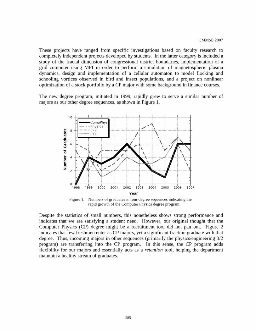
CMMSE 2007
These projects have ranged from specific investigations based on faculty research to completely independent projects developed by students. In the latter category is included a study of the fractal dimension of congressional district boundaries, implementation of a grid computer using MPI in order to perform a simulation of magnetospheric plasma dynamics, design and implementation of a cellular automaton to model flocking and schooling vortices observed in bird and insect populations, and a project on nonlinear optimization of a stock portfolio by a CP major with some background in finance courses. The new degree program, initiated in 1999, rapidly grew to serve a similar number of majors as our other degree sequences, as shown in Figure 1.
0
2
4
6
8
10
1998 1999 2000 2001 2002 2003 2004 2005 2006 2007
CompPhysPhysics3/2PTE
Nu
mb
er o
f G
ra
du
ate
s
Year Figure 1. Numbers of graduates in four degree sequences indicating the
rapid growth of the Computer Physics degree program. Despite the statistics of small numbers, this nonetheless shows strong performance and indicates that we are satisfying a student need. However, our original thought that the Computer Physics (CP) degree might be a recruitment tool did not pan out. Figure 2 indicates that few freshmen enter as CP majors, yet a significant fraction graduate with that degree. Thus, incoming majors in other sequences (primarily the physics/engineering 3/2 program) are transferring into the CP program. In this sense, the CP program adds flexibility for our majors and essentially acts as a retention tool, helping the department maintain a healthy stream of graduates.
285

CMMSE 2007
0
10
20
30
40
50
60
Freshman T r an s f e r Graduates
CompPhys
Phys
3/2
PTE
Perc
ent
of
Popula
tio
n
Figure 2. Distribution of declared physics major sequence for incoming
freshmen, incoming transfer students, and outgoing graduates, 2000-2007.
In a five-year assessment of the CP sequence performed in 2005, surveyed students reported high satisfaction with the specialized CP courses in the physics department, with somewhat lower satisfaction with the two information technology classes particularly the computer architecture course, which students reported as not being very challenging (we continue to pursue other options with our colleagues in that department). When asked about the utility of the various courses to their current job or graduate student position, the PHY 390 capstone research course earned highest marks from CP alumni. Written comments suggesting that the capstone course's open structure, which essentially asks students to generate an interesting problem, design a computational model to solve it, and bring the project to some sort of closure, was useful for both graduate-school bound students and those moving directly into the job market -- perhaps an a posteriori justification for our programmatic guiding principles of putting the students “in command of the technology” and that computing should “enable the student to pursue independent study.” About 35% of CP majors, in the first five years of the program, continued on to graduate school, with 50% in physics, the remaining 50% in other technical fields including electrical and computer engineering, materials engineering, and environmental science. This percentage is somewhat lower than the graduate school-bound students in the physics major sequence, which has been near 40% in recent years. For those students who took jobs directly after graduation, more than 35% went to computing-related positions, 40% to other engineering jobs, and the remainder to a mix of technical and nontechnical business
286

CMMSE 2007
positions. Of the CP graduates employed in the computer area, a handful indicated that they had started their own businesses that involved computing. Statistically, the CP graduates do not look significantly different than their physics degree counterparts except for a somewhat higher percentage going into non-physics graduate study and more of the directly employed working in computing-related positions.
4. Conclusions After four decades of computational physics education development by a relatively small group of committed educators, there appears to be a sort of “critical mass” emerging. Whether the recent increase in collaboration, conferences, and publications will result in permanent changes in the education of future physicists remains to be seen, but given the rapid growth of computational physics in the research arena, and the growing number of young faculty with expertise in this area, perhaps this is one educational innovation that will, in fact, become an intrinsic part of future physics curricula. At Illinois State we count our experiment with CPE as a success, both the integration of computational methods and assignments into physics courses and the separate degree sequence. Physics, engineering physics, and even physics teacher education alumni have reported that they are ahead of their graduate student and workplace peers in the computational area, allowing them to seize opportunities not as easily available to their colleagues, or simply to feel more secure in their knowledge. The CP degree appears to be an attractive alternative to the engineering physics 3/2 program and to the physics degree to those students with the interest and the knack for computational science, and the added flexibility acts as a retention tool for some majors not satisfied with those more traditional programs. Finally, our research rationale for CPE has been a success since the CP program meshes synergistically with our undergraduate research effort. A department considering implementation of CPE in some form currently has a wealth of resources available to assist in the process. I have hinted in this article at some of the potential pitfalls and recommend learning the experiences of other departments beginning, for example, with the references herein cited. Our department's experience was relatively smooth partly due to the significant proportion of computational physicists on the faculty, but also because of our departmental culture of open discussion (and argument) of proposed changes -- a useful sieve for separating feasible goals from those that will not work. Acknowledgements The author would like to thank his colleagues in curriculum development at Illinois State University: George Skadron, Robert Young, Hiroshi Matsuoka, Rainer Grobe, Q. Charles Su, and Jean Standard for many years of fresh ideas and practical implementations.
287
CMMSE 2007
References [1] See, e.g., ALFRED M. BORK, A physics independent study course with computers,
Am. J. Physics 31 (1963) 364-368. [2] CHARLES P. FRAHM AND ROBERT D. YOUNG, PSI for low-enrollment junior-senior
physics courses, Am. J. Physics 44 (1976) 524-526. [3] STEVEN KOONIN, Computational physics, Benjamin/Cummings, 1985. [4] HARVEY GOULD AND JAN TOBOCHNIK, An introduction to computer simulation
methods, Addison-Wesley, Reading MA, 1987. [5] EDWARD F. REDISH AND JOHN S. RISLEY (EDS.), The conference on computers in
physics instruction: proceedings, Addison-Wesley, Redwood City CA, 1990. [6] RICHARD F. MARTIN JR., GEORGE SKADRON AND ROBERT D. YOUNG, Computers,
physics and the undergraduate experience, Computers in Physics 5 (1991) 302-310.
[7] RICHARD F. MARTIN JR. AND SHANG-FEN REN, Broadening the Physics Degree: A New Bachelor’s Degree in Computational Physics at Illinois State University, Forum on Education of the American Physical Society, Spring Newsletter (1988) 12.
[8] Computation in physics courses, special issue of Computing in Science and Engineering 8 (2006) 11-58; associated web extras are available at the CiSE website http://www.computer.org/portal/site/cise/.
[9] RUBIN LANDAU, Computational physics: a better model for physics education?, Computing in Science and Engineering 8 (2006) 22-30.
[10] American Institute of Physics Statistical Research Center, http://www.aip.org/statistics/
[11] NORMAN CHONACKY, Has computing changed physics courses?, Computing in Science and Engineering 8 (2006) 4-5.
[12] ROBERT G. FULLER, Numerical computation in US undergraduate physics courses, Computing in Science and Engineering 8 (2006) 16-21.
288

Proceedings of the International Conferenceon Computational and Mathematical Methodsin Science and Engineering, CMMSE 2007Chicago, 20–23 June 2007.
Exponential fitted Runge-Kutta methods of collocationtype
based on Gauss, Radau and Lobatto traditional methods.
J. Martın Vaquero1 and J. Vigo-Aguiar1
1 Departamento de Matematica Aplicada, Universidad de Salamanca, 37008,Salamanca, Spain
emails: [email protected], [email protected]
Abstract
Several exponential fitting Runge-Kutta methods of collocation type are derivedas a generalization of the Gauss, Radau and Lobatto traditional methods of twosteps. The new methods are capable of the exact integration (with only round-off errors) of differential equations whose solutions are linear combinations of anexponential and ordinary polynomials. Theorems of the truncation error revealthe good behavior of the new methods for stiff problems. Numerical examplesunderscore the efficiency of the proposed codes, especially when they are integratingstiff problems.
Key words: Runge-Kutta methods, collocation type, exponential fitting, stiffproblems
MSC 2000: 34A45, 65L06.
1 Introduction
The numerical integration of ordinary differential equations has been one of the prin-cipal concerns of numerical analysis. In the early 1950s, after the pioneering work ofCurtiss and Hirschfelder [1], it was realized that there was an important class of or-dinary differential equations which presented a severe challenge to numerical methodsavailable at that time. These problems have become known as stiff systems. Stiffproblems (and highly oscillatory problems) are very common problems in many fieldsof the applied sciences (see [2], for example): atmosphere, biology, combustion, con-trol theory, dynamics of missile guidance, dispersed phases, electronic circuit theory,fluids, heat transfer, chemical kinetics, lasers, mechanics, molecular dynamics, nuclear,process industries, process vessels, reactor kinetics, ...
289
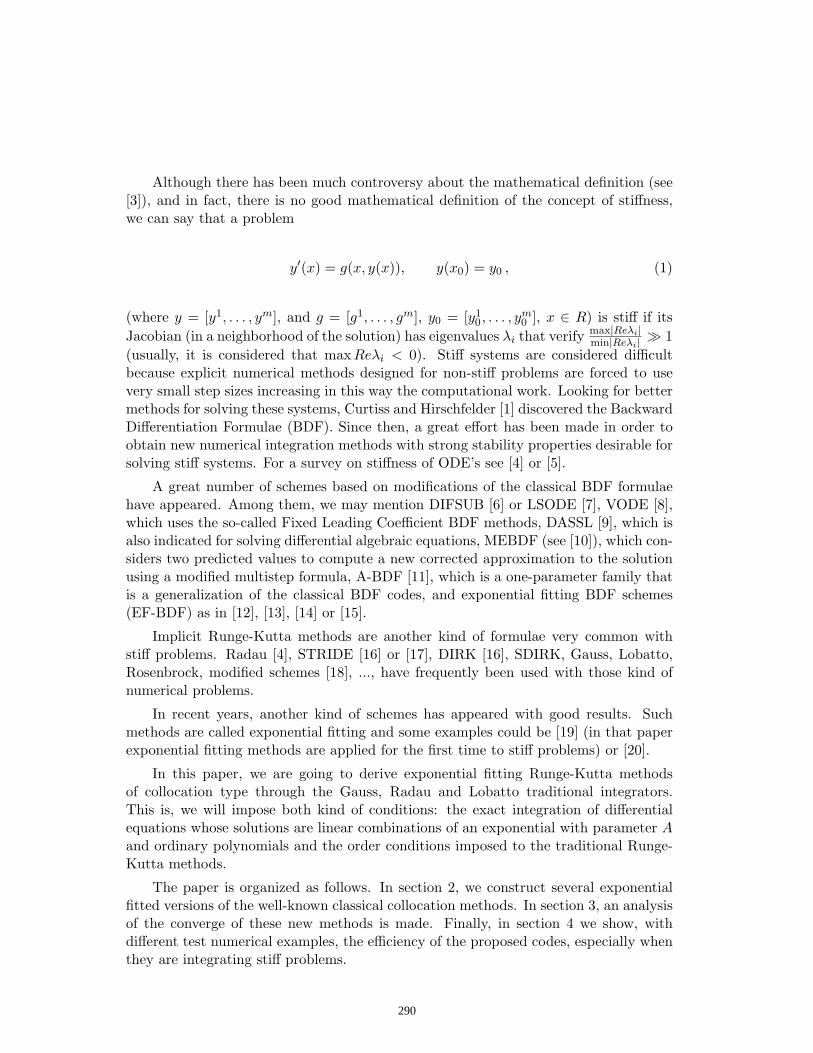
Although there has been much controversy about the mathematical definition (see[3]), and in fact, there is no good mathematical definition of the concept of stiffness,we can say that a problem
y′(x) = g(x, y(x)), y(x0) = y0 , (1)
(where y = [y1, . . . , ym], and g = [g1, . . . , gm], y0 = [y10, . . . , y
m0 ], x ∈ R) is stiff if its
Jacobian (in a neighborhood of the solution) has eigenvalues λi that verify max|Reλi|min|Reλi| À 1
(usually, it is considered that maxReλi < 0). Stiff systems are considered difficultbecause explicit numerical methods designed for non-stiff problems are forced to usevery small step sizes increasing in this way the computational work. Looking for bettermethods for solving these systems, Curtiss and Hirschfelder [1] discovered the BackwardDifferentiation Formulae (BDF). Since then, a great effort has been made in order toobtain new numerical integration methods with strong stability properties desirable forsolving stiff systems. For a survey on stiffness of ODE’s see [4] or [5].
A great number of schemes based on modifications of the classical BDF formulaehave appeared. Among them, we may mention DIFSUB [6] or LSODE [7], VODE [8],which uses the so-called Fixed Leading Coefficient BDF methods, DASSL [9], which isalso indicated for solving differential algebraic equations, MEBDF (see [10]), which con-siders two predicted values to compute a new corrected approximation to the solutionusing a modified multistep formula, A-BDF [11], which is a one-parameter family thatis a generalization of the classical BDF codes, and exponential fitting BDF schemes(EF-BDF) as in [12], [13], [14] or [15].
Implicit Runge-Kutta methods are another kind of formulae very common withstiff problems. Radau [4], STRIDE [16] or [17], DIRK [16], SDIRK, Gauss, Lobatto,Rosenbrock, modified schemes [18], ..., have frequently been used with those kind ofnumerical problems.
In recent years, another kind of schemes has appeared with good results. Suchmethods are called exponential fitting and some examples could be [19] (in that paperexponential fitting methods are applied for the first time to stiff problems) or [20].
In this paper, we are going to derive exponential fitting Runge-Kutta methodsof collocation type through the Gauss, Radau and Lobatto traditional integrators.This is, we will impose both kind of conditions: the exact integration of differentialequations whose solutions are linear combinations of an exponential with parameter Aand ordinary polynomials and the order conditions imposed to the traditional Runge-Kutta methods.
The paper is organized as follows. In section 2, we construct several exponentialfitted versions of the well-known classical collocation methods. In section 3, an analysisof the converge of these new methods is made. Finally, in section 4 we show, withdifferent test numerical examples, the efficiency of the proposed codes, especially whenthey are integrating stiff problems.
290

2 Derivation of the methods
Let us consider, first, the scalar initial-value problem of the form
y′(x) = f(x, y(x)), x ∈ [x0, xf ], y(x0) = y0, (2)
and assume that the function f : [x0, xf ]×R → R satisfies all the necessary requirementsfor the existence of a unique solution.
For the description of EFRK methods we use the classical Butcher notation [22]
yn+1 = yn + hs∑
i=1
bif(xn + cih, ui), (3)
ui = yn + hs∑
j=1
aijf(xn + cjh, uj),
with i = 1, . . . , s and the coefficients are displayed as a Butcher array:
c1 a11 . . . a1s
c2 a21 . . . a2s
......
. . ....
cs as1 . . . ass
b1 . . . bs
Then, we will choose ci the values of the classical Runge-Kutta methods, but, now, thenew coefficients ai,j , bi are those such that
y(xn + cih) = y(xn) + h
s∑
j=1
aijf(xn + cjh, y(xn + cjh)), (4)
y(xn + h) = y(xn) + hs∑
i=1
bif(xn + cih, y(xn + cih) (5)
when y(x) belongs to the space < 1, x, . . . , xs−1, eλx >.Case A: Derivation of the new exponential fitting Gauss method of 2-stages.The weights ci of the new Gauss method are the same as in the traditional method:
c1 = 12−
√3
6 and c2 = 12 +
√3
6 . But, ai,j , bi are those such that (4) and (5) when y(x) = 1,y(x) = x, y(x) = eλx.
In this way the new exponential fitting method can be written as
12 −
√3
6 −6−6e(−3+√
3)bλ/6+(−3+√
3)bλe√
3bλ/3
6bλ(−1+e√
3bλ/3)c1 − a11
12 +
√3
6e(−3+
√3)bλ/6(6+e(3+
√3)bλ/6(−6+(3+
√3)bλ))
6bλ(−1+e√
3bλ/3)c2 − a21
e(−3+√
3)bλ/6(1−ebλ+e(3+
√3)bλ/6bλ)
bλ(−1+e√
3bλ/3)1− b1
291

λ being the parameter λh in the method.Case B: Derivation of the new exponential fitting RadauIIA method of 2-stages.The weights ci of the new RadauIIA method are, then, the same as in the traditional
method: c1 = 13 and c2 = 1. The ai,j are those such that (4) and when y(x) = 1,
y(x) = x, y(x) = eλx. And, in this case, b1 = a21, b2 = a22
So, in this way the new exponential fitting method can be written as13
3−3e−bλ/3−bλe2bλ/3
3bλ−3bλe2bλ/3
13 − a11
1 e−bλ/3(1+ebλ(−1+bλ))
bλ(−1+e2bλ/3)1− a21
a21 a22
Case C: Derivation of the new exponential fitting LobattoIIIA method of 2-stages.The weights ci of the new LobattoIIIA method are c1 = 0 and c2 = 1. The ai,j are
those such that (4) and when y(x) = 1, y(x) = x, y(x) = eλx. And, as with RadauIIA,b1 = a21, b2 = a22.
So, in this way the new exponential fitting method can be written as
0 0 0
1 1+ebλ(−1+bλ)
bλ(−1+ebλ)1− a21
a21 a22
Vectorial examples are more interesting than scalar ones. With vectorial exampleswe only have to change λ by a matrix A, 1 by the identity matrix and we need toconsider B
C = BC−1. In that case the eigenvalues of the parameter should have anegative real part since positive exponentials give inaccuracies.
3 Convergence of the exponential fitting Runge-Kuttamethods
In this section we will study the consistency and stability properties of the new methods.Since they can be written as Runge-Kutta algorithms they are zero-stable and we onlyneed to study consistency and absolute stability of these formulas.
3.1 Consistency of the exponential fitting BDF-Runge-Kutta meth-ods
If we want to know the local truncation error of the methods in a classical way, we needto consider the Runge-Kutta algorithms and study the order conditions following thetheory of elementary differentials (the Frechet derivatives) and rooted trees (see [22]chapter five, for example).
The local truncation error of a Runge-Kutta method with constant coefficients isgiven by (formula (5.47) in [22])
LTE =hp+1
(p + 1)!
∑
r(t)=p+1
α(t)[1− γ(t)ψ(t)]F (t) + O(hp+2) (6)
292

being α(t) the number of essentially different ways of labelling the nodes of the tree twith the integers 1, 2, . . . , r(t). An easy way of computing α(t) is
α(t) =r(t)!
σ(t)γ(t),
where the order r(t), symmetry σ(t) and density γ(t) of a tree t are defined as in [22],p. 164.
The function F is defined on the set T of all trees as in (5.39) in [22] (see Table5.2 and the definition of the Mth. Frechet derivative, p. 158, too) and the relationsbetween y(q) and all elementary differentials of order q is the following theorem (seeButcher [23]):
Theorem 3.1 Let y′ = f(y), f: Rm → Rm. Then
y(q) =∑
r(t)=q
α(t)F (t).
Finally ψ(t) depends on the elements of the Butcher array as in [22], p. 167: fori = 1, 2, . . . , s, s + 1 define on the set T of all trees the functions ψi by
ψi(τ) =s∑
j=1
aij
ψi([t1t2 . . . tM ]) =s∑
j=1
aijψj(t1)ψj(t2) . . . ψj(tM ),
then, ψ(t) := ψs+1(t).
Now, we can study the local truncation error of the exponential fitting Runge-Kuttamethods in a similar way to [24].
Theorem 3.2 The leading term of the local truncation error of the new exponentialfitting Gauss-2s is
h5(CH24 + CH5)4320
,
whereCH24 = −λ3y′′ + 5λ2f2
y y′ + 10λ(fyyffy − f3y )y′,
CH5 = (fyyyyf3 + 2fyyyfyf
2 − 6f2yyf
2 + 4fyyf2y f + 6f4
y )y′.
Proof 3.3 i) The only one condition of a Runge-Kutta method to be consistent (atleast) is
∑si=1 bi = 1 + O(λ) (again λ is the parameter λh in the method). In this case∑s
i=1 bi = 1.ii) One method with order greater than one has to verify 2
∑si=1 bici = 1, in this
case
22∑
i=1
bici = −2√
3e(−3+√
3)bλ/6 − 2√
3e(3+√
3)bλ/6 + (3 +√
3)λ + (−3 +√
3)e√
3bλ/3
3λ(−1 + e√
3bλ/3),
293

whose Taylor series are 1 + bλ3
2160 + O(h5). Then, one part of the local truncation erroris h2
2 y(2)(xn)(− bλ3
2160 + O(h5)).iii) The two conditions of a third-order method are
3s∑
i=1
bic2i = 1 + O(h)
and
6s∑
i=1,j=1
biaijcj = 1 + O(h).
In this case
3s∑
i=1
bic2i = 1 +
λ3
1440+ O(h5)
and
6s∑
i=1,j=1
biaijcj = 1− λ2
144+
λ3
720+ O(h4).
Then,h3
3!
∑
r(t)=3
α(t)[1− γ(t)ψ(t)]F (t) =h3
3!λ2
144f2
y f + O(h6),
we are considering the scalar problem and the notation as in [22].iv) We study the four conditions to be a fourth-order method and we got that
h4
4!
∑
r(t)=4
α(t)[1− γ(t)ψ(t)]F (t) =h4
4!
(3
λ
54fyyffyf − λ
18f3
y f
)+ O(h6).
v) Finally, when we studied the conditions to be a fifth-order method and we gotthat they are not satisfied
h5
5!
∑
r(t)=5
α(t)[1− γ(t)ψ(t)]F (t) =h5
5!C5 + O(h6)
whereC5 =
136
(fyyyyf4 + 6fyyyfyf
3)− 124
(4f2yyf
3 + 4fyyf2y f2)−
−19(fyyyfyf
3 + 3fyyf2y f2) +
16(fyyf
2y f2 + f4
y f).
If we add the leading terms of local truncation error that we got in i) to v) andsimplify we get total expression of the local truncation error.
Theorem 3.4 The leading term of the local truncation error of the new exponentialfitting Radau-2s is
h4(λ2y′′ + (−4λf2y − fyyyf
2 + fyyffy + 3(fyfyyf + f3y ))y′)
216.
294

Proof 3.5 i) The condition to be a consistent method is satisfied since∑s
i=1 bi = 1.ii) The method has at least first-order because 2
∑si=1 bici = 1− bλ2
108 +O(h3). Then,one part of the local truncation error is h2
2 y(2)(xn)( bλ2
108 + O(h3)).iii) The method has order bigger than two because
h3
3!
∑
r(t)=3
α(t)[1− γ(t)ψ(t)]F (t) =h3
3!−λ
9f2
y f + O(h5).
iv) We studied the four conditions to be a forth-order method but they are notsatisfied
h4
4!
∑
r(t)=4
α(t)[1−γ(t)ψ(t)]F (t) =h4
4!
(−19
(fyyyf3 + fyyffyf) +
13(fyfyyf
2 + f3y f)
)+O(h5).
Theorem 3.6 The leading term of the local truncation error of the new exponentialfitting Lobatto-2s is
h3(λy′′ − y′′′)12
.
Proof 3.7 i) The condition to be a consistent method is satisfied since∑s
i=1 bi = 1.ii) While in the condition of a first-order method, we got 2
∑si=1 bici = 1− bλ6 +O(h3).
Then, one part of the local truncation error is h2
2 y(2)(xn)(bλ6 + O(h3)).iii) And we get that the method has order two because
h3
3!
∑
r(t)=3
α(t)[1− γ(t)ψ(t)]F (t) =h3
3!−12
(fyyf2 + f2
y f) + O(h5).
3.2 Absolute stability of the exponential fitting BDF-Runge-Kuttamethods
The classical definitions of absolute stability regions and A-stability were stated forlinear multistep methods with constant coefficients. The stability properties of theproposed methods are analyzed to demonstrate their relevance especially in the inte-gration of stiff oscillatory problems. In this section the definitions are extended toexponential fitting methods. The way is very similar to that used in [25] to extendthose definitions.
In [25] Coleman and Ixaru studied the stability properties of existing exponentialfitting methods that integrate exactly the problem
y′′(x) = g(x, y(x)), (7)
when y(x) = exp(±ikx), but when they want to study their stability properties, theyapply the method to the test equation
y′′(x) = −w2y(x), (8)
295

and then, they plot their regions of stability on the µ − θ plane (being µ = wh andθ = kh).
In our case, we shall consider, first the test problem
y′(x) = Ay(x), (9)
while we introduce in the method the estimated parameter A∗, so the weights arebi(A∗h) and aij(A∗h).
We are going to this analysis considering that there exist a nonsingular matrix Qsuch that
Q−1AQ = Λ = diag[λ1, ..., λm],
andQ−1A∗Q = Λ∗ = diag[λ∗1, ..., λ
∗m].
If Q−1A∗hQ = Λ∗h, Λ∗ = diag[λ∗1, ..., λ∗m], as bi(A∗h) and aij(A∗h) depend only
on eA∗h, Id and A∗h, then we have that Q−1bi(A∗h)Q = bi(Λ∗h) and Q−1aij(A∗h)Q =aij(Λ∗h) and the system can be coupled.
So we can reduce to consider as a test problem the very famous Dahlquist’s equation
y′(x) = µy(x), y0 = 1, z = hµ, (10)
where Re(µ) < 0, with µ = λ + ν. That is, we have introduced the value λ in themethod while the true solution depends on the exponential of µ. And we are going tocalculate the set
S = z ∈ C; | R(z) |≤ 1 ,
called the stability domain of the method, where R(z), the stability function of themethod, is that proposed by Hairer and Wanner in [4]:
R(z) = 1 + zbt(Id− zA)−11,
being bt = (b1, . . . , bs), A = (aij)si,j=1 and 1 = (1, . . . , 1)t, or (see [4], [26] or [27]), they
are both the same (see [4], Proposition 3.2, p. 41)
R(z) =det(Id− zA + z1bt)
det(Id− zA).
Again, as we mentioned in [28], [15], [29] or [30], it is impossible to plot regions ofabsolute stability. However we can fix u = hλ with different real and complex valuesand plot in the complex plane the values of νh that makes the method absolute stable.
We can begin showing some regions of absolute stability of the Gauss-2s and Radau-2s method when λh ∈ R−. Since the methods approach to the classical methods whenλh → 0, then both methods are A-stable in this case and when λh → −∞, the regionsof absolute instability are smaller and smaller, this means that the error (when wecalculate the parameter on the method) can be bigger and the method continues beingstable for the problem. We have shown some of these regions in Figure 1.
296

-4 -2 0 2 4
-4
-2
0
2
4
0 100 200 300 400
-200
-100
0
100
200
(a) λh → 0. EF-Gauss-2s method. (b) λh = −0.1. EF-Gauss-2s method.
0 10 20 30 40
-20
-10
0
10
20
0 2 4 6 8
-4
-2
0
2
4
(c) λh = −1. EF-Gauss-2s method. (d) λh = −7. EF-Gauss-2s method.
0 2 4 6 8-6
-4
-2
0
2
4
6
0 2 4 6 8-6
-4
-2
0
2
4
6
(e) λh → 0. EF-Radau-2s method. (f) λh = −0.1. EF-Radau-2s method.
0 2 4 6 8-6
-4
-2
0
2
4
6
0 2 4 6 8-6
-4
-2
0
2
4
6
(g) λh = −1. EF-Radau-2s method. (h) λh = −5. EF-Radau-2s method.
Figure 1: Absolute stability regions (in grey) of the exponential fitting Gauss-2s andRadau-2s methods. The parameters in the method are real. Horizontal and verticalaxes represent Re(µh) and Im(µh).
297

The behavior of the regions of these methods when λh ∈ C− is very similar as wecan see in Figure 2, where we have shown some stability regions of the Radau-2s andLobatto methods. Again, when ah → −∞ (a being the real part of λ), the regionsof absolute instability are smaller and smaller. We can check in this figure that if wechoose λ1h = a + ib ∈ C− a, b ∈ R and λ2h = a − ib, then the regions of absolutestability were symmetric.
4 Numerical examples
In other papers (see [31], [32], [33], [34], [35] or [30], for example), the chosen parameterhas been a matrix, so two big open questions appeared in this field: which is the bestway to calculate the exponential matrix and which is the best procedure to choose theparameter for the methods.
In this case, we have used scalar parameters λh ∈ R− in the method.We are going to suppose that the IVP is
y′(x) = g(x, y(x)), y(x0) = y0 , (11)
(where y = [y1, . . . , ym], and g = [g1, . . . , gm], y0 = [y10, . . . , y
m0 ], x ∈ R). The steps to
calculate the parameter λh ∈ R− are the following:1) In the first three steps we take the coefficients of the classical methods.2) We are going to suppose, now, that we want to calculate yn+1 and we have
calculated yn, yn−1, yn−2 and yn−3.
Sinceyi
n−3yin−1+3yi
n−2−yin−3
h3 ≈ (yin)′′′ and
2yin−5yi
n−1+4yin−2−yi
n−3
h3 ≈ (yin)′′, then λih =
yin−3yi
n−1+3yin−2−yi
n−3
2yin−5yi
n−1+4yin−2−yi
n−3≈ (yi
n)′′′(yi
n)′′′ . Then, we choose λh = maxλih.
3) Since positive parameters or very negative values could give inaccuracies, ifλh ≥ 0, then we have taken the weights aij , bi and ci of the classical methods. Finally,if λ ≤ −100, then we have taken λ = −100.
Problem 1, the first stiff problem is known as Robertson equation (see, for exam-ple, [4]),
y′1(x) = −0.04y1(x) + 104y2(x)y3(x),y′2(x) = 0.04y1(x)− 104y2(x)y3(x)− 3107y2
2(x),y′3(x) = 3107y2
2(x),y1(0) = 1, y2(0) = 0, y3(0) = 0, 0 ≤ x ≤ 40.
(12)
We have compared the numerical results of the traditional Radau-2s (of two steps)with constant step length and the EF-Radau-2s in Table 1.
The methods are in Mathematica and we used an Intel Pentium 4 with 1.40 GHz.We can observe that the error is smaller with the new algorithm, but te CPU Time (inseconds) is smaller, too. The reason is that the new scheme needed less iterations ofthe Newton’s method to solve the nonlinear equation.
Problem 2, the second stiff problem is known as Oregonator (see, for example,
298

0 2 4 6 8-6
-4
-2
0
2
4
6
0 2 4 6 8-6
-4
-2
0
2
4
6
(a) λh = −1 + 4i. EF-Lobatto-2s method. (b) λh = −1− 4i. EF-Lobatto-2s method.
0 2 4 6 8-6
-4
-2
0
2
4
6
0 2 4 6 8-6
-4
-2
0
2
4
6
(c) λh = −3 + 12i. EF-Lobatto-2s method. (d) λh = −3− 12i. EF-Lobatto-2s method.
0 2 4 6 8-6
-4
-2
0
2
4
6
0 2 4 6 8-6
-4
-2
0
2
4
6
(e) λ = −1 + 4i. EF-Radau-2s method. (f) λh = −1− 4i. EF-Radau-2s method.
0 2 4 6 8-6
-4
-2
0
2
4
6
0 2 4 6 8-6
-4
-2
0
2
4
6
(g) λh = −3 + 12i. EF-Radau-2s method. (h) λh = −3− 12i. EF-Radau-2s method.
Figure 2: Absolute stability regions (in grey) of the exponential fitting Radau-2s andLobatto-2s methods. The parameters in the method are complex. Horizontal andvertical axes represent Re(µh) and Im(µh).
299

Step length Method Error CPU Time (sec)h = 0.1 Radau-2s 2.745× 10⁻⁹ 11.677
EF-Radau-2s 7.8288× 10⁻¹⁰ 8.972h = 0.05 Radau-2s 3.6865× 10⁻¹⁰ 23.574
EF-Radau-2s 1.8237× 10⁻¹⁰ 18.226h = 0.025 Radau-2s 9.778× 10⁻¹¹ 46.147
EF-Radau-2s 2.1101× 10⁻¹¹ 35.911
Table 1: Numerical errors in the integration of problem 1.
[4]),y′1(x) = 77.27(y1(x)(1− 8.375× 10⁻⁶y1(x)− y2(x)) + y2(x)),y′2(x) = 1
77.27 (−(1 + y1(x))y2(x) + y3(x)) ,y′3(x) = 0.161(y1(x)− y3(x)),y1(0) = 1, y2(0) = 2, y3(0) = 3, 0 ≤ x ≤ 30.
(13)
We have compared the numerical results of the traditional Radau-2s with constantstep length and the EF-Radau-2s in Table 2.
Step length Method Error CPU T Method Error CPU Th = 0.01 Radau-2s 0.46543 238.624 EF-Radau-2s 0.46509 195.701h = 0.005 Radau-2s 0.054777 437.018 EF-Radau-2s 0.054663 364.755h = 0.0025 Radau-2s 0.006649 796.856 EF-Radau-2s 0.006618 667.239
Table 2: Numerical errors in the integration of problem 2.
Problem 3, we integrate the nonlinear IVP proposed by Frank and van derHouwen (from CWI) [36] or Kaps [37]
y′1(x) = −1002y1(x) + 1000y22(x),
y′2(x) = y1(x)− y2(x)(1 + y2(x)),y1(0) = 1, y2(0) = 1,
(14)
with solutiony1(x) = e−2x, y2(x) = e−x,
the Jacobian of the right-hand side of this problem at the initial point has the eigen-values λ1 = −1004, λ2 = −1.00199, then we can consider that this problem is stiff.
In table 3 we have compared the results obtained at point x = 5 with Gauss-2sand EF-Gauss-2s, using different step lengths.
References
[1] C.F. Curtiss and J.O. Hirschfelder, Integration of stiff equations, Proc. Nat. Acd.Sci. 38 (1952), pp. 235-243.
[2] R.C. Aitken, Stiff computation, Oxford University Press (1985), New York.
300

Step length Method Error CPU Time (sec)h = 0.1 Gauss-2s 5.1207× 10⁻⁶ 0.691
EF-Gauss-2s 8.3555× 10⁻⁷ 0.58h = 0.01 Gauss-2s 6.4579× 10⁻¹² 6.92
EF-Gauss-2s 4.2408× 10⁻¹² 5.648
Table 3: Error in the numerical integration of problem 3.
[3] M.N. Spijker, Stiffness in the numerical initial-value problems, J. Comput. Appl.Math. 72 (1996), pp. 393-406.
[4] E. Hairer and G. Wanner, Solving Ordinary Differential Equations II, Springer,Berlin (1993).
[5] D. J. Higham, Stiffness of ODEs, BIT 33 (1993), pp. 285-303.
[6] C.W. Gear, Algorithm 407-DIFSUB for solution of ordinary differential equations,Comm. ACM 14 (1971), pp. 185-190.
[7] A.C. Hindmarsh, LSODE and LSODI, two new initial value ordinary differentialequation solvers, ACM-Signum Newsletter 15 (1980), pp. 10-11.
[8] P.N. Brown, G.D. Byrne and A.C. Hidmarsh, VODE: A variable-coefficient ODEsolver, SIAM J. Sci. Statist. Comput. 10 (1989), pp. 1038-1051.
[9] L.R. Petzold, A description of DASSL: a differential-algebraic system solver,IMACS Trans. Scientific Computing, eds. R.S. Stepleman et al., North-Holland,Amsterdam (1993), pp. 65-68.
[10] J.R. Cash, The integration of stiff initial value problems in ODE’s using modifiedextended backward differentiation formulae, Comput. Math. Appl. 9 (1983), pp.645-657.
[11] C. Fredebul, A-BDF: A generalization of the backward differentiation formulae,SIAM J. Numer. Anal. 35 (1998), pp. 1917-1938.
[12] L.Gr. Ixaru, M. Rizea, G. Vanden Berghe and H. De Meyer, Weights of the expo-nential fitting multistep algorithms for ODEs, J. of Comput. and Appl. Math. 132(2001), pp. 83-93.
[13] L.Gr. Ixaru, G. Vanden Berghe and H. De Meyer, Frequency evaluation in expo-nential fitting multistep algorithms for ODEs, J. of Comput. and Appl. Math. 140(2002), pp. 423-434.
[14] L.Gr. Ixaru, G. Vanden Berghe and H. De Meyer, Exponentially fitted variabletwo-step BDF algorithms for first order ODEs, Comput. Phys. Comm. 100 (2003),pp. 56-70.
301

[15] J. Martin-Vaquero and J. Vigo-Aguiar, Adapted BDF Algorithms: higher-ordermethods and their stability, J. Scientific Comput. (accepted).
[16] R. Alexander, Diagonally implicit Runge-Kutta methods for stiff ODEs, SIAM J.Numer. Anal. 14 (1977), pp. 1006-1021
[17] S.P. Nørsett, Semi explicit Runge-Kutta methods, Mathematics and ComputingRpt. N. 6/74 (1974), University of Trodheim.
[18] T.E. Simos and J. Vigo-Aguiar, A modified Runge-Kutta method with phase-lagof order infinity for the numerical solution of the Schrodinger equation and relatedproblems, Computers and Chemistry 25 (2001), pp. 275-281.
[19] W. Liniger and R. Willoughby, Efficient integration for stiff systems of ordinarydifferential equations, SIAM J. Num. Anal. 7 (1970), pp. 47-66.
[20] H. Van de Vyver, Frequency evaluation for exponentially fitted Runge-Kutta meth-ods, J. Comput. Appl. Math. 184 (2005), pp. 442-463.
[21] G. Vanden Berghe, M. Van Daale and H. Vande Vyver, Exponential fitted Runge-Kutta methods of collocation type: fixed or variable knot points, J. of Comput.and Appl. Math. 159 (2003), pp. 217-239.
[22] J.D. Lambert, Numerical Methods for Ordinary Differential Systems. The initialValue Problem, Wiley (1991), Chichester.
[23] J.C. Butcher, The numerical analysis of ordinary differential equations: Runge-Kutta and general linear methods, Wiley (1987), Chichester.
[24] J. Vigo-Aguiar, J. Martın-Vaquero and H. Ramos, Exponential Fitting BDF-Runge-Kutta Algorithms, Computer Physics Communications (submitted).
[25] J.P. Coleman and L.Gr. Ixaru, P-stability and exponential-fitting methods fory”=f(x,y), IMA J. Numer. Anal. 16 (1996), pp. 179-199.
[26] R. Scherer, A necessary condition for B-stability, BIT 19 (1979), pp. 111-115.
[27] H.J. Stetter, Analysis of discretization methods for ordinary differential equations,Springer (1973), Berlin.
[28] J. Martın-Vaquero and J. Vigo-Aguiar, Exponential fitting BDF algorithms: ex-plicit and implicit 0-stable methods, J. Comp. Appl. Math. 192 (2006), pp. 100-113.
[29] J. Vigo-Aguiar, J. Martın-Vaquero, J. and R. Criado, On the stability of exponen-tial Fitting BDF Algorithms, Journal of Computational and Applied Mathematics175 (2005), pp. 183-194.
[30] J. Vigo-Aguiar and J. Martın-Vaquero, Exponential Fitting BDF Algorithms andtheir properties, Applied Mathematics and Computation (accepted).
302
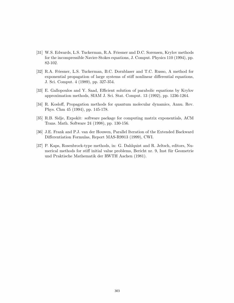
[31] W.S. Edwards, L.S. Tuckerman, R.A. Friesner and D.C. Sorensen, Krylov methodsfor the incompressible Navier-Stokes equations, J. Comput. Physics 110 (1994), pp.82-102.
[32] R.A. Friesner, L.S. Tuckerman, B.C. Dornblaser and T.C. Russo, A method forexponential propagation of large systems of stiff nonlinear differential equations,J. Sci. Comput. 4 (1989), pp. 327-354.
[33] E. Gallopoulos and Y. Saad, Efficient solution of parabolic equations by Krylovapproximation methods, SIAM J. Sci. Stat. Comput. 13 (1992), pp. 1236-1264.
[34] R. Kosloff, Propagation methods for quantum molecular dynamics, Annu. Rev.Phys. Chm 45 (1994), pp. 145-178.
[35] R.B. Sidje, Expokit: software package for computing matrix exponentials, ACMTrans. Math. Software 24 (1998), pp. 130-156.
[36] J.E. Frank and P.J. van der Houwen, Parallel Iteration of the Extended BackwardDifferentiation Formulas, Report MAS-R9913 (1999), CWI.
[37] P. Kaps, Rosenbrock-type methods, in: G. Dahlquist and R. Jeltsch, editors, Nu-merical methods for stiff initial value problems, Bericht nr. 9, Inst fur Geometrieund Praktische Mathematik der RWTH Aachen (1981).
303

Proceedings of the International Conferenceon Computational and Mathematical Methodsin Science and Engineering, CMMSE 2007Chicago, 20–23 June 2007.
Functional Support Vector Machines and GeneralizedLinear Models for Glacier Geomorphology Analysis
J. M. Matıas1, C. Ordonez2, J. Taboada2 and T. Rivas2
1 Department of Statistics, University of Vigo2 Department of Natural Resources, University of Vigo
emails: [email protected], [email protected], [email protected],[email protected]
Abstract
We propose a functional pattern recognition approach to the problem of iden-tifying the topographic profiles of glacial and fluvial valleys, using a functionalversion of support vector machines for classification. We compare a proposed func-tional version of support vector machines with functional generalized linear modelsand their vectorial versions: generalized linear models and support vector machinesthat use the original observations as input. The results indicate the benefit of ourproposed functional support vector machines and, in more general terms, the ad-vantages of using a functional rather than a vectorial approach.
Key words: Digital elevation models, functional data analysis, functional gen-eral lineal model, support vector machines, topographic profiles
MSC 2000: 62J12, 62J99, 68T05, 68T35, 86A40
1 Introduction
Geomorphology is the science that studies landforms in the Earth’s crust and the pro-cesses that form them. Valleys, which are principally shaped by the erosional activityof glaciers and rivers, are classified in two main classes in terms of their shape [1]–U-shaped valleys and V-shaped valleys. U-shaped valleys, which have typically beenformed by glaciers, have steeply sloped sides and a central concave part. V-shapedvalleys, which are formed by rivers, usually have gentler slopes and narrower, moreangular bases. Another type of fluvial river valley also exists, which is characterized bya flat rather than angular base.
Geomorphology experts have traditionally distinguished between different types ofvalleys on the basis of visual analyses of the topographical profiles of the valleys, contourmaps, and aerial photographs. Another way to study and compare valley shapes is to
304

simulate the topographic profiles using mathematical models, e.g., catenary functions[2]; [12], power law regression models [11]; [3] or generalized power law [8]. However,since these models are overly simple and fail to reflect the precise shapes of the realprofiles, this leads to error in reproducing the landforms and in differentiating betweenthe different types of valleys. For this reason, and also given the recent advent ofmodels capable of simulating valley erosion and evolution, more advanced techniqueswith a statistical focus are being used to describe and compare topographic profiles, asfollows:
1. Pre-defined non-linear regression models with a parametric focus, from which themodels with the best goodness-of-fit are chosen [5].
2. Functional data analysis [9], which applies two distinct strategies [4], namely, anunsupervised approach that clusters profiles and interprets the clusters in termsof the majority elements (e.g. the U shape), and a supervised approach thatconstructs predictive models of the profiles based on scalar covariables (elevation,etc.).
We propose a new machine-learning philosophy approach based on functional tech-niques, which involved the construction of an expert system, trained using a supervisedapproach, with artificially constructed theoretical profiles that enables the system todetermine the nature of new real profiles. Since real profiles rarely fall into one mor-phological group or another, this system also indicates the degree of belongingness ofa profile to a particular group (i.e., the a posteriori probability of membership in aparticular group).
To implement this approach, we used functional pattern recognition models, specif-ically functional generalized linear models [6] (functional 0-1 regression and logisticregression, [7]), as also a functional version of the support vector machines [10] in thefunctional space generated by a set of basic functions.
Although in this initial research phase, we use just two morphological groups,the method can be easily extended to include more groups using multiclass functionalpattern recognition techniques (to be the subject of a future article).
Our article is structured as follows:
1. Firstly we describe functional pattern recognition techniques, including the func-tional generalized linear model, particular cases of this model used in this work,and the proposed functional pattern recognition support vector machines.
2. Next we describe the details of the application problem, as also the results ofthe application of the above techniques to the data-smoothed functional versions.These results are compared with the results obtained from applying the vectorialversions of the same techniques to the original scalar data.
3. The final section describes our conclusions.
305

2 Application to the Identification of Valley Profiles
2.1 Training and Test Samples
In order to evaluate the capacity of the functional support vector machines to discrimi-nate between the different types of valley profiles, simulated profiles and real profiles forglacial valleys and fluvial valleys were used. In an initial phase, simulated profiles weregenerated in order to train the expert system, whereas the real profiles were reservedto test the behavior of the system. This system can later be enriched by incorporatingreal profiles whose morphology is known in the training sample.
The type of profiles considered in this initial research phase were U-shaped andV-shaped, although the method can incorporate other types of profiles (to be studiedin future research).
The training sample should include the full range of profiles in similar conditions asin reality, in other words, with observations subject to noise and in different positions.The profiles generated were contaminated with Gaussian noise with mean zero for boththe U-shaped and V-shaped valleys, the slope of one of the two branches of the profileswere modified from the origin—with a view to reflecting the asymmetry observed inreality—by assigning a lower value to one than the other.
In order to simulate the U-shaped profiles, catenary functions were used, expressedas follows [12]:
y = b0 + b1 cosh (x/b1) + ε (1)
where y is the vertical distance and x the horizontal distance from (0, 0) in the coor-dinate system, where b0 and b1 are coefficients, and where ε ∼ N
(0, σ2
)is an additive
term of error used to simulate deviations from the real profiles with respect to thecatenary function. The coefficient b1 determines how quickly the catenary opens up.
Figure 1 shows some of these catenaries, all with the same extremes but withdifferent depths.
In order to represent the V-shaped profiles, the general power model (GPL) [5] wasused, expressed as follows:
y = α |x− x0|β + y0 + ε (2)
The parameter β provides a direct measure of the profile curvature, with valuesnear 1 corresponding to V-shaped profiles and values near 2 corresponding to U-shapedprofiles.
The term (x0, y0) provides an estimate of the location of the minimum of the profile.Figure 2 shows various V-shaped profiles for the particular case of a minimum
located at the origin of the coordinates. The additive term for noise, as in the catenaries,is a normal distribution with a zero mean.
The real profiles used to evaluate the goodness-of-fit of the system were extractedfrom a digital elevation model (DEM) with a resolution 30 meters representing SierraNevada, a mountain range located in southern Spain with some of Spain’s most im-portant skiing slopes. The graph on the left of Figure 3 depicts the DEM, discretizedin altitude intervals of 100 meters, for altitudes varying between 410 meters and 1999
306
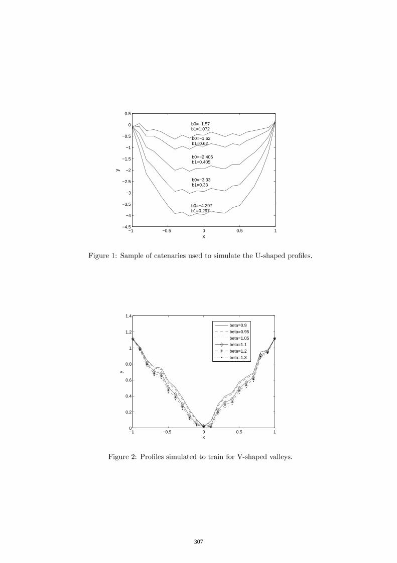
−1 −0.5 0 0.5 1−4.5
−4
−3.5
−3
−2.5
−2
−1.5
−1
−0.5
0
0.5
x
yb0=−1.57b1=1.072
b0=−1.62b1=0.62
b0=−2.405b1=0.405
b0=−3.33b1=0.33
b0=−4.297b1=0.297
Figure 1: Sample of catenaries used to simulate the U-shaped profiles.
−1 −0.5 0 0.5 10
0.2
0.4
0.6
0.8
1
1.2
1.4
x
y
beta=0.9
beta=0.95
beta=1.05
beta=1.1
beta=1.2
beta=1.3
Figure 2: Profiles simulated to train for V-shaped valleys.
307

-1.5 -1 -0.5 0 0.5 10
0.1
0.2
0.3
0.4
0.5
0.6
0.7
0.8
0.9
1
200 400 600 800 1000 1200 1400
100
200
300
400
500
600
700
800
900
1000
Figure 3: DEM of Sierra Nevada, showing two profiles, one U-shaped and the otherV-shaped (left). The real U-shaped and V-shaped profiles extracted from (and markedin) the DEM (right).
meters. The graph on the right of Figure 3 depicts two profiles extracted from themodel, one corresponding to a glacial valley and the other corresponding to a fluvialvalley (note that the coordinates are normalized in order to facilitate comparison).
In total, 137 training profiles (54 V-shaped and 83 U-shaped) and 25 test profiles(13 V-shaped and 12 U-shaped) were obtained (Figure 4).
Any differences in location of the center of the curves may imply differences in theprofiles that are based solely on the relative position of the center of the profile andnot on its U or V shape. For example, two mildly asymmetric V-shaped profiles couldbe considered to be very different if their centers are not properly aligned.
To simultaneously compare profiles on the basis of valley shape and not valleysize, a similar scale is needed. For this reason, all the training and test profiles werenormalized for the X and Y axes, the former in the interval [−1 1] (with the minimumat zero), and the latter in [0 1].
The training and test profiles were smoothed using a cubic B-splines basis with 30breaks (32 basic functions). A number of different options for the number of breaks wereevaluated producing similar results. Figure 4 shows the profiles that were registered asfunctional data in the manner described.
2.2 Results
Once the test and training profiles had been registered as functional data, the followingtechniques were used to construct the functional pattern recognition model: functionallinear regression with a 0 − 1 response variable, functional logistic regression, andfunctional support vector machines with linear and Gaussian kernels.
The parameters for the models (regularizer and Gaussian kernel parameter for thefunctional support vector machines, and regularizer for the functional logistic regres-
308
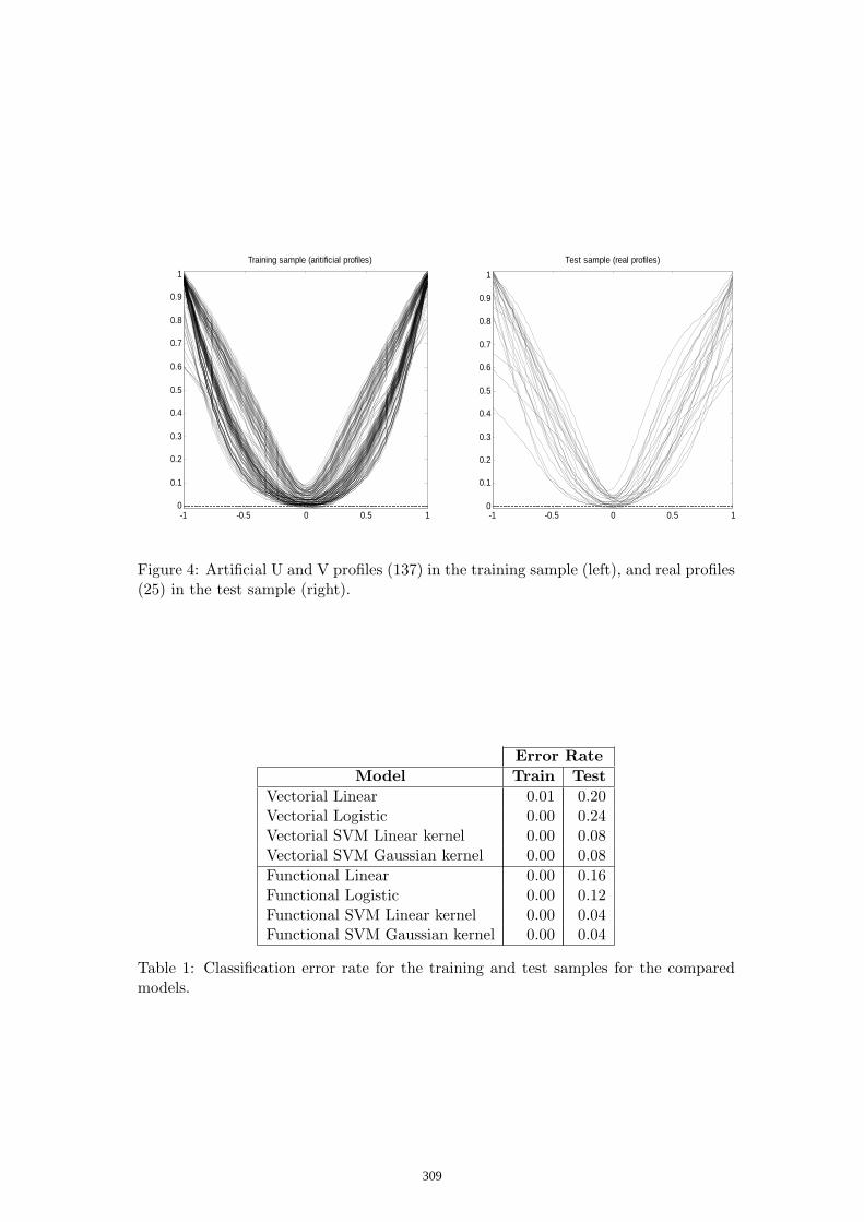
-1 -0.5 0 0.5 10
0.1
0.2
0.3
0.4
0.5
0.6
0.7
0.8
0.9
1
-1 -0.5 0 0.5 10
0.1
0.2
0.3
0.4
0.5
0.6
0.7
0.8
0.9
1
Test sample (real profiles)Training sample (aritificial profiles)
Figure 4: Artificial U and V profiles (137) in the training sample (left), and real profiles(25) in the test sample (right).
Error RateModel Train Test
Vectorial Linear 0.01 0.20Vectorial Logistic 0.00 0.24Vectorial SVM Linear kernel 0.00 0.08Vectorial SVM Gaussian kernel 0.00 0.08Functional Linear 0.00 0.16Functional Logistic 0.00 0.12Functional SVM Linear kernel 0.00 0.04Functional SVM Gaussian kernel 0.00 0.04
Table 1: Classification error rate for the training and test samples for the comparedmodels.
309
sion) were selected using 10-fold cross-validation.The results obtained are depicted in Table 1, which shows, for reference purposes,
the results obtained using vectorial versions of the above models applied to the scalarobservations of the profiles (from which the functional versions were constructed).
As can be observed, there were no training errors in any of the cases (except for thevectorial linear model), probably because of the theoretical nature of the training dataand the relatively low level of noise. Nonetheless, in the test sample of real profiles, itcan be observed how the functional model results improved significantly on the resultsproduced by the vectorial versions of the same models. Likewise, of the functionalmodels, the functional support vector machines produced the best results, irrespectiveof the kernel used (at least for this problem).
An analysis of the errors would indicate that these are associated with profiles thatare genuinely difficult to classify as either U-shaped or V-shaped, which, in turn, wouldindicate the need to extend the typology to other classes not covered by these two mainshapes (this will be the subject of future research).
3 Conclusions
In this work we evaluated the suitability of functional data analysis techniques forthe morphological classification of the topographic profiles of U-shaped and V-shapedvalleys.
From the results obtained it can be deduced that the functional techniques are animprovement on the vectorial techniques in terms of distinguishing between the twoprofile types, and that very satisfactory results can be obtained simply by training thesystem using simulated profiles. The functional models that produced the best resultswere the proposed functional support vector machines.
In this initial phase, the models were trained using only simulated profiles. How-ever, on a gradual basis, these models will be further enriched with real profiles oncetheir morphological characteristics have been established.
Future research will include the application of the methodology to a larger numberof morphological groups using a multiclass pattern recognition approach, and enrich-ment of the model by means of the inclusion of derivatives of the profiles as functionalcovariables.
Acknowledgements
J. M. Matıas’s research was supported by the Spanish Ministry of Education and Sci-ence, Grant No. MTM2005-00820.
References
[1] J. Campbell, Frost and fire, Edinburgh: Edmonston and Douglas, vol I., 1865.
310

[2] W.Davis, The Mission Range, Montana, Geographical Review 2 (1916) 267-288.
[3] W.Graf, The geomorphology of the glacial valley cross section. Arctic and AlpineResearch 2 (1970) 303-312.
[4] M. Greenwood, M. Functional Data Analysis for Glaciated Valley Profile Anal-ysis, Ph.D., Department of Statistics, University of Wyoming. December, 2004.
[5] M. Greenwood and N. Humphrey, Glaciated valley profiles: An applicationof nonlinear regression, Computing Science and Statistics 34 (2002) 452-460.
[6] P. McCullagh and J. A. Nelder, Generalized Linear Models, Chapman &Hal, 1989.
[7] H. G. Muller, Functional modelling and classification of longitudinal data, Scan-dinavian Journal of Statistics, 32 (2005) 223–240.
[8] F. Pattyn and W. Van Huele, Power law or power flaw? , Earth Surface Pro-cesses and Landforms 23 (1998) 761-767.
[9] J. O. Ramsay and B. W. Silverman, Functional data analysis, Springer, 1997.
[10] B. Scholkopf and A. J. Smola, Learning with Kernels, MIT Press, 2002.
[11] H. Svensson, Is the cross-section of a glacial valley a parabola?, Journal ofGlaciology, 3 (1959) 362-363.
[12] W.D. Thornbury, Principles of geomorphology, Wiley, New York, 1954.
311

Proceedings of the International Conferenceon Computational and Mathematical Methodsin Science and Engineering, CMMSE 2007Chicago, 20–23 June 2007.
On the Numerical Evaluation of Option Prices in theVariance Gamma Model
Anita Mayo1
1 Mathematics Department, Baruch College, CUNY
emails: anita [email protected]
Abstract
Because the pricing equations in Levy models contain integrals, it is difficult todevelop rapid numerical methods for solving them. Although the integrals are notperiodic, the standard evaluation methods use the FFT, and therefore require largecomputational regions to ensure accuracy. In earlier work we developed efficientmethods for pricing options in two Levy models, the Merton model and the Koudouble exponential model. The methods rely on the fact that in those models thedensity functions for the jump distributions satisfy ordinary or partial differentialequations, so differential methods can be used to evaluate the integrals. In thispaper we present effective numerical methods for pricing options in another Levymodel that has been shown to work particularly well in actual market conditions,the Variance Gamma model. We also provide numerical results.
Key words: Option pricing, Variance Gamma
1 Introduction
The Black Scholes pricing model does not produce the heavy tails and asymmetrythat one sees in practice. That is, large price movements occur more often than theBlack Scholes model predicts, and log scaled upward and downward movements arenot equally likely. These and other problems have led to the development of alternatepricing models. A common assumption is that in addition to the standard continuousBlack Scholes process, the process the asset price follows has a component with jumps.Such processes are called jump processes.
The earliest jump model is due to Merton [12] who assumes the process the assetfollows is the sum of the Black Scholes process and a jump process with lognormallydistributed jumps with constant parameters. Other models which combine a localvolatility function with a jump process have also been used for pricing options (An-dersen and Andreasen, [3]). Kou [8] has suggested a model with double exponentialdistribution for the log jump size. Models where the process is a pure jump process
312

and there is no continuous component have also been developed. For example, Madan,Carr, and Chang [9] more recently proposed what they call a Variance Gamma model.This model has been shown to be especially well suited for modeling in current marketconditions, and is the model we are considering in this paper.
Some of these jump models are analytically tractable. For example, in the Mertonmodel there is an analytic formula for European option prices in terms of Black Sc-holes prices, and there are formulas for certain option prices in the Kou and VarianceGamma models. But though analytic formulas exist for pricing certain options, nu-merical methods are required for pricing the most common ones, especially when theoption payoffs are path dependent.
Most numerical methods for finding option prices involve solving partial integro-differential equations (PIDEs). In particular, in an early paper Amim [2] used sim-ple but expensive tree methods to price European options. Later others (D’HalluinForsyth and Vetzal,[6], [7]) implemented more sophisticated methods for evaluatingvanilla European options, barrier options, and American options, and provided conver-gence results. These partial integro-differential equations have also also been solved byMatache, von Petersdorff and Schwab [10], Cont and Voltchkova [5] among others.
We note that combining a standard discretization method for the differential termswith a straightforward quadrature method for evaluating the integral term is costlysince the integral must be approximated at each point of the mesh used for discretizingthe the differential terms. However, it is possible to reduce the expense of evaluatingthe integral at all points of the computational grid by making an exponential changeof variables. This converts the integral term into a correlation integral which can beevaluated at all mesh points simultaneously using the Fast Fourier Transform. Thisapproach has often been used [2], [7].
One difficulty with Fourier methods is that they assume the function being eval-uated is periodic. Since the integrals are not periodic, it is necessary to extend thecomputational region, which is expensive, especially in higher dimensions. Fouriermethods are also slow to converge if the probability density is not smooth, as it is inthe Kou double exponential model and in the Variance Gamma model.
In earlier work we [10], [4], presented a different and more efficient class of methodsbased on the fact that the integrals often satisfy differential equations which can besolved more rapidly than the integrals can be accurately evaluated by quadrature, evenusing Fourier methods.
In particular, we used the fact that at any moment of time the integral in theMerton PIDE is equal to a translation of a solution of a heat equation with initialvalues equal to the solution of the PIDE at that time. The evaluation time τ of thesolution of the heat equation is half the variance of the jump process, and the translationamount is the expected value of the jump process. Therefore, we could evaluate thecorrelation integral by solving the heat equation numerically. Since the variance ofthe Poisson process is normally small we didn’t need many time steps to solve theheat equation very accurately. The fact that Fourier methods are more expensive thanusual differential methods for solving the heat equation meant that our methods weresometimes significantly faster. The methods we developed also extend to problems with
313

similar density functions.
The method we developed for evaluating the convolution integral in the Kou doubleexponential model uses the fact that after a linear change of variables the integrandis separable. Specifically, after the change of variables the value of the integral at apoint x can be expressed as the product of an exponential function of x and an integralwhere x only appears as the lower or upper limit of integration. Therefore the integralcan be evaluated at all n points of the grid using only Cn operations, where C is asmall number. The evaluation the integral can also be viewed as the solution of a firstorder ordinary differential equation. Again, our technique for evaluating the correlationintegrals in the Kou model can be extended to evaluating the integrals in other similarmodels.
In this paper we extend the methods we have developed for pricing in the Koumodel to pricing in the Variance Gamma model. The idea is that except very near theorigin one can approximate the Variance Gamma density by a function that is piecewisethe product of a linear function with the exponential with the same exponent as in theVariance Gamma density. That is, one can decompose the computational region intoseveral subregions, and in each subregion one can approximate the Variance Gammadensity by the product of the exponential term in the density and a different linearfunction. Once one has chosen the subregions, finding the best approximation onlyrequires a few operations per region. Our numerical experiments demonstrate that onecan achieve a very good approximation using around 4 or 5 subregions, so the cost ofthis part of the calculation is negligible.
The primary advantage of using such an approximation is that it greatly reducesthe cost of evaluating the correlation integral. As in our method for pricing in the Koumodel, one can evaluate the correlation integrals at each point of the computationalmesh at a cost of just a few operations per mesh point.
An important issue in our methods is how to choose the approximating linear func-tion. More precisely, it is necessary to find a good method for choosing the subregions.Finding the optimal subregions reduces to a a nonlinear least squares problem that insome cases could prove expensive to solve. On the other hand, as one might expect,having the nodes equally spaced does not produce extremely good results. We havechosen an intermediate method.
The Variance Gamma density cannot be well approximated by products of poly-nomials and exponentials very near the origin. Therefore, in a small region aroundeach mesh point we must evaluate the integral directly by quadrature. This region onlyconsists of a few mesh points, so the cost of this part of the calculation is small. Itis important to note that although the Variance Gamma density is unbounded at theorigin, the integrand of the correlation integral is always bounded.
An important advantage of our method is that it is not necessary to evaluate theintegral terms using a uniform mesh, nor does one obtain increased speed by requiringthe number of mesh points to be a power of 2. In particular, it should be possibleto use a very nonuniform grid when solving the pricing equation for digital options,concentrating the mesh points near the payoff discontinuity. This cannot be done asefficiently using Fourier methods.
314

The organization of this paper is as follows. In section 2 we present the pricingPIDE and discretization method for the differential terms, in the next section we presentour method for evaluating the integrals in the equation, and in the last section wepresent results of numerical experiments.
2 Pricing PIDE in the VG model
A Variance Gamma process is an infinite activity process of the form
X(t, σ, θ, ν) = b(γ(t, 1, ν), θ, σ)
where γ(t, 1, ν) is a unit mean gamma process and b(t, θ, σ) = θt+σW (t) is a Brownianmotion with drift θ and volatility σ. W (t) is a standard Brownian motion, and ν is thevariance of the gamma distributed time. If r is the risk free interest rate and q is thedividend rate, the risk neutral process for the price S of a risky asset is
S(t) = S(0)e(r−q+ω)t+X(t).
Here
ω =
∫
∞
−∞
(1 − ey) k(y)dy, (2.1)
where k(y) is the Levy measure
k(y) =e−λpy
νyfor y > 0 and k(y) =
e−λn|y|
ν|y|for y < 0
with
λp =
√
θ2
σ4+
2
σ2ν−
θ
σ2
λn =
√
θ2
σ4+
2
σ2ν+
θ
σ2.
The constant ν is a measure of the activity level, and λm and λp determine the expo-nential rates of decay of the density on the left and the right [9].
Under these assumptions European option prices V (S, τ) satisfy the PIDE
Vτ + (r − q + ω)SVS +
∫
∞
∞
[V (Sey, τ) − V (S, τ)] k(y)dy = rV. (2.2)
Before solving the equation we first make the standard exponential change of variablesS = ex and reverse time (t = T − τ):
Vt − (r − q + ω)Vx =
∫
∞
−∞
[V (x + y, t) − V (x, t)] k(y)dy − rV. (2.3)
We then discretize the differential and integral terms. Suppose xi are the dis-cretization points, h is the space step, and V n = (V n
0, V n
1, V n
2, , , V n
M ), n = 1, , , , ,N are
315

the the solution values at the nth time step. Following [1] we let ω(h) =∫
y>h(1 − ey)k(y)dy, and using (2.1) rewrite (2.3):
Vt−(r−q+ω(h))Vx =
∫
∞
−∞
[V (x + y, t) − V (x, t)] k(y)dy−
∫
y≤h
(ey−1)Vxdy−rV. (2.4)
We have chosen to discretize the differential terms using the Crank Nicolson scheme.Thus, at the nth time step we let
V n+1
i − V ni
∆t= a
V n+1
i+1− V n+1
i−1
2h+ a
V ni+1
− V ni−1
2h−
r
2
(
V ni + V n+1
i
)
+ I(V n)
where ∆t is the time step, a = q − r − ω(h), and I(V n) is our approximation to theintegrals in (2.4) at the n time step.
Boundary values are needed at the edges of the computational domain. Whenpricing call options it is common to assume that V n
0= 0 for all n, and V n
M = SM−Ke−rtn
where K is the strike price, SM = exM is the asset value at the upper edge of thecomputational region, and tn is the time at the nth time step. For a put we assumeV n
0= Ke−rtn and V n
M = 0.
At each time step the above equations and boundary conditions give rise to atridiagonal linear system of equations, which can be solved at a cost of 5M operationsper point at the first time step, and 3M operations at succeeding ones.
The Crank Nicolson scheme is in general second order accurate in h, but the abovescheme is explicit in the integral and only first order accurate in ∆t. In order to try toachieve second order accuracy in ∆t we have have used Richardson extrapolation. Wenote that several authors have solved the pricing PIDE using schemes that are implicitin the integral. In particular Wang et al. [13] used a semi Lagrangian discretizationof the differential terms, and both Picard iteration and BiCGstab method to solve theimplicit equations. We also note that when one is pricing European options one cancan use an operator splitting method originally suggested by Andersen and AndreasenWe used this method when we priced options in the Kou model [11], but although itis formally second order accurate we did not find the method to perform consistentlybetter than extrapolation. Since our primary contribution is a rapid and accuratemethod for evaluating the integral we have not yet implemented an implicit method,nor have we priced any American or other exotic options. In future work we will addresssuch issues.
At each time step one must also approximate the integral at all the points xi.Most schemes for evaluating the integral rely on the fact that it is a correlation integral,and use a Fourier method. However, because the integral is not periodic, one mustextend the computational region in order to avoid ”wrap around” effects. This increasesthe cost of the calculation.
In the next section we present a more efficient method for evaluating the integrals.
316

3 Evaluation of the Integral Terms
In this section we present our method for approximating the integrals in the VarianceGamma pricing equation:
∫
0
−∞
(V (x + y) − V (x)) Ce−λn|y|
|y|dy+
∫
∞
0
(V (x + y) − V (x)) Ce−λpy
ydy−Vx(x)
∫ h
−h
(ey− 1) k(y)dy
= I−(x) + I+(x) + VxIh
We first show how to approximate I+(x). By the further change of variables s = x + y
I+(x) can be written
I+(x) =
∫
∞
x
(V (s) − V (x))e−λ(s−y)
(s − y)ds
For any x and ǫ this integral can be decomposed into a part Iǫ(x) near x, and theremaining part Ir(x):
I+(x) =
∫ x+ǫ
x
(V (s) − V (x))e−λ(s−x)
(s − x)ds +
∫
∞
x+ǫ
(V (s) − V (x))e−λ(s−x)
(s − x)ds
For ǫ, xM > 0 the interval [ǫ, xM ] can be decomposed into NP subregions [ǫ = a0, a1], [a1, a2], , [aNP−1, aNP =
xM ], and on each subregion [ai, ai+1] the function e−λpx
xcan be approximated by the
product of the exponential eλpx and a linear function, bix + ci. The approximationsneed not be continuous from one subinterval to the next.
With these approximations one can approximate the integral Ir(x) =∑
i Iri (x)
where
Iri (x) =
∫ x+ai+1
x+ai
(V (s) − V (x)) (bi(s − x) + ci)e−λ(s−x)ds
= eλx
[
bi
∫ x+ai+1
x+ai
V (s)se−λsds + (ci − bix)
∫ x+ai+1
x+ai
V (s)e−λsds
]
−eλxV (x)
[
bi
∫ x+ai+1
x+ai
se−λsds + (ci − bix)
∫ x+ai+1
x+ai
e−λsds
]
The last two integrals in the above equation can be evaluated analytically.The other two integrals can be approximated at all M mesh points at a cost
of O(M) operations. For example, suppose we have approximated the first integral∫ xj+ai+1
xj+aiV (s)e−λsds at x = xj . To evaluate the integral at x = xj+1 we use the
approximation∫ xj+1+ai+1
xj+1+ai
V (s)e−λsds =
∫ xj+ai+1
xj+ai
V (s)e−λsds
−(V (xj+1 + ai+1) + V (xj + ai+1)
2λ
(
e−λ(xj+1+ai+1)− e−λ(xj+ai+1)
)
+V (xj+1 + ai) + V (xj + ai)
2λ
(
e−λ(xj+1+ai)− e−λ(xj+ai)
)
317
Thus, to compute the integral at the next mesh point we only need add and subtracttwo terms. The exponentials in the above formulas can be stored and reused. Thesecond integral can similarly be approximated at a point xj+1 from its values at xj.
To evaluate I+ we must extend the solution V (x) beyond the edge of the compu-tational region. When pricing a call, for x large we set the option value to ex
−Ke−rt,and for x ≤ x0 we set it to 0. For puts we set option values to 0 for x large, andKe−rt
− ex for x ≤ x0. We assume that the computational region is large enough sothese asymptotic approximations are sufficiently accurate.
We use essentially the same method to approximate I−(x) at all mesh points.
We also need to evaluate the integral Iǫ(x). We always chose ǫ to be an integernumber of mesh widths, ǫ = mh. (In our calculations we have generally chosen m =M/50 mesh widths.) On the interval [xj +h, xj + ǫ], we approximate the integral usingdirect quadrature. Finally, we note that by Taylor series approximations (see [1]) onecan show that the term
∫
y≤h(V (x + s) − V (s) − Vx(es
− 1))k(s)ds = O(h2), and cantherefore be neglected in the calculation.
It follows that the entire calculation is linear in the number of discretization pointsM . We also note that in our quadrature formulas truncation errors are due to approx-imating V (x) by it’s average value between mesh points, i.e. we integrate e−λx andxe−λx analytically.
An important issue in our method is the choice of the linear functions bix+ci. Whenthe nodes ai are prescribed beforehand we generally choose bi, cii = 1, , ,NP − 1so that
u(b1, c1, , , , , , bNP−1, cNP−1) =
NP−1∑
i=1
∫ ai+1
ai
(
bis + ci −1
s
)
2
e−λsds = min
If no other conditions are imposed this implies that for each 1 ≤ i ≤ NP − 1
∂u
∂bi
= 2
∫ ai+1
ai
s
(
bis + ci −1
s
)
e−λsds = 0 (3.1)
and∂u
∂ci
= 2
∫ ai+1
ai
(
bis + ci −1
s
)
e−λsds = 0. (3.2)
The above NP − 1 two by two linear systems of equations determine bi and ci.
We also performed calculations where we required the approximations be continu-ous from one interval to the next. Continuity implies
bixi+1 + ci = bi+1xi+1 + ci+1, (3.3)
which in turn implies the values of bi determine the values of ci for i = 2, , ,NP −1.We also require
∂u
∂bi
= 2
∫ ai+1
ai
s
(
bis + ci −1
s
)
e−λsds = 0 for i = 1, 2, , ,NP − 1. (3.4)
318

and∂u
∂c1
= 2
∫ ai+1
ai
(b1s + c1 − 1) e−λsds = 0. (3.5)
This set of equations (3.3)- (3.5) gives rise to a block lower bidiagonal matrix equationeasily solved by LU decomposition. However, as one might expect, we always obtainedmore accurate solutions when we did not impose continuity.
We also performed calculations where the nodes ai were not specified a priori.That is, for fixed NP − 1 we found 3NP − 4 numbers b1, ci1 ≤ i ≤ NP − 1, andaj , 2 ≤ j ≤ NP − 1 such that
v(bi, ci, ai) =
M−1∑
i=1
∫ ai+1
ai
(
bis + ci −1
s
)
2
e−λsds = min (3.6)
andbiai+1 + ci = bi+1ai+1 + ci+1. (3.7)
Because the nodes ai are not given this problem is nonlinear.By (3.7) the values of ci i = 2, , ,NP − 1 can be expressed in terms of the values
of bi, ai and c1. Therefore, we can view v as a function of the 2NP − 2 variablesbi1 ≤ i ≤ NP − 1, ai, 2 ≤ i ≤ NP − 1.
To determine values of the variables we use the fact that at the minimum of v itsderivatives with respect to all them are 0:
∂v
∂bi
=∂v
∂ai
=∂v
∂c1
= 0. (3.8)
In our numerical experiments we solved this system of equations by a modified dampedNewton’s method. We note that for a given interpolation domain [ǫ, xM ] and value ofλ the above calculations need only be performed once, i.e. the approximations do notdepend on the values of any other financial parameters. However, the calculations aremuch more expensive than ones where nodes are specified.
We also note that it may also be possible to approximate the Variance Gammadensity with other functions. Another possibility is having the approximating functionbe piecewise the product of a quadratic with an exponential. If one makes such anapproximation one can still evaluate the correlation integral at a cost of a few operationsper meshpoint, although the constant will be larger. However one should be able to usea smaller number of subregions, and this would decrease the cost of the calculation.
4 Numerical Results
In this section we report on results of numerical experiments we performed. We notethat the only way in which our method differs from others is in the way that weevaluate the integrals. We therefore first performed calculations to test the accuracyof our quadrature method.
We first tested our method on the function V (x) = x for which the the integral∫ b
a(V (x + s) − V (x)) eλs
sds can be evaluated analytically. Since V (x + s) − V (x) = s,
319

at any point x the value of the integral is∫ b
ae−λsds = −
1
λ
(
e−λb− e−λa
)
. Furthermore,when using our quadrature formula on this function there is no truncation error, soerrors are only due to interpolating the density function. In these experiments we leta = .01535 and b = 6.139.
Results of our calculations are given in Table 1. In the table NP is the number ofsubregions, and λ is the exponent in the density (We assumed that λp = λn = λ. Thenumbers in the last column are errors, which were the same at all quadrature points.In these and other experiments we always let C = 1, when λ was 5 we used the nodesai = ǫ+ i/ds2.33 and when λ was 10 (or 15) we let ai = ǫ+ i/ds2.53 where ds = xM −x0.We used M = 200 quadrature points to perform the calculation.
Table 1: Evaluation of Integral with V (x) = x
NP ǫ λ error
2 5. .246 9.89E-63 5. .246 8.28E-64 5. .246 1.70E-6
2 10. .246 4.89E-63 10. .246 2.34E-64 10. .246 9.61E-75 10. .246 5.94E-7
2 5. .123 3.34E-53 5. .123 1.78E-54 5. .123 8.97E-65 5. .123 6.41E-6
3 5. .062 5.78E-44 5. .062 4.26E-55 5. .062 2.43E-5
From these results we see that using 4 subregions or panels for interpolating providesa reasonable level of accuracy, and increasing the number does not change the resultssignificantly. Choosing ǫ smaller, of course, decreases the level of accuracy, but alsodecreases the cost of the calculation for a given value of h.
We next tested our method of evaluating the integral with V (x) equal to the payoffvalues for a call with strike K = 100, that is V (x) = ex
− K if ex≥ K, and V (x) = 0
otherwise. We compared the results with the exact values of the integral, which canbe expressed in terms of the exponential integral function. (We used MATLAB todetermine the values.) Results are given in Table 2. In this table M is the number ofdiscretization points and S = ex is the asset price at which we evaluated the integral.In this eample we always used NP = 4 subregions for interpolating the VG density,and integrated over the interval [.00674,5.43], We let ǫ = .0691 This ǫ corresponds tom=2 for M=100, to m=4 for M=200, m=8 for M=400, and m=16 for M=800. Theexact values of the integral for λ = 5. are 21.650 at S = 100. and 23.815 at S = 110.For λ = 15.0 the value of the integral is 6.2572 at S = 100.0.
320

Table 2: Evaluation of Integral with V (x) = x
M S λ error
100 100. 5 2. 21.730 0.080200 100. 5 4. 21.671 0.021400 100. 5 8. 21.657 0.006800 110. 5 16. 21.651 0.001
100 110. 5 2. 23.742 0.0027200 110. 5 4. 23.626 0.0011400 110. 5 8. 23.819 0.0004800 110. 5 16. 23.816 0.0001
100 100. 15 2. 6.316 0.059200 100. 15 4. 6.279 0.022400 100. 15 8. 6.264 0.007800 110. 15 16. 6.259 0.002
These results show that see that the method is almost second order accurate, and wecan achieve this level of accuracy using relatively few panels.
We also performed calculations where we used nodes determined by solving (3.8).It turned out that although these optimal nodes provided better results, the resultswere not significantly different. That is, they were usually only better, by a (linear)factor of 4, and the convergence rate was essentially the same.
In our final set of experiments we priced the European call and put options withλn = λp = 5, r = .1, T = 1,K = 100 at S = 100. Almendral and Oosterlee [1] pricedthe call option using a fine mesh, and determined the price to be 15.131. We obtainedthe same result. The price of the put is 5.6147. In our calculations we again choseǫ = .0691, but used NP = 5 subregions for interpolating, and used extrapolation withrespect to ∆t. The numbers in the second column are the number of time steps in thefiner mesh, and the numbers in the third column are the computed values.
Table 3: Evaluation of CallM nt Comp. vale error rate
100 30 15.205 0.074 .200 60 15.153 0.022 3.4400 120 15.137 0.006 3.8800 120 15.132 0.001 4.0
Table 4: Evaluation of PutM nt Comp. value error rate
100 30 5.6509 0.0362 .200 60 5.6220 0.0073 4.9400 120 5.6168 0.0021 3.5800 240 5.6152 0.0005 4.1
Figure 1 is the graph of the call price.
321

5 References
[1] A. Almendral and C. Oosterlee,On American options under the Variance GammaProcess, working paper.[2] K. Amin, Jump diffusion option valuation in discrete time, Journal of Finance,48:(1993) 1833-1863.[3] Andersen L. and J. Andreasen, Jump diffusion processes: Volatility smile fitting andnumerical methods for option pricing, Rev. of Derivatives Research, 4 (2000) 231-262.[4] P. Carr and A. Mayo, On the numerical evaluation of option prices in jump diffu-sion models, The European Journal of Finance, to appear, Proceedings of ForecastingFinancial Markets Conference, Paris, (2004). June, 2004.[5] Cont R. and E. Voltchkova, A finite difference scheme for option pricing in jumpdiffusion and exponential Levy models, Report 513, CMAP, Ecole Polytechnique, 2003.[6] d’Halluin, Y., P.A. Forsyth, and G. Labahn, A Penalty Method for American Op-tions with jump diffusion processes, Numerische Mathematik, 97 (2004) 321-352.[7] Y. d’Halluin, P.A. Forsyth, and K. R. Vetzal, A semi-Lagrangian approach for Amer-ican Asian options under jump diffusion, SIAM J. Sci. Comput., 27 (2005) 315-335.[8] S. Kou, A jump diffusion model for option pricing, Management Science, 48, (2002)1086-1101.[9] Madan, P., P. Carr, and E. Chang, The variance gamma process and option pricing,European Financial Review, 1 (1998) 75-105.[10] Matache, A., T. von Petersdorff, and C. Schwab, Fast deterministic pricing of op-tions on Levy driven assets, RiskLab Research Report, ETH, Zurich (2002).[11] Mayo, A., Methods for the pricing of PIDES in exponential and Merton models,Journal of Computational and Applied Math., to appear.[12] R. Merton, Option Pricing when underlying stock returns are discontinuous, Jour-nal of Financial Economics, 3 (1976) 125-144.[13] I Wang, J. Wan, and P. Forsyth, Robust Numerical Valuation of European andAmerican options under the CGMY process, working paper.
322

Black-Scholes equation: Green's function solution
for terminal-boundary value problems
Max MelnikovLabry School of Business and Economics
Cumberland University, USA
e-mail: [email protected]
AbstractA Green's function-based approach is proposed for obtaining solu-tion to a variety of terminal-boundary value problems stated forthe Black-Scholes equation that simulates the valuation of Euro-pean option pricing. It is shown that analytic representations ofrequired Green's functions can be constructed allowing a closedform solution to the considered problems.
Key words: Black-Scholes equation, Green's function method
1. Introduction
A linear backward in time parabolic type partial dierential equation, which is re-ferred to as the Black-Scholes equation [1], is widely used in the eld of nancialengineering in nowadays for quantitative and qualitative analysis of option pricingproblems. Green's function-based methods are traditionally used in partial dier-ential equations. They could also be productive for the Black-Scholes equation, buta limited number of computer-ready representations of Green's functions for thisequation represents a considerable obstacle.
This study aims at the development of a Green's function-based analytic approach toa class of terminal-boundary value problems stated for the nonhomogeneous Black-Scholes equation
@V (S; t)
@t+2S2
2
@2V (S; t)
@S2+ rS
@V (S; t)
@S rV (S; t) = (S; t) (1)
As an example, we consider a problem stated for Eq (1) in the semi-innite strip-shaped region =(S1<S<S2)(T >t>1) of the S; t-plane.Let a terminal condition be given by
V (S; T ) = '(S) (2)
323

while the Dirichlet type boundary conditions
V (S1; t) = A(t) and V (S2; t) = B(t) (3)
be imposed on the edges S=S1 and S=S2 of the region.
In the above problem setting, V =V (S; t) is the price of the derivative product, '(S)is the pay-o function of a given derivative problem at the expiration time T , withS and t being the share price of the underlying asset and time, respectively. Theparameters and r represent the volatility of the underlying asset and the risk-freeinterest rate, respectively.
It is evident that upon introducing of a new unknown function v(S; t)
V (S; t) = v(S; t)+SS1S2S1
[B(t)A(t)] +A(t) (4)
the terminal-boundary value problem in Eqs (1)-(3) reduces to
@v(S; t)
@t+2S2
2
@2v(S; t)
@S2+ rS
@v(S; t)
@S rv(S; t) = F (S; t) (5)
v(S; T ) = f(S) (6)
with the homogeneous boundary conditions imposed as
v(S1; t) = 0 and v(S2; t) = 0 (7)
In view of the relation in Eq (4), the right-hand side functions F (S; t) and f(S) inEqs (5) and (6) are expressed in terms of the right-hand sides (S; t) and (S) ofEqs (1) and (2) as
F (S; t) = (S; t) +SS1S2S1
[r (B(t)A(t))+A0(t)B0(t)]
A0(t) + rA(t) + rSA(t)B(t)S2S1
and
f(S) = '(S) SS1S2S1
[B(T )A(T )]A(T )
As it follows from the qualitative theory of partial dierential equations [2], thesolution to the problem setting in Eqs (5)-(7) can be written as the following sumof two integral representations
v(S; t) =
S2ZS1
G(S; t; eS)f( eS)d eS + TZt
S2ZS1
G(S; t et; eS)F ( eS; et)d eSdet (8)
whereG(S; t; eS) is the Green's function to the homogeneous terminal-boundary valueproblem corresponding to that in Eqs (5)-(7).
324

Thus, to obtain a computer-friendly analytic solution to the terminal-boundary valueproblem posed by Eqs (1)-(3), one ought to have a compact form of the Green'sfunction G(S; t; eS). The derivation procedure for such a form is described in detailin the next section.
2. Construction of the Green's function
Our approach to the construction of Green's function ows out from the procedurewhich was developed earlier [3] for problems in applied mechanics. It is based ona combination of two classical methods of applied mathematics. These are: themethod of integral Laplace transform that is widely implemented in the heat andmass transfer, for example, and the method of variation of parameters traditionallyused for nding general solution for linear high-order ordinary dierential equations.In going through the procedure, we consider the terminal-boundary value problem
@v(S; t)
@t+2S2
2
@2v(S; t)
@S2+ rS
@v(S; t)
@S rv(S; t) = 0 (9)
v(S; T ) = f(S) (10)
v(S1; t) = 0 and v(S2; t) = 0 (11)
Recall [2] that the solution to the above problem can be written in terms of theGreen's function G(S; t; eS) to the homogeneous problem corresponding to that inEqs (5)-(7) as
v(S; t) =
S2ZS1
G(S; t; eS)f( eS)d eS (12)
This representation is used, in the present study, to actually derive the Green'sfunction G(S; t; eS). The emphasis is put, in our study, on the parabolic type single-parameter equation forward in time
@u(x; )
@=@2u(x; )
@x2+(c1)@u(x; )
@xcu(x; ) (13)
which traditionally [4, 5] arises from Eq (9) by introducing new independent variablesx and
x = lnS and =2
2(T t) (14)
The parameter c in (13) is dened in terms of r and as c = 2r=2. Hence,Eq (13) has, in contrast to the Black-Scholes equation, constant coecients. Thissignicantly simplies the situation.
Upon introducing the variables x and in compliance with the relations of Eq (14),the terminal-boundary value problem of Eqs (9)-(11) transforms into the followinginitial-boundary value problem
u(x; 0) = f(ex) (15)
325

u(a; ) = 0 and u(b; ) = 0 (16)
for the equation in (13) posed on the semi-innite strip-shaped region (a < x <b)(0< <1) in the x; -plane, where
a = lnS1 and b = lnS2
Applying the Laplace transform
U(x; s) = Lfu(x; )g =Z 1
0esu(x; )d
to the setting in Eqs (13), (15) and (16), we obtain the following boundary valueproblem
d2U(x; s)
dx2+(c 1)dU(x; s)
dx (s+c)U(x; s) = f(ex) (17)
U(a; s) = 0; U(b; s) = 0 (18)
for the Laplace transform U(x; s) of u(x; ).
In compliance with the method of variation of parameters, the general solution toEq (17) is found as
U(x; s) =
xZa
e(x)
2!
e(x)! e(x)!
f(e)d
+M(s)e(+!)x +N(s)e(!)x (19)
where the parameter ! is dened as ! =ps+ , while the parameters and are
expressed as
=1 c2
and =
1 + c
2
2Satisfaction of the boundary conditions of Eq (18) yields the system of linear alge-braic equations
e(+!)a e(!)a
e(+!)b e(!)b
! M(s)N(s)
!=
0
(s)
!(20)
in M(s) and N(s), where
(s) = bZa
1
2!
he(!)(b) e(+!)(b)
if(e)d
Solving the system in (20), we obtain
M(s) =
bZa
e(!)ae(b)he(b)! e(b)!
i2!e(ab)! e(ba)!
f(e)d
326

and
N(s) = bZa
e(+!)ae(b)he(b)! e(b)!
i2!e(ab)! e(ba)!
f(e)d
Upon substituting these in (19), the latter reads as
U(x; s) =
xZa
e(x)
2!
e(x)! e(x)!
f(e)d
+
bZa
e(x)he(xa)!e(ax)!
ihe(b)!e(b)!
i2!e(ab)! e(ba)!
f(e)d
which can be expressed in a single-integral form
U(x; s) =
bZa
e(x)
2!e(ab)! e(ba)!
ne[(x+)(a+b)]!+e[(a+b)(x+)]!
e[(ab)+jxj]!e[(ba)jxj]!of(e)d
Transforming the factor e(ab)! e(ba)! in the denominator as
e(ab)! e(ba)!=e(ba)!h1e2(ab)!
iwe rewrite the above representation for U(x; s)
U(x; s) =bZa
e(x)
2!e(ba)!1 e2(ab)!
ne[(x+)(a+b)]!+e[(a+b)(x+)]!
e[(ab)+jxj]!e[(ba)jxj]!of(e)d (21)
The immediate inverse Laplace transform of U(x; s) is problematic if the latter iskept in its current form. Therefore, we adjust it rst by representing the factor1=[1e2(ab)!] in the integrand in (21) as the sum of the geometric series
1
1 e2(ab)!=
1Xn=0
e2n(ab)!
whose common ratio e2(ab)! is clearly less than one. This transforms (21) into
U(x; s) =
bZa
e(x)
2!
1Xn=0
ne[jxj2(n+1)(ab)]!
327

+e[jxj2n(ab)]! e[2b(x+)2n(ab)]!
e[(x+)2a2n(ab)]!of(e)d (22)
and the inverse Laplace transform of the above can be accomplished in the term-by-term manner. This yields the solution u(x; ) to the initial-boundary value problemin Eqs (13), (15) and (16) in the form
u(x; ) = L1fU(x; s)g
=
bZa
e(x)e
2p
1Xn=0
(exp
[jxj+2(n+1)(ab)]
2
4
!
+exp
[jxj2n(ab)]
2
4
!exp
[2b(x+)2n(ab)]
2
4
!
exp [(x+)2a2n(ab)]
2
4
!)f(e)d
which converts to a more compact form by rearranging the summation in the aboveseries. This yields
u(x; )=
bZa
e(x)e
2p
1Xm=1
(exp
[jxj+2m(ab)]
2
4
!
exp [2b(x+)2m(ab)]
2
4
!)f(e)d
The solution v(S; t) to the setting in Eqs (9)-(11) can be attained by the backwardsubstitution of the variables x, and with S, t and S, respectively, in compliancewith the relations in Eq (14). With and replaced with the original parametersr and of the Black-Scholes equation, we obtain v(S; t) in the form
v(S; t) =
S2ZS1
exp r2=2
2ln(S= eS) (r+2=2)2
22(Tt)
eSp2(Tt)
1X
m=1
(exp
[ln(S=
eS)+2m ln(S1=S2)]222(T t)
!
exp [ln(S
22=S
eS)2m ln(S1=S2)]222(T t)
!)f( eS)d eS
which can be transformed, by combining the logarithmic components in the seriesfactor. This yields
v(S; t) =
S2ZS1
exp r2=2
2ln(S= eS) (r+2=2)2
22(Tt)
eSp2(Tt)
328
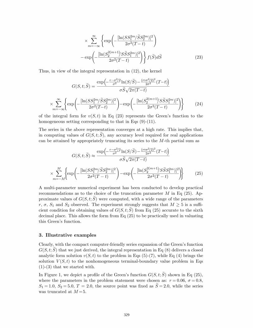
1X
m=1
(exp
[ln(SS
2m1 =
eSS2m2 )]2
22(T t)
!
exp [ln(S
2(m+1)2 =S eSS2m1 )]2
22(T t)
!)f( eS)d eS (23)
Thus, in view of the integral representation in (12), the kernel
G(S; t; eS) = exp r2=2
2ln(S= eS) (r+2=2)2
22(Tt)
eSp2(Tt)
1X
m=1
(exp
[ln(SS
2m1 =
eSS2m2 )]2
22(Tt)
!exp
[ln(S
2(m+1)2 =S eSS2m1 )]2
22(T t)
!)(24)
of the integral form for v(S; t) in Eq (23) represents the Green's function to thehomogeneous setting corresponding to that in Eqs (9)-(11).
The series in the above representation converges at a high rate. This implies that,in computing values of G(S; t; eS), any accuracy level required for real applicationscan be attained by appropriately truncating its series to the M -th partial sum as
G(S; t; eS) exp r2=2
2ln(S= eS) (r+2=2)2
22(Tt)
eSp2(Tt)
MX
m=M
(exp
[ln(SS
2m1 =
eSS2m2 )]2
22(T t)
!exp
[ln(S
2(m+1)2 =S eSS2m1 )]2
22(T t)
!)(25)
A multi-parameter numerical experiment has been conducted to develop practicalrecommendations as to the choice of the truncation parameter M in Eq (25). Ap-proximate values of G(S; t; eS) were computed, with a wide range of the parametersr, , S1 and S2 observed. The experiment strongly suggests that M 5 is a su-cient condition for obtaining values of G(S; t; eS) from Eq (25) accurate to the sixthdecimal place. This allows the form from Eq (25) to be practically used in valuatingthis Green's function.
3. Illustrative examples
Clearly, with the compact computer-friendly series expansion of the Green's functionG(S; t; eS) that we just derived, the integral representation in Eq (8) delivers a closedanalytic form solution v(S; t) to the problem in Eqs (5)-(7), while Eq (4) brings thesolution V (S; t) to the nonhomogeneous terminal-boundary value problem in Eqs(1)-(3) that we started with.
In Figure 1, we depict a prole of the Green's function G(S; t; eS) shown in Eq (25),where the parameters in the problem statement were chosen as: r= 0:06; = 0:8;S1 = 1:0; S2 = 5:0; T = 2:0; the source point was xed as eS = 2:0, while the serieswas truncated at M=5.
329
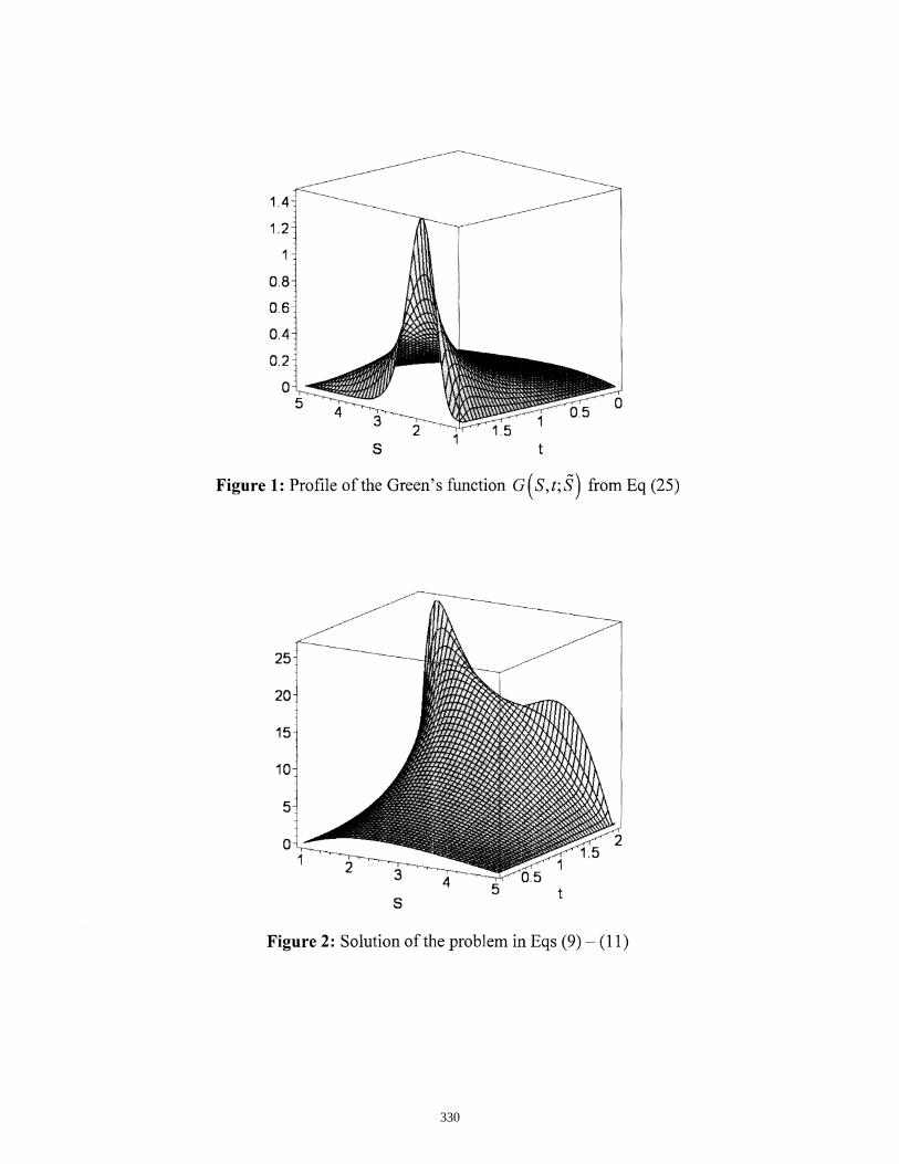
330

Figure 2 exhibits the solution v(S; t) to the statement in Eqs (9)-(11), where r=0:06;=0:8; S1=1:0; S2=5:0; T = 2:0; while the right-hand side function in the terminalcondition of Eq (10) is chosen as
f(S) = 5
"S S1 + S2
2
2+ 2
#and the truncation parameter of the series in Eq (25) is xed as M=5.
4. Other Green's functions
The proposed technique for the construction of computer-friendly representationsof Green's functions is also productive in other problem settings for the Black-Scholes equation. To illustrate this assertion, we consider, as an example, a terminal-boundary value problem on the semi-innite strip-shaped region = (0 < S <D)(T >t>1) with boudary conditions imposed as
jv(0; t)j <1 and@v(D; t)
@S= 0 (26)
Upon implementing the approach developed in this study, we obtain the followingcompact expression
G(S; t; eS) = 1eSSeSexp
2
2(Tt)
!
8><>: 1
p2(Tt)
264exp0B@
hln(S= eS)i222(Tt)
1CA+exp0B@
hln(S eS=D2)i222(Tt)
1CA375
S eSD2
!e
22(Tt)=2 erfc
2
q22(Tt) ln(S eS=D2)p
22(Tt)
!9=; (27)
for the Green's function to the homogeneous problem corresponding to that in Eqs(9), (10) and (26). The parameters and are expressed in terms of the parametersr and from the governing equation in (1) as
=2=2r2
and =
2=2r2
!2and where erfc() stays for a special function that is referred to in literature asthe complementary Gauss error-function. Subroutines for eective valuation of thisfunction represent in nowadays an inalienable part of every computer software. Thismakes the expression in (27) readily computable and attractive therefore for practi-cians working in the eld of nancial engineering.
For the homogeneous terminal-boundary value problem corresponding to that in Eqs(9) and (10) posed on the semi-innite strip-shaped region = (0 <S <D)(T >t>1) with boudary conditions imposed as
jv(0; t)j <1 and v(D; t) = 0
331

the Green's function is obtained in the form
G(S; t; eS) = 1eSSeSexp
2
2(Tt)
!
8><>: 1
p2(Tt)
264exp0B@
hln(S= eS)i222(Tt)
1CAexp0B@
hln(S eS=D2)i222(Tt)
1CA375
Concluding remarks
Compact analytic representations of Green's functions can be obtained for a varietyof terminal-boundary value problems for the Black-Scholes equation within the scopeof the present study. They are easily accessible for both theoretical analysis andnumerical work in the eld and can readily be used in solving a variety of problemssettings in nancial engineering.
References
[1] F. BLACK and M.S. SCHOLES, The pricing of options and corporate liabilities,J. Polit. Econ. 81 (1973) 637-654.
[2] V.I. SMIRNOV, A Course of Higher Mathematics, Pergamon Press, OxfordNew York, 1964.
[3] Y.A. MELNIKOV, In uence Functions and Matrices, Marcel Dekker, NewYorkBasel, 1998.
[4] P. WILMOTT, S. HOWISON and J. DEWYNNE, The Mathematics of Finan-cial Derivatives: A Student Introduction, Cambridge University Press, 1995.
[5] D. SILVERMAN, Solution of the Black-Scholes equation using the Green's func-tion of the diusion equation, Manuscript, Department of Physics and Astron-omy, University of California, Irvine (1999).
[6] S. NEFTCI, An Introduction to the Mathematics of Financial Derivatives, Aca-demic Press, New York, 2000.
332
Proceedings of the International Conferenceon Computational and Mathematical Methodsin Science and Engineering, CMMSE 2007Chicago, 20–23 June 2007.
H-matrix Preconditioners for Invariant ProbabilityDistribution in Dynamical Systems
S. Oliveira1 and F. Yang1
1 Computer Science Department, The University of Iowa
emails: [email protected], [email protected]
Abstract
An Hierarchical (H)-matrix is a hierarchical sparse data structure. H-matricescan be used to represent full or sparse matrices arising from integral equations ordifferential equations. The corresponding H-matrix arithmetic based on the H-matrix format defines approximate H-matrix operations with a time complexityalmost optimal. Previously we have used these approximations as precondition-ers for iterative solvers for diverse applications. In this paper, we apply theseH-matrix preconditioners for solving the invariant probability distribution in dy-namical systems. The experimental results show that the H-matrix preconditionersare effective to solve the problem.Key words: Hierarchical matrices, dynamical systems, invariant probability distri-
bution
1 Introduction
Hierarchical-matrices (H-matrices) and the corresponding hierarchical-matrix arith-metic was introduced and developed in [1, 2, 6, 8]. Since then, the H-matrix approachhas been applied to solve the linear systems arising from integral equations, partialdifferential equations[1, 3, 11, 12], etc.
The difference of H-matrices from the ordinary matrices is that H-matrices usea hierarchical tree structure to represent a hierarchical partitioning of a matrix andeach block that is not partitioned further is represented either by a low rank matrix(Rk-matrix) or a full matrix.
The corresponding hierarchical-matrix arithmetic includes operations such as H-matrix addition, H-matrix multiplication, H-matrix inversion, and H-matrix LU fac-torization, which approximate the corresponding ordinary matrix operations. Thehierarchical-matrix arithmetic takes advantage of those low rank blocks in the H-matrixrepresentation and uses approximation to achieve the optimal computation complexityof O(n loga n). The fixed-rank H-matrix arithmetic keeps the rank of Rk-matrix blocks
333

below a fixed constant k, and the adaptive-rank H-matrix arithmetic adjusts the rankof Rk-matrix blocks to maintain certain accuracy in approximation.
H-matrices are suitable to represent certain full and sparse matrices. For a fullmatrix, its H-matrix can be constructed based on the underlying geometric informationof the problem. Approximation is needed to represent some full blocks as low rank Rk-matrices[6].
For a sparse matrix, algebraic approaches [7, 10] can be used to represent it inthe H-matrix format. Algebraic approaches are based on Heavy Edge Matching[9],Nested Dissection[5] or Bisection and they do not need the geometric information ofthe problems. They can work on the matrix graphs directly and the off diagonal blockswith only zero entries are represented as Rk-matrices with rank 0.
The H-matrix approach provides an approximate but cheap way to perform matrixoperations. It can be used to build preconditioners in iterative methods to solve largescale systems of linear equations.
The problem considered in this paper is to compute the invariant probability dis-tribution p, in the dynamic system xt+1 = f(xt), where f is the shift function. To getp results in solving a dense system. Instead of solving the dense system directly, we usealgebraic H-matrix construction approach to partition and convert the dense matrixinto an H-matrix, which needs much less storage. Then H-matrix arithmetic is appliedto the H-matrix to obtain the H-matrix-LU factors, which are used as preconditionersin iterative methods. The numerical results show that the H-LU preconditioners arecheap to calculate, yet they speed up the convergence of GMRES greatly.
The paper is organized as follows: Section 2 is an introduction to H-matrices andH-matrix arithmetic; In Section 3 we introduce the dynamic system and describe theapproach we used to construct a H-matrix; finally in Section 4 we present the numericalresults.
2 H-matrix and H-matrix arithmetic
The structure and definition of H-matrices is based on the index cluster tree TI andthe block index cluster tree TI×I .
2.1 Index Cluster Tree and Block Cluster Tree
An index cluster tree TI defines a hierarchical partition tree over an index set I =(0, . . . , n− 1). TI has the following properties: its root is I; any node i ∈ TI either is aleaf or has children S(i); the children of a node are pairwise disjoint. So the leaves ofTI form a partition over I.
A block cluster tree TI×I is a hierarchical partition tree over the product of indexset I × I. TI×I is constructed based on TI and the admissibility condition: its root isI × I; if s× t in TI×I satisfies the admissibility condition, then it is an Rk-matrix leafand the corresponding block is represented in the Rk-matrix format; else if #s < Ns or#t < Ns, it is a full-matrix leaf and the corresponding block is represented in the full
334

matrix format; otherwise s×t has children on the next level and its children (subblocks)are defined as S(s× t) = i× j | i, j ∈ TI and i ∈ S(s), j ∈ S(t) .
Ns is a constant used to control the size of the leaf blocks in order to maintain theefficiency of the H-matrix arithmetic. Usually we choose Ns ∈ [10, 100].
An admissibility condition is used to determine whether a block should be ap-proximated by an Rk-matrix. Different admissibility conditions can be used in theconstruction of H-matrices. The papers [1, 2, 6] give further details on adapting theadmissibility condition to the underlying problem or the cluster tree.
Given TI×I , an H-matrix H can be defined as follows: H shares the same treestructure with TI×I ; the data are stored in the leaves; for each Rk-matrix leaf s× t ∈TI×I , its corresponding block Hs×t is a Rk-matrix; and full matrix leaves satisfy that#s < Ns or #t < Ns.
Fig. 1 shows an example of TI , TI×I and the corresponding H-matrix.
0 1X0 1 0 1X2 3 2 3X0 1 2 3X2 3
0 1 2 3
0 1 2 3
0X0 0X1 1X0 1X1
0 1 2 3X0 1 2 30 1 2 3
(a) (b) (c)
RK RK
0 1 2 3
0
1
2
3
Figure 1: (a) is TI , (b) is TI×I and (c) is the corresponding H-matrix. The dark blocksin (c) are Rk-matrix blocks and the white blocks are full matrix blocks.
2.2 H-matrix Arithmetic
H-matrix Arithmetic is based on the block tree structure and Rk-matrices.Rk-matrices are the basic building blocks of H-matrices. An m × n matrix M is
called an Rk-matrix if rank(M) ≤ k and it is represented in the form of a matrixproduct M = ABT , where A is m × k and B is n × k. The storage of a Rk-matrixis of O(k(m + n)). The multiplication of a Rk-matrix with another matrix yields aRk-matrix. But the addition of two Rk-matrix gives a R2k-matrix. Truncated SingularValue Decomposition (SVD) [1, 6] can be used to add two Rk-matrices together andgives an approximate sum which is a Rk-matrix.
The following is an introduction of the operations that are defined in the H-matrixarithmetic[1, 2]. Because of the hierarchical tree structure of H-matrices, these oper-ations are defined recursively, starting from the root of the cluster tree until reachingthe leaves. The multiplication of a H-matrix with a vector gives a vector and no ap-proximation is needed. The addition of two H-matrices with the same block clustergives the approximate sum with the same block tree structure. Truncated SVD is usedto add two Rk-matrix block to maintain the low rank.
The multiplication of two H-matrices gives an approximate result with the sametree structure. Hierarchical conversion is used to approximate an H-matrix by a Rk-matrix.
335
The inversion of an H-matrix is based on Gauss-Jordan elimination, except thatthe ordinary matrix operations are replaced by the H-matrix operations.
H-LU factorization factors a H-matrix and generates approximate LU factors in theH-matrix format. First a H-matrix triangular solve is defined, which solves an upperor a lower triangular system in the H-matrix format. Then the H-LU factorization ofH-matrix [
A11 A12
A21 A22
]=
[L11 0L21 L22
] [U11 U12
0 U22
](1)
is obtained by the following steps:
• first recursively call H-LU factorization applied to A11 and we get L11 and U11;
• second use a H-matrix triangular solver to solve A12 = L11U12;
• third using a H-matrix triangular solver to solve A21 = L21U11;
• finally recursively callingH-LU factorization to factor A22−HL21∗HU12 = L22U22.
if A11 or A22 is a full matrix block, then the LU-factorization for full matricesis called. Analogously H-Cholesky factorization can be defined. The computationalcomplexity of theH-matrix arithmetic strongly depends on the structure of TI×I . Underfairly general assumptions on the block cluster tree TI×I the complexity of H-matrixoperations is O(n logα n) [6, 8].
Mostly H-matrix operations only give approximate results, so we can not use themto solve the problem directly. But they are suitable for constructing preconditioners initerative methods. The candidate of H-matrix preconditioners are H-matrix inverses,H-LU factors and H-Cholesky factors. Among them, H-inverses are most expensiveto compute, so usually we use H-LU factors, or H-Cholesky factors if the matrices aresymmetric.
3 Model problem
3.1 Model problem
The problem is to find the invariant probability distribution p in the following dynamicsystem:
xt+1 = f(xt), x ∈ [0, 1], f(x) ∈ [0, 1]. (2)
To discretize (2), [0, 1] is divided into n subintervals of equal length l = 1/n. In ourcase f is defined as f = αx(1− x), where α is a constant. So for each x ∈ [xi, xi+1], fmaps x to some interval: f(x) ∈ [xj , xj+1].
A matrix A = [aij ] can be constructed, where ai,j is the probability that function fmaps x ∈ [xj , xj+1] to the interval [xi, xi+1]. Matrix A has the following properties: A issparse and nonsymmetric and
∑j aij = 1. Fig. 2 shows an example of the distribution
of nonzero entries in matrix A.
336

0 5 10 15 20 25 30 35 40
0
5
10
15
20
25
30
35
40
nz = 116
Figure 2: The distribution of nonzero entries in A. The black dots represent nonzeroentries.
Each entry pi in the invariant probability distribution vector p is the probabilitythat x ∈ [xi, xi + 1], and Ap = p.
So to get p, we need to solve the following system:
(A− I)p = 0, where eT p = 1, (3)
where e is a vector of 1’s.The system (3) is singular. To avoid solving the singular system, we solve the
following nonsingular linear system:
(A + eeT − I)p = e. (4)
The system (4) is nonsingular, but it is full. But most entries of (A + eeT − I)are 1’s, which means some of its blocks can be represented exactly in Rk-matrices ofrank 1. So we use iterative methods with H-matrix preconditioners to solve the abovesystem.
3.2 H-matrix construction
To build H-matrix preconditioners for solving (4), first we need to represent matrix(A + eeT − I) in the H-matrix format. (A + eeT − I) is nonsymmetric, so the algebraicH-matrix construction approaches which are based on the matrix graphs can not beapplied directly.
We choose the algebraic H-matrix construction based on bisection.So the process to construct an H-matrix H for (4) based on bisection works in the
following way: the root of H is I × I; for each node in H if it corresponds to a block ofrank 1, then it is a leaf and the block is represented in Rk-matrix format; otherwise ifthe number of rows or columns of the block is ≤ Ns, the node is a leaf and the blockis represented in full matrix format; otherwise the block is split into four subblocks ofroughly equal size and the node has four children.
The above process can represent A+ eeT − I exactly as an H-matrix. Fig. 3 showsan example of a H-matrix representation of matrix A + eeT − I with 8 rows and 8
337

columns. In this example, Ns = 1 and the blank blocks represented Rk-matrices ofrank 1 and the blocks with dots inside represent full matrix blocks.
0 1 2 3 4 5 6 7 8 9
0
1
2
3
4
5
6
7
8
9
nz = 27
R R
R
R
R
R
R R R
R
R R
R
R
R
R
R
R
R
R
R
R
Figure 3: An example of the H-matrix representation of matrix A + eeT − I. Letter Rindicate Rk-matrix blocks.
4 Experimental Results
In this section, we present the numerical results of applying the H-matrix approach tosolve the system (4).
To solve the problem, we first represent the matrix of (4) in the H-matrix format.Then we compute H-LU factors, which are used as the preconditioners for GMRES.
In our experiment, we use the fixed-rank H-matrix arithmetic, since it gives betteroverall performance than the adaptive H-matrix arithmetic. In the fixed-rank H-matrixarithmetic, we set k = 4. That means the rank of the RK-matrix blocks is remained≤ 4. We also set the constant Ns = 40 to control the size of the leaf block in theH-matrix format.
The size of the problems tested is 1024, 8192, 65536 and 261344 respectively. Theexperiments were carried out on a dual processor computer with 64-bit Athlon 64200++ CPUs and 3GB of memory.
To see the computation complexity at each stage in solving the problem, we split thetotal time that is needed to solve the problem into two parts: the time to compute H-LU preconditioners (set-up time) and the time of GMRES iteration (GMRES iterationtime). Fig. 4 shows the set-up time, the time of the GMRES iteration, and the totaltime.
Based on Fig. 4, the set-up time contributes to a major portion of the total time,compared the time of GMRES iteration. Yet the time of computing H-LU precondi-tioners increases almost linearly as we increase the size of the problem, even though(4) is a dense system. That means the H-matrix arithmetic is efficient to compute thepreconditioners to solve these systems.
338
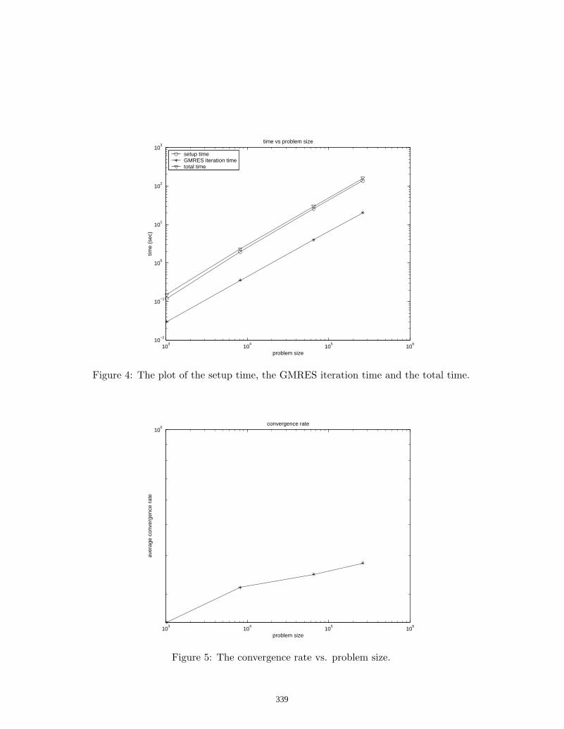
103
104
105
106
10−2
10−1
100
101
102
103
time vs problem sizetim
e (s
ec)
problem size
setup timeGMRES iteration timetotal time
Figure 4: The plot of the setup time, the GMRES iteration time and the total time.
103
104
105
106
100
convergence rate
aver
age
conv
erge
nce
rate
problem size
Figure 5: The convergence rate vs. problem size.
339
Fig. 5 shows the convergence rates. As the size of the problem increases, we cansee the convergence rates decrease gracefully.
Based on above results, we can see that H-LU preconditioners are cheap to computeyet they speed up GMRES iterative method greatly.
References
[1] S. Borm, L. Grasedyck, and W. Hackbusch. Introduction to hierarchical matriceswith applications. Engineering Analysis with Boundary Elements, 27:405–422,2003.
[2] S. Borm, L. Grasedyck, and W. Hackbush. Hierarchical matrices. 2005.
[3] S. Le Borne. Hierarchical matrix preconditioners for the Oseen equations. Comput.Vis. Sci., 2006. to appear.
[4] S. Le Borne and S. Oliveira. Joint domain-decomposition H-lu preconditioners forsaddle-point problems. Electronic Transactions on Numerical Analysis, 2007. toappear.
[5] A. George. Nested dissection of a regular finite element mesh. SIAM J. Numer.Anal., 10:345–363, 1973.
[6] L. Grasedyck and W. Hackbusch. Construction and arithmetics of H-matrices.Computing, 70(4):295–334, 2003.
[7] L. Grasedyck, R. Kriemann, and S. Le Borne. Parallel black box domain decom-position based H-LU preconditioning. Math. Comp, 2005. submitted.
[8] W. Hackbusch. A sparse matrix arithmetic based on H-matrices. part i: Introduc-tion to H-matrices. Computing, 62:89–108, 1999.
[9] G. Karypis and V. Kumar. A fast and high quality multilevel scheme for parti-tioning irregular graphs. SIAM J. Sci. Comput., 20(1):359–392, 1999.
[10] S. Oliveira and F. Yang. An algebraic approach for H-matrix preconditioners.Computing, 2007. to appear.
[11] S. Oliveira and F. Yang. H-matrix preconditioners for saddle-point systems frommeshfree discretization. proceeding of ICCES’07, pages 567–574, 2007.
[12] S. Oliveira and F. Yang. Hierarchical preconditioners for parabolic optimal controlproblems. In Proceedings of ICCS07, LNCS. Springer, 2007. To appear.
340
Proceedings of the International Conference on Computational and Mathematical Methods in Science and Engineering, CMMSE2007 Chicago, 20-23 June 2007
An Alternative to FFT for the Spectral Analysis
of Short or Discontinuous Time Series
Stella Pytharouli, Panos Psimoulis, Elina Kokkinou and
Stathis Stiros
Department of Civil Engineering, University of Patras
emails: [email protected], [email protected], [email protected],
Abstract
This is a template for the proceedings of CMMSE 2007, with instruction
for authors and some sample text. There are some requirements for the
spectral analysis using FFT (a minimum length of timeseries, continuous
rate of sampling), and this prevents from its use with a number of data in
various fields of engineering and natural sciences. To overcome these
problems, we present the “Normperiod” Code. This code is based on the
Lomb Normalized Periodogram and it permits the analysis of
discontinuous or non-equidistant time series without prior interpolations.
It is also very simple, it can be easily modified, it can be used in the
analysis of both very short and very long time series and it also permits
the determination of the statistical significance of obtained results. The
efficiency of this code is demonstrated on the basis of two examples: (1)
the spectral analysis of a steel bridge vibration record due to a passing
train and (2) the spectral analysis of Kremasta Dam reservoir level
fluctuations over a period of 37 years.
Key words: spectral analysis, unevenly spaced data, Lomb periodogram,
fortran code
1. Introduction
The most common spectral analysis technique is Fourier Transforms and more
specifically the algorithm of Fast Fourier Transforms (FFT; [1]). Since FFT was
developed mainly for digital signal processing purposes the algorithm was adjusted to the
characteristics of digital signals, i.e. hundreds or even thousands equally-spaced values, a
small signal-to-noise ratio etc.
However, in certain cases the requirements of this technique (a certain minimum number
of data, constant sampling rate) are not satisfied for various reasons (interruptions in
341

CMMSE 2007
sampling or irregularities in the records to be analyzed are common). Additionally, in
numerous cases data are collected non-automatically, at irregular intervals; for instance
geodetic, astronomic, geological, volcanological, climatological data etc [2], [3]. This
makes necessary an alternative technique for spectral analysis. Such a technique that
could easily be applied to non-equidistant data was proposed by [4] about thirty years
ago.
In this study we are based on the Lomb algorithm and present the “Normperiod” code, a
code that can analyze short and long irregularly spaced time series. This code also
permits estimation of the statistical significance of the obtained results. The effectiveness
of the code is demonstrated on the basis of two case studies.
2. The Lomb Normalized Periodogram
[4] and later [5] developed an algorithm for the spectral analysis of both evenly and
unevenly data, as well as of short time series. This algorithm, known as the ‘Lomb
normalized periodogram (LNP)’, is based on the least-squares fitting of a periodic
polynomial to the available data and leads to a spectrogram. What is known as
“amplitude” in the FFT spectrum is in our case is named “LNP”, it corresponds to a
normalized amplitude and for a specific period T is defined by
−
−−
+−
−−
=
∑
∑
∑
∑
=
=
=
=
N
j
j
N
j
j
j
N
j
j
N
j
j
j
T
t
T
txx
T
t
T
txx
TP
1
2
2
1
1
2
2
1
2 )(2sin
)(2sin)(
)(2cos
)(2cos)(
2
1)(
τπ
τπ
τπ
τπ
σ (1)
where the parameter τ is defined by the equation
∑
∑
=
=
=
N
j
j
N
j
j
T
t
T
t
T
1
1
4cos
4sin
4tan
π
π
πτ (2)
and N number of data points
ti time at which the displacement i was measured
x mean of the data values ∑=
≡N
i
ixN
x1
1 (3)
2σ variance of the data values ( )∑
=
−−
≡N
i
i xxN 1
22
1
1σ (4)
This process is repeated for all values of T, and hence a spectrogram is produced. In
addition, the significance level of LNP (i.e. of the normalized amplitude) is defined by
equation
])1(1ln[
1
0Npz −−−= (5)
342

CMMSE 2007
where z0 power level above which the value P(T) of the LNP is statistically
significant with (1-p)*100% confidence level.
p significance level
N number of data points.
Two basic advantages of this code are first, that results are rather insensitive to
limitations of the Nyquist frequency, if the spectrogram is based on non-equally spaced
data. And second, because it is based on least-squares and eq. (1) the LNP values can be
produced even with a short times series, since this equation permits a very high
redundancy.
3. The “Normperiod” code
“Normperiod” code was developed on the basis of the procedure proposed by [4]. It
computes (a) the value P(T) of the periodogram using eq. (1) and (b) the value of P(T) for
a (1-p)*100% confidence level using eq. (5).
The code is written in Fortran programming language, runs in DOS environment and
efforts were made in order to be easily modifiable by potential users.
The INPUT consists of two files written in simple format and the values of four
parameters ; the total length N of the time series to be analyzed, the total time interval tr
covered by the time series, the desired confidence level p (i.e. 95%) and the value for the
parameter named “fratio”, an integer taking values 1, 2, 3.. which defines how many
times higher than the Nyquist frequency fc the user desires to compute the periodogram
(for more information see [6]).
The total number of frequencies fi at which the periodogram is determined and is given
by the formula [1]
Np = 2
4* Nfratio (6)
where N is the length of the time series
The interval between two consecutive frequencies for the calculation of the periodogram
is equal to
fstep = p
rr
N
tt
Nfratio
4
1* −
(7)
The output file contains the values of the frequency spectrum of the time series. It
consists of two columns representing the frequency f and the corresponding
343

CMMSE 2007
dimensionless value P(T) of the LNP (power of spectrum). The format of the output file
permits a spectrum plot when exported into a graphic environment. Further details can be
found in [6].
The application and effectiveness of the Lomb periodogram is highlighted in the
following case studies.
4. Case study 1: Spectral Analysis of the RTS monitoring record of a railway
bridge
In order to investigate the response of the midspan of a 30m long steel railway bridge in
Central Greece under dynamic loads (passing trains) we carried out a number of
experiments. Using GPS (Global Positioning System) and RTS (robotic total station)
technology, we recorded the movements of a control point located on the middle span of
the bridge before, during and after a passing train.
Data used in this study consist of RTS recordings of the vertical movements-response of
the bridge to a passing train (Fig.1a).
Fig. 1 (a) Vertical displacements recorded by robotic theodolite (RTS) at the deck of a
short-span railroad bridge in central Greece. (b) The corresponding frequency spectrum
using the “Normperiod” code. Straight line represents the 95% confidence level. A
dominant frequency of 0.45Hz is revealed. Frequencies at the left edge of spectrum are
not statistically significant (edge effect; [1])
344

CMMSE 2007
What is evident is that this time series consists of three parts: a first and third part
indicating very small amplitude, apparent displacements before and after the passing of
the train (i.e. when no displacement of the bridge is expected). These parts of the time
series reflect and define the measurement noise and the accuracy level in our data. And a
middle section indicating a significant oscillation with duration of several tens of
seconds. Analysis of this last section can permit to define the dynamic characteristics of
this structure.
Spectral analysis was not possible using FFT, for the available time series was too short
(approximately 120 values). Zero padding could be used, but it would lead to biased
results, unacceptable for this particular case. Furthermore, data were not sampled at a
constant rate, and hence any transformation of the available time series to a new one,
based on interpolation techniques would lead to additional noise. For this reason we used
the method of the Lomb Normalized Periodogram and the “Normperiod” code. The result
of this spectral analysis is shown in Fig. 1b. A dominant frequency equal to 0.45Hz was
revealed. This frequency probably corresponds to the interaction between train and bridge
deck [8].
5. Case study 2: Spectral Analysis of the fluctuations of the Kremasta Dam
reservoir level
Dams deform in response to changes in their reservoir load, and the spectral analysis of
the fluctuations of the reservoir levels is important to understand dam dynamics [9], [7].
In this study we present the results of the analysis of the Kremasta dam (Greece), one of
the major earthen dams in Europe. Available data consisted of the daily values of the
reservoir level along a period of 37years. The total length of the reservoir level data set
was 13944 values, but this long record contained gaps of about 1.5% of its total length.
Spectral analysis was based on LNP and the periodogram was calculated using the
“Normperiod” code. Only the peaks that were detected above the 95% confidence level
were assumed as statistically significant. Spectral analysis of the reservoir level
fluctuations revealed > 10 statistically significant frequencies. The period corresponding
to one year representing the annual change of water was prevailing (fig.2b).
Since the percentage of gaps was small, as noticed above, we computed the spectrum of
these data using FFT and interpolations. For comparison, both FFT and LNP spectra are
shown in Fig.2. Results for both methods were almost the same for main frequencies,
certifying the accuracy of “Normperiod” results, but the FFT results were more noisy.
345

CMMSE 2007
Fig. 2 Spectral analysis of the Kremasta Dam reservoir level values: (a) FFT spectrum.
Periods with values between 8 months and 9.5 years were detected, (b) Lomb
periodogram. More than 10 significant frequencies were detected with values between
the range 1yr – 8.6yrs. In both spectra the period of 1 year is prevailing.
6. Conclusions
The case studies presented above indicate that the “Normperiod” code, based on the LNP,
has an important merit. It can effectively and easily analyze both short and very long,
evenly and non-evenly spaced, as well as discontinuous time series providing information
about their spectral characteristics as well as the statistical significance of the results.
This new code is available free of charge and can be used in various fields of engineering
[10] and natural sciences.
References
[1] W. H. PRESS, S. A. TEUKOLSKY, W. T. VELLERLING, B. P. FLANNERY, Numerical
Recipies in C. The Art of Scientific Computing, Cambridge University Press,
1988.
[2] S. D. PAGIATAKIS, Stochastic significance of peaks in the least-squares spectrum,
J. Geodesy 73 (1999) 67–78.
[3] P. HERTZ AND E. FEIGELSSON, Sample time series in astronomy, in Proceedings
of Applications of time series analysis in Astronomy and Meteorology, University
of Padova, Italy, 6 – 10 September, 1993.
[4] N. R. LOMB, Least-Squares Frequency Analysis of Unequally Spaced Data,
Astrophys.Space Sci. 39 (1976) 447–462.
[5] J. D. SCARGLE, Studies in Astronomical Time Series Analysis. II. Statistical
Aspects of Spectral Analysis of Unevenly Spaced Data, Astrophys. J. 263 (1982)
835–853.
[6] S. I. PYTHAROULI AND S. C. STIROS, Spectral Analysis of unevenly spaced or
discontinuous data using the “Normperiod” code, Comp. Struc.
doi:10.1016/j.compstruc.2007.02.022 (2007).
346

CMMSE 2007
[7] S. PYTHAROULI, V. KONTOGIANNI, P. PSIMOULIS AND S. STIROS, Kremasta Dam
(Greece): Long-term behaviour and performance of the highest earthfill dam in
Europe, in Proceedings of the 5th International Conference on Dam Engineering,
Lisbon, Portugal, 14 – 16 February, (2007) 465-471.
[8] E.M. KOKKINOU, P.A. PSIMOULIS, S.I. PYTHAROULI AND S.C. STIROS, Monitoring
of the Gorgopotamos steel railway bridge using a robotic total station (RTS), in
Proceedings of the 8th HSTAM International Congress on Mechanics, Patras 12 –
14 July (2007).
[9] S. I. PYTHAROULI AND S. C. STIROS, Ladon dam (Greece) deformation and
reservoir level fluctuations: evidence for a causative relationship from the
spectral analysis of a geodetic monitoring record, Eng. Struc. 27 (2005) 361–
370.
[10] P. OMENZETTER AND J. M. W. BROWNJOHN, Application of Time Series Analysis
for Bridge Monitoring, Smart Materials and Structures. 15(1) (2006) 129-138.
347

Proceedings of the International Conference on Computational and Mathematical Methods in Science and Engineering, CMMSE2007 Chicago, 20-23 June 2007
Computing Solutions of Systems of Nonlinear Polynomial Inequalities and Equations
R. Sharma1, and O. P. Sha1
1 Design Laboratory, Department of Ocean Engineering and Naval Architecture, Indian Institute of Technology, Kharagpur (WB) – 721302,
India
emails: [email protected], [email protected]
Abstract A fundamental problem in computer aided geometric design (CAGD) and computational science and engineering (CSE) is the efficient computation of all roots of a system of nonlinear polynomial equations in variables that are contained within an -dimensional box. This paper presents algorithms to bound solution sets of systems of polyno-mial inequalities and equations using the expansion of a multivariate polynomial into Bernstein polynomials, and this expansion is used to find tight bounds for the range of the polynomial over a given box. The presented techniques to solve such problems rely on expansion and subdivision. Then, the Bernstein expansion, and tight bounds for the range of the polynomial are used to present algorithms for solutions of a system of polynomial inequalities and equations, and to solve constrained convex optimization problems involving polynomials. In order to isolate all of the roots within the given domain, we use the tighter bounds, subdivision, and implement an existence test. The numerical example dealing with the enclosure of the solution set of systems of polynomial inequalities and equations, and the solution of constrained convex optimization problems are presented.
n n
Key words: Bernstein polynomials; CAD; CAGD; CAM; CSE, constrained convex optimization; geometric modeling; polynomial inequalities; polynomial equations range enclosure; robust stability; solid modelling MSC2000: 65D17, 65H10, and 68U07
1. Introduction Systems of polynomial inequalities and equations appear in difference branches of science and engineering, e.g. for example, in geometric intersection computations for
348

CMMSE 2007
computer aided geometric design (CAGD), computer aided design (CAD), computer aided manufacturing (CAM); chemical equilibrium problems; chemical combustion and kinematics; and control and robust stability in electrical science, etc., for application area details see Morgan [1]. A fundamental problem in the systems of polynomial inequalities and equations is the efficient computation of all solutions to a system of nonlinear polynomial inequalities and equations within some finite domain. Specifically, this problem arises in many different applications for example, in CAGD/CAD/CAM: it is often necessary to identify all characteristic points of an intersection curve between two surfaces, in order to trace out all of the branches of the curve; if the surfaces are piecewise rational polynomial, we must solve a system of nonlinear polynomial equations in order to identify these points; in feature recognition: computing the medial axis transform requires the determination of branch points, which can frequently be formulated as the solution set of a polynomial system; and in robotic motions: computing distance functions and extremum, in arranging distributive systems in complex mechanical platforms, etc. The methods for the solution of such a system can be classified as methodologies based on elimination theory, continuation, and subdivision. The methods based upon elimination theory for constructing Gröbner bases rely on symbolic computations which are inherently computationally expensive (i.e. for example solution of Problem 1 discussed later in Section 3 by a symbolic computation based method will take about 7200 seconds) for polynomials. Hence, these are unsuitable for larger problems. Additionally, the methods based upon elimination theory and continuation exhaustively computes more information than is really needed. For example they determine all complex solutions of the system though in applications often only the solutions in a given area of interest (i.e. within a box) are desired. The subdivision based methods apply a domain splitting approach that starts with the box of interest, and these algorithms sequentially splits the box of interest it into subboxes eliminating infeasible boxes by using bounds for the range of the polynomials under consideration over each of them and ending up with a union of boxes that contains all solutions to the system which lie within the given box. The methods utilizing this approach shall include interval computation techniques as well as the methods that apply the expansion of a multivariate polynomial into Bernstein polynomials. Theoretically, any interval computation method for solving a system of nonlinear equation (e.g. Hansen [2]; Jaulin et al. [3]; Kearfott [4]; and Neumaier [5]) can be applied to a polynomial system. The techniques specially designed for polynomial systems are more efficient in computing time. Therefore, in the present work we investigate a subdivision based method. Among the existing algorithms, the subdivision methods are used in-practice because of their performance and efficiency. The Interval Projected Polyhedral (IPP) algorithm (Sherbrooke and Patrikalakis [6]; Patrikalakis and Maekawa [7]) is most widely used in-practice. Sherbrooke and Patrikalakis [6], Patrikalakis and Maekawa [7], use Bernstein expansion sequences of bounding boxes for solutions of the nonlinear polynomial systems of equations. They have presented two methods: the first method projects control polyhedra onto a set of coordinate planes and the second exploits linear programming. But, neither have they explored the relationship between the Bernstein coefficients on neighboring subboxes, nor any existence test for a box to contain a solution that might have improved the computational efficiency of the algorithm. Furthermore, they formulate the
349

CMMSE 2007
]
optimization problem by simply a linear programming problem (LPP). The LPP can be solved efficiently, but in the absence of a functional analysis the solution can not be guaranteed to a global maximum/minimum and only local maxima/minima can be computed. In this paper, we describe techniques for computing all real solutions to a system of nonlinear polynomial equations in unknowns over an -dimensional rectangular domain. We use Bernstein expansion, and incorporate the relationship between the Bernstein coefficients on neighboring subboxes in all the algorithms. Additionally, from ‘real analysis’ we include an existence test (Neumaier [5]) for a box to contain a solution. As for the optimization problem, we use convex analysis (Rockafellar [8]; Magaril-Ilyaev and Tikhomirov [9]) and treat the optimization problem as a problem of convex optimization (Bertsekas et al. [10]; and Boyd and Vandenberghe [11]) that guarantees the computation of a global maximum/minimum.
nn n
The remaining of the paper is organized as follows: Section 2 briefly presents the mathematical preliminaries that are essential to present our work. The theoretical background to enclose the solution set of a system of polynomial inequalities is presented in Section 3. And, also we present the Bernstein expanded and interval subdivision algorithm (BEIS). 4. Section 4 presents the enclosing of the solution set of a system of polynomial equations, and Bernstein expanded projected polyhedron algorithm (BEPP) is presented. The constrained convex optimization is explained in Section 5, and the Bernstein expanded convex optimization (BECO) algorithm is presented. Section 6 concludes the paper by identifying some future applications, and scope of research. Comprehensive theoretical details and a thorough treatment of the results of this paper can be found in Sharma and Sha [12].
2. Preliminaries Following [7], Farin [13], and Garloff [14]; let a polynomial with real coefficients be given,
p
( ) ∑=
=l
0i
ii xaxp (1)
where is a real number, and is integer powered. It is of interest to know the range of over an interval , i.e.,
ia ixp [ ba,
[ ]( ) ( ) [ ] ba,ba, ∈= x;xpp . (2) We can assume without loss of generality that [ ]ba, is the ‘unit interval ’. Now, we present as a linear combination of the Bernstein polynomials of the same degree,
[0,1=U ]p
( ) l,...,0i,x1xil
B ilii =−⎟⎟
⎠
⎞⎜⎜⎝
⎛= − (3)
and i.e.,
350

CMMSE 2007
( ) ( )∑=
=l
0iii xBbxp . (4)
In Equation (4) the coefficients are the ‘Bernstein coefficients’, and are treated as weighted sums of the coefficients of
ibp ,
∑=
=
⎟⎟⎟⎟⎟
⎠
⎞
⎜⎜⎜⎜⎜
⎝
⎛⎟⎟⎠
⎞⎜⎜⎝
⎛
=i
0jji l,...,0i,a
jlji
b . (5)
Using a difference scheme derived from de Casteljau algorithm these coefficients are computed efficiently. The bounds for the range of over U are computed directly from Bernstein coefficients utilizing range enclosing property;
p
( ) [ ]il0ii
l0i bmax,bminUp ==⊆ . (6)
Similarly, we formulate this property by introducing the control points l,...,0i,bli
i
=⎟⎟⎟
⎠
⎞
⎜⎜⎜
⎝
⎛,
as the convex hull property,
( ) ⎪⎭
⎪⎬⎫
⎪⎩
⎪⎨⎧
=⎟⎟⎟
⎠
⎞
⎜⎜⎜
⎝
⎛⊆
⎭⎬⎫
⎩⎨⎧
∈⎟⎟⎠
⎞⎜⎜⎝
⎛l,...,0i:
bli
convxUx:xp
x
i
(7)
where denotes the convex hull of (i.e. convex set that is smallest, and contains ). For practical implementation these bounds are improved by subdividing (i.e. the number of divisions is decided with iterative method, and with user specified tolerance) the interval, and the same procedure is applied over the divided subintervals. The important steps in subdivision algorithm are given in Fig. 1. Then is contained in the union of the individual convex hulls of the control points on the subdivided intervals. The Bernstein coefficients of on subdivided intervals are calculated from those on U by implementing a recursive arithmetic algorithm (i.e. derived from de Casteljau algorithm). Since, the algorithm is recursive, Bernstein coefficients are computed efficiently. The sequential lower and upper bounds computed in the recursive algorithm converge with quadratic convergence (i.e. to and
). We obtain the Bernstein coefficients of the derivative of
Sconvx SS
( )Up
p
( )Upmin( )Upmax '
ib p by simply forming forward difference of its Bernstein coefficients,
( ) 1l,...,0i,bblb i1i'i −=−= + . (8)
For the multivariate case, the Bernstein polynomials are defined as the product of the univariate Bernstein polynomials,
( ) ( ),xB,...,xB nn1i (9) where is the number of variables in the multivariate polynomial. Now, we assign all indices of the univariate case multiindices (i.e.
n( )Tn1 i,...,ii = , as vectors and where all
351
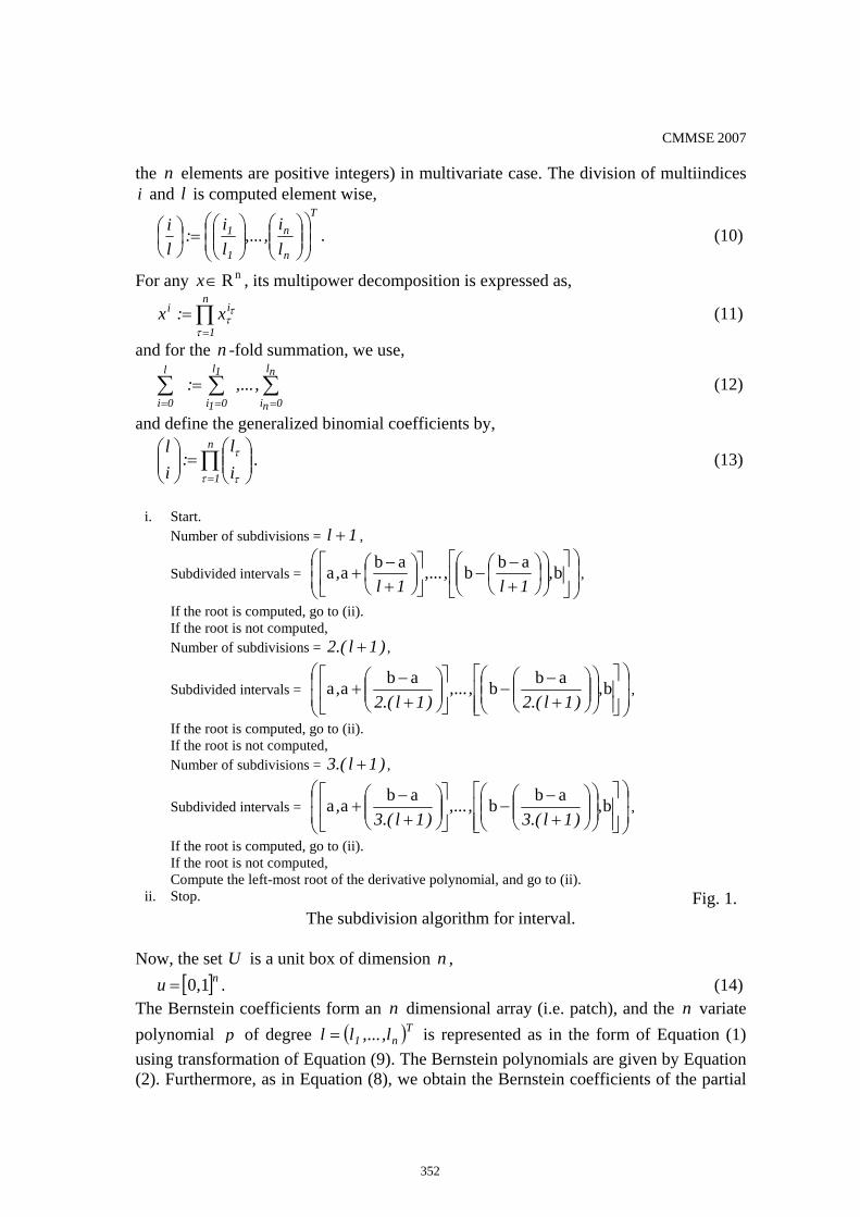
CMMSE 2007
the elements are positive integers) in multivariate case. The division of multiindices and is computed element wise,
ni l
T
n
n
1
1
li
,...,li
:li
⎟⎟⎠
⎞⎜⎜⎝
⎛⎟⎟⎠
⎞⎜⎜⎝
⎛⎟⎟⎠
⎞⎜⎜⎝
⎛=⎟
⎠⎞
⎜⎝⎛ . (10)
For any , its multipower decomposition is expressed as, nR∈x
∏=
=n
1
ii x:xτ
ττ (11)
and for the -fold summation, we use, n
∑∑∑===
=nl
0ni
1l
01i
l
0i,...,: (12)
and define the generalized binomial coefficients by,
∏=
⎟⎟⎠
⎞⎜⎜⎝
⎛=⎟⎟
⎠
⎞⎜⎜⎝
⎛ n
1 il
:il
τ τ
τ . (13)
i. Start.
Number of subdivisions = 1l + ,
Subdivided intervals = ⎟⎟⎠
⎞⎜⎜⎝
⎛⎥⎦
⎤⎢⎣
⎡⎟⎟⎠
⎞⎜⎜⎝
⎛⎟⎠⎞
⎜⎝⎛
+−
−⎥⎦
⎤⎢⎣
⎡⎟⎠⎞
⎜⎝⎛
+−
+ babbabaa ,1l
,...,1l
, ,
If the root is computed, go to (ii). If the root is not computed, Number of subdivisions = )1l.(2 + ,
Subdivided intervals = ⎟⎟⎠
⎞⎜⎜⎝
⎛
⎥⎥⎦
⎤
⎢⎢⎣
⎡⎟⎟⎠
⎞⎜⎜⎝
⎛⎟⎟⎠
⎞⎜⎜⎝
⎛+−
−⎥⎦
⎤⎢⎣
⎡⎟⎟⎠
⎞⎜⎜⎝
⎛+−
+ babbabaa ,)1l.(2
,...,)1l.(2
, ,
If the root is computed, go to (ii). If the root is not computed, Number of subdivisions = )1l.(3 + ,
Subdivided intervals = ⎟⎟⎠
⎞⎜⎜⎝
⎛
⎥⎥⎦
⎤
⎢⎢⎣
⎡⎟⎟⎠
⎞⎜⎜⎝
⎛⎟⎟⎠
⎞⎜⎜⎝
⎛+−
−⎥⎦
⎤⎢⎣
⎡⎟⎟⎠
⎞⎜⎜⎝
⎛+−
+ babbabaa ,)1l.(3
,...,)1l.(3
, ,
If the root is computed, go to (ii). If the root is not computed, Compute the left-most root of the derivative polynomial, and go to (ii).
ii. Stop. Fig. 1. The subdivision algorithm for interval.
Now, the set U is a unit box of dimension , n
[ ]nu 0,1= . (14) The Bernstein coefficients form an dimensional array (i.e. patch), and the n variate polynomial
np of degree is represented as in the form of Equation (1)
using transformation of Equation (9). The Bernstein polynomials are given by Equation (2). Furthermore, as in Equation (8), we obtain the Bernstein coefficients of the partial
( Tn1 l,...,ll = )
352

CMMSE 2007
derivatives of by forming forward differences of the Bernstein coefficients of in the direction that corresponds to the co-ordinate direction.
p p
3. Enclosing the solution set of a system of polynomial inequalities: Bernstein expanded and interval subdivision algorithm Following Prasolovand Leites [15], and Borwein and Erdelyi [16], let us consider a system of polynomial inequalities, i.e.,
( ) k,...,1i,0xpi =⟩ and (15) Xx∈where the variate polynomials and the dimensional box n ip n X are given, and it is desired to find the solution set ∑ (i.e. set of vectors that satisfies Equation (15)) of the sytem. Additionally, to present practical implementation, let a box,
x
⎥⎦⎤
⎢⎣⎡××⎥⎦
⎤⎢⎣⎡=
n
n
1
1q,q...q,qQ (16)
and a univariate polynomial,
( ) ( )∑−
=m
0i
ii xa,xp qq (17)
be given with coefficients dependent on parameters and , i.e., n1 q,...,q Tn1 )q,...,q(=q
( ) ( )( )
∑=
=kl
0i
ikik qαα q . (18)
The parametric vector q is varying inside . Now the problem is to determine -stablity (i.e. a polynomial is -stable if all its zeros lie inside the prescribed subset of the complex plane) region of the polynomial (i.e. Equation (17) in the given parametric box , i.e.,
Q DD D
Q( ) Dx,,xp:Q ∉∀≠∈ ϕqq (19)
where ϕ is a null set. Now, we present the Bernstein expanded and interval subdivision (BEIS) algorithm. To start the computation we need a approximation of the solution set
. For numerical purpose we define inner and outer approximations. The inner approximation (∑
I∑ ) is defined as the union of subboxes of Q on which all the polynomials are positively valued. Similarly, the outer approximation ( ) is
defined as the union of subboxes of on which all the polynomials are negatively valued. Then, the regions are clipped sharply to generate the boundary (
ip O∑
Q *ip
∑δ ). The boundary ( ∑δ ) is defined by the union of subboxes of Q on which the polynomials
are positively valued, but on which at least there is one polynomial that is negative valued. The positivity of a polynomial is checked by the sign of its Bernstein coefficients using the range enclosing property (i.e. the set
ip
I∑ consists of the subboxes on which the Bernstein coefficients of all the polynomials are positive) as given in Equation (6).
ip
353

CMMSE 2007
The above-mentioned algorithm, and all other algorithms of the present work have been implemented in C++ using its object-oriented features on a Silicon GraphicsTM* OriginTM* 200 workstation. Problem 1: From the application of stability criteria (Abdallah et al. [17]), we consider the following system of polynomial inequalities for the three positive parameters
, and the conditions are, 321 x,x,x
( ) 0x.x 221 ⟩ (20)
( ) 01xxxx.x 32
3121 ⟩−−++− (21)
( ) ( ) 0x4x4xx2x.xx.x 32
33
313121 ⟩+++−− (22)
( ) ( ) ( ) 3212
2132
213
21 x.x.x2x.x4x.x.xx.x +−− ( ) ( ) 322
323
3221 x.x2x.x5x.x2x.x4 ++++
( ) ( ) 0x4x4x 32
33
3 ⟩−− (23)
( ) 2322
32121 x4x.x4x.xx2x.x −−−− ( ) 02x3x2 32
3 ⟩−++ (24) with , , and [ ]90,130∈1x [ 1,3−∈2x ] [ ]0,30∈3x . In less than a second, the Bernstein expansion provides an inner approximation of the solution set. To visualize the solution set we select = 110. The set of feasible and unfeasible regions (i.e. region bounded by the closed curve is feasible, and the region outside of closed curve is unfeasible) for inner approximations of parameters , and for this parametric value (i.e. =110) is shown in Fig. 2.
1x
2x 3x 1x
Set of Feasible Values
0
10
20
30
-1 0 1 2Parameter (x2)
Para
met
er (x
3)
3
Fig. 2. The set of feasible values for the parameters , and for = 110. 2x 3x 1x
4. Enclosing the solution set of a system of polynomial equations: Bernstein expanded projected polyhedron algorithm Following [15], let us consider a system of equations, i.e.,
354

CMMSE 2007
( ) k,...,1i,0pi ==x ; ; and Q∈x ( ),...,y,x=x , (25) where ,...,y,x depend upon the number of variables, and again the are polynomials in variables and Q is an -dimensional box. These types of polynomial system of equations are important in many applications areas of engineering sciences (e.g. CAGD - geometric intersection computations; chemical and mechanical kinematics - chemical equilibrium problems, combustion, and kinematics, etc.). Now, we present the Bernstein expanded projected polyhedron (BEPP) algorithm. The important steps in solution algorithm for system of polynomial equations are given in Fig. 3.
ipn n
Problem 2: From the area of CAGD ([6]), we consider the problem of computation of significant points of a planar algebraic curve. This problem in computer aided design deals with the discovery and subsequent tracing of all branches of an implicit algebraic
curve . The computation of ‘turning points (i.e. where ( ) 0y,xpi = 0xpp =∂∂
= or
0ypp =∂∂
= )’ or ‘critical points (i.e. where 0yp
xp
=∂∂
=∂∂ )’ is important in solving this
problem, Sakkalis and Farouki [18]. Let us find the critical points of, ( ) v.u140v.u96v128v64y,xp 2234 +−+−= 422 u96v75v.u140v.u96v139 −+−+−
036u165u313u276 23 =−+−+ . (26) After the partial differentiation the polynomial reduces to two simultaneous equations which are solved. Now, this problem has nine solutions. All these solutions are computed within a tolerance of . The computational results are shown in Table 1. The details and a figure of the curve can be found in [12].
1010−
Table 1. Computational results for Problem 2.
Computational features
Tolerance = 1010− Steps in interval subdivision (ref. Fig. 1) = 3
Number of solutions = 9 Number of existence tests performed = 30 Number of boxes = 3367 Computational time (in seconds) = 90
5. Constrained convex optimization Following [10], and [11], a constrained optimization problem is defined as,
( )xfminMx∈
(27)
where the set M of the feasible solutions is given by inequality and equality constraints,
( ) 1i n,...,1i,0xg =≤ , (28) ( ) 2j n,...,1j,0xh == , (29)
Xx∈ . (30) Here is a subset of , D nR X is a box in , and , , and are real valued functions within the domain .
D f ig jhD
355

CMMSE 2007
i. Start. a. Implement affine parametric transformation from interval [ ]ba, to the ‘unit interval [ ]0,1=U ’. b. Transform the basis of functions from ‘monomial’ to ‘Bernstein’. c. Utilize ‘the linear precision property’ of the ‘Bernstein polynomial’ as given in Equation (3). d. Subdivide the interval using algorithm (ref. Fig. 1). e. Univariate case: Create the graph, and convex hull of the function ( ) k,...,1i,0pi ==x . Then, the graph will be a Bézier curve,
( ) ( ) ( )∑= ⎟
⎟⎟
⎠
⎞
⎜⎜⎜
⎝
⎛=⎟⎟
⎠
⎞⎜⎜⎝
⎛=
l
0il,i
Bi
tBbli
tpt
tp where 1t0 ≤≤ , and T
Bib,
li
⎟⎠⎞
⎜⎝⎛
are the control points.
The problem of finding roots of the polynomial is treated as a problem of finding the intersection of the convex hull of Bézier curve with the parameter axis. Test the sign of the polynomials ip on the subboxes that have been obtained by subdivision (ref. Fig. 1) by using Bernstein expansion. Retain the regions of subboxes with positive signs, discard the regions ofsubboxes with negative signs, and sharply define the boundary. Discard the subboxes which cannot contain a solution by applying the existence test (i.e. if a univariate continuous function f has a sign change at the
endpoints of an interval then this interval contains a zero of f ; Neumaier, 1990).
Scale the subboxes so that it will become [ ]0,1 using affine parameter transformation and go back to Step 1. Compute the intersection of the Bézier curve with the parameter axis. Go to step (ii). f. Two variables, and multivariate case: Create the graph, and convex hull of the function
( ) k,...,1i,0poi ==x , and Vk,...3,2,1o = ; where Vk is the number of variables. Then, the individual
graph for each variable will be a Bézier surface,
( )( )
( ) ( )∑=
⎟⎟⎟⎟⎟⎟⎟
⎠
⎞
⎜⎜⎜⎜⎜⎜⎜
⎝
⎛
=⎟⎟⎟⎟
⎠
⎞
⎜⎜⎜⎜
⎝
⎛
=l
0i
ol,j
ol,i
oBj,i
o
tBsB
b
ljli
t,sp
ts
t,sop where 1s0 ≤≤ , 1t0 ≤≤ , and
ToBj,ib,
lj,
li
⎟⎠⎞
⎜⎝⎛
are the control points.
The problem of finding roots of the polynomial consists of three steps: find the intersection of surfaces with
co-ordinate plane, project the control points of ( )t,sop onto co-ordinate planes, and for each co-ordinate plane
construct the D2 convex hulls. Intersection of the convex hull with the horizontal axis is the root. Test the sign of the polynomials ip on the subboxes that have been obtained by subdivision (ref. Fig. 1) by using Bernstein expansion. Retain the regions of subboxes with positive signs, discard the regions ofsubboxes with negative signs, and sharply define the boundary. Discard the subboxes which cannot contain a solution by applying the existence test (i.e. if a univariate continuous function f has a sign change at the
endpoints of an interval then this interval contains a zero of f ; Neumaier, 1990).
Scale the subboxes so that it will become [ ]0,1 using affine parameter transformation and go back to Step 1.
Compute the intersection of the convex hull with the horizontal axis. ii. Stop.
Fig. 3. The solution algorithm for system of polynomial equations.
356

CMMSE 2007
The examples of these types of problems can be found in engineering science, e.g., chemical science: pooling and blending; multi-component separation; phase stability analysis; and parametric modeling and simulation; aircraft science: weight allocation in aircraft engines. We are interested in the optimization problems in which the objective and constraint functions are all multivariate polynomials. In engineering sciences it is important to compute the global minimum/maximum rather than only local minima/maxima. In general, the optimization problems are tackled with a purely numerical procedure, and numerical optimization procedure is viewed as a black box. Though, functional analysis of ( )xf can provide a better insight into the behaviour of
, but it is not done in-practice frequently. It can be argued that the optimization problems resulting from practical applications are often very complex with large number variables and constraints, and hence functional analysis may be mathematically complicated. This is really not true. A simple procedure can be explored for functional analysis of that will avoid mathematical complexities. And, functional analysis of
will reveal whether the
( )xf
( )xf( )xf ( )xf is a convex function, or a concave function or a
highly non-linear function. If ( )xf is a convex function then the optimization problem of Equations (27) – (30), can be reformulated as a convex optimization problem. And, there are advantages in that, and these are: Basic computational advantages: problem can then be solved, very reliably and efficiently using interior-point methods or other special methods for convex optimization, and these solution methods are reliable enough to be embedded in a computer-aided design or analysis tool, or even a real-time reactive or automatic control system; and theoretical advantages: the associated dual problem, for example, often has an interesting interpretation in terms of the original problem, and sometimes leads to an efficient or distributed method for solving it, [11]. Following, [10], and [11]; an optimization is called a convex optimization problem if the objective and constraint functions are convex, and this means that they satisfy the inequality,
( ) ( ) ygxgyxg iii ( )βαβα +≤+ (31)
for all and all nR∈y,x α , β R∈ with 0,0,1 ≥≥=+ βαβα . To transform the problem as defined in Equations (27) – (30) to the problem of convex optimization, we use lower and upper bounds of convex functions, [8] and [9]. Now, let us define,
( ) ( ) ( )xfxfxf UBLB ≤≤ (32) ( )xfmin
Nx∈ (33)
where , MN ⊆ ( ) ( )( )xUBfSxLBfS EEEN −−≡ , =E domain space of , =
domain space of , and
( )xf ( )xLBfSE
( )xfLB ( ) =xUBfSE domain space of ( )xfUB . Now, we present the
Bernstein expanded convex optimization (BECO) algorithm. The important steps in solution algorithm for system of polynomial equations are given in Fig. 4.
357

CMMSE 2007
i. Start.
a. Define the optimization problem, ( )xfminMx∈
, ( ) 1i n,...,1i,0xg =≤ ,
( ) 2j n,...,1j,0xh == , and Xx∈ .
b. Implement affine parametric transformation from given domain intervals [ ]ba, etc., to the ‘unit
interval [ ]0,1=U ’. c. Transform the basis of functions from ‘monomial’ to ‘Bernstein’. d. Utilize ‘the linear precision property’ of the ‘Bernstein polynomial’ as given in Equation (3). e. Subdivide the domain intervals using algorithm (ref. Fig. 1). f. Univariate case:
Define ( ) ( ) ( )xfxfxf UBLB ≤≤ , and ( )xfminNx∈
, where MN ⊆ .
Define clipped constrained solution domain, ( ) ( )( )xUBfSxLBfS EEEN −−≡ , =E domain
space of ( )xf , ( )xLBfSE = domain space of ( )xfLB , and ( ) =xUBfSE domain space of
( )xfUB . Solve the convex optimization problem with convex solution methods (i.e. gradient descent method, infeasible start Newton method, primal-dual interior-point methods). In our implementation we have used primal-dual interior-point methods. Go to step (ii).
g. Two variable or multivariable case: Compute affine lower and upper bound functions as the solution of a linear programming (LP) problem. Integrated these bounded functions, and partition the problem into subproblems by subdivision. Define clipped constrained solution domain for each subdivided problem,
( ) ( )
( )xUBfSxLBfS EEEN −−≡ , =E domain space of ( )xf , ( )xLBfSE = domain space of
( )xfLB , and ( ) =xUBfSE domain space of ( )xfUB .
Solve the convex optimization problem with convex solution methods (i.e. gradient descentmethod, infeasible start Newton method, primal-dual interior-point methods). In our implementation we have used primal-dual interior-point methods. Go to step (ii).
ii. Stop. Fig. 4. The solution algorithm for cconstrained convex optimization problem.
Problem 3: From the area of aircraft science (Golinski, [19]), we consider the minimization problem,
( )xfmin ,
( ) ( ) ( )( 23
221 x3333.3.x.x7854.0xf = ) ( ) ( )( )2
72
613 xx.x5080.10934.43x9334.14 +−−+
( ) ( )( ) ( ) ( )( )275
264
37
36 xxxx7854.0xx4770.7 +++ (34)
subjected to eleven constraints that are rewritten in polynomial forms. Additionally, the constrained bounds on the seven variables are given. The computed minimum value of
is at 2994.7852346761. The computational results are shown in Table 2. The details can be found in [12]. ( )xf
358

CMMSE 2007
Table 2. Computational results for Problem 3. Computational features
Tolerance = 1010− Steps in interval subdivision (ref. Fig. 1) = 3
Number of solutions = 1 Number of subproblems as LP created = 1, 20, 000 Computational time(in seconds) = 450
6. Conclusions In this work, we have presented algorithms that are formulated to determine real roots. However, by substitution of for in equations and then splitting each equation into real and imaginary parts shall allow the computation of complex roots. Also, we have only considered the so called balanced system of equations, and the algorithms may be extended to systems of equations in unknowns (
ivu + x
m n nm ≠ ). These over and under determined systems appear in the computation of singularities on a planar implicit algebraic curve and in engineering design. These problems shall require a constrained formulation or multiple axis projection of polyhedra in the BEPP method. The use of Bernstein expansion requires efficient memory allocation because space required grows exponentially with the number of variables. Now, we have to explore a method that will improve memory allocation for larger number of parameters. We have implemented our algorithms in ‘floating point arithmetic (FPA)’ that guarantee only moderate tolerance (i.e. around - ), and the rounding errors appearing in the calculation cannot be controlled. A implementation in ‘interval arithmetic (IA)’ using ‘rounded interval arithmetic (RIA)’, ([2], and [3]), shall allow us to control rounding errors to compute ‘result within a guaranteed accuracy’ with high tolerance (i.e. around - ). The detailed analysis of efficiency and complexity of the algorithms has not been addressed in this work. Also, the relative merits of our methods and other existing techniques can be studied for a comparative study. Our future work shall go in this direction, and currently this is under investigation.
1010− 1510−
1510− 2510−
Acknowledgements This research was supported by the Defense Research and Development Organization (DRDO), MoD, GOI, India; via the grant-in-aid scheme number: ERIP/ER/0400237/M/01. The authors thank Prof. (Retd.) R. P. Gokarn for his assistance and comments.
Trademarks and copyrights
*Trademark and copyright with Silicon Graphics Corporation, USA.
References
359

CMMSE 2007
[1] A. P. Morgan, Solving Polynomial Systems using Continuation for Engineering and Scientific problems, Prentice Hall, Englewood Cliffs, NJ, USA, (1987). [2] E. R. Hansen, Global Optimization Using Interval Analysis, Pure and Applied Mathematics, Marcel Dekker, USA, (1992). [3] L. Jaulin, M. Kieffer, O. Didrit, and E. Walter, Applied Interval Analysis, Springer; 1st edition, Germany, (2004). [4] R. B. Kearfott, Rigorous Global Search: Continuous Problems, Kluwer Academic Publishers, Dordrecht Boston, London, UK, (1996). [5] A. Neumaier, Interval Methods for Systems of Equations, Cambridge University Press, Cambridge, UK, (1990). [6] E. C. Sherbrooke, and N. M. Patrikalakis, “Computation of the solutions of nonlinear polynomial systems”, Computer Aided Geometric Design, 10, pp. 379-405, (1993). [7] N. M. Patrikalakis, and T. Maekawa, Shape Interrogation for Computer Aided Design and Manufacturing, Springer-Verlag, Heidelberg, 1st edition, Germany, (2002). [8] R. T. Rockafellar, Convex Analysis, Princeton Landmarks in Mathematics and Physics, Princeton University Press, reprint edition, USA, (1996). [9] G. G. Magaril-Ilyaev, and V. M. Tikhomirov, Convex Analysis: Theory and Applications, Translations of Mathematical Monographs, American Mathematical Society, USA, (2003). [10] D. P. Bertsekas, A. Nedic, and A. E. Ozdaglar, Convex Analysis and Optimization, Athena Scientific Publisher, MIT, Cambridge, USA, (2003). [11] S. Boyd, and L. Vandenberghe, Convex Optimization, Cambridge University Press, UK, (2004). [12] R. Sharma, and O. P. Sha (2006) Solution of Non-linear Systems of Polynomial Inequalities and Equations, Design Laboratory Memorandum 06 – 7, Design Laboratory, Department of Ocean Engineering and Naval Architecture, Indian Institute of Technology, Kharagpur (WB) – 721302, India, July 2006, 06(7): 1 – 36, (2006). [13] G. Farin, Curves and Surfaces for Computer Aided Geometric Design: A Practical Guide, 5th edition, Morgan Kaufmann, USA, (2001). [14] J. Garloff, The Bernstein expansion and its applications, TE – 1, Fachbereich Informatik, Hochschule Für Technik, Wirtschaft Und Gestaltung Konstanz, Konstanz, Germany, pp. 1-8, (2006). [15] V. V. Prasolov, and D. Leites, Polynomials, Springer, Germany, 1st edition, November 18, (2004). [16] P. Borwein, and T. Erdelyi, Polynomials and Polynomial Inequalities, Springer, Germany, 1st edition, September 27, (1995). [17] C. Abdallah, P. Dorato, R. Liska, S. Steinberg, and W. Yang, Applications of quantifier elimination theory in control theory, in Proceedings of 4th IEEE Mediteranean Symposium on Control and Automation, Maleme, Crete, Greece, pp. 340-345, (1996). [18] T. Sakkalis, and R. T. Farouki, Singular points of algebraic curves, Journal of Symbolic Computations, 9, pp. 405-421, (1990). [19] J. Golinski, Optimal synthesis problems solved by means of nonlinear programming and random methods, Journal of Mechanisms, 5, pp. 287-309, (1970).
360
Proceedings of the International Conferenceon Computational and Mathematical Methodsin Science and Engineering, CMMSE 2007Chicago, 20–23 June 2007.
Balanced Proper Orthogonal Decomposition for ModelReduction of Infinite Dimensional Linear Systems
John R. Singler1 and Belinda A. Batten1
1 Department of Mechanical Engineering, Oregon State University
emails: [email protected], [email protected]
Abstract
In this paper, we extend a method for reduced order model derivation for fi-nite dimensional systems developed by Rowley to infinite dimensional systems.The method is related to standard balanced truncation, but includes aspects ofthe proper orthogonal decomposition in its computational approach. The methodis also applicable to nonlinear systems. The method is applied to a convectiondiffusion equation.
Key words: balanced truncation, proper orthogonal decomposition, infinite di-mensional systems
1 Introduction and Overview
In this work, we formally extend Rowley’s balanced POD algorithm [8] to the infi-nite dimensional case. The resulting algorithm is a POD-type procedure to design anapproximate balanced transformation of an infinite dimensional linear system
x(t) = Ax(t) +Bu(t), x(0) = x0,
y(t) = Cx(t),(1)
over a Hilbert space X with inner product (·, ·). We assume the linear operator A :D(A) ⊂ X → X generates an exponentially stable C0-semigroup eAt, and the operatorsB : U → X and C : X → Y are bounded and finite rank. We also assume the inputand output spaces are finite dimensional; specifically U = Rm and Y = Rp.
Model reduction via balanced truncation is performed by first determining a bal-anced realization in which the controllable and observable states of (1) coincide. Then,the balanced model is truncated based on the eigenvalues of the product of the observ-ability and controllability Gramians by eliminating the states corresponding to modes
361

that are difficult to control and observe. Specifically, define the controllability andobservability operators B : L2(0,∞;U) → X and C : X → L2(0,∞;Y ) by
Bu =∫ ∞
0eAtBu(t) dt, [Cx](t) = CeAtx.
The adjoint operators B∗ : X → L2(0,∞;U) and C∗ : L2(0,∞;Y ) → X are given by
[B∗x](t) = B∗eA∗t, C∗y =
∫ ∞
0eA
∗tC∗y(t) dt.
The controllability and observability Gramians, LB ∈ L(X) and LC ∈ L(X), aredefined by
LBx = BB∗x =∫ ∞
0eAtBB∗eA
∗tx dt, LCx = C∗Cx =∫ ∞
0eA
∗tC∗CeAtx dt.
The eigenvalues of LCLB ∈ L(X) are equal to the squares of the singular values of theHankel operator H : L2(0,∞;U) → L2(0,∞;Y ) defined by
[Hu](t) = [CBu](t) =∫ ∞
0CeA(t+s)Bu(s) ds.
An important fact is that that the Hankel singular values are independent of the chosencoordinate system, or system realization.
The coordinate change that balances the system—the balancing transformation—produces observability and controllability Gramians that are equal and diagonal. Inthe infinite dimensional setting, the Gramians are equal to a diagonal operator on `2,the space of square summable sequences; see [5, 7] and the review in [4]. The Hankelsingular values are then ordered from greatest to least, and the states corresponding tothe “small” singular values are truncated to produce a low order model. This methodis rather standard and known in the literature (see, e.g., [9]).
The balanced POD algorithm determines a truncated approximate balancing trans-formation Tr : Rr → X and its left inverse Sr : X → Rr (i.e., SrTr = Ir). To obtaina low order model, approximate the solution x(t) of the linear system (1) by Galerkinprojection as
x(t) ≈ xr(t) = TrSrx(t) = Tra(t), where a(t) = Srx(t). (2)
Substituting this approximate solution into the linear system yields the reduced ordermodel
a(t) = Ara(t) +Bru(t), a(0) = a0,
y(t) = Cra(t),(3)
where Ar = SrATr, Br = SrB, Cr = CTr, and a0 = Srx0.We may apply this Galerkin projection to obtain low order models of more general,
in fact nonlinear, systems. For example, suppose the model takes the form
x(t) = Ax(t) + F (x(t)) +Bu(t) +Dw(t), x(0) = x0,
y(t) = Cx(t) + Ew(t),(4)
362
where F is a nonlinear operator and w is a disturbance. Design the approximatebalancing transformation about the linearized system and use the approximation forthe solution (2) to obtain the model
a(t) = Ara(t) + Fr(a(t)) +Bru(t) +Drw(t), a(0) = a0,
y(t) = Cra(t) + Erw(t),(5)
where Ar, Br, Cr, and a0 are as above, Dr = SrD, Er = E, and Fr(a) = SrF (Tra).
2 Formal Derivation of the Algorithm
We now give a formal derivation of the balanced POD algorithm for the infinite dimen-sional setting described above. We do not attempt to rigorously justify the derivation;in some cases we simply proceed by analogy with the finite dimensional case. Conver-gence analysis of the algorithm is left for future work.
The complete algorithm is presented in Section 3 below. One possible numericalimplementation of the algorithm is given in Section 3.1.
2.1 Special Forms of the Gramians
One of the main components of the balanced POD algorithm is to compute approximatefactors of the Gramians using simulation data. This is possible because of the specialform of the Gramians.
Given the specific assumptions regarding the input and output operators, B andC, in Section 1, we can write them in the form
Bu =m∑
j=1
bjuj , Cx = [ (c1, x), . . . , (cp, x) ]T ,
where u = [u1, . . . , um ]T ∈ U , and each bj and cj are in X.This allows us to rewrite the Gramians. First, define the functions wj(t) = eAtbj ,
for j = 1, . . . ,m. Then wj is the solution of the evolution equation
wj(t) = Awj(t), wj(0) = bj .
The controllability operator B : L2(0,∞;U) → X defined above takes the form
Bu =∫ ∞
0eAtBu(t) dt =
∫ ∞
0
m∑j=1
wj(t)uj(t) dt,
and its adjoint operator B∗ : X → L2(0,∞;U) is easily computed to be
[B∗x](t) = [ (w1(t), x), . . . , (wm(t), x) ]T .
Therefore, the controllability Gramian LB = BB∗ ∈ L(X) is given by
LBx =∫ ∞
0
m∑j=1
wj(t)(wj(t), x) dt.
363

To treat the observability Gramian, we need the adjoint operator C∗ ∈ L(Y,X)given by
C∗y =p∑
j=1
cjyj ,
where y = [ y1, . . . , yp ]T ∈ Y . We follow a similar procedure as used for B and definezj(t) = eA
∗tcj , for j = 1, . . . , p. Then zj is the solution of the adjoint equation
zj(t) = A∗zj(t), zj(0) = cj .
The adjoint of the observability operator C∗ : L2(0,∞;Y ) → X takes the form
C∗y =∫ ∞
0eA
∗tC∗y(t) dt =∫ ∞
0
p∑j=1
zj(t)yj(t) dt
and the operator C : X → L2(0,∞;Y ) is given by [Cx](t) = [ (z1(t), x), . . . , (zp(t), x) ]T .Therefore, the observability Gramian LC = C∗C ∈ L(X) is
LCx =∫ ∞
0
p∑j=1
zj(t)(zj(t), x) dt.
2.2 The Empirical Gramians
The Gramians can be approximated using time snapshots of the states wi(t) and zi(t).Specifically, we approximate the time integrals with the quadratures
LBx =∫ ∞
0
m∑i=1
wi(t)(wi(t), x) dt ≈ Ln1B x =
m∑i=1
n1∑j=1
α2jwi(tj)(wi(tj), x),
LCx =∫ ∞
0
p∑i=1
zi(t)(zi(t), x) dt ≈ Ln2C x =
p∑i=1
n2∑k=1
β2kzi(tk)(zi(tk), x).
Here, α2j and β2
k are quadrature weights corresponding to the sets of quadraturepoints tj and tk; different quadrature points and weights can be used for each wi
and zi if desired. Since wi are zi are solutions to linear evolution equations, they arecontinuous in time and therefore have a well defined value at the quadrature points. Theapproximate Gramians Ln1
B ∈ L(X) and Ln2C ∈ L(X) are called empirical Gramians.
Following Rowley in the finite dimensional case, we factor the empirical Gramians.Define “vectors” of weighted snapshots
w = [α1w1(t1), . . . , αn1w1(tn1), . . . , α1wm(t1), . . . , αn1wm(tn1) ]T ∈ XN1 , (6)
z = [β1z1(t1), . . . , βn2z1(tn2), . . . , β1zp(t1), . . . , βn2zp(tn2) ]T ∈ XN2 , (7)
where N1 = mn1, N2 = pn2, and Xq = X × · · · ×X (q times). These vectors allow theempirical Gramians to be written as Ln1
B = PP ∗ and Ln2C = Q∗Q, where the operators
364

P : RN1 → X and Q : X → RN2 are defined by
Pa =N1∑i=1
aiwi, Qx = [ (z1, x), . . . , (zN2 , x) ]T ,
and their adjoint operators P ∗ : X → RN1 and Q∗ : RN2 → X are given by
P ∗x = [ (w1, x), . . . , (wN1 , x) ]T , Q∗a =N2∑i=1
aizi.
Note that P and Q and their adjoints depend on the quadrature points and weights;however, we suppress this dependence for notational simplicity.
2.3 The Approximate Balanced Transformation
Recall that the eigenvalues of the product of the Gramians can be used to compute abalancing transformation for the linear system. The balanced system is then truncatedto form a reduced order model. We approximate the product of the Gramians L =LCLB using the empirical Gramians, i.e., L ≈ Ln = Ln2
C Ln1B . Using the above factors,
we have Ln = Q∗QPP ∗. Following Curtain and Zwart ([6, Lemma 8.2.9, pages 401–402]), it is easy to show that Ln is compact and that the nonzero eigenvalues of Ln areequal to the squares of the nonzero singular values of QP .
The operator QP is a bounded linear mapping from RN1 to RN2 ; therefore, it canbe represented as an N2 × N1 matrix Γ with entries Γij = (zi, wj). Let the singularvalue decomposition of Γ be given by
Γ = UΣV ∗ = [U1 U2][Σ1
000
][V ∗1V ∗2
]= U1Σ1V
∗1 , (8)
where Σ1 ∈ Rs×s is diagonal and invertible, s = rank(Γ), U∗1U1 = Is = V ∗1 V1, and Is isthe identity matrix in Rs×s.
In the finite dimensional case, Rowley showed that an approximate balancing trans-formation is given by the operators T1 : Rs → X and S1 : X → Rs defined by
T1 = PV1Σ−1/21 , S1 = Σ−1/2
1 U∗1Q.
In this paper, we assume the same is true for the infinite dimensional setting and leavetheoretical analysis of the algorithm for future work due to size restrictions.
The operators T1 : Rs → X and S1 : X → Rs have the representations
T1a =s∑
j=1
ajϕj , S1x = [ (ψ1, x), . . . , (ψs, x) ]T ,
where the (primary) balanced POD modes ϕi and the adjoint balanced POD modesψi are given by[
ϕ1, . . . , ϕs ]T = Σ−1/21 V ∗1 w,
[ψ1, . . . , ψs ]T = Σ−1/2
1 U∗1 z.
365

As in the finite dimensional case, the primary and adjoint balanced POD modes arebiorthogonal, i.e., (ψi, ϕj) = δij . To see this, note S1T1a = [ (ψi, ϕj) ]a for any a ∈ Rs.Also, by definition,
S1T1a = Σ−1/21 U∗1QPV1Σ
−1/21 a = Isa.
Thus, [ (ψi, ϕj) ] = Is, or (ψi, ϕj) = δij .The approximate balancing transformations are truncated by picking r < s and
setting
Tra =r∑
j=1
ajϕj , Srx = [ (ψ1, x), . . . , (ψr, x) ]T .
Thus, only the first r primary and adjoint balanced POD modes need to be computed.Also, we have SrTr = Ir, and the modes can be computed by
[ϕ1, . . . , ϕr ]T = Σ−1/2r V ∗r w, [ψ1, . . . , ψr ]T = Σ−1/2
r U∗r z, (9)
where Σr, Ur, and Vr are appropriate truncations of Σ1, U1, and V1.
3 The Balanced POD Algorithm
The construction of the operators Tr and Sr as shown above completes the balancedPOD algorithm. As outlined in Section 1, we use these transformation to obtain thereduced order model (3). The complete procedure can be summarized as follows:
1. Approximate the solutions wj of the differential equations
wj(t) = Awj(t), wj(0) = bj , (10)
for j = 1, . . . ,m, where Bu =∑m
j=1 bjuj .
2. Approximate the solutions zj of the adjoint differential equations
zj(t) = A∗zj(t), zj(0) = cj , (11)
for j = 1, . . . , p, where Cx = [ (c1, x), . . . , (cp, x) ]T .
3. Form the matrix Γ, where Γij = (zi, wj), and the weighted snapshot vectors wand z defined in (6) and (7), respectively.
4. Compute the singular value decomposition of Γ as in (8), choose r < rank(Γ),and form the first r primary and adjoint balanced POD modes defined in (9):
[ϕ1, . . . , ϕr ]T = Σ−1/2r V ∗r w, [ψ1, . . . , ψr ]T = Σ−1/2
r U∗r z,
where Σr, Ur, and Vr are appropriate truncations of Σ1, U1, and V1.
5. Use the modes to form the matrices in the reduced order model (3):
Ar = SrATr = [ (Aϕj , ψi) ] ∈ Rr×r,Br = SrB = [ (bj , ψi) ] ∈ Rr×m,Cr = CTr = [ (ϕj , ci) ] ∈ Rp×r,a0 = Srx0 = [ (x0, ψ1), . . . , (x0, ψr) ]T ∈ Rr.
(12)
366

3.1 Finite Dimensional Galerkin Approximations
The algorithm presented above is flexible since we may use any procedure to approx-imate the solutions wi and zi of the linear differential equations (10) and (11). Wedescribe the balanced POD algorithm with Galerkin approximations.
Let W1 = spanξjkj=1 ⊂ D(A) and W2 = spanηj`
j=1 ⊂ D(A∗) be finite dimen-sional subsets of X. We compute the solutions of the primary and adjoint differentialequations by the finite dimensional Galerkin approximations
wα(t) ≈k∑
j=1
rjα(t)ξj , zβ(t) ≈∑j=1
sjβ(t)ηj ,
for α = 1, . . . ,m and β = 1, . . . , p. Here, k is the same for each α and ` is the same foreach β; this is not necessary in general, but it does simplify the resulting algorithm.Using these Galerkin approximations, the balanced POD algorithm becomes:
1. Form the k × k matrices Mk = [ (ξj , ξi) ] and Ak = [ (Aξj , ξi) ]. Approximate theGalerkin coefficient vectors rα = [ r1α, . . . , rmα ]T by solving the equations
Mkrα(t) = Akrα(t), Mkrα(0) = [ (bα, ξi) ], α = 1, . . . ,m. (13)
2. Form the `× ` matrices M` = [ (ηj , ηi) ] and A` = [ (A∗ηj , ηi) ]. Approximate theGalerkin coefficient vectors sβ = [ s1β , . . . , spβ ]T by solving the equations
M`sβ(t) = A`sβ(t), M`sβ(0) = [ (cβ, ηi) ], β = 1, . . . , p.
3. Define the weighted snapshot coefficient matrices R ∈ RN1×k and S ∈ RN2×` by
R = [α1r1(t1), . . . , αn1r1(tn1), . . . , α1rm(t1), . . . , αn1rm(tn1) ]T ,S = [β1s1(t1), . . . , βn2s1(tn2), . . . , β1sp(t1), . . . , βn2sp(tn2) ]T .
Then the weighted snapshot vectors w and z defined in (6) and (7), respectively,are approximated by
w ≈ R[ ξ1, . . . , ξk ]T , z ≈ S[ η1, . . . , η` ]T .
Also, the matrix Γ is approximated by Γ = SNRT , where the `× k matrix N isgiven by N = [(ηi, ξj)].
4. Compute the singular value decomposition of Γ as in (8) and choose r < rank(Γ).Then the first r primary and adjoint balanced POD modes are approximated by[
ϕ1, . . . , ϕr ]T ≈ Σ−1/2r V ∗r R[ ξ1, . . . , ξk ]T ,[
ψ1, . . . , ψr ]T ≈ Σ−1/2r U∗r S[ η1, . . . , η` ]T ,
where Σr, Ur, and Vr are appropriate truncations of Σ1, U1, and V1. Let Φ =Σ−1/2
r V ∗r R ∈ Rr×k and Ψ = Σ−1/2r U∗r S ∈ Rr×`. Then for each i,
ϕi ≈k∑
j=1
Φijξj , ψi ≈∑j=1
Ψijηj .
367

5. Substitute the approximate modes into the reduced order model matrices (12):
Ar = [ (Aϕj , ψi) ] ≈ Ψ[ (Aξj , ηi) ]ΦT ,
Br = [ (bj , ψi) ] ≈ Ψ[ (bj , ηi) ],Cr = [ (ϕj , ci) ] ≈ [ (ξj , ci) ]ΦT ,
a0 = [ (x0, ψ1), . . . , (x0, ψr) ]T ≈ Ψ[ (x0, η1), . . . , (x0, η`) ]T .
3.2 Comparison to the Finite Dimensional Algorithm
The Galerkin method presented above gives one way to compare the infinite dimensionalbalanced POD algorithm presented here which we term “balance POD then discretize”with the finite dimensional POD algorithm applied to a discretization of an infinitedimensional system which we call “discretize then balance POD”.
In the “discretize then balance POD” approach, one applies the Galerkin method(or some other discretization scheme) to the linear system (1) to obtain the ordinarydifferential equation system (13) in step 1 above along with the finite dimensionaloutput equation yk = Ckrα, where Ck = [ (ξj , ci) ]. Finite dimensional balanced PODis then performed on this system to obtain a reduced order model.
If certain conditions are satisfied, the “balance POD then discretize” approachpresented here produces the same reduced order model as the “discretize then balancePOD” approach outlined above. It can be checked that the following conditions aresufficient:
• The Galerkin subspaces W1 and W2 must be equal (therefore, k = `).
• The Galerkin scheme must satisfy A∗k = Ak.
• The same quadrature points and weights are used.
• The inner product for the finite dimensional balanced POD must be weighted bythe matrix Mk, i.e., (a, b) = aT Mkb.
In this case, the matrix ΦT is produced by the finite dimensional balanced POD algo-rithm, and the same reduced order model results from both approaches.
We note that certain problems and numerical schemes may not satisfy the first twoconditions above. For example, if the domain of A does not equal the domain of A∗, thefirst condition may be difficult or impossible to satisfy. Also, certain Galerkin schemesmay not satisfy the duality property required in the second condition; for an examplewith a delay equation, see [3]. In these cases, the “discretize then balance” approachmay not produce an actual approximate balancing transformation.
4 Numerical Results
All numerical results in this section are for the convection diffusion equation
wt(t, x) = µwxx(t, x)− κwx(t, x) + b(x)u(t),
y(t) =∫ 1
0c(x)w(t, x) dx,
w(t, 0) = 0, w(t, 1) = 0, w(0, x) = w0(x).
368

with µ = 0.1 and κ = 1. The functions b(x) and c(x) are piecewise constant withb(x) = 1 when 0.1 < x < 0.3, c(x) = 1 when 0.6 < x < 0.7, and both are zerootherwise. The linear operators are defined as
Aw = µwxx − κwx, D(A) = H2 ∩H10 , A∗w = µwxx + κwx, D(A∗) = D(A).
The solutions of the primary and dual linear systems were approximated withstandard piecewise linear finite elements using equally spaced nodes. The solutions wereintegrated over 0 ≤ t ≤ 2 using Matlab’s ode15s solver with default error tolerances.The quadrature points were chosen as the time points returned from ode15s and thetrapezoid rule was used for the quadrature weights. Time refinement was performedby decreasing the error tolerances of the ODE solver.
We compare the results of the balanced POD algorithm with standard balancingcomputations. We focus on the Hankel singular values and the balancing modes sincethese are used to construct the reduced order model. For this example problem, thetwo approaches give identical results when refined until convergence. In the balancedPOD computations, spatial refinement was more important for convergence than timerefinement. This is not surprising since the solutions of the primary and dual linearsystems are not highly variable in time.
In Figure 1, we show the first 20 approximate Hankel singular values for standardbalancing and for balanced POD. The methods produce identical results. For eachcomputation, we used 256 equally spaced finite element nodes. The singular valuesare converged — further refinement in space (and in time for balanced POD) produceslittle change. The remaining singular values are below machine precision. The first 5singular values contain over 99.99% of the “energy” or information in the dataset.
0 5 10 15 2010!20
10!15
10!10
10!5
100
Figure 1: Approximate Hankel singular values for standard balancing (squares) andbalanced POD (x).
In Figures 2 and 3, we show primary and adjoint balanced POD modes. All modesare converged and standard balancing produces identical results, as it should for thisexample. In general, the higher numbered modes are slower to converge under refine-ment with both standard balancing and balanced POD. For these computations, 128equally spaced finite element nodes were used.
369

0 0.2 0.4 0.6 0.8 10
0.5
1
1.5
2
2.5
x0 0.2 0.4 0.6 0.8 1
!2
!1.5
!1
!0.5
0
0.5
1
1.5
2
2.5
3
x
Figure 2: Balanced POD mode 1 (left) and mode 2 (right).
0 0.2 0.4 0.6 0.8 1!8
!6
!4
!2
0
2
4
6
8
10
x
Figure 3: Fifth adjoint balanced POD mode.
5 Conclusions and Future Work
In this paper, we extended Rowley’s balanced POD algorithm to infinite dimensionalsystems. In addition, we compared finite and infinite dimensional algorithms and gaveconditions when balanced POD “commutes” with discretization. Preliminary numericalresults for the convection diffusion equation indicate convergence of the algorithm bycomparing the balanced POD with standard balancing computations.
This method shows promise for reduced order model design. In particular, it iscomputationally tractable for infinite dimensional systems, even if approximating finitedimensional systems have very high dimensions. Additionally, it is applicable even ifmatrices from approximating systems are not available. One only needs to be able toapproximate solutions of standard and dual linear systems. Moreover, there is potentialto use error estimators for the solutions of the linear equations to show where to refineto improve accuracy.
We point out, however, that balanced POD may not be feasible for: 1) systemswith solutions that decay slowly to zero or are highly oscillatory in time because theymay need a large number of time quadrature points, or 2) systems that have a largenumber of inputs.
370

In a future paper, we will complete the convergence analysis of this method. Inaddition, we will compare this approach with balanced truncation methods using largescale matrix Lyapunov solvers (see [1, 2] and the references therein). Even in the casethat matrix solvers perform better, balanced POD may still be preferable due to theadvantages listed above. Future work includes extending this approach to systems withunbounded input and output operators.
References
[1] A. C. Antoulas, Approximation of Large-Scale Dynamical Systems, SIAM,Philadelphia, PA, 2005.
[2] P. Benner, V. Mehrmann, and D. C. Sorensen, eds., Dimension Reductionof Large-Scale Systems, Springer-Verlag, Berlin, 2005.
[3] J. Borggaard, J. A. Burns, E. Vugrin, and L. Zietsman, On strong conver-gence of feedback operators for non-normal distributed parameter systems, in Pro-ceedings of the IEEE Conference on Decision and Control, vol. 2, 2004, pp. 1526 –1531.
[4] R. F. Curtain, Model reduction for control design for distributed parameter sys-tems, in Research Directions in Distributed Parameter Systems, SIAM, Philadel-phia, PA, 2003, pp. 95–121.
[5] R. F. Curtain and K. Glover, Balanced realisations for infinite-dimensionalsystems, in Operator Theory and Systems (Amsterdam, 1985), Birkhauser, Basel,1986, pp. 87–104.
[6] R. F. Curtain and H. J. Zwart, An Introduction to Infinite-Dimensional LinearSystem Theory, Springer-Verlag, New York, 1995.
[7] K. Glover, R. F. Curtain, and J. R. Partington, Realization and approxi-mation of linear infinite-dimensional systems with error bounds, SIAM Journal onControl and Optimization, 26 (1988), pp. 863–898.
[8] C. W. Rowley, Model reduction for fluids, using balanced proper orthogonal de-composition, Internat. J. Bifur. Chaos Appl. Sci. Engrg., 15 (2005), pp. 997–1013.
[9] K. Zhou, J. C. Doyle, and K. Glover, Robust and Optimal Control, Prentice-Hall, 1996.
371

Proceedings of the International Conferenceon Computational and Mathematical Methodsin Science and Engineering, CMMSE 2007Chicago, 20–23 June 2007.
A Model Chemotaxis Systemand Its Numerical Solution
Michael W. Smiley1
1 Department of Mathematics, Iowa State University
emails: [email protected]
Abstract
A system of partial differential equations modeling the attraction of a pop-ulation of cells to a biochemical concentration in its environment is considered.The system incorporates convective and diffusive effects, either of which may dom-inate. A numerical method is presented that allows for both possible features,and is monotone and conservative. An efficient implementation of the method ina 2-dimensional setting is described. This includes the use of fast Fourier trans-form methods to solve the linear systems that arise in the algorithm. Key words:
chemotaxis,convection,diffusion,fast Fourier transform
1 A model chemotaxis system
We consider a system of two equations
ut +∇ · (uξ(v)∇v) = ∇ · (κ∇u) + g(u, v, x, y, t),vt = ∇ · (σ∇v) + f(u, v, x, y, t),
(1)
which is to hold for (x, y) ∈ Ω, t > 0, for a bounded domain Ω, together with Neumannboundary conditions ∂u/∂ν = ∂v/∂ν = 0 on the boundary ∂Ω of Ω (∂/∂ν denotes theouter normal derivative along the boundary). In the first equation, ξ(v) is function ofv that describes the chemotactic sensitivity of the cells u to a biochemical v. Systemsof this form were originally proposed in a seminal paper by Keller and Segel [3].
A numerical scheme for solving (1) has been proposed and analyzed in [5]. As-suming Ω = (0, 1) × (0, 1) is a (non-dimensionalized) rectangle in the plane, we setxi = i∆x, i = 0, 1, . . . ,Mα and yj = j∆y, j = 0, 1, . . . ,Mβ, where Mα, Mβ are thenumber of subdivisions in the x and y directions and ∆x = 1/Mα, ∆y = 1/Mβ. Theapproach uses control volumes Ri,j = [xi−1, xi] × [yj−1, yj ] with cell centers (xi, yj).With un+1
i,j ≈ u(xi, yj , tn+1) and vn+1i,j ≈ v(xi, yj , tn+1) the scheme has the general form
un+1i,j = Ci,j(vn+1, un) + ∆κ
i,jun+1+ ∆t gn+1i,j (un+1
i,j , vn+1i,j ),
vn+1i,j = vn
i,j + ∆σi,jvn+1+ ∆t fn+1
i,j (un+1i,j , vn+1
i,j ),(2)
372

where ∆κi,jun+1 ≈ ∇ · (κ∇u), ∆σ
i,jvn+1 ≈ ∇ · (σ∇v) that are standard 5 or 9point stencils (cf. [2]), gn+1
i,j (un+1i,j , vn+1
i,j ) = g(un+1i,j , vn+1
i,j , xi, yj , tn+1) and similarlyfn+1
i,j (un+1i,j , vn+1
i,j ) = f(un+1i,j , vn+1
i,j , xi, yj , tn+1). The term Ci,j(vn+1, un) is an ap-proximation of the convective term ∇ · (uξ(v)∇v) based on the use of characteristics.It can be written as a sum Ci,j(vn+1, un) =
∑1k,m=−1 M i,j
k,muni+k,j+m and is describe
more completely below.Due to the implicit way diffusion is handled and the properties of the multipliers
M i,jk,m the scheme preserves positivity of solutions under very mild assumptions on f
and g. Thus, if uni,j ≥ 0 and vn
i,j ≥ 0 then un+1i,j ≥ 0 and vn+1
i,j ≥ 0. It is also conservativein the sense that in the absence of sources or sinks it conserves mass. These and otherproperties are treated more completely in [5], where v is considered known a priori.The properties just mention extend easily to the present case.
An expanded version of the term Ci,j(vn+1, un) =∑1
k,m=−1 M i,jk,mun
i+k,j+m, inconservative form, is given as follows. Assuming vn+1 = vn+1
i,j is known, we definevalues, which are related to the characteristics associated with the left hand side of thefirst equation in (1), by (see [5] for details)
θxi,j = −∆t
∆x
(ξ(vn+1i+1,j) + ξ(vn+1
i,j )2
)(vn+1i+1,j − vn+1
i,j
∆x
)θyi,j = −∆t
∆y
(ξ(vn+1i,j+1) + ξ(vn+1
i,j )2
)(vn+1i,j+1 − vn+1
i,j
∆y
).
These formulas are valid at interior points. Special cases in the formulas below thatoccur along the boundaries of the domain must be accounted for
Assuming these values of θxi,j , θy
i,j satisfy |θxi,j | ≤ 1, |θy
i,j | ≤ 1, and
1 ≥ max0, θxi−1,j −min0, θx
i,j, 1 ≥ max0, θyi,j−1 −min0, θy
i,j,
for all i, j, we compute in order
ai,j = min0, θxi,j, Ai,j = max0, θx
i,j,bi,j = min0, θy
i,j, Bi,j = max0, θyi,j,
Sabi,j = ai,jbi,j , SaB
i,j = ai,jBi,j−1, SAbi,j = Ai−1,jbi,j , SAB
i,j = Ai−1,jBi,j−1,
and
Ex,ni,j = ai,ju
ni,j + Ai,ju
ni+1,j , Ey,n
i,j = bi,juni,j + Bi,ju
ni,j+1,
Vni,j = Sab
i,juni,j + SaB
i,j+1uni,j+1 + SAb
i+1,juni+1,j + SAB
i+1,j+1uni+1,j+1.
Then
Ci,j(vn+1, un) =1∑
k,m=−1
M i,jk,mun
i+k,j+m
= uni,j + Ex,n
i,j − Ex,ni−1,j + Ey,n
i,j − Ey,ni,j−1 + Vn
i,j − Vni,j−1 − Vn
i−1,j + Vni−1,j−1
This implicitly defines the matrix C(vn+1, un). In addition to its theoretical im-portance, the conservative form of this term provides efficiencies in its computation.
373

2 Discretizations of Poisson’s Equation in 2-D
Since the method (2) is partly implicit, efficient methods are needed to solve the re-sulting linear systems. These are closely related to finite difference approximations ofPoisson’s equation, −∇·(κ∇u) = g, which are well-known and can be derived in severalways. If homogeneous Neumann boundary conditions are used (as we intend to do)then 0 is an eigenvalue of algebraic multiplicity 1, and the Fredholm alternative applies.This is also true in the discrete version of the problem.
Let δxui,j = ui+1,j − ui,j , δyui,j = ui,j+1 − ui,j , and
δxyui,j = ui+1,j+1 + ui,j − ui+1,j − ui,j+1.
In terms of these differences the standard 5-pt stencil is
−( κ
(∆x)2(δxui,j − δxui−1,j) +
κ
(∆y)2(δyui,j − δyui,j−1)
)= gi,j . (3)
and the 9-pt stencil is
−[ κ
(∆x)2(δxui,j − δxui−1,j) +
κ
(∆y)2(δyui,j − δyui,j−1)+
112
( κ
(∆x)2+
κ
(∆y)2)(δxyui,j − δxyui,j−1 − δxyui−1,j + δxyui−1,j−1)
]= gi,j
(4)
The discrete problems associated with these stencils are linear systems which canbe presented in different ways (cf. Chapter 6 of [1] and Chapter 4 of [6]). A standardpresentation of either system involves a (N × N) block tridiagonal matrix, with N =MαMβ, and (N ×1) column vectors u and g whose entries are the values of u(x, y) andg(x, y) at the cell centers (xi, yj). We assume these values are stored in the vectors u, gso that the value at (xi, yj) is the i+(j−1)Mα entry of the column vector. We considertwo alternatives to the standard presentation, each of which has certain advantages.In one case we use Kronecker products (cf. [6]) and the column vectors u and g; inthe other case we use matrix versions of these vectors. Using the notational devicedescribed in §1.1 of [6], we let uα×β = [ui,j ], be the (Mα × Mβ) matrix version of u,where ui,j ≈ u(xi, yj). Similarly gα×β = [gi,j ] is the matrix version of the column vectorg.
The matrices associated with the stencils in either case will be given in terms ofmatrices Aα and Aβ that are (Mα ×Mα) and (Mβ ×Mβ) versions of the tridiagonalmatrix
A =
1 −1
−1 2. . .
. . . . . . . . .. . . 2 −1
−1 1
. (5)
If A is (M × M) and u = [uj ], g = [gj ] are (M × 1) column vectors then Au = gis a cell-centered finite volume approximation of the 1-dimensional Poisson problem
374

−uxx = g(x), subject to homogeneous Neumann boundary conditions. It’s not difficultto see that scheme (3) can be written as
κ
(∆x)2Aαuα×β +
κ
(∆y)2uα×βAβ = gα×β .
Using basic properties of Kronecker products (cf. [6]), and the fact that Aβ is symmetric,this matrix-matrix equation can be written as the matrix-vector system
[κ
(∆x)2(Iβ ⊗Aα) +
κ
(∆y)2(Aβ ⊗ Iα)]u = g.
It somewhat harder to show that scheme (4) can be written in the form
κ
(∆x)2Aαuα×β +
κ
(∆y)2uα×βAβ − 1
12
( κ
(∆x)2+
κ
(∆y)2)Aαuα×βAβ = gα×β ,
Since wα×β = Aαuα×βAβ is the matrix-matrix equivalent to of the matrix-vector prod-uct w = (Aβ ⊗Aα)u it follows that (4) can also be written as
[κ
(∆x)2(Iβ ⊗Aα) +
κ
(∆y)2(Aβ ⊗ Iα)− 1
12
( κ
(∆x)2+
κ
(∆y)2)(Aβ ⊗Aα)]u = g.
3 The connection with the discrete cosine transform
There are several discrete trigonometric transform pairs that can be computed in theframework of fast Fourier transforms. Here we establish a connection between thematrices arising in our descretizations and one of these transform pairs.
Let A be the (M ×M) tridiagonal matrix given in (5). It can be shown that theeigenvalues λk and eigenvectors vk ∈ RM for A are
λk = 2(1− cos(kπM )) = 4 sin2( kπ
2M ), vk = [cos((j−1
2 )kπ
M )], k = 0, . . . ,M − 1.
These vectors are the discrete analogs of the continous eigenfunctions v(x) = cos(kπx).In fact, vk
j = cos(kπxj). A routine calculation shows that (vk)T vm = 0, k 6= m, and(vk)T vk = 1
2M if k > 1 or M if k = 0. Thus, if u ∈ RM then
u = 12a0v
0 +M−1∑k=1
akvk if and only if ak = 2
M uT vk = 2M
M∑j=1
uj cos((j−1
2 )kπ
M )
In this case the components of u = [uj ] are given by
uj = eTj u = 1
2a0 +M−1∑k=1
akvkj = 1
2a0 +M−1∑k=1
ak cos((j−1
2 )kπ
M )
Notice that since v0 is the column vectors of ones, 12a0 is the mean value of u. This is
the discrete analog of the continuous case.
375

The identities above show that u = [uj ] and a = [ak] are a discrete cosine transformpair. They are a slightly modified version of the Discrete Cosine Transform II pair
yk =M∑
j=1
xj cos((j−1
2 )kπ
M ) xj = 2M
(12y0 +
M−1∑k=1
yk cos((j−1
2 )kπ
M ))
that is consider in [6].Let V = [v0, v1, . . . , vM−1] be the (M ×M) matrix whose columns are the eigen-
vectors of A, and Λ = diag(λ0, . . . , λM−1) be the corresponding diagonal matrix ofeigenvalues, so that A = V ΛV −1 is the eigen-decomposition of A. Also let D bethe diagonal matrix defined in terms of it inverse by D−1 = diag(2, 1, . . . , 1), and setD−1 = M
2 D−1. From the remarks above it follows that
V T V = D−1 and V T = D−1V −1.
Furthermore, the relationships between the Discrete Cosine Transform II pair x and ycan be written as the matrix vector products
y = V T x and x = 2M V Dy = V Dy.
It follows that the fast trigonometric transforms given as Algorithms 2.4.6 and 2.4.7in [6] are 2.5M log2 M algorithms for computing y = V T x and x = V Dy respectively,assuming M is a power of 2.
4 Fast Poisson Solvers
As shown in section 2, a discretization of the 2-dimensional Poisson equation, −∇ ·(κ∇)u = g, subject to Neumann boundary conditions, that uses a 5 point stencil,results in a matrix problem of the form
κ[mα(Iβ ⊗Aα) + mβ(Aβ ⊗ Iα)]u = g (6)
where Aα is an (Mα×Mα) version of the matrix A defined in (5), Aβ is an (Mβ ×Mβ)version, mα = 1/(∆x)2, mβ = 1/(∆y)2, and u, g are column vectors of length N =MαMβ. In this matrix-vector formulation we have used the fact that Aβ is symmetric.
Let Vα, Λα, Dα (resp. Vβ, Λβ , Dβ) be the matrices corresponding to Aα (resp. Aβ)as defined in section 3 so that
AαVα = VαΛα, V Tα Vα = D−1
α , AβVβ = VβΛβ, V Tβ Vβ = D−1
β .
To clarify the indexing we will assume
Vα = [vαj,k], vα
j,k = cos((j−1
2 )(k−1)π
Mα), 1 ≤ j, k ≤ Mα,
Λα = diag(λα1 , . . . , λα
Mα), λα
k = 4 sin2( (k−1)π2Mα
), 1 ≤ k ≤ Mα.
376

with the same convention also used for Vβ, Λβ.Since Aα and Aβ are symmetric, it also follows that
V Tα Aα = ΛαV T
α , V Tβ Aβ = ΛβV T
β ,
or equivalentlyV T
α Aα
(V T
α
)−1 = Λα, V Tβ Aβ
(V T
β
)−1 = Λβ .
We use these versions of the eigenvalue decompositions of Aα and Aβ to obtain forwardand inverse discrete cosine transforms, as will be seen below. From these identities andthe properties of Kronecker products it follows that
[V Tβ ⊗ V T
α ](Iβ ⊗Aα)[(V T
β
)−1 ⊗(V T
α
)−1] = (Iβ ⊗ Λα),
[V Tβ ⊗ V T
α ](Aβ ⊗ Iα)[(V T
β
)−1 ⊗(V T
α
)−1] = (Λβ ⊗ Iα).
Thus the change of variables
f = [V Tβ ⊗ V T
α ]g, w = [V Tβ ⊗ V T
α ]u
results in the diagonal system
κ[mα(Iβ ⊗ Λα) + mβ(Λβ ⊗ Iα)]w = f (7)
Using fα×β and wα×β , to denote the matrix analogs of the column vectors f, w thissystem can alternatively be written as
κ(mαΛαwα×β + mβwα×βΛβ) = fα×β
which is readily solved entry-wise:
(wα×β
)i,j
=
(fα×β
)i,j
κ(mαλαi + mβλβ
j ).
Of course division by zero must be avoided and a strategy for selecting a unique solutionsshould be employed. Clearly the denominators mαλα
i +mβλβj are the eigenvalues of the
matrix [mα(Iβ ⊗Aα) + mβ(Aβ ⊗ Iα)], and the zero eigenvalue appears when i = j = 1.The Fredholm alternative in this case requires
(fα×β
)1,1
= 0 for a solution to exist.Assuming this is the case, there is a 1-parameter family of solutions,
(wα×β
)1,1
∈ R.The choice
(wα×β
)1,1
= 0 picks out the solution with mean value zero.To see how the matrices wα×β , fα×β are related to the matrices uα×β , gα×β we
use the following property of Kronecker products. Since (assuming A is (n × n), B is(m×m)) A⊗B = (A⊗ Im)(In ⊗B), and
y = (In ⊗B)x ⇔ ym×n = Bxm×n, z = (A⊗ Im)y ⇔ zm×n = ym×nAT
it follows thatz = [A⊗B]x ⇔ zm×n = Bxm×nAT .
377

Hencefα×β = V T
α gα×βVβ, wα×β = V Tα uα×βVβ.
Since V Tα Vα = D−1
α and V Tβ Vβ = D−1
β , it follows that if wα×β = V Tα uα×βVβ then
uα×β =(V T
α
)−1wα×βV −1
β = VαDαwα×βDβV Tβ .
This observation leads to the following algorithm (a fast Poisson solver) for solving (6):
fα×β = V Tα gα×βVβ,(
wα×β
)i,j
=
(fα×β
)i,j
κ(mαλαi + mβλβ
j ),
uα×β = VαDαwα×βDβV Tβ .
(8)
The first and third steps above are 2-dimensional discrete cosine and discrete inverse co-sine transforms, which can be computed by using the fast versions of the corresponding1-dimensional transforms.
If the finite difference approximation of Poisson’s equations uses a 9 point stencilthen the matrix-vector equation has the form
κ[mα(Iβ ⊗Aα) + mβ(Aβ ⊗ Iα)− 112(mα + mβ)Aβ ⊗Aα)]u = g (9)
Again using a property of Kronecker products we find
[V Tβ ⊗ V T
α ](Aβ ⊗Aα)[(V T
β
)−1 ⊗(V T
α
)−1] = (Λβ ⊗ Λα)
Thus the same change of variables that was used above results in the diagonal system
κ[mα(Iβ ⊗ Λα) + mβ(Λβ ⊗ Iα)− 112(mα + mβ)(Λβ ⊗ Λα)]w = f,
orκ(mαΛαwα×β + mβwα×βΛβ − 1
12(mα + mβ)Λαwα×βΛβ
)= fα×β .
Solving for the components of wα×β we obtain
(wα×β
)i,j
=
(fα×β
)i,j
κ(mαλα
i + mβλβj −
112(mα + mβ)λα
i λβj
) .
Implicitly this shows that the eigenvalues of the discrete system (9) are
κ(mαλα
i + mβλβj −
112(mα + mβ)λα
i λβj
).
As with the 5 point stencil, 0 is an eigenvalue of algebraic multiplicity 1. The sameremarks that were made above apply also to this case. We note that all other eigenvaluesare positive. This can be shown by considering the function
h(x, y) = ax + by − 112(a + b)xy, (a, b > 0),
and finding extreme values of the square [0, 4]× [0, 4]. Clearly λαi , λβ
j ∈ [0, 4].
378

5 Solution of the Method Equations
Our goal in this section is to describe an efficient algorithm for solving the approxi-mate chemotaxis system (2). Throughout we use u, v, h, . . . to denote column vectorsand uα×β , vα×β , hα×β , . . . to denote the corresponding matrix representations of thesecolumn vectors as in previous sections
5.1 A special case
If f(u, v, x, y, t) is actually independent of u then the system (2) can be solved sequen-tially, first for vn+1 and then for un+1:
vn+1i,j −∆σ
i,jvn+1 −∆t fn+1i,j (vn+1
i,j ) = vni,j
un+1i,j −∆κ
i,jun+1 −∆t gn+1i,j (un+1
i,j , vn+1i,j ) = Ci,j(vn+1
i,j , uni,j)
In these equations the approximate Laplacians may be given in terms of 5-pt or 9-pt stencils. In the linear case, f = f(x, y, t), the system for vn+1 becomes a simplemodification of the discrete Poisson equation
vn+1i,j −∆σ
i,jvn+1 = hi,j
where hi,j = vni,j +∆t fn+1
i,j is an array of known values. Thus a matrix-vector equationof the form (in the case of a 5-pt stencil)
v + σ∆t[mα(Iβ ⊗Aα) + mβ(Aβ ⊗ Iα)]v = h (10)
must be solved for v = vn+1. This system can be solved by essentially the samealgorithm as given in (8). The only modification is that the eigenvalues used in thesecond step are now 1 + σ∆t(mαλα
i + mβλβj ).
In the nonlinear case we will need to solve a system of the form
v + σ∆t[mα(Iβ ⊗Aα) + mβ(Aβ ⊗ Iα)]v −∆t f(v) = h.
where now the matrix representation of h is hα×β = [vni,j ] and f(v) is the column vector
whose associated matrix is f(v)α×β = [f(vn+1i,j , xi, yj , tn+1)].
Let
Mσ = I + σ∆t[mα(Iβ ⊗Aα) + mβ(Aβ ⊗ Iα)], orMσ = I + σ∆t[mα(Iβ ⊗Aα) + mβ(Aβ ⊗ Iα)− 1
12(mα + mβ)Aβ ⊗Aα)],
depending on whether a 5 or 9 point stencil is used. Clearly the solution of the equationMσv = h can be obtained via the fast Poisson solver process as described above for(10). In the present case we need to solve Mσv −∆t f(v) = h and Newton’s methodcan be used for this purpose. It is readily seen that this problem fits into the standardframework for which local convergence can be proven (cf. [4]).
DefineF(v) = Mσv −∆t f(v)− h,
379

so that the system we need to solve is F(v) = 0. It easy to see that
F ′(v) = Mσ −∆tD(v)
where D = diag(d1, . . . , dN ), N = MαMβ, is a diagonal matrix whose vector of diagonalentries d has the equivalent matrix representation
dα×β = [∂f
∂v(vi,j , xi, yj , tn+1)].
Thus applying Newton’s method to this problem we obtain
Mσδv −∆tD(v(k))δv = F ′(vk)δv = F(v(k)) = Mσvk −∆t f(vk)− h,
v(k+1) = v(k) − δv.
Since the change of variables used to diagonalize Mσ in general does not preservethe diagonal structure of D(v(k)) an efficient solution of the linear system for the Newtonincrement δv cannot proceed along these lines. However an iterative approach can beused that makes use of the efficiency of a fast Poisson solver. (Alternatively, an inexactNewton method could be used.) Consider the iterative scheme
Mσ(δv)(p+1) −∆tD(v(k))(δv)(p) = Mσvk −∆t f(vk)− h. (11)
Clearly the iteration matrix for this scheme is ∆t (Mσ)−1D(v(k)). Since the eigenvaluesof Mσ are all bounded below by 1, with equality for one of the eigenvalues, the spectralradius of (Mσ)−1 is ρ((Mσ)−1) = 1. And, since D(v(k)) is diagonal,
ρ(D(v(k))) = max|d1|, . . . , |dN | = maxi,j
∣∣∣∂f
∂v(v(k)
i,j , xi, yj , tn+1)∣∣ ≤ ‖fv‖∞.
Hence the iterative scheme (11) will convergence if ∆t < 1/‖fv‖∞. An efficient schemethat can be used in computing the iterates (δv)(p) is described in section ?? below.
5.2 The general case
In the general scheme (2) cannot be solved sequentially since the values vn+1i,j will
depend on un+1i,j . We suggest a iterative scheme that can be used to solve this coupled
system. Let Mσ be defined as before and set
Mκ = I + κ∆t[mα(Iβ ⊗Aα) + mβ(Aβ ⊗ Iα)], orMκ = I + κ∆t[mα(Iβ ⊗Aα) + mβ(Aβ ⊗ Iα)− 1
12(mα + mβ)Aβ ⊗Aα)],
depending on whether a 5 or 9 point stencil is used. Set
F(u, v) = Mσv −∆t f(u, v)− h,
where now f(u, v)α×β = [f(ui,j , vi,j , xi, yj , tn+1)], and again hα×β = [vni,j ]. Next we set
G(u, v) = Mκu−∆t g(u, v)− C(v),
380

where g(u, v)α×β = [g(ui,j , vi,j , xi, yj , tn+1)], and C(v)α×β = [Ci,j(v, un)]. The ap-proximations un+1, vn+1 at the next time step are solutions of the couple nonlinearsystem F(u, v) = 0, G(u, v) = 0. An iterative scheme that can be used to solve thissystem is: u(0) = un, and for k = 0, 1, . . .
F(u(k), v(k+1)) = 0, G(u(k+1), v(k+1)) = 0. (12)
Solving the first equation can be done in essentially the same way as for the specialsystem considered in the previous subsection, and once v(k+1) has been determined thesame is true of the second. Convergence of this iteration scheme is discussed below.
5.3 Convergence of the Iteration Scheme
In this subsection we show that the iteration scheme (12), which is a nonlinear version ofGauss-Seidel iteration, converges under rather standard conditions on the time step ∆tand the Lipschitz’s constants for the nonlinear terms. We assume there are constantsLf and Lg such that the real-valued functions f , g satisfy
|f(u1, v1, x, y, t)− f(u2, v2, x, y, t)| ≤ Lf (|u1 − u2|+ |v1 − v2|),|g(u1, v1, x, y, t)− g(u2, v2, x, y, t)| ≤ Lg(|u1 − u2|+ |v1 − v2|),
for all u1, u2, v1, v2 ∈ [0,∞), (x, y) ∈ Ω and t ≥ 0.Consider two successive iterates v(k) and v(k+1) which satisfy F(u(k−1), v(k)) = 0
and F(u(k), v(k+1)) = 0, respectively, or equivalently
Mσv(k) = ∆t f(u(k−1), v(k)) + h
Mσv(k+1) = ∆t f(u(k), v(k+1)) + h.
Subtracting and using the Lipschitz continuity of f gives
‖v(k+1) − v(k)‖ ≤ ∆t Lf‖ (Mσ)−1 ‖(‖u(k) − u(k−1)‖+ ‖v(k+1) − v(k)‖
).
Thus, with Kσf = Lf‖ (Mσ)−1 ‖ we find
‖v(k+1) − v(k)‖ ≤∆t Kσ
f
1−∆t Kσf
‖u(k) − u(k−1)‖, (13)
provided of course that ∆t Kσf < 1.
For the next step we also need to assume
‖C(v(k+1))− C(v(k))‖ ≤ ∆t LC‖v(k+1) − v(k)‖,
for a constant LC . This is a reasonable assumption given the make-up of the entriesCi,j(v(k)), if we assume a fixed grid. If u(k) and u(k+1) satisfy G(u(k), v(k)) = 0 andG(u(k+1), v(k+1)) = 0, respectively, then
Mκ(u(k+1) − u(k)) = ∆t(g(u(k+1), v(k+1))− g(u(k), v(k))
)+ C(v(k+1))− C(v(k)).
381

Let Kκg = Lg‖ (Mκ)−1 ‖ and KC = LC‖ (Mκ)−1 ‖. Then proceeding as before we find
‖u(k+1) − u(k)‖ ≤ ∆t Kκg
(‖u(k+1) − u(k)‖+ ‖v(k+1) − v(k)‖
)+ ∆t KC‖v(k+1) − v(k)‖,
and hence
‖u(k+1) − u(k)‖ ≤∆t (Kκ
g + KC)1−∆t Kκ
g
‖v(k+1) − v(k)‖, (14)
provided that ∆t Kκg < 1. Combining (13) and (14) gives
‖u(k+1) − u(k)‖ ≤∆t (Kκ
g + KC)1−∆t Kκ
g
∆t Kσf
1−∆t Kσf
‖u(k) − u(k−1)‖,
Shifting the index in (14) and combining with (13) shows the same estimate is valid forthe sequence v(k)∞k=1. Therefore, a standard argument shows that if
∆t (Kκg + KC)
1−∆t Kκg
∆t Kσf
1−∆t Kσf
< 1
then there are vectors un+1, vn+1 such that (v(k), u(k)) → (un+1, vn+1), as k →∞, andF(un+1, vn+1) = G(un+1, vn+1) = 0.
Acknowledgements
This work has been partially supported by the National Institutes of Health undercontract grant number R01 GM072005-01.
References
[1] J.W.Demmel, Applied Numerical Linear Algebra, SIAM, Philadelphia, PA, 1997.
[2] W. Hundsdorfer, J.G. Verwer, Numerical Solution of Time-Dependent Advection-Diffusion-Reaction Equations, Springer-Verlag, New York, NY, 2003.
[3] E.F. Keller and L.A. Segel, Initiation of slime mold aggregation viewed as aninstablity, J. Theor. Biol., 26 (1970), 399-415.
[4] C.T. Kelley, Iterative Methods for Linear and Nonlinear Equations, SIAM,Philadelphia, PA, 1995.
[5] M.W. Smiley, A monotone conservative Eulerian-Lagrangian scheme for reaction-diffusion-convection equations modeling chemotaxis, Numerical Methods for Par-tial Differential Equations, 23 (2007), 553-586.
[6] C. Van Loan, Computational Frameworks for the Fast Fourier Transform, SIAM,Philadelphia, PA, 1992.
382

Chaotic dynamics in a three species mutual interference aquatic population model with Holling type II
functional response Ranjit Kumar Upadhyay Department of Applied Mathematics Indian School of Mines, Dhanbad, Jharkhand-826 004, India. E-mail: [email protected]
Abstract In this paper, we propose a new mathematical model for aquatic populations, based on a modified version of the Leslie-Gower scheme. This model incorporates mutual interference in all the three populations, an extra mortality term in middle population (zooplankton) and also taking into account the toxin liberation process of TPP population. We investigate the dynamical behavior of the model system and observe the role of mutual interference and TPP by considering the Holling type II functional response of toxin liberation process. The computed bifurcation diagrams and two-dimensional parameter scans suggest that chaotic dynamics is robust to changes in changes against rates in toxin production by phytoplanktons as it exists in large range of θ values. Many forms of complex dynamics are observed, including period-doubling bifurcation with period-halving bifurcation cascade, saddle –node bifurcation. Our study suggests that toxic substances released by TPP population may act as bio-control by changing the state of chaos to order and extinction of predator species and mutual interference also induces chaos and acting as both stabilizing as well as destabilizing factors. Keywords: Chaotic dynamics, mutual interference, toxin producing phytoplankton, aquatic system, functional form. 1. Introduction
Chaotic dynamics play an important role in continuous time models for ecological systems. There is some evidences that the real time evolution of species involving two or three species in a food chain could be characterized by chaotic attractors as observed in many natural food-chains [3, 12, 17, 19, 20]. Upadhyay and Rai [20] produced new examples of a chaotic population system in a simple tri-trophic food chain with Holling type II functional responses. Aziz- Alaoui [3] revisited the Upadhyay and Rai’s model and found that the chaotic dynamics is observed via sequences of period-doubling bifurcation of limit cycles which however suddenly break down and reverse giving rise to a sequence of period-halving bifurcation leading to limit cycles. Upadhyay and Chattopadhyay [18] modified the model of Upadhyay and Rai [20], by introducing an extra mortality term in middle predator and interpret the system for aquatic environment consisting of TPP-Zooplankton-Molluscs
383

food chain model. They observe that increasing the strength of toxic substance released by TPP population reduce the propensity of chaotic dynamics and changing the state of chaos to limit cycles and finally settled down to stable focus.
A number of studies have investigated the effect of mutual interference on the population dynamics. DeAngelis et al. [6] studied the dynamical properties of a continuous -time autonomous model system incorporating their interference model. This model was taken up by Hwang [13] to establish that the periodic orbits, if it exists, are unique. The models considered for interference have different mathematical expressions and different conceptual foundations [2]. From theoretical studies, and from some empirical evidence, a consensus has emerged to consider that interference has a stabilizing influence on population dynamics [5], although Hassell and May [11] pointed out that there was an upper limit on the interference constant beyond which the dynamics become unstable. Motivated from the above studies, we show that chaotic behaviour as described by Upadhyay and Rai [19, 20] could be controlled by an auto-control mechanism.
In this paper, we propose a new model of aquatic ecological system by introducing mutual interference in all the three populations, an extra mortality term in zooplankton population and also taking into account the toxin liberation pr ocess of TPP population. This model generalizes the several other known models in the literature like Upadhyay and Rai model [19, 20] and Hastings and Powell model [12]. Our study shows that chaotic dynamics is observed via sequences of period-doubling bifurcation of limit cycles. It also shows that chaotic dynamics is robust to changes in rates of toxin release. One of main objectives of our study is to examine the role of mutual interference parameters ( 3,2,1, =imi ) and the parameter θ , the rate of toxin release by TPP population on the chaotic dynamics of the model system in response to different types of toxin release functions )( 11 xf , which represents the toxin liberation process of TPP population.
This paper is organized as follows: In the next Section, we present the details of the model system. The methodology used is presented in Section 3, which helps us to select the biologically realistic parameter values to perform simulation experiments. Numerical results are summarized in Section 4 and some important conclusions are discussed in Section 5.
2. The Model System
Consider a situation where a prey population 1x is predated by individuals of population 2x . The population 2x , in turn serves as a favourite food for individuals of population 3x . This inte raction is represented by the following system of a simple prey - specialist predator - generalist predator interaction:
384

)1(33)2(2
33)3,2,1(3
)1(,2)1(123
2
22
2222
1
11
1122)3,2,1(2
)1(,221
01
10
21111)3,2,1(1
33
2
1
cm
xxfwm
cxxxxgdt
dx
bxxfmx
m
Dx
xwmx
m
Dx
xwxaxxxg
dtdx
amx
m
Dx
xwxbxaxxxg
dtdx
−≡=
−
+−
++−≡=
+−−≡=
θ
where 0>im for 3,2,1=i , cwwwwbaa ,,,,,,,, 3210121 θ and 43210 ,,,, DDDDD >0, )('
+∈ RCf i for i = 1, 2, 3. The parameters mi for i=1, 2, 3 are mutual interference parameters that model the intraspecific competition among predators when hunting for prey [4, 7, 8, 9, 10]. In this model, TPP population (prey) of size x1 serves as the only food for the specialist predator (zooplankton) population of size x2. This zooplankton population, in turn, serves as a favorite food for the generalist predator (mollusks) population of size x3. In this model, ,,,,,,,, 3210121 cwwwwbaa 43210 ,,,, DDDDD and θ are positive constants. The equations for rate of change of population size for prey and specialist predator have been written following the Volterra scheme that is, predator population dies out exponentially in the absence of its lone prey. The interaction between this predator x2 and the generalist predator x3 is modeled by the modified version of the Leslie -Gower scheme where the loss in a predator population is proportional to the reciprocal of per capita availability of its most favorite food. 1a is the intrinsic growth rate of the prey population x1, 2a is the intrinsic death rate of the predator population x2 in the absence of the only food x1, c measures the rate of self-reproduction of generalist predator x3 , w0, w1, w2, 3w are the maximum values which per capita growth rate can attain. 1b measures the strength of intra-specific competition among the individuals of the prey species x1. 0D and 1D quantify the extent to which environment provides protection to the prey x1 and may be thought of as a refuge or a measure of the effectiveness of the prey in evading a predator’s attack. 2D is the value of x2 at which per capita removal rate of x2 becomes 22w . 3D represents the residual loss in 3x population due to severe scarcity of its favourite food x2. For
,11 =m the coefficient )/( 010 Dxw + , of the third term on the right hand side of eq. (1a) is obtained by considering the probable effect of the density of the prey’s population on predators attack rate. If this coefficient is multiplied by x1 (the prey population at any instant of time), it gives the attack rate on the prey per predator. Denote ),/()( 01101 Dxxwxp += when, ,)(, 011 wxpx →∞→ which is the maximum that it can reach. Some aquatic or ganisms condition their medium by releasing substances that stimulate growth of species, which have similar genetic make -up. Sparse populations rarely provide sufficient opportunities for social interaction necessary for reproduction. Here )( 11 xf represents the toxin liberation process of TPP population for which the mortality of zooplankton increases and as a result, the grazing pressure of zooplankton on TPP population decreases. We assume that
385
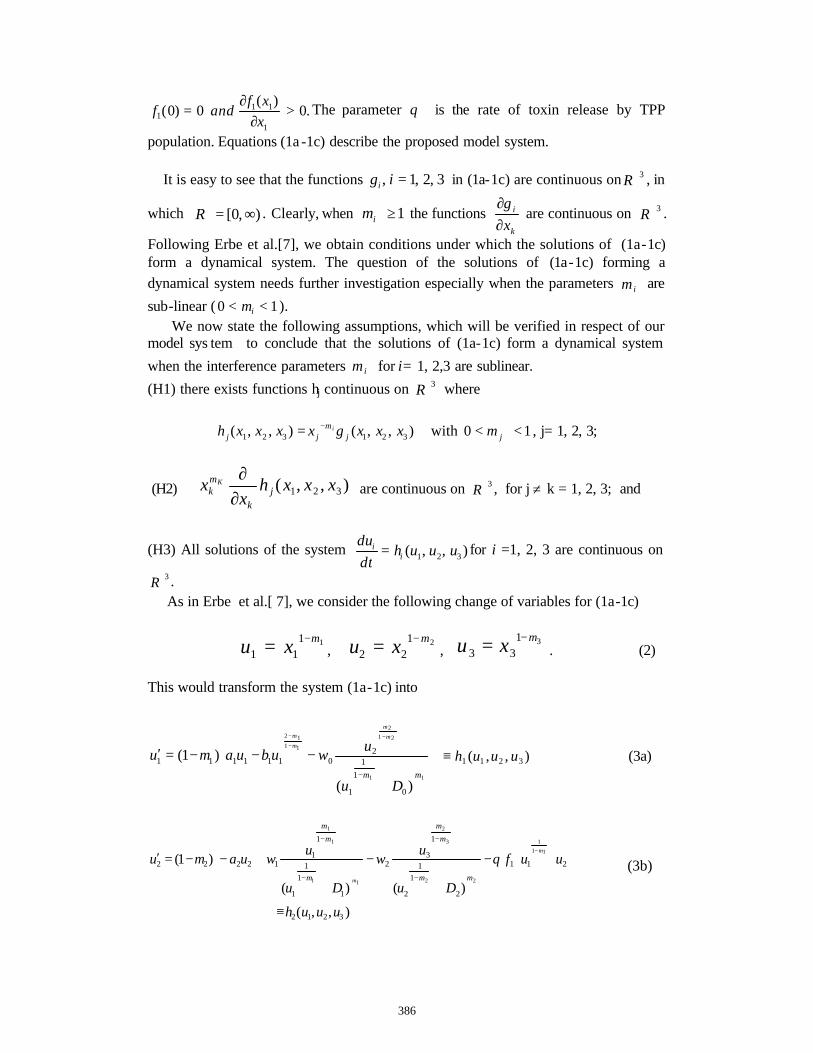
.0)(
0)0(1
111 >
∂∂
=xxf
andf The parameter θ is the rate of toxin release by TPP
population. Equations (1a -1c) describe the proposed model system. It is easy to see that the functions 3,2,1, =igi in (1a-1c) are continuous on 3
+R , in
which ),0[ ∞=+R . Clearly, when 1≥im the functions k
i
xg
∂∂
are continuous on 3+R .
Following Erbe et al.[7], we obtain conditions under which the solutions of (1a-1c) form a dynamical system. The question of the solutions of (1a-1c) forming a dynamical system needs further investigation especially when the parameters im are sub-linear ( 10 << im ). We now state the following assumptions, which will be verified in respect of our model sys tem to conclude that the solutions of (1a-1c) form a dynamical system when the interference parameters im for i= 1, 2,3 are sublinear. (H1) there exists functions hj continuous on 3
+R where
),,(),,( 321321 xxxgxxxxh jm
jji−= with 10 << jm , j= 1, 2, 3;
(H2) ),,( 321 xxxhx
x jk
mk
K
∂∂
are continuous on 3+R , for j ≠ k = 1, 2, 3; and
(H3) All solutions of the system ),,( 321 uuuhdtdu
ii = for i =1, 2, 3 are continuous on
3+R .
As in Erbe et al.[ 7], we consider the following change of variables for (1a-1c)
11
11mxu −= ,
2122
mxu −= , 31
33mxu −= . (2)
This would transform the system (1a-1c) into
+
−−−=′−
−−
−
11
212
1112
)(
)1(
0
11
1
20111111
mmDu
uwubuamum
m
m
m
),,( 3211 uuuh≡ (3a)
),,(
)()(
)1(
3212
211
2
11
2
1
32
1
11
1
1
112222
111
22
3
2
11
1
1
uuuh
uuf
Du
uw
Du
uwuamu
m
m mm
m
m
m
m
m
≡
−
+
−
+
+−−=′−
−
−
−
−
θ (3b)
386

),,()1( 32132233321
1
uuuhufwcmum
≡
−−=′
−
(3c)
Clearly the transformation (2) transforms the sublinear system (3c) into (3b) in which no sublinearities are present. Biologically, this amounts to requiring that the mutual interferences are not too strong. The above discussions may be summarized as follows. Theorem 2.1 Consider the system of equations (1a-1c) in which 0)0( ≥ix ,
10 << im , for i=1, 2, 3. Assume that the assumptions (H1), (H2) and (H3) hold. Then, the solutions of the system equations (1a-1c) form a dynamical system in the sense of Nemytskii and Stepanov [15] provided the mutual interference parameters satisfy the following inequalities:
,21,
21
21 ≥≥ mm and 132 ≥+mm .
3. Methods of investigation The model system presented above are multi-parameter system. Model parameters are selected in accordance with a method given in upadhyay et al. [19, 20]. A few hundred parameter combinations (choosing two at a time) are possible. This is simply not feasible for any one to scan the system in all the parameter spaces. Application of non-linear dynamics is unison with the knowledge of biology of the system enables one to choose parameter combinations for simulation experiments. The most crucial part of the present methodology is the following conjecture: Two coupled Kolmogorov systems in oscilla tory mode would yield either cyclic (stable limit cycles and quasi-periodic) or chaotic solutions depending on the strength of coupling between the two. In the present case, the set of parameter values for which the system admits a limit cycle solution is found to be
.0.2,95.0,95.0,10,10,0.1,03.0,003.0,10,55.0,10,0.2,0.1,0.1,05.0,0.2
321433
22112011
=======
=========
mmmDDwc
DwDwawba θ
There is one more important aspect of these simulation experiments i.e., choosing the step size for the variation of a system parameter from a parameter combination within the chosen range. It depends on the nature of the parameter concerned: whether it is a slow varying or fast varying one. The most useful way to study such a dynamical system is to monitor the amplitude (maxima) of the subsequent oscillations as the control parameter of the system is varied. A small change in parameter values may lead to a bifurcation: an abrupt, qualitative change in the dynamics.
387

4. Numerical Results In order to better understand the dynamics of the model system, we turn to numerical simulations. Computer simulations were performed on MATLAB for the system equation (1a -1c). The search for chaos was carried out using the Physics Academy Software (AIP, New York) ODE workbench package. Our primary interest is to explore the occurrence of chaotic dynamics in the mode l system. We try to observe the role of toxin producing phytoplankton on the chaotic dynamics in such ecosystems. We also examine the role of mutual interference parameter im and the parameter θ , the rate of toxin release by TPP population on the chaotic dynamics of the model system. Model system is integrated numerically using six-order Runge -Kutta method along with predictor corrector method. It is observed that the model system (1a-1c) has a chaotic solution at the following set of parameter values (see Fig. 1)
.0.0,0.2,0.1,0.1,0.20,0.1,03.0,0.10,405.0,0.10,0.2,0.1,0.10,0.1,06.0,93.1
321
33221
120011
====
============
θmmm
DwcDwDwaDwba
(9)
To confirm the existence of chaos, the dynamics of the model system is studied by constructing bifurcation diagrams. For Holling type II functional response form for toxin liberation process, we have plotted the successive maxima of top predator 3x as a function of the parameter θ (rate of toxin substances release by TPP population) keeping other parameters fixed as given in eqn. (9) for model system (1a-1c). The figures 2(a-b) are representing the bifurcation diagrams of model system (1a-1c) with
)( 11 xf as Holling type II functional response. These figures show clearly the transition from chaos to order through sequences of period-halving bifurcation. Therefore, for the model system, it is observed that, increase of value of toxic substances released by TPP population has a stabilizing effect. The blow –up bifurcation diagram (see Fig. 2b) show that the model system possesses rich variety of dynamical behaviour for bifurcation parameter θ in the ranges [0, 0.07] for Holling type II functional response. A period –doubling cascade is observed. After the accumulation point, the behaviour settles down onto a chaotic attractor. When θ, the bifurcation parameter is decreased, new periodic orbits are created. Two different bifurcations are involved. First, period-doubling bifurcations that are easily identified in the main period doubling cascade but also within each periodic window. Second, saddle –node bifurcations, creating one stable limit cycle and one unstable periodic orbit, both having the same period, may be identified at the beginning of each periodic window. Here, the most observable periodic windows are the one associated with the main period-doubling cascade and the other associated with the saddle-node bifurcation inducing the stable period-1 limit cycle. Two co-existing period-doubling cascades are then observed. Dynamical behavior of model system (1a-1c) depending on the results of bifurcation diagrams given in figs 2 is presented in table 1. We have observed stable focus, different order limit cycles and strange chaotic attractor in the different ranges of θ , the rate of toxic substance released by TPP. From the table 1, it is observed that for the model system, the increase of value of toxic substances released by TPP has a stabilizing effect. Model system also shows the extinction of the predator species for
388

higher values of θ. These observations indicate that to maintain the order of an ecosystem functioning, Holling type II functional form for toxin liberation process is more appropriate. Now, we have investigated the role of mutual interference parameters on the dynamics of trophic system in detail. The values of mutual interference parameters were chosen on the basis of the values reported in Katz [14]. We have observed stable focus, limit cycles and chaotic dynamics phenomena in the model system by changing the mutual interference parameters im , i=1, 2, 3 and the rate of toxin release by TPP population θ , in the fixed range for different cases. We have also reported the function error or argument domain error, the region in the parameter space where no dynamics is observed. In this domain, the values of mutual interference parameters are not conducive for simulation experiment i.e., in real situation, no species can attain these values of mutual interference. Our approach is first to fix 1m and 2m then vary 3m in the interval [1, 3] and θ in the interval [0,1) and then observe the exchange of states (stability - limit cycle - period doubling – chaos) in the model system for three different cases of ).,,( <=>im The results for model system (1a -1c) are summarized below: Case I: When 0>im
(A) For )(
1)(),IItypeHolling(
)()(
3222
41
111 Dx
xfDx
xxf
+=
+= . (see Table 3)
(i) For 1m = 2m =1.05 and 10,0.35.1 3 ≤≤≤≤ θm . Chaos exists at some discrete points. For example, chaos exists for
)55.0,25.2(),5.0,25.2(),55.0,0.2(),5.0,0.2(),45.0,0.2(),4.0,75.1(),( 3 =θm . Rest of the points it shows the limit cycle attractor. (ii) For 0.221 == mm and 10,31 3 ≤≤≤≤ θm . From the simulation, it is found that in most of the cases, 2x becomes extinct and
),( 31 xx rests on stable focus for higher values of θ . For lower values of θ , all the three populations rests on stable focus and limit cycle attractor in the phase plane. It is also observed that for 75.1,5.1,25.121 == mm and for whole range of the parameter space ),( 3 θm (i.e., 10,31 3 ≤≤≤≤ θm ), the model system (1a-1c) predicts no dynamics. The simulation results show function error or argument domain error. These values of mutual interference parameters are not conducive for the simulation experiment i.e., in real life situation, no species can attain these values of mutual interference. Case II: When 1=im (i.e., )1321 === mmm .
(A) For )(
1)(),IItypeHolling(
)()(
3222
41
111 Dx
xfDx
xxf
+=
+= , .10 ≤≤ θ
Chaos exists in the interval .25.00 ≤≤ θ For ]4.0,3.0[∈θ , and ]7.0,45.0[∈θ , we obtain the limit cycle and stable focus behaviour respectively. For rest values of
]0.1,8.0[∈θ , ),( 32 xx becomes extinct and 1x rests on a stable focus but at θ = 0.75, only 3x becomes extinct and other species rests on stable focus. Fig. 3 shows the
389

chaotic behaviour of the model system (1a-1c) in the domain .35.00,25.275.0 3 ≤≤≤≤ θm
Case III: When 0<im In this case, chaos does not exist at all. The domain in which we perform the two dimensional scans are
and 10 ≤≤ θ .
We obtain only function error in this domain except for .95.021 == mm We also did the simulation for the above values of 21, mm and ),( 3 θm in the domain
)10,325.0( 3 ≤≤≤≤ θm . Results are presented in the tabular form in table 4. From the tables, it is observed that the mutual interference also stabilize the system. From table 4, it is found that for 75.0,5.0,25.021 == mm and 3m in the range [1, 3] and θ in the range [0, 1], the dynamics is settled on stable focus. For 95.021 == mm and in whole range of 3m and θ , stable focus and limit cycles are observed. Case IV: (New Adventure) On the experimental basis, by looking the conditions of the Theorem 2.1, we have taken different combination of the mutual interference parameters and observed its influence on the dynamics of the model system (1a -1c). The results are reported in table 2. We observed only function error. These values of mutual interference parameters are not conducive for the simulation experiment i.e., in real life situations; no species can attain these values of mutual interference parameters. 5. Conclusions In this paper, we have attempted to answer the question does mutual interference and toxic substances released by TPP always stabilize the prey-predator dynamics in aquatic environment. Our simulation experiments suggest that the answer is definite ‘yes’. From the tables, it is observed that for different values of mutual interference parameters in different ranges, dynamics of the model system is also influenced by the functional form of toxin liberation process. For )3,2,1(1 =< imi , from table 4, no dynamics was observed (i.e., represented by function error in the tables) in the range
75.025.0 ≤≤ im , but if we take any one of the interference parameters value near 1, we observe the system dynamics on stable focus. In this case (Holling type II functional response), the top predator becomes extinct as 3m reaches 1. For 1>im , most of the time, dynamics rests on stable limit cycle or stable focus. From tables (3), it is found that for 05.121 == mm (i.e. near 1) and 3m in the range [1, 3], system dynamics settled on limit cycle attractor. In this case, model system also supports chaotic dynamics only at few discrete points. But for ,221 == mm and 3m in the range [1, 3], mostly system dynamics settled on stable focus and middle predator becomes extinct for all the three form of functional responses. These results show that the interaction between predators is a stabilizing factor, one could thus argue that evolution has selected species of predators that have values close to 1, but smaller
75.0,5.0,25.0;95.0,75.0,5.0,25.0 321 === mmm
390

than 1. This could be an explanation of why Arditi and Akcakaya [1] found in many sets of his experimental data, im was close to 1. From the tables and 2D scan diagram, it was also observed that the model system supports chaotic dynamics for .1≥im It is caused by deterministic changes in system parameters not by exogenous stochastic influences. In this case, the ecological systems are not able to lock themselves onto a fully developed chaotic state. Since it is constantly influenced by exogenous stochastic fluctuations [16], it is forced to leave the chaotic state as initial condition changes. We also observe from bifurcation diagrams is that chaotic dynamics is robust to changes in changes against rates in toxin production by phytoplankton as it exist for large range of θ value. Period doubling bifurcations seem to be responsible for this kind of dynamical behaviour. The study suggests that toxic substances release by TPP plays an important role in the termination of planktonic blooms which is of great importance to human health, ecosystems, environment and fishery. It may also act as biological control by changing chaos to order and has stabilizing contribution to aquatic systems. References [1] R. Ariditi, H.R. Akcakaya, Underestimation of mutual interference of predators, Oecologia 83 (1990) 358-361. [2] R. Arditi, J-M. Callois, Y. Tyutyunov, C. Jost, Does mutual interference always stabilize predator-prey dynamics? A comparison of models, Comptes Rendus Biologies 327 (2004) 1037-1057. [3] M.A. Aziz-Alaoui, Study of a Leslie-Gower-type tritrophic population model, Chaos Solitons and Fractals 14 (2002) 1275-1293. [4] J.R. Beddington, Mutual interference between parasites on predators and its effects on searching efficiency, J. Animal Ecology 44 (1975), 331-340. [5] M. Begon, M. Mortimer, D.J. Thompson, Population Ecology: A unified study of Animals and Plants, third ed. Blackwell Science, Oxf ord, U.K. 1996. [6] D.L. DeAngelis, R.A. Goldstein, R.V. O’Neill, A model for trophic interaction, Ecology 56 (1975) 881-892. [7] L.H. Erbe, H.I. Freedman, Modeling persistence and mutual interference among subpopulations of ecological communities, Bull. Math. Biol. 47 (1985) 295-304. [8] L.H. Erbe, H. I. Freedman, V. Sree Hari Rao, Three species food chain models with mutual interference and time delays, Math.Biosciences 80 (1986) 57-80. [9] H.I Freedman, V.Sree Hari Rao, The trade off between mutual interference and time lags in predator -prey Systems, Bull. Math. Biol. 45 (1983) 991-1004.
391

[10] M. P. Hassell, Mutual interference between searching insect parasites, J. Animal Ecology 40 (1971) 473-486. [11] M.P. Hassell, R. M. May, Stability in insect host -parasite models, J. Animal Ecology 42 (1973) 693-726. [12] A. Hastings, T. Powell, Chaos in three species food-chain, Ecology 72 (1991) 896-903. [13] T.W. Hwang, Uniqueness of limit cycles of the predator -prey system with Beddington-DeAnge lis functional response, J. Math. Anal. Appl. 290 (2004) 113-122. [14] C.H. Katz, A nonequilibrium marine predator -prey interaction, Ecology 66 (1985) 1426-1438. [15] V.V. Nemytskii and V.V. Stepanov, Qualitative Theory of Differential Equations, Princeton University Press, Princeton, 1960. [16] V. Rai, R.K. Upadhyay, Chaotic population dynamics and biology of the top-predator, Chaos Solitons and Fractals 21 (2004) 1195-1204. [17] G.D. Ruxton, Chaos in a three-species food chain with a lower bound on the bottom population, Ecology 71(1) (1996) 317-319. [18] R.K. Upadhyay, J. Chattopadhyay, Chaos to order: Role of toxin producing phytoplankton in aquatic systems. Nonlinear Analysis: Modelling and Control 10(4)(2005) 383-396. [19] R.K. Upadhyay, S.R.K. Iyengar, V. Rai, Chaos: an ecological reality?, Int. J. Bifurcation and Chaos 8(6) (1998) 1325-1333. [20] R.K. Upadhyay, V. Rai, Why chaos is rarely observed in natural populations?, Chaos Solitons and Fractals 8(12) (1997) 1933-1939.
392

Table 1. Dynamical behavior (DB) of model system depending on the results of bifurcation diagrams given in fig. 2. Pi - limit cycle of period i for (i = 2, 3, 4, 5, 6), SF – stable focus, LC – limit cycle, LP – long period, SCA – strange chaotic attractor, EX- Extinction.
Results of model 1 for
Holling type II: )()( 4Dxxxf +=
104 =D =θ DB 0.001-0.0111 SCA 0.0112 P6 0.0113-0.0115 P5 0.0116-0.0123 P4 0.0124-0.059 SCA 0.06 LP 0.061 P6 0.062-0.068 P4 0.07-0.16 P2 0.17 LP 0.18-0.39 LC 0.4-0.6 SF 0.7 EX
Table 2. Dynamical behaviour of the model system (1a-1c) depending on the results of the Theorem 2.1. The values of the common parameters are same as given in table 2. The mutual interference parameters )3,2,1(, =imi and θ varies in the given ranges.
Values of im
2 3
( ) 0 0.5 andthis violates 0
ia m
m m
< <
+ ≥
Values of θ in
10 ≤≤ θ
Dynamical Behaviour
)()(
41
111 Dx
xxf
+=
(i) 35.0,45.025.0 321 === mmm 0-1.0 Function Error
(ii) 25.0,25.025.0 321 === mmm 0-1.0 Function Error
(iii) 45.0,25.045.0 321 === mmm 0-1.0 Function Error
(iv) 45.0,45.035.0 321 === mmm 0-1.0 Function Error (v) 5.0,45.035.0 321 === mmm 0-1.0 Function Error (b) .5.0;5.00 321 ==<< mmm
.45.0,4.0,35.0,3.0,25.0,2.0,1.01 =m 0-1.0 Function Error
393

Table 3. Simulation experiments of model system (1a-1c) with )( 11 xf as Holling type II functional response. The values of the common parameters used in the model system are same as given in table 2 with 0.104 =D .
].1,0[rangetheinvariesand),3,2,1(1parametersceinterferenmutualThe θ=> imi
Values of
21 mandm 3m in
31 3 ≤≤ m
Values of θ in 10 ≤≤ θ
Dynamical behaviour
05.121 == mm
1.5 1.75 2.0 2.25 2.5 2.75 3.0
0-0.0001; 0.002-1.0 0.0002-0.001 0; 0.0004-0.001 0.0001-0.0003; 0.002-0.0095 0.01 -0.085; 0.095-0.35; 0.65-1.0 0.09; 0.5-0.6 0.4 0-0.0002; 0.0005-0.0008 0.0003-0.0004; 0.0009-0.007 0.0075-0.02 0.025-0.25 0.3-0.4; 0.6-0.65 0.45 -0.55 0.7-1.0 0-0.002 0.003; 0.02-0.088; 0.095-0.25 0.0035-0.015;0.09; 0.3-0.45 0.5-0.55 0.6-0.7 0.75 -1.0 0-0.02; 0.3-0.75 0.025-0.29; 0.77 -1.0 0.085, 0.095-0.28; 0.8 -1.0 0.09, 0.3-0.75 0.35 -0.42; 0.7– 0.75 0.44 - 0.66; 0.8-1.0
Function Error Limit cycle Function Error Limit cycle Function Error Limit cycle Chaos Limit cycle Function Error Limit cycle Function Error Limit cycle Chaos Function Error Limit cycle Function Error Limit cycle Chaos Limit cycle Function Error Limit cycle Function Error Function Error Limit cycle Limit cycle Function Error
25.121 == mm 1.0-3.0 0-1.0 Function Error
5.121 == mm 1.0-3.0 0-1.0 Function Error
75.121 == mm 1.0-3.0 0-1.0 Function Error
0.221 == mm 1.0 1.25 -2.0 2.25 2.5 2.75 3.0
0 -1.0 0 -1.0 0-0.1 0.15 -1.0 0 - 0.4 0.45 – 1.0 0 –0.5 0.55 – 0.6 0.65 -1.0 0 – 0.5 0.55 -0.85 0.86 – 1.0
x1 SF ; (x2, x3) extinct (x1, x3) SF; x2 extinct (x1, x2, x3) SF (x1, x3) SF; x2 extinct (x1, x2, x3) SF (x1, x3) SF; x2 extinct (x1, x2, x3) SF (x1, x2, x3) Limit cycle (x1, x3) SF; x2 extinct (x1, x2, x3) SF (x1, x2, x3) Limit cycle (x1, x3) SF; x2 extinct
394

Table 4. Simulation experiments of model system (1a-1c) with )( 11 xf as Holling type II functional response. The values of the common parameters used in the model system are same as given in table 2 with 0.104 =D . The mutual interference parameters θand3m varies in the ranges [0.25,3] and [0, 1] respectively.
Values of 21 mandm
3m in 325.0 3 ≤≤ m
Values of θ in 10 ≤≤ θ
Dynamical behaviour
25.021 == mm 0.25- 0.75 1.00- 3.0
0 –1.0 0-1.0
Function Error Stable Focus
5.021 == mm 0.25-0.75 1.0-3.0
0-1.0 0-1.0
Function Error Stable Focus
75.021 == mm 0.25-0.75 1.0-3.0
0-1.0 0-1.0
Function Error Stable Focus
95.021 == mm 0.25 0.5-0.75 1.0 1.25-2.25 2.5 2.75 3.0
0-0.004 0.005-0.009 0.01-0.1 0.2-0.4 0.45-1.0 0 -0.15 0.2-0.4 0.45-1.0 0-0.15 0.2-0.7 0.75-1.0 0-0.15 0.2-1.0 0-0.0002 0.0003-0.0004 0.0005-0.0006 0.0007-0.0009 0.001-0.006 0.007-0.02 0.03-0.15 0.2-1.0 0- 0.15 0.2-1.0 0-0.24 0.25-1.0
Limit cycle Function Error Limit cycle Stable Focus Function Error Limit cycle Stable Focus Function Error Limit cycle Stable Focus (x1, x2)SF, x3 extinct Limit cycle Stable Focus Limit cycle Function Error Limit cycle Function Error Limit cycle Function Error Limit cycle Stable Focus Integration Error Stable Focus Integration Error Stable Focus
395

Fig. 1. Phase plane diagram for model system (1a-1c) depicting chaotic attractor for 0=θ , other parameter are same as given in eq. (9).
Fig. 2. (a) Bifurcation diagram as a function of θ for model sy stem with )( 11 xf of Holling type II. (b)
Blown up bifurcation diagram of (a) in the range 2.00 ≤≤ θ . Here, z stands for 3x in model system (1a-1c).
chaos
0
0.05
0.1
0.15
0.2
0.25
0.3
0.35
0.4
0 0.5 1 1.5 2 2.5
m3
thet
a
Fig. 3. Model system. 2D scan diagram between ),( 3 θm parameter space for Holling type II functional responses with the parameter values
1 1 22, 0.05, 0.55,a b w= = = 4 10.0, 0.003.D θ= = other parameters are same as given in eq. (9).
396

Proceedings of the International Conferenceon Computational and Mathematical Methodsin Science and Engineering, CMMSE 2007Chicago, 20–23 June 2007.
An improved nonlinear algorithm appropriate for solvingspecial initial-value problems of the form y ′ = f(y)
Jesus Vigo-Aguiar1 and Higinio Ramos1
1 Departamento de Matematica Aplicada, Grupo de Computacion Cientıfica.University of Salamanca
emails: [email protected], [email protected]
Abstract
Recently the authors have presented a nonlinear explicit scheme suitable fornumerically solving first-order initial-value problems (IVP) of the form y′ = f(y).The algorithm is based on the local approximation of the function f(y) by a second-order Taylor expansion where the resulting approximated differential equation isthen solved without local truncation error. In this paper we proposed an improvedapproximation based on a Chebyshev interpolation polynomial of second degreetaken at the Chebyshev-Gauss-Lobato points.
Key words: initial value-problems, nonlinear methods, Chebyshev approxima-tion
MSC 2000: 65L05
1 Introduction
Many authors have worked on numerical methods suitable for solving initial valueproblems of special types in ordinary differential equations. Such problems are stiffproblems, singularly perturbed problems, or problems whose solution y(x) or the firstderivative of the solution y ′(x) contain singularities on the interval of integration.
We will consider the autonomous scalar initial-value problem given by
y ′ = f(y), y(a) = y0 , (1)
where y, f(y) ∈ R , and x ∈ [a, b] ⊂ R , and it is assumed that the solution is unique.The conventional explicit one-step method for (1) is given by yn+1 = α yn +hΦf (yn, h),where Φf (yn, h) is the incremental function, and the subscript f on the right hand sideindicates that the dependence of Φ on yn is through the function f . The selected stepsize h is such that for the mesh points we have xj = a + j h , j = 0, . . . , k. Typicalexamples of the above scheme are the linear one-step methods or the Runge-Kuttamethods (which are essentially substitution methods)[1].
397

Nonlinear multistep methods are usually designed for dealing with unconventionalproblems for which the classical schemes generally perform poorly [2], [4], [5], [6], [7],[8], [9]. On the contrary, some of the nonlinear schemes specifically designed for singularproblems do not perform well on non-singular problems [9]. In this paper we propose anon-linear scheme suitable for IVPs, based on the local approximation of the functionf(y) by a Chebyshev approximation. Some numerical experiments confirm the wellperformance of the method.
2 Approximation by a truncated Chebyshev series expan-sion
Recently the authors have presented in [7] an approach for handling some type ofspecial problems. This scheme was based on the approximation of the right hand sideof the differential equation by a second-order Taylor expansion and the use of an exactprocedure for solving the approximated problem. In this paper we propose a similarapproach, but this time we consider instead of the Taylor polynomial an interpolationpolinomial of second degree based on the Chebyshev-Gauss-Lobatto nodes [10].
We show this approximation that will be used in the next section for the develop-ment of the numerical scheme.
Let be a function f(y) defined on an interval named [yn, yn+1]. The transformationgiven by
y = yn +hy
2(1 + α)
where hy = yn+1 − yn introduces a new variable α ∈ [−1, 1] and the function
f(α) = f(yn +hy
2(1 + α))
may be approximated by means of a truncated series of Chebyshev polynomials in theform [11]
f(α) =2∑
k=0
′′ak Tk(α) (2)
where Tk(α) is the Chebyshev polynomial of fist kind of degree k, the double primesindicate that both the first and last terms in the summation are to be halved, and
ak =2∑
j=0
′′f(αj) Tk(αj) ,
where
αj = cos(θj) , j = 0, 1, 2 (3)
and
θj =(n− j)π
n
398
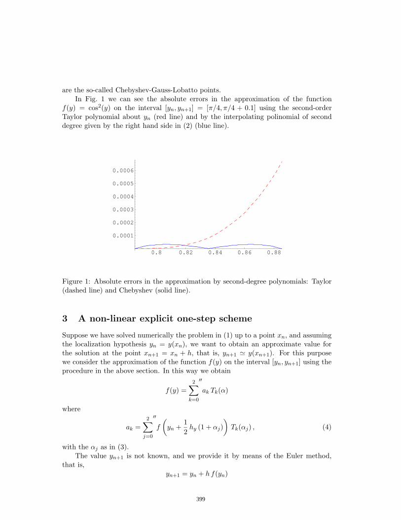
are the so-called Chebyshev-Gauss-Lobatto points.In Fig. 1 we can see the absolute errors in the approximation of the function
f(y) = cos2(y) on the interval [yn, yn+1] = [π/4, π/4 + 0.1] using the second-orderTaylor polynomial about yn (red line) and by the interpolating polinomial of seconddegree given by the right hand side in (2) (blue line).
0.8 0.82 0.84 0.86 0.88
0.0001
0.0002
0.0003
0.0004
0.0005
0.0006
Figure 1: Absolute errors in the approximation by second-degree polynomials: Taylor(dashed line) and Chebyshev (solid line).
3 A non-linear explicit one-step scheme
Suppose we have solved numerically the problem in (1) up to a point xn, and assumingthe localization hypothesis yn = y(xn), we want to obtain an approximate value forthe solution at the point xn+1 = xn + h, that is, yn+1 ' y(xn+1). For this purposewe consider the approximation of the function f(y) on the interval [yn, yn+1] using theprocedure in the above section. In this way we obtain
f(y) =2∑
k=0
′′ak Tk(α)
where
ak =2∑
j=0
′′f
(yn +
12
hy (1 + αj))
Tk(αj) , (4)
with the αj as in (3).The value yn+1 is not known, and we provide it by means of the Euler method,
that is,yn+1 = yn + h f(yn)
399

and so hy takes the form hy = h f(yn).With the above settings the approximated differential equation reads
y ′ =2∑
k=0
′′ak Tk
(2(y − yn)h f(yn)
− 1)
(5)
where now the ak are given by
ak =2∑
j=0
′′f
(yn +
12
h f(yn)(1 + αj))
Tk(αj) ,
that is, we have approximated on [xn, xn+1] the differential equation in (1) by thedifferential equation in (5) which is of Riccati type of the form
y ′ = a + b y + c y2 (6)
where a, b, c are certain constants which depend on h and yn through f . Explicitlythese constants reads
a =(h2f2
n + 3hynfn + 2y2n)fn − 4(y2
n + hfnyn)fn+1/2 + (hfnyn + 2y2n)fn+1
f2n h2
b =−(3fnh + 4yn)fn + 4(fnh + 2yn)fn+1/2 − (fnh + 4yn)fn+1
f2n h2
c =2(fn − 2fn+1/2 + fn+1)
f2n h2
where fn, fn+1/2, fn+1 are abbreviations for
fn = f(yn) , fn+1/2 = f(yn +h
2fn) , fn+1 = f(yn + hfn) .
We can solve on the interval [xn, xn+1] the problem in (6) with the initial conditiony(xn) = yn exactly, that is to say, without local truncation error, by considering thedifference scheme
yn+1 =
yn − 2 tan(hS)(b + 2c yn) tan(hS)− 2S
f(yn) , ∆ > 0 ,
yn − 2 tanh(hS)(b + 2c yn) tanh(hS)− 2S
f(yn) , ∆ < 0 ,
yn − 2h
b h + 2 c h yn − 2f(yn) , ∆ = 0
(7)
400
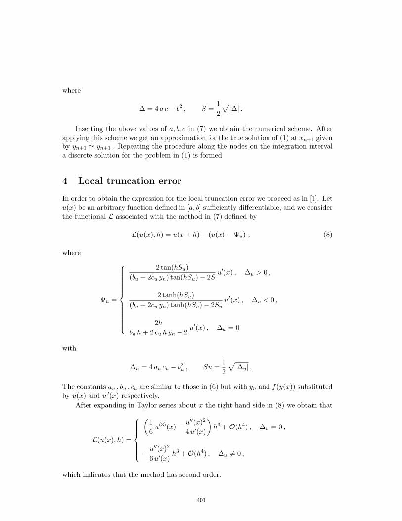
where
∆ = 4 a c− b2 , S =12
√|∆| .
Inserting the above values of a, b, c in (7) we obtain the numerical scheme. Afterapplying this scheme we get an approximation for the true solution of (1) at xn+1 givenby yn+1 ' yn+1 . Repeating the procedure along the nodes on the integration intervala discrete solution for the problem in (1) is formed.
4 Local truncation error
In order to obtain the expression for the local truncation error we proceed as in [1]. Letu(x) be an arbitrary function defined in [a, b] sufficiently differentiable, and we considerthe functional L associated with the method in (7) defined by
L(u(x), h) = u(x + h)− (u(x)−Ψu) , (8)
where
Ψu =
2 tan(hSu)(bu + 2cu yn) tan(hSu)− 2S
u′(x) , ∆u > 0 ,
2 tanh(hSu)(bu + 2cu yn) tanh(hSu)− 2Su
u′(x) , ∆u < 0 ,
2h
bu h + 2 cu h yn − 2u′(x) , ∆u = 0
with
∆u = 4 au cu − b2u , Su =
12
√|∆u| ,
The constants au , bu , cu are similar to those in (6) but with yn and f(y(x)) substitutedby u(x) and u ′(x) respectively.
After expanding in Taylor series about x the right hand side in (8) we obtain that
L(u(x), h) =
(16
u(3)(x)− u′′(x)2
4u′(x)
)h3 +O(h4) , ∆u = 0 ,
−u′′(x)2
6u′(x)h3 +O(h4) , ∆u 6= 0 ,
which indicates that the method has second order.
401

5 Stability analysis
As the numerical method in (7) is exact when the right hand side of the differentialequation is a polynomial up to second degree on y, the method is trivially A-stable.
In fact, if we apply the method to the scalar Dahlquist test problem given by
y′(x) = λ y(x) , Re(λ) < 0 ,
we obtain the difference equation
yn+1 = exp(λh) yn ,
where the stability function is given by R(λh) = exp(λ h), from which it is deducednot only A-stability but in fact a stronger property of L-stability (see [12]).
6 Numerical results
6.1 A non linear equation
The first example to be considered is the IVP given by
y′(x) = cos2(y(x)) , y(0) =π
4,
whose exact solution is y(x) = arctan(x + 1). We have integrated this problem on theinterval [0, π] taking different values for the constant stepsize h. In Table 1 the resultsfor this problem with the new method are shown, compared with those in [7]. Theerrors have been obtained as the absolute errors at the final point on the integrationinterval
Eend = |y(xend)− yNI | ,where NI refers to the number of steps used in the integration.
NI Eend (Method in [7] ) Eend (New Method)
25 2.4234× 10⁻⁶ 1.3669× 10⁻⁸
50 2.9198× 10⁻⁷ 9.5624× 10⁻¹⁰
100 3.5822× 10⁻⁸ 6.2627× 10⁻¹¹
200 4.4358× 10⁻⁹ 3.9959× 10⁻¹²
400 5.5187× 10⁻¹⁰ 2.5468× 10⁻¹³
800 6.8824× 10⁻¹¹ 2.2870× 10⁻¹⁴
Table 1: Errors for y′(x) = cos2(y(x)) , y(0) = π/4
A plot of the absolute errors for NI = 200 is shown in Fig. 2.
402

0.5 1 1.5 2 2.5 3
2.5·10-12
5·10-12
7.5·10-12
1·10-11
1.25·10-11
1.5·10-11
Figure 2: Absolute errors for Problem 6.1, NI = 200.
6.2 A singular problem
As a second example we consider the IVP given in by
y′ = 1 + y2 , y(0) = 1 , x ∈ [0, b] , (9)
The theoretical solution is y(x) = tan(x + π/4), which becomes unbounded inthe neighborhood of the singularity at x = π/4 ' 0.785398163397448, and so theconventional numerical integrators result inefficient. This problem has been used asnumerical test for different integrators intended for numerically solving singular initialvalue problems [2], [3], [4], [5], [6], [9]. As the right hand side of the differential equationis a polynomial in y of second degree, our method integrates the problem exactly, thatis, without local truncation error.
In Table 2 we have compared for different step sizes the results of our newly devel-oped scheme with those obtained by Odekunle el al. [9] with an inverse Runge-Kuttascheme of order four, and with the results obtained in [7]. There are small differencesbetween the results with the method in this paper an the results in [7], but these meth-ods are clearly better for this problem and we observe the ability of both methodsto overpass the singularity. The absolute errors were obtained at the point x = 0.8.Note that the smaller the step size is the bigger is the error, due to round off errorconsiderations.
6.3 A singularly perturbed problem
The last example corresponds to the singularly perturbed IVP taken from [13]
ε y′(x) = (x− 1) y(x) , y(0) = 1 ,
403
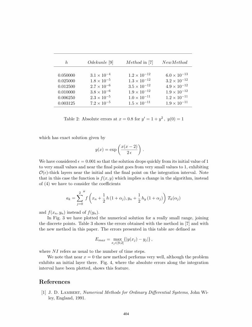
h Odekunle [9] Method in [7] NewMethod
0.050000 3.1× 10⁻⁴ 1.2× 10⁻¹² 6.0× 10⁻¹³
0.025000 1.8× 10⁻⁵ 1.3× 10⁻¹² 3.2× 10⁻¹²
0.012500 2.7× 10⁻⁶ 3.5× 10⁻¹² 4.9× 10⁻¹²
0.010000 3.8× 10⁻⁶ 1.9× 10⁻¹² 1.9× 10⁻¹²
0.006250 2.3× 10⁻⁵ 1.0× 10⁻¹¹ 1.2× 10⁻¹¹
0.003125 7.2× 10⁻⁵ 1.5× 10⁻¹¹ 1.9× 10⁻¹¹
Table 2: Absolute errors at x = 0.8 for y′ = 1 + y2 , y(0) = 1
which has exact solution given by
y(x) = exp(
x(x− 2)2 ε
).
We have considered ε = 0.001 so that the solution drops quickly from its initial value of 1to very small values and near the final point goes from very small values to 1, exhibitingO(ε)-thick layers near the initial and the final point on the integration interval. Notethat in this case the function is f(x, y) which implies a change in the algorithm, insteadof (4) we have to consider the coefficients
ak =2∑
j=0
′′f
(xn +
12
h (1 + αj), yn +12
hy (1 + αj))
Tk(αj)
and f(xn, yn) instead of f(yn).In Fig. 3 we have plotted the numerical solution for a really small range, joining
the discrete points. Table 3 shows the errors obtained with the method in [7] and withthe new method in this paper. The errors presented in this table are defined as
Emax = maxxj∈[0,2]
|y(xj)− yj | ,
where NI refers as usual to the number of time steps.We note that near x = 0 the new method performs very well, although the problem
exhibits an initial layer there. Fig. 4, where the absolute errors along the integrationinterval have been plotted, shows this feature.
References
[1] J. D. Lambert, Numerical Methods for Ordinary Differential Systems, John Wi-ley, England, 1991.
404

0.5 1 1.5 2
2·10-50
4·10-50
6·10-50
8·10-50
1·10-49
Figure 3: Numerical solution for Problem 6.3, NI = 2500.
NI Emax (Method in [7]) Emax (New Method)
2500 0.55067 1.43683× 10⁻²
5000 0.32968 1.73822× 10⁻³
7500 0.23407 5.05213× 10⁻⁴
75000 0.18126 2.09364× 10⁻⁴
12500 0.12598 8.91362× 10⁻⁵
Table 3: Maximum absolute errors for ε y′ = (x− 1) y , y(0) = 1 , ε = 0.001
[2] S. O. Fatunla, Numerical Methods for IVPs in ODEs, Academic Press Inc.,London, 1988.
[3] S. O. Fatunla, Nonlinear multistep methods for initial value problems, Comp. &Maths. with Appls. Vol. 8, No. 3 (1982) 231–239.
[4] S. O. Fatunla, Numerical treatment of singular initial value problems, Comp. &Maths. with Appls. Vol. 12B, No. 56 (1986) 1109–1115.
[5] F. D. Van Niekerk, Rational one-step methods for initial value problems, Comp.Math. Applic. Vol. 16, No. 12 (1987) 1035–1039.
[6] S. Abelman and D. Eyre, A numerical stydy of multistep methods based oncontinued fractions, Computers Math. Applic. Vol. 20, No. 8 (1990) 51–60.
405

0.5 1 1.5 2
0.002
0.004
0.006
0.008
0.01
0.012
0.014
Figure 4: Absolute errors for Problem 6.3, NI = 2500.
[7] H. Ramos and J. Vigo-Aguiar, A non-standard algorithm appropriate for solv-ing singular and singularly perturbed autonomous initial-value problems, Int. Jour-nal of Computer Mathematics, To appear (1990)
[8] H. Ramos , A non-standard explicit integration scheme for initial-value problems,Applied Mathematics and Computation. Vol. 189, No. 8 (2007) 710–718.
[9] M. R. Odekunle, N. D. Oye, s. O. Adee and R. A. Ademiluyi, A class ofinverse Runge-Kutta schemes for the numerical integration of singular problems,Appl. Math. Comput. 158 (2004) 149–158.
[10] W. S. Don and A. Solomonoff, Accuracy enhancement for higher derivativesusing Chebyshev collocation and a mapping technique, SIAM J. Sci. Comput. 18,No.4, (1997) 1040-1055
[11] L. Fox and I. B. Parker, Chebyshev Polynomials in Numerical Analysis. OxfordU. Press, London, 1968.
[12] E. Hairer and G. Wanner, Solving Ordinary Differential Equations II. Stiffand Differential-Algebraic Problems., Springer, Berlin, 1996.
[13] R. E. O’Malley, Jr., Give Your ODEs a Singular Perturbation!, Journal ofMathematical Analysis and Applications. 251 (2000) 433–450.
406

Proceedings of the International Conference on Computational and Mathematical Methods in Science and Engineering, CMMSE2007 Chicago, 20-23 June 2007
SVD Stabilized Block Diagonal Preconditioner for Large Scale Dense Complex Linear Systems in Electromagnetics
Yin Wang1, Jeonghwa Lee2 and Jun Zhang1 1 Laboratory for High Performance Scientific Computing and Computer
Simulation, Department of Computer Science, University of Kentucky
2 Department of Computer Science, Shippensburg University
emails: [email protected], [email protected], [email protected]
Abstract Preconditioned Krylov subspace methods are usually considered to be the methods of choice for solving large systems of linear equations arising from practical scientific and engineering modeling and simulations, such as in the electromagnetic applications. Due to its easy implementation and potential for parallelism, the block diagonal preconditioner is often used to accelerate the convergence rate of Krylov iterative methods. However, in some special electromagnetics computations, the block diagonal preconditioner actually slows down the Krylov subspace convergence. We propose to use singular value decomposition to stabilize the inverse of the blocks, which is generated from the multilevel fast multipole algorithm. Experimental results show that the new preconditioned iteration scheme converges faster compared with the standard block diagonal preconditioner and reduces the overall CPU time. Key words: Krylov subspace methods, Singular Value Decomposition (SVD), Block diagonal preconditioner, Multilevel fast multipole algorithm (MLFMA) MSC2000: 65F10, 65R20, 65F30, 78A45
1. Introduction In computational electromagnetics, we use hybrid volume and surface integral equations to model three-dimensional (3D) arbitrarily shaped dielectric and conducting objects. The computed solution has applications in radar cross-section (RCS) prediction for coated targets, printed circuit, and microstrip antenna analysis. The hybrid integral equation can be discretized into a linear system of the form
bAx = (1)
407
CMMSE 2007
by using the method of moments (MoM) [8, 14, 16, 22], where the coefficient matrix A is a large dense complex valued matrix for large targets in electromagnetic scattering.
The complex linear equation (1) can be solved by using direct solution methods or iterative solution methods. In this paper, our attention is on using efficient iterative methods. In particular, we use the biconjugate gradient (BiCG) method which is one of the Krylov methods as our iterative solver [1, 9, 18]. Let be the number of unknowns of the equation (1). The complexity of BiCG type iterative methods is , where indicates the number of iterations and is the computational cost of a matrix vector product operation, which accounts for the major cost of Krylov methods. We use the fast multipole method (FMM) to reduce the computational complexity of the matrix vector product operation from to [7, 17]. Furthermore, with the multilevel fast multipole algorithm (MLFMA) this complexity can be reduced to [6, 13, 20].
N)( 2NNO iter iterN
2N
)( 2NO )( 5.1NO)log( NNO
In order to further reduce the computational cost for solving the linear system (1), we can apply a carefully constructed preconditioning technique to equation (1) to accelerate the convergence rate of Krylov methods in the form of
bMAxM 11 −− = (2) where 1−M is a nonsingular matrix of order N . Our primary goal is to choose a robust and efficient preconditioner 1−M to make the new linear system (2) much easier to solve and to reduce the overall CPU time. Recently, the development and practice of efficient preconditioning techniques in iteratively solving dense linear systems has been the subject of growing interest [3, 4, 5, 11, 12]. The difficulty in constructing an efficient preconditioner for this class of dense linear system is that the global coefficient matrix A is not explicitly available in the MLFMA implementation. So, in the MLFMA, the block diagonal preconditioner has been more popular [13, 20, 23] because we can easily construct the block diagonal preconditioner from the small block diagonal submatrices, which are available explicitly. The ILUT preconditioner and sparse approximate inverse (SAI) preconditioner are reported to be more efficient, but more complex, preconditioning techniques in this application [3, 10, 11, 12]. Some cases arising from electromagnetic scattering problems show a bad convergence behavior with the block diagonal preconditioning [10]. We try to figure out what causes this bad convergence behavior. It is our suspicion that the LU factorizations of the individual blocks are not stable due to the ill-conditioning of some blocks. We intend to stabilize the block diagonal preconditioner by using singular value factorization (SVD) on each individual block instead of using the LU factorization. In our numerical experiments, we choose the BiCG method as an iterative solver combined with the different preconditioning strategies. These preconditioning
408

CMMSE 2007
strategies under comparison are (a) no preconditioner, (b) standard block diagonal preconditioner, and (c) SVD stabilized block (SVDB) preconditioner. Our numerical results show that the SVDB preconditioning technique coupled with the BiCG method accelerates the convergence rate of some difficult cases compared with the standard block diagonal preconditioner.
2. Discretization of Hybrid Integral Equation and MLFMA The hybrid integral equation approach combines the volume integral equation (VIE) and the surface integral equation (SIE) to model the scattering and radiation by mixed dielectric and conducting structures [14, 19]. The VIE is applied to the material region (V) and the SIE is enforced over the conducting surface (S). The integral equations can be formally written as follows:
),()(),()(),( tantan rErJrrLrJrrL incVVSS −=′⋅′+′⋅′ ,Sr∈
),()(),()(),( rErJrrLrJrrLE incVVSS −=′⋅′+′⋅′+− ,Vr∈
where stands for the excitation field produced by an instant radar, the subscript ‘‘tan’’ stands for taking the tangent component from the vector it applies to, and ,
, is an integral operator that maps the source to electric field and it is defined as:
incE
ΩL),( VS=Ω ΩJ )(rE
. )(),()()(),( 2 Ω′′⋅′∇∇+=′⋅′ ΩΩ′
−Ω ∫ drJrrGkIirJrrL bbS ωμ
Here is the 3D scalar Green’s function for the
background media and |)|4/(),( || rrerrG rrikb ′−=′ ′− π
1−=i . We note that J is related to in the above integral equations by
VJEiJ bV )( εεω −= . This results in a very general model as all the volume
and surface regions can be modeled properly. The advantage of this approach is that in the coated object scattering problems, the coating material can be inhomogeneous, and in the printed circuit and microstrip antenna simulation problems the substrate can be of finite size. The simplicity of the Green’s function in both the VIE and the SIE has an important impact on the implementation of the fast solvers. However, the additional cost here is the increase in the problem size since the volume that is occupied by the dielectric material is meshed. This results in larger memory requirement and longer solution time in solving the corresponding matrix equation. But this deficiency can be overcome by applying fast integral equation solvers such as the MLFMA [6].
Using the method of moments (MoM), the hybrid integral equations are discretized into a matrix equation of the form as the form
⎥⎦
⎤⎢⎣
⎡=⎥
⎦
⎤⎢⎣
⎡⋅⎥⎦
⎤⎢⎣
⎡V
S
V
S
VVVS
SVSS
UU
aa
ZZZZ , (3)
409

CMMSE 2007
where and stand for the vectors of the expansion coefficients for the surface current and the volume function, respectively [13, 14], and the matrix elements can be generally written as
Sa Va
.)(),(()( 2 Ω′−
Ω′Ω
Ω ′⋅′∇∇+Ω′⋅Ω= ∫∫ lbjbjl frrrGkIdrfdiZ χωμ )
The material function 1)( =′rχ if Ω′ is a surface patch, and )1/( −= bεεχ if Ω′
is a volume cell. The coefficient matrix arising from discretized hybrid integral equations is nonsymmetric. Once the matrix equation (3) is solved by numerical matrix equation solvers, the expansion coefficients and can be used to calculate the scattered field and the radar cross section (RCS). In antenna analysis problems the coefficients can be used to retrieve the antenna’s input impedance and to calculate the antenna’s radiation pattern. In the following, we use
Sa Va
A to denote the coefficient matrix in the Equation (3), , and for simplicity. TVS aax ],[= TVS UUb ],[=
The basic idea of the FMM is to convert the iteration of element-to-element to the interaction of group-to-group. Using the addition theorem for the free-space scalar Green’s function, the matrix-vector product can be written as [6, 7] Ax
,)( xVVxAAAx sfND Λ++= (4) where , , and are sparse matrices. In fact, the dense matrix fV Λ sV A can be structurally divided into three parts, and ,DA ,NA .sfF VVA Λ= is the block diagonal part of
DA
A , is the block near-diagonal part of NA A , and is the far part of FA A . Here the terms “near” and “far” refer to the distance between groups of elements. In FMM, those elements in are not explicitly computed and stored. Hence they are not numerically available. It can be shown that with optimum grouping, the number of nonzero elements in the sparse matrices in equation (3) are all on the order of , and hence the operation count to perform Ax is [7]. But if the above process is implemented in multilevel, the total cost can be further reduced to be proportional to for one matrix-vector multiplication.
FA
5.1N )( 5.1NO
NN log
3. SVD Stabilized Block Preconditioner There are two things we need to consider in order to choose an efficient preconditioner for solving the large dense linear system. One is to make the preconditioned matrix
AM 1− as close to the identity matrix I as possible, and the other is to choose a preconditioner which is not too expensive to construct and has a potential to be parallelizable. By using the block diagonal preconditioner, we construct a preconditioner 1−M from the block diagonal submatrix , and apply the block diagonal preconditioner DA
410

CMMSE 2007
1−M to the linear system (1). That is, . Here, is a block diagonal submatrix like in equation (4) consisting of several block submatrices such as
, . Each individual block can be decomposed independently by an LU factorization in the form of
bMAxM 11 −− = DA
,1A L,2A mA
)1( miULA iii ≤≤= and the linear system for each block will be solved as . The block diagonal preconditioner
iA
iiii bxUL = 1−M is of m independently inverted submatrix , where , so . It provides us a convenient structure to parallelize the preconditioner, because we can distribute the jobs into different processor for each block [13, 15, 20].
,11−A L,1
2−A ,1−
mA 11 )( −− = iii ULA 11 −− = DAM
Our previous studies shows that block diagonal preconditioner sometimes fail to improve the ill-conditioned linear systems in this application [10]. To alleviate the problem, we test the shift of the diagonal entries, and in some cases the convergence becomes more slowly than the block diagonal preconditioner without a diagonal shift. We suspect that some of these blocks may be ill-conditioned or close to singular. Their LU factorizations may not be stable, in the sense that large size entries are created in the inverse LU factors. SVD is known to be a very powerful technique for dealing with matrices that are either singular or else numerically very close to singular. In many cases when LU factorization fails to give satisfactory results, SVD may tell us what the problem is or how to solve it [2]. The computational and memory cost of SVD of large matrices may be expensive. To avoid this, we apply SVD to each small block submatrix )1( miAi ≤≤ . By using SVD, can be decomposed into three matrices as following [2, 15, 21, 24]
iA
H
iiii VUA ⋅Σ⋅= , (5) where and are orthogonal matrices, and all the singular values are stored in the
diagonal of as , iU iV
iΣ ],...,,[ 21 ki diag σσσ=Σ kσσσ ≥≥≥ K21 , k is the size of the block . iA
The inverse of is computed as . To stabilize the inverse, we replace some small singular values of
iA Hiiii UVA ⋅Σ⋅= −− 11
iΣ by a larger value. This can be done with a threshold strategy. Given a threshold value ε , if there exists an integer j such that
εσ >j , but εσ ≤+1j ( ), then for every l (kj ≤≤1 klj ≤< ), we set εσ =l .
Then we have the updated , and the stabilized inverse of is computed as:
],...,,,...,,[ 21 εεσσσ ji diag=Σ−
iA
(6) Hiiii UVA
11
−−− Σ=
The computational procedure is given in Algorithm 3.1, in which, ε is a user provided parameter. ALGORITHM 3.1 Computing the SVD stabilized block preconditioner from the block diagonal submatrices ( is the size of block ) ik iA
411

CMMSE 2007
0. For mi ,...,1= (where m is the number of blocks) Do 1. Obtain the ith block iA from DA and run the SVD subroutine to get iU , iΣ , and
HiV .
2. For each block, set the correct threshold ε and find the correct rank j , then for every ) , we set ( ikljl ≤< εσ =l .
3. Compute the HiU and HH
i . i VV )(=
4. Get 1−−
Σ i by computing jσ/1 ( kj ≤≤1 ).
5. Compute an SVD stabilized block as H iiii UVA1
1−−
− Σ=6. EndDo
The following explains how to choose the correct threshold value to update the singular values of each block in Algorithm 3.1. In our experiment, we use a static strategy to update the singular values, which means to choose a global threshold for every block. For a comparison, we can also compute some characteristics for each and every block during SVD thresholding, such as the mean value of all the singular values for each block or choosing the threshold . (bounderrorki _)/( 1 ⋅= σσε iε is the threshold for the ith block, and is bounderror _ 30.1 −e ). This can make the threshold more reasonable when the singular values are quite different in different blocks. Both methods have the same purpose, which is to make the SVD stabilized block inverse better conditioned than the block diagonal one. Because we know that
( is the column size of block Ai) (7) kiAcond σσ /)( 1= k
where 1σ is the largest singular value of the block andiA kσ is the smallest one. By using our updating strategies, the condition number of each block will be reduced to
, which means the inverse of that block will be more stable. We expect this stabilization will make the new preconditioner more effective than the block diagonal preconditioner.
εσ /1
Of course, there is always a trade-off between stability and accuracy. Choosing
a large threshold value produces a more stable, but less accurate inverse, while choosing a smaller threshold having the opposite effect.
4. Numerical Tests and Analysis In this section, we present a few numerical experiments to demonstrate the efficiency of the SVD stabilized block preconditioner for accelerating the BiCG iterations. All cases are tested using one processor of an HP Superdome cluster at the University of Kentucky. The processor has 2 GB local memory and runs at 1.5 GHz. The code is written in Fortran 77 and is run in single precision. We examine the convergence
412

CMMSE 2007
behavior based on the number of preconditioned iterations and some theoretical facts (such as the condition number). To demonstrate the performance of our preconditioned BiCG solver, we calculate the RCS of different conducting geometries with and without coating. The geometries considered include plates, spheres, and pipes (see Table 1). The mesh size for all the test structures are about one tenth of a wavelength.
Here are the explanations of the notations shown in the tables with numerical data and in some figures. • precond: the preconditioner used with the BiCG method:
ºNONE: no preconditioner; ºBLOCK: the block diagonal preconditioner ; ºSVDB: the SVD stabilized block preconditioner.
• level: the number of levels used in the MLFMA. • ε : the threshold value used to update the singular values in Algorithm 3.1 (static strategy). • itnum: the number of (preconditioned) BiCG iterations. • itcpu: the CPU time in seconds for the iteration phase. • Condition#: the condition number of each block.
For the class of the problems we tested, the block diagonal preconditioner can improve the BiCG convergence only in the P3C case. In the remaining three other cases, the block diagonal preconditioner actually hampers the BiCG convergence. Except for the sphere case, SVDB preconditioner can reduce the BiCG iteration steps and the total iteration CPU time compared with the BiCG solver without a preconditioner.
Table 1: Information about the matrices used in the experiments (all length units are in λ0, the wavelength in free-space) cases level unknowns matrices nonzeros target size and description
A 2,005,056P1C 4 1,416
DA 66,384
Dielectric plate over conducting plate 2.98824×2×0.1 Frequency=0.2GHz
A 223,502,500R5C 6 14,950
DA 607,838
Conduction pipe with 4 dielectric coating rings inside, 36×3.86236×3.87 Frequency=5GHz
A 10,160,640,000
P3C 7 100,800
DA 3,571,808
Antenna array Array size: 22.25×22.25 Frequency=0.3GHz
A 116,640,000S2C 4 10,800
DA 555,200Large conduction sphere 5×5×5 Frequency=0.3GHz
Table 2 and Fig. 1 show that the SVDB preconditioner is very efficient in case
the geometry is a plate. We also find that the larger static threshold we choose, the less number of iterations we need. But not all the computed solutions are correct. From
413

CMMSE 2007
Fig.1 (b), we can find that the solution of using mean value as the threshold is not correct. So, there should be a range to choose the threshold. If we choose the threshold beyond this range, we get false convergence or even no convergence at all.
Table 2: Numerical data of the P1C case Table 3: Numerical data of the R5C case
precond ε itnum itcpu
NONE - 445 478.83BLOCK - 2000 2012.60
6.0e-3 174 184.007.0e-3 75 79.82SVDB 8.0e-3 46 49.12
precond ε itnum itcpu
NONE - 1013 45.75BLOCK - 1319 59.94
Mean value
45 2.04
10.0 557 25.8215.0 467 21.52
SVDB
20.0 400 18.05
Fig. 1 shows the solutions of the P1C case using none preconditioner, block diagonal preconditioner, and SVDB preconditioner. Fig. 2 shows the solution of the R5C case and Fig.3 shows that of the S2C case. From these three figures we see that the RCS of the SVDB preconditioners for the S2C and R5C cases are much closer to the exact solution compared with the block diagonal preconditioner.
Table 4: Numerical data of the P3C case Table5: Numerical data of the S2C case
precond ε itnum itcpu
NONE - 2000 5892.03BLOCK - 1101 3257.47
0.15 416 1072.810.20 359 930.66SVDB 0.25 289 733.48
precond ε itnum itcpu
NONE - 320 264.98BLOCK - 2000 1965.15
1.50 1365 1331.312.00 798 786.38SVDB 2.50 340 331.00
Table 6 shows us some properties of the individual block in the P1C case, such
as the largest and smallest singular values, the condition number for each block, and the condition number after applying SVD with threshold. The threshold we use in this table to update the singular value is 15. Generally, we hope our preconditioned linear system has smaller condition number than the original one.
Table 6: The singular values and condition number of some blocks for the P1C case. Block largest
singular value
Smallest singular value
Condition #
Condition# after SVD (static)
1A 952.8143 7.406 128.6543 63.52089
9A 1625.496 7.043 230.7880 108.3664
17A 1724.973 22.09911 78.05623 78.05623
25A 697.4736 8.50674 81.99069 46.49824
32A 952.8133 7.40594 128.6553 63.52089
414

CMMSE 2007
(a) (b) Fig. 1. P1C case. (a) Convergence history comparison. (b) The solution accuracy
(a) (b)
Fig. 2. R5C case. (a) Convergence history comparison. (b) The solution accuracy
(a) (b) Fig. 3. S2C case. (a) Convergence history comparison. (b) The solution accuracy
415

CMMSE 2007
5. Conclusions We proposed a preconditioning technique based on the SVD stabilization of the block diagonal submatrices in the MLFMA. This SVD stabilized block preconditioner is easily constructed and also can be parallelized.
The standard block diagonal preconditioner is not robust and inefficient to solve the dense linear system arising from the combined hybrid integral formulation of electromagnetic scattering problem. We conducted a few numerical tests to show that the SVD stabilized block preconditioner is effective in solving some electromagnetic scattering problems. We also performed comparison for the block diagonal preconditioner, SVD stabilized block preconditioner, and none preconditioner.
Our numerical results indicate that the SVD stabilized block preconditioner can work more efficient than the standard block diagonal preconditioner in every case we tested. It also reduces the CPU time for these cases. We introduced two strategies to choose the threshold values for generating the SVD stabilized preconditioner. The RCS results show that the static strategy works quite well for plate case.
References [1] O. AXELSSON, Iterative Solution Methods, Cambridge University Press,
Cambridge, 1994. [2] D. KALMAN, A singularly valuable decomposition: The SVD of a matrix, Coll.
Math. J. 27(1) (1996) 2-23. [3] B. CARPENTIERI, I. S. DUFF, L. GIRAUD AND M. MAGOLU MONGA MADE, Sparse
symmetric preconditioners for dense linear systems in electromagnetism, Numer. Linear Alg. Appl., 11 (2004) 753-771.
[4] T. F. CHAN AND K. CHEN, On two variants of an algebraic wavelet preconditioner, SIAM J. Sci. Comput., 24 (2002) 260-283.
[5] K. CHEN, On a class of preconditioning methods for the dense linear systems from boundary elements, SIAM J. Sci. Comput., 20(2) (1998) 684-698.
[6] W. C. CHEW, J. M. JIN, E. MIDIELSSEN AND J. M. SONG, Fast and efficient algorithms in computational electromagnetics, Artech House, Boston, 2001.
[7] R. COIFMAN, V. ROKHLIN AND S. WANDZURA, The fast multipole method for the wave equation: a pedestrian prescription, IEEE Antennas Propagat. Mag., 35(3) (1993) 7-12.
[8] B. M. KOLUNDZIJA, Electromagnetic modeling of composite metallic and dielectric structures, IEEE Trans. Micro. Theory Tech., 47(7) (1999) 1021-1032.
[9] C. LANCZOS, Solution of systems of linear equations by minimized iterations, J. Res. Natl. Bur. Stand., 49 (1952) 33-53.
[10] J. LEE, J. ZHANG AND C. C. LU, Incomplete LU preconditioning for large scale dense complex linear systems from electromagnetic wave scattering problems, J. Comput. Phys., 185 (2003) 158-175.
[11] J. LEE, J. ZHANG AND C. C. LU, Sparse inverse preconditioning of multilevel fast multipole algorithm for hybrid integral equations in electromagnetics, IEEE Trans. Antennas Propagat., 52(9) (2004) 2277-2287.
416

CMMSE 2007
[12] J. LEE, J. ZHANG AND C. C. LU, Performance of preconditioned Krylov iterative methods for solving hybrid integral equations in electromagnetics, Appl. Comput. Electromagn. Society J., 18(4) (2003) 54-61.
[13] C. C. LU AND W. C. CHEW, A multilevel algorithm for solving a boundary integral equation of wave scattering, IEEE Trans. Micro. Opt. Tech. Lett., 7(10) (1994) 466-470.
[14] C. C. LU AND W. C. CHEW, A coupled surface-volume integral equation approach for the calculation of electromagnetic scattering from composite metallic and material targets, IEEE Trans. Antennas Propagat., 48(12) (2000) 1866-1868.
[15] Y. SAAD AND J. ZHANG, BILUTM: A domain-based multilevel block ILUT preconditioner for general sparse matrices, SIAM J. Matrix Anal. Appl., 21(1) (1999) 279-299.
[16] S. M. RAO, D. R. WILTON AND A. W. GLISSON, Electromagnetic scattering by surface of arbitrary shape, IEEE Trans. Antennas Propagat., AP-30(3) (1982) 409-418.
[17] V. ROKHLIN, Rapid solution of integral equations of scattering theory in two dimensions, J. Comput. Phys., 86(2) (1990) 414-439.
[18] Y. SAAD, Iterative Methods for Sparse Linear Systems, PWS Publishing, New York, NY, 1996.
[19] T. K. SHARK, S. M. RAO AND A. R. DJORDIEVIC, Electromagnetic scattering and radiation from finite microstrip structures, IEEE Trans. Micro. Opt. Tech., 38(11) (1990) 1568-1575.
[20] J. M. SONG, C. C. LU AND W. C. CHEW, Multilevel fast multipole algorithm for electromagnetic scattering by large complex objects, IEEE Trans. Antennas Propagat. AP-45(10) (1997) 1488-1493.
[21] Y. WANG, J. LEE AND J. ZHANG, A short survey on preconditioning techniques for large scale dense complex linear systems in electromagnetics, Accepted by Int. J. Comput. Math.
[22] T. VAUPEL AND V. HANSEN, Electrodynamic analysis of combined microstrip and coplanar/slotline structure with 3-D components based on a surface/volume integral equation approach, IEEE. Trans. Micro. Theory Tech., 47(9) (1999) 1150-1155.
[23] J. ZHANG, Sparse approximate inverse and multilevel block ILU preconditioning techniques for general sparse matrices, Appl. Numer. Math., 35(1) (2000) 67-86.
[24] M. DEGIORGI, G. TIBERI, A. MONORCHIO, G. MANARA AND R. MITTRA, An SVD-based method for analyzing electromagnetic scattering from plates and faceted bodies using physical optics bases, Proceeding of IEEE Antennas and Propagation Society International Symposium, 1(A) (2005) 147-150.
417

Proceedings of the International Conferenceon Computational and Mathematical Methodsin Science and Engineering, CMMSE 2007Chicago, 20–23 June 2007.
New Parallel Symmetric SOR Preconditioners byMulti-Type Partitioning
Dexuan Xie1
1 Department of Mathematical Sciences, University of Wisconsin,Milwaukee, WI 53201, USA
emails: [email protected]
Abstract
This paper proposes a new parallel symmetric successive over-relation (PSSOR)preconditioner by a multi-type partition technique. It then proves that the PSSORpreconditioner is symmetric and positive-definite and equivalent to a SSOR pre-conditioner using a special ordering called the multi-type ordering. Thus, thePSSOR preconditioner can be effectively applied to the preconditioned conjugategradient method (PCG), and can be analyzed under the framework of the classicalSSOR theory. Numerical tests on an anisotropic model problem show that withthe PSSOR preconditioner, PCG can have a much faster rate of convergence and abetter parallel performance than with the red-black SSOR preconditioner. More-over, the PSSOR preconditioner is shown numerically to have a condition numbernearly equal to that of the sequential SSOR preconditioner when the anisotropicratio is large enough.
Key words: preconditioned conjugate gradient, SSOR, domain decompositionMSC 2000: AMS 65Y05 (65F10)
1 Introduction
The symmetric successive over-relaxation (SSOR) preconditioner is often used in en-gineering and scientific computing due to its simplicity in implementation [5, 7, 13].It is known that the effects of the SSOR preconditioner on the convergence rate ofthe preconditioned conjugate gradient method (PCG) depends on the ordering of themesh points on which a finite element or finite difference approximation to an ellip-tic boundary value problem is defined. The natural ordering usually results in thefastest convergence rate, but is difficult to implement in parallel. The red-black (ormulticolor) ordering can overcome this difficulty, but seriously degrades the conver-gence rate of PCG compared to the natural ordering. To develop efficient parallelSSOR preconditioners, several other parallel orderings were proposed, which include
418

the wavefront ordering [2], the local column-wise ordering [8], the many-color ordering[6], and domain decomposition orderings [3, 9, 10]. On current MIMD parallel com-puters, however, it is only domain decomposition orderings that were found to lead tomore effective parallel SSOR preconditioners than the red-black SSOR preconditioner[9].
Recently, a new mesh domain partition and ordering, called the multi-type partitionand ordering, was proposed and applied to define a new block parallel SOR (BPSOR)method [12]. The BPSOR method was shown to have the same asymptotic convergencerate as the corresponding sequential block SOR method if the coefficient matrix of theblock linear system is “consistently ordered”. In particular, three particular multi-typeorderings are proposed based on strip and block mesh partitions, which lead to threeeffective BPSOR methods for solving the five-point like linear systems (in 2D) and theseven-point like linear systems (in 3D). In the point form, BPSOR is reduced to thePSOR method (a point parallel SOR method by mesh domain partitioning proposedin [11]). Obviously, the symmetric BPSOR (SBPSOR) method can be defined in thesame way as the SSOR method is defined [13]. A new symmetric parallel SOR (PSSOR)preconditioner is then well defined by one iteration of SBPSOR with an initial guessof zero. This paper intends to give the PSSOR preconditioner a general mathematicalformulation and to present a numerical study on its effect on the convergence rate ofthe PCG method. In particular, it proves that the PSSOR preconditioner is symmetricand positive-definite (SPD) if the coefficient matrix of the linear system is SPD. It alsoproves that the PSSOR preconditioner is equivalent to the SSOR preconditioner usingthe multi-type ordering. As a result, the analysis of the PSSOR preconditioner can bedone within the framework of the classic SOR theory [13].
To study the numerical behaviors of the PSSOR preconditioner, two particularPSSOR preconditioners – the 2-type and 3-type PSSOR preconditioners – are con-structed for a linear system arising from a five-point like finite difference approxima-tion to a simple anisotropic model problem. Their condition numbers are calculateddirectly for several small model problems by MATLAB, demonstrating that the 2-typeand 3-type PSSOR preconditioners can have a much smaller condition number than thered-black SSOR preconditioner. In the 2-type case, the PSSOR preconditioner is foundto have a condition number nearly equal to that of the sequential SSOR preconditionerfor a large anisotropic ratio. Hence, the PSSOR preconditioner is expected to have thesame effect as the sequential SSOR preconditioner on the convergence of PCG.
Finally, the PCG using the PSSOR preconditioner for solving the anisotropic modelproblem was implemented on a MIMD parallel computer (the SGI Origin 2000 atthe University of Wisconsin-Milwaukee) to investigate the parallel performance of thePSSOR preconditioner. Numerical results show that with the PSSOR preconditioner,PCG has a much faster convergence rate and much better parallel performance thanwith the red-black SSOR preconditioner. They also confirm that in the case of a largeanisotropic ratio, the PCG using the 2-type PSSOR preconditioner has the same rate ofconvergence as the PCG using the sequential SSOR preconditioner. In the case of thegrid size h = 1/517, a speedup of 12 was obtained for the 2-type PSSOR preconditioneron the 16 processors of the SGI Origin 2000.
419

The remainder of the paper is organized as follows: Section 2 introduces the multi-type partition and the related block linear system. Section 3 defines and analyzes thePSSOR preconditioner. Section 4 presents a condition number analysis to the 2-typeand 3-type PSSOR preconditioners for solving the model problem. Finally, the parallelperformance of the PCG using the PSSOR preconditioner is studied in Section 5.
2 The multi-type partition
Let the linear system Au = f arise from a finite element or finite difference approxi-mation to an elliptic boundary value problem with mesh domain Ωh. Here A denotesa SPD and consistently ordered matrix with entries aij . If aij 6= 0 with i 6= j, meshpoint i is said to be connected to mesh point j. Two subdomains of Ωh are said tobe connected if at least two of their mesh points are connected. It is assumed thatp processors of a large scale MIMD parallel computer are requested to implement thePCG for solving the linear system in parallel.
To define the multi-type partition, the mesh domain Ωh is partitioned into p disjointsubdomains, Ωh,j for j = 1, 2, . . . , p, such that each subdomain is only connected to itsneighboring subdomains. The mesh points of each subdomain are then grouped intot different types according to the following three criterions: (i) connected types mustbe adjacent; (ii) no adjacent types are the same type; and (iii) every interior type hasat least one adjacent type located in a neighboring subdomain. Here t is a positiveinteger determined by the connection information among neighboring subdomains. Itis clear that t is less than or equal to the number of neighboring subdomains. Thus,the multi-type partition with t types, which is also referred to as the t-type partition,is obtained.
Let Ωih,µ denote the ith type of subdomain µ for µ = 1, 2, . . . , p and i = 1, 2, . . . , t.
When these tp type subdomains are ordered in the natural ordering (i.e., from i = 1 tot for each µ from 1 to p), the linear system Au = f can be written in the block matrixform with
u =
U1
U2...Up
, Uµ =
U1µ
U2µ...U t
µ
, f =
F1
F2...Fp
, Fµ =
F1µ
F2µ...F t
µ
, (1)
A =
A11 A12 · · · A1p
A21 A22 · · · A2p...
.... . .
...Ap1 Ap2 · · · App
, Aµµ =
A11µµ A12
µµ · · · A1tµµ
A21µµ A22
µµ · · · A2tµµ
......
. . ....
At1µµ At2
µµ · · · Attµµ
, (2)
420
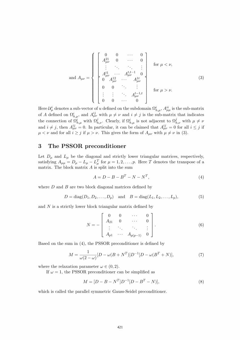
and Aµν =
0 0 · · · 0A21
µν 0 · · · 0...
. . . . . ....
At1µν · · · At,t−1
µν 0
for µ < ν,
0 A12µν · · · A1t
µν
0 0. . .
......
.... . . At−1,t
µν
0 0 · · · 0
for µ > ν.
(3)
Here U iµ denotes a sub-vector of u defined on the subdomain Ωi
h,µ, Aiiµµ is the sub-matrix
of A defined on Ωih,µ, and Aij
µν with µ 6= ν and i 6= j is the sub-matrix that indicatesthe connection of Ωi
h,µ with Ωjh,ν . Clearly, if Ωi
h,µ is not adjacent to Ωjh,ν with µ 6= ν
and i 6= j, then Aijµν = 0. In particular, it can be claimed that Aij
µν = 0 for all i ≤ j ifµ < ν and for all i ≥ j if µ > ν. This gives the form of Aµν with µ 6= ν in (3).
3 The PSSOR preconditioner
Let Dµ and Lµ be the diagonal and strictly lower triangular matrices, respectively,satisfying Aµµ = Dµ − Lµ − LT
µ for µ = 1, 2, . . . , p. Here T denotes the transpose of amatrix. The block matrix A is split into the sum
A = D −B −BT −N −NT , (4)
where D and B are two block diagonal matrices defined by
D = diag(D1, D2, . . . , Dp) and B = diag(L1, L2, . . . , Lp), (5)
and N is a strictly lower block triangular matrix defined by
N = −
0 0 · · · 0A21 0 · · · 0...
. . . . . ....
Ap1 · · · Ap(p−1) 0
. (6)
Based on the sum in (4), the PSSOR preconditioner is defined by
M =1
ω(2− ω)[D − ω(B + NT )]D−1[D − ω(BT + N)], (7)
where the relaxation parameter ω ∈ (0, 2).If ω = 1, the PSSOR preconditioner can be simplified as
M = [D −B −NT ]D−1[D −BT −N)], (8)
which is called the parallel symmetric Gauss-Seidel preconditioner.
421

Theorem 1 If the matrix A defined in (2) is symmetric and positive-definite, sois the PSSOR preconditioner M . Here M is defined in (7).
Proof: Set R = [D − ω(B + NT )]D−1[D − ω(BT + N)]. Since M = 1ω(2−ω)R, one
only needs to show that R is SPD .Clearly, R is symmetric. From (5) it can be seen that D consists of the main
diagonal entries of A, which are positive since A is positive-definite. Thus, xT Dx > 0and xT D−1x > 0 for nonzero vector x.
Set Λ = D − ω(BT + N). It is clear that xT Λx = xT ΛT x. From (4) it can followthat Λ + ΛT = (2− ω)D + ωA. Hence, for any nonzero vector x, and ω ∈ (0, 2),
xT Λx =12xT (Λ + ΛT )x =
12[(2− ω)xT Dx + ωxT Ax] > 0.
Thus, the vector y defined by y = Λx is not zero if x 6= 0. Hence, for any nonzerovector x,
xT Rx = xT [D − ω(B + NT )]D−1[D − ω(BT + N)]x= xT ΛT D−1Λx = yT D−1y > 0.
This proves that R is positive-definite. The proof is completed.Since M is SPD, the inverse of M exists and can be found as below:
M−1 = ω(2− ω)[D − ω(BT + N)]−1D[D − ω(B + NT )]−1. (9)
In application, the solution of Mz = r, z = M−1r, is found as one iteration ofthe symmetric BPSOR method with an initial guess of zero. Here each symmetricBPSOR iteration contains two half-iterations: the first one is the BPSOR method andthe other one is the BPSOR method using the reverse order, which is also called thebackward BPSOR method. In fact, from [12] it is known that the BPSOR method hasthe following iterative expression
u(k+1) = [D − ω(B + NT )]−1[(1− ω)D + ω(BT + N)]u(k)
+ ω[D − ω(B + NT )]−1r, k = 0, 1, 2, . . . , (10)
where u(0) is an initial guess. By reversing the ordering that is used in implementingeach BPSOR iteration, it is easy to obtain the backward BPSOR iterative expressionin the form
u(k+1) = [D − ω(BT + N)]−1[(1− ω)D + ω(B + NT )]u(k)
+ ω[D − ω(BT + N)]−1r, k = 0, 1, 2, . . . . (11)
With u(0) = 0, the first BPSOR iterate u(1) = ω[D − ω(B + NT )]−1r. Then, onebackward BPSOR iteration starting at u(1) immediately gives the solution of Mz = r.
The pt type subdomains Ωih,µ of the t-type partition can also be ordered from
µ = 1 to p for each value of type i from 1 to t while the original ordering is retained
422

within each type subdomain. Such an ordering is called the multi-type ordering. Inthe multi-type ordering, the sub-vectors U i
j are reordered in the form
u =
U1
U2...Ut
with Ui =
U i1
U i2...U i
p
.
Clearly, there exists a permutation matrix, P , such that u = Pu with u being givenin (1). In terms of P , the reordered linear system by the multi-type ordering can beexpressed as Au = f with A = PAP T , u = Pu, and f = Pf . Thus, the SSOR precon-ditioner using the t-type ordering, which is also called the t-type SSOR preconditioner,can be obtained as below:
M =1
ω(2− ω)[D − ωL]D−1[D − ωLT ], (12)
where D and L are diagonal and strictly lower triangular matrices, respectively, satis-fying A = D − L− LT .
Theorem 2 If M and M are the PSSOR preconditioner and the t-type SSORpreconditioner defined in (7) and (12), respectively, then there exists a permutationmatrix P such that
M = PMP T . (13)
Proof: Clearly, there exists the permutation matrix P such that u = Pu. In termsof P , it is easy to see that D = PDP T . With u(0) = 0, the first BPSOR iterate u(1)
for solving Au = f becomes
u(1) = ω[D − ω(B + NT )]−1f.
Multiplying the above expression by P from the left-hand side and using the identitiesP T P = I, Pf = f , and PDP T = D give that u(1) = ω[D − ωP (B + M)P T ]−1f . Onthe other hand, since u(0) = Pu(0) = 0, the first SOR iterate for solving the reorderedlinear system Au = f becomes u(1) = ω[D−ωL]−1f . Combining these two expressionsof u(1) yields the identity
[D − ωP (B + NT )P T ]−1f = [D − ωL]−1f for all nonzero vector f .
From the above identity it follows that [D−ωP (B+NT )P T ]−1 = [D−ωL]−1, which canbe simplified as L = P (B +NT )P T . Thus, combing it with PDP T = D and P T = P−1
gives
[D − ωL]D−1[D − ωLT ] = P [D − ω(B + NT )]D−1[D − ω(BT + N)]P T .
Multiplying both sides of the above identity by the constant 1/[ω(2 − ω)] yields M =PMP T . This completes the proof.
423

4 PSSOR preconditioners for an anisotropic model prob-lem
A simple anisotropic model problem is given by −(auxx + buyy) = f(x, y) in Ω,
u = 0 on ∂Ω.(14)
where a and b are positive constants with a ≥ b, Ω = (0, 1) × (0, 1), and ∂Ω denotesthe boundary of Ω. By the five-point finite difference formula, the model problem canbe approximated as the following linear system
2(1 +b
a)uij − (ui+1,j + ui−1,j)− b
a(ui,j+1 + ui,j−1) =
h2
afij , (15)
where i, j = 1, 2, . . . , n − 1, h = 1/n with n > 1, fij = f(ih, jh), uij denotes anapproximation of the solution u(ih, jh), and ui0 = uin = u0i = uni = 0 for i =0, 1, 2, . . . , n.
In the 2-type ordering (t = 2), the coefficient matrix A of (2) becomes a tridiagonalblock matrix in the form
A =
A11 A12
A21 A22. . .
. . . . . . Ap−1,p
Ap,p−1 App
with Aµµ =[
A11µµ A12
µµ
A21µµ A22
µµ
], (16)
Aµ,µ+1 =[
0 0A21
µ,µ+1 0
]and Aµ+1,µ = AT
µ,µ+1.
For the model problem (15), it can be found that
A11µµ = B, A12
µµ = −cI, A21µ,µ+1 = −cI,
A22µµ =
B −cI
−cI B . . .. . . . . . −cI
−cI B
, B =
α −1
−1 α. . .
. . . . . . −1−1 α
,
where α = 2(1 + b/a), c = b/a, I is an (n − 1) × (n − 1) identity matrix, B is an(n − 1) × (n − 1) tridiagonal matrix, A22
µµ is an ` × ` block matrix if Ω2h,µ contains `
mesh lines, and µ = 1, 2, . . . , p.In the 3-type partition, the block matrix A of (2) becomes a five-diagonal block
matrix with nonzero entries lying on the main diagonal, the second off-diagonal, andthe (m + 1)th off-diagonal. For example, for p = 4, the block matrix A has the form
A =
A G H 0GT A 0 HHT 0 A G0 HT GT A
with A =
A11 A12 0A12T
A22 A23
0 A23TA33
, A11 = α, (17)
424

0.4 0.6 0.8 1 1.2 1.4 1.6 1.8 20
5
10
15
20
25
30
35
40
45
Relaxation Parameter ω
Con
ditio
n N
umbe
r
SSOR2−type PSSOR3−type PSSORRed−Black SSOR
0.4 0.6 0.8 1 1.2 1.4 1.6 1.8 20
5
10
15
20
25
30
35
40
45
Relaxation Parameter ω
Con
ditio
n N
umbe
r
SSOR2−type PSSOR3−type PSSORRed−Black SSOR
Figure 1: Comparison of the condition numbers of the PSSOR preconditioners withthat of the sequential and red-black SSOR preconditioners for the model problem (15)with h = 1/7. The left plot for a = b = 1, and the right plot for a = 10, b = 1.
A22 =
α −1 0 0−1 α 0 00 0 α −c0 0 −c α
, A33 =
α −1 −c 0−1 α 0 −c−c 0 α −10 −c −1 α
,
A23 =
−c 0 0 00 −c 0 0−1 0 0 00 0 −1 0
, A12 = [−1 0 − c 0],
G is a 9× 9 matrix with only three nonzero entries given by g31 = g74 = g95 = −1, andH is a 9× 9 matrix with only three nonzero entries given by h51 = h82 = h93 = −c.
With the two matrix forms of A given in (16) and (17), the two sequential SSORpreconditioners can be constructed, respectively, according to the formula M = (D −ωL)D−1(D − ωLT ), where D is the diagonal matrix of A and L is the strictly lowertriangular matrix such that A = D−L−LT . Similarly, the 2-type and 3-type PSSORpreconditioners can also be constructed by formula (7). Furthermore, the red-blackmatrix form of A can be obtained by reordering the matrix A of (16) in the red-blackordering. Then, the red-black SSOR preconditioner can be constructed.
From the PCG theory [4] it is known that the effect of a preconditioner M on theconvergence rate of the PCG method can be studied directly by evaluating the conditionnumber of M−1A. The smaller the condition number, the faster the convergence rate[4]. For the model problem with h = 1/7, the condition numbers of the above fourpreconditioners were calculated on MATLAB, and reported in Figure 1.
Figure 1 shows that the 2-type and 3-type PSSOR preconditioners have muchsmaller condition numbers than the red-black SSOR preconditioner, while the SSORpreconditioner has the smallest condition number. Hence, the PSSOR preconditioneris more effective than the red-black SSOR preconditioner while the sequential SSOR
425

1 2 4 9 12 1640
60
80
100
120
140
160
180
200
a=1, b=1
a=10, b=1
a=100, b=1
a=1000, b=1
Number of Processors
Num
ber
of P
CG
Iter
atio
ns
0 2 4 6 8 10 12 14 16
10−1
100
101
Number of Processors
CP
U T
ime
(in s
econ
ds)
a=1a=10a=100a=1000
Figure 2: Convergence dependence ofthe PCG using the PSSOR precondi-tioner on the number of processors andthe anisotropic ratio a/b.
Figure 3: Parallel performance of thePCG using the PSSOR preconditioner.The dash lines indicate the total inter-processor data communication time.
preconditioner is the most effective among them. From the right plot (with a = 10 andb = 1) of Figure 1 it can be seen that the 2-type PSSOR preconditioner has the samecondition number as the SSOR preconditioner. Figure 1 also shows that the conditionnumber is a quadratic function of ω. Hence, for each preconditioner, there exists anoptimal value of ω at which the smallest condition number is reached.
5 Parallel performance of PSSOR preconditioner
To demonstrate the parallel performance of the PCG using the PSSOR preconditioner,numerical experiments were made on a MIMD parallel computer (the SGI Origin 2000computer at the University of Wisconsin-Milwaukee, which has 16 R12000 400 MHzprocessors) for the model problem (15) with f = 1.0 and h = 1/517. Four anisotropicratios a/b set by a = 1, 10, 100, 1000 for b = 1 were considered. All the numericaltests used an initial guess of zero, and the same iteration stop rule in which the rela-tive residue norm is less than 10−6. In addition, the optimal values of the relaxationparameter ω were used in these tests, which were determined by experiments.
The parallel program was written in Fortran 77 and MPI (the Message PassingInterface) [1]. The program was compiled using the optimization level O2. The CPUtime was measured by the MPI function MPI Wtime, which returns the wall time inseconds. All calculations were done with double precision. The sequential PCG methodusing the SSOR preconditioner was implemented on one processor of the computer byusing a sequential F77 program, where the F77 function etime() was used to measurethe CPU time.
Figure 2 shows that the PCG using the PSSOR preconditioner can have a fasterconvergence speed for a larger value of the ratio a/b. Also, it shows that the number of
426

4 9 16
93
232
620
2−type PSSOR
3−type PSSOR
Red−Black SSOR
Number of Processors
Num
ber
of P
CG
Iter
atio
ns
4 9 16
0.11
0.55
1.24
2.11
6.12
13.33
Number of Processors
CP
U T
ime
(in s
econ
ds)
2−type PSSOR 3−type PSSOR Red−black SSOR
Figure 4: Convergence comparison ofthe PCG using the PSSOR precondi-tioner with the PCG using the red-black SSOR preconditioner.
Figure 5: Parallel performance com-parison of the PCG using the PSSORpreconditioner with the PCG using thered-black SSOR preconditioner.
processors has less effects on the convergence rate for a larger anisotropic ratio of a/b.Figure 3 displays the parallel performances of the PCG using the PSSOR precondi-
tioner. It shows that the total CPU time is a linear decreasing function of the numberof processors. Compared to the total CPU time, the time consumed by interprocessordata communication is very small. A speedup of 12 was obtained on the 16 processorscompared to the sequential PCG using the sequential SSOR preconditioner.
Figures 4 and 5 compare the parallel performance of the PCG using the 3-typePSSOR preconditioner with that of the PCG using the red-black SSOR preconditioner.Here a = 10 and b = 1. The block partitions of two by two, three by three and fourby four blocks were used in the tests implemented on four, nine and sixteen processors,respectively. From these two figures it can be seen that the PSSOR preconditioner ac-celerated the convergence speed of PCG (in terms of the total number of PCG iterationsdetermined by the iteration stop rule) for about 3 to 6 times compared to the red-blackSSOR preconditioner, confirming that the PSSOR preconditioner is much more effec-tive than the red-black SSOR preconditioner. Moreover, the PSSOR preconditionerreduced the total CPU time of the PCG using the red-black SSOR preconditioner bya factor of 3 to 6 on both calculation and interprocessor data communication. In ad-dition, these two figures also show that the 2-type PSSOR preconditioner was moreeffective than the 3-type PSSOR preconditioner in improving the convergence rate andparallel performance of PCG.
Acknowledgements
This project was supported by the National Science Foundation through grant DMS-0241236.
427

References
[1] MPI: A Message-Passing Interface Standard. University of Tennessee, Knoxville,Tennessee, June 1995.
[2] C. Ashcraft and R. Grimes. On vectorizing incomplete factorization and SSORpreconditioners. SIAM J. Sci. Statist. Comput., 9:122–151, 1988.
[3] C. Farhat. Multiprocessors in computational mechanics. In Ph.D. thesis, CivilEngineering Department. University of California, Berkeley, CA, 1986.
[4] G. H. Golub and C. F. van Loan. Matrix Computations. John Hopkins UniversityPress, Baltimore, MD, Third edition, 1996.
[5] W. Hackbusch. Iterative Solution of Large Sparse Systems of Equations. Springer-Verlag, New York, 1994.
[6] D. Harrar and J. Ortega. Multicoloring with lots of colors. In Proc. Third Internat.conference Supercomputing, pages 1–6, Grete, Greece, 1989.
[7] Th. Lippert. Parallel SSOR preconditioner for lattice QCD. Parallel Computing,25:1357–1370, 1999.
[8] R. Melhem. Towards efficient implementations of preconditioned conjugate meth-ods on vector supercomputers. Internat. J. Supercomput. Appl., 1:70–98, 1987.
[9] S. A. Stotland and J. M. Ortega. Orderings for parallel conjugate gradient pre-conditioners. SIAM J. Sci. Comput., 18(3):854–868, 1997.
[10] H. A. van der Vorst. Large tridiagonal and block tridiagonal linear systems onvector and parallel computers. Parallel Computing, 5:45–54, 1987.
[11] D. Xie and L. Adams. New parallel SOR method by domain partitioning. SIAMJ. Sci. Comput, 20:2261–2281, 1999.
[12] D. Xie. A new block parallel SOR method and its analysis. SIAM J. Sci. Comput,27:1513-1533, 2006.
[13] D. M. Young. Iterative Solution of Large Linear System. Academic press, NewYork, 1971.
428

Proceedings of the International Conferenceon Computational and Mathematical Methodsin Science and Engineering, CMMSE 2007Chicago, 20–23 June 2007.
A New Quadrature Using Integration Lattices
Xiaoyan Zeng1, Rong-Xian Yue2 and Fred J. Hickernell1
1 Department of Applied Mathematics, Illinois Institute of Technology
2 Department of Applied Mathematics, Shanghai Normal University
emails: [email protected], [email protected], [email protected]
Abstract
In this paper we propose a new quadrature rule via approximating Fouriercoefficients of variable transformed integrand with multidimensional integrationlattice. The error analysis is derived for the proposed rule. A comparison is donebetween the new rule and the periodizing transformation methods. It shown thatthe new rule improves the periodizing transformation methods. In the last part ofthe paper, we also present a quadrature rule for weighted integrals whose integrandis in Banach space and we show it is semi-optimal.
Key words: quadrature, integration lattice, transformed integrand
429