ENSEEIHT-IRIT RT/APO/07/10 Also CERFACS TR/PA/07/71

Proceedings of the

2007 International Conferenceon Preconditioning Techniques for

Large Sparse Matrix Problems in

Scientific and Industrial ApplicationsJuly 9-12, 2007

Toulouse, France

Sponsored by

In collaboration with

Societe de Mathematique Appliquees et Industrielles / Groupe pourl’Avancement des Methodes Numeriques de l’Ingenieur (SMAI/GAMNI)Society for Industrial and Applied Mathematics / Activity Group onLinear Algebra (SIAM/SIGLA)

Editors:Luc Giraud, Esmond G. Ng, Yousef Saad and Wei-Pai Tang

Contents

1 Foreword 6

2 Committees 7

3 Awards 8

4 Invited presentations 9

4.1 Preconditioning of finite element systems using Hierarchical matrices - M. Beben-dorf . . . . . . . . . . . . . . . . . . . . . . . . . . . . . . . . . . . . . . . . . . . 9

4.2 Preconditioning techniques in optimization problems - J. Gondzio . . . . . . . . . 9

4.3 Agregation-based multigrid revisited - Y. Notay . . . . . . . . . . . . . . . . . . . 10

4.4 Parallel preconditioning with sparse incomplete factors - P. Raghavan . . . . . . 11

4.5 Multi-level preconditioners and applications in electromagnetic simulation - S. Re-itzinger . . . . . . . . . . . . . . . . . . . . . . . . . . . . . . . . . . . . . . . . . 11

4.6 Support preconditioners for finite-elements problems - S. Toledo . . . . . . . . . . 12

4.7 Uniform preconditioning techniques for nearly singular systems - L. Zikatanov . . 12

5 Contributed presentations 13

5.1 Two-stage physics-based preconditioners for porous media flow applications -B. Aksoylu . . . . . . . . . . . . . . . . . . . . . . . . . . . . . . . . . . . . . . . 13

5.2 A scalable multi-level preconditioner for matrix-free µ-finite element analysis ofhuman bone structures - P. Arbenz . . . . . . . . . . . . . . . . . . . . . . . . . 16

5.3 Using perturbed QR factorizations to solve linear Least Squares problems -H. Avron . . . . . . . . . . . . . . . . . . . . . . . . . . . . . . . . . . . . . . . . 17

5.4 Preconditioning techniques for large-scale adaptive optics - J. M. Bardsley . . . 19

5.5 Block preconditioning for saddle point problems with indefinite (1, 1) block -M. Benzi . . . . . . . . . . . . . . . . . . . . . . . . . . . . . . . . . . . . . . . . 20

5.6 Splittings for the two-sided Minimum Residual iteration - M. Byckling . . . . . 21

5.7 Multilevel domain decomposition preconditioners for inverse - X.-C. Cai . . . . . 24

5.8 Comparison of preconditioners for the simulation of hydroelectric reservoirs flood-ing - L. M. Carvalho . . . . . . . . . . . . . . . . . . . . . . . . . . . . . . . . . . 24

5.9 Improving preconditioners in interior-point methods for optimization throughquadratic regularizations - J. Castro . . . . . . . . . . . . . . . . . . . . . . . . . 27

2

5.10 A high-performance method for the biharmonic dirichlet problem on rectangles- C. C. Christara . . . . . . . . . . . . . . . . . . . . . . . . . . . . . . . . . . . . 29

5.11 A nested domain decomposition preconditioner based on a hierarchical h-adaptivefinite element code - C. Corral . . . . . . . . . . . . . . . . . . . . . . . . . . . . 32

5.12 Iterative solution of saddle-point problems for PDE-constrained problems - H. S.Dollar . . . . . . . . . . . . . . . . . . . . . . . . . . . . . . . . . . . . . . . . . . 33

5.13 An hybrid direct-iterative solver based on a hierarchical interface decomposition- J. Gaidamour . . . . . . . . . . . . . . . . . . . . . . . . . . . . . . . . . . . . . 34

5.14 Parallel performance of two different applications of a domain decompositiontechnique to the Jacobi-Davidson method - M. Genseberger . . . . . . . . . . . . 38

5.15 An approach recommender for preconditioned iterative solvers - T. George . . . 41

5.16 Weighted bandwidth reduction and preconditioning sparse systems - A. Ana-nth Grama . . . . . . . . . . . . . . . . . . . . . . . . . . . . . . . . . . . . . . . 44

5.17 A parallel additive Schwarz preconditioner and its variants for 3D elliptic non-overlapping domain decomposition - A. Haidar . . . . . . . . . . . . . . . . . . . 47

5.18 Jacobi-Davidson with AMG preconditioning for solving large generalized eigen-problems from nuclear power plant simulation - M. Havet . . . . . . . . . . . . . 49

5.19 Block preconditioners for electromagnetic cavity problems - Y. Huang . . . . . . 50

5.20 Comparison of various modified incomplete block preconditioners - T. Huckle . . 51

5.21 Aitken-Schwarz acceleration with auxiliary background grids - F. Hulsemann . . 52

5.22 Industrial out-of-core solver for ill-conditioned matrices - I. Ibragimow . . . . . . 53

5.23 Frobenius norm minimization and probing for preconditioning - A. Kallischko . 54

5.24 A single precision preconditioner for Krylov subspace iterative methods - T. Ki-hara . . . . . . . . . . . . . . . . . . . . . . . . . . . . . . . . . . . . . . . . . . . 55

5.25 Special preconditioners for Krylov subspace methods based on skew-symmetricsplitting - L. Krukier . . . . . . . . . . . . . . . . . . . . . . . . . . . . . . . . . 56

5.26 Variable transformations and preconditioning for large-scale optimization prob-lems in data assimilation - A. Lawless . . . . . . . . . . . . . . . . . . . . . . . . 57

5.27 ILU preconditioning for unsteady flow problems solved with higher order implicittime integration schemes - P. Lucas . . . . . . . . . . . . . . . . . . . . . . . . . 60

5.28 Algebraic multigrid methods and block preconditioning for mixed elliptic hy-perbolic linear systems, applications to stratigraphic and reservoir simulations -R. Masson . . . . . . . . . . . . . . . . . . . . . . . . . . . . . . . . . . . . . . . 63

5.29 A new class of preconditioners for large unsymmetric Jacobian matricies arisingin the solution of ODEs driven to periodic steady-state - R. Melville . . . . . . . 64

3

5.30 A preconditioner for Krylov subspace method using a sparse direct solver inbiochemistry applications - M. Okada . . . . . . . . . . . . . . . . . . . . . . . . 66

5.31 Hybrid iterative/direct strategies for solving the three-dimensional time-harmonicMaxwell equations discretized by discontinuous Galerkin methods - R. Perrussel 69

5.32 Multigrid preconditioned Krylov subspace methods for the solution of three-dimensional Helmholtz problems in geophysics - X. Pinel . . . . . . . . . . . . . 72

5.33 On acceleration methods for approximating matrix functions - M. Popolizio . . . 73

5.34 Characterizing the relationship between ILU-type preconditioners and the stor-age hierarchy - D. Rivera . . . . . . . . . . . . . . . . . . . . . . . . . . . . . . . 74

5.35 A nested iterative scheme for linear systems in computational fluid dynamics -A. H. Sameh . . . . . . . . . . . . . . . . . . . . . . . . . . . . . . . . . . . . . . 77

5.36 A symmetric sparse approximate inverse preconditioner for block tridiagonal -M. L. Sandoval . . . . . . . . . . . . . . . . . . . . . . . . . . . . . . . . . . . . . 79

5.37 On some preconditioning techniques for nonlinear Least Squares problems -A. Sartenaer . . . . . . . . . . . . . . . . . . . . . . . . . . . . . . . . . . . . . . 80

5.38 Sparse approximate inverse preconditioners for complex symmetric systems oflinear equations - T. Sogabe . . . . . . . . . . . . . . . . . . . . . . . . . . . . . 82

5.39 An efficient domain decomposition preconditioner for time-harmonic acousticscattering in multi-layered media - J. Toivanen . . . . . . . . . . . . . . . . . . . 85

5.40 Testing parallel linear Krylov space iterative preconditioners and solvers for finiteelement groundwater flow matrices - F. Tracy . . . . . . . . . . . . . . . . . . . 86

5.41 Improving algebraic updates of preconditioners - M. Tuma . . . . . . . . . . . . 87

5.42 A new Petrov-Galerkin smoothed aggregation preconditioner for nonsymmetriclinear systems - R. Tuminaro . . . . . . . . . . . . . . . . . . . . . . . . . . . . . 89

5.43 Preconditioning of ocean model equations - F. Wubs . . . . . . . . . . . . . . . . 91

5.44 Kronecker product approximation preconditioner for convection-diffusion modelproblems - H. Xiang . . . . . . . . . . . . . . . . . . . . . . . . . . . . . . . . . . 94

5.45 Preconditioned Krylov subspace methods for the solution of Least Squares prob-lems - J.-F. Yin . . . . . . . . . . . . . . . . . . . . . . . . . . . . . . . . . . . . 96

6 Posters 100

6.1 Concept of implicit correction multigrid method - T. Iwashita . . . . . . . . . . 100

6.2 Allreduce Householder factorizations - J. Langou . . . . . . . . . . . . . . . . . . 103

6.3 Some experiments on preconditioning via spectral low rank updates for electro-magnetism applications - J. Marin . . . . . . . . . . . . . . . . . . . . . . . . . . 106

4

6.4 Algebraic analysis of V-cycle multigrid - A. Napov . . . . . . . . . . . . . . . . . 108

6.5 A posteriori error estimates for elliptic problems and for hierarchical finite ele-ments - I. Pultarova . . . . . . . . . . . . . . . . . . . . . . . . . . . . . . . . . . 108

6.6 Incomplete preconditioners for symmetric quasi definite systems - J. Sirovljevic . 111

6.7 Time domain decomposition for the solution of the acoustic wave equation onlocally refined meshes - I. Tarrass . . . . . . . . . . . . . . . . . . . . . . . . . . . 112

6.8 Inexact Newton methods for solving stiff systems of advection-diffusion-reactionequations - S. van Veldhuizen . . . . . . . . . . . . . . . . . . . . . . . . . . . . . 115

7 List of participants 118

Speaker index

5

1 Foreword

The 2007 International Conference on Preconditioning Techniques for Large Sparse MatrixProblems in Scientific and Industrial Applications, Preconditioning 2007, is the fifth in a seriesof conferences that focus on preconditioning techniques in sparse matrix computation. PastPreconditioning Conferences were

• Preconditioning 1999, The University of Minnesota, Minneapolis, June 10-12 1999.

• Preconditioning 2001, The Granlibakken Conference Center, Tahoe City, April 29 - May1, 2001.

• Preconditioning 2003, Embassy Suites Napa Valley, Napa, October 27-29, 2003.

• Preconditioning 2005, Emory University, Atlanta, May 19-21, 2005.

The goal of this series of conferences is to address the complex issues related to the solutionof general sparse matrix problems in large-scale real applications and in industrial settings.The issues related to sparse matrix software that are of interest to application scientists andindustrial users are often fairly different from those on which the academic community is focused.For example, for an application scientist or an industrial user, improving robustness may befar more important than finding a method that would gain speed. Memory usage is also animportant consideration, but is seldom accounted for in academic research on sparse matrixsolvers. As a last example, linear systems solved in applications are almost always part of somenonlinear iteration (e.g., Newton) or optimization loop. It is important to consider the couplingbetween the linear and nonlinear parts, instead of focusing on the linear systems alone.

The speakers of this conference will discuss some of the latest developments in the field ofpreconditioning techniques for sparse matrix problems. The conference will allow participantsto exchange findings in this area and to explore possible new directions in light of emergingparadigms, such as parallel processing and object-oriented programming.

The innermost computational kernel of many large-scale scientific applications and industrialnumerical simulations is often a large sparse matrix problem, which typically consumes a signif-icant portion of the overall computational time required by the simulation. Many of the matrixproblems are in the form of systems of linear equations, although other matrix problems, suchas eigenvalue calculations, can occur too. A traditional approach to solving large sparse matrixequations is to use direct methods. This approach is often preferred in industry because directsolvers are robust and effective for moderate size problems. However, the unprecedented paceof the advance in technology has led to a dramatic growth in the size of the matrices to behandled. For example, the storage requirement for three-dimensional simulations makes directmethods prohibitively expensive. Iterative techniques are the only viable alternative.

Unfortunately, iterative methods lack the robustness of direct methods. They often fail when thematrix is very ill-conditioned. While a ”bullet-proof” iterative method may not exist, effective

6

and robust sparse matrix iterative solvers are becoming a vital part of large-scale scientific andindustrial applications. In the past decade or so, some emphasis has been devoted to exploringmore ”powerful” iterative solvers. The performance of these methods is eventually related tothe condition number of the coefficient matrix of the system. Many of the large linear systemsarising in industry still challenge most linear equations solvers available.

Constructing a preconditioner to improve the condition number of a matrix was proposed a fewdecades ago. These techniques did not have much impact initially due to the simplicity of theirheuristics and the relatively small size of the matrices to be solved. However, more and morecomputational experience indicates that a good preconditioner holds the key to an effectiveiterative solver. The big impact of these simple techniques on the performance of an iterativemethod have attracted increased attentions in recent years. Parallel computers also generatemany new research topics in the study of preconditioning. Many new promising techniqueshave been reported.

However, the theoretical basis for high performance preconditioners is still not well understood;many existing techniques still suffer from lack of robustness. Promising ideas need still to betested in real applications.

Of course, the issue of preconditioning does not arise only in the solution of linear equations. Forexample, preconditioning techniques are equally important in the use of the Jacobi-Davidsonmethod for solving eigenvalue problems.

This is the motivation for holding this conference specifically dedicated to the issues in pre-conditioning for large-scale scientific and industrial applications. The conference will bring theresearchers and application scientists in this field together to discuss the latest developments,progress made, and to exchange findings and explore possible new directions.

2 Committees

Program ChairsLuc Giraud ENSEEIHT-IRIT, FranceEsmond G. Ng Lawrence Berkeley National Laboratory, USAYousef Saad The University of Minnesota, USAWei-Pai Tang The Boeing Company, USA

7

Program CommitteeCleve Ashcraft Livermore Software Technology Corp., USAMichele Benzi Emory University, USAMatthias Bollhoefer Technische Universitat Berlin, GermanyIain Duff Rutherford Appleton Laboratory, UK and CERFACS, FranceStephane Grihon Airbus, FranceMisha Kilmer Tufts University, USAGerard Meurant CEA, FranceArnold Reusken University of Aachen, GermanyJean Roman LaBRI-INRIA Futurs, FranceValeria Simoncini University of Bologna, Italy

Local OrganizationPatrick Amestoy ENSEEIHT-IRIT, FranceLuc Giraud ENSEEIHT-IRIT, FranceSerge Gratton CERFACS, France

3 Awards

Two awards for the best student works were delivered to

• Azzam HAIDAR, CERFACS, for his work “ A parallel additive Schwarz preconditionerand its variants for 3D elliptic non-overlapping domain decomposition”.

• Marina POPOLIZIO, University of Bari, for her work “On acceleration methods for ap-proximating matrix functions”.

One award for the best poster was delivered to

• Artem NAPOV, Universite Libre de Bruxelles, for his poster “Algebraic analysis of V-cyclemultigrid”.

8

4 Invited presentations

4.1 Preconditioning of finite element systems using Hierarchical matrices -M. Bebendorf

Co-authored by:M. Bebendorf 1

Preconditioning finite element systems can be done in many ways. Most of the efficient methodsrun into difficulties if the coefficients of the underlying operator are non-smooth. In this talk itis shown that approximate LU decompositions can be computed in the algebra of hierarchicalmatrices with logarithmic-linear complexity and with the same robustness as the classical LUdecomposition. Low-precision approximants can then be used as approximate preconditioners.It will be seen from both, analysis and numerical experiments, that a problem independentnumber of iterations can be guaranteed.

The approximation by hierarchical matrices relies on a so-called admissibility condition, whichis a geometric condition on the localisation of the degrees of freedoms associated with the rowsand columns of each subblock. Since this condition is only sufficient, we will generalise it to apurely algebraic condition and prove existence of approximants.

4.2 Preconditioning techniques in optimization problems - J. Gondzio

Co-authored by:J. Gondzio 2

Interior point methods (IPMs) for linear, quadratic and nonlinear programming are one of themajor developments of the last 20 years. Their theory is very well understood. We look atIPMs from the perspective of the linear algebra techniques applied in their implementation andnotice the similarities of linear systems arising in IPMs for linear, quadratic, and nonlinearprogramming. These systems, possibly very large and almost always very sparse, take the formwhich among the PDE community is known as the “saddle point problem”:[

−Q−Θ−1P AT

A ΘD

] [∆x∆y

]=[

fh

]. (1)

In this system, Q ∈ Rn×n is a symmetric positive definite matrix, A ∈ Rm×n is the matrix oflinear constraints, and ΘP ∈ Rn×n, ΘD ∈ Rm×m are diagonal scaling matrices (with strictly

1Universitaet Leipzig, Germany2School of Mathematics, University of Edinburgh

JCMB, King’s BuildingsEdinburgh, EH9 3JZ, UKe-mail: J.Gondzio@ed.ac.uk

9

positive elements) well-known to display undesirable properties: as the optimal solution of theproblem is approached, some of their elements tend to zero, while others tend to infinity. Wediscuss the unavoidable (but in practice benign) ill-conditioning of these systems. Then wemention the use of direct methods for positive definite systems and the extensions needed tohandle indefinite symmetric systems. We briefly address the issues of structure exploitationin the implementation of direct approaches and advantages following from the use of modernobject-oriented programming techniques. In this talk we focus on the advantages of iterativesolution techniques applied to (1). Since the presence of matrices ΘP and ΘD causes unavoidableill-conditioning of linear systems, iterative methods fail to provide sufficient accuracy unlessappropriately preconditioned. We survey recent developments in this area. In particular, wediscuss the use of indefinite preconditioners in this context. The concern of the optimizationresearchers is to find a significantly sparser factorization than that of system (1) and still capturemost of the numerical properties of this system. The rich experience of the PDE community isa basis of many such developments.

4.3 Agregation-based multigrid revisited - Y. Notay

Co-authored by:Y. Notay 1

Multigrid methods are among the most efficient preconditioning techniques for large linearsystems arising from discretized PDEs. In particular, algebraic multigrid (AMG) methods offerthe needed flexibility for industrial applications. Unfortunately, they suffer sometimes fromsome lack of robustness, and improving AMG schemes is a hot research topic. The currenttrend leads to more involved algorithms with a significant impact on preprocessing costs andmemory requirements.

In this talk, we take the opposite viewpoint. We revisit the simplest and cheapest AMG scheme,in which the coarse problem is defined by a mere aggregation of the unknowns into disjointsubsets. This approach has many appealing features and has been studied for a long time, withrather negative conclusions. Here we show that it can nevertheless lead to an efficient multigridmethod when a robust aggregation algorithm is combined with a proper multigrid cycle.

Numerical experiments include challenging convection–diffusion problems with high Reynoldsnumber and varying convective flow, as well as some problems from industrial chemistry.

1Universite Libre de Bruxelles, Belgium

10

4.4 Parallel preconditioning with sparse incomplete factors - P. Raghavan

Co-authored by:P. Raghavan 1

We consider the development of parallel hybrid preconditioners that can accelerate the con-vergence of Conjugate Gradient solvers. We use the recursive separability of the graphs ofsparse matrices toward developing such parallel preconditioners. These preconditioners usetree-structured parallelism to combine the strengths of incomplete factorization and sparse ap-proximate inversion schemes. We will discuss our hybrid schemes and provide results on thequality of preconditioning and the costs of preconditioner construction and application.

4.5 Multi-level preconditioners and applications in electromagnetic simula-tion - S. Reitzinger

Co-authored by:S. Reitzinger 2

The design of high speed electronic devices becomes less and less feasible without the efficientapplication of 3D electromagnetic simulation techniques. Furthermore, increasing packagingdensities demand for robust full three dimensional solutions which require the application ofgeneral finite element (FE), boundary element (BE) or finite difference (FD) techniques. Thosemethods typically lead to (depending on the boundary conditions and the material properties)sparse, large scale, indefinite (non-)symmetric system matrix which need to be solved withoutuser interaction.

In this talk we give an overview of geometric and algebraic multi-level preconditioneres for thesolution process in 3D electromagnetic simulations (frequency domain). Our attention lies in a

• robust (w.r.t. discretization, material, frequency, ...),

• fast and memory efficient (e.g. O(N))

preconditioner for a wide range of different system matrices.

Numerical examples from real life applications are given which show the challenges of 3D elec-tromagnetic simulations.

1The pennsylania State University, USA2CST GmbH, Germany

11

4.6 Support preconditioners for finite-elements problems - S. Toledo

Co-authored by:S. Toledo 1

The talk will focus on two new paradigms for constructing so-called support (or combinatorial)preconditioners for linear systems arising in finite-elements problems. The first paradigm isbased on approximating most of the element matrices with diagonally-dominant approximateelements, assembling the approximations, and sparsifying the global approximation using agraph algorithm. This paradigm was invented by Boman, Hendrickson, and Vavasis; my stu-dents and I extended it theoretically and constructed the first practical solver based on it. Thesecond paradigm, called fretsaw preconditioning, is based on combinatorially sparsifying thedual graph of the finite-elements mesh, a graph in which edges represent continuity relations.This paradigm was developed by Shklarski and I; Spielman and Daitch recently used it todevelop provably-efficient preconditioners for two-dimensional problems in linear elasticity.

4.7 Uniform preconditioning techniques for nearly singular systems - L. Zikatanov

Co-authored by:L. Zikatanov 2

We discuss convergence results for general (successive) subspace correction methods as itera-tive methods for solving and preconditioning nearly singular systems of equations. The goalis to provide parameter independent estimates under appropriate assumptions on the subspacesolvers and space decompositions. The main result is based on the assumption that any com-ponent in the kernel of the singular part of the system can be decomposed into a sum of local(in each subspace) kernel components. This assumption also covers the case of “hidden” nearlysingular behavior due to decreasing mesh size in the systems resulting from finite element dis-cretizations of second order elliptic problems. To illustrate the abstract convergence framework,we show how these tools can be applied to analyze multigrid methods for H(div) and H(curl)systems. This is a joint work with Jinchao Xu (Penn State), Young Ju Lee (UCLA) and JnbiaoWu (Beijing University).

1Tel-Aviv University, Israel2Department of Mathematics, Center for Computational Mathematics and Applications,

The Pennsylvania State University, University Park, PA 16802, USA.e-mail: ludmil@psu.edu

12

5 Contributed presentations

5.1 Two-stage physics-based preconditioners for porous media flow applica-tions - B. Aksoylu

Co-authored by:B. Aksoylu 1 H. Klie 2 M. F. Wheeler 3

In this talk we present two-stage physics-based preconditioners that are designed to addresssevere contrasts in the underlying physical quantities such as permeability. The contrasts giverise to extremely small eigenvalues and they seem to be the main bottleneck for iterative solvers.The application of interest is single- or multi-phase flow in porous media where jumps in thePDE coefficients come from the contrasts in the permeability field. More detail on the proposedpreconditioners can be found in [1].

The main objective of the present work is to introduce a novel physics-based preconditioningstrategy for solving problems with high physical contrasts in porous media applications. Thesestringent situations commonly arise, for example, in multilayered geological formations com-posed of different type of rocks. We assume that the porous media consist of highly permeableinterconnected regions allowing for a strong global flow conductivity (e.g., channelized media).Figure 1 illustrates this type of permeability distribution settings that we are interested inhandling efficiently from the iterative solution standpoint. The matrices under investigationcorrespond to the pressure block in a pressure-saturation coupled system of a fully implicit dis-cretization of the underlying PDE system and they are symmetric positive definite, diagonallydominant, and highly ill-conditioned. We propose the following algorithm:

Algorithm 1 Physics-based two-stage preconditioner

1. Solve high permeability system: Ahyh = rh, where Ah := RtAR, rh := Rtr.

2. Obtain expanded solution: y = Ryh.

3. Compute new residual: r = r −Ay.

4. Correct the residual: v = r + y.

5. (If needed) apply a stage two preconditioner Md: v = M−1d v.

Before Algorithm 1, there is a preprocessing step which creates an ordering of the degrees offreedom (DOF) according to permeability contrasts. We define a threshold permeability value〈K〉. DOF with permeability value larger than 〈K〉 are ordered first and those with a lower

1Louisiana State University, Department of Mathematics and Center for Computation and Technology2The University of Texas at Austin, The Institute of Computational and Engineering Sciences3The University of Texas at Austin, The Institute of Computational and Engineering Sciences

13

value are ordered after. This gives a 2× 2 block formulation of the system matrix where DOFassociated to high and low permeability values reside in Aorig

h and Aorigl , respectively.

Diagonal scaling adds a new dimension to the understanding of the effects permeability con-trasts. Let A := Dorig−1

Aorig and Ah := Dorig−1

h Aorigh . In a stratified reservoir, diagonal scaling

reveals that the permeability contrasts give rise to eigenvalues of smallest magnitude. The num-ber of high permeable regions in the reservoir that are sandwiched by low permeable region givesthe exact the number of smallest eigenvalues [2, 3, 4]. Therefore, Ah contains vital informationand can capture the main features of A supported by our permeability based assumption. Mostimportantly, Ah can capture smallest eigenvalues of A which seem to be the main source ofill-conditioning. We end up with Ah which is ill-conditioned but very small in size. Furtherordering can be applied to DOF in Ah if there is still extra variation in the high permeabilityvalues. This makes the size of Ah even smaller, hence, its system solve easier. For instance,deflation methods, AMG, direct solvers can all be solver alternatives for Ah. Considering thebelow decompositions, we can relate Algorithm 1 to a matrix.

A =[

Ih 0AlhA−1

h Il

] [Ah 00 Il

] [Ih 00 AS

] [Ih A−1

h Ahl

0 Il

], (2)

A =[

Ih 0AlhA−1

h Il

] [Ih 00 AS

] [Ah 00 Il

] [Ih A−1

h Ahl

0 Il

]. (3)

The action of Algorithm 1 defines the left preconditioner in (4) which corresponds to the de-composition (2). We define a corresponding right preconditioner from (3):

M−1left =

[A−1

h 0−AlhA−1

h Il

], M−1

right =[

A−1h −A−1

h Ahl

0 Il

]. (4)

Then, we see that;σ(M−1

leftA) = σ(AM−1right) = σ(AS) ∪ 1. (5)

If smallest eigenvalues are well captured by Ah, we observe that the Schur complement AS

is free from smallest eigenvalues, and by (5), so is the preconditioned system (see the top inFigure 1). If not (see the bottom in Figure 1), we employ a deflation method as stage twopreconditioner on top of M−1

left and we show that this strategy is effective.

A typical deflation operator is designed to process the extremal eigenvalues in such a way thatthe resulting operator will a have better condition number in general. Let U ∈ Cn×r be the exactinvariant subspace corresponding to r smallest eigenvalues. One type of deflation operator—is utilized as the stage two preconditioner— that shifts the r smallest eigenvalues to |λmax(A)|and leaves the rest of the spectrum unchanged is given by:

C−1 = |λmax(A)|U(UT AU)−1UT + (I − UUT ).

Deflation methods can be classified as static or dynamic. In static deflation, the deflation op-erator is determined before the iteration process starts and remains fixed throughout. In the

14

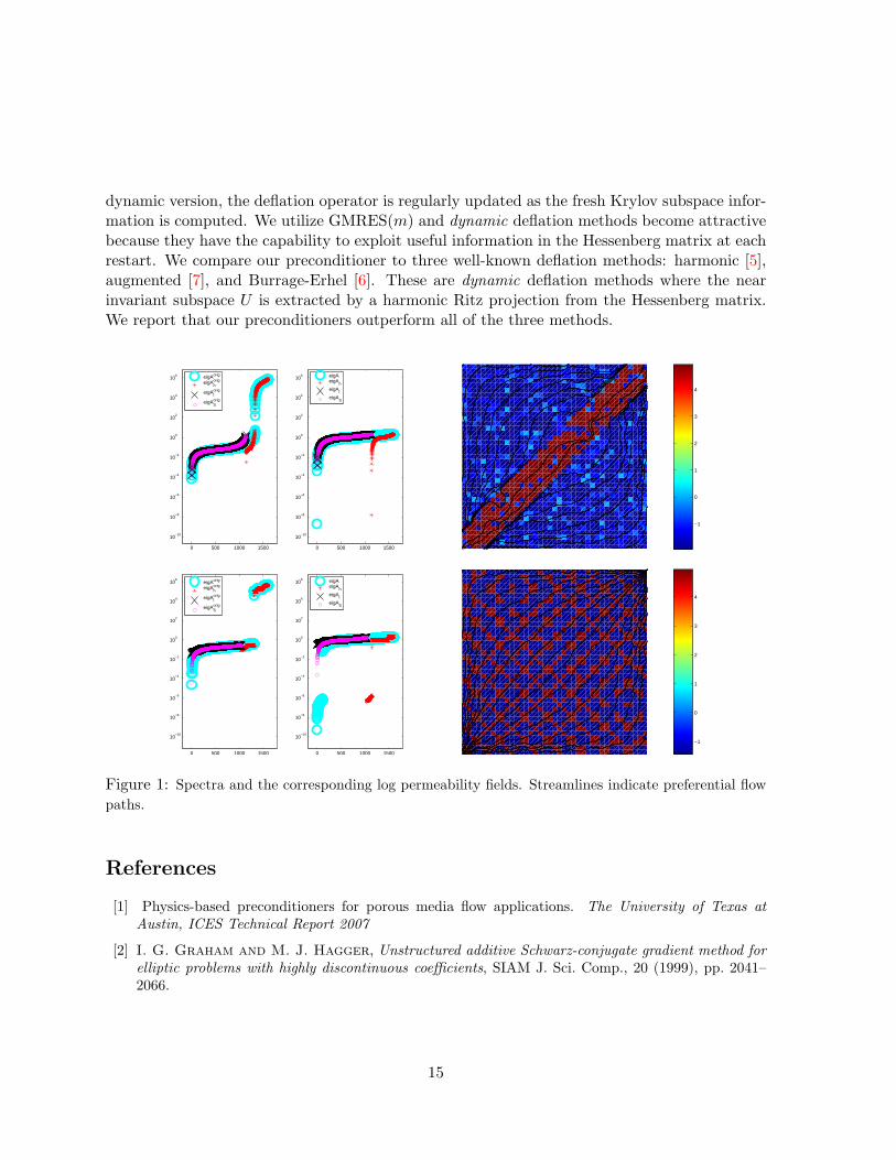
dynamic version, the deflation operator is regularly updated as the fresh Krylov subspace infor-mation is computed. We utilize GMRES(m) and dynamic deflation methods become attractivebecause they have the capability to exploit useful information in the Hessenberg matrix at eachrestart. We compare our preconditioner to three well-known deflation methods: harmonic [5],augmented [7], and Burrage-Erhel [6]. These are dynamic deflation methods where the nearinvariant subspace U is extracted by a harmonic Ritz projection from the Hessenberg matrix.We report that our preconditioners outperform all of the three methods.

0 500 1000 1500

10−10

10−8

10−6

10−4

10−2

100

102

104

106

eigAorig

eigAhorig

eigAlorig

eigASorig

0 500 1000 1500

10−10

10−8

10−6

10−4

10−2

100

102

104

106

eigAeigA

h

eigAl

eigAS

−1

0

1

2

3

4

0 500 1000 1500

10−10

10−8

10−6

10−4

10−2

100

102

104

106

eigAorig

eigAhorig

eigAlorig

eigASorig

0 500 1000 1500

10−10

10−8

10−6

10−4

10−2

100

102

104

106

eigAeigA

h

eigAl

eigAS

−1

0

1

2

3

4

Figure 1: Spectra and the corresponding log permeability fields. Streamlines indicate preferential flowpaths.

References

[1] Physics-based preconditioners for porous media flow applications. The University of Texas atAustin, ICES Technical Report 2007

[2] I. G. Graham and M. J. Hagger, Unstructured additive Schwarz-conjugate gradient method forelliptic problems with highly discontinuous coefficients, SIAM J. Sci. Comp., 20 (1999), pp. 2041–2066.

15

[3] C. Vuik, A.Segal, and J. Meijerink, An efficient preconditioned CG method for the solutionof a class of layered problems with extreme contrasts of coefficients, J. of Comp. Phys., 152 (1999),pp. 385–403.

[4] C. Vuik, A.Segal, J. Meijerink, and G.T.Wijma, The construction of projection vectors fora ICCG method applied to problems with extreme contrasts in the coefficients, J. of Comp. Phys.,172 (2001), pp. 426–450.

[5] J. Erhel, K. Burrage, and B. Pohl, Restarted GMRES preconditioned by deflation, J. ofComput. and Appl. Math., 69 (1996), pp. 303–318.

[6] K. Burrage and J. Erhel, On the performance of various adaptive preconditioned GMRESstrategies, Numer. Linear Alg. Appl., 5 (1998), pp. 101–121.

[7] R. B. Morgan, A Restarted GMRES Method augmented with eigenvectors, SIAM J. Matrix Anal.Appl., 16 (1995), pp. 1154–1171.

5.2 A scalable multi-level preconditioner for matrix-free µ-finite elementanalysis of human bone structures - P. Arbenz

Co-authored by:P. Arbenz 1 U. Mennel 2 M. Sala 3 G. Harry van Lenthe 4 R. Muller 5

The recent advances in microarchitectural bone imaging are disclosing the possibility to assessboth the apparent density and the trabecular microstructure of intact bones in a single measure-ment. Coupling these imaging possibilities with microstructural finite element (µFE) analysisoffers a powerful tool to improve bone stiffness and strength assessment for individual fracturerisk prediction. Many elements are needed to accurately represent the intricate microarchitec-tural structure of bone; hence, the resulting µFE models possess a very large number of degreesof freedom. In order to be solved quickly and reliably on state-of-the-art parallel computers, theµFE analyses require advanced solution techniques. In this paper, we investigate the solution ofthe resulting systems of linear equations by the conjugate gradient algorithm, preconditioned byaggregation-based multigrid methods. We introduce a variant of the preconditioner that doesnot need assembling the system matrix but uses element-by-element techniques to build themultilevel hierarchy. The preconditioner exploits the voxel approach that is common in bonestructure analysis, it has modest memory requirements, while being at the same time robustand scalable. Using the proposed methods, we have solved in less than 10 minutes a modelof trabecular bone composed of 247’734’272 elements, leading to a matrix with 1’178’736’360rows, using only 1024 CRAY XT3 processors.

1ETH Zurich, Institute of Computational Science2ETH Zurich, Institute of Computational Science3ETH Zurich, Institute of Computational Science4K.U. Leuven, Department of Mechanical Engineering5ETH Zurich, Institute for Biomechanics

16

References

[1] P. Arbenz, G. H. van Lenthe, U. Mennel, R. Muller, and M. Sala. A scalable multi-levelpreconditioner for matrix-free µ-finite element analysis of human bone structures. TechnicalReport 543, Institute of Computational Science, ETH Zurich, December 2006. Acceptedfor publication in the Internat. J. Numer. Methods Engrg.

5.3 Using perturbed QR factorizations to solve linear Least Squares prob-lems - H. Avron

Co-authored by:H. Avron 1 E. Ng 2 S. Toledo 3

Introduction This talk will show that the R factor from the QR factorization of a perturbationA of a matrix A is an effective least-squares preconditioner for A. More specifically, we willshow that the R factor of the perturbation is an effective preconditioner if the perturbationcan be expressed by adding and/or dropping a few rows from A or if it can be expressed byreplacing a few columns. If A is rank deficient or highly ill-conditioned, the R factor of aperturbation A is still an effective preconditioner if A is well-conditioned. Such an R factorcan be used in LSQR (an iterative least-squares solver [2]) to efficiently and reliably solve aregularization of the least-squares problem. We will present an algorithm for adding rows with asingle nonzero to A to improve its conditioning; it attempts to add as few rows as possible. Wewill also show that if an arbitrary preconditioner M is effective for A∗A, in the sense that thegeneralized condition number of (A∗A,M) is small, then M is also an effective preconditionerfor A∗A. This shows that we do not necessarily need the R factor of the perturbation A;we can use a preconditioner instead. These results, along with our algorithm for perturbinga matrix to improve its conditioning, have several applications which we will present. Theyallow us to drop rows from a sparse A to increase the sparsity of R. They allow us to solveupdated and downdated least-squares problems efficiently without recomputing the factor orthe preconditioner. They allow us to solve what-if scenarios. They allow us to solve numericallyrank-deficient least-squares problem without a rank-revealing factorization. Some of the resultspresented where already known experimentally (for example in [3]), but apparently without ananalysis of eigenvalues.

Theoretical Results The results presented are based on a comprehensive spectral analysis ofthe generalized spectrum of matrix pencils that arise from row and column perturbations. Thisanalysis is presented in [1]; we will review the main results of this analysis. The first part of theanalysis shows that if the number of rows/columns that are added, dropped, or replaced is small,then most of the generalized eigenvalues are 1. The number of runaway eigenvalues, which are

1Tel-Aviv University2Lawrence Berkeley National Laboratory3Tel-Aviv University

17

the ones that are not 1, is bounded by the number of rows added or dropped (for row perbuta-tions) or by twice the number of columns replaced (for column perbutaitons). This guaranteesrapid convergence of LSQR. The second part of the analysis concentrates on perbutations of apreconditioned system. We address the following question: if M is an effective preconditionerof A∗A is it an effective preconditioner of A∗A? The analysis shows that if the generalizedspectrum of (A∗A,M) is contained in a small interval, then nearly all of (A∗A,M)’s spectrumis contained in the same interval. The number of runaway eigenvalues, in this case ones that areoutside the interval, is bounded by the number of rows added or dropped (for row perbutations)or by twice the number of columns replaced (for column perbutaitons). This guarantees that ifM is an effective preconditioner of A∗A due to well-conditioning of the preconditioned matrix,it is also an effective preconditioner for A∗A. The ability of preconditioned LSQR to solve aregularization of an ill-conditioned system is dependent on whether the numerical rank of thepreconditioned system is similar to the numerical rank of the original system. The third partof the analysis shows that if a preconditioner is obtained from adding rows to A then, undersome restrictions, the numerical rank is maintained up to an appropriate relaxation of the rankthreshold. The restrictions are that the preconditioner is well-conditioned and the norm of theperturbation ois not too large.

Applications to Least-Squares Solvers We have began to explore applications of our theory.Dropping Dense Rows for Sparsity The R factor of A = QR is also the Cholesky factor ofA∗A. Rows of A that are fairly dense cause A∗A to be fairly dense, which usually cause R tobe dense. In the extreme case, a completely dense row in A causes A∗A and R to be completelydense. A simple solution is to drop fairly dense column before the factorization starts, and usethe factor as a preconditioner in LSQR. A sophisticated algorithm to decide when to drop rowsis an open research question.Updating and Downdating Updating a least-squares problem involves adding rows to thecoefficient matrix A and to the right-hand-side b. Downdating involved dropping rows. Ouranalysis shows that after adding and/or dropping a small number of rows from/to A, the Rfactor of A is an effective preconditioner of the new system, as long as the new system is full-rank.Adding Rows to Solve Numerically Rank-Deficient Problems When A is full rankbut highly ill-conditioned, it is desirable to solve a regularization of the least squares problemminx ‖Ax − b‖2, that is a solution of small norm. The factorization A = QR is not useful forsolving ill-conditioned least-squares problems. The factorization is backward stable, but thecomputed R is ill-conditioned. This often causes the solver to produce a solution x = R−1Q∗bwith a huge norm. We propose to add rows to the coefficient matrix A to avoid ill-conditioningin R. The factor R is no longer the R factor of A, but the R factor of a perturbed matrix[

AB

]. Our analysis shows that if R is well-conditioned and only a small number of rows where

added then R is an effective preconditioner for solving the regularized least-squares problemusing LSQR. We present an efficient algorithm that uses a threshold τ ≥ n + 1 to find a Bsuch that ‖B∗B‖2 ≤ m‖A∗A‖2 and κ(A∗A + B∗B) ≤ τ2. Along with finding the perturbationthe R factor of the perturbed matrix is found, usually with a small amount of additional workrelative to finding the R factor of the original matrix. Furthermore, B’s structure guarantees

18

that R factor will fill no more than the original factor. The algorithm attempts to add as fewrows as possible.Solving What-If Scenarios The theory presented in this paper allows us to efficiently solvewhat-if scenarios of the following type. We are given a least squares problem min ‖Ax − b‖2.We already computed the minimizer using the R factor of A or using some preconditioners.Now we want to know how the solution would change if we fix some of its entries, without lossof generality xn−k+1 = cn−k+1, . . . , xn = cn, where the ci’s are some constants. Our analysisshows that for small k the factor or the preconditioner of A is an effective preconditioner for amodified least-squares system that solves the what-if scenario.

References

[1] H. Avron, E. Ng and S. Toledo. Using Perturbed QR Factorizations to Solve Linear Least-Squares Problems Work in progress.

[2] C. Paige and M. Saunders. LSQR: An Algorithm for Sparse Linear Equations and SparseLeast Squares. ACM Trans. Math. Softw., 8(1):43–71, 1982.

[3] P. Gill, W. Murry, M. Saunders, J. Tomlin and M Wright. On Projected Newton BarrierMethods for Linear Programming and an Equivalence to Karmarkar’s Projective Method.Mathematical Programming, 36(2):183–209, 1986.

5.4 Preconditioning techniques for large-scale adaptive optics - J. M. Bard-sley

Co-authored by:J. M. Bardsley 1

In ground-based astronomy, a phase error estimate is typically obtained from a measurement gof the wavefront gradient, which is assumed to satisfy the discrete model

g = Γφ + η.

Here φ denotes the unknown wavefront, Γ a discrete gradient operator and η a Gaussian randomvector with zero mean and covariance matrix σ2I. Early approaches for estimating φ (see, e.g.,[2]) involve computing a solution of the least squares normal equations

ΓT Γφ = ΓT g.

For large-scale adaptive optics systems, however, least squares solutions can be unstable, andhence, the minimum variance estimator is preferred [1]. Minimum variance estimation is a

1Department of Mathematical Sciences, University of Montana, USA.

19

Bayesian statistical approach in which a prior probability density is assumed on the phase. Inour case, it can be accurately assumed that φ is a realization of a Gaussian random vector withzero mean and known covariance matrix Cφ. The minimum variance estimator for φ is then thesolution of the large sparse linear system

(ΓT Γ + σ2C−1φ )φ = ΓT g. (6)

The problem of efficiently solving (6) has seen much recent attention. An efficient direct methodusing sparse matrix techniques is explored in [1]. However, the most computationally efficientapproaches have involved the use of multigrid to precondition conjugate gradient iterations [3].In this talk, I will introduce two new preconditioners. The resulting methods will then becompared with the multigrid preconditioned algorithm of [3] on synthetically generated data.

References

[1] Brent L. Ellerbroek, Efficient computation of minimum-variance wave-front reconstructorswith sparse matrix techniques, J. Opt. Soc. Am. A, 19(9), 2002.

[2] Jan Herrmann, Least-squares wave front errors of minimum norm, J. Opt. Soc. Am., 70(1),1980.

[3] C. R. Vogel and Q. Yang, Multigrid algorithm for least-squares wavefront reconstruction,Applied Optics, 45(4), 2006, pp. 705-715.

5.5 Block preconditioning for saddle point problems with indefinite (1, 1)block - M. Benzi

Co-authored by:M. Benzi 1

We consider preconditioning techniques for the solution of generalized saddle point problems inwhich the symmetric part of the (1, 1) block is indefinite. This problem arises in computationalelectromagnetics and is also an important subproblem in shift-and-invert methods for computingselected eigenvalues of block matrices arising from the stability analysis of incompressible flows.We discuss an approach based on the augmented Lagrangian formulation combined with a blocktriangular preconditioner [1, 2]. The proposed approach is shown to be robust with respect toseveral problem parameters. Numerical experiments on both 2D and 3D problems will bepresented. This is joint work with Jia Liu (University of West Florida) and Maxim Olshanskii(Moscow State University).

1Department of Mathematics and Computer Science, Emory University, Atlanta, GA 30322, USA(benzi@mathcs.emory.edu).

20

References

[1] M. Benzi and J. Liu, Block preconditioning for saddle point systems with in-definite (1, 1) block, Int. J. Comp. Math., to appear (invited paper). Available athttp://www.mathcs.emory.edu/∼benzi.

[2] M. Benzi and M. A. Olshanskii, An augmented Lagrangian-based approach to theOseen problem, SIAM J. Sci. Comput., 28 (2006), pp. 1095–2113.

5.6 Splittings for the two-sided Minimum Residual iteration - M. Byckling

Co-authored by:M. Byckling 1 M. Huhtanen 2

We consider iteratively solving the linear system

Ax = c, (7)

with c ∈ Cn and matrix A ∈ Cn×n that is large and sparse. After splitting A as A = L + R,where L and R are readily invertible, and preconditioning by L from the left, we have

(I + S)x = b, (8)

with b = L−1c and S = L−1R. A Krylov-subspace method for solving linear systems of theform (8) by applying S and S−1 cyclically to the initial residual r0 = b−x0−Sx0 was proposedin [1]. Then two-sided Krylov subspaces

K±j (S; r0) = spanp,q∈Pjp(S)r0, q(S−1)r0 (9)

are generated, where Pj denotes the set of polynomials of degree j at most. Let Ql haveorthonormal columns spanning (9). Then, by using an Arnoldi-type method proposed in [1],we have SQl = Ql+1Hl, with Hl having a Hessenberg-like structure with 2-by-2 subdiagonalblocks. At the mth step of iteration, a correction zm for the iterate xm = x0 +zm is determinedin K±dm

2e(S; r0) by solving the least-squares problem

minz∈K±dm

2 e(S;r0)

||b− (I + S)(x0 + z)||2. (10)

We call this the two-sided minimum residual method (TSMRES). This minimum residual ap-proach is similar to the GMRES method of Saad and Schultz [2], except that the standard

1Institute of Mathematics, Helsinki University of Technology, Box 1100 FIN-02015, Finland(mikko.byckling@tkk.fi)

2Institute of Mathematics, Helsinki University of Technology, Box 1100 FIN-02015, Finland(marko.huhtanen@tkk.fi).

21

Krylov subspace is replaced with the two-sided Krylov subspace. Assuming that operatingwith S and S−1 is computationally equally expensive, the computational complexity of thealgorithms for spanning equidimensional subspaces is essentially the same. There exists severalways to split a matrix into the sum of two readily invertible matrices. The choice of the split-ting affects the properties of S, which defines the convergence rate of the method. We considersome options for the splitting of A and evaluate their performance numerically. A purely al-gebraic way is to take a Gauss-Seidel type of splitting of matrix A to have A = L + R with Llower triangular and R upper triangular. A straightforward extension is to take L and R blocklower and upper triangular; for other possible choices see [3] and references therein. Alreadywith these choices GMRES and TSMRES behave differently. Example 1. We take the matrixsherman5 from the MatrixMarket-collection [6]. The matrix is generated by a fully implicitblack oil simulator and it is of size n = 3312 with 20793 nonzero entries. We split the matrixas A = L + R, where L and R are block lower and- upper triangular matrices with blocksizek = 72. Common diagonal blocks are divided evenly among the two matrices. We comparethe restarted GMRES with restarted TSMRES iteration for the problem (I + S)x = b withrandomly generated right-hand side b having normally distributed entries. The dimension ofthe subspace before restart was chosen as m = 32. The results are shown in figure 2. Anotherextension of the Gauss-Seidel splitting of A is to take L and R lower and upper k-Hessenberg.By an upper (or lower) k-Hessenberg matrix we mean an upper (lower) triangular matrix withk extra non-zero diagonals below (above) the main diagonal, i.e., hi,j = 0, i > j + k (i+ k < j).Denote by τ = τ(n) the density of the matrix, i.e., the ratio of the number of nonzero entriesand n2. Linear systems involving sparse k-Hessenberg matrices with density τ can be solvedin O((k + 1)τn2) operations and O(kn) memory [5]. In addition, this solution procedure onlyrequires knowing the entries of the matrix locally. Therefore k-Hessenberg linear systems withsmall k are readily invertible. Using k-Hessenberg splitting with TSMRES for solving (7) isattractive and convergence theoretically challenging. We are also looking at ways to extendADI type of iterations. Then we have the system (H + V )u = b, in which H and V are as-sumed to be readily invertible [3, 4]. ADI iteration with acceleration parameter ρ > 0 leadsto splitting A = M − N with M = 1

2ρ(H + ρI)(V + ρI) and N = 12ρ(H − ρI)(V − ρI). The

iteration presented in [1] can be regarded to make ADI-iteration optimal when a fixed choiceof parameter ρ is employed.

References

[1] M. Huhtanen and O. Nevanlinna. A Minimum residual Algorithm for Solving LinearSystems. BIT Numerical Mathematics, 46:533–548, 2006.

[2] Y. Saad and M.H. Schultz. GMRES: a generalized minimal residual algorithm for solvingnonsymmetric linear systems. SIAM J. Sci. Stat. Comput., 7:856–869, 1986.

[3] Y. Saad. Iterative Methods for Sparse Linear Systems, 2nd edition. SIAM, Philadelphia,PA, 2003.

22

0 50 100 150 200 250 30010

−10

10−8

10−6

10−4

10−2

100

Matrix−vector products

||b−

x−S

x|| 2/||

b|| 2

Sherman5

GMRESTSMRES

Figure 2: Relative residuals for GMRES(32) (dashed line) and TSMRES(16)-iteration (solidline) for 72-by-72 block triangular splitted matrix Sherman5

[4] G. Starke. Alternating direction preconditioning for nonsymmetric systems of linear equa-tions. SIAM J. Sci. Comput., 15:369–384, 1994.

[5] M. Byckling and M. Huhtanen. Solving sparse k-Hessenberg linear systems. Submitted,2007.

[6] NIST. MatrixMarket http://math.nist.gov/MatrixMarket/.

23

5.7 Multilevel domain decomposition preconditioners for inverse - X.-C. Cai

Co-authored by:X.-C. Cai 1

In this talk we discuss several multilevel domain decomposition preconditioners for solving thesystem of equations arising from the fully coupled finite difference discretization of some inverseelliptic problems in two-dimensional space. We show that with these domain decompositionbased preconditioners good convergence can be obtained both at the linear and the nonlinearlevels even for some difficult cases when the solution is discontinuous and when the observationdata has high level of noise. We also report some promising parallel scalability results of aPETSc based implementation of the methods. This is a joint work with S. Liu and J. Zou.

5.8 Comparison of preconditioners for the simulation of hydroelectric reser-voirs flooding - L. M. Carvalho

Co-authored by:L. M. Carvalho 2 N. Mangiavacchi 3 C. B. P. Soares 4 W. R. Fortes 5 V. S. Costa 6

Introduction

In 2007, the Intergovernmental Panel on Climate Change (IPCC) stated that it is clear thathuman activities have changed the concentrations and distribution of greenhouse gases andaerosols over the 20th century and at the beginning of the 21th [1]. Altering the natural con-centrations of greenhouse gases (GHG) is likely to have significant consequences on the globalclimate. For instance, global mean temperature has increased by 0.3-0.6 oC since the late 19thcentury. Is flooding of soils, consecutive to the creation of water reservoirs, a significant an-thropic source of GHG emissions? And in a mid and long term perspective? Hydroelectricalenergy can be considered a clean energy? The answers of the scientific and industrial commu-nities for these questions are not conclusive [3], [6]. In order to participate to this discussion,we have been developing a numerical simulator for studying water physico-chemical propertiesduring the flooding of hydroelectric plants reservoirs. In the near future, this simulator will beable to analyze the production, stocking, consumption, transport, and emission of carbon diox-ide (CO2)and methane (CH4) in reservoirs. This is a joint work of researchers from Brazilianuniversities and FURNAS S/A, the Brazilian leading company of production and distribution

1Department of Computer Science University of Colorado at Boulder Boulder, CO 80309-0430, USA,cai@cs.colorado.edu

2University of the State of Rio de Janeiro3University of the State of Rio de Janeiro4FURNAS Centrais Eletricas S/A5University of the State of Rio de Janeiro6University of the State of Rio de Janeiro

24

of hydroelectricity, sponsored by the Electric Energy National Agency (ANEEL). The simulatortreats independently the different compartments of a reservoir. This approach allows a fineranalysis of the water quality during the flooding. Nonetheless, the yielded linear systems arehuge, and iterative methods are mandatory. In the first version, the matrices were symmetricand positive definite and we have used the preconditioned conjugate gradient (PCG) method[4, 5]. In the present version, the matrices are nonsymmetric and nonsingular then we apply thegeneralized minimum residual method (GMRES) [7] and the bi-conjugate gradient stabilizedmethod (BI-CGSTAB) [8]. We present the comparison of some well-known preconditioners andreorderings for both methods. We also present another preconditioner and discuss its perfor-mance. In the next sections, we address the simulator mathematical and numerical models, andsome numerical experiments.

Brief description of the model

The dimensionless unsteady incompressible Navier-Stokes equations in primitive variables canbe written as

∂u∂t

+ u · ∇u = −∇p +1

Re∇2u

∇ · u = 0,

where u, p are the nondimensional velocity vector and kinetic pressure, and Re is the Reynoldsnumber. We are using well-known and well-tested methods for numerically solving this system:we discretize via finite elements using the mini-element approach; to treat the nonlinearity ofthe convective term, we use a semi-Lagragian scheme. The matrix form of the system is(

A GD 0

)(up

)=(

b1b2

). (11)

One of the implemented numerical solutions is a projection method [2], which produces thefollowing factorization for the original matrix (11)(

A GD 0

)=(

A 0D −DA−1G

)(I A−1D0 I

), (12)

where A is an approximation for A. Depending on some assumptions the complete system canbe symmetric or nonsymmetric. We consider the case that A is symmetric and positive definite,and G = DT . For problems with very large Reynolds numbers A can be assumed diagonal.Then −DA−1G is also symmetric and both systems can be solved using PCG. Using anotherapproach, we solve the complete system (11) with different preconditioners and reorderings.Particularly, we have been testing a new variant of preconditioner for this problem: we usethe projection decomposition (12) as the preconditioner for the complete problem (11), in thefollowing this preconditioner is called Projection.

Numerical tests

In table 1, we summarize the figures for a test running in Matlab, on a Pentium 4, with 1.5Gbof RAM. We simulate a bi-dimensional channel flow with two different step size times (probs.

25

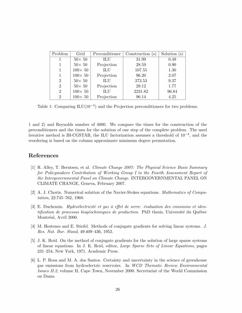
Problem Grid Preconditioner Construction (s) Solution (s)1 50× 50 ILU 31.99 0.491 50× 50 Projection 28.59 0.901 100× 50 ILU 107.55 1.301 100× 50 Projection 96.20 2.072 50× 50 ILU 273.53 9.372 50× 50 Projection 29.12 1.772 100× 50 ILU 2231.82 96.842 100× 50 Projection 96.14 4.25

Table 1: Comparing ILU(10−4) and the Projection preconditioners for two problems.

1 and 2) and Reynolds number of 4000. We compare the times for the construction of thepreconditioners and the times for the solution of one step of the complete problem. The usediterative method is BI-CGSTAB, the ILU factorization assumes a threshold of 10−4, and thereordering is based on the column approximate minimum degree permutation.

References

[1] R. Alley, T. Berntsen, et al. Climate Change 2007: The Physical Science Basis Summaryfor Policymakers Contribution of Working Group I to the Fourth Assessment Report ofthe Intergovernmental Panel on Climate Change. INTERGOVERNMENTAL PANEL ONCLIMATE CHANGE, Geneva, February 2007.

[2] A. J. Chorin. Numerical solution of the Navier-Stokes equations. Mathematics of Compu-tation, 22:745–762, 1968.

[3] E. Duchemin. Hydroelectricite et gaz a effet de serre: evaluation des emissions et iden-tification de processus biogeochimiques de production. PhD thesis, Universite du QuebecMontreal, Avril 2000.

[4] M. Hestenes and E. Stiefel. Methods of conjugate gradients for solving linear systems. J.Res. Nat. Bur. Stand, 49:409–436, 1952.

[5] J. K. Reid. On the method of conjugate gradients for the solution of large sparse systemsof linear equations. In J. K. Reid, editor, Large Sparse Sets of Linear Equations, pages231–254, New York, 1971. Academic Press.

[6] L. P. Rosa and M. A. dos Santos. Certainty and uncertainty in the science of greenhousegas emissions from hydroelectric reservoirs. In WCD Thematic Review EnvironmentalIssues II.2, volume II, Cape Town, November 2000. Secretariat of the World Commissionon Dams.

26

[7] Y. Saad and M. H. Schultz. GMRES: a generalized minimal residual algorithm for solvingnonsymmetric linear systems. SIAM J. Sci. Stat. Comput., 7(3):856–869, 1986.

[8] H. Van der Vorst. BI-CGSTAB: a fast and smoothly converging variant of BI-CG for thesolution of non-symmetric linear systems. SIAM Journal on Scien. and Stat. Computing,13(2):631–644, March 1992.

5.9 Improving preconditioners in interior-point methods for optimizationthrough quadratic regularizations - J. Castro

Co-authored by:J. Castro 1 J. Cuesta 2

Interior-point methods [7] are polynomial time algorithms for the solution of linear optimizationproblems

min cT xsubject to Ax = b

x ≥ 0.(13)

where A ∈ Rm×n,m < n, is assumed to have full row-rank. These methods are specially suitedfor very large-scale optimization problems. Its main computational burden is the solution ateach iteration of linear systems of equations with matrix AΘAT , Θ being a diagonal matrix.Those systems are usually solved by a sparse Cholesky factorization.

Despite its efficiency, for some classes of matrices A, as the primal block-angular onesN1

N2

. . .Nk

L1 L2 . . . Lk I

, (14)

they are computationally expensive due to the fill-in of AΘAT . For instance, for multicommod-ity network flows, a class of primal block-angular problems, the fill-in was proven to be veryhigh. The specialized interior-point algorithm of [3] for multicommodity flows overcame thisproblem by solving systems AΘAT trough a scheme that combined Cholesky factorizations forthe submatrix of AΘAT associated to the diagonal blocks of (14) and a preconditioned conjugategradient (PCG) for the subsystem associated to the linking constraints (last block of equationsin (14)). The particular preconditioner used is based on a splitting P − Q of the system ma-trix, and a truncated power series expansion (Neumann’s series) that approximates its inverse.

1Dept. of Statistics and Operations Research, Universitat Politecnica de Catalunya, Jordi Girona 1–3, 08034Barcelona, Catalonia, jordi.castro@upc.edu

2Unit of Statistics and Operations Research, Dept. of Chemical Engineering, Universitat Rovira i Virgili, Av.dels Paısos Catalans 26, 43007 Tarragona, Catalonia, jcuesta@xtec.net

27

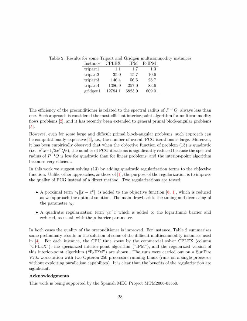
Table 2: Results for some Tripart and Gridgen multicommodity instancesInstance CPLEX IPM R-IPMtripart1 1.1 1.7 1.3tripart2 35.0 15.7 10.6tripart3 146.4 56.5 28.7tripart4 1386.9 257.0 83.6gridgen1 12784.1 6823.0 609.0

The efficiency of the preconditioner is related to the spectral radius of P−1Q, always less thanone. Such approach is considered the most efficient interior-point algorithm for multicommodityflows problems [2], and it has recently been extended to general primal block-angular problems[5].

However, even for some large and difficult primal block-angular problems, such approach canbe computationally expensive [4], i.e., the number of overall PCG iterations is large. Moreover,it has been empirically observed that when the objective function of problem (13) is quadratic(i.e., cT x+1/2xT Qx), the number of PCG iterations is significantly reduced because the spectralradius of P−1Q is less for quadratic than for linear problems, and the interior-point algorithmbecomes very efficient.

In this work we suggest solving (13) by adding quadratic regularization terms to the objectivefunction. Unlike other approaches, as those of [1], the purpose of the regularization is to improvethe quality of PCG instead of a direct method. Two regularizations are tested:

• A proximal term γk||x − xk|| is added to the objective function [6, 1], which is reducedas we approach the optimal solution. The main drawback is the tuning and decreasing ofthe parameter γk.

• A quadratic regularization term γxT x which is added to the logarithmic barrier andreduced, as usual, with the µ barrier parameter.

In both cases the quality of the preconditioner is improved. For instance, Table 2 summarizessome preliminary results in the solution of some of the difficult multicommodity instances usedin [4]. For each instance, the CPU time spent by the commercial solver CPLEX (column“CPLEX”), the specialized interior-point algorithm (“IPM”), and the regularized version ofthis interior-point algorithm (“R-IPM”) are shown. The runs were carried out on a SunFireV20z workstation with two Opteron 250 processors running Linux (runs on a single processorwithout exploiting parallelism capabilites). It is clear than the benefits of the regularization aresignificant.

Acknowledgments

This work is being supported by the Spanish MEC Project MTM2006-05550.

28

References

[1] A. Altman and J. Gondzio, Regularized symmetric indefinite systems in interior pointmethods for linear and quadratic optimization, Optimization Methods and Software, 11,275–302, 1999.

[2] R. E. Bixby, Solving real-world linear programs: a decade and more of progress, OperationsResearch, 50, 3–15, 2002.

[3] J. Castro, A specialized interior-point algorithm for multicommodity network flows, SIAMJournal on Optimization, 10, 852–877, 2000.

[4] J. Castro, Solving difficult multicommodity problems through a specialized interior-pointalgorithm, Annals of Operations Research, 124, 35–48, 2003.

[5] J. Castro, An interior-point approach for primal block-angular problems, ComputationalOptimization and Applications, in press, 2007.

[6] R. Setiono, Interior proximal point algorithm for linear programs, Journal of OptimizationTheory and Applications, 74, 425–444, 1992.

[7] S.J. Wright, Primal-Dual Interior-Point Methods, SIAM: Philadelphia, 1996.

5.10 A high-performance method for the biharmonic dirichlet problem onrectangles - C. C. Christara

Co-authored by:C. C. Christara 1 J. Zhang 2

We propose a fast solver for the linear system resulting from the application of a sixth-orderBi-Quartic Spline Collocation method to the biharmonic Dirichlet problem on a rectangle. Thefast solver is based on Fast Fourier Transforms (FFTs) and preconditioned GMRES (PGMRES)and has complexity O(n2 log(n)) on an n× n uniform partition. The FFTs are applied to twoauxiliary problems with different boundary conditions on the two vertical sides of the domain,while the PGMRES is applied to a problem related to the two vertical boundaries. We showthat the number of PGMRES iterations required to reduce the relative residual to a certaintolerance is independent of the gridsize n. Numerical experiments verify the effectiveness of thesolver.

1Department of Computer Science, University of Toronto2 Department of Computer Science, University of Toronto and Scotiabank, Toronto

29

The biharmonic Dirichlet problem on a rectangle is a two-dimensional fourth-order partialdifferential equation (PDE) problem given by

42u = g in Ω, (15)u = g1 on ∂Ω, (16)

∂u

∂n= g2 on ∂Ω, (17)

where 4 denotes the Laplacian, Ω is a rectangular domain, ∂Ω is the boundary of Ω, ∂/∂n isthe outer normal derivative on ∂Ω, and g, g1 and g2 are given functions of variables x and y.This problem arises in several scientific, engineering and industrial applications. For example,the biharmonic problem for the bending of a clamped rectangular plate has been considered as“one of the classical problems in the Theory of Elasticity” [4].

Various numerical methods have been developed for problem (15)-(17). These methods consistof a discretization strategy that converts the continuous problem into a discrete set of algebraicequations, and an associated solver for the resulting linear system. The effectiveness of anumerical method for a problem such as (15)-(17) depends primarily on the accuracy of thediscretization strategy and the efficiency of the solver.

We first introduce a Bi-Quartic Spline Collocation (BQSC) discretization method for generaltwo-dimensional linear fourth-order Boundary Value Problems involving variable coefficientsand any derivatives of the unknown function up to fourth order in the PDE operator and up tothird order in the boundary conditions operator. The discretization error for this method turnsout to be sixth order locally on the gridpoints and midpoints of a uniform rectangular partitionand fifth order globally in the uniform norm.

We then present two instances of biharmonic problems:(A) the problem (15)-(17), with g = g1 = g2 = 0 on the unit square;(B) the problem consisting of PDE (15) with boundary conditions

u = 0,∂2u

∂x2= 0 on x = 0, x = 1, for 0 ≤ y ≤ 1, (18)

u = 0,∂u

∂y= 0 on y = 0, y = 1, for 0 ≤ x ≤ 1. (19)

Notice that Problems (A) and (B) differ only in the boundary conditions along the verticalboundaries. Our goal is the efficient solution of Problem (A). The main ingredients of thesolution technique are a fast solver for Problem (B) and a preconditioned iterative solution ofa Schur-complement problem related to the two vertical boundaries. Below, we summarize themain results of this paper.

We give the tensor product form of the matrices arising from the application of the BQSCmethod to Problems (A) and (B). We develop explicit formulae for the eigenvalues and eigen-vectors of some of the constituent matrices. Based on these formulae, an FFT (direct) solverwith complexity O(n2 log n) is developed for the matrix of Problem (B).

30

A solution technique for the matrix arising from the application of the BQSC method to Problem(A) is then developed, which consists of two applications of the FFT solver to Problem (B) andthe solution of an one-dimensional problem along the two opposite boundaries of the domain,which can be viewed as a Schur-complement problem. This problem is solved by GMRES andappropriate preconditioners.

The analysis of PGMRES for the matrix A arising from the one-dimensional Schur-complementproblem is based on finding a lower bound above 0 for the minimum eigenvalue of A

T +A2 and an

upper bound for the maximum eigenvalue of ATA. Both bounds are shown to be independentof n, the size of the partition in one dimension. Using these bounds and a well-known result forthe convergence of the GMRES method ([5], pages 134 and 193), we show that the PGMRESmethod converges to a specified tolerance in a number of iterations independent of n. Withthe cost of each iteration being O(n2), the complete solver for Problem (A) runs at O(n2 log n)flops. The solver can be easily extended to problem (15)-(17) with non-homogeneous boundaryconditions.

Experimental results demonstrate the accuracy of the BQSC method, and verify the theoreticalanalysis of the convergence of PGMRES and the efficiency of the algorithm applied to problem(15)-(17).

Among the fast solvers for the biharmonic Dirichlet problem found in the literature, the one thatis closest to ours is the method in [2]. However, in [2], the discretization is obtained by standardsecond order finite differences, the arising matrices are symmetric and the PCG method is usedfor the solution of the problem related to the two opposite boundaries. Consequently, theconvergence analysis is simpler. Some other relevant methods found in the literature are themethods in [3, 1] which also solve a Schur complement problem related to the two oppositeboundaries. However, the methods in [3, 1] reduce the biharmonic to a coupled system ofsecond order PDEs, and apply fourth order discretizations to it, while we apply a sixth orderdiscretization directly to the fourth order derivatives.

References

[1] B. Bialecki. A fast solver for the orthogonal spline collocation solution of the biharmonicDirichlet problem on rectangles. Journal of Computational Physics, 191:601–621, 2003.

[2] P. Bjørstad. Fast numerical solution of the biharmonic Dirichlet problem on rectangles.SIAM Journal on Numerical Analysis, 20:59–71, 1983.

[3] D. B. Knudson. A piecewise Hermite bicubic finite element Galerkin method for the bihar-monic Dirichlet problem. PhD thesis, Colorado School of Mines, Golden, Colorado, U.S.A.,1997.

[4] V. V. Meleshko. Selected topics in the history of the two-dimensional biharmonic problem.Applied Mechanics Reviews, 56(1):33–85, 2003.

31

[5] Y. Saad. Iterative methods for sparse linear systems. PWS, 1996.

5.11 A nested domain decomposition preconditioner based on a hierarchicalh-adaptive finite element code - C. Corral

Co-authored by:C. Corral 1 J.J. Rodenas 2 J. Mas 3 J. Albelda 4 C. Adam 5

In [1] it is showed that the terms used to evaluate element stiffness matrices of geometricallysimilar finite elements (ke =

∫BtDB |J | dV ) are related by a constant, which is a function

of the ratio of element sizes (scaling factor). This geometrical similarity appears in h-adaptiverefinements based on element splitting. This and other parent-child relations were used in abasic implementation of a hierarchical 2-D h-adaptive Finite Element code, based on elementsubdivision, for linear elasticity problems. This hierarchical structure has been used in [2] toobtain a natural domain decomposition and an iterative solver has been developed. Memoryrequirements and execution times have been considerably reduced with the proposed solvercomparing to a reference solver without reordering strategies. In this paper the hierarchicaldata structure of the program is used to generate a nested domain decomposition of differentlevels. Figure 3 shows an example of the structure of the original stiffness matrix, the arrowheadmatrix obtained considering subdomains of level one as used in [2], and the nested arrowheadmatrix obtained by nested domain decomposition of level four. Since the stiffness matrix issymmetric and positive definite, we propose preconditioners for the conjugate gradient methodthat make use of the block structure. The first strategy consists of computing incompleteCholesky factorizations of the main diagonal blocks of the reordered stiffness matrix. The secondstrategy consists of evaluating an incomplete Cholesky factorization of the whole reorderedmatrix. Some numerical tests are included in order to compare these two preconditionerswith a reference solver without reordering strategies and to evaluate the relevance of the useof nested domain decompositions. Acknowledgements: This work has been supported by Ministerio de

Ciencia y Tecnologıa (grants DPI2004-07782-C02-02 and MTM2004-02998).

References

[1] J.J. Rodenas, J.E. Tarancon, J. Albelda, A. Roda, and J. Fuenmayor. Hierarquical prop-erties in elements obtained by subdivision: a hierarquical h-adaptivity program. Adaptive

1Instituto de Matematica Multidisciplinar, Universidad Politecnica de Valencia, Valencia, Spain2Centro de Investigacion de Tecnologıa de Vehıculos (CITV), Departamento de Ingenierıa Mecanica y de

Materiales, Universidad Politecnica de Valencia, Valencia, Spain3Instituto de Matematica Multidisciplinar, Universidad Politecnica de Valencia, Valencia, Spain4Centro de Investigacion de Tecnologıa de Vehıculos (CITV), Departamento de Ingenierıa Mecanica y de

Materiales, Universidad Politecnica de Valencia, Valencia, Spain5Centro de Investigacion de Tecnologıa de Vehıculos (CITV), Departamento de Ingenierıa Mecanica y de

Materiales, Universidad Politecnica de Valencia, Valencia, Spain

32

(A) (B) (C)

Figure 3: Structures of the stiffness matrix: (A) Original. (B) Reordering by one level subdo-mains. (C) Reordering by recursive subdomain decomposition

Modeling and Simulation 2005, P. Dıez and N.E. Wiberg Editors, CIMNE, 2005.

[2] J.J. Rodenas, J. Albelda, C. Corral, and J. Mas. Domain decomposition iterative solverbased on a hierarchical h-adaptive finite element code. Proceedings of the Fifth Interna-tional Conference on Engineering Computational Technology, Las Palmas de Gran Canaria,Spain, ISBN: 1-905088-10-8 (CD-ROM), 2006.

5.12 Iterative solution of saddle-point problems for PDE-constrained prob-lems - H. S. Dollar

Co-authored by:H. S. Dollar 1 N. I. M. Gould 2 W. H. A. Schilders 3 A. J. Wathen 4

In a recent paper by Forsgren, Fill and Griffin [1], the authors consider the solution of saddle-point problems of the form [

H AT

A −C

]︸ ︷︷ ︸

K

x = b,

where H is symmetric and C is assumed to be symmetric and positive definite. The authorsrewrite the system as an equivalent doubly augmented system which has the property of beingsymmetric and positive definite, thus allowing the use of the conjugate gradient method to solve

1 Rutherford Appleton Laboratory2 Oxford University and Rutherford Appleton Laboratory3 Technical University of Eindhoven and NXP Semiconductors4 Oxford University

33

the saddle-point system. Importantly, the preconditioning step may be carried out by solvinga system of the form [

G AT

A −C

]︸ ︷︷ ︸

P

z = r,

where G is a symmetric and A approximates A in some way. In this talk we will considerthe case of C being symmetric and positive semi-definite (possibly zero) and show that we canalso rewrite these systems as equivalent symmetric and positive definite systems. This alsoallows us to use a preconditioning step of the above form: we will call P an inexact constraintpreconditioner. In PDE-constrained problems, the dimension of K may be huge (O(109))and, hence, the use of an inexact constraint preconditioner along with a conjugate gradientmethod is extremely desirable. We will show that although K may be highly ill-conditioned, theeigenvalues which determine the convergence of our method will be O(1) with many clusteringaround 1, thus resulting in rapid convergence of our iterative method. Our theoretical resultswill be backed up with numerical examples.

References

[1] A. Forsgren, P. E. Gill, and J. D. Griffin, Iterative solution of augmented sys-tems arising in interior methods, Tech. Report TRITA-MAT-2005-OS3, Department ofMathematics, Royal Institute of Technology, 2005.

5.13 An hybrid direct-iterative solver based on a hierarchical interface de-composition - J. Gaidamour

Co-authored by:J. Gaidamour 1 P. Henon 2 J. Roman 3 Y. Saad 4

Parallel sparse direct solvers are now able to solve efficiently real-life three-dimensional prob-lems having in the order of several millions of equations. They are, however, constrained byprohibitive memory requirements. Iterative methods on the other hand require much less mem-ory, but they often fail to solve ill-conditioned systems. We propose an hybrid direct-iterativemethod which aims at bridging the gap between these two classes of method. In recent years,

1ScAlApplix Project, INRIA Futurs, LaBRI UMR 5800 and MAB UMR 5466, Universite Bordeaux 1, 33405Talence Cedex, France, gaidamou@labri.fr

2 ScAlApplix Project, INRIA Futurs, LaBRI UMR 5800 and MAB UMR 5466, Universite Bordeaux 1, 33405Talence Cedex, France, henon@labri.fr

3 ScAlApplix Project, INRIA Futurs, LaBRI UMR 5800 and MAB UMR 5466, Universite Bordeaux 1, 33405Talence Cedex, France, roman@labri.fr

4 University of Minnesota, 200 Union Street S.E., Minneapolis, MN 55455 (saad@cs.umn.edu).

34

a few Incomplete LU factorization techniques were developed with the goal of combining someof the features of standard ILU preconditioners with the good scalability features of multi-levelmethods. The key feature of these techniques is to reorder the system in order to extract par-allelism in a natural way. Often a number of ideas from domain decomposition are utilized andcombined to derive parallel factorizations [1, 2, 3]. We propose an approach which is in thiscategory.

The principle of this approach is to build a decomposition of the adjacency graph of the systeminto a set of small subdomains (the typical size of a subdomain is around a few hundreds orthousand nodes) with overlap. We build this decomposition from the separator tree obtained bya nested dissection ordering such as one that is computed by sparse matrix ordering software.

Thus, at a certain level of the separator tree, the subtrees rooted in this level are considered asthe interior of a subdomains partition and then the union of the separators in the upper partof the elimination tree constitutes the interface between these subdomains.

In [4], we introduce a Hierarchical Interface Decomposition (HID) which generalizes the notionof “faces” and “edge” of the “wire-basket” decomposition [5]. This consists in partitioning theset of unknowns of the interface into components called connectors that are grouped in “levels”of independent connectors; a level of connectors plays the role of separators for the immediateinferior level.

If we partition the matrix A according to an ordering associated with listing interior pointsfirst, followed by interface points, then we can define a block incomplete LU factorization asfollows:

A =(

B FE C

)≈(

LEU−1 LS

)×(

U L−1FUS

).

Here we assume that B = LU is a direct factorization of B and that LSUS is some incompletefactorization of the Schur complement matrix S = C − (EU−1)(L−1F ). The HID gives anatural dense block structure of the Schur complement on the interface nodes that can becomputed statically from the adjacency graph of the matrix A. Thus we are able to efficientlycompute block ILU preconditioners which allow the use of BLAS routines both in the directand iterative parts of the solver, with a high degree of parallelism. Figure 4 pictures a denseblock structure of the factors that can be obtained thanks to the HID ordering.

We define a two level solver using the equalities:xB = B−1(yB − F.xC)xC = S−1(yC − E.B−1yB)

Thanks to the direct factorization of the matrix B part, we can solve the first equation exactly.Then solving the whole system amounts to solving the Schur complement system on the interfacebetween the subdomains. A Krylov subspace method is used so solve the Schur complementsystem, preconditioned with LS and US .

We propose several algorithmic variants to solve the Schur complement system that can beadapted to the geometry and the numerical difficulty of the problem: typically some strategies

35

Figure 4: Fill-in of the matrix BCSSTK14 reordered according to the HID ordering with astrictly consistent nonzero pattern.

are more suitable for systems coming from a 2D problem discretization and others for a 3Dproblem; the choice of the method also depends on the numerical difficulty of the problem.

The figure 5 shows the performance of two different choices of the block sparse pattern of LS

and US on the MHD1 test case (unsymmetric matrix with 485 597 unknowns and 24 233 141nonzeros). This problem comes from a 3D magneto-hydrodynamic test case discretized on afinite element mesh composed of mixed tetrahedra and hexahedra elements. The strictly con-sistent dropping consists in prohibiting any fill-in entry between two uncoupled connectors ofa same level which preserve the diagonal block structure in each level. The locally consistentdropping allows fill-ins between connectors belonging to the same subdomain (in order to pre-serve the potential parallelism induced by the domain decomposition). The curves on the leftfigure show the number of iterations in function of the number of small subdomains createdand the curves on the right figure show the total sequential time to build the preconditionerand solve the system. These tests were performed on an IBM power 5. The locally consistentdropping achieves a faster convergence and the number of iteration seems asymptotically inde-pendent from the number of subdomains. However, it requires more computations to build thepreconditioner and to solve the triangular systems at each iteration than the strictly consistentdropping which performs better in time for this case. Of course, a time comparison is verydependent on the precision asked and the intrinsic difficulty of the problem. Also, note thatthe total sequential time increases when the number of small domains becomes two importantwhich may seem odd since the preconditioner becomes sparser: this is due to the fact that theBLAS efficiency is mush lower on dense blocks with small dimensions as those obtained in thefactors for a graph decomposition into very small subdomains.

The parallelisation of the solver consists in partitioning the set of small subdomains betweenthe set of processors in order to preserve a good load balancing. The talk will present theperformance of our solver using this parallelisation and a comparison of the different strategyon model problems as well as referenced tests cases.

36

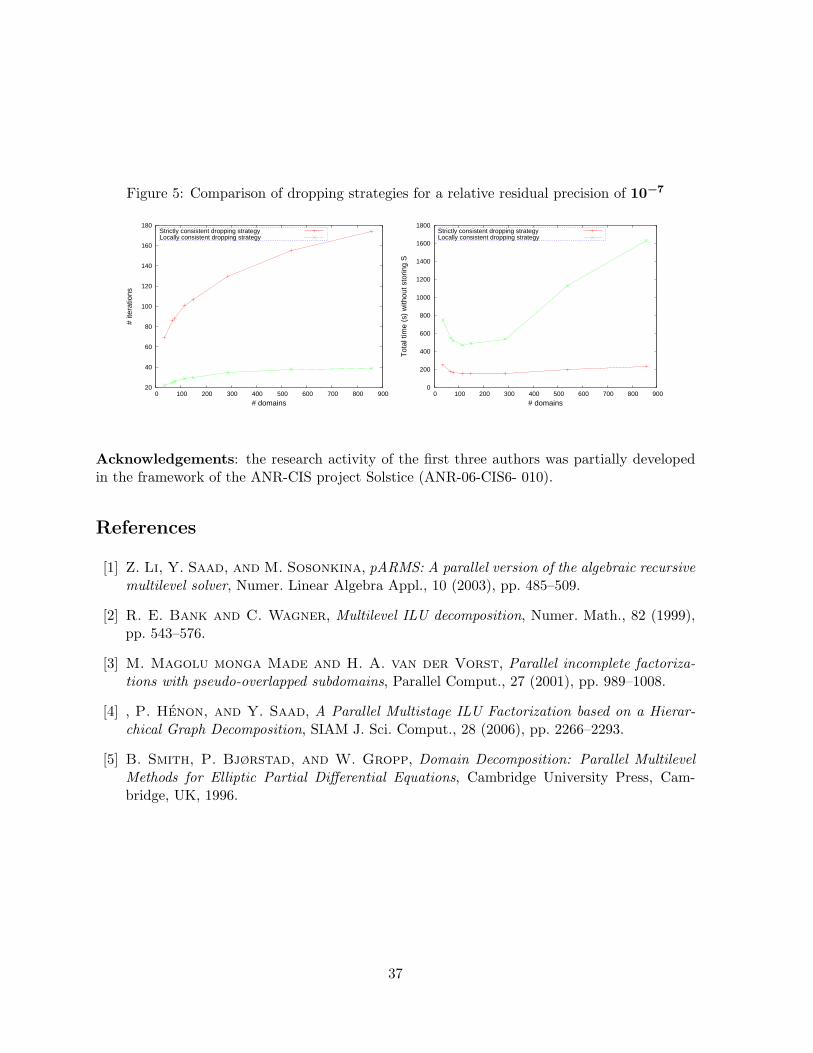
Figure 5: Comparison of dropping strategies for a relative residual precision of 10−7

20

40

60

80

100

120

140

160

180

0 100 200 300 400 500 600 700 800 900

# ite

ratio

ns

# domains

Strictly consistent dropping strategyLocally consistent dropping strategy

0

200

400

600

800

1000

1200

1400

1600

1800

0 100 200 300 400 500 600 700 800 900

Tot

al ti

me

(s)

with

out s

torin

g S

# domains

Strictly consistent dropping strategyLocally consistent dropping strategy

Acknowledgements: the research activity of the first three authors was partially developedin the framework of the ANR-CIS project Solstice (ANR-06-CIS6- 010).

References

[1] Z. Li, Y. Saad, and M. Sosonkina, pARMS: A parallel version of the algebraic recursivemultilevel solver, Numer. Linear Algebra Appl., 10 (2003), pp. 485–509.

[2] R. E. Bank and C. Wagner, Multilevel ILU decomposition, Numer. Math., 82 (1999),pp. 543–576.

[3] M. Magolu monga Made and H. A. van der Vorst, Parallel incomplete factoriza-tions with pseudo-overlapped subdomains, Parallel Comput., 27 (2001), pp. 989–1008.

[4] , P. Henon, and Y. Saad, A Parallel Multistage ILU Factorization based on a Hierar-chical Graph Decomposition, SIAM J. Sci. Comput., 28 (2006), pp. 2266–2293.

[5] B. Smith, P. Bjørstad, and W. Gropp, Domain Decomposition: Parallel MultilevelMethods for Elliptic Partial Differential Equations, Cambridge University Press, Cam-bridge, UK, 1996.

37

5.14 Parallel performance of two different applications of a domain decom-position technique to the Jacobi-Davidson method - M. Genseberger

Co-authored by:M. Genseberger 1

The Jacobi-Davidson method [4] is an iterative method suitable for computing solutions oflarge eigenvalue problems. For the computation of a solution (λ, x) to the standard eigenvalueproblem A x = λ x, in each iteration, this method extracts an approximate solution (θ, u) froma search subspace, corrects the approximate eigenvector u by computing a correction vectorfrom a correction equation, and uses the correction vector to expand the search subspace. Mostcomputational work of Jacobi-Davidson is due to the correction equation at the intermediatelevel. In [1, 2] a strategy for the computation of (approximate) solutions of the correctionequation was proposed. The strategy is based on a domain decomposition technique [5, 6] inorder to reduce wall clock time and local memory requirements.This talk discusses the aspect that the original strategy in [1, 2] can be improved by taking intoaccount the relation of the intermediate level with the top level of the Jacobi-Davidson method.This results in a different application of the domain decomposition technique to the Jacobi-Davidson method. Although the two approaches look similar, there are subtle differences inimplementation and the consequences in terms of computational time for large scale eigenvalueproblems are nontrivial.

First, the main ingredients of the domain decomposition technique are summarized. The tech-nique is based on a nonoverlapping additive Schwarz method with locally optimized couplingparameters by Tan & Borsboom [5, 6] which is a generalization of work by Tang [7].Consider some partial differential equation defined on a domain. Let the linear system B y = ddescribe the partial differential equation after discretization, with matrix B corresponding tothe discretized operator and y to the unknowns defined on the gridpoints, respectively. Thedomain is decomposed in nonoverlapping subdomains. The subdomains are covered by subgridssuch that no splitting of the original discretized operator has to be made. For that purpose,additional, so-called virtual gridpoints near the interfaces of the subdomains are introduced.This results in extra unknowns defined on the virtual gridpoints, coupled to their counterpartsin the opposite subdomain via a small coupling matrix C.The domain decomposition technique enhances the linear system B y = d to a so-called en-hanced linear system BC y∼ = d0. The matrix BC and vector y∼ correspond to the discretizedoperator and unknowns (including those on the virtual gridpoints) defined on the subdomains,respectively. BC is splitted in BC = M−N such that the preconditioner M is invertible locallyon subdomains. A solution is computed with a Krylov method with Km

(M−1 BC , M−1 d0

).

C is tuned such that errors due to the splitting BC = M − N are damped “as much aspossible”, optimal choices result in a coupling that annihilates the outflow from one domainto another: absorbing boundary conditions. This leads effectively to almost uncoupled sub-

1Amsterdam, The Netherlands

38

problems at subdomains: an ideal situation for implementation on parallel computers and/ordistributed memory.

The linear system that is described by the correction equation of the Jacobi-Davidson method,may be highly indefinite and is given in an unusual manner so that the application of the domaindecomposition technique needed special attention. This has been done in [1, 2].

However, there is more to gain. If solutions to the correction equation are computed with apreconditioned Krylov method then Jacobi-Davidson consists of two nested iterative solvers.In the innerloop a search subspace for the (approximate) solution of the correction equation isbuilt up by powers of M−1 ( A− θ I ) for fixed θ. In the outerloop a search subspace for the(approximate) solution of the eigenvalue problem is built up by powers of M−1 ( A− θ I ) forvariable θ. In [1, 2] the domain decomposition technique was applied to the innerloop. But,as θ varies slightly in succeeding outer iterations, one may take advantage of the nesting byapplying the same technique to the outerloop. From now on, application of the technique tothe innerloop will be labeled with “Jacobi-Davidson with enhanced innerloop”, application tothe outerloop with “Jacobi-Davidson with enhanced outerloop”.For exact solution of the correction equation both approaches are equivalent. Approximate so-lutions of the correction equation affect the two processes differently. The following numericalexample in Matlab illustrates this phenomenon. Jacobi-Davidson is applied to the discretizedeigenvalue problem for the two dimensional Laplace operator on the unit square. For the con-struction of the preconditioner, the unit square is decomposed into 8 × 8 square subdomains,each subdomain covered by a 25 × 25 grid. Per outer iteration, we compute approximate so-lutions to the correction equations of Jacobi-Davidson with enhanced innerloop and enhancedouterloop with right preconditioned GMRES(m) [3]. To obtain approximate solutions of dif-ferent accuracy, three fixed values for m are considered: m = 4, 8, and 16.

JD with GMRES(4) and enhanced JD with GMRES(8) and enhancedstep innerloop outerloop step innerloop outerloop1 6.23e+00 6.23e+00 1 6.23e+00 6.23e+002 1.14e+01 2.23e-01 2 4.67e-01 1.12e-023 4.00e+00 1.13e-01 3 6.65e-03 1.59e-044 3.19e-01 1.13e-04 4 9.88e-05 4.78e-075 4.24e-02 6.59e-05 5 2.43e-06 5.01e-106 8.59e-03 1.21e-06 6 1.61e-087 1.67e-03 1.34e-07 7 3.39e-108 2.04e-04 4.43e-099 2.23e-05 1.47e-10 JD with GMRES(16) and enhanced10 2.66e-06 step innerloop outerloop11 2.42e-07 1 6.23e+00 6.23e+0012 3.23e-08 2 1.13e-02 1.13e-0213 2.70e-09 3 9.41e-07 2.41e-0914 3.42e-10 4 1.10e-10 2.70e-11

39

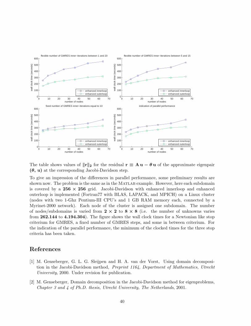
0 10 20 30 40 50 60 700

100

200

300

400

500

600

number of nodes

wal

l clo

ck ti

me

(sec

onds

)

flexible number of GMRES inner−iterations between 1 and 20

enhanced innerloopenhanced outerloop

0 10 20 30 40 50 60 700

100

200

300

400

500

600

number of nodes

wal

l clo

ck ti

me

(sec

onds

)

flexible number of GMRES inner−iterations between 5 and 15

enhanced innerloopenhanced outerloop

0 10 20 30 40 50 60 700

100

200

300

400

500

600

number of nodes

wal

l clo

ck ti

me

(sec

onds

)

fixed number of GMRES inner−iterations equal to 10

enhanced innerloopenhanced outerloop

0 10 20 30 40 50 60 700

100

200

300

400

500

600

number of nodes

wal

l clo

ck ti

me

(sec

onds

)

indication of parallel performance

enhanced innerloopenhanced outerloop

The table shows values of ‖r‖2 for the residual r ≡ A u − θ u of the approximate eigenpair(θ, u) at the corresponding Jacobi-Davidson step.

To give an impression of the differences in parallel performance, some preliminary results areshown now. The problem is the same as in the Matlab example. However, here each subdomainis covered by a 256 × 256 grid. Jacobi-Davidson with enhanced innerloop and enhancedouterloop is implemented (Fortran77 with BLAS, LAPACK, and MPICH) on a Linux cluster(nodes with two 1-Ghz Pentium-III CPU’s and 1 GB RAM memory each, connected by aMyrinet-2000 network). Each node of the cluster is assigned one subdomain. The numberof nodes/subdomains is varied from 2 × 2 to 8 × 8 (i.e. the number of unknowns variesfrom 262.144 to 4.194.304). The figure shows the wall clock times for a Newtonian like stopcriterium for GMRES, a fixed number of GMRES steps, and some in between criterium. Forthe indication of the parallel performance, the minimum of the clocked times for the three stopcriteria has been taken.

References

[1] M. Genseberger, G. L. G. Sleijpen and H. A. van der Vorst, Using domain decomposi-tion in the Jacobi-Davidson method, Preprint 1164, Department of Mathematics, UtrechtUniversity, 2000. Under revision for publication.

[2] M. Genseberger, Domain decomposition in the Jacobi-Davidson method for eigenproblems,Chapter 3 and 4 of Ph.D. thesis, Utrecht University, The Netherlands, 2001.

40

[3] Y. Saad and M. H. Schultz, GMRES: A generalized minimal residual algorithm for solvingnonsymmetric linear systems, SIAM J. Sci. Stat. Comp., 7:856–869, 1986.

[4] G. L. G. Sleijpen and H. A. van der Vorst, A Jacobi-Davidson iteration method for lineareigenvalue problems, SIAM J. Matrix Anal. Appl., 17:401–425, 1996.

[5] K. H. Tan and M. J. A. Borsboom, On generalized Schwarz coupling applied to advection-dominated problems, Domain decomposition methods in scientific and engineering comput-ing (DD7, University Park, PA, 1993), Amer. Math. Soc., Providence, RI, 125–130, 1994.

[6] K. H. Tan, Local Coupling in Domain Decomposition, Ph.D. thesis, Utrecht University,The Netherlands, 1995.

[7] W. P. Tang, Generalized Schwarz Splittings, SIAM J. Sci. Stat. Comput., 13:573–595, 1992.

5.15 An approach recommender for preconditioned iterative solvers - T. George

Co-authored by:T. George 1 V. Sarin 2

Large sparse linear systems involving millions and even billions of equations are becoming in-creasingly common and direct solvers might not be a feasible option in certain cases due totheir prohibitive computational and memory requirements. On the other hand, iterative solversthat require much lesser memory and possibly fewer computations than direct solvers, are oftenplagued by failure and or poor convergence. Decades of research [1] have culminated in thedevelopment of a wide range of iterative schemes and preconditioners that could easily leave anovice overwhelmed with the multitude of available options for solving a linear system. Fur-ther, determining the parameters required in the solution approach for general unsymmetricproblems pose a challenging task even for an expert in computational linear algebra. Typically,fine-tuning the parameters can affect the performance of the preconditioned-solver with respectto time, memory, accuracy of the solution and also the number of iterations required whilepossibly improving the robustness of the approach. Depending on the choice of the precondi-tioner/solver, the parameter space could be really huge and an exhaustive search of this spacefor optimal parameters is non-trivial since some of the parameters could be continuous, discreteor a nested/linear combination of both. This suggests the need for a recommendation modelthat could provide values for the parameters required for solving a linear system.

Incorporating domain knowledge could drastically reduce the parameter search space. However,a highly desirable feature is to learn the parameter recommendation model automatically basedon certain problem features so that it could be useful in gaining some insight into problemswhere there is hardly any theoretical knowledge. An effort to build an intelligent preconditioner

1Department of Computer Science, Texas A-M University2 Department of Computer Science, Texas A&M University

41

recommender can be seen in [2], however, their goal is restricted to predicting the solvability of alinear system. Machine learning techniques have also been used in the selection of linear solvers,with its corresponding parameters, using alternating decision tree classifiers [3]. In the currentwork, we propose a methodology that leverages the information in empirical performance datavia machine learning techniques to provide guidance on the choice of parameters needed for asolution approach given an input matrix and user specified constraints.

Problem Setting: Consider the recommendation problem setting where we have empiricalperformance results on past trials for various combinations of linear system and solution ap-proaches. Let X = ximi=1 denote the set of linear systems involved in the empirical trialswith xi ∈ RdLS denoting the feature vector associated with the ith linear system. Similarly,let Y = yjnj=1 represent the set of approach configurations3 involved in the empirical trialswith yj ∈ RdSC denoting the feature vector associated with the jth approach configuration.Further, let zij = z(xi, yj) denote a vector of the observed performance metrics for the pair(xi, yj). The empirical trial results can, therefore, be represented as a matrix Z ∈ Rm×n withthe ijth cell associated with the vector zij ∈ Rdperf , and a large number of missing valuescorresponding to the linear system-solver configuration pairs that were not part of the pastempirical trials.

Representation Issues: The choice of problem features, xi, is an important step and has tobe dealt with carefully since it affects the predictive capabilities of our recommender system.For our experiments, we use a few structural features in addition to the norm and conditionnumber estimates chosen from the list in [2, 3]. The approach features, yi, comprise the possiblecombinations of discrete and continuous parameters that need to be determined for the variousavailable options in solving a system. The performance features, zi, represent the most commoncriteria that could be of importance to a user. In certain cases, the accuracy of the solution mightbe more important than the time and memory usage or it could be a combination involvingmultiple criteria.

Recommendation Task: In the current work, we focus on the problem of identifying a rankedlist of feasible approach configurations for a given linear system. To formalize this problem, weneed to specify the criteria for determining the feasibility (e.g., numerical breakdown) as wellas goodness (e.g., fast reduction in residuals) of the approach configuration with respect to alinear system and these could be represented in terms of the performance features. First, wecharacterize the feasibility of the problem x using approach configuration y in terms of somewell-defined function g(x, y, z), that maps each trial to a binary class label ∈ 0, 1 with 1corresponding to a feasible case and 0 otherwise. We also quantify the goodness of an approachconfiguration y with respect to the linear system x in terms of a function f(x, y, z), thatmaps each trial to a real-valued score with higher score indicating better performance. Therecommendation problem can then be formally defined as follows.

3By approach configuration, we mean the entire configuration needed for solving a linear system includingpreconditioner and solver parameters, pre-processing steps etc.

42

Definition: Given a linear system x, a set of possible approach configurations Y , a feasibilitycriteria g(x, y, z) and a goodness criteria f(x, y, z), the recommendation problem involvesfinding a ranked list of the feasible approaches, i.e., a mapping h : 1, · · · , k 7→ Y such that

1. g(x, y, z(x, y)) = 1 for all y ∈ range(h) and 0 otherwise

2. f(x, h(j1), z(x, h(j1))) ≥ f(x, h(j2), z(x, h(j2))) ∀1 ≤ j1<j2 ≤ k

Proposed Approach: We address the above recommendation problem using a learningbased approach that leverages the information in the empirical trials DT = (xi, yj, zij)with (i, j) ∈ T to learn approximations to the feasibility and goodness criteria that dependonly on the combination (x, y). First, we observe that the notion of feasibility is fairly invariantand this helps in filtering out observations associated with the infeasible cases, which oftendeviate significantly from those of the feasible trials. On the other hand, one might desire torank the different approach options based on multiple goodness criteria. To take into accountthese practical considerations, we follow the following three step methodology:

Filtering Infeasible Approach Configurations via Classification: Using the empirical data, welearn a binary-valued function g∗(x, y) that best approximates the feasibility criteria using asuitable loss function such as misclassification error and then a search for the optimal g∗ isconducted among a well-defined hypothesis class, e.g.,linear separators [4].

Performance Modeling of Feasible Configurations via Regression: From the data, we also learna (vector-valued) function z∗(x, y) that best approximates the observed performance metricsover the feasible trials using a suitable loss function such as squared loss. To make the abovelearning problem tractable, z is assumed to be a parametric function z(θ, x, y) of (x, y) (e.g.,linear or quadratic function of the attributes in (x, y) and their interactions) and the optimalparameters θ∗ are identified as in linear regression [5].

Multi-purpose Ranking using the Performance Prediction Model: Given any goodness criteria,f(x, y, z(x, y)), the parametric performance prediction model z(θ∗, x, y) can be used to rankall the feasible options to yield a mapping h : 1, · · · , k 7→ Y such that

f(x, ˆh(j1), zθ∗(x, h(j1))) ≥ f(x, ˆh(j2), zθ∗(x, h(j2))) ∀1 ≤ j1<j2 ≤ k

Empirical Evaluation: Experiments were performed on a test bed of 594 matrices from theUFL Sparse Matrix Collection 4 using the drop tolerance version of the LUINC preconditionerand the restarted GMRES solver in MATLAB. Preliminary results show that the recommendersystem can provide parameter values that perform better than the default values. The approachdescribed in this paper is fairly general and can potentially work well assuming there is sufficientinformation in the empirical performance data. We are currently exploring other strategies toeffectively address the issues of sparsity in empirical performance data and missing links in thetheoretical understanding of problem features.

4http://www.cise.ufl.edu/research/sparse/matrices

43

References

[1] M. Benzi. Preconditioning Techniques for Large Linear Systems: A Survey. Journal ofComputational Physics, 182(2):418–477, 2002.

[2] S. Xu and J. Zhang. A Data Mining Approach to Matrix Preconditioning Problem. Tech-nical Report 433-05, University of Kentucky, Lexington, 2005.

[3] S. Bhowmick, V. Eijkhout,Y. Freund, E. Fuentes and D. Keyes Application of MachineLearning to the Selection of Sparse Linear Solvers. Submitted to IJHPCA, September 2006.

[4] P. Komarek and A. Moore. Fast Robust Logistic Regression for Large Sparse Datasetswith Binary Outputs. Artificial Intelligence and Statistics, 2003.

[5] S. Chatterjee and A. S. Hadi. Influential Observations, High Leverage Points, and Outliersin Linear Regression, Statistical Science, 1986, pp. 379- 416.

5.16 Weighted bandwidth reduction and preconditioning sparse systems -A. Ananth Grama

Co-authored by:A. A. Grama 1

B. Mehmet Koyuturk 2

In this paper, we demonstrate the performance and efficiency of the Spike banded solver asa preconditioner for sparse linear systems. Two critical aspects impacting performance of theoverall solver are: (i) performance of the Spike solver, and (ii) the effectiveness of a band-restricted matrix as a preconditioner. This paper primarily addresses the latter, relying on ahighly efficient Spike solver on a suitably reordered and band restricted form of the matrix.Appropriate matrix reordering is a critical aspect of Spike-based preconditioners with respectto performance and robustness. Traditional reordering schemes such as Cuthill-McKee andspectral reordering are aimed at minimizing the bandwidth of a matrix A, which is defined as

BW (A) = maxi,j:A(i,j)>0

|i− j|,

i.e., the maximum distance of a nonzero entry from the diagonal. While these algorithms areeffective in reducing the bandwidth, they do not take into account the magnitude of nonzeroentries. Such heavy (large-magnitude) entries, that are far away from the diagonal may sig-nificantly degrade the performance of the Spike algorithm when used as a preconditioner. To

1Computer Science Department, Purdue University.2Computer Science Department, Purdue University.

44

address this problem, we define the weighted bandwidth of a matrix as:

WBW (A) =

∑i,j |A(i, j)| × |i− j|

||A||F,

which estimates an additive cost function (in contrast to maximum) as the weighted averageof the distances of non-zeros from the diagonal. Spectral permutations are often used forminimizing a related additive cost function through continuous approximation. Specifically,these methods compute a vector x that minimizes∑

i,j:A(i,j)>0

(x(i)− x(j))2,

where ||x||2 = 1. The ordering of the entries of x provides the desired permutation. Theoptimal solution for this problem is given by the eigenvector corresponding to the second smallesteigenvalue of the Laplacian matrix (the Fiedler vector). The Laplacian matrix L of a matrixA is defined as:

L(i, j) = −1 if i 6= j ∧A(i, j) > 0L(i, i) = |j : A(i, j) > 0|.

While spectral reordering is shown to be effective in bandwidth reduction, the classical spectralapproach ignores the magnitude of non-zeros in the matrix. However, the Fiedler vector resultdirectly generalizes to the weighted case, i.e., the eigenvector x corresponding to the secondsmallest eigenvalue of the weighted Laplacian L minimizes

xT Lx =∑i,j

|A(i, j)|(x(i)− x(j))2,

where L is defined as:L(i, j) = −|A(i, j)| if i 6= jL(i, i) =

∑j |A(i, j)|.

Observing that this optimization function is closely related to the weighted bandwidth definedabove, we use weighted spectral reordering to minimize the weighted bandwidth of a matrix.Note that, in some applications, the entries of the Laplacian are adjusted in order to eliminatethe bias introduced by heavy entries or rows, i.e., rows with many heavy non-zeros. In order toaccount for such bias, we also consider the weight-adjusted Laplacian, defined as:

L(i, j) = −|A(i, j)|/(∑

k 6=i |A(i, k)|+∑

k 6=j |A(j, k)|)if i 6= j

L(i, i) = −∑

j 6=i L(i, j).

Performance comparison of several bandwidth reduction algorithms and weighted spectral per-mutation on the 494 bus matrix (obtained from MatrixMarket) is shown in Figure 6. It is clearthat, compared to bandwidth reduction algorithms, the weighted spectral permutation reducesthe weighted bandwidth dramatically at the cost of higher bandwidth. These results are typical,

45

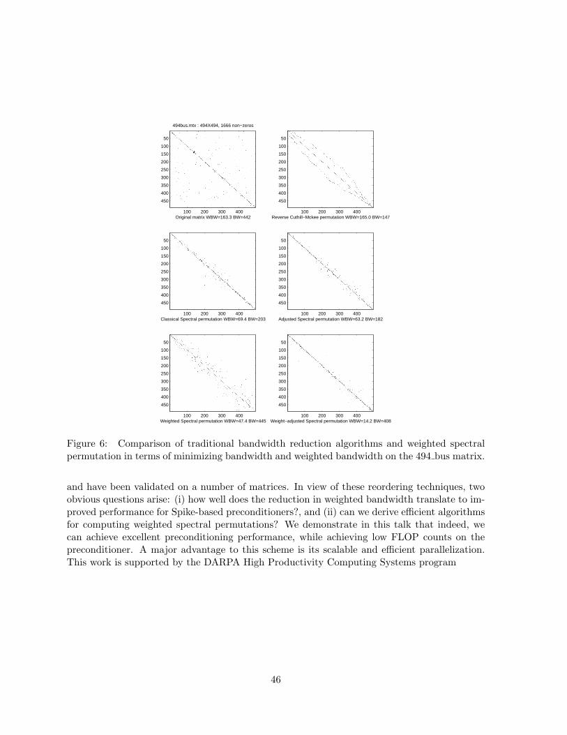
Original matrix WBW=163.3 BW=442

494bus.mtx : 494X494, 1666 non−zeros

100 200 300 400

50

100

150

200

250

300

350

400

450

Reverse Cuthill−Mckee permutation WBW=165.0 BW=147100 200 300 400

50

100

150

200

250

300

350

400

450

Classical Spectral permutation WBW=69.4 BW=203100 200 300 400

50

100

150

200

250

300

350

400

450

Adjusted Spectral permutation WBW=63.2 BW=182100 200 300 400

50

100

150

200

250

300

350

400

450

Weighted Spectral permutation WBW=47.4 BW=445100 200 300 400

50

100

150

200

250

300

350

400

450

Weight−adjusted Spectral permutation WBW=14.2 BW=408100 200 300 400

50

100

150

200

250

300

350

400

450

Figure 6: Comparison of traditional bandwidth reduction algorithms and weighted spectralpermutation in terms of minimizing bandwidth and weighted bandwidth on the 494 bus matrix.

and have been validated on a number of matrices. In view of these reordering techniques, twoobvious questions arise: (i) how well does the reduction in weighted bandwidth translate to im-proved performance for Spike-based preconditioners?, and (ii) can we derive efficient algorithmsfor computing weighted spectral permutations? We demonstrate in this talk that indeed, wecan achieve excellent preconditioning performance, while achieving low FLOP counts on thepreconditioner. A major advantage to this scheme is its scalable and efficient parallelization.This work is supported by the DARPA High Productivity Computing Systems program

46

5.17 A parallel additive Schwarz preconditioner and its variants for 3D el-liptic non-overlapping domain decomposition - A. Haidar

Co-authored by:A. Haidar 1 L. Giraud 2 L. T. Watson 3

In this talk, we describe a set of parallel algebraic additive Schwarz preconditioners for non-overlapping domain decomposition applied to the parallel solution of large three dimensionalelliptic PDE problems. These preconditioners exploit the explicit knowledge of the local Schurcomplement matrices that can be efficiently computed thanks to the unique feature of theparallel multi-frontal sparse direct solver Mumps [1]. In order to alleviate the computationalcost, both in terms of memory and floating-point complexity, we investigate variants based ona sparse approximation or on mixed 32- and 64-bit calculation [4, 6]. This latter strategy ismainly motivated by the observation that many recent processor architectures exhibit 32-bitcomputational power that is significantly higher than that for 64-bit. This leads us to definefour variants of preconditioners,namely Md−64 that uses dense 64-bit matrices; Md−mix thatuses dense 32-bit matrices, Msp−64 that uses sparsified 64-bit matrices and Msp−mix thatuses sparsified 32-bit matrices. The robustness of the preconditioners is illustrated on a set oflinear systems arising from the finite element discretization of elliptic PDEs through extensiveparallel experiments on up to 1000 processors. Their performance is illustrated in Figure 7where convergence history are displayed. As expected, for the sparsification strategy, we canobserve for various choices of the dropping parameter that for small values the convergence ismarginally affected while the memory saving is already significant; and for the mixed preci-sion implementation, it can be observed that for not too ill conditioned problems, the 32-bitcalculation of the preconditioning step does not delay too much the convergence of CG. Thenumerical scalability of these preconditioners is illustrated in Table 3, we perform some scaledexperiments where each sub-domain is handled by one processor. In this table reading a rowshows the behavior with fixed subdomain size when the number of the processors goes from 27up to 1000 while the overall problem size increases; for every column the number of processors(subdomains) is kept constant while refining the mesh size. The behavior is similar for the fourpreconditioners. When we go from subdomains with about 8,000 degrees of freedom (dof) tosubdomains with about 43,000 dof, the number of iterations can increase by over 25%. Noticethat with such an increase in the subdomain size, the overall system size is multiplied by morethan five; on 1000 processors the global system size varies from eight million dof up to about 43million dof. None of the preconditioners implements any coarse space component to account forthe global coupling of the elliptic PDEs, hence they do not scale perfectly when the number ofsubdomains is increased. However, the scalability is not that bad and clearly much better thanthat observed on two dimensional examples [2]. The number of iterations is multiplied by about

1CERFACS, 42 Avenue G. Coriolis, 31057 Toulouse Cedex, France - haidar@cerfacs.fr2ENSEEIHT-IRIT, 2 Rue Camichel 31071 Toulouse Cedex, France. giraud@n7.fr3Departments of Computer Science and Mathematics, Virginia Polytechnic Institute & State University,

Blacksburg, Virginia, USA. ltw@cs.vt.edu

47

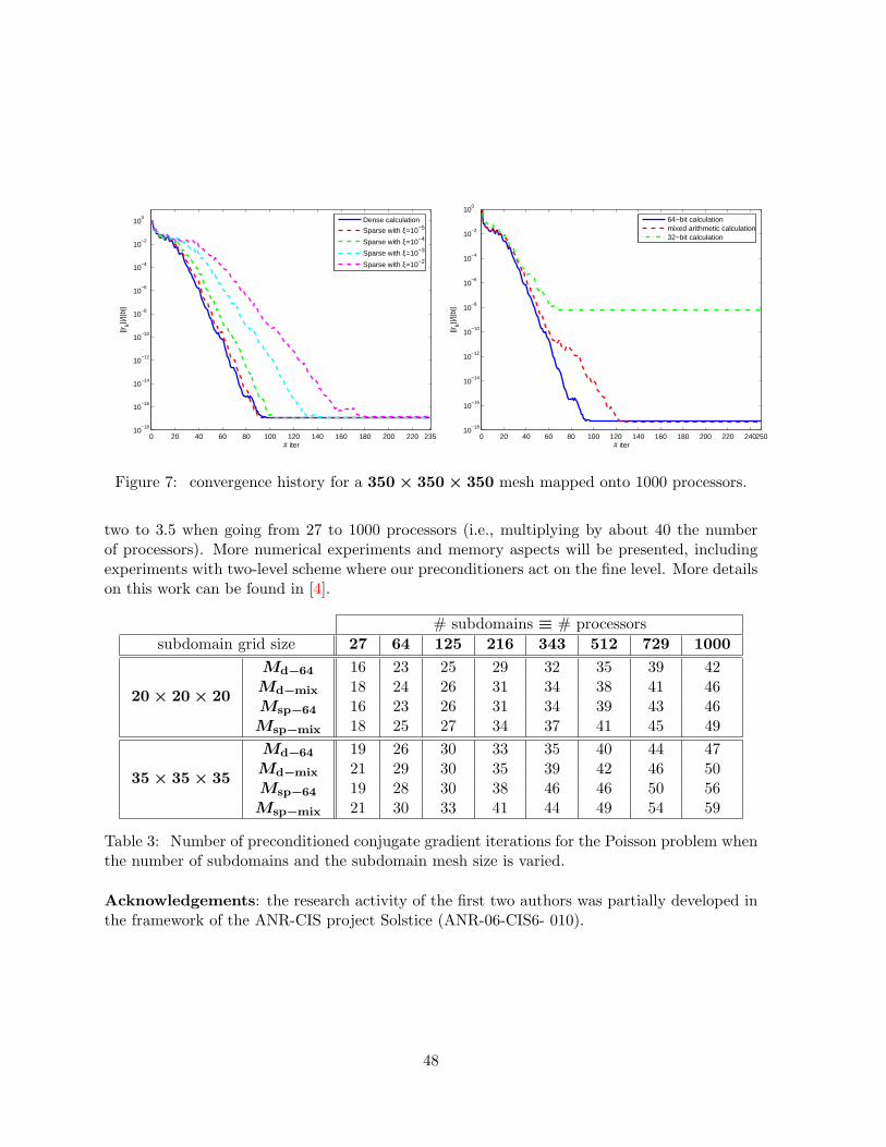
0 20 40 60 80 100 120 140 160 180 200 220 23510

−18

10−16

10−14

10−12

10−10

10−8

10−6

10−4

10−2

100

# iter

||rk||/

||b||

Dense calculation

Sparse with ξ=10−5

Sparse with ξ=10−4

Sparse with ξ=10−3

Sparse with ξ=10−2

0 20 40 60 80 100 120 140 160 180 200 220 24025010

−18

10−16

10−14

10−12

10−10

10−8

10−6

10−4

10−2

100

# iter||r

k||/||b

||

64−bit calculationmixed arithmetic calculation32−bit calculation

Figure 7: convergence history for a 350× 350× 350 mesh mapped onto 1000 processors.

two to 3.5 when going from 27 to 1000 processors (i.e., multiplying by about 40 the numberof processors). More numerical experiments and memory aspects will be presented, includingexperiments with two-level scheme where our preconditioners act on the fine level. More detailson this work can be found in [4].

# subdomains ≡ # processorssubdomain grid size 27 64 125 216 343 512 729 1000

Md−64 16 23 25 29 32 35 39 42Md−mix 18 24 26 31 34 38 41 4620× 20× 20Msp−64 16 23 26 31 34 39 43 46Msp−mix 18 25 27 34 37 41 45 49Md−64 19 26 30 33 35 40 44 47Md−mix 21 29 30 35 39 42 46 5035× 35× 35Msp−64 19 28 30 38 46 46 50 56Msp−mix 21 30 33 41 44 49 54 59

Table 3: Number of preconditioned conjugate gradient iterations for the Poisson problem whenthe number of subdomains and the subdomain mesh size is varied.

Acknowledgements: the research activity of the first two authors was partially developed inthe framework of the ANR-CIS project Solstice (ANR-06-CIS6- 010).

48

References

[1] P. R. Amestoy, I. S. Duff, J. Koster, and J.-Y. L’Excellent. A fully asynchronous mul-tifrontal solver using distributed dynamic scheduling. SIAM Journal on Matrix Analysisand Applications, 23(1):15–41, 2001.

[2] L. M. Carvalho, L. Giraud, and G. Meurant. Local preconditioners for two-level non-overlapping domain decomposition methods. Numerical Linear Algebra with Applications,8(4):207–227, 2001.

[3] T. F. Chan and T. P. Mathew. Domain decomposition algorithms. In Acta Numerica 1994,pages 61–143. Cambridge University Press, 1994.

[4] L. Giraud, A. Haidar, and L. T. Watson. Parallel scalability study of three dimensionaladditive Schwarz preconditioners in non-overlapping domain decomposition. TechnicalReport TR/PA/07/05, CERFACS, Toulouse, France, 2007. Also appeared as ENSEEIHT-IRIT Technical report RT/APO/07/01.

[5] L. Giraud, A. Marrocco, and J.-C. Rioual. Iterative versus direct parallel substructuringmethods in semiconductor device modelling. Numerical Linear Algebra with Applications,12(1):33–53, 2005.

[6] J. Langou, J. Langou, P. Luszczek, J. Kurzak, A. Buttari, and J. Dongarra. Exploitingthe performance of 32 bit floating point arithmetic in obtaining 64 bit accuracy. TechnicalReport LAPACK Working Note #175 UT-CS-06-574, University of Tennessee ComputerScience, April 2006.

5.18 Jacobi-Davidson with AMG preconditioning for solving large general-ized eigenproblems from nuclear power plant simulation - M. Havet

Co-authored by:M. Havet 1 Y. Notay 2

Nuclear power plant simulation requires solving very large nonsymmetric generalized eigenvalueproblems. So far, most industrial codes solve these problems with some variant of the coarsemesh rebalancing (CMR) method for acceleration of otherwise very lenghty computations. Thisapproach traces back to the sixties and may be seen as one of the earliest multilevel schemes,which, nevertheless, never spread outside the specific context of nuclear power plant simulation.In this talk we show that this method amounts to a particular aggregation-based algebraicmultigrid (AMG) scheme, with the prolongation improved using the current approximation

1AREVA NP GmbH, Freyeslebenstrae 1, 91058, Erlangen, Germany2Service de Metrologie Nucleaire, Universite Libre de Bruxelles, (C.P. 165/84), 50, Av. F.D. Roosevelt, 1050,

Bruxelles, Belgium

49

to the sought eigenvector (which corresponds to the ”lowest energy” mode). Based on this,we propose a new solution scheme which combines these ingredients with modern tools fromnumerical linear algebra.

More precisely, we solve the eigenvalue problem with the Jacobi-Davidson method, whichsearches for the best possible correction t to an approximate solution u of the eigenproblem.This correction is the solution to a linear system known as the correction equation. The solutiont is not directly taken as correction, but is used to expand a subspace U in which a new approx-imation u is sought by exact solution of a small projected eigenproblem. To efficiently solvethe correction equation, we use Flexible Generalized Minimization of the RESisual (FGMRES)method in combination with an AMG preconditioner inspired from the CMR methodology andadapted to the special form of the correction equation. The cycling strategy is further improvedusing FGMRES acceleration at every level.

More detail about the CMR methodology can be found in [1].

References

[1] R. van Geemert, Synergies of Acceleration Methods for Whole-Core N-TH-coupledSteady-State and Transient Computations, CD-ROM, Proceedings of PHYSOR 2006,American Nuclear Society, 2006

5.19 Block preconditioners for electromagnetic cavity problems - Y. Huang

Co-authored by:Y. Huang 1 M. Ng 2

In a radar detecting system, the radar cross section (RCS) of a target is an important applicationof electromagnetics computation[4]. Cavity prediction is usually required in the computationprocess [2, 4]. When wavelengths of electromagnetic field are large, cavity calculation is achallenging problem [2]. The main aim of this paper is to employ the preconditioned GMRESmethod to solve indefinite linear systems arising in cavity calculation of the transverse magneticand transverse electric problems. We develop new preconditioners based on fast transforms [1]and Toeplitz solvers [3]. Our numerical results show that the proposed preconditioners arequite efficient and effective. According to the experimental results, we discuss the spectra ofthe preconditioned matrices for different wavelengths of electromagnetic field used.

1Department of Mathematics, Hong Kong Baptist University, Kowloon Tong, Hong Kong. E-mail:ymhuang@math.hkbu.edu.hk .

2Department of Mathematics, Hong Kong Baptist University, Kowloon Tong, Hong Kong. E-mail:mng@math.hkbu.edu.hk .

50

References

[1] A. Banegas, Fast Poisson solvers for problems with sparsity, Math. Comp., 1978, Vol. 32,No. 142, pp. 441-446.

[2] G. Bao and W.-W. Sun, A fast algorithm for the electromagnetic scattering from a largecavity, SIAM J. Sci. Comput., 2005, Vol. 27, No. 2, pp. 553-574.

[3] R. Chan and M. Ng, Conjugate gradient methods for Toeplitz systems, SIAM Review,1996, Vol. 38, No. 3, pp. 427-482.

[4] J. Jin, The finite element method in electromagnetic, John Wiley and Sons, New York,1993.

5.20 Comparison of various modified incomplete block preconditioners -T. Huckle

Co-authored by:T. Huckle 1

We consider block tridiagonal matrices of the form

A =

A1 B1

C1. . . . . .. . . . . . BM−1

CM−1 AM

.

Incomplete block factorizations for A can be derived in three different forms. We can factorizeA by A = L ∗ T ∗ U with lower/upper block triangular L and U , and T either the identitymatrix, block diagonal, or the inverse of a block diagonal matrix. For each factorization weget equations defining the blocks of L, U , and T uniquely. To obtain sparsity we use onlysparse approximations for L, T , and U . Then the computations are based on incompletefactorizations, sparse approximate solutions of linear systems, and sparse approximate Schurcomplements. For modified incomplete block factorizations we want to obtain the behaviourof the preconditioner relative to the vector of all ones. Therefore, we will use also modifiedapproximations for the partial problems, e.g. MILU or MSPAI with probing. In this talk wewant to compare different methods for solving these problems for the three different variationsof modified incomplete block preconditioners. Especially we consider MILU where we allowlumping also on nondiagonal positions, and Frobenius norm probing.

1 Fakultat fur Informatik, Technische Universitat Munchen, Boltzmannstr. 3, D-85748 Garching, Germany(huckle@in.tum.de)

51

References

[1] Huckle, T., Kallischko, A., 2007, Frobenius Norm Minimization and Probing for Precondi-tioning. Int. Journal of Comp. Math., to appear.

[2] Meurant, G., Computer Solution of large linear systems, North Holland, 1999.

[3] Magolu, M.-M., Modified block-approximate factorization strategies, Numer. Math., 61,91–110, 1992.

5.21 Aitken-Schwarz acceleration with auxiliary background grids - F. Hulse-mann

Co-authored by:F. Hulsemann 1

The ease with which Schwarz domain decomposition methods allow existing single-threadedsolvers to be (re-)used for parallel computations is undoubtedly one of their advantages. How-ever, in order to be practical for large scale parallel computations, the slow convergence of thestandard Schwarz algorithm has to be overcome by some form of acceleration.

We present the Aitken-Schwarz method which is an example of an extrapolation based acceler-ation technique, exploiting the linearity of the operators that govern the error propagation fromone iteration to the next. Its fast convergence and its low additional communication require-ments make the Aitken-Schwarz method an attractive choice for metacomputing environmentssuch as clusters of clusters up to clusters of supercomputers as demonstrated in [1].

Originally, the Aitken-Schwarz method developed by Garbey and Tromeur-Dervout [2] wasmotivated by Fourier transformations on regular Cartesian grids. The method has since beenextended to different types of grids such as general tensor product grids or Chimera-type oversetgrids. In this presentation, we show how to adapt the Aitken-Schwarz method to grids withrefined stripes, as a step on the way to locally refined grids.

Although the Aitken-Schwarz method is a direct solver under certain circumstances, the empha-sis of the research has shifted to its iterative use [3]. With auxiliary grids for the extrapolation,the Aitken-Schwarz approach is necessarily an iterative scheme. While we consider only linearproblems, we note that the principal ideas can indeed be applied to non-linear problems andgive rise to the so-called Steffensen-Schwarz method.

In this presentation, we recall the basic form of the Aitken-Schwarz algorithm for the concretecase of a linear, separable, second order differential operator on two subdomains. One has tobear in mind that in a metacomputing setting, each subdomain will be treated by a, potentiallylarge, parallel computer. The question how to obtain acceptable parallel performance on clusters

1EDF R-D, Clamart

52

of powerful, parallel machines that are connected via comparatively slow, high-latency networks,such as the Internet, for example, is still open. In this context, the efficient coupling of onlytwo parallel machines is already far from trivial.

Numerical examples are presented to confirm the fast convergence when all eigenvectors ofthe differential operator on the partition interface enter the extrapolation. However, the de-termination of all eigenvectors may not always be desirable, hence the interest in reducing thecomputational complexity of the input or, in other words, the prerequisites, of the extrapolation.

The novelty of this contribution consists in the use of auxiliary background grids in the presenceof refined strips. The method presented here differs from the Aitken-Schwarz ”mainstream” inthat it uses the extrapolation in a correction scheme and not as a way to represent the algebraicsolution. This change of approach, which might seem minor, in fact overcomes convergenceproblems of the original formulation. Numerical examples illustrating the convergence behaviourof the iterative scheme are provided.

References

[1] Barberou, N., Garbey, M., Hess, M., Resch, M., Rossi, T., Toivanen, J., Tromeur-Dervout,D., “Aitken-Schwarz method for efficient metacomputing of elliptic equations”, in “DomainDecomposition Methods in Science and Engineering”, Herrera, I., Keyes, D.E., Widlund,O.B., Yates, R. (editors), UNAM, 349–356, 2003.

[2] Garbey, M., Tromeur-Dervout, D., “Two Level Domain Decomposition for Multiclusters”,in “12th Int. Conf. on Domain Decomposition Methods DD12”, Chan, T., Kako, T.,Kawarada, H., Pironneau, O. (editors), 325–340, 2001.

[3] Garbey, M., “Acceleration of the Schwarz method for elliptic problems”, SIAM J. of Scien-tific Computing, 26 (6), 1871–1893, 2005.

5.22 Industrial out-of-core solver for ill-conditioned matrices - I. Ibragimow

Co-authored by:I. Ibragimow 1 E. Ibragimowa 2

In this work we discuss a computation of LU preconditioner for large linear systems. Themain goal of this talk to understand a precondition quality of incomplete LU if we use differentpermutation methods. Permutations are applied for sparse matrices to reduce fill-in in ILU.

Nowadays several powerful methods are used for reduction of fill-in in ILU: metis, AMD andothers. However if the matrix is unsymmetric or non-hermitian, a zero or almost zero pivotentry can occur. Several robust approaches can handle it, for example, shift the pivot to the end

1University of Saarbrucken, Mathematical Department, 66041 Saarbrucken, Germany, ilgis@num.uni-sb.de2Elegant Mathematics Ltd., 66540, Hanauer Muhle, Germany, il@elegant-mathematics.com

53

or join zero pivot with other to construct 2 × 2 block nonsingular matrix. These approachesincrease fill-in and, in cases with very ill-conditioned matrices can significantly increase thememory usage.

In this talk we present an approach that computes a permutation together with computationof incomplete LU. It has following benefits:

• it escapes pivots with small norms, and it is possible to bound a priory a norm of off-diagonal entries in the decomposition;

• it gives easy possibility to find all columns and rows with similar sparsity structure, so itgives a way to construct a block structure of LU;

• it allows to approximate off-diagonal block entries as low rank structures, like it occurs inhierarchical matrices, hence, it saves a lot of computation efforts.

The out-of-core implementation of this algorithm is developed and used in a variety of largeand very ill-conditioned matrices. Some of these matrices constructed in 3D Navier-Stockssimulations with million unknowns we will solve during this presentation.

5.23 Frobenius norm minimization and probing for preconditioning - A. Kallis-chko

Co-authored by:A. Kallischko 1 T. Huckle 2

Large, sparse and ill-conditioned systems Ax = b of linear equations can be solved withiterative methods such as BiCGstab, GMRES or the preconditioned conjugate gradient method(pcg) in the case of symmetric A. Due to the ill-conditioning, the choice of the preconditioneris very important. We start off with an extension of the classic SPAI algorithm (see [3]),which allows us to compute approximations to any arbitrary matrix. With this approach,we can add probing conditions to the process of Frobenius norm minimization. This yieldsgeneralizations of the class of modified preconditioners (e.g. MILU in [1]), the interface probingin [2], and the class of preconditioners related to the Frobenius norm minimization (e.g. FSAI,SPAI). We obtain a toolbox for computing preconditioners that are improved relative to agiven small probing subspace. Furthermore, by this MSPAI (modified SPAI) probing we canimprove any given preconditioner with respect to this probing subspace. All the computationsare still embarrassingly parallel as the properties like independent columnwise computation

1Fakultat fur Informatik, Technische Universitat Munchen, Boltzmannstr. 3, D-85748 Garching, Germany(kallisch@in.tum.de)

2 Fakultat fur Informatik, Technische Universitat Munchen, Boltzmannstr. 3, D-85748 Garching, Germany(huckle@in.tum.de)

54

are inherited from the classic SPAI method. Additionally, for symmetric linear system weintroduce new techniques for symmetrizing both factorized and unfactorized preconditioners.We demonstrate the effectiveness and the variety of the MSPAI method in several numericalexamples.

References

[1] Axelsson, O., 1972, A generalized SSOR method. BIT, 13, 443–467.

[2] Axelsson, O., Polman, B., 1988, Block preconditioning and domain decomposition methodsII. J. Comp. Appl. Math., 24, 55–72.

[3] Grote, M. J., Huckle, T., May 1997, Parallel Preconditioning with Sparse ApproximateInverses. SIAM J. Sci. Comput., 18, No. 3, 838–853.

5.24 A single precision preconditioner for Krylov subspace iterative methods- T. Kihara

Co-authored by:T. Kihara 1 Hiroto Tadano 2 Tetsuya Sakurai 3

The calculation techniques using the Cell processor have attracted attention for high perfor-mance computing. It is a heterogeneous multicore chip that is significantly different fromconventional multi-processor or multicore architectures. The Cell processor provides extremelyhigh performance single-precision floating operations, however the majority of scientific appli-cations require results with double precision.

Large sparse linear systems Ax = b arise in many scientific applications. Krylov subspaceiterative methods [2] are often used for solving such linear systems. Preconditioning techniquesare efficient to reduce the number of iterations of Krylov subspace methods ([1]). However, thecomputational cost of the preconditioning part is sometimes large.

In [3], an acceleration technique of preconditioning with single precision arithmetic is considered.We can obtain the approximate solution with double precision by using the Krylov subspacemethods with the single precision arithmetic preconditioner. It is effective if the computationalcost of the preconditioner is dominant in a iterative method.

1Graduate School of Systems and Information Engineering, University of Tsukuba, Tsukuba 305-8573, Japan,kihara@mma.cs.tsukuba.ac.jp

2Core Research for Evolutional Science and Technology, Japan Science and Technology Agency, Japan,tadano@mma.cs.tsukuba.ac.jp

3Department of Computer Science, University of Tsukuba, Tsukuba 305-8573, Japan,sakurai@cs.tsukuba.ac.jp

55

We have implemented and tested the single precision preconditioner on the Cell Processor. Thecomputation of preconditioning is performed on Synergistic Processor Elements (SPE) withsingle precision arithmetic. Several numerical experiments illustrate the performance of thispreconditioner.

References

[1] M. Benzi, Preconditioning techniques for large linear systems: A survey, J. Comput. Phys.,182(2002), pp. 418–477.

[2] Y. Saad, Iterative methods for sparse linear systems (2nd edition), SIAM, Philadelphia,2003.

[3] H. Tadano and T. Sakurai: On single precision preconditioners for Krylov subspace iterativemethods (submitted).

5.25 Special preconditioners for Krylov subspace methods based on skew-symmetric splitting - L. Krukier

Co-authored by:L. Krukier 1 Z-Z. Bai 2 T. Martynova 3 O. Pichugina 4

New preconditioners for acceleration Krylov subspace methods are presented. The purpose is toconstruct simple and inexpensive from computational standpoint yet effective preconditionersfor solving strongly nonsymmetric linear equation systems. Special class of triangular and prod-uct triangular methods based on skew-symmetric part of the matrix has been proposed in [1],[2]. Two Krylov subspace methods BiCG and GMRES(m)were in focus of our investigation.Theoretical investigation was done for preconditioned GMRES iteration method. Linear equa-tion systems which we’ve got after finite central-difference approximation of two-dimensionalconvection-diffusion equation with big Peclet numbers are used to illustrate the advantage anddisadvantages of our preconditioners. Several numerical experiments for the solution of thestrongly nonsymmetric linear systems will be shown. This work was supported by RFBR,grants N06-01-00038-a and N06-01-39002-GFEN-a.

1Computer Center, Southern Federal University, Rostov-on-Don, Russia, kruker@rsu.ru2State Key Lab. of Sci. and Eng. Computing, Institute of Comp. Math and Eng. Comp., Academy of Math.

and Syst. Science CAS, Beijing, China, bzz@lsec.cc.ac.cn3Computer Center, Southern Federal University, Rostov-on-Don, Russia, martynova@rsu.ru4Computer Center, Southern Federal University, Rostov-on-Don, Russia, pichugina@rsu.ru

56

References

[1] Krukier L.A., Chikina L.G., Belokon T.V. Triangular skew-symmetric iterative solversfor strongly non-symmetric positive real linear system of equations Appl. Numer.Math.,41:89–105, 2002.

[2] L.A. Krukier, T.S. Martynova, Z.Z. Bai Two-step iterative methods for solving the station-ary convection-diffusion equation with small parameter at highest derivative on uniformgrid. Computational Mathematics and Mathematical Physics, v.46, N2:282–293, 2006.

5.26 Variable transformations and preconditioning for large-scale optimiza-tion problems in data assimilation - A. Lawless

Co-authored by:A. Lawless 1 D. Katz 2 N. K. Nichols 3 R.N . Bannister 4 M. J .P. Cullen 5

In many applications of environmental forecasting, such as numerical weather prediction orocean forecasting, it is necessary to estimate the current state of the system in order to make aforecast. Usually the number of observed data is not sufficient to determine the state uniquelyand so measurements must be combined with a numerical model forecast to produce the beststate estimate given all the available information. In many operational weather forecastingcentres this is done using a technique called four-dimensional variational data assimilation (4D-Var), which solves the data assimilation problem by means of the minimization of a cost functionconstrained by a numerical model. In practice these problems are very large, with the dimensionof the state being of the order 107−108 and the number of observations an order of magnitudeless than this.

We suppose that over a time interval [t0, tn] we have a set of observations yoi , i = 1, . . . , n

with error covariance matrices Ri and that at the initial time t0 we have an a priori estimateof the state xb with error covariance matrix B. The a priori estimate is usually obtained froma previous forecast and is referred to as the background state. The matrix B is the backgrounderror covariance matrix. Then the 4D-Var problem is posed as follows: Find the state x0 attime t0 which minimizes the function

J [x0] =1

2(x0 − xb)T B−1(x0 − xb) +

1

2

n∑i=0

Hi[xi]− yoi )

T R−1i (Hi[xi]− yo

i ), (20)

subject to the dynamical modelxi =M(ti, t0, x0),

1Department of Mathematics, University of Reading, U.K.2Department of Mathematics, University of Reading, U.K.3Department of Mathematics, University of Reading, U.K.4Department of Meteorology, University of Reading, U.K.5Met Office, U.K.

57

whereM(ti, t0, x0) represents the nonlinear model evolved to time ti, i = 1, . . . , n, xb. Theoperator H is a possibly nonlinear transformation from model space to observation space. Inpractice we cannot solve the problem in this form. The background error covariance matrix Bis of size approximately 107 × 107 and so it is impossible to represent it directly in this way.Furthurmore this a huge optimization problem subject to the constraint of a nonlinear modeland so efficient numerical methods must be found to solve it.

In order to minimize the cost function (20) in practice we form two approximations. The first isto apply a few iterations of an approximate Gauss-Newton method (Lawless et al. 2005, Grattonet al. 2007). Thus instead of minimizing (20) directly we minimize a series of linearized costfunctions

J(k)[x′0(k)] =

1

2(x′

0(k) − x′b)T B−1(x′

0(k) − x′b)

+1

2

n∑i=0

(Hix′i(k) − di)T R−1

i (Hix′i(k) − di), (21)

where k is the iteration count of the Gauss-Newton iteration and Hi is the linearization ofthe observation operator H. Here x′

i(k) = M(ti, t0, x(k))x′

0(k), where M(ti, t0, x(k)) ≡ Mi

denotes the evolution operator from t0 to ti of the linearization of the nonlinear model M.The background increment, x′b, is given by x′b = xb − x(k)

0 and the innovation vector, di,

by di = yoi − Hix

(k)i . For each Gauss-Newton iteration the linearized cost function (21) is

minimized using a conjugate gradient or quasi-Newton method.

The second set of approximations is designed to implicitly construct the matrix B and toprecondition the minimization of the linearized cost function (21). We define a new variable z′,called the control variable, and a variable transformation U such that

x′ = Uz′. (22)

Then the cost function (21) can be written

J(k)[z′0(k)] = 1

2(z′

0(k) − z′b)T UT B−1U(z′

0(k) − z′b)

+12

∑ni=0(Hi(MiUz′

0(k))− di)T R−1

i (Hi(MiUz′0(k))− di), (23)

If we choose U such thatUT B−1U = Λ−1,

where Λ is a block diagonal matrix specifying the auto-correlations of each control variable,then we have

B = UΛUT .

Susbstituting into (21) we obtain

J(k)[z′0(k)] = 1

2(z′

0(k) − z′b)T Λ−1(z′

0(k) − z′b)

+12

∑ni=0(Hi(MiUz′

0(k))− di)T R−1

i (Hi(MiUz′0(k))− di). (24)

58

This form of the cost function can more easily be minimzed for two reasons. The first is thatwe no longer need to represnt a full matrix in the first term, but just a block diagonal matrixΛ. This can be simplified by a further variable transformation to give an identity covariancematrix. The second reason is that the removal of the dense matrix B is believed to betterprecondition the problem.

In practice we cannot begin with a full matrix B to define the variable transformation U.Instead we define a set of control variables z′ which we assume to be uncorrelated from physicalarguments and then define an appropriate transformation U from these variables to the originalvariables x′. Thus we implicitly construct the matrix B. However the validity of this wholeapproach depends on the assumption that the control variables z′ which we choose truly areuncorrelated.

For the control variables currently used in operational weather prediction it is known that thisassumption is not valid across all dynamical regimes. Recently Cullen (2003) proposed a newset of control variables which are believed to exploit more accurately important dynamicalproperties of the atmosphere. In this study we compare the set of control variables which arecommonly used in numerical weather prediction with this new set of control variables. Thesenew variables are based on a conserved quantity of the atmosphere, potential vorticity. Using aone-dimensional shallow water model we investigate how well the new variable transformationremoves correlations in the model variables when compared with the currently used approach.We show how the variables proposed by Cullen are better able to remove correlations acrossa wide range of dynamical regimes. Comments will be made on the effect of these variablestransformations on the conditioning of the assimilation problem.

References

[1] Cullen, M. J. P. (2003): Four-dimensional variational data assimilation: A new formulationof the background-error covariance matrix based on a potential vorticity representation.Quart. J. Royal Met. Soc., 129:2777–2796.

[2] Gratton, S., Lawless, A.S. and Nichols, N.K. (2007): Approximate Gauss-Newton methodsfor nonlinear least squares problems, SIAM J. on Optimization, 18:106–132.

[3] Lawless, A.S., Gratton, S. and Nichols, N.K. (2005): An investigation of incremental 4D-Var using non-tangent linear models, Quart. J. Royal Met. Soc., 131, 459-476.

59

5.27 ILU preconditioning for unsteady flow problems solved with higherorder implicit time integration schemes - P. Lucas

Co-authored by:P. Lucas 1 H. Bijl 2

Problem of interest

Computational fluid dynamics has developed over the last decades into a comprehensive designtool. It is now possible to compute the flow around complex aerospace configurations, see forexample Vos et al. [4]. This rapid increase in cfd applications has become possible by anever increasing computer power, progress in physical modelling and more efficient algorithmsof which higher order implicit time integration schemes is an example.

In aerodynamic production codes typically nonlinear multigrid is used to solve the nonlinearsystem at each physical time step or Runge-Kutta stage, mainly because of its robustness.However, nonlinear multigrid cannot cope with the stiffness that is induced by the large aspectratio cells necessary when large Reynolds’ number flows are computed. In the literature manytechniques are proposed to alleviate this kind of stiffness, e.g. semi coarsening and line implicitsmoothing. However, the former is not really applicable in three dimensions whereas the latteris difficult to apply when unstructured grids are used. Finally, the system of nonlinear equationsis harder to solve when higher order implicit time integration schemes are employed.

Newton-Krylov algorithms to solve large sparse nonlinear systems are an alternative for non-linear multigrid and are often used in other research fields, like mathematics. Gradually thesemethods are introduced into the cfd community, see for example Bijl [1] for promissing re-sults. Therefore, we have also chosen to start using a Newton-Krylov method to solve thenonlinear systems at each Runge-Kutta stage. We are interested in two and three dimensionalunsteady flow problems on unstructured hexahedral grids. After Newton linearization typicallya nonsymmetric, definite and very ill conditioned system of linear equations is obtained.

Preconditioning techniques

The preconditioner is crucial for the performance of a Krylov method. Possibilities to precon-dition are among others: (non)linear multigrid, a recursive variant of GMRES (GMRESR) andapproximate factorizations of the Jacobian of which an incomplete lower upper factorization(ILU) is an example. (Non)linear multigrid and GMRESR have the advantage that the memoryconsumption is low. A disadvantage is that low frequency errors are poorly damped.

Approximate factorizations can be very powerfull because errors in the whole frequency rangeare damped. However, a disadvantage can be its robustness, see Chow and Saad [2]. Further-more the memory consumption of approximate matrix factorizations is large. A large memoryconsumption, however, is justified because: 1) nowadays computers have a large amount of

1Ph.D. student, Department of Aerodynamics, P.O. Box 5058, 2600 GB Delft, The Netherlands2Full professor, Department of Aerodynamics, P.O. Box 5058, 2600 GB Delft, The Netherlands

60

RAM memory available so why not use it and 2) people are willing to invest in memory if thatreduces the computational time from the order of months to the order of weeks.

In order to reduce the memory consumption it is possible to simplify the Jacobian. Possibilitiesfor simplifications are: 1) a lower order discretization in space, 2) neglecting small terms and3) reducing the numerical stencil. The first one has also the advantage that the resulting ILUfactors are more stable which leads to better performance, see for example Wong and Zingg [5].With the second simplification all terms in a row that are smaller than a certain fraction of thediagonal element in that row are deleted. With the third simplification not the full Jacobianis build, but it is based on a chosen (smaller) stencil. Terms that are not inside the chosenstencil are simply ignored. Although the latter two simplifications are very easy to apply theyare not often found in the literature. The first question we want to answer is what kind ofpreconditioner we should use for our type of problems.

Initial results

First the efficiency is assessed for a steady two dimensional test case, being a flow around a 25%thick wind turbine profile with a Mach number of 0.21 and a Reynolds’ number of 3 milion.The grid contains 11k cells and has a maximum aspect ratio of 550. This simple test case hasbeen used to gain the first knowledge in the quest for a robust and powerfull preconditioner.

The ITSOL package of Saad [3] has been used to compute the ILU type preconditioners. Amongothers the following ILU’s are possible: 1) ILU’s based on the footprint of the Jacobian and2) (multilevel) ILU’s based on thresholds. Furthermore it is possible to use column and rowscaling and a kind of reordering where the sparsity of the Jacobian and diagonal dominance aresimultaneously optimized.

Earlier investigations revealed that ILU’s based on the footprint of the Jacobian are much morerobust than ILU’s based on thresholds for this test case. An ILU based on a first order spatialdiscretized Jacobian did not nearly perform as good as an ILU based on the second order spatialdiscretized Jacobian. Because such a preconditioner consumes a large amount of memory wehave sought for means to reduce the memory consumption by simplifying the Jacobian.

In Fig. 8 a comparison is made between different simplifications. On the horizontal axis thenumber of nonzeros in L and U is plotted, which is controlled by deleting more or less elementsthat are smaller than the diagonal value. On the vertical axis the drop in linear residual isplotted. The drop in linear residual is plotted after 10, 20 and 30 Krylov iterations.

Our spatial discretization scheme uses a 253 points stencil in two dimensions. For the 13 pointsstencil neighbors of neighbors of neighbors are simply neglected. The most right point of thered solid line corresponds to the original Jacobian. The costs to compute the preconditionerare approximately linear dependent on the number of nonzeros in the L and U.

From this figure it becomes clear that the quality of the preconditioner per element can evenbe enhanced by neglecting small terms. Furthermore, with simplifying the Jacobian one hasan easy way to reduce memory consumption. The next step is to perform more elaborated

3True for a structured grid, for an unstructured grid this number may be larger.

61

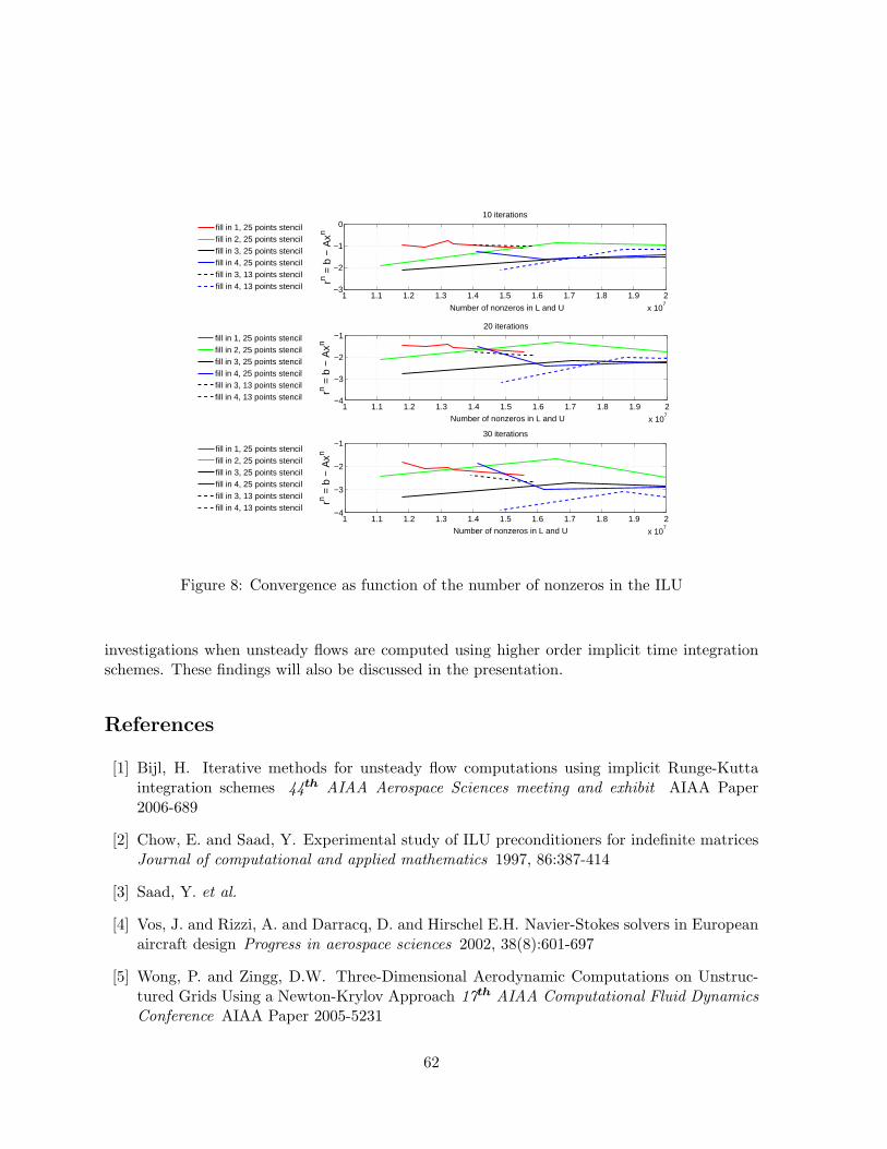
1 1.1 1.2 1.3 1.4 1.5 1.6 1.7 1.8 1.9 2

x 107

−3

−2

−1

0

Number of nonzeros in L and U

rn = b

− A

xn

10 iterations

1 1.1 1.2 1.3 1.4 1.5 1.6 1.7 1.8 1.9 2

x 107

−4

−3

−2

−1

Number of nonzeros in L and U

rn = b

− A

xn20 iterations

1 1.1 1.2 1.3 1.4 1.5 1.6 1.7 1.8 1.9 2

x 107

−4

−3

−2

−1

Number of nonzeros in L and U

rn = b

− A

xn

30 iterations

fill in 1, 25 points stencil fill in 2, 25 points stencilfill in 3, 25 points stencilfill in 4, 25 points stencilfill in 3, 13 points stencilfill in 4, 13 points stencil

fill in 1, 25 points stencil fill in 2, 25 points stencilfill in 3, 25 points stencilfill in 4, 25 points stencilfill in 3, 13 points stencilfill in 4, 13 points stencil

fill in 1, 25 points stencil fill in 2, 25 points stencilfill in 3, 25 points stencilfill in 4, 25 points stencilfill in 3, 13 points stencilfill in 4, 13 points stencil

Figure 8: Convergence as function of the number of nonzeros in the ILU

investigations when unsteady flows are computed using higher order implicit time integrationschemes. These findings will also be discussed in the presentation.

References

[1] Bijl, H. Iterative methods for unsteady flow computations using implicit Runge-Kuttaintegration schemes 44th AIAA Aerospace Sciences meeting and exhibit AIAA Paper2006-689

[2] Chow, E. and Saad, Y. Experimental study of ILU preconditioners for indefinite matricesJournal of computational and applied mathematics 1997, 86:387-414

[3] Saad, Y. et al.

[4] Vos, J. and Rizzi, A. and Darracq, D. and Hirschel E.H. Navier-Stokes solvers in Europeanaircraft design Progress in aerospace sciences 2002, 38(8):601-697

[5] Wong, P. and Zingg, D.W. Three-Dimensional Aerodynamic Computations on Unstruc-tured Grids Using a Newton-Krylov Approach 17th AIAA Computational Fluid DynamicsConference AIAA Paper 2005-5231

62

5.28 Algebraic multigrid methods and block preconditioning for mixed ellip-tic hyperbolic linear systems, applications to stratigraphic and reservoirsimulations - R. Masson

Co-authored by:R. Masson 1 Y. Achdou 2 P. Bonneau 3 P. Quandalle 4

In stratigraphic modeling and multiphase flow in porous media, the linear systems obtainedafter finite volume discretization in space, fully implicit time integration and Newton typelinearization couple basically an elliptic/parabolic variable (say the pressure) with hyperbolicvariables (say the compositions or saturations). For such systems, block preconditioning andtwo stage methods [2], [1] allow to adapt efficiently the preconditioner to each type of variableusing algebraic multigrid [3] for the pressure equations and e.g. incomplete factorizations for theremaining variables. The coupling between the variables is obtained either by Block Gauss Seidelapproaches or multiplicative combination of both the multigrid and incomplete factorizationpreconditioners.

In this paper, such methods will be detailed and discussed focusing on the definition andproperties of the pressure block for algebraic multigrid methods.

In reservoir simulation, implicit well equations lead to strongly non diagonal dominant lineswhich usually have a bad effect on the performance of algebraic multigrid methods. We willdetail a special treatment of such lines of the pressure block using a domain decompositiontechnique.

References

[1] R. Scheichl, R. Masson, J. Wendebourg Decoupling and block preconditioning forsedimentary basin simulations, Computational Geosciences 7, pp 295-318, 2003.

[2] S. Lacroix, Y.V. Vassilevski, and M.F. Wheeler, Decoupling preconditioners in theImplicit Parallel Accurate Reservoir Simulator (IPARS), Numerical Linear Algebra withApplications 8 (2001) pp. 537-549.

[3] J.W. Ruge and K. Stuben, Algebraic Multigrid (AMG), In Multigrid Methods (S.F. Mc-Cormick, ed.), Frontiers in Applied Mathematics, vol. 5, SIAM, Philadelphia, 1986.

1Institut Francais du Petrole2 University Paris VII3 Institut Francais du Petrole4 Institut Francais du Petrole

63

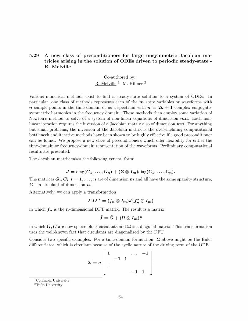
5.29 A new class of preconditioners for large unsymmetric Jacobian ma-tricies arising in the solution of ODEs driven to periodic steady-state -R. Melville

Co-authored by:R. Melville 1 M. Kilmer 2

Various numerical methods exist to find a steady-state solution to a system of ODEs. Inparticular, one class of methods represents each of the m state variables or waveforms withn sample points in the time domain or as a spectrum with n = 2k + 1 complex conjugate-symmetrix harmonics in the frequency domain. These methods then employ some variation ofNewton’s method to solve of a system of non-linear equations of dimension mn. Each non-linear iteration requires the inversion of a Jacobian matrix also of dimension mn. For anythingbut small problems, the inversion of the Jacobian matrix is the overwhelming computationalbottleneck and iterative methods have been shown to be highly effective if a good preconditionercan be found. We propose a new class of preconditioners which offer flexibility for either thetime-domain or frequency-domain representation of the waveforms. Preliminary computationalresults are presented.

The Jacobian matrix takes the following general form:

J = diag(G1, . . . , Gn) + (Σ⊗ Im)diag(C1, . . . , Cn).

The matrices Gi, Ci, i = 1, . . . , n are of dimension m and all have the same sparsity structure;Σ is a circulant of dimension n.

Alternatively, we can apply a transformation

FJF ∗ = (fn ⊗ Im)J(f∗n ⊗ Im)

in which fn is the n-dimensional DFT matrix. The result is a matrix

J = G + (Ω⊗ Im)c

in which G, C are now sparse block circulants and Ω is a diagonal matrix. This transformationuses the well-known fact that circulants are diagonalized by the DFT.

Consider two specific examples. For a time-domain formuation, Σ above might be the Eulerdifferentiator, which is circulant because of the cyclic nature of the driving term of the ODE

Σ = σ

1 . . . −1−1 1

...−1 1

1Columbia University2Tufts University

64

where σ is a scaling term.

Alternatively, for a frequency-domain representation, Ω is a pure-imaginary diagonal matrixdiag(−jkω, . . . ,−jω, 0, +jω, . . . , +jkω) where the 0 in the middle shows that the deriva-tive of the “DC” (constant) term in the Fourier expansion is zero.

We wish to solve linear systems involving this transformed matrix with a preconditioned iterativemethod. As the matrix is not Hermitian (although the sparsity pattern shows some symmetryproperties), we are restricted to iterative methods appropriate for such systems. In this talk,we consider preconditioned restarted GMRES for simplicity.

The theory of displacement rank suggests a method ways to construct a preconditioner J forthe above systems. We want J to be substantially easier to invert than J itself while theeigenspectrum of the preconditioned system is clustered around 1.

The displacement rank of a matrix T given the displacement operator for a fixed pair of matricesZa, Zb is the rank of the matrix G defined by

T − ZaTZTb = G = ABT .

Here, A, B are the generators of T with respect to the displacement operator. Depending onZa, Zb, algorithms exist for determining the LU factorization of T based only on the generatorswhich cost at most O(N2α) flops in the case of dense T where N is the dimension of the matrixand α is the displacement rank.

We wish to approximate J by a matrix J with relatively low displacement rank. We note thatthe diagonal entries of the matrix Ω vary smoothly. Thus, we can define an approximation Ω bypeforming piece-wise averaging along the diagonal, so that the diagonal is replaced by ρ piece-wise constant sections, ρ n. Now, define J using Ω rather than Ω. By construction it canbe shown that the displacement rank of J is at most α = m(1 + ρ) when Za = Zb = Z⊗ I,where Z is the m×m matrix with all zero entries except for ones on the first subdiagonal.

For the preconditioner, we then construct an approximate LU factorization of J using a general-ized Schur algorithm, adapted for the complex case and which exploits the sparsity of the matrix(and therefore, the generators). The approximation is obtained by keeping the magnitude ofthe entries in the generators in check, possibly reducing the displacement rank. Some degree ofpivoting is allowed during or before the factorization stage, provided that certain criteria arenot violated in the process.

We present preliminary results that indicate the effectiveness of the preconditioner in reducingthe number of iterations even for very sparse approximations to L and U .

65

5.30 A preconditioner for Krylov subspace method using a sparse directsolver in biochemistry applications - M. Okada

Co-authored by:M. Okada 1 T. Sakurai 2 K. Teranishi 3

We consider solution of sparse linear systems that arise from generalized eigenvalue problems formolecular orbital calculation of the biochemistry application [2]. This application predicts thereaction and properties of proteins in water molecules through the orbital of molecules indicatedby the status of electron distribution. The prediction of the electron distribution requires toobtain a large portion of the eigenpairs in the following generalized eigenvalue problems:

Fv = λSv, (25)

where F ∈ Rn×n is symmetric, and S ∈ Rn×n is symmetric positive definite. We solve thisproblem through countor integration [4] that enables spectrum splitting into complex domain.Consequently, this method allows us to compute these eigenpairs in embracingly parallel, andutilize multiple PC clusters managed by Grid middleware [5].

In our eigenvalue solution method, the computation at each contour involves sparse linearsystem solutions Ax = b where the coefficient matrix for each linear system is computed as:

A = ωS − F, (26)

where ω is a complex parameter. We seek efficient solution for these systems using precondi-tioned Krylov subspace method, because a large portion of A exhibits random nonzero patternsdue to water molecules as demonstrated in Figure 9 and A contains relatively large number ofnonzero elements due to the base function of middle-range interaction of molecules. For suchlinear systems, fill-reducing ordering [1] for A is not effective to utilize sparse direct methods[6, 7, 9] effectively.

We seek robust preconditioning using sparse complete factorization of the matrix LU = Aobtained from drop-thresholding of the original coefficient matrix A. Due to less nonzeroelements in A than A, we expect fewer nonzero elements in the preconditioner L and U thanthe matrix factor obtained from sparse LU factorization of A. The drop-thresholding on A canbe as simple as:

|aij| ≤ max1≤k,l≤n

(|akl|)× θ ⇒ aij = 0, (27)

where θ is a real number. The complete factorization is performed by parallel sparse directsolvers such as WSMP[9], UMFPACK[7] and SuperLU[6].

1Graduate School of Systems and Information Engineering, University of Tsukuba,okada@mma.cs.tsukuba.ac.jp

2Department of Computer Science, University of Tsukuba, sakurai@cs.tsukuba.ac.jp3Department of Computer Science and Engineering, The Pennsylvania State University, teranish@cse.psu.edu

66

Figure 9: The pattern of nonzero elements inA.

Figure 10: Molecular illustration of lysozyme.

We report the performance of our preconditioner for the sparse matrices that arise from ourapplication including comparison with variants of level-of-fill Incomplete Cholesky precondition-ing for complex numbers. The experiments were performed out on the PC cluster of Pentium42.8GHz, 2.0 Gbytes memory. Our preconditioning schemes were applied in conjunction withCOCG method [8] for complex symmetric systems. The maximum iteration counts were setto 1000, and the stopping criterion for the relative residual was 10−10. We set initial guessof the solution to x0 = 0 and all elements of b were set to 1. Our proposed method wascomputed using LU factorization in WSMP [9]. In addition, we tested Incomplete Choleskyfactorization(IC(0)) and Incomplete Cholesky factorization with Complex Shift(CSIC(0))[3] forcomparison.

The test matrices were obtained from computation of the molecular orbitals of lysozyme (129amino-acid residues, 1,961 atoms) with 20,758 basis functions [2]. The structure of the lysozymemolecule has been determined based on the real experiment, and we added counter-ions andwater molecules around the lysozyme molecule in order to simulate in vivo conditions. Thedimension of both F and S was 20,758, and the number of nonzero elements was 10,010,416;the pattern of nonzero elements is presented in Figure 9 and a molecular illustration of lysozymeis presented in Figure 10.

Table 1 shows the results for ω = −0.2+1.0−4i, where i is imaginary unit. In this case, IC(0)and CSIC(0) converged faster than our method. However, our method outperforms IC(0) andCSIC(0) for θ = 1.0× 10−2 and θ = 5.0× 10−3.

Table 2 shows the results for ω = −0.5+1.0−4i where the problem is harder than the previousinstance and associated with middle of the eigen spectrum in our application. In this case, IC(0)and CSIC(0) failed to solve due to the divergence of the COCG iterations, while our methodwas able to solve this problem.

We are currently investigating the performance of our method for parallel computing platformsand characterizing tradeoffs between the thresholding values and the performance of precondi-tioning.

67

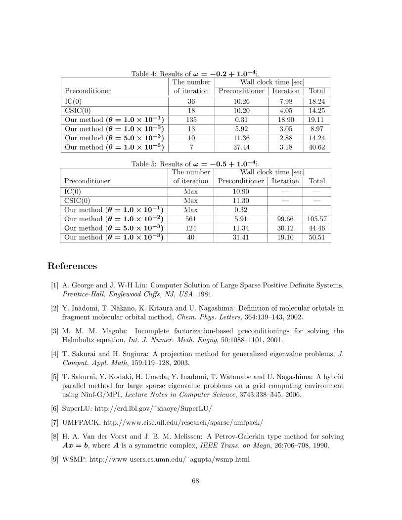
Table 4: Results of ω = −0.2 + 1.0−4i.The number Wall clock time [sec]

Preconditioner of iteration Preconditioner Iteration TotalIC(0) 36 10.26 7.98 18.24CSIC(0) 18 10.20 4.05 14.25Our method (θ = 1.0× 10−1) 135 0.31 18.90 19.11Our method (θ = 1.0× 10−2) 13 5.92 3.05 8.97Our method (θ = 5.0× 10−3) 10 11.36 2.88 14.24Our method (θ = 1.0× 10−3) 7 37.44 3.18 40.62

Table 5: Results of ω = −0.5 + 1.0−4i.The number Wall clock time [sec]

Preconditioner of iteration Preconditioner Iteration TotalIC(0) Max 10.90 — —CSIC(0) Max 11.30 — —Our method (θ = 1.0× 10−1) Max 0.32 — —Our method (θ = 1.0× 10−2) 561 5.91 99.66 105.57Our method (θ = 5.0× 10−3) 124 11.34 30.12 44.46Our method (θ = 1.0× 10−3) 40 31.41 19.10 50.51

References

[1] A. George and J. W-H Liu: Computer Solution of Large Sparse Positive Definite Systems,Prentice-Hall, Englewood Cliffs, NJ, USA, 1981.

[2] Y. Inadomi, T. Nakano, K. Kitaura and U. Nagashima: Definition of molecular orbitals infragment molecular orbital method, Chem. Phys. Letters, 364:139–143, 2002.

[3] M. M. M. Magolu: Incomplete factorization-based preconditionings for solving theHelmholtz equation, Int. J. Numer. Meth. Engng, 50:1088–1101, 2001.

[4] T. Sakurai and H. Sugiura: A projection method for generalized eigenvalue problems, J.Comput. Appl. Math, 159:119–128, 2003.

[5] T. Sakurai, Y. Kodaki, H. Umeda, Y. Inadomi, T. Watanabe and U. Nagashima: A hybridparallel method for large sparse eigenvalue problems on a grid computing environmentusing Ninf-G/MPI, Lecture Notes in Computer Science, 3743:338–345, 2006.

[6] SuperLU: http://crd.lbl.gov/˜xiaoye/SuperLU/

[7] UMFPACK: http://www.cise.ufl.edu/research/sparse/umfpack/

[8] H. A. Van der Vorst and J. B. M. Melissen: A Petrov-Galerkin type method for solvingAx = b, where A is a symmetric complex, IEEE Trans. on Magn, 26:706–708, 1990.

[9] WSMP: http://www-users.cs.umn.edu/˜agupta/wsmp.html

68

5.31 Hybrid iterative/direct strategies for solving the three-dimensional time-harmonic Maxwell equations discretized by discontinuous Galerkin meth-ods - R. Perrussel

Co-authored by:R. Perrussel 1 V. Dolean 2 H. Fol 3 S. Lanteri 4

This work aims at developing high-performance numerical strategies for the computer simu-lation of time-harmonic electromagnetic wave propagation problems in complex domains andheterogeneous media. In this context, we are naturally led to consider volumic discretizationmethods (i.e. finite difference, finite volume or finite element methods) as opposed to surfacicdiscretization methods (i.e. boundary element method). Most of the related existing works dealwith the second-order form of the time-harmonic Maxwell equations discretized by the edge fi-nite element method [15] and more recently, discontinuous Galerkin methods [11]. Recently,theoretical results concerning discontinuous Galerkin methods applied to the time-harmonicMaxwell equations have been obtained by several authors. Most of these results use a mixedformulation [16, 12] but the convergence of discontinuous Galerkin methods on the non-mixedformulation have also been proved [11, 4]. Here, we are concerned with the application of suchdiscontinuous Galerkin methods to the first order form of the three-dimensional time-harmonicMaxwell’s equations, and we aim to design a parallel solution strategy for the resulting large,sparse algebraic systems with complex coefficients.

Indeed, as far as non-trivial propagation problems are considered, classical iterative methodsbehave very poorly or even fail to converge. The preconditioning issues for highly indefiniteand non-symmetric matrices is for instance discussed by Benzi et al. in [3] in the context of in-complete factorization and sparse approximate inverse preconditioners. If a robust and efficientsolver is sought then a sparse direct method is the most practical choice. Over the last decade,a significant progress has been made in developing parallel direct methods for solving sparse lin-ear systems, due in particular to advances made in both the combinatorial analysis of Gaussianelimination process, and on the design of parallel block solvers optimized for high-performancecomputers [2, 10]. However, direct methods still fail to solve very large three-dimensional prob-lems, due to the potentially huge memory requirements for these cases. Iterative methods canbe used to overcome this memory problem but, in order to build robust preconditioners, someapproaches combine the direct solver techniques with iterative preconditioning techniques. Forexample, a popular approach in the domain decomposition framework is to use a direct solverinside each subdomain and to use an iterative solver at the interfaces between subdomains.This approach is adopted in this work.

1Ecole Centrale de Lyon, Laboratoire Ampere, CNRS UMR 5005, 69134 Ecully Cedex, France2Universite de Nice-Sophia/Antipolis, Laboratoire J.A. Dieudonne, CNRS UMR 6621, 06108 Nice Cedex,

France3INRIA, 2004 Route des Lucioles, BP 93, 06902 Sophia Antipolis Cedex, France4INRIA, 2004 Route des Lucioles, BP 93, 06902 Sophia Antipolis Cedex, France

69

Domain Decomposition methods are flexible and powerful techniques for the parallel numericalsolution of systems of PDEs. Concerning their application to time-harmonic wave propagationproblems, the simplest algorithm was proposed by Despres [6] for solving the Helmholtz equationand then extended and generalized for the time-harmonic Maxwell equations in [7, 5, 1]. Theanalysis of a larger class of Schwarz algorithms has been performed recently in [8]. Our ultimateobjective is the design and application of optimized Schwarz algorithms in conjunction withdiscontinuous Galerkin methods. The first step in this direction is to understand and analyzeclassical overlapping and non-overlapping Schwarz algorithms in the discrete framework of thesediscretization methods. To our knowledge, except Helluy [9], where such an algorithm is appliedto a discretization of the first-order time-harmonic Maxwell equations by a upwind finite volumemethod, no other attempts for higher order discontinuous Galerkin methods or different kind offluxes can be found in the literature. A classical domain decomposition strategy is adopted inthis study which takes the form of a Schwarz-type algorithm where Despres conditions [7] areimposed at the interfaces between neighboring subdomains. A multifrontal sparse direct solveris used at the subdomain level. Furthermore, in order to reduce the memory requirements forstoring the L and U factors associated to the factorization of subdomain problems, a mixed-precision approach is adopted where the factors are computed and stored in single precision(32 bits) arithmetic. Then, to recover double precision arithmetic (64 bits), these factors areused either as a preconditioner to a Krylov subspace method or within an iterative refinementprocedure. Similar strategies have recently been considered in the linear algebra communityessentially for performance issues [13, 14] on modern high-performance processors.

The resulting domain decomposition strategies can be viewed as hybrid iterative/direct solutionmethods for the large, sparse and complex coefficients algebraic system resulting from thediscretization of the time-harmonic Maxwell equations by a discontinuous Galerkin method. Weinvestigate in details the numerical and parallel performances of these strategies by consideringon one hand, classical diffraction problems by perfectly electric conductive objects and, on theother hand, the propagation of a plane wave in a heterogeneous medium defined as a realisticgeometrical model of the head of a mobile phone user.

References

[1] A. Alonso-Rodriguez and L. Gerardo-Giorda. New nonoverlapping domain decompositionmethods for the harmonic Maxwell system. SIAM J. Sci. Comput., Vol. 28, No. 1, pp. 102-122, 2006.

[2] P.R. Amestoy and I.S. Duff and J.-Y. L’Excellent. Multifrontal parallel distributed sym-metric and unsymmetric solvers. Comput. Meth. App. Mech. Engng., Vol. 184, pp. 501-520,2000.

[3] M. Benzi and J.C. Haws and M. Tuma. Preconditioning highly indefinite and nonsymmetricmatrices. SIAM J. Sci. Comput., Vol. 22, No. 4, pp. 1333-1353, 2000.

70

[4] A. Buffa and I. Perugia. Discontinuous Galerkin approximation of the Maxwell eigenprob-lem. SIAM J. Numer. Anal., Vol. 44, No. 5, pp. 2198-2226, 2006.

[5] P. Collino and G. Delbue and P. Joly and A. Piacentini. A new interface condition in thenon-overlapping domain decomposition. Comput. Methods Appl. Mech. Engrg., Vol. 148,pp. 195-207, 1997.

[6] B. Despres. Decomposition de domaine et probleme de Helmholtz. C.R. Acad. Sci. Paris,Vol. 1, No. 6, pp. 313-316, 1990.

[7] B. Despres and P. Joly and J.E. Roberts. A domain decomposition method for the harmonicMaxwell equations. Iterative methods in linear algebra, pp. 475-484, Amsterdam, North-Holland, 1992.

[8] V. Dolean and L.Gerardo-Giorda and M. Gander. Optimized Schwarz methods for Maxwellequations. Submitted, 2006. https://hal.archives-ouvertes.fr/ccsd-00107263.

[9] P. Helluy. Resolution numerique des equations de Maxwell harmoniques par une methoded’elements finis discontinus. PhD thesis, Ecole Nationale Superieure de l’Aeronautique,1994.

[10] P. Henon and P. Ramet and J. Roman. PaStiX: a high-performance parallel direct solverfor sparse symmetric definite systems. Parallel Comput., Vol. , No. 28, pp. 301-321, 2002.

[11] P. Houston and I. Perugia and A. Schneebeli and D. Schotzau. Interior penalty method forthe indefinite time-harmonic Maxwell equations. Numer. Math., Vol. 100, No. 3, pp. 485-518, 2005.

[12] P. Houston and I. Perugia and A. Schneebeli and D. Schotzau. Mixed discontinuousGalerkin approximation of the Maxwell operator: the indefinite case. ESAIM: Math.Model. Numer. Anal., Vol. 39, No. 4, pp. 727-753, 2005.

[13] J. Kurzak and J. Dongarra. Implementation of the mixed-precision in solving systems oflinear equations on the CELL processor. Technical Report UT-CS-06-580, University ofTennessee, 2006.

[14] J. Langou and J. Langou and P. Luszczek and J. Kurzak and A. Buttari and J. Dongarra.Exploiting the performance of 32 bit floating point arithmetic in obtaining 64 bit accuracy.Technical Report UT-CS-06-574, University of Tennessee, 2006.

[15] P. Monk. Finite element methods for Maxwell’s equations. Oxford University Press, 2003.

[16] I. Perugia and D. Schotzau and P. Monk. Stabilized interior penalty methods for the time-harmonic Maxwell equations. Comput. Methods Appl. Mech. Engrg., Vol. 191, No. 41-42,pp. 4675-4697, 2002.

71

5.32 Multigrid preconditioned Krylov subspace methods for the solution ofthree-dimensional Helmholtz problems in geophysics - X. Pinel

Co-authored by:X. Pinel 1 H. Calandra 2 I. Duff 3 S. Gratton 4 X. Vasseur 5

Our target application is a frequency-domain migration in seismics. This numerical simulationis of great importance in oil exploration for predicting correctly the structure of the subsurface.For practical applications, this requires the accurate computation of a wave propagation in aninhomogeneous medium. The wave propagation is modelled by the Helmholtz equation:

−∆u− (1− i α) k2u = g in Ω (28)

with first-order radiation boundary conditions:

∂u

∂n− iku = 0 on δΩ (29)

with u the pressure wavefield, α a damping coefficient, g the source term, n the unit out-ward normal to δΩ and i the imaginary unit (i2 = −1). In an unit computational domain

the wavenumber is defined as k =2πf

cwhere f is the frequency and c is the speed of

sound. A key point for an efficient migration is thus a robust and fast solution method forthe three-dimensional Helmholtz problem for large wavenumbers. Second-order finite differencediscretization schemes on equidistant grids are assumed here.In this talk we will consider geometric multigrid preconditioned Krylov subspace methods asiterative solution methods for such large linear systems. We will propose a detailed study oftwo numerical approaches. In these approaches, the preconditioner consists in a multigrid cycleapplied either to (28) or an equation close to (28). • The first approach retains the originalHelmholtz problem (28,29). As explained in [1] it is challenging to design a convergent multigridmethod especially for high wavenumbers because of difficulties associated to both smoothingand coarse grid correction. Here a two-grid method is thus adopted where the coarse grid prob-lem is handled by a direct solution method. The idea behind is to consider a large enough gridto avoid coarse grid correction difficulties. This combined direct-iterative two-grid method isthen used as a preconditioner for a Krylov subspace method. This strategy has been success-fully applied to a realistic seismic benchmark problem in two dimensions in [2]. It was shownby experiment that although this two-grid iteration is not converging as fixed point iteration,it is effective as a preconditioner for a Krylov method. For three-dimensional applications onepossible drawback is that using a sufficiently large coarse grid may not be a scalable approach.

1CERFACS, 42 avenue Gaspard Coriolis, F-31057 Toulouse cedex 1, France2 TOTAL, Centre Scientifique et Technique Jean Feger, Avenue Larribau, F-64018 Pau cedex, France3 CERFACS, 42 avenue Gaspard Coriolis, F-31057 Toulouse cedex 1, France4 CERFACS, 42 avenue Gaspard Coriolis, F-31057 Toulouse cedex 1, France5 CERFACS, 42 avenue Gaspard Coriolis, F-31057 Toulouse cedex 1, France

72

• In the second approach the preconditioner is based on a complex shifted Helmholtz operator(with real-valued β1 and β2 parameters):

−∆u− (β1 − iβ2) k2u = g in Ω (30)

the multigrid solution of which was first studied in [3] for two-dimensional problems. The sameabsorbing boundary conditions as in (29) were considered. In [3] it was shown by Fourier analysisand experiment that it is possible to design a convergent multigrid method for this problemthanks to the complex shift. A Krylov subspace method - preconditioned with this multigridmethod - is then used to further improve the convergence rate of the numerical method.Numerical experiments will be presented. We will especially address the behaviour of bothsolution methods when large wavenumbers are considered. We will also provide a comparisonin terms of robustness and scalability.

References

[1] Elman, H. R., Ernst, O. G. and O’Leary, D. P., 2001, A multigrid method enhanced byKrylov subspace iteration for discrete Helmholtz equations. SIAM J. Sci. Comput., 23,1291–1315.

[2] Duff, I. S., Gratton, S., Pinel, X. and Vasseur, X., 2007, Multigrid based preconditionersfor the numerical solution of two-dimensional heterogeneous problems in geophysics, CER-FACS Technical Report, TR/PA/07/03. Accepted in ”International Journal of ComputerMathematics”.

[3] Erlangga, Y. A., Oosterlee, C. and Vuik, C., 2006, A novel multigrid based preconditionerfor heterogeneous Helmholtz problems. SIAM J. Sci. Comput., 27, 1471–1492.

5.33 On acceleration methods for approximating matrix functions - M. Popolizio

Co-authored by:M. Popolizio 1 V. Simoncini 2

The recent interest in accelerating the numerical approximation of the matrix exponential in-spired this work. Our main result is that some recently developed acceleration procedures maybe restated as preconditioning techniques for the partial fraction expansion form of an approx-imating rational function. These new results allow us to devise a-priori strategies to selectthe associated acceleration parameters and the numerical results show the effectiveness of thechoice.

1Dipartimento di Matematica, Universita di Bari, Italia2 Dipartimento di Matematica, Universita di Bologna, Italia

73

References

[1] O. Axelsson and A. Kucherov, Real valued iterative methods for solving complex symmetriclinear systems, Numer. Linear Algebra Appl., 7 (2000), pp.197-218

[2] J. van den Eshof and M. Hochbruck, Preconditioning Lanczos approximations to the matrixexponential , SIAM J. Sci. Comput., 27 (2006), pp.1438-1457

5.34 Characterizing the relationship between ILU-type preconditioners andthe storage hierarchy - D. Rivera

Co-authored by:D. Rivera 1 D. Kaeli 2 M. Kilmer 3

ILU-type preconditioning techniques are widely recognized as being an extremely effective ap-proach to providing efficient solvers[1]. These techniques have been used to increase the perfor-mance and reliability of Krylov subspace methods. However, a drawback of these approachesis that it is difficult to choose appropriate values for the preconditioner tuning parameters[2].Usually, parameter selection is done through trial-and-error for a few sample matrices for agiven application.

In our work we have found that the performance of these techniques and methods also dependsupon the relationship between the preconditioner tuning parameters and the memory hierarchyof the machine used to carry out the computation. The parameter values used to obtain thefastest execution time, given an acceptable final error, may be different for different memoryhierarchies. This occurs due to 1) the non-zero structure of the new coefficient matrix dependingon the tuning parameter values and 2) the ability of the memory hierarchy to exploit the localitypresent in the new matrix.

The difference in performance on different memory hierarchies becomes significant when theproblem’s conditions make it more difficult to solve. These conditions are related to the drop-ping strategy adopted in the preconditioner algorithm. For example, the relation between thenumerical symmetry4 and the bandwidth (NS/B) of the coefficient matrix allows us to estimatehow difficult it will be to solve the problem using the ILUT preconditioner. This is because thedropping strategy for the ILUT preconditioner is based on dropping elements in the GaussianElimination process according to their magnitude. The results shown in Figure 11 support

1Department of Electrical and Computer Engineering, Northeastern University, Boston, MA2 Department of Electrical and Computer Engineering, Northeastern University, Boston, MA3 Department of Mathematics, Tufts University, Medford, MA4Numerical symmetry is computed as the rate between number of maches where ai,j = aj,i with i 6= j and

the total number of offdiagonal entries

74

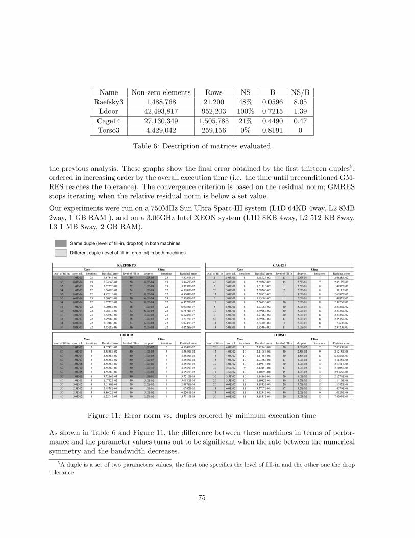
Name Non-zero elements Rows NS B NS/BRaefsky3 1,488,768 21,200 48% 0.0596 8.05

Ldoor 42,493,817 952,203 100% 0.7215 1.39Cage14 27,130,349 1,505,785 21% 0.4490 0.47Torso3 4,429,042 259,156 0% 0.8191 0

Table 6: Description of matrices evaluated

the previous analysis. These graphs show the final error obtained by the first thirteen duples5,ordered in increasing order by the overall execution time (i.e. the time until preconditioned GM-RES reaches the tolerance). The convergence criterion is based on the residual norm; GMRESstops iterating when the relative residual norm is below a set value.

Our experiments were run on a 750MHz Sun Ultra Sparc-III system (L1D 64KB 4way, L2 8MB2way, 1 GB RAM ), and on a 3.06GHz Intel XEON system (L1D 8KB 4way, L2 512 KB 8way,L3 1 MB 8way, 2 GB RAM).

UltraXeon

2.1274E-08104.0E-02201.1416E-08103.5E-0230

1.1416E-08103.5E-02301.1082E-08103.5E-0220

1.1082E-08103.5E-02203.1833E-08116.0E-0220

1.4079E-08103.5E-02173.7707E-08116.0E-0213

1.0323E-0892.0E-02303.3234E-08116.0E-0215

2.0350E-0871.0E-02302.1274E-08104.0E-0220

2.1215E-0892.5E-02302.1105E-08104.0E-0217

8.3086E-0981.5E-02304.1135E-08104.0E-0213

4.1135E-08104.0E-02132.9366E-08104.0E-0215

2.1951E-08104.0E-02302.1951E-08104.0E-0230

2.1105E-08104.0E-02172.1215E-0892.5E-0230

2.9366E-08104.0E-02151.4079E-08103.5E-0217

TORSO

Residual erroriterationsdrop tol.level of fill-inResidual erroriterationsdrop tol.level of fill-in

7.4593E-09103.0E-02203.1831E-08116.0E-0230

UltraXeon

2.3926E-0285.0E-01401.7308E-0285.0E-015

2.3926E-0285.0E-01502.3926E-0285.0E-0130

2.3926E-0285.0E-01202.2126E-0285.0E-019

2.3546E-0285.0E-01132.3926E-0285.0E-0150

1.7360E-0285.0E-0132.3420E-0285.0E-0111

2.6528E-0272.5E-01131.4892E-0285.0E-011

2.8517E-0272.5E-01152.3926E-0285.0E-0140

1.4892E-0282.5E-0111.5111E-0285.0E-012

1.5111E-0285.0E-0122.3926E-0285.0E-0120

2.6387E-0281.0E-0112.3882E-0285.0E-0117

1.4892E-0285.0E-0111.7360E-0285.0E-013

2.3926E-0285.0E-01302.3695E-0285.0E-0115

CAGE14

Residual erroriterationsdrop tol.level of fill-inResidual erroriterationsdrop tol.level of fill-in

2.3420E-0285.0E-01112.3546E-0285.0E-0113

UltraXeon

6.9058E-07221.0E-03366.9058E-07221.0E-0336

6.7871E-07226.0E-04326.7871E-07226.0E-0432

6.6286E-07234.0E-04306.6286E-07234.0E-0430

3.7978E-07221.0E-03383.7978E-07221.0E-0338

5.0248E-07226.0E-04345.0248E-07226.0E-0434

7.5754E-07231.0E-03307.5754E-07231.0E-0330

5.8466E-07238.0E-04305.8466E-07238.0E-0430

5.3237E-07231.0E-03325.3237E-07231.0E-0332

6.5689E-07221.0E-03346.5689E-07221.0E-0334

4.8701E-07228.0E-04324.8701E-07228.0E-0432

7.5087E-07236.0E-04307.5087E-07236.0E-0430

6.3722E-07228.0E-04346.3722E-07228.0E-0434

RAEFSKY3

Residual erroriterationsdrop tol.level of fill-inResidual erroriterationsdrop tol.level of fill-in

4.4528E-07228.0E-04364.4528E-07228.0E-0436

UltraXeon

3.7216E-0341.0E-01503.7216E-0341.0E-0150

5.0180E-0445.0E-02501.0742E-0241.0E-0140

2.4878E-0442.5E-02505.0180E-0445.0E-0250

1.0742E-0241.0E-01402.4878E-0442.5E-0250

6.2204E-0345.0E-02403.8002E-0352.5E-0150

4.5742E-0231.0E-02504.5742E-0231.0E-0250

4.5558E-0231.0E-03504.5558E-0231.0E-0350

4.5558E-0231.0E-04504.5558E-0231.0E-0450

4.5558E-0231.0E-07504.5558E-0231.0E-0750

4.5558E-0231.0E-06504.5558E-0231.0E-0650

4.5558E-0231.0E-10504.5558E-0231.0E-1050

4.5558E-0231.0E-05504.5558E-0231.0E-0550

LDOOR

Residual erroriterationsdrop tol.level of fill-inResidual erroriterationsdrop tol.level of fill-in

5.7514E-0342.5E-02406.2204E-0345.0E-0240

Same duple (level of fill-in, drop tol) in both machines

Different duple (level of fill-in, drop tol) in both machines

Figure 11: Error norm vs. duples ordered by minimum execution time

As shown in Table 6 and Figure 11, the difference between these machines in terms of perfor-mance and the parameter values turns out to be significant when the rate between the numericalsymmetry and the bandwidth decreases.

5A duple is a set of two parameters values, the first one specifies the level of fill-in and the other one the droptolerance

75

To illustrate that the overall execution time can be reduced because the memory hierarchy hasthe ability to exploit the locality in the new matrix, we use the PIN tool to capture cacheevents[5]. Our results show a high correlation among the execution time, memory accesses andcache misses.

We show that on one memory hierarchy, a greater level of fill-in can be used than on otherhierarchies. For instance, the fastest execution time on the Ultra Sparc-III system was obtainedfor the duple(30, 0.01), whereas the fastest execution time on the Intel XEON system wasobtained for the duple(20, 0.04).

We developed an algorithmic approach to: 1) extract the problem’s conditions related to thedropping strategies adopted in the preconditioner, 2) detect if the computation of a solutiondepends upon the relationship between the preconditioner’s parameters and the memory hier-archy of the machine used and 3) suggest values of the preconditioner’s parameters which canhelp to reduce the time required to compute the preconditioner and the solution for matriceswith similar characteristics.

We evaluated over 110 matrices from the MatrixMarket[3] and University of Florida[4] repos-itories. In addition to these, we created several slightly different matrices by adding randomvalues with a controlled standard deviation and by zeroing several of the non-zero elements.This gave us a complete set of 200 matrices to be tested. The ILU-type preconditioning algo-rithms included in the SPARSKIT[6] library were used together with restarted GMRES withrestart values equal to 30 and 40.

Our experimental results show that 78.4% of the time, the suggested values of the precondi-tioner’s parameters were appropriate in reducing the overall execution time.

We will explore more sophisticated heuristics for our algorithmic approach in order to increasethe percentage of suggested values of the preconditioner’s parameters appropriated. In addition,we will extend our study to multilevel preconditioners based on ILU factorization.

Acknowledgment

Many thanks to Michele Benzi for his help and insights during the early stages of this work.

This project is supported by the National Science Foundations Computing and Communica-tion Foundations Division, grant number CCF-0342555 and the Institute of Complex ScientificSoftware.

References

[1] Y. Saad. Iterative Methods for Sparse Linear Systems. Society for Industrial and AppliedMathematics, Philadelphia, PA, USA, 2003.

76

[2] Michele Benzi. Preconditioning techniques for large linear systems:a survey. J. Comput.Phys., 182(2):418–477, 2002.

[3] Matrix Market. http://math.nist.gov/MatrixMarket.

[4] University of Florida Sparse Matrix Collection. http://www.cise.ufl.edu/research/sparse/matrices/.

[5] Pin. http://rogue.colorado.edu/Pin/index.html.

[6] Y. Saad. SPARSKIT: A Basic Tool Kit for Sparse Matrix Computation. http://www-users.cs.umn.edu/saad/software/SPARSKIT/sparskit.html.

5.35 A nested iterative scheme for linear systems in computational fluiddynamics - A. H. Sameh

Co-authored by:A. H. Sameh 1 M. Manguoglui 2 T. E. Tezduyar 3 S. Sathe 4 F. Saied 5

We present an effective preconditioning scheme for solving nonsymmetric segregated linearsystems that arise from discretization of the Navier-Stokes equations in fluid flow problems.Often, these systems are of the form(

A BCT D

)(up

)=(

fg

). (31)

Here A is an n×n nonsingular matrix, B and C are n×m matrices, where m ≤ n. Methodsfor solving these systems have been extensively studied, e.g. see [4]. The approach we presenthere consists of solving Eq. 31 via a nested preconditioned Krylov subspace method, such asBiCGstab, with a structured preconditioner M , e.g. see [1]. Figure 12 decipts our proposednested scheme. M−1 is an approximation to the inverse of the original coefficient matrix inEq. 31. In each outer iteration we solve three linear systems . The first and third are systemsin which the coefficient matrix is A. These can be solved via a direct or iterative method. Thesecond system involves the Schur complement and is solved via BiCGstab with or without apreconditioner depending on the application at hand.

Applications

We consider two applications. The first is obtaining the time-accurate solution of flow in a longtube using the stabilized finite element formulation [5] . Figure 13 shows the coefficient matrixat time step 11 after reordering using the Reverse Cuthill-McKee algorithm for minimizing

1Department of Computer Science, Purdue University, USA2 Department of Computer Science, Purdue University, USA3 Department of Mechanical Engineering, Rice University, USA4 Department of Mechanical Engineering, Rice University, USA5 Rosen Center for Advanced Computing, Purdue University, USA

77

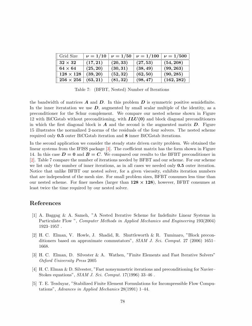
Grid Size ν = 1/10 ν = 1/50 ν = 1/100 ν = 1/50032× 32 (17, 21) (20, 33) (27, 53) (54, 208)64× 64 (25, 20) (30, 31) (38, 49) (99, 263)128× 128 (39, 20) (52, 32) (62, 50) (90, 285)256× 256 (63, 21) (81, 32) (98, 47) (162, 282)

Table 7: (BFBT, Nested) Number of Iterations

the bandwidth of matrices A and D. In this problem D is symmetric positive semidefinite.In the inner iteratation we use D, augmented by small scalar multiple of the identity, as apreconditioner for the Schur complement. We compare our nested scheme shown in Figure12 with BiCGstab without preconditioning, with ILU(0) and block diagonal preconditionersin which the first diagonal block is A and the second is the augmented matrix D. Figure15 illustrates the normalized 2-norms of the residuals of the four solvers. The nested schemerequired only 0.5 outer BiCGstab iteration and 8 inner BiCGstab iterations.

In the second application we consider the steady state driven cavity problem. We obtained thelinear systems from the IFISS package [3]. The coefficient matrix has the form shown in Figure14. In this case D = 0 and B = C. We compared our results to the BFBT preconditioner in[2]. Table 7 compare the number of iterations needed by BFBT and our scheme. For our schemewe list only the number of inner iterations, as in all cases we needed only 0.5 outer iteration.Notice that unlike BFBT our nested solver, for a given viscosity, exhibits iteration numbersthat are independent of the mesh size. For small problem sizes, BFBT consumes less time thanour nested scheme. For finer meshes (larger than 128 × 128), however, BFBT consumes atleast twice the time required by our nested solver.

References

[1] A. Baggag & A. Sameh, ”A Nested Iterative Scheme for Indefinite Linear Systems inParticulate Flow ”, Computer Methods in Applied Mechanics and Engineering 193(2004)1923–1957 .

[2] H. C. Elman, V. Howle, J. Shadid, R. Shuttleworth & R. Tuminaro, ”Block precon-ditioners based on approximate commutators”, SIAM J. Sci. Comput. 27 (2006) 1651–1668.

[3] H. C. Elman, D. Silvester & A. Wathen, ”Finite Elements and Fast Iterative Solvers”Oxford University Press 2005

[4] H. C. Elman & D. Silvester, ”Fast nonsymmetric iterations and preconditioning for Navier–Stokes equations”, SIAM J. Sci. Comput. 17(1996) 33–46 .

[5] T. E. Tezduyar, ”Stabilized Finite Element Formulations for Incompressible Flow Compu-tations”, Advances in Applied Mechanics 28(1991) 1–44.

78

5.36 A symmetric sparse approximate inverse preconditioner for block tridi-agonal - M. L. Sandoval

Co-authored by:M. L. Sandoval 1 G. Montero 2 A. Rodrıguez-Ferran 3

We propose a symmetric sparse approximate inverse (SSPAI) preconditioner for the iterativesolution of block tridiagonal systems with multiple right hand sides. The new preconditioneris based on Frobenius-norm minimization where the sparsity pattern is captured dynamically[1],[2].

We use the same theory presented in [2] to establish efficient and accumulative formulae toupdate the symmetric preconditioner M and to compute ‖AM − I‖F . Also, to completeour analysis, we compare the numeric results with the best family of incomplete Choleskyfactorizations (ICF) [3].

The effectiveness of the SSPAI preconditioner is illustrated by means of a technological ap-plication: the operation of actived-carbon filters. This transient convection-diffusion-reactionproblem is discretized by finite elements, and the convective term is stabilized with the stan-dard least-squares technique. The discretizing problem yields sparse and large systems whosematrices are symmetric and positive definite [4]. Also, due to the nature of the filters (chambersof actived-carbon and air), we have used an appropriate reordering of nodes to obtain blocktridiagonal matrices [3].

From our numerical experiments we conclude that it is necessary to consider the significantelements of the upper triangular part in order to construct a quality symmetric approximateinverse. We have also observed that it is important to parallelize the explicit preconditionerto be able to at least match the performance of incomplete Cholesky factorizations; even inthis way, the set-up phase of the first one would be more expensive. Hence, for transientconvection-diffusion problem, whose velocity field is constant, it is observed that the SSPAIwould outperform the best ICF considering both the memory requirements and total CPU time.Finally, we will see that although the parallelization of SSPAI has its limitations depending onthe number of blocks, the proposed SSPAI is an interesting strategy for the number of blocksused in the studied cases.

1Department of Mathematics, Universidad Autonoma Metropolitana-Iztapalapa. Mexico, D.F.2Department of Mathematics, University of Las Palmas de Gran Canaria, Edif. de Informatica y Matematicas,

Campus Universitario de Tafira, 35017 Las Palmas de Gran Canaria, Spain3Laboratori de Calcul Numeric (LaCaN), Department of Applied Mathematics III,

Civil Engineering School, Polytechnic University of Catalunya, Barcelona, Spain.

79

References

[1] Grote M, Huckle T. Parallel preconditioning with sparse approximate inverses. SIAMJournal of Scientific Computing, 18(3):838–853, 1997.

[2] Montero G, Gonzalez L, Florez E, Garcıa M. D, Suarez A. Approximate inverse computa-tion using Frobenius inner product. Numerical Linear Algebra with Applications, 9(3):239–247, 2002.

[3] Rodrıguez-Ferran A, Sandoval M L. Numerical performance of incomplete factoriza-tions for transient convection-diffusion problems. Advances in Engineering Software 2006,doi:10.1016/j.advengsoft.2006.09.003.

[4] Donea J, Huerta A. Finite element methods for flow problems. John Wiley & Sons:Chichester, 2003.

5.37 On some preconditioning techniques for nonlinear Least Squares prob-lems - A. Sartenaer

Co-authored by:A. Sartenaer 1 S. Gratton 2 J. Tshimanga 3

Our main interest is in the development and the study of preconditioning techniques for sym-metric positive definite linear systems arising when solving nonlinear least squares problems(see [1]). With this in mind, we first consider preconditioning techniques for the solution ofsymmetric positive definite linear systems with constant matrix A and multiple right-handsides bk (k = 1, 2, . . .). We assume that these systems are given in sequence, in the sensethat the right-hand sides are not known simultaneously, each one (except the first) possiblydepending on the solution of the previous system. In the context of (preconditioned) conju-gate gradient-like methods, we then propose a general class of preconditioners called LimitedMemory Preconditioners (LMPs). Their construction involves only a small number of linearlyindependent vectors (thus only little storage) and the matrix A through its product with thesevectors. We also show that the inverse form of these LMPs, as well as a numerically robustfactored form that we derive, are of limited memory type. Although the choice of the vectorsused to construct the LMPs is free, the key idea in building a preconditioner from this class is tocapture some relevant information gained during the solution of one system to precondition thenext one in the sequence. For that reason, we first explore some properties of the LMPs whenapplied to precondition the matrix A. More precisely, we study the effect of the LMPs on thespectrum of the preconditioned matrix in terms of clusterization and behaviour with respect to

1FUNDP (University of Namur), Belgium2CERFACS, France3FUNDP (University of Namur), Belgium

80

pre-existing clusters. We next consider special instances of LMPs by studying candidate setsof vectors having special properties, such as orthogonality, conjugacy or invariance with respectto the matrix A. We more particularly explore three members of the class: spectral-LMP,Quasi-Newton-LMP and Ritz-LMP ; the two first are well known preconditioners (see [2] and[3], respectively), and the third is new, up to our knowledge. The common particularity sharedby these three LMPs is the choice of conjugate directions with respect to the matrix A for thevectors used to build them. In addition to this, the Ritz-LMP uses vectors which are orthog-onal, whereas the spectral-LMP uses vectors which are not only orthogonal but also invariantwith respect to the matrix A. (Note that in this last case, the eigenvectors of the matrix aresupposed to be computationally available, an expensive task in most cases.)

We present an implementation of these three special instances, showing that:

• the cost of applying the Ritz- and Quasi-Newton-LMPs is twice the cost of applying thespectral-LMP;

• the Ritz-LMP is a generalization of the spectral-LMP and is mathematically equivalentto the Quasi-Newton-LMP when both are constructed with all relevant information takenfrom the same Krylov subspace;

• the Ritz-LMP uses about twice less memory than the Quasi-Newton-LMP and only onemore vector than the spectral-LMP (so nearly the same amount of memory).

We next consider the practical issue of using Ritz-information to approximate eigen-information(see [4]) and show that, in the context of LMPs, using this Ritz-information within the spectral-LMP yields a perturbed form of the Ritz-LMP. We end this first part by proposing a selectionstrategy for building the Ritz-LMP and show that this strategy is quite competitive with theone proposed in [3]. Although the proposed preconditioning techniques concern linear systemswith the same matrix and multiple right-hand sides, we investigate, in a second part, the issueof applying the LMPs on perturbed matrix systems (as occuring in nonlinear least squaresproblems). This study reveals that when LMPs are used for sequences of linear systems withslowly varying matrices, an important aspect to consider is the lost of conjugacy with respectto the new matrix in the sequence rather than the change in the whole matrix. We finallydescribe the implementation of the proposed ideas into a Lanczos solver that is used in someoperational centers for ocean and atmosphere data assimilation. Numerical experiments onacademic problems and on a real life data assimilation system (see [5]) are shown. Theseexperiments allow us to draw preliminary conclusions and to propose perpectives for furtherwork.

References

[1] A. Bjorck. Numerical Methods for Least Squares Problems. SIAM, Philadelphia, 1996.

81

[2] M. Fisher. Minimizing algorithms for variational data assimilation. in Proc. ECMWFseminar “Recent developments in numerical methods for atmospheric modelling”, pp. 364-385, September 1998.

[3] J. Nocedal and J. L. Morales. Automatic Preconditioning by Limited Memory Quasi-Newton Updating. SIAM J. Optimization, 10(4), pp. 1079–1096, 2000.

[4] G. H. Golub and C. F. Van Loan. Matrix Computations (Third Edition). Johns HopkinsUniversity Press, Baltimore, 1996.

[5] A. T. Weaver, J. Vialard and D. L. T. Anderson. Four-dimensional variational assimilationwith an ocean general circulation model of the tropical Pacific Ocean. Part 1: formulation,internal diagnostics and consistency checks. Monthly Weather Review, 131, pp. 1360-1378,2003.

5.38 Sparse approximate inverse preconditioners for complex symmetric sys-tems of linear equations - T. Sogabe

Co-authored by:T. Sogabe 1 S.-L. Zhang 2

In this talk, we will discuss an approach to constructing sparse approximate inverse precondi-tioniners for complex symmetric systems of linear equations.

Introduction

We consider the solution of nonsingular complex symmetric systems of linear equations of theform

Ax = b,

where A is an n×n non-Hermitian but symmetric matrix (A 6= AT , A = AT ). Such systemsarise in many important applications such as numerical computations in quantum chemistry,eddy current problems, and numerical solutions of the complex Helmholtz equation, and thenthere is a strong need for the fast solution of complex symmetric systems of linear equations.For solving such systems efficiently, some useful Krylov subspace methods such as the COCGmethod [7], the COCR method [6], and the QMR SYM method [4] have been proposed.

It is widely known that preconditioning techniques have an important role in improving theperformance of the Krylov subspace methods. Of various preconditioners, sparse approximateinverse preconditioners have recently received much attention since they are well suited for

1Dept. of Computational Science and Engineering, Graduate School of Engineering, Nagoya University, Japan.Email: sogabe@na.cse.nagoya-u.ac.jp

2Dept. of Computational Science and Engineering, Graduate School of Engineering, Nagoya University, Japan.Email: zhangr@na.cse.nagoya-u.ac.jp

82

parallel implementation. There are some kinds of sparse approximate inverse preconditionerssuch as Frobenius norm minimization (see [5]), factorized sparse approximate inverses [2], andrank-one update methods (see [3]). Since we apply COCG, COCR, and QMR SYM to complexsymmetric systems of linear equations, the coefficient matrices of preconditioned systems shouldbe complex symmetric. Factorized sparse approximate inverses can keep the coefficient matricescomplex symmetric, and thus factorized sparse approximate inverses can be a good approach.

The above reasons motivate us to consider an approach to sparse approximate inversepreconditioners for complex symmetric matrices, which is based on Benzi’s framework [1, 2].

In the next section, we will give an approach to constructing sparse approximate inversepreconditioners and show some procedures for the preconditioning matrices.

An approach to constructing sparse approximate inverse preconditioners

Let Z := [z1, z2, . . . , zn] be a nonsingular n×n complex matrix. Then, if there exist matricesZ and G such that

ZT AZ = G, (32)

we have

A−1 = ZG−1ZT . (33)

(zi, Azj) = 0 for all (i, j) ∈ S,

where (x, y) := xT y.

Here we consider two cases G = D and G = T for sparse approximate inverse precondi-tioners where D is a diagonal matrix and T is a tridiagonal matrix. When we choose G = D,the following algorithm makes it possible to obtain A−1 = ZD−1ZT .

Algorithm 1. The conjugate A-orthogonalization process

Set zi = ei for i = 1, 2, . . . , n,

p11 = a11,

for i = 2, 3, . . . , n

for j = 1, 2, . . . , i− 1

pji = (zj, ai),

for k = 1, 2, . . . , j

zki = zki −pji

pjjzkj,

endendpii = (zi, ai),

endReturn Z = [z1, z2, . . . , zn], D = diag(p11, p22, . . . , pnn).

83

The above algorithm is closely related to the AINV for Hermitian matrices [1] in that Algorithm1 uses improper inner product (x, y) and the AINV uses proper inner product (x, y). Herewe note that Algorithm 1 is equivalent to the AINV when the coefficient matrix A is realsymmetric.

Next, we consider the case G = T . Then we can obtain the inverse of (33) by using thefollowing complex symmetric Lanczos process [4].

Algorithm 2. The complex symmetric Lanczos process

set β0 = 0, z0 = 0,

set z1 = e1,

for i = 1, 2, . . . , n− 1

αi = (zi, Azi),

zi+1 = Azi − αizi − βi−1zi−1,

βi = (¯zi+1, zi+1)1/2,

zi+1 = zi+1/βi,

endReturn Z = [z1, z2, . . . , zn], T = tridiag(βi, αi, βi).

From Algorithm 2, we obtain A−1 = ZT −1ZT . When we use a sparse preconditioning matrixbased on this algorithm, we require the solution x = T −1y. The vector x can be obtained bysolving Tx = y with any O(n) direct method.

Dropping strategies for Algorithms 1,2 and the results of numerical experiments will bediscussed.

References

[1] M. Benzi, C. D. Meyer, and M. Tuma, A sparse approximate inverse preconditioner forthe conjugate gradient method, SIAM J. Sci. Comput., 17(1996), 1135-1149.

[2] M. Benzi and M. Tuma, A sparse approximate inverse preconditioner for nonsymmetriclinear systems, SIAM J. Sci. Comput., 19(1998), 968-994.

[3] R. Bru, J. Cerdan, J. Marın, and J. Mas, Preconditioning sparse nonsymmetric linearsystems with the Sherman-Morrison formula, SIAM J. Sci. Comput., 25(2003), 701-715.

[4] R. W. Freund, Conjugate gradient-type methods for linear systems with complex symmetriccoefficient matrices, SIAM J. Sci. Stat. Comput., 13(1992), 425-448.

[5] M. J. Grote and T. Huckle, Parallel preconditioning with sparse approximate inverses,SIAM J. Sci. Stat. Comput., 18(1997), 838-853.

84

[6] T. Sogabe and S.-L. Zhang, A COCR method for solving complex symmetric linear systems,J. Comput. Appl. Math., 199(2007), 297-303.

[7] H. A. van der Vorst and J. B. M. Melissen, A Petrov-Galerkin type method for solvingAx = b, where A is symmetric complex, IEEE Trans. Mag., 26(1990), 706-708.

5.39 An efficient domain decomposition preconditioner for time-harmonicacoustic scattering in multi-layered media - J. Toivanen

Co-authored by:J. Toivanen 1 K. Ito 2

A model for a pressure field p describing time-harmonic acoustic scattering in multi-layeredmedia is given by an inhomogeneous Helmholtz equation

−∆p− k2p = g,

where k = ωc

is the wave number, ω is the angular frequency, c is the speed of sound, andg corresponds to a sound source. Here the speed of sound and, thus, also the wave numberare assumed to be piecewise constant functions of location. For example, such problems resultfrom acoustic geological surveys. The exterior problem is truncated into a rectangle/cuboidand an absorbing boundary condition is posed on its boundaries. A low-order finite differencediscretization is performed on a uniform grid. This leads a system of linear equations with alarge sparse matrix A which is indefinite, complex symmetric, but not Hermitian.

Subdomains which overlap only on the interfaces are defined by the domains where the materialproperties are constants. Each of these subdomains is embedded into a larger rectangle/cuboidwith absorbing boundary conditions on its boundaries. The discretization of the jth extendedsubdomain problem leads a matrix Cj which has a block form

Cj =(

Cj,dd Cj,de

Cj,ed Cj,ee

),

where the subscripts d and e correspond to the subdomain and its extension, respectively. Thejth subdomain preconditioner is a Schur complement matrix

Bj = Cj,dd − Cj,deC−1j,eeCj,ed

and problems with it can be solved very efficiently using a fast direct solver; see [4], for example.Based on these subdomain preconditioners a Schwarz-type multiplicative preconditioner B =Pn is defined recursively as

P −1j = P −1

j−1 + RTj B−1

j Rj(I −AP −1j−1), j = 2, . . . , n, (34)

1Institute for Computational and Mathematical Engineering, Building 500, Stanford University, Stanford, CA94305, USA, E-mail: toivanen@stanford.edu

2Center for Research in Scientific Computation, Box 8205, North Carolina State University, Raleigh, NC27695, USA, E-mail: kito@ncsu.edu

85

where P −11 = RT

1 B−11 R1, the rectangular matrix Rj corresponds to the restriction operator

into the jth subdomain, and n is the number of subdomains.

Preconditioned systems are solved using the GMRES iterations which are reduced on a neigh-borhood of the interfaces between subdomains [1, 3]. As a result the memory requirement ofthe GMRES method is vastly reduced and, thus, it is not usually necessary to perform restarts.A more detailed description of the solution procedure can found from [2].

Numerical experiments demonstrate that two-dimensional problems with millions of unknownscan be solved in some tens of seconds on a PC [2]. Owing to the reduction of iterations onthe interfaces a three-dimensional problem with a billion unknowns is solved on a PC in a day.The experiments show that the convergence rate deteriorates only mildly when the frequencyis increased.

References

[1] E. Heikkola, T. Rossi, and J. Toivanen. A parallel fictitious domain method for the three-dimensional Helmholtz equation. SIAM J. Sci. Comput., 24:1567–1588, 2003.

[2] K. Ito and J. Toivanen. Efficient domain decomposition method for acoustic scattering inmulti-layered media. Proceedings of the Eccomas CFD 2006 Conference, Eccomas, 2006,in CD-ROM format.

[3] K. Ito and J. Toivanen. Preconditioned iterative methods on sparse subspaces. Appl. Math.Letters, 19:1191–1197, 2006.

[4] T. Rossi and J. Toivanen. Fast direct solver for block tridiagonal systems with separablematrices of arbitrary dimension. SIAM J. Sci. Comput., 20:1778–1796, 1999.

5.40 Testing parallel linear Krylov space iterative preconditioners and solversfor finite element groundwater flow matrices - F. Tracy

Co-authored by:F. Tracy 1 S. Gavali 2 R. Cheng 3 O. Eslinger 4

This talk will address the parallel performance of different preconditioners and Krylov spaceiterative solvers on sparse linear systems of equations coming from three-dimensional finiteelement discretizations of groundwater models where unsaturated flow exists. The interestingaspect of these matrices is that the entries of the resulting matrices can range in size by orders of

1Engineer Research and Development Center (ERDC), Vicksburg, MS, USA2NASA Ames Research Center, Moffett Field, CA, USA3ERDC4ERDC

86

magnitude because the material properties of the soil vary greatly for two reasons: (1) Saturatedhydraulic conductivities vary several orders of magnitude, for instance, between sand and clay.(2) When unsaturated flow is also present, relative hydraulic conductivity can further decreasethe material properties by several orders of magnitude. To continue the challenge, the governingpartial differential equation (PDE) becomes nonlinear in unsaturated flow. To clarify, pressurehead in unsaturated flow is modeled by Richards equation,

∇ ·[krKs ·

(∇h + k

)]=

∂θ

∂t(35)

where h is pressure head, Ks is the saturated hydraulic conductivity tensor, kr is the relativehydraulic conductivity, k is a unit vector in the z direction, θ is moisture content, and t is time.kr and θ are both functions of h, thus creating the nonlinear PDE. In this study, a standardGalerkin finite element formulation was used along with both Picard and Newton linearizationsof the nonlinear equations to create a linear system of equations to be solved at each nonlineariteration. One of these linear systems of equations was then saved from both a relatively easysmall problem and a relatively large hard problem for further testing. Twelve Krylov spacesolvers with five preconditioners (60 scenarios) were then used to solve the saved equationsusing the PETSc library. All runs were made on parallel computing platforms, specificallythe SGI Origin 3900 and Cray XT3 computers located at the ERDC Major Shared ResourceCenter. This presentation will provide timing, accuracy, number of iterations, and speedupdata obtained from these saved data sets for different processor element (PE) counts.

5.41 Improving algebraic updates of preconditioners - M. Tuma

Co-authored by:M. Tuma 1 J. D. Tebbens 2

We consider the solution of sequences of linear systems

A(i)x = b(i), i = 1, . . . ,

where A(i) ∈ Rn×n are general nonsingular sparse matrices and b(i) ∈ Rn are correspondingright-hand sides. Such sequences arise in many applications. For example, a system of nonlinearequations F (x) = 0 for F : IRn → IRn solved by a Newton or Broyden-type method leads toa sequence of problems J(xi)(xi+1−xi) = −F (xi), i = 1, . . . , where J(xi) is the Jacobianevaluated in the current iteration xi or its approximation.

The solution of such sequences of linear systems is often one of the main bottlenecks in appli-cations. Preconditioned iterative Krylov subspace solvers are often methods of choice when the

1Institute for Computer Science, Academy of Sciences of the Czech Republic Pod Vodarenskou , 182 07 Praha8 - Liben, Czech Republic

2 Institute for Computer Science, Academy of Sciences of the Czech RepublicPod Vodarenskou vezı 2, 182 07 Praha 8 - Liben, Czech Republic

87

systems are large. Computing preconditioners for individual systems separately may be ratherexpensive in many practical situations, in particular in matrix-free or parallel computationalenvironment.

In recent years, a few attempts to update preconditioners for sequences of large and sparsesystems have been made. In particular, straightforward approximations by updates of smallrank were presented in [2] and [8]. Sequences of shifted SPD linear systems were studied in [1]and [7]; see also extensions for complex symmetric linear systems [3].

Our contribution is targeted to improvements of techniques for algebraic updates of generalnonsymmetric preconditioners in the form of LDU decomposition. The basic approach from[5] and its improvements will be described. In particular, we will cover both more efficientimplementation of the basic triangular updates from [5] and their extension. Our experimentsdemonstrate that the general updates can be used in a black-box fashion.

References

[1] Benzi, M., Bertaccini, D.: Approximate inverse preconditioning for shifted linear systems.BIT 43 (2003) 231–244

[2] Bergamaschi, L., Bru, R., Martınez, A., Putti, M.: Quasi-Newton Preconditioners for theInexact Newton Method. ETNA 23 (2006) 76–87

[3] Bertaccini, D.: Efficient preconditioning for sequences of parametric complex symmetriclinear systems. ETNA 18 (2004) 49–64

[4] P. Birken, J. Duintjer Tebbens, A. Meister and Miroslav Tuma. Preconditioner updatesapplied to CFD model problems, in preparation, 2007.

[5] J. Duintjer Tebbens and M. Tuma. Preconditioner updates for solving sequences of largeand sparse nonsymmetric linear systems , SIAM Journal on Scientific Computing, 2006, toappear.

[6] J. Duintjer Tebbens and Miroslav Tuma. Improving triangular preconditioner updates fornonsymmetric linear systems, in preparation, 2007.

[7] Meurant, G. : On the incomplete Cholesky decomposition of a class of perturbed matrices.SIAM J. Sci. Comput. 23 (2001) 419–429

[8] Morales, J. L., Nocedal J.: Automatic preconditioning by limited-memory quasi-Newtonupdates. SIAM J. Opt. 10 (2000) 1079–1096

88

5.42 A new Petrov-Galerkin smoothed aggregation preconditioner for non-symmetric linear systems - R. Tuminaro

Co-authored by:R. Tuminaro 1

Introduction We propose a new variant of smoothed aggregation (SA) suitable for nonsym-metric linear systems. SA is a highly successful and popular algebraic multigrid method forsymmetric positive-definite systems [3, 2]. A relatively large number of significant parallelsmoothed aggregation codes have been developed at universities, companies, and laboratories.Many of these codes are quite sophisticated and represent a significant investment in time and ef-fort. Despite the large body of work on multigrid methods for fluid dynamics and the significantsuccesses of smoothed aggregation, there have been surprisingly few attempts at generalizingthe smoothed aggregation idea to nonsymmetric systems. Most smoothed aggregation variantsfor nonsymmetric systems either sacrifice performance on diffusion-dominated problems or donot perform well on highly convective problems. In this talk, a new variant is proposed thatperforms well in both the highly diffusive and highly convective regimes. The new algorithm isbased on two key generalizations of SA: restriction smoothing and local damping. Restrictionsmoothing refers to the smoothing of a tentative restriction operator via a damped Jacobi-likeiteration. Restriction smoothing is analogous to prolongator smoothing in standard SA and infact has the same form as the transpose of prolongator smoothing when the matrix is symmetric.Local damping refers to damping parameters used in the Jacobi-like iteration. In standard SA,a single damping parameter is computed via an eigenvalue computation. Here, local dampingparameters are computed by considering the minimization of an energy-like quantity for eachindividual grid transfer basis function. Restrictor Smoothing and Local Damping Let Arefer to a discretized partial differential equation, P be an interpolation operator, and R be arestriction operator. The key to any algebraic multigrid scheme is the precise definition of Pand R. In standard smoothed aggregation, P is normally defined by

P = (I − ω diag(A)−1A)P (tent) (36)

where P (tent) is a simple easy to construct grid transfer that perfectly interpolates the nearnull space of A. This near null space corresponds to the true null space of A where A isidentical to A except that the boundary conditions are essentially ignored. The basic idea isthat a simple prolongator is first developed which perfectly interpolates the lowest frequencymode. This prolongator is then improved by applying a Jacobi-like iteration to the prolongatorbasis functions. This effectively lowers basis function energy (measured in the A-norm) whilemaintaining the perfect interpolation of the lowest frequency. Restriction is then normallydefined by taking R = P T . In this talk, we consider a nonsymmetric generalization of smoothedaggregation. Unfortunately, generalization of the energy minimization concept is not at allobvious for nonsymmetric systems. What form should restriction and prolongator improvement

1Sandia National Laboratory

89

take? Given that A no longer defines a norm, what should be minimized? In the symmetriccase, damping parameters are determined by minimizing eigenvalues. In the nonsymmetriccase, should eigenvalues, singular values, or the field-of-values be considered? Additionally,should the absolute value be minimized or the largest real part? Yet another difficulty arises forproblems with strong convective and strong diffusive regions. Should the damping parameterbe chosen for the convective region or the diffusive region? In this talk, we propose two basicchanges. The first corresponds to replacing ω in (36) with a diagonal matrix. This effectivelyreplaces a single damping parameter over the entire domain with local damping parameters.The second change is that the restriction improvement step now takes the form:

R = (P (tent))T (I −A diag(A)−1Ω(r)) (37)

where Ω(r) is a diagonal matrix consisting of damping parameters. Notice that when A = AT ,the above restrictor is simply the transpose of the prolongator. However, it is fundamentallydifferent from P T when A is nonsymmetric. (37) is similar in spirit to ideas explored in [1]. Inthis talk, it follows naturally by considering a Schur complement of a transformed 2× 2 linearsystem. Given the simple form of the prolongator and restrictor, the main obstacle is to definesuitable damping parameters. Using the 2×2 linear system framework, a suitable minimizationprinciple is defined. This leads to a simple easy-to-compute formula for damping parameters.This formula effectively corresponds to minimizing the energy in the AT A norm of each indi-vidual grid transfer basis function. The main difficulty is that the minimization of individualbasis functions gives a prolongator that no longer perfectly interpolates the lowest frequencymode. Given the importance of this property to standard smoothed aggregation method, wepropose a relatively simple modification. This modification fixes the prolongator/restrictor ob-tained by the above local damping procedure so that the lowest frequency mode is properlyaddressed. While the resulting grid transfers do not have minimum energy, we will show thatthe basis functions have only slightly higher energy than those obtain before the modification.Numerical Results To evaluate the resulting multigrid algorithms, convergence results, se-quential/parallel timings and multigrid operator complexities are reported. Several realisticcompressible and incompressible flow examples as well as a semiconductor device modelingsimulation are presented using both serial and parallel computing platforms. Our applicationsinclude discretizations arising from finite differences, finite elements, and finite volumes. Inaddition to demonstrating the overall effectiveness of the new scheme, the tests will be usedto validate assumptions made in the development of the damping parameters. This includemeasures of the variation in local damping parameters as well as the increase in energy ofprolongator basis functions associated with the perfect interpolation of the near null space.

References

[1] J. Dendy, Black box multigrid for nonsymmetric problems, Appl. Math. Comput., 13(1983), pp. 261–283.

90

[2] P. Vanek, J. Mandel, and M. Brezina, Algebraic multigrid by smoothed aggregationfor second and fourth order elliptic problems, Computing, 56 (1996), pp. 179–196.

[3] P. Vanek, Acceleration of convergence of a two-level algorithm by smoothing transferoperator, Applications of Mathematics, 37 (1992), pp. 265–274.

5.43 Preconditioning of ocean model equations - F. Wubs

Co-authored by:F. Wubs 1 A. de Niet 2 J. Thies 3

Challenge Our climate is largely determined by the global ocean flow, which is driven by wind,and gradients in temperature and salinity. Nowadays numerical models exist that are able todescribe the occurring phenomena not only qualitatively but also quantitatively. For the latter,measurements are used to calibrate the parameters in the model. With such a model we wantto study whether under the current conditions there exist multiple solutions in the Atlanticocean and whether a transition can occur. Such a transition will cause a collapse of the WarmGulf stream and dampen the increase of temperature in northern Europe due to emission ofgreen house gasses. To study such stability questions we use continuation of steady states asa function of the forcing, for instance by increasing the amount of melt water entering theocean. This dynamical systems approach to the study of stability of ocean flows appeared tobe very fruitful [4, 5, 7]. The numerical side of this approach is that large linear systems haveto be solved, for which we use Krylov subspace methods combined with preconditioning. Ofcourse better predictions can be made if grids with high resolution are used, which poses severedemands on nowadays computers and solvers. In this contribution we will discuss a specialpurpose solver.

Model The ocean flow is modelled by a simplified form of the 3D Navier-Stokes equationsincluding the Coriolis force. These are extended with an equation for temperature and one forsalinity. In fact a Boussinesq form of the Navier-Stokes equations is used to model the varyingdensity due to temperature and salinity gradients. For the vertical momentum equation thehydrostatic assumption is used. The surface is assumed to be a rigid lid. At this surface we haveforcing of salinity due to evaporation and precipitation, of temperature due to solar heating andof momentum due to wind. At all other domain boundaries the normal velocity is zero andthere is flux of neither heat nor salinity.

In horizontal directions, these equations are discretized on an Arakawa B-grid and in the verticalon a C-grid, which is related to the importance of the Coriolis force in horizontal directions [8].

1University of Groningen, Institute of Mathematics and Computing Science (IWI) P.O. Box 800, 9700 AVGroningen, The Netherlands, Email: F.W.Wubs@math.rug.nl

2University of Groningen, Email: A.C.de.Niet@math.rug.nl3University of Groningen, Email: J.Thies@math.rug.nl

91

Approach To solve these equations we first restructure the system such that we can make ablock incomplete LU factorization of it in which a number of smaller systems are left to besolved, some of which are standard and others are not. We discuss two which needed moreattention.

The first system is a saddle-point problem with a 3D velocity field for the horizontal velocitiesand a 2D pressure field. The Coriolis force contributes a strong skew symmetry to the matrix,which precludes the use of standard saddle-point solvers. Where this matrix comes from iseasier described in the continuous case. We split the pressure in a part that depends only onthe horizontal coordinates by integrating it over the vertical and a remaining part of which thevertical integral vanishes. Furthermore by integrating the continuity equation in the verticalthe vertical velocity drops out.

For the solution of this system we tried several approaches. It turned out that a solver based onartificial compressibility and a modified simpler approach performed best [2]. For the solutionof the systems occurring in these approaches we use MRILU [1] and solvers from Trilinos [6].

The second non standard system is one which contains both advection-diffusion and an interac-tion between flow and gradients in temperature and salinity. The associated matrix occurs asa Schur complement in the factorization and will be full; therefore it is not computed, thoughapplication to a vector is possible.

For the solution of this system we also have two approaches. In the first we forget about theinteraction mentioned above and just solve an advection-diffusion system. This in fact meansthat the block ILU preconditioner becomes a block Gauss-Seidel preconditioner. In the secondapproach we use just an incomplete factorization of the advection diffusion equation usingMRILU for the Schur complement.

Since we have inner iterations in our preconditioning we have to use a Krylov subspace variantthat can handle a varying preconditioning. For that we use FGMRES (in sequential version)and GMRESR (in parallel version). The sequential version is partially described in [3].

Parallelization For the parallelization of the continuation process we employed Trilinos. Weused domain decomposition with two layers of overlap, which are needed for the discretization.The continuation is performed by LOCA and we combined the above block ILU factorizationwith AztecOO (Krylov subspace methods), Ifpack (incomplete sparse matrix factorizations)and ML (multilevel methods).

Gain Until one year ago we solved the system at once by MRILU and it was used manyyears as the workhorse. However, the drawback of MRILU for this system is that it takes toomuch memory and the number of iterations increased rapidly with the problem size. By usingthe above approach, the sequential version needed already 4 times less memory for a problemwith 100,000 unknowns. On the same problem the construction of the preconditioner and thesolution process is more than an order of magnitude cheaper than with MRILU. Currently weare running without difficulty problems which are 16 times as large. With the parallel versionwe currently can reproduce the results of the sequential version and are in a phase of finding

92

the right mix of solvers and parameters in Trilinos for optimal performance. At the time of theconference we hope to be able to run problems with 10 million unknowns, which are needed tosolve the problem we have posed ourselves (see Challenge).

During the conference we will explain the above in more detail, illustrated with computationalresults.

References

[1] E.F.F. Botta and F.W. Wubs. Matrix Renumbering ILU: An effective algebraic multilevelILU-preconditioner for sparse matrices. SIAM J. Matrix Anal. Appl., 20(4):1007–1026,1999.

[2] A.C. de Niet and F.W. Wubs. Two saddle point preconditioners for fluid flows. Internat.J. Numer. Methods Fluids, DOI:10.1002/fld.14 01, 2006.

[3] A.C. de Niet, F.W. Wubs, H.A. Dijkstra, and A. Terwisscha van Scheltinga. A tailoredsolver for bifurcations analysis of ocean-climate models. Technical report, RuG/UU, June2006. submitted to JCP, URL: http://www.math.rug.nl/˜wubs/reports/TailSolv.pdf.

[4] H. A. Dijkstra. Nonlinear Physical Oceanography: A Dynamical Systems Approach to theLarge Scale Ocean Circulation and El Nino, 2ed. . Springer, Dordrecht, the Netherlands,2005.

[5] H.A. Dijkstra, H. Oksuzoglu, F.W. Wubs, and E.F.F. Botta. A fully implicit model of thethree-dimensional thermohaline ocean circulation. J. Comput. Phys., 173:685–715, 2001.

[6] M.A. Heroux, R.A. Bartlett, V.E. Howle, R.J. Hoekstra, J.J. Hu, T.G. Kolda, R.B.Lehoucq, K.R. Long, R.P. Pawlowski, E.T. Phipps, A.G. Salinger, H.K. Thornquist, R.S.Tuminaro, J.M. Willenbring, A. Williams, and K.S. Stanley. An overview of the Trilinosproject. ACM Transactions on Mathematical Software, V(N):1–27, 2004.

[7] W Weijer, H.A. Dijkstra, H. Oksuzoglu, F.W. Wubs, and A.C. de Niet. A fully implicitmodel of the global ocean circulation. J. Comput. Phys., 192:452–470, 2003.

[8] F.W. Wubs, A.C. de Niet, and H.A. Dijkstra. The performance of implicit ocean modelson B- and C-grids. J. Comput. Phys., 211:210–228, 2006.

93

5.44 Kronecker product approximation preconditioner for convection-diffusionmodel problems - H. Xiang

Co-authored by:H. Xiang 1 L. Grigori 2

We discuss a Kronecker product approximation (KPA) preconditioner for the convection-diffusionmodel problems, such as the scalar convection-diffusion problem

Lu := −ν∆u + w · ∇u = f, u ∈ Ω,

and the Stokes problem and Oseen problem in a rectangle domain Ω = (0, 1) × (0, 1) withDirichlet boundary conditions. For the scalar convection-diffusion problem, it has been shownthat the coefficient matrix can be expressed as a sum of Kronecker products [2]. We showthat for some cases of Stokes problem and Oseen problem, the coefficient matrix has blockswhich can also be expressed as a sum of Kronecker products. Then we use an approximation ofthe Kronecker products to derive a preconditioner for these problems. We also present severalpreliminary experimental results and a comparison with ILU(t) that show the effectiveness ofthis approach.

Consider the scalar convection-diffusion problem with SUPG(Streamline Upwind Petrov-Galerkin).This leads to a linear system with the following form:[

M ⊗(

ν + δ

6K +

h

12C

)+

ν

6K ⊗M

]uvec(B),

where M = tridiag(1, 4, 1), K = tridiag(−1, 2 − 1), C = tridiag(−1, 0, 1), the vecoperator stacks the columns of a matrix one underneath the other.

We develop a KPA preconditioner for this problem by approximating the sum of the two Kro-necker products in the coefficient matrix by one Kronecker product G⊗ F , which is a similarapproach to [1]. One important characteristic of this preconditioner is that when the originalcoefficient matrix is of order n2, its KPA involves two matrices of order n.

Consider now the Stokes problem discreted with Q1−P0 element. The associated linear systemhas the following form:ν/6 (M ⊗K + K ⊗M) 0 h/2

(HT

2 ⊗HT1

)0 ν/6 (M ⊗K + K ⊗M) h/2

(HT

1 ⊗HT2

)h/2 (H2 ⊗H1) h/2 (H1 ⊗H2) −βh2(I ⊗ TN + TN ⊗ I)

u1

u2

p

=

f1

00

,

where H1, H2 are n-by-(n−1) bidiagonal matrices, and M, K, TN are tridiagonal matrices.1INRIA Futurs, Parc Club Orsay Universite, 4 rue Jacques Monod - Bat G, 91893 Orsay Cedex France.2INRIA Futurs, Parc Club Orsay Universite, 4 rue Jacques Monod - Bat G, 91893 Orsay Cedex France.

94

The preconditioner involves two approximations. The first approximation is used for the firsttwo diagonal blocks: M ⊗K + K ⊗M ≈ G⊗F . The second approximation is used for theSchur complement: S ≈ −3h2

2ν(S1⊗S2) . Then we can choose a diagonal block preconditioner

Pd and a tridiagonal block preconditioner Pt as following:

Pd =ν

6

G⊗ F 0 00 G⊗ F 00 0 −9h2

ν2 (S1 ⊗ S2)

, Pt =ν

6

G⊗ F 0 3hν

(HT2 ⊗HT

1 )0 G⊗ F 3h

ν(HT

1 ⊗HT2 )

0 0 −9h2

ν2 (S1 ⊗ S2)

.

At each iteration step we need to solve P −1d r or P −1

t r. Because we only deal with matrices ofordern n, we can compute it directly.

P −1d r =

6

ν

vec(F −1RuG−T )vec(F −1RvG−T )

vec(− ν2

9h2 S−12 RpS−T

1 )

, P −1t r =

6

ν

vec(F −1(Ru + ν3h

HT1 S−1

2 RpS−T1 H2)G−T )

vec(F −1(Rv + ν3h

HT2 S−1

2 RpS−T1 H1)G−T )

vec(− ν2

9h2 S−12 RpS−T

1 )

,

where u = vec(Ru), v = vec(Rv), p = vec(Rp), and r = [uT , vT , pT ]T . Note that h/νis the grid Reynolds number. Hence, the tridiagonal block preconditioner Pt can be seen as amodification of the diagonal block preconditioner Pd depending on the grid Reynolds number.

If we use MAC finite difference discretization on Oseen problem, where the discrete velocitiesand pressures are defined on a staggered grid, the discrete Laplace operator and the discreteconvection operator in one direction will result in a block involving a sum of (2n+1) Kroneckerproducts. We can use the similar approach to Oseen problem.

The numerical tests on the scalar convection-diffusion problem (Figures 1 and 2) , Stokes prob-lem (Figure 3) and Ossen problem (Figure 4) show that the KPA preconditoner accelerates theconvergence. In our current experiments, we compare KPA with ILU(t). When the coefficientmatrix is rank-one deficient (as for Oseen problem), ILU often yields a singular upper triangularmatrix, and can not be used as a preconditioner. But the KPA preconditoners are almost alwaysnonsingular. For example, in Figure 4, we need to choose a drop tolerance as small as 10−4,while the number of nonzero elements in the incomplete factors are about twenty times moreimportant than the number of nonzeros in the original matrix. Besides, we do not form thecoefficient matrix explicitly, one important advantage of KPA is that we only need to processwith matrices of order n although the original coefficient matrix is of order n2. This results inless memory usage. As future work, we will compare KPA with other preconditioners.

References

[1] A. N. Langville, W. J. Stewart, A Kronecker product approximate preconditioner for SANs,Numer. Lin. Algebra Appl., 11(2004), pp. 723-752.

[2] J. Liesen, Z. Strakos, GMRES convergence analysis for a convection-diffusion model prob-lem, SIAM J. Sci. Comput., 26(2005), pp. 1989-2009.

95

5.45 Preconditioned Krylov subspace methods for the solution of Least Squaresproblems - J.-F. Yin

Co-authored by:J.-F. Yin 1 K. Hayami 2

We consider preconditioned Krylov subspace iteration methods, e.g., CG [6], LSQR [10] andGMRES [8], for the solution of large sparse least-squares problem

minx∈Rn

‖b−Ax‖2, (38)

where A ∈ Rm×n, with either m ≥ n or m < n. First, we propose the following two Krylovsubspaces

Kk(AB, r) = spanr, (AB)r . . . , (AB)k−1r. (39)

andKk(BA, Br) = spanBr, (BA)Br, . . . , (BA)k−1Br, (40)

where B ∈ Rn×m is the mapping and preconditioning matrix, and apply Krylov subspaceiteration methods on these subspaces. For overdetermined problems, applying the standardCG method to Kk(BA, Br) leads to the preconditioned CGLS [3] or CGNR [9] method whilefor underdetermined problems it leads to preconditioned CGNE [9] method. The GMRESmethod applied to Kk(AB, r) and Kk(BA, Br) is respectively called AB-GMRES and BA-GMRES method [4, 5, 7]. Theoretical analysis [4, 5, 7] shows that a sufficient and necessarycondition for the above GMRES methods to give a least squares solution without breakdownfor arbitrary b, for over-determined, under-determined and possibly rank-deficient problems is

R(A) = R(BT ) and R(AT ) = R(B). (41)

Then, we propose and implement the matrix B with incomplete QR factorization methodbased on the Givens rotations [1, 11]. Two groups of preconditioners B satisfied the abovecondition are chosen to analysis. Numerical experiments show that for both overdetermined andunderdetermined least-squares problems, the preconditioned GMRES methods are the fastestmethod in terms of both CPU time and iteration step, for ill-conditioned problems. Also,comparisons with the diagonal scaling and the RIF preconditioners [2] are given to show thesuperiority of the newly-proposed GMRES-type methods.

1National Institute of Informatics,2-1-2,Hitotsubashi, Chiyoda-Ku, Tokyo 101-8430, Japan -Email:yinf@nii.ac.jp

2National Institute of Informatics,2-1-2,Hitotsubashi, Chiyoda-Ku, Tokyo 101-8430, Japan -Email:hayami@nii.ac.jp

96

References

[1] Z.-Z. Bai, I.S. Duff, and A.J. Wathen, A class of incomplete orthogonal factorization meth-ods I: methods and theories, BIT, 41:53–70, 2001.

[2] M. Benzi and M. Tuma, A robust preconditioner with low memory requirements for largesparse least squares problems, SIAM J. Sci. Comput., 25:499–512, 2003.

[3] A. Bjorck, Numerical Methods for Least Squares Problems, SIAM, Philadelphia, 1996.

[4] K. Hayami and T. Ito, The solution of least squares problems using GMRES methods,Proceedings of the Institute of Statistical Mathematics,53:331-348, 2005, (in Japanese).

[5] K. Hayami and T. ITO, Application of the GMRES method to singular systems andleast squares problems, Proc. 7th China-Japan Seminar on Numerical Mathematics andScientific Computing, Science Press, Beijing, pp. 31-44, 2006.

[6] M.R. Hestenes and E. Stiefel, Methods of conjugate gradients for solving linear systems,J. Res. Natl. Bur. Stand., 49:409-436, 1952.

[7] T. Ito and K. Hayami, Preconditioned GMRES methods for least square problems, NIITech. Report, May, 2004.

[8] Y. Saad and M.H. Schultz, GMRES: A generalized minimal residual algorithm for solvingnonsymmetric linear systems, SIAM J. Sci. Stat. Comput., 7:856-839, 1986.

[9] Y. Saad, Iterative Methods for Sparse Linear Systems, SIAM, Philadelphia, 2nd Edition,2003.

[10] C.C. Paige and M.A. Saunders, LSQR: an algorithm for sparse linear equations and sparseleast squares, ACM Tran. Math. Soft., 8:43-71, 1982.

[11] A.T. Papadopoulos, I.S. Duff, and A.J. Wathen, Incomplete orthogonal factorization meth-ods using Givens rotations. II: implementation and results, BIT, 45:159-179, 2005.

97

Figure 12: Nonsymmetric Nested Preconditioner

Figure 13: Narrow Pipe Figure 14: Driven Cavity

0 10 20 30 40 50 60 70 8010

−6

10−5

10−4

10−3

10−2

10−1

100

101

102

BiCGstab Iteration

||rk|| 2/||

r 0|| 2

No PreconditionerILU(0)Block DiagonalNested Preconditioner

Figure 15: Nested scheme vs. other preconditioners

98

0 5 10 15 20 25 3010

−10

10−9

10−8

10−7

10−6

10−5

10−4

10−3

10−2

10−1

100

No preconditioning

ILU(2x10−1)

ILU(10−2)KPA

0 20 40 60 80 100 120 140 160 18010

−10

10−5

100

105

No preconditioning

ILU(2x10−1)

ILU(10−2)KPA

Fig 1. GMRES(n=16,ν=0.01) Fig 2. BiCGStab(n=32,ν=0.0001)

0 20 40 60 80 100 120 140 160 180 20010

−8

10−7

10−6

10−5

10−4

10−3

10−2

10−1

100

101

102

No precondition

ILU(8x10−2)KPA diagonalKPA tridiagonal

0 20 40 60 80 100 120 140 160 180 20010

−6

10−5

10−4

10−3

10−2

10−1

100

101

102

103

No precondition

ILU(10−4)KPA diagonalKPA tridiagonal

Fig 3. Stokes(n=16,Re=100) Fig 4. Oseen(n=16,Re=1)

99

6 Posters

6.1 Concept of implicit correction multigrid method - T. Iwashita

Co-authored by:T. Iwashita 1 T. Mifune 2 M. Shimasaki 3

Introduction

This paper introduces a new multigrid type iterative method: the implicit correction multigridmethod, which the authors recently proposed in [1, 2]. While a multigrid method consists ofsmoothing and coarse grid correction processes, the coarse grid correction is a key function ofthe method. In a conventional multigrid method, the coarse grid correction including restrictionand prolongation operations is explicitly performed on each grid level. However, these opera-tions are not explicitly executed in the proposed method. In the implicit correction multigridmethod, the linear systems of equations on all grid levels in a conventional multigrid method areintegrated into a large linear system of equations. When the integrated equation is solved usinga preconditioned iterative method, we expect that the effect of the multigrid method such ascoarse grid correction is implicitly involved. The integrated equation has an improved conditionfor the coefficient matrix over that of the original one. Namely, the integration process worksas a kind of multigrid type preconditioning. Numerical tests show that the proposed methodattains convergence independent of grid-size even when the integrated equation is solved usingthe non-preconditioned CG method. It is also shown that the coefficient matrix of the inte-grated equation has an improved condition number compared with that of the original coefficientmatrix.

Implicit correction multigrid method

For simplicity, we first explain the 2-level implicit correction multigrid method. Let the linearsystems of equations on the fine level and the coarse level to be

Ahxh = bh, (42)

andAHxH = bH , (43)

respectively. In the proposed method, these two equations are integrated. On the fine grid level,the solution vector is updated in a coarse grid correction process of a conventional multigridsolver as follows:

xh ← xh + IhHxH , (44)

1Academic Center for Computing and Media Studies, Kyoto University2Graduate School of Engineering, Kyoto University3Graduate School of Engineering, Kyoto University

100

where IhH is the prolongation operator. When two equations (42) and (43) are combined, the

error correction (44) means that the solution of the linear system of equations (42) is describedin a form of xh + Ih

HxH . Thus, on the fine grid, we obtain

Ahxh + AhIhHxH = bh. (45)

On the coarse grid of a conventional multigrid method, the residual equation mapped on thecoarse level is solved, and the right-hand side of the coarse level equation is given by therestricted residual of the fine level equation:

bH = IHh (bh −Ahxh), (46)

where IHh is the restriction operator. Substituting the right-hand side of (43) by (46), we obtain

IHh Ahxh + AHxH = IH

h bh (47)

on the coarse level. From (45) and (47), the integrated fine and coarse equations in the matrixform are given by (

Ah AhIhH

IHh Ah AH

)(xh

xH

)(bh

IHh bh

). (48)

The integrated equations for multi levels can be determined in an inductive way. In this abstract,we describe only the resulting integrated equation (from 0 to m levels): M0,0 · · · M0,m

.... . .

...Mm,0 · · · Mm,m

x0

...xm

f0

...fm

, (49)

M i,i = Ai, (50)

M i,j = AiIii+1Ii+1

i+2 · · · Ij−1j (i < j), (51)

M i,j = Iii−1Ii−1

i−2 · · · Ij+1j Aj(i > j), (52)

f i = Iii−1Ii−1

i−2 · · · I10b0, (53)

where Ai is the coefficient matrix on the grid level i and b0 is the right-hand side of the originallinear system. In the implicit correction multigrid method, the integrated equation (49) issolved by a preconditioned iterative solver. For example, if we apply a stationary iterativemethod to the integrated equation, the solution process is mathematically the same as that ofa conventional V-cycle multigrid method. Since any preconditioning techniques are applicableto the integrated linear system, the proposed method can extend the areas for application ofconventional multigrid solvers.

Numerical results

We performed numerical tests to examine our new method. The test problem is given by a linearsystem of equations derived from a 2-d Poisson equation discretized by a five point difference

101

1e-012

1e-010

1e-008

1e-006

0.0001

0.01

1

100

0 5 10 15 20 25 30

Rel

ativ

e R

esid

ual N

orm

Number of iterations

CGICCG

MGCGiMG-SGS

iMG-CGiMG-ICCG

iMG-SGSCG

1e-012

1e-010

1e-008

1e-006

0.0001

0.01

1

100

0 5 10 15 20 25 30

Rel

ativ

e R

esid

ual N

orm

Number of iterations

CGICCG

MGCGiMG-SGS

iMG-CGiMG-ICCG

iMG-SGSCG

Fig. 1. Convergence behavior Fig. 2. Convergence behavior(15 × 15 grid) (127 × 127 grid)

method. Figures 1 and 2 show the comparison of convergence behaviors, where ”iMG” meansthe implicit correction multigrid method. When the CG and the ICCG methods are appliedto the original linear system, the convergence rate greatly declines in the case of the increasedproblem size. On the other hand, when the integrated equation based on the implicit correctionmultigrid method is solved by using the CG method, the number of iteration necessary forconvergence hardly depends on the problem size. Since the procedure does not include anyconventional multigrid process, this result indicates that the proposed method includes theeffect of the coarse grid correction. The condition number of the coefficient matrix of theintegrated equation is improved from that of the original matrix (1.03×102) to 3.89 in the caseof 15× 15 grid.

References

[1] T. Iwashita, T. Mifune, and M. Shimasaki, “Basic Concept of New Multigrid Type IterativeMethod: Implicit Multigrid Method”, in the Proceeding of the 2006 annual meeting of theJapan Society for Industrial and Applied Mathematics, pp.130-131, (2006).

102

[2] T. Iwashita, T. Mifune, and M. Shimasaki, “New Multigrid Method: Basic Concept of Im-plicit Correction Multigrid Method”, IPSJ Transactions on Advanced Computing Systems,Vol.48 (ACS18), accepted for publication, (in Japanese).

6.2 Allreduce Householder factorizations - J. Langou

Co-authored by:J. Langou 1

QR factorizations of tall and skinny matrices with their data partitioned vertically across severalprocessors arise in a wide range of applications. Various methods exist to perform the QRfactorization of such matrices: Gram-Schmidt, Householder, or CholeskyQR. We present theAllreduce Householder QR factorization. This method is stable and performs, in ourexperiments, from four to eight times faster than ScaLAPACK routines on tall and skinnymatrices. The idea of Allreduce algorithms can be extended to 2D block-cyclic LU or QRfactorization.

We will not review Gram-Schmidt algorithms and Householder algorithms but say a few wordson the CholeskyQR algorithm. To understand the CholeskyQR algorithm, we need to knowthat, for a nonsingular m–by–n matrix A, m ≥ n, the Cholesky factor of the normal equationsof A is the R-factor of the QR-factorization of A (see e.g. [6, Exercise 23.1, p. 177]). From thisfact, we can derive the CholeskyQR algorithm: first, form the normal equations (C = AT A);then, compute the Cholesky factor of the normal equations (R = chol(C)); finally, if the Q-factor is desired, compute Q with Q = A\R(= AR−1). The number of operations for threesteps are respectively mn2, n3/3, and mn2. When A has its rows distributed among theprocessors, we derive the parallel distributed CholeskyQR algorithm by noting that the globalnormal equations are the sum of the local normal equations on each processor, so insertingan IN PLACE Allreduce operation on the matrix C after the local computation of the normalequations makes the job.

This algorithm is briefly explained in Gander [3], then in more details in Bjorck [1]. Stathopoulosand Wu [5] presents an extensive bibliography, some applications and recent computer exper-iments to motivate the use of the CholeskyQR algorithm. The CholeskyQR algorithm hasbeen widely popularized by recent block eigenvalue software (e.g. ANASAZI, BLOPEX andPRIMME).

The CholeskyQR algorithm has three main advantages:

1. the algorithm only uses fast kernel operations (SYRK, CHOL, and GEMM) and the wholecomputation requires only one synchronization point so the resulting code is extremelyfast and scalable

1University of Colorado at Denver and Health Sciences Center

103

2. the algorithm relies on efficient and widespread kernels (MPI, BLAS, and LAPACK), sothat its performance is portable,

3. the resulting code is extremely simple and is no more than four lines.

Unfortunately, the CholeskyQR algorithm is unstable (‖I −QT Q‖ = O(εκ(A)2) and‖A−QR‖ = O(ε‖A‖)). In large preconditioned eigenvalue solver, it has been observed (e.g.[4]) that the whole computation can fail to converge or have a considerably slower convergencewhen this scheme is not able to maintain accurately the orthogonality of the Ritz vectors.

We generalize the one-synchronization-point property of CholeskyQR algorithm to the House-holder QR factorization. Since our algorithm will be based on Householder transformations, itwill be stable (‖I − QT Q‖ = O(ε) and ‖A − QR‖ = O(ε‖A‖)). In Figure 1, we explainthe algorithm on four processes. Communications are in black and computations are in red.

The experiments are performed on the Beowulf cluster at the University of Colorado at Denverand Health Sciences Center. The cluster is made of 35 bi-pro Pentium III (900MHz) connectedwith Dolphin interconnect. See Figure 2a and 2b.

1 2 4 8 16 32 640

20

40

60

80

100

120

140

# procs

MF

LOP

s/se

c/pr

oc

rhh_qr3cgsmgs_rowrhh_qrfqrf

1 2 4 8 16 32 640

20

40

60

80

100

120

140

160

180

200

# procs

MF

LOP

s/se

c/pr

oc

rhh_qr3cgsmgs_rowrhh_qrfqrf

Figure 2a: Q-factor and R-factor requested.Weak scalability with respect to m. m/p andn are kept constant when p increases from 1 to64. We set m/p = 100, 000 and n = 50.

Figure 2b: Only R-factor requested. Weakscalability with respect to n. m and n/

√p are

kept constant when p increases from 1 to 64.We set m = 100, 000 and n/

√p = 50.

rhh qr3 is Allreduce Householder with local recursive QR factorization [2], rhh qrf is Allre-duce Householder with local LAPACK block Householder QR factorization routine DGEQRF,qrf is ScaLAPACK Householder QR fatorization routine (PDGEQRF). FLOP counts is taken as2mn2 for all the algorithms. This means that the actual flop rate of rhh qr3, rhh qrf andqrf is twice as indicated in Figure 2a. CholeskyQR is not represented; its preformance rangesfrom 489.2 to 414.9 MFLOPs/sec/proc for Figure (2a), from 541.1 to 266.4 for Figure (2b).

104

R0(0)

( , )QR ( )

A0 V0(0)

11

R0(1)

( , )QR (V0

(1)

V1(1)

R1(0)

R0(0)

) 22

R( , )QR (

V0(2)

V2(2)

R2(1)

R0(2)

) 22

process 0

R1(0)

( , )QR ( )

A1 V1(0)

11

process 1

R2(0)

( , )QR ( )

A2 V2(0)

11

R2(1)

( , )QR (V2

(1)

V3(1)

R3(0)

R2(0)

) 22

process 2

R3(0)

( , )QR ( )

A3 V3(0)

11

process 3

Apply ( to )V0(2)

V2(2) 0n

(33 )Q0(2)

Q2(2)

Apply ( to )V0(1)

V1(1) 0n

(33 )Q0(2) Q0

(1)

Q1(1)

Q0V0(0)

In

Apply ( to )

0n

(44 )

Q0(1)

Q1V1(0)

Apply ( to )

0n

(44 )

Q1(1)

Apply ( to )V2(1)

V3(1) 0n

(33 )Q2(2) Q2

(1)

Q3(1)

Q2V2(0)

Apply ( to )

0n

(44 )

Q2(1)

Q3V3(0)

Apply ( to )

0n

(44 )

Q3(1)

Figure 1: Tree and operation for the AllReduce Householder algorithm on four processes.(When both the Q-factor and the R-factor are requested).

105

References

[1] A. Bjorck. Numerical Methods for Least Squares Problems. Society for Industrial andApplied Mathematics, Philadelphia, PA, USA, 1996.

[2] E. Elmroth and F. G. Gustavson. Applying recursion to serial and parallel QR factorizationleads to better performance. IBM Journal of Research and Development, 44(4):605–624,2000.

[3] W. Gander. Algorithms for the QR decomposition. Tech. Report 80-02, ETH, Zurich,Switzerland, 1980.

[4] U. Hetmaniuk and R. Lehoucq. Basis selection in LOBPCG. Journal of ComputationalPhysics, 218:324–332, 2006.

[5] A. Stathopoulos and K. Wu. A block orthogonalization procedure with constant synchro-nization requirements. SIAM Journal on Scientific Computing, 23(6):2165–2182, 2002.

[6] L. N. Trefethen and D. Bau III. Numerical Linear Algebra. Society for Industrial andApplied Mathematics, Philadelphia, PA, USA, 1997.

6.3 Some experiments on preconditioning via spectral low rank updates forelectromagnetism applications - J. Marin

Co-authored by:J. Marin 1 N. Martınez 2 E. Pascual 3

In this work we consider the solution of the linear systems arising from electromagentism ap-plications by preconditioned Krylov subspace methods [6]. Simulation of electromagnetic wavepropagation phenomena requires the numerical solution of Maxwell’s equations which it is oftendone by means of integral equation methods. The discretization of the integral equations withthe boundary element method results in dense linear systems with complex entries that arechallenging to solve.

Sparse approximate inverse preconditioners based on Frobenius norm minimization [4] are quiteeffective on solving these linear systems. In [2] a number of preconditioners are compared andit is shown that the SPAI preconditioner performs the best. This class of preconditionersare able to cluster the spectrum of the preconditioned matrix around one but still leave asmall subset of them close to the origin which makes difficult a fast convergence of the Krylov

1Institut de Matematica Multidisciplinar, Universitat Politecnica de Valencia, 46022 Valencia, Spain. jmar-inma@mat.upv.es

2 Institut de Matematica Multidisciplinar, Universitat Politecnica de Valencia, 46022 Valencia, Spain. namal-mar@doctor.upv.es

3 Computational Electromagnetics. Departamento EMC & MW, EADS-CASA MTAD.

106

method. Removing some of these eigenvalues can be done via low rank updates. In [1, 2] theauthors propose the explicit computation of the invariant subspace associated to the smallesteigenvalues solving the preconditioned system in this low dimensional space. The numericalresults show that this technique is quite effective on reducing the number of iterations neededto converge and the extra computation time required can be amortized provided that the samelinear system has to be solved with many different right-hand sides (which it is the case forsome electromagnetism applications, for instance the computation of the cross radar section).

In [1, 2] the IRA method (implicit restarted Arnoldi method) implemented in the ARPACKpackage [5] is used to compute the smallest eigenvalues and its corresponding eigenvectors. Inthis work we experiment with different variants of the Jacobi-Davidson [3, 7] method. Theresults obtained show that the number of linear systems needed to amortize the extra eigen-computation can be significantly improved.

References

[1] B. Carpentieri, I. S. Duff, and L. Giraud, A class of spectral two-level preconditioners.SIAM J. Sci. Comput., 25(2):749–765, 2003.

[2] B. Carpentieri. Sparse preconditioners for dense linear systems, from electromagneticsapplications. PhD thesis, l’Institut National Polytechnique de Toulouse, CERFACS, 2002.

[3] D. R. Fokkema, G. L. Sleijpen, and H. A. Van der Vorst. Jacobi-davidson style qr and qzalgorithms for the reduction of matrix pencils. SIAM J. Sci. Comput., 20(1):94–125, 1998.

[4] M. Grote and T. Huckle. Parallel preconditioning with sparse approximate inverses. SIAMJournal on Scientific Computing, 18(3):838–853, 1997.

[5] D. C. Sorensen R. B. Lehoucq and C. Yang. ARPACK Users’ Guide: Solution of Large-Scale Eigenvalue Problems with Implicitly Restarted Arnoldi Methods. SIAM, Philadelphia,1998.

[6] Y. Saad. Iterative Methods for Sparse Linear Systems. PWS Publishing Company, Boston,1996.

[7] S. L. Sleijpen and H. A. Van der Vorst. A jacobi-davidson iteration method for lineareigenvalue problems. SIAM J. Matrix Anal. Appl., 17:401–425, 1996.

107

6.4 Algebraic analysis of V-cycle multigrid - A. Napov

Co-authored by:A. Napov 1 Y. Notay 2

We develop the analysis of V-cycle multigrid, targeting results that are applicable to bothgeometric and algebraic multigrid methods. On the one hand, we reformulate and unify theclassical abstract theory of multigrid and multilevel subspace correction methods. On the otherhand, we extend to the V-cycle existing algebraic convergence theories so far limited to the two-grid case. We bring to the light the similarities between the different approaches, and deducesufficient criteria for V-cycle convergence, which we conjecture to be also necessary. Finally,we extend the classical scope of Fourier analysis, and show how it may be used to accuratelypredict the actual convergence of V-cycle multigrid.

6.5 A posteriori error estimates for elliptic problems and for hierarchicalfinite elements - I. Pultarova

Co-authored by:I. Pultarova 3

Hierarchical finite element bases can be used for preconditioning large systems of equationfor numerical solving elliptic partial differential equations. The a posteriori error estimateshave been developed for multilevel function spaces [3]. There are two main objectives in ourpresentation. We have derived new estimates, that exploit the quantities which are easilyobtained when using iterative multilevel methods [2]. As the second result, we compute theconstants in the strengthened Cauchy - Bunyakowski - Schwarz inequality for the hierarchicalfinite element functions on rectangles. We study both the h [4] and p hierarchical refinementand we compare the accuracy of the introduced error estimates in several numerical tests. Leta(., .) be a positive definite bilinear form defined on a Hilbert space H and let F be a linearfunctional on H. We want to find u in H, such that

a(u, v) = f(v)

for all v ∈ H. Let the energy norm be denoted by |||v||| =√

a(v, v). Let Uh be a finite-dimensional subspace in H generated by a set of finite element basis functions characterizedby parameter h. Let Vh be some larger space, Uh ⊂ Vh ⊂ H. The approximate solution vh

is defined bya(vh, v) = f(v), (54)

1Service de Mtrologie Nuclaire, Universit Libre de Bruxelles, 50 Av. F.D.Roosevelt, B-1050 Brussels, Belgium.2Service de Mtrologie Nuclaire, Universit Libre de Bruxelles (C.P. 165/84), 50 Av. F.D.Roosevelt, B-1050

Brussels, Belgium.3Department of Mathematics, Faculty of Civil Engineering, Czech Technical University in Prague

108

v ∈ Vh. Let the saturation assumption |||u − vh||| ≤ β|||u − uh||| be valid. We assume ahierarchical decomposition of Vh Vh = Uh ⊕Wh and the strengthened Cauchy - Bunyakowski- Schwarz (CBS) inequality

|a(u, w)| ≤ γ|||u||| |||w|||

for all u ∈ Uh, w ∈Wh, where γ is less than one and independent on h. The energy norm ofthe error u− uh in Wh can be estimated by the energy norm of eh such that

a(eh, w) = f(w)− a(uh, w)

for all w ∈Wh. By [3] we have

|||eh|||2 ≤ |||u− uh|||2 ≤1

(1− β2)(1− γ2)|||eh|||2.

The solution of (54) vh ∈ Vh can be decomposed uniquely into

vh = uh + wh,

where uh ∈ Uh and wh ∈ Wh. We provide new relations among the energy norms of eh,u− uh, uh and wh which may arise (or their approximate values) during multilevel iterativesolution processes. Theorem 1. Under the introduced assumptions, we have

(1− γ2)|||wh||| ≤ |||eh|||,

|||wh||| − γ|||uh − uh||| ≤ |||eh|||,

and|||eh||| ≤ |||wh|||+ γ|||uh − uh|||.

According to [3] and to Theorem 1, we obtain the inequalities

q1 ≤ q2 ≤ q3 ≤ q4 ≤ q5,

whereq1 = |||wh||| − γ|||uh − uh|||, q2 = |||eh|||, q3 = |||u− uh|||,

q4 =|||eh|||√

(1− β2)(1− γ2), q5 =

|||wh|||+ γ|||uh − uh|||√(1− β2)(1− γ2)

.

Now we are interested in the accuracy of the introduced estimates. Particularly we observe howq2 and q4 are approximated by q1 and q5, respectively. We consider two different hierarchicalfinite element function spaces

V lh = Uh ⊕W l

h and V qh = Uh ⊕W q

h ,

where Uh consists of piecewise bilinear functions with rectangular supports, the space W lh

includes complementary bilinear functions with smaller supports (of the size of a quarter of the

109

coarse ones, W lh ⊂ Uh

2), while the space W q

h involves piecewise quadratic polynomial functions

[1]. The numbers of the degrees of freedom for finite elements corresponding to V lh and to V q

h

are equal. The saturation constants βl and βq can be substituted by the approximate quantities14

and h for spaces V lh and to V q

h , respectively. The CBS constants γl and γq are

γl =

√3

2and γq =

5

6,

respectively, when a(., .) is a generalized laplacian and its coefficients are positive and piecewiseconstant on the coarse elements. When the operator a(., .) and the functions correspond tothe izotropic problem, the constants are

γl =1

2and γq =

5

11,

respectively.

Several simple numerical tests show that the lower a posteriori error estimates q2 = ||eh||obtained by using the space V q

h are more accurate compared to the estimates which use V lh.

This fact is partly compensated by a greater density of the corresponding stiffness matrix andby a worse conditioning of the diagonal block that corresponds to the finer space. Nevertheless,the quantities q2 and q4 are well approximated by q1 and q5, respectively, when using spacesV l

h and V qh , respectively.

References

[1] S. Adjerid, M. Aiffa, J. E. Flaherty. Hierarchical Finite Element Bases for Triangular andTetrahedral Elements. Computer Methods in Applied Mechanics and Engineering, 190:2925–2941, 2001.

[2] R. Blaheta, O. Axelsson. Two simple derivations of universal bounds for the C.B.S. in-equality constant, Applications of Mathematics, 49: 57–72, 2004.

[3] R. E. Bank, R. K. Smith. A posteriori error estimates based on hierarchical bases, SIAMJ. Numer. Anal., 30: 921–935, 1993.

[4] I. Pultarova. Strengthened C.B.S. inequality constant for second order elliptic partialdifferential operator and for hierarchical bilinear finite element functions, Applications ofMathematics, 50: 323–329, 2005.

[5] M. Jung, J. F. Maitre. Some Remarks on the Constant in the Strengthened C.B.S. In-equality. Application to h- and p-Hierarchical Finite Element Discretizations of ElasicityProblems. Preprint SFB393/97-15, Technische Universitat Chemnitz, 1997.

110

6.6 Incomplete preconditioners for symmetric quasi definite systems - J. Sirovl-jevic

Co-authored by:J. Sirovljevic 1 M. P. Friedlander 2

We consider a class of incomplete preconditioners for sparse symmetric quasi definite linearsystems [3], which are known to admit a Cholesky LDLT factorization (with D diagonaland indefinite). These specially structured systems arise when computing search directionsin interior-point methods for dual-regularized convex quadratic programs (QPs), and in thesolution of regularized least squares.

Using the CSparse [1] package, we implement an incomplete sparse Cholesky factorization thatallows the user to specify the amount of fill-in. The incomplete factorization proves to be aneffective preconditioner for SYMMLQ [2] used within an interior-point code. We illustrate theperformance of the preconditoner on a set of KKT matrices derived from QPs and regularizedlinear programs.

References

[1] T. A. Davis, Direct methods for sparse linear systems, vol. 2 of Fundamentals of Algo-rithms, Society for Industrial and Applied Mathematics (SIAM), Philadelphia, PA, 2006.

[2] C. C. Paige and M. A. Saunders, Solutions of sparse indefinite systems of linearequations, SIAM J. Numer. Anal., 12 (1975), pp. 617–629.

[3] R. J. Vanderbei, Symmetric quasidefinite matrices, SIAM J. Optim., 5 (1995), pp. 100–113.

1University of British Columbia, Vancouver, Canada2University of British Columbia, Vancouver, Canada

111

6.7 Time domain decomposition for the solution of the acoustic wave equa-tion on locally refined meshes - I. Tarrass

Co-authored by:I. Tarrass 1 L. Giraud 2 P. Thore 3

The 3D time domain solution of the wave propagation problem in heterogeneous media requiresa lot of computing ressources. When using a classical explicit scheme, the grid and time stepsfor the discretization are controlled by the dispersion and the stability conditions (i.e., CFLcondition). To comply with these conditions, one has to consider a small steps everywhere,even where it is not needed. Consequently, both the memory and floating-points requirementcan become very prohibitive.

The 1D acoustic wave equation on the domain R × [0, T ] with a variable wave speed c(x)writes

1

c2(x)∂2

ttu(x, t)− ∂2xxu(x, t) = f(x, t),

u(x, 0) = u0(x) x ∈ R,

∂tu(x, 0) = u1(x) x ∈ R.

(55)

A first route to tackle this problem is to solely refine the mesh in space where it is required (e.g.weathered zone ,reservoir, fractures...). In this case the CFL condition enforces us to use a timestep controlled by the smallest grid cell. However, a dispersion analysis shows that the accuracyof the numerical method increases with the ratio dt

dx[1, 3], where dt is the time step and dx

the mesh size. Another possibility is to use different time steps (adapted to the mesh) in thedifferent domains. The technique that we follow solves the wave equation in each sub-domainindependently and computes the transmission condition between adjacent sub-domains. It theniterates until the convergence of the solution. This method was first introduced by [2]. It is basedon non-overlapping additive Schwarz waveform relaxation and permits the computation on anon conforming grid, by choosing the grid and time steps optimally on each sub-domain. Whenthe locality of the transmission condition is ensured, each domain can solve the wave equationindependently on its area, which is well suited for parallelism. The theory for the 1D equationdeveloped in [2] assumes that the velocity is piecewise constant or continuous on the spatialdomain; which enables the authors to determine for piecewise constant wave speed the optimaltime window and conditions that ensure the convergence of the scheme in two iterations. In ourstudy we investigate the numerical behaviour of this time domain decomposition on a realisticcase when the velocity of the medium is general. In Figure 16 we display the 1D velocity fieldconsidered for the numerical result reported in Figure 17. In that latter figure, we depict theacoustic field computed using the domain decomposition technique with locally refined mesh

1TOTAL, Centre Scientifique et Technique Jean Feger, Avenue Larribau, F-64018 Pau cedex, France2ENSEEIHT-IRIT, 2 Rue Camichel 31071 Toulouse Cedex, France3TOTAL, Centre Scientifique et Technique Jean Feger, Avenue Larribau, F-64018 Pau cedex, France

112

and local time step to comply with the CFL condition in each of the 3 sub-domains. We alsoreport on the acoustic field computed using a classical explicit scheme where the time step iscomputed with respect to the smallest size of the mesh. It can be seen that this latter schemeis dispersive in the location corresponding to the first and last sub-domain where the CFL isequal to 0.5.

1000

1500

2000

2500

3000

3500

4000

4500

5000

0 200 400 600 800 1000 1200 1400

velo

city

grid points

c(x) m/s

domain 1 domain 2 domain 3

Figure 16: Velocity model for the general test.

The results obtained with the domain decomposition approach in 1D case are encouraging.The method exhibits two advantages in comparison with the classical approach. First, therefinement is performed in an adaptive way which induces an increase of performance (lessmemory and CPU). Second, because the CFL condition can be controlled locally, the computedsolution is more accurate. We are currently working on the extension of domain decompositiontechnique to 2D and 3D domains. The main difficulty is the proper treatment of the corners ofthe sub-domains that are geometrical singularities. Notice that considering 1D decomposition(i.e., layers) overcomes this difficulty.

References

[1] E. Becache, P. Joly, and J. Rodriguez. Space-time mesh refinement for elastodynamics.Comput. Methods Appl. Mech. Engrg, 194:355–366, 2005.

113

-2

0

2

4

6

8

10

12

0 200 400 600 800 1000 1200 1400

disp

lace

men

t

grid points

u( x , Tf )

domain 1 domain 2 domain 3

"finite_volume""new_method"

Figure 17: Displacement field at final time with optimal time window.

[2] M. J. Gander, L. Halpern, and F. Nataf. Optimal schwarz waveform relaxation for the onedimensional wave equation. SIAM J.Numer. Anal, 41(5):1643–1681, 2003.

[3] J. Rodriguez. Raffinement de Maillage Spatio-Temporel pour les Equations del’Elastodynamique. PhD thesis, Universite Paris Dauphine, 2004.

114

6.8 Inexact Newton methods for solving stiff systems of advection-diffusion-reaction equations - S. van Veldhuizen

Co-authored by:S. van Veldhuizen 1 C. Vuik 2 C. R. Kleijn 3

Thin solid films are widely applied in various technological areas, such as in micro electronics, inoptical devices as lens coatings and in the ceramics industry as protective and decorative layerson glass. One of the technologies to produce these thin layers is Chemical Vapor Deposition(CVD). In a typical CVD process, reactant gases that are diluted in a carrier gas enter a reactionchamber. Depending on the process and operation conditions, the reactant gases may undergoseveral heterogeneous gas phase reactions leading to the (de)formation of several intermediategas phase species. Both the reactants and intermediate species may diffuse to the depositionsurface to form a thin solid film.

References to the model assumptions and the mathematical model can be found in [3]. Thegas mixture, consisting of N species, is assumed to behave as a continuum, Newtonian fluid.For CVD systems the computation of the laminar flow and the temperature field is a relativelytrivial task. The difficulty, however, lies in solving the set of N highly nonlinear and stronglycoupled species equations of the advection-diffusion-reaction type

∂(ρωi)

∂t= −∇· (ρvωi)+∇· [(ρD′

i∇ωi)+(DTi ∇(ln T ))]+mi

K∑k=1

νikRgk, i = 1, . . . , N,

(56)which is the topic of this paper. Since the time scales of advection and diffusion often differorders of magnitude from the time scales of the chemical reactions, the system of species equa-tions is extremely stiff. In [3] we discussed properties of ODE methods to for integration of thesemi-discretization, obtained by a Finite Volume discretization, in time.

In this paper we examine the performance of three different time integration methods, i.e.,Euler Backward (EB), second order Rosenbrock (ROS2), see for instance [2], and IMplicit -EXplicit Runge-Kutta-Chebyshev (IMEX-RKC), see [4]. In particular, we focus on the totalcomputational costs of transient simulation of CVD, in which the costs of solving huge, sparse,non-symmetric linear systems play a major role. We are explicitly interested whether EB andROS2, which are equipped with an iterative linear solver, can compete with IMEX-RKC, whichis equipped with a direct linear solver, in terms of computational costs. IMEX-RKC is designedin such a way, that per per time step the costs of implicitly integrating the stiff reaction terms are

1Delft University of Technology, Delft Institute of Applied Mathematics, Mekelweg 4, 2628 CD Delft, TheNetherlands

2Delft University of Technology, Delft Institute of Applied Mathematics, Mekelweg 4, 2628 CD Delft, TheNetherlands

3Delft University of Technology, Department of Multi Scale Physics, Prins Bernardlaan 6, 2628 BW Delft,The Netherlands

115

minimized. By integration the moderate stiff advection-diffusion terms explicitly, it is possibleto split up the implicit relations into smaller subsystems of dimension N , with N the numberof species. For a comprehensive description of this method, and the resulting computationalcosts, we refer to [4]. On the other hand, we are also interested in the behavior of EB andROS2 with respect to positivity of the solution. Positivity is an important, but very restrictiveproperty for time integration methods. EB is the only known method being unconditionallypositive, whereas ROS2 and IMEX-RKC suffer from a severe condition on the time step size.

The implicit treatment in both EB and ROS2 results in respectively, a nonlinear system, and2 linear systems to be solved per time step. Where there is at first sight no direct relationbetween both systems, it appears there is. Application of (the inexact) Newton’s method tosolve the nonlinear relations in EB, turns out into solving

F ′(xk)sk = −F (xk), (57)

at each Newton step. The linear systems appearing in ROS2 are more or less the same. In fact,each stage in ROS2 can be seen as a linear approximation of one EB step.

Typically, the linear systems appearing in EB and ROS2 are non-symmetric, and due to thestiff reaction terms in (56) the condition-numbers can be of order O(1010). Reordering theunknowns as has been done in [3], still allows the usage of direct solvers for 2D systems.However, for 3D systems, or CVD systems with a huge number of species, iterative linearsolvers are needed.

In combination with the Newton solver in EB, we use Inexact Newton methods, as described forinstance in [1]. The linear solvers used are Krylov methods, where in our code we have selected,because of memory usage, the BiCGSTAB method. For the experiments that has been done sofar, the linear solver has been equipped with an ILU(0) preconditioner.

For the EB solver the stop-criteria of the linear solver are connected to the Newton searchdirection. In each inexact Newton step a vector sk has to be found that satisfies the inexactNewton condition

‖F (xk) + F ′(xk)sk‖ ≤ ηk‖F (xk)‖, (58)

for a certain ‘forcing term’ ηk ∈ [0, 1). How to choose the sequence of forcing terms iscomprehensively described in [1]. In the ROS2 solver, in which ‘only one Newton iteration’ pertime step is performed, we choose the forcing term fixed; we tested a series of different forcingterms, i.e., η = 10−2, 10−3, and 10−4.

In the experiments presented below we compare EB and ROS2, with direct and iterative linearsolvers, and IMEX-RKC. The transient experiments start from the instant that reactive gasesenter the reactor, until steady state is obtained. The CVD configuration considered in this paperconsists of 17 species, resulting in 16 stiffly, nonlinearly coupled species equations (56). The16 reactive gas phase species satisfy a gas phase reaction system of 25 reactions. The alreadysuccessful transient results [3] with direct linear solver, are substantially accelerated with Krylovsolvers; see Table 8. Note that application of Krylov subspace methods causes a slight increasein the number of function evaluations and Newton iterations/Jacobian evaluations for EB. The

116

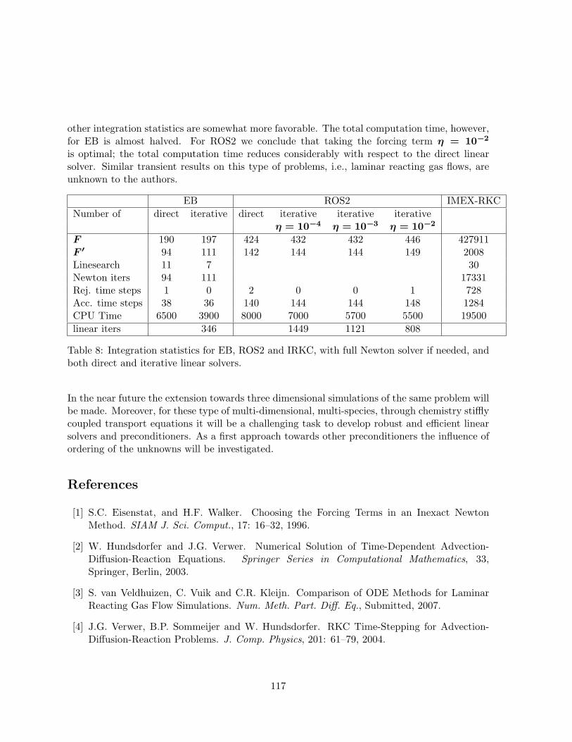
other integration statistics are somewhat more favorable. The total computation time, however,for EB is almost halved. For ROS2 we conclude that taking the forcing term η = 10−2

is optimal; the total computation time reduces considerably with respect to the direct linearsolver. Similar transient results on this type of problems, i.e., laminar reacting gas flows, areunknown to the authors.

EB ROS2 IMEX-RKCNumber of direct iterative direct iterative iterative iterative

η = 10−4 η = 10−3 η = 10−2

F 190 197 424 432 432 446 427911F ′ 94 111 142 144 144 149 2008Linesearch 11 7 30Newton iters 94 111 17331Rej. time steps 1 0 2 0 0 1 728Acc. time steps 38 36 140 144 144 148 1284CPU Time 6500 3900 8000 7000 5700 5500 19500linear iters 346 1449 1121 808

Table 8: Integration statistics for EB, ROS2 and IRKC, with full Newton solver if needed, andboth direct and iterative linear solvers.

In the near future the extension towards three dimensional simulations of the same problem willbe made. Moreover, for these type of multi-dimensional, multi-species, through chemistry stifflycoupled transport equations it will be a challenging task to develop robust and efficient linearsolvers and preconditioners. As a first approach towards other preconditioners the influence ofordering of the unknowns will be investigated.

References

[1] S.C. Eisenstat, and H.F. Walker. Choosing the Forcing Terms in an Inexact NewtonMethod. SIAM J. Sci. Comput., 17: 16–32, 1996.

[2] W. Hundsdorfer and J.G. Verwer. Numerical Solution of Time-Dependent Advection-Diffusion-Reaction Equations. Springer Series in Computational Mathematics, 33,Springer, Berlin, 2003.

[3] S. van Veldhuizen, C. Vuik and C.R. Kleijn. Comparison of ODE Methods for LaminarReacting Gas Flow Simulations. Num. Meth. Part. Diff. Eq., Submitted, 2007.

[4] J.G. Verwer, B.P. Sommeijer and W. Hundsdorfer. RKC Time-Stepping for Advection-Diffusion-Reaction Problems. J. Comp. Physics, 201: 61–79, 2004.

117

7 List of participants

Morad AHMADNASAB CERFACS France ahmadnasab@cerfacs.frBurak AKSOYLU Louisiana State Univ. USA burak@cct.lsu.eduPatrick AMESTOY ENSEEIHT-IRIT France amestoy@enseeiht.frPeter ARBENZ ETH Zurich Switzerland arbenz@inf.ethz.chMiguel ARGAEZ Univ. of Texas El PasoUSA earzuaga@gmail.comEmmanuel ARZUAGA Northeastern Univ. USA earzuaga@gmail.comLaila ASSAS Um-Al Qurah Univ. Sauda arabia aslaila201@yahoo.comHaim AVRON Tel-Aviv Univ. Israel haima@post.tau.ac.ilMarc BABOULIN CERFACS France baboulin@cerfacs.frShaymaa BADRAN Arab Open Univ. Egypt moongirl3000@gmail.comCaroline BALDASSARI INRIA-LMA France cbaldass3@yahoo.frJohn BARDSLEY Univ. of Montana USA bardsleyj@mso.umt.eduMario BEBENDORF Leipzig Univ. Germany mario.bebendorf@math.uni-leipzig.deMichele BENZI Emory Univ. USA benzi@mathcs.emory.eduMikko BYCKLING Helsinki Univ. of Tech. Finland mbycklin@cc.hut.fiXiao-Chuan CAI Univ. of Colorado USA cai@cs.colorado.eduLuiz MarianoCARVALHO FilhoRio de Janeiro Univ. Brazil luizmc@gmail.comJordi CASTRO Tech. Univ. of Catal. Spain jordi.castro@upc.eduCristina CHRISTARA Univ. of Toronto Canada ccc@cs.toronto.eduChristina CORRAL Inst. de Mat. Multi. Spain ccorral@imm.upv.esSue DOLLAR RAL UK s.dollar@rl.ac.ukIain DUFF CERFACS and RAL France duff@rl.ac.ukRomain DUJOL ENSEEIHT-IRIT France dujol@enseeiht.frRiadh FEZZANI CERFACS France fezzani@cerfacs.frNiklas FORS Uppsala Univ. Sweden nifo7723@student.uu.seJeremie GAIDAMOUR LaBRI-INRIA Futurs France gaidamou@labri.frMilagros GARCIA CERFACS France garcia@cerfacs.frAntoine GAYOU CERFACS France gayou@cerfacs.frMenno GENSEBERGER WL Delft Hydraulics The NetherlandMenno.Genseberger@wldelft.nlThomas GEORGE Texas A&M Univ. USA tgeorge@cs.tamu.eduLuc GIRAUD ENSEEIHT-IRIT France giraud@n7.frJacek GONDZIO Univ. of Edinburgh UK j.gondzio@ed.ac.ukDavid GOUDIN CEA/CESTA France david.goudin@cea.frAnath GRAMA Purdue Univ. USA ayg@cs.purdue.eduSerge GRATTON CERFACS France gratton@cerfacs.frLaura GRIGORI INRIA Futurs France laura.grigori@inria.frRonan GUIVARCH ENSEEIHT-IRIT France ronan.guivarch@enseeiht.frAzzam HAIDAR CERFACS France haidar@cerfacs.frMaxime HAVET Areva NP GmbH Germany maxime.havet@areva.comPascal HENON LaBRI-INRIA Futurs France henon@labri.fr

118

Yumei HUANG Hong Kong Baptist Univ. Hong Kong ymhuang@math.hkbu.edu.hkThomas HUCKLE Technische Univ. Munchen Germany huckle@in.tum.deFranck HULSEMANN EDF R&D France frank.hulsemann@edf.frIlgiz IBRAGIMOW Univ. of Saarbrucken Germany ilgis@num.uni-sb.deTakeshi IWASHITA Kyoto Univ. Japan iwashita@media.kyoto-u.ac.jpElMehdi JANATI IDRISSIENSEEIHT-IRIT France ElMehdi.Janatildrissi@etu.enseeiht.frAlexanderKALLISCHKO Technische Univ. Munchen Germany alex.k@arcor.deTakanori KIHARA Univ. of Tsukuba Japan kihara@mma.cs.tsukuba.ac.jpAndrew KNYAZEV Univ. of Colorado USA andrew.knyazev@cudenver.eduDimitri KOMATITSCH INRIA Magique 3D France dimitri.komatitsch@univ-pau.frLev KRUKIER Southern Federal Univ. Russia krukier@rsu.ruJulien LANGOU The Univ. of Colorado USA julien.langou@cudenver.eduBruno LATHUILIERE EDF-INRIA-LaBRI France bruno.lathuiliere@edf.frAmos LAWLESS Univ. of Reading UK a.s.lawless@rdg.ac.ukNicolas LE GOFF INRIA Futurs France nicolas.legoff@univ-pau.frPeter LUCAS Delft Univ.of Technology The Netherlandp.lucas@tudelft.nlJose MARIN Univ. Politecnica de Valencia Spain jmarinma@mat.upv.esRoland MASSON Institut Francais du Petrole France roland.masson@ifp.frRobert MELVILLE Self USA bobmelville1@gmail.comKatherine MER-NKONGA CEA/CESTA France katherine.nkonga@cea.frGerard MEURANT CEA/DIF France gerard.meurant@gmail.comTakeshi MIFUNE Kyoto Univ. Japan mifune@fem.kuee.kyoto-u.ac.jpSebastian MINJEAUD IRSN France sebastian.minjeaud@gmail.comMelodie MOUFFE CERFACS France mouffe@cerfacs.frGhislain MOUIL SIL Robert Bosch Germany ghislain.mouilsil@de.bosch.comArtem NAPOV Serv. de Metr. Nucleaire Belgium anapov@ulb.ac.beEsmond Ng Laurence Berkeley Nat. Lab. USA EGNg@lbl.govYvan NOTAY Univ. Libre de Bruxelles Belgium ynotay@ulb.ac.beMasayuki OKADA Univ. of Tsukuba Japan okada@mma.cs.tsukuba.ac.jpRonan PERRUSSEL INRIA Sophia Antipolis France ronan.perrussel@sophia.inria.frXavier PINEL CERFACS France pinel@cerfacs.frMarina POPOLIZIO Universita di Bari Italy popolizio@dm.uniba.itStephane PRALET SAMTECH Belgium stephane.pralet@samcef.comIvana PULVATORA Faculty of Civil Engineering Czech Republic ivana@mat.fsv.cvut.czPatrick QUILLEN The MathWorks USA pquillen@mathworks.comPadma RAGHAVAN The Pennsylvania State Univ.USA raghavan@cse.psu.eduPierre RAMET LaBRI-INRIA Futurs France ramet@labri.frStefan REITZINGER Numerical and Symbolic Austria stefan.reitzinger@cst.com

119

Nicolas RENON CICT France renon@cict.frDiego RIVERA Northeastern Univ. USA diegofernandorivera@gmail.comJean ROMAN LaBRI-INRIA Futurs France roman@labri.frDaniel RUIZ ENSEEIHT-IRIT France daniel.ruiz@enseeiht.frTetsuya SAKURAI Univ. of Tsukuba Japan sakurai@cs.tsukuba.ac.jpAhmed SAMEH Purdue Univ. USA sameh@cs.purdue.eduMaria Luisa SANDOVAL Univ. Metrop.-Iztapalapa Mexico miss@xanum.uam.mxAnnick SARTENAER Univ. of Namur Belgium annick.sartenaer@fundp.ac.beJennifer SCOTT RAL UK j.a.scott@rl.ac.ukGil SHKLARSKI Tel-Aviv Univ. Israel shagil@tau.ac.ilJelena SIROVLJEVIC Univ. of British Columbia Canada jelenas@cs.ubc.caTzvetomila SLAVOVA CERFACS France slavova@cerfacs.frTomohiro SOGABE Nagoya Univ. Japan sogabe@na.cse.nagoya-u.ac.jpPierre SPITERI ENSEEIHT-IRIT France spiteri@enseeiht.frGuillaume SYLVAND EADS Innovation Works France guillaume.sylvand@eads.netWei-Pai TANG The Boeing Company USA wei-pai.tang@boeing.comIssam TARRASS TOTAL France issam.tarrass@total.comJari TOIVANEN Stanford Univ. USA toivanen@stanford.eduSivan TOLEDO Tel-Aviv Univ. Israel stoledo@post.tau.ac.ilFred T. TRACY Eng. Res. and Dev. Cent.USA Fred.T.Tracy@erdc.usace.army.milAnke TROELTSCH CERFACS France anketr@web.deMiroslav TUMA Czech Acad. of Sciences Czech Republic tuma@cs.cas.czRay TUMINARO Sandia National Lab. USA rstumin@sandia.govBora UCAR CERFACS France ucar@cerfacs.frSander VAN VELDHUIZENTU Delft The Netherland s.vanveldhuizen@gmail.comXavier VASSEUR CERFACS France vasseur@cerfacs.frLeticia VELAZQUEZ Univ. of Texas at El Paso USA leti@utep.eduFred WUBS Univ. of Groningen The Netherlandwubs@math.rug.nlHua XIANG INRIA Futurs France hua.xiang@inria.frJun-Feng YIN National Inst. of Inf. Japan yinjf@nii.ac.jpShao-Liang ZHANG Nagoya Univ. Japan zhang@na.cse.nagoya-u.ac.jpLudmil ZIKATANOV Pennsylvania State Univ. USA ludmil@psu.edu

120

Index

AAksoylu ,B.

. . . . . . . . . . . . . . . . . . . . . . . . . . . . . . . . . . . . . . . 13Arbenz ,P.

. . . . . . . . . . . . . . . . . . . . . . . . . . . . . . . . . . . . . . . 16Avron ,H.

. . . . . . . . . . . . . . . . . . . . . . . . . . . . . . . . . . . . . . . 17

BBardsley ,J. M.

. . . . . . . . . . . . . . . . . . . . . . . . . . . . . . . . . . . . . . . 19Bebendorf ,M.

. . . . . . . . . . . . . . . . . . . . . . . . . . . . . . . . . . . . . . . . 9Benzi ,M.

. . . . . . . . . . . . . . . . . . . . . . . . . . . . . . . . . . . . . . . 20Byckling ,M.

. . . . . . . . . . . . . . . . . . . . . . . . . . . . . . . . . . . . . . . 21

CCai ,X.-C.

. . . . . . . . . . . . . . . . . . . . . . . . . . . . . . . . . . . . . . . 24Carvalho ,L. M.

. . . . . . . . . . . . . . . . . . . . . . . . . . . . . . . . . . . . . . . 24Castro ,J.

. . . . . . . . . . . . . . . . . . . . . . . . . . . . . . . . . . . . . . . 27Christara ,C. C.

. . . . . . . . . . . . . . . . . . . . . . . . . . . . . . . . . . . . . . . 29Corral ,C.

. . . . . . . . . . . . . . . . . . . . . . . . . . . . . . . . . . . . . . . 32

DDollar ,H. S.

. . . . . . . . . . . . . . . . . . . . . . . . . . . . . . . . . . . . . . . 33

GGaidamour ,J.

. . . . . . . . . . . . . . . . . . . . . . . . . . . . . . . . . . . . . . . 34Genseberger ,M.

. . . . . . . . . . . . . . . . . . . . . . . . . . . . . . . . . . . . . . . 38George ,T.

. . . . . . . . . . . . . . . . . . . . . . . . . . . . . . . . . . . . . . . 41

Gondzio ,J.. . . . . . . . . . . . . . . . . . . . . . . . . . . . . . . . . . . . . . . . 9

Grama ,A. A.. . . . . . . . . . . . . . . . . . . . . . . . . . . . . . . . . . . . . . . 44

HHaidar ,A.

. . . . . . . . . . . . . . . . . . . . . . . . . . . . . . . . . . . . . . . 47Havet ,M.

. . . . . . . . . . . . . . . . . . . . . . . . . . . . . . . . . . . . . . . 49Huang ,Y.

. . . . . . . . . . . . . . . . . . . . . . . . . . . . . . . . . . . . . . . 50Huckle ,T.

. . . . . . . . . . . . . . . . . . . . . . . . . . . . . . . . . . . . . . . 51Hulsemann ,F.

. . . . . . . . . . . . . . . . . . . . . . . . . . . . . . . . . . . . . . . 52

IIbragimow ,I.

. . . . . . . . . . . . . . . . . . . . . . . . . . . . . . . . . . . . . . . 53Iwashita ,T.

. . . . . . . . . . . . . . . . . . . . . . . . . . . . . . . . . . . . . . 100

KKallischko ,A.

. . . . . . . . . . . . . . . . . . . . . . . . . . . . . . . . . . . . . . . 54Kihara ,T.

. . . . . . . . . . . . . . . . . . . . . . . . . . . . . . . . . . . . . . . 55Krukier ,L.

. . . . . . . . . . . . . . . . . . . . . . . . . . . . . . . . . . . . . . . 56

LLangou ,J.

. . . . . . . . . . . . . . . . . . . . . . . . . . . . . . . . . . . . . . 103Lawless ,A.

. . . . . . . . . . . . . . . . . . . . . . . . . . . . . . . . . . . . . . . 57Lucas ,P.

. . . . . . . . . . . . . . . . . . . . . . . . . . . . . . . . . . . . . . . 60

MMarin ,J.

121

. . . . . . . . . . . . . . . . . . . . . . . . . . . . . . . . . . . . . . 106Masson ,R.

. . . . . . . . . . . . . . . . . . . . . . . . . . . . . . . . . . . . . . . 63Melville ,R.

. . . . . . . . . . . . . . . . . . . . . . . . . . . . . . . . . . . . . . . 64

NNapov ,A.

. . . . . . . . . . . . . . . . . . . . . . . . . . . . . . . . . . . . . . 108Notay ,Y.

. . . . . . . . . . . . . . . . . . . . . . . . . . . . . . . . . . . . . . . 10

OOkada ,M.

. . . . . . . . . . . . . . . . . . . . . . . . . . . . . . . . . . . . . . . 66

PPerrussel ,R.

. . . . . . . . . . . . . . . . . . . . . . . . . . . . . . . . . . . . . . . 69Pinel ,X.

. . . . . . . . . . . . . . . . . . . . . . . . . . . . . . . . . . . . . . . 72Popolizio ,M.

. . . . . . . . . . . . . . . . . . . . . . . . . . . . . . . . . . . . . . . 73Pultarova ,I.

. . . . . . . . . . . . . . . . . . . . . . . . . . . . . . . . . . . . . . 108

RRaghavan ,P.

. . . . . . . . . . . . . . . . . . . . . . . . . . . . . . . . . . . . . . . 11Reitzinger ,S.

. . . . . . . . . . . . . . . . . . . . . . . . . . . . . . . . . . . . . . . 11Rivera ,D.

. . . . . . . . . . . . . . . . . . . . . . . . . . . . . . . . . . . . . . . 74

SSameh ,A. H.

. . . . . . . . . . . . . . . . . . . . . . . . . . . . . . . . . . . . . . . 77Sandoval ,M. L.

. . . . . . . . . . . . . . . . . . . . . . . . . . . . . . . . . . . . . . . 79Sartenaer ,A.

. . . . . . . . . . . . . . . . . . . . . . . . . . . . . . . . . . . . . . . 80Sirovljevic ,J.

. . . . . . . . . . . . . . . . . . . . . . . . . . . . . . . . . . . . . . 111Sogabe ,T.

. . . . . . . . . . . . . . . . . . . . . . . . . . . . . . . . . . . . . . . 82

TTuma ,M.

. . . . . . . . . . . . . . . . . . . . . . . . . . . . . . . . . . . . . . . 87Tarrass ,I.

. . . . . . . . . . . . . . . . . . . . . . . . . . . . . . . . . . . . . . 112Toivanen ,J.

. . . . . . . . . . . . . . . . . . . . . . . . . . . . . . . . . . . . . . . 85Toledo ,S.

. . . . . . . . . . . . . . . . . . . . . . . . . . . . . . . . . . . . . . . 12Tracy ,F.

. . . . . . . . . . . . . . . . . . . . . . . . . . . . . . . . . . . . . . . 86Tuminaro ,R.

. . . . . . . . . . . . . . . . . . . . . . . . . . . . . . . . . . . . . . . 89

Vvan Veldhuizen ,S.

. . . . . . . . . . . . . . . . . . . . . . . . . . . . . . . . . . . . . . 115

WWubs ,F.

. . . . . . . . . . . . . . . . . . . . . . . . . . . . . . . . . . . . . . . 91

XXiang ,H.

. . . . . . . . . . . . . . . . . . . . . . . . . . . . . . . . . . . . . . . 94

YYin ,J.-F.

. . . . . . . . . . . . . . . . . . . . . . . . . . . . . . . . . . . . . . . 96

ZZikatanov ,L.

. . . . . . . . . . . . . . . . . . . . . . . . . . . . . . . . . . . . . . . 12

122