Paper HOW-067

PROC REPORT… Your How-to Guide for Producing Customized Summary Tables

Deborah Babcock Buck,

D. B. & P. Associates, Houston, TX

ABSTRACT A number of years ago SAS® developers responded to requests from SAS programmers for a single report-writing procedure that incorporated the features of PROC PRINT, PROC MEANS, PROC TABULATE, and the DATA _NULL_ step. The resulting procedure, PROC REPORT, is highly versatile with the capabilities to produce both detail and summary reports. In this workshop we will focus on PROC REPORT statements that will produce complex summary tables which include multiple dimensions, frequently reported descriptive statistics, columns of information not included in the data set, and customized summary statements. Although PROC REPORT can be used in a windowing environment with point-and-click report building, we will use a programming approach to create the reports. This workshop is intended primarily for beginning to intermediate SAS users, or anyone who would like to become more familiar with PROC REPORT, and is applicable to all operating systems.

INTRODUCTION Base SAS has a number of procedures to help you report your data in the form you would like to see it presented. Reports can be detail or summary in nature. Summary reports generally do some sort of collapsing of data so that each row represents information from more than one observation. PROC TABULATE and PROC REPORT are what I consider to be the ‘workhorses’ of report writing. Which of these two is more appropriate is based on your needs for a given situation. PROC TABULATE is also capable of producing summary tables and may satisfy your requirements for a given report. However, PROC REPORT offers much more flexibility in customizing the report. We will consider the PROC REPORT statements necessary to produce reports that include the following features:

• Cross-tabulations or hierarchical groupings, • Statistics, • Columns of variable-type information that do not exist in the data set (temporary variables), • Customized text or stylized look.

Examples of output and the code producing the report are presented. The data for the example in this paper are taken from the ‘sasuser.diabetes’ data set available in your SASUSER library. A temporary SAS data set named ‘work.diabetes’ was created and a variable for treatment was added using the following DATA step. data diabetes; set sasuser.diabetes; if mod(_n_,2)=0 then trt=’B’; else trt=’A’; run;

1

These statements assign a value of ‘B’ to the treatment variable (TRT) on every observation number that has a remainder of 0 when divided by 2, and a value of ‘A’ to all others. Below is a portion of the PROC CONTENTS output for the ‘work.diabetes’ SAS data set. Alphabetic List of Variables and Attributes # Variable Type Len 3 Age Num 8 7 FastGluc Num 8 4 Height Num 8 1 ID Char 4 8 PostGluc Num 8 6 Pulse Num 8 2 Sex Char 1 5 Weight Num 8 9 trt Char 1

PROC REPORT statements are more easily written if you decide what you want the report to include and look like before you begin writing the code. For our summary table we want to include the variables gender (called SEX in the data set), age category, treatment, fasting glucose, post glucose, and change from fasting to post glucose. (This last information, change, is not included in the data set.) We would like to see gender and age category within gender in the row dimension and the sample size, N, and mean for fasting and post glucose and the change in glucose from fasting to post within each treatment in the column dimension. The following output shows the desired completed summary table.

Treatment A Treatment B ƒƒƒƒƒƒƒƒƒƒƒƒƒƒGlucoseƒƒƒƒƒƒƒƒƒƒƒƒƒƒ ƒƒƒƒƒƒƒƒƒƒƒƒƒƒGlucoseƒƒƒƒƒƒƒƒƒƒƒƒƒƒ Fasting Post Mean Change Fasting Post Mean Change Gender Age N Mean N Mean from Fasting N Mean N Mean from Fasting ƒƒƒƒƒƒƒƒƒƒƒƒƒƒƒƒƒƒƒƒƒƒƒƒƒƒƒƒƒƒƒƒƒƒƒƒƒƒƒƒƒƒƒƒƒƒƒƒƒƒƒƒƒƒƒƒƒƒƒƒƒƒƒƒƒƒƒƒƒƒƒƒƒƒƒƒƒƒƒƒƒƒƒƒƒƒƒƒƒƒƒƒƒ Female 50 and Over 4 166.5 4 231.3 64.8 2 269.5 2 307.5 38.0 Under 50 4 329.0 4 392.3 63.3 1 267.0 1 319.0 52.0 === ====== === ====== ============ === ====== === ====== ============ 8 247.8 8 311.8 64.0 3 268.7 3 311.3 42.7 Male 50 and Over 2 360.5 2 417.0 56.5 2 316.5 2 363.0 46.5 Under 50 . . . . . 5 368.0 5 422.8 54.8 === ====== === ====== ============ === ====== === ====== ============ 2 360.5 2 417.0 56.5 7 353.3 7 405.7 52.4 All 10 270.3 10 332.8 62.5 10 327.9 10 377.4 49.5 Overall, the mean change in glucose from fasting to post treatment is greater in Treatment A.

2

STATEMENTS IN THE REPORT PROCEDURE There are several statements necessary to generate summary reports with the features listed above. We will discuss each of these statements separately and see how each contributes to producing the desired report. PROC REPORT options; COLUMN report-item-specifications; DEFINE report-item1/usage and options; DEFINE report-item2/usage and options; Additional DEFINE statements….; COMPUTE <location> report-item/options; SAS statements ENDCOMP; BREAK <location> report-item/options; RBREAK <location>/options; RUN;

PROC REPORT STATEMENT The REPORT procedure is started with the PROC REPORT statement. There are a number of options available on the PROC statement that control the input (and optionally output) data set, windowing environment, report layout, column headers, and handling of classification variables (including missing values), among others. The WINDOWS/NOWINDOWS option allows you to produce your report using either the interactive REPORT windows or programming code. The NOWD (NOWINDOWS) option indicates that you do not want to use the interactive REPORT windows, but to use programming statements. By default, if you do not include the NOWD option, SAS will take you to the REPORT window where you can interactively build the report. The DATA= option indicates which SAS data set should be used for generating the report, and the OUT= option allows you to output the information from the report into a new SAS data set. The new SAS data set contains one observation for each detail row of the report and one observation for each unique summary line. Information about customization (underlining, color, text, and so forth) is not data and therefore not included in the output data set. The output data set also contains one variable for each column of the report (whether the column is printed or not) and tries to use the name of the report item as the name of the corresponding variable in the output data set. It also includes an automatic variable, _BREAK_ whose values are determined by BREAK and RBREAK statements. The HEADSKIP and HEADLINE options indicate that you would like to insert a blank line (skip a line) under the column headers and underline the column headers and the spaces between them, respectively. The SPLIT=’ ‘ option in REPORT allows you to indicate which single character to use in determining where a column header should be split. The default splitting character is a slash (/). The SPACING= option allows you to direct REPORT in how many spaces you desire between variable columns within the report globally. By default, there are 2 spaces between columns. You can override this within the table for specific columns and control each column individually using the SPACING= option in the DEFINE statement. The spaces indicated in the SPACING= option within a DEFINE statement are placed in the table before the report-item. This option is very useful when you are trying to fit a large amount of information into a table or want to group certain columns. By default, PROC REPORT does not include observations with missing values for group, order, or across variables. The MISSING option tells REPORT to include a group for missing values (individual groups for each missing value, if special missing values are included in the data).

3

The following statement begins the PROC REPORT step, indicates that the data set to be used for the procedure is named ‘diabetes’, inserts a blank line under the column headers, and underlines the column headers. It also tells REPORT to split a column header at the ‘/’ symbol, and creates a SAS data set called ‘new’ which includes the columns and rows from the PROC REPORT table. proc report data=diabetes headskip headline split=’/’ out=new;

COLUMN STATEMENT The next statement is the COLUMN statement. This is comparable to a VAR statement in PROC PRINT in that it lists what variables or columns you want included and the order in which they should be listed in the report. However, more information can be included here. The COLUMN statement requires that you supply column specifications or report-items. These report-items can include data set variables, computed variables, or statistics and can be listed in several forms depending upon the purpose or layout. If you wish to subgroup items within columns (stack items), then the report-items are separated by commas. The header for the left-most column occurs first (the highest level). By default, the cells are filled with frequency counts, unless one of the report-items is an analysis, computed or group variable, or a statistic. Parentheses are used to group items that you want to appear on the same level. The following COLUMN statement begins building the layout of the table by showing SEX in the left-most column, followed by AGE (which will be collapsed into categories of ’50 and Over’ and ‘Under 50’ with a user-defined format). We then specify columns for treatment with fasting and post glucose within each treatment. (TRT separated from FASTGLUC and POSTGLUC by a comma, and FASTGLUC and POSTGLUC grouped within parentheses.) column sex age trt, (fastgluc postgluc); ← Note: This statement and the following COLUMN statements without DEFINE statements will cause ERROR messages. The COLUMN statement can also be utilized to display a report-item in more than one way or for more than one purpose. This is called creating an alias in PROC REPORT. The form of creating an alias is report-item=new-column-name. We will tell REPORT how to use the aliases in DEFINE statements. Since we want to include columns for statistics (N and Mean) for both fasting glucose and post glucose we will use aliases in the COLUMN statement. To obtain the sample sizes, N, for each variable we will include aliases, and we will use the actual variable name for our Mean statistics. You can also use an alias to display the same variable in more than one column, for instance, as a coded value and a formatted value. column sex age trt, (fastgluc=nfastgluc fastgluc postgluc=npostgluc postgluc); There is one more column that we would like to have included in the table – the change (difference) between the mean fasting glucose and mean post glucose. We include a column name, CHGGLUC, for this new information that does not exist in the data set. A COMPUTE statement will be used to calculate the values for this column. The following statement will also not work without the DEFINE and COMPUTE statements. column sex age trt, (fastgluc=nfastgluc fastgluc postgluc=npostgluc postgluc chggluc);

4

You can also create a header to span multiple columns in the COLUMN statements by using the form (‘desired-header’ report-items) – the header enclosed in quotes followed by the report-items to be spanned by the header, all inside parentheses. If you use any of the following symbols (: - = \ _ . * +) as the first and last characters of the header, then REPORT expands the symbol to fill all available space before and after the header. The following with column spanners (and appropriate parentheses) completes the COLUMN statement for our desired table. (Note that we have used two levels of spanners.) column sex age trt, (‘-Glucose-’ ((‘Fasting’ fastgluc=nfastgluc fastgluc) (‘Post’ postgluc=npostgluc postgluc) (chggluc) ));

DEFINE STATEMENT DEFINE statements give detailed information about each column in a report. The form of the statement is the keyword DEFINE followed by the report-item (variable, alias, computed variable or statistic), a slash, and options. These options can include usage options and/or attribute options, such as column width, format, header label, spacing, and justification. DEFINE statements are not always required, but without them REPORT will use various default values. Usage options in this example include GROUP, ACROSS, ANALYSIS, and COMPUTED. The DEFINE statement for SEX has a usage of GROUP which says that you want to summarize (collapse) observations within each level of SEX. AGE is also a GROUP variable since we want to collapse the data into formatted values within each level of SEX. The GROUP usage combines observations according to the specified variable and displays them in formatted, ascending order. The usage for TREATMENT is ACROSS, which allows the table to be presented as a cross-tabulation report. For FASTGLUC and NFASTGLUC, the usage is ANALYSIS, which denotes that you want to use statistics for these variables. Which statistics to be used are specified in the DEFINE statements for these columns. The N statistic with NFASTGLUC indicates that you want the number of non-missing observations for fasting glucose within each SEX-AGE-TREATMENT combination. Likewise, the MEAN statistic specified for FASTGLUC requests that this column should be the mean for fasting glucose for each SEX-AGE-TREATMENT combination. Although the ANALYSIS usage does not need to be specified when you supply a particular statistic, it helps make the code easier to read. The columns for the post glucose statistics are handled in the same manner. The final columns of information to be considered are the change from the fasting glucose mean to the post glucose mean in each TREATMENT. This CHGGLUC information does not exist in the ‘diabetes’ data set. In order to include these columns in the table, we need to specify a usage of COMPUTED and utilize a COMPUTE-ENDCOMP block to calculate the new columns’ information using the fasting and post glucose means produced in the table. We will examine COMPUTE and ENDCOMP statements later in this example. Let’s look more closely at the DEFINE statement for SEX and discuss the options used. define sex/group format=$sexfmt. width=6 ‘Gender’; As we mentioned above, we want to summarize (group) the data into the levels of SEX, so we include a usage option of GROUP. The actual SEX variable values in the ‘diabetes’ data set are the single letters ‘F’ and ‘M’ which we would like to see displayed as ‘Female’ and ‘Male’. Therefore, we utilize the FORMAT= option with the user-defined $sexfmt. to accomplish this. We will also use the FORMAT= option to group the AGE variable, which is continuous, into formatted values of ’50 and Over’ and ‘Under 50’.

5

By default, REPORT will order the values by formatted values. If we wanted to change the ordering of the levels of the variable to be ordered by the actual data values, we could specify ORDER=INTERNAL. Likewise, if we wanted them sorted by frequency of occurrence, we could include ORDER=FREQ. The WIDTH= option does exactly what it sounds like – it specifies how many spaces wide that variable column should be. We assign the SEX column a width of six spaces to be wide enough for the column header and the formatted values. (Note, there is no period after the width value, while format must include a period.) If there is a conflict between the specified width and format, the width option prevails. Finally, at the end of this DEFINE statement is ‘Gender’. By enclosing this label in quotes, REPORT knows that we want this header to be used for the SEX variable column. If you don’t include a header in the DEFINE statement, REPORT uses the variable’s label, if one is assigned in the data set. Several other options are included on the DEFINE statement for FASTGLUC. define fastgluc/analysis mean format=5.1 width=6 center spacing=1 ‘Mean’; Because we want the FASTGLUC column to contain the fasting glucose mean, we specify a usage option of ANALYSIS and the statistic MEAN in the DEFINE statement. (The usage ANALYSIS is not necessary because we have specified the statistic, but it makes the code easier to read.) Two other options on this DEFINE statement are CENTER and SPACING=. CENTER requests that the values should be center justified in the field. As mentioned earlier, the SPACING= option specifies how many spaces should be included in the report before that variable column. The SPACING=1 places one column between the N and MEAN for fasting glucose and makes them appear more closely grouped together when looking at the table. The following code includes the PROC FORMAT step which supplies the format for SEX, AGE, and TRT, the PROC REPORT statement, the COLUMN statement, and all of the DEFINE statements for the summary table in this paper and produces the table below. proc format; value $sexfmt 'F'='Female' 'M'='Male'; value $trtfmt 'A'='Treatment A' 'B'='Treatment B'; value agefmt low-49='Under 50' 50-high='50 and Over'; run; proc report nowd data=diabetes headline headskip split='/' out=new; column sex age trt, ('-Glucose-' (('Fasting' fastgluc=nfastgluc fastgluc) ('Post' postgluc=npostgluc postgluc) (chggluc) )); define sex/group format=$sexfmt. width=6 'Gender'; define age/group format=agefmt. width=12 center 'Age'; define trt/across format=$trtfmt. width=12 center ' '; define nfastgluc/analysis n format=2. width=3 center 'N'; define fastgluc/analysis mean format=5.1 width=6 center spacing=1 'Mean'; define npostgluc/analysis n format=2. width=3 center 'N'; define postgluc/analysis mean format=5.1 width=6 center spacing=1 'Mean'; define chggluc/computed format=5.1 width=12 center spacing=1 'Mean Change/from Fasting'; run;

6

Treatment A Treatment B ƒƒƒƒƒƒƒƒƒƒƒƒƒƒGlucoseƒƒƒƒƒƒƒƒƒƒƒƒƒƒ ƒƒƒƒƒƒƒƒƒƒƒƒƒƒGlucoseƒƒƒƒƒƒƒƒƒƒƒƒƒƒ Fasting Post Mean Change Fasting Post Mean Change Gender Age N Mean N Mean from Fasting N Mean N Mean from Fasting ƒƒƒƒƒƒƒƒƒƒƒƒƒƒƒƒƒƒƒƒƒƒƒƒƒƒƒƒƒƒƒƒƒƒƒƒƒƒƒƒƒƒƒƒƒƒƒƒƒƒƒƒƒƒƒƒƒƒƒƒƒƒƒƒƒƒƒƒƒƒƒƒƒƒƒƒƒƒƒƒƒƒƒƒƒƒƒƒƒƒƒƒƒ Female 50 and Over 4 166.5 4 231.3 . 2 269.5 2 307.5 . Under 50 4 329.0 4 392.3 . 1 267.0 1 319.0 . Male 50 and Over 2 360.5 2 417.0 . 2 316.5 2 363.0 . Under 50 . . . . . 5 368.0 5 422.8 .

COMPUTE AND ENDCOMP STATEMENTS COMPUTE blocks – beginning with a COMPUTE statement and ending with an ENDCOMP statement – can be used for a variety of purposes in the generation of PROC REPORT tables. Two of the purposes that we have utilized in this paper are

1. to create new columns of information that do not exist in the data set – CHGGLUC, for this report, and

2. to include additional customized lines in the table. The following statements show the general form of a COMPUTE block. COMPUTE <location> report-item/options; SAS statements ENDCOMP; When using a COMPUTE block, we can specify a location to indicate when the compute block should be executed. This location can refer to a grouping variable or the entire report. The location can be BEFORE or AFTER. If we want to execute a compute block after a grouping variable, we include the name of that report-item in the COMPUTE statement with the AFTER location. The report-item can be a variable, statistic, or computed variable. To execute the block after the entire report, we do not include a report-item after the AFTER location. The same process holds true for execution BEFORE a grouping variable or the entire report. When neither BEFORE or AFTER is specified, the COMPUTE calculation is carried out for every line of the report. In this table, we have a report-item called CHGGLUC with a usage designation of COMPUTED. Before we examine the compute block, we need to discuss the report-item naming conventions. There are four ways of naming report-items within a compute block, dependent upon what the report-item is and how it is being used. Report-items in a compute block can be named in the following ways.

1. By the actual variable name used in the COLUMN statement. 2. By an alias – from an alias name specified in the COLUMN statement. 3. By a compound name for a report-item with a DEFINE usage of ANALYSIS with the form: variable-name.statistic 4. By Column Number in the form ‘_Cn_’ where ‘n’ is the column number (from the left side to right).

Note: Any time you refer to a variable which shares a column with an ACROSS variable, you use the column number in the compute block.

7

In our summary table, it is not immediately obvious as to how to specify the correct columns to use in calculating the two CHGGLUC columns (one under each treatment). However, since the CHGGLUC shares a column with TRT, which is an ACROSS variable, it is necessary to refer to the appropriate column numbers in the compute block calculations. In order to see how PROC REPORT views the columns in the report, it is very useful to examine the output data set that REPORT creates. In our PROC REPORT statement, we included an ‘out=new’ data set option to create a new SAS data set called ‘work.new’. Below is the PROC PRINT output for the ‘new’ data set.

The SAS System Obs Sex Age _C3_ _C4_ _C5_ _C6_ _C7_ _C8_ _C9_ _C10_ _C11_ _C12_ _BREAK_ 1 F 50 4 166.5 4 231.25 . 2 269.5 2 307.5 . 2 F 15 4 329.0 4 392.25 . 1 267.0 1 319.0 . 3 M 50 2 360.5 2 417.00 . 2 316.5 2 363.0 . 4 M 15 . . . . . 5 368.0 5 422.8 . The ‘new’ data set includes one row for each summary row in the report and a variable for each column of information. We can see that _c3_ and _c4_ correspond to the N and Mean for fasting glucose, FASTGLUC, in Treatment A, while _c5_ and _c6_ contain the N and Mean for post glucose, POSTGLUC. The _c7_ column represents the field where the change from fasting glucose to post glucose should be displayed. However, because we have not yet included a compute block in our PROC REPORT all of the _c7_ values are missing. The following compute block assigns values to the CHGGLUC columns for treatments A and B. compute chggluc; _c7_ = (_c6_ - _c4_); _c12_= (_c11_ - _c9); endcomp; Note: This calculation may not produce the desired difference values if the sample sizes (or observations) differ between fasting and post glucose means within a treatment. As with any data calculation when programming, you need to be familiar with your data and the purpose of the calculation. We would also like to include a customized line of information at the bottom of our report that will say ‘Overall, the mean change in glucose from fasting to post treatment is greater in __________.’ The blank space will be filled in by either ‘Treatment A’ or ‘Treatment B’, depending upon which has a greater change overall. The following compute block specifies that some actions will be carried out AFTER the entire report. These actions include skipping two lines and then producing the desired text at the bottom of the table. compute after; line ' '; line ' '; if _c7_ gt _c12_ then x='Treatment A'; else if _c7_ lt _c12_ then x='Treatment B'; line 'Overall, the mean change in glucose from fasting to post treatment is greater in ' x $11. '.'; endcomp; The LINE statement in the compute block is similar to a PUT statement in a DATA step. Like a PUT statement, we can use @ column pointers to specify location in the line and can include text, variables,

8

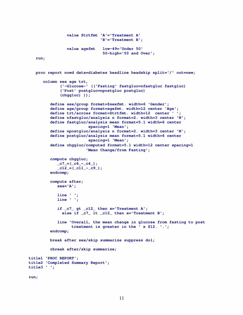
and formats for the variables. In the compute block we can also use a number of executable DATA step statements, including conditional IF-THEN statements. For our table we create a temporary variable named ‘X’ that will have a value of ‘Treatment A’ or ‘Treatment B’ based on the comparison of _c7_ and _c12_ (the CHGGLUC columns). The ENDCOMP statement is necessary to end the compute block.

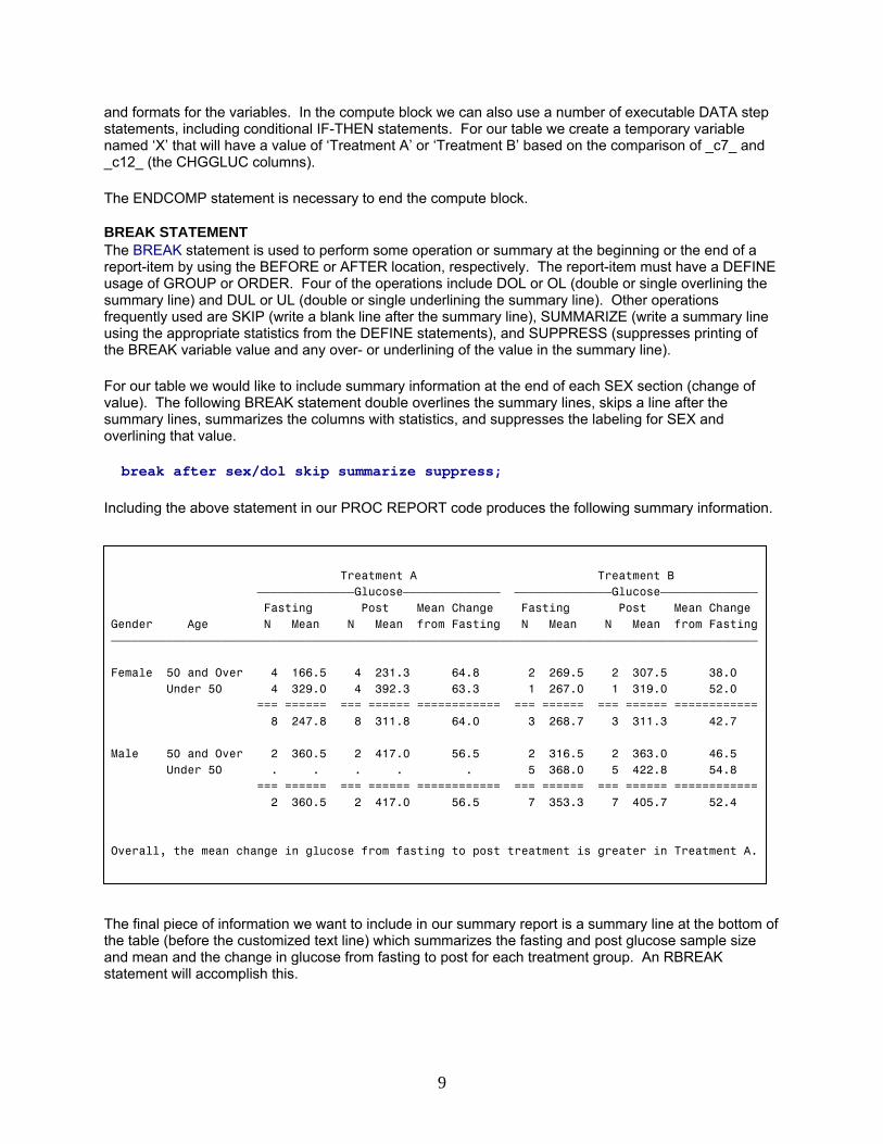
BREAK STATEMENT The BREAK statement is used to perform some operation or summary at the beginning or the end of a report-item by using the BEFORE or AFTER location, respectively. The report-item must have a DEFINE usage of GROUP or ORDER. Four of the operations include DOL or OL (double or single overlining the summary line) and DUL or UL (double or single underlining the summary line). Other operations frequently used are SKIP (write a blank line after the summary line), SUMMARIZE (write a summary line using the appropriate statistics from the DEFINE statements), and SUPPRESS (suppresses printing of the BREAK variable value and any over- or underlining of the value in the summary line). For our table we would like to include summary information at the end of each SEX section (change of value). The following BREAK statement double overlines the summary lines, skips a line after the summary lines, summarizes the columns with statistics, and suppresses the labeling for SEX and overlining that value. break after sex/dol skip summarize suppress; Including the above statement in our PROC REPORT code produces the following summary information.

Treatment A Treatment B ƒƒƒƒƒƒƒƒƒƒƒƒƒƒGlucoseƒƒƒƒƒƒƒƒƒƒƒƒƒƒ ƒƒƒƒƒƒƒƒƒƒƒƒƒƒGlucoseƒƒƒƒƒƒƒƒƒƒƒƒƒƒ Fasting Post Mean Change Fasting Post Mean Change Gender Age N Mean N Mean from Fasting N Mean N Mean from Fasting ƒƒƒƒƒƒƒƒƒƒƒƒƒƒƒƒƒƒƒƒƒƒƒƒƒƒƒƒƒƒƒƒƒƒƒƒƒƒƒƒƒƒƒƒƒƒƒƒƒƒƒƒƒƒƒƒƒƒƒƒƒƒƒƒƒƒƒƒƒƒƒƒƒƒƒƒƒƒƒƒƒƒƒƒƒƒƒƒƒƒƒƒƒ Female 50 and Over 4 166.5 4 231.3 64.8 2 269.5 2 307.5 38.0 Under 50 4 329.0 4 392.3 63.3 1 267.0 1 319.0 52.0 === ====== === ====== ============ === ====== === ====== ============ 8 247.8 8 311.8 64.0 3 268.7 3 311.3 42.7 Male 50 and Over 2 360.5 2 417.0 56.5 2 316.5 2 363.0 46.5 Under 50 . . . . . 5 368.0 5 422.8 54.8 === ====== === ====== ============ === ====== === ====== ============ 2 360.5 2 417.0 56.5 7 353.3 7 405.7 52.4 Overall, the mean change in glucose from fasting to post treatment is greater in Treatment A.

The final piece of information we want to include in our summary report is a summary line at the bottom of the table (before the customized text line) which summarizes the fasting and post glucose sample size and mean and the change in glucose from fasting to post for each treatment group. An RBREAK statement will accomplish this.

9

RBREAK STATEMENT The RBREAK (Report Break) statement is used to perform some operation at the beginning or the end of the report by using the BEFORE or AFTER location, respectively. The underlining and overlining operations and SKIP and SUMMARIZE options listed above for the BREAK statement are also available for use with the RBREAK statement. In the table for this paper we want a summary line at the bottom of the table across levels of SEX and AGE for the N and Mean of fasting glucose and post glucose and the overall change between fasting and post within each TREATMENT group. The following RBREAK statement skips a line before the summary line and summarizes the columns. rbreak after/skip summarize;

Treatment A Treatment B ƒƒƒƒƒƒƒƒƒƒƒƒƒƒGlucoseƒƒƒƒƒƒƒƒƒƒƒƒƒƒ ƒƒƒƒƒƒƒƒƒƒƒƒƒƒGlucoseƒƒƒƒƒƒƒƒƒƒƒƒƒƒ Fasting Post Mean Change Fasting Post Mean Change Gender Age N Mean N Mean from Fasting N Mean N Mean from Fasting ƒƒƒƒƒƒƒƒƒƒƒƒƒƒƒƒƒƒƒƒƒƒƒƒƒƒƒƒƒƒƒƒƒƒƒƒƒƒƒƒƒƒƒƒƒƒƒƒƒƒƒƒƒƒƒƒƒƒƒƒƒƒƒƒƒƒƒƒƒƒƒƒƒƒƒƒƒƒƒƒƒƒƒƒƒƒƒƒƒƒƒƒƒ Female 50 and Over 4 166.5 4 231.3 64.8 2 269.5 2 307.5 38.0 Under 50 4 329.0 4 392.3 63.3 1 267.0 1 319.0 52.0 === ====== === ====== ============ === ====== === ====== ============ 8 247.8 8 311.8 64.0 3 268.7 3 311.3 42.7 Male 50 and Over 2 360.5 2 417.0 56.5 2 316.5 2 363.0 46.5 Under 50 . . . . . 5 368.0 5 422.8 54.8 === ====== === ====== ============ === ====== === ====== ============ 2 360.5 2 417.0 56.5 7 353.3 7 405.7 52.4 10 270.3 10 332.8 62.5 10 327.9 10 377.4 49.5 Overall, the mean change in glucose from fasting to post treatment is greater in Treatment A.

Looking at the table above, we see there is no label associated with the final summary line. We would like to see the word ‘All’ at the beginning of the line. There are several approaches that can be used to include that text. The easiest solution would be to insert a statement into our COMPUTE AFTER block that would supply text for the summary line. However, the SEX variable has a length of 1. (The actual values in the data are ‘F’ and ‘M’.) So, if we insert an assignment statement of “ sex=’All’ ” in our compute block, the text will be truncated to only ‘A’. Therefore, we use the assignment statement of “ sex=’A’ ” in the compute block in conjunction with adding a format for ‘A’ in the $sexfmt. value statement. The following PROC FORMAT and PROC REPORT steps produce the final desired report. proc format; value $sexfmt 'F'='Female'

'M'='Male' 'A'='All';

10

value $trtfmt 'A'='Treatment A' 'B'='Treatment B'; value agefmt low-49='Under 50' 50-high='50 and Over'; run; proc report nowd data=diabetes headline headskip split='/' out=new; column sex age trt, ('-Glucose-' (('Fasting' fastgluc=nfastgluc fastgluc) ('Post' postgluc=npostgluc postgluc) (chggluc) )); define sex/group format=$sexfmt. width=6 'Gender'; define age/group format=agefmt. width=12 center 'Age'; define trt/across format=$trtfmt. width=12 center ' '; define nfastgluc/analysis n format=2. width=3 center 'N'; define fastgluc/analysis mean format=5.1 width=6 center spacing=1 'Mean'; define npostgluc/analysis n format=2. width=3 center 'N'; define postgluc/analysis mean format=5.1 width=6 center spacing=1 'Mean'; define chggluc/computed format=5.1 width=12 center spacing=1 'Mean Change/from Fasting'; compute chggluc; _c7_=(_c6_-_c4_); _c12_=(_c11_-_c9_); endcomp; compute after; sex='A'; line ' '; line ' '; if _c7_ gt _c12_ then x='Treatment A'; else if _c7_ lt _c12_ then x='Treatment B'; line 'Overall, the mean change in glucose from fasting to post treatment is greater in the ' x $12. '.'; endcomp; break after sex/skip summarize suppress dol; rbreak after/skip summarize; title1 'PROC REPORT'; title2 'Completed Summary Report'; title3 ' ';

run;

11

PROC REPORT Completed Summary Report Treatment A Treatment B ƒƒƒƒƒƒƒƒƒƒƒƒƒƒGlucoseƒƒƒƒƒƒƒƒƒƒƒƒƒƒ ƒƒƒƒƒƒƒƒƒƒƒƒƒƒGlucoseƒƒƒƒƒƒƒƒƒƒƒƒƒƒ Fasting Post Mean Change Fasting Post Mean Change Gender Age N Mean N Mean from Fasting N Mean N Mean from Fasting ƒƒƒƒƒƒƒƒƒƒƒƒƒƒƒƒƒƒƒƒƒƒƒƒƒƒƒƒƒƒƒƒƒƒƒƒƒƒƒƒƒƒƒƒƒƒƒƒƒƒƒƒƒƒƒƒƒƒƒƒƒƒƒƒƒƒƒƒƒƒƒƒƒƒƒƒƒƒƒƒƒƒƒƒƒƒƒƒƒƒƒƒƒ Female 50 and Over 4 166.5 4 231.3 64.8 2 269.5 2 307.5 38.0 Under 50 4 329.0 4 392.3 63.3 1 267.0 1 319.0 52.0 === ====== === ====== ============ === ====== === ====== ============ 8 247.8 8 311.8 64.0 3 268.7 3 311.3 42.7 Male 50 and Over 2 360.5 2 417.0 56.5 2 316.5 2 363.0 46.5 Under 50 . . . . . 5 368.0 5 422.8 54.8 === ====== === ====== ============ === ====== === ====== ============ 2 360.5 2 417.0 56.5 7 353.3 7 405.7 52.4 All 10 270.3 10 332.8 62.5 10 327.9 10 377.4 49.5 Overall, the mean change in glucose from fasting to post treatment is greater in Treatment A.

CONCLUSION PROC REPORT is a very versatile procedure in Base SAS that allow tremendous flexibility in report writing. We have focused on producing complex summary tables that include multiple dimensions, frequently reported descriptive statistics, columns of information not included in the data set, and customized summary statements. If you write customized summary reports, I would strongly encourage you to further explore PROC REPORT, as well as PROC TABULATE. Many additional capabilities are available in both procedures that are not within the scope of this paper.

RECOMMENDED READING Carpenter, Arthur L., 2007. Carpenter’s Complete Guide to the SAS® REPORT Procedure, SAS Institute Inc., Cary, NC.

REFERENCES SAS Institute Inc. 2008. Base SAS® 9.2 Procedures Guide. Cary, NC, USA. SAS Institute Inc. 2006. Base SAS® 9.1.3 Procedures Guide, Second Edition, Volumes 1, 2, 3, and 4. Cary, NC, USA.

12

AUTHOR CONTACT INFORMATION Debbie Buck

D. B. & P. Associates Houston, TX Voice: 281-256-1619 Fax: 281-256-1634 Email: debbie.buck@comcast.net

TRADEMARK INFORMATION SAS and all other SAS Institute Inc. product or service names are registered trademarks or trademarks of SAS Institute Inc. in the USA and other countries. ® indicates USA registration. Other brand and product names are trademarks of their respective companies.

13