Probabilistic Inference

Reading: Chapter 13

Next time: How should we define artificial intelligence?Reading for next time (see Links, Reading for Retrospective Class):Turing paperMind, Brain and Behavior, John SearlePrepare discussion points by midnight, wed night (see end of slides)

2

Transition to empirical AI

Add in Ability to infer new facts from old Ability to generalize Ability to learn based on past observation

Key: Observation of the world Best decision given what is known

3

Overview of Probabilistic Inference

Some terminology

Inference by enumeration

Bayesian Networks

4

5

6

7

8

9

Probability Basics

Sample space

Atomic event

Probability model

An event A

10

11

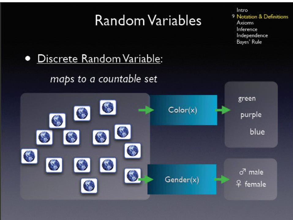
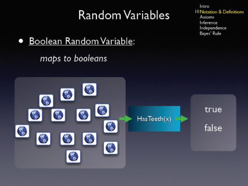
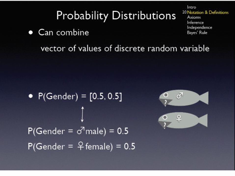
Random Variables

Random variable

Probability for a random variable

12

13

14

15

16

17

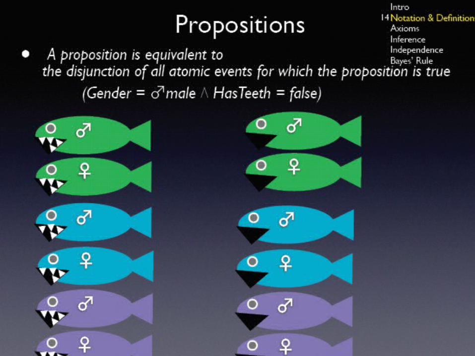
Logical Propositions and Probability

Proposition = event (set of sample points) Given Boolean random variables A and B:

Event a = set of sample points where A(ω)=true Event ⌐a=set of sample points where A(ω)=false Event aΛb=points where A(ω)=true and B(ω)=true

Often the sample space is the Cartesian product of the range of variables

Proposition=disjunction of atomic events in which it is true (aVb) = (⌐aΛb)V(aΛ⌐b)V(aΛb)

P(aVb)= P(⌐aΛb)+P(aΛ⌐b)+P(aΛb)

18

19

20

21

22

23

24

25

Axioms of Probability

All probabilities are between 0 and 1

Necessarily true propositions have probability 1. Necessarily false propositions have probability 0

The probability of a disjunction is P(aVb)=P(a)+P(b)-P(aΛb)

P(⌐a)=1-p(a)

26

The definitions imply that certain logically related events must have related probabilitiesP(aVb)= P(a)+P(b)-P(aΛb)

27

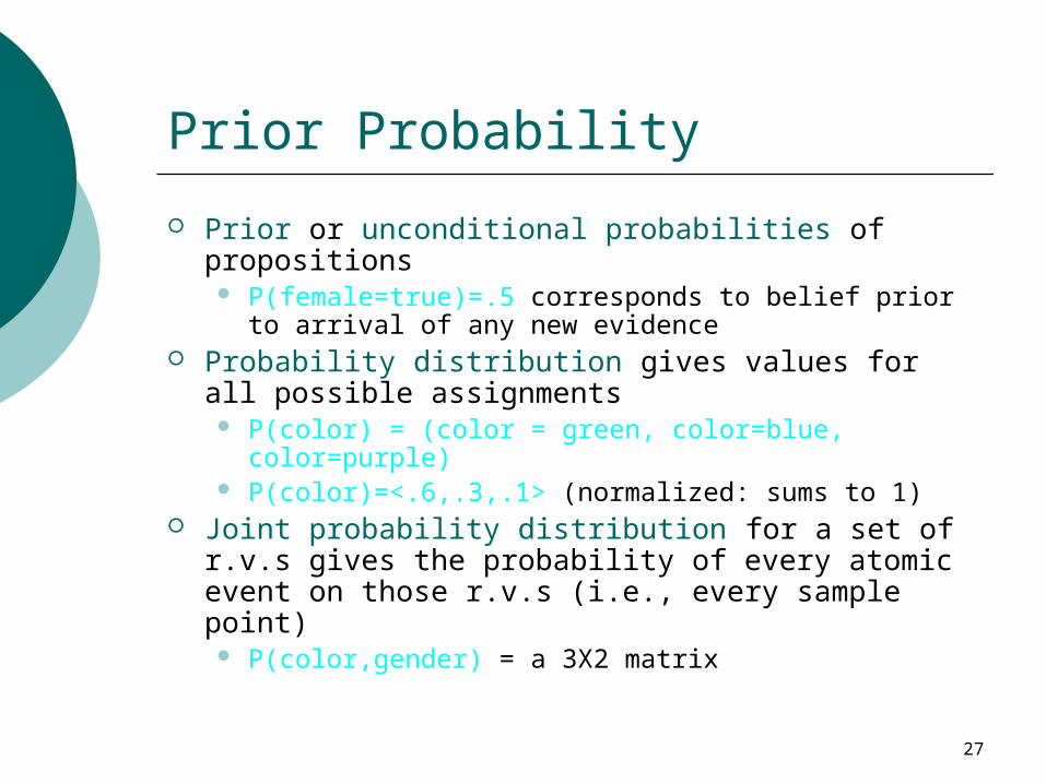
Prior Probability

Prior or unconditional probabilities of propositions P(female=true)=.5 corresponds to belief prior to

arrival of any new evidence Probability distribution gives values for all

possible assignments P(color) = (color = green, color=blue, color=purple) P(color)=<.6,.3,.1> (normalized: sums to 1)

Joint probability distribution for a set of r.v.s gives the probability of every atomic event on those r.v.s (i.e., every sample point) P(color,gender) = a 3X2 matrix

28

29

30

31

32

33

34

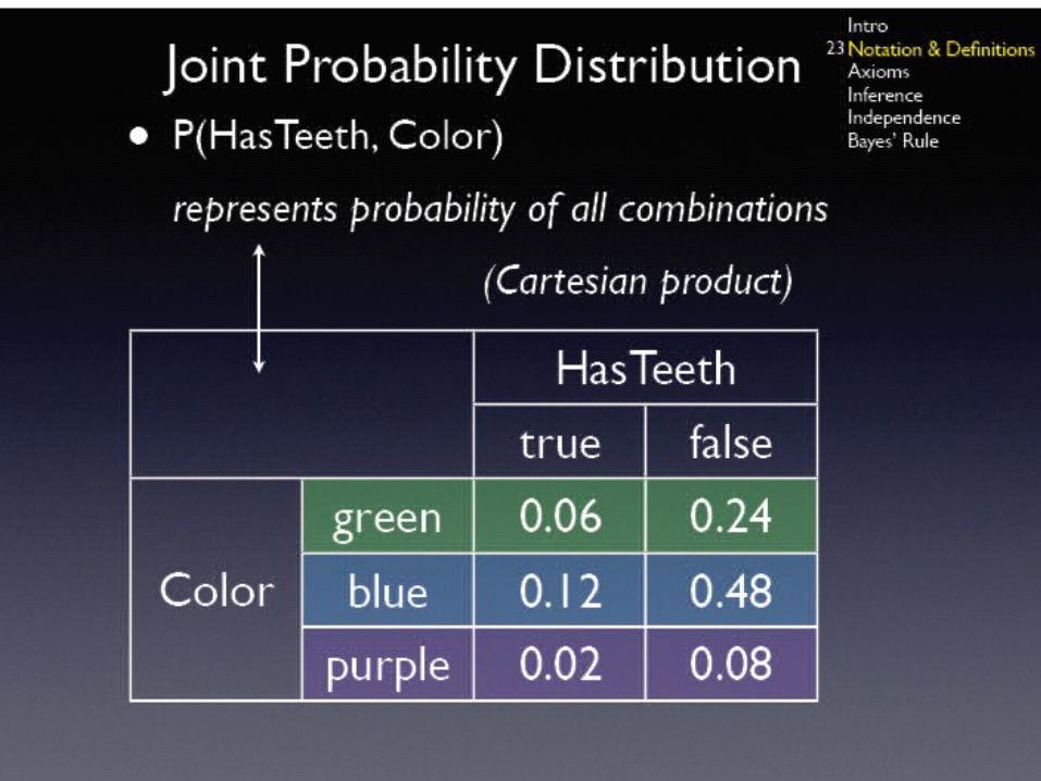
Inference by enumeration

Start with the joint distribution

35

Inference by enumeration

P(HasTeeth)=.06+.12+.02=.2

36

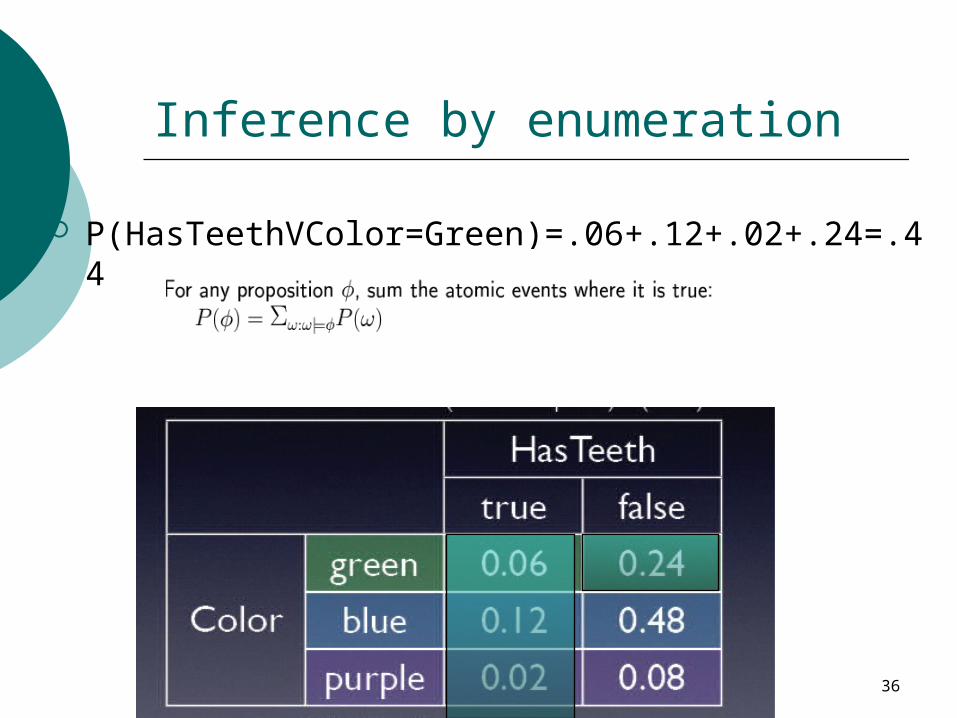
Inference by enumeration

P(HasTeethVColor=Green)=.06+.12+.02+.24=.44

37

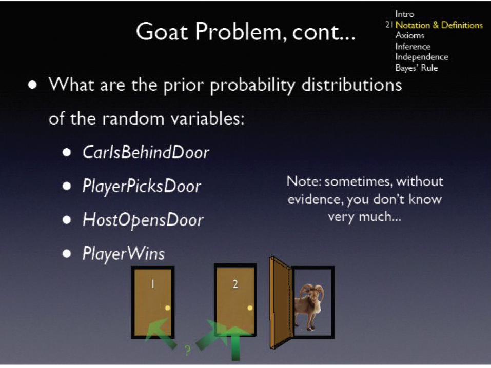
Conditional Probability

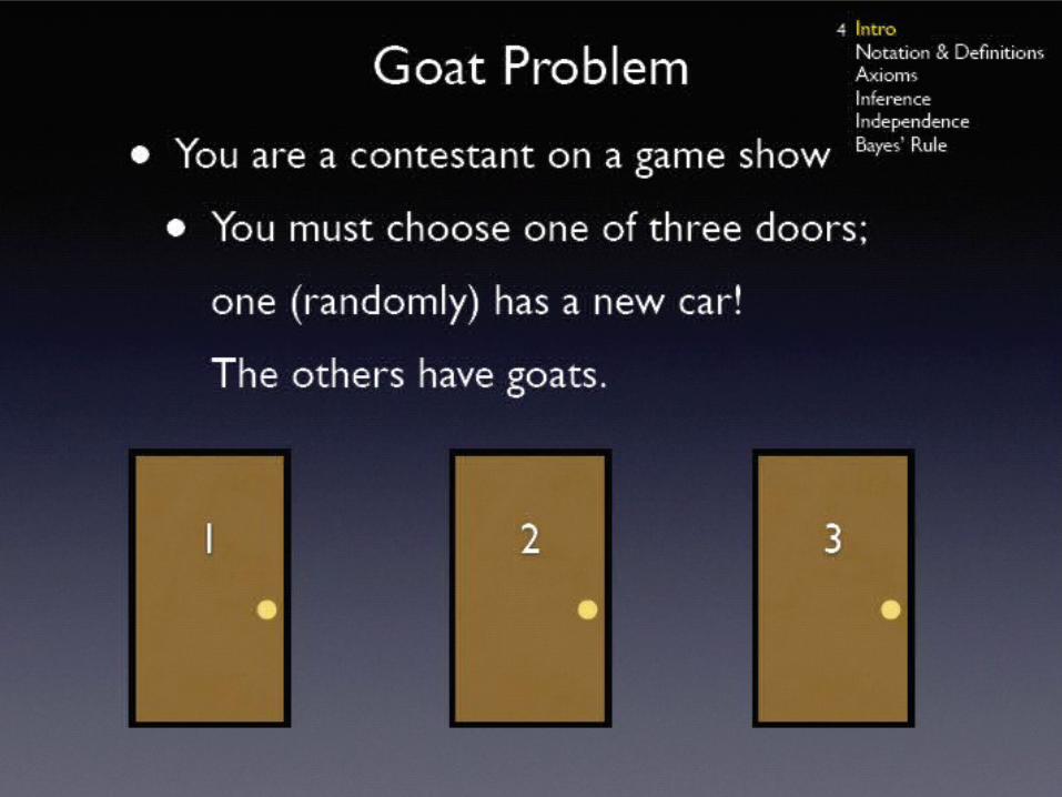
Conditional or posterior probabilities E.g., P(PlayerWins|HostOpenDoor=1 and

PlayerPickDoor2 and Door1=goat) = .5

If we know more (e.g., HostOpenDoor=3 and door3-goat):P(PlayerWins)=1Note: the less specific belief remains valid after more evidence arrives, but is not always useful

New evidence may be irrelevant, allowing simplification: P(PlayerWins|California-

earthquake)=P(PlayerWins)=.3

38

Conditional Probability

A general version holds for joint distributions:

P(PlayerWins,HostOpensDoor1)=P(PlayerWins|HostOpensDoor1)*P(HostOpensDoor1)

39

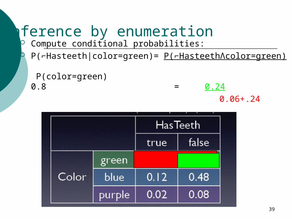
Inference by enumeration Compute conditional probabilities: P(⌐Hasteeth|color=green)= P(⌐HasteethΛcolor=green)

P(color=green)0.8 = 0.24

0.06+.24

40

Normalization Denominator can be viewed as normalization constraint α P(⌐Hasteeth|color=green) = α P(⌐Hasteeth|color=green)

=α[P(⌐Hasteeth,color=green, female)+ P(⌐Hasteeth,color=green, ⌐ female)]=α[<0.03,0.12>+<0.03,0.012>]=α<0.06,0.24>=<0.2,0.8>

Compute distribution on query variable by fixing evidence variables and summing over hidden variables

41

Inference by enumeration

42

Independence

A and B are independent iffP(A|B)=P(A) or P(B|A)=P(B) or P(A,B)=P(A)P(B)

32 entries reduced to 12; for n independent biased coins, 2n -> n

Absolute independence powerful but rare Any domain is large with hundreds of

variables none of which are independent

43

44

Conditional Independence

If I have length <=.2, the probability that I am female doesn’t depend on whether or not I have teeth: P(female|length<=.2,hasteeth)=P(female|hasteeth)

The same independence holds if I am >.2 P(male|length>.2,hasteeth)=P(male|

length>.2) Gender is conditionally independent of

hasteeth given length

45

In most cases, the use of conditional independence reduces the size of the representation of the joint distribution from exponential in n to linear in n

Conditional independence is our most basic and robust form of knowledge about uncertain environments

46

Next Class: Turing Paper

A discussion class

Graduate students and non-degree students: Anyone beyond a bachelor’s:

Prepare a short statement on the paper. Can be your reaction, your position, a place where you disagree, an explication of a point.

Undergraduates: Be prepared with questions for the graduate students

All: Submit your statement or your question by midnight Wed night.

All statements and questions will be printed and distributed in class on Wednesday.