(PRIME) Program Evaluation - Energize Connecticut
242
13 Railroad Square, Suite 504 Haverhill, Massachusetts 01832 (978) 521-2550 Fax: (978) 521-4588 www.ers-inc.com March 26, 2007 ers energy & resource solutions Process Reengineering for Increased Manufacturing Efficiency (PRIME) Program Evaluation prepared for The Energy Conservation Management Board and Connecticut Light & Power (CL&P)
Transcript of (PRIME) Program Evaluation - Energize Connecticut

13 Railroad Square, Suite 504 Haverhill, Massachusetts 01832
(978) 521-2550 Fax: (978) 521-4588
www.ers-inc.com
March 26, 2007
ers energy & resource
solutions
Process Reengineering for Increased Manufacturing Efficiency (PRIME)
Program Evaluation prepared for
The Energy Conservation Management Board and Connecticut
Light & Power (CL&P)


table of contents toc
table of contents i energy & resource solutions ers
1. EXECUTIVE SUMMARY............................................................................................................................ 1-1 1.1 INTRODUCTION........................................................................................................................................ 1-1 1.2 SUMMARY OF FINDINGS AND RECOMMENDATIONS................................................................................. 1-1
1.2.1 Review of Lean Manufacturing and Energy Efficiency..................................................................... 1-2 1.2.2 Prime Program Project Documentation Review ................................................................................ 1-3 1.2.3 Savings Methodology Assessment and Recommendations ............................................................... 1-4 1.2.4 General Findings and Recommendations for the PRIME Program ................................................... 1-8
1.3 EVALUATION PERSONNEL & DELIVERABLES ........................................................................................ 1-10 2. LEAN MANUFACTURING AND ENERGY EFFICIENCY.................................................................... 2-1
2.1 INTRODUCTION........................................................................................................................................ 2-1 2.2 LITERATURE REVIEW & INFORMAL SURVEY OF LEAN ORGANIZATIONS................................................. 2-1
2.2.1 Literature Search................................................................................................................................ 2-2 2.3 LEAN MANUFACTURING TECHNIQUES .................................................................................................... 2-3
2.3.1 5S....................................................................................................................................................... 2-3 2.3.2 Visual Management ........................................................................................................................... 2-4 2.3.3 Standardized Work ............................................................................................................................ 2-4 2.3.4 Quick Changeover or Single Minute Exchange of Dies (SMED)...................................................... 2-4 2.3.5 Value Stream Map (VSM)................................................................................................................. 2-4 2.3.6 Total Productive Maintenance (TPM) ............................................................................................... 2-5 2.3.7 Cellular Flow ..................................................................................................................................... 2-5 2.3.8 Kanban............................................................................................................................................... 2-5 2.3.9 Poka Yoke.......................................................................................................................................... 2-5 2.3.10 Point-of-Use (POU) Systems ........................................................................................................ 2-5 2.3.11 Kaizen ........................................................................................................................................... 2-6
2.4 PRODUCTIVITY IMPROVEMENT APPROACHES.......................................................................................... 2-6 2.4.1 Inventory Reduction .......................................................................................................................... 2-7 2.4.2 Changeover Time Reduction ............................................................................................................. 2-7 2.4.3 Downtime Reduction ......................................................................................................................... 2-8 2.4.4 Setup Time Reduction ....................................................................................................................... 2-8 2.4.5 Cycle Time Reduction ....................................................................................................................... 2-8 2.4.6 Increased Throughput ........................................................................................................................ 2-9 2.4.7 Rework/Scrap Reduction ................................................................................................................... 2-9 2.4.8 Part Travel Reduction ........................................................................................................................ 2-9 2.4.9 Space Reduction .............................................................................................................................. 2-10 2.4.10 Direct Equipment Efficiency Improvement ................................................................................ 2-10
2.5 INDUSTRIAL ENERGY USE ..................................................................................................................... 2-10 2.5.1 Industrial Plant Wide Energy Use.................................................................................................... 2-10 2.5.2 Equipment Energy Use .................................................................................................................... 2-12
2.6 LEAN MANUFACTURING AND ENERGY SAVINGS................................................................................... 2-13 2.6.1 Pre-event, ‘Non-Lean Productivity Increase’ and Post-event Scenarios.......................................... 2-13 2.6.2 Justification for Energy and Demand Savings................................................................................. 2-15
2.7 CALCULATING ENERGY SAVINGS.......................................................................................................... 2-15 2.7.1 Energy Breakdown Method ............................................................................................................. 2-16 2.7.2 Statistical Regression Model Method .............................................................................................. 2-22
2.8 CLOSING................................................................................................................................................ 2-22 3. PROJECT DOCUMENTATION REVIEW................................................................................................ 3-1

table of contents toc
table of contents ii energy & resource solutions ers
3.1 INTRODUCTION........................................................................................................................................ 3-1 3.2 INDUSTRY TYPE SUMMARY..................................................................................................................... 3-1 3.3 LEAN MEASURE SUMMARY..................................................................................................................... 3-2 3.4 CLAIMED SAVINGS SUMMARY ................................................................................................................ 3-5 3.5 CLAIMED SAVINGS AND BCR INPUT REVIEW ......................................................................................... 3-7
3.5.1 Annual Electricity Usage ................................................................................................................... 3-7 3.5.2 Percent of Affected Goods or Sales ................................................................................................... 3-9 3.5.3 Production Rates................................................................................................................................ 3-9
3.6 COMPARISONS OF FILED DATA WITH TRACKING SYSTEM ..................................................................... 3-10 3.7 FILE ADEQUACY AND COMPLETENESS .................................................................................................. 3-11 3.8 SUMMARY AND RECOMMENDATIONS.................................................................................................... 3-13
4. SAVINGS METHODOLOGY ANALYSIS AND RECOMMENDATIONS............................................ 4-1 4.1 INTRODUCTION AND SUMMARY OF RECOMMENDATIONS........................................................................ 4-1 4.2 NU SAVINGS ALGORITHM....................................................................................................................... 4-2
4.2.1 Algorithm Description ....................................................................................................................... 4-2 4.2.2 Algorithm Example............................................................................................................................ 4-3 4.2.3 Accuracy – Comparison of Calculated Savings from Site Visits....................................................... 4-5 4.2.4 Algorithm Assumptions Evaluation................................................................................................... 4-6
4.3 PROPOSED SAVINGS ALGORITHM............................................................................................................ 4-9 4.3.1 New Algorithm Outline ..................................................................................................................... 4-9 4.3.2 Algorithm Example.......................................................................................................................... 4-13 4.3.3 Proposed Algorithm Accuracy......................................................................................................... 4-16
4.4 DISCUSSION OF INTERMEDIATE PRODUCTION INCREASE ESTIMATE........................................................ 4-16 4.5 SPREADSHEET TOOL.............................................................................................................................. 4-17 4.6 SUMMARY ............................................................................................................................................. 4-19
5. EVALUATION FINDINGS AND RECOMMENDATIONS..................................................................... 5-1 5.1 INTRODUCTION........................................................................................................................................ 5-1 5.2 PROJECT DOCUMENTATION FINDINGS AND RECOMMENDATIONS ........................................................... 5-1
5.2.1 NAICS/SIC Codes ............................................................................................................................. 5-1 5.2.2 Lean Techniques ................................................................................................................................ 5-1 5.2.3 Savings Algorithm Input Assessment ................................................................................................ 5-1 5.2.4 Tracking System ................................................................................................................................ 5-2 5.2.5 Project Documentation ...................................................................................................................... 5-2
5.3 ALGORITHM AND SAVINGS FINDINGS AND RECOMMENDATIONS ............................................................ 5-3 5.4 PROGRAM FINDINGS AND RECOMMENDATIONS ...................................................................................... 5-4
APPENDICES A. Site A, Event 1 B. Site B C. Site C D. Site D E. Site E F. Site A, Event 2 G. Site Evaluation Supporting Analysis H. Logged Equipment Energy Use I. Section 2 Supporting Analysis J. Site Interviews K. Informal Organization Survey L. File Documentation Template/ 90 Day Follow-up Request

executive summary 1
prime program evaluation for CL&P 1-1 energy & resource solutions ers
1. EXECUTIVE SUMMARY
1.1 INTRODUCTION
This report presents the findings and recommendations for Connecticut Light and Power (CL&P) resulting from an evaluation of Northeast Utilities’ (NU) Process Reengineering for Increased Manufacturing Efficiency (PRIME) program administered by CL&P and Western Massachusetts Electric Company (WMECO). The NU PRIME program sponsors Lean Manufacturing events at eligible facilities in the CL&P and WMECO territories. The goal of each three- to four-day event is to improve productivity while decreasing energy use per unit produced. Through proper implementation of Lean Manufacturing techniques, utility customers are able to increase their manufacturing productivity with little additional electricity use, as compared to pre-event use.
Energy & Resources Solutions (ERS) was selected to conduct the evaluation. ERS worked closely with the NU representatives to achieve the primary objects of the evaluation as stated on Page 2 of the RFP, which were:
1. To verify through site visits that the actions taken by customers to improve their productivity have indeed taken place and that increased production has resulted.
2. To assess the merits of the method the Company uses to calculate the costs and benefits of the program, i.e., the electric savings.
3. To quantify the non-electric benefits resulting from each customer’s participation.
Several other tasks were outlined in the RFP for completion within deliverables, and are discussed in Section 1.3.
1.2 SUMMARY OF FINDINGS AND RECOMMENDATIONS1
A thorough literature search on Lean Manufacturing techniques as related to energy efficiency, combined with a comprehensive review of project documentation files, and five facility site visits provide the basis for our conclusion that the current algorithm employed to calculate energy savings (kWh) may misestimate the savings attributable to the PRIME program. Savings may be overestimated mainly due to input values of annual electricity use
1 While PRIME projects in both CL&P and WMECO service territories were examined in this study, the recommendations herein address the CL&P program and its savings calculation algorithm. References to proposed NU modifications to the PRIME savings calculations should be taken to refer only to CL&P.

section 1 executive summary
prime program evaluation for CL&P 1-2 energy & resource solutions ers
and production gains. With correct inputs, we believe the algorithm actually underestimates annual electricity savings, while overestimating lifetime savings. To some extent, lifetime savings overestimations can be attributed to the assumption of a 10-year measure life, which is very likely too high.
We evaluated the algorithm and assumption values based on data obtained from on-site evaluations of five PRIME events. This data sample is possibly non-representative and not statistically significant. However, the data does provide a starting point with which to examine the existing algorithm and assumption values. The dramatic difference in some assumption values suggests that revised values could provide more accurate savings estimates. Therefore, we are recommending several changes to the algorithm and the assumption values. These recommendations should be accepted with caution, and used only until refined values can be derived from a representative, statistically significant data set are determined.
Based on the results of our research and site evaluations, we also suggest several non-algorithmic recommendations for improving the PRIME program. Recommendations include: methods for more accurate assessments of electricity usage before, and energy savings after, a Lean Manufacturing event; strategies for targeting the types of companies most likely to experience significant increases in productivity and energy efficiency as a result of implementing Lean techniques; and guidelines for promoting use of the Lean Manufacturing productivity improvements that will result in the greatest energy savings.
Finally, we found that none of the PRIME projects evaluated had a positive benefit-to-cost ratio. The complete findings and recommendations are presented in the remaining four sections of this evaluation report and summarized below (1.2.1 to 1.2.4).
1.2.1 REVIEW OF LEAN MANUFACTURING AND ENERGY EFFICIENCY
Section 2, Lean Manufacturing and Energy Efficiency, contains a review of Lean Manufacturing techniques and productivity improvement methods. Included in this section are an overview of industrial energy use and a detailed discussion of the relationship between Lean Manufacturing and energy efficiency. The concepts and engineering methods outlined in this section provide the theoretical framework for evaluation of the existing NU savings algorithm (see Section 4). Detailed descriptions of the calculations employed in this section are provided in Appendix I.
ERS conducted a literature search and an informal survey of relevant publications on Lean Manufacturing and productivity improvement, its effect on energy use, and quantification approaches. Unfortunately, the relationship between productivity improvements and energy efficiency benefits has been minimally addressed in existing literature. Therefore, this report represents a unique contribution to the body of literature related to the energy efficiency impact of Lean Manufacturing techniques.
Lean Manufacturing is an umbrella term that includes many specific types of productivity improvement techniques. Energy savings associated with the implementation of Lean

section 1 executive summary
prime program evaluation for CL&P 1-3 energy & resource solutions ers
Manufacturing techniques most commonly result from waste reduction and decreased production hours. However, different Lean techniques have variable effects on energy consumption within a manufacturing facility.
The overall effect that Lean techniques will have on energy efficiency is dependent upon the type of equipment impacted by productivity improvement measures. Therefore, in order to determine the energy consumption effects of Lean Manufacturing techniques, it is important to identify and classify the types of equipment impacted by Lean Manufacturing techniques. Equipment can be grouped into five categories – one for office equipment and four representing manufacturing equipment, referred to in the report as Types A through D.
The five types of equipment are:
1. Office equipment
2. Manufacturing equipment with energy use independent of production hours and production quantity (Type A)
3. Manufacturing equipment with energy use dependent on production quantity (Type B)
4. Manufacturing equipment with energy use dependent on production hours (Type C)
5. Manufacturing equipment with energy use dependent on production hours and quantity (Type D)
To determine the energy savings that result from a Lean event all relevant equipment must first be grouped according to the five categories listed above. Then pre-event, non-Lean productivity increase, and post-event energy use are calculated as described in Section 2. Energy savings (kWh) due to the implementation of Lean techniques can be quantified as the difference between ERS estimated post-event energy use and the estimated energy use of a non-Lean productivity increase of the same magnitude. The energy that would be required for non-Lean productivity increases is an instructive metric, which we have used to quantify the efficiency impact of the PRIME program. A comparison between ERS estimated post-event energy use and the estimated energy use of a non-Lean productivity increase provides the basis for calculating the incremental energy savings that result from a Lean Manufacturing event. Electrical demand (kW) savings may also be claimed if excess hourly production capacity results from post-event implementation of Lean Manufacturing techniques.
1.2.2 PRIME PROGRAM PROJECT DOCUMENTATION REVIEW
Section 3, Project Documentation Review, contains a review of 20 PRIME project document files supplied by CL&P and WMECO. Project reviews include: industry sector summaries; descriptions of the Lean techniques employed; an assessment of the claimed savings and algorithm inputs; a summary account of completeness and adequacy for each project file; and recommended project documentation changes.

section 1 executive summary
prime program evaluation for CL&P 1-4 energy & resource solutions ers
Based on a documentation review of 20 projects in the CL&P and WMECO service territories, we provide several summary points and recommendations for the PRIME program. The PRIME program serves a range of industries. However, projects are concentrated in Fabricated Metal Product Manufacturing plants (NAICS 332, SIC 34). The Lean techniques most frequently employed in these projects were 5S, Visuals/Standardized Work, and Quick Changeover. The most common productivity improvements were reduced changeover, reduced cycle times, and reduced inventory. Please refer to Section 2 for a complete list of Lean Manufacturing terms and definitions.
Upon examination of the Benefit/Cost Ratio (BCR) and claimed savings calculation inputs for each project, we found, in many cases, that the input estimations were either incorrect or poorly justified. Annual electricity use inputs frequently did not match actual values, which significantly skewed the savings calculations. There were apparently many reasons for the miscalculation including summing two accounts when only one applied, summing one meter instead of two, and counting 13 months instead of 12. Furthermore, the percent of affected product/sales estimate often was not justified, nor were the production rates. Inconsistencies were not the result of data entry errors; in most cases the claimed savings entered into the NU tracking system matched the savings documented in the project files.
On the basis of this review, it does not appear that the current project file documentation adequately captures project descriptions and details. Therefore, it should be improved. In section 3, we recommend a number of changes to the project documentation. Recommendations include: improved project descriptions; inclusion of a document content sheet; stronger justification for percent affected production; production values and sample size; customer electricity billing history; and addition of NAICS/SIC code.
1.2.3 SAVINGS METHODOLOGY ASSESSMENT AND RECOMMENDATIONS
Section 4, Savings Methodology Analysis and Recommendations, is a review and evaluation of the existing NU savings algorithm. In this section we recommend modifications to the existing savings algorithm and assumption values. Estimated results of the ERS-recommended algorithm are compared to data generated using the existing NU algorithm.
Table 1-1 presents savings estimates of the NU algorithm compared with ERS calculated savings. We found that the existing savings algorithm regularly and significantly overestimated energy savings compared to ERS calculated results, both on an annual and lifetime basis (when using the Lean consultant-provided algorithm inputs). Overestimation of annual savings can be attributed primarily to inaccurate input variables, such as annual electricity use and production gains.

section 1 executive summary
prime program evaluation for CL&P 1-5 energy & resource solutions ers
Table 1-1: Reported versus ERS estimated Annual Savings Reported ERS Reported Savings
Savings from Estimated % ofSite NU Algorithm Savings Difference ERS Est. SavingsA - Event 1 20,904 2,205 18,699 948%A - Event 2 36,582 9,369 27,213 390%B 11,598 48,483 -36,884 24%C 885,620 0 885,620 NAD 1,191,124 21,787 1,169,337 5467%E 20,786 6,927 13,859 300%Average 1426%Total 1,280,994 88,771 1,192,224 1443%
*Site C had no production improvement and is not included in the Total sums
Table 1-2 depicts the significantly improved results that can be obtained simply by using accurate input variables with the existing algorithm. Given accurate input variables, the existing algorithm underestimated ERS estimated savings by about half in several instances.
Table 1-2: Adjusted versus ERS Estimated Annual Savings Adjusted ERS Reported Savings
Savings from Estimated % ofSite NU Algorithm Savings Difference ERS Est. SavingsA - Event 1 3,091 2,205 886 140%A - Event 2 9,499 9,369 130 101%B 19,710 48,483 -28,772 41%C 433,220 0 433,220 NAD 13,292 21,787 -8,495 61%E 2,095 6,927 -4,832 30%Total 47,687 88,771 -41,083 54%
*Site C had no production improvement and is not included in the Total sums
Overestimation of lifetime savings is due mainly to the assumption of a 10-year measure life. Furthermore, we believe the existing NU algorithm assumptions were inaccurate, and could result in misestimating of energy savings.
In order to obtain more accurate and representative energy savings estimates, we recommend the following changes to the existing NU energy savings algorithm and assumption values:
Decrease the assumed measure life from 10 to 5 years. Multiple factors such as employee turnover, procedural regression, market influence, and business turnover warrant a decreased measure life (See Section 4.2.4).
To accommodate energy savings variability among Lean productivity improvement techniques, choose the most appropriate savings algorithm for each project: (1) for general productivity increases; (2) for rework/scrap reduction improvements; and

section 1 executive summary
prime program evaluation for CL&P 1-6 energy & resource solutions ers
(3) for reduced setup times during non-production hours. These three distinct classes of Lean productivity improvement techniques save energy in different ways. Therefore, selection of the correct algorithm will increase the accuracy of energy savings estimates. (See Section 4.3.1).
Revise the 5% (no savings) component to 65%. Office Type A and Type B equipment, accounting for 65% of total energy use, are similar in that from the ‘Non-Lean Productivity Increase’ to Post-Event scenario they have no associated energy savings. Additionally, revise the 10% (production-hour dependent) component to 20%. Type C equipment accounts for 20% of total energy use and electricity savings are calculated the same as ‘Non-manufacturing’ savings were calculated in the existing NU algorithm. Finally, revise the 85% (production-quantity dependent) component to 15%. Electricity savings for Type D equipment are calculated similarly to how the “Manufacturing’ savings were calculated in the existing NU algorithm, except with a variable percentage savings factor applied to all production units. (See Section 4.2.4 and Section 2.7.1).
Replace the constant 6% savings factor currently applied to incremental production with a variable savings factor applied to all production. This factor should be based on reasonable assumptions of equipment cycle times and idle power draw (See Section 4.2.4).
Claim demand savings where appropriate by integrating demand savings calculations into the algorithm. Demand savings can be claimed when existing plant operating hours are 24 hours per day, seven days a week (See Section 4.3.1).
Provide an option to calculate labor savings within the savings spreadsheet. Labor savings can be calculated simply from avoided production hours (See Section 4.3.1).
These algorithm assumption changes will enhance the predictive accuracy of the PRIME program savings estimates. An in-depth discussion of the algorithm recommendations can be found in Section 4 of this report.
Table 1-3 shows annual energy savings estimated using the recommended algorithm compared with ERS estimated savings. ERS has independently created an analytical spreadsheet tool to help develop the recommendations and assess the results from this modified approach. If formalized for use in the program, this analytical tool would standardize calculations and provide a simple method for using the recommended algorithms in future PRIME programs.

section 1 executive summary
prime program evaluation for CL&P 1-7 energy & resource solutions ers
Table 1-3: Recommended Algorithm versus ERS Estimated Annual Savings Savings from ERS Reported Savings
Recommended Estimated % ofSite Algorithm Savings Difference ERS Est. SavingsA - Event 1 0 2,205 -2,205 0%A - Event 2 17,300 9,369 7,931 185%B 35,896 48,483 -12,587 74%C 0 0 0 NAD 24,207 21,787 2,420 111%E 3,815 6,927 -3,112 55%Average 85%Total 81,218 88,771 -7,553 91%
*Site C had no production improvement and is not included in the Total sums
Table 1-4 presents the energy intensity of the pre-event, non-Lean productivity increase, and post-event scenarios in terms of annual production and annual energy savings. The incremental energy savings (kWh) resulting from a Lean Manufacturing event are calculated by comparing ERS estimated post-event energy use with the estimated energy use of a non-Lean productivity increase. Annual energy savings can be calculated based on per unit production energy intensities for each scenario (see Section 2 for calculation details). Note that energy intensity decreases from the pre-event to the non-Lean productivity increase scenario, and decreases even further from the non-Lean productivity increase to the post-event scenario.
Table 1-4: ERS Estimated Energy Intensities and Energy Savings Annual Energy
Energy Intensity (kWh/unit) Production SavingsSite Pre-event Non-Lean Post-event (units) (kWh/yr)A - Event 1 55.9 50.4 49.4 2,284 2,205A - Event 2 0.0022 0.0017 0.0016 75,322,000 9,369B 0.0734 0.0733 0.0727 79,088,659 48,483D 0.0993 0.0990 0.0986 59,714,660 21,787E 3.135 3.130 3.118 593,194 6,927Total/Ave. 88,771
*Energy Savings (kWh/year) = (Non Lean kWh/unit – Post-event kWh/unit) x units/year
Table 1-5 depicts the lifetime savings, cost per kWh (i.e. benefit-cost-ratio), and program screening calculated using our recommended algorithm and adjusted measure life. The cost per kWh shown here is based only on electricity savings; it does not account for labor or other non-electric benefit (NEB) savings. We found that none of the events passed the BCR screen.

section 1 executive summary
prime program evaluation for CL&P 1-8 energy & resource solutions ers
Table 1-5: ERS estimated Lifetime Savings, BCR and Program Screening Total LifetimeEvent Savings Cost Passes
Site Events Cost (kWh) ($/kWh) ScreenA - Event 1 1 $4,800 11,026 $0.435 NoA - Event 2 1 $4,800 46,844 $0.102 NoB 2 $9,600 242,414 $0.040 NoC 1 $6,000 0 NA NoD 2 $6,000 108,935 $0.055 NoE 1 $12,000 34,634 $0.346 NoTotal/Ave. 8 $43,200 443,854 $0.196
1.2.4 GENERAL FINDINGS AND RECOMMENDATIONS FOR THE PRIME PROGRAM
Section 5, PRIME Program Evaluation Findings and Recommendations, presents the general findings and recommendations of this evaluation. In addition to the findings and recommendations presented above, our research and five site evaluations yielded several other suggestions for a more effective and successful PRIME program:
Verify annual electricity use with facility employees before calculating savings. Annual electricity use is frequently miscalculated from billing records obtained from NU. These records are sometimes printed out in a confusing way that has contributed to the miscalculation of annual electricity use. We have found that most facilities maintain accurate, clear records of electricity use. Thus, we recommend that the Lean consultant obtain annual electrical energy (kWh) and demand (kW) from the site employees during the PRIME event.
Calculate electricity savings using confirmed production gains obtained at least three months after the PRIME event. Currently, electricity savings are typically based on expected production gains calculated at the same time as the PRIME event. This more reflects an increase in maximum production capacity than real production gains. Because the Lean consultant contacts the facility for a three-month follow up as a matter of program protocol already, estimating productivity improvement at this point would yield a much more accurate value. Appendix L provides a template for information to gather at this point
Target companies with a stable and/or increasing product demand. Market influences on production often negatively influence the gains from the PRIME sponsored Lean events. During many of the site evaluations, we found that production gains were lower than expected which was almost always due to market factors.
Lower prioritize “job shop” type facilities. Job shops produce a large variety of products, and production requirements typically change from day to day. The frequency of product changes leads to decreased persistence of increased production and thus energy efficiency gains.
section 1 executive summary
prime program evaluation for CL&P 1-9 energy & resource solutions ers
Promote those types of Lean Manufacturing productivity improvements that result in energy savings. Through the evaluation process we identified a number of PRIME sponsored projects whose effect on plant production levels and manufacturing equipment was uncertain. We recommend that PRIME sponsored events utilize Lean techniques that significantly impact electricity use, such as:
o reducing changeover time;
o reducing downtime;
o reducing setup time;
o decreasing cycle time;
o increasing throughput; and
o reducing rework/scrap.
Projects geared towards inventory reduction should be given lower priority, because inventory reduction typically does not yield increased production or electricity savings. The five sites we evaluated participated in a total of eight PRIME sponsored Lean events, two of which were targeted towards inventory reduction.
Promote 5S, TPM, Visuals and Standardized Work projects that increase the operating efficiency of equipment. While Lean events will not change equipment efficiency, they can improve how the equipment is operated, often resulting in a direct decrease in electricity use. These low-cost/no-cost improvements typically rely on the integration of best practices into the company culture. This is exactly what TPM, Visuals, and Standardized Work are geared towards. In addition, 5S projects often improve equipment condition, resulting in increased operating efficiency. These types of projects may yield more measurable and consistent electricity savings.
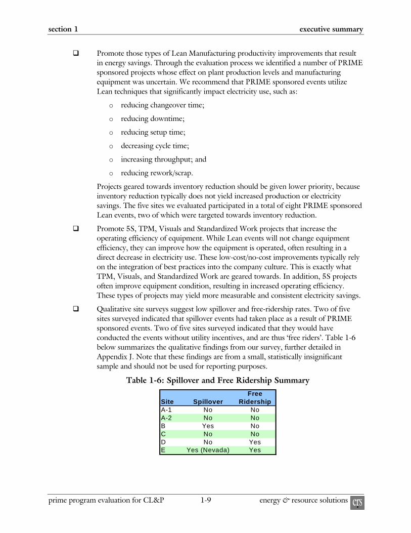
Qualitative site surveys suggest low spillover and free-ridership rates. Two of five sites surveyed indicated that spillover events had taken place as a result of PRIME sponsored events. Two of five sites surveyed indicated that they would have conducted the events without utility incentives, and are thus ‘free riders’. Table 1-6 below summarizes the qualitative findings from our survey, further detailed in Appendix J. Note that these findings are from a small, statistically insignificant sample and should not be used for reporting purposes.
Table 1-6: Spillover and Free Ridership Summary Free
Site Spillover RidershipA-1 No NoA-2 No NoB Yes NoC No NoD No YesE Yes (Nevada) Yes

section 1 executive summary
prime program evaluation for CL&P 1-10 energy & resource solutions ers
Hedge preliminary production increase estimates with site personnel estimates. Event estimates of production gains are often high, in the range of 10% to 30%. We found that realized production gains are typically much lower, under 5%. The evaluation team suggested that the facility employees should be asked before the PRIME event what they thought a realistic production increase would be. ERS agrees that this question would be helpful, in the sense that production increase estimates can be tempered. However, we do recommend that final savings should be based on production increased as derived from actual data.
Require beneficiaries of PRIME incentives to participate in a program evaluation, if asked. We found that it was difficult to schedule on-site assessments of some PRIME participants. This difficulty could be repeated for impact evaluations. Thus, we recommend that PRIME participants agree to host on-site evaluations if required.
1.3 EVALUATION PERSONNEL & DELIVERABLES
Mr. Gary Epstein and Mr. Mark D’Antonio served as project and technical advisors on the PRIME Program Evaluation project for ERS. Mr. John Seryak served as the day-to-day project manager and lead engineer for ERS, coordinating site visits and communication with the NU representatives and non-utility parties, hereafter referred to as the evaluation team. Mr. Yogesh Patil and Ms. Deborah Swarts of ERS also contributed to this evaluation as project engineers.
ERS worked closely with NU employees associated with the PRIME Program. Mr. Earle Taylor of NU served as the evaluation team leader. Mr. David Bebrin of CL&P assisted with consultation on the NU algorithm. Mr. James Motta of CL&P assisted in providing project documentation for PRIME events in CL&P territory and Mr. Carl Santoro of WMECO assisted in providing project documentation for PRIME events in WMECO territory. ERS would like to express our appreciation to all involved for their efforts in facilitating this evaluation and providing invaluable guidance and information for this project.
Evaluation project meetings included a kick-off meeting on August 16, 2005, including the evaluation team, and a conference call with Mr. Taylor and Mr. Bebrin on December 13, 2005. An evaluation team project review was meeting was held at CL&P’s New Britain offices on March 1, 2006.
In the course of the evaluation, we reviewed 20 PRIME documentation files, looked closely at five of these 20 projects, conducted five in-depth site visits, and evaluated the NU savings algorithm used to estimate electricity savings. Descriptions of each evaluation deliverable are provided below.
The following five deliverables were required and have been completed as part of the PRIME program evaluation conducted by ERS:

section 1 executive summary
prime program evaluation for CL&P 1-11 energy & resource solutions ers
1. Evaluation Workplan – Provided the scope of work, presented methodologies for implementation, and provided a general road map for the project. The full Evaluation Workplan is included as Appendix M.
2. Project Documentation Review – 20 project document files supplied by CL&P and WMECO were reviewed. The important characteristics of each project, including industry sector and Lean technique, were summarized. The availability of essential information (e.g. input annual electricity, percent of affected goods, and production rates) within each project file was assessed. The final Project Documentation Review document is included in this evaluation report as Section 3.
3. On-Site Measurement and Verification (M & V) Survey Forms – A survey form was created to guide the data collection process during site visits and ensure consistent information gathering at each of the five sites evaluated. Appendix J of this report contains the completed M&V Surveys for each site. The objectives of the On-Site M&V were to:
Verify affected production lines, line operating hours and pre and post-Event production rates.
Identify if and when productivity improvements were removed or are no longer in effect.
Determine the spill-over effect
Determine the free-rider effect
Derive an estimate of facility energy use broken down into appropriate components
Quantify the NEBs.
4. Site Evaluation Reports for PRIME projects – Five site visits were conducted to evaluate the implementation of PRIME recommendations, the associated production gains, and the energy savings. Site visit activities included: discussions with the Lean event participants, a tour of the facility, inventory of electricity-using equipment impacted by post-event Lean Manufacturing practices, and deployment of measurement equipment to log energy use when appropriate. Data collected during site visits were used to perform detailed calculations of productivity improvements and associated electricity savings. Site Evaluation Reports are submitted as Appendices A through F. In order to ensure confidentiality, these reports do not identify the customer by name or account number.
5. PRIME Program Evaluation Report – This document (sections 1 through 5 and appendices) represents the PRIME Program Evaluation Report, which provides a complete summary of all activities, findings, and conclusions of the ERS evaluation.


lean manufacturing and energy efficiency 2
prime program evaluation for CL&P 2-1 energy & resource solutions ers
2. LEAN MANUFACTURING AND ENERGY EFFICIENCY
2.1 INTRODUCTION
Lean Manufacturing is an umbrella term referring to a number of productivity improvement methods defined in this chapter. The primary goal of these techniques is to improve productivity, meaning an increase in production output per unit input of material, energy, labor and other resources. As a result, the energy consumption of the process is often impacted. In some situations, these techniques can result in energy savings, but this is not always the case. When energy is saved due to improved productivity, it can be saved in different ways. For example, reducing changeover may save energy differently than reducing scrap/rework. Thus, in order to accurately evaluate the electricity savings estimates of the PRIME program, it is imperative to understand the following:
1. Lean Manufacturing Techniques (Section 2.3)
2. Productivity Improvement Approaches (Section 2.4)
3. Variables Impacting Equipment Energy (Section 2.5)
4. Impacts of Productivity Improvements on Energy Usage (Sections 2.6 & 2.7).
These four points will be explored in detail in this section. In addition, the results of a literature search and an informal survey of Lean organizations will be discussed (Section 2.2). The conclusions documented here will be the foundation for examining the existing NU savings algorithm and assumptions, which are presented in Section 4.
2.2 LITERATURE REVIEW & INFORMAL SURVEY OF LEAN ORGANIZATIONS
As a starting point to evaluating the relationship between productivity and energy use, ERS conducted a thorough literature search and contacted several leading Lean Manufacturing organizations. The literature search revealed that very little has been published on the relationship between productivity and energy use. There has been only one published paper directly addressing the quantification of energy savings due to increased productivity. Despite contacting eleven prominent Lean Manufacturing or energy efficiency organizations (reference section 2.2.2) and conducting an exhaustive Internet search, little additional quantitative information was available.

lean manufacturing and energy efficiency section 2
energy & resource solutions 2-2 prime program evaluation for CL&P ers
2.2.1 LITERATURE SEARCH
Our literature search found one paper that directly addressed the quantification of energy savings due to increased productivity, which is discussed below.
On Accounting for Energy Savings from Industrial Productivity Improvements
The DOE Industrial Assessment Center Program sponsors industrial energy, waste, and productivity assessments. Productivity recommendations may report ‘effective’ energy savings. This approach was outlined with an example by Papadaratsakis, et al. Briefly, the approach recommends calculating a Current Energy Intensity (CEI) and New Energy Intensity (NEI), based on pre- and post-measure energy intensities, respectively. The savings are then calculated as the Current Energy Consumption (CEC) times the percentage improvement from CEI to NEI. Equation 2-1 presents the Effective Energy Savings (EES) equation as derived by Papadaratsakis.1
EES = CEC x [1 – NEI/CEI] (2-1)
This approach is significantly different than that taken by Northeast Utilities (see Section 4.2). The approach does not specify whether CEC should reflect total plant energy use or a percentage. Thus, this method could overestimate savings by including energy use that was not affected by the Lean event. This approach also assumes that energy savings would be applied to all units of production. NU’s algorithm applies a constant energy savings percentage to only the incremental units.
Other Relevant Information
ERS conducted an informal survey of several Lean Manufacturing and energy-efficiency promoting agencies, in search of related productivity and energy efficiency programs or research. We were unable to find any documentation of energy savings calculation methods. The organizations we contacted are listed below. Detailed descriptions of these organizations are provided in Appendix K.
The Institute of Industrial Engineers (IIE)
Society of Manufacturing Engineers (SME)
American Council for an Energy Efficient Economy (ACEEE)
Society of Automotive Engineers (SAE)
Environmental Protection Agency (EPA)
Department of Energy (DOE)
National Institute of Standards and Technology (NIST) Manufacturing Extension Partnership
1 Papakaratsakis, K., Kasten, D., Muller, M., (2003). On Accounting for Energy Savings from Industrial Productivity Improvements. Proceedings of the 2003 ACEEE Summer Study on Industry, West Point, NY.

section 2 lean manufacturing and energy efficiency
prime program evaluation for CL&P 2-3 energy & resource solutions ers
Northwest Lean Networks (NWLEAN)
Reference Books
In addition to the literature search and organization survey, we reviewed several Lean Manufacturing manuals such as “The Lean Manufacturing Pocket Handbook” by Kenneth Dailey, “The Lean Pocket Guide” by Don Tapping, and “Lean Manufacturing that Works” by Bill Carreira. These books, along with the contents of other books, did not address the relationship between productivity and energy efficiency.
ERS Publications
Employees of ERS have been involved in authoring several papers that address the measurement of energy savings with production as an independent variable. The approaches discussed in these papers are briefly discussed in Section 2.7.2.
2.3 LEAN MANUFACTURING TECHNIQUES
A variety of techniques comprise Lean Manufacturing. A Lean Manufacturing project may utilize any number of these techniques, with the different techniques affecting productivity in different ways. While the implementation of a Lean technique often improves productivity, it does not guarantee a productivity improvement. Briefly discussed below is a large sample of Lean techniques, and how each may improve productivity. Note that this is not a comprehensive list. However, it does represent the majority of Lean techniques used in support of the PRIME program. These techniques are not mutually exclusive, and some concepts encompass others. For example, Kaizen is an umbrella term referring to continuous improvement, which can include implementation of 5S, quick changeover, and other Lean Manufacturing techniques.
2.3.1 5S
5S is a method of cleaning and organizing the workplace. The five ‘S’s are Sort, Set-in-Order, Shine, Standardize, and Sustain. Conducting a 5S is standard for Lean Events, and was documented often in the PRIME program. 5S does not inherently improve productivity. However, cleaning and organizing an industrial setting may result in an environment where tools and parts are easier to find because employees spend less time searching for tools, materials and parts, and more time addressing production. This often results in reduced changeover times, reduced downtime, reduced start-up time, and in some cases even reduced cycle times. Thus, while 5S does not automatically result in improved productivity, more often than not it does.
2.3.2 VISUAL MANAGEMENT
Visual Management, commonly referred to simply as ‘Visuals’, is the practice of visually communicating information to employees. This could include displaying a graph trending
lean manufacturing and energy efficiency section 2
energy & resource solutions 2-4 prime program evaluation for CL&P ers
production data in a common area, posting visual safety advisories near equipment or providing photographs of part set-up techniques near production equipment. As with 5S, Visual Management does not definitively result in improved productivity. However, Visual Management aids are often used in standardizing production best practices. When equipment changeover, start-up, and even normal production tasks are targeted, the result is often plant-wide adoption of the best practice. Visual Management often results in productivity improvement.
2.3.3 STANDARDIZED WORK
Standardized Work is the process of documenting and standardizing best practices for tasks throughout the production path. Standardized Work projects may include Visual Management, but also include other forms of task documentation and training. As with 5S and Visual Management, Standardized Work does not definitively result in productivity improvements. However, standardizing best practices often results in plant-wide adoption, which can increase productivity.
2.3.4 QUICK CHANGEOVER OR SINGLE MINUTE EXCHANGE OF DIES (SMED)
The terms Quick Changeover, Single Minute Exchange of Dies (SMED), and Setup Reduction are essentially synonymous. They all refer to reducing the set-up and/or changeover time of equipment. Quick Changeover often utilizes other techniques discussed in this section. For example, nearly all Quick Changeovers implement 5S, Standardized Work, Visual Management and many implement Point-of-Use (POU) systems. However, Quick Changeover also relies heavily on the concept of changing ‘internal’ changeover tasks to ‘external’ changeover tasks. Internal tasks are those that occur while the changeover is taking place, and thus lengthen the changeover time. External tasks take place before or after the changeover, while the production equipment is still operating. Enabling an internal task to be done externally typically results in reduced changeover times. Reducing changeover times increases the available time for production. As a result, quick changeovers nearly always improve productivity.
2.3.5 VALUE STREAM MAP (VSM)
A Value Stream Map (VSM) is the visual representation of the information and material flows of the process, from raw material to finished good. Creating a VSM typically involves creating both a ‘Current State’ VSM and ‘Future State’ VSM. The current state reflects the existing process conditions and the future state reflects the expected process conditions resulting from Lean Manufacturing improvements. Creating current and future state VSMs does not inherently result in direct productivity improvements, but is a supporting tool that helps direct the Lean Event team to productivity improvement projects.

section 2 lean manufacturing and energy efficiency
prime program evaluation for CL&P 2-5 energy & resource solutions ers
2.3.6 TOTAL PRODUCTIVE MAINTENANCE (TPM)
Total Productive Maintenance (TPM) includes but is not limited to preventative maintenance. Whereas traditional preventative maintenance aims to prevent production equipment from failing, TPM intends to keep production equipment operating at the maximum effectiveness. In addition, TPM is an autonomous maintenance program; meaning maintenance of the production equipment is the responsibility of the equipment operators in addition to maintenance personnel. TPM is oriented towards directly improving productivity.
2.3.7 CELLULAR FLOW
Cellular flow is a method of arranging production equipment so that part travel time and distance are minimized. Cellular layouts are typically U-shaped. The U-shaped cells not only decrease part travel time and distance, but may also increase communication between production employees. Cellular flow can increase the rate of production, or decrease cycle time, by decreasing the time needed between production steps. In some cases, it may also directly reduce energy used for transporting parts, such as by eliminating conveyor belts.
2.3.8 KANBAN
Kanban creates a ‘pull’ system of material flow. Kanban is Japanese for ‘card’. Kanban cards indicate what materials or parts are needed for the next process step. With kanban, each production step is operated in anticipation of the needs of the subsequent step. Thus, production is based on demand. This is opposed to a ‘push’ system where raw material is made into goods independent of product demand. Kanban is implemented in support of the Kaizen goal of Just-in-Time (JIT) manufacturing and reducing inventory. Kanban does not typically increase production, but instead decreases inventory quantity and costs.
2.3.9 POKA YOKE
Poka Yoke is Japanese for ‘Mistake Proofing’. Poka Yoke is essentially synonymous with ‘Quality at the Source’ and ‘Zero Quality Control’. Poka Yoke is error prevention, attempting to design out product or process defects. Implementing Poka Yoke also moves the quality assurance task upstream. Quality inspection takes place closer to the point of production, so that errors are determined and alleviated more quickly. Poka Yoke may not increase production, but may improve productivity by reducing rework/scrap, yielding more goods produced from the same amount of raw materials.
2.3.10 POINT-OF-USE (POU) SYSTEMS
Point-of-Use (POU) systems position required manufacturing resources at the site of production. Resources may include tools, instructions and raw materials. The objective is to
lean manufacturing and energy efficiency section 2
energy & resource solutions 2-6 prime program evaluation for CL&P ers
decrease time needed to walk the plant and search for the resources. POU systems are often implemented in conjunction with other Lean techniques, such as Quick Changeover and 5S. As with many other Lean techniques, POU systems do not inherently improve productivity. However, an indirect result is typically shortened changeover times, startup times and/or production cycles.
2.3.11 KAIZEN
Kaizen is Japanese for ‘Continuous Improvement’. Kaizen is intended to be a day-to-day approach to improving the entire production process. Kaizen events, also known as Lean events, are typically three-days long and are intended to introduce Lean Manufacturing concepts as well as set goals and make improvements. Kaizen indirectly improves productivity by utilizing the Lean techniques discussed here.
2.4 PRODUCTIVITY IMPROVEMENT APPROACHES
The Lean Manufacturing techniques described in Section 2.3 may improve productivity in several ways that may or may not impact energy use (Production-Related Improvement Approaches). Conversely, Lean Manufacturing techniques might also improve energy use in ways that have no relation to productivity (Non-production Related Improvement Types), as listed below.
Production-Related Improvement Types
Inventory Reduction
Changeover Time Reduction
Downtime Reduction
Setup Time Reduction
Cycle Time Reduction
Increased Throughput
Rework/Scrap Reduction
Part Travel Reduction
Non-production Related Improvement Types
Space Reduction
Direct Equipment Efficiency Improvement
These types of improvements are discussed in this section. The quantification of energy savings from these improvement types is discussed in Section 2.7

section 2 lean manufacturing and energy efficiency
prime program evaluation for CL&P 2-7 energy & resource solutions ers
2.4.1 INVENTORY REDUCTION
Inventory reduction is a common goal of Lean events, and many of the Lean Manufacturing techniques discussed in Section 2.3 are geared towards this end. Inventory reduction can take place at finished goods inventory, raw material inventory, or in work-in-progress (WIP) inventory. No matter the stage at which inventory is reduced, it is usually advantageous to the company.
Inventory is useful for several purposes. Inventory protects against raw material supply disruptions and inconsistent demand for finished goods. WIP inventory acts as capacitance, helping to balance differing production rates within the process.
Inventory reduction is almost always associated with reduced lead time. Lead time is the amount of time required to bring an order to completion. This is typically directly proportional to the amount of time needed for raw material to be shipped as finished goods. Thus, reducing inventory reduces the amount of time purchased material remains in the plant. This is important, as the company must invest financial resources in raw materials, and the quicker the lead-time, the faster a return is realized on the company’s investment.
The only relationship inventory has with facility energy use is due to the space it requires. Thus, inventory areas such as warehouses have electrical loads from lighting, and sometimes space conditioning. In most cases, reduction in inventory will not decrease the inventory space. Thus, no energy savings would result. In some cases, it is feasible that a permanent reduction in inventory levels could result in reduced operation of lighting and space conditioning, although this would be rare.
Inventory reductions are achieved using a number of Lean techniques, most notably Kanban.
2.4.2 CHANGEOVER TIME REDUCTION
Changeover is the process of preparing production equipment to manufacture a different part than was previously produced. This may involve changing of molds or dies, cleaning of production equipment, loading of raw material into the equipment and many other time consuming tasks. The amount of time it takes to changeover a process directly affects production, as production equipment is typically inactive during changeovers. Thus, quicker changeovers result in more time available for production.
During a changeover, non-production equipment usually draws electricity. Production equipment may idle, or may shut off completely. Electricity consumption during a period of non-production is a form of energy inefficiency. That is, no value is being added to the product, even though energy is being consumed. Therefore, reducing changeover time increases the ratio of value-added energy to energy required, increasing the efficiency of the operation.

lean manufacturing and energy efficiency section 2
energy & resource solutions 2-8 prime program evaluation for CL&P ers
Changeover times may be reduced using the Lean techniques of Quick Changeover, 5S, Visual Management, Standardized Work, TPM and POU systems.
2.4.3 DOWNTIME REDUCTION
Downtime is when equipment failures, absent personnel, material shortages or other factors result in production stoppages. During these times non-production equipment typically keeps operating, while production equipment may idle or shut off completely. Lean events address equipment failures by implementing preventative maintenance programs and material shortages by implementing better supply chains, but typically cannot address employee absenteeism. The relationship between downtime, production and energy use is the same as that described for changeover. Energy savings calculations for changeover time reduction and downtime reduction will be identical.
2.4.4 SETUP TIME REDUCTION
Setup time is similar to changeover, in that it involves preparation of equipment for production. However, setup typically happens at the beginning of the workweek, and may involve different steps. For example, some processes may require equipment to reach a certain temperature before operating. This time is usually allotted for during set-up, but not during changeover. Setup may take place during normal production hours at the beginning of the week, or may take place before normal production hours. Thus, in some cases, setup time affects production, while in other cases it would not.
When setup takes place during normal production hours, the relationship between reduced setup time and increased production is similar to that of changeover time and production. That is, quicker setup times could yield more time available for production. In turn, the energy efficiency of the process is increased, as described in 2.4.2.
Alternately, when setup time takes place before normal production hours, set-up time reduction does not increase production, but may reduce facility operating hours. Assuming that operating hours would indeed be reduced, then energy would be saved as non-production equipment runtime is reduced, such as with lights being turned off.
Setup time reduction is achieved by a number of Lean techniques, included 5S, TPM, Visual Management and Standardized Work.
2.4.5 CYCLE TIME REDUCTION
Cycle time is the duration from when one unit of production enters the process until the next unit of production enters the process. Cycle time is commonly referred to as ‘Takt’ time in Lean Manufacturing, which is German for ‘beat’. Reducing the production cycle time will increase production quantity over a given period. This saves energy in three ways. First, non-production equipment energy use remains the same for an increased amount of

section 2 lean manufacturing and energy efficiency
prime program evaluation for CL&P 2-9 energy & resource solutions ers
production, decreasing the energy intensity of the process. Second, production equipment will typically have less idle time. Thus, while overall production energy may increase, the amount of energy required per production unit will decrease. Thirdly, decreasing cycle times may increase loading on certain equipment, which may increase the operating efficiency of that equipment.
As with other productivity improvement types, cycle time reductions may be achieved by a number of Lean techniques, such as TPM, Visual Management, Standardized Work, 5S, Cellular Flow and VSM.
2.4.6 INCREASED THROUGHPUT
Many Lean events focus on elimination of bottlenecks in production, typically resulting in improved cycle times, reduced setup and changeover times, and reduced downtime. However, in some cases, the bottleneck addressed may increase un-cyclical production rates. For example, processes that rely on flow of materials instead of cycled production of parts, such as a chemical or some food processing plants, have non-cyclical production rates. Here, increasing production, or throughput, may bring pump, fan and motor loads closer to design intentions. In such cases, equipment would operate more efficiently than when under-loaded. However, it is important to note that increased throughput could also overload equipment, resulting in decreased efficiency.
2.4.7 REWORK/SCRAP REDUCTION
Rework is a finished good that does not meet quality specifications. The good is reprocessed partly or entirely, so that it meets quality specifications. Scrap is a finished good that does not meet quality specifications, but cannot be reworked, and must be discarded. Reduction of rework and scrap will increase sellable production quantity, as well as reducing material use. However, unlike the other Lean improvement types discussed, while the percentage of sellable good produced increases, the production quantity of the equipment, and thus energy use, may not change at all. As will be demonstrated in Section 2.5.3, the energy savings calculations for this type of improvement are approached differently than other Lean techniques.
Rework and Scrap reduction may be achieved by a variety of Lean techniques, such as Poka Yoke, Visual Management and Standardized Work.
2.4.8 PART TRAVEL REDUCTION
Part travel reduction is beneficial as it can reduce WIP and thus lead time. Often, part travel is carried out through use of energized equipment, such as conveyor belts, vacuum tubes and monorails - all common material transport equipment in industrial facilities. Thus, if part travel reduction results in the elimination of energized equipment, it can have a direct energy reduction effect.

lean manufacturing and energy efficiency section 2
energy & resource solutions 2-10 prime program evaluation for CL&P ers
Part travel reduction will result mainly from VSM and Cellular Flow.
2.4.9 SPACE REDUCTION
Space reduction is beneficial as it provides the manufacturing plant with more capacity for growth. It could also directly reduce energy use, if the newly open space’s lighting and space conditioning equipment is turned off.
Space reduction may result from Cellular Flow, when equipment is rearranged.
2.4.10 DIRECT EQUIPMENT EFFICIENCY IMPROVEMENT
Finally, Lean techniques may result in traditional energy-efficiency improvements of operating equipment. For example, 5S implementation often results in better-maintained equipment, which operates more efficiently. Indeed, this was documented at the Site D facility as discussed in Appendix A. Other Lean techniques that may result in traditional energy efficiency gains include TPM, Visual Management and Standardized Work.
2.5 INDUSTRIAL ENERGY USE
Industrial facilities and industrial equipment use energy in differing ways in relation to production and other variables. The following sections present these issues.
2.5.1 INDUSTRIAL PLANT WIDE ENERGY USE
Industrial plant-wide energy use depends on many variables. For example, energy use will increase when new equipment is installed, and may decrease if better maintenance practices are adopted. However, should the manufacturing process and operation remain unchanged, plant wide energy use is mainly a function of two variables: production quantity, and for some plants, weather conditions. For example, as outdoor temperatures increase in the summer time, some plant’s electricity use will also increase due to air-conditioning. Similarly, in most plants an increase in production will result in an increase in energy use.
The impact of temperature and production on plant energy use can be quantified relatively easily using statistical regression software. Multivariable change-point regression models can be developed in minutes, using monthly energy, production and temperature data. These data are relatively easy to obtain. Plant management typically tracks monthly energy use and production, and weather data are readily available on the Internet. The regression models can be very useful. First, they allow a quick disaggregation of plant energy use into temperature-dependent, production-dependent and time-dependent energy use. Second, they provide coefficients of these three types of energy use. Thus, statistical regression models can derive kWh/part from historical data. Finally, using the regression models, plant energy use can be predicted based on outdoor temperature and production levels.

section 2 lean manufacturing and energy efficiency
prime program evaluation for CL&P 2-11 energy & resource solutions ers
Figure 2-1 shows an example of a two-parameter (2P) regression model of electricity use versus production, with the corresponding ‘Non-Lean Productivity Increase’ equation listed. ‘Non-Lean Productivity Increase’ electricity use can be approximated rather well by inputting post-event production quantity into the equation. Merits and weakness of this approach are discussed further in Section 2.7.2.
This example is from Site D, as documented in Appendix D.
Figure 2-1: Statistical Regression Model of Electricity Use versus Production Quantity
kWh/month = 812,524 kWh/month + 0.16 kWh/lb x lbs/month
This has important implications for energy efficiency programs dependent on production increases or productivity improvement. Using the statistical regression models, Pre-event and Post-event energy use can be calculated with a relatively high degree of confidence. ‘Non-Lean Productivity Increase’ energy use can also be calculated with aid from this equation, by proportionally altering the production independent coefficient, which is typically the Y-intercept, an example of which is provided in Section 2.7.2. This method will be used comparatively for the Site D evaluation.
There are drawbacks and obstacles to using this method to quantify energy savings from production improvements. First, this method works best when 100% of production is affected by the PRIME event, which is not always the case. Second, statistical correlations are often weak for “job shop” type plants, which can have thousands of part types and are thus difficult to quantify with production metrics. In addition, while the statistical models can be easily produced, their use often requires knowledgeable interpretation. Benefits to using this method are that accurate, custom savings estimates would be easily calculated.
Further reading on the development and use of regression models is available, as listed below. Statistical software packages that offer multi-variable change-point regression are

lean manufacturing and energy efficiency section 2
energy & resource solutions 2-12 prime program evaluation for CL&P ers
available in the public domain (ASHRAE Inverse Modeling Toolkit), with an easier to use privately developed counterpart (Energy Explorer). Both software packages are based on the same algorithms. Note that multi-variable change-point regression models cannot be constructed with Excel or other standard regression algorithm packages.
Further reading:
Patil, Y., Seryak, J., Kissock, K., (2005). Benchmarking Approaches: An Assessment of Best Practice Plant-Wide Energy Signatures. Proceedings of the ACEEE 2005 Summer Study on Energy Efficiency in Industry, West Point, NY, July 19-22, 2005.
Kissock, J.K. and Seryak, J., (2004). Understanding Manufacturing Energy Use Through Statistical
Analysis. Proceedings of National Industrial Energy Technology Conference, Houston, TX, April 20-23, 2004.
Kissock, K., Seryak, J., (2004). Lean Energy Analysis: Identifying, Discovering and Tracking Energy
Savings Potential. SME Technical Papers, Nov. 16, 2004. Kissock, J.K., Haberl. J. and Claridge, D.E. (2003). Inverse Modeling Toolkit (1050RP): Numerical
Algorithms. ASHRAE Transactions, Vol. 109, Part 2. Gorp, J.C., (2005). Using Key Performance Indicators to Manage Energy Costs. Strategic Planning
for Energy and the Environment, Vol. 25, No. 2.
2.5.2 EQUIPMENT ENERGY USE
The relationship between equipment energy use and production differs based on the type of equipment. There are five main categories; Office equipment, and four dealing with the manufacturing equipment, referred to as Types A through D:
1. Office equipment,
2. Manufacturing equipment with energy use independent of production (Type A),
3. Manufacturing equipment with energy use dependent on production quantity (Type B),
4. Manufacturing equipment with energy use dependent on production hours (Type C),
5. Manufacturing equipment with energy use dependent on both production quantity and production hours (Type D).
For example, an exhaust fan that operates 24 hours/day for a two-shift operation will use the same amount of energy no matter if production quantity or production hours increase. The exhaust fan is an example of equipment with energy use independent of production factors (Type A). An example of Type B equipment would be production presses that shut off during idle cycle times. This equipment uses energy directly proportional to production quantity, regardless of the production hours. Lighting equipment for this same operation, on the other hand, while not dependent on production quantity, may be dependent on

section 2 lean manufacturing and energy efficiency
prime program evaluation for CL&P 2-13 energy & resource solutions ers
production hours (Type C). Thus, if production increases by increasing production time, lighting energy use would increase. If production increases without increasing production time, lighting energy use would stay the same. Dedicated production presses that did not shut down, but instead idled, would have energy use dependent on both production quantity and production hours (Type D).
These equipment categories can be correlated to the existing NU categories, in the sense that energy savings are calculated similarly:
1). Office, Type A, and Type B, equipment have no associated savings from the ‘Non-Lean Productivity Increase’ to post-event scenario, similar to the existing ‘Office’ category.
2). Type C equipment energy savings are calculated in a similar fashion to the existing “Non-manufacturing energy use” category. That is, in the ‘Non-Lean Productivity Increase’ scenario energy use increases proportional to increased production, while in the post-event scenario, energy use is equivalent to that of the pre-event scenario.
3). Type D equipment energy savings are calculated in a similar fashion to the existing “Manufacturing energy use” category. To be discussed though, a variable savings factor on all production derived from cycled loading characteristics will be used instead of a constant savings factor on incremental production.
2.6 LEAN MANUFACTURING AND ENERGY SAVINGS
2.6.1 PRE-EVENT, ‘NON-LEAN PRODUCTIVITY INCREASE’ AND POST-EVENT SCENARIOS
Energy savings are typically calculated by comparing post-retrofit or post-event energy use to Baseline energy use. ‘Baseline’ is a standard industry term referring to pre-retrofit energy use, adjusted for variables that affect energy use, such as weather, occupancy and production.2 Often, the Baseline energy use is the same as the pre-event energy use. For example, if a working motor not at its end-of-life is replaced, the Baseline is the energy use of the pre-retrofit motor. In other cases, the Baseline energy use is not the same as the pre-retrofit energy use, as it is adjusted to account for the influence of variables. For example, consider the replacement of a 30-year old rooftop air conditioner with a new, more efficient unit. For the purpose of utility energy efficiency programs, the Baseline energy use is not that of the 30-year old rooftop unit, but that of an available standard-efficiency unit. In this case, as the rooftop unit would be replaced with a more efficient unit as a matter of course, the utility can claim only the incremental savings measured from the adjusted Baseline. Likewise, if pre-retrofit energy use was measured, it may need adjusted for abnormal weather conditions. Due to feedback from the NUPs and a technical editor, we are referring to the adjusted baseline as ‘Non-Lean Productivity Increase’.
2 International Performance Measurement and Verification Protocol: Concepts and Options for Determining Energy Savings, Volume 1. See Chapter 3. www.ipmvp.org

lean manufacturing and energy efficiency section 2
energy & resource solutions 2-14 prime program evaluation for CL&P ers
For PRIME, pre-event energy use also needs adjusted, to reflect the change in production. Productivity gains will always show ‘energy savings’, even without the implementation of Lean Manufacturing when using energy use per unit output as a metric. Therefore, pre-event energy use should be adjusted to a ‘‘Non-Lean Productivity Increase’’ energy use that reflects the impact of increased production, with other variables assumed constant.
Table 2-1 shows the energy intensity for the pre-event, ‘Non-Lean Productivity Increase’ and post-event scenarios for each of the evaluated sites. The values here show the nature of decreasing energy intensity with increasing production, and thus the importance of adjusting pre-event energy intensity to a ‘Non-Lean Productivity Increase’ value.
Table 2-1: Pre-event, ‘Non-Lean Productivity Increase’ and Post-Event Energy Intensity
Energy Intensity (kWh/unit)Site Pre-event Non-Lean Post-eventA - Event 1 55.9 50.4 49.4A - Event 2 0.0022 0.0017 0.0016B 0.0734 0.0733 0.0727D 0.0993 0.0990 0.0986E 3.135 3.130 3.118Total/Ave.
Therefore, electricity savings should be based on the incremental improvements in energy caused by the implementation of Lean Manufacturing techniques. We use the following definitions in the remainder of this report:
Pre-event Energy Use = the energy used for the pre-event production quantity using the pre-event manufacturing process.
Pre-event Energy Intensity = the energy intensity of pre-event production using the pre-event manufacturing process.
‘Non-Lean Productivity Increase’ Energy Use = the pre-event energy use adjusted to account of the energy impact of post-event production quantity, as is industry standard in the measurement of energy savings (IPMVP). That is, the energy used for the post-event production quantity using the pre-event manufacturing process.
‘Non-Lean Productivity Increase’ Energy Intensity = the energy intensity of post-event production using the pre-event manufacturing process.
Post-Event Energy Use = the energy used for the post-event production quantity using a Lean manufacturing process.
Post-Event Energy Intensity = the energy intensity of post-event production using a Lean manufacturing process.
Energy savings will be calculated as the difference between the post-event and ‘Non-Lean Productivity Increase’ energy use. Alternately, energy savings can also be calculated by

section 2 lean manufacturing and energy efficiency
prime program evaluation for CL&P 2-15 energy & resource solutions ers
multiplying the post-event production by the difference in energy intensity of the ‘Non-Lean Productivity Increase’ and post-event scenarios. For the remainder of the report, we will use the former method, as we believe it most accurately reflects energy savings and also is consistent with NU’s algorithm.
Thus, while production increases from the PRIME program increase net energy requirements, the increases are less than if production had been increased without using Lean Manufacturing techniques.
2.6.2 JUSTIFICATION FOR ENERGY AND DEMAND SAVINGS
As described above, electricity savings are calculated by comparing the Post-event electricity use to the ‘Non-Lean Productivity Increase’ electricity use. ‘Non-Lean Productivity Increase’ energy use is calculated acknowledging that increased production would be met by increasing production hours. In some cases, adding an extra shift, or manufacturing on weekends would be used to meet increased production. As to be explained in Section 2.7, calculation of ‘Non-Lean Productivity Increase’ energy use is directly related to production increases. Here, ‘Non-Lean Productivity Increase’ electrical energy use is increased from the Pre-event case, and comparing ‘Non-Lean Productivity Increase’ to Post-event energy use will likely show electrical energy (kWh) savings. However, in these cases ‘Non-Lean Productivity Increase’ peak demand would stay the same as in the Pre-event case, while staying the same or possibly increasing in the Post-event case. Comparing Post-event to ‘Non-Lean Productivity Increase’ electrical demand would show either no kW savings or negative kW savings.
In other cases, a plant may be operating three shifts, seven days per week. Thus, the only way to increase production would be to add additional manufacturing equipment. In these cases, ‘Non-Lean Productivity Increase’ electrical energy and demand would increase from the Pre-event case.
Whether or not there are demand savings can be determined by how much excess hourly production capacity the plant has. If the plant has no excess capacity (3 shifts, 7 day operation), then demand savings would be realized. If the plant has excess capacity in the form of an extra shift, or in weekends, then no demand savings would be realized.
2.7 CALCULATING ENERGY SAVINGS
Based on the above discussion, we can now develop methods for calculating energy savings for each type of productivity improvement described in Section 2.4. These methods lay the theoretical framework for evaluating the existing NU algorithm. As such, it is important to thoroughly examine and consider energy savings calculations for each type of productivity improvement. Energy savings should be calculated with the following general equation:

lean manufacturing and energy efficiency section 2
energy & resource solutions 2-16 prime program evaluation for CL&P ers
Energy Savings = Post-event Energy Use – ‘Non-Lean Productivity Increase’ Energy Use (2-2)
Alternately, using the energy intensity would require a slightly different equation:
Energy Savings = (‘Non-Lean Productivity Increase’ Energy Intensity – Post-event Energy Intensity) x Post-event Production Quantity (2-3)
For each site considered in this evaluation, the Pre-event ‘Non-Lean Productivity Increase’ and post-event energy use are calculated and presented in Appendices A through F. The general equation can be used either with statistical regression models, or by considering the energy use of the specific industrial equipment involved, which we will refer to as the ‘energy breakdown’ method. Examples of both methods are presented below. Detailed calculations for the ‘energy breakdown’ examples presented below can be found in Appendix I.
2.7.1 ENERGY BREAKDOWN METHOD
The Energy Breakdown method uses engineering calculations to determine the energy savings for each piece of electricity-using equipment associated with the affected production line. The main steps used in the Energy Breakdown method are:
1. Develop an inventory of electricity-using equipment associated with the affected production line.
2. Determine how each piece of equipment uses electricity, and categorize each as Type A, B, C or D.
3. Quantify Pre-event electricity use for each piece of equipment, based on pre-Lean event production.
4. Calculate ‘Non-Lean Productivity Increase’ electricity use for each piece of equipment, based on post-Lean event production and pre-Lean event processes; identify all assumptions.
5. Calculate Post-event electricity use for each piece of equipment, based on post-Lean event production and post-Lean event processes; identify all assumptions.
6. Compare Post-event to ‘Non-Lean Productivity Increase’ scenarios to calculate electricity savings.
The details of energy savings calculations using the energy breakdown method may differ depending on which improvement type results. For example, cycle time reductions may save energy in a similar fashion to changeover time reduction, although both save energy differently than a rework/scrap reduction. Thus, like methods will be explored for the energy breakdown method.

section 2 lean manufacturing and energy efficiency
prime program evaluation for CL&P 2-17 energy & resource solutions ers
Inventory Reduction and Space Reduction
In some cases an inventory reduction could result in a reduction in space use. Space use can also be reduced for other reasons, such as rearranging equipment during a Cellular Flow project. Reducing space use can yield energy savings, provided the lighting and air conditioning equipment in the eliminated space can be turned off or reduced. To calculate energy savings, lighting, air-conditioning and other building equipment should be inventoried, with power requirements and existing runtimes detailed.
For example, a small warehouse illuminated by ten 400-W Metal Halide fixtures, drawing 460-Watts each that operate 20 hours per day, and is ventilated by two 5 HP fans that operate 24 hours per day. A Lean Manufacturing event reduces inventory enough that the warehouse use can be eliminated. The first step for calculating energy savings would be to inventory equipment, as presented in Table 2-2.
Table 2-2: Equipment Inventory
Equipment Qty Rating Calculated Power (kW)
Runtime (hrs/day)
400-W Metal Halide 10 460 Watts 0.46 20
Ventilation Fans 2 5 HP 3.1* 24
*Power (kW) = HP x 0.746 kW/hp x 75% loaded / 90% efficient
From this information, the Pre-event, ‘Non-Lean Productivity Increase’ and Post-event energy use can be calculated as 241 kWh/day, 241 kWh/day and 0 kWh/day, respectively. Substituting these values into Equation (2-2), the savings would be 241 kWh/day.
Based on our qualitative experience assessing hundreds of industrial plants, we believe it is rare that inventory reductions result in an actual reduction in space or equipment usage. Lean events may result in a reduction in inventory, but not a complete elimination. The same amount of lighting, ventilation and conditioning is required regardless of inventory levels. Thus, we recommend that the basic assumption for inventory reductions is that they do not result in energy reductions.
Part Travel, Direct Efficiency Improvement
Part travel reduction and direct efficiency improvements are also rare in the PRIME program, and would involve specific knowledge of the manufacturing process and sometimes engineering knowledge to accurately calculate savings.
For example, consider a Cellular Manufacturing measure with reduced part travel, reducing the number of conveyor belts needed for part transport from ten to five, or a TPM program that increases the efficiency of a stamping press due to increased lubrication. ‘Non-Lean Productivity Increase’ and Post-event energy use for these scenarios would be calculated in a similar fashion to that described for space reduction, requiring specific knowledge of the process, equipment, and engineering calculations. Similarly to inventory reductions, direct efficiency gains are at this time rare. As a result, we do not believe an easy-to-use generalized

lean manufacturing and energy efficiency section 2
energy & resource solutions 2-18 prime program evaluation for CL&P ers
algorithm would have sufficient accuracy in estimating energy savings. We are thus recommending that NU not include efficiency gains from these types for most applications. Should these types of measures become commonplace in the future, reconsideration should be given on whether to calculate savings generically or on a custom basis.
Downtime, Changeover Time, Setup Time (During Production Hours) Reduction, Cycle Time Reduction and Throughput Increase
Calculating energy savings for reduced downtime, changeover time, setup time, cycle time or increased throughput, begins with inventorying electricity-consuming equipment. However, with these cases, equipment should be categorized into one of the four equipment types discussed in Section 2.5.2 above. In addition, knowledge of cycle loaded and unloaded times and power draw is required. Based on this information, the ‘Non-Lean Productivity Increase’ and Post-event energy use for each piece of equipment can be calculated using the Energy Breakdown method. The equation for calculating the ‘Non-Lean Productivity Increase’ and Post-event energy use differs for each type of equipment. Table 2-3 presents the general equations for Pre-event, ‘Non-Lean Productivity Increase’ and Post-event energy use for each type of equipment.
Table 2-3: Pre-event, ‘Non-Lean Productivity Increase’ and Post-event Energy Use General Equations
Equipment Type* Pre-event (kWh/dy) Non-Lean Prod. Increase (kWh/dy)
Post-event (kWh/dy)
Energy Independent = Calculated kWh/dy = Pre-event kWh/dy = Pre-event kW h/dy
Energy f(Production Hours)
= Calculated kW x Pre-event hrs/dy
= Calculated kW x Baseline hrs/dy
= Calculated kW x Pre-event hrs/dy
Energy f(Production Qty)
= kW /part x hr/unit x Pre-event units/dy
= kW/part x hr/unit x Post-event unit/dy
= kW/part x hr/unit x Post-event unit/dy
Energy f(Production Hours & Qty)
= kW h/unitpre-event x Pre-event units/dy
= kWh/unitpre-event x Post-event units/dy
= kWh/unitpost-event x Post-event units/dy
* f() indicates independent variables energy is a function of.
Detailed explanations for the units and equations presented in Table 2-3 can be found in Appendix I.
Example 1 – Cycle Time Reduction for Anodizing Process
Consider the following simplified manufacturing process. The process operates 10 hours per day, and produces 10 units during this period. Four pieces of electrical equipment support the process, and each is of a different type. An exhaust fan operates constantly, 24 hours per day, drawing one kW and thus 24 kWh/day. Lights operate constantly during production, drawing 10 kW. An anodizing tank rectifier operates only when a unit is being anodized, drawing 50 kW and shutting off between cycles. A chiller cooling the anodizing tank operates constantly during production, drawing 25 kW when a unit is being anodized, but idles when a unit is not being anodized, drawing 10 kW. Each unit is anodized for ½ hour,

section 2 lean manufacturing and energy efficiency
prime program evaluation for CL&P 2-19 energy & resource solutions ers
resulting in ½ idle time between units. In this simplified case, we would first categorize each piece of equipment, as shown in Table 2-4.
Table 2-4: Example Equipment Categorization
Equipment Type Equipment Name
Independent Exhaust FanProduction Hours Dependent LightsProduction Qty Dependent RectifierProduction Hours & Qty Dependent Chiller
A lean manufacturing event increases production to 13 units per day by reducing cycle time via a bottleneck reduction, while operating hours remain the same. The Pre-event, ‘Non-Lean Productivity Increase’ and Post-event energy use for each piece of equipment can be calculated, as shown in Table 2-5. Detailed calculations for Table 2-4 can be found in Appendix I.
Table 2-5: Example Pre-event, ‘Non-Lean Productivity Increase’ and Post-event Energy Use Calculations
Equipment Type & Name
Pre-event (kWh/day)
Non-Lean Prod. Increase (kWh/day)
Post-event (kWh/day)
Independent (Exhaust) 24 kW h/dy = 24 kW h/dy = 24 kW h/dy
Production Hours Dependent (Lights)
= 10 kW x 10 hrs/dy =100 kW h/dy
= 10 kW x 13 hrs/dy = 130 kW h/dy
= 10 kW x 10 hrs/dy = 100 kW h/dy
Production Qty Dependent (Rectifier)
= 50 kW /unit x 0.5 hr/unit x 10 units/dy
= 250 kW h/dy
= 50 kW h/unit x 0.5 hr/par x 13 units/dy =
325 kW h/dy
= 50 kW h/unit x 0.5 hr/par x 13 units/dy =
325 kW h/dy
Production Hours & Qty Dependent (Chiller)
= 17.5 kW h/unit x 10 units/dy = 175
kW h/dy
= 17.5 kW h/unit x 13 units/dy = 228 kW h/dy
= 15.2 kW h/unit x 13 units/dy = 198 kW h/dy
Total 549 kW/dy 707 kWh/dy 647 kWh/dy
Thus, the energy savings would be the difference between the Post-event and ‘Non-Lean Productivity Increase’ energy use, or 60 kWh/day. Note that only the equipment types with production hour dependent components result in energy savings.
In this example, because the plant has excess production hours, there would be no demand savings. The peak demand set in the Pre-event, ‘Non-Lean Productivity Increase’ and Post-event scenarios would be identical.
Example 2 – Changeover Time Reduction for Anodizing Process
Continuing with this same simplified manufacturing process, once per week the anodizing tanks must be changed over - that is, drained, cleaned and refilled with a fresh mixed

lean manufacturing and energy efficiency section 2
energy & resource solutions 2-20 prime program evaluation for CL&P ers
solution. This process takes four hours, reducing daily production to just six units or a weekly average of 9.2 units. During changeover, the rectifier turns completely off while the chiller idles. A Lean Manufacturing event focused on quick changeover reduces the changeover process to just two hours, thus increasing production to eight units on changeover days, and increasing the weekly average to 9.6 units. The Pre-event, ‘Non-Lean Productivity Increase’ and Post-event energy use for each piece of equipment can be calculated, as shown in Table 2-5. The calculations supporting the results in Table 2-6 can be found in Appendix I.
Table 2-6: Example Pre-event, ‘Non-Lean Productivity Increase’ and Post-event Energy Use Calculations
Equipment Type & Name Pre-event (kWh/day) Non-Lean Prod. Increase (kWh/day)
Post-event (kWh/day)
Independent (Exhaust) 24 kW h/dy = 24 kW h/dy = 24 kWh/dy Production Hours Dependent (Lights)
= 10 kW x 10 hrs/dy =100 kWh/dy
= 10 kW x 10.4 hrs/dy = 104 kW h/dy
= 10 kW x 10 hrs/dy = 100 kWh/dy
Production Qty Dependent (Rectifier)
= 50 kW /unit x 0.5 hr/unit x 9.2 units/dy =
230 kWh/dy
= 50 kWh/unit x 0.5 hr/par x 9.6 units/dy =
240 kW h/dy
= 50 kWh/unit x 0.5 hr/par x 9.6 units/dy = 240
kWh/dyProduction Hours & Qty Dependent (Chiller)
= 17.5 kW h/unit x 9.2 units/dy = 161 kWh/dy
= 17.5 kW h/unit x 9.6 units/dy = 168 kWh/dy
= 17.1 kW h/unit x 9.6 units/dy = 164 kW h/dy
Total 515 kW/dy 536 kWh/dy 528 kWh/dy
Thus, the energy savings would be the difference between the Post-event and ‘Non-Lean Productivity Increase’ energy use, or 8 kWh/day. Note that as before, only the equipment types with production hour dependent components result in energy savings.
Rework/Scrap
Calculating energy savings due to rework or scrap reductions is very similar to the method explored above for reduced downtime and changeover. The slight difference here is that production quantity reflects the sum of quality and defective units. For example, imagine the same imaginary process described above produces eight good units per day with a defective rate of 20%. Including defective units, the total production is really 10 units per day. Scrap reduction would keep the total production at 10 units per day, but may increase the number of quality units to nine per day. Therefore, the Pre-event and Post-event units per day are equal at 10 units per day. However, the ‘Non-Lean Productivity Increase’ units/day equals nine good units plus the 20% defective rate, for a total of 11.25 units per day. The Pre-event, ‘Non-Lean Productivity Increase’ and Post-event energy use for each piece of equipment can be calculated, as shown in Table 2-6. Detailed calculations for Table 2-7 can be found in Appendix I.

section 2 lean manufacturing and energy efficiency
prime program evaluation for CL&P 2-21 energy & resource solutions ers
Table 2-7: Example Pre-event, ‘Non-Lean Productivity Increase’ and Post-event Energy Use Calculations
Equipment Type & Name
Pre-event (kWh/day) Non-Lean Prod. Increase (kWh/day)
Post-Event (kWh/day)
Independent (Exhaust) 24 kW h/dy = 24 kW h/dy = 24 kW h/dy Production Hours Dependent (Lights)
= 10 kW x 10 hrs/dy =100 kW h/dy
= 10 kW x 11.25 hrs/dy = 113 kW h/dy
= 10 kW x 10 hrs/dy = 100 kW h/dy
Production Qty Dependent (Rectifier)
= 50 kW /unit x 0.5 hr/unit x 10 units/dy = 250
kW h/dy
= 50 kW h/unit x 0.5 hr/unit x 11.25 units/day =
281 kW h/dy
= 50 kW h/unit x 0.5 hr/par x 10 units/dy =
250 kW h/dyProduction Hours & Qty Dependent (Chiller)
= 17.5 kW h/unit x 10 units/dy = 175 kW h/dy
= 17.5 kW h/unit x 11.25 units/dy = 197 kW h/dy
= 16.4 kW h/unit x 10 units/dy = 164
kW h/dyTotal 549 kW/dy 615 kWh/dy 538 kWh/dy
Thus, the energy savings would be the difference between the Post-event and ‘Non-Lean Productivity Increase’ energy use, or 77 kWh/day. Note that with rework/scrap reductions, the production quantity dependent equipment realizes energy savings in addition to the production hour dependent equipment.
Setup Time (Non-Production Hours)
Finally, setup time may occur during production hours, or prior to production, such as early Monday morning or late Sunday evening. If setup time occurs during production hours, the energy savings resulting from reduced setup time should be calculated using the method previously described. Otherwise, the savings would result from only the reduction of use of hourly production equipment. For example, in the case previously described, setup each day takes two hours, extending the operation of the lights. Reducing setup time to one hour would not increase production, but would reduce the time the lights were on. The Pre-event, ‘Non-Lean Productivity Increase’ and Post-event energy use are presented in Table 2-7.
Table 2-8: Example Pre-event, ‘Non-Lean Productivity Increase’ and Post-event Energy Use Calculations
Equipment Type & Name Pre-event (kWh/dy) Non-Lean Prod. Increase (kWh/dy)
Post-event (kWh/dy)
Independent (Exhaust) = 24 kW h/dy Unchanged UnchangedProduction Hours Dependent (Lights)
= 10 kW x 12 hrs/dy =120 kW h/dy
= 10 kW x 12 hrs/dy = 120 kW h/dy
= 10 kW x 11 hrs/dy = 110 kWh/dy
Production Qty Dependent (Rectifier)
= 50 kW/unit x 0.5 hr/unit x 10 units/dy = 250
kW h/dy
Unchanged Unchanged
Production Hours & Qty Dependent (Chiller)
= 17.5 kW h/unit x 10 units/dy = 175 kW h/dy
Unchanged Unchanged
Total 569 kW/dy 569 kWh/dy 559 kWh/dy
The energy savings would be the difference between the Post-event and ‘Non-Lean Productivity Increase’ energy use, or 10 kWh/day.
lean manufacturing and energy efficiency section 2
energy & resource solutions 2-22 prime program evaluation for CL&P ers
2.7.2 STATISTICAL REGRESSION MODEL METHOD
Using the regression model and equation presented in Figure 2-1, we can calculate the Pre-event, ‘Non-Lean Productivity Increase’ and Post-event energy use for an entire plant given its ‘Non-Lean Productivity Increase’ and Post-event production quantity. For example, this plant produces 5,000,000 units/month currently, and a Lean event enables an increase in production to 6,000,000 units per day. Calculating Pre-event and Post-event energy can be done using the regression equation. The Pre-event and Post-event energy uses would be:
Pre-event: 812,524 kWh/mo + 0.16 kWh/lb x 5,000,000 units/dy = 1,612,524 kWh/mo
Post-event: 812,524 kWh/mo + 0.16 kWh/lb x 6,000,000 units/dy = 1,772,524 kWh/mo
‘Non-Lean Productivity Increase’ energy use would be calculated using the regression equation coefficients. Here, the production coefficient, 0.16 kWh/lb, represents only the value added portion of production energy. That is, it includes energy consumed directly when manufacturing a part, but does not include energy that production equipment may use when idling. The production coefficient would remain the same when calculating the ‘Non-Lean Productivity Increase’ energy use. However, the non-production coefficient would increase almost proportionally with increased production, as it includes Type C and Type D equipment. It also includes Type A equipment, which would not increase energy use proportionally. Nonetheless, ‘Non-Lean Productivity Increase’ energy use can be approximated using this equation. The ‘Non-Lean Productivity Increase’ energy use in this case would be:
‘Non-Lean Productivity Increase’: 812,524 kWh/mo x (6,000,000 / 5,000,000) + 0.16 kWh/lb x 6,000,000 lbs/mo = 1,935,029 kWh/mo
Electrical energy savings would be the difference between the ‘Non-Lean Productivity Increase’ and Post-event calculations, or 162,505 kWh/mo.
Obviously, this method is much simpler than the Energy Breakdown method. Provided that a PRIME event affects at or near 100% of plant production, and that a statistically significant model can be developed, this method is potentially more accurate and easily applicable on a broad basis.
2.8 CLOSING
As described in the sections above, ERS conducted a literature search and an informal survey searching for relevant publications on Lean Manufacturing and productivity improvement, its affect on energy use, and quantification approaches thereof. Unfortunately, the relationship between productivity improvements and energy efficiency benefits has been minimally addressed. Therefore this report, its conclusions and subsequent publication, represents a unique contribution to the energy efficiency body of literature related to the topic of the impacts of Lean Manufacturing on energy consumption.

section 2 lean manufacturing and energy efficiency
prime program evaluation for CL&P 2-23 energy & resource solutions ers
Lean Manufacturing is an umbrella term that includes many specific types of productivity improvement techniques, from 5S and Standardized Work, to Kanban and Poka Yoke. Different Lean Manufacturing techniques may result in different types of productivity improvements. In turn, the different productivity improvement types affect energy efficiency differently. This is dependent on how the productivity improvement affects different types of equipment. Industrial equipment can be grouped into five categories:
1. Office equipment,
2. Manufacturing equipment with energy use independent of production hours and production quantity (Type A),
3. Manufacturing equipment with energy use dependent on production quantity (Type B),
4. Manufacturing equipment with energy use dependent on production hours (Type C),
5. Manufacturing equipment with energy use dependent on production hours and quantity (Type D).
To calculate energy savings from a Lean event, all relevant manufacturing equipment should be grouped into these five categories. Then, Pre-event, ‘Non-Lean Productivity Increase’ and Post-event energy use is calculated. Pre-event energy use is the pre-Lean event energy use. ‘Non-Lean Productivity Increase’ energy use is calculated as the energy used for an increased production quantity using the same manufacturing process. The Post-event energy use is the energy use for an increased production quantity, but using a manufacturing process altered by Lean improvements. The energy savings are then calculated as the difference between the ‘Non-Lean Productivity Increase’ and Post-event energy use.
Whether electrical demand savings can be claimed is dependent on whether the plant has excess production capacity. That is, if the plant is operating three shifts, seven days per week, the increased production would require additional production equipment, and demand savings could be claimed. If the plant is operating less than three shifts, seven days per week, increased production would only require increased production hours, and there even may be increase in demand.
For different types of productivity improvements, these calculations may change slightly. In this section, we outlined six different ways energy savings are calculated due to productivity improvements. Typically, energy savings result from reductions in production hours from the ‘Non-Lean Productivity Increase’ scenario. However in some cases, such as with rework/scrap, energy savings result from reductions in material waste and production hours.
This section of the report has outlined the relationship between Lean Manufacturing, productivity improvements and energy efficiency. Engineering methods for quantifying energy savings for productivity improvements were presented. The concepts described above lay the theoretical framework for evaluating the existing NU savings algorithm. In light of

lean manufacturing and energy efficiency section 2
energy & resource solutions 2-24 prime program evaluation for CL&P ers
the concepts and engineering methods presented here, recommendations for savings algorithms will be presented in Section 4, with predictive results compared to those of the existing NU algorithm.

project documentation review 3
prime program evaluation for CL&P 3-1 energy & resource solutions ers
3. PROJECT DOCUMENTATION REVIEW
3.1 INTRODUCTION
ERS reviewed documentation for all twenty PRIME project files, twelve of which were selected and supplied by CL&P and eight by WMECO. The content of the files varied widely with some projects having substantial documentation and others with very little supporting information. For each project file, ERS reviewed the following items:
Documentation adequacy and completeness
Savings assumptions
Measure type
Industry type
The following sections detail summaries of the industry types and measures examined. In addition, adequacy and supporting documentation of the BCR analysis inputs are discussed. The claimed savings for each file are compared with the utility tracking systems for accuracy. Finally, the adequacy and completeness of the documentation is discussed, and recommendations for future documentation efforts are provided.
3.2 INDUSTRY TYPE SUMMARY
The twenty project files examined cover a wide range of industries. Table 3-1 presents a site-by-site summary of industry description, product manufactured, and SIC and NAICS code extracted from the files. The large amount of undocumented information, indicated by ‘NA’, made summarization of PRIME projects difficult. The standard categorization of industries is the North American Industrial Classification System (NAICS). Standard Industrial Classification (SIC) codes are also often used, but represent an older system. These code systems are used by the government and other organizations to categorize industrial facilities, and are well suited for use in this project. The highest percentage of participating facilities in the PRIME program are Fabricated Metal Product Manufacturing plants, covering heat-treating, anodizing, metal stamping, and assembly among other industries. These projects are identified as having a “332” prefix in their NAICS code.1 Table 3-2 presents the number of projects per NAICS category, and the percentage of sites at which
1 http://www.census.gov/epcd/naics02/

project documentation review section 3
energy & resource solutions 3-2 prime program evaluation for CL&P ers
they occurred. Many plants encompass more than one industrial type code and thus the total industry types will not sum to the total plants evaluated.
Table 3-1: Industry Type Summary
Project Manufacturing Designation Process NAICS SIC Product
CL & PCE-04-S-015 Metal Stamping 332116 3469 NAEA-04-S-023 NA 336411, 339111 3821, 3721 Aircraft PartsCE-04-S-132 NA NA NA NAEA-04-S-008 NA 332999, 314991 3429, 2298 Ripcords
EA-04-S-067 Heat Treating & Galvanizing 332618 3315, 3496 Steel Nails and
Spikes
EA-04-S-026 Assembly 336350 3714 Remanufactured Transmissions
EA-04-S-087 NA NA NA NAEA-04-S-074 Heat Treating NA NA NA
CE-05-S-033 NA 332912 3492 Fluid Power Valve and Hose Fittings
CE-04-S-124 NA 332710 3599 Machine ShopsEA-05-S-016 NA 325211 2821 NAEA-04-S-071 NA 323110, 326113, 326121, 326113 2752, 2759, 3089, 3081 NA
WMECOWM-05-S-100 Ice Cream Mfg. 311520 2099, 2024 Ice CreamWM-04-S-117 NA 326299, 327332, 332322 3272, 3444, 3084 NAWM-04-S-104 NA 33992 (3949?) NAWM-04-S-116 Forging 33241 NA Heat Exchangers
WM-05-S-116/01 Anodizing 332813 NA NAWM-05-S-105 NA 326199 (3089?) NA
WM-04-S-112Plastic
Manufacturing 325211, 311 2821 NAWM-04-S-114 NA 54182 NA
NA = Information Not Available in Project File Documentation
Table 3-2: Industry Participant Rate by NAICS2
NAICS Industry SiteCode Description Qty Percentage311 Food Manufacturing 1 5%314 Textile Product Mills 1 5%323 Printing and Related 1 5%325 Chemical Mfg. 2 10%326 Plastics & Rubber Mfg. 3 15%327 Nonmetallic Mineral Product Mfg. 1 5%332 Fabricated Metal Product Mfg. 8 40%336 Transportation Equipment Mfg. 2 10%339 Misc. Mfg. 2 10%541 Prof., Scientific and Tech. Services 1 5%
2 Table 3-2 summarizes information for only 17 of the 20 project files, as not all projects documented NAICS codes.
mdantonio
Line

section 3 project documentation review
prime program evaluation for CL&P 3-3 energy & resource solutions ers
3.3 LEAN MEASURE SUMMARY
The twenty Lean events conducted resulted in a variety of Lean techniques implemented, and a variety of productivity improvements achieved. Table 3-3 presents each company, the line/area affected by the Lean event, and which Lean techniques were implemented. Lean techniques include productivity improvement strategies such as quick changeover, 5S, poka yoke, total productive maintenance (TPM), kanban and many others. These Lean techniques and their relationship to energy are discussed in Section 2.
In general, we found that the documented Lean techniques used varied between CL&P and WMECO consultants. It is unclear whether this reflects actual events, or simply documentation. The WMECO consultant nearly always focuses on quick changeovers. In contrast, CL&P consultants seem to rely more on 5S, while also documenting a greater number of Lean techniques such as kanban, TPM, and standardized work/visuals. It is likely that in every case additional Lean techniques are used but not documented. For example, quick changeover projects are very likely to include 5S and visuals.
Also shown in Table 3-3 is a summary of claimed productivity improvement types and/or direct energy improvements from each project. Productivity improvements are the result of implementing Lean techniques. Productivity improvements include reduced changeover time, reduced cycle times, equipment downtime reduction, and reduced inventory levels (WIP reduction and/or lead time reduction). Many productivity improvements will reduce the energy per unit required of the manufacturing process. In addition, direct energy improvements include part travel distance reduction, space use reduction and direct equipment efficiency improvements. These gains in energy-efficiency are independent of production quantity, and are typically a side affect of better maintenance resulting from the lean event.

project documentation review section 3
energy & resource solutions 3-4 prime program evaluation for CL&P ers
Table 3-3: Lean Measure Summary
Company Lean Productivity Name Line/Area Technique Improvement
CL & P
CE-04-S-015 Delphia & NSK Product Families
Quick Changeover, Point-of-Use, 5S Changeover Time Reduction
EA-04-S-023 Aircraft parts Kanban, 5S, Quick Changeover
Inventory Reduction, Changeover Time Reduction
CE-04-S-132 Entire Plant NA Cycle Time Reduction
EA-04-S-008 Ripcord Line 5S, Visuals Changeover Time Reduction, Part Travel Reduction
EA-04-S-067 Galvanizer TPM, Visuals Equipment Efficiency Improvement, Cycle Time Reduction, Downtime Reduction
EA-04-S-026 De/Build F6305 Transmission 5S, Visuals NA
EA-04-S-087 Extruder Line #3 (Superbulk) 5S, Visuals Changeover Time Reduction, Downtime
Reduction
EA-04-S-074 CNC Machining 5S, Visuals, Point-of-UseCycle Time Reduction, Inventory
Reduction (Lead Time), Changeover Time Reduction
CE-05-S-033 Sleeve Assembly Cellular FlowInventory Reduction, Changeover Time
Reduction, Part Travel Reduction, Space Reduction
CE-04-S-124 W ire EDM Area 5S, Visuals Changeover Time ReductionEA-05-S-016 Entire Plant Value Stream Map Inventory Reduction (Lead Time)
EA-04-S-071 Rotomec Printing TPM, 5S, Visuals, Value Stream Map
Changeover Time Reduction, Rework Reduction
WMECOWM-05-S-100 56 OZ. Ice Cream Quick Changeover Changeover Time ReductionWM-04-S-117 Large Diameter Pipe Quick Changeover Changeover Time Reduction
WM-04-S-104 Entire Plant Quick Changeover, Visuals, Value Stream Map Changeover Time Reduction
WM-04-S-116 Large Forge Cellular Flow Part Travel Reduction, Cycle Time Reduction
W M-05-S-116/01 Chromic Anodiz Quick Changeover Changeover Time ReductionWM-05-S-105 NA NA Changeover Time Reduction
WM-04-S-112 Syntronics Digistack Machines NA Scrap Reduction
WM-04-S-114 NA NA (kanban?) Changeover Time ReductionNA= Not Available in Project File Documentation
Table 3-4 presents the number of times each Lean technique was used, and the percentage rate at which it is used. The most often implemented Lean techniques are 5S and standardized work/visuals, followed by quick changeover.

section 3 project documentation review
prime program evaluation for CL&P 3-5 energy & resource solutions ers
Table 3-4: Lean Technique Use Rate3
PercentageLean Technique Qty UsedKanban 2 10%5S 8 40%Quick Changeover 6 30%Visuals/Standardized Work 8 40%TPM 2 10%Cellular Flow 2 10%Value Stream Map 3 15%
Table 3-5 presents the number and percentage of occurrences each type of productivity improvement was realized. The most prevalent improvement was reduced changeover time, followed by inventory reduction, cycle time reduction, and part travel reduction.
Table 3-5: Productivity Improvement Rates4
Productivity Improvement PercentageType Qty OccurredInventory Reduction 4 20%Changeover Time Reduction 14 70%Cycle Time Reduction 4 20%Downtime Reduction 2 10%Rework/Scrap Reduction 2 10%Energy Use ImprovementPart Travel Reduction 3 15%Direct Equipment Efficiency Improvement 1 5%Space Reduction 1 5%
3.4 CLAIMED SAVINGS SUMMARY
The claimed annual electrical energy savings for each project were compared. The annual electrical energy savings were calculated using a spreadsheet developed by CL&P. We found that a minority of the projects accounted for the vast majority of electrical energy savings. Three projects, which represent 15% of the total number of projects, accounted for 83% of total claimed energy savings. Table 3-6 presents the claimed savings for each project and percent of total claimed savings for reviewed projects, while Figure 3-1 presents this information in graphical format. We also researched the tracking database used by NU and found that in 2004, 8% of the projects accounted for 50% of the savings, while in 2005, 13% of the projects accounted for 50% of the savings. Thus, it is apparent that a minority of the projects account for the majority of claimed savings.
3 Table 3-4 summarizes technique used for only 16 of the 20 project files, as not all projects had documented lean technique used. 4 Table 3-5 summarizes productivity improvement type for only 19 of the 20 project files.

project documentation review section 3
energy & resource solutions 3-6 prime program evaluation for CL&P ers
Table 3-6 Claimed Energy Savings Summary
Project UtilityClaimed Annual
kWh SavingsPercent
TotalW M-04-S-112 W MECO 9,182 0.2%EA-04-S-008 CL&P 10,008 0.2%W M-04-S-117 W MECO 11,598 0.3%EA-04-S-087 CL&P 19,896 0.5%EA-04-S-023 CL&P 20,088 0.5%EA-05-S-016 CL&P 20,786 0.5%W M-05-S-116/01 W MECO 20,904 0.5%CE-05-S-033 CL&P 21,536 0.5%CE-04-S-124 CL&P 21,851 0.5%W M-05-S-105 W MECO 24,851 0.6%EA-04-S-071 CL&P 27,283 0.7%CE-04-S-015 CL&P 31,692 0.8%W M-05-S-100 W MECO 39,268 1.0%W M-04-S-116 W MECO 60,903 1.5%W M-04-S-114 W MECO 80,031 2.0%EA-04-S-026 CL&P 106,982 2.6%EA-04-S-074 CL&P 168,633 4.1%CE-04-S-132 CL&P 885,620 21.7%EA-04-S-067 CL&P 1,191,124 29.1%W M-04-S-104 W MECO 1,316,720 32.2%
4,088,956
Tables 3-7, 3-8 and 3-9 present claimed savings by utility, NAICS code and Lean technique used. The percent of savings between WMECO and CL&P were approximately equal to each utility’s percentage of projects reviewed.
Categorizing claimed saving by NAICS code shows that by far the most savings have been claimed for Fabricated Metal Production and Miscellaneous Manufacturing facilities. Note that some facilities have more than one type of manufacturing process. Not knowing exactly which process was targeted during the Lean event, we divided claimed savings equally among the number of manufacturing process types at a facility to estimate these percentages. Finally, the Lean techniques of Visuals/Standardized work, Total Productive Maintenance, and Value Stream Mapping produced the greatest share of claimed savings. However, we note that it is likely that documentation of Lean techniques was not complete. Thus, this information should be interpreted with caution.
Table 3-7 Claimed Energy Savings by Utility
UtilityClaimed Annual
kWh SavingsPercent of Projects
Percent of Savings
WMECO 1,563,457 40% 38.2%CL&P 2,525,498 60% 61.8%Total 4,088,955

section 3 project documentation review
prime program evaluation for CL&P 3-7 energy & resource solutions ers
Table 3-8 Claimed Energy Savings by NAICS Code
NAICS Code Industry DescriptionClaimed Annual
kWh SavingsPercent of
Savings311 Food Manufacturing 39,268 0.9%314 Textile Product Mills 5,004 0.1%323 Printing and Related 13,642 0.3%325 Chemical Mfg. 29,968 0.7%326 Plastics & Rubber Mfg. 42,359 1.0%327 Nonmetallic Mineral Product Mfg. 3,866 0.1%332 Fabricated Metal Product Mfg. 2,536,729 60.2%336 Transportation Equipment Mfg. 117,026 2.8%339 Misc. Mfg. 1,326,764 31.5%541 Prof., Scientific and Tech. Services 80,031 1.9%NA NA 19,896 0.5%
Total 4,214,553
Table 3-9 Claimed Energy Savings by Lean Technique
Lean TechniqueClaimed Annual
kWh SavingsPercent of
SavingsKanban 86,727 2.1%5S 159,660 3.9%Quick Changeover 89,030 2.2%Visuals/ Standardized Work 1,396,322 34.1%TPM 602,383 14.7%Cellular Flow 82,439 2.0%Value Stream Map 685,967 16.8%NA 919,653 22.5%Point of Use 66,775 1.6%Total 4,088,956
3.5 CLAIMED SAVINGS AND BCR INPUT REVIEW
The claimed savings and BCR calculation results are dependent on a number of inputs that are quantified by the Lean consultant. These inputs include annual electricity usage, percent of affected goods or sales, and pre and post Lean event production rates. We address the appropriateness of claimed savings equation, inputs and calculation assumptions in Section 4. However, we also assessed each input to determine how it was developed, and if it is likely to be accurate. Our comments are discussed below.
3.5.1 ANNUAL ELECTRICITY USAGE
Annual electricity usage is an important input into the claimed savings and BCR calculations. In NU’s approach, the claimed savings are derived from annual plant-wide electricity use based on a number of interim steps. Accurate estimates of the annual plant wide energy use thus directly affects the accuracy of the claimed electric savings estimates.

project documentation review section 3
energy & resource solutions 3-8 prime program evaluation for CL&P ers
For each of the twenty files examined we recalculated the facility’s annual electricity consumption with billing information provided by CL&P and WMECO in the project files. Discrepancies were found in nearly every case. In some cases the difference was small, while in others it was quite significant. For example, annual electricity use estimated for project WM-05-S-100 was approximately 40% of ERS’ calculated annual electricity usage. The result was that claimed savings were only approximately 40% of what should have been calculated. Similarly scaled discrepancies were common, suggesting claimed savings are significantly misestimated.
Reasons for miscalculating annual electricity usage were double counting months, counting 13 months instead of 12, only counting one meter instead of two, double counting meters, counting demand instead of energy or simply miscounting. Table 3-10 below lists each company, the input annual electricity use, the actual billed annual electricity use, and the reason for discrepancy, if discernable. As discussed in other sections of the report, the NU billing history printouts used to derive annual electricity consumption seem to be the source of much of the confusion. We found that often two like, but slightly different billing histories are presented with different meter designations, such as ‘A’ or ‘2’. However, in reality the facility is billed on the usage from only one meter. This is the reason estimated annual electricity use was twice actual usage for many sites. It may also be the reason why some sites appear to underestimate actual usage by half. That is, while documentation suggests there are two meters, there may actually be only one.
Table 3-10: Annual Electricity Usage Input Versus Actual
Project Input Actual % Reason forName Annual kWh Annual kWh Difference DiscrepancyCL & P
CE-04-S-015 1,049,400 1,594,405 -34.2% May have excluded some accounts & Counted 13 months on multiple meters
EA-04-S-023 1,423,240 1,696,770 -16.1% Count 13 months on 5 of 7 metersCE-04-S-132 9,775,058 4,781,680 104.4% Double counting one meterEA-04-S-008 708,480 658,560 7.6% Counted 13 months EA-04-S-067 30,989,506 18,420,827 68.2% Double counted meterEA-04-S-026 708,492 588,705 20.3% Counted 13 months for all 4 meters
EA-04-S-0872,281,584 554,304 311.6%
Counted 13 months, double counted another month, included 2 additional non-
facility metersEA-04-S-074 563,300 511,600 10.1% Counted 13 months for both metersCE-05-S-033 770,925 770,925 0.0% NoneCE-04-S-124 1,507,360 1,368,320 10.2% Counted 13 monthsEA-05-S-016 1,258,272 1,190,880 5.7% Counted 13 months on 1 meter
EA-04-S-071 11,292,463 10,856,283 4.0% Counted 13 months on two of three meters
WMECOWM-05-S-100 8,500,000 20,134,800 -57.8% Possible Inclusion of Only 1 MeterWM-04-S-117 4,267,254 12,361,104 -65.5% Counting of only one meterWM-04-S-104 20,928,000 40,545,600 -48.4% Possible Inclusion of Only 1 MeterWM-04-S-116 1,260,400 1,848,000 -31.8% Miscount.WM-05-S-116/01 2,215,000 517,200 NA Counted kW as mmkW hWM-05-S-105 2,194,315 2,391,552 -8.2% Only Counted 11 MonthsWM-04-S-112 1,929,066 3,512,064 -45.1% Counted 13 Months, Only 1 Meter
WM-04-S-114 983,520 Non Complete Billing History NA Appears to be based on only ON Peak

section 3 project documentation review
prime program evaluation for CL&P 3-9 energy & resource solutions ers
3.5.2 PERCENT OF AFFECTED GOODS OR SALES
The PRIME sponsored Lean events do not typically affect all production in the facility, and thus not all electricity use. The claimed savings calculation directly correlates the percent of goods (in parts or sales) that is affected to the percent of total facility electricity use that is affected. Thus, the ‘percent of goods affected’ input is a critical estimate that can greatly affect the calculated energy savings.
We were unable to assess the accuracy of the ‘percent of goods affected’ estimates, as we did not have production data for each file from the corresponding plant. However, in general we found that the input values for percent of affected goods were not well documented in the CL&P files, but were reasonably well documented in the WMECO files. For example, WMECO files generally specified with detailed numbers where the estimate came from: 780,000 lbs of 3,000,000 lbs total in the plant is 26% affected. CL&P files generally reported their estimates with simple statements such as “sales” or “$”. As discussed later in Section 4, we believe that percent affected electricity is most accurate when based on percent affected production in units, not sales or percent floor area. In cases where production unit metrics are not available, percent sales is an acceptable substitution.
3.5.3 PRODUCTION RATES
The claimed savings calculation correlates efficiency improvement to productivity gains, described in the NU calculation spreadsheet as “Raw Improvement Index” (see Section 4.2 for a detailed description of the NU algorithm). The Raw Improvement Index is derived by comparing the production quantities before and after the Lean event. The production quantities can be measured over any time period, and do not necessarily represent an extrapolated annualized production amount. We found that with WMECO in general the basis for production rates is well enumerated, while there is little documentation in the CL&P reports. For example, if there is a changeover time reduction for a WMECO project, the pre and post-changeover times are reported along with the frequency of changeovers and the number of parts produced per unit time. Then, productivity gains can be recalculated and the numbers can be verified at a later time. The CL&P reports do not document this information, instead just listing the end productivity gains. This documentation practice does not enable the recalculation of productivity gains, and makes it difficult to verify the claimed productivity gains at a later time. In no case have we found documented pre and post-event production data from the facility, only estimates from the consultants.
The time increment for which production is considered is also important to accuracy of production rate estimates. If production were measured for just one day, pre and post days may not be representative of the average production day. If so, in some cases there is considerable potential to skew savings results from considering non-typical production days.
Finally, productivity improvement estimates would be much more accurate at the 90-day evaluation period, or later. It appears that many of the productivity estimates are made at the completion of the Lean event. However, often the process changes made are based on

project documentation review section 3
energy & resource solutions 3-10 prime program evaluation for CL&P ers
behavioral changes, standardizing work aided by visual signs, and other changes that can be easily abandoned over time. Thus, the claimed productivity increases as now estimated may not accurately reflect real productivity improvements.
3.6 COMPARISONS OF FILED DATA WITH TRACKING SYSTEM
We compared the claimed savings estimates from the project site reports with the claimed savings entered into NU’s tracking system. We found that the majority of claimed savings estimates entered into the tracking system were identical to those in the site reports. However, we did find some notable discrepancies. For three sites (WM-04-S-117, WM-04-S-112, WM-04-S-116), claimed savings in the site report and tracking system are identical for 2004. However in 2005, the tracking system savings figures for these sites were adjusted without explanatory documentation. The project numbers documented for two sites (CE-05-S-033, EA-04-S-074) were not entered into the tracking database. These same sites were associated with other project numbers, although the claimed savings estimates in the tracking database did not match those of our project files. For one site (WM-04-S-104), the tracking database value did not match the value of the project files.
During this process, we the input values from the project files into NUs algorithm to recalculate estimated savings, and compare them to the documented savings. We found two sites (WM-04-S-114, WM-04-S-104), for which claimed savings differed from our recalculated savings. Without the original electronic spreadsheet, we were unable to verify NU’s claimed savings calculations. Table 3-11 presents the claimed savings from the report files and from the tracking database, discrepancies and their associated causes.

section 3 project documentation review
prime program evaluation for CL&P 3-11 energy & resource solutions ers
Table 3-11: Claimed Energy Savings Documentation Comparison with Tracking System
Project Name
Site Report Savings (kWh/yr)
Tracking System Savings (kWh/yr)
ERS Calculated Savings (kWh/yr),
If DifferentDifference Comments
CE-04-S-124 21,851 21,851 0W M-04-S-117 11,598 11,598 0 1W M-04-S-112 9,182 9,182 0 1EA-04-S-071 27,283 27,283 0W M-04-S-114 62,939 62,939 80,031 0CE-04-S-132 885,620 885,620 0EA-04-S-026 106,982 106,982 0EA-04-S-008 10,008 10,008 0W M-04-S-116 60,903 60,903 0 1EA-04-S-087 19,896 19,896 0EA-04-S-023 20,088 20,088 0CE-04-S-015 31,692 31,692 0EA-05-S-016 20,786 20,786 0W M-05-S-100 39,268 NA NACE-05-S-033 21,536 56,213 34,677 2W M-05-S-105 24,851 NA NAW M-05-S-116/01 20,904 NA NAEA-04-S-074 15,310 29,770 14,460 3EA-04-S-074 65,429 - NA 3EA-04-S-074 68,047 - NA 3EA-04-S-074 19,847 - NA 3EA-04-S-067 1,191,124 1,191,124 0W M-04-S-104 1,422,058 65,500 1,316,720 1,356,5581). Correct value as listed in 2004 database, but changed in 2005 database.2). We were given project –033, which was not entered into the tracking system. Project –045 is listed here.3). We were given project –074 in four parts, not entered into the tracking system. Project –035 and –036 entered.
3.7 FILE ADEQUACY AND COMPLETENESS
In evaluating each file’s adequacy and completeness, we judged several important factors on a scale from 1-5, with 1 being poor, 3 representing average and 5 representing excellent. We evaluated the following factors:
Spreadsheet tool completeness – How adequately the spreadsheet tool was completed. One point was deducted from the default value of five for each piece of information missing.
Documentation of participants – Whether the lean team participants team position was noted (ex: Team Leader) and company position (ex: maintenance manager). One point was deducted for lack of team or company position identification.
Lean manufacturing approach documented –Documentation adequacy of the Lean approach used (ex: kanban, 5S, point of use, quick changeover).

project documentation review section 3
energy & resource solutions 3-12 prime program evaluation for CL&P ers
Basis for percentage affected – How clearly stated the basis for the percent affected estimate was, and if numbers justifying this estimate were documented.
Problem statement – How clearly and completely was the problem statement documented.
Details of productivity improvement – Documentation adequacy of how the productivity improvement was achieved. (For example, was a point-of-use board implemented, and if so, what tools were relocated there?)
Documentation of productivity improvement supporting numbers – How well were supporting numbers documented, such as pre and post changeover times and frequency.
Other Documentation – Was other project related information documented, such as billing history, project invoices, project presentations, etc.?
Table 3-12 presents a summary of our judgment for CL&P and WMECO files for each of these categories. Each file was judged separately, and the average for each utility is presented in Table 3-12.
In general, we found that CL&P file documentation was not as complete as WMECO’s. We found that the CL&P files did not describe the project well, justify the basis for percentage of affected production, detail actual productivity improvements, document supporting numbers for the productivity improvement, or document other project information. We found that the WMECO files did not identify team member’s positions within the company and did not consistently document project specific details.
Table 3-13 presents common problem areas we identified with the files, and a check mark is presented for each project file if it had that problem.
Table 3-12: Summary of Evaluation of Project Files
Topic Area CL & P WMECOSpreadsheet tool completeness 4.0 3.5Documentation of participants 3.3 3.6Description of Line/Area Affected 4.1 4.4Description of project in logical progression 2.8 3.8Lean Manfacturing approach documented (kanban, 5S, point of use, etc.) 3.3 2.8Basis for % affect justified 2.4 3.3Problem Statement 4.0 4.9Details of how productivity improvement was achieved 2.3 3.3Documented supporting numbers for productivity improvement 2.8 3.9Utility bills, invoices, etc. 1.1 4.0Overall Average 3.0 3.7*On a scale of 1 (poor) to 5 (excellent), with 3 (average)

section 3 project documentation review
prime program evaluation for CL&P 3-13 energy & resource solutions ers
Table 3-13: Common Problem Areas
Project Number
Lean Leader/ Champion/ Coach Not Identified
Team Member Company
Positions Not Identified
No Project Specific Detailed
Description
Supporting Numbers Not Documented
Utility History, Invoices, etc
Not Documented
No Justification
for % AffectedCL&PCE-04-S-015EA-04-S-023CE-04-S-132EA-04-S-026EA-04-S-074EA-04-S-026W M-04-S-116W M-05-S-116/01CE-05-S-033CE-04-S-124CE-04-S-015EA-04-S-071WMECOW M-05-S-100CE-04-S-124W M-04-S-104EA-04-S-067W M-05-S-105W M-05-S-105W M-04-S-117EA-04-S-071
3.8 SUMMARY AND RECOMMENDATIONS
Based on our file review, there are several summary points and recommendations that are worthy of note. These are presented in the section below.
NAICS/SIC Codes
Various types of industries participate in the PRIME program, although projects have been concentrated in Fabricated Metal Product Manufacturing plants. We recommend that future documentation include NAICS codes. Often the plant manager or accountant will already know the NAICS code, and if not, they are relatively easy to determine. Currently, WMECO project documents include the NAICS codes while the CL&P files do not.
Lean Techniques
A variety of Lean techniques were implemented, with correspondingly varied productivity improvements. The most often used Lean techniques were 5S, visuals/standardized work and quick changeover, with the most common improvements being reduced changeover, reduced cycle times and reduced inventory.

project documentation review section 3
energy & resource solutions 3-14 prime program evaluation for CL&P ers
BCR/Savings Input Assessment
We examined the BCR and claimed savings calculation inputs, and found in many cases that the input estimations were either incorrect or poorly justified. Often input annual electricity use did not match calculated values. Greater care in calculating the annual electricity input could increase the accuracy of the savings calculations. In addition, the percent of affected product/sales estimate was not justified with numbers by CL&P, nor were the production rates. Justification of the percent affected number and the production rates would lend confidence to the production gains. Neither CL&P nor WMECO provide details on the time span considered with the production rates, opening the possibility for consideration of non-typical production rates. The time span from which the production rates were sampled should be documented.
Tracking System
The claimed savings entered into the NU tracking system for the most part match the savings documented in the project files. However, we found several discrepancies. First, a number of the projects appear to have had their claimed savings estimates updated in later years, while this was not documented in the project files. These changes should be documented in the project file. Second, some of the project numbers were not documented in the tracking system. In addition, some of the savings estimates were entered into the tracking database correctly, but it appears that the savings were calculated incorrectly in the first place.
Project Documentation
Based on our review, we do not think that the current project file documentation accurately captures project descriptions and details sufficiently, and should be improved. Listed below are recommend changes to project documentation efforts. At the request of CL&P, we’ve attached a File Documentation Template in Appendix L.
WMECO and CL&P
Precede the project file with a documentation content sheet or table of contents.
Identify team member positions within the company.
Provide project specific detailed descriptions that provide the reader with an adequate description of what happened. (For example, “The original Value Stream Map pointed to changeover times as a bottleneck. The quick changeover project involved implementing 5S, visuals and a point-of-use system. The POU system involved locating wrenches on a shadow board near Presses #1 through #7.”)
CL&P
Identify which team member is the Lean Leader, Lean Champion and Lean Coach.

section 3 project documentation review
prime program evaluation for CL&P 3-15 energy & resource solutions ers
Document facility NAICS code.
Better document detailed supporting information for productivity improvements. For example, if changeover time is reduced, document pre and post-event changeover times, how often changeovers occur, hours of production and rate of production for the affected line. This would enable the productivity improvement to be recalculated and easily verified at a later time.
Document other relevant project information such as billing history, invoices and agreements, and project presentations.
Better justify the percentage of affected product, with numbers when available. For example, “25%” should be justified with 250 widgets/month of a plant-wide 1000 widgets/month, or similar.


savings methodology analysis and recommendations
4
prime program evaluation for CL&P 4-1 energy & resource solutions ers
4. SAVINGS METHODOLOGY ANALYSIS AND RECOMMENDATIONS
4.1 INTRODUCTION AND SUMMARY OF RECOMMENDATIONS
A main goal of the PRIME program evaluation is to assess the accuracy and appropriateness of the existing NU savings algorithm, and to recommend changes for enhancing the validity or value of the calculated savings estimates. We found that the reported annual savings were overestimated based on the provided inputs. The NU algorithm underestimated annual savings with the correct inputs, but we believe overestimated savings on a lifetime basis. To correct these problems, we are recommending several fundamental changes to the savings algorithm and assumption values.
We evaluated the algorithm and assumption values based on data obtained from on-site evaluations of five PRIME events. This data sample is possibly non-representative and not statistically significant. However, the data does provide a starting point with which to examine the existing algorithm and assumption values. The dramatic difference in some assumption values suggests that revised values could provide more accurate savings estimates. These recommendations should be accepted with caution, and used only until refined values can be derived from a representative, statistically significant data set are determined.:
Decrease the measure life from 10 to five years. The measure life is a very influential factor in calculating lifetime savings. We believe that the assumed 10-year measure life is contributing to an overestimation of achievable lifetime savings.
Use three different savings algorithms for general production increase, material reduction, and setup time reduction during non-production hours.
Revise electricity breakdown based on the five equipment categories. Five percent will be increased to 65%, 10% increased to 20% and 85% decreased to 15%.
Discontinue use of the constant 6% savings factor applied to incremental use in favor of a variable factor applied to all use. This variable factor will be based on assumptions of Type D equipment loading characteristics.
Provide an option to calculate labor savings within the savings spreadsheet.
Integrate demand savings calculations into the algorithms and claim demand savings where appropriate. As discussed in Section 2, we believe that in some cases demand savings may be achieved with productivity improvements.

savings methodology analysis and recommendations section 4
energy & resource solutions 4-2 prime program evaluation for CL&P ers
We believe that these algorithm changes, in conjunction with other programmatic recommendations detailed in Section 5, will greatly increase the accuracy of the PRIME program savings estimates. In addition, we believe the modifications to the algorithm are based on a transparent and defensible theoretical foundation that can readily be reviewed by the sponsors and scrutinized by outside parties.
This section presents a review of the existing NU savings algorithm and discusses recommended changes based on specific supporting details. Based on these revised changes, a new savings algorithm is presented. In addition, a custom ERS spreadsheet tool based on this algorithm is also presented.
4.2 NU SAVINGS ALGORITHM
The NU savings algorithm used to determine savings in support of the PRIME program was developed by NU engineers along with consultants prior to the implementation of the program. The algorithm was intended to provide savings estimates for a wide variety of industry types and productivity projects. In addition, the algorithm tool had to be usable by non-engineers. Therefore, the savings algorithm was reduced to a few easily obtainable inputs and based on broad assumptions. Any future tool, while striving to increase accuracy, must also be usable by non-engineers.
4.2.1 ALGORITHM DESCRIPTION The algorithm inputs influence savings calculations and vary significantly from site to site. Other factors not as easily obtained may take more time and effort to calculate. Factors that do not vary significantly are substituted with generic assumptions. Required inputs include:
1. Total Annual Electricity Use (kWh/year): This input is the starting point for the savings calculations. Affected electricity use and percent savings will be derived from this input. It is thus important that estimate of annual electricity use be accurate. Total annual electricity use is easily obtainable, either through the manufacturing facility’s records, or directly from the electric utility (CL&P or WMECO).
2. Percent Affected Electricity Use (%): Many of the PRIME events do not target the entire manufacturing facility. As a result, determining how much of the total annual electricity use is attributable to the production lines in question is important. Currently, the NU algorithm allows the Lean consultant to estimate this value. The percent affected electricity use value is based on percent affected floor area, sales, production or similar parameters.
3. Pre- and Post-Event Production (units/time period): Estimates of pre- and post-event production are required inputs. Based on these values, the NU savings algorithm will calculate the expected savings from the affected energy use.
In addition to these three inputs, standard assumptions applied to each site include:

section 4 savings methodology analysis and recommendations
prime program evaluation for CL&P 4-3 energy & resource solutions ers
1. 10-year Measure Life: Results of each PRIME event are assumed to have a 10-year lifetime. This value is used to convert annual savings to lifetime savings.
2. 85%/10%/5% Energy Distribution Assumption: The savings algorithm assumes that of the electricity use effected by PRIME, 5% is attributable to office energy use, such as lights and computers. The algorithm assumes no Lean Manufacturing savings on this component of energy use. 10% of electricity is assumed attributable to non-production manufacturing equipment, such as lights, exhaust fans and other support equipment. The energy use of this equipment is dependent on production hours, and is thus can be affected by productivity changes. The remaining 85% of affected electricity use is assumed attributable to production related manufacturing equipment, such as the primary production equipment and supporting equipment such as air compressors, chillers, and cooling towers.
3. Savings on Incremental Production: The algorithm assumes that energy savings are only achieved on incremental units of production, and only on the 10% and 85% manufacturing equipment components of affected electricity use.
4. 6% Savings: After calculating the energy intensity (kWh/part) of the process, energy savings are calculated as 6% of the energy required for the incremental production.
The NU savings algorithm calculates, essentially, a Pre-event, ‘Non-Lean Productivity Increase’ and Post-event electricity use. The Pre-event energy use is referred to as “Before Lean” and calculated as the energy required for pre-event production with pre-event manufacturing processes. The ‘Non-Lean Productivity Increase’ energy use is referred to as “Increased Production w/o Lean” and calculated as the energy required for post-event production levels, but with pre-event manufacturing processes. Finally, the Post-event energy use is referred to as “After Lean” and calculated as the energy required for post-event production levels, with post-event manufacturing processes incorporating Lean techniques. Savings are calculated as the difference between the ‘Non-Lean Productivity Increase’ and Post-event energy use. To demonstrate the workings of the NU savings algorithm, an example is provided in the following section.
4.2.2 ALGORITHM EXAMPLE
The following is a simplified, hypothetical example of how the NU algorithm calculates electricity savings for a PRIME event. A plant uses 1,000,000 kWh annually and produces 1,000 units annually during 50 weeks of the year. The PRIME event targeted only Line #2, which accounts for 50% of plant production by units produced. The lean techniques implemented during the PRIME event increased weekly production of Line #2 from 10 to 20 units.
Based on this information, the NU algorithm can be used to calculate electricity savings.
First, the affected electricity use is determined as:
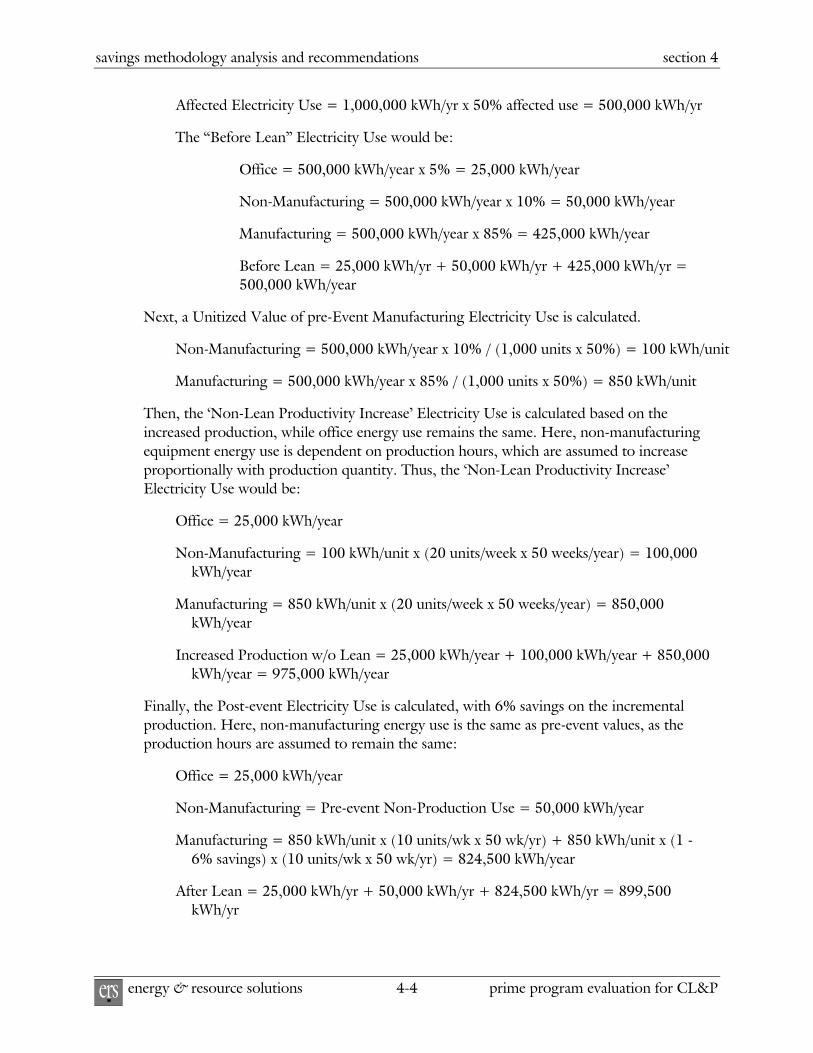
savings methodology analysis and recommendations section 4
energy & resource solutions 4-4 prime program evaluation for CL&P ers
Affected Electricity Use = 1,000,000 kWh/yr x 50% affected use = 500,000 kWh/yr
The “Before Lean” Electricity Use would be:
Office = 500,000 kWh/year x 5% = 25,000 kWh/year
Non-Manufacturing = 500,000 kWh/year x 10% = 50,000 kWh/year
Manufacturing = 500,000 kWh/year x 85% = 425,000 kWh/year
Before Lean = 25,000 kWh/yr + 50,000 kWh/yr + 425,000 kWh/yr = 500,000 kWh/year
Next, a Unitized Value of pre-Event Manufacturing Electricity Use is calculated.
Non-Manufacturing = 500,000 kWh/year x 10% / (1,000 units x 50%) = 100 kWh/unit
Manufacturing = 500,000 kWh/year x 85% / (1,000 units x 50%) = 850 kWh/unit
Then, the ‘Non-Lean Productivity Increase’ Electricity Use is calculated based on the increased production, while office energy use remains the same. Here, non-manufacturing equipment energy use is dependent on production hours, which are assumed to increase proportionally with production quantity. Thus, the ‘Non-Lean Productivity Increase’ Electricity Use would be:
Office = 25,000 kWh/year
Non-Manufacturing = 100 kWh/unit x (20 units/week x 50 weeks/year) = 100,000 kWh/year
Manufacturing = 850 kWh/unit x (20 units/week x 50 weeks/year) = 850,000 kWh/year
Increased Production w/o Lean = 25,000 kWh/year + 100,000 kWh/year + 850,000 kWh/year = 975,000 kWh/year
Finally, the Post-event Electricity Use is calculated, with 6% savings on the incremental production. Here, non-manufacturing energy use is the same as pre-event values, as the production hours are assumed to remain the same:
Office = 25,000 kWh/year
Non-Manufacturing = Pre-event Non-Production Use = 50,000 kWh/year
Manufacturing = 850 kWh/unit x (10 units/wk x 50 wk/yr) + 850 kWh/unit x (1 - 6% savings) x (10 units/wk x 50 wk/yr) = 824,500 kWh/year
After Lean = 25,000 kWh/yr + 50,000 kWh/yr + 824,500 kWh/yr = 899,500 kWh/yr

section 4 savings methodology analysis and recommendations
prime program evaluation for CL&P 4-5 energy & resource solutions ers
The Annual Electricity Savings would be:
Increased Production w/o Lean – After Lean = 975,000 kWh/yr – 899,500 kWh/yr = 75,500 kWh/yr
Lifetime Savings would be:
75,500 kWh/year x 10 years = 755,000 kWh
4.2.3 ACCURACY – COMPARISON OF CALCULATED SAVINGS FROM SITE VISITS
ERS used the “energy breakdown” method presented in Section 2 to calculate energy savings for each site. These savings are presented in detail in Appendices A through F. Table 4-1 shows a comparison of savings calculated by the NU algorithm to those calculated by ERS. It is apparent that the algorithm calculated savings differ frequently from ERS estimated savings, sometimes by large margins.
Table 4-1: NU Savings versus Calculated Savings (Excluding Site C)
Reported ERS Reported SavingsSavings from Estimated % of
Site NU Algorithm Savings Difference ERS Est. SavingsA - Event 1 20,904 2,205 18,699 948%A - Event 2 36,582 9,369 27,213 390%B 11,598 48,483 -36,884 24%C 885,620 0 885,620 NAD 1,191,124 21,787 1,169,337 5467%E 20,786 6,927 13,859 300%Average 1426%Total 1,280,994 88,771 1,192,224 1443%
NA – Note that Site C had no measurable production increase, and thus no electricity savings. Site C savings are not included in the average or total statistics.
There are a number of factors that contribute to this wide range. These factors include all of the inputs - the input total annual electricity use, the input percent affected electricity use and the production estimate – as well as the algorithm itself. As discussed in detail for each site in the appropriate appendix, the input total annual electricity is typically overestimated.
Also, in general the measured production levels did not achieve expected gains. To evaluate the accuracy of just the algorithm, we’ve recalculated savings using the NU algorithm, but with the same inputs as used in our calculations.
Table 4-2 shows the influence of just the algorithm on savings. It is apparent that if the appropriate values are input into the NU algorithm, much greater accuracy is achieved on savings calculations. Recommendations on improving the accuracy of the input values are discussed in Section 5. Nonetheless, the NU algorithm savings estimates still differ from ERS estimated savings - sometimes by large factors. On average, the NU savings algorithm with the correct input factors underestimates savings by approximately 55%.

savings methodology analysis and recommendations section 4
energy & resource solutions 4-6 prime program evaluation for CL&P ers
Table 4-2: Adjusted NU Savings versus Calculated Savings (Excluding Site C)
Adjusted ERS Reported SavingsSavings from Estimated % of
Site NU Algorithm Savings Difference ERS Est. SavingsA - Event 1 3,091 2,205 886 140%A - Event 2 9,499 9,369 130 101%B 19,710 48,483 -28,772 41%C 433,220 0 433,220 NAD 13,292 21,787 -8,495 61%E 2,095 6,927 -4,832 30%Total 47,687 88,771 -41,083 54%
NA – Note that Site C had no measurable production increase, and thus no electricity savings. Site C savings are not included in the average or total statistics.
4.2.4 ALGORITHM ASSUMPTIONS EVALUATION
Measure Life
The existing NU savings algorithm assumes a 10-year measure life. The measure life is used to convert annual savings to lifetime savings for the improvements implemented as a result of the PRIME event. The five site evaluations we conducted provided considerable evidence that the 10-year life is an overestimation of the actual period for which savings is realized. A number of important factors affect the lifetime of Lean Manufacturing improvements. Table 4-3 lists some of these factors, and provides a qualitative assessment of their impact on measure lifetime. This list is not quantitative, nor intended to be a comprehensive list, but provides a starting point with which to make judgments of an appropriate measure life.
Table 4-3: Qualitative Assessment of Factors Influencing Lean Manufacturing Measure Lifetime
Affect on Factor Measures Life Persistence
Employee Turnover Decreases Measure LifeProcedural Regression Decreases Measure Life
Market Influence on Prod. Qty Decreases Measure LifeMarket Influence on Product Type Decreases Measure Life
Business Turnover Decreases Measure LifeStrong Lean Culture Increases Measure Life
We believe Employee Turnover is a major factor in the lasting effect of implemented measures. The implemented Lean Manufacturing changes are typically not equipment changes, but procedural changes. These changes are often dependent on the employees and management involved in the Lean event. Employee turnover at manufacturing facilities is typically quite frequent. Even in our site evaluation selection process, we encountered several facilities where management involved in the PRIME event had left the company, and remaining management was unfamiliar with the project. In addition, production employees may experience even more frequent turnover, or change positions within the company.

section 4 savings methodology analysis and recommendations
prime program evaluation for CL&P 4-7 energy & resource solutions ers
While this is not always the case, when employee turnover does happen, knowledge transfer is an issue.
In addition to employee turnover, employees may also choose to return to pre-event procedures – also termed Procedural Regression. Unlike typical efficiency measures, which involve equipment replacement and are thus not easily removed, some Lean measures can be “removed” as soon as the Lean consultant leaves. That is, the ease with which a Lean measure can be discontinued suggests it is inherently more susceptible to early retirement.
In almost all of the sites we evaluated, Product Demand was an issue. While the employee turnover and procedural regression factors appeared to be potential issues in the sites we evaluated, during our visits most of the implemented Lean measures seemed to be in place and operational. Even so, production quantity of the effected lines remained the same, or even decreased. This may have been a result of the multiple ‘job shop’ type facilities we visited. Job shops manufacture many different types of products, and can regularly experience widely varying production from day to day and month to month. While outside of the company’s control, demand for production does affect electricity savings. When product demand drops, the only way electricity savings would be achieved is if plant operating hours were reduced. We found in the plants we visited, and based on our experience with industrial assessments, that this is generally not the case. As market factors could also increase production as expected, this factor is technically a “savings persistence” factor as opposed to “measure life persistence” factor. However, for simplicity we are recommending its effect be included in the measure life.
Market influence can even have a significant effect on non-“job shop” facilities and the demand for specific product types (Market Influence on Product Type). For example, at Site D, affected production decreased due to demand for a different type of product. This happens fairly regularly in industrial facilities. It is one of the drivers inherent in industrial management’s requirement for short paybacks on projects. Unlike commercial buildings, which will exist for another 10 to 30 years, manufacturers do not know if they will be making the same product, or even be in business (Business Turnover), in the next few years. Thus, changes in product type, or even in business, have a large impact on measure life.
Finally, we found that the facilities’ with existing, strong Lean Manufacturing corporate cultures seem to have integrated the PRIME measures well into their manufacturing process (Strong Lean Culture). Companies that have integrated these concepts with programs like Six Sigma or ISO certification, may have management leadership that increases the lifetime of Lean measures. However, it should be noted that companies with strong Lean cultures are those most likely to proceed with the Lean events absent NU’s incentive.
The factors presented in Table 4-3 and discussed above strongly suggest a decreased measure lifetime. We are recommending decreasing measure life from 10 to five years.
Percent Affected of Total Energy Use
As stated previously, PRIME events often do not target an entire manufacturing facility, only a portion of it - perhaps one or two production lines. The Lean consultant therefore

savings methodology analysis and recommendations section 4
energy & resource solutions 4-8 prime program evaluation for CL&P ers
breaks out the affected electricity use from the total. In every report we reviewed, percent of affected production was used. Either percent of sales, percent of units produced, percent of affected floor space or similar metrics were used as the basis to determine the percent of affected production.
Table 4-4 shows affected energy use using percent floor area and percent production as the bases respectively, to compare against the ERS estimated energy use attributed to the affected equipment determined through our site visits. The values in Table 4-4 suggest that using percent production will slightly overestimate affected energy use. However, it is more accurate than using percent floor area, which significantly underestimated affected electricity use. We do suggest using percent affected production instead of percent affected floor area where appropriate. In cases where production unit metrics are not available, percent sales is an acceptable substitution.
Table 4-4: Affected Energy Use Comparison
Total Elec. Percent Affected Energy Calculated Affected Energy Percent ofSite (kWh/year) Production (kWh/year) (kWh/year) Calculated EnergyA - Event 1 517,200 25% 129,300 110,275 117%A - Event 2 517,200 25% 129,300 109,173 118%B 13,939,200 26% 3,624,192 5,525,790 66%C 4,763,122 100% 4,763,122 4,763,122 100%D 19,215,984 55% 10,568,791 5,777,347 183%E 1,845,720 100% 1,845,720 1,849,685 100%Average 21,060,425 18,135,392 114%
Total Elec. Percent Affected Energy Calculated Affected Energy Percent ofSite (kWh/year) Floor Area (kWh/year) (kWh/year) Calculated EnergyA - Event 1 517,200 6% 28,963 110,275 26%A - Event 2 517,200 11% 58,961 109,173 54%B 13,939,200 10% 1,393,920 5,525,790 25%C 4,763,122 100% 4,763,122 4,763,122 100%D 19,215,984 20% 3,843,197 5,777,347 67%E 1,845,720 100% 1,845,720 1,849,685 100%Average 11,933,883 18,135,392 62%
Based on Percent Affected Floor Area
Based on Percent Affected Production
6% Savings on Incremental Production versus Production Gain Proportional Savings on Entire Production
The existing NU algorithm attributes savings to only the incremental production units. We believe energy savings are realized on all production units. Thus, we are recommending that a variable percent savings factor be applied to all production, to be described in Section 4.3.
Affected Energy Use Breakdown of 85% / 10% / 5%
The existing algorithm disaggregates total affected energy use into 5% office equipment, 10% non-production related manufacturing equipment and 85% production related manufacturing equipment. We believe that the percentage for these three categories should

section 4 savings methodology analysis and recommendations
prime program evaluation for CL&P 4-9 energy & resource solutions ers
be changed, as well as the labels. The percentage breakdown should be based on the five equipment categories (Type A through Type D and Office).
4.3 PROPOSED SAVINGS ALGORITHM
To be explained below, we believe adjustments to a number of the algorithm assumptions could improve the accuracy of calculated savings. The algorithm revisions are based on the theoretical approach outlined in Section 2, and on the evaluation of the existing NU algorithm presented above.
4.3.1 NEW ALGORITHM OUTLINE
Three versus Singular Algorithm
The recommended new approach has three algorithms instead of one. The three algorithms target:
Standard increased production projects (reduced downtime, changeover time, etc.)
Reduced setup time during non-production hours, and
Reduced scrap or rework.
The algorithms are based on the different ways that Lean techniques can improve productivity, as outlined in Section 2. The consultant has the ability to choose more than one of the algorithms for a given event.
Percent Affected Electricity Use
Percent affected electricity use is based on percent affected production, and when possible should be determined by units, not sales or percent floor area.
Suggested Electricity Use Breakdowns
Table 4-5 presents energy use breakdowns for the five equipment categories for each site of the five-site sample. There is a wide variation of breakdown values within this sample. Differences may exist in the breakdown values between the five-site sample and the full program population. This suggests that a more expansive study performed with a statistically robust site sample would yield more accurate breakdown values. However, absent that study, the values presented here are sufficiently indicative to adequately examine existing baseline assumptions.

savings methodology analysis and recommendations section 4
energy & resource solutions 4-10 prime program evaluation for CL&P ers
Table 4-5: Recommended Energy Breakdowns
Office Type A Type B Type C Type DSite Equipment Energy Use Energy Use Energy Use Energy UseA - Event 1 7.2% 68.7% 14.5% 13.9% 0.0%A - Event 2 7.2% 58.4% 18.8% 19.8% 0.0%B 0.1% 1.3% 53.4% 42.3% 0.0%D 0.2% 11.3% 69.4% 11.6% 4.7%E 1.7% 18.6% 15.3% 36.6% 26.5%Average 3% 28% 33% 21% 14%Suggested 5% 25% 35% 20% 15%
Office, Type A and Type B equipment, accounting for 65% of total energy use, are similar in that from the ‘Non-Lean Productivity Increase’ to post-event scenario they have no associated energy savings. Type C equipment accounts for 20% of total energy use and electricity savings are calculated the same as 'Non-manufacturing' savings were calculated in the existing NU algorithm. Finally Type D equipment accounts for 15% of total energy use. The electricity savings for Type D equipment are calculated similarly to how the 'Manufacturing' savings were calculated in the existing NU algorithm, except with a variable percentage savings factor applied to all production units.
Type D Equipment Savings Factor
We recommend that a variable savings factor, based on the percent production increase, be applied to all production units to replace the constant 6% savings factor currently applied to incremental production. The factor will also be derived from more realistic assumptions of Type D equipment percent cycle time loaded, and loaded to unloaded power ratio. The following steps present our approach to calculating a variable savings factor. First, we assessed measured power or amperage data from the PRIME sites we examined, post-event. Additionally, we assessed data from manufacturing facilities we've visited over the past year. Again, while not a statistically significant data set, this data is helpful to use as a basis to determine an approximation of the loaded to unloaded ratio and percent time loaded for Type D equipment. The loaded-to-unloaded ratio and percent time loaded values could be further refined from an in-depth study of Type D equipment. Table 4-6 shows the equipment type, measured loaded and unloaded power or amps, and the percent of time the equipment was loaded.
Table 4-6: Type D Loaded/Unloaded Power Ratio and Percent Loaded
Average Average Loaded toEquipment Loaded Unloaded Unloaded Percent
Site Type Power or Amp Power or Amp Ratio LoadedD Chiller 24.5 16.3 1.50 85.6%A Plastic Extruder 25.6 11.6 2.20 64.2%A Plastic Extruder 24.4 6.7 3.66 82.9%Average 2.46 77.6%Client 1 Rubber Compression Press 2.6 1.2 2.06 38.5%Client 2 Metal CNC 5.5 2.89 1.89 44.6%Client 2 Metal CNC 32.3 3.51 9.21 51.5%Client 3 Rubber Compression Press 222.7 89.10 2.50 31.4%Client 3 Rubber Compression Press 36.2 11.79 3.07 86.6%Average 3.7 50.5%

section 4 savings methodology analysis and recommendations
prime program evaluation for CL&P 4-11 energy & resource solutions ers
Based on these measured data, we can approximate that typical Type D equipment will have a Loaded/Unloaded power ratio of 3, and will be loaded 50% of the time. Again, these values are not derived from statistically significant data sets, and could be refined with further study. However, the represent a marked improvement from the existing NU assumption, which is based on no data. Given values for electricity use and operating hours, the percent savings can be calculated for any given percent production increase. For example, if Type D annual electricity use is 25,000 kWh at 4,000 operating hours, then Loaded and Unloaded times are each 2,000 hours/year. Additionally, Loaded and Unloaded power draw can be calculated by rearranging the following equation:
Type D annual electricity use = (Loaded Power x Annual Hours x Percent Loaded) + (Unloaded Power x Annual Hours x Percent Unloaded) (4-1)
As Unloaded Power is equivalent to the Loaded Power divided by the power ratio, we can substitute and solve for Loaded Power:
Loaded Power (kW) = 25,000 kWh/yr/4,000 hours/yr / (50% Loaded+ (1 – 50% Loaded)/3) = 9.38 kW
Given a 10% production increase, ‘Non-Lean Productivity Increase’ energy use would be:
(9.38 kW x 2,200 hours/year) + (9.38 kW/3 x 2,200 hours/year) = 27,515 kWh/year
In the post-event scenario, total operating hours would remain the same and unloaded time would decrease to 1,800 hours. Thus, total annual energy use would be:
(9.38 kW x 2,200 hours/year) + (9.38 kW/3 x 1,800 hours/year) = 26,264 kWh/year
Savings and savings percent would be:
(27,515 – 26,264) kWh/year = 1,251 kWh/year
1,251 kWh/year / 27,515 kWh/year = 4.5% savings
As the values for annual Type D electricity use or production hours are changed, the energy savings will change, although the percent savings will remain the same. That is, the only factors that affect percent savings are percent production increase, and the Loaded/Unloaded Power Ratio and Percent Time Loaded assumptions. Given our assumptions based on measured data, a curve can be constructed to provide percent savings as a function of percent production increase. The data points, curve and equation of the curve are listed in Figure 4-1. If further study was conducted to determine statistically robust values of Loaded/Unloaded Power Ratio and Percent Time Loaded assumptions, the data points, curve and equation presented in Figure 4-1 would change. Nonetheless, this equation provides an informed basis with which to base the variable percent savings factor.

savings methodology analysis and recommendations section 4
energy & resource solutions 4-12 prime program evaluation for CL&P ers
Figure 4-1: Percent Savings versus Percent Production Increase Curve
y = 0.1168x3 - 0.3402x2 + 0.4732x + 0.0011
0%
5%
10%
15%
20%
25%
30%
0% 10% 20% 30% 40% 50% 60% 70% 80% 90% 100%
% Production Increase
% S
avin
gs
Demand Savings & Plant Operating Hours
We are recommending that plant-operating hours be obtained and documented within the savings algorithm. With this information, the algorithm can determine if the plant has excess production hour capacity. Excess production quantity will typically be met with increased production hours. If so, there are no demand savings, as the ‘Non-Lean Productivity Increase’ demand is the same as the pre-event demand. If that option does not exist, then the ‘Non-Lean Productivity Increase’ scenario assumes that production equipment would be added, and demand would increase proportionally. Thus, given production hours, the algorithm can automatically determine whether electrical demand savings can be claimed. For example, if a plant were operating 24 hours per day, 7 days per week, and 52 weeks per year, demand savings could be claimed for the project. To calculated demand savings, demand in the Pre-Event, ‘Non-Lean Productivity Increase’ and Post-Event scenarios can be calculated by dividing the annual electricity use by the annual operating hours.
NEBS The site evaluation reports show there are sometimes non-electric benefits (NEBs), such as natural gas, water or labor savings, resulting from the PRIME events. However, we typically did not find material or energy NEBs in most of our evaluations. Additionally, most material and energy NEBs are so unique to the process, their quantification defies broad
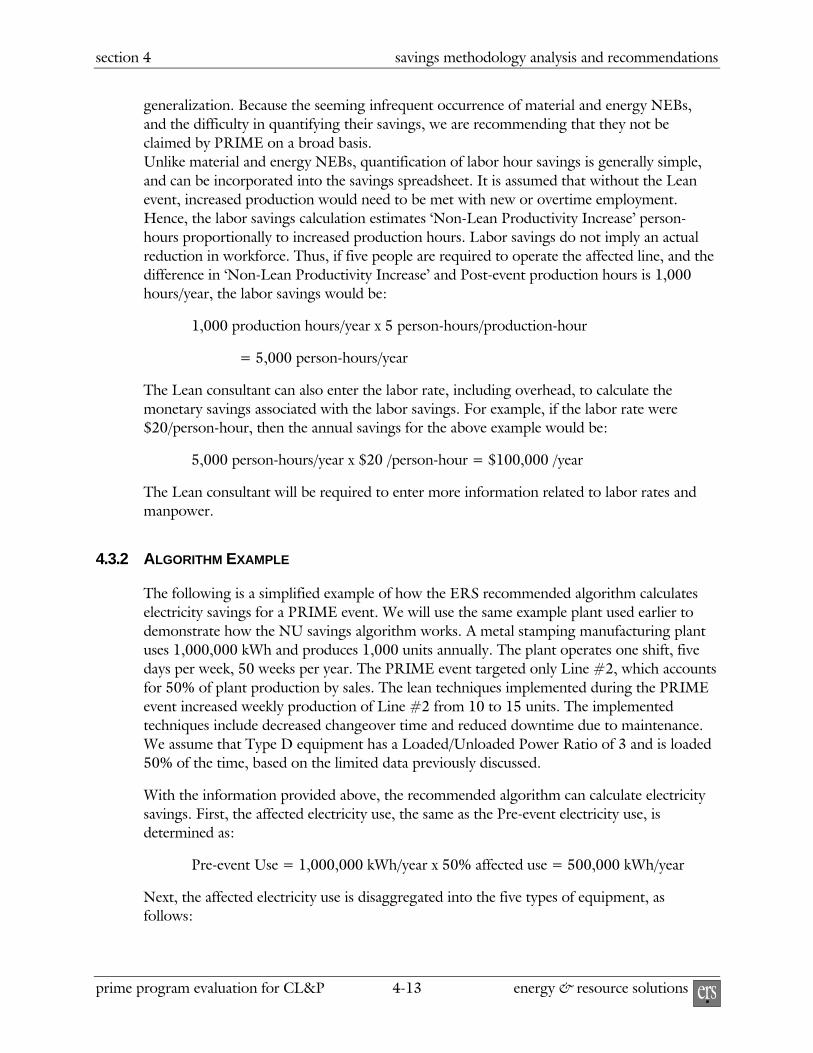
section 4 savings methodology analysis and recommendations
prime program evaluation for CL&P 4-13 energy & resource solutions ers
generalization. Because the seeming infrequent occurrence of material and energy NEBs, and the difficulty in quantifying their savings, we are recommending that they not be claimed by PRIME on a broad basis. Unlike material and energy NEBs, quantification of labor hour savings is generally simple, and can be incorporated into the savings spreadsheet. It is assumed that without the Lean event, increased production would need to be met with new or overtime employment. Hence, the labor savings calculation estimates ‘Non-Lean Productivity Increase’ person-hours proportionally to increased production hours. Labor savings do not imply an actual reduction in workforce. Thus, if five people are required to operate the affected line, and the difference in ‘Non-Lean Productivity Increase’ and Post-event production hours is 1,000 hours/year, the labor savings would be:
1,000 production hours/year x 5 person-hours/production-hour
= 5,000 person-hours/year
The Lean consultant can also enter the labor rate, including overhead, to calculate the monetary savings associated with the labor savings. For example, if the labor rate were $20/person-hour, then the annual savings for the above example would be:
5,000 person-hours/year x $20 /person-hour = $100,000 /year
The Lean consultant will be required to enter more information related to labor rates and manpower.
4.3.2 ALGORITHM EXAMPLE
The following is a simplified example of how the ERS recommended algorithm calculates electricity savings for a PRIME event. We will use the same example plant used earlier to demonstrate how the NU savings algorithm works. A metal stamping manufacturing plant uses 1,000,000 kWh and produces 1,000 units annually. The plant operates one shift, five days per week, 50 weeks per year. The PRIME event targeted only Line #2, which accounts for 50% of plant production by sales. The lean techniques implemented during the PRIME event increased weekly production of Line #2 from 10 to 15 units. The implemented techniques include decreased changeover time and reduced downtime due to maintenance. We assume that Type D equipment has a Loaded/Unloaded Power Ratio of 3 and is loaded 50% of the time, based on the limited data previously discussed.
With the information provided above, the recommended algorithm can calculate electricity savings. First, the affected electricity use, the same as the Pre-event electricity use, is determined as:
Pre-event Use = 1,000,000 kWh/year x 50% affected use = 500,000 kWh/year
Next, the affected electricity use is disaggregated into the five types of equipment, as follows:

savings methodology analysis and recommendations section 4
energy & resource solutions 4-14 prime program evaluation for CL&P ers
Pre-event Office Use = (500,000 kWh/yr x 5%) = 25,000 kWh/yr
Pre-event Type A = (500,000 kWh/yr x 25%) = 125,000 kWh/yr
Pre-event Type B = (500,000 kWh/yr x 35%) = 175,000 kWh/yr
Pre-event Type C = (500,000 kWh/yr x 20%) = 100,000 kWh/yr
Pre-event Type D = (500,000 kWh/yr x 15%) = 75,000 kWh/yr
Next, we can calculate electricity savings for the each equipment category. As Office, Type A and Type B equipment have no savings from the ‘Non-Lean Productivity Increase’ to post-event scenario, we will group these components together. However, Type B equipment energy use increases proportionally with production increases. Thus, electricity increases from the pre-event to ‘Non-Lean Productivity Increase’ scenario, but remains the same from ‘Non-Lean Productivity Increase’ to post-event. For this example, pre-event, ‘Non-Lean Productivity Increase’ and post-event electricity use, and savings would be approximately:
Office, Type A and Type B
Use = Office + Type A + Type B
Pre-event Use = 25,000 kWh/yr + 125,000 kWh/yr + 175,000 kWh/yr = 325,000 kWh/yr
‘Non-Lean Productivity Increase’ Use = 25,000 kWh/yr + 125,000 kWh/yr + 175,000 kWh/yr x 15 units/10 units = 412,500 kWh/yr
Post-event Use = 25,000 kWh/yr + 125,000 kWh/yr + 175,000 kWh/yr x 15 units/10 units = 412,500 kWh/yr
Electricity Savings = 412,500 kWh/yr - 412,500 kWh/yr = 0 kWh/yr
Type C equipment is dependent on operating hours. Thus, the post-event and pre-event operating hours are identical, while the ‘Non-Lean Productivity Increase’ operating hours increase proportionally with production. Thus, the ‘Non-Lean Productivity Increase’ operating hours, electricity use in each scenario and energy savings would be approximately:
Type C
Pre-event Operating Hours = (8 hrs/dy x 5 dys/wk x 50 wks/yr) = 2,000 hrs/yr
‘Non-Lean Productivity Increase’ Operating Hours = 2,000 hrs/yr x 15 units/10 units = 3,000 hrs/yr
Post-event Operating Hours = Pre-event Operating Hours
Pre-event Use = 100,000 kWh/yr
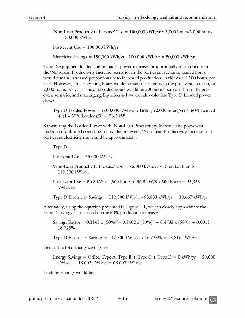
section 4 savings methodology analysis and recommendations
prime program evaluation for CL&P 4-15 energy & resource solutions ers
‘Non-Lean Productivity Increase’ Use = 100,000 kWh/yr x 3,000 hours/2,000 hours = 150,000 kWh/yr
Post-event Use = 100,000 kWh/yr
Electricity Savings = 150,000 kWh/yr - 100,000 kWh/yr = 50,000 kWh/yr
Type D equipment loaded and unloaded power increases proportionally to production in the ‘Non-Lean Productivity Increase’ scenario. In the post-event scenario, loaded hours would remain increased proportionally to increased production, in this case 1,500 hours per year. However, total operating hours would remain the same as in the pre-event scenario, or 2,000 hours per year. Thus, unloaded hours would be 500 hours per year. From the pre-event scenario, and rearranging Equation 4-1 we can also calculate Type D Loaded power draw:
Type D Loaded Power = (500,000 kWh/yr x 15%) / (2,000 hours/yr) / (50% Loaded + (1 – 50% Loaded)/3) = 56.3 kW
Substituting the Loaded Power with ‘Non-Lean Productivity Increase’ and post-event loaded and unloaded operating hours, the pre-event, ‘Non-Lean Productivity Increase’ and post-event electricity use would be approximately:
Type D
Pre-event Use = 75,000 kWh/yr
‘Non-Lean Productivity Increase’ Use = 75,000 kWh/yr x 15 units/10 units = 112,500 kWh/yr
Post-event Use = 56.3 kW x 1,500 hours + 56.3 kW/3 x 500 hours = 93,833 kWh/year
Type D Electricity Savings = 112,500 kWh/yr - 93,833 kWh/yr = 18,667 kWh/yr
Alternately, using the equation presented in Figure 4-1, we can closely approximate the Type D savings factor based on the 50% production increase:
Savings Factor = 0.1168 x (50%)3 – 0.3402 x (50%)2 + 0.4732 x (50%) + 0.0011 = 16.725%
Type D Electricity Savings = 112,500 kWh/yr x 16.725% = 18,816 kWh/yr
Hence, the total energy savings are:
Energy Savings = Office, Type A, Type B + Type C + Type D = 0 kWh/yr + 50,000 kWh/yr + 18,667 kWh/yr = 68,667 kWh/yr
Lifetime Savings would be:

savings methodology analysis and recommendations section 4
energy & resource solutions 4-16 prime program evaluation for CL&P ers
68,667 kWh/year x 5 years = 343,335 kWh
4.3.3 PROPOSED ALGORITHM ACCURACY
We calculated savings for each of the evaluated sites using a spreadsheet tool based on our recommended savings algorithm. Table 4-6 compares these savings to the savings calculated in each of the site reports. The savings presented here are on average more accurate than those calculated with the existing NU algorithm, as shown above in Table 4-2. Savings from the recommended algorithm are 89% of ERS estimated, opposed to the 54% of ERS estimated value calculated by the existing algorithm. While the data sample presented here is certainly not statistically robust, we believe that the recommended savings algorithm will in general provide more accurate results than the existing algorithm.
Table 4-6: Recommended Algorithm Savings versus ERS estimated Savings
Savings from ERS Reported SavingsRecommended Estimated % of
Site Algorithm Savings Difference ERS Est. SavingsA - Event 1 5,125 2,205 2,920 232%A - Event 2 15,727 9,369 6,358 168%B 32,632 48,483 -15,850 67%C 0 0 0 NAD 22,006 21,787 219 101%E 3,468 6,927 -3,458 50%Average 124%Total 78,959 88,771 -9,811 89%
NA – Note that Site C had no measurable production increase, and thus no electricity savings. Site C savings are not included in the average or total statistics.
4.4 DISCUSSION OF INTERMEDIATE PRODUCTION INCREASE ESTIMATES
Due to the consistent and very large differences between maximum production capacity newly available and capacity actually utilized after productivity improvements are complete, the evaluation team suggests that facility employees be asked before the PRIME event what a realistic estimate would be for increased production post-event. Experience from this evaluation indicates that the employee estimate will still be higher than the actual post-event production, but asking for an estimate reduces the gap between estimated and actual production gains. The evaluation team feels, and ERS agrees, that an employee estimate of likely production increase will produce a more accurate ex ante estimate. The evaluation team members also agree that actual data provide the best, and only, measurement of post hoc production increases.
4.5 SPREADSHEET TOOL
While outside the scope of work for the PRIME Program evaluation, ERS developed a spreadsheet to assess and work through our revised savings approaches and to verify specific

section 4 savings methodology analysis and recommendations
prime program evaluation for CL&P 4-17 energy & resource solutions ers
project calculations. Figure 4-1 shows an overview of the summary sheet and multiple tabs for the various analysis categories. Figure 4-2 shows the required and optional input boxes. Figure 4-3 shows the Pre-event, ‘Non-Lean Productivity Increase’ and Post-event energy use calculations. Finally, Figure 4-4 presents the output display.
This spreadsheet can be further enhanced so that is suitable for direct use by NU and its Lean consultants. If it is of interest to NU, we are prepared to share such an enhanced tool with NU at no cost, providing that it is only used by NU for the NU PRIME Program and for other internal use by NU.
Figure 4-1: Spreadsheet Tabs

savings methodology analysis and recommendations section 4
energy & resource solutions 4-18 prime program evaluation for CL&P ers
Figure 4-2: Required and Optional Input Boxes
Customer: ACME Corp.Address: 1 Main StreetCity/State/Zip: Springfield, MANU Account #: ######Project Projected Start Date (month/year): 2/10/2006Project Projected Finish Date (month/year): 2/13/2006In-Service Projected Date of Changes (month/year): 3/5/2006Lean Project Number: W E-######Project Cost $6,000
Total Annual Electricity Use (kW h): 1,000,000Average Annual Electric Demand (kW ): 500Annual Pre Event Production: 1,000Percent Affected Production: 50%Production Hours/Day: 8Production Days/W eek: 5Production W eeks/Year: 50
Reduced Changeover Time: YChangeovers/Day: 2Annual Changeovers: 500Pre-Event Changeover Time (minutes): 40Post-Event Changeover Time (minutes): 20Reduced DownTime: NPre-Event Downtime (hrs/week) 8Post-Event Downtime (hrs/week) 6Reduced Setup Time (During Production Hours): NPre-Event Setup Time (hrs/week) 4Post-Event Setup Time (hrs/week) 2Reduced Cycle Time: NPre-Event Cycle Time (minutes/unit) 3Post-Event Cycle Time (minutes/unit) 2Throughput Increase: NPre-Event Throughput (units/hour) 2Post-Event Throughput (units/hour) 3Generic Production Increase: YPre-Event Production (units/week) 10Post-Event Production (units/week) 20Rework/Scrap Reduction: NPre-Event Scrap/Rework Rate (%) 20%Post-Event Scrap/Rework Rate (%) 10%Reduced Setup Time (Non Production Hours): NPre-Event Setup Time (hrs/week) 4Post-Event Setup Time (hrs/week) 2
Person-hours per Production-hour: 1Labor Rate: $20
Projected Energy Savings from Lean Manufacturing Projects
Required
Optional
Required: Project Specific
Project Description Inputs
Calculation Inputs

section 4 savings methodology analysis and recommendations
prime program evaluation for CL&P 4-19 energy & resource solutions ers
Figure 4-3: Energy Use Calculation
Calculations
EXISTING NON-LEAN Post-EventOffice 25,000 25,000 25,000Independent Manufacturing
Equipment 150,000 150,000 150,000Production QTY Dependent
Manufacturing Equipment 175,000 350,000 350,000Plant Production HOURS Dependent
Manufacturing Equipment 100,000 200,000 100,000Prod. QTY & HOURS Dependent
Manufacturing Equipment 50,000 100,000 66,667Total 500,000 825,000 691,667
Annual Electricity Use (kWh)
Figure 4-4: Output Display
Projected Energy Savings from Lean Manufacturing Projects
Customer: ACME Corp.
Project Component (kWh) (kW) (labor hours) (kWh) (kW-months) (labor hours)Generic Increased Production 20,833 0 333 52,083 0 833Reduced Changeover Time 0 0 0 0 0 0Reduced Downtime 0 0 0 0 0 0Reduced Setup Time (During Production) 0 0 0 0 0 0Reduced Cycle Time 0 0 0 0 0 0Throughput Increase 0 0 0 0 0 0Rework/Scrap Reduction 0 0 0 0 0 0Reduced Setup (Non-Production Hours) 0 0 0 0 0 0Total 20,833 0 333 52,083 0 833
Lifetime SavingsAnnual Savings
4.6 SUMMARY
In closing, Section 4 has presented the findings of our review and evaluation of the existing NU savings algorithm. There are several recommended changes that we have put forth in efforts to enhance the accuracy and defensibility of the algorithm, as follows:
Decrease the measure life from 10 to five years.
Integrate demand savings calculations into the algorithm and claim demand savings where appropriate.
Use three savings algorithms for general production increase, material reduction, and setup time reduction during non-production hours.
Revise electricity breakdown based on the five equipment categories. Five percent will be increased to 65%, 10% increased to 20% and 85% decreased to 15%.
Disregard the 6% incremental savings factor in favor of a production proportional approach.
Provide an option to calculate labor savings within the savings spreadsheet.

savings methodology analysis and recommendations section 4
energy & resource solutions 4-20 prime program evaluation for CL&P ers
Percent affected electricity use should be based on percent production in units, as opposed to percent sales or floor area.
In addition, a new savings spreadsheet with multiple algorithms was recommended, and a draft of such a spreadsheet tool was described. As previously discussed, an enhanced version of the savings spreadsheet can be developed and provided to NU at no cost for internal use and for use in the PRIME Program.

evaluation findings and recommendations 5
prime program evaluation for CL&P 5-1 energy & resource solutions ers
5. EVALUATION FINDINGS AND RECOMMENDATIONS
5.1 INTRODUCTION
The preceding sections of this report presented findings and recommendations from the project documentation review, site visit and savings algorithm evaluations. This section summarizes these findings and conclusions and in addition puts forth recommendations for the PRIME program not yet discussed.
5.2 PROJECT DOCUMENTATION FINDINGS AND RECOMMENDATIONS
5.2.1 NAICS/SIC CODES
Various types of industries are addressed through the PRIME program, however projects are concentrated in Fabricated Metal Product Manufacturing plants. The standard categorization of manufacturing facilities is with the North American Industrial Classification System (NAICS). Currently, these codes are not tracked. We recommend that future documentation include NAICS codes. Often the plant manager or accountant will already know the NAICS code, and if not, they are relatively easy to determine.
5.2.2 LEAN TECHNIQUES
A variety of Lean techniques were implemented, with correspondingly varied productivity improvements. The most often used Lean techniques were 5S, visuals/standardized work and quick changeover, with the most common improvements being reduced changeover, reduced cycle times and reduced inventory.
5.2.3 SAVINGS ALGORITHM INPUT ASSESSMENT
We examined the BCR and claimed savings calculation inputs, and found in many cases that the input estimations were either incorrect or poorly justified. Often, the annual electricity use that was entered did not match calculated values. In addition, the percent of affected product/sales estimate was not justified with calculations, nor were the production rates. Justification of the percent affected number and the production rates would lend confidence to the production gains. Typically details on the time span considered with the production rates were not considered, opening the possibility for consideration of non-typical

evaluation findings and recommendations section 5
energy & resource solutions 5-2 prime program evaluation for CL&P ers
production rates. The time span from which the production rates were sampled should be documented.
5.2.4 TRACKING SYSTEM
The claimed savings entered into the NU tracking system was mostly consistent with the savings documented in the project files. However, we found discrepancies due to several reasons. First, a number of the projects appear to have had their claimed savings estimates updated in later years, but this was not documented in the project files. We believe that all changes should be documented in the project file as a matter of good practice. Second, some of the project numbers were not documented in the tracking system. In addition, some of the savings estimates were entered into the tracking database correctly, however it appears that the savings were calculated incorrectly prior to entering the data.
5.2.5 PROJECT DOCUMENTATION
Based on our review, we think that project file documentation could be improved. We recommend the following changes to project documentation efforts:
WMECO and CL&P
Provide project specific detailed descriptions that provide the reader with an adequate description of what happened. (For example, “The original Value Stream Map pointed to changeover times as a bottleneck. The quick changeover project involved implementing 5S, visuals and a point-of-use system. The POU system involved locating wrenches on a shadow board near Presses #1 through #7.”)
Note that much of this information is available in the consultant’s reports. Currently, we found that WMECO typically includes these reports with project documentation while CL&P does not.
Precede the project file with a documentation content sheet or table of contents.
Identify team member positions within the company.
CL&P
Identify which of the team members are the Lean Leader, Lean Champion and Lean Coach.
Document facility NAICS code.
Better document detailed supporting information for productivity improvements. For example, if changeover time is reduced, document pre and post-event changeover times, how often changeovers occur, hours of production and rate of production for the affected line. This would enable the productivity improvement to be recalculated and easily verified at a later time.

section 5 evaluation findings and recommendations
prime program evaluation for CL&P 5-3 energy & resource solutions ers
Document other relevant project information such as billing history, invoices and agreements, and project presentations.
Better justify the percentage of affected product, with numbers when available. For example, “25%” should be justified with 250 widgets/month of a plant-wide 1000 widgets/month, or similar.
5.3 ALGORITHM AND SAVINGS FINDINGS AND RECOMMENDATIONS
As a result of the steps taken in this evaluation, we have identified several ways to improve upon the existing approach used for savings calculations. Currently, the PRIME program employs the use of a single algorithm for all applications, and although this approach is simple to implement, may not be as accurate as desired. We found that the existing algorithm typically calculated savings values that were considerably lower when compared to ERS estimated results, both on an annual basis and on a lifetime basis. (Reported savings were considerably higher due to incorrect algorithm inputs). We also believe that the algorithm does not approach the calculation of energy savings due to production increases in the most appropriate manner. Therefore, we are recommending several fundamental changes to the savings algorithm as follows:
Decrease the measure life from 10 to five years. The measure life is a very influential factor in calculating lifetime savings. We feel that the 10-year measure life is contributing to an overestimation of realized lifetime savings due to the PRIME events.
Integrate demand savings calculation into the algorithm and claim demand savings where appropriate. As discussed in Section 2, we believe that in some cases demand savings may be achieved with productivity improvements.
Revise electricity breakdown from 5%/10%/85% to 65%/20%/15% based on five equipment categories.
Use three savings algorithms for general production increase, material reduction, and setup time reduction during non-production hours.
Disregard the constant 6% savings factor applied to incremental use in favor of a variable factor applied to all use. This variable factor will be based on assumptions of Type D equipment loading characteristics.
Provide an option to calculate labor savings within the savings spreadsheet. Note that labor savings are based on reduce need for new or overtime employment, and typically do not affect the existing workforce.

evaluation findings and recommendations section 5
energy & resource solutions 5-4 prime program evaluation for CL&P ers
Hedge preliminary production increase estimates with site personnel estimates. Event estimates of production gains are often high, in the range of 10% to 30%. We found that realized production gains are typically much lower, under 5%. The evaluation team suggested that the facility employees should be asked before the PRIME event what they thought a realistic production increase would be. ERS agrees that this question would be helpful, in the sense that production increase estimates can be tempered. However, we do recommend that final savings should be based on production increased as derived from actual data.
We believe that these changes will greatly increase the accuracy of the PRIME program savings estimates and provide a transparent and defensible foundation for the algorithm.
5.4 PROGRAM FINDINGS AND RECOMMENDATIONS
In addition to the findings and recommendations presented above, evaluation of the five specific sites visited, in conjunction with our other research, yielded several other suggestions for greater accuracy and success of the PRIME program.
We found that none of the PRIME projects evaluated had a positive benefit-to-cost ratio. The following bullet points include recommendations to the savings algorithm as well as to the PRIME program. The program recommendations are aimed at improving the benefit-to-cost ratio of the PRIME projects.
Verify annual electricity use with facility employees before calculating savings. We found that one of the major factors that contributed to inaccuracies in calculating savings was due to the overestimation of annual facility electricity use. The value for the total annual facility electricity use is calculated from billing records provided by NU. We found multiple errors were made in the process of developing the facility usage, including: using 13 months of history instead of 12 months; using only 1 account instead of 2 (where appropriate); accidentally summing electrical demand instead of energy use; using accounts for the same company, but for multiple facilities; and counting 1 meter instead of 2 (where appropriate). Due to the frequent miscalculation of this important value, we recommend that the Lean consultant obtain annual electrical energy (kWh) and demand (kW) from the site employees during the PRIME event to verify annual electricity usage.
Calculate electricity savings using confirmed production gains obtained at least three months after the PRIME event. Currently, electricity savings are calculated based on expected production gains calculated at the same time as the PRIME event. The calculated productivity improvement reflects expected production gains, as opposed to actual gains. These calculations often rely on assumptions and ballpark figures determined with the aid of plant employees. Actual

section 5 evaluation findings and recommendations
prime program evaluation for CL&P 5-5 energy & resource solutions ers
production improvements may differ from these expected values significantly. For example, often not all the Lean techniques recommended are actually implemented. Currently, the Lean consultant contacts the facility for a three-month follow up. We believe that estimating productivity improvement at this point would yield a much more accurate value. As always, obtaining production data would be the most accurate way to calculate productivity increases.
Target companies with a stable and/or increasing product demand. As discussed in the site reports, and in Section 4, market influences on production often negatively influence the gains from the PRIME sponsored Lean events. We found in many of our site evaluations that production gains were lower than expected, which was almost always due to market factors. Thus, while productivity improved, production did not always increase. From an evaluation perspective, it does not help the results when no evidence of a production increase is discernable when upwards of 25% increases have been claimed.
Many of the plants most influenced by market factors are “job shop” type facilities. Job shops produce a large variety of products, and production requirements typically change from day to day. In these cases, production quantity is very much dependent on the market. Alternately, manufacturing facilities that only produce a few products are more likely to be insulated from market factors. In these facilities, production quantity is more likely limited by bottlenecks and downtime.
Thus, we recommend targeting facilities with stable or increasing product demand as a first priority. While job shops should not be entirely excluded, other facilities will likely yield more consistent and measurable production increases.
Promote productivity improvement types that result in energy savings. Through the evaluation process we identified a number of projects whose effect on plant production levels and manufacturing equipment was uncertain. For example, we encountered one event that was focused on streamlining paperwork in the facilities front office. This event was targeted at decreasing product lead-time and inventory, a valuable benefit to the company. However, in general, events targeted to reduce inventory will have little to no affect on the facilities’ electricity use.
Thus, we recommend that PRIME sponsored events utilize Lean techniques that affect electricity use, such as reducing changeover time, reducing downtime, reducing setup time, decreasing cycle time, increasing throughput, and reducing rework/scrap. Projects geared towards inventory reduction should be prioritized lower. Finally, while 5S projects are often beneficial, they must be associated with manufacturing equipment to impact energy use. 5S events targeting warehousing or similar areas will probably not yield electricity savings.

evaluation findings and recommendations section 5
energy & resource solutions 5-6 prime program evaluation for CL&P ers
Promote 5S, TPM, Visuals and Standardized Work projects that increase the operating efficiency of equipment. As stated, the primary purpose of the PRIME program is to decrease energy intensity of a manufacturing process by increasing production while using the same or slightly less electricity. However, many of the Lean techniques implemented during these events may also increase the operating efficiency of the manufacturing equipment. That is, while Lean events will not change the equipment efficiency, they can improve how the equipment is operated, often resulting in a direct decrease in electricity requirements. These low-cost/no-cost improvements typically rely on the integration of best practices into the company culture. This is exactly what TPM, Visuals and Standardized Work are geared towards. In addition, 5S projects often improve equipment condition, resulting in increased operating efficiency. For example, a Lean event at one of the sites we evaluated created Standardized Work for the cleaning of rectifier electrodes. The cleaning of these electrodes resulted in a direct efficiency improvement of the rectifier and anodizing equipment. Note that identification of these types of improvements, and education of how to operate equipment energy efficiently, probably would require some engineering energy efficiency expertise in addition to Lean Manufacturing expertise.

appendix a A
prime program evaluation for CL&P energy&resource solutions
A INTRODUCTION
SITE A, EVENT 1
FOR
PRIME PROGRAM EVALUATION


site reports – site A, event 1 A
prime program evaluation for CL&P A-1 energy & resource solutions ers
A. SITE A SITE REPORT, EVENT 1
A.1 INTRODUCTION
This document presents the evaluation and findings of an NU sponsored PRIME event. For confidentiality purposes, this site will be referred to as Site A, and no external photos of the facility are shown. Mr. Seryak of ERS evaluated the event during a site visit from Tuesday, September 13th through Friday, September 16th, 2005. The event targeted a chromic anodizing line in the facility, and the event team members consisted of this line’s operators.
ERS’ calculated energy savings differed quite significantly from those calculated by the existing NU algorithm, as shown in Table A-1. The reported savings using the NU spreadsheet and the consultant calculated productivity gains were 20,904 kWh/year. Based on observations and data collected from the site, ERS has calculated energy savings to be only 2,205 kWh/year, which is significantly lower (nearly a factor of 10 times). As discussed prior with Mr. Taylor and Mr. Bebrin of NU, the large discrepancy was due to differences in the input values for the spreadsheet: total annual electricity use (kWh), percent affected production and productivity improvement. ERS’ values for percent affected production were the same as the consultants, and productivity improvement was close. The main influence was the difference in annual electricity use. ERS calculated annual electricity use at 517,200 kWh/year while NU used 2,215,000 kWh/year, which was an overestimation. As shown in Table A-1, using the correct inputs, the NU algorithm’s estimated savings is much closer to ERS estimated savings. Table A-1 also shows estimated savings from the recommended algorithm.
Table A-1: NU and ERS Calculated Energy Savings
Savings(kWh/year)
NU Reported Savings 20,904Adjusted NU Savings 3,091New Algorithm Savings 5,467ERS Est. Savings 2,205
Table A-2 presents the pre-event, ‘Non-Lean Productivity Increase’ and post-event energy intensity, the production gain and the savings calculated based on energy intensity.

appendix A site reports
prime program evaluation for CL&P A-2 energy & resource solutions ers
Table A-2: Energy Intensity for each Scenario
ScenarioEnergy
IntensityPre-event 55.93 kW h/runNon-Lean 50.38 kW h/runPost-event 49.43 kW h/runProduction 2,284 runs/yrElectricity Savings 2,205 kWh/yr
A.2 SITE INFORMATION
Site A is a 60,000 ft2 metal anodizing facility of old brick construction with a corrugated metal roof. The facility uses approximately 517,200 kWh of electricity annually, with an average demand of 218 kW.
The facility has multiple anodizing lines, although production is mainly in the A, B and C lines. The facility has significant non-electric energy and material uses. For example, natural gas boilers provide steam to heat the dip tanks. Water and anodizing chemicals are also used in the anodizing process. Multiple employees operate each line. Thus, the potential for non-electric benefits (NEBs) is significant. The plant operates five days per week, 10 hours each day, from 5 AM to 3 PM. Typically, seven of the 10 hours are used for production. The remaining three hours are allotted for set-up and shutdown.
A.3 LEAN EVENT AFFECTED PROCESS & EQUIPMENT DESCRIPTION
The Lean event targeted the “C-line”, which is a chromic anodizing line. Four employees operate the C-Line. The chromic anodizing process involves washing, caustic etching, deoxidizing, chromic anodizing, nickel or hot-water sealing and other processes as detailed in the flow chart in Figure A-1.

appendix A site reports
prime program evaluation for CL&P A-3 energy & resource solutions ers
Figure A-1: C-Line Process Flow
Recieving
Part Racking
Soap Wash(5 min, 130 F)
Rinse(1 min)
Deox(3 min)
Chromic Anodizing(40 min, 90 F)
Rinse(1 min)
Dry Part in Hotbox
Unrack
Inspection & Count
QA
Repack
Shipping
Rinse(1 min)
Nickel or HW Seal
The major electricity using equipment in the C-line includes the dedicated and general exhaust fans, the DC rectifiers, the air compressor and the lights. As Figure A-2 shows, the dedicated tank exhaust fan is the largest use of electricity in the C-Line, mainly due to runtime hours. The energy use calculations for this site and all other sites evaluated are presented in Appendix G. The manufacturing equipment can be grouped into three of the equipment categories described in Section 2. The dedicated and general area exhaust fans all operate 24 hours per day, seven days per week, and are thus operating independent of production hours or production quantity. The lights and air compressor energy use is dependent on production hours. Finally, the rectifier energy use is dependent on production quantity. Office equipment would be unaffected. Photo A-1 shows the C-Line dip tanks and processing area.

appendix A site reports
prime program evaluation for CL&P A-4 energy & resource solutions ers
Figure A-2: C-Line Electricity Use Breakdown
Lights5% Air
Compressor9%
Recitifier15%
General Exhaust
34%
Dedicated Exhaust
37%
Photo A-1: C-Line
A.4 PROJECT DETAILS & PRODUCTIVITY IMPROVEMENT
A primary objective of any Lean event is to improve productivity. In this case, the objective was to reduce the average changeover time by 50%, with the existing average changeover

appendix A site reports
prime program evaluation for CL&P A-5 energy & resource solutions ers
time being 27 minutes. According to the Lean consultant, the changeover time was reduced to an average of 8 minutes, a 70% improvement. This would increase the average number of tank runs from eight to ten runs per day, a 25% productivity improvement.
The consultant’s data source of two “test” days was deemed too small to sufficiently quantify production increases. Thus, ERS sought a larger sample of productivity data that would give greater confidence to the calculated results. ERS obtained over two weeks of pre and post-Lean event production data. With this data, ERS quantified a productivity gain of 16%, with a statistically tested confidence of 99%. ERS was satisfied with the productivity metric, metric calculations and qualitative description of the productivity improvement presented in the project file.
Productivity Metric – The number of runs per day was used as the productivity metric, with a claim of an increase from eight to ten runs per day. On other production lines (and as discussed in the evaluation of another event at Site A, detailed in Appendix F), the time per run can vary, rendering ‘runs/day’ an inadequate metric. However, on the C-Line every run is 40 minutes. In addition, examining production records reveals that amperage levels (an indicator of tank capacity) are relatively constant. For the C-Line, ‘runs/day’ is an acceptable productivity metric. Table A-3 presents the daily runs for the pre and post-Lean event data sample.
Table A-3: Pre and Post-Event Production Tank Hours
Pre-Event Post-EventRuns/ Runs/
Date Day Date Day4/13/2005 8.0 8/24/2005 8.04/14/2005 9.0 8/25/2005 8.04/19/2005 7.0 8/26/2005 9.04/21/2005 7.0 8/29/2005 8.04/22/2005 6.0 8/30/2005 9.04/25/2005 6.0 8/31/2005 9.04/26/2005 9.0 9/1/2005 9.04/27/2005 10.0 9/2/2005 7.04/28/2005 6.0 9/6/2005 8.04/29/2005 7.0 9/7/2005 10.05/3/2005 6.0 9/8/2005 11.05/4/2005 10.0 9/9/2005 9.0
9/10/2005 9.09/13/2005 9.0
Average 7.6 8.8

appendix A site reports
prime program evaluation for CL&P A-6 energy & resource solutions ers
Data Sample Size – The consultant rightly used average numbers as a productivity metric. Production can vary from day to day for various reasons. Thus, average daily post-event production should be compared to average daily pre-event production. A large sample of pre and post-event days should be considered to give confidence in the claimed production increase.
It is unclear how many days were used to calculate the consultant’s average daily pre-event production rate. The consultant calculated average daily post-event production rates from two “test” run days. ERS used over 12 days of pre and post-event production for comparison. ERS conducted a T-test for means comparison, and found that the post-production rate of 8.8 runs/day was significantly greater than the pre-production rate of 7.6 runs/day, with a 99% confidence level.
Qualitative Description of the Productivity Improvement – According to project documentation, several permanent changes were made to the changeover procedure in the C-Line. Each workstation was equipped with its own tools, conductivity meters and an air gun. Also, a consistent timing method was arranged to prepare the next order at 20 minutes into the current order’s anodizing time. During our visit, the additional conductivity meters were in place and operational. It was difficult to determine if the timing method had been maintained.
While production data shows a definitive improvement in production, the nature of the procedural changes calls into question the measure life of the improvement. The additional conductivity meters are likely to remain in place and operational for a number of years. However, as they are mobile, it is possible they could be removed to aid other production lines. The duration of the timing method is also questionable. The improvements made from better production timing are integrated with the current C-Line team. Thus, the improved production rates could end when employee turnover occurs for the C-Line. The high employee turnover rate suggests that the measure life of such an improvement may only be a few years, possibly only a few months or weeks, but certainly not the default 10 years currently used in the BCR calculation. The appropriateness of the 10-year measure life is discussed in Section 4.
A.5 ELECTRICAL ENERGY AND DEMAND SAVINGS
ERS used both the existing NU algorithm and the ERS Breakdown Method to calculate energy savings. As stated prior, the submitted savings differed significantly from our calculated savings. The savings were recalculated with the NU algorithm using the accurate annual electricity use of 517,000 kWh/year. We discovered that the 2,215,000 kWh/year value was calculated by summing monthly demand, interpreting kW as thousands of kilowatt-hours. The resulting savings of 4,881 kWh/year is much closer to ERS estimated savings. Next, we calculated savings using the NU algorithm with accurate productivity improvement of 16% compared to the consultant calculated 25%. Using the more accurate productivity improvement estimates resulted in savings of 13,237 kWh/year. We see that both inputs have a significant effect on savings. However, by far the impact of total annual electricity use is greatest.

appendix A site reports
prime program evaluation for CL&P A-7 energy & resource solutions ers
We also calculated the savings using the NU algorithm with both the accurate productivity improvement and annual electricity use, which resulted in even closer savings estimates. Finally, we calculated savings with the recommended algorithm spreadsheet. Table A-4 presents the savings results of each approach. Note that both the existing and recommended algorithm are reasonably accurate. The largest impact on accurate savings in this case is the input values for annual electricity use and production gains.
Table A-4: NU and ERS Calculated Energy Savings Calculation SavingsMethod (kWh/year)NU Reported Savings 20,904Accurate Input kW h, Existing Algorithm 4,881
Accurate Productivity, Existing Algorithm 13,237
Accurate Input kW h & Productivity, Existing Algorithm
3,091
Recommended Algorithm 5,467ERS Est. Savings 2,205
A.5.1 ERS CALCULATED SAVINGS USING ERS BREAKDOWN METHOD
As outlined in Section 2, we calculated Pre-event, ‘Non-Lean Productivity Increase’ and Post-event annual energy use, shown in Tables A-5, A-6 and A-7, respectively. As the tables indicate, Post-event electricity use compared to ‘Non-Lean Productivity Increase’ electricity use shows electricity savings of 2,205 kWh/year. Detailed calculations are presented in Appendix G.
Table A-5: Pre-event Annual Electricity Use
Equipment Daily (kWh) Annual (kWh) PercentIntensity
(kWh/run)Recitifier 63.2 16,423 14.9% 8.3Lights 22.0 5,710 5.2% 2.9Dedicated Exhaust 158.0 41,074 37.2% 20.8Air Compressor 38.9 10,102 9.2% 5.1Through the wall Exst. 142.2 36,966 33.5% 18.7Total 424.1 110,275 55.9

appendix A site reports
prime program evaluation for CL&P A-8 energy & resource solutions ers
Table A-6: ‘Non-Lean Productivity Increase’ Annual Electricity Use (Increased Production without Lean Mfg)
Equipment Daily (kWh) Annual (kWh) PercentIntensity
(kWh/run)Recitifier 73.2 19,027 17.3% 8.3Lights 24.3 6,313 5.7% 2.8Dedicated Exhaust 158.0 41,074 37.2% 18.0Air Compressor 45.0 11,704 10.6% 5.1Through the wall Exst. 142.2 36,966 33.5% 16.2Total 442.6 115,084 50.4
Table A-7: Post-event Annual Electricity Use (Increased Production with Lean Mfg)
Equipment Daily (kWh) Annual (kWh) PercentIntensity
(kWh/run)Recitifier 73.2 19,027 17.3% 8.3Lights 22.0 5,710 5.2% 2.5Dedicated Exhaust 158.0 41,074 37.2% 18.0Air Compressor 38.9 10,102 9.2% 4.4Through the wall Exst. 142.2 36,966 33.5% 16.2Total 434.1 112,879 49.4
A.5.2 SAVINGS BASED ON ENERGY INTENSITY REDUCTION
As discussed in Section 2, savings can also be based on the energy intensity of each scenario. It is still important to calculate energy intensity for different the types of equipment separately. For example, as detailed in Appendix G, the rectifiers are Type B equipment, dependent solely on production quantity. The energy intensity of their operation remains constant in the Pre-event, ‘Non-Lean Productivity Increase’ and Post-Event Scenarios, as shown in Tables A-5, 6 and 7. Most other equipment has varying energy intensities.
Table A-8 presents the total energy intensity of each scenario and the annual electricity savings from comparing various scenarios. The data in this table support the theory of comparing the ‘Non-Lean Productivity Increase’ to Post-event energy use to calculate savings. Recall that the ‘Non-Lean Productivity Increase’ scenario is the post-event production with the pre-event manufacturing process. From Table A-8 we see that the bulk of ‘energy savings’ from the Pre-event to Post-event scenarios is not due to the implementation of Lean Manufacturing or the PRIME events, but simply to the nature of increased production. This reinforces that claimable energy savings should always be measured from the ‘Non-Lean Productivity Increase’ energy use. Here we see that using the energy intensity method, energy savings from the ‘Non-Lean Productivity Increase’ to Post-event scenarios are identical to those calculated using the Energy Breakdown methodology.

appendix A site reports
prime program evaluation for CL&P A-9 energy & resource solutions ers
Table A-8: Savings Based on Energy Intensity Production Savings
Savings Comparison Pre Post (runs/yr) kWh/yrPre-event to Post-event 55.9 49.4 2,284 14,881Pre-event to Non-Lean 55.9 50.4 2,284 12,676Non-Lean to Post-event 50.4 49.4 2,284 2,205
Energy Intensity (kWh/run)
A.5.2A.5.3 DEMAND SAVINGS
As discussed in Section 2, whether demand savings can be claimed depends on how increased production would be achieved in the ‘Non-Lean Productivity Increase’ scenario. In review, demand savings can be claimed when increased production in the ‘Non-Lean Productivity Increase’ scenario is achieved with added production equipment. If increased production were achieved with extended production hours, there would actually be a demand cost or no demand savings at all.
In this case, the facility only operates 10 hours/day, five days per week. In the ‘Non-Lean Productivity Increase’ scenario, increased production would be achieved by extending the production hours into a second shift, or into the weekend. Thus, while energy (kWh) is increased from Pre-event to ‘Non-Lean Productivity Increase’, the energy intensity of the operation (kW) during the day would remain the same. In the Post-event operation, as production is increased over a set period of time, the average kW draw of the plant would increase during production hours. At first glance, this would suggest a demand cost in this case. However, as the plant has three major production lines, demand is likely set when all three are anodizing parts at the same time, but peak demand of the plant would be unaffected. Thus, there is neither demand savings nor cost for this case.
A.6 NEBS
The C-Line process includes many energy and material inputs in addition to electricity. The major inputs are natural gas, which generates steam that heats the hot tanks, and water, which must be supplied to replace evaporated water. Other minor material inputs include the anodizing and etching chemicals, such as soap, caustic solution, chromic acid and nickel solution. ERS modeled the hourly evaporative water loss from the tank tops, and hourly heat loss from the tank top and sides using the HeatSim software package developed by the University of Dayton Industrial Assessment Center. Figure A-3 presents a sample output of the HeatSim software.

appendix A site reports
prime program evaluation for CL&P A-10 energy & resource solutions ers
Figure A-3: Sample HeatSim Software Output
The C-Line has 15 total dip tanks, nine of which are heated and would experience significant hourly heat and water loss. Each dip tank was approximately eight feet long, five feet wide and four feet high. The ISO-Prep 44 (Tank 1C), caustic etch (Tank 2C) and hot water rinse (Tank 3C) dip tanks had liquid temperatures ranging from 130 – 140 F. The Deox (Tank 4C), and two chromic acid (Tanks 7C and 8C) dip tanks had liquid temperatures ranging from 90 – 95 F. The dilute chromate (Tank 17C), sodium dichromate (Tank 15 C) and one unlabeled tank had liquid temperatures ranging from 160 – 180 F. Table A-9 below presents the hourly heat and water loss for the C-line.
Table A-9: C-Line Hourly Heat and Water Loss Liquid Tank Water Water Loss Heat Loss Heat Loss Heat LossTemp (F) Qty Loss (gal/hr) Total (gal/hr) Top (Btu/hr) Sides (Btu/hr) Total (Btu/hr)90 - 95 F 3 0.4 1.3 5,443 2,860 24,909130 F - 135 F 3 2.0 5.9 22,502 10,606 99,324160 F - 180 F 3 5.3 15.8 53,313 18,945 216,774Total 9 23.0 341,007
In addition to water and natural gas savings, another major NEB is labor savings. As stated, four employees operate the C-Line. Table A-10 presents the labor savings associated with this Lean event. Finally, Table A-11 presents the annual natural gas, water and labor savings associated with the reduced operating hours from the ‘Non-Lean Productivity Increase’ to Post-event scenarios. These savings are attributable to the PRIME event.
Table A-10: Labor Hour Savings Line Hour Annual Labor
Line Savings (hrs/dy) People/Line Hour Savings*C-Line 1.6 4 1,600.0*Line Hours/day x People/Line x 5 days/week x 50 weeks/year

appendix A site reports
prime program evaluation for CL&P A-11 energy & resource solutions ers
Table A-11: Annual NEB Savings
Daily Operating Hour Savings 1.59Annual Operating Hour Savings 396Annual Labor Hour Savings 1,586Hourly Heat Savings (Btu/hr) 341,007Hourly Gas Savings (ccf/hr)* 4.3Annual Gas Savings (ccf/year) 1,690Hourly Water Savings (gal/hr) 23.0Annual Water Savings (gal/year) 9,111*Assuming boiler efficiency of 80%
Annual NEB Savings Summary
A.7 CONCLUSIONS
The primary goal of the PRIME sponsored Lean events is to increase productivity of a manufacturing facility. We note that the statistical means tests show that there was a definitive increase in production, although slightly lower than the Lean consultants had calculated. However, we showed that the savings were overestimated by nearly a factor of ten. This was mainly due to overestimated total annual electricity use by the Site A facility. Finally, we note that the nature of the procedural changes made suggest a much shorter lifetime than the default 10-years.
This case study suggests several areas of improvement for PRIME events. First, the input value for annual electricity use was the largest factor in the overestimation of energy savings. As discussed in Section 5, we are recommending that the Lean consultant obtain annual electricity use from the site during the event, for verification. Second, a smaller factor in overestimating savings was the overestimation of the productivity gain. More accurate results would be obtained if production gains were calculated several months after the Lean event, and if a large data sample was considered.


appendix b B
prime program evaluation for CL&P energy&resource solutions
A INTRODUCTION
SITE B
FOR
PRIME PROGRAM EVALUATION


site reports- site B B
prime program evaluation for CL&P B-1 energy & resource solutions ers
B. 7SITE B REPORT
B.1 INTRODUCTION
This document presents the evaluation and findings of an NU sponsored PRIME event. For confidentiality purposes, this site will be referred to as Site B, and no external photos of the facility are shown. Mr. Seryak and Ms. Swarts of ERS visited the site on December 14, 2005. The event targeted the large diameter pipe lines, which include the Type VI and Type VII extruders.
ERS’s calculated savings differed significantly from those calculated by the existing NU algorithm, as shown in Table D-1. The reported savings using the NU spreadsheet and the consultant calculated productivity improvements and other input values were 11,598 kWh/year. Based on observations and data collected from the site, ERS has calculated energy savings to be 48,883 kWh/year, which is significantly higher (nearly a factor of 4 times).
There are several reasons for this discrepancy. First, the largest influencing factor is the estimation of total annual electricity use. The reported savings were based on an annual electricity use that was approximately 1/3 of actual usage. Second, the reported savings were based on a production gain of 6.9%. ERS estimated production increases were approximately 1.9%. Third, the reported savings apparently only included one of the extruders, estimating affected production at 26%. Actually, affected production was 54%. Finally, the algorithm itself contributed to misestimating savings.
Table B-1: NU and ERS Calculated Energy Savings
Savings(kWh/year)
NU Reported Savings 11,598Adjusted NU Savings 19,710New Algorithm Savings 73,967ERS Est. Savings 48,483
Table B-2 presents the pre-event, ‘Non-Lean Productivity Increase’ and post-event energy intensity, the production gain and the savings calculated based on energy intensity.

appendix B site reports
prime program evaluation for CL&P B-2 energy & resource solutions ers
Table B-2: Energy Intensity for each Scenario
Scenario Energy IntensityPre-event 0.0734 kW h/lbNon-Lean 0.0733 kW h/lbPost-event 0.0727 kW h/lbProduction 79,088,659 lbs/yrElectricity Savings 48,483 kWh/yr
B.2 SITE INFORMATION
Site B is a 60,000-ft2 polyethylene pipe manufacturing facility. The facility uses approximately 12,361,104 kWh of electricity annually, with an average demand of approximately 2,434 kW.
The facility has multiple production lines, producing several different sizes of drainage pipe. The facility also uses natural gas for space heating and some water for equipment cooling. Approximately five employees operate the two lines. The plant operates seven days per week, 24 hours a day in the summer and five days per week, 24 hours a day in the winter. This was not affected by the Lean improvements.
B.3 LEAN EVENT AFFECTED PROCESS & EQUIPMENT DESCRIPTION
The Lean event targeted the Type VI and Type VII changeover process, which is divided into three sections as shown in the process flow chart in Figure B-1.

appendix B site reports
prime program evaluation for CL&P B-3 energy & resource solutions ers
Figure B-1: Site B Changeover Process
ReplaceHead
Start Heaterand Connect
Lines
Align Headand Molds
SetupMolds forChange
MoveMolds into
Rack
Flip Rackand
Remove
Repeat forall Molds
InstallMolds
Set Stop,Seal, andPunches
Change ClampShoes for
Saws
Adjust PipeGuides, Jack
Stand, Depths,and Gaps
Set Sensorsand Computer
Set Height,Rollers, SawDepth, and
Roller Guide
Move Tank,Belt Puller and
PerforatorBack in Line
Auxilary Machines Changeover
Mold Changeover
Head Changeover
The major electricity using equipment in the manufacturing lines consists of the screw motors, feedstock vacuums, and cooling tower pumps. In addition there are some smaller pumps, fans, and lights. As Figure B-2 shows, the screw motors are by far the largest users of electricity in the manufacturing lines. The complete energy use calculations are presented in Appendix G.
The Type VI heating elements, both extruder’s screw motors, cut-off saws and corrugators energy use is dependent on production quantity. The chilled water pumps’, chiller’s, air compressor’s, vacuum pumps’, exhaust fans’, blowers’ and lights’ energy use is dependent on production hours. The Type VII heating elements operate independent of production hours or quantity. Figure B-2 shows the electricity use breakdown for the Type VI and VII lines combined. The production equipment for Type VI and VII is shown in photos B-1 and B-2, respectively.

appendix B site reports
prime program evaluation for CL&P B-4 energy & resource solutions ers
Figure B-2: Site B Electricity Use Breakdown
Cooling Tower Pumps17%
Screw Motors52%
Roof Exhaust and Blowers
6%
Lights4%
Chillers & Circ Pumps3%
Feedstock Vacuums13%
Heaters2%Compressor
1%
Saws and Corrugators2%
Photo B-1: Type VI Extruder

appendix B site reports
prime program evaluation for CL&P B-5 energy & resource solutions ers
Photo B-2: Type VII Extruder
B.4 PROJECT DETAILS & PRODUCTIVITY IMPROVEMENT
The Lean event objective was to reduce the changeover time on the large diameter product family by fifty percent. According to Site B management, the setup time decreased from approximately 15 hours to 7 hours, a 53% improvement.
Prior to the Lean event, changeovers would be conducted during the weekend over first shift. Seven employees from 3rd shift would work overtime for approximately four hours and seven employees from 2nd shift would come in early and work for approximately four hours. The changeover took approximately 10 hours with a crew of seven. Post event, changeover is approximately eight hours with a crew of five people. In addition, before the event all changeovers were conducted on Saturday and finished during Sunday startup. Post event, changeovers are done during the week, requiring less overtime and reducing mistakes.
The changeover procedure has stayed the same. The Lean event targeted standardizing the procedure and reducing timely tasks. Some of the changes made were to cross train employees, implement a dedicated tool cart, pre-stage molds and tooling, pre-heat heads (wait time down from 4 to 1.5 hours), and scribe benchmarks into the existing equipment. Photo B-3 shows the dedicated tool cart used for changeovers.

appendix B site reports
prime program evaluation for CL&P B-6 energy & resource solutions ers
Photo B-3: Site B Changeover Tool Cart
Percent Affected Energy Use – Reported savings were based on 26% affected energy use. This is similar to the percent production on either the Type VI or Type VII lines, but not the sum of the two. ERS calculated the Type VI line as 28% of plant production and Type VII as 26%. Thus, it appears that the Lean consultant only accounted for one of the lines, while both were affected by the event.
Based on our equipment inventory, the Type VI and VII lines and associated equipment account for 40% of plant energy use. Thus, accounting for both lines production is a more accurate estimate of affected energy use.
Productivity Improvement – Pre-event average monthly production was 1,491,764 lbs/month and post-event average monthly production was 1,520,936 lbs/month for the Type VI and Type VII lines. This is a production gain of 1.9%, compared to the 6.9% reported.
A statistical t-test was used to determine if there is a meaningful difference in the pre and post-event means. In this case, a t-test indicated only a 13% chance that the two means are statistically different. Thus, while the average monthly production indicates an increase, this value should be used with caution.
Data Sample Size and External Production Factors – Figure B-3 shows the two-years of production for the Type VI and VII lines. Two trends are distinctly noticeable. First, production quantity varies significantly with time of year, as Site B produces a seasonal construction production. This shows the importance of using a sufficient data set that encompasses at least a year for pre and post-event production estimates. Second, the type of product being extruded changes significantly from month to month. Thus, the market demand for products can also affect the production quantity. This highlights the importance and effect external factors can have on production levels. There may be times when Lean

appendix B site reports
prime program evaluation for CL&P B-7 energy & resource solutions ers
techniques have been implemented, but production does not increase. This calls into question the factors that contribute to calculating lifetime savings, as further discussed in Section 4.
Figure B-3: Type VI and Type VII Production
Lines 3640 and 3650 Production
0
500,000
1,000,000
1,500,000
2,000,000
2,500,000
Jan-0
4
Feb-04
Mar-04
Apr-04
May-04
Jun-0
4Ju
l-04
Aug-04
Sep-04
Oct-04
Nov-04
Dec-04
Jan-0
5
Feb-05
Mar-05
Apr-05
May-05
Jun-0
5Ju
l-05
Aug-05
Sep-05
Oct-05
Nov-05
Dec-05
month
lbs
3650 24" lbs
3650 18" single wall lbs
3650 18" lbs
3650 15" single wall lbs
3650 15" lbs
3650 12" lbs
3640 24" lbs
3640 18" lbs
3640 15" single wall lbs
3460 15" lbs
3640 12" single wall lbs
3640 12" lbs
B.5 ELECTRICAL ENERGY AND DEMAND SAVINGS
ERS used both the existing NU algorithm and the ERS Breakdown Method to calculate energy savings. As stated prior, the submitted savings differed significantly from our calculated savings. There are several reasons for this discrepancy. The algorithm inputs were all misestimated by large degrees, and the algorithm itself contributed to misestimating savings.
First, the largest influencing factor is the estimation of total annual electricity use. The reported savings were based on an annual electricity use that was approximately 1/3 of actual usage. We found that Site B is billed based on readings from two electric meters. The reported savings were based on annual electricity derived from annual use of just one of these meters. Second, the reported savings were based on a production gain of 6.9%. The reported production gain was based on projections of estimated production increases however, not actual data. Actual data showed that production increases were approximately 1.9%, much lower than the reported savings. Third, the reported savings apparently only included one of the extruders, estimating affected production at 26%. Actually, affected

appendix B site reports
prime program evaluation for CL&P B-8 energy & resource solutions ers
production was 54%. Table B-3 shows the NU reported savings, and sequentially the savings using the NU algorithm with the correct inputs, individually and together. Using the accurate annual electricity use or the percent affected electricity use increased savings estimates. Using the accurate production gain resulted in a decrease in savings estimates. All three correct inputs nearly doubled savings estimates. Nonetheless, this estimate was still significantly different than ERS estimated savings.
Table B-3: NU and ERS Calculated Energy Savings
Calculation SavingsMethod (kWh/year)NU Reported Savings 11,598Accurate Input kWh, Existing Algorithm 33,597
Accurate Productivity, Existing Algorithm 3,276
Accurate Affected Elec. Use, Existing Algorithm 24,089
Accurate Inputs, Existing Algorithm 19,710
Recommended Algorithm 73,967ERS Est. Savings 48,483
B.5.1 ERS CALCULATED SAVINGS USING ERS BREAKDOWN METHOD
As outlined in Section 2, we calculated Pre-event, ‘Non-Lean Productivity Increase’ and Post-event annual energy use, shown in Tables B-4, B-5 and B-6, respectively. As the tables indicate, Post-event electricity use compared to ‘Non-Lean Productivity Increase’ electricity use shows electricity savings of 48,483 kWh/year. Detailed calculations are presented in Appendix G.

appendix B site reports
prime program evaluation for CL&P B-9 energy & resource solutions ers
Table B-4: Pre-event Annual Electricity Use
Equipment Weekly (kWh) Annual (kWh) PercentIntensity (kWh/lb)
Lights 3,931 204,422 3.6% 0.00264VII heaters* 1,390 72,267 1.3% 0.00093VII screw motor* 28,877 1,501,626 26.4% 0.01936VII feedstock vacuums* 7,411 385,351 6.8% 0.00497VII cooling tower pumps 9,135 475,004 8.3% 0.00612VII chiller* 195 10,134 0.2% 0.00013VII chiller circ pump* 423 21,970 0.4% 0.00028VII cutoff saw 1 36 1,870 0.0% 0.00002VII cutoff saw 2 245 12,726 0.2% 0.00016VII exhaust fans 1,172 60,965 1.1% 0.00079VII blower 2,251 117,026 2.1% 0.00151VII corrugators 434 22,553 0.4% 0.00029VI heaters* 1,187 61,735 1.1% 0.00080VI screw motor* 28,877 1,501,626 26.4% 0.01936VI feedstock vacuums* 7,411 385,351 6.8% 0.00497VI cooling tower pumps 9,135 475,004 8.3% 0.00612VI chiller* 166 8,657 0.2% 0.00011VI chiller circ pump* 2,286 118,886 2.1% 0.00153VI cutoff saw 1 36 1,870 0.0% 0.00002VI cutoff saw 2 245 12,726 0.2% 0.00016VI exhaust fans 1,172 60,965 1.1% 0.00079VI blower 2,251 117,026 2.1% 0.00151VI corrugators 434 22,553 0.4% 0.00029Air Compressor* 741 38,535 0.7% 0.00050Total 109,439 5,690,851 100.0% 0.07336
Table B-5: ‘Non-Lean Productivity Increase’ Annual Electricity Use (Increased Production without Lean Mfg)
Equipment Daily (kWh) Annual (kWh) PercentIntensity (kWh/lb)
Lights 4,008 208,420 3.7% 0.00264VII heaters* 1,390 72,267 1.3% 0.00091VII screw motor* 29,442 1,530,990 26.9% 0.01936VII feedstock vacuums* 7,556 392,887 6.9% 0.00497VII cooling tower pumps 9,313 484,293 8.5% 0.00612VII chiller* 199 10,332 0.2% 0.00013VII chiller circ pump* 431 22,400 0.4% 0.00028VII cutoff saw 1 37 1,907 0.0% 0.00002VII cutoff saw 2 250 12,975 0.2% 0.00016VII exhaust fans 1,195 62,157 1.1% 0.00079VII blower 2,295 119,315 2.1% 0.00151VII corrugators 442 22,995 0.4% 0.00029VI heaters* 1,210 62,943 1.1% 0.00080VI screw motor* 29,442 1,530,990 26.9% 0.01936VI feedstock vacuums* 7,556 392,887 6.9% 0.00497VI cooling tower pumps 9,313 484,293 8.5% 0.00612VI chiller* 170 8,826 0.2% 0.00011VI chiller circ pump* 2,331 121,211 2.1% 0.00153VI cutoff saw 1 37 1,907 0.0% 0.00002VI cutoff saw 2 250 12,975 0.2% 0.00016VI exhaust fans 1,195 62,157 1.1% 0.00079VI blower 2,295 119,315 2.1% 0.00151VI corrugators 442 22,995 0.4% 0.00029Air Compressor* 756 39,289 0.7% 0.00050Total 111,552 5,800,723 0.07334

appendix B site reports
prime program evaluation for CL&P B-10 energy & resource solutions ers
Table B-6: Post-event Annual Electricity Use (Increased Production with Lean Mfg)
Equipment Daily (kWh) Annual (kWh) PercentIntensity (kWh/lb)
Lights 3,931 204,422 3.6% 0.00258VII heaters* 1,390 72,267 1.3% 0.00091VII screw motor* 29,442 1,530,990 26.9% 0.01936VII feedstock vacuums* 7,411 385,351 6.8% 0.00487VII cooling tower pumps 9,135 475,004 8.3% 0.00601VII chiller* 195 10,134 0.2% 0.00013VII chiller circ pump* 423 21,970 0.4% 0.00028VII cutoff saw 1 37 1,907 0.0% 0.00002VII cutoff saw 2 250 12,975 0.2% 0.00016VII exhaust fans 1,172 60,965 1.1% 0.00077VII blower 2,251 117,026 2.1% 0.00148VII corrugators 442 22,995 0.4% 0.00029VI heaters* 1,210 62,943 1.1% 0.00080VI screw motor* 29,442 1,530,990 26.9% 0.01936VI feedstock vacuums* 7,411 385,351 6.8% 0.00487VI cooling tower pumps 9,135 475,004 8.3% 0.00601VI chiller* 166 8,657 0.2% 0.00011VI chiller circ pump* 2,286 118,886 2.1% 0.00150VI cutoff saw 1 37 1,907 0.0% 0.00002VI cutoff saw 2 250 12,975 0.2% 0.00016VI exhaust fans 1,172 60,965 1.1% 0.00077VI blower 2,251 117,026 2.1% 0.00148VI corrugators 442 22,995 0.4% 0.00029Air Compressor* 741 38,535 0.7% 0.00049Total 110,620 5,752,240 0.07273
B.5.2 SAVINGS BASED ON ENERGY INTENSITY REDUCTION
As discussed in Section 2, savings can also be based on the energy intensity of each scenario. It is still important to calculate energy intensity for different the types of equipment separately. For example, as detailed in Appendix G, the screw motors are Type B equipment, dependent solely on production quantity. The energy intensity of their operation remains constant in the Pre-event, ‘Non-Lean Productivity Increase’ and Post-Event Scenarios, as shown in Tables B-3, 4 and 5. Most other equipment has varying energy intensities.
Table B-7 presents the total energy intensity of each scenario and the annual electricity savings from comparing various scenarios. The data in this table support the theory of comparing the ‘Non-Lean Productivity Increase’ to Post-event energy use to calculate savings. Recall that the ‘Non-Lean Productivity Increase’ scenario is the post-event production with the pre-event manufacturing process. From Table B-7 we see that some of the ‘energy savings’ from the Pre-event to Post-event scenarios is not due to the implementation of Lean Manufacturing or the PRIME events, but simply to the nature of increased production. This reinforces that claimable energy savings should always be measured from the ‘Non-Lean Productivity Increase’ energy use. Here we see that using the energy intensity method, energy savings from the ‘Non-Lean Productivity Increase’ to Post-event scenarios are identical to those calculated using the Energy Breakdown methodology.

appendix B site reports
prime program evaluation for CL&P B-11 energy & resource solutions ers
Table B-7: Savings Based on Energy Intensity Production Savings
Savings Comparison Pre Post (lbs/yr) (kWh/yr)Pre-event to Post-event 0.0734 0.0727 79,088,659 49,896Pre-event to Baseline 0.0734 0.0733 79,088,659 1,413Baseline to Post-event 0.0733 0.0727 79,088,659 48,483
Energy Intensity (kWh/lb)
B.5.2B.5.3 DEMAND SAVINGS
As discussed in Section 2, whether demand savings can be claimed depends on how increased production would be achieved in the ‘Non-Lean Productivity Increase’ scenario. In review, demand savings can be claimed when increased production in the ‘Non-Lean Productivity Increase’ scenario is achieved with added production equipment. If increased production were achieved with extended production hours, there would actually be a demand cost or no demand savings at all.
In this case, the facility operates 24 hours/day, five days per week during five winter months and seven days per week during seven summer months. In the ‘Non-Lean Productivity Increase’ scenario, increased production would be achieved by extending the production hours into the weekend during the winter months. In fact, should product demand increase, this is exactly Site B’s plan, as they have recently expanded storage capacity to increase off-peak production. Thus, while energy (kWh) is increased from Pre-event to ‘Non-Lean Productivity Increase’, peak demand of the plant would be unaffected. Thus, there is neither demand savings nor cost for this case.
B.6 NEBS
Site B uses natural gas for space heating, polyethylene pellets for product, and minimal water for cooling. As the use of these energy and material streams would not change from the ‘Non-Lean Productivity Increase’ to Post-event scenarios, there would be no associated savings. However, the reduction in production hours from the ‘Non-Lean Productivity Increase’ to Post-event scenario would result in a decrease in labor hours. Table B-8 presents the associated labor savings.
Table B-8: Labor Hour Savings
Line Hour Annual LaborLine Savings (hrs/wk) People/Line Hour Savings*C-Line 2.35 5 610.1*Labor Hour Savings = Line Hour Savings (hrs/week) x People/line x 52 weeks/year
B.7 CONCLUSIONS
In summary, production gains were not as high as expected, only 1.9% compared to the claimed 6.9%. In addition, a statistical t-test of the pre and post-event production data calls into question the confidence in stating a 1.9% gain. Despite the overestimated production gain, electricity savings were underestimated for several other reasons. The reported annual

appendix B site reports
prime program evaluation for CL&P B-12 energy & resource solutions ers
electricity use was derived from only one of two electric meters. Also, the Lean event affected two production lines, while the percent affected production accounted for only one line. Finally, we noted that lifetime savings for this site could be overestimated due to external factors, which affect production quantity.

appendix c C
prime program evaluation for CL&P energy&resource solutions
A INTRODUCTION
SITE C
FOR
PRIME PROGRAM EVALUATION


site reports – site C C
prime program evaluation for CL&P C-1 energy & resource solutions ers
C. SITE C SITE REPORT
C.1 INTRODUCTION
This document presents the evaluation and findings of an NU sponsored PRIME event. For confidentiality purposes, this site will be referred to as Site C, and no external photos of the facility are shown. Mr. Seryak and Mr. Patil of ERS visited the site on October 18, 2005. The event targeted front office paper work, which affects the entire plant.
ERS’ calculated savings differed significantly from those calculated by the existing NU algorithm, as shown in Table C-1. There were two main reasons for this discrepancy. First, the estimate of total annual electricity use was approximately twice actual usage. Second, while a 60% increase in productivity was claimed, actual production did not appear to change. Table C-1 presents the reported savings, and savings using the NU algorithm and correct annual electricity use. As there was no productivity gain, there are no savings.
Table C-1: NU and ERS Calculated Energy Savings
Savings(kWh/year)
NU Reported Savings 885,620Elec. Adjsted NU Savings 433,220New Algorithm Savings 0Actual Savings 0
C.2 SITE INFORMATION
Site C is a 40,000 ft2 heat-treating facility, which uses approximately 4,800,000 kWh of electricity annually, with an average demand of 560 kW. The facility consists of numerous heat-treating furnaces broadly categorized into four different types - belt furnaces, vacuum furnaces, pit furnaces and atmosphere furnaces. The facility has significant non-electric energy and material uses. Propane, compressed natural gas (CNG), hydrogen, argon and nitrogen are used in the facility on a regular basis. The plant operates seven days a week, 24 hours a day.
C.3 LEAN EVENT EFFECTED PROCESS & EQUIPMENT DESCRIPTION
The lean event targeted the administrative tasks (paperwork) required prior to heat-treating the metal parts and hence affected the entire plant. Prior to the lean event, the paperwork required 50 steps. Implementing recommendations from the event reduced paperwork steps

appendix C site reports
prime program evaluation for CL&P C-2 energy & resource solutions ers
to 27. The reduction in paperwork has reportedly enabled reduced lead-time for orders. As discussed in Section 2, reduced lead times also lead to reduced inventory. However, reduction in lead-time does not necessarily affect the manufacturing process. Figure C-1 presents a general process flow for the plant. Processes may vary slightly for different products, but the overall concept is the same.
Figure C-1: General Process Flow
Shipping
Locator paperwork
Contractreview
Scheduling
Racking
Furnace gridsetup
AtmospherefurnaceGenerator
Oil Quenching
WasherWater
Temperfurnace
Inspection
Storage
Shipping
The major electricity using equipment in the plant includes the vacuum furnaces, belt furnaces, temper furnaces, heat recovery equipment, air compressors and exhaust and make-up air fans.
The temper, belt and pit furnaces, and the atmosphere generators’ electricity use is dependent on production quantity. Only the lighting energy use is dependent on production hours. The vacuum furnaces and water heat recovery equipment’s energy use is dependent on production and quantity. The air compressors, exhaust and make-up air fans’ energy use is independent of production. Figure C-2 shows the overall energy use breakdown for the plant based on the information obtained during the site visit.

appendix C site reports
prime program evaluation for CL&P C-3 energy & resource solutions ers
Figure C-2: Energy Use Breakdown
Misc. Motors3%Generators
1%Lights5%
Office0%
Other0%Roof Exhaust/Make Up
6%
Harris Deep Freeze1%
Temper Furnaces12%
Vacuum Furnaces46%
Belt Furnaces8%
Lindbergh Box3%
Pit Furnaces2%
Air Compressors6%
Water Heat Recovery7%
C.4 PROJECT DETAILS & PRODUCTIVITY IMPROVEMENT
The lean event objective was to enable faster throughput of customer orders through the process by streamlining the processing of completed orders. The event was targeted at reducing the cycle time by 20% and improving productivity by 25%. According to the Lean consultant, the cycle time was reduced by 37% and the productivity improved by 60%. In addition, procedures were also established to maintain process control by P/N to eliminate the quality and cost discrepancies. We note that typically PRIME sponsored Lean events last three to four days. However, due to the cost involved, Site C opted for only a one-day event.
Based on discussion with the site contact, ERS was able to verify the reduced number of steps in the paperwork process. It appeared that eliminating repetitive tasks, and better labeling and tracking parts reduced the number of steps in the paper work process. However, enough production information such as orders per customer or orders per month, etc. was not available. Due to the lack of information, ERS was unable to verify the extent of productivity improvement.
Furthermore, ERS found many important aspects of the calculations to be questionable, which will be evaluated in turn.

appendix C site reports
prime program evaluation for CL&P C-4 energy & resource solutions ers
Productivity Metric – The consultant used the number of orders per labor hour as the productivity metric, with a claim of an increase from 2 orders/hr to 3.2 orders/hr. This claim was based on estimates from Site C employees. The increase in orders handled per hour affects the efficiency of the front office. It results in decreased lead-time, and thus inventory. According to Site C, the decreased lead-time has helped them gain 154 new customers. Unfortunately, as described in Section 2, while decreased lead-time is financially beneficial to the company, it does not necessarily affect production quantity or energy use. While orders/hour is a good metric of front-office productivity, it is a poor metric of manufacturing output. In addition, the facility is a job shop, and hence the orders per hour can vary significantly with production quantity. For example, the size and type of the material to be treated plays an important part in production levels. Only 40% of the plant’s production deals with the same product consistently.
Based on the observations made during the site visit and discussions with the site contact, it was perceived that the measures implemented as a result of the event could be capable of increasing the production. We agreed with Site C management that the most accurate metric of production was “oven utilization”. This metric is tracked by Site C as a key performance indicator. It represents how much the ovens are used compared to available time. Given the varying nature of order size and type, this is the best metric of production. The utilization numbers we obtained indicated that production did not increase, and may have even slightly decreased. Enough information was not available to indicate whether the low oven utilization rate resulted from the Lean event, or due to poor market conditions. Table C-2 presents the monthly oven utilization rates before and after the event took place. Given the nature of how product demand affects production levels at Site C, using a 10-year measure life may not accurately reflect achieved lifetime savings.
Table C-2: Pre and Post-Event Oven Utilization
Month Pre Event Post Event % ChangeJan 61.2% 54.0% -11.8%Feb 62.3% 54.0% -13.3%Mar 68.9% 63.3% -8.1%Apr 69.6% 61.5% -11.6%May 61.3% 53.5% -12.7%Jun 52.6% 55.3% 5.1%Jul 54.5% 59.7% 9.5%Ave. 61.5% 57.3% -6.8%
C.5 ELECTRICAL ENERGY AND DEMAND SAVINGS
ERS used both the existing NU algorithm and the ERS Breakdown Method to calculate energy savings. As stated prior, the submitted savings are overestimated. This was due to several reasons. First, the reported savings were based on overestimated annual electricity use. Similar to Site A, the confusion appears to be based in the NU printouts of electricity use. The printout shows two electric meters, one designated as “A” and the other as “2”. However, Site C is only billed on one electric meter. As this is the second time we’ve

appendix C site reports
prime program evaluation for CL&P C-5 energy & resource solutions ers
encountered this mistake, it could be more widespread. Thus, we recommend that the consultant obtain annual electricity use from the site contacts to verify electricity use.
Second, the Lean consultant estimated productivity improvement at 60% based on orders processed per hour. However, production data shows that there was no gain in production from the event. Table C-3 shows reported savings and savings based on accurate annual electricity use and production gains individually and together. Note that using the correct annual production greatly reduces the estimated savings. However, as there was no real production gain, there are no electricity savings either.
Table C-3: NU and ERS Calculated Energy Savings
Calculation SavingsMethod (kWh/year)NU Reported Savings 885,620Accurate Input kWh, Existing Algorithm 433,220
Accurate Productivity, Existing Algorithm 0
Accurate Inputs, Existing Algorithm 0
Recommended Algorithm 0Actual Savings 0
C.5.1 DEMAND SAVINGS
As discussed in Section 2, whether demand savings can be claimed depends on how increased production would be achieved in the ‘Non-Lean Productivity Increase’ scenario. In review, demand savings can be claimed when increased production in the ‘Non-Lean Productivity Increase’ scenario is achieved with added production equipment. If increased production were achieved with extended production hours, there would actually be a demand cost or no demand savings at all.
In this case, the facility operates 24 hours/day, seven days per week. In the ‘Non-Lean Productivity Increase’ scenario, increased production would be achieved by obtaining additional production equipment. Thus, the energy intensity of the operation (kW) during the day would increase. In the Post-event operation, as production is increased over a set period of time, the average kW draw of the plant would remain the same or only slightly higher. Would this site have actually had a production increase, demand savings may have been claimed.
C.6 NEBS
In addition to electricity, various processes use hydrogen, nitrogen, propane, argon and natural gas. Nitrogen and argon are primarily used to maintain an inert atmosphere inside the ovens and from preventing oxidization. Natural gas is used in a number of ovens and also is used to derive protective atmosphere in the heat-treating process. Increase in the production will increase the use of these materials. Also, some of these material uses are

appendix C site reports
prime program evaluation for CL&P C-6 energy & resource solutions ers
dependent on production hours as well. For example, some of the gas-fired ovens are heated whether loaded or not. Therefore, there would be material and labor NEB savings for this event. However, as there was no real production increase, there were no achieved NEB savings.
C.7 CONCLUSIONS
In summary, production gains were not achieved with this event. This is not entirely unexpected. The Lean event targeted front-office paperwork in an effort to reduce lead-time. While lead-time typically also reduces inventory, it does not necessarily increase production nor affect energy use. The Site C case study supports this conclusion.
In addition, even if production gains had resulted, the electricity savings would still have likely been misestimated. First, annual electricity use was estimated as twice actual use. Second, the chosen productivity metric of orders/hour did not reflect production levels. Finally, we noted that lifetime savings for this site could be overestimated due to external market factors, which affect production quantity.

appendix d D
prime program evaluation for CL&P energy&resource solutions
A INTRODUCTION
SITE D
FOR
PRIME PROGRAM EVALUATION


site reports – site D D
prime program evaluation for CL&P D-1 energy & resource solutions ers
D. SITE D SITE REPORT
D.1 INTRODUCTION
This document presents the evaluation and findings of an NU sponsored PRIME event. For confidentiality purposes, this site will be referred to as Site D, and no external photos of the facility are shown. Mr. Seryak and Ms. Swarts of ERS visited the site on November 4, 2005. The event targeted the galvanizing operation in the facility, and the event team members consisted of this area’s operators.
ERS’s calculated savings differed drastically from those calculated by the existing NU algorithm, as shown in Table D-1. The reported savings using the NU spreadsheet and the consultant calculated productivity improvements and other input values were 1,191,124 kWh/year. Based on observations and data collected from the site, ERS has calculated energy savings to be only 21,787 kWh/year, which is significantly lower (nearly a factor of 127 times). There are several reasons for this extremely large discrepancy. First, the largest factor is the estimation of productivity improvements. Second, the reported savings were calculated based on total annual electricity use of 30,989,506 kWh/year, while actual use was closer to 18,420,837 kWh/year. Third, the reported savings were based on percent affected sales of 70% to determine percent affected electricity use. Percent affected pounds at 19% is a much more accurate basis for percent affected electricity use. Finally, the algorithm itself contributed to overestimation of savings.
Aside, this case study showed the effect that maintenance issues can have on achieved production gains. As discussed in detail later, ignoring maintenance and equipment change out downtime, productivity gains were approximately twice as high at 8% with a much better confidence of 98% in this production gain. Thus, maintenance and equipment issues decreased achievable savings by almost half.
Table D-1: NU and ERS Calculated Energy Savings
Savings(kWh/year)
NU Reported Savings 1,191,124Adjusted NU Savings 13,292New Algorithm Savings 49,881Stat. Reg. Savings 4,000Actual Savings 21,787
Table D-2 presents the pre-event, ‘Non-Lean Productivity Increase’ and post-event energy intensity, the production gain and the savings calculated based on energy intensity.

appendix D site reports
prime program evaluation for CL&P D-2 energy & resource solutions ers
Table D-2: Energy Intensity for each Scenario
ScenarioEnergy Intensity
(kWh/lb)Pre-event 0.0993 kW h/lbNon-Lean 0.0990 kW h/lbPost-event 0.0986 kW h/lbProduction (lbs/yr) 59,714,660 lbs/yrElectricity Savings (kWh/yr) 21,787 kWh/yr
D.2 SITE INFORMATION
Site D is a 175,000-ft2 wire drawing and galvanizing facility using approximately 18,420,827 kWh of electricity annually, with an average demand of approximately 3,064 kW. The plant operates seven days per week, twenty-four hours a day.
Manufacturing in the facility consists of three main steps: rod breakdown, galvanizing and fine wire. All material is processed in rod breakdown, while only 55% of total material is galvanized. The facility has significant non-electric energy and material uses. For example, a natural gas oven heats wire prior to the galvanizing process. Water, zinc, and acids are also used in large quantities in the galvanizing process. Thus, the potential for NEB savings is significant.
D.3 LEAN EVENT AFFECTED PROCESS & EQUIPMENT DESCRIPTION
The Lean event targeted the galvanizing process. Work-in-progress inventory exists before and after the galvanizing process. Thus, only the galvanizing equipment energy use was affected. The galvanizing line process consists of heating wire in an oven and then coating it as it passes through acid baths using zinc electrodes, as shown in the process flow chart in Figure D-1.

appendix D site reports
prime program evaluation for CL&P D-3 energy & resource solutions ers
Figure D-1: Galvanizing-Line Process Flow
RodBreakdown
Galvanizing Line
Fine Wire
GalvanizingAcid Baths
SheaveWheels
Oven
GalvanizedWire Pins
DrawnWirePins
The major electricity using equipment in the Galvanizing line consists of the DC rectifiers, draw motors, circulation pumps, chillers, roof exhaust fans and a combustion blower. In addition there are some smaller pumps, fans, and lights. As Figure D-2 shows, the rectifiers are by far the largest users of electricity in the Galvanizing line. The complete energy use calculations are presented in Appendix G.
The manufacturing equipment can be grouped into the four equipment categories described in Section 2. The roof exhaust fans, air circulation fans and combustion blower operate independent of production hours and quantity. The rectifiers, draw motors and all circulation pumps operate dependent on production quantity. The lighting operates dependent on production hours and the chillers operate dependent on production hours and quantity. Figure D-2 shows the electricity use breakdown for the galvanizing line. Photo D-1 shows the galvanizing line oven, and Photo D-2 depicts the galvanizing line feed pins.

appendix D site reports
prime program evaluation for CL&P D-4 energy & resource solutions ers
Figure D-2: Galvanizing-Line Electricity Use Breakdown
Recitifiers60%
Draw Motors10%
Chillers & Fans6%
Roof Exhaust6%
Combustion Blower
5%
Circulation Pumps10%
H2SO4 Supply Pumps
1%Floor/Box Fans1%
Lights1%
Photo D-1: Galvanizing-Line Oven

appendix D site reports
prime program evaluation for CL&P D-5 energy & resource solutions ers
Photo D-2: Galvanizing-Line Feed Pins
D.4 PROJECT DETAILS & PRODUCTIVITY IMPROVEMENT
The Lean event objective was to reduce the average maintenance downtime by half and increase weekly production from 1.21 million pounds to 1.65 million pounds. According to the Lean event summary, the weekly production did increase to the goal of 1.65 million pounds, a 36.4% productivity improvement.
Qualitative Description of the Productivity Improvement – Project file documentation never explicitly describes specific actions taken to improve productivity. Instead, the steps taken to identify these actions were listed, such as identifying key plating factors, identifying and monitoring maintenance needs, prioritizing bottlenecks, and creating a TPM board.
In speaking with management at Site D, ERS determined which specific actions have resulted in productivity improvements. The event targeted scheduling maintenance to reduce downtime. However, according to management, these scheduled maintenance changes have not yet been made. In addition, zinc bar change-out was altered to being conducted in-situ, instead of shutting down the line. At the same time, the contacts are cleaned. Previously, the entire line would shut down for approximately five hours when this occurred, approximately twice per week. Also, line speed was increased as a result of the Lean event, from 170 to 180 feet/minute. Finally, sulfuric bath changeover, which used to require eight to 12 hours once per week, now only takes four to six hours every four to five weeks. In all, the galvanizer line downtime due to reduced downtime and changeover time is approximately 19 hours per week. At pre-event production rates of 8,000 lbs/hour, weekly production should have increased approximately 360,000 lbs/week.

appendix D site reports
prime program evaluation for CL&P D-6 energy & resource solutions ers
Percent Affected Energy Use – The reported savings were based on 70% of affected total annual electricity use. This was determined based on galvanized wire accounting for 70% of Site D’s sales. However, the galvanized wire only accounts for 55% of Site D’s production based on pounds. Furthermore, the galvanized wire also is processed by the rod breakdown and fine wire areas, which were not affected by the Lean event. Thus, the affected electricity use is maybe approximately 1/3 of 55%, about 19%. Based on our energy breakdown calculations, affected energy use was actually 30% of the plant’s energy use. Here we see the importance of the assumptions for calculating percent affected energy use. By using percent affected production, and then reasonably assessing the percent affected equipment within this, a much more accurate percent affected energy use is estimated.
Data Sample Size – As stated, the Lean consultant calculated a productivity improvement of 1.21 million lbs/week to 1.65 million lbs/week. It is not clear what data these values were derived from. However, using a year of pre and post-event data, ERS estimated production rates were 1.119 million lbs/week to 1.144 million lbs/week. This highlights the importance of calculating production gains from a sufficiently large data sample. Without a large data sample, productivity improvements can be largely overestimated.
Production Improvement Persistence – While the data suggest only a small increase in production, actual production improvements may be greater. For example, not all the Lean improvements were implemented immediately after the Lean event. Thus, as more action items from the event are implemented, production could increase further. In addition, production levels were affected greatly by other factors such as maintenance issues. Figure D-3 shows production levels for the previous 2.5 years. Note that there were many weeks of downtime due to maintenance and equipment changes post-event, that were not present before event. Absent maintenance and equipment changing downtime, production was increased nearly 8% with a confidence of 98%! This is a dramatic improvement from the measured 2.6%, and highlights the importance of other factors on production.
However, according to management, market factors have led Site D to decrease the amount of wire being galvanized. Thus, production could decrease based on external factors. Considering the frequent changes in production, the appropriateness of the ten-year measure life is evaluated in Section 4.

appendix D site reports
prime program evaluation for CL&P D-7 energy & resource solutions ers
Figure D-3: Production
0
200,000
400,000
600,000
800,000
1,000,000
1,200,000
1,400,000
1,600,000
1,800,000
Date
Prod
uctio
n (lb
s)
lean event
year-end shutdown
Thanksgivingholiday
scrubber maintenence
oven change
D.5 ELECTRICAL ENERGY AND DEMAND SAVINGS
ERS used both the NU existing algorithm and the ERS Breakdown Method to calculate energy savings. As stated prior, the submitted savings differed significantly from our calculated savings. The dramatic difference in savings resulted for several reasons, most related to the algorithm inputs.
First, the largest factor in overestimation of savings was the estimation of productivity improvements. At the time of the event, the Lean consultant calculated a production gain of 36.4%. However, based on recorded production numbers, ERS calculated a production gain of only 2.6%. In addition, according to a statistical T-test of the pre and post-event production means, this production gain can only be stated with a 45% confidence level, which essentially gives little confidence to a production increase at all. Second, the input total annual electricity use also had a large effect on estimated savings. The reported savings were calculated based on total annual electricity use of 30,989,506 kWh/year, while actual use was closer to 18,420,837 kWh/year. This discrepancy is significant, and appears to be based in a confusing printout of usage from NU’s electrical use database. Third, the reported savings were based on percent affected sales of 70% to determine percent affected electricity use. Percent affected pounds at 55% is a much more accurate basis for percent affected electricity use. With further thought, it is easily determined that affected equipment only

appendix D site reports
prime program evaluation for CL&P D-8 energy & resource solutions ers
accounts for about 1/3 of the affected production. Thus, affected electricity use is closer to 19%. Finally, the algorithm itself contributed to overestimation of savings. Table D-3 presents reported savings and savings calculated using the existing NU algorithm with correct input electricity use, productivity and percent affected electricity use. Table D-3 also shows adjusted savings using the NU algorithm using all the correct inputs. This allows us to see the impact of each input on savings estimates. Finally, we also present the savings estimates using the Statistical Regression Method and the new ERS recommended algorithm with estimated savings based on the ERS Breakdown Method.
Aside, this case study showed the effect that maintenance issues could have on achieved production gains. As discussed in detail later, ignoring maintenance downtime, productivity gains were approximately twice as high at 8% with a much better confidence of 98% in this production gain. Thus, maintenance and equipment change-out issues decreased achievable savings by almost half.
Table D-3: NU and ERS Calculated Energy Savings
Calculation SavingsMethod (kWh/year)NU Reported Savings 1,191,124Accurate Input kW h, Existing Algorithm 708,030
Accurate Productivity, Existing Algorithm 85,379
Accurate Affected Elec. Use, Existing Algorithm 311,961
Accurate Inputs, Existing Algorithm 13,292
Statistical Regression Method 11,999
Recommended Algorithm 49,881Actual Savings 21,787
D.5.1 ERS CALCULATED SAVINGS USING ERS BREAKDOWN METHOD
As outlined in Section 2, we calculated Pre-event, ‘Non-Lean Productivity Increase’ and Post-event annual energy use, shown in Tables D-4, D-5 and D-6, respectively. As the tables indicate, Post-event electricity use compared to ‘Non-Lean Productivity Increase’ electricity use shows electricity savings of 21,787 kWh/year. Detailed calculations are presented in Appendix G.

appendix D site reports
prime program evaluation for CL&P D-9 energy & resource solutions ers
Table D-4: Pre-event Annual Electricity Use
Equipment Power (kW) Weekly (kWh) Annual (kWh) PercentIntensity (kWh/lb)
Lights 8 1,390 72,282 1.3% 0.0012Rectifiers 394 66,275 3,446,285 59.7% 0.0592Rectifier Chiller* 28 4,654 241,987 4.2% 0.0042Condenser Fans 5 632 32,859 0.6% 0.0006Chiller Circ. Pumps 10 1,657 86,154 1.5% 0.0015H2SO4 Supply Pumps 1 7 1,094 56,901 1.0% 0.0010H2SO4 Supply Pumps 2 2 355 18,468 0.3% 0.0003Roof Exhaust 39 6,565 341,406 5.9% 0.0059Draw Motors* 80 11,510 598,505 10.4% 0.0103M1 HCl Water Curtain 1 121 6,315 0.1% 0.0001M2-3 HCl Tray 7 1,122 58,327 1.0% 0.0010M4-6 HCl Rinse 2 364 18,945 0.3% 0.0003M7 HCl Heat Exchange 1 121 6,315 0.1% 0.0001M9-10 H2SO4 Tray 4 685 35,634 0.6% 0.0006M11 H2SO4 Rinse 1 121 6,315 0.1% 0.0001M12-21 ZnSO4 Tray 20 3,426 178,170 3.1% 0.0031M22 ZnSO4 Rinse 1 121 6,315 0.1% 0.0001M23 Wax Tray 1 121 6,315 0.1% 0.0001M24 Dryer Blower 2 343 17,817 0.3% 0.0003M25-26 Filter 13 2,188 113,802 2.0% 0.0020M27 ZnSO4 Heat Exch. 3 561 29,163 0.5% 0.0005M28 Air Wipe Blower 7 1,094 56,901 1.0% 0.0010M29-30 ZnSO4 Evap Fan 1 201 10,474 0.2% 0.0002M31 DI Pump (off) 0 0 0 0.0% 0.0000Combustion Blower* 31 5,257 273,366 4.7% 0.0047Auxilary Space Fans 7 1,122 58,327 1.0% 0.0010Total 674 111,103 5,777,347 100.0% 0.0993

appendix D site reports
prime program evaluation for CL&P D-10 energy & resource solutions ers
Table D-5: ‘Non-Lean Productivity Increase’ Annual Electricity Use (Increased Production without Lean Mfg)
Equipment Power (kW) Daily (kWh) Annual (kWh) PercentIntensity (kWh/lb)
Lights 8 1,426 74,166 1.3% 0.0012Rectifiers 405 68,002 3,536,112 61.2% 0.0592Rectifier Chiller* 28 4,775 248,295 4.3% 0.0042Condenser Fans 5 648 33,716 0.6% 0.0006Chiller Circ. Pumps 10 1,700 88,399 1.5% 0.0015H2SO4 Supply Pumps 1 7 1,123 58,384 1.0% 0.0010H2SO4 Supply Pumps 2 2 364 18,949 0.3% 0.0003Roof Exhaust 39 6,565 341,406 5.9% 0.0057Draw Motors* 82 11,810 614,105 10.6% 0.0103M1 HCl Water Curtain 1 125 6,480 0.1% 0.0001M2-3 HCl Tray 7 1,151 59,847 1.0% 0.0010M4-6 HCl Rinse 2 374 19,439 0.3% 0.0003M7 HCl Heat Exchange 1 125 6,480 0.1% 0.0001M9-10 H2SO4 Tray 4 703 36,563 0.6% 0.0006M11 H2SO4 Rinse 1 125 6,480 0.1% 0.0001M12-21 ZnSO4 Tray 21 3,516 182,814 3.2% 0.0031M22 ZnSO4 Rinse 1 125 6,480 0.1% 0.0001M23 Wax Tray 1 125 6,480 0.1% 0.0001M24 Dryer Blower 2 352 18,281 0.3% 0.0003M25-26 Filter 13 2,246 116,768 2.0% 0.0020M27 ZnSO4 Heat Exch. 3 575 29,924 0.5% 0.0005M28 Air Wipe Blower 7 1,123 58,384 1.0% 0.0010M29-30 ZnSO4 Evap Fan 1 207 10,747 0.2% 0.0002M31 DI Pump (off) 0 0 0 0.0% 0.0000Combustion Blower* 31 5,257 273,366 4.7% 0.0046Auxilary Space Fans 7 1,122 58,327 1.0% 0.0010Total 690 113,661 5,910,388 102.3% 0.0990

appendix D site reports
prime program evaluation for CL&P D-11 energy & resource solutions ers
Table D-6: Post-event Annual Electricity Use (Increased Production with Lean Mfg)
Equipment Power (kW) Daily (kWh) Annual (kWh) PercentIntensity (kWh/lb)
Lights 8 1,390 72,282 1.3% 0.0012Rectifiers 405 68,002 3,536,112 61.2% 0.0592Rectifier Chiller* 28 4,714 245,141 4.2% 0.0041Condenser Fans 5 640 33,287 0.6% 0.0006Chiller Circ. Pumps 10 1,700 88,399 1.5% 0.0015H2SO4 Supply Pumps 1 7 1,094 56,901 1.0% 0.0010H2SO4 Supply Pumps 2 2 355 18,468 0.3% 0.0003Roof Exhaust 39 6,565 341,406 5.9% 0.0057Draw Motors* 80 11,810 614,105 10.6% 0.0103M1 HCl Water Curtain 1 121 6,315 0.1% 0.0001M2-3 HCl Tray 7 1,122 58,327 1.0% 0.0010M4-6 HCl Rinse 2 364 18,945 0.3% 0.0003M7 HCl Heat Exchange 1 121 6,315 0.1% 0.0001M9-10 H2SO4 Tray 4 685 35,634 0.6% 0.0006M11 H2SO4 Rinse 1 121 6,315 0.1% 0.0001M12-21 ZnSO4 Tray 20 3,426 178,170 3.1% 0.0030M22 ZnSO4 Rinse 1 121 6,315 0.1% 0.0001M23 Wax Tray 1 121 6,315 0.1% 0.0001M24 Dryer Blower 2 343 17,817 0.3% 0.0003M25-26 Filter 13 2,188 113,802 2.0% 0.0019M27 ZnSO4 Heat Exch. 3 561 29,163 0.5% 0.0005M28 Air Wipe Blower 7 1,094 56,901 1.0% 0.0010M29-30 ZnSO4 Evap Fan 1 201 10,474 0.2% 0.0002M31 DI Pump (off) 0 0 0 0.0% 0.0000Combustion Blower* 31 5,257 273,366 4.7% 0.0046Auxilary Space Fans 7 1,122 58,327 1.0% 0.0010Total 685 113,242 5,888,601 101.9% 0.0986
D.5.2 ERS CALCULATED SAVINGS USING STATISTICAL REGRESSION MODEL METHOD
As detailed in Section 2, an alternate method of estimating electricity savings from productivity improvements can be used based on statistical regression models of electricity use versus production quantity. Figure D-4 presents one such model, for Site D. As discussed in Section 2, this method works best for events that affect 100% of a plants electricity use. While this event did not affect all of the plants electricity use, we calculated electricity savings to exhibit this method’s usefulness. Assuming correct estimation of production gains, this method calculated savings of 11,999 kWh/year. Additional details are documented in Appendix G.

appendix D site reports
prime program evaluation for CL&P D-12 energy & resource solutions ers
Figure D-4: Statistical Regression Model of Site D Electricity Use versus Production
D.5.3 SAVINGS BASED ON ENERGY INTENSITY REDUCTION
As discussed in Section 2, savings can also be based on the energy intensity of each scenario. It is still important to calculate energy intensity for different the types of equipment separately. For example, as detailed in Appendix G, the draw motors are Type B equipment, dependent solely on production quantity. The energy intensity of their operation remains constant in the Pre-event, ‘Non-Lean Productivity Increase’ and Post-Event Scenarios, as shown in Tables D-4, 5 and 6. Most other equipment has varying energy intensities.
Table D-7 presents the total energy intensity of each scenario and the annual electricity savings from comparing various scenarios. The data in this table support the theory of comparing the ‘Non-Lean Productivity Increase’ to Post-event energy use to calculate savings. Recall that the ‘Non-Lean Productivity Increase’ scenario is the post-event production with the pre-event manufacturing process. From Table D-7 we see that nearly half of the ‘energy savings’ from the Pre-event to Post-event scenarios is not due to the implementation of Lean Manufacturing or the PRIME events, but simply to the nature of increased production. This supports that claimable energy savings should always be measured from the ‘Non-Lean Productivity Increase’ energy use. Here we see that using the energy intensity method, energy savings from the ‘Non-Lean Productivity Increase’ to Post-event scenarios are identical to those calculated using the Energy Breakdown methodology.

appendix D site reports
prime program evaluation for CL&P D-13 energy & resource solutions ers
Table D-7: Savings Based on Energy Intensity Production Savings
Savings Comparison Pre Post (lbs/year) kWh/yrPre-event to Post-event 0.0993 0.0986 59,714,660 39,331Pre-event to Non-Lean 0.0993 0.0990 59,714,660 17,544Non-Lean to Post-event 0.0990 0.0986 59,714,660 21,787
Energy Intensity (kWh/lb)
D.5.4 DEMAND SAVINGS
As discussed in Section 2, whether demand savings can be claimed depends on how increased production would be achieved in the ‘Non-Lean Productivity Increase’ scenario. In review, demand savings can be claimed when increased production in the ‘Non-Lean Productivity Increase’ scenario is achieved with added production equipment. If increased production were achieved with extended production hours, there would actually be a demand cost or no demand savings at all.
In this case, the facility operates 24 hours/day, seven days per week and 52 weeks/year. In the ‘Non-Lean Productivity Increase’ scenario, increased production would be achieved by adding additional production equipment. In fact, in the past, Site D had a second galvanizing oven, which contributed to production. As such, the average and peak demand in the ‘Non-Lean Productivity Increase’ scenario would be greater than that in the Post-event scenario. Thus, there would be avoided demand savings of 5 kW. Calculations are provided in Appendix G.
D.6 NEBS
The galvanizing line process includes many energy and material inputs in addition to electricity. The major inputs are natural gas, which heats the wire passing through the oven, and water, which must be supplied to replace evaporated water. Other material inputs include the galvanizing chemicals, such as sulfuric acid, hydrochloric acid, zinc, and wax. However, the natural gas and material streams are either independent of production quantity or dependent on production quantity. None are dependent on production hours. Thus, there is no difference in gas and material stream use between the ‘Non-Lean Productivity Increase’ and Post-event scenarios. However, as stated, 10 employees operate the galvanizing area, and there would be labor savings. Table D-8 presents the labor savings based on reduced operating hours from the ‘Non-Lean Productivity Increase’ to Post-event scenarios.
Table D-8: Labor Hour Savings Line Hour Annual Labor
Line Savings (hrs/week) People/Line Hour Savings*C-Line 4.4 10 2,277.0*Line hours/week x people/line x 52 weeks/year

appendix D site reports
prime program evaluation for CL&P D-14 energy & resource solutions ers
D.7 CONCLUSIONS
We showed that savings were overestimated by a huge factor. The main reasons for overestimation included overestimating production gains, over-calculating total annual electricity use, and overestimating affected electricity use. However, with these inputs corrected, the NU algorithm still overestimated savings by approximately a four-fold factor. We also showed in this case study the importance other production factors could have on achieving productivity improvements. Here, maintenance and equipment change-out issues dramatically decreased production. Finally, as with other evaluated sites, we note the effect that market forces can have on product demand, and thus production levels.
This case study suggests several areas of improvement for PRIME events. First, more accurate estimates of production gains would be achieved by calculating improvement several months after the Lean event, based on implemented items and real production data. Second, the annual electricity use should be obtained from the site during the Lean event, to verify use. Third, the percent affected electricity use should be based on affected production in units, pounds or some other physical unit when possible, as opposed to sales. Finally, the affect of product demand and maintenance factors shows the need for an adjustment in measure life.

appendix e E
prime program evaluation for CL&P energy&resource solutions
A INTRODUCTION
SITE E
FOR
PRIME PROGRAM EVALUATION


site reports – site E E
prime program evaluation for CL&P E-1 energy & resource solutions ers
E. SITE E SITE REPORT
E.1 INTRODUCTION
This document presents the evaluation and findings of two NU sponsored PRIME events conducted during February and May, 2005. For confidentiality purposes, this site will be referred to as Site E, and no external photos of the facility are shown. Mr. Seryak of ERS evaluated the events during a site visit on Tuesday, November 15th, 2005.
According to event documentation, the February event targeted the entire facility’s production. Accomplishments included qualifying additional plastic mediums to increase extruder loading, reducing changeover time, reducing cycle time, increased throughput and introducing a kanban system. In addition, two other possible Lean event projects were identified.
The May event addressed the front office, as opposed to production, and targeted the process of order entry and the product lead-time. Specific actions included addressing the invoicing logistics, using Process Pro when creating quotes, enlisting engineering to create a Bill-of-Materials (BOM) on all new items, replacing manual with electronic sign-offs and only involving the purchasing loop when necessary.
As discussed in Section 2, reducing lead-time does not necessarily reduce energy use. According to site employees, the May Lean event reduced lead-time due to paperwork, which in turn allowed extra production days for a given item. With the extra production days, greater flexibility was allowed with scheduling, and like materials could be run on the same extruder. This reduces the amount of changeovers required. Thus, while originally targeting only the May PRIME event, ERS decided to evaluate both events.
ERS’ calculated energy savings differed quite significantly from those calculated by the existing NU algorithm, as reported in Table E-1. The reported savings using the NU spreadsheet and the consultant calculated productivity gains were 20,786 kWh/year. Based on observations and data collected from the site, ERS has calculated energy savings to be only 6,927 kWh/year, which is significantly lower (nearly a factor of four times). In this case, the difference was due mainly to productivity estimates. The Lean consultant estimated a productivity gain of 10.9%, while ERS calculated a productivity gain of 0.75%. As shown in Table E-1, using the correct inputs, the NU algorithm’s estimated savings is much closer to ERS estimated savings. Table E-1 also shows estimated savings from the recommended algorithm.

appendix E site reports
prime program evaluation for CL&P E-2 energy & resource solutions ers
Table E-1: Savings Summary
Savings(kWh/year)
NU Reported Savings 20,786Adjusted NU Savings 2,095New Algorithm Savings 3,700ERS Est. Savings 6,927
Table E-2 presents the pre-event, ‘Non-Lean Productivity Increase’ and post-event energy intensity, the production gain and the savings calculated based on energy intensity.
Table E-2: Energy Intensity for each Scenario
ScenarioEnergy
IntensityPre-event 3.1349 kW h/lbNon-Lean 3.1299 kW h/lbPost-event 3.1182 kW h/lbProduction 293,194 lbs/yrElectricity Savings 6,927 kWh/yr
E.2 SITE INFORMATION
Recently relocated, the Site E facility is a newly constructed 46,000 ft2 plastic compounding and extruding facility, including 5,000 ft2 of R&D and 6,000 ft2 of office space. The facility uses approximately 1,845,720 kWh of electricity annually, with an average demand of 353 kW.
The facility has four production extruders: A, B, C and D. Extruders A through C handle 98% of orders, while Extruder D only handles 2%. The extruders are major users of electricity due to their heating elements and screw actuator motors. Natural gas, used for heating, is the major non-electric energy and material stream at the facility. The manufacturing division operates 24 hours per day, five days per week.
E.3 LEAN EVENT AFFECTED PROCESS & EQUIPMENT DESCRIPTION
The Lean event in February targeted the entire production process, while the May event targeted the front-office lead-time paperwork. Figure E-1 presents a simplified process flow chart.

appendix E site reports
prime program evaluation for CL&P E-3 energy & resource solutions ers
Figure E-1: Plastic Pellet Extrusion Process Flow
Order Entry &Specifications Recieving
QA
Packing & Shipping
Pellet Weighing andMixing
Extrusion
The major electricity using equipment in the facility includes the extruders, air conditioning, plant lighting, dust collectors, ovens, cooling tower equipment and the pelletizers. As Figure E-2 shows, the extruders are the largest use of electricity. The energy use calculations for this site and all other sites evaluated are presented in Appendix G. The manufacturing equipment can be grouped into the four equipment categories described in Section 2. The HVAC equipment, and office lighting and plug loads operate independent of production hours or production quantity. The air compressors, air wipes, dust collectors, fume exhaust and cooling tower equipment energy use is dependent on production hours. The ovens’, pelletizers’, dryers’ and feeders’ energy use is dependent largely on production quantity. The extruders have distinct production mode and idle power draw, and they’re energy use is thus dependent on production hours and quantity.

appendix E site reports
prime program evaluation for CL&P E-4 energy & resource solutions ers
Figure E-2: Electricity Use Breakdown
Other3%
Air Compressors4%
Pelletizers5%
Cool. Tower Pumps and Fans5%
Ovens6%
Dust Collectors11%
Plant Lighting14%
HVAC16%
Extruders26%
Air Wipes1%
Dryers1%
Chilled Water Pumps1%
Miscellaneous3%
Office Lighting1%
Office Plugload1%
Fume Exhaust2%
E.4 PROJECT DETAILS & PRODUCTIVITY IMPROVEMENT
The two Lean events targeted different areas of improvement. The February event addressed production issues, resulting in increased throughput, decreased changeover time and other production benefits. The May event addressed front-office paperwork. This event reduced lead-time. Shorter lead times generally lead to reduced inventory, which in turn results in quicker returns on investment. In this case, Site E claims that the decreased lead times will allow flexibility in scheduling production runs. This could result in reduced changeover times, as like materials can be scheduled on the same extruders, and cleanout and other tasks would not need to be performed.
For the February event, the consultant estimated a productivity improvement of 30%. For the May event, the consultant estimated a productivity improvement of 11%. The metrics used in both cases were pounds per month. Using recorded monthly production data, we calculated the productivity improvement from both events is 0.75%.
ERS obtained monthly production data from May 2004 through October 2005, including data from before, between and after both events. Average post May-event production was slightly higher than pre February-event data. However, a t-test on the mean values showed that the averages could not be confidently stated as different. That is, there was essentially no increase in production. This is not entirely unexpected, even with the implementation of productivity improvements. Site E compounds and extrudes many different types and

appendix E site reports
prime program evaluation for CL&P E-5 energy & resource solutions ers
quantities of product. Depending on the orders in a particular month, production could decrease despite improved productivity. Table E-3 presents the monthly pre and post-event production levels.
Table E-3: Pre and Post-Event Monthly Production Production
Month (lbs)May-04 46,656Jun-04 51,229Jul-04 45,352Aug-04 39,090Sep-04 40,455Oct-04 47,811Nov-04 54,608Dec-04 54,726Jan-05 55,659Feb-05 55,051Mar-05 47,579Apr-05 40,747May-05 42,865Jun-05 57,064Jul-05 45,628Aug-05 53,333Sep-05 52,665Oct-05 38,474Pre-February Average 49,064Feb - May Average 43,730Post-May Average 49,433
Data Sample Size – It is unclear how many days were used to calculate the consultant’s average daily pre-event production rate. ERS used over several months of pre and post-event production for comparison. ERS conducted a T-test for means comparison, and found that the post-production rate of 49,433 lbs/month was not significantly different than the pre-production rate of 49,064 lbs/month, only a 16% confidence level.
Qualitative Description of the Productivity Improvement – According to employees and project documentation, several changes were made during the February event to increase productivity. First, the number of plastic mediums qualified to run through Extruder D were increased. This allowed Extruder D to be run more often. Second, new screws were purchased for Extruder X, allowing easier changeovers, and a reduction of one-hour per changeover. Third, new bowls were purchased for the Robot Coupe mixers. This reduced changeover time by eliminating the need to wait for the unit to be cleaned. Fourth, at least one compound that required double passes through the extruder was reduced to a single pass. Fifth, changeover was reduced from three to four hours to five minutes, resulting from improved die design and investing in a new underwater pelletizer. Despite these numerous improvements, there was no measurable production gain. As discussed earlier, this is likely due to the product demand nature of Site E’s business.

appendix E site reports
prime program evaluation for CL&P E-6 energy & resource solutions ers
E.5 ELECTRICAL ENERGY AND DEMAND SAVINGS
ERS used both the existing NU algorithm and the ERS Breakdown Method to calculate energy savings. As stated previously, the submitted savings differed significantly from our calculated savings. The savings were recalculated with the NU algorithm using the accurate annual electricity use of 18,45,720 kWh/year. The resulting savings of 30,490 kWh/year were even further from ERS estimated savings. Using the accurate production gain of 0.75%, the savings were 1,428 kWh/year. And using both the accurate annual electricity use and the accurate productivity gain resulted in savings of 2,095 kWh/year, closer to the ERS estimated savings, yet much lower. We see that both inputs have a significant effect on savings. However, by far the impact of productivity estimates is greatest.
Table E-4: NU and ERS Calculated Energy Savings
Calculation SavingsMethod (kWh/year)NU Reported Savings 20,786Accurate Input kW h, Existing Algorithm 30,490
Accurate Productivity, Existing Algorithm 1,428
Accurate Input kW h & Productivity, Existing Algorithm
2,095
Recommended Algorithm 3,700ERS Est. Savings 6,927
E.5.1 ERS CALCULATED SAVINGS USING ERS BREAKDOWN METHOD
As outlined in Section 2, we calculated Pre-event, ‘Non-Lean Productivity Increase’ and Post-event annual energy use, shown in Tables E-5, E-6 and E-7, respectively. As the tables indicate, Post-event electricity use compared to ‘Non-Lean Productivity Increase’ electricity use shows electricity savings of 6,927 kWh/year. Detailed calculations are presented in Appendix G.

appendix E site reports
prime program evaluation for CL&P E-7 energy & resource solutions ers
Table E-5: Pre-event Annual Electricity Use
Equipment Weekly (kWh) Annual (kWh) PercentIntensity (kWh/lb)
Air Compressors 1,296 64,777 3.5% 0.110Air Wipes 355 17,772 1.0% 0.030Extruders 9,804 490,219 26.6% 0.833Dryers 340 17,000 0.9% 0.029Ovens 2,257 112,860 6.1% 0.192Pelletizers 1,746 87,295 4.7% 0.148Cool. Tower Pumps and Fans 1,949 97,446 5.3% 0.166Chilled Water Pumps 365 18,266 1.0% 0.031Fume Exhaust 658 32,881 1.8% 0.056Dust Collectors 3,957 197,855 10.7% 0.336HVAC 5,775 288,771 15.6% 0.490Plant Lighting 5,314 265,680 14.4% 0.451Office Lighting 550 27,500 1.5% 0.047Office Plugload 550 27,500 1.5% 0.047Miscellaneous 940 47,021 2.5% 0.080Other 1,058 52,877 2.9% 0.090Total 36,914 1,845,720 3.135
Table E-6: ‘Non-Lean Productivity Increase’ Annual Electricity Use (Increased Production without Lean Mfg)
Equipment Weekly (kWh) Annual (kWh) PercentIntensity (kWh/lb)
Air Compressors 1,305 65,264 3.5% 0.110Air Wipes 358 17,906 1.0% 0.030Extruders 9,878 493,903 26.8% 0.833Dryers 343 17,128 0.9% 0.029Ovens 2,274 113,709 6.2% 0.192Pelletizers 1,759 87,952 4.8% 0.148Cool. Tower Pumps and Fans 1,964 98,179 5.3% 0.166Chilled Water Pumps 368 18,403 1.0% 0.031Fume Exhaust 663 33,128 1.8% 0.056Dust Collectors 3,987 199,342 10.8% 0.336HVAC 5,775 288,771 15.6% 0.487Plant Lighting 5,354 267,677 14.5% 0.451Office Lighting 550 27,500 1.5% 0.046Office Plugload 550 27,500 1.5% 0.046Miscellaneous 947 47,374 2.6% 0.080Other 1,058 52,877 2.9% 0.089Total 37,132 1,856,612 3.130

appendix E site reports
prime program evaluation for CL&P E-8 energy & resource solutions ers
Table E-7: Post-event Annual Electricity Use (Increased Production with Lean Mfg)
Equipment Weekly (kWh) Annual (kWh) PercentIntensity (kWh/lb)
Air Compressors 1,296 64,777 3.5% 0.109Air Wipes 355 17,772 1.0% 0.030Extruders 9,841 492,061 26.7% 0.830Dryers 343 17,128 0.9% 0.029Ovens 2,274 113,709 6.2% 0.192Pelletizers 1,759 87,952 4.8% 0.148Cool. Tower Pumps and Fans 1,949 97,446 5.3% 0.164Chilled Water Pumps 368 18,403 1.0% 0.031Fume Exhaust 658 32,881 1.8% 0.055Dust Collectors 3,957 197,855 10.7% 0.334HVAC 5,775 288,771 15.6% 0.487Plant Lighting 5,314 265,680 14.4% 0.448Office Lighting 550 27,500 1.5% 0.046Office Plugload 550 27,500 1.5% 0.046Miscellaneous 947 47,374 2.6% 0.080Other 1,058 52,877 2.9% 0.089Total 36,994 1,849,685 3.118
E.5.2 SAVINGS BASED ON ENERGY INTENSITY REDUCTION
As discussed in Section 2, savings can also be based on the energy intensity of each scenario. It is still important to calculate energy intensity for different the types of equipment separately. For example, as detailed in Appendix G, the chilled water pumps are Type B equipment, dependent solely on production quantity. The energy intensity of their operation remains constant in the Pre-event, ‘Non-Lean Productivity Increase’ and Post-Event Scenarios, as shown in Tables E-5, 6 and 7. Most other equipment has varying energy intensities.
Table E-8 presents the total energy intensity of each scenario and the annual electricity savings from comparing various scenarios. The data in this table support the theory of comparing the ‘Non-Lean Productivity Increase’ to Post-event energy use to calculate savings. Recall that the ‘Non-Lean Productivity Increase’ scenario is the post-event production with the pre-event manufacturing process. From Table E-8 we see that some of the ‘energy savings’ from the Pre-event to Post-event scenarios is not due to the implementation of Lean Manufacturing or the PRIME events, but simply to the nature of increased production. This supports that claimable energy savings should always be measured from the ‘Non-Lean Productivity Increase’ energy use. Here we see that using the energy intensity method, energy savings from the ‘Non-Lean Productivity Increase’ to Post-event scenarios are identical to those calculated using the Energy Breakdown methodology.
Table E-8: Savings Based on Energy Intensity Production Savings
Savings Comparison Pre Post (lbs/year) kWh/yrPre-event to Post-event 3.13 3.12 593,194 9,908Pre-event to Non-Lean 3.13 3.13 593,194 2,981Non-Lean to Post-event 3.13 3.12 593,194 6,927
Energy Intensity (kWh/lb)

appendix E site reports
prime program evaluation for CL&P E-9 energy & resource solutions ers
E.5.3 DEMAND SAVINGS
As discussed in Section 2, whether demand savings can be claimed depends on how increased production would be achieved in the ‘Non-Lean Productivity Increase’ scenario. In review, demand savings can be claimed when increased production in the ‘Non-Lean Productivity Increase’ scenario is achieved with added production equipment. If increased production is achieved with extended production hours, there would actually be a demand cost or no demand savings at all.
In this case, the facility operates 24 hours/day, five days per week. In the ‘Non-Lean Productivity Increase’ scenario, increased production would be achieved by extending the production hours into the weekend. Thus, while energy (kWh) is increased from Pre-event to ‘Non-Lean Productivity Increase’, the energy intensity of the operation (kW) during the day would remain the same. In the Post-event operation, as production is increased over a set period of time, the average kW draw of the plant would increase during production hours. At first glance, this would suggest a demand cost. However, demand at the facility is likely set when all four extruders operate at the same time. Thus, even though average demand would increase, peak demand remains the same from Pre-event to ‘Non-Lean Productivity Increase’ to Post-event scenarios. Thus, there is neither demand savings nor cost for this case.
E.6 NEBS
The facility uses natural gas for space heating. In this case, the natural gas use is independent of production quantity or hours. That is, Pre-event, ‘Non-Lean Productivity Increase’ and Post-event gas use is the same. While the plant does have other material streams, such as plastics and water, none of these streams would have different ‘Non-Lean Productivity Increase’ to Post-event scenarios.
One source of NEBs that would be achieved here are labor savings. Table E-9 presents the labor savings associated with this PRIME event.
Table E-9: Labor Hour Savings
Line Hour Annual LaborLine Savings (hrs/dy) People/Line Hour Savings*C-Line 0.9 10 2,250.0*Line Hours/day x People/Line x 5 days/week x 50 weeks/year
E.7 CONCLUSIONS
We calculated a much lower productivity increase than the Lean consultant had calculated. We note that the statistical means test shows that there was not a definitive increase in production. With this increase in production, we showed that the savings were overestimated by over a 4-fold factor. Finally, we note that the nature of Site E’s business suggests a much shorter lifetime than the default 10-years.

appendix E site reports
prime program evaluation for CL&P E-10 energy & resource solutions ers
This case study suggests several areas of improvement for PRIME events. First, the estimated production gain was the largest factor in overestimation of energy savings. More accurate results would be obtained if production gains were calculated several months after the Lean event, and if a large data sample was considered. In addition, the NU algorithm was also a factor in the misestimating of energy savings. As shown above, the ERS recommended algorithm yields more accurate results.

appendix f F
prime program evaluation for CL&P energy&resource solutions
A INTRODUCTION
SITE A, EVENT 2
FOR
PRIME PROGRAM EVALUATION


site reports – site A, event 2 F
prime program evaluation for CL&P F-1 energy & resource solutions ers
F. SITE A SITE REPORT, EVENT 2
F.1 INTRODUCTION
This document presents the evaluation and findings of an NU sponsored PRIME event. For confidentiality purposes, this site will be referred to as Site A, and no external photos of the facility are shown. The event evaluated here was the second PRIME sponsored event at Site A. Mr. Seryak of ERS evaluated the event in-situ from Tuesday, September 13th through Friday, September 16th, 2005. The event targeted the sulfuric anodizing line in the facility, and the event team members consisted of this line’s operators.
The intention of ERS’ participation was to gain a better understanding of how the PRIME projects are conducted, and to evaluate the energy savings of the productivity improvement. ERS’s calculated energy savings differed quite significantly from those calculated by the default NU spreadsheet. This is due to several factors: First, the default assumptions and equations used by the NU spreadsheet were not accurate for this case. Second, ERS found that the productivity metrics used were insufficient in gauging productivity improvements. Thirdly, the pre and post-event production data samples were too small to draw confident conclusions from. Finally, unfavorable data was discarded as “anomalies” while similarly favorable data was not discarded. These factors suggest not only dubious electricity savings, but also questionable productivity gains. Table F-1 also shows estimated savings from the recommended algorithm.
Table F-1: NU and ERS Calculated Energy Savings
Savings(kWh/year)
NU Reported Savings 36,582Adjusted NU Savings 9,499New Algorithm Savings 14,751ERS Est. Savings 9,369
Table F-2 presents the pre-event, ‘Non-Lean Productivity Increase’ and post-event energy intensity, the production gain and the savings calculated based on energy intensity.

appendix F site reports
prime program evaluation for CL&P F-2 energy & resource solutions ers
Table F-2: Energy Intensity for each Scenario Scenario Energy IntensityPre-event 0.56 kW h/amp-minNon-Lean 0.445 kW h/amp-minPost-event 0.412 kW h/amp-minProduction 289,700 amp-min/yrElectricity Savings 9,369 kWh/yr
F.2 SITE INFORMATION
Site A is a 60,000 ft2 metal anodizing facility of old brick construction with a corrugated metal roof. The facility uses approximately 517,000 kWh of electricity annually, with an average demand of 218 kW.
The facility has multiple anodizing lines, although production is mainly in the A, B and C lines. The facility has significant non-electric energy and material uses. For example, natural gas boilers provide steam to the heated dip tanks. Water and anodizing chemicals are also used in large quantities in the anodizing process. Multiple employees operate each line. Thus, the potential for non-electric benefits (NEBs) savings is significant. The plant operates five days per week, 10 hours each day, from 5 AM to 3 PM. Typically, seven of the 10 hours are used for production. The remaining three hours are allotted for set-up and shutdown.
F.3 LEAN EVENT EFFECTED PROCESS & EQUIPMENT DESCRIPTION
The Lean event targeted the “B-line”, which is a sulfuric anodizing line. Four employees operate the B-Line. The sulfuric anodizing process involves cold etching, hot etching, deoxidizing, anodizing and other processes as detailed in the process flow chart in Figure F-1.

appendix F site reports
prime program evaluation for CL&P F-3 energy & resource solutions ers
Figure F-1: B-Line Process Flow
Shipping
Racking
Soap Wash(3-5 min, 130 F)
Rinse(1 min)
Cold Etch(1 min)
Rinse(1 min)
Hot Etch(10 s, 145 F)
Rinse(1 min)
Deox(10 s)
Sulfuric Anodizing(12/20/30 min, 70 F-
chilled)
Rinse(1 min)
Dichromic Seal(10 s, 200 F)
Rinse(1 min)
Dye(30 s, 110 F)
Rinse(1 min)
Nickel Seal(20 min, 212 F)
Hot Rinse(1 min, 150 F
Blow-off & Unrack
Inspection & Count
QA
Repack
Shipping
Rinse(1 min)
Nitric Acid(10 s)
The major electricity using equipment in the B-line includes the hi-bay lights, the DC rectifiers, the dedicated chiller, the air compressor, the dedicated tank exhaust fans and the area roof exhaust and floor fans. As Figure F-2 shows, the dedicated tank exhaust fan is the largest use of electricity in the B-line, mainly due to runtime hours. The complete energy use calculations are presented in Appendix G. The manufacturing equipment can be grouped into three of the equipment categories described in Section 2. The dedicated exhaust fans and general area exhaust fans all operate 24 hours per day, seven days per week, and are thus operating independent of production hours or production quantity. The lights, air compressor and floor box fans’ energy use is dependent on production quantity. Finally, the rectifier and dedicated chiller’s energy use is dependent on production quantity. Office equipment would be unaffected. Photo F-1 shows the B-line dip tanks and processing area.

appendix F site reports
prime program evaluation for CL&P F-4 energy & resource solutions ers
Figure F-2: B-Line Electricity Use Breakdown
Chiller4%
Floor/Box Fans3% Lights
8%
Dedicated Exhaust
37%Air Compressor
9%
Recitifier16%
General Exhaust
23% Photo F-2: B-Line
F.4 PROJECT DETAILS & PRODUCTIVITY IMPROVEMENT
The Lean event objective was to reduce the average run changeover time by 50%, the current average changeover time being 41 minutes. According to the Lean consultant, the changeover time was reduced to an average of 19 minutes, a 54% improvement. This would increase the average number of tank runs from eight to 11.5 runs per day, a 43.8% productivity improvement.

appendix F site reports
prime program evaluation for CL&P F-5 energy & resource solutions ers
The consultant’s data source of two “test” days was deemed to small to sufficiently quantify production increases. ERS found many important aspects of the calculations to be questionable, specifically the productivity metric use, the data sample size, the metric calculations, data selectivity and the qualitative description of the productivity improvement. Each of these will be evaluated in turn.
Productivity Metric – The consultant used number of runs per day as the productivity metric, with a claim of an increase from eight to 11.5 runs/day. Unfortunately, runs/day on the B-Line can vary significantly while overall productivity remains the same. Thus, runs/day is not an accurate metric of productivity. For example, B-Line runs in the sulfuric anodizing tank can last 12, 20 or 30 minutes. Thus, running only 12-minute batches during the day would result in an increased amount of runs/day over running only 30-minute batches. The result is an appearance of a productivity improvement when there may not be one. In addition, the quantity of parts/run may vary. For example, runs may have a half-full bar in the anodizing tank, a full-bar or up to two full bars. Half-bar runs would enable a much quicker changeover time, and thus more runs/day than a two-bar run. However, production might actually be less. An event team member noted this during the Lean event. The team member stated that during the Thursday test run, although 14 runs were achieved, they all consisted of one-bar runs. The previous day only nine runs were conducted, however each run had two-bars. Nine two-bar runs are approximately equivalent to 18 one-bar runs. Thus, while the productivity metric used indicated a production increase, in reality there may have been a production decrease.
One tracked indicator of how much product is in any run is the amperage setting of the rectifier. The rectifier amperage setting increases with the quantity of parts, with the maximum setting being 1500 Amps. Thus, the utilization capacity of the tank can be measured by the amperage setting during the run. Multiplying the amperage by the run minutes gives a good indicator of production levels. Therefore we believe a metric such as “Amp-minutes” would have more accurately reflected production rates. Table F-3 presents the Amp-minutes for the data sample we were given. September 1st through 9th are pre-event data, and September 15th is the post-event data. The consultant calculated productivity improvement based on runs and two days of data was 44% and the improvement based on amp-minutes and one day was 49%.
Table F-3: Pre and Post-Event Production Amp-Minutes
Amp-Date Minutes9/1/2005 163,5009/2/2005 165,1009/6/2005 177,8009/7/2005 257,4509/8/2005 231,2509/9/2005 174,200Average 194,8839/15/2005 289,700

appendix F site reports
prime program evaluation for CL&P F-6 energy & resource solutions ers
Data Sample Size – The consultant rightly used average numbers for the productivity metric. Production can vary from day to day for various reasons and average daily post-event production should be compared to average daily pre-event production. One-week of pre-event production data was used to calculate the average daily production rate of eight runs/day. This size data sample may have been too small to accurately reflect average daily production. If the week of production data used was non-typical, results could be skewed. Furthermore, the post-event production data used consisted of only two days. This is much too small of a sample size to have confidence in the results. For example, the first day of data had nine runs/day. Using only this data point would conclude that a productivity improvement had occurred. However, nine runs/day falls well within the range of typical production rates. Even expanding to two days of post-event production data will not likely yield a meaningful result. Ideally statistical tests such as a T-test should be used to determine if there is meaningful difference in the pre and post-event means.
We did in fact conduct a T-test to compare the singular day of post-event amp-minutes to the pre-event data. The T-test results suggest confidence in that the one-day of sampling was greater than the mean day. Absent use of these statistical tools, the data sample size for both pre and post-event production should consist of a larger number of days spanning a number of weeks.
Metric Calculation – Assuming an accurate productivity metric and a significant data population are chosen, the next step in calculating the productivity improvements is to actually calculate the productivity metric. In most cases, this is going to be the average, or mean, daily or weekly production. While seemingly straightforward, we found that even here the mean production was not calculated correctly. For example, Table F-4 shows the daily pre-event production data used. The mean daily production is 8.7 runs per day. However, the reported pre-event production rate was eight runs per day. This discrepancy came about from the use of an approximate number provided by a team member who had just conducted back of the envelope calculations. In this case, the increased precision of a calculated number is more accurate than the approximate number used. In any case, the Lean consultants should in general examine production data themselves, applying independent rigor.
Table F-4: One-Week Pre-Event Production Sample
Total TankDate Runs Time (min)9/1/2005 7 4059/2/2005 8 3659/6/2005 9 4559/7/2005 10 4559/8/2005 10 4279/9/2005 8 357Average 8.7 410.7
Data Selectivity – Often it is appropriate to disregard outlier production data, if that data does not represent the typical range of daily production rates. This occurred during the second event for Site A. During the second test day, Friday, production was significantly

appendix F site reports
prime program evaluation for CL&P F-7 energy & resource solutions ers
slowed by an unforeseen, and non-typical event. A customer was at the plant inspecting the production process, and thus the employees were taking more time than usual to conduct a run. The Lean consultant was right to disregard this day of production data. However, this left only one day (Thursday) of tested data. Anticipating that one-day of production data was too small of a sample size to draw a meaningful conclusion, Wednesday’s production data was also included as post-event data, even though the team had not implemented the Lean event ideas until Thursday. It was justified that the mere presence of the Lean consultants and team had encouraged an improved production rate on Wednesday, and thus this data was valid to use. Unfortunately, any perceived improvement in Wednesday’s production is not likely to last, and the data should not have been used as post-event production data.
Qualitative Description of the Productivity Improvement – Unfortunately, the project documentation never explicitly states what was done to improve production, except for saying that “quick changeover” was implemented. How changeover time was reduced is still in question. This is a common problem throughout program documentation, and was discussed in Section 3. As such, ERS paid close attention to how the changeover time was actually reduced at this event. Throughout the event, the consultant and team decided that poor communication was the major factor in long changeover times, and it was suggested that the employees communicate better to reduce changeover times. After the first test day, Thursday, the B-line employees stated that while production runs had increased, they had not really done anything different than previous days. The line leader attributed the increased number of runs not to better communication, but to increased work effort. Thus, whether or not real changes were made is dubious. In addition, the event happened in conjunction with an employee change at Line B. This makes future estimation of production improvements difficult to attribute to the Lean event.
The high employee turnover rate suggests that the measure life of such an improvement may only be a few years, possibly only a few months or weeks, but certainly not the default 10 years currently used in the BCR calculation. The appropriateness of the 10-year measure life is discussed in Section 4.
F.5 ELECTRICAL ENERGY AND DEMAND SAVINGS
ERS used both the existing NU algorithm and the ERS Breakdown Method to calculate energy savings. As stated prior, the submitted savings differed significantly from our calculated savings. The savings were recalculated with the NU algorithm using the accurate annual electricity use of 517,000 kWh/year. We discovered that the 2,215,000 kWh/year value was calculated by summing monthly demand, interpreting kW as thousands of kilowatt-hours. The resulting savings of 9,369 kWh/year is much closer to ERS estimated savings. Next we calculated savings using the NU algorithm with accurate productivity improvement, based on amp-minutes instead of runs. Using the more accurate productivity estimates the resulting savings were 40,682 kWh/year. We see that both inputs have a significant effect on savings. However, by far the impact of total annual electricity use is greatest.

appendix F site reports
prime program evaluation for CL&P F-8 energy & resource solutions ers
We also calculated the savings using the NU algorithm with both the accurate productivity improvement and annual electricity use, which resulted in even closer savings estimates. Finally, we calculated savings with the recommended algorithm spreadsheet. Table F-5 presents the savings results of each approach.
Table F-5: NU and ERS Calculated Energy Savings
Calculation SavingsMethod (kWh/year)NU Reported Savings 36,582Accurate Input kWh, Existing Algorithm 8,542
Accurate Productivity, Existing Algorithm 40,682
Accurate Input kWh & Productivity, Existing Algorithm
9,499
Recommended Algorithm 14,751ERS Est. Savings 9,369
F.5.1 ERS CALCULATED SAVINGS USING ERS BREAKDOWN METHOD
As outlined in Section 2, we calculated Pre-event, ‘Non-Lean Productivity Increase’ and Post-event annual energy use for Line B, shown in Tables F-6, F-7 and F-8, respectively. As the tables indicate, Post-event electricity use compared to ‘Non-Lean Productivity Increase’ electricity use shows electricity savings of 9,369 kWh/year.
Table F-6: Pre-event Annual Electricity Use
Equipment Daily (kWh) Annual (kWh) PercentIntensity
(kWh/unit)Recitifier 65.4 17,011 15.6% 0.00034Lights 34.8 9,056 8.3% 0.00018Chiller 16.0 4,168 3.8% 0.00008Dedicated Exhaust 158.0 41,074 37.6% 0.00081Air Compressor 38.9 10,102 9.3% 0.00020General Exhaust 94.8 24,644 22.6% 0.00049Floor/Box Fans 12.0 3,117 2.9% 0.00006Total 419.9 109,173 0.00215
Table F-7: ‘Non-Lean Productivity Increase’ Annual Electricity Use (Increased Production without Lean Mfg)
Equipment Daily (kWh) Annual (kWh) PercentIntensity
(kWh/unit)Recitifier 97.3 25,288 23.2% 0.00034Lights 46.1 11,993 11.0% 0.00016Chiller 23.8 6,196 5.7% 0.00008Dedicated Exhaust 158.0 41,074 37.6% 0.00055Air Compressor 57.8 15,017 13.8% 0.00020Through the wall Exst. 94.8 24,644 22.6% 0.00033Floor/Box Fans 17.8 4,634 4.2% 0.00006Total 495.6 128,846 0.00171

appendix F site reports
prime program evaluation for CL&P F-9 energy & resource solutions ers
Table F-8: Post-event Annual Electricity Use (Increased Production with Lean Mfg)
Equipment Daily (kWh) Annual (kWh) PercentIntensity
(kWh/unit)Recitifier 97.3 25,288 23.2% 0.00034Lights 34.8 9,056 8.3% 0.00012Chiller 23.8 6,196 5.7% 0.00008Dedicated Exhaust 158.0 41,074 37.6% 0.00055Air Compressor 38.9 10,102 9.3% 0.00013Through the wall Exst. 94.8 24,644 22.6% 0.00033Floor/Box Fans 12.0 3,117 2.9% 0.00004Total 459.5 119,477 0.00159
F.5.2 SAVINGS BASED ON ENERGY INTENSITY REDUCTION
As discussed in Section 2, savings can also be based on the energy intensity of each scenario. It is still important to calculate energy intensity for different the types of equipment separately. For example, as detailed in Appendix G, the rectifiers are Type B equipment, dependent solely on production quantity. The energy intensity of their operation remains constant in the Pre-event, ‘Non-Lean Productivity Increase’ and Post-Event Scenarios, as shown in Tables F-6, 7 and 8. Most other equipment has varying energy intensities.
Table F-9 presents the total energy intensity of each scenario and the annual electricity savings from comparing various scenarios. The data in this table support the theory of comparing the ‘Non-Lean Productivity Increase’ to Post-event energy use to calculate savings. Recall that the ‘Non-Lean Productivity Increase’ scenario is the post-event production with the pre-event manufacturing process. From Table F-9 we see that the bulk of ‘energy savings’ from the Pre-event to Post-event scenarios is not due to the implementation of Lean Manufacturing or the PRIME events, but simply to the nature of increased production. This supports that claimable energy savings should always be measured from the ‘Non-Lean Productivity Increase’ energy use. Here we see that using the energy intensity method, energy savings from the ‘Non-Lean Productivity Increase’ to Post-event scenarios are identical to those calculated using the Energy Breakdown methodology.
Table F-9: Savings Based on Energy Intensity Production Savings
Savings Comparison Pre Post (units/yr) kWh/yrPre-Event to Post-event 0.00215 0.00159 75,322,000 42,811Pre-Event to Non-Lean 0.00215 0.00171 75,322,000 33,443Non-Lean to Post-event 0.00171 0.00159 75,322,000 9,369
Energy Intensity (kWh/unit)
F.5.3 DEMAND SAVINGS
As discussed in Section 2, whether demand savings can be claimed depends on how increased production would be achieved in the ‘Non-Lean Productivity Increase’ scenario. In review, demand savings can be claimed when increased production in the ‘Non-Lean Productivity Increase’ scenario is achieved with added production equipment. If increased

appendix F site reports
prime program evaluation for CL&P F-10 energy & resource solutions ers
production were achieved with extended production hours, there would actually be a demand cost or no demand savings at all.
In this case, the facility only operates 10 hours/day, five days per week. In the ‘Non-Lean Productivity Increase’ scenario, increased production would be achieved by extending the production hours into a second shift, or into the weekend. Thus, while energy (kWh) is increased from Pre-event to ‘Non-Lean Productivity Increase’, the energy intensity of the operation (kW) during the day would remain the same. In the Post-event operation, as production is increased over a set period of time, the average kW draw of the plant would increase during production hours. At first glance, this would suggest a demand cost in this case. However, as the plant has three major production lines, demand is likely set when all three are anodizing parts at the same time. Thus, peak demand of the plant would be unaffected. Thus, there is neither demand savings nor cost for this case.
F.6 NEBS
The B-Line process includes many energy and material inputs in addition to electricity. The major inputs are natural gas, which generates steam that heats the hot tanks, and water, which must be supplied to replace evaporated water. Other minor material inputs include the anodizing and etching chemicals, such as soap, caustic solution, sulfuric acid and nickel solution. ERS modeled the hourly evaporative water loss from the tank tops, and hourly heat loss from the tank top and sides using the HeatSim software package developed by the University of Dayton Industrial Assessment Center. Figure F-3 presents a sample output of the HeatSim software.
Figure F-3: Sample HeatSim Software Output
The B-Line has 16 total dip tanks, ten of which are heated and would experience significant hourly heat and water loss. Each dip tank was approximately eight feet long, five feet wide and four feet high. The black dye (tank 8B), caustic etch (1B), blue dye (16B), green dye (15B), red dye (13B) and Isoprep 44 (23B) dip tanks had liquid temperatures ranging from

appendix F site reports
prime program evaluation for CL&P F-11 energy & resource solutions ers
130 – 140 F. The cold-water rinse (7B) dip tank had a liquid temperature ranging from 90 – 95 F. The sodium dichromate seal (6B) and gold dye (18B) had liquid temperatures ranging from 160 – 180 F. Table F-10 below presents the hourly heat and water loss for the C-line.
Table F-10: C-Line Hourly Heat and Water Loss
Liquid Tank Water Water Loss Heat Loss Heat Loss Heat LossTemp (F) Qty Loss (gal/hr) Total (gal/hr) Top (Btu/hr) Sides (Btu/hr) Total (Btu/hr)90 - 95 F 1 0.4 0.4 5,443 2,860 8,303130 F - 135 F 6 2.0 11.9 22,502 10,606 198,648160 F - 180 F 2 5.3 10.5 53,313 18,945 144,516Total 9 22.8 351,467
In addition to water and natural gas savings, another major NEB is labor savings. As stated, four employees operate the B-Line. Table F-11 presents the labor savings associated with this Lean event. Finally, Table F-12 presents the annual natural gas, water and labor savings associated with the reduced operating hours from the ‘Non-Lean Productivity Increase’ to Post-event scenarios. These savings are attributable to the PRIME event.
Table F-11: Labor Hour Savings
Line Hour Annual LaborLine Savings (hrs/dy) People/Line Hour Savings*C-Line 4.9 4 4,865*Line hours/day x people/line x 5 days/week x 50 weeks/year
Table F-12: Annual NEB Savings
Daily Operating Hour Savings 4.87Annual Operating Hour Savings 1,216Annual Labor Hour Savings 4,865Hourly Heat Savings (Btu/hr) 351,467Hourly Gas Savings (ccf/hr)* 4.4Annual Gas Savings (ccf/year) 5,344Hourly W ater Savings (gal/hr) 22.8Annual W ater Savings (gal/year) 27,765*Assuming boiler efficiency of 80%
Annual NEB Savings Summary
F.7 CONCLUSIONS
The primary goal of the PRIME sponsored Lean events is to increased productivity of a manufacturing facility. We note that the statistical means tests show that there was a definitive increase in production, even slightly higher than the Lean consultants had calculated. However, this was based on only one day of implementation, and may not reflect actual achieved increases. We showed that the savings were overestimated by an approximate factor of four. This was mainly due to overestimated total annual electricity use at the Site A facility. Finally, we note that the nature of the procedural changes made suggest a much shorter lifetime than the default 10-years.

appendix F site reports
prime program evaluation for CL&P F-12 energy & resource solutions ers
This case study suggests several areas of improvement for PRIME events. First, the input value for annual electricity use was the largest factor in the overestimation of energy savings. As discussed in Section 5, we are recommending that the Lean consultant obtain annual electricity use from the site during the event, for verification. Second, a smaller factor in misestimating savings was the misestimating of the productivity gain. More accurate results would be obtained if production gains were calculated several months after the Lean event, and if a large data sample was considered.

appendix g G
prime program evaluation for CL&P energy&resource solutions
A INTRODUCTION
SITE EVALUATION SUPPORTING ANALYSIS
FOR
PRIME PROGRAM EVALUATION


site reports supporting analysis G
prime program evaluation for CL&P G-1 energy & resource solutions ers
G. SITE REPORTS SUPPORTING ANALYSIS This appendix presents analysis in support of the savings calculations presented for the site reports in Appendices A through F. The calculations consist of several main steps:
Quantify production increase in the appropriate metric, and calculate increased production hours from this increase.
Categorize manufacturing equipment as Type A, B, C or D. Equipment with energy use independent of production quantity or hours (A), equipment with energy use dependent on production quantity (B), equipment with energy use dependent on production hours (C) and equipment with energy use dependent on production quantity and hours (D).
Inventory equipment and calculate power (kW) and weekly demand (kWh) for each line item. This will serve also as Pre-event energy use.
Calculate ‘Non-Lean Productivity Increase’ and Post-event energy use.
The sections below present these steps for each site evaluation.
G.1 SITE A, EVENT 1 SUPPORTING ANALYSIS
As described in Appendix A, the production for Site A, Event 1 increased from 7.6 runs/day to 8.8 runs/day. Table G-1 presents the Pre-event, ‘Non-Lean Productivity Increase’ and Post-event production and operating hours.
Table G-1: Production Hour and Quantity Metrics Production Level Pre-event Post-event Post-eventTechnique Normal Normal LeanRuns/day 7.6 8.8 8.8Operating Hours/day 10.0 11.6 10.0
Table G-2 presents the total weekly energy use for the manufacturing equipment, categorized by how the equipment uses energy. The weekly energy use is based on the Pre-event scenario energy use equipment inventory, presented in Tables G-3, G-4 and G-5.

appendix G site reports supporting analysis
prime program evaluation for CL&P G-2 energy & resource solutions ers
Table G-2: Equipment Type Categorization Weekly %
Type kWh Total CodeInd. 78,040 70.8% AQty. 16,423 14.9% BHrs. 15,812 14.3% CQty. & Hrs. 0 0.0% DTotal 110,275
Table G-3 presents the daily energy use for the rectifier. The daily energy use was derived from measured data from the affected rectifier in Event 2. Logged amperage for this rectifier is shown in Appendix H.
Table G-3: PRE-EVENT Equipment Energy Use Calculations Average Ave. Daily
Line B Daily kWh* Tank Time (hrs) CodeRectifier (C7) 63.2 7.6 B
Table G-4 presents the daily energy use for various motor-driven equipment. Power and daily energy were calculated based on motor horsepower and estimated load and efficiency. Equations are presented below the table. Note that in this table “DF” stands for diversity factor. Diversity factor is an estimate of how often the equipment is operating during the workday. From this point, all tables will refer to diversity factor simply as DF.
Table G-4: PRE-EVENT Equipment Energy Use Calculations Power Diversity Operating Energy
Equipment Qty HP % Load Efficiency (kW) Factor (DF) Hours/day (kWh/day) CodeDedicated Exhaust 1 10 0.75 0.85 6.58 1 24 158.0 AAir Compressor 1 25 0.75 0.9 15.54 0.25 10 38.9 CGeneral Exhaust 3 3 0.75 0.85 5.92 1 24 142.2 APower (kW) = Qty x HP x 0.746 kW /HP x % Load / Efficiency; Energy (kWh/day) = Power (kW) x DF x Hours/day
Table G-5 presents the daily energy use for the lights in the affected area. Power and daily energy equations are presented below the table.
Table G-5: PRE-EVENT Equipment Energy Use Calculations Operating Energy
Type Qty Wattage Power (kW) DF Hours/day (kWh/day) Code4L 4FT T5 6 234 1.404 1 15 21.1 C2L 4FT T8 1 60 0.06 1 15 0.9 C
Total 22.0Power (kW) = Qty x W attage, Energy (kWh/day) = Power (kW ) x DF x Hours/day
Table G-6 presents the daily energy use for the rectifier in the ‘Non-Lean Productivity Increase’ scenario. Daily energy use was calculated based on production quantity and hours increase, and on the type of equipment (Type A, B, C or D). Note that in this case, the rectifier is Type B, meaning its energy use is proportional with production quantity. The equation used to calculate daily energy use is listed below the table. All other tables in this appendix will follow this format, presenting appropriate equations below the summary table.

appendix G site reports supporting analysis
prime program evaluation for CL&P G-3 energy & resource solutions ers
Table G-6: ‘NON-LEAN PRODUCTIVITY INCREASE’ Equipment Energy Use Calculations
Average Ave. DailyLine B Daily kWh Tank Time (hrs)Rectifier (C7) 73.2 8.8
Type B: ‘Non-Lean Productivity Increase’ (kWh/day) = Pre-event (kWh/day) x ‘Non-Lean Productivity Increase’ Qty / Pre-event Qty
Table G-7 presents the daily energy use for various motor-driven equipment in the ‘Non-Lean Productivity Increase’ scenario.
Table G-7: ‘NON-LEAN PRODUCTIVITY INCREASE’ Equipment Energy Use Calculations
Power Operating Energy Equipment Qty HP % Load Efficiency (kW) DF Hours/day (kWh/day)Dedicated Exhaust 1 10 0.75 0.85 6.58 1 24 158.0Air Compressor 1 25 0.75 0.9 3.89 1 11.6 45.0General Exhaust 3 3 0.75 0.85 5.92 1 24 142.2
Type A: ‘Non-Lean Productivity Increase’ (kWh/day) = Pre-event (kWh/day), Type C: ‘Non-Lean Productivity Increase’ (kWh/day) = Pre-event (kWh/day) x ‘Non-Lean Productivity Increase’ Hours / Pre-event Hours
Table G-8 presents the daily energy use for the lighting equipment in the ‘Non-Lean Productivity Increase’ scenario.
Table G-8: ‘NON-LEAN PRODUCTIVITY INCREASE’ Equipment Energy Use Calculations
Power Operating EnergyType Qty Wattage (kW) DF Hours/day (kWh/day)
4L 4FT T5 6 234 1.404 1 16.6 23.32L 4FT T8 1 60 0.06 1 16.6 1.0
Total 24.3 Type C: ‘Non-Lean Productivity Increase’ (kWh/day) = Pre-event (kWh/day) x ‘Non-Lean Productivity Increase’ Hours / Pre-event Hours
Table G-3 presents the daily energy use for the rectifier in the Post-event scenario.
Table G-9: POST-EVENT Equipment Energy Use Calculations Average Ave. Daily
Line B Daily kWh Tank Time (hrs)Rectifier (C7) 73.2 8.8
Type B: Post-event (kWh/day) = Pre-event (kWh/day) x Post-event Qty / Pre-event Qty
Table G-7 presents the daily energy use for various motor-driven equipment in the Post-event scenario.
Table G-10: POST-EVENT Equipment Energy Use Calculations Power Operating Energy
Equipment Qty HP % Load Efficiency (kW) DF Hours/day (kWh/day)Dedicated Exhaust 1 10 0.75 0.85 6.58 1 24 158.0Air Compressor 1 25 0.75 0.9 3.89 1 10.0 38.9General Exhaust 3 3 0.75 0.85 5.92 1 24 142.2
Type A: Post-event (kWh/day) = Pre-event (kWh/day), Type C: Post-event (kWh/day) = Pre-event (kWh/day) x Post-event Hours / Pre-event Hours

appendix G site reports supporting analysis
prime program evaluation for CL&P G-4 energy & resource solutions ers
Table G-11 presents the daily energy use for the lighting equipment in the Post-event scenario.
Table G-11: POST-EVENT Equipment Energy Use Calculations Power Operating Energy
Type Qty Wattage (kW) DF Hours/day (kWh/day)4L 4FT T5 6 234 1.404 1 15.0 21.12L 4FT T8 1 60 0.06 1 15.0 0.9
Total 22.0 Type C: Post-event (kWh/day) = Pre-event (kWh/day) x Post-event Hours / Pre-event Hours
G.2 SITE B SUPPORTING ANALYSIS
As described in Appendix B, the production for Site B increased from 1,481,764 lbs/week to 1,520,936 lbs/week. Table G-12 presents the Pre-event, ‘Non-Lean Productivity Increase’ and Post-event production and operating hours.
Table G-12: Production Hour and Quantity Metrics Production Level Pre-Event Post-event Post-eventTechnique Normal Normal LeanProduction (lbs/wk) 1,491,764 1,520,936 1,520,936Operating Hours/Week 120 122 120
Table G-13 presents the total weekly energy use for the manufacturing equipment, categorized by how the equipment uses energy. The weekly energy use is based on the Pre-event scenario energy use equipment inventory, presented in Tables G-14 and G-15.
Table G-13: Equipment Type Categorization Total Non-Lean Post-eventkWh % Total code Multiplier Multiplier
Indepen. 1,390 1.3% A 1.00 1.00Qty 60,371 55.2% B 1.02 1.02Hours 47,679 43.6% C 1.02 1.00Qty & Hrs. 0.0% D 1.04 1.02Total 109,439
Table G-14 presents the daily energy use for motor driven applications and electric heaters. The daily energy use for the VII and VI heaters and screw motors, the air compressor, vacuum pumps, chiller and chiller circulation pumps were derived from measured data. Logged amperage for this equipment is shown in Appendix H.

appendix G site reports supporting analysis
prime program evaluation for CL&P G-5 energy & resource solutions ers
Table G-14: PRE-EVENT Equipment Energy Use Calculations Power Operating Energy
Equipment Qty HP % Load Efficiency (kW) DF Hours/week (kWh/wk)VII heaters* 26 N/A 0.75 11.6 1 120 1,390 AVII screw motor* 1 500 0.6 0.93 240.6 1 120 28,877 BVII feedstock vacuums* 2 50 0.75 0.906 61.8 1 120 7,411 CVII cooling tower pumps 6 20 0.75 0.882 76.1 1 120 9,135 CVII chiller* 1 0.75 1.6 1 120 195 CVII chiller circ pump* 2 15 0.42 0.881 10.7 0.33 120 423 CVII cutoff saw 1 1 0.75 0.75 0.7 0.6 1 60 36 BVII cutoff saw 2 2 3 0.75 0.823 4.1 1 60 245 BVII exhaust fans 1.5 10 0.75 0.859 9.8 1 120 1,172 CVII blower 1 30 0.75 0.895 18.8 1 120 2,251 CVII corrugators 5 1 0.75 0.774 3.6 1 120 434 BVI heaters* 28? N/A 0.75 9.9 1 120 1,187 BVI screw motor* 1 400 0.75 0.93 240.6 1 120 28,877 BVI feedstock vacuums* 2 50 0.75 0.906 61.8 1 120 7,411 CVI cooling tower pumps 6 20 0.75 0.882 76.1 1 120 9,135 CVI chiller* 1 0.75 1.4 1 120 166 CVI chiller circ pump* 2 15 0.75 0.881 19.1 1 120 2,286 CVI cutoff saw 1 1 0.75 0.75 0.7 0.6 1 60 36 BVI cutoff saw 2 2 3 0.75 0.823 4.1 1 60 245 BVI exhaust fans 1.5 10 0.75 0.859 9.8 1 120 1,172 CVI blower 1 30 0.75 0.895 18.8 1 120 2,251 CVI corrugators 5 1 0.75 0.774 3.6 1 120 434 BAir Compressor* 0.2 50 0.75 0.906 6.2 1 120 741 C
Classification
*Power derived from measured data Else, Power (kW) = HP x 0.746 kW/hp x % Load / % Efficiency x Qty
Energy (kWh) = Power (kW) x DF x Hours
Table G-15 presents the daily energy use for the lights in the affected area.
Table G-15: PRE-EVENT Equipment Energy Use Calculations Operating Energy
Type Qty Wattage Power (kW) DF Hours/Wk (kWh/wk) Code400 W MH 36 455 16.38 1 120 1,966 C400 W MH 36 455 16.38 1 120 1,966 C
Total 3,931Power (kW) = Wattage/1000 x Qty, Energy (kWh) = Power (kW) x DF x Hours
Table G-16 presents the daily energy use for motor driven applications and electric heaters in the ‘Non-Lean Productivity Increase’ scenario.

appendix G site reports supporting analysis
prime program evaluation for CL&P G-6 energy & resource solutions ers
Table G-16: ‘NON-LEAN PRODUCTIVITY INCREASE’ Equipment Energy Use Calculations
Power Operating Energy Equipment Qty HP % Load Efficiency (kW) DF Hours/wk (kWh/wk)VII heaters* 26 N/A 0.75 0 11.58 1 122 1,390VII screw motor* 1 500 0.6 0.93 240.65 1 122 29,442VII feedstock vacuums* 2 50 0.75 0.906 61.75 1 122 7,556VII cooling tower pumps 6 20 0.75 0.882 76.12 1 122 9,313VII chiller* 1 0 0.75 0 1.62 1 122 199VII chiller circ pump* 2 15 0.42 0.881 10.67 1 122 431VII cutoff saw 1 1 0.75 0.75 0.7 0.60 1 61 37VII cutoff saw 2 2 3 0.75 0.823 4.08 1 61 250VII exhaust fans 1.5 10 0.75 0.859 9.77 1 122 1,195VII blower 1 30 0.75 0.895 18.75 1 122 2,295VII corrugators 5 1 0.75 0.774 3.61 1 122 442VI heaters* 28? N/A 0.75 0 9.89 1 122 1,210VI screw motor* 1 400 0.75 0.93 240.65 1 122 29,442VI feedstock vacuums* 2 50 0.75 0.906 61.75 1 122 7,556VI cooling tower pumps 6 20 0.75 0.882 76.12 1 122 9,313VI chiller* 1 0 0.75 0 1.39 1 122 170VI chiller circ pump* 2 15 0.75 0.881 19.05 1 122 2,331VI cutoff saw 1 1 0.75 0.75 0.7 0.60 1 61 37VI cutoff saw 2 2 3 0.75 0.823 4.08 1 61 250VI exhaust fans 1.5 10 0.75 0.859 9.77 1 122 1,195VI blower 1 30 0.75 0.895 18.75 1 122 2,295VI corrugators 5 1 0.75 0.774 3.61 1 122 442Air Compressor* 0.2 50 0.75 0.906 6.18 1 122 756
Type A Equipment: ‘Non-Lean Productivity Increase’ kWh = Pre-event kWh, Type B: ‘Non-Lean Productivity Increase’ kWh = Pre-event kWh x ‘Non-Lean Productivity Increase’ Qty/Pre-event Qty,
Type C: ‘Non-Lean Productivity Increase’ kWh = Pre-event kWh x ‘Non-Lean Productivity Increase’ Hrs/Pre-event Hrs,
Table G-17 presents the daily energy use for the lights for the ‘Non-Lean Productivity Increase’ scenario.
Table G-17: ‘NON-LEAN PRODUCTIVITY INCREASE’ Equipment Energy Use Calculations
Operating EnergyType Qty Wattage Power (kW) DF Hours/wk (kWh/wk)
400 W MH 36 455 16.38 1 122.3 2,004400 W MH 36 455 16.38 1 122.3 2,004
Total 4,008 Type C: ‘Non-Lean Productivity Increase’ kWh = Pre-event kWh x ‘Non-Lean Productivity Increase’ Hrs/Pre-event Hrs,
Table G-18 presents the daily energy use for motor driven applications and electric heaters in the Post-event scenario.

appendix G site reports supporting analysis
prime program evaluation for CL&P G-7 energy & resource solutions ers
Table G-18: POST-EVENT Equipment Energy Use Calculations Power Operating Energy
Equipment Qty HP % Load Efficiency (kW) DF Hours/wk (kWh/wk)VII heaters* 26 N/A 0.75 0 11.58 1 120 1,390VII screw motor* 1 500 0.6 0.93 240.65 1 120 29,442VII feedstock vacuums* 2 50 0.75 0.906 61.75 1 120 7,411VII cooling tower pumps 6 20 0.75 0.882 76.12 1 120 9,135VII chiller* 1 0 0.75 0 1.62 1 120 195VII chiller circ pump* 2 15 0.42 0.881 10.67 1 120 423VII cutoff saw 1 1 0.75 0.75 0.7 0.60 1 120 37VII cutoff saw 2 2 3 0.75 0.823 4.08 1 120 250VII exhaust fans 1.5 10 0.75 0.859 9.77 1 120 1,172VII blower 1 30 0.75 0.895 18.75 1 120 2,251VII corrugators 5 1 0.75 0.774 3.61 1 120 442VI heaters* 28? N/A 0.75 0 9.89 1 120 1,210VI screw motor* 1 400 0.75 0.93 240.65 1 120 29,442VI feedstock vacuums* 2 50 0.75 0.906 61.75 1 120 7,411VI cooling tower pumps 6 20 0.75 0.882 76.12 1 120 9,135VI chiller* 1 0 0.75 0 1.39 1 120 166VI chiller circ pump* 2 15 0.75 0.881 19.05 1 120 2,286VI cutoff saw 1 1 0.75 0.75 0.7 0.60 1 60 37VI cutoff saw 2 2 3 0.75 0.823 4.08 1 60 250VI exhaust fans 1.5 10 0.75 0.859 9.77 1 120 1,172VI blower 1 30 0.75 0.895 18.75 1 120 2,251VI corrugators 5 1 0.75 0.774 3.61 1 120 442Air Compressor* 0.2 50 0.75 0.906 6.18 1 120 741
Type A Equipment: ‘Non-Lean Productivity Increase’ kWh = Pre-event kWh, Type B: ‘Non-Lean Productivity Increase’ kWh = Pre-event kWh x Post-event Qty/Pre-event Qty,
Type C: ‘Non-Lean Productivity Increase’ kWh = Pre-event kWh x Post-event Hrs/Pre-event Hrs,
Table G-19 presents the daily energy use for the lights for the ‘Non-Lean Productivity Increase’ scenario.
Table G-19: POST-EVENT Equipment Energy Use Calculations Operating Energy
Type Qty Wattage Power (kW) DF Hours/day (kWh/day)400 W MH 36 455 16.38 1 120.0 1,966400 W MH 36 455 16.38 1 120.0 1,966
Total 3,931 Type C: Post-event kWh = Pre-event kWh x Post-event Hrs/Pre-event Hrs
G.3 SITE C SUPPORTING ANALYSIS
Table G-20 presents the Site C equipment inventory and equipment type. Power was calculated from a previous inventory and power use assessment conducted at the site. Annual energy use (kWh) was calculated based on the power and operating hours, and estimated diversity factors for each line item.
Further calculations for this site were not conducted, as there was no measurable production increase.

appendix G site reports supporting analysis
prime program evaluation for CL&P G-8 energy & resource solutions ers
Table G-20: PRE-EVENT Equipment Energy Use Calculations Equipment Load (kW) Annual (kWh) Percent CodeVacuum Furnaces 246.8 2,161,968 45.4% DTemper Furnaces 66.3 580,350 12.2% BBelt Furnaces 46.0 402,960 8.5% BPit Furnaces 10.8 94,170 2.0% BAir Compressors 33.0 289,080 6.1% AW ater Heat Recovery 40.0 350,400 7.4% DLindbergh Box 16.4 143,664 3.0% BHarris Deep Freeze 4.0 35,040 0.7% BRoof Exhaust/Make Up 33.6 294,336 6.2% ALights 25.0 219,000 4.6% CGenerators 5.6 49,056 1.0% BMisc. Motors 14.8 129,648 2.7% BOffice 5.0 12,750 0.3% AOther 19,258 0.4% ATotal 459.2 4,762,422
G.4 SITE D SUPPORTING ANALYSIS
As described in Appendix D, the production for Site D increased from 1,119,187 lbs/week to 1,148,359 lbs/week. Table G-21 presents the Pre-event, ‘Non-Lean Productivity Increase’ and Post-event production and operating hours.
Table G-21: Production Hour and Quantity Metrics Production Level Pre-event Post-event Post-eventTechnique Normal Normal LeanPlant Hours/Week 168 172 168Production (lbs/wk) 1,119,187 1,148,359 1,148,359Line Hours/W eek 168 172 168
Table G-22 presents the total weekly energy use for the manufacturing equipment, categorized by how the equipment uses energy. The weekly energy use is based on the Pre-event scenario energy use equipment inventory, presented in Tables G-23, G-24 and G-25.
Table G-22: Equipment Type Categorization Weekly % Non-Lean Post-event
Type kWh Total Code Multiplier MultiplierIndep. 12,944 11.7% A 1.00 1.00Qty 79,441 71.5% B 1.03 1.03Hours 13,432 12.1% C 1.03 1.00Hours & Qty 5,286 4.8% D 1.03 1.01Total 111,103
Table G-23 presents the daily energy use for the rectifier. The daily energy use was derived from measured data from several rectifiers. Logged amperage for this rectifier is shown in Appendix H.

appendix G site reports supporting analysis
prime program evaluation for CL&P G-9 energy & resource solutions ers
Table G-23: PRE-EVENT Equipment Energy Use Calculations Power Plant Avg Wkly
Galvanizer Number Current Power Factor (kW) Hours/Wk kWh CodeRectifiers 10 69 0.69 394.5 168 66,275 B
Table G-24 presents the daily energy use for various motor-driven equipment. Power and daily energy were calculated based on motor horsepower and estimated load and efficiency.
Table G-24: PRE-EVENT Equipment Energy Use Calculations Power Plant Energy
Equipment Qty HP % Load Efficiency (kW) DF Hours/week (kWh/wk)Rectifier Chiller* 2 27.70 1 168 4,654 DCondenser Fans 4 2 0.75 85.0% 5.27 1 120 632 DChiller Circ. Pumps 2 7.5 0.75 85.1% 9.86 1 168 1,657 BH2SO4 Supply Pumps 1 1 10 0.75 85.9% 6.51 1 168 1,094 CH2SO4 Supply Pumps 2 2 1.5 0.75 79.4% 2.11 1 168 355 CRoof Exhaust 6 10 0.75 85.9% 39.08 1 168 6,565 ADraw Motors* 24 5 0.75 84.0% 79.93 1 144 11,510 BM1 HCl Water Curtain 1 1 0.75 77.4% 0.72 1 168 121 CM2-3 HCl Tray 2 5 0.75 83.8% 6.68 1 168 1,122 CM4-6 HCl Rinse 3 1 0.75 77.4% 2.17 1 168 364 CM7 HCl Heat Exchange 1 1 0.75 77.4% 0.72 1 168 121 CM9-10 H2SO4 Tray 2 3 0.75 82.3% 4.08 1 168 685 CM11 H2SO4 Rinse 1 1 0.75 77.4% 0.72 1 168 121 CM12-21 ZnSO4 Tray 10 3 0.75 82.3% 20.39 1 168 3,426 CM22 ZnSO4 Rinse 1 1 0.75 77.4% 0.72 1 168 121 CM23 Wax Tray 1 1 0.75 77.4% 0.72 1 168 121 CM24 Dryer Blower 1 3 0.75 82.3% 2.04 1 168 343 CM25-26 Filter 2 10 0.75 85.9% 13.03 1 168 2,188 CM27 ZnSO4 Heat Exch. 1 5 0.75 83.8% 3.34 1 168 561 CM28 Air W ipe Blower 1 10 0.75 85.9% 6.51 1 168 1,094 CM29-30 ZnSO4 Evap Fan 2 0.75 0.75 70.0% 1.20 1 168 201 CM31 DI Pump (off) 1 0 70.0% 0.00 1 0 0 CCombustion Blower* 1 50 0.75 89.4% 31.29 1 168 5,257 AAuxilary Space Fans 2 5 0.75 83.8% 6.68 1 168 1,122 A
Codemeasure data
*Power derived from measured data
Else, Power (kW) = HP x 0.746 kW/hp x % Load / % Efficiency x Qty Energy (kWh) = Power (kW) x DF x Hours
Table G-25 presents the daily energy use for the lights in the affected area.
Table G-25: PRE-EVENT Equipment Energy Use Calculations Operating Energy
Type Qty Wattage Power (kW) DF Hours/Wk (kWh/wk) Code4L 4FT T5 21 234 4.9 1 168 826 C4L 4FT T8 30 112 3.4 1 168 564 C
Total 8.3 1,390Power (kW) = Wattage/1000 x Qty, Energy (kWh) = Power (kW) x DF x Hours
Table G-26 presents the daily energy use for the rectifier in the ‘Non-Lean Productivity Increase’ scenario.
Table G-26: ‘NON-LEAN PRODUCTIVITY INCREASE’ Equipment Energy Use Calculations
Power Plant AverageGalvanizer (kW) Hours Weekly kWhRectifier 405 168.0 68,002
Type B: ‘Non-Lean Productivity Increase’ kWh = Pre-event kWh x ‘Non-Lean Productivity Increase’ Qty/Pre-event Qty

appendix G site reports supporting analysis
prime program evaluation for CL&P G-10 energy & resource solutions ers
Table G-27 presents the daily energy use for various motor-driven equipment in the ‘Non-Lean Productivity Increase’ scenario.
Table G-27: ‘NON-LEAN PRODUCTIVITY INCREASE’ Equipment Energy Use Calculations
Power Plant Energy Equipment Qty HP % Load Efficiency (kW) DF Hours/wk (kWh/wk)Rectifier Chiller* 2 measure data 0 0 28 1 168 4,775Condenser Fans 4 2 0.75 0.85 5.40 1 120 648Chiller Circ. Pumps 2 7.5 0.75 0.851 10.12 1 168 1,700H2SO4 Supply Pumps 1 1 10 0.75 0.859 6.68 1 168 1,123H2SO4 Supply Pumps 2 2 1.5 0.75 0.794 2.17 1 168 364Roof Exhaust 6 10 0.75 0.859 39.08 1 168 6,565Draw Motors* 24 5 0.75 0.84 82.01 1 144 11,810M1 HCl W ater Curtain 1 1 0.75 0.774 0.74 1 168 125M2-3 HCl Tray 2 5 0.75 0.838 6.85 1 168 1,151M4-6 HCl Rinse 3 1 0.75 0.774 2.23 1 168 374M7 HCl Heat Exchange 1 1 0.75 0.774 0.74 1 168 125M9-10 H2SO4 Tray 2 3 0.75 0.823 4.19 1 168 703M11 H2SO4 Rinse 1 1 0.75 0.774 0.74 1 168 125M12-21 ZnSO4 Tray 10 3 0.75 0.823 20.93 1 168 3,516M22 ZnSO4 Rinse 1 1 0.75 0.774 0.74 1 168 125M23 W ax Tray 1 1 0.75 0.774 0.74 1 168 125M24 Dryer Blower 1 3 0.75 0.823 2.09 1 168 352M25-26 Filter 2 10 0.75 0.859 13.37 1 168 2,246M27 ZnSO4 Heat Exch. 1 5 0.75 0.838 3.43 1 168 575M28 Air W ipe Blower 1 10 0.75 0.859 6.68 1 168 1,123M29-30 ZnSO4 Evap Fan 2 0.75 0.75 0.7 1.23 1 168 207M31 DI Pump (off) 1 0 0 0.7 0.00 1 0 0Combustion Blower* 1 50 0.75 0.894 31.29 1 168 5,257Auxilary Space Fans 2 5 0.75 0.838 6.68 1 168 1,122
Type A Equipment: ‘Non-Lean Productivity Increase’ kWh = Pre-event kWh, Type B: ‘Non-Lean Productivity Increase’ kWh = Pre-event kWh x ‘Non-Lean Productivity Increase’ Qty/Pre-event Qty,
Type D: ‘Non-Lean Productivity Increase’ kWh = Pre-event kWh x ‘Non-Lean Productivity Increase’ Hrs/Pre-event Hrs,
Table G-28 presents the daily energy use for the lights for the ‘Non-Lean Productivity Increase’ scenario.
Table G-28: ‘NON-LEAN PRODUCTIVITY INCREASE’ Equipment Energy Use Calculations
Operating EnergyType Qty Wattage Power (kW) DF Hours/wk (kWh/wk)
4L 4FT T5 21 234 5.0 1 168.0 8474L 4FT T8 30 112 3.4 1 168.0 579
Total 8.5 1,426 Type C: ‘Non-Lean Productivity Increase’ kWh = Pre-event kWh x ‘Non-Lean Productivity Increase’ Hrs/Pre-event Hrs
Table G-29 presents the daily energy use for the rectifier in the Post-event scenario.
Table G-29: POST-EVENT Equipment Energy Use Calculations Power Ave. Weekly Average
Galvanizer (kW) Line Hours Weekly kWhRectifier 405 168.0 68,002
Type B: Post-event kWh = Pre-event kWh x Post-event Qty/Pre-event Qty
Table G-30 presents the daily energy use for various motor-driven equipment in the Post-event scenario.

appendix G site reports supporting analysis
prime program evaluation for CL&P G-11 energy & resource solutions ers
Table G-30: POST-EVENT Equipment Energy Use Calculations Power Plant Energy
Equipment Qty HP % Load Efficiency (kW) DF Hours/wk (kWh/wk)Rectifier Chiller* 2 measure data 0 0 28.06 1 168 4,714Condenser Fans 4 2 0.75 0.85 5.33 1 120 640Chiller Circ. Pumps 2 7.5 0.75 0.851 10.12 1 168 1,700H2SO4 Supply Pumps 1 1 10 0.75 0.859 6.51 1 168 1,094H2SO4 Supply Pumps 2 2 1.5 0.75 0.794 2.11 1 168 355Roof Exhaust 6 10 0.75 0.859 39.08 1 168 6,565Draw Motors* 24 5 0.75 0.84 82.01 1 144 11,810M1 HCl W ater Curtain 1 1 0.75 0.774 0.72 1 168 121M2-3 HCl Tray 2 5 0.75 0.838 6.68 1 168 1,122M4-6 HCl Rinse 3 1 0.75 0.774 2.17 1 168 364M7 HCl Heat Exchange 1 1 0.75 0.774 0.72 1 168 121M9-10 H2SO4 Tray 2 3 0.75 0.823 4.08 1 168 685M11 H2SO4 Rinse 1 1 0.75 0.774 0.72 1 168 121M12-21 ZnSO4 Tray 10 3 0.75 0.823 20.39 1 168 3,426M22 ZnSO4 Rinse 1 1 0.75 0.774 0.72 1 168 121M23 W ax Tray 1 1 0.75 0.774 0.72 1 168 121M24 Dryer Blower 1 3 0.75 0.823 2.04 1 168 343M25-26 Filter 2 10 0.75 0.859 13.03 1 168 2,188M27 ZnSO4 Heat Exch. 1 5 0.75 0.838 3.34 1 168 561M28 Air W ipe Blower 1 10 0.75 0.859 6.51 1 168 1,094M29-30 ZnSO4 Evap Fan 2 0.75 0.75 0.7 1.20 1 168 201M31 DI Pump (off) 1 0 0 0.7 0.00 1 0 0Combustion Blower* 1 50 0.75 0.894 31.29 1 168 5,257Auxilary Space Fans 2 5 0.75 0.838 6.68 1 168 1,122
Type A Equipment: Post-event kWh = Pre-event kWh, Type B: Post-event kWh = Pre-event kWh x Post-event Qty/Pre-event Qty, Type D: Post-event kWh = Post-event Hrs x (Loaded kW x Post-event Loaded% +Unloaded kW x Post-event Unloaded%)
Table G-31 presents the daily energy use for the lights for the Post-event scenario.
Table G-31: POST-EVENT Equipment Energy Use Calculations Operating Energy
Type Qty Wattage Power (kW) DF Hours/day (kWh/day)4L 4FT T5 21 234 4.9 1 168.0 8264L 4FT T8 30 112 3.4 1 168.0 564
Total 8.3 1,390 Type C: Post-event kWh = Pre-event kWh x Post-event Hrs/Pre-event Hrs
G.5 SITE E SUPPORTING ANALYSIS
As described in Appendix E, the production for Site E increased from 49,064 lbs/month to 49,433 lbs/month. Table G-32 presents the Pre-event, ‘Non-Lean Productivity Increase’ and Post-event production and operating hours.
Table G-32: Production Hour and Quantity Metrics Production Level Pre-event Post-event Post-eventTechnique Normal Normal LeanLbs/month 49,064 49,433 49,433Weekly Operating Hours 120 120.9 120
Table G-33 presents the total weekly energy use for the manufacturing equipment, categorized by how the equipment uses energy. The weekly energy use is based on the Pre-event scenario energy use equipment inventory, presented in Tables G-34 and G-35.

appendix G site reports supporting analysis
prime program evaluation for CL&P G-12 energy & resource solutions ers
Table G-33: Equipment Type Categorization Weekly %
Type kWh Total CodeIndep. 6,875 19.2% AQty 5,649 15.8% BHours 13,528 37.7% CHours & Qty 9,804 27.3% DTotal 35,857
Table G-34 presents the daily energy use for various motor-driven equipment. Power and daily energy were calculated based on motor horsepower and estimated load and efficiency.
Table G-34: PRE-EVENT Equipment Energy Use Calculations Unit Power Operating Operating Energy
Equipment Qty HP % Load Efficiency (kW) DF Hours/day Days/wk (kWh/wk) TypeAir Compressors (Lead)* 1 25 0.75 0.93 15.1 0.66 24 5.0 1,205 CAir Compressors (Lag) 1 25 0.75 0.93 15.0 0.05 24 5.0 90 CAir Wipes 3 2 0.75 0.85 1.3 0.75 24 5.0 355 CProduction Extruder A* 1 - - - 20.6 1 24 5.0 2,473 DProduction Extruder B 1 - - - 21.0 1 24 5.0 2,519 DProduction Extruder C* 1 - - - 21.4 0.99 24 5.0 2,544 DProduction Extruder D 1 - - - 21.0 0.5 24 5.0 1,260 DClean Room Extruder 1 - - - 21.0 0.40 24 5.0 1,008 DDryers* 9 - - - 1.4 0.19 24 5.0 291 BDryers 2 - - - 1.1 0.19 24 5.0 49 BGrieve Oven 1 - - - 29.1 0.50 24 0.8 262 BPowder Drying Ovens* 2 - - - 16.6 0.50 24 5.0 1,995 BPelletizers 4 10 0.75 0.90 6.2 0.58 24 5.0 1,746 BCoolTower Process Pump 1 15 0.25 0.90 3.1 1 24 5.0 373 CCooling Tower Cond. Pump 1 10 0.75 0.90 6.2 1 24 5.0 746 CCooling Tower Sand Filter 1 1 0.75 0.80 0.7 1 24 5.0 84 CCooling Tower Fans 2 5 0.75 0.90 3.1 1 24 5.0 746 CChilledWater Process Pump 1 7.5 0.25 0.85 1.6 1 24 5.0 197 BChilled Water Evap. Pump 1 2 0.75 0.80 1.4 1 24 5.0 168 BFume Exhaust 1* 1 10 0.60 0.91 4.8 0.75 24 5.0 434 CFume Exhaust 2 1 5 0.60 0.90 2.5 0.75 24 5.0 224 CDust Collector 1* 1 30 0.92 0.94 21.8 0.75 24 5.0 1,961 CDust Collector 2 1 20 0.92 0.93 14.7 0.75 24 5.0 1,321 CDust Collector 3 1 10 0.92 0.91 7.5 0.75 24 5.0 675 CBath Water Pump 4 0.75 0.75 0.75 0.6 1 24 5.0 269 BHVAC, 40-ton* 2 - - - 9.6 1 24 7.0 3,226 AHVAC, 30-ton 1 - - - 7.2 1 24 7.0 1,210 AClean Room HVAC* 1 - - - 5.9 1 24 7.0 996 AClean Room Reheat 1 - - - 5.1 0.40 24 7.0 344 AFluidized Bath Heater (kW) 1 - - - 7.2 0.58 24 5.0 504 BFeeders 4 0.5 0.75 0.80 0.3 1 24 5.0 168 BWeekly Total 29,443
*Power derived from measured data Else, Power (kW) = HP x 0.746 kW/hp x % Load / % Efficiency x Qty
Energy (kWh) = Power (kW) x DF x Hours
Table G-35 presents the daily energy use for the lights in the affected area.
Table G-35: PRE-EVENT Equipment Energy Use Calculations Total Operating Operating Energy
Type Qty Wattage Power (kW) DF Hours/day Days/wk (kWh/week) Code350-W MH (Manufact.) 108 410 44.28 1 24 5 5,314 C
Office Lighting 1 W/ft2 11 1 10 5 550 AOffice Plugload 1 W/ft2 11 1 10 5 550 A
Total 6,414
Power (kW) = Wattage/1000 x Qty, Energy (kWh) = Power (kW) x DF x Hours Table G-36 presents the daily energy use for various motor-driven equipment in the ‘Non-Lean Productivity Increase’ scenario.

appendix G site reports supporting analysis
prime program evaluation for CL&P G-13 energy & resource solutions ers
Table G-36: ‘NON-LEAN PRODUCTIVITY INCREASE’ Equipment Energy Use Calculations
Unit Power Operating Operating Energy Equipment Qty HP % Load Efficiency (kW) DF Hours/day Days/wk (kWh/wk)Air Compressors (Lead) 1 25 0.75 0.93 15.1 0.66 24 5.0 1,214Air Compressors (Lag) 1 25 0.75 0.93 15.0 0.05 24 5.0 91Air W ipes 3 2 0.75 0.85 1.3 0.75 24 5.0 358Production Extruder A 1 - - - 20.6 1 24 5.0 2,492Production Extruder B 1 - - - 21.0 1 24 5.0 2,538Production Extruder C 1 - - - 21.4 0.99 24 5.0 2,563Production Extruder D 1 - - - 21.0 0.5 24 5.0 1,269Clean Room Extruder 1 - - - 21.0 0.40 24 5.0 1,015Dryers 9 - - - 1.4 0.19 24 5.0 294Dryers 2 - - - 1.1 0.19 24 5.0 49Grieve Oven 1 - - - 29.1 0.50 24 0.8 264Powder Drying Ovens 2 - - - 16.6 0.50 24 5.0 2,010Pelletizers 4 10 0.75 0.90 6.2 0.58 24 5.0 1,759Cooling Tower Process Pump 1 15 0.25 0.90 3.1 1 24 5.0 376Cooling Tower Cond. Pump 1 10 0.75 0.90 6.2 1 24 5.0 752Cooling Tower Sand Filter 1 1 0.75 0.80 0.7 1 24 5.0 85Cooling Tower Fans 2 5 0.75 0.90 3.1 1 24 5.0 752Chilled Water Process Pump 1 7.5 0.25 0.85 1.6 1 24 5.0 199Chilled Water Evap. Pump 1 2 0.75 0.80 1.4 1 24 5.0 169Fume Exhaust 1 1 10 0.60 0.91 4.8 0.75 24 5.0 437Fume Exhaust 2 1 5 0.60 0.90 2.5 0.75 24 5.0 225Dust Collector 1 1 30 0.92 0.94 21.8 0.75 24 5.0 1,976Dust Collector 2 1 20 0.92 0.93 14.7 0.75 24 5.0 1,331Dust Collector 3 1 10 0.92 0.91 7.5 0.75 24 5.0 680Bath Water Pump 4 0.75 0.75 0.75 0.6 1 24 5.0 271HVAC, 40-ton 2 - - - 9.6 1 24 7.0 3,226HVAC, 30-ton 1 - - - 7.2 1 24 7.0 1,210Clean Room HVAC 1 - - - 5.9 1 24 7.0 996Clean Room Reheat 1 - - - 5.1 0.40 24 7.0 344Fluidized Bath Heater (kW) 1 - - - 7.2 0.58 24 5.0 508Feeders 4 0.5 0.75 0.80 0.3 1 24 5.0 169Weekly Total 29,621
Type A Equipment: ‘Non-Lean Productivity Increase’ kWh = Pre-event kWh, Type B: ‘Non-Lean Productivity Increase’ kWh = Pre-event kWh x ‘Non-Lean Productivity Increase’ Qty/Pre-event Qty,
Type C: ‘Non-Lean Productivity Increase’ kWh = Pre-event kWh x ‘Non-Lean Productivity Increase’ Hrs/ Pre-event Hrs, Type D: ‘Non-Lean Productivity Increase’ kWh = Pre-event kWh x ‘Non-Lean Productivity Increase’ Hrs/Pre-event Hrs
Table G-37 presents the daily energy use for the lights in the ‘Non-Lean Productivity Increase’ scenario.
Table G-37: ‘NON-LEAN PRODUCTIVITY INCREASE’ Equipment Energy Use Calculations
Total Operating Operating EnergyType Qty Wattage Power (kW) DF Hours/day Days/wk (kWh/week)
350-W MH (Manufact.) 108 410 44.28 1 24 5 5,354Office Lighting 1 W /ft2 11 1 10 5 550Office Plugload 1 W /ft2 11 1 10 5 550
Total 6,454 Type A Equipment: ‘Non-Lean Productivity Increase’ kWh = Pre-event kWh, Type B: ‘Non-Lean Productivity Increase’ kWh = Pre-event kWh x ‘Non-
Lean Productivity Increase’ Qty/Pre-event Qty
Table G-38 presents the daily energy use for various motor-driven equipment in the Post-event scenario.

appendix G site reports supporting analysis
prime program evaluation for CL&P G-14 energy & resource solutions ers
Table G-38: POST-EVENT Equipment Energy Use Calculations Unit Power Operating Operating Energy
Equipment Qty HP % Load Efficiency (kW) DF Hours/day Days/wk (kWh/wk)Air Compressors (Lead) 1 25 0.75 0.93 15.1 0.66 24 5.0 1,205Air Compressors (Lag) 1 25 0.75 0.93 15.0 0.05 24 5.0 90Air W ipes 3 2 0.75 0.85 1.3 0.75 24 5.0 355Production Extruder A 1 - - - 20.6 1 24 5.0 2,483Production Extruder B 1 - - - 21.0 1 24 5.0 2,529Production Extruder C 1 - - - 21.4 0.99 24 5.0 2,554Production Extruder D 1 - - - 21.0 0.5 24 5.0 1,264Clean Room Extruder 1 - - - 21.0 0.40 24 5.0 1,012Dryers 9 - - - 1.4 0.19 24 5.0 294Dryers 2 - - - 1.1 0.19 24 5.0 49Grieve Oven 1 - - - 29.1 0.50 24 0.8 264Powder Drying Ovens 2 - - - 16.6 0.50 24 5.0 2,010Pelletizers 4 10 0.75 0.90 6.2 0.58 24 5.0 1,759Cooling Tower Process Pump 1 15 0.25 0.90 3.1 1 24 5.0 373Cooling Tower Cond. Pump 1 10 0.75 0.90 6.2 1 24 5.0 746Cooling Tower Sand Filter 1 1 0.75 0.80 0.7 1 24 5.0 84Cooling Tower Fans 2 5 0.75 0.90 3.1 1 24 5.0 746Chilled Water Process Pump 1 7.5 0.25 0.85 1.6 1 24 5.0 199Chilled Water Evap. Pump 1 2 0.75 0.80 1.4 1 24 5.0 169Fume Exhaust 1 1 10 0.60 0.91 4.8 0.75 24 5.0 434Fume Exhaust 2 1 5 0.60 0.90 2.5 0.75 24 5.0 224Dust Collector 1 1 30 0.92 0.94 21.8 0.75 24 5.0 1,961Dust Collector 2 1 20 0.92 0.93 14.7 0.75 24 5.0 1,321Dust Collector 3 1 10 0.92 0.91 7.5 0.75 24 5.0 675Bath Water Pump 4 0.75 0.75 0.75 0.6 1 24 5.0 271HVAC, 40-ton 2 - - - 9.6 1 24 7.0 3,226HVAC, 30-ton 1 - - - 7.2 1 24 7.0 1,210Clean Room HVAC 1 - - - 5.9 1 24 7.0 996Clean Room Reheat 1 - - - 5.1 0.40 24 7.0 344Fluidized Bath Heater (kW) 1 - - - 7.2 0.58 24 5.0 508Feeders 4 0.5 0.75 0.80 0.3 1 24 5.0 169Weekly Total 29,523
Type A Equipment: Post-event kWh = Pre-event kWh, Type B: Post-event kWh = Pre-event kWh x Post-event Qty/Pre-event Qty, Type C: Post-event kWh = Pre-event kWh x Post-event Hrs/ Pre-event Hrs, Type D: Post-event kWh = Post-event Hrs x (Loaded kW x Post-
event Loaded% +Unloaded kW x Post-event Unloaded%)
Table G-39 presents the daily energy use for the lights in the Post-event scenario.
Table G-39: POST-EVENT Equipment Energy Use Calculations Total Operating Operating Energy
Type Qty Wattage Power (kW) DF Hours/day Days/wk (kWh/week)350-W MH (Manufact.) 108 410 44.28 1 24 5 5,314
Office Lighting 1 W/ft2 11 1 10 5 550Office Plugload 1 W/ft2 11 1 10 5 550
Total 6,414 Type A Equipment: Post-event kWh = Pre-event kWh, Type B: Post-event kWh = Pre-event kWh x Post-event Qty/Pre-event Qty
G.6 SITE A, EVENT 2 SUPPORTING ANALYSIS
As described in Appendix A, the production for Site A, Event 2 increased from 194,883 amp-minutes/day to 289,700 amp-minutes/day. Table G-40 presents the Pre-event, ‘Non-Lean Productivity Increase’ and Post-event production and operating hours.
Table G-40: Production Hour and Quantity Metrics Production Level Pre-Event Post-event Post-eventTechnique Normal Normal LeanAmp-Minutes/Day 194,883 289,700 289,700Tank Hours/Day 2.9 4.3 4.3Production Hours/Day 10 14.9 10

appendix G site reports supporting analysis
prime program evaluation for CL&P G-15 energy & resource solutions ers
Table G-41 presents the total weekly energy use for the manufacturing equipment, categorized by how the equipment uses energy. The weekly energy use is based on the Pre-event scenario energy use equipment inventory, presented in Tables G-42, G-43 and G-44.
Table G-41: Equipment Type Categorization Total %
Type kWh Total CodeInd. 65,718 60.2% AQty. 21,180 19.4% BHrs. 22,275 20.4% CQty. & Hrs. 0 0.0% DTotal 109,173
Table G-42 presents the daily energy use for the rectifier. The daily energy use was derived from measured data. Logged amperage for this rectifier is shown in Appendix H.
Table G-42: PRE-EVENT Equipment Energy Use Calculations Average Ave. Daily
Line B Daily kWh Tank Time (hrs) CodeRectifier 65.4 2.9 B
Table G-43 presents the daily energy use for various motor-driven equipment.
Table G-43: PRE-EVENT Equipment Energy Use Calculations Power Operating Energy
Equipment Qty HP % Load Efficiency (kW) DF Hours/day (kWh/day) CodeChiller 1 10 0.75 0.917 6.10 1 2.6 16.0 BExhaust 1 10 0.75 0.85 6.58 1 24 158.0 ACompressor 1 25 0.75 0.9 3.89 1 10 38.9 CGeneral Exhaust 2 3 0.75 0.85 3.95 1 24 94.8 AFloor/Box Fans 3 0.5 0.75 0.7 1.20 1 10 12.0 CPower (kW) = Qty x HP x 0.746 kW/HP x % Load / Efficiency; Energy (kWh/day) = Power (kW) x DF x Hours/day
Table G-44 presents the daily energy use for the lights in the affected area.
Table G-44: PRE-EVENT Equipment Energy Use Calculations Operating Energy
Type Qty Wattage Power (kW) DF Hours/day (kWh/day) Code4L 4FT T5 1 234 0.234 1 15 3.5 C2L 4FT T8 4 60 0.24 1 15 3.6 C4L 4FT T5 2 234 0.468 1 15 7.0 C2L 4FT T8 23 60 1.38 1 15 20.7 C
Total 34.8Power (kW) = Qty x Wattage, Energy (kWh/day) = Power (kW) x DF x Hours/day
Table G-45 presents the daily energy use for the rectifier in the ‘Non-Lean Productivity Increase’ scenario.
Table G-45: ‘NON-LEAN PRODUCTIVITY INCREASE’ Equipment Energy Use Calculations
Average Ave. DailyLine B Daily kWh Tank Time (hrs)Rectifier 97.3 4.3

appendix G site reports supporting analysis
prime program evaluation for CL&P G-16 energy & resource solutions ers
Type B: ‘Non-Lean Productivity Increase’ (kWh/day) = Pre-event (kWh/day) x ‘Non-Lean Productivity Increase’ Qty / Pre-event Qty
Table G-46 presents the daily energy use for various motor-driven equipment in the ‘Non-Lean Productivity Increase’ scenario.
Table G-46: ‘NON-LEAN PRODUCTIVITY INCREASE’ Equipment Energy Use Calculations
Power Operating Energy Equipment Qty HP % Load Efficiency (kW) DF Hours/day (kWh/day)Chiller 1 10 0.75 0.917 6.10 1 3.9 23.8Exhaust 1 10 0.75 0.85 6.58 1 24 158.0Compressor 1 25 0.75 0.9 3.89 1 14.9 57.8Thru-the-wall Exst. 2 3 0.75 0.85 3.95 1 24 94.8Floor/Box Fans 3 0.5 0.75 0.7 1.20 1 14.9 17.8
Type A: ‘Non-Lean Productivity Increase’ (kWh/day) = Pre-event (kWh/day), Type C: ‘Non-Lean Productivity Increase’ (kWh/day) = Pre-event (kWh/day) x ‘Non-Lean Productivity Increase’ Hours / Pre-event Hours
Table G-47 presents the daily energy use for the lighting equipment in the ‘Non-Lean Productivity Increase’ scenario.
Table G-47: ‘NON-LEAN PRODUCTIVITY INCREASE’ Equipment Energy Use Calculations
Power Operating EnergyType Qty Wattage (kW) DF Hours/day (kWh/day)
4L 4FT T5 1 234 0.234 1 19.9 4.62L 4FT T8 4 60 0.24 1 19.9 4.84L 4FT T5 2 234 0.468 1 19.9 9.32L 4FT T8 23 60 1.38 1 19.9 27.4
Total 46.1 Type C: ‘Non-Lean Productivity Increase’ (kWh/day) = Pre-event (kWh/day) x ‘Non-Lean Productivity Increase’ Hours / Pre-event Hours
Table G-48 presents the daily energy use for the rectifier in the Post-event scenario.
Table G-48: POST-EVENT Equipment Energy Use Calculations Average Ave. Daily
Line B Daily kWh Tank Time (hrs)Rectifier 97.3 4.3
Type B: Post-event (kWh/day) = Pre-event (kWh/day) x Post-event Qty / Pre-event Qty
Table G-49 presents the daily energy use for various motor-driven equipment in the Post-event scenario.
Table G-49: POST-EVENT Equipment Energy Use Calculations Power Operating Energy
Equipment Qty HP % Load Efficiency (kW) DF Hours/day (kWh/day)Chiller 1 10 0.75 0.917 6.10 1 3.9 23.8Exhaust 1 10 0.75 0.85 6.58 1 24 158.0Compressor 1 25 0.75 0.9 3.89 1 10.0 38.9Thru-the-wall Exst. 2 3 0.75 0.85 3.95 1 24 94.8Floor/Box Fans 3 0.5 0.75 0.7 1.20 1 10.0 12.0
Type A: Post-event (kWh/day) = Pre-event (kWh/day), Type C: Post-event (kWh/day) = Pre-event (kWh/day) x Post-event Hours / Pre-event Hours
Table G-50 presents the daily energy use for the lighting equipment in the Post-event scenario.

appendix G site reports supporting analysis
prime program evaluation for CL&P G-17 energy & resource solutions ers
Table G-50: POST-EVENT Equipment Energy Use Calculations Operating Energy
Type Qty Wattage Power (kW) DF Hours/day (kWh/day)4L 4FT T5 1 234 0.234 1 15.0 3.52L 4FT T8 4 60 0.24 1 15.0 3.64L 4FT T5 2 234 0.468 1 15.0 7.02L 4FT T8 23 60 1.38 1 15.0 20.7
Total 34.8 Type C: Post-event (kWh/day) = Pre-event (kWh/day) x Post-event Hours / Pre-event Hours


appendix h H
prime program evaluation for CL&P energy&resource solutions
A INTRODUCTION
LOGGED EQUIPMENT ENERGY USE
FOR
PRIME PROGRAM EVALUATION


logged equipment energy use H
prime program evaluation for CL&P H-1 energy & resource solutions ers
H. LOGGED EQUIPMENT ENERGY USE This appendix presents graphs of measured and logged amperage draw of electrical equipment at each site that was evaluated. In some cases we present two graphs for the same piece of equipment. The first graph shows the amperage draw over a multi-day logging period. The second graph presents a zoomed in portion of the data to show the nature of the equipment electricity use, such as whether it cycles or not.
Measuring and logging equipment amperage draw aided the site evaluations in two ways. First, combined with an equipment inventory, it aided in calculating how much electricity was affected by the PRIME Lean events. Second, logging allowed us to evaluate the nature of how the equipment was using electricity. That is, with multi-day logging periods, we were able to determine whether equipment electricity use is dependent on production quantity, production hours, both production quantity and hours, or independent of production. Table H-1 summarizes these findings.
In the sections that follow, graphs of the logged amperage are presented and interpreted.

appendix H logged equipment energy use
prime program evaluation for CL&P H-2 energy & resource solutions ers
Table H-1: Logged Electricity – Equipment Use Summary Production Production Production
Quantity Hours Quantity & Hours ProductionSite/Equipment Dependent Dependent Dependent IndependentSite ALine B RectifierSite BChilled W ater PumpChillerType VII Extruder HeatsType VI Extruder HeatsType VII Screw MotorType VI Screw MotorLead Air CompressorVacuum PumpSite CVacuum FurnaceBell FurnaceSite DRectifier 3BRectifier 2BLead ChillerLag ChillerDraw MotorCombustion BlowerSite ELead Air CompressorDryerDust CollectorFume ExhaustExtruder AExtruder CCleanroom ReheatCleanroom HVACTotal 8 8 3 6% Total Equipment 32% 32% 12% 24%
H.1 SITE A LOGGED DATA
At Site A we were only able to log amperage draw for the Line B rectifier, due to space and safety constraints with other equipment. Figure H-1 shows a two-day electricity use history of the rectifier. Note that the rectifier only operates during the daytime operating shift. Figure H-2 shows the cycling nature of the rectifier. Here we see that the rectifier draws no power when not in use. Thus, the rectifier energy use is wholly dependent on production. Note that the longer the metal parts are left to anodize, electricity use drops. This is due to decreasing unanodized surface area on the parts.

appendix H logged equipment energy use
prime program evaluation for CL&P H-3 energy & resource solutions ers
Figure H-1: Line B Rectifier Two-Day History
Figure H-2: Line B Rectifier Cycling

appendix H logged equipment energy use
prime program evaluation for CL&P H-4 energy & resource solutions ers
H.2 SITE B LOGGED DATA
At Site B we were able to log energy use for multiple pieces of equipment, including the chilled water pump, chiller, Type VII and Type VI Six extruder heating elements and screw motors, the lead air compressor and one vacuum pump.
Figure H-3 shows the chilled water pump energy use. While the amperage draw of the pump varied slightly depending on cooling requirements, the pump never shut off during production hours, even when production was halted. As such, the chilled water pump is mainly dependent on production hours, but not quantity.
Figure H-3: Chilled Water Pump 1137
12/18/2005 11:21:55 AM 12/20/2005 2:43:50 PM12:00:00 PM 12:00:00 AM 12:00:00 PM 12:00:00 AM 12:00:00 PM
Amps
0
1
2
3
4
5
6
7
8
9
Figure H-4 shows the chiller energy use. While the chilled water pump operated continuously, it is clear that the chiller did not. This is not due to cooling requirements, but instead on outdoor temperature. The outdoor temperature was low enough at most times that the chiller compressor and condenser fans were not required to operate. Thus, the chiller energy use is somewhat dependent on when the machine operates, but more so dependent on outdoor temperature. As such, we’ll regard chiller energy use as production hours dependent. Figure H-5 shows that when the chiller did turn on, it cycled to meet cooling requirements.

appendix H logged equipment energy use
prime program evaluation for CL&P H-5 energy & resource solutions ers
Figure H-4: Chiller
1138
12/13/2005 12:00:00 AM 12/23/2005 12:00:00 AM12/13 12/15 12/17 12/19 12/21 12/23
Amps
0
5
10
15
20
25
30
35
40
45
Curr Amps c:3
Figure H-5: Chiller Cycling
1138
12/19/2005 12:37:18 AM 12/19/2005 3:55:10 AM1:00:00 AM 2:00:00 AM 3:00:00 AM
Amps
0
2
4
6
8
10
12
14
16
18
20
Figures H-6 through H-9 present heating element power draw for the Type VII extruder. In these figures we see that while the extruder is operating, the heating elements are continuously on, and cycle to meet heating requirements. The heating elements even operate

appendix H logged equipment energy use
prime program evaluation for CL&P H-6 energy & resource solutions ers
through the weekend, when the off status of the screw motor suggests that there was no production. As such, the Type VII’s heating elements’ energy use is independent of production quantity or hours.
Figure H-6: Type VII Extruder, Phase A, Multi-Day History
1140
12/14/2005 12:00:00 AM 12/17/2005 12:00:00 PM12/14 12/15 12/16 12/17
Amps
0
2
4
6
8
10
12
14
16
18
Curr Amps c:3

appendix H logged equipment energy use
prime program evaluation for CL&P H-7 energy & resource solutions ers
Figure H-7: Type VII Extruder, Phase A, Cycling
1140
12/14/2005 1:54:24 PM 12/14/2005 2:06:34 PM56:00 58:00 00:00 02:00 04:00 06:00
Amps
0
2
4
6
8
10
12
14
16 Curr Amps c:3
Figure H-8: Type VII Extruder, Phase B
1162
12/14/2005 12:00:00 AM 12/17/2005 12:00:00 PM12/14 12/15 12/16 12/17
Amps
0
5
10
15
20
25
30
35
Curr Amps c:3

appendix H logged equipment energy use
prime program evaluation for CL&P H-8 energy & resource solutions ers
Figure H-9: Type VII Extruder, Phase B
1162
12/15/2005 4:46:19 AM 12/15/2005 5:13:09 AM50:00 55:00 00:00 05:00 10:00
Amps
5
10
15
20
25
Curr Amps c:3
Figures H-10 and H-11 show heating element power draw for the Type VI extruder. Note that unlike the Type VII, the Type VI heating elements do turn off for significant periods of time, indicating that power use does vary directly with production quantity.

appendix H logged equipment energy use
prime program evaluation for CL&P H-9 energy & resource solutions ers
Figure H-10: Type VI Extruder, Phase A
Boston Mutual 1141
12/14/2005 12:00:00 AM 12/17/2005 12:00:00 PM12/14 12/15 12/16 12/17
Amps
0
2
4
6
8
10
12
14
16
18
20
Curr Amps c:3
Figure H-11: Type VI Extruder, Phase A
Boston Mutual 1141
12/15/2005 9:58:27 AM 12/15/2005 4:50:37 PM10:00:00 AM 12:00:00 PM 2:00:00 PM 4:00:00 PM
Amps
0
2
4
6
8
10
12
14
16Curr Amps c:3
Figures H-12 and H-13 show the Type VII and VI’s extruder screw motors electricity use. The power draw of these motors indicates when the extruders are manufacturing product.

appendix H logged equipment energy use
prime program evaluation for CL&P H-10 energy & resource solutions ers
We note that when the extruders are not operating, such as during the weekend or changeover times, that the screw motors also shut down. Thus, the screw motors electricity use is dependent on production quantity, but not hours.
Figure H-12: Type VII Extruder Screw Motor
Boston Mutual Logger 1142
12/13/2005 12:00:00 AM 12/23/2005 12:00:00 AM12/13 12/15 12/17 12/19 12/21 12/23
Amps
0
100
200
300
400
500
600
Curr Amps c:3

appendix H logged equipment energy use
prime program evaluation for CL&P H-11 energy & resource solutions ers
Figure H-13: Type VI Extruder Screw Motor
Boston Mutual Logger 1165
12/13/2005 12:00:00 AM 12/23/2005 12:00:00 AM12/13 12/15 12/17 12/19 12/21 12/23
Amps
0
50
100
150
200
250
300
350
400
Curr Amps c:3
Figure H-14 presents the lead air compressor’s electricity use. Air compressor electricity use varies with compressed air requirements, and shuts off during the weekend. Thus, the air compressor energy use is dependent mainly on production hours.

appendix H logged equipment energy use
prime program evaluation for CL&P H-12 energy & resource solutions ers
Figure H-14: Lead Air Compressor
Boston Mutual
12/13/2005 12:00:00 AM 12/23/2005 12:00:00 AM12/13 12/15 12/17 12/19 12/21 12/23
Amps
0
10
20
30
40
50
60
70
Curr Amps c:3
Figure H-15 presents the one of the vacuum pump’s electricity use. The vacuum pump electricity use is dependent on production hours, remaining fairly constant, and shutting off during the weekend.

appendix H logged equipment energy use
prime program evaluation for CL&P H-13 energy & resource solutions ers
Figure H-15: Vacuum Pump
1249
12/13/2005 12:00:00 AM 12/23/2005 12:00:00 AM12/13 12/15 12/17 12/19 12/21 12/23
Amps
0
20
40
60
80
100
120
Curr Amps c:3
H.3 SITE C LOGGED DATA
At Site C, we logged energy use for one heat-treating belt furnace and one heat-treating vacuum furnace. Figures H-16 and H-17 show the amperage draw of the vacuum furnace. The most distinguishing characteristic of this furnace is that when unloaded, the furnace idles, still drawing about 30 Amps. Thus, the vacuum furnace’s electricity use is a function of both production quantity and hours.

appendix H logged equipment energy use
prime program evaluation for CL&P H-14 energy & resource solutions ers
Figure H-16: Vacuum Furnace
10/18/2005 8:10:37 AM 10/26/2005 3:55:34 AM10/19 10/21 10/23 10/25
Amps
20
25
30
35
40
45
50
Figure H-17: Vacuum Furnace Cycling
10/21/2005 11:56:46 PM 10/23/2005 12:00:16 AM12:00:00 AM 6:00:00 AM 12:00:00 PM 6:00:00 PM 12:00:00 AM
Amps
20
25
30
35
40
45
50

appendix H logged equipment energy use
prime program evaluation for CL&P H-15 energy & resource solutions ers
In contrast, the bell furnace, shown in Figures H-18 and H-19, cycles as needed. The belt furnace also completely shuts off at times. Thus, the belt furnace’s electricity use is dependent on production, but not production hours.
Figure H-18: Belt Furnace
10/18/2005 10:00:33 AM 10/26/2005 3:15:45 AM10/19 10/21 10/23 10/25
Amps
0
20
40
60
80
100
120
140
Figure H-19: Belt Furnace Cycling
10/19/2005 6:29:29 PM 10/19/2005 7:04:31 PM30:00 40:00 50:00 00:00
Amps
0
20
40
60
80
100
120
140

appendix H logged equipment energy use
prime program evaluation for CL&P H-16 energy & resource solutions ers
H.4 SITE D LOGGED DATA
At Site D we were able to log energy use of two rectifiers, the lead and lag chillers, one draw motor, and the combustion blower. Figures H-20 and H-21 show amperage draw for rectifiers 3B and 2B. Each rectifier draws about 72 Amps. As shown, each rectifier also shuts down when production is halted. It also appears that power draw may be related to line speed, as both rectifiers had reduced power draw at similar time periods. Thus, the rectifiers electricity use is dependent on production quantity.
Figure H-20: Rectifier 3B
PRIME TopFlite Logger 1245 Long
11/3/2005 12:00:00 AM 11/13/2005 12:00:00 AM11/3 11/5 11/7 11/9 11/11 11/13
Amps
0
10
20
30
40
50
60
70
80
Curr Amps c:3

appendix H logged equipment energy use
prime program evaluation for CL&P H-17 energy & resource solutions ers
Figure H-21: Rectifier 2B
11/4/2005 12:46:27 PM 11/12/2005 1:36:13 AM11/5 11/7 11/9 11/11
Amps
0
10
20
30
40
50
60
70
80
Figures H-22 and H-23 shows the amperage draw for the lead and lag chillers that cool the rectifier tanks. Here we see that the lead chiller unloads when the rectifiers are off, but never turns off. The lag chiller will turn off when the rectifiers are off. This suggests that the chiller operation is a function of the galvanizing line bath temperatures. Bath temperatures are dependent on line speed and plant temperatures. As such, the chillers often operate absent production. Thus, chiller operation is mostly independent of production quantity and hours.

appendix H logged equipment energy use
prime program evaluation for CL&P H-18 energy & resource solutions ers
Figure H-22: Lead Rectifier Chiller
11/4/2005 12:43:41 PM 11/11/2005 10:46:33 PM11/5 11/7 11/9 11/11
Amps
0
10
20
30
40
50
Figure H-23: Lag Rectifier Chiller
PRIME TopFlite Logger 1165 Long
11/3/2005 12:00:00 AM 11/13/2005 12:00:00 AM11/3 11/5 11/7 11/9 11/11 11/13
Amps
0
5
10
15
20
25 Curr Amps c:4
Figure H-24 shows the amperage draw for one of the draw motors. Obviously, the motor is not drawing wire for certain periods of time, in which the motor turns off. These periods of time correlate with the same times that the rectifiers are off and the chillers unload. This

appendix H logged equipment energy use
prime program evaluation for CL&P H-19 energy & resource solutions ers
suggests a changeover or maintenance downtime. Also, this shows the draw motors are dependent on production quantity.
Figure H-24: Draw Motors
11/4/2005 1:44:13 PM 11/12/2005 3:14:36 AM11/5 11/7 11/9 11/11
Amps
1
2
3
4
5
6
7
Figure H-25 shows the amperage draw for the combustion blower. While the blower will briefly shut off when the galvanizing line is down, it mostly remains on during these periods. The cyclic nature of the blower amperage is due to fluctuating outdoor air temperature. During the night, cooler outdoor air temperatures require greater heat rates to the oven. As such, greater amounts of air are brought in by the combustion blower to meet these requirements. The energy requirements of the combustion blower are mostly independent of production quantity and hours.

appendix H logged equipment energy use
prime program evaluation for CL&P H-20 energy & resource solutions ers
Figure H-25: Combustion Blower
PRIME TopFlite Logger 1248 Long
11/3/2005 12:00:00 AM 11/13/2005 12:00:00 AM11/3 11/5 11/7 11/9 11/11 11/13
Amps
0
10
20
30
40
50
Curr Amps c:3
H.5 SITE E LOGGED DATA
At Site E we logged eight different pieces of equipment, the lead air compressor, one dryer, one dust collector, one fume exhaust, extruders A and C, the clean room reheat and rooftop unit.
Figure H-26 shows the amperage draw of the lead air compressor over a week period. Figure H-27 shows the cycling of the air compressor over a 20-minute period. Because the compressor shuts off during the weekend, the air compressor is mainly dependent on production hours.

appendix H logged equipment energy use
prime program evaluation for CL&P H-21 energy & resource solutions ers
Figure H-26: Lead Air Compressor
Figure H-27: Lead Air Compressor Cycling
The amperage draw of one dryer is shown in Figure H-28 and in detail in Figure H-29. While the dryer amperage cycles, it appears to be on a timed basis. Additionally, the dryer shuts off during the weekend. As such, the dryer electricity use appears to be based on production hours.

appendix H logged equipment energy use
prime program evaluation for CL&P H-22 energy & resource solutions ers
Figure H-28: Dryer
Figure H-29: Dryer Cycling
Figures H-30 and H-31 show amperage draw for one dust collector and fume exhaust, respectively. The electricity use of the dust collector and fume exhaust are very similar, in that they are dependent on production hours.

appendix H logged equipment energy use
prime program evaluation for CL&P H-23 energy & resource solutions ers
Figure H-30: Dust Collector
Figure H-31: Fume Exhaust
Figures H-32 and H-33 show the electricity use of Extruders A and C. The higher trend in each figure represents amperage for the entire extruder, while the lower trend represents amperage for only the screw motor. From these figures, we see that when the screw motor is off, and thus no production is occurring, the extruders are still using electricity. This is likely

appendix H logged equipment energy use
prime program evaluation for CL&P H-24 energy & resource solutions ers
to supply heat to the barrel. This shows that the extruder electricity use is dependent on both production hours and production quantity.
Figure H-32: Extruder A
Figure H-33: Extruder C
Figure H-34 presents the amperage history for the clean room reheat coils, while Figure H-35 shows the cycling characteristics. The weekly history shown in Figure H-35 shows that while the reheat shuts off periodically, it typically operates 24 hours/day, seven days/week.

appendix H logged equipment energy use
prime program evaluation for CL&P H-25 energy & resource solutions ers
This suggests that the reheat is not dependent on production hours or production quantity, but is independent of these factors. Instead, reheat appears to be more dependent on temperature requirements.
Figure H-34: Clean Room Reheat
Figure H-35: Cleanroom Reheat

appendix H logged equipment energy use
prime program evaluation for CL&P H-26 energy & resource solutions ers
Figure H-36 shows the clean room HVAC. Here, we see when that the clean room HVAC operates constantly, and may run unloaded for days at a time. This trend suggests that the fan in the unit operates constantly, while the air conditioning only when needed. As such, the clean room HVAC operates independent of production hours or quantity.
Figure H-36: Logger 1072, Cleanroom HVAC

appendix i I
prime program evaluation for CL&P energy&resource solutions
A INTRODUCTION
SECTION 2 SUPPORTING ANALYSIS
FOR
PRIME PROGRAM EVALUATION


section 2 supporting analysis I
prime program evaluation for CL&P I-1 energy & resource solutions ers
I. SECTION 2 SUPPORTING ANALYSIS Section 2.7, Calculating Energy Savings, presents various examples of the “energy breakdown” method and statistical analysis method for calculating energy savings. Supporting equations and details for these methods are presented here.
I.1 CALCULATING ENERGY SAVINGS
Based in the above discussion, we can now develop methods for calculating energy savings for each type of productivity improvement described in Section 2.4. These methods lay the theoretical framework for evaluating the existing NU algorithm. As such, it is important to thoroughly examine and consider each type of productivity improvement.
Energy savings should be calculated with the following general equation:
Energy Savings = Post-event Energy Use – ‘Non-Lean Productivity Increase’ Energy Use (I-1)
As discussed above, this general equation can be used with either statistical regression models, or by considering the energy use of the specific industrial equipment involved, which we will refer to as the “energy breakdown” method. Examples of both methods are presented below.
I.2 ENERGY BREAKDOWN METHOD
The Energy Breakdown method uses engineering calculations to determine the energy savings for each piece of electricity-using equipment associated with the affected production line. The main steps used in the Energy Breakdown method are:
1. Develop inventory of electricity-using equipment associated with the affected production line.
2. Determine how each equipment uses electricity, as outlined in Section 2.5.2.
3. Quantify Pre-event electricity use for each piece of equipment, based on pre-Lean event production.
4. Calculate ‘Non-Lean Productivity Increase’ electricity use for each piece of equipment, based on post-Lean event production and pre-Lean event processes.

appendix I section 2 supporting analysis
prime program evaluation for CL&P I-2 energy & resource solutions ers
5. Calculate Post-event electricity use for each piece of equipment, based on post-Lean event production and post-Lean event processes.
6. Compare Post-event to ‘Non-Lean Productivity Increase’ scenarios to calculate electricity savings.
How energy savings are calculated using the energy breakdown method may differ depending on which improvement type results. For example, cycle time reductions may save energy in a similar fashion to changeover time reduction, although both save energy differently than a rework/scrap reduction. As such, like methods will be explored for the energy breakdown method.
I.2.1 INVENTORY REDUCTION AND SPACE REDUCTION
As discussed, inventory reductions are financially beneficial to a manufacturing facility. In addition, in some cases an inventory reduction could result in a reduction in space use. Space use can also be reduced for other reasons, such as rearranging equipment during a Cellular Flow project. Reducing space use can have energy savings, provided the lighting and air conditioning equipment in the eliminated space can be turned off or reduced. To calculate energy savings, lighting, air-conditioning and other building equipment should be inventoried, with power requirements and existing runtimes detailed. With this information, energy savings can be calculated.
For example, imagine a small warehouse illuminated by ten 400-W Metal Halide fixtures, drawing 460-Watts each that operate 20 hours per day, and is ventilated by two 5 HP fans that operate 24 hours per day. The first step for calculating energy savings would be to inventory equipment, as presented in Table I-1.
Table I-1: Equipment Inventory
Equipment Qty Rating Calculated Power (kW)
Runtime (hrs/day)
400-W Metal Halide 10 460 Watts 0.46 20
Ventilation Fans 2 5 HP 3.1* 24
*Power (kW) = HP x 0.746 kW/hp x 75% loaded / 90% efficient From this information, the Pre-event, ‘Non-Lean Productivity Increase’ and Post-event energy use is calculated, shown in equations I-2, I-3 and I-4, respectively.
Pre-event = (10 MH fixtures x 0.46 kW/fixture x 20 hrs/day) + (2 fans x 3.1 kW/fan x 24 hrs/day) = 241 kWh/day (I-2)
‘Non-Lean Productivity Increase’ = (10 MH fixtures x 0.46 kW/fixture x 20 hrs/day) + (2 fans x 3.1 kW/fan x 24 hrs/day) = 241 kWh/day (I-3)

appendix I section 2 supporting analysis
prime program evaluation for CL&P I-3 energy & resource solutions ers
Post-event = (10 MH fixtures x 0.46 kW/fixture x 0 hrs/day) + (2 fans x 3.1 kW/fan x 0 hrs/day) = 0 kWh/day (I-4)
Substituting these values into Equation (I-1), the savings would be 241 kWh/day. As stated previously, it is rare that inventory reductions result in a space reduction. Thus, we recommend that the basic assumption for inventory reductions is that they do not result in energy reductions. In cases where inventory space use is eliminated, the type of calculation exhibited above may be too complex for Lean consultants.
I.2.2 PART TRAVEL, DIRECT EFFICIENCY IMPROVEMENT
Similarly, part travel reduction and direct efficiency improvements are rare in the PRIME program, and would involve specific knowledge of the manufacturing process and sometimes engineering knowledge to accurately calculate savings.
For example, consider a Cellular Manufacturing measure with reduced part travel, reducing the number of conveyor belts needed for part transport from ten to five. Or a TPM program that increases the efficiency of a stamping press due to increased lubrication. ‘Non-Lean Productivity Increase’ and Post-event energy use for these scenarios would be calculated in a similar fashion to that described for space reduction, requiring specific knowledge of the process, equipment, and engineering calculations. As such, it would be very difficult to assign a generic percentage efficiency gain for direct efficiency or part travel.
However, direct efficiency improvements could be a common result of TPM and 5S efforts, and should be encouraged. Because much of industrial energy inefficiency stems from incorrect operation of equipment, it is possible that implementing a TPM program may reliably increase the efficiency of the manufacturing equipment. However, as this has yet to be even anecdotally proven on a wide basis, we are recommending that efficiency gains from these types of improvements not be considered. Should these types of measures be come commonplace in the future, reconsideration should be given on whether to calculate savings generically or on a custom basis.
I.2.3 DOWNTIME, CHANGEOVER TIME, SETUP TIME (DURING PRODUCTION HOURS) REDUCTION, CYCLE TIME REDUCTION AND THROUGHPUT INCREASE
As before, calculating energy savings for reduced downtime, changeover time, setup time, cycle time or increased throughput, begins with inventorying electricity-consuming equipment. However, with these cases, equipment should be categorized into one of the four equipment types discussed in Section 2.5.2 above. In addition, knowledge of cycle loaded and unloaded times and power draw are required. Based on this information, the ‘Non-Lean Productivity Increase’ and Post-event energy use for each piece of equipment should be calculated. However, the equation for calculating the ‘Non-Lean Productivity Increase’ and Post-event energy use differs for each type of equipment. Table I-2 presents the general equations for Pre-event, ‘Non-Lean Productivity Increase’ and Post-event energy use for each type of equipment.

appendix I section 2 supporting analysis
prime program evaluation for CL&P I-4 energy & resource solutions ers
Table I-2: Pre-event, ‘Non-Lean Productivity Increase’ and Post-event Energy Use General Equations
Equipment Type* Pre-event (kWh/dy) Non-Lean Prod. Increase (kWh/dy)
Post-event (kWh/dy)
Energy Independent = Calculated kWh/dy = Pre-event kWh/dy = Pre-event kWh/dy
Energy f(Production Hours)
= Calculated kW x Pre-event hrs/dy
= Calculated kW x Baseline hrs/dy
= Calculated kW x Pre-event hrs/dy
Energy f(Production Qty)
= kW/part x hr/unit x Pre-event units/dy
= kW/part x hr/unit x Post-event unit/dy
= kW/part x hr/unit x Post-event unit/dy
Energy f(Production Hours & Qty)
= kWh/unitpre-event x Pre-event units/dy
= kWh/unitpre-event x Post-event units/dy
= kWh/unitpost-event x Post-event units/dy
* f() indicates independent variables energy is a function of. Where “Post-event units/day” is the calculated or measured value of the post-event production quantity, and increased ‘Non-Lean Productivity Increase’ hours is proportional to increased production. For equipment that idles in production lags, there would be a calculated pre and post kWh/unit. Equations (I-5) through (I-7) present these variables:
‘Non-Lean Productivity Increase’ hours/day = Pre-event hours/day x Post-event units/day / Pre-event units/day (I-5)
kWhPre-event/unit = kWloaded x Pre-event Hoursloaded + kWidle x Pre-event Hoursidle (I-6)
kWhPost-event/unit = kWloaded x Post-event Hoursloaded + kWidle x [(Pre-event hrs/day / ‘Non-Lean Productivity Increase’ hrs/day) x (Pre-event Hoursloaded + Pre-event Hoursidle) – Pre-event Hoursloaded] (I-7)
Example 1 – Cycle Time Reduction for Anodizing Process
Consider the following simplified imaginary manufacturing process. The process operates 10 hours per day, and produces 10 units during this period. Four pieces of electrical equipment support the process, and each is of a different type. An exhaust fan operates constantly, 24 hours per day, drawing one kW and thus 24 kWh/day. Lights operate constantly during production, drawing 10 kW. An anodizing tank rectifier operates only when a unit is being anodized, drawing 50 kW and shutting off between cycles. A chiller cooling the anodizing tank operates constantly during production, drawing 25 kW when a unit is being anodized, but idles when a unit is not being anodized, drawing only 10 kW. Each unit is anodized for ½ hour, resulting in ½ idle time between units. In this simplified case, we would first categorize each piece of equipment, as shown in Table I-3.

appendix I section 2 supporting analysis
prime program evaluation for CL&P I-5 energy & resource solutions ers
Table I-3: Example Equipment Categorization
Equipment Type Equipment Name
Independent Exhaust FanProduction Hours Dependent LightsProduction Qty Dependent RectifierProduction Hours & Qty Dependent Chiller
A lean manufacturing event increases production to 13 units per day by reducing cycle time via a bottleneck reduction, while operating hours remain the same. The ‘Non-Lean Productivity Increase’ hours/day and kWh/unit for the chiller can be calculated using Equations (I-5) through (I-7), shown below in Equations (I-8) through (I-10).
‘Non-Lean Productivity Increase’ hours/day = 10 hours/day x 13 units/day / 10 units/day = 13 hours/day (I-8)
kWhPre-event/unit = 25 kWloaded x 0.5 Hoursloaded + 10 kWidle x 0.5 Hoursidle = 17.5 kWh/unit (I-9)
kWhPost-event/unit = 25 kWloaded x 0.5 Hoursloaded + 10 kWidle x [(10 hrs/day / 13 hrs/day) x (0.5 Hoursloaded + 0.5 Hoursidle) – 0.5 Hoursloaded] = 15.2 kWh/unit (I-10)
Substituting into Table I-2, the Pre-event, ‘Non-Lean Productivity Increase’ and Post-event energy use for each piece of equipment can be calculated, as shown in Table I-4.
Table I-4: Example Pre-event, ‘Non-Lean Productivity Increase’ and Post-event Energy Use Calculations
Equipment Type & Name
Pre-event (kWh/day)
Non-Lean Prod. Increase (kWh/day)
Post-event (kWh/day)
Independent (Exhaust) 24 kWh/dy = 24 kWh/dy = 24 kWh/dy
Production Hours Dependent (Lights)
= 10 kW x 10 hrs/dy =100 kWh/dy
= 10 kW x 13 hrs/dy = 130 kWh/dy
= 10 kW x 10 hrs/dy = 100 kWh/dy
Production Qty Dependent (Rectifier)
= 50 kW /unit x 0.5 hr/unit x 10 units/dy
= 250 kWh/dy
= 50 kW h/unit x 0.5 hr/par x 13 units/dy =
325 kWh/dy
= 50 kWh/unit x 0.5 hr/par x 13 units/dy =
325 kWh/dy
Production Hours & Qty Dependent (Chiller)
= 17.5 kW h/unit x 10 units/dy = 175
kW h/dy
= 17.5 kWh/unit x 13 units/dy = 228 kWh/dy
= 15.2 kW h/unit x 13 units/dy = 198 kW h/dy
Total 549 kW/dy 707 kWh/dy 647 kWh/dy Thus, the energy savings would be the difference between the Post-event and ‘Non-Lean Productivity Increase’ energy use, or 84 kWh/day. Note that only the equipment types with production hour dependent components result in energy savings.

appendix I section 2 supporting analysis
prime program evaluation for CL&P I-6 energy & resource solutions ers
In this case, as our imaginary plant has excess production hours, there would be no demand savings. The peak demand set in the Pre-event, ‘Non-Lean Productivity Increase’ and Post-event scenarios would be identical.
Example 2 – Changeover Time Reduction for Anodizing Process
Now, consider the same imaginary, simplified manufacturing process. Once per week the anodizing tanks must be changed over, that is, drained, cleaned and refilled with a fresh mixed solution. This process takes four hours, reducing daily production to just six units or a weekly average of 9.2 units. During changeover, the rectifier turns completely off while the chiller idles. A Lean Manufacturing event focused on quick changeover reduces the changeover process to just two hours, thus increasing production to eight units on changeover days, and increasing the weekly average to 9.6 units. We can follow a similar process in calculating energy savings as just described above. The ‘Non-Lean Productivity Increase’ hours/day and kWh/unit for the chiller can be calculated using Equations (I-5) through (I-7), shown below in Equations (I-11) through (I-13).
‘Non-Lean Productivity Increase’ hours/day = 10 hours/day x 9.6 units/day / 9.2 units/day = 10.4 hours/day (I-11)
kWhPre-event/unit = 25 kWloaded x 0.5 Hoursloaded + 10 kWidle x 0.5 Hoursidle = 17.5 kWh/unit (I-12)
kWhPost-event/unit = 25 kWloaded x 0.5 Hoursloaded + 10 kWidle x [(10 hrs/day / 10.4 hrs/day) x (0.5 Hoursloaded + 0.5 Hoursidle) – 0.5 Hoursloaded] = 17.1 kWh/unit (I-13)
Substituting into Table I-2, the Pre-event, ‘Non-Lean Productivity Increase’ and Post-event energy use for each piece of equipment can be calculated, as shown in Table I-5.
Table I-5: Example Pre-event, ‘Non-Lean Productivity Increase’ and Post-event Energy Use Calculations
Equipment Type & Name Pre-event (kWh/day) Non-Lean Prod. Increase (kWh/day)
Post-event (kWh/day)
Independent (Exhaust) 24 kWh/dy = 24 kWh/dy = 24 kWh/dy Production Hours Dependent (Lights)
= 10 kW x 10 hrs/dy =100 kW h/dy
= 10 kW x 10.4 hrs/dy = 104 kW h/dy
= 10 kW x 10 hrs/dy = 100 kWh/dy
Production Qty Dependent (Rectifier)
= 50 kW/unit x 0.5 hr/unit x 9.2 units/dy =
230 kW h/dy
= 50 kWh/unit x 0.5 hr/par x 9.6 units/dy =
240 kW h/dy
= 50 kWh/unit x 0.5 hr/par x 9.6 units/dy = 240
kWh/dyProduction Hours & Qty Dependent (Chiller)
= 17.5 kWh/unit x 9.2 units/dy = 161 kWh/dy
= 17.5 kW h/unit x 9.6 units/dy = 168 kW h/dy
= 17.1 kW h/unit x 9.6 units/dy = 164 kWh/dy
Total 515 kW/dy 536 kWh/dy 528 kWh/dy
Thus, the energy savings would be the difference between the Post-event and ‘Non-Lean Productivity Increase’ energy use, or 8 kWh/day. Note that as before, only the equipment types with production hour dependent components result in energy savings.

appendix I section 2 supporting analysis
prime program evaluation for CL&P I-7 energy & resource solutions ers
As noted previously, while increased throughput may also increase the operating efficiency of pumps, fans or motors, it could also decrease the efficiency. As such, we recommend neglecting this effect for savings calculations, and only considering the affect on product energy intensity.
I.2.4 REWORK/SCRAP
Calculating energy savings due to rework or scrap reductions is very similar to the method explored above for reduced downtime and changeover. The slight difference here is that production quantity reflects the sum of quality and defective units. For example, imagine the same imaginary process described above produces eight good units per day with a defective rate of 20%. Including defective units, the total production is really 10 units per day. Scrap reduction would keep the total production at 10 units per day, but increase the number of quality units to nine per day. Therefore, the Pre-event and Post-event units per day are equal at 10 units per day. However, the ‘Non-Lean Productivity Increase’ units/day equals nine good units plus accounts for the 20% defective rate, for a total of 11.25 units per day. Thus, the production metrics should be calculated as follows:
Pre-event Production = Quality Units/day / (1 – Pre-event Defective Rate) (I-14)
‘Non-Lean Productivity Increase’ Production = [Quality Units/day / (1 – Pre-event Defective Rate) x (1 – Post-event Defective Rate)] / (1 – Pre-event Defective Rate) (I-15)
Post-event Production = Pre-event Production (I-16)
We can follow a similar process in calculating energy savings as just described above. The ‘Non-Lean Productivity Increase’ hours/day and kWh/unit for the chiller can be calculated using Equations (I-5) through (I-7). These calculations are shown below in Equations (I-17) through (I-19).
‘Non-Lean Productivity Increase’ hours/day = 10 hours/day x 11.25 units/day / 10 units/day = 11.25 hours/day (I-17)
kWhPre-event/unit = 25 kWloaded x 0.5 Hoursloaded + 10 kWidle x 0.5 Hoursidle = 17.5 kWh/unit (I-18)
kWhPost-event/unit = 25 kWloaded x 0.5 Hoursloaded + 10 kWidle x [(10 hrs/day / 11.25 hrs/day) x (0.5 Hoursloaded + 0.5 Hoursidle) – 0.5 Hoursloaded] = 16.4 kWh/unit (I-19)
Substituting into Table I-2, the Pre-event, ‘Non-Lean Productivity Increase’ and Post-event energy use for each piece of equipment can be calculated, as shown in Table I-6.

appendix I section 2 supporting analysis
prime program evaluation for CL&P I-8 energy & resource solutions ers
Table I-6: Example Pre-event, ‘Non-Lean Productivity Increase’ and Post-event Energy Use Calculations
Equipment Type & Name
Pre-event (kWh/day) Non-Lean Prod. Increase (kWh/day)
Post-Event (kWh/day)
Independent (Exhaust) 24 kW h/dy = 24 kW h/dy = 24 kW h/dy Production Hours Dependent (Lights)
= 10 kW x 10 hrs/dy =100 kW h/dy
= 10 kW x 11.25 hrs/dy = 113 kW h/dy
= 10 kW x 10 hrs/dy = 100 kW h/dy
Production Qty Dependent (Rectifier)
= 50 kW /unit x 0.5 hr/unit x 10 units/dy = 250
kW h/dy
= 50 kW h/unit x 0.5 hr/unit x 11.25 units/day =
281 kW h/dy
= 50 kW h/unit x 0.5 hr/par x 10 units/dy =
250 kW h/dyProduction Hours & Qty Dependent (Chiller)
= 17.5 kW h/unit x 10 units/dy = 175 kW h/dy
= 17.5 kW h/unit x 11.25 units/dy = 197 kW h/dy
= 16.4 kW h/unit x 10 units/dy = 164
kW h/dyTotal 549 kW/dy 615 kWh/dy 538 kWh/dy
Thus, the energy savings would be the difference between the Post-event and ‘Non-Lean Productivity Increase’ energy use, or 77 kWh/day. Note that with rework/scrap reductions, the production quantity dependent equipment realizes energy savings in addition to the production hour dependent equipment.
I.2.5 SETUP TIME (NON-PRODUCTION HOURS)
Finally, as discussed previously, setup time may occur during production hours, or prior to production, such as early Monday morning or late Sunday evening. If setup time occurs during production hours, the energy savings resulting from reduced setup time should be calculated using the method previously described. Otherwise, the savings would result from only the reduction of use of hourly production equipment. For example, imagine that for our previously described imaginary industry that setup each day takes two hours, extending the operation of the lights. Reducing setup time to one hour would not increase production, but would reduce the time the lights were on. As such, the Pre-event, ‘Non-Lean Productivity Increase’ and Post-event energy use can be described as below:
Table I-7: Example Pre-event, ‘Non-Lean Productivity Increase’ and Post-event Energy Use Calculations
Equipment Type & Name Pre-event (kWh/dy) Non-Lean Prod. Increase (kWh/dy)
Post-event (kWh/dy)
Independent (Exhaust) = 24 kW h/dy Unchanged UnchangedProduction Hours Dependent (Lights)
= 10 kW x 12 hrs/dy =120 kWh/dy
= 10 kW x 12 hrs/dy = 120 kW h/dy
= 10 kW x 11 hrs/dy = 110 kW h/dy
Production Qty Dependent (Rectifier)
= 50 kW /unit x 0.5 hr/unit x 10 units/dy = 250
kWh/dy
Unchanged Unchanged
Production Hours & Qty Dependent (Chiller)
= 17.5 kW h/unit x 10 units/dy = 175 kWh/dy
Unchanged Unchanged
Total 569 kW/dy 569 kWh/dy 559 kWh/dy Thus, the energy savings would be the difference between the Post-event and ‘Non-Lean Productivity Increase’ energy use, or 10 kWh/day.

appendix I section 2 supporting analysis
prime program evaluation for CL&P I-9 energy & resource solutions ers
I.3 STATISTICAL REGRESSION MODEL METHOD
Using the regression model and equation presented previously in Figure 2-1, we can calculate the Pre-event, ‘Non-Lean Productivity Increase’ and Post-event energy use for an entire plant given its ‘Non-Lean Productivity Increase’ and Post-event production quantity. For example, imagine this plant produces 5,000,000 units/month currently, and a Lean event increases production to 6,000,000 units per day. Calculating Pre-event and Post-event energy can be done using the regression equation. The Pre-event and Post-event energy use would be:
Pre-event: 812,524 kWh/mo + 0.16 kWh/lb x 5,000,000 lbs/mo = 1,612,524 kWh/mo
Post-event: 812,524 kWh/mo + 0.16 kWh/lb x 6,000,000 lbs/mo = 1,772,524 kWh/mo
‘Non-Lean Productivity Increase’ energy use would be calculated using the regression equation coefficients. Here, the production coefficient, 0.16 kWh/lb, represents only the value added portion of production energy. That is, it does not include the idle energy of production equipment. The production coefficient would remain the same when calculating the ‘Non-Lean Productivity Increase’ energy use. However, the non-production coefficient would increase proportionally with increased production. This coefficient includes equipment with independent energy use, equipment with energy use dependent on production hours and the production-hour dependent component of equipment with energy use dependent on hours and quantity. Thus, the ‘Non-Lean Productivity Increase’ energy use in this case would be:
‘Non-Lean Productivity Increase’: 812,524 kWh/mo x (6,000,000 / 5,000,000) + 0.16 kWh/lb x 6,000,000 lbs/mo = 1,935,029 kWh/mo
Obviously, this method is much simpler than the Energy Breakdown method. Provided that a PRIME event affects 100%, or near 100%, of plant production, and that a statistically significant model can be developed, this method is potentially more accurate and easily applicable on a broad basis.


appendix j J
prime program evaluation for CL&P energy&resource solutions
A INTRODUCTION
SITE INTERVIEWS
FOR
PRIME PROGRAM EVALUATION


site interviews J
prime program evaluation for CL&P J-1 energy & resource solutions ers
J. SITE INTERVIEWS This appendix contains the completed site evaluation survey forms for each site. The site evaluation survey was created in conjunction with the evaluation team prior to the site visits.
J.1 SITE A, EVENT 1 – PROJECT # WM-05-S-116/01 (MAY EVENT)
J.1.1 COMPANY INFORMATION
Interview Date: 9/13/2005
Contact Title: President
Company Product: Various, anodized metal
Floor Area: 60,000 ft2
Operating Hours: 10 hrs/dy, 5 days/week, 50 weeks/year
J.1.2 PRODUCTION AND ELECTRICITY USE DATA
Pre-Annual kWh: 517,200
Post-Annual kWh: Not yet available
Pre-Annual Production: 1,896 runs/year (extrapolated from a two week data sample)
Post-Annual Production: 2,196 runs/year (extrapolated from a two week data sample)
Describe Production Line Affected: Line C – Chromic acid anodizing
Percent Production Affected: 25% - Based on employee estimates as a function of sales. We were
unable to obtain order records.
Describe Other Factors Affecting Production: Market factors – orders received, employee efforts
Describe Equipment Affected: Rectifiers, dedicated and general exhaust fans, air compressor, lights
Percent Equipment Affected: 21% - Based on calculated electricity use
Equipment to Monitor: None due to safety and space constraints – similar rectifier on Line B
was logged.
Describe Space Affected: Line C anodizing area

appendix J site interviews
prime program evaluation for CL&P J-2 energy & resource solutions ers
Percent Space Affected: 6% - Based on estimates from plant layout
NEB Types: Natural gas, water, labor
J.1.3 IMPLEMENTATION AND RETENTION QUESTIONS:
Q1. Are all of the productivity improvements still in place? a) Yes b) No Q2. Have these productivity improvements been applied to other parts of the company’s operation? Why or why not? a) Yes b) No If yes, please list, (attach worksheet with quantifications): Subsequent PRIME event sponsored for B-Line.
Q3. Would the company have proceeded with this Lean event absent the utility incentive? Why or why not? a) Yes b) No Q4. Has the company undertaken Lean events on its own on other parts of its operation? a) Yes b) No Q5. Have you experienced any benefits from the Lean event other than those listed in the site report? Employee education.
Q6. Have you experienced any downsides from the productivity improvements? [These could be comfort, productivity of other processes, increased use of other fuels ..IF YES ask] Do you believe that the benefits of the Lean event outweigh these downsides? None. Additional Comments:
Lean manufacturing philosophy had not yet been integrated company wide. However, the PRIME events seemed to be encouraged in this atmosphere.

appendix J site interviews
prime program evaluation for CL&P J-3 energy & resource solutions ers
J.2 SITE B – PROJECT # WM-04-S-117
J.2.1 COMPANY INFORMATION Interview Date: December 14, 2005
Contact Title: Plant Manager, Production Manager, Facilities
Company Product: Corrugated polyethylene drainage pipe
Floor Area: 60,000 ft2
Operating Hours: 24 hrs/dy, 7 days/week, 7 months/year
24 hrs/dy, 5 days/week, 5 months/year
J.2.2 PRODUCTION AND ELECTRICITY USE DATA
Pre-Annual kWh: 12,361,104 kWh/year
Post-Annual kWh: 13,825,440 kWh/year
Pre-Annual Production: 17,901,171 lbs/year
Post-Annual Production: 18,251,229 lbs/year
Describe Production Line Affected: Production lines 3640 and 3650 – Type VI and VII extruders
Percent Production Affected: 17,901,171 lbs/year / 33,032,609 lbs/year (entire plant) = 54%
Describe Equipment Affected: Type VI and Type VII extruders, air compressors, vacuum pumps,
chiller, chilled water pumps, lights
Percent Equipment Affected: 17% (2 of 12 systems)
Equipment to Monitor: Extruder screw motors , extruder barrel heaters, vacuum pump,
chillers and circulation pumps, air Compressor
Describe Space Affected: Manufacturing space near extruders Type VI and VII
Percent Space Affected: 10% estimated based on plant layout
NEBs: Water, propane
J.2.3 IMPLEMENTATION AND RETENTION QUESTIONS:
Q1. Are all of the productivity improvements still in place? a) Yes b) No Q2. Has the productivity improvement been incorporated in any other process? Why or why not? a) Yes b) No

appendix J site interviews
prime program evaluation for CL&P J-4 energy & resource solutions ers
If yes, please list: Company intends to incorporate this into all product lines eventually. The changeover style for each
line is different, and integrating their findings to other lines has been time consuming.
Q3. Do you think the company would have proceeded with the Lean event absent the utility incentive? Why or why not? a) Yes b) No This Lean event would not have been done without the utility incentive. In the future, the company will proceed with Lean events absent utility incentives.
Q4. Do you think the company will look for a Lean event improvement for other components of its production?
a) Yes b) No Company will be seeking to do a 3rd Lean event through the PRIME program.
Q5. Have you experienced any benefits from the Lean event other than those listed in the site report? Reduced labor, overtime and overhead due to reduced overtime changeovers. Management like that the Lean projects were employee driven. Workforce is more educated on Lean Manufacturing principles.
Q6. Have you experienced any downsides from the productivity improvements? [These could be comfort, productivity of other processes, increased use of other fuels ..IF YES ask] Do you believe that the benefits of the Lean event outweigh these downsides? None.
Additional Comments:
None.

appendix J site interviews
prime program evaluation for CL&P J-5 energy & resource solutions ers
J.3 SITE C – PROJECT # CE-04-S-132
J.3.1 COMPANY INFORMATION
Interview Date: October 18, 2005
Contact Title: General Manager
Company Product: Various - heat treating of metal parts
Floor Area: 40,000 ft2
Operating Hours: 24 hrs/dy, 7 days/week, 51 weeks/year
J.3.2 PRODUCTION AND ELECTRICITY USE DATA
Pre-Annual kWh: 4,781,680
Post-Annual kWh: 4,849,205
Pre-Annual Production: 61.5% oven utilization
Post-Annual Production: 57.3% oven utilization
Describe Production Line Affected: Entire plant
Percent Production Affected (show calculations): 100%
Describe Equipment Affected: Bell furnace, vacuum furnaces, air compressor, lights, quench tank
pumps, exhaust fans
Percent Equipment Affected: 100%
Equipment to Monitor: Bell and vacuum furnaces
Describe Space Affected: Entire plant
Percent Space Affected: 100%
NEBs: Natural gas (NG) – There are two NG furnaces operating 24x7, NG additive for gas
mixture (methane, carbon, oxygen), quench oil, water, glycol
J.3.3 IMPLEMENTATION AND RETENTION QUESTIONS:
Q1. Are all of the productivity improvements still in place? a) Yes b) No

appendix J site interviews
prime program evaluation for CL&P J-6 energy & resource solutions ers
Improvements were mainly front office improvements. As such, it was difficult to verify that
improvements were still in place. However, employee testimony suggests that all improvements are
still in place.
Q2. Has the productivity improvement been incorporated in any other process? Why or why not? a) Yes b) No Improvement dealt with order timing for the entire process, and so can not be replicated within the
plant.
Q3. Do you think the company would have proceeded with the Lean event absent the utility incentive? Why or why not? a) Yes b) No The national company has a strong Lean culture promoting these types of projects. However, the
facility did need the resources and expertise.
Q4. Do you think the company will look for a Lean event improvement for other components of its production?
a) Yes b) No The company has already been exploring other possible projects.
Q5. Have you experienced any benefits from the Lean event other than those listed in the site report? None.
Q6. Have you experienced any downsides from the productivity improvements? [These could be comfort, productivity of other processes, increased use of other fuels ..IF YES ask] Do you believe that the benefits of the Lean event outweigh these downsides? Let go of a production manager, possibly because of Lean improvements.

appendix J site interviews
prime program evaluation for CL&P J-7 energy & resource solutions ers
J.4 SITE D – PROJECT # EA-04-S-067
J.4.1 COMPANY INFORMATION
Interview Date: 11/4/2005
Contact Title: SPS Coordinator/Maintenance Manager
Company Product: Galvanized wire, drawn wire
Floor Area: 175,000 ft2
Operating Hours: 24 hrs/dy, 7 days/week, 52 weeks/year
J.4.2 PRODUCTION AND ELECTRICITY USE DATA
Pre-Annual kWh: 18,420,827
Post-Annual kWh: 19,215,984
Pre-Annual Production: 14,306,484
Post-Annual Production: 14,380,092
Describe Production Line Affected: Galvanizing line
Percent Production Affected (show calculations): 55% based on pounds, 70% based on dollar
sales value – values from facility management
Describe Other Factors Affecting Production: Demand for non-galvanized wire, other process
bottlenecks
Describe Equipment Affected: Rectifiers, draw motors, chiller, circulation pumps, floor fans, roof
exhaust, air wipe blowers, lights
Percent Equipment Affected: 5,777,347 kWh/year / 19,215,984 kWh/year = 30%
Equipment to Monitor: Draw Motor (1), Chiller (2), Rectifiers (2 short term, 2 long term),
Combustion Blower (1)
Describe Space Affected: Galvanizer oven and rectifier bath area.
Percent Space Affected: 20% estimated from plant layout
NEB Types (Attach annual quantities separately):
Natural Gas, Sulfuric Acid, Hydrochloric Acid, Zinc, Water, Labor, Material throw out

appendix J site interviews
prime program evaluation for CL&P J-8 energy & resource solutions ers
J.4.3 IMPLEMENTATION AND RETENTION QUESTIONS:
Q1. Are all of the productivity improvements still in place? a) Yes b) No If no, please explain: Not continuing contact cleaning, not feeding wire at 200 fpm
Q2. Have these productivity improvements been applied to other parts of the company’s operation? Why or why not? a) Yes b) No Q3. Would the company have proceeded with this Lean event absent the utility incentive? Why or why not? a) Yes b) No The event would have been addressed eventually. However, it had been back-burnered, and the extra person (the Lean consultant) helped make it a priority.
Q4. Has the company undertaken Lean events on its own on other parts of its operation? a) Yes b) No If yes, please list: The company is conducting Six Sigma events on its own accord, and has done so before.
Q5. Have you experienced any benefits from the Lean event other than those listed in the site report? None.
Q6. Have you experienced any downsides from the productivity improvements? [These could be comfort, productivity of other processes, increased use of other fuels ..IF YES ask] Do you believe that the benefits of the Lean event outweigh these downsides? None.
Additional Comments:
None.

appendix J site interviews
prime program evaluation for CL&P J-9 energy & resource solutions ers
J.5 SITE E – PROJECT # EA-05-S-016
J.5.1 COMPANY INFORMATION
Interview Date: 11/15/2005
Contact Title: Supply Chain Manager
Company Product: Plastic compounding
Floor Area: 46,000 ft2
Operating Hours: 24 hrs/dy, 5 days/week, 50 weeks/year
J.5.2 PRODUCTION AND ELECTRICITY USE DATA
Annual kWh: 1,845,720 (pre and post data not available)
Pre-Annual Production: 588,768 lbs/year
Post-Annual Production: 593,196 lbs/year
Describe Production Line Affected: Entire plant – Extruders A through D.
Percent Production Affected (show calculations): 100%
Describe Other Factors Affecting Production: Job –shop orders
Describe Equipment Affected: Extruders, chillers, cooling tower, air compressors, dust collectors,
fume collectors, dryers, recirculating baths
Percent Equipment Affected: 100%
Equipment to Monitor: Extruder D, Extruder A, air compressor, dust collector, fume
exhaust, dryer, clean room HVAC, clean room reheat
Describe Space Affected: Entire facility
Percent Space Affected: 100%
NEB Types (Attach annual quantities separately): Natural Gas
J.5.3 IMPLEMENTATION AND RETENTION QUESTIONS:
Q1. Are all of the productivity improvements still in place? a) Yes b) No If no, please explain: A mix of implementation with continuing progress

appendix J site interviews
prime program evaluation for CL&P J-10 energy & resource solutions ers
Q2. Have these productivity improvements been applied to other parts of the company’s operation? Why or why not? a) Yes b) No If yes, please list, (attach worksheet with quantifications): These methods are to be implemented in the Company. Nevada plant with the reassignment of
Supply Chain Manager.
Q3. Would the company have proceeded with this Lean event absent the utility incentive? Why or why not? a) Yes b) No The company is continually applying these concepts.
Q4. Has the company undertaken Lean events on its own on other parts of its operation? a) Yes b) No Company has implemented up to 13 weeks of training for some employees.
Q5. Have you experienced any benefits from the Lean event other than those listed in the site report? None.
Q6. Have you experienced any downsides from the productivity improvements? [These could be comfort, productivity of other processes, increased use of other fuels ..IF YES ask] Do you believe that the benefits of the Lean event outweigh these downsides? None. Additional Comments:
None.

appendix J site interviews
prime program evaluation for CL&P J-11 energy & resource solutions ers
J.6 SITE A, EVENT 2 – PROJECT # WM-05-S-116/01 (SEPTEMBER EVENT)
J.6.1 COMPANY INFORMATION
Interview Date: 9/13/2005
Contact Title: President
Company Product: Various, anodized metal
Floor Area: 60,000 ft2
Operating Hours: 10 hrs/dy, 5 days/week, 50 weeks/year
J.6.2 PRODUCTION AND ELECTRICITY USE DATA
Pre-Annual kWh: 517,200 kWh/year
Post-Annual kWh: Not yet available
Pre-Annual Production: 48,721 kAmp-minutes/year
Post-Annual Production: 72,425 kAmp-minutes/year
Describe Production Line Affected: Line B – Sulfuric anodizing line
Percent Production Affected (show calculations): 25% - Based on employee estimates as a
function of sales. We were unable to obtain order records.
Describe Other Factors Affecting Production: Market factors – orders received, employee efforts
Describe Equipment Affected: Rectifiers, chiller, dedicated and general exhaust fans, air
compressor, lights
Percent Equipment Affected: 21.3% -Based on calculated electricity use
Equipment to Monitor: Line B rectifier
Describe Space Affected: Line B area
Percent Space Affected: 6% - Based on estimates from plant layout
NEB Types (Attach annual quantities separately):
Natural gas, water, labor
J.6.3 IMPLEMENTATION AND RETENTION QUESTIONS:
Q1. Are all of the productivity improvements still in place? Event evaluated while in progress

appendix J site interviews
prime program evaluation for CL&P J-12 energy & resource solutions ers
Q2. Have these productivity improvements been applied to other parts of the company’s operation? Why or why not? a) Yes b) No Q3. Would the company have proceeded with this Lean event absent the utility incentive? Why or why not? a) Yes b) No Q4. Has the company undertaken Lean events on its own on other parts of its operation? a) Yes b) No Q5. Have you experienced any benefits from the Lean event other than those listed in the site report? Event just completed, not yet applicable.
Q6. Have you experienced any downsides from the productivity improvements? [These could be comfort, productivity of other processes, increased use of other fuels ..IF YES ask] Do you believe that the benefits of the Lean event outweigh these downsides? Event just completed, not yet applicable. Additional Comments:
None.

appendix k K
prime program evaluation for CL&P energy&resource solutions
A INTRODUCTION
INFORMAL SURVEY OF LEAN ORGANIZATIONS
FOR
PRIME PROGRAM EVALUATION


informal survey of lean organizations K
prime program evaluation for CL&P K-1 energy & resource solutions ers
K. Site Interviews ERS contacted several Lean Manufacturing and energy-efficiency promoting agencies in search of related productivity and energy efficiency programs or research. Unfortunately, promoting energy efficiency through productivity enhancements is not yet a widely accepted component of most energy-efficiency technical assistance or incentive programs, such as PRIME. Related examples include NSTAR’s Eco Efficiency and NGRID’s Industrial Systems Optimization Study (ISOS) programs, which allow the inclusion of waste reduction and productivity improvement measures within the audit structure. However, these programs do not tie productivity improvement to energy savings. Nationally, the Department of Energy’s Industrial Assessment Center program promotes productivity improvements in their energy audits. The IAC program allows for the reporting of energy savings due to productivity improvements in its tracking database. While other sources often mention the beneficial co-relationship between energy-efficiency and productivity improvements, we were unable to find any documentation of energy savings calculation methods.
The organizations we consulted are listed below with a brief summary of our findings for each.
IIE (The Institute of Industrial Engineers) IEE is the professional engineering organization for industrial engineers. Industrial engineers are most often those that design and implement Lean Manufacturing projects. As such, the IEE can be considered an authority on the topic of Lean Manufacturing and related topics. Unfortunately, IEE does not address energy use in any of its Lean Manufacturing on-line literature. We also contacted IIE through its member-only “Ask the Expert” website function. We found their replies too vague and qualitative, and were of no real value.
SME (Society of Manufacturing Engineers) Similar to IEE, SME is a professional engineering organization for manufacturing engineers. While manufacturing engineering may include industrial engineers, it may also include mechanical, chemical, electrical, and other engineering disciplines. As SME is focused on manufacturing, it is of no surprise that much attention has been given to Lean Manufacturing. Unfortunately, SME on-line literature does not address energy usage in respect to productivity improvements.
ACEEE (American Council for an Energy Efficient Economy) ACEEE is considered an authoritative source for energy efficiency expertise in a wide variety of applications. ACEEE conducts an industrial energy efficiency conference every two years,

appendix k informal survey of lean organizations
prime program evaluation for CL&P K-2 energy & resource solutions ers
the most recent in 2005. The 2001 conference was titled “Increasing Productivity Through Energy Efficiency”. Despite the promising title, the conference proceedings offered little value to our effort. Other conference years bore the same result. The one article pertaining directly to quantifying energy savings from productivity improvements was discussed above. Finally, in addition to the conference proceedings, ACEEE’s website did not provide any other sources on Lean Manufacturing or productivity improvements.
SAE (Society of Automotive Engineers) Lean Manufacturing was developed by Toyota, and has found broad implementation in the automotive industry. As such, SAE is an excellent source of information on Lean Manufacturing. However, although SAE has a large section devoted to lean manufacturing on its website, there is no information on energy efficiency.
EPA (Environmental Protection Agency) The EPA, besides managing environmental protection regulations, additionally promotes systemic solutions to pollution problems, often encouraging energy efficiency. The EPA website indeed has a section dedicated to the environmental benefits of Lean Manufacturing, however, it is not specific to energy efficiency. We followed this promising lead with a number of phone calls, which yielded no results.
DOE (Department of Energy) The DOE is a nation-wide promoter of energy efficiency. While we were able to find reference to DOE-sponsored projects, which attribute energy savings to Lean Manufacturing projects, we could not find quantitative information.
NIST (National Institute of Standards and Technology) Manufacturing Extension Partnership NIST sponsors the Manufacturing Extension Partnership, which offers Lean Manufacturing consulting as a service. We contacted Susan Hayduk of NIST, who had no information concerning the productivity/energy efficiency relationship. Susan referred us to Drew Casani of the Texas Manufacturing Assistance Center. We contacted Drew several times, but our phone calls were not returned.
NWLEAN (Northwest Lean Networks) NWLEAN offers seminars, workshops and other tools and information on Lean Manufacturing and Lean Production systems. We contacted NWLEAN, but our calls were not returned.
Reference Books In addition to the literature search and organization survey, we reviewed several Lean Manufacturing manuals such as “The Lean Manufacturing Pocket Handbook” by Kenneth Dailey, “The Lean Pocket Guide” by Don Tapping, and “Lean Manufacturing that Works” by Bill Carreira. These books, along with the contents of other books, did not address the relationship between productivity and energy efficiency.

appendix l L
prime program evaluation for CL&P energy&resource solutions
A INTRODUCTION
FILE DOCUMENTATION TEMPLATE &
90-DAY FOLLOW-UP DATA REQUEST TEMPLATE
FOR
PRIME PROGRAM EVALUATION


Appendix L - 90-Day Follow-Up Data Request Template
Project Implementation DetailsImplemented Physical or Procedural Changes
Post-Event Production Rate (@ 90 Days)If Production Quantity Did Not Increase, Did Operating Hours De (yes or no)
If yes, please quantify (show calculations)Post-Event Material Reduction (%) (Show Calculations)Requested Information to AttachPost-Event DataPost-Event Production Rate Calculations

Appendix L - File Documentation TemplateCompany InformationCompany NameAddressCity, State, ZipAccount NumbersAnnual Electricity UsageNAICS CodePrimary ProductProcess Type Example: Metal stamping, anodizing, injection moldingPrimary ContactPositionPhoneEmail
Consultant InformationConsultant CompanyAddressCity, State, ZipLean CoachPhoneEmail
Project DetailsPRIME Project NumberEvent DatesTeam Leader (w/ Company Position) Example: Joe Smith (Plant Manager)Team Members (w/ Company Position) Example: Todd Smith (C-Line Operator), John Jones (Maintenance)Affected Line or AreaAffected Production (% of Plant Total)Affected Production Units Example: lbs/month, units/dayPre-event Production Rate
(Attach Calculations)Post-event Production Rate
(Attach Calculations)Material Reduction (%) (Attach Calculations)Lean Manufacturing Techniques Used Example: Quick Changeover, 5S, TPM, Poka Yoke, Point-of-Use
Productivity Improvement Type Example: Inventory Reduction, Changeover Time Reduction, Downtime Reduction, Setup Time Reduction, Cycle Time Reduction, Rework/Scrap Reduction,Part Travel Reduction, Space Reduction, Direct Equipment Efficiency Improvement
Physical and/or Procedural Changes Example: "Changeover times were identified as a bottleneck. The quick changeover project involved implementing 5S, visuals and a POU system. The visuals included diagrams of mold cleaning procedures. The POU system involved locating wrenches on a shadow board near presses #1 through #7."
Requested Information to AttachBilling historyProject presentation fileInvoicesPre-Event DataPre-Event Production Rate CalculationsPost-Event DataPost-Event Production Rate Calculations