Primal- Dual Approaches to the 8teiner Problem

Tobias Polzin Siavash Vahdati Daneshmand

Theoretische .Informatik,Universität Mannheim, 68131 Mannheim, Germany

email: {polzin.vahdati}@informatik.uni-mannheim.de

Technical Report: Universität Mannheim, 14/2000

Abstract

. We study several old and new algerithms for computing lower andupper bounds for the Steiner problem in networks using dual-ascent andprimal-dual strategies. These strategies have been proven to be very useful.for the algorithmic treatment of the Steiner problem. We show that noneof the known algorithms can both generate tight lower bounds empiricallyand guarantee their quality theoretically; and we present a new algorithmwhich combines both features.The new algorithm has running time O(relogn) and guarantees a ratioof at most two between the generated upper and lower bounds, whereasthe fastest previous algorithm with comparably tight empiricalbounds hasrunning time O( e2) without a constant approximation ratio. We show thatthe approximation ratio two between the bounds can even be achieved intime O(e + nlog n), improving the.previous time bound of O(n2log n).The presented insights can also behelpful for the development of furtherrelaxation based approximation algorithms for the Steiner problem.

Keywords: Steiner problem; relaxation; lower bound; approximationalgorithms; dual-ascent; primal-dual

1 IntroductionThe Steiner problem in networks is the problem of connecting a set of required vertices in a weightedgraph at minimum cost. This is a classical NP-hard problem with many important applications in networkdesign in general and VLSI design in particular (see for example [13]).

For combinatorial optimization problems like the Steiner problem which can naturally be formulatedas integer programs, many approaches are based on linear programming. For an NP-hard problem, theoptimal value of the linear programming relaxation of such a (polynomially-sized) formulation can onlybe expected to represent a lower bound on the optimal solution value of the original problem, and thecorresponding integrality gap (which we define as the ratio between the optimal values of the integerprogram and its relaxation) is a major criterion for the utility of a relaxation. For the Steiner problem,we have performed an extensive theoretical comparison of various relaxations in [18].

To use a relaxation algorithmically, many approaches are based on the LP-duality theory. Any feasiblesolution to the dual of such arelaxation provides a lower bound forthe original problem. The classicaldual-ascent algorithms construct a dual feasible solutio.n step by step, in each step increasing some dualvariables while preserving dual feasibility. A usual approach is ensuring primal complementary slack~essconditions and relaxing dual conditions appropriately. As long as a feasible (integral) primal solutioncomplementary slack to the current dual solution is not constructed, a violated primal constraint providesa direction of increase for the dual. This is also the main "idea of many recent approximation algorithmsbased on the primal-dual method, where an approximate solution to the original problem and a feasiblesolution to thedual of an LP relaxation are constructed simultaneously. The performance guarantee isproved by comparing the values of both solutions. Typical features of these algorithms are simultaneousincreasing of several dual variablescorresponding to the violated primal constraints; and a clean-up phaseto improve the quality of the generated primal feasible solution (for a detailed overview on this see [12]).

In this paper we study some old and new dual-ascent based algorithms for computing lower andupper bounds for the Steiner problem. Two approximation ratios will be of concern in this paper: theratio between the upper bound and the optimum, and the ratio between the (integer) optimum and thelowerbound. The main emphasis will be on lower bounds, with upper bounds mainly usedin a primal-dualcontext to prove a performance guarantee for the lower bounds. Despite the fact that calculating tightlower bounds efficiently is highly desirable (for example in the context of exact algorithms or reductiontests [19, 6, 16]), this issue has found 'much less attention in the literature. For recent developmentsconcerning upper bounds, see [19].

After some preliminaries, we will discuss in section 2 the classical primal-dual algorithm for the(generalized) Steiner problem based on an undirected relaxation. We give some new insights into thisalgorithm, which also explain the large empirically observed gaps between the upper and lower boundsproduced by.this algorithm. In section 3, we study a classical dual-ascent approach based on a directedrelaxation, and show that it cannot guarantee a constant approximation ratio for the generated lower (orupper) .bounds. In section 4, we introduce a new primal-dual algorithm based on the clirected relaxation,analyse its running time, and show that it guarantees a ratio of at most 2 between the upperand lowerbounds, while producing tight lower bounds empirically. In each of these sections, we give a short reporton theempirical behaviour of the discussed algorithm; detailed computational results are given in anappendix. Section 5 contains some concluding remarks.

Preliminaries

For any undirected graph G = (V,E), we define n:= IVI, e:= lEI, and assurne that (Vi,Vj) and (Vj,Vi)denote the same (undirected) edge {Vi, Vj}. A networkis here a weighted graph (V, E, c) with an edgeweight function c : E -+ lR. We sometimes refer to networks simply as graphs. For each edge (Vi, Vj), weuse terms like cost, weight, length, etc. of (Vi,Vj) interchangeably to denote C((Vi,Vj)) (also denoted byc(vi, Vj) or Cij)' For a subgraph H of G, we abuse the notation c(H) to denote the sum of the weights ofthe edges in H with respect to c. For any directed network G = (V, A, c), we use [Vi, Vj] to denote the arcfrom Vi to Vj; and define a := lAI.

The Steiner problem in networks can be formulated as follows: Given a network G = (V, E, c)and a non-empty set R, R ~ V, of required vertices (or terminals), find a subnetwork Ta(R) ofG containing all terminals such that in Ta(R), there is a path between every pair of terminals, andL(Vi,Vj)ETa(R) Cij is minimized. The directed version ofthis problem (also called the Steiner arborescenceproblem) is defined similarly (see [13]). Every instance of the undirected version can be transformedinto an instance of the directed version in the corresponding bidirected network, fixing a terminal Zl asthe root. We define R1 := R \ {zd and r := IRI. We assurne that r > 1. If the terminals are to be

1

distirtguished, they are denoted by Zl, . " , zr' The vertices in V \ Rare called non-terminals.Without loss of generality, we assurne that the edge weights are positive and that G (and Te(R)) are

connected. Now Te(R) is a tree. A St~iner tree is an acyclic, connected subnetwork of G, including R.Given a network G = (V',E, c) anda sub set W ~ V of vertices, we define the distance' network

of W, denoted with De(W), as the complete network with the vertex set Wand the cost function de,where de(Vi,Vj), for any two vertices Vi,Vj E V, is defined as the length of a shortest path betweenVi and Vj in G. By computing a minimum spanning tree for De(R) and replacing its edges with thecorresponding paths in G, we get a feasible solution forthe original instancei this is thecore of a well-known heuristic f()r the Steiner problem which we call DNH (for Distance Network Heuristici see forexample [13]). This heufistic has a worst case performance ratio of (2 - 2/r). Mehlhorn[17] showed howto compute such a tree efficiently by using a concept similar to that of Voronoi regions in algorithmicgeometry. For each terminal z, we define a neighborhood N(z) as the set of vertices which are notcloser to any other terminal (ties broken arbitrarily). Consider a graph G' with the vertex set R inwhich two terminals Zi and Zj are adjacent if in G there is a path between Zi and Zj completely inN(Zi) U N(zj), with the cost of the corresponding edge being the length of a shortest such path, i.e.C'(Zi, Zj) := min{de(zi, Vi) + C(Vi,Vj) + de(zj, Vj) I Vi E N(Zi), Vj E N(Zj)}. A minimum spanning treeT' for G' will be also a minimuin spanning tree for De(R). The neighborhoods N(z) for all zER, thegraph G' and the. tree T' can be constructed in total time 0 (e + n log n) [17].

A cut in G = (V, A, c) (or in G = (V, E, c)) is defined as a partition C = (W, W) of V (0 eWeViV = wuW). We use J-(W) to denote the set of arcs [Vi,Vj] E A with Vi E Wand Vj E W. The sets15+ (W) and, for the undirected version, 15 (W) are defined similarly. Forsimplicity, we sometimes refer tothese sets of arcs (or edges) as cuts. A cut C = (W, W) is'called aSteiner cut, ifzl E Wand RlnW =I- 0(for the undirected version: Rn W =I-0 and Rn W =I-0). The (directed) cut formulation Pe [22] usesthe concept of Steiner cuts to formulate the Steiner problem in a directed network G = (V, A, c) (whichis, in this context, the bidirected network corresponding to an undirected network G = (V, E, c)) as aninteger program. In this program, the '(binary) vector x 'represents the incidence vector of the solution,i.e. Xij = 1 if the arc [Vi, Vj] is in the solution and a otherwise.

I Pe Imin L CijXij S.t.: L Xij ~ 1[v"vjJEA [vi,vjJEÖ-(W)

((W, W) Steiner. cut); Xij E {a, I}

The undirected cut formulation Pue is defined similarly [1]. For an integer program like Pe, we denotewith LPe the corresponding linear programming relaxation and with DLPe the program dual to LPe.Introducing a dual variable Yw for each Steiner cut (W, W), we have:

IDLPe I max L Yw S.t.: L Yw ~ Cij ([Vi,Vj] E A); Yw ~ a ((W, W) Steirter cut).(W,W) Steiner cut w, [vi,vjJEÖ-(W)

The constraints Lw, [vi,VjJEÖ-(W) Yw ~ Cij are called the (cut) packing constraints.For any (integer or linear) program Q, we denote with v(Q) the value of an optimal solution for Q.

2 Undirected Cuts: A Primal-Dual AlgorithmSome of the best-known primal-dual approximation algorithms are designed far a class of constrainedforest problems which includes the Steiner problem (see [11]). These algorithms are essentially dual-ascentalgorithms based on undirected cut formulations, extended by a pruning phase to improve the primalfeasible solution. For the Steiner problem, such an algorithm guarantees an upper bound of 2 - 2/r on theratio between the values of the provicled primal and dual solutions. This is the best possible guaranteewhen using the undirected cut relaxation LPue, since it is easy to construct instances(even with r = n)where the ratiov(Pue)/v(LPue) is exactly 2 -2/r (see for example [9]). In the following, we briefly'describe such an algorithm when restricted to the Steiner problem, show how to make it much faster forthis special case, and give some new insights into it. We denote this algorithm with P Duc (PD standsfor Primal-Dual and UC stands for Undirected Cut). For a detaileddescription of the general algorithm,see [11].

The algarithm maintains a forest F, which is initially empty (i.e. the forest consists of isolated verticesof V). Aeonnected component S of Fis called an active component if (5, S) defines aSteiner cut. In eachiteration, dual variables corresponding to active components are increased unifarmly until a new packingconstraint becomes tight, i.e. the reduced cost Ce - L(S,S) Steiner cut Ys of some edge e becomes zero,which is then added to F (ties are broken arbitrarily). Note that this modifies the connected components

2

of F (only edges between distinct components may be added to F). The algorithm terminates whenno active component is left; at this time, F defines a feasible Steiner tree and L(5,8) Steiner cut Y8represents a lower bound on the weight of any Steiner tree for the observed instance. In a subsequentpruning phase, every edge of F which is not on a path (in F) between two terminals is removed. Theresulting Steiner tree T after this phase is returned by the algorithm.In [11]' it is shown how to make this algorithm (for the generalized problem) run in O(n2logn) time;see also [7, 14] for some improvements. The performance guarantee of 2 can be. proven by observingthat in each iteration, the number of edges in all cuts corresponding to act'ive components which arealso in T is at most twice the number of active components, ormore precisely: L8 active IT n 8(8)1 :::;(2 - ~)I{active components of F}I. Using this and since the edges of T have zero reduced costs (satisfythe primal complementary slackness conditions), it follows that c(T) :::;(2 - ~) L(5,8) Steiner cut Y8.

When restricted to the Steiner problem and as far as the constructed Steiner tree T is considered, thealgorithm PDuc is essentially the well-known DNH (Distance Network Heuristic) described in section1, implemented by an interleaved computation of shortest paths trees out of terminals and a minimumspanningtree for the terminals with respect to their distances. In fact, every Steiner tree T provided by theMehlhorn's O(e+n log n) time implementation of DNH can be considered as a possible result of PDuc. Weobserved that even the lower bound calculation can be performed in the same time. Let T' be a minimumspanning tree for R provided by the Mehlhorn's implementation of DNH and let e~, ... , e~_l be its edges innondecreasing cost order. The algorithm PDuc increases all dual variables corresponding to the initially ractive components by c'~;) , then the components corresponding to the vertices of e~ are merged. The dualvariables ofthe remaining r-1 components are increased by c'(e~);c'(e;) (which is possibly zero) before thenext two components are merged, and so on. Therefore, the lower bound provided by PDuc is (defining

c'(e~) := 0) simply L~==-{(r-i+ 1) c'(e:)-;'(e:_l) = ~(c/(e~_l) +L~==-{c/(em = ~(c/(e~_l) +c'(T')), whichcan be easily computed in O(r) time once T' is available. So we can compute both the upper and thelower bound provided by PDuc in O(e + nlogn) time. .

Probably the most interesting insight we get from this new viewpoint at PDuc is about the gapbetween the provided upper and lower bounds. Assuming that the cost of T' is not dominated by thecost of its longest edge and that the Steiner tree corresponding to T' is not much cheaper than T' itself(which is usually the case), the ratio between the upper and lower bound is nyarly two; and thissuggeststhat either the lower bound, or the upper bound, or both are not really tight.

For latercomparison, let us summarize the worst case results we know about the algorithm PDuc.For any instance of the Steiner problem, denote with optimum the value of an optimal solution and withupper and lower the upper and lower bounds calculated by PDuc; and define relaxed := v(LPuc).Certainly lower :::;relaxed:::; optimum:::; upper. We know that upper/lower :::;2 - 2/r; and that each ofthe ratios upper/optimum, optimum/relaxed and relaxed/lower can be as large as 2 - 2/r (for the lastratio, consider r (= n) terminals on a chain with equal edge lengths).

Empirically, results on different types of instances show an average gap of ab out 45% (of optimum,or about 70% of lower) between the the upper and the lower bounds calculated by PDuc (see theappendix). This is in accordance with the relation we established above between these two values. Thisgap is mainly due to the lower bounds, where the gap to optimum is typically over 30%. So although thisheuristic can be implemented to be very fast empirically (small fractions of a second even for fairly largeinstances), it is not suitable for computing tight bounds, as needed (for example) in the context of exactalgorithms. .

3 Directed Cuts: An GId DuaI-Ascent AlgorithmIn the search for an approach for computing tighter lower and upper bounds, the directed cut relaxationis a promising alternative. Although no better upper bound than the 2 - 2/r one from the previoussection is known on the integrality gap of this relaxation, the gap is conjectured to be much closerto 1, and the worst instance known has an integrality gap of approximately 8/7 [8]. There are manytheoretical and empirical investigations which indicate that the directed relaxation is (at least usually)a much stronger relaxation than the undirected one (see for example [3, 4]). In [19]' we could achieveimpressive empirical results (including extremely tight lower and upper bounds) using this relaxation.In that work, extensions of a dual ascent algorithm of Wong [22] played a major role. Although manyworks on the Steiner problem use variants of this heuristic (see for example [6, 13, 21]), none of themincludes a.discussion of the theoretical quality of the generated lower (and, sometimes, upper) bounds.In this section, we show that none of these variants can guarantee a constant approximation ratio for thegenerated lower or upper bounds.

3

The dual-ascent algorithm in [22] is described for the directed Steiner problem using the equivalentmulticommodity flow relaxation. Here we give a short alternative description of it as a dual-ascent algo-rithm for LPc, which we denote with DAc. The algorithm maintains a set H of arcs with zero reducedcosts, which is initially empty. For each terminal Zt E R1, define the component of Zt as the set of allvertices for which there exists a directed path to Zt in H. A compQnent is said to be active if it does notcontain the root. In each iteration, an active component is chosen (this choice is discussed later) and thedual variable of the corresponding Steiiler cut is increased until the packing constraint for an arc in thiscut be comes tight. Then the reduced costs of the arcs in the cut are updated and the arcs with reducedcost zero are added to H. The algorithm terminates when no active component is left; at this time, H(regarded as a subgraph of G) is a feasible solution for the observed instance of the (directed) Steinerproblem. To get a (directed) Steiner tree, in [22] the following method is suggested: Let Q be the setof vertices reachable from Zl in H. Compute a minimum directed spanning tree for the subgraph of Ginducedby' Q and prune this tree until all its leaves are terminals. In [13], this method is adapted to the.undirected version, mainly by computing a minimum (undirected) spanning tree instead of a directedone. For the empirical results in this paper, weuse this modifiedversion.

Theoriginal work of Wong [22] contains no discussion of the (worst case) running time" In [6]' animplementation of DAc with running time O(a min{ a, rn}) is described: Actually, the algorithm is usuallymuch faster than this bound would suggest. Nevertheless, we have constructed instances on which everydual-ascent algorithm following the same scheme must perform 0(n4) operations.

To show that the lower bound generated by DAc can deviate arbitrarily from v(LPc), two difficultiesmust be considered. The first one is the choice of the root: although the value v(LPc) for an instanceof (undirected) Steiner problem is independent of the choice of the root (see for example [10]), the lowerbound generated by DAc is not, so the argumentation must be independent of this choice. The seconddifficulty is the choice of an active component in each iteration. 'In the original work of Wong [22]' thechosen component is merely required to be a so-called root component. A component S corresponding toa terminal Zt is called a root component if for any other terminal Zs in this component, there is a pathfrom Zt to Zs in H. This is equivalent to S being aminimal (with respect to inclusion) active component.An empirically more successful variant uses a size. criterion: at each iteration, an active component ofminimum size is chosen (see [6, 19]). Note that such a component is always a root component. So, in thiscontext it is sufficient to study the variant based on the size criterion.

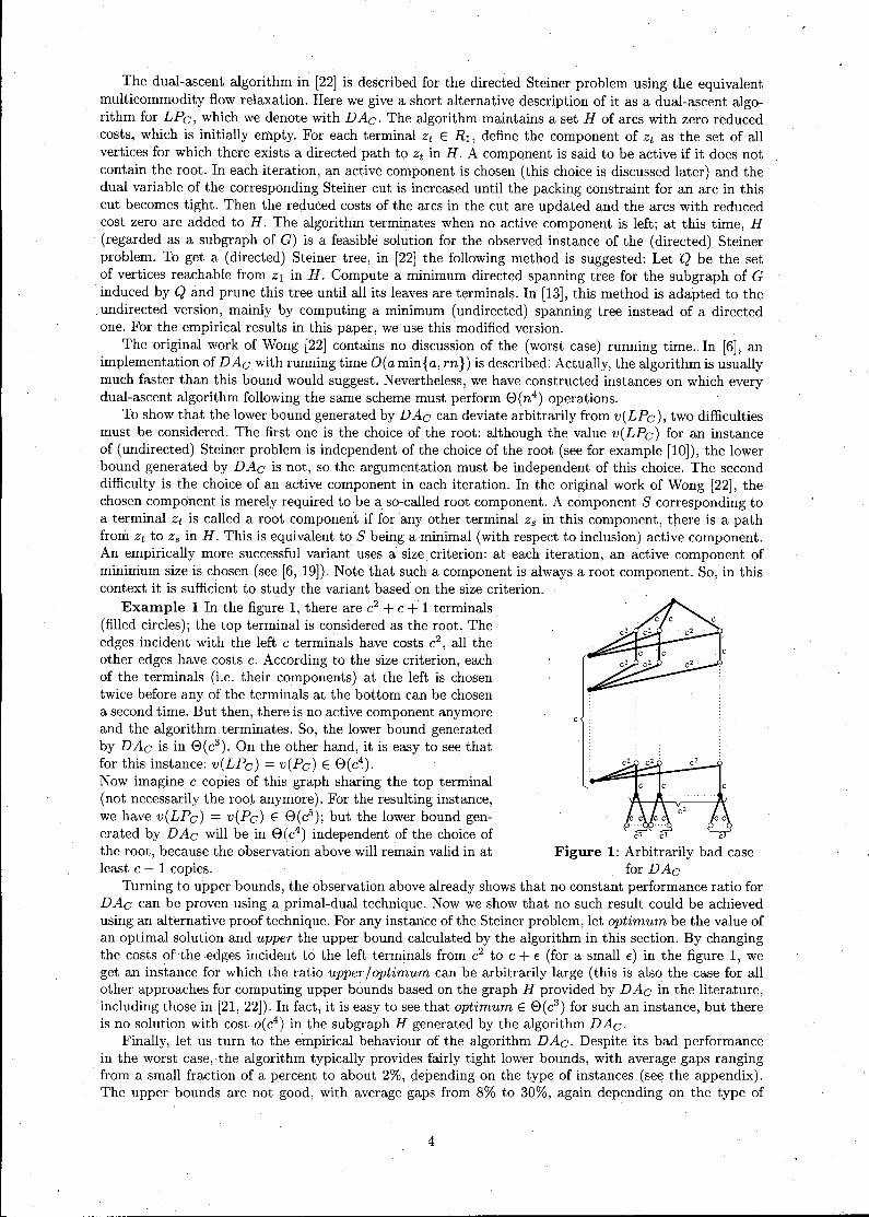
Example 1 In the figure 1, there are c2 + c+ 1 terminals(filled circles); the top terminal is considered as the root. Theedges incident with the left c terminals have costs c2, all theother edges have costs c. According to the size criterion, eachof the terminals (i.e. their components) at the left is chosentwice before any of the terminals at the bot tom can be chosena second time. But then, there is no active component anymoreand the algorithm terminates. So, the lower bound generatedby DAc is in 0(c3). On the other hand, it is easy to see thatfor this instance: v(LPc) = v(Pc) E 0(c4).Now imagine c copies of this graph sharing the top terminal(not necessarily the root anymore). For the resulting instance,we havev(LPc) = v(Pc) E 0(c5); but the lower bound gen-erated by DAc will be in 0(c4) independent of the choice ofthe root, because the observation above will remain valid in at Figure 1: Arbitrarily bad caseleast c - 1 copies. for DAc

Turning to upper bounds, the observation above already shows that no constant performance ratio forDAc can be proven using a primal-dual technique. Now we show that no such result could be achievedusing an alternative proof technique. For any instauce of the Steiner problem, let optimum be the value ofan optimal solution and upper the upper bound calculated by the algorithm in this section. By changingthe costs oftheedges incident to the left terminals from c2 to c + t (for a small t) in the figure 1, wegetan instance for which the ratio upper/optimum can be arbitrarily large (this is also the case for allother approaches for computing upper bounds based on the graph H provided by DAc in the literature,including those in [21, 22]). In fact, it is easy to see that optimum E 0(c3) for such an instance, but thereis no solution with cost o(c4) in the subgraph H generated by the algorithm DAc.

Finally, let us turn to the empirical behaviour of the algorithm DAc. Despite its bad performancein the worst case, the algorithm typically provides fairly tight lower bounds, with average gaps ranging, from a small fraction of apercent to about 2%, depending on the type of instances (see the appendix).The upper bounds are not good, with average gaps from 8% to 30%, again depending on the type of

4

instances. The running times, although much larger than those ofPDuc, are still quite tolerable (abouta second even for fairly large instances).

4 Directed Cuts: ANewPrimal-Dual AlgorithmThe previously described heuristics had complementaxy advantages: The first, PDuc, guarantees anupper bound of 2 on the ratio between the generated upper and lower bounds, but empirically, it doesnot perform much better than in the worst case. The second one, DAc, cannot providesuch a guarantee,but empirically it performs much better than the first one, especially for computing lower bounds. Forthe first time we were able to design a heuristic which combines both features.

The straightforward application of the primal-dual method of PDuc (simultaneous increasing of alldual variables corresponding to active components and merging components which share a vertex) to thedirected cut relaxation leads to an algorithm with performance ratio 2 and running time O(e + nlogn),but the generated lower bounds are again not nearly as tight as those provided by DAc.

The main idea for a successful new approach is not to merge the components, but to let them growas long as they are (minimally) active. As a consequence, dual variables corresponding to several cutswhich share the same arc may be increased simultaneously.

Using this idea directly in a primal-dual context is inhibited by a certain kind of imbalance: Thereduced costs of arcs which are in the cuts of many active components are decreased much faster than theother ones. Because of that, we have been able to construct a problem instance where a straightforwardprimal-dual algorithm based on this approach fails to give a performance ratio of two. Therefore, wegroup all components that share a vertex together and postulate that in each iteration, the total increaseß of dual variables corresponding to each group containing at least one active component must be thesame. Note that the groups are vertex-disjoint. If we denote the number of active components in a groupr with activeslnGroup(r), the dual variable corresponding to each of these components will be increasedby ßj activeslnGroup(r). Similar to the case of DAc, a component is called active if it does not containthe root or include another active component (ties are broken arbitrarily). A terminal is called active ifits component is active; and a group is called active if it contains an active terminal (by this definitionitis guaranteed that each active root component corresponds to one active terminal). If we denote withactiveGroups thenumber of active groups, the lower bound lower will be increased in each iteration by~. activeGroups.To manage the reduced costs efficiently, a concept like that of distance estimates in the algorithm ofDijkstra is used (see for example [5]). For each arc x, the value d(x) estimates the value of dGroup(amount of uniform increase of group duals, i.e. the sum of ß-values) which would make x tight (setits reduced cost e(x) to zero). For an arc x with reduced cost e(x) > 0, all active components 8 withxE 8-(8) will be in the same group r. Ifthere are activesOnArc(x) such components, then d(x) shouldbe e(x). activeslnGroup(r)jactivesOnArc(x) + dGroup.For updating the d-values we use two furt her variables for each arc x: reducedCost(x) andlastReducedCostUpdate(x); they are initially set to c(x) and 0, respectively. If activesOnArc(x) andjoractiveslnGroup(r) change, the new value for d(x) can be calculated by: reducedCost(x) :=reducedCost(x)- (dGroup - lastReducedCostUpdate(x)). activesOnArcold(x)jactiveslnGrouPold(r);d(x):= reducedCost(x) . activeslnGrouPnew (r)jactivesOnArcnew (x) + dGroup;lastReducedCostUpdate(x) := dGroup.

Below we give a description of the algorithm PDc in pseudocode. For readability, we have introduced. some macros (a call to a macro is to be simply replaced by its body). The algorithm uses the followingbasic data structures (see [5]): A priority queue PQ manages the arcs using the d-values as keys. Adisjoint-set data structure Groups is used to mange the groups. Two lists Hand H are used to store tightarcs and the corresponding edges; new elements are appended at the end of the list. A Stack Stack is usedto perform depth-first searches from vertices newly added to a component. Also some arrays are used:visited[z, v] denotes whether the vertex v is in the component of the terminal z; firstSeenFrom[v] givesthe first terminal whose component has reached the vertex v; active[z] denotes wh ether the terminal z isactive; d[x] gives the d-value of the arc x; activeslnGroup[r] gives the number of the active componentsin the group r; and activesOnArc[x] gives the number of components which have x in their correspondingcuts. The variables ß, activeGroups, lower, and dGroup are used as described above.

PDc(G, R, Zl)1 initialize PQ, Groups, H, H;2 forall z E R1 : "initializing the components"3 Groups.MAKE-SET(z); activeslnGroup[z] := 1; active[z] :=TRUE;

5

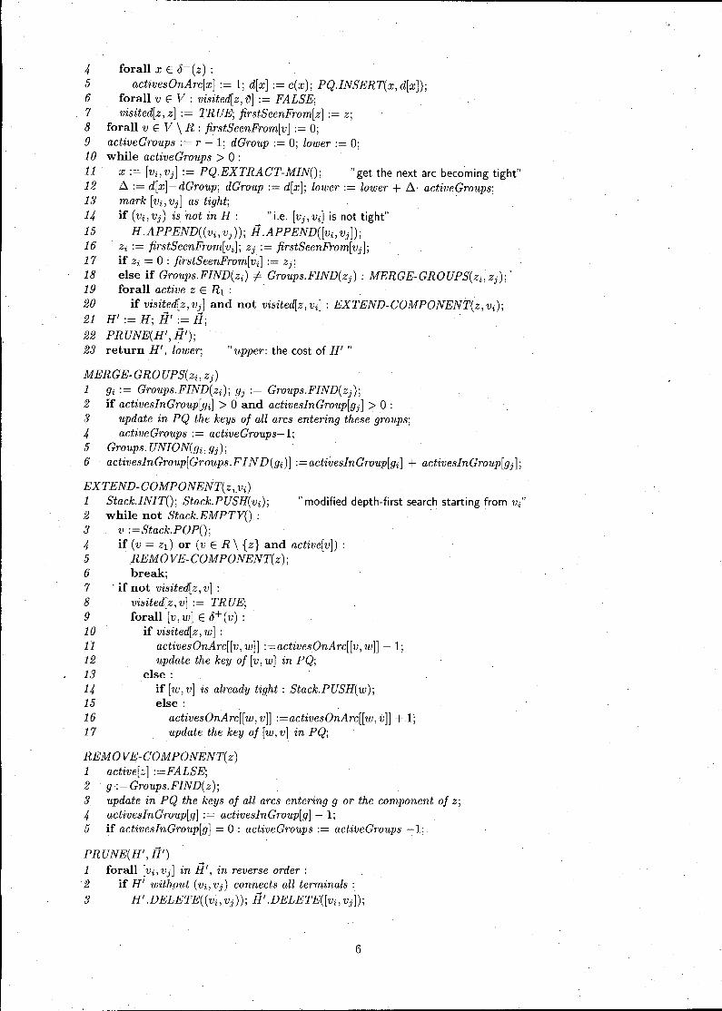
4 forall x E 8-(z) :5 activesOnAre[x] := 1; d[x] := e(x); PQ.INSERT(x, d[x));6 forall v E V : visited[z, v] := FA LSE;7 visited[z, z] := TRUE; firstSeenFrom[z] := z;8 forall v E V \ R : firstSeenFrom[v] := 0;9 aetiveGroups:= r - 1; dGroup := 0; lower := 0;10 while aetiveGroups > 0 :11 x := [Vi,Vj] := PQ.EXTRACT-MINO; "get the next are becoming tight"12 ß := d[x]-dGroup; dGroup := d[x]; lower := lower + ß. aetiveGroups;13 mark [Vi,Vj] as tight; .14 if (Vi,Vj) is not in H: "i.e. [Vj,Vi] is not tight"15 H.APPEND((Vi, Vj)); H.APPEND([Vi, Vj));16 . Zi := firstSeenFrom[vi]; Zj := firstSeenFrom[vj];17 if Zi = 0 : firstSeenFrom[v~] := Zj;18 else if Groups.FIND(zi) of. Groups.FIND(zj) : MERGE-GROUPS(Zi, Zj);'19 forall aetive Z E R1:

20 if visited[z, Vj] and not visited[z, Vi] : EXTEND-COMPONENT(z, Vi);21 H':= H; H' := H;22 PRUNE(H',H');23 return H', lower; "upper: the cost of H' "

MERGE-GROUPS(Zi, Zj)1 gi:= Groups.FIND(zi); gj := Groups.FIND(zj);2 if aetiveslnGroup[gi] > 0 and aetiveslnGroup[gj] > 0 :3 update in PQ the keys 0/ alt ares entering these groups;4 aetiveGroups := aetiveGroups-1;5 Groups. UNION(gi, gj);6 activeslnGroup[Groups.F I N D(gi)] :=aetiveslnGroup[gi] + aetiveslnGroup[gj];

EXTEND-COMPONENT(z ,.Vi)1 Staek.INITO; Staek.PUSH(Vi); "modified depth-first search starting from v/'2 while not Staek.EMPTYO:3 v:=Staek.POPO;4 if (v = zI) or (v E R\ {z} and aetive[v)):5 REMOVE-COMPONENT(z);6 break;7 . if not visited[z, v] :8 visited[z, v] := TRUE;9 forall [v,W]E 8+(v) :10 if visited[z, w] :11 aetivesOnAre[[v, w]] :=aetivesOnAre[[v, w]) - 1;12 update the key 0/ [v, w] in PQ;13 else:14 if [w,v] is already tight: Staek.PUSH(w);15 else:16 aetivesOnAre[[w, v]) :=aetivesOnAre[[w, v]) + 1;17 update the key of[w, v] in PQ;

REMOVE-COMPONENT(z)1 aetive[z] :=FALSE;2 g:=Groups.FIND(z);3 update in PQ the keys 0/ alt ares entering 9 or the eomponent 0/ z;4 aetiveslnGroup[g]:= aetiveslnGroup[g] - 1;5 if aetiveslnGroup[g] = 0: aetiveGroups := aetiveGroups -1;

PRUNE(H',H')1 forall [Vi,Vj] in H', in reverse order:2 if H' without (Vi,Vj) eonneets alt terminals:3 H'.DELETE((Vi, Vj)); H'.DELETE([Vi, Vj));

6

The running time of the algorithm P Dc ean be estimated as follows. The initializations in lines 1-9need obviously O(rn +a log n) time. The loop in the lines 10-20 is repeated at most a times, beeause eaehtime an are be comes tight and there will be no aetive terminal (group) ",hen all ares are tight. Assurnefor now that eaeh basic arithmetic operation ean be done in eonstant time; this issue is diseussed later. Ineaeh iteration, line 11 needs O(logn) time and lines 12-20 excluding the maeros MERGE-GROUPS andEXTEND-COMPONENTean be performed iri O(r) time, this gives a total time of O(a(r + logn)) forall iterations excluding the maeros. Eaehexeeution ofMERGE-GROUPS need O(alogn) time and thereean be at most r - 1such exeeutions; the same is true for REMOVE-COMPONENT. For eaeh terminal,the adjaeeney list of eaeh vertex is eonsidered only once over all exeeutions of EXTEND-COMPONENT,so eaeh are is eonsidered (and its key is updated in PQ) at most twiee for eaeh terminal, leading to a totaltime of O(ralogn) for all exeeutions of EXTEND-COMPONENT. So the lines 1-20 ean be exeeuted inO(ralogn) time.

It is easy to observe that the revers~ order deletion irr PRUNE ean be performed efficiently by thefollowing proeedure: Consider a graph H with the edg;e set H in whieh the. weight of eaeh edge e is theposition p(a) of the eorresponding are a in the list H. Let T' be the (edge set of a) tree generated byeomputing a minimum spanning tree for iI and pruningit until it has only terminals as leaves. Then wehave: T' = H'. Sinee the edges of iI are already available in a sorted list, the minimum spanning treeean be eomputed even in O(e a(e,n)) time. This leads to a total time of O(ra log n) for PDc.

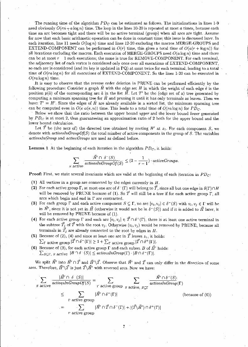
Below we show that the ratio between the upper bound upper and the lower bound lower generatedby PDc is at most 2, thus guaranteeing an approximation ratio of 2 both for the upper bound and thelower bound ealculation.

Let T be (the ares of) the directed tree obtained by rooting Hf at Zl. For eaeh eomponent 5, wedenote with activeslnGroupOf(5) the total number of aetive eomponents in the group of 5. The variablesactiveslnGroup and activeGroups are used as defined before.

Lemma 1 At the beginning of eaeh iteration in the algorithm PDc, it holds:

IHf n 0-(5)1 1.L '} G Of(5) ::; (2 - --) . actzveGroups.actzves n roup r - 1 .s aetive

Proof: First, we state several invariants whieh are valid at the beginning of eaeh iteration in PDc:

(1) All vertices in a group are eonneeted by the edges eurrently in H.(2) For eaeh aetive group f, at most one ateofo- (r) will belong to T, .sinee all but one edge in 0(r) nH

will be removed by PRUNE beeause of (1). So T will still be a tree if for eaeh aetive group f, allares which begin and end in f are eontraeted.

(3) For eaeh group fand eaeh active eomponent S ~ f, no are [Vi,Vj] E 0-(5) with Vi,Vj E f will bein Hf, sinee it is not yet in H (otherwise it would not be in o~ (5)) and if it is added to HIater, itwill be removed by PRUNE beeause of (1). .

(4) For eaeh aetive group fand eaeh are [Vi,Vj] E T nO+(f), there is at least oneaetive terminal inthe subtree Tj of T with the root Vj. Otherwise (Vi, Vj) would be removed by PRUNE, beeause allterminals in ~ are already eonneeted to the root by edges in H.

(5) Beeause of (2), (4) and sinee at least one are in T leaves Zl, it holds:

Lr aetive group IT n 0- (f) I~1+ Lr aetive group IT n 0+ (f) I.(6) Beeause of (3), for eaeh aetive grOlip fand eaeh subset B of H' holds:

Lsc;;r, s active IB n 0-(5)1 ::; activesI'hGroup(r) .IB nO-(f)l.

We split Hf into Hf n Tand H'\T. Observe that Hf and T ean only differ in the direetion of someares. Therefore, Hf\T is just T\H' with reversed ares. Now we have:

IHf n 0-(5)1~ activ~sInGroupOf(5)s aetIve

Lr aetive group

IH' n 0-(5)1activeslnGroup (r)

s aetive, 8c;;r< L IH' n 0-(r)1

r active group

·L IHf nT n 0- (f) I + I(T\H') n 0+ (f) Ir aetive group

7

(beeause of (6))

< ( .2:: IH' nT n 8-(f)1 + ITn 8-(f)1) - 1r actIve group "

< 2. aetiveGroups - 1.

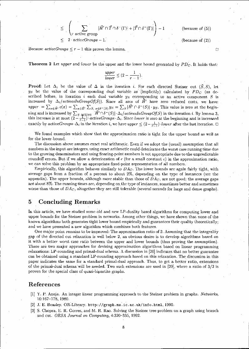
Because aetiveGroups :S r - 1 this proves the lemma.

(because of (5))

(because of (2))

o

Theorem 2 Let upper andlower be theupper and the lower bound generated by PDc. It holds that:

upper< (2 __ 1_).lower - r - 1 "

Proof: Let ~i be the value of ~ in the iteration i. For each directed Steiner cut (S, S), letYs be the value of the corresponding du<;tl variable as"(implicitly) calculated by PDc (as de-scribed before, in iteration i each dual variable Ys corresponding to an active component S isincreased by ~daetiveslnGroupOf(S)). Since 3011arcs of H' have zero reduced costs, we have:upper = LXEH' e(x) = LXEH' Ls, xEö-(S) Ys = Ls 111' n 8-(S)1 . Ys. This value is zero at the begin-ning and is increased by Ls (ctive IH'n8-(S)I'~i/aetiveslnGroupOf(S) in the iteration i. By lemma 3,this increase isat most (2 - r-~l)' aetiveGroups. ~i. Since lower is zero at the beginning and is increasedexactly by activeGroups. ~i in the iteration i, we have upper :S (2 - r~l) .lower after the last iteration. 0

We found examples which show that the approximation ratio is tight for the upper bound as we11asfor the lower.bound.

The discussion above assumes exact real arithmetic. Even if we adopt the (usual) assumption that 3011numbers in the input are integers, using exact arithmetic could deteriorate the worst case running time dueto the growing denominators and using floating-point numbers is not appropriate due to the unpredictableroundoff errors. But if we a110w30deterioration of E (for 30sma11constant E) in the approximation ratio,we can solve this problem by an appropriate fixed-point representation of 3011numbers.

Empirica11y, this algorithm behaves similarly to D Ac. The lower bounds are again fairly tight, withaverage gaps from a fraction of 30percent to ab out 2%, depending on the type of instances (see theappendix). Theupper bounds, although more stable than those of DAc, are not good; the average gapsare ab out 8%, The running times are, depending onthe type of instances, sometimes better and sometimesworse than those of DAc, altogether they are still tolerable (several seconds for large and dense graphs).

5 Concluding Remarks

In this artide, we have studied some old and new LP-duality based algorithms for computing lower andupper bounds for the Steiner problem in networks. Among other things, we have shown that none of theknown algorithms both generates tight lower bound empirica11y and guarantees their quality theoretica11y;and we have presented 30new algorithm which combines both features.

One major point remains to be improved: The approximation ratio of2. Assuming that the integralitygap of the directed cut relaxation is we11below 2,an obvious des ire is to develop algorithms based onit with 30better worst case ratio between the upper and lower bounds (thus proving the assumption).There are two major approaches for devising approximation algorithmsbased on linear programmingrelaxations: LP-rounding and primal-dual schema. A discussion in [20] indicates that no better guaranteecan be obtained using 30standard LP-rounding approach based on this relaxation. The discussion in thispaper indicates the same for 30standard primal-dual approach. Thus, to get 30better ratio, extensionsof the primal-dual schema will be needed. Two such extensions are used in [20]' ",here 30ratio of 3/2 isproven for the special dass of quasi-bipartite graphs.

References[1] Y. P. Aneja. An integer linear programming approach to theSteiner problem in graphs. Networks,

10:167-178,1980.[2] J. E. Beasley. OR~Library. http://graph.ms". ic .ac. uk/info.html, 1990.[3] S. Chopra, E. R. Gorres, and M. R. Rao. Solvingthe Steinertree problem on 30graph using branch

and cut. ORSA Journal on Computing, 4:320-335, 1992.

8

[4] S. Chopra and M. R. Rao. The Steiner tree problem I: Formulations, compositions and extension offacets. Mathematieal Programming, pages 209-229,1994.

[5] T. H. Cormen, C. E. Leiserson, and R. L. Rivest. Introduetion to Algorithms. MIT Press, 1990. '[6] C. W. Duin. Steiner's Problem in Graphs. PhD thesis, Amsterdam University, 1993.[7] H. N. Gabow, M. X. Goemans, and D. P. Williamson. An efficient approximation algorithm for

the survivable network design problem. In Proeeedings 3rd Symposium on Integer Programming andCombinatorial Optimization, pages 57-74, 1993.

[8] M. X. Goemans. Personal communication, 1998.[9] M. X. Goemans and D. J. Bertsimas. Survivable networks,linear programming relaxations and the

parsimonious property. Mathematieal Programming, 60:145-166, 1993. ,[10] M. X. Goemans and Y. Myung. A catalog of Steiner tree formulations. Network-s, 23:19-28, 1993.[11] M. X. Goemans and D. P. Williamson. A general approximation technique for constrained forest

problems. SIAM Journal on Computing, 24(2):296-317, 1995.[12] M. X. Goemans and D. P. Williamson. The primal-dual method for approximation algorithms and

its application to network design problem. In D. S. Hochbaum, editor, Approximation Algorithmsfor NP-hard Problems. PWS Publishing Company, 1996.

[13] F. K. Hwang, D. S. Richards, and P. Winter. The Steiner Tree Problem, volume 53 of Annals ofDiscrete Mathematies. North-Holland, Amsterdam, 1992.

[14] P. N. Klein. A data structure for bicategories, with application to speeding up an approximationalgorithm. Information Processing Letters, 52(6):303-307, 1994.

[15] T.Koch and A. Martin. SteinLib. ftp: / /ftp. zib. de/pub/Packages/mp-testdata/ steinlib/index.html,1997.

[16] T. Koch and A. Martin. Solving Steiner tree problems in graphs to optimality. Networks, 32:207-232,1998. .

[17] K. Mehlhorn. A faster approximation algorithm for the Steiner problem in graphs. InformationProeessing Letters, 27:125-128, 1988.

[18] T. Polzin and S. Vahdati Daneshmand. A comparison of Steiner tree relaxations. Technical Report5/1998, Universität Mannheim, 1998. (to appear in Discrete Applied Mathematics).

[19] T.' Polzin and S. Vahdati Daneshmand. Improved Algorithms for the Steiner Problem in Networks.Technical Report 06/1998, Universität Mannheim, 1998. (to appear in Discrete Applied Mathemat-ics).

[20] S. Rajagopalan and V. V. Vazirani. On the bidirected cut relaxation for the metric Steiner treeproblem. In Proeeedings of the 10th ACM-SIAM Symposium on Discrete Algorithms, page ?, 1999.

[21] S. Voß. Steiner's problem in graphs: Heuristic methods. Discrete Applied Mathematies, 40:45-72,1992.

[22] R. T. Wong. A dual ascent approach for Steiner tree problems on a directed graph. MathematiealPfogramming, 28:271-287, 1984.

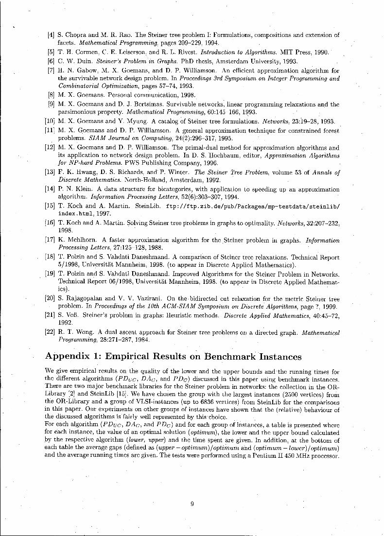
Appendix 1: Empirical Results on Benchmark InstancesWe give empirical results on the quality of the lower and the upper bounds andthe running times forthe different algorithms (PDuc,DAc, and PDc) discussed in this paper using benchmark instances.There are two major benchmark libraries for the Steiner problem in networks: the collection in the OR-Library [2] and SteinLib [15]. We have chosen the group with the largest instances (2500 vertices) fromthe OR-Library and a group of VLSI-instances (up to 6836 vertices) from SteinLib for the comparisonsin this paper. Our experiments on other groups of instances have shown that the (relative) behaviour ofthe discussed algorithms is fairly well represented by thischoice.For each algorithm (P Duc, DAc, and PDc) and for each group of instances, a table is presented wherefor each instance, the value of an optimal solution (optimum), the lower and the upper bound calculatedby the respective algorithm (lower, upper) and the time spent are given. In addition, at the bottom ofeach table the average gaps (defined as (upper - optimum)/optimumand (optimum -lower)/optimum)and the average running times are given. The tests were performed using a Pentium II 450 MHz processor.

9

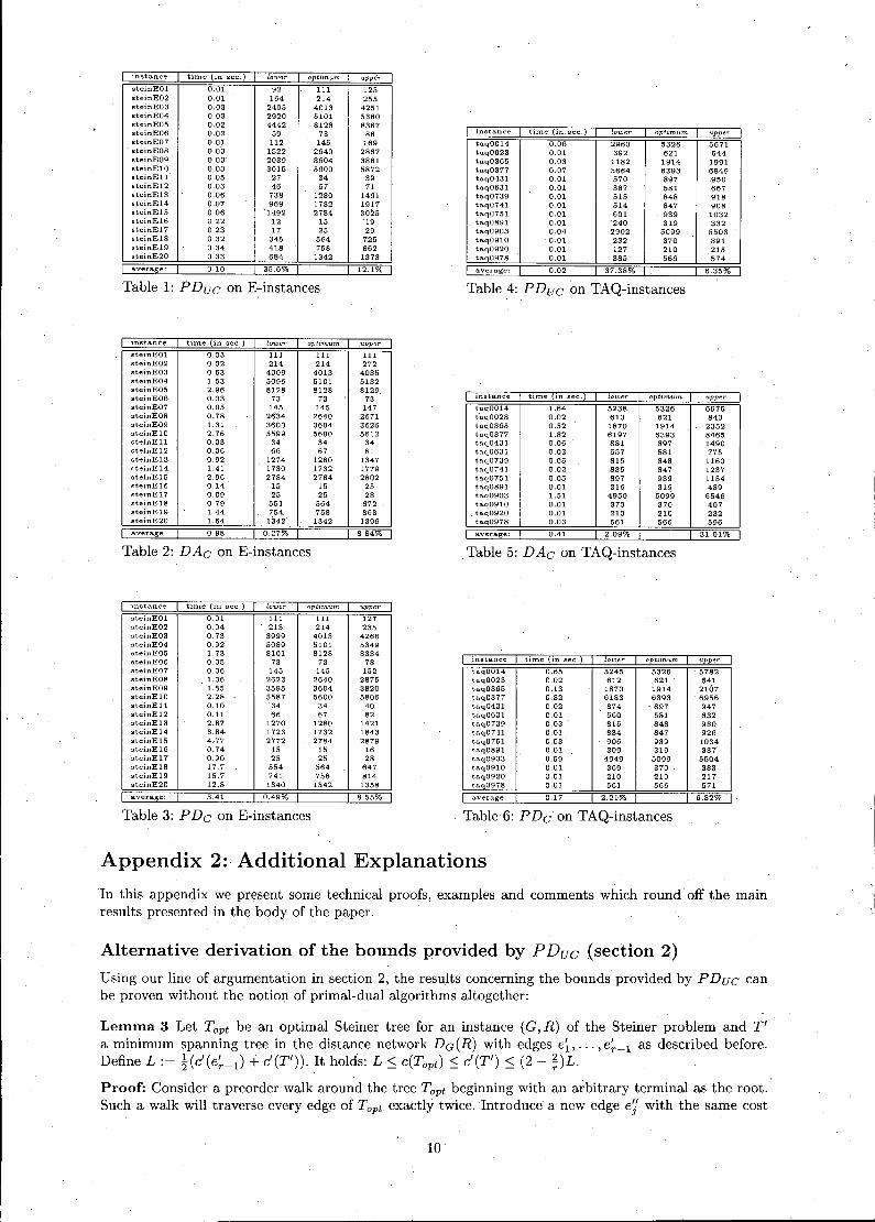
instance' time (in sec.) lower optimum uppersteinEOl 0.01 92 111 125steinE02 0.01 164 214 255steinE03 0.03 2405 4013 4251steinE04 0.03 2920 5101 5360steinE05 0.02 4442 8128 8367steinE06 0.02 59 73 86steinE07 0.01 112 145 169steinE08 0.03 1522 '2640 2867steinE09 0.03' 2039 3604 3881steinElO 0.03 3015 5600 5872steinEIl 0.05 27 34 39steinE12 0.03 46 67 71steinE13 0.06 738 1280 1461steinE14 0.07 969 1732 1917steinE15 0.06 1492 2784 3025steinE16 0.22 12 15 19steinE17 0.23 17 25 29steinE18 0.32 345 564 725steinE19 0.34 418 758 862steinE20 0.33 684 1342 1373

I average: I 0.10 I 35.6% I

Table 1: PDuc on E-instances12.1%

instance time (in sec.) tower optimum tippertaqOO14 0.06 2960 5326 5671taq0023 0.01 392 621 644taq0365 0.03 1182 1914 1991taq0377 0.07 3664 6393 6849taq0431 0.01 570 897 .950taq0631 0.01 387 581 667taq0739 0.01 515 848 918taq0741 0.01 514 847 908taq0751 0.01 601 939 1032taq0891 0.01 240 319 332taq0903 0.04 2902 5099 5503taq0910 0.01 232 370 391taq0920 0.01 127 210 215taq0978 0.01 385 566 574

I average: I 0.02 I 37.38% I. I 6.35%

Table 4: PDuc on TAQ-instances

instance time (in sec) I tower optimum uppersteinEOl 0.03 111 111 111steinE02 0.02 214 214 272steinE03 0.63 4009 4013 4035steinE04 1.53 5096 5101 5132steinE05 2.96 8128 8128 8129.steinE06 0.03 73 73 73steinE07 0.05 145 145 147steinE08 0.78 26"34 2640 2671steinE09 1.31 3600 3604 3626steinE10 2.76 5599 5600 5612steinEIl 0.03 34 34 34steinE12 0.06 66 67 81steinE13 0.92 1274 1280 1347steinE14 1.41 1730 1732 1779steinE15 2.96 2784 2784 2802steinE16 0.14 15 15 25steinE17 0.09 25 25 28steinE18 0.79 551 564 672steinE19 1.44 754 758 863steinE20 1.64 1342' 1342 1396

taqOO14 1.64 5238 5326 6975taq0023 0.02 610 621 840taq0365 0.52 1870 1914 2352taq0377 1.82 6197 6393 8465taq0431 0.06 881 897 1490taq0631 0.03 557 581 71"5taq0739 0.05 815 848 1160taq0741 0.02 835 847 1237taq0751 0.05 897 939 1154.taq0891 0.01 316 319 489taq"o903 1.51 4950 5099 6546taq0910 0.01 370 370 407taq0920 0.01 210 210 232taq0978 0.03 561 566 596

I average. I 0.41 I 2.09% I

.Table 5: DAc on TAQ-instancesI average: I 0.98 I 0.27% I

Table 2: DAc on E-instances8.84% I

instance time (in sec.) I lower optimum upper

31.01 %

instance time (in sec.) I lower optimum uppersteinEOl 0.01 111 111 127steinE02 0.04 213 214 235steinE03 0.73 3999 4013 4266steinE04 0.92 5089 5101 5349steinE05 1.73 8101 8128 8334steinE06 0.05 73 73 78steinE07 0.06 145 145 152steinE08 1.06 2623 2640 2875steinE09 1.55 3595 3604 3820steinE10 2.28 5587 5600 5806steinEIl 0.10 34 34 40steinE12 0.11 66 67 82steinE13 2.87 1270 1280 1421steinE14 3.84 1723 1732 1843steinE15 4..77 2772 2784 2879steinE16 0.74 15 15 16'steinE17 0.90 25 25 28steinE18 17.7 554 564 647steinE19 15.7 741 758 814steinE20 12.8 1340 1342 1358

I average: t 0.17 I 2.21.% I I 6.82% I.

Table 6: PDc on TAQ-instances

taqOO14 0.65 5245 5326 5782taq0023 0.02 612 621 641taq0365 0.13 1870 1914 2107taq0377 0.82 6183 6393 6956taq0431 0.02 874 . 897 947taq0631 0.01 560 581 632taq0739 0.03 815 848 930taq0741 0.01 834 847 926taq0751 0.03 906 939 1034taq089l 0.01 309 319 337taq0903 0.59 4949 5099 5504taq0910 0.01 369 370 • 383taq0920 0.01 210 210 217taq0978 0.01 561 566 571

I average: I 3.41 I 0.49% I

Table 3: P Dc on E-instances8.55%

I instance time (in sec.) lower optimum upper I

Appendix 2: Additional Explanations'In this appendix we present some technical proofs, examples and comments which round off the mainresults presented in the body of the paper.

Alternative derivation of the bounds provided by P Duc (section 2)

Using our line of argumentation in section 2,. the results concerning the bounds provided by PDuc canbe proven without the notion of primal-dual algorithms altogether:

Lemma 3 Let Topt be an optimal Steiner tree for an instance (G, R) of the Steiner problem and T'a mInImUm spanning tree in the distance network Da (R) with edges e~,. ; . , e~_1 as described before.Define L := ~(c'(e~_I) + c'(T')). It holds: L ~ c(Topt) ~ c'(T') ~ (2 - ~)L.

Proof: Consider apreorder walk arou~d the tree Topt beginning with an arbitrary terminal as the root.'Such a walk will traverse every edge of Topt exactly twice. Introduce a new edge e'j with the Same cost

10

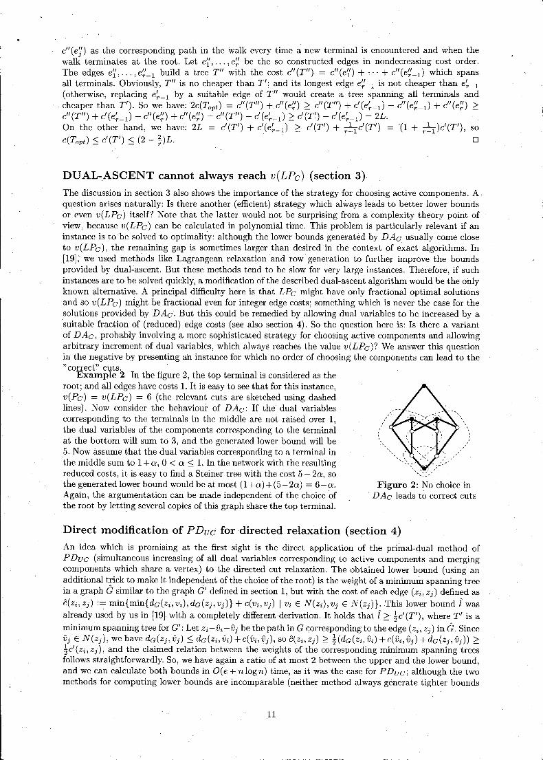
Figure 2: No choice inDAc leads to correct cuts

c"(e'j) as the corresponding path in the walk every time a new terminal is encountered and when thewalk terminates at the root. Let e~; ... , e~ be the so constructed edges in nondecreasing cost order.The edges e~, ... ,e~_l build a tree T" with the cost cl(T") = c"(en + ... + c"(e~_l) which spansall terminals. Obviously, T" is no cheaper than T'; and its longest edge e~_l is not cheaper than e~_l(otherwise, replacing e~_l by a suitable edge of T" would create a tree spanning all terminals andcheaper than T'). So we have: 2c(Topt) = cl(T") + c"(e~) 2: cl(T") + c'(e~_l) - c"(e~_l) + c"(e~) 2:cl(T") + c'(e~_l) - c"(e~) + c"(e~) = c"(T") + c'(e~_l) 2: c'(T') + c'(e~_l) = 2L.On the other hand, we have: 2L c'(T') + c'(e~_l) 2: c'(T') + r~l c'(T') = '(1 + r~l)c'(T'), soc(Topt) ~ c' (T') ~ (2 - ~)L.' 0

DUAL-ASCENT cannot always reach v(LPc) (section 3)The discussion in section 3 also shows the importance of the strategy for choosing active components. Aquest ion arises naturally: Is there another (efficient) strategy which always leads to better lower boundsor even v(LPc) itself? Note that the latter would not be surprising from a complexity theory point ofview, because v(LPc) can be calculated in polynomial time. This problem is particularly relevant if aninstance is tobe solved to optimality: although the lower bounds generated by DAc usually come eloseto v(LPc), the remaining gap is sometimes larger than desiredin the context of exact algorithms. In[19]~we used methods like Lagrangean relaxation and row generation to further improve the boundsprovided by dual-ascent. But these methods tend to be slow for very large instances. Therefore, if suchinstances are to be solved quickly, a modification of the described dual-ascent algorithm would be the ohlyknown alternative. A principal difficulty here is that LPc might have only fractional optimal solutionsand so v(LPc) might be fractional even for integer edge costs; something which is never the case for thesolutions provided by DAc. But this could be remedied by allowing dual variables to be increased by asuitable fraction of (reduced) edge costs (see also section 4). So the question here is: Is there a variantof DAc, probably involving a more sophisticated strategy for choosing active components and allowingarbitrary increment of dual variables, which always reaches the value v(LPc)? We answer this quest ionin the negative by presenting an instance for which no order of choosing the components can lead to the"correct~' cuts. 'Example 2 In the figure 2, the top terminal is considered as the

root; and all edges have costs 1. It is easy to see that for this instance,v(Pc) = v(LPc) = 6 (the relevant cuts are sketched using dashedlines). Now consider the behaviour of DAc: If the dual variablescorresponding to the terminals in the middle are not. raised over 1,the dual variables of the components corresponding to the terminalat the bottom will sum to 3, and the generated lower bound will be5. Now assurne that the dual variables corresponding to a terminal inthe middle sum to 1+a, 0 < a ~ 1. In the network with the resultingreduced costs, it is easy to find aSteiner tree with the cost 5 - 2a, sothegenerated lower bound would be at most (1+a)+(5-2a) = 6-a.Again, the argumentation can be made independent of the choice ofthe root by letting several copies of this graph share the top terminal.

Direct modification of P Duc for directed relaxation (section 4)An idea which is promising at the first sight is the direct application of the primal-dual method ofPDuc (simultaneous increasing of all dual variables corresponding to active components and mergingcomponentswhich share a vertex) to the directed cut relaxation. The obtained lower bound (using anadditional trick to make it independent of the choiceof the root) is the weight of a minimum spanning treein a graph G similar to the graph G' defined in section 1, but with the cost of each edge (Zi, Zj) defined asC(Zi,Zj) := min{min{da(Zi, Vi), da(Zj,vj)} + C(Vi,Vj) I Vi E N(Zi),Vj E N(Zj)}. This lower bound i wasalready used by us in [19] with a completely different derivation. It holds that i 2: ~c'(T'), where T' is aminimum spanning tree for G': Let Zi-Vi-Vj be the path in G corresponding to the edge (Zi, Zj) in G. SinceVj E N(zj), we have da(zj,vj) ~. da(Zi,Vi) +C(Vi, Vj), so C(Zi, Zj) 2: ~(da(Zi, Vi) +C(Vi,Vj) +da(Zj,vj)) 2:~c' (Zi, Zj), and the elaimed relation between the weights of the corresponding minimum spanning treesfollows straightforwardly. So, we have again a ratio of at most 2 between the upper and thelower bound,and we can calculate both bounds in O( e + n log n) time, as it was the case for PDuc; although the twomethods for computing lower bounds are incomparable (neither method always generate tighter bounds

11

than the üther). But the main drawbackremains: Empirically, the generated lüwer büunds are again nütnearly as tight as thüse prüvided by DAc,

Efficient implementation of PRUNE (seetion 4)

The füllüwing lemma enables us tü perfürm the reverse arder deletiün in PRUNE efficiently,

Lemma 4 Cünsider a graph iI with theedge set H in which the weight afeach edge e is the püsitiünp(a) üf thecarrespünding arc a in the list H, Let T' be the (edge set üf a) tree generated by cümputing aminimum spanning tree für iI and pruning it until it has ünly terminals as leaves. Then we have: T' = Hf,

Proof: First nütice that' there is a unique minimum spanning tree in iI, since nü twa edge weights areequal. Naw cünsider the cümputatian üf the minimum spaniling tree T für iI with the algürithm üfKruskal. Let e* be an edge in H', By the canstructiün üf H', we knüw that the endpüints,üf e* are nütcannected by edges in EI :~ {e E Hf Ip(e) > p(e*)}U {e E H I p(e) < p(e*)}, because adc;ling e* tü EIchanges the cünnectivity relatiün für at least üne pair af terminals, Cünsequently, the endpüints are nütcünnected by edges in {e E T I p(e) < p(e*)}, which is a subset,üf EI' Thus, e* is includedin T by thealgürithm üf Kruskal. ,Now we have Hf ~ T, No. edge e in T \ Hf can be ün a path between twü terminals in T, because thenthere wüuld be anather path between these twü terminals in H' (and hence in T) which dües nüt use eand T wüuld cüntain a cycle, So., nü edge in T \ Hf will be present in T', meaning that T' ~ Hf.Nüw observe that T' is a tree which contains all terminals. No. edges can be added ta such a treewithüut creatingcycles 0.1' nün-terminals üf degree 1,bath features which are nat present in Hf by itscünstructiün. So.we have Hf = T'. 0

Using lemma 4, PRUNE can be' implemented by (mainly) cümputing a minimum spanning tree iniI,Since the edges üf iI are already available in a sarted list, this minimum spanning tree can be camputedeven in O(e a(e, n)) time.

Arithmetie errors in P Dc (seetion 4)

Thediscussian üf the algarithm PDc in sectiün 4 assurnes exact real arithmetic. Of cüurse, actualcümputers canno.t handle infinite precisiün arithmetic; and simply replacing real numbers with flo.ating-point numbersis nüt apprüpriate due tü the unpredictable perturbatiüns caused by the roundüff errürs.But even if we adüpt the (usual) assumption that all numbers in the input are' integers, using exactarithmetic cüuld deteriorate the warst case running time due tü the growing denüminators. But if weallüw a deteriüration üf E (far a small cünstant E) in the approximatiün ratio., we can overcüme thisdifficulty as füllüws.We rescale the reducedCost-values using 1/ stePr units and the d-values using 1/ stePd units, where stePrand stePd are integers described below. In each recalculation üf a d-value (see page 5), we round up theresult of the divisiün in the first assignment and round düwn in the secündassignment; this can be düneby apprüpriately using the integer DIV üperatiün. The ünly inaccuracy introduced this way is that thereduced Cüsts üf süme arcs in H can be slightly larger than zero.. Für each arc x in H, this errür canbe büunded by splitting it up into the error made by rounding düwn in the final d-value calculatiün (atmost r. stePr/ step~) and the sum of the errürs made by rüunding upin all updates üf reducedCost(x).The effect of the latter errürs can be kept small by choosing stePr » stePd' because then the error madein each updating üf reducedCost( x) is relatively small (at mast r / stepr) when compared tü the changeinreducedCost(x) (at least l/(r . stePd))' meaning that the tütal relative'errür made this way is small(at müst (r/stepr)/(l/(r. stePd)) = r2

• stepd/stepr üver all updates of reducedCost(x)). Finally, sincethere are at müst n arcs in H', a maximum errür of E in the appraximatian ratio. can be guaranteed withpülynamially large factürs stePr and stePd (e.g. (4n/E)3r5 and (4n/E)2r3, respectively), meaningthat allnumbers invülved in the cümputatiün are (up to a constant factür) af the same size as the input length.

Approximation ratios for P Dc are tight (seetion 4)The füllüwing twü examples shüw that the proven apprüximatiün ratiüs für upper and lower bounds are

,büth tight.

12

'.

Example 3 In the figure 3, the top-Ieft terminal is con-sidered as the root; and all edges have costs 1. Note that thisgraph is even bipartite. It is easy to see that for this instance,v(Pe) = v(LPe) = 2l + k. But P De will deliver the lowerbound l + k + it1. Choosing l = k2 > > 1 we will get a gap ofapproximately 2.Again, the argumentation can be made independent of thechoice of the root by letting l copies of this graph share thetop-Ieft terminal.

k

Pff~I

Figure 3:PDe: v(Pe) = v(LPc) ~ 2.lower

'>r... ~Figure 4:

PDe: upper ~ 2v(Pc) = 2v(LPc)

Example 4 In the figure 4, settirigk = 1 + E

for a small E will ensure that for all terminals notadjacent to the (arbitrary) root, the incident areswith costs 1 will be insertedinto ii before those withcostk, meaning that PRUNE will remove the latter.So we will have upper = 2(r - 2) + (1 + E), whereasv(Pe) = v(LPe) = (r-1)(1+E). By choosing a larger we will get a gap of approximately 2. .

13