Pricing Poseidon: Extreme Weather Uncertainty and Firm ...
57
FEDERAL RESERVE BANK OF SAN FRANCISCO WORKING PAPER SERIES Pricing Poseidon: Extreme Weather Uncertainty and Firm Return Dynamics Mathias S. Kruttli The Board of Governors of the Federal Reserve System Brigitte Roth Tran Federal Reserve Bank of San Francisco Sumudu W. Watugala Cornell University March 2021 Working Paper 2021-23 https://www.frbsf.org/economic-research/publications/working-papers/2021/23/ Suggested citation: Kruttli, Mathias S., Brigitte Roth Tran, Sumudu W. Watugala. 2021 “Pricing Poseidon: Extreme Weather Uncertainty and Firm Return Dynamics,” Federal Reserve Bank of San Francisco Working Paper 2021-23. https://doi.org/10.24148/wp2021-23 The views in this paper are solely the responsibility of the authors and should not be interpreted as reflecting the views of the Federal Reserve Bank of San Francisco or the Board of Governors of the Federal Reserve System.
Transcript of Pricing Poseidon: Extreme Weather Uncertainty and Firm ...

FEDERAL RESERVE BANK OF SAN FRANCISCO
WORKING PAPER SERIES
Pricing Poseidon: Extreme Weather Uncertainty and Firm Return Dynamics
Mathias S. Kruttli
The Board of Governors of the Federal Reserve System
Brigitte Roth Tran Federal Reserve Bank of San Francisco
Sumudu W. Watugala
Cornell University
March 2021
Working Paper 2021-23
https://www.frbsf.org/economic-research/publications/working-papers/2021/23/
Suggested citation:
Kruttli, Mathias S., Brigitte Roth Tran, Sumudu W. Watugala. 2021 “Pricing Poseidon: Extreme Weather Uncertainty and Firm Return Dynamics,” Federal Reserve Bank of San Francisco Working Paper 2021-23. https://doi.org/10.24148/wp2021-23 The views in this paper are solely the responsibility of the authors and should not be interpreted as reflecting the views of the Federal Reserve Bank of San Francisco or the Board of Governors of the Federal Reserve System.

Pricing Poseidon: Extreme Weather Uncertaintyand Firm Return Dynamics∗
Mathias S. Kruttli, Brigitte Roth Tran, and Sumudu W. Watugala†
March 2021
We present a framework to identify market responses to uncertainty faced by firmsregarding both the potential incidence of extreme weather events and subsequent eco-nomic impact. Stock options of firms with establishments in forecast and realizedhurricane landfall regions exhibit large increases in implied volatility, reflecting signif-icant incidence uncertainty and long-lasting impact uncertainty. Comparing ex anteexpected volatility to ex post realized volatility by analyzing volatility risk premiachanges shows that investors significantly underestimate extreme weather uncertainty.After Hurricane Sandy, this underreaction diminishes and, consistent with Merton(1987), these increases in idiosyncratic volatility are associated with positive expectedstock returns.
JEL classification: G12, G14, Q54.Keywords: extreme weather, uncertainty, implied volatility, expected returns, climate risks.
∗We thank Lint Barrage (discussant), Michael Bauer (discussant), Riccardo Colacito (discussant), BenGroom (discussant), Matthew Gustafson (discussant), Burton Hollifield (discussant), Kris Jacobs (discus-sant), Scott Mixon (discussant), Aurelio Vasquez (discussant), Andrea Vedolin (discussant), Jawad Addoum,Rui Albuquerque, Vicki Bogan, Mikhail Chernov, Byoung-Hyoun Hwang, Andrew Karolyi, Fang Liu, DavidNg, Ian Martin, Justin Murfin, Emilio Osambela, Andrew Patton, Tarun Ramadorai, Laura Starks, ScottYonker, Youngsuk Yook, and seminar participants at the Federal Reserve Board, Cornell University, NOAA,UCSD, UCSB, CFTC, University of Zurich, UConn Finance Conference, UToronto-McGill Risk Manage-ment and Financial Innovation Conference in Memory of Peter Christoffersen, Conference on Commodities,Volatility and Risk Management, AERE Summer Conference, Northeast Workshop at Harvard KennedySchool, CEPR-EBRD-EoT-LSE Workshop, Resources for the Future, University of Oklahoma Energy andCommodities Finance Research Conference, Federal Reserve Day Ahead Conference, 2020 NBER AssetPricing Spring Meeting, 2021 AFA Meeting, UCLA Luskin Symposium on Climate Adaptation for helpfulcomments. Keely Adjorlolo, David Rubio, and Alan Yan provided outstanding research assistance. Theviews stated herein are those of the authors and are not necessarily the views of the Federal Reserve Board,the Federal Reserve Bank of San Francisco, or the Federal Reserve System.
†Kruttli: The Board of Governors of the Federal Reserve System. Email: [email protected]. RothTran: The Federal Reserve Bank of San Francisco. Email: [email protected]. Watugala: CornellUniversity. Email: [email protected].
1

1 Introduction
From hurricanes and severe snow storms to droughts and wildfires, extreme weather events
have caused widespread devastation in recent years. For instance, in the record year of 2017,
the estimated damages from extreme weather events in the U.S. were over $300 billion.1 De-
spite an emerging climate finance literature, little is known about the uncertainty generated
by extreme weather events for firms or how that uncertainty is priced. Filling this gap in
the literature is important. Uncertainty, measured as the expectation of future volatility,
has been shown to affect financial markets and real economic activity in other contexts,2
and could impact the cost of capital for a firm.3 While the unpredictable impact of extreme
weather on productive capital, supply chains, local labor, and product demand could create
significant uncertainty, firms can potentially offset these effects through insurance, adapta-
tion, or relocation. Thus, it is not obvious a priori that extreme weather events generate
substantial uncertainty for firms. Moreover, the pricing of uncertainty related to extreme
weather is previously unstudied though highly relevant to the emerging, urgent debate about
the potential impact of climatic events on financial stability.4 Mispricing of such events in
asset markets could lead to sudden large price corrections that are destabilizing (Carney,
2015).
In this paper, we first use financial markets to isolate and quantify the extent of extreme
weather uncertainty faced by firms, and then analyze the pricing of this uncertainty. We
distinguish between two components of extreme weather uncertainty: (a) the “incidence
uncertainty” regarding where, when, and whether an extreme weather event will occur, and
(b) the “impact uncertainty” about an extreme weather event’s effect conditional on an
event occurring. The exogenous nature of the inception of extreme weather events allows
us to isolate the associated uncertainty cleanly and examine its pricing in our empirical
analysis because prevailing conditions of the firms do not affect the timing and likelihood
1National Oceanic and Atmospheric Administration (NOAA) damage estimates (https://www.climate.gov/news-features/blogs/beyond-data/2017-us-billion-dollar-weather-and-climate-disasters-historic-year).
2For example, political uncertainty is reflected in index option prices (Kelly, Pastor, and Veronesi, 2016)and leads to lower corporate investment (Julio and Yook, 2012; Jens, 2017). As in this paper, Bloom(2009); Pastor and Veronesi (2012, 2013); Jurado, Ludvigson, and Ng (2015) and others define uncertaintyas expected volatility, which is distinct from other strands of the literature on Knightian uncertainty.
3For example, Merton (1987) shows theoretically how even firm-specific uncertainty could impact theexpected return of a stock.
4Government agencies responsible for ensuring the resilience of the financial system have started toexamine the potential impact of climatic events. In 2020, the Commodity Futures Trading Commission’sreleased a report dedicated to climate risks (https://www.cftc.gov/PressRoom/PressReleases/8234-20). TheFederal Reserve Board states in its Financial Stability Report, November 2020: “...uncertainty about thetiming and intensity of severe weather events and disasters, as well as the poorly understood relationshipsbetween these events and economic outcomes, could lead to abrupt repricing of assets.” (https://www.federalreserve.gov/publications/2020-november-financial-stability-report-near-term-risks.htm).
2

of an extreme weather event. This distinguishes our analysis from studies on other types
of uncertainty like macroeconomic or political uncertainty where periods of uncertainty are
generally endogenous to prevailing conditions of the economy or firm.5
Our empirical analysis focuses on hurricanes. We do so for a number of reasons. First,
hurricanes are among the most economically destructive extreme weather events.6 States all
along the Atlantic and Gulf coasts of the US, which include a wide variety of major centers
of economic activity, have been impacted by hurricanes. Second, NOAA publishes a range
of relevant forecast and realized data on hurricanes. These data are accessible to investors in
real-time. Third, hurricanes develop from inception at sea and resolve following landfall or
dissipation over fairly short but well-defined time frames, which allows us to estimate effects
in isolation. However, our framework can be applied to other extreme weather events like
snow storms and severe floods that are also subject to uncertainty about whether and where
they occur, and what the eventual impact will be.
We proxy for extreme weather uncertainty using changes to the implied volatility of stock
options, a measure that captures investor expectations of volatility.7 We carefully collect
novel data from NOAA on hurricane forecast and landfall spanning 22 years. We combine
those data with location data on establishments of individual firms to construct a granular
dataset that allows us to measure firm exposure to regions affected by each hurricane, which
determines treatment in our difference-in-differences analysis.
We present a simple theoretical framework to characterize how the two components of ex-
treme weather uncertainty affect the expected variance of a firm. While an extreme weather
event like a hurricane is forming and approaching an area in which a firm is located, the
associated extreme weather uncertainty for the firm comprises both incidence uncertainty
and expected impact uncertainty, and varies with the probability of incidence. Incidence
uncertainty is fully resolved at hurricane landfall (or dissipation in the case of a hurricane
that “missed”). Only impact uncertainty remains after landfall. Interestingly, under certain
conditions, incidence uncertainty can be high enough such that the total uncertainty faced
by a firm prior to hurricane landfall can even exceed the total uncertainty conditional on
landfall.
5See, for example, Bloom (2009); Jurado, Ludvigson, and Ng (2015); Baker, Bloom, and Davis (2016);Dew-Becker, Giglio, Le, and Rodriguez (2017); Hassan, Hollander, Van Lent, and Tahoun (2019). Somestudies on political uncertainty like Julio and Yook (2012); Kelly, Pastor, and Veronesi (2016); Jens (2017)focus on prescheduled political events, which are interpreted as known, exogenous points in time when apolicy (or regime) change might occur. However, the likelihood of whether a policy/regime change occurson the prescheduled date can still be endogenous to prevailing economic conditions. As Pastor and Veronesi(2012) discuss, such a change is more likely during downturns.
6For instance, in 2017, $265 billion of the aforementioned $300 billion in damages from extreme weatherevents in the US were due to hurricanes.
7As do Bloom (2009) and others.
3

In our empirical analysis, first, using hurricane forecasts and associated landfall proba-
bilities (probabilities of incidence) issued in the days leading up to a hurricane’s landfall or
dissipation, we find that before landfall, implied volatilities of firms with exposure to the
forecast path increase even at a low landfall probability and increase up to 21 percent for a
high probability greater than 50%.8 These results imply that hurricanes cause substantial
uncertainty prior to landfall and that investors pay attention to hurricane forecasts.
After landfall, indicative of significant impact uncertainty, we find that the implied
volatility of firms with establishments in the landfall region are significantly elevated, rising
up to 23 percent higher than before the hurricane’s inception. Implied volatilities remain
elevated for several months after hurricane landfall, suggesting that the resolution of impact
uncertainty is slow. Comparing these impact uncertainty estimates to our total extreme
weather uncertainty estimates based on forecasts indicates that substantial incidence uncer-
tainty is reflected in options prices prior to landfall. These results on the extreme weather
uncertainty generated before and after landfall hold across and within industries, and are
economically significant.9
We next examine the accuracy of investor expectations of the volatility generated by
extreme weather events, which is important given the role of volatility in determining, for
instance, the risk associated with investment decisions, the cost of hedging physical climate
risks, and option prices. We analyze how volatility risk premia (VRP)—computed as the
difference between option-implied volatility and the subsequent realized volatility of the un-
derlying stock over the remaining life of an option—change due to a hurricane. We find
that the VRP of firms exposed to a hurricane forecast path or landfall region is substantially
lower for over a month, compared to control firms with no concurrent hurricane exposure.
This result implies that investors underreact to the volatility caused by a hurricane. Interest-
ingly, for hurricanes after Hurricane Sandy in 2012, the underreaction goes away, suggesting
that market efficiency improved after a particularly salient hurricane. This analysis con-
tributes to the discussion on whether markets efficiently price climatic risks. Our analysis
focused on volatility is distinct from recent work focused on returns that analyze if stock
investors efficiently price exposure to extreme weather events, which find evidence of both
underreaction (see Hong, Li, and Xu (2019) on how drought indices predict food company
stock returns) and overreaction (see Alok, Kumar, and Wermers (2020) on mutual fund
8We note here that unlike at the aggregate market level, stock returns and volatility at the firm level gen-erally exhibit positive contemporaneous correlation as shown in Duffee (1995); Albuquerque (2012); Grullon,Lyandres, and Zhdanov (2012). As such, the negative return-volatility relationship documented for marketindex volatility is not impacting our results, since our analysis is on firm-level volatility.
9Disclosures by firms following exposure to a hurricane reveal a myriad of unpredictable economic impactsthat illustrate the uncertainty regarding eventual firm outcomes (see, for example, excerpts of sample firmdisclosures in Table A.2).
4
performance following natural disasters).
We also analyze whether investors demand compensation for the extreme weather uncer-
tainty faced by firms that our previous results establish to be substantial. Levy (1978) and
Merton (1987) show theoretically how such idiosyncratic volatility can be “priced” and be
positively related to expected stock returns because, in practice, investors may be underdi-
versified and unable to hold the market portfolio as predicted by the capital asset pricing
model.10 Prior papers such as Ang, Hodrick, Xing, and Zhang (2006) and Fu (2009) have
empirically tested this prediction assuming a particular volatility model or factor structure
for stock returns and arrived at mixed conclusions. We contribute to this debate by ex-
ploiting our empirical setting, which allows us to isolate exogenous increases to idiosyncratic
uncertainty faced by firms.11 We analyze how these shocks to idiosyncratic volatility are
related to expected stock returns. While in the early sample we do not find an impact
on expected returns, after Hurricane Sandy, we find strong evidence consistent with Merton
(1987) that firms exposed to higher idiosyncratic volatility have significantly higher expected
stock returns. Together with the VRP result, this is further evidence of investors learning
to price extreme weather uncertainty.
Our findings hold across and within industries, are not driven by small firms, are robust
to the exclusion of individual hurricanes from the sample, and are robust to measuring the
geographic footprint of a firm in terms of the distribution of sales instead of establishments.
While financial firms are excluded from our baseline analyses, we show that single stock
options of property and casualty insurance firms also reflect substantial extreme weather
uncertainty.
We extend our analysis in several ways. We show that for firms hit by hurricanes there is
a large cross-sectional dispersion in the cumulative abnormal stocks returns from hurricane
inception to up to six months after landfall, which is consistent with the large increases in
uncertainty established in our baseline results. The larger dispersion in cumulative abnormal
returns leads to both significant underperformance and outperformance in the sample of hit
firms compared to control firms, implying that some firms may benefit from a hurricane
making landfall. Further, while our results show that investors are attentive to short-term
forecasts and price in incidence uncertainty and expected impact uncertainty, we find no
evidence that they react to NOAA’s medium-term seasonal forecasts, which are much less
10These models are distinct from those, for example, in Martin and Wagner (2019), which concern thepricing of firm-specific sensitivity to aggregate volatility shocks like the global financial crisis. Here, weisolate and examine variation in firm-specific idiosyncratic volatility independent of market-wide shocks.
11Each hurricane can be considered an exogenous idiosyncratic shock in this context because it affects asubset of firms distributed across different industries (see, for example, Barrot and Sauvagnat (2016)). Thevast majority of firms within the market will be unaffected by a specific hurricane. Moreover, the set ofaffected firms will vary for each hurricane.
5

informative than the forecasts for individual hurricanes. Also, analyzing the open interest
and trading volume of options, we find an increase in open interest following landfall in line
with increased hedging demand (see Hong and Yogo (2012)) and a dip in trading volume
right before hurricanes make landfall.12
This paper makes several important contributions. First, we present a novel framework
of incidence and impact uncertainty to formalize our understanding of uncertainty before
and after extreme weather events. Second, we estimate incidence and impact uncertainty
empirically and find that both are large and reflected in option prices with impact uncer-
tainty resolving slowly. A comprehensive analysis of extreme weather uncertainty is novel
to the existing literature on uncertainty. In addition, we characterize and empirically ana-
lyze incidence uncertainty, which is not possible in other settings that generally analyze the
uncertainty generated from endogenous or prescheduled events.13 Third, we contribute to a
nascent literature that analyzes how efficiently financial markets price climate risks by show-
ing that investor expectations of a hurricane’s impact on volatility are systematically too
low but improve over our sample period. The fact that markets consistently underreacted to
repeated events like hurricanes and only learned slowly is concerning for the efficient pricing
of novel risks caused by climate change. Finally, we further contribute to the asset pricing
literature by taking advantage of our unique empirical setting that allows us to identify ex-
ogenous increases to idiosyncratic volatility to analyze the relationship between idiosyncratic
volatility and expected stock returns.
The remainder of this paper is structured as follows. We describe our research design
and data in Sections 2 and 3, respectively. Section 4 presents our main results, followed by
extensions and robustness tests in Section 5. We conclude in Section 6.
2 Research design
2.1 Theoretical framework on incidence and impact uncertainty
Our framework distinguishes between two types of uncertainty that surround an extreme
weather event: incidence uncertainty and impact uncertainty. Prior to a (potential) extreme
weather event occurring, there is uncertainty regarding whether, when, and where the ex-
treme weather event will occur. We call this incidence uncertainty. Impact uncertainty is
12The dip in trading volume right before landfall is possibly caused by very high uncertainty inhibitingtrading (see Easley and O’Hara (2010)).
13 See, for example, Bloom (2009); Jurado, Ludvigson, and Ng (2015); Baker, Bloom, and Davis (2016)on macroeconomic uncertainty or Julio and Yook (2012); Kelly, Pastor, and Veronesi (2016); Jens (2017) onpolitical uncertainty around scheduled elections.
6

the uncertainty regarding how an extreme weather event will impact a firm once the event
occurs. Intuitively, one can think of impact uncertainty as uncertainty about the inten-
sive margin of an extreme weather event and incidence uncertainty as uncertainty regarding
the extensive margin. While the empirical analysis in this paper focuses on hurricanes, our
framework is general enough that it can be applied to other types of extreme weather events.
More formally, if an extreme weather event h is expected to occur at time t+ 1, then an
all-equity firm i’s stock return at t+ 1 is given by
ri,t+1 = εi,t+1 + θi,h,t+1gi,h,t+1, (1)
where εi,t+1 ∼ N(0, σ2) represents a random shock to the firm’s return at time t + 1 that
is unrelated to the extreme weather event.14 The random variable gi,h,t+1 ∼ N(µg, σ2g) is
independent of εi,t+1 and captures the impact of the extreme weather event on the value of
firm i, conditional on the the firm being hit. The random variable θi,h,t+1 indicates whether
firm i is hit by extreme weather event h. θi,h,t+1 has a Bernoulli distribution (one draw of a
binomial distribution), θi,h,t+1 ∼ B(1, φ), where Pr(θi,h,t+1 = 1) = 1 − Pr(θi,h,t+1 = 0) = φ
and 0 ≤ φ ≤ 1. The product of the two random variables, θh,t+1gi,h,t+1, is the component of
the return attributable to the extreme weather event.
Conditional on an extreme weather event occurring at time t + 1, σ2g represents the
impact uncertainty.15 While in our framework, the occurrence of an extreme weather event
introduces impact uncertainty for affected firms, it is unclear empirically how substantial
this uncertainty is. On the one hand, predicting at the time of an event which firms will
be most affected could be challenging due to different factors. Knowing ex ante which
areas will actually flood in a particular storm, the extent and duration of power outages,
whether a levy will break, or how long infrastructure repairs will take, is challenging if not
impossible. On the other hand, firms could be insured against extreme weather events or
move establishments to locations that are less likely to be affected.
Prior to a (potential) extreme weather event, at time t, we can decompose the uncer-
tainty generated for the firm from the event into incidence uncertainty and expected impact
uncertainty as follows.
The expected return conditional on whether or not the extreme weather event occurs is
Et[ri,t+1|θ = 1] = µg and Et[ri,t+1|θ = 0] = 0. The conditional variance of firm i’s return is,
14Here, we have normalized the unconditional drift term of the stock to 0 without loss of generality becausethe extreme weather event is exogenous to εi,t+1. Using εi,t+1 ∼ N(µ, σ2) instead has no impact on equation(6).
15This definition of uncertainty as the variance of an unpredictable disturbance is in line with, for example,Pastor and Veronesi (2012, 2013); Jurado, Ludvigson, and Ng (2015).
7

V art(ri,t+1|θ = 0) = σ2, (2)
V art(ri,t+1|θ = 1) = σ2 + σ2g . (3)
It follows that the expected conditional variance16 and the variance of the conditional ex-
pectation17 are, respectively,
E[V art(ri,t+1|θ)] = σ2 + φσ2g , (4)
V ar(Et[ri,t+1|θ]) = φ(1− φ)µ2g. (5)
Applying the law of total variance, we can derive the unconditional variance V art(ri,t+1)
using (4) and (5),
V art(ri,t+1) = E[V art(ri,t+1|θ)] + V ar(Et[ri,t+1|θ]),
= σ2 + φσ2g + φ(1− φ)µ2
g. (6)
Incidence uncertainty is captured in the total variance by the third term in equation (6),
φ(1 − φ)µ2g. For a given µg 6= 0, incidence uncertainty is highest when the probability
of incidence, φ, is 0.5. When µg = 0, meaning that an extreme weather event has no
mean impact on firm returns, there is no contribution from incidence uncertainty to total
variance at time t. In this case, V art(ri,t+1) varies with φ purely due to the expected impact
uncertainty, φσ2g .
Figure 1 depicts how the variance prior to an extreme weather event, V art(ri,t+1), varies
with the probability of incidence φ when σ = 0.4 and σg = 0.05. The four dashed lines
have absolute value of µg of 0.1, 0.07, 0.05, and 0. The horizontal solid line shows the level
of variance conditional on the firm being hit by the extreme weather event, V art(ri,t+1|θ =
1) = σ2 + σ2g . The x-axis intersects the y-axis at the level of variance if the firm is not hit
by the extreme weather event, V art(ri,t+1|θ = 0) = σ2.
Prior to an event, as the probability of incidence, φ, varies from 0 to 1, the relative
contribution to total variance from incidence uncertainty and expected impact uncertainty
will vary depending on the parameter values of µg and σ2g . All else equal, as µg increases,
the contribution of incidence uncertainty to total variance increases. In Figure 1, incidence
uncertainty at a given φ is the vertical distance between a curve and the red dot-dash
straight line depicting V art(ri,t+1) when µg = 0.18 In our empirical analysis, we analyze the
16E[V art(ri,t+1|θ)] = (1− φ)σ2 + φ(σ2 + σ2g) = σ2 + φσ2
g .17E[Et[ri,t+1|θ]] = φµg;V ar(Et[ri,t+1|θ]) = E[(Et[ri,t+1|θ]− E[Et[ri,t+1|θ]])2] = φ(µg − φµg)2 + (1− φ)(0− φµg)2 = φ(1− φ)µ2
g.18V art(ri,t+1) will in fact be greater than V art(ri,t+1|θ = 1) when |µg| > 1√
φσg. In the figure, this is
the case where the dashed lines are above the solid black line. When φ > 0 and at least one of µg or σg isnon-zero, V art(ri,t+1) is always greater than V art(ri,t+1|θ = 0) = σ2.
8

uncertainty reflected in option prices prior to a potential extreme weather event at different
probabilities of incidence.
2.2 Firm exposure to hurricanes
We separately determine firm exposure to hurricane forecast and hurricane landfall regions.
In both cases, we first determine which counties are in the forecast path or the landfall region
of a hurricane, and then measure a firm’s exposure based on the share of establishments
located in these counties. Figure 2 Panels A and B show stylized examples of how we measure
a firm’s exposure to a forecast path or a landfall region, respectively. We are agnostic on
the channel through which the hurricane affects a firm. A firm could be negatively affected
through, for example, damage to property, disruption to production processes, or decrease
in demand due to the wealth shock to the local population. On the other hand, a firm
could be positively affected because, for example, demand for its products increases in the
rebuilding process or local competitors were more severely affected. We show a sample of
firm disclosures in Appendix Table A.2, which illustrate how varied the impacts can be. Due
to these range of possible channels, establishment locations is a general way to capture firm
exposure to hurricanes.19
We use hurricane wind speed forecasts to develop daily firm-specific exposures to hurri-
canes before landfall. For each potential hurricane, NOAA issues high frequency location-
specific probabilities of hurricane force winds occurring within the following five day period.
While NOAA updates these forecasts multiple times a day, we use the last forecast made
before market close on each trading day. We denote the set of counties that have a probabil-
ity of at least P of experiencing hurricane level wind speeds, based on the forecast on day t,
as FP,t. Importantly, counties in a forecast hurricane path include both counties later hit by
hurricanes and those spared by evolving hurricane paths. These probabilities facilitate the
connection between our framework from Section 2.1 and our empirical analysis. Forecasts on
the hurricane eye or rainfall lack such granularity and exact probabilities.20 Figure 3 shows a
graphical depiction of an example of NOAA’s wind speed forecasts. We present more detail
on the forecast data in Section 3.1.
We compute firm i’s exposure to the forecast path of hurricane h, Γ days before hurricane
landfall or dissipation, as the share of i’s establishments located in the set of counties in the
19County-firm level sales are used instead of county-firm establishment counts as a robustness check in theInternet Appendix. County-firm sales data are often imputed and hence, less reliable than establishmentlocation data.
20Also, a storm is officially considered a hurricane based on wind speed and not rainfall. There is clearlya strong positive correlation between hurricane wind speed and rainfall. Therefore, the wind speed forecastsalso proxy for rainfall.
9
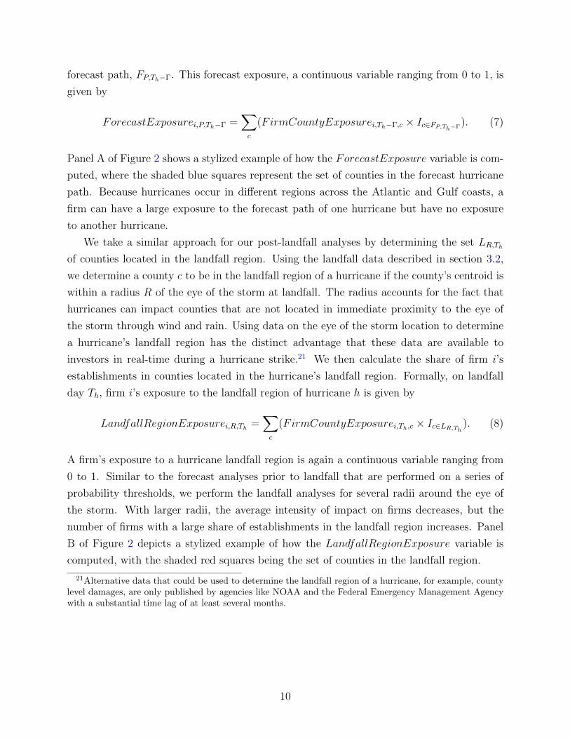
forecast path, FP,Th−Γ. This forecast exposure, a continuous variable ranging from 0 to 1, is
given by
ForecastExposurei,P,Th−Γ =∑c
(FirmCountyExposurei,Th−Γ,c × Ic∈FP,Th−Γ). (7)
Panel A of Figure 2 shows a stylized example of how the ForecastExposure variable is com-
puted, where the shaded blue squares represent the set of counties in the forecast hurricane
path. Because hurricanes occur in different regions across the Atlantic and Gulf coasts, a
firm can have a large exposure to the forecast path of one hurricane but have no exposure
to another hurricane.
We take a similar approach for our post-landfall analyses by determining the set LR,Thof counties located in the landfall region. Using the landfall data described in section 3.2,
we determine a county c to be in the landfall region of a hurricane if the county’s centroid is
within a radius R of the eye of the storm at landfall. The radius accounts for the fact that
hurricanes can impact counties that are not located in immediate proximity to the eye of
the storm through wind and rain. Using data on the eye of the storm location to determine
a hurricane’s landfall region has the distinct advantage that these data are available to
investors in real-time during a hurricane strike.21 We then calculate the share of firm i’s
establishments in counties located in the hurricane’s landfall region. Formally, on landfall
day Th, firm i’s exposure to the landfall region of hurricane h is given by
LandfallRegionExposurei,R,Th =∑c
(FirmCountyExposurei,Th,c × Ic∈LR,Th). (8)
A firm’s exposure to a hurricane landfall region is again a continuous variable ranging from
0 to 1. Similar to the forecast analyses prior to landfall that are performed on a series of
probability thresholds, we perform the landfall analyses for several radii around the eye of
the storm. With larger radii, the average intensity of impact on firms decreases, but the
number of firms with a large share of establishments in the landfall region increases. Panel
B of Figure 2 depicts a stylized example of how the LandfallRegionExposure variable is
computed, with the shaded red squares being the set of counties in the landfall region.
21Alternative data that could be used to determine the landfall region of a hurricane, for example, countylevel damages, are only published by agencies like NOAA and the Federal Emergency Management Agencywith a substantial time lag of at least several months.
10

2.3 Baseline estimation strategy
2.3.1 Incidence and impact uncertainty estimation
We employ a difference-in-differences framework to estimate the uncertainty dynamics sur-
rounding hurricanes. We separately analyze hurricane forecasts and landfalls. We jointly
estimate the treatment effect across all hurricanes, where each hurricane landfall (or forecast)
yields a separate treatment. The treatment intensity varies, because treatment is defined
continuously as exposure to the forecast path or landfall region, shown in equations (7) and
(8), respectively. Firms with zero exposure to a hurricane serve as the controls for that event.
We follow the recommendation of Bertrand, Duflo, and Mullainathan (2004) by collapsing
the time series information into a pre- and post-treatment period for each difference-in-
differences, that is, each hurricane. Panel C of Figure 2 illustrates the hurricane timeline.
The pre-treatment period is the trading day before hurricane inception, where the day of
hurricane inception is denoted T ∗h .22 For the hurricane forecast analysis, the post-treatment
period is Γ days before the landfall or dissipation date, Th. For the hurricane landfall analysis,
the post-treatment period is τ days after landfall.
We examine how hurricane forecasts affect implied volatilities of firms located in the path
of a hurricane by estimating the following firm-hurricane panel regression model
log
(IVi,Th−Γ
IVi,T ∗h−1
)= λF,P,ΓForecastExposurei,P,Th−Γ + πh + ψInd + εi,h,Γ. (9)
Here, each hurricane represents a separate time period. The dependent variable is the change
in implied volatility IVi,t of firm i from the last trading day before the inception of hurricane
h, to Γ calendar days before hurricane landfall or dissipation. Details on the IVi,t measure
are presented in Section 3.3. ForecastExposurei,P,Th−Γ is our continuous treatment variable
that ranges from 0 to 1, as defined in equation (7). We include hurricane fixed effects (πh),
which is equivalent to including time fixed effects because each hurricane enters the regression
as a separate time period. We include industry fixed effects (ψInd) based on firm two-digit
SIC numbers. Given the geographic nature of our treatment, we cluster standard errors
by the county to which the firm has the largest exposure (see Abadie, Athey, Imbens, and
Wooldridge (2017)).
We estimate the regression separately for each combination of calendar days before land-
fall Γ ∈ {1, 2, 3, 4, 5} and probability threshold P ∈ {1, 10, 20, 30, 40, 50}. Estimating the
regression for different probability thresholds allows us to empirically trace the predictions on
22The inception day of a hurricane is defined as the first day on which the hurricane is predicted to makelandfall with at least a 1 percent probability. For hurricanes before 2007, we do not have hurricane forecastdata available and choose as inception day the first day that the hurricane appeared as a tropical depression.
11

incidence and expected impact uncertainty developed by our framework and shown in Figure
1. Only storms for which the day Th − Γ is a trading day are included in a regression for a
given Γ. This means that the set of hurricanes included in the regression sample depends on
Γ and P .23 We exclude firms that have missing implied volatility estimates for more than
half of the trading days from inception to Γ days before landfall/dissipation. The time series
for these forecast regressions start in 2007, because we have hurricane wind speed forecast
data from 2007 onwards, and ends in 2017 due to the establishment data time series. In
terms of interpreting results, a positive and significant λF,P,Γ is consistent with firms in the
forecast path of a hurricane facing substantial incidence uncertainty and expected impact
uncertainty prior to landfall (as shown in equation (6)).
After landfall—when the incidence uncertainty has been fully resolved—options should
only reflect impact uncertainty. We isolate and estimate impact uncertainty by examining
the implied volatilities after landfall, when investors know where the hurricane has hit, but
do not necessarily know what the eventual impact on exposed firms will be.
We estimate impact uncertainty using the following firm-hurricane panel regression model,
where again each hurricane enters the regression as a separate time period.
log
(IVi,Th+τ
IVi,T ∗h−1
)= λL,R,τLandfallRegionExposurei,R,Th + πh + ψInd + εi,h,τ , (10)
where the dependent variable is the change in implied volatility from the day before inception
to τ trading days after landfall. LandfallRegionExposurei,R,Th is the measure defined in
equation (8) of firm i’s exposure to counties within the landfall region, which can vary from
0 to 1.24 The regression sample begins in 1996 when the option data time series starts. A
positive and significant λL,R,τ reflects impact uncertainty in the aftermath of a hurricane.
2.3.2 Testing the accuracy of volatility expectations
The question on how accurately investors price climatic event has recently received consid-
erable attention in policy discussions, because inefficient pricing of extreme weather events
is a potential financial stability concern (see Carney (2015)). Other papers analyze how effi-
ciently markets price physical climate risks by looking at food company stock returns (Hong,
23Some storms dissipate or make landfall before reaching higher probability levels in NOAA forecasts.24Because this regression is estimated up to long periods post landfall (for large values of τ), we exclude
firms that have been hit (treated) by a hurricane from the control set of other hurricanes that occur within180 calendar days to avoid distortions due to overlapping. For this purpose, we consider a firm as hit if thelandfall region exposure is at least 0.25. Varying this threshold leads to qualitatively similar results.
12

Li, and Xu (2019)) and mutual fund performance (Alok, Kumar, and Wermers (2020)).25,26
Our analysis sheds light on the accuracy of investors’ volatility expectations, which is in-
strumental for the hedging of climate risks.
To test the efficiency of the volatility expectations derived from option prices, we define
the volatility risk premium as the difference between the ex ante risk-neutral expectation
and ex post realization of return volatility and examine how this spread varies as a firm is
exposed to a hurricane. We use IVi,t,M as the proxy for the ex ante risk-neutral expected
value of the future stock return volatility of firm i between time t and M . Details on the
IVi,t,M measure are presented in Section 3.3. We use the annualized standard deviation of
the underlying stock’s daily returns between t and M as the measure of realized volatility
RVi,t,M .
V RPi,t = V RPi,t,M = IVi,t,M −RVi,t,M . (11)
Note that this definition of VRP captures the difference between ex ante market expectations
of future volatility over a period and the ex post realized volatility over the same period (not
a lagged or predicted measure of physical realized volatility). This is important because we
use our VRP measure to analyze how efficiently investors price the uncertainty associated
with hurricanes, not to predict future returns as in, for example, Bollerslev, Tauchen, and
Zhou (2009) or Della Corte, Ramadorai, and Sarno (2016).27
To analyze the effect of hurricane landfall on VRP, we estimate the regression specification
given by
V RP i,Th+τ = λV RPL,R,τLandfallRegionExposurei,R,Th + πh + Ψi + εi,h,τ , (12)
The dependent variable is the level of the VRP averaged from landfall to τ trading days after
25A different literature focuses on the pricing of a transition to a low carbon economy, as opposed tophysical climatic events (see, for example, Andersson, Bolton, and Samama (2016); Roth Tran (2019);Baker, Hollifield, and Osambela (2020); Engle, Giglio, Kelly, Lee, and Stroebel (2020); Krueger, Sautner,and Starks (2020); Ilhan, Sautner, and Vilkov (2021)). The fact that this transition has not materialized asof now makes it difficult to assess whether financial markets efficiently price this risk.
26For long-run physical risks, for example, sea level rise, assessing pricing efficiency is challenging, becausesuch risks have not yet been realized and can only be proxied for through forecasts with unknown accuracy(see Giglio, Maggiori, Rao, Stroebel, and Weber (2021); Bernstein, Gustafson, and Lewis (2019); Bakkensenand Barrage (2019); Baldauf, Garlappi, and Yannelis (2020); Murfin and Spiegel (2020)).
27The definition of volatility risk premia we use is similar in spirit to definitions of variance risk premia inBollerslev, Tauchen, and Zhou (2009); Kelly, Pastor, and Veronesi (2016) and others. For instance, Kelly,Pastor, and Veronesi (2016) effectively define the variance risk premium as EQ
t [RV 2i,t,M ] − EP
t [RV 2i,t,M ] =
IV 2i,t,M −RV 2
i,t,M because RV 2i,t,M is an unbiased estimate of the expected volatility under the physical mea-
sure. We use volatility risk premia in our empirical analysis for its intuitive interpretation, as in Della Corte,Ramadorai, and Sarno (2016).
13

landfall. Ψi is a firm fixed effect that absorbs differences in VRP levels across firms that are
unrelated to hurricanes.28 A negative (positive) estimate of λV RPL,R,τ implies a decline (increase)
in VRP and is consistent with investor underreaction (overreaction). This would represent a
systematic bias in option prices for hurricane-exposed firms compared to unexposed (control)
firms. The regression specification that estimates the effect of hurricane forecasts on the VRP
is similar to equation (12) with the independent variable of interest being the exposure to
the forecast path instead of the landfall region.
2.3.3 Expected returns and extreme weather uncertainty
Several theories assume that investors are not perfectly diversified and predict that this
underdiversification will lead to expected idiosyncratic volatility being positively related
to the expected stock returns (see Levy (1978); Merton (1987)). However, the empirical
evidence of idiosyncratic shocks to expected volatility being priced in stocks returns is mixed
with Ang, Hodrick, Xing, and Zhang (2006, 2009) finding that high idiosyncratic volatility
predicts low stock returns and Fu (2009) coming to the opposite conclusion.29 Unlike these
papers whose estimates of idiosyncratic volatility depend on a factor model that can be
subject to misspecifications, our setting allows us to exploit an exogenous and idiosyncratic
shock to a stock’s volatility, and to analyze if such a shock is priced in stock returns. Each
hurricane affects a subset of firms distributed across different industries. The vast majority
of firms will be unaffected by a specific hurricane. Moreover, the set of affected firms varies
for each hurricane.
To test how idiosyncratic shocks to a firm caused by extreme weather events are related
to expected returns, we estimate a firm-hurricane panel regression model that is similar to
the previously discussed models. The specification is given by
ExcessReturni,h,PostLandfall − ExcessReturni,h,PreInception =
λERL,RLandfallRegionExposurei,R,Th + πh + ψInd + εi,h, (13)
where LandfallRegionExposurei,R,Th is again our proxy for firm uncertainty caused by a
hurricane landfall. If a hurricane landfall leads to uncertainty and an idiosyncratic increase
in uncertainty is compensated with higher expected returns, then the estimate of λERL,R would
28Unlike with the implied volatility regression (10), it is not possible subtract the pre-inception value ofthe dependent variable in these VRP regressions because the realized volatility over the remaining life of anoption calculated on the pre-inception date, RVi,T∗
h−1,M , will include the impact of the hurricane. Includinga firm fixed effect effectively allows for the estimation of deviations from a firm’s mean VRP.
29Martin and Wagner (2019) derive excess return predictions from option prices. However, their methoddoes not capture idiosyncratic shocks to firms but the differences in firm sensitivity to market wide shocks.
14

be positive and significant.
For our baseline specification, we compute ExcessReturni,h,t as the firm’s stock return
minus the risk-free rate over a horizon of 20 trading days. This horizon is in line with
the approximately one month average time to expiry of options in our sample (see Table
2). For robustness, we also show results using a shorter (10 trading days) and a longer
(40 trading days) horizon in place of 20 trading days. The pre-inception excess returns are
computed over 20 trading days up to the last trading day before hurricane inception. The
post landfall excess returns are computed over 20 trading days starting from 5 trading days
after landfall.30 The independent variable is the exposure to a hurricane’s landfall region, as
defined in equation (8). The time period starts in 1996 and ends in 2017 to correspond to
the option sample used previously.
3 Data and summary statistics
Our analysis uses data from a range of sources. We combine NOAA data on wind speed fore-
casts and realized storm tracks with firm establishment data from the National Establishment
Time-Series (NETS) database. We obtain stock and options data from CRSP-Compustat
and OptionMetrics. We describe each of these data sources below. Additional information
on the hurricane data can be found in the Internet Appendix.
3.1 Hurricane forecasts
We use NOAA’s National Hurricane Center (NHC) wind speed probability forecasts to mea-
sure uncertainty prior to hurricane landfall. Figure 3 shows an example of the forecast chart
of cumulative probability bands for hurricane force winds, as presented by the NHC, in the
case of Hurricane Sandy in 2012. The NHC publishes hurricane forecast charts and text
advisories, both produced from the same underlying hurricane forecast models. The charts
are used in real-time by news outlets in the run-up to hurricanes and stored in NOAA’s
hurricane archives.31
We use these time-stamped text files from the NOAA website which contain the probabil-
ities that a given set of locations, for example, Norfolk, VA, will experience winds in excess of
34, 50, and 64 knots for a particular hurricane over the subsequent days. These forecasts are
updated every six hours and available starting in 2007. We obtain the forecasts just before
market close for each trading day in our analysis. Our analysis is based on the forecasts for
30The results are qualitatively similar to changing the starting point of the post landfall excess return.31The NOAA hurricane archives: https://www.nhc.noaa.gov/archive.
15

64 knots, the minimum wind speed at which a tropical storm is considered a hurricane. The
wind speed probabilities are presented up to five days out from the time of each forecast.
We translate the reported location-specific wind speed forecasts to county specific forecasts
in two steps. First, we determine the set of locations that have reported probabilities of
hurricane force winds above each probability threshold P ∈ {1, 10, 20, 30, 40, 50}, and match
these locations to counties. Second, we add counties that are within a 75 mile radius of the
counties identified in the first step.32 Figure 4 illustrates a sample of processed wind speed
data at different probability thresholds for Hurricane Sandy over a four day period. Table 1
Panel A lists the hurricanes included in our forecast sample. In the Internet Appendix, we
provide further details on how we process the hurricane forecast data.
3.2 Hurricane landfall regions
To identify hurricane landfall regions, we use hurricane track data also collected from the
NOAA hurricane archives. These data show the actual location and intensity of the hur-
ricane’s eye at various points of time. To account for the fact that hurricanes can impact
counties that are not located in immediate proximity to the eye of a storm, we consider
a county to be in the hurricane landfall region if the county’s centroid is inside a given
radius of the hurricane eye location within 24 hours before and after the hurricane makes
landfall.33,34 We generate the sets of counties that lie within 50, 100, 150, 200 miles of the
eye of each hurricane. Having the time window around the time of landfall ensures that we
capture counties that lie more inland and, for hurricanes that move along the coast before
turning inland, counties that were close to the eye of the hurricane before landfall. Figure 5
shows which counties fall within each set for the hurricanes: 2005 Katrina, 2012 Sandy, 2016
Matthew, and 2017 Harvey. Table 1 Panel B lists the hurricanes included in our landfall
region sample. We present additional details on the landfall data in the Internet Appendix.
Importantly, these data are published by NOAA in real-time. Therefore, investors have
access to the information on the landfall region of a hurricane as soon as it makes landfall.
Other papers use damaged counties to discern which firms were affected by natural disasters
(for example, Barrot and Sauvagnat (2016) and Dessaint and Matray (2017).) In our setting,
32For the 75 mile radius, our forecast data derived from NOAA’s text advisories are closely comparableto the charts published by NOAA, for example Figure 3. However, our results are robust to using otherreasonable radii.
33We also consider other time windows, for example, within 12, 36, and 48 hours before and after landfall,and the results are qualitatively similar.
34Two hurricanes in the sample, 2004 Charley and 2005 Katrina, made two landfalls in the US. To avoiddouble-counting with these two hurricanes, the date when the hurricane made landfall at a higher windspeed—corresponding to a higher storm category on the Saffir-Simpson scale—is considered the landfalldate in our analysis.
16

doing so would introduce a forward-looking bias because investors do not know at the time
of a hurricane landfall which counties will experience damage from a hurricane—this is part
of the uncertainty. County-specific damage data only become available with a substantial
lag of at least several months.
3.3 Firm establishment, option, and stock data
We use NETS firm establishment location data to precisely estimate a firm’s exposure to each
hurricane. These data have been used in several other studies.35 The NETS data contain
establishment information at the county level and are updated annually.36 For each hurricane
season, we use firm geographic footprints from the previous year to avoid the possibility that
we will miss establishments closed during the year. Because our NETS data extend only
through 2014, we use the 2014 geographic footprint for 2016 and 2017, in addition to 2015.
Figure 6 shows the number of establishments per county sorted into deciles using the NETS
data for 2010 and 2014. This map illustrates that economic activity as measured by the
density of firm establishments is high in areas exposed to hurricanes along the Atlantic and
the Gulf Coasts.
We obtain daily data on stocks from CRSP-Compustat and single-name stock options
from OptionMetrics. We use standard stock return filters.37 We use data from traded
options with non-missing pricing information in OptionMetrics that are slightly out-of-the-
money. As discussed in previous studies using stock options, such options are more liquid
and have a relatively small difference due to any potential early-exercise premium between
American versus European options (see, among others, Carr and Wu (2009); Kelly, Pastor,
and Veronesi (2016); Martin and Wagner (2019)). We apply standard filters to the options
data consistent with the existing literature. In our sample, we include single-stock options
which meet the following criteria: (i) standard settlement, (ii) a positive open interest, (iii)
a positive bid price and bid-ask spread (valid prices), (iv) the implied volatility estimate is
not missing, (v) greater than 7 days and at most 200 calendar days to expiry, and (vi) an
option delta, δ, that satisfies 0.2 ≤ |δ| ≤ 0.5. The estimate for the average implied volatility
35For example, Neumark, Wall, and Zhang (2011) investigate the job creation of small businesses basedon NETS. Addoum, Ng, and Ortiz-Bobea (2020) use NETS to analyze the effect of temperature fluctuationson firm sales.
36Our baseline results rely on the establishment location data. NETS also contains establishment-levelsales data, but these data are often imputed and not as reliable as the establishment location data. Ananalysis using sales data to compute firm exposure yield qualitatively similar results and is shown in theInternet Appendix.
37To ensure that stocks with stale prices are excluded from our analysis, a stock is required to have returndata for at least half of all trading days within the period of a particular analysis. Further, we exclude stockswith share prices below $5 (see Amihud (2002)) and micro-cap stocks, defined as stocks in the bottom 20percent in terms of market capitalization of listed equity (see Fama and French (2008)).
17

of firm i at time t is,
IVi,t = IVi,t,M =1
N
N∑j=1
IVi,j,t,M , (14)
where M is the nearest-to-maturity expiration at time t of options on firm i stock, which
satisfy the above six criteria and N is the number of valid options for firm i with that expiry.
Here, IVi,t,M proxies for the ex ante risk-neutral expected value of the future stock return
volatility of firm i between time t and M .38
We use firm name and headquarter address to link the firms in NETS to those in Option-
Metrics and CRSP-Compustat, as described in the Internet Appendix. Our linked sample
starts in 1996, the first year in our OptionMetrics data. Because financial firms’ geographic
exposure to natural disasters may not be reflected by their establishment locations and fi-
nancial firms are generally excluded in asset pricing studies, our baseline results exclude all
financial firms by dropping firms with SIC numbers from 6000 to 6799 from our analysis.
We provide a separate analysis on insurance firms in the Internet Appendix.
We report summary statistics on our sample of firms in Table 2. Panel A shows that
we have 2,509 unique firms in our sample. For comparison, we show summary statistics for
the set of firms with significant exposure to a hurricane at least once in our sample period.
A firm is included in this subsample of “hit” firms if its establishment share in the landfall
region of at least one hurricane is 0.25 or higher for a landfall region based on a 200 mile
radius around a hurricane eye. This subsample includes 1,119 firms. On average, a firm
has 113 establishments in a given year. For the subsample of hit firms, the average number
of establishments is 109. Interestingly, these hit firms are also comparable to the non-hit
firms in terms of market capitalization, with a $5.2 billion average market capitalization for
hit firms and an average of $5.0 billion for all firms. The summary statistics of the option
measures are also similar between the total sample and the subsample of hit firms. The
average (annualized) IV and VRP for all firms are 48.7 and 4.8 percent, respectively.
Panel B reports summary statistics on firm exposure to hurricane landfall regions. For
landfall regions based on the 50 and 200 mile radii around the eye of the hurricane, the average
firm establishment share in a given hurricane landfall region is 0.01 and 0.07, respectively.
These values are reasonable, as a hurricane generally only affects a few states and our sample
encompasses firms across the US. Columns five to eight show that our sample includes a large
number of firms with high shares of their establishments in hurricane landfall regions. For
example, for the 50 and 200 mile radii, we have 172 and 2,471 firm-hurricane observations,
respectively, with establishment shares in hurricane landfall regions of at least 0.25.
38This measure of IVi,t is similar to that used in Kelly, Pastor, and Veronesi (2016) for options on inter-national stock indices.
18

4 Baseline Results
4.1 Uncertainty before landfall
We first test whether option prices react to hurricane forecasts before landfall or dissipation
and price in incidence and expected impact uncertainty, as predicted by our framework. The
change in a firms’ implied volatilities should depend on the probability that a hurricane will
make landfall in counties in which the firm operates. The total sample of hurricanes used in
the analysis is listed in Table 1 Panel A. In Table 3, we report results of estimating equation
(9) for each combination of days before landfall (Γ) and hurricane-force wind probability
threshold (P ) for which we have sufficient observations.39
Each column in Table 3 presents results from a separate regression performed for the
specified Γ (1 to 5 days before landfall) and P (1 to 50 percent). Because the location-
specific NOAA wind speed probabilities rarely get high when a hurricane is far from the
coast, the maximum P for which we can estimate equation (9) declines as the number of
days to landfall or dissipation increases. Also, because for a given hurricane Th − Γ might
be a non-trading day, the sample of hurricanes differs across the columns of Table 3. For
example, not all of the 13 hurricanes with 1% probability 5 days before landfall are in the
sample for the regression for 1% probability 2 days before landfall and vice versa. For each
regression, the table reports the total number of firm observations with a forecast exposure
(share of establishments in the forecast region) greater than 0 and at least 0.2. The number
of firms with a given exposure to the forecast path decreases as the probability threshold
increases because the region covered by a higher probability is smaller, as shown in Figure
4, which illustrates the forecast data for Hurricane Sandy.
The results in Table 3 show that substantial uncertainty arises for firms in the forecast
path of a hurricane. The estimates of λF,P,Γ are always positive, regardless of whether time
and industry fixed effects are included separately (Panel A) or interacted with each other
(Panel B). The λF,P,Γ estimates are always significant with the exception of some of the
estimates at the 1% probability threshold in Panel B. For a given Γ, the magnitude of λF,P,Γ
generally increases with higher landfall probabilities, reaching up to 21.40 This implies that
a firm with all its establishments located in the path of a hurricane sees an increase in its
implied volatility of 21 percent. The results in Panels A and B show qualitatively similar
estimates. The coefficients are positive and increase with the probability threshold. The
changes to implied volatility represent substantial increases in hedging costs.
39We require a sample to include at least three hurricanes.40The results for the 30% threshold are omitted to ensure readability of the table, but they are in line
with the reported results.
19
These results show that extreme weather uncertainty is large. Option markets price
in substantial uncertainty before hurricane landfall, in line with the framework presented
in Section 2.1 that shows incidence uncertainty and expected impact uncertainty should
be priced in before hurricane landfall. The empirical estimates confirm that uncertainty
generally increases with the probability of landfall as predicted in Figure 1. Also, these
increases in implied volatilities are not driven by underlying stock price responses to expected
damage. While at the aggregate stock index level, volatility is known to increase when
returns decrease, the relationship changes at the individual stock level. Generally, at the
individual stock level, contemporaneous returns and volatility are positively correlated (see
Duffee (1995); Albuquerque (2012); Grullon, Lyandres, and Zhdanov (2012)).
These estimates of uncertainty before landfall implicitly test for investor attention to
hurricane forecasts. If investors did not pay attention to NOAA’s hurricane forecasts, then
we would not observe an option price reaction. The emerging climate finance literature
investigates investor attention to other climatic events. For example, using drought indices
and food company stock prices, Hong, Li, and Xu (2019) show that investors are inattentive
to droughts. Also, there exists mixed evidence on whether or not residential real estate
owners pay attention to sea level rise forecasts.41 In this context, the strong evidence of
investors paying attention to hurricane forecasts documented in this paper is not a given.
These climatic events are different from one another in terms of, for example, intensity and
duration, and it might be these differences that capture investors’ attention in distinct ways.
4.2 Uncertainty after landfall
We now turn to estimating uncertainty post landfall. Incidence uncertainty resolves at
hurricane landfall, and only impact uncertainty remains. In Table 4, we present results from
estimating equation (10) for 5 trading days (1 week) after landfall in Panel A and for 30
trading days (1.5 months) after landfall in Panel B. We show results from regressions for
which the landfall region is based on different radii around the eye of the storm, ranging
from 50 to 200 miles. The specifications include either separate industry and time (hurricane)
fixed effects or interacted industry and time (hurricane) fixed effects. Table 1 Panel B lists
the 33 hurricanes included in the full sample.
Table 4 Panel A shows that the λL,R,τ estimate goes up to 13 percent, and are positive
and significant across all specifications. Interestingly, while these estimates are large, they
are lower than the increases in IV right before landfall for high probabilities of landfall shown
in Table 3 (there the estimates show increases of up to 21 percent). This result of higher
41See, for example, Bernstein, Gustafson, and Lewis (2019); Giglio, Maggiori, Rao, Stroebel, and Weber(2021); Bakkensen and Barrage (2019); Baldauf, Garlappi, and Yannelis (2020); Murfin and Spiegel (2020).
20
uncertainty before landfall than after landfall is in line with our framework, which shows
that in certain scenarios the total expected variance before the realization of the extreme
weather event can exceed the total expected variance at realization (see Figure 1).
Panel B shows that even 30 trading days (1.5 months) after landfall, hurricanes yield a
large and significant increase in IV. The estimated magnitude of the effect is up to 23 percent
for the 50 mile radius. This implies that relative to its pre-inception IV level, a firm with
100 percent of its establishments in the landfall region will see its implied volatility increase
by 23 percent. These are substantial magnitudes for impact uncertainty. The magnitude of
the effect decreases with larger radii, which implies that firms with establishments located
further away from the epicenter of the storm face less impact uncertainty. Also, while
the statistical significance is stronger 5 trading days post landfall, the coefficient estimates
are often higher 30 trading days after landfall. This result points to a delayed reaction of
investors to hurricane landfall.
In Figure 7, we build on the results in Table 4 by showing how affected firms’ implied
volatilities evolve over the 100 trading days (5 months) after landfall. Each point in the
figure shows the coefficient estimate from a separate regression estimating equation (10) for
a range of trading days after landfall, τ . In Panel A, which uses a 50 mile radius around
the eye of the hurricane to determine a firm’s landfall region exposure, the estimate of λL,R,τ
increases until 30 trading days post landfall, at which point it reaches about 23 percent.
Thereafter, the implied volatility effect gradually decreases until it becomes insignificant
around 60 trading days (3 months) after landfall based on 95% confidence bands. In Panel
B, where we apply a 200 mile radius for the hurricane landfall region, we similarly observe
that the increase in implied volatility rises for some time before peaking and falling back
to baseline. The peak happens earlier at 20 trading days after landfall and has a smaller
magnitude of around 8 percent.
To assess the economic significance of these estimates, we use our regression coefficient
estimates to compute how much hedging costs increase in the aftermath of a hurricane for
investors of firms with exposure to the landfall region, if, hypothetically, investors were
to hedge 100 percent of the equity of exposed firms.42 After hurricane landfall, the total
additional cost of hedging the impact uncertainty over our sample period would have been
as high as 45 to 85 billion U.S. dollars in 2017 inflation-adjusted terms.43 This magnitude
42The higher the implied volatility of an option, all else equal, the higher the option premium, reflectingincreasing costs to hedging.
43These values are based on IV change coefficient estimates for the landfall region of 200 mile radiusaround the eye of the storm, as shown in Table 4, of 3.748 and 6.924 for 5 and 30 trading days post landfall,respectively. These estimates are transformed from log into simple changes and multiplied by the average IVlevel of the firms, 0.48, to obtain the percentage point change in IV for a fully exposed firm. This in turn ismultiplied by the average LandfallRegionExposurei,R,Th
for a firm in the landfall region, 0.14. To obtain
21

is considerable, representing up to 15 percent of the $583 billion (also inflation-adjusted to
2017) in total hurricane damages estimated by NOAA for the same time period (see Table
1).
4.3 Do investors underreact to extreme weather uncertainty?
The results in the previous sections show that investors price in substantial uncertainty before
and after a hurricane makes landfall. A question that naturally follows is how this higher
expected volatility priced in option markets compares to the subsequent realized volatility
for hurricane-hit firms. Do option markets efficiently price the effects of extreme weather on
volatility or is there evidence of underreaction?
The results of the regression specification in equation (12), which compare ex ante market
expectations of future volatility with ex post realized volatility for a firm are reported in
Table 5. Panel A shows the estimates for one day before landfall.44 The coefficient on firm
exposure to the forecast hurricane path is negative in all cases and strongly significant in
the majority of specifications. The economic significance of the coefficient estimates is also
large. The coefficient estimates imply a decrease in VRP of up to 37 percentage points for a
firm with all its establishments in the forecast path of the hurricane. Considering that the
average VRP is around 5 percent (see Table 2), the ex post realized volatility is generally
substantially larger than the ex ante expected volatility for firms in the forecast hurricane
path. Further, VRP becomes more negative—the underreaction is more pronounced—when
landfall probability increases.
Table 5 Panel B shows the effects of hurricanes on average VRP over five trading days
post landfall. In line with investors underreacting to hurricanes, the coefficient estimates are
consistently negative and strongly significant in nearly all specifications. The underreaction
is particularly strong for the firms with establishments within 50 miles of the eye of the
hurricane, which experience 8 to 19 percentage points lower VRPs.
In Figure 8, we show how long it takes for the negative VRP effect due to landfall exposure
to revert back to zero, that is, for the underreaction to resolve. The figure depicts the
estimates of λV RPL,R,τ in equation (12) with VRP averaged over five-trading-day increments post
landfall. In Panel A, the landfall region is based on a radius around the eye of the hurricane
the increase in the option premium, we multiply this average increase in implied volatility by the averagevega of the same options, $0.035, where the option vega is defined as the change in option premium for a1 percentage point change in implied volatility. Finally, we multiply the average premium increase for oneoption of an exposed firm by the total number of shares outstanding of the exposed firms (4,395.8 billion intotal for the period) to obtain the total increase in hedging costs in dollars. The values are inflation-adjustedto 2017 dollars.
44The results are qualitatively similar for two to five days before landfall.
22

of 50 miles. The negative VRP gradually reverts back to zero, but the underreaction persists
for about 2 months (40 trading days). Panel B shows a similar picture but with a faster
reversion of VRP back to 0 for the landfall region based on a 200 mile radius around the eye
of the hurricane.
While these results imply that investors underestimate the hurricanes’ impact on return
volatility, it is possible that this underreaction has diminished over time if investors have
learned to price extreme weather events more efficiently. Particularly, one could imagine
that after a salient hurricane this underreaction disappears for subsequent hurricanes. In our
sample the hurricane most likely to have had such an effect is Hurricane Sandy, which made
landfall in the New Jersey and New York area in 2012. Sandy was not only exceptionally
damaging, as reported in Table 1, but it also hit the financial center of the US, an area that
had previously been largely unaffected by hurricanes, and therefore likely increased investor
attention to hurricanes.
We test whether the negative VRP effect diminished after Hurricane Sandy by estimating
the regression in equation (12) with an additional term that interacts the landfall exposure
variable with a PostSandyh indicator that takes the value one for hurricanes from 2013
onwards. We only conduct the analysis for the post landfall data where we have a large
number of hurricanes available.45 We report the results for 5 and 30 trading days post landfall
in Table 6. The coefficient estimates on the interaction term are always positive and at least
weakly significant for the majority of the specifications. Particularly, for the landfall regions
based on 150 and 200 miles around the eye of the hurricane, where we have more treated
firms and statistical power, the coefficients are strongly significant for all 4 specifications.
The coefficients are also economically large, canceling out the negative coefficient estimate
on LandfallRegionExposure in several specifications. These results suggest that option
markets have started to price extreme weather uncertainty more efficiently. However, it
took a particular salient event for an improvement in efficiency to take place. This finding
casts doubt on whether financial markets will be able to react quickly to climate change and
efficiently price extreme weather events that are novel in terms of their intensity and where
they occur.
The Internet Appendix presents an analysis of the returns to a trading strategy that
takes on the implied volatility exposure (using delta-neutral straddles) at landfall for firms
hit by hurricanes compared to the returns to the same strategy for control firms that are
not exposed. The results are consistent with an underestimation in option prices to the
45For the forecast analysis, the number of hurricanes is as low as three for certain probability thresholdsas shown in Table 5, which does not leave sufficient observations for an analysis after dividing hurricanesinto pre- and post-Sandy.
23
uncertainty generated for firms from hurricane landfall.
4.4 Extreme weather uncertainty and expected returns
Our results in the previous sections show that hurricanes cause a significant increase in
uncertainty for exposed firms. A question that naturally follows is whether this uncertainty
leads to higher expected returns.
If a hurricane strike leads to an increase in excess returns, we would expect the estimate
of λERL,R in equation (13) to be positive and significant. We show the results in Table 7 Panel
A. The coefficient estimates are negative in all but one specification and significant in half
of the cases. These results are inconsistent with investors demanding a premium for holding
stocks exposed to higher uncertainty due to hurricanes. If anything, the results suggest that
the uncertainty surrounding the impact of the hurricane leads to negative excess returns.46
The reason for this finding could be twofold. First, the theories of Levy (1978) and Merton
(1987) may not be empirically supported, and idiosyncratic shocks to the expected volatility
of a stock lead to lower and not higher expected returns. Second, investors may fail to
correctly price the uncertainty associated with a hurricane. Our findings in Section 4.3 show
that after Hurricane Sandy, the implied volatility of option prices more accurately reflects
future realized volatility. If investors price hurricanes more accurately later in the sample, the
natural question to examine is if a similar pattern exists for the expected returns associated
with hurricane strikes.
We extend the regression model in equation (13) by adding a term that interacts our
landfall region exposure variable with an indicator that takes the value one for hurricanes
after Hurricane Sandy. We report the results in Table 7 Panel B. While the coefficient esti-
mate on LandfallRegionExposure is still negative and of a larger magnitude than in Panel
A, the coefficient estimate on LandfallRegionExposure interacted with the post-Sandy in-
dicator is always positive and significant for the majority of specifications. Interestingly, the
magnitude of the coefficient estimate is generally more than double the magnitude of the
estimate on LandfallRegionExposure. These estimates imply that the idiosyncratic shock
to a firm that comes with an exogenous event like a hurricane leads to positive expected
returns and provide empirical support for the theory of Merton (1987).
46We find similar results when analyzing exposure to the forecast path of the hurricane instead of exposureto the (realized) landfall region.
24

5 Robustness and extensions
In this section, we present several extensions and robustness tests of our main results.
5.1 Robustness
5.1.1 Firm selection
A potential concern with our specification is whether our results are driven by small firms.
However, as reported in Table 2, relative to the total sample, the subsample of firms that had
large exposure to a hurricane making landfall at least once, where we define large exposure
as having an establishment share of at least 0.25 in a landfall region, has a comparable, if
slightly higher, average market capitalization. Firms with coastal exposure can differ from
other firms based on unobserved characteristics, but for a given hurricane event, we have
coastal firms in both treated and control sets. A firm that is severely affected to one hurricane
could have zero exposure to others. As such, selection on a set of coastal firms is unlikely
to drive our results. Further, it is possible that firms that would be more vulnerable to
hurricanes because of their particular line of business avoid being exposed to the Atlantic or
Gulf Coasts. However, such sorting would bias us against finding evidence of large extreme
weather uncertainty in option markets.
5.1.2 Industry effects
One question that may arise is whether the uncertainty caused by hurricanes varies substan-
tially across industries. To answer this question, we test whether our baseline post-landfall
results are driven by a particular industry. We choose the post-landfall analysis for this
purpose because the larger number of hit firms provides a more representative sample of
firms for each industry. Building on equation (10), an industry-specific interaction term is
added as follows
log
(IVi,Th+τ
IVi,T ∗h−1
)=λL,R,τLandfallRegionExposurei,R,Th
+ ωL,R,τLandfallRegionExposurei,R,Th × Ii∈Industryg + πh + ψInd + εi,h,τ ,
(15)
where Ii∈Industryg indicates whether firm i is in Industryg, the industry being examined.
We estimate this regression separately for each industry, varying the interacted industry
indicator. Based on a firm’s two-digit SIC number, the analyzed industries are construc-
25

tion, manufacturing, mining, retail, services, transportation, and wholesale.47 If our baseline
effects were driven primarily by one industry, then we would expect λL,R,τ to be statisti-
cally indistinguishable from zero in the regression where we include an interaction with the
indicator for that industry.
In Table 8, we present our results for the 200 mile radius, a landfall region for which we
have a sufficient number of firms in each industry with a large exposure to hurricane landfall
regions.48 The parameter τ is set to five trading days. The estimates of λL,R,τ are positive
and significant in every industry specification, suggesting that our baseline results are not
driven primarily by one sector. The estimate of ωR,τ , the coefficient on the interaction term,
is insignificant for most specifications, suggesting limited industry-specific heterogeneity.
Construction is the only industry for which the estimates of ωR,τ are strongly significant
regardless of fixed effect specification. The negative sum λL,R + ωR,τ for the construction
industry suggests that investors perceive lower uncertainty for construction firms due to
hurricanes, which could reflect an expected boost from rebuilding activity.
5.1.3 Other robustness
We include several robustness tests in the Internet Appendix. In particular, we show that
our baseline results on extreme weather uncertainty before and after landfall are robust to
using county-level sales rather than establishment locations to measure firm exposure to
hurricanes. Finally, we show that our baseline results are not driven by any one particular
hurricane by showing the results are robust to excluding individual hurricanes.
5.2 Long-run impact on firm value
The resolution of the uncertainty following hurricane landfall is likely to lead to a large
cross-sectional dispersion in cumulative abnormal stock returns of hit firms. The resolution
of impact uncertainty may take time and investors may only learn over time how individual
firms are affected by exposure to a hurricane. Moreover, it is also unclear if hit firms will
only be negatively affected by the hurricane, or if some firms can profit from the opportunity
that a hurricane presents. For example, firms could benefit from rebuilding activity and an
increase in demand for their products.
We examine the cross-sectional dispersion of the cumulative abnormal stock returns of hit
firms compared to control firms. We estimate the Fama-French five-factor model (see Fama
and French (2015)) for each stock with 250 trading days (roughly one calendar year) before
47We exclude the agriculture and non-classified categories because of the small number of firms.48The results are qualitatively similar when using smaller radii.
26

the inception day of the hurricane. The coefficient estimates from this first stage regression
are then used to compute abnormal returns for each firm and hurricane as follows:
rai,d = ri,d − (α̂i + β̂1,irm,d + β̂2,irsmb,d + β̂3,irhml,d + β̂4,irrmw,d + β̂5,ircma,d). (16)
We next aggregate the abnormal returns to a cumulative abnormal return from inception to
τ trading days after landfall, raci,T ∗h :Th+τ .
49
Importantly, here we aggregate the cumulative returns from hurricane inception, based on
the initial stock price before the hurricane existed. In Section 4.4, we estimate the hurricane’s
effect on expected returns by analyzing how the hurricane is priced as it evolves.
To account for market shocks that coincide with but are independent of a given hurricane,
we take the cumulative abnormal return for a given firm i and hurricane h and subtract
the mean cumulative abnormal return across all stocks for the concurrent period of the
hurricane. We split the firm-hurricane observations into two groups. One group contains the
cumulative abnormal returns of the hit firms, that is, the firms with at least 25 percent of their
establishments in the hurricane landfall region. The other group contains the cumulative
abnormal returns of the control firms, that is, firms with less than 25 percent establishment
exposure. Then, we compute the differences in percentiles between the cumulative abnormal
return distributions of the hit and control firms across all the hurricanes. We run this analysis
separately for different τ from 5 to 120 trading days (6 months) after landfall.50
We illustrate the results for the 200 mile landfall region in Figure 9.51 At the short
horizons of τ=5 trading days after landfall, the cumulative returns from inception of hit
and control firms are not significantly different across the distribution. After τ=10 trading
days, the larger return dispersion of the hit firms is visible at the left tail of the distribution.
At longer horizons of τ=60 and τ=120 trading days, the hit firms have a substantially
larger dispersion of their returns, in line with the higher realized volatility. Interestingly,
the dispersion is not only driven by the left tail of the distribution. High performing hit
firms have higher abnormal returns than high performing control firms. By 120 trading days
post-landfall, the differences of the hit and control firms’ return distributions are -8.9 and
-7.4 percentage points and strongly significant for the 5th and 10th percentile, respectively.
However, for the 90th and 95th percentiles, the differences are 5.5 and 12.3 percentage points,
respectively, and also strongly significant.
There are numerous reasons why firms in the landfall region might outperform the control
49The results are qualitatively similar when simply using excess returns instead of abnormal returns.50We choose a horizon of 120 trading days as that corresponds to half a calendar year. The hurricane
season lasts half a calendar year (from June to November), and thus, we avoid overlaps with the subsequentyear’s hurricane season.
51Results for other radii are shown in the Internet Appendix.
27

firms. For example, firms could benefit from rebuilding activity, struggling competitors,
population migrations, or generous disaster aid. While other papers find small mean return
effects of hurricanes and natural disasters (see, for example, Barrot and Sauvagnat (2016);
Dessaint and Matray (2017); Lanfear, Lioui, and Siebert (2019)), we find that focusing on
mean returns ignores the large differences in the cross-sectional dispersion of returns.
5.3 Hurricane season effects
Hurricanes off the US Atlantic and Gulf coasts generally occur during the hurricane season
which starts in June and ends in November. The hurricane season could consistently increase
uncertainty and be priced in options. However, because the timing of the hurricane season
does not vary from year-to-year, it is challenging to disentangle hurricane season effects from
other seasonal effects that are unrelated to hurricanes but also affect firms with establish-
ments in coastal locations. Because of that, we use variation in NOAA’s hurricane season
outlooks to estimate the effect of the hurricane season on uncertainty.
NOAA releases hurricane seasonal outlooks in May of each year. Dating back to 2001,
each seasonal outlook reports the probability that the season will be above-normal, near-
normal, or below-normal.52 Panel A of Figure A.1 shows that there is significant variation
in the probabilities reported in these pre-season outlooks.
Examining options with a longer time to expiration than in our baseline analyses (120
to 210 calendar days to expiry), we test if the options of firms that have establishments
located in counties historically affected by hurricanes exhibit higher implied volatilities af-
ter NOAA issues a forecast of a hurricane season with above-normal activity. We choose
options with a longer expiry because they cover the majority of the hurricane season.
We use two methods to determine which counties could be hit by a hurricane during
the hurricane season and construct firm-level variables capturing exposure to a hurricane
season. First we use coastal counties from the Atlantic and Gulf coasts as the set of
counties that could reasonably be exposed to a hurricane in any given hurricane season
(CoastalExposurei,Ts). Second, we use historical landfall regions over the preceding 30
years to compute the annual probability with which a county ends up in the landfall region
of a hurricane (HistoricalHurricaneExposurei,Ts). In the Internet Appendix, we provide
further detail on the counties included in each method.
52See National Weather Service “NOAA 2012 Atlantic Hurricane Season Outlook” https://www.cpc.ncep.noaa.gov/products/outlooks/hurricane2012/May/hurricane.shtml for an example.
28

For the first method, the regression specification is given by
log
(IVi,Ts+5
IVi,Ts−1
)=λS,1CoastalExposurei,Ts
+ λS,2CoastalExposurei,Ts ×AboveNormalSeasonProbTs+ πTs + ψInd + εi,Ts , (17)
where Ts−1 is the last trading day before NOAA’s hurricane season outlook is announced
in May, and Ts+5 occurs 5 trading days later.53 The regression jointly estimates the effect
of the seasonal outlooks for the years 2001 to 2017. Following the methodology in equations
(7) and (8), CoastalExposurei,Ts is a variable that ranges from 0 to 1 and measures the
share of establishments of firm i located in counties along the Atlantic and Gulf coast.
Under the second method of measuring seasonal exposure, we replace CoastalExposurei,Ts
in equation (17) with HistoricalHurricaneExposurei,Ts , which measures the share of a
firm’s establishments located in counties with an elevated probability of being hit during a
hurricane season. The variable AboveNormalSeasonProbs is the probability NOAA issues
in May of a given year for an above-normal hurricane season. A positive estimate of λS,2
would be consistent with investor attention to medium-term seasonal forecasts and imply
heightened uncertainty if the probability of an above-normal season is high.
Table A.1 presents the estimates of equation (17). Panel A shows the results for the spec-
ification using CoastalExposurei,Ts , and Panel B uses HistoricalHurricaneExposurei,Ts .
Across both panels, none of the estimates of λS,2 are statistically significant, and some of
the point estimates even have a negative sign. Thus, we find no support for the hypothesis
that implied volatility increases for exposed firms when NOAA’s hurricane season outlook
reports a high probability of an above-normal season.54
Our results in Section 4.1 established that investors pay close attention to NOAA’s fore-
cast of hurricane paths. What might explain investors not paying attention to seasonal
forecasts? This could result from NOAA’s seasonal forecasts being less predictive of damag-
ing hurricanes making landfall on the Atlantic and Gulf coasts. The scatter plots in Figure
A.1 Panel B show only a weakly positive relationship between the seasonal outlooks and the
number of hurricanes making landfall in a given year. Another potential explanation is that
investors pay no attention to seasonal forecasts because they are medium term and lack the
immediacy of the hurricane path forecasts. Distinguishing between these two explanations
53Varying the window length leads to qualitatively similar results.54The coefficient estimate of λS,1 is positive and marginally significant for some specifications. A possible
explanation is that the saliency of any up coming hurricane season leads to a general increase in uncertaintyin May for firms with establishments located along the Atlantic and Gulf coasts. However, the significanceof the λS,1 estimate is weak and not robust to alternative specifications.
29

is not feasible with the available data.
5.4 Other extensions
The Internet Appendix contains additional analyses. First, while the analyses in this paper
focus on the universe of firms excluding financials, we conduct a similar analysis on stock
options of property and casualty insurance firms and find even larger estimates of extreme
weather uncertainty. Second, in an analysis on option trading volume and open interest, we
find that volume decreases right before landfall, in line with findings that investors refrain
from trading when uncertainty is high (see Easley and O’Hara (2010)). Post landfall, we find
that open interest increases, consistent with an increase in hedging activity (see Hong and
Yogo (2012)). Finally, we analyze the returns to a trading strategy that takes on the implied
volatility exposure of stock options at landfall (using delta-neutral straddles held till expiry)
for firms hit by a hurricane, compared to the returns to the same strategy for control firms
that are not exposed to the hurricane. The results are consistent with an underestimation
in option prices to the uncertainty generated for firms from hurricane landfall.
6 Conclusion
This paper fills a gap in the literature on the uncertainty faced by firms due to extreme
weather. We present a framework that distinguishes between incidence uncertainty (on where
an extreme weather event will occur, if at all) and impact uncertainty (on the consequences to
the local firms and economy following the extreme weather event). We isolate and estimate
extreme weather uncertainty, assess how efficiently extreme weather uncertainty is priced in
option markets, and analyze if investors are compensated for extreme weather uncertainty
with higher expected stock returns.
Using daily hurricane forecasts from NOAA, we find that both incidence uncertainty and
expected impact uncertainty are reflected in option prices before a hurricane makes land-
fall, consistent with our framework. We also show that options of firms operating in regions
affected by hurricanes have considerably higher implied volatility after hurricanes hit, imply-
ing substantial impact uncertainty. The impact uncertainty resolves slowly, and the implied
volatilities return to pre-hurricane levels only several months after landfall. This finding of
significant and prolonged increases to uncertainty for firms hit by hurricanes suggests that
firms are not fully insured or that there is uncertainty regarding the extent to which firms
are insured against such events.
Despite these large increases in the expectations of volatility implied in option markets,
30

we find that investors underestimate a hurricane’s impact on the eventual realized return
volatility of hit firms. After Hurricane Sandy in 2012, the ex ante expectations of future
volatility embedded in the option prices of hit firms are closer to the ex post realized volatility,
suggesting that option markets have improved the efficiency with which they price extreme
weather events. When analyzing expected stock returns following a hurricane strike, we find
further evidence that the efficiency with which markets price hurricane strikes improved later
in the sample. Merton (1987) predicts idiosyncratic shocks to expected volatility of a stock
are compensated with higher expected stock returns. Our results show that while hurricanes
did not cause higher expected returns for hit firms over the whole sample, post Hurricane
Sandy, the expected returns of hit firms are indeed positive in the aftermath of a hurricane
landfall.
Our novel analysis and framework contribute to a nascent climate finance literature that
examines how efficiently financial markets price climatic events. Also, we add to the uncer-
tainty literature by introducing a novel type of uncertainty and showing how idiosyncratic
shocks to firms’ uncertainty are priced. Our results suggest that markets need time to learn
how to price extreme weather events and are unlikely to efficiently price novel climate risks
stemming from climate change.
One potential method to reduce uncertainty associated with extreme weather events and
increase pricing efficiency could be better firm disclosures of exposure to extreme weather
events and associated hedging and insurance decisions. Future research could apply our
framework and methodology to examine uncertainty resulting from other types of extreme
weather events and shed more light on the link between extreme weather uncertainty and
real economic activity.
31

References
Abadie, Alberto, Susan Athey, Guido W. Imbens, and Jeffrey Wooldridge, 2017, When
should you adjust standard errors for clustering?, Working Paper.
Addoum, Jawad M., David Ng, and Ariel Ortiz-Bobea, 2020, Temperature shocks and es-
tablishment sales, Review of Financial Studies 33, 1331–1366.
Albuquerque, Rui, 2012, Skewness in stock returns: Reconciling the evidence on firm versus
aggregate returns, Review of Financial Studies 25, 1630–1673.
Alok, Shashwat, Nitin Kumar, and Russ Wermers, 2020, Do fund managers misestimate
climatic disaster risk?, Review of Financial Studies 33, 1146–1183.
Amihud, Yakov, 2002, Illiquidity and stock returns: Cross-section and time-series effects,
Journal of Financial Markets 5, 31–56.
Andersson, Mats, Patrick Bolton, and Frederic Samama, 2016, Hedging climate risk, Finan-
cial Analysts Journal 72, 13–32.
Ang, Andrew, Robert J Hodrick, Yuhang Xing, and Xiaoyan Zhang, 2006, The cross-section
of volatility and expected returns, Journal of Finance 61, 259–299.
, 2009, High idiosyncratic volatility and low returns: International and further us
evidence, Journal of Financial Economics 91, 1–23.
Baker, Steven D., Burton Hollifield, and Emilio Osambela, 2020, Asset prices and portfolios
with externalities, Working Paper.
Baker, Scott R., Nicholas Bloom, and Steven J. Davis, 2016, Measuring economic policy
uncertainty, Quarterly Journal of Economics 131, 1593–1636.
Bakkensen, Laura, and Lint Barrage, 2019, Flood risk belief heterogeneity and coastal home
price dynamics: Going under water?, Working Paper.
Baldauf, Markus, Lorenzo Garlappi, and Constantine Yannelis, 2020, Does climate change
affect real estate prices? only if you believe in it, Review of Financial Studies 33, 1256–
1295.
Barrot, Jean-Noel, and Julien Sauvagnat, 2016, Input specificity and the propagation of
idiosyncratic shocks in production networks, Quarterly Journal of Economics 131, 1543–
1592.
32

Bernstein, Asaf, Matthew Gustafson, and Ryan Lewis, 2019, Disaster on the horizon: The
price effect of sea level rise, Journal of Financial Economics 134, 253–272.
Bertrand, Marianne, Esther Duflo, and Sendhil Mullainathan, 2004, How much should we
trust differences-in-differences estimates?, Quarterly Journal of Economics 119, 249–275.
Bloom, Nicholas, 2009, The impact of uncertainty shocks, Econometrica 77, 623–685.
Bollerslev, T., G. Tauchen, and H. Zhou, 2009, Expected stock returns and variance risk
premia, Review of Financial Studies 22, 4463–4492.
Carney, Mark, 2015, Breaking the tragedy of the horizon - climate change and financial
stability, Speech given at Lloyd’s of London (29 September).
Carr, P., and L. Wu, 2009, Variance risk premiums, Review of Financial Studies 22, 1311–
1341.
Della Corte, Pasquale, Tarun Ramadorai, and Lucio Sarno, 2016, Volatility risk premia and
exchange rate predictability, Journal of Financial Economics 120, 21–40.
Dessaint, Olivier, and Adrien Matray, 2017, Do managers overreact to salient risks? Evidence
from hurricane strikes, Journal of Financial Economics 126, 97–121.
Dew-Becker, Ian, Stefano Giglio, Anh Le, and Marius Rodriguez, 2017, The price of variance
risk, Journal of Financial Economics 123, 225–250.
Duffee, Gregory R, 1995, Stock returns and volatility a firm-level analysis, Journal of Fi-
nancial Economics 37, 399–420.
Easley, David, and Maureen O’Hara, 2010, Liquidity and valuation in an uncertain world,
Journal of Financial Economics 97, 1–11.
Engle, Robert, Stefano Giglio, Bryan Kelly, Heebum Lee, and Johannes Stroebel, 2020,
Hedging climate change news, Review of Financial Studies 33, 1184–1216.
Fama, Eugene F., and Kenneth R. French, 2008, Dissecting anomalies, Journal of Finance
63, 1653–1678.
, 2015, A five-factor asset pricing model, Journal of Financial Economics 116, 1–22.
Fu, Fangjian, 2009, Idiosyncratic risk and the cross-section of expected stock returns, Journal
of Financial Economics 91, 24–37.
33

Giglio, Stefano, Matteo Maggiori, Krishna Rao, Johannes Stroebel, and Andreas Weber,
2021, Climate change and long-run discount rate: Evidence from real estate, Review of
Financial Studies Forthcoming.
Grullon, Gustavo, Evgeny Lyandres, and Alexei Zhdanov, 2012, Real options, volatility, and
stock returns, Journal of Finance 67, 1499–1537.
Hassan, Tarek A, Stephan Hollander, Laurence Van Lent, and Ahmed Tahoun, 2019, Firm-
level political risk: Measurement and effects, The Quarterly Journal of Economics 134,
2135–2202.
Hong, Harrison, Frank W. Li, and Jiangmin Xu, 2019, Climate risks and market efficiency,
Journal of Econometrics 208, 265–281.
Hong, Harrison, and Motohiro Yogo, 2012, What does futures market interest tell us about
the macroeconomy and asset prices?, Journal of Financial Economics 105, 473–490.
Ilhan, Emirhan, Zacharias Sautner, and Grigory Vilkov, 2021, Carbon tail risk, Review of
Financial Studies 34, 1540–1571.
Jens, Candace E., 2017, Political uncertainty and investment: Causal evidence from U.S.
gubernatorial elections, Journal of Financial Economics 124, 563–579.
Julio, Brandon, and Youngsuk Yook, 2012, Political uncertainty and corporate investment
cycles, Journal of Finance 67, 45–83.
Jurado, Kyle, Sydney C. Ludvigson, and Serena Ng, 2015, Measuring uncertainty, American
Economic Review 105, 1177–1216.
Kelly, Bryan, Lubos Pastor, and Pietro Veronesi, 2016, The price of political uncertainty:
Theory and evidence from the option market, Journal of Finance 71, 2417–2480.
Krueger, Philipp, Zacharias Sautner, and Laura T Starks, 2020, The importance of climate
risks for institutional investors, Review of Financial Studies 33, 1067–1111.
Lanfear, Matthew G., Abraham Lioui, and Mark G. Siebert, 2019, Market anomalies and
disaster risk: Evidence from extreme weather events, Journal of Financial Markets 46,
1–29.
Levy, Haim, 1978, Equilibrium in an imperfect market: A constraint on the number of
securities in theportfolio, American Economic Review 68, 643–658.
34

Martin, Ian W.R., and Christian Wagner, 2019, What is the expected return on a stock?,
The Journal of Finance 74, 1887–1929.
Merton, Robert C., 1987, A simple model of capital market equilibrium with incomplete
information, Journal of Finance 42, 483–510.
Murfin, Justin, and Matthew Spiegel, 2020, Is the risk of sea level rise capitalized in residen-
tial real estate?, Review of Financial Studies 33, 1217–1255.
Neumark, David, Brandon Wall, and Junfu Zhang, 2011, Do small businesses create more
jobs? New evidence for the united states from the national establishment time series,
Review of Economics and Statistics 93, 16–29.
Pastor, Lubos, and Pietro Veronesi, 2012, Uncertainty about government policy and stock
prices, Journal of Finance 67, 1219–1264.
, 2013, Political uncertainty and risk premia, Journal of Financial Economics 110,
520–545.
Roth Tran, Brigitte, 2019, Divest, disregard, or double down? Philanthropic endowment
investments in objectionable firms, American Economic Review: Insights 2, 241–256.
35
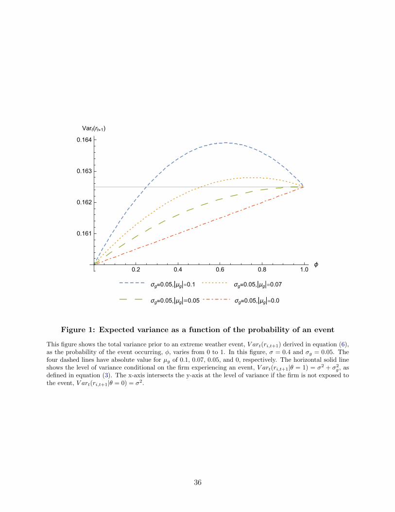
0.2 0.4 0.6 0.8 1.0ϕ
0.161
0.162
0.163
0.164
Vart(rt+1)
σg=0.05,|μg|=0.1 σg=0.05,|μg|=0.07
σg=0.05,|μg|=0.05 σg=0.05,|μg|=0.0
Figure 1: Expected variance as a function of the probability of an event
This figure shows the total variance prior to an extreme weather event, V art(ri,t+1) derived in equation (6),as the probability of the event occurring, φ, varies from 0 to 1. In this figure, σ = 0.4 and σg = 0.05. Thefour dashed lines have absolute value for µg of 0.1, 0.07, 0.05, and 0, respectively. The horizontal solid lineshows the level of variance conditional on the firm experiencing an event, V art(ri,t+1|θ = 1) = σ2 + σ2
g , asdefined in equation (3). The x-axis intersects the y-axis at the level of variance if the firm is not exposed tothe event, V art(ri,t+1|θ = 0) = σ2.
36

(a) Stylized example of firm exposure to hurricane forecast
(b) Stylized example of firm exposure to hurricane landfall region
(c) Hurricane timeline
Figure 2: Identification strategy
Panel A shows a stylized example of firm exposure to a hurricane forecast based on the share of establishmentslocated in counties in the forecast path. These firm exposures illustrate the variable ForecastExposure inour analysis. Panel B shows a stylized example of firm exposure to a hurricane landfall region based on theshare of establishments located in counties in the landfall region. These firm exposures illustrate the variableLandfallRegionExposure in our analysis. Panel C illustrates the timeline of a hurricane.
37

Figure 3: Example of a hurricane forecast
This figure from NOAA illustrates the five-day forecast for Hurricane Sandy on October 27, 2012. We obtainand process the raw data underpinning such hurricane forecast visualizations for our analysis.
38

4 days before landfall
3 days before landfall
2 days before landfall
1 day before landfall
≥1% ≥10% ≥20% ≥50%
Figure 4: Hurricane forecasts at different time frames and wind speed probabilitythresholdsThis figure presents an example of the processed forecast data used in the paper. Each map shows thecounties indicated as being in the forecast path for Hurricane Sandy given the number of days before landfallin each row and the wind speed probability threshold in each column. For each day, the last available forecastbefore 4pm (market close) is shown.
39

(a) 2005 Katrina (b) 2012 Sandy
(c) 2016 Matthew (d) 2017 Harvey
Figure 5: Counties in a hurricane landfall region
This figure highlights the counties that are within 50, 100, 150, and 200 miles of the eye of the hurricane atlandfall for four selected hurricanes from our sample of 33 hurricane landfalls.
40

0.0 2.5 5.0 7.5 10.0
(a) Year 2010
0.0 2.5 5.0 7.5 10.0
(b) Year 2014
Figure 6: Firm establishments by county
This figure plots counties based on the number of establishments located in that county for the years 2010(Panel A) and 2014 (Panel B). Data are from the National Establishment Time Series and only firms in oursample included. The counties are sorted into deciles based on the number of establishments.
41

0
20
40
0 10 20 30 40 50 60 70 80 90 100Trading days after landfall
Per
cent
cha
nge
in im
plie
d vo
latil
ity
(a) 50 mile radius around eye of hurricane
0
4
8
12
0 10 20 30 40 50 60 70 80 90 100Trading days after landfall
Per
cent
cha
nge
in im
plie
d vo
latil
ity
(b) 200 mile radius around eye of hurricane
Figure 7: Changes in implied volatilities post hurricane landfall
This figure plots coefficient estimates from running separate regressions with the specification (10) varyingthe number of tradings days after landfall. Changes in implied volatilities from inception of the hurricane toup to 100 trading days (5 months) post hurricane landfall are regressed on the landfall region establishmentshare of firms. A coefficient estimate of, for example, 20 means that a firm with all of its establishments inthe landfall region is estimated to experience a 20% increase in the implied volatility. The landfall region isbased on a 50 mile radius around the eye of the hurricane in Panel A and 200 mile radius around the eye ofthe hurricane in Panel B. Confidence bands of 95% are shown.
42

−40
−30
−20
−10
0
0 10 20 30 40 50Trading days after landfall
Per
cent
age
poin
t cha
nge
in V
RP
(a) 50 mile radius around eye of hurricane
−5
0
0 10 20 30 40 50Trading days after landfall
Per
cent
age
poin
t cha
nge
in V
RP
(b) 200 mile radius around eye of hurricane
Figure 8: Changes in volatility risk premium post hurricane landfall
This figure plots coefficient estimates from running separate regressions with the specification (12) varyingthe number of tradings days after landfall. A coefficient estimate of, for example, -10 means that a firm withall of its establishments in the landfall region is estimated to have a 10 percentage points lower VRP thanthe control firms. The landfall region is based on a 50 mile radius around the eye of the hurricane in PanelA and 200 mile radius around the eye of the hurricane in Panel B. Confidence bands of 95% are shown. TheVRP is the difference between ex ante expected and ex post realized volatility as shown in equation (11).
43

−10
0
10
20
10 20 30 40 50 60 70 80 90Percentile
Diff
. in
cum
. abn
orm
al r
etur
ns
(a) 5 trading days (1 week) post landfall
−10
0
10
20
10 20 30 40 50 60 70 80 90Percentile
Diff
. in
cum
. abn
orm
al r
etur
ns
(b) 10 trading days (2 weeks) post landfall
−10
0
10
20
10 20 30 40 50 60 70 80 90Percentile
Diff
. in
cum
. abn
orm
al r
etur
ns
(c) 60 trading days (3 months) post landfall
−10
0
10
20
10 20 30 40 50 60 70 80 90Percentile
Diff
. in
cum
. abn
orm
al r
etur
ns
(d) 120 trading days (6 months) post landfall
Figure 9: Differences in cumulative abnormal returns between hit and controlfirms
This figure plots the difference in cumulative abnormal returns between firms with at least 25% of theirestablishments in the landfall region of a hurricane (the hit firms) and firms with less than 25% of theirestablishments in the landfall region (the control firms), as described in Section 5.2. The differences betweenpercentiles of the two return distributions (hit and control) are shown. The cumulative abnormal returns arecomputed from hurricane inception up to 5, 10, 60, and 120 trading days (1 week, 2 weeks, 3 months, and 6months) post landfall. The landfall region is based on 200 miles around the eye of the hurricane. Confidencebands of 95% are shown.
44

Table 1: Hurricane sample
This table shows the hurricanes included in our analyses. Panel A reports the sample for the forecastanalyses, which includes storms that were at least once forecast to make landfall with hurricane force windswith a 1% probability or more. Because the forecasts include storms that never make landfall in the U.S.,we indicate storms that make landfall with asterisks (*). The forecast sample is from 2007 to 2017. PanelB shows the landfall and inception dates for storms that are included in the post-landfall analyses. Thedamage estimates shown come from the National Hurricane Center’s Tropical Cyclone Reports and havebeen inflated to 2017 values using the consumer price index from the U.S. Census Bureau. Landfall datescome from the Tropical Cyclone Reports. The landfall sample is from 1996 to 2017.
Panel A: Hurricanes included in forecast analyses
2007 2008 2009 2010 2011 2012 2013 2014 2015 2016 2017
Dean Dolly* Ana Alex Don Debby Andrea Arthur* Ana Colin Harvey*Humb.* Edouard Bill Bonnie Emily Isaac* Karen Erika Herm.* Irma*Noel Fay Danny Earl Irene* Leslie Joaquin Matt.* Jose
Gustav* Ida Paula Nate Sandy* MariaHanna Nate*Ike*KylePaloma
Panel B: Hurricanes included in post-landfall analyses
Post-landfall analysis only Forecast and post-landfall analyses
Damages DamagesHurricane Landfall Inception 2017 $mn Hurricane Landfall Inception 2017 $mn
Bertha Jul. 12, 96 Jul. 5, 96 421 Humberto Sep. 13, 07 Sep. 13, 07 N/AFran Sep. 6, 96 Aug. 23, 96 4,994 Dolly Jul. 23, 08 Jul. 20, 08 1,198Danny Jul. 18, 97 Jul. 16, 97 153 Gustav Sep. 1, 08 Aug. 25, 08 5,271Bonnie Aug. 27, 98 Aug. 19, 98 1,085 Ike Sep. 13, 08 Sep. 2, 08 33,692Earl Sep. 3, 98 Aug. 31, 98 119 Irene Aug. 27, 11 Aug. 21, 11 17,258Georges Sep. 28, 98 Sep. 15, 98 9,594 Isaac Aug. 29, 12 Aug. 22, 12 2,514Bret Aug. 23, 99 Aug. 18, 99 89 Sandy Oct. 30, 12 Oct. 24, 12 53,481Floyd Sep. 16, 99 Sep. 7, 99 10,184 Arthur Jul. 4, 14 Jul. 1, 14 2Irene Oct. 15, 99 Oct. 13, 99 1,181 Hermine Sep. 2, 16 Sep. 1, 16 562Lili Oct. 3, 02 Sep. 21, 02 1,264 Matthew Oct. 8, 16 Sep. 30, 16 10,215Claudette Jul. 15, 03 Jul. 8, 03 240 Harvey Aug. 26, 17 Aug. 23, 17 125,000Isabel Sep. 18, 03 Sep. 6, 03 7,175 Irma Sep. 10, 17 Sep. 4, 17 50,000Charley Aug. 13, 04 Aug. 9, 04 19,661 Nate Oct. 8, 17 Oct. 5, 17 225Frances Sep. 5, 04 Aug. 25, 04 12,368Ivan Sep. 16, 04 Sep. 2, 04 24,483Jeanne Sep. 26, 04 Sep. 13, 04 9,965Dennis Jul. 10, 05 Jul. 4, 05 3,202Katrina Aug. 29, 05 Aug. 23, 05 135,894Rita Sep. 24, 05 Sep. 18, 05 15,146Wilma Oct. 24, 05 Oct. 15, 05 26,433
45

Tab
le2:
Fir
mest
abli
shm
ent
and
opti
on
sum
mary
stati
stic
s
Th
ista
ble
rep
orts
the
sum
mar
yst
atis
tics
onth
efi
rms
incl
ud
edin
ou
rsa
mp
le.
Th
esa
mp
leis
from
1996
to2017.
InP
an
elA
rep
ort
sst
ati
stic
sfo
ral
lfi
rms
and
asu
bsa
mp
leof
“hit
”fi
rms.
Hit
firm
sh
ad
at
least
on
cean
esta
bli
shm
ent
share
of
0.2
5or
more
ina
hu
rric
an
ela
nd
fall
regio
n(u
sin
g200
mil
era
diu
sar
oun
dth
eey
eof
the
hu
rric
ane)
.E
stab
lish
men
tsd
ata
are
at
an
an
nu
al
freq
uen
cy;
mark
etca
pit
aliza
tion
at
aqu
art
erly
freq
uen
cy;
an
dall
opti
ons
dat
aar
eat
ad
aily
freq
uen
cy.
Imp
lied
and
reali
zed
vola
tili
tyle
vels
are
an
nu
ali
zed
.P
an
elB
rep
ort
ssu
mm
ary
stati
stic
son
firm
s’es
tab
lish
men
tsh
ares
inhu
rric
ane
lan
dfa
llre
gion
s.T
he
last
fou
rco
lum
ns
show
the
tota
lnu
mb
erof
firm
obse
rvati
on
sw
ith
an
esta
bli
shm
ent
share
that
exce
eds
agi
ven
thre
shold
for
lan
dfa
llre
gion
sbase
don
agiv
enra
diu
saro
un
dth
eey
eof
ahu
rric
an
e.
Pan
elA
:F
irm
char
acte
rist
ics
Nu
mb
erof
un
iqu
efi
rms
2,5
09
Nu
mb
erof
un
iqu
eh
itfi
rms
1,1
19
Avg.
Std
.d
ev.
10
thp
erce
nti
le25
thp
erce
nti
le50
thp
erce
nti
le75
thp
erce
nti
le90
thp
erce
nti
le
Est
abli
shm
ents
113
.304
422.6
32
1.0
002.
000
10.0
00
51.0
00218.
000
Est
abli
shm
ents
hit
firm
s109
.137
382.6
32
1.0
00
3.000
12.0
00
55.0
00
219.
000
Mark
etca
p.
(in
bil
lion
$)5.0
12
22.1
35
0.0
78
0.223
0.7
12
2.3
998.
219
Mark
etca
p.
hit
firm
s(i
nb
illi
on
$)5.2
0920.6
72
0.0
97
0.279
0.8
56
2.8
439.
541
IVi,t
(in
%)
48.7
3427.7
50
22.3
93
29.9
98
41.
792
59.9
42
83.
382
IVi,t
hit
firm
s(i
n%
)47.7
0826.
645
22.
254
29.6
97
41.0
9158.6
32
81.2
06
VRPi,t
(in
%)
4.824
21.5
53-1
3.6
28-2
.330
5.3
60
13.3
92
23.
954
VRPi,t
hit
firm
s(i
n%
)4.
562
21.0
95
-13.6
42
-2.3
86
5.2
36
13.1
11
23.
334
log(IVi,t/IVi,t−
1)
(in
%)
0.1
29
11.
373
-9.7
17
-3.9
05
0.0
38
4.148
10.2
76
log(IVi,t/IVi,t−
1)
hit
firm
s(i
n%
)0.1
2711.
065
-9.5
26
-3.8
50
0.0
28
4.068
10.0
81
Day
sto
exp
iryi,t
36.
374
32.5
0610
.000
17.0
00
26.0
00
38.
000
81.0
00
Day
sto
exp
iryi,t
hit
firm
s35
.447
31.
408
10.
000
17.0
00
26.0
0038.0
00
78.0
00
Tot
al
open
inte
resti,t
2,117.3
418,2
84.
665
13.0
00
50.0
00237.
000
1,1
65.0
00
4,5
01.
000
Tot
al
open
inte
resti,t
hit
firm
s1,
958.8
526,8
25.
444
14.0
00
53.
000
245.
000
1,1
83.0
00
4,4
79.
000
Pan
elB
:F
irm
obse
rvat
ion
cou
nts
and
esta
bli
shm
ent
shar
es(0
to1)
inhu
rric
an
ela
nd
fall
regi
on
Tot
alfi
rmob
serv
ati
ons
wit
hla
nd
fall
regio
nes
tab
.sh
are≥x
Nu
mb
erof
Avg.
firm
SD
firm
Est
ab.
share
Est
ab
.sh
are
Est
ab.
shar
eE
stab
.sh
are
Rad
ius
arou
nd
eye
ofth
ehu
rric
an
ehu
rric
an
eses
tab
.sh
are
esta
b.
share
≥0.1
≥0.2
5≥
0.5
0=
1
50
mil
es33
0.0
08
0.0
43
504
172
64
27100
mil
es33
0.0
27
0.0
84
2,122
742
288
84
150
mil
es33
0.0
48
0.1
18
4,367
1,5
38
619
183
200
mil
es33
0.0
71
0.1
46
6,995
2,4
71
976
298
46

Table
3:
Fore
cast
hurr
icane
path
and
impli
ed
vola
tili
ty
Th
ista
ble
rep
orts
the
coeffi
cien
tsan
dte
stst
atis
tics
wh
enes
tim
ati
ng
the
firm
-hu
rric
an
ep
an
elm
od
elin
equ
ati
on
(9).
Th
em
od
elis
esti
mate
dfo
rd
iffer
ent
pro
bab
ilit
ies
ofla
nd
fall
and
day
sb
efor
ela
nd
fall
or
dis
sip
ati
on
,Γ
.T
he
dep
end
ent
vari
ab
leis
the
chan
ge
(in
%)
inth
eim
pli
edvo
lati
lity
of
firm
ifr
omth
etr
adin
gd
ayb
efor
ehu
rric
ane
ince
pti
on
,T∗ h,
toΓ
day
sb
efore
lan
dfa
llor
dis
sip
ati
on
,Th,
of
the
hu
rric
an
e.H
urr
ican
esfo
rw
hic
hΓ
day
sb
efor
ela
nd
fall
ord
issi
pat
ion
fall
son
an
on-t
rad
ing
day
are
excl
ud
edfo
rth
at
regre
ssio
n.
Th
ein
dep
end
ent
vari
ab
lem
easu
res
how
mu
ch(f
rom
0to
1)
ofth
ege
ogra
ph
icfo
otp
rint
ofa
firm
,in
term
sof
fract
ion
of
esta
bli
shm
ents
,is
inco
unti
eslo
cate
din
the
fore
cast
path
of
ahu
rric
an
e.T
he
fore
cast
pat
hof
the
hu
rric
ane
isfr
omN
OA
Aan
dgi
ves
am
inim
um
pro
bab
ilit
yof
bei
ng
hit
by
asp
ecifi
chu
rric
an
efo
rea
chco
unty
.F
or
each
regre
ssio
n,
the
tota
lnu
mb
erof
firm
obse
rvat
ion
sw
ith
anes
tab
lish
men
tsh
are
inth
efo
reca
stp
ath
of
gre
ate
rth
an
0an
dat
least
0.2
are
rep
ort
ed.
Th
ed
ata
are
from
2007
to20
17.
Th
eva
lues
inpar
enth
eses
are
the
t-st
ati
stic
s.T
he
stan
dard
erro
rsare
clu
ster
edby
cou
nty
base
don
afi
rm’s
larg
est
exp
osu
re.
Ind
ust
ryan
dti
me
fixed
effec
tsar
eu
sed
sep
arat
ely
inP
anel
Aan
dare
inte
ract
edin
Pan
elB
.T
he
tim
efi
xed
effec
tca
nb
ein
terp
rete
das
ahu
rric
an
efi
xed
effec
tas
we
incl
ud
ea
sep
arat
eti
me
per
iod
inth
ep
anel
for
each
hu
rric
an
eas
show
nin
equ
ati
on
(9).
Th
esi
gn
ifica
nce
of
the
coeffi
cien
tes
tim
ate
isin
dic
ate
dby
*fo
rp<
0.10
,**
forp<
0.05
,an
d**
*fo
rp<
0.0
1.
Pan
elA
:W
ith
tim
e(h
urr
ican
e)an
din
dust
ryfixed
effec
ts
Dep
enden
tva
riab
le:
Chan
gein
IVfr
omhurr
ican
ein
cepti
onto
Γday
sb
efor
ela
ndfa
ll/d
issi
pat
ion
(in
%),log( IV i,
Th−
Γ/IVi,T
∗ h−
1
)Γ
1D
ay2
Day
s3
Day
s4
Day
s5
Day
s
Pro
b.
ofhurr
ican
ehit≥
1%10
%20
%40
%50
%1%
10%
20%
40%
50%
1%10%
20%
1%
10%
1%
ForecExposurei,P,T
h−
Γ3.
814∗∗∗
9.58
0∗∗∗
18.3
83∗∗∗
20.8
17∗∗∗
20.
398∗∗∗
1.619∗∗
7.20
4∗∗∗
9.12
4∗∗∗
16.3
52∗∗∗
11.3
33∗
1.2
21∗
8.7
17∗∗∗
14.7
91∗∗∗
1.3
52∗
11.0
11∗∗∗
1.7
88∗∗
(3.5
58)
(6.3
06)
(7.1
64)
(7.7
75)
(7.5
37)
(1.9
72)
(4.4
36)
(4.6
97)
(4.8
05)
(1.8
80)
(1.7
96)
(3.1
18)
(6.0
96)
(1.8
73)
(3.3
71)
(2.4
14)
Adju
sted
R2
12.8
4716
.482
15.8
6716
.284
21.5
7310
.878
12.1
3113
.565
16.4
244.
706
11.6
60
16.1
73
14.2
15
14.8
99
20.1
51
10.9
12
Obse
rvat
ions
36,7
3211
,027
9,86
06,3
004,9
9427
,296
13,6
219,
993
5,04
13,
843
20,7
45
9,8
51
4,908
15,7
78
6,1
76
15,6
67
Obs.
For
ecE
xp
o.>
011
,556
2,81
02,
234
1,3
23
1,091
12,1
644,
059
2,947
1,64
11,
038
10,2
82
2,9
96
1,6
90
8,7
46
2,2
32
7,5
01
Obs.
For
ecE
xp
o.≥
0.2
1,13
216
196
7069
2,51
929
621
811
737
2,48
8212
114
2,9
37
162
1,6
70
Hurr
ican
es30
98
54
2211
84
317
84
13
513
Indust
ryF
EY
esY
esY
esY
esY
esY
esY
esY
esY
esY
esY
esY
esY
esY
esY
esY
esT
ime
(Hurr
ican
e)F
EY
esY
esY
esY
esY
esY
esY
esY
esY
esY
esY
esY
esY
esY
esY
esY
es
Pan
elB
:W
ith
indust
ry×
tim
e(h
urr
ican
e)fixed
effec
ts
ForecExposurei,P,T
h−
Γ2.
486∗∗
5.96
2∗∗∗
12.4
99∗∗∗
13.0
36∗∗∗
13.
391∗∗∗
1.3
18
4.50
6∗∗
6.0
05∗∗
10.8
91∗∗∗
12.0
48∗∗
0.74
84.4
19∗
8.6
93∗∗∗
0.8
37
6.3
20∗∗∗
1.8
21∗∗
(2.3
43)
(3.3
16)
(5.1
30)
(4.5
26)
(4.7
98)
(1.5
26)
(2.4
12)
(2.5
75)
(3.5
68)
(1.9
98)
(1.1
30)
(1.9
51)
(3.4
51)
(1.2
23)
(2.7
94)
(2.3
76)
Adju
sted
R2
13.2
5416
.860
16.2
0016
.685
22.2
4011
.334
12.5
9914
.043
17.1
214.
695
12.2
15
16.7
96
14.8
74
15.8
09
21.1
35
11.4
72
Indust
ry×
Yes
Yes
Yes
Yes
Yes
Yes
Yes
Yes
Yes
Yes
Yes
Yes
Yes
Yes
Yes
Yes
Tim
e(H
urr
ican
e)F
E
47

Table 4: Hurricane effects on implied volatility post landfall
This table reports the coefficients and test statistics when estimating the panel model in equation (10).The dependent variable is the change (in %) in the implied volatility of firm i from the trading day beforehurricane inception, T ∗h , until 5 trading days (1 week) and 30 trading days (1.5 months) after landfall, Th, inPanel A and B, respectively. The independent variable measures how much (from 0 to 1) of the geographicfootprint of a firm, in terms of fraction of establishments, is in counties located in the landfall region of ahurricane. To identify counties that lie in the landfall region of a hurricane we rely on the location of the eyeof the hurricane and a radius of 50, 100, 150, and 200 miles surrounding the eye. The data are from 1996 to2017. The values in parentheses are the t-statistics. The standard errors are clustered by county based ona firm’s largest exposure. Industry and time fixed effects are used. The time fixed effect can be interpretedas a hurricane fixed effect as we include a separate time period in the panel for each hurricane as shown inequation (10). The significance of the coefficient estimate is indicated by * for p < 0.10, ** for p < 0.05,and *** for p < 0.01.
Panel A: Inception to 5 trading days (1 week) after landfall
Dependent variable: Change in IV (in %), log(IVi,Th+5/IVi,T∗
h−1
)Radius around eye of the hurricane
50 miles 100 miles 150 miles 200 miles
LandfallRegionExposurei,R,Th13.009∗∗∗ 8.337∗ 6.193∗∗∗ 4.474∗∗ 3.898∗∗∗ 3.014∗∗ 3.748∗∗∗ 2.511∗∗∗
(2.675) (1.872) (3.363) (2.572) (3.250) (2.560) (3.939) (2.772)
Adjusted R2 (%) 12.229 12.748 12.276 12.821 12.286 12.828 12.330 12.882Observations 33,408 33,408 33,131 33,131 32,863 32,863 32,785 32,785Hurricanes 33 33 33 33 33 33 33 33
Industry FE Yes No Yes No Yes No Yes NoTime (Hurricane) FE Yes No Yes No Yes No Yes NoIndustry × Time (Hurricane) FE No Yes No Yes No Yes No Yes
Panel B: Inception to 30 trading days (1.5 months) after landfall
Dependent variable: Change in IV (in %), log(IVi,Th+30/IVi,T∗
h−1
)Radius around eye of the hurricane
50 miles 100 miles 150 miles 200 miles
LandfallRegionExposurei,R,Th23.481∗∗ 14.085∗ 5.272∗ 1.771 5.659∗∗∗ 3.857∗∗ 6.924∗∗∗ 5.156∗∗∗
(2.535) (1.910) (1.709) (0.718) (3.039) (2.167) (3.403) (2.874)
Adjusted R2 (%) 35.301 35.617 35.609 35.957 35.722 36.054 35.772 36.082Observations 33,485 33,485 33,202 33,202 32,932 32,932 32,853 32,853Hurricanes 33 33 33 33 33 33 33 33
Industry FE Yes No Yes No Yes No Yes NoTime (Hurricane) FE Yes No Yes No Yes No Yes NoIndustry × Time (Hurricane) FE No Yes No Yes No Yes No Yes
48

Table 5: Hurricane effects on volatility risk premium
This table reports the coefficients and test statistics when estimating the panel model in (12). The VRPis computed as the difference between the ex ante expected and ex post realized volatility, as specified inequation (11). The hurricane forecast regressions are in Panel A. The dependent variable is the averageVRP (in %) of firm i from inception of the hurricane, T ∗h , to one day before landfall or dissipation, Th, ofthe hurricane. The regression is estimated separately for different probabilities of landfall. Hurricanes forwhich one day before landfall or dissipation falls on a non-trading day are excluded. The independent variablemeasures how much (from 0 to 1) of the geographic footprint of a firm, in terms of fraction of establishments,is in counties located in the forecast path of a hurricane. The forecast path of the hurricane is from NOAAand gives a minimum probability of being hit by a specific hurricane for each county. The forecast data arefrom 2007 to 2017. The hurricane landfall regressions are in Panel B. The dependent variable is the averageVRP (in %) of firm i from the landfall day of the hurricane, Th, until 5 trading days (1 week) after landfall.The independent variable measures how much (from 0 to 1) of the geographic footprint of a firm, in termsof fraction of establishments, is in counties located in the landfall region of a hurricane. To identify countiesthat lie in the landfall region of a hurricane we rely on the location of the eye of the hurricane and a radiusof 50, 100, 150, and 200 miles surrounding the eye. The landfall data are from 1996 to 2017. In both panels,the values in parentheses are the t-statistics. The standard errors are clustered by county based on a firm’slargest exposure. Firm, time, and time interacted with industry fixed effects are used. The time fixed effectcan be interpreted as a hurricane fixed effect as we include a separate time period in the panel for eachhurricane as shown in equation (12). The significance of the coefficient estimate is indicated by * for p <0.10, ** for p < 0.05, and *** for p < 0.01.
Panel A: Forecast hurricane path
Dependent variable: VRP (in %) avg. over inception to 1 day before landfall, V RP i,Th−1,
Prob. of hurricane hit ≥ 1% 10% 20% 40% 50% 1% 10% 20% 40% 50%
ForecastExposurei,P,Th−1 -2.777 -18.829∗∗∗ -28.531∗∗∗ -35.975∗∗∗ -36.886∗∗∗ -1.551 -9.697∗∗ -15.005∗∗ -17.397 -18.980∗
(-1.520) (-5.320) (-6.012) (-3.801) (-3.613) (-0.880) (-2.266) (-2.433) (-1.622) (-1.686)
Adjusted R2 (%) 34.479 35.254 36.143 44.010 44.348 35.367 36.759 37.595 45.593 46.155Observations 33,910 10,176 9,094 5,813 4,590 33,910 10,176 9,094 5,813 4,590Hurricanes 30 9 8 5 4 30 9 8 5 4
Firm FE Yes Yes Yes Yes Yes Yes Yes Yes Yes YesTime (Hurricane) FE Yes Yes Yes Yes Yes No No No No NoIndustry X Time (Hurricane) FE No No No No No Yes Yes Yes Yes Yes
Panel B: Post landfall (5 trading days)
Dependent variable: VRP (in %) avg. over 5 trading days post landfall, V RP i,Th+5
50 miles 100 miles 150 miles 200 miles
LandfallRegionExposurei,R,Th-19.297∗∗∗ -8.565∗∗ -7.331∗∗∗ -3.634∗∗ -4.830∗∗∗ -2.502∗ -5.246∗∗∗ -2.942∗∗∗
(-2.873) (-2.501) (-3.693) (-2.102) (-3.324) (-1.921) (-4.020) (-2.777)
Adjusted R2 (%) 28.275 29.704 28.408 29.895 28.628 30.165 28.711 30.209Observations 31,400 31,400 31,121 31,121 30,883 30,883 30,793 30,793Hurricanes 33 33 33 33 33 33 33 33
Firm FE Yes Yes Yes Yes Yes Yes Yes YesTime (Hurricane) FE Yes No Yes No Yes No Yes NoIndustry X Time (Hurricane) FE No Yes No Yes No Yes No Yes
49

Table 6: Hurricane effects on volatility risk premium post Sandy
This table reports the coefficients and test statistics when estimating the panel model in equation (12) witha post Sandy 2012 interaction term added. The VRP is computed as the difference between the ex anteexpected and ex post realized volatility, as specified in equation (11). The dependent variable is the averageVRP (in %) of firm i averaged over 5 and 30 trading days (1 week and 1.5 months), respectively, post landfall,Th. The independent variable measures how much (from 0 to 1) of the geographic footprint of a firm, interms of fraction of establishments, is in counties located in the landfall region of a hurricane. Further, thelandfall region exposure variable is interacted with a dummy variable that takes the value 1 for all hurricanespost Sandy 2012. To identify counties that lie in the landfall region of a hurricane we rely on the locationof the eye of the hurricane and radii of 50, 100, 150, and 200 miles surrounding the eye. The data are from1996 to 2017. The values in parentheses are the t-statistics. The standard errors are clustered by countybased on a firm’s largest exposure. Firm, time, and time interacted with industry fixed effects are used. Thetime fixed effect can be interpreted as a hurricane fixed effect as we include a separate time period in thepanel for each hurricane as shown in equation (12). The significance of the coefficient estimate is indicatedby * for p < 0.10, ** for p < 0.05, and *** for p < 0.01.
Dependent variable: VRP (in %) avg. over τ trading days post landfall, V RP i,Th+τ
Radius around eye of hurricane 50 miles 100 miles 150 miles 200 miles
Trading days post landfall, τ 5 30 5 30 5 30 5 30
LandfallRegionExposurei,R,Th-21.027∗∗∗ -15.385∗∗ -7.936∗∗∗ -4.174∗∗ -5.571∗∗∗ -2.646∗∗ -6.368∗∗∗ -4.474∗∗∗
(-3.179) (-2.551) (-3.905) (-2.419) (-3.344) (-2.239) (-3.894) (-2.946)
LandfallRegionExposurei,R,Th14.406 12.499∗ 3.719 2.656 4.950∗∗ 4.719∗∗ 4.899∗∗ 7.085∗∗∗
×PostSandyh (1.645) (1.680) (1.032) (0.888) (2.126) (2.246) (2.344) (3.672)
Adjusted R2 (%) 29.295 39.730 29.399 39.853 29.610 40.099 29.705 40.377Observations 31,530 31,539 31,251 31,259 31,012 31,019 30,926 30,926Hurricanes 33 33 33 33 33 33 33 33Hurricanes post Sandy 6 6 6 6 6 6 6 6
Firm FE Yes Yes Yes Yes Yes Yes Yes YesTime (Hurricane) FE Yes Yes Yes Yes Yes Yes Yes YesIndustry FE Yes Yes Yes Yes Yes Yes Yes Yes
50

Table
7:
Hurr
icane
eff
ect
son
exce
ssre
turn
s
Th
ista
ble
rep
orts
the
coeffi
cien
tsan
dte
stst
atis
tics
wh
enes
tim
ati
ng
the
effec
tsof
hu
rric
an
eson
exce
ssre
turn
sth
rou
gh
the
pan
elm
od
elgiv
enin
equ
atio
n(1
3)w
ith
and
wit
hou
tp
ost
San
dy
2012
inte
ract
ion
term
.T
he
dep
end
ent
vari
ab
leis
the
diff
eren
ce(i
np
erce
nta
ge
poin
ts)
bet
wee
nth
ecu
mu
lati
veex
cess
retu
rnof
firm
ip
rein
cep
tion
an
dp
ost
lan
dfa
llof
the
hu
rric
ane.
Th
eh
ori
zon
for
the
exce
ssre
turn
sis
10,
20,
an
d40
trad
ing
day
s,re
spec
tive
ly.
Th
eex
cess
retu
rns
pre
ince
pti
onar
eco
mp
ute
du
pto
the
trad
ing
day
bef
ore
hu
rric
an
ein
cep
tion
,T∗ h−
1.
Th
eex
cess
retu
rns
post
lan
dfa
llar
eco
mp
ute
dfr
om5
trad
ing
day
saf
ter
lan
dfa
ll,Th
+5.
Th
ein
dep
end
ent
vari
ab
lem
easu
res
how
much
(fro
m0
to1)
of
the
geo
gra
ph
icfo
otp
rint
of
afi
rm,
inte
rms
offr
acti
onof
esta
bli
shm
ents
,is
inco
unti
eslo
cate
din
the
lan
dfa
llre
gio
nof
ahu
rric
an
e.In
Pan
elB
,th
ela
nd
fall
regio
nex
posu
reva
riab
leis
inte
ract
edw
ith
ad
um
my
vari
able
that
take
sth
eva
lue
1fo
rall
hu
rric
an
esp
ost
San
dy
2012.
To
iden
tify
cou
nti
esth
at
lie
inth
ela
nd
fall
regi
onof
ahu
rric
ane
we
rely
onth
elo
cati
onof
the
eye
of
the
hu
rric
an
ean
dra
dii
of
50,
100,
150,
an
d200
mil
essu
rrou
nd
ing
the
eye,
resp
ecti
vely
.T
he
dat
aar
efr
om19
96to
2017
.T
he
valu
esin
pare
nth
eses
are
the
t-st
ati
stic
s.T
he
stan
dard
erro
rsare
clu
ster
edby
cou
nty
base
don
afi
rm’s
larg
est
exp
osu
re.
Ind
ust
ryan
dti
me
fixed
effec
tsar
eu
sed
.T
he
tim
efi
xed
effec
tca
nb
ein
terp
rete
das
ahu
rric
an
efi
xed
effec
tas
we
incl
ud
ea
sep
ara
teti
me
per
iod
inth
ep
anel
for
each
hu
rric
ane
assh
own
ineq
uati
on
(13).
Th
esi
gn
ifica
nce
of
the
coeffi
cien
tes
tim
ate
isin
dic
ate
dby
*fo
rp<
0.1
0,
**
forp
<0.
05,
and
***
forp<
0.01
.
Pan
elA
:W
ith
out
San
dy
inte
ract
ion
Dep
end
ent
vari
able
:D
iffer
ence
inex
cess
retu
rns
(in
per
centa
ge
poin
ts),ExcessReturns i,h,PostLandfall−ExcessReturns i,h,PreInception
Rad
ius
aro
un
dey
eof
hu
rric
ane
50
mil
es10
0m
iles
150
mil
es200
mil
es
Exce
ssre
turn
hor
izon
(tra
din
gd
ays)
10
20
40
1020
40
10
20
40
1020
40
LandfallRegionExposurei,R,T
h-3
.488
-0.8
55
2.160
-3.1
63∗∗∗
-4.3
45∗∗∗
-2.4
31
-2.5
81∗∗∗
-2.2
95∗∗∗
-1.1
26
-2.3
43∗∗∗
-2.0
37∗∗∗
-1.4
57
(-1.5
70)
(-0.4
41)
(0.4
56)
(-3.2
31)
(-3.8
11)
(-1.2
19)
(-4.2
40)
(-2.8
14)
(-0.8
07)
(-4.3
92)
(-2.
905)
(-1.1
10)
Ad
just
edR
2(%
)21.
105
31.8
8630.
048
21.
350
32.3
35
30.8
66
21.6
3332.
578
31.2
24
21.6
13
32.5
92
31.2
66
Ob
serv
atio
ns
39,
241
38,9
58
38,4
4138,8
72
38,
593
38,
083
38,5
36
38,2
75
37,7
64
38,5
02
38,2
42
37,7
30
Hu
rric
anes
33
3333
33
33
33
33
33
33
33
33
33
Ind
ust
ryF
EY
esY
esY
esY
esY
esY
esY
esY
esY
esY
esY
esY
esT
ime
(Hu
rric
an
e)F
EY
esY
esY
esY
esY
esY
esY
esY
esY
esY
esY
esY
es
Pan
elB
:W
ith
San
dy
inte
ract
ion
LandfallRegionExposurei,R,T
h-3
.824
-1.2
81
1.864
-3.4
75∗∗∗
-5.1
06∗∗∗
-2.9
79
-3.0
22∗∗∗
-3.1
06∗∗∗
-1.8
05
-2.7
44∗∗∗
-2.8
73∗∗∗
-2.3
53∗
(-1.
640
)(-
0.625
)(0
.374
)(-
3.3
40)
(-4.1
27)
(-1.3
74)
(-4.2
53)
(-3.5
98)
(-1.
285)
(-4.3
81)
(-3.5
80)
(-1.7
84)
LandfallRegionExposurei,R,T
h7.9
849.
958
6.7
80
5.0
40∗
11.
932∗∗∗
8.4
79
5.793∗∗∗
10.4
49∗∗∗
8.624∗∗
3.0
32∗
6.2
64∗∗
6.6
33∗∗
×PostSandy h
(1.4
84)
(1.1
07)
(0.7
38)
(1.8
86)
(2.7
77)
(1.3
34)
(2.7
36)
(3.2
27)
(2.2
84)
(1.8
60)
(2.3
16)
(2.4
52)
Ad
just
edR
2(%
)21.
105
31.8
8630.
047
21.
354
32.3
48
30.8
68
21.6
4832.
602
31.2
31
21.6
23
32.6
12
31.2
76
Ob
serv
atio
ns
39,
241
38,9
58
38,4
4138,8
72
38,
593
38,
083
38,5
36
38,2
75
37,7
64
38,5
02
38,2
42
37,7
30
Hu
rric
anes
33
3333
33
33
33
33
33
33
33
33
33
Hu
rric
anes
pos
tS
and
y6
66
66
66
66
66
6
Ind
ust
ryF
EY
esY
esY
esY
esY
esY
esY
esY
esY
esY
esY
esY
esT
ime
(Hu
rric
an
e)F
EY
esY
esY
esY
esY
esY
esY
esY
esY
esY
esY
esY
es
51

Table
8:
Hu
rric
ane
eff
ect
son
impli
ed
vola
tili
typ
ost
landfa
llw
ith
indust
ryin
tera
ctio
ns
Th
ista
ble
rep
orts
the
coeffi
cien
tsan
dte
stst
atis
tics
wh
enes
tim
ati
ng
the
panel
mod
elin
equ
ati
on
(10)
bu
tin
clu
din
gan
ind
ust
ryd
um
my
inte
ract
ion
term
.T
he
dep
end
ent
vari
able
isth
ech
ange
(in
%)
inth
eim
pli
edvo
lati
lity
of
firm
ifr
om
the
day
bef
ore
the
ince
pti
on
day
of
the
hu
rric
an
e,T∗ h,
unti
l5
trad
ing
day
saf
ter
lan
dfa
ll,Th.
Th
ein
dep
end
ent
vari
ab
lem
easu
res
how
much
(fro
m0
to1)
of
the
geo
gra
ph
icfo
otp
rint
of
afi
rm,
inte
rms
of
fract
ion
ofes
tab
lish
men
ts,
isin
cou
nti
eslo
cate
din
the
lan
dfa
llre
gio
nof
ahu
rric
an
e.T
oid
enti
fyco
unti
esth
at
lie
inth
ela
nd
fall
regio
nof
ahu
rric
an
ew
ere
lyon
the
loca
tion
ofth
eey
eof
the
hu
rric
ane
and
ara
diu
sof
200
mil
essu
rrou
nd
ing
the
eye.
Th
ed
ata
are
from
1996
to2017.
Th
eva
lues
inp
are
nth
eses
are
the
t-st
atis
tics
.T
he
stan
dar
der
rors
are
clu
ster
edby
county
base
don
afi
rm’s
larg
est
exp
osu
re.
Ind
ust
ryan
dti
me
fixed
effec
tsare
use
d.
Th
eti
me
fixed
effec
tca
nb
ein
terp
rete
das
ahu
rric
ane
fixed
effec
tas
we
incl
ud
ea
sep
ara
teti
me
per
iod
inth
epan
elfo
rea
chhu
rric
an
eas
show
nin
equati
on
(10)
.T
he
sign
ifica
nce
ofth
eco
effici
ent
esti
mat
eis
ind
icate
dby
*fo
rp<
0.1
0,
**
forp<
0.0
5,
an
d***
forp<
0.0
1.
Dep
enden
tva
riab
le:
Chan
gein
IV(i
n%
),log( IV i,
Th
+5/IVi,T
∗ h−
1
)In
dust
ryin
tera
cted
wit
hLandfallRegionExposurei,R,T
h
Man
ufa
cturi
ng
Whole
sale
Ser
vic
esT
ransp
ort
ati
on
Ret
ail
Min
ing
Const
ruct
ion
LandfallRegionExposurei,R,T
h6.
482∗∗∗
4.64
5∗∗∗
4.7
90∗∗∗
3.2
22∗∗∗
5.4
49∗∗∗
3.7
23∗∗∗
4.5
87∗∗∗
3.1
04∗∗
5.3
23∗∗∗
3.8
28∗∗∗
3.3
12∗∗
3.55
0∗∗
5.2
68∗∗∗
3.8
55∗∗∗
(4.6
67)
(2.9
58)
(4.0
28)
(2.6
13)
(4.4
72)
(2.9
81)
(3.8
59)
(2.3
71)
(4.7
20)
(3.1
44)
(2.5
63)
(2.5
24)
(4.5
86)
(3.2
24)
LandfallRegionExposurei,R,T
h×I i∈Indg
-3.8
95∗
-2.4
224.8
67
8.9
23
-2.5
51
-0.3
02
2.8
25
3.3
04
-8.2
55-3
.930
8.3
27∗∗
0.77
4-2
3.5
08∗∗∗
-17.
048∗∗
(-1.
711)
(-1.
004)
(1.1
64)
(1.7
79)
(-0.8
16)
(-0.0
88)
(0.7
79)
(0.8
50)
(-1.4
23)
(-0.5
49)
(2.0
52)
(0.1
75)
(-2.
963
)(-
2.003
)
Adju
sted
R2
(%)
12.3
8412.
943
12.3
74
12.9
51
12.3
73
12.9
38
12.3
74
12.9
43
12.3
8012.
940
12.4
1012
.938
12.3
93
12.9
48O
bse
rvat
ions
19,5
7019,
570
19,5
70
19,5
70
19,5
70
19,5
70
19,5
70
19,5
70
19,
570
19,
570
19,5
7019
,570
19,
570
19,5
70O
bse
rvat
ions
inte
ract
ion
indust
ry8,
564
8,5
64610
610
3,674
3,6
74
2,5
75
2,5
75
1,91
91,9
191,7
58
1,75
832
9329
Hurr
ican
es33
3333
33
33
33
33
33
3333
33
3333
33
Indust
ryF
EY
esN
oY
esN
oY
esN
oY
esN
oY
esN
oY
esN
oY
esN
oT
ime
(Hurr
ican
e)F
EY
esN
oY
esN
oY
esN
oY
esN
oY
esN
oY
esN
oY
esN
oIn
dust
ryX
Tim
e(H
urr
ican
e)F
EN
oY
esN
oY
esN
oY
esN
oY
esN
oY
esN
oY
esN
oY
es
52

Appendix A Additional figures and tables
0
0.1
0.2
0.3
0.4
0.5
0.6
0.7
0.8
0.9
2001 2002 2003 2004 2005 2006 2007 2008 2009 2010 2011 2012 2013 2014 2015 2016 2017
(a) Probability of above average hurricane season
0
1
2
3
4
5
0 0.2 0.4 0.6 0.8 1H
urric
anes
mak
ing
land
fall
in U
.S.
May Outlook on Chance of Above Normal Season
(b) Hurricane landfall count per year
Figure A.1: NOAA’s Atlantic and Gulf Hurricane Season Outlook
Panel A shows the probability of an above average hurricane season that NOAA issues each year in the MayOutlook for the Atlantic and Gulf hurricane season. Whether a season is above average is based on thenumber of hurricanes that are predicted to form in the Atlantic Ocean and the Gulf. Panel B depicts therelationship between the season outlook and the number of hurricanes that make landfall for that season.
53

Table A.1: Hurricane season outlook effects on implied volatility
This table reports the coefficients and test statistics when estimating the panel model in equation (17). Thedependent variable is the change (in %) in the implied volatility of firm i from the last trading day beforeNOAA’s outlook for the hurricane season is released (Ts−1) to 5 trading days thereafter. Longer-dated optionsthat cover the majority of the hurricane season (120 to 210 days to expiry) are used. The independent variableAboveNormalSeasonProbabilityTs is the probability which NOAA assigns to an above average hurricaneseason in terms of number of storms. In Panel A, the independent variable CoastalExposurei,Ts
measuresthe share of a firm’s establishments that are located in Atlantic and Gulf coastal counties. For columns 4and 5, the counties on the Atlantic coast north of Florida are excluded. In Panel B, the independent variableHistoricalHurricaneExposurei,Ts
measures the share of a firm’s establishments (0 to 1) that are locatedin counties that had a probability of being hit by a hurricane in a given season of at least 0.05 and 0.1,respectively, based on hurricane landfalls over the previous 30 years. The data range from 2001 to 2017.The values in parentheses are the t-statistics. The standard errors are clustered by county based on a firm’slargest exposure. Industry and time fixed effects are used separately and interacted. The significance of thecoefficient estimate is indicated by * for p < 0.10, ** for p < 0.05, and *** for p < 0.01.
Panel A: Atlantic and Gulf coast counties
Dependent variable: Change in IV (in %), log(IVi,Ts+5
IVi,Ts−1
)All coastal counties Excl. counties north of FL
CoastalExposurei,Ts0.393 0.437 1.499∗ 1.538∗
(0.571) (0.609) (1.782) (1.711)
CoastalExposurei,Ts0.451 0.374 -0.946 -0.938
×AboveNormalSeasonProbTs(0.391) (0.318) (-0.718) (-0.644)
Adjusted R2 (%) 3.702 4.038 3.713 4.051Observations 18,396 18,396 18,396 18,396
Industry FE Yes No Yes NoTime FE Yes No Yes NoIndustry X Time FE No Yes No Yes
Panel B: Counties selected based on historical probability of being hit
Counties with prob. ≥ 0.05 Counties with prob. ≥ 0.1
HistoricalHurricaneExposurei,Ts0.342 0.245 1.628∗ 1.671
(0.356) (0.239) (1.669) (1.587)
HistoricalHurricaneExposurei,Ts-0.020 0.188 -1.224 -1.209
×AboveNormalSeasonProbTs (-0.015) (0.127) (-0.779) (-0.690)
Adjusted R2 (%) 3.675 4.010 3.710 4.048Observations 18,396 18,396 18,396 18,396
Industry FE Yes No Yes NoTime FE Yes No Yes NoIndustry X Time FE No Yes No Yes
54

Table
A.2
:Sam
ple
Fir
mD
iscl
osu
res
of
Hurr
icane
Impact
Th
ese
illu
stra
tive
exam
ple
ssh
owqu
otes
from
Sec
uri
ties
an
dE
xch
an
ge
Com
mis
sion
(SE
C)
fili
ngs
for
firm
sth
at
had
at
least
half
of
thei
rN
ET
Sd
ata
esta
bli
shm
ents
wit
hin
200
mil
esof
the
eye
ofa
hu
rric
an
e.T
he
ind
ust
ryis
base
don
each
firm
’s2-d
igit
SIC
cod
e.
Ph
enom
enon
Fir
mN
am
e(Industry)
Exce
rpt
Filin
g
No
sign
ifica
nt
neg
ati
ve
imp
act
s
Horn
bec
kO
ffsh
ore
Ser
vic
es,
Inc.
(WaterTransportation)
“T
he
Com
pany
exp
erie
nce
dn
od
am
age
toany
of
its
ves
sels
as
are
sult
of
Hu
rric
an
eIs
aac.
...
Inad
dit
ion
,H
urr
ican
eIs
aac
did
not
resu
ltin
cust
om
erca
nce
llati
on
sof
any
pre
-sto
rmsp
ot
or
term
ves
sel
chart
ers.
...
No
physi
cal
dam
age
rela
ted
toH
urr
ican
eIs
aac
occ
urr
edto
the
Com
pany’s
corp
ora
teh
ead
qu
art
ers
inC
ovin
gto
n,
LA
,w
hic
hre
main
sfu
lly
op
erati
on
al
wit
hall
elec
tric
al
pow
er,
Inte
rnet
con
nec
tivit
yand
tele
com
mu
nic
ati
on
sse
rvic
e.”
Sep
4,
2012
8-K
Physi
cal
dam
age
Bel
lSou
thC
orp
ora
tion
(Communications)
“H
urr
ican
e-re
late
dex
pen
ses
-R
epre
sents
the
incr
emen
tal
lab
or
an
dm
ate
rial
cost
sin
curr
edd
uri
ng
the
thir
dqu
art
erre
late
dto
serv
ice
rest
ora
tion
an
dn
etw
ork
rep
air
sin
the
wir
elin
eb
usi
nes
sd
ue
toH
urr
ican
esC
harl
ey,
Fra
nce
s,Iv
an
an
dJea
nn
e.”
Jan
25,
2005
8-K
Tem
pora
rycl
osu
res
wit
hou
tm
enti
on
of
physi
cal
dam
ages
Sea
Worl
dE
nte
rtain
men
t,
Inc.
(Aumsemen
tand
RecreationServices)
“A
tten
dan
cefo
rth
eth
ird
qu
art
erw
as
als
oad
ver
sely
imp
act
edby
the
effec
tsof
Hu
rric
an
eIr
ma
inF
lori
da,
wh
ich
cau
sed
park
closu
res
inO
rlan
do
an
dT
am
pa,
an
dto
ale
sser
exte
nt,
the
effec
tsof
Hu
rric
an
eH
arv
ey,
wh
ich
cau
sed
park
closu
res
an
dtr
avel
dis
rup
tion
sin
Tex
as
as
wel
las
wea
ther
imp
act
sin
Vir
gin
ia.”
Nov
7,
2017
8-K
Tem
pora
rysl
ow
dow
nin
dem
an
d
En
zoB
ioch
em,
Inc.
(HealthServices)
“E
nzo
Clin
ical
Lab
s,as
note
d,
was
tem
pora
rily
imp
act
edby
Hu
rric
an
eS
an
dy,
suff
erin
gn
op
hysi
cal
imp
air
men
tof
faci
liti
esb
ut
con
stra
ined
by
the
wea
ther
wh
ich
esse
nti
ally
elim
inate
dsp
ecim
envolu
me
for
thre
efu
lld
ays.
”
Dec
10,
2012
8-K
Per
man
ent
dec
lin
ein
dem
an
das
firm
sad
ap
tto
hu
rric
an
esby
relo
cati
ng
Allis
-Ch
alm
ers
En
ergy
Inc.
(Oil&
GasExtraction)
“O
ilan
dn
atu
ral
gas
op
erati
on
sof
ou
rcu
stom
ers
loca
ted
off
shore
an
donsh
ore
inth
eG
ulf
of
Mex
ico
an
din
Mex
ico
may
be
ad
ver
sely
aff
ecte
dby
hu
rric
an
esan
dtr
op
ical
storm
s,re
sult
ing
inre
du
ced
dem
an
dfo
rou
rse
rvic
es.
For
exam
ple
,...
inA
ugu
stto
Oct
ob
erof
2007
we
wit
nes
sed
ad
eclin
ein
off
shore
dri
llin
gri
gop
erati
on
sin
the
Gu
lfof
Mex
ico
inanti
cip
ati
on
of
the
hu
rric
an
ese
aso
n.
Many
of
those
rigs
have
not
retu
rned
toth
eU
.S.
Gu
lfan
dh
ave
bee
nre
loca
ted
toth
ein
tern
ati
on
al
mark
ets.
”
Ju
l25,
2008
8-K
Incr
ease
dd
eman
dO
cean
eeri
ng
Inte
rnati
on
al,
Inc.
(Oil&
GasExtraction)
“In
gen
eral,
ou
rO
ilan
dG
as
bu
sin
ess
focu
ses
on
sup
ply
ing
serv
ices
an
dp
rod
uct
sto
the
dee
pw
ate
rse
ctor
of
the
off
shore
mark
et.
Inth
ep
ast
cou
ple
of
yea
rs,
we
have
had
ah
igh
level
of
dem
an
dd
ue
toh
isto
rica
lly
hig
hhyd
roca
rbon
pri
ces
an
dhu
rric
an
ed
am
age
toth
eoil
an
dgas
pro
du
cin
gin
frast
ruct
ure
inth
eG
ulf
of
Mex
ico.
”
Au
g7,
2008
10-Q
Pri
cech
an
ges
Ply
Gem
Hold
ings,
Inc.
(Lumber&
Wood
Products)
“H
urr
ican
eH
arv
eysi
gn
ifica
ntl
yim
pact
edth
ep
etro
chem
icalin
du
stry
inth
eT
exas
Gu
lfC
oast
wh
ich
resu
lted
insh
ut
dow
ns
of
PV
Cre
sin
manu
fact
ure
rsan
dch
emic
al
feed
erst
ock
toth
ese
PV
Cre
sin
faci
liti
es.
Alt
hou
gh
Ply
Gem
was
ab
leto
ob
tain
an
ad
equ
ate
sup
ply
of
PV
Cre
sin
an
doth
erch
emic
ally
dep
end
ent
raw
mate
rials
,th
em
ark
etco
sts
an
dass
oci
ate
dfr
eight
cost
sh
ave
sign
ifica
ntl
yin
crea
sed
.”
Nov
6,
2017
8-K
Su
pp
lych
ain
effec
ts
Nort
hro
pG
rum
man
Corp
ora
tion(Instru
men
ts&
RelatedProducts)
“In
2008,
the
Exp
edit
ion
ary
Warf
are
bu
sin
ess
had
net
neg
ati
ve
per
form
an
cead
just
men
tsof
$263
million
du
ep
rin
cip
ally
toad
just
men
tson
the
LH
D8
contr
act
,co
stgro
wth
an
dsc
hed
ule
del
ays
on
the
LP
Dp
rogra
man
dth
eeff
ects
of
Hu
rric
an
eIk
eon
asu
bco
ntr
act
or’
sp
erfo
rman
ce.”
Feb
9,
2011
10-K
55

Tab
leA
.2:
Sam
ple
Fir
mD
iscl
osu
res
of
Hurr
icane
Impact
(Conti
nued)
Ph
enom
enon
Fir
mN
am
e(Industry)
Exce
rpt
Filin
g
Insu
ran
ceex
pec
ted
toco
ver
dam
ages
Bri
stow
Gro
up
,In
c.
(Transportationby
Air)
“W
hile
ath
oro
ugh
dam
age
ass
essm
ent
of
the
faci
liti
esis
curr
entl
yu
nd
erw
ay,
itis
exp
ecte
dth
at
loss
esw
ill
be
cover
edby
insu
ran
ce,
net
of
ded
uct
ible
s,an
dth
eref
ore
will
not
have
am
ate
rial
effec
ton
the
Com
panys
fin
an
cial
resu
lts.
”
Oct
6,
2005
8-K
Inco
mp
lete
an
d/or
un
cert
ain
insu
ran
cep
ayou
ts
San
der
son
Farm
sIn
c.
(Food&
Kindred
Products)
“T
he
un
reco
gn
ized
lost
pro
fits
an
dex
pen
ses
of
$5.1
million
wer
eth
ed
irec
tre
sult
of
the
effec
tof
Hu
rric
an
eK
atr
ina
an
dth
eco
mp
any’s
effort
sto
min
imiz
ep
ote
nti
al
loss
esfr
om
the
hu
rric
an
e,an
dw
illb
ere
cogn
ized
as
are
ceiv
ab
leon
cen
egoti
ati
on
sw
ith
ou
rin
sura
nce
carr
iers
are
com
ple
tean
dth
efi
nal
am
ou
nts
are
det
erm
ined
.”
Dec
12,
2005
8-K
Cost
lyp
rep
ara
tion
sto
pre
ven
tim
min
ent
hu
rric
an
ed
am
age
Exact
ech,
Inc.
(Instru
men
ts&
Related
Products)
“W
ew
ere
fort
un
ate
that
ou
rfa
cili
ties
wer
eu
nd
am
aged
du
rin
gth
ehu
rric
an
es.
How
ever
,...
du
eto
hu
rric
an
ep
rep
ara
tion
pro
ced
ure
sat
ou
rG
ain
esville
an
dS
ara
sota
loca
tion
s,ou
rm
anu
fact
uri
ng
an
dsh
ipp
ing
op
erati
on
slo
sttw
od
ays
of
op
erati
ng
cap
aci
ty.
”
Oct
12,
2017
8-K
Inves
tmen
tin
futu
rere
silien
ce
Pep
coH
old
ings(E
lectric,
Gas,
&Sanitary
Services)
“T
oh
elp
imp
rove
ou
rp
erfo
rman
cein
futu
reem
ergen
cies
,w
een
gaged
form
erF
EM
Ad
irec
-to
rJam
esL
eeW
itt
toco
nd
uct
an
ind
epen
den
tev
alu
ati
on
of
ou
rd
isast
erre
spon
seeff
ort
s.M
r.W
itt
an
dh
iste
am
of
exp
erts
...
reco
mm
end
edw
eex
pan
dou
rap
pro
ach
by
trea
tin
gsu
chev
ents
as
com
mu
nit
yd
isast
ers
requ
irin
gm
uch
gre
ate
rco
ord
inati
on
wit
hoth
erre
spon
seagen
-ci
es,ra
ther
than
sim
ply
as
asi
gn
ifica
nt
pow
erou
tage.
Th
eyals
ore
com
men
ded
that
we
ad
op
tad
van
ced
emer
gen
cyp
lan
nin
gp
roce
sses
sim
ilar
toth
ose
use
dby
the
fed
eral
gover
nm
ent,
bu
tn
ot
typ
ically
follow
edby
uti
liti
esin
the
past
.”
Ap
r1,
2004
DE
F14A
Dam
age
ass
essm
ents
take
tim
e
Ap
ach
eC
orp
ora
tion(O
il
&GasExtraction)
“T
he
Com
pany
isco
nti
nu
ing
its
ass
essm
ent
ofd
am
age
cau
sed
by
the
hu
rric
an
es,b
ut
isu
nab
leto
esti
mate
the
ult
imate
cost
sof
ab
an
don
men
tan
dre
pair
at
this
tim
e.”
Nov
9,
2005
10-Q
Ban
kru
ptc
yE
nte
rgy
Corp
ora
tion
(Electric,
Gas,
&Sanitary
Services)
“B
ecau
seof
the
effec
tsof
Hu
rric
an
eK
atr
ina,
on
Sep
tem
ber
23,
2005,
Ente
rgy
New
Orl
ean
sfi
led
avolu
nta
ryp
etit
ion
inth
eU
nit
edS
tate
sB
an
kru
ptc
yC
ou
rtfo
rth
eE
ast
ern
Dis
tric
tof
Lou
isia
na
seek
ing
reorg
an
izati
on
relief
un
der
the
pro
vis
ion
sof
Ch
ap
ter
11
of
the
Un
ited
Sta
tes
Ban
kru
ptc
yC
od
e(C
ase
No.
05-1
7697).
”
Nov
9,
2005
10-Q
Fed
eral
aid
Ente
rgy
Corp
ora
tion
(Electric,
Gas,
&Sanitary
Services)
“E
nte
rgy
pla
ns
top
urs
ue
ab
road
ran
ge
ofin
itia
tives
tore
cover
storm
rest
ora
tion
an
db
usi
nes
sco
nti
nu
ity
cost
san
din
crem
enta
llo
sses
.In
itia
tives
incl
ud
eob
tain
ing
reim
bu
rsem
ent
ofce
rtain
cost
sco
ver
edby
insu
ran
ce,ob
tain
ing
ass
ista
nce
thro
ugh
fed
eralle
gis
lati
on
for
Hu
rric
an
eR
ita
as
wel
las
Hu
rric
an
eK
atr
ina,an
dp
urs
uin
gre
cover
yth
rou
gh
exis
tin
gor
new
rate
mec
han
ism
sre
gu
late
dby
the
FE
RC
an
dlo
cal
regu
lato
ryb
od
ies.
”
Nov
9,
2005
10-Q
Unu
sual
hu
rric
an
e
even
ts
Kir
by
Corp
ora
tion
(WaterTransportation)
“H
isto
rica
lly,
the
imp
act
of
ahu
rric
an
eis
short
tom
ediu
m-t
erm
posi
tive
for
Kir
by
as
are
sult
of
dev
iati
on
sin
the
norm
al
sup
ply
an
dd
istr
ibu
tion
patt
ern
s,le
ad
ing
toin
crea
sed
volu
mes
tran
sport
ed.
How
ever
,w
eh
ave
nev
erex
per
ien
ced
back
tob
ack
Gu
lfC
oast
hu
rric
an
esof
such
magn
itu
des
,m
akin
git
diffi
cult
top
roje
ctre
cover
yvolu
mes
an
dra
tes
from
such
wid
esp
read
dis
rup
tion
s.”
Oct
13,
2005
8-K
56