Pressure prediction on a variable-speed pump controlled hydraulic system using structured recurrent...

Pressure prediction on a variable-speed pump controlled hydraulicsystem using structured recurrent neural networks

Ergin Kilic a,n, Melik Dolen b, Hakan Caliskan c, Ahmet Bugra Koku d, Tuna Balkan e

a Suleyman Demirel University, Department of Mechanical Engineering, Room: E-4, Isparta 32260, Turkeyb Middle East Technical University, Department of Mechanical Engineering, Room: A-142, Ankara 06800, Turkeyc Middle East Technical University, Department of Mechanical Engineering, Room: G-135, Ankara 06800, Turkeyd Middle East Technical University, Department of Mechanical Engineering, Room: C-209, Ankara 06800, Turkeye Middle East Technical University, Department of Mechanical Engineering, Room: F-211, Ankara,06800, Turkey

a r t i c l e i n f o

Article history:Received 20 February 2013Accepted 5 January 2014Available online 6 February 2014

Keywords:Pump controlled hydraulic systemPressure dynamicsLong-term pressure predictionStructured recurrent neural networksNonlinear system identificationKalman filtering

a b s t r a c t

This paper presents a study to predict the pressures in the cylinder chambers of a variable-speed pumpcontrolled hydraulic system using structured recurrent neural network topologies where the rotationalspeed of the pumps, the position and the average velocity of the hydraulic actuator are used as theirinputs. The paper elaborates the properties of such networks in extended time periods through detailedsimulation- and experimental studies where black-box modeling approaches generally fail to yieldacceptable performance. As alternative estimation techniques, both linear- and extended Kalman filtersare considered in this paper. The estimation properties of the devised network models are comparativelyevaluated and their potential application areas are discussed in detail.

& 2014 Elsevier Ltd. All rights reserved.

1. Introduction

Fluid power transmission/control is commonly preferred overits electrical counterpart in many applications such as aircrafts,excavators, presses, mining- and agricultural machinery due toseveral well-justified reasons including the ability to generatelarge forces at higher speeds (with a high power-to-weight ratio),long operation life (in harsh environments), and easy heat dis-sipation of moving elements by means of hydraulic transmissionoil. In electro-hydraulic servo-systems (EHSSs), the hydraulic poweris either controlled by throttling principle (using servo-valves) orby volumetric control principle (via adjusting the rotational speedof a constant-displacement pump by a servo motor or via adjust-ing the pump displacement by a swash plate). The formerprinciple offers good dynamic behavior at the expense of sub-stantial energy losses at the flow control device. On the otherhand, the latter principle yields increased efficiency with a poordynamic response.

When the emphasis is placed on the high power transmissionwith low energy losses (i.e. cost-effectiveness), variable-speed

pump-controlled hydraulic systems are generally preferred inthe drive systems of the contemporary machine systems (Helbig,2002; Helduser, 2003; Lovrec, Kastrevc, & Ulaga, 2008; Lovrec &Ulaga, 2007). However, there exist some critical problems such asthe compressibility of the hydraulic fluid, friction, and leakagein the actuator. Due to compressibility, the dynamic behavior ofhydraulic system becomes highly nonlinear while the friction andleakage in the hydraulic actuator poses difficulty in the modeldevelopment and control efforts for such systems.

To achieve the control objectives in such systems, the controloutputs (or states) such as pressure, actuator force, position,velocity and flow-rate are measured via instruments. Amongthose states, the pressures in cylinder chambers of the EHSSs arespecifically needed to implement a closed-loop force and/orposition control or to estimate disturbances on the hydraulicactuator. To be specific, some studies (Guan & Pan, 2008; Guo,Liu, Liu, & Li, 2008; Kaddissi, Kenne, & Saad, 2011; Mohanty & Yao,2011; Pi & Wang, 2011; Yao, Bu, Reedy, & Chiu, 2000) in the currentstate-of-the-art use pressure measurements to control accuratelythe position of the hydraulic actuator via advanced techniquessuch as adaptive robust control, sliding-mode control and cascadecontrol. However, the measurement of hydraulic (actuator cham-ber) pressures decreases reliability and increases the cost/com-plexity of the overall system due to extra sensors and interfacecircuitry incorporated to the system. Therefore, the number ofdedicated pressure sensors has to be minimized so as to reducethe overall cost along with the sensor-related malfunctions. Hence,

Contents lists available at ScienceDirect

journal homepage: www.elsevier.com/locate/conengprac

Control Engineering Practice

0967-0661/$ - see front matter & 2014 Elsevier Ltd. All rights reserved.http://dx.doi.org/10.1016/j.conengprac.2014.01.008

n Correspondence to: Mechanical Engineering Department, Suleyman DemirelUniversity, Cunur, 32260 Isparta, Turkey. Tel.: þ90 246 211 1230;fax: þ90 246 237 0859.

E-mail addresses: [email protected] (E. Kilic), [email protected] (M. Dolen),[email protected] (H. Caliskan), [email protected] (A. Bugra Koku),[email protected] (T. Balkan).

Control Engineering Practice 26 (2014) 51–71

www.sciencedirect.com/science/journal/09670661

www.elsevier.com/locate/conengprac

http://dx.doi.org/10.1016/j.conengprac.2014.01.008



http://crossmark.crossref.org/dialog/?doi=10.1016/j.conengprac.2014.01.008&domain=pdf



mailto:[email protected]






the objective of this paper is to predict the long-term pressuredynamics of a variable speed pump controlled hydraulic systemvia neural networks without the introduction of any extra sensors.Due to nonlinear nature of the hydraulic system, a structuredneural network (SNN) is proposed as the solution of this challen-ging long-term pressure prediction problem at hand. Eventually,the paper investigates the feasibility (and conditions) of replacingthe “physical” pressure sensors in variable-speed pump controlledhydraulic systems by these SNN based estimators which are toserve as “soft sensors.”

The rest of the paper is organized as follows: After Section 1, avariable-speed pump controlled hydraulic system and its model isintroduced in Section 2. Section 3 considers the use of classicalestimation methods (including open-loop state observers andKalman filters) on the prediction problem at hand. The followingsection focuses on the design of SNN architectures to predict thecylinder chamber pressures using black-box- and gray-box mod-eling approaches. Section 5 illustrates the practical use of the SNN(as devised in Section 3) on the hydraulic experimental test set up.Finally, some concluding remarks are presented in Section 6.

2. Pump controlled hydraulic system and its model

2.1. Experimental setup

The experimental test setup used in this study was originallyconstructed for the evaluation of state feedback control techniqueson a hydraulic system via a servo-valve or a variable-speed pump

(Caliskan, 2006). This test set up is illustrated in Fig. 1 while itscircuit schematic is presented in Fig. 2. The dark lines representthe variable-speed pump controlled circuit and the gray linesdenote the valve controlled circuit. The (quick) coupling connec-tions 1, 2, and 3 are used to switch between two different modes.Since the pressure prediction of the variable-speed pump con-trolled hydraulic system is to be investigated; only the relevantportion of the circuit is taken into account in the present study.The components of the test setup are listed in Table 1.

In the setup, a double-acting asymmetric cylinder serves as theactuator that is rigidly connected to a steel plate. This plate isguided by two sliders at both ends to restrict the rotation ofthe actuator. Apart from the friction acting on the seals of theactuator and the support bearings; the weight of the steel plate

Nomenclature

AA hydraulic cylinder cap end side areaAB hydraulic cylinder rod end side areaA system matrix (continuous time)b viscous friction coefficientB input matrix (continuous time)b bias vectorCi internal leakage coefficient of the pumpCea external leakage coefficient at port ACeb external leakage coefficient at port BC output matrix (continuous time)Dp pump displacemente prediction error vectorfL hydraulic force transmitted to the loadFc Coloumb frictionF nonlinear vector functionf system matrix of operating-point modelg gravitational accelerationG input matrix (discrete-time)H measurement matrixI identity matrixk discrete time indexm load massn1o offset drive speed of pump 1n2o offset drive speed of pump 2n1 dynamic drive speed of pump 1n2 dynamic drive speed of pump 2n1t total drive speed of pump 1n2t total drive speed of pump 2N number of data samplePA hydraulic pressure in chamber APB hydraulic pressure in chamber B

PL load pressureP posteriori estimate error covariance matrixP� priori estimate error covariance matrixpsum desired sum pressure valueqp2A flow rate of the pump 2 outlet portqp2B flow rate of the pump 2 inlet portqp1A flow rate of the pump 1 outlet portqA flow rate in chamber AqB flow rate in chamber BQ process noise covariance matrixR measurement noise covariance matrixT sampling periodu process inputu process input vectorv hydraulic cylinder velocityVA volume of hydraulic oil in chamber AVA0 chamber A initial volumeVB volume of hydraulic oil in chamber BVB0 chamber B initial volumeW weight matrixx hydraulic cylinder positionx state vectorxref reference positionŷ model output vectory output vectorβ bulk modulus of hydraulic fluidΦ state transition matrixφ regression vectorγ hydraulic cylinder area ratioλ offset pump speed ratioθ model parameter vectorψ conversion factor between psum and n2oΨ activation vector function

Servo-Valve

Servo Motors

Pumps Position Transducer

Hydraulic Cylinder

Oil Tank

Steel Plate

Pressure Relief Valve

Pressure Transmitters

Valve Driver

Motor Driver

Fig. 1. View of the experimental test setup (Caliskan, 2006).

E. Kilic et al. / Control Engineering Practice 26 (2014) 51–7152

and cylinder rod constitute the load of the actuator. The position ofthe cylinder is controlled by adjusting the flow rates of the pumpsvia controlling the drive speeds of the servo-motors. Pumps, whichfunction in four quadrants, can rotate in either direction depend-ing on the flow needed by the system. In this study, the servo-motor drivers, which are operated in velocity control mode, areassumed to be ideal velocity modulators for all practical purposes.

2.2. Mathematical model

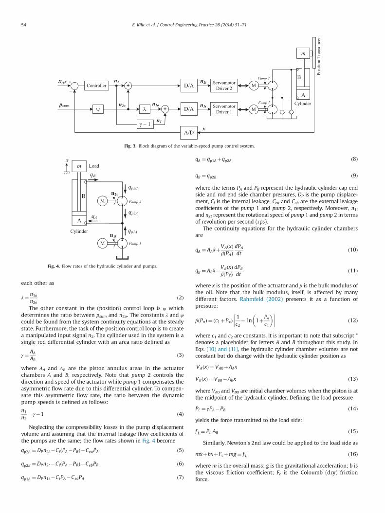
First of all, a simplified model describing the pump controlledmode of the system is developed to reveal the interactions amongthe certain hydraulic components and sub-systems. Fig. 3 shows theblock diagram of the (variable-speed pump-controlled) differential-cylinder position-control system.

The system consists of two independent control loops whichregulate the piston pressure and the position separately. Theinputs to the system are xref (the reference position) and psum(the desired value for the sum of chamber pressures at the steady

state):

psum ¼ PA;ssþPB;ss ð1Þ

The pressure control-loop is used both to pressurize thecylinder chambers to a predetermined value and to compen-sate the pump leakages so as to maintain a stationary hydraulicactuator at the steady state. Otherwise, the hydraulic cylinder willmove under the action of disturbances due to pump leakages.Thus, Pump 2 needs to turn in negative direction and supply flowto the cylinder chamber B. Some of the oil is compressed toform PB,ss and some to compensate the internal and externalleakages of the chamber B. Pump 1 turns in positive direction inorder to form PA,ss and compensate the leakages of chamber A. It isimportant to note that the speeds of pump 1 and pump 2 are co-dependent. As the static force balance of the cylinder is aimed toassure a stationary hydraulic actuator at steady state, there exists anegative ratio (λ) between speeds of pumps which completelydepends on the leakage characteristics of the system. Therefore,the offset speeds of pump 1 (n1o) and pump 2 (n2o) are related to

m

A

B Pump 2

Pump1

Cylinder

Motor 2

Motor 1

QC2

CheckValve 1

CheckValve 2

QC 1Pressure

ReliefValve

QuickCouplings

HydraulicOilTank

Servo SolenoidValve

Load

A

B T

P

QC 3

M

M

Fig. 2. Hydraulic circuit diagram of the experimental test setup.

Table 1Components of the test setup.

Components Remarks

Hydraulic pumpsEffective displacement: 15.6 cm3/revMax. speed: 3900 rpm

Hydraulic actuator

Stroke: 100 mmCap side area: 1963.5 mm2

Rod side area: 1001.4 mm2

Cap side initial chamber volume: 142,580 mm3

Rod side initial chamber volume: 76,821 mm3

Load Steel plate: 11.6 kg; actuator rod: 0.7 kgTransmission line elements Diameter of steel tubes: 12 mmServo motors and motor drivers Nominal power: 1 kW

Data acquisition (DAQ) cardNational Instruments 6025E16 Analog inputs (ADCs), 2 Analog outputs (DACs)

Pressure transmitterStauff SPT B0100 seriesOperating range: 0–10 MPa; output: 4–20 mA

Position transducerBalluff BTL series micropulse transducerStroke: 0–100 mm; resolution: 10 μm; output: 0–10 V

Hydraulic oilShell Tellus 37Kinematic viscosity (at 20 1C): 100 mm2/sBulk modulus: 1300 MPa

E. Kilic et al. / Control Engineering Practice 26 (2014) 51–71 53

each other as

λ¼ n1o

n2oð2Þ

The other constant in the (position) control loop is ψ whichdetermines the ratio between psum and n2o. The constants λ and ψcould be found from the system continuity equations at the steadystate. Furthermore, the task of the position control loop is to createa manipulated input signal n2. The cylinder used in the system is asingle rod differential cylinder with an area ratio defined as

γ ¼ AA

ABð3Þ

where ΑA and ΑB are the piston annulus areas in the actuatorchambers A and B, respectively. Note that pump 2 controls thedirection and speed of the actuator while pump 1 compensates theasymmetric flow rate due to this differential cylinder. To compen-sate this asymmetric flow rate, the ratio between the dynamicpump speeds is defined as follows:

n1

n2¼ γ�1 ð4Þ

Neglecting the compressibility losses in the pump displacementvolume and assuming that the internal leakage flow coefficients ofthe pumps are the same; the flow rates shown in Fig. 4 become

qp2A ¼DPn2t�CiðPA�PBÞ�CeaPA ð5Þ

qp2B ¼DPn2t�CiðPA�PBÞþCebPB ð6Þ

qp1A ¼DPn1t�CiPA�CeaPA ð7Þ

qA ¼ qp1Aþqp2A ð8Þ

qB ¼ qp2B ð9Þ

where the terms PA and PB represent the hydraulic cylinder cap endside and rod end side chamber pressures, DP is the pump displace-ment, Ci is the internal leakage, Cea and Ceb are the external leakagecoefficients of the pump 1 and pump 2, respectively. Moreover, n1tand n2t represent the rotational speed of pump 1 and pump 2 in termsof revolution per second (rps).

The continuity equations for the hydraulic cylinder chambersare

qA ¼ AA _xþVAðxÞβðPAÞ

dPA

dtð10Þ

qB ¼ AB _x�VBðxÞβðPBÞ

dPB

dtð11Þ

where x is the position of the actuator and β is the bulk modulus ofthe oil. Note that the bulk modulus, itself, is affected by manydifferent factors. Rahmfeld (2002) presents it as a function ofpressure:

βðPnÞ ¼ ðc1þPnÞ1c2

� ln 1þPn

c1

� �� ð12Þ

where c1 and c2 are constants. It is important to note that subscript *denotes a placeholder for letters A and B throughout this study. InEqs. (10) and (11), the hydraulic cylinder chamber volumes are notconstant but do change with the hydraulic cylinder position as

VAðxÞ ¼ VA0þAAx

VBðxÞ ¼ VB0�ABx ð13Þ

where VA0 and VB0 are initial chamber volumes when the piston is atthe midpoint of the hydraulic cylinder. Defining the load pressure

PL ¼ γPA�PB ð14Þ

yields the force transmitted to the load side:

f L ¼ PL AB ð15Þ

Similarly, Newton’s 2nd law could be applied to the load side as

m€xþb_xþFcþmg¼ f L ð16Þ

wherem is the overall mass; g is the gravitational acceleration; b isthe viscous friction coefficient; Fc is the Coloumb (dry) frictionforce.

+Controller D/A

D/A+

A/D

n2

n2o n1o

n2t

n1t

n1

xref

psum

+_

ServomotorDriver 2

ServomotorDriver 1

m

A

B Posi

tion

Tran

sduc

er

x

Pump 2

Pump 1 Cylinder

M

M

Fig. 3. Block diagram of the variable-speed pump control system.

Fig. 4. Flow rates of the hydraulic cylinder and pumps.


3. Conventional estimation techniques

Before developing advanced estimator topologies, two conven-tional estimator schemes (open-loop state observer and Kalmanfilter) are taken into consideration.

3.1. Open-loop observer

First, the direct use of “first-principle” models will be consid-ered to predict the chamber pressures in long time intervals. Thereare three distinct problems in designing (“reduced order”) closed-loop observers that employ the presented models in previoussection: (i) unlike their electro-magnetic counterparts; no physicalquantities, which are highly correlated with the chamber pres-sures, are measured/available to “lock in” on the individualchamber pressures. Even if the load force were directly measured,one would only be able to track the pressure differentials at best.(ii) the model is highly nonlinear and the development of aperturbation model (especially for servo-valve controlled EHSS)that accommodates a wide range of operating conditions can bequite challenging due to singularities and discontinuities asso-ciated with the model; (iii) the physical parameters of the system(e.g. viscosity, bulk modulus, leakage, etc.) might change duringthe operation of the system. Hence, such deviations may lead toinaccuracies in the estimates of the observer.

To illustrate the accompanying problems, an open-loop obser-ver, which makes good use of the models presented in theprevious section, is designed. The observer is simulated viaMatlab/Simulink in which the Dormand-Prince solver is utilizedwith a fixed integration time-step of 0.001 s. Employing the(statistically coherent) experimental data, the unknown para-meters of the “nonlinear” observer (i.e. bulk modulus, leakagecoefficients, etc.) have been identified by a basic stochastic searchalgorithm whose flow chart is shown in Fig. 5. The identifiedparameters are presented in Table 2.

To assess the prediction performance of this open-loop obser-ver, an experimental case is considered as illustrated in Fig. 6a. Inthis case, the (pump) velocity commands in the form of the chirpsignals (0.1–10 Hz with increasing amplitude) is applied to theservo-motors driving the pumps of the hydraulic system in Fig. 4.Similarly, Fig. 6b represents the observer’s (50,000 step-ahead)

pressure estimates and the measured ones. It is obvious that theprediction performance of the observer is not satisfactory inthe sense that the root-mean-square (RMS) error in PA is about0.34 MPa and RMS error in PB is about 0.61 MPa. For that reason,with the utilization of the experimental data (where the observerhas failed to yield an acceptable prediction performance); somemodel parameters are readjusted as b¼1.98 N s/mm, Fc¼287 N,Ci¼1013 mm3/(MPa s), Cea¼170.8 mm3/(MPa s), Ceb¼119.6 mm3/(MPa s), c1¼57.88 MPa and c2¼0.1587 to minimize the corre-sponding error as much as possible.

After this operation, the performance of the observer hasbeen improved as could be seen from Fig. 6c where the RMSerrors now drop down to 0.19 MPa and 0.32 MPa for PA and PB,respectively. Unfortunately, the performance of the “re-tuned”observer is still unacceptable on a different test case as illustratedin Fig. 7.

This deterioration in performance (Fig. 7b) appears to berelated to not only the slight changes in the physical systemparameters but also the deviations in the measurements due tonoise or drift (especially in pump velocities). Consequently, theprediction performance of the open-loop observer that directlyutilizes the “first-principle” models is found inadequate for allpractical purposes. Hence, the physical nonlinear models to beused in observer design should intrinsically take into account thechange associated with most significant parameters (especially thebulk modulus owing to the fact that any change in this factorwould highly affect the pressure estimates).

(random)parameter perturbation vector:

21

( ) ( , )N

kE k ky y

Determine the modeling error:

(1 )EeCompute the new parameter vector:

END

Select initial parameter vector (range scalar ( error threshold

(E*), and max. iteration number(imax). Let i:=1; E :=

(E < E*) or (i > imax) ?

(E < E

Update the best state:E

Y

N

N

Y

Increase the iteration counter:i := i + 1

Fig. 5. Flow chart of the stochastic (parameter) search algorithm.

Table 2Model parameters used in the open-loop observer.

Par. Value Par. Value

m 12.3 kg Ceb 120 [mm3/(s MPa)]AA 1.9635 mm2 b 2.6 N s/mmAB 1.0014 mm2 Fc 330 NVAo 1.4258�105 mm3 λ �1.2195VBo 7.6821�104 mm3 ψ �0.0279Dp 15.6�103 mm3/rev c1 99.993 MPaCi 1097 [mm3/(s MPa)] c2 0.0733Cea 120 [mm3/(s MPa)] g 9.81


3.2. Kalman Filter

Kalman Filter (KF), which is known to be an optimal stateestimator for linear systems, is considered to predict the pres-sure states of the hydraulic cylinder. If the hydraulic cylinderchamber volumes and the bulk modulus of the oil are assumedconstant, the system at hand could be classified as a linear (time-invariant) dynamic system that one can directly construct theconventional KF. Employing the model given in Section 2.2 and

the above-mentioned simplifications, the standard (continuous-time) state-space model could be obtained:

_x¼

0 1 0 00 � b

mγABm �AB

m

0 �AAβVA

�ð2Ci þ2CeaÞβVA

CiβVA

0 ABβVB

CiβVB

�ðCi þCebÞβVB

2666664

3777775

|fflfflfflfflfflfflfflfflfflfflfflfflfflfflfflfflfflfflfflfflfflfflfflfflfflfflfflfflfflfflfflfflfflfflfflffl{zfflfflfflfflfflfflfflfflfflfflfflfflfflfflfflfflfflfflfflfflfflfflfflfflfflfflfflfflfflfflfflfflfflfflfflffl}A

x_x

PA

PB

26664

37775

|fflfflffl{zfflfflffl}x

0 0.5 1 1.5 2 2.5 3 3.5 4 4.5 5x 104

-10

-8

-6

-4

-2

0

2

4

6

8

10

Time index k (sample time T=0.001 second)

Rot

atio

nal s

peed

[rps

]

Pump1Pump2

Pump1

Pump2

0 0.5 1 1.5 2 2.5 3 3.5 4 4.5 5x 104

0

1

2

3

4

5

6

7

8

9

10


Pres

sure

[MPa

]

estimated PAestimated PBmeasured PAmeasured PB

0 0.5 1 1.5 2 2.5 3 3.5 4 4.5 5x 104

0

1

2

3

4

5

6

7

8

9

Pres

sure

[MPa

]


estimated PAestimated PBmeasured PAmeasured PB

Fig. 6. Estimation performance of the open-loop observer on a test case: (a) rotational speed of pumps, (b) measured- and estimated pressure, and (c) measured- andestimated pressure after the observer was re-tuned.


þ

0 00 0

γDpβVA

DpΨ ðλþ1ÞβVA

�DpβVB

�DpΨβVB

2666664

3777775

|fflfflfflfflfflfflfflfflfflfflfflfflfflfflfflfflffl{zfflfflfflfflfflfflfflfflfflfflfflfflfflfflfflfflffl}B

n2

psum

" #|fflfflfflffl{zfflfflfflffl}

u

ð17aÞ

y¼ Cx¼ Ix ð17bÞIn Kalman filtering theory, a general linear discrete-time

system is a process that can be described by the following diff-erence equations:

xðkþ1Þ ¼ΦxðkÞþGuðkÞþwðkÞ ð18aÞ

yðkÞ ¼HxðkÞþvðkÞ ð18bÞwhere x(k) is the estimated state vector; y(k) is the system outputvector; u(k) is the control input vector; w(k) is the process noisevector while v(k) refers to the measurement noise vector. Thesystem matrices (Φ, G, and H) are computed via well-known(discrete-time) conversion techniques in modern control theorywith the utilization of A, B, C matrices of (17) along with thesampling period T.

Both process- and measurement noise [w(k), v(k)] are pre-sumed to be random processes with zero-mean Gaussian prob-ability density functions. The covariances of these noise vectorsare represented by R and Q matrices in KF equations where

the covariance matrix Q of the process noise w(k) is defined byQ ¼ E½wUwT �while the covariance matrix R of the measurementnoise v(k) is defined by R¼ E½vUvT �. The R and Q matrices dependon the noise level of the measurements together with the accuracyof the sensors, and the modeling uncertainties. Implementationdetails of the conventional KF are given by Grewal and Andrews(2001).

To find the element(s) of the measurement noise matrix (R),the position and pressure data are acquired through the sensorswhile providing zero reference signals to the servo-motors. Basedon the collected data, Caliskan (2006) computes the varianceof the above-mentioned signals as 2.36�10�2 (mm)2, 5.77�10�3 (MPa)2 and 6.55�10�3 (MPa)2. The correlation amongdifferent measurements is found to be negligible. Similarly, todetermine the process noise covariance matrix Q, Caliskan (2006)adopts an iterative (trial-and-error based) process with the utili-zation of the (measurement) covariance information at hand:

Q ¼

2� 10�3 0 0 00 2� 10�6 0 00 0 5� 10�4 00 0 0 5� 10�4

266664

377775 ð19Þ

Since all the states of the hydraulic system are not expectedto be measured, only the position of the hydraulic cylinder isassumed to be available as the first case. Hence, the measurement

0 0.5 1 1.5 2 2.5 3 3.5 4 4.5 5x 104

-6

-4

-2

0

2

4

6

8


Rot

atio

nal s

peed

[rps

]

Pump1Pump2

Pump2

Pump1

0 0.5 1 1.5 2 2.5 3 3.5 4 4.5 5x 10

4

0

1

2

3

4

5

6

7

8

9

Pres

sure

[MPa

]


estimated PA

estimated PB

measured PA

measured PB

Fig. 7. Estimation performance of the fine-tuned observer on a different test case: (a) rotational speed of pumps and (b) measured- and estimated pressure.


matrix is modified as H ¼ 1 0 0 0� �

while the measurementcovariance matrix is taken as R¼ ½2:36� 10�2�.

Fig. 8 shows the predicted pressure states of the Kalman filter.As can be seen, the prediction performance of the filter is far frombeing acceptable for this case.

As a second case, the position of the hydraulic actuator and thepressure in cylinder chamber A are measured to predict thepressure in the other chamber. Hence, the measurement matrixH and the measurement covariance matrix R take the followingform:

H¼ 1 0 0 00 0 1 0

� �ð20aÞ

R¼ 2:36� 10�2 00 5:77� 10�3

" #ð20bÞ

The corresponding result for this case is presented in Fig. 9. KFis now able to predict the pressure in chamber B (with an RMSerror of 0.267 MPa) once the pressure measurement for the otherchamber is available.

Similarly, the case, where the position of the hydraulic actua-tor and pressure state in cylinder chamber B are available, areconsidered to predict the pressure value in chamber A. Hence, the

measurement matrix H and the measurement covariance matrix Rare now updated as

H¼ 1 0 0 00 0 0 1

� �ð21aÞ

R¼ 2:36� 10�2 00 6:55� 10�3

" #ð21bÞ

The result is shown in Fig. 10. For this case, using a singlepressure sensor for chamber B will result in the prediction of thechamber A pressures with an RMS error of 0.188 MPa.

3.3. Extended Kalman Filter

The Extended Kalman Filter (EKF), which is regarded as a non-optimal state filter (unlike its linear counterpart), is frequentlyused to estimate the states of nonlinear dynamic systems wherethe generic (continuous-time) model can be expressed as

_x¼ Fðx;uÞþw ð22aÞ

y¼Hðx;uÞþv ð22bÞ

0 0.5 1 1.5 2 2.5 3 3.5 4 4.5 5

x 104

0

1

2

3

4

5

6

7

8

9

Pres

sure

[MPa

]


measured PAmeasured PBpredicted PApredicted PB

Fig. 8. Prediction performance of the KF when only position (x) is provided.

0 0.5 1 1.5 2 2.5 3 3.5 4 4.5 5x 104

0

1

2

3

4

5

6

7

8

9

Pres

sure

[MPa

]


measured P

measured P

estimated P

predicted P

Fig. 9. Prediction performance of the KF when x and PA are provided.


Using the model given in Section 2.2, the nonlinear (contin-uous-time) state-space model of the pump-controlled hydraulicsystem can be simply written as follows:

In the EKF approach, the nonlinear state-propagation modellike (23) is linearized around an operating point. Hence, thelinearized system matrix becomes

f ¼ ½f ij� ¼∂F∂x

� �ðx;uÞ

ð24Þ

where

f 11 ¼ 0; f 12 ¼ 1; f 13 ¼ 0; f 14 ¼ 0 ð25aÞ

f 21 ¼ 0; f 22 ¼ � bm; f 23 ¼

γAB

m; f 24 ¼ �AB

mð25bÞ

f 31 ¼AAβðPAÞ

ðVA0þAAxÞ2½AA _xþ2ðCiþCeaÞPA�CiPB�γDpn2�Dpψðλþ1Þpsum�

ð25cÞ

f 32 ¼ � AAβðPAÞVA0þAAx

; f 34 ¼CiβðPAÞ

VA0þAAxð25dÞ

f 33 ¼∂βðPAÞ∂PA

1ðVA0þAAxÞ

�AA _x�2ðCiþCeaÞ βðPAÞ∂βðPAÞ=∂PA

þPA

� ��

þCiPBþγDpn2þDpψ ðλþ1Þpsum�

ð25eÞ

f 41 ¼ABβðPBÞ

ðVB0�ABxÞ2½AB _xþCiPA�ðCiþCebÞPB�Dpn2�Dpψpsum� ð25f Þ

f 42 ¼ABβðPBÞVB0�ABx

; f 43 ¼CiβðPBÞVB0�ABx

ð25gÞ

f 44 ¼∂βðPBÞ∂PB

1ðVB0�ABxÞ

AB _xþCiPA�ðCiþCebÞβðPBÞ

∂βðPBÞ=∂PBþPB

� ��

�Dpn2�Dpψpsum

�ð25hÞ

∂βðPnÞ∂Pn

¼ 1c2

�1� ln 1þPn

c1

� �ð25iÞ

Note that the states that appear in (25) are to be interpreted asthe estimated quantities at an operating point. Similarly, the statetransition matrix of the operating model is

ΦðkÞ ¼ eTfðt ¼ kTÞ ð26ÞConsequently, the priori error covariance at each discrete time

step becomes

P� ðkÞ ¼ΦT ðkÞPðk�1ÞΦðkÞþQ ðkÞ ð27Þwhere

Q ðkÞ ¼Z T

τ ¼ 0ΦðτÞQΦT ðτÞdτ ð28Þ

It is critical to note that the state propagation in EKF isperformed utilizing the nonlinear model of the system. Hence,one needs to apply advanced numerical integration techniques tosolve (23) for the purpose of propagating the state vector. In thisstudy, the fourth-order Runge–Kutta method is employed to carry-out a numerically stable/accurate integration. Further implemen-tation details of the EKF are discussed in Grewal and Andrews(2001).

First, the prediction performance of the EKF for the first case(with H¼ 1 0 0 0

� �and R¼ ½2:36� 10�2�) is considered. As

can be observed in Fig. 11, the performance of the EKF for this caseappears to be comparable to that of the linear KF (see Fig. 8).Hence, the EKF fails to estimate the pressure states when only theposition is provided to the filter.

Next, the position of the hydraulic actuator and the pressure incylinder chamber A are utilized to predict the pressure in chamberB. Hence, the measurement matrix H and the measurementcovariance matrix R are modified accordingly as indicated byEq. (20). Fig. 12 shows the prediction performance for this case.As can be seen, the EKF is now able to estimate the pressure PBwith an RMS error of 0.241 MPa where the linear KF couldestimate this quantity with an error of 0.267 MPa.

_x¼

_x1m ð�b_xþγABPA�ABPB�mg�FcÞ

1VA0 þ AAx

�AAβðPAÞ_x�2ðCiþCeaÞβðPAÞPAþCiβðPAÞPBþγDpβðPAÞn2þDpΨ ðλþ1ÞβðPAÞpsum� �1

VB0 � ABxABβðPBÞ_xþCiβðPBÞPA�ðCiþCebÞβðPBÞPB�DpβðPBÞn2�DpΨβðPBÞpsum� �

2666664

3777775 ð23Þ

0 0.5 1 1.5 2 2.5 3 3.5 4 4.5 5x 104

0

1

2

3

4

5

6

7

8

9

Pres

sure

[MPa

]


measured PAmeasured PBpredicted PAestimated PB

Fig. 10. Prediction performance of the KF when x and PB are provided.


Finally, the case in which the aim is to predict the pressurevalue in chamber A is considered. The prediction performance ofthe EKF is presented in Fig. 13. The improvement in the predictionof PA (RMS error is 0.176 MPa) is marginal since the predictionerror associated with the linear KF was registered as 0.188 MPa.

Despite the fact that the both linear KF and EKF fail to predict thechamber pressures when only the position of the actuator ismeasured, the experimental results indicate that these filters mightbe successfully utilized to predict the pressure state of a particularchamber when the pressure associated with the other one ismeasured. Hence, these filters will be further evaluated in Section 5.

4. Nonlinear prediction models and parameter estimation

Just like most engineering systems, EHSSs considered in thisstudy are highly nonlinear in nature. Artificial neural networks(ANNs) are considered as universal modeling and functionalapproximation tools and find their use in many engineering fieldssuch as estimation, filtering, identification, and control (Narendra &Parthasarathy, 1990; Widrow & Walach, 1996). Unfortunately, sinceneural networks employ weak assumptions about the system understudy, the selection of the network’s architecture (or structure), size,memory model, training set while satisfying a given set of con-straints on the (identification) performance remain a complex task.

As an alternative modeling technique for nonlinear dynamicsystems; this study makes good use of the SNN methodology,

which can be classified as a gray-box modeling technique (Kilic,Dolen, Koku, Caliskan, & Balkan, 2012). Unlike conventional ANNdevelopment paradigms, this method embodies strong assump-tions on the system to be modeled and thus makes good use ofavailable information about the process to decompose the pro-blem into its fundamental components. A number of well-knownANNs can then be devised to represent the behaviors of eachsubsystem of the dynamic system under study. Consequently, anSNN emerges by combining these individual ANNs to model theoverall nonlinear system. Kilic (2012) presents a comprehensiveliterature review on the SNN methodology.

In this section, accurate ANN models for the long-term pressureprediction in the cylinder chambers for a (variable-speed) pump-controlled hydraulic system are to be developed using twodifferent approaches: black-box- (i.e. conventional ANN develop-ment) and gray-box (i.e. SNN development). The details follow.

4.1. Black-box approach

As illustrated in Fig. 14, the black-box model of a nonlineardynamic system (such as the one considered in this study) couldbe generically expressed in the form of

yðkÞ ¼ fðθ;φðkÞÞ ð29Þwhere k refers to a discrete-time index while f : ℝn-ℝm denotes aBorel measurable continuous function. A feed-forward neural net-work (FNN) is generally used to capture the desired functional

0 0.5 1 1.5 2 2.5 3 3.5 4 4.5 5x 104

0

1

2

3

4

5

6

7

8

9

Pres

sure

[MPa

]


measured PAmeasured PBestimated PApredicted PB

Fig. 12. Prediction performance of the EKF when x and PA are provided.

0 0.5 1 1.5 2 2.5 3 3.5 4 4.5 5x 104

0

1

2

3

4

5

6

7

8

9

Pres

sure

[MPa

]


measured P

measured P

predicted P

predicted P

Fig. 11. Prediction performance of the EKF when only position (x) is provided.


relationship since an FNN with one hidden-layer is known to becapable of approximating such continuous functions to the desiredaccuracy (Cybenko, 1989). Similarly, the regression vector

φðkÞ ¼ ½uT ðkÞ;uT ðk�1Þ;…; yT ðk�1Þ;yT ðk�2Þ;…; yT ðk�1Þ; yT ðk�2Þ;…; eT ðk�1Þ; eT ðk�2Þ;…�T

ð30Þcan contain previous (and possibly current) process inputs (u),previous process (or model) outputs (y or ŷ) and previous predic-tion errors (eðkÞ8yðkÞ� yðkÞ). In Eq. (29), θ represents the modelparameters (i.e. the free weights of the FNN) to be determinedsuch that for a number of collected samples (N), the correspondingprediction errors are minimized:

θ¼ argminθ

∑N

k ¼ 1eT ðkÞeðkÞ

( )ð31Þ

In this optimization problem, θ can be solved numerically via anumber of well-known techniques like the Levenberg–Marquardt(LM) algorithm (Nelles, 2001). Note that the parameter estimationcould be realized based on the prediction error (PE) or simulationerror (SE) minimization technique as shown in Fig. 14. In thetechnical literature, the minimization of PE is preferred forthe equation error (EE) models while the minimization of SE isrecommended when the output error (OE) models are utilized(Aguirre, Barbosa, & Braga, 2010). Furthermore, the minimizationof SE, which has a high computation cost, gives out unbiasedparameter estimation of a nonlinear input–output model, regard-less of the measurement/process noise (Farina & Piroddi, 2008;Piroddi, Farina, & Lovera, 2012).

If one is specifically interested in long-term prediction, it would bebetter to consider nonlinear output error (NOE) type models (which are

trained with SE minimization mode) rather than nonlinear autoregres-sive external input (NARX) type models (which are trained withPE minimization mode) since NOE models are regarded as optimalsimulators (Witters & Swevers, 2010; Wong & Worden, 2007).

Now, the black-box regression models based on NARX and NOEare to be devised to predict the chamber pressures (PA and PB) inthe long run without any pressure feedback. Hence, only theposition sensor output x(k) along with the rotational speed ofthe pumps (n1t and n2t) are to be utilized in the designed predictor.

Next, the regression vector size along with the model ordersmust be determined. That is, the regression vector can be given as

φðkÞ ¼ n1tðkÞ;…;n1tðk� lÞ;n2tðkÞ;…;n2tðk� lÞ;�xðkÞ;…;xðk� iÞ; :::; vðkÞ;…; vðk� jÞ;PAðk�1Þ;…; PAðk�pÞ; PBðk�1Þ;…; PBðk�pÞ�T ð32Þ

The selection for the model orders (l,i,j and p) [i.e. the size oftapped delay lines (TDLs) for various signals of interest] used in theregression vector closely governs the prediction performance.Various NARX models, which constitute FNNs, can be trained ina straightforward fashion for the case scenario given in Fig. 6. Thatis, the previous pressure values coming from the pressure sensorsare directly fed to the network. The properties of the trainingsession are summarized in Table 3. The training performances allof the NARX models are very satisfactory. However, the networksmust be arranged in recurrent (feedback) form meaning that theprevious pressure values must be provided by the network itselffor both the training scenario and the validation case. As can beseen from Table 3, Architecture #7 is selected as the best topologyfor the NARX model since it has a small RMS error value.

As the next step, the outputs of the chosen NARX network (#7)are delayed and fed back to the first hidden layer. Since thearchitecture of the network is now changed, the resulting networkis hereafter renamed as NOE. The NOE network could be trainedwithout any problems in a recurrent form provided that the initialweight values are taken from the original (NARX) network. After atraining process (with 10 epochs) in which the training duration isabout 1511 min,1 it is found that the training error of the NOE wasabout 0.1 MPa. Hence, the final network model is theoretically ableto predict the pressure states without the need for pressuresensors. A model validation study of the resulting network (NOE)is to be conducted for the case given in Fig. 7. Unfortunately, the

0 0.5 1 1.5 2 2.5 3 3.5 4 4.5 5x 104

0

1

2

3

4

5

6

7

8

9

Pres

sure

[MPa

]


measured PAmeasured PBpredicted PAestimated PB

Fig. 13. Prediction performance of the EKF when x and PB are provided.

Fig. 14. Black-box modeling approach for (MISO) dynamic systems.

1 A PC workstation with Intel Core i5 processor and a SDRAM of 4 GB is utilizedin this study. All of the neural networks considered in this paper are developed viaMATLAB™ Neural Network Toolbox.


long-term (50,000 steps) prediction performance of this networkis found unsatisfactory as the results are presented in Fig. 15.

4.2. Gray-box approach

If the physical model of this hydraulic system is examined, themodel could be conveniently separated into two parts: flow-ratemodel and pressure model. Fig. 16 illustrates the schematic of the

proposed SNN (recurrent-type). ANNs in Fig. 16 can be trained in apiecewise fashion provided that the experimental data areacquired to form the relevant training sets. In this study, thesenetworks are developed in two stages as suggested by Kilic et al.(2012):

1. Preliminary training of the above-mentioned networks usingthe data generated by the simulated hydraulic system.

Table 3Trained NARX modelsa in black-box approach.

Architecture #1 #2 #3 #4 #5 #6 #7 #8 #9

Inputs n1t(k), n2t(k),x(k) v(k),PA(k�1),PB(k�1) n1t(k), n1t(k�1) n1t(k), n1t(k�1), n1t(k�2)n2t(k), n2t(k�1) n2t(k), n2t(k�1), n2t(k�2)x(k), x(k�1) x(k), x(k�1), x(k�2)v(k), v(k�1) v(k), v(k�1), v(k�2)

PA(k�1), PA(k�2) PA(k�1), PA(k�2), PA(k�3)PB(k�1), PB(k�2) PB(k�1), PB(k�2), PB(k�3)

Outputs PA(k) and PB(k)Training RMS error (MPa) 7.25� 10�3 7.19� 10�3 7.12� 10�3 2.31� 10�3 2.2� 10�3 2.18� 10�3 9.28� 10�4 9.26�10�4 9.23� 10�4

Training data 50,001 sample for each variableEpochs 1000Training time (min) 18 39 67 30 70 118 47 107 2061st layer neurons 10 20 30 10 20 30 10 20 30Activation function Tangent sigmoidTraining method Levenberg–Marquardt

a Linear activation function is utilized at the output layers.

0 0.5 1 1.5 2 2.5 3 3.5 4 4.5 5x 104

0

1

2

3

4

5

6

7

8

9

10

11

Pres

sure

[MPa

]


measured PAmeasured PBNOE PANOE PB

Fig. 15. Long-term pressure prediction performance of the NOE model.

Fig. 16. Schematic of the proposed structured (recurrent) neural network.


2. Final training of the “pre-trained” networks with the utilizationof experimental data.

At this point, a critical question might naturally arise: why arethese NNs developed when detailed models (as used in thesimulation study) are available in the first place? First of all, asdemonstrated by Kilic et al. (2012), capturing the pressuredynamics of the hydraulic system without the use of flow ratesin both chambers is extremely difficult. To develop such models,the flow-rates for both chambers (qA and qB) are needed togenerate the (preliminary) training data. Since they are notmeasured in experimental set-up due to the high cost associated

with high accuracy/bandwidth flow-meters, the simulation modelshould be utilized to estimate the flow-rates. However, the first-principle models to be utilized in the simulation do not need to beaccurate. The main purpose of this training phase (i.e. preliminaryphase) is to set the initial weights (i.e. start-off weights) of thenetworks reasonably. It is critical to notice that despite the devisednetworks serving as a reduced-order nonlinear state observer areshown to have the optimal architecture (e.g. the right architecturewith the proper size), the structured network (as presented inFig. 16) fails to yield expectable performance in the trainingsession (conducted with the experimental data) when its weightsare initialized in a random fashion. That is, the training operation

0 1 2 3 4 5 6 7 8 9 10-10

-8

-6

-4

-2

0

2

4

6

8

10

Time [sec]

Con

trolle

r Out

put

0 1 2 3 4 5 6 7 8 9 10-50

-25

0

25

50

Time [sec]

Posi

tion

[mm

]

0 1 2 3 4 5 6 7 8 9 10-300

-150

0

150

300

Vel

ocity

[mm

/s]

velocityposition

0 1 2 3 4 5 6 7 8 9 100

1

2

3

4

5

6

7

8

9

10

Time [sec]

Pres

sure

[MPa

]

PBPA

Fig. 17. Training scenario (simulation): (a) controller output, (b) cylinder position and velocity and (c) pressures in the cylinder chambers.


with arbitrary initial weights will increase the probability ofgetting trapped at a local minimum in the vast weight (search)space.

Finally, the networks are to be further trained (i.e. “fine tuned”)with experimental data where only pressure, piston position/velocity and pump velocities are sufficient quantities to train the

overall network to the desired accuracy. As mentioned previously,a similar training procedure is adapted by Kilic et al. (2012) wherea SNN is pre-trained to capture the pressure dynamics of a specific(servo-valve driven) hydraulic system. They demonstrate that thesame network can successfully learn the dynamics of a differenthydraulic system using the experimental data collected on thenew system. In our study, once the initial weights are roughlygenerated by the simulation data, the proposed SNN is trainedthereafter with solely experimental data that do not constitute anyflow rate measurements.

Notice that in the (preliminary) training session, one shouldselect a proper excitation signal with extreme care in order tocapture relevant (and statistically significant) data points thatcover all the operating regimes of interest. In the literature,pseudo-random multi-level signal (PRMS) is the most commonexcitation signal used in the identification of hydraulic systems(Barbosa, Aguirre, Martinez, & Braga, 2011; Jelali & Kroll, 2003;Xue-miao, Yuan, Zong-yi, Yong, & Li-min, 2010). Therefore, a PRMS

0 0.5 1 1.5 2 2.5 3 3.5 4 4.5 5x 104

0

1

2

3

4

5

6

7

8

9

10


Pres

sure

[MPa

]

Exact PASRNN PAExact PBSRNN PB

Fig. 18. Validation test result of the SNN on the simulated system.

Fig. 19. RNN PA for the pressure prediction in chamber A (assuming PB is measured).

Fig. 20. RNN PB for the pressure prediction in chamber B (assuming PA is measured).

Table 4Properties of trained flow-rate networks.

Network qA Network qB

Training data 10,001 sampleTraining RMS error (mm3/s) 2.151� 10�6 1.4034� 10�6

Epochs 1

1st layer neurons 1

Activation function Linear

Training method Least mean square


type signal (given in Fig. 17a) is applied to system and then, the n1tand n2t signals are formed based on this n2 signal as shown inFig. 3. Note that psum is set to 12 MPa in the simulated system.

Furthermore, Fig. 17b represents the position and velocity profileof the hydraulic actuator and Fig. 17c shows chamber pressures. Itcan be seen that the pressure states are getting more oscillatory

0 0.5 1 1.5 2 2.5 3 3.5 4 4.5 5-10

-8

-6

-4

-2

0

2

4

6

8

10


Rot

atio

nal s

peed

[rps

]

Pump1Pump2

Pump1

Pump2

0 0.5 1 1.5 2 2.5 3 3.5 4 4.5 5x 104

x 104

x 104

x 104

-5

-4

-3

-2

-1

0

1

2

3

4

5


Posi

tion

[mm

]

0 0.5 1 1.5 2 2.5 3 3.5 4 4.5 5-150

-100

-50

0

50

100

150

Vel

ocity

[mm

/s]


0 0.5 1 1.5 2 2.5 3 3.5 4 4.5 5-1

0

1

2

3

4

5

6

7

8

9

Pres

sure

[MPa

]


measured PAmeasured PBRNN PARNN PB

Fig. 21. Training case: (a) rotational speed of pumps, (b) measured cylinder position, (c) calculated cylinder velocity from filtered position signal, and (d) target pressures andmodel outputs after training.


when the piston approaches to its stroke limit (�0.05 m) at about9.2 s in this training scenario.

4.2.1. Flow rate modelWhen Eqs. (5)–(9) are examined closely; one can presume that

the normalized flow-rates could be estimated via a simple linearmodel as

qnðkÞ ¼ θTnφnðkÞ ð33aÞ

φAðkÞ ¼ ½n1tðkÞ;n2tðkÞ; PAðkÞ; PBðkÞ�T ð33bÞ

φBðkÞ ¼ ½n2tðkÞ; PAðkÞ; PBðkÞ�T ð33cÞ

To realize (33a), a neuron with linear activation function wouldbe sufficient. Hence, this network model simply gives rise to anAutoRegreressive eXternal input (ARX) model. Again, the traininginput signal in Fig. 17a is applied and the normalized input andoutput signals, which will be required in the training operation ofthe flow-rate networks, are acquired from the simulated system.Table 4 shows the training performances of the linear models(labeled as Network qA and Network qB) that are used to predict theflow rates in each chamber.

Notice that to estimate the current flow rate (at t¼kT), the net-work requires both the pump rotational speeds and the pressureestimate at t¼kT. Since such the pressure estimate is not readilycalculated for that instant, the previous pressure state should beemployed for all practical purposes. This requirement impliesthat the chamber pressures do not change considerably withinone sampling interval: P*(k)ffiP*(k�1) (where * stands for lettersA or B).

4.2.2. Pressure modelEqs. (10) and (11) describing the pressure dynamics of the

system indirectly state that the gradient of the pressure, whichdepends on not only the corresponding flow rate but also thepiston’s kinematic states, should be estimated in the first place.Hence, once the flow rates are computed to the desired accuracy,one could calculate the chamber pressures as

PnðkÞ ¼ Pnðk�1ÞþTf nðqnðkÞ; xðkÞ; vðkÞÞ ð34Þusing a simple integration technique (e.g. Euler integrationmethod). After normalizing the variables in Eq. (34) with theirmaximum nominal values, a pressure model, whose recurrent neuralnetwork (RNN) implementation is given in Eq. (35), can be devel-oped to represent the pressure dynamics of the hydraulic system:

PnðkÞ ¼ Pnðk�1ÞþG2W2Ψ ½W1φðkÞþb� ð35aÞ

φðkÞ ¼ ½qnðkÞ; vðkÞ; xðkÞ�T ð35bÞwhere Ψ( � ) is the activation vector function (bipolar/tangentsigmoid); the weight matrices are W1Aℝ20�3, W2Aℝ1�20, and biasvector is bAℝ20�1. Note that in Fig. 16, G2 ¼ ðβqmaxTÞ=ðVn0PmaxÞ

refers to a gain with lumped parameters. This gain is, in fact, an endresult of input normalization procedure. Two pressure networks,named as Network PA and Network PB, are devised to implement thisarchitecture where their preliminary training are to be performedusing the data collected from the simulation study as illustrated bythe training scenario in Fig. 17.

4.2.3. Overall modelAll the modules are connected to each other to form the unified

SNN where it could be further trained to fine tune its weights (in aglobal fashion). Therefore, the final (pre)training operation willfurther increase the performance of the final network model. Thisstep is important since the entire network modules are onlytrained for their specific operating regimes in order to capture asub-system’s behavior. Now, the SNN will be trained in a unifiedform to characterize the dynamic behavior of the nonlinear systemusing a general training scenario. It is seen that the training errors(root-mean-square – RMS) of the SNN decreases from 0.4 MPalevel to 0.2 MPa level within 5 epochs while the final trainingsession lasts about 35 min.

A validation test on the overall SNN is then conducted on thesimulated system. The rotational speed of the pumps, which werepresented in Fig. 6a, are employed to create a 50,000 step-aheadprediction task. Fig. 18 represents the pressure states in thecylinder chambers that are calculated from the simulated systemmodel and the overall SNN model. It is found that the RMS errorsof the SNN model are 0.0547 MPa and 0.0911 MPa for the predic-tion of PA and PB respectively. Therefore, it could be inferred thatthe pressure dynamics of the simulated system is successfullycaptured by the SNN model to a certain extend.

5. Pressure prediction results and discussion

In this section, the general prediction performance of the SNN(as elaborated in Section 4) is to be evaluated on the experimentalsetup. The networks, which was initially developed in a simulationenvironment (called “preliminary” training phase), is to be trainedvia the data collected on the experimental setup. Unfortunately,training the SNN as a whole is a very difficult feat for a testduration of 50 s (meaning that 50,000 step ahead prediction isrequired) where the workstation used in the study will bestretched to its limits. For that reason, the SNN shown in Fig. 16is divided into two (titled as RNN PA and RNN PB) parts and aretrained (separately) to predict the pressure change in eachchamber assuming that the opposite chamber pressure is knownin the training session. Figs. 19 and 20 illustrate the networks insuch a configuration.

The reconfigured RNNs (called “decoupled” SNN models) aretrained using the measurements presented in Fig. 21. As could beseen, the noise on the position transducer will aggravate the noiseon the calculated velocity significantly unless any filtering opera-tion is applied on position signal. Therefore, the position signal,given in Fig. 21b, is filtered before the computation of velocity viathe first-order difference method. For that purpose, a discrete-time low-pass (Butterworth) filter with a cut-off frequency of15 Hz is utilized. Fig. 21c presents the calculated cylinder velocity(as required in the regression vector) from the filtered actuatorposition signal. Similarly, the target pressure values and the RNNoutputs after the training operation is given in Fig. 21d whileTable 5 represents the training performance of each RNN.

To assess the generalization performance, a validation scenario,which is illustrated in Fig. 22, is considered. As can be seen, theperformances of the RNNs are very satisfactory [since the RMS ofthe prediction errors are 0.112 MPa (PA) and 0.195 MPa (PB)] whenthe pressure in the other chamber are measured and provided to

Table 5Training properties of the RNNs.

RNN PA RNN PB

Training data size 50,001 samplesTraining RMS error (MPa) 0.092 0.116Epochs 10Training time 365 min1st layer neurons 1 Linear2nd layer neurons 20 Tangent sigmoid3rd layer neurons 1 LinearTraining method Levenberg–Marquardt


0 0.5 1 1.5 2 2.5 3 3.5 4 4.5 5

x 104

x 104

x 104

x 104

-6

-4

-2

0

2

4

6

8


Rot

atio

nal s

peed

[rps

]

Pump1Pump2

Pump2

Pump1

0 0.5 1 1.5 2 2.5 3 3.5 4 4.5 5-80

-60

-40

-20

0

20

40

60

80

100

120


Vel

ocity

[mm

/s]

0 0.5 1 1.5 2 2.5 3 3.5 4 4.5 5-20

-15

-10

-5

0

5

10

15

20

Time index k (sampling time T=0.001 second)

Posi

tion

[mm

]

0 0.5 1 1.5 2 2.5 3 3.5 4 4.5 50

1

2

3

4

5

6

7

8

9

10


Pres

sure

[MPa

]

measured P

measured P

RNN P

RNN P

Fig. 22. First validation case of the decoupled RNNs: (a) rotational speed of pumps, (b) cylinder position, (c) cylinder velocity, and (d) measured pressures and RNN outputs.


the RNNs shown in Figs. 19 and 20. A second validation case isillustrated in Fig. 23 where prediction error in PA is 0.099 MPawhile it is 0.101 MPa for PB. The prediction performance of the“decoupled” model appears to be exceptional for all practical

purposes. It is critical to note that in this study, the measurementaccuracy of the pressure sensors utilized in the study is 1% withinthe range of 0–10 MPa which translates to an overall measurementuncertainty of 0.1 MPa. Since the performance of an estimation

0 0.5 1 1.5 2 2.5 3 3.5 4 4.5 5

x 104

x 104

x 104

x 104

-10

-8

-6

-4

-2

0

2

4

6

8

10

Rot

atio

nal S

peed

[rps

]


Pump 1Pump 2

Pump 1

Pump 2

0 0.5 1 1.5 2 2.5 3 3.5 4 4.5 5-150

-100

-50

0

50

100

150


Vel

ocity

[mm

/s]

0 0.5 1 1.5 2 2.5 3 3.5 4 4.5 5-6

-4

-2

0

2

4

6


Posi

tion

[mm

]

0 0.5 1 1.5 2 2.5 3 3.5 4 4.5 50

1

2

3

4

5

6

7

8

9

10

Pres

sure

[MPa

]


measured P

measured P

RNN P

RNN P

Fig. 23. Second validation case for the decoupled RNNs: (a) rotational speed of pumps, (b) cylinder position, (c) cylinder velocity, and (d) measured pressures and RNNoutputs.


technique is evaluated with respect to the output of these physicaldevices/sensors, the overall uncertainty of the method should beassessed by superimposing the pronounced uncertainties asso-ciated with the technique onto that of the physical device.

Finally, the RNN PA and RNN PB are coupled to each other toform the overall SNN (called “coupled” SNN model) that does notrequire any feedback (at any rate) from the pressure sensors.Therefore, the inputs to the designed model will only be therotational speed of pump 1 and pump 2, the position, and the

velocity of the hydraulic cylinder. It is critical to notice that theoptical position encoders for the servo motors, position transducerof the hydraulic actuator as well as pressure sensors are notspecifically added to the system in order to demonstrate theperformance of the proposed soft sensor. In the studied system,the servo-valve is replaced by two pumps being driven by servo-motors. Since the contemporary servo-motors (i.e. brushless DCtype or induction/AC motor) are all equipped with built-in opticalposition encoders to implement field-oriented control principles

0 0.5 1 1.5 2 2.5 3 3.5 4 4.5 5

x 104

-1

-0.8

-0.6

-0.4

-0.2

0

0.2

0.4

0.6

0.8

1

Erro

r [M

Pa]


0 0.5 1 1.5 2 2.5 3 3.5 4 4.5 5

x 104

-1

-0.8

-0.6

-0.4

-0.2

0

0.2

0.4

0.6

0.8

1

Erro

r [M

Pa]


Fig. 24. Prediction performance of the coupled RNNs on the training case: (a) prediction error for PA and (b) prediction error for PB.

0 0.5 1 1.5 2 2.5 3 3.5 4 4.5 5

x 104

-3

-2.5

-2

-1.5

-1

-0.5

0

0.5

1

Erro

r [M

Pa]


error in PAerror in PB

Fig. 25. Prediction errors of the coupled RNNs for the first validation case.


(along with precise velocity- and position regulation of the motorshaft), no extra transducers are needed to obtain the rotationalspeed of the pumps.

As could be seen from Fig. 24, which was the training case(Fig. 21) for decoupled RNNs, the coupled RNN outputs deviatesignificantly from the chamber pressures measured on the experi-mental setup in long time intervals. Furthermore, a validation test(where its input conditions are as shown in Fig. 22) is performedand the prediction errors are given in Fig. 25. Similarly, theprediction errors of the SNN on the second validation case (referto Fig. 23) is shown in Fig. 26. Since the two outputs of the SNN arehighly cross-coupled to each other, the presented model could notsatisfactorily predict the pressure states in the cylinder chambers.Due to the integration operation associated with the model, even aslight prediction error (attributed to either flow- or pressurenetworks) is accumulated in time which in turn yields a significantdrift in the long run.

Consequently, the experimental results indicate that the pre-sented “decoupled” model could be reliably able to predict thepressure in the other chamber with an RMS error of 0.2 MPa whenone of the chamber pressures is provided. Hence, an RMS predic-tion error of 0.2 MPa is presumed to be “acceptable” in accordancewith the characteristics of the sensors employed in this research.

Finally, Table 6 summarizes all the experimental results. Forcomparison purposes, the prediction errors (RMS) associated withboth Kalman filters are also given in this table. As can be seen, theprediction errors of the Kalman filters are significantly higher (atleast twice as high) than those of its SNN based counterpart. It is

critical to note that the presented SNNs are all developed via“sketchy-guidance” of the nonlinear models at hand and areextensively trained through the experimental data collected onthe electro-hydraulic system under study. The identified nonlinearmodels by the SNNs are quite likely to include the unaccountedsystem dynamics (i.e. higher-order effects). Consequently, the SNNbased estimator appears to yield a better performance than the KF(especially EKF) whose performance highly depends on the under-lying nonlinear models and the statistical attributes associatedwith the system.

6. Conclusion

This paper presented a structured neural network based model-ing/identification technique for variable-speed pump controlledelectro-hydraulic systems. Some critical points of this work can besummarized as follows:

� The proposed SNN (incorporating two cross-coupled RNNs) hasyielded exceptional prediction performance in the simulationstudies and has been able to predict the pressures in bothchambers of the hydraulic cylinder accurately. However, theexperimental studies have revealed that the outputs of thisSNN have diverged in the extended time periods owing to thefact that the underlying model inherently constitutes integra-tion process. Hence, any estimation error (no matter how smallit is) would naturally accumulate (or build-up) in time.

� Experimental studies have also indicated that the decoupledRNNs are capable of predicting the pressure state of a particularcylinder chamber accurately provided that the pressure in theother chamber is measured and fed to the networks. Therefore,the devised RNNs in this configuration could serve as a softsensor which in turn could reduce the total number of pressuresensors in electro-hydraulic systems by half. This feature alonecould yield significant technical and economical benefits incertain industrial applications [such as the ones considered byGuo et al. (2008) and Pi and Wang (2011)] where large numberof pressure transmitters must be utilized. It is critical to notethat the cost of a pressure sensor that is suitable for a particularapplication highly depends on its measurement attributes(e.g. accuracy, precision/repeatability, resolution, bandwidthfrequency, linearity, etc.). While there exist inexpensive pres-sure sensors for low-end applications in industrial automationfield, the cost of pressure transmitters used in industry could beon the order of a few hundred USD (excluding the cost of theirconverters/interfaces). Under the condition that reliable soft

0 0.5 1 1.5 2 2.5 3 3.5 4 4.5 5

x 104

-0.5

0

0.5

1

1.5

2

Erro

r [M

Pa]


error in PAerror in PB

Fig. 26. Prediction errors of the coupled RNNs for the second validation case.

Table 6Pressure prediction errors (RMS) of various techniques in (MPa).

Experimental cases Predictedstate(s)

SNN KF EKF

Training (see Fig. 21) PA 0.092 0.188 0.176PB 0.116 0.267 0.241PA & PB 0.186 (PA) 1.037 (PA) 1.032 (PA)

0.246 (PB) 2.076 (PB) 1.982 (PB)

1st Validation(see Fig. 22)

PA 0.112 0.161 0.160PB 0.195 0.335 0.328PA & PB 0.654 (PA) 0.979 (PA ) 0.994 (PA )

1.296 (PB) 1.992 (PB) 2.018 (PB)

2nd Validation(see Fig. 23)

PA 0.099 0.146 0.141PB 0.101 0.264 0.256PA & PB 0.577 (PA) 1.016 (PA) 0.981 (PA)

1.034 (PB) 1.994 (PB) 1.936 (PB)


sensors could be designed, it may certainly make economicalsense to replace these (high-end) sensors with a soft (orvirtual) sensor based on a computing device (such as DSP/FPGA/GPU) that costs only (a few) tens of USDs in the currentstate-of-the art.

� If the SNN topologies developed in this paper were trained via arandom set of initial weights, they would not be able to learn thepressure dynamics of the system. Consequently, determining theoptimal architecture (type, size, regression vector, etc.) is not,alone, sufficient for the solution of the estimation problem athand. On the other hand, the SNNs, which were trained initiallyvia the data on simulated plant, can be easily modified toaccommodate any variable-speed pump control hydraulic sys-tem since the resulting networks will not commence thetraining procedure in any arbitrary location in the vast weightspace (domain) but nearly about the global optimum point.

� All of the neural networks considered in this study have beendeveloped via MATLAB Neural Network Toolbox which is ageneral-purpose software tool. Hence, the network trainingdurations did appear to be high (35–1511 min). However, oncethe paradigm (i.e. NN architecture, training algorithms, corre-sponding parameters, re-training protocols, etc.) is firmlyestablished, one might expect that the training periods (onPC) could be reduced dramatically (at least 20–100 folds) viadeveloping “tailored” training- and NN-simulation programs torun on multi-kernel microprocessors. Devising specialized(real-time) NN hardware with the utilization of Field Program-mable Gate Arrays (FPGAs) and/or Graphics Processing Units(GPUs) could further improve the training performance agreat deal.

� As alternative prediction techniques, the Kalman filters (linearand EKF) have been also assessed in the paper. Despite the factthat the prediction errors of EKF (that incorporates the non-linear model of the system) appear to be much higher thanthose of its counterpart (SNN), this study shows that the EKFhas the potential to be utilized as a soft sensor when one of thechamber pressures is measured.

� The experimental results in this paper also suggest the possi-bility that the presented network topologies could be employedas (pressure) sensor backup for sensitive industrial applicationswhere sensor failures could have devastating consequences. Insuch applications, the neural network (just like some of themodel-based estimation schemes) has to be re-trained on aperiodic basis so as to maintain “acceptable” estimation accu-racy in lieu of ever-changing physical system parameters.However, the self-commissioning of the proposed estimator(incorporating pre-trained RNNs) will require no/little humansupervision/intervention and can be naturally integrated to theestimation scheme.

� The outputs of the SNN based estimator depend on manydifferent sensors (including the encoders of the servo-motors,the position transducer of the actuator, pressure transmitter).The estimator would totally fail in case all of its associatedsensors (where the pressure transmitters are presumed to formthe weakest link in this chain) malfunctioned catastrophicallyat the same time. However, the (conditional) probability ofsuch an occurrence is extremely low. Furthermore, as a remedyfor unavailable motion states (such as pump velocities, actua-tor’s position) due to sensor failure, one might feed thecorresponding reference signals of the controllers (along withthe measurements) to the estimator. It is critical to note thatthe malfunctions of critical motion sensors [especially, the

(built-in) angular position encoders of the servo-motors thatdrive the pumps] will lead to the shut-down of the wholesystem (unless there is a backup system). In such a case, thenon-functional estimator serving as a pressure sensor backupwould be definitely the least significant problem.

References

Aguirre, L. A., Barbosa, B. H. G., & Braga, A. P. (2010). Prediction and simulationerrors in parameter estimation for nonlinear systems. Mechanical Systems andSignal Processing, 24, 2855–2867.

Barbosa, B. H. G., Aguirre, L. A., Martinez, C. B., & Braga, A. P. (2011). Black and gray-box identification of a hydraulic pumping system. IEEE Transactions on ControlSystems Technology, 19(2), 398–406.

Caliskan, H. (2006). Modeling and experimental evaluation of variable speed pumpand valve controlled hydraulic servo drives (M.S. thesis). Ankara, Turkey: MiddeEast Technical University.

Cybenko, G. (1989). Approximation by superpositions of a sigmoidal function.Mathematics of Control, Signals, and Systems, 2, 303–314.

Farina, M., & Piroddi, L. (2008). Some convergence properties of multi-stepprediction error identification criteria. In Proceedings of the 47th IEEE conferenceon decision and control (pp. 756–761).

Grewal, M. S., & Andrews, A. P. (2001). Kalman filtering: Theory and practice.New York: John Wiley & Sons.

Guan, C., & Pan, S. (2008). Adaptive sliding mode control of electro-hydraulicsystem with nonlinear unknown parameters. Control Engineering Practice, 16,1275–1284.

Guo, H., Liu, Y., Liu, G., & Li, H. (2008). Cascade control of hydraulically driven 6-DOFparallel robot manipulator based on a sliding mode. Control EngineeringPractice, 16, 1055–1068.

Helbig, A. (2002). Injection molding machine with electric-hydrostatic drives. In 3rdInternational fluid power colloquium (Vol. 1, pp. 67–81).

Helduser, S. (2003). Improved energy efficiency in plastic injection moldingmachines. In 8th Scandinavian international conference on fluid power.

Jelali, M., & Kroll, A. (2003). Hydraulic servo-systems modelling, identification andcontrol. London: Springer.

Kaddissi, C., Kenne, J. P., & Saad, M. (2011). Indirect adaptive control of anelectrohydraulic servo system based on nonlinear backstepping. IEEE/ASMETransactions on Mechatronics, 16(6), 1171–1177.

Kilic, E. (2012). Structured neural networks for modeling and identification ofnonlinear mechanical systems (Ph.D. dissertation. Ankara, Turkey: Middle EastTechnical University.

Kilic, E., Dolen, M., Koku, A. B., Caliskan, H., & Balkan, T. (2012). Accurate pressureprediction of a servo-valve controlled hydraulic system. Mechatronics, 22,997–1014.

Lovrec, D., Kastrevc, M., & Ulaga, S. (2008). Electro-hydraulic load sensing withspeed-controlled hydraulic supply system on forming machines. InternationalJournal Advanced Manufacturing Technology, 1, 1066–1075.

Lovrec, D., & Ulaga, S. (2007). Pressure control in hydraulic systems with variable orconstant pumps. Experimental Techniques, 31(2), 33–41.

Mohanty, A., & Yao, B. (2011). Indirect adaptive robust control of hydraulicmanipulators with accurate parameter estimates. IEEE Transactions on ControlSystems Technology, 19(3), 567–575.

Narendra, K. S., & Parthasarathy, K. (1990). Identification and control of dynamicalsystems using neural networks. IEEE Transactions on Neural Networks, 1, 4–27.

Nelles, O. (2001). Nonlinear system ıdentification. New York: Springer.Pi, Y., & Wang, X. (2011). Trajectory tracking control of a 6-DOF parallel robot

manipulator with uncertain load disturbances. Control Engineering Practice, 19,185–193.

Piroddi, L., Farina, M., & Lovera, M. (2012). Black-box identification of nonlinearinput–output models: A Weiner–Hammerstein benchmark. Control EngineeringPractice, 20, 1109–1118.

Rahmfeld, R. (2002). Development and control of energy saving hydraulic servo drivesfor mobile systems (Ph.D. thesis). Germany: Technical University of Hamburg.

Widrow, B., & Walach, E. (1996). Adaptive ınverse control. New Jersey: Prentice-Hall.Witters, M., & Swevers, J. (2010). Black-box model identification for a continuously

variable, electro-hydraulic semi-active damper. Mechanical Systems and SignalProcessing, 24, 4–18.

Wong, C. X., & Worden, K. (2007). Generalised NARX shunting neural networkmodeling of friction. Mechanical Systems and Signal Processing, 21, 553–572.

Xue-miao, P., Yuan, Z., Zong-yi, X., Yong, Q., & Li-min, J. (2010). Research on neuralnetworks based modeling and control of electrohydraulic system. In Proceed-ings of the 2nd International Conference on Advanced Computer Control (ICACC)(pp. 34–38).

Yao, B., Bu, F., Reedy, J., & Chiu, G. T. C. (2000). Adaptive robust motion control ofsingle-rod hydraulic actuators: Theory and experiments. IEEE/ASME Transac-tions on Mechatronics, 5(1), 79–91.


http://refhub.elsevier.com/S0967-0661(14)00038-0/sbref1



















































Pressure prediction on a variable-speed pump controlled hydraulic system using structured recurrent...

Documents

Transcript of Pressure prediction on a variable-speed pump controlled hydraulic system using structured recurrent...