2

Advanced Methods for Time Series Prediction Using Recurrent Neural Networks

Romuald Boné1,2 and Hubert Cardot2 1National Engineering School of Loire Valley

2University François Rabelais Tours France

1. Introduction

Time series prediction has important applications in various domains such as medicine, ecology, meteorology, industrial control or finance. Generally the characteristics of the phenomenon which generates the series are unknown. The information available for the prediction is limited to the past values of the series. The relations which describe the evolution should be deduced from these values, in the form of functional relation approximations between the past and the future values.

The most usually adopted approach to consider the future values ( )1tx̂ + consists in using a

function f which takes as input a time window of fixed size M representing the recent

history of the time series.

( ) ( ) ( ) ( )( )[ ]τ−−τ−= 1Mtx,,tx,txt …x (1)

( ) ( )( )tftx̂ x=τ+ (2)

where ( )tx , for lt0 ≤≤ , is the time series data that can be used for building a model.

Most of the current work on single-step-ahead prediction relies on a result released in

(Takens, 1981) which shows that under several assumptions (among which the absence of

noise), it is possible to obtain a perfect estimate of ( )τ+tx according to (2) if 1d2M +≥ ,

where d is the dimension of the stationary attractor generating the time series. In this

approach, the memory of the past is preserved in the sliding time window.

In multi-step-ahead prediction, given ( ) ( ) ( ){ }…… ,ntx,,tx,tx τ−τ− , one is looking for a good

estimate ( )τ+ htx̂ of ( )τ+ htx , h being the number of steps ahead. Given their universal approximation properties, neural networks, such as multi-layer perceptrons (MLPs) or recurrent networks (RNs), are good candidate models for the global approaches. Among the many neural network architectures employed for time series prediction, one can mention MLPs with a time window in the input (Weigend et al., 1990), MLPs with finite impulse response (FIR) connections (equivalent to time windows) both from the input to the hidden layer and from the hidden layer to the output (Wan, 1994), recurrent networks obtained by providing MLPs with a feedback from the output (Czernichow, 1996), simple recurrent networks (Suykens & Vandewalle, 1995), recurrent

www.intechopen.com

Recurrent Neural Networks for Temporal Data Processing

16

networks with FIR connections (El Hihi & Bengio, 1996), (Lin et al., 1996) and recurrent networks with both internal loops and feedback from the output (Parlos et al., 2000). But the use of these architectures for time-series prediction has inherent limitations, since the size of the time window or the number of time delays of the FIR connections is difficult to choose.

An alternative solution is to keep a small length (usually 1M = ) time window and enable

the model to develop on its own a memory of the past. This memory is expected to represent the past information that is actually needed for performing the task more accurately. Time series prediction with RNNs usually corresponds to such a solution. Memory of the past – of variable length, see e.g. (Aussem, 2002; Hammer & Tino, 2003) – is

maintained in the internal state of the model, ( )ts , of finite dimension d at time t , which

evolves (for 1M = ) according to:

( ) ( ) ( )( )tx,tt sgs =τ+ (3)

where g is a mapping function assumed to be continuous and differentiable. The time

variable t can either be continuous or discrete and h is the output function. Assuming that

the system is noise free, the observed output is related to the internal dynamics of the

system by:

( ) ( )( )x̂ t tτ+ = h s (4)

where ( )τ+tx̂ is the estimate of ( )τ+tx and the function h is called the measurement

function. Globally feed-forward architectures, both very common and with a short calculation time, are widely used. They share the characteristic of having been initially elaborated for using the error gradient back-propagation of feed-forward neural networks (some of which have an adapted version today (Campolucci et al., 1999)). Hence the locally recurrent globally feed-forward networks (Tsoi & Back, 1994) introduce particular neurons, with local feedback loops. In the most general form, these neurons feature delays in inputs as well as in their loops. All these architectures remain limited: hidden neurons are mutually independent and therefore, cannot pick up some complex behaviors which require the collaboration of several neurons of the hidden layer. In order to overcome this problem, a certain number of recurrent architectures have been suggested (see (Lin et al., 1996) for a presentation). It has been shown that in practice the use of delay connections in these networks gives rise to a reduction in learning time (Guignot & Gallinari, 1994) as well as an improvement in the taking into account of long term dependencies (Lin et al., 1996; Boné et al., 2002). The resulting network is named Time Delay Recurrent Neural Networks (TDRNN). In this case, unless to apply an algorithm for selective addition of connections with time delays (Boné et al., 2002), which improve forecasting performance capacity but at the cost of increasing computations, the networks finally retained are often oversized and use meta-connections with consecutive delay connections, also named Finite Impulse Response (FIR) connections or, if they contain loops, Infinite Impulse Response (IIR) connections (Tsoi & Back, 1994). Recurrent neural networks (RNNs) is a class of neural networks where connections between neurons form a directed cycle. They possess an internal memory owing to cycles in their connection graph and do no longer need a time window to take into account the past values

www.intechopen.com

Advanced Methods for Time Series Prediction Using Recurrent Neural Networks

17

of the time series. They are able to model temporal dependencies of unspecified duration between the inputs and the associated desired outputs, by using internal memory. The passage of information from one neuron to the other through a connection is not instantaneous (one time step), unlike MLP, and thus the presence of the loops makes it possible to keep the influence of the information for a variable time period, theoretically infinite. The memory is coded by the recurrent connections and the outputs of the neurons themselves. Throughout the training, the network learns how to complete three complementary tasks: the selection of useful inputs, their retention in coded form and their use in the calculation of its outputs. RNNs are computationally more powerful than feed-forward networks (Siegelmann et al, 1997), and valuable approximation results were obtained for dynamical systems (Seidl & Lorenz, 2001).

2. RNNs learning

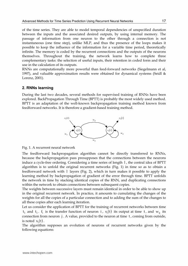
During the last two decades, several methods for supervised training of RNNs have been explored. BackPropagation Through Time (BPTT) is probably the most widely used method. BPTT is an adaptation of the well-known backpropagation training method known from feedforward networks. It is therefore a gradient-based training method.

w21

w12

( )y t2

w11w22

( )s t1 ( )s t2

x t1( )

Fig. 1. A recurrent neural network

The feedforward backpropagation algorithm cannot be directly transferred to RNNs, because the backpropagation pass presupposes that the connections between the neurons

induce a cycle-free ordering. Considering a time series of length l , the central idea of BPTT algorithm is to unfold the original recurrent networks (Fig. 1) in time so as to obtain a

feedforward network with l layers (Fig. 2), which in turn makes it possible to apply the learning method by backpropagation of gradient of the error through time. BPTT unfolds the network in time by stacking identical copies of the RNN, and duplicating connections within the network to obtain connections between subsequent copies. The weights between successive layers must remain identical in order to be able to show up in the original recurrent network. In practice, it amounts to cumulating the changes of the weights for all the copies of a particular connection and to adding the sum of the changes to all these copies after each learning iteration.

Let us consider the application of BPTT for the training of recurrent networks between time

1t and lt . if is the transfer function of neuron i , ( )tsi its output at time t , and ijw its

connection from neuron j . A value, provided to the neuron at time t , coming from outside,

is noted ( )txi . The algorithm supposes an evolution of neurons of recurrent networks given by the following equations:

www.intechopen.com

Recurrent Neural Networks for Temporal Data Processing

18

( )w21 1 ( )w12 1

( )w11 3 ( )w22 3

( )s1 1 ( )s2 1

( )s1 2 ( )s2 2

( )s1 3 ( )s2 3

( )s1 4 ( )s2 4

( )w11 2

( )w11 1

( )w22 2

( )w22 1

( )w12 2

( )w12 3

( )w21 2

( )w21 3

( )x1 1

( )y2 1

( )x1 2

( )x1 3

( )x1 4

( )y2 2

( )y2 3

( )y2 4

Fig. 2. RNN of Fig. 1 unfolded in time

( ) ( )( ) ( ) N,,1i;tx1tnetfts iii …=+−= (5)

( ) ( ) ( )1ts1tw1tnet j)i(predj

iji −−=− ∑∈ (6)

The set ( )iPred contains, for each neuron i , the index of the incoming neurons

( ) ( ){ }ijij ,wNjiPred τ∃∈= . Likewise, we have defined the successors of a neuron i :

( ) ( ){ }jiji ,wNjiSucc τ∃∈= .

The variation of the weight for all the sequence is calculated by the sum of the variations of

this weight on each element of the sequence. By noting ( )τT the set of neurons which have a

desired output ( )τpd at time τ , we define the mean quadratic error ( )l1 t,tE of the

recurrent neural networks between time 1t and lt as:

( ) ( ) ( )( )( )∑ ∑= ∈

−= l

1

t

tt tTp

2ppl1 tstd

2

1t,tE

(7)

To minimize total error, gradient descent is used to change each weight in proportion to its derivative with respect to the error, provided the non-linear activation functions are differentiable ( η is the learning step):

( ) ( )( )∑−=τ τ∂∂η−=∂

∂η−=−Δ 1t

t ij

l1

ij

l1l1ij

l

1w

t,tE

w

t,tE)1t,t(w (8)

www.intechopen.com

Advanced Methods for Time Series Prediction Using Recurrent Neural Networks

19

with

( )( ) ( )( ) ( )( )τ∂τ∂

τ∂∂=τ∂

∂ij

i

i

l1

ij

l1

w

net

net

t,tE

w

t,tE (9)

where ( )τijw is the duplication of the weight ijw of the original recurrent networks, for the

time τ=t . We expand ( ) ( )τ∂∂ il1 nett,tE :

( )( ) ( )( ) ( )( )τ∂+τ∂

+τ∂∂=τ∂

∂i

i

i

l1

i

l1

net

1s

1s

t,tE

net

t,tE

with

( )( ) ( )( )τ=τ∂+τ∂

i'

i

i netfnet

1s

(10)

If neuron i belongs to the last layer ( 1t l −=τ ):

( )( ) ( )( ) ( ) ( ) ( )( )1 l

i l i li T 1i i l

E t , t e ts t d t

s 1 s tl

τ∂ ∂ δ∂ τ ∂ ∈ += = −+ (11)

where ( ) 11Ti=δ +τ∈ if ( )1Ti +τ∈ and 0 otherwise. If neuron i belongs to the preceding layers:

( )( ) ( )( ) ( )( )( )( )( )∑∈ ⎟⎟⎠

⎞⎜⎜⎝⎛

+τ∂+τ∂

+τ∂∂++τ∂

+τ∂=+τ∂∂

iSuccj i

j

j

l1

ii

l1

1s

1net

1net

t,tE

1s

1e

1s

t,tE (12)

As ( ) ( ) ( )1w1s1net jiij +τ=+τ∂+τ∂ , the equations of BPTT algorithm are finally obtained:

( ) ( )( ) ( )∑−=τ ττ∂∂η−=−Δ 1t

tj

i

l1l1ij

l

1

snet

t,tE1t,tw

(13)

• with, for the output layer

( )( ) ( ) ( )[ ] ( )( ) ( )⎪⎩⎪⎨⎧ +τ∈τ−=τ∂

∂else0

1Tiifnetftdts

net

t,tE i'ilili

i

l1

(14)

• and for the hidden layer

( )( )( ) ( )[ ]( )( ) ( )

( )( )( ) ( )

( )( ) ( )( )

( )( )⎪⎪⎪⎩

⎪⎪⎪⎨

⎧

τ+τ+τ∂∂

+τ∈τ⎥⎥⎥⎦

⎤⎢⎢⎢⎣

⎡+τ+τ∂

∂++τ−+τ

=τ∂∂

∑∑

∈

∈

elsenetf1w1net

t,tE

1Ti ifnetf.1w

1net

t,tE

1d1s

net

t,tE

i'i

iSuccjji

j

l1

i'i

iSuccjji

j

l1

ii

i

l1

(15)

Eq. (13) to (15) allow to apply error gradient backpropagation through time: after the

forward pass, witch consists in updating the unfolded network, starting from the first copy

of the recurrent network and working upwards through the layers, ( ) ( )τ∂∂ il1 net/t,tE is

computed, by proceeding backwards through the layers lt ,.., 1t . One epoch requires O(lM) multiplications and additions, where M is the total number of network connections. Many speed-up techniques for gradient descent approach are

www.intechopen.com

Recurrent Neural Networks for Temporal Data Processing

20

described in the literature, e.g. dynamic learning rate adaptation schemes. Another approach to achieve faster convergence is to use second-order gradient descent techniques. Unfortunately, the gradient descent algorithms which are commonly used for training RNNs have several limitations, the most important one being the difficulty of dealing with long-term dependencies in the time series (Bengio et al, 1994; Hochreiter & Schmidhuber 1997) i.e. problems for which the desired output depends on the inputs presented at times far in the past. Backpropagated error gradient information tends to "dilute" exponentially over time. This phenomenon is called “vanishing gradient” or “forgetting behavior” (Frasconi et al., 1992; Bengio et al, 1994). (Bengio et al, 1994) have demonstrated the existence of a condition on the eigenvalues of the RNN Jacobian to be able to store information for a long period of time in the presence of noise. But this implies that the portion of gradient due to information at times t<<τ is insignificant compared to the portion of gradient at times near t.

w21

w12

( )y t2

w11w22

( )s t1 ( )s t2

x t1( ) B

Fig. 3. Delayed connection added to a RNN (dotted line)

Fig. 4. The RNN of Fig. 3 unfolded in time. Duplicated dotted connections correspond to the added connection

www.intechopen.com

Advanced Methods for Time Series Prediction Using Recurrent Neural Networks

21

We can give a more intuitive explanation for backpropagated gradient vanishing. Considering eq. (13) to (15), gradient calculation for each layer is done by a product with transfer function derivate. Most of the time, this last value is bounded between 0 and 1 (i.e. sigmoid function). Each time the signal is backpropagated through a layer, the gradient contribution of the forward layers is attenuated. Along the time-delayed connections the signal does no longer cross nonlinear activation functions between successive time steps (see Fig. 3 and Fig. 4). Adding connections with time delays to the RNN (El Hihi & Bengio, 1996; Lin, T., et al., 1996) often allows gradient descent algorithms to find better solutions in these cases. Indeed, by acting as a linear link between two distant moments, such a connection has beneficial effects on the expression of the gradient. Adding a delayed connection to an RNN (Fig. 3) creates several connections in the unfolded network (Fig. 4) jumping as many layers as the delay. Gradient backpropagated by these connections avoids attenuation of intermediate layers. But in the absence of prior knowledge concerning the problem to solve, how can one choose the locations and the delays associated to these new connections? By systematically adding meta-connections with consecutive delay connections, also named Finite Impulse Response (FIR) connections, one obtains oversized networks which are slow to train and have poor generalization abilities. Various regularization techniques can be employed in order to improve generalization and this further increases the computational cost. Constructive approaches for adapting the architecture of a neural network are usually more economical. An algorithm for the addition of time-delayed connections to recurrent networks should start with a simple, ordinary RNN and progressively add new connections according to some heuristic. An alternative solution could be found in the learning of the connection delays themselves. We suggested, for an RNN that associates a delay to each connection, an algorithm based on the gradient which simultaneously adjusts weights and delays. To improve the obtained results, we may also adapt general methods which authorize to improve the performances of various models. One such approach is to use a combination of models to obtain a more precise estimate than the one obtained by a single model. One such procedure is known under the name of boosting.

3. Constructive algorithms

Instead of systematically adding finite impulse response (FIR) connections to a recurrent network, each connection encompassing a whole range of delays, we opted for a constructive approach: starting with an RN having no time-delayed connections, then selectively adding a few such connections. The two algorithms we present in the following allow us to choose the location and the delay associated with a time-delayed connection which is added to an RN. The assumption we make is that significantly better results can be obtained by the addition of a small number of time-delayed connections to a recurrent network. The reader is invited to consult (Boné et al., 2000a; Boné et al, 2000b; Boné et al., 2002) for a more detailed discussion regarding the role of time-delayed connections in RNs. The iterative and constructive aspects diminish the effect of the vanishing gradient on the outcome of the algorithm. Indeed, by reinforcing the long-term dependencies in the network, the first time-delayed connections favor the subsequent learning steps. A high selectivity should allow us to avoid over-parameterized networks. For every iteration, we rank the candidate connections according to their relevance.

www.intechopen.com

Recurrent Neural Networks for Temporal Data Processing

22

We retained two alternative methods for defining the relevance of a candidate connection. The first one is based on the amount by which the error diminishes after the addition of the connection. The second one relies on a more detailed study of various quantities computed inside the network during gradient descent.

3.1 Bounded exploration for the addition of time-delayed connections

The first heuristic is a breadth-first search (BFS). It explores the alternatives for the location

and the delay associated with a new connection by adding that connection and performing a

few iterations of the underlying learning algorithm. The connection that produces the

largest increase in performance during these few iterations is then added, and the learning

continues until error increases on the stop set. Another exploratory stage begins for the

addition of a new connection. The algorithm eventually ends when the error on the stop set

no longer decreases upon the addition of a new connection, or a (user-specified) bound on

the number of new connections is reached. We employed BPTT as the underlying learning

algorithm and we called this constructive algorithm Exploratory Back-Propagation Through

Time (EBPTT). We must note that the breadth-first heuristic does not need any gradient

information and can be applied in combination with learning algorithms which are not

based on the gradient.

If the RNN we start with does not account well for the medium or long-term dependencies in the data, and these dependencies are not too complex, then by adding the appropriate connection the error is likely to diminish relatively fast. Three new parameters are required for this constructive algorithm: the maximal value for

the delay of a new connection, the maximal number of new connections and the number of

BPTT steps performed for each candidate connection during the exploratory stage. In

choosing the value of the first parameter one should ideally use prior knowledge related to

the problem. If such information is not available one can rely on simple, linear measures

such as auto or cross-correlations to find a bound for the long-term dependencies.

Computational cost governs the choice of the two other parameters. However, the

experiments we present in the following show that the contribution of the new connections

diminishes quickly as their number increases. The complexity of the exploratory stage may

seem quite high, O(N4), since after the addition of each candidate connection we carry out

several steps of the BPTT algorithm on the entire network. The user is supposed to find a

tradeoff between the quality of the results and the computation cost. When compared to the

complete exploration of all the alternative architectures, this breadth-first search is only

interesting if good results can be obtained with few learning steps during the exploratory

stage. Fortunately, experimental evidence shows that this appears to be the case, so the

global cost of the algorithm remains low.

3.2 Internal correlations

The second heuristic for defining the relevance of a candidate connection is closely

dependent on BPTT-like underlying learning algorithms. Since this method makes use of

quantities computed during gradient descent, its computation cost is significantly lower

than for the breadth-first search.

When applying BPTT on the training set between 1t and lt , we obtain the following

expression for the variation of one weight of delay k , ( ) ( )1t,tw l1k

ij−Δ :

www.intechopen.com

Advanced Methods for Time Series Prediction Using Recurrent Neural Networks

23

( )( ) ( )( ) ( )( )( )∑ ∑−

+=τ

−

+=τ τ∂∂η−=τΔ=−Δ 1t

kt

1t

ktk

ij

l1kijl1

kij

l

1

l

1w

t,tEw1t,tw (16)

( )( )τkijw being the copy of ( )k

ijw for τ=t in the unfolded network employed by BPTT. We

may write

( )( ) ( ) ( )( ) ( ) [ ]1t;ktks

net

t,tE

w

t,tEl1j

i

l1

kij

l1 −+∈τ−τ⋅τ∂∂=τ∂

∂ (17)

We are looking for connections which are potentially useful in capturing (medium or long-

term) dependencies in the data. A connection ( )kijw is then useful only if it has a significant

contribution to the computation of the gradient, i.e. ( ) ( )( )τ∂∂ kijl1 wt,tE is significantly

different from zero for many iterations of the learning algorithm. We select the output of a

neuron ( )ks j −τ which best contributes to a reduction in error by means of ( ) ( )τ∂∂ il1 nett,tE .

The resulting algorithm, called Constructive Back Propagation Through Time (CBPTT),

computes during several BPTT steps the correlation between the values of ( ) ( )τ∂∂ il1 nett,tE

and ( )ks j −τ for [ ]1t;kt l1 −+∈τ . The relevance of a candidate connection ( )kijw is defined

as the absolute value of this correlation. The connection with the highest relevance factor is

then added to the RNN, its weight is initialized to 0, and learning continues. The process

stops when a new connection has no further positive effect on the performance of the RNN,

as evaluated on a stop set. The time complexity and the storage complexity of CBPTT is the

same as for BPTT. This constructive algorithm requires two new parameters: the maximal value for the delays

of the new connections and the maximal number of new connections. The choice of these

parameters is independent from the constructive heuristic, so the rules already mentioned

for EBPTT should be applied. Experiments reported in (Boné et al., 2002) support the view

that the precise value of this parameter does not have a high influence on the outcome, as

long as it is higher than the significant linear dependencies in the data, which are given by

the autocorrelation. The same experiments show that performance is not very sensitive to

the bound on the number of new connections either, because the contribution of the new

connections quickly diminishes as their number increases.

This definition for the relevance of a candidate connection is well adapted to time

dependencies which are well represented in the available data. If this is not the case for the

dependencies one is interested in, a more thorough study of the distribution of the product ( ) ( ) ( )τ∂∂⋅−τ il1j nett,tEks should suggest more adequate measures for the relevance.

4. Time Delay Learning

An alternative to the adding of connections with time delays could be found in the learning

of the connection delays themselves. (Duro & Santos Reyes, 1999) (see also (Pearlmutter

1990)) have suggested, for a feed-forward neural networks that associate a delay to each

connection, an algorithm based on the gradient which simultaneously adjusts weights and

delays. We adapted this technique to a recurrent architecture.

www.intechopen.com

Recurrent Neural Networks for Temporal Data Processing

24

Considering an RNN in which two values are associated to each connection from a neuron j

to a neuron i, these two values are of a usual weight ijw of the signal and a delay ijτ which

is a real value indicating the needed time for the signal to propagate through the connection.

Note that this parameter is not the same as the maximal order of a FIR connection: indeed,

when we consider a connection of delay ijτ , we do not have simultaneously 1ij −τ

connections with integer delays between 1 and ijτ . The neuron output ( )tsi is given by:

( ) ( )( )1tnetfts iii −= with ( ) ( )( )∑∈ −τ−=−

iPredjijjiji 1tsw1tnet (15)

The values ( )1ts ijj −τ− are obtained by applying a linear interpolation between the two

nearest whole numbers of the delay ijτ .

We have adapted the BPTT algorithm to this architecture with a simultaneous learning of

weights and delays of the connections, inspired from (Duro & Santos Reyes, 1999). The

variation of a delay ijτ can be computed as the sum of the variations of this parameter

copies corresponding to the times from 1t to lt . Then we add this variation to all copies of

ijτ . We will only give here the demonstration of the learning of the delays as the learning of

the weight can easily be deducted from it.

We note ( )ττij the copy of ijτ for t τ= in the unfold in time neural net which is virtually

constructed with BPTT. ⎡ ⎤. is the operator of upward roundness.

We apply a back-propagation of the gradient of the mean quadratic error ( )1 lE t , t which is

defined as the sum of the instantaneous errors ( )e t from 1t to lt :

( ) ( ) ( ) ( )( )( )∑ ∑∑ = ∈=−== l

1

l

1

t

tt tTp

2pp

t

ttl1 tstd

2

1tet,tE (16)

( )⎡ ⎤

( )( )⎡ ⎤∑∑ −

τ+=τ

−

τ+=τ τ∂τ∂λ−=ττΔ=∂τ

∂λ−=−τΔ 1t

t ij

l11t

tij

ij

l1l1ij

l

ij1

l

ij1

t,tE)(

t,tE)1t,t( (17)

We can write ( ) ( ) ( ) ( ) ( ) ( )ττ∂τ∂•τ∂∂=ττ∂∂ ijiil1ijl1 netnett,tEt,tE . With a first order

approximation, ( ) ( ) ( ) ( )( )ijjijjijiji s1swnet τ−τ−−τ−τ≈ττ∂τ∂ . We expand ( ) ( )τ∂∂ il1 nett,tE

following Eq. 10. If neuron i belongs to the last layer ( 1t l −=τ ), we apply Eq. 11. If neuron i

belongs to one of the preceding layers:

( )( ) ( )( ) ( )( ) ( )( )( )∑∈ ⎟⎟⎠⎞

⎜⎜⎝⎛

+τ∂+τ+τ∂

+τ+τ∂∂++τ∂

+τ∂=+τ∂∂

iSuccj i

jij

jij

l1

ii

l1

1s

1net

1net

t,tE

1s

1e

1s

t,tE (18)

As ( ) ( ) ( )1w1s1net jiijij +τ=+τ∂+τ+τ∂ , we obtain the final relations to learn the delay

associated to each connection:

( ) ( )( ) ( ) ( )( )ijjijj

1t

ktij

i

l1l1ij s1sw

net

t,tE1t,t

l

1

τ−τ−−τ−ττ∂∂λ−=−τΔ ∑−+=τ

(19)

with for 1t l −=τ

www.intechopen.com

Advanced Methods for Time Series Prediction Using Recurrent Neural Networks

25

( )( ) ( ) ( ) ( )( ) ( )( )τ−δ=τ∂∂

+τ∈ i'ilili

1Tii

l1 netftdtsnet

t,tE (20)

and for 1t t 1lτ≤ < −

( )( )( ) ( ) ( )( )

( )( ) ( )( )( )( )τ

⎥⎥⎥⎥⎦

⎤

⎢⎢⎢⎢⎣

⎡+τ+τ+τ∂

∂++τ−+τδ

=τ∂∂ ∑∈

+τ∈i

'i

iSuccjji

jij

l1

ii1Ti

i

l1 netf1w

1net

t,tE

1d1s

net

t,tE

(21)

5. Boosting Recurrent Neural Networks

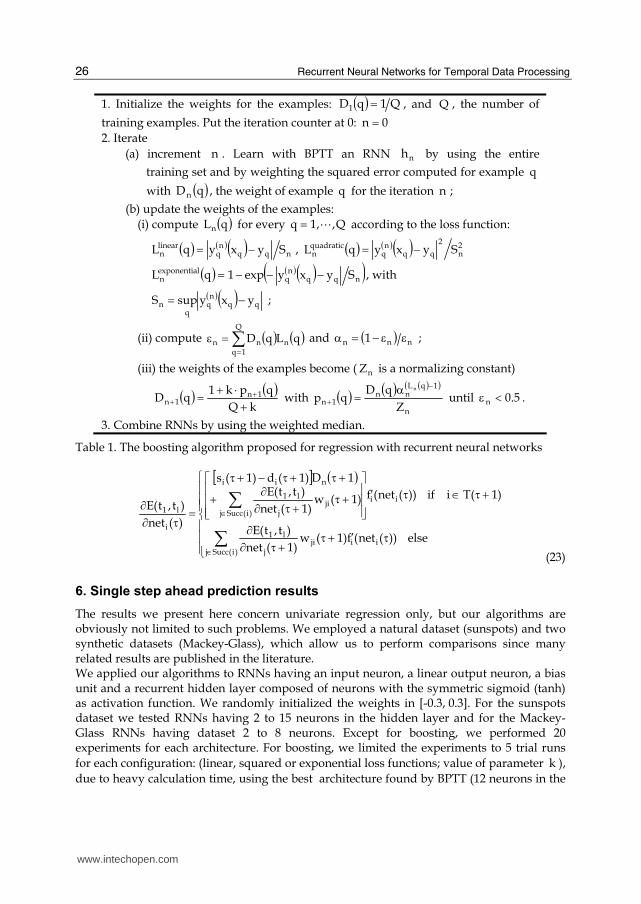
To improve the RNN forecasting results, we may use a combination of models to obtain a more precise estimate than the one obtained by a single model. In the boosting algorithm, the possible small gain a “weak” model can bring compared to random estimate is boosted by the sequential construction of several such models, which concentrate progressively on the difficult examples of the original training set. Boosting (Schapire, 1990; Freund & Schapire, 1997; Ridgeway et al., 1999) works by sequentially applying a classification algorithm to re-weighted versions of the training data, and then taking a weighted majority vote of the sequence of classifiers thus produced. Freund and Schapire (Freund & Schapire, 1997) presented the Adaboost. R algorithm that attacks the regression problem by reducing it to a classification problem. A different approach to regressor boosting as residual-fitting was developed in (Duffy & Helmbold, 2002; Buhlmann & Yu 2003). Instead of being trained on a different sample of the same training set, as in previous boosting algorithms, a regressor is trained on a new training set having different target values (e.g. the residual error). Before presenting briefly our algorithm, studied in (Assaad et al, 2005), let us mention that in (Cook & Robinson, 1996) a boosting method is applied to the classification of phonemes, with RNNs as learners. The authors are the first ones to have noticed the implications of the internal memory of the RNNs on the boosting algorithm. The boosting algorithm employed should comply with the restrictions imposed by the general context of the application. In our case, it must be able to work well when a limited amount of data is available and to accept RNNs as regressors. We followed (Assaad et al, 2008) the generic algorithm of (Freund, 1990). Our updates are based on the suggestion in (Drucker, 1999), but we apply a linear transformation to the weights before we employ them

(see the definition of ( )qD 1n+ in Table 1) in order to prevent the RNNs from simply ignoring

the easier examples. Then, instead of sampling with replacement according to the updated distribution, we prefer to weight the error computed for each example (thus using all the data points) at the output of the RNN with the distribution value corresponding to the example. For stage (2a), BPTT equations (14) and (15) become for the output layer:

[ ] ( )i l i l n i i1

i

s (t )-d (t ) D 1 f (net (τ)) if i T(τ 1)E(t , t )

net (τ) 0 elsel

τ ′⎧ + ∈ +∂ ⎪= ⎨∂ ⎪⎩ (22)

and for the hidden layer:

www.intechopen.com

Recurrent Neural Networks for Temporal Data Processing

26

1. Initialize the weights for the examples: ( ) Q1qD1 = , and Q , the number of

training examples. Put the iteration counter at 0: 0n =

2. Iterate

(a) increment n . Learn with BPTT an RNN nh by using the entire

training set and by weighting the squared error computed for example q

with ( )qDn , the weight of example q for the iteration n ;

(b) update the weights of the examples:

(i) compute ( )qLn for every Q,,1q A= according to the loss function:

( ) ( )( ) nqqn

qlinearn SyxyqL −= , ( ) ( )( ) 2

n

2

qqn

qquadraticn SyxyqL −=

( ) ( )( )( )nqqn

qlexponentia

n Syxyexp1qL −−−= , with

( )( ) qqn

qq

n yxysupS −= ;

(ii) compute ( ) ( )∑==ε Q

1qnnn qLqD and ( ) nnn 1 εε−=α ;

(iii) the weights of the examples become ( nZ is a normalizing constant)

( ) ( )kQ

qpk1qD 1n

1n +⋅+= ++ with ( ) ( ) ( )( )

n

1qLnn

1nZ

qDqp

n −+

α= until 5.0n <ε .

3. Combine RNNs by using the weighted median.

Table 1. The boosting algorithm proposed for regression with recurrent neural networks

[ ] ( )

⎪⎪⎪⎩

⎪⎪⎪⎨

⎧

τ′+τ+τ∂∂

+τ∈τ′⎥⎥⎥⎦⎤

⎢⎢⎢⎣⎡

+τ+τ∂∂+

+τ+τ−+τ=τ∂

∂∑∑

∈

∈

else))(net(f)1(w)1(net

)t,t(E

)1(Tiif))(net(f)1(w)1(net

)t,t(E1D)1(d)1(s

)(net

)t,t(E

)i(Succjiiji

j

l1

ii

)i(Succjji

j

l1

nii

i

l1

(23)

6. Single step ahead prediction results

The results we present here concern univariate regression only, but our algorithms are obviously not limited to such problems. We employed a natural dataset (sunspots) and two synthetic datasets (Mackey-Glass), which allow us to perform comparisons since many related results are published in the literature. We applied our algorithms to RNNs having an input neuron, a linear output neuron, a bias unit and a recurrent hidden layer composed of neurons with the symmetric sigmoid (tanh) as activation function. We randomly initialized the weights in [-0.3, 0.3]. For the sunspots dataset we tested RNNs having 2 to 15 neurons in the hidden layer and for the Mackey-Glass RNNs having dataset 2 to 8 neurons. Except for boosting, we performed 20 experiments for each architecture. For boosting, we limited the experiments to 5 trial runs

for each configuration: (linear, squared or exponential loss functions; value of parameter k ),

due to heavy calculation time, using the best architecture found by BPTT (12 neurons in the

www.intechopen.com

Advanced Methods for Time Series Prediction Using Recurrent Neural Networks

27

hidden layer for sunspots, 7 neurons for the Mackey-Glass series). We set the maximal number n of RNNs at 50 for each experiment. In the following we employ the normalized mean square error (NMSE) which is the ratio between the mean square error and the variance of the time series. It is defined, for a time

series l1 t,,tt)t(x …= , by

( )( )

( )2

t

tt

2

t

tt

2

t

tt

2

l

)t(x̂)t(x

)t(x)t(x

)t(x̂)t(xl

1

l

1

l

1 σ−

=−− ∑

∑∑ =

=

= (24)

where )t(x̂ is the prediction given by the RNN and )t(x , 2σ are the mean value and

variance estimated from the available data. A value of NMSE=1 is achieved by predicting

the unconditional mean of a time series. The normalized root mean squared error (NRMSE)

used for some of the results in the literature is the square root of the NMSE. We compared the results obtained using our algorithms to other results in the literature.

6.1 Sunspots

The sunspots dataset (Fig. 5) is a natural dataset that contains the yearly number of dark

spots on the sun from 1700 to 1979. The time series has a pseudo-period of 10 to 11 years. It

is common practice to use as the training set the data from 1700 to 1920 and to evaluate the

performance of the model on two sets, composed respectively of the data from 1921 to1955

(test1) and of the date from 1956 to 1979 (test2). Test2 is considered to be more difficult.

0

20

40

60

80

100

120

140

160

180

200

1700 1725 1750 1775 1800 1825 1850 1875 1900 1925 1950 1975

ye

arly s

un

sp

ot a

ve

rag

es

Test 1 Test 2

Fig. 5. The sunspots time series

For both CBPTT and EBPTT we set to 20 the upper bound for the delays of the new

connections, to 4 the maximal number of new connections and to 20 the number of BPTT

iterations performed for each candidate connection during the exploratory stage of EBPTT.

Tables 2 and 3 show the NMSE obtained by various models on the two test sets of this

benchmark, and the total number of parameters.

www.intechopen.com

Recurrent Neural Networks for Temporal Data Processing

28

Model Parameters Test1 Test2

Carbon copy 0 0.427 0.966

TAR 18 0.097 0.280

MLP Weigend 43 0.086 0.350

MLP Kouam 43 0.082 0.320

RNR/BPTT 181 0.102 0.371

RNR/EBPTT 20 it. 15 0.096 0.320

RNR/EBPTT 100 it. 15 0.092 0.308

RNR/CBPTT 15 0.094 0.281

RNR/Boosting (quad., 20) 0.090 0.296

RNR/Boosting (lin., 10) 0.082 0.314

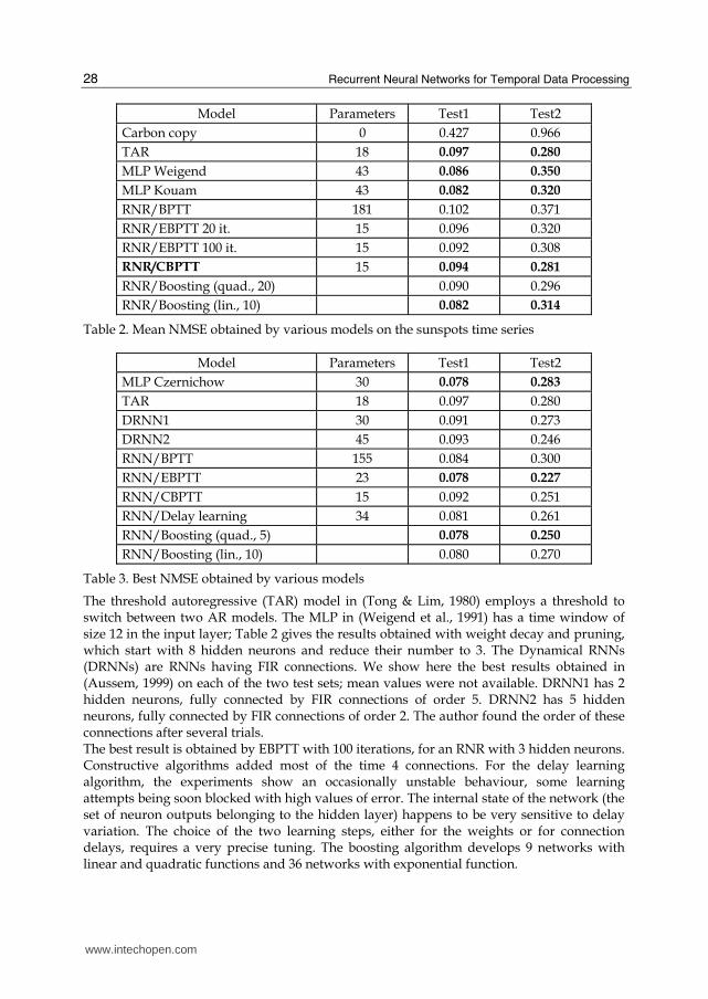
Table 2. Mean NMSE obtained by various models on the sunspots time series

Model Parameters Test1 Test2

MLP Czernichow 30 0.078 0.283

TAR 18 0.097 0.280

DRNN1 30 0.091 0.273

DRNN2 45 0.093 0.246

RNN/BPTT 155 0.084 0.300

RNN/EBPTT 23 0.078 0.227

RNN/CBPTT 15 0.092 0.251

RNN/Delay learning 34 0.081 0.261

RNN/Boosting (quad., 5) 0.078 0.250

RNN/Boosting (lin., 10) 0.080 0.270

Table 3. Best NMSE obtained by various models

The threshold autoregressive (TAR) model in (Tong & Lim, 1980) employs a threshold to switch between two AR models. The MLP in (Weigend et al., 1991) has a time window of size 12 in the input layer; Table 2 gives the results obtained with weight decay and pruning, which start with 8 hidden neurons and reduce their number to 3. The Dynamical RNNs (DRNNs) are RNNs having FIR connections. We show here the best results obtained in (Aussem, 1999) on each of the two test sets; mean values were not available. DRNN1 has 2 hidden neurons, fully connected by FIR connections of order 5. DRNN2 has 5 hidden neurons, fully connected by FIR connections of order 2. The author found the order of these connections after several trials. The best result is obtained by EBPTT with 100 iterations, for an RNR with 3 hidden neurons. Constructive algorithms added most of the time 4 connections. For the delay learning algorithm, the experiments show an occasionally unstable behaviour, some learning attempts being soon blocked with high values of error. The internal state of the network (the set of neuron outputs belonging to the hidden layer) happens to be very sensitive to delay variation. The choice of the two learning steps, either for the weights or for connection delays, requires a very precise tuning. The boosting algorithm develops 9 networks with linear and quadratic functions and 36 networks with exponential function.

www.intechopen.com

Advanced Methods for Time Series Prediction Using Recurrent Neural Networks

29

0

20

40

60

80

100

120

140

160

180

200

1921 1926 1931 1936 1941 1946 1951 1956 1961 1966 1971 1976

RealForecast

Fig. 6. The predictions obtained with EBPTT on the sunspots test sets

6.2 Mackey-Glass series

The Mackey-Glass benchmarks (Mackey and Glass, 1977) are well-known for the evaluation of SS and MS prediction methods. The time series are generated by the following nonlinear differential equation:

10

dx 0.2 x(t θ)0.1 x(t)

dt 1 x (t θ)

⋅ −= − ⋅ + + − (25)

The behavior is chaotic for τ > 16,8. The results in the literature usually concern τ = 17

(known as MG17, see Fig. 7) and τ = 30 (MG30). The data is generated and then sampled with a period of 6, according to the common practice, see e.g. (Wan 1993). We use the first 500 values as our learning set and the next 100 values as our test set.

0.4

0.5

0.6

0.7

0.8

0.9

1

1.1

1.2

1.3

1.4

0 100 200 300 400 500 600

0.2

0.4

0.6

0.8

1

1.2

1.4

0 100 200 300 400 500 600

Fig. 7. The Mackey-Glass time series for θ = 17 (left) and θ = 30 (right)

The linear, polynomial, local approaches, RBF and MLP models are mentioned in (Casdagli,

1989). The FIR MLP put forward in (Wan, 1993) has 15 neurons in the hidden layer. FIR

connections of order 8 are employed between the inputs and the hidden neurons, while the

order of the connections between the hidden neurons and the output is 2. The resulting

networks have 196 parameters. The feed-forward network employed in (Duro & Santos

Reyes, 1999) consists of a single input neuron, 20 hidden neurons and one output neuron. A

delay is associated to every connection in the network, and the value of the delay is

modified by a learning algorithm inspired by back-propagation. In (McDonnell & Waagen,

1994) an evolutionary algorithm produces an RNN having 2 hidden neurons with sinusoidal

transfer functions and several time-delayed connections.

www.intechopen.com

Recurrent Neural Networks for Temporal Data Processing

30

Model MG(17) MG(30)

Linear 269 324

Polynomial 11.2 39.8

Local approach 1 33.1 57.5

Local approach 2 12.9 380.2

RBF 10.7 25.1

FFN 10 31.6

RNN/BPTT 0.99 13.1

RNN/EBPTT 0.62 1.8

RNN/CBPTT 1.66 2.51

Boosting (quad., 100) 0.16 0.45

Boosting (quad., 200) 0.18 0.45

Table 4. Mean EQMN (*103) obtained by various models on the MG time series

The DRNNs have FIR connections of order 4 between the input and the hidden layer, FIR connections of order 2 between the 4 to 7 hidden neurons, and simple connections to the output neuron (for a total of 197 parameters). Throughout our experiments, for both EBPTT and CBPTT we set to 34 the maximal value for

the delays of the new connections and to 10 the maximal number of new connections. The

number of BPTT steps performed for each candidate connection during the exploratory

stage of EBPTT was always set to 20; a higher value has a negligible effect here. The mean

results reported in Table 4 were obtained with RNNs having 6 hidden neurons, so with 10

time-delayed connections we have a maximum of 65 parameters. The best results were

obtained with RNNs having up to 7 hidden neurons, for a maximum of 81 parameters.

Our constructive algorithms significantly improve the results reported in the literature for

the two datasets, with regard both to the mean NMSE and to the lowest NMSE. There is also

an improvement upon BPTT without the constructive stage.

During our experiments we noticed that the mean value of the delays associated with the new connections was significantly lower for MG(17) than for MG(30). Also, CBPTT added on the average fewer connections than EBPTT. Again, only the first new connections produce a significant reduction in the NMSE.

Model MG(17) MG(30)

FIR MLP 4.9 16.2

TDFFN 0.8

RNN evolutionary algorithm 2.5

DRNN 4.7 7.6

RNRN/BPTT 0.23 0.89

RNN/EBPTT 0.13 0.05

RNN/CBPTT 0.14 0.73

RNN/delay learning 0.15

Boosting (lin.,150) 0.13 0.45

Boosting (quad., 100) 0.15 0.41

Table 5. Best EQMN (*103) obtained by various models on the MG time series

www.intechopen.com

Advanced Methods for Time Series Prediction Using Recurrent Neural Networks

31

7. Multi step ahead prediction results

While reliable multi-step-ahead (MS) prediction has important applications ranging from system identification to ecological modeling, most of the published literature considers single-step-ahead (SS) time series prediction. The main reason for this is the inherent difficulty of the problems requiring MS prediction and the fact that the results obtained by simple extensions of algorithms developed for SS prediction are often disappointing. Moreover, if many different techniques perform rather similarly on SS prediction problems, significant differences show up when extensions of these techniques are employed on MS problems. There are several methods for dealing with a MS prediction problem after finding a satisfactory solution to the associated SS problem. The first and most common method consists in building a predictor for the SS problem and using it recursively for the corresponding MS problem. The estimates provided by the model for the next time step are fed back to the input of the model until the desired prediction horizon is reached. This method is usually called iterated prediction. This simple method is plagued by the accumulation of errors on the difficult data points encountered; the model can quickly diverge from the desired behavior. A better method consists in training the predictor on the SS problem and, at the same time, in making use of the propagation of penalties across time steps in order to punish the predictor for accumulating errors in MS prediction. This method is called corrected iterated prediction. When the models are MLPs or RNNs, such a procedure is directly inspired from the BPTT algorithm performing gradient descent on the cumulated error. The model is thus simultaneously trained on both the SS and the associated MS prediction problem. Unfortunately, the gradient of the error usually “vanishes” when moving away from the time step during which the penalty was received (Bengio, 1994). According to the direct method, the predictor is no longer concerned with an SS problem and is directly trained on the MS problem. By a formal analysis of the expected error, it is shown in (Atiya et al., 1999) that the direct method always performs better than the iterated method and at least as well as the corrected iterated method. However, this result relies on several assumptions, among which the ability of the model to perfectly learn the different target functions (the one for SS prediction and the one for direct MS prediction). The results of the learning algorithm may been improved, e.g. when it suffers from the vanishing gradient phenomenon. For instance, improved results were obtained by using recurrent networks and training them with progressively increasing prediction horizons (Suykens & Vandewalle, 1995) or including time-delayed connections from the output of the network to its input (Parlos et al., 2000). We decided to test on MS prediction problems the previous algorithms that were originally developed for learning long-term dependencies in time series (Boné & al, 2000) or for improving general performance. Constructive algorithms provide a selective addition of time-delayed connections to recurrent networks and were shown to produce parsimonious models (few parameters, linear prior on the longer-range dependencies) with good results on SS prediction problems. These results, together with the fact that a longer-range memory embodied in the time delays should allow a network to better retain the past information when predicting at a long horizon, let us anticipate improved results on MS prediction problems. Some further support for this claim is provided by the experimental evidence in (Parlos et al., 2000) concerning the successful use of time delays in recurrent networks for

www.intechopen.com

Recurrent Neural Networks for Temporal Data Processing

32

MS prediction. We expected the constructive algorithms to identify the most useful delays for a given problem and network architecture, instead of using an entire range of delays.

7.1 Sunspots

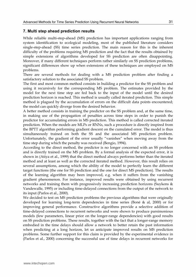
All the tested algorithms perform better than standard BPTT and exhibit a fast degradation while simultaneously increasing prediction horizon (Table 6, Fig. 8).

Model Steps ahead h BPTT CBPTT EBPTT lin. 10 quad. 20 quad. 5 exp. 20

1 0.24 0.17 0.19 0.18 0.17 0.18 0.18

2 0.88 0.69 0.53 0.43 0.40 0.43 0.42

3 1.14 0.99 0.79 0.54 0.54 0.56 0.67

4 1.22 1.17 0.80 0.67 0.73 0.64 0.76

5 1.01 0.99 0.88 0.74 0.69 0.73 0.77

6 1.02 1.01 0.84 0.73 0.68 0.65 0.74

10 - - - 0.64 0.69 0.67 0.75

12 - - - 0.86 0.97 0.77 1.09

Table 6. Best mean NMSE on the sunspots cumulated set (test1+test2) as a function of the prediction horizon

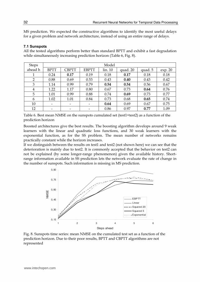
Boosted architectures give the best results. The boosting algorithm develops around 9 weak learners with the linear and quadratic loss functions, and 30 weak learners with the exponential function, as for the SS problem. The mean number of networks remains practically constant while the horizon increases. If we distinguish between the results on test1 and test2 (not shown here) we can see that the deterioration is mainly due to test2. It is commonly accepted that the behavior on test2 can not be explained (by some longer-range phenomenon) given the available history. Short-range information available in SS prediction lets the network evaluate the rate of change in the number of sunspots. Such information is missing in MS prediction.

0,15

0,30

0,45

0,60

0,75

0,90

1 2 3 4 5 6

Steps ahead

NMSE

EBPTTLinearSquared 20Squared 5Exponential

Fig. 8. Sunspots time series: mean NMSE on the cumulated test set as a function of the prediction horizon. Due to their poor results, BPTT and CBPTT algorithms are not represented

www.intechopen.com

Advanced Methods for Time Series Prediction Using Recurrent Neural Networks

33

7.2 Mackey-Glass series

For the two MG series, we obtained (Tables 7 and 8) around 26 networks with the linear

function, 37 with the squared function and between 46 and 50 for the exponential function.

The maximal number of networks is set to 50. Tables 7 and 8 show the strong improvements

obtained on the original BPTT and on the constructive algorithms.

Model Steps ahead h BPTT CBPTT EBPTT Lin. 150 quad. 100 exp. 100

1 22 13 1 0.17 0.16 0.17

2 179 124 101 0.24 0.28 0.25

3 145 124 16 0.57 0.57 0.52

4 8 7 4 0.57 0.54 0.52

5 266 253 181 0.98 1.26 1.27

6 321 321 232 2.11 15.2 4.66

10 336 331 219 14.1 12.2 15.0

11 289 218 252 9.80 12.0 16.8

12 167 156 158 6.72 8.66 7.57

Table 7. Best mean results (NMSE*103) on MG17 as a function of the prediction horizon

Comparisons with other published results concerning MG17 MS prediction can only be

performed for a horizon of 14; the results presented here are inferior to those of the local

methods put forward in (Chudy & Farkas 1998; McNames 2000), but for the RNNs trained

by our algorithm, significantly fewer data points were employed for training (500 compared

to 3000 or 10000), which is the usual benchmark (Casdagli 1989; Wan, 1994). However, the

use of a huge number of points for learning the MG17 artificial time series, generated

without noise, can lead to models with poor generalization to noisy data.

Model Steps ahead h BPTT CBPTT EBPTT lin. 300 quad. 200 exp. 150

1 11.7 2.5 1.8 0.45 0.45 0.47

2 19.9 9.7 3.3 0.49 0.48 0.59

3 4 2.2 1.6 0.56 0.55 0.64

4 2.2 2.1 1.6 0.47 0.43 0.48

5 2.6 2.3 0.9 0.85 0.67 0.72

6 8.9 8.3 6.4 1.75 1.92 1.80

7 70.1 65.6 64.3 2.98 4.56 2.72

8 336 203 112 5.08 109 57.0

9 801 379 257 84.0 276 3.71

10 892 383 73.7 2.79 204 2.63

11 411 230 285 6.34 21.3 8.05

Table 8. Best mean results (NMSE*103) on MG30 as a function of the prediction horizon

www.intechopen.com

Recurrent Neural Networks for Temporal Data Processing

34

8. Conclusion

Adding time-delayed connections to recurrent neural networks helps gradient descent algorithms in learning medium or long-term dependencies. However, by systematically adding finite impulse response connections, one obtains oversized networks which are slow to train and need regularization techniques in order to improve generalization. We apply here two constructive approaches, which starts with a RNN having no time-delayed connections and progressively adds some, an approach based on a particular type of neuron whose connections have a real value and adapted to recurrent networks and a boosting algorithm. The experimental results we obtained on three benchmark problems show that by adding only a few time-delayed connections we are able to produce networks having comparatively few parameters and good performance for SS problems. The results show also that boosting recurrent neural networks improve strongly MS forecasting. The boosting effect proved to be less effective for sunspots MS forecasts because some short-term dependencies are essential for the prediction of some parts of the data. The fact that for the Mackey-Glass datasets the results are better on the most difficult of the two sets (MG30) can be explained by noticing that long-range dependencies play a more important role for MG30 than for MG17.

9. References

Assaad, M.; Boné, R. & Cardot, H. (2005). Study of the Behavior of a New Boosting Algorithm for Recurrent Neural Networks, Proceeding of Int. Conference on Artificial Neural Networks, LNCS, Vol. 3697, 169-174, Warsaw, Poland, Springer-Verlag

Assaad, M.; Boné, R. & Cardot, H. (2008). A New Boosting Algorithm for Improved Time-Series Forecasting with Recurrent Neural Networks, Information Fusion, Vol. 9, No. 1, January 2008, 41-55

Atiya, A. F.; El-Shoura, S. M.; Shaheen, S. I. & El-Sherif, M. S. (1999). A Comparison Between Neural Network Forecasting Techniques - Case Study: River Flow Forecasting. IEEE Transactions on Neural Networks, Vol. 10, No. 2, 402-409.

Aussem, A. (1999). Dynamical Recurrent Neural Networks: Towards Prediction and Modelling of Dynamical Systems, Neurocomputing, Vol. 28, 207-232

Aussem, A. (2002). Sufficient Conditions for Error Backflow Convergence in Dynamical Recurrent Neural Networks, Neural Computation, Vol. 14, No. 8, 1907-1927.

Bengio, Y.; Simard, P. & Frasconi, P. (1994). Learning Long-Term Dependencies with Gradient Descent is Difficult, IEEE Transactions on Neural Networks, Vol. 5, No. 2, 157-166

Boné, R.; Crucianu, M. & Asselin de Beauville, J.-P. (2000a). An Algorithm for the Addition of Time-Delayed Connections to Recurrent Neural Networks, Proceedings of European Symposium on Artificial Neural Networks, pp. 293-298, Bruges, Belgium

Boné, R.; Crucianu, M.; Verley, G. & Asselin de Beauville, J.-P. (2000b). A Bounded Exploration Approach to Constructive Algorithms for Recurrent Neural Networks, Proceedings of International Joint Conference on Neural Networks, Vol. 3, pp. 27-32, Como, Italy

Boné, R.; Crucianu, M. & Asselin de Beauville, J.-P. (2002). Learning Long Term Dependencies by the Selective Addition of Time-Delayed Connections to Recurrent Neural Networks, NeuroComputing, Vol 48, 251-266

www.intechopen.com

Advanced Methods for Time Series Prediction Using Recurrent Neural Networks

35

Bühlmann, P. & Yu, B. (2003). Boosting with L2-loss: Regression and Classification, Journal of the American Statistical Association, Vol. 98 , 324-340

Campolucci, P.; Uncini, A.; Piazza, F. & Rao, B. D. (1999). On-line learning algorithms for locally recurrent neural networks. IEEE Transaction on Neural Networks, Vol. 10, No. 2, 253-271

Casdagli, M. (1989). Nonlinear Prediction of Chaotic Time Series, Physica, Vol. 35D , 335-356. Chudy, L. & Farkas, I. (1998). Prediction of Chaotic Time-Series Using Dynamic Cell

Structures and Local Linear Models. Neural Network World, Vol. 8, 481-489 Cook, G.D. & Robinson, A.J. (1996). Boosting the Performance of Connectionist Large

Vocabulary Speech Recognition, Proceedings of International Conference in Spoken Language Processing, pp. 1305-1308, Philadelphia, PA

Czernichow, T.; Piras, A.; Imhof, K.; Caire, P.; Jaccard, Y.; Dorizzi, B. & Germont, A. (1996) Short Term Electrical Load Forecasting with Artificial Neural Networks, Engineering Intelligent Systems, Vol. 4, No. 2, 85-99

Drucker, H. (1999). Boosting Using Neural Nets, In Combining Artificial Neural Nets: Ensemble and Modular Learning, A. Sharkey, (Ed.), 51-77, Springer

Duffy, N. & Helmbold, D. (2002). Boosting Methods for Regression, Machine Learning, Vol. 47, 153-200

Duro, R.J. & Santos Reyes, J. (1999). Discrete-Time Backpropagation for Training Synaptic Delay-Based Artificial Neural Networks. IEEE Transactions on Neural Networks, Vol. 10, No. 4, 779-789.

El Hihi, S. & Bengio, Y. (1996). Hierarchical Recurrent Neural Networks for Long-Term Dependencies, Advances in Neural Information Processing Systems VIII, M. Mozer, D. S. Touretzky and M. Perrone, (Eds), 493-499, MIT Press, Cambridge, MA

Frasconi, P. ; Gori, M. & Soda, G. (1992). Local Feedback Mulitlayered Networks. Neural Computation, Vol. 4, No. 1, 120-130

Freund, Y. (1990,). Boosting a Weak Learning Algorithm by Majority, Proceedings of Workshop on Computational Learning Theory, pp. 202-216

Freund, Y. 1 Schapire, R.E. (1997). A Decision-Theoretic Generalization of On-Line Learning and an Application to Boosting. Journal of Computer and System Sciences, Vol. 55, 119-139

Guignot, J. & Gallinari, P. (1994). Recurrent Neural Networks with Delays, Proceedings of International Conference on Artificial Neural Networks, pp. 389-392, Sorrento

Hammer, B. & Tino, P. (2003). Recurrent Neural Networks with Small Weights Implement Definite Memory Machines, Neural Computation, Vol. 15, No. 8, 1897-1926

Hochreiter, S. & Schmidhuber, J. (1997). Long Short-Term Memory. Neural Computation, Vol. 9, No. 8, 1735-1780

Lin, T.; Horne, B.G.; Tino, P. & Giles, C.L. (1996). Learning Long-Term Dependencies in NARX Recurrent Neural Networks. IEEE Transactions on Neural Networks, Vol.7, No. 6, 1329-1338

McNames, J. (2000). Local Modeling Optimization for Time Series Prediction. Proceedings of 8th European Symposium on Artificial Neural Networks, pp. 305-310, Bruges, Belgium

Mackey, M. & Glass, L. (1977). Oscillations and Chaos in Physiological Control Systems, Science, 197-287

Parlos, A.G.; Rais, O.T. & Atiya, A.F (2000). Multi-Step-Ahead Prediction Using Dynamic Recurrent Neural Networks. Neural Networks, Vol. 13, 765-786

www.intechopen.com

Recurrent Neural Networks for Temporal Data Processing

36

Pearlmutter, B.A. (1990). Dynamic Recurrent Neural Networks. Research Report CMU-CS-90-196. Carnegie Mellon University.

Schapire, R.E. (1990). The Strength of Weak Learnability, Machine Learning, Vol. 5, 197-227. Seidl, D.R. & Lorenz, R.D. (1991). A Structure by which a Recurrent Neural Network Can

Approximate a Nonlinear Dynamic System, Proceedings of International Joint Conference on Neural Networks, pp. 709-714.

Siegelmann, H.T.; Horne, B.G. & Giles C.L. (1997). Computational Capabilities of Recurrent NARX Neural Networks. IEEE Transactions on Systems, Man and Cybernetics, Vol. 27, No. 2, 209-214

Suykens, J.A.K. & Vandewalle, J. (1995). Learning a Simple Recurrent Neural State Space Model to Behave Like Chua’s Double Scroll. IEEE Transactions on Circuits and Systems-I, Vol. 42, 499-502

Takens, F. (1981). Detecting Strange Attractors in Turbulence. Dynamical Systems and Turbulence. Dynamical Systems and Turbulence, Lecture Notes in Mathematics, Vol. 898, 366–381, Springer-Verlag, Berlin

Tong, H. & Lim, K.S. (1980). Threshold Autoregression, Limit Cycles and Cyclical Data, Journal of the Royal Statistical Society, Vol. B42 , 245-292

Tsoi, A.C. & Back, A.D. (1994). Locally Recurrent Globally Feedforward Networks: A Critical Review of Architectures. IEEE Transactions on Neural Networks, Vol. 5, No 2, 229-239

Wan, E. A. (1993). Finite Impulse Response Neural Networks with Applications in Time Series Prediction, PhD Thesis, Stanford University, 140p

Wan, E.A. (1994). Time Series Prediction by Using a Connection Network with Internal Delay Lines, In: Time Series Prediction: Forecasting the Future and Understanding the Past, A. S. Weigend and N. A. Gershenfeld, (Eds), 195-217, Addison-Wesley

Weigend, A.S.; Rumelhart, D.E. & Huberman, B.A. (1991). Generalization by Weight-Elimination applied to Currency Exchange Rate Prediction, Proceedings of International Joint Conference on Neural Networks, pp. 837-841, Seattle, USA

www.intechopen.com

Recurrent Neural Networks for Temporal Data ProcessingEdited by Prof. Hubert Cardot

ISBN 978-953-307-685-0Hard cover, 102 pagesPublisher InTechPublished online 09, February, 2011Published in print edition February, 2011

InTech EuropeUniversity Campus STeP Ri Slavka Krautzeka 83/A 51000 Rijeka, Croatia Phone: +385 (51) 770 447 Fax: +385 (51) 686 166www.intechopen.com

InTech ChinaUnit 405, Office Block, Hotel Equatorial Shanghai No.65, Yan An Road (West), Shanghai, 200040, China

Phone: +86-21-62489820 Fax: +86-21-62489821

The RNNs (Recurrent Neural Networks) are a general case of artificial neural networks where the connectionsare not feed-forward ones only. In RNNs, connections between units form directed cycles, providing an implicitinternal memory. Those RNNs are adapted to problems dealing with signals evolving through time. Theirinternal memory gives them the ability to naturally take time into account. Valuable approximation results havebeen obtained for dynamical systems.

How to referenceIn order to correctly reference this scholarly work, feel free to copy and paste the following:

Romuald Boné and Hubert Cardot (2011). Advanced Methods for Time Series Prediction Using RecurrentNeural Networks, Recurrent Neural Networks for Temporal Data Processing, Prof. Hubert Cardot (Ed.), ISBN:978-953-307-685-0, InTech, Available from: http://www.intechopen.com/books/recurrent-neural-networks-for-temporal-data-processing/advanced-methods-for-time-series-prediction-using-recurrent-neural-networks

© 2011 The Author(s). Licensee IntechOpen. This chapter is distributedunder the terms of the Creative Commons Attribution-NonCommercial-ShareAlike-3.0 License, which permits use, distribution and reproduction fornon-commercial purposes, provided the original is properly cited andderivative works building on this content are distributed under the samelicense.