Football Match Prediction using Deep...

Football Match Prediction usingDeep LearningRecurrent Neural Network Applications

Master’s Thesis in Computer Science – algorithms, languages and logic

DANIEL PETTERSSONROBERT NYQUIST

Department of Electrical EngineeringCHALMERS UNIVERSITY OF TECHNOLOGYGothenburg, Sweden 2017EX031/2017

Master’s Thesis EX031/2017

Football Match Prediction using Deep Learning

Recurrent Neural Network Applications

DANIEL PETTERSSONROBERT NYQUIST

Supervisor and Examiner:Professor Irene Yu-Hua Gu, Department of Electrical Engineering

Department of Electrical EngineeringChalmers University of Technology

Gothenburg, Sweden 2017

Football Match Prediction using Deep LearningRecurrent Neural Network ApplicationsDANIEL PETTERSSONROBERT NYQUIST

© DANIEL PETTERSSON, ROBERT NYQUIST, 2017.

Supervisor and Examiner:Professor Irene Yu-Hua Gu, Department of Electrical Engineering

Master’s Thesis EX031/2017Department of Electrical EngineeringChalmers University of TechnologySE-412 96 GothenburgTelephone +46 31 772 1000

Typeset in LATEXGothenburg, Sweden 2017

iv

Football Match Predicition using Deep LearningRecurrent Neural Network ApplicationsDANIEL PETTERSSONROBERT NYQUISTDepartment of Electrical EngineeringChalmers University of Technology

Abstract

In this thesis, the deep learning method Recurrent Neural Networks (RNNs) hasbeen investigated for predicting the outcomes of football matches. The dataset con-sists of previous recorded matches from multiple seasons of leagues and tournamentsfrom 63 different countries and 3 tournaments that include multiple countries.

In the thesis work, we have studied several different ways of forming up input datasequences, as well as different LSTM architectures of RNNs that may lead to effectiveprediction, along with LSTM hyper-parameter tuning and testing. Extensive testshave been conducted through many case studies for the prediction and classificationof football match winners.

Using the proposed LSTM architectures, we show that the classification accuracyof the football outcome is 98.63% for many-to-one strategy, and 88.68% for many-to-many strategy. The prediction accuracy starts from 33.35% for many-to-one and43.96% for many-to-many, and is increasing when more information about a matchfrom longer time duration of data sequence is fed to the network. Using the full timedata sequence, the RNN accuracy reached 98.63% for many-to-one, and 88.68% formany-to-many strategy.

Our test results have shown that deep learning may be used for successfully pre-dicting the outcomes of football matches. For further increasing the performanceof the prediction, prior information about each team, player and match would bedesirable.

Keywords: Football, deep learning, machine learning, predictions, recurrent neuralnetwork, RNN, LSTM

v

Acknowledgements

We would firstly like to thank our supervisor Irene Yu-Hua Gu at the Departmentof Electrical Engineering at Chalmers University of Technology, where this thesishas been conducted. We would like to thank her for the help she has been givingthroughout this work.

We would also like to express our thanks to Forza Football for providing us withdata, equipment, and workspace.

We have grown both academically and personally from this experience and are verygrateful for having had the opportunity to conduct this study.

Daniel Pettersson, Robert Nyquist, Gothenburg, June 2017

vii

Contents

List of Figures xi

List of Tables xiii

1 Introduction 11.1 Background . . . . . . . . . . . . . . . . . . . . . . . . . . . . . . . . 11.2 Goals . . . . . . . . . . . . . . . . . . . . . . . . . . . . . . . . . . . . 11.3 Constraints . . . . . . . . . . . . . . . . . . . . . . . . . . . . . . . . 11.4 Problem Formulation . . . . . . . . . . . . . . . . . . . . . . . . . . . 21.5 Disposition . . . . . . . . . . . . . . . . . . . . . . . . . . . . . . . . 2

2 Background Theory 32.1 Machine Learning . . . . . . . . . . . . . . . . . . . . . . . . . . . . . 3

2.1.1 Neural Networks . . . . . . . . . . . . . . . . . . . . . . . . . 32.1.2 Deep Learning . . . . . . . . . . . . . . . . . . . . . . . . . . . 42.1.3 Recurrent Neural Networks . . . . . . . . . . . . . . . . . . . 4

2.1.3.1 Long Short-Term Memory . . . . . . . . . . . . . . . 62.1.3.2 Gated Recurrent Unit . . . . . . . . . . . . . . . . . 9

2.1.4 Dropout . . . . . . . . . . . . . . . . . . . . . . . . . . . . . . 102.1.5 Embeddings . . . . . . . . . . . . . . . . . . . . . . . . . . . . 112.1.6 Softmax Classifier . . . . . . . . . . . . . . . . . . . . . . . . . 112.1.7 Cross Entropy Error . . . . . . . . . . . . . . . . . . . . . . . 122.1.8 Adam Optimizer . . . . . . . . . . . . . . . . . . . . . . . . . 122.1.9 Hardware . . . . . . . . . . . . . . . . . . . . . . . . . . . . . 12

2.1.9.1 Central Processing Unit . . . . . . . . . . . . . . . . 122.1.9.2 Graphics Processing Unit . . . . . . . . . . . . . . . 12

2.1.10 Software Libraries . . . . . . . . . . . . . . . . . . . . . . . . . 132.2 Predicting the Outcome of Football Matches . . . . . . . . . . . . . . 13

2.2.1 Challenges in Predicting the Outcome of Football Matches . . 132.2.2 Previous Work . . . . . . . . . . . . . . . . . . . . . . . . . . 14

3 Proposed Methods for Football Match Prediction 153.1 Data . . . . . . . . . . . . . . . . . . . . . . . . . . . . . . . . . . . . 153.2 Network Input . . . . . . . . . . . . . . . . . . . . . . . . . . . . . . . 16

3.2.1 Deep Embeddings . . . . . . . . . . . . . . . . . . . . . . . . . 173.2.2 One-Hot Vector with all Attributes . . . . . . . . . . . . . . . 17

ix

Contents

3.2.3 Concatenated Embedding Vectors for all Attributes . . . . . . 183.3 Naive Statistical Model . . . . . . . . . . . . . . . . . . . . . . . . . . 183.4 Deep Learning Architecture . . . . . . . . . . . . . . . . . . . . . . . 19

3.4.1 Many-To-One . . . . . . . . . . . . . . . . . . . . . . . . . . . 203.4.2 Many-To-Many . . . . . . . . . . . . . . . . . . . . . . . . . . 21

4 Results and Evaluation 234.1 Setup . . . . . . . . . . . . . . . . . . . . . . . . . . . . . . . . . . . . 234.2 Dataset . . . . . . . . . . . . . . . . . . . . . . . . . . . . . . . . . . 244.3 Training . . . . . . . . . . . . . . . . . . . . . . . . . . . . . . . . . . 24

4.3.1 Tuning Parameters . . . . . . . . . . . . . . . . . . . . . . . . 254.4 Classification . . . . . . . . . . . . . . . . . . . . . . . . . . . . . . . 26

4.4.1 Discussion . . . . . . . . . . . . . . . . . . . . . . . . . . . . . 274.5 Prediction . . . . . . . . . . . . . . . . . . . . . . . . . . . . . . . . . 32

4.5.1 Discussion . . . . . . . . . . . . . . . . . . . . . . . . . . . . . 334.6 Comparison . . . . . . . . . . . . . . . . . . . . . . . . . . . . . . . . 40

4.6.1 Naive Statistical Model . . . . . . . . . . . . . . . . . . . . . . 404.6.2 Human Accuracy . . . . . . . . . . . . . . . . . . . . . . . . . 40

4.6.2.1 Betting Companies . . . . . . . . . . . . . . . . . . . 404.6.2.2 10 Newspapers . . . . . . . . . . . . . . . . . . . . . 414.6.2.3 Forza Football Users . . . . . . . . . . . . . . . . . . 42

4.6.3 Discussion . . . . . . . . . . . . . . . . . . . . . . . . . . . . . 424.7 Remarks and Further Discussion . . . . . . . . . . . . . . . . . . . . . 43

5 Conclusion 45

A Raw data I

B Leagues and tournaments VII

x

List of Figures

2.1 Example neural network, two input nodes, three hidden, one output. 42.2 Example of a synced recurrent neural etwork, many-to-many. At each

timestep, there is an output corresponding to the input at that time. 52.3 Many-to-one Recurrent Neural Network where a sequence input re-

turns a fixed output. . . . . . . . . . . . . . . . . . . . . . . . . . . . 62.4 Illustration of a LSTM unit. . . . . . . . . . . . . . . . . . . . . . . . 72.5 An example of a multi-layer LSTM network with 3 layers. xt is the

input at time t, hjt is the output of layer j at time t. The output from

layer j at time t is fed to layer j + 1 at time t. The output of layer jat time t is also passed on to the same layer j at time t+ 1. . . . . . 8

2.6 Illustration of a GRU. . . . . . . . . . . . . . . . . . . . . . . . . . . 102.7 Left: A standard neural net with 1 hidden layer. Right: An example

of a thinned network produced by applying dropout to the networkon the left. . . . . . . . . . . . . . . . . . . . . . . . . . . . . . . . . . 10

3.1 Architecture of deep embeddings. . . . . . . . . . . . . . . . . . . . . 173.2 Example of one-hot encoded attributes concatenated with player and

team embedding. . . . . . . . . . . . . . . . . . . . . . . . . . . . . . 173.3 The simple high level architecture of the model. . . . . . . . . . . . . 193.4 Detailed illustration of the architecture used. xt is the input vector

at time step t, ot is a single layer feed forward neural network, yt isthe predicted class at time t, L represents the number of layers, andu number of LSTM units per layer. . . . . . . . . . . . . . . . . . . . 20

4.1 An illustrative map of the system describing different parts of thischapter. . . . . . . . . . . . . . . . . . . . . . . . . . . . . . . . . . . 23

4.2 Confusion matrices for classification. Each row is actual truth, row 1for home win, row 2 for draw, and row 3 for away win. Each columnis the predicted value in the same order. The color of the backgroundshows how big part of the distribution is on that cell, where blackmeans 100%, white 0%, and gray shades for all the values in between.The values in the confusion matrices are calculated for only the lastevent. . . . . . . . . . . . . . . . . . . . . . . . . . . . . . . . . . . . 27

4.3 Accuracy for classification of Case studies 1–6. The color and shapeof the legend is used throughout the rest of the following plots. . . . . 28

4.4 Accuracy for classification of case study 7. . . . . . . . . . . . . . . . 29

xi

List of Figures

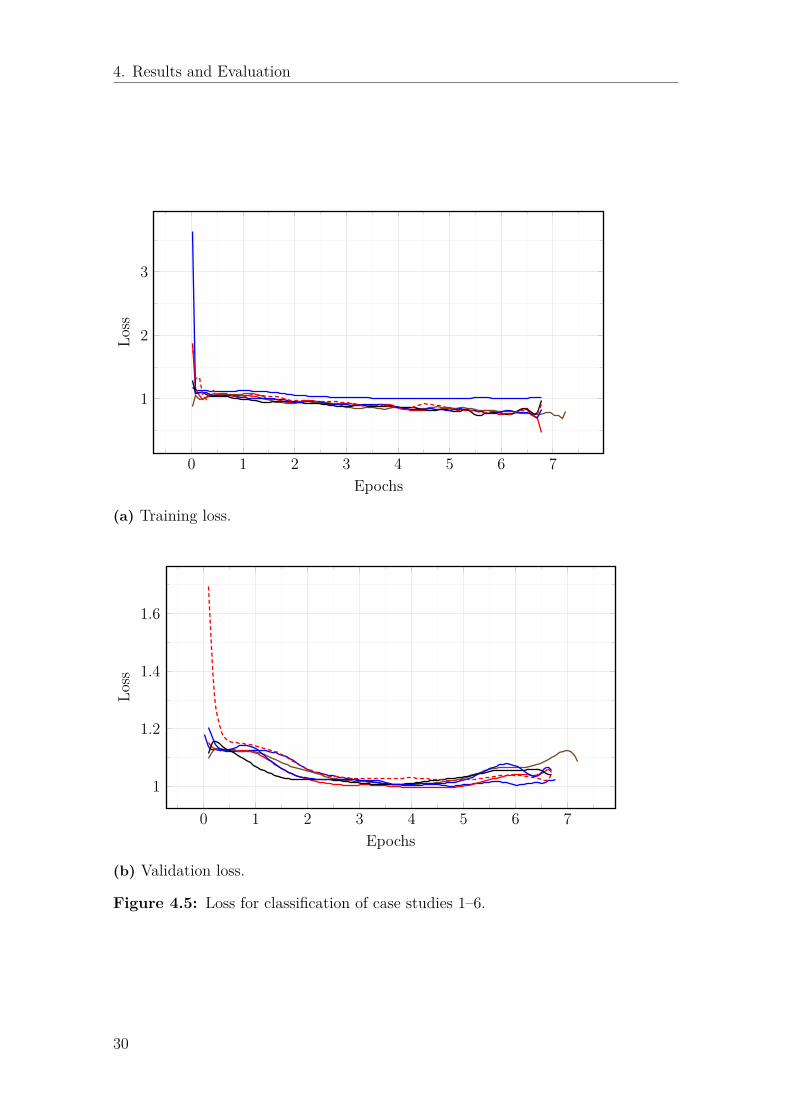
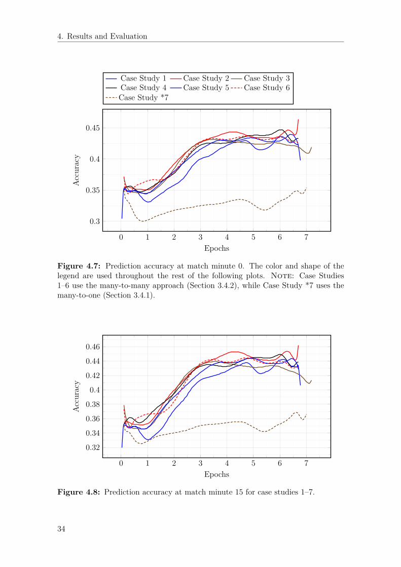
4.5 Loss for classification of case studies 1–6. . . . . . . . . . . . . . . . . 304.6 Loss for classification of case study 7. . . . . . . . . . . . . . . . . . . 314.7 Prediction accuracy at match minute 0. The color and shape of the

legend are used throughout the rest of the following plots. Note:Case Studies 1–6 use the many-to-many approach (Section 3.4.2),while Case Study *7 uses the many-to-one (Section 3.4.1). . . . . . . 34

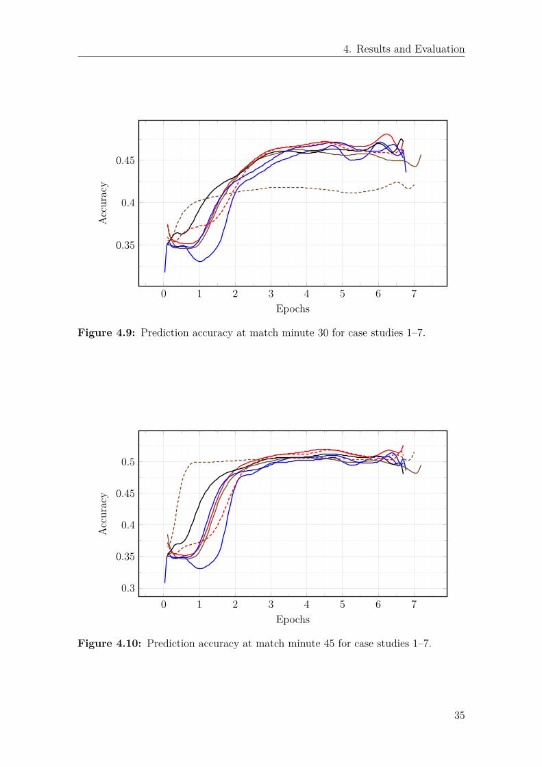
4.8 Prediction accuracy at match minute 15 for case studies 1–7. . . . . . 344.9 Prediction accuracy at match minute 30 for case studies 1–7. . . . . . 354.10 Prediction accuracy at match minute 45 for case studies 1–7. . . . . . 354.11 Prediction accuracy at match minute 60 for case studies 1–7. . . . . . 364.12 Prediction accuracy at match minute 75 for case studies 1–7. . . . . . 364.13 Prediction accuracy at match minute 90 for case studies 1–7. . . . . . 374.14 Prediction accuracy at full time for case studies 1–7. . . . . . . . . . . 374.15 Confusion matrices for match minute 0, 15, 30, 45, 60, 75, and 90 for

network case study 3 with two layers of 256 units. . . . . . . . . . . . 384.16 Confusion matrices for match minute 0, 15, 30, 45, 60, 75, and 90 for

network case study 7 with two layers of 256 units. . . . . . . . . . . . 39

xii

List of Tables

4.1 Specifications of the computer specifications used for training. . . . . 244.2 Specifications of the graphics card specifications used for training. . . 244.3 Software used for training. . . . . . . . . . . . . . . . . . . . . . . . . 244.4 Dataset split into three parts used for training, validation, and testing. 254.5 Comparison between the different training case studies. Case Study 7

uses the many-to-one approach where the accuracy is only calculatedat the end of the sequence, while Case Studies 1–6 uses many-to-manyand calculates the accuracy for all events in the sequence and takesthe average of them all. The “Train Accuracy” and “Test Accuracy”columns contains the last event classification for both approaches. . . 26

4.6 Prediction comparison between the different case studies. . . . . . . . 324.7 Leagues and tournaments that odds were gathered for. . . . . . . . . 404.8 Betting companies, their accuracy and prediction distribution. . . . . 414.9 Competitors in the 10 Newspapers challenge 2015 and their accuracy. 424.10 Accuracy for Forza Football users predictions. The predictions can

be made both before and after the lineups are known. . . . . . . . . . 42

xiii

List of Tables

xiv

1Introduction

There have been several tries at predicting sport games using data from the past, buthumans are still superior at predicting sport outcomes. There are multiple commer-cial services which have sports analysis and prediction as their main business. Theyuse “sophisticated software and statistical algorithms” to aid their data tracking,but at the core they still have experts analysing the games manually1.

This work aims at predicting the outcome of football matches using deep learningand recurrent neural networks, RNNs.

1.1 Background

Accurate football prediction is very valuable for the small Gothenburg based com-pany Football Addicts and their smartphone application Forza Football. This thesisis a collaboration with the company Football Addicts and the project has used dataavailable from the company.

1.2 Goals

This thesis aims at predicting football matches using deep learning and RNNs. Thegoal is to have a prediction accuracy that can compete with betting companies, byletting the network focus on players performance.

1.3 Constraints

There are many deep learning methods that can be used to predict football matches,depending on, for example, the data available. Due to the type of data available forthis project, RNN is the method chosen and no other methods will be tested.

The thesis only uses data from a fixed set of leagues. Players transferred from aleague outside of the leagues to one league in the set will not have the historic data.

1Examples: http://www.stats.com/football/ and http://instatfootball.com/

1

http://www.stats.com/football/

http://instatfootball.com/

1. Introduction

All these players will be treated the same, even though in real life they have differenthistory.

Our project does not consider any kind of ranking of different leagues used to trainthe model. This means that the model might predict a draw or even a win for atop team in a lower ranked league, even though it is highly improbable. Matcheswith two teams from different leagues with a large rank difference occur rarely andshould therefore not be a problem.

1.4 Problem Formulation

This report aims at investigating whether deep learning can be used to predictfootball matches by analyzing the following:

• Can RNNs be used for the purpose of match predictions?

• Is history about players important when predicting the outcome of a match?

• How long history is relevant for a player?

1.5 Disposition

The disposition of this report generally follows that of a standard technical report.Chapter 2 covers the background theory necessary to understand the conductedstudy. The proposed methods can be found in Chapter 3. The results along withthe setup used for the study can be found in Chapter 4, where the result of eachexperiment is followed by a discussion. Finally in Chapter 5 the conclusion from thestudy is presented.

2

2Background Theory

This chapter aims at describing the theory needed to understand the work con-ducted, as well as present related work that is useful for this thesis. It starts offwith an introduction to machine learning, neural networks, and deep learning.

2.1 Machine Learning

Machine learning is a subfield to artificial intelligence which has increased in pop-ularity over the last few years (especially neural networks and deep learning), bothin research and in industries. In contrast to traditional rule-based artificial intelli-gence, where an algorithm is more or less a list of predefined static rules, machinelearning tries to use data to learn to make predictions or decisions. Many problemsmake it unfeasible to construct or design rules to help find a solution due to thesheer amount of constraints or complexity of the problem, which is where machinelearning can leverage data to learn a solution.

2.1.1 Neural Networks

Artificial neural networks (ANNs) are a computational approach that is based on theway a biological brain solves problems. The human brain is composed of nerve cellscalled neurons that are connected with each other by axons. ANNs are composed ofmultiple nodes, which imitate the biological neurons of a human brain. The neuronsare connected by links, which imitate the biological axons, and they interact witheach other. Each node takes input data, performs a simple operation, and passesthe result to other nodes. Like a biological brain, an ANN is self-learning and cantherefore excel in areas where the solution is difficult to express by a traditionalprogramming approach.

The core of neural networks, neurons, is just a simple activation function that hasmultiple inputs and one output. The neuron can be seen as a composition of severalother weighted neurons and the network can be described by the network function

f(x) = K

(∑i

wigi(x))

(2.1)

3

2. Background Theory

Inputlayer

Hiddenlayer

Outputlayer

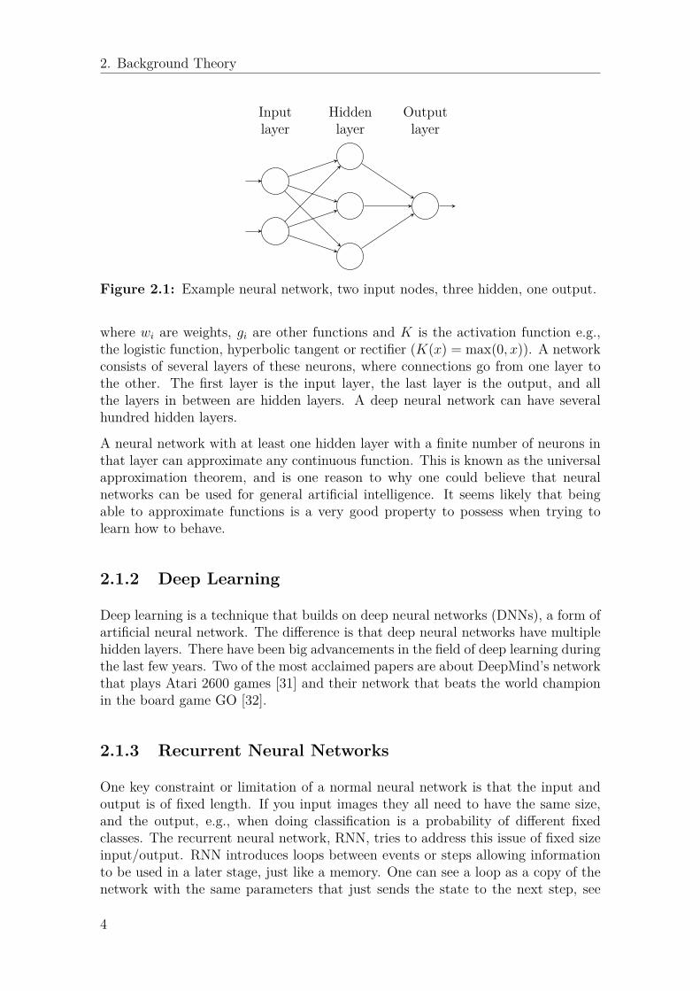
Figure 2.1: Example neural network, two input nodes, three hidden, one output.

where wi are weights, gi are other functions and K is the activation function e.g.,the logistic function, hyperbolic tangent or rectifier (K(x) = max(0, x)). A networkconsists of several layers of these neurons, where connections go from one layer tothe other. The first layer is the input layer, the last layer is the output, and allthe layers in between are hidden layers. A deep neural network can have severalhundred hidden layers.

A neural network with at least one hidden layer with a finite number of neurons inthat layer can approximate any continuous function. This is known as the universalapproximation theorem, and is one reason to why one could believe that neuralnetworks can be used for general artificial intelligence. It seems likely that beingable to approximate functions is a very good property to possess when trying tolearn how to behave.

2.1.2 Deep Learning

Deep learning is a technique that builds on deep neural networks (DNNs), a form ofartificial neural network. The difference is that deep neural networks have multiplehidden layers. There have been big advancements in the field of deep learning duringthe last few years. Two of the most acclaimed papers are about DeepMind’s networkthat plays Atari 2600 games [31] and their network that beats the world championin the board game GO [32].

2.1.3 Recurrent Neural Networks

One key constraint or limitation of a normal neural network is that the input andoutput is of fixed length. If you input images they all need to have the same size,and the output, e.g., when doing classification is a probability of different fixedclasses. The recurrent neural network, RNN, tries to address this issue of fixed sizeinput/output. RNN introduces loops between events or steps allowing informationto be used in a later stage, just like a memory. One can see a loop as a copy of thenetwork with the same parameters that just sends the state to the next step, see

4


Figure 2.2. This enables a RNN to be used on sequences of input and output whichcan take previous information into account. It has been shown that this works verywell for a number of situations like natural language processing, video classification,image classification, etc. [38, 3, 7, 43].

Given a sequence x = (x1,x2, ...,xT ), the RNN updates its recurrent hidden stateht by

ht =

0, t = 0Φ(ht−1,xt), otherwise

(2.2)

where Φ is a nonlinear function. Traditionally the update for the recurrent hiddenstate, ht, is implemented as

ht = g(Wxt + Uht−1), (2.3)

where g is a smooth and bounded function such as a logistic sigmoid function, Wand U are weight matrices.

One big problem with a straightforward RNN is the vanishing or exploding gradient.This can happen during training and the calculation of gradients for the backprop-agation. The gradients are calculated using the chain rule which multiplies smallnumbers many times, making the error signal decrease with an exponential factor.The same thing can also happen when gradients are too large, which can result inthe exploding gradient. This is just as bad because the network’s early layers areunable to learn as the error cannot propagate properly [21]. Both problems can beavoided by using Long Short-Term Memory and Gated Recurrent Unit, discussedin the next 2 sections.

xt

ct

yt

=

x1

c1

y1

x2

c2

y2

x3

c3

y3

x4

c4

y4

x5

c5

y5

Figure 2.2: Example of a synced recurrent neural etwork, many-to-many. At eachtimestep, there is an output corresponding to the input at that time.

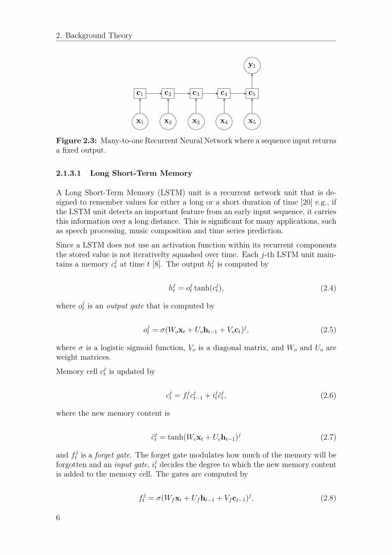
Figure 2.3 shows a RNN where only one output is used, classifying the entire se-quence given instead of every timestep in a sequence.

5


x1

c1

x2

c2

x3

c3

x4

c4

x5

c5

y1

Figure 2.3: Many-to-one Recurrent Neural Network where a sequence input returnsa fixed output.

2.1.3.1 Long Short-Term Memory

A Long Short-Term Memory (LSTM) unit is a recurrent network unit that is de-signed to remember values for either a long or a short duration of time [20] e.g., ifthe LSTM unit detects an important feature from an early input sequence, it carriesthis information over a long distance. This is significant for many applications, suchas speech processing, music composition and time series prediction.

Since a LSTM does not use an activation function within its recurrent componentsthe stored value is not iterativelty squashed over time. Each j-th LSTM unit main-tains a memory cj

t at time t [8]. The output hjt is computed by

hjt = oj

t tanh(cjt), (2.4)

where ojt is an output gate that is computed by

ojt = σ(Woxt + Uoht−1 + Voct)j, (2.5)

where σ is a logistic sigmoid function, Vo is a diagonal matrix, and Wo and Uo areweight matrices.

Memory cell cjt is updated by

cjt = f j

t cjt−1 + ijt c

jt , (2.6)

where the new memory content is

cjt = tanh(Wcxt + Ucht−1)j (2.7)

and f jt is a forget gate. The forget gate modulates how much of the memory will be

forgotten and an input gate, ijt decides the degree to which the new memory contentis added to the memory cell. The gates are computed by

f jt = σ(Wfxt + Ufht−1 + Vfct−1)j, (2.8)

6


ijt = σ(Wixt + Uiht−1 + Vict−1)j. (2.9)

A LSTM unit is able to decide whether to keep the existing memory via the intro-duced gates. See Figure 2.4 for a graphical illustration of a LSTM unit and Figure2.5 for an example of a multi-layer LSTM network.

cjt +

+

f jt

Forget Gate

ojt

Output Gate

cjt

ijt

Input Gate

hjt

xt

Figure 2.4: Illustration of a LSTM unit.

The following part will describe some different variants of LSTM.

• LSTM with peepholes

LSTM units with peepholes include the internal state when calculating the valuesof all gates [13]. The gates for the j-th LSTM with peephole at time step t arecalculated by

ojt = σ(Woxt + Uoht−1 + Poct−1)j (2.10)

f jt = σ(Wfxt + Ufht−1 + Pfct−1)j (2.11)

ijt = σ(Wixt + Uiht−1 + Pict−1)j (2.12)

where P are matrices with weights that need to be learned by the network.

A LSTM with peephole has an improved ability to learn tasks that require precisetiming and counting of the internal states [17].

• Convolutional LSTM

A drawback for LSTM is its usage of full connections in input-to-state and state-to-state transitions in which no spatial information is encoded when handling spa-tiotemporal data [42]. To overcome this problem, all the inputs xt, outputs ht,

7


LSTMcell 1

LSTMcell 2

LSTMcell 3

x1

y1

h31

LSTMcell 1

LSTMcell 2

LSTMcell 3

x2

y2

h32

h11

h21

LSTMcell 1

LSTMcell 2

LSTMcell 3

x3

y3

h33

h12

h22

h13

h23

Inputs

First layer

Second layer

Third layer

Outputs

Figure 2.5: An example of a multi-layer LSTM network with 3 layers. xt is theinput at time t, hj

t is the output of layer j at time t. The output from layer j attime t is fed to layer j + 1 at time t. The output of layer j at time t is also passedon to the same layer j at time t+ 1.

8


memory cells ct and gates ot, ft, it of the convolutional LSTM are 3D tensors whoselast two dimensions are the spatial dimensions. The outputs, memory cells and gatesfor the j-th convolutional LSTM at time t are calculated by

hjt = oj

t ◦ tanh(cjt) (2.13)

cjt = f j

t ◦ cjt−1 + ijt ◦ tanh(Wc ∗ xt + Uc ∗ hj

t−1) (2.14)

ojt = σ(Wo ∗ xt + Uo ∗ ht−1 + Vo ◦ ct)j (2.15)

f jt = σ(Wf ∗ xt + Uf ∗ ht−1 + Vf ◦ ct)j (2.16)

ijt = σ(Wi ∗ xt + Ui ∗ ht−1 + Vi ◦ ct)j (2.17)

where U , V and W are weight matrices, ∗ is the convolution operator [41] and ◦ isthe entrywise product [22].

2.1.3.2 Gated Recurrent Unit

A gated recurrent unit, GRU, is designed to adaptivly reset or update its memory[8]. Unlike a LSTM, a GRU does not have a separate memory cell.

The activation hjt of GRU j at time t is a linear interpolation between the previous

activation hjt−1 and the candidate activation hj

t [8]. An update gate zjt decides how

much the unit updates its activation:

hjt = (1− zj

t )hjt−1 + zj

t hjt (2.18)

zjt = σ(Wzxt + Uzht−1)j (2.19)

The candidate activation hjt is computed by

hjt = tanh(Wxt + U(rt � ht−1))j, (2.20)

where rt is a set of reset gates. When rjt is off (rj

t is close to 0), the reset gate makesthe unit act as if it is reading the first symbol of an input sequence. This way it isallowed to forget the previously computed state.

Reset gate rjt is computed by

rjt = σ(Wrxt + Urht−1)j. (2.21)

9


See Figure 2.6 for a graphical illustration.

As the forget and input gates are combined into a single update gate the GRU issimpler than a standard LSTM unit and therefore computationally more efficient.

hjt

zjt

Update Gate

rjt

Reset Gate

hjt

xt

hjt

Figure 2.6: Illustration of a GRU.

2.1.4 Dropout

Neural networks with a large amount of parameters have a problem with overfitting[34]. A model that overfits on the training data will result in bad performance.By introducing dropout, the risk for overfitting decreases. The idea is to randomlydrop units along with their connections during the training to prevent units fromco-adapting too much. At training time each node has a probability p to be droppedout.

Inputlayer

Hiddenlayer

Outputlayer

(a) Network without dropout applied.

Inputlayer

Hiddenlayer

Outputlayer

(b) Network with dropout applied.

Figure 2.7: Left: A standard neural net with 1 hidden layer. Right: An exampleof a thinned network produced by applying dropout to the network on the left.

10


Applying dropout to a neural networks can be seen as sampling a “thinned” networkfrom the original. The thinned network consists of all nodes (with respective con-nection) that survived the dropout. Figure 2.7(b) show a sampled thinned networkfrom the network in Figure 2.7(a). A neural network with n units can be seen asa collection of 2n possible thinned neural networks. For each training stage a newthinned neural network is sampled and trained. So training a neural network withdropout can be seen as training a collection of 2n thinned networks. Each networkgets trained rarely or not at all.

2.1.5 Embeddings

Entities in the dataset can be modeled in a d-dimensional vector space, called the“embedding space” or distributed representation. Each entity i is assigned a vectorVi ∈ Rd [5]. Within the embedding space there is a specific similarity measurethat captures the relation between entities. One of the earliest use of distributedrepresentation date back to 1988 due to Rumelhart, Hinton and Williams [40].

Embeddings can be used to fight the curse of dimensionality [4]. The curse of dimen-sionality is the phenomena that arises when working with data in high-dimensionalspace. Choosing attributes, and how many, that describes the entities is tricky. Thesolution is to let the network learn the distributed representation. The network willadjust the representations during training which enables it to capture informationabout the entities [30].

Representing entities in an embedding space has helped algorithms to achive betterperformance in various areas, such as statistical language modeling and variousnatural language processing (NLP) tasks [10, 15, 39, 33].

2.1.6 Softmax Classifier

The softmax function is a generalization of the logistic function that squashes aK-dimensional vector of arbitrary values to a K-dimensional vector of real valuesin range [0,1] that add up to 1 [6]. The output of the softmax function can then beused to represent a probability distribution over K different possible classes.

σ(z)j = ezj∑Kk=1 e

zkfor i = 1 . . . K (2.22)

The softmax function is used in various multiclass classification methods, such asmultinomial logistic regression, multiclass linear discriminant analysis, naive Bayesclassifiers, and artificial neural networks. In a neural network-based classifier thefunction in the final layer is often a softmax function.

11


2.1.7 Cross Entropy Error

The cross entropy can be used as an error measure for neural networks. It describesthe entropy of a distribution y′ with respect to another distribution y and measureshow many bits you need to encode data on average [16].

H(y′,y) = −∑

i

y′i log yi (2.23)

2.1.8 Adam Optimizer

Adam, derived from adaptive moment estimation, is an algorithm for first-ordergradient-based optimization of stochastic objective functions that is well suited forproblems that are large in terms of data and parameters [27]. Adam is also suited forproblems with very noisy and sparse gradients. The method only requires first-ordergradient.

Adam computes individual adaptive learning rates for different parameters fromestimates of first and second moments of the gradients. The magnitudes of param-eter updates are invariant to rescaling the gradient, its stepsizes are approximatelybounded by the stepsize hyperparameter, it does not require stationary objective,it works with a sparse gradient and naturally performs a form of step size anneal-ing. It combines the advantages of AdaGrad [11], to deal with sparse gradients, andRMSProp [19], to deal with non-stationary objectives. It is proven to be well-suitedfor a wide range of non-convex optimization problems in the field machine learning.

2.1.9 Hardware

A deep learning algorithm can contain a large number of parameters. This may leadto training taking a long time and therefore the choice of hardware is important.

2.1.9.1 Central Processing Unit

Traditionally, mathematical computations have been done on the Central ProcessingUnit (CPU). This includes the computations done for training a neural network. To-day’s CPUs have multiple cores [12]. In order to optimize the run time, calculationsthat can be done separately should be done on separate cores.

2.1.9.2 Graphics Processing Unit

A Graphics Processing Unit (GPU) is a processor that is designed to execute com-putations in parallel, which is common in 3D graphics[35].

Modern CPUs often have an integrated GPU, which shares the system memory withthe CPU. A GPU can also be a standalone chip, which it is often referred to as a

12


dedicated GPU. A dedicated GPU has its own memory which is often faster thanthe system memory, helping to speed up computations. It is the dedicated GPUsthat nowadays are common to use for machine learning. Operations required totrain a DNN can be made in parallel. Therefore GPUs exceed CPUs in performancewhen it comes to training. Running a program for training a neural network on aGPU requires that the GPU manufacturer supports it. For high-end GPUs thereare two major manufacturers today, AMD and NVIDIA. Both of them supports thepossibility to train neural networks.

NVIDIA have developed their hardware-software architecture CUDA [28] that al-lows code to be run on their GPUs with a high computational power. An alternativeto CUDA is OpenCL for parallel computing on the most common types of proces-sor, including GPUs, from multiple manufactures [36]. OpenCL is maintained bythe non-profit consortium The Khronos Group. Both alternatives have their prosand cons [25]. Which one should be used differs from project to project and whathardware is available.

2.1.10 Software Libraries

There exist several software libraries for simplifying the process of implementingmachine learning algorithms. They provide tools for setting up a functional neuralnetwork.

For this project the software library Tensorflow [1] was used to build the neuralnetwork. Tensorflow was chosen because it is a well documented library that ispopular and therefore a lot of functions available via forums and blogs.

2.2 Predicting the Outcome of Football Matches

Predicting the outcome of football matches is today done by both football expertsand machine learning algorithms, with various outcome. This section discusses somechallenges in predicting the outcome and some previous work.

2.2.1 Challenges of Predicting the Outcome ofFootball Matches

Both human and computer predictions have their challenges. Humans are emotionaland can affect the analysis of teams playing each other and therefore the prediction.A computer does not have the knowledge of the current mental health of the team.Cracks between players and coaches might affect the outcome. For both humansand computer there is also always the problem of deciding which attributes areimportant.

13


Football, as many other sports, is highly stochastic. One lucky hit among hundredsof passes, shots, and dribbles can in the end change the whole outcome of the game.This makes it more complicated to predict the outcome of football matches, bothfor humans and computers.

2.2.2 Previous Work

Several attempts have been made to predict the outcome of football matches, andother sports [24, 18, 23, 2]. The accuracy varies depending on what sport, leagueand approach that has been used. Most attempts are done on one or a low number ofleagues by building statistical models. Basic neural networks have been used in a fewcases, but none have used deep learning to train a network to learn football matchesand high dimensional representations of players and teams. These approaches arejust predictions before the match and cannot be used for prediction for ongoingmatches.

14

3Proposed Methods for Football

Match Prediction

Previous works on predicting outcomes of team sport matches using machine learn-ing have mainly focused on team data [24, 18, 23, 2]. The focus also lies on a singletournament, league or team.

Players representing a football club during a match are constantly changing. Bothbecause a specific player does not make the team or that a player is transferred toa different team. The approach for this thesis is to focus on the players. In such away it takes into account if a player does not play for a team in a specific match,which will have an impact.

A match is played at a specific time, and events occur at a relative time in a game.The order of matches and events matter since they have an impact on the fu-ture. Therefore a long short-term memory network (LSTM) [14] is exploited forthis project.

3.1 Data

The dataset used for this project includes the information for each player in theteams. The dataset includes matches for leagues and tournaments for the 54 coun-tries in the Union of European Football Associations (UEFA)1, USA, Brazil, Chile,Mexico, Argentina, Uruguay, Australia, Japan and China. A full list of leagues andtournaments can be seen in Appendix B.

Since players move between clubs and leagues, the data used is for multiple leaguesover multiple years. In this way, information about a player is moved along withthe player when a player changes club and therefore changes in teams are noticed.Information about players is gathered from events in which they are involved induring a game. The following events in each game have players connected to them:

Lineups: Each starting player and head coach for a team.

Position: Starting position for each starting player.1http://www.uefa.com/memberassociations/uefarankings/index.html

15

http://www.uefa.com/memberassociations/uefarankings/index.html

3. Proposed Methods for Football Match Prediction

Goal: Goalscorer and possible assisting player.

Card: Which player gets the card and which type of card.

Substitution: Player entering the field and player leaving the field.

Penalty: Which player takes the penalty, and what is the outcome. Whether thepenalty is saved the by goalkeeper is also connected to the event.

Below is an example of how the raw data of a goal looks like and Appendix Acontains the structure of the raw data for a whole match.

"goal": [{

"assistPlayerId": "f54pd3cld0qkc8ol15bk9ye39","assistPlayerName": "F. Fernández","contestantId": "410jti6axb01yhvbc0axsp8li","lastUpdated": "2017-02-12T16:36:59.362Z","periodId": 1,"scorerId": "ex186m2z3yp666b1g219a8ted","scorerName": "A. Mawson","timeMin": 36,"type": "G"

}]

The dataset consists of 35234 games distributed between 45.50% home wins, 29.61%away wins and 24.89% draws. All events include either the absolute or relativetime. There is no ranking on what events are more important than others. Varioussites and newspapers provide this information about football games, in differentstructures. Therefore, the project can be remade without having the data providedfrom a specific source.

3.2 Network Input

There are several ways to encode the data before feeding it to the network. Thedataset contains several event types, with different structures and different numbersof attributes. We somehow need to merge or fuse this into a generalized inputwhich the network can work with. A normal feed forward neural network requiresall input to be of a fixed size, meaning that the dataset needs to be preprocessedso that everything is the same size. By using a RNN we can let all examples beof different length, but we still need the input vector at each time step to be fixedin size. This means that even though we have different types of events, they musthave the same shape when fed to the network. There are several possibilities andtechniques that can be can utilized to solve this problem that are outlined below.

16


3.2.1 Deep Embeddings

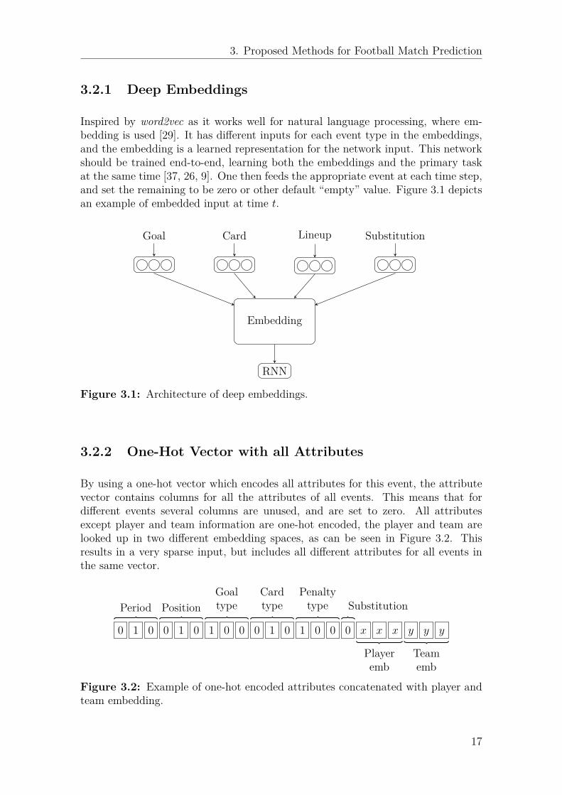
Inspired by word2vec as it works well for natural language processing, where em-bedding is used [29]. It has different inputs for each event type in the embeddings,and the embedding is a learned representation for the network input. This networkshould be trained end-to-end, learning both the embeddings and the primary taskat the same time [37, 26, 9]. One then feeds the appropriate event at each time step,and set the remaining to be zero or other default “empty” value. Figure 3.1 depictsan example of embedded input at time t.

Embedding

RNN

Goal Card Lineup Substitution

Figure 3.1: Architecture of deep embeddings.

3.2.2 One-Hot Vector with all Attributes

By using a one-hot vector which encodes all attributes for this event, the attributevector contains columns for all the attributes of all events. This means that fordifferent events several columns are unused, and are set to zero. All attributesexcept player and team information are one-hot encoded, the player and team arelooked up in two different embedding spaces, as can be seen in Figure 3.2. Thisresults in a very sparse input, but includes all different attributes for all events inthe same vector.

0 1 0 0 1 0 1 0 0 0 1 0 1 0 0 0 x x x y y y

Period PositionGoaltype

Cardtype

Penaltytype Substitution

Playeremb

Teamemb

Figure 3.2: Example of one-hot encoded attributes concatenated with player andteam embedding.

17


3.2.3 Concatenated Embedding Vectors for all Attributes

This is a slight variant of the one-hot vector above. Instead of using a sparse one-hotencoded vector we provide one embedding per event type, and a lookup for all thevalues in the attribute vector, and concatenate the resulting embeddings. Theseembeddings are also learned during end-to-end training of the network.

3.3 Naive Statistical Model

A pure statistical model is created to see what prediction accuracy is possible toreach with a simple model using the same data. The model does not care aboutplayers in each team. It only considers goals and cards. Below is the algorithm topredict the outcome of a match.

GoalScoret = ght · kgh + gat · kga − cht · kch − cat · kca (3.1)

Y ellowCardScoret = yt · ky (3.2)

RedCardScoret = rt · ry (3.3)

Feature scaling is applied to each score to normalize the data.

x′ = x−min(x)max(x)−min(x) (3.4)

TotalScoret = GoalScore′t − Y ellowCardScore′t −RedCardScore′t (3.5)

Scorem = TotalScoret1 − TotalScoret2 (3.6)

f(Scorem) =

home win, if Scorem > Home win thresholdaway win, if Scorem < Away win thresholddraw, otherwise

(3.7)

18


GoalScoret Goal score for team tght Home goals for team tkgh Home goal rategat Away goals for team tkga Away goal ratecht Goals conceded home for team tkch Goal conceded home ratecat Goals conceded away for team tkca Goal conceded away rateY ellowCardScoret Yellow card score for team tyt Yellow cards for team tky Yellow card rateRedCardScoret Red card score for team trt Red cards for team tkr Red card rateTotalScoret Total score for team tScorem Score for match m

Each team t in each match gets a score that depends on goals, made and conceded,yellow and red cards for the 2015, 2015/2016, 2016, 2016/017 seasons until 2016-11-05. The predicted outcome is then decided by the difference in score betweenTotalScore’t1 and TotalScore’t2. The k variables are used as a ratio to tune themodel.

3.4 Deep Learning Architecture

A few different models have been used and tested in this project. The core of ourRNN consists of LSTM or GRU cells and a softmax classifier. For input both one-hot, see Secion 3.2.2, and embedding vectors, see Section 3.2.3, are used and tested.The longest sequence in the dataset is calculated and that is used to pad all the othersequences with zero vectors so that they are the same length. Dynamic unrolling ofthe sequence takes place by also feeding a sequence length parameter. This makesthe network only run for as many time steps that each sequence contains.

Inputs10 Features

EmbeddingsOne-hot transform LSTM Softmax classifier

Figure 3.3: The simple high level architecture of the model.

The block diagram of the model can be seen in Figure 3.3 that consists of inputs,input processing, some number of LSTM layers and units, and lastly a softmaxclassifier. This architecture can also be seen in detail in Figure 3.4. The inputvector consists of 10 integer features: period, home team, away team, main player,assisting player, position, goal type, card type, penalty type, and substitute. These

19


x1LSTM 1u units

LSTM Lu units

. . . o1 softmax y1

x2LSTM 1u units

LSTM Lu units

. . . o2 softmax y2

x3LSTM 1u units

LSTM Lu units

. . . o3 softmax y3

xtLSTM 1u units

LSTM Lu units

. . . ot softmax yt

...

...

...

...

...

...

Figure 3.4: Detailed illustration of the architecture used. xt is the input vectorat time step t, ot is a single layer feed forward neural network, yt is the predictedclass at time t, L represents the number of layers, and u number of LSTM units perlayer.

features are then either transformed to a one-hot encoding per feature and thenconcatenated together, or an embedding lookup per feature and then concatenatedto form a bigger vector with real valued numbers. An example of an input vectorcan be (penalty event by the away team in the second half):

[2 0 1309 929 28619 0 0 0 1 0

]and the concatenated embedding vector like this (abbreviated for readability):[0.8029604 0.18677819 0.58298826 . . . 0.3224628 0.41138625 0.05778933

]The softmax classifier has an output of three different classes, being home win,draw, and away win. The loss function used to calculate the error is a standardcross entropy error, discussed in Section 2.1.7 The loss and accuracy are tested intwo different ways, many-to-one and many-to-many, both introduced in Section 2.1.3and further discussed in Sections 3.4.1 and 3.4.2.

3.4.1 Many-To-One

One being many-to-one, meaning that the loss was only calculated once, on the lasttime step and then being used to do backpropagation through time for the entiresequence. The calculations for accuracy of this technique is described as follows:

For each match m, there is a target (i.e., class label) ym:

20


ym =

[1, 0, 0] (Home victory)[0, 1, 0] (Draw)[0, 0, 1] (Away victory)

and an output ym from the last event in match m

ym ∈ {[1, 0, 0], [0, 1, 0], [0, 0, 1]}

The accuracy is then calculated by

rm =

1 if ym = ym

0 otherwise(3.8)

accuracy =

M∑m=1

rm

M(3.9)

where M is the number of matches.

3.4.2 Many-To-Many

The second approach is an average loss over the entire sequence, calculating theloss for each time step and then averaging this loss for the backpropagation. Thistechnique is called sequence loss, since it calculates the total loss of a sequence ofoutputs. It is used to get a better prediction over the entire sequence. Since theaim is to predict the result at any time, not just in the end, this might give a betterresult. The calculations for the accuracy of this technique is described as follows:

For each match m, there is a target (i.e., class label) ym:

ym =

[1, 0, 0] (Home victory)[0, 1, 0] (Draw)[0, 0, 1] (Away victory)

ym = [y1m, y

2m, ..., y

nm], yi

m ∈ {[1, 0, 0], [0, 1, 0], [0, 0, 1]} for i = 1...n,

where yim is the predicted outcome for event i, and n is the number of events in the

match m.

The number of correct predictions for each match is calculated by

rim =

1 if yim = ym

0 otherwisefor i = 1...n, (3.10)

21


and then the accuracy over all matches is calculated by

accuracy =

M∑m=1

n∑i=1

rim

M∑m=1

#elements in rm

(3.11)

where M is the number of matches.

22

4Results and Evaluation

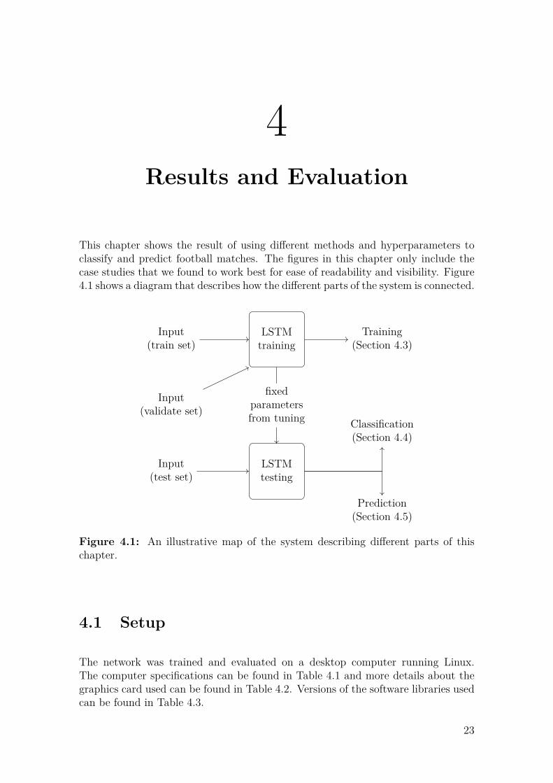
This chapter shows the result of using different methods and hyperparameters toclassify and predict football matches. The figures in this chapter only include thecase studies that we found to work best for ease of readability and visibility. Figure4.1 shows a diagram that describes how the different parts of the system is connected.

Input(train set)

LSTMtraining

Training(Section 4.3)

Input(validate set)

LSTMtesting

Input(test set)

Classification(Section 4.4)

Prediction(Section 4.5)

fixedparametersfrom tuning

Figure 4.1: An illustrative map of the system describing different parts of thischapter.

4.1 Setup

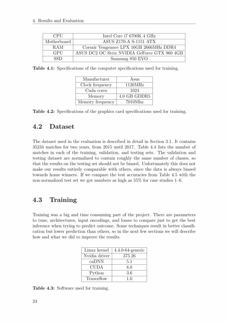
The network was trained and evaluated on a desktop computer running Linux.The computer specifications can be found in Table 4.1 and more details about thegraphics card used can be found in Table 4.2. Versions of the software libraries usedcan be found in Table 4.3.

23

4. Results and Evaluation

CPU Intel Core i7 6700K 4 GHzMotherboard ASUS Z170-A S-1151 ATX

RAM Corsair Vengeance LPX 16GB 2666MHz DDR4GPU ASUS DC2 OC Strix NVIDIA GeForce GTX 960 4GBSSD Samsung 850 EVO

Table 4.1: Specifications of the computer specifications used for training.

Manufacturer AsusClock frequency 1126MHz

Cuda cores 1024Memory 4.0 GB GDDR5

Memory frequency 7010Mhz

Table 4.2: Specifications of the graphics card specifications used for training.

4.2 Dataset

The dataset used in the evaluation is described in detail in Section 3.1. It contains35234 matches for two years, from 2015 until 2017. Table 4.4 lists the number ofmatches in each of the training, validation, and testing sets. The validation andtesting dataset are normalized to contain roughly the same number of classes, sothat the results on the testing set should not be biased. Unfortunately this does notmake our results entirely comparable with others, since the data is always biasedtowards home winners. If we compare the test accuracies from Table 4.5 with thenon-normalized test set we got numbers as high as 55% for case studies 1–6.

4.3 Training

Training was a big and time consuming part of the project. There are parametersto tune, architectures, input encodings, and losses to compare just to get the bestinference when trying to predict outcome. Some techniques result in better classifi-cation but lower prediction than others, so in the next few sections we will describehow and what we did to improve the results.

Linux kernel 4.4.0-64-genericNvidia driver 375.26

cuDNN 5.1CUDA 8.0Python 3.6

Tensorflow 1.0

Table 4.3: Software used for training.

24


Train Validate Test Discarded Total24410 3608 6660 557 3523469.3% 10.2% 18.9% 1.6% 100%

Table 4.4: Dataset split into three parts used for training, validation, and testing.

4.3.1 Tuning Parameters

Several combinations of hidden layers, units per layer, batch size, learning rate, andembedding sizes were tested. This subsection includes the result for the parametersthat were most successful, both in terms of accuracy and how feasible the perfor-mance requirements were. We were constrained by hardware and time which forcedus to pick branches of parameters that seemed good to explore further, most of theresults gathered during this project has been discarded since we only chose a few topones. In the following section we describe the parameters of our LSTM architecturesand how they were tuned.

Dropout The first networks we trained did not utilize dropout (see Section 2.1.4).After analyzing the first few networks performance it was very clear that over-fitting was occuring, reducing the accuracy of the network. We understoodthat dropout must be used in this case to reduce overfitting and increase ac-curacy. Therefore all networks shown in this chapter have been trained witha 50% dropout rate, all other networks were discarded because of the lowaccuracy in comparison.

Learning rate We experimented with changing the learning rate of the networkbut found no surprise here. When increasing the learning rate too much theloss randomly jumped or improved just very little. When decreasing the learn-ing rate too much the loss never improved at all. We found values around 10−4

to work very well, both in times of convergence and time used to train whichis why we choose to fix it as 10−4.

Batch size We tried batch sizes between 1 and 500 and noticed that sizes over 100were too large for our data and setup. The accuracy of the network was verystable, but the loss could not make it improve on the training set at all. Wedecided to use values like 30 or 50 to make the training time faster for newtests, but decided to keep it at 10 when doing the final training.

Embedding dimensions When using the inputs to do embedding lookups beforefeeding to the LSTM one needs to decide on how big and how many dimen-sions the embeddings should contain. We first started with the team andplayer embeddings. We tried values between 1 and 100, it seemed to make nodifference between having 10 or 100 dimensions for teams or players. We didnotice a big difference when having as low as 1 or 2, then we would not seeany convergence and the loss would just randomly jump around. We also trieddifferent values for the rest of the embeddings, but saw the same thing as withthe teams or players embedding dimension size. Since there are many differentvalues for the team and players we decided to continue with a dimension size

25


of 30, and for the rest of the values we used 10 to ease the size of the inputfor computational reasons.

4.4 Classification

Our tests are divided into two parts, classification and prediction. Classificationuses all the data available and simply does a classification of which class a matchbelongs to. There are three different classes, home win, draw, and away win.

We decided to pick seven different case studies out of all that we have tried andshow data and plots of all of these. They are numbered and the first six uses themany-to-many approach described in Section 3.4, where the loss and accuracy werecalculated as the average loss/accuracy of all outputs for every time step, see Section3.4.2.

The seventh case study uses the many-to-one approach, see Section 3.4.1, whichcalculated the loss and accuracy only on the last prediction. This has of courseaffected the value “accuracy” in tables, as the average accuracy is much lower thanthe last accuracy since it includes all of the accuracies at all time steps. This canbe seen in Table 4.5 where all the case study parameters and accuracy are shown.

Case Study Layers LSTM Units TrainAverageAccuracy

TestAverageAccuracy

TrainAccuracy

TestAccuracy

1 1 3 0.5979 0.4595 – 0.77772 1 256 0.6150 0.5003 – 0.88683 2 256 0.6179 0.4952 – 0.84594 2 512 0.6254 0.4909 – 0.85325 2 1024 0.6221 0.4873 – 0.83896 1 2048 0.6116 0.5022 – 0.8682*7 2 256 – – 1.0000 0.9863

Table 4.5: Comparison between the different training case studies. Case Study 7uses the many-to-one approach where the accuracy is only calculated at the end ofthe sequence, while Case Studies 1–6 uses many-to-many and calculates the accu-racy for all events in the sequence and takes the average of them all. The “TrainAccuracy” and “Test Accuracy” columns contains the last event classification forboth approaches.

Observing the classification results there is one clear winner out of all case studies.Case study 7 has a training accuracy of 100% and a testing accuracy of 98% whichis very high. Comparing this with the other six having a test accuracy at 45–50%,we can see that it is much easier to classify using only the latest information insteadof doing a prediction at every time step and then averaging this. This is also veryevident when looking at the accuracy in Figures 4.3, and 4.4, and loss in Figures4.5, and 4.6. Case study 7 quickly drops the loss below 1, both for training andtesting, before running training for the first epoch. Figure 4.2 shows the confusion

26


2194 80 26

171 1723 131

11 143 2181

(a) Case study 3, using many-to-many (Section 3.4.2).

2284 7 9

7 2011 7

30 18 2287

(b) Case study 7, using many-to-one(Section 3.4.1).

Figure 4.2: Confusion matrices for classification. Each row is actual truth, row 1for home win, row 2 for draw, and row 3 for away win. Each column is the predictedvalue in the same order. The color of the background shows how big part of thedistribution is on that cell, where black means 100%, white 0%, and gray shades forall the values in between. The values in the confusion matrices are calculated foronly the last event.

matrices for case studies 3 and 7. These matrices visualizes the detailed performanceof our predictions, we can see that case study 7 has very few errors and a clear blackdiagonal. Case study 3 not as good, some gray areas close to the diagonal. Theaccuracy of case Study 7 follows the loss and reaches above 90% before finishing thefirst epoch, and after that slighty increasing towards 98%. Ignoring this clear winnerand just comparing case studies 1–6 we see that case study 1 never reaches the sameaccuracy as the others, the same thing with the loss, it never goes as low as for theother 2–5. This is not surprising since Case study 1 only has one layer of LSTMwith three units, not much room to recognize patterns in the data. Comparing therest of the Case studies 2–5, it is slighty disappointing, no clear winner by the plotsin Figure 4.5, 4.6 or 4.3, 4.4, but at least Table 4.5 can show us the values in the endof training by zooming in. Some values are a bit surprising, case studies 3, 4, and 5are all lower in test accuracy than case study 2 even though it has the least amountof parameters available, the only one better than case study 2 is case study 6 whichhas one huge layer with 2048 units inside. We also tried networks much larger thanthis, all the way up to 10 layers with 2048 units, but saw no convergence even afterseveral days of training.

4.4.1 Discussion

We thought and hoped that there would be a bigger difference between the differentcase studies, but it seems that it only makes a small difference in classification results.We thought that bigger networks would result in better classification accuracy, butit seems to be only slighty better if even better at all.

One thing that makes a huge difference is how the accuracy is calculated. When

27


0 1 2 3 4 5 6 70.1

0.2

0.3

0.4

0.5

0.6

0.7

Epochs

Accuracy

Case Study 1 Case Study 2 Case Study 3Case Study 4 Case Study 5 Case Study 6Case Study *7

(a) Training accuracy.

0 1 2 3 4 5 6 70.3

0.35

0.4

0.45

0.5

Epochs

Accuracy

(b) Validation accuracy.

Figure 4.3: Accuracy for classification of Case studies 1–6. The color and shapeof the legend is used throughout the rest of the following plots.

28


0 1 2 3 4 5 6 7

0

0.2

0.4

0.6

0.8

1

Epochs

Accuracy

(a) Training accuracy.

0 1 2 3 4 5 6 70.4

0.5

0.6

0.7

0.8

0.9

1

Epochs

Accuracy

(b) Validation accuracy.

Figure 4.4: Accuracy for classification of case study 7.

29


0 1 2 3 4 5 6 7

1

2

3

Epochs

Loss

(a) Training loss.

0 1 2 3 4 5 6 7

1

1.2

1.4

1.6

Epochs

Loss

(b) Validation loss.

Figure 4.5: Loss for classification of case studies 1–6.

30


0 1 2 3 4 5 6 7

0

0.5

1

1.5

2

2.5

3

Epochs

Loss

(a) Training loss.

0 1 2 3 4 5 6 7

0

0.2

0.4

0.6

0.8

1

Epochs

Loss

(b) Validation loss.

Figure 4.6: Loss for classification of case study 7.

31


calculating the outcome on all events and then taking the average we get a lowerclassification accuracy than when we calculated the outcome on only the last event.This is no surprise, in the first case the calculated outcome on the first event has thesame impact as the calculated outcome on the last event. This does not make sensesince the calculated outcome on the last event contains more information about thematch, it should have a bigger impact.

For case study 3 we can see that it does few away winner classifications when theoutcome is home winner and the other way around, which is a positive thing. Thisis not the case with case study 7. It does more away win predictions than drawpredictions when the outcome is home winner and more home winenr in predictionsthan draw predictions when the outcome is away winner. This is however so fewcases that it should not be considered a problem.

The interested reader who wonders what accuracy case studies 1–6 have on the lastprediction Table 4.6 shows this as we move on to the prediction section.

4.5 Prediction

This section describes the results from prediction. Prediction is performed by usingonly part of the previous data. The network predicts the future values which have notyet been seen. We decided to predict every 15th minute of all matches. This meansthat we have one prediction before the match starts, 15th minute, 30th minute,45th minute (half time), 60th minute, 75th minute, 90th minute, and full time(since matches can have extended full time).

Prediction Accuracy During MatchCaseStudy

Layers LSTMUnits

0 m 15 m 30 m 45 m 60 m 75 m 90 m FullTime

1 1 3 0.4284 0.4361 0.4631 0.5039 0.5747 0.6469 0.7305 0.77772 1 256 0.4396 0.4479 0.4705 0.5151 0.5831 0.6797 0.8048 0.88683 2 256 0.4226 0.4283 0.4537 0.4982 0.5661 0.6644 0.7784 0.84594 2 512 0.4355 0.4404 0.4621 0.5062 0.5741 0.6728 0.7813 0.85325 2 1024 0.4313 0.4393 0.4659 0.5051 0.5740 0.6687 0.7775 0.83896 1 2048 0.4324 0.4380 0.4638 0.5115 0.5811 0.6813 0.7954 0.8682*7 2 256 0.3335 0.3539 0.4151 0.5048 0.6280 0.7409 0.8825 0.9863

Table 4.6: Prediction comparison between the different case studies.

Table 4.6 lists all the case studies with their parameters (same as before), andprediction accuracy before the match starts and every 15th minute until full time.Figures 4.7, 4.8, 4.9, 4.10, 4.11, 4.12, 4.13, and 4.14 shows the prediction accuracyat each 15th minute time interval and full time. Unfortunately due to smoothing,since the accuracy varies a lot, the values are a bit lower as compared to the bestresults recorded into Table 4.6. Out of case studies 1–6, case study 1 is also theworst one, same as in the classification, since it has such a small set of parametersto learn.

32


We can see that case study 7 still has the best full time accuracy, which is to beexpected, but if we look at the “0th minute” column we can see that case study 7actually is the worst. Even the tiny case study 1 has a better prediction than casestudy 7 with a 42% accuracy compared to 33%. This can also be seen in Figures4.7, 4.8, and 4.9, where case study 7 is by far the worst predictor. Although thischanges when we reach minute 45, then case study 7 is somewhat equal to the restof the networks, and after this time step it improves and exceeds the other networksperformance. It seems to sacrifice earlier accuracy for the later, where it has anexcellent result.

Figures 4.15 and 4.16 show confusion matrices for case study 3 and case study7. What can be seen in both case study 3 and case study 7 is that in the earlierpredictions a lot of the guesses are on home winner. This is somewhat expected sincethe training dataset has a bias towards the home winners. As the time progressesto later predictions we can see that the distribution moves towards the correct statewith black on the diagonal. Case study 3 is much better at finding away winners inthe earlier predictions, in minute 0 it correctly predicts 999 away wins in comparisonto 134 for case study 7. Towards the end of predictions we can see that very fewmistakes happen where both networks predict an away winner when the target isa home winner and vice versa, most of the mistakes there are instead towards the“closest” class which must be seen as a positive result. It is a lot more likely to endin a draw than an away winner when the target is a home winner, it requires morefor the actual result to go from one team winning to the other team winning. Onthe last prediction we can see just how good case study 7 is, predicting 173 and 25matches wrong on home winner compared with 186 and 47 for case study 3. Fordraw matches case study 7 predicts 157 and 161 matches wrong, where case study3 has 301 and 239. And last, when away winner is the true target, case study 7 has28 and 233 wrong, and case study 3 has 36 and 309.

4.5.1 Discussion

The fact that all case studies gets better prediction the further match time goes isnot a surprise, as more information should lead to a better prediction.

As seen in Figures 4.15 and 4.16 both case study 3 and 7 seem to have learnedfrom the training data. It is more likely that the outcome is a home winner. Casestudy 3 also seems to have learned a better representation, than case study 7, of theoutcome from the begining. Home winner is most likely, away winner the secondand draw the last. The further a match goes, both networks make few away winnerpredictions when the outcome is home winner and the other way around which is apositive result.

The two different networks in case study 7 and case study 2 switch at beeing best atpredictions around half-time. It could be due to the reason that the further a matchgoes on, the more data the networks need to handle. Therefore the smaller networkmight not be able to handle the amount of data in the end of a match, while thelarge network does not have any advantages over the small network in the begining

33


0 1 2 3 4 5 6 7

0.3

0.35

0.4

0.45

Epochs

Accuracy

Case Study 1 Case Study 2 Case Study 3Case Study 4 Case Study 5 Case Study 6Case Study *7

Figure 4.7: Prediction accuracy at match minute 0. The color and shape of thelegend are used throughout the rest of the following plots. Note: Case Studies1–6 use the many-to-many approach (Section 3.4.2), while Case Study *7 uses themany-to-one (Section 3.4.1).

0 1 2 3 4 5 6 7

0.32

0.34

0.36

0.38

0.4

0.42

0.44

0.46

Epochs

Accuracy

Figure 4.8: Prediction accuracy at match minute 15 for case studies 1–7.

34


0 1 2 3 4 5 6 7

0.35

0.4

0.45

Epochs

Accuracy


0 1 2 3 4 5 6 70.3

0.35

0.4

0.45

0.5

Epochs

Accuracy


35


0 1 2 3 4 5 6 70.3

0.4

0.5

0.6

Epochs

Accuracy


0 1 2 3 4 5 6 70.3

0.4

0.5

0.6

0.7

0.8

Epochs

Accuracy


36


0 1 2 3 4 5 6 7

0.3

0.4

0.5

0.6

0.7

0.8

0.9

Epochs

Accuracy


0 1 2 3 4 5 6 7

0.4

0.6

0.8

1

Epochs

Accuracy

Figure 4.14: Prediction accuracy at full time for case studies 1–7.

37


1681 174 445

1229 233 563

1105 231 999

(a) Match minute 0

1680 173 447

1213 244 568

1050 236 1049

(b) Match minute 15

1692 187 421

1174 250 601

923 261 1151

(c) Match minute 30

1745 208 347

1102 291 632

697 277 1361

(d) Match minute 45

1811 302 187

872 571 582

390 397 1548

(e) Match minute 60

1876 331 93

527 1092 406

125 504 1706

(f) Match minute 75

2067 186 47

301 1485 239

36 309 1990

(g) Match minute 90

Figure 4.15: Confusion matrices for match minute 0, 15, 30, 45, 60, 75, and 90 fornetwork case study 3 with two layers of 256 units.

38


1925 289 86

1658 272 95

1873 328 134

(a) Match minute 0

1833 363 104

1546 352 127

1683 383 269

(b) Match minute 15

1630 517 153

1218 566 241

1187 561 587

(c) Match minute 30

1475 638 187

887 798 340

653 659 1023

(d) Match minute 45

1608 562 130

512 1129 384

249 673 1413

(e) Match minute 60

1811 422 67

336 1372 317

80 516 1739

(f) Match minute 75

2102 173 25

157 1707 161

28 233 2074

(g) Match minute 90

Figure 4.16: Confusion matrices for match minute 0, 15, 30, 45, 60, 75, and 90 fornetwork case study 7 with two layers of 256 units.

39


since the amount of data is small. The results presented in Table 4.6 discard thisguess since no other larger network than case study 7 outperformed the network incase study 2 at any time.

4.6 Comparison

In this section we present the result from the naive statistical model from Section3.3, as well as human performance, to get a clear picture of what kind of performancewe have achieved.

4.6.1 Naive Statistical Model

The model is tested on matches played after 2016-11-05, which is 20% of the matchesin the dataset. After each match in the test set the TotalScore for both teams areupdated. It was able to reach 46.45% in test accuracy.

4.6.2 Human Accuracy

Since there are no recorded human predictions in our data set, different predictionstatistics have been used to get an estimation of how good humans are at predictingthe outcome of football games. Only statistics where home winner, away winner ordraw predictions have been made have been used for the estimation.

4.6.2.1 Betting Companies

Odds from 5 different betting companies were collected, A, B, C, D and E. Wegathered odds for 5 leagues and 2 tournaments between 2017-04-18 and 2017-05-21,which once is shown in Table 4.7.

League/Tournament RegionLa Liga SpainBundesliga GermanyPremier League EnglandSerie A ItalyLigue 1 FranceChampions League EuropeEuropa League Europe

Table 4.7: Leagues and tournaments that odds were gathered for.

For each game we assume that the team with the lowest odds on it is the predictedwinner, without taking to account that betting companies can change their odds

40


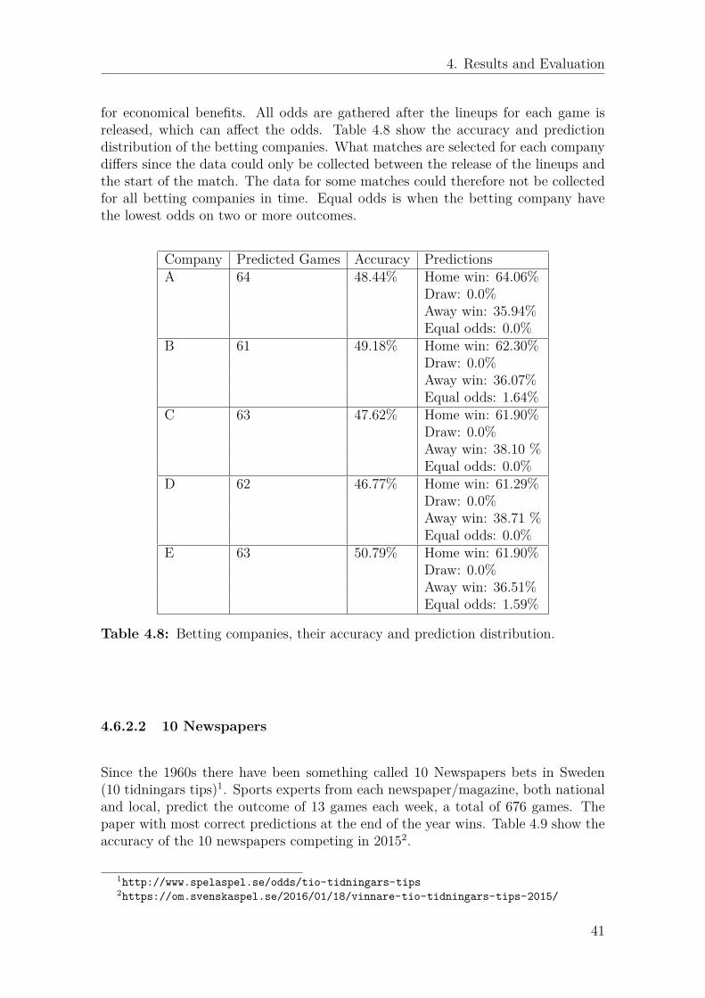
for economical benefits. All odds are gathered after the lineups for each game isreleased, which can affect the odds. Table 4.8 show the accuracy and predictiondistribution of the betting companies. What matches are selected for each companydiffers since the data could only be collected between the release of the lineups andthe start of the match. The data for some matches could therefore not be collectedfor all betting companies in time. Equal odds is when the betting company havethe lowest odds on two or more outcomes.

Company Predicted Games Accuracy PredictionsA 64 48.44% Home win: 64.06%

Draw: 0.0%Away win: 35.94%Equal odds: 0.0%

B 61 49.18% Home win: 62.30%Draw: 0.0%Away win: 36.07%Equal odds: 1.64%

C 63 47.62% Home win: 61.90%Draw: 0.0%Away win: 38.10 %Equal odds: 0.0%

D 62 46.77% Home win: 61.29%Draw: 0.0%Away win: 38.71 %Equal odds: 0.0%

E 63 50.79% Home win: 61.90%Draw: 0.0%Away win: 36.51%Equal odds: 1.59%

Table 4.8: Betting companies, their accuracy and prediction distribution.

4.6.2.2 10 Newspapers

Since the 1960s there have been something called 10 Newspapers bets in Sweden(10 tidningars tips)1. Sports experts from each newspaper/magazine, both nationaland local, predict the outcome of 13 games each week, a total of 676 games. Thepaper with most correct predictions at the end of the year wins. Table 4.9 show theaccuracy of the 10 newspapers competing in 20152.

1http://www.spelaspel.se/odds/tio-tidningars-tips2https://om.svenskaspel.se/2016/01/18/vinnare-tio-tidningars-tips-2015/

41

http://www.spelaspel.se/odds/tio-tidningars-tips

https://om.svenskaspel.se/2016/01/18/vinnare-tio-tidningars-tips-2015/


Newspaper AccuracySydsvenska dagbladet 46.75%Expressen 46.60%Aftonbladet 46.45%Dala-Demokratin 46.45%Borlänge Tidning 45.86%Vi Tippa 45.86%TT 45.71%Dagens Spel 45.56%Skånska Dagbladet 45.12%Dagens Nyheter 43.05%

Table 4.9: Competitors in the 10 Newspapers challenge 2015 and their accuracy.

4.6.2.3 Forza Football Users

The Forza Football application has the possibility for users to predict the outcomeof a game. By comparing which outcome for a match that got the highest amountof predictions with the actually outcome we were able to get an insight into theaccuracy of football fans. We looked at matches between 2015-06-01 and 2017-04-01. Table 4.10 shows the accuracy depending on how many predictions the gameshave.

Predictions Amount of Matches AccuracyAll matches 83963 47.49%>100 predictions 40916 50.92%>500 predictions 17490 52.57%>1000 predictions 10520 54.34%>5000 predictions 2858 59.13%>10000 predictions 1215 59.50%>20000 predictions 317 55.21%

Table 4.10: Accuracy for Forza Football users predictions. The predictions can bemade both before and after the lineups are known.

Since users just predict without any chance of winning money, gut feeling might playa big role in how they predict. They are more likely to predict wins for their favouriteteams or against teams that they don’t like when there is no reward involved.

4.6.3 Discussion

The human accuracy on predicting the outcome of football matches is difficult tomeasure. The accuracy differs depending on what matches are predicted. Predic-tions on different leagues and tournaments give different accuracies and humanspredict the outcome on a much smaller set of leagues and tournaments than thenetwork. This makes it hard compare the network against human accuracy.

42


Other statistical models are made for one or few leagues and can therefore be tunedto work for that specific league or leagues. Therefore it is not entirely fair to compareit with other models.

The human accuracy and the naive statistical model accuracy should just be viewedas a guideline of what peformance the network should have.

4.7 Remarks and Further Discussion

One theory of why the prediction accuracy is not higher is that the networks haveproblems with learning multi-dimensional representations of the teams and players.This could be solved with having deeper data about the matches. Since each matchdoes not have more information than teams, lineups, goals, assists, penalties, cardand substitutions, a lot of leagues have to be used. Since the data set only consistsof the 2-3 last seasons for each league and tournament, a lot of different leagues,without any large amount of transfers between them, have to be used to get enoughamount of data. If a smaller set of leagues were used, however with more seasons foreach league and more data about each match, most of the teams and players wouldoccur more often in the dataset. This would probably require a bigger network tobe able to use all the data and to learn more about the players and the teams andthereby make better predictions. Also the only pure positive event for a team duringa game in our dataset are goals and penalties. These events include forwards andmidfielder a lot more than defenders and goalkeepers. Therefore the network mightnot realise the importance of which defenders and goalkeepers play in a game.

One important thing to take in consideration when predicting games is the physicaland psychological health of the team and the players. These are things that are hardto both gather information about, to put a measure on and use for a computer.

Since there exist few documented predictions from one and the same person overa lot of matches it is hard to measure how good he performance of the network iscompared to humans. For the competitions that exist, the competitors are able toconcentrate on a few leagues while the network predicts the outcome for matchesall over the world. This also increases the difficulty with compareing the networkagainst a human.

43


44

5Conclusion

A LSTM network performs wells on classification and has potential to performwell on predictions of the outcome of football games. Using the proposed LSTMarchitecture the final test classification accuracy of the outcome was 98.63% for themany-to-one approach and 88.68% for the many-to-many approach. When onlyteams and lineups are known the prediction accuracy is 34.30% for many-to-oneand 45.90% for many-to-many. The more informaion the networks are fed about amatch, i.e. the longer an ongoing match is played, the better the network performceon predicting the outcome. At full time many-to-one reached 98.63% and many-to-many 88.68%. This is no suprise since more information should lead to betterpredictions. However, the increased prediction accuracy over minutes played in amatch indicates that the network is able to learn about football.

Future work can be performed on this subject; for example, different data couldbe used, different inputs and architectures could be tested and other things thanwinner could be predicted, such as the amout of goals or cards.

45

5. Conclusion

46

Bibliography

[1] Martín Abadi et al. “Tensorflow: Large-scale machine learning on heteroge-neous distributed systems”. In: arXiv preprint arXiv:1603.04467 (2016).

[2] Burak Galip Aslan and Mustafa Murat Inceoglu. “A comparative study onneural network based soccer result prediction”. In: Intelligent Systems De-sign and Applications, 2007. ISDA 2007. Seventh International Conferenceon. IEEE. 2007, pp. 545–550.

[3] Dzmitry Bahdanau, Kyunghyun Cho, and Yoshua Bengio. “Neural MachineTranslation by Jointly Learning to Align and Translate”. In: CoRR abs/1409.0473(2014). url: http://arxiv.org/abs/1409.0473.

[4] Yoshua Bengio et al. “A neural probabilistic language model”. In: Journal ofmachine learning research 3.Feb (2003), pp. 1137–1155.

[5] Antoine Bordes et al. “Learning structured embeddings of knowledge bases”.In: Conference on artificial intelligence. EPFL-CONF-192344. 2011.

[6] John S Bridle. “Probabilistic interpretation of feedforward classification net-work outputs, with relationships to statistical pattern recognition”. In: Neu-rocomputing. Springer, 1990, pp. 227–236.

[7] Kyunghyun Cho et al. “Learning Phrase Representations using RNN Encoder-Decoder for Statistical Machine Translation”. In: CoRR abs/1406.1078 (2014).url: http://arxiv.org/abs/1406.1078.

[8] Junyoung Chung et al. “Empirical evaluation of gated recurrent neural net-works on sequence modeling”. In: arXiv preprint arXiv:1412.3555 (2014).

[9] Vataya Chunwijitra, Ananlada Chotimongkol, and Chai Wutiwiwatchai. “AHybrid Input-type Recurrent Neural Network for LVCSR Language Model-ing”. In: EURASIP J. Audio Speech Music Process. 2016.1 (Dec. 2016), 93:1–93:12. issn: 1687-4714. doi: 10.1186/s13636- 016- 0093- x. url: https://doi.org/10.1186/s13636-016-0093-x.

[10] Ronan Collobert and Jason Weston. “A unified architecture for natural lan-guage processing: Deep neural networks with multitask learning”. In: Proceed-ings of the 25th international conference on Machine learning. ACM. 2008,pp. 160–167.

[11] John Duchi, Elad Hazan, and Yoram Singer. “Adaptive subgradient meth-ods for online learning and stochastic optimization”. In: Journal of MachineLearning Research 12.Jul (2011), pp. 2121–2159.

[12] David Geer. “Chip makers turn to multicore processors”. In: Computer 38.5(2005), pp. 11–13.

47

http://arxiv.org/abs/1409.0473


http://dx.doi.org/10.1186/s13636-016-0093-x

https://doi.org/10.1186/s13636-016-0093-x

https://doi.org/10.1186/s13636-016-0093-x

Bibliography

[13] Felix A Gers and Jürgen Schmidhuber. “Recurrent nets that time and count”.In: Neural Networks, 2000. IJCNN 2000, Proceedings of the IEEE-INNS-ENNS International Joint Conference on. Vol. 3. IEEE. 2000, pp. 189–194.

[14] Felix A Gers, Jürgen Schmidhuber, and Fred Cummins. “Learning to for-get: Continual prediction with LSTM”. In: Neural computation 12.10 (2000),pp. 2451–2471.

[15] Xavier Glorot, Antoine Bordes, and Yoshua Bengio. “Domain adaptation forlarge-scale sentiment classification: A deep learning approach”. In: Proceedingsof the 28th international conference on machine learning (ICML-11). 2011,pp. 513–520.

[16] Ian Goodfellow, Yoshua Bengio, and Aaron Courville. Deep Learning. http://www.deeplearningbook.org. MIT Press, 2016.

[17] Alex Graves. “Long short-term memory”. In: Supervised Sequence Labellingwith Recurrent Neural Networks (2012), pp. 37–45.

[18] Jordan Gumm, Andrew Barrett, and Gongzhu Hu. “A machine learning strat-egy for predicting march madness winners”. In: Software Engineering, Arti-ficial Intelligence, Networking and Parallel/Distributed Computing (SNPD),2015 16th IEEE/ACIS International Conference on. IEEE. 2015, pp. 1–6.

[19] Geoffrey Hinton, NiRsh Srivastava, and Kevin Swersky. “Neural Networks forMachine Learning Lecture 6a Overview of mini–batch gradient descent”. In:(2012).

[20] Sepp Hochreiter and Jürgen Schmidhuber. “Long short-term memory”. In:Neural computation 9.8 (1997), pp. 1735–1780.

[21] Sepp Hochreiter et al.Gradient Flow in Recurrent Nets: the Difficulty of Learn-ing Long-Term Dependencies. 2001.

[22] Roger A Horn. “The hadamard product”. In: Proc. Symp. Appl. Math. Vol. 40.1990, pp. 87–169.

[23] Josip Hucaljuk and Alen Rakipović. “Predicting football scores using machinelearning techniques”. In: MIPRO, 2011 Proceedings of the 34th InternationalConvention. IEEE. 2011, pp. 1623–1627.

[24] Anito Joseph, Norman E Fenton, and Martin Neil. “Predicting football resultsusing Bayesian nets and other machine learning techniques”. In: Knowledge-Based Systems 19.7 (2006), pp. 544–553.

[25] Kamran Karimi, Neil G Dickson, and Firas Hamze. “A performance compar-ison of CUDA and OpenCL”. In: arXiv preprint arXiv:1005.2581 (2010).

[26] Douwe Kiela and Léon Bottou. “Learning Image Embeddings using Convo-lutional Neural Networks for Improved Multi-Modal Semantics”. In: Proceed-ings of the Conference on Empirical Methods in Natural Language Processing(EMNLP-14). Doha, Qatar, 2014.

[27] Diederik P. Kingma and Jimmy Ba. “Adam: A Method for Stochastic Opti-mization”. In: CoRR abs/1412.6980 (2014). url: http://arxiv.org/abs/1412.6980.

[28] David Luebke. “CUDA: Scalable parallel programming for high-performancescientific computing”. In: Biomedical Imaging: From Nano to Macro, 2008.ISBI 2008. 5th IEEE International Symposium on. IEEE. 2008, pp. 836–838.

48

http://www.deeplearningbook.org

http://www.deeplearningbook.org



Bibliography

[29] Tomas Mikolov et al. “Distributed Representations of Words and Phrasesand their Compositionality”. In: CoRR abs/1310.4546 (2013). url: http ://arxiv.org/abs/1310.4546.

[30] Tomas Mikolov et al. “Efficient estimation of word representations in vectorspace”. In: arXiv preprint arXiv:1301.3781 (2013).

[31] Volodymyr Mnih et al. “Playing atari with deep reinforcement learning”. In:arXiv preprint arXiv:1312.5602 (2013).

[32] David Silver et al. “Mastering the game of Go with deep neural networks andtree search”. In: Nature 529.7587 (2016), pp. 484–489.

[33] Richard Socher et al. “Parsing natural scenes and natural language with re-cursive neural networks”. In: Proceedings of the 28th international conferenceon machine learning (ICML-11). 2011, pp. 129–136.

[34] Nitish Srivastava et al. “Dropout: a simple way to prevent neural networksfrom overfitting”. In: Journal of Machine Learning Research 15.1 (2014), pp. 1929–1958.

[35] D Steinkraus, I Buck, and PY Simard. “Using GPUs for machine learning al-gorithms”. In: Document Analysis and Recognition, 2005. Proceedings. EighthInternational Conference on. IEEE. 2005, pp. 1115–1120.

[36] John E Stone, David Gohara, and Guochun Shi. “OpenCL: A parallel pro-gramming standard for heterogeneous computing systems”. In: Computing inscience & engineering 12.3 (2010), pp. 66–73.

[37] Jaeyong Sung, Ian Lenz, and Ashutosh Saxena. “Deep Multimodal Embed-ding: Manipulating Novel Objects with Point-clouds, Language and Trajecto-ries”. In: CoRR abs/1509.07831 (2015). url: http://arxiv.org/abs/1509.07831.

[38] Ilya Sutskever, Oriol Vinyals, and Quoc V. Le. “Sequence to Sequence Learningwith Neural Networks”. In: CoRR abs/1409.3215 (2014). url: http://arxiv.org/abs/1409.3215.

[39] Peter D Turney and Patrick Pantel. “From frequency to meaning: Vector spacemodels of semantics”. In: Journal of artificial intelligence research 37 (2010),pp. 141–188.

[40] DRGHR Williams and Geoffrey Hinton. “Learning representations by back-propagating errors”. In: Nature 323.6088 (1986), pp. 533–538.

[41] David A Wilson. “Convolution and Hankel operator norms for linear systems”.In: IEEE Transactions on Automatic Control 34.1 (1989), pp. 94–97.

[42] SHI Xingjian et al. “Convolutional LSTM network: A machine learning ap-proach for precipitation nowcasting”. In: Advances in Neural Information Pro-cessing Systems. 2015, pp. 802–810.

[43] Wojciech Zaremba, Ilya Sutskever, and Oriol Vinyals. “Recurrent Neural Net-work Regularization”. In: CoRR abs/1409.2329 (2014). url: http://arxiv.org/abs/1409.2329.

49









Bibliography

50

Appendix A

Raw data

{"liveData": {

"card": [{

"contestantId": "a3nyxabgsqlnqfkeg41m6tnpp","lastUpdated": "2017-02-13T20:10:56.553Z","optaEventId": "1381274270","periodId": 1,"playerId": "eczc8ttdfagqliov10cuqeuol","playerName": "Y. Toure","timeMin": 10,"type": "YC"

}],"goal": [

{"contestantId": "a3nyxabgsqlnqfkeg41m6tnpp","lastUpdated": "2017-02-13T20:29:43.523Z","optaEventId": "1268066259","periodId": 1,"scorerId": "e9l5r0txzrjbenli05rn3k4wl","scorerName": "R. Sterling","timeMin": 29,"type": "G"

},{

"contestantId": "1pse9ta7a45pi2w2grjim70ge","lastUpdated": "2017-02-13T21:41:59.188Z","optaEventId": "491505339","periodId": 2,"scorerId": "2smmv9hdoiet7necaf00ol51x","scorerName": "T. Mings","timeMin": 69,"type": "OG"

I

A. Raw data

}],"lineUp": [

{"contestantId": "1pse9ta7a45pi2w2grjim70ge","player": [

{"firstName": "Artur","lastName": "Boruc","matchName": "A. Boruc","playerId": "eaeh3ogbfsfp0obus2wk66r4l","position": "Goalkeeper","positionSide": "Centre","shirtNumber": 1

},{

"firstName": "Dan","lastName": "Gosling","matchName": "D. Gosling","playerId": "80y7k4ht4s4nkta9wnf30y40l","position": "Substitute","shirtNumber": 4

}],"teamOfficial": {

"firstName": "Eddie","id": "ezlkz2b39qic4wu066cgl1o0l","lastName": "Howe","type": "manager"

}},{

"contestantId": "a3nyxabgsqlnqfkeg41m6tnpp","player": [

{"firstName": "Wilfredo Daniel","lastName": "Caballero","matchName": "W. Caballero","playerId": "6bhm9cfkwxv5ojh49rqv11g45","position": "Goalkeeper","positionSide": "Centre","shirtNumber": 13

},{

"firstName": "Fabian","lastName": "Delph",

II

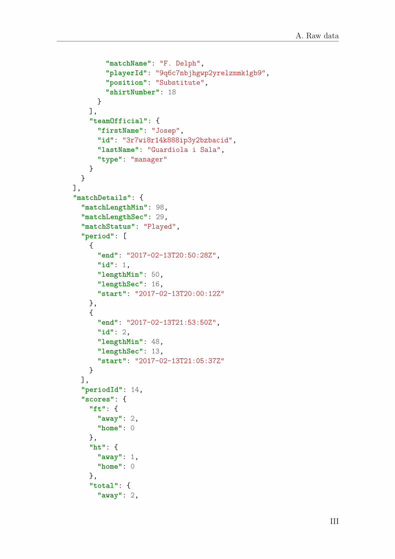
A. Raw data

"matchName": "F. Delph","playerId": "9q6c7nbjhgwp2yrelznmk1gb9","position": "Substitute","shirtNumber": 18

}],"teamOfficial": {

"firstName": "Josep","id": "3r7wi8r14k888ip3y2bzbacid","lastName": "Guardiola i Sala","type": "manager"

}}

],"matchDetails": {

"matchLengthMin": 98,"matchLengthSec": 29,"matchStatus": "Played","period": [

{"end": "2017-02-13T20:50:28Z","id": 1,"lengthMin": 50,"lengthSec": 16,"start": "2017-02-13T20:00:12Z"

},{

"end": "2017-02-13T21:53:50Z","id": 2,"lengthMin": 48,"lengthSec": 13,"start": "2017-02-13T21:05:37Z"

}],"periodId": 14,"scores": {

"ft": {"away": 2,"home": 0

},"ht": {

"away": 1,"home": 0

},"total": {

"away": 2,

III

A. Raw data

"home": 0}

},"winner": "away"

},"missedPen": [],"substitute": [

{"contestantId": "a3nyxabgsqlnqfkeg41m6tnpp","lastUpdated": "2017-02-13T20:15:31.422Z","periodId": 1,"playerOffId": "d66tmyj9pt69gub8pcjgo3bh1","playerOffName": "Gabriel Jesus","playerOnId": "5ch5dk1z9opa2iwd64kb4e5sl","playerOnName": "S. Aguero","timeMin": 15

}]

},"matchInfo": {

"competition": {"country": {

"id": "1fk5l4hkqk12i7zske6mcqju6","name": "England"

},"id": "2kwbbcootiqqgmrzs6o5inle5","name": "Premier League"

},"contestant": [

{"country": {

"id": "1fk5l4hkqk12i7zske6mcqju6","name": "England"

},"id": "1pse9ta7a45pi2w2grjim70ge","name": "AFC Bournemouth","position": "home"

},{

"country": {"id": "1fk5l4hkqk12i7zske6mcqju6","name": "England"

},"id": "a3nyxabgsqlnqfkeg41m6tnpp","name": "Manchester City","position": "away"

IV

A. Raw data

}],"date": "2017-02-13Z","description": "AFC Bournemouth vs Manchester City","id": "9n1lozeiz5rv8atl9hs5cjkyx","lastUpdated": "2017-02-13T22:16:15Z","ruleset": {

"id": "79plas4983031idr6vw83nuel","name": "Men"

},"sport": {

"id": "289u5typ3vp4ifwh5thalohmq","name": "Soccer"

},"time": "20:00:00Z","tournamentCalendar": {

"endDate": "2017-05-21Z","id": "2c1fh40r28amu4rgz0q66ago9","name": "Premier League 2016/2017","startDate": "2016-08-13Z"

},"venue": {

"id": "8vnu2g41orfaa25n2djgrv4jm","longName": "Vitality Stadium","shortName": "Vitality Stadium"

},"week": "25"

}}

V

A. Raw data

VI

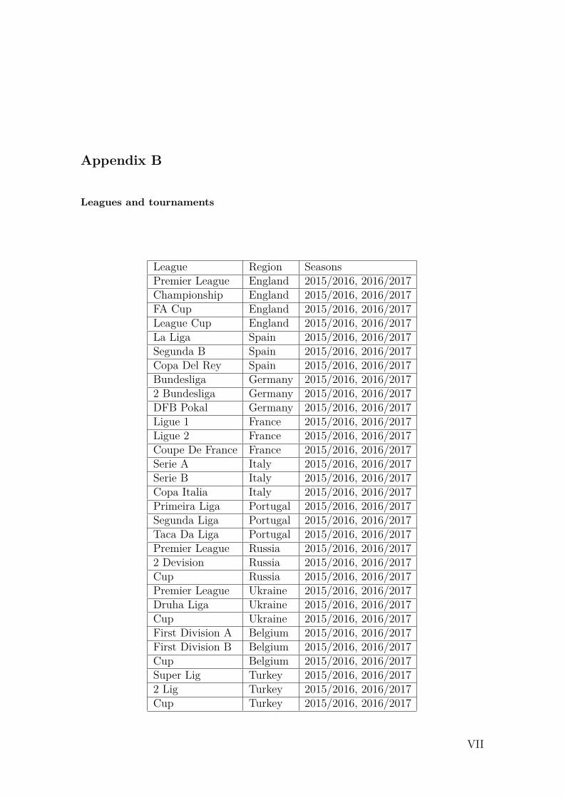
Appendix B

Leagues and tournaments

League Region SeasonsPremier League England 2015/2016, 2016/2017Championship England 2015/2016, 2016/2017FA Cup England 2015/2016, 2016/2017League Cup England 2015/2016, 2016/2017La Liga Spain 2015/2016, 2016/2017Segunda B Spain 2015/2016, 2016/2017Copa Del Rey Spain 2015/2016, 2016/2017Bundesliga Germany 2015/2016, 2016/20172 Bundesliga Germany 2015/2016, 2016/2017DFB Pokal Germany 2015/2016, 2016/2017Ligue 1 France 2015/2016, 2016/2017Ligue 2 France 2015/2016, 2016/2017Coupe De France France 2015/2016, 2016/2017Serie A Italy 2015/2016, 2016/2017Serie B Italy 2015/2016, 2016/2017Copa Italia Italy 2015/2016, 2016/2017Primeira Liga Portugal 2015/2016, 2016/2017Segunda Liga Portugal 2015/2016, 2016/2017Taca Da Liga Portugal 2015/2016, 2016/2017Premier League Russia 2015/2016, 2016/20172 Devision Russia 2015/2016, 2016/2017Cup Russia 2015/2016, 2016/2017Premier League Ukraine 2015/2016, 2016/2017Druha Liga Ukraine 2015/2016, 2016/2017Cup Ukraine 2015/2016, 2016/2017First Division A Belgium 2015/2016, 2016/2017First Division B Belgium 2015/2016, 2016/2017Cup Belgium 2015/2016, 2016/2017Super Lig Turkey 2015/2016, 2016/20172 Lig Turkey 2015/2016, 2016/2017Cup Turkey 2015/2016, 2016/2017

VII

B. Leagues and tournaments

League Region SeasonsFirst League Czech Republic 2015/2016, 2016/2017Super League Switzerland 2015/2016, 2016/2017Eredivisie Netherlands 2015/2016, 2016/2017Super League Greece 2015/2016, 2016/2017Bundesliga Austria 2015/2016, 2016/20171. HNL Croatia 2015/2016, 2016/2017Liga 1 Romania 2015/2016, 2016/2017Superliga Denmark 2015/2016, 2016/2017Premier League Belarus 2015/2016, 2016/2017Ekstraklasa Poland 2015/2016, 2016/2017Allsvenskan Sweden 2015, 2016, 2017Major League Soccer USA 2016, 2017Serie A Brazil 2016, 2017Liga MX Mexico 2015/2016, 2016/2017Primera Division Argentina 2016, 2016/2017Liga Alef Israel 2015/2016, 2016/2017Championship Scotland 2015/2016, 2016/2017Primera Division Uruguay 2015/2016, 2016/2017A League Australia 2015/2016, 2016/2017Super League China 2015, 2016, 2017J1 League Japan 2015, 2016, 2017Super Liga Slovakia 2015/2016, 2016/2017Fl1 active cup Liechtenstein 2015/2016, 2016/2017NB1 Hungary 2015/2016, 2016/2017Divizia Nationala Moldovia 2015/2016, 2016/20171 Deild Iceland 2015, 2016, 2017Veikkausliiga Finland 2015, 2016, 2017Superliga Albania 2015/2016, 2016/2017Premier Division Republic of Ireland 2015, 2016, 2017Premier Liga Bosnia and Herzegovina 2015/2016, 2016/2017Erovnuli liga Georgia 2015/2016, 2016, 2017Virsliga Latvia 2015, 2016, 2017First league Macedonia 2015/2016, 2016/2017Esiliiga A Estonia 2015, 2016, 2017First League Montenegro 2015/2016, 2016/2017Premier League Armenia 2015/2016, 2016/2017National Division Luxembourg 2015/2016, 2016/2017A Lyga Lithuania 2015, 2016, 2017Premier League Malta 2015/2016, 2016/2017Premier League Wales 2015/2016, 2016/20171 Deild Faroe Islands 2015, 2016, 2017Premier Division Gibraltar 2015/2016, 2016/20171 Divisio Andorra 2015/2016, 2016/2017Campionato San Marino 2015/2016, 2016/2017Champions League Europe 2015/2016, 2016/2017Europa League Europe 2015/2016, 2016/2017Club World Cup Worldwide 2015/2016, 2016/2017VIII

Football Match Prediction using Deep...

Documents

Transcript of Football Match Prediction using Deep...