PRESENTED BY SUNIL MANJERI Maximum sub-triangulation in pre- processing phylogenetic data Anne Berry...

P R E S E N T E D BY S U N I L M A N J E R I

Maximum sub-triangulation in pre-processing phylogenetic data

Anne Berry * Alain Sigayret * Christine Sinoquet

Outline

IntroductionPhylogeny PreliminariesChordal Graphs PreliminariesThreshold Family of GraphsMaintaining a family of chordal graphsComposition SchemeAlgorithmReferences

Introduction

The best evidence strongly support that all life currently on earth is descended from a single common ancestor

In last 3.8 million years the single ancestor has split repeatedly into new species

The evolutionary relationship between these species is referred to as phylogeny

Phylogenetic trees illustrates the phylogeny of groups of organisms

Basics of Phylogeny

Introduction

A sample data set and phylogeny for it is shown below

Basics of Phylogeny

a b c d e f

lamprey 0 0 0 0 0 1

shark 1 1 0 1 0 0

salmon 1 1 1 1 0 0

lizard 1 1 1 0 1 0 lamprey shark salmon lizard

a, b

fc

d d e

Characters

Taxa

a – paired fins, b – jaws, c – large dermal bones, d – fin rays, e – lungs, f – rasping tongue

Introduction

Data for Phylogeny

Numerical Distance between objects or species

distance (man, mouse) = 500 distance (man, chimp) = 100

Discrete characters Each character has finite number of states

Number of legs = 1, 2, 4 DNA = {A, C, T, G}

Basics of Phylogeny

Introduction

Distance method of reconstructing Phylogeny trees

Basics of Phylogeny

Input: Given a n x n matrix M where Mij >= 0 and Mij is the distance between objects or species i and j Goal: Build and edge-weighted tree where each leaf corresponds to one object of M and so that the distances measured on the tree between leaves i and j correspond to Mij

M A b c d e

a 0 6 12

12

16

b 0 12

12

16

c 0 6 10

d 0 8

a

b

c

e

d3

3

6

3

1

6

2

Fig. 1

Phylogeny Preliminaries

Definitions and properties

Dissimilarity on a finite set X is a function δ:X2 -> IR+ such that for all x, y є X

δ(x, y) = δ(y, x)

Distance is a dissimilarity such that for all x, y є X δ(x, y) = 0 for x=y for all x, y, z є X δ(x, y) + δ(y, z) ≥ δ(x, z)

In Fig. 1 let £ the set of leaves representing the taxa. For a,b є £, denote d(a,b) be the length of the ab-path or the evolutionary distance between a and b. This distance is called additive distance and the associated matrix on £ x £ is called an additive matrix

Additive Matrices

M A b c d e

a 0 6 12

12

16

b 0 12

12

16

c 0 6 10

d 0 8


The set of values of a dissimilarity matrix M can be ordered from 0 (as M[x, y] = 0) to the maximal value. This defines a number of different thresholds (θ): 0,1,…k in increasing order

The 6 dissimilarity values are: θ-1(0)=0, θ-1(1)=6, θ-1(2)=8, θ-1(3)=10, θ-1(4)=12, θ-1(5)=16 The 6 threshold values are: θ(0)=0, θ(6)=1, θ(8)=2, θ(10)=3, θ(12)=4, θ(16)=5

Ordinal Matrix of a dissimilarity matrix is defined as the matrix obtained by replacing each dissimilarity value by its threshold

Ordinal Matrices

M a b c d e

a 0 6 12

12

16

b 0 12

12

16

c 0 6 10

d 0 8

Dissimilarity matrix M

M a b c d e

a 0 1 4 4 5

b 0 4 4 5

c 0 1 3

d 0 2Ordinal matrix W


Characterization 2.1 From [3], a distance matrix M on a set of taxa is additive if and only if for any quadruple {a, b, c, d} of taxa, from the 3 sums d(a, b)+d(c, d), d(a, c)+d(b, d) and d(a, d)+d(b, c), the two largest are equal

Additive Matrices

M a b c d e

a 0 6 12

12

16

b 0 12

12

16

c 0 6 10

d 0 8


d(a, b)+d(c, d) = 12d(a, c)+d(b, d) = 24d(a, d)+d(b, c) = 24

The Problems

Reconstructing the tree is easy and can be done in polynomial time

Experimental results usually does not always generate additive matrices, and inferring phylogeny remains costly and inaccurate

Instead examine the ordinal properties of the dissimilarity matrix thereby examining the structure of the thresholds rather than depending only the values themselves. This approach seems to be less sensitive to small data variations.

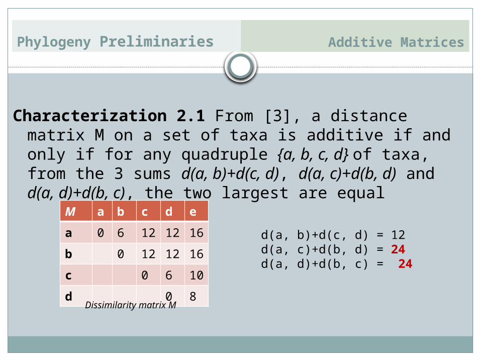
Huson, Nettles and Warnow in [2] proved that if the matrix is additive, all the graphs of the threshold family are chordal or triangulated

Problem: Experimental results show that not only do the dissimilarity matrices biologists have to work with fail to be additive, but the corresponding graphs very often fail to be chordal.

Chordal Graphs Preliminaries

A graph G = (V, E) is said to be chordal or triangulated if it contains no chordless cycle on more that 3 vertices

Characterization 2.3 - A graph is chordal if and only if it is the intersection graph of a family of subtrees of a tree [4]

Graph Inclusion – If G=(V, E) is a graph and G`=(V, E`) is another graph on the same vertex set, we can write

G ⊆ G` if and only if E ⊆ E`and

G ⊂ G` if and only if E ⊂ E`

Chordal Graphs Preliminaries

Methods of correcting non-chordal graph Minimal triangulation

Adding an inclusion-minimum set of edges to the graph in order to make it chordal

For a given graph of n vertices and m edges, computing minimum triangulation can be done in O(nm) time

Adding edges to a graph of threshold family means lowering the thresholds of the corresponding edges.

Maximal triangulation Removing edges rather than adding them to make a graph

chordal Maximum triangulation can be computed in O(Δm) time,

where Δ is the maximum degree in the graph

Correcting Chordal Graphs

Chordal graphs Preliminaries

Rose, Tarjan and Lueker gave the following definition of minimal triangulation

Definition 2.4 – From [5] If G = (V, E) is a non-chordal graph, a chordal graph H = (V, E + F) is said to be a minimal triangulation of G if ∀ F`⊂ F, graph ( V, E+F` ) fails to be chordal

Minimal Triangulation

a

b

c

de

f

g

H

a

b

c

de

f

g

G

F = {bd, af}F` = {bd} or {af}


Rose, Tarjan and Lueker also proved that only one edge needs to be removed and the resulting graph becomes non-chordal

Theorem 2.5 – From [5] Let G = (V, E) be a non-chordal graph, let H = (V, E + F) be a chordal graph; H is minimum triangulation of G iff ∀ f ∈ F, graph ( V, (E+ (F \ {f}))) fails to be chordal


a

b

c

de

f

g

H

a

b

c

de

f

g

G

F = {bd, af}f = {bd} or {af}


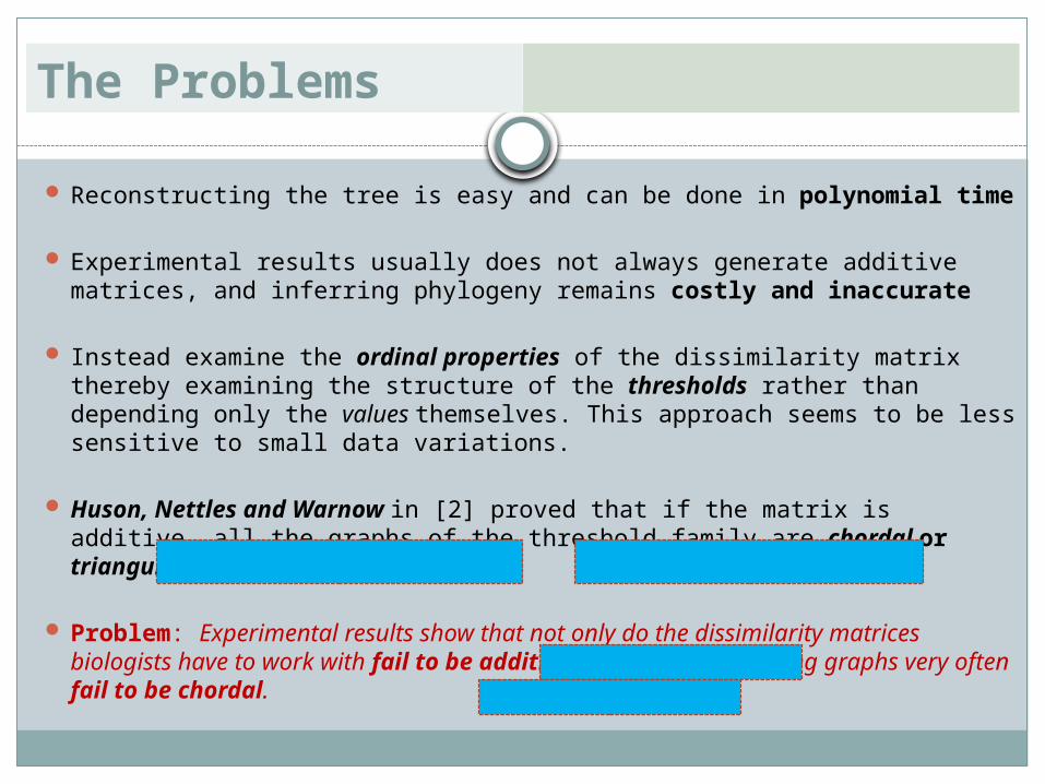
The above theorem relies on the following Lemma, which ensures that, given two chordal graphs which are mutually inclusive, there is an ordering on the edges which need to be added to the smaller graph which will maintain chordality at each edge-addition step

Lemma 2.6 – From [5] Let G1 = (V, E1) be a chordal graph, let G2 = (V, E2) be a chordal graph such that G1 ⊂

G2 . Then ∃f ∈ E2 \ E1 such that G` = (V, E2 \ {f}) is chordal


a

b

c

de

f

g

G1

a

b

c

de

f

g

G2

E2 \ E1 = {ce, dg, bf, af, ag}Proper Ordering: ce, dg, bf,

af, agIn-Proper Ordering: ce, dg, ag, af, bf


Definition 2.8 – Let G = (V, E) be a non-chordal graph, let H = (V, E \ F) be a chordal graph. We will say that H is a maximal sub-triangulation of G if ∀F`⊂ F, (V, (E \ F) + F`) fails to be chordal

Maximal sub-triangulation

a

b

c

de

f

g

G

a

b

c

de

f

g

H

F = {cb, fb}F` = {cb} or {fb}

Maintaining Chordality

Given a dissimilarity matrix, we use the associated ordinal matrix to define the corresponding threshold family of graphs

Let A be a set of taxa, M be the dissimilarity matrix, W be the corresponding ordinal matrix, on thresholds be 0,1,…,k;We can define a family of graphs G0 ⊂ G1 ⊂ … ⊂ Gk, called threshold family of graphs associated with W (and thus with M), with

Gi = (V, Ei), V = A and ab ∈ Ei iff WA[a, b] ≤ I Example The threshold matrix induces a preorder relation

ℛ: ab ℛ cd iff W[a, b] ≤ W[c, d]

ℛ defines an ordered partition of edges of Gk; Each class Fi of edges is defines by

Fi = Ei – Ei-1 = {xy |W[x, y] = i]

Graph Gi is obtained from graph Gi-1 by adding set of edges Fi

Threshold Family of Graphs

Maintaining Chordality Threshold Family of Graphs

M a b c d e

a 0 6 12

12

16

b 0 12

12

16

c 0 6 10

d 0 8


M a b c d e

a 0 1 4 4 5

b 0 4 4 5

c 0 1 3


a b

d c

eG0

a b

d c

eG2

a b

d c

eG3

a b

d c

eG4

Gi = (V, Ei), V = A and ab ∈ Ei iff WA[a, b] ≤ i

a b

d c

eG1

Maintaining Chordality

Property 3.4 If M is an additive matrix then the threshold family of graphs defined by M is a family of chordal graphs

Proofo Let T be the phylogeny associated with an additive matrix

Mo Let Gi be the graph corresponding to threshold i ∈ [0…k]o Add internal nodes to T in order obtain a tree T`(where

there is a node at mid-distance between any pair {a, b} of verticeso Consider family of subtrees of T` defined by: for each leaf

x, T`x is the subtree containing all nodes at distance θ-1(i)/2 or less from x; Example

o Then Gi is the intersection graph of the family of subtreeso By virtue of Characterization 2.3

(Gavril’s theorem), Gi is Chordal

Threshold family of graphs / Chordal graphs

a

b

c

e

d3

3

6

3

1

6

2

Example For i=1, θ-1(1)/2 =3

For i=2, θ-1(1)/2 =4

Threshold family of graphs Vs. Chordal graphs

a

b

c

e

d3

3

3

3

1

4

22 111

a b

d c

eG1

a b

d c

eG2

T`1

a

b

c

e

d3

3

3

3

1

4

22 111

T`2

Composition Scheme

To compute a threshold family of graphs which are chordal, such that each graph Gi is a sub graph of the original graph G, we construct a clique Gk from independent set G0 by adding at each step an inclusion-maximal set of edges which maintains Chordality.

Definition 3.7 From [6], a pair {a, b} of non-adjacent vertices is called a 2-pair iff every chordless path from a to b is of length exactly 2

An edge-addition composition scheme for chordal graphs

a b

{a, b} is a 2-pair

Composition Scheme

Theorem 3.8 Let G1 be a chordal graph, let {a, b} be a pair of non-adjacent vertices of G1, let G2 be the graph obtained from G1 by adding edge ab; then G2 is chordal iff {a, b} is a 2-pair of G1

Proofo Let G1 be a chordal graph

o Let {a, b} be a pair of non-adjacent vertices of G1

o Let G2 be the graph obtained from G1 by adding edge ab

o Let μ = ax1x2…xkb be a longest chordless path from a to b in G1

o In G2 , ax1x2…xkba will be chordless path on more

than 3 vertices iff μ is of length greater than 2, i.e. iff {a, b} fails to be a 2-pair of G1 . This

contradicts the fact that G1 is chordal.

o Hence {a, b} is a 2-pair of G1


a b

Composition Scheme

Property 3.9 Let G1 be a chordal graph, let G2 be a chordal graph such that G1 ⊂ G2 . Then G2 can be obtained from G1 by repeatedly adding an edge between the two vertices forming a 2-pair.

Proofo Let G1 be a chordal graph, let G2 be a chordal graph such that G1 ⊂ G2

o By Lemma 2.6, ∃xy ∈ E2 \ E1

Such that (V, E2 \ {xy}) is chordal.

o By theorem 3.8, {x, y} is a 2-pair of G2 \ {xy}

o Repeat this until we obtain graph G1. We have constructed (in reverse) a 2-pair edge addition ordering which enables us to construct G2 from G1


a

b

c

de

f

g

G1

a

b

c

de

f

g

G2

E2 \ E1 = {ce, dg, bf, af, ag}

Composition Scheme

Composition Scheme 3.10 From above theorem, a graph on n vertices is chordal iff it can be constructed by starting with an independent set on n vertices, and by adding at each step an edge between the two vertices forming a 2-pair.

Algorithm

Input: A dissimilarity matrix M on n taxa, with threshold 0,1,…,kOutput: A dissimilarity matrix M`, such that every graph in the threshold family is chordalInitialization: G0 is an independent set on n vertices; Create an empty FIFO queue Q;

beginFor i = 1 to k-1 do

Assign Gi-1 to Gi

Compute the set Fi of pairs of {a, b} such that M[a, b] = θ-1(i);

Add Fi to the queue Q;

RepeatScan Q and remove the first pair of ab which is a 2-pairAdd edge ab to graph Gi;

Set the value of M`[a, b] with θ-1(i);

Until Q contains no 2-pair of Gi

Give all remaining edges in Q value θ-1(k) in M`;Add all remaining edges in Q to Gk-1 to form Gk, a clique on n vertices

end

An additive data pre-processing algorithm

Threshold family of graphs

M a b c d e

a 0 6 12 8

16

b 0 812

16

c 0 6 10

d 0 8


M a b c d e

a 0 1 4 2 5

b 0 2 4 5

c 0 1 3


Example: Consider an incorrect matrix

M` a b c d e

a 0 6 12

12

16

b 0 12

12

16

c 0 6 10

d 0 8

Dissimilarity matrix M`

Computing the Algorithm will generate the following corrected dissimilarity matrix

Complexity of running the above algorithm is O(n5)

Reference

[1] – Anne Berry, Alain Sigayret, Christine Sinoquet (2005) Maximal sub-triangulation in pre-processing phylogenetic data

[2] –Huson D, Nettles S, Warnow T (1999) Obtaining highly accurate topology estimates of evolutionary trees from very short sequences.

[3] – Barthelemy J-P, Guenoche A (1991) Trees and proximity representations

[4] – Gavril F (1974) The intersection graphs of subtrees of trees are exactly the chordal graphs

[5] – Rose D, Tarjan RE, Lueker G (1976) Algorithmic aspects of vertex elimination on graphs

[6] – Hayward R, Hoang C, Maffray F (1989) Optimizing weakly triangulated graphs

PRESENTED BY SUNIL MANJERI Maximum sub-triangulation in pre- processing phylogenetic data Anne Berry...

Documents

Transcript of PRESENTED BY SUNIL MANJERI Maximum sub-triangulation in pre- processing phylogenetic data Anne Berry...