Predicting the winner of NFL-games using Machine and

Deep Learning.

Pablo Bosch

Supervisor: Sandjai Bhulai

Vrije universiteit, Amsterdam, Nederland

Research Paper Business Analytics

February 2018

Abstract

Predicting the winner of American Football games has been a hot topic for decades.

Since the 1950’s people have tried to classify the strength of an athlete or team and

predict the outcome of sports games. More recently, people have tried to predict the

binary outcome of a game-winner or to estimate the number of goals applying Machine

Learning methods. In recent past Deep Learning methods have been widely developed

and have a significant impact in research fields such as Natural Language Processing

and in 2015 Google has opened the open-source software library Tensorflow which

enables users to perform Deep Learning methods in a more efficient way. The increase

of open-source data of NFL-games and the availability of open-source software for ap-

plying Deep Learning methods makes one wonder if Deep Learning methods can out-

perform classical Machine Learning methods in predicting the winner of NFL-games.

In this paper we analyze if Deep Learning can outperform Machine Learning in pre-

dicting the winner of NFL-games.

2

Contents Abstract ............................................................................................................. 1

1 Introduction .............................................................................................. 3

2 Background & literature research............................................................. 4

An American Football game .......................................................................... 4

Log 5 method ................................................................................................ 5

ELO ranking ................................................................................................... 5

Machine Learning approaches ...................................................................... 5

Football Match Prediction using Deep Learning ........................................... 6

3 Data gathering .......................................................................................... 7

Feature engineering ...................................................................................... 7

4 Methods .................................................................................................... 8

Machine Learning algorithms ....................................................................... 8

Support Vector Machine ........................................................................... 8

Logistic regression ..................................................................................... 9

Random Forest .......................................................................................... 9

Deep Learning methods .............................................................................. 10

Artificial Neural network ......................................................................... 10

Recurrent Neural Network ...................................................................... 11

5 Data preprocessing ................................................................................. 13

6 Parameter optimization .......................................................................... 15

Artificial Neural Network ............................................................................ 15

Recurrent neural network .......................................................................... 16

7 Evaluation ............................................................................................... 17

8 Conclusion and further work .................................................................. 18

Bibliography .................................................................................................... 19

Appendix 1: 63 created characteristics ........................................................... 20

3

1 Introduction

American football is one of the most popular sports in the United States. Betting on

National Football League (NFL)-games is immensely popular and creates a gigantic

cash flow. The American Gaming Association (AGA) estimated that fans in the United

States would bet $90 billion on NFL and college football games in the 2017 season [1].

One of the most common known betting option is gambling on the winner of a game.

As a results, being able to predict the correct winner of a NFL-game has become an

interesting and lucrative business.

The popularity of American Football has led to huge information resources on

games, players and statistics, such as the total yards passed average points scored per

game. Experts of well-known sports-related organizations like ESPN, CBS sports and

gambling institutions try to predict the outcome of NFL-games. Numerous attempts

have been performed to outperform these experts and gambling institutions to predict

the outcome of NFL-games using data-analytics or Machine Learning.

All of these projects have tried to predict game-winners of NFL-games using Ma-

chine Learning classification algorithms like Naïve Bayes, logistic regression, Random

Forest or Support Vector Machines. However, in recent past Deep Learning methods

have been widely developed and have a significant impact on research fields such as

Natural Language Processing. Also, in 2015 Google has opened the open-source soft-

ware library Tensorflow which enables users to perform Deep Learning methods in a

more efficient and faster way. The increase of open-source data of NFL-games and the

availability of open-source software for applying Deep Learning methods makes one

wonder if Deep Learning methods can outperform classical Machine Learning methods

in classifying NFL game-winners. This leads to the following research question ana-

lyzed in this paper:

Can Deep Learning outperform Machine Learning in predicting the winner of regular

season NFL- games?

In this report a brief recap of past attempts of classifying via mathematical or data

analytical methods is presented in Chapter 1. In Chapter 2 the data collection and fea-

ture engineering is elaborated, in Chapter 3 the applied Machine and Deep Learning

methods are explained and in Chapter 4 the results are presented and analyzed.

4

2 Background & literature research

Scientists have been trying to predict game-winners of sports games with multiple

mathematical and data science techniques. This chapter contains a brief explanation of

an American football game and presents several earlier attempts and methods to classify

game winners.

An American Football game

An American football game is played in 4 quarters. In contrast to a lot of other sports

such as football/soccer or rugby, a game is played by multiple units within a team con-

sisting of 11 players, an offensive, defensive and a special team unit. The offense of

team A takes on the defense of team B and vice versa. The special teams unit play each

other.

Figure 1 Schematic overview of a football field

The task of the offensive unit is to move the ball into to “end-zone” and score a

“touchdown”. In order to move the ball towards the end-zone, the offense has the option

to run with the football or to pass it to a teammate. Each run or passed ball is called a

play. In addition to the task of getting into the end zone, the offense must come at least

10 yards closer to the end zone within 4 plays. If they fail, the offense of the opposing

team will get the ball. The task of the defense is to prevent the offense from being able

to move to ball into the end-zone.

5

Log 5 method

In 1981, Bill James introduced the log 5 method [2]. It provides a method, mostly

applied in baseball, for taking the strengths of two teams and estimating the probability

of one team beating the other using the win percentages of both teams, respectively p

and q. The probability that the team with win percentage p wins is estimated by:

p − pq

p + q − 2pq

ELO ranking

Another popular ranking system is the ELO-ranking, originally introduced by phys-

ics professor Arpad Elo to rank chess-players [3]. This system uses four-digit ratings

between 1000 and 2900 and is used to measure each player's relative strength and is

based on the Pairwise comparison method.

The ratings of the ELO-method are based on results in tournament and match play

weighted according to the opponents' strength. Since its introduction, the ELO-ranking

has been adopted by multiple sports, such as American Football and basketball.

In 2014, Nate Silver introduced an ELO-ranking system to rank all 32 NFL-teams.

It takes into account basic knowledge, such as wins and losses, strength of schedule or

point differential, but also knowledge of previous seasons [4]. The probability that

team A will defeat team B can be estimated with this ranking system using the follow-

ing formula:

Pr(A) =1

10D + 1

With D corresponding to: (ELO−ranking team A) – (ELO−ranking team B)

−400

Machine Learning approaches

In more recent attempts of predicting NFL-games, Machine Learning methods have

been applied. Microsoft currently predicts NFL-games with its digital assistant an AI

Engine Cortana [5]. Other attempts have applied Machine Learning models like Sup-

port Vector Machine, Logistic Regression, Random Forest and AdaBoost Decision

Stumps to predict the binary win or loss outcomes. For example, Jim Warner was able

to predict game-winners in 2011 with an accuracy of 64.36% training a Gaussian pro-

cess model on a dataset of 2000 games between 2000 and 2009 [6]. Albert Shau pre-

dicted in 2011 68.4% of the game-winners correctly using a Support Vector Machine

(SVM) model trained on game data from 1970 to 2011 [7]. Zachary Owen and Virgile

Galle were able to predict 68.6% of the game-winners correctly using an SVM-model

trained on game data from 2009 to 2014 [8].

6

Football Match Prediction using Deep Learning

In 2017 Daniel Petterson and Robert Nyquist predicted soccer matches using Deep

Learning applying Recurrent Neural Networks [9]. They have studied several ways to

use LSTM architectures and were able to correctly classify 98% for a many-to-one

strategy, which indicates Deep Learning may be a successful method for predicting

sports games. In Chapter 4 Methods, the LSTM architecture is further elaborated. The

amount of data Petterson and Nyquist were able to process is significantly more than

the amount of data available for predicting American Football games, since soccer is a

world-wide played sport. They were able to process data from 63 different countries

which resulted in over 35000 matches.

7

3 Data gathering

In this project NFL-data from the 2009 to 2016 season is used. This data is obtained

using the API “NFL Game” and the database “nfldb”. The dataset contains a lot of data,

since it registered all events play by play and player by play. Only data of regular-

season games is used.

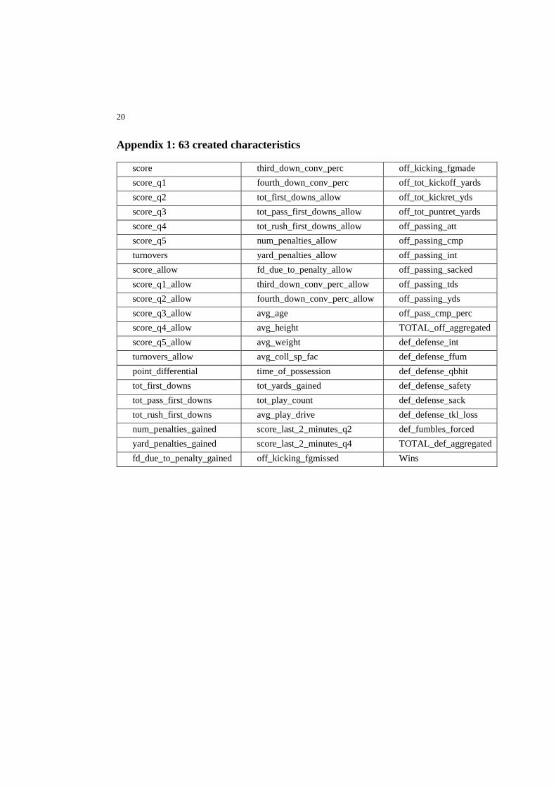
Feature engineering

To train the Machine and Deep Learning methods multiple datasets with relevant

features were created. First, for each team 63 post-priori characteristics per game were

determined. These features were chosen based on prior knowledge on important indi-

cators of team performance and are presented in Appendix 1. Since data of a game itself

or future data cannot be used for predicting the outcome, the post-priori features of a

team were used to calculate averages of a-priori known features. These averages have

been determined for the following 13 scenarios:

• Averages of the current season

• Averages of the mutual games played

• Averages of the last n games, for n = 3, 5, 7, 8, 9, 10, 11

• Averages of the last m mutual games, for m = 2, 3, 5, 7

To create datasets per game, the data of the home and away team were combined

together with the essential features to identify the game (year, week, home team, away

team and result of the game). This enabled to create other relevant features comparing

both teams in:

• Number of wins

• Average turnover differential per game

• Average point differential per game

• Average age, weight and height

• Average number of first downs per game

The above activities have resulted in 13 different datasets containing over 130 fea-

tures.

8

4 Methods

In this research we explore if Deep Learning methods can outperform Machine

Learning methods in predicting the winner of NFL-games. In this chapter the methods

applied in this research are theoretically explained.

Machine Learning algorithms

Support Vector Machine

Support Vector Machines or SVMs are Machine Learning methods used for classi-

fication, regression and outlier detection [10]. SVMs aims at finding the optimal sepa-

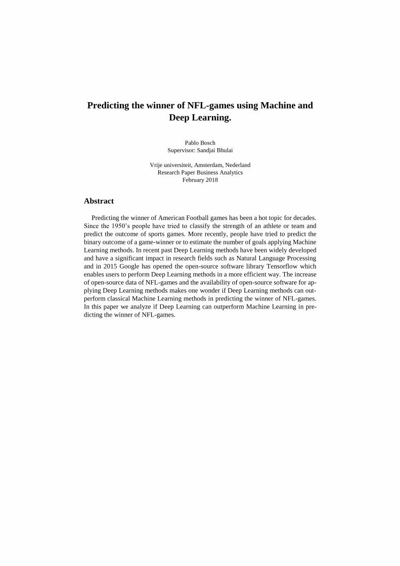
rating hyperplane to distinct classes. Figure 2 shows an example of a separable problem

in a 2-dimensional space. The vector through the margin lines and grey squares are

known as the support vectors. An optimal hyperplane maximizes the length between

the support vectors.

Figure 2 Separable problem in a 2-dimensional space [11].

In Figure 2 all data points lie outside the hyperplane. Training a model to find a

hyperplane as narrow as possible, could potentially increase the risk of overfitting. To

reduce the risk of overfitting one could lower the constraint of all data points outside

the hyperplane with a regularization parameter C. A large value for C causes a narrow

margin by meeting the constraints and vice versa.

9

Not linearly separable data

Not all data can be separated into classes linearly. Transforming non-linear data into

linear separable data (via e.g., polynomial functions) could cause an increase in dimen-

sions and possibly computation time. A simpler trick could be to apply the “kernel

trick”. This method enlarges the feature space by computing the inner product of data

points without computing the coordinates.

Logistic regression

A logistic Regression model tries to predict the probability of all K categorical clas-

ses assuming the outcome variable has a linear relationship with the features [10]. Con-

sider a binary classification problem. Let the probability of the output being 1 with

known input x.

𝑃(𝑦 = 1|𝑥)

A representation of this probability with n features could be:

𝑃(𝑦 = 1 ∣ 𝑥) = 𝑤𝑜 + 𝑤1𝑥1 + 𝑤2𝑥2+. . . +𝑤𝑛𝑥𝑛

With each linear combination of inputs between −∞ < 𝑤𝑛𝑥𝑛 > ∞

The odds ratio is the probability of success divided by the probability of failure. Prob-

abilities range from 0 to 1 but odds range from 0 to positive infinity.

𝑜𝑑𝑑𝑠(𝑃) =p

1 − p log (𝑜𝑑𝑑𝑠(𝑃)) = ln (

p

1 − p)

Mapping all features to the log(odds) allows us to model a relationship between a bi-

nary classification and its features, which is often called the logistic function :

𝑙𝑜𝑔_𝑜𝑑𝑑𝑠(𝑃(𝑦 = 1 ∣ 𝑥)) = 𝑤𝑜 + 𝑤1𝑥1 + 𝑤2𝑥2+. . . +𝑤𝑛𝑥𝑛

Random Forest

Random forests are ensemble Machine Learning algorithms. Random Forests are a

collection of de-correlated decision trees such that each tree depends on a random boot-

strapped sample from a training set [10]. For each tree, the following procedure is ap-

plied recursively until the minimum node size is reached:

1. Apply feature bagging to decrease correlation between trees (i.e., select m

random variables)

2. Split the tree on the variable of subset m with highest Information Gain

After growing all trees, the Random Forest classifies each instance based on the

mode of all classifications of each tree. The usage of de-correlated bootstrap samples

and feature bagging prevents Random Forest models often from overfitting than deci-

sion trees.

10

Deep Learning methods

Deep Learning models are based on artificial neural networks and have multiple lay-

ers. In this research, an Artificial Neural Network and a Recurrent Neural Network were

implemented to test the hypothesis if Deep Learning methods can outperform Machine

Learning methods in predicting NFL-game winners. Taking into account the small

amount of data available of approximately 2000 games, the restriction to include mul-

tiple layers into these models was dropped. Instead, the optimal settings of number of

layers and neurons and parameter settings have been tuned.

Artificial Neural network

An Artificial Neural Network (ANN) is a biologically inspired computational model,

which consists of processing elements (called neurons), and connections between them

with coefficients (weights) bound to the connections [12]. Generally speaking, an ANN

consists of three key elements; an input layer containing features, one or more hidden

layers with multiple nodes (or neurons) and an output layer. An ANN is called a Feed-

forward neural network while the information is only processed in the forward direc-

tion. In the figure below, a schematic overview of a single hidden layer neural network

is shown. In an ANN all nodes of a layer are fully connected to all nodes of surrounding

layers.

Figure 3 Schematic overview of a single hidden layer neural network [10]

Most computations in an ANN occur in the neurons. Neurons behave like an activa-

tion function, transforming multiple inputs multiplied by weights plus a bias into a sin-

gle output. The most common known activation functions are the sigmoid function, the

hyperbolic tangent or the “relu” function.

11

Fitting Neural networks

The output of an ANN is a classification or prediction of a training instance. The

training error of misclassified training samples after each epoch can be represented by

for example the square root error or the cross-entropy function. By minimizing the

training error, i.e., the cost function, the model learns from the training data. The gen-

eral approach in Neural Networks to minimize the cost function is to apply gradient

descent and backpropagation. Gradient descent is an optimization algorithm applied to

find the minimum of the cost function and backpropagation calculates the error of the

output of the model which is distributed back through the network.

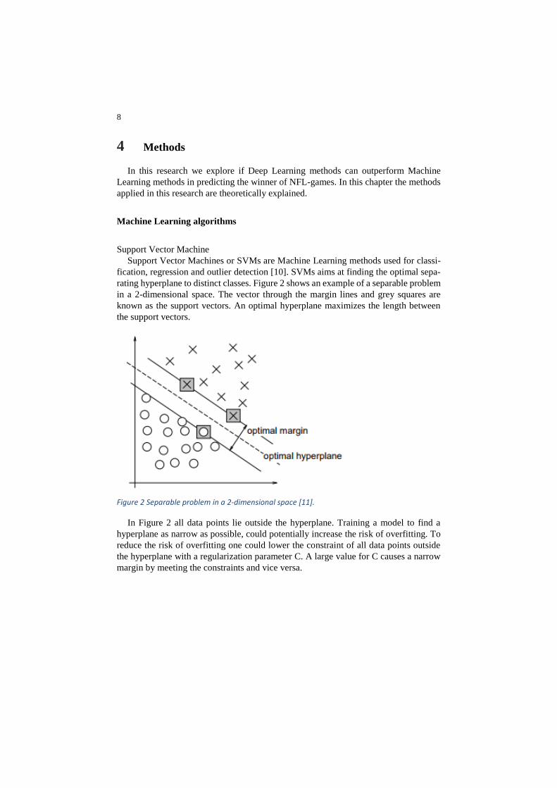
Recurrent Neural Network

Recurrent Neural Networks (RNN) are so-called feedback neural networks while the

connections between neurons can form directed cycles. RNNs have been applied with

success in Natural Language Processing and speech recognition.

Figure 4 Schematic recurrent neuron is shown over time [12]

In the figure above a schematic recurrent neuron is shown over time. Each output at

time t-1 serves as input at time t. Since a neuron does not only possesses the knowledge

of features known at time t, but also receives information of the previous time steps,

RNNs might be able to connect previous information to the present tasks. This property

could be useful for predicting NFL-games, since it could learn better which teams tend

to win more often.

RNNs are flexible in their in and outputs. For time-series analysis RNNs are able to

convert a sequential input into a sequential output. In this research, a many-to-one strat-

egy is used since the objective of this research is to predict a binary classifier of a game-

winner. The input of the implemented RNN-model is a sequence of all features and the

output is the binary classification of the game.

12

Vanishing or exploding gradient.

A commonly known issue for deeper neural networks is the Vanishing and exploding

gradient. A vanishing gradient occurs when gradients for the “lower” or earliest layers

get so small that the weights in this layers never change. An exploding gradient occurs

when the gradients explode, causing the weights to change too much. To fix this prob-

lem for RNNs, multiple architectures have been developed such as a Long-Short-Term

Memory unit, or LSTM unit. An LSTM is capable of learning long-term dependencies.

They are able to remember information for long periods of time, which they do better

than standard RNN units [13]. In this research a RNN and LSTM structure has been

implemented.

Input format

Recurrent neural networks require a certain input format. The input should represent

three components:

1. Batch size

2. Time steps

3. Features

Considering a training dataset of shape (K, N) with K training samples and N fea-

tures. The batch size defines the number of samples of the training data that is going to

be propagated through the network in one time. The number of time steps is determined

by how many batches are propagated so that all training samples are passed through.

Dropout

Recurrent neural networks have a tendency to over fit. Unfortunately, common drop-

out methods to dropout in/outputs fail when applied to recurrent layers. Yarin and

Zoubin [14] introduced an addition to regular dropout by also dropping connections

between the recurrent units. In this research this additional dropout method is applied

to the RNN and LSTM method.

13

5 Data preprocessing

The data gathering and feature engineering resulted in 13 different datasets contain-

ing over 130 features. All datasets contained all 2048 regular season NFL-games played

between 2009 and 2016. The binary outcome “home_win” is approximately evenly bal-

anced (57% 1 and 43% 0). Since the features of the first weeks of the 2009 season did

not have any information of games played before the 2009 season, the first 10 weeks

of the 2009 season of each dataset were deleted, resulting in 1904 games. For purposes

involving the input data for RNNs, only the first 1900 games were selected.

For all 13 datasets two smaller datasets were independently created containing the

10 and 25 most correlating features with the binary outcome of the game, resulting in

39 datasets. Features essential for identifying a game were added too. All 39 data-sets

were pre-processed by the following activities:

• Encode categorical features such as season, week, home/away team into nu-

meric using the “One-Hot” strategy of the python package “Category_encod-

ers”. This method transforms a categorical column into multiple categories,

with a 1 or 0 in each cell if the row contained that column's category

• Scale all numerical data by centering the data by removing the mean value of

each feature and scale it by dividing by its standard deviation.

After pre-testing the 39 data-sets, it was observed that the dataset containing features

of the last 10 games would be the most appropriate to use for testing the hypothesis.

This corresponded with the research of Owen and Galle [8]. Two datasets involving the

features of the last 10 games were used:

• The dataset containing only the 10 best features was used for the models

SVM, NN and RNN to avoid overfitting.

• The dataset containing all features was used for models Random Forest and

Logistic Regression. The pre-testing showed that both models had a better

accuracy when trained on datasets with more features. Especially for Ran-

dom Forest this is theoretically substantiated, while they are very robust of

overfitting because of the bootstrap method.

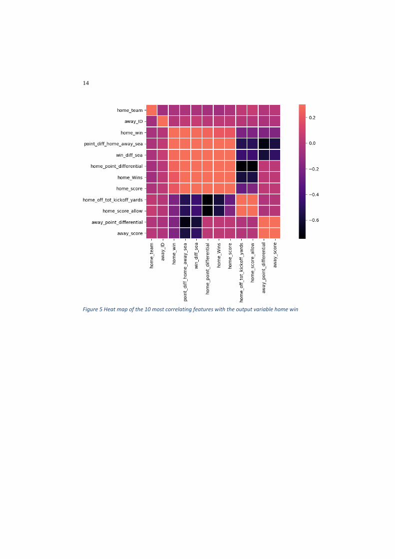
Figure 5 shows a heat map of 10 most correlating features with the output variable

home win of the dataset containing features of the last 10 games. One can observe a

correlation between the features “home_score_allowed”, “away_point_differential”

and “away_score” with “home_win”. One should not confuse the features “home_win”,

the binary outcome of the game and “home_Wins”, the number of wins by the home

team in the last 10 games.

14

Figure 5 Heat map of the 10 most correlating features with the output variable home win

15

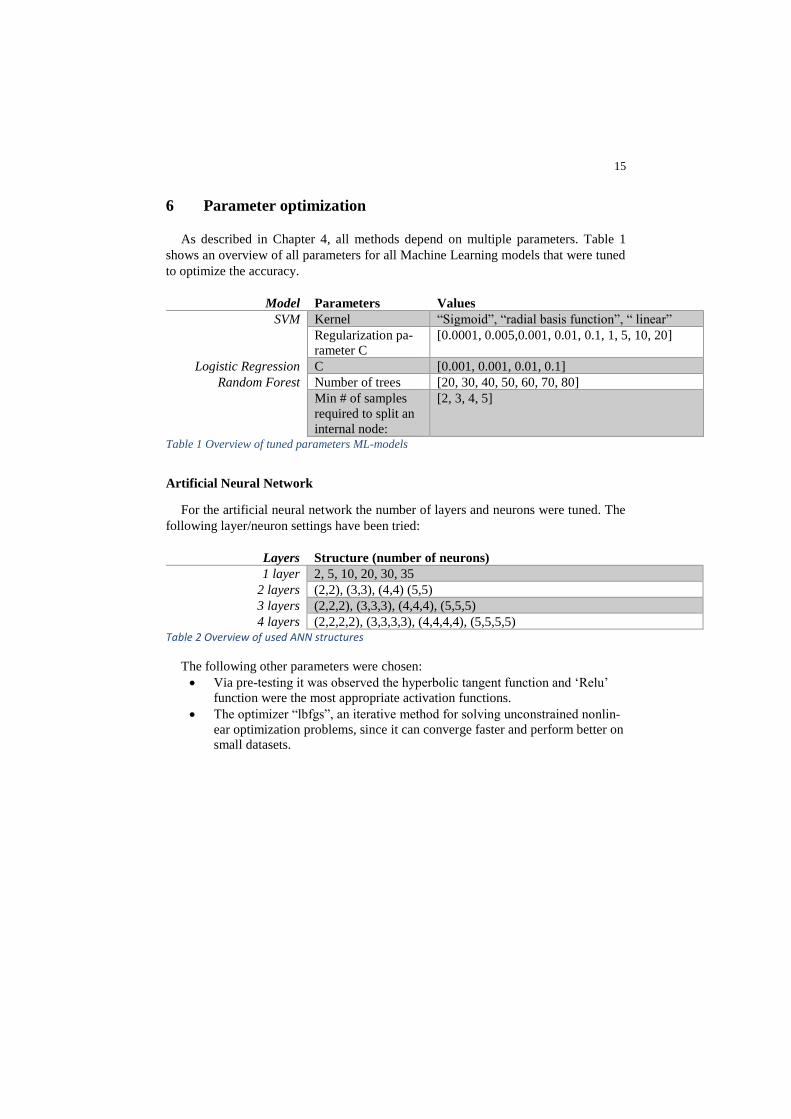
6 Parameter optimization

As described in Chapter 4, all methods depend on multiple parameters. Table 1

shows an overview of all parameters for all Machine Learning models that were tuned

to optimize the accuracy.

Model Parameters Values

SVM Kernel “Sigmoid”, “radial basis function”, “ linear”

Regularization pa-

rameter C

[0.0001, 0.005,0.001, 0.01, 0.1, 1, 5, 10, 20]

Logistic Regression C [0.001, 0.001, 0.01, 0.1]

Random Forest Number of trees [20, 30, 40, 50, 60, 70, 80]

Min # of samples

required to split an

internal node:

[2, 3, 4, 5]

Table 1 Overview of tuned parameters ML-models

Artificial Neural Network

For the artificial neural network the number of layers and neurons were tuned. The

following layer/neuron settings have been tried:

Layers Structure (number of neurons)

1 layer 2, 5, 10, 20, 30, 35

2 layers (2,2), (3,3), (4,4) (5,5)

3 layers (2,2,2), (3,3,3), (4,4,4), (5,5,5)

4 layers (2,2,2,2), (3,3,3,3), (4,4,4,4), (5,5,5,5) Table 2 Overview of used ANN structures

The following other parameters were chosen:

• Via pre-testing it was observed the hyperbolic tangent function and ‘Relu’

function were the most appropriate activation functions.

• The optimizer “lbfgs”, an iterative method for solving unconstrained nonlin-

ear optimization problems, since it can converge faster and perform better on

small datasets.

16

Recurrent neural network

For the recurrent neural network the following parameter settings have been chosen:

• The “binary cross entropy” loss function is used during training

• After each RNN-structure, one fully connected density layer is added.

• Using manual pre-testing a recurrent dropout of 0.4 was observed as most

appropriate.

As discussed, the input format for the RNN should be three dimensional. Also, the

input format should take into account that the train and test set both need to be divisible

by the batch size, otherwise the input vector and output vector of an epoch, i.e., all

batches together, would change in length. Using a K-fold of 10, each train set will con-

tain 1710 samples and the test set 190. To account for this problem, batch sizes of 1710,

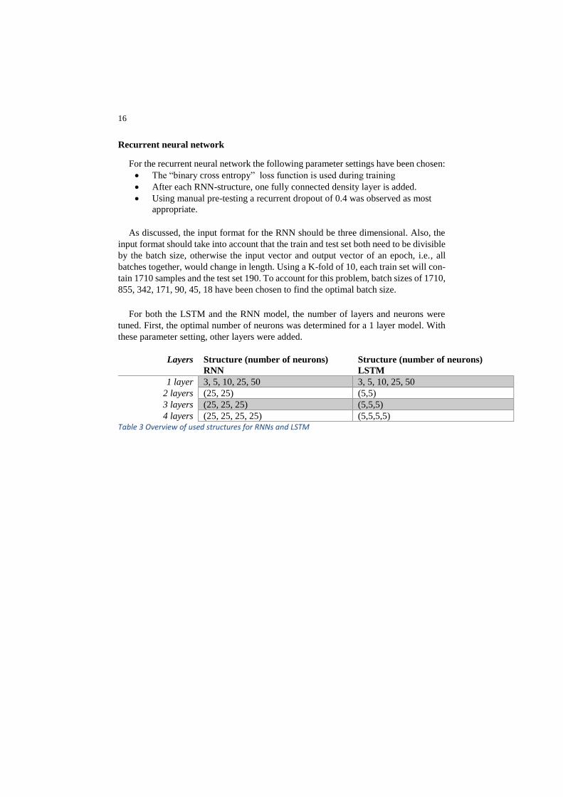
855, 342, 171, 90, 45, 18 have been chosen to find the optimal batch size. For both the LSTM and the RNN model, the number of layers and neurons were

tuned. First, the optimal number of neurons was determined for a 1 layer model. With

these parameter setting, other layers were added.

Layers Structure (number of neurons)

RNN

Structure (number of neurons)

LSTM

1 layer 3, 5, 10, 25, 50 3, 5, 10, 25, 50

2 layers (25, 25) (5,5)

3 layers (25, 25, 25) (5,5,5)

4 layers (25, 25, 25, 25) (5,5,5,5) Table 3 Overview of used structures for RNNs and LSTM

17

7 Evaluation

To evaluate all models 10-fold cross-validation was applied. The performance of the

models is compared based on their accuracy of predicting correct game-winners.

Model Optimal parameter Accuracy (%) 95% confidence interval

SMV Kernel: Linear

C: 0.005

63.25 [0.60, 0.67]

Logistic regression C: 0,001 63.33 [0.58, 0.69]

Random Forest Trees: 80

Min split: 2

62.26 [0.57, 0.68]

ANN Structure: (2,2,2)

Activation: tanh

61.73 [0.56, 0.68]

LSTM Structure: (5,5,5)

Batch size: 1790

Activation: tanh

63.31 [0.61, 0.66]

RNN Structure: (25,25,25)

Batch size: 1790

Activation: tanh

62.05 [0.57, 0.67]

Table 4 Optimal parameters, accuracy and confidence interval for all applied methods

Based on the above results, the following observations can be made:

• The performance of the applied models does not differ much.

• The SVM and the LSTM have the smallest 95% confidence intervals, re-

spectively 7% and 5%.

Other observations on the results:

• The hyperbolic tangent was the best performing activation function for all

neural networks. It probably was not causing a vanishing or exploding

gradient because of the small number of layers.

• The optimal batch size as input for the RNN and LSTM contained all

training data at once.

• All neural network models had an optimal number of three layers

• Compared to the results of Shau [7] and Owen & Galle [8], the accuracy

of the applied models was low. However, Shau was able to build a model

on games played between 1970 and 2011 and had extra data such as the

number of pro-bowlers. Owen & Galle had a different experimental setup

where they trained their model on three seasons and tested on the next

season. In this research, another setup is used. Using 10-fold cross-valida-

tion, 10 train and test datasets where chosen randomly from games be-

tween 2009 and 2016. Because of the randomness of the test set, the accu-

racy of the models could be lower.

18

8 Conclusion and further work

For this experimental set-up, the Deep Learning methods ANN, RNN and LSTM

were not able to have a better accuracy than the Machine Learning model SVM, Ran-

dom Forest and logistic regression. However, the LSTM-model has proven to be a more

robust model for predicting NFL-games, since it has the smallest confidence interval of

the accuracy. One could say that because of this robustness, an LSTM could outperform

Machine Learning models.

Further work to investigate the research question would be to expand the training

data:

• One could utilize more historical data from before 2009.

• In this research no data of players was used. Implementing the

knowledge what team has which players and what qualities do these

players have (such as pro-bowls, MVPs), could affect the performance of

all models.

19

Bibliography

[1] American Gaming Association, "www.americangaming.org," American

Gaming Association, 09 July 2016. [Online]. Available:

https://www.americangaming.org/newsroom/press-releasess/football-bets-

top-90-billion-second-straight-season. [Accessed 13 February 2018].

[2] S. J. MILLER, "A JUSTIFICATION OF THE log 5 RULE FOR

WINNING PERCENTAGES".

[3] K. W. Regan and G. M. Haworth, "Intrinsic Chess Ratings," 2011.

[4] N. Silver, "fivethirtyeight.com," ESPN, September 2014. [Online].

Available: https://fivethirtyeight.com/features/introducing-nfl-elo-ratings/.

[Accessed January 2018].

[5] C. Gaines, "www.businessinsider.com," 14 December 2017. [Online].

Available: http://www.businessinsider.com/nfl-picks-microsoft-cortana-elo-

week-15-2017-12. [Accessed 13 February 2018].

[6] J. Warner, "Predicting Margin of Victory in NFL Games:," 2010.

[7] A. Shau, "Predicting outcomes of NFL games," 2011 .

[8] Z. Owen and V. Galle, "Predicting the NFL," 2014.

[9] D. Petterson and R. Nyquist, "Football Match Prediction using Deep

Learning," 2017.

[10] T. Hastie, R. Tibshirani and J. Friedman, The Elements of Statistical

Learning, Springer, 2008.

[11] C. Cortes and V. Vapnik, "support vector networks," 1995.

[12] S. Shanmuganathan and S. Samarasinghe, Artificial neural network

modelling, Springer.

[13] S. Hochreiter and J. Schmidhuber, "LONG SHORT-TERM MEMORY,"

1997.

[14] Y. Gal and Z. Ghahramani, "A Theoretically Grounded Application of

Dropout in," 2015.

20

Appendix 1: 63 created characteristics

score third_down_conv_perc off_kicking_fgmade

score_q1 fourth_down_conv_perc off_tot_kickoff_yards

score_q2 tot_first_downs_allow off_tot_kickret_yds

score_q3 tot_pass_first_downs_allow off_tot_puntret_yards

score_q4 tot_rush_first_downs_allow off_passing_att

score_q5 num_penalties_allow off_passing_cmp

turnovers yard_penalties_allow off_passing_int

score_allow fd_due_to_penalty_allow off_passing_sacked

score_q1_allow third_down_conv_perc_allow off_passing_tds

score_q2_allow fourth_down_conv_perc_allow off_passing_yds

score_q3_allow avg_age off_pass_cmp_perc

score_q4_allow avg_height TOTAL_off_aggregated

score_q5_allow avg_weight def_defense_int

turnovers_allow avg_coll_sp_fac def_defense_ffum

point_differential time_of_possession def_defense_qbhit

tot_first_downs tot_yards_gained def_defense_safety

tot_pass_first_downs tot_play_count def_defense_sack

tot_rush_first_downs avg_play_drive def_defense_tkl_loss

num_penalties_gained score_last_2_minutes_q2 def_fumbles_forced

yard_penalties_gained score_last_2_minutes_q4 TOTAL_def_aggregated

fd_due_to_penalty_gained off_kicking_fgmissed Wins