1

PRECISE HEIGHT ESTIMATION BY DIFFERENTIAL AMPLITUDE MEASUREMENTFOR AN AIRBORNE CW DOPPLER PROXIMITY SENSOR

A THESIS SUBMITTED TOTHE GRADUATE SCHOOL OF NATURAL AND APPLIED SCIENCES

OFMIDDLE EAST TECHNICAL UNIVERSITY

BY

AYDIN VURAL

IN PARTIAL FULFILLMENT OF THE REQUIREMENTSFOR

THE DEGREE OF PHILOSOPHY OF DOCTORATEIN

ELECTRICAL AND ELECTRONICS ENGINEERING

SEPTEMBER 2012

Approval of the thesis:

PRECISE HEIGHT ESTIMATION BY DIFFERENTIAL AMPLITUDE

MEASUREMENT FOR AN AIRBORNE CW DOPPLER PROXIMITY SENSOR

submitted by AYDIN VURAL in partial fulfillment of the requirements for the degree ofPhilosophy of Doctorate in Electrical and Electronics Engineering Department, MiddleEast Technical University by,

Prof. Dr. Canan OzgenDean, Graduate School of Natural and Applied Sciences

Prof. Dr. Ismet ERKMENHead of Department, Electrical and Electronics Engineering

Prof. Dr. Altunkan HIZALSupervisor, Electrical and Electronics Engineering Dept., METU

Assoc. Prof. Dr. Simsek DEMIRCo-supervisor, Electrical and Electronics Engineering Dept., METU

Examining Committee Members:

Prof. Dr. Sencer KOCElectrical and Electronics Engineering Dept., METU

Prof. Dr. Altunkan HIZALElectrical and Electronics Engineering Dept., METU

Prof. Dr. Erdem YAZGANElectrical and Electronics Engineering Dept., Hacettepe Univ.

Assoc. Prof. Dr. Cagatay CANDANElectrical and Electronics Engineering Dept., METU

Assoc. Prof. Dr. Ali Ozgur YILMAZElectrical and Electronics Engineering Dept., METU

Date:

I hereby declare that all information in this document has been obtained and presentedin accordance with academic rules and ethical conduct. I also declare that, as requiredby these rules and conduct, I have fully cited and referenced all material and results thatare not original to this work.

Name, Last Name: AYDIN VURAL

Signature :

iii

ABSTRACT

PRECISE HEIGHT ESTIMATION BY DIFFERENTIAL AMPLITUDE MEASUREMENTFOR AN AIRBORNE CW DOPPLER PROXIMITY SENSOR

VURAL, Aydın

Ph.D., Department of Electrical and Electronics Engineering

Supervisor : Prof. Dr. Altunkan HIZAL

Co-Supervisor : Assoc. Prof. Dr. Simsek DEMIR

September 2012, 110 pages

Airborne Continuous Wave (CW) Doppler proximity sensors are very sensitive, but leaks pre-

cise height measurement. It may be possible to estimate the height at the terminal phase (the

case where the sensor is close to terrain) precisely by using the Doppler shift and amplitude

information. The thesis includes this novel concept with theoretical analysis and simulation

results.

Keywords: Doppler Shift, Land Clutter, Proximity Fuze, Radio Sensing

iv

OZ

HAVADAN BIRAKILAN SUREKLI DALGA DOPPLER YAKLASMASENSORLERINDE DIFERANSIYEL GENLIK OLCUMU ILE HASSAS YUKSEKLIK

TAHMINI

VURAL, Aydın

Doktora, Elektrik ve Elektronik Muhendisligi Bolumu

Tez Yoneticisi : Prof. Dr. Altunkan HIZAL

Ortak Tez Yoneticisi : Doc. Dr. Simsek DEMIR

Eylul 2012, 110 sayfa

Havadan bırakılan surekli dalga Doppler yaklasma sensorleri oldukca hassastır, ancak has-

sas yukseklik olcumlerinde eksik kalırlar. Doppler kayması ve genlik bilgisini kullanarak

mesafeyi son safhada (sensorun yeryuzune yakın oldugu durumda) hassas olarak tahmin et-

mek mumkun olabilir. Tez bu yeni konsept icin teorik analizleri ve simulasyon sonuclarını

icermektedir.

Anahtar Kelimeler: Doppler Kayması, Yeryuzu Kargasası, Yaklasma Sensoru, Radyo Algılaması

v

To my Wife (Elit AYDIN VURAL), Mother (Guler VURAL) and Sister (Gulden VURAL).

vi

ACKNOWLEDGMENTS

I would like to express my deepest gratitude to my Supervisor Prof.Dr. Altunkan HIZAL and

Co-Supervisor Assoc.Prof.Dr. Simsek DEMIR for their guidance and trust on me. I thank my

wife Elit AYDIN VURAL for her unlimited support during the long study period.

vii

TABLE OF CONTENTS

ABSTRACT . . . . . . . . . . . . . . . . . . . . . . . . . . . . . . . . . . . . . . . . iv

OZ . . . . . . . . . . . . . . . . . . . . . . . . . . . . . . . . . . . . . . . . . . . . . v

ACKNOWLEDGMENTS . . . . . . . . . . . . . . . . . . . . . . . . . . . . . . . . . vii

TABLE OF CONTENTS . . . . . . . . . . . . . . . . . . . . . . . . . . . . . . . . . viii

LIST OF TABLES . . . . . . . . . . . . . . . . . . . . . . . . . . . . . . . . . . . . xi

LIST OF FIGURES . . . . . . . . . . . . . . . . . . . . . . . . . . . . . . . . . . . . xii

CHAPTERS

1 INTRODUCTION . . . . . . . . . . . . . . . . . . . . . . . . . . . . . . . 1

1.1 Radio Sensing for Proximity Fuzes . . . . . . . . . . . . . . . . . . 1

1.2 General Height Estimation Techniques used in Proximity Fuzes . . . 2

2 PROXIMITY SENSING CAPABILITIES OF FUZES . . . . . . . . . . . . . 5

2.1 Proximity Fuzes . . . . . . . . . . . . . . . . . . . . . . . . . . . . 5

2.1.1 Fuzes for Army Munitions . . . . . . . . . . . . . . . . . 6

2.1.2 Fuzes for Airborne Ballistic Munitions . . . . . . . . . . . 9

2.1.3 Proximity Capabilities of Proximity Sensors/Fuzes . . . . 13

3 HEIGHT ESTIMATION USING DIFFERENTIAL AMPLITUDE MEASURE-MENTS . . . . . . . . . . . . . . . . . . . . . . . . . . . . . . . . . . . . . 15

3.1 Theory of the Height Estimation Method . . . . . . . . . . . . . . . 15

3.1.1 Land Clutter and Normalized Cross Section . . . . . . . . 20

3.1.1.1 Radar Cross Section . . . . . . . . . . . . . . 20

3.1.1.2 Normalized RCS . . . . . . . . . . . . . . . 22

3.1.1.3 Fluctuation Statistics for Clutter Modelling . . 25

Autocorrelation Function and Power DensitySpectrum . . . . . . . . . . . . . 25

Fluctuation Statistic . . . . . . . . . . . . . . 26

viii

Common Distributions . . . . . . . . . . . . 26

Decorrelation Time for the Land Clutter . . . 27

3.1.1.4 Mathematical Clutter Model . . . . . . . . . 29

3.1.2 Error Correction Factor . . . . . . . . . . . . . . . . . . . 33

4 SIMULATION FOR FLAT TERRAIN . . . . . . . . . . . . . . . . . . . . . 39

4.1 Simulation (Flat Terrain) . . . . . . . . . . . . . . . . . . . . . . . 39

4.2 Estimation Results for the Flat Terrain . . . . . . . . . . . . . . . . 40

4.3 Noise Analysis . . . . . . . . . . . . . . . . . . . . . . . . . . . . . 43

4.3.1 Effect of VCO Phase Noise . . . . . . . . . . . . . . . . . 44

4.3.2 Thermal Noise . . . . . . . . . . . . . . . . . . . . . . . 50

4.3.3 Noise Reduction . . . . . . . . . . . . . . . . . . . . . . 52

4.3.3.1 Moving Average Filtering for Noise Reduction 53

4.3.3.2 Linear Regression (LR) for Noise Reduction . 54

5 SIMULATION FOR DOUBLE-PLANE TERRAIN . . . . . . . . . . . . . . 58

5.1 Simulation for Double-Plane Terrain . . . . . . . . . . . . . . . . . 58

5.1.1 Calculating Reflection from a Rectangular Patch . . . . . 59

5.1.2 Simulation (Double-Plane Terrain) . . . . . . . . . . . . . 62

5.1.3 Simulation Results (Double-Plane Terrain) . . . . . . . . 64

5.2 Simulation for a Terrain which is Generated by DTED . . . . . . . . 66

5.2.1 Digital Terrain Elevation Data (DTED) Structure . . . . . 66

5.2.2 Simulation (DTED Terrain) . . . . . . . . . . . . . . . . . 69

5.2.2.1 Triangulation of DTED . . . . . . . . . . . . 71

5.2.2.2 Calculation of Parameters . . . . . . . . . . . 73

5.2.2.3 Simulation GUI . . . . . . . . . . . . . . . . 76

5.2.3 Simulation Results (DTED Terrain) . . . . . . . . . . . . 76

5.3 Doppler Shift Spectrum . . . . . . . . . . . . . . . . . . . . . . . . 79

5.4 Return Power from a Side Patch . . . . . . . . . . . . . . . . . . . . 81

6 CONCLUSION . . . . . . . . . . . . . . . . . . . . . . . . . . . . . . . . . 86

6.1 Height Estimation Method . . . . . . . . . . . . . . . . . . . . . . . 86

6.2 Future Studies . . . . . . . . . . . . . . . . . . . . . . . . . . . . . 87

ix

REFERENCES . . . . . . . . . . . . . . . . . . . . . . . . . . . . . . . . . . . . . . 89

APPENDICES

A MATLAB CODES IN THE SIMULATION . . . . . . . . . . . . . . . . . . 92

A.1 Codes for Estimating Height from a Single Planar Surface . . . . . . 92

A.1.1 Calculating Trajectory of the Ballistic Platform . . . . . . 92

A.1.2 Generating Exponential Model of the Land Clutter . . . . 93

A.1.3 Calculating Correction Factor by Initial Conditions . . . . 94

A.1.4 Calculating Reflected Power from the Terrain . . . . . . . 95

A.1.5 Graphical User Interface (GUI) Initialization (Automati-cally Generated by MATLAB™) . . . . . . . . . . . . . . 96

A.1.6 Height Estimation and Displaying Results in GUI . . . . . 98

A.2 Codes for Estimating Height from the Terrain Composed of Two-Planes102

A.2.1 Calculating Reflected Power from Two-Planes . . . . . . . 102

A.3 Codes for Estimating Height from the Terrain Generated Using DTED 104

A.3.1 Calculating Trajectory over DTED Terrain . . . . . . . . . 104

A.3.2 Adjusting DTED Limits . . . . . . . . . . . . . . . . . . 105

A.3.3 Decreasing DTED Resolution (Increase in DTED Spacing) 107

A.3.4 Triangulation and Calculation Reflections from Clutter El-ements . . . . . . . . . . . . . . . . . . . . . . . . . . . . 108

CURRICULUM VITAE . . . . . . . . . . . . . . . . . . . . . . . . . . . . . . . . . 110

x

LIST OF TABLES

TABLES

Table 2.1 Proximity Fuzes . . . . . . . . . . . . . . . . . . . . . . . . . . . . . . . . 13

Table 3.1 Decorrelation Time at 3.6 GHz for Open-Wood Type Terrain . . . . . . . . 28

Table 3.2 Measured Clutter Data for Grazing Angles between 20° to 70° . . . . . . . 29

Table 3.3 Clutter Model Parameters (a,b,c,d) for Various Terrain Types . . . . . . . . 32

Table 4.1 Thermal Noise Levels at Different Ports of the Receiver . . . . . . . . . . . 52

Table 5.1 Matrix Intervals for DTED . . . . . . . . . . . . . . . . . . . . . . . . . . 68

Table 5.2 Release Parameters for DTED Simulation . . . . . . . . . . . . . . . . . . 77

xi

LIST OF FIGURES

FIGURES

Figure 1.1 Conventional Proximity Sensor Triggering . . . . . . . . . . . . . . . . . 3

Figure 2.1 General Purpose Bomb . . . . . . . . . . . . . . . . . . . . . . . . . . . . 6

Figure 2.2 Mortar Projectile . . . . . . . . . . . . . . . . . . . . . . . . . . . . . . . 6

Figure 2.3 Artillery Projectile . . . . . . . . . . . . . . . . . . . . . . . . . . . . . . 6

Figure 2.4 M734A1 Proximity Fuze (Mounted) . . . . . . . . . . . . . . . . . . . . . 8

Figure 2.5 M782 Multi-Option Fuze for Artillery (MOFA) . . . . . . . . . . . . . . . 8

Figure 2.6 Proximity Fuze Configurations for General Purpose Bombs . . . . . . . . 10

Figure 2.7 MK 43 MOD 1 Target Detecting Device . . . . . . . . . . . . . . . . . . 11

Figure 2.8 High Accuracy Radar Proximity Sensor (HARPS) . . . . . . . . . . . . . 12

Figure 2.9 Burst Height of HARPS . . . . . . . . . . . . . . . . . . . . . . . . . . . 12

Figure 2.10 DSU-33 C/B Proximity Sensor . . . . . . . . . . . . . . . . . . . . . . . 13

Figure 3.1 Clutter Element in Spherical Coordinate System . . . . . . . . . . . . . . 16

Figure 3.2 Angle Definitions . . . . . . . . . . . . . . . . . . . . . . . . . . . . . . 17

Figure 3.3 Length of the Differential Area, dρ . . . . . . . . . . . . . . . . . . . . . 18

Figure 3.4 PSD of Doppler Shift (h0 = 100 m and ζ = 60°) . . . . . . . . . . . . . . 21

Figure 3.5 Elliptically Illuminated Area (Beam-width Limited Case) . . . . . . . . . 22

Figure 3.6 Range Resolution Interval for a Pulsed Transmitter . . . . . . . . . . . . . 23

Figure 3.7 Illuminated Area Strip (Pulse-length Limited Case) . . . . . . . . . . . . . 24

Figure 3.8 Standard Deviation of Clutter vs Wind Velocity . . . . . . . . . . . . . . . 28

Figure 3.9 Decorrelation Times vs Wind Velocity at 3.6 GHz for Open-Wood Type

Terrain . . . . . . . . . . . . . . . . . . . . . . . . . . . . . . . . . . . . . . . . 29

xii

Figure 3.10 Multipath Effect at Near Grazing Incidence . . . . . . . . . . . . . . . . . 31

Figure 3.11 Constant Gamma Model . . . . . . . . . . . . . . . . . . . . . . . . . . . 31

Figure 3.12 Mathematical Clutter Model for Various Types of Terrain . . . . . . . . . 32

Figure 3.13 Correction Factor for Various Velocities and Various Release Angles (θB =

φB = 70°) . . . . . . . . . . . . . . . . . . . . . . . . . . . . . . . . . . . . . . . 37

Figure 3.14 Clutter Model for Wooded Hill and Desert Road . . . . . . . . . . . . . . 37

Figure 3.15 Correction Factor for Wooded Hill and Desert Road (θB = φB = 70°) . . . 38

Figure 3.16 Rate of Change in Correction Factor per Degree for Wooded Hill . . . . . 38

Figure 4.1 Graphical User Interface for Simulating the Reflection from Flat Terrain . . 40

Figure 4.2 Return Power (h0 = 300 m, ν0 = 100 m/s, and ζ0 = 80° . . . . . . . . . . . 41

Figure 4.3 Estimation Result (h0 = 100 m, ν0 = 100 m/s, and ζ0 = 80° . . . . . . . . 41

Figure 4.4 Corrected Estimation (h0 = 2000 m, ν0 = 200 m/s, ζ0 = 80°, and C = 0.0269) 42

Figure 4.5 Corrected Estimation (h0 = 300 m, ν0 = 100 m/s, ζ0 = 80°, and C = 0.0179) 42

Figure 4.6 Relative Error for Various Release Angles (h0 = 300 m, ν0 = 100 m/s) . . . 43

Figure 4.7 Relative Error for Various Release Velocities (h0 = 300 m, ζ0 = 90°) . . . 43

Figure 4.8 Single Channel Proximity Sensor Tx/Rx Module . . . . . . . . . . . . . . 44

Figure 4.9 Sources of the Phase Noise . . . . . . . . . . . . . . . . . . . . . . . . . . 45

Figure 4.10 Sample Phase Noise Characteristic (Minicircuits’ ROS-3600-619 VCO) . . 46

Figure 4.11 Distance between the Sensor and the Reflecting Surface Element . . . . . 46

Figure 4.12 Doppler Spectrum Isodops . . . . . . . . . . . . . . . . . . . . . . . . . . 49

Figure 4.13 Signal to Noise Ratio . . . . . . . . . . . . . . . . . . . . . . . . . . . . . 50

Figure 4.14 Sample Receiver Stage with Gains and Noise Figures . . . . . . . . . . . . 51

Figure 4.15 Return Signal with Phase and Thermal Noises . . . . . . . . . . . . . . . 52

Figure 4.16 Height Estimation (h0 = 100 m, ν0 = 100 m/s, and ζ0 = 60°) . . . . . . . . 53

Figure 4.17 Height Estimation, SNR=80 dB (h0 = 100 m, ν0 = 100 m/s, and ζ0 = 60°) 54

Figure 4.18 Height Estimation, SNR=60 dB (h0 = 100 m, ν0 = 100 m/s, and ζ0 = 60°) 54

Figure 4.19 Height Estimation, SNR=80 dB, Linear Regression Duration 30 ms (h0 =

100 m, ν0 = 100 m/s, and ζ0 = 60°) . . . . . . . . . . . . . . . . . . . . . . . . . 56

xiii

Figure 4.20 Height Estimation, SNR=80 dB (h0 = 200 m, ν0 = 100 m/s, and ζ0 = 60°) 57

Figure 5.1 Structure of the Double-Plane Geometry . . . . . . . . . . . . . . . . . . 58

Figure 5.2 Differential Clutter Element . . . . . . . . . . . . . . . . . . . . . . . . . 59

Figure 5.3 Distances on xx, xz and yz Planes . . . . . . . . . . . . . . . . . . . . . . 60

Figure 5.4 Differential Distance, dy . . . . . . . . . . . . . . . . . . . . . . . . . . . 61

Figure 5.5 Integral Limits for Calculating Return Power from Double-Plane Terrain . 63

Figure 5.6 Intersection Regions between Plane-1 and Plane-2, (a) Sensor is in Region-

1, (b) Sensor is in Region-2 . . . . . . . . . . . . . . . . . . . . . . . . . . . . . 63

Figure 5.7 Intersection Regions between Plane-1 and Plane-2, (a) Sensor is in Region-

1 (b) Sensor is in Region-2 . . . . . . . . . . . . . . . . . . . . . . . . . . . . . 64

Figure 5.8 Estimation Error for a Two-Plane Terrain (h0 = 100 m, ν0 = 200 m/s, and

ζ0 = 60°) . . . . . . . . . . . . . . . . . . . . . . . . . . . . . . . . . . . . . . . 65

Figure 5.9 Off-Set Distances from the Impact Points . . . . . . . . . . . . . . . . . . 65

Figure 5.10 Estimation Results for Different Off-Set Distances (h0 = 100 m, ν0 = 200

m/s, and ζ0 = 60°) . . . . . . . . . . . . . . . . . . . . . . . . . . . . . . . . . . 66

Figure 5.11 Sample Digital Terrain Elevation Data . . . . . . . . . . . . . . . . . . . . 67

Figure 5.12 Sample Structure for a 7 Cell DTED Data . . . . . . . . . . . . . . . . . . 69

Figure 5.13 Sample Visibility Map Generated by MATLAB™ . . . . . . . . . . . . . 71

Figure 5.14 Triangulation Structure of the DTED Matrix . . . . . . . . . . . . . . . . 71

Figure 5.15 Triangulation of DTED with Two Invisible Posts . . . . . . . . . . . . . . 72

Figure 5.16 Surface Normals Located at Patch Centroids after Triangulation for a Sam-

ple Terrain . . . . . . . . . . . . . . . . . . . . . . . . . . . . . . . . . . . . . . 72

Figure 5.17 Vectors for Sensor and the Clutter Patch . . . . . . . . . . . . . . . . . . . 73

Figure 5.18 Grazing and Bore-sight Decline Angles for a Clutter Patch . . . . . . . . 75

Figure 5.19 Graphical User Interface of Simulation which is Calculating Parameters for

DTED Generated Terrain . . . . . . . . . . . . . . . . . . . . . . . . . . . . . . 76

Figure 5.20 Relation of Doppler Spectrum with Terrain . . . . . . . . . . . . . . . . . 77

Figure 5.21 Effect of Tilt Angle on to the Received Power . . . . . . . . . . . . . . . . 77

Figure 5.22 Simulation Result for Parameters Given in Table 5.2 . . . . . . . . . . . . 78

xiv

Figure 5.23 Estimation Result for Parameters Given in Table 5.2 . . . . . . . . . . . . 78

Figure 5.24 Same Terrain Profile with Three Different Heights . . . . . . . . . . . . . 79

Figure 5.25 Angles between the Sensor and Terrain . . . . . . . . . . . . . . . . . . . 80

Figure 5.26 Doppler Shift Spectrum for Terrain Profiles given in Figure 5.24 . . . . . . 80

Figure 5.27 Two Patch Geometry . . . . . . . . . . . . . . . . . . . . . . . . . . . . . 81

Figure 5.28 Patch Clutter Model . . . . . . . . . . . . . . . . . . . . . . . . . . . . . 82

Figure 5.29 Ratio d/h vs Grazing Angle (α2) . . . . . . . . . . . . . . . . . . . . . . . 83

Figure 5.30 Ratio d/h vs Patch Tilt Angle for Different Antenna Beamwidths . . . . . . 84

Figure 5.31 Effect of Reflectivity on Ratio (Identical Patches) . . . . . . . . . . . . . . 84

Figure 5.32 Effect of Reflectivity on Ratio . . . . . . . . . . . . . . . . . . . . . . . . 85

xv

CHAPTER 1

INTRODUCTION

1.1 Radio Sensing for Proximity Fuzes

Fuze is a device that ensures safety of the munitions before and during launch that arms

the munitions after launch and that detonates the munitions at a specified condition. There

are many kinds of fuzes, the main functions of which are safety, arming and detonation.

Detonation timing is crucial to obtain the optimum damage to the target. Some fuzes detonate

after the contact with the target, whereas some detonate when approaching to the target and

some detonate at a specific time delay. Remote sensing with well planned timing for burst

height increases the reliability of the fuze.

A very common remote sensing type is the radio sensing and these type of fuzes are called

radio proximity fuzes. The VT fuze, appearing during World War II, is the first proximity

fuze, which was used to obtain a stand-off distance for artillery bombs [1, 2]. The early

development of fuzes is further discussed in [3] and [4]. Acoustic and photoelectric methods

were used in addition to the radio proximity fuzing. Contemporary methods now also include

infra-red technology [5].

Radio proximity techniques are not only used for artillery purposes, but these techniques are

also utilized in level-sensing and collision avoidance-like applications [6, 7]. Application-

specific integrated circuits are also used [8]. To obtain a safe final decision the natural con-

clusion is that fuzes should combine more than one sensing method [9]. Nevertheless, there

is a trade off between complexity and the range resolution. Very fine resolutions could, how-

ever, be obtained by utilizing wide bandwidth signals; Ultra-Wide-Band (UWB) solutions are

being studied [10–13].

1

Infrared technology used in proximity sensing is capable of producing accurate results. How-

ever, infrared waves suffer in atmospheric conditions such as dust and smoke, both of which

are likely to be present on occasions in which proximity sensing is utilized. In such cases

radio waves are the remedy for getting a return signal from a target - generally a land surface,

building wall or vehicle.

Modulated radio waves are commonly chosen because the signal is time stamped when it is

transmitted and when it is received; the range can be calculated by the time difference on the

time stamp. The higher the bandwidth of the transmit signal is, the higher the resolution of the

range decision. Pulsed or frequency modulated waveforms are used in most of the ranging

applications. However, for proximity sensing, pulsed waveforms are not preferable due to

blind ranges during the transmission period. Use of UWB, in this sense, is an endeavour

towards the use of pulsed waveforms. On the other hand, Frequency Modulated Continuous

Wave (FMCW) signals do not suffer from blind ranges due to the low transmit power levels.

Nevertheless, leakage, coupling or return from the antenna input terminal will crowd the low

frequency spectrum, which corresponds to the spectrum of the near-range targets.

Use of unmodulated Continuous Wave (CW) is simple to implement and eliminates modu-

lated signal problems.

1.2 General Height Estimation Techniques used in Proximity Fuzes

In the earliest applications of the proximity sensors used in the fuzes, sensor perceive the

capacitive volume between the ground and the sensor antenna. The capacitance between

sensor and the ground adjust the oscillator frequency of the sensor. The change in the fre-

quency of the sensor’s oscillator initiates the fuze. The later conventional proximity fuzes

use radio waves to sense the proximity. In this technique wave is transmitted from the sen-

sor and reflected back from the terrain. The sensor is functioned after the envelope of the

received voltage of the reflected signal exceeds a specific threshold level which can be called

“Threshold Detection” (Figure 1.1). These types of fuzes are used mainly for mortar/artillery

projectiles and air-to-ground ballistic bombs. The threshold detection technique is used in

many conventional applications for height estimation. However, the threshold highly depends

on the clutter properties.

2

1 1.5 2 2.5 3 3.5 4-0.8

-0.6

-0.4

-0.2

0

0.2

0.4

0.6

0.8

Rec

eive

d Si

gnal

(V)

Time (106 s)

Threshold Level Trigger

Figure 1.1: Conventional Proximity Sensor Triggering

The reflected energy levels are subject to change for different types of targets due to the

different Radar Cross Sections (RCS) which leads a mismatch at the pre-selected height of

detonation. Generally target is the terrain where the troops are positioned. To overcome the

deviation in the distance estimation due to different reflected energy levels some techniques

such as Frequency Modulated Continuous Wave (FMCW) altimeter, pulsed radar, infrared or

Ultra Wide Band (UWB) sensors [14] are used for precise height measurement. Acoustic and

photoelectric methods were used in addition to the radio proximity fuzing.

Both of these height measurement methods have their own disadvantages especially when the

distance is decreased from a few kilometres to a few ten meters and the distance of interest in

a few ten meters. There are many studies and variety of patents to overcome the specific limi-

tations of these methods [15–19]. The limitations of FMCW technique especially at relatively

short distances can be summarized by:

• Receiver saturation due to leakage of the transmitted signal through the receiver,

• Non-linearity of the chirp pulse,

• Truncation of the beat frequency due to the limited modulated bandwidth,

• Suppression due to oscillator noise when the beat frequency is closer to the oscillation

frequency.

3

For the pulsed system, the complication of the design is a challenging issue and the clutter

power reflected from the land is much more higher compared to the return pulse [20]. To

avoid blind range for short distances, very short pulse duration is needed which makes the

pulsed system more complicated and the required peak signal power is very high when the

pulses are shorter.

In this dissertation, a height estimation method using the differential amplitude and the as-

sociated Doppler shift of the returned signal from the terrain was defined. The theory is

applicable for the sensors used to determine the height of the ballistic platforms. Also this

method is applicable for determining the distance between a missile and air-borne target. The

main advantage of the theory is the elimination of the clutter effects.

4

CHAPTER 2

PROXIMITY SENSING CAPABILITIES OF FUZES

2.1 Proximity Fuzes

There are many type of remote sensing used by the fuzes to detect the target at a distance for

optimum blast effect. The remote sensing types are Radio Frequency (RF), Inductive, Electro-

static, Magnetic, Electro-Optical, Millimeter Wave, Capacitive, Seismic, and Acoustic. Our

interest is the sensing types used to detect the distance between the airborne munitions and

the terrain. For this purpose RF sensing and Millimeter Wave sensing is primarily used. The

latter is used much more lately than the RF sensing. RF sensing causes the detonation of

the explosive charge in the vicinity of the target. It is useful to obtain optimum dispersion

of fragments or sub munitions. Since a direct hit is not necessary net effect is that of having

an enlarged target. The example of this type of influence-sensing fuze is the radio proximity

type. Originally, such fuzes were called “VT” (variable time) fuzes, but the term “proximity”

is now preferred.

The optimum distance is calculated according the type of explosive, approach angle to the

target, type of the target and intended effect of the explosive. The fuzes used for army and air

force applications initiate the munitions, in general, at 2-12 meters. However, the optimum

distance is around 4 to 5 meters for airborne general purpose bombs (Figure 2.1) for maximum

blast effect. JMEM (Joint Munitions Effectiveness Manual) is one of the calculation sources

for the optimum burst height for proximity fuzes.

The most common operation principle of the proximity fuzes is the Threshold Detection. As

the bomb approaches the target, the interaction between the emitted and reflected RF energy

5

High Explosive Charge Fuze Fuze

Figure 2.1: General Purpose Bomb

causes a Doppler signal in the reciver stage of the sensor. This return signal from the target is

amplified sufficiently to trigger the firing circuit.

In this section, only the proximity sensors used for measuring the air to ground level of the

ballistic munitions are investigated.

2.1.1 Fuzes for Army Munitions

Mortar and Artillery projectiles (Figure 2.2 and 2.3) needs proximity distance both for op-

timum fragmentation effect as well as to achieve the stand-off distance for shaped charged

munitions. The very first proximity applications used in the mortars and projectiles against

the surface targets during the World War II.

High Explosive Charge Fuze

Figure 2.2: Mortar Projectile

High Explosive Charge Fuze

Figure 2.3: Artillery Projectile

M513 Proximity Fuze

These series of mortar fuzes have a CW Doppler sensor. The transmitted signal is returned

6

with a Doppler shift. When the amplitude of the Doppler shift reaches to a predetermined

level, an electrical signal is generated to initiate the detonation of the explosive charge in

the fuze (Threshold Detection). These fuzes are expected to detonate within 1 to 10 meters.

Due to the different reflectivity characteristics of the terrain the return signal has not the

same energy for every type of terrain. If the terrain has high reflectivity the Doppler signal

reaches to the threshold level earlier and the detonation occurs early than expected. While the

detonation is expected to occur at 1 to 10 meters it may occur at higher distances up to 16

meters. If this is the condition, a metal cap is placed over the fuze to decrease the height of

bust by a factor of four. Sometimes, the low reflectivity of the terrain together with the low

grazing angle causes the Doppler shift does not reach the threshold level before impact on the

terrain. An impact switch is used to initiate the explosive train if the proximity sensor does

not function to avoid having unexploded ammunition.

M514 Proximity Fuze

These series of fuzes have the same principle of operation (Threshold Detection). They have

higher height of burst compared with the standard VT fuzes (M728 and M732). These fuzes

have the same problems to determine the burst height with M513 series fuzes.

M517 and M532 Proximity Fuzes

These series of fuzes have the same principle of operation (Threshold Detection). The height

of burst depends on the angle of fall, the nature of the terrain and the approach velocity. These

fuzes have the same problems with M513 series fuzes to determine the burst height.

M728 Proximity Fuze

These series of fuzes have the same principle of operation (Threshold Detection). The differ-

ence of this fuze from the previous fuzes is the immunity to fall angle. Regardless of the angle

of fall the burst height remains the same. But these fuzes still have the problem to correctly

determine the burst height.

M766 Proximity Fuze

The M766 Proximity Fuze is used primarily against aerial targets. They have a sensitivity

regulation device built-in to the electronic circuitry to adjust the triggering threshold level.

The sensitivity device is set according to the clutter whether it is sea or land.

M734A1 Proximity Fuze

7

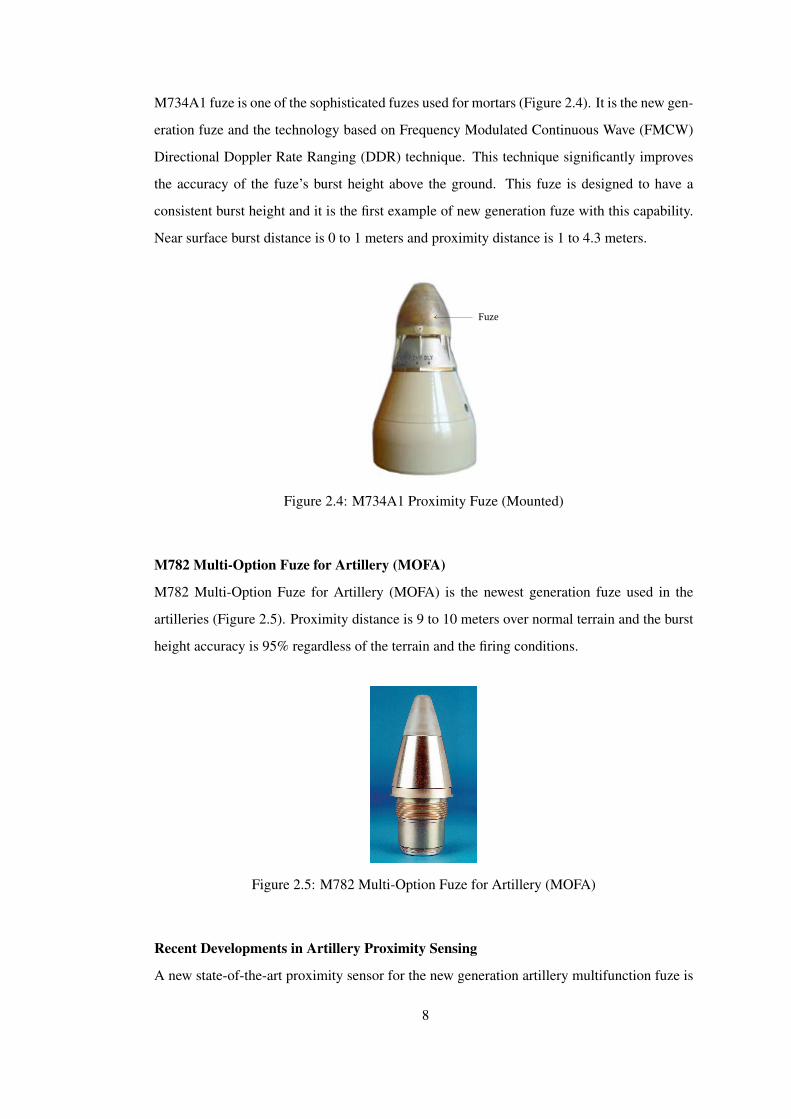
M734A1 fuze is one of the sophisticated fuzes used for mortars (Figure 2.4). It is the new gen-

eration fuze and the technology based on Frequency Modulated Continuous Wave (FMCW)

Directional Doppler Rate Ranging (DDR) technique. This technique significantly improves

the accuracy of the fuze’s burst height above the ground. This fuze is designed to have a

consistent burst height and it is the first example of new generation fuze with this capability.

Near surface burst distance is 0 to 1 meters and proximity distance is 1 to 4.3 meters.

Fuze

Figure 2.4: M734A1 Proximity Fuze (Mounted)

M782 Multi-Option Fuze for Artillery (MOFA)

M782 Multi-Option Fuze for Artillery (MOFA) is the newest generation fuze used in the

artilleries (Figure 2.5). Proximity distance is 9 to 10 meters over normal terrain and the burst

height accuracy is 95% regardless of the terrain and the firing conditions.

Figure 2.5: M782 Multi-Option Fuze for Artillery (MOFA)

Recent Developments in Artillery Proximity Sensing

A new state-of-the-art proximity sensor for the new generation artillery multifunction fuze is

8

FRAPPE. It has an FM-CW Microwave Radar Sensor and it has Full Digital Signal Processing

capability [21]. The accuracy information does not exists. However, FMCW systems have

problems to calculate the short distances.

Extended Range Guided Munitions (ERGM) designated as EX171 achieved 3.3 m burst

height with a 0.65 m (20%) accuracy. However, this system is vulnerable to Approach Angle

which is ∓10 degrees [22].

Millimeter wave systems (UWB fuzes) are also favorable due to

• Antenna Performance. Narrower bandwidths and higher attainable gain for a given

aperture will reduce multipath effects.

• Electronic Countermeasures (ECM). High free space attenuation means low vulnera-

bility to ECM and extremely low side lobe delectability.

• Fog, Cloud, Rain, and Snow Immunity. Low-loss atmospheric propagation characteris-

tics of millimeter waves enhance immunity to obscurants.

• Size and Weight. Components scale with wavelength, thus reducing packaging volume

and weight.

But the main disadvantage of the UWB systems is the immaturity.

2.1.2 Fuzes for Airborne Ballistic Munitions

For the modern jet fighter the variety of the proximity fuzes are limited. External Store Cer-

tification Process is a challenging and costly task. Thus, the aircraft manufacturers certifies

limited number of the fuzes. F-16 Aircraft proximity fuzes will be introduced. There is two

type of proximity fuzes used for air-drop munitions. One is the cluster type fuze and the

other is pre-frag type of fuze. Pre-frag bombs have metal balls inside the explosive and for

maximum effect the bombs must be detonated at an optimum height above the ground.

FMU-56 B/B and D/B Fuzes

These series of fuzes are designed to dispense sub-munitions over a wide area by function-

ing between 100 to 1000 meters. The accuracy is ∓10%. The operation principle of these

dispenser type fuzes is FMCW.

9

FMU-110/B Fuze

Similar to FMU-56 fuze, FMU-110/B fuze is used for dispenser munitions. The burst height

is 80 to 1000 meters. The accuracy is ∓16 meters at 235 meters.

FMU-56 and FMU-110 series fuzes are both utilize FMCW Radar Altimeter to measure the

distance to ground. They are used for the dispenser munitions. Other types of fuzes which

are used for airborne ballistic platforms are the proximity fuzes. They are designed to detect

the distances shorter than 15 meters. For airborne platforms fuze and the proximity sensor is

utilized separately as shown in the Figure 2.6.

Tail Fuze Well General Purpose Bomb

Nose Fuze Well

FMU-139 fuze & DSU-33 sensor FMU-54 fuze & MK-43 TDD

FMU-113 fuze AB-104 fuze

Figure 2.6: Proximity Fuze Configurations for General Purpose Bombs

MK 43 MOD 1 Target Detecting Device(TDD)

MK 43 MOD 1 Target Detecting Device (TDD) is a proximity nose element that gives airburst

capability to general purpose bomb fuzes. It is used with FMU-54 A/B impact tail fuze. The

form factor is same of a general purpose bomb fuze to be mountable to the fuze well (Figure

2.7). The nominal burst height is 5.3 meters.

DSU-33 A/B, B/B Proximity Sensor

DSU-33 is a proximity sensor used together with FMU-139 series fuzes when the FMU-139

is mounted into the tail fuze well of the bomb. DSU-33 is the most common proximity sensor

10

Figure 2.7: MK 43 MOD 1 Target Detecting Device

used for general purpose bombs. The nominal burst height is 6.7 meters with a tolerance of

±2 meters.

FMU-113/B Proximity Fuze

Unlike the MK43 MOD1 TDD and DSU-33 Proximity Sensor this is a complete fuze used

with general purpose bombs with proximity sensing capability. The nominal burst height is 5

meters, however, the burst height varies between 0 to 8.3 meters.

AB-104 Proximity Fuze

AB-104 fuzes are like FMU-113 fuzes and their burst height is between 2 to 12 meters.

MK-43 MOD1 Target Detecting Device and DSU-33 Proximity Sensor together with FMU-

113/B and AB-104 fuzes have the same conventional operation principle “Threshold Detec-

tion”.

Recent Developments in Proximity Sensing for Airborne Ballistic Munitions

High Accuracy Radar Proximity Sensor (HARPS) [23] is as an updated design to compete

with the DSU-33 sensor and based on M734A1 fuze technology (Figure 2.8).

This fuze has a burst height 5±1 meters over target surfaces which reflectivity ranges +5 to

-16 dB as:

• Soil (Wet and Dry)

• Concrete (Wet and Dry)

• Water

11

Figure 2.8: High Accuracy Radar Proximity Sensor (HARPS)

• Dense Foliage

• Desert Scrub

with Approach Velocity from 30 to 500 m/s and with Approach Angles from 15° to 90° from

horizontal. The burst height is given in Figure 2.9.

Hei

ght o

f Bur

st (m

)

Surface Reflectivity (dB)

Figure 2.9: Burst Height of HARPS

DSU-33 A/B and B/B sensors are also upgraded as DSU-33 C/B (Figure 2.10) to improve

HOB accuracy, as well as to reduce labor and production costs. DSU-33 A/B and B/B sensors

have a burst height accuracy of ∓2 meters in theoretical. This accuracy has a reliability less

than 80%. The accuracy of the sensor is ∓5 meters when the reliability is 80%. When having

a reliability of 100%, the range of the burst height is measured as 0 to 16.7 meters [24]. This

statistical data show that the DSU-33 sensors may actuate a firing signal between 0 to 16.7

meters.

12

Figure 2.10: DSU-33 C/B Proximity Sensor

2.1.3 Proximity Capabilities of Proximity Sensors/Fuzes

The lethal range of the fragmented munitions are affected by the proximity distance. The

proximity distances of some sensors and fuzes are given in Table 2.1.

Table 2.1: Proximity Fuzes

FUZE TYPE USED IN BURST HEIGHT COMMENT(HOB)

M513, M513B Mortar 1 - 10 m HOB>17 m observed

M513A1, A2 Mortar + Artillery 1-10 m HOB>17 m observed

M514A3 Artillery >10 m Threshold Detection

M517 Mortar 1-10 m Threshold Detection

M532 Mortar 1-10 m Angle of Fall Immunity

M728 Mortar + Artillery 1-10 m Angle of Fall Immunity

M766 Air Defence - Terrain Selection(Land or Sea)

M734A1 Mortar 0-1 m, 1-4.3 m FCW-DDR

M728 (MOFA) Artillery 9-10 m HOB Accuracy: 95%

FMU-56B/B, D/B Cluster Bombs 80-1000 m FMCW

FMU-110/B Cluster Bombs 100-1000 m FMCW

MK 43 MOD 1 GP Bombs 5.3 m Nominal

DSU-33A/B, B/B GP Bombs 6.7 ±2 m Varies 0-16.7 m

FMU-113/B GP Bombs 5 m Varies 0-8.3 m

AB-104 GP Bombs 2-12 m Threshold Detection

HARPS GP Bombs 5±1 m FMCW-DDR

13

Proximity fuzes and sensors used for mortar, artillery and general purpose bombs need much

more precise height estimation methods. The constraints to design a height estimation method

are:

• Low-cost. When the production quantities are taken into account, the sensor solution

must be a low cost solution.

• Simplicity. The fuzing system must be as simple as possible to achieve high reliability

required for the munition systems. For some application the available physical space

for implementing the fuze sensor is very small, thus a simple solution generally requires

less space compared to complicated systems.

• Accuracy. High accuracy is the basic operational requirement for proximity sens-

ing. The effectiveness of the shape-charged munitions used for target penetration, air-

defence munitions and anti-personnel fragmented bombs are all highly depended on the

precise stand-off distance.

FMCW-DDR and UWB systems reaches to the desired accuracy but the method described

within the dissertation promotes a more simpler and low-cost solution compared to FMCW-

DDR and UWB systems.

14

CHAPTER 3

HEIGHT ESTIMATION USING DIFFERENTIAL

AMPLITUDE MEASUREMENTS

3.1 Theory of the Height Estimation Method

This study focused on the sensors mounted on ballistic platform (like general purpose bombs

and mortar/artillery shells without any propulsion or guidance) to obtain a simple and conve-

nient sensor solution. The target was assumed to be the terrain throughout the thesis. This

method can be applied to missile warheads for determining the distance of the missile to air-

borne targets. The main problem for the current sensors used on the ballistic platforms is the

change of the land reflectivity (land clutter). The energy level of a reflected wave from the

ground is subject to change for different types of terrain due to the different Land Reflectivity.

The various reflection behaviours of the terrain leads a mismatch at the pre-selected height of

burst for munitions. Therefore the time and space variation behaviour of the land reflectivity

plays an important role in the height estimation technique. The initial assumptions were:

• The region of interest for height estimation is the distance where the ballistic platform

(whenever it is an ammunition) is most effective. While the estimation start from a few

kilometres down to a few ten meters, reliability of the estimation is important at the

proximity distance which is a few ten meters.

• While the distance is a few ten meters, due to the axial high velocity of the platform

and the high grazing angle (which is generally between 30°-70° in real conditions for

air drop ballistic munitions), the spatial variation of the clutter can be disregarded in

many cases.

15

• Decorrelation of the reflected signal due to the temporal variation of the clutter (which

have been calculated in Section 3.1.1.3) is assumed to be slower than estimation speed.

The total received power reflected back from the target at the sensor with continues wave

(CW) transmission was calculated by the radar equation (3.1). (P0) is the transmitted signal

power, (G0) is the gain of the system, (λ) is the wavelength, (σ) is the target RCS, (F) is the

pattern-propagation factor and (r) is the distance from sensor to the target.

Pr =P0G2

0λ2σF4

(4π)3r4 (3.1)

The energy level of the reflected power from different regions with different clutter properties

is related to:

• Forth power of the inverse of the distance (r),

• Change in the land reflectivity (σ),

• Forth power of the Pattern-Propagation Factor (F)

the other factors such as transmitted power (P0), gain of the system (G0), and wavelength (λ))

remains the same during the trajectory of the sensor.

h

x

y

z

dρ

ρ

dϕ θ

dA

Sensor

ρa

r

Clutter Element

Figure 3.1: Clutter Element in Spherical Coordinate System

The sensor and the relative position of the sensor over the flat terrain is given in Figure 3.1

and Figure 3.2. The received power (dPr) reflected back from an infinitesimally small area

16

Land Surface

ζ Tilt Angle

Incidence Angle, α

Hei

ght,

h

Depression or Release Angle

Grazing Angle, ψ

θ Sensor

Figure 3.2: Angle Definitions

(dA) equal to:

dPr =P0G2

0λ2F4(θ, φ, ζ)σ0(θ) dA

(4π)3r4 (3.2)

where σ0(θ) is the normalized cross section (details are given in Section 3.1.1). Normalized

cross section times the clutter area accounts for the radar cross section of the terrain. Radar

cross section σ is the reflectivity of the terrain. The transmission line loss, atmospheric at-

tenuation and noise did not included for the calculation of the reflected power (3.1). F is the

pattern-propagation factor [25, p.378] which accounts for the polarization and antenna radi-

ation pattern effects. Pattern-propagation factor is the ratio of actual field strength at a point

to the field strength if the propagation was in free-space. In the calculations only the antenna

field pattern was included for the propagation factor (F). The height of interest is higher than

the linear dimension of the antenna which satisfies the far-field assumption.

F = fA(θ, φ, ζ) = exp

−2 ln(2)(θ − ζ

θB

)2 · exp

−2 ln(2)(φ

φB

)2 (3.3)

If we assume the land reflectivity σ0 and the tilt angle of the sensor ζ remains unchanged

during the estimation period, the derivative of the received power will be related to change of

height. With this fact the radar range equation (3.1) was modified to estimate the height.

Using the definitions in Figure 3.3 infinitesimally small area dA is equal to

17

Land Surface

θ

Hei

ght,

h

dθ

dρ

Sensor

r r sin(dθ)

Figure 3.3: Length of the Differential Area, dρ

dA = r dφ dρ = r dφr dθ

cos(θ)(3.4)

then substituting the distance (r) with the height of the sensor (h) the equation for received

power (3.2) is:

dPr =P0G2

0λ2

(4π)3 h4

cos4(θ)

h2

cos3(θ)f 4A(θ, φ, ζ)σ0(θ) dθ dφ (3.5)

dPr =P0G2

0λ2

(4π)3

cos(θ)h2 f 4

A(θ, φ, ζ)σ0(θ) dθ dφ (3.6)

Integrating (3.6) over the elevation beam-width (θB) and azimuth beam-width (φB) we get the

total received power (Pr) reflected back from the area illuminated by the antenna.

Pr =P0G2

0λ2

(4π)3h2

ζ+θB/2∫θ=ζ−θB/2

φB/2∫φ=−φB/2

f 4A(θ, φ, ζ)σ0(θ) cos(θ) dθ dφ (3.7)

K =P0G2

0λ2

(4π)3 (3.8)

I = I(θ, φ, ζ) =

ζ+θB/2∫θ=ζ−θB/2

cos(θ)σ0(θ)

φB/2∫φ=−φB/2

f 4A(θ, φ, ζ) dθ dφ (3.9)

Pr =K.Ih2 (3.10)

18

Vr =√

2 Z0 Pr Vr =

√2 Z0 K I

h(3.11)

where Z0 is the characteristic impedance. Time derivative of the received voltage that we can

measure in the sensor results (3.12). To elicit the height (h) information measuring of the time

derivative of the height is needed. The time derivative of the height is the vertical velocity (νz)

which is the z-axis component of the velocity vector (ν0) of the sensor.

dVr

dt=

√2 Z0 K

(1h

d√

Idt︸ ︷︷ ︸

zero

+√

Iddt

(1h

) )= −

√2 Z0 K I

h2

dhdt

(3.12)

It was assumed that integral I (3.9) is constant through the final phase of the sensor. The

constant term of (3.12)√

2 Z0 K I cancels by dividing (3.12) to (3.11).

dVr

dt1Vr

= −

√2 Z0 K I

h2

dhdt

h√

2 Z0 K I= −

1h

dhdt

(3.13)

h = −Vr

(dVr

dt

)−1 dhdt

(3.14)

The negative rate of change of the height (dh/dt) of the sensor is the vertical velocity νz.

h =

(dVr

dt

)−1

Vr νz (3.15)

Vertical velocity was measured from the Doppler frequency ( fDoppler). The relation between

the Doppler frequency and the vertical velocity (νz) of the sensor is:

fDoppler =2 ν0 cos(ζ)

λνz = ν0 cos(ζ) = −

dhdt

(3.16)

where ν0 is the axial velocity of the sensor and λ is the wavelength of the signal. With the

information of the time derivative of the received voltage and Doppler frequency shift the

height of the sensor was estimated (3.17).

h = Vr

(dVr

dt

)−1 fDoppler λ

2(3.17)

19

In the integral equation (3.9), σ0 was assumed to be constant due to the assumption that the

temporal change of σ0 (within the estimation period of height) and the change in the tilt angle

ζ can be neglected. If the initial axial velocity of the sensor is high and the initial tilt angle

ζ is small than the rate of change of ζ with respect to time is negligible. It was observed in

simulation results (Chapter 4) that the effect of the variations of the integral with respect to

time is negatively effective upon the height estimation. A correction factor was needed to

account for the temporal variations of the integral. The calculation of the correction factor is

given in Section (3.1.2). The units are as follows:

P0, Pr = dBm,

G0, F = dB,

λ, r = m,

σ0 = m−2,

A = m2

Unless specified, in the calculations gain of the antenna G0 = 7.5 dB, signal frequency f0 =

3.6 MHz, and the beamwidths on elevation and azimuth planes θB = φB = 70°.

Doppler spectrum was measured by determining the spectrum of the reflected voltage. The

spectrum of the Doppler signal will be maximum for the reflections from the terrain closest

to the sensor. A sample power spectrum density (PSD) of the Doppler shift is given in Figure

3.4.

3.1.1 Land Clutter and Normalized Cross Section

The theory rely on the fact that the reflectivity (clutter) of the terrain will remain same during

the estimation calculation at a moment in time. The land clutter is the Radar Cross Section

(RCS) of the land.

3.1.1.1 Radar Cross Section

When an electromagnetic wave impinges upon a target, the energy reflects back or the target

act as an radiating antenna [26]. The reflected energy is scattered isotropically from the radi-

ating element and produce an echo at the receiver of the radar which is equal to the absorbed

20

Rec

eive

d Po

wer

(W)

Sensor

(a) ∆φ,∆θ=10°

Rec

eive

d Po

wer

(W)

Sensor

(b) ∆φ,∆θ=5°R

ecei

ved

Pow

er (W

)

Sensor

(c) ∆φ,∆θ=1°

Figure 3.4: PSD of Doppler Shift (h0 = 100 m and ζ = 60°)

power by the frictional area of target. This area is called Radar Cross Section (RCS) [27].

Radar Cross Section (RCS) denoted as σ is sensitive to orientation and wavelength. The

cross section is equal to the projected area if the target scatters isotropically, i.e. the cross

section of a sphere is equal to the projected area σ = πa2 where a is the radius of sphere

(metal lossless) when a > λ where λ is the wavelength of the signal illuminating the target.

If the radius of the sphere is small with respect to λ then the RCS will vary with λ4. The

forth dependence is known as Rayleigh Law. Resonance phenomenon occurs when the linear

dimensions of the target is of the same order of wavelength. This is a highly sensitive and

oscillating condition. If the target scatters towards the radar then σ will be larger than its pro-

jected area. Each element on the target re-radiates so the separate radiations adds up. While

calculating the reflection from a ground the each clutter element acts as a separate radiator. To

find the total received power from the terrain the differential power returns from each clutter

element are summed up by integrating over the beam-widths of the antenna which illuminates

the ground. For a flat sheet of metal with area A, if the radar beam propagating normal to the

21

sheet σ = 4πA2/λ2. RCS is a function of angle of incidence and it varies rapidly if λ is small

compared to the linear dimensions of object. The average σ for the plate for small angles

γ (excluding main lobe) is σ � 4πλ2/(2πγ)4. Men made targets are generally have larger

echoes compared to the echoes coming from the ground, which is also known as ground

clutter. Ground clutter is also dependent to the wavelength but there is no exact explained

mathematical model for the clutter behaviour.

3.1.1.2 Normalized RCS

Helbert Goldstein (1950) introduced the normalized RCS, σ0, radar cross section per unit area

of surface. Then the radar cross section σ is equal to σ0A where A is the area of the smooth

surface of land or sea. Smooth surface is the mean for land and sea. When dealing with A the

range resolution of the radar must be considered for pulsed radar applications for determining

the illuminated area within one pulse duration. Our study is based on CW transmission thus

no consideration for pulse was necessary. The area A was calculated by taking the integral

of dPr (3.7) over the antenna beam-widths that accounts for the area covered by the antenna

beam illumination. The total illuminated area can be calculated easily by considering the

illuminated area as an ellipse (Figure 3.5). The area of the ellipse is equal to (3.19). The total

radar cross section of the terrain is calculated by multiplying the area A and the normalized

cross section σ0.

Land Surface

θ

Sensor

θB ϕB

Illuminated Area

R

ψ D1

D2

Figure 3.5: Elliptically Illuminated Area (Beam-width Limited Case)

22

D1 = 2R tan(θB

2

)D2 = 2R tan

(φB

2

)csc(ψ) (3.18)

A =π

4D1 D2 = πR2 tan

(θB

2

)tan

(φB

2

)csc(ψ) (3.19)

This case is the beam-width limited case. θB is the half power beam-width in elevation plane

and φB is the half power beam-width in azimuth plane. θB and φB are generally taken as

the two way half power beam-widths as they are approximately 0.71 times the normal beam-

widths [26, p.75]. If the range resolution interval is less than D2 the illuminated area will

be less than the beam-width limited case due to the range resolution interval (Figure 3.6).

This condition is most likely to occur for pulsed Doppler sensors especially when the pulse

duration is relatively short. In this case the radar cross section of the terrain will be σ0A∗

where A∗ is the illuminated area by the pulse (Figure 3.7).

Land Surface

Transmitter

R

ΔR=cτ/2

ΔR.sec(ψ)

ψ

Figure 3.6: Range Resolution Interval for a Pulsed Transmitter

Illuminated area by the pulse (A∗) is calculated by (3.21).

D1 = 2R tan(θB

2

)D∗2 = ∆R sec(ψ) =

cτ2

sec(ψ) (3.20)

A∗ = D1 · D∗2 = 2Rcτ2

tan(θB

2

)sec(ψ) (3.21)

23

Sensor

θB

ΔR ψ

D1

D2*

D2

Illuminated Area=A *=D1 D2*

Figure 3.7: Illuminated Area Strip (Pulse-length Limited Case)

The length of the pulse or the beam-width is the key for determining whether the case is beam

or pulse limited:

• D2 < ∆R sec(ψ) is the condition for beam-width limited case,

• D2 > ∆R sec(ψ) is the condition for pulse-length limited case.

then beam-width limited case is:

2R tan(θB

2

)cτ2

< tan(ψ) (3.22)

and pulse-length limited case is:

2R tan(θB

2

)cτ2

> tan(ψ) (3.23)

These cases for calculating the reflecting area are rough approximations while integrating

differential area (dA) yields finer results. In the simulations while the total reflecting terrain

was divided into small clutter elements therefore from each patch we have calculated the

Doppler frequency and power (Section 5.2).

24

3.1.1.3 Fluctuation Statistics for Clutter Modelling

Autocorrelation Function and Power Density Spectrum The echo from one type of sur-

face will vary if the target (target is the terrain in our study) orientation or sensor transmitter

frequency changed. If the target consist of large numbers of simple targets which are in rel-

ative motion the echo will fluctuate in a noise like manner. The fluctuation spectrum will be

a composition of the spectra of individual scatterers and the spectra of the group or ensemble

of scatterers [26, Chapter 3] [28, Chapter 13].

Rate of this fluctuation can be described by the power density spectrum and by the time auto-

correlation function. Autocorrelation function (otherwise specified autocorrelation function

is the temporal correlation) R(τ) of temporally homogeneous function X(t) is defined as:

R(τ) = limT→∞

12T

∞∫−∞

X(t) X(t + τ) dt (3.24)

The power density spectrum is:

P( f ) = limT→∞

12T

T∫−T

X(t) e− j2π f t dt

2

(3.25)

P( f ) is the Fourier Transform of the correlation function

P( f ) =

∞∫−∞

R(τ) e− j2π f τ dτ (3.26)

R(τ) =

∞∫−∞

P( f ) e j2π f τ d f (3.27)

The total power combined in the spectrum is

R(0)) =

∞∫−∞

P( f ) d f (3.28)

Correlation function and the corresponding power spectra contain the same information in

25

different forms. The Fourier transform of the Gaussian function is also Gaussian and as an

example:

R(τ) = e−α2 τ2

⇒ P( f ) =2√π

αe−π

2 f 2/α2(3.29)

Fluctuation Statistic Land clutter is a random process so the probability statistics is a mean

to model it. The data available for the clutter is matched to the random probability functions

of the some kind. The ratio of occurrence of an event to the number of identical experiments

is called the probability of that event. While p(x) is the probability density function which is

equal or greater than zero. The probability that x is between all values of x is:

∞∫−∞

p(x) dx = 1 (3.30)

The average or mean value of a random variable x is:

x =

∞∫−∞

x p(x) dx (3.31)

The best known distribution is the Gaussian or normal distribution (3.32). σ is the standard

deviation and a is the median.

p(x) =1

σ√

2πexp

[−

(x − a)2

2σ2

](3.32)

Common Distributions The most common probability density distributions to express the

land clutter properties are Rayleigh, Ricean (Rayleigh plus a constant) and log-normal dis-

tributions. If there are many positionally independent scatterers and the average intensity is

constant in time, the probability of echo power P is being between a level P and P + dP

is given by Rayleigh Distribution (3.33). This is valid for the large number of independent

scatterers. P is the average power.

W(P) dP =1

Pe−P/P dP (3.33)

26

P =

∞∫0

P W(P) dP (3.34)

The probability of the received echo power is being less or greater than a value (Pr {P1 < P <

P2}) for the half of the time called the median (Pm). The most probable value is called mode

and for the Rayleigh distribution mode is zero.

Pr {0 < P < Pm} =

Pm∫0

W(P) dP = 0.5 (3.35)

If a random component and a constant component exist in the echo the peak power of the

distribution is shifted so do mode. This distribution is called Ricean (Rice, 1944).

W(P) dP =(1 + m2

)e−m2

e−P(1+m2/P

)J0

(2im

√1 + m2

√P/P

)dP/P (3.36)

The probability density function for the log-normal distribution can be obtained from normal

distribution by the transformation X = ln Y .

W(Y) =1

Yσ0√

2πexp

− 12σ2

(ln

YYm

)2 (3.37)

Decorrelation Time for the Land Clutter Temporal correlation function specifies to what

degree the value of the time function f (t) at one time is correlated with another value τ time

units later [26, p.79]. The autocorrelation function R(τ) is

R(τ) = limT→∞

12T

T∫−T

f (t) f (t − τ) dt (3.38)

There are three types of correlation functions. One is the temporal, the other is the frequency

(which replaces τ with frequency parameter f ), and the last one is spatial (which replaces τ

with spatial parameters). The time required for independence of the samples taken from a

return with clutter is given by [26, p.79]

27

TI =λ

2√

2πσv(3.39)

where σv is the standard deviation in m/s and TI is in seconds. σv is in velocity rather than

frequency for the easy of investigating the different frequencies. σv = 0.42 ∆V is in velocity

units where ∆V is the half power width for a standard Gaussian shaped spectrum. Spectrum

width for land clutter is given in Figure (3.8).

0 5 10 15 20 25 300

0.1

0.2

0.3

0.4

0.5

0.6

0.7

Stan

dard

Dev

iatio

n (m

/s)

Wind Velocity (m/s)

Figure 3.8: Standard Deviation of Clutter vs Wind Velocity

Table 3.1: Decorrelation Time at 3.6 GHz for Open-Wood Type Terrain

Wind Velocity (m/s) 1 4 10 15 20 25 30

Decorrelation Time, TI (sec) 1.6 0.223 0.089 0.059 0.045 0.036 0.029

Values of the decorrelation time for the land clutter was measured (Table 3.1) and they were

found to be similar with the experimental results of N. R. Narayanan, et al [29]. They stated

that at the wind velocities of 7 to 9 m/s decorrelation time was 40-60 milliseconds at X-

band (8-12.4 GHz) at their experiments. We calculated that for a 8 m/s wind velocity, the

decorrelation time was 112 milliseconds at 3.6 GHz transmitting frequency (Figure 3.9). For

X-band the decorrelation time was been calculated as 32.5 milliseconds and 50 milliseconds

respectively for 12.4 GHz and 8 GHz. The estimation period for a specific spot at a time

must be less than the decorrelation time to have better results. For 3.6 GHz decorrelation

time decreased from 1.6 seconds to 29 milliseconds. In practical application all calculation

for estimating the height must be finished before 30 milliseconds to preserve the correlation

28

of the clutter.

Dec

orre

latio

n Ti

me

(s)

Wind Velocity (m/s) 0 5 10 15 20 25 30

0

0.1

0.2

0.3

0.4

0.5

0.6

0.7

0.8

0.9X: 1Y: 0.8923X: 1Y: 0.8923X: 1Y: 0.8923X: 1Y: 0.8923X: 1Y: 0.8923

X: 2Y: 0.4462

X: 3Y: 0.2974

X: 15Y: 0.05949

X: 5Y: 0.1785

X: 10Y: 0.08923 X: 20

Y: 0.04462X: 30Y: 0.02974

Figure 3.9: Decorrelation Times vs Wind Velocity at 3.6 GHz for Open-Wood Type Terrain

3.1.1.4 Mathematical Clutter Model

Clutter (land reflectivity) is a random variable and there is not a direct formulation or math-

ematical model. The value of the clutter usually observed experimentally by various labora-

tories and studies [27], [26, p.314-324], [30], [31]. Some of the measured clutter [26, p.273]

data for different type of terrain is given in Table 3.2.

Table 3.2: Measured Clutter Data for Grazing Angles between 20° to 70°

Terrain Type Average UHF L S X Kuγm γm γmax γm γmax γm γmax γm γmax γm γmax

Desert Road 25 37 30 32 28 28 22 23 10 23 17

Cultivated Land 22 32 18 - - - 10 18 10 19 10

Open Woods 16 22 12 15 8 17 10 15 10 15 8

Wooded Hill 15 16 - - - - - 13 6 15 8

Cities 11 6 -2 11 4 15 5 12 3 - -

All values are in dB m2/m2 and negative.

For land clutter the experimental data is valid for a wide range of frequencies because land

clutter is depended to the frequency of the reflecting signal. While the land clutter data is

expressed by σ0 (radar reflectivity or radar cross section per unit area) sometimes a param-

29

eter γ which is equal to σ0/ sin(ψ) is used. Average RCS is commonly used to describe the

strength of the land clutter echo. Another used parameter is the median cross section, σ0.

Echo strength from terrain fluctuates over a wide range, thus σm is easier to measure which

is the half of the time the strength is exceeded that value. G.R.Valenzuela and M.B.Laing

(1971,1972) studied the many statistical echoes of land and sea and concluded that the echo

distributions lie somewhere between Rayleigh and Log-normal distributions [30].

Dependence of σ0 on incidence angle is divided into three region. First is the Near Grazing

Incidence, second is the Plateau Region and the third is the Near Vertical Incidence.In the

near grazing there is a rapid change in σ0,dB which is the result of the interference formed

by the multipath effect (Figure 3.10). In the measurement of σ0 due to the multipath effect

around near grazing incidence, path propagation factor (F) is included.

F = 1 + ρ e− jβ∆R e− jφ (3.40)

ρ is the reflection coefficient for the multipath effect. While the wave propagates in the free

space reflection coefficient is zero. Each power is proportional to F4 therefore forward scatter-

ing from the terrain significantly effects the cross section of the targets. At higher frequencies

such as X-band averaged results approaches to the σ0 rather than σ0F4. Multipath effects are

less significant for the frequencies above L-band. For multipath effect to be observed surface

must be smooth such as

he · sin(ψc) =λ

4π(3.41)

where he is the equivalent surface roughness.

In the Plateau Region the change in the σ0 is relatively small compared to the changes in

the grazing angle (ψ). The change in σ0 can be approximated by a sin(ψ) dependence. By

assigning a constant γ = σ0/ sin(ψ) the variations due to sin(ψ) can be neglected. In the near

vertical incidence, the measured values of the σ0 depends to the beam-width of the antenna

and it is quite large.

A mathematical model was constructed using the collected data for the grazing angle and the

frequency dependence of the land clutter (Figure 3.2). Grazing angle is the angle between the

30

Land Surface

Depression Angle

Grazing Angle, ψ

Transmitter

1st Path 2nd Path

Figure 3.10: Multipath Effect at Near Grazing Incidence

clutter patch and the direction of wave propagation. Land clutter amplitude versus grazing

angle was simulated by Constant Gamma Model [25], [32] which is defined by parameters,

σmin, γ, σmax.

Ref

lect

ivity

(10

logσ

0)

Grazing Angle, ψ 0o 90o

σmax

σmin 20o 70o

σ0 =γSin(ψ)

Plateau Region

Near Vertical

Incidence

Near Grazing

Incidence

Figure 3.11: Constant Gamma Model

The model defines σmin in the near grazing (0°-20°) incidence, σ0 = γ sin(ψ) in plateau (20°-

70°) region and σmax near vertical (70°-90°) incidence (Figure 3.11).

Using “polyfit” function in the curve fitting toolbox of MATLAB™, the constant gamma

model was formulated with a polynomial P(ψ) (3.42). Where [a, b, c, d] are the result of the

polyfit function. Appendix (A.1.2) is the source code used to generate [a, b, c, d] parameters

by polyfit function.

P(ψ) = a · eb(ψ) + c · ed(ψ) (3.42)

31

The polynomial parameters of the mathematical model were calculated (Table 3.3) for differ-

ent types of terrain according to measured clutter data (Table 3.2). Clutter level with respect to

grazing angle (Figure 3.12) was generated using equation (3.42) and polynomial parameters

(a,b,c,d).

Table 3.3: Clutter Model Parameters (a,b,c,d) for Various Terrain Types

Terrain Type σmax γ σminClutter Parameters

a b c d

A Desert Road -5 -25 -40 0.4642 -0.4400 0.0153 -0.0523

B Cultivated Land -2 -22 -37 0.9261 -0.4400 0.0304 -0.0523

C Open Woods 4 -16 -31 3.6874 -0.4390 0.1178 -0.0509

D Wooded Hill 5 -15 -30 4.6422 -0.4390 0.1483 -0.0509

E Cities 9 -11 -26 11.6608 -0.4388 0.3708 -0.0507

Grazing Angle (degrees) 0 10 20 30 40 50 60 70 80 90

-40

-30

-20

-10

0

10

20

A Desert RoadB Cultivated LandC Open WoodsD Wooded HillE Cities

Ref

lect

ivity

(dB

m2 /m

2 )

Figure 3.12: Mathematical Clutter Model for Various Types of Terrain

The value of the clutter for Constant Gamma Model at near grazing incidence (0°-20°) rapidly

decreases especially towards 0° but our mathematical model is approximated to a linear func-

tion at near grazing incidence. The value of the clutter at near grazing incidences is very small

such that σmin is around -25 to -40 dB. For a flat terrain these small grazing angles occur at

the points far away from the sensor and the distances between these points and the sensor are

relatively long compared with the locations near the sensor with higher grazing angles. The

clutter reduction due to the grazing angle and the distance from the sensor is very high at the

32

locations with small grazing angles. Thus the total effect of these points to the resulting total

received power where located at the near grazing incidences is very small. The generated

mathematical model matches with the Constant Gamma Model at the near vertical incidence

and at the plateau regions better than the match at the near grazing incidence region. But the

effect of the points with a smaller grazing angle at the near grazing incidence region is very

small so the deviation of the mathematical model from the Constant Gamma Model at near

grazing incidences can be neglected.

Unless specified; in the calculations, clutter parameters are taken as σmin = −30 dB, γ = −15

dB, and σmax = +5 dB.

3.1.2 Error Correction Factor

Vr =

√2 Z0 K

√I

h⇒

√I =

Vr · h√

2 Z0 K(3.43)

Taking the time derivative of the received voltage and dividing it with the received voltage

the constant terms cancels and time varying parameters remains. The integral I was assumed

to be constant (3.12) and the time derivative of the integral I was assumed to be zero. Time

derivative of integral I (3.50) is zero unless there is no time varying parameters. While the

integral I is a time varying parameter the time derivative of it will be non-zero and a new

equation was derived for height estimation according to non-zero time derivative of the inte-

gral I. Negative change in the height of the sensor with respect to time is the vertical velocity

(νz) of the sensor.

dVr

dt=

√2 Z0 K

1h

d√

Idt−

√I

h2

dhdt

=

√2 Z0 K

h

d√

Idt

+Vr · νz√

2 Z0 K

(3.44)

Height of the sensor was estimated by (3.45). If the integral I in (3.45) is zero we get the

height estimation equation (3.15) which have been used in the simulation.

h =

√2 Z0 K

d√

Idt

+ Vrνz

dVr

dt

(3.45)

A new parameter called Correction-Factor (C) was defined. C is the time derivative of the

33

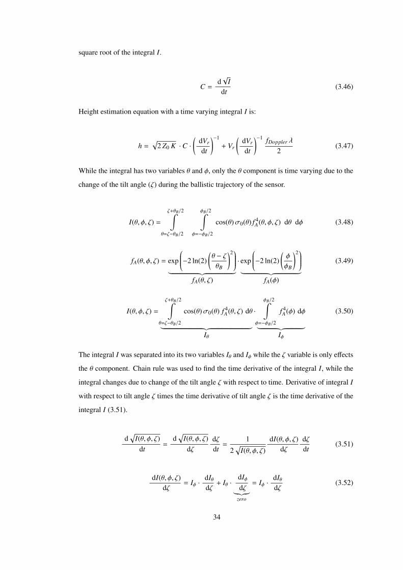
square root of the integral I.

C =d√

Idt

(3.46)

Height estimation equation with a time varying integral I is:

h =√

2 Z0 K ·C ·(

dVr

dt

)−1

+ Vr

(dVr

dt

)−1 fDoppler λ

2(3.47)

While the integral has two variables θ and φ, only the θ component is time varying due to the

change of the tilt angle (ζ) during the ballistic trajectory of the sensor.

I(θ, φ, ζ) =

ζ+θB/2∫θ=ζ−θB/2

φB/2∫φ=−φB/2

cos(θ)σ0(θ) f 4A(θ, φ, ζ) dθ dφ (3.48)

fA(θ, φ, ζ) = exp

−2 ln(2)(θ − ζ

θB

)2︸ ︷︷ ︸fA(θ, ζ)

· exp

−2 ln(2)(φ

φB

)2︸ ︷︷ ︸fA(φ)

(3.49)

I(θ, φ, ζ) =

ζ+θB/2∫θ=ζ−θB/2

cos(θ)σ0(θ) f 4A(θ, ζ) dθ

︸ ︷︷ ︸Iθ

·

φB/2∫φ=−φB/2

f 4A(φ) dφ

︸ ︷︷ ︸Iφ

(3.50)

The integral I was separated into its two variables Iθ and Iφ while the ζ variable is only effects

the θ component. Chain rule was used to find the time derivative of the integral I, while the

integral changes due to change of the tilt angle ζ with respect to time. Derivative of integral I

with respect to tilt angle ζ times the time derivative of tilt angle ζ is the time derivative of the

integral I (3.51).

d√

I(θ, φ, ζ)dt

=d√

I(θ, φ, ζ)dζ

dζdt

=1

2√

I(θ, φ, ζ)

dI(θ, φ, ζ)dζ

dζdt

(3.51)

dI(θ, φ, ζ)dζ

= Iφ ·dIθdζ

+ Iθ ·dIφdζ︸︷︷︸

zero

= Iφ ·dIθdζ

(3.52)

34

There is no variation of Iφ with respect to tilt angle ζ and the derivative of Iφ is zero then the

correction factor C is:

C =d√

Idt

=Iφ

2√

Iθ Iφ

dIθdζ

dζdt

=12

√IφIθ

dIθdζ

dζdt

(3.53)

To find the derivative of Iθ with respect to tilt angle ζ Leibniz’ Rule (3.54) was used because

the tilt angle ζ appears in the limits of the integral Iθ and in the integrand.

ddα

b(α)∫a(α)

f (x, α) dx =db(α)

dαf (b(α), α) −

da(α)dα

f (a(α), α) +

b(α)∫a(α)

∂

∂αf (x, α) dx (3.54)

Applying Leibniz’ Rule to integral Iθ:

dIθdζ

=ddζ

ζ+θB/2∫ζ−θB/2

σ0(θ) f 4A(θ, ζ) cos(θ) dθ

=ddζ

b(ζ)∫

a(ζ)

g(ζ, θ) dθ

= g (ζ, b(ζ))

db(ζ)dζ︸ ︷︷ ︸

A

− g (ζ, a(ζ))da(ζ)

dζ︸ ︷︷ ︸B

+

b(ζ)∫a(ζ)

g(ζ, θ)dζ

dθ

︸ ︷︷ ︸C

(3.55)

we getdIθdζ

= A B C where A,B and C are given in (3.57), (3.58) and (3.59) respectively.

db(ζ)dζ

=d(ζ + θB/2)

dζ= 1

da(ζ)dζ

=d(ζ + θB/2)

dζ= 1 (3.56)

A = g (ζ, b(ζ)) · 1 = σ0(ζ + θB/2) exp[−8 ln 2

(−θB/2θB

)]cos(ζ + θB/2) (3.57)

B = g (ζ, a(ζ)) · 1 = σ0(ζ − θB/2) exp[−8 ln 2

(θB/2θB

)]cos(ζ − θB/2) (3.58)

35

C =

ζ+θB/2∫ζ−θB/2

σ0(θ) cos(θ)ddζ

exp

−8 ln 2(ζ − θ

θB

)2 dθ

=

ζ+θB/2∫ζ−θB/2

σ0(θ) cos(θ)(−16 ln 2)ζ − θθ2

B

exp

−8 ln 2(ζ − θ

θB

)2 dθ (3.59)

Tilt angle ζ changes with the gravitational force (g) and ζ approaches to zero at infinity. The

rate of change in the tilt angle ζ is given in (3.60)

dζdt

=ddt

(arctan

(νx

νz

))=

ddt

(arctan

(ν0x

ν0x + gt

))= −

ν0x · g(ν0z + gt)2 + ν2

0x

(3.60)

To calculate the correction factor, the information of the release angle and velocity must be

known.

In real situations, before the release of the munitions, operation planners prepares an oper-

ation plan which defines the release velocity and angle. Using the planned information, the

correction factor can be loaded on ground prior to the operation. Another possible way to

load the correction factor to the sensor is to get the actual release velocity and angle from the

carrier (such as an aircraft) and the correction factor can be calculated by the sensor processor.

This solution seems to be complicated at first sight but to send actual initial release parameters

from the aircraft to the sensor is feasible. Main timing setups, such as arming time, function-

ing time, or burst height can be programmed by the pilot in many modern fuze systems by

using the wire communication (via an umbilical cable) or magnetic coupling just before the

release of the munitions. The same connection setup may be used to provide the initial release

parameters from aircraft to the sensor. A good estimated normalized cross section σ0 can be

preloaded if the target location and the reflection properties of the terrain are known.

For the reflection parameters σmax = 1, γ = −10 and σmin = −20 dB the correction factors

were calculated for velocities 100 m/s to 500 m/s and for the release angles of 0° to 90°

(Figure 3.13). It was observed that the correction factor approaches to zero when the release

angle approaches to vertical (towards the center of the earth’s gravitational force). If the

sensor release angle is near vertical the gravitational force is nearly aligned with the sensor

axial velocity so there is not any change in the direction of the sensor keeping the angles

36

Cor

rect

ion

Fact

or

Release Angle (degrees) 0 10 20 30 40 50 60 70 80 90 100

0

0.005

0.01

0.015

0.02

0.025

0.03

100 m/s200 m/s300 m/s400 m/s500 m/s

Figure 3.13: Correction Factor for Various Velocities and Various Release Angles (θB = φB =

70°)

unchanged and yielding zero correction factor. The reflection coefficients differs for different

types of terrain. From Table 3.2 the difference between average γ values for desert road and

wooded hill is approximately 10 dB. For the wooded hill type terrain the clutter modelled with

the clutter parameters σmax = 5, γ = −15 and σmin = −30 dB and for the desert road type

terrain the clutter modelled with the clutter parameters σmax = −5, γ = −25 and σmin = −40

dB (Figure 3.14).

Grazing Angle, ψ 0 10 20 30 40 50 60 70 80 90

-50

-40

-30

-20

-10

0

10

Wooded HillDesert Road

Ref

lect

ivity

(dB

m2 /m

2 )

Figure 3.14: Clutter Model for Wooded Hill and Desert Road

The correction factor for wooded hill and desert road for different velocities and release angles

was calculated (Figure 3.15) using the clutter model for desert road and wooded hill.

37

Cor

rect

ion

Fact

or

Release Angle (degrees) 0 10 20 30 40 50 60 70 80 90 100

0

0.005

0.01

0.015

0.02

0.025

0.03

0.035

0.04

100 m/s200 m/s300 m/s400 m/s500 m/s

Wooded Hill

0 10 20 30 40 50 60 70 80 90 1000

0.005

0.01

0.015

0.02

0.025

0.03

0.035

0.04

100 m/s200 m/s300 m/s400 m/s500 m/s

Cor

rect

ion

Fact

or

Release Angle (degrees)

Desert Road

Figure 3.15: Correction Factor for Wooded Hill and Desert Road (θB = φB = 70°)

The rate of change in correction factor per degree is the measure of the sensitivity of the sensor

to the release parameter. For higher beamwidths and higher velocities the sensor is more

sensitive to release angle variations (Figure 3.16). In practical situations, if the correction

factor is calculated for a low release angle at the planning phase and then the actual release

deviates from the planned, the adversely effects of the erroneous correction factor on the

height estimation if higher for large antenna beamwidths when compared with the narrower

antenna beamwidths.

0 10 20 30 40 50 60 70 80 90-2

-1.5

-1

-0.5

0

0.5

1x 10

-3

100 m/s200 m/s300 m/s400 m/s500 m/sR

ate

of C

hang

e pe

r Deg

ree

Release Angle (degrees)

θB=ϕB=70°

(a) Antenna Beamwidths=70°

0 10 20 30 40 50 60 70 80 90-2.5

-2

-1.5

-1

-0.5

0

0.5

1

1.5x 10

-3

100 m/s200 m/s300 m/s400 m/s500 m/sR

ate

of C

hang

e pe

r Deg

ree

Release Angle (degrees)

θB=ϕB=30°

(b) Antenna Beamwidths=30°

Figure 3.16: Rate of Change in Correction Factor per Degree for Wooded Hill

38

CHAPTER 4

SIMULATION FOR FLAT TERRAIN

4.1 Simulation (Flat Terrain)

A numerical simulation for calculating the trajectory and received power at the antenna port

was programmed using MATLAB™GUI to estimate the height using (3.45) (Figure 4.1). Ini-

tially, the release (dive) angle and the trajectory of the sensor was calculated. Initial velocity

of the sensor generally ranges from 125 m/s to 250 m/s for fighter aircraft and the release

angle ranges from 0° to 50°. At each defined sampling point vertical and horizontal velocities

and the tilt angle was calculated. The received power at the antenna port and the Doppler shift

were calculated using predefined system parameters such as: transmitted power, antenna ele-

vation and azimuth beamwidths, gain, and land clutter parameters. Finally, calculated power

was used to estimate the height.

To simulate the environment in a more realistic manner, the land reflectivity was modeled

as described in Section 3.1.1.4. Normalized RCS σ0 (radar cross section per unit area) was

used in the calculations. The radar cross section σ is equal to σ0A where A is the area of the

illuminated terrain. In the new approach this area was calculated indirectly by integrating the

received signal power (dPr) reflected from the infinitesimally small area dA over the antenna

beamwidth, thus resulting in the total reflection from the whole area covered by the antenna

beam. Land clutter with the parameters σmin, γ, σmax were expressed as an exponential para-

metric model (3.42). Using MATLAB curve fitting toolbox the parameters a, b, c, and d, were

determined. With the help of this model of the land clutter, the experimental data collected

by various experiments for land clutter were used in the simulation to take the dependence of

reflectivity to the grazing angle into account.

39

020406080-30

-20

-10

0

10

← Land Clutter

Land Clutter Model

Grazing Angle

Land

Ref

lect

ivity

0 50 100 150 2000

20

40

60

80

100Trajectory

Horizontal Distance (m)

Ver

tical

Dis

tanc

e (m

)

← Height

0 0.2 0.4 0.6 0.8 150

100

150

200

250

Time (s)

Vel

ocity

(m/s

)

Velocity vs Time

← Vz

← Vx

← Velocity

30 30.5 31 31.5 32 32.50.013

0.014

0.015

0.016

0.017

0.018

0.019

← Integral Value

Integral Value

Grazing Angle

Inte

gral

Val

ue

02040608010010

-10

10-8

10-6

10-4

← Power

Received Power vs Height

Heigth (m)

Rec

eive

d P

ower

(W)

0 0.2 0.4 0.6 0.80

20

40

60

80

Height vs Time

Time(s)

Hei

ght (

m)

← Actual Height

← Estimation

← Corrected Estimation

0102030405060708090100-12

-10

-8

-6

-4

-2

0

2Relative Error

Height (m)

Erro

r

EstimatedCorrected

Figure 4.1: Graphical User Interface for Simulating the Reflection from Flat Terrain

In the simulation, release parameters (height, velocity, and angle), land reflectivity parameters

(σmin, γ, σmax), sensor parameters (P0, G0, θB, φB, λ), and sampling time can be set. At

every sampling time the received power with respect to sensor position and tilt angle were

calculated.

The outputs of the simulation are:

• Trajectory and velocity components of the sensor,

• Land clutter mathematical model according to the constant gamma model parameters,

• Received power,

• Estimated height (without correction factor applied), and corrected estimation of the

height (with correction factor applied).

4.2 Estimation Results for the Flat Terrain

As an application example, consider a sensor with an initial velocity of 100 m/s and release

angle of 20°. For this sensor, spatial distribution of the received power is given in Figure 4.2.

It was assumed that transmitted power is 33 dBm, gain of the antenna is 7.5 dB, frequency is

3.6 GHz and elevation and azimuth beamwidths are 70 degrees.

40

Cro

ss-R

ange

(m)

Down-Range (m)

Rec

eive

d Po

wer

(dB

m)

Sensor Position

Direction of Motion

Figure 4.2: Return Power (h0 = 300 m, ν0 = 100 m/s, and ζ0 = 80°

The estimation of the height of this sensor released from 300 m is calculated to be as given in

Figure 4.3. As seen in this figure, there is a considerable initial estimation error.

0 0.5 1 1.5 2 2.5 3 3.5 4 4.5 50

50

100

150

200

250

Sensor HeightEstimation

Hei

ght (

m)

Time (s)

Figure 4.3: Estimation Result (h0 = 100 m, ν0 = 100 m/s, and ζ0 = 80°

The results with corrected estimation for a sensor released at two different altitudes, velocities

and angles are given in Figure 4.4 and Figure 4.5.

Main source of estimation error is the change of the tilt angle during the sensor trajectory.

Corrected estimation yields a maximum relative error less than 12.5% (Figure 4.5). When the

release velocity is smaller the tilt angle change is faster. Similarly, the rate of change in the

tilt angle is faster when the release angle is small. For the cases with higher release angles and

higher release velocities, lower margin of error can be obtained as depicted in Figure 4.6 and

41

0 0.5 1 1.5 2 2.5 3 3.5 4 4.5 50

50

100

150

200

250

E

Actual HeightEstimationCorrected Estimation

Hei

ght (

m)

Time (s)

Figure 4.4: Corrected Estimation (h0 = 2000 m, ν0 = 200 m/s, ζ0 = 80°, and C = 0.0269)

Hei

ght (

m)

Time (s) 0 5 10 15

0

200

400

600

800

1000

1200

1400

1600

1800

Actual HeightEstimationCorrected Estimation

Figure 4.5: Corrected Estimation (h0 = 300 m, ν0 = 100 m/s, ζ0 = 80°, and C = 0.0179)

Figure 4.7. While the release angle increases change in the tilt angle of the sensor during the

trajectory decreases and this results in less absolute error in height estimation (Figure 4.6),

similarly, while the release velocity is higher the change in the tilt angle and in the integral I

is smaller yielding more accurate results (Figure 4.7).

Variation in the received voltage amplitude depends on the change in height, but the change

partially depends on the integral I. The change in I is caused by the changes in land reflectivity

and by the changes in tilt angle ζ.

42

050100150200250300-25

-20

-15

-10

-5

0

5

40 degrees30 degrees20 degrees10 degrees

Rel

ativ

e Er

ror (

%)

Height (m)

Figure 4.6: Relative Error for Various Release Angles (h0 = 300 m, ν0 = 100 m/s)

050100150200250300-35

-30

-25

-20

-15

-10

-5

0

250 m/s200 m/s150 m/s100 m/s

Rel

ativ

e Er

ror (

%)

Height (m)

Figure 4.7: Relative Error for Various Release Velocities (h0 = 300 m, ζ0 = 90°)

4.3 Noise Analysis

Transmit and receive sections of a sample Proximity Sensor system is given in Figure 4.8.

This sample system was analysed for noise considerations.

Flow of charges and holes in the solid state devices and the thermal vibrations in any mi-

crowave component at a temperature above absolute zero is the cause of the noise. Noise

temperature (T ) is the expression of the noise introduced to the system. For the receivers,

noise considerations play an important role because it is one of the dominant limitations lim-

iting the effectiveness of the receiver. System will be subjected to two kinds of noises. One

is the phase noise and the other is the thermal noise. The phase noise (PN) is oriented from

43

PA

STALO

IF 2nd Mixer

1st Mixer

COHO

ωc

ωL ωL

ωc

DSP

Circulator

Antenna

Figure 4.8: Single Channel Proximity Sensor Tx/Rx Module

the voltage controlled oscillator (VCO); the thermal noise (TN) is oriented from VCO, so-

lar/galactic noises (which are called cosmic noises) and atmospheric absorption noises. The

amplitude noise of a VCO is approximately 20 dB lower than the phase noise.

4.3.1 Effect of VCO Phase Noise

The sources of the phase noise of a VCO is caused mainly by;

• Flicker Noise depends on the VCO characteristics at low frequencies. The traps (holes

and electrons) in the emitter-base depletion layer (formed by the contaminations and

crystal defects) holds and release the carriers in a random way and cause low-frequency

noise.

• The Thermal Noise in the oscillator loop may be selectively enhanced by the loop,

resulting phase noise. Also, the thermal noise may directly modulate the oscillation

frequency in the oscillation loop.

The phase noise levels according to the carrier frequency is expressed in dBC/Hz and the

characteristics of the VCOs are measured in 1 Hz bandwidth centred at the off-set frequency

from the carrier. The phase noise sources are given in Figure 4.9.

The phase and the thermal noises of the VCO may be injected to the receiver IF side via;

44

-10

fm

dBc/Hz

Off-set from carrier

f -4 Random Walk FM

f -3 Flicker FM

f -2 White FM

f -1 Flicker Phase

f 0 White Phase Phas

e N

oise

(dB

c/H

z)

1

Figure 4.9: Sources of the Phase Noise

• Local Oscillator (LO) port of the mixer,

• Leaking from circulator,

• Reflecting back from antenna,

• Reflecting back from ground.

The phase noise of the local oscillator (wpnc) in dBc/Hz can be mathematically modeled by a

power equation (4.1). Sample data is taken from Mini-Circuits’ ROS-3600-619 VCO which

is a 2950 to 3600 MHz VCO [33](Figure 4.10).

wpnc,dBc/Hz = 680. f −0.017 − 680 (4.1)

Spectral density S pn(ωn) of the phase noise at the input of the DSP port in Figure(4.8) can be

modelled by (4.2) [34]. χn(ωn) is the correlation factor (4.4). ωn is the rate of deviation from

from the carrier frequency.

S pn(ωn) = wpn(ωn) × χ2n(ωn) (4.2)

wpn(ωn) = 10(wpnc,dBc/Hz)/10 (4.3)

45

100

101

102

103

104

105

106

107

108

-200

-180

-160

-140

-120

-100

-80

-60

-40

-20

0X: 10Y: -26.1

X: 100Y: -51.21

X: 1000Y: -75.34

X: 1e+004Y: -98.55

X: 1e+005Y: -120.9

X: 1e+006Y: -142.3

X: 1e+007Y: -163

Off-set from carrier, f (Hz)

Phas

e N

oise

(dB

c/H

z)

Figure 4.10: Sample Phase Noise Characteristic (Minicircuits’ ROS-3600-619 VCO)

χn(ωn) = 2 sin(ωnTd

2

)= 2 sin

(ωn

22|~r |

c

)(4.4)

The time delay between the transmitted signal Td is related to the position of the reflection

point on the surface. The relative position of the reflecting surface is a function of (θ, φ, ζ) in

Figure (4.11).

h

x

y

z

ϕ

θ

(dA)

Sensor (on y-z plane)

Reflecting Surface

Λ ζ ryz

r

Figure 4.11: Distance between the Sensor and the Reflecting Surface Element

The frequency deviation from the carrier is the Doppler shift and expressed by (4.5)

fDoppler =2 ν0 cos(Λ)

λ(4.5)

46

cos(Λ) =~ryz · ~r| ~ryz| × |~r |

(4.6)

cos(Λ) =

1 +cos(φ)

tan(ζ) tan(θ)√1 + cot2(ζ)

√1 + cot2(θ)

(4.7)

The time delay between the transmitted signal and the received signal (Td) is a function of

distance (r), and r is related to the Doppler shift through the angles (θ, φ, ζ). Therefore r can

be expressed by a function of Doppler shift (g( fDoppler)) resulting in (4.8)

χn(ωn) == 2 sin(ωn

22g( fDoppler)

c

)(4.8)

Phase noise will be entering to the system through the FFT process of the echo signal. If the

relative error due to the Doppler frequency measurement is assumed to be less than 1%, then

the maximum Doppler shift deviation (∆ fDoppler) must be;

∆h = C ·(

dVr

dt

)−1

+ Vr

(dVr

dt

)−1 ∆ fDoppler λ

2(4.9)

∆hh<

∆ fDoppler

fDoppler< 0.01 ⇒ ∆ fDoppler = 20Hz @ ν0 = 100m/s, f0 = 3.6GHz (4.10)

Thus, the phase noise power (Ppn) entering to the system can be found by (4.14), where Pr is

the received power.

∆PCenterpn ( fDoppler,∆ fDoppler) = ∆Pr( fDoppler,∆ fDoppler) ·

3∆ fd/2∫∆ fd/2

wpn(ωn) χ2n(ωn

Td

2) d fn (4.11)

∆PLe f tpn ( fDoppler,∆ fDoppler) = ∆Pr( fDoppler,∆ fDoppler) ·

3∆ fd/2∫∆ fd/2

wpn(ωn) χ2n(ωn

Td1

2) d fn (4.12)

47

∆PRightpn ( fDoppler,∆ fDoppler) = ∆Pr( fDoppler,∆ fDoppler) ·

3∆ fd/2∫∆ fd/2

wpn(ωn) χ2n(ωn

Td2

2) d fn (4.13)

∆PTotalpn = ∆PCenter

pn + ∆PLe f tpn + ∆PRight

pn (4.14)

Spectral Density of the Return Power

Spectral density of the return power (Pr( fDoppler)) can be calculated analytically. Doppler

spectrum for an airborne radar was derived by [26, p.388]. Spectrum at the radar receiver

is dominated by the platform motion. The assumptions for deriving the spectrum were as

follows:

• The antenna beam-width is less than 0.25 radians with a circular symmetry in radiation

pattern. The antenna pattern was also assumed to have a circular symmetry in radiation

pattern (5.25).

• Clutter is assumed to be homogeneous with a mean velocity smaller than the velocity

of the platform so the Doppler spectrum was dominated by the platform motion.

• Target and clutter are many times the unambiguous range and the unambiguous range

is related to the pulse duration.

One or more side-lobe involved in the calculations where the calculations were based on the

main beamwidth. Outside of the first side-lobe the side-lobe clutter spectrum is essentially

flat.

The Doppler spectral density is given in (4.15) where the angle between the antenna axis and

the direction of the platform (squint angle) is Λ (Figure 4.12).

wm( fd) =10−8Pt dt G2

0 λ3 θ1 sin(ψ)σ0(ψ)

h2 ν sin(Λ)(4.15)

wm is the maximum spectral density in watts/hertz at fd where

dt transmit duty cycle,

48

V (on y-z plane) Λ

ψ y

z

x

Sensor

Constant Doppler or Isodops

Figure 4.12: Doppler Spectrum Isodops

G0 peak antenna gain,

θ1 one-way half-power beamwidth,

σ(ψ) normalized backscatter coefficient at angle ψ,,

ν velocity of the platform in Knots.

The shape of the main beam clutter spectrum is:

wm( fd ± ∆ f ) = wm( fd) erfc[0.0387 λ∆ fν θ1 sin(Λ)

]W/Hz (4.16)

where erfc is the complement of the error function.

erfc(x) =2√π

∞∫x

e−t2dt (4.17)

fd is the Doppler frequency of the echoes from the center of the main beam and calculated by

(4.18) where ν is in meter/seconds.

fd =2 ν cos(Λ)

λ(4.18)

49

The relation between the distance (r) and the Doppler shift ( fDoppler) is directly available in

the DTED simulation in Section (5.2). Using the DTED simulation the phase noise of the

system was calculated. The SNR level is given in Figure 4.13. The parameters are; Release

velocity=100 m/s, Release Angle=40°, Transmitted Power=33 dBm, Frequency=3.6 GHz,

and Antenna Beamwidths (azimuth and elevation)=30°.

0 500 1000 1500 2000 250050

60

70

80

90

100

110

Sensor height = 10 mSensor height = 20 mSensor height = 30 mSensor height = 40 m

Doppler Shift (Hz)

SNR

(dB

)

Figure 4.13: Signal to Noise Ratio

The low frequency components are much more correlated resulting higher SNR levels. The

SNR is more than 50 dB for the heights lower than 50 meters.

4.3.2 Thermal Noise

Thermal noise (T N) is oriented from VCO and from solar, galactic (which are called cosmic

noises) and atmospheric absorption noises. It is assumed that the thermal noise due to galactic

and solar noises will be dominant. VCO will contribute to overall system noise by introducing

phase noise to the receiver side from the LO port and due to reflection from ground. Total

antenna temperature (TA) is the sum of the cosmic noise temperature (Tb,ant) and atmospheric

absorption noise temperature (Te). Cosmic noise temperature also called brightness tempera-

ture (Tb) is equal approximately to 100° K. Ta is the ambient temperature, Te is the effective

noise temperature (result of atmospheric absorption noise).

TA = Tb,ant + Te = Tb

(1 −

Te

Ta

)+ Te (4.19)

50

For the case of the ambient temperature is 323° K (50° C) and atmospheric absorption loss

(L) is 1 dB, the effective noise temperature (Te) and the total effective antenna temperature

(TA) is equal to:

Te = Ta(L − 1) = 323(10

110 − 1

)≈ 84° K (4.20)

TA = Tb

(1 −

Te

Ta

)+ Te = 100

(1 −

84323

)+ 84 ≈ 154° K (4.21)

For a network with noise figure Fn, gain G, and bandwidth BW, the relationship between the

input and the output noise temperature can be found by (4.22) and the thermal noise power

T N can be calculated by (4.23). k is the Boltzmann constant and is equal to 1.38 × 10−23.

Tn,out =((F − 1)T0 + Tn,in

)G (4.22)

T N = k Tn G BW (4.23)

The noise figure, gain and bandwidth values for a single channel receiver is given in Figure

4.14.

IF

2nd Mixer Fn : 5 dB CL : 5 dB

1st Mixer Fn : 5 dB CL : 5 dB

DSP

Circulator

Antenna

Filtering and Amplifying Fn : 5 dB G : 70 dB BW : 30 KHz

LNA and Circulator Fn : 3 dB G : 10 dB BW : 100 MHz

Figure 4.14: Sample Receiver Stage with Gains and Noise Figures

The thermal noise levels at different ports are given in Table 4.1.

51

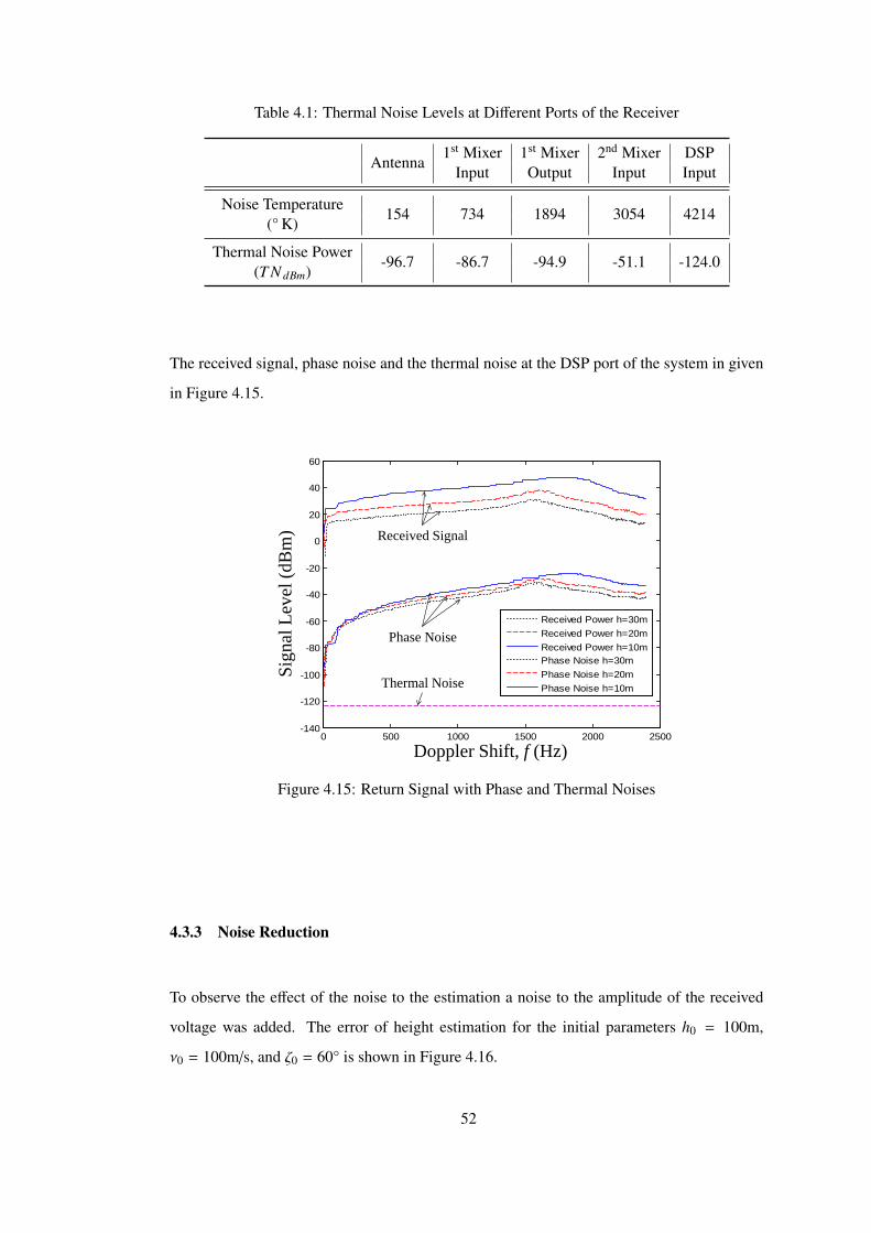
Table 4.1: Thermal Noise Levels at Different Ports of the Receiver

Antenna1st Mixer 1st Mixer 2nd Mixer DSP

Input Output Input Input

Noise Temperature154 734 1894 3054 4214

(° K)

Thermal Noise Power-96.7 -86.7 -94.9 -51.1 -124.0

(T N dBm)

The received signal, phase noise and the thermal noise at the DSP port of the system in given

in Figure 4.15.

0 500 1000 1500 2000 2500-140

-120

-100

-80

-60

-40

-20

0

20

40

60

Received Power h=30mReceived Power h=20mReceived Power h=10mPhase Noise h=30mPhase Noise h=20mPhase Noise h=10m

Doppler Shift, f (Hz)

Sign

al L

evel

(dB

m) Received Signal

Phase Noise

Thermal Noise

Figure 4.15: Return Signal with Phase and Thermal Noises

4.3.3 Noise Reduction

To observe the effect of the noise to the estimation a noise to the amplitude of the received

voltage was added. The error of height estimation for the initial parameters h0 = 100m,

ν0 = 100m/s, and ζ0 = 60° is shown in Figure 4.16.

52

0 0.2 0.4 0.6 0.8 1 1.2 1.4 1.60

10

20

30

40

50

60

70

80

90

Actual HeightEstimationCorrected Estimation

Hei

ght (

m)

Time (s) 020406080100

-35

-30

-25

-20

-15

-10

-5

0

5

EstimationCorrected Estimation

Rel

ativ

e Er

ror (

%)

Height (m)

Figure 4.16: Height Estimation (h0 = 100 m, ν0 = 100 m/s, and ζ0 = 60°)

4.3.3.1 Moving Average Filtering for Noise Reduction

For the ideal case with the specified parameters there is only a relative error of less than 5%

for the corrected estimation. However, the estimation of height is much worse than the ideal

case if there is a noise on the envelope of the received voltage (Figure 4.17.(a)). The estimated

height is maximum 10 meters.

In this case the SNR level was around 80 dB and the inserted noise was Additive White

Gaussian Noise (AWGN). Additive White Gaussian Noise is assumed to have zero mean and

unknown variance σ2 is normally distributed. It is a random process having the uniform spec-

trum density at all frequencies. Two values of white noise in any moments of time (regardless

how close each other) are always independent [35, p.288]. To overcome this problem filtering

the envelope of the received signal can enhance the performance of the estimation. For using

only a moving average window filter (with a duration of 10 ms) the height can be estimated

tolerably up to 50 meters (Figure 4.17.(b)).

For an SNR of 60 dB the maximum estimation limit decreases down to 5 meters (Figure

4.18.(a)). By taking the average of the voltage signal the noise effect decreases and the maxi-

mum estimation height can be increases up to 30 meters (Figure 4.18.(b)).

53

Hei

ght (

m)

Time (msec) 0 200 400 600 800 1000

0

10

20

30

40

50

60

70

80

90

100

110

EstimatedCalculated

Actual Height Estimation

SNR=80dB

(a) Without Filtering

Hei

ght (

m)

Time (msec) 0 200 400 600 800 1000 1200

0

20

40

60

80

100

120

140

160

180

EstimatedCalculated

Actual Height Estimation

SNR=80dB

(b) With Filtering

Figure 4.17: Height Estimation, SNR=80 dB (h0 = 100 m, ν0 = 100 m/s, and ζ0 = 60°)

Hei

ght (

m)

Time (msec) 0 200 400 600 800 1000 1200

0

20

40

60

80

100

120

Actual Height Estimation

SNR=60dB

(a) Without Filtering

0 200 400 600 800 10000

20

40

60

80

100

120

EstimatedCalculated

Hei

ght (

m)

Time (msec)

Actual Height Estimation

SNR=60dB

(b) With Filtering

Figure 4.18: Height Estimation, SNR=60 dB (h0 = 100 m, ν0 = 100 m/s, and ζ0 = 60°)

4.3.3.2 Linear Regression (LR) for Noise Reduction

Estimation of the height for a noiseless ideal environment yielded very close results for the

estimation of height. When a Gaussian white noise is added to the received signal amplitude

the estimation had some high estimation errors especially when the SNR is considerably low.

A linear model for the voltage level using linear regression to avoid resulting peaks in the

estimation due to the additive noise was modelled. The estimated model (4.24) is a linear

second order model whereas the order of the model can be any size.

Y = β0 + β1χ + β11χ2 + ε (4.24)

By using Least Squares Estimation (LSE) the error was tried to minimized by (∑ε2 ) which

54

is the sum of the deviations of the estimation from the true line. For a linear first order model

let Y be the model to be predicted (4.25) and Y is the prediction of Y (4.26).

Y = β0 + β1χ + ε (4.25)

Y = b0 + b1χ. (4.26)

Sum of the errors S is

S =

n∑i=1

ε2i =

n∑i=1

(Yi − β0 − β1χi) (4.27)

to estimate b0 and b1 they were replaced with β0 and β1 and the sum of the squares of the

deviation was set to zero.

∂S∂β0

= −2n∑

i=1

(Yi − b0 − b1χi) = 0 (4.28)

∂S∂β1

= −2n∑

i=1

χi (Yi − b0 − b1χi) = 0. (4.29)

Equations (4.28) and (4.29) are called the normal equations. Deriving b0 and b1 from normal

equations we get

b1 =

∑(χi − χ)

(Yi − Y

)(χi − χ)2 (4.30)

b0 = Y − b1χ (4.31)

χ =∑ χi

nY =

∑ Yi

n(4.32)

Then the final predicted model Y was found by (4.33)

55

Y = Y + b1 (χ − χ) (4.33)

The normally distributed error is assumed to be have zero mean and an unknown variance σ2

and is only for the response data not in predictor data [36]. While the AWGN have zero mean

and normally distributed, linear regression method was applied in the estimation. The noisy

voltage envelope in predicted by linear regression to acquire a smoother envelope. Linear

regression method was applied to the voltage envelope before estimating the height for a

duration of 30 ms and the estimation result is given in Figure 4.19 and in Figure 4.20.(a) and

for a linear regression with a duration of 50 ms the estimation is given in Figure 4.20.(b).

0 200 400 600 800 1000 1200-20

0

20

40

60

80

100

120

140

160

CalculatedEstimated

Hei

ght (

m)

Time (msec)

Actual Height Estimation

SNR=80dB LR Duration=30 msec

Figure 4.19: Height Estimation, SNR=80 dB, Linear Regression Duration 30 ms (h0 = 100m, ν0 = 100 m/s, and ζ0 = 60°)

56

0 500 1000 1500 2000 25000

20

40

60

80

100

120

140

160

180

200

CalculatedEstimated

Hei

ght (

m)

Time (msec)

Actual Height Estimation

SNR=80dB LR Duration=30 msec

(a) Linear Regression Duration=30 ms

0 500 1000 1500 2000 25000

20

40

60

80

100

120

140

160

180

200

CalculatedEstimated

Hei

ght (

m)

Time (msec)

Actual Height Estimation

SNR=80dB LR Duration=50 msec

(b) Linear Regression Duration=50 ms

Figure 4.20: Height Estimation, SNR=80 dB (h0 = 200 m, ν0 = 100 m/s, and ζ0 = 60°)

57

CHAPTER 5

SIMULATION FOR DOUBLE-PLANE TERRAIN

5.1 Simulation for Double-Plane Terrain

In Section (3) the reflection from a planar surface was calculated without any irregularities on

the terrain. This is an ideal situation but in real conditions terrain has a lot of irregularities.

At the final phase of the sensor which is a height less than 30 meters the illuminated area by

the antenna is limited and it may be though as a planar surface depending on the structure of

the terrain. Reflections from a terrain composed of two planes was calculated and the height

is estimated to investigate the behaviour of the sensor over non uniform terrain.

Sensor

Trajectory

h1 h2

d

p1 p2

Plane-1

Intersection

Figure 5.1: Structure of the Double-Plane Geometry

The condition with a two planar surface is the easiest condition to simulate and calculate rele-

vant parameters except one single planar terrain which was calculated in Section (4). Problem

of the two-planes structure was defined and the reflected power together with the Doppler shift

58

was calculated according to Figure 5.1.

5.1.1 Calculating Reflection from a Rectangular Patch

In Section (3) the reflected power from a clutter element was calculated using spherical co-

ordinate system (3.2). The received power from a differential clutter element (Figure 5.2) in

rectangular coordinate system given in (5.1).

z

y

x

dy

dx

h

dθ

dA Clutter Element

r

ζ

θ β

dβ

Figure 5.2: Differential Clutter Element

dPr =P0G0λ

2F4(θ, β, ζ)σ0(α) dA(4π)3r4 (5.1)

Integral of (5.1) was taken at the limits of the antenna beam-widths both at the azimuth and

elevation planes to calculate the total reflection by summing-up the reflections from each

clutter elements which are illuminated by the sensor beam (5.2). Clutter area is dx times dy.

Integral limits were between the beam-widths of both the azimuth and elevation patterns. In

the rectangular coordinate system (ζ − θ) was the angle on the elevation plane and β was the

angle on the azimuth plane. The sensor axis was assumed to be lying on the yz plane which is

the elevation plane for the easy of formulation (Figure 5.3).

59

z

y

x

h rxz

α

r

β ryz θ

rxy

Figure 5.3: Distances on xx, xz and yz Planes

Pr =P0G0λ

2

(4π)3

ζ+θB/2∫θ=ζ−θB/2

φB/2∫β=−φB/2

f 4A(θ, β, ζ)σ0(α) dx dy

r4 (5.2)

where

F = fA(θ, β, ζ) = exp

−2 ln(2)(θ − ζ

θB

)2 · exp

−2 ln(2)(β

φB

)2 (5.3)

Total reflected power was calculated after defining the problem on a spherical coordinate

system due to the fact that the antenna beam illuminated the terrain on a conical basis which is

appropriate to calculate with a spherical coordinate system. In the geometry with two-planes

the intersection of the planes constitute a straight line which is more suitable to rectangular

coordinate system. Reflection from Plane-1 and Plane-2 was calculated separately to find the

total reflection from the whole terrain. Lower and upper integral limits were taken up to or

down to intersection point for each plane. To take the integral in the rectangular coordinate

system the clutter element was defined in rectangular coordinate system. In the rectangular

coordinate system area of the clutter element was found by dx times dy. Differential distances

dx and dy was calculated from Figure 5.4. The slant distances from sensor to the clutter

element dA on the xy, xz and yz planes is rxy, rxz and ryz respectively (Figure 5.3).

60

θ

h dθ

dy

Sensor

ryz ryz sin(dθ)

θ+dθ

Figure 5.4: Differential Distance, dy

dx =rxz sin(dβ)

cos(β + dβ)=

rxzdβcos(β)

(5.4)

dy =ryz sin(dθ)cos(θ + dθ)

=ryzdθcos(θ)

(5.5)

rxz =h

cos(β)ryz =

hcos(θ)

(5.6)

dA = dx dy =rxz

cos(β)ryz

cos(θ)dβ dθ =

h2

cos2(β) cos2(θ)dβ dθ (5.7)

Relation between the height of the sensor and the distance of the sensor to the clutter element

can be defined by:

r2xy = h2 tan2(θ) + h2 tan2(β) (5.8)

r2 = h2 + r2xy = h2 + h2 tan2(θ) + h2 tan2(β) (5.9)

r =h√

1 + tan2(θ) + tan2(β)(5.10)

61

α = tan−1(rxy

h

)= tan−1

√h2 tan2(θ) + h2 tan2(β)

h

= tan−1(√

tan2(θ) + tan2(β))

(5.11)

Using differential clutter area (5.7) and replacing r by h (5.10) in radar range equation (5.2)

we got the equation for the total received power for rectangular coordinate system (5.12). For

the land clutter, the grazing angle α is expressed in terms of the azimuth angle β and elevation

angle θ in equation (5.11).

Pr =P0G2

0λ2

(4π)3h2

ζ+θB/2∫θ=ζ−θB/2

φB/2∫β=−φB/2

f 4A(θ, β, ζ)σ0(α)[

1 + tan2(θ) + tan2(β)]2 cos2(θ) cos2(β)

dθ dβ (5.12)

5.1.2 Simulation (Double-Plane Terrain)

The simulation used for flat-terrain was modified to calculate the received power and Doppler

shift from the double plane terrain. Grazing angle of the second plane α and the off-set

distance (ys − y0) between projection of the sensor’s tip coordinate to the Plane-1 and the

intersection point of two planes can be set as a parameter in the simulation to define the

terrain (Figure 5.5).

Calculation of Received Power

The received power reflected from the double-terrain was calculated using (5.12). The integral

was separated to two pieces to calculate the returns from each plane. For the first region the

integral limit L1 and for the second region the integral limit L2 is shown in Figure 5.5.

While we defined the total received power on a rectangular basis we can easily calculate the

return power from double-plane by splitting the integral into two. If the total received power

formulation was based on circular coordinate system as in flat-terrain it was not possible to

calculate the total return from double-plane structure.

Calculation of Doppler Shift

While we estimate the height of the sensor we use the Doppler shift information as the tempo-

ral variation of the height. Whenever two surfaces is exists there will be two Doppler maxima

from each planes. Neglecting the antenna pattern we can roughly assume that the sensor mea-

sure the Doppler shift from Plane-1 when it is on Region-1 and from Plane-2 when it is on

62

y

z

ζ

α y0 yS

β

L1

L2

Sensor

Plane-2

Plane-1

Figure 5.5: Integral Limits for Calculating Return Power from Double-Plane Terrain

Region-2. The border of the Region-1 and Region-2 is defined as the plane dividing the whole

region into two equal pieces over the planes as shown in Figure 5.6.

ζ

α

(0,y0,h)

y0 yS

β

γ

z

y

Region-1 Region-2 Sensor

Plane-2

Plane-1

(a) β < γ

y

z

ζ

α

(0,y0,h)

y0 yS

β

γ

Region-1 Region-2

Sensor

Plane-2

Plane-1

(b) β > γ

Figure 5.6: Intersection Regions between Plane-1 and Plane-2, (a) Sensor is in Region-1, (b)Sensor is in Region-2

Figure 5.6.(a) shows when the sensor is in the first region (case-1) and Figure 5.6.(b) shows

when the sensor is in the second region (case-2). For the power spectral density of the Doppler

signal two factors play major role, one is the angle of reflection (grazing angle) and the other

is the distance of the reflecting surface. The peak power of the Doppler spectrum occurs due

to the reflection from the nearest point on the surface when the sensor is looking towards the

surface as shown in Figure 3.4. While we defined two cases for the sensor, one is when the

sensor is on the Region-1 and the other is on the Region-2, the nearest point from the surface

63

to the sensor in case-1 is from the Plane-1 and in case-2 from the Plane-2 (Figure 5.7).

y

z

α

(0,y0,h)

h2 h1

Region-1 Region-2 Sensor

Plane-2

Plane-1

(a) h1 < h2

y

z

α

(0,y0,h)

h2 h1

Region-1 Region-2

Sensor

Plane-2

Plane-1

(b) h1 > h2

Figure 5.7: Intersection Regions between Plane-1 and Plane-2, (a) Sensor is in Region-1 (b)Sensor is in Region-2

In the first case the peak Doppler power results from Plane-1 (h1 < h2) and in the second

case peak power results from Plane-2 (h1 > h2). So in the simulation the Doppler shift from

the first plane is used in case-1 and the Doppler shift from the second plane is used in case-

2. Therefore a vivid change in the vertical velocity occurs when the sensor passes from first

region to the second region.

5.1.3 Simulation Results (Double-Plane Terrain)

This approach is shown to be useful for flat surfaces. This method is still applicable when the

reflections come from two planar surfaces as shown in Figure 5.1.

The estimation and corrected estimation for sensor’s height relative to terrain is calculated

with the same method and the result is given in Fig. 5.8. The peak amplitude of the Doppler

shift occurs from the nearest point from sensor to the plane (terrain). The peak amplitude

of the Doppler shift occurs due to the reflections from Plane-1 if h1 (the nearest distance

from sensor to the Plane-1) is shorter than h2. If h1 is longer than h2 the peak amplitude

occurs due to the Plane-2. Regarding the sensor position, h1 is shorter than h2 initially and the

vertical velocity is calculated according to Plane-1 using the Doppler shift information. When

h2 becomes shorter than h1, the peak amplitude return occurs from Plane-2 and the vertical

velocity is calculated according to the Plane-2. This sudden change in the highest Doppler

64

0102030405060708090100-80

-60

-40

-20

0

20

40

Estimated HeightCorrected Estimation

Rel

ativ

e Er

ror (

%)

Height (m)

Figure 5.8: Estimation Error for a Two-Plane Terrain (h0 = 100 m, ν0 = 200 m/s, andζ0 = 60°)

frequency causes a sharp change in estimation (between 50 to 25 meters).

The sudden change in the highest Doppler frequency is expected to occur earlier if the sensor

is moved towards the intersection of Region-1 and Region-2 as shown in Figure 5.9.

Region-1 Region-2

Sensor

+ Offset - Offset

Sensor

Plane-1

Plane-2

Figure 5.9: Off-Set Distances from the Impact Points

Position of the sensor was shifted towards the intersection between Region-1 and Region-2

by an off-set distance. While the sensor passes through Region-1 to Region-2 the peak errors

in the height estimation occurs. For different off-set distances height estimation results are

given in Figure 5.10.

65

Rel

ativ

e Er

ror (

%)

Height (m) 020406080100

20

0

-20

-40

-60

+10 m-10 m-30 m-50 m-70 m

Figure 5.10: Estimation Results for Different Off-Set Distances (h0 = 100 m, ν0 = 200 m/s,and ζ0 = 60°)

5.2 Simulation for a Terrain which is Generated by DTED

The theory is shown to be effective for flat-terrain and double-plane terrain. To analyse the

performance of the sensor over realistic terrain we need to calculate the received power and

Doppler shift spectrum over the realistic terrain. Digital Terrain Elevation Data (DTED) can

be easily used to generate a sample realistic terrain. We need to manipulate DTED to find

the total reflected power and Doppler shift spectrum. DTED is only used to generate digital

terrain data.

5.2.1 Digital Terrain Elevation Data (DTED) Structure

Digital Terrain Elevation Data (DTED) is a standard for terrain elevation values of National

Imagery and Mapping Agency (NIMA) [37]. DTED was used to simulate the terrain in our

study (Figure 5.11). The terrain elevation information is expressed in meters and by the inter-

sections of rows and columns within the elevation data matrix the position of the data point is

calculated. Theoretical range of elevations are between ±32,767 meters and in practice the el-

evation values are between +9,000 meters to -12,000 meters. Horizontal Datum is the World

Geodetic System (WGS 84). and Vertical Datum is the Mean Sea Level (MSL) as determined

by the Earth Gravitational Model (EGM) 1996. While the simulation used the DTED data as

a sample terrain the reliability of the World Geodetic System or the elevation data is not im-

portant. DTED files consist of several files and the data file includes the elevation information

66

of the related position. DTED has three levels of detail in use:

• DTED Level 0 has a resolution of approximately 900 meters,

• DTED Level 1 has a resolution of approximately 90 meters and

• DTED Level 2 has a resolution of approximately 30 meters between adjacent data

points.

Latit

ude

(m)

Longitude (m)

Elev

atio

n (m

)

Figure 5.11: Sample Digital Terrain Elevation Data

A data file of DTED is a 1° by 1° cell defined by latitudes and longitudes of a geographic

reference system regardless of the level. The “.dt0”, “.dt1”, and “.dt2” file extensions in

a DTED file cluster are the elevation data files for DTED Level 0, Level 1 and Level 2,

respectively. DTED specifications vary by the region of interest and are divided into groups

by the latitude of the region (Table 5.1).

We used the DTED data for the region 0° - 50° in northern hemisphere but the distance of 1°

of latitude and longitude assumed to the same. The resolution of a m by n elevation data file

varies by the total number of the data points in one degree of latitude (m) and one degree of

longitude (n) (5.13).

67

Table 5.1: Matrix Intervals for DTED

Data Spacing (seconds)

Zone Latitude Latitude Longitude

I 0° - 50° North-South 30 × 30II 50° - 70° North-South 30 × 60

DTED-0 III 70° - 75° North-South 30 × 90IV 75° - 80° North-South 30 × 120V 80° - 90° North-South 30 × 180

I 0° - 50° North-South 3 × 3II 50° - 70° North-South 3 × 6

DTED-1 III 70° - 75° North-South 3 × 9IV 75° - 80° North-South 3 × 12V 80° - 90° North-South 3 × 18

I 0° - 50° North-South 1 × 1II 50° - 70° North-South 1 × 2

DTED-2 III 70° - 75° North-South 1 × 3IV 75° - 80° North-South 1 × 4V 80° - 90° North-South 1 × 6

Dmxn =

Total elevation points in one degree of latitude︷ ︸︸ ︷

d11 d12 . . . d1n

d21 d22 . . . d2n...

.... . .

...

dm1 dm2 . . . dmn

(5.13)

DTED elevation data cover 1° of latitude and longitude and the resolution is defined by the

total number of cells in 1° of latitude (cell size is the same for latitudinal direction, or vice

versa). The spatial reference is the Northern Latitude Limit and Western Latitude Limit de-

fined in the reference vector (Figure 5.12).

The reference file associated with the DTED data file is an a three by one reference vector

(VRe f erence). The first element is the total number of cells within 1° of latitude or longitude

(cells/degree), the second element is the Northern Latitude Limit and the third element is

the Western Latitude Limit (5.14). To convert latitude and longitude information in units of

metres; distance between two consecutive latitude and longitude lines (1°) was assumed to

be constant (111194.9 metres). Reference vector is used to determine the resolution and the

68

Wes

tern

Lon

gitu

de

Lim

it

Northern Latitude Limit

cells/degree

(m,0) (m,n)

(0,0) (0,n)

DTED Reference Point

cell

Data Points

Figure 5.12: Sample Structure for a 7 Cell DTED Data

geographical position of the DTED. To convert latitude longitude information of DTED to

any element in the matrix requires to use of the whole reference vector information.

VRe f erence =[(cells/degree) Northern Latitude Limit Western Longitude Limit

](5.14)

5.2.2 Simulation (DTED Terrain)

In our study DTED was used to simulate the terrain. While the DTED used in the simulation

just for a terrain model the latitude and longitude limits and the reliability of the elevation

data was not essential. The Northern Latitude Limit was taken as 1200 meters (and was

converted to the units of degrees) initially and The Southern Latitude Limit was taken as 0.

The Western Longitude Limit was taken as zero, and The Eastern Longitude Limit was taken

as 1200 meters (and was converted to the units of degrees). The conversion was conducted

using (5.15) and (5.16).

latitude =(x0 + x)

111, 194.9{x in meters} (5.15)

69

longitude =(y0 + y)

111, 194.9{y in meters} (5.16)

Relevant problem with the use of DTED in the simulation can be summarized by:

• Spatial Resolution:

The worst resolution is approximately 900 meters and with DTED Level 2 resolution

is 30 meters at best. The region of interest in the sensor is less than 50 meters and

while the sensor approach to the terrain the resolution of the terrain is insufficient for

calculations and discrimination.

• Latitude and Longitude Limits:

DTED matrix represent the elevation within a region of 1° by 1° cell defined by latitudes

and longitudes. The number of the cells per degree is the resolution of DTED. To

calculate the return power from such a large area is unnecessary in many cases. To

have a smaller area than 1° by 1° needs matrix manipulation.

For different positions of the sensor different resolution in DTED was used in the simulation

(regarding to the height of the sensor) to lessen the calculation load. The majority of the

calculation load is the determination of the visibility of the elevation points from the sensor

position. For visibility the MATLAB™’s command “viewshed”. viewshed command com-

putes points visible from a point on a digital elevation data grid. The sensor position was

provided to viewshed command as latitude and longitude in units of degrees. So the position

of the sensor which is defined as x,y in units of meters was converted to latitude and longitude

in units of degrees. The visibility map then contains ones at the positions visible from the

sensor location, and zeros where the line of sight is obscured by terrain (Figure 5.13). While

the position of the sensor in viewshed is in units of degrees we converted the position of the

sensor (x,y) in units of meters to (latitude, longitude) in units of degree. Regardless of the

spatial position of the DTED on the World 1 degree of latitude and longitude was assumed to

be 111,194.9 kilometres for conversion purposes.

70

Cro

ss-R

ange

(m)

Down-Range (m)

Sensor Position

Direction of Motion

Figure 5.13: Sample Visibility Map Generated by MATLAB™

5.2.2.1 Triangulation of DTED

Using the visibility map calculated by viewshed triangulation of the elevation data was cal-

culated to set-up the patches of the terrain. Numbering of the vertices of patches is shown in

Figure 5.14.

Wes

tern

Lon

gitu

de L

imit

Northern Latitude Limit p11

p12

p13 p23

p21 p22

patch1

patch2

p0

Patch area dA

Centroid

Figure 5.14: Triangulation Structure of the DTED Matrix

The visible elevation points (posts) from the sensors current position were calculated using

viewshed and while a data point was obscured or shadowed the related patches with that point

undermined. It was possible to undermine the patch whenever at least one point related to that

71

patch was invisible (obscured or shadowed) or at least two points related to that patch were

invisible and the triangulation code (A.3.4) eliminates any patch in the first case. An example

of the triangulation process with two posts are invisible is given in Figure (5.15).

Invisible Digital Terrain Elevation Data Posts

Figure 5.15: Triangulation of DTED with Two Invisible Posts

The triangulation was based on the grid triangulation which is easier to implement. The result

after applying the grid triangulation and normal vector calculation for a sample terrain is given

in Figure 5.16.

Figure 5.16: Surface Normals Located at Patch Centroids after Triangulation for a SampleTerrain

72

5.2.2.2 Calculation of Parameters

In the simulation DTED-1 file which has a resolution approximately 90 meters. The distance

between two consecutive data posts were translated as 1 meter in the simulation as the data

used as a random terrain. Therefore, the highest resolution was 1 meter per each cell. A single

DTED-2 type file has 1201 by 1201 data posts (which actually covers 1 degree of latitude

and longitude) corresponds to 90 meters of separation and the separation was translated as 1

meter resulting a total of 1200 meters by 1200 meters area. Total number of data posts were

1.442.401. The triangulation and the calculation of reflection parameters such as return power

and Doppler frequency were calculated in a short time but to find the visible points from the

sensor position using viewshed command last longer to execute compared to calculation of

parameters.

To calculate the totalpower received from the terrain generated using DTED; area, normal

vector, distance vector from sensor to the patch, the angle between sensor antenna bore-sight

axis and distance vector to calculate the antenna pattern effect and grazing angle for each

triangle clutter element patch (dA) were calculated (Figure 5.17).

xs,ys,zs

n

v

d

p1

p2

p3

rs

pn

rp

Sensor

x y

z

Figure 5.17: Vectors for Sensor and the Clutter Patch

p1(x, y), p2(x, y) and p3(x, y) are the positions of the three corners of the patch on x − y axis

and Z(p1), Z(p2) and Z(p3) are the elevation of the each corner of a patch where position

vector of the nth corner ~pn is

73

~pn = pn(x) · ax + pn(y) · ay + Z(pn) · az (5.17)

Let ~rs be the position vector and v be the direction vector of the sensor and ~rp be the patch

position vector which is the centroid of the triangle

v = vx + vy + vz =νx

|~ν0|· ax +

νy

|~ν0|· ay +

νz

|~ν0|· az (5.18)

where the initial velocity vector of the sensor is ~ν0 = νx · ax + νy · ay + νz · az.

~rp =p1(x) + p2(x) + p3(x)

3·ax+

p1(y) + p2(y) + p3(y)3

·ay+Z(p1) + Z(p2) + Z(p3)

3·az (5.19)

The normal vector n of the triangle patch is

n = ~u × ~v = ( ~p3 − ~p2) × ( ~p1 − ~p2) = det

∣∣∣∣∣∣∣∣∣∣ax ay az

ux uy uz

vx vy vz

∣∣∣∣∣∣∣∣∣∣ (5.20)

The distance vector ~d from the sensor to the triangle patch centroid is

~d = ~rp − ~rs (5.21)

The angle decline from the antenna bore-sight is β and the grazing angle is α. Angle α was

found from the negative of the dot product of the normal vector of the patch n and the distance

vector ~d. The decline angle was calculated by the dot product of the velocity vector v of the

sensor and the unit vector d of distance vector ~d (Figure 5.18).

α = −n · d = −n ·~d

| ~d |β = v · d = v ·

~d

| ~d |(5.22)

Then the area of the triangle patch (dAp) was calculated by the cross product of the adjacent

edges of the patch referencing with the right hand rule.

74

dA

α n

β v Sensor

d

Figure 5.18: Grazing and Bore-sight Decline Angles for a Clutter Patch

dAp =12

√√√√√√∣∣∣∣∣∣∣det

p1(x) p2(x) p3(x)

p1(y) p2(y) p3(y)

1 1 1

∣∣∣∣∣∣∣2

+

∣∣∣∣∣∣∣∣det

p1(y) p2(y) p3(y)

Z(p1) Z(p2) Z(p3)

1 1 1

∣∣∣∣∣∣∣∣2

+

∣∣∣∣∣∣∣∣det

Z(p1) Z(p2) Z(p3)

p1(x) p2(x) p3(x)

1 1 1

∣∣∣∣∣∣∣∣2

(5.23)

The received power reflected back from the clutter patch element at the sensor is calculated

using (3.2).

dPr =P0 G2

0 λ2 F4(β)σ0(α) dAp

(4π)3 | ~d |4(5.24)

Assuming the antenna beam-widths are equal both for the elevation and azimuth (θB = φB)

with a circular symmetry then the equation (3.49) becomes

F(β) = exp

−2 ln(2)(0.5βθB

)2 (5.25)

The terrain was assumed to have a uniform reflectivity (clutter) over the area of interest. By

using DTED patches each patch can be assigned to a different reflection coefficient and by

doing so complex terrain types can be simulated.

75

5.2.2.3 Simulation GUI

A MATLAB™GUI is programmed to calculate the Return Power and Doppler Shift Spectrum

from the terrain which is generated by DTED (Figure 5.19).

Figure 5.19: Graphical User Interface of Simulation which is Calculating Parameters forDTED Generated Terrain

Visible points from the sensor point of view, power return and Doppler shift frequency from

each patch was calculated by the simulation.

5.2.3 Simulation Results (DTED Terrain)

Two main outputs of the simulation are the Power Spectrum and Frequency Spectrum of

the Doppler Shift. The spectral density of the reflected signal at the receiver was directly

calculated by the reflections from each clutter element patch dAp on the DTED terrain. The

calculated power spectrum by the simulation for a flat terrain generated from DTED and

the relation of the spectrum components with respect to the terrain is shown in Figure 5.20.

Return power from each patch is represented by a red dot in the spectrum.

The results for return power for a sensor located 300 m above the terrain is given in Figure

5.21. In Figure 5.21.(a) the sensor is tilted 30° down (ζ = 60°) from the horizon and in Figure

5.21.(b) the sensor is down-looking (ζ = 0°) towards the terrain.

76

Am

plitu

de (d

Bm

)

Doppler Frequency (Hz)

Sensor Velocity Vector

Flat-Terrain

Figure 5.20: Relation of Doppler Spectrum with Terrain

Cro

ss-R

ange

(m)

Down-Range (m) 0 100 200 300 400 500 600 700

300

400

500

600

700

800

900

-140

-135

-130

-125

-120

-115

-110

R

ecei

ved

Pow

er (d

Bm

)

(a) ζ=60°

Cro

ss-R

ange

(m)

Down-Range (m)

0 100 200 300 400 500 600 700300

400

500

600

700

800

900

-140

-135

-130

-125

-120

-115

-110

-105

-100

Rec

eive

d Po

wer

(dB

m)

(b) ζ=0°

Figure 5.21: Effect of Tilt Angle on to the Received Power

The received power and Doppler shift obtained with a 10 ms sampling rate for a flat terrain

was calculated using the DTED simulation. The parameters are given in Table 5.2.

Table 5.2: Release Parameters for DTED Simulation

Release height 30 m Transmitted power 33 dBm Frequency 3.6 GHz

Release velocity 100 m/s Antenna gain 7.5 dB Sampling Rate 10 ms

Release angle 40° Antenna beamwidths 30° Terrain Wooded

Received power for the sample simulation is given in Figure 5.22.(a) and the Doppler shift is

given in Figure 5.22.(b). The ripples observed at the Doppler shift is caused by low DTED

resolution. In the simulation 1×1m DTED was used. For lower heights especially when the

77

sensor gets closer to the ground the low relative resolution of the DTED causes calculation

errors.

0 50 100 150 200 250 300 350 400 45010

-8

10-7

10-6

10-5

10-4

10-3

Rec

eive

d Po

wer

(W)

Time (milliseconds)

(a) Received Power at the Antenna Port

0 50 100 150 200 250 300 350 400 4501400

1600

1800

2000

2200

2400

Dop

pler

Shi

ft (H

z)

Time (milliseconds)

(b) Doppler shift

Figure 5.22: Simulation Result for Parameters Given in Table 5.2

The estimated height is given in Figure 5.23. While the estimation was calculated for a flat

terrain the relative error is expected to be less. However the low resolution of DTED cause

calculation errors. The derivative of the received voltage is sensitive to the errors in the

received voltage thus small variations of the received voltage causes large estimation errors.

0 50 100 150 200 250 300 350 400 4500

5

10

15

20

25

30

35

Trajectory of sensorEstimated height

Hig

ht (m

)

Time (milliseconds)

Figure 5.23: Estimation Result for Parameters Given in Table 5.2

78

5.3 Doppler Shift Spectrum

The reflected power and Doppler shift were calculated for a sensor released from 30 meters

Above Ground Level (AGL) with an initial velocity of 100 m/s and the release angle is 50°.

The beamwidths both in azimuth and elevation were 30°. Three different terrain profiles are

given in Figure 5.24. In case-1 the nearest distance from sensor to the ground is at the 40° and

two surfaces facing towards the sensor at 50° and 60° down the sensor as seen in Figure 5.25.

In case-2 the same terrain is extruded and still the nearest distance from sensor to the ground

is at the 40° and two surfaces facing towards the sensor at 50° and 60° down the sensor. In

case-3 the terrain is extruded more than case-1 and case-2.

250 300 350 400 45010

20

30

40

250 300 350 400 45020

30

40

50

TerrainTrajectory of Sensor

TerrainTrajectory of Sensor

250 300 350 400 450100

110

120

130

140

150

160

TerrainTrajectory of Sensor

Hig

ht (M

SL) (

m)

Distance (m)

Case-1

Case-2

Case-3

Figure 5.24: Same Terrain Profile with Three Different Heights

When the resulting echo signal is analysed the highest power density of the Doppler shift

occurs due to the nearest distance for case-1 and case-2. In case-1, the maximum Doppler

shift in power density occurs at the frequency which is −0.8 times the maximum Doppler

shift. The maximum frequency of the Doppler shift is 2400 Hz according the sensor velocity

(ν0 = 100 m/s and f0 = 3.6 GHz). The shift with the maximum power density corresponds

approximately to a 37° off-set from the sensor direction which is the result of the reflection

79

250 300 350 400 45010

20

30

40

250 300 350 400 45020

30

40

50

TerrainTrajectory of Sensor

TerrainTrajectory of Sensor

Hig

ht (M

SL) (

m)

Distance (m)

50º

40º

~10º

40º

Case-1

Case-2

Figure 5.25: Angles between the Sensor and Terrain

from the nearest point. The nearest point is located approximately 40° off-set from the sensor

direction for case-1 and case-2. In case-2 when the terrain height is increased two more

maxima of the power density occurs at 50° and 57° off-sets from the sensor direction as

expected (Figure 5.26).

600 800 1000 1200 1400 1600 1800 2000 2200 2400-60

-55

-50

-45

-40

-35

X: 1239Y: -45.57

X: 1533Y: -44.17

X: 1927Y: -39.26

Case-1Case-2Case-3

Am

plitu

de (d

Bm

)

Doppler Frequency (Hz)

fd = 2400 Hz cosθ = 0° fd = 1927 Hz cosθ = 37° fd = 1533 Hz cosθ = 50° fd = 1239 Hz cosθ = 59°

Figure 5.26: Doppler Shift Spectrum for Terrain Profiles given in Figure 5.24

In case-3, while the height of the terrain is increased more the faces of the terrain looking

80

to the sensor are also increased at the bore-sight direction. The increase in the area of the

bore-sight patches over the terrain results maximum peak to occur at the bore-sight of the

sensor. The results shows that the information of the terrain roughness is an important factor

effecting the power density of the Doppler shift spectrum. From the Doppler spectrum ob-

tained from various terrains shows that it is not a straightforward task to make a conclusion for

determining the maximum power density of the Doppler shift spectrum directly from terrain

information. Therefore, conditions when the return signal from a side patch is higher than the

return signal from the bore-sight patch was analysed in Section 5.4.

5.4 Return Power from a Side Patch

The geometry of the two patches (one is the bore-sight and the other is the side patch) is given

in Figure 5.27.

θ2 β

Sensor

α2

Bore-sight Patch

Side Patch

Figure 5.27: Two Patch Geometry

In the case of two patches, the power density of the return signal for the side patch is greater

than the power density from the bore-sight patch when the condition (5.26) is satisfied.

dPr1 < dPr2 ⇒P0G2

0λ2F4(θ1, φ1, ζ)σ0(α1) dA1

(4π)3r41

<P0G2

0λ2F4(θ2, φ2, ζ)σ0(α2 + β) dA2

(4π)3r42

(5.26)

It was assumed that;

81

• Two patches have the same identical area ( dA1 = dA2) and clutter properties (Figure

5.28)

• The first patch (bore-sight patch) is located directly in front of the sensor axis (ζ = θ1 =

φ1 = 0) and the first patch’s normal is directed towards the sensor (α1 = 0),

• The two patches lie on the elevation axis (φ2 = 0).

0 10 20 30 40 50 60 70 80 9010

-4

10-3

10-2

10-1

100

101

Grazing Angle (α2)

Constant Gamma Model Parameters: σmax = 5, γ = -15, σmin = -30 σmax = 0, γ = -20, σmin = -40

Ref

lect

ivity

(10

logσ

0)

Figure 5.28: Patch Clutter Model

Deriving the equation (5.26) we get the condition (5.27) for the distances of the patches rela-

tive to the sensor axis.

r2 < r1F(θ2, φ2, ζ)F(θ1, φ1, ζ)

4

√σ0(α2)σ0(α1)

(5.27)

F(θ, φ, ζ) = exp

−2 ln(2)(θ

θB

)2 · exp

−2 ln(2)(φ

φB

)2 (5.28)

r2 =d

sin(α2)r1 = h +

dtan(α2)

(5.29)

r2

r1=

dsin(α2)

1h + d

tan(α2)

=d sin(α2)

h sin(α2) + d cos(α2)(5.30)

82

d sin(α2)h sin(α2) + d cos(α2)

<exp

(−2 ln(2)

(θ2θB

)2)· exp

(−2 ln(2)

(φ2φB

)2)

exp(−2 ln(2)

(θ1θB

)2)· exp

(−2 ln(2)

(φ1φB

)2) 4

√σ0(α2 + β)σ0(α1)

(5.31)

d sin(α2)h sin(α2) + d cos(α2)

< exp

−2 ln(2)(α2

θB

)2 4

√σ0(α2 + β)σ0(0)︸ ︷︷ ︸

G(α,β,θB)

(5.32)

Finally, the condition for the return power density from patch-2 exceeds the return from the

patch-1 is found by the ratio of the distances of the patches to the sensor (5.33). As an

example, for the side patch (patch-2) return power density is greater than the return power

density of the bore-sight patch (patch-1) if ratio d/h is smaller than the values in Figure 5.29.

dh<

sin(α2)G(α2, β, θB)sin(α2) − cos(α2)G(α2, β, θB)

(5.33)

0 10 20 30 40 50 60 70 80 90 10010

-14

10-12

10-10

10-8

10-6

10-4

10-2

100

102

Rat

io (d

/h)

Grazing Angle (α2)

θB =ϕB = 20° θB =ϕB = 70°

β = 0°

Figure 5.29: Ratio d/h vs Grazing Angle (α2)

The return power density of the side patch will be greater than the return power density from

the bore-sight patch if the ratio of d/h is smaller than the value given in Figure 5.30 for different

patch tilt angles (β). This condition is satisfied only for specific grazing angles (α2).

The ratio of d/h is obviously much more smaller for an antenna with narrower beam compared

with a larger beam antenna as shown in Figure 5.29 and 5.30. Different reflectivity values

(patches are identical) does not effect the ratio considerably as shown in Figure 5.31. For

83

0 10 20 30 40 50 60 70 80 9010

-14

10-12

10-10

10-8

10-6

10-4

10-2

100

102

Rat

io (d

/h)

Patch Tilt Angle (β)

θB =ϕB = 20° θB =ϕB = 70°

Figure 5.30: Ratio d/h vs Patch Tilt Angle for Different Antenna Beamwidths

non-identical patches the condition (5.34) was used for calculations, σ01 and σ02 which are

the reflectivity of bore-sight and side patches, respectively.

r2 < r1F(θ2, φ2, ζ)F(θ1, φ1, ζ)

4

√σ02(α2)σ01(0)

(5.34)

The result for non-identical and identical patches is given Figure 5.31 and 5.32.

0 10 20 30 40 50 60 70 80 90-6

-5

-4

-3

-2

-1

0

1

Rat

io (d

/h)

Grazing Angle (α2)

θB =ϕB = 70° β = 0°

σmax = 5, γ = -15, σmin = -30 σmax = 0, γ = -20, σmin = -40

Figure 5.31: Effect of Reflectivity on Ratio (Identical Patches)

84

0 20 40 60 80 100-12

-10

-8

-6

-4

-2

0

2

4

Non-identical PatchesIdentical Patches

Rat

io (d

/h)

Grazing Angle (α2)

Non-Identical: Bore-sight Patch : σmax=5, γ=-15, σmin=-30 Side Patch : σmax=0, γ=-20, σmin=-40 Identical: Both Patches : σmax=5, γ=-15, σmin=-30

0 10 20 30 40 50 60 70 80 90-12

-10

-8

-6

-4

-2

0

2

4R

atio

(d/h

)

Grazing Angle (α2)

σ0,Side Patch < σ 0,Bore-sight Patch σ0,Side Patch = σ 0,Bore-sight Patch σ0,Side Patch > σ 0,Bore-sight Patch

Figure 5.32: Effect of Reflectivity on Ratio

85

CHAPTER 6

CONCLUSION

6.1 Height Estimation Method

Use of radio waves is a very common choice for proximity fuzes. The stand-off distance for

fuzes varies between a lower and an upper limit depending on the electromagnetic reflectivity

of terrain (target). If the reflectivity of the terrain is comparably higher, the return power at

the receiver reaches to the threshold level more quickly and the stand-off distance increases.

This dissertation introduces an approach to estimate the height of airborne ballistic platforms

more precisely compared to the conventional fuzes regardless of the reflection properties of

the terrain. Independent measurements of the rate of change of voltage from the receiver and

the rate of change of height (from Doppler shift) allow the height to be estimated when the

terrain reflectivity is unknown. Fuze systems for munitions play two very important roles; one

is to provide the safety of the munitions during storage, handling and carriage and the other

is to provide exact timing for activation. One type of fuze which is used for airborne general

purpose bombs is the proximity fuze with the ability to estimate height. These kinds of fuze

sensors are desired to produce an activation signal at a specific height, however, they cannot

measure the exact height and generate the trigger signal generally somewhere between 2 and

12 meters depending on the land clutter. The purpose of this article is to estimate the height

of the ballistic platforms for detonation at a specific height with accuracy for different type of

terrains.

Modulated waveforms are used for to increase the range resolution of fuzes, however, there

are limiting factors in proximity applications. Use of CW, with a pre-set threshold level, is

a simple method - immune to the problems of modulated signals although highly suscepti-

86

ble to the variations in the target’s back scattering properties. The method presented in this

study benefits from the following: simplicity of CW and immunity to variations in target’s

backscattering properties. Independent measurements of the rate of change in return power

and Doppler shift (rate of change in height) allow the sensor’s height to be estimated when

terrain reflectivity is unknown.

The introduced method can be used effectively to estimate the sensor’s proximal distance with

a small relative error if the region of interest is shorter than 30 meters. Using this method, the

height of the ballistic platform can be estimated with a simpler manner compared to Pulsed

Doppler or FMCW altimeter sensor systems. Signal processing capability must be higher

for our proposed method when compared with conventional proximity sensors. Moreover,

processor solutions with sufficient process capability are easy to find at reasonable prices.

The theory is simple and seems applicable for a sensor system. However, the derivative of the

received voltage used for estimation is very sensitive to the errors in the received voltage thus

small variations of the received voltage causes large estimation errors. An effective signal

processing is crucial to achieve a good estimation.

6.2 Future Studies

The noise analysis and some simple improvements for height estimation have been analysed

in Section 4.3. Digital Signal Processing techniques must be investigated for better noise

cancellation to get better results in estimation.

Multipath propagation may occur due to the reflections from the multiple surfaces and various

man-made structures over the terrain. The effect of multipath propagation can be problematic.

The multipath propagation causes additional Doppler frequencies [38] which result in Doppler

spread in the spectrum. Additional Doppler frequencies, in the worst case, may result in false

measurement of the sensor velocity. However, the frequency component with the highest

amplitude will be resulted from the nearest distance from sensor to terrain when the sensor is

at the near-to-the-terrain region. Moreover, due to the band spreading nature of the multipath

signal, the multipath signal can be rejected by narrow band filtering [39] in a CW application.

Multipath effect also cause rapid fluctuations in return signal’s amplitude and phase due to

the high velocity of the sensor. Adverse effects of these rapid amplitude fluctuations can be

87

decreased by averaging the return signal. A detail study for Multipath Effect Analysis will

improve the results of the simulation. The results observed after adding the multipath effect

will be a guide for improvement in Digital Signal Processing techniques.

The height estimation is based on the rate of amplitude change in the return signal and the

Doppler shift. Both amplitude and the Doppler shift of the return signal is corrupted by

additive random noise and interference of different kinds. When the signal is corrupted by

noise and interference, we need to extract the desired signal from this data. The height can be

estimated using the extracted data obtained from the noisy environment. Then the estimation

can be compared with the previous estimations. A convenient solution for this sequential

approach is the recursive filters such as Kalman or extended Kalman filters. In fact, the

Kalman filter estimates the current state of the system by a recursive weighted least-squares

method with special weighting using the previous estimations [40]. This approach can be

called a form of Linear regression which have been proved to be useful for height estimation

from a noisy return signal in Section 4.3.3.2. Kalman filter can be used for better estimation

using the initial height estimation. The correction factor in Section 3.1.2 proved to improve

the initial height estimation at a very good amount. The initial parameters such as initial

velocity (ν0), tilt angle (ζ), and a good guess of the clutter (σ0(ψ)) play a very important role

for a well corrected estimation. While these information is used for correction factor, they

can also be used in Kalman Filter for better estimation of the height and the results can be

improved by using Kalman Filter technique.

The theory needs to be proved by a laboratory prototype at the final stage. Thus the RF

circuitry can be implemented as a single channel Doppler system given in Figure 4.8. Digital

signal processing techniques and the limitations of the system can be investigated using this

laboratory prototype.

An air-borne platform approaching towards the sensor can be thought as a single clutter patch.

The possibility of using this technique for the proximity measurement against air-borne mov-

ing platforms such as aircrafts or ballistic missiles can be studied as a future work as a new

proximity sensor for air-to-air munitions or air defence missiles.

88

REFERENCES

[1] W. S. Jr. Hinman and C. Brunetti. Radio proximity-fuze development. In Proceedingsof the IRE, volume 34, pages 976–986, Dec 1946.

[2] R.W. Burns. Early history of the proximity fuze (1937-40). Science, Measurement andTechnology, IEE Proceedings A, 140(3):224–236, May 1993.

[3] L. Brown. The origins of the proximity fuze. In Microwave Symposium Digest, 1998IEEE MTT-S International, volume 2, pages 425–428, Jun 1998.

[4] M.A. Kolodny. Radar proximity fuzing and the cold war paradigm. In MicrowaveSymposium Digest (MTT), 2011 IEEE MTT-S International, pages 1–4, 5-10 Jun 2011.

[5] G.R. Osche and D.S. Young. Imaging laser radar in the near and far infrared. Proceed-ings of the IEEE, 84(2):103–125, Feb 1996.

[6] E. Lissel, H. Rohling, and W. Plagge. Radar sensor for car applications. In VehicularTechnology Conference, 1994 IEEE 44th, volume 1, pages 438–442, Jun 1994.

[7] S. Fericean, A. Dorneich, R. Droxler, and D. Krater. Development of a microwaveproximity sensor for industrial applications. Sensors Journal, IEEE, 9(7):870–876, Jul2009.

[8] M.D. Pollman, P. Katzin, B. Bedard, V. Aparin, W. Grammer, and R. Orgusaar. A MMICradar chip for use in air-to-air missile fuzing applications. In Microwave SymposiumDigest, 1996., IEEE MTT-S International, volume 1, pages 253–256, Jun 1996.

[9] Yuan Ping, Zhang He, Chen Bingling, and Sun Lei. Research and application of multi-function electronic fuze. In Circuits and Systems, 2004. MWSCAS ’04. The 2004 47thMidwest Symposium on, volume 2, pages 261–264, Jul 2004.

[10] I.I. Immoreev and P.G.S.D.V. Fedotov. Ultra wideband radar systems: Advantages anddisadvantages. In Ultra Wideband Systems and Technologies, 2002. Digest of Papers.2002 IEEE Conference on, pages 201–205, 2002.

[11] R.J. Fontana. Recent system applications of short-pulse ultra-wideband (UWB) tech-nology. Microwave Theory and Techniques, IEEE Transactions on, 52(9):2087–2104,Sep 2004.

[12] I.Y. Immoreev. Practical applications of UWB technology. Aerospace and ElectronicSystems Magazine, IEEE, 25(2):36–42, Feb 2010.

[13] L. ZhaoBo. Implementation and development of compact UWB proximity fuze sensorsystem. In Computational Problem-Solving (ICCP), 2011 International Conference on,pages 120–122, Oct 2011.

89

[14] F. Herbert. Ultra wideband technology for precision proximity fuzing [PDF Doc-ument]. In 49th Annual Fuze Conference. Seattle, WA, 5-7 Apr 2005. Retrievedfrom http://proceedings.ndia.org/5560/Wednesday/Session III-A/Fluhler.pdf [Accessed27 April 2012].

[15] S. Kurt, S. Demir, and A. Hızal. Zero-crossing counter for accuracy improvement ofFMCW range detection. Turk Journal of Electronic Engineers, 16(2), 2008. TUBITAK.

[16] S.O. Piper. FMCW radar range resolution effects with sinusoidal nonlinearities in thefrequency sweep. In Record of the IEEE 1995, volume International, pages 563–567.Radar Conference, 8-11 May 1995.

[17] Y. Tokieda, H. Sugawara, S. Niimura, and T. Fujise. High precision waterlevel gaugewith an FMCW radar under limited bandwidth. In Radar Conference, 2005, pages 339–342. EURAD 2005, 6-7 Oct 2005.

[18] M. Pichler, A. Stelzer, P. Gulden, and M. Vossiek. Influence of systematic frequency-sweep non-linearity on object distance estimation in FMCW/FSCW radar systems. In33rd European Microwave Conference, 2003, volume 3, pages 1203–1206, 7-9 Oct2003.

[19] M. Secmen, K. Topalli, M. Unlu, E. Erdil, O.A. Civi, and A. Hizal. Dual widebandantenna analysis for linear FMCW radar applications. In Signal Processing and Com-munications Applications, pages 1–4. IEEE 2006, 17-19 Apr 2006.

[20] G.P. Kulemin. Clutter rejection in short-range radar with uncoded and wideband pulsedsignals. In Physics and Engineering of Millimeter and Submillimeter Waves, 1998.MSMW ’98. Third International Kharkov Symposium, volume 2, pages 523–525, Sep1998.

[21] Max Perrin. New Generation Artillery Proximity Sensor, Application to Naval Fuzes.http://www.dtic.mil/ndia/2008fuze/IVAPerrin.pdf, 2008. [Online].

[22] Robert P. Hertlein. Extended Range Guided Munition Height-of-Burst Sensor. http://www.dtic.mil/ndia/2003fuze/hertlien.pdf, 2003. [Online].

[23] Robert P. Hertlein. High Accuracy Radar Proximity Sensor (HARPS). http://www.dtic.mil/ndia/2004fuze/hertlein.pdf, 2004. [Online].

[24] Michael J. Balk. The Evolution of the DSU-33 C/B Proximity Sensor, A Success inCustomer-Contractor Partnership. http://www.dtic.mil/ndia/2006fuze/balk.pdf, 2006. [Online].

[25] D.K. Barton and S.A. Leonov. Radar Technology Encyclopedia. Artech House, Inc.,Electronic edition, 1998.

[26] F.E. Nathanson. Radar Design Principles. McGraw Hill, Third edition, 1991.

[27] M.I. Skolnik. Introduction to Radar Systems. McGraw Hill, Newyork, Second edition,2000.

[28] M.I. Skolnik. Radar Handbook. McGraw Hill, Second edition, 1990.

90

[29] R.M. Narayanan, D.W.Doerr, and D.C. Rundquist. Temporal decorrelation of x-bandbackscatter from wind influenced vegetation. Transactions on Aerospace and ElectronicSystems, 28(2), Apr 1992.

[30] J.B. Billingsley, A. Farina, F. Gini, M.V. Greco, and L. Verrazzani. Statistical analysesof measured radar ground clutter data. IEEE Transactions on Aerospace and ElectronicSystems, 35(2):579–593, Apr 1999.

[31] M.W. Long. Radar Reflectivity of Land and Sea. Artech House, Third edition, 2001.

[32] D.K. Barton. Land clutter models for radar design and analysis. In Proceedings of theIEEE, volume 73, pages 198–204, Feb 1985.

[33] Mini-Circuits. ROS-3600-619+ Voltage Controlled Oscillator Datasheet. http://www.minicircuits.com/pdfs/ROS-3600-619+.pdf, 2012. [Online PDF Docu-ment].

[34] Altunkan HIZAL. Supplementary lecture notes for EE-625 Radar Systems. MiddleEast Technical University, Ankara, 2001. Part-X.

[35] D.K. Barton and S.A. Leonov. Radar Technology Encyclopedia. Artech House, Lon-don, electronic edition edition, 1998.

[36] N.R. Draper and H. Smith. Applied Regression Analysis. Wiley, 1981.

[37] Mil-Prf-89020B. Performance Specification Digital Terrain Elevation Data. 12310Sunrise Valley Drive, Reston, Va, 23 May 2000.

[38] V.F. Mecca, D. Ramakrishnan, and J.L. Krolik. Mimo radar space-time adaptive pro-cessing for multipath clutter mitigation. In Sensor Array and Multichannel Processing,2006. Fourth IEEE Workshop on, pages 249 –253, july 2006.

[39] E.I. Muehldorf. The effect of multipath reflections on spaceborne interferometer accu-racy. Aerospace and Electronic Systems, IEEE Transactions on, AES-7(1):122 –131,jan. 1971.

[40] J. Mochnac, S. Marchevsky, and P. Kocan. Bayesian filtering techniques: Kalman andextended kalman filter basics. In Radioelektronika, 2009. RADIOELEKTRONIKA ’09.19th International Conference, pages 119 –122, april 2009.

91

APPENDIX A

MATLAB CODES IN THE SIMULATION

A.1 Codes for Estimating Height from a Single Planar Surface

A.1.1 Calculating Trajectory of the Ballistic Platform

function [t,h,x,Vz,Vx,V,Z,time]=newtrajectory(h0,V0,Zeta,sampletime)

i=1;t=0;h=[];x=[];Vz=[];Vx=[];V=[];Z=[];g=9.81; %meters per secondZ(1)=Zeta;Zeta=Zeta*pi/180;time(1)=0;h(1)=h0;x(1)=0;V(1)=V0;Vx(1)=V*cos(Zeta);Vz(1)=V*sin(Zeta);

while (h(i)-Vz(i)*sampletime*10ˆ-3-0.5*g*(sampletime*10ˆ-3)ˆ2)>=0t=t+(sampletime*10ˆ-3);Vz(i+1)=Vz(i)+g*sampletime*10ˆ-3;Vx(i+1)=Vx(i);Z(i+1)=atan(Vz(i+1)/Vx(i+1))*180/pi;h(i+1)=h(i)-Vz(i)*sampletime*10ˆ-3-0.5*g*(sampletime*10ˆ-3)ˆ2;x(i+1)=x(i)+Vx(i)*sampletime*10ˆ-3;V(i+1)=sqrt(Vz(i)ˆ2+Vx(i)ˆ2);time(i+1)=time(i)+(sampletime*10ˆ-3);i=i+1;

end

92

A.1.2 Generating Exponential Model of the Land Clutter

function [expcoeff]=lcfit(SmaxdB,G0dB,SmindB,PolyDeg)

%[expcoeff]=lcfit(SmaxdB,G0dB,SmindB,PolyDeg) land clutter fitting tool;%Output is in DB and the angle is the one between the surface normal and%thedirection of propagation and is in DEGREES.%SmaxdB=input(’Maksimum sigma value at Zeta 0 Degree (dB)=’);%G0dB=input(’Gama for Zeta 20-80 Degrees (dB)=’);%SmindB=input(’Minimum sigma value at Zeta 90 Degrees (dB)=’);%PolyDeg=input(’Degree of the curve fitting polynomial=’);%Ouput of this function is the coefficients of the curve fitting polynomial%of PolyDeg degree and land clutter data and exponential fit coefficients.%ydata=land clutter model%ydatadB=land clutter model (dB)%coeffdB=polynomial coefficients%expcoeff=exponential coefficients

Smax=10ˆ(SmaxdB/10);Smin=10ˆ(SmindB/10);G0=10ˆ(G0dB/10);polytype=strcat(’Poly’,num2str(PolyDeg));

%Construct ydata%Zeta=0-20 degrees => exponential y=A*exp(-a*Z)+B%Zeta=20-80 degrees => cosine y=Gama*cos(Z)%Zeta=80-90 degrees => loglinear

%For 0-20 degreesB=G0dB+log10(cos(20*pi/180))-5;A=SmaxdB-B;a=-1/20*log((G0dB+log10(cos(20*pi/180))-B)/A);i=0:20;ydatadB(i+1)=A*exp(-a*i)+B;ydata(i+1)=10.ˆ(ydatadB/10);

%For 20-80 degreesj=21:80;ydata(j+1)=G0*cos(j*pi/180);ydatadB(j+1)=10*log10(ydata(j+1));

%For 80-90 degreesk=81:90;egim=(10*log10(G0*cos(80*pi/180))-SmindB)/10;ydatadB(k+1)=10*log10(G0*cos(80*pi/180))-(k-80)*egim;ydata(k+1)=10.ˆ(ydatadB(k+1)./10);ydata=(ydata)’;ydatadB=(ydatadB)’;xdata=(1:91)’;

fitdata=fit(xdata,ydata,’Exp2’);

% General model Exp2:% a(x) = a*exp(b*x) + c*exp(d*x)% expcoeff= [a b c d]

expcoeff=mean(confint(fitdata,0.95));coeffdB=polyfit(xdata,ydatadB,PolyDeg);

93

A.1.3 Calculating Correction Factor by Initial Conditions

function [C]=corrfac2(Z,v0,Tb,Fb,c,sampletime,tol)

g=9.81; %meter/secondsquareV=v0; %meter/second% Z release angle in degreeZeta=90-Z;Vz=V*cos(Zeta*pi/180);Vx=V*sin(Zeta*pi/180);t=sampletime*0.001;

S=@(Ga) c(1).*exp(c(2).*(abs(Ga)))+c(3).*exp(c(4).*(abs(Ga)));%while calculating land reflectivity zeta angle should be in degrees.

f1=S(90).*exp(-2.*log(2)).*cos((90).*pi/180);f2=S(-90).*exp(-2.*log(2)).*cos((-90).*pi/180);

f3=@(T) -16.*log(2).*(Zeta-T)/Tb.ˆ2.*S(T).*cos(T*pi/180).*exp(-8.*log(2)....*((Zeta-T)/Tb).ˆ2).*10ˆ4;

dZdt=-(Vx.*g)./((Vz+g.*t).ˆ2+Vx.ˆ2);

dIdZ=quadl(f3,-90,90)./10ˆ4+f1-f2;

[It,If]=rpower3(Tb,Fb,90-Zeta,c,tol);

C=dZdt.*dIdZ.*sqrt(If./It)./2;

94

A.1.4 Calculating Reflected Power from the Terrain

function [It,If]=rpower3(Tb,Fb,z,c,tol)%[It,If]=rpower3(Tb,Fb,Z,c)%Tb:Elevation Beamwidth%Fb:Horizontal Beamwidth%z:Angle between trajectory axis (velocity vector) and horizontal axis%c:Coefficients of the clutter exponential model calculated using lcfit.m%Pr=4*K*It*If Pr:received power%If:Integral over the azimuth%It:Integral over the elevation

Tb=Tb*pi/180; Fb=Fb*pi/180;wb=waitbar(0,’Calculating Parameters!’);

for i=1:length(z)Z=z(i)*pi/180;Zi=pi/2-Z;

Tfunc=@(T) (c(1).*exp(c(2).*(abs(T).*180/pi))+c(3).*exp(c(4).*...(abs(T).*180/pi))).*(exp(-2*log(2).*((T-Zi)./Tb).ˆ2)).ˆ4.*cos(T).*10ˆ4;

Ffunc=@(F) (exp(-2.*log(2).*(F/Fb).ˆ2)).ˆ4.*10ˆ4;

It(i)=quadl(Tfunc,-pi/2,pi/2,tol)./10ˆ4;

If(i)=quadl(Ffunc,-pi/2,pi/2,tol)./10ˆ4;

waitbar(i/length(z),wb);end;

close(wb);

95

A.1.5 Graphical User Interface (GUI) Initialization (Automatically Generated by MAT-LAB™)

function varargout = ProjectGui1(varargin)gui_Singleton = 1;gui_State = struct(’gui_Name’, mfilename, ...

’gui_Singleton’, gui_Singleton, ...’gui_OpeningFcn’, @ProjectGui1_OpeningFcn, ...’gui_OutputFcn’, @ProjectGui1_OutputFcn, ...’gui_LayoutFcn’, [] , ...’gui_Callback’, []);

if nargin && ischar(varargin{1})gui_State.gui_Callback = str2func(varargin{1});

endif nargout

[varargout{1:nargout}] = gui_mainfcn(gui_State, varargin{:});else

gui_mainfcn(gui_State, varargin{:});endfunction ProjectGui1_OpeningFcn(hObject, eventdata, handles, varargin)handles.output = hObject;guidata(hObject, handles);function varargout = ProjectGui1_OutputFcn(hObject, eventdata, handles)varargout{1} = handles.output;function height_CreateFcn(hObject, eventdata, handles)if ispc && isequal(get(hObject,’BackgroundColor’), ...

get(0,’defaultUicontrolBackgroundColor’))set(hObject,’BackgroundColor’,’white’);

endfunction Velocity_CreateFcn(hObject, eventdata, handles)if ispc && isequal(get(hObject,’BackgroundColor’), ...

get(0,’defaultUicontrolBackgroundColor’))set(hObject,’BackgroundColor’,’white’);

endfunction ReleaseAngle_CreateFcn(hObject, eventdata, handles)if ispc && isequal(get(hObject,’BackgroundColor’), ...

get(0,’defaultUicontrolBackgroundColor’))set(hObject,’BackgroundColor’,’white’);

endfunction sampletime_CreateFcn(hObject, eventdata, handles)if ispc && isequal(get(hObject,’BackgroundColor’), ...

get(0,’defaultUicontrolBackgroundColor’))set(hObject,’BackgroundColor’,’white’);

endfunction Smin_CreateFcn(hObject, eventdata, handles)if ispc && isequal(get(hObject,’BackgroundColor’), ...

get(0,’defaultUicontrolBackgroundColor’))set(hObject,’BackgroundColor’,’white’);

endfunction power_CreateFcn(hObject, eventdata, handles)if ispc && isequal(get(hObject,’BackgroundColor’), ...

get(0,’defaultUicontrolBackgroundColor’))set(hObject,’BackgroundColor’,’white’);

endfunction frequency_CreateFcn(hObject, eventdata, handles)if ispc && isequal(get(hObject,’BackgroundColor’), ...

get(0,’defaultUicontrolBackgroundColor’))set(hObject,’BackgroundColor’,’white’);

endfunction gain_CreateFcn(hObject, eventdata, handles)

96

if ispc && isequal(get(hObject,’BackgroundColor’), ...get(0,’defaultUicontrolBackgroundColor’))

set(hObject,’BackgroundColor’,’white’);endfunction calmethod_CreateFcn(hObject, eventdata, handles)

global selection;selection=1;

97

A.1.6 Height Estimation and Displaying Results in GUI

function calculatebutton1_Callback(hObject, eventdata, handles)global releaseangle velocity height slang sloff selection expcoeff;

sampletime=str2num(get(handles.sampletime,’String’));releaseangle=str2num(get(handles.ReleaseAngle,’String’));velocity=str2num(get(handles.Velocity,’String’));height=str2num(get(handles.height,’String’));

reflection_coefficient (hObject, eventdata, handles);

txpowerdBm=str2num(get(handles.power,’String’));frequency=str2num(get(handles.frequency,’String’));gaindB=str2num(get(handles.gain,’String’));

Tb=str2num(get(handles.teta,’String’));Fb=str2num(get(handles.phi,’String’));

tol=10ˆ(str2num(get(handles.tol,’String’)));

sloff=str2num(get(handles.sloff,’String’));slang=str2num(get(handles.slang,’String’));

t=0;h=[];y=[];Vz=[];Vx=[];V=[];Z=[];time=[];

[t,h,y,Vz,Vx,V,Z,time]=newtrajectory(height,velocity,releaseangle,sampletime);

txpower=10ˆ(txpowerdBm/10-2); %wattgain=10ˆ(gaindB/10);lambda=0.3/frequency; %mK=txpower*gainˆ2*lambdaˆ2/(4*pi)ˆ3; %W/mˆ2set(handles.K,’String’,K);

axes(handles.axes1);

if selection[It,If]=rpower3(Tb,Fb,Z,expcoeff,tol);Ia=It.*If;hreal=h;cla

else[Ia,hslp,Vzslp,ys,beta]=rpowerslp(Tb,Fb,Z,expcoeff,h,y,Vz,sloff,slang,tol);%reduce the dimensions if the sensor hits the slopehreal=reducelength(h,hslp);h=hslp;Vz=Vzslp;y=reducelength(y,hslp);time=reducelength(time,hslp);Vx=reducelength(Vx,hslp);V=reducelength(V,hslp);Z=reducelength(Z,hslp);beta=reducelength(beta,hslp);claline([ys ys+300*cos(slang*pi/180)], [0 300*sin(slang*pi/180)]);

end

hold onplot(y,hreal);title(’Trajectory’);

98

text(y(round(length(y)/2)),h(round(length(h)/2)),’ \leftarrow Height’);xlabel(’Horizontal Distance (m)’);ylabel(’Vertical Distance (m)’)hold off

axes(handles.axes2);claplot(time,Vz,’c’);hold on;title(’Velocity vs Time’);text(time(round(length(time)/10)),Vz(round(length(Vz)/10)),’\leftarrow Vz’);plot(time,Vx,’r’);text(time(round(length(time)/2.5)),Vx(round(length(Vx)/2.5)),’\leftarrow Vx’);plot(time,V);text(time(round(length(time)/1.5)),V(round(length(V)/1.5)));xlabel(’Time (s)’);ylabel(’Velocity (m/s)’);

axes(handles.axes4)plot(Z,Ia)text(Z(round(length(Ia)/3)),Ia(round(length(Ia)/3)),’\leftarrow Integral Value’);title(’Integral Value’);xlabel(’Grazing Angle’);ylabel(’Integral Value’);

axes(handles.axes5)Pr=K.*Ia./h.ˆ2;semilogy(h,Pr)text(h(round(length(h)/2)),Pr(round(length(Pr)/2)),’ \leftarrow Power’);title(’Received Power vs Height’);xlabel(’Heigth (m)’);ylabel(’Received Power (W)’);set(handles.axes5,’XDir’,’reverse’)

axes(handles.axes6)

doppler=2.*Vz./lambda;Vrec=sqrt(100*Pr);

mVz=[];mIa=[];mh=[];mdoppler=[];Vr=[];dVr=[];hest=[];cla

wb2=waitbar(0,’Estimating Height!’);

for i=1:(length(Vrec)-1)mVr(i)=(Vrec(i+1)+Vrec(i))/2;mVz(i)=(Vz(i+1)+Vz(i))/2;mIa(i)=(Ia(i+1)+Ia(i))/2;mh(i)=(h(i+1)+h(i))/2;mtime(i)=time(i);waitbar(i/(length(Vrec)-1),wb2);

end

doppler(1)=[];mdoppler=doppler;

close(wb2);

%FINAL ESTIMATIONdVr=diff(Vrec)*10ˆ3/sampletime;hest=mVr./dVr.*mdoppler.*lambda./2;

hold ondIadt=(sqrt(Ia(2))-sqrt(Ia(1)))*10ˆ3/sampletime;

99

set(handles.mancorfac,’String’,dIadt);

%If calculation with two slopes selected C coefficient won’t be calculatedif selection

C=corrfac2(releaseangle,velocity,Tb,Fb,expcoeff,sampletime,tol);set(handles.corfactor,’String’,C);

elseC=dIadt(1);set(handles.corfactor,’String’,’Not Calc.’);

end

dIadt=C;hcor=(sqrt(100*K)*dIadt+mVr.*mVz)./dVr;

title(’Height vs Time’);xlabel(’Time(s)’);ylabel(’Height (m)’);

text(time(round(length(time)/8)),mh(round(length(mh)/8))...,’ \leftarrow Actual Height’);

text(time(round(length(time)/3)),hest(round(length(hest)/3))...,’ \leftarrow Estimation’);

if (selection)text(time(round(length(time)/4)),hcor(round(length(hcor)/4))...

,’ \leftarrow Corrected Estimation’);end

plot(mtime,mh,’b’)plot(mtime,hest,’r’)plot(mtime,hcor,’-.r’)

axis([0 max(mtime) 0 max(max(max(mh,hest),hcor))])

axes(handles.axes7)clagrid onhold ontitle(’Relative Error’);xlabel(’Height (m)’);ylabel(’Error’);

hesterr=(hest-mh)./mh*100;hcorerr=(hcor-mh)./mh*100;

plot(mh,hesterr,’b’)if (selection)

plot(mh,hcorerr,’-.r’)else

plot(mh,hcorerr,’-.r’)end

if (height>=300)axis([ min(mh) 300 -inf inf])

elseaxis auto

endset(gca,’XDir’,’reverse’);legend(’Estimated’,’Corrected’);legend(’Location’,’SouthEast’);plot(mh,hesterr,’b’);

100

msgbox(’Estimation Completed!’);

function pushbutton2_Callback(hObject, eventdata, handles)global releaseangle velocity height slang sloff;cd (’C:\Program Files\MATLAB\R2006a\work\sonuclar’);a=clock;SavedFigure=[ datestr(date) ’_r’ num2str( releaseangle ) ’_v’ ...

num2str(velocity ) ’_h’ num2str( height) ’_s’ num2str(slang) ’_s’ ...num2str(sloff) ’_h’ num2str(a(4)) ’_’ num2str(a(5))]

saveas(gcf,SavedFigure,’emf’);cd ..

function calmethod_SelectionChangeFcn(hObject, eventdata, handles)global selection;switch get(hObject,’Tag’)

case ’radiobutton1’selection=1;

case ’radiobutton2’selection=0;

end

function reflection_coefficient (hObject, eventdata, handles)global smax smin gamma expcoeff;axes(handles.axes3);smax=str2num(get(handles.Smax,’String’));gamma=str2num(get(handles.Gamma,’String’));smin=str2num(get(handles.Smin,’String’));expcoeff=lcfit(smax,gamma,smin,4);i=0:90;a=expcoeff(1).*exp(expcoeff(2).*(i+1))+expcoeff(3).*exp(expcoeff(4).*(i+1));semilogy(90-i,a)text(i(round(length(i)/1.5)),a(round(length(a)/3)),’ \leftarrow Land Clutter’);title(’Land Clutter Model’);xlabel(’Grazing Angle’);ylabel(’Land Reflectivity’);set(handles.axes3,’XDir’,’reverse’)set(handles.axes3,’XLim’,[0 90])

101

A.2 Codes for Estimating Height from the Terrain Composed of Two-Planes

A.2.1 Calculating Reflected Power from Two-Planes

function [I,hslp,Vzslp,ys,beta]=rpowerslp(Tb,Fb,z,c,h,y,Vz,yoff,alfa,tol)

%Tb:Elevation Beamwidth%Fb:Horizontal Beamwidth%z:Angle between trajectory axis (velcity vector) and horizontal axis%c:Coefficients of the clutter exponential model calculated using lcfit.m%h is the hight, y is y position of the sensor%p is the position vector of sensot at (x,y,z)%alfa is the angle of the slope and%ys is the distance of the start of the slope to the impact point

Tb=Tb*pi/180;Fb=Fb*pi/180;alfa=alfa*pi/180;ys=max(y)+yoff;

wb3=waitbar(0,’Calculating Parameters!’);

for i=1:length(z)Z=z(i)*pi/180;Zi=pi/2-Z;%beta is the angle of the line from slope start to sensor positionbeta(i)=atan2(h(i),(ys-y(i)));

Ga=@(T,F) atan(sqrt(tan(T).ˆ2+tan(F).ˆ2));

cossin=@(T,F) 1./((1+tan(T).ˆ2+tan(F).ˆ2).ˆ2.*cos(T).ˆ2.*cos(F).ˆ2);

func=@(T,F) (c(1).*exp(c(2).*(abs(Ga(T,F)).*180/pi)) + c(3)....*exp(c(4).*(abs(Ga(T,F)).*180/pi)))....*(exp(-2*log(2).*((T-Zi)./Tb).ˆ2)).ˆ4 ....*(exp(-2*log(2).*(F./Fb).ˆ2)).ˆ4 ....*cossin(T,F).*10ˆ4;

func2=@(T,F) (c(1).*exp(c(2).*(abs(Ga(T,F)).*180/pi)) + c(3)....*exp(c(4).*(abs(Ga(T,F)).*180/pi)))....*(exp(-2*log(2).*((T-(Zi-alfa))./Tb).ˆ2)).ˆ4 ....*(exp(-2*log(2).*(F./Fb).ˆ2)).ˆ4 ....*cossin(T,F).*10ˆ4;

if alfa ==0I(i)=dblquad(func,-pi/2,pi/2,-pi/2,pi/2,tol)./10ˆ4;Vzslp(i)=Vz(i);hslp(i)=h(i);

elseif sin(beta(i)+alfa)/sin(beta(i))>0

I(i)=dblquad(func,-pi/2,(pi/2-beta(i)),-pi/2,pi/2,tol)./10ˆ4+ ...dblquad(func2,(pi/2-beta(i)-alfa),pi/2,-pi/2,pi/2,tol)./10ˆ4;

if beta(i)<=((pi-alfa)/2)hslp(i)=h(i);Vzslp(i)=Vz(i);

elsehslp(i)=h(i)./sin(beta(i)).*sin(beta(i)+alfa);

102

Vzslp(i)=Vz(i).*cos(Zi-alfa)./cos(Zi);end;

end;end;waitbar(i/length(z),wb3);end;close(wb3)

103

A.3 Codes for Estimating Height from the Terrain Generated Using DTED

A.3.1 Calculating Trajectory over DTED Terrain

function [h,z,x,y,Vz,Vx,V,time]=trajectory(x0,y0,z0,V0,Zeta0,sampletime,terrain)

i=1;t=0;z=[];x=[];y=[];Vz=[];Vx=[];V=[];Zeta=[];time=[];g=9.81; %metre/saniyekare%Zeta0 is the release angle; Angle between the sensor and the horizon.Zeta0=Zeta0*pi/180;time(1)=0;z(1)=z0;x(1)=x0;y(1)=y0;V(1)=V0;Vx(1)=V0*cos(Zeta0);Vz(1)=-V0*sin(Zeta0);dx=V0*cos(Zeta0)*sampletime*10.ˆ-3;

while ((z(i)-Vz(i).*sampletime*10.ˆ-3-0.5*g*(sampletime.*10.ˆ-3).ˆ2)>=0);t=t+(sampletime*10ˆ-3); %in secondsVz(i+1)=Vz(i)-g*sampletime* (10.ˆ-3);Vx(i+1)=Vx(i);y(i)=y0;z(i+1)=z(i)+Vz(i).*sampletime.* (10.ˆ-3) +0.5*g* (sampletime.*10.ˆ-3)ˆ2;x(i+1)=x(i)+dx;V(i+1)=sqrt(Vz(i).ˆ2+Vx(i).ˆ2);time(i+1)=time(i)+(sampletime*10.ˆ-3);i=i+1;

end

terrainpiece=interp1(terrain,x);h=z-terrainpiece;index=0;

for i=1:length(h);index=index+1;if (h(index)<0)

index=index-1;break

endend

if (index+1)<length(time);time(index+1:length(time))=[]; %time vectorVz(index+1:length(Vz))=[];%vertical velocityVx(index+1:length(Vx))=[];%horizontal velocityz(index+1:length(z))=[];%height (MSL)x(index+1:length(x))=[];y(index+1:length(y))=[];h(index+1:length(h))=[];

end

104

A.3.2 Adjusting DTED Limits

function [Zs,RMs,Smallmaporigin]=reducemapsize(Z,RM,Maporigin,x,y,h,mode)

Zs=Z;mapylim=[Maporigin(2) (Maporigin(2)+deg2km((size(Z,1)-1)/RM(1))*1000)];mapxlim=[Maporigin(1) (Maporigin(1)+deg2km((size(Z,2)-1)/RM(1))*1000)];

if (y-h)>mapylim(1)m=round(km2deg((y-h-mapylim(1))/1000)*RM(1));mdimS=round(km2deg(h/1000)*RM(1));

elsem=0;mdimS=round(km2deg((y-mapylim(1))/1000)*RM(1));

end

if (y+h)>mapylim(2)mdimN=round(km2deg((mapylim(2)-y)/1000)*RM(1));

elsemdimN=round(km2deg(h/1000)*RM(1));

end

if (x-h)>mapxlim(1)n=round(km2deg((x-h-mapxlim(1))/1000)*RM(1));ndimW=round(km2deg(h/1000)*RM(1));

elsen=0;ndimW=round(km2deg((x-mapxlim(1))/1000)*RM(1));

end

if (x+mode*h)>mapxlim(2)ndimE=round(km2deg((mapxlim(2)-x)/1000)*RM(1));

elsendimE=round(km2deg(mode*h/1000)*RM(1));

end

mdim=mdimN+mdimS;ndim=ndimE+ndimW;

if mdim>(size(Z,1)-1)mdim=(size(Z,1)-1);

end

if ndim>(size(Z,1)-1)ndim=(size(Z,1)-1);

end

%First the far elements must be erasedif (m+mdim+2)<size(Z,1);

Zs((m+mdim+2):size(Z,1),:)=[];end

if m>1Zs((1:m),:)=[];end

if n+ndim+2<size(Z,2)Zs(:,(n+ndim+2):size(Z,2))=[];end

105

if n>1Zs(:,(1:n))=[];end

Smallmaporigin=[(Maporigin(1)+ deg2km(n/RM(1))*1000) (Maporigin(2)...+ deg2km(m/RM(1))*1000)];

Newlatitude = km2deg(Smallmaporigin(2)/1000)+mdim/RM(1);Newlongitude = km2deg(Smallmaporigin(1)/1000);

RMs=[RM(1) Newlatitude Newlongitude];

106

A.3.3 Decreasing DTED Resolution (Increase in DTED Spacing)

function [Z R] = refine(Z,R,ratio)

sz=size(Z);newindex=1;control=1;

for i=1:(sz(1)-1);newindex=newindex+1;if control<ratio

Z(newindex,:)=[];newindex=newindex-1;control=control+1;

elsecontrol=1;

endendnewindex=1;control=1;

for i=1:(sz(2)-1);newindex=newindex+1;if control<ratio

Z(:,newindex)=[];newindex=newindex-1;control=control+1;

elsecontrol=1;

endend

R=[R(1)/ratio (length(Z)-1)/R(1)*ratio 0];end

107

A.3.4 Triangulation and Calculation Reflections from Clutter Elements

function [xcentroid,ycentroid,receivedpower,dopplershift]=...calculate_reflection(Z,RM,Maporigin,Vismap,x,y,z,Vx,Vy,Vz,...expcoeff,K,frequency,Beamwidth)

Velocity=norm([Vx Vy Vz]);VelocityVector=[Vx Vy Vz]/Velocity;

receivedpower=zeros(2*(size(Z,1)-1),(size(Z,2)-1));dopplershift=receivedpower;xcentroid=receivedpower;ycentroid=receivedpower;

for m=1:(size(Z,1)-1)for n=1:(size(Z,2)-1)

P1=[(Maporigin(1) + deg2km((n-1)/RM(1))*1000), (Maporigin(2)...+ deg2km((m-1)/RM(1))*1000), Z(m,n) ];

P2=[(Maporigin(1) + deg2km((n-1)/RM(1))*1000), (Maporigin(2)...+ deg2km((m)/RM(1))*1000) , Z(m+1,n)];

P3=[(Maporigin(1) + deg2km((n)/RM(1))*1000) , (Maporigin(2)...+ deg2km((m-1)/RM(1))*1000), Z(m,n+1)];

centroid=(P1+P2+P3)/3;

if (Vismap(m+1,n) && Vismap(m,n+1) && Vismap(m+1,n+1))[receivedpower(2*m-1,n),dopplershift(2*m-1,n)]=power(P1,P2,P3...

,centroid,VelocityVector,Velocity,x,y,z,expcoeff,K,...frequency,Beamwidth);

elsereceivedpower(2*m-1,n)=NaN;

end

xcentroid(2*m-1,n)=centroid(1,1);ycentroid(2*m-1,n)=centroid(1,2);

P1=[(Maporigin(1) + deg2km((n-1)/RM(1))*1000), (Maporigin(2)...+ deg2km((m)/RM(1))*1000) , Z(m+1,n) ];

P2=[(Maporigin(1) + deg2km(n/RM(1))*1000) , (Maporigin(2)...+ deg2km((m)/RM(1))*1000) , Z(m+1,n+1)];

P3=[(Maporigin(1) + deg2km(n/RM(1))*1000) , (Maporigin(2)...+ deg2km((m-1)/RM(1))*1000), Z(m,n+1) ];

centroid=(P1+P2+P3)/3;

if (Vismap(m,n) && Vismap(m+1,n) && Vismap(m,n+1))[receivedpower(2*m,n),dopplershift(2*m,n)]=power(P1,P2,P3,...

centroid,VelocityVector,Velocity,x,y,z,expcoeff,K,...frequency,Beamwidth);

elsereceivedpower(2*m,n)=NaN;

endxcentroid(2*m,n)=centroid(1,1);ycentroid(2*m,n)=centroid(1,2);

endend

function [ReceivedPower,Dopplershift]=power(P1,P2,P3,centroid,...VelocityVector,Velocity,x,y,z,expcoeff,K,frequency,Beamwidth)

u=cross(P3-P1,P2-P1);surfacenormal=u/norm(u);R=norm(centroid-[x y z]);

108

RVector=(centroid-[x y z])/R;

ons = [1 1 1];X=[P1(1) P2(1) P3(1)];Y=[P1(2) P2(2) P3(2)];Z=[P1(3) P2(3) P3(3)];

Area = 0.5*sqrt(det([X;Y;ons])ˆ2 + det([Y;Z;ons])ˆ2 + det([Z;X;ons])ˆ2);

GrazingAngle = rad2deg(atan2 (norm(cross(-RVector , surfacenormal))...,dot(-RVector , surfacenormal)));

AntennaAngle = rad2deg(atan2 (norm(cross(RVector , VelocityVector))...,dot(RVector , VelocityVector)));

Reflectivity = expcoeff(1).*exp(expcoeff(2).*(GrazingAngle))+expcoeff(3)....*exp(expcoeff(4).*(GrazingAngle));

ReceivedPower = K* exp(-2*log(2)*(0.5*AntennaAngle/Beamwidth)ˆ2)...

*Area* Reflectivity /Rˆ4;

Dopplershift = 2* Velocity * cos(deg2rad(AntennaAngle))* (frequency/.3);

109

CURRICULUM VITAE

PERSONAL INFORMATION

Surname, Name : Aydın VURALNationality : Turkish (T.C.)Date and Place of Birth : 15 April 1978, KonyaMaritial Status : MarriedPhone : 0090 530 327 3113e-mail : e1219526@metu.edu.tr

EDUCATION

Degree Institution Year of GraduationMS METU Electrical and Electronics Engineering 2002BS Hacettepe Uni. Electrical and Electronics Engineering 1999High School Erzurum Science High School 1995

WORK EXPERIENCE

Year Place Enrollement2011-Present Turkish Air Force Head Quarters EW Project Management Officer2009-2011 3rd Air Supply and Maintenance Center Chief of R&D Group2004-2007 3rd Air Supply and Maintenance Center Chief of Quality Control1999-2004 3rd Air Supply and Maintenance Center Chief of Production

FOREIGN LANGUAGES

Advanced English, Beginner German.

HOBBIES

Swimming, Scuba Diving, Under Water Hockey, Life-Guarding, Motorcycle, Chess.

110