Practical approach to full-field wavefront aberration measurement using phase wheel targets

Lena V. Zavyalova*a, Bruce W. Smitha, Anatoly Bourova,

Gary Zhangb, Venugopal Vellankic, Patrick Reynoldsc, Donis G. Flagellod aRochester Institute of Technology, 82 Lomb Memorial Drive, Rochester, NY, USA 14623;

bTexas Instruments Inc., 13560 N Central Expwy, Dallas, TX, USA 75243; cBenchmark Technologies, 7 Kimball Lane, Bldg E, Lynnfield, MA, USA 01940;

dASML US Inc., 8555 S. River Pkwy, Tempe, AZ, USA 85284

ABSTRACT

An automated aberration extraction method is presented which allows extraction of lithographic projection lens’ aberration signature having only access to object (mask) and image (wafer) planes. Using phase-wheel targets on a two-level 0/π phase shift mask, images with high sensitivity to aberrations are produced. Zernike aberration coefficients up to 9th order have been extracted by inspection of photoresist images captured via top-down SEM. The automated measurement procedure solves a multi-dimensional optimization problem using numerical methods and demonstrates improved accuracy and minimal cross-correlation. Starting with a detailed procedure analysis, recent experimental results for 193-nm projection optics in commercial full field exposure tools are discussed with an emphasis on the performance of the aberration measurement approach.

Keywords: Phase wheel monitor, aberrations, lithography, wavefront, Zernike polynomials

1. INTRODUCTION Aberration measurement is an integral part of lithographic projection system (exposure tool) characterization. State-of-the-art lithography lenses are of the highest quality, imposing new requirements on detection limits of the measurement methods; a method’s precision must be under λ/1000. Previously we reported on an aerial-image based method for extracting aberrations that approaches that that requirement.1 We now extend this method to working with photoresist images. This paper discusses the details of our approach, the mathematical framework, the expected sensitivity, the optimization steps necessary, and the latest results. An overview of other wafer-based methods for measuring aberrations is outside the scope of this paper and has been well addressed in Reference 2.

The phase wheel aberration monitor target is shown in Figure 1. The same target can be used to extract the aberrations from intensity images or from images in resist. The target is a transparent pattern of nine circular zones, each phase-shifted relative to the background, so that each prints as a ring in photoresist coated on a wafer (Figure 2). Image shape deviations will be the result of aberrations in that system. These patterns change uniquely with different aberration type and sign (negative and positive), which allows for the determination of the aberration causing the change.3 Spatially such a target extends an advantage of having multiple sensing regions within the instantaneous field of view.

The basis of the aberration retrieval method is the study of changes in phase wheel images with respect to defocus. Taking an in-focus image as well as the images recorded through focus makes use of defocus similarly to the phase diversity methods.4 Defocusing an image perturbs it with an additional known phase error. Since the object (target) is known, forward calculations can predict image shape in the image plane using modeling. We compare modeled and measured image shape using numerical methods and decrease the difference through varying the pupil phase function. An iterative gradient-search algorithm finds the aberration signature that is consistent with in-focus and out of focus images. This method uses target images collected through focus at a single illumination setting (low but practical σ) at a maximum NA.

* lvzemc@rit.edu; phone 1 585 475 7991; fax 1 585 475 5041; www.rit.edu/lithography

As outlined in our last report,1 when aerial image intensity of the phase wheel target can be obtained for analysis, the error in the recovered coefficients is low. Due to the fact that resist is thresholding the aerial image, the wafer-based detection technique requires additional optimization, which is the focus of this paper. Sections 2 and 3 describe approaches to deal with these limitations; the recent developments in the algorithm, in how we treat wafer-based method, and the simulation-based simplified computational model.

Figure 1: Phase wheel target on the mask (object). L1/L2/L3 dimensions are customizable.

Figure 2: Phase wheel target on the wafer (image in resist). FOV = 1.5 microns.

2. MODELS AND IMPLEMENTATION To obtain a solution we need to solve an inverse imaging problem. Lithographic projection tools are partially coherent optical systems, making analytical solutions non-trivial if not impossible. Therefore, this indirect approach taken requires the numeric solution of an optimization problem. The application of nonlinear fitting to this problem has been introduced previously in Reference 1.

Figure 3: Flowchart representation of steps involved in the overall process.

The full description of solving techniques is quite detailed. We will present the framework and describe in detail the most relevant features from each module of the process, in an attempt to convey the basic idea of our method. In

L1 L2 L3

5

general, the method follows the steps of data preparation, data analysis, modeling, and solving of an optimization problem. The overall process is given in Figure 3.

Step 1. Target selection and processing

Several important factors must be considered in designing the optimal target shape. The final choice of the object function is made such that the Fourier transform of the target yields a high level of correlation with as many aberrations as possible. A Fourier transform of a phase wheel target can be seen in Figure 5. Modifying the dimensions of the phase features in the target, such as phase wheel diameter and center to center wheel spacing (labeled as L1/L2/L3 in Figure 1) determine the pattern’s pupil fill. The strength of the method is the flexibility in target design, which makes it possible to have different targets sensitive to different aberrations.

The target is exposed at a single illumination setting (maximum NA and low σ) through focus and dose. Images of the patterns are formed in a thin layer of conventional, high contrast resist with the scanner operating in a standard FEM mode. An SEM is used to collect and store digitized images for use in Step 6.

Figure 4: The phase function of the mask (spatial domain). A phase- shift mask was designed to have discrete phase values of 0 and 180 deg.

Figure 5: Fourier transform of the mask function (frequency domain).

Step 2. Build response model

In selecting the model that will be used to describe our data, we must address how much detail will be included. Full physical resist simulation methods are computationally expensive and render the use of such simulations over a broad multidimensional sample space impractical. An alternative is to build a regression model, matching the physical model and statistical analysis engine which is compact and deterministic.

It is possible to build such a model based on strictly feasible typical inputs. Inputs to the model are assumed to be ideal, however, system non-idealities and/or fabrication errors can also be included. We choose the focus and Zernike space to ensure the actual predictive capability of the model falls within a similar range in space (which means the model will have the minimum error in the range and sample space being investigated). This response surface model may be thought of as a simplified model based on a Taylor series approximation about the solution point assuming small deviation from the solution point around the zero point. In other words, the term that is allowed to have the largest deviation from the zero (it needed a whole wave) was the focus term, while say Zernikes have a smaller range of about 0.02 waves; therefore focus is included in many terms of the model equation.

The design must be adequate to fit the quadratic model for 35+ factors and the 400+ cross factor interactions. Such a large number of terms make a D-Optimal design appropriate for this situation, to minimize the build cycle. When trying to build this simplified model some important assumptions must be made about the interactions put into the model (the computing power limitations forced certain subsets of the complete range of interactions to be chosen based on prior knowledge). Those interactions that were kept included those of similar aberration type,1 for example comatic X terms 6, 13, 22, and 33, and so on. All interactions were then coupled with focus and dose to make sure no important effects were missed.

F.T.

φ

When the model is analyzed, special care must be taken to select only significant effects. Within the individual models describing the shape of each target, a given term and/or interaction’s significance is determined by its p-value for the null hypotheses (less than 0.05); all terms failing the significance test are removed. Then models whose R2

adj value is below 0.95 are discarded and not used in analyzing the experimental data. In the end, the final response model includes several hundred parameters. In its simplest most general form, the quadratic model with two inputs is:

εββββββ ++++++= 2222

2111211222110 XXXXXXY (1)

As a result, using the simulation5 and statistical analysis engines, we are able to develop a compact mathematical model of the system. In the remainder of this paper we show how our methods can be used for computation of edge-contour functions, the implication being that it is now much more practical to solve this large-scale estimation problem as the current techniques allow. Where full physical simulation model took 7 seconds per iteration, the new model takes only 0.001 seconds while still maintaining good predictive ability.

Step 3. Processing of the SEM images in photoresist

Additional tasks are performed when dealing with experimental resist images compared to aerial images. The typical steps include: image preprocessing (removal of noise and artifacts, histogram equalization, low-level image processing operations, and thresholding), edge detection to help extract features within the target (image segmentation with edge-based methods), and post processing (edge smoothing, pixel-to-physical coordinate transformation, image registration, centering, scale and rotation). Images at representative processing steps are shown in Figures 6 and 7; edges have been highlighted around all elements.

Step 4. Dose and focus calibration

The model uses aerial image information while measured data is obtained from images measured by an SEM in photoresist. A calibration step is needed in order to equilibrate aerial image threshold from the model with dose used on the exposure tool. Similarly, the focus offset of experimental images is calibrated based on a subset of data.

This is an important step designed to calibrate the predictive capability of the regression model or the simulation model. When either model is developed from given data, it is important that the selected model (threshold, focus) is well-calibrated to the data at hand (exposure dose & focus centering). A further example of this procedure is given in the Results Section 3.2.

Figure 6: SEM image of the phase wheel pattern on the wafer. Also shown are the raw resist edges found by the segmenta- tion procedure.

Figure 7: Example of SEM image of the resist pattern on the wafer, with the smoothing procedure applied to the edges.

Step 5. Define the optimization problem.

Aberration extraction is approached as optimization problem. The essence of this step is to set up the optimization problem. Since the model of the optical system cannot be inverted, an optimization must be used. The details of this were summarized in Reference 1.

Step 5a. Nonlinear least squares approach.

On the output side, we have a set of image functions, i.e. the edge contours. Each set is vector valued. The wavefront is parameterized into the orthogonal basis functions (Zernike polynomials), coefficients for which are accepted into the model as inputs. The error metric is computed from the residual differences between modeled and recorded images, and the wavefront estimate is refined iteratively to drive the metric to a desired minimum. We explore the best-fit solution for 33 Zernike parameters simultaneously across all images.

Parameter estimation is an N-dimensional problem requiring a nonlinear optimization algorithm to find a numeric solution. We make use of large-scale gradient based methods of optimization such as Trust-Region methods.6 Here we show that it can be done for the 35-dimensional space and applied to our problem. The total number of iterations depends on optimality criteria and tuning options such as step size, etc. Also, the bounds on each parameter must be defined to ensure the solution spans strictly feasible points. The algorithm reaches convergence when the objective function (the sum of squared errors in this case) appears to be unchanging relative to a certain tolerance.

Step 6. Zernike coefficient estimation

Image information from the SEM images is matched against a prediction model. Once the initial set of images is compared, the iterative algorithm is deployed to arrive at an estimate of Zernike coefficients that give the best match between the model and the measured data.

3. RESULTS In order to keep measurement and simulation burdens realistic, two paradigms were considered. In one scenario, multiple targets were used at a single focus and dose setting. In a second scenario, a single target was analyzed through dose and focus.

The first scenario has the advantage of sampling the pupil in many different ways. This enhances the correlation of the spectrum of the target with many different aberrations. The second scenario has the advantage of capturing the pattern’s image through dose and focus, effectively allowing the examination of multiple aerial image thresholds.

3.1. Reconstruction error

To validate the regression model and its predictive ability the Monte Carlo method was applied.

The first approach was to use multiple targets (with varied sizing and/or spacing such as example in Figure 8) at a single dose, through focus.

Target 1 Target 2 Target 3 Target 4 Target 5 Target 6Target 1 Target 2 Target 3 Target 4 Target 5 Target 6 Figure 8: Multiple targets example at best dose. Note the difference in outer ring shapes.

Figure 9 displays average error per Zernike term using multiple targets at a single dose through focus, indicating the method’s accuracy to approximately 0.0012 waves. Reported is an average error after 10 Monte-Carlo runs against each Zernike term according to single index ordering,7 where each color is a contribution to that error after each run. The few

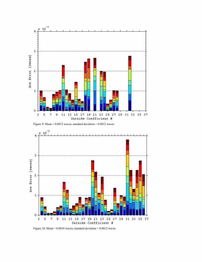
Figure 9: Mean = 0.0012 waves; standard deviation = 0.0012 waves

Figure 10: Mean = 0.0010 waves; standard deviation = 0.0012 waves

terms that are omitted in Figure 9 had larger amounts of error, whose source was traced to higher cross-correlation between them. Instead of explicitly adding more levels of interaction between those terms, dose was added as a new factor into the model as well as interactions of dose with all of the existing terms.

The reason why the aerial-image based approach has been successful is because it contains gradient information with respect to dose. Adding dose terms to the edge-based model therefore is expected to help resolve interactions and improve the Jacobian, as it allows to extract some of the gradient information present in the aerial image. Our second approach shown here uses a single target at multiple exposures as well as focus.

The accuracy that can be gained from the second approach (using a single target at multiple dose and focus conditions) is shown in Figure 10, where the largest error in the coefficients is 0.004 waves. The average error is 0.001 waves, across all Zernike coefficients. The number of coefficients in the expansion that are estimated with accuracy < 0.002 waves is 80%; and 65% of the terms are below 0.001 waves. It is also noted that using a single target at multiple dose and focus settings allows fitting of additional Zernike terms; including those terms with higher power in the radial term. The coefficients of certain high order terms are more difficult to fit compared to others. As power of the radial term in Zernike polynomial is increasing and the angular frequency is increasing, the shapes of the terms get more complicated. The optimization effort was focused on fitting all terms, particularly these higher order radial terms. The dose was indeed the key factor that helped resolve some interaction between the offending terms. The accuracy is expected to further improve when we include a second target. The goal is to keep the number of targets to a minimum for a manageable data collection cycle.

focu

s

14 mj 15 mj 16 mj 17 mj 18 mj

dose

f =0.

12

f =

0.1

5

f = 0

.18

f =

0.2

1f =

0.2

4

focu

s

14 mj 15 mj 16 mj 17 mj 18 mj

dose

f =0.

12

f =

0.1

5

f = 0

.18

f =

0.2

1f =

0.2

4

Figure 11: Single target Focus-Exposure matrix example. Focus step is 0.03 µm, dose step is 1 mJ/cm2.

The results of the Monte Carlo study have validated the chosen regression model versus the full physical model. These results are promising, suggesting significant improvement in coefficient estimation when including through dose information. In general, an optimum convergence (solution) is obtained with this approach.

3.2. Dose and focus calibration

Before we attempt to extract Zernike coefficients, we run a calibration on the FEM of the resist data to be fit. The set of 25 FE images shown in Figure 11 is the training sample used on the developed model. Representative data illustrating the calibration procedure are given in Figures 12–14. It is essential to perform this cross-validation, in order to determine what the aerial image threshold should be to feed it back to the model. The points on plots in Figures 13 and 14 are the measured SEM image data, and the fits are the threshold prediction by the response model. In this example, the threshold of 29.1% corresponds to the dose value of 16mJ/cm2. The dashed line is the plane of best focus which coincides with a tool setting of 0.17µm. The quality of this fit is excellent (R2

adj is above 0.98), and thus the confidence in our imaging model has been confirmed. The Focus/Exposure lookup table created based on this regression fit is fed back in to the response model to tune the optimization model. This is the first in a series of validation steps used to evaluate the predictive ability of this new model. These data suggests that the thresholded aerial image model is working and there is no need to build a separate resist model.

Figure 12: SEM image of the phase wheel target with the parameters that are used for regression model fitting pointed out. Both inner and outer ring radius (Rin, Rout) are utilized in the response model calibration. 102

103

104

105

106

107

108

109

110

111

112

113

Rad

ius,

nm

-0.05 -0.025 0 .025 .05 .075Focus, microns

0.2660.2780.2910.3060.323

18 mj

17 mj

16 mj

15 mj

14 mj

Figure 13: Comparison of the measured (points) and modeled (lines) inner ring radii

through dose and focus. The agreement between the observed and predicted data is good (R2

adj=0.987).

Rin

Rout Aerial Image Threshold Levels

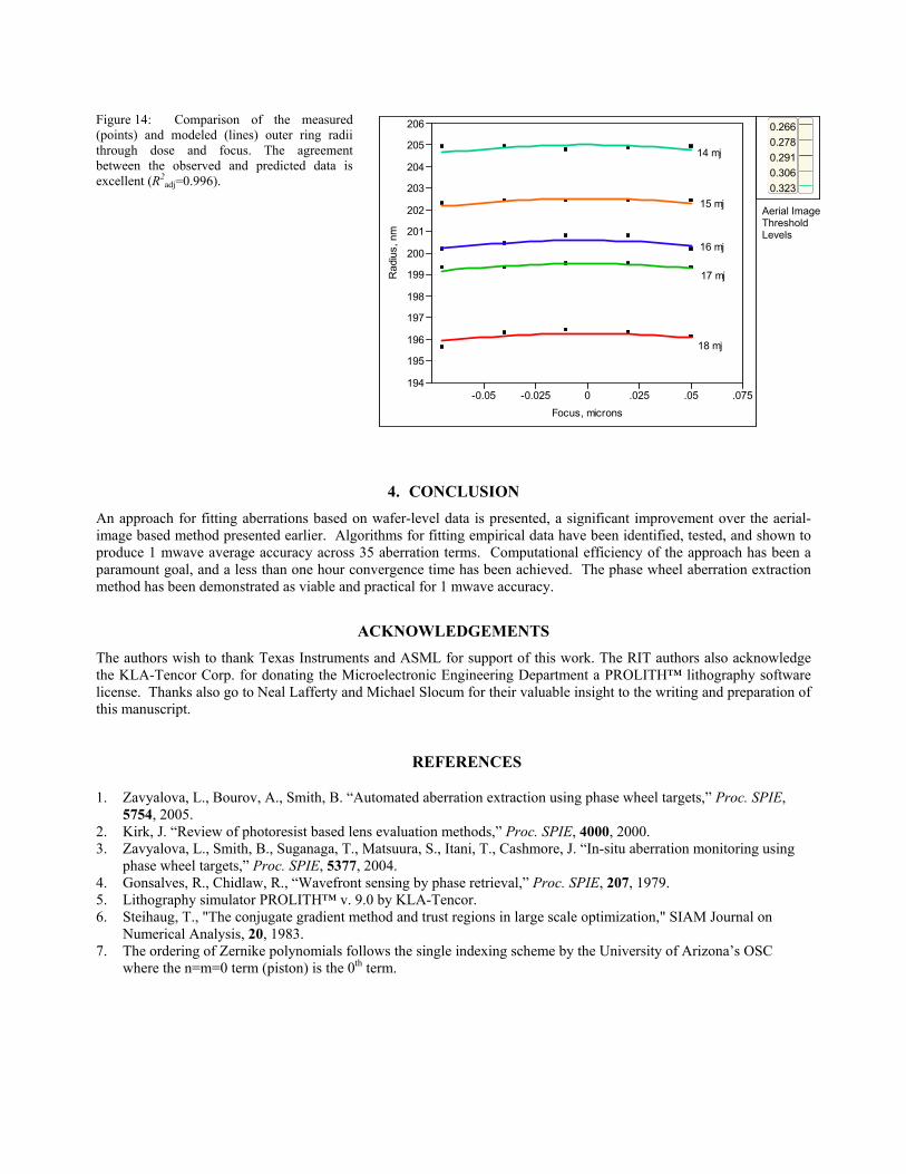
Figure 14: Comparison of the measured (points) and modeled (lines) outer ring radii through dose and focus. The agreement between the observed and predicted data is excellent (R2

adj=0.996).

194

195

196

197

198

199

200

201

202

203

204

205

206

Rad

ius,

nm

-0.05 -0.025 0 .025 .05 .075Focus, microns

0.2660.2780.2910.3060.323

14 mj

15 mj

16 mj

17 mj

18 mj

4. CONCLUSION An approach for fitting aberrations based on wafer-level data is presented, a significant improvement over the aerial-image based method presented earlier. Algorithms for fitting empirical data have been identified, tested, and shown to produce 1 mwave average accuracy across 35 aberration terms. Computational efficiency of the approach has been a paramount goal, and a less than one hour convergence time has been achieved. The phase wheel aberration extraction method has been demonstrated as viable and practical for 1 mwave accuracy.

ACKNOWLEDGEMENTS The authors wish to thank Texas Instruments and ASML for support of this work. The RIT authors also acknowledge the KLA-Tencor Corp. for donating the Microelectronic Engineering Department a PROLITH™ lithography software license. Thanks also go to Neal Lafferty and Michael Slocum for their valuable insight to the writing and preparation of this manuscript.

REFERENCES

1. Zavyalova, L., Bourov, A., Smith, B. “Automated aberration extraction using phase wheel targets,” Proc. SPIE, 5754, 2005.

2. Kirk, J. “Review of photoresist based lens evaluation methods,” Proc. SPIE, 4000, 2000. 3. Zavyalova, L., Smith, B., Suganaga, T., Matsuura, S., Itani, T., Cashmore, J. “In-situ aberration monitoring using

phase wheel targets,” Proc. SPIE, 5377, 2004. 4. Gonsalves, R., Chidlaw, R., “Wavefront sensing by phase retrieval,” Proc. SPIE, 207, 1979. 5. Lithography simulator PROLITH™ v. 9.0 by KLA-Tencor. 6. Steihaug, T., "The conjugate gradient method and trust regions in large scale optimization," SIAM Journal on

Numerical Analysis, 20, 1983. 7. The ordering of Zernike polynomials follows the single indexing scheme by the University of Arizona’s OSC

where the n=m=0 term (piston) is the 0th term.

Aerial Image Threshold Levels