Pollution markets with imperfectly observed emissions

Juan-Pablo Montero∗

Catholic University of Chile and MIT

November 20, 2003

Abstract

I study the advantages of pollution permit markets over traditional standard regulations

when the regulator has incomplete information on firms’ emissions and costs of production

and abatement (e.g., air pollution in large cities). Because the regulator only observes

each firm’s abatement technology but neither its emissions nor its output, there are cases

in which standards can lead to lower emissions and, hence, welfare dominate permits. If

permits can be optimally combined with standards, however, in many cases this hybrid

policy converges to the permits-alone policy but (almost) never to the standards-alone

policy. I then empirically examine these issues using evidence from a permits market in

Santiago, Chile.

Keywords: asymmetric information, imperfect monitoring, pollution markets, permits

JEL classification: L51, Q28

∗<jmontero@faceapuc.cl> Department of Economics, Catholic University of Chile, Vicuna Mackenna 4860,Santiago, Chile. The author is also Research Associate at the MIT Center for Energy and Environmental PolicyResearch (MIT-CEEPR). I am grateful to Luis Cifuentes, Denny Ellerman, Paul Joskow, Matti Liski, José MiguelSánchez and seminar participants at Columbia, Econometric Society Meeting (UCLA), Global DevelopmentNetwork Conference (Cairo), Helsinki School of Economics, MIT, PUC and Universidad de Concepción forcomments and discussions; Joaquín Poblete for research assistance; and MIT-CEEPR for financial support.

1

1 Introduction

In recent years, environmental policy makers are paying more attention to pollution mar-

kets (i.e., tradable emission permits) as an alternative to the traditional command-and-control

(CAC) approach of setting emission and technology standards. A notable example is the 1990

U.S. acid rain program that implemented a nationwide market for electric utilities’ sulfur diox-

ide (SO2) emissions (Schmalensee et al., 1998; Ellerman et al., 2000). In order to have a precise

estimate of the SO2 emissions that are actually going to the atmosphere, the acid rain program

requires each affected electric utility unit to install costly equipment that can continuously

monitor emissions.1

This and other market experiences suggest that conventional permits markets are likely

to be implemented in those cases where emissions can be closely monitored, which almost

exclusively occurs in large stationary sources like electric power plants and refineries. Then,

it is not surprising that, among other reasons, environmental authorities continue relying on

CAC instruments to regulate emissions from smaller sources because compliance with such

instruments only requires the authority to ensure that the regulated source has installed the

required abatement technology or that its emissions per unit of output are equal or lower than

a certain emissions rate standard.2 In addition, some regulators view that a permits program

where emissions cannot be closely monitored may result in higher emissions than under an

alternative CAC regulation. Since compliance cannot be made contingent on firm’s output or

1Another example with similar monitoring requirements is the Southern California RECLAIM program thatimplemented separated markets for nitrogen oxide (NOx) and SO2 emissions from power plants, refineries andother large stationary sources. This program did not include a market for volatile organic compounds (VOC) inlarge part because of the difficulties with monitoring actual emissions from smaller and heterogeneous sources(Harrison, 1999).

2Note that there are some credit-based trading programs aimed at curbing air pollution in urban areas workingin the US (Tietenberg, 1985). New sources (or expansion of existing ones) must acquire emission credits to covertheir emissions through, for example, shutting down existing plants or scrapping old vehicles. Although theseprograms have the merit of involving small sources, they are very limited in scope in the sense that they areembedded within an existing CAC regulation and are particularly designed to prevent further deterioration ofair quality from the entry of new sources.

2

utilization, emissions could in fact be higher if the trade pattern is such that lower-output firms

sell permits to higher-output firms.

Thus, pollution markets may appear inapproapriate for effectively reducing air pollution in

large cities where emissions come from many small (stationary and mobile) sources rather than

a few large stationary sources (e.g., air pollution in large cities like Mexico City, Sao Paulo in

Brasil and Santiago-Chile). While one cannot neglect a priori that a permits market in which

emissions (and ouput) are only imperfectly monitored may eventually lead to higher emissions

than an alternative regulation, I think that rather than disregard pollution markets as a policy

tool, the challenge faced by policy makers is when and how to implement these markets using

monitoring procedures that are similar to those under CAC regulation.

Most of the literature on environmental regulation under asymmetric information deals with

the case in which firms’ costs are privately known but emissions are publicly observed (see Lewis

(1996) for a survey). While there is some literature considering imperfect observation of emis-

sions (e.g., Segerson, 1988; Fullerton and West, 2002),3 there seems to be no work specifically

studying the effect of imperfect information on emissions and costs on the design and perfor-

mance of a permits market. Yet, it is interesting to observe that despite its limited information

on each source’s actual emissions (and costs), Santiago-Chile’s environmental agency has al-

ready implemented a (small) market to control total suspended particulate (TSP) emissions

from a group of about 600 stationary sources (Montero et al., 2002).4 Based on estimates

from annual inspection for technology parameters such as source’s size and fuel type, Santi-

ago’s environmental regulator approximates each source’s actual emissions by the maximum

amount of emissions that the source could potentially emit in a given year.5 I believe that a

3Fullerton and West (2002) study the control of vehicle emissions using a combination of taxes on cars and ongasoline as an alternative to an (unavailable) tax on emissions. Segerson (1988) study the control of emissionsfrom (few) non-point sources using a ”moral hazard in teams” approach.

4Sources affected by the TSP program are responsible for only 5% of 2000 TSP emissions in Santiago.5As we shall see later, using the source’s maximum emissions as a proxy does not prevent any adverse effects

3

close (theoretical and empirical) examination of this permits program represents a unique case

study of issues of instrument choice and design that can arise in the practical implementation

of environmental markets in which regulators face important information asymmetries.

In the next section (Section 2) I develop a theoretical model and start by showing that

the regulator cannot implement the first-best when emissions are imperfectly measured (even

in the absence of budget constraints and perfect cost information). In Section 3, I derive the

optimal design of two policy instruments: emission standards and emission permits. I focus on

these two policies rather than on more optimal ones not only because the latter include the use

of nonlinear instruments and transfers to firms which has not been used in practice (Stavins,

2003; Hahn et al., 2003), but more importantly, because I want to specifically explore whether

permits can still provide an important welfare advantage over traditional CAC regulation when

emissions are imperfectly monitored.

In Section 4, I first discuss the conditions under which permits are welfare superior to

standards. I show that permits provide firms not only with flexibility to reduce production

and abatement costs but sometimes with perverse incentives to choose socially suboptimal

combinations of output and abatement (something that would not occur if emissions were

accurately measured). There are two situations in which the latter possibility can lead permits

to higher emissions, and hence, be potentially welfare dominated by standards: (1) when firms

with relatively large output ex-ante (i.e., before the regulation) are choosing low abatement

(i.e., when there is a negative correlation between production and abatement costs), and (2)

when firms doing more abatement find it optimal to reduce output ex-post. Because in deciding

whether to use permits or standards, the regulator is likely to face this trade-off between cost

that the use of permits (instead of CAC regulation) could eventually have on aggregate emissions. The choice ofproxy is an arbitrary matter because the number of permits being allocated can always be adjusted accordinglywith no efficiency effects.

4

savings and possible higher emissions, I then discuss the advantages of implementing an optimal

hybrid policy in which permits are combined with an optimally chosen standard. I find that

in many situations the hybrid policy converges to the permits-alone policy but it almost never

converges to the standards-alone policy.

In Section 5, I empirically examine the advantages of a permits program using emissions

and output data from the Santiago’s TSP permits program. I find evidence of large cost savings

but also of higher emissions (about 6%) relative to what would have been observed under an

equivalent standards policy. However, the welfare loss from higher emissions is only 8% of the

welfare gain from lower abatement and production costs. Final remarks are in Section 6.

2 The model

Consider a competitive market for an homogeneous good supplied by a continuum of firms of

mass 1. Each firm produces output q and emissions e of a uniform flow pollutant. To simplify

notation, I assume that when the firm does not utilize any pollution abatement device e = q.

Market inverse demand is given by P = P (Q), where Q is total output and P 0(Q) ≤ 0. Total

damage from pollution is given by D(E), where E are total emissions and D0(E) > 0. Functions

P (Q) and D(E) are known to the regulator.

A firm can abate pollution at a positive cost by installing technology x, which reduces

emissions from q to e = (1 − x)q. Hence, the firm’s emission rate is e/q = 1 − x. Each firm

is represented by a pair of cost parameters (β, γ). A firm of type (β, γ) has a cost function

C(q, x, β, γ) where β and γ are firm’s private information. To keep the model mathematically

tractable, I assume that the cost function has the following quadratic form in the relevant

5

output-abatement range6

C(q, x, β, γ) =c

2q2 + βq +

k

2x2 + γx+ vxq (1)

where c, k and v are known parameters common to all firms and c > 0, k > 0, Λ ≡ ck− v2 > 0

and v T 0.7

Function (1) incorporates two key cost parameters that are essential to understand firms’

behavior under permits and standards regulation. One of these cost parameters is the correla-

tion between β and γ (that we shall denote by ρ), which captures whether firms with higher

output ex-ante (i.e., before the regulation) are more or less likely to install more abatement

x. The other cost parameter is v, which captures the effect of abatement on output ex-post

(note that we have constrained v to be the same for all firms, thus, a negative value of v would

indicate that, on average, the larger the x the larger the increase in q ex-post). As we shall see,

the values of the cost parameters v and ρ play a fundamental role in the design and choice of

policy instruments when emissions are not closely monitored.

Although the regulator does not observe firms’ individual values for β and γ, we assume

that he knows that they are distributed according to the cumulative joint distribution F (β, γ)

on β ∈ [β, β] and γ ∈ [γ, γ].8 To simplify notation further and without any loss of generality I

let E[β] =E[γ] = 0, where E[·] is the expected value operator.9 I also use the following notation:

6This approach was first introduced by Weitzman (1974).7The parameter v can be negative, for example, if switching to a cleaner fuel saves on fuel costs but involves

such a large retrofitting cost (i.e., high k) that no firm switches to the cleaner and cheaper fuel unless regulated.8Note that we can easily add aggregate uncertainty to this formulation by simply letting βi = βi + θ and

γi = γi + η, where θ and η are random variables common to all firms.9Note that because β and γ are negative for some firms, one can argue that marginal costs can take negative

values. This possibility is eliminated by assuming parameter values (including those in the demand and damagefunctions) that lead to interior solutions for q and x in which ∂C/∂q > 0 and ∂C/∂x > 0 for all β and γ.Furthermore, since these interior solution are assumed to fall within the range in which (1) is valid, what happensbeyond this range is not relevant for the analysis of instrument design and choice that follows. Alternatively, onecan let β ∈ [0, β] and γ ∈ [0, γ] with some further notation in the optimal designs but no change in the welfarecomparisons.

6

Var[β] ≡ σ2β, Var[γ] ≡ σ2γ , Cov[β, γ] ≡ ρσβσγ and Fβγ ≡ ∂2F (β, γ)/∂β∂γ.

Firms behave competitively, taking the output clearing price P as given. Hence, in the

absence of any environmental regulation, each firm will produce to the point where its marginal

production cost equals the product price (i.e., Cq(q, x, β, γ) = P ), and install no abatement

technology (i.e., x = 0). Because production involves some pollution, this market equilibrium

is not socially optimal. The regulator’s problem is then to design a regulation that maximizes

social welfare.

I let the regulator’s social welfare function be

W =

Z Q

0P (z)dz −

Z β

β

Z γ

γC(q, x, β, γ)Fγβdβdγ −D(E) (2)

where Q =Rβ

Rγ q(β, γ)Fγβdγdβ is total output and E =

Rβ

Rγ(1 − x(β, γ))q(β, γ)Fγβdγdβ is

total emissions. In this welfare function, the regulator does not differentiate between consumer

and producer surplus and transfers from or to firms are lump-sum transfers between consumers

and firms with no welfare effects.10

The firms’ outputs and abatement technologies that implement the social optimum or first-

best outcome are given by the following two first-order conditions

q : P (Q)−Cq(q, x, β, γ)−D0(E) · (1− x) = 0 (3)

x : −Cx(q, x, β, γ)−D0(E) · (−q) = 0 (4)

If rearranged, eq. (3) says that the benefits from consuming an additional (small) unit of output

is equal to its cost of production and environmental effects. Eq (4), on the other hand, says

10The model can be generalized by allowing the regulator to consider a weight µ 6= 1 for firm profits and ashadow cost λ > 0 for public funds. However, this would not add much to our discussion.

7

that emissions should be reduced to the point where the marginal cost of emissions abatement

(i.e., Cx/q) is equal to marginal damages (i.e., D0(E)).

Because of various information asymmetries between firms and the regulator it is not clear

that the latter can design an environmental policy that can attain the first-best resource alloca-

tion. The regulator’s problem then becomes to maximize (2) subject to information constraints

(and sometimes administrative and political constraints as well). From the various possible

type of information constraints, the case that have attracted most attention in the literature

is that in which the regulator knows little or nothing about firms’ costs (i.e., he may or may

not know F ) but can costlessly monitor each firm’s actual emissions e (Kwerel, 1977; Dasgupta

et al.,1980; Spulber, 1988; Lewis, 1996). These authors show that in many cases the first-best

can be implemented. It is the case here, for example, if the regulator announces a (non-linear)

emissions tax schedule τ(E) equal to D0(E).11

In this paper, however, I am interested in the problem where the regulator cannot directly

observe firms’ actual emissions e = (1 − x)q; although he can costlessly monitor firms’ abate-

ment technologies or emission rates x. As in Santiago’s permits program, this information

asymmetry will be present when both continuous monitoring equipment is prohibitively costly

and individual output q is not observable.12 Thus, if the regulator asks for an output report

from the firm, we anticipate that the firm would misreport its output whenever this was to its

advantage. In this case, the regulator cannot implement the social optimum regardless of the

information he or she has about firm’s costs.13

11A competitive firm (β, γ) takes the price P (Q) and tax rate τ(E) = D0(E) as given and maximizeπ(q, x, β, γ) = P (Q)q − C(q, x, β, γ) − D0(E) · (1 − x)q with respect to q and x. The firm’s first order con-ditions for q and x are those given by (3) and (4).12The regulator can nevertheless estimate total output Q from the observation of the market clearing price P .13Consider the extreme situation in which regulator knows both β and γ. His optimal policy will be some

function T (x;β, γ) in the form of either a transfer from the firm or to the firm. Then, firm (β, γ) takes P (Q)and T (x;β, γ) as given and maximizes π(q, x, β, γ) = P (Q)q − C(q, x, β, γ)− T (x;β, γ) with respect to q and x.It is not difficult to see that firm’s first order conditions for q and x will always differ from (3) and (4) for anyfunction T (x;β, γ).

8

Even if the regulator has perfect knowledge of firm’s costs and, therefore, can ex-post deduce

firm’s output based on this information and the observation of x, the fact that he cannot make

the policy contingent on either emissions or output prevents him from implementing the first-

best. In other words, the regulator cannot induce the optimal amounts of output and emissions

with only one instrument (i.e., x).14 Consequently, the regulator must necessarily content

himself with less optimal policies.

3 Instrument design

Rather than considering a full range of policies, I focus here on those policies that are either

currently implemented or have drawn some degree of attention from policy makers in the context

of urban air pollution control (Stavins, 2003). I first study the optimal design of a traditional

technology (or emission rate) standard and then the optimal design of a permits market. I leave

the optimal design of the hybrid policy, which builds upon the individual designs, for Section

4. To keep the model simple, I make two further simplifications regarding the demand curve

and the damage function. I let P (Q) = P (constant) and D(E) = hE, where h > v.15

To visualize how the two policy designs depart from the social optimum, it is useful to

compute the first-best and keep it as a benchmark. Plugging the above assumptions in (3) and

(4), the first-best outcome is given by

x∗ =(P − h− β)(h− v)− γc

ck − (h− v)2(5)

14Since the regulator can have a good idea of total emissions E from air quality measures, one might arguethat Holmström’s (1982) approach to solving moral hazard problems in teams may apply here as well. However,in our context this approach is unfeasible because the large number of agents would require too big transfers;either from firms as penalties or to firms as subsidies.15Besides that these assumptions facilitate the empirical estimation, they tend to offset each other, and if

anything, they tend to favor the standards policy. Because costs are always lower under the permits policy, abackward sloping demand would lead to higher output, and hence, to higher surplus under such policy. On theother hand, because it is not clear a priory whether emissions are higher or lower under the permits policy, aconvex damage function may or may not lead to higher environmental damages under such policy.

9

q∗ =P − h− β + (h− v)x∗

c(6)

It is immediate that ∂x∗/∂β < 0, ∂x∗/∂γ < 0, ∂q∗/∂β < 0 and ∂q∗/∂γ < 0. As expected,

higher production and abatement costs lead to lower output and abatement levels.

3.1 Standards

The regulator’s problem here is to find the emission rate standard xs to be required to all firms

that maximizes social welfare (subscript “s” denotes standards policy). The regulator knows

that for any given xs, firm (β, γ) will maximize π(q, xs, β, γ) = Pq−C(q, xs, β, γ). Hence, firm’s

(β, γ) output decision will solve the first-order condition

P − cq − β − vxs = 0

which provides the regulator with firm’s output q as a function of the standard xs

qs(xs) ≡ qs =P − β − vxs

c(7)

Since xs will be the same across firms, it is clear that production under a standard will also be

suboptimal relative to the first-best q∗ as qs does not adapt to changes in γ.

Based on the welfare function (2), the regulator now solves

maxxs

Z β

β

Z γ

γ[Pqs − C(qs, xs)− h · (1− xs)qs]Fβγdγdβ

By the envelope theorem, the first-order condition is

Z β

β

Z γ

γ

·−kxs − γ − vqs − h · (1− xs)

∂qs∂xs

+ hqs

¸Fβγdγdβ = 0 (8)

10

By replacing (7) and ∂qs/∂xs = −v/c into (8), the first-order condition (8) reduces to

−ckxs − v · (P − vxs) + h · (1− xs)v + h · (P − vxs) = 0

which leads to the optimal standard

xs =P · (h− v) + hv

Λ+ 2vh(9)

where Λ ≡ ck − v2 > 0. Comparing this result to the first-best (5), it is interesting to observe

that xs > x∗(β = 0, γ = 0). This indicates that even in the absence of production and

abatement cost heterogeneity (i.e., β = γ = 0 for all firms), the standards policy still require

firms to install more abatement technology than is socially optimal. Because qs(x∗) > q∗, it is

optimal to set xs somewhat above x∗ to bring output qs closer to its optimal level q∗.

3.2 Permits

The regulator’s problem now is to find the total number permits ee0 to be distributed amongfirms that maximizes social welfare. Let R denote the equilibrium price of permits, which will

be determined shortly.16 The regulator knows that firm (β, γ) will take R as given and solve

maxq,x

π(q, x, β, γ) = Pq − C(q, x, β, γ)−R · (ee− ee0)where ee = (1−x)eq are firm’s proxied emissions and eq is some arbitrarily output or capacity levelthat is common to all firms (recall that the regulator only observes x). For example, eq couldbe set equal to the maximum possible output that could ever be observed, which would occur

16Note that under a tax policy, the optimal price R will be the quasi-emissions tax. If we add aggregateuncertainty to the model, both policies will not be equivalent from an efficiency standpoint.

11

when x = 0 and β = β. As we shall see later, the exact value of eq turns out to be irrelevantbecause it simply works as a scaling factor. Note that if ee < ee0 the firm will be a seller of

permits.

From firms’ first-order conditions

x : − kx− γ − vq +Req = 0 (10)

q : P − cq − β − vx = 0 (11)

we have that firm’s (β, γ) optimal abatement and output responses to R and eq (or, moreprecisely, to Req) are

xp =Reqc− γc− (P − β)v

Λ(12)

qp =P − β − vxp

c(13)

where the subscript “p” denotes permits policy. Comparing (12) and (13) with (5) and (6)

illustrates the trade-off a regulator faces when implementing a permits program with imperfect

observation of emissions. While ∂qp/∂β and ∂xp/∂γ are negative as in the first-best, ∂qp/∂γ

and ∂xp/∂β are both positive when v > 0.17

Now we can solve the regulator’s problem of finding the optimal ee0. Since the market

clearing condition is

Z β

β

Z γ

γeeFβγdγdβ = Z β

β

Z γ

γ(1− xp)eqFβγdγdβ = ee0 (14)

and xp is a function of Req as indicated by (12), it is irrelevant whether we solve for Req or ee0/eq.Hence, we let the regulator solve (permits purchases and sales are transfers with no net welfare

17Note that ∂qp/∂β = −k/Λ, ∂xp/∂β = ∂qp/∂γ = v/Λ and ∂xp/∂γ = −c/Λ.

12

effects)

maxReq

Z β

β

Z γ

γ[Pqp(xp(Req))−C(qp(xp(Req)), xp(Req))− h · (1− xp(Req))qp(xp(Req))]Fβγdγdβ

By the envelope theorem, the first-order condition is

Z β

β

Z γ

γ

·−(1− xp)h

∂qp∂(Req) + hqp

∂xp∂(Req) −Req ∂xp

∂(Req)¸Fβγdγdβ = 0 (15)

By plugging ∂qp/∂(Req) = [∂qp/∂xp][∂xp/∂(Req)], ∂qp/∂xp = −v/c, (12) and (13) into (15), thefirst-order condition can be rearranged to obtain the optimal permits price

Req = Ph(kc+ v2) + hvΛ

(Λ+ 2hv)c(16)

which, in turn, allows us to obtain the optimal permits allocation ee0/eq by simply replacing (16)in (12) and that in (14). As in the standards policy, this allocation induces, on average, more

abatement than is socially optimal (note that xp(0, 0) > x∗(0, 0)).

We can now replace Req in (12) and (13) to obtain expressions for qp and xp that are more

readily comparable to qs and xs (see eqs. (7) and (9)). After some algebra, the following

expressions are obtained

xp = xs +vβ − cγ

Λ(17)

qp =P − vxs

c− kβ − vγ

Λ= qs − v2β − cvγ

cΛ(18)

If firms are homogeneous (i.e., β = γ = 0 for all firms), it is not surprising that xp = xs

and qp = qs and that both regulations provide the same welfare. As firms become more

heterogenous, x and q move in different directions depending on the regulatory regime and

13

the value of v (it will also depend on ρ as we will see next). In fact, when v > 0 and firms

differ on γ, firms’ abatement decisions x tend to remain closer to the social optimum x∗ under

the permits regulation than under the CAC regulation since ∂x∗/∂γ and ∂xp/∂γ are both

negative.18 However, as firms differ on β, firms’ abatement decisions remain closer to x∗ under

the CAC regulation since ∂x∗/∂β and ∂xp/∂β have opposite signs. A similar trade-off can

be found analyzing firms’ production decisions to changes in β and γ. Because this eventual

output/abatement “misalignment” may result in higher emissions under the permits policy, in

deciding whether or not to implement a permits program, the regulator will inevitably face

a trade-off between abatement flexibility and possible higher emissions. I study this trade-off

more formally in the next section.

4 Instrument choice

The regulator must now decide wether to use permits or standards or, eventually, a combination

of both. Although by construction a hybrid policy cannot be welfare dominated by either single-

instrument policy, it is useful to compare first single-instrument policies and then explore the

extra gains, if any, of implementing a hybrid policy.

4.1 Permits versus standards

For a regulator that is limited to use a single instrument, the difference in the social welfare

between the optimal permits policy and the optimal standards policy is

∆ps =Wp(ee0/eq)−Ws(xs) (19)

18Note that ∂x∗/∂γ = ∂xp/∂γ for v = 0.

14

where ee0 is the optimal number of permits normalized by some eq and xs is the optimal standard.The normative implication of (19) is that if∆ps > 0, the regulator should implement the permits

policy.

To explore under which conditions this is the case, we write (19) as

∆ps =

Z β

β

Z γ

γ[Pqp −C(qp, xp)− (1− xp)qph− Pqs + C(qs, xs) + (1− xs)qsh]Fβγdγdβ (20)

where qp, xp, qs and xs can be expressed according to (17) and (18). Since Qp = Qs =

(P − vxs)/c, eq. (20) can be re-written as

∆ps =

Z β

β

Z γ

γ[{C(qs, xs)− C(qp, xp)}+ {(1− xs)qs − (1− xp)qp}h]Fβγdγdβ (21)

Recalling that e = (1−x)q, the first curly bracket of the right hand side of (21) is the difference

in costs between the two policies, whereas the second curly bracket is the difference in emissions

that multiplied by h gives the difference in pollution damages.

If we plug (17) and (18) into (21), after some algebra (21) becomes

∆ps =v2σ2β − 2cvρσβσγ + c2σ2γ

2cΛ−

h ·³kvσ2β − (kc+ v2)ρσβσγ + cvσ2γ

´Λ2

(22)

and after collecting terms, it reduces to

∆ps = A1σ2β +A2σ

2γ +A3ρσβσγ (23)

where A1 = (v2Λ − 2ckhv)/2cΛ2, A2 = (cΛ− 2chv)/2Λ2 and A3 = (ckh + hv2 − vΛ)/Λ2 > 0.

Since A1, A2 and ρ can be either positive, negative or zero,19 the sign of (23) will depend upon

19Recall that for interior solutions in all cases we must have ck > (h− v)2, ck > v2, and h > v.

15

the value of the different parameters. As the heterogeneity across firms decreases (i.e., σ2β and

σ2γ approach zero), however, the welfare difference between the two policies tend to disappear.20

The ambiguous sign of (23) should not be surprising given the trade-off between flexibility

and potential higher emissions that we identified in the previous section. Expression (22)

illustrates this trade-off more clearly. The first term is the difference in costs between the two

policies. Since −1 ≤ ρ ≤ 1, this term is always positive which indicates that the optimal

permits policy is always less costly than the optimal standards policy. The second term is the

difference in damages, which can either be positive, negative or zero depending on the value of

the different parameters of the cost function. Hence, a permits policy will always lead to cost

savings but it can also lead to higher emissions.

The magnitude of ∆ps depends on the value of the different parameters of the model, but

its sign is governed by the key cost parameters v and ρ. If v = ρ = 0, for example, the second

term of (22) is zero, so ∆ps > 0. But if v > 0 and ρ < 0, this second term becomes negative

and depending on the value of h relative to other parameters, ∆ps may become negative as well

(it would be so, for example, for σβ = σγ , v = 0 and ρ < −c/h). More generally, one can draw

a line ∆=0 in the (v, ρ)-space that solves ∆ps(v, ρ) = 0. These results can be summarized in

the following proposition

Proposition 1 The permits policy can lead to either higher or lower welfare than the standards

policy. A necessary condition for permits to be welfare dominated by standards is that either

v > 0 or ρ < 0.

To understand this proposition one must first recognize that a permits program can create

“perverse” incentives for shifting output from cleaner to dirtier firms resulting in higher total

emissions. The latter could happen under two circumstances: (i) when firms doing more abate-

20Note that the welfare difference remains if we consider regulator’s aggregate uncertainty.

16

ment are at the same time decreasing output relative to other firms (i.e, when v > 0) and (ii)

when highly utilized firms are doing less abatement (i.e., when ρ < 0). A low (or negative)

value of v, on the other hand, reduces both the effect of the environmental regulation on the

firm’s output under either policy (see (7) and (13)) and the effect of production cost hetero-

geneity (i.e., β) on firms’ abatement decisions under the permits policy (see (12)). A positive

correlation between production and abatement costs (i.e., ρ > 0) also makes the permits policy

more attractive because when both cost parameters (β and γ) are either simultaneously high

or low, output and abatement remain closer to the first-best.

Contrary to what occur when emissions are perfectly monitored, Proposition 1 indicates

that neither permits nor standards is the appropriate policy choice in all cases. Because of this

ambiguity, there seems to be room for a hybrid policy to improve upon either single-instrument

policy. In fact, in the classic problem of prices versus quantities under uncertainty pioneered by

Weitzman (1974), Roberts and Spence (1980) shows that a hybrid policy that combines permits

with taxes/subsidies is always superior to either permits or taxes/subsidies alone. The reason

for this result is that in Weitzman (1974) taxes are always superior in terms of costs (lower

expected compliance costs) while permits are always superior in terms of emissions (higher

expected environmental benefits). In our problem, however, permits are always superior in

terms of costs but standards are not always superior in terms of emissions, so it remains to be

seen whether and when a hybrid policy would provide a net welfare gain.

4.2 The hybrid policy

The regulator’s design problem here is to find the allocation eeh0 of permits (together with anutilization factor eqh) and an emission standard xhs that maximize social welfare. The superscript“h” stands for hybrid policy. Under this hybrid policy, firms are free to trade permits but each

17

of them cannot reduce less than xhs . As in the permits-alone policy, there will be a price Rheqh

(the scaling factor eqh can be the same as in the permits-alone policy; its actual value is notrelevant).

Depending on the values of β and γ, the standard xhs will be binding for some firms. Thus,

we can divide the universe of firms in two groups: those that comply with the permits policy

(xh ≡ xhp and qh ≡ qhp ) and those that comply with the standards policy (x

h ≡ xhs and qh ≡ qhs ).

Note that the latter group of firms must still cover its (proxied) emissions with permits, which

will ultimately affect the equilibrium price of permits. The values of β and γ of those firms that

are in the frontier that divides the two groups of firms satisfy xhp = xhs . From the first order

condition (12), we know that

xhp =Rheqhc− γc− (P − β)v

Λ

which combined with xhp = xhs gives us such frontier

γ =v

cβ − Λ

cxhs +Rheqh − Pv

c≡ bγ(β) (24)

Because the initial allocation of permits does not affect behavior, firms with γ ≥ bγ(β)will behave as in the standard-alone policy and firms with γ < bγ(β) will behave as in the apermits-alone policy. Then, the regulator’s problem can be written as

maxxhs ,eeh0/eqh

Z β

β

Z bγ(β)γ

hPqhp − C(qhp , x

hp , β, γ)− h(1− xhp)q

hp

iFβγdγdβ+Z β

β

Z γ

bγ(β)hPqhs − C(qhs , x

hs , β, γ)− h(1− xhs )q

hs

iFβγdγdβ (25)

where qhs , xhp and qhp can be obtained, respectively, from (7), (12) and (13) (simply add the

18

superscript “h”). The regulator ensures full compliance, so the market clearing condition is (all

firms must cover their emissions with permits)

Z β

β

Z bγ(β)γ

(1− xhp)eqhFβγdγdβ + Z β

β

Z γ

bγ(β)(1− xhs )eqhFβγdγdβ = eeh0Since eqh is a constant and xhp depends on Rheqh, it is clear again that it is irrelevant to solve

for either the Rheqh or eeh0/eqh. As before, we solve for Rheqh. Following the derivations for thesingle-instrument policies, the first order conditions for the optimal hybrid policy are (we allow

for corner solutions)

Rheqh : Z β

β

Z bγ(β)γ

"−(1− xhp)h

∂qhp∂(Rheqh) + hqhp

∂xhp∂(Rheqh) −Rheqh ∂xhp

∂(Rheqh)#Fβγdγdβ

+

Z β

β

hPqhp − C(qhp , x

hp , β, bγ(β))− h(1− xhp)q

hp

iFβ(β, bγ(β))dβ

−Z β

β

hPqhs −C(qhs , x

hs , β, bγ(β))− h(1− xhs )q

hs

iFβ(β, bγ(β))dβ ≤ 0

[= 0 if Rheqh > 0; < 0 if Rheqh = 0] (26)

xhs :

Z β

β

Z γ

bγ(β)·−kxhs − γ − vqhs − (1− xhs )h

∂qhs∂xhs

+ hqhs

¸Fβγdγdβ

− Λc

Z β

β

hPqhp −C(qhp , x

hp , β, bγ(β))− h(1− xhp)q

hp

iFβ(β, bγ(β))dβ

+Λ

c

Z β

β

hPqhs − C(qhs , x

hs , β, bγ(β))− h(1− xhs )q

hs

iFβ(β, bγ(β))dβ ≤ 0

[= 0 if xhs > 0; < 0 if xhs = 0] (27)

19

Since at bγ(β) we have that xhs = xhp and hence, qhs = qhp , (26) and (27) reduce, respectively, to

Z β

β

Z bγ(β)γ

"−(1− xhp)h

∂qhp∂xhp

+ hqhp −Rheqh#Fβγdγdβ ≤ 0 (28)

Z β

β

Z γ

bγ(β)·−kxhs − γ − vqhs − (1− xhs )h

∂qhs∂xhs

+ hqhs

¸Fβγdγdβ ≤ 0 (29)

where ∂qhp/∂xhp = ∂qhs /∂x

hs = −v/c.

The solution of the optimal hybrid policy can result in a corner solution if either (28) or

(29) is negative at the optimum. When (28) is negative, the hybrid policy converges to the

standards-alone policy (i.e., Rheqh = 0 and xhs = xs) and when (29) is negative, the hybrid

policy converges to the permits-alone policy (i.e., Rheqh = Req and xhs = 0). Formal exploration

of these possibilities lead to the following proposition

Proposition 2 The optimal hybrid policy converges to the optimal permits-alone policy for

many combinations of v and ρ (e.g., v = ρ = 0). If abatement cost heterogeneity is significantly

smaller than production cost heterogeneity (more precisely, if −γ/β < (h − v)/c), the optimal

hybrid policy converge to the optimal standards-alone policy for ρ = −1.

Proof. See the Appendix.

Contrary to what happens in Roberts and Spence (1980) and Kwerel (1980), in this model

the combination of instruments does not necessarily leads to higher welfare. In those papers,

taxes are superior in terms of costs (i.e., lower expected costs) but permits are superior in terms

of benefits (i.e., lower expected emissions),21 so an optimal combination of instruments strictly

dominates either single instrument. Here, permits are not only less costly than standards but

also they can lead to lower emissions, so it is reasonable to think that in such cases standards

21See also Weitzman (1974).

20

may add nothing to the policy design.22 It is not so obvious, however, that in some cases,

although very few, permits may also add nothing to the policy design.

The exact shape of the region in which the hybrid policy dominates either single-instrument

policy depends on the parameter values. A simple numerical exercise may be useful. In Figure

1, line h=p indicates the combinations of v and ρ for which the hybrid policy just converges to

the permits policy for the following parameters values: P = k = c = 4, h = 2, β = 2, β = −2,

γ = 1, γ = −1.23 The figure also includes the line ∆=0 (i.e., combinations of v and ρ that yield

∆ps = 0) and the line ∆E=0 (i.e., combinations of v and ρ for which the permits policy and

the standards policy yield the exact same level of emissions). One can distinguish three regions

in the figure. To the left of h=p, there are those combinations for which the hybrid policy

coincides with the permits policy. As the first row of Table 1 shows, if v = −0.5 and ρ = 0.6,

for example, social net benefits (W ) are 33% higher under the permits policy than under the

standards policy. Note also that in some places of this region the hybrid policy does not improve

upon the permits-alone policy despite the fact that emissions are higher than under a standards-

alone policy. The logic behind this result is that the introduction of some binding standard (in

combination with permits) would not only reduce emissions but also increase production and

abatement costs. And in this particular region, the latter effect dominates.

The second region –between the lines h=p and ∆=0– includes all those combinations

for which the hybrid policy is superior to the permits-alone policy, which in turn, is superior

to the standards-alone policy. For example, if v = 0.6 and ρ = 0.6, the welfare gain from

implementing the hybrid policy (∆h) is 12.6% of ∆ps, as shown in the second row of the table.

It is interesting to observe that despite welfare may not increase by much, policy designs are

22A similar situation would occur in the analysis of permits and taxes if the slope of the marginal benefit curvewere assumed negative instead of positive, as normally the case. Taxes would be superior to permits in terms ofboth cost and benefits and there would be no gains from adding permits into the tax design.23The simulation is carried out with only four type of firms: (β, γ),(β, γ), (β, γ) and (β, γ). Also, the value of

the different parameters limit the range of v to [−0.5, 0.7].

21

0=∆l

-1

-0.8

-0.6

-0.4

-0.2

0

0.2

0.4

0.6

0.8

1

-0.5 -0.3 -0.1 0.1 0.3 0.5 0.7 v

ph=l

ρ

0=∆El

Figure 1: Hybrid and single-instrument policies

quite different (the hybrid policy includes a standard that is almost half the one in the standards-

alone policy; though the equilibrium permit price do not vary much). Finally, the third region

–to the right of ∆=0– includes those combinations of v and ρ for which the hybrid policy is

welfare superior to the standards-alone policy, which in turn, is superior to the permits-alone

policy. Here, the gain from implementing the hybrid policy as opposed to the standards-alone

policy is substantial, 32.5% of |∆ps|.24

Table 1. Hybrid and single-instrument policies: design and welfare

v ρ xs Req xhs Rheqh Ws ∆ps ∆h

−0.5 0.6 0.65 2.08 0 2.08 123.64 41.08 0

0.6 0.5 0.38 2.07 0.18 1.99 82.04 13.66 1.72

0.7 −0.5 0.36 2.10 0.21 1.49 79.74 −6.37 2.07

24Note that despite that σγ = 0.5σβ , there is no region in Figure 1 where the hybrid policy converges to thestandards-alone policy.

22

5 An empirical evaluation

In this section, I use the experience from Santiago’s total suspended particulate emissions

(TSP) trading program to evaluate the advantages (if any) of using permits when emissions are

imperfectly observed. Because firms are not required to provide the regulator with information

on production and abatement costs, I apply the theoretical framework previously developed

(including the assumption of a benevolent regulator given his choice of h) to infer the cost

structure of the firms affected by the TSP program and other parameters such as h and P based

on observables such as emission rates and utilization. This information is then used to compare

the actual performance of the TSP permits program with the performance of a hypothetical

and equivalent standards policy (and with a hybrid policy). The equivalent standards policy

is constructed under the assumption that if the regulator would have to introduce a standard

he will do it optimally using the same value of h (together with the other parameters) that he

used to implement the permits policy.25

5.1 The TSP program

The city of Santiago has constantly presented air pollution problems since the early 1980s.

The TSP trading program, established in March of 1992, was designed to curb TSP emissions

from the largest stationary sources in Santiago (industrial boilers, industrial ovens, and large

residential and commercial heaters) whose emissions are discharged through a duct or stack at

a flow rate greater than or equal to 1,000 m3/hr. Because sources were too small to require

sophisticated monitoring procedures, the authority did not design the program based on sources’

actual emissions but on a proxy variable equal to the maximum emissions that a source could

emit in a given period of time if it operates without interruption.

25Allowing for a regulator with objective functions and parameter values that dependen on the instrumentunder consideration introduces new elements to the policy analysis that go well beyond the scope of this paper.

23

The proxy for emissions (expressed in kg of TSP per day) used by the authority in this

particular program was defined as the product of emissions concentration (in mg/m3) and

flow rate (in m3/hrs) of the gas exiting the source’s stack (multiplied by 24 hrs and 10−6

kg/mg to obtain kg/day).26 Although the regulatory authority monitors each affected source’s

concentration and flow rate once a year,27 emissions ee and permits ee0 are expressed in dailyterms to be compatible with the daily TSP air quality standards. Thus, a source that holds one

permit has the right to emit a maximum of 1 kg of TSP per day indefinitely over the lifetime

of the program.

Sources registered and operating by March 1992 were designated as existing sources and

received grandfathered permits equal to the product of an emissions rate of 56 mg/m3 and their

flow rate at the moment of registration. New sources, on the other hand, receive no permits,

so must cover all their emissions with permits bought from existing sources. The total number

of permits distributed (i.e., the emissions cap) was 64% of aggregate (proxied) emissions from

existing sources prior to the program. After each annual inspection, the authority proceeds to

reconcile the estimated emissions with the number of permits held by each source (all permits

are traded at a 1:1 ratio). Note that despite permits are expressed in daily terms, the monitoring

frequency restricts sources to trade permits only on an annual or permanent basis.28

26 In terms of our model, this is equivalent as to make eq equal to the maximum possible output, which in ourcase is (P − β)/c. But note that the program would have worked equally well with an either higher or lower eq.The use of a different eq only requires to adjust the number of quasi-permits ee0 to be distributed such that Reqremains at its optimal level.27There are also random inspections to enforce compliance throughout the year.28 In addition, the authority introduced an emission rate standard of 112 mg/m3 (as in the hybrid design) to be

comply by all stationary sources. It is not clear in the case of the TSP sources, however, whether this standardwas actually enforced or whether sources could simply buy extra permits. By 1997 several sources (29 out of576) are above the standard, some of which with earlier emission rates below the standard.

24

5.2 The data

The data for the study was obtained from PROCEFF’s databases for the years 1993 through

1999.29 Each database includes information on the number of sources and their dates of regis-

tration, flow rates, fuel types, emission rates and utilization (i.e., days and hours of operation

during the year). While information on flow rates, fuel types and emission rates is directly

obtained by the authority during its annual inspections, information on utilization is obtained

from firms’ voluntary reports.30 The 1993 database contains all the information, including the

flow rate used to calculate each source’s allocation of permits, before the program became effec-

tive in 1994. Table 2 presents a summary of the data. The first two rows show the proportion

of existing and new sources.31

[INSERT TABLE 2 HERE OR BELOW]

The next rows of Table 2 provide information on the evolution of flow rates, emission rates

and utilization. The large standard deviations indicate that these three variables vary widely

across sources in all years.32 In order to comply with the TSP trading program, affected sources

can hold permits, reduce emissions or do both. They can reduce emissions by either decreasing

their size (i.e., flow rate) or their emission rates, through either fuel switching (for example,

from wood, coal, or heavy oil to light oil, liquid gas, or natural gas) or the installation of end-

of-pipe technology such as filters, electrostatic precipitators, cyclones, and scrubbers.33 Sources

29PROCEFF is the government office responsible for enforcing the TSP program.30Since utilization has no effect at all on the source’s compliance status, there is no reason to beleive that firms

have incentives to misreport their true utilization. For the same reason, this information is available for mostbut not all sources.31 It is interesting to point out that by 1999 36% of the affected sources were new sources despite the fact they

did not receive any permits.32 It may seem strange to observe some flow rates below the 1,000 (m3/hr) mark. In general, these are

existing sources for which their flow rates were wrongly estimated above 1,000 (m3/h) at the time of registration.Nevertheless, these sources chose to remain in the program to keep the permits they had already received.33Note that for most sources their flow rates do not change over time.

25

do not gain anything, in terms of emissions reduction, by changing their utilization level (i.e.,

days and hrs of operation), because by definition it is assumed to be at 100%. Given that the

authority controls for the size of the source (i.e., flow rate) at the moment of permits allocation

and monitoring, in terms of our theoretical model changes in emission rates is captured by xp

and utilization by qp.

The last two rows of Table 2 show data on total emissions and permits.34 Although 1994 was

in principle the first year of compliance with the program, trading activity did not occur until

1996 when compliance was more effectively enforced (Montero et al, 2002). The emissions goal

of the TSP program was only achieved by 1997 (total emissions below total permits);35 year

after which natural gas became available from Argentina at unexpectedly attractive prices that

many affected sources switched to this cleaner fuel leaving the cap of 4,087.5 permits largely

unbinding.36 Consequently, the empirical evaluation that follows is mainly based on the 1997

data and to a lesser extent on the 1998 data.37

5.3 Preliminary estimation of ∆ps

Before attempting an estimate of each of the parameters of (23), it is useful to derive first an

alternative (and simpler) expression to estimate ∆ps. From (17) and (18) it is immediate that

Var[xp] =1

Λ2(v2σ2β + c2σ2γ − 2vcρσβσγ) (30)

34A few permits were retired from the market in 1997 as the authority revised the eligibility of some sourcesto receiving permits (Montero et al., 2002).35The fact that aggregate quasi-emissions in 1997 are somewhat below the cap should not be interpreted as

either overcompliance or unbinding regulation. One explanation is that firms tend to hold a few extra permits asan insurance against some measurement uncertainty (inherent to a monitoring precedure of this sort). A secondexplanation is the uncertainty associated to the revision of the initial allocation of permits carried out by theauthority since the beginning of the program. The 1997 allocation drop is, in fact, the result of such revision.

36This is consistent with the fact that inter-firm trading activity stopped by mid 1998.Obviously, intra-firmtrading activity has continued as new sources come into operation.37 It should be mentioned that in addition to the TSP program the authority introduced an emission rate

standard of 112 mg/m3 (as in the hybrid design). It seems, however, that this either was only enforced by 1998or became unbinding after the arrival of natural gas.

26

Cov[xp, qp] ≡ E[xpqp]− E[xp]E[qp] = 1

Λ2[(kc+ v2)ρσβσγ − kvσ2β − vcσ2γ ] (31)

Note that (31) is the negative value of the difference in total emissions, E, between the permits

and the standards policy, that is Ep − Es = −Cov[xp, qp]. In turn, eqs. (30) and (31) allow us

to re-write ∆ps = A1σ2β +A2σ

2γ +A3ρσβσγ as

∆ps =Λ

2cVar[xp] + hCov[xp, qp] (32)

As in (22), the first term in (32) is the difference in costs savings between the permits

and the standards policies, which is always positive, while the second term, hCov[xp, qp], is the

difference in environmental benefits.

However, (32) cannot be immediately applied to our data because of the wide heterogeneity

in emission rates before the TSP program was implemented. While this heterogeneity does not

affect the permits policy design (and firms’ behavior with regard to xp and qp), it does affect

the standards policy design in that the regulator now sets an emission rate standard rs instead

of the reduction rate standard xs. Depending of their counterfactual emission rates (i.e., rates

before the regulation), some firms will reduce more than others.

Heterogeneity in counterfactual rates can be easily incorporated into the theoretical model

by assigning to each firm some α ∈ [α, α] and letting e = rq, where r = 1 + α − x > 0 is the

emissions rate, 1+α is the counterfactual rate and E[α] = 0. Since it is likely to be cheaper to

reduce emissions for sources with high counterfactual emission rates, it is reasonable to expected

a strong (negative) correlation between α and γ (to be confirmed in the econometrics results

below). Introducing these extensions to the model and allowing possible correlations between

α and β, and between α and γ, the welfare difference between the permits policy and the

27

(optimal) standard rs is38

∆ps =Λ

2cVar[rp]− hCov[rp, qp] (33)

where rp = (1+α−xp) is the observed emissions rate under the permits policy. Note that now

Ep −Es =Cov[rp, qp].

The sign of (33) the can then be explored by looking at the covariance matrix for the emission

rate (rp) and utilization (qp). Using the flow rate as a weight to control for size differences across

sources, the weighted statistics for the 1997 data (499 obs.) are Var[qp] = 0.112, Var[rp] = 0.211

and Cov[rp, qp] = 0.026 (to work with dimensionless variables hereafter, emission rates are

divided by its 1993 mean value of 94.9 mg/m3)39 and for the 1998 data (543 obs.) the weighted

statistics are, respectively, 0.111, 0.056 and 0.005. Although these figures do not allows us to

sign ∆ps yet, they indicate that emissions has been somewhat larger than what would have

been under an equivalent standards policy. Since Ep =E[rpqp] and the weighted value of E[rpqp]

in 1997 is 0.445, emissions would have been 0.419 under the equivalent standard of 0.663 (the

latter is the weighted value of E[rp] in 1997).

The 1997 figures also show that Var[rp] is more than eight times larger than Cov[rp, qp],

raising the possibility that the higher emissions may be more than offset by cost savings. To

test for this possibility, however, more information on various parameters is required.

5.4 Estimation of parameters

A more precise estimate of ∆ps requires values of v, c, k, h and P ; information that is to

be recovered from the data described in Table 2 (no detailed information on production and

abatement costs is available elsewhere; at least to my knowledge). I start with the estimation

38The optimal emission rate standard is rs = 1−xs, where xs is as in (9). Note that now the actual reductionunder the standards policy is 1− rs + α.39The unweighted statistics are, respectively, 0.101, 0.221 and 0.004.

28

of v. Based on first order conditions (10) and (11), v is obtained by estimating the following

simultaneous-equation system

REDUCi = a0 + a1UTILi + a2FLOW93i + a3EMRTE93i

+ a4ENDPIPEi + a5INDUSTi + a6STATEi + εi (34)

UTILi = b0 + b1REDUCi + b2UTIL93i + a2FLOW93i

+ b4INDUSTi + b5STATEi + ui (35)

where i indexes sources, εi and ui are error terms whose characteristics will be discussed shortly,

and the different variables relate to those in (10)—(11) as follows. REDUC corresponds to xp,

i.e., the level of reduction under the permits policy. REDUC is calculated as the difference

between the source’s counterfactual emission rate (1 + α) and its actual emission rate (rp).40 I

use the 1993 as the counterfactual year,41 so EMRTE93 is the counterfactual emissions rate.

The variable UTIL corresponds to qp, i.e., the level of utilization or output. As in the

theoretical model, the TSP program’s authority does not observe UTIL, and therefore, he

cannot use it for monitoring and enforcement purposes. Put it differently, because the regulator

only observes source’s flow rate and emissions rate, he has only control over changes in emissions

due to changes in source’s size (i.e., flow rate) and emission rates but not over changes in

emissions due to changes in utilization.

The variables FLOW93, EMRTE93, ENDPIPE, INDUST and STATE included in (34)

are intended to capture differences in abatement costs across sources (i.e., γ). FLOW93 is the

40Recall that emission rates are normalized by the 1993 mean.41Results do not qualitatively change when I use 1995 as the counterfactual year; year in which I have a few

more data points.

29

source’s flow rate in 1993. If there are any scale economies associated with pollution abatement

we should expect more abatement from bigger sources (i.e., larger FLOW93), other things equal

(I also use FLOW932 and lnFLOW93).42 Similarly, I expect that a source with a high emission

rate before the TSP program (i.e., high EMRTE93) should face more abatement possibilities

and hence lower costs. Conversely, I expect a source already equipped with some end-of-pipe

abatement technology required by previous (and source specific) regulation to be less likely

to reduce emissions. Hence, I introduce the dummy variable ENDPIPE that equals 1 if the

source has any type of end-of-pipe abatement technology by 1993. I also introduce the dummy

variables INDUST and STATE to see whether there is any difference in abatement costs (or

abatement behavior) between industrial sources (INDUST = 1) and residential/commercial

sources, and between state or municipality owned sources (STATE = 1) and privately owned

sources.43

The variables UTIL93, FLOWRTE93, INDUST and STATE included in (35) are in-

tended to capture differences in production costs across sources (i.e., β). UTIL93 is the source’s

utilization in 1993 and serves as a proxy for the level of utilization that would have been ob-

served in the absence of the TSP program and of changes in exogenous factors (e.g., input

prices, demand, etc.).44 Since, on average, utilization has been increasing overtime, FLOW93

should capture whether expansion in larger units is relatively cheaper than in smaller units.

For the same reason, I also include INDUST and STATE.

An estimate of the sign (and relative value) of v can then be inferred from either a1 =

−v/k or b1 = −v/c. Since UTIL and REDUC enter as endogenous variables in (34)—(35),

42 I use the 1993 flow rate instead of the actual flow rate to control for possible endogeneity problems. However,results are virtually the same when I use the actual flow rate. This is in part because the firm’s flow rate barelychange overtime (the drop in average flow rates shown in Table 2 is mainly due to changes in one particular largefirm).43For example, INDUST = 0 and STATE = 1 for the boiler of the central heating system of a public hospital.44To work with a larger dataset I use the 1995 utilization for 66 sources. This should not baised the results in

any particular way since the TSP program was not effectively enforced until 1996 (see Table 2).

30

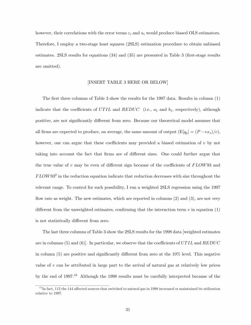
however, their correlations with the error terms εi and ui would produce biased OLS estimators.

Therefore, I employ a two-stage least squares (2SLS) estimation procedure to obtain unbiased

estimates. 2SLS results for equations (34) and (35) are presented in Table 3 (first-stage results

are omitted).

[INSERT TABLE 3 HERE OR BELOW]

The first three columns of Table 3 show the results for the 1997 data. Results in column (1)

indicate that the coefficients of UTIL and REDUC (i.e., a1 and b1, respectively), although

positive, are not significantly different from zero. Because our theoretical model assumes that

all firms are expected to produce, on average, the same amount of output (E[qp] = (P−vxs)/c),

however, one can argue that these coefficients may provided a biased estimation of v by not

taking into account the fact that firms are of different sizes. One could further argue that

the true value of v may be even of different sign because of the coefficients of FLOW93 and

FLOW932 in the reduction equation indicate that reduction decreases with size throughout the

relevant range. To control for such possibility, I run a weighted 2SLS regression using the 1997

flow rate as weight. The new estimates, which are reported in columns (2) and (3), are not very

different from the unweighted estimates, confirming that the interaction term v in equation (1)

is not statistically different from zero.

The last three columns of Table 3 show the 2SLS results for the 1998 data [weighted estimates

are in columns (5) and (6)]. In particular, we observe that the coefficients of UTIL andREDUC

in column (5) are positive and significantly different from zero at the 10% level. This negative

value of v can be attributed in large part to the arrival of natural gas at relatively low prices

by the end of 1997.45 Although the 1998 results must be carefully interpreted because of the

45 In fact, 112 the 144 affected sources that switched to natural gas in 1998 increased or maintained its utilizationrelative to 1997.

31

apparently slack cap, they prove to be useful to illustrate the estimation of ∆ps when v is

different than zero, as we shall see next.

We can now use the value of v to obtain an estimate for the remaining parameters of the

model, and hence, for ∆ps. Following the 1997 econometric results, let us consider first the case

in which v = 0. When this is the case, we have that h = cReq/P from (16), Req = kE[xp] from

(12), and P = cE[qp] from (13). Replacing the 1997 (weighted) statistics for E[xp] = 0.203 and

E[qp] = 0.631 in the expression for h, (33) reduces to

∆ps|97,v=0 =k

2Var[rp]− kE[xp]

E[qp]Cov[rp, qp] = (0.1055− 0.0084)k = 0.097k

These numbers not only indicate that the permits policy is welfare superior to an equivalent

standards policy but more importantly, that the welfare loss from higher emissions is only 8%

of the welfare gain from cost savings.

Based on the 1998 results contained in column (5) of Table 3, let us consider now the case

in which v < 0. Normalizing v to −a (where a is some positive number), from the coefficients

of UTIL and REDUC we obtain, respectively, k = 1.86a and c = 15.87a (which in turn,

yields Λ = 28.52a2). In addition, by simultaneously solving (12) and (13) for P and Req withE[xp] = 0.466 and E[qp] = 0.669, we get P = 10.15a and Req = 0.20a that replaced into (16)

gives h = 0.31a. Plugging these numbers and the corresponding statistics into (33), we finally

obtain ∆ps|98,v<0 = (0.0503− 0.0016)a = 0.049a. This result, while qualitatively similar to the

1997 result, shows an even smaller welfare loss from higher emissions –only 3% of the welfare

gain from cost savings.

32

5.5 Gains from a hybrid policy

To explore the design of and the gains from implementing a hybrid policy, we need, in addition

to the previous parameters, some idea about the properties of the cumulative joint distribution

F (α, β, γ). Since we cannot recover F (α, β, γ) from the data, I will simply estimate σ =

(σα, σβ, σγ) and ρ = (ραβ, ραγ , ρβγ) and then impose a multinomial distribution of 12 types

consistent with such estimates.46 Values for σ and ρ are obtained by simultaneously solving

Var[xp], Var[rp], Var[qp], Cov[xp, rp], Cov[xp, qp] and Cov[rp, qp] (see, e.g., eqs. (30) and (31)).

The solution is of the form σ(c, k, v) and ρ(c, k, v) that combined with the previous estimates

of c, k and v allows us to obtain σ = (σα, σβ, σγ) and ρ = (ραβ, ραγ , ρβγ). Note that if v = 0, σ

remains a function of k and c, which cannot be independently estimated. Conversely, if v 6= 0,

we can leave σ and all the other parameters of the model (i.e., k, c, P and h) as a function of v,

as we did in the previous section for the 1998 numbers. Thus, instead of choosing any arbitrary

combination of k and c, I use the results of column (2) of Table 3 and set c/k = 25.35 for 1997.

The results for 1997 are σ/k = (0.63, 8.48, 0.60) and ρ = (−0.04,−0.72,−0.08), and for 1998

are σ/a = (0.63, 5.34, 1.29) and ρ = (0.11,−0.90,−0.39), where a = −v. Looking at Figure 1

and the 1997 numbers (v = 0 and ρβγ < 0), there seems to be room, although little, for extra

benefits from the hybrid policy.47 However, the heterogeneity in counterfactual emission rates

and the negative correlation between α and γ (consistent with the coefficient of EMRTE93)

shift the line h=p in Figure 1 to the right leaving the cost structure of the TSP firms within

the region in which the hybrid policy converges to the permits policy.48 I also find for 1998

46The types are (α, β, 0), (α, β, 0),..., (0, β, γ). If anything this distribution would favor the introduction of ahybrid policy because it puts more weight on extreme combinations of α, β and γ.47 In fact, if we impose σα = 0, and hence ραβ = ραγ = 0, the hybrid policy design is r

hs = 1.62 (or 153 mg/m

3)and Rheqh = 0.97Req (the equivalent standards is rs = 0.88) and the increase in net benefits over ∆ps is less than1%.48A negative ραγ reduces the advantages of introducing a standard because many of the sources that are

supposed to be hit by the standard (those with high α) are likely to be already reducing under the permits-alonepolicy.

33

that the hybrid policy converges to the permits-alone policy.

6 Conclusions

I have developed a model to study the design and performance of pollution markets (i.e.,

tradable permits) when the regulator has imperfect information on firms’ emissions and costs.

A salient example is the control of air pollution in large cities where emissions come from many

small (stationary and mobile) sources for which continuous monitoring is prohibitely costly. In

such a case the cost-savings superiority of permits over the traditional command and control

approach of setting technology and emission standards is no longer evident. Since the regulator

only observes a firm’s abatment technology but neither its emissions nor its output (utilization),

permits could result in higher emissions if firms doing more abatement are at the same time

reducing output relative to other firms and/or if more highly utilized firms find it optimal

to abate relatively less. Because of this trade-off between cost savings and possible higher

emissions, I also examined the advantages of a hybrid policy that optimally combines permits

and standards. I found that in many cases the hybrid policy converges to the permits-alone

policy but it almost never converges to the standards-alone policy.

Having studied the theoretical advantages of pollution markets (whether alone or in com-

bination with a standard), I then used emissions and output data from Santiago-Chile’s TSP

permits program to explore the implications of the theoretical model. I found that the produc-

tion and abatement cost characteristics of the sources affected by the TSP program are such

that the permits policy is welfare superior. The estimated cost savings are only partially offset

(about 8%) by a moderate increase in emissions relative to what would have been observed

under an equivalent standards policy. In addition, I found no gain from implementing a hybrid

policy for this particular group of sources.

34

Since sources under the TSP program are currently responsible for less than 5% of total

TSP emissions in Santiago, the model developed here can be used to study how to expand

the TSP program to other sources of TSP that today are subject to command and control

regulation. A good candidate would be powered-diesel buses which are responsible for 36.7% of

total TSP emissions. According to Cifuentes (1999), buses that abate emissions by switching

to natural gas are likely to reduce utilization relative to buses that stay on diesel and that

older-less utilized buses are more likely to switch to natural gas. In the understanding that

switching to natural gas is a major abatement alternative, both of these observations would

suggest that the optimal way to integrate buses to the TSP program is by imposing, in addition

to the allocation of permits, an emission standard specific to buses. It may also be optimal

to use different utilization factors (eq) for each type of source. These and related design issuesdeserve further research.

References

[1] Cifuentes, L. (1999), Costos y beneficions de introduccir gas natural en el transporte público

en Santiago, mimeo, Catholic University of Chile.

[2] Dasgupta, P., P. Hammond and E. Maskin (1980), On imperfect information and optimal

pollution control, Review of Economic Studies 47, 857-860.

[3] Ellerman, A.D, P. Joskow, R. Schmalensee, J.-P. Montero and E.M. Bailey (2000), Markets

for Clean Air: The U.S. Acid Rain Program, Cambridge University Press, Cambridge, UK.

[4] Fullerton, D. and S.E. West ( 2002), Can taxes on cars and on gasoline mimic an unavailable

tax on emissions?, Journal of Environmental Economics and Management 43, 135-157.

35

[5] Hahn, R.W., S.M Olmstead and R.N. Stavins (2003), Environmental regulation in the

1990s: A retrospective analysis, Harvard Environmental Law Review 27, 377-415.

[6] Harrison, David Jr. (1999), Turning theory into practice for emissions trading in the Los

Angeles air basin, in Steve Sorrell and Jim Skea (eds), Pollution for Sale: Emissions

Trading and Joint Implementation, Edward Elgar, Cheltenham, UK.

[7] Holmström, B. (1982), Moral hazard in teams, Bell Journal of Economics 13, 324-340.

[8] Kwerel, E. (1977), To tell the truth: Imperfect information and optimal pollution control,

Review of Economic Studies 44, 595-601.

[9] Lewis, T. (1996), Protecting the environment when costs and benefits are privately known,

RAND Journal of Economics 27, 819-847.

[10] Montero, J.-P., J.M. Sánchez, R. Katz (2002), A market-based environmental policy ex-

periment in Chile, Journal of Law and Economics XLV, 267-287.

[11] Roberts, M. and M. Spence (1976), Effluent charges and licenses under uncertainty, Journal

of Public Economics 5, 193-208.

[12] Schmalensee, R, P. Joskow, D. Ellerman, J.P. Montero, and E. Bailey (1998), An interim

evaluation of sulfur dioxide emissions trading, Journal of Economic Perspectives 12, 53-68.

[13] Segerson, K. (1988), Uncertainty and incentives for nonpoint pollution control, Journal of

Environmental Economics and Management 15, 87-98.

[14] Spulber, D. (1988), Optimal environmental regulation under asymmetric information,

Journal of Public Economics 35, 163-181.

36

[15] Stavins, R. (2003), Experience with market-based environmental policy instruments, in

Handbook of Environmental Economics, Karl-Göran Mäler and Jeffrey Vincent eds., Am-

sterdam: Elsevier Science.

[16] Tietenberg, T (1985), Emissions Trading: An Exercise in Reforming Pollution Policy,

Resources for the Future, Washington, D.C.

[17] Weitzman, M. (1974), Prices vs quantities, Review of Economic Studies 41, 477-491.

Appendix: Proof of Proposition 2

The proof is divided in four parts. The first three parts demonstrate that there exist several

combinations of v and ρ for which the hybrid policy converges to the permits-alone policy (note

that a more general proof would require specifying F (β, γ), but this, in turn, would make the

proof particular to the specified distribution function). Part 1 demonstrates so for v = ρ = 0.

Part 2 demonstrates that for v = 0 and ρ 6= 0, the hybrid policy converges to the permits-

alone policy only if ρ > 0. Part 3 demonstrates that for v 6= 0 and ρ = 1, the hybrid policy

always converges to the permits-alone policy if v < 0 but not necessarily so if v > 0. Part 4,

which finishes the proof, demonstrates that for ρ = −1 and some values of v the hybrid policy

converges to the standards-alone policy if −γ/β < (h− v)/c.

Part 1. For ρ = 0, F (β, γ) can be expressed as F β(β)F γ(γ) where F β and F γ are in-

dependent cumulative distribution functions for β and γ respectively (fβ and fγ are their

corresponding probability density functions). Thus, when v = ρ = 0, bγ is independent of β andthe first order conditions (28) and (29) become, respectively

Z β

β

hhqhp −RheqhiF γ(bγ)fβdβ ≤ 0 (36)

37

Z β

β

Z γ

bγh−kxhs − γ + hqhs

ifβ(β)fγ(γ)dγdβ ≤ 0 (37)

where qhp = qhs = (P−β)/c. Before solving for Rheqh and xhs , note that from first order condition(11) we have that −kxhp − γ + Rheqh = 0 for γ ≤ bγ and that −kxhs − γ + Rheqh < 0 for γ > bγ(otherwise the standard would not be binding). Since (36) cannot be positive, its solution yields

Rheqh = Ph/c = Req (see (16)). On the other hand, developing (37) we obtainZ γ

bγ·−kxhs − γ +

Ph

c

¸fγ(γ)dγ ≤ 0

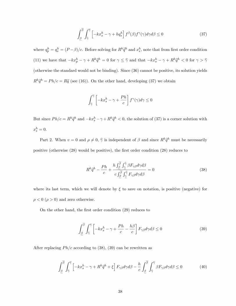
But since Ph/c = Rheqh and −kxhs −γ+Rheqh < 0, the solution of (37) is a corner solution withxhs = 0.

Part 2. When v = 0 and ρ 6= 0, bγ is independent of β and since Rheqh must be necessarilypositive (otherwise (28) would be positive), the first order condition (28) reduces to

Rheqh − Ph

c+

hR ββ

R bγγ βFγβdγdβ

cR ββ

R bγγ Fγβdγdβ

= 0 (38)

where its last term, which we will denote by ξ to save on notation, is positive (negative) for

ρ < 0 (ρ > 0) and zero otherwise.

On the other hand, the first order condition (29) reduces to

Z β

β

Z γ

bγ·−kxhs − γ +

Ph

c− hβ

c

¸Fγβdγdβ ≤ 0 (39)

After replacing Ph/c according to (38), (39) can be rewritten as

Z β

β

Z γ

bγh−kxhs − γ +Rheqh + ξ

iFγβdγdβ − h

c

Z β

β

Z γ

bγ βFγβdγdβ ≤ 0 (40)

38

where its last term (without the negative sign in front) has the exact opposite sign of ξ. Now,

from condition (11) we know that −kxhs − γ + Rheqh < 0 for γ > bγ, so if ρ < 0 there must

be an interior solution (i.e., xhs > 0) because ξ is positive. To see this, let us imagine we

increase the standard xhs from cero to the point where we reach the very first firm for which

there is no difference between complying with the standard and buying permits. At this point

−kxhs − γ + Rheqh = 0 but ξ > 0, so condition (40) would be positive. It would be beneficial

then to increase xhs a bit further until (40) reaches cero. Conversely, if ρ > 0, ξ is negative, so

the solution of (40) is indeed a corner solution with xhs = 0.

Part 3. When v 6= 0 and ρ 6= 0, it is useful to first to express qhp (Rheqh, β, γ), xhp(Rheqh, β, γ)and qhs (x

hs , β) according to (7), (12) and (13) (simply add the superscript “h”) and then sub-

stitute them into (28) and (29) to obtain, respectively, the first order conditions

Z β

β

Z bγ(β)γ

·(Req −Rheqh)µΛ+ 2hv

Λ

¶+2hv

Λγ − h(ck + v2)

cΛβ

¸Fγβdγdβ ≤ 0 (41)

Z β

β

Z γ

bγ(β)·(xs − xhs )

µΛ+ 2hv

c

¶− γ − (h− v)

cβ

¸Fγβdγdβ ≤ 0 (42)

To demonstrate now that the hybrid policy converges to the permits-alone policy if ρ = 1 and

v < 0, it is sufficient to show that the extra benefits from introducing xhs > 0 that is just binding

for a marginal firm are negative when Rheqh = Req. For ρ = 1 and v < 0, the cost parameters of

the marginal firm are β > 0 and γ > 0 and the extra benefits are (from (42))

(xs − xhs )

µΛ+ 2hv

c

¶− γ − (h− v)

cβ (43)

Since this marginal firm is indifferent between permits and standards, i.e., bγ(β) = γ, we have

39

from (24) that

γ =v

cβ − Λ

cxhs +Req − Pv

c(44)

We also know from (9) and (16) that Reqc = xsΛ+ Pv. Using this to substitute Req into (44),we obtain an expression for xs − xhs that replaced into (43) leads to

2hv

Λγ − h(ck + v2)

cΛβ < 0 (45)

which demonstrates that the extra benefits are negative.

For ρ = 1 and v > 0, on the other hand, the marginal firm is still (β, γ) and the extra benefits

are also given by (45). But because v > 0, these extra benefits can now be either negative or

positive, in which case it is optimal to implement a hybrid policy with xhs > 0 (using a similar

procedure , it can be demonstrated that when ρ = 1, the authority always wants to use some

permits).

Part 4. Let us now demonstrate that the hybrid policy may converge to the standards-alone

policy for ρ = −1 and some values of v.49 As analogous to Part 3, this will be the case if the

extra benefits from introducing Rheqh > 0 that is just binding for a marginal firm are negative

when xhs = xs. When ρ = −1, the cost parameters of the marginal firm are β > 0 and γ < 0

and the extra benefits are (from (41))

(Req −Rheqh)µΛ+ 2hvΛ

¶+2hv

Λγ − h(ck + v2)

cΛβ (46)

Following the same procedure as in Part 3 to obtain an expression for Req−Rheqh, (46) reducesto −γ − (h− v)β/c, which is negative (and hybrid policy converges to standards-alone policy)

if −γ/β < (h− v)/c.¥

49Note that to work with interior solutions v cannot be any arbitrary value.

40

TABLE 2. Summary statistics for all affected sources: 1993–1999. Variable 1993 1995 1996 1997 1998 1999No. of sources Existing 635 578 504 430 365 365 New 45 112 127 146 221 208 Total Affected 680 690 631 576 566 573

Flow rate (m3/h) Average 4,910.7 4,784.1 4,612.6 4,062.1 4,213.9 4,146.6 Standard dev. 15,058.8 14,908.0 15,490.9 9,498.6 13,091.0 11,793.5 Max. 261,383.9 261,304.7 261,304.7 182,843.0 207,110.6 183,739.5 Min. 499.2 204.3 204.3 493.3 216.9 165.6

Emission rate (mg/m3)

Average 94.9 83.1 78.5 54.7 31.1 27.8 Standard dev. 88.1 77.8 76.8 43.0 21.1 18.5 Max. 702.0 698.2 674.0 330.7 110.0 108.2 Min. 1.5 1.5 3.4 3.6 2.9 4.6 Utilization (%)* Average 39.4 48.0 47.1 49.2 51.7 53.7 Standard dev. 30.3 31.5 31.7 31.8 32.0 32.3 Max. 100 100 100 100 100 100 Min. 0 0 0 0 0 0 No. of obs. 278 463 457 499 543 542

Total proxied- emissions (kg/day)

7,051.9 6,320.9 5,094.4 3,535.0 1,975.3 1,665.0

Total permits (kg/day)

4,604.1 4,604.1 4,604.1 4,087.5 4,087.5 4,087.5

Source: Elaborated from PROCEFF’s databases * An utilization of 100% corresponds to 24 hrs of operation during 365 days a year. As indicated by the No. of observations, utilization figures are not based on all sources (recall that information on utilization is not required for monitoring and enforcement purposes).

Figure 2: Table 2

41

TABLE 3. 2SLS estimates for the reduction and utilization equations Independent Variables (1) (2) (3) (4) (5) (6) Reduction Equation UTIL 0.078 0.137 0.087 0.256* 0.539* 0.308 (0.153) (0.175) (0.175) (0.132) (0.309) (0.322) FLOW93 -0.789** -0.788*** -0.937*** -1.090*** (0.330) (0.275) (0.345) (0.422) FLOW932 0.270** 0.271** 0.346*** 0.373** (0.131) (0.111) (0.129) (0.151) ln(FLOW93) -0.088*** -0.093*** (0.032) (0.031) EMRTE93 0.741*** 0.717*** 0.698*** 0.987*** 0.944*** 0.940*** (0.094) (0.115) (0.116) (0.019) (0.039) (0.035) ENDPIPE -0.058 -0.191 -0.027 -0.128 -0.032 0.182 (0.198) (0.251) (0.140) (0.083) (0.100) (0.129) INDUST -0.008 0.079 0.120 0.014 -0.031 0.023 (0.077) (0.149) (0.153) (0.042) (0.061) (0.056) STATE -0.137 -0.193** -0.193** -0.105** -0.083 -0.118 (0.106) (0.084) (0.082) (0.050) (0.077) (0.074) Constant -0.390*** -0.474*** 0.217 -0.420*** -0.512*** 0.272 (0.075) (0.116) (0.201) (0.050) (0.115) (0.211) Utilization Equation REDUC -0.003 0.005 -0.017 0.012 0.063* 0.054 (0.030) (0.032) (0.039) (0.029) (0.035) (0.039) UTIL93 0.560*** 0.567*** 0.532*** 0.364*** 0.313*** 0.275*** (0.055) (0.064) (0.061) (0.064) (0.093) (0.089) FLOW93 0.401*** 0.384*** 0.416 0.417*** (0.130) (0.096) (0.267) (0.129) FLOW932 -0.095** -0.087*** -0.101 -0.098** (0.048) (0.033) (0.101) (0.045) ln(FLOW93) 0.078*** 0.090*** (0.012) (0.011) INDUST 0.069* 0.038 0.022 0.141*** 0.077 0.044 (0.037) (0.045) (0.049) (0.044) (0.057) (0.057) STATE -0.077* -0.042 -0.038 -0.039 -0.117** -0.098* (0.045) (0.045) (0.043) (0.058) (0.051) (0.055) Constant 0.158*** 0.182*** -0.407*** 0.221*** 0.293*** -0.376*** (0.034) (0.045) (0.100) (0.042) (0.057) (0.090) No. Obs. 344 344 344 288 288 288 Notes: First-stage results are omitted. White corrected standard errors are in parenthesis. Columns (2), (3), (5) and (6) present weighted estimates (the 1997 flow rate is the weight in (2) and (3) and the1998 flow rate in (5) and (6)) * significant at 10%, ** significant at 5%, *** significant at 1%

Figure 3: Table 3

42