On the Nonlinear Chernical Dynamics of the Imperfectly Mixed CSTR

Fathei M. Ali

A thesis submitted in conformity with the requirements

for the degree of Doctor of Phiiosophy

Graduate Department of Chemistry

University of Toronto

@Copyright by Fathei M. Ali (1998)

National Library Bibliottièque nationaie du Canada

Acquisitions and Acquisitions et Bibliographie Services senrices bibliographiques

395 Wenington Street 395, rue Welligton OüawaON KIA W OttawaON K 1 A W Canada canada

The author has granted a non- L'auteur a accordé une licence non excIusive licence dlowing the exclusive permettant à la National Library of Canada to Bibliothèque nationale du Canada de reproduce, loan, distriiute or sell reproduire, prêter, distribuer ou copies of this thesis in microform, vendre des copies de cette thèse sous paper or electronic formats. la forme de microfiche/nlm, de

reproductioii sur papier ou sur format électronique.

The author retains ownership of the L'auteur conserve la propriété du copyright in this thesis. Neither the droit d'auteur qui protège cette thèse. thesis nor substantial extracts fiom it Ni la thése ni des extraits substantie1s may be printed or otheIUrise de celle-ci ne doivent être imprimés reproduced without the author's ou autrement reproduits sans son permission. autorisation.

ABSTRACT

On the Nonlinear Chernical Dynamics of the Imperfectly

Mixed CSTR

-4 dissertation presented to the Graduate Department of Chemistv at the

University of Toronto. Toronto, Canada.

In partial fulfilrnent for the degree of Doctor of Philosophy

Fathei M. Ali , 1998

This t hesis =amines the role of spatial inhomogeneity in rapidly reacting flcws wit h nonlinear

kinetics. P henomenologicai rnodelling, theoretical considerat ions, and experirnents are combined

to relate the mixing-induced spatial inhomogeneity in the continuously-fed stirred tank reactor

(CSTR) to the macroscopica.iiy observed stirring and mixing effects (e-g. shift of steady states,

bifurcation points. and modification of induction periods and oscillation attributes).

The interaction among flow, mixing, and chernical reaction in a CSTR is examined in detail

for two simple reactions: birnolecular and cubic autocatalysis. The stirring effects for premked

and nonpremixed feedstreams are shown to ciiffer qualitatively due to age- and stream-mktcing.

For a generai one-variable kinetic model, the random coalescence-redispersion (RCR) model

is reduced to a Langevin equation in which the mixing-induced fluctuating term is a multiplica-

tive colored noise process. The anaiysis of the equation leads to a closed-fonn solution for the

inhomogeneous stochastic steady states of the reactor. The shift of steady states from tbeir

deterministic values is proportional to the reactor inhomogeneity where the proportionality con-

stant is expiicitly reiated to the rate function. The validity of the RCR mode1 (simuiations and

theoretical analysis) is demonstrated by cornparisons with experiments on the iodate-arsenous

acid reaction.

The information content of signais is shown to depend on the size of the sarnpling voIume

of the detector: fluctuations in micredetector signak measuse the spatial inhomogeneity of the

reactor. whereas fluctuations in macro-detector signais reflect the Iong range coUectiver temporal

dynamics of the reactor. Their quantitative relationship is given,

For the osciiiating Belousov-Zhabotinskii (BZ) reaction, RCR-based simuiations are used to

obtain the time-dependent probability distribution, which is a measure of the spatial reactor

inhomogeneity, and to dernonstrat e its dramatic dependence on osciliation phase. The notion

of locai stabiIity of limit cycIes is elaborated. Local stability is shown to play a key role in

detennining the phase dependence of spatial inhomogeneity.

To my parents

Acknowledgement

I wish to express my sincere appreciation to my research supervisor, Professor .Michad

Slenzinger for his guidance, patience and most of a,li for his fiiendship and camaraderie. My

appreciations are &O extended to Dr. Peter Strizhak, Dr. Vladimir Yakhnin. Dr. -4rkady

Rovinsky, Sebastian Weissenberger and Mads Kaern for hundreds of hours of invaluable discus-

sions. 1 am also grateful to the University of Toronto School of Graduate Studies for several

-'Open FelIowships" and to Professor Menzinger for Research Assistanship support.

Contents

1 Introduction 1

. . . . . . . . . . . . . . . . . . . . . . . . . . . . . . . . . . . . . . . . . . . . . . . . 1.1 Background 1

. . . . . . . . . . . . . . . . . . . . . . . . . . . . . . . . . . . . . . . . . . . . . . . 1.2 Organization 3

2 Review of experimental resutts 5

. . . . . . . . . . . . . . . . . . . . . . . . . . . . . . . . . . . . 2.1 The shift of bistability hysteresis 6

2.2 Mixingrnode . . . . . . . . . . . . . . . . . . . . . . . . . . . . . . . . . . . . . . . . . . . . . . . 7

2.3 Clock reactioas: induction periods . . . . . . . . . . . . . . . . . . . . . . . . . . . . . . . . . . . 8

2.4 The effects of stirring on oscillations . . . . . . . . . . . . . . . . . . . . . . . . . . . . . . . . . . 3

. . . . . . . . . . . . . . . . . . . . . . . . . . . . . . . . . . . . . . . . . . . . . . . . 2.5 Fluctuations 1 1

Mixing 14

. . . . . . . . . . . . . . . . . . . . . . . . . . . . . . . . . . . . . . . . . . . . . . . 3.1 Slacromixing 16

. . . . . . . . . . . . . . . . . . . . . . . . . . . . . . . . . . . . . . . 3.1.1 hlacromixing modeis 18

. . . . . . . . . . . . . . . . . . . . . . . . . . . . . . 3.1.1.1 Recycle plug flow model 18

. . . . . . . . . . . . . . . . . . . . . . . . . . 3.1.1.2 Axially dispersed plug flow rnodel 18

. . . . . . . . . . . . . . . . . . . . . . . . . . . . . . . . 3.1.1.3 Coupled reactor models 18

. . . . . . . . . . . . . . . . . . . . . . . . . 3.1.2 .C fodelling macrornixing in nonlinear reactions 19

. . . . . . . . . . . . . . . . . . . . . . . . . . . . . . . . . . . . . . . . . . . . . . . . 3.2 SIicromixing 20

. . . . . . . . . . . . . . . . . . . . . . . . . . . . . . . . . . . . . . . 3.2.1 Sticromixing rnodelç 2L

. . . . . . . . . . . . . . . . . . . . . . . . . . . . . . . . . . . . . 3.2.1. 1 Formal modeis 21 . . . . . . . . . . . . . . . . . . . . . . . . . . . . . . . . . . 3.2. t -2 Agglornerate rnodelç 21

. . . . . . . . . . . . . . . . . . . . . . . . . . . . . . . . . . . . 3.2.L.3 Detailedmodels: 23

3 - 2 2 Micrornixing simulations in nonlinear reactionç . . . . . . . . . . . . . . . . . . . . . . . . 23

4 Interaction of flow. mixing. and chemistry 24

. . . . . . . . . . . . . . . . . . . . . . . . . . . . . . . . . . . . . . . . . . 4.1 Bimolecular reactions 28 . . . . . . . . . . . . . . . . . . . . . . . . . . . . . . . . . . . 4.1.1 The perfect mixing limit 28

. . . . . . . . . . . . . . . . . . . . . . . . . . . . . . . . . 4.1.2 The cornpiete segregation limit 29

. . . . . . . . . . . . . . . . . . . . . . . . . . . . . . . . . . . . . . 4.1.3 In~errnediate mixing 29

. . . . . . . . . . . . . . . . . . . . . . . . . . . . . . . . . . . . . . 4.1.4 Reactornonuniformity 33

. . . . . . . . . . . . . . . . . . . . . . . . . . . . . . . . . . . . . . . . . . . 4.2 Cubic autocatalysis 38

. . . . . . . . . . . . . . . . . . . . . . . . . . . . . . . . . . . . . . . . . 4.2.1 Induction period 39

. . . . . . . . . . . . . . . . . . . . . . . . . . . . . . . . . . . . . . . 4.2.2 Bistability hysteresis 4 1

4.2.3 Reactor inhomogeneities and fluctuat;ons . . . . . . . . . . . . . . . . . . . . . . . . . . . 44

4.3 Oscillations in the Gray-Scott reaction . . . . . . . . . . . . . . . . . . . . . . . . . . . . . . . . . 44

5 A stochastic descript ion of CSTR bistabiiity 47

. . . . . . . . . . . . . . . . . . . . . . . . . . . . . . . . . . . 5.1 The coalescence-redispersion mode1 48

5.1.1 The random codescence-redispersion (RCR) mode1 . . . . . . . . . . . . . . . . . . . . . . 19

. . . . . . . . . . . . . . 5.1.2 Heuristic derivation of the Langevin equation for the RCR mode1 50

. . . . . . . . . . . . . . . . . . . . . . . . . . . . . . . 5.1.3 Anaiysis of the Langevin equation 53

5.2 Mixing e f k t s . . . . . . . . . . . . . . . . . . . . . . . . . . . . . . . . . . . . . . . . . . . . . . . 55

. . . . . . . . . . . . . . . . . . . . . . . . . . . . . . . . 5.2.1 The iodate-arsenous acid system 56

. . . . . . . . . . . . . . . . . . . . . . . . . . . . . . . . . . . . . . . . . . 5.2.2 Experirnents 57

. . . . . . . . . . . . . . . . . . . . . . . . . . . . . . . . . . . . . . . . 5.2.2.1 Procedure 57 5.2.2.2 ResuIts . . . . . . . . . . . . . . . . . . . . . . . . . . . . . . . . . . . . . . . . . 38

. . . . . . . . . . . . . . . . . . . . . . . . . . . . . . . . . . . . . . . 5.2.3 Simulation results 60 . . . . . . . . . . . . . . . . . . . . . . . . . . . . . . . . . . . . . . . . 5.2.4 Xnaiytical resulu 63

. . . . . . . . . . . . . . . . . . . . . . . . . . . . . . . . . . . . . . . . . . . . .3. 2.5 Discussion 65

. . . . . . . . . . . . . . . . . . . . . . . . . . . . . . . . . . . . . . . . . . 5.3 Tempord fluctuations 69

. . . . . . . . . . . . . . . . . . . . . . . . . . . . . . . . . . . 5.3.1 Local v~ . giobd fluctuations 69

. . . . . . . . . . . . . . . . . . . . . . . . . . . . . . . . . . . . . . . 5.3.2 Cnticai fluctuations 74 . . . . . . . . . . . . . . . . . . . . . . . . . . . . . . . . . . . . . . . . . . . . . 5.3.3 Discussion 76

6 Phase-dependent sensitivity of Iimit cycles 78

. . . . . . . . . . . . . . . . . . . . . . . . . . . . . . . . . . . . 6-1 Local (in)stability of limit cycIes 78

. . . . . . . . . . . . . . . . . . . . . . . . . . . . . . . . . . . . 6.1.1 Measures of local stability 80

. . . . . . . . . . . . . . . . . . . . . . . . . . . . . . . . . . . . . . . . . . . . . . 6.1.2 Results d4

. . . . . . . . . . . . . . . . . . . . . . . . . . . . . 6.1.2.1 The generalized BvdP mode] 84

. . . . . . . . . . . . . . . . . . . . . . . . . . . . . . . . . . . 6.1.22 Hopf bifurcation 85

6.1.2.3 Saddle-node bifurcation . . . . . . . . . . . . . . . . . . . . . . . . . . . . . . . 87

. . . . . . . . . . . . . . . . . . . . . . . . . . . . 6.1.2.4 Period iengthening bifurcations 91

. . . . . . . . . . . . . . . . . . . . . . . . . . . . . . . . . . . . 6.1.2.5 Period doubling 92

. . . . . . . . . . . . . . . . . . . . . . . . . . . . . . . . . . . . . . . . . . . . 6-13 Discussion 93

6.2 Phase dependent fluctuations . . . . . . . . . . . . . . . . . . . . . . . . . . . . . . . . . . . 94

. . . . . . 62.1 The fiow-Oregonator . . . . . . . . . . . . . . . . . . . . . . . . . . . . 94

6.2.2 Results . . . . . . . . . . . . . . . . . . . . . . . . . . . . . . . . . . . . . . . . . . 95

6.2.2.1 Time-dependent probability density . . . . . . . . . . . . . . . . . . . . . . . . . . 9.5

6.2.2.2 Stirring effects . . . . . . . . . . . . . . . . . . . . . . . . . . . . . . . . 93

7 Surnrnary and conclusions 102

A A primer on nonlinear chernical dynamics

X.1 Chernical Dynamical systems . . . . . . . . . . . . . . . . . . . . . . . . . . . . . . . . . . . . . . . . . . . . . . . . . . . . . . . . . . . . . . . . . . . . . . . . . . . . . . . . . . A.1.1 The CSTR

A.2 Dynarnical Systems . . . . . . . . . . . . . . . . . . . . . . . . . . . . . . . . . . . . . . . . . . .

A.L.1 Stability .anal .ais . . . . . . . . . . . . . . . . . . . . . . . . . . . . . . . . . . . . . . . .

. . . . . . . . . . . . . . . . . . . . . . . . . . . . . . . . A.2.1.1 Stability of fixed points

A.2.1.2 Stability of lirnit cycles . . . . . . . . . . . . . . . . . . . . . . . . . . . . . . . .

A.3 Xumerical Analysis . . . . . . . . . . . . . . . . . . . . . . . . . . . . . . . . . . . . . . . . . . . . X.3.1 Integration of ODE Systems . . . . . . . . . . . . . . . . . . . . . . . . . . . . . . . . . . . X.3.2 Continuation methods . . . . . . . . . . . . . . . . . . . . . . . . . . . . . . . . . . . . . .

Chapter 1

Introduction

Background

The theoretical description of chernical reactions in open systems usually falls into one of two

categories. In stirred systems, the medium is taken to be spatidy uniforrn and a set of ordi-

nary differential equations is used to describe, as in classical chernical kinetics, the macroscopic

behavior of the system. In the absence of stirring, the spatiotemporal evolution is describecl

by reaction-diffusion equations. Experimental studies on the effect of mixing on chemical dy-

namics, carried out over the last two decades, have clearly demonstrated that stirred reactive

systems should be viewed as intermediates between the asymptotic Limits of perfectly mived and

unst irred reaction-diffusion syst ems.

The study of stirring and muMg effects2s-107 has shown that the dynamics of noniinear re-

actions may depend sensitively on inhomogeneities that sunrive the mixing process. The rate

of stirring and the mixing mode (e.g. premked or nonpremived feed streams) affect steady

state concentrations, bifurcation points, oscillation attributes and the amplitude of concentra-

tion fluctuations in the reactor. These effects on the dynamics arise fiom the dependence of

macroscopic reaction rates on the spatial nonunifonnity in the reactor.

Alt hough considerable effort is devoted by chemicai engineers to eiixninat ing inhomogeneities

in chemical reactors, the study of the origins, nature and consequences of inhomogeneities is

important for two reasons. First, perfect mixing is an ideal limit that is not achieved in practice

and spatial inhomogenei ties are facts of industriai and biological systems. Second, alt hough some

reactors might approach the homogeneous limit, when cornplex systems are involved, even small

deviations from ideality can lead to considerable quantitative and qualitative consequences.

Our unders tanding of chemical dynamical systems depends on the correct interpretation of

experirnental observations. Furthermore, the study of the dynamics of inhomogeneous nonlinear

C W T E R 1. INTRODUCTION

reactions may have implications in other fields. In classical chemicai kinetics, reacting systems

are considered homogeneous and little is known quantitat idy about the dependence of rates of

arbitraq reactions on mïxhg-induced noise. The nonUIilformity of reacting media modifies the

rates of nonlinear processes. For instance, it has been suggested recently that inhomogeneity

may play a role in the rate of ozone destruction in the polar s t r a t ~ s ~ h e r e s ~ ~ * ~ ~ , and in the

increase of spatial biomass production of ecotogicai process92.

The study of the effect of inhomogeneities and fluctuations on the dynarnics of chemicai

systems has been an active subject in three areas of research, in addition to nodinear chernical

dynamics: nonequiiibrium statistical mechanics, chemicai reaction engineering, and combustion

engineering.

In nonequiiibriurn statisticai mechanics the need to include fluctuations in the description of

reactive chemical systems arose from two considerations. First, macroscopic rate equations (i.e.

mas-action laws) are mean field descriptions that ignore internai fluctuations. Second, open

and closed systems are coupled to their surroundings which constitute a source of fluctuating

forces (extemal fluctuations). An easy and widely used approach to indude fluctuations into

the description of ciparnical systems is the Langevin method where the phenomenological rate

equations are supplemented with randomly fiuctuating term(s). Usually, interna1 fluctuations

are modelled as additive noise terms with intensities that are independent of the state of the

system but inversely proportionai to the system size. Externd noise, on the other hand, is

usudy reduced to fluctuations in the system parameters and results in multiplicative (Le. state-

dependent) noise terms. The mixing-induced inhomogeneities in the CSTR are not due to

fluctuations in control parameters but arise from the turbulent or stochastic couphg of the

large number of constituent subsystems (subvolume or fluid elements) in the reactor. It will be

shown in this thesis that such inhomogeneities can be reduced to multiplicative noise terms in

the Langevin equation for the CSTR. The study of the effect of noise on dynamical systems has

led to the characterization of noiseinduced transitionss4 and the mechanisms through which

such transitions may o c ~ u r ~ ~ .

In chernical reaction engineering, the impetus to investigate the role of spatial inhomogeneities

in chemicai reactors stems from the need to assess the effects of deviations from ideai mixing

on the conversion (yield), selectivity, and quaiity of products and to determine scaie-up criteria

for industriai reactors. To simplify the complex hydrodynamics of stirred reactors, chemical

engineers have divided the mixing process into two aspects: macromixing and rnicromixing.

The first concerns macroscopic concentration gradients and nonideal residence tirne distribution.

hlicromixing addresses the continuous breakup and erosion of entering Auid elements and their

incorporation into the bulk medium on a cascade of spatial scales. Accordingly, a hierarchy

of mixing models has been developed that range from the simple coupling of ided reactors

to the detailed fluid dynamics of reactive f l o ~ s ~ ~ ~ ~ ~ ~ . The study of turbulent mixing may be

approached using the langauge of stochastic processes and of noise-induced transitions. iMixing

models may be reduced to stochastic equations whose solutions rnay exhibit qualitatively new

dynamics as the mixhg rate is changeci.

In combustion, one distinguishes between frontal combustion (i.e. flame or wave propagation)

and volumetric or continuous combustion (the reactive medium ignites uniformly) . It is the latter

type of combustion where mixing is relevant. Mixing of the fuel and oxygen/air streams and of

the bulk reaction medium are needed to maintain a self-igniting system. The role of mixing in

combustion is usudy studied in the framework of probability density function (PDF) methods

or computationd Buid dynamics (CFD). In the PDF approach, the probabiiity density

function of point-wise concentrations and temperatures are governed by balance equations with

terms for reaction, transport and turbulent mbcing. CFD involves the numerical solution of the

Xavier-S tokes equations of the turbdent reacting 0ow.

In the study of stirring and rnixing effects, the langauge of stochastic processes was used to

interpret the observed effects72-90~94 wwhile rnixing modeb were used to simulate the experimental

,,dts ~.14.32,60 . However, no clear attempt was made to establish a casual link between the

origins of inhomogeneity and their consequence. This work is an attempt at providing a common

framework to interpret the seemingly disjointed aspects of stirring and miving effects- Its airn is

not ody to interpret e-xperimentai Cindings but to predict, at least q ~ ~ t a t i v e l y , the consequences

of aonideal mixing on reaction systems. Theoretical considerations, phenornenological modeliing

and experiments are combined to provide a more unifieci view of the kinetics and dynamics of

inhomogeneous nonlinear reacting systems.

1.2 Organization

In addition to this introduction and a chapter summarizing the fiadings and conclusions of this

work, the thesis contains five chapters and an appendix. They are organized as follows:

Chapter 2 outlines the key experimental findings which led to the main questions which form

the basis for this thesis.

Chapter 3 is a review of the physical concepts of macro and micromixing that engineers have

developed to explain the nature of mking in flow reactors. Emphasis will be put on simplified

descriptions and models and not on the detailed and complex hydrodynamics. -4 particular

scheme which is chosen to model the mixing process is the random codescence-redispersion

(RCR) model.

CHAPTER 1. INTRODUCTION 4

Chapter 4 examines the interaction between simple chernical reactionç and mixhg in a CSTR.

The RCR mode1 is used to examine the stirring &kt on simple bimolecdar reactions in terms

of the relative t h e scales of fiow, mkhg and chernicd reaction. Also examined is the effect of

mixing on the bistabiiity hysteresis and on the induction period in simple cubic autocatalysis.

.A third issue is the effect of mixing on the period of Iimit cycle osciilations. The main emphasis

in this chapter is to document and understand the opposite ('antagonistic') effects of stirring in

CSTR experiments wit h premixed and nonpremixed feedstreams.

Chapter 5 treats the mWng effect on bistability hysteresis in a quantitative rnanner. The

RCR mode1 is examined in detail and, for a one-variable generic kinetic scheme, is reduced to

a Langevin equation whose solution teads to a closed-form expression for the stochastic steady

states. A relationship between the stirring effect (shift of the steady states) and the spatial

inhomogeneity of the CSTR is obtained and tested by both simulations and experiments. A

second issue that is investigated in this chapter is the comection between spatial nonuniformity

of concentrations in the reactor and the temporal fluctuations observed in experimental tirne

series. A particular issue addressed is whether the magnitude of fluctuations in the system

response grows near the bistabiiity transition. Attention is paid to the relationship between

signals obtained from local (rnicroelectrodes) and global (macroelectrodes) detectors.

Chapter 6 examines the relation between the local stability of lirnit cycles and the observed

dynamical consequences of inhomogeneities on oscillations. The first part of the chapter is used

to eiaborates the concept and rneasures of Iocai stabiiity and the second part of the chapter

is devoted to studying the dynamical consequences of inhomogeneities on limit cycles and the

role of the nonunifonnity of the Iocal stabiiity of limit cycles in detennining the degree of

concentration nonuniforrnities in a CSTR.

Xppendiv -4 gives a primer on dynamitai systems, their stability and local bifurcations. ft

also includes a section on numerical methods, including the techniques used to perform the

numerical simulations in this work.

Chapter 2

Review of experimental results

The cornmon assumptioa during the early years of the e-xperimental study of chemical instabili-

ties (late sixties to early eighties) was that stirring in a chemical reactor was sufficient to achieve

ideal m k h g in the reactor. The concentrations of chemical species in the reactor were believed

to be spatially unifonn- Based on th& belief, such systems were described in terms of a global

set of ordinary differential equations giving the rate of change of the variable concentrations in

the reactor. Although t here were some early indications t hat inhomogeneities affect oscillatory

reactions, both under batch20-28 and CSTR20*" conditions, the importace of these effects was

not cleariy appreciated until Roux et aLgO showed that the rate of stirring in a chemical reactor

can greatly iduence the dynamics of non-linear reactions when they demonstrated that the

bistabiiity hysteresis lirnits in the chlorite-iodide (CLO.,lI') reaction vary with stimng.

-4lthough chemical and combustion engineers were well aware of the role of miving on chemical

kinetics and of the importance of miving in the scale up and performance of chemical reactors,

Roux's fincihg came as a surprise to many nonlinear chemical dynamists for two reasons: (1)

the effects of stirring on the dynamics were very dramatic, and (2) the e-xperiments were carried

out a t stirring rates considered at the t h e to be sufiîcient to guarantee homogeneity.

Since Roux's =periment, a considerable amount of work has been done to study the effects

of mkuing on the dynamics of nonlinear reactions. This chapter is not meant as a complete

review of the experimental work; 1 only highlight the key experimentai findings which have led

to the work in this thesis. The results are arranged in terms of the key questions they raised.

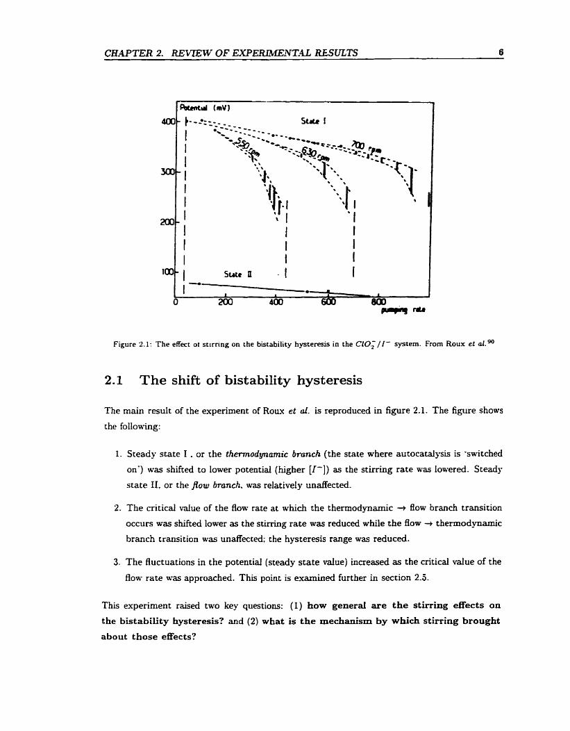
Figure 2. l: The effect or stirring on the bistability hysteresis in the CIO; / I - system. Frorn Roux et dgO

2.1 The shift of bistability hysteresis

The main result of the e-xperiment of R o u et al. is reproduced in figure 2.1. The figure shows

the following:

1. Steady state 1 . or the thennodynamic branch (the state where autocatalysis is 'switched

on') was shifted to lower potential (higher [I-1) as the stirring rate was lowered. Steady

state II. or the Pow branch. was relatively unaffecteci.

2. The critical value of the flow rate at which the thermodynamic + flow branch transition

occurs was shifted lower as the stirring rate was reduced while the flow + thermodpamic

branch transition was undected; the hysteresis range was reduced.

3. The fluctuations in the potential (steady state d u e ) increased as the critical d u e of the

flow rate was approached. This point is examined further in section 2.5.

This =periment raised two key questions: (1) how general are the stirring egects on

the bistability hysteresis? and (2) what is the mechanism by which stirring brought

about those effects?

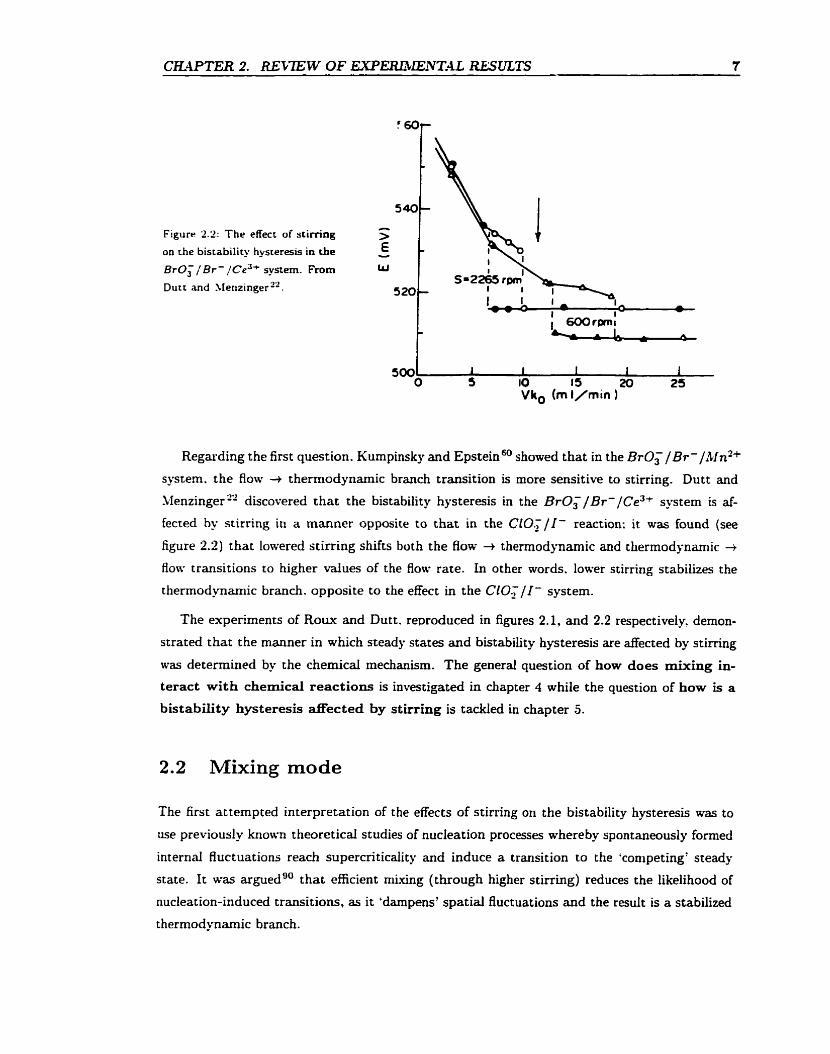
Figure 2.2: The effect of stimng

on the bistability hysteresis in the

Br03 / Br- /Ce3+ system. From

Dutt and Menzinger".

Regarding the first question. Kumpinsky and Epstein" showed that in the Br03 / B+-/hf nzf

system. the flow 4 therrnodynarnic branch transition is more sensitive to stirring. Dutt and

Menzinger2' discovered that the bistability hysteresis in the BrO;/Br-/Ce3+ system is af'-

fected by stirring in a manner opposite to that in the ClOT/ I - reaction: it was found (see

figure 2.2) that lowered stirring shifts both the flow + thermodynarnic and thermodynamic -+ flow transitions to higher values of the flow rate. Ln other words. lower stirring stabilizes the

thermodynamic branch. opposite to the effect in the CIO,/ I - system.

The experiments of R o u and Dutt. reproduced in figures 2-1, and 2.2 respectively. dernon-

strated that the manner in which steady states and bistability hysteresis are affected by stirring

was determined by the chemicai mechanism. The general question of how does rnixing in-

teract with chernical reactions is investigated in chapter 4 while the question of how is a

bistability hysteresis affected by stirring is tackled in chapter 5.

Mixing mode

The first attempted interpretation of the effects of stirring on the bistability hysteresis was to

use previously known theoretical studies of nucleation processes whereby spontaneously formed

interna1 fluctuations reach supercnticaiity and induce a transition to the 'conipeting' steady

state. It was arguedgO that efficient niking (through higher stirring) reduces the likelihood of

nucleacion-induced transitions, as it 'dampens' spatial fluctuations and the result is a stabilized

thermodynarnic branch.

-4lthough internal fluctuations may play a role in modifying the state of a chernical reactor,

further experiments have shown that nucleation can be ruleci out as a major mechanism behind

the effects of stirring. MenWngei et ak6' have demonstrated that if the feedstreams in the

ClO;/I- experiment were premixed prior to entry into the CSTR, the observed stirring effects

(figure 2.1) were dramaticaliy reduced (the steady states were not shifted, the therrnodynamic

+ flow branch transition was shifted to higher d u e s of the flow rate). This experiment showed

that nucleation (due to internal fluctuations which should be independent of the mLuing mode)

can be ruled out and that the incomplete mixing of feeds was the main source of inhomogeneities

in the reactor.

The above-mentioned premkxing e-xperiment showed that both premixing and higher stirring

reduced the magnitude of fluctuations and stabiiized the t hermodynamic branch and the question

raised a t the tirne was: is premixing of feeds equivalent to enhanced stirring? Additionai

experiments2, however, have s h o w that premixing induces a different (in fact opposite) effect

on the bistability hysteresis of the BrO;/Br-/Ce3+ system lrom that produced by enhanced

stirring: premiving stabilizes the thennodynamic branch and shifts the hysteresis to higher flow

rat es while enhanced s t irring, under nonpremixed mode, dest a bilizes the t hermodynamic branch

and thus shifts the hysteresis to lower values of the flow rate.

Further experiments by Menzir~ger'~ and by Schneiders1 have demonstrated that in experi-

rnents where three feed streams are involved the order of premkxing and the direction of stirring

in the reactor have ciramatic effects on the dynamics. Chapter 4 illustrates that premixing

should be treated as an additionai aspect of nonlinear reaction in stirred reactors. Consequently

1 examine the contrast between the prernixed (PM) and nonpremixed (NPM) modes by Exam-

ining the mannes stirring affects the rates of simple nonlinear reactions under the two modes.

2.3 Clock reactions: induction periods

In autocatalytic systems, usually there are two states: a largely unreacted state and a reacted

state (where autocatalysis is 'switched on'). If the system is initially prepared in the unreacted

state and a parameter (e-,a. a reactant input concentration, temperature or, in the CSTR, ffow rate) is then changed such that the reacted state is the only attractor, the relaxation

towards this state proceeds in two stages: a slow induction period followed by a sudden sharp

transition. Reactions giving rise to such autocatalytic explosions are often referred to as clock

reactions. There are two aspects to stirring effects on clock reactions: (1) the effect of stimng

on the induction penod and (2) the stochasticity - under certain conditions - of some clock

reactions.

Most clock reactions are studied under batch conditions. It is o b s e r ~ e d ~ ~ * ' ~ that higher

stirring leads to longer induction periods. This is consistent with the framework of nucieation

theory; the transitions are induced through supercriticai concentration fluctuations. Lower

stirring increases the probability that spontaneous fluctuations grow to a critical size and the

induction period is shortened. Under flow conditions, there are few experiments on the effect

of mixing on the induction period. In the chloriteiodide system, it was found6' t hat premixing

leads to shorter induction periods. In chapter 4, I address the questions: how does inhomo-

geneity (lower stirring) affect the induction period? does the effect depend on t h e

mixing mode?

In some clock reactions (chlorite-thiosulphate 74, chlorite-iodide 75), for a narrow range of

concentrations. the induction period becomes irreproducible. In such cases, although the ex-

perimenters were careful in reproducing the experimentd conditions, the reaction times varied

so much that, in some cases, they were severd orders of magnitude apart. The distribution of

reaction times (from a large number of replicate experirnents) was reproducible and dependent

on stirring. The mean of the distributions (i.e. average reaction time) increased with stirring.

The stochasticity of clock reactions was explained by analyzing the reaction rnechanisms.

In the chlorite-thiosulphate system, it is believed that the autocatalytic explosion is due to a

'supercatalytic' reaction step (rate z [ H + j Z ) . If , in a small region in the reactor. a fluctuation

Ieads to a suficiently large [Hf], the supercataiytic step can produce a rapid build-up of H+ which tben sprezds throughour the solution. Supercritical fluctuations are belie~ed'~*~?o be

rare and random, accounting for the stochastic nature of the reaction times. This nucleâtion-

based mechanism explains also the stirring dependence of the distributions: enhanced stirring

decreases the probability that spontaneous concentration fluctuations attains critical size.

2.4 The effects of stirring on oscillations

Stirring affects the dynamics of oscillatory states under CSTR conditions in two ways: (1)

the onset and death of oscillations (Le. bifurcation points) are shifted to different values of

the control parameter, (2) the attributes of the oscillations - shape, period, amplitude - are rnodified, and the regularity (or conversely the 'jitter') in the period and amplitude of the

oscillations depends on stirring.

Luo and Epstein6' showed that the bifurcation from steady state to oscillations in the

chiori te-iodide sys tem depends on the stirring rate. Menzinger and Guaudilo demonstrated

that, a t constant input concentrations, pH and flow rate, the chlorite-iodide system oscillates

only within a small window of stirring rates. In short, the stirring rate can be used as a bi-

furcation parameter. This is dernonstrated by the reçults in figures 2.3 and 2.4. Lower stirring

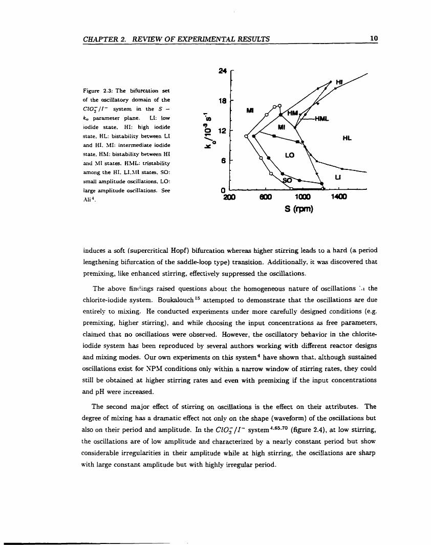
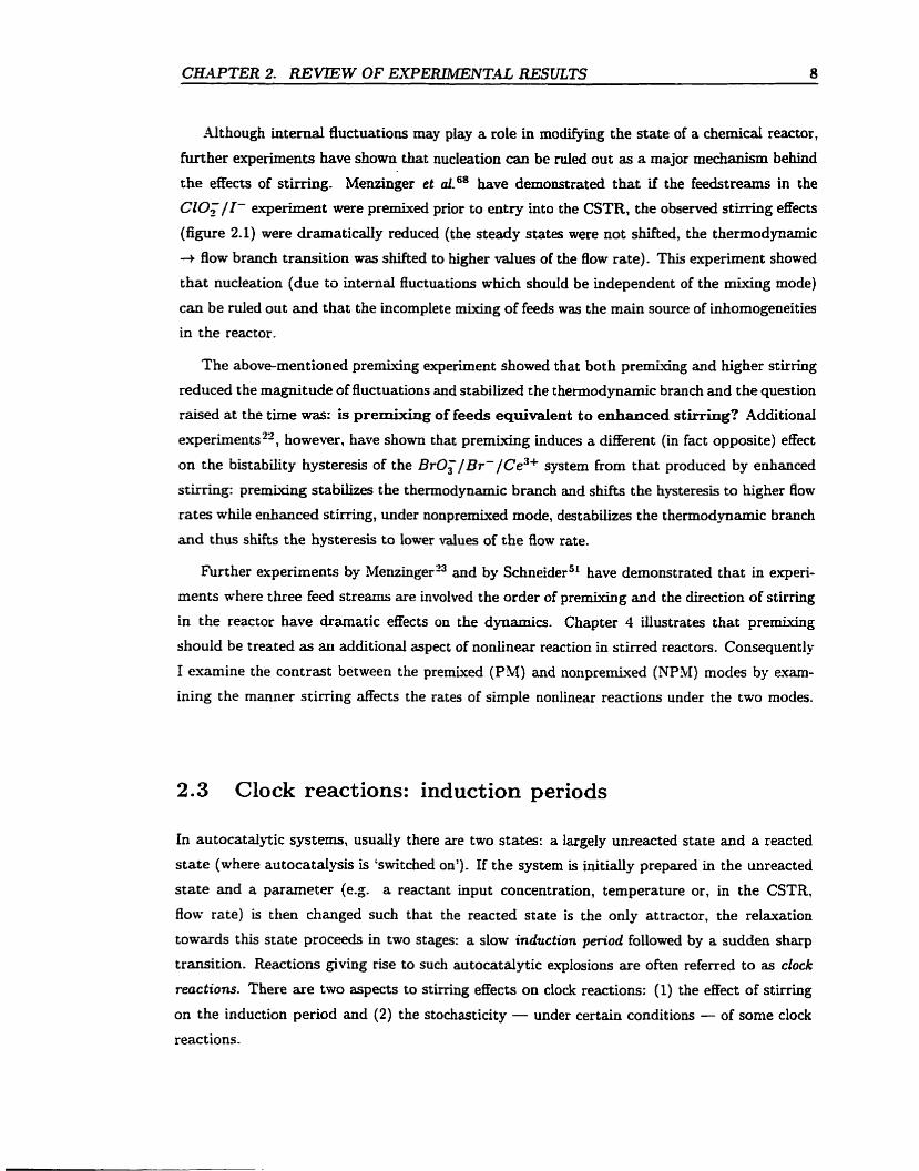
Figure 2.3: The bifurcation set

of the oscillatory domain of the

C f O ; / I - system in the S - k, parameter plane. LI: low

iodide state, HI: high iodide

state, HL: bistability between LI and HI. .MI: intermediate iodide

state. HM: bistability between HI

and .Cf1 states, HSIL: trïstability

among the HI. Ll.311 states. SO:

srnall amplitude oscillations, LO:

large amplitude osciIlations. See

.41i 4 .

induces a soft (supercritical Hopf) bifurcation whereas higher st imng leads to a hard (a period

lengtheniag bifurcation of the saddie-loop type) transition. Additionaily, it was discovered that

premixing, like enhanceri stirring, effectiveiy suppressed the oscillations.

The above f i n h g s raised questions about the homogeneous nature of oscillations the

chlorite-iodide system. Boukalouch '' attempted to dernonstrate that the oscillations are due

entireiy to miuing. He conducted experiments under more carefully designed conditions (e-g.

premising, higher stirring), and whiie choosing the input concentrations as free parameters,

clainied that no oscillations were obsemed. However, the oscillatory behavior in the chlorite-

iodide systern has been reproduced by several authors working with different reactor designs

and miuing modes- Our own e-xperiments on this system4 have shown that. although sustained

oscillations exist for NPSI conditions only within a narrow window of stirring rates, they could

still be obtained at higher stirring rates and even with premixing if the input concentrations

and pH were increased.

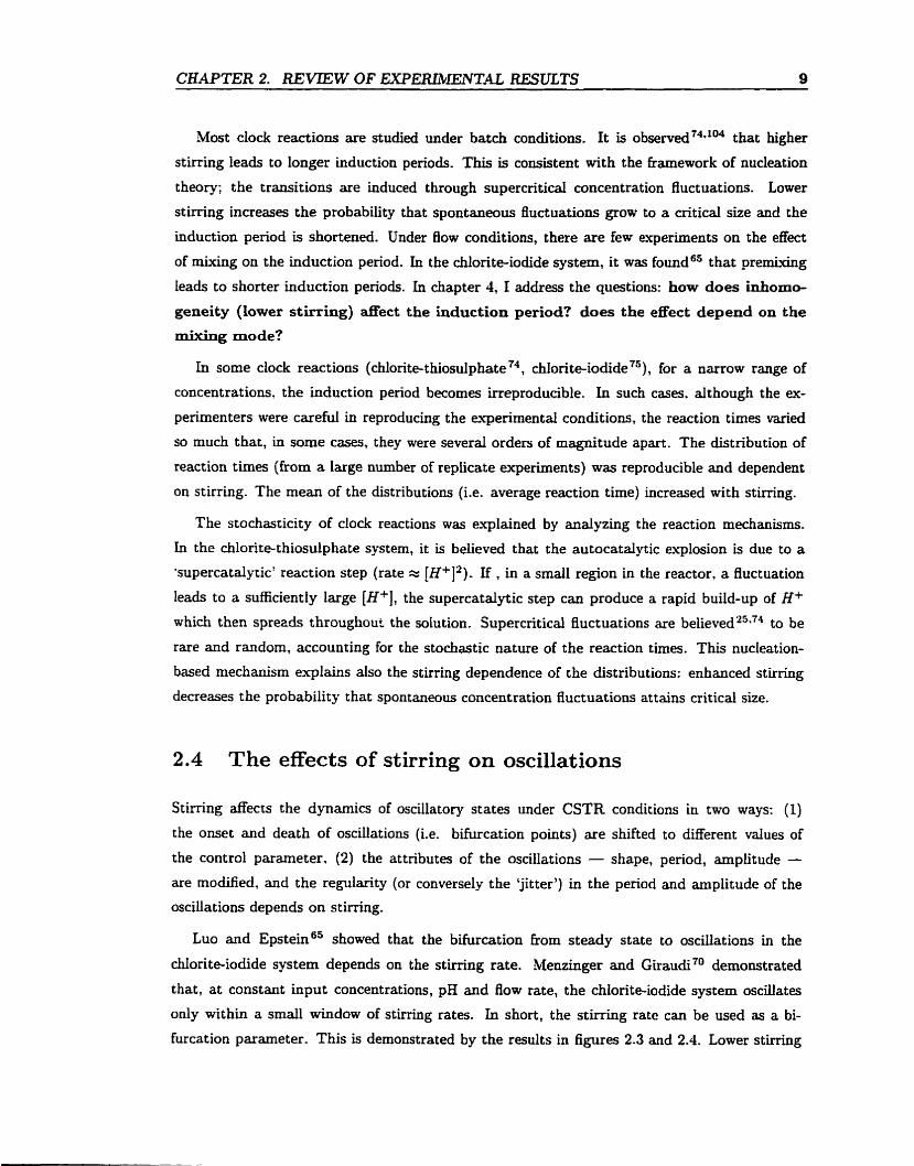
The second major effect of stirring on oscillations is the effect on their attributes. The

degree of rnixing has a dramatic effect not only on the shape (waveform) of the osciiïations but

also on their period and amplitude. In the CIO,/I- systern4*65-70 (figure 2.4), at low stirring,

the oscillations are of low amplitude and characterized by a nearly constant period but show

considerable irregularities in their amplitude while at high stirring, the osciHations are sharp

with large constant amplitude but with highiy irreguîar period.

Figure 2.4: The effect of stirring on the oscillations in the chtonte iodide systern. From Menzinger et di0

Experiments in the batch BZ ~ ~ s t e r n ~ ' . ~ ~ and in the CSTR CIO; / I - system have demon-

strated that the average oscillation period decreases with reduced stirring. However this trend

is not generic and the opposite stirring effect - longer periods at decreased stirring - has been

r e p ~ r t e d ~ ~ . ~ ~ . ' ~ ~ . in chapter 4. 6. 1 shed some light on the questions: (1) what determines

the effect of stirring on the period? and (2) does the effect depend on the mùcing

mode and in what way?

2.5 Fluctuations

The state of a chernical reactor, be it batch or CSTR, is rnost ofken monitored using metai or

ion-specific electrodes. The potential reported by such devices depends logarithmically on the

local concentrations . The measuring process Ieads to both spatial averaging (over the surface

of the electrode) and to tirne averaging (a function of the response time of the electrode and

electronics). Menzinger and co-workers have studied the fluctuations in electrode signais under

different mixing conditions for both steady state and oscillatory behaviors. Their results axe

sumrnarized here:

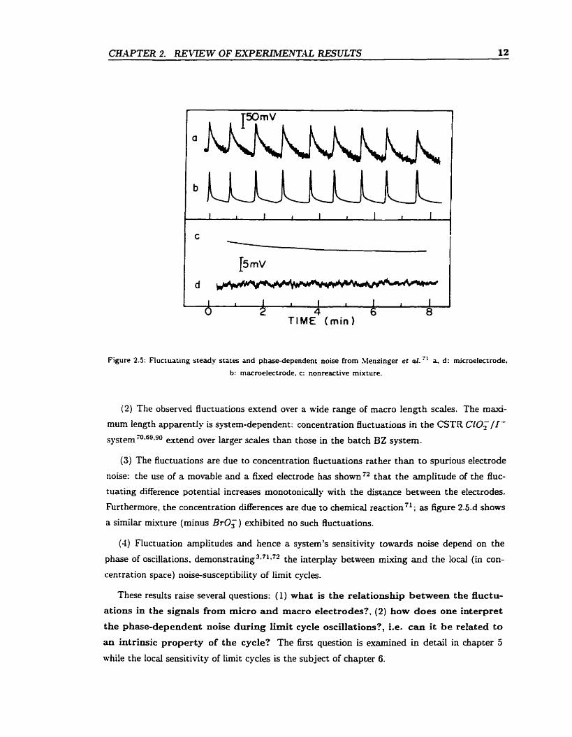
(1) The amplitude of fluctuations is inversely proportional to the size of the electrode. Figure

2.5 giws the signais of a micro- and a macro-electrodes. Fluctuations in micro-electrode signals

can be quite izrge: fluctuations corresponding to a twofold change in the cataiyst concentration

in the BZ system were observeda. The noise reflects spatial concentration distribution with a

coherence length that is short cornpared witt the length of a macro-e!ectrode.

CEAPTER 2. REVLEW OF E X P E m î E N T 4 L RESULTS 12

I 1 1 J I I I 1 1 I O 2 TlME 4 (min ) 6 8

Figure 2.5: Fluctuating steady States and phase-dependent noise from hlenzinger et al. '' a. d: rnicroeiectrode.

b: rnacroelectrode, c: nonreactive mixture.

(2) The observed fluctuations extend over a wide range of macro length scales. The maxi-

mum length apparently is system-dependent: concentration fluctuations in the CSTR CIO, /Id

sysrernï0~6g~90 extend over larger scaies than those in the batch BZ system.

(3) The fluctuations are due to concentration fluctuations rather than to spurious electrode

noise: the use of a rnovable and a &xed electrode has s h o ~ n ~ ~ that the amplitude of the Auc-

tuating difference potentiai increases rnonotonicdy with the distance between the elmrodes.

Furthemore, the concentration ciifferences are due to chernical reaction7'; as figure 2.5.d shows

a similar mixture (minus B r 0 3 ) e-xhibited no such fluctuations.

(4) Fluctuation amplitudes and hence a systern's sensitivity towards noise depend on the

phase of oscillations, demonstrating 3-71*72 the interplay between rnLxing and the local (in con-

cent ration space) noise-susceptibility of Iimit cycles.

These results raise severai questions: (1) what is the relationship between the fluctu-

ations in the signals from micro and macro electrodes?. (2) how does one interpret

the phase-dependent noise during iimit cycle oscillations?, i.e. can it be related to

an intrinsic property of the cycle? The first question is examined in detail in chapter 5

while the local sensitivity of limit cycles is the subject of chapter 6.

A second issue regarding fluctuations that raised some questions was the nature of the growth

of fluctuations near bistability transitions. The Roux experiment has shown that if the flow rate

was useci as the control parameter, then the fluctuations in the steady state concentrations on the

thermodynamic branch become larger as the thermodynamic -+ flow branch transition was a p

proached. If those fluctuations were interpreted as a measure of the spatiotempord fluctuations

in the system's response at a constant enviconment, then the experiment suggests . in a manner

analogous to phase transitions, t hat those fluctuations have a critical character. However, since

the control parameter was the flow rate, which directly affects the hydrodynamics in the CSTR.

a stilt open question is: did the observed fluctuations indeed reflect critical growth?

To shed some light on this issue, 1 focus on the relationship between spatial inhomogeneity in

the reactor and the observed fluctuations in the observable signals and on the critical nature of

the growth of the fluctuations in chapter 5.

Chapter 3

Mixing

C hemical engineers have ~ t u d i e d ~ ' ~ ' ~ ~ in detail the hydrodynamics of mixing in flow reactors.

This chapter examines some of the key mking concepts. 1 review the classes of miving models

that have been developed, without any reference to the interaction between imperfect mixing

and chemical reaction. The effect of imperfect mixing on the rates and dynamics of simple and

complex chemical reactions is the subject of the next two chapters.

The dynamics of a flow reactor results from the interplay of three processes occurring on

distinct characteristic t h e scaies:

1. !vIiuing: If the reactants are fed into the reactor premixed (PM mode), rn~uing involves

the homogenization of the reaction material (including fresh' fluid elements). On the

other hand, under nonpremixed (NPM) conditions, reactants must first corne in contact

for reaction to occur and müing time involves contact time.

2. Flow or m a s transfer: the reacting medium has a lifetime given by the residence tzme in

the reactor,

3. Chemical reaction: may proceed on one or more time scales (chemical relaxation times).

The concept of the ideal or perfectly mixed reactor implies instant miving of the feeds into

the buik and a high and spa t idy uniform mixing efficiency in the reactor. This ideaikation

simplifies the study of the reactor dynamics and its dependence on control parameters. However,

when two or more of the above t h e scales are of the same order of magnitude, strong coupling

arnong these processes rnay occur. Of particular interest is the case where a chemical reaction

step cornpetes with rnixing. In this case, even sniall deviations from ideal mixing conditions

can have dramatic effects on the dynamics. The experimental evidence for such effects is the

dependence of the dynamics on the stirring rate in the reactor and on the mixing mode. Systems

where the mixing and chemical relaxation have similar tirnecales, and hence mixing and stllring

effects are prominent, include the followingLO':

1. reactions involving viscous fluids, for example, polymerization reactions where the rate of

mixing affects the rnolecular weight distribution.

2. fast rnulti-step reactions, for =ample, organic synthesis where the rate of mixing affects

product selectivity.

3. nonlinear reactions with chemical instabilities (see chapter 2).

4. reactions involving immiscible fluids, for example, emulsions.

5. precipitation or crystaüization reactions (&g affects nucleation and consequently the

crystal size distribution).

6. fast non-isothermal reactions, for example, fiames.

hfixing is a complex process that occurs on multiple length scaies and in stages. It c m be

observed and described from Eulerian or Lagrangian perspectives8. In the Lagrangian view, one

describes the evolution of fluid elernents in the tirne domain whereas in the Eulerian view, one

studies the interaction between reaction and mking in physical space. The spirit of this work

falls into the realm of the Lagragian perspective.

Furthermore, the rnixing process occurs on macro and micro Iength scale .~~,~" Formally,

macromixing refers to large-scale mixing of Auid elements such that the reaction medium ap-

pear homogeneous on a macroscopic scale whereas micromiring in volve^^^'^^ (a) the convective

disintegration of large eddies, (b) viscous formation of striated laminar structures and (c) molec-

ular difision. The definitions of macro- and micromixing can be made more concrete by relating

them to the concept of residmce tàme distribution, a topic that 1 will discuss shortly.

The miuing process may be visualized by considering the fluid entenng the reactor as a

continuous Stream or series of parcels or agglomerates. The size of such fluid elements depends

on hydrodynamic factors such as energy dissipation, viscosity, and difisivity of the fluid. There

is a cascade of agglomerate sizes down to a length scale under which oniy molecular diffusion

achieves miuing. This limiting size, where viscous and inertial forces are balanced, is known

as the Kolmogorov limit 'O6. In laminar flows, the Buid elements are mixed and deformed by

stretching and folding leading to striated structures while in turbulent flows, the fluid elements

are broken down to smaller ones. Finally, a t the srnailest length scale, molecular diffusion leads

to molecular rnixing.

Next, 1 will define some of the terms needed to make the above description of the m g

process easier to analyze. The age of a fluid element is the time that elapsed since that element

entered the reactor. The fluid element's life ezpectancy is the length of time before it passes out

of the reactor'. Mxing, through stirring or other means results in:

1. stream mixing: refers to the mixing of reactant streams under nonprenrixed (NPM) con-

ditions. It is necessary for reaction to occur.

2. age mizing: reduces reanor inhomogeneities or non-unifonnities by the mixïng of fluid

elements of different ages. This is also referred to as back minng7.

Consider a flow reactor with a volume V and a total volumetric Bow rate Q. The nominal

holding time of the reactor is given by O = 6. What are the ages and life expectancies of Buid

elements in the reactor? In one idealized reactor, the plug pour reactor, the reaction mixture

flows like a plug through the reactor. A11 fluid elements leaving the reactor have the same age

(O) and aU those entering the reactor have the same life expectancy (8 ) . In a CSTR, however,

mhcing leads to by-pass (some fluid elements spend relatively less time in the reactor than 9 )

and stagnation (other fluid elements spend considerably more time in the reactor than 8). There

is a distribution of residence times (RTD).

Macromixing and rnicromixing in a flow reactor can, now, be defined in the foiIowing manner:

macrorniung effects are those that can be accounted for by the deviations in the form of the

ideal RTD for that reactor. Micromixing effects result £rom the mixing of fluid elements which

may not be reflected in the RTD.

3.1 Macromixing

Residence time distributions are measured experimentaiiy by injecting a tracer into the reactor

and monitoring the tracer's concentration a t the exit of the reactor as a function of time.

Consider a tracer material that is instantly injected into a reactor at t = O (Le. a singIe pulse).

If the concentration of the tracer a t the exit is denoted by C(t), then the RTD can be defined as 7.34.64:

Clearly, /; E( t ) = 1 and E(t)dt is the fiaction of tracer leaving the reactor and which

has resided in the reactor between t i and t2.

There are two extreme limits of macromixing:

(1) In the plug flow reactor (PFR) Lunit, ail fluid parcels have the same residence time and

the FtTD is a Dirac delta function.

(2) In the perfectly mked CSTR (PMCSTR) Limit, the instantaneous miuing of incoming

fluid into the bulk leads to a uniform concentration throughout the reactor. The tracer material

is washed out according to:

dC C - = -- dt 8

(3.2)

where 8 is the nominal holding time of the reactor. Integrating the above equation Ieads to:

and hence

This is the RTD for a perfectly mked CSTR. The mean residence time in the reactor is

obtained from the RTD:

and hence the mean residence time equais the holding cime. The spread in the residence tirne

distribution, Le. the variance in the ages of fluid elements, is given by:

Le. the deviation from the mean residence time has the same magnitude as the mean itself.

In practical situations, the reactor has a RTD intermediate between the PFR and PMCSTR

limits. P.V. Danckwerts lg pioneered the use of RTD in describing macromixing. The e-qeri-

mental RTD and hence macromixing effects are accounted for by modifving the RTD of ideal

reactors (PFR, PMCSTR). This can be accomplished in many ways, including the following

three macromiving models:

3.1.1 Macromixing models

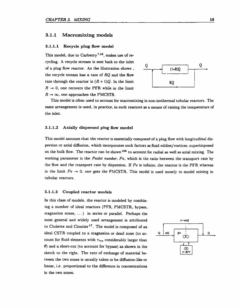
3.1.1-1 Recycle plug flow model

This model, due to Carberry7-16, makes use of re-

cyciïng. A recycle stream is sent back to the iniet

of a plug flow reactor. 4 s the illustration shows , Q - 6 ( 1 +NQ 1 1 Q

the recycle stream has a rate of RQ and the flow l L r i rate through the reactor is (R + 1)Q. Ln the limit

R + 0, one recovers the PFR whiIe in the limit j R Q - 1

R + x, one approaches the PMCSTR. This model is often used to account for macromixing in non-isothermal tubular reactors. The

same arrangement is used, in practice, in such reactors as a means of raising the temperature of

the idet.

3.1.1.2 Axialiy dispersed plug flow model

This model açsurnes that the reactor is essentidy composed of a plug flow with longitudinai dis-

persion or axial diffusion, which incorporates such factors as fluid ed&es/vortices, superimposed

on the bulk Bow. The reactor can be shownlo6 to account for radial as weii as avid mixing. The

working parameter is the Peclet number, Pe, which is the ratio between the transport rate by

the fion- and the transport rate by dispersion. If P e is infinite, the reactor is the PFR wheres

in the limit Pe + 0, one gets the PMCSTR. This model is used mostly to mode1 miuing in

tubular reactors.

3.1.1.3 Coupled reactor models

In this class of models, the reactor is modeled by combin-

ing a number of ideal reactors (PFR, PMCSTR, bypass,

stagnation zones, . . . ) in series or parailel. Perhaps the

most generaI and widely used arrangement is attributed (l-a)Q

CO Cholette and Cloutier 17. The model is composed of an

ideai CSTR coupled to a stagnation or dead zone (to ac-

count for fluid elements with r,,, considerably larger than

8 ) and a short-cut (to account for bypass) as shown in the a %?- sketch to the right. The rate of exchange of material be- [ il-B)V 1 tween the two zones is usually taken to be diffusion-like or

linear , Le. proportional t o the difference in concentrations

in the two zones.

3.1.2 Modelling macromixing in nonlinear reactions

Kumpinski and ~ ~ s t e i n ~ ~ used a coupled reactor mode1 to describe the s t i r ~ g dependence of

the bistability hysteresis in the chiorite-iodide reaction. Their mode1 was made of a PMCSTR or 'active zone' coupled to a 'dead zone' in a fâshion similar to the Cholette model. The dead

zone 'groups' together any inhomogeneities in the reactor. Enhanced mixing reduces inhomo-

geneities and hence leads to a smaller dead zone to active zone ratio. Their study qualitatively

reproduced the sturing dependence of the bistability hysteresis in both the C10T/I- and the

Br03 / Br-/Ce3+ systems.

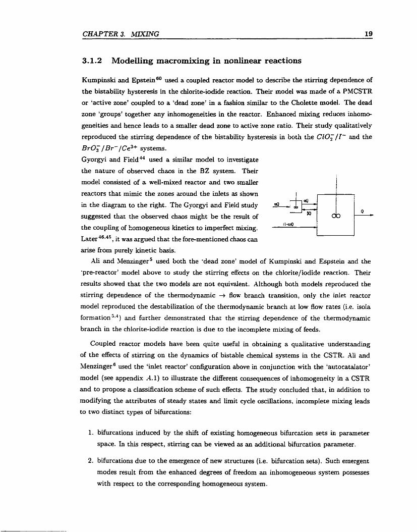
Gyorgyi and ~ield'" used a similar mode1 to investigate

the nature of observed chaos in the BZ system. Their

mode1 consisted of a weli-mixed reactor and two smaller

reactors that mimic the zones around the iniets as shown

in the diagram to the right. The Gyorgyi and Field study

suggested that the obsemed chaos might be the resdt of

the coupling of homogeneous kinetics to imperfect mixing.

la ter"^^^, it was argued that the forementioned chaos cm

arise from purely kinetic basis.

Ali and Menzinger5 used both the 'dead zone' model of Kumpinski and Espstein and the

pre-reactor' model above to study the stirring effects on the chlorite/iodide reaction. Their

resuits showed that the two rnodels are not equivalent. Although both modets reproduced the

stirring dependence of the thermodynamic + flow branch transition, only the iolet reactor

model reproduced the destabilization of the thermodynamic branch at low flow rates (Le. isoIa

formation ' v 4 ) and further demonstrated that the stirring dependence of the t hermodynamic

branch in the chlorite-iodide reaction is due to the incomplete mixing of feeds.

Coupled reactor models have been quite useful in obtaining a qualitative understanding

of the effects of stirring on the dynamics of bistable chernical systems in the CSTR. Ali and

Menzinger6 used the 'inlet reactor' configuration above in conjunction with the 'autocatalator'

model (see appendix -4.1) to illustrate the difFerent consequences of inhomogeneity in a CSTR

and to propose a classification scheme of such effects. The study concluded that, in addition to

modifying the attributes of steady States and iimit cycle oscillations, incomptete mking leads

to two distinct types of bifurcations:

bifurcations induced by the shift of existing homogeneous bifurcation sets in parameter

space. In this respect, stirring can be viewed as an additional bifurcation parameter.

bifurcations due to the emergence of new structures (Le. bifurcation sets). Such emergent

modes result from the enhanced degrees of freedom an inhomogeneous system possesses

with respect to the correspondig homogeneous system.

Despite their usefulness, coupled reactor models can not M y describe the coupling between

chernical reaction and W n g in flow reactors because

1. Depending on the complexity of the coupling model, few parameters may need to be

adjusted to reproduce the experimentai effect. There is no clear correlation between those

parameters and m k h g in the reactor.

2. Can not be used to study concentration fluctuations (in time) or nonuniformities (in space).

They are deterministic models and hence can not be used to account for the stochasticity

of induction periods or of oscillation periods and amplitudes.

The deficiency of coupled reactor models, and of ali rnacromiving models, is due to the fact

that they account for only the deviations from an ideal RTD and not for the ways such deviations

may arise. The deficiency stems Erom the Fact that the RTD gives the distribution of ages of

fluid elements but says nothing about the mixing of fluid elements. In order to describe how

fluid eiements of different ages interact, one m u t turn to micromixing.

3.2 Micromixing

There is more to &ng than just examining the factors that shape the overall RTD for a given

reactor. Micromixing encompasses not only the distribution of ages of fluid elements but also

two related aspects of the interaction (Le. mkxing) of these elements 'O7:

(a) Segregation. This concept describes the intensity of mixing among fluid elements (in

space). The two extremes are (a) complete segregation: fluid elements remain segregated with

no mass exchange among them. Fluids e-uhibiting a high degree of segregation (e-g. viscous

flows) are usually called macro-puids. Yotice that the fluid is macromked in the sense that the

RTD is that of an ideal reactor. (b) ideal minng. there are egectively no aggregates and the

fluid consists of individual molecules free to move in a micro-puid.

(b) Earliness of mhing. This concept deds with the question: if mass exchange (Le. mucing)

among fluid elements takes place, when does it occur? (relative to the ages of the elements).

If the mixing occurs a t the earliest possible moment, the reactor is said to be at a state of

muxinium mùedness and if the miviDg occurs at the latest possible moment, the reactor is said

to be in a state of minimum mizedness.

The concepts of micrornixing introduced here are relative. -4 fluid is described as a macro- or

micro-fluid depending on the relative tirne scales of mixing, flow and chemistry. If the reaction

time or the residence time is short compared to the life span of the fluid aggregates, one may

assume that the fluid is completely segregated, even though the stirring rate rnay be very high.

3.2.1 Micromixing models

The rnodek enumerated beiow usually assume an ideal FKCD (Le. weii macromixed reactors)

but in principle can be applied to reactors with any arbitrary RTD.

3.2.1.1 Formal models

These modeis are not related to any physicd understanding of the reactors and are simply an

at tempt to find an intermediate description between the two limits of segregation. An example of

such models is the one proposed and rehed by Villermaw107*105. In this model, the feed enters

the reactor into a region of complete segregation and exits from one with maximum mixedness.

The residence tirne in the complete segregation region is used as the mixing parameter (zero

means perfect mixing and oo gives complete segregation) .

3-2.1.2 Agglomerate models

In this group of phenornenological muàng models, the aim is to provide a description of the

consequences of irnperfect mixing rather than to mode1 the actud physical process of miuing.

The fluid is assumed to consist of agglomerates that exchange matter with each other or with

some other environment. The exchange rate corresponds to the mixing rate. This class of models

can also be labeiied as population balance or birth-death methods. Fluid elements undergo birth

(entry into the reactor), aging, mixing, and h a l l y death (exit from the reactor).

(a) The coalescence-redisperion mode1 (CR) :

This is used extensively in this thesis. A full description of the model and the

algorithm used to Mplement it are given in chapter 5. III this model, the reactor is made up of

equally sized fluid elernents that interact in pair-wise collisions. The interactions are ctssumed to

occur by codescence (i.e. joining) foilowed by redispersion (Le. splitting). The fiow introduces

new fluid elernents containing pure reactants and removes an equal number of fiuid elements.

The concentrations of al1 chernicd species in a given fluid element are unifonn throughout that

e!ement and evolve according to their homogeneous batch kinetics. The state of the reactor cm

be described by a concentration probability distribution, p(c), which gives the fraction of Buid

elements having concentrations in the range (c, c + dc).

(b) The Interaction by Exchange with the Mean (IEM) model:

In this model, developed and refined by Viiermaux and co-w~rkers '~~ , Buid elements are

assumed to continuously exchange matter with an average 'bulk' material. -4 single typical fluid

element is followed as it exchanges matter with an 'effective' medium whose concentration is

obtained by averaging the concentrations of typical fluid eiements that correspond to residence

times chosen from a given RTD.

The rate of change of the concentration of a species i a t a given point (Le. in a given Buid

element) is determiried by:

where l/r,,, is the rate of mkxing and < c' > is the average concentration

For a well macromixed CSTR:

(3-7)

of i in the reactor.

The âbove two equations can be solved numericaily using an iterative scheme.

Xlthough the IEM modei Ieads to simple deterrninistic equations that are easier to solve than

the CR model. the CR mode1 is more suited to study the effects of rnixing on complex non-

Iinear reactions in a CSTR for the foliowing reasons: (1) the distribution of concentrations in

the CSTR may not be gaussian and the average given by equation 3.8 may not be representative

of a typicai fluid element. (2) The modei is vahd106 oniy near the perfect micromixing k t .

(c) The shrinking aggregate model:

This model. developed by Villermaax and c e w o r k e r ~ ~ ~ , assumes that the main process of

micromixing is the erosion of fresh fluid aggregates. The size of sphericaliy-shaped fluid elements

is assumed CO decrease linearly as a function of time (Le. age a):

where 1,, the initiai size of the aggregates and te , the characteristic tirne constant, are estimated

from hydrodynamic consideratioris and adjusted to fit experimental results.

(d) Zwietering's dilut ed aggregat e model:

In this model1l3, it is assumed that a fluid element, upon entry into the reactor, is diluted

by the bulk (which consists of 'older' fluid elements). The dilution changes both the volume of

the fluid parce1 and the concentrations of the chernical species inside the parcel. A fluid element

of age û would have a volume given by w = w,ePQ where w, is the initial size of the element and

p is a parameter that describes the mixing rate. Z w i e t e r i ~ ~ ~ " ~ derived the equations describing

the evolution of such a fluid element for the case of one and two feed streams.

3.2.1.3 Detailed models:

(a) Physical models:

These models attempt to take into account the details of d l possible physical processes

occurring in the flow (convection, d W i o n , reaction) tu predict the consequences of coupling

between chernistry and hydrodynamics. They include the lamellar structure model of Ottino

(molecdar diffusion Mthin stretching laminae), and the mplfment model of Baldyga and

B o ~ r n e ~ . ~ ( e n m e n t of fresh material by periodic bursts of vorticity in a stretching fluid

element) .

(b) Models based on computational fluid dynamics (CFD):

These models describe the geometry and properties of the reactive flow either by directly

solving the Navier-Stokes equations or by reducing the description to a pro bability density func-

tion {pdfl formulation 32v86. These methods require huge computationd power and employ heavy

formalism.

3.2.2 Micromking simulations in noniinear react ions

Several groups have studied the effect of micromixing on the dynamics of nonIinear reaction.

Hannon and H o r ~ t h e r n k e ~ ~ * ~ ~ used a power series expansion of the equation describing the

coalescence-redispersion mode1 n e z the perfect miving limit to model the shift of bistability

hysteresis. Puhl and N i ~ o l i s ~ ~ used a sirniiar expansion in conjunction wit h Zwietering's mixing

model. Boissonade and De Kepper l4 used both the coalescence-redispersion and EM models

with a realistic kinetic scheme and found a general agreement between the simulations and

earlier experiments on the mixing effects in the chlorite-iodide system. Fox and V i l l e r m a ~ x ~ ~

used a version of the IEM model to study the mixing dependence of bistability and oscillatory

region of the CLO,/I- system.

Chapter 4

Interaction of flow, mixing, and 'simple'

chemical reactions in a CSTR.

in the previous chapter, 1 reiterated some of the physical concepts used to describe mixîng

in a continuously fed stirred tank reactor (CSTR) and highiighted the main methods used

to model the mkuing process. Here, 1 tum the attention to the interaction between chernical

reaction (isothermal, aqueous) and hydrodynamic transport (flow, mkng) of matter. 1 focus

on two simple reactions: bimolecular and cubic uutocatalysis. In addition to their importance

in industrial and academic work, these two reactions are building blocks for larger and more

cornplex reaction schernes.

Two main questions are addressed: (1) how does rnixing affect the rate and outcome of a

given chemical reaction? and (2) what are the conditions under which mixing effects are largest?

The random coalescence-redispersion model (RCR), introduced in chapter 3 and examuied in

d e t d in chapter 5, is used to demonstrate the effect of nonideal micromiuing. The role of

nonideal macromixing (i.e. nonideal RTD) in modifying the rates of chemicai reactions is not

addressed here and can be found elsewhere ' O 6 .

Consider a single step chemical reaction. h,kxing may affect the rate of the reaction in one

of two ways:

( 1 ) If the reactants are fed into the reactor via separate strearns (NPM), miving increases the

rate at which reactants are brought into contact and hence enhanced miuing increases the rate

of reaction.

(2) kfLxing also reduces reactor inhornogeneity. How does inhomogeneity affect the overall

rate of reaction in a mixture? Epsteinz5 pointed out that nonuniformities increase the rate of a

nonlinear reaction involving a single reactant (i.e. rate=kan, n > 1). The idea be can generalized

to include multiple reactants:

CE4PTER 4. INTERACTION OF FLOW, hLLXING, AND CEEMTSTRY 25

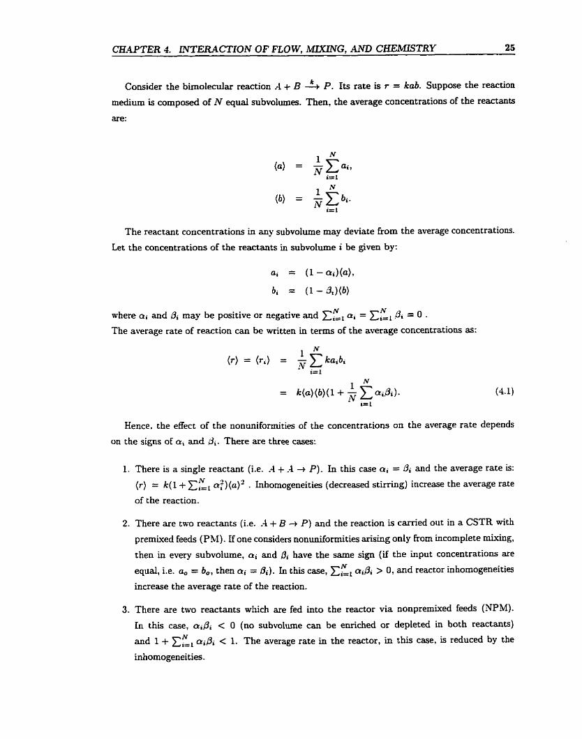
Consider the bimotecular reaction .4 + B 5 P. Its rate is r = kab. Suppose the reactim

medium is composed of N qua1 subvolumes. Then, the average concentrations of the reactants

are:

The reactant concentrations in any subvolume may deviate fiom the average concentrations.

Let the concentrations of the reactants in subvolume i be given by:

N N where ai and Oi may be positive or negative and xi=I Q i = ,di = O - The average rate of reaction can be written in terms of the average concentrations as:

1 (r ) = ( r i ) = - 1 kaibi 1v

i= 1

Hence, the effect of the nonuniformities of the concentrations on the average rate depends

on the signs of a, and 13,- There are three cases:

1. There is a single reactant (i.e. -4 + -4 + P), In this case cri = Bi and the average rate is:

(t) = k ( l + xLL cr:)(a)' . Inhomogeneities (decreased stirring) increase the average rate

of the reaction.

2. There are two reactants (Le. -4 + B -, P) and the reaction is carried out in a CSTR with

premked feeds (PM). If one considers nonuniformities arising only fiom incomplete mixing,

then in every subvolume, ai and Bi have the same sign (if the input concentrations are N equal, i.e. a, = b,, then ai = ,Bi). In this case, Ci=, aiPi > 0, and reactor inhomogeneities

increase the average rate of the reaction.

3. There are two reactants wsch are fed into the reactor via nonpremixed feeds (NPM).

In this case, aiBi < O (no subvolume can be enriched or depleted in both reactants)

and 1 + CE, aipi < 1. The average rate in the reactor, in this case, is reduced by the

inhomogenei ties.

CHAPTER 4, ZNTERACTION OF FLOW- MIXING, AND (7EEM2STRY 26

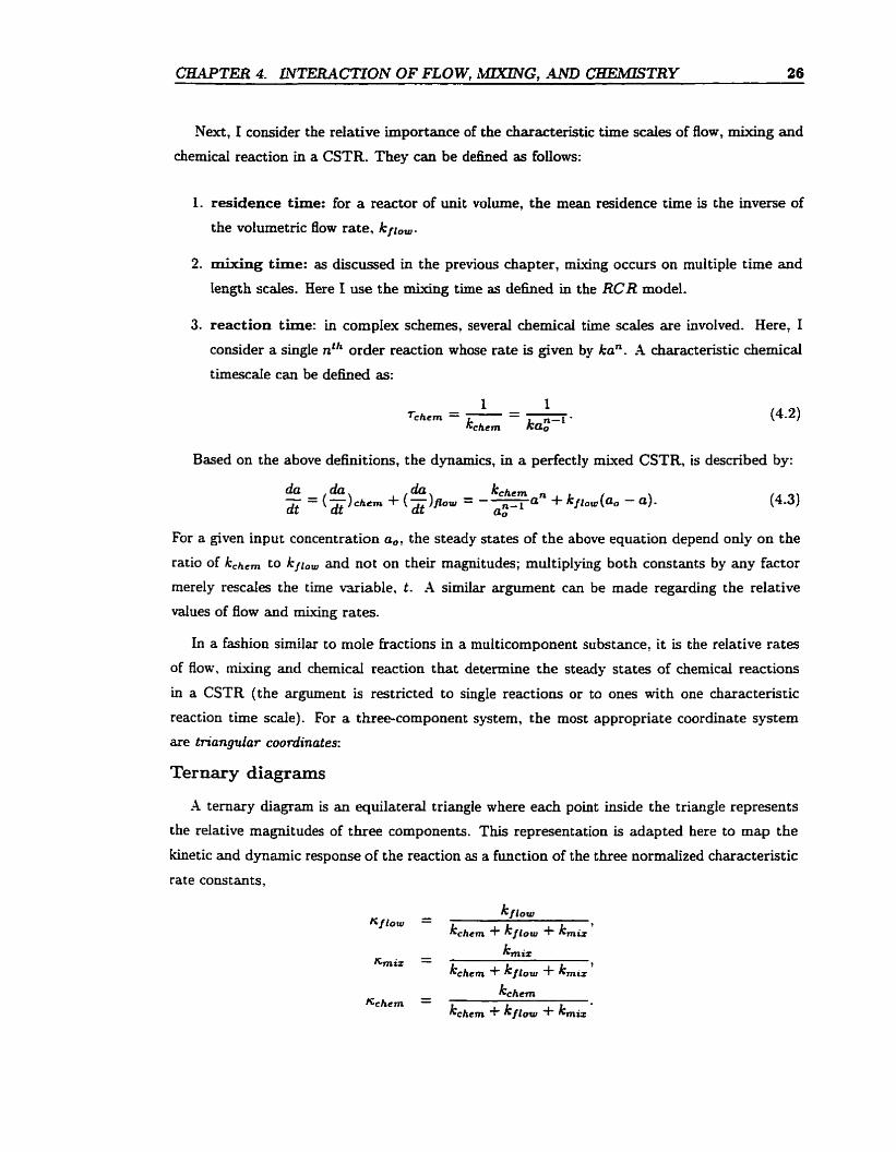
Next, 1 consider the relative importance of the characteristic time scaies of flow, mixing and

chernicd reaction in a CSTR. They can be defineci as follows:

1. residence t h e : for a reactor of unit volume, the mean residence tirne is the inverse of

the volumetric flow rate, kfro,.

2. mixing tirne: as discussed in the previous chapter, mixing occurs on multiple time and

length scaies. Here 1 use the mixing t h e as dehed in the RCR model.

3. reaction tirne: in cornplex schemes, several chemical time scaies are involved. Here, 1

consider a single nth order reaction whose rate is given by ka". A characteristic chemical

timescale can be defined as:

Based on the above definitions, the dynamics, in a pedectly &ed CSTR, is described by:

For a given input concentration a,, the steady states of the above equation depend only on the

ratio of kchem to kIlow and not on their magnitudes; multiplying both constants by any factor

rnerely rescales the time variable, t. A similar argument can be made regarding the relative

values of flow and mixing rates.

In a fashion similar to mole fractions in a multicomponent substance, it is the relative rates

of flow, duing and chernicd reaction that determine the steady states of chemical reactions

in a CSTR (the argument is restricted to single reactions or to ones with one characteristic

reaction time scde). For a threecomponent system, the most appropriate coordinate system

are trianguiar coordinates:

Ternary diagrams

A temary diagram is an equilateral triangle where each point inside the triangle represents

the relative magnitudes of three components. This representation is adapted here to map the

kinetic and dynamic response of the reaction as a function of the three normalized characteristic

rate constants,

CEa4PTER 4. LNTERACTION OF FLOW. MLXING, rUVD C&EbmTRY 27

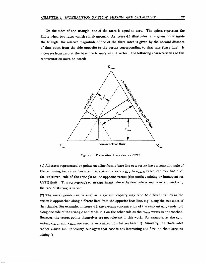
On the sides of the triangle, one of the rates is equd to zero. The apices represent the

iimits when two rates vanish simdtaneously. As figure 4.1 illustrates, at a given point inside

the triangie, the relative magnitude of one of the thee rates is given by the normal distance

of that point from the side opposite to the vertex corresponding to that rate (base line). It

increases fiom zero at the base line to unity at the vertex. The foilowing characteristics of this

representation must be noted:

non-reactive flow

Figure 4.1: The relative tirne scales in a CSTR.

(1) XI1 states represented by points on a line from a base Iine to a vertex have a constant ratio of

the remaining two rates. For example, a given ratio of ~ f l ~ ~ to &hem is reduced to a iine from

the 'unstirred' side of the triangle to the opposite vertex (the perfect mixing or homogeneous

CSTR lirnit). This corresponds to an experirnent where the flow rate is kept constant and only

the rate of stirring is varied.

(2) The vertex points can be singular: a systern property may tend to different values as the

vertex is approached dong different iines h-om the opposite base line, e-g. dong the two sides of

the triangle. For example, in figure 4.3, the average concentration of the reactant aSt, tends to O

dong one side of the triangle and tends to 1 on the other side as the Kmiz vertei is approached.

However, the vertex points themselves are not relevant in this work. For example, at the nmiz

vertex, rs,,,,, and ~,i,, are zero (a well-mked nomeactive bat& !). Similarly, the three rates

cannot vmish simultaneously, but again that case is not interesthg (no flow, no chemistry, no

aiking !)

CE.4PTER 4, LlVTERACTION OF FLOW. IWXING. .4ND CHE2MLSTRY 28

In the next section, 1 =amine the rnïxing effect on a simple bimoIecuIar reaction and demon-

strate how the triangular representation can be used to map the different rneasures of the system

response as functions of the relative time s d e s of flow, miuin. g and chernicd reaction.

4.1 Bimolecular react ions

Consider the bimolecular reaction

Its rate law is :

da db fate = - - = - - dt dt

= kab.

The reactants -4 and B are fed into the CSTR at a flow rate kf l , , with feed concentrations a, and

6, respectiveiy. X convenient chernical time scale can be defined by r,h,, = l /kchCm = I/ka,.

4.1.1 The perfect mixing limit

The rates of change of the concentrations of -4 and B are given by:

However. from the stoichiornetry of the reaction. a, - a = b, - b and the system can be

reduced to one dimension. For the case a, = b,, a = b and one gets the equation:

I = - ka2 + k (a, - a)

which can be soIved for its steady state solutions (a = 0):

Or, in tem'ls of kchem ,

This is the mozimurn mixedness limit.

CE4.PTER 4. INTERACTION OF FLOW, MIXLNG, AND CHEMISTRY 29

4.1.2 The complete segregation limit

In this case, no mixing among 0uid elements occurs. i f the reactants are fed into the unstirred

reactor via separate streams (NPM), no reaction takes place (a = a,, b = b,). In the prernixed

(PM) mode, fluid elements behave like independent batch reactors where the rate of change of

a (for the case a, = b,) is given by:

and hence

The time a fluid element spends in the CSTR is given by the foilowing residence time distri-

bution:

then, the average concnetration of .-l is

4.1.3 Intermediate mWng

The RCR model is used to calculate the mk&g dependence of the stochastic steady state which -

is characterized by a,t, = (a) where (a) is the average concentration over the N cells of the

RCR model. The conversion in the reactor is given by a, - a.,. and the miwing efTect rnay be

quantified by A,

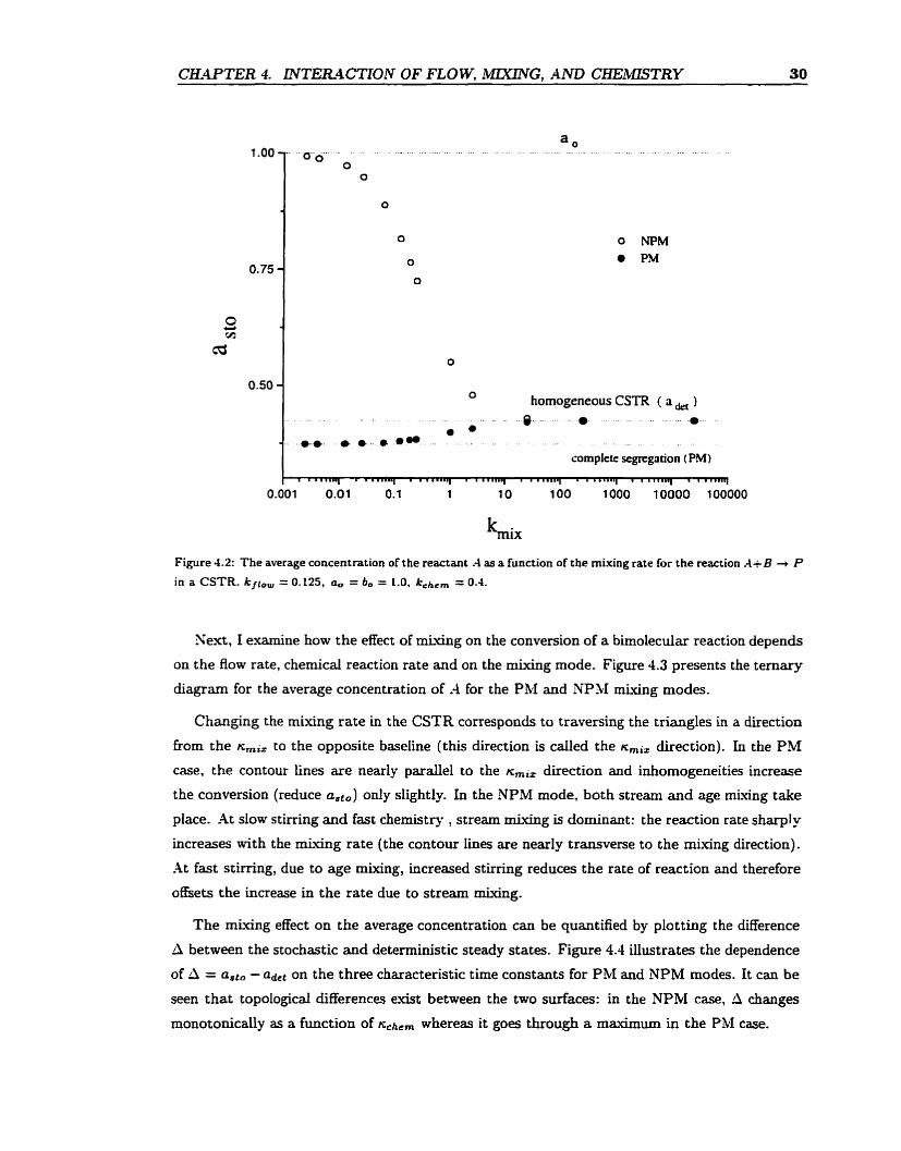
Figure 4.2 gives the effect of rnixing on a,to for a given flow and chemicd rate constants under

both Ph1 and NPM conditions. One c m note that (1) lowered stirring has opposite eEects

for the two r n ~ ~ n g modes: under PM conditions, it leads to higher conversion (nonuniforrnity

enhances the overd reaction rate) whereas under NPM, it leads to lower conversion (inefficient

Stream miuing limits the reaction). (2) the efLect is more pronounced under NPM conditions.

(3) the conversion ranges from zero in the unstirred reactor with nonpremixed feeds to ao(l - k j < o w jo =

- kfloui ' I fkcheni t

dt) in the unstirred reactor with premixed feeds.

CKWTER 4. LNTElL4CTION OF FLOW, MLXLNG, AND CHEhIISTRY 30

O NPM PM

O homogeneous CSTR ( a &, )

complete segregation (PM)

Figure 4.2: The average concentration of the reactant -4 as a function of the mixing rate for the reaction .4+B + P

in a CSTR. k f i , , = 0.125, a, = b, = 1.0, kch,, = 0.4.

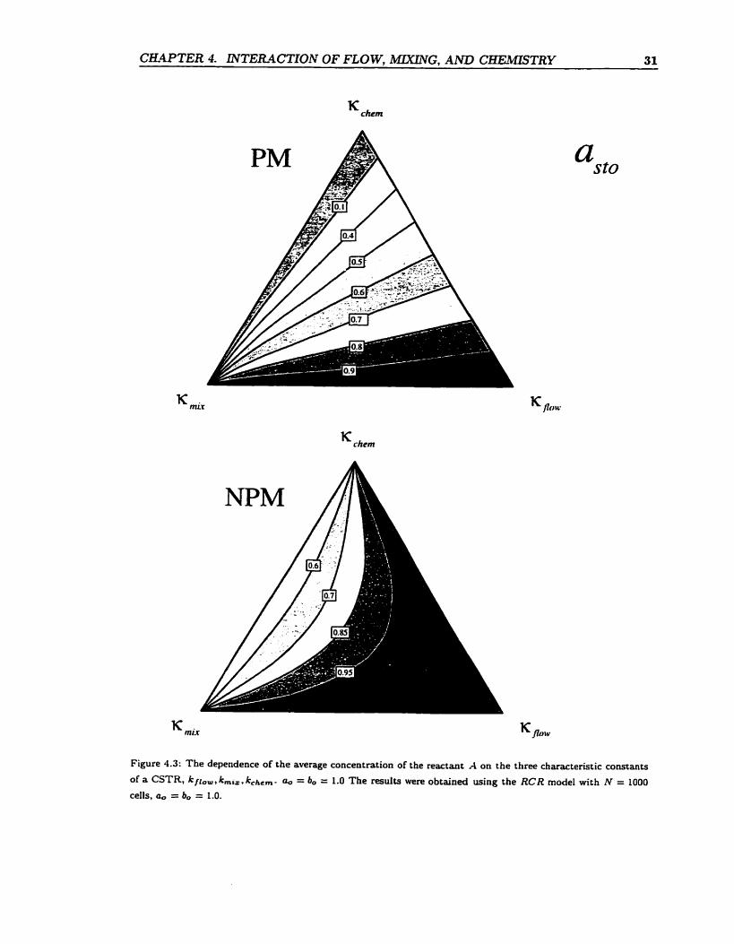
Ses,, 1 examine how the effect of mixing on the conversion of a bimolecular reaction depends

on the flow rate, chernical reaction rate and on the mixing mode- Figure 4.3 presents the ternary

diagram for the average concentration of -4 for the PM and NP31 mi.-.-g modes.

Changing the mixing rate in the CSTR corresponds to traversing the triangles in a direction

from the Kmiz to the opposite baseline (this direction is cailed the rc,i, direction). In the PM

case, the contour lines are nearly pa rde l to the Kmiz direction and inhomogeneities increase

the conversion (reduce aSt,) only slightly- In the NPM mode, both stream and age miving take

place. At slow stirring and fast chemistry , stream duing is dominant: the reaction rate sharpl y

increases with the mixing rate (the contour lines are nearly transverse to the rnixing direction).

At fast stirring, due to age rnixing, increased stirring reduces the rate of reaction and therefore

offsets the increase in the rate due to stream miuing.

The miving effect on the average concentration can be quantified by plotting the difference

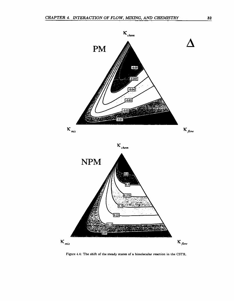
h between the stochastic and deterministic steady states. Figure 4.4 illustrates the dependence

of A = a,t, - adct on the three characteristic time constants for PM and NPM modes. It can be

seen that topologicai ciifferences exist between the two surfaces: in the NPM case, A changes

monotonically as a function of /+hem whereas it goes through a maximum in the Pb1 case.

CKAPTER 4. ilVTER4CTXON OF FLOW, MXRVG, AND CHEMLSTRY 31

K chem

a sto

Figure 4.3: The depeadence of the average concentration of the reactant A on the three characteristic constants

of a CSTR, kfl,,, km,,, k,h,,- a, = bo = 1.0 The results were obtained using the RCR mode1 with N = 1000

cells, a,, = bo = 1.0.

CRAPTER 4. INTERACTION OF FLOW, MDUNG, AND CHEMETRY 32

K chem

K mir

K chem

K m u , h v

Figure 4.4: The shift of the steady States of a bimolecular reaction in the CSTR.

CH-4PTER 4. INTER4CTION OF FLOW, MZXING, AVD C&E,;MISTRY 33

It should be noted, however, that the results in figures 4 . 2 4 4 are for a macromixed (i.e. ided

RTD) CSTR. In real experiments, both micro and macromixing may be nonideal and deviations

from the results presented here wouid not be unexpected-

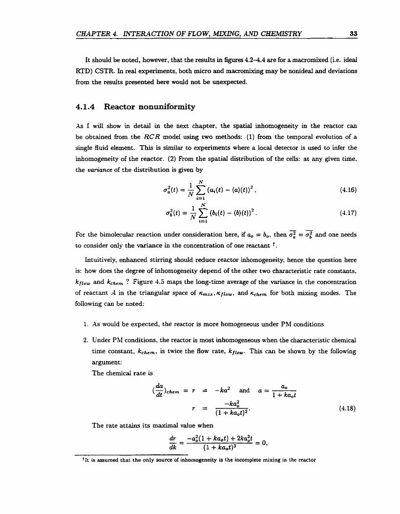
4.1.4 Reactor nonuniformity

As I will show in detaii in the next chapter, the spatial inhomogeneity in the reactor can

be obtained from the RCR mode1 using two methods: (1) from the temporal evolution of a

single fi uid element. This is similar to experiments where a local detector is used to infer the

inhomogeneity of the reactor. (2) Fkom the spatial distribution of the ce&: at any given time.

the val-iance of the distribution is given by

- - For the bimolecdar reaction under consideration here, if a, = b,, then CT; = 0; and one needs

to consider only the variance in the concentration of one reactant t.

Intuitively, enhanced stirrïng should reduce reactor inhomogeneity. hence the question here

is: how does the degree of inhomogeneity depend of the other two characteristic rate constants,

k f l o , and kchem ? Figure 4.5 rnaps the long-time average of the variance in the concentration

of reactant -4 in the triangular space of Kmir fi^^^ and K,,,,, for both miuing modes. The

following can be noted:

1. As would be e-qected, the reactor is more homogeneous under PM conditions

2. Under PM conditions, the reactor is most inhomogeneous when the characteristic chernical

tirne constant, kchemr is twice the flow rate, kfl,,. This c m be shown by the folowing

argument:

The diemical rate is

da QO

(dt)chem = r = -ka2 and a = 1 + ka,t

The rate attains its maximal value when

-- -

t f t is assurneci that the only source of inhomogeneity is the incomplete mixing in the reactor

CHAPTER 4. INTERACTION OF FLOW, MLXING, AND CEEMlSTRY 34

Kg,

Figure 4.5: The degree of inhomogeneity in a CSTR: birnolecuIar reaction.

C W T E R 4. INTERACTION OF FLOW. , ' G . AND CHE,WTRY 35

or when

But a t t = I/(ka,). a = a0/2 (Le. the chernical rate is largest at the haif-life of the

reaction). In a CSTR. a = -ka2 + kfr,(a, - a) and the steady States (a = O ) are given

by

and hence the chernical rate is Iargest (a = ao/2) when:

or when

In rnost experiments, measurements are made using metal and ion sensitive electrodes. The

electrode potential is proportional to the logarithm of the concentration of a given species.

The absolute variation in the electrode signal is proportional to the relative variation in the

concentration. The relative variance, ru = z / ( a s r 0 ) * is plotted in figure 4.6. Under premixed

conditions (PM), the relative variance depends on the three characteristic time scales in a

fashion simiiar to the way the variance does. The line of m=cimum relative variance occurs

at a (nch,,/rcfi0,) ratio about twice the ratio for the absotute variance. For the nonpremixed

mode (NPM), the cornpetition betw-en Stream mixhg and age mking introduces few important

trends in the dependence of the relative variance (i.e. the variance in electrode potential) on

the characteristic rate constants. This is illustrated in detail in figure 4.7:

(1) Dependence on mixhg: if the reaction is slow compared to residence tirne. the relative

variance decreases monotonically as the rnUang rate is increased (figure 4.7.a). If the reaction

is fast compared to the residence time, the relative variance has a maximum value a t a finite

non-zero m g rate (figure 4.7.b.)

(2) Dependence on the flow rate: if the reaction is slow compared to mixing, the relative variance

has a pronounced minimum (figure 4.7.d) at a Cinite non-zero flow rate compared to the nearly

monotonic shape it has for a fast reaction (figure 4.7.c).

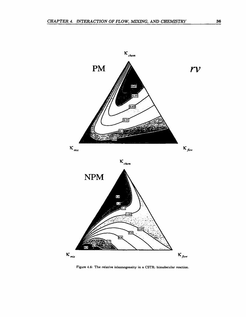
CH-@TER 4- I1VTEELACTION OF FLOW, MZXLNG, AND CBEMTSTRY 36

K chem

NPM

K chem

Figure 4.6: The relative inhomogeneity in a CSTR: birnolecula

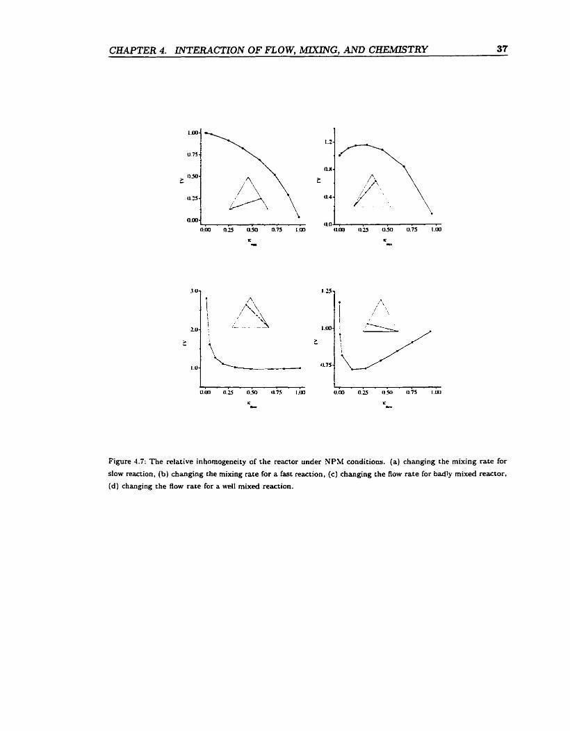
CEWTER 4. l2VTE2L4CTION OF FLOW. iUIXING, AND C&EMISTRY 37

Figure 1.7: The relative inhornogeneity of the reactor under NPM conditions. (a) dianging the mixing rate for

slow reaction. (b) changing the mixing rate for a fast reaction, (c ) changing the Aow rate for badly mixed reactor,

id) changing the flow rate for a well mixed reaction.

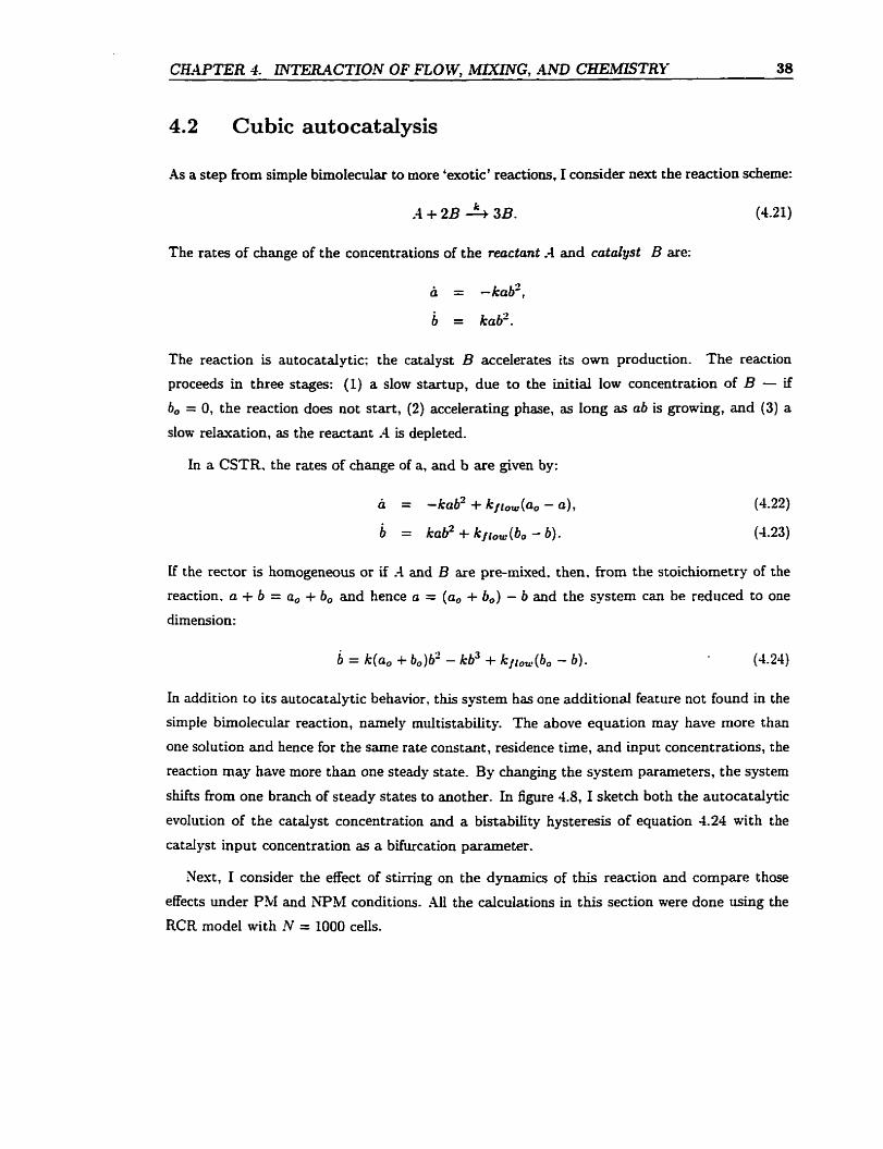
CEWTER 4. INTERACTION OF FLOW. MlXNG. .UVD C H E m T R Y 38

4.2 Cubic autocatalysis

As a step fkom simple bimoledar to more 'exotic' reactions, 1 consider next the reaction scheme:

The rates of change of the concentrations of the reactant A and catalyst B are:

The reaction is autocataiytic; the catalyst B accelerates its own production. The reaction

proceeds in three stages: (1) a slow startup, due to the initial low concentration of B - if b, = 0, the reaction does not start, (2) accelerating phase, as long as ab is growing, and (3) a

slow relaxation, as the reactant A is depleted.

In a CSTR, the rates of change of a, and b are given by:

= -kab2+ kjlo,(ao -a),

b = kab2 + kjrow(b,, - b).

If the rector is homogeneous or if -4 and B are pre-mixed. then, from the stoichiometry of the

reaction, a + b = a, + b, and hence a = (a, + 6,) - b and the system can be reduced to one

dimension:

In addition to its autocatalytic behavior, this system has one additional feature not found in the

simple bimolecular reaction, narnely mirltistability. The above equation may have more than

one solution and hence for the same rate constant, residence time, and input concentrations, the

reaction may have more than one steady state. By changing the system parameters, the system

shifts from one branch of steady States to another. In figure 4.8, 1 sketch both the autocatalytic

evolution of the catalyst concentration and a bistabiiity hysteresis of equation 4.24 with the

catdyst input concentration as a bifurcation parameter.

Next, 1 consider the effect of stirring on the dynamics of this reaction and compare those

effects under PM and NPM conditions. 411 the calculations in this section were done using the

RCR mode1 with N = 1000 cells.

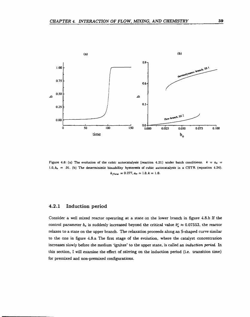
C W T E R 4. INTERACTION OF FLOW, , ' G , C-TRY 39

Figure 4.8: (a) The evolution of the cubic autocatalysis (reaction 4-21) under batch conditions. k = ( ~ o = L.O,b, = .01. (b) The deteministic bisiability hysteresis of cubic autocatalysis in a CSTR (equation 4-24).

kilo, = 0.277, a. = 1.0. k = 1.0.

4.2.1 Induction period

Consider a well mixed reactor operacing a t a state on the lower branch in figure 4.8.b If the

control parameter 6, is suddenly increased beyond the critical \ due bC, H 0.07553, the reactor

relayes to a state on the upper branch. The relaxation proceeds dong an S-shaped curve similar

to the one in figure 4.8.a The first stage of the evolution, where the catalyst concentration

increases slowly before the medium 'ignites' to the upper state, is c d e d an induction period. In

this section, 1 will examine the effect of stirring on the induction period (i.e. transition tirne)

for prernixed and non-premked configurations.

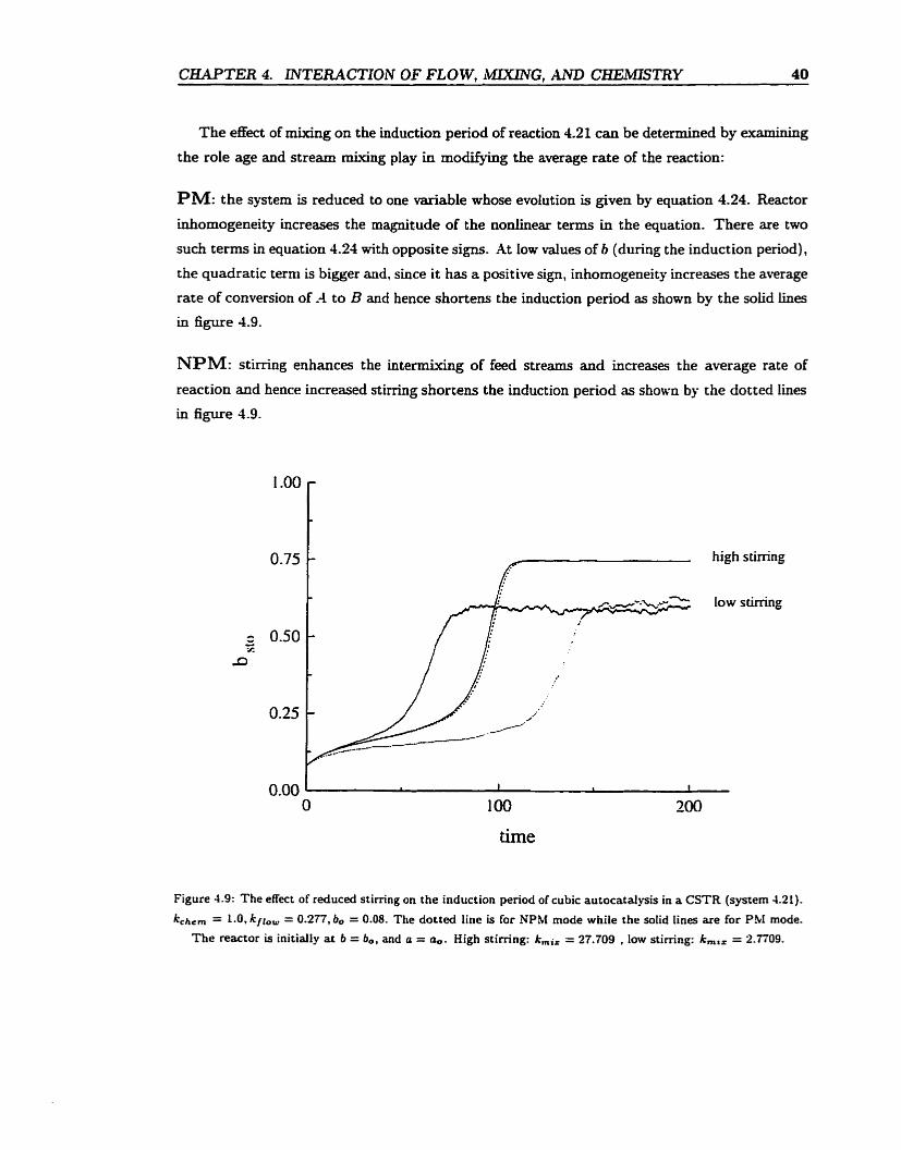
CHAPTER 4. INTERACTION OF FLOW, MIXLNG, AND C&EMTSTRY 40

The effect of mixing on the induction period of reaction 4.21 can be determined by examining

the role age and Stream miving play in modifying the average rate of the reaction:

PM: the system is reduced to one variable whose evolution is given by equation 4.24. Reactor

inhomogeneity increases the magnitude of the nonlinear terms in the equation. There are two

such terrns in equation 4.24 with opposite signs. At low d u e s of b (during the induction period),

the quadratic term is bigger and, since i t has a positive sign, inhomogeneity increases the average

rate of conversion of -4 to B and hence shortens the induction period as shown by the solid h e s

in figure 4.9.

NPM: s t i h g enhances the intennWng of ieed streams and inmeases the average rate of

reaction and hence increased stirring shortens the induction period as shoun by the dotted lines

in figure 4.9.

high stirring

low srirring

Figure 4.9: The effect of reduced stirring on the induction period of cubic autocatalysis in a CSTR (systern 4.21).

kchcm = 1.0, kflow = 0.271, bo = 0.08. The dotted line is for NPM mode while the solid Iines are for PM mode.

The reactor is initially at b = b,, and a = a,. High stimng: kmi, = 27.709 . low stimng: km,, = 2.7709.

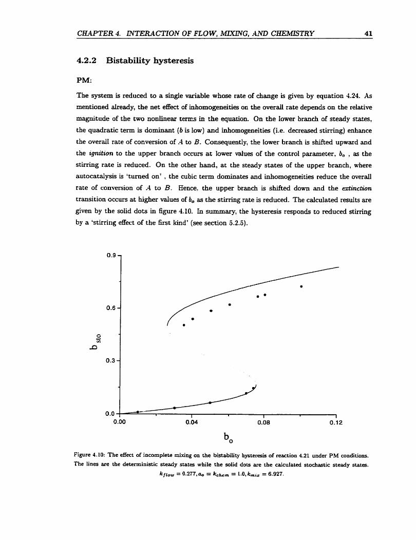
CE4PTER 4. LNTERACTlON OF FLOW, MLXüVG. -4ND CaEMTSTRY 41

4.2.2 Bistability hysteresis

PM:

The system is reduced to a single variable whose rate of change is given by equation 4.24. As

mentioned aiready, the net effect of inhomogeneities on the overall rate depends on the relative

magnitude of the two nonlinear tenrs in the equation. On the lower branch of steady states,

the quadratic tenn is dominant (b is low) and lnhomogeneities (i-e. decreased stirring) enhance

the overail rate of conversion of -4 to B. Consequently, the lower branch is shifted upward and

the ignition to the upper branch occurs a t lower values of the control parameter, b, , as the

stirring rate is reduced. On the other hand, at the steady states of the upper branch, where

autocatalysis is 'turned on' , the cubic term dominates and inhomogeneities reduce the overail

rate of conversion of A to B. Hence. the upper branch is shifted down and the eztinction

transition occurs at higher values of b, as the stirring rate is reduced. The calculated results are

given by the soiid dots in figure 4.10. In siimmary, the hysteresis responds to reduced stirring

by a 'stirring effect of the k t kind' (see section 5.2.5).

Figure 4.10: The effect of incomplete rnixing on the bistability hysteresis of reaction 4.21 under PM conditions.

The lines are the deterministic steady states while the solid dots are the calculated stochastic steady states.

krlow = 0.277, = kchem = L-O, kmiz = 6.927-

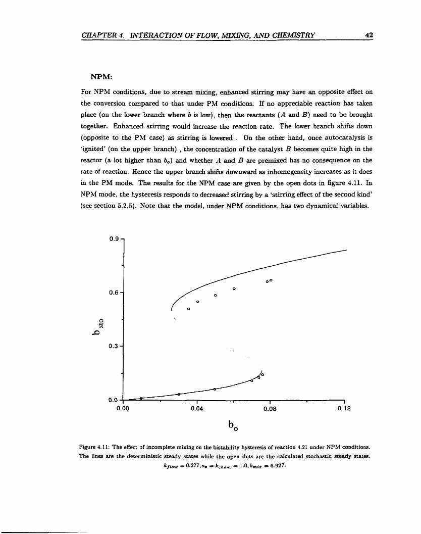
CEWTER 4. INTERACTION OF FLOW, MLxn\lG, .4ND C&EMTSTRY 42

NPM:

For NPM conditions, due to Stream mixing, enhanceci stirring may have an opposite effect on

the conversion cornpared to that under PM conditions. If no appreciabie reaction has taken

place (on the lower branch where b is low), then the reactants (-4 and B) need to be brought

together. Enhanced stirring would increase the reaction rate. The iower branch shifts dom

(opposite to the PM case) as stirring is lowered . On the other hand, once autocatalysis is

'ignited' (on the upper branch) , the concentration of the catalyst B becomes quite high in the

reactor (a lot higher than 6,) and whether A and B are premïxed has no consequence on the

rate of reaction. Hence the upper branch shifts downward as ïnhomogeneity increases as it does

in the PM mode. The results for the NPM case are given by the open dots in figure 4.11. In

NP31 mode, the hysteresis responds to decreased s t i r ~ g by a 'stirring effect of the second kind'

(see section 5.2.5). Note that the model, under NPM conditions, has two dynarnical variables.

Figure 4.11: The effect of incornplete mixing on the bistability hysteresis of reaction 4.21 under NPM conditions.

The lines are the deterministic steady states while the open dots arc the calculated stochastic steady states.

kfiow = 0.27?,% = kCh,, = 1.0, kmi, = 6.927.

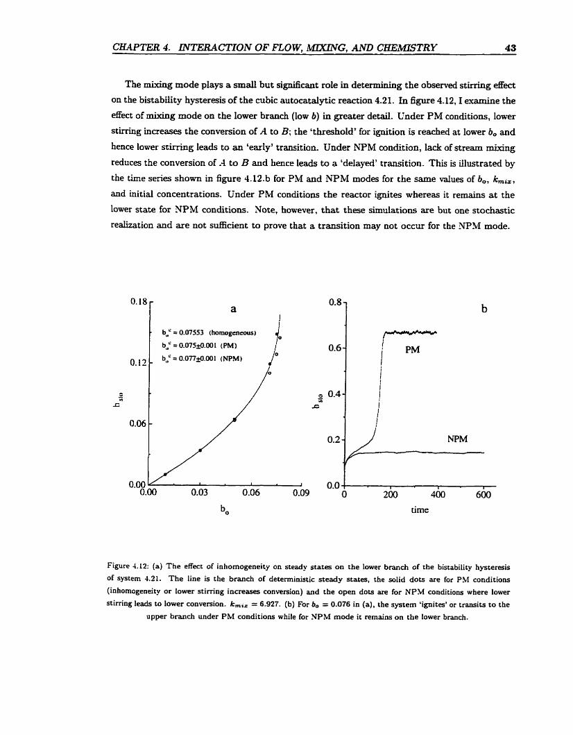
CE4PTER 4. INTERACTION OF FLOW, MKüVG, AND C!EEMETRY 43

The dxing mode plays a s m d but significant role in determining the obsened stirring effect

on the bistabiiity hysteresis of the cubic autocatalytic reaction 4.21. In figure 4.12,I euamine the

effect of m g mode on the Iower branch (low 6) in greater detail. Under P M conditions, lower

stimng increases the conversion of A to B; the cthreshoId' for ignition is reached at lower b, and

hence lower stimng leads to an 'early' transition. Under NPM condition, la& of stream rnixing

reduces the conversion of -4 to B and hence leads to a Ldelayed' transition- This is illustrated by

the time series shown in figure 4.12.b for PM and NPM modes for the same values of b,, km,, , and initial concentrations. Under PM conditions the reactor ignites whereas it remains a t the

lower state for NPM conditions. Note, however, that these simulations are but one stochastic

realization and are not sufficient to prove that a transition may not occur for the YPM mode.

Figure 4.12: (a) T h e effect of inhomogeneity on steady states on the lower branch of the bistability hysteresis

of system 4.21. The line is the branch of deterministic steady states, the solid dots are for P M conditions

(inhornogeneity or lower stirring increases conversion) and the open dots are for NPM conditions where lower

stirring leads to lower conversion. k,i= = 6.927. (b) For 6, = 0.076 in (a), the system 'ignites' or transits to the

upper branch under P M conditions while for NPM mode it remains on the lower branch.

0.18 - 0.8 - a

b,: = 0.OXd.W 1 (PM) 0.6 - b,: = 0.077fl.001 (NPM) o.1z -

- - e 0.4- V1

d

Y)

z s

0.06 -

7 ' PM i i 1

0.2 - - 1

NPM

0.00 J 0.0 , 0.00 0.03

1 1

0.06 I

0.09 O 200 400 600

CK4PTER 4. LNTERACTION OF FLOW. W G . AND CHEMLSTRY 44

4.2.3 Reactor inhomogeneities and fluctuations

Here, 1 examine the dependence of the degree of inhomogeneity of the CSTR on the bifurcation

parameter b,. 1 consider the long-time averages of the absolute and relative variances in the

concentration of the cataiyst:

Figure 4.13 gives the absolute and relative variances for both branches of the hysteresis

(figures 4.8, 4.10, 4.11) under PM conditions- Interestingly, the value of the absolute variance

decreases on the thermodynamic branch (SSI) as the transition is approached. As explained

in appendk -4.23, Linear stability anaiysis predicts that the relaxation tirne of perturbations

from steady states diverges as saddle-node bifurcations are approached and the magnitude of

fluctuations in the steady states of the system is therefore expected to grow in a critical manner

on both branches of the hysteresis. X detailed discussion of the relatioaship between the reactor

inhomogeneity and the temporal fluctuations in its steady states and of the nature of cn'tical

behavior in the CSTR will be presented in chapter 5.

4.3 Oscillations in the Gray-Scott reaction

One of the most readily observed effects of stirring on the dynamics of nonlinear reactions is the

effect on oscillation periods and amplitudes. In most e , u p e r i r n e n t ~ ~ ~ ~ ~ ' * ~ ~ the oscillation period

increases with the rate of stirring. This is however not generic since a few e - ~ p e r i m e n t s ' ' ' ~ ~ ~ ~ ~

have s h o w the opposite effect. Here, 1 will demonstrate how Stream and age miving lead to

opposite stirring effects on the period.

The cubic autocatalytic reaction 4.21, coupled with a simple decay of the catalyst (Le. the

Gray-Scott r n~de l - ' ~ ) is perhaps the simplest-chernical system e-uhibiting limit cycle oscillations:

In a CSTR, the rates of change of a and b are:

a = -kLab2 + kllow (ao - a),

b = k iab2 -k2b+kf , , ( bo -b ) .

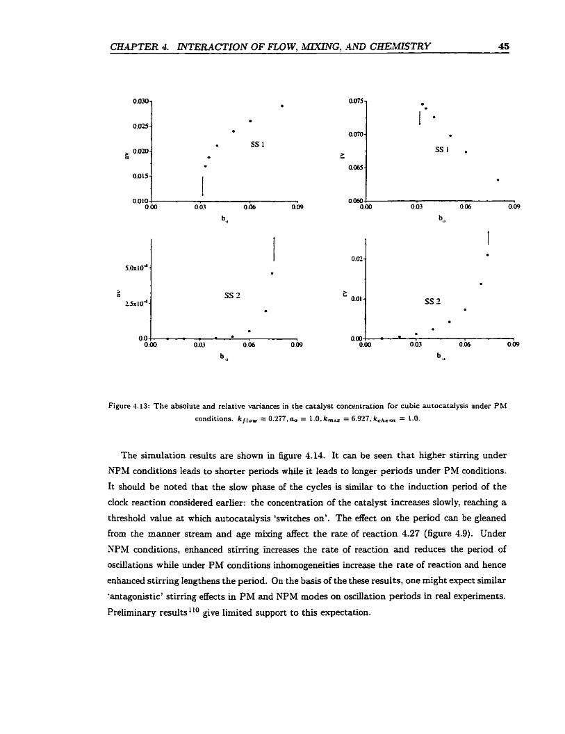
CH-UTER 4. LNTER4CTION OF FLOW. kflXüVG, .IUVD CKEl'M7STRY 45

Figure 4.13: The absolute and relative variances in the catalyst concentration for cubic autocatdysis under PM

conditions. C c l r , , = 0.277, a, = t.O,k,,, = 6.927, kCh,, = 1.0.

The simulation results are shown in figure 4.14. It can be seen that higher stirring under

NPM conditions leads to shorter periods while it leads to longer periods under PM conditions.

It should be noted that the slow phase of the cycles is similar to the induction period of the

clock reaction considered earlier: the concentration cf the catalyst increases slowly, reaching a

threshold value a t which autocatalysis 'switches on'. The effect on the period can be gleaned

from the manner Stream and age mixing affect the rate of reaction 4.27 (figure 4.9). Under

XPM conditions, enhanced st imng increases the rate of reaction and reduces the period of

oscillations while under PM conditions inhomogeneities increase the rate of reaction and hence

enhanced stirring Iengthens the period. On the basis of the these results, one might expect similar

'antagonistic' stirring effects in PM and NPM modes on oscillation periods in real experiments.

Preliminary resultsl10 give limited support to this expectation.

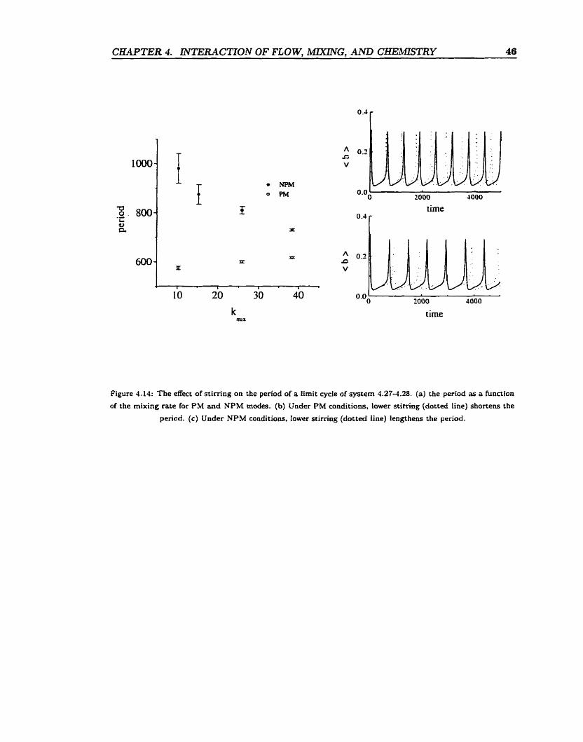
CHAPTER 4. INTERACTION OF FLOW, k€üCûVG, AND CEEmTRY 46

time

Figure 4.14: The effect of stimng on the period of a limit cycle of systern 4.27-4.28. (a) the period as a function

of the muùng rate for PM and NPM modes. (b) Under PM conditions, Lower stirring (dotted Iine) shortens the

period. (c) Under NPM conditions, Iower stirring (dotted iine) lengthens the penod.

Chapter 5

A stochastic description of one-variable bistable systems

in a CSTR

in the previous three chapters, 1 demonstrated that spatiotempord inhomogeneities arising from

nonideal mlIring in flow reactors affect the dynarnics of nonlinear reactions both quantitatively

and quaiitatively. The aim of this chapter is to present a quantitative stochastic description

of bistable systems in the CSTR, based on the random coalescence-redispersion miving model.

Two key issues are addressed: (1) The stirring effects on the bistabiiity hysteresis are quanti-

lied by deriving closed-form expressions for the stochastic steady states of general one-variable

systems as functions of the control parameters. UseN scaiing relations between the reactor

inhornogeneity and the shift of the steady states are obtained and the dependence of the degree

of inhomogeneity in the reactor on control parameters is detennined. The anaiysis is supported

bg experimental results from the iodate-arsenous acid system. (2) The relationship between

the spatial nonuniforrnity of the reactor and the fiuctuations in the global steady states of the

reactor is investigated. Particular attention is paid to the behavior of the two measures near

the bistability transitions.

Let x be a vector of concentrations whose chernical rate of change is given by the vector

function f(x). If the reactor is homogeneous, it can be described by the deterministic equation:

where kll,, is the inverse residence time and x, is the value of x in the feed.

In order to account for the inhomogeneity and fluctuations of the concentrations in the

reactor? one must view x ( t ) as a random variable and characterize the state of the system in

terms of the probability P(x, t )dx that the concentration vector has a value within a domain

dx centered a t x at time t. In theoretical ternis, the determination of P(x, t) requires that one

observes the time evolution of a large number of similarly prepared systems (an ensemble). For

CK4PTER 5. A STOCE4STIC DESCRLPTlON OF CSTR B I S T 1 4 B m 48

a stationary process, the probability distribution can be obtained from obsenring x ( t ) of one

system over a long period of time (the ergodic condition).

For spatidy extended systems, one may consider a random variable x(t) that describes the

evolution of a representatzue point in the system and approximate p(x, t) by the distribution

of the random variables componding to a large number of such representative points. In this

construction, one may divide the global system into many regions or subsystems. Each subsystem

is mal1 compared to the global system's macroscopic dimensions but each contains a sufficiently

large number of constituent microscopic elements (e-g. molecules) that macroscopic variables

and concepts (concentration, temperature, etc.) can be associated with it. The subsystems can

be thoiight of as miniature systems governed by the same macroscopic equations and hence have

the same steady states as the global systern.

In this chapter, 1 anaIyze the random coalescence-redispersion rnicromking model of the

CSTR in which the reactor is regarded as a collection of fluid elements which are randody

replaced by fresh reactant elements and coUide randornly with each other at given flow and

miving rates. The fluid cells are statisticaüy identical and hence the evolution of a single ceU is

representative of aU celis. -4 one-dimensional stochastic equation is derived which describes the

evolution of the concentration in a single cell. Its solution is show to agree very well with the

experimental stirring effects in the one-variable iodate arsenous acid system. On the other hand,

the evolution of a single ceii is not representative of the global, collective dynamics of the CSTR.

In particdar, the concentration fluctuations in a single ceU do not describe the fluctuations in

the global state of the system (Le. average concentration). The latter part of the chapter is

devoted to examining in detail the stochastic dynamics of local (single ceIl) and globd (whole

reactor ) systems and t heir interrelationship.

5.1 The coalescence-redispersion model

In this r n ~ d e l ' ~ , the reactor is regarded as made up of equafly çized fluid elements that inter-

act in pair-wise collisions. The interactions are assumed to occur by coalescence (Le. joining)

followed by redispersion (Le. splitting). The flow introduces new fluid elements containing pure

reactants and results in the removd of an equal number of fluid elements fiom the reactor.

The concentrations of ail chernical species in a given fluid element are d o m throughout that

element and evolve according to their homogeneous batch kinetics. The state of the reactor

can be described by a concentration probability distribution, P(x)dx, which gives the fraction

of the reactor (Le. fraction of the total number of fluid elements) having concentrations in the

range (x, x + dx). Curl l8 was the first to derive the intego-differential equation describing the

evolution UF such a probability distribution:

CWTER 5. A STOCHASTIC LIESCRIPTION OF CSTR BISTABEITY 49

where the first term on the right accounts for chernical reaction, the second terrn for the flow

and the last term for the pair-wise mixing of fluid elements.

The original scheme (i.e. equation 5.2) can be solved directly by finite-merence schemes " .

Such techniques usuaiiy suffer from numerical instabiiity and convergence problems and can be

used only with the simplest kinetic schemes. Evangelista et developed a perturbation ex-

pansion method to solve equation 5.2. In this method, the probability distribution is expanded

in powers of (kf low/kmiZ) leading to a set of linear equations for the different powers of the

moments of the distribution. Horsthemke and h an non^^*^^ derived equation 5.2 using the tan-

guage of stochastic processes. They appiied the perturbation expansion of Evangelista to obtain

expressions for the mean and variance of the concentration of a simple one variable system. The

perturbation expansion method assumes that the probability distribution is stationary. It is

valid only in the high stirring limit and becomes cumbersome for systems with more than one

variable.

A more useful approach is to simulate the rnodel directly. This method adds flexibiiity to

the rnodel in that it can be used with multiple feed streams and complex kinetic schemes. The

coalescence-redispersion events can be made instantaneous or delayed (to reflect the h i t e t i r n e

nature of molecular di&ision). The events may resdt in complete equalization of concentrations

or just partial =change of matter. Spielman and Levenspielg8 were the 6rst to describe a Monte-

Car10 scheme to simulate the random codescence-redispersion mode1 of a CSTR. The algorithm

is described next.

5.1.1 The random coalescence-redispersion (RCR) mode1

The CSTR is made up of N identical Suid parcels or c e k Labeiled i, where each behaves as a

homogeneous batch reactor. For the ith cell, the rate of change of the concentrations xi is given

by :

C W T E R 5. A STOCHASTIC DESCRPTlON OF CSTR BISTABLLITY 50

The algorithm consists of the following steps:

(1) The reactor is fed at intervais 71 by replacing k randomly chosen cells with k new ceUs

with feedstream concentrations where k is the number of feecistreams. The feeding interval TI

is related to the residence time by T,.. = q. (2) M k b g is achieved by randomly choosing at intervals r, a pair of cells and averaging

('coalescing and redispersing') their concentrations: xi = xj = (xi + z j ) / 2 . For any c d to

undergo a mixing event, it takes on average r,,,, = , ~ m NT time units. This is used as the

characteristic mixing time in the reactor.

(3) Between the periodic feeding and m g events, the concentrations in each of the N c&

evolve according to equation 5.3.

The dynamical state of the reactor at a given instant is given by the instantaneous concen-

trations of all species in aü ceus.

5.1.2 Heuristic derivation of the Langevin equation for the RCR model

In this section, the above RCR algorithm is reduced, for the case of single-variable kinetics,

to a one-dimensional Langevin equation for the concentration xi in a representative celi. The

random term in the Langevin equation is a multiplicative colored noise process. In the limit of

high stirring, employed here, the latter is approximated by white noise.

Consider the evolution of the concentration zi in the i th ceil. Mixing and flow contribute to

the stochasticity of xi: mixing is described by the stochastic process

1 if the ith and jth ceils are mixed at time t x&) = O otherwise.

The probability per unit tirne that x i j ( t ) = 1 is kmY = l/r,,, (the cumulative probability for

the interval At is Atkmir)-

Flow is described by the stochastic process

1 if the i th ceiI is replaced by a new ceil with concentration x, at t h e t 4i ( t ) =

O otherwise. (5-5)

The probability per unit t h e that 4j = 1 is kfl,, = 1 / ~ ~ 1 a ~ ((the cumulative probability for

the interval At is Atkfl,,).

1 wiIl derive an equation for the change of concentration Azi = xi ( t + At) - xi ( t ) during the

time interval At. In this discrete representation of the model, mixing and feeding events take

place only at tirnes t, t + At, t + 2 4 t , --•-. During the interval At, xi evolves according to the

deterministic batch kinetics (% = f ( ~ i ) ) . From physical considerations, a ceil i cannot undergo

CEAPTER 5- A STOCaASTIC DESCRIPTION OF CSTR BISTABL&lTY 51

feeding and mixïng events at the same instant in tirne. Hence I chose to account for mixing a t

the beginning and for feeding at the end of the interval. The opposite choice is equalIy valid

and leads to the same resdt.

If the ith ceU is mixed with another ce11 j, at time t (Le. x i j ( t ) = 1 ) then the concentration

in the ith cell at tirne t + 4 t is given by

xi(t + At) = xi ( t ) + zj ( t ) zi ( t ) + xj ( t ) 2 + 4 t f ( 2 1

where 6xji = f ( z j ( t ) - ~ i ( t ) ) is half the dinerence in the concentration in the two ceUs prior to

their miuing.

If no mixing event takes place at time t (Le. ~ ~ ( t ) = O ) ,

xi(t + At) = Zi(t) + At f ( ~ i ( t ) ) (5.7)

and hence

z i ( t + At) = [ 1 - x i j ( t ) ] [ z i ( t ) + 4 t f ( ~ i ( t ) ] + ~ i ~ ( t ) [ ~ i ( t ) + 6xji + At f ( ~ i ( t ) + h ~ j i ) ] - (5-8)

If the ith ceil is replaced by a new ceIl at t + At (Le. &(t i- At) = i), then

~ i ( t + At) = z0 ( 5 -9)

and hence the concentration in the i th ceell at tirne t + At is given be the following stochastic

equation:

and

In the limit of high stirring dxji(t) << z i ( t ) , the last term in equation 5.11 becomes negligible

compared to the other terms. Dropping this term, performing a Taylor series expansion of f

near z i ( t ) and keeping only linear terms in 6zj i , one obtains

CEWTER 5. -4 STOCaASTIC DESCRlPTION OF CSTR BSTABLLITY 52

Since the goal is to describe the role of stochastic m g , the random feeding process #i(t + At) is now replaced by a constant process whose value is equal to the time average of &(t + At)

(Le. di(t + At) + kfr,At ). Thus,

where [6xjij is the value of &rji when the flow occurs as just descnbed, and O(2) denotes terms

containing

In the E t of At + O one obtains the Langevin equation

for the evolution of the concentration in a representative celi (Le. local variable), where the

index i has been dropped and f ( t ) is a random process given by

This random process models the stochastic miuing of the representative ceii with other cells.

It is assumed to have a zero mean

function:

where l/y is the correlation tirne, c

(< ( ( t ) >= 0) and an exponentiaily decaying correlation

is the amplitude and D is the variance of (.

The random term in the Langevin equation describes micromixing as a multiplicative colored

noise process, if the rate function f (x) is nonlinear. On the other hand, If f (x) is linear, the

noise process becornes additive and stining effects vanish (since < >= 0).

The main source of fluctuations in the CSTR is the forcing of the reactor by the feeding

process. Accordingty, the square of the amplitude of the fluctuations is empiricaiiy set to

CTL4.îTER 5. A STOCKASTIC DESCRIPTION OF CSTR BBTABZITY 53

where x, is the stochastic steady state of the system. The correlation time of Xi j and hence of

( is given by 1/7 = r,it - Thus,

The simplest way to analyze equation 5.15 is to consider the limit of white noise, which is

a good approximation for weakly colored noise3'. The transition from colored to white noise is

performed formciliy by substituthg e q ( t / r ) -+ d(t). This gives the correlation fiinction:

< C(t)e(t1) >= Dd(t - t'). (5.20)

It can be seen that the deterministic equation 5.1 is the limiting case of equation 5.15 for

vanishing fluctuations O + O, which is achieved in the 'weil-stirred' limit rm, + 0.

5.1.3 Andysis of the Langevin equation

Equation 5.15 can be investigated by formally introducing the density distribution

P(x , t 1 20, to) I P ( x , t), for the conditionai probability of finding the system at a point z at

time t, provided that it was at xo a t time to. The evolution of this probability density is governed

by a Fokker-Planck equation which is obtained by the standard te~hni~ues"l*~':

where the Stratonovicb interpretation of the white-noise approximation of 5.15 is used. The

stationary solution of 5.21 is

where .?l is a normalking factor and U ( x ) is given by

For a bistable system, the probability distribution has two maxima. The stnchastic steady states

of the system correspond to these maxima (provided that the intensity of the noise is sufkiently

smaU and the gap between the steady states is sdiiciently large) and are obtained from the

stationarity condition dP(z ) /& = 0:

C W T E R 5. A S T O C ' S T I C DESCRIPTTON OF CSTR BISTABXLITY 54

The roots of 5.25 give the position of the stochastic steady states x,.

The variance in of x is given by54

At sufnciently high stimng, E ( z s - z,)*($)~ 1 and

Since

local

rmtx < 6x2 >= 2-(~r - ~ 0 ) ~ -

Tf low

this is the variance of the concentration in a single representative ceil, 1 designate this

vanance by 0: to distinguish ic boom O:, the variance of the global or average reactor

concentration. The difference and relationship between the two quantities are discussed in

section 5.3.

The equation

Tm iz 0; = 2- (z, - x,J2 (5.28)

Tf low

describes the degree of spatial inhomogeneity in the reactor and is a consequence of the assump

tions made in specifying the stochastic process c ( t ) through equations 5.17, 5.19, i.e. it resdts

fiom considering the forcing (perturbation) of the reactor by the feeding process as the main

source of fluctuations. The equation wiil be shown to correctly reproduce both the RCR mode1

simulations and experiments.

Finaily, the stirring effect on the deterministic steady states of the reactor c m be quantifiecl

by introducing the shift of the stochastic steady state from the detenninistic high stirring b i t

A = x, - xd. Here the detemiinistic steady states xd are the roots of g(xd) = O and the

stochastic steady states z, are the roots of g(x,) - D(xs)g'(x,)gl'(x,) = O . Substituting in 5.24,

performing a Taylor-expansion, and keeping only h e a r terms in h Iead to

CHAPTER 5. A STOCKASTIC DESCRLPTION OF CSTR BISTABLLITY 55

Sufficiently far from the transitions, 4 c m be approximated by

In the range of MLidity (sufEciently high stirring and far h m the transition) of this key result,

the observed shift A of the stochastic steady state is proportionai to the reactor inhomogeneity

o:. For ûxed control parameters (Mlying only the stirring rate), the relationship is linear and

the direction of the shift is detennined by the sign of gM(zd), since g t ( x d ) is always negative

because z d is a stable steady state. As I will elaborate in the discussion at the end of section 5.2,

equation 5.30 allows one to make general conclusions regardhg the stirring effect on bistability

hystereses.

5.2 Mixing effects

In this section, simulations and experiments are used to illustrate:

1. The suitability of the RCR model in describing the stirring effects in the CSTR.

2. The validity of the reduction of the model to the Langevin equation 5.15.

The stirring effect on bistability hysteresis in the CSTR is the simplest and most studied

e~ample, highiighting the consequences of imperfect mixing on the dynamics of nonlinear reac-

tions.

The iodate-arsenous acid reaction is chosen as a test case because it can be reduced to a one-

variable system if arsenous acid is in excess. The concentration of iodide in the feed is chosen

as a bifurcation parameter instead of the often used flow rate. This choice has the advantage

that changing the bifurcation parameter does not directly affect the hydrod-vnamic state of the

reactor.

C W T E R 5. A STOCEASTIC DESCRLPTION OF CSTR BISTABDXY 56

5.2.1 The iodate-arsenous acid systernss

The reaction is cornposeci of two processes:

If H3.4s03 is in stoichiometric excess, the net reaction is given by (0.31)+3(5.32):

Process 5.31, wtiose empiricai rate law is @en by

is the rate deterrnining step for 5.33. Hence, from 5.33,

where [I-Io , [IO,], are the initial concentrations of iodide and iodate. Combining 5.36 and

6.36, one obtains the following one-variable system:

dx - = f (x) = (kl + kzx)h2z (xo + y, - x) dt

(5.37)

where, x G [I-] , zo i LI-], ,y, z [IO;], , ki = 4.5 - lo31LI -3s-L , k2 = 4.5 ~ - 1 0 ~ i C I - ~ s - ~ .

If the reaction is carried out in a CSTR where the iodide and iodate are fed into the reactor

via a single Stream (PM), the detenninistic or homogeneous dynamics is governed by:

Depending on the d u e s of the control parameters (kf x,, y,, h), the above equation

admits one or three positive real roots. In the 6 r s t case, the reactor possesses a single stable

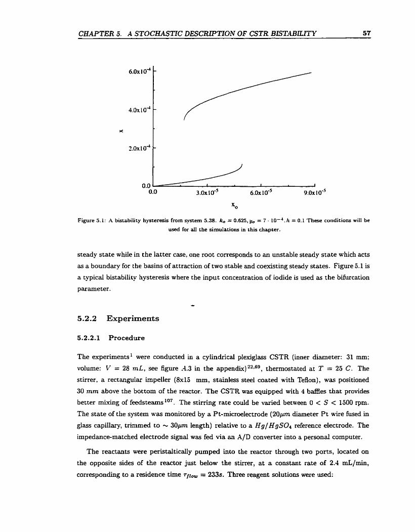
C&9PTER 5. A STOCEASTIC DESCRIPTION OF CSTR BLST,A.BIU"N 57

Figure 5.1: h bistability hysteresis from systern 5.38. k, = 0.625, y, = 7 - IO-". h = 0.1 These conditions will be

used for al1 the simulations in this chapter.

steady state while in the latter case. one root corresponds to an unstabte steady state which acts

as a boundary for the basins of attraction of two stable and coeiasting steady States. Figure 5.1 is

a typicd bistability hysteresis where the input concentration of iodide is used as the bifurcation

parameter.

*

5.2.2 Experiments

5.2.2.1 Procedure

The e-xperiments' were conducted in a cylindncal plexiglass CSTR (inner diameter: 31 mm;

volume: V = 28 m L , see figure -4.3 in the a p p e n d i ~ ) ' ~ * ~ ~ , thermostated at T = 25 C. The

stirrer, a rectangular impeller (8x15 mm, stainiess steel coated with Teflon), was positioned

30 mm above the bottom of the reactor. The CSTR was equipped with 4 ba£Eies that provides

better rnking of f e e d ~ t e a r n s ' ~ ~ . The stirring rate couid be varied between O < S < 1500 rpm.

The state of the system was monitored by a Pt-microelectrode (20pm diameter P t wire fused in

glas capiIlary, tnmmed CO - 30pm length) relative to a H g / HgS04 reference electrode. The

impedance-matched electrode signal was fed via an A/D converter into a persona1 cornputer.

The reactants were peristalticaiiy pumped into the reactor through two ports, located on

the opposite sides of the reactor just below the stirrer, a t a constant rate of 2.4 mL/min,

corresponding to a residence time r j l , , = 233s. Three reagent solutions were used:

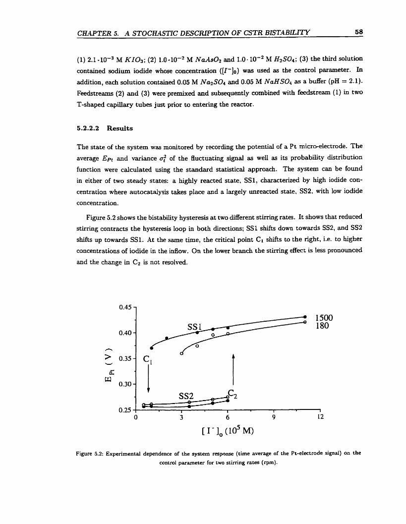
CE4PTER 5. -4 STOCE4STIC DESCRIPTION O F CSTR B S T - 4 B W 58

(1) 2.1 -10-~ M KI03; (2) 1.0 -10-~ M NaAsoz a d 1.0 - 10-~ M H2S04; (3) the third solution

contained sodium iodide whobe concentration ([I-Io) was used as the control parameter. In

addition. each solution contallied 0.05 M Na2S04 and 0.05 M N a H S 0 4 as a b d e r (pH = 2.1).

Feedstreams (2) and (3) were premixed and subsequently combined Mth feedstream (1) in two

T-shaped capillary tubes just prior to entering the reactor.

The state of the system was monitored by recording the potentiai of a P t micro-electrode. The

average Ept and Mnance o; of the fluctuating signal as well as its probability distribution

function were calcdated using the standard statisticd approach. The system can be found

in either of two steady States: a highly reacted state, SS1, characterized by high iodide con-

centration where autocatalysis takes place and a largely unreacted state, SS2, with low iodide

concentration.

Figure 5.2 shows the bistability hysteresis at two different stirring rates. It shows that reduced

stimng contracts the hysteresis bop in both directions; SS1 shifts down towards SS2, and SS2

shifts up towards SS1. At the same time, the critical point Ci shifts to the right, i.e. to higher

concentrations of iodide in the M o w . On the lower branch the stimng effect is less pronounced

and the change in Cz is not resolved.

Figure 5.2: Experimental dependence of the system response (time average of the Pt-electrode signal) on the

control parameter for two stimng rates (rpm).

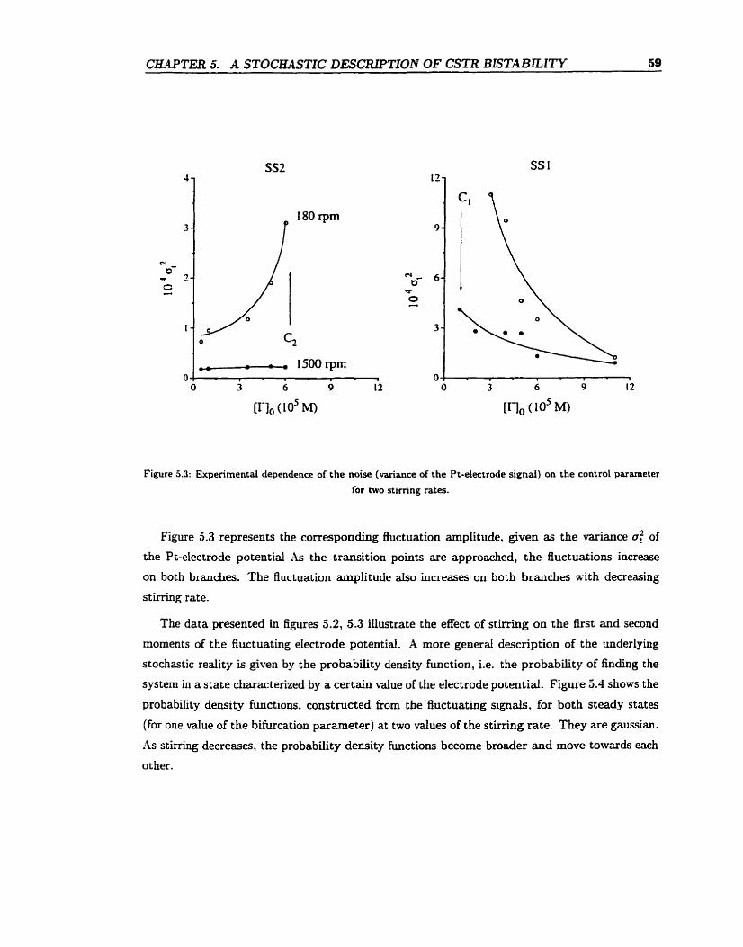
ClM-PTER 5. -4 STOCHASTIC DESCRlPTfON OF CSTR BISTABiLITY 59

Figure 5.3: Experimental dependence of the noise (variance of the Pt-electrode signal) on the control parameter

for two stirring rates.

O

Figure 5.3 represents the co~esponding fluctuation ampütude, given as the variance o: of

the P t-electrode potential As the transition points are approached, the fluctuations increase

on both branches. The fluctuation amplitude &O increases on both branches with decreasing

stirring rate.

-. 1500 rpm , - a . i

The data presented in figures 5.2, 5.3 illustrate the effect of stirring on the first and second

moments of the fluctuating electrode potentiai. A more general description of the underiying

stochastic reality is given by the probability density function, i.e. the probability of finding the

system in astate characterized by a certain value of the electrode potential. Figure 5.4 shows the

probability density functions, constmcted from the fluctuating signals, for both steady States

(for one value of the bifurcation parameter) at two d u e s of the stirring rate. They are gaussian.

As stirring decreases, the probability density functions become broder and move towards each

other.

O 3 6 9 12

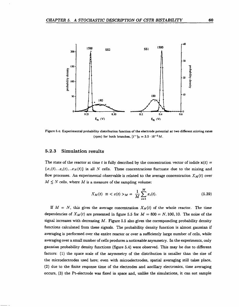
Figure 5.4: Experimental probability distribution function of the electrode potential at two different stirring rates

(rpm) for both branches, [I - jo = 3.5 - 10-5M.

5.2.3 Simulation results

The state of the reactor at t h e t is fully described by the concentration vector of iodide x ( t ) = {zl ( t ) . -.xi ( t ) , ..IN ( t ) ) in al1 !V cells. These concentrations fluctuate due to the miving and

flow processes. An e-xperimental observable is related to the average concentration X , L ~ ( ~ ) over

$1 5 N cells. where M is a measure of the sarnpling volume:

If AI = NT thiç gives the average concentration X N ( t ) of the whole reactor. The time

dependencies of XAf (t) are presented in figure 5.5 for hf = 800 = N , 100,lO. The noise of the

signal increases with decreasing M . Figure 5.5 also gives the corresponding probability density

functions calculated from tbese signais. The probability density function is ahos t gaussian if

averaging is perfomed over the entire reactor or over a sufficiently large number of celIs, while

averaging over a srnall number of cells produces s noticeable asymmetry. In the experiments, only

gaussian probability density functions (figure 5.4) were observed. This may be due to different

factors: (1) the space scale of the asymmetry of the distribution is srnalier than the size of

the microelectrodes used here; even with microelectrodes, spatial averaging still takes place,

(2) due to the finite response time of the electrodes and ancillary electronics, time averaging

occurs, (3) the Pt-electrode was fixed in space and, d e the simulations, it can not sarnple

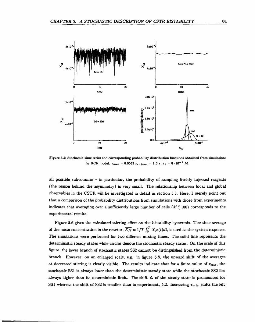
C W T E R 5. -4 STOCKASTIC DESCRIPTïON OF CSTR B I S T A B W 61

O 10 20

time

Figure 5.5: Stochastic tirne series and corresponding probabiiity distribution functions obtained from simulations

by RCR model. r,,, = 0.0533 s, r~~,, = 1.6 s, r, = 8 - 1 0 ' ~ M .

al1 possible subvolumes - in particdar, the probabiiity of sampling freshly injected reagents

(the reason behind the asymmetry) is very smaii. The relationship between local and global

observables in the CSTR will be investigated in detail in section 5.3. Here, 1 mereIy point out

that a cornparison of the probability distributions from simulations with those from e-xperiments

indicates that averaguig over a sufllciently large number of ceils (Ad> 100) corresponds to the

experimental results.

Figure 5.6 gives the calculated stirring effect on the bistability hysteresis. The time average T of the mean concentration in the reactor, = 1/T Io . (N(t )dt , is used as the system response.

The simulations were performed for two difEerent mixing times. The solid iine represents the

deterministic steady states whiie circles denote the stochastic steady states. On the scale of this

figure, the lower branch of stochastic states SS2 cannot be cüstinguished from the deterministic

branch. However, on an enlarged scaIe, e.g, in figure 5.8, the upward shift of the average

at decreased stimng is clearly visible. The results indicate that for a finite value of Tmiz , the

stochastic SS1 is always lower than the deterministic steady state while the stochastic SS2 lies

dways higher than its deterministic b i t . The shift 4 of the steady state is pronounced for

SS 1 whereas the shift of SS2 is smder than in experiment, 5.2. Increasing rmiz shifts the left

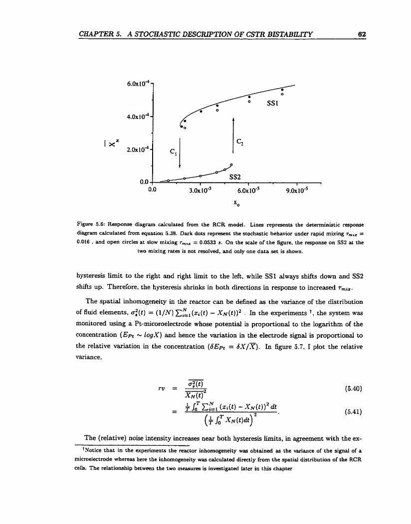
CEAPTER 5- A STOCMSTIC DESCRIPTTON OF CSTR BISTABILïTY 62

Figure 5.6: Response diagram calculated frorn the RCR modei. Lines represents the deterministic response

diagram calculated frorn equation 5.38. Dark dots represent the stochastic behavior under rapid rnixiag r,,, = 0.016 . and open circles at slow rnixing T,,, = 0.0533 S. On the scale of the figure, the response on SS2 at the

two rnixing rates is not resolved, and oniy one data set is shown.

hysteresis Limit to the right and right lunit to the Left, while SS1 always shifts down and SS2

shifts up. Therefore, the hysteresis shrinks in both directions in response to increased Tmiz.

The spatial inhomogeneity in the reactor can be defined as the variance of the distribution

of fluid eiements, o: ( t ) = ( 1 / N ) CE, (x i ( t ) - .yN ( t ) )Z . In the experiments t , the system was

monitored using a Pt-micoroelectrode whose potential is proportional to the logarithm of the

concentration ( E P ~ - l o g X ) and hence the variation in the electrode signal is proportionai to

the relative variation in the concentration (dEpt = 6X/T). In figure 5.7, 1 plot the relative

variance.

The (reIative) noise intensity increases near both hysteresis Limits, in agreement with the ex-

t ~ o t i c e that in the experiments the reactor inhomogeneity was obtained as the Mtiance of the signal of a

microelectmde whereas hem the inhomogeneity was calculated directly from the spatial distribution of the RCR cells. The relationship between the two measures is inwstigated Iater in this chapter

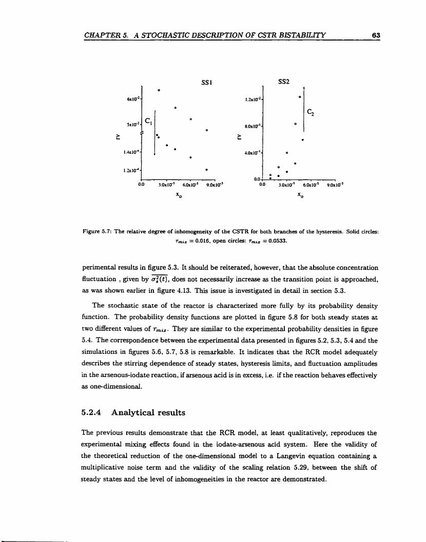
C W T E R 5. -4 STOCKASTIC DESCRLPTION OF CSTR BISTABlIJTY 63

Figure 5.7: The relative degree of inhomogeneity of the CSTR for both branches of the hysteresis. Solid circles:

rmi, = 0.0 16, open circIes: r,,,,, = 0.0533.

perimental results in figure 5.3. It should be reiterated, however, that the absolute concentration

fluctuation , given by a:(t), does not necessarily increase as the transition point is approached,

as was shown earlier in figure 4.13. This issue is investigated in detail in section 5.3.

The stochastic state of the reactor is characterized more f d y by its probabiiity density

function. The probability density functions are plotted in figure 5.8 for both steady states at

two different values of r,i,. They are similar to the experimentai probability densities in figure

5.4. The correspondence between the experimental data presented in figures 5.2,5.3,5.4 and the

simulations in figures 0.6, 5.7, 5.8 is remarkable. It indicates that the RCR model adequateIy

describes the stirring dependence of steady states, hysteresis Iimits, and ff uctuation amplitudes

in the arsenous-iodate reaction, if arsenous acid is in excess, Le. if the reaction behaves effectively

as one-dimensional.

5.2.4 Analytical results

The previous resuits demonstrate that the RCR model, at least qualitatively, reproduces the

experimental mixing effects found in the iodate-arsenous acid system. Here the validity of

the theoreticai reduction of the one-dimensionai model to a Langevin equation containing a

multiplicative noise term and the vaiidity of the scaiing relation 5.29, between the shift of

steady states and the level of inhomogeneities in the reactor are demonstrated-

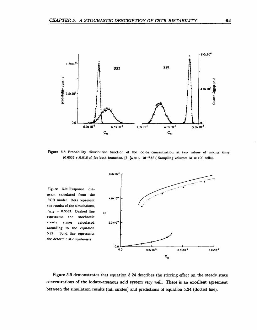
CHAPTER 5. A STOCKASTIC DESCRIPTlON OF CSTR BETABLLITY 64

Figure 5.8: Probability distribution function of the iodide concentration at two values of rnixing time

(0.0533 s.0.016 s) for both branches, [ I - ] O = 4 - 10-~ibf ( Sampling volume: ICI = 100 cells).

6 . 0 ~ 1 0 ~ /_.---.

.__...--+-

-5"" Figure 5.9: Response dia-

gram calculated from the

RCR rnodel. Dots represent 4.0x104 [[

Figure 5.9 demonstrates that equation 5.24 describes the stirring effect on the steady state

concentrations of the iodate-arsenous acid system very well. There is an excellent agreement

between the simulation results (full circles) and predictions of equation 5.24 (dotted line).

the results of the simulations,

r,,, = 0.0533. Dashed line

represents the stochastic

steady states caiculated 2 . 0 ~ 1 0 ~

according to the equation

/ =.=

-

5.24. Solid line represents

the deterministic hysteresis.

0.0 1 1

0.0 3.0~1 tY5 6 .0~10 '~ 9 .0~10 '~

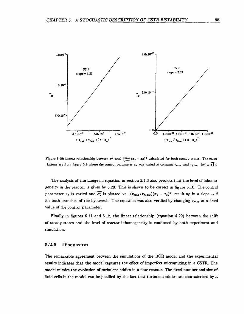
CEAPTE.. 5. A STOCaASTIC DESCRIPTlON OF CSTR BISTABLLITY 65

Figure 5.10: Linear relationship between u2 and *(z, - x0)* cdculated for both steady States. The calcu- - lacions are from figure 5.9 where the control parameter z, was varieci at constant r,,, and rjl,,. (a2 EE a:).

The andysis of the Langevin equation in section 5.1.3 also predicts that the level of inhomo-

geneity in the reactor is given by 5.28. This is shown to be correct in figure 5.10. The control

parameter xo is varied and is plotted vs. ( T ~ ~ ~ / T / ~ ~ ~ ) ( x ~ - z. )~, resulting in a slope - 2

For both branches of the hysteresis. The equation was also verified by changing r,,, at a fked

d u e of the control parameter.

Finally in figures 5.1 1 and 5.12, the Linear relationship (equation 5.29) between the shift

of steady states and the level of reactor inhomogeneity is confirmed by both experiment and

simulation.

5.2.5 Discussion

The remarkable agreement between the simulations of the RCR model and the eqerimental

resdts indicates that the model captures the effect of Mperfect micromixing in a CSTR. The

model mimics the evolution of turbulent eddies in a flow reactor. The fixed number and size of

fluid celis in the mode1 can be justified by the fact that turbulent eddies are characterized by a

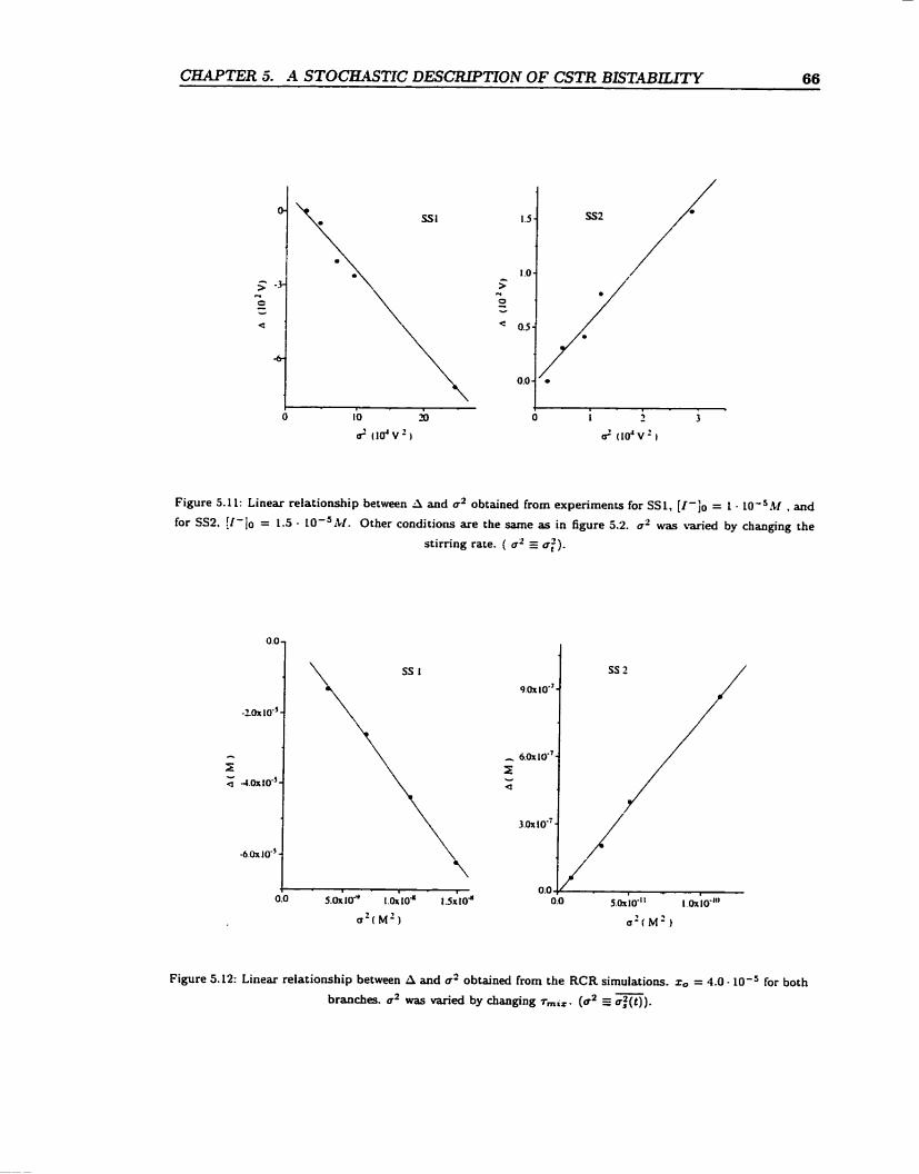
CKA-PTER 5. -4 STOC&UTIC DESCRLPrCTON OF CSTR BLSTABLLITY 66

Figure 5.11: Linear relationship between A and u2 obtained from experiments for SSl, [ i - j o = L . 104M , and

for SS2. [[-]O = 1.5 - 1O-'M. Other conditions are the same as in figure 5.2. u2 was varied by chaoging the

stirring rate. ( a' cf ) .

Figure 5.12: Linear reiationship between A and u2 obtained frorn the RCR simulations. z, = 4.0 - 10-= for both - branches. u2 was varied by changing Tmi=. (u2 EE uS(t)).

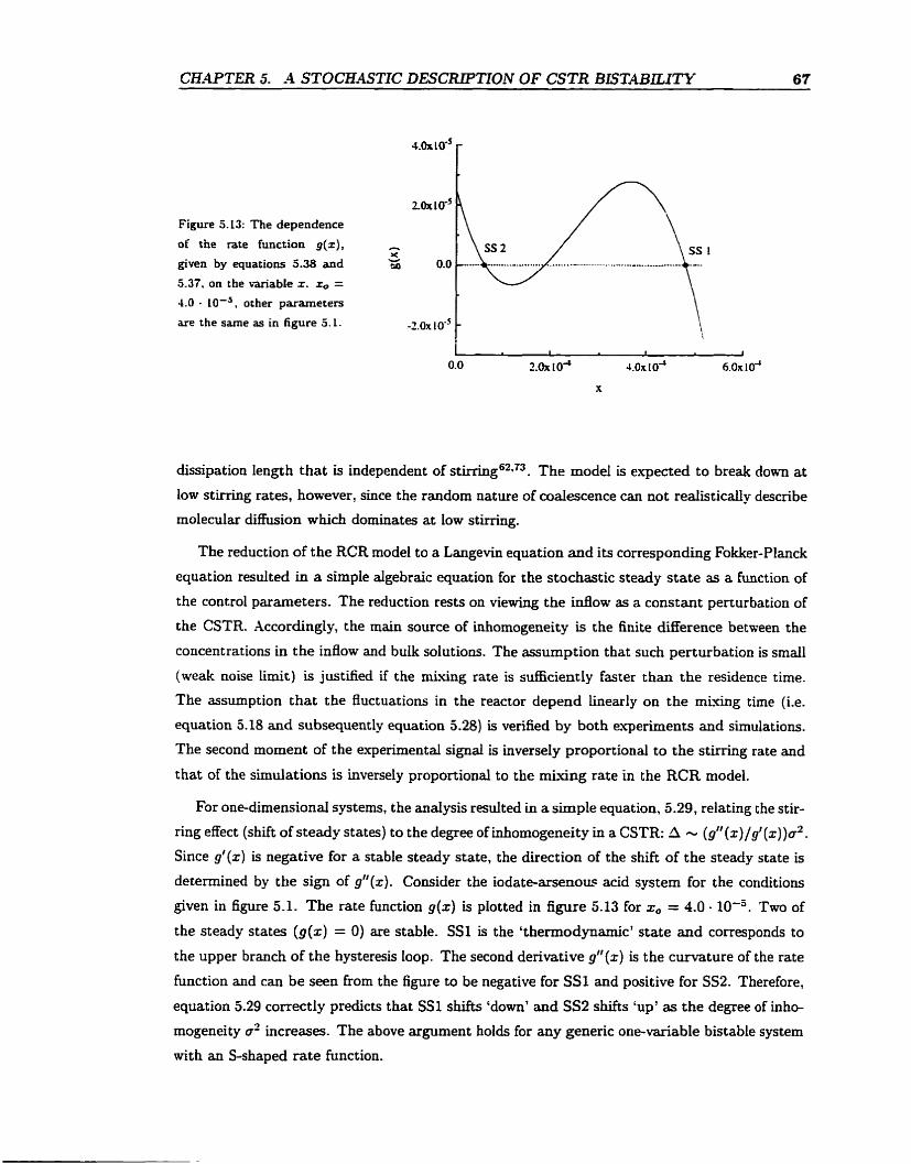
CEa4PTER 5- -4 STOCHASTIC DESCRlPnON OF CSTR BLST'LLITY 67

Figure 5. L3: The dependence

of the rate function g(x) ,

given by equations 5.38 and

5.37, on the variable z. x, = 4.0 - IO-', other parameters

are the sanie as in figure 5. L.

dissipation length that iç independent of s t i r ~ g ~ ~ - ~ ~ . The model is expected to break down at

low stirring rates, however, since the random nature of coalescence can not redisticdy describe

molecular diffusion which dominates at Iow stïrring.

The reduction of the RCR mode1 to a Langevin equation and its corresponding Fokker-Planck

equation resulted in a simple algebraic equation for the stochastic steady state as a Function of

the control parameters. The reduction rests on viewing the inflow as a constant perturbation of

the CSTR. XccordingIy, the main source of inhomogeneity is the finite ciifference between the

concentrations in the inflow and buik solutions. The assumption that such perturbation is srnaIl

(weak noise Lirnit) is justikd if the mkuing rate is sufficiently faster than the residence time.

The assumption that the fluctuations in the reactor depend linearly on the mixing time (Le.

equation 5.18 and subsequently equation 5.28) is verified by both experiments and simulations.

The second moment of the experimental signal is inverseIy proportional to the stirring rate and

that of the simulations is inversely proportional to the mLxing rate in the RCR model.

For one-dimensional systems, the analysis resulted in a simple equation, 5.29, relating the stir-

ring effect (shift of steady states) to the degree of inhomogeneity in a CSTR: A - (g" (x)/~'(x))o*.

Since g'(z) is negative for a stable steady state, the direction of the shift of the steady state is

determined by the sign of gn(z ) . Consider the iodate-arsenow acid system for the conditions

given in figure 5.1- The rate function g(x) is plotted in figure 5.13 for x, = 4.0 - 10'" Two of

the steady states (g(z) = 0) are stable. SS1 is the 'thennodynamic' state and corresponds to

the upper branch of the hysteresis Ioop. The second derivative gl'(z) is the curvature of the rate

function and c m be seea from the figure to be negative for SS1 and positive for SS2. Therefore,

equation 5.29 correctly predicts that SSl shifts 'down' and SS2 shifts 'up' as the degree of inho-

mogeneity a' increases. The above argument hoids for any generic one-variable bistai.de system

with an S-shaped rate function.

CHAPTER 5. -4 STOCE4STIC DESCRLPTION OF CSTR BIiSTAB17,ITY 68

S trizhak and Menzinger '* proposed to classify the above stirring effects , where the hysteresis

shrinks dong both coordinates, as a stirring effect of the first kind- This is the simplest case

of stirring effects on a bistability hysteresis and is exhibited, in addition to the iodate-arsenous

acid system, by the chiorite-iodide and the BZ s y ~ t e r n ' ~ * ~ ~ ~ . Nthough real systemç

that show this response are most often muiti-dimensional, they behave, as far as bistability is

concemed, as effectively one-variable systems. S ystems which behave quaiitat ively differently

are ~ a i d ' * ~ to exhibit stirring effect of the second kind. Such systems can not be regardeci as

effectiveIy one-dimensional. g"(z) is not a scaiar but represents a curvatures of an n-dimensionai

hypersurface. The hysteresis may shift a p*ori in any direction when projected into a one-

dimensional response diagram. A notable experimental system which exhibits stirring effects

which are not described by the current one-dimensional picture is the minimal bromate system 9 9 -- (figure 2.2).

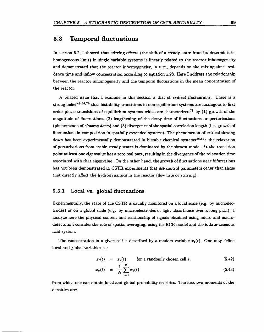
CEWTER 5. A STOCHASTlC DESCEUPTrON OF CSTR BLSTABLLITY 69

5.3 Temporal fluctuations

Ln section 5.2, 1 showed that stirring effects (the shift of a steady state from its deterministic,

homogeneous limit) in single variable systems is linearly related to the reactor tnhornogeneity

and demonstrated that the reactor uihomogeneity, in turn, depends on the mucing t h e , resi-

dence time and inflow concentration according to equation 5.28. Here 1 address the relationship

between the reactor inhomogeneity and the temporal fluctuations in the mean concentration of

the reactor.

-4 related issue that 1 examine in this section is that of critical fluctuations. There is a

strong belief49.5J*78 that bistability transitions in non-equiiibrium systems are analogous to k t

order phase transitions of equilibrium systems which are characteri~ed'~ by (1) growth of the

magnitude of fluctuations, (2) lengthening of the decay time of fluctuations or perturbations

(phenomenon of slowing d o m ) and (3) divergence of the spatial correlation length (Le- growth of

fluctuations in composition in spatialiy extended systems) . The phenomenon of criticai slowing

down has been experimentdy demonstrated in bistable chemicai systems36*63: the relaxation

of perturbations from stable steady States is dominated by the slowest mode. .4t the transition

point at least one eigenvalue has a zero real part, resulting in the divergence of the relaxation time

associated with that eigenvalue. On the other hand, the growth of fluctuations near bifurcations

has not been demonstrated in CSTR experiments that use control parameters other than those

that directly affect the hydrodynamics in the reactor (flow rate or s t i r ~ g ) .

5.3.1 Local vs. global fluctuations

E-xperimentally, the state of the CSTR is usually monitored on a local scale (e.g. by microelec-

trodes) or on a global scale (e.g. by rnacroelectrodes or Iight absorbance over a Iong path). 1

andyze here the physical content and relationship of signals obtained using micro and macro-

detectors; 1 consider the role of spatial averaging, using the RCR mode1 and the iodate-arsenous

acid system.

The concentration in a given cell is described by a random variable xi(t)- One may define

local and global variables as:

q ( t ) = xi(t) for a randomly chosen ce11 i, (5.42)

from which one can obtain local and global probability densities. The fkst two moments of the

densities are:

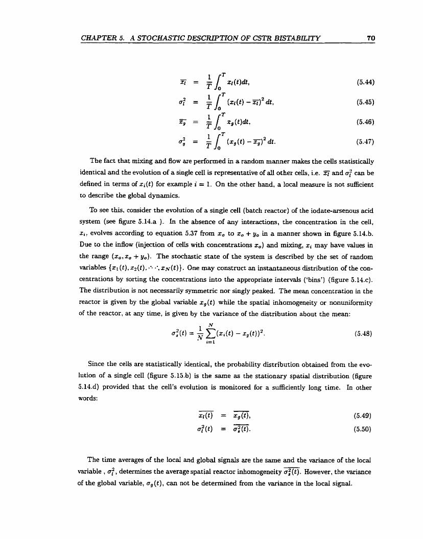
C W T E R 5. -4 STOCKASTIC DESCRlPTIOlV OF CSTR BLSTrlBEITY 70

The fact that miving and flow are performed in a random manner makes the ceih statisticdy

identical and the evolution of a single celi is representative of ail other cells, i.e. and o;' can be

defineci in terms of zi(t) for example i = 1. On the other hand, a local measure is not sufficient

to describe the global dynamics.

To see this, consider the evolution of a single ce11 (batch reactor) of the iodate-arsenous acid

system (see figure 5.14.a ). In the absence of any interactions, the concentration in the celi,

xi, evolves according to equation 5.37 from z, to z, + y, in a manner shown in figure 5.14. b.

Due to the inflow (injection of cells with concentrations 2,) and mixing, xi may have values in

the range (z,,~, + y,). The stochastic state of the system is described by the set of random

variables {xl (t), x 2 ( t ) , S., zN(t)) . One may constmct an instantanmus distribution of the con-

centrations by sorting the concentrations into the appropriate intervals ('bins') (figure 5.14.~).

The distribution is not nece s sdy symrnetric nor singly peaked. The mean concentration in the

reactor is given by the global variable x, (t) whiie the spatial inhornogeneity or nonuniforrnity

of the reactor, at any tirne, is given by the variance of the distribution about the mean:

Since the cells are statistically identical, the probabiiity distribution obtained from the evo-

lution of a single ceil (figure 5.15.b) is the same as the stationary spatial distribution (figure

5.14.d) provided that the cellts evolution is monitored for a sufficiently long time. In other

woràs:

- o;(t) = of (t).

The time averages of the local and global signals are the same and the variance of the locai

variable , a:, determines the average spatial reactor inhomogeneity cr: (t) . However, the variance

of the global variable, ag(t), c m not be detennined from the variance in the local signai.

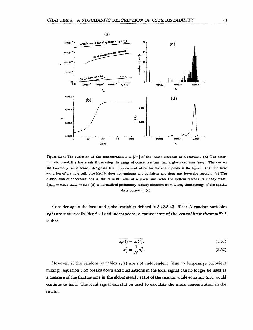
C W T E R 5. A STOCE4STIC DESCRIPTTON OF CSTR BISTABILITk' 71

Figure 5.14: The evolution of the concentration x = I I - ] of the iodate-menous acid reaction. (a) The deter-

ministic bistability hysteresis illustrating the range of concentrations that a given ceIl may have. The dot on

the therrnodynamic brandi designate the input concentration for the other plots in the figure. (b) The tirne

evolution of a single ceII, provided i t does not undergo any colIisions and does not leave the reactor. (c) The

distribution of concentrations in the iV = 800 celIs a t a given time, after the system reaches its steady state.

kflo,,, = 0.625, km,, = 62.5 (d) A normalized probability density obtained from a long tirne average of the spatial

distribution in (c).

Consider again the local and global variabLes defined in 5.42-5.43. If the N random variables

~ i ( t ) are statisticaily identical and independent, a consequence of the central lirnit the~rern"+"~

is that:

However, if the random variables z i ( t ) are not independent (due to Iong-range turbulent

m~.uing), equation 5.52 breaks down and fluctuations in the local signal can no longer be used as

a measure of the fluctuations in the global steady state of the reactor while equation 5.51 would

continue to hold. The local signal can still be used to caicdate the mean concentration in the

reactor.

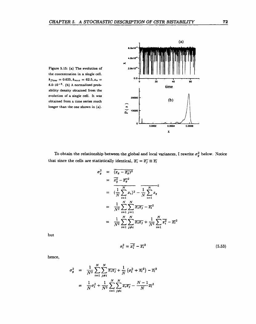
Figure 5-15: (a) The evolution of

the concentration in a single cell.

k f l , , = 0.625, km,, = 6 2 . 5 , ~ ~ = 8.0-10-5. (b) A normaiized prob-

ability density obtained from the

evolution of a single cell. ft was

obtained from a tirne series mu&

longer than the one shown in (a).

O 20 40 BO

1 time

To obtain the relationship between the global and local variances, 1 rewrite O: below. Notice

that suice the cells are statisticdy identical, 2; = n

but

hence,

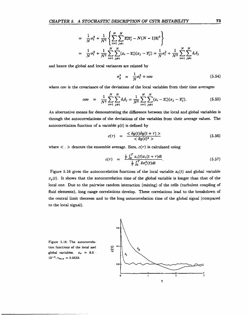
CHAPTER 5. A STOCKASTIC DESCRLPTlON OF CSTR BISTABLLITY 73

and hence the global and local variances are related by

where cou is the covariance of the deviations of the locai variables from their time averages:

An alternative means for demonstrating the Merence between the Iocal and globai variables is

through the autocorrelations of the deviations of the variables fkom their average values. The

autocorrelation function of a variable y(t) is dehed by

where < . > denotes the ensemble average. Here, c ( r ) is calculated

Figure 5.16 gives the autocorrelation functions of the locai variable xl(t) and global variable

x,(t). It shows that the autocorrelation tirne of the global variable is longer than that of the

locd one. Due to the pairwise random interaction (mkxing) of the ceiis (turbulent coupling of

fluid elernents), long range correlations develop. These correlations lead to the breakdown of

the central limit theorem and to the long autocorrelation time of the global signai (compared

to the local signal).

Figure 5. L6: The autocorrela-

tion functions of the local and

global wiables. zo = 8.0 -

1 0 - ~ , r,,, = 0.0533.

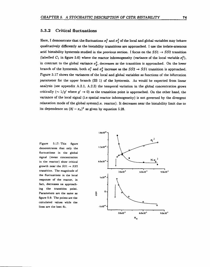
C W T E R 5. -4 STOCHASTK DESCRLPTION OF CSTR BISTABLLITY 74

5.3.2 Criticai fluctuations

Here, 1 demonstrate that the fluctuations 4 and of the local and global variables may behave

qualitatively differently as the bist ability transitions are approached- 1 use the iodate-arsenous

acid bistability hysteresis studied in the previous section. 1 focus on the SS1 + 552 transition

(labelled Ci in figure 5.6) where the reactor inhomogeneity (variance of the local variable $),

in contrast to the globai variance ui, decreases as the transition is approached. On the lower

brandi of the hysteresis, both 4 and ai increase as the SS2 + SS1 transition is approached.

Figure 5.17 shows the variances of the locai and globai variables as functions of the bifurcation

parameter for the upper branch (SS 1) of the hysteresis. As would be expected from linear

analysis (see appendix A.2.1, -4.2.3) the temporal variation in the global concentration grows

c n t i c d y (-Y l/gt where g' + O) as the transition point is approached. On the other hand, the

variance of the locai signal (i.e spatial reactor inhomogeneity) is not governed by the divergent

relaxation mode of the globai system(i.e. reactor). It decreases near the bistability Iimit due to

its dependence on (z - z, )' as given by equation 5 -28.

Figure 5-17: This figure

demonstrates that only the

fluctuations in the globai

signal (mean concentration

in the reactor) show critical

growth near the SSI 4 SS2

transition. The magnitude of

the fluctuations in the local

response of the reactor, in

fact, decreases on approach-

ing the transition point.

Parameters are the same as

figure 5.9. The points are the

calculateci values while the

lines are the best fit.

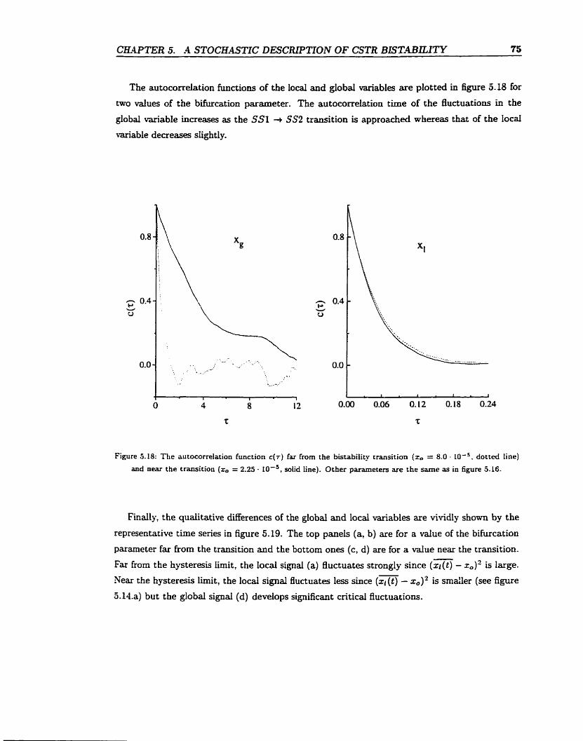
CEWTER 5. A STOCHMTIC DESCRIPTION OF CSTR BIST-4BLLITY 75

The autocorrelation functions of the local and global variables are plotted in figure 5.18 for

two values of the bifurcation parameter. The autocorrelation t h e of the fluctuations in the

global variable increases as the SSI + SS2 transition is approached whereas that of the local

variable decreases siightly.

Figure 5.18: The autocorrelation function c ( r ) far from the bistabiiity transition (zo = 8.0 - 1 0 ' ~ . dotted line)

and near the transition (z,, = 2.25 - IO'=, solid line). Other parameters are the same as in figure 5-16.

Finally, the qualitative diierences of the global and local variables are vividly shown by the

representative tirne series in figure 5.19. The top panels (a, b) are for a value of the bifurcation

parameter far £rom the transition and the bottom ones (c, d) are for a value near the transition. - Far from the hysteresis iimit, the local signal (a) fluctuates strongly since (z,(t) - x,)' is large.

Near the hysteresis lirnit, the local signal fluctuates less since ( q ( t ) - 2,)' is srnalier (see figure

5.14.a) but the global signal (d) develops significant critical fluctuations.

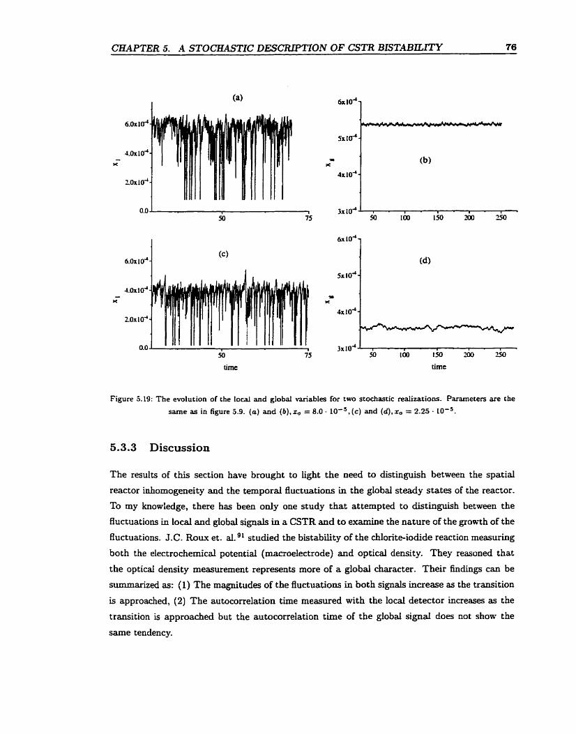
C W T E R 5. A STOCKASTIC DESCRIPTION OF CSTR BiSTABLLITY 76

Figure 5.19: The evolution of the Iocal and global variabtes for two stochastic realizations. Parameters are the

same as in figure 5.9. (a) and ( b ) , r , = 8.0 - lo-=,(c) and ( d ) , ~ , = 2.25 - ~ 0 ' ~ .

5.3.3 Discussion

The results of this section have brought to light the need to distinguish between the spatial

reactor inhomogeneity and the temporal fluctuations in the global steady states of the reactor.

To my knowledge, there has been only one study that attempted to distinguish between the

fluctuations in local and global signals in a CSTR and to examine the nature of the growth of the

ff uctuations. J-C. Roux et. ai. 91 studied the bistability of the chlorite-iodide reaction rneasuring

both the electrochemical potential (macroelectrode) and optical density. They reasoned that

the optical density measurement represents more of a global character. Their findings can be

summarized as: (1) The magnitudes of the fluctuations in both signals increase as the transition

is approached, (2) The autocorrelation t h e measured with the local detector increases as the

transition is approached but the autocorrelation time of the global signal does not show the

same tendency.

CEAPTER 5. A STOCHASTIC DESCRIPTION OF CSTR BISTABIWTY 77

In hght of the present results, the physicai content of the experiments of Roux et al. is not

clear for two reasons: (1) since a macroelectrode (- lm Pt.67) and an optical absorption path

of the order of lcm were used, the s amphg volumes of both detectors were similar, and (2) since

the flow rate and the stirring rate were used as bifurcation parameters, the increased ff uctuation

amplitude near the transition point was partly due to the increased segregation in the reactor.

Preliminary experiments done at our lab on the iodate-arsenous acid using microelectrodes

and macroelectrodes and using the input concentration of iodide as a control parameter have

suggested that the simulations of this section are correct. The variance in the concentration

of iodide (calculateci frorn the variance in the potential) of the microelectrode decreases as

the transition point is approached while the variance of the concentration obtained from the

macroeIectrode signal grows as the bifurcation is approached.

In siimmary, this section showed that monitoring a CSTR on Iocal and global scales reveal

différent aspects of the reactor dynarnics. A local detector (e-g. a micro electrode) provides a

measure of the average concentration (provided that the reactor is macromixed) and the spatial

reactor inhomogeneity. To detect fluctuations that reflect the long-range cooperative dynamics

of the reactor, one should sample the concentration in a macrovlume that is of the same order

of magnitude as the reactor.

Chapter 6

Phase-dependent fluctuations: local stability of

limit cycles

The rate and mode of mixing in a CSTR have profound effects on Limit cycle oscillations. There

are four aspects to such mixhg effects: (1) the onset or death of oscillations (i.e. bifurcation

points) are shifted to different values of the control parameters, (2) the attributes of the oscil-

lations - shape, period, amplitude - are modified by rnkxing (3) the regularity (or conversely

the 'jitter') of the period and amplitude of the osciUations depends on miuing, and (4) local

concentration fluctuations depend sensitively on the phase of the cycle. In chapter 4, 1 demon-

strated how Stream and age miving modify the rates of nonlinear reactions and consequently

affect limit cycles. In this chapter 1 investigate the relationship between the locai stabàiàty (as

opposed to global or orbital stability) of b i t cycles and the observed dynamical consequences

of inhomogeneities on limit cycle oscillations. In the first part of the chapter, 1 elaborate the

concept and measures of locai stability. The second part of the chapter is devoted to studying

the role of the nonuniformity of the local stability of a iimit cycle in determining the degree of

concentration nonuniformities in a CSTR and the dynamitai consequences of inhomogeneities

on lirnit cycles.

6.1 Local (in)stability of limit cycles

Limit cycles are usually illustrated by flow fields as in figure 6.1.a to emphasize their global

stability. A better representation would not neglect the important aspects of local stability

(LS), d e h e d as the local rate of convergence (or divergence) of neighbouring trajectories- This

locaI stability generdly varies in phase space and may change its sign dong a trajectory- TO

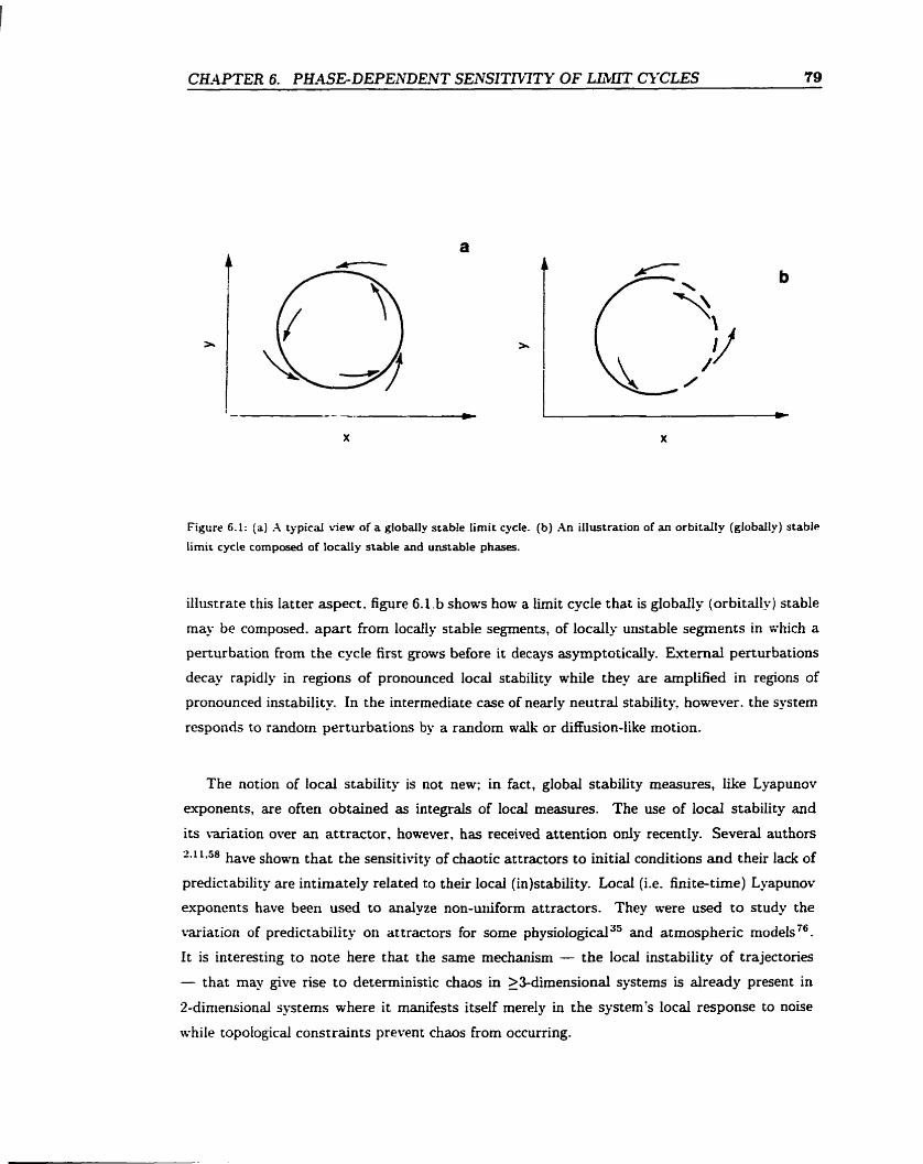
Figure 6.1: (a) .-\ tgpicai view of a globally stable Iirnit cycle. (b) An illustration of an orbitaily (giobally) stable

limit cycle composed of 1ocaIly stable and unstable phases.

illustrate this latter aspect. figure 6.1.b shows how a iirnit cycle that is globaily (orbitaII?) stable

may be composed. apart from locally stable segments, of locally unstable segments in =hich a

perturbation from the cycle first grows beiore it decays asymptocicaily. E-utenai perturbations

decay rapidly in regions of pronounced local stability while they are amplified in regions of

pronounced instability. In the intermediate case of nearly neutral stability. however. the system

responds to random perturbations by a random w d k or diffusion-like motion.

The notion of local stability is not new; in fact, global stability measures, like Lyapunov

exponents, are oiten obtained as integrals of local measures. The use of local stability and

its variation over an attractor, however, has received attention only recently. Several authors

2,"*58 have shown that the sensitivity of chaotic attractors to initiai conditions and their lack of

predictability are intimately related to their local (in)stability. Local (i.e. finite-time) Lyapunov

exponents have been used to analyze non-uniform attractors. They were used to study the

variation of predictability on at tractors for some physiological 35 and atmospheric models 76.

It is interesting to note here that the same rnechanism - the local instability of trajectories

- that may give rise t o deterministic chaos in 23-dimensional systems is already present in

2-dinlensional systems where it manifests itself merely in the çystem's local response CO noise

tvhile topological constraints prevent chaos from occurring.

CELWTER 6. PIUSEDEPENDENT SENSIT.MTY OF LlMTT CYCLES 80

For ümit cycles, two key papers andyze the problem of local stability. Tomita et. al. 'O2

suggested that such analysis should be carried out in a frame of reference whicb moves with

the orbital revolution itself to effectively separate the effect of transverse fluctuations fkom the

orbital motion dong the cycle. Kurrer and Schultensl used an approximate solution of the

Fokker-Planck equation govenzing the evolution of an ensemble of U t cycle systems subjected

to weak gaussian white noise to obtain measures for the response of the b i t cycle to noise in

the normal and tangent ial directions.

The a i . here is to elaborate on the notion of locai stability for limit cycles near and far

from bifurcation points and to illustrate the non-uniformity of the dynamics in phase space

by examining the evolution of srnall perturbations for simple dynamical flows. The Merent

possible measures of local stability are compared. A generalized Bonhoeffer-van der Pol (BvdP)

modei that exhibits Hopf, saddle-node, and saddle-loop cycle bifurcations is used to illustrate

the nonuniformity of local stability (as a fûnction of phase) for different limit cycles far and near

those bifurcations.

6.1.1 Measures of local stability

Consider the dynarnical system

where F defines a flow in Rn and c is a control parameter. Let ~ ( t ) be a non-stationary

reference solution (e.g. a limit cycle) and x( t ) = a ( t ) + 6x(t) be a perturbed trajectory. The

initial perturbation dx(to) is taken to be sufficiently smaü so that its evolution may be described

by the linearized equation:

d -6x = A6x where A is a matrix whose elementr are a,, ( t ) = 1 dt

- (6.2) a21 x(i,=x.(t

There are regions in phase space where perturbations decay and others where they grow- The

notion of locai stability and instability associated with this local decay or growth gains quanti-

tative meaning nrhen viewed fiom a frame of reference in which bx(t ) is projected. Associated

with different frames of reference are different measures of local stability:

(a) The natural measure of local stability are the eigenvalues X i ( i = l...n) of the stability

matrkv A(t) and the associated eigenvectors ei* The short-the evolution of bx, on the scale dt

is given by:

where the b, are amplitudes detennined by the initial condition dx(to). The trajectory xo ( t ) is

said to be locaily stable if Re(Xi) < O for al1 i . Otherwise it is locaily unstable.

Despite the conceptuai simplicity of the eigenvalues Xi and the fact that the decay rates

dong different eigenvectors are not coupled, they are not the most convenient for the present

purpose since eigenvalues and eigenvectors are Erequently cornplex and since the directions of

the (generaiiy non-orthogonal) eigenvectors change dong m(t) in a manner that is not rdated

to the LS in a physicdy meaningfui and convenient way.

(b) Instead one is interestecl in the local decay or growth rates of bx in a coordinate fiame that

is locally adapted to the LS problem. For instance one may project dx(t) onto the coordinate axes

of the phase variables x i ( i = l...n). In this case the decay rates are given by the corresponding

diagonal elements aii(t) of the stability matriu, together with the coupling elements aij (t). This

is the appropriate choice for interpreting, e.g. a noisy time series of a phase variable xi(t) (e-g.

figure 2.5.a).

(c) h o t h e s priviiegeà measure of local stabiiity is associated with the direction of slowest

decay. This also provides the connection with the largest global Lyapunov exponent Am,,.

Suppose one nurnerically integrates the equations of motion 6.1 starting at x(t,) = h ( t , ) i-

bx(t,) and renormalizes the size of the perturbation every few integration steps. In this way ail

components bi of dx(t), that correspond to the eigenvalues except the one with the kges t real

part, decay and the perturbation eventuaiiy aligns itself with the direction of this least rapidly

decaying cornponent. Once this alignment of bx(t) has taken place, the slowest locai decay rate,

or largest local Lyapunov exponent X,,,(t) is given by

The corresponding

X,,,(t) = lim log IlW + Wll At-O IlWt)ll '

global Lyapunov e-xponent A,,, is given by

A,,, = lim log IIWO + 411 r4CC II~x(to>ll

or sirnply by the t h e average of A,,, , e.g. for a periodic solution:

A , , , = A ( t vbere T is the asdat ion period. T O

(d) A further convenient choice are the directions tangentiai to the flow and those contained

in the manifold transverse to the flow (for n=2, see figure 6.2). This local coordinate system

will be adopted here for the numerical illustrations.

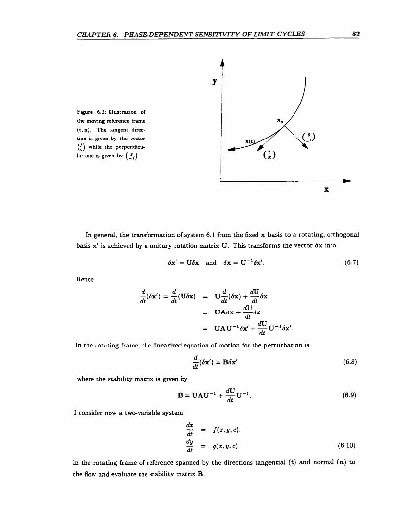
Figure 6.2: Illustration of

the moving reference frame

(t. n). The tangent direc-

tion is given by the vector

(i) while the perpendicu-

lar one is given by (O,).

In generd, the transformation of system 6.1 from the k e d x basis to a rotating, orthogonal

basis x' is achieved by a unitary rotation matLu U. This transforrns the vector bx into

dx' = U6x and dx = IJ-'dx'. (6.7)

Hence

In the rotating frame, the linearized equation of motion for the perturbation is

d -(dx') = Bdx' dt

where the stability matrix is given by

B = UAU-' + % r i . dt

1 consider now a two-variable system

in the rotating frame of reference spanned by the directions tangential (t) and normal (n) to

the flow and evaluate the stability rnatriv B.

C W T E R 6. PHASEDEPENDENT SENSIl7VITY OF LJMlT CYCLES 83

-4 reference trajectory is iiiustrated in figure 3. The tangential direction (t) is given by the

velocity vector (i) and the normal (n) is given by (zf). Hence the orthogonal b a i s for the

rotating kame is given by

and the unitary transformation matrix by

The stability rnatrk in the fixed fiame,

where A,, represents the rate of convergence normal to the flow and Xtt is the rate of convergence

tangential to the trajectory. The latter necessarily averages to zero over a closed orbit.

Note that: (1) in this reference frame the directions ( t , n) are partly uncoupled in the sense

that Xnt = O, i.e. a tangential perturbation remains tangential, in agreement with physicai

considerations. On the other hand, At, # O. This means that a perpendicular perturbation

couples to the tangential motion and leads to a resetting of the hase "2. (2) The rnatrix

elernents are algebraic functions of the phase variables and rnay be readily evaiuated. These

facts make A,, and Att preferable to the eigenvahes X i as Iocal stability measures. (3) The Iocal

rate of contraction of volumes (here: areas) in phase space is given by the divergence of the flow

af + a g divF = - - = t rA = t rB = A,, + Xtt. a x ay

In three and more dimensions, t is given by the vector (fl f2 --• f,) and Att by a

generalization of Act in equation 6.14. But the normal directions that would define n are not

unique. The rate of convergence (divergence) of trajectories in the hypersurface I' normai t o t

is , however, given by trA - Att . Furthemore, the convergence (divergence) rate dong the l e m

decaying direction in the hypersurface I' may be computed in a fashion simiiar to the caicdation

CE4PTER 6- PEUSEDEPENDENT SENSITITTTY OF LXbIIT CYCLES 84

of A,,,: an arbitrary initiai perturbation, bx(t,) is chosen in ï, equation 6.2 is integrated for

a penod of thne T to obtain bx(T), the projection of 6x(T) in I' is renormalized and the step

is repeated- 1 use this method below to calculate A,, for the 3-d Rksler mode1 (figure 6.8.)

Furthermore, the local stability measures may be averaged (equation 6.6) over a cyde to

obtain the corresponding global stability measures- Ln the computations, the discretized version

of equation 6.6 is used:

where m a t = T and A, can be X i , , X i j , .... or X ,,,.

Finally, one can define a local 'nonuniformity f a ~ t o r ' ~ ~ a s the average deviation of the local

stability measure from its mean value over the orbit:

to characterize the variability of local stabiiity/convergence rate dong an orbit.

6.1.2 Results

In this section the local stability of limit cycles is examined using a general, yet simple dynarnicai

model: the generalized Bonhoeffer-van der Pol (BvdP) This model is usehl since it

exhibits different types of bifurcations of limit cycles as well as cross shaped bifurcation diagram

13." similar to rnany real systems. 1 examine its local stability by caiculating the local decay

rates Xi,, X i j in the moving reference frame tangentid and normal to the 0ow. 1 illustrate how

the local measures and their global (orbital) averages behave as the following bifurcations are

approached: supercritical Hopf, saddle-node bifurcation of a periodic branch, and saddle-loop

bifurcations. Zn addition 1 also briefly examine tocal stability for a limit cycle near the first

perïod-doubling bifurcation of the 3-variable R6ssler model 6.19.

6.1.2.1 The generalized BvdP mode1

1 consider the generalized BvdP system 59 :

dx 1 3 - = f (z, 3) = ; (y - alx - azx - a,) , dt

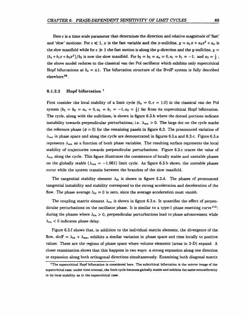
CEWTER 6. PHMEDEPENDENT SENSrT'NITY OF LtMT CYCLES 85

Here E is a time scale parameter that determines the direction and relative magnitude of 'fast'

and 'slow' motions: For r < 1, z is the fast variable and the x -dc l ine , y = a l z + a2x3 + a, is

the slow manifold whiie for E » 1 the f a t motion is d o n g the y-direction and the y-ndcline, y =

(b, + blx+û&)/b is now the slow manifold. For = 63 = a, = 0,al = bl = -1, and a:! = 3 '

the above mode1 reduces to the classical van der Pol oscillator which exhibits only supercnticai

Hopf bifurcations a t b, = f 1. The bifurcation structure of the BvdP system is fuiiy described

elsewhereS9.

6.1.2.2 Hopf bifimcation t

First consider the local stability of a iimit cycle (b, = 0, E = 1.0) in the classicd van der Pol

system (b = 4 = a, = O, ai = bl = -1,- = f ) far from its supercriticai Hopf bifurcation.

The cycle, dong with the nuilclines, is shown in figure 6.3.b where the dotted portions indicate

instability towards perpendicular perturbations, i.e. A,, > O. The large dot on the cycle marks

the reference phase (4 = 0) for the remaining panels in figure 6.3. The pronounced variation of

A,, in phase space and along the cycle are demonstrated in figures 6.3.a and 6.3.c. Figure 6.3.a

represents A,, as a function of both phase variables. The resulting surface represents the local

stability of trajectories towards perpendicular perturbations. Figure 6.3.c traces the value of

A,, along the cycle. This figure iilustrates the coexistence of Iocaily stable and unstable phases

on the globally stable (A , , = -1.061) iimit cycle. As figure 6.3.b shows, the unstabfe phases

occur while the system transits between the branches of the slow manifold.

The tangential stabiiity element Xtt iS shown in figure 6.3.d. The phases of pronounced

tangential instability and stability correspond to the strong acceleration and deceleration of the

flow. The phase average r i t t = O is zero, since the average acceleration must vanish.

The coupling matrix element At, is shown in figure 6.3.e. It quantifies the effect of perpen-

dicular perturbations on the oscillator phase. It is s i d a r to a type-1 phase resetting curve"*:

during the phases where At, > 0, perpendicular perturbations Iead to phase advancement whiie

X t n < O indicates phase delay.

Figure 6.3.f shows that, in addition to the individual matrix elements, the divergence of the

Oowl divF = Xtt + A,,, exhibits a sirnilar variation in phase space and rises l o c d y to positive

values. These are the regions of phase space where volume elements (areas in 2-D) expand. -4

closer examination shows that this happens in two ways: a strong expansion along one direction

or expansion d o n g both orthogonal directions simultaneously. Euamining both diagonal matrku

t ~ h e supercriticai Hopf bifurcation is considered here. The subcriticai bifurcation is the mirror image of the

supercritical case; under time reversal, the limit cycle becomes globally stable and exhibits the same nonuniformity

in its local stability as in the supercritical case.

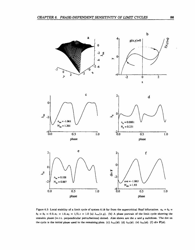
CK4PTER 6. PHASEDEPENDENT SENSITrVITY OF LIMIT CYCLES 86

phase

phase

Figure 6.3: Local stability of a Iimit cycle of system 6.18 far from the supercritical Hopf bifurcation. a, = b, = b2 = b3 = O.O,ar = L.O.al = 1/3,r = 1.0 (a) X,,(X,Y). (b) A phase portrait of the lirnit cycle showing the

unstable phase (w.r.t. perpendicular perturbations) dotted. Also shown are the z and y nullclines. The dot on

the cycle is the initiai phase used in the remaining plots. (c) X,,(4). (d) Xtt(4). ( e ) Atm(@)- (f) div F(4).

CHAPTER 6. PIUSEDEPENDENT S E N S m OF LIMIT' CYCLES 87

elements (figures 6.3.c16.3.d), one ûnds that phases ex& where the cycle is unstable in both

directions simult aneously.

Next consider the Van der Pol oscillator for simiIar parameter values as above except that it

is close to its supercritical Hopf point (b, = 0.999). The cycle is now small and nearly circular.

ït consists of locaiiy stabie and unstable portions of nearly equal extent (figure 6.4.b) and

consequently the orbital average A,, approaches zero (Ann = -0.0019). AU the local measures,

A,, (figures 6.4.a and 6 .4 .~)~ Act (figure 6.4.d), At, (figure 6.4.e), and diuF (figure 6.4.f) depend

nearly sinusoidally and weakiy on the phase, indicating that their nonuniformity (equation 6.17)

tends to zero at the bifurcation point.

6.1.2.3 Saddle-node bifurcation

Ne-ut consider the locai stability of a limit cycle which is about to lose its orbital stability via

a saddle-node bifurcation (SN). For the foiiowing parameter values: = a, = O, al = b1 =

- 1. al = ?, b3 = 0.75 and r = 0.1, the generaiized BvdP system 6.18 exhibits a stable ümit cycle

that couides with an unstable limit cycle at the turning point (b, = O.329OEi506 ... ) of a branch

of periodic solutions as the parameter b, is varieci.

Figures 6.5.a, 6.5.b, 6.5.c give the variation of A,, for the three limit cycles shown in figures

6.5.d, 6.5.e. 6.5.f : far from the SN bifurcation (b, = 0.0 and b, = 0.2), and very close to the

bifurcation (6, = 0.32905505.) The figures show that, as the SN is approached, the orbital

average of A,, tends to zero while the cycle rernains non-uniform (Nnn is non-zero at the

bifurcation point.).

The supercritical Hopf and SN bifurcations may be characterized further by comparing.

in figure 6.6, the parameter dependence of the global stability measures, A,, and .Mn, of the

cycles. The difference between the two bifurcations lies a t the level of nonuniformity (equation

6.17): N,, goes to zero smoothly at the supercriticd Hopf bifurcation, i.e. the m a n c e of A,,

vanishes as the limit cycle contracts to zero amplitude a t the bifurcation point. At the SN

bifurcation, on the other hand. the well-developed cycle suddenly loses its s tabsty as it collides

with an unstable cycle and its locai stability measure A,, (figure 6.5.c) deviates strongly £rom

uniforrnity.

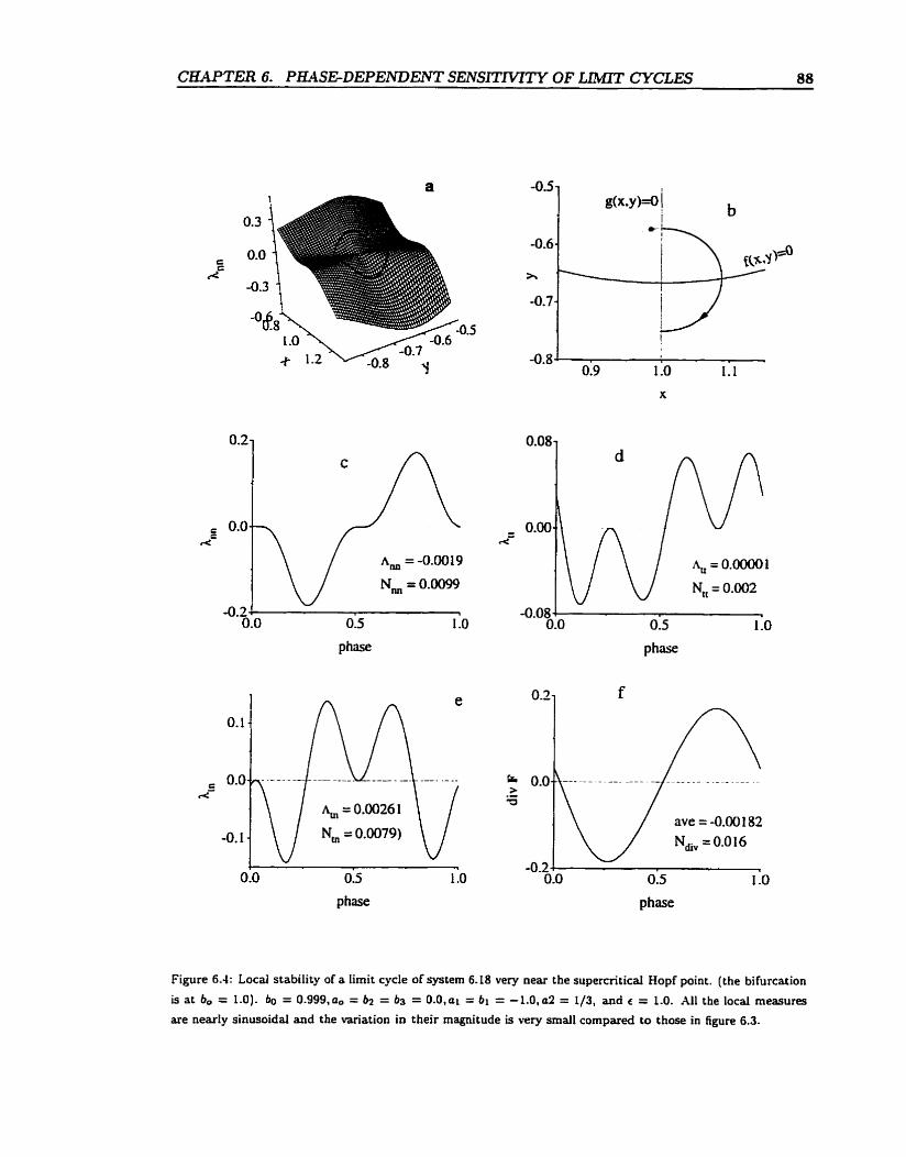
CBAPTER 6. PUSEDEPENDENT SENSITMTY OF LIMTT CYCLES 88

phase phase

Figure 6.4: Local stability of a limit cycle of systern 6.L8 very near the supercritical Hopf point. (the bifurcation

is at 6, = 1.0)- 60 = 0.999,a0 = b2 = bs = O.O,at = bi = -1.O1a2 = L/3, and c = 1.0. A11 the local measures

are nearly sinusoidal and the variation in their magnitude is very small compared to those in figure 6.3.

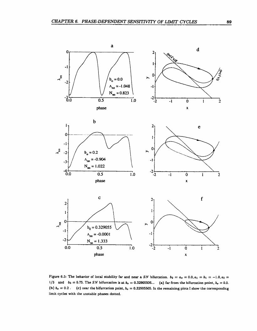
CHAPTER 6. PKASEDEPENDENT SENSITNZTY OF LIMIT CYCLES 89

phase x

Figure 6.5: The behavior of IocaI stability far and near a SN bifurcation. = a, = 0.0, ai = br = -1.0, aa = 1/3 and 63 = 0.75. The SN bifurcation is at bo = 0.32905506. .. (a) far from the bifurcation point, bo = 0.0. (b) bo = 0.2 . ( c ) near the bifurcation point, b, = 0.32905505. In the remaining plots 1 show the correspondi~g lirnit cycles with the unstable phases dotted.

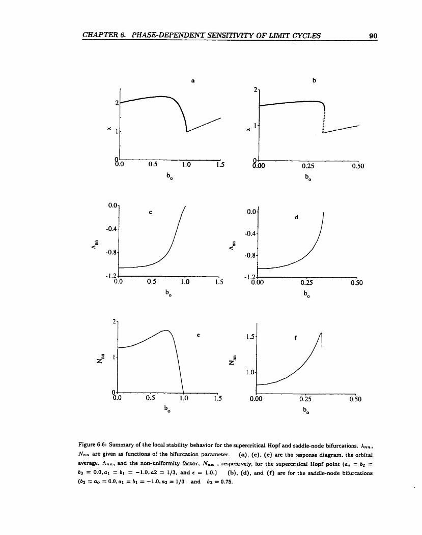
CWTER 6. PHASEDEPENDENT SENSlTNITY OF Lt&flT CYCLES 90

Figure 6.6: Surnmaq of the locai stability behavior for the supercritical Hopf and saddle-node bifurcations. An,,

Nnn are given as functions of the bifurcation parameter. (a), (c), (e) are the response diagram, the orbital average, An,, and the non-uniformity factor, Nnn , respectively, for the supercritical Hopf point (a, = bz = 63 = 0 . 0 , ~ ~ = b i = -1.O,a2 = 1/3, and É = 1.0.) (b), (d), and (f) are for the saddle-node bifurcations

(b2 = a,, = O.O,al = 61 = -1.0, a 2 = 1/3 and b3 = 0.75.

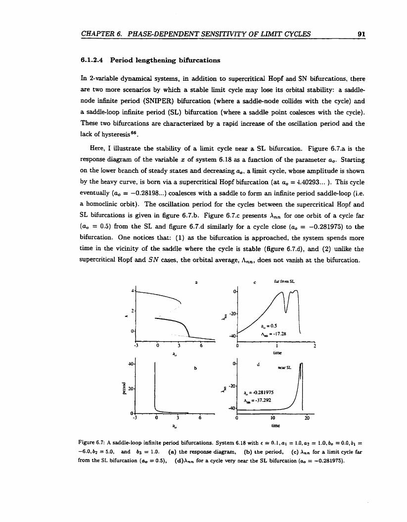
CXUPTER 6- PE4SEDEPENDENT SE.ïVSR7HTY OF LiMIT CYCLES 91

6.1.2.4 Period lengt hening bifirrcations

In Zvariable dynamical systems, in addition to supercritical Hopf and SN bifurcations, there

are two more scena.rios by which a stable E t cycle may Iose its orbital stability: a saddle-

node infinite period (SNIPER) bifurcation (where a saddle-node coIiides with the cycle) and

a saddIe-Ioop infinite penod (SL) bifurcation (where a saddle point coalesces with the cycle).

These tnro bifurcations are characterized by a rapid increase of the oscillation period and the

lack of hysteresis " .

Here, 1 illustrate the stability of a b i t cycle near a SL bifurcation. Figure 6.7.a is the

response diagram of the variable z of system 6.18 as a function of the parameter a,. Starting

on the Iower branch of steady States and decreasing a,, a limit cycle, whose amplitude is shown

by the heavy curve, is boni via a supercritical Hopf bifurcation (at a, = 4.40293 ... ). This cycle

eventuaiiy (a, = -0.28195...) coaiesces with a saddIe to form an infinite period saddle-loop (Le.

a homochic orbit). The oscillation period for the cycles between the supercritical Hopf and

SL bifurcations is given in figure 6.7.b. Figure 6.7.c presents Xnn for one orbit of a cycle far

(a, = 0.5) from the SL and figure 6.7.d similarly for a cycle close (a, = -0.281975) to the

bifurcation. One notices that: (1) as the bifurcation is approached, the system spends more

time in the vicinity of the saddle where the cycle is stable (figure 6.7.d), and (2) unlike the

supercritical Hopf and SN cases, the orbital average, A,,, does not vanish at the bifurcation.

Figure 6.7: A saddle-loop infinite penod bifurcations. System 6.18 with c = 0 . 1 , ~ ~ = l.O,a? = l.O,bo = 0.0, bi = -6.0,bz = 5.0, and b j = 1.0. (a) the response diagram, (b) the period, (c ) A,, for a limit cycle far

from the SL bifurcation (co = OS), (d)Ann for a cycle very near the S L bifurcation (a, = -0.281975).

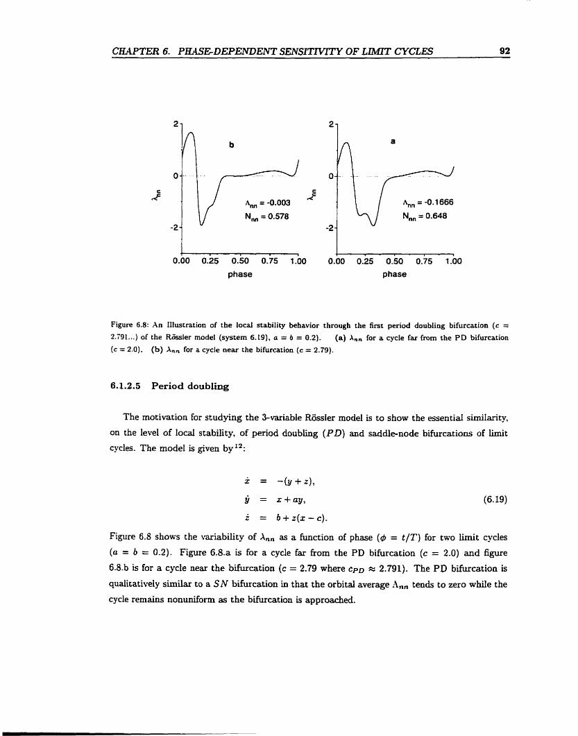
phase phase

Figure 6.8: An IIlustration of the local stability behavior through the first period doubling bifurcation ( c = 2.791 ...) of the Roçsler model (systern 6. tg), a = 6 = 0.2). (a) A,, for a cycle far h m the PD bifurcation

(c = 2.0). (b) A,, for a cycle near the bifurcation (c = 2.79).

6.1.2.5 Period doubling

The motivation For studying the %variable R o d e r model is to show the essentiai similarity,

on the level of locai stability, of period doubling (PD) and saddle-node bifurcations of limit

cycies. The model is given byE:

Figure 6.8 shows the variability of A,, as a hnction of phase (# = t /T ) for two limit cycles

(a = b = 0.2). Figure 6.8.a is for a cycle far from the PD bifurcation (c = 2.0) and figure

6.8.b is for a cycle near the bifurcation (c = 2.79 where cpo x 2.791). The P D bifurcation is

qualitativeiy similar to a SN bifurcation in that the orbital average A,, tends to zero whiIe the

cycle remains nonuniform as the bifurcation is approached.

C U T E R 6. PHASEDEPENDENT SEIiJSITMTY OF ~~ CYCLES 93

6.1.3 Discussion

In section 6.1, attention was drawn to the fact that orbital stability of limit cycles is the average

result of the competing tendencies of Iocal stability and of local instability, averaged over a cycle.

A cycle rnay lose its global or average stability either 'sofily' as its non-uniformity A f goes to

zero? or in a 'hard' rnanner where the nonuniformity fl remains b i t e and locally stable phases

compete with locally unstable phases, as in the case of SN and P D bifurcations. Examinhg

these local rates of convergence in a reference h e that moves with the orbital revolution

proved to be advantageous- It takes into account the time-dependence of the rotation of the

CO-ordinate system and it effectively decouples the tangential motion fiom that normal to the

cycle and hence perturbations dong the cycle effect only the phase. For different applications,

other reference fiames may be preferable.

The variability of the local stability behavior of iimit cycles can explain the evperimentai

observations of fluctuations that depend on the oscillation phase. Furthermore, the existence of

unstable phases indicates that perturbations during these phases, even in the case of strongly

attractive b i t cycles, can lead to large deviations from the deterministic trajectory. This local

instability can act as a mechanisru for maintaining an initial phase distribution (e-g. initia1

concentration gradients in a chernicai reactor). 1 expect that the non-uniforrnity of cycles rnay

play a role in dephasing and synchronization of weakly coupled oscillators.

Finally, the value of the Iocal stability rneasures is stressed. Although these measures are

essentialiy based on the calculation of the fmite-time rates of the growth (decay) of distances in

phase space and are not mathernatically robust (distance is not topologically invariant in phase

s ~ a c e ~ ~ ) , they convey some physical meaning. Phase space distance is associated with physical

observables like concentrations of chernicd species and local stabiiity measures can be used to

predict the response of dynamical systems to their fluctuating environment.

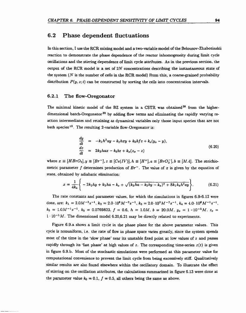
CHAPTER 6. PHASEDEPENDENT SElVSrrrVITY OF LIMTT CYCLES 94

6.2 Phase dependent fluctuations

In this section, 1 use the RCR mixing model and a two-variable model of the Belousov-Zhabotinskii

reaction to demonstrate the phase dependence of the reactor inhomogeneity durhg iiinit cycle

oscillations and the stirring dependence of limit cycle attributes. As in the previous section, the

output of the RCR mode1 is a set of 2N concentrations describing the instantaneous state of

the system (N is the number of ceils in the RCR modei) From this, a coârse-grained probabiiity

distribution P(y, z; t) can be constructed by sorting the celis into concentration intervais.

6.2.1 The flow-Oregonator

The minimai kinetic model of the BZ system in a CSTR was ~ b t a i n e d ~ ~ from the higher-

dimensional batch-0regonator30 by adding flow terms and eliminating the rapidly varying re-

action intermediates and retaining as dynamical variables only those input species that are not

bath species LO. The resuiting 2-variable flow-Oregonator is:

where x r [HBr02] , y z [Br- ] , r [Ce(IV)j, h [H+] ,a E [BrOT], b i [M.-11. The stoichio-

metric parameter f determines production of Br-. The value of x is given by the equation of

state, obtained by adiabatic elunination:

The rate constants and parameter values, for which the simulations in figures 6.9-6.12 were

done, are: kl = 2.0hf'3s-i, k2 = 2.0-10~kf-'s-~, k3 = 2 . 0 - 1 0 ~ l b f - ~ ~ - ~ , k4 = 4.0- ~ O ~ M - ~ S - ~ .

kg = l.OM-'s-', ko = 0.0769823, f = 0.6, h = 1.OM. b = 20.0Mt y, = 1 -- 10-~&1. Z, =

1 . 10-5M. The dimensioned model 6.20,6.21 may be directly related to experiments.

Figure 6.9.a shows a Iimit cycle in the phase plane for the above parameter values. This

cycle is nonuniform, i.e. the rate of flow in phase space varies greatly, since the system spends

most of the t h e in the 'slow phase' near its unstable fixed point a t low vaIues of z and passes

rapidly through its 'fast phase' a t high values of z. The correspondhg time-series t ( t ) is given

in figure 6.9.b. Most of the stochastic simulations were performed a t this parameter value for

computational convenience to prevent the limit cycle fiom being excessively stiE Qualitatively

similar results are also found elsewhere within the oscillatory domain. To illustrate the effect

of stirring on the oscillation attnbutes, the calculations summarized in figure 6.13 were done at

the parameter value I;o = 0.1, f = 0.5, ail others being the same as above.

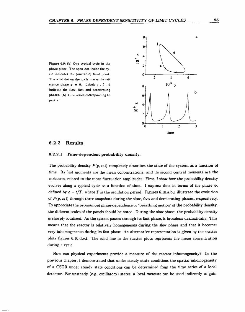
CE-1PTER 6. PR4SBDEPENDENT SENSITftTTY OF LIMlT CYCLES 95

Figure 6.9: (b) One typicid cycle in the

phase plane. The open dot inside the cy-

cle indicats the (unstable) fixed point.

The solid dot on the cycle marks the ref-

erence phase O = O. Labels s . f . d

indicate the slow, fast and decelerating

phases. (b) Tirne series corresponding to

part a.

time

6.2.2 Results

6-2-2.1 Time-dependent pro bability density.

The probability density P(y, z: t ) completely describes the state of the system as a hnction of

tirne- Its first moments are the mean concentrations, and its second central moments are the

variances. related to the mean fluctuation amplitudes. Fust. I show how the probability density

evolves dong a tgpical cycle as a function of time. 1 express tirne in terms of the phase P,

defined by O = t / T . where T is the oscillation period. Figures 6.lO.a,b,c illustrate the evotution

of P ( y , z: t) through three snapshots during the slow, fast and decelerating phases, respectively.

TO appreciate the pronounced phase-dependence or 'breathing motion' of the probability density,

the different scales of the panels shodd be noted. During the slow phase, the probability density

is sharply locaiized. As the system passes through its fast phase, it broadens dramaticaiiy. This

rneans that the reactor is relatively homogeneous during the slow phase and that it becomes

very inhomogeneous during its fast phase. -4n alternative represertation is given by the scatter

pIots figures 6.lO.d.e.f. The solid line in the scatter plots represents the mean concentration

during a cycle.

Hou. can physicai experiments provide a measure of the reactor inhomogeneity? In the

previous chapter, I demonstrated that under steady state conditions the spatial inhornogeneity

of a CSTR under steady state conditions can be determined from the time series of a local

detector. Fur unsteady (e-g. oscillatory) States. a local measure can be used indirectly to gain

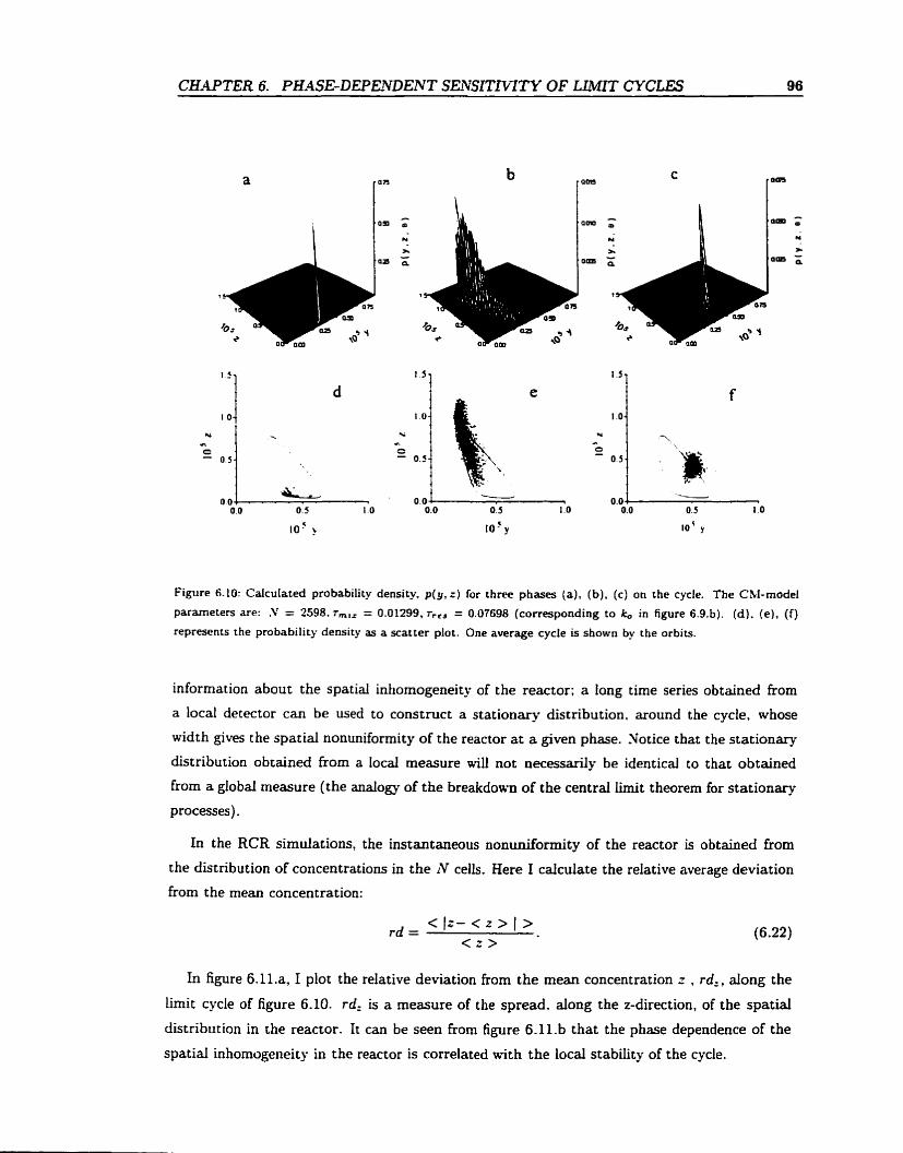
CHMTER 6. PH.4SEDEPEWDENT SENSITAf7TY OF LlMIT CYCLES 96

Figure 6.10: CaIcuIated probability density, p(y, r ) for three phases (a), (b) , (c) on the cycle. The Chl-mode1

parameters are: .V = 2598. r,,, = 0.01299, r,,, = 0.07698 (corresponding to ka in figure 6.9.b). (d), ( e ) , ( f ) represents the probability density as a scatter plot. One average cycle is shown by the orbits.

information about the spatial inhomogeneity of the reactor; a long tirne series obtained from

a local detector can be used to construct a stationary distribution. around the cycle, whose

width gives the spatial nonuniformity of the reactor a t a aven phase. Sotice that the stationary

distribution obtained from a local measure will not necessarily be identicai to that obtained

from a global rneasure (the analogy of the breakdown of the central Iimit theorem for stationary

processes).

In the RCR simulations, the instantaneous nonuniformity of the reactor is obtained from

the distribution of concentrations in the 1V cells. Hem 1 caiculate the relative average deviation

frorn the mean concentration:

In figure 6.11.a, 1 plot the relative deviation from the mean concentration z , rd,, dong the

lirnit cycle of figure 6.10. rdz is a rneasure of the spread. dong the z-direction, of the spatiai

distribution in the reactor. It can be seen from figure 6.11.b that the phase dependence of the

spatial inhornogeneity in the reactor is correlated with the local stability of the cycle.

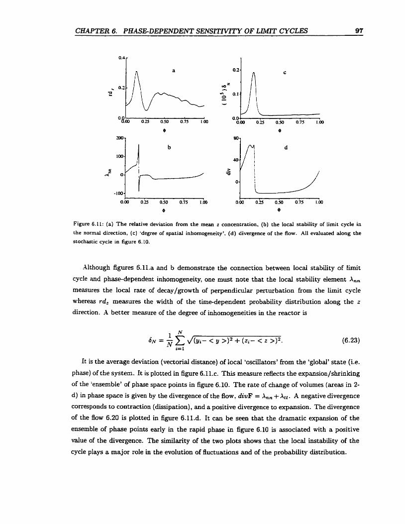
CEI.4PTER 6- PHASEDEPENDENT SENSlTIVlTY OF LJWï CYCLES 97

Figure 6.11: (a) The relative deviation from the rnean z concentration, (b) the local stabiiity of lirnit cycle in

the normal direction, (c) 'degree of spatial inhomogeneity'. (d) divergence of the Row. AI1 evahated along the

stochatic cycle in figure 6.10.

Although figures 6.11.a and b demonstrate the connection between locd stability of limit

cycle and phase-dependent inhomogeneity, one must note t hat the local stability element A,,

measures the Iocal rate of decay/growth of perpendicular perturbation fiom the limit cycle

whereas rd: mesures the width of the tirne-dependent probability distribution along the z

direction. -4 better rneasure of the degree of inhornogeneities in the reactor is

It is the average deviation (vectorial distance) of local 'osciUators' from the 'global' state (Le.

phase) of the system. It is plotted in figure 6.11.c. This measure reflects the expansion/shrinking

of the 'ensemble' of phase space points in figure 6.10. The rate of change of volumes (areas in 2-

d) in phase space is given by the divergence of the flow, divF = A,, + Xt f . A negative divergence

corresponds to contraction (dissipation), and a positive divergence to expansion. The divergence

of the flow 6.20 is plotted in figure 6.11.d. It can be seen that the dramatic expansion of the

ensemble of phase points early in the rapid phase in figure 6.10 is associated with a positive

value of the divergence. The similarity of the two plots shows that the local instability of the

cycle plays a major role in the evolution of fluctuations and of the probability distribution.

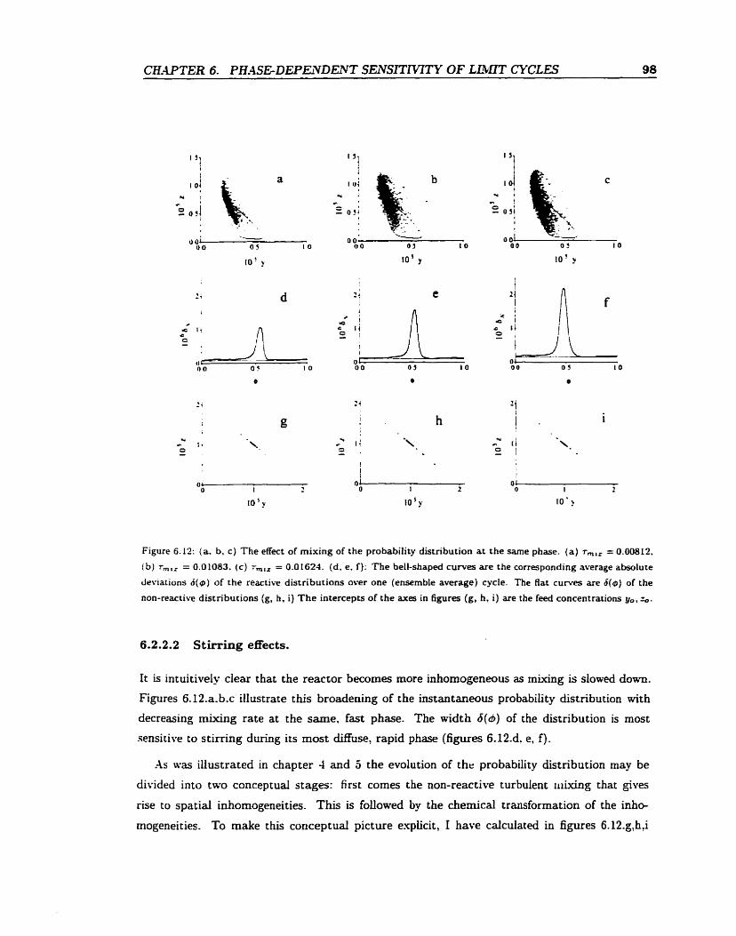
CHAPTER 6. PHa4SE-DEPE1VDEï\TT SEVSITMTY OF L E b T CYCLES 98

Figure 6.12: (a. b, c ) The effect of mixing of the probability distribution at the same phase. (a) r,,,,, = 0.00812,

(b ) r,,, = 0.0 1083. (c) r,,, = 0.0 1624. (d. e. f); The bell-shaped curves are the corresponding average absolute

deviations d ( 0 ) of the reactive distributions over one (ensemble average) cycle. The Rat cuwes are 49) of the

non-reactive distributions (g, h. i ) T h e intercepu of the axes in figures (g, II, i) are the feed concentrations y,, a.

6.2.2.2 Stirring effects.

It is intuitively clear that the reactor becomes more inhomogeneous as mixing is slowed down.

Figures 6.12.a. b.c illustrate this broadening of the instantaneous probabiiity distribution with

decreasing mWng rate at the same, fast phase. The width 6(b) of the distribution is most

sensitive to stirring during its most diffuse, rapid phase (figures 6.12.d, e, f).

-4s was iliustrated in chapter 4 and 5 the evolution of the probabiiity distribution may be

divided into two conceptual stages: fi rst cornes the non-reactive turbulent riiixing that gives

rise to spatial inhomogeneities. This is foliowed by the chexnical transformation of the inho-

mogeneities. To make this conceptuai picture e-upiicit , 1 have calculated in figures 6. 12.g,h7i

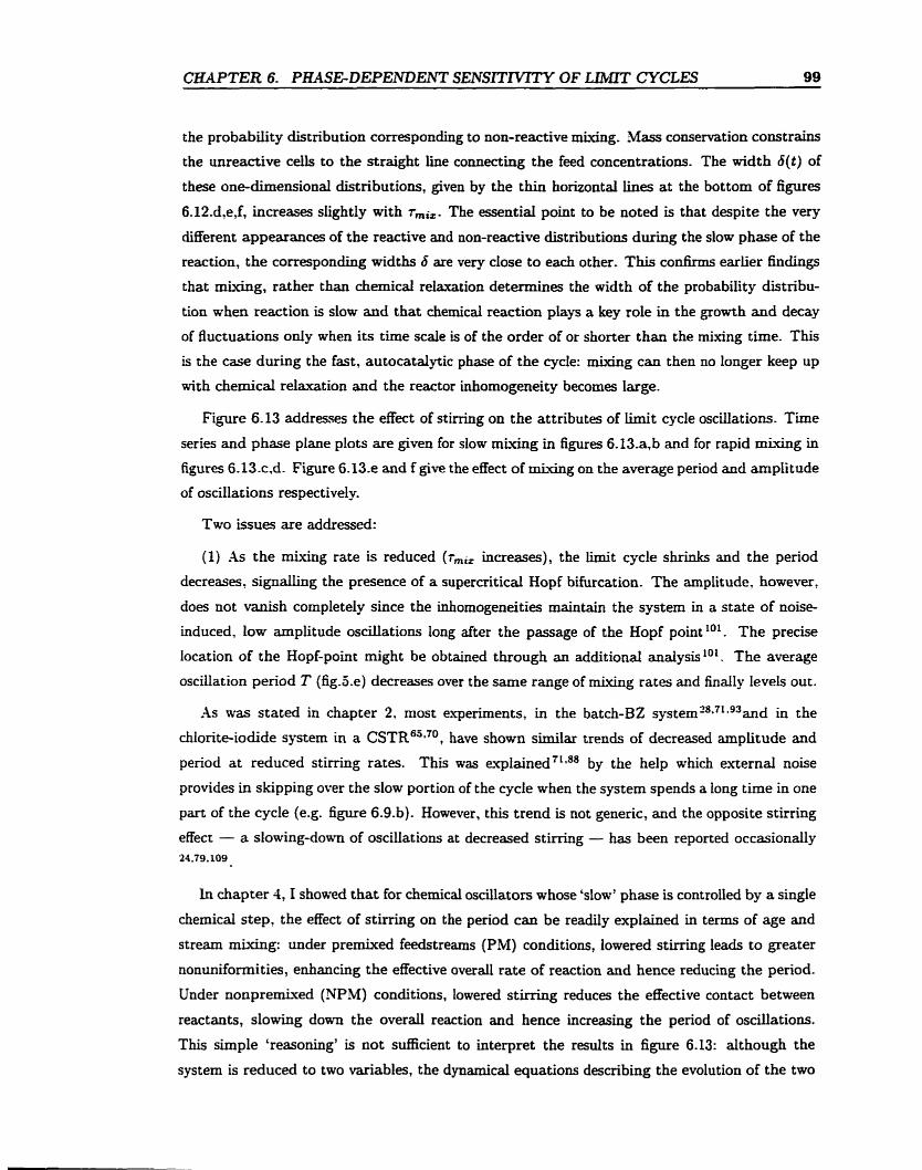
C W T E R 6. PHASEDEPENDENT SENSrTIV?TY OF JXMïï' CYCLES 99

the probability distribution corresponding to non-reactive mi.uing. .Mas conservation constrains

the unreactive cells to the straight line connecting the feed concentrations. The width 6 ( t ) of

these one-dimensional distributions, given by the thin horizontal lines at the bottom of figures

6.12.d,e,f7 increases siightIy with Tm,. The essentiai point to be noted is that despite the very

different appearances of the reactive and non-reactive distributions during the slow phase of the

reaction, the corresponding widths 6 are very close to each other. This confirms earlier findings

that mbchg, rather than chernical relaxation determines the width of the probability distribu-

tion when reaction is slow and that chernicd reaction plays a key role in the growth and decay

of fluctuations o d y when its time scale is of the order of or shorter than the mucing tirne. This

is the case during the fast, autocatalytic phase of the cycle: mixing can then no longer keep up

with chemical relaxation and the reactor inhornogeneity becornes large.

Figure 6.13 addresses the effect of stirring on the attributes of iimit cycle oscillations. Time

series and phase plane plots are given for slow m S n g in figures 6.13.aTb and for rapid rnixing in

figures 6.13.c.d- Figure 6.13.e and f give the effect of mixing on the average period and amplitude

of oscillations respectively.

Two issues are addressed:

(1) As the mkuing rate is reduced (rmiZ increases), the limit cycle shrinks and the period

decreases, s ignalhg the presence of a supercritical Hopf bifurcation. The amplitude, however,

does not vanish completely since the inhornogeneities maintain the system in a state of noise-

induced, low amplitude oscillations long &ter the passage of the Hopf point 'O1. The precise

location of the Hopf-point might be obtained through an additional a n a l y s i ~ ' ~ ~ . The average

oscillation period T (fig.5.e) decreases over the same range of mixing rates and finally levels out.

As was stated in chapter 2, most e-xperiments, in the batch-BZ s y ~ t e m ' ~ * ~ ' - ~ ~ a n d in the

chlorite-iodide system in a CSTR6L70, have shown similar trends of decreased ampiitude and

period a t reduced stirring rates. This was e ~ p l a i n e d ~ ' * ~ ~ by the help which external noise

provides in skipping over the slow portion of the cycle when the system spends a long time in one

part of the cycle (e-g. figure 6-9.b). However, this trend is not generic, and the opposite stining

effect - a slowing-down of oscillations at decreased stirring - has been reported occasiondy 24.79.109

In chapter 4,1 showed that for chemical oscillators whose 'slow' phase is controlled by a single

chemical step, the effect of stirring on the period c m be readily explained in terms of age and

Stream mixing: under premixed feedstreams (PM) conditions, lowered stimng leads to greater

nonuniformities, enhancing the effective overall rate of reaction and hence reducing the period.

Under nonpremixed (NPM) conditions, lowered stirring reduces the effective contact between

reactants, slowing down the overall reaction and hence increasing the period of oscillations.

This simple 'reasoning' is not s a c i e n t to interpret the results in figure 6.13: although the

system is reduced to two variables, the dynamitai equations describing the evolution of the two

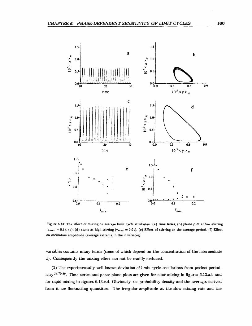
CHAPTER 6. PEL4SlGDEPENDENT SENSITMTY OF LIMTT CYCLES 100

20

time

time

Figure 6.L3: The effect of mixing on average limit cycle attributes. (a) tirne series, (b) phase plot at low stimng

(rmlZ = 0.1). (c), (d) same at high stirring (T,,, = 0.01). (e) Effect of stimng on the average period. ( f ) Effect

on oscillation amplitude (average extrema in the z variable).

variables contains many terms (some of which depend on the concentration of the intermediate

x). Consequently the mixing effect can not be readily deduced.

(2) The experimentally well-known deviation of limit cycle oscillations from perfect period-

i ~ i t y ~ ~ * " ' * ~ ~ . Time series and phase pIane plots are given for slow mixing in figures 6.13.a.b and

for ropid miving in figures 6.13.c.d. Obviously. the probability density and the averages derived

from it are fluctuating quantities. I he irregular amplitude at the slow mixing rate and the

CE-4PTER 6. PHASEDEPENDENT SENSIZW7TY OF LJWT CYCLES 101

jittery cyde in the phase plane are a consequeme of the broad probability distribution during

the fast oscillation phase. -4s the distribution narrows at the higher mking rate, the irregularity

of the amplitude decreases. The irreguiarity of the period c m be explained in the same manner:

lower stirring (longer T,, ) Ieads to the broadening of the probability distribution at the fast

phase of the cycle. The fast phase is a smaii fraction of the total period and hence the effect

on the period is smaiI. However, for cycles which are not excessively stifï (e-g. near the Hopf

bifurcation in figure 6.13) the jitter in the period can be noticeable.

Chapter 7

Summary and concIusions

This thesis addresses the problem of how inhornogeneities of the reacting medium in a CSTR affect its nonliiear dynamics - macroscopic changes of rates, steady state concentrations, induc-

cion periods, and oscillation attributes. Its aim was to obtain a better physicai understanding of

macroscopicdy obsewed inhomogeneity effects and to interpret them in terms of the underlying

mesoscopic fluctuations.

The emphasis was put on simplified modelling of the mixing process rather than on trying

to understand the intricate and complc,u hydrodynamics. To arrive at a tractable picture of the

interaction between chernical reaction and m g , it was assumed that the reactor is perfectly

macrornixed. Xccordingly, the random coalescence-redispersion (RCR) model was chosen to

simulate the dynamics of the imperfectly mixed CSTR. The model was chosen for its compu-

tationd and analyticd tractability and for the fact that it provides a probabilistic view of the

CSTR. The turbulent flow field with its infinite number of hydrodynamic modes is reduced to

a stochastic description that contains only two parameters: the flow and mixing rates.

In chapter 4, the RCR model was used to demonstrate the role of mixîng in determining the

average macroscopic reaction rate, and hence conversion, of the bimolecular reaction -4 + B + P

in a CSTR for premixed (PM) and nonpremixed (NPM) feedstream configurations. Mixing was

found to have opposite ('antagonistic') effects on the conversion and rate for the two mixing

configurations. If the reactants enter the reactor in a single P M feed, increasing the rnixing rate

decreases the rate, and hence the conversion, of the reaction. This effect, known as age miuing,

is due to the fact that the reactant concentrations are maximai in the feed stream and hence at

their maximal reaction rate. Mixing fiesh reactants into the reactor bulk dilutes the reactants

and hence reduces the overall reaction rate. If the reactants enter the reactor via separate NPM

feeds, stream m k h g cornes into play: mixing increases the overail rate of reaction since it brings

the reactants into contact. Stirring and mixing effects are important when the tirne scales of

C W T E R 7- SmIMARY -4ND CONCLUSIONS

flow, rnixing, and chemistry are similar. I used ternary diagrarns to map the kinetic response

(conversion, shift of steady states, absolute and relative inhomogeneity) in terms of the relative

magnitudes of the characteristic rate constants of the three processes.

The simple second order reaction has a rate function consisting of a single noniinear term

and the effects of Stream and age mixing are easily predicted. In complex reactions, the rate

function may involve few terms which may have opposite signs. For Merent steady states or in

different regions of parameter space, stirring may affect the rate in opposite manners depending

on which term in the rate law dominates the kinetics. This was iilustrated for the bistable, cubic

autocatalytic reaction -4 + 2 8 + 38. Under premived conditions, the rate function contains

two nonlinear terms with opposite signs. Enhanced stirnng increases the rate of reaction on

one branch of the hysteresis while it reduces it on the other brmch. The RCR simulations

also confirmed similar predictions for the induction period of cubic autocataiysis and for the

oscillation period of the Gray-Scott reaction (A + 2B + 3B and B + P).

In chapter 5, the RCR model was analyzed in detail. The goais were to obtain an explicit

relationship between the observed mUcing effects and the spatial inhomogeneity of the reactor

and to arrive at a better physical understanding of the interaction of chemical reaction and mix-

hg. This was achieved for a generic one-variable kinetic system by reducing the RCR model,

in the high stirring limit, to a Langevin equation in which the mking-induced fluctuating term

is a multiplicative colored noise process. Using the white noise approximation, an analytic

e-upression is obtained for the stochastic steady states from the stationary solutions of the cor-

responding Fokker-Planck equation. The shift of the bistabiiity hysteresis was e-uplicitly related

to the reactor inhomogeneity and the latter was shown to be deterrnined by a balance between

the forcing of the reactor bulk by the idow and by m&g. The validity of the K R mode1

(simulations and theoretical anaiysis) was confirrned by cornparisons with experiments on the

one-variable iodate-arsenous acid reaction.

.A third aspect that was investigated in chapter 5 was the distinction between local and glo bal

signais (e-g. obtained from micro and rnacroelectrodes, respectively). It was shown that the

variance of the local signal, of, measures the spatial inhomogeneity whiie that of the global

signai, oi reflects the fluctuations in the collective, temporal dynamics of the reactor. It was

shown that fluctuations of the global steady states grow critically as bistability transitions are

approached, reflecting the divergence of the global relaxation time. The spatial inhomogeneity,

however, is not governed by the globai relaxation mode of the reactor and was shown to decrease,

under certain conditions, as the transition is approached. The explicit expression relating 4 and 05 was piven.

In chapter 6, RCR-based simulations are used to obtain the time-dependent probability dis-

tribution for the oscillating BZ reaction. The distribution, which is a measure of the spatial

CEAPTER 7. SUMMARY a4Mû CONCLUSIONS

inhomogeneity of the reactor, was shown to depend dramatically on oscillation phase. To in-

terpret these observation, the notion of local stability of limit cycles was elaborated. Orbitd

stability of iimit cycles is the resuit of the competing local tendencies of perturbations to decay

(during phases of local stability) and to grow (during phases of local instability), averaged over

a cycle. The local (in)stability of ümit cycles was examined, both far from and near to different

types of bifurcations exhibited by the generalized Bonhoeffer-van-der-Pol and R6ssIer rnodels,

in a kame of reference that rnoves dong the orbit, to partially decouple motions tangentid and

perpendicular to the cycle.

The andysis of the RCR model in chapter 5 was simpiified by two restrictions: the reactor

was assumed to be well mixed on the macroscaie, and only a one-variable but generic kinetic

scheme was considered. Further progress in understanding the interaction of chernicd reaction

and mixing in the CSTR would benefit from extensions of the cment treatment to account for

a more realistic view of the mixing process (e.g. including rnacromixing) and for more complex

chemistry (Le. two and more variables).

The RCR mode1 c m be modified to incorporate macromiving effects by replacing ceiis in

a rnanner that reflects a nonideal residence tirne distribution (RTD) rather than randody.

The model can &O be modifieci to account for nonuniform (in space) rnixing in the reactor

and hence to simulate the macroscopic concentration gradients that cm6' exist in the reactor.

These gradients were recentlyg9 shown to arise kom the spatial dependence of the micromixing

time in the reactor.

The current analysis demonstrated that in one-variable systerns, a bistability hysteresis

shrinks dong both coordinates as a resdt of reduced stirring. The experiments simulations

and theory showed that the one-variable iodate-arsenous acid system exhibits stirring effects of

the first kind loO. Extending the m e n t treatment to two and more variables may prove fniitful

in providing a generai description and classification of stirring effects of the second kindloO.

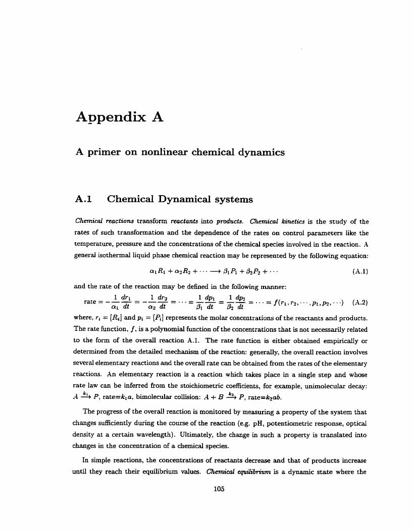
A primer on nonlinear chemical dynamics

A.1 Chemical Dynamical systems

Chemical mactions transform reactants into products. Chernical kinetics is the study of the

rates of such transformation and the dependence of the rates on control parameters Iike the

temperature, pressure and the concentrations of the chemical species involved in the reaction. -4

general isothermal liquid phase chernical reaction may be represented by the foiiowing equation:

and the rate of the reaction may be defined in the foiiowing manner:

where, ri = [&] and pi = [Pi] represents the molar concentrations of the reactants and products.

The rate function, f , is a polynomial function of the concentrations that is not necessarily related

to the form of the overall reaction A.1. The rate function is either obtained empiricaiiy or

determined from the detailed mechanism of the reaction: generaiiy, the overall reaction involves

several elementary reactions and the overd rate can be obtained from the rates of the elementary

teactions. An elementary reaction is a reaction which takes place in a single step and whose

rate law can be inferred from the stoichiometnc coefficients, for example, iinimolecular decay: k A % P, rate=kia, bimoleeular collision: 4 + B 4 P, rate=k2ab.

The progress of the overall reaction is monitored by rneasuring a property of the system that

changes sufficient ly during the course of the reaction (e.g. pH, potentiometric response, optical

density at a certain wavelength). bltimately, the change in such a property is translated into

changes in the concentration of a chemicai species.

In simple reactions, the concentrations of reactants decrease and that of products increase

until they reach their equilibrium values. Chenrical equilibrium is a dynamic state where the

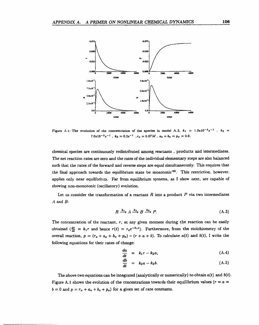
Figure .LI: The evolution of the concentration of the species in mode1 -4.3, ki = ~ . O X L O - ~ S " , kz = 7 . 0 ~ 1 0 - ~ ~ ' ' , ks = 0.29" ,r, = 0.07M , a, = 6, = po = 0-0.

chernical species are continuously redistributed among reactants , products and intermediates.

The net reaction rates are zero and the rates of the individuai elementary steps are also balanceci

such that the rates of the forward and reverse steps are q u a i simdtaneously. This requires that

the final approach towards the equilibrium state be monotonie 40. This restriction, however.

applies only near equilibriila. Far hom equiiibrium systems, as I show ne=, are capable of

showing non-rnonotonic (oscillatory) evotution.

Let us consider the transformation of a reactant R into a product P via two intermediates

-4 and B:

The concentration of the reactant, r , at any given moment during the reaction can be easily

obtained (2 = kir and hence r(t) = r 0 ë k l t ) . Furthemore, from the stoichiornetry of the

overad reaction, p = (r, + a , + ba -+ p,) - ( r + a + 6). To calculate a ( t ) and b( t ) , 1 write the

foilowing equations for their rates of change:

The above two equations can be uitegrated (analyticdy or numerically) to obtain a ( t ) and b ( t ) .

Figure A.1 shows the evolution of the concentrations towards their equilibrium values (r = a = b = O and p = r, + a, + b, + p,) for a given set of rate constants.

-4s the figure shows, the evolution towards eqdibriurn proceeds in a steady and monotonic

fashion (a and b £ùst rise then decline monotonically). Next, 1 aus t ra te how this smoothly

varying evolution can become oscillat ory.

Oscillations about a stationary or a slowly varying state impIy that this refertrnce state is

unstable with respect to s m d perturbations. A necessary eIement behind such an instability

is feedback : a chernical species affects the rate of its production or degradation. The resulting

rate equations are necessarily non-linear- .4 feedback is positive when the species directly or

indirectly enhances its own production (autoccrtalysis) and it is negative when a species directly

or indirectly inhibits its own production. Feedback can be thermal through the weU-known

Arrhenius dependence of the rate constants on temperature or it can be chemicai. In this thesis

our scope is restricted to isothermal reactions where the non-linearity in the rates is due to the

reaction mechanism. In the remainder of this section, 1 demonstrate how a direct autocatalytic

step can lead to oscillations in the example discussed earlier.

Suppose that, in additior, to the uncatalysed conversion of -4 to B, the intermediate B acts

as its own cataiyst , e.g. a cubic autocataiytic step is involved:

then the equations for the rate of change of a and b (-4.5-A.5) becorne:

Xumerically integrating the two above equations for the same set of rate constants and

initial concentrations as in figure A.1, one obtains the concentration profiles shown in figure

A.2. After an induction penod, the concentrations of the intermediates start to oscillate before

monotonically reaching their equiiibrium values.

The oscillations illustrated in figure -4.2, although in some cases can be remarkably long-lived,

are transient behavior that gives way to monotonic relaxation towards equilibrium. To obtain

sustained osciHations (and carry out quantitative measurements) , the reacting medium bas to

be kept far from equilibriurn by a continuous flu of matter and/or energy into the system.

An relatively easy realization of such open flow conditions is the wntinuously-fed s t i d tank

reactor (CSTR).

timc 6 . 0 ~ 1 O~

cime timc

Figure A.2: the evolution of the concentration of the species in madel A.3.X.6. ki = l .Oxl~( '~ )s - , k2 = 7 . 0 ~ 1 0 ( - ~ ) s - ~ , k3 = 0 . 2 ~ - ~ k4 = 5 .0x10~hf-~s - ' , r, = 0.07PuI , a, = bo = po = 0.0.

A.1-1 The CSTR

Figure A.3 is a schematic diagram of a typical laboratory CSTR. The reactor is a cylindricd ves-

sel made of glass/ple.uiglass. It is equipped with a cooling/heating jacket to maintain a constant

temperature. The fresh reagents are pumped into reactor (either premixed or via separate feed

streams) and the reactor mixture flows out through an outlet (constant volume). The state of

the reactor is monitored either potentiometrically by using metai redox or ion-specific electrodes

or spectrophotometricaliy by measuring light absorbance at a given wavelengtb. The reactor

contents are mived using a magnetic stirrer or more often through the use of a mechanically-

driven multi-blade propeller. In an ideal CSTR, the reaction medium is spatially homogeneous

and concentration changes are given by a set of rate equations containing kinetic and flux terms.

The solutions of such set of ordinary differentid equations account for ail the possible dynamic

behavior of the perfectly rnixed CSTR-

Let us consider the case where the kinetic scheme involves only the autocatalytic production

of B and its decay to a stable product :

(A-9)

(A. IO)

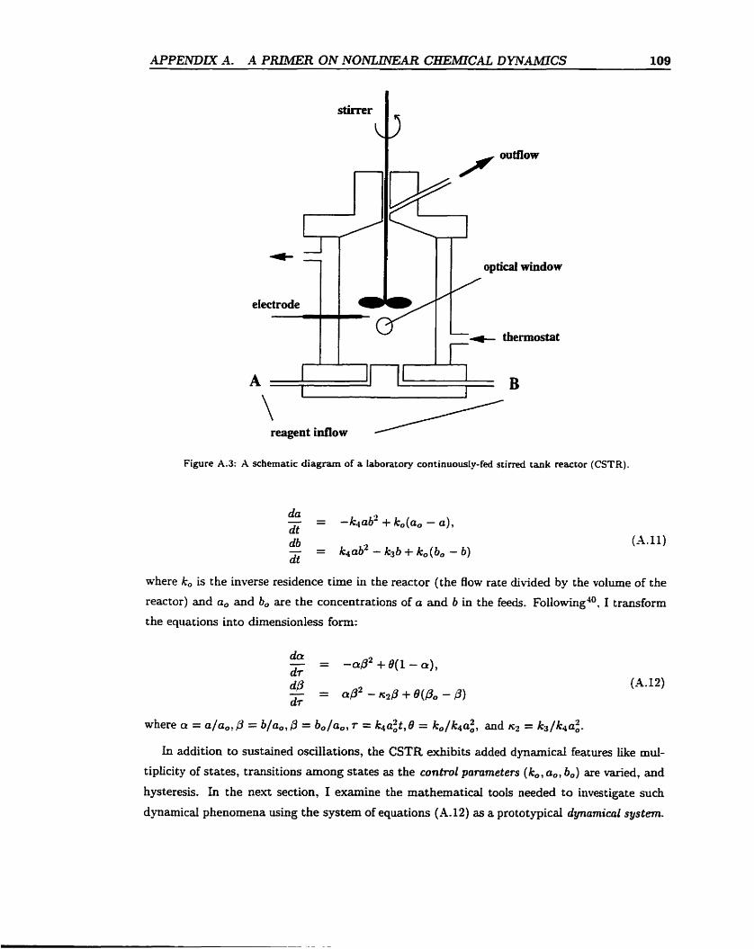
op tical window

eIectrode

thermostat

\ reagent inflow

Figure A.3: .A schematic diagram of a laboratory continuously-fed stirred tank reactor (CSTR).

where k, is the inverse residence time in the reactor (the flow rate divided by the volume of the

reactor) and a, and b, are the concentrations of a and b in the feeds. Following4*, I transform

the equations into dimensionless form:

(A. 12)

where a = a/ao ,@ = bla,, @ = bo/ao, r = k4a:t,6 = ko/k4a:, and r z = k3/k4a:.

In addition to sustained oscïliations, the CSTR exhibits added dynamical features like mul-

tiplicity of states, transitions among states as the contml parameters (k,, a,, b,) are varied, and

hysteresis. In the next section, 1 examine the mathematical tools needed to investigate such

dynarnicai phenomena using the system of equations (-4.12) as a prototypicai dynamicul system.

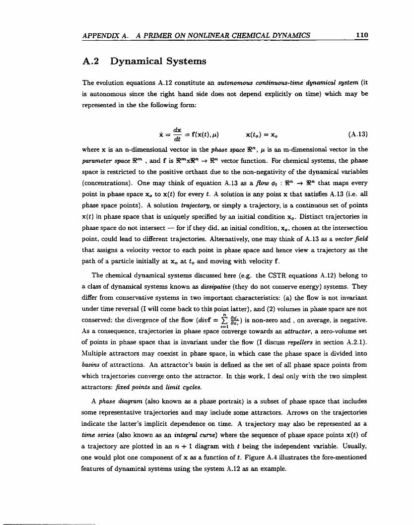
APPERiDIX A. A PRIMER ON NONUNE.1IR C&EIM;ICC4L DYN.41MTCS 110

A.2 Dynamical Systems

The evolution equations A.12 constitute an autonomous contànuous-tzme dynamical system (it

is autonomous since the right hand side does not depend expiïcitly on time) which rnay be

represented in the the following form:

(A. 13)

where x is an n-dimensional vector in the phase space Sn, p is an m-dimensional vector in the

parameter space Rm , and f is Rmx!Rn + Sn vector function. For chernical systems, the phase

space is restricted to the positive orthant due to the non-negativity of the dynamical variables

(concentrations). One may think of equation A.13 as a f?ow dt : Sin -+ Sn that maps every

point in phase space x, to x(t) for every t . A solution is any point x that satisfies .4.13 (Le. ail

phase space points). A solution trujectory, or simply a trajectory, is a continuous set of points

x ( t ) in phase space that is uniquely specified by an initiai condition x,. Distinct trajectories in

phase space do not intersect - for if they did, an initial condition, x,, chosen a t the intersection

point, could lead to different trajectories. Alternatively, one may think of A.13 as a vector field

that assigns a velocity vector to each point in phase space and hence view a trajectory as the

path of a particle initially a t x, a t to and moving with velocity f.

The chemicai dynamical systems discussed here (e.g. the CSTR equations -4.12) belong to

a class of dynamitai systems known as disszpative (they do not conserve energy) systems. They

M e r from conservative systems in two important characteristics: (a) the flow is not invariant

under time reversai (1 wili corne back to this point latter), and (2) volumes in phase space are not n

conserveci: the divergence of the flow (dzuf = 1 5) is non-zero and , on average, is negative. a= 1

4 s a consequence, trajectories in phase space converge towards an attractor, a zero-volume set

of points in phase space that is invariant under the flow (1 discuss repellers in section X.2.1).

&lultiple attractors may coexist in phase space, in which case the phase space is divided into

basins of attractions. An attractor's basin is defined as the set of al1 phase space points from

which trajectories converge ont0 the attractor. In this work, 1 deal only with the two simplet

attractors: fized points and limit cycles.

A phase d i a p m (also known as a phase portrait) is a subset of phase space that includes

some representative trajectories and may include some attractors. Arrows on the trajectories

indicate the latter's implicit dependence on time. -4 trajectory rnay also be represented as a

tame senes (&O knoun as an inte@ curve) where the sequence of phase space points x ( t ) of

a trajectory are plotted in an n + 1 diagram with t being the independent variable. Usually,

one would plot one component of x as a function of t . Figure A.4 illustrates the fore-mentioned

features of dynamical systems using the system A.12 as an example.

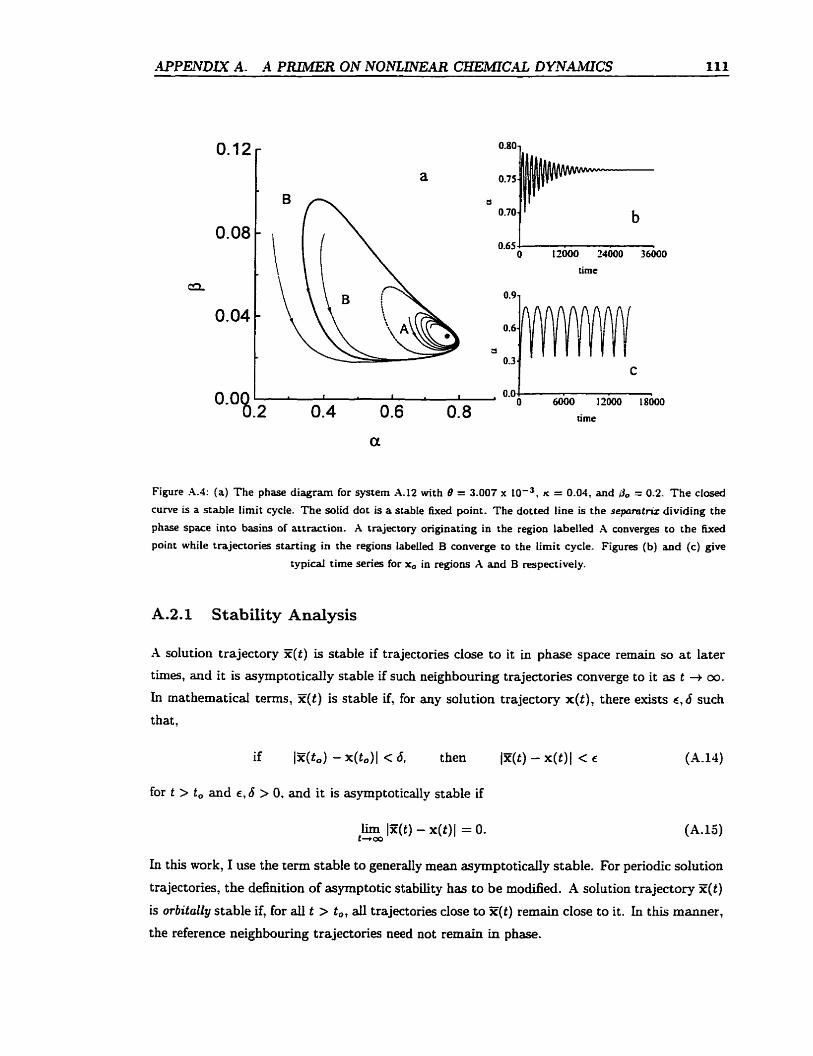
Figure -4.4: (a) The phase diagram for system A.12 with 0 = 3.007 x L O - ~ . rc = 0.04, and b,, = 0-2- The closed

curve is a stable limit cycle. The solid dot is a stable fixeci point. The dotted line is the separutriz dividing the

phase space into basins of attraction. A trajectory origînating in the region labelled A converges to the h e d

point white trajectories starting in the regions labelled B converge to the limit cycle. Figures (b) and (c) give

typical tirne series for x, in regions X and B respectively.

A.2.1 Stability Analysis

X solution trajectory Z(t) is stable if trajectories close to it in phase space remain so at later

times, and it is asymptotically stable if such neighbouring trajectories converge to it as t + ou. In mathematical terms, ~ ( t ) is stable if, for any solution trajectory x( t ) , there ewists c, 6 such

that,

for t > t , and E , 6 > 0. and it is asymptotically stable if

In this work, 1 use the term stable to generdy mean asymptotically stable. For periodic solution

trajectories, the definition of asymptotic stability has to be modified. A solution trajectory Z(t)

is orbitally stable if, for all t > t,, all trajectories close to Z(t) remain close to it. In this rnanner,

the reference neighbouring trajectories need not remain in phase.

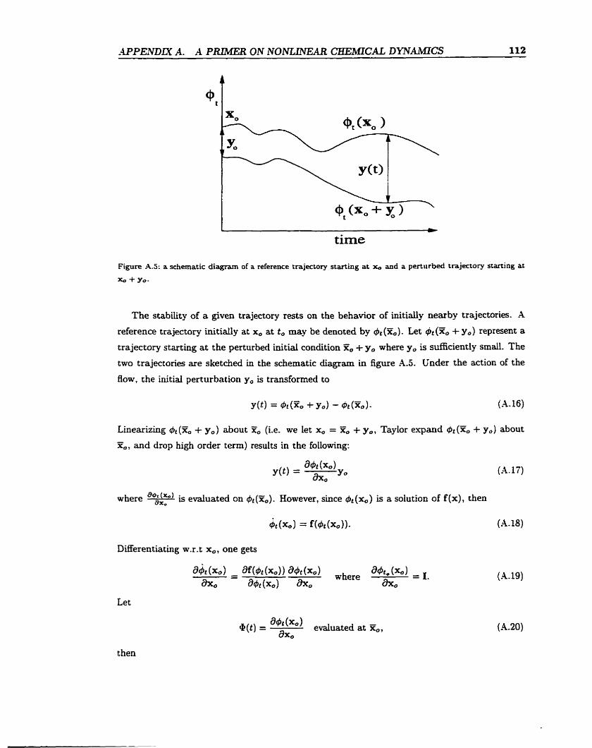
time

Figure A S : a schernatic diagram of a refereoce trajectory starting at xo and a perturbed trajectory starting at

x, + Yo-

The stabiiity of a given trajectory rests on the behavior of initially nearby trajectories. X

reference trajectory initially at x, at t, may be denoted by q5t (X,) . Let bt (Z, + y,) represent a

trajectory starting at the perturbed initial condition + y, where y, is sufficiently smaii. The

two trajectories are sketched in the schematic diagram in figure A.3. Under the action of the

flowt the initiai perturbation y, is transformed to

Linearizing &(Xo + y,) about K, (Le. we let x, = K,

X,, and drop high order term) results in the foiiowing:

+ yo, Taylor eupanci 4t (TE, t y* ) about

(A. 17)

where - a*tcb) is evaiuated on & (Z,). However, since & ( x o ) is a solution of f (x), then Bx,

DifFerentiating w.r.t x,, one gets

Let

t hen

4(t) = A(t)d(t) and @(t.) = 1 where A = /Ers Equation A21 is a generalized tirne-dependent uariationa2 equation. It describes the evolution

of a srnaii perturbation y, from a reference trajectory starting at 3,:

Xext I iflustrate the method of solution of equations A.21 and -4.22 for the cases when Z(t)

constitutes a Lxed point or a bit cycle.

A.2.1.1 Stability of fixed points

The simplest attractors are fixed points (also known as equilibriurn points, critical points, sin-

gular points, rest points, steady states, and stationary states). They are points Z(p) in phase

space such that f(X, p ) = O. They are invariant under the flow: &(X) = X.

.4t a fived point, the matrix A is time-independent and the variationai equation, X.21,

simplifies to:

and hence

@ ( t ) = eAt (A. 24)

and, from -4.22, the evolution of an initiai perturbation y, is @en by:

If the mat&- A has eigenvalues X i and correspondhg eigenuectors ui (i = 1, . . . , n): then

where c, are determined by y,.

The component of the perturbation y (t,) dong the eigenvector ui would asymptotically

decay (grow) if X i is negative (positive). Table 1.1 Iists the different possible stabiiities of üxed

points.

The distinction between instability and non-stability becomes more apparent under time

reversal. Following the evolution of the perturbation y(t,) backwards in time (Le. t + -oo), a

stable &ed point (attractor) becomes unstable (repelier) and vice versa. A non-stable fked point

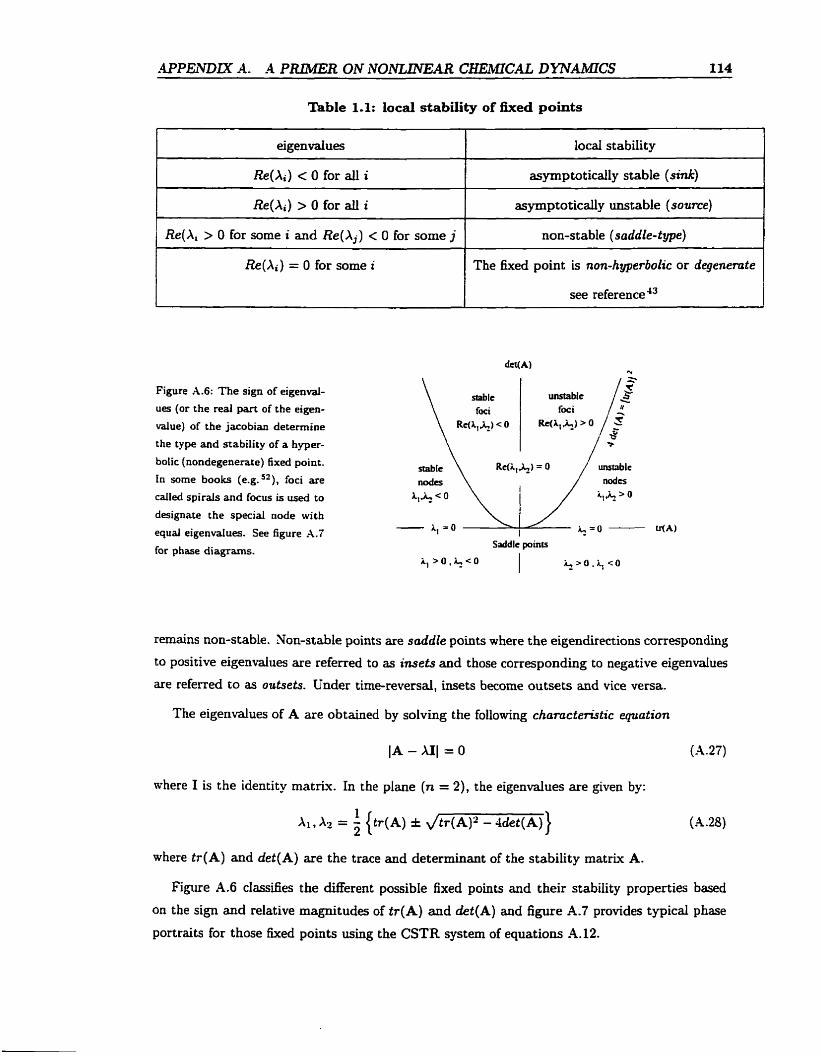
Table 1.1: local stability of ffxed points

eigenvaiues

Re(A,) < O for ail i

Re(A,) > O for ail i

Re(X, > O for some i and &(Aj) < O for some 1

Re(Xi) = O for some i

Figure A.6: The sign of eigenval-

ues (or the real part of the eigen-

value) of the jacobian determine

the type and stability of a hyper-

bolic (nondegenerate) fked point.

In some books (e.g.s2), foci are

called spirals and focus is used to

designate the special node with

equd eigenvaiues. See figure -4.7

for phase diagrams.

locai stability

asymptoticaiiy stable ( s i d )

asymptoticdy unstable (source)

non-stable (saddle-type)

The fixed point is non-hyperbolic or degenmte

I

stable foci

Rd+) < 0

see reference 43

remains non-stable. Non-stable points are saddle points where the eigendirections corresponding

to positive eigendues are referred to as insets and those corresponding to negative eigendues

are referred to as outsets. Under tirne-reversal, insets become outsets and vice versa.

The eigenvalues of A are obtauied by solving the following characteristic eqvation

where I is the identity rnatrix. In the plane (n = 2), the eigenvdues are given by:

where tr(A) and det(A) are the trace and d e t e d a n t of the stability matrix A.

Figure A.6 classifies the different possible fued points and their stabiIity properties based

on the sign and relative magnitudes of tr(A) and det(A) and figure A.7 provides typical phase

portraits for those fixed points using the CSTR system of equations A.12.

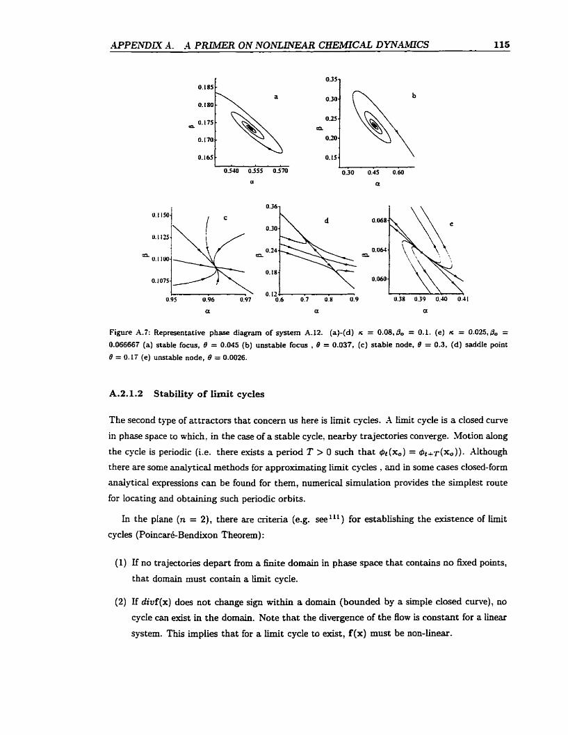
Figure A.7: Representative phase diagram of system A.12. (a)-(d) ti = 0.08,80 = 0.1. (e) n = 0.025,@, = 0.066667 (a) stable focus, 8 = 0.045 (b) unstable focus , 8 = 0.037, (c) stable node, 0 = 0.3, (d) saddle point

0 = 0.17 (e ) unstable node, 8 = 0.0026.

A.2.1.2 Stability of Iimit cycles

The second type of attractors that concern us here is limit cycles. X iimit cycle is a closed curve

in phase space to which, in the case of a stable cycle, nearby trajectories converge. Motion dong

the cycle is periodic (Le. there e'rists a period T > O such that & ( x 0 ) = &+T(X~)) . Although

there are some analytical methods for approximating l i t cycles , and in some cases closed-form

anaiflical e-qressions can be found for them, numerical simulation provides the simplest route

for locating and obtaining such periodic orbits.

In the plane (n = 2), there are criteria (e.g. see1l1) for establishing the existence of l h i t

cycles (Poincaré-Bendixon Theorem) :

(1) If no trajectories depart fkom a b i t e domain in phase space that contains no fixed points,

that domain must contain a tirnit cycle.

(2) If d iv f (x ) does not change sign within a domain (bounded by a simple closed curve), no

cycle can exist in the domain. Note that the divergence of the flow is constant for a linear

system. This implies that for a lirnit cycle to &t, f(x) must be non-linear.

The stability of periodic soiutions is u s d y determined by either of two dosely reiated meth-

ods: (1) the variational equation method (Floquet theory), and (2) Poincaré sections method.

Let us consider again a reference trajectory starting at and a trajectory starting from

the perturbai initia1 condition 3, + y, (figure A.5). Suppose that the refeience trajectory is

periodic with a period T, then, for t = T, equations A.21 and A.22 become:

P(T) = A(T)9 where O(to) = 1 (A.29)

Floquet theory establishes that there is a constant nonsinguiar matriv M (usudy caiied the

monodromy mat*) such that:

@(jT) = Mj

and hence. in the iinear appro-ximation,

y ( j T ) = M'y,. (-4.32)

The matnv M is an nxn matrix that describes the evolution of a smdl initial perturbation

y, from 2, after a period of time T has elapsed- If M has eigenvalues mi with correspondhg

where the coefficients ci are determined by A perturbation in the direction exactly dong the

lirnit cycle (or any trajectory) neither decays nor grows - it merely shifts the phase of oscillations.

In this case, h(jlo + y,) = 2, + y,, or y ( jT) = Mjy, and hence the matrix M must have an

eigenvalue equal to unity and whose eigenvector is directed dong the periodic trajectory. The stability of the limit cycles is determined by the moduii of the rernaining (n- 1 ) eigenvalues (they

are cailed chartzcteristic multipliers or Floquet multipliers). Table 1.2 summa.rizes the clifferent

stabilities of b i t cycles.

In the Poincaré method, t is chosen such that the flow & (x,) transforms points x, on a given

trajectory to points in the same (n - 1)-hypersurface as x,. Let r denote a b t cycle in Rn and

let E be an (n - 1)-hyperswface that is trunsverse to the flow (Le. the vector field is, nowhere,

tangent to C ) and such that trajectories cross C in the same direction. Let r intersect 2, once,

at s (see figure 4.8 for a schematic diagram). For points S in C sufnciently near S, a Poincaré

map is defined by P(S) = &(S) where T is the time it takes the flow to retum the trajectory

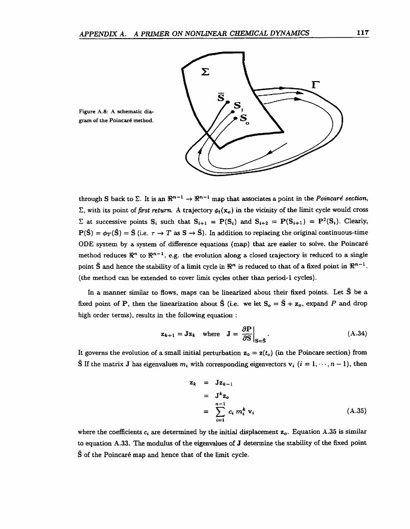
Figure -4.8: A schernatic dia-

gram of the Poincaré method.

through S back to C. It is an Sn-' + Y?"'+ map that associates a point in the Pozncaré section,

C, with its point of first return. A trajectory &(x,) in the vicinity of the liniit cycle wodd cross

E at successive points Si such that Si+i = P(Si) a d Si+2 = P(Si+l) = P2(Si)- Clearly,

P(S) = h ( ~ ) = s (Le. r + T as S + s). In addition to replacing the original continuous-time

ODE system by a system of ciifference equations (map) that are easier to solve, the Poincaré

method reduces 92" CO !Rn-1? e.g. the ecrolution dong a closed trajectory is reduced to a single

point s and hence the stability of a lunit cycle in Sn is reduced to that of a 6..xed point in In-'.

(the method can be extended to cover limit cycles other than period-1 cycles).

In a manner similar to flows, maps c m be linearized about their Gxed points. Let s be a

fked point of P, then the linearization about S (Le.

high order terrns), tesults in the following equation :

zkfl = Jzk where J =

we let S, = s + z,, expand P and &op

It governs the evolution of a small initiai perturbation z, = z(t,) (in the Poincare section) from

s If the matrix J has eigendues mi with correspondhg eigenvectors vi (i = 1, - - - , n - 1 ) , then

where the coefficients ci are deterrnined by the initid displacement 2,. Equation A.35 is similar

to equation 4-33. The modulus of the eigenvalues of J determine the stability of the ûxed point

s of the Poincaré map and hence that of the b i t cycle.

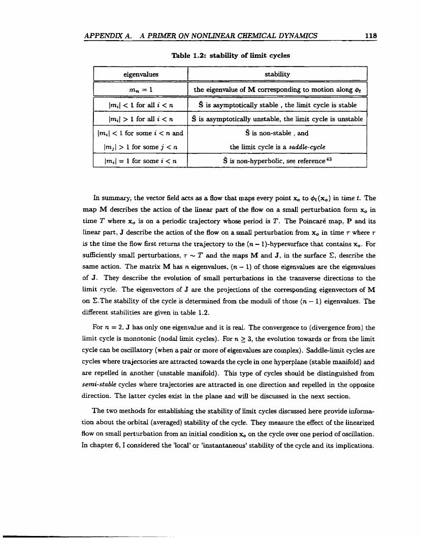
Table 1.2: stability of iimit cycles

1 lm,j > 1 for d i < n 1 s is asymptotically unstable, the E t cycle is unstable 1

eigenvaiues

m, = 1

Inri( < 1 for all. i < n

(mi( < 1 for some i < n and

jm,i > 1 for some j < n

stability

the eigmvaiue of M correspondhg to motion dong bt

S is asymptoticdy stable , the limit cycle is stable

S is non-stable , and

the limit cycle is a saddle-cycle

In siimmary, the vector field acts as a flow that maps every point x, to & (x, ) in time t. The

map M describes the action of the bear part of the flow on a s m d perturbation form x, in

time T where x, is on a periodic trajectory whose period is T. The Poincaré map, P and its

iinear part, J describe the action of the flow on a small perturbation from x, in tirne T where r

is the tirne the fiow first retunis the trajectory to the (n - 1)-hypersurface that contains x,. For

sufficiently smali perturbations, r - T and the maps M and J, in the surface C, describe the

same action. The matrix M has n eigendues, (n - 1) of those eigenvalues are the eigenvalues

of J. They describe the evolution of srnall perturbations in the transverse directions to the

limit cycle. The eigenvectors of J are the projections of the corresponding eigenvectors of M

on C.The stabibty of the cycle is determined from the moduli of those (n - 1) eigenvalues. The

different stabilities are given in table 1.2.

For n = 2, J has only one eigenvalue and it is real. The convergence to (divergence £rom) the

1 s t cycle is rnonotonic (nodal Iirnit cycles). For n 5 3, the evolution towards or £kom the limit

cycle can be oscillatory (when a pair or more of eigendues are cornplex). Saddle-Limit cycles are

cycles where trajectories are attracted towards the cycle in one hyperplane (stable manifold) and

are repelled in another (unstable manifold). This type of cycles should be distinguished from

semi-stable cycles where trajectories are attracted in one direction and repelled in the opposite

direction. The latter cycles exist in the plane and will be discussed in the next section.

The two methods for establishg the stability of limit cycles discussed here provide informa-

tion about the orbital (averaged) stability of the cycle. They measure the effect of the linearized

flow on srna11 perturbation from an initial condition x, on the cycle over one period of oscillation.

In chapter 6, I considered the 'local' or 'instantaneous' stability of the cycle and its implications.

A.3 Numericd Analysis

Generaüy, noniinear dynarnicai systems do not admit analytical solutions and one has to mor t

to numerical cornputations to obtain solution trajectories. In this section, I describe some of

the techniques used to obtain solution trajectories and construct phase portraits and bifucation

sets.

A.3.1 Integration of ODE Systems

The system

x = f(x) and x(t,) = x,

constitutes an initial value pmblem (IVP). Numerous techniques for the numericd solution of

NP'S have been developed, the most predominant ones are the finite-dBerence methods: a

solution trajectory, &(xo) is approxbated by a sequence of points x,, xl, xz, - - at t , , t ~ , t2 , - - - such that xi x &, (x,). The continuous-time system is approxhated by a discrete one where

the main task is to advance (Le. integrate) a d u e xi to xi+i in an accurate and efficient (in

terms of computation time) manner. The integration scheme can be formulated as:

X ~ + L = x i + h i 3(hj,~j,~j,.-.) where hi = t i - t i - ~ is the tirne-step. (-4.37)

Before desccibing the methods used to advance solution trajectories (i.e. the form of the function

3 above), 1 describe the types of errors that may result from such numericai cornputations.

Numericai errors are usudy classified as local e m r - the error introduced by a single integra-

tion step, and global error - caused by the repeated use of the integration formula. The local error,

at step i, is estimated by assuming that the previous i - 1 points are exact (Le xi - 1 = @ti - (x, ) ) . It does not account for propagated error, and can be defined by: €1 = ( ~ i + l -#ri+, ( x i ) ( . Locd er-

ror may result from two sources: round-OH ewor and truncation error. Round-off error is due to

the digital nature of cornputers and depends on the computer hardware and precision used(e.g.

double precision - 15 decimal places). It depends on the nurnber of arithmetic manipulations

per integration step but not on the step size. Truncation error is due to the finite-ciifference

approximation of the vector field and hence it decreases with the step size. It depends on

the integration algorithm used but not on the type of computer (assuming no round-off error).

Global round-off error is the accumulation of local round-OB error and hence for a unit of tirne,

it is equal to q / h . A large step size reduces the global effect of round-off error. On the other

hand, globd truncation error is the sum of local tmncation error. It is reduced by reducing the

integration step size.

First 1 describe single-step q l i c i t methoàs - the function 3 involves only xi, h. The simplest

of these methods is Euler's formuka. It can be derived from the formal definition of the derivative:

The hite-clifference

dx Xc+ L - Xi - = f (x ) = dt h - Hence,

The above formula can be thought of as a truncation of a Taylor expansion of x,+l about xi:

d ~ i 1 ,&xi x,+l = xi + h- + --h - + . - -

dt dt*

and thus Euler's formula is called first order or O(h). The local tnuication error is 0 ( h 2 ) and

hence, except for very small h, the method is not particularly accurate.

The Euler method can be improved by e d u a t i n g the dope (i.e. f ( x ) ) at different points in

the intervai between xi and x i + i - The most commonly used integration methods - those based

on the Runge-Kutta schemes - average the slopes at several intermediate States. For exampie,

the classical forth order algorithm is given by:

It is an 0(h4) and its truncation error is O(hS).

Zncreasing the order of a single-step aigorithm increases the accuracy of integration but tends

to make it less efficient; the Runge-Kutta scheme above requires four evaluations of f per step.

In addition, single-step explicit methods suffer from numerical instabilities when applied to s t i '

systems. Before discussing st if iess and how it can be overcome, 1 cl- what is meant by

numerical instability.

The estimation of local error, and hence global error, discussed earlier, assumes that there is

no propagation of error from one step to the next. The propagation of error by an integration

algorithm c m lead to the numerical instability of that algorithm if the error becomes unbounded.

The numerical instability of an algorithm is determined by testing it against a stable linear

system. I iliustrate this principle using the Euler method. Consider the foilowing linear system:

It has a solution

The Euler formula discretizes the system to:

Both the ana1ytica.i solution and numericai approximation diverge for X > O, as t + oc. For

X < 0, the numerical scheme converges to the origin only if

Similar regions of numerical stability can be obtained for other integration schemes.

The restriction placed on the stepsize poses a special problem for a class of systems known

as stifF systerns - systems that contain widely varying t h e çcales, e.g. dynamical systems arising

kom chernical kinetics. AiternativeIy, stifF systems may be defmed numerically as those systems

where numerical stabiiity rather than accuracy determines the step-size. Consider a system that

bas a solution evolving with two ciifFering tirne-çcales (e-g. XI = -1, As = -10000). An Euler-

type method m u t use a step-size h - 1x10'~ (due to X2) to be stable. However, due to the slow

component, the solution decays (e-t + O) in t -- 20s which requires - 2x106 steps. In many

cases, stabiLity requirernents result in stepsizes so smali that global round-off error becornes

important. Although. for the trivial case above, one rnay ignore the fast mode ccmpletely, in

chernical dynarnicai systems (e-g. autocataiysis, osciilations) tirne-scdes change frequentIy and

quickly and the fast modes have to be resolved for an accurate simulation of a solution trajectory.

Although single-step schemes can be cornbined with an adaptive step-size aigorithm to hancile

rnildly stiff systems, a more reiiable approach is needed. Several techniques have been dewloped

for this purpose. Interested readers may consult detailed monographs, e.g. 39v47. Here, 1 focus on

two schemes that were used extensively in the work leading to this thesis. The most cornmonly

used stiff integrators are based on bachard differentiation. The derivative (equation X.39) is

approximated by:

resulting in the following backward Euler j"mula:

Since the right hand side involves xi+l, it is an implicit scheme and requires additionai com-

putation to detennine xi+i (usually an iterative procedure is employed, see next section). Now,

applying the backward Euler formula to the linear system A.43, one gets:

The numericd solution converges to the correct solution if

( 1 - h A ) > 1 for X < O and ( 1 - h X ) < 1 for X > O (A.50)

and there is no restriction on the step-size.

Higher order implementations of -4.48 result in algonthms that use information from several

previous steps and hence they are cailed multi-step algonthms. A kth order scheme may be

represented by:

Xote that the k steps are equaiiy spaced. These formulas are generally known as Gear's method.

For example, a forth order Gear's scheme is given by:

The widely used ODE solver LSODE uses such a scheme to integrate stiff equations (it uses an

analogous explkit formula to solve nonstiff equations) .

Muiti-step methods have two disadvantages: (1) information from several previous steps has

to be stored resulting in large memory requirements, and (2) they can be used oniy after several

steps have been taken and hence a Iower order scheme or a single-step method has to be used to

initiaiize the integration process. These 'start-up' costs are usually compensated for by the fact

that they require o d y one function evaluation per step. For the computations using the cellular

mixing mode1 in chapters 4,5,6, however, the initiai condition x, changes (and the integration

process is restarted) so frequently that a muiti-step aigorithm t o t d y loses its computational

advantages due to reinitiaiization costs.

For stiff equations that are integrated for short intervals a t a time (due to discrete and

stochastic jumps in their solution trajectories), 1 found that single-step irnplicit methods com-

bined with an extrapolation scheme compare favorably to Gear's method, especidly for high

accuracy levels: the equations are integrated using a single-step implicit rnethod (e-g. implicit

Euler) and a more accurate solution is found by extrapolating to the h = O limit. For most

of the simulations in this work, I have used the linearly implicit Euler extrapolation algorithm

developed by Hairer and Wanner".

Numerical integration provides approximate solution trajectories and is best suited for simu-

lating the evolution of a dynarnical system and to produce representative trajectories for phase

portraits (another good use, as we will see, is locating basin boundaries). It can be used as a

'brute-force' method to construct bifurcation diagrams: in a manner analogous to experimental

procedures, a control parameter is set, an initial condition is chosen, and the system is integrated

until an asymptotic state is reached. The procedure is repeated for a grid of bifurcation param-

eter values. If qualitative changes are observeci, the transition points are made more precise by

refhing the grid near those points. Although nrimencai integration is easy to use and closely

mimics the corresponding experirnental systern, it suffers from some disadvantages:

(1) it can not locate nonstable (saddle-type) 'attractors' or non-hyperboiic points. Repellers

can be Iocated via time-reversai (ti < t i - 1 ) .

(2) it converges slowly ne= bifurcation points (numerical couterpart of critical slowing dom).

(3) it can be time-consuming and computationally inefficient for the purpose of constmcting

bifurcation diagrams.

A better approach is the use of the now well-developed continuation or path-following methods.

A.3.2 Continuation methods

A bifurcation diagram requires locating attractors (this is restricted to hd ing fixed points and

limit cycles) and determining their stability and dependence on bifurcation parameter(s) . Fixed

points of a dynamicd system are the zeros of the vector field, f(x). The most commonly used

method for locating the zeros (roots) of a noniiiear function is the Newton-Raphson method.

Suppose one replaces the function f(x) by its linearization about x,,

then the zeros of f(x) will be given by:

Despite its form, the mat* equation above can be solved

(4.54)

using Linear algebra (e-g. LU decom-

position) without the need to invert 1 x=xo . If x, is chosen sufnciently close to a root of f (x) :

the iterative formula usuaiiy converge quickly to that root - regardless of the stability of that so-

lution. The method has to be modified to work near fuced points with zero eigeni-aluesW. Once

a fixed point is iocated, its value can be used as a good initial guess for an incremented value of

the bifurcation parameter and a branch of fixed points can be constructed as a function of the

bifurcation parameter. The stabiiity of the fixed points is assessed by evaluating the eigenvalues

of at those points. Eigenvalues are determined using standard and Mdely-adable routines,

e.g. EISP.4CK " .

Penodic orbits are usually located by applying the Newton algorithm to the function &-(X)-X

in a scheme called the shooting method. The stability of the orbits is determined from the

eigenvalues of the monodromy matrix which can be calculateci from the variationai equation or

obtained as a by-product of the shooting methodg6.

Bifurcation points are detennined by examining the eigenvalues of the jacobian matrix or the

monodromy matrix. The process of obtaining solution branches and construction of bifurcation

diagrams and sets is automated via bàjùrccrtion following packages. A good package consists

of algonthms for choosing the appropriate stepsize, locating fixed points and limit cycles and

determining t heir st abilities, diagnosing bifurcation points, tradcing branches around turning

points. and branch switching. -4 detailed treatment of continuation methods is @en in the

excellent book by Riidiger Seydeig6. Two bifurcation packages are widely used:

1. BlFPACP5 ; an easy-to-use smail package that is best suited for foUowing branches of fked

points. 1 was unable to foilow periodic branches reLiably using it. It can map bifurcations

in 2-parameter planes by adding explicitly the condition for the particular bifurcation

2. AUTO^'; a very flexible package that can foilow branches of fixed points and periodic

solutions. It automates the tracing of 2-parameter bifurcation curves. Requins the tuning

of many parameters to work ideaily and thus bas a steeper 'learning m e ' .

Bibliography

[Il 1997. The experiments were conducted by Dr. P. Strizhak.

[2] H. D. 1. AbarbaneI, B. Brown, and M. B. K e ~ e l . J. Nonlin. Sci., 1:175, 1991.

[3] F. Alit 2992. Unpubiished.

[4] F. Xi. Stirring and mkhg effects in chernical imtabilities: The dorite-iodide reaction.

Master's thesis, University of Toronto, 1992.

[a] F. Ali and M. Menzinger. J. Phys. Chem., 956408. 1991.

161 F. -U and M. Menzinger. J. Phys. Chem., 96:1511, 1992.

[7] R. Aris. Elementary Chemicul Reactor Analysis. Butterworths, 1989.

[S] J. Baldyga and J. R. Bourne. Encyclopedia of Ruad Mechanics. chapter 6. Gulf Publishing,

Houston, 1986.

[9] J. Baldyga and J. R. Bourne. Chem. Eng. Sci., 47:1839, 1992.

[IO] K. Bar-Eli and R. J. Field. J. Phys. Chem., 94:3660, 1990.

[Il] R. Benzi and G. F. Carnevale. J. Atm. Sci, 46:3595, 1989.

[12] P. Bergé, Y. Pomeau, and C. Vidal. Order within Chaos. John Wiley & Som, 1984.

[13] J. Boissonade and P. DeKepper. J. Phys. Chem., 84502, 1980.

(141 J. Boissonade and P. DeKepper. J. Chem. Phys., 87:210, 1987.

[l j j 11. Boukalouch. Efeb d'inhomogénéités spatiaies dans la réaction oscillante et bistable-

PhD thesis, L'Université de Bordeaux 1, 1988.

[16] J. J. Carberry. Ind. Eng. Chm., 58:40, 1966.

[l?] A. Cholette, J. Blanchet, and L. Cloutier. Can J. Chem. Eng., 38:1, 1960.

[18] R. L. Curl. A. I. Ch. E. J., 9: 175, 1963.

[19] P. V. Danckwerts. C'hem. Eng- Sci., 2:1, 1953.

[20] P. DeKepper. PhD thesis, L'Université de Bordeaux 1, 1978.

(211 E. J. Doedel and J. P. Kernevéz. AUTO: Softtuare for continuation and bifurcation prob-

lems in ordinary differential equations. Technical report. A p piied Mat hematics , California

Institute of Technology., 1986.

[221 A. K. Dutt and 31. Menzinger. J. Phys. Chem., 94:4867. 1990.

[23] A. K. Dutt and M. Menzinger. J. Phys. C'hm.: 963429, 1991.

[24] -4. K. Dutt and S. C. Muller. J. Phys. Chem., 97:10059, 1993.

[25] 1. R. Epstein. Nature, 34636, 1990.

[26] 1. R. Epstein. Nature, 374:321, 1995.

[27] J. J. Evangelista, S. Katz, and R. Shinnar. A.1.CTi.E. J., 15:843, 1969.

[28] V. J. Farage and D. Janjic. Chimia, 35:289, 1981.

[29] W. Feller. An Intmduction to Probabillty Theory, Vol. 1. Wiley, New York, 1957.

[30] R. J. Field and R. M. Noyes. J. Chem. Phys., 60:1877. 1974.

[31] R. F. FOX. Phys. Rev. A, 344525, 1986.

[32] R. O. Fox. Chem. Eng. Sci., 46:1829, 1991.

[33] R. O. FOX and J. Villermawr. Chem. Eng. Sci., 45:2857, 1990.

[34] G. F. Froment and K. B. Bischoff. Chernical Reactor Analysis and Design, 2nd Ed. John

Wiley & Sons, New York, 1990.

[35] D. Gailez and A. Babloyantz. Phys. Lett. A, 161:247, 1991.

[36] 3. Ganapathisubramanian and K. Showaiter. J. Chern. Phys., 845427, 1986.

[37] C . W . Gardiier. Handbwk of Stochastic Methods, 2nd Ed. Springer-Verlag, Berlin, 1983.

[38] V. G a p & and K. Showalter. J. f iem. Phys., 88:778, 1988.

[39] C. W. Gear. Numerical Initial Value Probiems in Ordinary Differential equations. Prentce

Hall, 1971.

[40] P. Gray and S. K. Scott. Chernicd Osdlations and Instabilities. Claredon Press: Oxford.,

1994.

[41] K. R. Graziani, J. L. Hudson, and R. A. Schmitz. Chem. Eng. J., 12:9, 1976.

[43] J. Guckenheimer and P. J. Hohes. Noniinear Osciltations, D y n a m i d Systems, and

Bifufcations of Vector Fiel&. Springer-Verlag: New York., 1983.

[44] L. Gyorgyi and R. Field. J. Chenz. Phys., 91:6131, 1989.

-51 L. Gy6rgyi and R. Field. J. Phys. Chem., 95:6594, 1991.

[46] L. Gy6rgyi and R. Field. Nature, 355:808, 1992.

[47] E. Hairer and G. Wanner. Solving Odinary Diffmntial Equations II. Stzff and

Diflerential-.4lgebraic Problems. Springer-C'erlag: Berlin, 1991.

[48] H. Haken. Synergetics. Springer, Berlin, 1978.

[49] H. Haken. Advanced Synergetàcs. Springer, Berlin, 1983.

[5O] L. Hannon and W. Horsthemke. J. Chem. Phys., 86:140, 1987.

[51] M. J. Hauser, D. Lebender, and F. W. Schneider. J. Phys. Chem., 96:9332, 1992.

[52] M. W. Hirsch and S . Smale. Diffmntial Epations, Dynarnicd Systems, and Linear

Algebra. -4cademic Press: Xew York., 1974.

[53j W. Horsthemke and L. Hannon. J. Chem. Phys.. 81:4363, 1984.

[54] W. Horsthemke and R. Lefever. Noise-lnduced rrclnsitions. Springer-Verlag, Berlin, 1984.

1551 E. .A. Jackson. Perspectives of nonlinear dynamics. Cambridge University Press, Cam-

brdige, 1989.

[56] M. Juckes and M. E. MacInyre. Nature, 328590, 1987.

(571 R. Kaprd and E. Celarier. Noise in Noniinear Dynamicol Systems, volume 2, chapter 9.

Cambridge University Press, Cambridge, 1989. Edited by F. Moss and P. V. E. McClintock.

[58] J. Keizer, R. F. Fox, and J. Wagner. Phys. Lett. A, 175:17, 1993.

[59] M. T. M. Koper. J. Chem. Phys., 102:5278, 1995.

[60] E. Kumpinsky and 1. R. Epstein. J. Chem. Phys., 82:53, 1985.

[6f] C. Kurrer and K . Schulten. Physim D, 50:311, 1991.

[62] L. D. Landau and E. M. Lifshitz. Statistical Physics. Pergamon, London, 1958.

1631 J. P. Laplante, P. Borckmans, G. Dewel, M. Gimenez, and J. C. .Micheau. J. Phys. C'hem.,

91:3401, 1987.

[64] 0. Levenspiel. Chernical Reaction Engineering. Wiley, New York, second edition, 1972.

[65] L. Luo and 1. R. Epstein. J. C'hem. Phys., 855733, 1986.

[66] J. Maselko. Chem. Phys., 67:17, 1982.

[67] M. Menzinger, 1997. Personal communication.

(681 M. Menzinger, M. Boddouch, P. DeKepper, J. Boisçonade, J. C. Roux, and H. Saadaoui.

J. Phys. Chem., 90:313, 1986.

[69] M. Menzinger and A. K. Dutt. J. Phys. C h m . , 94:4510, 1990.

[70] M. Menzinger and A. Giraudi. J. Phys. C'hem-, 91:4391, 1987.

[71] M. Menzinger and P. Jankowski. J. Phys. Chem., 90:1217, 1986.

[72] hl. Menzinger and P. Jankowski. J. Phys. Chem., 94:4123, 1990.

[73] S. Nagata. Mking: Principles and Applicutions. John Wiley & Sons, -Jew York. 1975.

[C4] 1. Yagypd and 1. R. Epstein. J. Phys. Chem., 90:6285, 1986.

[75] 1. Nagypd and 1. R. Epstein. J. Chem. Phys-, 89:6925, 1988.

[76] J. M. Nese. Physica D, 35:237, 1989.

[77] J. S. Nicolis, G. Meyer-Kress, and G. Haubs. 2. Naturforsch, 38a:ll57, 1983.

[78] A. Nitzan, P. OrtoIeva. J. Deutch, and J. Ross. J. Chem. Phys., 61:1056, 1974

[79] 2. Noszticzius, S. Bodnk, L. Garamszegi: and M. Wittman. J. Phys. Chem., 95:6575,

1991.

[BO] E. E. O'Brien. Turbulent Reactive Flows, chapter 5. Springer-Verlag, Berlin, 1980. Edited

by P. -4. Libby and F. -4. Williams.

[81] J. M. Ottino. Chem. Eng- Sci., 351377, 1980.

[82] J. M. Ottino. Chern. Eng. Sci., 49:4005, 1994.

1631 T. f ., N. Ganapathisubramanian, and K. Showalter. J. Chern. Phys., 83:1101, 1985.

[84] R. B. Pierce and T. D. Fairlie. J. Geophys. Res., 98589, 1993.

[85] E- Plasari, R. David, and J. Viermaux. ACS Symposium Series, Chem. React. Engng.,

65:126, 1978.

[86] S. B. Pope. h g . Energy Combust. Sci., 11:119, 1985.

[B?] A. Puhl and G. Nicolis. Chm. Eng. Sci., 41:3111,1986.

[88] W. J. Rappel and S. H- Strogatz. Phys. Rev. E, 50:3249, 1994.

1891 P. Resch, A. F. Münster, and F. W. Schneider. J. Phys. Chem., 95:6275, 1991.

[901 J. C. R o u , P. DeKepper, and J. Boissonade. Phys. Lett. A, 97:168, 1983.

[9 11 J. C- ROUX, H. Saadaoui, P. DeKepper, and J. Boissonade. In W. Horsthemke and K. Kon-

depudi, editors, Fluctuations and Sensitivity in Nonequiiibriurn System. Springer-Verlag,

Berlin, 1984.

[92] A. Rovinsk? H. Adiwidjaja, V. Yakhnin, and M. hlenzinger. Ozkos, 78:101, 1997.

[93] P. Ruoff. Chem. Phys. Lett., 90:76, 1982.

[94] F. W. Schneider and A. F. Münster. J. Phys. Chern., 95:2130, 1991.

[95] R. Seydel. BIFPACK: A progmm package for continuation, bifircation and stabiiity

analysis. Technical report. Mathematisches Institut der Julius-Maximilans-Universitat:

Würzburg.. 1988.

[96] R. Seydel. nom Equiiibriurn to Chaos. Elsevier: Xew York, 1988.

[97] Smith et al. Matriz eigensystem routines-Eispack guide. Lecture notes in Comp. Sci. 6.

Springer: Berlin, 1976.

[98] L. A. Spielman and O. Levempiel. Chem. Eng. Sci., 20:247, 1965.

[99] P. Strizhak, F. Ali, and M. Menzinger. J. Phys. Chem., 1997. In press.

[100] P. Strizhak and M. Menzinger. J. Phys. C'hem., 100:19182, 1996.

[101] P. Strizhak and M. Menzinger. J. Chem. Phys., 105:10905, 1996.

[IO21 K. Tomîta, T. Ohta, and H. Tomita. Pmg. Theoret. Phys., 52:1744? 1974.

(1031 H. Treutiien and K. Schdten. Ber. Bunsenges Phys. Chern., 89:710, 1985.

[104] V. K. Vanag and b1. Alfimov. J. Phys. Chem., 97:1884, 1993.

[105] J. Viermaux- ACS Symposium Series, Chem. React. Engng., 226:135, 1983.

11061 J. Villemaux. Encyclopedia of f i i d Mechanics, chapter 27. Gulf Publishing, Houston,

1986.

[IO?] J. Villemaux. In P. Gray, G. Nicoh, F. Baras, P. Borckmans, and S. K. Scott, edi-

tors, Spatial Inhonaogeneities and Thnsient Behavior In Chernical Kinetics. Manchester

University Press: Manchester, UK, 1990.

[IO81 J. Vüiermaux and L. Falk. Chem. Eng. Sei-, 495127, 1994.

[log] S. Weissenberger. Master's thesis, University of Würzburg, 1993.

[ 110f S. Weissenberger. Master's thesis, University of Toronto, 1997.

[111] S. Wiggins. Intmduction to Applaed Nonlinerrr Dynamical Systems and Chaos. Springer-

Verlag: New York, 1990.

[Il21 A. T. Winfree. The Geometry of Biological Time. Springer-Verlag, New York, 1980.

[113] T. Y. Zwietering. Chem. Eng. Sci., 39:1765, 1984.

IMAGE EVALUATION TEST TARGET (QG~)

1.6 11111i iioi1.4 il,

APPLIED iL IMAGE. lnc - = 1653 East Main Slreet - -. , , Rochester. NY 14609 USA -- -= Phone: i l 6/4û2-0300 -- -- - - Fax: 7i6/28&5989