POLITICAL ALIGNMENT AND TAX EVASION

PRELIMINARY

PLEASE DO NOT CITE

POLITICAL ALIGNMENT AND TAX EVASION

JULIE BERRY CULLEN, NICHOLAS TURNER, & EBONYA WASHINGTON*

September 2015

ABSTRACT. We explore whether the decision to evade federal personal income taxes depends

on the taxpayer’s level of approval of government. We first demonstrate using survey data the

positive association between political alignment with the current president and the respondent’s

trust in the administration and support for government taxation and spending. We then show

using IRS tax return data and county-level fixed effects regressions that the larger the typical

share of county residents who vote for the president’s party the smaller the tax gap across a

variety of tax gap measures. Responses are concentrated in income components that are more

likely to be invisible to the government, such as small business income. Our results provide real-

world evidence that a positive outlook on government lowers tax evasion.

* University of California, San Diego; U.S. Treasury, Office of Tax Analysis; Yale University

E-mail addresses: jbcullen[at]ucsd.edu; Nicholas.Turner[at]Treasury.gov; ebonya.washington[at]yale.edu

We thank Daniel Brownstead, Stephanie Hao and Claudio Labanca for excellent research assistance, and Jeffrey

Clemens, Danny Yagan and participants in the Austin-Bergen Labor Conference and All California Labor

Economics Conference for helpful comments. All errors are our own. This research represents our private research

efforts and does not necessarily reflect the views or opinions of the U.S. Treasury.

1

Tax evasion lowered federal tax revenue for the United States government by roughly $450

billion in 2006.1 This was not an atypical year. Generally under 85% of federal taxes are paid

initially, with another 2-3 percentage points recovered through enforcement (and late payments).

The vast majority of losses come through personal income taxation, reflecting the US

government’s great reliance on this form of taxation. While some taxpayers fail to file taxes at

all, the more typical form of evasion is underreporting. Underreporting is concentrated in forms

of income that are not directly reported by the payer to the government, so are less visible to tax

collectors.

Failure to pay taxes impacts the efficiency, equity and incidence of the tax system and alters

the distribution of resources to and across economic activities. Given the widespread

consequences of evasion, economists have a long history of studying the behavior. The classic

model (e.g., Allingham and Sandmo, 1972) is one of evasion as a financial gamble that the agent

undertakes if the benefits exceed expected costs. The impact of the marginal tax rate on evasion

is ambiguous,2 but the model clearly predicts and the empirical evidence generally supports the

idea that evasion is decreasing in the cost (i.e., audit and penalty rates).3 Given currently low

levels of enforcement, we are then left with a puzzle: why is tax compliance so high?

Our work builds on two potential explanations raised in the literature. The first notes that one

limitation of the basic model is that it fails to account for heterogeneity across income sources

with regard to the probability of audit. In the context of Denmark, Kleven et al. (2011) point out

that discrepancies between the self-report and third-party report of wage income will trigger an

audit with a probability approaching one. These types of ex ante differences in the probability of

audit can help to explain observed differences in evasion across more and less visible sources of

income.

The second possible explanation that we explore in this paper is that the benefits of tax

compliance are broader than simply avoiding a penalty in expectation. Among the factors that

might affect willingness to pay taxes is the perceived value of government spending. Falkinger

(1988) presents the direct self-interest version, extending the basic model to allow the agent to

value her share of public goods provided. Congdon, Kling and Mullainathan (2009) propose that

tax behavior may be affected not only by public goods directly received but also by one’s views

of government and its policies. This expanded view of the benefits of tax compliance is

supported by both survey and experimental lab evidence, reviewed in the next section.

Our innovation is to take this expanded view to a real world setting where there is plausibly

exogenous variation in attitudes toward government.4 We measure the impact of changes in

approval of government and its spending priorities on changes in the level of tax evasion at the

county level. This exercise presents two data challenges. The first is the well-known difficulty of

quantifying an illegal activity. We use Internal Revenue Service (IRS) personal income tax

returns to measure aggregates for reported taxable income components, and then attempt parse

out the share that is due to evasion. Recognizing that government attitudes are not only

1 See Tables 1a and 1b and Figure 1 for more details and sources for the facts in this paragraph.

2 If the penalty depends on the amount of tax evaded, the marginal rate plays no role, but there are competing

income and substitution effects if the penalty depends on the amount of under-reporting. The empirical relationship

between the marginal tax rate and evasion is similarly non-robust, with, for example, Clotfelter (1983) and Kleven et

al. (2011) finding a positive relationship, and Feinstein (1991) finding a negative one. 3 See Barbuta-Misu (2011) for a review of this literature.

4 The IRS mentions ―socio-political‖ factors as one of the key influences on voluntary tax compliance, and notes that

there is little empirical evidence regarding the importance of these factors (―Reducing the Federal Tax Gap: A

Report on Improving Voluntary Compliance,‖ Internal Revenue Service, August 2, 2007).

2

correlated with a wide variety of factors that might affect opportunities to engage in evasion, but

may also impact economic activity directly through own consumption (Gerber and Huber, 2009)

or government transfers,5 we control flexibly for the amount and types of income generated in a

county. We also divide reported taxable income into categories by level of third party reporting.

If poorly documented income is more sensitive to government attitudes, then this is a pattern

consistent with evasion.

The second data challenge is measuring approval of government at the same level of

geography. Our proxy is political alignment—a match between own party and presidential party.

To support the validity of this proxy, we first use national survey data (from the General Social

Survey) to confirm that an individual’s alignment predicts positive views of government and

government taxes and spending. We then construct an analogous county-level measure, equal to

the share of the two-party vote cast for the party of the current president. In light of evidence that

voters’ preferences are sensitive to current economic conditions (e.g., Brunner, Ross and

Washington, 2011), rather than using the vote share from the most recent election, we use the

average over several elections. Residents of partisan counties—those that voted consistently for

one party over our time frame—are either shifted into or out of alignment by turnover elections.

We focus on these partisan counties, and either treat swing counties as within-state controls or

exclude them from the analysis.

In regressions that include years surrounding turnover elections and that control for economic

controls, government transfers, county and state-by-year fixed effects, we find that taxable

income reported increases by 0.3% as a county moves into alignment. The majority of the

increase is attributable to income categories that are subject to little third party reporting, such as

income from small businesses. While reported income in these less visible categories expands by

3%, we generally find no elasticity of third party reported income to alignment. Corroborating

the view that evasion falls, earned income tax credit (EITC) claims and audit rates also fall.6 The

responses are muted when federal income tax reports are direct inputs to state tax returns—cases

where tax morale would be mediated by another layer of alignment. Finally, the responses are

magnified when the county is aligned with both the president and governor, particularly when

these executives share the same party.

Our results provide novel evidence from real world data for the link between tax morale and

tax compliance, confirming a behavioral component to tax compliance.7 Combining evidence

from our survey (GSS) and administrative (IRS) data, we demonstrate that where a higher

5 Dynes and Huber (2014) is a current study that shows an explicit link between voter alignment with the president

and federal government transfers. Prior work has demonstrated a link that is moderated by congressional

representation. For example, Albouy (2013) finds that representation by a member of the majority party predicts

greater transfers, and Berry, Burden and Howell (2010) find the same for House representation by the party of the

president. 6 Chetty, Friedman and Saez (2013) find that the self-employed are particularly likely to report income levels that

maximize EITC tax refunds, and provide evidence that this sharp bunching reflects evasion. Audit rates can

similarly serve as proxies for evasion, since audits are initiated when reported amounts are discrepant with norms for

similar returns in ways that correlate with detected evasion from prior audits. 7 Ours is among the first studies to consider the role of political alignment in tax evasion. Previous work has looked

at the relationship between a CEO’s political affiliation and corporate tax avoidance, with conflicting results.

Christensen et al. (2014) find that firms led by CEOs who donate more to the Republican party are less likely to

avoid taxes, while Francis, Hasan and Sun (2012) find these are exactly the firms that are more likely to avoid

taxation. Besley and Jensen (2014) rely on election-induced shifts in the single-majority party status of local

governments to provide shocks to the tax enforcement regime, and, in their UK setting, it is the unpopular shift to a

poll tax to fund local government that alters intrinsic motives to pay taxes.

3

fraction of county residents hold a positive view of government, a lower fraction of taxes is

evaded.

The remainder of the paper proceeds as follows. Section 1 reviews the recent literature on tax

morale, and provides evidence that political alignment is a meaningful proxy for the component

of tax morale that operates through government approval. The data and methods are presented in

Section 2, and the results in Section 3. Finally, Section 4 offers a brief conclusion.

1. Tax morale and the role of political alignment

1.1 Literature on tax morale

There is a growing literature exploring mechanisms underlying differences in the willingness

to pay taxes, or ―tax morale.‖ In their recent review of this literature, Luttmer and Singhal (2014)

provide a typology for classifying these. In addition to other categories, such as intrinsic

motivations (e.g., guilt) and peer influences (e.g., social image and norms), they define

―reciprocity‖ to refer to those that depend on the individual’s relationship to the state. Political

alignment is a composite construct that falls under this umbrella. Being aligned with the

president’s party might increase trust in the administration in general, as well as approval of the

government’s tax and spending activities.

There is both survey and experimental lab evidence in support of the idea that taxes paid are a

positive function of the payee’s trust in and approval of government. Webley et al. (1991)

demonstrate a correlation between negative attitudes toward government and evasion in the lab,

while Scholz and Lubell (1988) and Torgler (2003) show that trust in government is correlated

with reported compliance in surveys. In a cross-country analysis, Feldman and Slemrod (2009)

find that attitudes toward compliance are increasing in the number and length of conflicts but

decreasing in the number of casualties. Further, experimental economists have found that

individuals are more likely to be tax compliant the more they value the public good (Alm,

Jackson and McKee, 1992) and when those individuals have selected that public good (Alm,

McClelland and Schulze, 1992). Hanousek and Palda (2004) find complimentary evidence that

(Czech and Slovak) individuals who believe that the quality of government services is low are

more likely to report ever evading. Authors have also repeatedly found that perceptions that the

tax system is fair increase reported compliance (e.g., Cummings et. al, 2009; Fortin, Lacroix and

Villeval, 2007; Steenbergen, McGraw and Scholz, 1992).

Our study fills a gap in this literature by linking evasion as it occurs under the existing tax

system to quasi-experimental variation in attitudes.

1.2 Linking political alignment to tax morale

In this subsection, we use US survey data to show that our chosen measure of political

alignment is a valid proxy for government approval, and relates to self-reported tax morale in a

similar way to other measures that have been used in the literature. For this exercise, we employ

data from the General Social Survey (GSS).8 Begun in 1972, the GSS is an annual or biannual

repeated cross section of the political and social attitudes of adults. Relevant for our purposes,

the survey includes questions on confidence in government and views on government spending

and taxation as well as respondent partisanship.

8 Smith, TW, M. Hout, and P.V. Marsden. General Social Survey, 1972-2012 [Cumulative File]. ICPSR34802-v1.

Storrs, CT: Roper Center for Public Opinion Research, University of Connecticut /Ann Arbor, MI: Inter-university

Consortium for Political and Social Research [distributors], 2013-09-11. doi:10.3886/ICPSR34802.v1.

4

Using the pooled 1972-2012 samples, weighted to be representative of the non-institutionalized

English speaking population,9 we run models of the form:

(1)

Government attitudeit 1 Presalignmentit 2 Congalignmentit Xit it ,

where Government attitude is a measure of confidence in a government institution or support for

government activities. Presalignment is calculated from a party identification variable whose

values range from 0 (strong democrat) through 6 (strong Republican). We create a ―party id‖

index by rescaling this variable to range from 0 to 1, for ease of interpretation. Then, we define

alignment to be equal to party id during Republican administrations, and to 1 – party id during

Democratic administrations.10

We define Congalignment analogously. It is equal to party id

when the House and Senate are both majority Republican, 1 – party id when the House and

Senate are both majority Democrat, and ½ when the chambers are split. The vector X is a

detailed set of individual controls, including party id and an ideological index (ranging from 0

for extremely liberal to 1 for extremely conservative).11

The reported standard errors are robust

to clustering by party id-by-year, the level of variation.

We begin by exploring the relationship between alignment with the president and confidence in

the executive branch. In Table 2a, our outcome variable is the level of confidence the respondent

has in the executive branch. We have rescaled this from the original to range from 0 to 1 and to

increase with confidence, so that 0 is ―hardly any‖ and 1 is ―a great deal.‖ We see that as

presidential alignment increases so too does confidence. Whether we incorporate individual level

controls (column 2) or not (column 1), the point estimate on presidential alignment indicates that,

when aligned, the strongest partisans (whose values of alignment are 0 or 1) are 22 percentage

points more likely to say they have a great deal of confidence in the executive branch. For the

moderate partisans (who answer 1 or 5 on the original scale), the difference in confidence across

aligned and unaligned administrations is 15 percentage points.

In our main analysis, our measure of partisanship will be calculated from county vote shares

rather than party identification. The absence of information on county in the GSS precludes

aggregating respondents’ political views. However, we can explore robustness to moving from

self-reported partisanship to self-reported vote choice.12

In column 3 we restrict the sample to all

those indicating their preferred candidate in the most recent presidential election. We find having

favored the president in the last election is associated with an increase of 16 percentage points in

the likelihood of great confidence. The association is strengthened when in column 4 we limit the

9 The GSS did not begin interviewing in Spanish until 2006, so we drop the Spanish language interviews to maintain

consistency. Because the GSS only interviews one adult per household, we weight respondents by the number of

adults in the household. We interact this weight with multipliers that adjust for 1) oversamples conducted in 1982

and 1987, and 2) imperfect randomization of survey forms in 1978, 1980 and 1982-85. 10

The GSS is administered during February through April and presidents take office in January following election

years, so that the relevant administration is always that of the most recently elected president. 11

We include an expansive set of individual controls to address concerns about changes in the composition of

respondents and administration over time. The set includes the following demographic characteristics for the

respondent: gender, age, race, years of education, employment status, marital status, household composition (by age

and earner status), family income, religion and region. The set also includes variables characterizing the interview:

interviewer reports of respondent’s friendliness, cooperativeness, and understanding of the questions, and type of

administration (phone or in-person). 12

We recognize that self-reported vote choice is influenced by party identification (Gerber, Green and Washington

2010) and the election winner. Across the years 1950-1988, Wright (1993) finds over reports of voting for the

winner in the American National Election Study only for the 1964 Goldwater-Johnson election.

5

sample to those who report having actually voted for their preferred candidate.

In order to tighten the link between party alignment and approval of the federal government,

and more specifically the executive branch that houses the IRS, we next explore the extent to

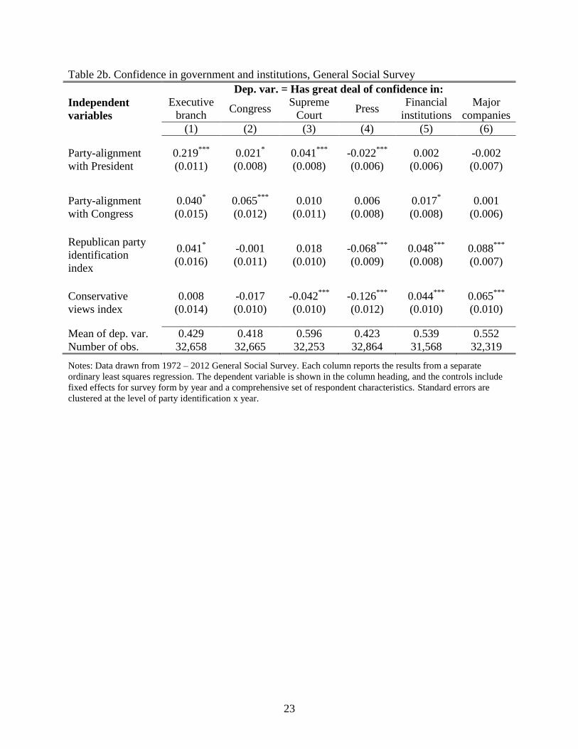
which alignment predicts confidence in other institutions. For the results shown in Table 2b, the

confidence variables are all rescaled from 0 to 1, with 1 representing ―a great deal‖ of

confidence. The first column repeats column 2 from Table 2a, our preferred specification, for

comparison. Columns 2 and 3 show how opinions about Congress and the Supreme Court vary

with alignment. In both cases, we find that presidential alignment is associated with much

smaller increases in the likelihood of approval. For Congress we find congressional alignment

has a greater impact than presidential alignment, as expected. In column 4, interestingly, we find

a negative (but again small) relationship between approval of the press and presidential

alignment. Perhaps this reflects some frustration at the press ―attacking‖ the respondent’s

president. In the remainder of the table, we find no relationship between alignment and

confidence in financial institutions (column 5) or major companies (column 6). These two

specifications can be viewed as placebo tests and suggest that shifts in views toward government

induced by changes in party representation at the national level do not alter views toward the

private sector.

In the final GSS table, Table 2c, we further ask whether alignment predicts support for federal

government taxation and spending. The answer is yes. On the tax side, while fewer than 1% of

respondents say their taxes are too low, alignment is associated with a five percentage point

decrease in responding that taxes are ―too high‖ over ―just right‖ and ―too low‖.13

To create

measures of approval for federal spending, we sum across a series of questions that ask whether

spending in a particular area is too much, just right or too little14

to create variables on the

fraction of categories for which the respondent held a given view. In column 2 we see that

presidential alignment is negatively and significantly associated with often feeling there is too

much spending. We do not find that the too little spending margin moves with alignment. These

findings are echoed in respondents’ attitudes toward government action. Transforming a GSS

scale on whether the government should do more or leave more to the private sector into

indicators, we find that alignment negatively and significantly predicts the view that the

government should do less. Alignment is not significantly associated with the view that

government should do more.

Thus the results from the GSS analysis provide support for alignment being a meaningful

proxy of approval of the executive branch. There is also an elasticity of disapproval for taxation

and spending with respect to alignment, but not an elasticity of approval. In the main analysis we

ask whether these more negative government attitudes translate into a lower willingness to

comply with taxation.

2. Methodology and data

2.1 Methodology

Our goal is to estimate the impact of political alignment on evasion, which clearly requires a

13

While there are questions even more directly related to tax morale, such as whether it is okay to cheat on taxes,

these are asked in too few years to identify the role of alignment conditional on party identification. 14

The spending categories are education, health, welfare, the environment, law enforcement, drug rehabilitation,

assistance to big cities, assistance to blacks, defense, space exploration and foreign aid.

6

method for measuring evasion. A variety of methods have been used in the literature. In rare

instances, data from random audits are available (e.g., Kleven et al., 2011). More typically,

evasion is inferred from discrepancies between what is observed and what is expected. For

example, Feldman and Slemrod (2007) compare the estimated elasticity of charitable giving

across different sources of taxable income. Absent evasion, their presumption is that the

propensity to donate would be constant across more and less visible income sources. The

primary approach that we follow is known as the tax gap approach. We use reported taxable

income measures as our dependent variables, and include a battery of economic controls to proxy

as closely as possible for generated taxable income. The idea is that movements in reported

amounts, holding generated amounts fixed, should reflect changes in evasion.

Consider the following ordinary least squares specification relating (the log of) taxable income

reported by residents of county c in state s in year t to the county’s political alignment in that

year:

(2)

ln Reported income cst alignmentcst Xcstc st cst ,

where alignment is defined to be the share of the two-party vote cast for the current president in

the most recent election. Only non-election years are included in the sample. During election

years, income is earned under one president and is reported (in the following April) under

another. For these years, it is not obvious how to define alignment as long as any real costs to

evasion are borne in advance of filing.15

We would like to interpret as the percent change in

reported income caused by one-unit change in alignment, holding all else equal.

To begin, presume that generated taxable income is perfectly controlled by the vector X. An

immediate concern with respect to causal interpretation is that, in the cross-section, alignment is

far from randomly assigned. Not only is the partisanship status of a county correlated with

county demographics, it is also likely correlated with opportunities for evasion due to differences

in sources of income. This motivates the inclusion of county fixed effects, so that changes in

alignment within a county over time provide the identifying variation.

To ensure that changes in alignment are exogenous to a county, we also replace the time-

varying alignment measure with one based on the average vote share across all elections in the

analysis period. For partisan counties that consistently vote for the same party’s candidate,

changes in alignment only arise when there is a turnover election. If 80% of the two-party vote

typically goes to the Democratic candidate, then the county’s alignment measure will be 80%

when the president is a Democrat, and 20% when the president is a Republican. It is the swing

counties that will determine the winner, and this county’s degree of alignment.

By tracking the behavior of residents of the same counties under different imposed regimes, we

are attempting to provide a quasi-experimental equivalent to manipulating tax morale in the lab.

In our setting, though, we cannot hold all other determinants of evasion constant. First, there may

be confounding changes in federal and state tax policy and enforcement. We attempt to absorb

these by adding further controls for state-by-year fixed effects and interactions between (our

15

One might think that election years form the cleanest experiment in that, if we assume that respondents do not

know the identity of the new president until the end of the election year, respondents do not have much opportunity

to alter real income generation activity but do at the time of filing have the opportunity to misreport income.

However, evasive maneuvers may also involve changes in real behaviors that are spread over time, and forecasts for

the election winner be quite accurate even by mid-year. These factors preclude a more standard event-study

approach since the election year reflects a partial transition rather than a discrete jump.

7

proxies for) generated income and year. Second, we cannot rule out that taxpayers perceive the

probability or cost of audit as varying inversely with alignment.16

Since this would work in the

opposite direction, we interpret our estimates as providing lower bounds on the role of improved

morale.

We also have to confront the reality that we do not observe true generated taxable income. If

the vector of economic variables X is insufficient, reported income and alignment may be

positively related through a shared correlation with any unobserved components. One channel

for such a link is studied in Gerber and Huber (2009). The authors use the same definition of

alignment as we do, showing that it predicts optimism about the future of the economy in survey

data. They then demonstrate increased sales tax collections from the quarter before to the quarter

after the election when a county moves into alignment, consistent with increased consumption

(though also perhaps with reduced evasion). Another channel that has been documented is

federal spending targeted to counties on the basis of political alignment. To address these, we

directly control for the flow of federal funds to a county, and indirectly control for consumer

confidence using variables such as the amount of banking deposits and number of housing starts.

A third channel—changes in tax policy and other factors that alter the mapping from economic

variables to the amount of income that is required to be reported—should be minimized by the

inclusion of the flexible interactions with year effects already mentioned.

Our identifying assumption is that economically similar Democratic and Republican (and more

and less partisan) counties facing common state and federal tax systems would exhibit similar

movements in reported taxable income in the absence of differential changes in alignment. The

fact that counties transition from aligned to not aligned (and possibly back again) helps to

disentangle causality from within county concurrent trends in the dependent and independent

variables.

Nonetheless the timing of alignment for Democratic and Republican counties differs, and it is

possible that our identifying assumption is violated. In this case, causal estimates may still be

recovered by comparing the results of models predicting reported income with low, middle and

high levels of third-party reporting, in essence with a third difference. Under the assumption that

alignment has the same impact on real income generation across these types of income, the

differential impact of alignment on self-reported versus third-party-reported income can be

attributed to evasion. This estimate will be an even further lower bound as it differences out any

evasion that occurs in information reported income categories.

Another robust solution to time-varying omitted variables is to use proxies for evasion that are

less dependent on accurately measuring true taxable income. The one we employ is the audit

rate.17

Under the assumption that the IRS allocates enforcement resources efficiently to

maximize revenues recouped, the audit rate should closely correspond to the underlying evasion

rate. If the mechanism is evasion, we should see audit rates fall when reported incomes rise.

2.2 Data and sample

To measure reported income, we use two separate sources of administrative tax data from the

IRS, both of which draw from the population of US individual income tax returns. The first is the

county tax statistics reported publicly by the Statistics of Income Division (SOI) of the IRS.

16

Though there is no evidence that the IRS has targeted individuals for audit on the basis of partisan status, there

have been recent well-publicized controversies over the targeting of organizations. 17

We are in the process of compiling other alternatives, such as the rate of sharp bunching at income levels that

maximize the tax refund under the EITC.

8

These data include a limited set of variables derived solely from the 1040 tax form for the years

1989 to 2009 and 2011 to 2012. The second consists of our own aggregations from the

population returns, collapsed to the county year level for the years 1996 to 2012.18

The advantage of the SOI dataset is the relatively long time period that it covers, spanning five

presidential elections. The key drawback is that it includes only the number of returns and

exemptions and the amounts of adjusted gross income (AGI), wages and salaries, and financial

income. AGI includes all earned income (such as wages and salaries), financial income (such as

interest and dividends), retirement income (such as government and private pensions), and

business income (such as sole proprietor and pass-through net profits). It also subtracts

adjustments (such as self-employed pension and health insurance deductions). The components

of AGI differ in the level of third party reporting. For example, wages and salaries reported on

the 1040 have strong information reporting from the W2 tax form, but business income reported

on Schedule C and on the 1040 tax form has relatively weak information reporting. Given that it

is not possible to separately consider more and less visible income sources, we primarily use

these data for descriptive purposes.

For more detailed data, we access the underlying individual income tax returns from the

Compliance Data Warehouse (CDW). Unfortunately, these data are not available prior to 1996.

However, they do include information on nearly every line of the 1040 and any supporting

schedules filed, as well records of audits. The broadest income measure we create is total income

reported on the tax return net of capital gains, which we refer to as gross income. We exclude

capital gains since these are highly volatile and realizations can be timed strategically with

respect to changes in tax rates. We also separately consider components differentiated by

visibility. The components we consider are: i) information reported and withheld income (wages

and salaries), ii) income that is subject to substantial information reporting (financial and

retirement income), and iii) income that is subject to little information reporting (Schedule C

proprietor income and Schedule E pass-through and rental income). Figure 1 and Table 1b show

that this categorization aligns well with evasion rates detected by IRS audit studies. In moving

from gross income to AGI and then from AGI to taxable income, there are successive allowed

adjustments and deductions, many of which are not third party reported. Thus, there is additional

scope for evasion at these steps in reporting. To complement the income measures, we also

calculate filing rates overall, for Schedules C and E and for the EITC, as well as audit rates.

We construct two versions of the CDW income and filing variables, one that includes all

returns, and another that includes only the subset filed by ―policy-constant‖ tax filers. The set of

policy constant filers is determined by applying the 1996 tax law (adjusted for inflation) to later

years. Intuitively, we attempt to hold fixed the tax filing population by limiting the sample to

taxpayers who would have filed under 1996 policy.19

This helps guard against the possibility that

changes in reported income that we attribute to evasion actually result from differential impacts

of tax policies, such as expansions to existing tax credits or the introduction of temporary tax

credits that induce filing among those not otherwise required to file.

The CDW also includes information returns submitted by third party reports starting in 1999.

18

The returns are mapped to counties using year-specific 5-digit zip code to county crosswalks. 19

More specifically, we retain all returns that would have positive taxable income under 1996 tax policy, after

adjusting reported income, adjustments and deductions for provisions in place in that year. This represents taxpayers

who meet the filing threshold based on a policy constant taxable income measure. We also keep returns that do not

meet this threshold but that qualify for the EITC, based on 1996 parameters. The last group we retain is returns with

negative total income, typically associated with high wealth households with large reported losses. Appendix Figure

A1 shows the relative counts of all tax returns and for policy constant tax returns in the analysis sample.

9

These include W2 forms for wages and salaries and 1099 forms for interest and dividends and

distributions from retirement accounts. We use these to create some of our controls for generated

taxable income. In addition to calculating the aggregate taxable amounts reported on these forms,

we also link the W2 forms to various business tax returns using the employer identification

number. This allows us to construct the share of wage income that is attributable to employees of

partnerships, S-corporations, and C-corporations. These shares control for the composition of

business activity, and possible shifting between personal and corporate tax bases.

The other controls for county economic activity come from a variety of government sources.

The Bureau of Economic Analysis (BEA) estimates annual wage and salary income and farm

proprietorship income. Though the BEA also estimates nonfarm proprietorship income and other

components of personal income, these estimates incorporate IRS tax return data, so are not

independent of reported taxable income. The Social Security Administration (SSA) reports

payments distributed to disability and social security beneficiaries. The Census County Business

Patterns (CBP) reports the number of establishments with employees and the breakdown by

industry. The unemployment rate, amount of commercial bank deposits, and number of housing

starts are from the Bureau of Labor Statistics, the FDIC, and the Census building permits survey,

respectively. Annual county population estimates are produced by the Census, while other slow-

moving demographic controls are linearly interpolated from decadal Census values.

Our key independent variable is political alignment, our proxy for the share of county residents

who support the president. Data on two-party vote shares from presidential election returns are

available for the entire period when IRS data are available. This period spans the administrations

elected in the 1988 through 2008 elections.20

The sample of counties and years included in the analysis is based on those that have available

data. Starting from an unbalanced panel of the 3,149 counties that ever existed 1989 to 2012, we

drop counties that:

i) are not represented in the voting data (34 counties, including all 33 Alaska counties),

ii) are deleted over the period (3 counties),

iii) are combined with other areas for reporting by the BEA, BLS or SOI (71 counties,

including 54 in Virginia),

iv) ever have a population less 1,000 (30 counties), or

v) ever have negative aggregate AGI (5 counties).

The remaining sample is a balanced panel of 3,006 counties, representing more than 95% of ever

existing counties. Finally, we drop all observations from 1989, since county unemployment is a

key control and is not available in that year.

2.3 Descriptive and summary statistics

We characterize county’s partisanship status by the average two-party vote shares in either the

medium term (across the 1996 to 2008 elections) or the long term (across the 1988 to 2008

elections). Figure 2a shows the distribution of county Democratic vote shares across the separate

elections. Voters in general expressed more Democratic support moving into the 1990s, and then

swung toward more Republican support in the 2000s. Despite these movements across elections,

county vote shares are actually quite stable over time. Figure 2b shows that the county

Democratic vote share in the 1988 presidential election is a strong predictor of the county

Democratic vote share in the 2008 election. The raw correlation is over 0.8. Further, county fixed

20

County vote returns were purchased from http://uselectionatlas.org/. These data also allow us to calculate turnout

rates, but we have yet to incorporate voter turnout in the analysis.

http://uselectionatlas.org/

10

effects explain 85% of the variation in vote shares across the 1988 through 2008 elections.

Classifying counties according to average two-party vote shares in the medium term, 15% are

always majority Democratic, 48% are always majority Republican, and the remaining counties

are swing counties. In the longer term, more are classified as swing counties and fewer as

partisan counties, with 11% Democratic and 42% Republican. Figure 3 shows the geographic

distribution of counties by partisan status (in the medium term). There is substantial clustering in

party views by state, but few states have counties of only one leaning.

When alignment is based on a time-constant measure of partisanship, variation over time

comes only from turnover elections. Figure 4 shows how challenging this makes identification

during our sample period. Since 1990, there are only three turnover elections—from Republican

(Bush senior) to Democratic (Clinton) in the 1992 election, to Republican (Bush junior) in the

2000 election, and back to Democratic (Obama) in the 2008 election. Further, the detailed IRS

data only span the two most recent of these. The first of these recent turnovers coincides with an

economic recovery, while the second coincides with the onset of the Great Recession. Though

swings in alignment for Democratic and Republican counties occur under contrasting economic

environments, Figure 5 reassuringly shows that these counties exhibit similar macroeconomic

trends in reported filing and income components.

Tables 3a and 3b report means and standard deviations for the dependent and control variables,

respectively, by the partisan status of the county. Note that all financial variables have been

converted to real per capita 2010 dollars. The reported income statistics show that the most

visible form of income is also the most common, with wage and salary income making up three-

quarters of gross income. The least visible forms make up less than 10%. Republican counties

tend to have higher shares self-employed and more income from less visible sources,

highlighting the importance of comparing reporting behavior for a given county over time.

3. Results

For this draft, we present results from a restricted version of the panel regression in equation 2.

We estimate the model using only the ―window years‖ bracketing the turnover elections in 2000

and 2008, so for 1999, 2001, 2007 and 2009. This choice is motivated by the desire to balance

the number of years each county is in versus out of alignment, recognizing that the turnover

elections occur close to the boundaries of the availability of the highest quality data. In future

drafts, we will estimate panel models on the full set of nonelection years as well, as well as

potentially use the transitional election years to infer when any real costs of evasion are borne.

Table 4a presents the results for reported income from a sample that includes all counties,

including the swing counties. Swing counties, one could argue, are the ideal control. Because the

share of the vote going to Democrats and Republicans is generally close to 50-50, these counties

do not see the large changes in alignment that their partisan counterparts do. We abstract from

even these small changes, by setting swing county alignment to zero. This allows these counties

to help to identify the coefficients on the numerous income-by-year and state-by-year effects,

without contributing the estimated impact of the intensity of alignment. The inclusion of these

counties further ensures that the results generalize to all states. As indicated in Appendix Table

A1, 11 states have partisan counties from only one side of the aisle. Without the inclusion of the

swing counties, these states contribute little (in the case of continuous alignment) or nothing (in

the case of binary alignment) to identification of the alignment coefficient.

Each cell in Table 4a represents the coefficient on an alignment measure (described in the first

column) from a different specification. The dependent variable—components of reported taxable

11

income—varies across columns. The first row presents results for the baseline alignment

measure, derived from average county vote shares 1996 to 2008 interacted with the party of the

current administration. The .010 in the first cell of the table indicates that as alignment increases

by one, reported gross income increases by 1%. An increase of one in alignment would occur for

a county that voted unanimously for the Democratic Presidential candidate from 1996 to 2008, at

the time when a Democratic President succeeds a Republican. In our data, the average

Democratic (Republican) county gives 63% (35%) of its vote to the Democrat; therefore the

average alignment change is only about 30 percentage points. The results of the first cell thus

indicate that, for the average partisan county, moving into alignment would increase the gross

income reported by 0.3%.

We examine various components of gross income in the next three columns of the table. We

find that alignment has no significant impact on income for which there is less scope for evasion,

income that is withheld or substantially information reported. However we find that alignment

predicts a significant 3.5% increase in the self-reporting of less visible income for the average

county, a finding that is consistent with alignment causally decreasing evasion.

In the first four columns, the dependent variables considered capture evasion by means of

failure to report income. Another route is to erroneously report activities that entitle one to

additional exemptions and deductions. In the remaining columns of the table we look for

evidence of this behavior by examining the impact of alignment on AGI (reported gross income

minus deductions) and taxable income (AGI minus additional deductions). We find that for the

average county alignment increases AGI by 0.3% and taxable income by 0.4%. This pattern of

larger impacts of alignment as scope for misreporting increases is also consistent with a causal

impact on evasion.

In the remaining rows of the table we examine the robustness of our results to alternative

measures of alignment. In the second row, we calculate alignment from the average vote shares

across more elections. This gives us a better measure of a county’s long run partisanship status,

but also leaves fewer counties by which to estimate the impact of alignment, as some counties

that were formerly classified as partisan move to the swing column. The pattern of results is

robust to this change.

In the next two rows we move away from exploiting the intensity of alignment and rely solely

on the aligned/unaligned margin for identification, modeling alignment as a binary variable that

takes the value 1 when the average vote share is greater than 50% for the current president’s

party. Reflecting the fact that our variation was coming largely through the aligned/unaligned

margin even in prior specifications, the results are little changed. The interpretation of the first

cell of row 3 is that moving into alignment increases total income reported by 0.3%. There is

once again no significant impact of alignment on the reporting of those forms of income that are

withheld or information reported. However alignment increases the reporting of the most easily

evaded income—that with little information reporting—by 2.9%. Impacts on AGI and taxable

income are 0.3 and 0.4% respectively. Thus for the average county the predicted impact is nearly

identical in magnitude across the continuous and binary alignment specifications. The binary

specification is further robust to expanding the years over which county partisanship is

calculated (row 4).

Using the window approach, we effectively compare reported taxable income in the third year

of the old president’s term to the first year of the new president’s term. As presidential approval

often dips throughout a president’s tenure, vote share could be a less accurate measure of

presidential approval in the third year than in the first. In the final rows of the table we use as our

12

key independent variable Gallup’s measure of national presidential approval averaged across the

tax year, stratified by party. We assign the Democratic (Republican) approval measure to the

Democratic (Republican) counties. We see swings (from unaligned to aligned) double in size for

approval (approximately 0.6) as compared to continuous alignment (0.3). The fact that estimated

coefficients fall by half as we move from continuous alignment to Presidential approval indicates

that both models predict a similar magnitude in the impact of alignment for the average county.

Like the alignment measures, the presidential approval specification is robust to increasing the

years over which partisanship is calculated.

While including swing counties confers some advantages, their inclusion also relies on the

unproven assumption that these counties are a valid control—that swing counties represent how

partisan counties would behave were these counties neither aligned nor unaligned. In Table 4b,

we examine the robustness of our analysis to the exclusion of the swing counties. Table 4b

repeats all of the specifications of 4a for the sample of partisan counties. As expected given the

drop in sample size, standard errors increase somewhat. The magnitudes of the coefficients also

tend to fall. But the pattern of results remains the same: alignment increases total income

reported with the impact driven by those forms of income with little information reporting.

Across all measures of alignment and approval, the impact on taxable income (with full scope for

evasion and deductions) is greater than the impact on AGI (fewer deductions), which is in turn

greater than the impact on gross income reported. Across measures, the magnitude of the

predicted impact of alignment on reported taxable income for the average county also remains

stable. Given the fall in magnitude, to be conservative, we continue to eliminate swing counties

from the sample for the remainder of the analyses.

We subject the partisan county only models to a variety of robustness checks in Table 5. In the

first row of the table we repeat the basic model, from the first row of Table 4b for comparison. In

the next section of the table (alternative control sets) we explore our concern, highlighted in

Figure 4 that Republican and Democratic counties are aligned at different points in the business

cycle, making it crucial that we control adequately for county economic conditions. In the first

row of this section we omit a subset of our controls, the interactions between income sources and

year. All of the coefficients except for one increase in magnitude, demonstrating that our results

are sensitive to the inclusion of these controls. In the next row of the table, therefore, we explore

whether additional economic controls (beyond those included in the baseline specification) are

justified. We add wage and salary shares by employer tax type (partnerships, S-corporation, or

C-corporation) to the model to control for shifts in the size of the sector that would be expected

to file personal income taxes. Comparing row 3 to row 1 we see that our baseline results are

robust in pattern and magnitude to these additional economic controls and thus we retain the

more parsimonious row 1 model as our preferred specification.

In the final section of the table we examine robustness to alternative samples. In the first row

of this section we drop counties containing capital cities from our model. Federal transfers

destined for other parts of the state may be incorrectly assigned to the capital city. In the second

row of the section we drop counties with large commuter flows.21

In these counties our measures

of county economic activity may not be good controls for the economic behavior of the residents,

who file taxes from the county. Finally, we exclude all years for counties with missing values for

21

We use the BEA’s residential adjustment to classify the size of the commuter flow. We calculate the ratio of the

net flow of wages to residents inside versus outside the city to those working in the county. We take the absolute

value of this quotient, averaged across 1990 to 2010, and classify counties as commuter counties if the value is 0.3

or greater. Ten percent of our counties have large commuter flows by this definition.

13

any control variables (typically due to obvious data reporting errors in the CDW) in any year, in

case these values are missing in a nonrandom fashion. Results are robust to all three exclusions.

While the majority of evasion happens on the reporting margin, the IRS estimates that it loses

some $25 billion due to nonfiling. In Table 6 we examine the impact of alignment on filing. One

concern with filing as an outcome is that the incentives to file vary from year to year. For

example, many more people filed during the Great Recession to collect tax rebates. For this

outcome, it is particularly important to estimate results for the aggregates that are derived from

the set of policy constant filers in the CDW (who would have also chosen to file under 1996

policy).22

Assuming that alignment increases evasion, its impact on filing is ambiguous, as those

who owe taxes have an incentive not to file while those whom the government owes have an

incentive to file. If alignment increases the amount that individuals want to contribute to

government, then the filing behavior of those who owe would be the opposite of those who are

owed. In the first column of the Table 6, we find that filing is either not or is positively related to

alignment depending on whether we include the swing districts in our sample. However, when

we move to the filing measure created using only policy constant filers, we find that alignment

increases filing in both samples.

In the next two columns of the table we move to filing outcomes for specific income sources

and credits. Filing Schedule C or E to inform the IRS about non third party income can often

increase one’s tax liability. Claiming the EITC unambiguously decreases the liability. Thus, if

alignment increases the funds the individual wishes to transfer to the government, then alignment

should increase Schedule C/E filing and decrease EITC filing. Across specifications, this is

exactly what we find.23

In the final column of Table 6 we employ audit rates as an outcome. If we assume optimal

targeting by the IRS, then the audit rate should increase with the rate of evasion. Because audits

are triggered by automated computer routines—for instance returns with high revenues and high

business expenses are flagged—this assumption seems reasonable. Consistent with decreased

evasion under alignment, we find that county alignment predicts a lower audit rate.

The final table, Table 7, incorporates variation across states in the degree to which alignment

with the president would be expected to matter for evasion under the federal personal income

tax. Some states closely tie their own income tax calculations to amounts reported on the federal

return. In these cases, taxpayers may be less sensitive to approval of the federal government

when deciding how much to report, since it is necessary to evade at the federal level to evade at

the state level, and vice versa. To test this, an interaction between the baseline alignment

measure and an indicator for states that piggyback on the federal income tax is added to the

specification. The results are consistent with these ties moderating the responsiveness to

alignment for the reporting and filing of Schedule C income, claiming of EITC, and the

likelihood of audit. The lower section of Table 7 shows that the role of presidential alignment

varies depending on whether the county is also aligned with the governor, and whether the

governor is of the same party as the President.

22

Results for the income measures calculated for this subsample of returns are nearly identical to the results for the

measures based on all returns. This is not surprising since the population induced to file by temporary incentives

typically has minimal taxable income. 23

Previous work has demonstrated that evasion on the EITC is driven precisely by the self-employed. We plan to

examine the self-employed EITC filers in future iterations, including the share bunching near the amount that

maximizes the refund.

14

4. Discussion and conclusion

[To be added.]

References

Albouy, D. 2013. Partisan representation in Congress and the geographic distribution of federal

funds. The Review of Economics and Statistics 95(1): 127-41.

Allingham, M.G., and A. Sandmo. 1972. Income tax evasion: a theoretical analysis. Journal of

Public Economics 1(3-4): 323-338.

Alm, J., B.R. Jackson, and M. McKee. 1992. Estimating the determinants of taxpayer

compliance with experimental data. National Tax Journal 45(1): 107-114.

Alm, J., G.H. McClelland, and W.D. Schulze. 1992. Why do people pay taxes? Journal of Public

Economics 48(1): 21-38.

Barbuta-Misu, N. 2011. A review of factors for tax compliance. Economics and Applied

Informatics 1: 69-76.

Berry, C.R., B.C. Burden, and W.G. Howell. 2010. The president and the distribution of federal

spending. American Political Science Review 104(4): 783-99.

Beron, K.J., H.V. Tauchen, and A.D. Witte. 1992. The effect of audits and socioeconomic

variables on compliance. In J. Slemrod (ed.), Why people pay taxes: tax compliance and

enforcement. Ann Arbor: University of Michigan Press.

Besley, T., and A. Jensen. 2014. Norms, enforcement and tax evasion. Working paper

(February).

Brunner, E., S.L. Ross, and E. Washington. 2011. Economics and policy preferences: causal

evidence of the impact of economic conditions on support for redistribution and other

proposals. The Review of Economics and Statistics 93(3): 888-906.

Chetty, R., J.N. Friedman, and E. Saez. 2013. Using differences in knowledge across

neighborhoods to uncover the impacts of the EITC on earnings. American Economic Review

103(7): 2683-2721.

Christensen, D.M., D.S. Dhaliwal, S. Boivie, and S.D. Graffin. 2014. Top management

conservatism and corporate risk strategies: Evidence from manager’s personal political

orientation and corporate tax avoidance. Strategic Management Journal doi:

10.1002/smj.2313.

Clotfelter, C.T. 1983. Tax evasion and tax rates: an analysis of individual returns. The Review of

Economics and Statistics 65(3): 363-73.

Congdon, W., J.R. Kling, and S. Mullainathan. 2009. Behavioral economics and tax policy.

National Tax Journal 62(3):375-86.

Cummings, R.G., J. Martinez-Vazquez, J., M. McKee, and B. Torgler. 2009. Tax morale affects

tax compliance: Evidence from surveys and an artefactual field experiment. Journal of

Economic Behavior & Organization 70: 447-57.

Dynes, A., and G.A. Huber. 2014. Partisanship and the allocation of federal spending: do same-

party legislators or voters benefit from shared party affiliation? Working paper (September).

Falkinger, J. 1988. Tax evasion and equity: a theoretical analysis. Public Finance, 43(3): 388-

395.

Feinstein, J.S. 1991. An econometric analysis of income tax evasion and its detection. The RAND

Journal of Economics 22(1): 14-35.

15

Feldman, N., and J. Slemrod. 2009. War and taxation: when does patriotism overcome the free-

rider impulse? In I.W. Martin, A.K. Mehrotra, and M. Prasad (eds.), The new fiscal

sociology: taxation in comparative and historical perspective. Cambridge: Cambridge

University Press.

Feldman, N., and J. Slemrod. 2007. Estimating tax noncompliance with evidence from unaudited

tax returns. The Economic Journal 117(518): 327-352.

Fortin, B., G. Lacroix, and M. Villeval. 2007. Tax evasion and social interactions. Journal of

Public Economics 91: 2089–2112.

Francis, B.B., I. Hasan, and X. Sun. 2012. CEO political affiliation and firms’ tax avoidance.

Working paper (January).

Gerber, A.S., G.A. Huber, and E. Washington. 2010. Party affiliation, partisanship, and political

beliefs: a field experiment. The American Political Science Review 104(4): 720-744.

Gerber, A.S., and G.A. Huber. 2009. Partisanship and economic behavior: do partisan

differences in economic forecasts predict real economic behavior? The American Political

Science Review 103(3): 407-426.

Hanousek, J,, and F. Palda. 2004. Quality of government services and the civic duty to pay taxes

in the Czech and Slovak Republics, and other transition countries. Kyklos 57(2): 237-52.

Kleven, H., M. Knudsen, C. Kreiner, S. Pedersen, and E. Saez. 2011. Unable or unwilling to

cheat? Evidence from a tax audit experiment in Denmark. Econometrica 79(2): 541-692.

Luttmer, E.F.P., and M. Singhal. 2014. Tax morale. NBER Working Paper No. 20458.

Plumley, A.H. 1996. The determinants of individual income tax compliance. Internal Revenue

Service Publication 1916 (Rev. 11-96).

Scholz. J.T., and M. Lubell. 1998. Trust and taxpaying: testing the heuristic approach to

collective action. American Journal of Political Science 42(2): 398-417.

Steenbergen, M.R., K.H. McGraw, and J.T. Scholz. 1992. Taxpayer adaptation to the 1986 Tax

Reform Act: do new tax laws affect the way taxpayers think about taxes?‖ In J. Slemrod

(ed.), Why people pay taxes: tax compliance and enforcement. Ann Arbor: University of

Michigan Press.

Torgler. B. 2003. Tax morale, rule-governed behaviour and trust. Constitutional Political

Economy 14(2): 119-140.

Webley, P., H.S.J. Robben, H. Elffers, and D.J. Hessing. 1991. Tax evasion: an experimental

approach. Cambridge: Cambridge University Press.

Wright, G.C. 1993. Errors in measuring vote choice in the National Election Studies, 1952-88.

American Journal of Political Science 37(1): 291-316.

16

Figure 1. Underreporting by the extent of withholding and information reporting

Notes: This chart is from the U.S. Department of the Treasury, Internal Revenue Service, 2011 (December), Effect

of information reporting on taxpayer compliance, 2006. The net misreporting percentage is the net misreported

amount of income as a ratio to the true amount.

17

Figure 2a. Cross-sectional probability distribution of county Democratic vote shares by election

Figure 2b. Correlation between 1988 and 2008 county Democratic vote shares

Notes: The sample for Figures 2a and 2b is the 3,006 counties from the analysis sample. The raw correlation

between the vote share in 1988 and 2008 is 0.62. The thin dashed line shows the predicted value from a linear

regression of the 2008 vote share on the 1988 vote share and a constant (which yields a coefficient of 0.84 (standard

error 0.02) and an adjusted R-squared of 0.38).

18

Figure 3. Partisanship status, 1996 through 2008 elections

Notes: The blue shading indicates Democratic counties, identified as those that have a minimum Democratic share

of the two-party vote across the 1996, 2000, 2004 and 2008 elections above 0.5. The red shading indicates

Republican counties, where the maximum is always below 0.5. The purple shading indicates swing counties, where

the share does not always fall on the same side of the threshold of 0.5.

Figure 4. Time series for alignment and macroeconomic conditions

Notes: The sample is based on the 3,006 analysis counties, assigned to partisan status based on 1996 through 2008

elections. Alignment is the share of two-party voters that voted for the current President in the most recent election.

19

Figure 5. Average filing rates and reported income shares, 1990 to 2012

Notes: The sample is the 3,006 analysis counties. Averages by year are plotted separately for all counties and

separately by county partisan status (based on 1996 through 2008 elections). The tax return aggregates are from the

Statistics of Income Tax Stats, County Data.

20

Table 1a. Tax gap statistics, 2001 and 2006

2006 2001

Total Tax Liability 2,660 2,112

Gross Tax Gap 450 345

Voluntary Compliance Rate 83.10% 83.70%

Net Tax Gap 385 290

Nonfiling Gap 28 27

Individual Income Tax 25 25

Estate Tax 3 2

Underreporting Gap 376 285


Corporation Income Tax 67 30

Employment Tax 72 54

Estate Tax 2 4

Underpayment Gap 46 33


Corporation Income Tax 4 2

Employment Tax 4 5

Estate Tax 2 2

Excise Tax 0.1 0.5

Notes: The statistics are from the Internal Revenue Service Tax Gap Facts and Figures, 2006. Values are in billions

of current dollars. Employment taxes include FICA payroll taxes, the unemployment tax and the self-employment

tax.

21

Table 1b. Individual income underreporting Statistics, 2001

Dollars

(billions)

Percent of

tax gap

Percent of

income source

Total Underreporting Gap 187 100 NA

Non-Business Income 57 30.5 1.0

Wages, salaries and tips 15 8.0 0.3

Net capital gains, other gains 9 4.8 2.5

Taxable pensions, annuities, IRA distributions 8 4.3 1.8

Taxable interest and dividend income 5 2.7 1.6

Business Income 100 53.5 15.8

Non-farm proprietor net income 65 34.8 26.1

Partnership, S-corporation, estate/trust net income 24 12.8 7.6

Rent, royalty net income 8 4.3 13.2

Farm net income 3 1.6 39.2

Offsets to Income or to Tax 30 16.0 1.4

Deductions 18 9.6 1.3

Credits 14 7.5 30.7

Exemptions 5 2.7 0.7

Adjustments: 1/2 of Self-Employment Tax 7 3.7 38.6

Adjustments: All others 1 0.5 2.4

Notes: The sources for the statistics are the Internal Revenue Service Tax Gap Facts and Figures, 2001 and the

Internal Revenue Service, Individual Income Tax Returns 2001. The percent of the tax gap and income source are

based on authors’ calculations.

22

Table 2a. Alignment and confidence in government, General Social Survey

Independent variables Dep. var. = Has confidence in executive branch

(1) (2) (3) (4)

Party-alignment with President 0.219***

(0.011)

0.219***

(0.011)

Voted for the President

0.163***

(0.007)

0.185***

(0.008)

Party-alignment with Congress 0.038*

(0.015)

0.040*

(0.015)

0.032

(0.020)

0.033

(0.021)

Republican party identification index 0.040**

(0.014)

0.041*

(0.016)

0.054**

(0.018)

0.044*

(0.018)

Conservative views index

0.008

(0.014)

-0.001

(0.014)

-0.001

(0.017)

Includes respondent controls No Yes Yes Yes

Restricted to voters No No No Yes

Mean of dependent variable 0.434 0.429 0.431 0.432

Number of observations 36,001 32,658 30,335 21,357

Notes: Data are drawn from the 1972 – 2012 General Social Survey. Each column reports the results from a separate

ordinary least squares regression. All specifications include survey form by interview year fixed effects. Standard

errors are clustered at the level of party identification x year.

23

Table 2b. Confidence in government and institutions, General Social Survey

Independent

variables

Dep. var. = Has great deal of confidence in:

Executive

branch Congress

Supreme

Court Press

Financial

institutions

Major

companies

(1) (2) (3) (4) (5) (6)

Party-alignment

with President

0.219***

(0.011)

0.021*

(0.008)

0.041***

(0.008)

-0.022***

(0.006)

0.002

(0.006)

-0.002

(0.007)

Party-alignment

with Congress

0.040*

(0.015)

0.065***

(0.012)

0.010

(0.011)

0.006

(0.008)

0.017*

(0.008)

0.001

(0.006)

Republican party

identification

index

0.041*

(0.016)

-0.001

(0.011)

0.018

(0.010)

-0.068***

(0.009)

0.048***

(0.008)

0.088***

(0.007)

Conservative

views index

0.008

(0.014)

-0.017

(0.010)

-0.042***

(0.010)

-0.126***

(0.012)

0.044***

(0.010)

0.065***

(0.010)

Mean of dep. var. 0.429 0.418 0.596 0.423 0.539 0.552

Number of obs. 32,658 32,665 32,253 32,864 31,568 32,319

Notes: Data drawn from 1972 – 2012 General Social Survey. Each column reports the results from a separate

ordinary least squares regression. The dependent variable is shown in the column heading, and the controls include

fixed effects for survey form by year and a comprehensive set of respondent characteristics. Standard errors are

clustered at the level of party identification x year.

24

Table 2c. Tax and spending morale, General Social Survey

Dependent variables

Independent variables

Own

income tax

too high

Gov.

spends too

much

Gov.

spends too

little

Gov.

should do

less

Gov.

should do

more

(1) (2) (3) (4) (5)

Party-alignment with

President

-0.055***

(0.010)

-0.022***

(0.003)

-0.002

(0.004)

-0.063***

(0.013)

0.005

(0.014)

Party-alignment with

Congress

0.017

(0.012)

0.004

(0.004)

-0.003

(0.004)

-0.015

(0.014)

0.013

(0.014)

Republican party

identification index

0.038***

(0.010)

0.026***

(0.004)

-0.085***

(0.003)

0.247***

(0.012)

-0.166***

(0.012)

Conservative views index 0.094

***

(0.016)

0.063***

(0.006)

-0.092***

(0.006)

0.246***

(0.023)

-0.141***

(0.019)

Mean of dep. var. 0.636 0.241 0.432 0.321 0.275

Number of obs. 27697 44315 44315 24177 24177

Notes: Data drawn from 1972 – 2012 General Social Survey. Each column reports the results from a separate

ordinary least squares regression. The dependent variable is shown in the column heading, and the controls include

fixed effects for survey form by year and a comprehensive set of respondent characteristics. Standard errors are

clustered at the level of party identification x year.

25

Table 3a. Summary statistics for aggregates created from the IRS population files

Dependent variables 1996 to 2008 elections 1988 to 2008 elections

D R Swing D R Swing

Reported income, per capita $2010

Gross income less capital gains 21,021 18,920 18,010 19,646 19,147 18,511

(9,111) (6,073) (5,753) (9,132) (6,204) (6,198)

Information-reported and withheld (wages,

salaries and tips)

15,713 13,887 13,413 14,674 14,061 13,766

(6,441) (4,650) (4,246) (6,388) (4,763) (4,573)

Substantial information reporting (interest,

dividend and retirement income)

3,396 3,268 3,047 3,171 3,281 3,145

(1,780) (1,382) (1,219) (1,781) (1,397) (1,297)

Little information reporting (Schedule C and E

income)

1,824 1,910 1,525 1,722 1,945 1,590

(1,689) (1,292) (1,010) (1,763) (1,284) (1,112)

Adjusted gross income less capital gains (subtracts

adjustments to income from gross income)

20,707 18,616 17,756 19,356 18,836 18,246

(8,890) (5,987) (5,653) (8,913) (6,118) (6,081)

Taxable income less capital gains (subtracts

deductions to income from AGI)

18,291 15,997 15,132 16,897 16,217 15,653

(9,078) (6,047) (5,751) (9,069) (6,191) (6,205)

Filing rates, per capita, all filers

Filed an income tax return 0.456 0.447 0.441 0.448 0.449 0.443

(0.065) (0.067) (0.064) (0.069) (0.066) (0.064)

Filed a Schedule C or E form with the return 0.115 0.144 0.123 0.113 0.145 0.124

(0.043) (0.051) (0.037) (0.046) (0.052) (0.037)

Claimed the EITC on the return 0.096 0.079 0.087 0.102 0.078 0.086

(0.048) (0.025) (0.030) (0.050) (0.025) (0.030)

Filing rates, per capita, policy constant filers only

Filed an income tax return 0.432 0.420 0.413 0.423 0.423 0.416

(0.060) (0.061) (0.058) (0.064) (0.061) (0.058)

Filed a Schedule C or E form with the return 0.112 0.139 0.119 0.110 0.141 0.120

(0.042) (0.048) (0.036) (0.045) (0.050) (0.036)

Claimed the EITC on the return 0.096 0.079 0.086 0.101 0.078 0.086

(0.048) (0.025) (0.030) (0.050) (0.025) (0.030)

Number of observations (county x year) 1,836 5,756 4,432 1,304 5,108 5,612

Notes: The sample is the 3,006 analysis counties for the four years (1999, 2001, 2007, 2009) bracketing the turnover elections in 2000 and 2008. Means are

shown for counties by partisan status, with standard errors in parentheses.

26

Table 3b. Summary statistics for independent variables

Independent variable 1996 to 2008 elections 1988 to 2008 elections

D R Swing D R Swing

Partisanship measures

Average Democratic two-party vote share, 1996-2008 0.619 0.339 0.475 0.637 0.333 0.474

Average Democratic two-party vote share, 1988-2008 0.609 0.356 0.489 0.633 0.348 0.487

Generated income, per capita $2010

Aggregate income from information returns

Taxable wages and salaries (W2 box 1) 13,179 10,266 10,236 12,156 10,407 10,628

(6,768) (4,4710 (4,202) (6,759) (4,598) (4,624)

Share from employees of partnerships 0.044 0.048 0.044 0.044 0.048 0.045

Share from employees of S-corporations 0.112 0.108 0.110 0.108 0.107 0.111

Share from employees of C-corporations 0.185 0.178 0.180 0.183 0.178 0.180

Dividend and interest income (1099-DIV and -INT) 846 780 702 774 789 733

(692) (398) (366) (654) (406) (424)

Social Security benefits (1099-SSA) 2,077 2,310 2,372 2,075 2,303 2,343

(605) (628) (644) (635) (626) (638)

Unemployment compensation (1099-G) 209 146 185 210 144 185

(181) (163) (173) (174) (162) (175)

BEA wage and salary income earned in county 17,199 12,339 12,089 16,401 12,589 12,561

(11,954) (8,769) (6,062) (13,418) (9,132) (6,383)

BEA farm proprietorship income 390 1,121 646 470 1,183 602

(851) (2,392) (1,399) (948) (2,472) (1,365)

Other economic controls

BLS unemployment rate 0.067 0.054 0.064 0.071 0.053 0.063

Census self-employment rate (interpolated) 0.077 0.108 0.092 0.079 0.109 0.092

CBP establishments with employees, per capita 0.024 0.025 0.022 0.023 0.025 0.023

(0.010) (0.008) (0.008) (0.011) (0.008) (0.008)

FDIC bank deposits, per capita $2010 17,129 16,349 15,664 16,473 16,489 15,906

(18,334) (8,155) (13,738) (18,071) (8,370) (13,709)

Census number of housing starts, per capita 0.003 0.004 0.003 0.003 0.004 0.003

(0.003) (0.005) (0.004) (0.003) (0.005) (0.004)

27

Notes: The sample is the 3,006 analysis counties for the four years (1999, 2001, 2007, 2009) bracketing the turnover elections in 2000 and 2008. Means are

shown for counties by partisan status, with standard errors in parentheses. Included in the control set, but not shown are: monthly Social Security, Disability

Insurance and Supplemental Security Income benefits per capita; Federal government expenditures for federal government wages, grants and procurement

contracts in the county; Share of establishments with payroll by broad industry category (agriculture, mining, construction, manufacturing, transportation and

warehousing, wholesale trade, retail trade, and finance, insurance and real estate); Demographic characteristics interpolated between Census/ACS years

(race/ethnicity shares, age distribution, educational attainment, urban); Household characteristics (average household size, share single parent, nonfamily, and

owner occupied).

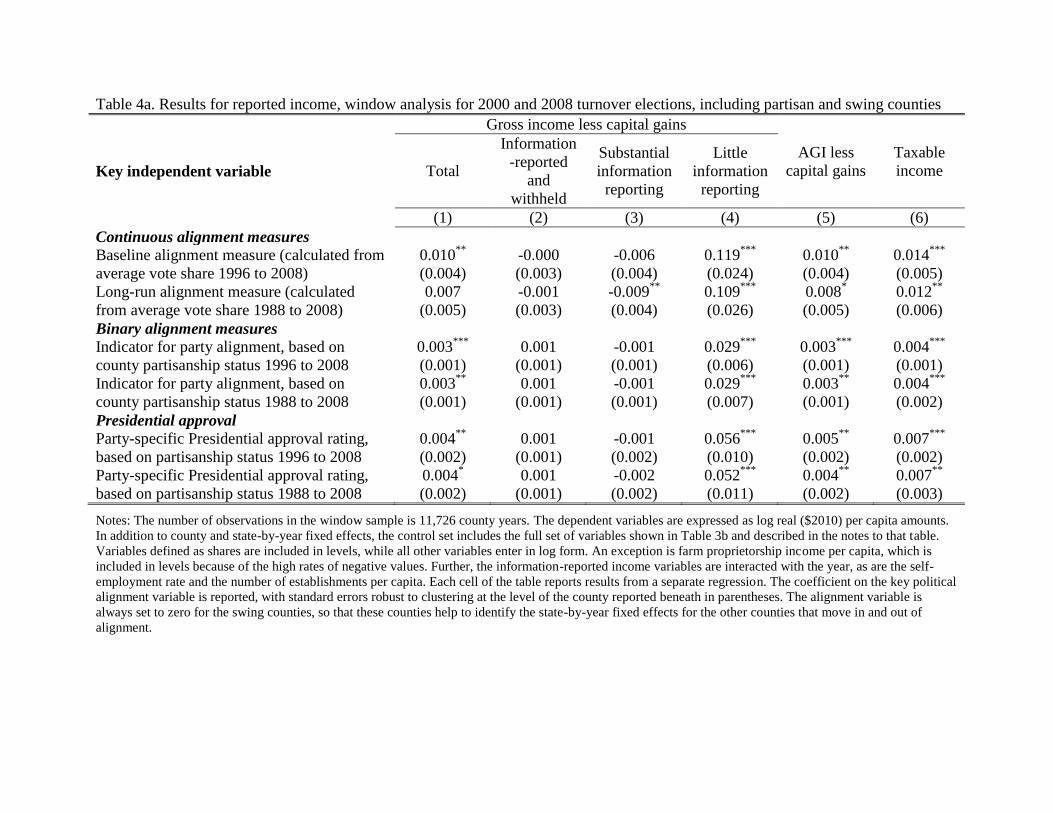
Table 4a. Results for reported income, window analysis for 2000 and 2008 turnover elections, including partisan and swing counties

Gross income less capital gains

AGI less

capital gains

Taxable

income Key independent variable Total

Information

-reported

and

withheld

Substantial

information

reporting

Little

information

reporting

(1) (2) (3) (4) (5) (6)

Continuous alignment measures

Baseline alignment measure (calculated from

average vote share 1996 to 2008)

0.010**

(0.004)

-0.000

(0.003)

-0.006

(0.004)

0.119***

(0.024)

0.010**

(0.004)

0.014***

(0.005)

Long-run alignment measure (calculated

from average vote share 1988 to 2008)

0.007

(0.005)

-0.001

(0.003)

-0.009**

(0.004)

0.109***

(0.026)

0.008*

(0.005)

0.012**

(0.006)

Binary alignment measures

Indicator for party alignment, based on

county partisanship status 1996 to 2008

0.003***

(0.001)

0.001

(0.001)

-0.001

(0.001)

0.029***

(0.006)

0.003***

(0.001)

0.004***

(0.001)

Indicator for party alignment, based on

county partisanship status 1988 to 2008

0.003**

(0.001)

0.001

(0.001)

-0.001

(0.001)

0.029***

(0.007)

0.003**

(0.001)

0.004***

(0.002)

Presidential approval

Party-specific Presidential approval rating,

based on partisanship status 1996 to 2008

0.004**

(0.002)

0.001

(0.001)

-0.001

(0.002)

0.056***

(0.010)

0.005**

(0.002)

0.007***

(0.002)

Party-specific Presidential approval rating,

based on partisanship status 1988 to 2008

0.004*

(0.002)

0.001

(0.001)

-0.002

(0.002)

0.052***

(0.011)

0.004**

(0.002)

0.007**

(0.003)

Notes: The number of observations in the window sample is 11,726 county years. The dependent variables are expressed as log real ($2010) per capita amounts.

In addition to county and state-by-year fixed effects, the control set includes the full set of variables shown in Table 3b and described in the notes to that table.

Variables defined as shares are included in levels, while all other variables enter in log form. An exception is farm proprietorship income per capita, which is

included in levels because of the high rates of negative values. Further, the information-reported income variables are interacted with the year, as are the self-

employment rate and the number of establishments per capita. Each cell of the table reports results from a separate regression. The coefficient on the key political

alignment variable is reported, with standard errors robust to clustering at the level of the county reported beneath in parentheses. The alignment variable is

always set to zero for the swing counties, so that these counties help to identify the state-by-year fixed effects for the other counties that move in and out of

alignment.

29

Table 4b. Results for reported income, window analysis for 2000 and 2008 turnover elections, including only partisan counties


AGI less

capital

gains

Taxable

income Key independent variable Total

Information

-reported

and

withheld

Substantial

information

reporting

Little

information

reporting

(1) (2) (3) (4) (5) (6)

Continuous alignment measures

Baseline alignment measure (calculated from


0.005

(0.005)

-0.000

(0.003)

-0.005

(0.005)

0.112***

(0.028)

0.006

(0.005)

0.008

(0.006)

Long-run alignment measure (calculated from


0.004

(0.006)

-0.002

(0.004)

-0.007

(0.005)

0.112***

(0.031)

0.005

(0.006)

0.008

(0.007)

Binary alignment measures

Indicator for party alignment, based on county

partisanship status 1996 to 2008

0.002*

(0.001)

0.001*

(0.001)

-0.000

(0.001)

0.026***

(0.007)

0.002*

(0.001)

0.003**

(0.001)

Indicator for party alignment, based on county

partisanship status 1988 to 2008

0.002

(0.001)

0.001

(0.001)

-0.001

(0.001)

0.029***

(0.008)

0.002

(0.001)

0.003**

(0.002)

Presidential approval

Party-specific Presidential approval rating, based

on partisanship status 1996 to 2008

0.003

(0.002)

0.002

(0.001)

-0.001

(0.002)

0.048***

(0.012)

0.004*

(0.002)

0.005**

(0.003)

Party-specific Presidential approval rating, based

on partisanship status 1988 to 2008

0.003

(0.003)

0.001

(0.002)

-0.002

(0.002)

0.053***

(0.014)

0.004

(0.003)

0.006*

(0.003)

Notes: The number of observations in the window sample that excludes swing counties based on the 1996 to 2008 partisan classification of counties is 7,400

county years. The number of county years is 6,247 when excluding swing counties based on the 1988 to 2012 partisan classification. For other details, see the

notes to Table 4a.

30

Table 5. Robustness of results for reported income, window analysis for 2000 and 2008 turnover elections, including only partisan

counties


AGI less

capital

gains

Taxable

income Alternative specification or sample Total

Information

-reported

and

withheld

Substantial

information

reporting

Little

information

reporting

(1) (2) (3) (4) (5) (6)

Baseline specification and sample 0.005

(0.005)

-0.000

(0.003)

-0.005

(0.005)

0.112***

(0.028)

0.006

(0.005)

0.008

(0.006)

Alternative control sets

Omitting interactions between income sources

and year

0.008

(0.005)

0.002

(0.004)

0.006

(0.005)

0.096***

(0.026)

0.010**

(0.005)

0.014**

(0.006)

Adding wage and salary shares by employer tax

type

0.005

(0.005)

0.000

(0.003)

-0.006

(0.005)

0.111***

(0.028)

0.007

(0.005)

0.009

(0.006)

Omitting demographic controls 0.010*

(0.005)

0.004

(0.004)

0.005

(0.005)

0.102***

(0.026)

0.012**

(0.005

0.017**

(0.007)

Alternative samples

Exclude counties containing capital cities 0.006

(0.005)

-0.001

(0.004)

-0.005

(0.005)

0.114***

(0.029)

0.007

(0.005)

0.009

(0.006)

Exclude counties with large commuter flows 0.008

(0.005)

-0.003

(0.003)

-0.007

(0.005)

0.125***

(0.046)

0.005

(0.006)

0.008

(0.007)

Exclude counties with any missing tax return

values

0.003

(0.006)

-0.004

(0.006)

0.007

(0.011)

0.101***

(0.034)

0.004

(0.006)

0.006

(0.008)

Notes: The first row reports results for the baseline specification shown in row 1 of Table 4b. The remaining rows report the coefficient and standard error

(robust to clustering at the county level) on the baseline alignment measure. Only 1.6 percent of county years are from counties containing capital cities, while

11.0 percent are classified as commuter counties. 20.2% of counties are missing an observation on some component of income at over the period 1996 to 2010

due to apparent data errors. For other details regarding the specification, see the notes to Table 4a.

31

Table 6. Results for filing and audit rates, window analysis for 2000 and 2008 turnover elections

Number of returns

Baseline alignment measure (calculated from average vote

shares across 1996 to 2008 elections) Filed

Attaching

Schedule C or E

Claiming the

EITC Audited

(1) (2) (3) (4)

Counting all returns

Including swing districts -0.000

(0.003)

0.011***

(0.003)

-0.033***

(0.003)

-0.089***

(0.023)

Including only partisan districts 0.007**

(0.003)

0.016***

(0.004)

-0.034***

(0.004)

-0.124***

(0.027)

Counting only returns from policy-constant filers

Including swing districts 0.006***

(0.002)

0.012***

(0.003)

-0.033***

(0.003)

-0.080***

(0.024)

Including only partisan districts 0.009***

(0.002)

0.018***

(0.004)

-0.033***

(0.004)

-0.115***

(0.028)

Notes: The number of observations in the window sample is 11,726 county years. The dependent variables are expressed as log real ($2010) per capita amounts.

In addition to county and state-by-year fixed effects, the control set includes the full set of variables shown in Table 3b and described in the notes to that table.

Variables defined as shares are included in levels, while all other variables enter in log form. An exception is farm proprietorship income per capita, which is

included in levels because of the high rates of negative values. Each cell of the table reports results from a separate regression. The coefficient on the key

political alignment variable is reported, with standard errors robust to clustering at the level of the county reported beneath in parentheses. The alignment variable

is always set to zero for the swing counties, so that these counties help to identify the state-by-year fixed effects for the other counties that move in and out of

alignment.

32

Table 7. Interactions with state tax system and politics, window analysis for 2000 and 2008 turnover elections, including only partisan

counties

Income with low reporting Number of returns

Key controls Schedule C

income

Schedule E

income

Attaching

Schedule

C

Attaching

Schedule E

Claiming

EITC Audited

(1) (2) (3) (4) (5) (6)

State income tax piggybacking

Baseline alignment 0.146***

(0.032)

0.196***

(0.065)

0.034***

(0.010)

0018***

(0.006)

-0.043***

(0.006)

-0.191***

(0.046)

Interaction with indicator for state tax system

tied to reports on the federal return

-0.107**

(0.047)

-0.093

(0.079)

-0.022**

(0.012)

-0.008

(0.008)

0.015**

(0.008)

0.125**

(0.053)

Dual alignment with President and governor

Party-aligned with both the President and the

governor, and are of the same party

0.038***

(0.013)

0.047**

(0.023)

-0.005

(0.005)

0.005

(0.003)

-0.021***

(0.003)

-0.073**

(0.015)

Party-aligned with both the President and the

governor, and are of different parties

0.014

(0.016)

0.023

(0.032)

0.000

(0.006)

0.014***

(0.004)

-0.004

(0.005)

-0.050*

(0.028)

Only party-aligned with the President 0.019**

(0.009)

0.025

(0.024)

0.004

(0.003)

0.007***

(0.002)

-0.010***

(0.003)

-0.042**

(0.022)

Only party-aligned with the governor, who is of

the same party of the President

-0.004

(0.013)

0.043

(0.027)

-0.000

(0.005)

0.010**

(0.004)

-0.002

(0.004)

-0.049***

(0.019)

Only party-aligned with the governor, who is of

a different party from the President

0.022

(0.014)

-0.002

(0.029)

-0.011**

(0.005)

0.004

(0.004)

-0.014***

(0.004)

-0.038

(0.025)

Notes: The Presidential alignment variables are calculated based on county partisan status over the 1996 to 2008 Presidential elections. Party alignment with the

governor is based on the governor’s party and the party with the majority share of the two-party vote from the most recent gubernatorial election. For other

details regarding the specification, see the notes to Table 4a.

33

Appendix Figure A1. Average filing rates and reported income shares, 1990 to 2012

Notes: The figure shows the counts of all returns and the counts of policy-constant tax filers by year for the 3,006

analysis counties.

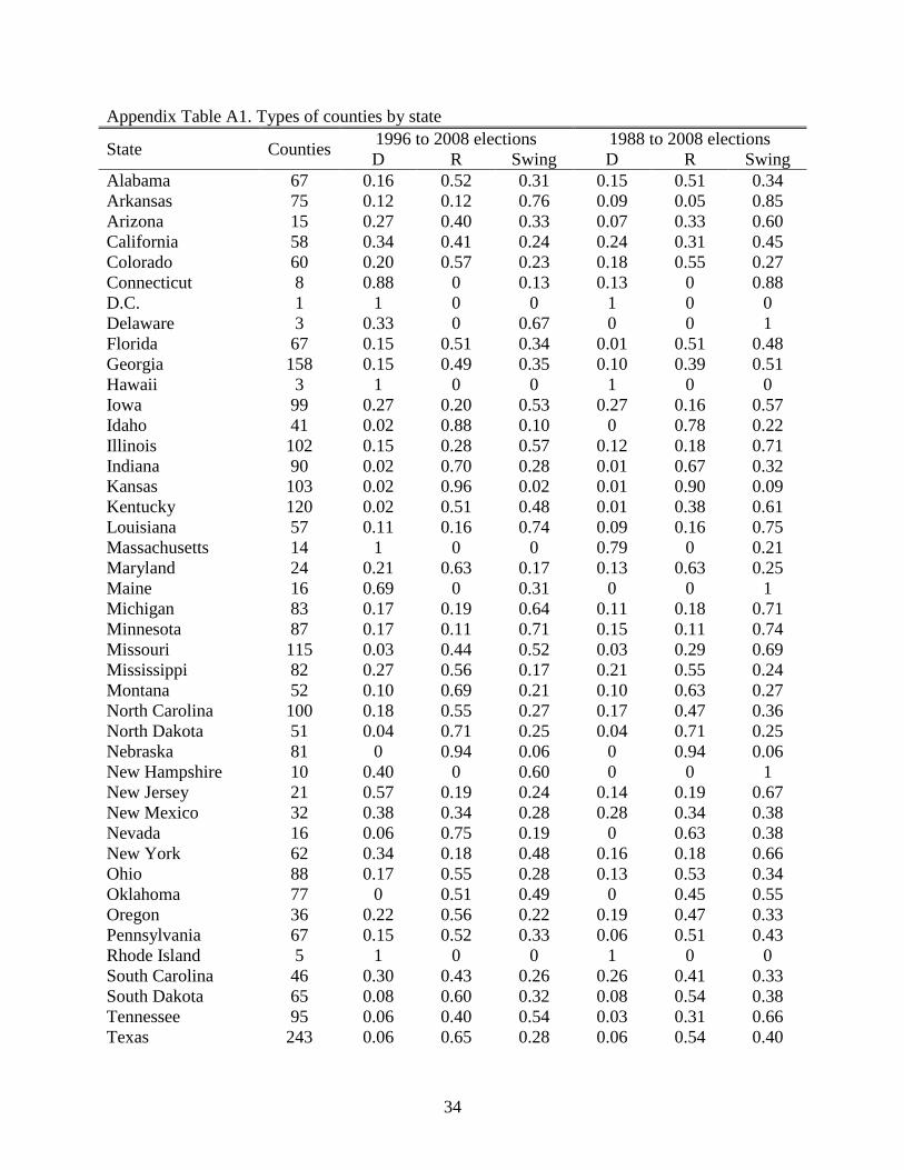
34

Appendix Table A1. Types of counties by state

State Counties 1996 to 2008 elections 1988 to 2008 elections

D R Swing D R Swing

Alabama 67 0.16 0.52 0.31 0.15 0.51 0.34

Arkansas 75 0.12 0.12 0.76 0.09 0.05 0.85

Arizona 15 0.27 0.40 0.33 0.07 0.33 0.60

California 58 0.34 0.41 0.24 0.24 0.31 0.45

Colorado 60 0.20 0.57 0.23 0.18 0.55 0.27

Connecticut 8 0.88 0 0.13 0.13 0 0.88

D.C. 1 1 0 0 1 0 0

Delaware 3 0.33 0 0.67 0 0 1

Florida 67 0.15 0.51 0.34 0.01 0.51 0.48

Georgia 158 0.15 0.49 0.35 0.10 0.39 0.51

Hawaii 3 1 0 0 1 0 0

Iowa 99 0.27 0.20 0.53 0.27 0.16 0.57

Idaho 41 0.02 0.88 0.10 0 0.78 0.22

Illinois 102 0.15 0.28 0.57 0.12 0.18 0.71

Indiana 90 0.02 0.70 0.28 0.01 0.67 0.32

Kansas 103 0.02 0.96 0.02 0.01 0.90 0.09

Kentucky 120 0.02 0.51 0.48 0.01 0.38 0.61

Louisiana 57 0.11 0.16 0.74 0.09 0.16 0.75

Massachusetts 14 1 0 0 0.79 0 0.21

Maryland 24 0.21 0.63 0.17 0.13 0.63 0.25

Maine 16 0.69 0 0.31 0 0 1

Michigan 83 0.17 0.19 0.64 0.11 0.18 0.71

Minnesota 87 0.17 0.11 0.71 0.15 0.11 0.74

Missouri 115 0.03 0.44 0.52 0.03 0.29 0.69

Mississippi 82 0.27 0.56 0.17 0.21 0.55 0.24

Montana 52 0.10 0.69 0.21 0.10 0.63 0.27

North Carolina 100 0.18 0.55 0.27 0.17 0.47 0.36

North Dakota 51 0.04 0.71 0.25 0.04 0.71 0.25

Nebraska 81 0 0.94 0.06 0 0.94 0.06

New Hampshire 10 0.40 0 0.60 0 0 1

New Jersey 21 0.57 0.19 0.24 0.14 0.19 0.67

New Mexico 32 0.38 0.34 0.28 0.28 0.34 0.38

Nevada 16 0.06 0.75 0.19 0 0.63 0.38

New York 62 0.34 0.18 0.48 0.16 0.18 0.66

Ohio 88 0.17 0.55 0.28 0.13 0.53 0.34

Oklahoma 77 0 0.51 0.49 0 0.45 0.55

Oregon 36 0.22 0.56 0.22 0.19 0.47 0.33

Pennsylvania 67 0.15 0.52 0.33 0.06 0.51 0.43

Rhode Island 5 1 0 0 1 0 0

South Carolina 46 0.30 0.43 0.26 0.26 0.41 0.33

South Dakota 65 0.08 0.60 0.32 0.08 0.54 0.38

Tennessee 95 0.06 0.40 0.54 0.03 0.31 0.66

Texas 243 0.06 0.65 0.28 0.06 0.54 0.40

35

Utah 28 0 0.82 0.18 0 0.82 0.18

Virginia 80 0.16 0.59 0.25 0.13 0.59 0.29

Vermont 14 0.71 0 0.29 0.36 0 0.64

Washington 39 0.28 0.36 0.36 0.23 0.33 0.44

Wisconsin 72 0.35 0.13 0.53 0.29 0.11 0.60

West Virginia 55 0.09 0.22 0.69 0.09 0.20 0.71

Notes: The second column shows the number of counties included in the analysis sample from each state. The next

three columns show the share of counties that are classified as Democratic (D), Republican (R), and swing based on

two-party vote shares across the 1996 through 2008 elections. The last three columns show the same shares based on

vote shares across the 1988 through 2008 elections.

POLITICAL ALIGNMENT AND TAX EVASION

Documents

Transcript of POLITICAL ALIGNMENT AND TAX EVASION