Polarimetry from the Ground Up

Polarimetry from the Ground Up

Christoph Keller & Frans Snik

Utrecht University

Outline

1 Introduction2 Statistical Errors in Polarimetry3 Polarization Calibration4 Polarimetry Error Budget

Introduction

Polarimetry Systems Engineering

goal: model and understand performance of polarimeter designs

Give answers to the following questions

how to define polarimeter performance?how to compare different polarimeter designs?how to maximize performance?how to do all of this for different polarimeter designs?

Statistical Errorsphoton statisticsdetector read-out noise

Some Systematic Errors (instrumental errors)Atmospheric seeing and guiding errorsInstrumental polarization due to

Telescope and instrument opticsPolarized scattered light in telescope and instrumentSpectrograph slit polarizationAngle, wavelength, temperature dependence of retardersCrystal aberrationsPolarized fringes

Ghost imagesVariable sky backgroundUnpolarized scattered light in atmosphere and opticsLimited calibration accuracy...

Assumptions to Derive Expected Noiselinear relation between Stokes parameters and measured signalsnoise in the various measurements is independentnoise is independent of the signal, if

noise is dominated by signal-independent detector noise (e.g.read-out noise)incoming vector is only slightly polarized

noise statistic has a Gaussian distribution

Signal Matrixm intensity measurements combined into signal vector Srelated to incoming Stokes vector, I by 4×m signal matrix X(also modulation matrix

S = XI

X (v) is function of free design parameters veach row of X corresponds to first row of Mueller matrixdescribing the particular intensity measurement

Measuring Stokes Parameters

estimate of incoming Stokes vector I

I ′ = YS = X−1S

Y is called synthesis or demodulation matrixerror propagation provides standard deviations of Stokesparameters

σI′i=

√√√√ 4∑j=1

Y2ijσ

2Sj

σSj is standard deviation of intensity in measurement j

Polarimetric Efficiencydesired properties:

comparable between different polarimeter designs andmeasurement approacheslarger values should correspond to better designsindependent of the intensity throughputconsist of 4 quantities (“Stokes efficiency”)theoretical maximum efficiency shall be 1

Noise propagation

if all measurements have same noise

σI′i= σS

√√√√ m∑j=1

Y2ij .

polarimetric efficiency independent of number of measurements(del Toro Iniesta and Collados 2000)

εi =

mm∑

j=1

Y 2ij

− 12

in most cases Xi1 = 1, i.e. all measurements have the samethroughput, normalize the measurements

ε1 ≤ 1 ;4∑

i=2

ε2i ≤ 1

Analytic Optimizationequations for properties of optimum polarimeter by e.g. del ToroIniesta and Collados (2000) and Tyo (2002)maximum performance: best performance of all polarimeterdesignsoptimum performance: best performance that can be achievedwith given polarimeter designchoose X(v), Y to minimize difference between I ′ and I , given σSj

3 steps:derive equation for optimum Y given X(v)using the equation for optimum Y, derive optimum Xchoose optimum X and Y to obtain polarimeter with maximumperformance

Optimum synthesis matrixif m = 4, four measurements represent linearly independentcombinations of Stokes parameters, then Y is uniquelydetermined by

Y = X−1 .

if m > 4, matrix inverse is not uniquely definedgeneralized inverse (e.g. Albert 1972) of X

Y =(

XT X)−1

XT

among all possible Y that fulfill YX = 1, the generalized inverseminimizes the sum of squares of its rowsoptimum polarimetric efficiencies given by

εopt,i =

√1

m(XT X

)−1ii

Signal matrix for maximum performance

follow scheme of del Toro Iniesta and Collados (2000)minimize sum of squares of rows of Y with XY = 1squares of maximum possible polarimetric efficiencies

ε2max,i =1m

m∑j=1

X2ji =

1m

(XT X

)ii.

signal matrix X of maximum performance polarimeter

XT X = m

ε2max,1 0 0 0

0 ε2max,2 0 00 0 ε2max,3 00 0 0 ε2max,4

optimum efficiency for measuring polarized Stokes componentswith equal efficiencies given by 1√

n , where n is the number ofpolarized Stokes parameters

Generation of maximum performance signal matrices

elements of first column of signal matrix X are 1, XT X = diagonal

each row of the signal matrix: point on the Poincaré spheremaximize average distance squared between points on Poincarésphere for signal matrix with maximum polarimetric efficiency

distance ∆ =√

2 + 2m−1

m = 2: ∆ = 2 (opposite sides of Poincaré sphere)m = 3: ∆ =

√3 (side length of triangle whose plane includes the

origin of Poincaré sphere)

m = 4: ∆ =√

83 (side length of tetrahedron inside Poincaré

sphere)

average distance is indepenent of the number of polarizedStokes componentsfour measurements for linear polarization only, spaced 90 deg

apart, square root of average distance squared is also ∆ =√

83

Caveatmaximizing average square distance of points is a necessary butnot a sufficient criteria for generating a signal matrixcorresponding to a polarimeter with maximum performancesignal matrix

X =

1 x x x1 x x x1 −x −x −x1 −x −x −x

(1)

also has an average distance of√

83 , but XT X is obviously not

diagonal

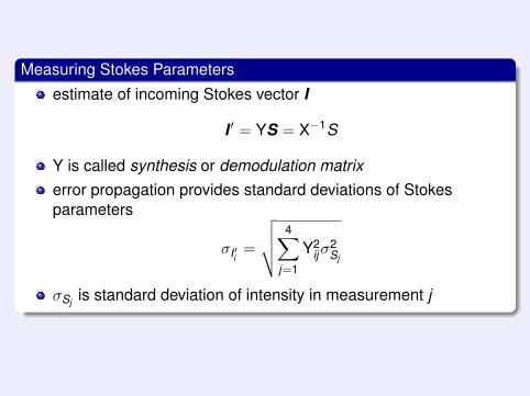
Optimum Calibration

Basic Approachoptimum way to calibrate polarimeter, i.e. measure X

S = XI

at least 16 measurements of signal vector elements S i , i = 1..mat least 4 different input Stokes vectors Ic

i , i = 1..mgroup calibration input Stokes vectors, signal vectors into 4 by 4matrices (Azzam et al. 1988)

S = XIc

S = (S1S2...Sm)

Ic = (Ic1Ic

2...Icm)

signal matrix X = SJ with IcJ = 1

Equivalence with Maximum Polarimetric Performance

choose calibration Stokes vectors Ici to minimize error in X, given

errors in measurements Sequivalent to optimizing polarimetric efficiencycalibration input Stokes vectors Ic

i equivalent to rows of thesignal matrix X of maximum performance polarimetervector-polarimeter: corners of a tetrahedron as suggested byAzzam et al. (1988)only true if there are no systematic errorsbetter to use many more measurements and also modelnon-ideal calibration optics

Polarization Error Budget

Optical Error Budgetsclassical tool in systems engineeringsets requirements of parts such that system as a whole meetsrequirementsmuch faster than end-to-end simulationsprovides more insight than end-to-end simulations

Example: 80% Encircled Energy in arcseclevel 1 item level 2 item level 3 item level 1 level 2 level 3atmosphere 0.50telescope 0.25

primary mirror 0.17mirror polishing 0.10mirror support 0.10thermal distortion 0.10

secondary mirror 0.17mirror polishing 0.10mirror support 0.10thermal distortion 0.10

instrument 0.25

total 0.61

Example: 80% Encircled Energy in arcseclevel 1 item level 2 item level 3 item level 1 level 2 level 3atmosphere 0.50telescope 0.25

primary mirror 0.17mirror polishing 0.10mirror support 0.10thermal distortion 0.10

secondary mirror 0.17mirror polishing 0.10mirror support 0.10thermal distortion 0.10

instrument 0.25total 0.61

Structure of an Error Budget

parts can consist of smaller parts⇒ several levelsoverall error estimated from combination of many error sourcesmistakes in estimates tend to average outerrors can be allocated in different waysallocation minimizes complexity and costmain contributors to system error easily identified

Adding Wavefront Errors

wavefront errors of individual elements are not correlatedsquare of final error given by squares of errors of individualelements (root sum of squares (RSS))

Polarization Error Budget Issues

polarimeter: final errors often non-linear combinations of errorsof very different nature (e.g. instrumental polarization andnon-linearity of detector)some (but not all) errors can be drastically reduced by calibrationpolarization error budgets not (yet) used to design polarimeters

Schematic Polarization Error Budgetlevel 1 item level 2 item level 3 itemsource variationatmospheretelescopepolarimeter

polarizerdetector system

undetected bias variationnonlinearity

calibrationpolarizerretarder

positioning repeatabilitytemperature change of retarder

data reductiontotal

VLT SPHERE Polarimetric Error Budget

Errors in Mueller Matricesneed standard deviation of Mueller matrix elements as a functionof errors in parametersMueller matrix with two parameters α and β

M (α, β)

variance over uniform distribution of errors in α over ±∆

Mα (∆) =

∫ +∆

−∆(M (α + ε, β)−M (α, β))2 δε

linearized standard deviation in ∆

mα = lim∆⇒0

∂

∂∆Mα (∆)

errors in Mueller matrix elements can be written as

M (α, β)±mα · δα±mβ · δβ

Example: Linear Retarder, fast axis angle θ, retardance φMueller matrix:0BB@

1 0 0 00 cos2(2θ) + cos(φ) sin2(2θ) cos(2θ) sin(2θ)− cos(2θ) cos(φ) sin(2θ) sin(2θ) sin(φ)

0 cos(2θ) sin(2θ)− cos(2θ) cos(φ) sin(2θ) cos(φ) cos2(2θ) + sin2(2θ) − cos(2θ) sin(φ)0 − sin(2θ) sin(φ) cos(2θ) sin(φ) cos(φ)

1CCA

uniform error distribution of retardance in interval ±∆ leads tovariance of Mueller matrix elements

0BBBB@0 0 0 00 1

2 (4(∆− sin(∆)) + cos(2φ)(2∆− 4 sin(∆) + sin(2∆))) sin4(2θ) 18 (4(∆− sin(∆)) + cos(2φ)(2∆− 4 sin(∆) + sin(2∆))) sin2(4θ) sin2(2θ)

“2(∆− 2 sin(∆)) sin2(φ) + ∆− cos(∆) cos(2φ) sin(∆)

”0 1

8 (4(∆− sin(∆)) + cos(2φ)(2∆− 4 sin(∆) + sin(2∆))) sin2(4θ) 12 cos4(2θ)(4(∆− sin(∆)) + cos(2φ)(2∆− 4 sin(∆) + sin(2∆))) cos2(2θ)

“2(∆− 2 sin(∆)) sin2(φ) + ∆− cos(∆) cos(2φ) sin(∆)

”0 sin2(2θ)

“2(∆− 2 sin(∆)) sin2(φ) + ∆− cos(∆) cos(2φ) sin(∆)

”cos2(2θ)

“2(∆− 2 sin(∆)) sin2(φ) + ∆− cos(∆) cos(2φ) sin(∆)

”2(∆− 2 sin(∆)) cos2(φ) + ∆ + cos(∆) cos(2φ) sin(∆)

1CCCCA

derivative with respect to ∆0BBBBBBBB@

0 0 0 0

0

qsin4(2θ) sin2(φ)

√3

qsin2(4θ) sin2(φ)

2√

3

qcos2(φ) sin2(2θ)

√3

0

qsin2(4θ) sin2(φ)

2√

3

qcos4(2θ) sin2(φ)

√3

qcos2(2θ) cos2(φ)

√3

0

qcos2(φ) sin2(2θ)

√3

qcos2(2θ) cos2(φ)

√3

qsin2(φ)√

3

1CCCCCCCCA

Stenflo 1994

Adding Mueller matrix errors

for weakly polarizing and retarding elements, RSS can beappliedfor strongly polarizing and retarding elements, we obtain

n∏i=1

(Mi + mi) ≈n∏

i=1

Mi +n∑

i=1

i−1∏j=1

Mj

mi

n∏j=i+1

Mj

Mueller matrix errors need to be transformed using ideal Muellermatrices of elements before and after current element

Outlookfirst attempts at polarimetry systems engineeringadd calibration and data reduction influencesdetermine Mueller matrix errors for various parameterstest against end-to-end simulations and real instruments