The Annals of Applied Statistics2011, Vol. 5, No. 2A, 684–704DOI: 10.1214/10-AOAS401© Institute of Mathematical Statistics, 2011

POINT PROCESS MODELING OF WILDFIRE HAZARD INLOS ANGELES COUNTY, CALIFORNIA

BY HAIYONG XU AND FREDERIC PAIK SCHOENBERG

University of California, Los Angeles

The Burning Index (BI) produced daily by the United States govern-ment’s National Fire Danger Rating System is commonly used in forecastingthe hazard of wildfire activity in the United States. However, recent evalua-tions have shown the BI to be less effective at predicting wildfires in Los An-geles County, compared to simple point process models incorporating similarmeteorological information. Here, we explore the forecasting power of a suiteof more complex point process models that use seasonal wildfire trends, dailyand lagged weather variables, and historical spatial burn patterns as covari-ates, and that interpolate the records from different weather stations. Resultsare compared with models using only the BI. The performance of each modelis compared by Akaike Information Criterion (AIC), as well as by the powerin predicting wildfires in the historical data set and residual analysis. We findthat multiplicative models that directly use weather variables offer substantialimprovement in fit compared to models using only the BI, and, in particular,models where a distinct spatial bandwidth parameter is estimated for eachweather station appear to offer substantially improved fit.

1. Introduction. This paper explores the use of space–time point processmodels for the short-term forecasting of wildfire hazard in Los Angeles County,California. The region is especially well suited to such an analysis, since the LosAngeles County Fire Department and Department of Public Works have collectedand compiled detailed records on the locations burned by large wildfires datingback over a century. The landscape in Los Angeles County is uniquely vulnera-ble to high intensity crown-fires, largely because the predominant local vegetationconsists of dense, highly flammable contiguous chaparral shrub [Keeley (2000)].In addition, the dry summers and early autumns in Los Angeles County are typ-ically followed by high winds known locally as Santa Ana winds [Keeley andFotheringham (2003)]. These offshore winds reach speeds exceeding 100 kph at arelative humidity below 10%, and are annual events lasting several days to severalweeks, creating the most severe fire weather in the United States [Schroeder et al.(1964)].

In order to forecast wildfire hazard, the United States National Fire Danger Rat-ing System (NFDRS), created in 1972, produces several daily indices that are de-signed to aid in planning fire control activities on a fire protection unit [Deeming et

Received April 2009; revised August 2010.Key words and phrases. Burning index, conditional intensity, point process, residual analysis.

684

POINT PROCESS MODELS OF WILDFIRES 685

al. (1977); Bradshaw et al. (1983); Burgan (1988)]. These include the OccurrenceIndex, the Burning Index (BI), and the Fire Load Index. These indices are derivedfrom three fire behavior components—a Spread Component, an Energy ReleaseComponent, and an Ignition Component, that are in turn computed based on fuelage, environmental parameters (slope, vegetation type, etc.), and meteorologicalvariables such as wind, temperature, and relative humidity. Local wildfire man-agement agencies may combine these components in different ways or calibratethe inherent parameters to adapt the system to the local environment for wildfirehazard assessment.

Fire managers use this information in making decisions about the appropriate-ness of prescribed burning or alerts for increased preparedness, both in terms offire suppression staffing and fire prevention activities. Since fireline intensity is animportant factor in predicting fire containment and the likelihood of fire escape,the Burning Index is the rating of most interest to many fire managers [Schoen-berg et al. (2010)]. This is especially the case for natural crown-fire ecosystemssuch as southern California shrublands, where BI is commonly employed to as-sess fire danger [Mees and Chase (1991)]. Indeed, in Los Angeles County, as wellas at least 90% of counties nationwide, the BI is the index primarily used by firedepartment officials as a measure of overall wildfire hazard, and its use has beenjustified largely based on its observed empirical correlation with wildfire incidenceand burn area in different regions [Haines et al. (1983); Haines, Main and Simard(1986); Mees and Chase (1991); Andrews, Loftsgaarden and Bradshaw (2003)].However, several recent investigations have shown that the BI is far from an idealpredictor of wildfire incidence in Los Angeles County; Schoenberg et al. (2010)showed that a simple point process model, which used only the same weathervariables as those incorporated by the BI, vastly outperformed the BI in terms ofpredictive efficacy in Los Angeles County, using historical data from 1977–2000.In fact, the simple model in Schoenberg et al. (2010) not only offered improvementin terms of likelihood scores such as the Akaike Information Criterion (AIC), butthe study suggested that substantial improvement in short-term forecasting couldbe achieved by the simple model using the weather variables directly, compared toa point process model that interpolates BI measurements.

Here, we adopt the same basic modeling framework of Schoenberg et al. (2010),but extend the models in two important ways. First, we consider not only dailyweather variables but also additional covariates with management relevance, suchas historical spatial burn patterns and wind direction, using the directional kernelregression method described in Schoenberg and Xu (2008). Second, unlike thesimple models of Mees and Chase (1991) and Schoenberg et al. (2010) that av-erage daily weather variables over weather stations within Los Angeles County,here we explore models that interpolate the records from different weather sta-tions, weighting these data based on their spatial distance from the location wherewildfire hazard is to be estimated. Thus, the models considered here should havemore direct relevance for forecasting wildfire hazard in precise spatial locations

686 H. XU AND F. P. SCHOENBERG

within Los Angeles County, compared to previous work that essentially averagedweather variables and hazard estimates over Los Angeles County as a whole. Aswith Schoenberg et al. (2010), our results are compared with models using the BImeasurements recorded at each of the weather stations, so that the effectiveness ofthe BI in summarizing the wildfire hazard as a function of the weather variablesmay be assessed.

While alternative models may be more useful for forecasting long-term wild-fire hazard, that is, estimating the number of wildfires occurring within a month,season, or year, the focus here is on forecasting short-term wildfire hazard, thatis, the probability of a wildfire occurring within a specific day. To compare theoverall performance of the models considered, we employ diagnostics includinglikelihood-based numerical summaries such as the Akaike Information Criterion(AIC), as well as power diagrams summarizing the predictive efficacy of eachmodel for short-term forecasting. Residual analysis is also used to highlight spe-cific areas and times where the performance of a model is poor and to suggest areasfor improvement.

The paper proceeds as follows. Section 2 describes the wildfire and weatherdata that are used in the analysis. The models used, as well as methods for theirestimation, are outlined in Section 3, and methods for goodness-of-fit assessmentare discussed in Section 4. Section 5 presents the main results, and a discussion isgiven in Section 6.

2. Data.

2.1. Wildfire data. Los Angeles County is an ideal test site for models forwildfire hazard, with detailed wildfire data having been collected and compiled byvarious agencies, including the Los Angeles County Fire Department (LACFD)and the Los Angeles County Department of Public Works, the Santa MonicaMountains Recreation Area, and the California Department of Forestry and FireProtection. Regional records of the occurrence of wildfires date back to 1878, andinclude information on each fire, including its origin date, the polygonal outlineof the resulting area burned, and the centroidal location of this polygon. LACFDofficials have noted that the records prior to 1950 are believed to be completefor fires greater than 0.405 km2 (100 acres), and data since 1950 are believedto be complete for fires burning greater than 0.0405 km2, or 10 acres [Schoen-berg et al. (2003)]. As in Schoenberg et al. (2010), our analysis in this paper isfocused primarily on models for the occurrences of the 592 wildfires burning atleast 0.0405 km2 recorded between January 1976 and December 2000. The dailyburn area is highly right-skewed and closely follows the tapered Pareto distrib-ution [Schoenberg, Peng and Woods (2003)]. For further details, images of thespatial locations of these wildfires, and information about missing data, see Peng,Schoenberg and Woods (2005).

POINT PROCESS MODELS OF WILDFIRES 687

2.2. Meteorological data. Since 1976, daily meteorological observations fromthe Remote Automatic Weather Stations (RAWS) were archived across the UnitedStates. The analysis here is based on sixteen RAWS located within Los Ange-les County, California. The RAWS record daily measures of many meteorologicalvariables, including air temperature, relative humidity, precipitation, wind speed,and wind direction [Warren and Vance (1981)]. Summaries of these records arecollected daily at 1300 hr and transmitted by satellite to a central archiving sta-tion. These daily RAWS data are used as inputs by the NFDRS in order to con-struct fire behavior components that are in turn combined to construct the BI. Itshould be noted that data were missing on certain days for several of the 16 RAWS,though the biases resulting from such missing data are likely to be small; see Peng,Schoenberg and Woods (2005) for details.

3. Methodology. We follow previous research including Schoenberg et al.(2010) in modeling the catalog of wildfire centroids in Los Angeles County asa realization of a point process that may depend on daily meteorological variables.We begin with a basic reference model using merely a spatial background rate andseasonal component, and a model using the Burning Index in addition to the spa-tial and seasonal background rates. We then introduce competing models that usedaily meteorological variables recorded at the RAWS, and extend the research ofSchoenberg et al. (2010) by including additional covariates, such as wind directionand fuel age. Further, instead of averaging daily weather variables or the BurningIndex over all weather stations within Los Angeles County, here we explore meth-ods of obtaining an estimated spatial intensity at any location x on any particularday by interpolating the meteorological variables from different weather stations,weighting each record based on its distance from the location x in question.

3.1. A review of point process modeling. A spatial-temporal point process N ismathematically defined as a random measure on a spatial-temporal region S, takingvalues in the nonnegative integers Z+ or infinity [Daley and Vere-Jones (2003)].In this framework the measure N(A) represents the number of points falling in thesubset A of S. Since any analytical spatial-temporal point process is characterizeduniquely by its associated conditional rate (or intensity) !(s), assuming it exists,modeling of such point processes is typically performed by specifying a parametricmodel for this rate. For the case where the spatial region is planar, for any point tin time and location (x, y) in the plane, the conditional rate is defined as a limitingfrequency at which events are expected to occur within time range (t, t + "t)and rectangle (x, x + "x) ! (y, y + "y), conditional on the prior history, Ht , ofthe point process up to time t . For references on space–time point processes andconditional rates, see, for example, Daley and Vere-Jones (1988) or Schoenberg,Brillinger and Guttorp (2002).

Given a parametric function for !(t, x, y), estimates of the parameters # may beobtained by maximizing the log-likelihood function [see Schoenberg, Brillinger

688 H. XU AND F. P. SCHOENBERG

and Guttorp (2002), page 1576, or Daley and Vere-Jones (2003), page 232, equa-tion 7.24]:

L(#) =! T1

T0

!

x

!

ylog[!(t, x, y; #)]dN(t, x, y) "

! T1

T0

!

x

!

y!(t, x, y; , #) dy dx dt

=n"

i=1

log!(ti, xi, yi; #) "! T1

T0

!

x

!

y!(t, x, y; #) dy dx dt.

In the case of a Poisson process, the intuition behind this formula is that#ni=1 !(ti, xi, yi; #) reflects the likelihood associated with the observed events,

and exp{$ T1T0

$x

$y !(t, x, y; #) dy dx dt} represents the probability of no events in

any other portions of the spatial-temporal region, the full likelihood is the productof these two terms, and the logarithm of this product yields L(#) above. Underrather general conditions, the maximum likelihood estimates (MLEs) are consis-tent, asymptotically normal, and efficient [Ogata (1978)], and estimates of theirvariance can be derived from the negative of the diagonal elements of the inverseHessian of the likelihood function [Ogata (1978), Rathbun and Cressie (1994)]. Inmost cases, explicit solutions for MLEs are not available and iterative numericaloptimization methods are used instead.

3.2. A simple reference model. In this analysis we explore several spatial-temporal point process models for predicting wildfire occurrence rates. As an ini-tial baseline model, one may consider an inhomogeneous Poisson process, wherethe conditional intensity at time t and at location (x, y) depends only on the seasonassociated with time t , as well as the background rate m(x,y) of wildfires for thelocation in question. That is, one may consider a baseline model such as

!1(t, x, y) = $m(x,y) + %S(t),(1)

where $ and % are parameters to be estimated in modeling fitting.Parametric or nonparametric methods can be used to estimate the seasonal pat-

tern S(t) and spatial background m(x,y). While nonparametric methods can beespecially flexible for estimating complex patterns such as spatial burn averages,a possible drawback to such methods is their potential for overfitting, particularlywhen the same data are used for fitting and evaluation of the fit of the model. Asin Schoenberg et al. (2010), we propose estimating the spatial background m(x,y)for fires between 1976–2000 by kernel smoothing the centroidal locations of wild-fires recorded during the previous 25 years, that is, from January 1950 to December1975. That is,

m(x,y) = 1n0&m

n0"

j=1

K

%#(x, y) " (xj , yj )#&m

&,

where K is a kernel function, &m is a bandwidth to be estimated in modeling fit-ting, (xj , yj ) indicates the spatial coordinates of the j th wildfire between 1950

POINT PROCESS MODELS OF WILDFIRES 689

and 1975, n0 is the number of observed 1951–1975 wildfire occurrences, and#(x, y) " (xj , yj )# is the Euclidian distance between (x, y) and (xj , yj ). Stan-dard kernel functions can be used, and attention is usually limited to functions thatare unimodal, symmetric about zero, and that integrate to 1, such as the Gaussiandensity of the Epanechnikov kernel [Härdle (1994)]. It is well known that the re-sults are far more sensitive to the choice of bandwidth than the choice of kernelfunction, and much research has focused on automated methods for choosing band-width parameters, including cross-validation, penalty functions, and plug-in meth-ods [Silverman (1986); Härdle (1994)]. Here, since the data (xj , yj ) used in theestimation of m(x,y) is distinct from that used in the rest of the model fitting andin the evaluation, the problem of overfitting is far less severe, and the bandwidthparameter may simply be fitted by maximum likelihood.

Figure 1 shows an estimate of the spatial background rate m(x,y), with band-width estimated by maximum likelihood. One sees the general pattern of fire ac-tivity in Los Angeles County during 1951–1975, with most fires occurring in theAngeles National Forest, as well as parts of the Los Padres National Forest andthe Santa Monica Mountains, while many other wildfires were located in or nearBuckweed, Santa Clarita, and Glendale, California.

Helmers, Magku and Zitikis (2003) propose a kernel-based estimate for the con-sistent estimation of a seasonal time series. Here, in order to safeguard againstoverfitting, we propose estimating the seasonal pattern S(t) describing the over-all seasonal variation of wildfire activity in a fashion similar to that used for thespatial background rate, that is, by kernel smoothing the times of wildfires duringprevious years:

S(t) = 1n0&t

n0"

j=1

K

%T $(t) " T $(tj )

&t

&.

In the above equation, T $(t) represents the date within the year associated withtime t , that is, T $(t) is the number of days since the beginning of the year for timet , tj is the time of the j th wildfire occurrence in the data set (1950–1975), and &t

is a bandwidth parameter to be estimated. A wrapped kernel function K shouldbe used so that, for instance, January 1 and December 31 are treated as one dayapart. The bandwidth may be estimated by maximum likelihood, fitting the kernelsmoothing of the 1950–1975 data to the 1976–2000 data set. This procedure maybe preferable for relatively small data sets such as the one considered here in orderto prevent overfitting.

Figure 2 displays the smoothed function S(t) applied to wildfire incidence inLos Angeles County from January 1950 to December 1975, with bandwidth esti-mated by MLE by fitting the resulting function to wildfire data from 1976–2000. Itis evident that the mean number of wildfires is highest between July and Octoberand rapidly decreases during November and December, reaching its minimum inJanuary and February. Schoenberg et al. (2010) pointed out that the Burning Index

690 H. XU AND F. P. SCHOENBERG

FIG. 1. Spatial background rate m(x,y), with centroid locations of wildfires occurring during1878–1976. (The spatial bandwidth &m is 0.6 miles).

typically assumes moderate values in December, January, and February, thoughfew wildfires occur during these months.

3.3. A point process model using Burning Index. To evaluate the potential ofthe Burning Index (BI) in predicting wildfire incidence, one may consider a modelsuch as

!2(t, x, y) = $m(x,y) + %S(t) + µBIB(t, x, y)(2)

for some function B(t, x, y) which interpolates the BI records at time t and lo-cation (x, y), since BI records are only available at fixed RAWS sites. Differentmethods of interpolation are possible. One possibility is to average the BI recordson day t , weighing each by the distance between the RAWS and the location (x, y)

POINT PROCESS MODELS OF WILDFIRES 691

FIG. 2. Estimate of the seasonal pattern S(t) for model (1), using kernel regression with a wrappedGaussian kernel and bandwidth &̂t = 9.86 days, estimated by MLE.

in question. That is,

B(t, x, y) = 1CBI

"

s%St

'K

%#(x, y) " (xs, ys)#&BI

&BI(t, s)

(,

where BI(t, s) is the BI value recorded at time t from the sth station, (xs, ys) arethe coordinates of the sth station, St represents the collection of stations for whichBI records are available on day t , and CBI is a normalizing constant given by

CBI ="

s%St

'K

%#(x, y) " (xs, ys)#&BI

&(.

3.4. Models using spatial interpolation of meteorological variables, includingwind speed and wind direction. As an alternative to the model (2) incorporatingBI measurements, one may instead consider examining the direct impact on wild-fire hazard estimates of meteorological variables used in the computation of theBI, by replacing the function B(t, x, y) in (2) by functions of the meteorologicalvariables themselves. That is, one may consider models such as

!3(t, x, y) = $m(x,y) + %S(t) + F1(t, x, y),(3)

where F1(t, x, y) takes into account the contribution of temperature (T ), relativehumidity (H ), wind speed (W ), and precipitation (P ) at time t from each RAWSwhere the data are available.

Since nonlinearities have been detected in the dependence of burn area on cli-matic variables [Schoenberg et al. (2003)], one may wish to avoid simple averaging

692 H. XU AND F. P. SCHOENBERG

of the meteorological variables in estimating wildfire hazard. Instead, one optionis to describe the association between each climatic variable and wildfire burn areaby an explicit function g and weight the information from each RAWS by the dis-tance to the point (x, y) to be estimated using kernel smoothing. This suggests amodel such as

F1(t, x, y) = µT

CT

"

s%St

'K

%#(x, y) " (xs, ys)#&T

&gT (T (t, s))

(

+ µH

CH

"

s%St

'K

%#(x, y) " (xs, ys)#&H

&gH (H(t, s))

(

+ µW

CW

"

s%St

'K

%#(x, y) " (xs, ys)#&W

&gW(W(t, s))

(

+ µP

CP

"

s%St

'K

%#(x, y) " (xs, ys)#&P

&gP (P (t, s))

(,

where T (t, s), H(t, s), W(t, s), and P(t, s) are records of temperature, relativehumidity, directed wind speed, and precipitation, respectively, on day t at the sthRAWS, the parameters µT ,µR,µW , and µP represent weights associated withthese meteorological variables, &T ,&H ,&W , and &P are bandwidths to be esti-mated, and CT ,CH ,CW , and CP are normalizing constants.

Note that the bandwidth parameters are somewhat different here than in or-dinary kernel regression models. While ordinarily in kernel regression or kerneldensity estimation bandwidth parameters may not typically be estimated by max-imum likelihood because the likelihood would tend to increase as the bandwidthshrinks to 0 [Silverman (1986)], here this is not the case. Instead, the bandwidthparameters &T ,&H ,&W , and &P in model (3) merely control the spheres of influ-ence of the relative weather stations in terms of the impact of each on wildfirehazard. That is, if &T is small, for instance, then each RAWS station’s recordedtemperature will affect the wildfire incidence more locally, whereas if &T is verylarge, then the wildfire hazard at any particular location will depend more closelyon the average temperature throughout Los Angeles County.

Functional forms can be suggested for gT , gH ,gW , and gP , by individually ex-amining the empirical relationship between daily area burned and each of thesevariables. In order to smooth these relationships, one possibility would be to uselocal linear regression or segmented regression, since the relationships betweenwildfire burn area and temperature, precipitation, and other weather variables ap-pear to have thresholds [Schoenberg et al. (2003)]. Another possibility is to usekernel regression of daily area burned on the average temperature, relative hu-midity, and precipitation over all RAWS, respectively. For instance, the impact of

POINT PROCESS MODELS OF WILDFIRES 693

temperature may be estimated via

gT (T ) =)n1

j=1{K(|T " Tj |/hT )Aj })

j {K(|T " Tj |/hT )} ,

where Aj is the area burned on the j th day during 1976–2000, Tj is the aver-age temperature readings over all RAWS on that day, hT is the bandwidth of thekernel regression which can be selected by methods such as cross-validation or theplug-in method [Silverman (1986)], and n1 is the number of days with records dur-ing this period. Figure 3 displays such kernel regression estimates of gT , gH , andgP . Not surprisingly, one sees that daily area burned generally increases as tem-perature increases, and decreases as relative humidity and precipitation increase,though some local fluctuations are seen in the kernel regressions on temperatureand relative humidity. These fluctuations are likely attributable to the high vari-

FIG. 3. Kernel regression estimates of the relationship between daily burn area and (a) tempera-ture, (b) relative humidity, and (c) precipitation. Gaussian kernels are used, bandwidths are estimatedby cross-validation, and edge correction is performed via reflection [Silverman (1986)].

694 H. XU AND F. P. SCHOENBERG

ability of the estimates due to the relatively small sample of large fires containedin the catalog.

Special care should be taken in estimating gW , since wind is directional, andthis direction may provide important information related to wildfire incidence. Onepossible way to estimate the relationship between daily area burned and directionalwind speed is via directional kernel regression, as outlined in Schoenberg and Xu(2008). An example of a two-dimensional directional kernel is the von Mises dis-tribution suggested by Mardia and Jupp (2000):

vM(#;µ,') = 12(I0(')

e' cos(#"µ),

where I0 denotes the modified Bessel function of the first kind and order 0, µ isthe directional center, and ' is known as the concentration parameter. FollowingSchoenberg and Xu (2008), the corresponding two-dimensional kernel regressionfunction gW would then be estimated via

gW(W, #) =)n1

j=1{K(|W " Wj |/hW)vM(# " #j ;µ0,'0)Aj })n1

j=1{K(|W " Wj |/hW)vM(# " #j ;µ0,'0)},

where Wj and #j represent the mean wind speed and wind direction, respectively,on day j . Cross-validation can be used to optimize the estimates of hsp , µ0, and '0.

Figure 4 displays a kernel regression estimate of the relationship between dailyburning area and daily mean wind direction, weighted by wind speed, averagedover all 16 RAWS stations. The sharp increase in mean wildfire burn area, indi-cated by darker shading in Figure 4, is very strongly associated with higher windspeeds. In addition, one sees from Figure 4 the extent to which winds from thenortheast, which are often warm, dry Santa Ana winds, are associated with higherburn areas. Since the impact on average wildfire burn area of wind direction mightbe different at distinct weather stations, one might wish to estimate 16 distinctkernel regression functions g

(s)W , one for each RAWS station s.

The model (3) described above is additive in each of the weather variables,implying that an extreme value in only one weather variable may lead to a high es-timate of wildfire hazard on the corresponding day, which might be questionable.For instance, one would expect few large wildfires occur on days when tempera-tures are extremely high yet there is some moderate amount of precipitation andrelative humidity. An alternative approach is to use a multiplicative componentinstead, where once again

!4(t, x, y) = $m(x,y) + %S(t) + µF2(t, x, y),(4)

where now the fire weather (F ) term has the multiplicative form

F2(t, x, y) = 1C2

"

s%St

'K

%#(x, y) " (xs, ys)#&2

&gT (t, s)gH (t, s)gW(t, s)gP (t, s)

(.

POINT PROCESS MODELS OF WILDFIRES 695

FIG. 4. Two-dimensional kernel regression of burn area versus wind speed and wind direction.Wind speed and wind direction are represented in a polar system: wind speed is represented by thedistance to the center and wind direction is represented by the angle. The grey scale represents thesmoothed average wildfire burn area during 1976–2000.

3.5. Models allowing records at different RAWS to have different relationshipswith wildfire hazard. In both model (3) and model (4), gT , gH , and gP may beestimated using kernel regression of burn area on average temperature, relativehumidity, and precipitation over all weather stations, where each station has thesame regression function. However, because of differences in the locations of theweather stations, including differing altitudes of these stations, some stations mayhave lower average temperatures or higher relative humidities than others through-out the year. Hence, a particular temperature and relative humidity at one stationmight indicate a very different wildfire hazard than the same values observed at adifferent RAWS station. In order to deal with this, one may estimate distinct kernelregression curves for each RAWS in model (3) and model (4). That is, one mightconsider

!5(t, x, y) = $m(x,y) + %S(t) + F3(t, x, y),(5)

696 H. XU AND F. P. SCHOENBERG

where

F3(t, x, y) = µT

CT

"

s%St

'K

%#(x, y) " (xs, ys)#&T

&g

(s)T (t, s)

(

+ µH

CH

"

s%St

'K

%#(x, y) " (xs, ys)#&H

&g

(s)H (t, s)

(

+ µW

CW

"

s%St

'K

%#(x, y) " (xs, ys)#&W

&g

(s)W (t, s)

(

+ µP

CP

"

s%St

'K

%#(x, y) " (xs, ys)#&P

&g

(s)P (t, s)

(

or

!6(t, x, y) = $m(x,y) + %s(t) + µF4(t, x, y),(6)

where

F4(t, x, y)

= 1C

"

s%St

'K

%#(x, y) " (xs, ys)#&

&g

(s)T (t, s)g

(s)H (t, s)g

(s)W (t, s)g

(s)P (t, s)

(.

The kernel regression functions such as g(s)T (t, s) for each station s may be esti-

mated as in models (3) and (4), that is, by kernel regression of the total daily burnarea in Los Angeles County against the temperature at station s.

3.6. Incorporating fuel age. One may further improve the models by addingfuel age as a covariate. Fuel age, or its proxy, the time since the location’s lastrecorded burn, appears to have a nonlinear, threshold-type relationship with burnarea [Peng and Schoenberg (2008)]. Indeed, burn area appears to increase steadilywith fuel age up to ages of approximately 20–30 years [Peng and Schoenberg(2008)]. This suggests incorporating the contribution of fuel age into model (5) bya truncated linear function, that is,

!7(t, x, y) = $m(x,y) + %s(t) + F3(t, x, y) + µD min{D(t, x, y),)},(7)

where D(t, x, y) is the fuel age at the space–time pixel (t, x, y), and where ) isan upper truncation time. Fuel age may be incorporated similarly into model (6) aswell:

!8(t, x, y) = $m(x,y) + %S(t) + µF4(t, x, y) + µD min{D(t, x, y),)}.(8)

POINT PROCESS MODELS OF WILDFIRES 697

4. Model assessment. Equations (1)–(8) describe eight point process modelsthat may be used to predict wildfire hazard at any time and location within LosAngeles County. In order to compare the performance of these models, one com-monly used method is the Akaike Information Criterion (AIC), which is definedas "2L(&) + 2p, where L(&) is the log-likelihood and p is the number of fittedparameters in the model. Smaller values of AIC indicate better fit. The AIC makesa good trade-off between model complexity and overfitting by rewarding a higherlikelihood while penalizing the addition of more parameters [Akaike (1977)].

The predictive capacity of competing point process models may also be com-pared by examining the models’ performance on the 1976–2000 wildfire data, assuggested in Schoenberg et al. (2010). Consider a grid of space–time cells, witheach cell’s center separated by some distance "d in space and a temporal distance"t , and let these cells represent locations and times where alarms may potentiallybe issued. For any such space–time point (t, x, y), one may compute the estimatedconditional intensity !̂(t, x, y) for a particular model. Consider issuing an alarmif the value of !̂(t, x, y) is above some certain threshold. We say the alarm is suc-cessful if a wildfire occurs within the cell; otherwise, it is a false alarm. The falsepositive rate of the alarms, defined as the proportion of cells without wildfireswhere !̂ exceeded the alarm threshold, can be compared to the true positive rate,that is, the proportion of wildfires occurring in cells where !̂ exceeded the alarmthreshold, using traditional Receiver Operating Characteristic (ROC) curves. Eachpossible alarm threshold represents a single point on the ROC curve, and the re-sulting curve summarizes the potential efficacy of a model in forecasting wildfires.

While numerical likelihood scores such as AIC and ROC curves can be usefulin evaluating the overall performance of a point process model, neither methodis useful at identifying particular times and locations where a model fits poorlyor suggesting ways in which a model might be improved. For these purposes, it isuseful to inspect plots of residuals, which may be defined as the difference betweenthe number of events occurring in a certain space–time interval and the integral ofthe estimated conditional intensity over the same interval [Baddeley et al. (2005)].Negative residuals indicate overestimates of wildfire hazard, and very large resid-uals indicate places and times where the model underestimated wildfire hazard.

5. Results. The maximum likelihood estimates of the parameters for the mod-els (1)–(8) are listed in Tables 1 and 2. In Tables 1 and 2, the parameter ) was fixedat 22 years for models 7 and 8, based on Peng and Schoenberg (2008); this para-meter was also fit by maximum likelihood, yielding very similar results, so, forsimplicity, here we report the fit of the model with ) fixed at 22 years. The band-widths in spatial background &m range from 0.25 km to 1.20 km and the bandwidthin the seasonal component fall within 8.6 to 34.1 days. The bandwidths related tospatially kernel smoothing the weather variables range from 0.024 km to 0.40 kmin models (3), (5), and (7), with the smallest value for wind speed in model (7) andthe largest value corresponding to relative humidity in model (3). As mentioned in

698 H. XU AND F. P. SCHOENBERG

TABLE 1Maximum likelihood estimates of scaling parameters

Model ! " µB µT µH µW µP µ µD

(1) 24 2.0(1.3) (0.20)

(2) 4.9 0.65 8.6 ! 10"4

(0.26) (0.039) (2.0 ! 10"5)(3) 6.4 0.66 0.18 0.21 1.0 0.15

(0.64) (0.043) (0.017) (0.012) (0.071) (0.010)

(4) 6.4 2.7 2.1 ! 103

(0.31) (0.24) (130)(5) 13 0.60 0.58 0.19 17 2.1

(0.84) (0.051) (0.054) (0.011) (0.85) (0.14)

(6) 12 1.0 5.1 ! 103

(0.15) (0.057) (260)(7) 6.9 0.60 0.19 0.21 52 0.71 1.0

(0.44) (0.054) (0.018) (0.020) (2.4) (0.068) (0.066)

(8) 4.8 0.54 1980 ! 103 0.10(0.37) (0.049) (85 ! 103) (0.0094)

All entries have been multiplied by 103 for brevity.

TABLE 2Maximum likelihood estimates of bandwidth parameters

Model #m (km) #t (day) #B (km) #T (km) #H (km) #W (km) #P (km) # (km)

(1) 1.20 9.86(0.004) (2.8)

(2) 0.92 8.64 0.40(0.00077) (3.30) (0.0055)

(3) 0.36 29.6 0.37 0.40 0.30 0.24(0.002) (5.6) (0.002) (0.001) (0.004) (0.001)

(4) 0.92 8.6 0.03(0.1) (2.3) (0.003)

(5) 0.34 34 0.31 0.20 0.04 0.28(0.002) (8.3) (0.001) (0.001) (0.002) (0.0005)

(6) 0.25 20 0.19(0.025) (9.7) (0.003)

(7) 0.46 19 0.36 0.39 0.024 0.20(0.00069) (5.2) (0.00071) (0.0011) (3.2e"8) (0.00025)

(8) 0.99 13 0.037(0.17) (2.6) (0.00064)

POINT PROCESS MODELS OF WILDFIRES 699

TABLE 3Relative AIC values

Model (1) (2) (3) (4) (5) (6) (7) (8)Relative AIC 3783 2859 2509 2631 2223 2209 1308 0p 4 6 12 6 12 6 13 7

Section 3, these bandwidths can perhaps be interpreted as reflecting the scales ofinfluence of the weather variables in terms of their effect on wildfire incidence.

Table 3 presents the relative AIC values for models (1)–(8). For simplicity andease of presentation, the AIC for the best fitting model (8) has been subtracted fromthe AIC of each model. It is evident that the BI model (2) offers very substantialimprovement over the baseline model (1). However, all the other models that useweather information directly have much better fits than the BI model (2). Themultiplicative model (8) with fuel age appears to offer by far the best fit amongthese models, without using the BI directly, and only involves one more fittedparameter than the BI model.

Figure 5 shows a comparison of the predictive efficacy of models described inSection 3. Models (6) and (8) vastly outperform the other models. The performancewas evaluated using a regular space–time grid, so that each alarm’s success orfailure was evaluated over a space–time window with "d = 4.0 km and "t = 1.0day.

For any given success rate, the models that directly use the meteorological dataoffer substantially fewer false alarms than the model (2) that uses the BI. For in-stance, for a false positive rate fixed at 0.08, model (8) correctly signals approxi-mately 29% of the wildfires in the data set, compared to 18% for model (2). Model(6), which uses only temperature, relative humidity, wind speed, wind direction,and precipitation, but does not use fuel age, signals nearly 25% of the wildfirescorrectly with a false positive rate of 0.08. Note that this method of evaluating pre-dictive efficacy over a fine grid of spatial-temporal locations is rather cumbersomefor models (7)–(8), due to the need to individually estimate the fuel age associatedwith each wildfire, with respect to each spatial-temporal grid location and time,and each such evaluation requires a rather burdensome computation described inPeng and Schoenberg (2008).

The fit of the models can be evaluated by examining their spatial-temporal resid-uals over a relatively coarse grid. For instance, Figure 6 shows the medians of theabsolute values of the residuals in each month, for models (1)–(8), where eachresidual is computed over a space–time grid of 25.6 sqkm ! 30.0 days. It is evidentthat models (3), (5), (6), (7), and (8) outperform the other three models, especiallyin the late Summer and Fall months when most wildfires in Los Angeles Countyoccur. The months of October and November are especially critical, since SantaAna winds prevail and can cause catastrophic wildfires. Figure 7 shows a spatial

700 H. XU AND F. P. SCHOENBERG

FIG. 5. ROC curves for models (1)–(8), with "t = 1.0 day and "d = 4.0 km.

FIG. 6. Median absolute value of residuals, by month, using a space–time grid of 25.6 sqkm !30.0 days.

POINT PROCESS MODELS OF WILDFIRES 701

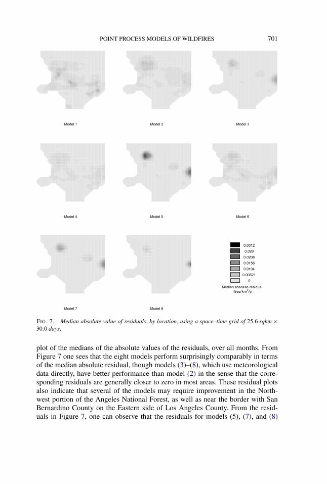
FIG. 7. Median absolute value of residuals, by location, using a space–time grid of 25.6 sqkm !30.0 days.

plot of the medians of the absolute values of the residuals, over all months. FromFigure 7 one sees that the eight models perform surprisingly comparably in termsof the median absolute residual, though models (3)–(8), which use meteorologicaldata directly, have better performance than model (2) in the sense that the corre-sponding residuals are generally closer to zero in most areas. These residual plotsalso indicate that several of the models may require improvement in the North-west portion of the Angeles National Forest, as well as near the border with SanBernardino County on the Eastern side of Los Angeles County. From the resid-uals in Figure 7, one can observe that the residuals for models (5), (7), and (8)

702 H. XU AND F. P. SCHOENBERG

are highly concentrated around zero except a few large values that occur in theNorthwest part and east part of Los Angeles County.

6. Discussion. The models explored here use the identical informationrecorded at the RAWS stations and used as inputs into the computation of theBI. Hence, it seems relevant to compare the fit of such models with comparablespatial interpolations of BI measurements, and the fact that the models using theweather variables directly appear to offer superior fit suggests that the BI may notbe effective as a short-term forecasting measure of wildfire hazard in Los AngelesCounty.

It should be noted that the empirical relationship between a fire danger ratingindex such as the BI and wildfire incidence is only one way to evaluate the effec-tiveness of such an index; alternatives may include assessing the cost-effectivenessof staffing or other decisions made based on the index. Furthermore, the use of firedanger ratings by fire department officials for wildfire suppression and preventionactivities may confound the empirical relationship between fire danger ratings andobserved wildfire activity. Nevertheless, most evaluation studies of fire danger rat-ing systems relate such indices to ultimate fire responses, including fire incidenceand fire size. Indeed, Andrews and Bradshaw (1997), whose work was instrumentalin the current implementation of the BI, suggested that the value of a fire dangerindex be evaluated according to its relationship with fire activity, which may bedefined as the incidence of large wildfires. Such empirical relationships have beenused as support for the use of such rating systems for predictive purposes [Haineset al. (1983); Haines, Main and Simard (1986); Mees and Chase (1991); Man-dallaz and Ye (1997a, 1997b); Viegas et al. (1999); Andrews, Loftsgaarden andBradshaw (2003)]. The results here suggest that, for the purpose of forecastingwildfire hazard, point process models using RAWS records and previous wildfireactivity as covariates may represent a promising alternative to existing indices thatuse essentially the same information.

However, we must emphasize that the point process models proposed here re-main rather simplistic and could potentially be improved by incorporating a host ofother important variables, such as detailed vegetation type, vegetation cover, soilcharacteristics, other weather variables such as cloud cover and lightning, as wellas human factors such as land use and public policy. The exclusion of such vari-ables from this analysis is solely motivated by our aim to optimize forecasts giventhe same remote, automatically-recorded information used in the computation ofthe BI. The models considered here could also perhaps be improved in variousways. For instance, one might allow long-term temporal trends and/or allow theseasonal component to vary from year to year. In addition, one may consider esti-mating the kernel function in models (5) and (6) for each station using only localwildfires close to the corresponding station, or perhaps by some more sophisti-cated weighting scheme where nearby fires are given higher weight in the esti-mation of this function. Because daily burn areas are right-skewed [Schoenberg,

POINT PROCESS MODELS OF WILDFIRES 703

Peng and Woods (2003)], perhaps kernel regressions where the response variableis some transformation of the daily burn area might yield superior results. An addi-tional important direction for future work is the exploration of similar point processmodels for wildfire occurrences in other locations and for other vegetation types oralternative wildfire regimes, as well as the use of such models for actual prospec-tive predictions of wildfire activity, rather than merely the empirical assessment ofgoodness of fit to historical data.

Acknowledgments. Thanks to Larry Bradshaw at the USDA Forest Servicefor generously providing us with RAWS data and helping us to process it. Thanksalso to James Woods, Roger Peng, and members of the LACFD and LADPW(especially Mike Takeshita, Frank Vidales, and Herb Spitzer) for sharing their dataand expertise.

REFERENCES

AKAIKE, H. (1977). On entropy maximization principle. In Applications of Statistics (P. R. Krishna-iah, ed.) 27–41. North-Holland, Amsterdam. MR0501456

ANDREWS, P. L. and BRADSHAW, L. S. (1997). FIRES: Fire Information Retrieval and EvaluationSystem—a program for fire danger rating analysis. Gen. Technical Report INT-GTR-367. Ogden,UT; U.S. Dept. Agriculture, Forest Service, Intermountain Research Station. 64 p.

ANDREWS, P. L., LOFTSGAARDEN, D. O. and BRADSHAW, L. S. (2003). Evaluation of fire dangerrating indexes using logistic regression and percentile analysis. Int. J. Wildland Fire 12 213–226.

BADDELEY, A., TURNER, R., MØLLER, J. and HAZELTON, M. (2005). Residual analysis for spatialpoint processes (with discussion). J. Roy. Statist. Soc. Ser. B 67 617–666. MR2210685

BRADSHAW, L. S., DEEMING, J. E., BURGAN, R. E. and COHEN, J. D. (1983). The 1978 NationalFire-Danger Rating System: Technical Documentation. United States Dept. Agriculture ForestService General Technical Report INT-169. Intermountain Forest and Range Experiment Station,Ogden, Utah. 46 p.

BURGAN, R. E. (1988). 1988 revisions to the 1978 National Fire-Danger Rating System. USDAForest Service, Southeastern Forest Experiment Station, Research Paper SE-273.

DALEY, D. and VERE-JONES, D. (1988). An Introduction to the Theory of Point Processes. Springer,New York. MR0950166

DALEY, D. and VERE-JONES, D. (2003). An Introduction to the Theory of Point Processes. Vol. 1:Elementary Theory and Methods. Springer, New York. MR1950431

DEEMING, J. E., BURGAN, R. E. and COHEN, J. D. (1977). The National Fire-Danger Rating Sys-tem — 1978. Technical Report INT-39, USDA Forest Service, Intermountain Forest and RangeExperiment Station.

HAINES, D. A., MAIN, W. A., FROST, J. S. and SIMARD, A. J. (1983). Fire-danger rating and wildfireoccurrence in the Northeastern United States. Forest Science 29 679–696.

HAINES, D. A., MAIN, W. A. and SIMARD, A. J. (1986). Fire-danger rating observed wildfire behav-ior in the Northeastern United States. Res. Pap. NC-274. St. Paul, MN: U.S. Dept. Agriculture,Forest Service, 23 p.

HÄRDLE, W. (1994). Applied Nonparametric Regression. Cambridge, Cambridge University Press.HELMERS, R., MAGKU, I. W. and ZITIKIS, R. (2003). Consistent estimation of the intensity function

of a cyclic Poisson process. J. Multivariate Anal. 84 19–39. MR1965821KEELEY, J. E. (2000). Chaparral. P. 203–253 in North American Terrestrial Vegetation, 2nd ed.

(M. G. Barbour and W. D. Billings, eds.). Cambridge University Press, Cambridge.

704 H. XU AND F. P. SCHOENBERG

KEELEY, J. E. and FOTHERINGHAM, C. J. (2003). Impact of past, present, and future fire regimes onNorth American Mediterranean shrublands. In: Fire and Climatic Change in Temperate Ecosys-tems of the Western Americas (T. T. Veblen, W. L. Baker, G. Montenegro and T. W. Swetnam,eds.) 218–262. Springer, New York.

MANDALLAZ, D. and YE, R. (1997a). A new dryness index and the non-parametric estimate of forestfire probabilities. Schweiz. Z. Forstwes. 148 809–822.

MANDALLAZ, D. and YE, R. (1997b). Prediction of forest fires with Poisson models. Can. J. For.Res. 27 1685–1694.

MARDIA, K. V. and JUPP, P. E. (2000). Directional Statistics. Wiley, New York. MR1828667MEES, R. and CHASE, R. (1991). Relating burning index to wildfire workload over broad geographic

areas. Int. J. Wildland Fire 1 235–238.OGATA, Y. (1978). The asymptotic behaviour of maximum likelihood estimators for stationary point

processes. Ann. Inst. Statist. Math. 30 243–261. MR0514494PENG, R. and SCHOENBERG, F. P. (2008). Estimating fire interval distributions using coverage

process data. Environmetrics. Unpublished manuscript.PENG, R. D., SCHOENBERG, F. P. and WOODS, J. (2005). A space–time conditional intensity model

for evaluating a wildfire hazard index. J. Amer. Statist. Assoc. 100 26–35. MR2166067RATHBUN, S. L. and CRESSIE, N. (1994). Asymptotic properties of estimators for the parameters of

spatial inhomogeneous Poisson point processes. Adv. Appl. Probab. 26 122–154. MR1260307SCHOENBERG, F. P., BRILLINGER, D. R. and GUTTORP, P. M. (2002). Point processes, spatial-

temporal. In Encyclopedia of Environmetrics (A. El-Shaarawi and W. Piegorsch, eds.) 3 1573–1577. Wiley, New York.

SCHOENBERG, F. P., CHANG, C., KEELEY, J., POMPA, J., WOODS, J. and XU, H. (2010). A criticalassessment of the burning Index in Los Angeles County, California. Int. J. Wildland Fire. Toappear.

SCHOENBERG, F. P., PENG, R., HUANG, Z. and RUNDEL, P. (2003). Detection of nonlinearities inthe dependence of burn area on fuel age and climatic variables. Int. J. Wildland Fire 12 1–10.

SCHOENBERG, F. P., PENG, R. and WOODS, J. (2003). On the distribution of wildfire sizes. Envi-ronmetrics 14 583–592.

SCHOENBERG, F. P. and XU, H. (2008). Directional kernel regression for wind and fire data. Envi-ronmetrics. Unpublished manuscript.

SCHROEDER, M. J., GLOVINSKY, M., HENDRICKS, V., HOOD, F., HULL, M., JACOBSON, H.,KIRKPATRICK, R., KRUEGER, D., MALLORY, L., OERTEL, A., REESE, R., SERGIUS, L. andSYVERSON, C. (1964). Synoptic weather types associated with critical fire weather. Institute forApplied Technology, National Bureau of Standards, U.S. Dept. Commerce, Washington, DC.

SILVERMAN, B. W. (1986). Kernel Density Estimation and Data Analysis. Chapman and Hall, Lon-don.

VIEGAS, D. X., BOVIO, G., FERREIRA, A., NOSENZO, A. and SOL, B. (1999). Comparative studyof various methods of fire danger evaluation in Southern Europe. Int. J. Wildland Fire 9 235–246.

WARREN, J. R. and VANCE, D. L. (1981). Remote Automatic Weather Station for Resource andFire Management Agencies. United States Dept. Agriculture Forest Service Technical ReportINT-116. Intermountain Forest and Range Experiment Station.

DEPARTMENT OF STATISTICS

UNIVERSITY OF CALIFORNIA

8125 MATH-SCIENCE BUILDING

LOS ANGELES, CALIFORNIA 90095–1554USAE-MAIL: xuhy@ucla.edu

frederic@stat.ucla.edu