POD/DEIM Strategies for reduced data assimilation...
44
POD/DEIM Strategies for reduced data assimilation systems R˘ azvan S ¸tef˘ anescu 1 Adrian Sandu 1 Ionel M. Navon 2 1 Computational Science Laboratory, Department of Computer Science, Virginia Polytechnic Institute and State University 2 Department of Scientific Computing,The Florida State University R˘ azvan S ¸tef˘ anescu , Adrian Sandu , Ionel M. Navon POD/DEIM Strategies for reduced data assimilation systems 1/40
Transcript of POD/DEIM Strategies for reduced data assimilation...

POD/DEIM Strategies for reduced data assimilationsystems
Razvan Stefanescu 1 Adrian Sandu 1 Ionel M. Navon 2
1Computational Science Laboratory, Department of Computer Science, Virginia PolytechnicInstitute and State University
2Department of Scientific Computing,The Florida State University
Razvan Stefanescu , Adrian Sandu , Ionel M. Navon
POD/DEIM Strategies for reduced data assimilation systems 1/40

Outline
1 Data Assimilation
2 Reduced order data assimilation
3 Reduced Order Modelling
4 ROM 4D-Var DA systems - Choice of bases
5 4D-Var SWE DA reduced order systems
6 Numerical results
7 Conclusions and future research
Razvan Stefanescu , Adrian Sandu , Ionel M. Navon
POD/DEIM Strategies for reduced data assimilation systems 2/40

Data Assimilation
Data assimilation - process of combining information from models,measurements, and priors - all with associated uncertainties - toobtain the best estimate of the state of a physical system.
Two families of methods: variational and statistical methods.
Variational methods - rooted in control theory and requiredevelopments of tangent linear and adjoint models.
Statistical methods: Ensemble based sequential data assimilation andBayesian inversion
Razvan Stefanescu , Adrian Sandu , Ionel M. Navon
POD/DEIM Strategies for reduced data assimilation systems 3/40

4D-Var Data AssimilationThe objective function J to be optimized is defined based onmodel-data misfit penalty terms as:
J(x0) =1
2
(xb − x0
)TB−1
0
(xb − x0
)+
1
2
N∑i=1
(yi − H(xi )
)TR−1i
(yi − H(xi )
),
(1)
subject toxi+1 =Mi (xi ), i = 0, ..,N − 1, (2)
The optimality conditions:
Adjoint model: λi = MTi λi+1 + HTR−1
i
(yi − H(xi )
), i = N − 1, 1;
λN =HTR−1N
(yN − H(xN)
)and λ0 = MT
0 λ1.
(3)
Cost function gradient: ∇x0L = −B−10
(xb− x0
)−λ0 = 0;
(4)Razvan Stefanescu , Adrian Sandu , Ionel M. Navon
POD/DEIM Strategies for reduced data assimilation systems 4/40

4D-Var Data Assimilation
Razvan Stefanescu , Adrian Sandu , Ionel M. Navon
POD/DEIM Strategies for reduced data assimilation systems 5/40

Incremental 4D-Var Data Assimilation Courtier et al. [8]
Razvan Stefanescu , Adrian Sandu , Ionel M. Navon
POD/DEIM Strategies for reduced data assimilation systems 6/40

Reduced order data assimilation
Razvan Stefanescu , Adrian Sandu , Ionel M. Navon
POD/DEIM Strategies for reduced data assimilation systems 7/40

Why do we need reduced order data assimilation?
Replace the current linearized cost function to be minimized in theinner loop
Surrogate models that accurately represent sub-grid-scale processesinstead of linearized low-fidelity models
Suitable reduced order models can be derived successively and giveglobal convergence results - Arian et al. [2] - This approach can beinterpreted in the context of trust region methods using generalnonlinear model functions with inexact gradient information.
Highly non-linear and non-smooth observation operators
Increased space and time resolutions
Razvan Stefanescu , Adrian Sandu , Ionel M. Navon
POD/DEIM Strategies for reduced data assimilation systems 8/40

Reduced Order Modelling
dependent and independent of input
For linear models we are able to produce input-independent highlyaccurate reduced models: balanced truncation, moment matching
For general nonlinear systems, the transfer function approach is notyet applicable and input-specified semi-empirical methods are usuallyemployed
Application of generalized transfer functions and generalized momentmatching (Benner and Breiten [3]) for nonlinear model order reduction
Razvan Stefanescu , Adrian Sandu , Ionel M. Navon
POD/DEIM Strategies for reduced data assimilation systems 9/40

Proper Orthogonal DecompositionThe desired simulation is well approximated in the input collection.
Data analysis is conducted to extract basis functions, fromexperimental data or detailed simulations of high-dimensional systems
Galerkin projections that yield low dimensional dynamical models.
Standard POD models: Its nonlinear reduced terms still have to beevaluated on the original state space making the simulation of thereduced-order system too expensive.
Tensorial POD - Stefanescu et al. [14] - ”Comparison of POD reducedorder strategies for the nonlinear 2D Shallow Water Equations”
We assume a Petrov-Galerkin projection for constructing the reducedorder models. U denotes the POD basis and the test functions arestored in W . W TU = Ik , Ik being the identity matrix of order k . Forsimplicity we assume a POD expansion of x = U x.
Razvan Stefanescu , Adrian Sandu , Ionel M. Navon
POD/DEIM Strategies for reduced data assimilation systems 10/40

ROM 4D-Var DA systems - Choice of bases
The “reduced adjoint” (RA) approach projects the first orderoptimality equations of the full system onto the POD reduced spaces
Accurate low-order surrogate models; Its not clear what informationshould be included in the reduced basis used for full space gradientequation projection
The “adjoint of reduced” (AR) model approach formulates the firstorder optimality conditions from the forward reduced order model
Consistent KKT discrete optimality conditions; Reduced adjointmodel approximates poorly its full counterpart and POD bases relyonly on forward dynamics information.
Razvan Stefanescu , Adrian Sandu , Ionel M. Navon
POD/DEIM Strategies for reduced data assimilation systems 11/40

ROM 4D-Var DA systems - Choice of bases
To guide the POD bases snapshots selection process forPetrov-Galerkin based reduced data assimilation systems governed bynon-linear models
Consistent reduced Karush Kuhn Tucker (KKT) optimality conditionsand accurate reduced POD adjoint model solutions with respect tothe full adjoint model outputs
Every type of reduced optimization involving adjoint models andprojection based reduced order methods including reduced basisapproach will benefit.
Razvan Stefanescu , Adrian Sandu , Ionel M. Navon
POD/DEIM Strategies for reduced data assimilation systems 12/40

ROM 4D-Var DA systems - Choice of bases
We derive the optimality conditions as in the AR approach
Forward POD manifold Uf is computed using snapshots of the fullforward model solution only x ≈ Uf x
Petrov-Galerkin (PG) projection; the test functions POD basis Wf isdifferent than the trial functions POD manifold Uf
JPOD(x0) =1
2
(xb − Uf x0
)TB−1
0
(xb − Uf x0
)T+
1
2
N∑i=1
(yi − H(Uf xi )
)TR−1i
(yi − H(Uf xi )
)T,
(5)
subject to xi+1 = W Tf Mi (Uf xi ), , i = 0, ..,N − 1. (6)
Razvan Stefanescu , Adrian Sandu , Ionel M. Navon
POD/DEIM Strategies for reduced data assimilation systems 13/40

ROM 4D-Var DA systems - Choice of bases
Reduced adjoint model
λi = UTf MT
i Wf λi+1 + UTf HTR−1
i
(yi − H(Uf xi )
), i = N − 1, 1;
λN = UTf HTR−1
N
(yN − H(Uf xN)
)and λ0 = UT
f MT0 Wf λ1
(7)
Reduced Cost Function gradient
∇x0LPOD = −UT
f B−10
(xb − Uf x0
)− λ0 = 0; (8)
Definition
A reduced KKT system is said to be consistent if it represents the firstorder optimality conditions of some reduced order optimization problem.
Razvan Stefanescu , Adrian Sandu , Ionel M. Navon
POD/DEIM Strategies for reduced data assimilation systems 14/40

ROM 4D-Var DA systems - Choice of bases
RA approach: the full forward and adjoint models are projected ontoseparate reduced manifolds
Uf and Ua are the trial POD reduced subspaces and Wf and Wa arethe test functions POD manifolds, xi ≈ Uf xi , λi ≈ Uaλi , i = 0, ..,N.
Reduced forward model:
xi+1 = W Tf Mi (Uf xi ), i = 0, ..,N − 1. (9)
Reduced adjoint model:
λi = W Ta MT
i Uaλi+1 + W Ta HTR−1
i
(yi − H(Uf xi )
), i = N − 1, 1
λN = W Ta HTR−1
N
(yN − H(Uf xN)
)and λ0 = W T
a MT0 Uaλ1,
(10)
Razvan Stefanescu , Adrian Sandu , Ionel M. Navon
POD/DEIM Strategies for reduced data assimilation systems 15/40

ROM 4D-Var DA systems - Choice of bases
AR adjoint model:
λi = UTf MT
i Wf λi+1 + UTf HTR−1
i
(yi − H(Uf xi )
), i = N − 1, 1;
λN = UTf HTR−1
N
(yN − H(Uf xN)
)and λ0 = UT
f MT0 Wf λ1
(11)
RA adjoint model:
λi = W Ta MT
i Uaλi+1 + W Ta HTR−1
i
(yi − H(Uf xi
), i = N − 1, 1
λN = W Ta HTR−1
N
(yN − H(Uf xN)
)and λ0 = W T
a MT0 Uaλ1,
(12)
For Petrov Galerkin and Galerkin projections - ARRA technique
Wf = Ua and Wa = Uf , and Uf = Ua. (13)
Razvan Stefanescu , Adrian Sandu , Ionel M. Navon
POD/DEIM Strategies for reduced data assimilation systems 16/40

ROM 4D-Var DA systems - Choice of bases
Theorem
Assume that the model operatorsMi ,i+1 : RNstate → RNstate , i = 0, ..,N−1and observation operators Hi : RNstate → RNobs i = 0, ..,N belong toC2[RNstate ] and the high-fidelity and AR optimization problems admitunique optimal pairs (xa,λa) ∈ RNstate×N × RNstate×N and(xa, λa) ∈ Rk×N × Rk×N , with projection (xa, λa) = (Uf xa,Wf λ
a) layingin the neighbourhood of (xa,λa).Then there exist “impact factors” ξ, νi and µi ∈ RNstate , i = 0, ..,N suchthat the error in a component of the high-fidelity optimizer computedusing the minimizer of reduced order problem is approximated to firstorder by formula
ε(x0)− ε(xa0) ≈ ∆fwd + ∆adj + ∆opt. (14)
Razvan Stefanescu , Adrian Sandu , Ionel M. Navon
POD/DEIM Strategies for reduced data assimilation systems 17/40

ROM 4D-Var DA systems - Choice of bases
Forward model contribution:
∆fwd = −N−1∑i=0
νTi+1
(UfW
Tf − I
)Mi ,i+1(xai )
(15a)
Adjoint model contribution
∆adj = −µTN(Wf U
Tf − I
)HT
NR−1N
(yN −HN(xaN)
)−
N−1∑i=0
µTi
(Wf U
Tf − I
)[MT
i ,i+1λai+1 + HT
i R−1i
(yi −Hi (xai )
)],
(15b)
Optimality equation contribution:
∆opt = −ξT(Wf U
Tf − I
)B−1
0
(xb0 − xa0
).
(15c)

ROM 4D-Var DA systems - Choice of bases
Definition
The triplet (x,λ,∇x0L) ∈ RNstate×N × RNstate×N × RNstate is said to beKKT-feasible if x is the solution of the forward model (2) initiated with agiven x0 ∈ RNstate , λ is the solution of the adjoint model (3) linearizedacross the trajectory x, and ∇x0L is the gradient of the Lagrangianfunction computed from (4).
ROM 4D-Var DA systems - Choice of bases
Definition
Let (x,λ,∇x0L) ∈ RNstate×N × RNstate×N × RNstate be a KKT-feasible tripletof the full order optimization problem (1). If for any positive εf , εa and εgthere exists k ≤ Nstate and three bases U, V and W ∈ RNstate×k such thatthe reduced KKT-feasible triplet (x, λ,∇x0Lpod) ∈ Rk×N × Rk×N × Rk ofthe reduced optimization problem (5) satisfies:
‖xi − U xi‖2 ≤ εf, i = 0, ..,N, (16a)
‖λi − V λi‖2 ≤ εa, i = 0, ..,N, (16b)
‖∇x0L − W∇x0Lpod‖2 ≤ εg, (16c)
then the reduced order AR KKT system built using Uf = U, Wf = [V , W ]that generated (x, λ,∇Lpodx0
) is said to be accurate with respect to the fullorder KKT system.

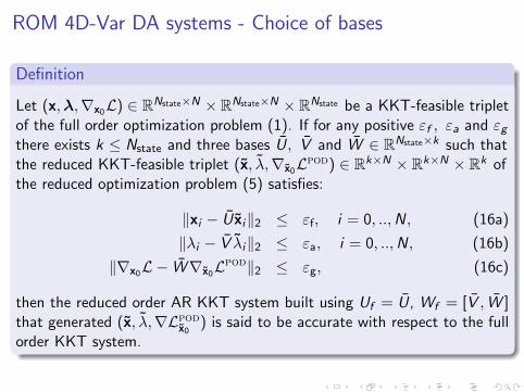
4D-Var SWE DA reduced order systems
Algorithm 1 Standard and Tensorial POD SWE DA systems
Off-line stage
1: Generate background state u, v and φ.2: Solve full forward ADI SWE model to generate state variables snapshots.
3: Solve full adjoint ADI SWE model to generate adjoint variables snap-shots.
4: For each state variable compute a POD basis using snapshots describingdynamics of the forward and its corresponding adjoint trajectories.
5: Compute tensors as T required for reduced Jacobian calculations. Cal-culate other POD coefficients corresponding to linear terms.
Razvan Stefanescu , Adrian Sandu , Ionel M. Navon
POD/DEIM Strategies for reduced data assimilation systems 21/40
4D-Var SWE DA reduced order systems
Algorithm 1 Standard and Tensorial POD SWE DA systems
On-line stage - Minimize reduced cost functional JPOD (5)
1: Solve forward reduced order model (6)2: Solve adjoint reduced order model (7)3: Compute reduced gradient (8)
Decisional stage
4: Project the suboptimal reduced initial condition generated by the on-line stage and perform steps 1 and 2 of off-line stage. Using full forwardinformation evaluate J in (1). If ‖J‖ > ε3 then continue the off-linestage from step 3, otherwise STOP.
Razvan Stefanescu , Adrian Sandu , Ionel M. Navon
POD/DEIM Strategies for reduced data assimilation systems 22/40

4D-Var SWE DA reduced order systems
The on-line stage - minimization of the cost function JPOD performedon a reduced POD manifold
The stoping criteria are
‖∇JPOD‖ ≤ ε1, ‖JPOD(i+1) − JPOD
(i) ‖ ≤ ε2, MXFUN ≤ iterMax (17)
The off-line stage - outer iteration - general stopping criterion
‖J‖ ≤ ε3
Razvan Stefanescu , Adrian Sandu , Ionel M. Navon
POD/DEIM Strategies for reduced data assimilation systems 23/40

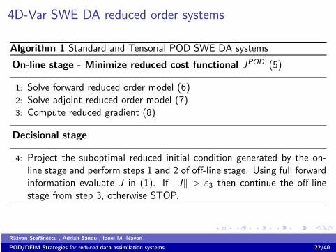
4D-Var SWE DA reduced order systems
Three POD based reduced order models will be considered forderiving reduced order SWE data assimilation systems: standardProper Orthogonal Decomposition (SPOD), tensorial POD (TPOD)and standard POD/Discrete Empirical Interpolation Method(POD/DEIM)
The reduced Jacobians are obtained using tensorial calculus for allthree ROMs and their computational complexity depends only on kthe dimension of POD basis - Stefanescu and Sandu [15]
The methods differ in the way the nonlinear terms are treated -polynomial quadratic nonlinearity u2.
Razvan Stefanescu , Adrian Sandu , Ionel M. Navon
POD/DEIM Strategies for reduced data assimilation systems 24/40
4D-Var SWE DA reduced order systemsStandard POD
N(u) = W T︸︷︷︸k×Nstate
Uu�Uu︸ ︷︷ ︸Nstate×1
, N(u) ∈ Rk (18)
where � is the componentwise multiplication Matlab operator and n isusually the number of spatial mesh points.
Tensorial POD
N(u) =[Ni
]i=1,..,k
∈ Rk ; Ni =k∑
j=1
k∑l=1
Ti ,j ,l uj ul . (19)
N(u) = T︸︷︷︸k×k2
U︸︷︷︸k2×1
T =(Ti ,j ,l
)i ,j ,l=1,..,k
∈ Rk×k×k , Ti ,j ,l =n∑
r=1
Wi ,rUj ,rUl ,r .
Razvan Stefanescu , Adrian Sandu , Ionel M. Navon
POD/DEIM Strategies for reduced data assimilation systems 25/40

4D-Var SWE DA reduced order systems
Standard POD/DEIM
N(u) ≈W TV (PTV )−1︸ ︷︷ ︸k×m
((PTUu)� (PTUu)
)︸ ︷︷ ︸
m×1
(20)
where m is the number of interpolation points, V ∈ Rn×m gathers the firstm POD basis modes of the nonlinear term while P ∈ Rn×m is the DEIMinterpolation selection matrix (Chaturantabut [5], Chaturantabut andSorensen [7, 6], Stefanescu and Navon [13]).
Razvan Stefanescu , Adrian Sandu , Ionel M. Navon
POD/DEIM Strategies for reduced data assimilation systems 26/40

4D-Var SWE DA reduced order systems
F11(u,φ) = u � Axu +1
2φ� Axφ, F12(u, v) = v � Ayu
F21(u, v) = u � Axv ,F22(v ,φ) = v � Ayv +1
2φ� Ayφ,
F31(u,φ) =1
2φ� Axu + u � Axφ, F32(v ,φ) =
1
2φ� Ayv + v � Ayφ.
Full ADI SWE Standard POD Tensorial POD POD/DEIM m=180 POD/DEIM m=70
CPU time 950.0314s 161.907 2.125 0.642 0.359
u - 5.358e-5 5.358e-5 5.646e-5 7.453e-5
v - 2.728e-5 2.728e-5 3.418e-5 4.233e-5
φ - 8.505e-5e 8.505e-5 8.762e-5 9.212e-5
Table: CPU time gains and the root mean square errors for each of the modelvariables at tf = 3h for a 3h time integration window. Number of POD modeswas k = 50 and two tests with different number of DEIM points m = 180, 70were simulated.103, 776 spatial points.
Razvan Stefanescu , Adrian Sandu , Ionel M. Navon
POD/DEIM Strategies for reduced data assimilation systems 27/40

4D-Var SWE DA reduced order systems
103
104
105
10−1
100
101
102
103
No. of spatial discretization points
CP
U t
ime
(sec
on
ds)
SPODTPODPOD/DEIM m=70POD/DEIM m=180FULL
(a) On-line stage
103
104
105
100
101
102
103
No. of spatial discretization points
CP
U t
ime
(sec
on
ds)
SPODTPODPOD/DEIM m=70POD/DEIM m=180
(b) Off-line stage
Figure: Cpu time vs. the number of spatial discretization points for tf = 3h ;number of POD modes = 50; two different numbers of DEIM points 70 and 180have been employed.
Razvan Stefanescu , Adrian Sandu , Ionel M. Navon
POD/DEIM Strategies for reduced data assimilation systems 28/40

Numerical Results
ADI SWE model
10% uniform perturbations on the initial conditions of Grammeltvedt[9] and generate twin-experiment observations at every grid spacepoint location and every time step
Background state is computed using a 5% perturbations of the initialconditions
The length of the assimilation window: 3h.
BFGS optimization method (CONMIN)
We use ε1 = 10−14 and ε2 = 10−5.
We select 31× 23 mesh points 91 time steps and use 50 POD basisfunctions. MXFUN is set to 25 and ε3 = 10−16
Razvan Stefanescu , Adrian Sandu , Ionel M. Navon
POD/DEIM Strategies for reduced data assimilation systems 29/40

Numerical Results - Choice of POD basis
0 25 50 75 100 125 150 175 200−15
−13
−10
−7
−4
−1
2
5
8
log
arit
hm
ic s
cale
Number of eigenvalues
uvφ
(a) Forward model snapshots only
0 25 50 75 100 125 150 175 200−13
−10
−7
−4
−1
2
5
8
log
arit
hm
ic s
cale
Number of eigenvalues
uvφ
(b) Forward and adjoint models snapshots
Figure: The decay around the singular values of the snapshots solutions foru, v , φ for ∆t = 960s and integration time window of 3h .
Razvan Stefanescu , Adrian Sandu , Ionel M. Navon
POD/DEIM Strategies for reduced data assimilation systems 30/40

Numerical Results - Choice of POD basis
0 10 20 30 40 50 60 70 80 9010
−25
10−20
10−15
10−10
10−5
100
J/J(
1)
Number of iterations
0 10 20 30 40 50 60 70 80 9010
−25
10−20
10−15
10−10
10−5
100
105
Gra
d/G
rad(
1)
0 10 20 30 40 50 60 70 80 9010
−25
10−20
10−15
10−10
10−5
100
105
0 10 20 30 40 50 60 70 80 9010
−25
10−20
10−15
10−10
10−5
100
105
Grad red. of adj. + adj. of red.Grad adj. of red.
Grad full
Cost func − red. of adj. + adj. of red.Cost func − adj. of red.Cost func − full
Figure: Tensorial POD/4DVAR ADI 2D Shallow water equations – Evolution ofcost function and gradient norm as a function of the number of minimizationiterations. The information from the adjoint equations has to be incorporatedinto POD basis.

POD/DEIM SWE 4D-Var DA systemMesh of 31× 23 and 17× 13 points, a POD basis dimension ofk = 50, and various number of DEIM interpolation points are used.MXFUN is set to 100 and ε3 = 10−16
0 200 400 600 800 100010
−5
10−4
10−3
10−2
10−1
100
J/J(
1)
Number of iterations
0 200 400 600 800 100010
−8
10−6
10−4
10−2
100
102
Gra
d/G
rad(
1)
0 200 400 600 800 100010
−8
10−6
10−4
10−2
100
102
Grad m=50
Grad m=180
Cost func − m = 50Cost func − Cost func − m = 180
(a) Number of mesh points 31 × 23
0 50 100 150 20010
−25
10−20
10−15
10−10
10−5
100
J/J(
1)
Number of iterations
0 50 100 150 20010
−25
10−20
10−15
10−10
10−5
100
Gra
d/G
rad(
1)
0 50 100 150 20010
−25
10−20
10−15
10−10
10−5
100
0 50 100 150 20010
−25
10−20
10−15
10−10
10−5
100
Grad m=50
Grad m=135
Grad m=165
Cost func − m=50Cost func − m=135Cost func − m=165
(b) Number of mesh points 17 × 13
Figure: Standard POD/DEIM ADI SWE 4D-Var system – Evolution of costfunction and gradient norm as a function of the number of minimizationiterations for different number of mesh points and various number of DEIMpoints.

Hybrid POD/DEIM SWE 4D-Var DA system
10 1 0.1 0.01 0.001 0.0001 1e−005 1e−006 1e−007−7
−6
−5
−4
−3
−2
−1
0
1
(J(x
+δx
) −
J(x
))/ <
∇J(
x),δ
x>
Perturbation ||δx||
0.94
0.96
0.98
1
||M(x
+δx
)(N
T)
− M
(x)(
NT
)||/|
|δ M
(δx)
(NT
)||
Adjoint TestTangent Linear Test
(a) Tangent Linear and Adjoint test
0 10 20 30 40 50 60 7010
−30
10−20
10−10
100
J/J(
1)
Number of iterations
0 10 20 30 40 50 60 7010
−30
10−25
10−20
10−15
10−10
10−5
100
0 10 20 30 40 50 60 7010
−30
10−25
10−20
10−15
10−10
10−5
100
Gra
d/G
rad(
1)
Grad Standard POD/DEIM
Grad Hybrid POD/DEIM
Cost func − Hybrid POD/DEIMCost func − Standard POD/DEIM
(b) Cost function and gradient decays
Figure: Tangent linear and adjoint test for standard POD/DEIM SWE 4D-Varsystem. Optimization performances of Standard POD/DEIM and HybridPOD/DEIM 4DVAR ADI 2D shallow water equations for 50 DEIM points and -n = 17× 13 space points.

POD based SWE 4D-Var DA systems
n = 151× 111 space points, number of POD basis modes k = 50,MXFUN = 15 and ε3 = 10−1.
0 5 10 15 20 25 30 3510
−10
10−8
10−6
10−4
10−2
100
Number of iterations
J/J(
1)
hybrid POD/DEIM m=30hybrid POD/DEIM m=50standard PODtensorial PODFull configuration
(a) Iteration performance
100
101
102
103
104
10−12
10−10
10−8
10−6
10−4
10−2
100
Cpu time
J/J(
1)
hybrid POD/DEIM m=30hybrid POD/DEIM m=50standard PODtensorial PODFull configuration
(b) Time performance
Figure: Number of iterations and CPU time comparisons for the reducedOrder SWE DA systems vs. full SWE DA system.
Razvan Stefanescu , Adrian Sandu , Ionel M. Navon
POD/DEIM Strategies for reduced data assimilation systems 34/40

Conclusions and future research
New POD bases selection strategies for POD based reduced 4DVardata assimilation systems governed by nonlinear state models usingboth Petrov-Galerkin and Galerkin projections.
Consistent reduced Karush Kuhn Tucker (KKT) optimality conditions+ accurate feasible reduced POD KKT condtitions.
Petrov-Galerkin projection - test functions POD bases of the forwardand adjoint models have to match the trial functions POD bases ofthe adjoint and forward models
Galerkin projection - one single POD basis is required and thecorrelation matrix must contain snapshots from both forward andadjoint full models. Include also the optimality condition information.
Razvan Stefanescu , Adrian Sandu , Ionel M. Navon
POD/DEIM Strategies for reduced data assimilation systems 35/40
Conclusions and future research
Every type of reduced optimization involving adjoint models andprojected based reduced order methods including reduced basisapproach benefit from the new strategies.
The POD/DEIM approximations of four nonlinear terms involvingheight field out of ten partially lost their accuracy during theoptimization where input data are different than the ones used togenerate the interpolation points - Hybrid tensorial POD/DEIM4D-Var SWE.
For meshes of 151× 111 points or higher the hybrid POD/DEIMreduced data assimilation system is approximately 10 times fasterthen the full space data assimilation system
Razvan Stefanescu , Adrian Sandu , Ionel M. Navon
POD/DEIM Strategies for reduced data assimilation systems 36/40

Conclusions and future research
This rate increases directly proportional with the the mesh size
Stabilization strategies proposed by Amsallem and Farhat[1], Bui-Thanh et al. [4] must be pursued in order to obtain feasiblePetrov-Galerkin reduced order data assimilation systems
Multifidelity techniques: Local in time adaptive ROMs. (Peherstorferet al. [10], Rapun and Vega [12]);
Exploit the structure of the weak constraints variational approach(Tremolet [17]), consistent reduced KKT conditions (Stefanescu et al.[16]) and formulate a piecewise-in-space-time approximation strategythat uses different ROMs on different subintervals, and constructsthem concurrently;
Develop reduced order parallel 4D-Var framework using AugmentedLagrangian (Rao and Sandu [11]) .
Razvan Stefanescu , Adrian Sandu , Ionel M. Navon
POD/DEIM Strategies for reduced data assimilation systems 37/40

Manuscripts related to the present research effort
Stefanescu, Razvan, Adrian Sandu, and Ionel Michael Navon.”POD/DEIM reduced-order strategies for efficient four dimensionalvariational data assimilation.” Journal of Computational Physics 295(2015): 569-595.
Stefanescu, Razvan, and Adrian Sandu. ”Efficient approximation ofsparse Jacobians for time-implicit reduced order models.” arXivpreprint arXiv:1409.5506 (2014).
Stefanescu, Razvan, Adrian Sandu, and Ionel Michael Navon.”Comparison of POD reduced order strategies for the nonlinear 2Dshallow water equations.” International Journal for NumericalMethods in Fluids 76.8 (2014): 497-521.
Stefanescu, Razvan and I.M. Navon, POD/DEIM Nonlinear modelorder reduction of an ADI implicit shallow water equations model,Journal of Computational Physics, Vol 237 , pp 95–114.

Manuscripts related to the present research effort
Stefanescu, Razvan, I.M. Navon, Max Marchand, Henry Fuelberg,”1D+ 4D-VAR data assimilation of lightning with WRFDA systemusing nonlinear observation operators.” arXiv preprintarXiv:1306.1884 (2013).
Razvan Stefanescu , Adrian Sandu , Ionel M. Navon
POD/DEIM Strategies for reduced data assimilation systems 39/40

POD/DEIM Strategies for reduced data assimilationsystems
Razvan Stefanescu , Adrian Sandu , Ionel M. Navon
POD/DEIM Strategies for reduced data assimilation systems 40/40
[1] D. Amsallem and C. Farhat. Stabilization of projection-basedreduced-order models. Int. J. Numer. Meth. Engng., 91:358–377,2012.
[2] E. Arian, M. Fahl, and E.W. Sachs. Trust-region proper orthogonaldecomposition for flow control. ICASE: Technical Report 2000-25,2000.
[3] P. Benner and T. Breiten. Two-sided moment matching methods fornonlinear model reduction. Technical Report MPIMD/12-12, MaxPlanck Institute Magdeburg Preprint, June 2012.
[4] T. Bui-Thanh, K. Willcox, O. Ghattas, and B. vanBloemen Waanders. Goal-oriented, model-constrained optimizationfor reduction of large-scale systems. J. Comput. Phys., 224(2):880–896, 2007.
[5] S. Chaturantabut. Dimension Reduction for Unsteady NonlinearPartial Differential Equations via Empirical Interpolation Methods.Technical Report TR09-38,CAAM, Rice University, 2008.
[6] S. Chaturantabut and D.C. Sorensen. Nonlinear model reduction viaRazvan Stefanescu , Adrian Sandu , Ionel M. Navon
POD/DEIM Strategies for reduced data assimilation systems 40/40

discrete empirical interpolation. SIAM Journal on ScientificComputing, 32(5):2737–2764, 2010.
[7] S. Chaturantabut and D.C. Sorensen. A state space error estimate forPOD-DEIM nonlinear model reduction. SIAM Journal on NumericalAnalysis, 50(1):46–63, 2012.
[8] P. Courtier, J.-N. Thepaut, and A. Hollingsworth. A strategy foroperational implementation of 4D–Var using an incrementalapproach. Quarterly Journal of the Royal Meteorological Society, 120:1367–1388, 1994.
[9] A. Grammeltvedt. A survey of finite difference schemes for theprimitive equations for a barotropic fluid. Monthly Weather Review,97(5):384–404, 1969.
[10] B. Peherstorfer, D. Butnaru, K. Willcox, and H. Bungartz. LocalizedDiscrete Empirical Interpolation Method. SIAM Journal on ScientificComputing, 36(1):A168–A192, 2014.
[11] V. Rao and A. Sandu. Parallel 4D-Var framework using AugmentedLagrangian. In preparation, 2015.
Razvan Stefanescu , Adrian Sandu , Ionel M. Navon
POD/DEIM Strategies for reduced data assimilation systems 40/40

[12] M.L. Rapun and J.M. Vega. Reduced order models based on localPOD plus Galerkin projection. Journal of Computational Physics, 229(8):3046–3063, 2010.
[13] R. Stefanescu and I.M. Navon. POD/DEIM Nonlinear model orderreduction of an ADI implicit shallow water equations model. Journalof Computational Physics, 237:95–114, 2013.
[14] R. Stefanescu, A. Sandu, and I.M. Navon. Comparisons of PODreduced order strategies for the nonlinear 2D Shallow WaterEquations Model. Technical Report TR 2, Virginia PolytechnicInstitute and State University, February 2014, also submitted toInternational Journal for Numerical Methods in Fluids.
[15] R. Stefanescu and A. Sandu. Efficient Approximation of SparseJacobians for Time-Implicit Reduced Order Models. Technical ReportTR 15, Virginia Polytechnic Institute and State University, September2014.
[16] R. Stefanescu, A. Sandu, and I.M. Navon. POD/DEIMReduced-Order Strategies for Efficient Four Dimensional Variational
Razvan Stefanescu , Adrian Sandu , Ionel M. Navon
POD/DEIM Strategies for reduced data assimilation systems 40/40

Data Assimilation. Technical Report TR 3, Virginia PolytechnicInstitute and State University, March 2014.
[17] Y. Tremolet. Accounting for an imperfect model in 4D-Var. Q.J.R.Meteorol. Soc., 132:2483–2504, 2006.
Razvan Stefanescu , Adrian Sandu , Ionel M. Navon
POD/DEIM Strategies for reduced data assimilation systems 40/40