NASA Contractor Report 198325

J/Y.' -

Planetary Boundary Layer SimulationUsing TASS

David G. Schowalter, David S. DeCroix, Yuh-Lang Lin, S. Pal Arya, and

Michael Kaplan

North Carolina State University, Raleigh, North Carolina

Cooperative Agreement NCC1-188

April 1996

National Aeronautics and

Space AdministrationLangley Research CenterHampton, Virginia 23681-0001

https://ntrs.nasa.gov/search.jsp?R=19960017580 2018-06-01T02:01:13+00:00Z

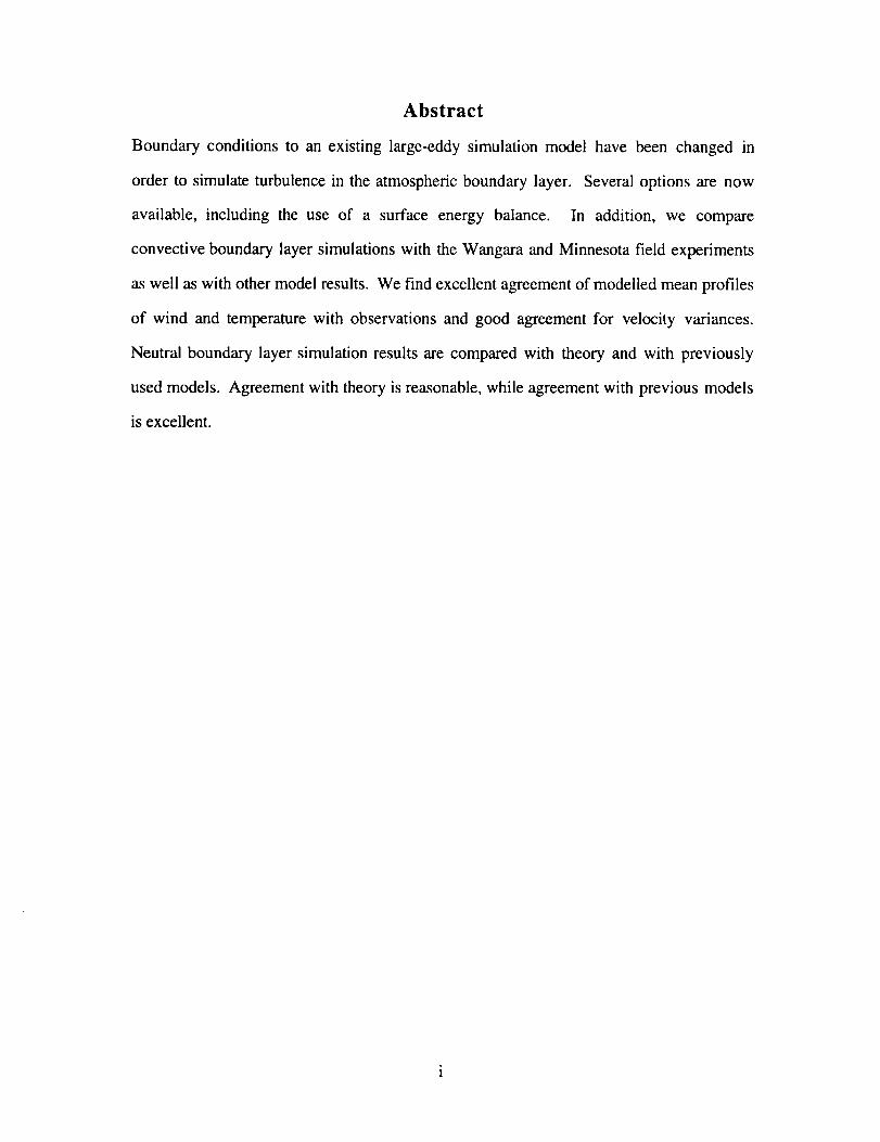
Abstract

Boundary conditions to an existing large-eddy simulation model have been changed in

order to simulate turbulence in the atmospheric boundary layer. Several options are now

available, including the use of a surface energy balance. In addition, we compare

convective boundary layer simulations with the Wangara and Minnesota field experiments

as well as with other model results. We find excellent agreement of modelled mean profiles

of wind and temperature with observations and good agreement for velocity variances.

Neutral boundary layer simulation results are compared with theory and with previously

used models. Agreement with theory is reasonable, while agreement with previous models

is excellent.

TABLE OF CONTENTS

Section Page

1. INTRODUCTION ............................................................. 1

2. NEW BOUNDARY CONDITIONS IN TASS ............................... 1

2.1 Surface Energy Budget: Theory ......................................................... 3

3. VALIDATION ................................................................. 9

J

3.1

3.2

3.3

NEUTRAL

Surface energy budget validation ......................................................... 9

Wangara Validation ......................................................................... 12

Minnesota Validation ...................................................................... 14

BOUNDARY LAYER .......................................... 2 2

5. SUMMARY .................................................................. 2 6

APPENDIX : DIRECTIONS FOR USING TASS PBL BOUNDARY

CONDITIONS .................................................................. 2 9

°°o

111

LIST OF TABLES

Table 1. Soil parameters used for energy budget validation case.

Table 2. Soil parameters used for the Wangara case.

iv

LIST OF FIGURES

Figure 1. Sensible heat flux for the validation case compared with observed values. Observed values were

calculated from observed profiles by assuming surface layer similarity.

Figure 2. Radiative, latent, and soil heat flux for the validation case. Observed values were measured

directly for the radiative heat fluxes, were numerically calculated in Lettau & Davidson for the soil

heat flux from temperature profiles, and were deduced for the latent heat flux by assuming surface

layer similarity.

Figure 3. Observed and computed potential temperature profiles for the Wangara Experiment, Day 33.

The 0900 profile was used to initialize the model.

Figure 4. Comparison of mean horizontal velocity results from TASS with Deardorff (1974) and with

observed data. (a) Eastward wind component and (b) northward wind component. Results shown are

for 1200 local time, after three hours of simulation.

Figure 5. (a) Horizontal and (b) vertical velocity variances for the TASS simulation of the Wangara

Experiment. Values were averaged horizontally over the domain as well as over one hour in time,

centered on the local hour indicated. Subgrid contributions are estimates based on the magnitude of

the local deformation tensor.

Figure 6. Observed and computed potential temperature profiles for Wangara Day 33 using the energy

budget scheme in TASS. The observed 0900 profile was used to initialize the model.

Figure 7. Comparison of computed mean winds with observed winds, Run 5A1 of the Minnesota

experiment.

Figure 8. Same as figure 7, but for vertical momentum fluxes.

Figure9. (a)Horizontaland(b)verticalvelocityvariancesfortheMinnesotaExperiment,Run5A1.

Figure 10. Vertical heat flux for Run 5AI of the Minnesota Experiment.

Figure 11. Dimensionless wind shear profiles for a neutral boundary layer from (a) TASS and (b) Andren

et al. (1994).

Figure 12. Same as figure 11 but for • c.

vi

1. Introduction

Over the past two years, this group has been working in support of the numerical

modeling arm of the NASA Wake Vortex Program. It is believed that the turbulence in the

planetary boundary layer will have a significant effect on the evolution of wake vortices.

Therefore, a first step is the accurate simulation of this turbulence using Large-eddy

simulation. Eventually, a nested grid capability will enable the insertion of a wake vortex

pair into the boundary layer. Our goal has been to add proper boundary conditions and to

validate the TASS (Terminal Area Simulation System) model for the planetary boundary

layer simulation.

What follows in Section 2 is a description of the boundary condition changes to TASS

and the associated theory. Section 3 discusses the validation results and Section 4 contains

a discussion of neutral boundary layer runs. Section 5 is a summary and we have also

included an appendix with instructions for using the boundary layer options with the

model.

2. New boundary conditions in TASS

The horizontal velocity at the top of the computational domain may now be specified.

This is accomplished with a three layer sponge technique much like what was done

previously with potential temperature. This velocity may be a function of time.

The geostrophic wind may now be specified. It is not a function of time, but may be

a function of height. This is equivalent to specification of the horizontal pressure gradient.

There is a choice of four possible heating (cooling) boundary conditions at the bottom

of the computational domain:

1. Simpleuniformheatingspecifiedasafunctionof timein whicharateterm(in W/m2) is

addedto theequationfor potentialtemperatureat theground. This shouldnot beusedfor

largeheatingratesbecausestrongtemperaturegradientswill not beproperlyaccountedfor

in thesurfacelayersimilarityscheme.

2. Specificationof surfaceheatandmoisturefluxes in kinematicunits ( °K.rn/s andm/s).

In thiscase,theratetermsareaddedto theequationsfor potentialtemperatureandfor water

vaporattheground. In addition,theObukhovlengthisproperlycalculatedusingthe value

of theheatflux ratherthanusingtemperaturegradientswhichmaybeunder-resolved.

3. Specificationof theair temperatureand moisturecloseto the ground. Surfacelayer

similarity is then used to calculatethe proper heatand moisturefluxes. Again, the

Obukhovlengthis calculatedusingthesurfaceheatflux. This methodwas describedin

detail inour recentAnnualReport(Lin et al. 1994).

4. Use of a surface energy budget for calculation of soil moisture, soil temperature, and

the resulting heat and moisture fluxes to the atmosphere. We use the slab model introduced

by Bhumralkar (1975) and Blackadar (1976).

The details and validation of method 4 have not been shown previously and will be

given here. In addition, we will discuss validation results for the simulation of the

Atmospheric Boundary Layer in general.

2

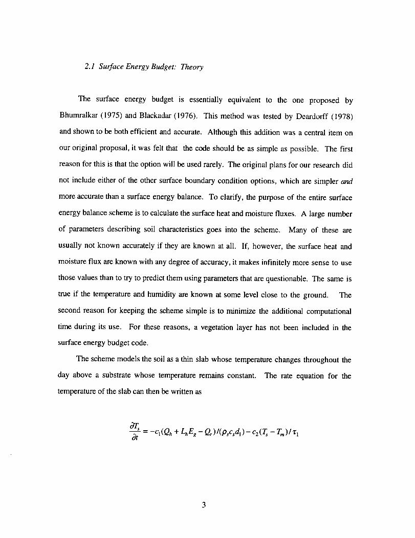
2.1 Surface Energy Budget: Theory

The surface energy budget is essentially equivalent to the one proposed by

Bhumralkar (1975) and Blackadar (1976). This method was tested by Deardorff (1978)

and shown to be both efficient and accurate. Although this addition was a central item on

our original proposal, it was felt that the code should be as simple as possible. The first

reason for this is that the option will be used rarely. The original plans for our research did

not include either of the other surface boundary condition options, which are simpler and

more accurate than a surface energy balance. To clarify, the purpose of the entire surface

energy balance scheme is to calculate the surface heat and moisture fluxes. A large number

of parameters describing soil characteristics goes into the scheme. Many of these are

usually not known accurately if they are known at all. If, however, the surface heat and

moisture flux are known with any degree of accuracy, it makes infinitely more sense to use

those values than to try to predict them using parameters that are questionable. The same is

true if the temperature and humidity are known at some level close to the ground. The

second reason for keeping the scheme simple is to minimize the additional computational

time during its use. For these reasons, a vegetation layer has not been included in the

surface energy budget code.

The scheme models the soil as a thin slab whose temperature changes throughout the

day above a substrate whose temperature remains constant. The rate equation for the

temperature of the slab can then be written as

OaTs _ .Cl(Q h + LhEg - Qr )/(p,c, dl ) - c2(T _ - Tm)/'c 1&

3

where Ts is the slab temperature, T,, is the temperature of the substrate, cs is the heat

capacity of the soil, _'1is the diurnal period, Ps is the density of the soil, d_ is the depth of

the slab, Qh is the sensible heat flux to the atmosphere, Qr is the net radiative heat flux to

the slab, Eg is the rate of evaporation of soil moisture, and L_ is the latent heat of

evaporation, cl and c2 are constants, set to 2_ t2 and 27r respectively. The last term

represents the heat exchanged between the slab and the substrate. We may write

d I -- _af_sT_ ,

where ;I.s is the thermal conductivity of the soil.

The radiative heat flux may be written as

Qr- $-,r $,

where K, represents the solar radiation, I,I, the incoming longwave radiation, and/1" the

outgoing longwave radiation. The outward radiative flux is straightforwardly written as

11"=e crr,

eg being the emmisivity of the ground and cr being the Stefan-Boltzmann constant. The

incoming longwave radiation is more complicated and must be parameterized. Like

Deardorff, we use the approximation of Staley and Jurica (1972),

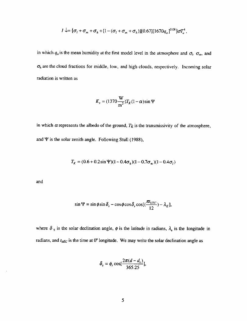
I ,1,= {tr t + tr,, + trh + [1 - (tr I + a m + crh )][0.67][1670q, ]0.08}oTfl,

in which q_ is the mean humidity at the first model level in the atmosphere and o't, O'm, and

Crhare the cloud fractions for middle, low, and high clouds, respectively. Incoming solar

radiation is written as

K s = (1370_-f2)Tr (1 - a)sinW

in which a represents the albedo of the ground, Tk is the transmissivity of the atmosphere,

and _F is the solar zenith angle. Following Stull (1988),

TK = (0.6 + 0.2sin W)(1 - 0.4or h)(1 - 0.70" m)(1 - 0.40" t)

and

sin _F = sin _sin g, - cos_cos3 s cos[(-_-2 c) - ;_E],

where t5 s is the solar declination angle, _ is the latitude in radians, Xe is the longitude in

radians, and tutc is the time at 0 ° longitude. We may write the solar declination angle as

_ = ¢,. cos[ 2_ dr).],

5

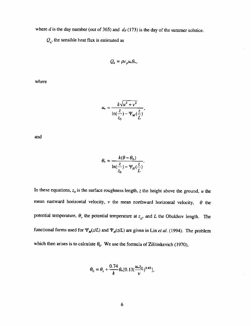
whered is the day number (out of 365) and dr (173) is the day of the summer solstice.

Qh' the sensible heat flux is estimated as

Qh = pc, u.O.,

where

U, --"

k_u 2 + v2

and

k(O-Oo)

ln(!) - _u(L)Zo

In these equations, Zo is the surface roughness length, z the height above the ground, u the

mean eastward horizontal velocity, v the mean northward horizontal velocity, 0 the

potential temperature, 0 o the potential temperature at z o, and L the Obukhov length• The

functional forms used for _Fu(z/L) and Wu(z/L) are given in Lin et al. (1994). The problem

which then arises is to calculate 0o. We use the formula of Zilitinkevich (1970),

Oo = Os + 0.74 O,[O.13(U, Zo )o.45],k v

6

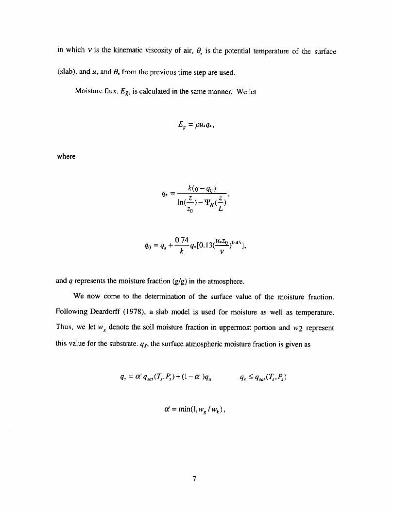
in which v is the kinematic viscosity of air, 0 s is the potential temperature of the surface

(slab), and u, and 0, from the previous time step are used.

Moisture flux, Eg, is calculated in the same manner. We let

Ee = pu.q.,

where

q, ._--

k(q - qo )

0.74

q0 = qs + ---k---q, [0.13( u-z° )0.4s ],V

and q represents the moisture fraction (g/g) in the atmosphere.

We now come to the determination of the surface value of the moisture fraction.

Following Deardorff (1978), a slab model is used for moisture as well as temperature.

Thus, we let w e denote the soil moisture fraction in uppermost portion and w2 represent

this value for the substrate, qs, the surface atmospheric moisture fraction is given as

q, = a'qs,,t(Ts,P_)+ (l- ot')q,, q, <- qsat(T_,P_)

a'= min(1,wg/wt),

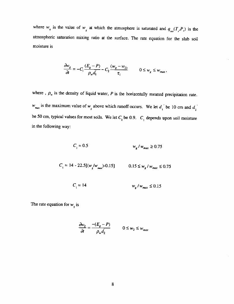
where w k is the value of w at which the atmosphere is saturated and q,,,(T,p,) is theg . ,

atmospheric saturation mixing ratio at the surface. The rate equation for the slab soil

moisture is

(Eg-P) - w2)= 0 <_wg <_w,,_,& Cl pwd', C2 'rt

where, p,_ is the density of liquid water, P is the horizontally meaned precipitation rate.

w is the maximum value of w above which runoff occurs. We let d' be 10 cm and d 2'max g

be 50 cm, typical values for most soils. We let C 2 be 0.9. Cj depends upon soil moisture

in the following way:

C 1 = 0.5 wg I w,,_ >_0.75

C I = 14 - 22.5[(wJw,,,,_)-O. 15] 0.15 _<Wg Iw,,_x < 0.75

C I = 14 wglWma x < 0.15

The rate equation for w 2 is

0 ¢( W 2 <-- Wma x

8

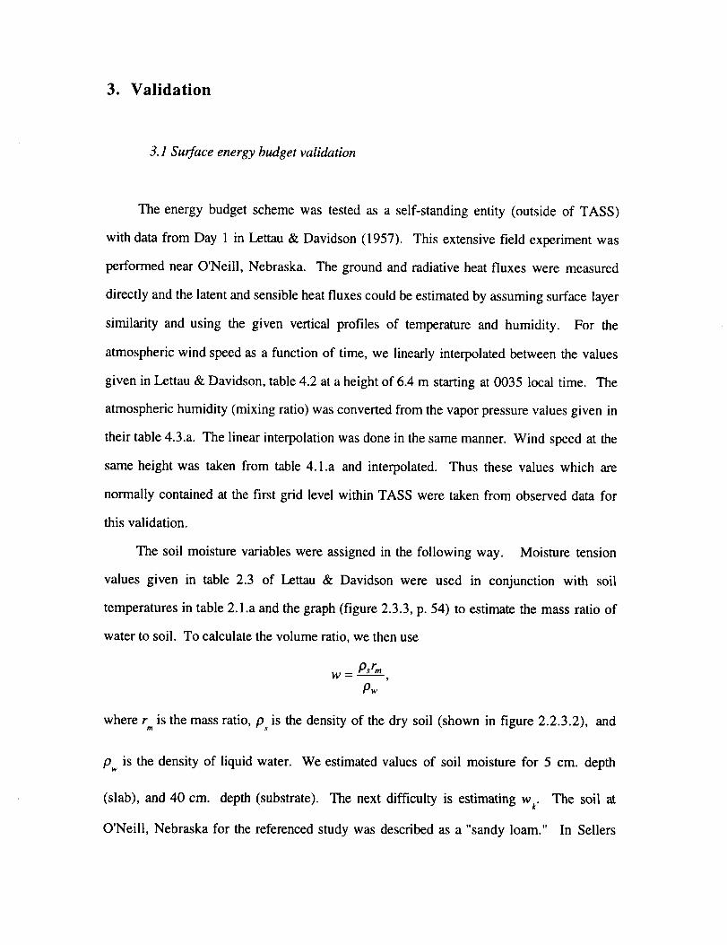
3. Validation

3.1 Surface energy budget validation

The energy budget scheme was tested as a self-standing entity (outside of TASS)

with data from Day 1 in Lettau & Davidson (1957). This extensive field experiment was

performed near O'Neill, Nebraska. The ground and radiative heat fluxes were measured

directly and the latent and sensible heat fluxes could be estimated by assuming surface layer

similarity and using the given vertical profiles of temperature and humidity. For the

atmospheric wind speed as a function of time, we linearly interpolated between the values

given in Lettau & Davidson, table 4.2 at a height of 6.4 m starting at 0035 local time. The

atmospheric humidity (mixing ratio) was converted from the vapor pressure values given in

their table 4.3.a. The linear interpolation was done in the same manner. Wind speed at the

same height was taken from table 4.1.a and interpolated. Thus these values which are

normally contained at the first grid level within TASS were taken from observed data for

this validation.

The soil moisture variables were assigned in the following way. Moisture tension

values given in table 2.3 of Lettau & Davidson were used in conjunction with soil

temperatures in table 2.1 .a and the graph (figure 2.3.3, p. 54) to estimate the mass ratio of

water to soil. To calculate the volume ratio, we then use

P._rmW_

Pw

where r is the mass ratio, p, is the density of the dry soil (shown in figure 2.2.3.2), and

Pw is the density of liquid water. We estimated values of soil moisture for 5 cm. depth

(slab), and 40 cm. depth (substrate). The next difficulty is estimating w k. The soil at

O'Neill, Nebraska for the referenced study was described as a "sandy loam." In Sellers

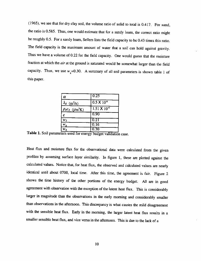
(1965),weseethatfor dry claysoil, thevolumeratioof solid to total is 0.417. For sand,

theratio is 0.585.Thus,onewouldestimatethat for asandyloam, thecorrectratiomight

beroughly0.5. For asandyloam,Sellerslists thefield capacityto be0.43timesthisratio.

Thefield capacityis the maximumamountof waterthat a soil can hold againstgravity.

Thuswehaveavolumeof 0.22for thefield capacity.Onewould guessthat themoisture

fractionatwhichtheair at the ground is saturated would be somewhat larger than the field

capacity. Thus, we use wk=0.30. A summary of all soil parameters is shown table 1 of

this paper.

2,s (m2/s)

pscs 0/m3K)

E

w2

Wk

Table 1. Soil parameters

0.25

0.5 X 10.6

1.51 X 10 .6

0.90

0.21

0.16

0.30

used for energy budget validation case.

Heat flux and moisture flux for the observational data were calculated from the given

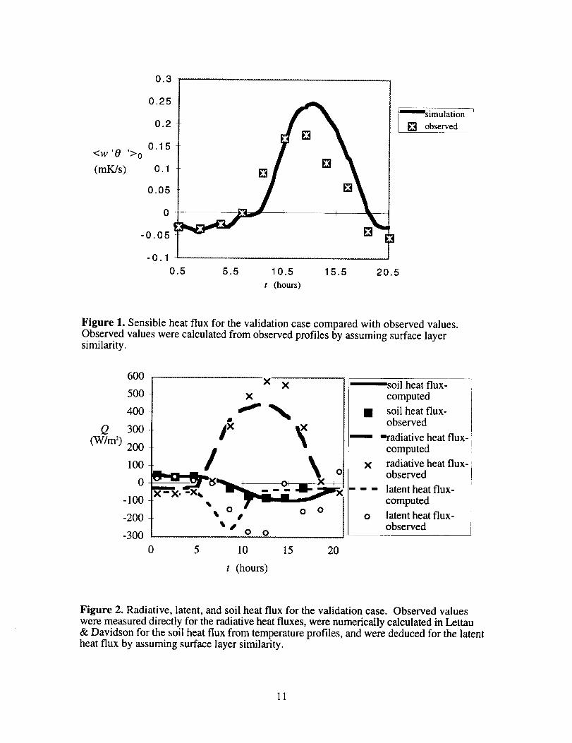
profiles by assuming surface layer similarity. In figure 1, these are plotted against the

calculated values. Notice that, for heat flux, the observed and calculated values are nearly

identical until about 0700, local time. After this time, the agreement is fair. Figure 2

shows the time history of the other portions of the energy budget. All are in good

agreement with observation with the exception of the latent heat flux. This is considerably

larger in magnitude than the observations in the early morning and considerably smaller

than observations in the aftemoon. This discrepancy is what causes the mild disagreement

with the sensible heat flux. Early in the morning, the larger latent heat flux results in a

smaller sensible heat flux, and vice versa in the afternoon. This is due to the lack of a

10

0.3

O. 25 _=_msimulation q

0.2 l [] observed

0.15<W '0 '>0

(mK/s) 0.1

0.05

0

-0.05

-0.1

0.5 5.5 10.5 15.5 20.5

t (hours)

Figure 1. Sensible heat flux for the validation case compared with observed values.

Observed values were calculated from observed profiles by assuming surface layersimilarity.

600

500

400

Q 300

x x

jx

soil heat flux- 1

computed

• soil heat flux-observed

"_- -radiative heat flux-i

computed

radiative heat flux-observed

(W/m2) 200

lOO I \

"-l®-200 • o

-300 J- " " o o l

0 5 10 15 20

latent heat flux-

computed

latent heat flux-observed

t (hours)

Figure 2. Radiative, latent, and soil heat flux for the validation case. Observed values

were measured directly for the radiative heat fluxes, were numerically calculated in Lettau& Davidson for the soil heat flux from temperature profiles, and were deduced for the latentheat flux by assuming surface layer similarity.

11

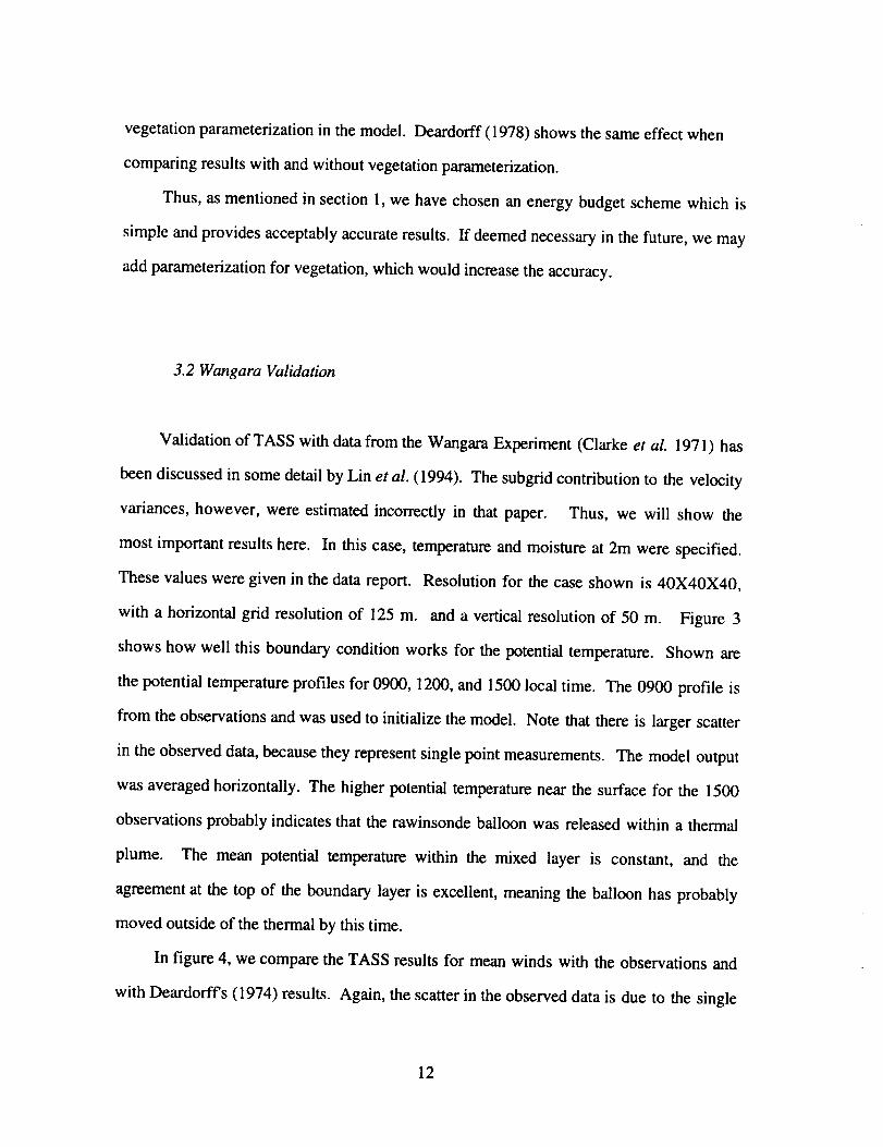
vegetation parameterization in the model. Deardorff (1978) shows the same effect when

comparing results with and without vegetation parameterization.

Thus, as mentioned in section 1, we have chosen an energy budget scheme which is

simple and provides acceptably accurate results. If deemed necessary in the future, we may

add parameterization for vegetation, which would increase the accuracy.

3.2 Wangara Validation

Validation of TASS with data from the Wangara Experiment (Clarke et al. 1971) has

been discussed in some detail by Lin et al. (1994). The subgrid contribution to the velocity

variances, however, were estimated incorrectly in that paper. Thus, we will show the

most important results here. In this case, temperature and moisture at 2m were specified.

These values were given in the data report. Resolution for the case shown is 40X40X40,

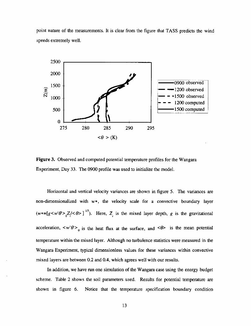
with a horizontal grid resolution of 125 m. and a vertical resolution of 50 m. Figure 3

shows how well this boundary condition works for the potential temperature. Shown are

the potential temperature profiles for 0900, 1200, and 1500 local time. The 0900 profile is

from the observations and was used to initialize the model. Note that there is larger scatter

in the observed data, because they represent single point measurements. The model output

was averaged horizontally. The higher potential temperature near the surface for the 1500

observations probably indicates that the rawinsonde balloon was released within a thermal

plume. The mean potential temperature within the mixed layer is constant, and the

agreement at the top of the boundary layer is excellent, meaning the balloon has probably

moved outside of the thermal by this time.

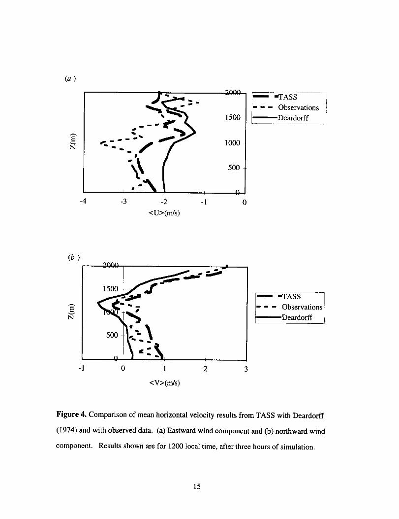
In figure 4, we compare the TASS results for mean winds with the observations and

with Deardorffs (1974) results. Again, the scatter in the observed data is due to the single

12

point natureof themeasurements.It is clearfrom thefigure thatTASSpredictsthe wind

speedsextremelywell.

N

2500

2000

1500

1000

500

0 I

275 280 285 290 295

<0 > (K)

0900 observed

m ,,-- 1200 observed

- - 1500 observed

--- 1200 computed

1500 computed

Figure 3. Observed and computed potential temperature profiles for the Wangara

Experiment, Day 33. The 0900 profile was used to initialize the model.

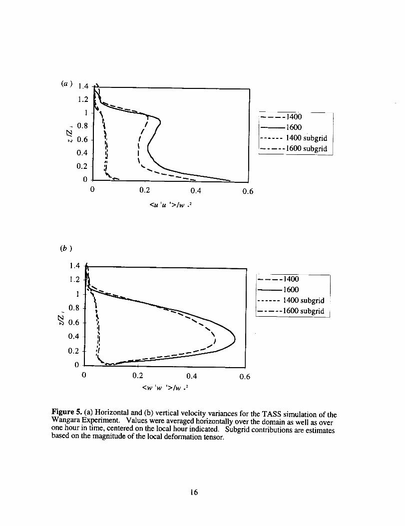
Horizontal and vertical velocity variances are shown in figure 5. The variances are

non-dimensionalized with w., the velocity scale for a convective boundary layer

(w.=[g<w,O,>oZ/<O>] i/3). Here, Z is the mixed layer depth, g is the gravitational

acceleration, <w'0'> is the heat flux at the surface, and </9> is the mean potential0

temperature within the mixed layer. Although no turbulence statistics were measured in the

Wangara Experiment, typical dimensionless values for these variances within convective

mixed layers are between 0.2 and 0.4, which agrees well with our results.

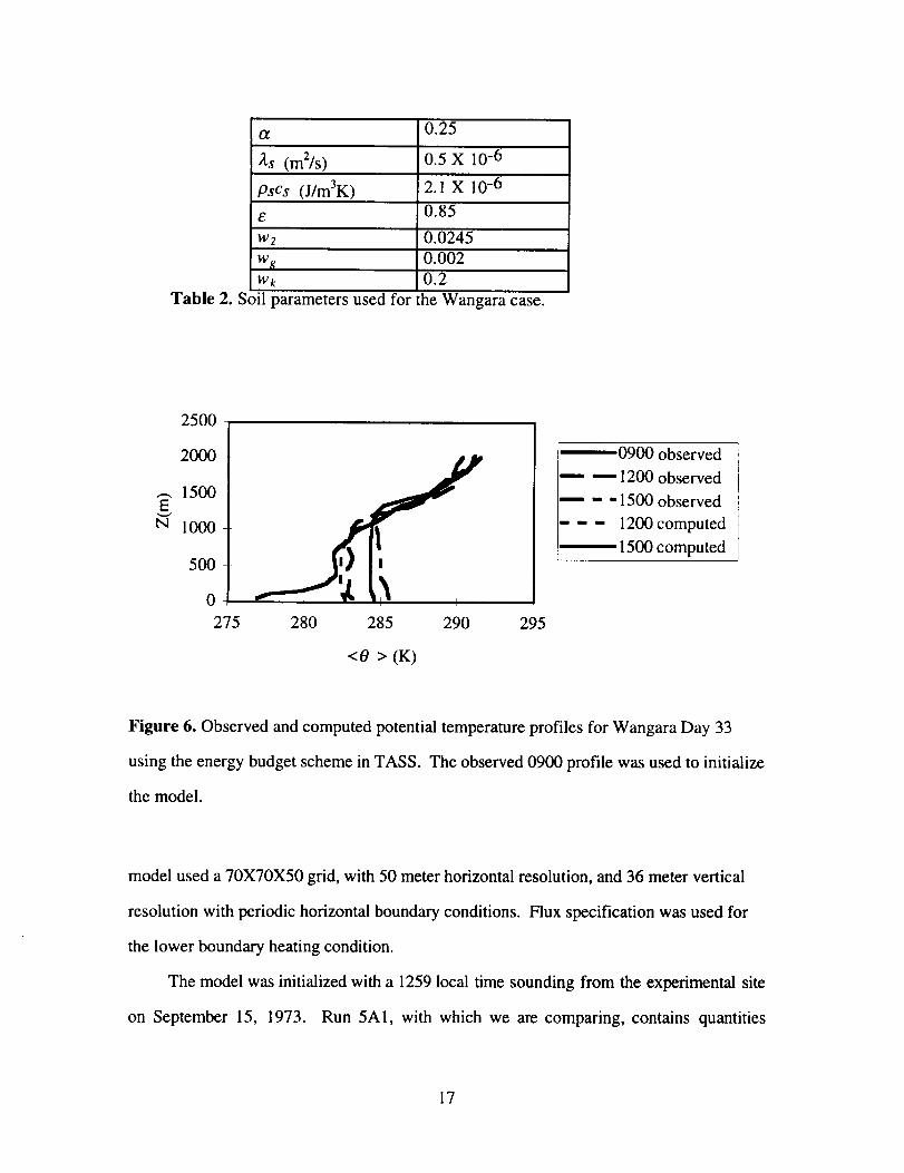
In addition, we have run one simulation of the Wangara case using the energy budget

scheme. Table 2 shows the soil parameters used. Results for potential temperature are

shown in figure 6. Notice that the temperature specification boundary condition

13

(previouslyshown) is muchmoreaccurate.Theenergybudgetresults,however,arejust

asaccurateastheresultsof Pleim& Xiu (1995),whouseda similarsoil modelwith a one

dimensionalsimulationof WangaraDay33.

3.3 Minnesota Validation

Because the Wangara Experiment contained no data on turbulent intensities and

fluxes, it was necessary to look elsewhere for validation of these quantities. We chose the

Minnesota Experiment of 1973 ( Izumi & Caughey, 1976). One of the difficulties in this

case is that the large scale pressure gradients are not known. For example, as previously

mentioned, the geostrophic wind profile may be used by the model. These profiles,

however, were not measured in the experiment. To account for this forcing, we obtained

synoptic network rawinsonde data (available every twelve hours) on the day of the

experiment we chose to simulate. We then performed an objective analysis to extract

geostrophic winds as a function of height within our model domain. This is extremely

important for predicting mean horizontal winds and for comparing momentum fluxes with

observed values. As described in Lin et al. (1994), for a steady flow,

{_ I W t

f((u)-u#) =---_(V )

t W _

f((v)- vg) = -_(u )

where f is the Coriolis parameter, u is the eastward velocity, v the northward

velocity, w the vertical velocity, us and vg denote the geostrophic components, and

denotes averaging. The twelve hour spaced geostrophic wind data was then interpolated in

time to correspond to the middle of our run, remaining constant throughout the run. The

14

(a)

t,q

1500

1000

500

b 0

-4 -3 -2 - 1 0

<U>(m/s)

I

-TASS--- Observations

Deardorff

(b)

tq

1500

5OO

-1 0 I 2 3

<V>(ngs)

-TASS

--- Observations

Deardorff

Figure 4. Comparison of mean horizontal velocity results from TASS with Deardorff

(1974) and with observed data. (a) Eastward wind component and (b) northward wind

component. Results shown are for 1200 local time, after three hours of simulation.

15

(a) 1.4

1.2

1

0.8_ 0.6

0.4

0.2

00 0.2 0.4 0.6

<U 'U '>]W 2

1400

i_-57 16001400 subgrid

- 1600 subgrid

(b)

1.4

1.2

1

0.8

0.6

0.4

0.2

0 I I

0 0.2 0.4 0.6

<W 'W '>/W 2

-,4oo1600

1400 subgridI

l..... 1600 subgrid

Figure 5. (a) Horizontal and (b) vertical velocity variances for the TASS simulation of theWangara Experiment. Values were averaged horizontally over the domain as well as overone hour in time, centered on the local hour indicated. Subgrid contributions are estimatesbased on the magnitude of the local deformation tensor.

16

a 0.25

_t,s (m2/s) 0.5 X 10 -6

pscs (j/m3K) 2.1 X 10 -6

e 0.85

w2 0.0245

0.002

Wk 0.2

Table 2. Soil parameters used for the Wangara case.

EN

2500

2000

1500

1000

500

0

275 280 285 290 295

<0 > (K)

0900 observed

---- "---- 1200 observed

m . . 1500 observed

--- 1200 computed

1500 computed

Figure 6. Observed and computed potential temperature profiles for Wangara Day 33

using the energy budget scheme in TASS. The observed 0900 profile was used to initialize

the model.

model used a 70X70X50 grid, with 50 meter horizontal resolution, and 36 meter vertical

resolution with periodic horizontal boundary conditions. Flux specification was used for

the lower boundary heating condition.

The model was initialized with a 1259 local time sounding from the experimental site

on September 15, 1973. Run 5A I, with which we are comparing, contains quantities

17

averagedfrom 1622to 1737localtime. Thusthemodelis run for over threehoursbefore

thecomparison.Model averagingwas accomplishedby averaginghorizontallyover the

entiredomain.Theseaveragesweretakeneveryfive minutesand, in turn, averagedover

the 75 minutesof theexperiment. Theexperimentalmixedlayer height,Z i, was 1085

meters. The model, however, predicted a height of 1420 meters. This disparity is due

primarily to an overestimate of the heat flux between 1259 and the observation period.

Only the average surface heat flux during the observation period was given.

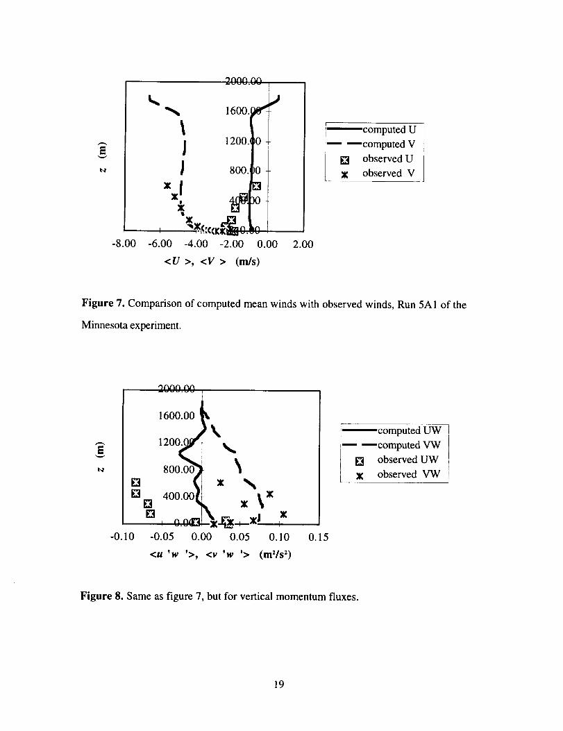
Figure 7 shows a comparison of observed and modeled average winds. The overall

magnitude is in good agreement, but the observed winds show a large shear within the

mixed layer. This is most probably due to a mesoscale effect which could not be captured

by the geostrophic wind profiles deduced from the synoptic data. This brings us to figure

8, which shows the vertical momentum fluxes as a function of height. The flux of

northward momentum, <v'w'>, is in excellent agreement with the observed values. The

flux of eastward momentum, <u'w'>, is in fair agreement. The curve's shape is similar to

the observed profile, but the magnitudes do not agree higher up in the mixed layer. Again,

this is a mesoscale effect and the results are quite good considering the data available for

our synoptic forcing.

18

_vvv.vv i

1600.

JJ

-8.00 2.00

1200. 0

800. 0

x[ i_l

I , ":._(.._._,m .....

-6.00 -4.00 -2.00 0.00

<U>, <V> (m/s)

computed U--- _computed V

[] observedU

X observed V

Figure 7. Comparison of computed mean winds with observed winds, Run 5A 1 of the

Minnesota experiment.

1600"O0_k

1200._- _,

8ooo_ x _%,

400.00_ X _X

-0.10 -0.05 0.00 0.05 0.10 0.15

m -'_computed VW

[] observed UW

X observed VW

computed UW

<U t W t t>'>, <v w (m'/s _)

Figure 8. Same as figure 7, but for vertical momentum fluxes.

19

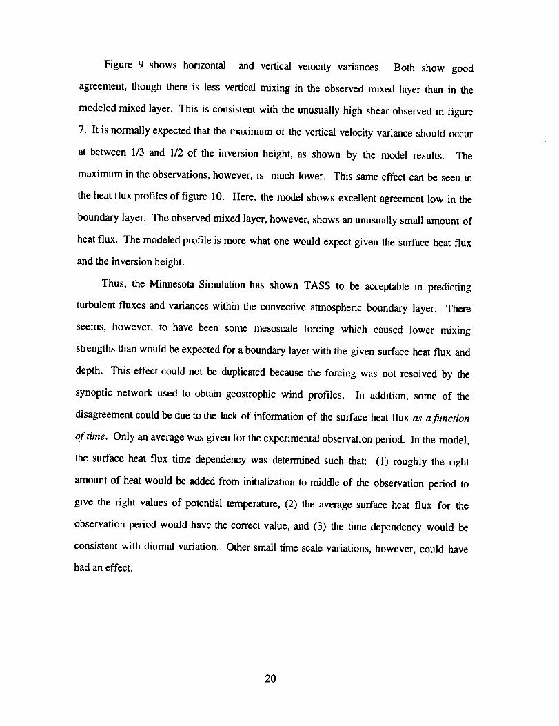
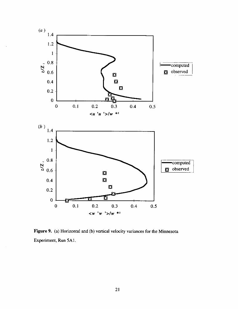
Figure 9 shows horizontal and vertical velocity variances. Both show good

agreement,thoughthereis lessverticalmixing in the observedmixed layer than in the

modeledmixedlayer. This is consistentwith theunusuallyhighshearobservedin figure

7. It isnormallyexpectedthat themaximumof theverticalvelocityvarianceshouldoccur

at between1/3 and 1/2 of the inversionheight, as shown by the model results. The

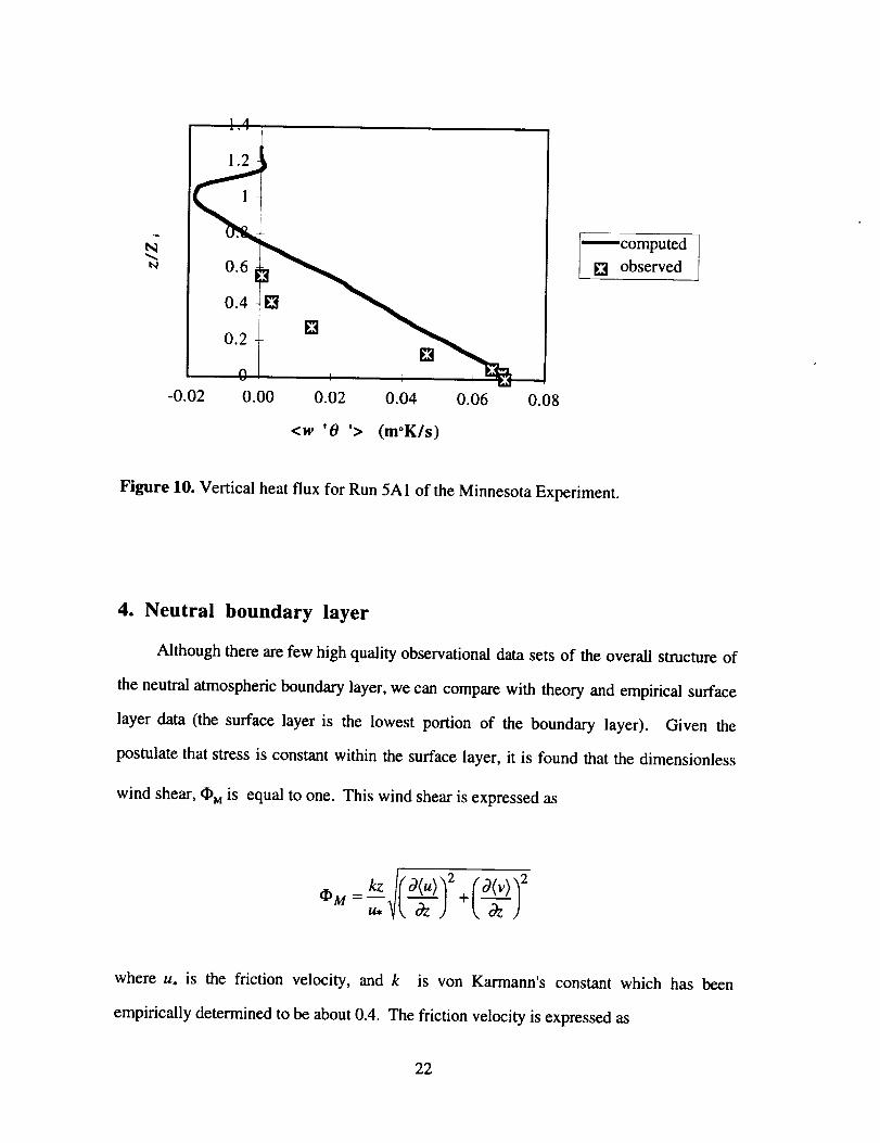
maximumin theobservations,however,is muchlower. This sameeffectcanbe seenin

theheatflux profilesof figure 10. Here,themodelshowsexcellentagreementlow in the

boundarylayer. Theobservedmixedlayer,however,showsanunusuallysmallamountof

heatflux. Themodeledprofile is morewhatonewould expectgiventhesurfaceheatflux

andtheinversionheight.

Thus, the MinnesotaSimulationhas shown TASS to be acceptablein predicting

turbulentfluxesandvarianceswithin theconvectiveatmosphericboundarylayer. There

seems,however, to have been some mesoscaleforcing which causedlower mixing

strengthsthanwouldbeexpectedfor a boundarylayerwith the givensurfaceheatflux and

depth. This effectcouldnot be duplicatedbecausethe forcing wasnot resolvedby the

synopticnetwork usedto obtaingeostrophicwind profiles. In addition, someof the

disagreementcouldbedueto thelackof informationof thesurfaceheatflux as a function

of time. Only an average was given for the experimental observation period. In the model,

the surface heat flux time dependency was determined such that: (1) roughly the right

amount of heat would be added from initialization to middle of the observation period to

give the right values of potential temperature, (2) the average surface heat flux for the

observation period would have the correct value, and (3) the time dependency would be

consistent with diurnal variation. Other small time scale variations, however, could have

had an effect.

20

(a)

1

0.8_q

0.6

0.4

0.2

0

[][]

[]

_-computed[] observed

(b)

1

.. 0.8

0.6

0.4

0.2

0

[]

[]

[]

0 0.1 0.2 0.3 0.4 0.5

<W tW _>]W *_

_computed

[] observed

Figure 9. (a) Horizontal and (b) vertical velocity variances for the Minnesota

Experiment, Run 5A1.

21

1.2

0.6

0.4

-0.02 0.00 0.02 0.04 0.06 0.08

<w 'O '> (m°K/s)

----computed t

[] observed

Figure 10. Vertical heat flux for Run 5A1 of the Minnesota Experiment.

4. Neutral boundary layer

Although there are few high quality observational data sets of the overall structure of

the neutral atmospheric boundary layer, we can compare with theory and empirical surface

layer data (the surface layer is the lowest portion of the boundary layer). Given the

postulate that stress is constant within the surface layer, it is found that the dimensionless

wind shear, @M is equal to one. This wind shear is expressed as

where u. is the friction velocity, and k is von Karmann's constant which has been

empirically determined to be about 0.4. The friction velocity is expressed as

22

='Col p

where % is the surface stress. In addition, the dimensionless scalar gradient, 0 c should be

one. This is expressed as

kz(I) c -

¢,

where -u.c. is the surface flux of the scalar c. In order to compare to other computer

codes, we have duplicated neutral simulations performed by Andren et al. (1994), who

compared four computer codes.

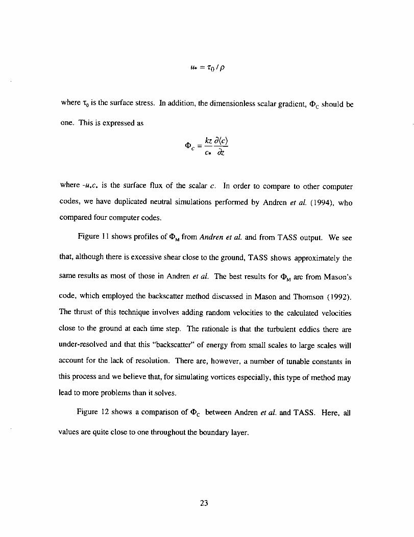
Figure 11 shows profiles of • Mfrom Andren et al. and from TASS output. We see

that, although there is excessive shear close to the ground, TASS shows approximately the

same results as most of those in Andren et al. The best results for • M are from Mason's

code, which employed the backscatter method discussed in Mason and Thomson (1992).

The thrust of this technique involves adding random velocities to the calculated velocities

close to the ground at each time step. The rationale is that the turbulent eddies there are

under-resolved and that this "backscatter" of energy from small scales to large scales will

account for the lack of resolution. There are, however, a number of tunable constants in

this process and we believe that, for simulating vortices especially, this type of method may

lead to more problems than it solves.

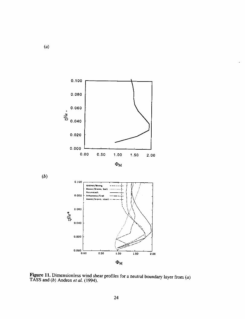
Figure 12 shows a comparison of @c between Andren et al. and TASS. Here, all

values are quite close to one throughout the boundary layer.

23

(a)

0.100

0.080

0.060

_ 0.040

0.020

0.000

0.00 0.50

I I I I

1.00 1.50 2.00

OM

(b)0.100

0.000

o 060

0.040

0,020

0.0000.00

i • " i _ I n . ._d_../uo.., ..... "i- t !l ".... _ ..... b.o, ........... _,. i t ."

Seha.,ann/Cr*r ----"---r-- '_ !1 :

t ; .:

',\.\ \

•" / _l

""/J _ t.,..--.._-

• I * "_ * I n

0.50 1.00 1.50 2.00

OM

Figure ll. Dimensionless wind shear profiles for a neutral boundary layer from (a)TASS and (b) Andren et al. (1994).

24

(a)

0.100

0.080

0.060

.,)(.

"_ 0.040

0.020

0.000

0.00

' ' I I ' I

0.50 1.00 1.50 2.00

(b)

O. IO0

0.080

0060

0.040

0.020

O.OGO

0.00

/u_dren/Moen| ......

Uuon/Drown. b=ct .........

NieuwsLadt --_---_,*_

Seh ..... //Gr_ ---- -T-- ,'_- \ }14_son/IE]rown, nb=ct ...... .L-it

'_¢/ '

f" ,

.!.1.jl I, /

0.50 1.00 1.50

Figure 12. Same as figure 11 but for _c.

2.00

25

5. Summary

In summary, we have added planetary boundary layer simulation capability to TASS

and validated results with observed data. There are several options for the surface

boundary conditions, one of which is a validated surface energy budget using the slab

model. We have made comparisons with both the Wangara and Minnesota boundary layer

experiments and have shown that results compare well with the observed data, especially

considering the limitations in determining initial conditions.

References

Andren, A. Brown, A. R., Graf, J., Mason, P. J, Moeng, C.-H., Nieuwstadt, F.T.M., &

Schumann, U. 1994. Large-eddy simulation of a neutrally stratified boundary layer:

A comparison of four computer codes. Q. J. R. Meteor. Soc., 120, 1457-1484.

Bhumralkar, C. M. 1975. Numerical experiments on the computation of ground surface

temperature in an atmospheric general circulation model. J. Appl. Meteorol. 14,

1246-1258.

Blackadar, A. K. 1976. Modeling the nocturnal boundary layer, Proceedings of the Third

Symposium on Atmospheric Turbulence, Diffusion and Air Quality, pp. 46-49,

American Meteorological Society, Boston, MA.

26

Clarke,R. H., Dyer, A. J., Brook, R. R., Reid, D. G., & Troup, A.J. 1971. The

WangaraExperiment:BoundaryLayerData. CSIRODiv. of Meteorol.Phys. Tech.

PaperNo. 19.

Deardorff,J.W. 1978. Efficientpredictionof groundsurfacetemperatureandmoisture,

with inclusionof a layerof vegetation. J. Geophys. Res. 83 (C4), 1889-1903.

Izumi, Y. & Caughey, S. J. 1976. Minnesota 1973 Boundary Layer Data Report.

Environmental Research Paper No. 547, AFGL, Bedford, MA.

Lettau, H. H. & Davidson, B. 1957. Exploring the Atmosphere's First Mile, vols. 1 and

2. Pergamon, New York.

Lin, Y.-L., Arya, S. P. Kaplan, M. L., & Schowalter, D. G. 1994. Numerical modeling

studies of wake vortex transport and evolution within the planetary boundary layer.

FY94 Annual Report. Grant #NCC- 1-188.

Mason, P.J. & Thomson, D.J. 1992. Stochastic backscatter in large-eddy simulation of

boundary layers. J. Fluid Mech., 242, 51-78.

Pleim, J. E. & Xiu, A. 1995. Development and testing of a surface flux and planetary

boundary layer model for application in mesoscale models. J. App. Met. 34, pp. 16-

32.

Sellers, W. A. 1965. Physical Climatology. University of Chicago Press, Chicago,

Illinois.

27

Staley,D. O. & Jurica, G.M. 1972. Effectiveatmosphericemissivityunderclearskies.

J. Appl. Meteorol. 11, 349-356.

Stull, R.B. 1988. An Introduction to Boundary Layer Meteorology. Kluwer Academic

Publishers, Dordrecht.

Zilitinkevich, S. S. 1970. Dynamics of the Atmospheric Boundary, Layer,

Hydrometeorological Publishing House, Leningrad.

28

Appendix : Directions for using TASS PBL boundary

conditions

To run TASS in the boundary layer mode, one additional input file is needed, fortran unit

7. If this file is not present, the model will run in the original mode In the boundary layer

mode, unit 7 must be present for all restarts, and unit 7 must contain the following

information.

. Five logical variable values, format (5L4) each in the following order: UNHEAT,

TSPEC, FLXSPEC, EBUDG, TKE. UNHEAT refers to uniform heating. If this

variable is true, then a uniform heating is input at the first grid level. The Obukhov

length is not explicitly calculated. TSPEC refers to temperature specification. When

true, the heat and moisture fluxes are calculated by assuming surface layer similarity.

The Obukhov length is explicitly calculated for stress determination. If FLXSPEC is

true, then the heat and moisture fluxes are specified in kinematic units. Again, the

Obukhov length is explicitly calculated. When EBUDG is true, the energy balance

scheme is used to calculate the fluxes. Only one of the previous four variables may be

true, otherwise an error message will appear and the run will be terminated. In

addition, if any of the above variables are true, a random temperature perturbation is

introduced into the first three layers of the domain to start up perturbations on a

resolvable scale. When TKE is true, the amount of turbulent kinetic energy at each

level in z may be specified.

2. X1TMAX, the number of data items for heating specification.

3. Heating data. Each line is free format, with the data in the following order:

29

if UNHEAT=.T.: time in minutes,heatrate in W/m 2, U(m/s) at top boundary,

V(m/s) at top boundary.

if TSPEC-.T.: time in minutes, temperature (C) at Za, humidity (g/g) at Za,

U(m/s) at top boundary, V(m/s) at top boundary.

if FLXSPEC=.T.: time in minutes, heat flux (K-m/s), moisture flux (m/s), U(m/s)

at top boundary, V(rn/s) at top boundary.

if EBUDG=.T.: time in minutes, middle cloud fraction, high cloud fraction,

U(m/s) at top boundary, V(m/s) at top boundary.

4. If TSPEC=.T., then Za appears on the line below the heating data items.

. Logical variable value for GFORCE (L4). If this is true, then the geostrophic wind is

specified and the logical variable NOSTEADY should be set to true. If GFORCE is

false, NOSTEADY may be either true or false.

, If GFORCE is true, the next line must contain a logical value to be assigned to

GWCONST (L4). If GWCONST is true, the geostrophic wind is constant with

height and only one value of the eastward and northward components of the

geostrophic winds need be specified.

7. If GFORCE is true, next comes a line delimited list of geostrophic wind values, with

the eastward component first and the northward component second on each line.

30

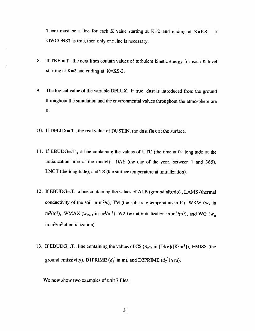
Theremust be a line for eachK valuestartingat K=2 and ending at K=KS. If

GWCONSTis true,thenonly oneline is necessary.

8. If TKE =.T., thenext linescontainvaluesof turbulentkineticenergyfor eachK level

startingat K=2 andendingat K=KS-2.

. The logical value of the variable DFLUX. If true, dust is introduced from the ground

throughout the simulation and the environmental values throughout the atmosphere are

0.

10. If DFLUX=.T., the real value of DUSTIN, the dust flux at the surface.

11. If EBUDG=.T., a line containing the values of UTC (the time at 0 ° longitude at the

initialization time of the model), DAY (the day of the year, between 1 and 365),

LNGT (the longitude), and TS (the surface temperature at initialization).

12. If EBUDG=.T., a line containing the values of ALB (ground albedo), LAMS (thermal

conductivity of the soil in mZ/s), TM (the substrate temperature in K), WKW (Wk in

m3/m3), WMAX (Wmax in m3/m3), W2 (w2 at initialization in m3/m3), and WG (Wg

in m3/m 3 at initialization).

13. If EBUDG=.T., line containing the values of CS (psCs in [J.kg]/[K.m3]), EMISS (the

ground emissivity), D1PRIME (dl' in m), and D2PRIME (d2' in m).

We now show two examples of unit 7 files.

31

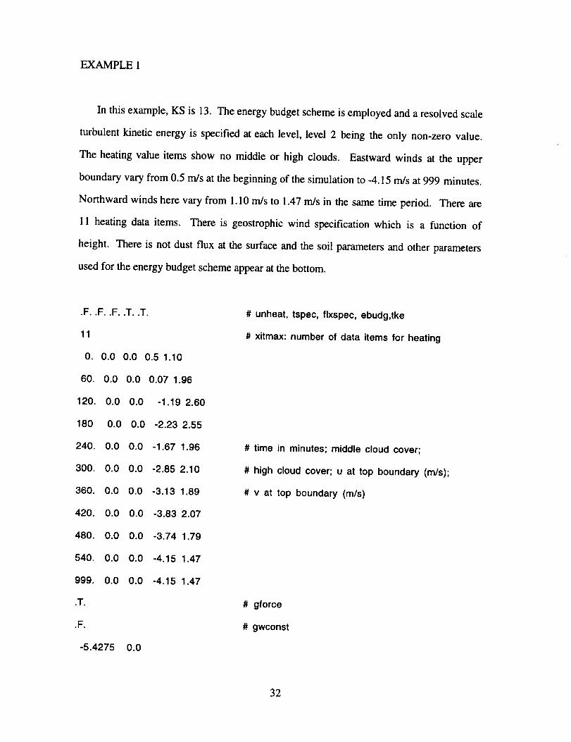
EXAMPLE 1

In this example, KS is 13. The energy budget scheme is employed and a resolved scale

turbulent kinetic energy is specified at each level, level 2 being the only non-zero value.

The heating value items show no middle or high clouds. Eastward winds at the upper

boundary vary from 0.5 m/s at the beginning of the simulation to -4.15 m/s at 999 minutes.

Northward winds here vary from 1.10 rn/s to 1.47 rn/s in the same time period. There are

11 heating data items. There is geostrophic wind specification which is a function of

height. There is not dust flux at the surface and the soil parameters and other parameters

used for the energy budget scheme appear at the bottom.

.F..F..F..T..T.

11

O. 0.0 0.0 0.5 1.10

60. 0.0 0.0 0.07 1.96

120. 0.0 0.0 -1.19 2.60

180 0.0 0.0 -2.23 2.55

240. 0.0 0.0 -1.67 1.96

300. 0.0 0.0 -2.85 2.10

360. 0.0 0.0 -3.13 1.89

420. 0.0 0.0 -3.83 2.07

480. 0.0 0.0 -3.74 1.79

540. 0.0 0.0 -4.15 1.47

999. 0.0 0.0 -4.15 1.47

.T.

.F.

-5.4275 0.0

# unheat, tspec, flxspec, ebudg,tke

# xitmax: number of data items for heating

# time in minutes; middle cloud cover;

# high cloud cover; u at top boundary (m/s);

# v at top boundary (m/s)

# gforce

# gwconst

32

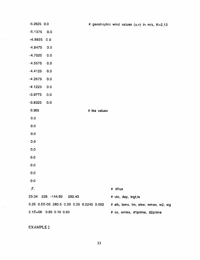
-5.2825 0.0

-5.1375 0.0

-4.9925 0.0

-4.8475 0.0

-4.7025 0.0

-4.5575 0.0

-4.4125 0.0

-4.2675 0.0

-4.1225 0.0

-3.9775 0.0

-3.8325 0.0

0.365

0.0

0.0

0.0

0.0

0.0

0.0

0.0

0.0

0.0

.F.

# geostrophic wind values (u,v) in m/s, K=2,13

# tke values

23.34 226. -144.93 282.43

0.25 0.5E-06 280.5 0.20 0.25 0.0245 0.002

2.1E+06 0.85 0.10 0.50

# dflux

# utc, day, Ingt,ts

# alb, lams, tm, wkw, wmax, w2, wg

# cs, emiss, dlprime, d2prime

EXAMPLE 2

33

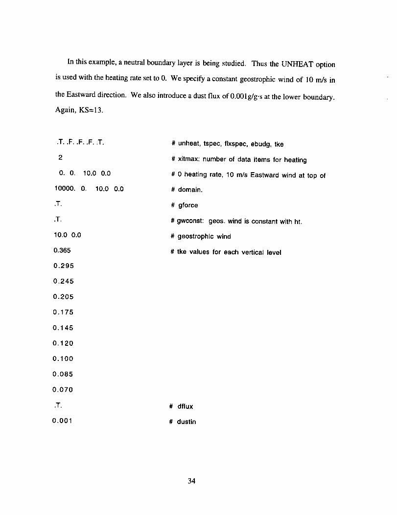
In thisexample,aneutralboundarylayeris beingstudied. ThustheUNHEAT option

is usedwith theheatingratesetto 0. We specifyaconstantgeostrophicwind of 10m/sin

theEastwarddirection.We alsointroduceadustflux of 0.001g/g.satthelower boundary.

Again, KS=13.

.T..F..F..F..T.

2

O.O. 10.0 0.0

10000. O. 10.0

.T.

.T,

10.0 0.0

0.365

0.295

0.245

0.205

0.175

0.145

0.120

0.100

0.085

0.070

.T.

0.001

0.0

# unheat, tspec, flxspec, ebudg, tke

# xitmax: number of data items for heating

# 0 heating rate, 10 m/s Eastward wind at top of

# domain.

# gforce

# gwconst: geos. wind is constant with ht.

# geostrophic wind

# tke values for each vertical level

# dflux

# dustin

34

Form ApprovedREPORT DOCUMENTATION PAGE OMB No. 070,S-01_

Public.mDorbr_l:_m_m,f_ lhB ool_ion ofInformalion11;e_imale(:l1O_ I hour _ rI_oormQ.Im::It_n_thetime1or_ irking'tin,i_u_ _mltm_ dau_ &our_.gsthenng _ .n'mJn_nmg the jOa_aneeded. I_. co_etl_ 0 _ revtpwtng !he G)lkK:_lon Oflnformal,_'l_ Senocommonts m_,_,ng this burden _lmll_ ot ,wry ofhet ,1_ of Ihlscolle0bon of inlormal0on, a'tcluoirvl_suggestions tot reducing lhti I_roen, 10 Walhlr_ I'qlaOquaflors _orvtcel,, Dif_orllll_ lot inlomll_lon Oper_lohs Bid R40o4_, 1215 Jeflmso_ DavisHQhw_y. St/to 1204, Adinglon. VA 222024302, and Io 1he Off¢o ol Manageffv)_ _ Bu_, Papefwo_ Reducllon Pro_ (0704-O188), Washington. DC 20503.

1. AGENCY USE ONLY (LRave b/ank.) 2. REPORT DATE 3. REPORT TYPE AND DATES COVERED

April 1996 Contractor Report4. TITLE AND SUBTITLE

Planetary Boundary Layer Simulation Using TASS

6. AUTHOR(S)

David G. Schowalter, David S. DeCroix, Yuh-Lang Lin, S. Pal Arya, and

Michael Kaplan

7. PERFORMINGORGANIZATIONNAME(S)ANDADDRESS(ES)

Department of Marine, Earth and Atmospheric Sciences

North Carolina State UniversityBox 8208

Raleigh, NC 27695-8208

9. SPONSORING/MONITORING AGENCY NAME(S) AND ADDRESS(F.S)

National Aeronautics and Space Administration

Langley Research CenterHampton, VA 23681-0001

5. FUNDING NUMBERS

NCC 1- 188

538-04-11-11

8. PERFORMING ORGANIZATION

REPORT NUMBER

I10. SPONSORING I MONITORING

AGENCY REPORT NUMBER

NASA CR-198325

11. SUPPLEMENTARYNOTES

Langley Technical Monitor: Fred H. Proctor

12a. DISTRIBUTION I AVAILABILITY STATEMENT

Unclassified-Unlimited

Subject Category 34

12b. DISTRIBUTION COOE

13. ABSTRACT (Maximum 200 words)

Boundary conditions to an existing large-eddy simulation model have been changed in order to simulateturbulence in the atmospheric boundary layer. Several options are now available, including the use of a surfaceenergy balance. In addition, we compare Convective boundary layer simulations with the Wangara andMinnesota field experiments as well as with other model results. We find excellent agreement of modelled meanprofiles of wind and temperature with observations and good agreement for velocity variances. Neutralboundary simulation results are compared with theory and with previously used models. Agreement with theory

is reasonable, while agreement with previous models is excellent.

,14. SUBJECTTERMS

Large-eddy simulation; Planetary boundary layer; Model boundary conditions;Turbulence; Aircraft wake vortices

,17. SECURITY CLASSIFICATION

OF REPORT

Unclassified

NSN 7540-01-280-5500

18. SECURITY CLASSIFICATIONOF THIS PAGE

Unclassified

19. SECURITY CLASSIFICATIONOF ABSTRACT

Unclassified

15. NUMBER OF PAGES

41

16. PRICE CODE

A03

20. UMITATION OF ABSTRACT

Standard Form 298 (Roy. 2-89)Pmorlt_d by ANSI SId. Z39-16298-102