Planetary Boundary Layer TurbulenceIn previous chapters boundary layers were evident as thin layers across which thermal, dy-

namic, and material properties of a free interior flow make a transition to their boundary valuesand/or boundary fluxes. In those cases the thinness of the boundary layer was typically a statementof the smallness of the relevant diffusivity; e.g., the depth h of the laminar Ekman boundary layerscales as ν1/2 (Shear Turbulence) and the thermal boundary layer in convection scales as eitherκ2/3 or κ4/7 in soft or hard turbulence regimes (Convective Turbulence). Boundary layers are alsoevident in geophysical flows, for instance at the bottom of the atmosphere, and at the top and bot-tom of the ocean. And, they serve essentially the same purpose: to match a free or interior flow tothe conditions imposed at the surface, i.e., no-slip, fixed temperature, specified material properties,or specified boundary fluxes.

Unlike boundary layers in many engineering flows, these planetary boundary layers (or PBLs)are almost always turbulent. The turbulence expresses the instability of the laminar boundarylayer solutions, thus giving rise to an effective (eddy) diffusivity that allows the flow to make thetransition between its surface and free-flow properties over a much deeper layer than would occurwith only molecular diffusion and no turbulent mixing. Through this layer turbulent vertical fluxes,w′u′h and w′c′, are expected to be significant in shaping the mean vertical profiles, uh(z) and c(z),where c is any material property. To have any asymptotic utility, the concept of a PBL also requiresthat its depth h remain much smaller than the vertical scale of the free flow. The PBL in the oceanand atmosphere is typically tens or hundreds of meters thick, respectively; this is thin compared tothe 3-10 km depth scale of free oceanic and atmospheric flows. Some authors prefer to define thePBL as that layer of the atmosphere that intensively, or actively, mediates the exchanges with theunderlying surface (in the case of the atmosphere) or the overlying atmosphere (in the case of theocean), but such a characterization fails to ensure the thinness of the layer that is fundamental toits identification as a special layer.

The basic mechanisms for generating turbulence with in the PBL are familiar: shear and buoy-ancy. However these usual suspects take on unusual guises in many geophysical situations. Con-sider the following:

• Shear boundary layers are usually influenced by Earth’s rotation, at least on time scaleslonger than several hours (i.e., Ekman layers). This limits the otherwise unbounded growthin the layer thickness seen in non-rotating shear layers , unless stable stratification furtherlimits the thickness.

• For PBLs in the upper ocean, solar radiation may be absorbed over a depth of order h andmay act to stabilize flows that are otherwise destabilized by a boundary shear stress.

• Both the atmosphere and ocean are two component fluids, whose minor constituents (mois-ture and salinity), contribute significantly to density fluctuations. In the case of the atmo-sphere, the degree that moisture and thermal fluctuations project onto density (buoyancy)depends strongly on whether or not the fluid is saturated.

• In the atmosphere, moisture, and particularly condensed moisture, strongly modulates theemission, absorption, and reflection of radiant streams of energy, and this in turn helps de-termine the rate that radiative processes stabilize or destabilize the flow.

• Infrared emission and absorption confined to thin boundaries — for instance at the top of thePBL in the upper ocean, or along the interior edge of stratocumulus topped boundary layers— can significantly affect the buoyancy forcing of turbulence.

• Surface gravity waves provide a different type of boundary than land and sea-bottom topog-raphy because they are a moving surface. The gravity wave effects are somewhat differentin the air and water marine PBLs. The turbulence above a spatially and temporally varyingboundary is quite different than above a flat boundary, whether smooth or rough.

• In upper ocean PBLs, wave breaking may be an important source of turbulence, while terraineffects and wave breaking may contribute strongly to turbulent transports in stably stratifiedatmospheric PBLs.

b(z)

h

v

v

v

v

τ B

b(z)

hv

v

v

v

τ B

remnant layer

Figure 1: Schematic showing an oceanic mixed layer at night with net infrared and evaporativesurface cooling (left) and a shallower daytime oceanic PBL with solar heating above a remnantlayer (right).

Geophysical boundary layers go through cycles — diurnally, synoptically, and seasonally.Since the sign of B strongly influences the PBL depth h, we often see vertical profiles like thetwo classes sketched in Fig. 1. Under convective forcing, the boundary layer tends to be deeperand its mean profiles more nearly well-mixed. Under stable forcing, the layers are shallower, theprofiles have bigger gradients, and often the residual (or remnant)1 decaying turbulence of a previ-ously deeper PBL layer is evident beyond the currently active one. Convective forcing and/or deeplayers are more prevalent in the oceanic winter (high winds and weak insolation), oceanic night(infrared radiative cooling and evaporation), atmospheric storms (high winds), and atmosphericday (surface heating by insolation). Stable forcing and/or shallow layers are more prevalent in theoceanic summer and daytime (solar absorption), in the atmospheric night (infrared radiative cool-ing), and during weak winds. There are also significant climatological gradients in the PBL depth(e.g., deep convective layers in the atmospheric tropics and oceanic sub-polar zones), as well assynoptic and mesoscale gradients related to their larger eddy flow patterns.

1The atmospheric literature prefers the former terminology, while the oceanic literature prefers the latter.

2

Figure 2: Profiles of dissipation rate ε, θ and σθ taken at four stages of the diel cycle. Clockwisefrom upper left: (a) convective deepening phase; (b) convective equilibrium in a deep mixed layerextending to seasonal thermocline; (c) developing diurnal thermocline; (d) strong diurnal thermo-cline. At left are the estimates of mixed layer depth based on density difference criteria, and at theright are mixed layer depths based on density gradient criteria. The “depth” scale here is pressure,which is mostly hydrostatic with 1 MPa ≈ 100 m. (Brainerd and Gregg, 1995)

3

An illustration of a diel (daily) cycle in the upper ocean is shown in Fig. 2, for both b(z, t) andε(z, t), from microstructure measurements with a slowly dropping instrument. Here the PBL depthvaries from about 10-50 m, and the dissipation rate varies by several orders of magnitude. The waysthat the diel cycle is manifest on the atmospheric winds at two levels is shown in Fig. 3. Duringthe night, when buoyancy stabilizes the flow, the winds at 50 and 0.5 m are strongly differentiated.While during the day, when heating at the surface forces convective eddies that mix a deep layer,the winds are well mixed through 50 m.

Figure 3: Daily march of winds at two levels as observed during day 33 of the Wangara, Australiaexperiment (Sorbjan, 1989)

The daily cycling of the PBL over land — from a shallow, stably-stratified state at night toa deep, well-mixed state during the daytime hours — means that in the morning hours the PBLcan be expected to grow through the remnants of the previous day’s mixed layer. Because thestratification is so weak, this growth can be explosive, at least until the height of the previous day’smixed layer is reached. Thereafter subsequent deepening is slowed by the stratification within thefree-troposphere. This tendency of the previous layer to be left as a residual layer above the nighttime boundary layer can be important to atmospheric chemistry; it separates the previous dayspollutants from emissions at the surface during the night. These are mixed when the boundarylayer re-forms in the morning, and this can be a time of very interesting chemistry. On longertimescales it also can bias estimates of material transport. For example, photosynthesis by plantsduring the day draws down CO2 from the reservoir of a relatively deep, dilute PBL, while itscounterpart, respiration by microbes in the soil, tends to dominate at night when the PBL is stablystratified and shallow. Such effects, when not properly accounted for, produce biases in estimatesof carbon uptake derived from near-surface measurements of CO2 in the atmosphere. Because theseasonal cycle of boundary layer depth correlates with cycles of photosynthesis and respiration,similar biases are also evident on seasonal timescales. Hence an understanding of boundary layerprocesses is critical to the quantification of material budgets.

4

1 Surface Layer

U(z)

zs

h

d

Outer (Ekman) Layer

Inner (Surface or Log) Layerln z

z0

f

-<u'w'> = u*u

*

Figure 4: Schematic of inner and outer layers within the shear PBL.

Although we speak of the PBL as a single layer, it typically is comprised of several layers, asillustrated in Fig. 4 for the case of a neutrally stratified shear layer. Viscous forces and the detailsof the surface may be important on the scale d for the individual roughness elements (centimetersto tens of meters) that defines the roughness sub-layer, while the large eddies, whose scale iscommensurate with the boundary layer depth h � d, dominate the turbulent transport throughthe bulk of the boundary layer. If h and d are sufficiently well separated, there may be a rangeof intermediate scales near, but not immediately abutting, the boundary h � z � d, for whichone can make a similarity hypothesis that z is the only relevant length-scale. Doing so definesthe surface layer. The concept of a surface layer is fundamental to boundary layer turbulence,because it sweeps all of the details of the surface shape under the rug through the definition ofa virtual boundary height z0 that characterizes the surface roughness. The existence of a surfacelayer encourages the nomenclature of the inner and outer layers regions of the PBL as a whole(Fig. 4).

In a neutrally stratified fluid, the surface-layer scaling is just that given in Shear Turbulence,2

i.e., the law of the wall:u(z) = k−1u∗ ln(z/z0) , (1)

where u∗ is the friction velocity (i.e., the square root of the surface stress divided by density) andk = 0.4 is von Karman’s constant. z0 is the roughness length and is defined as the height above thesurface where the extrapolated velocity profile (1) vanishes. Although z0 is determined empiricallyby this extrapolation procedure, for simple rough surfaces (grains of sand) it can be shown to bea function of the height and spatial density (i.e., closely packed versus sparse) of the roughnesselements. Typical values for empirically determined z0 are listed in Table 1. Note that the valuesare typically much smaller than the size d of the actual roughness elements (e.g., a tree in a forest).

2This can be derived most simply as a scaling theory, but it also can be derived more formally as a matchedasymptotic expansion in an overlap region between a smooth-boundary viscous sublayer and an inertial interior layer;see the Shear Turbulence lecture notes.

5

surface z0 [m]water 0.0001 - 0.001bare soil 0.001 - 0.01crops 0.005 - 0.05forest 0.5

Table 1: Approximate roughness heights for various surfaces.

In geophysical flows, rotation might be expected to play a role in the nature of the near surfacematching. The fact that it does not (insofar as the law of the wall is valid) is often expressed in termsof what is called Rossby number similarity, where the surface Rossby number Ro = u∗/(fz0) (ameasure of the ratio of the local vorticity on the scale of roughness elements to the planetaryvorticity) is large. Although planetary rotation can generally be neglected in the surface layer,buoyancy cannot. To incorporate buoyancy into the surface-layer scaling, Obukhov postulated thatthe non-dimensional shear should be a function of the non-dimensional height,

ζ = z/L, where L = − u3∗kB

. (2)

The length-scale L chosen to non-dimensionalize z measures the height where the local productionof turbulence by the shear-stress exactly balances the rate of working against (assuming B < 0)the mean state stability. It is called the Obukhov length (sometimes Monin-Obukhov). Hence ζmeasures the relative importance of shear and buoyancy to the development of turbulence kineticenergy. The shear-flow limit corresponds to L = ±∞ or ζ = 0 (but not z = 0 where the surface-layer formula is not valid). Convective flows have upward buoyancy flux, B > 0, hence ζ < 0.Stable shear boundary layers have B < 0 and ζ > 0; sometimes a distinction is made betweenweakly and strongly stable surface layers based on whether ζ is greater than or less than one.

1.1 Monin-Obukhov Similarity TheoryThe generalization of the law of the wall to account for buoyancy and shear is referred to as Monin-Obukhov (or simply M-O) similarity theory. It postulates that(

kz

u∗

)du

dz= Φm(ζ) . (3)

Here Φm is the non-dimensional shear, also called the non-dimensional flux profile, the flux-gradient relation, or the stability function. To reproduce the law of the wall Φm should approachunity as ζ → 0. Since we expect that the flow will be less stratified when buoyancy contributes tomixing, and more stratified when buoyancy resists mixing, then we might expect that Φm > 1 forζ > 0 and Φm ≤ 1 otherwise. Analogously,(

kz

T∗

)dT

dz= Φh(ζ), (4)(

kz

c∗

)dc

dz= Φh(ζ), (5)

6

where T is temperature and c is some material property (e.g., salinity, or specific humidity). (Foratmospheric flows, it is more appropriate to use θ than T to eliminate compressional heating.) T∗and c∗ are flux scales defined in analogy to u∗ such that:

u∗T∗ = −w′T ′ and u∗c∗ = −w′c′ . (6)

The fact that Φh appears in both (4) and (5) reflects the assumption that the non-dimensionalmaterial gradient function is independent of the particular material property being scaled (thisneed not be true).

1.51.00.5-0.5-1.0-1.5-2.0

1

2

3

4

5

6

-2.5 0

Φm=1+4.7ζ

Φm= (1-15ζ)-1/4

ζ

Φm

Figure 5: Non-dimensional shear function for the Monin-Obukhov similarity model (also calledthe stability function). (Adapted from Businger, 1970, Fig. 2.1)

Many experiments have been conducted to experimentally evaluate the theory, and within therange of expected validity the theory can be considered to be a great success. That is, the non-dimensional gradient functions do indeed exhibit universality given the assumptions of the the-ory (i.e., h � z � d, Ro � 1, steady flow, etc.). An illustration of the ability of this non-dimensionalization to collapse the data is given in Fig. 5, where Φm is derived from a series ofmeasurements made over wheat stubble in Kansas. Many similar measurements have been madeover a wide variety of surfaces with the result being that

Φm ≈

{1 + βmζ ζ > 0

(1− γmζ)am ζ ≤ 0(7)

Φh ≈

{1 + βhζ ζ > 0

(1− γhζ)ah ζ ≤ 0. (8)

For our purposes it is sufficient to take βh = βm = 5, γh = γm = 16, am = −1/4 and ah = −1/2.The actual values of these constants is a matter of some debate with most studies finding that

7

5 < βm < 7, 5 < βh < 9, 16 < γm < 20, and 12 < γh < 16. These fits are accurate for |ζ| valuesthat are not too large, but for |ζ| � 1, little reliable data exists. Instead the general shape of thegradient functions is constrained by asymptotic considerations that, as we shall see below, arguesfor different values of am and ah than those given above.

The general form of (7) and (8) allows one to analytically integrate (3)-(5), thereby yieldingnon-dimensional profile functions:

u(z) =u∗k

[ln(z/z0)−Ψm(ζ) + Ψm(zo/L)] (9)

T (z)− T (z0) = T∗ [ln(z/z0)−Ψh(ζ) + Ψh(z0/L)] (10)

where for ζ ≥ 0Ψm = −βmζ and Ψh = −βhζ . (11)

While for ζ < 0

Ψm = 2 ln

(1 + Φ−1m

2

)+ ln

(1 + Φ−2m

2

)− 2 tan−1(Φ−1m ) +

π

2(12)

Ψh = 2 ln

(1 + Φ−1h

2

). (13)

We should note that T (z0) is not necessarily the surface temperature, but for simple surfaces itshould be close to this value, and so we will subsequently take it as such. Actually estimatingthe flux, given T (z) and u(z), requires us to solve the equations above for u∗ and T∗. BecauseL depends on u∗ and T∗, this is not as trivial a procedure as we might hope, nonetheless thedependencies are simple enough in the stable case to yield closed form expressions. In the unstablecase we must resort to iteratively solving a system of implicit equations for the flux.

It is difficult to overstate the importance of these results. They provide a means for estimatingthe flux from the profiles and are used in some form in virtually every atmospheric or oceanic flowsolver that requires some surface boundary conditions. They are undoubtedly the most importantresult from similarity theory in atmospheric and oceanic sciences.

1.2 Monin-Obukhov ExtensionsEddy Viscosity and Dissipation: Accompanying the mean profiles are other log-layer proper-ties: (1) the eddy momentum flux is in the direction of the mean surface stress eτ and is constantwith height in the surface layer,

u′w′(z) = − eτu∗2 ; (14)

(2) the eddy viscosity varies linearly with height,

νe(z) = − u′w′

∂zu= ku∗z ; (15)

and (3) the kinetic energy dissipation varies inversely with height,

ε(z) = νe(z)(∂zu)2 =u3∗kz

, (16)

where obviously the final relation cannot be taken all the way to z = 0. With MO similarity, thereare stability-function generalizations of these relations.

8

Mixing-Length Theory: The non-dimensional gradients implicitly embody the mixing-lengthhypothesis. For

Km = −u′w′(du

dz

)−1(17)

and similarly for Kh, MO theory requires that

Km = kzu∗Φ−1m (18)

Kh = kzu∗Φ−1h . (19)

These indicate that in a mixing length theory of turbulent flows Km and Kh should depend on thestability following the stability dependence of Φh and Φm. From the result in previous chapters,we do not expect turbulence for Ri values greater than about 1/4. Thus we expect the empiricallyderived values of Φm and Φh to become infinite as the stable stratification increases, L decreases,and ζ increases, and indeed they do. Equations (18) and (19) also provide a basis for deriving aturbulent Prandtl number

Pre =Km

Kh

=Φh

Φm

. (20)

Thus we see, for stable through neutral coefficients, (7) and (8) imply a Pre value one. As theflow becomes increasingly convective, Pre decreases, indicating rather more efficient turbulenttransport of heat relative to momentum, as could be expected from the transport efficiency ofbuoyant plumes.

Higher-Order Moments: The similarity hypothesis does not need to be restricted to a scaling ofthe mean gradients. It can be extended to non-dimensionalize second- and higher-order moments.The same experiments that demonstrated the universality of Φm and Φh also demonstrate that thesecond order quantities, when appropriately non-dimensionalized, are also universal. So that

u′iu′j

u2∗= Φij(ζ),

u′T ′

u∗T∗= Φ1θ(ζ),

T ′T ′

T∗T∗= Φθθ(ζ), and

θεz

u3∗= Φε(ζ) . (21)

Free Convection: A special limit of the MO theory is free convection, wherein ζ → −∞. Inthis limit it has been proposed that the surface stress (effectively u∗) ceases to be a parameter,hence the list of parameters produces no non-dimensional parameters, and similarity implies thatnon-dimensional profiles must be universal. Here, following Wyngaard et al. (1971), the availableparameters allow us to define the local convective velocity and temperature scales,

wf = (Bz)1/3 (22)

Tf = (g/θ0)−1 Bwf

(23)

that are used as the basis for arguing that

kz

Tf

dT

dz= const. . (24)

9

Equation (24) implies that the temperature profile near the surface should scale as z−1/3. Multiply-ing both sides of (24) by u∗/wf suggests that

limζ→−∞

Φh ∝ −ζ−1/3 . (25)

We note that this limit is not respected by the empirical fit given in (7). The differences in ex-ponents are, however, not large (-1/2 versus -1/3), and it may well be that the data underlying(7) is insufficient to constrain the asymptotic behavior of the fit. Attempts to correct for this andconstrain the shape of Φm and Φh based on asymptotic corrections have led to a wide variety ofproposals for their basic form, most of which are very similar in regions well constrained by data(i.e., occur commonly in nature).

Figure 6: Φ1/233 and Φ

1/2θθ based on data from the Kansas field program of the AFCRL. (Wyngaard

et al., 1971)

Free convective scaling can also be used as a basis for arguing that

w′w′

w2f

= const. , (26)

hence thatlim

ζ→−∞Φ33 ∝ −ζ2/3 . (27)

This is the variance of vertical velocity that can be expected to increase with z2/3 in the surfacelayer (i.e., for z values much less than the depth of the PBL). Empirical support for this scalingrelation, and a similar scaling applied to Φθθ, is shown in Fig. 6. Similar arguments would alsosuggest that Φ11 ∝ Φ22 ∝ z2/3, which is not supported by the data. In the case of the non-dimensional variances of horizontal velocity, it appears that other factors are important, most likelythe large-eddies whose splatting at the surface induces outer-scale fluctuations in the variances ofu and v that might be expected to scale with the PBL depth h (not accounted for in the abovearguments).

10

hm

= 528mhB

hθ

δ = 406m

290 292.555 θ [K]

dθ/dz = Γ [Km-1]z [m]

θ

θi

θm

∆mθ

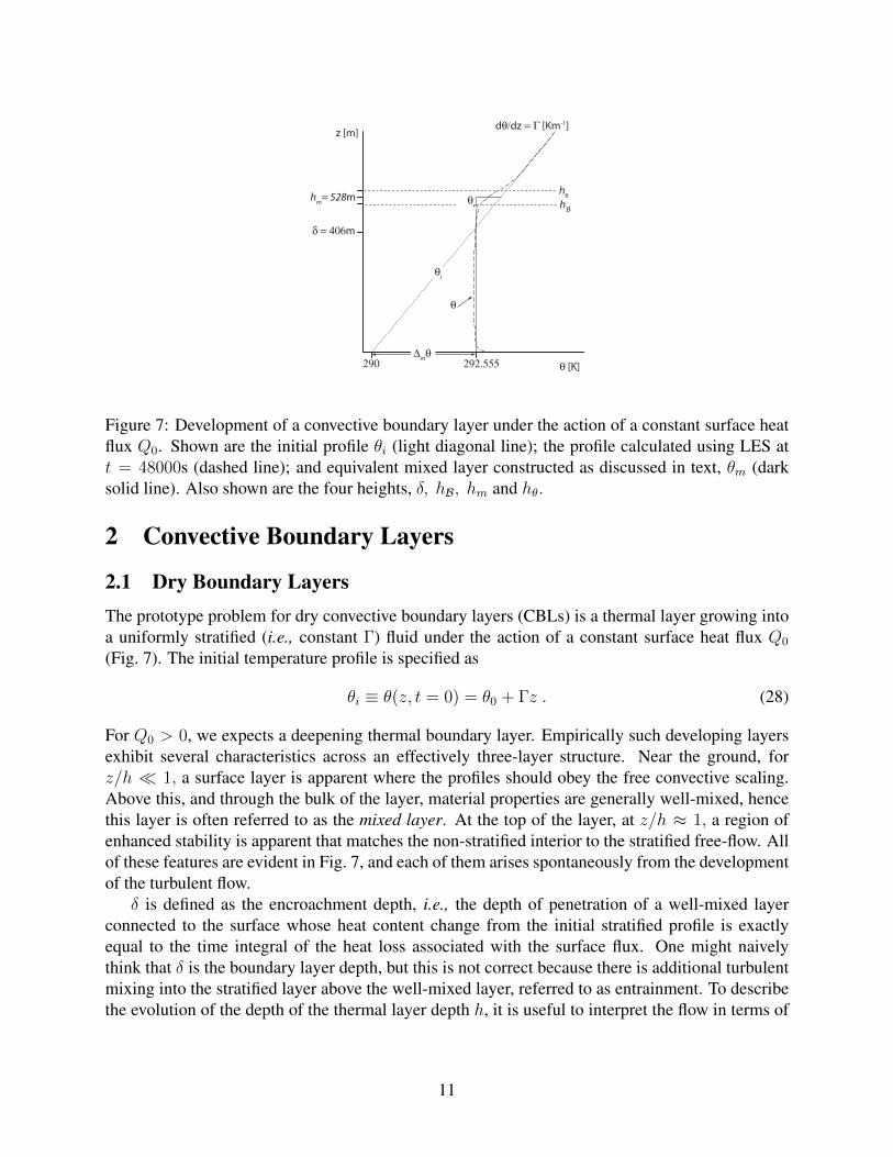
Figure 7: Development of a convective boundary layer under the action of a constant surface heatflux Q0. Shown are the initial profile θi (light diagonal line); the profile calculated using LES att = 48000s (dashed line); and equivalent mixed layer constructed as discussed in text, θm (darksolid line). Also shown are the four heights, δ, hB, hm and hθ.

2 Convective Boundary Layers

2.1 Dry Boundary LayersThe prototype problem for dry convective boundary layers (CBLs) is a thermal layer growing intoa uniformly stratified (i.e., constant Γ) fluid under the action of a constant surface heat flux Q0

(Fig. 7). The initial temperature profile is specified as

θi ≡ θ(z, t = 0) = θ0 + Γz . (28)

For Q0 > 0, we expects a deepening thermal boundary layer. Empirically such developing layersexhibit several characteristics across an effectively three-layer structure. Near the ground, forz/h � 1, a surface layer is apparent where the profiles should obey the free convective scaling.Above this, and through the bulk of the layer, material properties are generally well-mixed, hencethis layer is often referred to as the mixed layer. At the top of the layer, at z/h ≈ 1, a region ofenhanced stability is apparent that matches the non-stratified interior to the stratified free-flow. Allof these features are evident in Fig. 7, and each of them arises spontaneously from the developmentof the turbulent flow.

δ is defined as the encroachment depth, i.e., the depth of penetration of a well-mixed layerconnected to the surface whose heat content change from the initial stratified profile is exactlyequal to the time integral of the heat loss associated with the surface flux. One might naivelythink that δ is the boundary layer depth, but this is not correct because there is additional turbulentmixing into the stratified layer above the well-mixed layer, referred to as entrainment. To describethe evolution of the depth of the thermal layer depth h, it is useful to interpret the flow in terms of

11

an equivalent mixed layer depth hm that we define as

hm =∆mθ

Γ

(1 +

√1 +

2Q0Γt

(∆mθ)2

), (29)

where

∆mθ ≡(

2Γ

∫ ∞0

(θ − θi)H(θ − θi) dz

)1/2

, (30)

with H(x) the Heaviside function. ∆mθ measures the entropy increase of the component of theboundary layer that has warmed compared to the initial state. Hence hm measures the depth ofa mixed layer whose region of warming has the same mean potential temperature as the actuallayer of interest. To make this definition energetically consistent, θ should be replaced by θv whenworking with moist layers, while for freely convecting oceanic layers a description simply in termsof T will suffice. Note that the definition of ∆mθ above defines the potential temperature of thismixed layer as θm = θ0 + ∆mθ,; this also being illustrated in Fig. 7.

The equivalent mixed-layer depth hm differs from more familiar measures of the PBL depth,such as hθ, which associates the boundary layer depth with the height where ∂zθ is a maximum,or what we call hB, the height where the buoyancy flux profile, B(z), is a minimum. However,because hm is based on an integral measure of the PBL heat content, it tends to provide a morerobust estimate of the PBL depth than either hθ or hB, both of which depend on the structureof a profile at a point. Both hθ and hB may be more suitable for empirical studies, where theinitial state temperature profile may be ill-defined, but they tend to be ill-defined for the mixed-layer idealization of the PBL thickness that motivates the introduction of hm. For comparison,one can imagine a well-mixed boundary layer that is nowhere gravitationally unstable and extendsno farther into the stratified interior region than is required by the growing heat content imposedby the positive surface heat flux Q0. This is sometimes called encroachment or non-penetrativeconvection, with

θ(z, t) ≥ θi(z) ∀{z, t} =⇒ (∆mθ)2 = 2ΓQ0t hence h = δ ≡

(2Q0t

Γ

)1/2

. (31)

so h is well defined and is equal to the encroachment depth δ. To the extent the actual boundarylayer profile approaches a well-mixed shape, these various measures of h converge to the samevalue, although in reality departures from well-mixed tend to result in δ < hB < hm < hθ. Thestatement that δ is smaller than the other depth measures is equivalent to the statement that somefluid from the stably stratified region aloft is being drawn into the actively turbulent boundary layer,i.e., entrainment of warm interior air is occurring (Fig. 8).

For small diffusivities, large temperature gradients can be expected to develop that for suffi-ciently small viscosity will lead to the development of convective eddies and turbulent circula-tions within the boundary layer. These eddies are responsible for the homogenization of the flowthrough the depth of the boundary layer and initiate additional mixing (entrainment) between thefree-troposphere and the surface. An example of such processes is illustrated in Fig. 8; it showsthe spatial structure and temporal evolution in the vicinity of a convective plume impinging on theregion of stable stratification topping the mixed layer. The overshooting of the eddy flow results inthe region of enhanced stratification near the top of the PBL and is accompanied by the engulfment

12

Sullivan et al., J. Atmos. Sci. (1998)

Figure 8: Temporal and spatial evolution of the entrainment interface in a sub-domain of a convec-tive boundary layer as represented by large-eddy simulation. Temperature is contoured, and flowvectors are shown by arrows. For clarity only every third vertical, and every second horizontal gridpoint is shown. Panels (b)-(h) are 107, 134, 161, 228, 255, 295, and 335 s, respectively, later than(a). (Sullivan et al., 1998)

13

of free tropospheric air at its edges. This expresses the entrainment process, at least for situationswhere convective eddies are sufficiently strong relative to the overlying stratification to penetrateinto the stable layer capping the PBL. The warm air that mixes down as a result of entrainmentcauses the boundary layer to warm more rapidly, such that ∆mθ > 2ΓQ0t, from which it followsthat h > δ. Without loss of generality we can express this by writing

h = Aδ , (32)

where A ≥ 1 measures the amount of entrainment.The advantage of this prototype problem is that the paucity of parameters allows us to constrain

A on purely dimensional grounds. In the Boussinesq limit the equations admit three fundamentaldimensions (distance, time, and energy/temperature) and six parameters: Γ, Q0, t, g/Θ, as wellas the molecular viscosity ν and thermal diffusivity κ. This leads to the identification of threenon-dimensional numbers

π1 =ν

κ, π2 = (tN)1/3, and π3 =

(t

N2

)2/3 Bκ. (33)

Here π1 is the Prandtl number that is fixed by the fluid’s material properties. Based on a subsequentinterpretation of the energetics it is straightforward to show that π2 can be interpreted as a ratio ofthe convective time scale in the boundary layer to that of gravity waves above the layer, while π3can be interpreted as the ratio of a convective time-scale to a diffusive timescale across the layer— effectively a Rayleigh number. Based on these considerations A = A(π1, π2, π3).

Because κ/B is typically much less than N2, for t � 1/N ≈ 100 s both π2 and π3 aremuch larger than unity. This motivates the assumption of complete similarity in π2 and π3; this isequivalent to saying that

limπ2,π3→∞

A∣∣∣∣π1=const.

= A , (34)

and that A is a universal O(1) constant. Physically we can think of A as measuring how deep amixed layer, constrained to match the heat content in both the warmed layer and overall, must be.This interpretation is illustrated graphically in Fig. 7, where θm and hm were calculated from anactual large-eddy simulation using the methods outlined above.

The entrainment constant A can be further constrained energetically. For instance, given h ,

∆+θ ≡ θi(h)− θm =(1− A−2

) hΓ

2, (35)

which defines the operator ∆+ that measures a difference in the bulk value of a quantity andits value just above the PBL. An equivalent mixed layer growing at the same rate as the actualboundary layer is characterized by a heat flux that is linear with height and discontinuous at h. Itsvalue at h− ε can be obtained by integrating over the discontinuity, (e.g., Lilly, 1968) such that

Qh− = −∆+θdh

dt= Q0(1− A2) . (36)

Choosing A2 = 6/5 yields the entrainment law, Qh−/Q0 = −1/5, equivalently, Bh−/B0 = −1/5,that is frequently the basis of parameterizations. This relation can be expressed in terms of the

14

non-dimensional entrainment velocity, we, scaling with a bulk Richardson number, such that

wew∗

=µ

Riwhere Ri ≡ g∆+θh

θ0w2∗

(37)

and µ = 1/5. This is equivalent to a statement that the entrainment heat flux is a constant fractionof the surface flux,

we∆+θ = −µQ0 . (38)

Furthermore, analogous to the encroachment relations in (31) and with reference to the mixed-layersketch in Fig. 7, the penetrative-convection mixed-layer properties are the following:

hm =

(2Q0t

Γ

)1/21 + µ√1− µ

, δm =hm

1 + µ,

∆mθ =

(2Q0Γt

1− µ

)1/2

, ∆+θ = µ∆mθ . (39)

That is, with penetrative convection the bulk temperature is warmer and the layer is deeper thanwith simple encroachment convection.

What is missing in this mixed-layer model is a characterization of the entrainment layer thick-ness, because it is idealized as a zero-thickness temperature jump at the top; however, a plausibleextrapolation is that a self-similar evolution in the profile θ(z) will have all vertical lengths scale∝ hm(t), in particular it will be thinner when Γ is stronger.

In general, θ(z), or any material property for that matter, will not be discontinuous at h and theheat (equivalently buoyancy) flux at h will depend on the vertical structure of the boundary layer.That said, to the extent our similarity hypothesis is valid, then the particular profile of θ(z, t) mustgrow self-similarly in time (to do otherwise would imply a dependence on either π2 or π3) andhence the non-dimensional profile of θ must be universal; this means that the actual buoyancy fluxat h, or the actual rate of change of θ over some distance at h, will be related by fixed constants(determined by the actual boundary layer structure) to the values determined for an equivalentmixed layer. The requirement that B > 0 places an upper bound on A of

√2.

Knowing the structure of the equivalent mixed layer buoyancy flux allows us to specify a ve-locity scale, w∗ based on the dissipation rate, ε, of turbulence kinetic energy averaged across thelayer. Doing so doing yields

w∗ = Aε [εh]1/3 = Aε

[Bh]1/3

, (40)

in the limit dh/dt � w∗, and with a vertical average over h denoted by the carat. ChoosingA3ε = 2(2 − A2)−1 for the order unity prefactor yields w∗ = (B0h)1/3 in the mixed layer limit.

This velocity scale is analogous to wf , discussed earlier to scale free convection in the surfacelayer. It was originally proposed by Deardorff (1970). Given w∗ it is straight forward to define theturbulence timescale τ∗ and a turbulent temperature θ∗ = Q0w

−1∗ . The latter allows us to define an

effective Rayleigh number,

Ra ∝ gh3θ∗Θ0νκ

=B

2/30 h8/3

νκ=π3π1

(2A2

)4/3, (41)

15

z/h

u’2/w*

2 w’2/w*

2v’2/w*

2

0.2

0.4

0.6

0.8

1.0

0.2 0.4 0.6 0.2 0.4 0.6 0.2 0.4 0.6

Minnesota 1973 1.8(z/h)2/3(1-0.8z/h)2

Figure 9: Convective, or mixed-layer, scaling of convective layer variance budgets (Lenschow etal., 1980).

from which our interpretations above of π2 and π3 originate.The convective (or mixed-layer) scaling used to non-dimensionalize the mean PBL structure

can, in analogy to the treatment of the surface layer, also be used to non-dimensionalize higher-order moments through the mixed layer. For example, Fig. 9 demonstrates the ability of convectivelayer scaling to collapse the variance profiles of u, v and w over the depth of many convectivelayers, with h varying by a factor of three, and w∗ varying by a factor of 2.5. The tendency forww/(w∗w∗) to peak at a value between 0.4 and 0.5, roughly a third of the way up in the PBL isalso evident in simulations and convection tank experiments, and is a hallmark of turbulence inconvective PBLs.

Convective Layer Momentum Budgets In the presence of a weak interior flow, Ug, the meanvelocity profile must still satisfy the momentum balance equations. In a CBL U is assumed tobe uniform in the mixed layer, with u′hw

′ linearly proportional to z. The eddy fluxes at the topof the mixed layer are assumed to be related to velocity differences across the entrainment layer,somewhat analogous to the heat-flux relation in (36), e.g.,

u′w′(zi) = −we(Ug − U) , v′w′(zi) = −weVg , (42)

where we now have oriented the axes such that V = 0 in the mixed layer (hence the surface stressis only in the x direction, with u′w′(0+) = −u2∗). Using this in the PBL momentum budget, weobtain integral relations for the CBL momentum balances,

−we(Ug − U) + u2∗ = −fhVg (43)−weVg = fh(Ug − U) . (44)

We can solve these exactly given u∗ and we, and the latter can be obtained from w∗ and Ricbl by(37).

16

A particularly simple solution arises if we make the approximation, Roe = we/fh � 13,viz.,

Ug − Uu∗

= −RoeVgu∗

= Roeu∗fh

+O(Ro2e) (45)

Vgu∗

= − u∗fh

+O(Ro2e). (46)

Thus, Vg < 0 and Ug > U here, with U2 < U2g + V 2

g . Since the mixed layer velocity is in the xdirection, the turning angle can be defined by

tan[β] = − VgUg≈ u∗

Ug

u∗fh, (47)

and β is often small. In particular, for Ug = 10 m s−1 and the other values mentioned previously,a typical value is u∗ = 0.5 m s−1, hence β ≈ 14o. This β value is much less than that foundin the non-convective Ekman PBL, where β ≈ 30o in the turbulent regime or 45o in the laminarregime (i.e., with constant eddy viscosity).

Transport Asymmetry: We can consider three types of scalar fields in the CBL: the activescalar b that is forced in a destabilizing way by the flux at z = 0 and in a partly compensating,stabilizing way at z = h due to the inversion; a passive scalar being transported from the inte-rior towards the boundary (sometimes called “top-down” when the boundary is at the bottom)where the surface flux is zero; and a passive scalar being transported away from the boundary(i.e., “bottom-up”) because of a flux at z = 0. Remarkably, each of these has a different transportstructure, as expressed in terms of an eddy diffusivity, κe(z). The cause of this asymmetry is inthe driving at the flow, where the bottom-up flux is destabilizing while the top-down buoyancy fluxstabilizes the flow (cf., Rayleigh-Benard convection where both boundary fluxes are destabilizing).As a result it is not surprising that transport away from the boundary — in association with risingbuoyant plumes — is more efficient by this measure than towards it, by a factor of 2-3. These aresketched in Fig. 10.

A further consequence of this asymmetry is that the active scalar diffusivity even becomessingular for the buoyancy flux in the middle of the layer where db/dz changes sign and w′b′ doesnot (further discussed in Sec. 6). Also, since Km(z) ≤ 0.1w∗h, an eddy Prandtl number,Pre = Km/Kh, is < 1 for all three types of scalars. Because of the combination of thesurface flux and the entrainment-layer flux, the vertical profile of buoyancy flux can be view as asuperposition of top-down and bottom-up scalar transports.

Because of this variety of behavior, we must conclude that local eddy diffusion is not a fun-damentally correct characterization of turbulent transport in the CBL, hence a more non-local de-scription is required (i.e., one incorporating knowledge of the surface fluxes and interior gradientsand permitting finite turbulent fluxes at levels with zero or reverse-sign mean gradient). The cir-culation pattern underlying the non-local transport, of course, is the coherent plumes. The plumedynamics control the vertical profiles of variance and skewness for turbulent vertical velocity in

3To illustrate this for an atmospheric CBL, consider the following numerical values: B = (g/To)(100 Wm−2)/(ρcp = 103 J m−3 K−1) = 3−3 m2 s−3, h = 103 m, w∗ ≈ 1 m s−1, we ≈ 0.01 m s−1 (i.e., ≈ 1km day−1), f = 10−4 s−1, w∗/fh ≈ 10, Roe ≈ 0.1.

17

Figure 10: Sketches of the mean and eddy flux profiles, the mean gradient, and the diagnosed eddydiffusivity for scalar fields in a convective atmospheric boundary layer: (left) bottom-up transportfrom surface flux and (right) top-down transport from entrainment flux. (Wyngaard and Brost,1984)

z/h

1.0

0.8

0.6

0.4

0.2

0.60.40.2w2/w

*2 w3/w

*3

0.0 0.2 0.30.1

Figure 11: Convective, or mixed-layer, scaling of convective layer variance budgets (Moeng andWyngaard, 1989). Left panel: Variance from (96)3 LES (solid curve), (40)3 LES (dashed curve),AMTEX (circles, e.g., previous figure) and convection tank experiments (open squares). Rightpanel: Vertical velocity skewness from LES (solid line).

18

surface heat and moisture fluxes

radiative driving

cool ocean

qtθlwarm, dry, subsiding free-troposphere

h

entrainment warming, drying qlql,adiabatic

Figure 12: Schematic of stratocumulus topped boundary layer

the CBL (Fig. 11). The maximum in w′2(z) below the mid-plane is due to the acceleration nearthe boundary where the buoyancy anomaly is created and the deceleration into the entrainmentlayer where stable stratification is encountered, and the mid-level maximum in skewness reflectsthe intense updrafts inside the narrow plumes relative to the weaker downdrafts in the broader re-gion outside them. The decay of w′w′ as z approaches h is accompanied with a general decay inturbulence throughout the PBL as the capping inversion limits the extent of turbulence productionand turbulence over all.

h/L Regimeh/L > 0 stable boundary layerh/L ≈ 0 neutral (or Ekman when f 6= 0), layer−1 < h/L < 0 shear dominated, but weakly convective−10 < h/L < −1 convection with shearh/L < −10 free convection

Table 2: Boundary Layer Regimes.

Most boundary layers are neither purely convective, nor are they neutrally stratified shear lay-ers. To quantify the various intermediate states boundary layers are often classified according toh/L.Here h is non-dimensionalized by L because the overall buoyancy production in the boundarylayer scales with h, consequently h/L is a better measure of the overall stability of the boundarylayer. Such a classification scheme leads to the definition of different regimes as shown in Table2. The regimes are often associated with varied phenomena, for instance for −10 < h/L < −1convective rolls are often found in the boundary layer, while plumes or thermals are found at morenegative values of h/L. PBL regimes where h/L ≥ 0 are discussed in Sec. 3 below.

2.2 Stratocumulus-Topped Boundary LayersThere are frequent associations between clouds and the convective boundary layer in the atmo-sphere, for the obvious reason that overturning motions can bring moist air to a condensation level(Stevens, 2005).

19

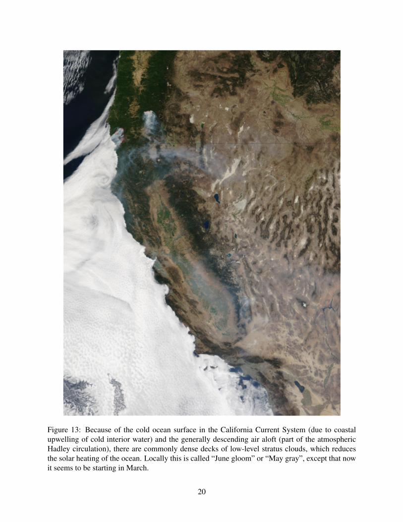
Figure 13: Because of the cold ocean surface in the California Current System (due to coastalupwelling of cold interior water) and the generally descending air aloft (part of the atmosphericHadley circulation), there are commonly dense decks of low-level stratus clouds, which reducesthe solar heating of the ocean. Locally this is called “June gloom” or “May gray”, except that nowit seems to be starting in March.

20

In some situations where very stable boundary layers might be expected, clouds develop and actto help destabilize the layer. Stratocumulus, for instance, are common in regions where the lower-tropospheric stability, as measured by the difference between the potential temperature in the freeatmosphere (typically at 700 hPa) and its value at the surface, is very large. However given anadequate supply of surface moisture, this stability can limit entrainment mixing, and hence drying,leading to the development of a shallow cloud layer at the PBL’s top. This opacity of the cloudlayer at infrared wavelengths acts to concentrate strong radiative cooling in a thin (tens of meters)layer at the top of the cloud. The air cooled at the top of the cloud becomes convectively unstableand promotes the overturning of the layer. Especially at night when the radiative cooling is notoffset by solar heating, cloud-top cooling can be an effective driver of turbulence resulting in well-mixed cloud-topped boundary layers. An example, based on observations during the DYCOMS-IIfield program, is in Figs. 12-13.

In Fig. 12 the marine boundary layer is a well-mixed, cool, and moist layer, capped by a muchwarmer and drier free troposphere. The cloud topping this layer has water content that is nearlyadiabatic, i.e., equal to what would be expected for parcels lifted reversibly from the sub-cloudlayer. The figure also shows that the strength of the capping inversion is strong compared to thefluctuations of quantities within the PBL (shown in the observational data points by the whiskersthat span the entire range) indicative of the fact that entrainment (mixing with the free troposphere)is weak. For typical stratocumulus-topped mixed layers, the radiative driving of turbulence is theprimary source, although it may be somewhat influenced by modest fluxes of heat and moisture atthe surface.

Because the stratocumulus-topped PBL critically involves the change of phase of moisture, itsdescription benefits from the use of variables that are conserved under this process. Examples arethe total water specific humidity qt for moisture and either a moist entropy (such as the equivalentpotential temperature), or a moist static energy for temperature. An example of the latter is

sl = cpT + gz − Lql , (48)

which is called the liquid water static energy. Here L is the enthalpy of vaporization, ql is theliquid water specific humidity, and other variables have their traditional meanings. Because thevertical structure of the stratocumulus-topped boundary layer is typically simple, the first-orderquestion is what controls its bulk properties. To investigate this we integrate the conservation lawsfor moisture and sl to some height h+ just above the top of the turbulent boundary layer, and if wedenote a vertical average of a quantity by a hat, then the evolution of the mean mass, liquid-waterstatic energy and moisture are described as follows,

D

Dth = w+ + E (49)

D

Dtsl = Rs +

1

h[V (sl,0 − sl) + E(sl,+ − sl)] (50)

D

Dtqt = Rq +

1

h[V (qt,0 − qt) + E(qt,+ − qt)] . (51)

Here V parameterizes the surface fluxes, E parameterizes the entrainment rate, and R denotes adiabatic process, for instance radiative fluxes acting on sl or precipitation acting on q. To close thesystem it is assumed thatR, V, and E are functions of the state of the system. Given an assumption

21

about the layer’s vertical structure, it is straightforward to use M-O theory to estimate V. In theabsence of drizzle, knowledge of the state of the system is sufficient to determine R based on theprinciples of radiative transfer, hence all that remains is to specify E.

The dynamics of this system are relatively simple to understand in some limiting circumstances.For instance a minimal representation of stratocumulus consists of a horizontally homogeneous,non-precipitating layer with V fixed to some specified value,E modeled as discussed subsequently,and a radiative driving

Rs = −∂zF =⇒ hRs = F0 − F+ ≡ −∆F . (52)

Here, and subsequently, ∆φ is used to denote φ+−φ0,where φ is arbitrary. Although ∆F is relatedto the structure of the layer, for our immediate purposes we can consider it constant. For sufficientlythick clouds (more than 100 m deep) at night this is not a particularly limiting assumption. Withthese assumptions the mixed-layer equations can be written as a system of three ODEs:

d

dth = w+ + E (53)

d

dtsl =

1

h[−∆F + V (sl,0 − sl) + E(sl,+ − sl)] (54)

d

dtqt =

1

h[V (qt,0 − qt) + E(qt,+ − qt] . (55)

The model of E is crucial. For now we consider a simple, physically plausible relation that sim-plifies the analysis, viz., the case when

E = α∆F/∆sl , (56)

where α is a constant of order unity. Heuristically this expression for E suggests that the en-trainment rate is proportional to the rate of driving of the flow (as measured by Rs) and inverselyproportional to the stability of the interface at cloud top, as measured by ∆sl. ∆q measures thejump in q at the BL top (Fig. 12). Closures that more faithfully respect the energetics of the sys-tem account for the uncertain stability of the cloud top layer across which radiative cooling, phasechanges, and mixing all effect the density in uncertain ways.

With (56), as a model for E the steady states of the system (which we denote by subscript ‘∞’)are as follows:

h∞ = h0

(α

1 + σ − α

)(57)

s∞ = s0 −∆s

(1− ασ

)(58)

q∞ = q0 + ∆q

(α

1 + σ

), (59)

whereh0 =

V

Dand σ =

V∆s

∆F. (60)

The height-scale h0 measures the height the equilibrium boundary layer would obtain for α =σ = 1. In the stratocumulus regions, D ≈ 1 × 10−5 s−1 and V ≈ 0.01 ms−1 yielding values of

22

1000

600

200

-10 0 10 20 0 0.2 0.4 0.6 -0.1 0 0.1[cm2 s-3] [m3 s-3][m2 s-2]

[m]

resolved buoyancy production vertical velocity variance third moment of w

Figure 14: Turbulence production by buoyancy, vertical velocity variance and skewness for LES(shaded) of the stratocumulus topped boundary layer. Symbols denote observed variances andskewness. The shading reflects the spread among an ensemble of 18 LES, with the darkened areashowing the inter-quartile spread and the light shading showing the full range. (Stevens et al.,2005)

h0 ≈ 1 km. Similarly for a radiative flux divergence of 100 Wm−2 and ∆s ≈ 104 J kg−1 we canexpect σ ≈ 1. By inspection we see that α is critical to the balances of mass, heat and moisture.Large α corresponds to deeper PBLs that are warmer and drier, while small α provides no basisfor deepening the PBL against the countervailing force of large-scale subsiding motion. For α > 1(super entrainment), processes other than radiative driving are important to the entrainment rate,s∞ > 0, and hence heat fluxes are into the surface ocean.

Energetics: Before addressing the energetics it is worthwhile to introduce the important conceptof quasi-stationarity. We say that a flow is quasi-steady when a conserved scalar φ (i.e., one whereRφ vanishes) has linear fluxes. To see this, recall that for a horizontally homogeneous flow, anadvected scalar φ satisfies the equation,

∂tφ = − ∂zw′φ′ , (61)

so linearity of the fluxes means that ∂t∂zφ = 0. Thus the shape of the φ profile is not changingwith time when the fluxes are linear. This motivates the descriptive word “quasi-steady.” Whereas,the boundary layer flows only approach equilibrium on long timescales and are set by the meanflow; they generally approach quasi-steady states on the timescales of the turbulent quantities thatwe shall later show are typically minutes to tens of minutes. This idea of quasi-stationarity placesimportant constrains on the fluxes that can be quite useful for a number of purposes.

For the case when h is the only length-scale, we can posit the existence of a velocity scale w∗that non-dimensionalizes the dissipation, such that

ε

(h

w3∗

)(62)

is universal. In equilibrium (62) implies that in the limit E/w∗ � 1

w3∗ ∝ Cε

∫ h+

0

Bdz , (63)

23

where the constant of proportionality is typically specified as 5/2; this definition of w∗ corre-sponds to the velocity scale, w∗ = (B0h+)1/3, that Deardorff introduced to scale the dry convectiveboundary layer. The velocity scale (63) is often used to scale a stratocumulus topped boundarylayer, although, as we might anticipate (discuss further shortly), the assumption that h is the onlylength-scale in the problem is much less justified.

Given a length-scale h and the velocity scale w∗ we can define a turbulent timescale t∗ = h/w∗.Because w∗ is typically near unity, this t∗ ≈ 10 − 20 minutes for typical boundary layer depths.It is on this timescale that one expects boundary layers to approach quasi-steady states. In so faras changes to the forcings occur on timescales much larger than t∗, quasi-steadiness is a goodassumption.

An example of stratocumulus energetics is given in Fig. 14 showing an ensemble representa-tion of the energetics of an observed case of stratocumulus. The spread among the various LESis large, reflecting differences in the entrainment rates produced by different simulations arisingfrom the difficulty of representing the energetics at what amounts to a very sharp, and poorly re-solved, entrainment interface at cloud top. Those simulations that tend to entrain the least have thegreatest buoyancy production by turbulence, the largest turbulence activity, and are most negativelyskewed, reflecting the downdraft dominance in the radiatively-driven layer that, on the whole, mostof the LES do not represent very well compared to the measured negative skewness in this thin en-trainment layer. An interesting aspect of this figure is the large increase in the buoyancy in thecloud layer. This is due to the way that fluctuations in the state parameters project onto the buoy-ancy. In the cloud layer, buoyancy fluctuations are dominated by fluctuations in qt, while in thesub-cloud layer buoyancy fluctuations are mostly driven by fluctuations in sl. This illustrates theimportant energetic role of the depth of the cloud layer, and hence the non-universality of w∗ asdescribed above. It can also lead to interesting phenomena, such as the cloud layer doing work onthe sub-cloud layer, effectively, moisture fluxes driving reverse heat fluxes.

2.3 Cumulus-Topped Boundary LayersCumulus clouds often top convective boundary layers over the ocean in regions where the lowertropospheric stability is insufficiently large to trap the moisture in a thin layer. These clouds act tovent the sub-cloud layer of mass and moisture. For most practical purposes, the sub-cloud layerof a cumulus topped PBL is thought to be similar to that of a dry convective PBL, although theturbulence and energetics of the cloud layer is considerably more complex.

3 Neutral and Stable Boundary Layers

3.1 Ekman LayerA paradigm for neutral, or unstratified, PBLs is the turbulent Ekman layer. This is thought to differin at least two fundamental ways from the classical Ekman layer discussed in Shear Turbulence.First, the turbulence does not provide a constant eddy viscosity. Second, there is almost always acapping inversion that demarcates the vertical extent of the PBL and provides a rather sharp interiorboundary to the mean shear and turbulent variance and flux profiles.

24

Surface Fluxes

Large Scale Subsidence

h

zi

Radiative Cooling

Convective Mixed Layer

Compensating Subsidence

Q Θ

Shear

Figure 15: Schematic of cumulus-topped boundary layer based on simulations and observationsduring ATEX. (Stevens et al., 2001.)

Figure 16: Numerical simulation of a turbulent Ekman layer. Dotted lines are for the laminarsolution; solid lines are for turbulent flow at Re = 1000. Upper panel: Mean velocity on axesaligned with the geostrophic wind. Lower panel: Hodograph, with vectors showing mean velocityat zf/u∗ = 0.1, 0.2, 0.3, and 0.4. (Coleman, 1999)

25

Figure 17: Schematic of stable boundary layer regimes. The surface layer has Monin-Obukhovsimilarity, the “local” layer has a z similarity scaling with the Ozmidov length LO(z). Above thelocal layer there is no similarity scale (i.e., “z-less”). For weakly stable conditions the distanceto the top at z = h may be relevant. Very stable layers have ill-defined tops and an amorphoustransition into the interior regime. (Mahrt, 1999)

For idealized flows, wherein an externally imposed stratification does not set the depth of thePBL, we can investigate the effects of turbulence on the developing Ekman layer through numericalsimulation. Figure 16, taken from direct numerical simulations by Coleman (1999), shows thatthe turbulent Ekman layer has a less pronounced Ekman spiral than the laminar solutions with theturning angle for the near-surface wind, ≈ 29o, as compared to 45o, and the depth of the layer ofO(u∗/f). The eddy viscosity profile, Km(z), (not shown) increases from zero (as we expect in aturbulent shear layer) near the surface, peaks in the middle of the PBL, and tends to decrease intothe interior (though not sharply in this situation without a capping inversion) scale for the turbulentsolutions

The analytic Ekman layer solution (Shear Turbulence) shows that h is finite in equilibriumin a uniform density fluid with rotation. When h is less than O(u∗/f), either because of a stableinversion or because the latter depth is diverging near the equator, the shear-driven PBL will alwaysbe developing (i.e., continuing to deepen). Often, however, this rate of deepening is quite slow onthe scale of an energetic eddy turn-over time, h/u∗, and, on any long time scale of many days,buoyancy forcing is not negligible, so that a purely shear-driven solution is not relevant to nature.

3.2 Stable Boundary LayerA good overview of the stable boundary layer (SBL) is provided in Fig. 17. Further illustration ofthe influence of B on the shear PBL is given in Fig. 18, based on observations during a diurnalcycle in the atmosphere, where the afternoon convective layer, the CBL with B > 0, is muchdeeper and has its U(z) more uniform with height (i.e., showing a less pronounced Ekman spiral)than the evening stable layer, the SBL with B < 0. The stabilizing buoyancy flux at the surfaceextracts energy from the turbulence generated by shear production (in addition to ε), it makes hsmaller, it provides a stable stratification through the actively turbulent layer, and it makes the

26

turbulent eddies smaller (even when rescaled by the smaller h) because of N2 > 0. Also, it throwsthe momentum equation,

∂U

∂t− f(V − Vg) = −∂w

′u′

∂z, (64)

out of balance at levels previously within the PBL when the Reynolds stress collapses throughTKE dissipation; this has the effect of generating inertial oscillations in this residual layer, whichare related to the frequent occurrence of a nocturnal jet near z = h in a stable PBL (Fig. 18).Another view of this transition from a CBL to a SBL is shown in Fig. 20, where the drop in u∗ ispartly due to a change in Ug as well.

Figure 18: (Left) Early afternoon profiles of mean wind and potential temperature in the 1973Minnesota experiment, i.e., during a convective period. This moderately convective PBL had h =1250 m and h/L ≈ −30 (Kaimal et al., 1976). (Right) Early evening profiles of mean wind andpotential temperature in the 1973 Minnesota experiments, i.e., after the transition to a stable period(Caughey et al., 1979).

Large Eddy Simulations (LES) are more difficult for the SBL than for the CBL or neutralEkman layer because of the very fine spatial scales that occur near its top where the N2(z) is largeand the turbulence is weak and especially intermittent as Ri(z) goes crosses a critical value. Themean profiles show stable stratification and shear throughout the layer (i.e., it is not a mixed layer;Fig. 21). The energy cascade is, of course, forward in a boundary layer, and it exhibits an energyinertial range shape, anisotropically at larger scales and isotropically at smaller ones (Fig. 21).Its coherent structures are manifested as tilted temperature fronts in the downstream-vertical plane(Fig. 23) and hairpin vortices qualitatively elongated in the same plane and broadly similar to thoseseen in uniform-shear or shear boundary-layers (Fig. 24).

The range of actively turbulent scales of motion is squeezed in the remnant layer above theSBL, between the Ozmidov and Kolmogorov scales (i.e., LO = (ε/N3)1/2 and LK = (ν3/ε)1/4),much the same as seen previously in stratified turbulence. This is illustrated in Fig. 25 for thediurnal cycle in the upper ocean. Note that the range of scales shrinks once the transition toa SBL occurs, due to the decay of turbulence, hence the decrease in ε. There is also a strongcoupling between the decaying 3D turbulence in this layer and internal gravity waves, since theeddy turnover time, τL = ε−1/3L2/3, at the top of the inertial range, L = LO, is the same as a

27

Figure 19: Some observed statistics from the nocturnal PBL (data points) and theoretical predic-tions from Nieuwstadt (1984). Abscissa is ζ = z/L. Plotted are TKE scaled with the frictionvelocity (top), non-dimensional eddy viscosity, νe/u∗L (middle), and Ri(z) (bottom).

Figure 20: The late-afternoon decay of friction velocity u∗ in the 1973 Minnesota experiment.(Wyngaard, 1975)

28

Figure 21: Mean vertical profiles in LES of the SBL. These are shown as functions of verticalresolution, (A,B/Bw,C) = (2,0.8,0.4) m, which is notoriously demanding to adequately resolve theentrainment at the layer top. Notice the persistent stable stratification in spite of the turbulentmixing and the “nocturnal jet” near the top (also seen in Fig. 18, right). (Sullivan et al., 2016)

Figure 22: 2D horizontal wavenumber spectra for T (blue), (u, v) (red), and w (black) at a heightz = 0.2h. Notice the k−5/3 shape, broadly in T and (u, v), and only at smaller scales in w,indicating isotropy there. (Sullivan et al., 2016)

29

Figure 23: Contours of T (x, z) for a given y from a LES of the SBL. The top panel has h/L = 1.7and the bottom panel has h/L = 6.0. Temperature “fronts” or “ramps” are evident, and their tiltangle is reduced with stronger stratification. (Sullivan et al., 2016)

30

Figure 24: Oblique view of the typical 3D vortical structure in a SBL LES. This is based onconditional averaging of “strong events” at a height of z = 0.2h. The isosurface is a specifiedsmall magnitude of an eigenvalue of the local velocity gradient tensor that indicates local swirl,and the coloration of the surface indicates the sign of the local vertical vorticity (red = positive; blue= negative). This has the shape of a hairpin vortex reaching well into the middle of the boundarylayer, with a tilted orientation favorable for eddy momentum flux, u′w′ < 0. (Sullivan et al., 2016)

31

buoyancy oscillation time, τigw = N−1; this is probably why internal waves are often vigorous inthis layer. Of course, once the turbulence has collapsed to a state of anisotropic stratified turbulencein the remnant layer, then the coupling with the wave field largely ceases. Another interesting scaleshown in Fig. 25 is the Thorpe scale, LT , defined as the r.m.s.; vertical distance parcels have tobe moved in a profile b(z) to achieve marginal stability, db/dz ≥ 0 ∀ z. Empirically, it is foundthat LT ≈ 0.84LO, indicating that overturning is actively occurring at nearly the theoretical limitpredicted by the energy argument underlying the definition of LO.

Figure 25: (Left) Regimes of the oceanic diurnal cycle. (Right) Length scales in the remnantturbulence layer: Thorpe scale LT , Ozmidov scale LO, and Kolmogorov scale η = LK that formsafter t = 0 and then decays. (Brainerd and Gregg, 1993)

The dynamics of the SBL are best understood as a combination of Monin-Obukhov similaritynear the surface and near-critical stratified shear instability, with Ri ≈ Ricr ∼ 0.25, in the outerregions (Fig. 19). For z > h in the remnant layer, Ri > Ricr at least intermittently. Thus, theturbulent dynamics in the outer SBL is much more local than in either the CBL or the Ekman PBL,with Kelvin-Helmholtz vortices as its dominant coherent structure. Nevertheless, we can identifya dominant length-scale,

h ∼ u∗N, (65)

outside of the near-surface Monin-Obukhov and local-similarity layers (which can be very shallowin the SBL; see Fig. 1), and associate it with an interior eddy diffusivity,

K ∼ u∗h =u2∗N

(66)

(Mahrt and Vickers, 2003). Measurements of the SBL are notoriously variable: the turbulence isrelatively weak compared to other PBL regimes, and shear instability and internal waves in theoverlying region often encroach down toward the surface.

32

4 Langmuir Boundary LayersThe upper-oceanic and lower-atmospheric PBLs can be strongly influenced by surface gravitywaves on the air-sea interface. One important regime is called the Langmuir PBL, because Lang-muir circulations are the dominant coherent structures (Figs. 26-27); it is the focus of this section.Other important surface wave effects (not further discussed here) are due to breaking waves (Sul-livan et al., 2007) and to wave-induced drag on the PBL winds (Sullivan et al., 2008).

Figure 26: Photograph of the surface of the Great Salt Lake showing surface convergence linesdue to Langmuir circulations. The wind and surface waves are into the plane of the picture. (S.Monismith, personal communication)

Surface gravity waves have phase speeds c that are given by the deep water dispersion relation,

c =√g/k , (67)

where k is the horizontal wavenumber. A typical value for c is 10 ms−1 (for a spectrum-peakwavelength 2π/k of 60 m), which is comparable to a typical near-surface wind speed, Ua. Forsuch waves, the slope of the sea surface ak is typically small, say 0.1 for a sea level amplitudeof a = 1 m). Since ak is a measure of the nonlinearity of the wave dynamics, this means thatthey are linear to leading order. Furthermore, wave-induced particle velocities are O(akc) ≈ 1m s−1. Turbulent and mean current velocities in the oceanic PBL are typically smaller than this,comparable to O([ak]2c) ≈ 0.1 ms−1, which as we will see is also the order of the wave-inducedLagrangian mean flow, called the Stokes drift ush. The implication of these various magnitudes isthat wave-induced effects on the oceanic PBL, acting through the Stokes drift, can be as important

33

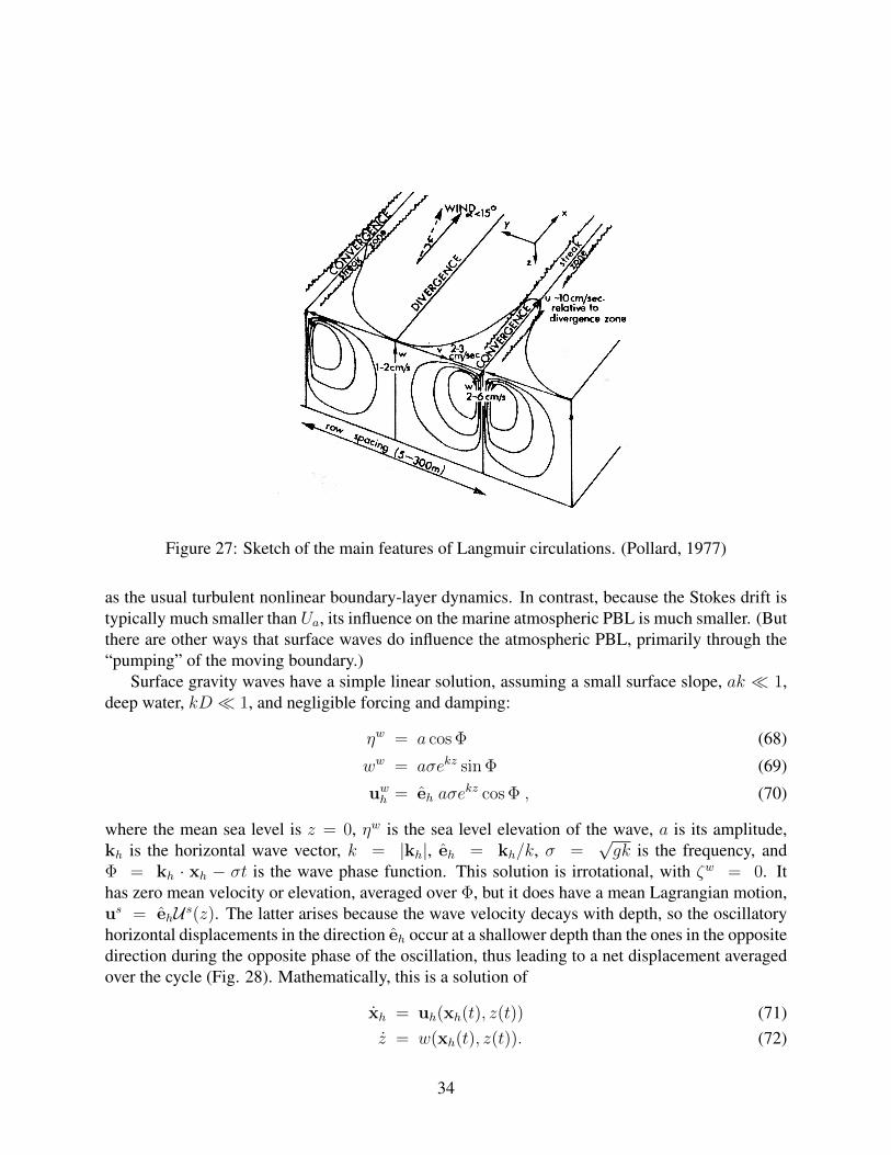
Figure 27: Sketch of the main features of Langmuir circulations. (Pollard, 1977)

as the usual turbulent nonlinear boundary-layer dynamics. In contrast, because the Stokes drift istypically much smaller than Ua, its influence on the marine atmospheric PBL is much smaller. (Butthere are other ways that surface waves do influence the atmospheric PBL, primarily through the“pumping” of the moving boundary.)

Surface gravity waves have a simple linear solution, assuming a small surface slope, ak � 1,deep water, kD � 1, and negligible forcing and damping:

ηw = a cos Φ (68)

ww = aσekz sin Φ (69)

uwh = eh aσekz cos Φ , (70)

where the mean sea level is z = 0, ηw is the sea level elevation of the wave, a is its amplitude,kh is the horizontal wave vector, k = |kh|, eh = kh/k, σ =

√gk is the frequency, and

Φ = kh · xh − σt is the wave phase function. This solution is irrotational, with ζw = 0. Ithas zero mean velocity or elevation, averaged over Φ, but it does have a mean Lagrangian motion,us = ehU s(z). The latter arises because the wave velocity decays with depth, so the oscillatoryhorizontal displacements in the direction eh occur at a shallower depth than the ones in the oppositedirection during the opposite phase of the oscillation, thus leading to a net displacement averagedover the cycle (Fig. 28). Mathematically, this is a solution of

xh = uh(xh(t), z(t)) (71)z = w(xh(t), z(t)). (72)

34

Figure 28: Sketch of surface waves and Stokes drift.

Inserting the previous solution forms, expanding in ak, and averaging over a wave phase cycleleads to

U s(z) = 〈[∫ t

uwdt′] · ∇uw〉 (73)

= a2σke2kz , (74)

where the angle brackets denote an average over the wave cycle, and U s is the vertical profileof the Stokes velocity whose direction is equal to the surface wave propagation direction. (Thederivation can be found in even ancient monographs on surface gravity waves, and in McWilliamset al., 2004.)

Now consider a perturbation theory for waves and currents, where the velocity is assumed tohave the form

u = uw + (ak)2(v0 + (ak)v1 + . . .

), (75)

where v has both higher order corrections to the wave dynamics, with time variability on the scale1/σ, as well as slower variability on a time scale 1/akσ that can be calculated by averaging thedynamical equations over the wave scale. Note that uw itself is O(ak) (consistent with a leading-order linearization) and U s is O([ak]2) . We therefore further decompose the correction velocityfields by time scale,

v = 〈v〉+ vw , (76)

where the angle brackets denote an average over the wave and the superscript w denotes a fluctua-tion around the average.

35

We can write the vorticity equation in a uniformly rotating frame as

∂ω

∂t= ∇× (u× [ω + f z]− bz) + ν∇2ω . (77)

We now insert the solution form (75)-(76) into (77), where we make a similar expansion for b andassume that f and ν are O([ak]2). With reference to uw, (77) is trivial because the wave solution(70) is irrotational. At the leading order in ω, (77) becomes

∂ω0,w

∂t= 0 , (78)

implying that ω0 = 〈ω0〉. At the next order,

∂ω1,w

∂t= ∇×

(uw × [〈ω0〉+ f z]

), (79)

and, at the next,

∂〈ω0〉∂t

= ∇×(〈v0〉 × [〈ω0〉+ f z]− 〈b0〉z

)+ ν∇2〈ω0〉+∇× 〈uw × ω1,w〉 . (80)

The form of (80) is identical to that of (77), applied here to the leading order current fields, exceptfor the addition of the final term. By manipulations of (70), (74), and (79) — as first demonstratedby Craik and Leibovich (1976) — we can derive

∇× 〈uw × ω1,w〉 = ∇×(us × [〈ω0〉+ f z]

), (81)

and thus close the current dynamics at leading order. An analogous derivation can be made for thewave-averaged buoyancy equation. The upshot is that the wave-averaged Boussinesq Equations,for (u, b) ≡ (〈v0〉, 〈b0〉), can be written as

Du

Dt= −∇φ+ ν∇2u + zb− f z× (u + us) + us × ω

∇ · u = 0Db

Dt= κ∇2b− us · ∇b . (82)

Thus, there are added advective and Coriolis vortex forces in the momentum balance and a wave-added advection in the buoyancy and other tracer balances, all of which are proportional to theStokes drift, as well as a Bernoulli-head increment (i.e., 1

2uw 2) that is now part of the wave-

averaged pressure (McWilliams et al., 2004).Now consider a shear PBL in the presence of waves, where (82) is the governing dynamics.

An obvious first problem is the analytic Ekman layer problem, where we modify (42) both for anoceanic configuration with an imposed top boundary stress τa and for the inclusion of the Coriolisvortex force in (82):

−f(V + V s) = νe∂2U

∂z2(83)

f(U + U s) = νe∂2V

∂z2(84)

36

with boundary conditions,

νe∂U

∂z=

τa

ρ0at z = 0 (85)

(U, V ) → 0 as z → −∞ . (86)

Here (U s, V s)(z) are the vector components of the Stokes drift velocity us(z). If we specialize tothe case where both us and τa are in the x direction (that is appropriate for wind-generated waves),then the solution of (84)-(86) is

U =τa

ρ0√

2fνeeγz (cos γz + sin γz) − DU s(z)

+ eγz (R− cos γz + R+ sin γz)U s(0)

V =τa

ρ0√

2fνeeγz (− cos γz + sin γz) + 2(k/γ)2D U s(z)

+ eγz (R− sin γz − R+ cos γz)U s(0) , (87)

where γ =√f/2νe as above, U s is given by (74), and

D = (1 + 4(k/γ)4)−1 , R± =k

γ(1± 2(k/γ)2)D .

The hodograph for (87) is plotted in Fig. 29 for a particular set of parameters, as listed. It showsan Ekman spiral turning to the right of the surface stress for f > 0. However, there are now twovertical decay scales, 1/k and 1/γ. The transport has both a component 90o to the right of thestress, but also one opposed to the Stokes-drift transport:∫ 0

−∞dzU = −

∫ 0

−∞dzUs − z× τa/f . (88)

The wave-averaged dynamics in (82) are especially relevant to the frequently observed phe-nomenon of Langmuir circulations. These are longitudinal roll cells parallel to the wind andwaves, made visible through the gathering of surfactants (scum) along the lines of surface con-vergence (Fig. 26). The essential mechanism for this can be seen in (82) by doing an early-time,rapid-distortion analysis with f = g = 0:

ω(x− ust, t) = ω(x, 0) +dus

dzω(z)(x, 0)t+ . . . . (89)

The initial vorticity vector will move with the Stokes drift, and its vertical component will tiltand amplify in the longitudinal direction; thus, the vortex force is conducive to growth of thelongitudinal vorticity component.

Now consider the problem of a wind-driven, upper-ocean current with Re as a control parame-ter, and with f = g = 0 for now. For smallRe, the equilibrium solution is a 1D steady flow, U(z)x.At a critical value of Re, this flow is unstable to 2D steady rolls that are identifiable with Langmuircirculations. For larger Re, there are 3D secondary instabilities and eventually a transition to a

37

Figure 29: Hodograph of the non-dimensional laminar Stokes-Ekman layer velocity vector withLatur = 0.3 (solid line) vs. the pure Ekman layer (dashed line). (McWilliams et al., 1997)

fully developed flow that can be called Langmuir turbulence. For the ocean, we are interested inthis latter stage, with a finite value of the turbulent Langmuir number,

Latur =√u∗/U s(0) , (90)

Re→∞, and f,N 6= 0. Empirically it has been found that Latur ≈ 0.3 in wind-wave equilibrium.This problem has been solved with LES of the equations (82) for a horizontally homogeneous,

wind-driven PBL with a weakly unstable surface buoyancy flux above a stable inversion layer(McWilliams et al., 1997). The mean flow, uh(z), is in Fig. 30. It shows the effect of the Coriolisvortex force seen in the constant-νe solution (87)-(88), viz., an enhanced turning angle to the rightof the surface stress. In addition, it shows a diminished spiral, compared to the analytic solutionwith constant νe, to an even greater degree than in the turbulent Ekman solution (also shown inFig. 30 for the identical problem configuration but for U s = 0 and Latur = ∞). The TKEand ε profiles (Fig. 31) show an enhanced turbulent intensity with finite Latur, and the eddymomentum flux efficiency (i.e., νe(z) in Fig. 32) and entrainment-layer buoyancy flux (Fig. 33)are also enhanced. In particular, ε is much larger than the MO similarity prediction (16) nearthe surface due to wave breaking and below it decays much more steeply as ∼ z−2 due to theLangmuir turbulence enhancement of the boundary-layer energy cycle (Terray et al., 1996). Thus,we conclude that the presence of the wave-added terms, and the vortex force in particular makesboth the turbulence and its vertical transports stronger.

We see the turbulent Langmuir circulations in Figs. 34-36 that show surface-trapped particletrajectories and distributions and the near-surface longitudinal vorticity field. The cell structure isstill evident, but it is more irregular in shape and has finite correlation scales in x and t, comparedto the idealized form in Fig. 27. As a final example, Fig. 37 shows the multi-scale structure that

38

Figure 30: Horizontal and time mean velocity profiles. The solid line is for the pure Ekman layerand the broken lines are for Latur = 0.3 in two different domain sizes. (McWilliams et al., 1997)

Figure 31: Mean kinetic energy dissipation rate profiles, ε(z). The solid line is for the pure Ekmanlayer and the broken lines are for Latur = 0.3 in two different domain sizes. (McWilliams et al.,1997)

39

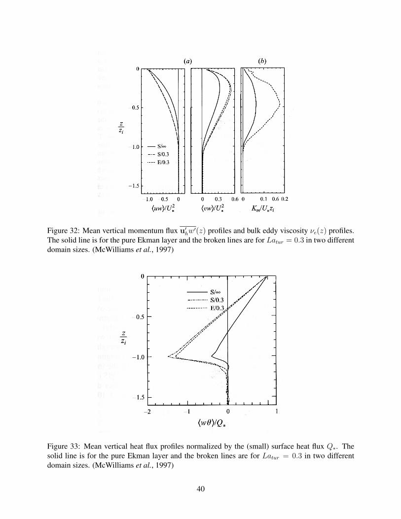
Figure 32: Mean vertical momentum flux u′hw′(z) profiles and bulk eddy viscosity νe(z) profiles.

The solid line is for the pure Ekman layer and the broken lines are for Latur = 0.3 in two differentdomain sizes. (McWilliams et al., 1997)

Figure 33: Mean vertical heat flux profiles normalized by the (small) surface heat flux Q∗. Thesolid line is for the pure Ekman layer and the broken lines are for Latur = 0.3 in two differentdomain sizes. (McWilliams et al., 1997)

40

can develop in w(x, y) for Langmuir turbulence in the presence of both local-equilibrium windwaves and stronger, remotely generated swell waves.

Figure 34: (a) Trajectories of surface parcels released along a transverse line over a continuoustime interval in equilibrium Langmuir turbulence with Latur = 0.3. (b) Locations of 104 surfaceparcels 1500 s after being released randomly within 0 ≤ x, y ≤ 300 m. (McWilliams et al., 1997)

Figure 35: Distributions at successive times about 5 minutes apart for buoyant surface particlesinitially released randomly in the midst of oceanic equilibrium Langmuir turbulence with Latur =0.3. Note the gathering into surface convergence lines due to Langmuir circulations. The finalpanel here is the same as in Fig. 34. (McWilliams et al., 1997)

41

Figure 36: Temporal and spatial variation of surface particles (dots) and near-surface streamwisevorticity (light and dark shading indicate different signs above a specified threshold magnitude) inLangmuir turbulence with Latur = 0.3. The time intervals between the panels are about 120 s.The position of a single particle that is near the early-time Y-junction of two convergence lines isindicated by the large dot. Note the merger of two circulation cells that occurs to the left of thisparticle. (McWilliams et al., 1997)

42

Figure 37: w(x, y) snapshot at z = − 1 m for Langmuir Turbulence with both local wind-wavesand remotely generated swell waves. The horizontal width of this domain is 1200 m. (McWilliamset al., 2014)

43

Figure 38: Wind component u(y, z) in the direction of the lower-tropospheric geostrophic wind ina transverse cross-section from an atmospheric LES with a wave-specified moving lower boundary.(Sullivan et al., 2014)

5 Waves Under the Atmospheric Boundary LayerSurface waves also alter the atmospheric boundary layer compared to flow over land. Not only arewaves sometimes rather large roughness elements (as are trees), but they present a moving surfaceas well. An important concept is that when winds drag over water, an instability of the surfaceinterface develops and wave grow, primarily by form stress momentum transfer from winds towaves. At some point the momentum and energy input to the waves is balanced by the output tothe ocean currents, mostly by wave breaking when the wind is not slow; this phase is referred toas wind-wave equilibrium. (N.b., this is the true mechanism of momentum transfer from waves tocurrents.) A parameter that measures this progression is the wave age,

A =CpUa

, (91)

where Cp is the phase speed of the wavenumber associated with the peak of the wave energyspectrum and Ua is a low-level wind speed (e.g., at z = 10 m, as often used in bulk-formulaestimates of surface stress). For young and growing waves, A < 1; for wind-wave equilibrium,A ≈ 1; and for old waves, generated by stronger winds elsewhere or left over from previouslystronger winds locally, A > 1. Old waves present the interesting situation where the surface ismoving faster than the adjacent wind, hence the momentum flux can actually accelerate the surfacewind rather than damp it.

We present several illustrations of a wavy atmospheric boundary layer simulated by LES wherethe water movement at the bottom is specified from measured wave spectra. Fig. 38 shows a cross-

44

Figure 39: u(x, z) in relation to surface elevation η(x) in the lower third of the atmospheric bound-ary layer shown in Fig. 38. Notice the “wave-pumping” relationship between forward surface uin the troughs and backward u above the crests. The wave-pumped u signals extend only to aboutz = 50 m here (comparable to a peak wavelength). (Sullivan et al., 2014)

Figure 40: Profiles of the mean wind u(z) near the surface, where ζ is height above the sea surface.The surface wave pumping disrupts MO similarity over a vertical distance that is larger for largerwave age A. (Sullivan et al., 2014)

45

section of the wind over the whole boundary layer in the direction of the atmospheric troposphericflow at around 500 m height. The layer is primarily a shear Ekman layer with weakly convectivesurface flux. The large eddies are visible and here have a kind of longitudinal roll-cell pattern.Near the surface the wind is much slower, of course, but it also shows strong correlations with thelocal wave surface (Fig. 39 for rather old waves, A = 4.2); i.e., the orbital motions of the waves arepushing and pumping the atmospheric eddies nearby, and in doing so these wave-pumped eddiesare the ones carrying the mean momentum flux, u′w, which is upward in this case. In this large-Asituation the surface layer does not conform to a Monin-Obukhov similarity profile up to a heightof about z = 10 m, although its discrepancy is limited to much lower heights z < 1 m withequilibrium waves (Fig. 40). In part this is because the wave-pumping effect provides anotherrelevant length scale besides the similarity assumption of only the distance from the boundary, z.

6 K-Profile PBL Parameterization ModelOceanic and atmospheric models of large- and meso-scale circulations need to include the effectsof turbulent transport and dissipation by smaller-scale motions through parameterizations. In theirfluid interiors, the usual parameterization forms are some type of eddy diffusion, though oftenanisotropic (i.e., with κv � κh) and unequal for momentum and scalars (i.e., Pre 6= 1). Theeffects of the PBL, however, are usually not well represented by a constant eddy diffusivity, so anumber of different types of parameterization have been developed for it. Among the popular typesare mixed-layer models (Sec. 2.1) and local moment closure models (Shear Turbulence). However,these models, respectively, can aptly be criticized because mean profiles are often not well mixed inthe PBL (especially in non-convective situations) and turbulent fluxes are not entirely determinedby local properties (e.g., plumes in convection), especially in the entrainment layer at the interioredge of the PBL.

A different type of PBL parameterization model — called K-Profile Parameterization (KPP) —has become widely used in both atmospheric and oceanic models. KPP is still an evolving model,whose detailed rules are being changed as new observations and LES simulations are made, but itsoverall framework is considered to be a good match to the following criteria for utility in larger-scale models:

• It specifies the rates of turbulent mixing, not the shape of the mean profile (cf., a mixed-layermodel).

• It is consistent with Monin-Obukhov similarity structure near the surface (Sec. 1.1).

• It is intended to span a wide range of regimes in surface fluxes and mean profiles.

• It has vertically nonlocal transport (especially in convection).

• It has continuity with interior mixing processes.

• It is computationally compatible with a GCM (i.e., it can be calculated on a discrete grid andis not too expensive).

46

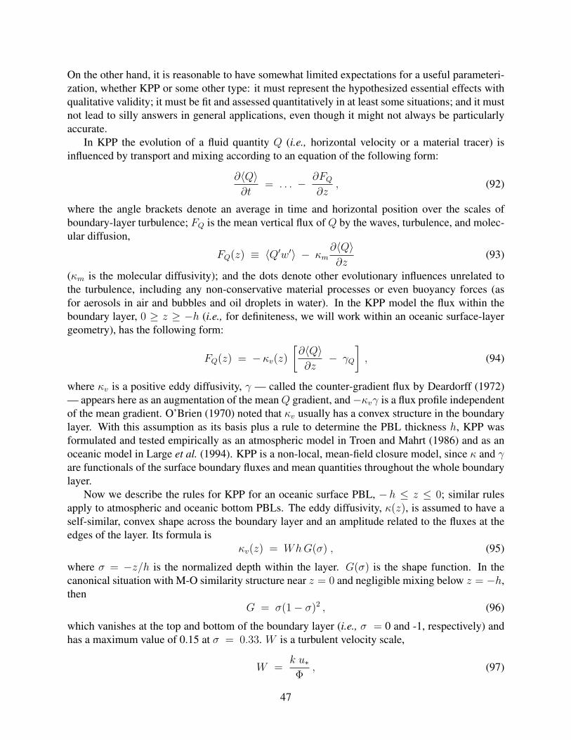
On the other hand, it is reasonable to have somewhat limited expectations for a useful parameteri-zation, whether KPP or some other type: it must represent the hypothesized essential effects withqualitative validity; it must be fit and assessed quantitatively in at least some situations; and it mustnot lead to silly answers in general applications, even though it might not always be particularlyaccurate.

In KPP the evolution of a fluid quantity Q (i.e., horizontal velocity or a material tracer) isinfluenced by transport and mixing according to an equation of the following form:

∂〈Q〉∂t

= . . . − ∂FQ∂z

, (92)

where the angle brackets denote an average in time and horizontal position over the scales ofboundary-layer turbulence; FQ is the mean vertical flux of Q by the waves, turbulence, and molec-ular diffusion,

FQ(z) ≡ 〈Q′w′〉 − κm∂〈Q〉∂z

(93)

(κm is the molecular diffusivity); and the dots denote other evolutionary influences unrelated tothe turbulence, including any non-conservative material processes or even buoyancy forces (asfor aerosols in air and bubbles and oil droplets in water). In the KPP model the flux within theboundary layer, 0 ≥ z ≥ −h (i.e., for definiteness, we will work within an oceanic surface-layergeometry), has the following form:

FQ(z) = −κv(z)

[∂〈Q〉∂z

− γQ

], (94)

where κv is a positive eddy diffusivity, γ — called the counter-gradient flux by Deardorff (1972)— appears here as an augmentation of the meanQ gradient, and−κvγ is a flux profile independentof the mean gradient. O’Brien (1970) noted that κv usually has a convex structure in the boundarylayer. With this assumption as its basis plus a rule to determine the PBL thickness h, KPP wasformulated and tested empirically as an atmospheric model in Troen and Mahrt (1986) and as anoceanic model in Large et al. (1994). KPP is a non-local, mean-field closure model, since κ and γare functionals of the surface boundary fluxes and mean quantities throughout the whole boundarylayer.

Now we describe the rules for KPP for an oceanic surface PBL, −h ≤ z ≤ 0; similar rulesapply to atmospheric and oceanic bottom PBLs. The eddy diffusivity, κ(z), is assumed to have aself-similar, convex shape across the boundary layer and an amplitude related to the fluxes at theedges of the layer. Its formula is

κv(z) = WhG(σ) , (95)

where σ = −z/h is the normalized depth within the layer. G(σ) is the shape function. In thecanonical situation with M-O similarity structure near z = 0 and negligible mixing below z = −h,then

G = σ(1− σ)2 , (96)

which vanishes at the top and bottom of the boundary layer (i.e., σ = 0 and -1, respectively) andhas a maximum value of 0.15 at σ = 0.33. W is a turbulent velocity scale,

W =k u∗Φ

, (97)

47

where k (= 0.4) is von Karman’s constant and Φ is the stability function in M-O theory (Sec. 1.1. Inthe KPP model φ is a function of h/L outside of the near-surface layer (i.e., 0 ≥ −z ≥ 0.1h), andits values differ between scalar quantities and momentum when L < 0). L is the Monin-Obukhovlength defined in (2). The non-gradient flux, γ(z), is assumed in KPP to have a uniform profilethroughout the interior part of the boundary layer,

γ = CγFQ(0)

W h, (98)

where Cγ is a positive constant. This formula implies that, after the multiplication by the positive,convex κv(z) in (94), there is a transport of Q from the upper part of the boundary layer (i.e.,above the maximum in G) to the lower part (below the maximum) in the sense set by the sign ofthe surface flux, FQ(0). For example, surface cooling implies FT (0) > 0, hence γ > 0, hence−κγ < 0 and its divergence acts in (27) to increase T in the upper part of the boundary layerand cool the lower part and thus contributes to the movement of heat from below up towards thesurface. Thus, (98) represents an intrinsically non-local flux process, since it is not linked to thelocal mean gradient at any particular depth. The utility of γ was recognized by Deardorff (1972) forconvective boundary layers in which gravitationally unstable plumes carry heat and material acrossthe boundary layer, even though the interior mean gradients are small; of course, an analogousstatement can be made for the Langmuir Cells, some of which also span the whole boundary layer(McWilliams and Sullivan, 2001). For temperature in thermal convection, the mean gradient evenreverses sign within the layer, due to entrainment of interior fluid that provides a heat flux near theedge of the layer with a sign opposite to the surface flux, but the sign reversals of FQ and ∂〈Q〉/∂zrarely occur at the same z value. Thus, γ can prevent singularities and negative values in κ(z)when (94) is fit to actual profiles of FQ(z) and 〈Q〉(z), and γ is commonly fit simultaneously tomake κ(z) > 0 and smooth in z. Without γ, an eddy-diffusion model like (92)-(94), with a smooth,positive κ, will make 〈Q〉(z, t) evolve such that zeros in FQ and the mean gradient occur in thesame location, unlike what is observed in convective boundary layers, for example.

The boundary-layer depth, h, is determined in KPP as the first non-zero depth, z ≤ 0, at whichCr(z) = 0, where

Cr(z) =

∫ 0

z

J(z′)

[(∂u

∂z

)2

− N2(z)

Ric− Cekf

2

]dz′ +

V 2t (z)

|z|≡ Ish − Ist − Irot + Ient . (99)

N2 = αg∂T/∂z is the square of the Brunt-Vaisalla frequency. J(z) = |z|/(|z|+εh) is a weightingfunction that excludes the surface Monin-Obukhov layer from controlling the extent of the bound-ary layer; i.e., 0 > z ≥ − εh, assuming ε� 1 (ε = 0.1 here). The component I(z) terms in Cr(z)are, respectively, the destabilizing mean shear, the (usually) stabilizing stratification, the stabiliz-ing rotation, and the destabilizing turbulent entrainment at the interior interface. The turbulententrainment term has a velocity magnitude Vt = Cent[ws(z)N(z)|z| ]1/2, where ws(z) is the usualturbulent velocity magnitude in KPP. The constants Cek = 211, Ric = 0.3, and Cent = 5.07 are de-termined by fitting KPP solutions to extreme situations where the empirical results are well known.These are, respectively, the situations of non-rotating, penetrative free convection (Ist = Ient), anunstratified Ekman layer (Ish = Irot), and a stratified shear layer (Ist = Ish). In more general

48

circumstances the Cr(−h) = 0 condition allows for smooth transitions among these different sta-bilizing and destabilizing influences, without requiring any logical if-tests in the code. The originalKPP rules for h are differently expressed but give rather similar answers to (99).

Examples of KPP solutions are in Large and Crawford (1995), McWilliams and Huckle (2006),and McWilliams et al. (2009). A future development is to include surface gravity wave effects(Secs. 4-5).

References

Brainerd, K.E., and M.C. Gregg, 1993: Diurnal restratification and turbulence in the oceanic sur-face mixed layer 1. Observations. J. Geophys. Res. 98, 22645-22656.

Brainerd, K.E., and M.C. Gregg, 1995: Surface mixed and mixing layer depths, Deep Sea Res. 42,1521-1543.

Businger, J.A., 1970: Turbulent transfer in the atmospheric surface layer. Workshop on Microme-teorology, American Meteorol. Soc., 67-100.

Caughey, S.J., J.C. Wyngaard, and J.C. Kaimal, 1979: turbulence in the evolving stable boundarylayer. J. Atmos. Sci. 36, 1041-1052.

Coleman, G.N, 1999: Similarity statistics from a direct numerical simulation of the neutrally strat-ified planetary boundary layer. J. Atmos. Sci. 56, 891-900.

Craik, A.D.D., and S. Leibovich, S., 1976: A rational model for Langmuir circulations. J. FluidMech. 73, 401-426.

Deardorff, J., 1970: Convective velocity and temperature scales for the unstable planetary bound-ary layer and for Rayleigh convection. J. Atmos. Sci. 27, 1211-1213.

Deardorff, J., 1972: Theoretical expression for the counter-gradient vertical heat flux. J. Geophys.Res. 77, 5900-5904.

Kaimal, J.C., J.C. Wyngaard, D.A. Haugen, O.R. Cote, Y. Izumi, S.J. Caughey and C.J. Readings,1976: Turbulence Structure in the convective boundary layer. J. Atmos. Sci. 33, 2152-2169.

Large, W.G., J.C. McWilliams, and S.C. Doney, 1994: Oceanic vertical mixing: a review and amodel with a non-local K-profile boundary layer parameterization. Rev. Geophys. 32, 363-403.

Large, W.G., and G.B. Crawford, 1995: Observations and simulations of upper-ocean response towind events during the Ocean Storms Experiment. J. Phys. Ocean. 25, 2831-2582.

Lenschow, D.H., J.C. Wyngaard, W.T. Pennell, 1980: Mean-field and second-moment budgets ina baroclinic, convective boundary layer, J. Atmos. Sci. 37, 1313-1326.

Lilly, D., 1968: Models of cloud-topped mixed layers under a strong inversion. Quart. J. RoyalMeteorol. Soc. 94, 292-309.

Mahrt, L., 1999: Stratified atmospheric boundary layers, Boundar. Layer. Meteor. 90, 375-396.

Mahrt, L., and D. Vickers, 2003: Formulation of turbulent fluxes in the stable boundary layer. J.Atmos. Sci. 60, 2538-2548.

49

McWilliams, J.C., P.P Sullivan, and C.H. Moeng, 1997: Langmuir turbulence in the ocean. J. FluidMech. 334, 1-30.

McWilliams, J.C., and P.P. Sullivan, 2001: Vertical mixing by Langmuir circulations. Spill Scienceand Technology 6, 225-237.

McWilliams, J.C., J.M. Restrepo, & E.M. Lane, 2004: An asymptotic theory for the interaction ofwaves and currents in coastal waters. J. Fluid Mech. 511, 135-178.

McWilliams, J.C., and E. Huckle, 2006: Ekman layer rectification, J. Phys. Ocean. 36, 1646-1659.

McWilliams, J.C., E. Huckle, and A. Shcheptkin, 2009: Buoyancy effects in a stratified Ekmanlayer. J. Phys. Ocean. 39, 2581-2599.

McWilliams, J.C., E. Huckle, J. Liang, & P. Sullivan, 2014: Langmuir Turbulence in swell. J.Phys. Ocean. 44, 870-890.

Moeng, C.H., and J.C. Wyngaard, 1989: Evaluation of turbulent transport and dissipation closuresin second-order modeling, J. Atmos. Sci. 46, 2311-2330.

Nieuwstadt, F.T.M., 1984: The turbulent structure of the stable, nocturnal boundary layer. J. At-mos. Sci. 41, 2202-2216.

O’Brien, J.J., 1970: A note on the vertical structure of the eddy exchange coefficient in the plane-tary boundary layer. J. Atmos. Sci. 27, 1213-1215.

Pollard, R.T., 1977: Observations and theories of Langmuir circulations and their role in nearsurface mixing. A Voyage of Discovery: George Deacon’s 70th Anniversary Volume, M. Angel(ed.), Pergamon Press, 235-251.

Sorbjan, Z. 1989: Structure of the Atmospheric Boundary Layer, Prentice Hall.

Stevens et al., 2001: Simulations of trade-wind cumuli under a strong inversion J. Atmos. Sci. 58,1870-1891.

Stevens, B., 2005: Atmospheric moist convection. Ann. Rev. Earth & Planetary Sci. 33, 605-643.

Stevens et al., 2005: Evaluation of large-eddy simulations via observations of nocturnal marinestratocumulus. Mon. Weather Review 133, 1443-1462.

Sullivan, P.P., C.H. Moeng, B. Stevens, D.H. Lenschow, and S.D. Mayor, 1998: Entrainment andstructure of the inversion layer in the convective planetary boundary layer. J. Atrmos. Sci. 55,3042-3064.

Sullivan, P.P., J.C. McWilliams, and W.K. Melville, 2007: Surface gravity wave effects in theoceanic boundary layer: Large Eddy Simulation with vortex force and stochastic breakers. J. FluidMech. 593, 405-452.

Sullivan, P.P, J.B. Edson, T. Hristov, and J.C. McWilliams, 2008: Large eddy simulations andobservations of atmospheric marine boundary layers above non-equilibrium surface waves. J.Atmos. Sci. 65, 1225-1245.

Sullivan, P.P., J.C. McWilliams, & E.G. Patton, 2014: Large eddy simulation model of marineatmospheric boundary layers above a spectrum of moving waves. J. Atmos. Sci. 71, 4001-4027.

50

Sullivan, P.P., J.C. Weil, E.G. Patton, H.J.J. Jonker, and D.V. Mironov, 2016: Turbulent winds andtemperature fronts in large-eddy simulations of the stable atmospheric boundary layer. J. Atmos.Sci. 73, 1815-1840.

Terray, E., M. Donelan, Y. Agrawal, W. Drennan, K. Kahma, A. Williams, P. Hwang, and S. Ki-taigorodskii, 1996: Estimates of kinetic energy dissipation under breaking waves. J. Phys. Ocean26, 792807.

Troen, I.B., and L. Mahrt, 1986: A simple model of the atmospheric boundary layer: Sensitivityto surface evaporation. Boundary Layer Met. 37, 129-148.

Wyngaard, J.C., O.R. Cote and Y. Izumi, 1971: Local free convection, similarity, and the budgetsof shear stress and heat flux, J. Atmos. Sci. 28, 1171-1182.

Wyngaard, J.C., 1975: Modeling the planetary boundary layer: Extension to the stable case.Boundary-Layer Met. 9, 441-460.

Wyngaard, J.C., and R.A. Brost, 1984: Top-down and bottom-up diffusion of a scalar in the con-vective boundary layer. J. Atmos. Sci. 41, 102-112.

51