
PJM Empirical Analysis of Demand Response Baseline Methods
113
PJM Empirical Analysis of Demand Response Baseline Methods Prepared for the PJM Markets Implementation Committee Clark Lake, Michigan, April 20, 2011
Transcript of PJM Empirical Analysis of Demand Response Baseline Methods

PJM Empirical Analysis of Demand Response Baseline Methods
Prepared for the PJM Markets Implementation Committee
Clark Lake, Michigan, April 20, 2011
PJM Load Management Task Force April 20, 2011
i
Copyright © 2011, KEMA, Inc.
The information contained in this document is the exclusive, confidential and proprietary property of KEMA, Inc. and is protected under the trade secret and copyright laws of the U.S. and other international laws, treaties and conventions. No part of this work may be disclosed to any third party or used, reproduced or transmitted in any form or by any means, electronic or mechanical, including photocopying and recording, or by any information storage or retrieval system, without first receiving the express written permission of KEMA, Inc. Except as otherwise noted, all trademarks appearing herein are proprietary to KEMA, Inc.

Table of Contents
PJM Load Management Task Force April 20, 2011 i
E. Executive Summary ............................................................................................................. 1
E.1 Analysis ............................................................................................................................... 1
E.1.1 Baseline Protocols and Adjustments .................................................................... 2
E.1.2 Performance Metrics ............................................................................................ 3
E.2 Accuracy, Bias and Variability Results ................................................................................. 5
E.2.1 Accuracy .............................................................................................................. 5
E.2.2 Bias...................................................................................................................... 5
E.2.3 Variability ............................................................................................................. 6
E.3 Administration ...................................................................................................................... 7
E.4 Segmentation ....................................................................................................................... 7
E.4.1 Segmentation by Variability .................................................................................. 7
E.4.2 Segmentation by Weather Sensitivity ................................................................... 8
E.4.3 Segmentation by Customer Size .......................................................................... 8
E.5 Measurement of Capacity Compliance vs. Energy Reductions ............................................ 9
E.6 Recommendations ............................................................................................................... 9
1. Introduction ........................................................................................................................ 12
2. Methodology ...................................................................................................................... 12
2.1 Data Sources ............................................................................................................ 12
2.1.1 Hourly Load Data .......................................................................................... 15
2.1.2 Supporting Customer Information .................................................................. 15
2.1.3 Event Day and Hour Data .............................................................................. 16
2.1.4 Hourly Weather Data ..................................................................................... 16
2.2 Hourly Load Data Availability and Quality ................................................................. 16
2.2.1 Load Data Quality Check ............................................................................... 17
2.2.2 Rules for Dropping Sites from the Analysis.................................................... 17
2.2.3 Rules for Editing Hourly Load Data ............................................................... 17
2.2.4 Rules for Dropping Days or Sites from Specific Baselines ............................. 18
2.3 Sampling Strategy .................................................................................................... 19
2.3.1 Demand Response Participants .................................................................... 19
2.3.2 Nonparticipant Data ....................................................................................... 22
2.4 Baseline Development .............................................................................................. 23
2.4.1 Discussion: Baselines ................................................................................... 26
2.4.2 Description of Baselines Included in Evaluation ............................................ 27
Table of Contents
PJM Load Management Task Force April 20, 2011 ii
2.4.3 Adjustments .................................................................................................. 31
2.4.4 Discussion: Adjustments ............................................................................... 33
2.5 Performance Metrics ................................................................................................. 35
2.5.1 Examples of Metric Calculations .................................................................... 36
2.5.2 Explanation of Performance Metrics .............................................................. 39
2.6 Segmentation of Baseline Results ............................................................................ 41
2.6.1 Weather Sensitive and Non-weather Sensitive .............................................. 41
2.6.2 Size of Customer ........................................................................................... 44
2.6.3 Load Variability .............................................................................................. 45
2.6.4 Interactions among Segments ....................................................................... 50
2.7 Baseline Analysis Examples ..................................................................................... 51
2.7.1 Example of Baselines without Adjustments ................................................... 52
2.7.2 Adjusted Baselines ........................................................................................ 55
3. Baseline Analysis ............................................................................................................... 63
3.1 Most Accurate Non-Variable Baselines ..................................................................... 64
3.1.1 Best Summer Baseline .................................................................................. 66
3.1.2 Best Unadjusted Summer Baseline ............................................................... 66
3.1.3 Weather Sensitive Adjusted Baseline ............................................................ 67
3.1.4 Baseline Bias for Summer Events ................................................................. 67
3.2 Baseline Performance under Other Conditions ......................................................... 68
3.2.1 Baseline Accuracy under High Temperature Conditions ................................ 68
3.2.2 Baseline Bias under High Temperature Conditions ....................................... 70
3.2.3 Baseline Accuracy for Winter Morning Events ............................................... 72
3.2.4 Segment Level Results ................................................................................. 74
3.2.5 Control Group Results ................................................................................... 77
3.3 Administration ........................................................................................................... 78
3.3.1 Baseline Operational Feasibility .................................................................... 78
3.3.2 Participant Manipulation of the Baselines ...................................................... 80
3.4 Measurement of Capacity Compliance vs. Energy Reductions ................................. 81
4. Conclusions ....................................................................................................................... 82
A. Appendix Baseline Rankings .............................................................................................. 85
Results for Weekdays during Summer for Extreme Conditions .......................................... 86
Results for Weekdays during Summer for Regular Conditions ........................................... 91
Table of Contents
PJM Load Management Task Force April 20, 2011 iii
Results for Weekdays during Winter for Extreme Conditions ............................................. 96
Results for Weekdays during Winter for Regular Conditions ............................................ 101
List of Tables:
Table 1 Comparison of Accuracy of Baselines .......................................................................... 5
Table 2 Comparison of Bias of Baselines .................................................................................. 6
Table 3 Comparison of Variability of Baselines ......................................................................... 6
Table 4 Summary of Results for Summer Weekdays, all Sizes of Customers, for All Weather Customers, with Non-Variable Load. ..................................................................................11
Table 5 Number of Sites in DR Participant Population and Sample by EDC .............................14
Table 6 Number of Nonparticipant Sites with Load Data ...........................................................14
Table 7 Load Data Coverage of Seasons..................................................................................15
Table 8 List of EDCs Providing Verified Load Data ...................................................................17
Table 9 Number of Sites and Intervals with Load Data Values Set to Missing ...........................18
Table 10 Demand Response Participant Counts and PLC by EDC ...........................................20
Table 11 Participant Counts Updated with Sample Counts ......................................................21
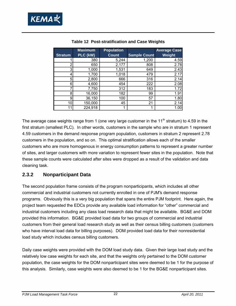
Table 12 Post-stratification and Case Weights .........................................................................22
Table 13 Baseline Protocols Proposed by the Parties ..............................................................24
Table 14 Baseline Adjustments ................................................................................................32
Table 15 Baseline Protocols Included in the Assessment ........................................................35
Table 16 Example Customer Actual Hourly Load and Baseline Data .......................................36
Table 17 Example Calculation of Bias Metric ...........................................................................37
Table 18 Example Calculation of Variability Metric ...................................................................38
Table 19 Example Calculation of Accuracy Metric ....................................................................38
Table 20 Distribution of 99th Percentile of Summer Demand ...................................................45
Table 21 Distribution of Relative RMSE ...................................................................................49
Table 22 Number of Sites by Segment .....................................................................................50
Table 23 Definition of Analysis Periods (Morning/Afternoon Pre-Event/Event) .........................63
Table 24 Comparison of Accuracy of Baselines for Non-Variable Customers for Summer Afternoon Events ...............................................................................................................66
Table 25 Comparison of Accuracy of Baselines for Non-Variable Customers for High Temperature Summer Afternoon Events ............................................................................69
Table of Contents
PJM Load Management Task Force April 20, 2011 iv
Table 26 Comparison of Bias of Baselines for Non-Variable Customers for High Temperature Summer Afternoon Events .................................................................................................72
Table 27 Comparison of Accuracy of Baselines for Non-Variable Customers for Winter Morning Events ................................................................................................................................74
Table 28 Comparison of Accuracy of Baselines for Weather Sensitive, Non-Variable Customers for 15 Hottest Summer Afternoons .....................................................................................75
Table 29 Comparison of Accuracy of Baselines for Non-Weather Sensitive, Non-Variable Customers for 15 Hottest Summer Afternoons ...................................................................76
Table 30 Qualitative Comparison of Administration Required for Different CBLs ......................78
Table 31 Hypothetical Case Studies ........................................................................................79
Table 32 Summary of Results for Summer Weekdays, all Sizes of Customers, for All Weather Customers, with Non-Variable Load ...................................................................................84
Table 33 Results for Extreme Summer Weekdays, All Sizes of Customers, For All Weather Customers, with All Loads sorted by Accuracy Median and Variability Median ..................86
Table 34 Results for Extreme Summer Weekdays, All Sizes of Customers, For All Weather Customers, with Non-Variable Load sorted by Accuracy Median and Variability Median ....88
Table 35 Results for Extreme Summer Weekdays, All Sizes of Customers, Weather Sensitive Customers, with All Loads sorted by Accuracy Median and Variability Median ..................89
Table 36 Results for Extreme Summer Weekdays, All Sizes of Customers, Non-Weather Sensitive Customers, with All Loads sorted by Accuracy Median and Variability Median ...90
Table 37 Results for Summer Weekdays, All Sizes of Customers, For All Weather Customers, with All Loads sorted by Accuracy Median and Variability Median .....................................91
Table 38 Results for Summer Weekdays, All Sizes of Customers, For All Weather Customers, with Non-Variable Load sorted by Accuracy Median and Variability Median .......................93
Table 39 Results for Summer Weekdays, All Sizes of Customers, Weather Sensitive Customers, with All Loads sorted by Accuracy Median and Variability Median ..................94
Table 40 Results for Summer Weekdays, All Sizes of Customers, Non-Weather Sensitive Customers, with All Loads sorted by Accuracy Median and Variability Median ..................95
Table 41 Results for Extreme Winter Weekdays, All Sizes of Customers, For All Weather Customers, with All Loads sorted by Accuracy Median and Variability Median ..................96
Table 42 Results for Extreme Winter Weekdays, All Sizes of Customers, For All Weather Customers, with Variable Load sorted by Accuracy Median and Variability Median ...........97
Table of Contents
PJM Load Management Task Force April 20, 2011 v
Table 43 Results for Extreme Winter Weekdays, All Sizes of Customers, For All Weather Customers, with Non-Variable Load sorted by Accuracy Median and Variability Median ....98
Table 44 Results for Extreme Winter Weekdays, All Sizes of Customers, Weather Sensitive Customers, with All Loads sorted by Accuracy Median and Variability Median ..................99
Table 45 Results for Extreme Winter Weekdays, All Sizes of Customers, Non-Weather Sensitive Customers, with All Loads sorted by Accuracy Median and Variability Median ................ 100
Table 46 Results for Winter Weekdays, All Sizes of Customers, For All Weather Customers, with All Loads sorted by Accuracy Median and Variability Median ................................... 101
Table 47 Results for Winter Weekdays, All Sizes of Customers, For All Weather Customers, with Non-Variable Load sorted by Accuracy Median and Variability Median ..................... 103
Table 48 Results for Winter Weekdays, All Sizes of Customers, Weather Sensitive Customers, with All Loads sorted by Accuracy Median and Variability Median ................................... 104
Table 49 Results for Winter Weekdays, All Sizes of Customers, Non-Weather Sensitive Customers, with All Loads sorted by Accuracy Median and Variability Median ................ 105
List of Figures:
Figure 1 Weather Sensitivity Ratio Example ............................................................................43
Figure 2 Distribution of WS Ratio (When Ratio less than 1) .....................................................44
Figure 3 Example of Low Load Variability Customer ................................................................46
Figure 4 Example of a Median Load Variability Customer ........................................................47
Figure 5 Example of a High Load Variability Customer ............................................................48
Figure 6 Distribution of Relative RMSE ....................................................................................49
Figure 7 Example of a Comparison of Unadjusted Baselines for a Non-Variable Load .............53
Figure 8 Alternative Comparison of Unadjusted Baselines for a Non-Variable Load ................54
Figure 9 Comparison of Unadjusted Baselines for a Weather Sensitive Load ..........................55
Figure 10 Comparison of Additive Adjusted Baselines for a Non-variable Load .......................56
Figure 11 Alternative Comparison of Additive Adjusted Baselines for a Non-variable Load ......57
Figure 12 Comparison of Additive Adjusted Baselines for a Weather Sensitive Load ...............58
Figure 13 Additive Adjusted Baselines for a Winter Morning Period .........................................59
Figure 14 Comparison of Multiplicative Adjusted Baselines for a Weather Sensitive Load .......60
Figure 15 Multiplicative Adjusted Baselines for a Winter Morning Period .................................61
Table of Contents
PJM Load Management Task Force April 20, 2011 vi
Figure 16 Comparison of Weather Sensitive Adjusted Baselines for a Weather Sensitive Load ..........................................................................................................................................62
Figure 17 Comparison of Accuracy of Baselines for Non-Variable Customers for Summer Afternoon Events ...............................................................................................................65
Figure 18 Comparison of Bias of Baselines for Non-Variable Customers for Summer Afternoon Events ................................................................................................................................68
Figure 19 Comparison of Accuracy of Baselines for Non-Variable Customers for High Temperature Summer Afternoon Events ............................................................................69
Figure 20 Comparison of Bias of Baselines for Non-Variable Customers for High Temperature Summer Afternoon Events .................................................................................................71
Figure 21 Comparison of Accuracy of Baselines for Non-Variable Customers for Winter Morning Events ..................................................................................................................73
Figure 22 Non-Variable, Median Control Group Accuracy for the Summer Period ...................77
PJM Load Management Task Force April 20, 2011
1
E. Executive Summary
PJM established the Load Management Task Force (“LMTF”) to focus on improving capacity based demand response (“DR”) products. Based on practical experience gained with the first mandatory test requirement conducted in the summer of 2009, the LMTF has become concerned with the lack of specificity for the current guaranteed load drops (“GLD”) methods. These methods are used to determine the load reduction under emergency conditions for DR resources with a firm capacity commitment. The Markets Implementation Committee (“MIC”), which governs the LMTF, has requested PJM staff to move forward with an empirical analysis of a variety of customer baseline (“CBL”) methods used to measure performance in the energy and capacity markets. This report presents the results of such an analysis.
The analysis was designed to be a comprehensive examination of the issues surrounding the development of accurate baselines. Specifically, the objectives of the project were to:
1. Determine the accuracy and bias of a variety of CBL methods;
2. Determine the feasibility of administering each CBL method for all market participants under consideration; and
3. Attempt to develop objective criteria to associate a customer load with a specific CBL method if this will result in significantly improved accuracy, less bias and less variability.
E.1 Analysis
The analysis used a very large, robust sample of participants and non-participants, over a multiple year frame, testing a broad range of representative baselines and the commonly accepted adjustment approaches and using multiple metrics to define the baselines‟ efficacy.
The analysis:
Was based on data requested from most PJM electric distribution companies (EDCs). The EDCs were asked to provide load information on all the end use customers that were registered to participate as an economic or emergency demand resource in their service territories. In total, 4,565 of 11,730 emergency and economic participants (40 percent) were provided for the analysis. The sample represented over 9,000 MW of the total 16,000 MW (54 percent) of program‟s Peak Load Contribution (PLC). Two EDCs also provided 16,000 nonparticipating customers for a control pool.
Included hourly load data from June 1, 2008 through September 30, 2010.
PJM Load Management Task Force April 20, 2011 2
Featured a total of 11 baselines, with up to four variants of each baseline for a total of 36 different CBL and adjustment methods analyzed. The variants represent common adjustments to the baseline approaches.
Compared the seasonal efficacy of the baselines by analyzing the baseline performance during the summer afternoon and winter morning event periods.
Used three metrics to establish the baselines‟ statistical properties. These metrics measured each baseline‟s accuracy, variability and bias.
Resulted in nearly 150 million estimated baselines (CBLs * Customers * events estimated).
E.1.1 Baseline Protocols and Adjustments
The analysis featured a total of 11 baselines, with up to four variants of each baseline. The variants represent common adjustments to the baseline approaches including an additive adjustment, a multiplicative adjustment, a weather sensitive adjustment, and no adjustment. Accordingly, there were up to 44 different baseline/variants included in the analysis1. The baselines included in the analysis are:
PJM Economic
PJM Emergency Comparable Day Non-weather Sensitive
PJM Emergency Comparable Day Weather Sensitive
PJM Emergency Same Day
PJM Emergency Energy Settlement
California ISO (“CAISO”) Standard
New York ISO (“NYISO”) Standard
ISO New England (“ISONE”) Standard
Electric Reliability Council of Texas (“ERCOT”) Regression
1 Certain combinations of baselines and adjustments, though produced, were not practical alternatives. For instance, it makes little sense to adjust the flat baseline set at the level of the last pre-event period, or to apply a weather-sensitive adjustment to a regression baseline that includes a weather component. See Table 14 for a complete list of the baseline variants that were analyzed for this report.
PJM Load Management Task Force April 20, 2011 3
KEMA Regression
Middle 4 of 6
The adjustments included same day, load-based multiplicative (ratio) and additive adjustments as well as a regression-based regression based on the PJM alternative weather sensitive adjustment.
E.1.2 Performance Metrics
Three statistics were chosen to measure the three quantitative aspects of baseline performance: accuracy, bias, and variability. The attribute given the most emphasis in the analysis was accuracy, or how closely a baseline method predicts customers‟ actual loads in the sample. The statistic chosen to measure accuracy was the median of the relative root mean squared error (RRMSE). This statistic expresses the baseline‟s average hourly accuracy as a fraction of average hourly load for the typical customer. The RRMSE is based on squared prediction errors. This technique in essence weights large errors much more heavily than small or midsized errors. In contrast, the errors are weighted evenly with a technique that measures errors based on the absolute values of the prediction errors. This means that the effect of large hourly errors in the predicted load will result in a higher RRMSE as opposed to a mean absolute percentage error (MAPE). The RRMSE combines the systematic errors measured by the bias metric (the baseline‟s average relative error) and the variability of errors captured by the variability metric (relative error ratio ). For this reason, the RRMSE was chosen as the accuracy metric. A baseline for a typical customer with a median RRMSE of 0.10 is one where that baseline could expect to have an hourly error, on average, of 10 percent of their actual hourly load. The smaller the RRMSE, the better the baseline performs as a predictor of the actual hourly load. The second baseline attribute analyzed was bias, or the systematic tendency of a baseline method to over- or under-predict actual loads. Bias was measured using the median of the baseline‟s average relative error (ARE). This statistic, for a given customer, is the average hourly baseline less the average hourly actual load, expressed as a fraction of actual hourly load. A median ARE value of zero would indicate that the typical customer in our sample had no systematic tendency to over- or under-predict loads using that baseline, whereas a positive (negative) value would indicate a tendency to over- (under-) predict loads. The closer ARE is to zero, the closer the baseline is to being unbiased.
PJM Load Management Task Force April 20, 2011 4
The third baseline attribute analyzed was variability. The variability is the measure of how well the baseline is at predicting hourly load under many different conditions and across many different customers. For example, two baselines may have the same RRMSE but one baseline may be able to better estimate hourly load across a wider variety of situations such that the dispersion of errors is much closer to actual load than the other baseline. In other words, one baseline may estimate the load shapes more closely than the other baseline. The variability measurement chosen was the relative error ratio (RER), which is the standard deviation of the baseline‟s prediction errors expressed as a fraction of average load. The smaller the median RER, the less variable a baseline‟s error is for the typical customer and therefore the better the baseline performs across a wide variety of circumstances. It should be noted that the accuracy, bias and variability were all calculated for the 10th percentile, median, mean and 90th percentile for each baseline method within each segment. This allows for a detailed analysis of the different baselines across a wide variety of circumstances to get a thorough understanding of how well each baseline estimates a customer actual hourly load. The 10th percentile in effect illustrates an expected “top” case performance scenario while the 90th percentile illustrates a “bottom” case performance scenario so an analyst can understand the range of expected outcomes for the various metrics. For example, based on the top performing baselines in this analysis we find:
Accuracy represented by median RRMSE is 0.10 o 10th percentile Accuracy is 0.04 o 90th percentile is 0.19
Variability represented by RER is 0.08 Bias represented as ARE is 0
The simple way to interpret this is one can expect the baseline to estimate the typical customers hourly load within + or – 10% of their actual load while the baseline will accurately estimate the load shape over time and not have a tendency to over or underestimate. Further, for 1 in 10 customers this estimate will be much better or within 4% of actual hourly load while we can conclude that for 9 in 10 customers the prediction will be no worse than 19% of the actual load. This helps to understand how well the baseline is expected to perform over a variety of customers and circumstances and illustrates that it is expected that the accuracy will be between 4% and 19% on an hourly basis where baseline accuracy for cumulative load will be much closer to perfect, over longer period of time, because it does not have an tendency to over or under predict the load.
PJM Load Management Task Force April 20, 2011 5
E.2 Accuracy, Bias and Variability Results
E.2.1 Accuracy
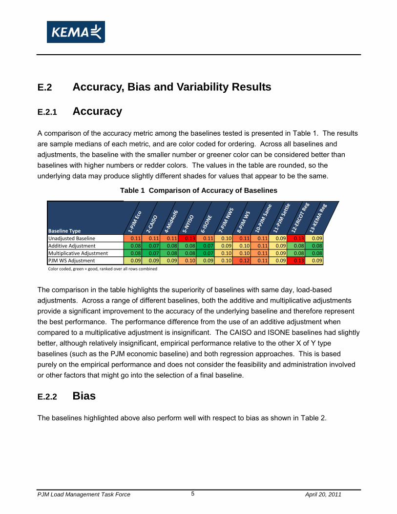
A comparison of the accuracy metric among the baselines tested is presented in Table 1. The results are sample medians of each metric, and are color coded for ordering. Across all baselines and adjustments, the baseline with the smaller number or greener color can be considered better than baselines with higher numbers or redder colors. The values in the table are rounded, so the underlying data may produce slightly different shades for values that appear to be the same.
Table 1 Comparison of Accuracy of Baselines
Baseline Type 1-PJ
M E
co
2-CA
ISO
4-M
id4o
f6
5-N
YISO
6-IS
ON
E
7-PJ
M N
WS
8-PJ
M W
S
10-P
JM S
ame
11-P
JM S
ettl
e12
-ER
COT
Reg
13-K
EMA
Reg
Unadjusted Baseline 0.11 0.11 0.11 0.13 0.11 0.10 0.11 0.11 0.09 0.13 0.09
Additive Adjustment 0.08 0.07 0.08 0.08 0.07 0.09 0.10 0.11 0.09 0.08 0.08
Multiplicative Adjustment 0.08 0.07 0.08 0.08 0.07 0.10 0.10 0.11 0.09 0.08 0.08
PJM WS Adjustment 0.09 0.09 0.09 0.10 0.09 0.10 0.12 0.11 0.09 0.13 0.09
Color coded, green = good, ranked over all rows combined
The comparison in the table highlights the superiority of baselines with same day, load-based adjustments. Across a range of different baselines, both the additive and multiplicative adjustments provide a significant improvement to the accuracy of the underlying baseline and therefore represent the best performance. The performance difference from the use of an additive adjustment when compared to a multiplicative adjustment is insignificant. The CAISO and ISONE baselines had slightly better, although relatively insignificant, empirical performance relative to the other X of Y type baselines (such as the PJM economic baseline) and both regression approaches. This is based purely on the empirical performance and does not consider the feasibility and administration involved or other factors that might go into the selection of a final baseline.
E.2.2 Bias
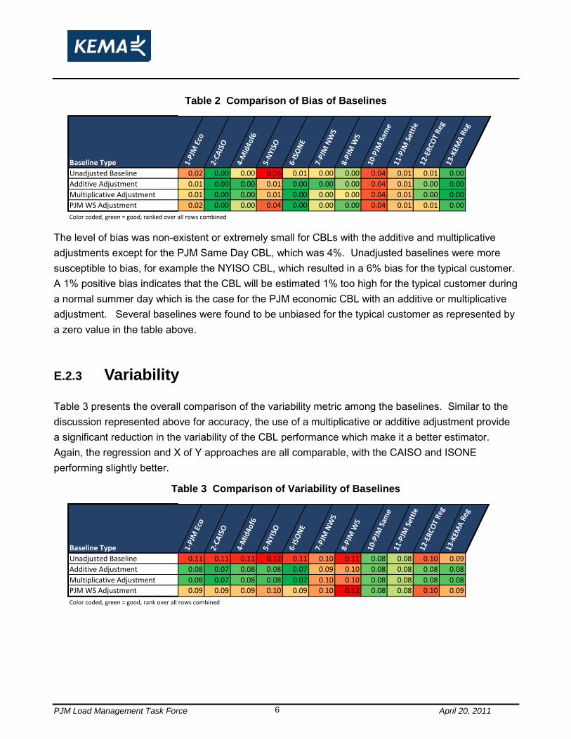
The baselines highlighted above also perform well with respect to bias as shown in Table 2.
PJM Load Management Task Force April 20, 2011 6
Table 2 Comparison of Bias of Baselines
Baseline Type 1-PJ
M E
co
2-CA
ISO
4-M
id4o
f6
5-N
YISO
6-IS
ON
E
7-PJ
M N
WS
8-PJ
M W
S
10-P
JM S
ame
11-P
JM S
ettl
e12
-ER
COT
Reg
13-K
EMA
Reg
Unadjusted Baseline 0.02 0.00 0.00 0.06 0.01 0.00 0.00 0.04 0.01 0.01 0.00
Additive Adjustment 0.01 0.00 0.00 0.01 0.00 0.00 0.00 0.04 0.01 0.00 0.00
Multiplicative Adjustment 0.01 0.00 0.00 0.01 0.00 0.00 0.00 0.04 0.01 0.00 0.00
PJM WS Adjustment 0.02 0.00 0.00 0.04 0.00 0.00 0.00 0.04 0.01 0.01 0.00
Color coded, green = good, ranked over all rows combined
The level of bias was non-existent or extremely small for CBLs with the additive and multiplicative adjustments except for the PJM Same Day CBL, which was 4%. Unadjusted baselines were more susceptible to bias, for example the NYISO CBL, which resulted in a 6% bias for the typical customer. A 1% positive bias indicates that the CBL will be estimated 1% too high for the typical customer during a normal summer day which is the case for the PJM economic CBL with an additive or multiplicative adjustment. Several baselines were found to be unbiased for the typical customer as represented by a zero value in the table above.
E.2.3 Variability
Table 3 presents the overall comparison of the variability metric among the baselines. Similar to the discussion represented above for accuracy, the use of a multiplicative or additive adjustment provide a significant reduction in the variability of the CBL performance which make it a better estimator. Again, the regression and X of Y approaches are all comparable, with the CAISO and ISONE performing slightly better.
Table 3 Comparison of Variability of Baselines
Baseline Type 1-PJ
M E
co
2-CA
ISO
4-M
id4o
f6
5-N
YISO
6-IS
ON
E
7-PJ
M N
WS
8-PJ
M W
S
10-P
JM S
ame
11-P
JM S
ettl
e12
-ER
COT
Reg
13-K
EMA
Reg
Unadjusted Baseline 0.11 0.11 0.11 0.12 0.11 0.10 0.11 0.08 0.08 0.10 0.09
Additive Adjustment 0.08 0.07 0.08 0.08 0.07 0.09 0.10 0.08 0.08 0.08 0.08
Multiplicative Adjustment 0.08 0.07 0.08 0.08 0.07 0.10 0.10 0.08 0.08 0.08 0.08
PJM WS Adjustment 0.09 0.09 0.09 0.10 0.09 0.10 0.12 0.08 0.08 0.10 0.09
Color coded, green = good, rank over all rows combined

PJM Load Management Task Force April 20, 2011 7
E.3 Administration
The ultimate results and conclusions were based on the baselines‟ empirical performance as well as the estimated cost, across all market participants, to administer the baselines. Market participants that have a cost impact based on the complexity of administering a CBL include: electric distribution companies (EDCs), load serving entities (LSEs), curtailment service providers (CSPs), PJM, and end use customers.
Administrative costs and the associated level of investment in activities such as data transfer, data quality review, analysis, training, and IT systems requirements were considered for a simple baseline, a baseline of medium complexity, and a complex baseline methodology. The results of the baseline operational feasibility analysis shows that the annual total cost to administer a complex baseline methodology is estimated to be more than three times as much as a simple baseline methodology. For market participants the baseline operational feasibility is an important factor when determining the CBL to be utilized. As represented in the empirical analysis above, many of the CBLs with an additive or multiplicative adjustment have very similar results. In these instances, the administrative costs become a significant factor in determining which CBL to choose.
E.4 Segmentation
One of the goals of the evaluation was to determine whether or not customers should be segmented and then aligned to different CBLs in order to achieve more accurate results. Our criterion for choosing which segments to consider was that the segments should be sufficiently transparent that the market would readily understand which CBL goes with what type of customer.
The following customer segments were chosen to be evaluated as part of the analysis:
Customers with weather sensitive load versus customers with non-weather sensitive load;
Size of customer, based on demand; and
Customers with variable load versus customers with non-variable load.
E.4.1 Segmentation by Variability
Baseline approaches considered in this analysis to measure load reductions may not be applicable for customers with certain kinds of variable loads. When a customer‟s load is uncorrelated with any identifiable previous load pattern, no generalized baseline methodology can produce an effective
PJM Load Management Task Force April 20, 2011 8
baseline. Additional analysis to determine whether there is a better way to eliminate the inter-day variability (e.g.: Monday load data is always different than Wednesday and therefore we should only use a Monday to predict a Monday and not a Wednesday), the intra-day variability (e.g.: load for each hour is highly variable but cumulative load for weekdays is consistent) will be required to come up with an appropriate solution. For the purpose of segmenting accounts for this analysis, KEMA identified accounts with non-weather-related load variability. As variability increased, the ability of the resulting baseline to produce a reasonable estimate of load reduction decreased. The aggregate analysis results indicate that an upper limit on variability should be considered and that customers that fall above it should be measured using a different methodology than other customers.
E.4.2 Segmentation by Weather Sensitivity
An important goal of the segmentation analysis was to determine whether the different groups should be assigned different baselines. In fact, the x of y type baselines with same day load-based adjustments are equally effective across all account segmentations as well as event conditions. Thus, there is no need to segment based on weather sensitivity because the use of a same day adjustment improves both the non-weather sensitive and weather sensitive segments. A common structure of DR programs stipulates an unadjusted baseline for all accounts with an option for a same-day, load-based adjustment for accounts that are weather sensitive. This approach is not justified on the basis of the accuracy results reported in this study. While the same-day, load-based adjustment does not improve the accuracy for non-weather sensitive accounts to quite the same degree, there is still an improvement of 20 to 30 percent. A decision to forgo the load-based adjustment must be based on other considerations, such as administrative costs and/or non-typical event day behavior (e.g.: pre-cooling).
E.4.3 Segmentation by Customer Size
There is no reason to segment by size based on the results of this study unless the administrative costs associated with variable load accounts are sufficiently large that it is only feasible to include medium and large accounts. This is, in part, because the structural aspect of baseline performance does not change as a result of account load level. In this respect, the size segmentation ends up being a proxy for business type segmentation. The size segmentation shows that baselines for smaller accounts are less accurate, in general, than they are for larger segments. This is likely due to the greater diversity of business types in the smaller
PJM Load Management Task Force April 20, 2011 9
account segments. Other than this observation, the segmentation by size provides little additional perspective on the choice of optimal baseline.
E.5 Measurement of Capacity Compliance vs. Energy
Reductions
This report focuses on the measurement of real time energy reductions through the use of a variety of customer baseline calculations. Since capacity requirements are inherently different than the measurement of energy reductions, it is important to understand how to measure capacity compliance relative to such capacity requirements. PJM rules limit the amount of capacity that can be offered into the market as a demand resource based on each customer‟s capacity commitment (which is referred to as the “peak load contribution” or “PLC”). It therefore follows that the measurement of capacity compliance should be based on the customer‟s load relative the customer‟s capacity commitment or PLC. This approach does not require a CBL for measurement purposes and would rely on a maximum base load (“MBL”)2 which is both accurate and simple to administer. In PJM, the maximum base load method is referred to as the Firm Service Level method.
E.6 Recommendations
Selection of an appropriate CBL should consider the results of the empirical analysis, the expected administrative costs, and any other known issues based on previous practical experience, including strategic behavior to maximize the baseline and applicability of baselines for customers that frequently respond.
The analysis clearly indicates that a same day additive or multiplicative adjustment has superior performance to an unadjusted CBL or a CBL using the PJM weather sensitive adjustment. The decision of whether to use a multiplicative or additive adjustment is fairly arbitrary because the impact on the performance metrics is not significant. However, due to a somewhat greater susceptibility of multiplicative adjustments to gross inaccuracies under certain demand conditions, we therefore recommend that an additive adjustment be utilized.
2 See NAESB Measurement and Verification standards for a description of the maximum baseload approach – this is same approach that is referred to at PJM as the “Firm Service Level.”
PJM Load Management Task Force April 20, 2011 10
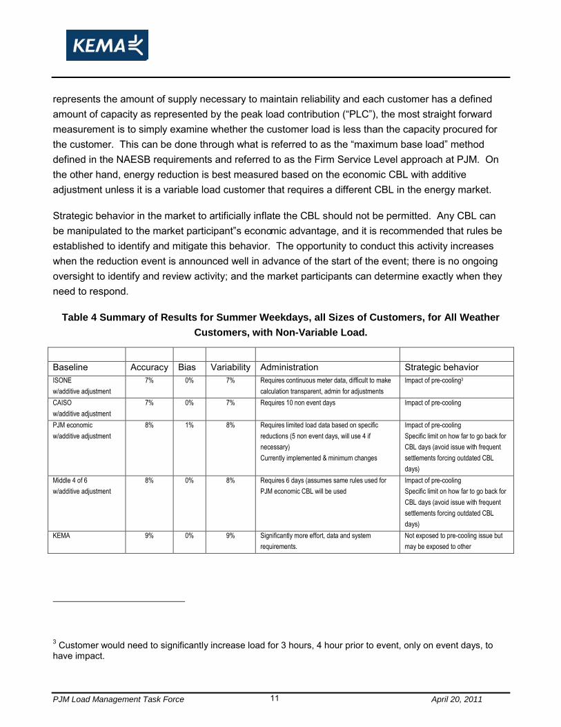
The X of Y (i.e., CALISO, ISONE, PJM economic and mid 4 of 6) and regression approaches with a same day additive adjustment have similar results and performed well across all segments, time periods and weather conditions, except for predicting loads for variable load customers. It is therefore recommended that variable load customers be segmented for purposes of applying a different CBL and/or market rule. Since the empirical results for non-variable load customers are similar, it is important to understand the administrative cost and other factors in the final decision. Table 4 presents a comparison of the four approaches.
Since the administrative costs and associated complexity of the regression approaches are significantly higher than those of the X of Y approaches, there is no reason to pursue this method based on the results of the analysis. Therefore, the choice of which method to use for all non-variable load customers should reduce to a choice from among the CALISO, ISONE, PJM economic and Mid 4 of 6 type approaches.
While all four methods produce stable and good results, the CAISO approach requires twice the load data to provide similar results to the other three. Also, the true impact of customers that have frequent settlements has not been considered in this analysis. This issue may have a bigger impact on the CAISO baseline since it requires more days to be selected (as more event days occur, more days closer to the event are skipped which results in the use of days further from the event day). Therefore the CAISO method is not recommended.
The ISONE CBL, which has slightly better empirical performance than the other two methods, entails significantly more administrative costs because it requires contiguous load data (since each baseline is based on the prior day‟s baseline). This approach also requires additional administration to ensure transparency to all market participants, and requires significantly more administration for settlement adjustments that result in corrections in load data. Since the empirical performance of the ISONE baseline is only marginally better than that of the remaining two, it is not apparent that this additional administrative effort is warranted and therefore is not recommended.
The remaining two CBLs, the PJM economic and the mid 4 of 6 are reasonably similar in terms of empirical performance and ease of administration. Therefore the PJM economic CBL with the additive adjustment is recommended simply because it has already been implemented and is currently operational in the PJM market.
Finally, the measurement of reductions in the energy market should be done on a consistent basis. Conducting such measurements differently based on whether the reduction results from an economic program or an emergency energy reduction appears inconsistent. The measurement of load reductions in the energy market is different than measuring capacity compliance in the Capacity market and therefore each requires a different measurement method. Clearly, since capacity
PJM Load Management Task Force April 20, 2011 11
represents the amount of supply necessary to maintain reliability and each customer has a defined amount of capacity as represented by the peak load contribution (“PLC”), the most straight forward measurement is to simply examine whether the customer load is less than the capacity procured for the customer. This can be done through what is referred to as the “maximum base load” method defined in the NAESB requirements and referred to as the Firm Service Level approach at PJM. On the other hand, energy reduction is best measured based on the economic CBL with additive adjustment unless it is a variable load customer that requires a different CBL in the energy market.
Strategic behavior in the market to artificially inflate the CBL should not be permitted. Any CBL can be manipulated to the market participant‟s economic advantage, and it is recommended that rules be established to identify and mitigate this behavior. The opportunity to conduct this activity increases when the reduction event is announced well in advance of the start of the event; there is no ongoing oversight to identify and review activity; and the market participants can determine exactly when they need to respond.
Table 4 Summary of Results for Summer Weekdays, all Sizes of Customers, for All Weather
Customers, with Non-Variable Load.
Baseline Accuracy Bias Variability Administration Strategic behavior ISONE
w/additive adjustment
7% 0% 7% Requires continuous meter data, difficult to make
calculation transparent, admin for adjustments
Impact of pre-cooling3
CAISO
w/additive adjustment
7% 0% 7% Requires 10 non event days Impact of pre-cooling
PJM economic
w/additive adjustment
8% 1% 8% Requires limited load data based on specific
reductions (5 non event days, will use 4 if
necessary)
Currently implemented & minimum changes
Impact of pre-cooling
Specific limit on how far to go back for
CBL days (avoid issue with frequent
settlements forcing outdated CBL
days)
Middle 4 of 6
w/additive adjustment
8% 0% 8% Requires 6 days (assumes same rules used for
PJM economic CBL will be used
Impact of pre-cooling
Specific limit on how far to go back for
CBL days (avoid issue with frequent
settlements forcing outdated CBL
days)
KEMA 9% 0% 9% Significantly more effort, data and system
requirements.
Not exposed to pre-cooling issue but
may be exposed to other
3 Customer would need to significantly increase load for 3 hours, 4 hour prior to event, only on event days, to have impact.
PJM Load Management Task Force April 20, 2011 12
1. Introduction
The Markets Implementation Committee (“MIC”) has requested PJM staff to move forward with an empirical analysis of a variety of customer baseline (“CBL”) methods used to measure performance in the energy and capacity markets. The current project has the following objectives:
1) Determine the accuracy and bias of a variety of CBL methods;
2) Determine the feasibility of administering each CBL method for all market participants under consideration; and
3) Attempt to develop objective criteria to associate a customer load with a specific CBL method if this will result in significantly improved accuracy, less bias and less variability.
The project work plan specified that a comprehensive set of baseline protocols be specified, and the performance of the candidate protocols be tested on a robust set of data of actual PJM participants. The testing included:
Protocol‟s ability to predict actual loads on non-event days;
Comparison of the baseline with actual load by hour for each non-event day, for each baseline method;
Calculation of empirical performance metrics to measure how well the calculated baseline simulated actual load;
Comparison of metrics to evaluate empirical performance among the various CBL methods;
This report presents the results of the empirical analysis of demand response baseline methods. After this introductory section, the next sections describe the methodology, analysis, and results including recommendations.
2. Methodology
2.1 Data Sources
The analysis is based on a sample of commercial and industrial customers in PJM‟s service territory who are demand response program participants. The following Electric Distribution Companies (“EDCs”) in PJM‟s service territory were given the opportunity to provide data to this analysis:
American Electric Power
Allegheny Energy

PJM Load Management Task Force April 20, 2011 13
Baltimore Gas & Electric
Commonwealth Edison
Dayton Power and Light
Dominion Virginia Power
Duquesne Light Company
FirstEnergy
Philadelphia Electric Company
Potomac Electric Power
Pennsylvania Power & Light
Public Service Electric & Gas
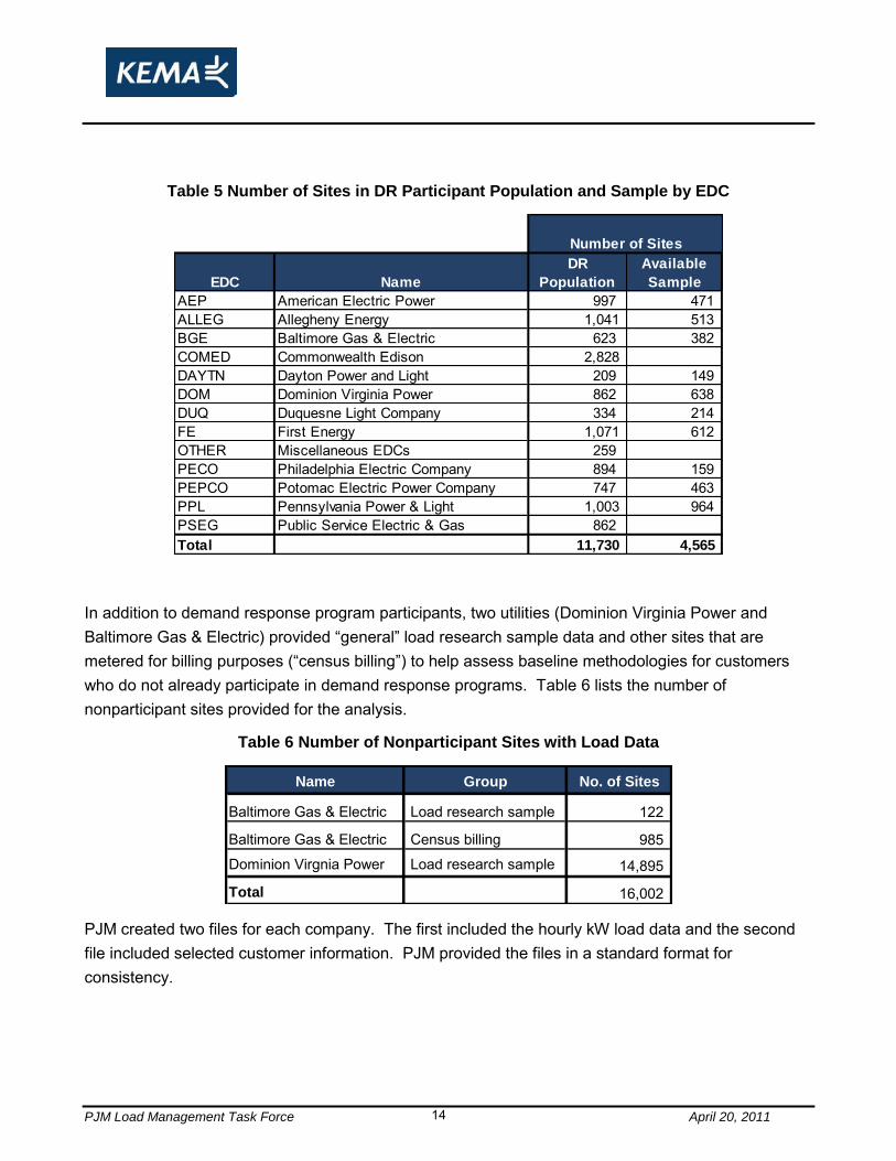
Almost all of these companies provided hourly load data and some basic supporting customer information for at least a sample of demand response participants. There are other EDCs in PJM‟s service territory who were not asked to provide data due to their low volume of demand response participants. Table 5 lists the distribution companies in PJM‟s service territory, the total number of commercial and industrial demand response participants (population) by EDC, and the number of customers in the available sample of hourly load data used for the analysis. The “other” EDC category (miscellaneous EDCs) includes the EDCs with a low number of demand response participants who were not asked to provide data.
PJM Load Management Task Force April 20, 2011 14
Table 5 Number of Sites in DR Participant Population and Sample by EDC
EDC Name
DR
Population
Available
Sample
AEP American Electric Power 997 471 ALLEG Allegheny Energy 1,041 513 BGE Baltimore Gas & Electric 623 382 COMED Commonwealth Edison 2,828 DAYTN Dayton Power and Light 209 149 DOM Dominion Virginia Power 862 638 DUQ Duquesne Light Company 334 214 FE First Energy 1,071 612 OTHER Miscellaneous EDCs 259 PECO Philadelphia Electric Company 894 159 PEPCO Potomac Electric Power Company 747 463 PPL Pennsylvania Power & Light 1,003 964 PSEG Public Service Electric & Gas 862 Total 11,730 4,565
Number of Sites
In addition to demand response program participants, two utilities (Dominion Virginia Power and Baltimore Gas & Electric) provided “general” load research sample data and other sites that are metered for billing purposes (“census billing”) to help assess baseline methodologies for customers who do not already participate in demand response programs. Table 6 lists the number of nonparticipant sites provided for the analysis.
Table 6 Number of Nonparticipant Sites with Load Data
Name Group No. of Sites
Baltimore Gas & Electric Load research sample 122
Baltimore Gas & Electric Census billing 985
Dominion Virgnia Power Load research sample 14,895
Total 16,002
PJM created two files for each company. The first included the hourly kW load data and the second file included selected customer information. PJM provided the files in a standard format for consistency.
PJM Load Management Task Force April 20, 2011 15
2.1.1 Hourly Load Data
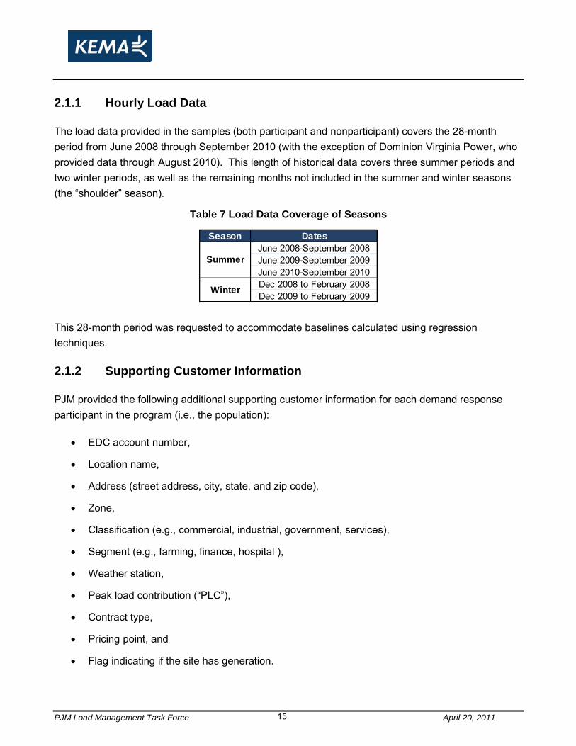
The load data provided in the samples (both participant and nonparticipant) covers the 28-month period from June 2008 through September 2010 (with the exception of Dominion Virginia Power, who provided data through August 2010). This length of historical data covers three summer periods and two winter periods, as well as the remaining months not included in the summer and winter seasons (the “shoulder” season).
Table 7 Load Data Coverage of Seasons
Season Dates
June 2008-September 2008June 2009-September 2009June 2010-September 2010Dec 2008 to February 2008Dec 2009 to February 2009
Summer
Winter
This 28-month period was requested to accommodate baselines calculated using regression techniques.
2.1.2 Supporting Customer Information
PJM provided the following additional supporting customer information for each demand response participant in the program (i.e., the population):
EDC account number,
Location name,
Address (street address, city, state, and zip code),
Zone,
Classification (e.g., commercial, industrial, government, services),
Segment (e.g., farming, finance, hospital ),
Weather station,
Peak load contribution (“PLC”),
Contract type,
Pricing point, and
Flag indicating if the site has generation.
PJM Load Management Task Force April 20, 2011 16
2.1.3 Event Day and Hour Data
PJM provided datasets containing flags indicating demand response event dates and hours by site. This information was used to appropriately exclude those days when events (including test events) had occurred when calculating baselines.
2.1.4 Hourly Weather Data
Hourly weather data from the National Oceanic and Atmospheric Administration‟s (“NOAA”) Integrated Surface Hourly service was obtained for each weather station indicated in the customer file. Depending on the baseline method, temperature or temperature humidity index (“THI”) data were used for baseline methods using weather as part of the calculation.
2.2 Hourly Load Data Availability and Quality
PJM has identified those companies who have provided participant load data files that have not been validated. Table 8 is a list of the distribution companies in PJM‟s service territory who provided participant load data, the number of sites and whether the load data was considered validated. About 85 percent of the sites with interval load data were reported having been Validated, Edited, and Estimated (“VEE”) by the EDC. VEE is a set of NAESB rules, guidelines, and techniques for taking raw meter data and performing validation and, as necessary, editing and estimation of corrupt or missing data, to create validated data. A full description of VEE standards and techniques can be found in “Uniform Business Practices for Unbundled Electric Metering Volume 2” by Edison Electric Institute on the NAESB website: http://www.naesb.org/pdf/ubp120500.pdf.

PJM Load Management Task Force April 20, 2011 17
Table 8 List of EDCs Providing Verified Load Data
EDC Name
Available
Sample
VEE by
EDC?
American Electric Power 471 YesAllegheny Energy 513 NoBaltimore Gas & Electric 382 YesDayton Power and Light 149 YesDominion Virgnia Power 638 YesDuquesne Light Company 214 YesFirst Energy 612 YesPhiladelphia Electric Company 159 NoPotomac Electric Power Company 463 YesPennsylvania Power & Light 964 YesTotal 4,565
2.2.1 Load Data Quality Check
Given there were data that had not been verified, KEMA performed validation routines on all the data provided. It was the project team‟s goal to preserve as many sites for the analysis while excluding obviously erroneous load data values. The project team developed rules (presented in subsequent sections) for setting a load data value to missing as well as rules for when it is appropriate to drop an entire site from the analysis. 2.2.2 Rules for Dropping Sites from the Analysis
KEMA dropped sites only when absolutely necessary in order to preserve as much data as possible for the analysis. The project team developed following rules to drop sites from the analysis overall:
1. If a site has does not have data for May 2010 through August 2010.
2. If a site uses no energy for the entire analysis period of June 2008 through September 2010.
A total of 530 participant sites were dropped from the analysis due to not having the full period of May 2010 through August 2010. 2.2.3 Rules for Editing Hourly Load Data
The project team developed the following rules for preparing the hourly load data for analysis:
PJM Load Management Task Force April 20, 2011 18
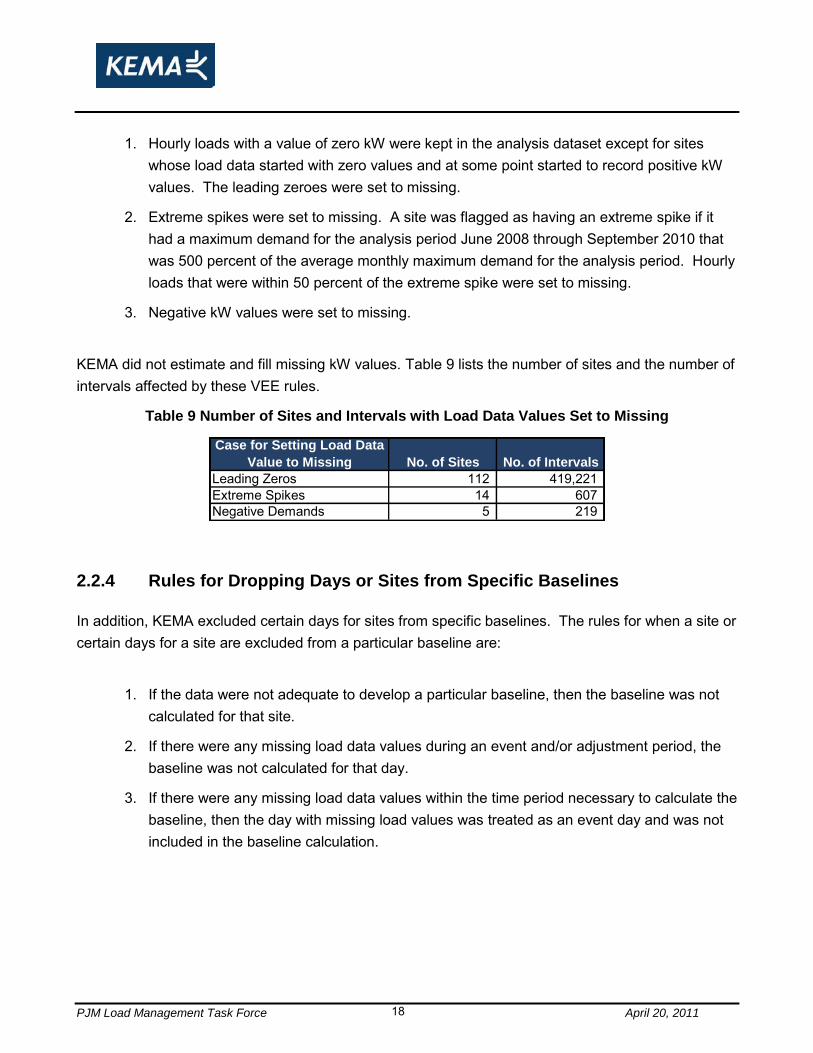
1. Hourly loads with a value of zero kW were kept in the analysis dataset except for sites whose load data started with zero values and at some point started to record positive kW values. The leading zeroes were set to missing.
2. Extreme spikes were set to missing. A site was flagged as having an extreme spike if it had a maximum demand for the analysis period June 2008 through September 2010 that was 500 percent of the average monthly maximum demand for the analysis period. Hourly loads that were within 50 percent of the extreme spike were set to missing.
3. Negative kW values were set to missing.
KEMA did not estimate and fill missing kW values. Table 9 lists the number of sites and the number of intervals affected by these VEE rules.
Table 9 Number of Sites and Intervals with Load Data Values Set to Missing
Case for Setting Load Data
Value to Missing No. of Sites No. of Intervals
Leading Zeros 112 419,221 Extreme Spikes 14 607 Negative Demands 5 219
2.2.4 Rules for Dropping Days or Sites from Specific Baselines
In addition, KEMA excluded certain days for sites from specific baselines. The rules for when a site or certain days for a site are excluded from a particular baseline are:
1. If the data were not adequate to develop a particular baseline, then the baseline was not calculated for that site.
2. If there were any missing load data values during an event and/or adjustment period, the baseline was not calculated for that day.
3. If there were any missing load data values within the time period necessary to calculate the baseline, then the day with missing load values was treated as an event day and was not included in the baseline calculation.
PJM Load Management Task Force April 20, 2011 19
2.3 Sampling Strategy
Once the load data and supporting information was received and VEE was performed, the customer information was statistically analyzed to support the development of weights that could be used to expand the sample to the population(s) of interest.
2.3.1 Demand Response Participants
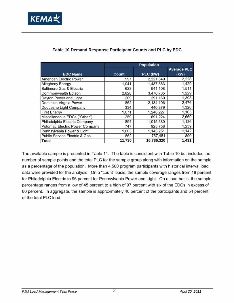
As previously discussed, the primary source of data is the population of existing demand response program participants. Table 10 provides an updated listing of the EDC and the respective population count of program participants. We have included the total Peak Load Contribution (“PLC”) estimated for the program participants in each service territory along with the average PLC calculation. Commonwealth Edison has the most participants with over 2,800 with a total PLC of nearly 3.5 GW. The “Other” category has the fewest participants with 259 participants and 691 MW of load. The “Other” category contains fourteen distinct entities where the numbers of participants range from 1 to 54. Interestingly, this group has the largest average PLC per participant and just over 2.6 MW. The aggregate load represented in the participant population is in excess of 16.7 GW, or approximately 11 percent of the PJM Summer Peak demand forecast for 20114. The average PLC per EDC ranges from less than 1 MW for PSE&G to over 2.5 MW for the “Other” category.
4 The PJM 2011 summer peak demand forecast is approximately 154 GW.
PJM Load Management Task Force April 20, 2011 20
Table 10 Demand Response Participant Counts and PLC by EDC
Count PLC (kW)
Average PLC
(kW)
American Electric Power 997 2,221,349 2,228 Allegheny Energy 1,041 1,487,563 1,429 Baltimore Gas & Electric 623 941,108 1,511 Commonwealth Edison 2,828 3,476,735 1,229 Dayton Power and Light 209 291,169 1,393 Dominion Virgnia Power 862 2,134,196 2,476 Duquesne Light Company 334 440,879 1,320 First Energy 1,071 1,248,227 1,165 Miscellaneous EDCs ("Other") 259 691,224 2,669 Philadelphia Electric Company 894 1,015,380 1,136 Potomac Electric Power Company 747 925,758 1,239 Pennsylvania Power & Light 1,003 1,145,251 1,142 Public Service Electric & Gas 862 767,481 890 Total 11,730 16,786,320 1,431
Population
EDC Name
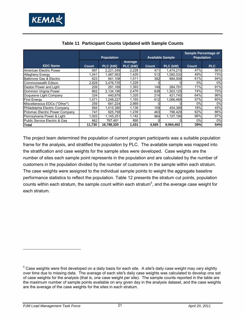
The available sample is presented in Table 11. The table is consistent with Table 10 but includes the number of sample points and the total PLC for the sample group along with information on the sample as a percentage of the population. More than 4,500 program participants with historical interval load data were provided for the analysis. On a “count” basis, the sample coverage ranges from 18 percent for Philadelphia Electric to 96 percent for Pennsylvania Power and Light. On a load basis, the sample percentage ranges from a low of 45 percent to a high of 97 percent with six of the EDCs in excess of 80 percent. In aggregate, the sample is approximately 40 percent of the participants and 54 percent of the total PLC load.
PJM Load Management Task Force April 20, 2011 21
Table 11 Participant Counts Updated with Sample Counts
Count PLC (kW)
Average
PLC (kW) Count PLC (kW) Count PLC
American Electric Power 997 2,221,349 2,228 471 1,474,215 47% 66%Allegheny Energy 1,041 1,487,563 1,429 513 1,092,032 49% 73%Baltimore Gas & Electric 623 941,108 1,511 382 884,008 61% 94%Commonwealth Edison 2,828 3,476,735 1,229 0 0 0% 0%Dayton Power and Light 209 291,169 1,393 149 264,791 71% 91%Dominion Virgnia Power 862 2,134,196 2,476 638 1,503,125 74% 70%Duquesne Light Company 334 440,879 1,320 214 421,745 64% 96%First Energy 1,071 1,248,227 1,165 612 1,066,468 57% 85%Miscellaneous EDCs ("Other") 259 691,224 2,669 0 0 0% 0%Philadelphia Electric Company 894 1,015,380 1,136 159 454,389 18% 45%Potomac Electric Power Company 747 925,758 1,239 463 796,429 62% 86%Pennsylvania Power & Light 1,003 1,145,251 1,142 964 1,107,199 96% 97%Public Service Electric & Gas 862 767,481 890 0 0 0% 0%Total 11,730 16,786,320 1,431 4,565 9,064,402 39% 54%
Population
EDC Name
Available Sample
Sample Percentage of
Population
The project team determined the population of current program participants was a suitable population frame for the analysis, and stratified the population by PLC. The available sample was mapped into the stratification and case weights for the sample sites were developed. Case weights are the number of sites each sample point represents in the population and are calculated by the number of customers in the population divided by the number of customers in the sample within each stratum. The case weights were assigned to the individual sample points to weight the aggregate baseline performance statistics to reflect the population. Table 12 presents the stratum cut points, population counts within each stratum, the sample count within each stratum5, and the average case weight for each stratum.
5 Case weights were first developed on a daily basis for each site. A site‟s daily case weight may vary slightly over time due to missing data. The average of each site‟s daily case weights was calculated to develop one set of case weights for the analysis (that is, one case weight per site). The sample counts reported in the table are the maximum number of sample points available on any given day in the analysis dataset, and the case weights are the average of the case weights for the sites in each stratum.
PJM Load Management Task Force April 20, 2011 22
Table 12 Post-stratification and Case Weights
Stratum
Maximum
PLC (kW)
Population
Count Sample Count
Average Case
Weight
1 380 5,244 1,200 4.592 650 2,177 808 2.783 1,000 1,531 649 2.434 1,700 1,018 479 2.175 2,800 666 316 2.146 4,600 454 222 2.087 7,750 312 183 1.728 16,000 182 99 1.919 36,150 100 57 1.80
10 150,000 45 21 2.1411 224,918 1 1 1.00
The average case weights range from 1 (one very large customer in the 11th stratum) to 4.59 in the first stratum (smallest PLC). In other words, customers in the sample who are in stratum 1 represent 4.59 customers in the demand response program population, customers in stratum 2 represent 2.78 customers in the population, and so on. This optimal stratification allows each of the smaller customers who are more homogenous in energy consumption patterns to represent a greater number of sites, and larger customers with more variation to represent fewer sites in the population. Note that these sample counts were calculated after sites were dropped as a result of the validation and data cleaning task.
2.3.2 Nonparticipant Data
The second population frame consists of the program nonparticipants, which includes all other commercial and industrial customers not currently enrolled in one of PJM‟s demand response programs. Obviously this is a very big population that spans the entire PJM footprint. Here again, the project team requested the EDCs provide any available load information for “other” commercial and industrial customers including any class load research data that might be available. BG&E and DOM provided this information. BG&E provided load data for two groups of commercial and industrial customers from their general load research study as well as their census billing customers (customers who have interval load data for billing purposes). DOM provided load data for their nonresidential load study which includes census billing customers. Daily case weights were provided with the DOM load study data. Given their large load study and the relatively low case weights for each site, and that the weights only pertained to the DOM customer population, the case weights for the DOM nonparticipant sites were deemed to be 1 for the purpose of this analysis. Similarly, case weights were also deemed to be 1 for the BG&E nonparticipant sites.
PJM Load Management Task Force April 20, 2011 23
2.4 Baseline Development
A list of baselines included in the evaluation was developed in consultation with PJM staff and representatives of PJM‟s Independent Market Monitor (MMU). For the analysis, CBLs were sought that met the following criteria:
Cover a range of estimation methods (averaging, matching, regression);
Cover a range of timeframes (from same/previous day to previous year);
Cover a range of data selection rules (proximity to event, similarity of load, similarity of weather, highest or middle x of y);
Can address weather-sensitive loads; and,
Cover a range of complexities.
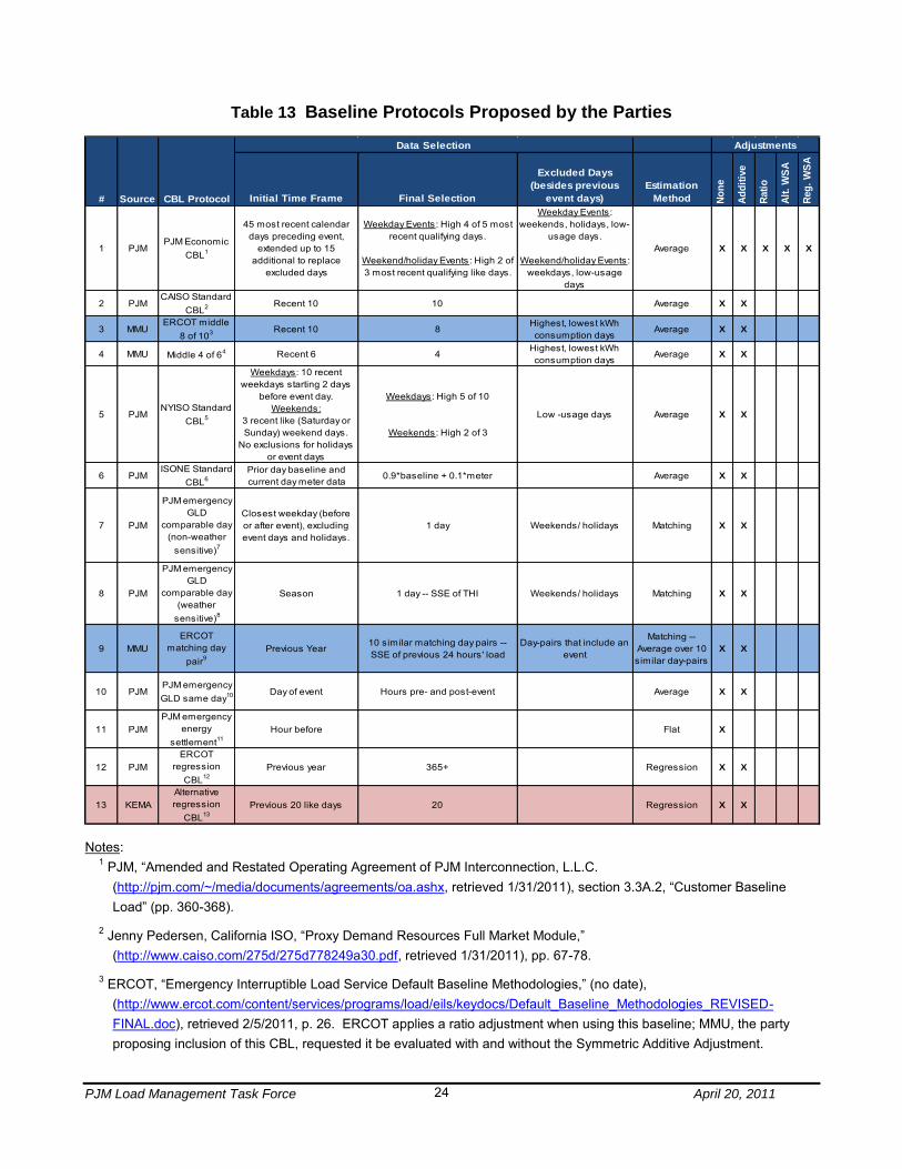
Table 13 presents the CBLs considered in this project. The table shows the party proposing the baseline, the initial time frame from which candidate comparison days are selected, the data selection rule, the estimation method, and, where relevant, the adjustment factor(s) to be applied to the provisional (unadjusted) baseline. The proposed protocols that were not included in the evaluation are shaded in blue in Table 13. An alternative regression baseline approach that KEMA developed is shaded in purple. Table 13 also includes columns summarizing the types of baseline adjustments that were proposed for evaluation with each provisional baseline.
PJM Load Management Task Force April 20, 2011
24
Table 13 Baseline Protocols Proposed by the Parties
Initial Time Frame Final Selection
Excluded Days
(besides previous
event days)
Estimation
Method No
ne
Ad
dit
ive
Rati
o
Alt
. W
SA
Reg
. W
SA
1 PJMPJM Economic
CBL1
45 most recent calendar days preceding event,
extended up to 15 additional to replace
excluded days
Weekday Events: High 4 of 5 most recent qualifying days.
Weekend/holiday Events : High 2 of 3 most recent qualifying like days.
Weekday Events: weekends, holidays, low-
usage days.
Weekend/holiday Events : weekdays, low-usage
days
Average X X X X X
2 PJMCAISO Standard
CBL2 Recent 10 10 Average X X
3 MMUERCOT middle
8 of 103 Recent 10 8Highest, lowest kWh consumption days
Average X X
4 MMU Middle 4 of 64 Recent 6 4Highest, lowest kWh consumption days
Average X X
5 PJMNYISO Standard
CBL5
Weekdays: 10 recent weekdays starting 2 days
before event day.Weekends:
3 recent like (Saturday or Sunday) weekend days.
No exclusions for holidays or event days
Weekdays: High 5 of 10
Weekends: High 2 of 3
Low -usage days Average X X
6 PJMISONE Standard
CBL6Prior day baseline and current day meter data
0.9*baseline + 0.1*meter Average X X
7 PJM
PJM emergency GLD
comparable day (non-weather
sensitive)7
Closest weekday (before or after event), excluding event days and holidays.
1 day Weekends/ holidays Matching X X
8 PJM
PJM emergency GLD
comparable day (weather
sensitive)8
Season 1 day -- SSE of THI Weekends/ holidays Matching X X
9 MMUERCOT
matching day pair9
Previous Year10 similar matching day pairs -- SSE of previous 24 hours' load
Day-pairs that include an event
Matching --Average over 10 similar day-pairs
X X
10 PJMPJM emergency GLD same day10 Day of event Hours pre- and post-event Average X X
11 PJMPJM emergency
energy settlement11
Hour before Flat X
12 PJMERCOT
regression CBL12
Previous year 365+ Regression X X
13 KEMAAlternative regression
CBL13Previous 20 like days 20 Regression X X
# Source CBL Protocol
Data Selection Adjustments
Notes:
1 PJM, “Amended and Restated Operating Agreement of PJM Interconnection, L.L.C. (http://pjm.com/~/media/documents/agreements/oa.ashx, retrieved 1/31/2011), section 3.3A.2, “Customer Baseline Load” (pp. 360-368).
2 Jenny Pedersen, California ISO, “Proxy Demand Resources Full Market Module,” (http://www.caiso.com/275d/275d778249a30.pdf, retrieved 1/31/2011), pp. 67-78.
3 ERCOT, “Emergency Interruptible Load Service Default Baseline Methodologies,” (no date), (http://www.ercot.com/content/services/programs/load/eils/keydocs/Default_Baseline_Methodologies_REVISED-FINAL.doc), retrieved 2/5/2011, p. 26. ERCOT applies a ratio adjustment when using this baseline; MMU, the party proposing inclusion of this CBL, requested it be evaluated with and without the Symmetric Additive Adjustment.
PJM Load Management Task Force April 20, 2011 25
Notes (continued): 4 Personal communication, Pete Langbein (email 1/14/2011). The comments regarding adjustments in footnote 3 also
apply here. 5 NYISO, “Manual 5: Day-Ahead Demand Response Program Manual,” July 2003
(http://www.nyiso.com/public/webdocs/documents/manuals/planning/dadrp_ mnl.pdf, retrieved 2/1/2011), pp. 21-23.
6 ISO New England Manual for Measurement and Verification of Demand Reduction Value from Demand Resources (Manual M-MVDR), Revision 2, June 1, 2010, pp. 6-5 through 6-10.
7 PJM, “Manual 19: Load Forecasting and Analysis,” Attachment A: Load Drop Estimate Guidelines (redline edited version), p. 24.
8 Ibid., pp. 24-25. 9 ERCOT, op. cit., p. 27.
10 PJM, op. cit., p. 25. 11 PJM, “RFP for PJM Empirical Analysis of Demand Response Baseline Methods,” October 29, 2010, p. 5.
12 ERCOT, op.cit., pp. 2-23. ”. The ERCOT regression model consists of a daily energy equation and 24 hourly energy fraction equations. For detailed description, see ERCOT, “Emergency Interruptible Load Service Default Baseline Methodologies,” (http://www.ercot.com/content/services/programs/load/eils/keydocs/Default_Baseline_Methodologies_REVISED-FINAL.doc), retrieved 2/5/2011, pp. 2-23. KEMA estimated the parameters of this model using one full year of hourly load and weather data for the year October 1, 2008 through September 30, 2009, then applied them to hourly data for October 1, 2009 through September 30, 2010 to produce the baseline forecasts. The forecasted baseline for a particular hour of any given date consists of the product of the predicted daily energy value for that date and the predicted hourly fraction for the relevant hour of the day.
13 KEMA, memorandum to Pete Langbein, Jim McAnany, Don Kujawski dated January 20, 2011, “Proposed additional regression CBL
PJM Load Management Task Force April 20, 2011 26
2.4.1 Discussion: Baselines
We recommended dropping two of the proposed baselines from the evaluation, and adding an alternative regression-based approach. The dropped baselines include:
The ERCOT Middle 8 of 10 baseline (CBL #3): Six baselines of the “x previous days out of y” type were proposed for this evaluation. These baselines are important, in particular, because these represent the most common baselines used by the ISOs. In addition, these baselines are relatively similar and simple to calculate, so there is less need to remove them from the list. The ERCOT Middle 8 of 10 closely matches the middle 4 of 6 baseline (4) but starts from the longer set of 10 recent days common to many of the other ISO baselines. In the interest of keeping a baseline that drops the highest and lowest recent days, but doing so with the shorter set of recent days, we felt the middle 4 of 6 was the preferred option.
The ERCOT Matching Day-Pair baseline (CBL #9):Table 13 contains two comparable-day algorithms that use different data with which to establish similarity through a quantitative assessment. The PJM Comparable Day (weather-sensitive) baseline (CBL #8) compares THI in the compliance period on the event day to the corresponding hours on other like, non-event days in the same season. The ERCOT matching day-pair baseline (9) compares loads on the “business-as-usual” hours of the event day itself up to one hour before the start of event plus the entire 24 hours of the preceding day to like day-pairs in the preceding year. Both baselines use sums of squared differences to assess similarity and determine the final comparison day(s). The ERCOT baseline goes the additional step of choosing multiple comparable days and then averaging over them to get the final baseline. Both approaches have strengths and weakness. The PJM approach has the advantage of using actual event period data for matching, and disengages from using loads altogether. However, in so doing it relies entirely on THI to identify similar days, despite the fact that there are many other possible drivers of load. The ERCOT approach matches on the hourly loads of the day-pairs. This approach would be expected to match loads more closely, but would likely include days with quite different weather characteristics than the event day. The combination of multiple comparable days is an additional touch that makes the ERCOT baseline less sensitive to any specific day
PJM Load Management Task Force April 20, 2011 27
chosen. KEMA originally recommended the ERCOT approach in favor of the PJM approach on the ground that it might provide a better alternative for a matching-day algorithm. However, PJM requested that their baseline protocol be included because it is actually being used by PJM customers. In addition, the ERCOT matching day-pair method includes some ambiguities involving classification of day-pairs containing mixtures of day types (weekdays and either weekends or holidays) that we were unable to resolve.
We recommended both the ERCOT regression model (CBL #12) and the alternative regression based on the previous 20 like days (CBL #13) be included. We felt that these two methods represent a reasonable range of the possible regression approaches – at one extreme the ERCOT model using a minimum of a year of historical data and employing a relatively complex specification, at the other the KEMA alternative model employing a much simpler specification and requiring much less data.
Finally, we recommended including the baselines which match the closest weekday or same-day hours be evaluated because they are simple, easy to understand, and could be included at relatively low time cost. The CBL method that uses the closest weekday is the PJM GLD Comparable Day (CBL #7). The CBL methods that use the same-day hours are the PJM GLD Same Day CBL (CBL #10) and the PJM Emergency Energy Settlement (CBL # 11).
2.4.2 Description of Baselines Included in Evaluation
CBL #1: PJM Economic Baseline: The PJM Economic Baseline (CBL #1) consists of hourly loads averaged across the “highest x out of y” most recent days, where x and y are numbers that depend on day type:
For weekday events, the baseline consists of the average hourly loads of the 4 highest
kWh days out of the 5 most recent weekdays preceding the event, excluding NERC holidays, weekend days, and event days.
For weekend or holiday events, the baseline consists of the average hourly loads of the
2 highest kWh days out of the 3 most recent weekend or NERC holiday days, excluding event days.
The loads in each event hour are averaged over the selected comparison days to form the baseline. The protocol described in the PJM Operating Agreement (see footnote 1 of Table 13) limits the “look-back window” for calculating the baseline to 45 calendar days in most cases. We did not explicitly impose this limitation because in our analysis dataset it was never violated.
PJM Load Management Task Force April 20, 2011 28
CBL #2: CAISO Standard Baseline: The CAISO Standard Baseline (CBL #2) is also of the “highest x out of y most recent days” type, except that there are no excluded days (that is, x = y):
For weekday events, the baseline consists of the hourly loads averaged over the 10 most recent days preceding the event, excluding holidays, weekend days, and event days.
For weekend or holiday events, the baseline consists of the average hourly loads of the
4 most recent weekend or holiday days, excluding event days.
The loads in each event hour are averaged over the selected comparison days to form the baseline. The protocol (see footnote 2 of Table 13 prescribes actions to take if there are too few qualifying days in the preceding 45 days to reach the target number of days. We did not explicitly include these in our analysis, since the occasion never arose.
CBL #4: Middle 4 of 6 Preceding Like Days Baseline: The Middle 4 of 6 Preceding Like Days Baseline (CBL #4) is similar to the x of y baselines except that the selection criterion for comparison days is to drop the highest and lowest kWh days out of the most recent six. The hourly loads are then averaged over the remaining four days for form the baseline. CBL #5: NYISO Standard Baseline: The NYISO Standard Baseline (CBL #5) is another of the “highest x out of y most recent days” type, with a selection criterion of the 5 highest kWh days out of the preceding 10 non-holiday days (for weekday events), or the 2 highest out of the preceding 3 (for weekend or holiday events). See footnote 5 of Table 13 CBL #6: ISONE Standard Baseline: This baseline differs from the preceding ones, in that it consists of a weighted average of the preceding day‟s baseline and the current day‟s actual metered load. The baseline is updated on every non-event weekday. It is not calculated on weekends or holidays. On (weekday) event days, the baseline is defined as the previous day‟s baseline.
For a new asset with no previously computed baseline, the baseline is the simple average hourly load calculated for each hour of the day from the five most recent preceding business days with complete meter data. Since the asset isn‟t permitted to

PJM Load Management Task Force April 20, 2011 29
participate in a DR program during this initial 5-day window, event days are not excluded for these calculations. (All of our accounts are “new” at the start of the file, or on the date they first enter the dataset, whichever comes later.)
For an existing asset (i.e., one with at least five days of usable load data), the current-day baseline is obtained as follows: o If the current day is an event day, the asset‟s baseline for the day is equal to the
baseline from the previous day. o If the current day is not an event day, then the asset‟s baseline is updated
according to the following algorithm:
Current day baseline = 0.9*previous day baseline + 0.1*current day metered load
for each hour of the current day.
We departed from the ISONE methodology in our analysis in one respect: we did not assign zero values to missing load values. See footnote 6 of Table 13. CBL #7: PJM Emergency GLD Comparable Day (non-weather sensitive) Baseline: This baseline only exists for weekdays. It consists of the hourly loads from the non-holiday weekday in close proximity to the event day, either preceding or following it. In the event of a tie, the previous day is chosen. See footnote 7 of Table 13. CBL #8: PJM Emergency GLD Comparable Day (weather sensitive) Baseline: This baseline, too, is only defined for weekdays. The comparison day is chosen using a similarity measure based on the temperature-humidity index (THI)6:
The temperature-humidity index (THI) is calculated for each hour of the event period on
the event day, and for the same hour on every other non-event, non-holiday weekday in the same season.
The sum of squared differences between the hourly THI values for the event period on
the event day and the same hours on each comparison day is calculated.
6 THI = temp – 0.55*(1 – humid)*(temp – 58), where temp is dry-bulb temperature in degrees Fahrenheit, and humid is relative humidity expressed as a decimal fraction.
PJM Load Management Task Force April 20, 2011 30
The comparable days are ranked by their sums of squared differences, and the
minimum is chosen as the comparison day.
The baseline consists of the hourly loads from the selected comparison day. See footnote 8 of of Table 13. CBL #10: PJM Emergency GLD Same Day (Before/After Event) Baseline: This is a flat baseline consisting of the average of the hourly loads in the two hours ending one hour prior to the event hour and the two hours beginning one hour after the end of the event hour. See footnote 10 of Table 13.
CBL #11: PJM Emergency Energy Settlement Baseline: This is a flat baseline consisting of the average load in the hour before the hour in which the event begins. See footnote 11 of Table 13.
CBL #12: ERCOT Regression Baseline: The ERCOT Regression Baseline (CBL #12) is calculated using a regression model consisting of a daily energy equation, which has the customer‟s total daily kWh as the dependent variable, and 24 hourly energy fraction equations, in each of which is the dependent variable is the fraction of the daily load occurring in each hour of the day. The explanatory variables in the model include calendar variables (e.g., day of the week, holiday indicators, season), weather variables (dry-bulb temperature and various functions thereof), and daylight variables (e.g., daylight saving time, times of sunrise and sunset). For a detailed description of the specification and all of the explanatory variables, see ERCOT, “Emergency Interruptible Load Service Default Baseline Methodologies” (no date), (http://www.ercot.com/content/services/programs/load/eils/keydocs/Default_Baseline_Methodologies_REVISED-FINAL.doc), retrieved 2/5/2011, pp. 2-23. KEMA estimated the parameters of this model for each customer using the one full year of hourly load and weather data running from October 1, 2008 through September 30, 2009, then applied these coefficients to hourly data for October 1, 2009 through September 30, 2010 to produce the baseline forecasts. The baseline for a particular hour of any given day consists of the product of the predicted daily energy value for that date and the predicted hourly fraction for the relevant hour of the day.
CBL #13: KEMA Alternative Regression Baseline: The KEMA Alternative Regression Baseline (CBL #13) is calculated using a simple, one-equation linear regression with hourly load as the dependent variable, and a set of hourly indicators, singly and interacted with daily THI, as the explanatory variables. KEMA estimated this model using the previous 20 non-holiday, non-event weekdays preceding the day of the event. The baseline on any given day consists of the
PJM Load Management Task Force April 20, 2011 31
estimated coefficients from fitting the model to the set of 20 preceding qualifying days, applied to the event-day‟s data.
2.4.3 Adjustments
A total of eight different baseline adjustment algorithms were considered for this evaluation, the result of a) having been expressly requested by PJM in the RFP, b) proposed by the MMU, or c) being integral to one or more of the proposed baseline approaches.
Table 14 provides a simplified overview of the eight proposed adjustment methods. Despite numerous details that distinguish these particular adjustments from each other, they fall into longstanding categories of baseline adjustments. Because there are endless variations of adjustments, only adjustments that represented common adjustment approaches (e.g., adjusting the baseline line to the usage in a period before the event) were considered in the analysis. Accordingly, the adjustments included represent the range of possible adjustment algorithms.
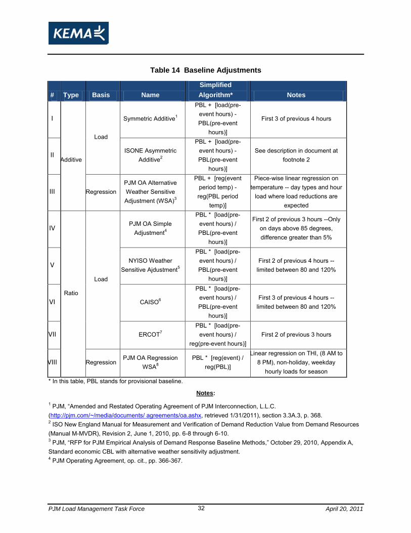
PJM Load Management Task Force April 20, 2011 32
Table 14 Baseline Adjustments
# Type Basis Name
Simplified
Algorithm* Notes
I
Additive
Load
Symmetric Additive1
PBL + [load(pre-event hours) - PBL(pre-event
hours)]
First 3 of previous 4 hours
II ISONE Asymmetric
Additive2
PBL + [load(pre-event hours) - PBL(pre-event
hours)]
See description in document at footnote 2
III Regression PJM OA Alternative Weather Sensitive Adjustment (WSA)3
PBL + [reg(event period temp) - reg(PBL period
temp)]
Piece-wise linear regression on temperature -- day types and hour
load where load reductions are expected
IV
Ratio
Load
PJM OA Simple Adjustment4
PBL * [load(pre-event hours) / PBL(pre-event
hours)]
First 2 of previous 3 hours --Only on days above 85 degrees, difference greater than 5%
V NYISO Weather
Sensitive Ajdustment5
PBL * [load(pre-event hours) / PBL(pre-event
hours)]
First 2 of previous 4 hours -- limited between 80 and 120%
VI CAISO6
PBL * [load(pre-event hours) / PBL(pre-event
hours)]
First 3 of previous 4 hours -- limited between 80 and 120%
VII ERCOT7 PBL * [load(pre-
event hours) / reg(pre-event hours)]
First 2 of previous 3 hours
VIII Regression PJM OA Regression
WSA8 PBL * [reg(event) /
reg(PBL)]
Linear regression on THI, (8 AM to 8 PM), non-holiday, weekday
hourly loads for season * In this table, PBL stands for provisional baseline.
Notes:
1 PJM, “Amended and Restated Operating Agreement of PJM Interconnection, L.L.C. (http://pjm.com/~/media/documents/ agreements/oa.ashx, retrieved 1/31/2011), section 3.3A.3, p. 368. 2 ISO New England Manual for Measurement and Verification of Demand Reduction Value from Demand Resources (Manual M-MVDR), Revision 2, June 1, 2010, pp. 6-8 through 6-10. 3 PJM, “RFP for PJM Empirical Analysis of Demand Response Baseline Methods,” October 29, 2010, Appendix A, Standard economic CBL with alternative weather sensitivity adjustment. 4 PJM Operating Agreement, op. cit., pp. 366-367.
PJM Load Management Task Force April 20, 2011 33
5 NYISO, “Manual 5: Day-Ahead Demand Response Program Manual,” July 2003 (http://www.nyiso.com/public/webdocs/ documents/manuals/planning/dadrp_mnl.pdf, retrieved 2/1/2011), pp. 21-23. 6 Jenny Pedersen, California ISO, “Proxy Demand Resources Full Market Module,” (http://www.caiso.com/275d/275d778249 a30.pdf, retrieved 1/31/2011), pp. 79-88. 7 ERCOT, “Emergency Interruptible Load Service Default Baseline Methodologies,” (no date), (http://www.ercot.com/content/ services/programs/load/eils/keydocs/Default_Baseline_Methodologies_REVISED-FINAL.doc), retrieved 2/5/2011, p. 28. 8 PJM Operating Agreement,pp.365-366.
2.4.4 Discussion: Adjustments
The two basic kinds of pre-event period adjustments are difference (additive) and ratio (multiplicative) adjustments. Traditionally, these approaches compare observed load and baseline load for some pre-event period. An adjustment that makes the pre-event period baseline load equal to the pre-event period observed load is applied to the baseline throughout the event period. The additive approach measures the magnitude of the pre-event period load difference (positive or negative), and adds that to the baseline throughout the event period. The ratio approach applies the ratio that makes the pre-event period baseline load equal to the pre-event period observed load to the baseline throughout the event period.
The list of proposed adjustments included basic versions of these adjustments: Symmetric and Asymmetric Additive (I,II) and simple ratio adjustments: PJM OA Simple/NYISO Weather Sensitive/CAISO/ ERCOT (IV, V, VI and VII). There are differences among the proposed adjustment methods with respect to the hours used to produce these adjustments. There is the symmetric/asymmetric distinction among the additive adjustments. (The asymmetric additive adjustment is no longer used by ISONE because of its gaming potential.) There are also some other restrictions, most prominently, NYISO‟s and CAISO‟s limitation bracketing the adjustment between 80 and 120 percent. Other than these relatively minor differences, the underlying adjustments are basic additive and ratio adjustments. Even the ERCOT adjustment, though applied to a baseline created using a regression approach, is a simple ratio adjustment based on the first 2 of the 3 previous hours.
Table 14 also includes adjustments that use regression results to adjust a standard “x of y” type baseline (III and VIII). Both adjustments use regressions to establish a relationship between load and weather (either temperature or THI). They then compare estimated load as a function of temperature or THI during the baseline days and during the event period. The difference between those two estimates is used to adjust the baseline hour by hour.
PJM Load Management Task Force April 20, 2011 34
In the analysis, all of the selected provisional baselines were evaluated without adjustments. In addition, these baselines with at least one adjustment of each type – additive and ratio – were considered. The basic additive and ratio adjustments used included:
The Symmetric Additive adjustment (I): This is the simple additive adjustment based on load differences in the first 3 of 4 previous hours used by PJM already. The asymmetric additive adjustments have been abandoned on the grounds that they can be too easily gamed.
A Simple Ratio Adjustment based on the first 3 of 4 previous hours: The simple ratio adjustment we propose is similar to the PJM Simple adjustment (IV) or the ERCOT adjustment (VII), but maintains consistency with the symmetric additive adjustment with regard to the hours used for the adjustment. This adjustment will allow an “apples to apples” comparison of additive and ratio adjustments. To maintain consistency with the numbering system we are using for the baselines, this one is labeled VIIa.
This approach tests the basic mechanism of adjustment. Idiosyncratic limitations, like those for the PJM OA Simple adjustment (85 degree temperature cut off or minimum adjustment levels), or the NYISO and CAISO ratio adjustments (limitation of the adjustment ratio to between 80 percent and 120 percent), were not be included in the interest of maintaining consistency, and thus comparability, across adjustment methods. In addition, a regression-based adjustment was also incorporated to be able to compare the performance of regression-based adjustments to those of simple load difference and ratio adjustments. The Alternative Weather Sensitive Adjustment was used because of its more flexible regression approach, and the fact that it is actually being used by PJM customers.
Table 15 presents the list of baselines and baseline adjustments included in the evaluation. There are 11 baselines with three adjustments, resulting in total of 44 different baseline combinations.

PJM Load Management Task Force April 20, 2011 35
Table 15 Baseline Protocols Included in the Assessment
Initial Time Frame Final Selection
Excluded Days
(besides previous
event days)
Estimation
Method No
ne
Ad
dit
ive (
I)
Rati
o (
VIa
)
Reg
. A
dd
. (V
II)
1 PJMPJM Economic
CBL
45 most recent calendar days preceding event,
extended up to 15 additional to replace
excluded days
Weekday Events: High 4 of 5 most recent qualifying days.
Weekend / holiday Events: High 2 of 3 most recent qualifying like days
Weekday Events: weekends, holidays, low-
usage days.
Weekend/holiday Events : weekdays, low-usage
days
Average X X X X
2 PJMCAISO Standard
CBLRecent 10 10 Average X X X X
4 MMU Middle 4 of 6 Recent 6 4Highest, lowest kWh consumption days
Average X X X X
5 PJMNYISO Standard
CBL
Weekdays: 10 recent weekdays starting 2 days before event day.Weekends: 3 recent like (Saturday or Sunday) weekend days. No exclusions for holidays or event days
Weekdays: High 5 of 10
Weekends: High 2 of 3
Low -usage days Average X X X X
6 PJMISONE Standard
CBLPrior day baseline and current day meter data
0.9*baseline + 0.1*meter Average X X X X
7 PJM
PJM emergency GLD
comparable day (non-weather
sensitive)
Closest weekday (before or after event), excluding event days and holidays.
1 day Weekends / holidays Matching X X X X
8 PJM
PJM emergency GLD
comparable day (weather sensitive)
Season 1 day -- SSE of THI Weekends / holidays Matching X X X X
10 PJMPJM emergency GLD same day
Day of event Hours pre- and post-event Average X
11 PJMPJM emergency
energy settlement
Hour before Flat X
12 PJMERCOT
regression CBLPrevious year 365+ Regression X X X
13 KEMAAlternative
regression CBLPrevious 20 like days 20 Regression X X X
# Source CBL Protocol
Data Selection Adjustments
2.5 Performance Metrics
One of the key elements of this project was to compare the empirical performance of the evaluated CBL methods. The CBLs were evaluated on how well they performed with respect to three performance metrics: accuracy, bias, and variability.
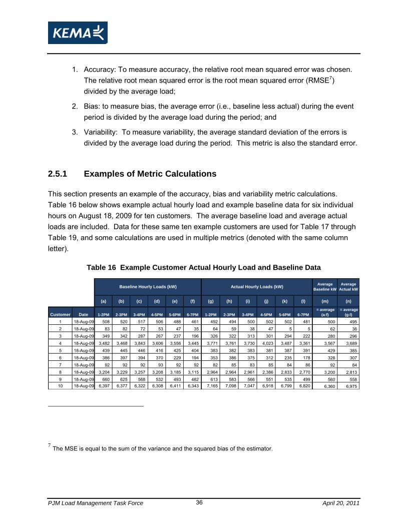
PJM Load Management Task Force April 20, 2011 36
1. Accuracy: To measure accuracy, the relative root mean squared error was chosen. The relative root mean squared error is the root mean squared error (RMSE7) divided by the average load;
2. Bias: to measure bias, the average error (i.e., baseline less actual) during the event period is divided by the average load during the period; and
3. Variability: To measure variability, the average standard deviation of the errors is divided by the average load during the period. This metric is also the standard error.
2.5.1 Examples of Metric Calculations
This section presents an example of the accuracy, bias and variability metric calculations. Table 16 below shows example actual hourly load and example baseline data for six individual hours on August 18, 2009 for ten customers. The average baseline load and average actual loads are included. Data for these same ten example customers are used for Table 17 through Table 19, and some calculations are used in multiple metrics (denoted with the same column letter).
Table 16 Example Customer Actual Hourly Load and Baseline Data
(a) (b) (c) (d) (e) (f) (g) (h) (i) (j) (k) (l) (m) (n)
Customer Date 1-2PM 2-3PM 3-4PM 4-5PM 5-6PM 6-7PM 1-2PM 2-3PM 3-4PM 4-5PM 5-6PM 6-7PM
= average
(a:f)
= average
(g:l)
1 18-Aug-09 508 520 517 506 488 461 492 494 500 502 502 481 500 495 2 18-Aug-09 83 82 72 53 47 35 64 59 38 47 5 5 62 36 3 18-Aug-09 349 342 287 267 237 196 326 322 313 301 294 222 280 296 4 18-Aug-09 3,482 3,468 3,843 3,606 3,556 3,445 3,771 3,761 3,730 4,023 3,487 3,361 3,567 3,689 5 18-Aug-09 439 445 446 416 425 404 383 382 383 381 387 391 429 385 6 18-Aug-09 386 397 394 370 229 194 353 386 375 312 235 178 328 307 7 18-Aug-09 92 92 92 93 92 92 82 85 83 85 84 86 92 84 8 18-Aug-09 3,204 3,229 3,257 3,208 3,185 3,115 2,964 2,964 2,961 2,386 2,833 2,770 3,200 2,813 9 18-Aug-09 660 625 568 532 493 482 613 583 566 551 535 499 560 558 10 18-Aug-09 6,397 6,377 6,322 6,308 6,411 6,343 7,165 7,098 7,047 6,918 6,799 6,820 6,360 6,975
Actual Hourly Loads (kW)Baseline Hourly Loads (kW)Average
Actual kW
Average
Baseline kW
7 The MSE is equal to the sum of the variance and the squared bias of the estimator.
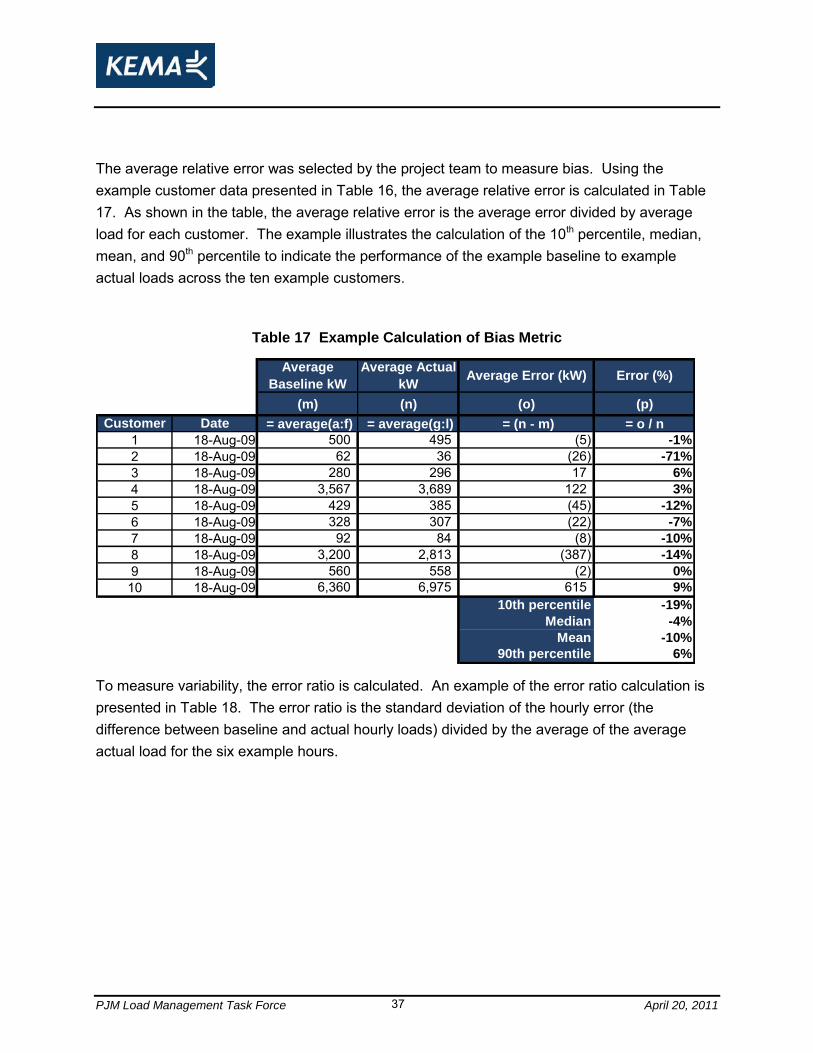
PJM Load Management Task Force April 20, 2011 37
The average relative error was selected by the project team to measure bias. Using the example customer data presented in Table 16, the average relative error is calculated in Table 17. As shown in the table, the average relative error is the average error divided by average load for each customer. The example illustrates the calculation of the 10th percentile, median, mean, and 90th percentile to indicate the performance of the example baseline to example actual loads across the ten example customers.
Table 17 Example Calculation of Bias Metric
(m) (n) (o) (p)
Customer Date = average(a:f) = average(g:l) = (n - m) = o / n
1 18-Aug-09 500 495 (5) -1%
2 18-Aug-09 62 36 (26) -71%
3 18-Aug-09 280 296 17 6%
4 18-Aug-09 3,567 3,689 122 3%
5 18-Aug-09 429 385 (45) -12%
6 18-Aug-09 328 307 (22) -7%
7 18-Aug-09 92 84 (8) -10%
8 18-Aug-09 3,200 2,813 (387) -14%
9 18-Aug-09 560 558 (2) 0%
10 18-Aug-09 6,360 6,975 615 9%
10th percentile -19%
Median -4%
Mean -10%
90th percentile 6%
Average
Baseline kW
Average Actual
kWAverage Error (kW) Error (%)
To measure variability, the error ratio is calculated. An example of the error ratio calculation is presented in Table 18. The error ratio is the standard deviation of the hourly error (the difference between baseline and actual hourly loads) divided by the average of the average actual load for the six example hours.
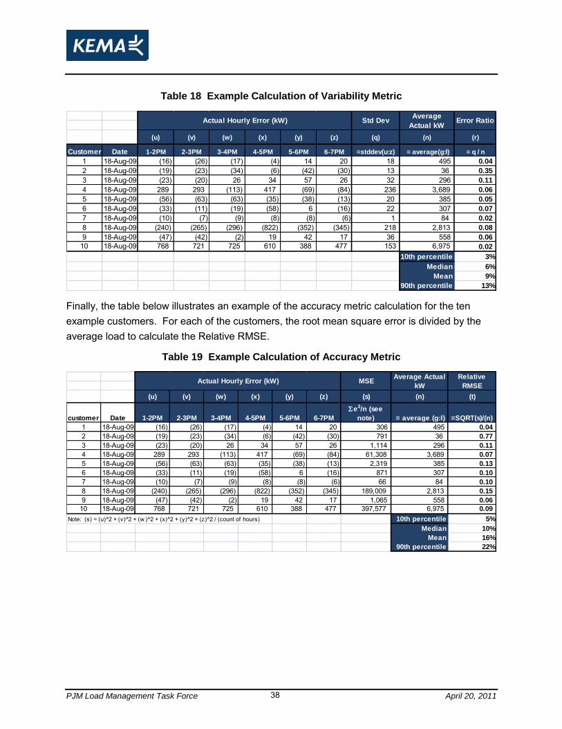
PJM Load Management Task Force April 20, 2011 38
Table 18 Example Calculation of Variability Metric
(u) (v) (w) (x) (y) (z) (q) (n) (r)
Customer Date 1-2PM 2-3PM 3-4PM 4-5PM 5-6PM 6-7PM =stddev(u:z) = average(g:l) = q / n
1 18-Aug-09 (16) (26) (17) (4) 14 20 18 495 0.04
2 18-Aug-09 (19) (23) (34) (6) (42) (30) 13 36 0.35
3 18-Aug-09 (23) (20) 26 34 57 26 32 296 0.11
4 18-Aug-09 289 293 (113) 417 (69) (84) 236 3,689 0.06
5 18-Aug-09 (56) (63) (63) (35) (38) (13) 20 385 0.05
6 18-Aug-09 (33) (11) (19) (58) 6 (16) 22 307 0.07
7 18-Aug-09 (10) (7) (9) (8) (8) (6) 1 84 0.02
8 18-Aug-09 (240) (265) (296) (822) (352) (345) 218 2,813 0.08
9 18-Aug-09 (47) (42) (2) 19 42 17 36 558 0.06
10 18-Aug-09 768 721 725 610 388 477 153 6,975 0.02
10th percentile 3%
Median 6%
Mean 9%
90th percentile 13%
Actual Hourly Error (kW) Std DevAverage
Actual kWError Ratio
Finally, the table below illustrates an example of the accuracy metric calculation for the ten example customers. For each of the customers, the root mean square error is divided by the average load to calculate the Relative RMSE.
Table 19 Example Calculation of Accuracy Metric
(u) (v) (w) (x) (y) (z) (s) (n) (t)
customer Date 1-2PM 2-3PM 3-4PM 4-5PM 5-6PM 6-7PM
Se2/n (see
note) = average (g:l) =SQRT(s)/(n)
1 18-Aug-09 (16) (26) (17) (4) 14 20 306 495 0.04
2 18-Aug-09 (19) (23) (34) (6) (42) (30) 791 36 0.77
3 18-Aug-09 (23) (20) 26 34 57 26 1,114 296 0.11
4 18-Aug-09 289 293 (113) 417 (69) (84) 61,308 3,689 0.07
5 18-Aug-09 (56) (63) (63) (35) (38) (13) 2,319 385 0.13
6 18-Aug-09 (33) (11) (19) (58) 6 (16) 871 307 0.10
7 18-Aug-09 (10) (7) (9) (8) (8) (6) 66 84 0.10
8 18-Aug-09 (240) (265) (296) (822) (352) (345) 189,009 2,813 0.15
9 18-Aug-09 (47) (42) (2) 19 42 17 1,065 558 0.06
10 18-Aug-09 768 721 725 610 388 477 397,577 6,975 0.09
Note: (s) = (u)^2 + (v)^2 + (w )^2 + (x)^2 + (y)^2 + (z)^2 / (count of hours) 10th percentile 5%
Median 10%
Mean 16%
90th percentile 22%
Actual Hourly Error (kW) MSERelative
RMSE
Average Actual
kW
PJM Load Management Task Force April 20, 2011 39
2.5.2 Explanation of Performance Metrics
Three statistics were chosen to measure the three quantitative aspects of baseline performance: accuracy, bias, and variability. The attribute given the most emphasis in the analysis was accuracy, or how closely a baseline method predicts customers‟ actual loads in the sample. The statistic chosen to measure accuracy was the median of the relative root mean squared error (RRMSE). This statistic expresses the baseline‟s average hourly accuracy as a fraction of average hourly load for the typical customer. The RRMSE is based on squared prediction errors. This technique in essence weights large errors much more heavily than small or midsized errors. In contrast, the errors are weighted evenly with a technique that measures errors based on the absolute values of the prediction errors. This means that the effect of large hourly errors in the predicted load will result in a higher RRMSE as opposed to a mean absolute percentage error (MAPE). The RRMSE combines the systematic errors measured by the bias metric (the baseline‟s average relative error) and the variability of errors captured by the variability metric (relative error ratio ). For this reason, the RRMSE was chosen as the accuracy metric. A baseline for a typical customer with a median RRMSE of 0.10 is one where that baseline could expect to have an hourly error, on average, of 10 percent of their actual hourly load. The smaller the RRMSE, the better the baseline performs as a predictor of the actual hourly load. The second baseline attribute analyzed was bias, or the systematic tendency of a baseline method to over- or under-predict actual loads. Bias was measured using the median of the baseline‟s average relative error (ARE). This statistic, for a given customer, is the average hourly baseline less the average hourly actual load, expressed as a fraction of actual hourly load. A median ARE value of zero would indicate that the typical customer in our sample had no systematic tendency to over- or under-predict loads using that baseline, whereas a positive (negative) value would indicate a tendency to over- (under-) predict loads. The closer ARE is to zero, the closer the baseline is to being unbiased. The third baseline attribute analyzed was variability. The variability is the measure of how well the baseline is at predicting hourly load under many different conditions and across many different customers. For example, two baselines may have the same RRMSE but one baseline may be able to better estimate hourly load across a wider variety of situations such that the
PJM Load Management Task Force April 20, 2011 40
dispersion of errors is much closer to actual load than the other baseline. In other words, one baseline may estimate the load shapes more closely than the other baseline. The variability measurement chosen was the relative error ratio (RER), which is the standard deviation of the baseline‟s prediction errors expressed as a fraction of average load. The smaller the median RER, the less variable a baseline‟s error is for the typical customer and therefore the better the baseline performs across a wide variety of circumstances. It should be noted that the accuracy, bias and variability were all calculated for the 10th percentile, median, mean and 90th percentile for each baseline method within each segment. This allows for a detailed analysis of the different baselines across a wide variety of circumstances to get a thorough understanding of how well each baseline estimates a customer actual hourly load. The 10th percentile in effect illustrates an expected “top” case performance scenario while the 90th percentile illustrates a “bottom” case performance scenario so an analyst can understand the range of expected outcomes for the various metrics. For example, based on the top performing baselines in this analysis we find:
Accuracy represented by median RRMSE is 0.10 o 10th percentile Accuracy is 0.04 o 90th percentile is 0.19
Variability represented by RER is 0.08 Bias represented as ARE is 0
The simple way to interpret this is one can expect the baseline to estimate the typical customers hourly load within + or – 10% of their actual load while the baseline will accurately estimate the load shape over time and not have a tendency to over or underestimate. Further, for 1 in 10 customers this estimate will be much better or within 4% of actual hourly load while we can conclude that for 9 in 10 customers the prediction will be no worse than 19% of the actual load. This helps to understand how well the baseline is expected to perform over a variety of customers and circumstances and illustrates that it is expected that the accuracy will be between 4% and 19% on an hourly basis where baseline accuracy for cumulative load will be much closer to perfect, over longer period of time, because it does not have an tendency to over or under predict the load.
PJM Load Management Task Force April 20, 2011 41
2.6 Segmentation of Baseline Results
One of the goals of the evaluation was to determine if transparent customer segmentation would result in significantly better results. An important criterion for segmentation is that the segments must be reasonably transparent so the market understands which CBL will go with what customer.
The following customer segments were evaluated as part of the analysis:
Customers with weather sensitive load versus customers with non-weather sensitive load;
Size of customer, based on demand; and
Customers with variable load versus customers with non-variable load.
A discussion of the segments and their applicability follows.
2.6.1 Weather Sensitive and Non-weather Sensitive
Dividing the sample into weather sensitive and non-weather sensitive segments was accomplished using the parameter estimates from a simple regression of each account‟s load on cooling degree-days.
Using summer data, each account‟s hourly load was regressed on cooling degree-hours and an intercept. The intercept represents the average non-weather sensitive (“base”) load for that customer. The cooling parameter estimate represents the average increase in load with each degree increase in temperature above 60 degrees. A single ratio compares the average event period weather sensitive load at 90 degrees to the average base load estimate at 60 degrees. The ratio represents the percentage increase above base load that occurs as temperature rises from 60 to 90 degrees.

PJM Load Management Task Force April 20, 2011 42
Figure 1 provides an example of the weather sensitivity ratio for summer weekdays for two different customers. The left-hand plot shows a non-weather sensitive customer with relatively little increase in load as temperatures increase from 60 to 90 degrees. The second plot shows a weather sensitive load where the increased demand as temperatures rise from 60 to 90 degrees represents 36 percent of the base load.
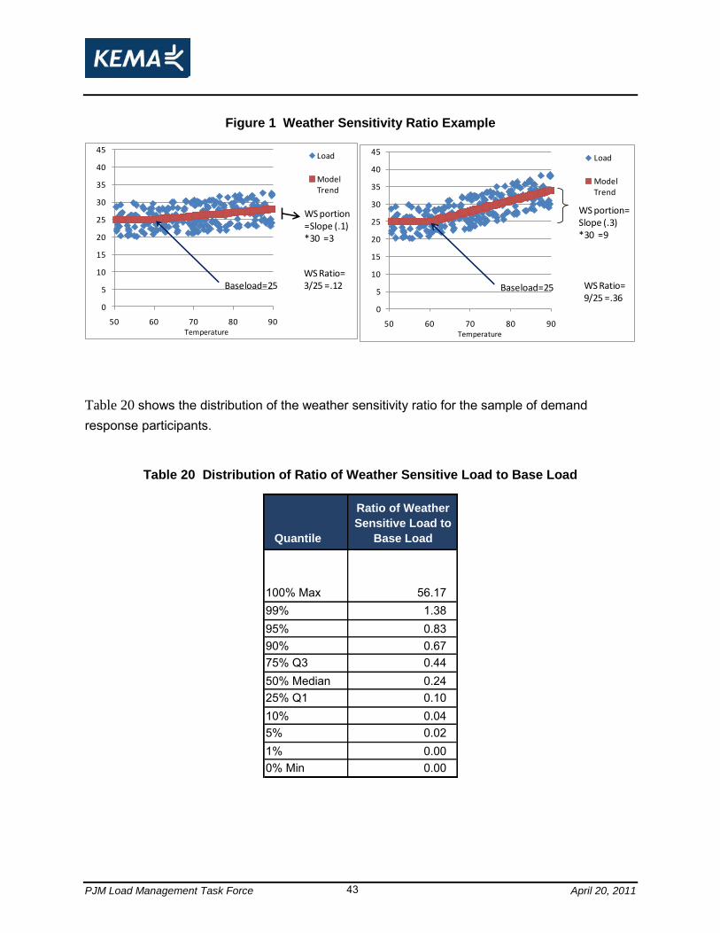
PJM Load Management Task Force April 20, 2011 43
Figure 1 Weather Sensitivity Ratio Example
0
5
10
15
20
25
30
35
40
45
50 60 70 80 90
Load
Model Trend
WS portion=Slope (.1) *30 =3
Baseload=25WS Ratio=3/25 =.12
Temperature
0
5
10
15
20
25
30
35
40
45
50 60 70 80 90
Load
Model Trend
WS portion=Slope (.3) *30 =9
Baseload=25 WS Ratio=9/25 =.36
Temperature
Table 20 shows the distribution of the weather sensitivity ratio for the sample of demand response participants.
Table 20 Distribution of Ratio of Weather Sensitive Load to Base Load
Quantile
Ratio of Weather
Sensitive Load to
Base Load
100% Max 56.1799% 1.3895% 0.8390% 0.6775% Q3 0.4450% Median 0.2425% Q1 0.1010% 0.045% 0.021% 0.000% Min 0.00

PJM Load Management Task Force April 20, 2011 44
Further examination of the distribution of ratios less than 1.0 (100%) is presented in Figure 2 below.
Figure 2 Distribution of WS Ratio (When Ratio less than 1)
Absolute Ratio of Cooling/Intercept
0 0.1 0.2 0.3 0.4 0.5 0.6 0.7 0.8 0.9 1.00
5
10
15
20
25
Per
cent
Ratio
Based on this analysis, a customer is identified as having weather sensitive load when the ratio of weather sensitive load to base load is 0.30 or greater. Using this cut off identifies 40 percent of the sample as weather sensitive.
2.6.2 Size of Customer
The sample was also segmented based on the size of customer. Segmentation by customer size was based on each site‟s 99th percentile of load (that is, very near maximum) during the summer months. Table 20 below is the distribution of the 99th percentile of load for the sample of demand response participants.
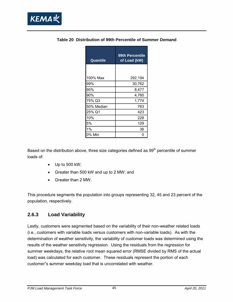
PJM Load Management Task Force April 20, 2011 45
Table 20 Distribution of 99th Percentile of Summer Demand
Quantile
99th Percentile
of Load (kW)
100% Max 292,19499% 30,76295% 8,47790% 4,76075% Q3 1,77450% Median 76325% Q1 42310% 2285% 1291% 360% Min 0
Based on the distribution above, three size categories defined as 99th percentile of summer loads of:
Up to 500 kW;
Greater than 500 kW and up to 2 MW; and
Greater than 2 MW.
This procedure segments the population into groups representing 32, 45 and 23 percent of the population, respectively.
2.6.3 Load Variability
Lastly, customers were segmented based on the variability of their non-weather related loads (i.e., customers with variable loads versus customers with non-variable loads). As with the determination of weather sensitivity, the variability of customer loads was determined using the results of the weather sensitivity regression. Using the residuals from the regression for summer weekdays, the relative root mean squared error (RMSE divided by RMS of the actual load) was calculated for each customer. These residuals represent the portion of each customer‟s summer weekday load that is uncorrelated with weather.
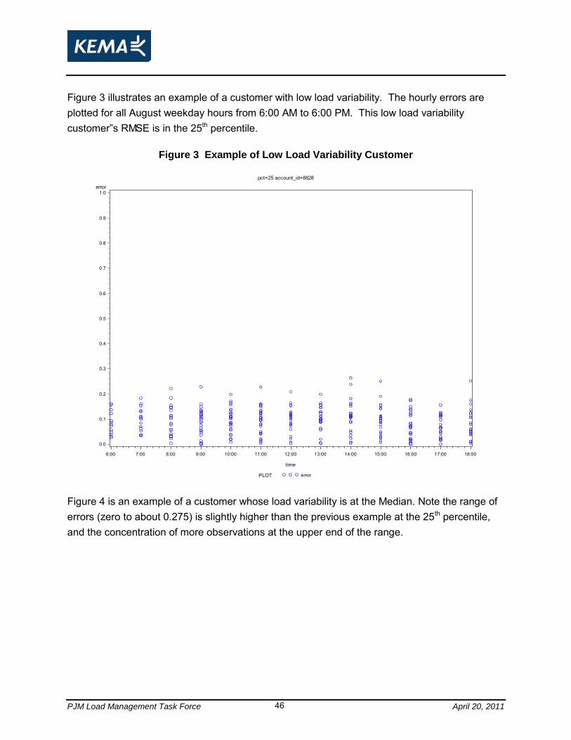
PJM Load Management Task Force April 20, 2011 46
Figure 3 illustrates an example of a customer with low load variability. The hourly errors are plotted for all August weekday hours from 6:00 AM to 6:00 PM. This low load variability customer‟s RMSE is in the 25th percentile.
Figure 3 Example of Low Load Variability Customer
error
0.0
0.1
0.2
0.3
0.4
0.5
0.6
0.7
0.8
0.9
1.0
time
6:00 7:00 8:00 9:00 10:00 11:00 12:00 13:00 14:00 15:00 16:00 17:00 18:00
pct=25 account_id=8828
PLOT error
Figure 4 is an example of a customer whose load variability is at the Median. Note the range of errors (zero to about 0.275) is slightly higher than the previous example at the 25th percentile, and the concentration of more observations at the upper end of the range.

PJM Load Management Task Force April 20, 2011 47
Figure 4 Example of a Median Load Variability Customer
error
0.0
0.1
0.2
0.3
0.4
0.5
0.6
0.7
0.8
0.9
1.0
time
6:00 7:00 8:00 9:00 10:00 11:00 12:00 13:00 14:00 15:00 16:00 17:00 18:00
pct=50 account_id=5120
PLOT error
Figure 5 is an example of a highly variable load customer with an RMSE at the 95th percentile. The range of the errors is much greater for each of the August hours than for the low and median customer examples.
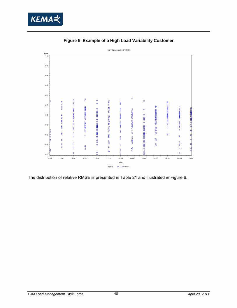
PJM Load Management Task Force April 20, 2011 48
Figure 5 Example of a High Load Variability Customer
error
0.0
0.1
0.2
0.3
0.4
0.5
0.6
0.7
0.8
0.9
1.0
time
6:00 7:00 8:00 9:00 10:00 11:00 12:00 13:00 14:00 15:00 16:00 17:00 18:00
pct=95 account_id=7832
PLOT error
The distribution of relative RMSE is presented in Table 21 and illustrated in Figure 6.
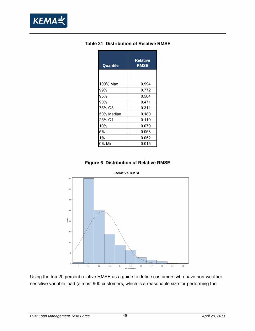
PJM Load Management Task Force April 20, 2011 49
Table 21 Distribution of Relative RMSE
Quantile
Relative
RMSE
100% Max 0.99499% 0.77295% 0.56490% 0.47175% Q3 0.31150% Median 0.18025% Q1 0.11010% 0.0795% 0.0681% 0.0520% Min 0.015
Figure 6 Distribution of Relative RMSE
Relative RMSE
0 0.1 0.2 0.3 0.4 0.5 0.6 0.7 0.8 0.9 1.00
5
10
15
20
25
30
35
40
Per
cent
Relative RMSE
Using the top 20 percent relative RMSE as a guide to define customers who have non-weather sensitive variable load (almost 900 customers, which is a reasonable size for performing the
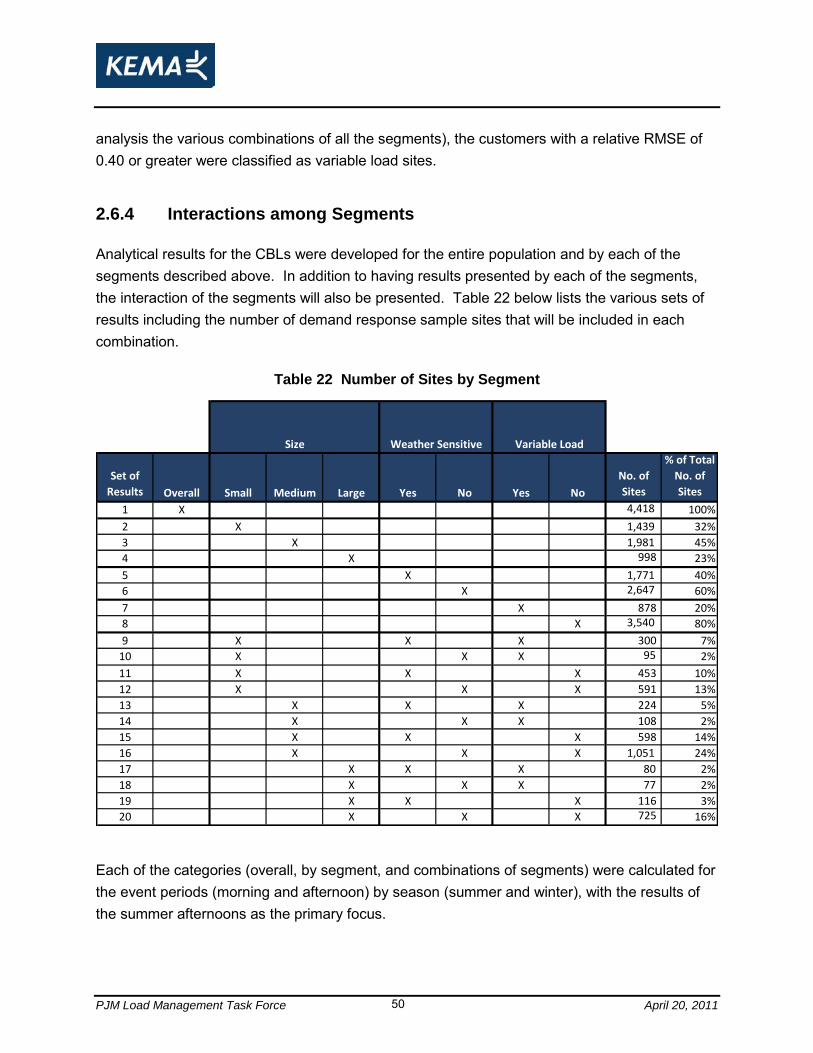
PJM Load Management Task Force April 20, 2011 50
analysis the various combinations of all the segments), the customers with a relative RMSE of 0.40 or greater were classified as variable load sites.
2.6.4 Interactions among Segments
Analytical results for the CBLs were developed for the entire population and by each of the segments described above. In addition to having results presented by each of the segments, the interaction of the segments will also be presented. Table 22 below lists the various sets of results including the number of demand response sample sites that will be included in each combination.
Table 22 Number of Sites by Segment
Set of
Results Overall Small Medium Large Yes No Yes No
No. of
Sites
% of Total
No. of
Sites
1 X 4,418 100%
2 X 1,439 32%
3 X 1,981 45%
4 X 998 23%
5 X 1,771 40%
6 X 2,647 60%
7 X 878 20%
8 X 3,540 80%
9 X X X 300 7%
10 X X X 95 2%
11 X X X 453 10%
12 X X X 591 13%
13 X X X 224 5%
14 X X X 108 2%
15 X X X 598 14%
16 X X X 1,051 24%
17 X X X 80 2%
18 X X X 77 2%
19 X X X 116 3%
20 X X X 725 16%
Size Variable LoadWeather Sensitive
Each of the categories (overall, by segment, and combinations of segments) were calculated for the event periods (morning and afternoon) by season (summer and winter), with the results of the summer afternoons as the primary focus.

PJM Load Management Task Force April 20, 2011 51
2.7 Baseline Analysis Examples
This section presents examples of comparison of the baselines that are the basis for the analysis and conclusions.
In these examples, the analysis is performed on an account basis. The observed load for the account is provided for the full 24 hours of the example day. The loads used for this analysis are typical, non-event day loads. Accordingly, the loads do not exhibit load reduction related to demand response. Observed load during the event period, then, is the standard against which baselines are judged.
The examples feature baseline plots. These plots focus on the summer afternoon event period. Assuming that the event takes place between 1pm and 7pm. It is the accuracy with which a baseline can reproduce the observed load during this period that defines the success of a baseline. The four hours prior to the event period, 9am to 1pm, are the period during which baseline adjustments are calculated. The additive and multiplicative adjustments use the earlier three of those four hours as their adjustment reference period.
For the examples, all eleven baselines are included in each plot. Though the plots include the baselines considered in this analysis, the plots provided here are only designed to illustrate baselines in general. These plots are not designed to distinguish certain baselines. They are examples of the kind of data that underlie the aggregate statistics that we use to distinguish baselines.
The following legend provides a fuller description for each of the baselines featured in the following plots.
PJM Load Management Task Force April 20, 2011 52
cbl1 PJM Economic CBL
cbl2 CAISO Standard CBL
cbl4 Middle 4 of 6
cbl5 NYISO Standard CBL
cbl6 ISONE Standard CBL
cbl7PJM emergency GLD comparable day (non-
weather sensitive)
cbl8PJM emergency GLD
comparable day (weather sensitive)
cbl10PJM emergency GLD
same day
cbl11 PJM emergency energy settlement
cbl12 ERCOT regression CBL
cbl13Alternative regression
CBL
Label in
Plots Description
2.7.1 Example of Baselines without Adjustments
Figure 7 shows an example of a customer with a large, flat load. This figure shows that the load is not variable across the day. In this example, all of the baselines provide a reasonably good estimate of the observed load during the event period. The similarity of the eleven plotted baselines, despite the wide range of time spans and methods, indicates that this account‟s load is also not variable from day to day or even year to year.
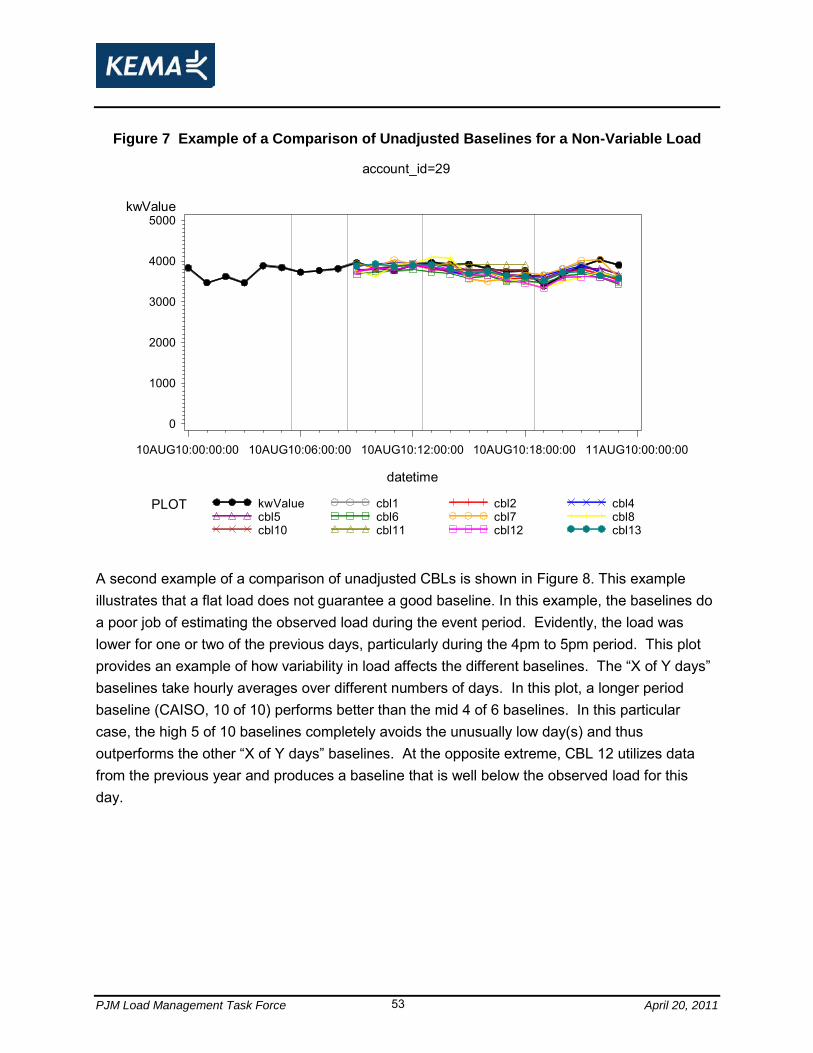
PJM Load Management Task Force April 20, 2011 53
Figure 7 Example of a Comparison of Unadjusted Baselines for a Non-Variable Load
kwValue
0
1000
2000
3000
4000
5000
datetime
10AUG10:00:00:00 10AUG10:06:00:00 10AUG10:12:00:00 10AUG10:18:00:00 11AUG10:00:00:00
account_id=29
PLOT kwValue cbl1 cbl2 cbl4cbl5 cbl6 cbl7 cbl8cbl10 cbl11 cbl12 cbl13
A second example of a comparison of unadjusted CBLs is shown in Figure 8. This example illustrates that a flat load does not guarantee a good baseline. In this example, the baselines do a poor job of estimating the observed load during the event period. Evidently, the load was lower for one or two of the previous days, particularly during the 4pm to 5pm period. This plot provides an example of how variability in load affects the different baselines. The “X of Y days” baselines take hourly averages over different numbers of days. In this plot, a longer period baseline (CAISO, 10 of 10) performs better than the mid 4 of 6 baselines. In this particular case, the high 5 of 10 baselines completely avoids the unusually low day(s) and thus outperforms the other “X of Y days” baselines. At the opposite extreme, CBL 12 utilizes data from the previous year and produces a baseline that is well below the observed load for this day.
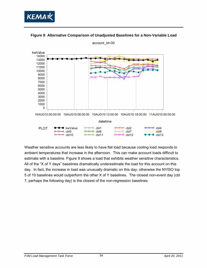
PJM Load Management Task Force April 20, 2011 54
Figure 8 Alternative Comparison of Unadjusted Baselines for a Non-Variable Load
kwValue
0100020003000400050006000700080009000
1000011000120001300014000
datetime
10AUG10:00:00:00 10AUG10:06:00:00 10AUG10:12:00:00 10AUG10:18:00:00 11AUG10:00:00:00
account_id=30
PLOT kwValue cbl1 cbl2 cbl4cbl5 cbl6 cbl7 cbl8cbl10 cbl11 cbl12 cbl13
Weather sensitive accounts are less likely to have flat load because cooling load responds to ambient temperatures that increase in the afternoon. This can make account loads difficult to estimate with a baseline. Figure 9 shows a load that exhibits weather sensitive characteristics. All of the “X of Y days” baselines dramatically underestimate the load for this account on this day. In fact, the increase in load was unusually dramatic on this day; otherwise the NYISO top 5 of 10 baselines would outperform the other X of Y baselines. The closest non-event day (cbl 7, perhaps the following day) is the closest of the non-regression baselines.
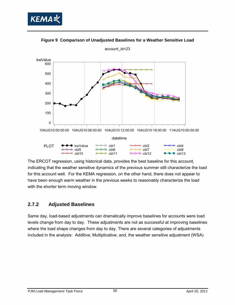
PJM Load Management Task Force April 20, 2011 55
Figure 9 Comparison of Unadjusted Baselines for a Weather Sensitive Load
kwValue
0
100
200
300
400
500
600
datetime
10AUG10:00:00:00 10AUG10:06:00:00 10AUG10:12:00:00 10AUG10:18:00:00 11AUG10:00:00:00
account_id=23
PLOT kwValue cbl1 cbl2 cbl4cbl5 cbl6 cbl7 cbl8cbl10 cbl11 cbl12 cbl13
The ERCOT regression, using historical data, provides the best baseline for this account, indicating that the weather sensitive dynamics of the previous summer still characterize the load for this account well. For the KEMA regression, on the other hand, there does not appear to have been enough warm weather in the previous weeks to reasonably characterize the load with the shorter term moving window.
2.7.2 Adjusted Baselines
Same day, load-based adjustments can dramatically improve baselines for accounts were load levels change from day to day. These adjustments are not as successful at improving baselines where the load shape changes from day to day. There are several categories of adjustments included in the analysis: Additive; Multiplicative; and, the weather sensitive adjustment (WSA)
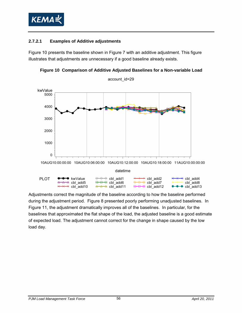
PJM Load Management Task Force April 20, 2011 56
2.7.2.1 Examples of Additive adjustments
Figure 10 presents the baseline shown in Figure 7 with an additive adjustment. This figure illustrates that adjustments are unnecessary if a good baseline already exists.
Figure 10 Comparison of Additive Adjusted Baselines for a Non-variable Load
kwValue
0
1000
2000
3000
4000
5000
datetime
10AUG10:00:00:00 10AUG10:06:00:00 10AUG10:12:00:00 10AUG10:18:00:00 11AUG10:00:00:00
account_id=29
PLOT kwValue cbl_add1 cbl_add2 cbl_add4cbl_add5 cbl_add6 cbl_add7 cbl_add8cbl_add10 cbl_add11 cbl_add12 cbl_add13
Adjustments correct the magnitude of the baseline according to how the baseline performed during the adjustment period. Figure 8 presented poorly performing unadjusted baselines. In Figure 11, the adjustment dramatically improves all of the baselines. In particular, for the baselines that approximated the flat shape of the load, the adjusted baseline is a good estimate of expected load. The adjustment cannot correct for the change in shape caused by the low load day.

PJM Load Management Task Force April 20, 2011 57
Figure 11 Alternative Comparison of Additive Adjusted Baselines for a Non-variable
Load
kwValue
0
2000
4000
6000
8000
10000
12000
14000
16000
18000
datetime
10AUG10:00:00:00 10AUG10:06:00:00 10AUG10:12:00:00 10AUG10:18:00:00 11AUG10:00:00:00
account_id=30
PLOT kwValue cbl_add1 cbl_add2 cbl_add4cbl_add5 cbl_add6 cbl_add7 cbl_add8cbl_add10 cbl_add11 cbl_add12 cbl_add13
Figure 12 shows an example of the additive adjusted baselines for a weather sensitive load. The adjustments bring the baselines to the same level of load as the observed load for that day. This will improve the performance of most baselines at least during the early hours of the event period.
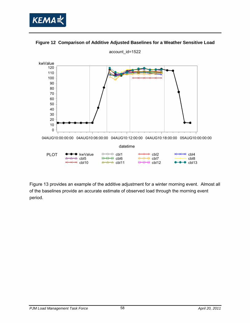
PJM Load Management Task Force April 20, 2011 58
Figure 12 Comparison of Additive Adjusted Baselines for a Weather Sensitive Load
kwValue
0102030405060708090
100110120
datetime
04AUG10:00:00:00 04AUG10:06:00:00 04AUG10:12:00:00 04AUG10:18:00:00 05AUG10:00:00:00
account_id=1522
PLOT kwValue cbl1 cbl2 cbl4cbl5 cbl6 cbl7 cbl8cbl10 cbl11 cbl12 cbl13
Figure 13 provides an example of the additive adjustment for a winter morning event. Almost all of the baselines provide an accurate estimate of observed load through the morning event period.
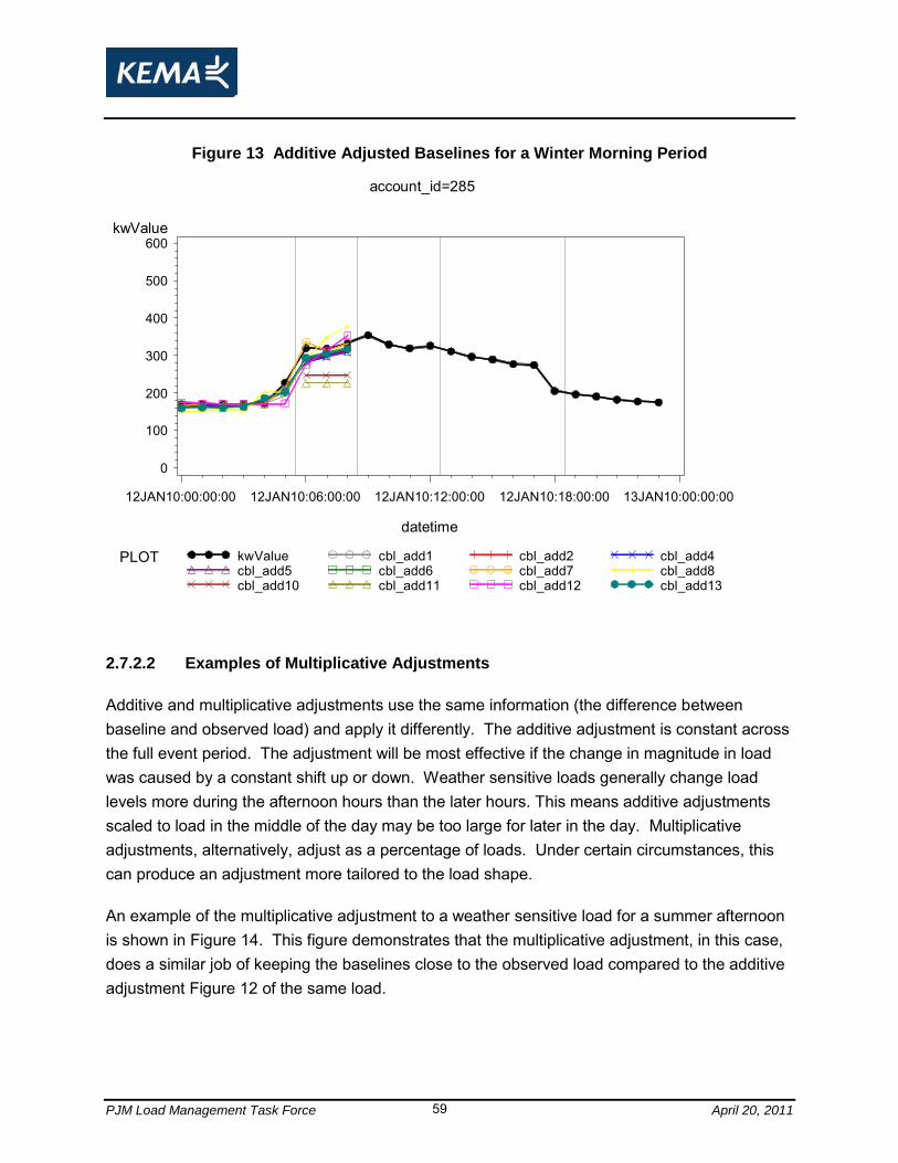
PJM Load Management Task Force April 20, 2011 59
Figure 13 Additive Adjusted Baselines for a Winter Morning Period
kwValue
0
100
200
300
400
500
600
datetime
12JAN10:00:00:00 12JAN10:06:00:00 12JAN10:12:00:00 12JAN10:18:00:00 13JAN10:00:00:00
account_id=285
PLOT kwValue cbl_add1 cbl_add2 cbl_add4cbl_add5 cbl_add6 cbl_add7 cbl_add8cbl_add10 cbl_add11 cbl_add12 cbl_add13
2.7.2.2 Examples of Multiplicative Adjustments
Additive and multiplicative adjustments use the same information (the difference between baseline and observed load) and apply it differently. The additive adjustment is constant across the full event period. The adjustment will be most effective if the change in magnitude in load was caused by a constant shift up or down. Weather sensitive loads generally change load levels more during the afternoon hours than the later hours. This means additive adjustments scaled to load in the middle of the day may be too large for later in the day. Multiplicative adjustments, alternatively, adjust as a percentage of loads. Under certain circumstances, this can produce an adjustment more tailored to the load shape.
An example of the multiplicative adjustment to a weather sensitive load for a summer afternoon is shown in Figure 14. This figure demonstrates that the multiplicative adjustment, in this case, does a similar job of keeping the baselines close to the observed load compared to the additive adjustment Figure 12 of the same load.
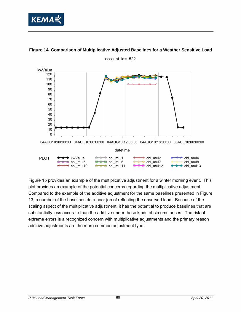
PJM Load Management Task Force April 20, 2011 60
Figure 14 Comparison of Multiplicative Adjusted Baselines for a Weather Sensitive Load
kwValue
0102030405060708090
100110120
datetime
04AUG10:00:00:00 04AUG10:06:00:00 04AUG10:12:00:00 04AUG10:18:00:00 05AUG10:00:00:00
account_id=1522
PLOT kwValue cbl_mul1 cbl_mul2 cbl_mul4cbl_mul5 cbl_mul6 cbl_mul7 cbl_mul8cbl_mul10 cbl_mul11 cbl_mul12 cbl_mul13
Figure 15 provides an example of the multiplicative adjustment for a winter morning event. This plot provides an example of the potential concerns regarding the multiplicative adjustment. Compared to the example of the additive adjustment for the same baselines presented in Figure 13, a number of the baselines do a poor job of reflecting the observed load. Because of the scaling aspect of the multiplicative adjustment, it has the potential to produce baselines that are substantially less accurate than the additive under these kinds of circumstances. The risk of extreme errors is a recognized concern with multiplicative adjustments and the primary reason additive adjustments are the more common adjustment type.
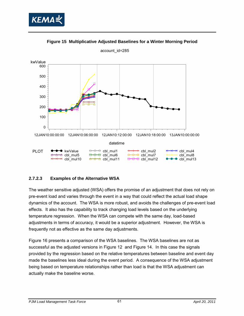
PJM Load Management Task Force April 20, 2011 61
Figure 15 Multiplicative Adjusted Baselines for a Winter Morning Period
kwValue
0
100
200
300
400
500
600
datetime
12JAN10:00:00:00 12JAN10:06:00:00 12JAN10:12:00:00 12JAN10:18:00:00 13JAN10:00:00:00
account_id=285
PLOT kwValue cbl_mul1 cbl_mul2 cbl_mul4cbl_mul5 cbl_mul6 cbl_mul7 cbl_mul8cbl_mul10 cbl_mul11 cbl_mul12 cbl_mul13
2.7.2.3 Examples of the Alternative WSA
The weather sensitive adjusted (WSA) offers the promise of an adjustment that does not rely on pre-event load and varies through the event in a way that could reflect the actual load shape dynamics of the account. The WSA is more robust, and avoids the challenges of pre-event load effects. It also has the capability to track changing load levels based on the underlying temperature regression. When the WSA can compete with the same day, load-based adjustments in terms of accuracy, it would be a superior adjustment. However, the WSA is frequently not as effective as the same day adjustments.
Figure 16 presents a comparison of the WSA baselines. The WSA baselines are not as successful as the adjusted versions in Figure 12 and Figure 14. In this case the signals provided by the regression based on the relative temperatures between baseline and event day made the baselines less ideal during the event period. A consequence of the WSA adjustment being based on temperature relationships rather than load is that the WSA adjustment can actually make the baseline worse.
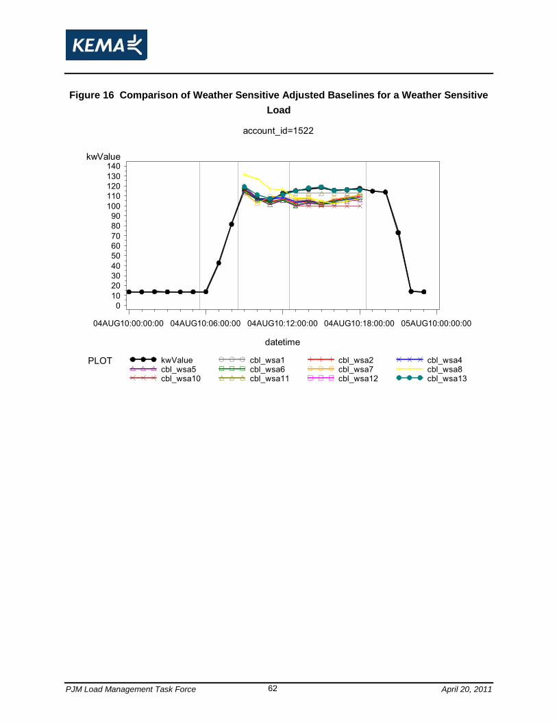
PJM Load Management Task Force April 20, 2011 62
Figure 16 Comparison of Weather Sensitive Adjusted Baselines for a Weather Sensitive
Load
kwValue
0102030405060708090
100110120130140
datetime
04AUG10:00:00:00 04AUG10:06:00:00 04AUG10:12:00:00 04AUG10:18:00:00 05AUG10:00:00:00
account_id=1522
PLOT kwValue cbl_wsa1 cbl_wsa2 cbl_wsa4cbl_wsa5 cbl_wsa6 cbl_wsa7 cbl_wsa8cbl_wsa10 cbl_wsa11 cbl_wsa12 cbl_wsa13
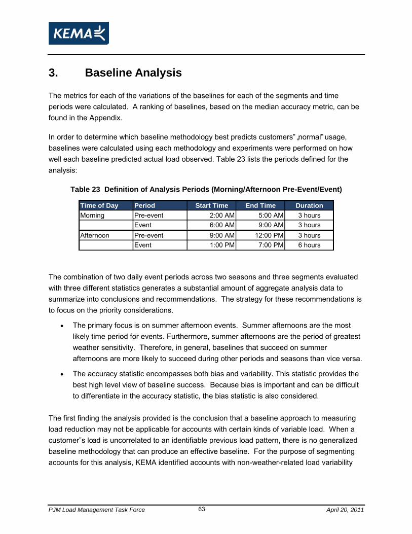
PJM Load Management Task Force April 20, 2011 63
3. Baseline Analysis
The metrics for each of the variations of the baselines for each of the segments and time periods were calculated. A ranking of baselines, based on the median accuracy metric, can be found in the Appendix.
In order to determine which baseline methodology best predicts customers‟ „normal‟ usage, baselines were calculated using each methodology and experiments were performed on how well each baseline predicted actual load observed. Table 23 lists the periods defined for the analysis:
Table 23 Definition of Analysis Periods (Morning/Afternoon Pre-Event/Event)
Time of Day Period Start Time End Time Duration
Morning Pre-event 2:00 AM 5:00 AM 3 hoursEvent 6:00 AM 9:00 AM 3 hours
Afternoon Pre-event 9:00 AM 12:00 PM 3 hoursEvent 1:00 PM 7:00 PM 6 hours
The combination of two daily event periods across two seasons and three segments evaluated with three different statistics generates a substantial amount of aggregate analysis data to summarize into conclusions and recommendations. The strategy for these recommendations is to focus on the priority considerations.
The primary focus is on summer afternoon events. Summer afternoons are the most likely time period for events. Furthermore, summer afternoons are the period of greatest weather sensitivity. Therefore, in general, baselines that succeed on summer afternoons are more likely to succeed during other periods and seasons than vice versa.
The accuracy statistic encompasses both bias and variability. This statistic provides the best high level view of baseline success. Because bias is important and can be difficult to differentiate in the accuracy statistic, the bias statistic is also considered.
The first finding the analysis provided is the conclusion that a baseline approach to measuring load reduction may not be applicable for accounts with certain kinds of variable load. When a customer‟s load is uncorrelated to an identifiable previous load pattern, there is no generalized baseline methodology that can produce an effective baseline. For the purpose of segmenting accounts for this analysis, KEMA identified accounts with non-weather-related load variability
PJM Load Management Task Force April 20, 2011 64
using the alternative weather sensitive adjustment. As variability increased, the ability of the resulting baseline to produce a reasonable estimate of load reduction decreased. The aggregate analysis results indicate that an upper limit on variability should be considered. Accounts that exhibit variation greater than that level would not qualify for the program. The greater the variability of the underlying loads, the more difficult it is for PJM to estimate load reduction at the aggregate level. The level of allowable account-level variability should be determined by PJM‟s requirements with respect to aggregated load reduction variability. In practice, measures of load variability based on the actual baseline approaches used for the program should provide the basis for setting an upper limit on load variability. Based on this recommendation, the remainder of the analysis focuses on results for non-variable accounts. Limiting the level of variability allowed in the program has multiple benefits. It improves the overall accuracy of estimates of expected load directly, because the more variable accounts are removed. Just as importantly, the removal of variable loads makes it possible to focus on the baselines that specifically address more tractable issues like of weather sensitivity.
3.1 Most Accurate Non-Variable Baselines
Figure 17 and Table 24 provide the accuracy results for non-variable accounts for the afternoon event period across the full summer. The plot shows the 11 different baselines across the bottom. For each baseline, the accuracy statistic is plotted for four different versions: Unadjusted, additive adjusted, multiplicative adjusted and PJM weather-sensitive adjusted (WS). Recall, the accuracy statistic combines bias and variation in a single statistic. The smaller the accuracy statistic is, the better the performance of that baseline-adjustment combination.
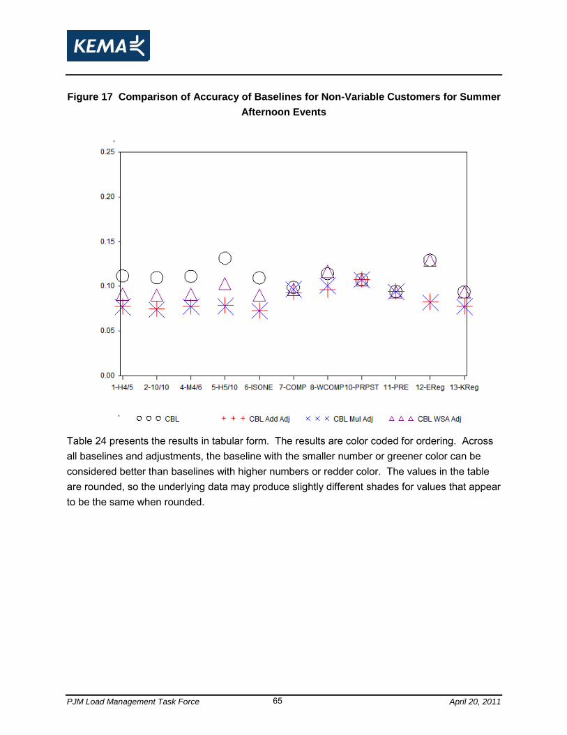
PJM Load Management Task Force April 20, 2011 65
Figure 17 Comparison of Accuracy of Baselines for Non-Variable Customers for Summer
Afternoon Events
Table 24 presents the results in tabular form. The results are color coded for ordering. Across all baselines and adjustments, the baseline with the smaller number or greener color can be considered better than baselines with higher numbers or redder color. The values in the table are rounded, so the underlying data may produce slightly different shades for values that appear to be the same when rounded.
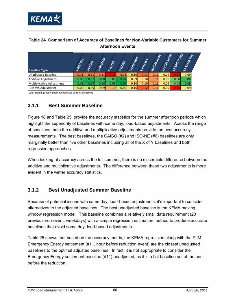
PJM Load Management Task Force April 20, 2011 66
Table 24 Comparison of Accuracy of Baselines for Non-Variable Customers for Summer
Afternoon Events
Baseline Type 1-PJ
M E
co
2-CA
ISO
4-M
id4o
f6
5-N
YISO
6-IS
ON
E
7-PJ
M N
WS
8-PJ
M W
S
10-P
JM S
ame
11-P
JM S
ettl
e12
-ER
COT
Reg
13-K
EMA
Reg
Unadjusted Baseline 0.11 0.11 0.11 0.13 0.11 0.10 0.11 0.11 0.09 0.13 0.09
Additive Adjustment 0.08 0.07 0.08 0.08 0.07 0.09 0.10 0.11 0.09 0.08 0.08
Multiplicative Adjustment 0.08 0.07 0.08 0.08 0.07 0.10 0.10 0.11 0.09 0.08 0.08
PJM WS Adjustment 0.09 0.09 0.09 0.10 0.09 0.10 0.12 0.11 0.09 0.13 0.09
Color coded, green = good, ranked over all rows combined 3.1.1 Best Summer Baseline
Figure 18 and Table 25 provide the accuracy statistics for the summer afternoon periods which highlight the superiority of baselines with same day, load-based adjustments. Across the range of baselines, both the additive and multiplicative adjustments provide the best accuracy measurements. The best baselines, the CAISO (#2) and ISO-NE (#6) baselines are only marginally better than five other baselines including all of the X of Y baselines and both regression approaches.
When looking at accuracy across the full summer, there is no discernible difference between the additive and multiplicative adjustments. The difference between these two adjustments is more evident in the winter accuracy statistics.
3.1.2 Best Unadjusted Summer Baseline
Because of potential issues with same day, load-based adjustments, it‟s important to consider alternatives to the adjusted baselines. The best unadjusted baseline is the KEMA moving window regression model. This baseline combines a relatively small data requirement (20 previous non-event, weekdays) with a simple regression estimation method to produce accurate baselines that avoid same day, load-based adjustments.
Table 25 shows that based on the accuracy metric, the KEMA regression along with the PJM Emergency Energy settlement (#11, hour before reduction event) are the closest unadjusted baselines to the optimal adjusted baselines. In fact, it is not appropriate to consider the Emergency Energy settlement baseline (#11) unadjusted, as it is a flat baseline set at the hour before the reduction.
PJM Load Management Task Force April 20, 2011 67
3.1.3 Weather Sensitive Adjusted Baseline
The PJM alternative weather sensitive adjustment (WSA) offers an adjustment that avoids the potential issues of same day, load-based adjustments. Figure 19 and Table 26 show that the WSA does not perform quite as well as the same day, load-based adjustments across the whole summer. However, this adjustment was designed for weather sensitive loads, and is particularly designed to provide adjustments for more extreme temperatures. Given these considerations, the appropriate comparisons for the WSA adjustment are the unadjusted baselines. All of the X of Y baselines (with the exception of the NYISO baseline (#5)) are improved by the WSA adjustment to a slightly better level of accuracy than the unadjusted KEMA regression. Though in magnitude, the difference is small, the non-adjusted and WSA-adjusted baselines represent an approximately 20 percent loss in accuracy. 3.1.4 Baseline Bias for Summer Events
Figure 18 shows the bias statistics for the baseline and adjustment combinations looking at all event days across the summer. The baselines highlighted above perform well with respect to bias. The CAISO and ISO-NE baselines were found to be unbiased (on average) with all three adjustments, the two same day load-based adjustments as well as the WSA adjustment. The KEMA regression baseline was also effectively unbiased (on average). The unadjusted PJM Economic baseline was biased on the high side, with the adjustments improving but not removing the bias.
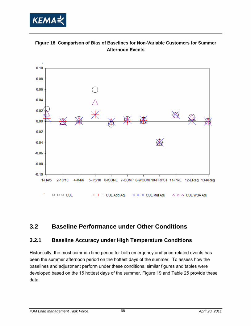
PJM Load Management Task Force April 20, 2011 68
Figure 18 Comparison of Bias of Baselines for Non-Variable Customers for Summer
Afternoon Events
3.2 Baseline Performance under Other Conditions
3.2.1 Baseline Accuracy under High Temperature Conditions
Historically, the most common time period for both emergency and price-related events has been the summer afternoon period on the hottest days of the summer. To assess how the baselines and adjustment perform under these conditions, similar figures and tables were developed based on the 15 hottest days of the summer. Figure 19 and Table 25 provide these data.
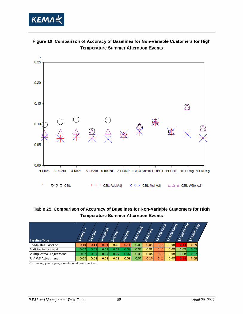
PJM Load Management Task Force April 20, 2011 69
Figure 19 Comparison of Accuracy of Baselines for Non-Variable Customers for High
Temperature Summer Afternoon Events
Table 25 Comparison of Accuracy of Baselines for Non-Variable Customers for High
Temperature Summer Afternoon Events
Baseline Type 1-PJ
M E
co
2-CA
ISO
4-M
id4o
f6
5-N
YISO
6-IS
ON
E
7-PJ
M N
WS
8-PJ
M W
S
10-P
JM S
ame
11-P
JM S
ettl
e12
-ER
COT
Reg
13-K
EMA
Reg
Unadjusted Baseline 0.10 0.11 0.11 0.08 0.11 0.08 0.09 0.11 0.08 0.14 0.09
Additive Adjustment 0.07 0.07 0.07 0.07 0.06 0.07 0.08 0.11 0.08 0.08 0.07
Multiplicative Adjustment 0.07 0.07 0.07 0.07 0.07 0.08 0.08 0.11 0.08 0.08 0.07
PJM WS Adjustment 0.08 0.08 0.08 0.08 0.08 0.07 0.10 0.11 0.08 0.14 0.09
Color coded, green = good, ranked over all rows combined
PJM Load Management Task Force April 20, 2011 70
The results for the high temperature days are consistent with the conclusions in the previous section. All of the baselines identified as performing well across the whole summer, perform well under extreme summer conditions. The ISONE and CAISO baselines with same day, load-based adjustment are still the best performing baselines across all baselines and adjustments. The moving window regression and the PJM high 4 of 5 WS adjusted baselines continue to be among the best performing baselines without load-based adjustment. None of these baselines perform substantially better than the standard PJM economic baseline (#1) with additive adjustment.
Under high temperature conditions, other baselines stand out. These are baselines that are specifically designed to perform well on hot days. In particular, the NYISO baseline, which chooses the highest 5 of the previous 10 days, performs well relative other unadjusted baselines. Also the PJM nearest comparable day (#7) and the pre-event, flat PJM settlement baseline (#11) continue to do well precisely because they use load data from an adjacent day or hour. These results do not change the set of best baselines identified in the previous section.
3.2.2 Baseline Bias under High Temperature Conditions
Figure 20 and Table 26 provide the bias statistic results for the hottest 15 summer days. The table includes the statistics on an absolute value basis and ranks them accordingly. The bias statistic results highlight the particular strength of the load-based adjusted baselines – both the same day, load-based adjusted CAISO and ISO-NE baselines. The PJM WS adjusted economic baseline performs almost as well.
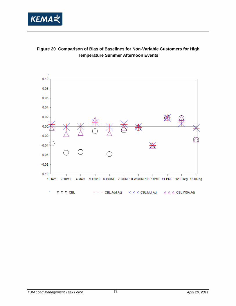
PJM Load Management Task Force April 20, 2011 71
Figure 20 Comparison of Bias of Baselines for Non-Variable Customers for High
Temperature Summer Afternoon Events
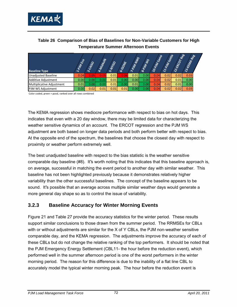
PJM Load Management Task Force April 20, 2011 72
Table 26 Comparison of Bias of Baselines for Non-Variable Customers for High
Temperature Summer Afternoon Events
Baseline Type 1-PJ
M E
co
2-CA
ISO
4-M
id4o
f6
5-N
YISO
6-IS
ON
E
7-PJ
M N
WS
8-PJ
M W
S
10-P
JM S
ame
11-P
JM S
ettl
e12
-ER
COT
Reg
13-K
EMA
Reg
Unadjusted Baseline 0.04 0.05 0.05 0.01 0.06 0.01 0.00 0.04 0.02 0.02 0.03
Additive Adjustment 0.00 0.00 0.00 0.01 0.00 0.00 0.00 0.04 0.02 0.01 0.00
Multiplicative Adjustment 0.01 0.00 0.00 0.01 0.00 0.01 0.00 0.04 0.02 0.01 0.00
PJM WS Adjustment 0.00 0.02 0.01 0.01 0.01 0.00 0.00 0.04 0.02 0.02 0.03
Color coded, green = good, ranked over all rows combined The KEMA regression shows mediocre performance with respect to bias on hot days. This indicates that even with a 20 day window, there may be limited data for characterizing the weather sensitive dynamics of an account. The ERCOT regression and the PJM WS adjustment are both based on longer data periods and both perform better with respect to bias. At the opposite end of the spectrum, the baselines that choose the closest day with respect to proximity or weather perform extremely well.
The best unadjusted baseline with respect to the bias statistic is the weather sensitive comparable day baseline (#8). It‟s worth noting that this indicates that this baseline approach is, on average, successful in matching the event period to another day with similar weather. This baseline has not been highlighted previously because it demonstrates relatively higher variability than the other successful baselines. The concept of the baseline appears to be sound. It‟s possible that an average across multiple similar weather days would generate a more general day shape so as to control the issue of variability.
3.2.3 Baseline Accuracy for Winter Morning Events
Figure 21 and Table 27 provide the accuracy statistics for the winter period. These results support similar conclusions to those drawn from the summer period. The RRMSEs for CBLs with or without adjustments are similar for the X of Y CBLs, the PJM non-weather sensitive comparable day, and the KEMA regression. The adjustments improve the accuracy of each of these CBLs but do not change the relative ranking of the top performers. It should be noted that the PJM Emergency Energy Settlement (CBL11- the hour before the reduction event), which performed well in the summer afternoon period is one of the worst performers in the winter morning period. The reason for this difference is due to the inability of a flat line CBL to accurately model the typical winter morning peak. The hour before the reduction event is
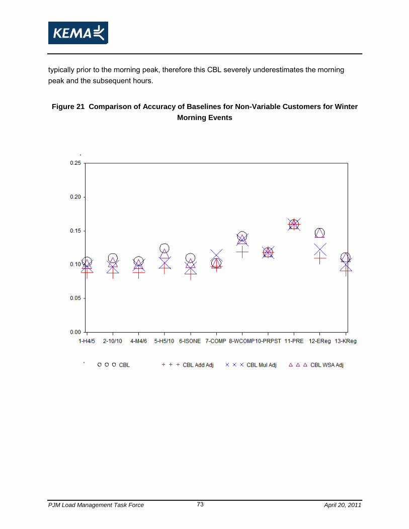
PJM Load Management Task Force April 20, 2011 73
typically prior to the morning peak, therefore this CBL severely underestimates the morning peak and the subsequent hours.
Figure 21 Comparison of Accuracy of Baselines for Non-Variable Customers for Winter
Morning Events

PJM Load Management Task Force April 20, 2011 74
Table 27 Comparison of Accuracy of Baselines for Non-Variable Customers for Winter
Morning Events
Baseline Type 1-PJ
M E
co
2-CA
ISO
4-M
id4o
f6
5-N
YISO
6-IS
ON
E
7-PJ
M N
WS
8-PJ
M W
S
10-P
JM S
ame
11-P
JM S
ettl
e12
-ER
COT
Reg
13-K
EMA
Reg
Unadjusted Baseline 0.10 0.11 0.11 0.12 0.11 0.10 0.14 0.12 0.16 0.15 0.11
Additive Adjustment 0.09 0.09 0.09 0.09 0.09 0.10 0.12 0.12 0.16 0.11 0.09
Multiplicative Adjustment 0.10 0.10 0.10 0.10 0.10 0.11 0.14 0.12 0.16 0.12 0.10
PJM WS Adjustment 0.10 0.10 0.10 0.12 0.10 0.10 0.14 0.12 0.16 0.15 0.11
Color coded, green = good, ranked over all rows combined The winter accuracy statistics do not change much when the results are limited to the coldest 15 days of the winter. The segmentation between weather-sensitive and non-weather-sensitive accounts also does not have much effect on the results. The overall trends across all of the baselines and adjustments are remarkably similar to the summer events.
The winter period does provide differentiation between the two same-day, load-based adjustments. The additive adjustment performs better than the multiplicative adjustment for the winter events. With the adjustment period effectively in the middle of the night, the additive adjustments tend to be smaller. This can be seen in the plots. For the multiplicative adjustment, the magnitude of the adjustment is a function of the ratio between baseline and observed load rather than the difference between the two. If baseline load is low, there is greater potential for the multiplicative adjustments to get unrealistically high. When applied to the normal loads in the morning hours, these inflated adjustments produce inflated baselines.
3.2.4 Segment Level Results
This section provides a high level summary of the segment-level results. A full set of summary results tables is provided in a supplement to this report.
3.2.4.1 Segmentation Variability Measure
The analysis in this report, as developed, only focuses on non-variable accounts. This is because variability, in contrast to weather sensitivity, for instance, is not an account characteristic that can be practically addressed with baseline selection.
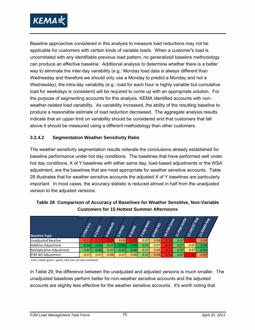
PJM Load Management Task Force April 20, 2011 75
Baseline approaches considered in this analysis to measure load reductions may not be applicable for customers with certain kinds of variable loads. When a customer‟s load is uncorrelated with any identifiable previous load pattern, no generalized baseline methodology can produce an effective baseline. Additional analysis to determine whether there is a better way to eliminate the inter-day variability (e.g.: Monday load data is always different than Wednesday and therefore we should only use a Monday to predict a Monday and not a Wednesday), the intra-day variability (e.g.: load for each hour is highly variable but cumulative load for weekdays is consistent) will be required to come up with an appropriate solution. For the purpose of segmenting accounts for this analysis, KEMA identified accounts with non-weather-related load variability. As variability increased, the ability of the resulting baseline to produce a reasonable estimate of load reduction decreased. The aggregate analysis results indicate that an upper limit on variability should be considered and that customers that fall above it should be measured using a different methodology than other customers.
3.2.4.2 Segmentation Weather Sensitivity Ratio
The weather sensitivity segmentation results reiterate the conclusions already established for baseline performance under hot day conditions. The baselines that have performed well under hot day conditions, X of Y baselines with either same day, load-based adjustments or the WSA adjustment, are the baselines that are most appropriate for weather sensitive accounts. Table 28 illustrates that for weather sensitive accounts the adjusted X of Y baselines are particularly important. In most cases, the accuracy statistic is reduced almost in half from the unadjusted version to the adjusted versions.
Table 28 Comparison of Accuracy of Baselines for Weather Sensitive, Non-Variable
Customers for 15 Hottest Summer Afternoons
Baseline Type 1-PJ
M E
co
2-CA
ISO
4-M
id4o
f6
5-N
YISO
6-IS
ON
E
7-PJ
M N
WS
8-PJ
M W
S
10-P
JM S
ame
11-P
JM S
ettl
e12
-ER
COT
Reg
13-K
EMA
Reg
Unadjusted Baseline 0.11 0.12 0.12 0.08 0.12 0.07 0.08 0.12 0.07 0.12 0.09
Additive Adjustment 0.06 0.06 0.07 0.06 0.06 0.07 0.07 0.12 0.07 0.07 0.06
Multiplicative Adjustment 0.07 0.06 0.07 0.07 0.06 0.07 0.08 0.12 0.07 0.07 0.06
PJM WS Adjustment 0.07 0.07 0.08 0.07 0.08 0.07 0.09 0.12 0.07 0.12 0.09
Color coded, green = good, rank over all rows combined
In Table 29, the difference between the unadjusted and adjusted versions is much smaller. The unadjusted baselines perform better for non-weather sensitive accounts and the adjusted accounts are slightly less effective for the weather sensitive accounts. It‟s worth noting that
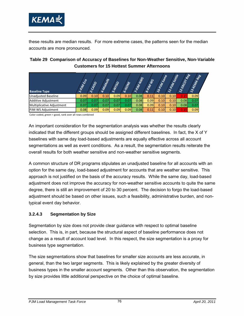
PJM Load Management Task Force April 20, 2011 76
these results are median results. For more extreme cases, the patterns seen for the median accounts are more pronounced.
Table 29 Comparison of Accuracy of Baselines for Non-Weather Sensitive, Non-Variable
Customers for 15 Hottest Summer Afternoons
Baseline Type 1-PJ
M E
co
2-CA
ISO
4-M
id4o
f6
5-N
YISO
6-IS
ON
E
7-PJ
M N
WS
8-PJ
M W
S
10-P
JM S
ame
11-P
JM S
ettl
e12
-ER
COT
Reg
13-K
EMA
Reg
Unadjusted Baseline 0.09 0.10 0.10 0.09 0.10 0.08 0.11 0.10 0.10 0.15 0.09
Additive Adjustment 0.07 0.07 0.07 0.07 0.07 0.08 0.09 0.10 0.10 0.08 0.07
Multiplicative Adjustment 0.07 0.07 0.07 0.07 0.07 0.08 0.09 0.10 0.10 0.08 0.07
PJM WS Adjustment 0.08 0.09 0.09 0.09 0.09 0.08 0.11 0.10 0.10 0.15 0.09
Color coded, green = good, rank over all rows combined
An important consideration for the segmentation analysis was whether the results clearly indicated that the different groups should be assigned different baselines. In fact, the X of Y baselines with same day load-based adjustments are equally effective across all account segmentations as well as event conditions. As a result, the segmentation results reiterate the overall results for both weather sensitive and non-weather sensitive segments.
A common structure of DR programs stipulates an unadjusted baseline for all accounts with an option for the same day, load-based adjustment for accounts that are weather sensitive. This approach is not justified on the basis of the accuracy results. While the same day, load-based adjustment does not improve the accuracy for non-weather sensitive accounts to quite the same degree, there is still an improvement of 20 to 30 percent. The decision to forgo the load-based adjustment should be based on other issues, such a feasibility, administrative burden, and non-typical event day behavior.
3.2.4.3 Segmentation by Size
Segmentation by size does not provide clear guidance with respect to optimal baseline selection. This is, in part, because the structural aspect of baseline performance does not change as a result of account load level. In this respect, the size segmentation is a proxy for business type segmentation.
The size segmentations show that baselines for smaller size accounts are less accurate, in general, than the two larger segments. This is likely explained by the greater diversity of business types in the smaller account segments. Other than this observation, the segmentation by size provides little additional perspective on the choice of optimal baseline.
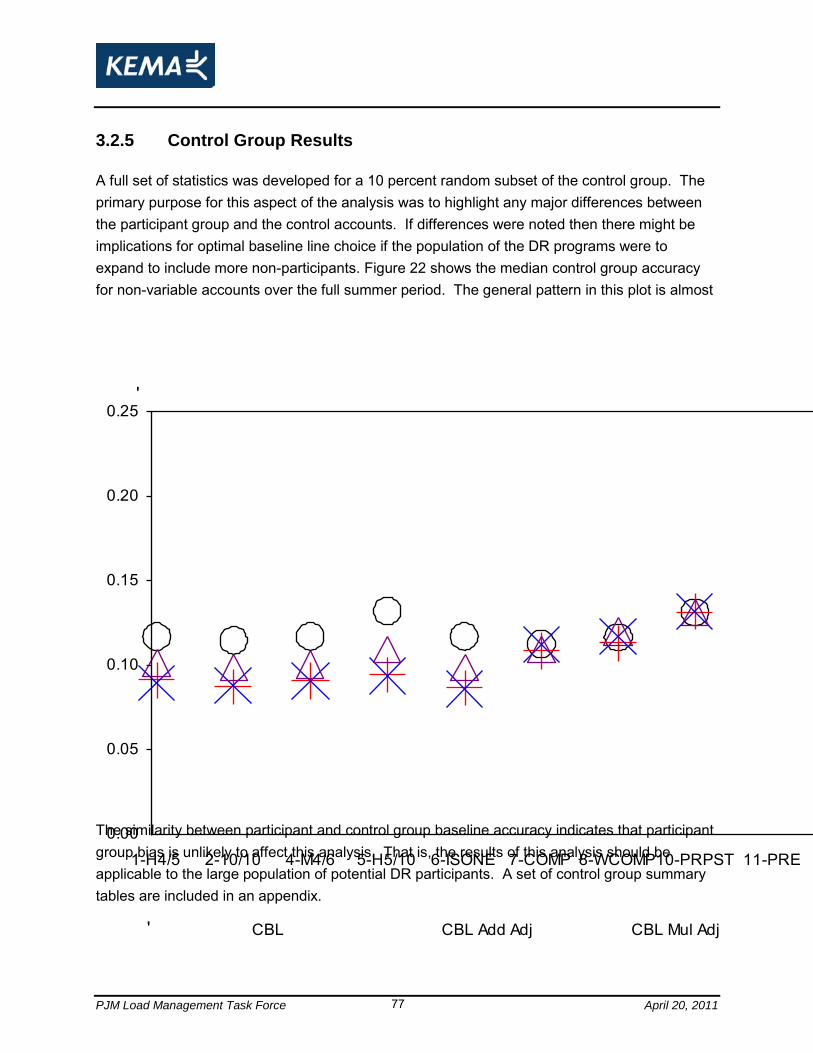
PJM Load Management Task Force April 20, 2011 77
3.2.5 Control Group Results
A full set of statistics was developed for a 10 percent random subset of the control group. The primary purpose for this aspect of the analysis was to highlight any major differences between the participant group and the control accounts. If differences were noted then there might be implications for optimal baseline line choice if the population of the DR programs were to expand to include more non-participants. Figure 22 shows the median control group accuracy for non-variable accounts over the full summer period. The general pattern in this plot is almost identical to the same plot for participants.
Figure 22 Non-Variable, Median Control Group Accuracy for the Summer Period
'
0.00
0.05
0.10
0.15
0.20
0.25
1-H4/5 2-10/10 4-M4/6 5-H5/10 6-ISONE 7-COMP 8-WCOMP10-PRPST 11-PRE 12-EReg 13-KReg
' CBL CBL Add Adj CBL Mul Adj CBL WSA Adj
The similarity between participant and control group baseline accuracy indicates that participant group bias is unlikely to affect this analysis. That is, the results of this analysis should be applicable to the large population of potential DR participants. A set of control group summary tables are included in an appendix.
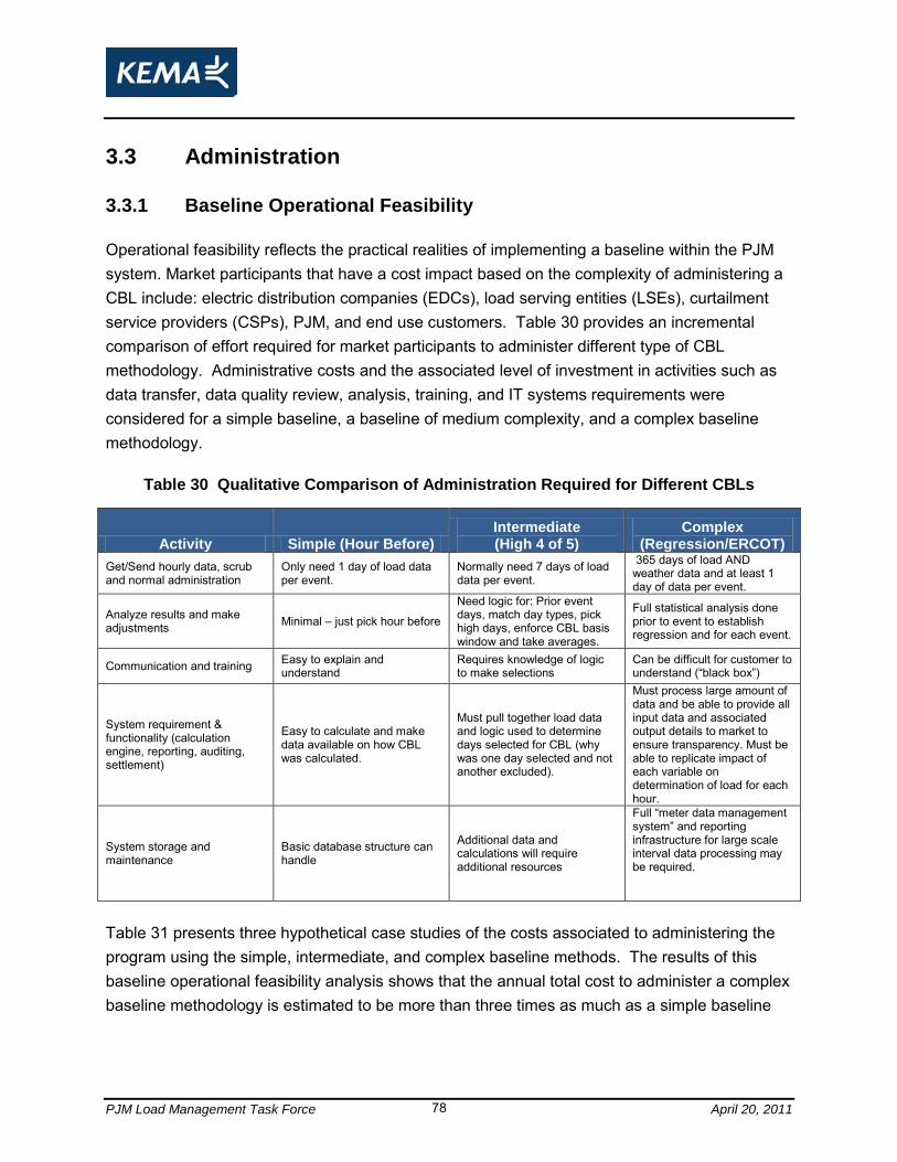
PJM Load Management Task Force April 20, 2011 78
3.3 Administration
3.3.1 Baseline Operational Feasibility
Operational feasibility reflects the practical realities of implementing a baseline within the PJM system. Market participants that have a cost impact based on the complexity of administering a CBL include: electric distribution companies (EDCs), load serving entities (LSEs), curtailment service providers (CSPs), PJM, and end use customers. Table 30 provides an incremental comparison of effort required for market participants to administer different type of CBL methodology. Administrative costs and the associated level of investment in activities such as data transfer, data quality review, analysis, training, and IT systems requirements were considered for a simple baseline, a baseline of medium complexity, and a complex baseline methodology.
Table 30 Qualitative Comparison of Administration Required for Different CBLs
Activity Simple (Hour Before) Intermediate (High 4 of 5)
Complex (Regression/ERCOT)
Get/Send hourly data, scrub and normal administration
Only need 1 day of load data per event.
Normally need 7 days of load data per event.
365 days of load AND weather data and at least 1 day of data per event.
Analyze results and make adjustments Minimal – just pick hour before
Need logic for: Prior event days, match day types, pick high days, enforce CBL basis window and take averages.
Full statistical analysis done prior to event to establish regression and for each event.
Communication and training Easy to explain and understand
Requires knowledge of logic to make selections
Can be difficult for customer to understand (“black box”)
System requirement & functionality (calculation engine, reporting, auditing, settlement)
Easy to calculate and make data available on how CBL was calculated.
Must pull together load data and logic used to determine days selected for CBL (why was one day selected and not another excluded).
Must process large amount of data and be able to provide all input data and associated output details to market to ensure transparency. Must be able to replicate impact of each variable on determination of load for each hour.
System storage and maintenance
Basic database structure can handle
Additional data and calculations will require additional resources
Full “meter data management system” and reporting infrastructure for large scale interval data processing may be required.
Table 31 presents three hypothetical case studies of the costs associated to administering the program using the simple, intermediate, and complex baseline methods. The results of this baseline operational feasibility analysis shows that the annual total cost to administer a complex baseline methodology is estimated to be more than three times as much as a simple baseline
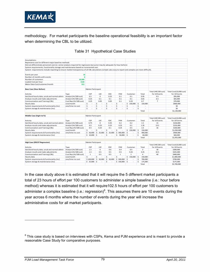
PJM Load Management Task Force April 20, 2011 79
methodology. For market participants the baseline operational feasibility is an important factor when determining the CBL to be utilized.
Table 31 Hypothetical Case Studies
Assumptions:
Represents cost for different major baseline methods
Did not differentiate personnel cost (ie: senior analysis required for regressons but junior may be adequate for hour before)
System requirements, functionality storage and maintenance based on incremental cost.
System requirements include reporting to ensure market transparency of all CBL calculations (simple calcs easy to report and complex are more difficult).
Events per year 10
Number of months with events 6
Number of customers 10,000
Loaded Cost per hour $100
Meter Data Cost/customer/month $15
Base Case (Hour Before) Market Participant
Activity Type CSP LSE EDC PJM Customer Total
Total (HR/100 cust)
for 10 Events
Total Cost(10,000 cust)
for 10 Events
Get/Send hourly data, scrub and normal admin Analyst (Hr/100 cust) 0.5 0 0.25 0.1 0.1 0.95 9.5 $95,000
Analyze results and make adjustments Analyst (Hr/100 cust) 0.25 0.1 0.1 0.1 0.1 0.65 6.5 $65,000
Communication and Training (CBL) Cust Rep (Hr/100 cust) 0.25 0.05 0.05 0.1 0.25 0.7 7 $70,000
Hourly data cost/month -$ -$ -$ -$ 150,000$ 150,000$ $900,000
System requirements & functionality (Inc) one/time inc cost -$ -$ -$ -$ -$ -$ $0
System storage & maintenance (Inc) -$ -$ -$ -$ -$ -$ $0
Total $1,130,000
Middle Case (high 4 of 5) Market Participant
Activity Type CSP LSE EDC PJM Customer Total
Total (HR/100 cust)
for 10 Events
Total Cost(10,000 cust)
for 10 Events
Get/Send hourly data, scrub and normal admin Analyst (Hr/100 cust) 0.75 0 0.35 0.2 0.2 1.5 15 $150,000
Analyze results and make adjustments Analyst (Hr/100 cust) 0.5 0.25 0.25 0.25 0.1 1.35 13.5 $135,000
Communication and Training (CBL) Cust Rep (Hr/100 cust) 0.5 0.25 0.1 0.25 0.5 1.6 16 $160,000
Hourly data cost/month -$ -$ -$ -$ 150,000$ 150,000$ $1,050,000
System requirements & functionality (Inc) one/time inc cost 50,000$ 25,000$ 25,000$ 300,000$ -$ 400,000$ $400,000
System storage & maintenance (Inc) 10,000$ -$ -$ 50,000$ -$ 60,000$ $60,000
Total $1,955,000
High Case (ERCOT Regression) Market Participant
Activity Type CSP LSE EDC PJM Customer Total
Total (HR/100 cust)
for 10 Events
Total Cost(10,000 cust)
for 10 Events
Get/Send hourly data, scrub and normal admin Analyst (Hr/100 cust) 1.5 0 0.6 0.4 0.5 3 30 $300,000
Analyze results and make adjustments Analyst (Hr/100 cust) 1.5 0.5 0.5 0.5 0.25 3.25 32.5 $325,000
Communication and Training (CBL) Cust Rep (Hr/100 cust) 1 0.5 0.5 1 1 4 40 $400,000
Hourly data cost/month -$ -$ -$ -$ 150,000$ 150,000$ $1,800,000
System requirements & functionality (Inc) one/time inc cost 100,000$ 50,000$ 50,000$ 500,000$ -$ 700,000$ $700,000
System storage & maintenance (Inc) 25,000$ -$ -$ 150,000$ -$ 175,000$ $175,000
Total $3,700,000 In the case study above it is estimated that it will require the 5 different market participants a total of 23 hours of effort per 100 customers to administer a simple baseline (i.e.: hour before method) whereas it is estimated that it will require102.5 hours of effort per 100 customers to administer a complex baseline (i.e.: regression)8. This assumes there are 10 events during the year across 6 months where the number of events during the year will increase the administrative costs for all market participants.
8 This case study is based on interviews with CSPs, Kema and PJM experience and is meant to provide a reasonable Case Study for comparative purposes.
PJM Load Management Task Force April 20, 2011 80
The cost of hourly data will increase based on the amount of hourly data required to perform the CBL calculation. It is estimated that that cost to get hourly load data is $15 per customer per month and that there are 10,000 customers that require load data for 10 events that occurred over 6 months. Based on this, a simple CBL method is estimated to cost $0.9 million whereas a more complicated method, such as a regression, would cost $1.8 million. The last part of the case study examined the system cost to administer the range of CBLs. This was focused on incremental system requirements necessary for the middle (high 4 or 5) and high case (Regression) and the associated incremental system storage and maintenance. For example, a system necessary to maintain hourly load data for only event days and then take the difference between the load prior to an event and during in event will require much less functionality, maintenance and storage then a system that must perform a regression analysis that requires a year of load data, weather data and a variety of other inputs. Further, to ensure transparency and audit ability, a more complex method will require more administrative effort to implement and maintain. It was estimated that the incremental cost of a complicated methodology would cost $0.875 million more across the market participants than the use of a simple methodology. This hypothetical case study was meant to provide a general understanding of the relative difference of administrative cost between the different CBL methods. Clearly, a full regression approach will require significantly more effort than a simple hour before approach and therefore administrative cost should be considered when making the final decision on the CBL method to utilize. Administrative cost and feasibility only become a factor when 2 different CBL methods have significantly different empirical results such that stakeholders should determine whether additional administrative cost are warranted based on an improvement in CBL accuracy. 3.3.2 Participant Manipulation of the Baselines
Strategic behavior in the market to artificially inflate the CBL should not be permitted. Any CBL can be manipulated to the market participant‟s economic advantage, and it is recommended that rules to identify and mitigate this behavior be reviewed or established. The opportunity to conduct this activity increases when the event is announced well in advance of the start of the event, the CSP has a known CBL and there is no ongoing oversight to identify and review activity. Advanced notification is also important to enable the participant to execute the load reduction and therefore cannot simply be eliminated.

PJM Load Management Task Force April 20, 2011 81
Strategic behavior normally takes one of two forms: i) manipulate the baseline such that it will overestimate what the load would have been and ii) take explicit advantage of inherent fluctuations in the accuracy of the baseline and claim load reductions when it did not occur or when it is known they will be overestimated.
Any baseline that relies on prior historic information without a regular update is susceptible to manipulation and the less time contained in the baseline the easier it will be to influence. For example, a baseline that is based on 1 hour, such as the hour before method, is much easier to manipulate than a baseline that is based on 4 historic days. Any baseline that is known well in advance combined with market participant self selection can lead to manipulation by a market participant. This is the case for all CBL approaches including the regression approach – a more complicate CBL does not eliminate the ability for this behavior.
Same day adjustments, like the additive adjustment, are predicated on the notion that adjusting a baseline for known levels of typical load on an event day will generally improve performance. Accordingly, assuming the load is not increased on purpose, the adjustment provides more accurate baselines. However, an adjustment procedure that is known to the participants allows the possibility that participants may attempt to manipulate the load and produce baselines that provide unearned economic benefits. The extent that participants manipulate the adjustment period will be a function of the sophistication of the customer, the cost of engaging in the manipulation, and the economic benefits that the manipulation would produce if successful. For example, the additive adjustment used in this analysis represents 3 hours of consumption starting 4 hours prior to the event. From a practical standpoint, a participant would need to have notification well in advance of 4 hours prior to the event and be capable of significantly increasing load for 3 full hours prior to the event to have any material impact on the CBL.
All baselines can be manipulated and it is important to have clear market rules on inappropriate market activity. Further, certain circumstances may warrant the use of an alternative CBL to address the specific situation. For example, it is perfectly legitimate to pre-cool space prior to an event to minimize discomfort and if this will result in a significant change in usage during the additive adjustment period another CBL or adjustment approach may be more appropriate.
3.4 Measurement of Capacity Compliance vs. Energy
Reductions
This report focuses on the measurement of real time energy reductions through the use of a variety of customer baseline calculations. Since capacity requirements are inherently different

PJM Load Management Task Force April 20, 2011 82
than the measurement of energy reductions, it is important to understand how to measure capacity compliance relative to such capacity requirements. PJM rules limit the amount of capacity that can be offered into the market as a demand resource based on each customer‟s capacity commitment. It therefore follows that the measurement of capacity compliance should be based on the customer‟s load relative the customer‟s capacity commitment. This approach does not require a CBL for measurement purposes and relies on a maximum base load (“MBL”)9 which is both accurate and simple to administer.
4. Conclusions
Selection of an appropriate CBL should consider the results of the empirical analysis, the expected administrative costs, and any other known issues based on previous practical experience, including strategic behavior to maximize the baseline and applicability of baselines for customers that frequently respond.
The analysis clearly indicates that a same day additive or multiplicative adjustment has superior performance to an unadjusted CBL or a CBL using the PJM weather sensitive adjustment. The decision of whether to use a multiplicative or additive adjustment is fairly arbitrary because the impact on the performance metrics is not significant. However, due to a somewhat greater susceptibility of multiplicative adjustments to gross inaccuracies under certain demand conditions, we therefore recommend that an additive adjustment be utilized.
The X of Y (i.e., CALISO, ISONE, PJM economic and mid 4 of 6) and regression approaches with a same day additive adjustment have similar results and performed well across all segments, time periods and weather conditions, except for predicting loads for variable load customers. It is therefore recommended that variable load customers be segmented for purposes of applying a different CBL and/or market rule. Since the empirical results for non-variable load customers are similar, it is important to understand the administrative cost and other factors in the final decision. Table 32 presents a comparison of the four approaches.
Since the administrative costs and associated complexity of the regression approaches are significantly higher than those of the X of Y approaches, there is no reason to pursue this
9 See NAESB Measurement and Verification standards for a description of the maximum baseload approach – this is same approach that is referred to at PJM as the “Firm Service Level.”
PJM Load Management Task Force April 20, 2011 83
method based on the results of the analysis. Therefore, the choice of which method to use for all non-variable load customers should reduce to a choice from among the CALISO, ISONE, PJM economic and Mid 4 of 6 type approaches.
While all four methods produce stable and good results, the CAISO approach requires twice the load data to provide similar results to the other three. Also, the true impact of customers that have frequent settlements has not been considered in this analysis. This issue may have a bigger impact on the CAISO baseline since it requires more days to be selected (as more event days occur, more days closer to the event are skipped which results in the use of days further from the event day). Therefore the CAISO method is not recommended.
The ISONE CBL, which has slightly better empirical performance than the other two methods, entails significantly more administrative costs because it requires contiguous load data (since each baseline is based on the prior day‟s baseline). This approach also requires additional administration to ensure transparency to all market participants, and requires significantly more administration for settlement adjustments that result in corrections in load data. Since the empirical performance of the ISONE baseline is only marginally better than that of the remaining two, it is not apparent that this additional administrative effort is warranted and therefore is not recommended.
The remaining two CBLs, the PJM economic and the mid 4 of 6 are reasonably similar in terms of empirical performance and ease if administration. Therefore the PJM economic CBL with the additive adjustment is recommended simply because it has already been implemented and is currently operational in the PJM market.
Finally, the measurement of reductions in the energy market should be done on a consistent basis for both economic and emergency resources. Conducting such energy measurements differently based on whether the reduction results from an economic or emergency condition is inconsistent. The measurement of load reductions in the energy market is different than measurement of capacity compliance in the Capacity market and therefore each requires a different measurement method. Clearly, since capacity represents the amount of supply necessary to maintain system reliability and each customer has a defined amount of capacity as represented by the peak load contribution (“PLC”), the most straight forward measurement is to simply examine whether the customer load is less than the capacity procured for the customer. This can be done through what is referred to as the “maximum base load” method defined in the NAESB requirements and referred to as the Firm Service Level approach at PJM. On the other hand, energy reduction is best measured based on the economic CBL with additive adjustment unless it is a variable load customer that requires a different CBL in the energy market.

PJM Load Management Task Force April 20, 2011 84
Strategic behavior in the market to artificially inflate the CBL should not be permitted. Any CBL can be manipulated to the market participant‟s economic advantage, and it is recommended that rules be established to identify and mitigate this behavior. The opportunity to conduct this activity increases when the reduction event is announced well in advance of the start of the event, there is no ongoing oversight to identify and review activity, and the market participants can determine exactly when they need to respond.
Table 32 Summary of Results for Summer Weekdays, all Sizes of Customers, for All
Weather Customers, with Non-Variable Load
Baseline Accuracy Bias Variability Administration Strategic behavior ISONE
w/additive adjustment
7% 0% 7% Requires continuous meter data, difficult to
make calculation transparent, admin for
adjustments
Impact of pre-cooling10
CAISO
w/additive adjustment
7% 0% 7% Requires 10 non event days Impact of pre-cooling
PJM economic
w/additive adjustment
8% 1% 8% Requires limited load data based on specific
reductions (5 non event days, will use 4 if
necessary)
Currently implemented & minimum changes
Impact of pre-cooling
Specific limit on how far to go back
for CBL days (avoid issue with
frequent settlements forcing
outdated CBL days)
Middle 4 of 6
w/additive adjustment
8% 0% 8% Requires 6 days (assumes same rules used
for PJM economic CBL will be used
Impact of pre-cooling
Specific limit on how far to go back
for CBL days (avoid issue with
frequent settlements forcing
outdated CBL days)
KEMA 9% 0% 9% Significantly more effort, data and system
requirements.
Not exposed to pre-cooling issue
but may be exposed to other
10 Customer would need to significantly increase load for 3 hours, 4 hour prior to event, only on event days, to have impact.
PJM Load Management Task Force April 20, 2011 85
A. Appendix Baseline Rankings
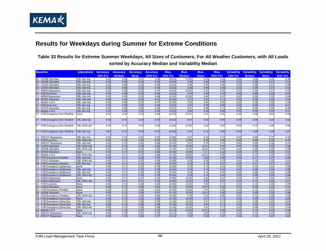
PJM Load Management Task Force April 20, 2011 86
Results for Weekdays during Summer for Extreme Conditions
Table 33 Results for Extreme Summer Weekdays, All Sizes of Customers, For All Weather Customers, with All Loads
sorted by Accuracy Median and Variability Median
Accuracy Accuracy Accuracy Accuracy Bias Bias Bias Bias Variability Variability Variability Variability
10th Pct Median Mean 90th Pct 10th Pct Median Mean 90th Pct 10th Pct Median Mean 90th Pct06 - ISONE Standard CBL Mul Adj 0.03 0.08 0.21 0.39 (0.03) (0.00) 0.03 0.05 0.03 0.08 0.20 0.38 06 - ISONE Standard CBL Add Adj 0.03 0.08 0.23 0.45 (0.03) 0.00 0.04 0.08 0.03 0.08 0.21 0.43 02 - CAISO Standard CBL Mul Adj 0.03 0.08 0.22 0.40 (0.03) 0.00 0.03 0.06 0.03 0.08 0.21 0.39 02 - CAISO Standard CBL Add Adj 0.03 0.08 0.23 0.45 (0.03) 0.00 0.04 0.09 0.03 0.08 0.21 0.43 13 - KEMA Regression CBL Mul Adj 0.03 0.08 0.22 0.41 (0.04) (0.00) 0.03 0.05 0.03 0.08 0.21 0.40 01 - PJM Economic CBL Add Adj 0.03 0.09 0.23 0.45 (0.02) 0.01 0.05 0.10 0.03 0.08 0.22 0.43 13 - KEMA Regression CBL Add Adj 0.03 0.09 0.24 0.46 (0.03) (0.00) 0.04 0.07 0.03 0.08 0.22 0.45 05 - NYISO Standard CBL Add Adj 0.03 0.09 0.25 0.47 (0.02) 0.01 0.07 0.13 0.03 0.08 0.23 0.44 04 - Middle 4 of 6 CBL Add Adj 0.03 0.09 0.23 0.47 (0.03) 0.00 0.04 0.08 0.03 0.08 0.22 0.44 01 - PJM Economic CBL Mul Adj 0.03 0.09 0.25 0.43 (0.02) 0.01 0.05 0.08 0.03 0.08 0.23 0.41 05 - NYISO Standard CBL Mul Adj 0.03 0.09 0.26 0.44 (0.01) 0.01 0.08 0.12 0.03 0.08 0.24 0.42 04 - Middle 4 of 6 CBL Mul Adj 0.03 0.09 0.25 0.43 (0.03) 0.00 0.04 0.06 0.03 0.08 0.24 0.41 07 - PJM Emergency Non-Weather None 0.04 0.09 0.23 0.49 (0.03) (0.01) 0.01 0.05 0.04 0.09 0.23 0.49
07 - PJM Emergency Non-Weather CBL Add Adj 0.04 0.10 0.24 0.53 (0.02) 0.01 0.03 0.06 0.04 0.09 0.24 0.52
07 - PJM Emergency Non-Weather CBL WSA Adj 0.04 0.10 0.24 0.50 (0.03) (0.00) 0.02 0.05 0.04 0.10 0.24 0.50
07 - PJM Emergency Non-Weather CBL Mul Adj 0.04 0.10 0.60 0.57 (0.02) 0.01 0.12 0.08 0.04 0.09 0.59 0.57
12 - ERCOT Regression CBL Mul Adj 0.04 0.10 0.83 0.52 (0.08) 0.01 0.33 0.13 0.03 0.09 0.73 0.45 01 - PJM Economic CBL WSA Adj 0.04 0.10 0.28 0.53 (0.12) (0.00) 0.03 0.09 0.04 0.09 0.25 0.49 12 - ERCOT Regression CBL Add Adj 0.04 0.10 0.40 0.58 (0.07) 0.01 0.14 0.16 0.03 0.09 0.32 0.51 02 - CAISO Standard CBL WSA Adj 0.04 0.10 0.26 0.55 (0.18) (0.02) (0.01) 0.05 0.03 0.09 0.22 0.48 06 - ISONE Standard CBL WSA Adj 0.04 0.10 0.25 0.55 (0.19) (0.02) (0.02) 0.05 0.04 0.09 0.22 0.49 05 - NYISO Standard None 0.04 0.11 0.31 0.56 (0.05) (0.00) 0.11 0.23 0.04 0.10 0.25 0.51 04 - Middle 4 of 6 CBL WSA Adj 0.04 0.11 0.27 0.56 (0.18) (0.02) (0.01) 0.06 0.04 0.10 0.24 0.50 08 - PJM Emergency Weather CBL Add Adj 0.04 0.11 0.28 0.57 (0.03) (0.00) 0.03 0.06 0.04 0.11 0.27 0.56 05 - NYISO Standard CBL WSA Adj 0.04 0.11 0.30 0.58 (0.05) 0.02 0.09 0.19 0.04 0.10 0.25 0.51 08 - PJM Emergency Weather CBL Mul Adj 0.04 0.11 0.73 0.62 (0.03) 0.00 0.15 0.07 0.04 0.11 0.71 0.61 11 - PJM Emergency Settlement None 0.04 0.11 0.30 0.79 (0.04) 0.03 0.14 0.44 0.03 0.09 0.24 0.58 11 - PJM Emergency Settlement CBL Add Adj 0.04 0.11 0.30 0.79 (0.04) 0.03 0.14 0.44 0.03 0.09 0.24 0.58 11 - PJM Emergency Settlement CBL Mul Adj 0.04 0.11 0.30 0.79 (0.04) 0.03 0.14 0.44 0.03 0.09 0.24 0.58 11 - PJM Emergency Settlement CBL WSA Adj 0.04 0.11 0.30 0.79 (0.04) 0.03 0.14 0.44 0.03 0.09 0.24 0.58 13 - KEMA Regression None 0.05 0.11 0.27 0.53 (0.08) (0.03) 0.02 0.07 0.04 0.10 0.24 0.51 13 - KEMA Regression CBL WSA Adj 0.05 0.11 0.27 0.53 (0.08) (0.03) 0.02 0.07 0.04 0.10 0.24 0.51 01 - PJM Economic None 0.05 0.12 0.28 0.50 (0.09) (0.03) 0.04 0.11 0.04 0.10 0.24 0.47 02 - CAISO Standard None 0.06 0.12 0.26 0.50 (0.12) (0.05) (0.01) 0.05 0.03 0.09 0.22 0.47 08 - PJM Emergency Weather None 0.04 0.13 0.28 0.61 (0.05) (0.00) 0.01 0.05 0.04 0.12 0.27 0.61 06 - ISONE Standard None 0.06 0.13 0.26 0.51 (0.12) (0.06) (0.01) 0.05 0.04 0.09 0.22 0.48 08 - PJM Emergency Weather CBL WSA Adj 0.05 0.13 0.29 0.62 (0.05) 0.00 0.01 0.06 0.04 0.13 0.28 0.62 10 - PJM Emergency Same Day None 0.05 0.13 0.28 0.58 (0.16) (0.03) 0.01 0.13 0.03 0.09 0.23 0.54 10 - PJM Emergency Same Day CBL Add Adj 0.05 0.13 0.28 0.58 (0.16) (0.03) 0.01 0.13 0.03 0.09 0.23 0.54 10 - PJM Emergency Same Day CBL Mul Adj 0.05 0.13 0.28 0.58 (0.16) (0.03) 0.01 0.13 0.03 0.09 0.23 0.54 10 - PJM Emergency Same Day CBL WSA Adj 0.05 0.13 0.28 0.58 (0.16) (0.03) 0.01 0.13 0.03 0.09 0.23 0.54 04 - Middle 4 of 6 None 0.06 0.13 0.27 0.51 (0.12) (0.05) (0.01) 0.06 0.04 0.10 0.23 0.48 12 - ERCOT Regression CBL WSA Adj 0.06 0.18 0.91 0.76 (0.21) 0.02 0.57 0.27 0.04 0.13 0.43 0.63 12 - ERCOT Regression None 0.06 0.18 0.95 0.77 (0.22) 0.02 0.53 0.27 0.04 0.13 0.47 0.64
Baseline Adjustment
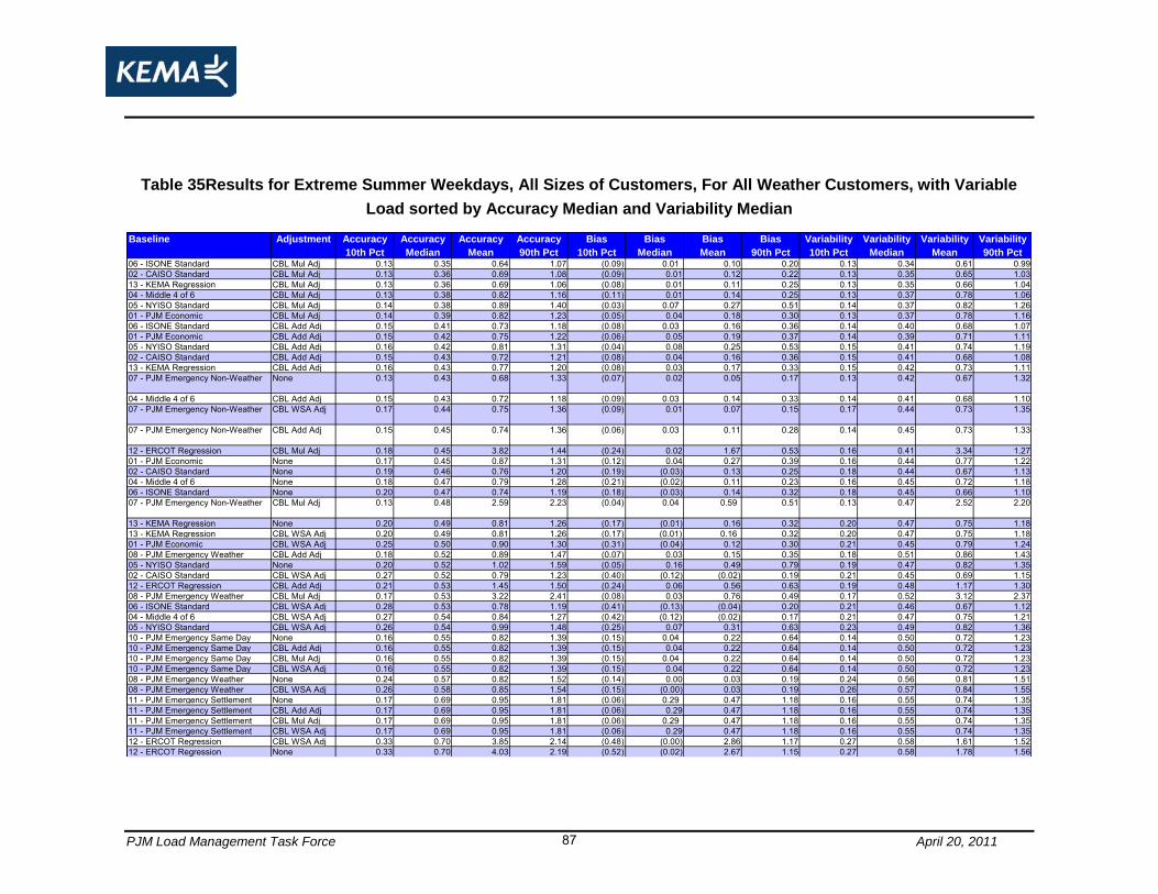
PJM Load Management Task Force April 20, 2011 87
Table 35Results for Extreme Summer Weekdays, All Sizes of Customers, For All Weather Customers, with Variable
Load sorted by Accuracy Median and Variability Median
Accuracy Accuracy Accuracy Accuracy Bias Bias Bias Bias Variability Variability Variability Variability
10th Pct Median Mean 90th Pct 10th Pct Median Mean 90th Pct 10th Pct Median Mean 90th Pct06 - ISONE Standard CBL Mul Adj 0.13 0.35 0.64 1.07 (0.09) 0.01 0.10 0.20 0.13 0.34 0.61 0.9902 - CAISO Standard CBL Mul Adj 0.13 0.36 0.69 1.08 (0.09) 0.01 0.12 0.22 0.13 0.35 0.65 1.0313 - KEMA Regression CBL Mul Adj 0.13 0.36 0.69 1.06 (0.08) 0.01 0.11 0.25 0.13 0.35 0.66 1.0404 - Middle 4 of 6 CBL Mul Adj 0.13 0.38 0.82 1.16 (0.11) 0.01 0.14 0.25 0.13 0.37 0.78 1.0605 - NYISO Standard CBL Mul Adj 0.14 0.38 0.89 1.40 (0.03) 0.07 0.27 0.51 0.14 0.37 0.82 1.2601 - PJM Economic CBL Mul Adj 0.14 0.39 0.82 1.23 (0.05) 0.04 0.18 0.30 0.13 0.37 0.78 1.1606 - ISONE Standard CBL Add Adj 0.15 0.41 0.73 1.18 (0.08) 0.03 0.16 0.36 0.14 0.40 0.68 1.0701 - PJM Economic CBL Add Adj 0.15 0.42 0.75 1.22 (0.06) 0.05 0.19 0.37 0.14 0.39 0.71 1.1105 - NYISO Standard CBL Add Adj 0.16 0.42 0.81 1.31 (0.04) 0.08 0.25 0.53 0.15 0.41 0.74 1.1902 - CAISO Standard CBL Add Adj 0.15 0.43 0.72 1.21 (0.08) 0.04 0.16 0.36 0.15 0.41 0.68 1.0813 - KEMA Regression CBL Add Adj 0.16 0.43 0.77 1.20 (0.08) 0.03 0.17 0.33 0.15 0.42 0.73 1.1107 - PJM Emergency Non-Weather None 0.13 0.43 0.68 1.33 (0.07) 0.02 0.05 0.17 0.13 0.42 0.67 1.32
04 - Middle 4 of 6 CBL Add Adj 0.15 0.43 0.72 1.18 (0.09) 0.03 0.14 0.33 0.14 0.41 0.68 1.1007 - PJM Emergency Non-Weather CBL WSA Adj 0.17 0.44 0.75 1.36 (0.09) 0.01 0.07 0.15 0.17 0.44 0.73 1.35
07 - PJM Emergency Non-Weather CBL Add Adj 0.15 0.45 0.74 1.36 (0.06) 0.03 0.11 0.28 0.14 0.45 0.73 1.33
12 - ERCOT Regression CBL Mul Adj 0.18 0.45 3.82 1.44 (0.24) 0.02 1.67 0.53 0.16 0.41 3.34 1.2701 - PJM Economic None 0.17 0.45 0.87 1.31 (0.12) 0.04 0.27 0.39 0.16 0.44 0.77 1.2202 - CAISO Standard None 0.19 0.46 0.76 1.20 (0.19) (0.03) 0.13 0.25 0.18 0.44 0.67 1.1304 - Middle 4 of 6 None 0.18 0.47 0.79 1.28 (0.21) (0.02) 0.11 0.23 0.16 0.45 0.72 1.1806 - ISONE Standard None 0.20 0.47 0.74 1.19 (0.18) (0.03) 0.14 0.32 0.18 0.45 0.66 1.1007 - PJM Emergency Non-Weather CBL Mul Adj 0.13 0.48 2.59 2.23 (0.04) 0.04 0.59 0.51 0.13 0.47 2.52 2.20
13 - KEMA Regression None 0.20 0.49 0.81 1.26 (0.17) (0.01) 0.16 0.32 0.20 0.47 0.75 1.1813 - KEMA Regression CBL WSA Adj 0.20 0.49 0.81 1.26 (0.17) (0.01) 0.16 0.32 0.20 0.47 0.75 1.1801 - PJM Economic CBL WSA Adj 0.25 0.50 0.90 1.30 (0.31) (0.04) 0.12 0.30 0.21 0.45 0.79 1.2408 - PJM Emergency Weather CBL Add Adj 0.18 0.52 0.89 1.47 (0.07) 0.03 0.15 0.35 0.18 0.51 0.86 1.4305 - NYISO Standard None 0.20 0.52 1.02 1.59 (0.05) 0.16 0.49 0.79 0.19 0.47 0.82 1.3502 - CAISO Standard CBL WSA Adj 0.27 0.52 0.79 1.23 (0.40) (0.12) (0.02) 0.19 0.21 0.45 0.69 1.1512 - ERCOT Regression CBL Add Adj 0.21 0.53 1.45 1.50 (0.24) 0.06 0.56 0.63 0.19 0.48 1.17 1.3008 - PJM Emergency Weather CBL Mul Adj 0.17 0.53 3.22 2.41 (0.08) 0.03 0.76 0.49 0.17 0.52 3.12 2.3706 - ISONE Standard CBL WSA Adj 0.28 0.53 0.78 1.19 (0.41) (0.13) (0.04) 0.20 0.21 0.46 0.67 1.1204 - Middle 4 of 6 CBL WSA Adj 0.27 0.54 0.84 1.27 (0.42) (0.12) (0.02) 0.17 0.21 0.47 0.75 1.2105 - NYISO Standard CBL WSA Adj 0.26 0.54 0.99 1.48 (0.25) 0.07 0.31 0.63 0.23 0.49 0.82 1.3610 - PJM Emergency Same Day None 0.16 0.55 0.82 1.39 (0.15) 0.04 0.22 0.64 0.14 0.50 0.72 1.2310 - PJM Emergency Same Day CBL Add Adj 0.16 0.55 0.82 1.39 (0.15) 0.04 0.22 0.64 0.14 0.50 0.72 1.2310 - PJM Emergency Same Day CBL Mul Adj 0.16 0.55 0.82 1.39 (0.15) 0.04 0.22 0.64 0.14 0.50 0.72 1.2310 - PJM Emergency Same Day CBL WSA Adj 0.16 0.55 0.82 1.39 (0.15) 0.04 0.22 0.64 0.14 0.50 0.72 1.2308 - PJM Emergency Weather None 0.24 0.57 0.82 1.52 (0.14) 0.00 0.03 0.19 0.24 0.56 0.81 1.5108 - PJM Emergency Weather CBL WSA Adj 0.26 0.58 0.85 1.54 (0.15) (0.00) 0.03 0.19 0.26 0.57 0.84 1.5511 - PJM Emergency Settlement None 0.17 0.69 0.95 1.81 (0.06) 0.29 0.47 1.18 0.16 0.55 0.74 1.3511 - PJM Emergency Settlement CBL Add Adj 0.17 0.69 0.95 1.81 (0.06) 0.29 0.47 1.18 0.16 0.55 0.74 1.3511 - PJM Emergency Settlement CBL Mul Adj 0.17 0.69 0.95 1.81 (0.06) 0.29 0.47 1.18 0.16 0.55 0.74 1.3511 - PJM Emergency Settlement CBL WSA Adj 0.17 0.69 0.95 1.81 (0.06) 0.29 0.47 1.18 0.16 0.55 0.74 1.3512 - ERCOT Regression CBL WSA Adj 0.33 0.70 3.85 2.14 (0.48) (0.00) 2.86 1.17 0.27 0.58 1.61 1.5212 - ERCOT Regression None 0.33 0.70 4.03 2.19 (0.52) (0.02) 2.67 1.15 0.27 0.58 1.78 1.56
Baseline Adjustment
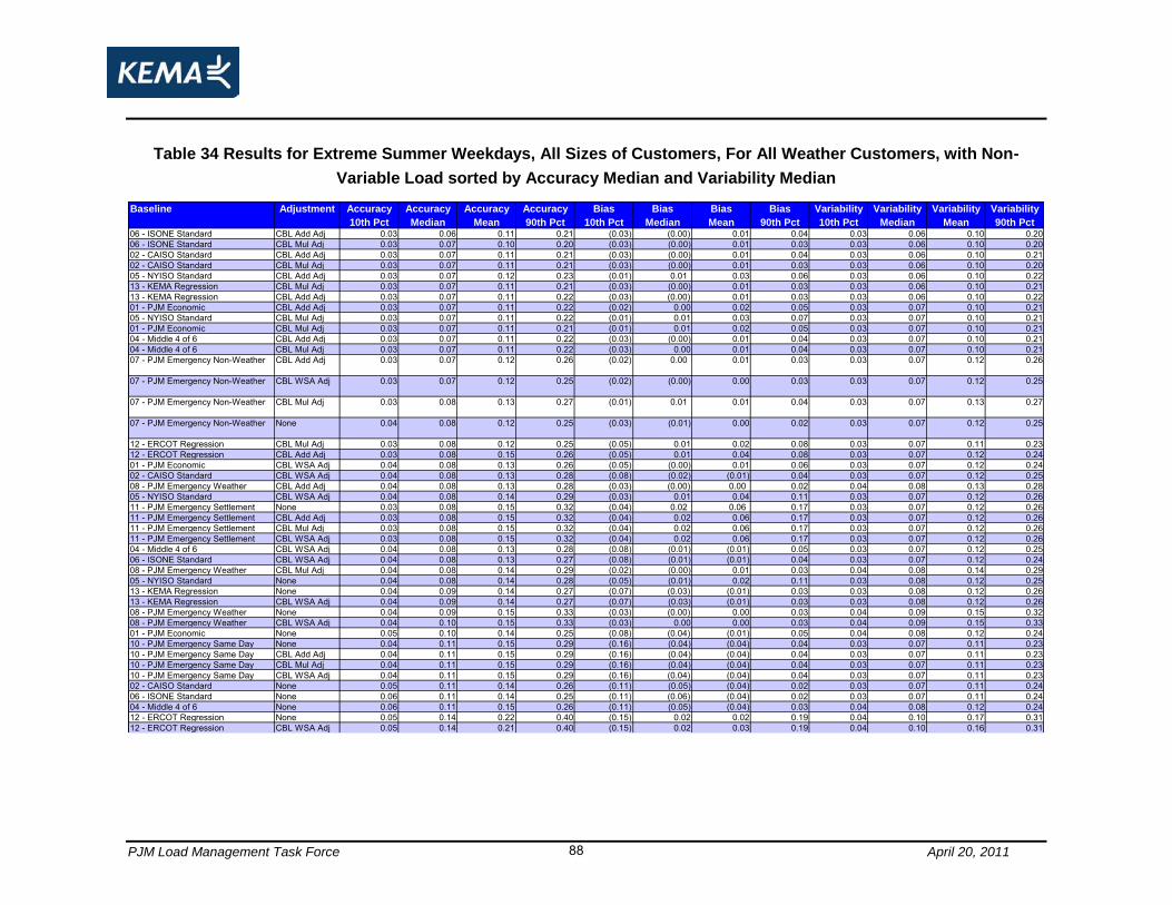
PJM Load Management Task Force April 20, 2011 88
Table 34 Results for Extreme Summer Weekdays, All Sizes of Customers, For All Weather Customers, with Non-
Variable Load sorted by Accuracy Median and Variability Median
Accuracy Accuracy Accuracy Accuracy Bias Bias Bias Bias Variability Variability Variability Variability
10th Pct Median Mean 90th Pct 10th Pct Median Mean 90th Pct 10th Pct Median Mean 90th Pct06 - ISONE Standard CBL Add Adj 0.03 0.06 0.11 0.21 (0.03) (0.00) 0.01 0.04 0.03 0.06 0.10 0.2006 - ISONE Standard CBL Mul Adj 0.03 0.07 0.10 0.20 (0.03) (0.00) 0.01 0.03 0.03 0.06 0.10 0.2002 - CAISO Standard CBL Add Adj 0.03 0.07 0.11 0.21 (0.03) (0.00) 0.01 0.04 0.03 0.06 0.10 0.2102 - CAISO Standard CBL Mul Adj 0.03 0.07 0.11 0.21 (0.03) (0.00) 0.01 0.03 0.03 0.06 0.10 0.2005 - NYISO Standard CBL Add Adj 0.03 0.07 0.12 0.23 (0.01) 0.01 0.03 0.06 0.03 0.06 0.10 0.2213 - KEMA Regression CBL Mul Adj 0.03 0.07 0.11 0.21 (0.03) (0.00) 0.01 0.03 0.03 0.06 0.10 0.2113 - KEMA Regression CBL Add Adj 0.03 0.07 0.11 0.22 (0.03) (0.00) 0.01 0.03 0.03 0.06 0.10 0.2201 - PJM Economic CBL Add Adj 0.03 0.07 0.11 0.22 (0.02) 0.00 0.02 0.05 0.03 0.07 0.10 0.2105 - NYISO Standard CBL Mul Adj 0.03 0.07 0.11 0.22 (0.01) 0.01 0.03 0.07 0.03 0.07 0.10 0.2101 - PJM Economic CBL Mul Adj 0.03 0.07 0.11 0.21 (0.01) 0.01 0.02 0.05 0.03 0.07 0.10 0.2104 - Middle 4 of 6 CBL Add Adj 0.03 0.07 0.11 0.22 (0.03) (0.00) 0.01 0.04 0.03 0.07 0.10 0.2104 - Middle 4 of 6 CBL Mul Adj 0.03 0.07 0.11 0.22 (0.03) 0.00 0.01 0.04 0.03 0.07 0.10 0.2107 - PJM Emergency Non-Weather CBL Add Adj 0.03 0.07 0.12 0.26 (0.02) 0.00 0.01 0.03 0.03 0.07 0.12 0.26
07 - PJM Emergency Non-Weather CBL WSA Adj 0.03 0.07 0.12 0.25 (0.02) (0.00) 0.00 0.03 0.03 0.07 0.12 0.25
07 - PJM Emergency Non-Weather CBL Mul Adj 0.03 0.08 0.13 0.27 (0.01) 0.01 0.01 0.04 0.03 0.07 0.13 0.27
07 - PJM Emergency Non-Weather None 0.04 0.08 0.12 0.25 (0.03) (0.01) 0.00 0.02 0.03 0.07 0.12 0.25
12 - ERCOT Regression CBL Mul Adj 0.03 0.08 0.12 0.25 (0.05) 0.01 0.02 0.08 0.03 0.07 0.11 0.2312 - ERCOT Regression CBL Add Adj 0.03 0.08 0.15 0.26 (0.05) 0.01 0.04 0.08 0.03 0.07 0.12 0.2401 - PJM Economic CBL WSA Adj 0.04 0.08 0.13 0.26 (0.05) (0.00) 0.01 0.06 0.03 0.07 0.12 0.2402 - CAISO Standard CBL WSA Adj 0.04 0.08 0.13 0.28 (0.08) (0.02) (0.01) 0.04 0.03 0.07 0.12 0.2508 - PJM Emergency Weather CBL Add Adj 0.04 0.08 0.13 0.28 (0.03) (0.00) 0.00 0.02 0.04 0.08 0.13 0.2805 - NYISO Standard CBL WSA Adj 0.04 0.08 0.14 0.29 (0.03) 0.01 0.04 0.11 0.03 0.07 0.12 0.2611 - PJM Emergency Settlement None 0.03 0.08 0.15 0.32 (0.04) 0.02 0.06 0.17 0.03 0.07 0.12 0.2611 - PJM Emergency Settlement CBL Add Adj 0.03 0.08 0.15 0.32 (0.04) 0.02 0.06 0.17 0.03 0.07 0.12 0.2611 - PJM Emergency Settlement CBL Mul Adj 0.03 0.08 0.15 0.32 (0.04) 0.02 0.06 0.17 0.03 0.07 0.12 0.2611 - PJM Emergency Settlement CBL WSA Adj 0.03 0.08 0.15 0.32 (0.04) 0.02 0.06 0.17 0.03 0.07 0.12 0.2604 - Middle 4 of 6 CBL WSA Adj 0.04 0.08 0.13 0.28 (0.08) (0.01) (0.01) 0.05 0.03 0.07 0.12 0.2506 - ISONE Standard CBL WSA Adj 0.04 0.08 0.13 0.27 (0.08) (0.01) (0.01) 0.04 0.03 0.07 0.12 0.2408 - PJM Emergency Weather CBL Mul Adj 0.04 0.08 0.14 0.29 (0.02) (0.00) 0.01 0.03 0.04 0.08 0.14 0.2905 - NYISO Standard None 0.04 0.08 0.14 0.28 (0.05) (0.01) 0.02 0.11 0.03 0.08 0.12 0.2513 - KEMA Regression None 0.04 0.09 0.14 0.27 (0.07) (0.03) (0.01) 0.03 0.03 0.08 0.12 0.2613 - KEMA Regression CBL WSA Adj 0.04 0.09 0.14 0.27 (0.07) (0.03) (0.01) 0.03 0.03 0.08 0.12 0.2608 - PJM Emergency Weather None 0.04 0.09 0.15 0.33 (0.03) (0.00) 0.00 0.03 0.04 0.09 0.15 0.3208 - PJM Emergency Weather CBL WSA Adj 0.04 0.10 0.15 0.33 (0.03) 0.00 0.00 0.03 0.04 0.09 0.15 0.3301 - PJM Economic None 0.05 0.10 0.14 0.25 (0.08) (0.04) (0.01) 0.05 0.04 0.08 0.12 0.2410 - PJM Emergency Same Day None 0.04 0.11 0.15 0.29 (0.16) (0.04) (0.04) 0.04 0.03 0.07 0.11 0.2310 - PJM Emergency Same Day CBL Add Adj 0.04 0.11 0.15 0.29 (0.16) (0.04) (0.04) 0.04 0.03 0.07 0.11 0.2310 - PJM Emergency Same Day CBL Mul Adj 0.04 0.11 0.15 0.29 (0.16) (0.04) (0.04) 0.04 0.03 0.07 0.11 0.2310 - PJM Emergency Same Day CBL WSA Adj 0.04 0.11 0.15 0.29 (0.16) (0.04) (0.04) 0.04 0.03 0.07 0.11 0.2302 - CAISO Standard None 0.05 0.11 0.14 0.26 (0.11) (0.05) (0.04) 0.02 0.03 0.07 0.11 0.2406 - ISONE Standard None 0.06 0.11 0.14 0.25 (0.11) (0.06) (0.04) 0.02 0.03 0.07 0.11 0.2404 - Middle 4 of 6 None 0.06 0.11 0.15 0.26 (0.11) (0.05) (0.04) 0.03 0.04 0.08 0.12 0.2412 - ERCOT Regression None 0.05 0.14 0.22 0.40 (0.15) 0.02 0.02 0.19 0.04 0.10 0.17 0.3112 - ERCOT Regression CBL WSA Adj 0.05 0.14 0.21 0.40 (0.15) 0.02 0.03 0.19 0.04 0.10 0.16 0.31
Baseline Adjustment

PJM Load Management Task Force April 20, 2011 89
Table 35 Results for Extreme Summer Weekdays, All Sizes of Customers, Weather Sensitive Customers, with All
Loads sorted by Accuracy Median and Variability Median
Accuracy Accuracy Accuracy Accuracy Bias Bias Bias Bias Variability Variability Variability Variability
10th Pct Median Mean 90th Pct 10th Pct Median Mean 90th Pct 10th Pct Median Mean 90th Pct06 - ISONE Standard CBL Add Adj 0.04 0.09 0.35 0.67 (0.04) (0.00) 0.07 0.16 0.04 0.09 0.32 0.6402 - CAISO Standard CBL Add Adj 0.04 0.09 0.34 0.68 (0.04) (0.00) 0.07 0.17 0.04 0.09 0.32 0.6513 - KEMA Regression CBL Mul Adj 0.04 0.10 0.33 0.59 (0.04) (0.01) 0.05 0.07 0.04 0.09 0.31 0.5806 - ISONE Standard CBL Mul Adj 0.04 0.10 0.31 0.58 (0.05) (0.00) 0.05 0.07 0.04 0.09 0.29 0.5502 - CAISO Standard CBL Mul Adj 0.04 0.10 0.32 0.58 (0.04) (0.00) 0.05 0.08 0.04 0.09 0.31 0.5613 - KEMA Regression CBL Add Adj 0.04 0.10 0.36 0.70 (0.04) (0.01) 0.07 0.15 0.04 0.10 0.34 0.6601 - PJM Economic CBL Add Adj 0.04 0.10 0.36 0.69 (0.03) 0.01 0.09 0.16 0.04 0.10 0.34 0.6605 - NYISO Standard CBL Add Adj 0.04 0.10 0.39 0.71 (0.02) 0.01 0.11 0.21 0.04 0.09 0.35 0.6704 - Middle 4 of 6 CBL Add Adj 0.04 0.10 0.34 0.69 (0.04) 0.00 0.07 0.15 0.04 0.10 0.32 0.6601 - PJM Economic CBL Mul Adj 0.04 0.10 0.37 0.63 (0.02) 0.01 0.08 0.11 0.04 0.10 0.35 0.6105 - NYISO Standard CBL Mul Adj 0.04 0.10 0.42 0.66 (0.02) 0.01 0.12 0.17 0.04 0.10 0.38 0.6304 - Middle 4 of 6 CBL Mul Adj 0.04 0.10 0.35 0.62 (0.04) 0.00 0.05 0.08 0.04 0.10 0.33 0.6107 - PJM Emergency Non-Weather None 0.05 0.10 0.31 0.73 (0.03) (0.01) 0.02 0.07 0.04 0.10 0.31 0.73
07 - PJM Emergency Non-Weather CBL Add Adj 0.04 0.10 0.35 0.79 (0.02) 0.01 0.05 0.11 0.04 0.10 0.34 0.77
07 - PJM Emergency Non-Weather CBL Mul Adj 0.04 0.10 0.92 0.85 (0.02) 0.01 0.19 0.11 0.04 0.10 0.90 0.84
11 - PJM Emergency Settlement None 0.04 0.11 0.48 1.32 (0.05) 0.01 0.25 0.84 0.03 0.09 0.37 0.9411 - PJM Emergency Settlement CBL Add Adj 0.04 0.11 0.48 1.32 (0.05) 0.01 0.25 0.84 0.03 0.09 0.37 0.9411 - PJM Emergency Settlement CBL Mul Adj 0.04 0.11 0.48 1.32 (0.05) 0.01 0.25 0.84 0.03 0.09 0.37 0.9411 - PJM Emergency Settlement CBL WSA Adj 0.04 0.11 0.48 1.32 (0.05) 0.01 0.25 0.84 0.03 0.09 0.37 0.9407 - PJM Emergency Non-Weather CBL WSA Adj 0.04 0.11 0.35 0.75 (0.04) (0.00) 0.03 0.06 0.04 0.11 0.34 0.74
05 - NYISO Standard None 0.05 0.12 0.47 0.80 (0.06) (0.02) 0.18 0.33 0.04 0.10 0.38 0.7301 - PJM Economic CBL WSA Adj 0.05 0.12 0.42 0.76 (0.23) (0.01) 0.04 0.08 0.04 0.11 0.37 0.6802 - CAISO Standard CBL WSA Adj 0.05 0.12 0.38 0.79 (0.32) (0.02) (0.03) 0.06 0.04 0.10 0.32 0.7006 - ISONE Standard CBL WSA Adj 0.05 0.12 0.37 0.79 (0.32) (0.02) (0.03) 0.06 0.04 0.11 0.32 0.6908 - PJM Emergency Weather CBL Add Adj 0.05 0.12 0.42 0.87 (0.03) 0.00 0.07 0.13 0.04 0.12 0.41 0.8408 - PJM Emergency Weather CBL Mul Adj 0.05 0.12 1.28 0.91 (0.03) 0.00 0.28 0.12 0.05 0.12 1.25 0.9112 - ERCOT Regression CBL Mul Adj 0.04 0.12 0.39 0.77 (0.11) 0.02 0.08 0.20 0.04 0.10 0.35 0.7005 - NYISO Standard CBL WSA Adj 0.05 0.12 0.46 0.84 (0.17) 0.01 0.12 0.21 0.04 0.11 0.38 0.7413 - KEMA Regression None 0.06 0.12 0.38 0.75 (0.10) (0.04) 0.04 0.09 0.05 0.11 0.34 0.7413 - KEMA Regression CBL WSA Adj 0.06 0.12 0.38 0.75 (0.10) (0.04) 0.04 0.09 0.05 0.11 0.34 0.7404 - Middle 4 of 6 CBL WSA Adj 0.05 0.12 0.40 0.78 (0.31) (0.02) (0.02) 0.06 0.04 0.11 0.35 0.7012 - ERCOT Regression CBL Add Adj 0.04 0.13 0.67 0.91 (0.10) 0.02 0.29 0.30 0.04 0.11 0.50 0.7908 - PJM Emergency Weather None 0.05 0.13 0.38 0.88 (0.06) (0.00) 0.01 0.07 0.05 0.13 0.37 0.8801 - PJM Economic None 0.07 0.13 0.42 0.71 (0.10) (0.05) 0.08 0.15 0.05 0.11 0.36 0.6908 - PJM Emergency Weather CBL WSA Adj 0.05 0.14 0.40 0.91 (0.07) 0.00 0.02 0.07 0.05 0.14 0.39 0.8902 - CAISO Standard None 0.08 0.14 0.38 0.68 (0.15) (0.08) 0.01 0.07 0.04 0.10 0.31 0.6706 - ISONE Standard None 0.09 0.15 0.37 0.69 (0.14) (0.08) 0.01 0.07 0.04 0.10 0.31 0.6804 - Middle 4 of 6 None 0.08 0.15 0.39 0.70 (0.15) (0.08) 0.00 0.07 0.05 0.11 0.34 0.6910 - PJM Emergency Same Day None 0.06 0.17 0.44 0.95 (0.18) (0.06) 0.05 0.27 0.03 0.09 0.36 0.8910 - PJM Emergency Same Day CBL Add Adj 0.06 0.17 0.44 0.95 (0.18) (0.06) 0.05 0.27 0.03 0.09 0.36 0.8910 - PJM Emergency Same Day CBL Mul Adj 0.06 0.17 0.44 0.95 (0.18) (0.06) 0.05 0.27 0.03 0.09 0.36 0.8910 - PJM Emergency Same Day CBL WSA Adj 0.06 0.17 0.44 0.95 (0.18) (0.06) 0.05 0.27 0.03 0.09 0.36 0.8912 - ERCOT Regression None 0.06 0.21 1.84 1.11 (0.27) 0.02 1.37 0.36 0.05 0.14 0.73 0.9312 - ERCOT Regression CBL WSA Adj 0.06 0.21 1.82 1.09 (0.26) 0.02 1.39 0.38 0.05 0.14 0.71 0.93
Baseline Adjustment
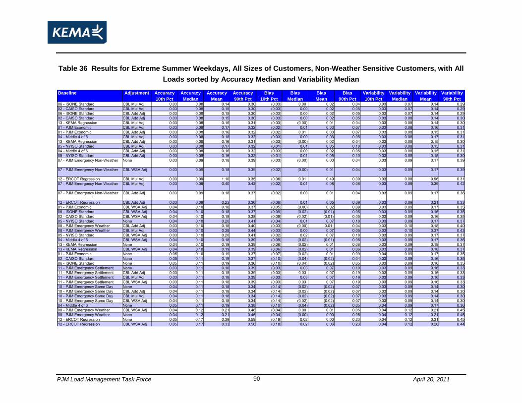
PJM Load Management Task Force April 20, 2011 90
Table 36 Results for Extreme Summer Weekdays, All Sizes of Customers, Non-Weather Sensitive Customers, with All
Loads sorted by Accuracy Median and Variability Median
Accuracy Accuracy Accuracy Accuracy Bias Bias Bias Bias Variability Variability Variability Variability
10th Pct Median Mean 90th Pct 10th Pct Median Mean 90th Pct 10th Pct Median Mean 90th Pct06 - ISONE Standard CBL Mul Adj 0.03 0.08 0.14 0.30 (0.03) 0.00 0.02 0.04 0.03 0.07 0.14 0.2902 - CAISO Standard CBL Mul Adj 0.03 0.08 0.15 0.30 (0.03) 0.00 0.02 0.05 0.03 0.07 0.14 0.2906 - ISONE Standard CBL Add Adj 0.03 0.08 0.15 0.30 (0.03) 0.00 0.02 0.05 0.03 0.07 0.14 0.2902 - CAISO Standard CBL Add Adj 0.03 0.08 0.15 0.30 (0.03) 0.00 0.02 0.05 0.03 0.08 0.14 0.3013 - KEMA Regression CBL Mul Adj 0.03 0.08 0.15 0.31 (0.03) (0.00) 0.01 0.04 0.03 0.08 0.14 0.3001 - PJM Economic CBL Mul Adj 0.03 0.08 0.17 0.32 (0.02) 0.01 0.03 0.07 0.03 0.08 0.16 0.3101 - PJM Economic CBL Add Adj 0.03 0.08 0.16 0.32 (0.02) 0.01 0.03 0.07 0.03 0.08 0.15 0.3104 - Middle 4 of 6 CBL Mul Adj 0.03 0.08 0.18 0.32 (0.03) 0.00 0.03 0.05 0.03 0.08 0.17 0.3113 - KEMA Regression CBL Add Adj 0.03 0.08 0.16 0.31 (0.03) (0.00) 0.02 0.04 0.03 0.08 0.15 0.3005 - NYISO Standard CBL Mul Adj 0.03 0.08 0.17 0.32 (0.01) 0.01 0.05 0.10 0.03 0.08 0.15 0.3104 - Middle 4 of 6 CBL Add Adj 0.03 0.08 0.16 0.32 (0.03) 0.00 0.02 0.05 0.03 0.08 0.15 0.3105 - NYISO Standard CBL Add Adj 0.03 0.08 0.16 0.32 (0.01) 0.01 0.05 0.10 0.03 0.08 0.15 0.3007 - PJM Emergency Non-Weather None 0.03 0.09 0.18 0.39 (0.03) (0.00) 0.00 0.04 0.03 0.09 0.17 0.39
07 - PJM Emergency Non-Weather CBL WSA Adj 0.03 0.09 0.18 0.39 (0.02) (0.00) 0.01 0.04 0.03 0.09 0.17 0.39
12 - ERCOT Regression CBL Mul Adj 0.03 0.09 1.10 0.35 (0.06) 0.01 0.49 0.09 0.03 0.08 0.96 0.3107 - PJM Emergency Non-Weather CBL Mul Adj 0.03 0.09 0.40 0.42 (0.02) 0.01 0.08 0.06 0.03 0.09 0.39 0.42
07 - PJM Emergency Non-Weather CBL Add Adj 0.03 0.09 0.18 0.37 (0.02) 0.00 0.01 0.04 0.03 0.09 0.17 0.36
12 - ERCOT Regression CBL Add Adj 0.03 0.09 0.23 0.36 (0.06) 0.01 0.05 0.09 0.03 0.09 0.21 0.3301 - PJM Economic CBL WSA Adj 0.04 0.10 0.18 0.37 (0.05) (0.00) 0.02 0.09 0.03 0.09 0.17 0.3506 - ISONE Standard CBL WSA Adj 0.04 0.10 0.18 0.37 (0.09) (0.02) (0.01) 0.05 0.03 0.09 0.16 0.3502 - CAISO Standard CBL WSA Adj 0.04 0.10 0.18 0.38 (0.09) (0.02) (0.01) 0.05 0.03 0.09 0.16 0.3505 - NYISO Standard None 0.04 0.10 0.20 0.41 (0.04) 0.01 0.07 0.18 0.03 0.09 0.17 0.3708 - PJM Emergency Weather CBL Add Adj 0.03 0.10 0.18 0.40 (0.03) (0.00) 0.01 0.04 0.03 0.10 0.18 0.4008 - PJM Emergency Weather CBL Mul Adj 0.03 0.10 0.38 0.44 (0.03) 0.00 0.07 0.05 0.03 0.10 0.37 0.4305 - NYISO Standard CBL WSA Adj 0.03 0.10 0.20 0.41 (0.02) 0.02 0.07 0.18 0.03 0.09 0.17 0.3704 - Middle 4 of 6 CBL WSA Adj 0.04 0.10 0.18 0.39 (0.09) (0.02) (0.01) 0.06 0.03 0.09 0.17 0.3613 - KEMA Regression None 0.04 0.10 0.19 0.39 (0.06) (0.02) 0.01 0.06 0.03 0.09 0.18 0.3713 - KEMA Regression CBL WSA Adj 0.04 0.10 0.19 0.39 (0.06) (0.02) 0.01 0.06 0.03 0.09 0.18 0.3701 - PJM Economic None 0.05 0.10 0.19 0.37 (0.07) (0.02) 0.01 0.09 0.04 0.09 0.17 0.3502 - CAISO Standard None 0.05 0.11 0.19 0.37 (0.10) (0.04) (0.02) 0.04 0.03 0.09 0.16 0.3506 - ISONE Standard None 0.05 0.11 0.19 0.36 (0.10) (0.04) (0.02) 0.05 0.03 0.09 0.16 0.3511 - PJM Emergency Settlement None 0.03 0.11 0.18 0.39 (0.03) 0.03 0.07 0.19 0.03 0.09 0.16 0.3311 - PJM Emergency Settlement CBL Add Adj 0.03 0.11 0.18 0.39 (0.03) 0.03 0.07 0.19 0.03 0.09 0.16 0.3311 - PJM Emergency Settlement CBL Mul Adj 0.03 0.11 0.18 0.39 (0.03) 0.03 0.07 0.19 0.03 0.09 0.16 0.3311 - PJM Emergency Settlement CBL WSA Adj 0.03 0.11 0.18 0.39 (0.03) 0.03 0.07 0.19 0.03 0.09 0.16 0.3310 - PJM Emergency Same Day None 0.04 0.11 0.18 0.34 (0.14) (0.02) (0.02) 0.07 0.03 0.09 0.14 0.3010 - PJM Emergency Same Day CBL Add Adj 0.04 0.11 0.18 0.34 (0.14) (0.02) (0.02) 0.07 0.03 0.09 0.14 0.3010 - PJM Emergency Same Day CBL Mul Adj 0.04 0.11 0.18 0.34 (0.14) (0.02) (0.02) 0.07 0.03 0.09 0.14 0.3010 - PJM Emergency Same Day CBL WSA Adj 0.04 0.11 0.18 0.34 (0.14) (0.02) (0.02) 0.07 0.03 0.09 0.14 0.3004 - Middle 4 of 6 None 0.05 0.11 0.19 0.38 (0.10) (0.04) (0.02) 0.05 0.04 0.09 0.17 0.3608 - PJM Emergency Weather CBL WSA Adj 0.04 0.12 0.21 0.46 (0.04) 0.00 0.01 0.05 0.04 0.12 0.21 0.4508 - PJM Emergency Weather None 0.04 0.12 0.21 0.46 (0.04) (0.00) 0.00 0.05 0.04 0.12 0.21 0.4512 - ERCOT Regression None 0.05 0.17 0.39 0.59 (0.19) 0.02 0.00 0.23 0.04 0.12 0.31 0.4512 - ERCOT Regression CBL WSA Adj 0.05 0.17 0.33 0.58 (0.18) 0.02 0.06 0.23 0.04 0.12 0.26 0.44
Baseline Adjustment
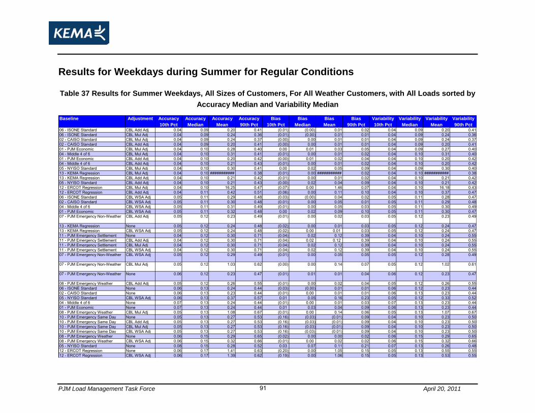
PJM Load Management Task Force April 20, 2011 91
Results for Weekdays during Summer for Regular Conditions
Table 37 Results for Summer Weekdays, All Sizes of Customers, For All Weather Customers, with All Loads sorted by
Accuracy Median and Variability Median
Accuracy Accuracy Accuracy Accuracy Bias Bias Bias Bias Variability Variability Variability Variability
10th Pct Median Mean 90th Pct 10th Pct Median Mean 90th Pct 10th Pct Median Mean 90th Pct06 - ISONE Standard CBL Add Adj 0.04 0.09 0.20 0.41 (0.01) (0.00) 0.01 0.02 0.04 0.09 0.20 0.4106 - ISONE Standard CBL Mul Adj 0.04 0.09 0.24 0.36 (0.01) (0.00) 0.01 0.01 0.04 0.09 0.24 0.3602 - CAISO Standard CBL Mul Adj 0.04 0.09 0.24 0.37 (0.00) 0.00 0.01 0.01 0.04 0.09 0.24 0.3702 - CAISO Standard CBL Add Adj 0.04 0.09 0.20 0.41 (0.00) 0.00 0.01 0.01 0.04 0.09 0.20 0.4101 - PJM Economic CBL Mul Adj 0.04 0.10 0.28 0.40 0.00 0.01 0.03 0.05 0.04 0.09 0.27 0.4004 - Middle 4 of 6 CBL Mul Adj 0.04 0.10 0.31 0.41 (0.01) 0.00 0.01 0.02 0.04 0.10 0.31 0.4001 - PJM Economic CBL Add Adj 0.04 0.10 0.20 0.42 (0.00) 0.01 0.02 0.04 0.04 0.10 0.20 0.4204 - Middle 4 of 6 CBL Add Adj 0.04 0.10 0.21 0.43 (0.01) 0.00 0.01 0.02 0.04 0.10 0.20 0.4205 - NYISO Standard CBL Mul Adj 0.04 0.10 0.30 0.41 0.00 0.02 0.05 0.09 0.04 0.09 0.30 0.4013 - KEMA Regression CBL Mul Adj 0.04 0.10 ########### 0.38 (0.01) 0.00 ########### 0.02 0.04 0.10 ########### 0.3813 - KEMA Regression CBL Add Adj 0.04 0.10 0.21 0.42 (0.01) 0.00 0.01 0.02 0.04 0.10 0.21 0.4205 - NYISO Standard CBL Add Adj 0.04 0.10 0.21 0.43 (0.00) 0.02 0.04 0.09 0.04 0.10 0.21 0.4212 - ERCOT Regression CBL Mul Adj 0.04 0.10 16.25 0.47 (0.07) 0.00 1.46 0.07 0.04 0.10 16.18 0.4312 - ERCOT Regression CBL Add Adj 0.04 0.11 0.42 0.51 (0.06) 0.00 0.11 0.10 0.04 0.10 0.37 0.4706 - ISONE Standard CBL WSA Adj 0.05 0.11 0.29 0.48 (0.03) (0.00) 0.04 0.02 0.05 0.11 0.28 0.4702 - CAISO Standard CBL WSA Adj 0.05 0.11 0.30 0.48 (0.01) 0.00 0.05 0.01 0.05 0.11 0.29 0.4804 - Middle 4 of 6 CBL WSA Adj 0.05 0.11 0.31 0.49 (0.01) 0.00 0.05 0.03 0.05 0.11 0.30 0.4901 - PJM Economic CBL WSA Adj 0.05 0.11 0.32 0.48 0.00 0.02 0.09 0.10 0.05 0.11 0.30 0.4707 - PJM Emergency Non-Weather CBL Add Adj 0.05 0.12 0.23 0.49 (0.01) 0.00 0.02 0.03 0.05 0.12 0.23 0.49
13 - KEMA Regression None 0.05 0.12 0.24 0.48 (0.02) 0.00 0.01 0.03 0.05 0.12 0.24 0.4713 - KEMA Regression CBL WSA Adj 0.05 0.12 0.24 0.48 (0.02) 0.00 0.01 0.03 0.05 0.12 0.24 0.4711 - PJM Emergency Settlement None 0.04 0.12 0.30 0.71 (0.04) 0.02 0.12 0.39 0.04 0.10 0.24 0.5511 - PJM Emergency Settlement CBL Add Adj 0.04 0.12 0.30 0.71 (0.04) 0.02 0.12 0.39 0.04 0.10 0.24 0.5511 - PJM Emergency Settlement CBL Mul Adj 0.04 0.12 0.30 0.71 (0.04) 0.02 0.12 0.39 0.04 0.10 0.24 0.5511 - PJM Emergency Settlement CBL WSA Adj 0.04 0.12 0.30 0.71 (0.04) 0.02 0.12 0.39 0.04 0.10 0.24 0.5507 - PJM Emergency Non-Weather CBL WSA Adj 0.05 0.12 0.29 0.49 (0.01) 0.00 0.05 0.05 0.05 0.12 0.28 0.49
07 - PJM Emergency Non-Weather CBL Mul Adj 0.05 0.12 1.03 0.62 (0.00) 0.00 0.14 0.07 0.05 0.12 1.02 0.61
07 - PJM Emergency Non-Weather None 0.06 0.12 0.23 0.47 (0.01) 0.01 0.01 0.04 0.06 0.12 0.23 0.47
08 - PJM Emergency Weather CBL Add Adj 0.05 0.12 0.26 0.55 (0.01) 0.00 0.02 0.04 0.05 0.12 0.26 0.5506 - ISONE Standard None 0.06 0.13 0.24 0.44 (0.03) (0.00) 0.01 0.01 0.06 0.12 0.23 0.4402 - CAISO Standard None 0.06 0.13 0.23 0.44 (0.01) 0.00 0.01 0.01 0.06 0.13 0.23 0.4405 - NYISO Standard CBL WSA Adj 0.06 0.13 0.37 0.57 0.01 0.05 0.16 0.23 0.05 0.12 0.33 0.5204 - Middle 4 of 6 None 0.07 0.13 0.24 0.44 (0.01) 0.00 0.01 0.03 0.07 0.13 0.23 0.4401 - PJM Economic None 0.07 0.13 0.24 0.44 0.01 0.03 0.04 0.09 0.06 0.13 0.23 0.4408 - PJM Emergency Weather CBL Mul Adj 0.05 0.13 1.08 0.67 (0.01) 0.00 0.14 0.06 0.05 0.13 1.07 0.6710 - PJM Emergency Same Day None 0.05 0.13 0.27 0.53 (0.16) (0.03) (0.01) 0.09 0.04 0.10 0.23 0.5010 - PJM Emergency Same Day CBL Add Adj 0.05 0.13 0.27 0.53 (0.16) (0.03) (0.01) 0.09 0.04 0.10 0.23 0.5010 - PJM Emergency Same Day CBL Mul Adj 0.05 0.13 0.27 0.53 (0.16) (0.03) (0.01) 0.09 0.04 0.10 0.23 0.5010 - PJM Emergency Same Day CBL WSA Adj 0.05 0.13 0.27 0.53 (0.16) (0.03) (0.01) 0.09 0.04 0.10 0.23 0.5008 - PJM Emergency Weather None 0.06 0.15 0.29 0.65 (0.02) 0.00 0.00 0.02 0.06 0.15 0.29 0.6508 - PJM Emergency Weather CBL WSA Adj 0.06 0.15 0.32 0.66 (0.01) 0.00 0.02 0.02 0.06 0.15 0.32 0.6605 - NYISO Standard None 0.08 0.15 0.28 0.52 0.03 0.07 0.11 0.21 0.07 0.13 0.26 0.4812 - ERCOT Regression None 0.06 0.17 1.41 0.63 (0.20) 0.00 1.05 0.15 0.05 0.13 0.55 0.5512 - ERCOT Regression CBL WSA Adj 0.06 0.17 1.39 0.62 (0.19) 0.00 1.06 0.15 0.05 0.13 0.53 0.55
Baseline Adjustment

PJM Load Management Task Force April 20, 2011 92
Table 40 Results for Summer Weekdays, All Sizes of Customers, For All Weather Customers, with Variable Load
sorted by Accuracy Median and Variability Median
Accuracy Accuracy Accuracy Accuracy Bias Bias Bias Bias Variability Variability Variability Variability
10th Pct Median Mean 90th Pct 10th Pct Median Mean 90th Pct 10th Pct Median Mean 90th Pct06 - ISONE Standard CBL Mul Adj 0.14 0.34 0.87 0.86 (0.02) 0.00 0.03 0.05 0.14 0.34 0.87 0.8602 - CAISO Standard CBL Mul Adj 0.14 0.35 0.86 0.90 (0.01) 0.00 0.04 0.04 0.14 0.35 0.86 0.9013 - KEMA Regression CBL Mul Adj 0.15 0.36 ########### 0.97 (0.03) 0.01 ########### 0.08 0.15 0.36 ########### 0.9601 - PJM Economic CBL Mul Adj 0.15 0.37 1.00 1.04 0.00 0.04 0.10 0.13 0.15 0.36 1.00 1.0305 - NYISO Standard CBL Mul Adj 0.15 0.38 1.14 1.05 0.01 0.07 0.18 0.25 0.15 0.37 1.12 1.0404 - Middle 4 of 6 CBL Mul Adj 0.15 0.38 1.19 1.03 (0.03) 0.00 0.06 0.07 0.15 0.38 1.18 1.0302 - CAISO Standard CBL Add Adj 0.17 0.39 0.63 0.95 (0.01) 0.01 0.07 0.17 0.17 0.39 0.62 0.9306 - ISONE Standard CBL Add Adj 0.17 0.40 0.62 0.93 (0.02) 0.01 0.07 0.18 0.17 0.39 0.61 0.9101 - PJM Economic CBL Add Adj 0.17 0.40 0.63 0.95 (0.01) 0.03 0.08 0.17 0.17 0.39 0.62 0.9404 - Middle 4 of 6 CBL Add Adj 0.18 0.40 0.63 0.96 (0.03) 0.01 0.05 0.13 0.17 0.40 0.63 0.9413 - KEMA Regression CBL Add Adj 0.19 0.41 0.64 0.98 (0.02) 0.01 0.07 0.20 0.19 0.41 0.63 0.9505 - NYISO Standard CBL Add Adj 0.19 0.41 0.66 0.98 (0.02) 0.06 0.13 0.28 0.18 0.40 0.65 0.9602 - CAISO Standard None 0.22 0.44 0.66 0.97 (0.03) 0.00 0.03 0.04 0.22 0.43 0.66 0.9604 - Middle 4 of 6 None 0.21 0.44 0.66 1.00 (0.05) 0.01 0.02 0.06 0.20 0.44 0.66 1.0001 - PJM Economic None 0.21 0.44 0.67 1.02 0.03 0.08 0.11 0.18 0.20 0.43 0.66 1.0107 - PJM Emergency Non-Weather None 0.18 0.45 0.65 1.08 (0.02) 0.02 0.04 0.12 0.18 0.44 0.65 1.07
06 - ISONE Standard None 0.22 0.45 0.68 0.96 (0.05) (0.00) 0.05 0.06 0.22 0.44 0.66 0.9512 - ERCOT Regression CBL Mul Adj 0.19 0.45 84.45 1.06 (0.22) 0.00 7.64 0.28 0.18 0.42 84.15 1.0107 - PJM Emergency Non-Weather CBL Add Adj 0.18 0.47 0.70 1.14 (0.02) 0.02 0.08 0.20 0.18 0.47 0.69 1.12
07 - PJM Emergency Non-Weather CBL WSA Adj 0.22 0.48 0.97 1.12 (0.02) 0.03 0.21 0.15 0.22 0.47 0.93 1.12
13 - KEMA Regression None 0.24 0.48 0.72 0.99 (0.06) 0.01 0.06 0.08 0.24 0.48 0.70 0.9913 - KEMA Regression CBL WSA Adj 0.24 0.48 0.72 0.99 (0.06) 0.01 0.06 0.08 0.24 0.48 0.70 0.9902 - CAISO Standard CBL WSA Adj 0.27 0.48 1.06 1.02 (0.03) 0.00 0.26 0.06 0.27 0.48 0.99 1.0206 - ISONE Standard CBL WSA Adj 0.27 0.48 1.01 1.01 (0.07) (0.01) 0.21 0.05 0.27 0.48 0.94 1.0007 - PJM Emergency Non-Weather CBL Mul Adj 0.16 0.49 3.87 4.21 (0.00) 0.05 0.57 0.65 0.16 0.49 3.82 4.15
01 - PJM Economic CBL WSA Adj 0.28 0.49 1.14 1.06 0.03 0.09 0.36 0.21 0.27 0.48 1.05 1.0512 - ERCOT Regression CBL Add Adj 0.22 0.49 1.64 1.19 (0.18) 0.04 0.52 0.42 0.21 0.47 1.44 1.1004 - Middle 4 of 6 CBL WSA Adj 0.27 0.49 1.10 1.06 (0.04) 0.02 0.25 0.08 0.27 0.49 1.03 1.0610 - PJM Emergency Same Day None 0.18 0.52 0.80 1.23 (0.14) 0.03 0.16 0.43 0.17 0.50 0.72 1.1410 - PJM Emergency Same Day CBL Add Adj 0.18 0.52 0.80 1.23 (0.14) 0.03 0.16 0.43 0.17 0.50 0.72 1.1410 - PJM Emergency Same Day CBL Mul Adj 0.18 0.52 0.80 1.23 (0.14) 0.03 0.16 0.43 0.17 0.50 0.72 1.1410 - PJM Emergency Same Day CBL WSA Adj 0.18 0.52 0.80 1.23 (0.14) 0.03 0.16 0.43 0.17 0.50 0.72 1.1405 - NYISO Standard None 0.26 0.52 0.82 1.21 0.08 0.20 0.29 0.47 0.24 0.48 0.76 1.1108 - PJM Emergency Weather CBL Add Adj 0.24 0.55 0.82 1.22 (0.01) 0.04 0.11 0.24 0.24 0.54 0.81 1.2005 - NYISO Standard CBL WSA Adj 0.31 0.58 1.36 1.27 0.08 0.22 0.61 0.50 0.29 0.53 1.19 1.1708 - PJM Emergency Weather CBL Mul Adj 0.23 0.60 4.34 3.89 (0.02) 0.04 0.65 0.57 0.23 0.59 4.28 3.8712 - ERCOT Regression CBL WSA Adj 0.35 0.61 6.52 1.46 (0.37) (0.06) 5.51 0.59 0.29 0.55 2.15 1.1912 - ERCOT Regression None 0.35 0.62 6.61 1.51 (0.38) (0.06) 5.44 0.56 0.29 0.55 2.24 1.2308 - PJM Emergency Weather None 0.33 0.66 0.84 1.33 (0.05) 0.01 0.01 0.06 0.33 0.66 0.84 1.3208 - PJM Emergency Weather CBL WSA Adj 0.34 0.67 1.01 1.34 (0.05) 0.01 0.10 0.08 0.34 0.67 0.98 1.3311 - PJM Emergency Settlement None 0.19 0.68 0.94 1.73 (0.06) 0.28 0.44 1.13 0.18 0.55 0.75 1.2811 - PJM Emergency Settlement CBL Add Adj 0.19 0.68 0.94 1.73 (0.06) 0.28 0.44 1.13 0.18 0.55 0.75 1.2811 - PJM Emergency Settlement CBL Mul Adj 0.19 0.68 0.94 1.73 (0.06) 0.28 0.44 1.13 0.18 0.55 0.75 1.2811 - PJM Emergency Settlement CBL WSA Adj 0.19 0.68 0.94 1.73 (0.06) 0.28 0.44 1.13 0.18 0.55 0.75 1.28
Baseline Adjustment
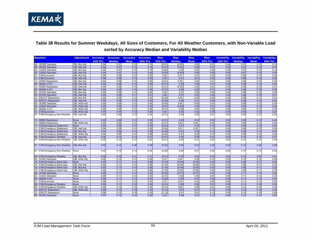
PJM Load Management Task Force April 20, 2011 93
Table 38 Results for Summer Weekdays, All Sizes of Customers, For All Weather Customers, with Non-Variable Load
sorted by Accuracy Median and Variability Median
Accuracy Accuracy Accuracy Accuracy Bias Bias Bias Bias Variability Variability Variability Variability
10th Pct Median Mean 90th Pct 10th Pct Median Mean 90th Pct 10th Pct Median Mean 90th Pct06 - ISONE Standard CBL Mul Adj 0.04 0.07 0.10 0.19 (0.01) (0.00) 0.00 0.01 0.04 0.07 0.10 0.1906 - ISONE Standard CBL Add Adj 0.04 0.07 0.10 0.19 (0.01) (0.00) 0.00 0.01 0.04 0.07 0.10 0.1902 - CAISO Standard CBL Mul Adj 0.04 0.07 0.10 0.19 (0.00) 0.00 0.00 0.00 0.04 0.07 0.10 0.1902 - CAISO Standard CBL Add Adj 0.04 0.07 0.10 0.20 (0.00) (0.00) 0.00 0.00 0.04 0.07 0.10 0.2001 - PJM Economic CBL Mul Adj 0.04 0.08 0.10 0.20 0.00 0.01 0.01 0.02 0.04 0.08 0.10 0.2001 - PJM Economic CBL Add Adj 0.04 0.08 0.10 0.20 0.00 0.01 0.01 0.02 0.04 0.08 0.10 0.2013 - KEMA Regression CBL Mul Adj 0.04 0.08 0.10 0.20 (0.01) 0.00 0.00 0.01 0.04 0.08 0.10 0.2004 - Middle 4 of 6 CBL Add Adj 0.04 0.08 0.10 0.20 (0.01) 0.00 0.00 0.01 0.04 0.08 0.10 0.2013 - KEMA Regression CBL Add Adj 0.04 0.08 0.10 0.21 (0.01) (0.00) 0.00 0.01 0.04 0.08 0.10 0.2104 - Middle 4 of 6 CBL Mul Adj 0.04 0.08 0.10 0.20 (0.01) 0.00 0.00 0.01 0.04 0.08 0.10 0.2005 - NYISO Standard CBL Mul Adj 0.04 0.08 0.10 0.20 0.00 0.01 0.02 0.05 0.04 0.08 0.10 0.2005 - NYISO Standard CBL Add Adj 0.04 0.08 0.11 0.21 0.00 0.01 0.02 0.04 0.04 0.08 0.10 0.2112 - ERCOT Regression CBL Mul Adj 0.04 0.08 0.12 0.23 (0.04) 0.00 0.00 0.04 0.04 0.08 0.11 0.2112 - ERCOT Regression CBL Add Adj 0.04 0.08 0.13 0.24 (0.04) 0.00 0.01 0.04 0.04 0.08 0.12 0.2206 - ISONE Standard CBL WSA Adj 0.05 0.09 0.12 0.24 (0.02) 0.00 0.00 0.01 0.05 0.09 0.12 0.2402 - CAISO Standard CBL WSA Adj 0.05 0.09 0.12 0.24 (0.01) (0.00) 0.00 0.01 0.05 0.09 0.12 0.2404 - Middle 4 of 6 CBL WSA Adj 0.05 0.09 0.12 0.25 (0.01) 0.00 0.00 0.02 0.05 0.09 0.12 0.2501 - PJM Economic CBL WSA Adj 0.05 0.09 0.12 0.25 0.00 0.02 0.02 0.05 0.05 0.09 0.12 0.2407 - PJM Emergency Non-Weather CBL Add Adj 0.05 0.09 0.12 0.24 (0.01) 0.00 0.00 0.01 0.05 0.09 0.12 0.24
13 - KEMA Regression None 0.05 0.09 0.12 0.25 (0.01) 0.00 0.00 0.02 0.05 0.09 0.12 0.2413 - KEMA Regression CBL WSA Adj 0.05 0.09 0.12 0.25 (0.01) 0.00 0.00 0.02 0.05 0.09 0.12 0.2411 - PJM Emergency Settlement None 0.04 0.09 0.14 0.29 (0.04) 0.01 0.05 0.15 0.04 0.08 0.12 0.2411 - PJM Emergency Settlement CBL Add Adj 0.04 0.09 0.14 0.29 (0.04) 0.01 0.05 0.15 0.04 0.08 0.12 0.2411 - PJM Emergency Settlement CBL Mul Adj 0.04 0.09 0.14 0.29 (0.04) 0.01 0.05 0.15 0.04 0.08 0.12 0.2411 - PJM Emergency Settlement CBL WSA Adj 0.04 0.09 0.14 0.29 (0.04) 0.01 0.05 0.15 0.04 0.08 0.12 0.2408 - PJM Emergency Weather CBL Add Adj 0.04 0.10 0.13 0.27 (0.01) 0.00 0.00 0.01 0.04 0.10 0.13 0.2707 - PJM Emergency Non-Weather CBL WSA Adj 0.05 0.10 0.13 0.24 (0.01) 0.00 0.01 0.02 0.05 0.10 0.13 0.24
07 - PJM Emergency Non-Weather CBL Mul Adj 0.05 0.10 0.36 0.28 (0.00) 0.00 0.03 0.03 0.05 0.10 0.36 0.28
07 - PJM Emergency Non-Weather None 0.05 0.10 0.13 0.24 (0.00) 0.00 0.01 0.02 0.05 0.10 0.13 0.24
08 - PJM Emergency Weather CBL Mul Adj 0.04 0.10 0.31 0.31 (0.01) 0.00 0.02 0.02 0.04 0.10 0.30 0.3105 - NYISO Standard CBL WSA Adj 0.05 0.10 0.14 0.28 0.01 0.04 0.05 0.12 0.05 0.10 0.13 0.2610 - PJM Emergency Same Day None 0.05 0.11 0.14 0.28 (0.16) (0.04) (0.05) 0.03 0.04 0.08 0.11 0.2210 - PJM Emergency Same Day CBL Add Adj 0.05 0.11 0.14 0.28 (0.16) (0.04) (0.05) 0.03 0.04 0.08 0.11 0.2210 - PJM Emergency Same Day CBL Mul Adj 0.05 0.11 0.14 0.28 (0.16) (0.04) (0.05) 0.03 0.04 0.08 0.11 0.2210 - PJM Emergency Same Day CBL WSA Adj 0.05 0.11 0.14 0.28 (0.16) (0.04) (0.05) 0.03 0.04 0.08 0.11 0.2206 - ISONE Standard None 0.06 0.11 0.13 0.23 (0.02) (0.01) (0.01) 0.01 0.06 0.11 0.13 0.2302 - CAISO Standard None 0.06 0.11 0.13 0.24 (0.01) 0.00 0.00 0.01 0.06 0.11 0.13 0.2404 - Middle 4 of 6 None 0.06 0.11 0.13 0.24 (0.00) 0.00 0.01 0.02 0.06 0.11 0.13 0.2401 - PJM Economic None 0.06 0.11 0.13 0.23 0.01 0.02 0.03 0.05 0.06 0.11 0.13 0.2308 - PJM Emergency Weather None 0.05 0.11 0.16 0.34 (0.01) 0.00 0.00 0.01 0.05 0.11 0.16 0.3408 - PJM Emergency Weather CBL WSA Adj 0.06 0.12 0.16 0.34 (0.01) 0.00 0.00 0.01 0.06 0.12 0.16 0.3412 - ERCOT Regression CBL WSA Adj 0.06 0.13 0.18 0.33 (0.13) 0.01 0.01 0.12 0.05 0.10 0.15 0.2812 - ERCOT Regression None 0.06 0.13 0.18 0.33 (0.13) 0.01 0.01 0.12 0.05 0.10 0.15 0.2805 - NYISO Standard None 0.07 0.13 0.16 0.28 0.03 0.06 0.07 0.12 0.06 0.12 0.14 0.25
Baseline Adjustment
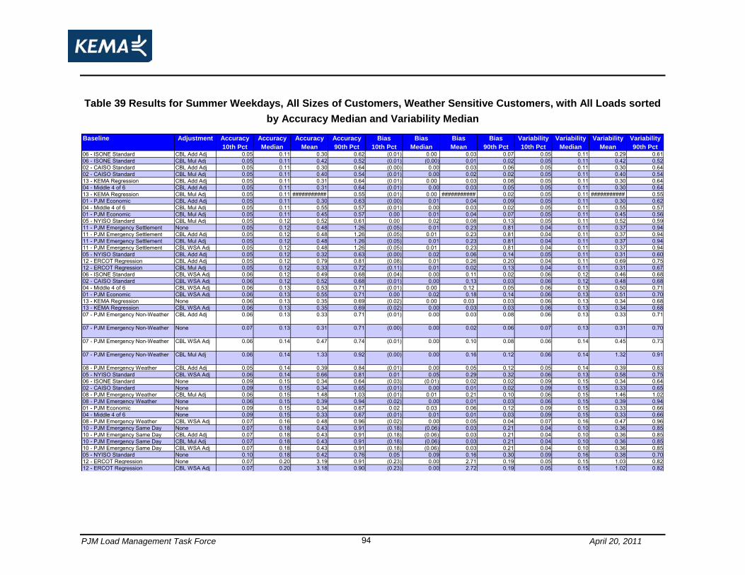
PJM Load Management Task Force April 20, 2011 94
Table 39 Results for Summer Weekdays, All Sizes of Customers, Weather Sensitive Customers, with All Loads sorted
by Accuracy Median and Variability Median
Accuracy Accuracy Accuracy Accuracy Bias Bias Bias Bias Variability Variability Variability Variability
10th Pct Median Mean 90th Pct 10th Pct Median Mean 90th Pct 10th Pct Median Mean 90th Pct06 - ISONE Standard CBL Add Adj 0.05 0.11 0.30 0.62 (0.01) 0.00 0.03 0.07 0.05 0.11 0.29 0.6106 - ISONE Standard CBL Mul Adj 0.05 0.11 0.42 0.52 (0.01) (0.00) 0.01 0.02 0.05 0.11 0.42 0.5202 - CAISO Standard CBL Add Adj 0.05 0.11 0.30 0.64 (0.00) 0.00 0.03 0.06 0.05 0.11 0.30 0.6402 - CAISO Standard CBL Mul Adj 0.05 0.11 0.40 0.54 (0.01) 0.00 0.02 0.02 0.05 0.11 0.40 0.5413 - KEMA Regression CBL Add Adj 0.05 0.11 0.31 0.64 (0.01) 0.00 0.03 0.08 0.05 0.11 0.30 0.6404 - Middle 4 of 6 CBL Add Adj 0.05 0.11 0.31 0.64 (0.01) 0.00 0.03 0.05 0.05 0.11 0.30 0.6413 - KEMA Regression CBL Mul Adj 0.05 0.11 ########### 0.55 (0.01) 0.00 ########### 0.02 0.05 0.11 ########### 0.5501 - PJM Economic CBL Add Adj 0.05 0.11 0.30 0.63 (0.00) 0.01 0.04 0.09 0.05 0.11 0.30 0.6204 - Middle 4 of 6 CBL Mul Adj 0.05 0.11 0.55 0.57 (0.01) 0.00 0.03 0.02 0.05 0.11 0.55 0.5701 - PJM Economic CBL Mul Adj 0.05 0.11 0.45 0.57 0.00 0.01 0.04 0.07 0.05 0.11 0.45 0.5605 - NYISO Standard CBL Mul Adj 0.05 0.12 0.52 0.61 0.00 0.02 0.08 0.13 0.05 0.11 0.52 0.5911 - PJM Emergency Settlement None 0.05 0.12 0.48 1.26 (0.05) 0.01 0.23 0.81 0.04 0.11 0.37 0.9411 - PJM Emergency Settlement CBL Add Adj 0.05 0.12 0.48 1.26 (0.05) 0.01 0.23 0.81 0.04 0.11 0.37 0.9411 - PJM Emergency Settlement CBL Mul Adj 0.05 0.12 0.48 1.26 (0.05) 0.01 0.23 0.81 0.04 0.11 0.37 0.9411 - PJM Emergency Settlement CBL WSA Adj 0.05 0.12 0.48 1.26 (0.05) 0.01 0.23 0.81 0.04 0.11 0.37 0.9405 - NYISO Standard CBL Add Adj 0.05 0.12 0.32 0.63 (0.00) 0.02 0.06 0.14 0.05 0.11 0.31 0.6012 - ERCOT Regression CBL Add Adj 0.05 0.12 0.79 0.81 (0.08) 0.01 0.26 0.20 0.04 0.11 0.69 0.7512 - ERCOT Regression CBL Mul Adj 0.05 0.12 0.33 0.72 (0.11) 0.01 0.02 0.13 0.04 0.11 0.31 0.6706 - ISONE Standard CBL WSA Adj 0.06 0.12 0.49 0.68 (0.04) 0.00 0.11 0.02 0.06 0.12 0.46 0.6802 - CAISO Standard CBL WSA Adj 0.06 0.12 0.52 0.68 (0.01) 0.00 0.13 0.03 0.06 0.12 0.48 0.6804 - Middle 4 of 6 CBL WSA Adj 0.06 0.13 0.53 0.71 (0.01) 0.00 0.12 0.05 0.06 0.13 0.50 0.7101 - PJM Economic CBL WSA Adj 0.06 0.13 0.55 0.71 0.00 0.02 0.18 0.14 0.06 0.13 0.51 0.7013 - KEMA Regression None 0.06 0.13 0.35 0.69 (0.02) 0.00 0.03 0.03 0.06 0.13 0.34 0.6813 - KEMA Regression CBL WSA Adj 0.06 0.13 0.35 0.69 (0.02) 0.00 0.03 0.03 0.06 0.13 0.34 0.6807 - PJM Emergency Non-Weather CBL Add Adj 0.06 0.13 0.33 0.71 (0.01) 0.00 0.03 0.08 0.06 0.13 0.33 0.71
07 - PJM Emergency Non-Weather None 0.07 0.13 0.31 0.71 (0.00) 0.00 0.02 0.06 0.07 0.13 0.31 0.70
07 - PJM Emergency Non-Weather CBL WSA Adj 0.06 0.14 0.47 0.74 (0.01) 0.00 0.10 0.08 0.06 0.14 0.45 0.73
07 - PJM Emergency Non-Weather CBL Mul Adj 0.06 0.14 1.33 0.92 (0.00) 0.00 0.16 0.12 0.06 0.14 1.32 0.91
08 - PJM Emergency Weather CBL Add Adj 0.05 0.14 0.39 0.84 (0.01) 0.00 0.05 0.12 0.05 0.14 0.39 0.8305 - NYISO Standard CBL WSA Adj 0.06 0.14 0.66 0.81 0.01 0.05 0.29 0.32 0.06 0.13 0.58 0.7506 - ISONE Standard None 0.09 0.15 0.34 0.64 (0.03) (0.01) 0.02 0.02 0.09 0.15 0.34 0.6402 - CAISO Standard None 0.09 0.15 0.34 0.65 (0.01) 0.00 0.01 0.02 0.09 0.15 0.33 0.6508 - PJM Emergency Weather CBL Mul Adj 0.06 0.15 1.48 1.03 (0.01) 0.01 0.21 0.10 0.06 0.15 1.46 1.0208 - PJM Emergency Weather None 0.06 0.15 0.39 0.94 (0.02) 0.00 0.01 0.03 0.06 0.15 0.39 0.9401 - PJM Economic None 0.09 0.15 0.34 0.67 0.02 0.03 0.06 0.12 0.09 0.15 0.33 0.6604 - Middle 4 of 6 None 0.09 0.15 0.33 0.67 (0.01) 0.01 0.01 0.03 0.09 0.15 0.33 0.6608 - PJM Emergency Weather CBL WSA Adj 0.07 0.16 0.48 0.96 (0.02) 0.00 0.05 0.04 0.07 0.16 0.47 0.9610 - PJM Emergency Same Day None 0.07 0.18 0.43 0.91 (0.18) (0.06) 0.03 0.21 0.04 0.10 0.36 0.8510 - PJM Emergency Same Day CBL Add Adj 0.07 0.18 0.43 0.91 (0.18) (0.06) 0.03 0.21 0.04 0.10 0.36 0.8510 - PJM Emergency Same Day CBL Mul Adj 0.07 0.18 0.43 0.91 (0.18) (0.06) 0.03 0.21 0.04 0.10 0.36 0.8510 - PJM Emergency Same Day CBL WSA Adj 0.07 0.18 0.43 0.91 (0.18) (0.06) 0.03 0.21 0.04 0.10 0.36 0.8505 - NYISO Standard None 0.10 0.18 0.42 0.76 0.05 0.09 0.16 0.30 0.09 0.16 0.38 0.7012 - ERCOT Regression None 0.07 0.20 3.19 0.91 (0.23) 0.00 2.71 0.19 0.05 0.15 1.03 0.8212 - ERCOT Regression CBL WSA Adj 0.07 0.20 3.18 0.90 (0.23) 0.00 2.72 0.19 0.05 0.15 1.02 0.82
Baseline Adjustment

PJM Load Management Task Force April 20, 2011 95
Table 40 Results for Summer Weekdays, All Sizes of Customers, Non-Weather Sensitive Customers, with All Loads
sorted by Accuracy Median and Variability Median
Accuracy Accuracy Accuracy Accuracy Bias Bias Bias Bias Variability Variability Variability Variability
10th Pct Median Mean 90th Pct 10th Pct Median Mean 90th Pct 10th Pct Median Mean 90th Pct06 - ISONE Standard CBL Mul Adj 0.03 0.08 0.13 0.27 (0.01) (0.00) 0.00 0.01 0.03 0.08 0.13 0.2702 - CAISO Standard CBL Mul Adj 0.03 0.08 0.14 0.27 (0.00) 0.00 0.00 0.01 0.03 0.08 0.14 0.2706 - ISONE Standard CBL Add Adj 0.03 0.09 0.13 0.27 (0.01) (0.00) 0.00 0.01 0.03 0.08 0.13 0.2702 - CAISO Standard CBL Add Adj 0.03 0.09 0.14 0.28 (0.00) (0.00) 0.00 0.01 0.03 0.09 0.14 0.2801 - PJM Economic CBL Mul Adj 0.04 0.09 0.16 0.29 0.00 0.01 0.02 0.03 0.04 0.09 0.16 0.2904 - Middle 4 of 6 CBL Mul Adj 0.04 0.09 0.16 0.29 (0.01) 0.00 0.01 0.02 0.04 0.09 0.16 0.2905 - NYISO Standard CBL Mul Adj 0.04 0.09 0.16 0.30 0.00 0.01 0.03 0.06 0.04 0.09 0.16 0.2901 - PJM Economic CBL Add Adj 0.04 0.09 0.14 0.29 (0.00) 0.01 0.01 0.03 0.04 0.09 0.14 0.2904 - Middle 4 of 6 CBL Add Adj 0.04 0.09 0.14 0.29 (0.01) 0.00 0.00 0.01 0.04 0.09 0.14 0.2913 - KEMA Regression CBL Mul Adj 0.04 0.09 0.16 0.28 (0.01) 0.00 0.00 0.01 0.03 0.09 0.16 0.2805 - NYISO Standard CBL Add Adj 0.04 0.09 0.15 0.30 (0.00) 0.01 0.03 0.06 0.04 0.09 0.14 0.2913 - KEMA Regression CBL Add Adj 0.04 0.09 0.14 0.28 (0.01) (0.00) 0.00 0.01 0.04 0.09 0.14 0.2812 - ERCOT Regression CBL Mul Adj 0.04 0.10 26.24 0.33 (0.05) 0.00 2.37 0.05 0.03 0.09 26.15 0.3012 - ERCOT Regression CBL Add Adj 0.04 0.10 0.19 0.32 (0.05) 0.00 0.01 0.05 0.03 0.10 0.18 0.3106 - ISONE Standard CBL WSA Adj 0.05 0.10 0.16 0.34 (0.02) (0.00) 0.00 0.01 0.05 0.10 0.16 0.3402 - CAISO Standard CBL WSA Adj 0.05 0.11 0.16 0.34 (0.01) (0.00) 0.00 0.01 0.05 0.11 0.16 0.3404 - Middle 4 of 6 CBL WSA Adj 0.05 0.11 0.17 0.35 (0.01) 0.00 0.00 0.02 0.05 0.11 0.17 0.3501 - PJM Economic CBL WSA Adj 0.05 0.11 0.17 0.35 0.01 0.02 0.03 0.07 0.05 0.11 0.16 0.3407 - PJM Emergency Non-Weather CBL Add Adj 0.04 0.11 0.17 0.34 (0.01) 0.00 0.01 0.02 0.04 0.11 0.17 0.34
13 - KEMA Regression None 0.05 0.11 0.17 0.36 (0.02) 0.00 0.00 0.02 0.05 0.11 0.17 0.3613 - KEMA Regression CBL WSA Adj 0.05 0.11 0.17 0.36 (0.02) 0.00 0.00 0.02 0.05 0.11 0.17 0.3607 - PJM Emergency Non-Weather None 0.05 0.11 0.18 0.35 (0.01) 0.01 0.01 0.03 0.05 0.11 0.17 0.35
07 - PJM Emergency Non-Weather CBL WSA Adj 0.05 0.11 0.17 0.35 (0.01) 0.00 0.01 0.03 0.05 0.11 0.17 0.35
07 - PJM Emergency Non-Weather CBL Mul Adj 0.04 0.11 0.85 0.46 (0.00) 0.00 0.12 0.05 0.04 0.11 0.84 0.46
06 - ISONE Standard None 0.06 0.11 0.17 0.34 (0.02) (0.00) 0.00 0.01 0.06 0.11 0.17 0.3402 - CAISO Standard None 0.06 0.11 0.17 0.34 (0.01) (0.00) 0.00 0.01 0.06 0.11 0.17 0.3410 - PJM Emergency Same Day None 0.05 0.11 0.16 0.32 (0.14) (0.02) (0.03) 0.04 0.04 0.09 0.14 0.2910 - PJM Emergency Same Day CBL Add Adj 0.05 0.11 0.16 0.32 (0.14) (0.02) (0.03) 0.04 0.04 0.09 0.14 0.2910 - PJM Emergency Same Day CBL Mul Adj 0.05 0.11 0.16 0.32 (0.14) (0.02) (0.03) 0.04 0.04 0.09 0.14 0.2910 - PJM Emergency Same Day CBL WSA Adj 0.05 0.11 0.16 0.32 (0.14) (0.02) (0.03) 0.04 0.04 0.09 0.14 0.2904 - Middle 4 of 6 None 0.06 0.11 0.17 0.35 (0.01) 0.00 0.01 0.02 0.06 0.11 0.17 0.3501 - PJM Economic None 0.06 0.11 0.17 0.35 0.01 0.02 0.03 0.07 0.06 0.11 0.17 0.3408 - PJM Emergency Weather CBL Add Adj 0.04 0.12 0.18 0.37 (0.01) 0.00 0.01 0.02 0.04 0.12 0.18 0.3711 - PJM Emergency Settlement None 0.04 0.12 0.18 0.38 (0.02) 0.03 0.05 0.16 0.04 0.10 0.16 0.3211 - PJM Emergency Settlement CBL Add Adj 0.04 0.12 0.18 0.38 (0.02) 0.03 0.05 0.16 0.04 0.10 0.16 0.3211 - PJM Emergency Settlement CBL Mul Adj 0.04 0.12 0.18 0.38 (0.02) 0.03 0.05 0.16 0.04 0.10 0.16 0.3211 - PJM Emergency Settlement CBL WSA Adj 0.04 0.12 0.18 0.38 (0.02) 0.03 0.05 0.16 0.04 0.10 0.16 0.3205 - NYISO Standard CBL WSA Adj 0.05 0.12 0.19 0.40 0.02 0.05 0.08 0.17 0.05 0.11 0.17 0.3608 - PJM Emergency Weather CBL Mul Adj 0.04 0.12 0.83 0.47 (0.01) 0.00 0.10 0.04 0.04 0.12 0.82 0.4605 - NYISO Standard None 0.07 0.13 0.20 0.40 0.03 0.06 0.08 0.17 0.06 0.12 0.18 0.3608 - PJM Emergency Weather None 0.05 0.14 0.22 0.47 (0.01) 0.00 0.00 0.02 0.05 0.14 0.22 0.4708 - PJM Emergency Weather CBL WSA Adj 0.06 0.14 0.23 0.47 (0.01) 0.00 0.00 0.02 0.06 0.14 0.22 0.4712 - ERCOT Regression None 0.06 0.16 0.30 0.46 (0.17) 0.00 0.00 0.14 0.05 0.13 0.25 0.3812 - ERCOT Regression CBL WSA Adj 0.06 0.16 0.27 0.45 (0.16) 0.00 0.02 0.14 0.05 0.13 0.22 0.38
Baseline Adjustment

PJM Load Management Task Force April 20, 2011 96
Results for Weekdays during Winter for Extreme Conditions
Table 41 Results for Extreme Winter Weekdays, All Sizes of Customers, For All Weather Customers, with All Loads
sorted by Accuracy Median and Variability Median
Accuracy Accuracy Accuracy Accuracy Bias Bias Bias Bias Variability Variability Variability Variability
10th Pct Median Mean 90th Pct 10th Pct Median Mean 90th Pct 10th Pct Median Mean 90th Pct01 - PJM Economic CBL Add Adj 0.03 0.10 0.23 0.41 (0.02) 0.01 0.05 0.10 0.02 0.10 0.22 0.4006 - ISONE Standard CBL Add Adj 0.02 0.10 0.25 0.42 (0.04) 0.00 0.06 0.08 0.02 0.10 0.23 0.4002 - CAISO Standard CBL Add Adj 0.02 0.10 0.23 0.40 (0.04) 0.00 0.03 0.07 0.02 0.10 0.22 0.3904 - Middle 4 of 6 CBL Add Adj 0.03 0.10 0.22 0.41 (0.04) 0.00 0.02 0.06 0.02 0.10 0.21 0.4013 - KEMA Regression CBL Add Adj 0.03 0.11 0.24 0.41 (0.03) 0.00 0.04 0.06 0.02 0.10 0.23 0.4107 - PJM Emergency Non-Weather CBL Add Adj 0.03 0.11 0.21 0.43 (0.03) 0.00 0.02 0.08 0.03 0.11 0.20 0.43
05 - NYISO Standard CBL Add Adj 0.03 0.11 0.31 0.46 (0.01) 0.02 0.12 0.20 0.03 0.11 0.28 0.4107 - PJM Emergency Non-Weather None 0.03 0.12 0.22 0.46 (0.03) 0.00 0.03 0.09 0.03 0.11 0.22 0.45
02 - CAISO Standard CBL Mul Adj 0.03 0.12 0.25 0.48 (0.03) 0.01 0.04 0.12 0.03 0.11 0.24 0.4701 - PJM Economic CBL Mul Adj 0.03 0.12 0.26 0.51 (0.02) 0.01 0.05 0.14 0.03 0.11 0.25 0.4907 - PJM Emergency Non-Weather CBL WSA Adj 0.03 0.12 0.26 0.50 (0.03) 0.00 0.03 0.09 0.03 0.12 0.25 0.49
06 - ISONE Standard CBL Mul Adj 0.03 0.12 0.27 0.50 (0.04) 0.01 0.06 0.14 0.02 0.11 0.25 0.4804 - Middle 4 of 6 CBL Mul Adj 0.03 0.12 0.25 0.51 (0.03) 0.01 0.04 0.12 0.03 0.12 0.24 0.5013 - KEMA Regression CBL Mul Adj 0.03 0.12 0.26 0.51 (0.03) 0.01 0.04 0.11 0.03 0.12 0.25 0.5001 - PJM Economic CBL WSA Adj 0.03 0.13 0.27 0.52 (0.03) 0.01 0.04 0.12 0.03 0.12 0.25 0.4807 - PJM Emergency Non-Weather CBL Mul Adj 0.03 0.13 0.38 0.65 (0.02) 0.01 0.08 0.14 0.03 0.12 0.37 0.64
01 - PJM Economic None 0.03 0.13 0.28 0.49 (0.04) 0.01 0.07 0.13 0.03 0.12 0.26 0.4704 - Middle 4 of 6 CBL WSA Adj 0.03 0.13 0.25 0.52 (0.07) (0.00) 0.00 0.06 0.03 0.12 0.24 0.4905 - NYISO Standard CBL Mul Adj 0.03 0.13 0.34 0.58 (0.02) 0.02 0.12 0.23 0.03 0.12 0.31 0.5206 - ISONE Standard CBL WSA Adj 0.03 0.13 0.26 0.51 (0.07) (0.00) 0.00 0.06 0.03 0.12 0.24 0.4602 - CAISO Standard CBL WSA Adj 0.03 0.13 0.25 0.52 (0.07) (0.00) 0.00 0.06 0.03 0.13 0.24 0.4704 - Middle 4 of 6 None 0.03 0.13 0.25 0.49 (0.07) (0.00) 0.02 0.07 0.03 0.12 0.24 0.4712 - ERCOT Regression CBL Add Adj 0.03 0.14 0.42 0.54 (0.13) 0.01 0.15 0.15 0.03 0.11 0.31 0.4410 - PJM Emergency Same Day None 0.04 0.14 0.21 0.42 (0.25) (0.04) (0.06) 0.05 0.03 0.10 0.16 0.3210 - PJM Emergency Same Day CBL Add Adj 0.04 0.14 0.21 0.42 (0.25) (0.04) (0.06) 0.05 0.03 0.10 0.16 0.3210 - PJM Emergency Same Day CBL Mul Adj 0.04 0.14 0.21 0.42 (0.25) (0.04) (0.06) 0.05 0.03 0.10 0.16 0.3210 - PJM Emergency Same Day CBL WSA Adj 0.04 0.14 0.21 0.42 (0.25) (0.04) (0.06) 0.05 0.03 0.10 0.16 0.3208 - PJM Emergency Weather CBL Add Adj 0.03 0.14 0.24 0.50 (0.05) (0.00) 0.01 0.06 0.03 0.14 0.24 0.5013 - KEMA Regression None 0.03 0.14 0.34 0.49 (0.07) (0.00) 0.05 0.07 0.03 0.13 0.32 0.4813 - KEMA Regression CBL WSA Adj 0.03 0.14 0.34 0.49 (0.07) (0.00) 0.05 0.07 0.03 0.13 0.32 0.4802 - CAISO Standard None 0.03 0.14 0.28 0.48 (0.08) (0.00) 0.03 0.07 0.03 0.12 0.26 0.4606 - ISONE Standard None 0.03 0.14 0.33 0.50 (0.10) (0.00) 0.08 0.09 0.03 0.12 0.29 0.4705 - NYISO Standard CBL WSA Adj 0.03 0.15 0.32 0.61 (0.01) 0.04 0.12 0.25 0.03 0.13 0.28 0.5005 - NYISO Standard None 0.04 0.15 0.38 0.59 (0.02) 0.05 0.18 0.28 0.03 0.13 0.33 0.4912 - ERCOT Regression CBL Mul Adj 0.03 0.15 0.38 0.69 (0.15) 0.01 0.07 0.21 0.03 0.13 0.33 0.5708 - PJM Emergency Weather CBL Mul Adj 0.03 0.16 0.46 0.72 (0.05) 0.00 0.08 0.12 0.03 0.16 0.45 0.7008 - PJM Emergency Weather None 0.04 0.17 0.29 0.61 (0.06) (0.00) 0.01 0.08 0.04 0.17 0.29 0.6008 - PJM Emergency Weather CBL WSA Adj 0.04 0.17 0.30 0.64 (0.06) (0.00) 0.01 0.07 0.04 0.17 0.30 0.6211 - PJM Emergency Settlement None 0.05 0.18 0.27 0.59 (0.44) (0.11) (0.16) 0.01 0.03 0.11 0.18 0.3811 - PJM Emergency Settlement CBL Add Adj 0.05 0.18 0.27 0.59 (0.44) (0.11) (0.16) 0.01 0.03 0.11 0.18 0.3811 - PJM Emergency Settlement CBL Mul Adj 0.05 0.18 0.27 0.59 (0.44) (0.11) (0.16) 0.01 0.03 0.11 0.18 0.3811 - PJM Emergency Settlement CBL WSA Adj 0.05 0.18 0.27 0.59 (0.44) (0.11) (0.16) 0.01 0.03 0.11 0.18 0.3812 - ERCOT Regression CBL WSA Adj 0.05 0.19 0.62 0.78 (0.18) 0.01 0.28 0.27 0.03 0.14 0.39 0.5212 - ERCOT Regression None 0.05 0.19 0.68 0.80 (0.18) 0.01 0.23 0.26 0.03 0.14 0.44 0.55
Baseline Adjustment
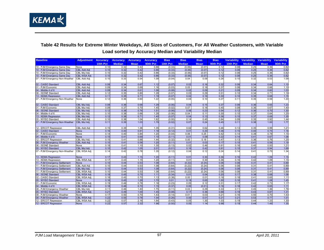
PJM Load Management Task Force April 20, 2011 97
Table 42 Results for Extreme Winter Weekdays, All Sizes of Customers, For All Weather Customers, with Variable
Load sorted by Accuracy Median and Variability Median
Accuracy Accuracy Accuracy Accuracy Bias Bias Bias Bias Variability Variability Variability Variability
10th Pct Median Mean 90th Pct 10th Pct Median Mean 90th Pct 10th Pct Median Mean 90th Pct10 - PJM Emergency Same Day None 0.10 0.32 0.42 0.86 (0.33) (0.06) (0.07) 0.12 0.08 0.25 0.36 0.8210 - PJM Emergency Same Day CBL Add Adj 0.10 0.32 0.42 0.86 (0.33) (0.06) (0.07) 0.12 0.08 0.25 0.36 0.8210 - PJM Emergency Same Day CBL Mul Adj 0.10 0.32 0.42 0.86 (0.33) (0.06) (0.07) 0.12 0.08 0.25 0.36 0.8210 - PJM Emergency Same Day CBL WSA Adj 0.10 0.32 0.42 0.86 (0.33) (0.06) (0.07) 0.12 0.08 0.25 0.36 0.8207 - PJM Emergency Non-Weather CBL Add Adj 0.10 0.33 0.54 1.09 (0.04) 0.04 0.09 0.26 0.10 0.32 0.53 1.09
02 - CAISO Standard CBL Add Adj 0.08 0.34 0.67 1.12 (0.07) 0.02 0.16 0.32 0.08 0.34 0.64 1.1001 - PJM Economic CBL Add Adj 0.09 0.34 0.69 1.16 (0.03) 0.05 0.18 0.37 0.08 0.34 0.66 1.1004 - Middle 4 of 6 CBL Add Adj 0.09 0.34 0.61 1.06 (0.08) 0.02 0.09 0.21 0.09 0.34 0.60 1.0306 - ISONE Standard CBL Add Adj 0.12 0.35 0.80 1.28 (0.07) 0.03 0.29 0.51 0.10 0.34 0.71 1.1913 - KEMA Regression CBL Add Adj 0.11 0.35 0.71 1.19 (0.07) 0.02 0.16 0.30 0.10 0.35 0.68 1.1507 - PJM Emergency Non-Weather None 0.12 0.36 0.60 1.22 (0.05) 0.04 0.10 0.27 0.11 0.35 0.59 1.20
02 - CAISO Standard CBL Mul Adj 0.08 0.36 0.68 1.29 (0.06) 0.04 0.15 0.37 0.08 0.36 0.65 1.2301 - PJM Economic CBL Mul Adj 0.09 0.37 0.70 1.45 (0.02) 0.07 0.18 0.45 0.09 0.36 0.67 1.4006 - ISONE Standard CBL Mul Adj 0.12 0.38 0.76 1.51 (0.06) 0.06 0.23 0.54 0.12 0.36 0.70 1.3004 - Middle 4 of 6 CBL Mul Adj 0.10 0.38 0.66 1.28 (0.06) 0.04 0.11 0.30 0.10 0.37 0.64 1.2513 - KEMA Regression CBL Mul Adj 0.12 0.38 0.71 1.40 (0.07) 0.04 0.13 0.36 0.10 0.37 0.69 1.3505 - NYISO Standard CBL Add Adj 0.10 0.38 1.04 1.62 (0.00) 0.14 0.45 0.84 0.09 0.35 0.92 1.4407 - PJM Emergency Non-Weather CBL Mul Adj 0.11 0.39 1.03 1.79 (0.02) 0.07 0.24 0.45 0.11 0.38 1.00 1.77
12 - ERCOT Regression CBL Add Adj 0.15 0.39 1.36 1.35 (0.31) 0.02 0.62 0.46 0.13 0.35 0.99 1.2102 - CAISO Standard None 0.16 0.40 0.81 1.18 (0.12) 0.01 0.20 0.36 0.15 0.40 0.75 1.1601 - PJM Economic None 0.14 0.40 0.84 1.20 (0.04) 0.06 0.25 0.42 0.14 0.39 0.78 1.1504 - Middle 4 of 6 None 0.15 0.41 0.69 1.10 (0.11) 0.01 0.09 0.22 0.14 0.41 0.67 1.0812 - ERCOT Regression CBL Mul Adj 0.15 0.41 0.88 1.44 (0.32) 0.00 0.18 0.47 0.13 0.36 0.76 1.2508 - PJM Emergency Weather CBL Add Adj 0.10 0.41 0.58 1.20 (0.11) 0.01 0.03 0.17 0.10 0.41 0.58 1.1906 - ISONE Standard None 0.18 0.41 1.10 1.30 (0.13) 0.02 0.46 0.61 0.16 0.40 0.93 1.2105 - NYISO Standard CBL Mul Adj 0.10 0.42 1.05 2.01 (0.01) 0.16 0.42 0.91 0.10 0.37 0.94 1.6907 - PJM Emergency Non-Weather CBL WSA Adj 0.14 0.42 0.78 1.35 (0.12) 0.04 0.12 0.24 0.14 0.41 0.75 1.34
13 - KEMA Regression None 0.17 0.43 1.15 1.20 (0.11) 0.01 0.30 0.36 0.16 0.42 1.09 1.1513 - KEMA Regression CBL WSA Adj 0.17 0.43 1.15 1.20 (0.11) 0.01 0.30 0.36 0.16 0.42 1.09 1.1511 - PJM Emergency Settlement None 0.10 0.44 0.53 1.08 (0.64) (0.22) (0.24) 0.06 0.08 0.31 0.41 0.8911 - PJM Emergency Settlement CBL Add Adj 0.10 0.44 0.53 1.08 (0.64) (0.22) (0.24) 0.06 0.08 0.31 0.41 0.8911 - PJM Emergency Settlement CBL Mul Adj 0.10 0.44 0.53 1.08 (0.64) (0.22) (0.24) 0.06 0.08 0.31 0.41 0.8911 - PJM Emergency Settlement CBL WSA Adj 0.10 0.44 0.53 1.08 (0.64) (0.22) (0.24) 0.06 0.08 0.31 0.41 0.8906 - ISONE Standard CBL WSA Adj 0.18 0.45 0.75 1.11 (0.34) 0.01 0.04 0.20 0.17 0.38 0.68 1.0802 - CAISO Standard CBL WSA Adj 0.18 0.45 0.70 1.13 (0.38) 0.00 0.01 0.18 0.18 0.41 0.65 1.1105 - NYISO Standard None 0.16 0.45 1.29 1.70 0.01 0.19 0.65 1.00 0.16 0.41 1.08 1.4501 - PJM Economic CBL WSA Adj 0.19 0.46 0.78 1.18 (0.23) 0.05 0.12 0.31 0.17 0.42 0.73 1.1704 - Middle 4 of 6 CBL WSA Adj 0.18 0.46 0.70 1.15 (0.37) 0.00 (0.01) 0.16 0.18 0.42 0.65 1.1108 - PJM Emergency Weather CBL Mul Adj 0.11 0.46 1.40 1.75 (0.11) 0.03 0.29 0.33 0.11 0.45 1.36 1.7605 - NYISO Standard CBL WSA Adj 0.21 0.49 1.00 1.45 (0.08) 0.17 0.36 0.68 0.19 0.43 0.87 1.3108 - PJM Emergency Weather None 0.17 0.50 0.70 1.43 (0.14) 0.01 0.03 0.21 0.16 0.50 0.70 1.4308 - PJM Emergency Weather CBL WSA Adj 0.22 0.55 0.78 1.54 (0.26) 0.00 0.01 0.21 0.21 0.53 0.77 1.5112 - ERCOT Regression CBL WSA Adj 0.22 0.57 2.16 1.64 (0.43) 0.05 1.30 1.03 0.19 0.44 1.33 1.3012 - ERCOT Regression None 0.22 0.57 2.32 1.96 (0.50) 0.05 1.14 0.98 0.19 0.44 1.49 1.35
Baseline Adjustment

PJM Load Management Task Force April 20, 2011 98
Table 43 Results for Extreme Winter Weekdays, All Sizes of Customers, For All Weather Customers, with Non-Variable
Load sorted by Accuracy Median and Variability Median
Accuracy Accuracy Accuracy Accuracy Bias Bias Bias Bias Variability Variability Variability Variability
10th Pct Median Mean 90th Pct 10th Pct Median Mean 90th Pct 10th Pct Median Mean 90th Pct06 - ISONE Standard CBL Add Adj 0.02 0.08 0.12 0.25 (0.04) 0.00 0.00 0.04 0.02 0.08 0.12 0.2401 - PJM Economic CBL Add Adj 0.02 0.08 0.12 0.27 (0.02) 0.01 0.02 0.06 0.02 0.08 0.12 0.2602 - CAISO Standard CBL Add Adj 0.02 0.08 0.12 0.26 (0.03) 0.00 0.01 0.04 0.02 0.08 0.12 0.2604 - Middle 4 of 6 CBL Add Adj 0.02 0.08 0.12 0.27 (0.03) 0.00 0.01 0.04 0.02 0.08 0.12 0.2713 - KEMA Regression CBL Add Adj 0.02 0.08 0.12 0.26 (0.03) 0.00 0.01 0.04 0.02 0.08 0.12 0.2607 - PJM Emergency Non-Weather CBL Add Adj 0.03 0.09 0.13 0.28 (0.02) 0.00 0.01 0.05 0.03 0.09 0.13 0.28
07 - PJM Emergency Non-Weather CBL WSA Adj 0.03 0.09 0.14 0.30 (0.02) 0.00 0.01 0.06 0.03 0.09 0.14 0.30
07 - PJM Emergency Non-Weather None 0.03 0.09 0.14 0.30 (0.03) 0.00 0.01 0.06 0.03 0.09 0.13 0.29
05 - NYISO Standard CBL Add Adj 0.02 0.09 0.13 0.29 (0.01) 0.02 0.04 0.11 0.02 0.08 0.12 0.2706 - ISONE Standard CBL Mul Adj 0.02 0.09 0.15 0.32 (0.03) 0.00 0.02 0.08 0.02 0.09 0.14 0.3101 - PJM Economic CBL Mul Adj 0.02 0.09 0.15 0.33 (0.02) 0.01 0.03 0.08 0.02 0.09 0.15 0.3202 - CAISO Standard CBL Mul Adj 0.02 0.09 0.15 0.33 (0.03) 0.00 0.02 0.07 0.02 0.09 0.14 0.3101 - PJM Economic CBL WSA Adj 0.03 0.09 0.15 0.32 (0.02) 0.01 0.02 0.08 0.03 0.09 0.14 0.3104 - Middle 4 of 6 CBL Mul Adj 0.02 0.09 0.16 0.34 (0.03) 0.00 0.02 0.07 0.02 0.09 0.15 0.3313 - KEMA Regression CBL Mul Adj 0.02 0.09 0.16 0.33 (0.03) 0.00 0.02 0.06 0.02 0.09 0.15 0.3201 - PJM Economic None 0.03 0.10 0.15 0.32 (0.04) 0.01 0.02 0.08 0.03 0.09 0.14 0.3104 - Middle 4 of 6 CBL WSA Adj 0.03 0.10 0.15 0.33 (0.05) (0.00) 0.00 0.05 0.03 0.09 0.14 0.3206 - ISONE Standard CBL WSA Adj 0.03 0.10 0.14 0.31 (0.05) (0.01) (0.01) 0.04 0.03 0.09 0.14 0.3007 - PJM Emergency Non-Weather CBL Mul Adj 0.03 0.10 0.22 0.41 (0.01) 0.01 0.04 0.09 0.03 0.10 0.22 0.40
02 - CAISO Standard CBL WSA Adj 0.03 0.10 0.15 0.31 (0.05) (0.00) (0.01) 0.04 0.03 0.09 0.14 0.3105 - NYISO Standard CBL Mul Adj 0.03 0.10 0.17 0.36 (0.02) 0.02 0.04 0.13 0.02 0.09 0.16 0.3404 - Middle 4 of 6 None 0.03 0.10 0.15 0.33 (0.06) (0.00) 0.00 0.05 0.02 0.09 0.14 0.3212 - ERCOT Regression CBL Add Adj 0.03 0.11 0.20 0.34 (0.09) 0.01 0.04 0.11 0.03 0.09 0.15 0.2805 - NYISO Standard CBL WSA Adj 0.03 0.11 0.16 0.35 (0.01) 0.03 0.06 0.16 0.03 0.10 0.15 0.3113 - KEMA Regression None 0.03 0.11 0.15 0.32 (0.06) (0.00) (0.01) 0.04 0.03 0.10 0.14 0.3113 - KEMA Regression CBL WSA Adj 0.03 0.11 0.15 0.32 (0.06) (0.00) (0.01) 0.04 0.03 0.10 0.14 0.3102 - CAISO Standard None 0.03 0.11 0.15 0.32 (0.08) (0.00) (0.01) 0.04 0.03 0.10 0.14 0.3108 - PJM Emergency Weather CBL Add Adj 0.03 0.11 0.16 0.34 (0.04) (0.00) 0.00 0.04 0.03 0.11 0.16 0.3406 - ISONE Standard None 0.03 0.11 0.15 0.31 (0.09) (0.00) (0.01) 0.05 0.03 0.10 0.14 0.3005 - NYISO Standard None 0.03 0.11 0.17 0.35 (0.02) 0.04 0.07 0.17 0.03 0.10 0.15 0.3110 - PJM Emergency Same Day None 0.04 0.12 0.16 0.33 (0.22) (0.04) (0.06) 0.04 0.03 0.08 0.11 0.2410 - PJM Emergency Same Day CBL Add Adj 0.04 0.12 0.16 0.33 (0.22) (0.04) (0.06) 0.04 0.03 0.08 0.11 0.2410 - PJM Emergency Same Day CBL Mul Adj 0.04 0.12 0.16 0.33 (0.22) (0.04) (0.06) 0.04 0.03 0.08 0.11 0.2410 - PJM Emergency Same Day CBL WSA Adj 0.04 0.12 0.16 0.33 (0.22) (0.04) (0.06) 0.04 0.03 0.08 0.11 0.2412 - ERCOT Regression CBL Mul Adj 0.03 0.12 0.26 0.46 (0.11) 0.01 0.04 0.17 0.03 0.10 0.22 0.3708 - PJM Emergency Weather CBL Mul Adj 0.03 0.12 0.24 0.46 (0.04) 0.00 0.03 0.08 0.03 0.12 0.24 0.4508 - PJM Emergency Weather CBL WSA Adj 0.04 0.13 0.19 0.42 (0.04) (0.00) 0.00 0.06 0.03 0.13 0.19 0.4108 - PJM Emergency Weather None 0.03 0.13 0.19 0.41 (0.05) (0.00) 0.00 0.05 0.03 0.13 0.19 0.4112 - ERCOT Regression CBL WSA Adj 0.04 0.15 0.25 0.42 (0.15) 0.01 0.04 0.18 0.03 0.11 0.17 0.3112 - ERCOT Regression None 0.04 0.15 0.29 0.42 (0.15) 0.01 0.01 0.18 0.03 0.11 0.19 0.3111 - PJM Emergency Settlement None 0.04 0.16 0.21 0.46 (0.39) (0.10) (0.14) 0.01 0.03 0.09 0.13 0.2711 - PJM Emergency Settlement CBL Add Adj 0.04 0.16 0.21 0.46 (0.39) (0.10) (0.14) 0.01 0.03 0.09 0.13 0.2711 - PJM Emergency Settlement CBL Mul Adj 0.04 0.16 0.21 0.46 (0.39) (0.10) (0.14) 0.01 0.03 0.09 0.13 0.2711 - PJM Emergency Settlement CBL WSA Adj 0.04 0.16 0.21 0.46 (0.39) (0.10) (0.14) 0.01 0.03 0.09 0.13 0.27
Baseline Adjustment
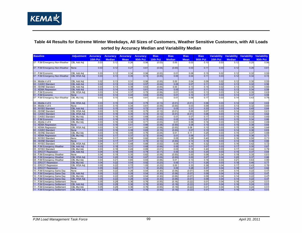
PJM Load Management Task Force April 20, 2011 99
Table 44 Results for Extreme Winter Weekdays, All Sizes of Customers, Weather Sensitive Customers, with All Loads
sorted by Accuracy Median and Variability Median
Accuracy Accuracy Accuracy Accuracy Bias Bias Bias Bias Variability Variability Variability Variability
10th Pct Median Mean 90th Pct 10th Pct Median Mean 90th Pct 10th Pct Median Mean 90th Pct07 - PJM Emergency Non-Weather CBL Add Adj 0.03 0.12 0.26 0.56 (0.03) 0.00 0.03 0.10 0.03 0.12 0.25 0.56
07 - PJM Emergency Non-Weather None 0.03 0.12 0.27 0.61 (0.04) (0.00) 0.03 0.11 0.03 0.12 0.26 0.61
01 - PJM Economic CBL Add Adj 0.03 0.12 0.34 0.56 (0.02) 0.01 0.08 0.15 0.02 0.12 0.32 0.5507 - PJM Emergency Non-Weather CBL WSA Adj 0.03 0.13 0.35 0.74 (0.05) 0.00 0.04 0.11 0.03 0.12 0.34 0.72
04 - Middle 4 of 6 CBL Add Adj 0.02 0.13 0.31 0.56 (0.05) 0.00 0.04 0.09 0.02 0.12 0.30 0.5502 - CAISO Standard CBL Add Adj 0.02 0.13 0.33 0.57 (0.04) 0.00 0.07 0.11 0.02 0.13 0.32 0.5606 - ISONE Standard CBL Add Adj 0.03 0.13 0.39 0.63 (0.05) 0.00 0.13 0.15 0.02 0.13 0.35 0.6013 - KEMA Regression CBL Add Adj 0.03 0.14 0.35 0.61 (0.04) 0.00 0.07 0.11 0.02 0.13 0.34 0.5901 - PJM Economic CBL WSA Adj 0.03 0.14 0.37 0.75 (0.06) 0.01 0.05 0.13 0.03 0.14 0.35 0.6301 - PJM Economic None 0.03 0.14 0.40 0.63 (0.05) 0.01 0.10 0.17 0.03 0.13 0.37 0.5907 - PJM Emergency Non-Weather CBL Mul Adj 0.03 0.15 0.44 0.81 (0.02) 0.01 0.09 0.17 0.03 0.14 0.43 0.79
04 - Middle 4 of 6 CBL WSA Adj 0.03 0.15 0.34 0.75 (0.13) (0.01) (0.01) 0.06 0.03 0.14 0.32 0.6304 - Middle 4 of 6 None 0.03 0.15 0.34 0.61 (0.09) (0.00) 0.03 0.09 0.03 0.13 0.32 0.6005 - NYISO Standard CBL Add Adj 0.03 0.15 0.50 0.72 (0.01) 0.03 0.21 0.33 0.03 0.14 0.45 0.6406 - ISONE Standard CBL WSA Adj 0.03 0.15 0.35 0.75 (0.12) (0.01) 0.00 0.07 0.03 0.14 0.32 0.6102 - CAISO Standard CBL WSA Adj 0.03 0.16 0.35 0.74 (0.12) (0.01) (0.01) 0.06 0.03 0.15 0.32 0.6202 - CAISO Standard CBL Mul Adj 0.03 0.16 0.35 0.69 (0.03) 0.01 0.07 0.17 0.03 0.15 0.33 0.6501 - PJM Economic CBL Mul Adj 0.03 0.16 0.35 0.72 (0.02) 0.02 0.08 0.21 0.03 0.15 0.34 0.6604 - Middle 4 of 6 CBL Mul Adj 0.03 0.16 0.34 0.71 (0.03) 0.01 0.06 0.16 0.03 0.15 0.33 0.6913 - KEMA Regression None 0.03 0.16 0.41 0.66 (0.08) (0.00) 0.08 0.10 0.03 0.15 0.38 0.6413 - KEMA Regression CBL WSA Adj 0.03 0.16 0.41 0.66 (0.08) (0.00) 0.08 0.10 0.03 0.15 0.38 0.6402 - CAISO Standard None 0.03 0.16 0.39 0.65 (0.10) (0.00) 0.07 0.10 0.03 0.14 0.36 0.6306 - ISONE Standard CBL Mul Adj 0.03 0.16 0.40 0.76 (0.04) 0.01 0.11 0.25 0.03 0.15 0.37 0.6813 - KEMA Regression CBL Mul Adj 0.03 0.17 0.37 0.73 (0.04) 0.01 0.06 0.17 0.03 0.16 0.36 0.7105 - NYISO Standard None 0.04 0.17 0.59 0.82 (0.02) 0.05 0.28 0.40 0.03 0.16 0.50 0.7106 - ISONE Standard None 0.03 0.17 0.47 0.70 (0.12) (0.00) 0.14 0.16 0.03 0.14 0.39 0.6605 - NYISO Standard CBL WSA Adj 0.04 0.17 0.48 0.88 (0.02) 0.04 0.16 0.32 0.03 0.16 0.42 0.7208 - PJM Emergency Weather CBL Add Adj 0.03 0.18 0.31 0.68 (0.06) 0.00 0.01 0.07 0.03 0.17 0.30 0.6705 - NYISO Standard CBL Mul Adj 0.03 0.18 0.49 0.89 (0.01) 0.03 0.18 0.40 0.03 0.17 0.44 0.7912 - ERCOT Regression CBL Add Adj 0.04 0.18 0.55 0.79 (0.17) 0.00 0.23 0.20 0.03 0.15 0.37 0.6408 - PJM Emergency Weather None 0.04 0.19 0.35 0.82 (0.08) (0.00) 0.00 0.08 0.04 0.19 0.35 0.8108 - PJM Emergency Weather CBL WSA Adj 0.04 0.20 0.38 0.87 (0.09) (0.00) 0.00 0.07 0.04 0.20 0.37 0.8608 - PJM Emergency Weather CBL Mul Adj 0.03 0.21 0.65 0.93 (0.06) 0.01 0.13 0.16 0.03 0.21 0.63 0.9012 - ERCOT Regression CBL Mul Adj 0.04 0.22 0.54 0.92 (0.23) 0.00 0.11 0.26 0.03 0.18 0.46 0.7712 - ERCOT Regression CBL WSA Adj 0.05 0.22 0.72 1.05 (0.22) 0.00 0.33 0.38 0.04 0.17 0.43 0.7612 - ERCOT Regression None 0.05 0.22 0.77 1.12 (0.25) 0.00 0.28 0.37 0.04 0.18 0.47 0.8210 - PJM Emergency Same Day None 0.05 0.22 0.28 0.54 (0.30) (0.06) (0.07) 0.09 0.04 0.14 0.22 0.4710 - PJM Emergency Same Day CBL Add Adj 0.05 0.22 0.28 0.54 (0.30) (0.06) (0.07) 0.09 0.04 0.14 0.22 0.4710 - PJM Emergency Same Day CBL Mul Adj 0.05 0.22 0.28 0.54 (0.30) (0.06) (0.07) 0.09 0.04 0.14 0.22 0.4710 - PJM Emergency Same Day CBL WSA Adj 0.05 0.22 0.28 0.54 (0.30) (0.06) (0.07) 0.09 0.04 0.14 0.22 0.4711 - PJM Emergency Settlement None 0.05 0.29 0.36 0.76 (0.55) (0.18) (0.22) 0.01 0.04 0.16 0.24 0.5111 - PJM Emergency Settlement CBL Add Adj 0.05 0.29 0.36 0.76 (0.55) (0.18) (0.22) 0.01 0.04 0.16 0.24 0.5111 - PJM Emergency Settlement CBL Mul Adj 0.05 0.29 0.36 0.76 (0.55) (0.18) (0.22) 0.01 0.04 0.16 0.24 0.5111 - PJM Emergency Settlement CBL WSA Adj 0.05 0.29 0.36 0.76 (0.55) (0.18) (0.22) 0.01 0.04 0.16 0.24 0.51
Baseline Adjustment

PJM Load Management Task Force April 20, 2011 100
Table 45 Results for Extreme Winter Weekdays, All Sizes of Customers, Non-Weather Sensitive Customers, with All
Loads sorted by Accuracy Median and Variability Median
Accuracy Accuracy Accuracy Accuracy Bias Bias Bias Bias Variability Variability Variability Variability
10th Pct Median Mean 90th Pct 10th Pct Median Mean 90th Pct 10th Pct Median Mean 90th Pct02 - CAISO Standard CBL Add Adj 0.02 0.09 0.16 0.33 (0.03) 0.00 0.01 0.05 0.02 0.09 0.15 0.3206 - ISONE Standard CBL Add Adj 0.02 0.09 0.16 0.32 (0.04) 0.00 0.01 0.06 0.02 0.09 0.15 0.3104 - Middle 4 of 6 CBL Add Adj 0.03 0.09 0.16 0.34 (0.03) 0.00 0.01 0.05 0.02 0.09 0.16 0.3301 - PJM Economic CBL Add Adj 0.02 0.10 0.16 0.34 (0.02) 0.01 0.03 0.07 0.02 0.09 0.16 0.3313 - KEMA Regression CBL Add Adj 0.03 0.10 0.16 0.33 (0.03) 0.00 0.01 0.05 0.02 0.09 0.16 0.3305 - NYISO Standard CBL Add Adj 0.03 0.10 0.19 0.36 (0.01) 0.02 0.06 0.13 0.02 0.09 0.17 0.3302 - CAISO Standard CBL Mul Adj 0.03 0.10 0.19 0.37 (0.03) 0.00 0.03 0.09 0.03 0.10 0.18 0.3706 - ISONE Standard CBL Mul Adj 0.03 0.10 0.18 0.38 (0.04) 0.00 0.03 0.10 0.02 0.10 0.17 0.3601 - PJM Economic CBL Mul Adj 0.03 0.10 0.20 0.40 (0.02) 0.01 0.04 0.10 0.03 0.10 0.19 0.3813 - KEMA Regression CBL Mul Adj 0.03 0.10 0.20 0.39 (0.03) 0.00 0.02 0.08 0.03 0.10 0.19 0.3904 - Middle 4 of 6 CBL Mul Adj 0.03 0.10 0.19 0.39 (0.03) 0.00 0.03 0.09 0.03 0.10 0.19 0.3907 - PJM Emergency Non-Weather CBL Add Adj 0.03 0.11 0.18 0.38 (0.02) 0.01 0.02 0.06 0.03 0.10 0.17 0.38
05 - NYISO Standard CBL Mul Adj 0.03 0.11 0.24 0.42 (0.02) 0.02 0.08 0.16 0.03 0.10 0.22 0.3807 - PJM Emergency Non-Weather CBL WSA Adj 0.03 0.11 0.20 0.40 (0.02) 0.01 0.02 0.08 0.03 0.11 0.20 0.39
07 - PJM Emergency Non-Weather None 0.03 0.11 0.19 0.39 (0.03) 0.01 0.02 0.08 0.03 0.11 0.19 0.38
10 - PJM Emergency Same Day None 0.04 0.11 0.16 0.33 (0.21) (0.04) (0.06) 0.03 0.03 0.08 0.12 0.2510 - PJM Emergency Same Day CBL Add Adj 0.04 0.11 0.16 0.33 (0.21) (0.04) (0.06) 0.03 0.03 0.08 0.12 0.2510 - PJM Emergency Same Day CBL Mul Adj 0.04 0.11 0.16 0.33 (0.21) (0.04) (0.06) 0.03 0.03 0.08 0.12 0.2510 - PJM Emergency Same Day CBL WSA Adj 0.04 0.11 0.16 0.33 (0.21) (0.04) (0.06) 0.03 0.03 0.08 0.12 0.2501 - PJM Economic CBL WSA Adj 0.03 0.12 0.20 0.41 (0.02) 0.01 0.03 0.11 0.03 0.11 0.19 0.4012 - ERCOT Regression CBL Add Adj 0.03 0.12 0.34 0.42 (0.09) 0.01 0.11 0.13 0.03 0.10 0.28 0.3407 - PJM Emergency Non-Weather CBL Mul Adj 0.03 0.12 0.34 0.55 (0.01) 0.01 0.07 0.12 0.03 0.11 0.33 0.55
04 - Middle 4 of 6 CBL WSA Adj 0.03 0.12 0.20 0.42 (0.05) (0.00) 0.00 0.07 0.03 0.11 0.19 0.4106 - ISONE Standard CBL WSA Adj 0.03 0.12 0.20 0.41 (0.06) (0.00) 0.00 0.06 0.03 0.11 0.19 0.3801 - PJM Economic None 0.03 0.12 0.20 0.41 (0.03) 0.01 0.04 0.12 0.03 0.11 0.19 0.3902 - CAISO Standard CBL WSA Adj 0.03 0.12 0.19 0.40 (0.05) (0.00) 0.00 0.06 0.03 0.12 0.19 0.3908 - PJM Emergency Weather CBL Add Adj 0.03 0.12 0.20 0.42 (0.05) (0.00) 0.00 0.05 0.03 0.12 0.20 0.4204 - Middle 4 of 6 None 0.03 0.13 0.20 0.41 (0.06) 0.00 0.01 0.07 0.03 0.12 0.19 0.4112 - ERCOT Regression CBL Mul Adj 0.03 0.13 0.28 0.55 (0.11) 0.01 0.04 0.18 0.03 0.10 0.24 0.4313 - KEMA Regression None 0.03 0.13 0.30 0.40 (0.06) (0.00) 0.04 0.06 0.03 0.12 0.29 0.4013 - KEMA Regression CBL WSA Adj 0.03 0.13 0.30 0.40 (0.06) (0.00) 0.04 0.06 0.03 0.12 0.29 0.4002 - CAISO Standard None 0.03 0.13 0.20 0.40 (0.07) (0.00) 0.01 0.06 0.03 0.12 0.19 0.3905 - NYISO Standard CBL WSA Adj 0.03 0.13 0.23 0.45 (0.01) 0.05 0.09 0.22 0.03 0.12 0.20 0.4006 - ISONE Standard None 0.03 0.14 0.25 0.40 (0.08) (0.00) 0.04 0.07 0.03 0.12 0.22 0.3908 - PJM Emergency Weather CBL Mul Adj 0.03 0.14 0.34 0.57 (0.04) 0.00 0.05 0.10 0.03 0.13 0.33 0.5605 - NYISO Standard None 0.04 0.14 0.25 0.45 (0.01) 0.05 0.11 0.24 0.03 0.12 0.22 0.4011 - PJM Emergency Settlement None 0.04 0.15 0.22 0.46 (0.35) (0.09) (0.12) 0.02 0.03 0.09 0.14 0.2911 - PJM Emergency Settlement CBL Add Adj 0.04 0.15 0.22 0.46 (0.35) (0.09) (0.12) 0.02 0.03 0.09 0.14 0.2911 - PJM Emergency Settlement CBL Mul Adj 0.04 0.15 0.22 0.46 (0.35) (0.09) (0.12) 0.02 0.03 0.09 0.14 0.2911 - PJM Emergency Settlement CBL WSA Adj 0.04 0.15 0.22 0.46 (0.35) (0.09) (0.12) 0.02 0.03 0.09 0.14 0.2908 - PJM Emergency Weather CBL WSA Adj 0.04 0.16 0.26 0.52 (0.05) 0.00 0.01 0.07 0.04 0.16 0.25 0.5108 - PJM Emergency Weather None 0.04 0.16 0.25 0.51 (0.05) 0.00 0.01 0.08 0.04 0.16 0.25 0.5112 - ERCOT Regression CBL WSA Adj 0.05 0.18 0.55 0.59 (0.16) 0.01 0.25 0.22 0.03 0.13 0.37 0.4012 - ERCOT Regression None 0.05 0.18 0.61 0.59 (0.16) 0.01 0.19 0.22 0.03 0.13 0.42 0.42
Baseline Adjustment

PJM Load Management Task Force April 20, 2011 101
Results for Weekdays during Winter for Regular Conditions
Table 46 Results for Winter Weekdays, All Sizes of Customers, For All Weather Customers, with All Loads sorted by
Accuracy Median and Variability Median
Accuracy Accuracy Accuracy Accuracy Bias Bias Bias Bias Variability Variability Variability Variability
10th Pct Median Mean 90th Pct 10th Pct Median Mean 90th Pct 10th Pct Median Mean 90th Pct06 - ISONE Standard CBL Add Adj 0.03 0.11 0.36 0.37 (0.02) 0.00 0.10 0.02 0.03 0.11 0.33 0.3701 - PJM Economic CBL Add Adj 0.03 0.11 0.19 0.37 0.00 0.01 0.03 0.06 0.03 0.11 0.19 0.3702 - CAISO Standard CBL Add Adj 0.03 0.11 0.28 0.37 (0.01) 0.00 0.03 0.02 0.03 0.11 0.28 0.3704 - Middle 4 of 6 CBL Add Adj 0.03 0.11 0.19 0.37 (0.01) 0.00 0.01 0.02 0.03 0.11 0.19 0.3713 - KEMA Regression CBL Add Adj 0.03 0.11 0.28 0.39 (0.02) 0.00 0.03 0.03 0.03 0.11 0.28 0.3805 - NYISO Standard CBL Add Adj 0.03 0.12 0.45 0.41 0.00 0.02 0.12 0.14 0.03 0.12 0.43 0.3906 - ISONE Standard CBL Mul Adj 0.03 0.12 0.24 0.46 (0.01) 0.00 0.02 0.05 0.03 0.12 0.23 0.4607 - PJM Emergency Non-Weather CBL Add Adj 0.03 0.12 0.21 0.41 (0.01) 0.00 0.01 0.03 0.03 0.12 0.21 0.41
02 - CAISO Standard CBL Mul Adj 0.03 0.12 0.24 0.46 (0.01) 0.00 0.02 0.03 0.03 0.12 0.24 0.4601 - PJM Economic CBL Mul Adj 0.03 0.12 0.29 0.49 (0.00) 0.01 0.04 0.07 0.03 0.12 0.28 0.4804 - Middle 4 of 6 CBL Mul Adj 0.03 0.13 0.27 0.49 (0.01) 0.00 0.02 0.05 0.03 0.13 0.27 0.4901 - PJM Economic CBL WSA Adj 0.03 0.13 0.40 0.45 0.00 0.02 0.14 0.09 0.03 0.13 0.37 0.4506 - ISONE Standard CBL WSA Adj 0.03 0.13 0.42 0.44 (0.03) (0.00) 0.11 0.02 0.03 0.13 0.38 0.4313 - KEMA Regression CBL Mul Adj 0.03 0.13 0.28 0.51 (0.02) 0.00 0.02 0.05 0.03 0.13 0.27 0.5107 - PJM Emergency Non-Weather None 0.04 0.13 0.22 0.44 (0.01) 0.00 0.01 0.03 0.04 0.13 0.22 0.43
07 - PJM Emergency Non-Weather CBL WSA Adj 0.04 0.13 0.38 0.47 (0.01) 0.00 0.10 0.03 0.04 0.13 0.35 0.47
04 - Middle 4 of 6 CBL WSA Adj 0.03 0.13 0.40 0.45 (0.02) 0.00 0.10 0.02 0.03 0.13 0.37 0.4502 - CAISO Standard CBL WSA Adj 0.03 0.13 0.41 0.45 (0.03) (0.00) 0.10 0.01 0.03 0.13 0.37 0.4501 - PJM Economic None 0.03 0.13 0.22 0.42 0.01 0.02 0.04 0.08 0.03 0.13 0.22 0.4104 - Middle 4 of 6 None 0.03 0.13 0.22 0.42 (0.02) 0.00 0.00 0.02 0.03 0.13 0.22 0.4205 - NYISO Standard CBL Mul Adj 0.03 0.13 0.34 0.54 (0.00) 0.02 0.08 0.15 0.03 0.13 0.33 0.5102 - CAISO Standard None 0.03 0.14 0.33 0.42 (0.03) (0.00) 0.03 0.01 0.03 0.14 0.33 0.4206 - ISONE Standard None 0.03 0.14 0.42 0.43 (0.05) (0.00) 0.11 0.03 0.03 0.13 0.38 0.4213 - KEMA Regression None 0.04 0.14 0.34 0.45 (0.05) (0.01) 0.03 0.03 0.04 0.14 0.34 0.4513 - KEMA Regression CBL WSA Adj 0.04 0.14 0.34 0.45 (0.05) (0.01) 0.03 0.03 0.04 0.14 0.34 0.4512 - ERCOT Regression CBL Add Adj 0.04 0.14 0.35 0.53 (0.12) 0.00 0.09 0.13 0.03 0.12 0.27 0.4310 - PJM Emergency Same Day None 0.05 0.14 0.24 0.43 (0.26) (0.04) (0.06) 0.04 0.04 0.10 0.19 0.3310 - PJM Emergency Same Day CBL Add Adj 0.05 0.14 0.24 0.43 (0.26) (0.04) (0.06) 0.04 0.04 0.10 0.19 0.3310 - PJM Emergency Same Day CBL Mul Adj 0.05 0.14 0.24 0.43 (0.26) (0.04) (0.06) 0.04 0.04 0.10 0.19 0.3310 - PJM Emergency Same Day CBL WSA Adj 0.05 0.14 0.24 0.43 (0.26) (0.04) (0.06) 0.04 0.04 0.10 0.19 0.3308 - PJM Emergency Weather CBL Add Adj 0.04 0.15 0.25 0.48 (0.02) 0.00 0.00 0.02 0.04 0.15 0.25 0.4807 - PJM Emergency Non-Weather CBL Mul Adj 0.04 0.15 0.50 0.69 (0.00) 0.01 0.08 0.10 0.04 0.15 0.49 0.69
05 - NYISO Standard CBL WSA Adj 0.04 0.15 0.55 0.53 0.01 0.05 0.25 0.22 0.04 0.14 0.49 0.4705 - NYISO Standard None 0.04 0.16 0.55 0.51 0.02 0.06 0.18 0.22 0.04 0.14 0.51 0.4612 - ERCOT Regression CBL Mul Adj 0.04 0.16 0.57 0.70 (0.15) 0.00 0.06 0.16 0.04 0.14 0.52 0.5908 - PJM Emergency Weather CBL Mul Adj 0.04 0.17 0.50 0.80 (0.01) 0.00 0.07 0.09 0.04 0.17 0.49 0.7908 - PJM Emergency Weather None 0.05 0.17 0.29 0.58 (0.02) 0.00 0.00 0.03 0.05 0.17 0.29 0.5808 - PJM Emergency Weather CBL WSA Adj 0.05 0.17 0.34 0.60 (0.02) 0.00 0.03 0.03 0.05 0.17 0.33 0.6012 - ERCOT Regression CBL WSA Adj 0.06 0.18 0.47 0.75 (0.17) 0.01 0.17 0.24 0.04 0.14 0.32 0.5112 - ERCOT Regression None 0.06 0.18 0.52 0.75 (0.18) 0.01 0.12 0.23 0.04 0.14 0.36 0.5311 - PJM Emergency Settlement None 0.05 0.19 0.29 0.62 (0.47) (0.12) (0.17) 0.01 0.04 0.11 0.19 0.3811 - PJM Emergency Settlement CBL Add Adj 0.05 0.19 0.29 0.62 (0.47) (0.12) (0.17) 0.01 0.04 0.11 0.19 0.3811 - PJM Emergency Settlement CBL Mul Adj 0.05 0.19 0.29 0.62 (0.47) (0.12) (0.17) 0.01 0.04 0.11 0.19 0.3811 - PJM Emergency Settlement CBL WSA Adj 0.05 0.19 0.29 0.62 (0.47) (0.12) (0.17) 0.01 0.04 0.11 0.19 0.38
Baseline Adjustment
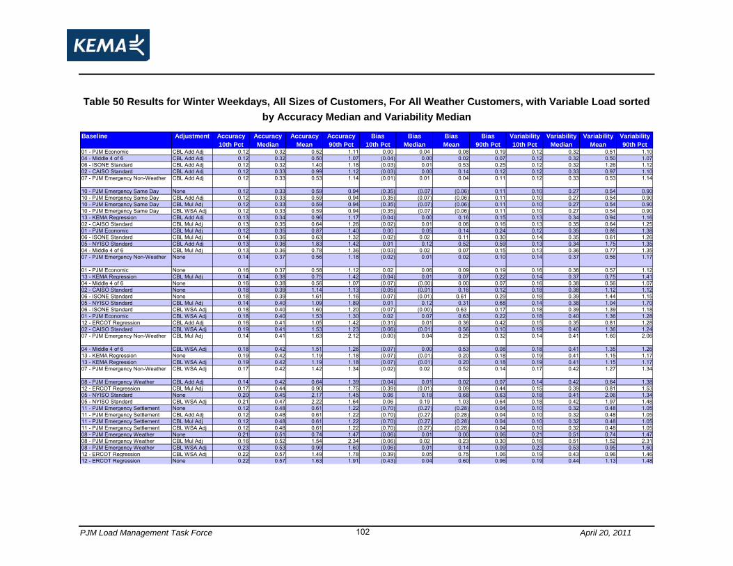
PJM Load Management Task Force April 20, 2011 102
Table 50 Results for Winter Weekdays, All Sizes of Customers, For All Weather Customers, with Variable Load sorted
by Accuracy Median and Variability Median
Accuracy Accuracy Accuracy Accuracy Bias Bias Bias Bias Variability Variability Variability Variability
10th Pct Median Mean 90th Pct 10th Pct Median Mean 90th Pct 10th Pct Median Mean 90th Pct01 - PJM Economic CBL Add Adj 0.12 0.32 0.52 1.11 0.00 0.04 0.08 0.19 0.12 0.32 0.51 1.1004 - Middle 4 of 6 CBL Add Adj 0.12 0.32 0.50 1.07 (0.04) 0.00 0.02 0.07 0.12 0.32 0.50 1.0706 - ISONE Standard CBL Add Adj 0.12 0.32 1.40 1.18 (0.03) 0.01 0.53 0.25 0.12 0.32 1.26 1.1202 - CAISO Standard CBL Add Adj 0.12 0.33 0.99 1.12 (0.03) 0.00 0.14 0.12 0.12 0.33 0.97 1.1007 - PJM Emergency Non-Weather CBL Add Adj 0.12 0.33 0.53 1.14 (0.01) 0.01 0.04 0.11 0.12 0.33 0.53 1.14
10 - PJM Emergency Same Day None 0.12 0.33 0.59 0.94 (0.35) (0.07) (0.06) 0.11 0.10 0.27 0.54 0.9010 - PJM Emergency Same Day CBL Add Adj 0.12 0.33 0.59 0.94 (0.35) (0.07) (0.06) 0.11 0.10 0.27 0.54 0.9010 - PJM Emergency Same Day CBL Mul Adj 0.12 0.33 0.59 0.94 (0.35) (0.07) (0.06) 0.11 0.10 0.27 0.54 0.9010 - PJM Emergency Same Day CBL WSA Adj 0.12 0.33 0.59 0.94 (0.35) (0.07) (0.06) 0.11 0.10 0.27 0.54 0.9013 - KEMA Regression CBL Add Adj 0.13 0.34 0.96 1.17 (0.04) 0.00 0.16 0.15 0.13 0.34 0.94 1.1602 - CAISO Standard CBL Mul Adj 0.13 0.35 0.64 1.26 (0.02) 0.01 0.06 0.16 0.13 0.35 0.64 1.2501 - PJM Economic CBL Mul Adj 0.12 0.35 0.87 1.40 0.00 0.05 0.14 0.24 0.12 0.35 0.86 1.3806 - ISONE Standard CBL Mul Adj 0.14 0.36 0.63 1.32 (0.02) 0.02 0.11 0.30 0.14 0.35 0.61 1.2605 - NYISO Standard CBL Add Adj 0.13 0.36 1.83 1.42 0.01 0.12 0.52 0.59 0.13 0.34 1.75 1.3504 - Middle 4 of 6 CBL Mul Adj 0.13 0.36 0.78 1.36 (0.03) 0.02 0.07 0.15 0.13 0.36 0.77 1.3507 - PJM Emergency Non-Weather None 0.14 0.37 0.56 1.18 (0.02) 0.01 0.02 0.10 0.14 0.37 0.56 1.17
01 - PJM Economic None 0.16 0.37 0.58 1.12 0.02 0.06 0.09 0.19 0.16 0.36 0.57 1.1213 - KEMA Regression CBL Mul Adj 0.14 0.38 0.75 1.42 (0.04) 0.01 0.07 0.22 0.14 0.37 0.75 1.4104 - Middle 4 of 6 None 0.16 0.38 0.56 1.07 (0.07) (0.00) 0.00 0.07 0.16 0.38 0.56 1.0702 - CAISO Standard None 0.18 0.39 1.14 1.13 (0.05) (0.01) 0.16 0.12 0.18 0.38 1.12 1.1206 - ISONE Standard None 0.18 0.39 1.61 1.16 (0.07) (0.01) 0.61 0.29 0.18 0.39 1.44 1.1505 - NYISO Standard CBL Mul Adj 0.14 0.40 1.09 1.89 0.01 0.12 0.31 0.68 0.14 0.38 1.04 1.7006 - ISONE Standard CBL WSA Adj 0.18 0.40 1.60 1.20 (0.07) (0.00) 0.63 0.17 0.18 0.39 1.39 1.1801 - PJM Economic CBL WSA Adj 0.18 0.40 1.53 1.30 0.02 0.07 0.63 0.22 0.18 0.40 1.36 1.2812 - ERCOT Regression CBL Add Adj 0.16 0.41 1.05 1.42 (0.31) 0.01 0.36 0.42 0.15 0.35 0.81 1.2802 - CAISO Standard CBL WSA Adj 0.19 0.41 1.53 1.23 (0.06) (0.01) 0.56 0.10 0.19 0.40 1.36 1.2407 - PJM Emergency Non-Weather CBL Mul Adj 0.14 0.41 1.63 2.12 (0.00) 0.04 0.29 0.32 0.14 0.41 1.60 2.06
04 - Middle 4 of 6 CBL WSA Adj 0.18 0.42 1.51 1.26 (0.07) 0.00 0.53 0.08 0.18 0.41 1.35 1.2613 - KEMA Regression None 0.19 0.42 1.19 1.18 (0.07) (0.01) 0.20 0.18 0.19 0.41 1.15 1.1713 - KEMA Regression CBL WSA Adj 0.19 0.42 1.19 1.18 (0.07) (0.01) 0.20 0.18 0.19 0.41 1.15 1.1707 - PJM Emergency Non-Weather CBL WSA Adj 0.17 0.42 1.42 1.34 (0.02) 0.02 0.52 0.14 0.17 0.42 1.27 1.34
08 - PJM Emergency Weather CBL Add Adj 0.14 0.42 0.64 1.39 (0.04) 0.01 0.02 0.07 0.14 0.42 0.64 1.3812 - ERCOT Regression CBL Mul Adj 0.17 0.44 0.90 1.75 (0.39) (0.01) 0.09 0.44 0.15 0.39 0.81 1.5305 - NYISO Standard None 0.20 0.45 2.17 1.45 0.06 0.18 0.68 0.63 0.18 0.41 2.06 1.3405 - NYISO Standard CBL WSA Adj 0.21 0.47 2.22 1.64 0.06 0.19 1.03 0.64 0.18 0.42 1.97 1.4811 - PJM Emergency Settlement None 0.12 0.48 0.61 1.22 (0.70) (0.27) (0.28) 0.04 0.10 0.32 0.48 1.0511 - PJM Emergency Settlement CBL Add Adj 0.12 0.48 0.61 1.22 (0.70) (0.27) (0.28) 0.04 0.10 0.32 0.48 1.0511 - PJM Emergency Settlement CBL Mul Adj 0.12 0.48 0.61 1.22 (0.70) (0.27) (0.28) 0.04 0.10 0.32 0.48 1.0511 - PJM Emergency Settlement CBL WSA Adj 0.12 0.48 0.61 1.22 (0.70) (0.27) (0.28) 0.04 0.10 0.32 0.48 1.0508 - PJM Emergency Weather None 0.21 0.51 0.74 1.47 (0.06) 0.01 0.00 0.06 0.21 0.51 0.74 1.4708 - PJM Emergency Weather CBL Mul Adj 0.16 0.52 1.54 2.34 (0.06) 0.02 0.23 0.30 0.16 0.51 1.52 2.3108 - PJM Emergency Weather CBL WSA Adj 0.23 0.53 0.99 1.60 (0.06) 0.01 0.14 0.09 0.23 0.53 0.95 1.6012 - ERCOT Regression CBL WSA Adj 0.22 0.57 1.49 1.78 (0.39) 0.05 0.75 1.06 0.19 0.43 0.96 1.4612 - ERCOT Regression None 0.22 0.57 1.63 1.91 (0.43) 0.04 0.60 0.96 0.19 0.44 1.13 1.48
Baseline Adjustment

PJM Load Management Task Force April 20, 2011 103
Table 47 Results for Winter Weekdays, All Sizes of Customers, For All Weather Customers, with Non-Variable Load
sorted by Accuracy Median and Variability Median
Accuracy Accuracy Accuracy Accuracy Bias Bias Bias Bias Variability Variability Variability Variability
10th Pct Median Mean 90th Pct 10th Pct Median Mean 90th Pct 10th Pct Median Mean 90th Pct06 - ISONE Standard CBL Add Adj 0.03 0.09 0.11 0.23 (0.01) 0.00 0.00 0.01 0.03 0.09 0.11 0.2302 - CAISO Standard CBL Add Adj 0.03 0.09 0.12 0.24 (0.01) (0.00) 0.00 0.01 0.03 0.09 0.12 0.2401 - PJM Economic CBL Add Adj 0.03 0.09 0.12 0.24 (0.00) 0.01 0.01 0.03 0.03 0.09 0.11 0.2404 - Middle 4 of 6 CBL Add Adj 0.03 0.09 0.12 0.24 (0.01) 0.00 0.00 0.02 0.03 0.09 0.12 0.2413 - KEMA Regression CBL Add Adj 0.03 0.09 0.12 0.24 (0.02) 0.00 0.00 0.02 0.03 0.09 0.12 0.2405 - NYISO Standard CBL Add Adj 0.03 0.09 0.13 0.26 0.00 0.02 0.03 0.08 0.03 0.09 0.12 0.2506 - ISONE Standard CBL Mul Adj 0.03 0.10 0.14 0.30 (0.01) 0.00 0.00 0.03 0.03 0.10 0.14 0.2902 - CAISO Standard CBL Mul Adj 0.03 0.10 0.15 0.30 (0.01) 0.00 0.01 0.02 0.03 0.10 0.15 0.3007 - PJM Emergency Non-Weather CBL Add Adj 0.03 0.10 0.13 0.26 (0.01) 0.00 0.00 0.02 0.03 0.10 0.13 0.26
01 - PJM Economic CBL Mul Adj 0.03 0.10 0.15 0.30 (0.00) 0.01 0.02 0.04 0.03 0.10 0.15 0.3004 - Middle 4 of 6 CBL Mul Adj 0.03 0.10 0.15 0.31 (0.01) 0.00 0.01 0.03 0.03 0.10 0.15 0.3113 - KEMA Regression CBL Mul Adj 0.03 0.10 0.16 0.31 (0.01) 0.00 0.01 0.03 0.03 0.10 0.16 0.3104 - Middle 4 of 6 CBL WSA Adj 0.03 0.10 0.14 0.28 (0.01) 0.00 0.00 0.02 0.03 0.10 0.14 0.2801 - PJM Economic CBL WSA Adj 0.03 0.10 0.14 0.27 0.00 0.02 0.02 0.05 0.03 0.10 0.14 0.2707 - PJM Emergency Non-Weather CBL WSA Adj 0.04 0.10 0.14 0.28 (0.01) 0.00 0.00 0.02 0.04 0.10 0.14 0.28
07 - PJM Emergency Non-Weather None 0.03 0.10 0.14 0.28 (0.01) 0.00 0.00 0.02 0.03 0.10 0.14 0.27
06 - ISONE Standard CBL WSA Adj 0.03 0.10 0.14 0.27 (0.03) (0.00) (0.01) 0.01 0.03 0.10 0.13 0.2705 - NYISO Standard CBL Mul Adj 0.03 0.10 0.16 0.33 (0.00) 0.01 0.03 0.08 0.03 0.10 0.16 0.3202 - CAISO Standard CBL WSA Adj 0.03 0.10 0.14 0.28 (0.02) (0.00) 0.00 0.01 0.03 0.10 0.14 0.2801 - PJM Economic None 0.03 0.10 0.14 0.27 0.01 0.02 0.02 0.05 0.03 0.10 0.13 0.2704 - Middle 4 of 6 None 0.03 0.11 0.14 0.28 (0.01) 0.00 0.00 0.02 0.03 0.10 0.14 0.2812 - ERCOT Regression CBL Add Adj 0.04 0.11 0.18 0.31 (0.09) 0.00 0.02 0.09 0.03 0.09 0.15 0.2502 - CAISO Standard None 0.03 0.11 0.14 0.28 (0.03) (0.00) 0.00 0.01 0.03 0.11 0.14 0.2806 - ISONE Standard None 0.03 0.11 0.14 0.27 (0.04) (0.00) (0.01) 0.02 0.03 0.11 0.14 0.2713 - KEMA Regression None 0.03 0.11 0.14 0.29 (0.04) (0.00) (0.01) 0.02 0.03 0.11 0.14 0.2813 - KEMA Regression CBL WSA Adj 0.03 0.11 0.14 0.29 (0.04) (0.00) (0.01) 0.02 0.03 0.11 0.14 0.2807 - PJM Emergency Non-Weather CBL Mul Adj 0.03 0.11 0.24 0.43 (0.00) 0.01 0.03 0.06 0.03 0.11 0.23 0.43
05 - NYISO Standard CBL WSA Adj 0.04 0.12 0.16 0.31 0.01 0.04 0.06 0.13 0.03 0.11 0.15 0.2810 - PJM Emergency Same Day None 0.04 0.12 0.16 0.33 (0.22) (0.04) (0.06) 0.03 0.03 0.08 0.11 0.2310 - PJM Emergency Same Day CBL Add Adj 0.04 0.12 0.16 0.33 (0.22) (0.04) (0.06) 0.03 0.03 0.08 0.11 0.2310 - PJM Emergency Same Day CBL Mul Adj 0.04 0.12 0.16 0.33 (0.22) (0.04) (0.06) 0.03 0.03 0.08 0.11 0.2310 - PJM Emergency Same Day CBL WSA Adj 0.04 0.12 0.16 0.33 (0.22) (0.04) (0.06) 0.03 0.03 0.08 0.11 0.2308 - PJM Emergency Weather CBL Add Adj 0.04 0.12 0.16 0.32 (0.01) (0.00) 0.00 0.01 0.04 0.12 0.16 0.3212 - ERCOT Regression CBL Mul Adj 0.04 0.12 0.49 0.43 (0.10) 0.00 0.06 0.13 0.03 0.10 0.45 0.3505 - NYISO Standard None 0.04 0.12 0.16 0.31 0.02 0.05 0.07 0.13 0.03 0.11 0.15 0.2808 - PJM Emergency Weather CBL Mul Adj 0.04 0.14 0.26 0.48 (0.01) 0.00 0.03 0.06 0.04 0.14 0.25 0.4808 - PJM Emergency Weather CBL WSA Adj 0.04 0.14 0.18 0.38 (0.01) 0.00 0.00 0.02 0.04 0.14 0.18 0.3808 - PJM Emergency Weather None 0.04 0.14 0.19 0.38 (0.01) 0.00 0.00 0.02 0.04 0.14 0.19 0.3812 - ERCOT Regression CBL WSA Adj 0.05 0.15 0.23 0.39 (0.14) 0.01 0.03 0.15 0.04 0.11 0.16 0.2912 - ERCOT Regression None 0.05 0.15 0.25 0.39 (0.14) 0.01 0.01 0.15 0.04 0.11 0.18 0.2911 - PJM Emergency Settlement None 0.05 0.16 0.22 0.46 (0.39) (0.11) (0.15) 0.01 0.04 0.09 0.13 0.2611 - PJM Emergency Settlement CBL Add Adj 0.05 0.16 0.22 0.46 (0.39) (0.11) (0.15) 0.01 0.04 0.09 0.13 0.2611 - PJM Emergency Settlement CBL Mul Adj 0.05 0.16 0.22 0.46 (0.39) (0.11) (0.15) 0.01 0.04 0.09 0.13 0.2611 - PJM Emergency Settlement CBL WSA Adj 0.05 0.16 0.22 0.46 (0.39) (0.11) (0.15) 0.01 0.04 0.09 0.13 0.26
Baseline Adjustment

PJM Load Management Task Force April 20, 2011 104
Table 48 Results for Winter Weekdays, All Sizes of Customers, Weather Sensitive Customers, with All Loads sorted by
Accuracy Median and Variability Median
Accuracy Accuracy Accuracy Accuracy Bias Bias Bias Bias Variability Variability Variability Variability
10th Pct Median Mean 90th Pct 10th Pct Median Mean 90th Pct 10th Pct Median Mean 90th Pct04 - Middle 4 of 6 CBL Add Adj 0.03 0.14 0.26 0.57 (0.01) 0.00 0.01 0.03 0.03 0.14 0.26 0.5707 - PJM Emergency Non-Weather CBL Add Adj 0.03 0.14 0.27 0.56 (0.01) 0.00 0.01 0.04 0.03 0.14 0.26 0.56
01 - PJM Economic CBL Add Adj 0.03 0.14 0.26 0.57 0.00 0.01 0.04 0.09 0.03 0.14 0.26 0.5606 - ISONE Standard CBL Add Adj 0.03 0.14 0.69 0.63 (0.02) 0.00 0.25 0.05 0.03 0.14 0.63 0.6002 - CAISO Standard CBL Add Adj 0.03 0.14 0.49 0.58 (0.02) 0.00 0.07 0.03 0.03 0.14 0.49 0.5707 - PJM Emergency Non-Weather None 0.04 0.14 0.27 0.58 (0.01) 0.00 0.01 0.03 0.04 0.14 0.27 0.58
07 - PJM Emergency Non-Weather CBL WSA Adj 0.04 0.15 0.69 0.74 (0.01) 0.00 0.25 0.05 0.04 0.15 0.61 0.74
04 - Middle 4 of 6 CBL WSA Adj 0.03 0.15 0.74 0.75 (0.02) 0.00 0.26 0.03 0.03 0.15 0.66 0.7513 - KEMA Regression CBL Add Adj 0.03 0.15 0.48 0.64 (0.03) 0.00 0.08 0.05 0.03 0.15 0.47 0.6301 - PJM Economic CBL WSA Adj 0.03 0.15 0.75 0.74 0.00 0.02 0.30 0.12 0.03 0.15 0.67 0.7404 - Middle 4 of 6 None 0.03 0.15 0.28 0.61 (0.03) (0.00) 0.00 0.02 0.03 0.15 0.28 0.6106 - ISONE Standard CBL WSA Adj 0.03 0.15 0.78 0.73 (0.04) 0.00 0.30 0.04 0.03 0.15 0.68 0.7201 - PJM Economic None 0.03 0.15 0.29 0.61 0.01 0.02 0.05 0.11 0.03 0.15 0.28 0.6102 - CAISO Standard CBL WSA Adj 0.03 0.15 0.75 0.73 (0.03) 0.00 0.27 0.03 0.03 0.15 0.67 0.7305 - NYISO Standard CBL Add Adj 0.03 0.16 0.90 0.74 0.00 0.03 0.25 0.26 0.03 0.16 0.86 0.6902 - CAISO Standard None 0.03 0.16 0.57 0.64 (0.03) (0.00) 0.08 0.03 0.03 0.16 0.56 0.6413 - KEMA Regression None 0.03 0.16 0.57 0.72 (0.04) (0.00) 0.09 0.06 0.03 0.16 0.55 0.7213 - KEMA Regression CBL WSA Adj 0.03 0.16 0.57 0.72 (0.04) (0.00) 0.09 0.06 0.03 0.16 0.55 0.7206 - ISONE Standard None 0.03 0.17 0.79 0.68 (0.05) (0.00) 0.29 0.07 0.03 0.16 0.71 0.6601 - PJM Economic CBL Mul Adj 0.03 0.17 0.34 0.72 0.00 0.01 0.05 0.12 0.03 0.17 0.34 0.7104 - Middle 4 of 6 CBL Mul Adj 0.03 0.17 0.34 0.74 (0.01) 0.00 0.02 0.08 0.03 0.17 0.34 0.7306 - ISONE Standard CBL Mul Adj 0.03 0.18 0.35 0.74 (0.02) 0.00 0.05 0.10 0.03 0.17 0.33 0.7202 - CAISO Standard CBL Mul Adj 0.03 0.18 0.33 0.73 (0.01) 0.00 0.03 0.07 0.03 0.18 0.33 0.7307 - PJM Emergency Non-Weather CBL Mul Adj 0.04 0.18 0.61 0.91 (0.00) 0.01 0.09 0.12 0.04 0.18 0.60 0.90
05 - NYISO Standard CBL WSA Adj 0.04 0.18 1.07 0.92 0.01 0.06 0.49 0.38 0.04 0.17 0.95 0.8313 - KEMA Regression CBL Mul Adj 0.03 0.18 0.40 0.83 (0.02) 0.00 0.04 0.09 0.03 0.18 0.39 0.8108 - PJM Emergency Weather CBL Add Adj 0.04 0.18 0.34 0.73 (0.02) 0.00 0.01 0.03 0.04 0.18 0.34 0.7305 - NYISO Standard None 0.04 0.19 1.05 0.85 0.02 0.07 0.33 0.37 0.04 0.18 1.00 0.7612 - ERCOT Regression CBL Add Adj 0.04 0.19 0.56 0.85 (0.18) 0.00 0.19 0.17 0.04 0.16 0.43 0.7005 - NYISO Standard CBL Mul Adj 0.03 0.19 0.46 0.96 (0.00) 0.03 0.12 0.29 0.03 0.18 0.44 0.8708 - PJM Emergency Weather None 0.04 0.20 0.37 0.90 (0.02) 0.00 0.00 0.03 0.04 0.20 0.37 0.9008 - PJM Emergency Weather CBL WSA Adj 0.04 0.21 0.49 0.95 (0.02) 0.00 0.07 0.04 0.04 0.21 0.48 0.9512 - ERCOT Regression CBL WSA Adj 0.05 0.21 0.72 1.03 (0.20) 0.01 0.31 0.35 0.04 0.18 0.47 0.8212 - ERCOT Regression None 0.05 0.21 0.77 1.08 (0.22) 0.01 0.25 0.34 0.04 0.18 0.53 0.8510 - PJM Emergency Same Day None 0.05 0.23 0.36 0.59 (0.30) (0.06) (0.06) 0.08 0.04 0.15 0.30 0.4910 - PJM Emergency Same Day CBL Add Adj 0.05 0.23 0.36 0.59 (0.30) (0.06) (0.06) 0.08 0.04 0.15 0.30 0.4910 - PJM Emergency Same Day CBL Mul Adj 0.05 0.23 0.36 0.59 (0.30) (0.06) (0.06) 0.08 0.04 0.15 0.30 0.4910 - PJM Emergency Same Day CBL WSA Adj 0.05 0.23 0.36 0.59 (0.30) (0.06) (0.06) 0.08 0.04 0.15 0.30 0.4912 - ERCOT Regression CBL Mul Adj 0.04 0.23 0.53 0.98 (0.23) 0.00 0.06 0.20 0.04 0.20 0.47 0.9108 - PJM Emergency Weather CBL Mul Adj 0.04 0.24 0.65 1.06 (0.01) 0.01 0.08 0.10 0.04 0.24 0.64 1.0411 - PJM Emergency Settlement None 0.05 0.30 0.40 0.86 (0.57) (0.19) (0.24) 0.00 0.04 0.17 0.27 0.5711 - PJM Emergency Settlement CBL Add Adj 0.05 0.30 0.40 0.86 (0.57) (0.19) (0.24) 0.00 0.04 0.17 0.27 0.5711 - PJM Emergency Settlement CBL Mul Adj 0.05 0.30 0.40 0.86 (0.57) (0.19) (0.24) 0.00 0.04 0.17 0.27 0.5711 - PJM Emergency Settlement CBL WSA Adj 0.05 0.30 0.40 0.86 (0.57) (0.19) (0.24) 0.00 0.04 0.17 0.27 0.57
Baseline Adjustment
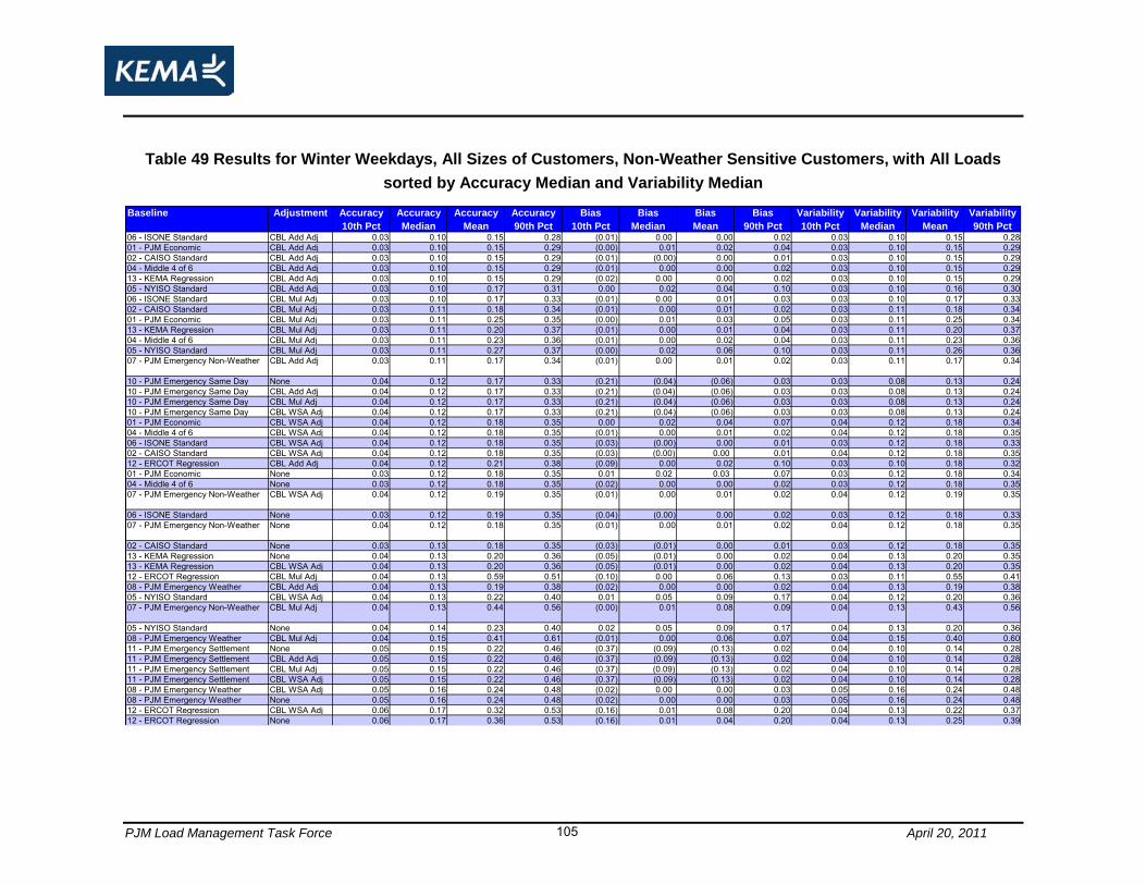
PJM Load Management Task Force April 20, 2011 105
Table 49 Results for Winter Weekdays, All Sizes of Customers, Non-Weather Sensitive Customers, with All Loads
sorted by Accuracy Median and Variability Median
Accuracy Accuracy Accuracy Accuracy Bias Bias Bias Bias Variability Variability Variability Variability
10th Pct Median Mean 90th Pct 10th Pct Median Mean 90th Pct 10th Pct Median Mean 90th Pct06 - ISONE Standard CBL Add Adj 0.03 0.10 0.15 0.28 (0.01) 0.00 0.00 0.02 0.03 0.10 0.15 0.2801 - PJM Economic CBL Add Adj 0.03 0.10 0.15 0.29 (0.00) 0.01 0.02 0.04 0.03 0.10 0.15 0.2902 - CAISO Standard CBL Add Adj 0.03 0.10 0.15 0.29 (0.01) (0.00) 0.00 0.01 0.03 0.10 0.15 0.2904 - Middle 4 of 6 CBL Add Adj 0.03 0.10 0.15 0.29 (0.01) 0.00 0.00 0.02 0.03 0.10 0.15 0.2913 - KEMA Regression CBL Add Adj 0.03 0.10 0.15 0.29 (0.02) 0.00 0.00 0.02 0.03 0.10 0.15 0.2905 - NYISO Standard CBL Add Adj 0.03 0.10 0.17 0.31 0.00 0.02 0.04 0.10 0.03 0.10 0.16 0.3006 - ISONE Standard CBL Mul Adj 0.03 0.10 0.17 0.33 (0.01) 0.00 0.01 0.03 0.03 0.10 0.17 0.3302 - CAISO Standard CBL Mul Adj 0.03 0.11 0.18 0.34 (0.01) 0.00 0.01 0.02 0.03 0.11 0.18 0.3401 - PJM Economic CBL Mul Adj 0.03 0.11 0.25 0.35 (0.00) 0.01 0.03 0.05 0.03 0.11 0.25 0.3413 - KEMA Regression CBL Mul Adj 0.03 0.11 0.20 0.37 (0.01) 0.00 0.01 0.04 0.03 0.11 0.20 0.3704 - Middle 4 of 6 CBL Mul Adj 0.03 0.11 0.23 0.36 (0.01) 0.00 0.02 0.04 0.03 0.11 0.23 0.3605 - NYISO Standard CBL Mul Adj 0.03 0.11 0.27 0.37 (0.00) 0.02 0.06 0.10 0.03 0.11 0.26 0.3607 - PJM Emergency Non-Weather CBL Add Adj 0.03 0.11 0.17 0.34 (0.01) 0.00 0.01 0.02 0.03 0.11 0.17 0.34
10 - PJM Emergency Same Day None 0.04 0.12 0.17 0.33 (0.21) (0.04) (0.06) 0.03 0.03 0.08 0.13 0.2410 - PJM Emergency Same Day CBL Add Adj 0.04 0.12 0.17 0.33 (0.21) (0.04) (0.06) 0.03 0.03 0.08 0.13 0.2410 - PJM Emergency Same Day CBL Mul Adj 0.04 0.12 0.17 0.33 (0.21) (0.04) (0.06) 0.03 0.03 0.08 0.13 0.2410 - PJM Emergency Same Day CBL WSA Adj 0.04 0.12 0.17 0.33 (0.21) (0.04) (0.06) 0.03 0.03 0.08 0.13 0.2401 - PJM Economic CBL WSA Adj 0.04 0.12 0.18 0.35 0.00 0.02 0.04 0.07 0.04 0.12 0.18 0.3404 - Middle 4 of 6 CBL WSA Adj 0.04 0.12 0.18 0.35 (0.01) 0.00 0.01 0.02 0.04 0.12 0.18 0.3506 - ISONE Standard CBL WSA Adj 0.04 0.12 0.18 0.35 (0.03) (0.00) 0.00 0.01 0.03 0.12 0.18 0.3302 - CAISO Standard CBL WSA Adj 0.04 0.12 0.18 0.35 (0.03) (0.00) 0.00 0.01 0.04 0.12 0.18 0.3512 - ERCOT Regression CBL Add Adj 0.04 0.12 0.21 0.38 (0.09) 0.00 0.02 0.10 0.03 0.10 0.18 0.3201 - PJM Economic None 0.03 0.12 0.18 0.35 0.01 0.02 0.03 0.07 0.03 0.12 0.18 0.3404 - Middle 4 of 6 None 0.03 0.12 0.18 0.35 (0.02) 0.00 0.00 0.02 0.03 0.12 0.18 0.3507 - PJM Emergency Non-Weather CBL WSA Adj 0.04 0.12 0.19 0.35 (0.01) 0.00 0.01 0.02 0.04 0.12 0.19 0.35
06 - ISONE Standard None 0.03 0.12 0.19 0.35 (0.04) (0.00) 0.00 0.02 0.03 0.12 0.18 0.3307 - PJM Emergency Non-Weather None 0.04 0.12 0.18 0.35 (0.01) 0.00 0.01 0.02 0.04 0.12 0.18 0.35
02 - CAISO Standard None 0.03 0.13 0.18 0.35 (0.03) (0.01) 0.00 0.01 0.03 0.12 0.18 0.3513 - KEMA Regression None 0.04 0.13 0.20 0.36 (0.05) (0.01) 0.00 0.02 0.04 0.13 0.20 0.3513 - KEMA Regression CBL WSA Adj 0.04 0.13 0.20 0.36 (0.05) (0.01) 0.00 0.02 0.04 0.13 0.20 0.3512 - ERCOT Regression CBL Mul Adj 0.04 0.13 0.59 0.51 (0.10) 0.00 0.06 0.13 0.03 0.11 0.55 0.4108 - PJM Emergency Weather CBL Add Adj 0.04 0.13 0.19 0.38 (0.02) 0.00 0.00 0.02 0.04 0.13 0.19 0.3805 - NYISO Standard CBL WSA Adj 0.04 0.13 0.22 0.40 0.01 0.05 0.09 0.17 0.04 0.12 0.20 0.3607 - PJM Emergency Non-Weather CBL Mul Adj 0.04 0.13 0.44 0.56 (0.00) 0.01 0.08 0.09 0.04 0.13 0.43 0.56
05 - NYISO Standard None 0.04 0.14 0.23 0.40 0.02 0.05 0.09 0.17 0.04 0.13 0.20 0.3608 - PJM Emergency Weather CBL Mul Adj 0.04 0.15 0.41 0.61 (0.01) 0.00 0.06 0.07 0.04 0.15 0.40 0.6011 - PJM Emergency Settlement None 0.05 0.15 0.22 0.46 (0.37) (0.09) (0.13) 0.02 0.04 0.10 0.14 0.2811 - PJM Emergency Settlement CBL Add Adj 0.05 0.15 0.22 0.46 (0.37) (0.09) (0.13) 0.02 0.04 0.10 0.14 0.2811 - PJM Emergency Settlement CBL Mul Adj 0.05 0.15 0.22 0.46 (0.37) (0.09) (0.13) 0.02 0.04 0.10 0.14 0.2811 - PJM Emergency Settlement CBL WSA Adj 0.05 0.15 0.22 0.46 (0.37) (0.09) (0.13) 0.02 0.04 0.10 0.14 0.2808 - PJM Emergency Weather CBL WSA Adj 0.05 0.16 0.24 0.48 (0.02) 0.00 0.00 0.03 0.05 0.16 0.24 0.4808 - PJM Emergency Weather None 0.05 0.16 0.24 0.48 (0.02) 0.00 0.00 0.03 0.05 0.16 0.24 0.4812 - ERCOT Regression CBL WSA Adj 0.06 0.17 0.32 0.53 (0.16) 0.01 0.08 0.20 0.04 0.13 0.22 0.3712 - ERCOT Regression None 0.06 0.17 0.36 0.53 (0.16) 0.01 0.04 0.20 0.04 0.13 0.25 0.39
Baseline Adjustment