Pieri’s Formula for Generalized Schur Polynomialsnu/tex/thesis/thesis/x2.pdfSchur polynomials have...
55
Pieri’s Formula for Generalized Schur Polynomials Numata, Yasuhide
Transcript of Pieri’s Formula for Generalized Schur Polynomialsnu/tex/thesis/thesis/x2.pdfSchur polynomials have...
Pieri’s Formula
for Generalized Schur Polynomials
Numata, Yasuhide

Contents
Preface 5
Chapter 1. Introduction — the original Pieri’s formula 91. Definition of original Schur polynomials 92. Pieri’s formula, Cauchy identity and so on 133. Symmetric polynomials, Quasi-symmetric polynomials 14
Chapter 2. Pieri’s formula — main results and their proofs 171. Generalized Schur Operators 172. Definition of Our Polynomials 233. Pieri’s formula and Cauchy’s formula 27
Chapter 3. Examples of Generalized Schur Operators 351. Young’s Lattice 352. Shifted Shapes 403. Rooted Planar Binary Trees 41
Bibliography 55
3

Preface
In this thesis, we consider combinatorial operators called general-ized Schur operators. In particular, we introduce a generalization ofSchur polynomials defined by using generalized Schur operators. Weshow an analogue of Pieri’s formula for them. We also introduce anexample of generalized Schur operators concerning planer binary trees.
Schur polynomials are symmetric polynomials parametrized by par-titions or Young diagrams. Schur polynomials associated with Youngdiagrams consisting of one row are the homogeneous complete sym-metric polynomials, and Schur polynomials corresponding Young di-agrams consisting of one row are elementary symmetric polynomials.Schur polynomials often play important roles. For example, Schur poly-nomials give irreducible characters of representations of special lineargroups, the set of Schur polynomials is a basis of symmetric polyno-mials, and so on. Schur polynomials have many equivalent definitions.One can define Schur polynomials by the weighted generating functionsof semi-standard Young tableaux. This definition implies combinato-rial formulae such as Pieri’s formula. Pieri’s formula is the formula de-scribing the product of a complete symmetric polynomial and a Schurpolynomial as a sum of Schur polynomials:
hi(t1, . . . , tn)sλ(t1, . . . , tn) =∑
µ
sµ(t1, . . . , tn),
where the sum is over all µ’s that are obtained from λ by adding i boxes,with no two in the same column, hi is the i-th complete symmetricpolynomial, and sλ is the Schur polynomial associated with λ. Similarformulae for other families of symmetric functions are known.
The lattice of the poset of Young diagrams is called Young’s lat-tice. Paths from the minimum element in Hasse graph of Young’slattice is identified with standard Young tableaux. Young’s lattice hasthe Robinson correspondence, the correspondence between permuta-tions and pairs of standard tableaux whose shapes are the same Youngdiagram.
Young’s lattice is a prototypical example of differential posets firstdefined by Stanley [17, 18]. Consider the vector space whose basis isthe set of vertices of the Hasse graph of a poset. A differential poset isa graded poset whose Hasse graph’s up and down operators satisfy asimilar relation to x and d
dxin the Weyl algebra, where the up operator
5
6 PREFACE
of a graph is a linear operator that maps a vertex to the sum of all endpoints of edges whose start points equal the vertex, the down operatorof a graph is a linear operator on that maps a vertex to the sum of allstart points of edges whose end points equal the vertex. The Robinsoncorrespondence was generalized for paths in differential posets or dualgraphs (generalizations of differential posets [2]) by Fomin [1, 3]. (Seealso [15].)
Semi-standard Young tableaux have the Robinson-Schensted-Knuthcorrespondence, the correspondence between certain matrices and pairsof semi-standard Young tableaux. Similarly to the case of standardYoung tableaux, a semi-standard Young tableau is identified with apath in a certain graph whose vertices are Young diagrams. Fomin [4]introduced operators called generalized Schur operators. The pair ofup and down operators of the graphs whose paths are identified withsemi-standard Young tableaux is a prototypical example. Fomin gen-eralized the method of the Robinson correspondence to that of theRobinson-Schensted-Knuth correspondence. In this sense, generalizedSchur operators are generalizations of semi-standard Young tableaux.
We define a generalization of Schur polynomials as expansion coef-ficients of generalized Schur operators. In the prototypical example ofYoung’s lattice, the polynomials are Schur polynomials (or skew Schurpolynomials). We generalize the Pieri’s formula to generalized Schurpolynomials.
We also construct an example of generalized Schur operators con-cerning rooted planer binary trees. We introduce two graphs whosevertices are rooted planer binary trees. We show that the down oper-ator of one of them and the up operator of the other are generalizedSchur operators. While some paths in one of them are identified with la-belling on rooted planer binary trees called binary-searching labellings,some paths in the other are identified with labelling on rooted planerbinary trees called right-strictly-increasing labellings. Some general-ized Schur polynomials of this example are identified with weightedgenerating functions of binary-searching labellings and right-strictly-increasing labellings.
Young diagrams has the operation called transposition. Rootedplaner binary trees also has a similar operation. We also show thatthe down operator of one of the graphs and the up operator of thegraph obtained from the other by transposition are generalized Schuroperators.
Generalized Schur polynomials of this example are not symmetricbut quasi-symmetric, while generalized Schur polynomials of other well-known examples are symmetric. This example is closely related withthe Hopf algebra called Loday-Ronco algebra. It is related with thesorting algorithm using binary-searching trees.
PREFACE 7
This thesis is organized as follows: In Chapter 1, we recall Schurpolynomials and their Pieri’s formula. First we define Schur polyno-mials in Section 1. Next we recall Pieri’s formula in Section 2. Finallywe recall the ring of symmetric functions in Section 3. In Chapter 2,we introduce generalized Schur polynomials and show their Pieri’s for-mula. First we recall generalized Schur operators in Section 1. Nextwe introduce generalized Schur polynomials in Section 2. Finally weshow Pieri’s formula in Section 3. In Chapter 3, we give some examplesof generalized Schur operators. First we give two kinds of generalizedSchur operators for Young’s lattice in Section 1. Next we give gener-alized Schur operators for shifted shapes in Section 2. Finally we givegeneralized Schur operators for rooted planar binary trees in Section 3.
Acknowledgment. I would like to express my deep gratitude toeveryone who helped me. Especially, I would like to thank my supervi-sor, Professor Mutsumi Saito, for his patient guidance, encouragementand advice.
I would also like to thank Takeshi Umehara for his continued en-couragement. Finally I would like to thank my parents, Hitoshi andNoriko, for their continued support.


CHAPTER 1
Introduction — the original Pieri’s formula
In this chapter, we recall the definition of Schur polynomials andthe original Pieri’s formula.
The results in this chapter is well-known. See for example [5, 9].
1. Definition of original Schur polynomials
In this section, we define Young diagrams, Young tableaux, Schurpolynomials and so on.
We call a weakly-decreasing sequence λ = (λ1 ≥ λ2 ≥ · · · ) ofnonnegative integers such that
∑i λi = n a partition of n. We write
λ ` n to say that λ is a partition of n. For example, (6, 4, 4, 3, 2, 1, 0)is a partition of 20. We allow one or more zeros to occur at the end,and to identify sequences that differ only by such zeros. We often write(1m1(λ), 2m2(λ), . . .) for a partition λ = (λ1, λ2, . . .) such that mj(λ) =|{ i λi = j }| for each j. We call such a number mj(λ) the multiplicityof j. We write (i, j) ∈ λ for (i, j) such that 1 ≤ j ≤ λi. For partitionsλ, µ, we define λ ⊂ µ if λi ≤ µi for each i. We write ∅ for the partition(0, 0, . . .) ` 0.
For a partition λ, the set { (i, j) 1 ≤ j ≤ λi } is called a Youngdiagram or a Ferrers diagram of λ. We identify a Young diagram ofλ with the array of boxes having left-justified rows with the i-th rowcontaining λi boxes; for example,
is the Young diagram of (2, 2, 1) ` 5. We can recover the partitionλ from the Young diagram of a partition λ. Hereafter we identify apartition with its Young diagram. We call (i, j) ∈ λ a box in the i-throw of λ. We also call (i, j) ∈ λ a box in the j-th column of λ.
Let λ be a Young diagram with m boxes. We call a map T :λ → { 1, . . . , n } a filling on λ with { 1, . . . , n }. We identify a mapT : µ → N with a diagram putting Ti,j in each box in the (i, j) position;for example,
2 16 15
9
10 1. INTRODUCTION — THE ORIGINAL PIERI’S FORMULA
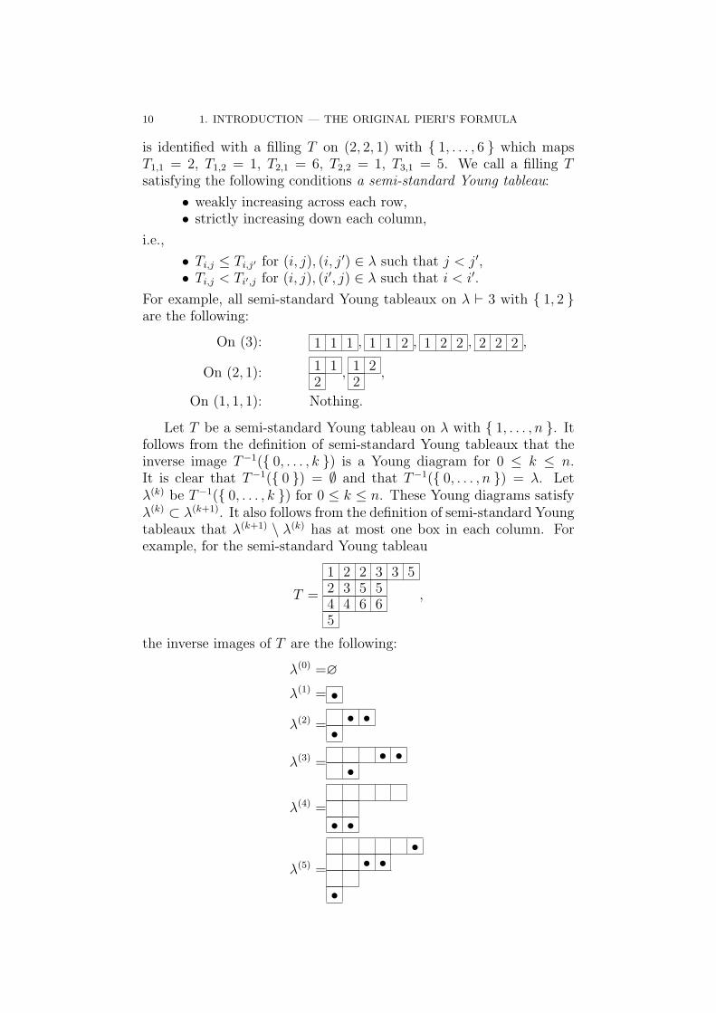
is identified with a filling T on (2, 2, 1) with { 1, . . . , 6 } which mapsT1,1 = 2, T1,2 = 1, T2,1 = 6, T2,2 = 1, T3,1 = 5. We call a filling Tsatisfying the following conditions a semi-standard Young tableau:
• weakly increasing across each row,• strictly increasing down each column,
i.e.,
• Ti,j ≤ Ti,j′ for (i, j), (i, j′) ∈ λ such that j < j′,• Ti,j < Ti′,j for (i, j), (i′, j) ∈ λ such that i < i′.
For example, all semi-standard Young tableaux on λ ` 3 with { 1, 2 }are the following:
On (3): 1 1 1 , 1 1 2 , 1 2 2 , 2 2 2 ,
On (2, 1): 1 12
, 1 22
,
On (1, 1, 1): Nothing.
Let T be a semi-standard Young tableau on λ with { 1, . . . , n }. Itfollows from the definition of semi-standard Young tableaux that theinverse image T−1({ 0, . . . , k }) is a Young diagram for 0 ≤ k ≤ n.It is clear that T−1({ 0 }) = ∅ and that T−1({ 0, . . . , n }) = λ. Letλ(k) be T−1({ 0, . . . , k }) for 0 ≤ k ≤ n. These Young diagrams satisfyλ(k) ⊂ λ(k+1). It also follows from the definition of semi-standard Youngtableaux that λ(k+1) \ λ(k) has at most one box in each column. Forexample, for the semi-standard Young tableau
T =
1 2 2 3 3 52 3 5 54 4 6 65
,
the inverse images of T are the following:
λ(0) =∅
λ(1) = •
λ(2) = • ••
λ(3) = • ••
λ(4) =• •
λ(5) =
•• •
•
1. DEFINITION OF ORIGINAL SCHUR POLYNOMIALS 11
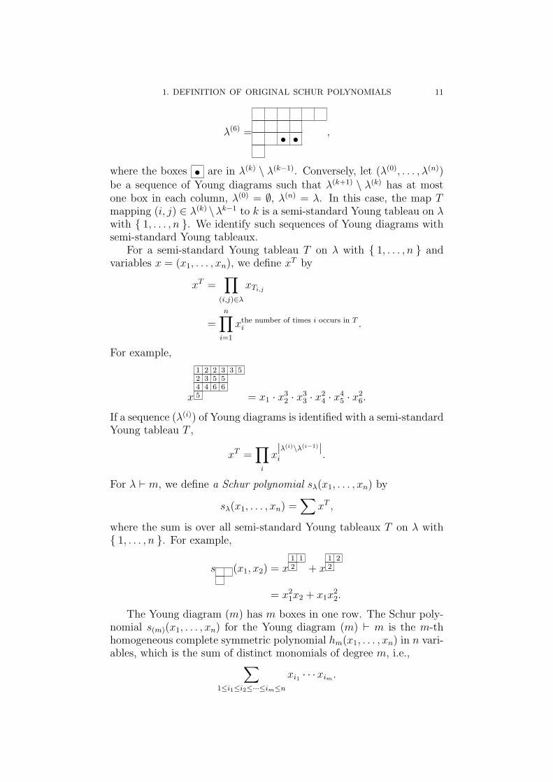
λ(6) = • • ,
where the boxes • are in λ(k) \ λ(k−1). Conversely, let (λ(0), . . . , λ(n))
be a sequence of Young diagrams such that λ(k+1) \ λ(k) has at mostone box in each column, λ(0) = ∅, λ(n) = λ. In this case, the map Tmapping (i, j) ∈ λ(k) \λk−1 to k is a semi-standard Young tableau on λwith { 1, . . . , n }. We identify such sequences of Young diagrams withsemi-standard Young tableaux.
For a semi-standard Young tableau T on λ with { 1, . . . , n } andvariables x = (x1, . . . , xn), we define xT by
xT =∏
(i,j)∈λ
xTi,j
=n∏
i=1
xthe number of times i occurs in Ti .
For example,
x
1 2 2 3 3 52 3 5 54 4 6 65 = x1 · x3
2 · x33 · x2
4 · x45 · x2
6.
If a sequence (λ(i)) of Young diagrams is identified with a semi-standardYoung tableau T ,
xT =∏
i
x|λ(i)\λ(i−1)|i .
For λ ` m, we define a Schur polynomial sλ(x1, . . . , xn) by
sλ(x1, . . . , xn) =∑
xT ,
where the sum is over all semi-standard Young tableaux T on λ with{ 1, . . . , n }. For example,
s (x1, x2) = x1 12 + x
1 22
= x21x2 + x1x
22.
The Young diagram (m) has m boxes in one row. The Schur poly-nomial s(m)(x1, . . . , xn) for the Young diagram (m) ` m is the m-thhomogeneous complete symmetric polynomial hm(x1, . . . , xn) in n vari-ables, which is the sum of distinct monomials of degree m, i.e.,
∑
1≤i1≤i2≤···≤im≤n
xi1 · · ·xim .
12 1. INTRODUCTION — THE ORIGINAL PIERI’S FORMULA
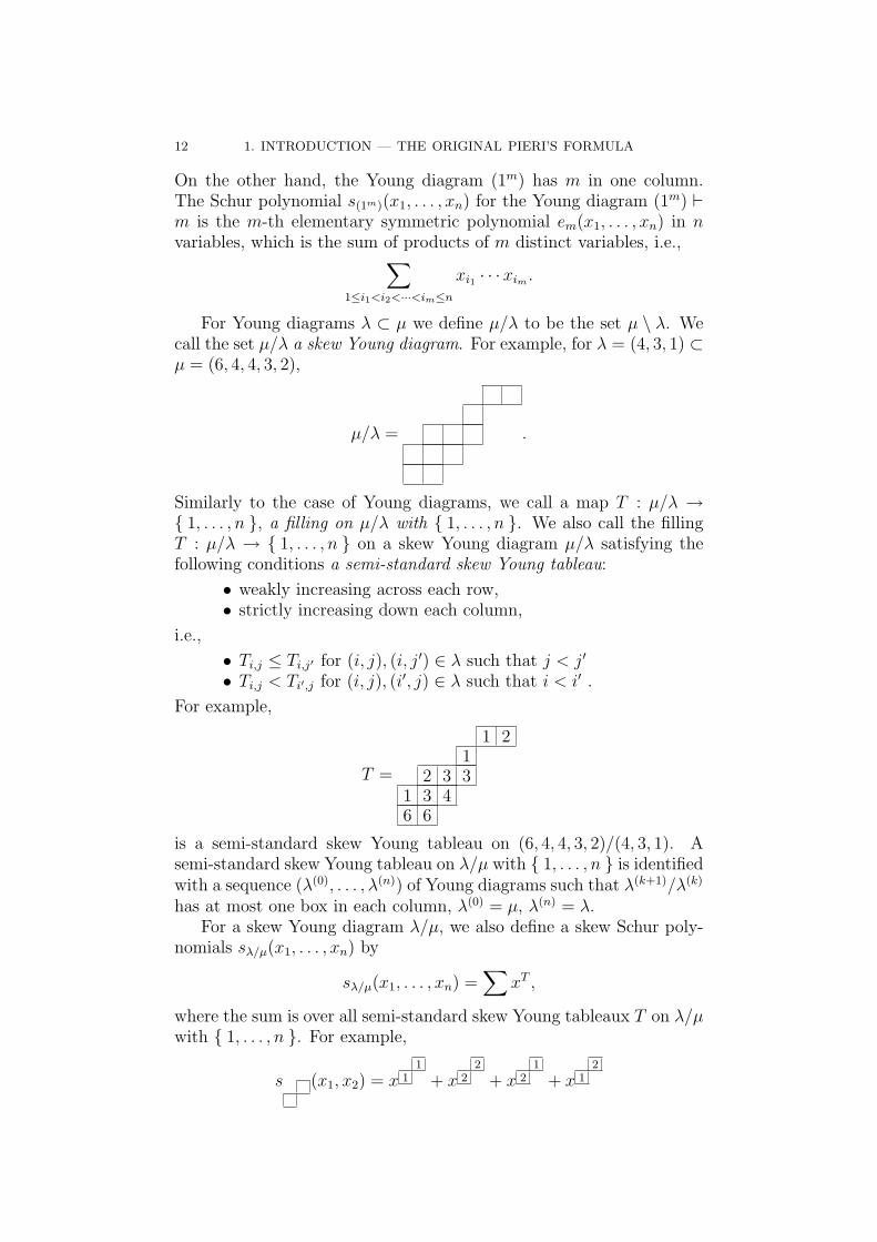
On the other hand, the Young diagram (1m) has m in one column.The Schur polynomial s(1m)(x1, . . . , xn) for the Young diagram (1m) `m is the m-th elementary symmetric polynomial em(x1, . . . , xn) in nvariables, which is the sum of products of m distinct variables, i.e.,
∑
1≤i1<i2<···<im≤n
xi1 · · ·xim .
For Young diagrams λ ⊂ µ we define µ/λ to be the set µ \ λ. Wecall the set µ/λ a skew Young diagram. For example, for λ = (4, 3, 1) ⊂µ = (6, 4, 4, 3, 2),
µ/λ = .
Similarly to the case of Young diagrams, we call a map T : µ/λ →{ 1, . . . , n }, a filling on µ/λ with { 1, . . . , n }. We also call the fillingT : µ/λ → { 1, . . . , n } on a skew Young diagram µ/λ satisfying thefollowing conditions a semi-standard skew Young tableau:
• weakly increasing across each row,• strictly increasing down each column,
i.e.,
• Ti,j ≤ Ti,j′ for (i, j), (i, j′) ∈ λ such that j < j′
• Ti,j < Ti′,j for (i, j), (i′, j) ∈ λ such that i < i′ .
For example,
T =
1 21
2 3 31 3 46 6
is a semi-standard skew Young tableau on (6, 4, 4, 3, 2)/(4, 3, 1). Asemi-standard skew Young tableau on λ/µ with { 1, . . . , n } is identifiedwith a sequence (λ(0), . . . , λ(n)) of Young diagrams such that λ(k+1)/λ(k)
has at most one box in each column, λ(0) = µ, λ(n) = λ.For a skew Young diagram λ/µ, we also define a skew Schur poly-
nomials sλ/µ(x1, . . . , xn) by
sλ/µ(x1, . . . , xn) =∑
xT ,
where the sum is over all semi-standard skew Young tableaux T on λ/µwith { 1, . . . , n }. For example,
s (x1, x2) = x1
1 + x2
2 + x1
2 + x2
1
2. PIERI’S FORMULA, CAUCHY IDENTITY AND SO ON 13
= x21 + x2
2 + 2x1x2.
2. Pieri’s formula, Cauchy identity and so on
In this section, we show some well-known formulae for the classicalSchur polynomials such as the classical Pieri’s formula. (See [5] for thepoofs of propositions in this section.)
Proposition 2.1 (Pieri’s formula). Schur polynomials and homo-geneous complete polynomials satisfy the equation:
sλ(x1, . . . , xn) · hi(x1, . . . , xn) =∑
µ
sµ(x1, . . . , xn),
where the sum is over all µ that are obtained from λ by adding i boxes,with no two in the same column.
Proposition 2.2 (dual Pieri’s formula). Schur polynomials andelementary polynomials satisfy the equation:
sλ(x1, . . . , xn) · ei(x1, . . . , xn) =∑
µ
sµ(x1, . . . , xn),
where the sum is over all µ that are obtained from λ by adding i boxes,with no two in the same row.
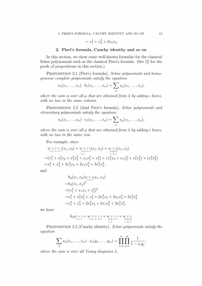
For example, since
s (x1, x2) + s (x1, x2) + s (x1, x2)
=(x41 + x3
1x2 + x21x
22 + x1x
32 + x4
2) + (x31x2 + x1x
32 + x2
1x22) + (x2
1x22)
=x41 + x4
2 + 2x31x2 + 2x1x
32 + 3x2
1x22,
and
h2(x1, x2)s (x1, x2)
=h2(x1, x2)2
=(x21 + x1x2 + x2
2)2
=x41 + x2
1x22 + x4
2 + 2x31x2 + 2x1x
32 + 2x2
1x22
=x41 + x4
2 + 2x31x2 + 2x1x
32 + 3x2
1x22,
we have
h2s = s + s + s .
Proposition 2.3 (Cauchy identity). Schur polynomials satisfy theequation
∑
λ
sλ(x1, . . . , xn) · sλ(y1, . . . , ym) =n∏
i=1
m∏
j=1
1
1 − xiyj
,
where the sum is over all Young diagrams λ.
14 1. INTRODUCTION — THE ORIGINAL PIERI’S FORMULA
Proposition 2.4 (Schur identity). Schur polynomials satisfy theequation
∑
λ
sλ(x1, . . . , xn) =∏
i
1
1 − xi
·∏
k<j
1
1 − xkxj
,
where the sum is over all Young diagrams λ.
3. Symmetric polynomials, Quasi-symmetric polynomials
In this section, we define quasi-symmetric polynomials and sym-metric polynomials. Then we define the ring of symmetric functionsand show the role of Schur function in the ring of symmetric functions.
First we define symmetric polynomials and quasi-symmetric poly-nomials.
Definition 3.1. The polynomial f(x1, . . . , xn) is said to be quasi-symmetric if the coefficients in f(x1, . . . , xn) of xj1
i1· · ·xjk
ikand xj1
i′1· · ·xjk
i′kare the same for ji ∈ N, i1 < · · · < ik and i′1 < · · · < i′k.
Definition 3.2. The polynomial f(x1, . . . , xn) is said to be sym-metric if the coefficients in f(x1, . . . , xn) of xj1
i1· · ·xjk
ikand xj1
i′1· · ·xjk
i′kare
the same for ji ∈ N, i1, . . . , ik and i′1, . . . , i′k such that il 6= il′ and i′l 6= i′l′
for l 6= l′. We write Λin for the Z-module generated by homogeneous
symmetric polynomials of degree i in Z[x1, . . . , xn].
Remark 3.3. This definition of symmetric polynomials is equiva-lent to the ordinary condition, i.e., f(x1, . . . , xn) = f(xσ(1), . . . , xσ(n))for all σ ∈ Sn, where Sn denotes the n-th symmetric group.
For example, f(x1, x2, x3) = x1x22 + x2x
23 + x1x
23 is not symmetric
but quasi-symmetric. Schur polynomials are symmetric.
Remark 3.4. By definition, all symmetric polynomials are quasi-symmetric.
Next we define some families of symmetric polynomials. We definethe Newton power sum polynomials pi(x1, . . . , xn) by
pi(x1, . . . , xn) = xi1 + · · · + xi
n.
For a Young diagram λ ` m, we define hλ(x1, . . . , xn), eλ(x1, . . . , xn)and pλ(x1, . . . , xn), by
hλ(x1, . . . , xn) =∏
i
hλi(x1, . . . , xn),
eλ(x1, . . . , xn) =∏
i
eλi(x1, . . . , xn),
pλ(x1, . . . , xn) =∏
i
pλi(x1, . . . , xn).
3. SYMMETRIC POLYNOMIALS, QUASI-SYMMETRIC POLYNOMIALS 15
For a Young diagram λ ` m such that λn+1 = 0, we also define themonomial symmetric polynomial mλ(x1, . . . , xn) to be the sum of alldistinct monomials obtained from xλ1
1 · · ·xλnn by permuting all the vari-
ables.
Proposition 3.5. The following are Z-bases for the homogeneoussymmetric polynomials Λi
n of degree i in n variables:
• { mλ(x1, . . . , xn) λ ` i, λn+1 = 0 }• { sλ(x1, . . . , xn) λ ` i, λn+1 = 0 }• { hλ(x1, . . . , xn) λ ` i, λn+1 = 0 }• { hλ(x1, . . . , xn) λ ` i, λ1 ≤ n }• { eλ(x1, . . . , xn) λ ` i, λ1 ≤ n }
The direct sum Λn =⊕
i≥0 Λin has a structure of a graded ring. For
f(x1, . . . , xn, xn+1) ∈ Λn+1, f(x1, . . . , xn, 0) is in Λn. This restriction isa homomorphism from Λn+1 to Λn of rings. In general, for m ≥ n, themap ρm,n : Λm → Λn mapping f(x1, . . . , xm) to f(x1, . . . , xn, 0 . . .)is a ring homomorphism, and the map ρi
m,n : Λim → Λi
n mappingf(x1, . . . , xm) to f(x1, . . . , xn, 0, . . .) is a module homomorphism. Themaps ρi
m,n and ρm,n are surjective. For m ≥ n ≥ i, ρim,n is bijective.
For each i ≥ 0, ({ Λin } ,
{ρi
m,n
}) is a projective system of modules. We
define Λi to be the inverse limit lim←−Λin. We write sλ for the element in
Λi whose image in Λin is the Schur polynomial sλ(x1, . . . , xn) for each
n. Similarly, we define hλ, eλ and so on.
Proposition 3.6. The following are Z-bases for Λi:
• { mλ λ ` i }• { sλ λ ` i }• { hλ λ ` i }• { eλ λ ` i }.
We define Λ to be the direct sum⊕
i Λi. It is clear that Λ has a
structure of a graded ring. We call the ring Λ the ring of symmetricfunctions in countably many independent variables x1, x2, . . ..
Proposition 3.7. The following are Z-bases for Λ:
• { mλ λ ` i, i ∈ N }• { sλ λ ` i, i ∈ N }• { hλ λ ` i, i ∈ N }• { eλ λ ` i, i ∈ N }.
Remark 3.8. The ring Λ is not the inverse limit Λ = lim←−Λn of the
projective system ({ Λn } , { ρm,n }) in the category of rings, but theinverse limit in the category of graded rings. For example,
∏∞i=1(1 +
xi) 6∈ Λ while∏∞
i=1(1 + xi) ∈ Λ.


CHAPTER 2
Pieri’s formula — main results and their proofs
In this chapter, we recall generalized Schur operators defined byFomin [4] and define polynomials determined by generalized Schur op-erators. In a prototypical example of generalized Schur operators, thesepolynomials are Schur polynomials. We show analogues of Pieri’s for-mula and Cauchy identity for them.
1. Generalized Schur Operators
In this section, we recall generalized Schur operators defined byFomin [4]. Then we consider the relations between other combinatorialoperators and generalized Schur operators.
1.1. Definition and Notation. Let K be a field of characteristiczero that contains all formal power series of variables t, t′, t1, t2, . . . LetVi be finite-dimensional K-vector spaces for all i ∈ Z. Fix a basisYi of each Vi so that Vi = KYi. Let Y =
∐i Yi, V =
⊕i Vi and
V =∏
i Vi, i.e., V is the vector space consisting of all finite linear
combinations of elements of Y and V is the vector space consistingof all linear combinations of elements of Y . The rank function on Vmapping v ∈ Vi to i is denoted by ρ. We say that Y has a minimum∅ if Yi = ∅ for i < 0 and Y0 = { ∅ }.
For a sequence { Ai } and a formal variable x, we write A(x) forthe generating function
∑i≥0 Aix
i.
Definition 1.1. We call D(t1) · · ·D(tn) and U(tn) · · ·U(t1) gen-eralized Schur operators with { am } if the following conditions aresatisfied:
• { am } is a sequence of elements of K.• Ui is a linear map on V satisfying Ui(Vj) ⊂ Vj+i for all j.• Di is a linear map on V satisfying Di(Vj) ⊂ Vj−i for all j.• The equation D(t′)U(t) = a(tt′)U(t)D(t′) holds.
Remark 1.2. The equation
D(t′)U(t) = a(tt′)U(t)D(t′)
is equivalent to the equations
DiUj =
min { i,j }∑
k=0
akUj−kDi−k
17
18 2. PIERI’S FORMULA — MAIN RESULTS AND THEIR PROOFS
for all i, j. Since D0U0 = a0U0D0, a0 = 1 in the case where U0 or D0 isI.
Remark 1.3. In general, D(t1) · · ·D(tn) and U(tn) · · ·U(t1) are not
linear operators on V but linear operators from V to V .
We define 〈 , 〉 to be the natural pairing, i.e., the bilinear form on
V × V such that 〈∑
λ∈Y aλλ,∑
µ∈Y bµµ〉 =∑
λ∈Y aλbλ.
For generalized Schur operators D(t1) · · ·D(tn) and U(tn) · · ·U(t1),U∗
i and D∗i denote the maps obtained from the adjoints of Ui and Di
with respect to 〈 , 〉 by restricting to V , respectively. For all i, U∗i and
D∗i are linear maps on V satisfying U∗
i (Vj) ⊂ Vj−i and D∗i (Vj) ⊂ Vj+i.
By definition,
〈v, Uiw〉 = 〈w, U∗i v〉, 〈v, Diw〉 = 〈w,D∗
i v〉
for v, w ∈ V . We write U∗(t) and D∗(t) for∑
U∗i ti and
∑D∗
i ti,
respectively. By definition,
〈U(t)µ, λ〉 = 〈U∗(t)λ, µ〉, 〈D(t)µ, λ〉 = 〈D∗(t)λ, µ〉for λ, µ ∈ Y . The equation D(t′)U(t) = a(tt′)U(t)D(t′) impliesthe equation U∗(t′)D∗(t) = a(tt′)D∗(t)U∗(t′). Hence U∗(t1) · · ·U∗(tn)and D∗(tn) · · ·D∗(t1) are generalized Schur operators with { am } whenD(t1) · · ·D(tn) and U(tn) · · ·U(t1) are.
Example 1.4. Our prototypical example is Young’s lattice Y thatconsists of all Young diagrams. Let Y be Young’s lattice Y, V theK-vector space KY whose basis is Y, and ρ the ordinary rank functionmapping a Young diagram λ to the number of boxes in λ. Young’slattice Y has a minimum ∅, the Young diagram with no boxes. Wecall a skew Young diagram µ/λ a horizontal strip if µ/λ has no twoboxes in the same column. Define Ui by Ui(µ) =
∑λ λ, where the sum
is over all λ’s that are obtained from µ by adding a horizontal stripconsisting of i boxes; and define Di by Di(λ) =
∑µ µ, where the sum
is over all µ’s that are obtained from λ by removing a horizontal stripconsisting of i boxes. For example,
D27−→ +
U27−→ + + + .
(See also Figure 2, the graph of D1 (U1) and D2 (U2).)In this case, the equation
D(t)U(t′) =1
1 − tt′U(t′)D(t)
holds. Equivalently, D(t1) · · ·D(tn) and U(tn) · · ·U(t1) are generalizedSchur operators with { am = 1 }. For example, since
U27−→ + +

1. GENERALIZED SCHUR OPERATORS 19
D17−→ + ( + ) +
D07−→U17−→ +
D17−→U27−→ + ,
we have
D1U2 = (U1D0 + U2D1) .
Example 1.5. Our second example is the polynomial ring K[x]with a variable x. Let V be K[x] and ρ the ordinary rank functionmapping a monomial axn to its degree n. Fix a basis Y = { cix
i }. Inthis case, dim Vi = 1 for all i ≥ 0 and dim Vi = 0 for i < 0. Hence itsbasis Y is identified with N and has a minimum c0, nonzero constant.Define Di and Ui by ∂i
i!and xi
i!, where ∂ is the partial differential oper-
ator in x. Then D(t) and U(t) are exp(t∂) and exp(tx), respectively.Since D(t) and U(t) satisfy
D(t)U(t′) = exp(tt′)U(t′)D(t),
D(t1) · · ·D(tn) and U(tn) · · ·U(t1) are generalized Schur operators with{am = 1
m!
}. In general, for differential posets or dual graphs, we can
construct generalized Schur operators in a similar manner. (See alsoSection 1.2.1 for the definitions of differential posets and dual graphs.)
Remark 1.6. In [4], Fomin introduced generalized Schur operators,and constructed an algorithm which is a generalization of Robinson-Schensted-Knuth correspondence, the correspondence between certainmatrices and pairs of semi-standard tableaux.
1.2. Relations between some combinatorial operators andgeneralized Schur operators. In this subsection, we consider re-lations between generalized Schur operators and some combinatorialoperators. Particularly, we consider differential posets, dual graphs,operators in [12] and operators in Lam [8].
1.2.1. Differential posets and dual graphs. We recall the definitionsof r-differential posets and Fomin’s r-dual graphs. Then we considerthe relations between them and generalized Schur operators.
An oriented graph is a quadruple G = (Y, E, start, end), where
• Y is a discrete set of vertices,• E is a discrete set of edges (or arcs),• start is a map from E to V of start point,• end is a map from E to V of end point,• the multiplicity |{ a ∈ E start(a) = x, end(a) = y }| for each
edges is finite.

20 2. PIERI’S FORMULA — MAIN RESULTS AND THEIR PROOFS
A graph G = (Y, E, start, end) is said to be simple if the multiplicityof any edge is 1 (or 0). For simple graph G = (Y,E, start, end), weoften identify E with the set E ′ = { (start(a), end(a)) ∈ Y 2 a ∈ E },and shortly write G = (Y, E ′).
A semi-graded graph is a quintuple G = (Y, ρ, E, start, end), where
• (Y,E, start, end) is an oriented graph,• ρ : Y → Z is a map of rank function satisfying
– for any edge a ∈ E, ρ(start(a)) ≤ ρ(end(a)),– start(a) = end(a) if a ∈ E, ρ(start(a)) = ρ(end(a)).
We write Yi for ρ−1({ i }).For a semi-graded graph G = (Y, ρ, E, start, end), we define Gi =
(Y, ρ, Ei, start, end) by
Ei = { a ∈ E ρ ◦ start(a) + i = ρ ◦ end(a) } .
Remark 1.7. For a semi-graded graph G = (Y, ρ, E, start, end),the subgraph Gi = (Y, ρ, Ei, start, end) is semi-graded for each i.
A graded oriented graph is a quintuple G = (Y, ρ, E, start, end),where
• (Y,E, start, end) is an oriented graph,• ρ : Y → Z is a map of rank function satisfying ρ(start(a))+1 =
ρ(end(a)) for any edge a ∈ E.
Remark 1.8. A semi-graded graph G is graded if and only if G =G1. For a semi-graded graph G, the subgraph of G1 is always graded.
For a semi-graded oriented graph G = (Y, ρ, E, start, end), we define
up and down operators UG, DG ∈ End(KV ), (or End(KV )) associatedwith the graph G for x ∈ V by
UGx =∑
a∈E,start(a)=x
end(a)
and
DGx =∑
a∈E,end(a)=x
start(a).
Let G = (Y, ρ, U, start, end) and G′ = (Y, ρ, D, start, end) be a pairof graded graphs with a common vertex set Y and a common rank func-tion ρ. The pair (G,G′) of graphs is said to be r-dual if the followingcommuting relation of up and down operators holds:
DG′UG − UGDG′ = rI,
where I is the identity, and r ∈ Z.If G and G′ are the same simple graded graphs, the pair (G,G′)
is determined by a certain poset P . Furthermore, if (G,G) is r-dual,then the poset P is said to be r-differential.
1. GENERALIZED SCHUR OPERATORS 21
In [17,18], Stanley introduced r-differential posets and showed enu-merative results by using linear algebraic methods and some methodsof solvable differential equations. In [1–3], Fomin introduced r-dualgraphs, generalizations of r-differential posets, and constructed an algo-rithm which is a generalization of Robinson correspondence, the corre-spondence between permutations and pairs of standard tableaux whoseshapes are the same Young diagram. This algorithm gives combinato-rial proofs for some of the Stanley’s results.
Let (G = (Y, ρ, U , start, end), G′ = (Y, ρ, D, start, end)) be a pair ofsemi-graded graphs. Let Di be the down operator DG′
iand Ui the up
operator UGi. We consider the case where D(t′) and U(t) are general-
ized Schur operators with { ai } satisfying D0 = U0 = I. Let
G =(Y, ρ, U, start, end)
=(Y, ρ, U1, start, end)
and
G′ =(Y, ρ, D, start, end)
=(Y, ρ, D1, start, end).
Since D(t′) and U(t) are generalized Schur operators with { ai }, theequation
D1U1 + U1D1 = a1U0D0 = a1I
holds. Hence (G, G′) is a1-dual, i.e., the equation
DG′UG + UGDG′ = a1I.
holds.Conversely, (G,G′) be a0-dual graphs. Let D(t′) = exp(DG′ ·t′) and
U(t) = exp(UG · t) In this case, D(t′) and U(t) are generalized Schuroperators. See also Example 1.5.
1.2.2. Operators in [12]. We recall the operators in [12] and con-sider the relation between these operators and generalized Schur oper-ators.
Let G = (Y, ρ, U, start, end) be a graded graph, and G′ = (Y, ρ,D,start, end) a semi-graded graphs with a common vertex set Y and acommon rank function ρ. In [12], the pairs (G,G′) whose up and downoperators satisfy the following commuting relation are considered:
DG′UG − UGDG′ = rDG′ ,
where r ∈ Z. In [12], an analogue of the Robinson-Schensted correspon-dence, a correspondence between words and pairs of a semi-standardYoung tableau and a standard Young tableau, was constructed forpaths of such pairs of graded graph and a semi-graded graph.
22 2. PIERI’S FORMULA — MAIN RESULTS AND THEIR PROOFS
Let (G = (Y, ρ, U , start, end), G′ = (Y, ρ, D, start, end)) be a pair ofsemi-graded graphs. Let Di be the down operator DG′
iand Ui the up
operator UGi. We consider the case where D(t′) and U(t) are general-
ized Schur operators with { ai } satisfying D0 = U0 = I. In this case,the operators U1 and Di satisfy the equations
Di+1U1 + U1Di+1 = a1Di
for all i ∈ Z. Hence, the operators UG and DG′ satisfy the equation
DG′UG1− UG1
DG′ = a1DG′ .
Conversely, Let G = (Y, ρ, U, start, end) be a graded graph andG′ = (Y, ρ, D, start, end) a semi-graded graph with a common vertexset Y and a common rank function ρ satisfying
DG′UG − UGDG′ = a0DG′ .
Let D(t′) be exp(DG′ · t′) and U(t) the generating function∑
i UGiti In
this case, D(t′) and U(t) are generalized Schur operators.1.2.3. Lam’s operator. In [8], Lam introduced a generalization of
the Boson-Fermion correspondence. In the paper, he also showedPieri’s and Cauchy’s formulae for some families of symmetric func-tions in the context of Heisenberg algebras, i.e., the algebra defined bythe generators { Bi i ∈ Z } and the relations
[Bl, B−l] = l · bl · I (l > 0),
[Bk, Bl] = 0 (l 6= −k),
B0 = I,
where bl are scalar and I is the identity.Some important families of symmetric functions, e.g., Schur func-
tions, Hall-Little wood polynomials, Macdonald polynomials and soon, are examples of them. He proved Pieri’s formula using essentiallythe same method as ours. Since the assumptions of generalized Schuroperators are less than those of Heisenberg algebras, our polynomi-als are more various than his; e.g., some of our polynomials are notsymmetric. An example of generalized Schur operators which providesnon-symmetric polynomials is in Section 3. Here we consider the rela-tion between [8] and ours.
First we construct operators Bl from generalized Schur operatorsD(t1) · · ·D(tn) and U(tn) · · ·U(t1). These operators Bl are closely re-lated to the results of Lam [8]. Furthermore we can construct othergeneralized Schur operators D(t1) · · ·D(tn) and U ′(tn) · · ·U ′(t1) fromBl.
Let D(t1) · · ·D(tn) and U(tn) · · ·U(t1) be generalized Schur op-erators with { am }. For a partition λ ` l, we define zλ by zλ =1m1(λ)m1(λ)! ·2m2(λ)m2(λ)! · · · , where mi(λ) = |{ j λj = i }|. Let U0 =

2. DEFINITION OF OUR POLYNOMIALS 23
D0 = I, where I is the identity map. For positive integers l, we induc-tively define bl, Bl and B−l by
bl =al −∑
λ
bλ
zλ
,
Bl =Dl −∑
λ
Bλ
zλ
,
B−l =Ul −∑
λ
B−λ
zλ
,
where bλ = bλ1 · bλ2 · · · , Bλ = Bλ1 · Bλ2 · · · , B−λ = B−λ1 · B−λ2 · · · andthe sums are over all partitions λ of l such that λ1 < l. Let bl 6= 0 forany l. It follows from direct calculations that
[Bl, B−l] = l · bl · I,
[Bl, B−k] = 0
for positive integers l 6= k. If Ui and Di respectively commute with Uj
and Dj for all i, j, then { Bl, B−l l ∈ Z>0 } generates the Heisenbergalgebra. In this case, we can apply the results of Lam [8]. See also Re-mark 2.11 for the relation between his complete symmetric polynomi-als hi[bm](t1, . . . , tn) and our weighted complete symmetric polynomials
h{ am }i (t1, . . . , tn).
For a partition λ ` l, let sgn(λ) denote (−1)P
i(λi−1), where thesum is over all i’s such that λi > 0. Although Ui and Di do not com-mute with Uj and Dj, we can define dual generalized Schur operatorsD(t1) · · ·D(tn) and U ′(tn) · · ·U ′(t1) with { a′
m } by
a′l =
∑
λ
sgn(λ)bλ
zλ
,
U ′−l =
∑
λ
sgn(λ)B−λ
zλ
,
where the sums are over all partitions λ of l. In this case, it followsfrom direct calculations that a(t) · a′(−t) = 1.
2. Definition of Our Polynomials
We introduce two types of polynomials in this section. One is ageneralization of Schur polynomials. The other is a generalization ofcomplete symmetric polynomials.
2.1. Generalized Schur Polynomials. We define a generaliza-tion of Schur polynomials as expansion coefficients of generalized Schuroperators. The polynomials for the prototypical example Y are skewSchur polynomials.
24 2. PIERI’S FORMULA — MAIN RESULTS AND THEIR PROOFS
Definition 2.1. Let D(t1) · · ·D(tn) and U(tn) · · ·U(t1) be general-ized Schur operators with { am }. For v ∈ V and µ ∈ Y , sD
v,µ(t1, . . . , tn)and sµ,v
U (t1, . . . , tn) are respectively defined by
sDv,µ(t1, . . . , tn) = 〈D(t1) · · ·D(tn)v, µ〉,
sµ,vU (t1, . . . , tn) = 〈U(tn) · · ·U(t1)v, µ〉.
We call these polynomials sDv,µ(t1, . . . , tn) and sµ,v
U (t1, . . . , tn) generalizedSchur polynomials.
Remark 2.2. Generalized Schur polynomials sDv,µ(t1, . . . , tn) are
symmetric in the case where D(t)D(t′) = D(t′)D(t), but not symmet-ric in general. Similarly, generalized Schur polynomials sµ,v
U (t1, . . . , tn)are symmetric if U(t)U(t′) = U(t′)U(t).
Remark 2.3. Generalized Schur polynomials sDv,µ(t1, . . . , tn) are
quasi-symmetric if D0 is the identity map, but not quasi-symmetricin general. Similarly, generalized Schur polynomials sµ,v
U (t1, . . . , tn) arequasi-symmetric if U0 is the identity map.
Example 2.4. We consider the prototypical example (Example1.4), i.e., Y is the Young ’s lattice Y; Ui(µ) is the sum over all λ’sthat are obtained from µ by adding a horizontal strip consisting ofi boxes; Di(λ) is the sum over all µ’s that are obtained from λ byremoving a horizontal strip consisting of i boxes.
In this case, the operators D(t1) · · ·D(tn) and U(tn) · · ·U(t1) aregeneralized Schur operators with { am = 1 }. Both sD
λ,µ(t1, . . . , tn) and
sλ,µU (t1, . . . , tn) are equal to the skew Schur polynomial sλ/µ(t1, . . . , tn)
for λ, µ ∈ Y. For example, since
D(t2) = + t2 + t2 + t22
D(t1)D(t2) = + t1 + t1 + t21
+ t2( + t1 ) + t2( + t1 + t21∅)
+ t22( + t1∅),
sD(2,1),∅(t1, t2) = s(2,1)(t1, t2) = t21t2 + t1t
22.
Example 2.5. We consider the second example N (Example 1.5,K[x]). Since ∂ and x commute with t, the following equations hold:
D(t1) · · ·D(tn) = exp(∂t1) · · · exp(∂tn) = exp(∂(t1 + · · · + tn)),
U(tn) · · ·U(t1) = exp(xtn) · · · exp(xt1) = exp(x(t1 + · · · + tn)).
It follows from direct calculations that
exp(∂(t1 + · · · + tn))cixi =
i∑
j=0
(t1 + · · · + tn)j
j!
i!
(i − j)!cix
i−j
2. DEFINITION OF OUR POLYNOMIALS 25
=i∑
j=0
i!(t1 + · · · + tn)jci
(i − j)!j!ci−j
ci−jxi−j,
exp(x(t1 + · · · + tn))cixi =
∑
j
(t1 + · · · + tn)jxj
j!cix
i
=∑
j
(t1 + · · · + tn)jci
j!ci+j
ci+jxi+j.
Hence it follows that
sDci+jxi+j ,cixi(t1, . . . , tn) =
(i + j)!
i!j!
ci+j
ci
(t1 + . . . + tn)j
sci+jxi+j ,cix
i
U (t1, . . . , tn) =1
j!
ci
ci+j
(t1 + . . . + tn)j,
if we take { cixi } as the basis Y .
If ci = 1 for all i, then sDxi+j ,xi(t1, . . . , tn) = (i+j)!
i!j!(t1 + . . .+ tn)j, and
sxi+j ,xi
U (t1, . . . , tn) = 1j!(t1 + . . . + tn)j.
Lemma 2.6. Generalized Schur polynomials satisfy the followingequations:
sDλ,µ(t1, . . . , tn) = sλ,µ
D∗ (t1, . . . , tn),
sλ,µU (t1, . . . , tn) = sU∗
λ,µ(t1, . . . , tn)
for λ, µ ∈ Y . Generalized Schur polynomials also satisfy the followingequations:
sDv,µ(t1, . . . , tn) =
∑
ν∈Y
〈v, ν〉sν,µD∗(t1, . . . , tn),
sµ,vD∗(t1, . . . , tn) =
∑
ν∈Y
〈v, ν〉sDµ,ν(t1, . . . , tn),
sU∗
v,µ(t1, . . . , tn) =∑
ν∈Y
〈v, ν〉sν,µU (t1, . . . , tn),
sµ,vU (t1, . . . , tn) =
∑
ν∈Y
〈v, ν〉sU∗
µ,ν(t1, . . . , tn)
for µ ∈ Y , v ∈ V .
Proof. It follows by definition that
sDλ,µ(t1, . . . , tn) = 〈D(t1) · · ·D(tn)λ, µ〉
= 〈D∗(tn) · · ·D∗(t1)µ, λ〉 = sλ,µD∗ (t1, . . . , tn).
It also follows by definition that
sλ,µU (t1, . . . , tn) = 〈U(tn) · · ·U(t1)µ, λ〉
= 〈U∗(t1) · · ·U∗(tn)λ, µ〉 = sU∗
λ,µ(t1, . . . , tn)

26 2. PIERI’S FORMULA — MAIN RESULTS AND THEIR PROOFS
for λ, µ ∈ Y .Since v =
∑ν∈Y 〈ν, v〉ν for v ∈ V , the following equations hold:
sDv,µ(t1, . . . , tn) =
∑
ν∈Y
〈v, ν〉sν,µD∗(t1, . . . , tn),
∑
ν∈Y
〈v, ν〉sDµ,ν(t1, . . . , tn) = sµ,v
D∗(t1, . . . , tn),
∑
ν∈Y
〈v, ν〉sν,µU (t1, . . . , tn) = sU∗
v,µ(t1, . . . , tn),
sµ,vU (t1, . . . , tn) =
∑
ν∈Y
〈v, ν〉sU∗
µ,ν(t1, . . . , tn)
for µ ∈ Y , v ∈ V . ¤2.2. Weighted Complete Symmetric Polynomials. Next we
introduce a generalization of complete symmetric polynomials. Wedefine weighted symmetric polynomials inductively.
Definition 2.7. Let { am } be a sequence of elements of K. We de-
fine the i-th weighted complete symmetric polynomial h{ am }i (t1, . . . , tn)
by
h{ am }i (t1, . . . , tn) =
aiti1 (for n = 1),
i∑
j=0
h{am}j (t1, . . . , tn−1)h
{ am }i−j (tn) (for n > 1).
(1)
By definition, for each i, the i-th weighted complete symmetric
polynomial h{am}i (t1, . . . , tn) is a homogeneous symmetric polynomial
of degree i.
Remark 2.8. In general, the formal power series∑
i h{am}i (t) equals
the generating function a(t) =∑
aiti by the definition of weighted com-
plete symmetric polynomials. Since the weighted complete symmetricpolynomials satisfy the equation (1), we have
a(t1) · · · a(tn−1)a(tn) =∑
i
h{am}i (t1, . . . , tn−1)
∑
j
h{am}j (tn)
=∑
i
i∑
k=0
h{ am }i−k (t1, . . . , tn−1)h
{ am }k (tn)
=∑
i
h{ am }i (t1, . . . , tn),
if a(t1) · · · a(tn−1) =∑
h{am}i (t1, . . . , tn−1). Hence
a(t1) · · · a(tn) =∑
i
h{am}i (t1, . . . , tn).
3. PIERI’S FORMULA AND CAUCHY’S FORMULA 27
Example 2.9. When am equals 1 for each m, h{1,1,...}j (t1, . . . , tn)
equals the complete symmetric polynomial hj(t1, . . . , tn). In this case,the formal power series
∑i hi(t) equals the generating function a(t) =∑
i ti = 1
1−t.
Example 2.10. When am equals 1m!
for each m, h{ 1
m!}
j (t1, . . . , tn) =
1j!(t1 + · · · + tn)j and
∑j h
{ 1m!
}j (t) = exp(t) = a(t).
Remark 2.11. Let {bm} be a sequence of elements of K. We definehi[bm](t1, . . . , tn) by
hi[bm](t1, . . . , tn) =∑
λ`i
bλpλ(t1, . . . , tn)
zλ
,
where bλ = bλ1 ·bλ2 · · · , pλ(t1, . . . , tn) = pλ1(t1, . . . , tn)·pλ2(t1, . . . , tn) · · ·and pi(t1, . . . , tn) = ti1+· · ·+tin. These polynomials satisfy the equation
hi[bm](t1, . . . , tn) =i∑
j=0
hj[bm](t1, . . . , tn−1)hi−j[bm](tn).
Let ai =∑
λ`ibλ
zλ. Then it follows hi[bm](t1) = ait
i. Hence
hi[bm](t1, . . . , tn) = h{am}i (t1, . . . , tn).
3. Pieri’s formula and Cauchy’s formula
In this section, we show some properties of generalized Schur poly-nomials and weighted complete symmetric polynomials.
Throughout this section, let D(t1) · · ·D(tn) and U(tn) · · ·U(t1) begeneralized Schur operators with {am}.
3.1. Statements of Pieri’s formula and Cauchy’s formula.In Proposition 3.1, we describe the commuting relation of Ui andD(t1) · · ·D(tn), proved in Section 3.3. This relation implies Pieri’s for-mula for our polynomials (Theorem 3.2), the main result. It also followsfrom this relation that the weighted complete symmetric polynomialsare written as linear combinations of generalized Schur polynomialswhen Y has a minimum (Proposition 3.6).
First we describe the commuting relation of Ui and D(t1) · · ·D(tn).We prove it in Section 3.3.
Proposition 3.1. The equations
D(t1) · · ·D(tn)Ui =i∑
j=0
h{am}i−j (t1, . . . , tn)UjD(t1) · · ·D(tn)
hold for all i.
These equations imply the following main theorem.
28 2. PIERI’S FORMULA — MAIN RESULTS AND THEIR PROOFS
Theorem 3.2 (Pieri’s formula). For each µ ∈ Yk and each v ∈ V ,generalized Schur polynomials satisfy
sDUiv,µ(t1, . . . , tn) =
i∑
j=0
h{am}i−j (t1, . . . , tn)
∑
ν∈Yk−j
〈Ujν, µ〉sDv,ν(t1, . . . , tn).
Proof. It follows from Proposition 3.1 that
〈D(t1) · · ·D(tn)Uiv, µ〉 = 〈i∑
j=0
h{am}i−j (t1, . . . , tn)UjD(t1) · · ·D(tn)v, µ〉
=i∑
j=0
h{am}i−j (t1, . . . , tn)〈UjD(t1) · · ·D(tn)v, µ〉
for v ∈ V and µ ∈ Y . This means
sDUiv,µ(t1, . . . , tn)
=i∑
j=0
h{am}i−j (t1, . . . , tn)
∑
ν∈Yk−j
〈Ujν, µ〉sDv,ν(t1, . . . , tn).
¤
This formula becomes simple in the case when v ∈ Y .
Corollary 3.3. For each λ, µ ∈ Y , generalized Schur polynomialssatisfy
sDUiλ,µ(t1, . . . , tn) =
i∑
j=0
h{am}i−j (t1, . . . , tn) · sλ,U∗
j µ
D∗ (t1, . . . , tn).
Proof. It follows from Theorem 3.2 that
sDUiλ,µ(t1, . . . , tn) =
i∑
j=0
h{am}i−j (t1, . . . , tn)
∑
ν∈Y
〈Ujν, µ〉sDλ,ν(t1, . . . , tn).
Lemma 2.6 implies∑
ν∈Y
〈Ujν, µ〉sDλ,ν(t1, . . . , tn) =
∑
ν∈Y
〈ν, U∗j µ〉sD
λ,ν(t1, . . . , tn)
= sλ,U∗
j µ
D∗ (t1, . . . , tn).
Hence
sDUiλ,µ(t1, . . . , tn) =
i∑
j=0
h{am}i−j (t1, . . . , tn) · sλ,U∗
j µ
D∗ (t1, . . . , tn).
¤
If Y has a minimum ∅, Theorem 3.2 implies the following corollary.
3. PIERI’S FORMULA AND CAUCHY’S FORMULA 29
Corollary 3.4. Let Y have a minimum ∅. For all v ∈ V , thefollowing equations hold:
sDUiv,∅(t1, . . . , tn) = u0 · h{am}
i (t1, . . . , tn) · sDv,∅(t1, . . . , tn),
where u0 is the element of K that satisfies U0∅ = u0∅.
Example 3.5. In the prototypical example Y (Example 1.4), forλ ∈ Y, Uiλ means the sum of all Young diagrams obtained from λ byadding i boxes, with no two in the same column. Hence the generalizedSchur polynomial sD
Uiλ,∅(t1, . . . , tn) equals∑
ν sν , where the sum is overall ν’s that are obtained from λ by adding i boxes, with no two in the
same column. On the other hand, u0 is 1, and h{1,1,1,...}i (t1, . . . , tn) is the
i-th complete symmetric polynomial hi(t1, . . . , tn) (Example 2.9). ThusCorollary 3.4 is nothing but the classical Pieri’s formula. Theorem 3.2means Pieri’s formula for skew Schur polynomials; for a skew Youngdiagram λ/µ and i ∈ N,
∑
κ
sκ/µ(t1, . . . , tn) =i∑
j=0
∑
ν
hi−j(t1, . . . , tn)sλ/ν(t1, . . . , tn),
where the first sum is over all κ’s that are obtained from λ by addingi boxes, with no two in the same column; the last sum is over all ν’sthat are obtained from µ by removing j boxes, with no two in the samecolumn.
In the case when Y has a minimum ∅, weighted complete symmetricpolynomials are written as linear combinations of generalized Schurpolynomials.
Proposition 3.6. Let Y have a minimum ∅. The following equa-tions hold for all i ≥ 0:
sDUi∅,∅(t1, . . . , tn) = dn
0u0 · h{am}i (t1, . . . , tn),
where d0, u0 are the elements of K that satisfy D0∅ = d0∅ and U0∅ =u0∅.
Proof. By definition, sD∅,∅(t1, . . . , tn) is dn
0 . Hence it follows fromCorollary 3.4 that
sDUi∅,∅(t1, . . . , tn) = u0h
{am}i (t1, . . . , tn)dn
0 .
¤Example 3.7. We consider the prototypical example Y (Example
1.4). In this case, Proposition 3.6 means that the Schur polynomial s(i)
corresponding to Young diagram with only one row equals the completesymmetric polynomial hi.
Example 3.8. In the second example N (Example 1.5), Proposition
3.6 means that the constant term of exp(∂(t1 + · · · + tn)) · xi
i!equals
(t1+···+tn)i
i!.

30 2. PIERI’S FORMULA — MAIN RESULTS AND THEIR PROOFS
Rewriting generalized Cauchy identity [4, 1.4. Corollary] with ournotation, we obtain Cauchy’s formula for generalized Schur polynomi-als.
Theorem 3.9. The equations∑
ν∈Y
sDν,µ(t1, . . . , tn)sν,v
U (t′1, . . . , t′n)
=∏
i,j
a(tit′j)
∑
κ∈Y
sµ,κU (t′1, . . . , t
′n)sD
v,κ(t1, . . . , tn)
hold for v ∈ V , µ ∈ Y .
Theorem 3.9 implies the following corollary.
Corollary 3.10. Let Y have a minimum ∅. The equation∑
ν∈Y
sDν,∅(t1, . . . , tn)sν,∅
U (t′1, . . . , t′n)
= un0d
n0
∏
i,j
a(tit′j)
holds.
Example 3.11. In the prototypical example Y (Example 1.4), sinceai = 1 for all i, a(tjt
′j′) = 1
1−tjt′j′. Hence Corollary 3.10 is nothing but
the classical Cauchy identity,∑
ν∈Y
sν(t1, . . . , tn)sν(t′1, . . . , t
′n)
=∏
i,j
1
1 − tit′j.
Theorem 3.10 is Cauchy identity for skew Schur polynomials; for askew Young diagram λ/µ and i ∈ N,
∑
ν∈Y
sν/µ(t1, . . . , tn)sν/v(t′1, . . . , t
′n)
=∏
i,j
1
1 − tit′j
∑
κ∈Y
sµ/κ(t′1, . . . , t
′n)sλ/κ(t1, . . . , tn)
hold for λ, µ ∈ Y.
3.2. Some Variations of Pieri’s Formula. In this section, weshow some variations of Pieri’s formula for generalized Schur polyno-mials, i.e., we show Pieri’s formula not only for sD
•,•• but also for s•,•U •,s•,•D∗• and sU∗
•,••.The next proposition follows from Proposition 3.1.
3. PIERI’S FORMULA AND CAUCHY’S FORMULA 31
Proposition 3.12. The following equations hold:
DiU(tn) · · ·U(t1) =i∑
j=0
h{am}i−j (t1, . . . , tn)U(tn) · · ·U(t1)Dj,(2)
U∗i D(tn)∗ · · ·D∗(t1) =
i∑
j=0
h{am}i−j (t1, . . . , tn)D∗(tn) · · ·D∗(t1)U
∗j ,(3)
U∗(t1) · · ·U∗(tn)D∗i =
i∑
j=0
h{am}i−j (t1, . . . , tn)D∗
jU∗(t1) · · ·U∗(tn).(4)
Proof. It follows from Proposition 3.1 that
D(t1) · · ·D(tn)Ui =i∑
j=0
h{am}i−j (t1, . . . , tn)UjD(t1) · · ·D(tn).(5)
We obtain the equation (3) from the equation (5) by applying ∗.Since D(t1) · · ·D(tn) and U(tn) · · ·U(t1) are generalized Schur op-
erators with {am}, U∗(t1) · · ·U∗(tn) and D∗(tn) · · ·D∗(t1) are also gen-eralized Schur operators with {am}. Applying the equation (3) andProposition 3.1 to U∗(t1) · · ·U∗(tn) and D∗(tn) · · ·D∗(t1), we obtainthe equation (2) and (4), respectively. ¤
Theorem 3.13 (Pieri’s formula). For each µ ∈ Yk and each v ∈ V ,generalized Schur polynomials satisfy the following equations:
∑
κ∈Y
〈Diκ, µ〉sκ,vU (t1, . . . , tn)
=i∑
j=0
h{am}i−j (t1, . . . , tn)s
µ,DjvU (t1, . . . , tn),
sU∗
D∗i v,µ(t1, . . . ,tn)
=i∑
j=0
h{am}i−j (t1, . . . , tn)
∑
ν∈Yk−j
〈D∗jν, µ〉sU∗
v,ν(t1, . . . , tn),
∑
κ∈Y
〈U∗i κ, µ〉sκ,v
D∗(t1, . . . , tn)
=i∑
j=0
h{am}i−j (t1, . . . , tn)s
µ,U∗j v
D∗ (t1, . . . , tn).
Proof. Applying Theorem 3.2 to the generalized Schur operatorsU∗(t1) · · ·U∗(tn) and D∗(t1) · · ·D∗(tn), we obtain
sU∗
D∗i v,µ(t1, . . . , tn) =
i∑
j=0
h{am}i−j (t1, . . . , tn)
∑
ν∈Yk−j
〈D∗jν, µ〉sU∗
v,ν(t1, . . . , tn).

32 2. PIERI’S FORMULA — MAIN RESULTS AND THEIR PROOFS
It follows from Proposition 3.12 that
〈DiU(tn) · · ·U(t1)v, µ〉 = 〈i∑
j=0
h{am}i−j (t1, . . . , tn)U(tn) · · ·U(t1)Djv, µ〉
for v ∈ V and µ ∈ Y . This equation means
∑
κ∈Y
〈Diκ, µ〉sκ,vU (t1, . . . , tn) =
i∑
j=0
h{am}i−j (t1, . . . , tn)s
µ,DjvU (t1, . . . , tn).
For generalized Schur operators U∗(t1) · · ·U∗(tn) and D∗(tn) · · ·D∗(t1),this equation means
∑
κ∈Y
〈U∗i κ, µ〉sκ,v
D∗(t1, . . . , tn) =i∑
j=0
h{am}i−j (t1, . . . , tn)s
µ,U∗j v
D∗ (t1, . . . , tn).
¤Corollary 3.14. For all v ∈ V , the following equations hold:
sU∗
D∗i v,∅(t1, . . . , tn) = d0 · h{am}
i (t1, . . . , tn) · sU∗
v,∅(t1, . . . , tn),
where d0 is the element of K that satisfies D0∅ = d0∅.
Proof. We obtain this corollary by applying Theorem 3.4 to thegeneralized Schur operators U∗(t1, . . . , tn) and D∗(t1, . . . , tn). ¤
Proposition 3.15. Let Y have a minimum ∅. Then
sU∗
D∗i ∅,∅(t1, . . . , tn) = un
0d0 · h{am}i (t1, . . . , tn),
where u0 and d0 are the elements of K that satisfy D0∅ = d0∅ andU0∅ = u0∅.
Proof. We obtain this proposition by applying Theorem 3.6 to thegeneralized Schur operators U∗(t1) · · ·U∗(tn) and D∗(t1) · · ·D∗(tn). ¤
3.3. Proof of Proposition 3.1. In this section, we prove Propo-sition 3.1, i.e.,
D(t1) · · ·D(tn)Ui =i∑
j=0
h{am}i−j (t1, . . . , tn)UjD(t1) · · ·D(tn)
for all i.
Proof. Since D(t1) · · ·D(tn) and U(tn) · · ·U(t1) are generalized
Schur operators with {am}, the equations D(t)Ui =∑i
j=0 ajtjUi−jD(t)
hold for all integers i. Hence D(t1) · · ·D(tn)Ui is written as a K-linearcombination of UjD(t1) · · ·D(tn). We write Hi,j(t1, . . . , tn) for the co-efficient of UjD(t1) · · ·D(tn) in D(t1) · · ·D(tn)Ui.
It follows from the equation D(t)Ui =∑i
j=0 ajtjUi−jD(t) that
Hi,i−j(t1) = ajtj(6)
3. PIERI’S FORMULA AND CAUCHY’S FORMULA 33
for 0 ≤ j ≤ i.We apply the relation (6) to D(tn) and Ui to have
D(t1) · · ·D(tn−1)D(tn)Ui =i∑
j=0
ai−jti−jn D(t1) · · ·D(tn−1)UjD(tn).
Since D(t1) · · ·D(tn−1)Ui =∑
j Hi,j(t1, . . . , tn−1)UjD(t1) · · ·D(tn−1) by
the definition of Hi,j(t1, . . . , tn−1), the equation
i∑
j=0
ai−jti−jn D(t1) · · ·D(tn−1)UjD(tn)
=i∑
j=0
ai−jti−jn
j∑
k=0
Hj,k(t1, . . . , tn−1)UkD(t1) · · ·D(tn−1) · D(tn)
holds. It follows that
D(t1) · · ·D(tn−1)D(tn)Ui
=i∑
j=0
ai−jti−jn
j∑
k=0
Hj,k(t1, . . . , tn−1)UkD(t1) · · ·D(tn−1) · D(tn)
=i∑
k=0
i∑
j=k
ai−jti−jn Hj,k(t1, . . . , tn−1)UkD(t1) · · ·D(tn).
Since D(t1) · · ·D(tn)Ui equals
i∑
k=0
Hi,k(t1, . . . , tn)UkD(t1) · · ·D(tn)
by definition, the equation
i∑
k=0
i∑
j=k
ai−jti−jn Hj,k(t1, . . . , tn−1)UkD(t1) · · ·D(tn)
=i∑
k=0
Hi,k(t1, . . . , tn)UkD(t1) · · ·D(tn)
holds. Hence the equation
i∑
j=k
ai−jti−jn Hj,k(t1, . . . , tn−1) = Hi,k(t1, . . . , tn)(7)
holds.It follows from the relation (7) that
Hk+l,k(t1, . . . , tn) =k+l∑
j=k
ak+l−jtk+l−jn Hj,k(t1, . . . , tn−1)

34 2. PIERI’S FORMULA — MAIN RESULTS AND THEIR PROOFS
=l∑
j′=0
ak+l−(j′+k)tk+l−(j′+k)n Hj′+k,k(t1, . . . , tn−1)
=l∑
j′=0
al−j′tl−j′
n Hj′+k,k(t1, . . . , tn−1).
Since the monomials al−j′tl−j′n do not depend on k, the equations
H(i−k)+k,k(t1, . . . , tn) = H(i−k)+k′,k′(t1, . . . , tn)
hold if the equations Hk+j,k(t1, . . . , tn−1) = Hk′+j,k′(t1, . . . , tn−1) holdfor all k, k′ and j ≤ i − k. In fact, since Hi+k,k(t1) equals ait
i1,
Hi+k,k(t1) does not depend on k. Hence it follows inductively thatHi+k,k(t1, . . . , tn) does not depend on k, either. Hence we may write
Hi−j(t1, . . . , tn) for Hi,j(t1, . . . , tn).It follows from the equations (6) and (7) that{
Hi(t1) = aiti1 (for n = 1),
Hi(t1, . . . , tn) =∑i
k=0 Hi−k(t1, . . . , tn−1)Hk(tn) (for n > 1).
Since Hi(t1, . . . , tn) equals the i-th weighted complete symmetric poly-
nomial h{am}i (t1, . . . , tn), Proposition 3.1 follows. ¤
CHAPTER 3
Examples of Generalized Schur Operators
In this chapter, we consider some examples of generalized Schuroperators. In Section 1, we consider the Young’s lattice Y; we considerthe prototypical example again, and then we construct another exam-ple. In Section 2, we consider shifted shapes corresponding strict par-titions. Generalized Schur polynomials of this example are the Schur’sP -functions, Q-functions and their “skew” versions. Finally, in Section3, we consider an example concerning rooted planner binary trees.
1. Young’s Lattice
In this section we consider Young’s lattice Y that consists of allYoung diagrams again. First we give another definition of Young dia-gram. Then we consider prototypical example of Young’s lattice again.Finally we consider dual construction of prototypical example.
1.1. Definition. In this subsection, we define Young diagrams asan ideal of a poset.
Let A be the free commutative monoid of generated by the alphabet{ 1, 2 }, i.e., A = { 1i2j i, j ∈ N }. We often write (i, j) for 1i2j. Wegive A a structure of a poset by v ≤ vw for w, v ∈ A. We call afinite ideal λ of the poset A Young diagram. An element of a Youngdiagram is called a box. For a Young diagram λ, let λi+1 be the number|{ 1i2j ∈ λ }|. It follows by the definition of ideal that λi ≥ λi+1 and∑
i λi ∈ N. Conversely, a partition (λ1, λ2, . . .) of a nonnegative integerdetermines a Young diagram. We identify a Young diagram with apartition of a nonnegative integer. We define Yi to be the set of Youngdiagrams with i boxes. The set Y =
⋃i Yi has a structure of a graded
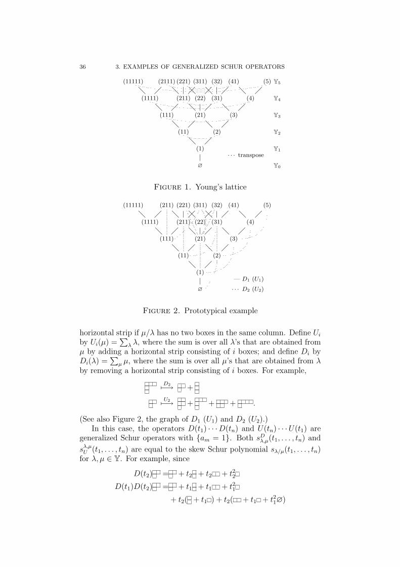
poset by the inclusion ⊂ as sets. Figure 1 is the Hasse graph for Y.The isomorphism on A swapping 1 and 2 induces a bijection on
Y. For a Young diagram λ, the image λ′ of the bijection is called thetransposition of λ. This definition of transposition is equivalent to theoriginal one. The map of transposition preserves the order of Y.
1.2. Prototypical Example. In this section, we consider the pro-totypical example of Young’s lattice Y again.
Let Y be Young’s lattice Y, V the K-vector space KY whose basisis Y, and ρ the ordinary rank function mapping a Young diagram λ tothe number of boxes in λ. Young’s lattice Y has a minimum ∅, theYoung diagram with no boxes. We call a skew Young diagram µ/λ a
35
36 3. EXAMPLES OF GENERALIZED SCHUR OPERATORS
Y0
Y1
Y2
Y3
Y4
Y5
∅
(1)
(2)(11)
(3)(21)(111)
(4)(31)(22)(211)(1111)
(5)(41)(32)(311)(221)(2111)(11111)
@ ¡
¡@¡@
¡@¡@ ¡ @
¡@¡@¡@@ ¡ @ ¡
· · · transpose
Figure 1. Young’s lattice
∅
(1)
(2)(11)
(3)(21)(111)
(4)(31)(22)(211)(1111)
(5)(41)(32)(311)(221)(211)(11111)
@ ¡
¡@¡@
¡@¡@ ¡ @
¡@¡@¡@@ ¡ @ ¡
— D1 (U1)
· · · D2 (U2)
Figure 2. Prototypical example
horizontal strip if µ/λ has no two boxes in the same column. Define Ui
by Ui(µ) =∑
λ λ, where the sum is over all λ’s that are obtained fromµ by adding a horizontal strip consisting of i boxes; and define Di byDi(λ) =
∑µ µ, where the sum is over all µ’s that are obtained from λ
by removing a horizontal strip consisting of i boxes. For example,
D27−→ +
U27−→ + + + .
(See also Figure 2, the graph of D1 (U1) and D2 (U2).)In this case, the operators D(t1) · · ·D(tn) and U(tn) · · ·U(t1) are
generalized Schur operators with {am = 1}. Both sDλ,µ(t1, . . . , tn) and
sλ,µU (t1, . . . , tn) are equal to the skew Schur polynomial sλ/µ(t1, . . . , tn)
for λ, µ ∈ Y. For example, since
D(t2) = + t2 + t2 + t22
D(t1)D(t2) = + t1 + t1 + t21
+ t2( + t1 ) + t2( + t1 + t21∅)

1. YOUNG’S LATTICE 37
+ t22( + t1∅),
sD(2,1),∅(t1, t2) = s(2,1)(t1, t2) = t21t2 + t1t
22.
When am equals 1 for each m, a(t) =∑
i ti = 1
1−t. In this case,
h{1,1,...}j (t1, . . . , tn) equals the homogeneous complete symmetric poly-
nomial hj(t1, . . . , tn).In the prototypical example Y (Example 1.4), for λ ∈ Y, Uiλ is
the sum of all Young diagrams obtained from λ by adding a horizon-tal strip consisting of i boxes. Hence sD
Uiλ,∅(t1, . . . , tn) equals∑
ν sν ,where the sum is over all ν’s that are obtained from λ by addinga horizontal strip consisting of i boxes. On the other hand, u0 is
1, and h{1,1,1,...}i (t1, . . . , tn) is the i-th complete symmetric polynomial
hi(t1, . . . , tn) (Example 2.9). Thus Corollary 3.4 is nothing but theclassical Pieri’s formula. Theorem 3.2 is Pieri’s formula for skew Schurpolynomials; for a skew Young diagram λ/µ and i ∈ N,
∑
κ
sκ/µ(t1, . . . , tn) =i∑
j=0
∑
ν
hi−j(t1, . . . , tn)sλ/ν(t1, . . . , tn),
where the first sum is over all κ’s that are obtained from λ by adding ahorizontal strip consisting of i boxes; the last sum is over all ν’s that areobtained from µ by removing a horizontal strip consisting of j boxes.For example,
s
• •
+ s•
•
+ s •
•
+ s ••
+ s • •
= h2 · s + h1 · s • + h0 · s • • .
In this example, Proposition 3.6 says that the Schur polynomial s(i)
corresponding to Young diagram with only one row equals the completesymmetric polynomial hi.
Remark 1.1. The vector space CY can be identified with the ringC ⊗ Λ of symmetric functions via mapping a Young diagram λ to theSchur function sλ corresponding to λ. In this case, the operator Ui is themultiplication by the i-th homogeneous complete symmetric functionhi. The operator Di is the operator h∗
i , where h∗i is the adjoint of
multiplication by hi. See also [6].
1.3. Dual Identities. This example is the same as [4, Example2.4]. Let Y be Young’s lattice Y, and Di the same ones in the proto-typical example, i.e., Diλ =
∑µ µ, where the sum is over all µ’s that
are obtained from λ by removing i boxes, with no two in the samecolumn. For λ ∈ Y , U ′
i are defined by U ′iλ =
∑µ µ, where the sum is
over all µ’s that are obtained from λ by adding i boxes, with no two in

38 3. EXAMPLES OF GENERALIZED SCHUR OPERATORS
∅
(1)
(2)(11)
(3)(21)(111)
(4)(31)(22)(211)(1111)
(5)(41)(32)(311)(221)(2111)(11111)
@ ¡
¡@¡@
¡@¡@ ¡ @
¡@¡@¡@@ ¡ @ ¡
— D1
· · · D2
∅
(1)
(11)(2)
(111)(21)(3)
(1111)(211)(22)(31)(4)
(11111)(2111)(221)(311)(32)(41)(5)
@ ¡
¡@¡@
¡@¡@ ¡ @
¡@¡@¡@@ ¡ @ ¡
— U ′1
· · · U ′2
Figure 3. The graphs of D1, D2, U ′1 and U ′
2
the same row. In other words, Di removes horizontal strips, while U ′i
adds vertical strips. For example,
U ′27−→ + + + +
U ′27−→ + + +
It follows by definition that Uiλ′ = (U ′
iλ)′, where λ′ is the transpositionof λ. For example,
U27−→ + + +
U ′27−→ + + +
See also Figure 3.
1. YOUNG’S LATTICE 39
In this case, since D(t) and U ′(t) satisfy
D(t)U ′(t′) = (1 + tt′)U ′(t′)D(t),
D(t1) · · ·D(tn) and U ′(tn) · · ·U ′(t1) are generalized Schur operatorswith {1, 1, 0, 0, 0, . . .}. (See [4].) In this case, for λ, µ ∈ Y , gener-
alized Schur polynomials sλ,µU ′ equal sλ′/µ′(t1, . . . , tn), where λ′ and µ′
are the transpositions of λ and µ, and sλ′/µ′(t1, . . . , tn) are skew Schurpolynomials.
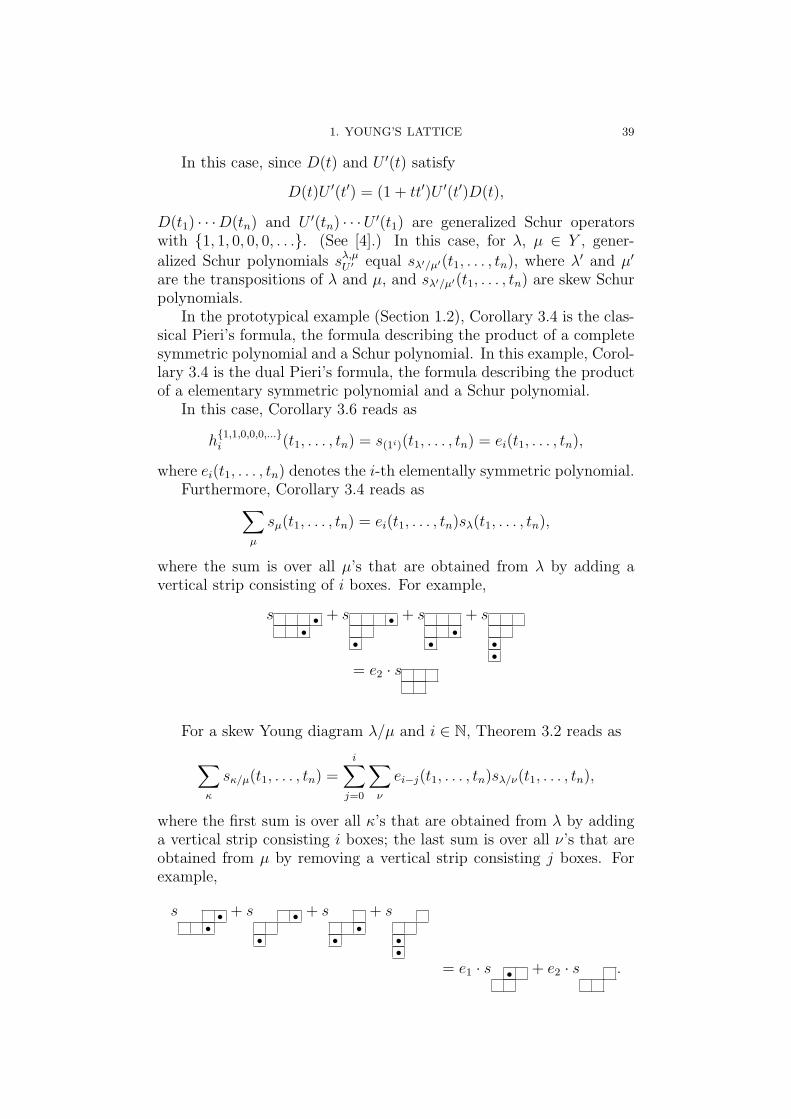
In the prototypical example (Section 1.2), Corollary 3.4 is the clas-sical Pieri’s formula, the formula describing the product of a completesymmetric polynomial and a Schur polynomial. In this example, Corol-lary 3.4 is the dual Pieri’s formula, the formula describing the productof a elementary symmetric polynomial and a Schur polynomial.
In this case, Corollary 3.6 reads as
h{1,1,0,0,0,...}i (t1, . . . , tn) = s(1i)(t1, . . . , tn) = ei(t1, . . . , tn),
where ei(t1, . . . , tn) denotes the i-th elementally symmetric polynomial.Furthermore, Corollary 3.4 reads as
∑
µ
sµ(t1, . . . , tn) = ei(t1, . . . , tn)sλ(t1, . . . , tn),
where the sum is over all µ’s that are obtained from λ by adding avertical strip consisting of i boxes. For example,
s ••
+ s •
•
+ s•
•
+ s
••
= e2 · s
For a skew Young diagram λ/µ and i ∈ N, Theorem 3.2 reads as
∑
κ
sκ/µ(t1, . . . , tn) =i∑
j=0
∑
ν
ei−j(t1, . . . , tn)sλ/ν(t1, . . . , tn),
where the first sum is over all κ’s that are obtained from λ by addinga vertical strip consisting i boxes; the last sum is over all ν’s that areobtained from µ by removing a vertical strip consisting j boxes. Forexample,
s ••
+ s •
•
+ s•
•
+ s
••
= e1 · s • + e2 · s .
40 3. EXAMPLES OF GENERALIZED SCHUR OPERATORS
∅
(1)
(2)
(3)(21)
(4)(31)
(5)(41)(32)
@@
¡
¡@@
¡@@¡
¡@@¡@
— D1
· · · D2 ∅
(1)
(2)
(3)(21)
(4)(31)
(5)(41)(32)
@@
¡¡
¡¡@@
¡¡@@¡¡
¡¡@@¡¡@@
— U1
· · · U2
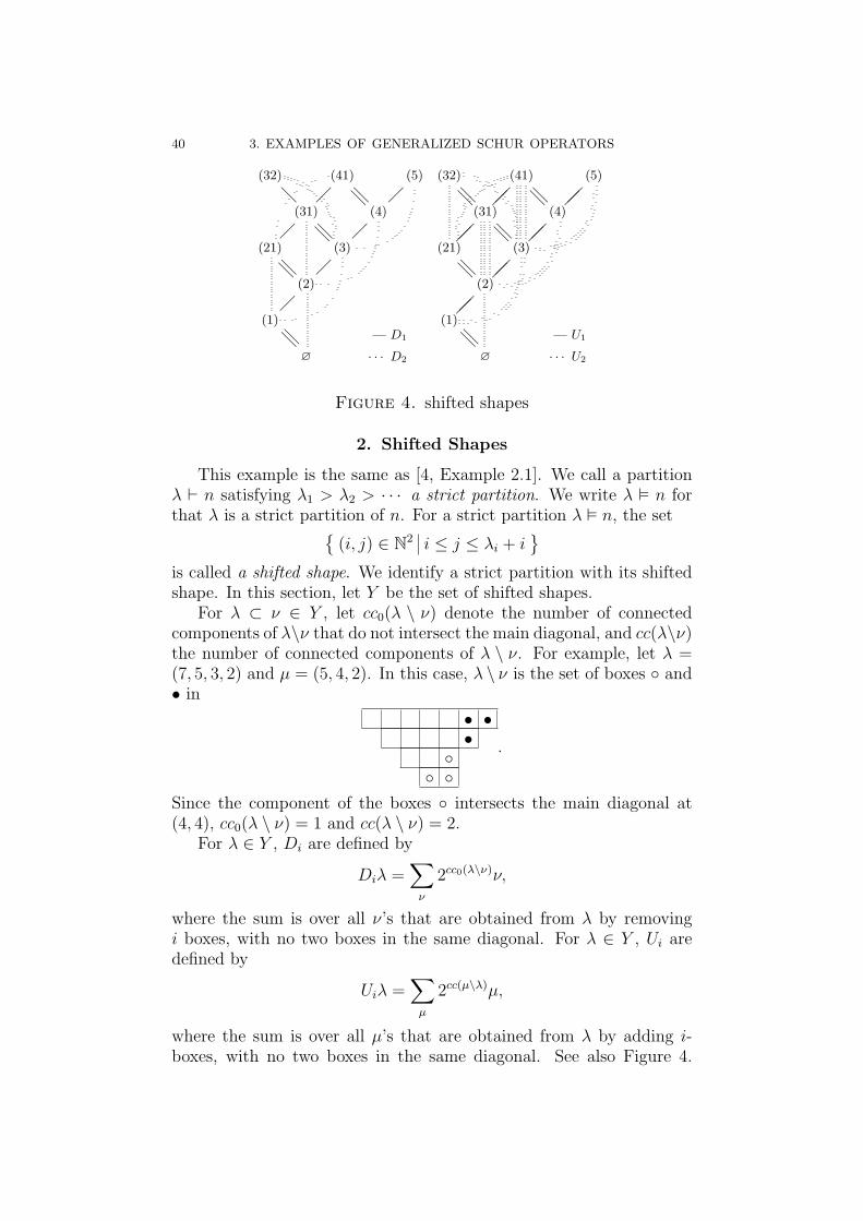
Figure 4. shifted shapes
2. Shifted Shapes
This example is the same as [4, Example 2.1]. We call a partitionλ ` n satisfying λ1 > λ2 > · · · a strict partition. We write λ ² n forthat λ is a strict partition of n. For a strict partition λ ² n, the set
{(i, j) ∈ N2 i ≤ j ≤ λi + i
}
is called a shifted shape. We identify a strict partition with its shiftedshape. In this section, let Y be the set of shifted shapes.
For λ ⊂ ν ∈ Y , let cc0(λ \ ν) denote the number of connectedcomponents of λ\ν that do not intersect the main diagonal, and cc(λ\ν)the number of connected components of λ \ ν. For example, let λ =(7, 5, 3, 2) and µ = (5, 4, 2). In this case, λ \ ν is the set of boxes ◦ and• in
• ••
◦◦ ◦
.
Since the component of the boxes ◦ intersects the main diagonal at(4, 4), cc0(λ \ ν) = 1 and cc(λ \ ν) = 2.
For λ ∈ Y , Di are defined by
Diλ =∑
ν
2cc0(λ\ν)ν,
where the sum is over all ν’s that are obtained from λ by removingi boxes, with no two boxes in the same diagonal. For λ ∈ Y , Ui aredefined by
Uiλ =∑
µ
2cc(µ\λ)µ,
where the sum is over all µ’s that are obtained from λ by adding i-boxes, with no two boxes in the same diagonal. See also Figure 4.

3. ROOTED PLANAR BINARY TREES 41
In this case, since D(t) and U(t) satisfy
D(t′)U(t) =1 + tt′
1 − tt′U(t)D(t′),
D(t1) · · ·D(tn) and U(tn) · · ·U(t1) are generalized Schur operators with{1, 2, 2, 2, . . .}. (See [4].) In this case, for λ, µ ∈ Y , generalized Schur
polynomials sDλ,µ and sλ,µ
U are respectively the shifted skew Schur poly-nomials Qλ/µ(t1, . . . , tn) and Pλ/µ(t1, . . . , tn). (See also [16].)
In this case, Proposition 3.6 reads as
h{1,2,2,2,...}i (t1, . . . , tn) =
{2Q(i)(t1, . . . , tn) i > 0
Q∅(t1, . . . , tn) i = 0.
It also follows from Proposition 3.15 that
h{1,2,2,2,...}i (t1, . . . , tn) = P(i)(t1, . . . , tn).
Furthermore, Corollary 3.4 reads as∑
µ
2cc(µ\λ)Qµ(t1, . . . , tn) = h{1,2,2,2,...}i Qλ(t1, . . . , tn),
where the sum is over all µ’s that are obtained from λ by adding iboxes, with no two in the same diagonal.
3. Rooted Planar Binary Trees
In this section, first we recall the definition of rooted planar bi-nary trees and labellings on them. Next we introduce linear operatorson the vector space whose basis is the set of rooted planar binarytrees. Then we show the operators are generalized Schur operators.Generalized Schur polynomials of this example are not symmetric butquasi-symmetric.
3.1. Rooted Planar Binary Trees. We define rooted planar bi-nary trees and their labellings. The definition of rooted planar binarytrees in this section is similar in concept to the definition of Youngdiagrams as ideals of a poset.
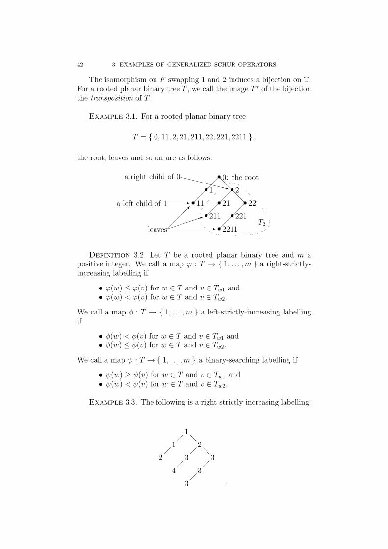
Let F be the monoid of words generated by the alphabet {1, 2} andlet 0 denote the word whose length is 0. We identify F with a posetby v ≤ vw for v, w ∈ F . We call an ideal of poset F a rooted planarbinary tree. Let T denote the set of rooted planar binary trees.
Let T be a rooted planar binary tree. An element of T is called anode of T . We write Ti for the set of rooted planar binary trees of inodes. We respectively call nodes v2 and v1 right and left children ofv. A node without children is called a leaf. If T is nonempty, 0 ∈ T .We call 0 the root of T .
For T ∈ T and v ∈ F , we define Tv by Tv = { w ∈ T v ≤ w }.
42 3. EXAMPLES OF GENERALIZED SCHUR OPERATORS
The isomorphism on F swapping 1 and 2 induces a bijection on T.For a rooted planar binary tree T , we call the image T τ of the bijectionthe transposition of T .
Example 3.1. For a rooted planar binary tree
T = { 0, 11, 2, 21, 211, 22, 221, 2211 } ,
the root, leaves and so on are as follows:
@@
@@¡
¡¡
¡
¡¡
¡¡
¡¡
¡¡
••
•
••
•
••
•
0: the root
2
22
1
21
221
11
211
2211T2¡
¡¡¡µ
³³³³³³1
-leaves
-a left child of 1
XXXXXXXXz
a right child of 0
.
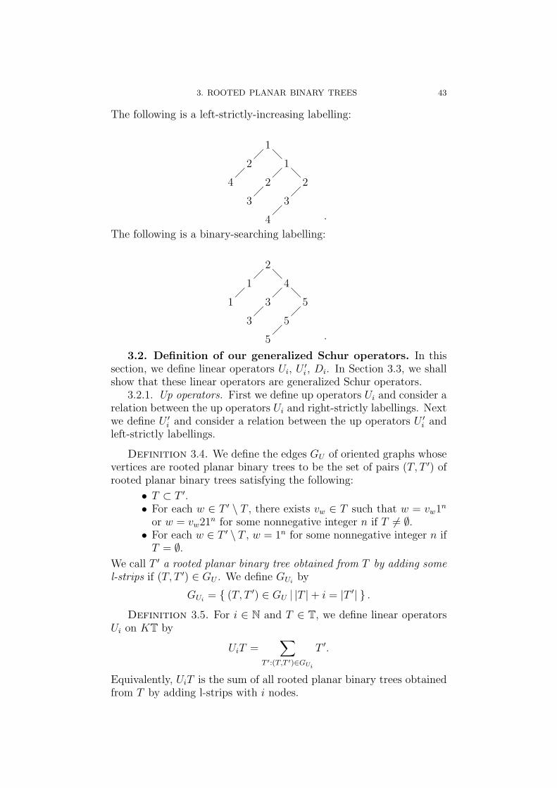
Definition 3.2. Let T be a rooted planar binary tree and m apositive integer. We call a map ϕ : T → { 1, . . . ,m } a right-strictly-increasing labelling if
• ϕ(w) ≤ ϕ(v) for w ∈ T and v ∈ Tw1 and• ϕ(w) < ϕ(v) for w ∈ T and v ∈ Tw2.
We call a map φ : T → { 1, . . . , m } a left-strictly-increasing labellingif
• φ(w) < φ(v) for w ∈ T and v ∈ Tw1 and• φ(w) ≤ φ(v) for w ∈ T and v ∈ Tw2.
We call a map ψ : T → { 1, . . . , m } a binary-searching labelling if
• ψ(w) ≥ ψ(v) for w ∈ T and v ∈ Tw1 and• ψ(w) < ψ(v) for w ∈ T and v ∈ Tw2.
Example 3.3. The following is a right-strictly-increasing labelling:
¡
¡
¡
¡
¡
¡
@
@
1
2
3
1
3
3
2
4
3 .
3. ROOTED PLANAR BINARY TREES 43
The following is a left-strictly-increasing labelling:
¡
¡
¡
¡
¡
¡
@
@
1
1
2
2
2
3
4
3
4 .
The following is a binary-searching labelling:
¡
¡
¡
¡
¡
¡
@
@
2
4
5
1
3
5
1
3
5 .
3.2. Definition of our generalized Schur operators. In thissection, we define linear operators Ui, U ′
i , Di. In Section 3.3, we shallshow that these linear operators are generalized Schur operators.
3.2.1. Up operators. First we define up operators Ui and consider arelation between the up operators Ui and right-strictly labellings. Nextwe define U ′
i and consider a relation between the up operators U ′i and
left-strictly labellings.
Definition 3.4. We define the edges GU of oriented graphs whosevertices are rooted planar binary trees to be the set of pairs (T, T ′) ofrooted planar binary trees satisfying the following:
• T ⊂ T ′.• For each w ∈ T ′ \ T , there exists vw ∈ T such that w = vw1n
or w = vw21n for some nonnegative integer n if T 6= ∅.• For each w ∈ T ′ \ T , w = 1n for some nonnegative integer n if
T = ∅.We call T ′ a rooted planar binary tree obtained from T by adding somel-strips if (T, T ′) ∈ GU . We define GUi
by
GUi= { (T, T ′) ∈ GU |T | + i = |T ′| } .
Definition 3.5. For i ∈ N and T ∈ T, we define linear operatorsUi on KT by
UiT =∑
T ′:(T,T ′)∈GUi
T ′.
Equivalently, UiT is the sum of all rooted planar binary trees obtainedfrom T by adding l-strips with i nodes.
44 3. EXAMPLES OF GENERALIZED SCHUR OPERATORS
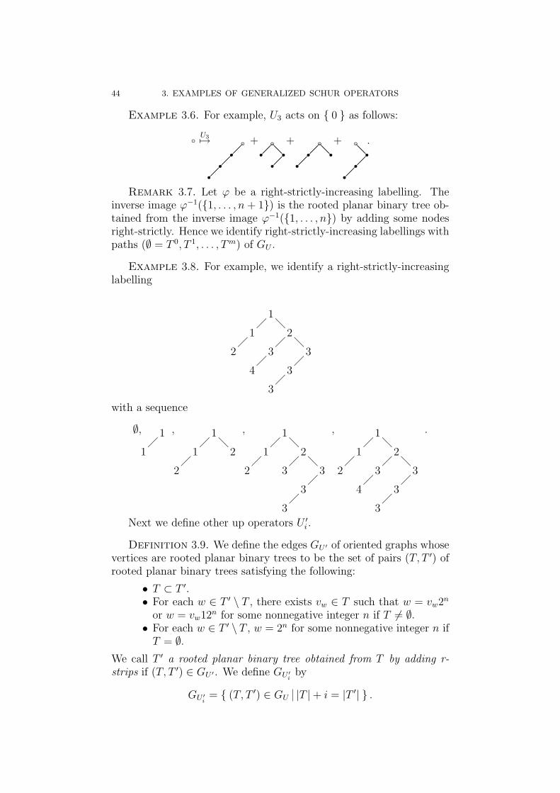
Example 3.6. For example, U3 acts on { 0 } as follows:
b U37→
¡¡¡¡
¡¡br
r r+
¡¡¡¡@@br rr
+
¡¡¡¡ @@
br rr+
¡¡
@@¡¡
b rrr.
Remark 3.7. Let ϕ be a right-strictly-increasing labelling. Theinverse image ϕ−1({1, . . . , n + 1}) is the rooted planar binary tree ob-tained from the inverse image ϕ−1({1, . . . , n}) by adding some nodesright-strictly. Hence we identify right-strictly-increasing labellings withpaths (∅ = T 0, T 1, . . . , Tm) of GU .
Example 3.8. For example, we identify a right-strictly-increasinglabelling
¡
¡
¡
¡
¡
¡
@
@
1
2
3
1
3
3
2
4
3
with a sequence
∅,¡
1
1
,
¡
¡ @1
21
2
,
¡
¡
¡
¡
¡
@
@
1
2
3
1
3
3
2
3
,
¡
¡
¡
¡
¡
¡
@
@
1
2
3
1
3
3
2
4
3
.
Next we define other up operators U ′i .
Definition 3.9. We define the edges GU ′ of oriented graphs whosevertices are rooted planar binary trees to be the set of pairs (T, T ′) ofrooted planar binary trees satisfying the following:
• T ⊂ T ′.• For each w ∈ T ′ \ T , there exists vw ∈ T such that w = vw2n
or w = vw12n for some nonnegative integer n if T 6= ∅.• For each w ∈ T ′ \ T , w = 2n for some nonnegative integer n if
T = ∅.We call T ′ a rooted planar binary tree obtained from T by adding r-strips if (T, T ′) ∈ GU ′ . We define GU ′
iby
GU ′i= { (T, T ′) ∈ GU |T | + i = |T ′| } .

3. ROOTED PLANAR BINARY TREES 45
Definition 3.10. For i ∈ N and T ∈ T, we define linear operatorsU ′
i on KT to be
U ′iT =
∑
T ′:(T,T ′)∈GU′i
T ′.
Equivalently, U ′iT is the sum of all rooted planar binary trees obtained
from T by adding r-strips with i nodes.
Remark 3.11. Similarly to the case of right-strictly-increasing la-bellings and Ui, we identify left-strictly-increasing labellings with paths(∅ = T 0, T 1, . . . , Tm) of GU ′ .
3.2.2. Down operators. Next we define down operators Di on KTand we see relations between the down operators Di and binary search-ing labellings.
First we prepare some terms to define the linear operators Di.For T ∈ T, let RT denote the set { w ∈ T w2 6∈ T }, i.e., the set of
nodes of T without right children. For w ∈ RT , we define
T Ä w = (T \ Tw) ∪ {wv | w1v ∈ Tw } .
There exists the natural inclusion νT,w from T Ä w to T defined by{
νT,w(wv) = w1v (wv ∈ Tw)
νT,w(v′) = v′ (v′ 6∈ Tw).
Example 3.12. For example, for w = 1221 and
T =
¢¢¢¢AA¡¡
AA¢¢AA¢¢
@@©©©
@@¢¢
¢¢¢¢AA
r r rbrb rb bb
brrr
r
rqqq
¢
, T Ä w =
¢¢¢¢AA¡¡
AA¢¢AA¢¢
@@©©©
@@¢¢
¢¢AA
r r rbrb rb bbb
rrr
rqq,
where • are nodes in RT or RTÄw, and r is w = 1221. The natural
inclusion νT,w maps the nodes in of T Ä w to the nodes in of T ,
and the nodes in of T Ä w to the nodes in of T ,respectively.
For T ∈ T, let ET denote {w ∈ T | If w = v1w′ then v2 6∈ T}.Roughly speaking, it is the set of nodes of T between the root 0 andthe right-most node of T . We define rT by rT = ET ∩RT . The set rT is
46 3. EXAMPLES OF GENERALIZED SCHUR OPERATORS
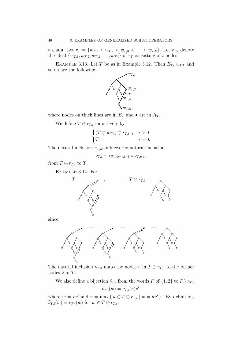
a chain. Let rT = {wT,1 < wT,2 < wT,3 < · · · < wT,k}. Let rT,i denotethe ideal {wT,1, wT,2, wT,3, . . . , wT,i} of rT consisting of i nodes.
Example 3.13. Let T be as in Example 3.12. Then ET , wT,k andso on are the following:
¢¢¢¢AA¡¡
AA¢¢AA¢¢
@@©©©
@@¢¢
¢¢¢¢AA
r r rbrb rb bb
brrr
r
rwT,1
wT,2
wT,3
wT,4
wT,5 ,
where nodes on thick lines are in ET and • are in RT .
We define T ª rT,i inductively by{
(T Ä wT,i) ª rT,i−1 i > 0
T i = 0.
The natural inclusion νT,w induces the natural inclusion
νT,i = νTÄwT,i,i−1 ◦ νT,wT,i
from T ª rT,i to T .
Example 3.14. For
T =
¢¢¢¢AA¡¡
AA¢¢AA¢¢
@@©©©
@@¢¢
¢¢¢¢AA
b b bbbb bb bb
brrb
b
rqqq
©©*
¢¢
, T ª rT,3 =
¢¢¢¢AA¡¡
AA¢¢AA¢¢
@@@@¢¢AA
b b bbbb bb bb
b bb
since
¢¢¢¢AA¡¡
AA¢¢AA¢¢
@@©©©
@@¢¢
¢¢¢¢AA
b b bbbb bb bb
brrb
b
rqqq
¢
→
¢¢¢¢AA¡¡
AA¢¢AA¢¢
@@©©©
@@¢¢
¢¢AA
b b bbbb bb bb
rbb b
r¢
→
¢¢¢¢AA¡¡
AA¢¢AA¢¢
@@©©©
@@¢¢AA
b b bbb bb bb
bb b
r©©*
→
¢¢¢¢AA¡¡
AA¢¢AA¢¢
@@@@¢¢AA
b b bbbb bb bb
b bb.
The natural inclusion νT,3 maps the nodes ◦ in T ª rT,3 to the formernodes ◦ in T .
We also define a bijection νT,i from the words F of {1, 2} to F \ rT,i
νT,i(w) = νT,i(v)v′,
where w = vv′ and v = max {u ∈ T ª rT,i | w = uu′ }. By definition,νT,i(w) = νT,i(w) for w ∈ T ª rT,i.
3. ROOTED PLANAR BINARY TREES 47
Definition 3.15. We define the edges GDiand GD of graphs whose
vertices are rooted planar binary trees by
GDi= { (T ª rT,i, T ) |rT | ≥ i }
and
GD =⋃
i
GDi.
Remark 3.16. By definition, GD0 = { (T, T ) T ∈ T }. For each iand each T ∈ T, the in-degree of T in GDi
, i.e. |{ (T ′, T ) ∈ GDi}|, is
1.
Definition 3.17. We define linear operators DiT to be T ′ suchthat (T ′, T ) ∈ GDi
for T ∈ T.
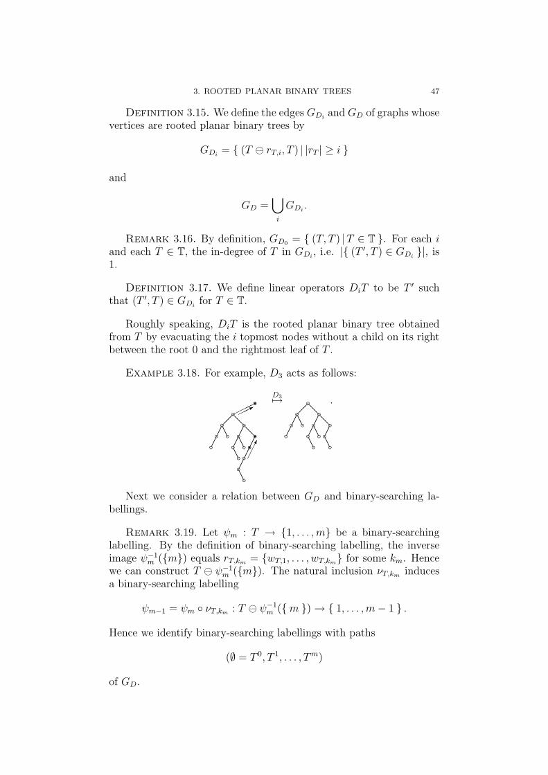
Roughly speaking, DiT is the rooted planar binary tree obtainedfrom T by evacuating the i topmost nodes without a child on its rightbetween the root 0 and the rightmost leaf of T .
Example 3.18. For example, D3 acts as follows:
¢¢¢¢AA¡¡
AA¢¢AA¢¢
@@©©©
@@¢¢
¢¢¢¢AA
b b bbbb bb bb
bbbb
b
bqqq
©©*
¢¢
D37→
¢¢¢¢AA¡¡
AA¢¢AA¢¢
@@@@¢¢AA
b b bbbb bb bb
b bb.
Next we consider a relation between GD and binary-searching la-bellings.
Remark 3.19. Let ψm : T → {1, . . . ,m} be a binary-searchinglabelling. By the definition of binary-searching labelling, the inverseimage ψ−1
m ({m}) equals rT,km = {wT,1, . . . , wT,km} for some km. Hencewe can construct T ª ψ−1
m ({m}). The natural inclusion νT,km inducesa binary-searching labelling
ψm−1 = ψm ◦ νT,km : T ª ψ−1m ({ m }) → { 1, . . . ,m − 1 } .
Hence we identify binary-searching labellings with paths
(∅ = T 0, T 1, . . . , Tm)
of GD.

48 3. EXAMPLES OF GENERALIZED SCHUR OPERATORS
Example 3.20. For example, we identify a binary-searching la-belling
¡
¡
¡
¡
¡
¡
@
@
2
4
5
1
3
5
1
3
5
with a sequence
∅,¡
1
1
,
¡
¡2
1
1
,
¡
¡
¡
@2
31
31
,
¡
¡
¡
¡
@2
41
31
3
,
¡
¡
¡
¡
¡
¡
@
@
2
4
5
1
3
5
1
3
5
.
3.3. Main Results. In this section, we show that D(t1) · · ·D(tn)and U(tn) · · ·U(t1) are generalized Schur operators with {1, 1, 1, . . .}.We also show that D(t1) · · ·D(tn) and U ′(tn) · · ·U ′(t1) are generalizedSchur operators with {1, 1, 0, 0, 0, 0, . . .}. To prove the assertion forD(t1) · · ·D(tn) and U(tn) · · ·U(t1), we construct correspondences be-
tween Ni,j(T, T ′) and Sj,i(T, T ′), where Ni,j(T, T ′) is the set of paths of
graphs from T to T ′ via GDjafter GUi
, and Sj,i(T, T ′) is the set of pathsof graphs from T to T ′ via GUi−k
after GDj−k, where 0 ≤ k ≤ min{i, j}.
(See Definition 3.29.) The correspondence for i = j = 1 is an r-correspondence introduced by Fomin [3], which is needed to constructRobinson correspondences for r-dual graphs. We also prove the asser-tion for D(t1) · · ·D(tn) and U ′(tn) · · ·U ′(t1) similarly.
We prove the following theorems in Section 3.4.
Theorem 3.21. Let Di be the linear operators defined in Defini-tion 3.17 and Ui the linear operators defined in Definition 3.5. Theoperators D(t) and U(t′) satisfy the equation
D(t)U(t′) =1
1 − tt′U(t′)D(t).
Equivalently, operators D(t1) · · ·D(tn) and U(tn) · · ·U(t1) are general-ized Schur operators with {1, 1, 1, . . .}.
Theorem 3.22. Let Di be the linear operators defined in Defini-tion 3.17 and U ′
i the linear operators defined in Definition 3.10. Theoperators D(t) and U ′(t′) satisfy the equation
D(t)U ′(t′) = (1 + tt′)U ′(t′)D(t).
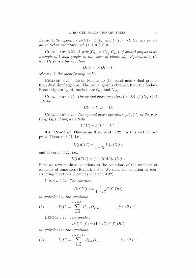
3. ROOTED PLANAR BINARY TREES 49
Equivalently, operators D(t1) · · ·D(tn) and U ′(tn) · · ·U ′(t1) are gener-alized Schur operators with {1, 1, 0, 0, 0, 0 . . .}.
Corollary 3.23. A pair (GU1 = GU ′1, GDi
) of graded graphs is anexample of 1-dual graphs in the sense of Fomin [4]. Equivalently, U1
and D1 satisfy the equation
D1U1 − U1D1 = I,
where I is the identity map on V .
Remark 3.24. Janvier Nzeutchap [13] constructs r-dual graphsfrom dual Hopf algebras. The 1-dual graphs obtained from the Loday-Ronco algebra by his method are GU1 and GD1 .
Corollary 3.25. The up and down operators (U1, D) of (GU1 , GD)satisfy
DU1 − U1D = D.
Corollary 3.26. The up and down operators (D∗1, U
∗) of the pair(GD1 , GU) of graphs satisfy
U∗D∗1 − D∗
1U∗ = U∗.
3.4. Proof of Theorems 3.21 and 3.22. In this section, weprove Theorem 3.21, i.e.,
D(t)U(t′) =1
1 − tt′U(t′)D(t),
and Theorem 3.22, i.e.,
D(t)U ′(t′) = (1 + tt′)U ′(t′)D(t).
First we rewrite these equations as the equations of the numbers ofelements of some sets (Remark 3.30). We show the equation by con-structing bijections (Lemmas 3.31 and 3.32).
Lemma 3.27. The equation
D(t)U(t′) =1
1 − tt′U(t′)D(t)
is equivalent to the equations
DjUi =
min (i,k)∑
k=0
Ui−kDj−k for all i, j.(8)
Lemma 3.28. The equation
D(t)U ′(t′) = (1 + tt′)U ′(t′)D(t)
is equivalent to the equations
DjU′i =
min (1,i,k)∑
k=0
U ′i−kDj−k for all i, j.(9)
50 3. EXAMPLES OF GENERALIZED SCHUR OPERATORS
Definition 3.29. We define Ni,j(T, T ′) and N ′i,j(T, T ′) to be
{((T, T ′′), (T ′, T ′′)) ∈ GUi
× GDj
}
and
{((T, T ′′), (T ′, T ′′)) ∈ GU ′
i× GDj
}.
We respectively define sets Sj,i(T, T ′) and S ′j,i(T, T ′) of paths to be
{((T ′′, T ), (T ′′, T ′)) ∈ GDj
× GUi
}
and
{((T ′′, T ), (T ′′, T ′)) ∈ GDj
× GU ′i
},
respectively. We also define Sj,i(T, T ′) and S ′j,i(T, T ′) by
Sj,i(T, T ′) =
min(i,j)∐
k=0
Sj−k,i−k(T, T ′)
S ′j,i(T, T ′) =
min(1,i,j)∐
k=0
S ′j−k,i−k(T, T ′),
where∐
means the disjoint union.
Remark 3.30. By definition,
〈DjUiT, T ′〉 = |Ni,j(T, T ′)| ,⟨D′
jUiT, T ′⟩ =∣∣N ′
i,j(T, T ′)∣∣ ,
〈UjDiT, T ′〉 =∣∣S ′
i,j(T, T ′)∣∣ ,
and
〈UjD′iT, T ′〉 =
∣∣S ′i,j(T, T ′)
∣∣
for each T, T ′ ∈ T. Hence the equations (8) and (9) are respectivelyequivalent to the equations
|Ni,j(T, T ′)| =∣∣∣Sj,i(T, T ′)
∣∣∣
and
∣∣N ′i,j(T, T ′)
∣∣ =∣∣∣S ′
j,i(T, T ′)∣∣∣ .
Lemma 3.31. For each T , T ′ ∈ T and each i, j ∈ N, there exists
bijection from Ni,j(T, T ′) to Sj,i(T, T ′).
3. ROOTED PLANAR BINARY TREES 51
Proof. First we construct an element of Sj,i(T, T ′) from an ele-ment of Ni,j(T, T ′).
Let ((T, T ′′), (T ′, T ′′)) be an element of Ni,j(T, T ′). Equivalently,(T, T ′′) is an edge of GUi
such that T ′′ ª rT ′′,j = T ′. Let k be j −|rT ′′,j ∩ rT |. We have rT,j−k = rT ′′,j∩rT since rT ′′ is one of the following:
rT ,
rT,l ∪{
wT,l+121i i ≤ n}
,
rT,l ∪{
wT,l+11i i ≤ n
}
for some l, n ∈ N. We consider
((T ª rT,j−k, T ), (T ª rT,j−k, T′)).
By definition, (T ª rT,j−k, T ) is in GDj−k. Since (T, T ′′) is in GUi
,(T ªrT,j−k, T
′′ªrT ′′,j) is in GUi−k. Since T ′ = T ′′ªrT ′′,j, (T ªrT,j−k, T
′)
is in GUi−k. Hence we have ((T, T ª rT,k), (T
′, T ª rT,k)) ∈ Sj,i(T, T ′).Next we construct an element of Ni,j(T, T ′) from an element of
Sj,i(T, T ′). Let ((T ′′′, T ), (T ′′′, T ′)) be an element of Sj,i(T, T ′). Equiv-alently, (T ′′′, T ′) is an edge of GUi−k such that T ª rT,j−k = T ′′′.
First we consider the case where |rT | > j − k. Let ω = wT,j−k+1
and ω′ ∈ ν−1T,j−k(ω). Since ω′ ∈ T ªrT,j−k and ω′2 6∈ T ªrT,j−k, we have
T ′ω′2 =
{ω′2, ω′21, . . . , ω′21n−1
}
for some n ∈ N, where this is empty for n = 0. For such n, let R denote{ω2, ω21, . . . , ω21n−1+k
},
where this is empty for n + k = 0.We define T ′′ to be
νT,j−k(T ) ∪ rT,j−k ∪ R.
Since rT ′′ = rT,j−k ∪ R, ((T, T ′′), (T ′, T ′′)) is in Ni,j(T, T ′).Next we consider the case where |rT | = j − k. Let ω be
max { w 6∈ rT w < wT,j−k }
and ω′ ∈ ν−1T,j−k(r). Since ω′ ∈ T ª rT,j−k and ω′2 6∈ T ª rT,j−k, we have
T ′ω′2 =
{ω′2, ω′21, . . . , ω′21n−1
}
for some n ∈ N, where this is empty for n = 0. For such n, let R denote{wT,j−k+11, . . . , wT,j−k+11
n−1+k}
,
where this is empty for n + k = 0.We define T ′′ to be
νT,j−k(T ) ∪ rT,j−k ∪ R.
Since rT ′′ = rT,j−k ∪ R, ((T, T ′′), (T ′, T ′′)) is in Ni,j(T, T ′).Thus we can construct an element of Ni,j(T, T ′) from an element of
Sj,i(T, T ′).
52 3. EXAMPLES OF GENERALIZED SCHUR OPERATORS
By the definition of them, these constructions are the inverses ofeach other. Hence we have the lemma. ¤
Lemma 3.32. For each T , T ′ ∈ T, there exists a bijection from
N ′i,j(T, T ′) to S ′
j,i(T, T ′).
Proof. First we construct an element of S ′j,i(T, T ′) from an ele-
ment of N ′i,j(T, T ′).
Let ((T, T ′′), (T ′, T ′′)) be an element of N ′i,j(T, T ′). Equivalently,
(T, T ′′) is an edge of GU ′isuch that T ′′ªrT ′′,j = T ′. Let k be |rT ′′,j ∩ rT |.
We have rT,j−k = rT ′′,j ∩ rT since rT ′′ is one of the following:
rT ,
rT,l ∪ { wT,l+112n } ,
rT,l ∪ { wT,l+12n }
for some l, n ∈ N. It also follows that k = 0 or 1. We consider
((T, T ª rT,k), (T′, T ª rT,k)).
By definition, (T ª rT,j−k, T ) is in GDj−k. Since (T, T ′′) is in GU ′
i,
(T ªrT,j−k, T′′ªrT ′′,j) is in GU ′
i−k. Since T ′ = T ′′ªrT ′′,j, (T ªrT,j−k, T
′)
is in GU ′i−k
. Hence we have ((T, T ª rT,k), (T′, T ª rT,k)) ∈ Sj,i(T, T ′).
Next we construct an element of N ′i,j(T, T ′) from an element of
S ′j,i(T, T ′). Let ((T ′′′, T ), (T ′′′, T ′)) be an element of S ′
j,i(T, T ′). Equiv-alently, (T ′′′, T ′) is an edge of GU ′
i−k such that T ª rT,j−k = T ′′′.First we consider the case where |rT | > j − k. Let ω = wT,j−k+1
ω′ ∈ ν−1T,j−k(ω). Since ω′ ∈ T ª rT,j−k and ω′2 6∈ T ª rT,j−k, we have
T ′ω′2 = { ω′2, . . . , ω′2n }
for some n ∈ N, where this is empty for n = 0. For such n, let R denote{
ω2, . . . , ω21n+k}
,
where this is empty for n + k = 0.We define T ′′ to be
νT,j−k(T ) ∪ rT,j−k ∪ R.
Since rT ′′ = rT,j−k ∪{
ω21n+k}, ((T, T ′′), (T ′, T ′′)) is in N ′
i,j(T, T ′).Next we consider the case where |rT | = j − k. Let ω be
max { w 6∈ rT w < wT,j−k }
and ω′ ∈ ν−1T,j−k(ω). Since ω′ ∈ T ªrT,j−k and ω′2 6∈ T ªrT,j−k, we have
T ′ω′2 = { ω′2, . . . , ω′2n }
for some n ∈ N, where this is empty for n = 0. For such n, let R denote{
wT,j−k1, wT,j−k12, . . . , wT,j−k12n−1+k}
,
where this is empty for n + k = 0.
3. ROOTED PLANAR BINARY TREES 53
We define T ′′ to be
νT,j−k(T ) ∪ rT,j−k ∪ R.
Since
rT ′′ = rT,j−k ∪{
wT,j−k+112n−1+k}
,
((T, T ′′), (T ′, T ′′)) is in N ′i,j(T, T ′).
Thus we can construct an element of N ′i,j(T, T ′) from an element of
S ′j,i(T, T ′).
By the definitions of them, these constructions are the inverses ofeach other. Hence we have the lemma. ¤
By Lemmas 3.31 and 3.32, we have Theorems 3.21 and 3.22.
3.5. Some remarks. In this section, we consider a relation be-tween our generalized Schur operators and the Loday-Ronco algebra.
Remark 3.33. We have bijections between the sets Ni,j(T, T ′) and
Si,j(T, T ′) for all i, j by the proof of 3.31. From them, we can constructa Robinson-Schensted-Knuth correspondence for paths of GU and GD
by the method in [4]. This correspondence is a generalization of theLoday-Ronco correspondence, which is a Robinson correspondence forrooted planar binary trees.
Remark 3.34. Maxime Rey gave a new construction of the Loday-Ronco algebra in [14]. He introduced a new Robinson-Schensted-Knuthcorrespondence for rooted planar binary trees to construct the Loday-Ronco algebra. Some of our correspondences are equivalent to his cor-respondence.
Next we give descriptions to generalized Schur polynomials for thisexample as weighted generating functions of labellings.
Remark 3.35. For a labelling ϕ from T to {1, . . . , m}, we definetϕ =
∏w∈T tϕ(w). For a rooted planar binary tree T , it follows by the
definition of labellings that
sDT,∅(t1, . . . , tm) =
∑
ψ
tψ,
sT,∅U (t1, . . . , tm) =
∑
ϕ
tϕ,
sT,∅U ′ (t1, . . . , tm) =
∑
φ
tφ,
where the first sum is over all binary-searching labellings ψ on T , thesecond sum is over all right-strictly-increasing labellings ϕ on T , andthe last sum is over all left-strictly-increasing labellings φ on T .
54 3. EXAMPLES OF GENERALIZED SCHUR OPERATORS
Since D(t) and U(t) are generalized Schur operators with {ai =
1}, we have Pieri’s formula and Cauchy’s formula for sT,∅U (t1, . . . , tn),
sDT,∅(t1, . . . , tn) and the classical homogeneous complete symmetric poly-
nomials. We also have “skew” versions of them.
Remark 3.36. The generalized Schur polynomials sT,∅U (t1, . . . , tn)
and sDT,∅(t1, . . . , tn) are the commutativizations of the basis elements
QT and PT of PBT in Hivert-Novelli-Thibon [7].
Remark 3.37. The generalized Schur polynomials sT,∅U (t1, . . . , tn)
and sDT,∅(t1, . . . , tn) are not symmetric in general. For example, since
D(t1)D(t2) { 0, 1, 12 }=D(t1)({ 0, 1, 12 } + t2 { 0, 2 } + t22 { 0 })=({ 0, 1, 12 } + t1 { 0, 2 } + t21 { 0 })
+ t2({ 0, 2 } + t1 { 0 })+ t22({ 0 } + t1∅),
〈D(t1)D(t2)T, ∅〉 = t1t22 is not symmetric for T = { 0, 1, 12 }. The fact
that Di does not commute with Dj in general implies this fact.
Bibliography
[1] S. Fomin, The generalized Robinson-Schensted-Knuth correspondence, ZariskiNauchn. Sem. Leningrad. Otdel. Mat. Inst. Steklov. (LOMI) 155 (1986), 156–175, 195 (Russian); English transl., J. Soviet Math. 41(1988), 979–991.
[2] S. Fomin, Duality of graded graphs, J. Algebraic Combin. 3 (1994), 357–404.[3] S. Fomin, Schensted algorithms for dual graded graphs, J. Algebraic Combin.
4 (1995), 5–45.[4] S. Fomin, Schur operators and Knuth correspondences, J. Combin. Theory,
Ser. A 72 (1995), 277–292.[5] Fulton,W., Young Tableaux; with applications to representation theory and ge-
ometry, volume 35 of London Mathematical Society Student Texts, CambridgeUniversity Press, New York, 1997.
[6] Ira M. Gessel, Counting paths in Young’s lattice, J. Statistical planning andinference. 34 (1993), 125–134.
[7] F. Hivert, J. Novelli and J. Thibon, The algebra of binary search trees, Theor.Comput. Sci. 339, 1 (Jun. 2005), 129–165. DOI=http://dx.doi.org/10.1016/j.tcs.2005.01.012
[8] T. Lam , A Combinatorial Generalization of the Boson-Fermion Correspon-dence, Math. Res. Lett. 13 (2006), no.3, 377–329.
[9] I.G. Macdonald, Symmetric Functions and Hall Polynomials, Oxford Mathe-matical Monographs, 2nd Edition, Oxford University Press, 1995.
[10] Y. Numata, Pieri’s Formula for Generalized Schur Polynomials, preprint,arXiv:math.CO/0606386, to appear in J. Algebraic Combin.
[11] Y. Numata, An example of generalized Schur operators, preprint, arXiv:math.CO/0609376.
[12] Y. Numata, Robinson-Schensted Correspondences for certain pairs of Semi-graded graphs, in preperation,
[13] J. Nzeutchap, Graded Graphs and Fomin’s r-correspondences associated tothe Hopf Algebras of Planar Binary Trees, Quasi-symmetric Functions andNoncommutative Symmetric Functions, FPSAC ’06, 2006. http://garsia.math.yorku.ca/fpsac06/papers/53.pdf
[14] M. Rey, A new construction of the Loday-Ronco algebra, FPSAC ’06, 2006.http://garsia.math.yorku.ca/fpsac06/papers/51.pdf
[15] T. Roby, Applications and extensions of Fomin’s generalization of theRobinson-Schensted correspondence to differential posets, Ph.D. thesis, M.I.T.,1991.
[16] B. E. Sagan, The ubiquitous Young tableau, Invariant theory and tableaux(Stanton,D.,ed.), IMA volumes in mathematics and its applications, Springer-Verlag, New York, 262–298.
[17] R. Stanley, Differential posets, J. American Math. Soc, 1 (1988), 919–961.[18] R. Stanley, Variations on differential posets, Invariant theory and tableaux
(Stanton,D.,ed.), IMA volumes in mathematics and its applications, Springer-Verlag, New York, 145–165.


![Operators on k-tableaux and the k case · k-Schur functions were introduced by Lapointe, Lascoux, and Morse in [3], rst de-veloped to assist in studying Macdonald polynomials. These](https://static.fdocuments.net/doc/165x107/5f039b357e708231d409e1e2/operators-on-k-tableaux-and-the-k-case-k-schur-functions-were-introduced-by-lapointe.jpg)
![Introduction - University Of Marylandharryt/papers/scharak.pdf · the Schur Q-functions [S], but the latter are not polynomials in the Chern roots of any homogeneous vector bundle](https://static.fdocuments.net/doc/165x107/5b5139367f8b9a056a8bd286/introduction-university-of-harrytpapersscharakpdf-the-schur-q-functions.jpg)