Coinductive Definitions and Real Numbers

BSc Final Year Project Report

Michael HerrmannSupervisor: Dr. Dirk Pattinson

Second Marker: Prof. Abbas Edalat

June 2009

Abstract

Real number computation in modern computers is mostly done via floatingpoint arithmetic which can sometimes produce wildly erroneous results. Analternative approach is to use exact real arithmetic whose results are guaran-teed correct to any user-specified precision. It involves potentially infinite datastructures and has therefore in recent years been studied using the mathematicalfield of universal coalgebra. However, while the coalgebraic definition principlecorecursion turned out to be very useful, the coalgebraic proof principle coin-duction is not always sufficient in the context of exact real arithmetic. A newapproach recently proposed by Berger in [3] therefore combines the more generalset-theoretic coinduction with coalgebraic corecursion.

This project extends Berger’s approach from numbers in the unit intervalto the whole real line and thus further explores the combination of coalgebraiccorecursion and set-theoretic coinduction in the context of exact real arithmetic.We propose a coinductive strategy for studying arithmetic operations on thesigned binary exponent-mantissa representation and use it to define and reasonabout operations for computing the average and linear affine transformationsover Q of real numbers. The strategy works well for the two chosen operationsand our Haskell implementation shows that it lends itsels well to a realizationin a lazy functional programming language.

Acknowledgements

I would particularly like to thank my supervisor, Dr. Dirk Pattinson, for takingme on as a project student at an unusually late stage and for his continuoussupport. He provided me with all the help I needed and moreover always foundtime to answer questions that were raised by, but went far beyond, the topicsof this project. I would also like to thank my second marker, Professor AbbasEdalat, for his feedback on an early version of the report.

I am extremely grateful to my family for enabling me to study abroad eventhough this demands a great deal of them, in many respects. Likewise, I wouldlike to thank my girlfriend Antonia for standing by me in the last three labour-intensive years. This project is dedicated to her.

Contents

1 Introduction 11.1 Why Exact Real Number Computation? . . . . . . . . . . . . . . . 11.2 Coinductive Proof . . . . . . . . . . . . . . . . . . . . . . . . . . . . 21.3 Contributions . . . . . . . . . . . . . . . . . . . . . . . . . . . . . . . 5

2 Background 62.1 Alternatives to Floating Point Arithmetic . . . . . . . . . . . . . . 62.2 Representations in Exact Real Arithmetic . . . . . . . . . . . . . . 7

2.2.1 The Failure of the Standard Decimal Expansion . . . . . . 82.2.2 Signed Digit Representations . . . . . . . . . . . . . . . . . 82.2.3 Other Representations . . . . . . . . . . . . . . . . . . . . . 10

2.3 Computability Issues . . . . . . . . . . . . . . . . . . . . . . . . . . 122.3.1 Computable Numbers . . . . . . . . . . . . . . . . . . . . . . 13

2.4 Coalgebra and Coinduction . . . . . . . . . . . . . . . . . . . . . . . 132.4.1 Coalgebraic Coinduction . . . . . . . . . . . . . . . . . . . . 152.4.2 Set-theoretic Coinduction . . . . . . . . . . . . . . . . . . . 16

3 Arithmetic Operations 193.1 Preliminaries . . . . . . . . . . . . . . . . . . . . . . . . . . . . . . . 193.2 The Coinductive Strategy . . . . . . . . . . . . . . . . . . . . . . . . 223.3 Addition . . . . . . . . . . . . . . . . . . . . . . . . . . . . . . . . . . 23

3.3.1 Coinductive Definition of avg . . . . . . . . . . . . . . . . . 233.3.2 Correctness of avg . . . . . . . . . . . . . . . . . . . . . . . . 263.3.3 Definition and Correctness of ⊕ . . . . . . . . . . . . . . . . 27

3.4 Linear Affine Transformations over Q . . . . . . . . . . . . . . . . 283.4.1 Coinductive Definition of linQ . . . . . . . . . . . . . . . . . 283.4.2 Correctness of linQ . . . . . . . . . . . . . . . . . . . . . . . . 313.4.3 Definition and Correctness of LinQ . . . . . . . . . . . . . . 31

4 Haskell Implementation 334.1 Overview . . . . . . . . . . . . . . . . . . . . . . . . . . . . . . . . . . 334.2 Related Operations in Literature . . . . . . . . . . . . . . . . . . . 34

5 Conclusion, Related and Future Work 36

A Code Listings 40A.1 Calculating the Muller-Sequence . . . . . . . . . . . . . . . . . . . . 40A.2 Haskell Implementation . . . . . . . . . . . . . . . . . . . . . . . . . 43

Chapter 1

Introduction

1.1 Why Exact Real Number Computation?

The primary means of real number calculation in modern computers is floatingpoint arithmetic. It forms part of the instruction set of most CPUs, can there-fore be done very efficiently and is a basic building block of many computerlanguages. The fact that it is used for astronomic simulations which requiremany trillions (= 1012) of arithmetic operations shows that, although being anapproximation, it can be used for applications that require a high degree ofaccuracy. This results in a high level of confidence in floating point arithmetic.

Unfortunately, however, there are cases where floating point arithmetic fails.Consider for example the following sequence discovered by Jean-Michel Muller(found in [6, 14]):

a0 = 112

, a1 = 6111

, an+1 = 111 − 1130 − 3000/an−1

an(1.1)

It can easily be shown via induction that

an = 6n+1 + 5n+1

6n + 5n

⎛⎝=

6

1 + ( 56)n + 5

( 65)n + 1

⎞⎠

from which we deduce that (an) converges to 6. However, when using the Cprograms given in Appendix A.1 to calculate the first few terms of Equation (1.1)with (IEEE 754) floating point arithmetic, we obtain the following results:

1

Already after 6 iterations (that is, after a mere 12 divisions and 10 subtrac-tions), single precision floating point arithmetic yields wrong results that makeit seem like the sequence converges to 100. Double precision performs slightlybetter, however only in that it takes a little longer until it exhibits the samebehaviour. Interestingly, this trend continues when the size of the number repre-sentation is increased: using higher precisions only seems to defer the apparentconvergence of the values to 100 [14].

Another surprising property of this sequence is that sometimes the errorintroduced by the floating point approximation increases when the precision isincreased. We use the Unix utility bc similarly to [6] to compare two approxi-mations to a10 (for the code see Appendix A.1). Using number representationswith precisions of 8 and 9 decimal places, respectively, we obtain:

Precision Computed Value Abs. Dist. from a10

8 110.95613220 105.095180689 -312.454929592 318.315881114

We can see that the approximation error triples (!) when increasing the precisionfrom 8 to 9 decimal places. This is a strong counterexample to the commonlyheld belief that using a larger number representation is sufficient to ensure moreaccurate results.

Several approaches have been proposed to overcome the problems of floatingpoint arithmetic, including interval arithmetic [9], floating point arithmetic witherror analysis [11], stochastic rounding [1] and symbolic calculation [4,22]. Eachof these techniques has advantages and disadvantages, however none of themcan be used to obtain exact results in the general case (cf. Section 2.1).

Exact real (or arbitrary precision) arithmetic is an approach to real numbercomputation that lets the user specify the accuracy to which results are to becomputed. The desired precision is accounted for in each step of the computa-tion, even when this means that some intermediate results have to be calculatedto a very high accuracy. Arbitrary precision arithmetic is usually considerablyslower than more conventional approaches, however its generality makes it animportant theoretical tool. This is why it is one of the main subjects of thisproject.

An interesting property of exact real arithmetic is that redundancy playsan important role for its representations and that for instance the standarddecimal expansion cannot be used. This is because producing the first digit ofthe sum of two numbers given in the decimal expansion sometimes requires aninfinite amount of input (see Section 2.2.1). Using a (sufficiently) redundantrepresentation allows algorithms to make a guess how the input might continueand correct this guess later in case it turns out to be wrong. An importantrepresentation that uses redundancy to this end is the signed binary expansionwhich forms the basis for the arithmetic operations of this project.

1.2 Coinductive Proof

Many algorithms for exact real arithmetic have been proposed but their cor-rectness is rarely proved formally (argued for instance in [3]). This is quitesurprising – after all, the goal of providing results that are known to be cor-rect can only be achieved through proof. Moreover, those proofs that are given

2

in literature use a large variety of different techniques that are usually onlyapplicable to the respective approach or algorithm.

One of the most important aspects of exact real arithmetic is the inherent in-finiteness of the real numbers. Consider for example the mathematical constantπ which can be represented using the well-known decimal expansion as

π = 3.14159265 . . .

Ignoring the decimal point for the moment, this corresponds to the infinitesequence of digits (3,1,4,1,5,9,2,6,5, . . . ). Any implementation of exact realarithmetic can only store a finite number of these digits at a time, however theunderlying mathematical concept of π must be represented in such a way (typi-cally an algorithm) that arbitrarily close approximations to it can be computed.This tension between finite numerical representations and the underlying infinitemathematical objects is a key characteristic of arbitrary precision arithmetic.

In recent years, the inherent infiniteness of the objects involved has beenexploited in work on exact real arithmetic using a field called universal coalgebra.Universal coalgebra provides a formal mathematical framework for studyinginfinite data types and comes with associated definition and proof principlescalled corecursion and coinduction that can be used similarly to their algebraicnamesakes. In the context of arbitrary precision arithmetic, universal coalgebramakes it possible to reason about infinite approximations to the underlyingmathematical objects (in the example above, the whole sequence (3,1,4,1, . . . ))and thus to avoid the distinction between finite representations and infiniteconcepts.

Universal coalgebra models infinite structures by viewing them as states ofsystems which have a set of possible states, properties that can be observed ineach state and actions that result in state transitions. In this way, for instancean infinite stream (a1, a2, . . . ) of elements can be modelled as state 1 of thesystem whose possible states are the natural numbers N, whose (one) propertythat can be observed has value an in state n and whose (one) action that takesit to the next state is the successor function n↦ n + 1:

?>=<89:;1a1 //?>=<89:;2

a2 //?>=<89:;3 // . . .

Each system described in such a way is formally called a coalgebra and specifyinga system amounts to giving a coinductive definition.

In the context of a coinductive definition, corecursion is one way of spec-ifying the observations and effects of actions for a particular state. Considerfor example the following corecursive definitions in the functional programminglanguage Haskell:

ones , blink , blink ’ :: [ Int ]ones = 1 : onesblink = 0 : blink ’blink ’ = 1 : blink

add :: [ Int ] -> [ Int ] -> [ Int ]add (a : as) (b : bs) = (a + b) : add as bs

This specifies for instance that in state ones, the observation one can makeis the digit 1 and that the next state is again ones. Similarly, for the state

3

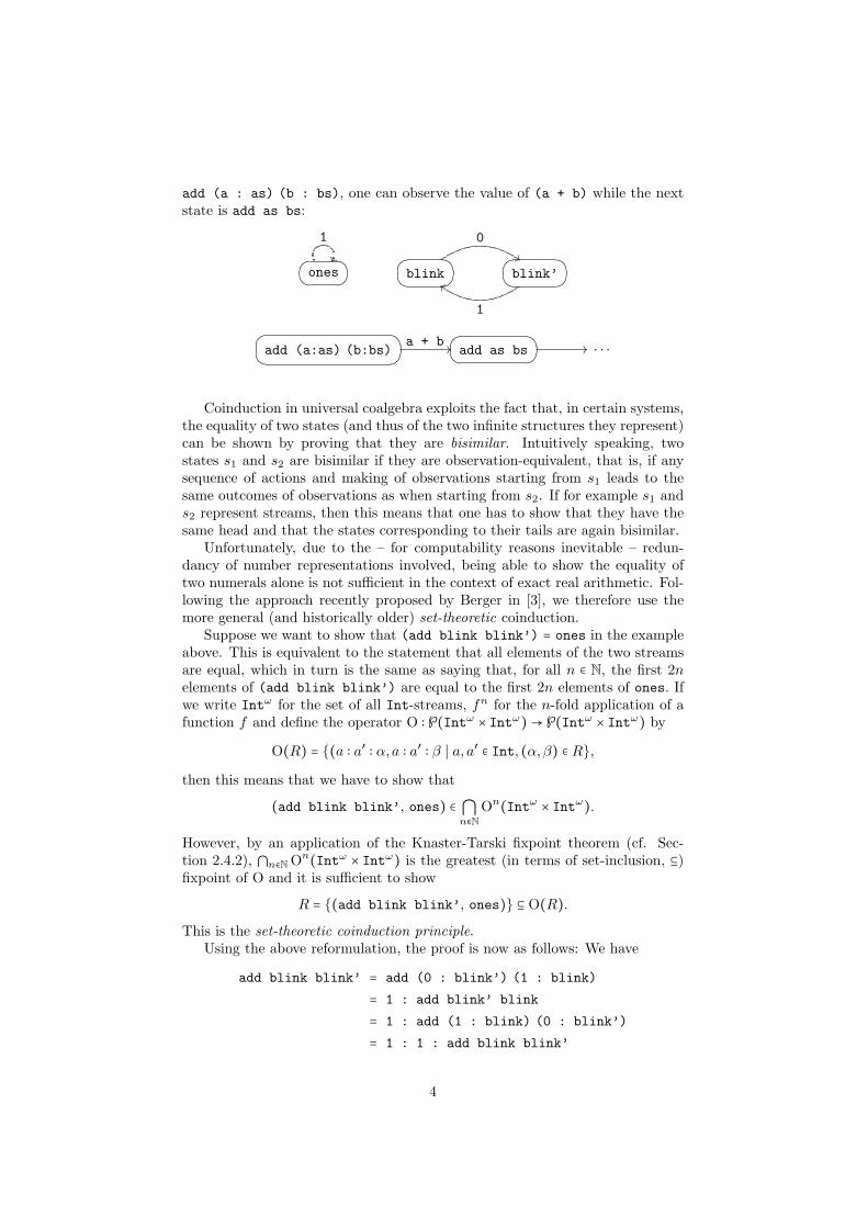
add (a : as) (b : bs), one can observe the value of (a + b) while the nextstate is add as bs:

76 5401 23ones

1

¨¨ 76 5401 23blink

0$$76 5401 23blink’

1

dd

76 5401 23add (a:as) (b:bs)a + b //76 5401 23add as bs // . . .

Coinduction in universal coalgebra exploits the fact that, in certain systems,the equality of two states (and thus of the two infinite structures they represent)can be shown by proving that they are bisimilar. Intuitively speaking, twostates s1 and s2 are bisimilar if they are observation-equivalent, that is, if anysequence of actions and making of observations starting from s1 leads to thesame outcomes of observations as when starting from s2. If for example s1 ands2 represent streams, then this means that one has to show that they have thesame head and that the states corresponding to their tails are again bisimilar.

Unfortunately, due to the – for computability reasons inevitable – redun-dancy of number representations involved, being able to show the equality oftwo numerals alone is not sufficient in the context of exact real arithmetic. Fol-lowing the approach recently proposed by Berger in [3], we therefore use themore general (and historically older) set-theoretic coinduction.

Suppose we want to show that (add blink blink’) = ones in the exampleabove. This is equivalent to the statement that all elements of the two streamsare equal, which in turn is the same as saying that, for all n ∈ N, the first 2nelements of (add blink blink’) are equal to the first 2n elements of ones. Ifwe write Intω for the set of all Int-streams, fn for the n-fold application of afunction f and define the operator O ∶ ℘(Intω × Intω)→ ℘(Intω × Intω) by

O(R) = {(a ∶ a′ ∶ α,a ∶ a′ ∶ β ∣ a, a′ ∈ Int, (α,β) ∈ R},then this means that we have to show that

(add blink blink’, ones) ∈ ⋂n∈N

On(Intω × Intω).

However, by an application of the Knaster-Tarski fixpoint theorem (cf. Sec-tion 2.4.2), ⋂n∈NOn(Intω × Intω) is the greatest (in terms of set-inclusion, ⊆)fixpoint of O and it is sufficient to show

R = {(add blink blink’, ones)} ⊆ O(R).This is the set-theoretic coinduction principle.

Using the above reformulation, the proof is now as follows: We have

add blink blink’ = add (0 : blink’) (1 : blink)

= 1 : add blink’ blink

= 1 : add (1 : blink) (0 : blink’)

= 1 : 1 : add blink blink’

4

and clearly

ones = 1 : 1 : ones.

This shows that R ⊆ O(R) and hence, by set-theoretic coinduction, that

add blink blink’ = ones.

Despite the fact that set-theoretic coinduction does not reside in the fieldof universal coalgebra, the steps it involves can often be interpreted in terms ofobservations, actions and states. For this reason, set-theoretic coinduction maygreatly benefit from coalgebraic coinductive definitions of the objects involved.

The aim of this project is to explore the combination of coalgebraic coin-ductive definitions and set-theoretic coinduction in the context of exact realarithmetic. To this end, we coinductively define arithmetic operations thatcompute the sum and linear affine transformations over Q of real numbers givenin the signed binary exponent-mantissa representation and prove their correct-ness using set-theoretic coinduction.

1.3 Contributions

The main contributions of this project can be summarized as follows:

� We propose a general strategy for studying exact arithmetic operations onthe signed binary exponent-mantissa representation that combines coal-gebraic-coinductive definitions and set-theoric coinduction. This strategyis similar to that used in [3], however it explains the ensuing definitionsfrom a coalgebraic perspective and can be used for operations on the realline rather than just those on the unit interval.

� We explore the proposed strategy (and thus the combination of coalgebraiccoinductive definitions and set-theoretic coinduction) by using it to obtainoperations that compute the sum and liner affine transformations over Qand prove their correctness.

� We give a Haskell implementation of the operations thus obtained and usethis implementation for a brief comparison with related algorithms fromliterature.

5

Chapter 2

Background

This chapter provides more detail on some of the relevant technical backgroundonly touched upon in the previous chapter.

2.1 Alternatives to Floating Point Arithmetic

The Muller-sequence described in the previous chapter shows that there arecases in which floating point arithmetic can not be used. This section brieflydescribes some of its alternatives, including a slightly more exhaustive accountof exact real arithmetic than that given in the introduction. A more detailedoverview of these alternatives can be found in [15].

Floating point arithmetic with error analysis Floating point arithmeticwith error analysis is similar to floating point arithmetic except that itkeeps track of possible rounding errors that might have been introducedduring the computation. It produces two floating point numbers: the firstis the result obtained using normal floating point arithmetic while the sec-ond gives the range about this point that the exact result is guaranteedto be in if rounding errors are taken into account. In the example givenin the introduction, the bound on the error would be very large. Knuthgives a theoretical model for floating point error analysis in [11].

Interval arithmetic Interval Arithmetic can be seen as a generalization offloating point arithmetic with error analysis. Instead of using two floatingpoint numbers to specify the center and half length of the interval theexact result is guaranteed to be in, it uses two numbers of any finitelyrepresentable subset of the reals (eg. the rational numbers) to specify thelower and upper bounds of the interval, respectively. Similarly to float-ing point arithmetic with error analysis, each calculation is performed onboth bounds, with strict downwards and upwards rounding respectively ifthe result on a bound cannot be represented exactly. Interval arithmeticis very useful, however it does not make the calculations any more ex-act. An accessible introduction to interval arithmetic and how it can beimplemented using IEEE floating point arithmetic is given in [9].

Stochastic rounding Unlike ordinary floating point arithmetic, which roundseither always upwards or always downwards in case the result of a compu-

6

tation falls exactly between two floating point numbers, stochastic round-ing chooses by tossing a (metaphorical) fair coin. The desired computationis repeated several times and the true result is then estimated using prob-ability theory. While stochastic rounding cannot guarantee the accuracyof the result in a fashion similar to floating point arithmetic with erroranalysis, it will in general give more exact results. Moreover, it allows toobtain probabilistic information about the reliability of its calculations.An implementation of stochastic rounding is described in [20]. When usedto compute the first 25 terms of the Muller-sequence, this implementationdoes not give more accurate results than ordinary floating point arith-metic. However, it does correctly detect the numerical instabilities andwarns the user that the results are not guaranteed [1].

Symbolic calculation Symbolic approaches represent real numbers as expres-sions consisting of function symbols, variables and constants. Calculationsare performed by simplifying such expressions rather than by manipulat-ing numbers. It is important to note that the number to be computed isthus represented exactly at each stage of the calculation.

The problem with symbolic calculation is that the simplifaction of arbi-trary mathematical expressions is very difficult and that there are manycases where it cannot be done at all. In these cases, the expression hasto be evaluated numerically in order to be usable, which is why symbolicapproaches are rarely used on their own. This can be seen in the twomathematics packages Maple [4] and Mathematica [22] that are knownfor the strength of their symbolic engines but offer support for numericcalculations as well.

Exact real arithmetic As explained in the introduction, exact real arithmeticguarantees the correctness of its results up to some user-specified preci-sion. Since this may require calculating some intermediate results to avery high accuracy, implementations of exact real arithmetic have to beable to handle arbitrarily large number representations and are thereforeoften considerably slower than more conventional approaches. In returnhowever, arbitrary precision arithmetic solves the problems of inaccuracyand uncertainty associated with interval arithmetic and stochastic round-ing and can be used in many cases in which a symbolic approach wouldnot be appropriate. Various approaches to exact real arithmetic can forinstance be found in [3, 6, 7, 14,15].

We see that, of all these approaches, only exact real arithmetic can be usedto obtain arbitrarily precise results for the general case. As mentioned in theintroduction, this is why exact real arithmetic holds an important place amongapproaches to real number computation.

2.2 Representations in Exact Real Arithmetic

It is clear that in any approach to exact real arithmetic the choice of representa-tion largely determines how operations can be defined and reasoned about. Aswe will see now, this impact goes even further in that there are representationsfor which some operations cannot (reasonably) be defined at all.

7

2.2.1 The Failure of the Standard Decimal Expansion

Consider adding the two numbers 13= 0.333 . . . and 2

3= 0.666 . . . using the

standard decimal expansion (this is a well-known example and can for instancebe found in [6, 15]). After having read the first digit after the decimal pointfrom both expansions, we know that they lie in the intervals [0.3,0.4] and[0.6,0.7], respectively. This means that their sum is contained in the interval[0.9,1.1] and so we do not know at this stage whether the first digit of theresult should be a 0 or a 1. This problem continues: all that reading any finitenumber of digits from the inputs can tell us is that they lie in the invervals[0.3 . . .33,0.3 . . .34] and [0.6 . . .66,0.6 . . .67], and thus that their sum is con-tained in [0.9 . . .99,1.0 . . .01], whose bounds are strictly less and greater than1, respectively. We would therefore never be able to output even the first digitof the result.

The way to get around this problem is to introduce some form of redundancyinto the representation (see eg. [2]). This allows us in cases as above to makea guess how the input might continue and then undo this guess later in caseit turns out to be wrong. The next section describes an important class ofrepresentations that use redundancy to this end.

2.2.2 Signed Digit Representations

One of the most widely-studied represenations (see eg. [2,6,11]) for real numbersis the signed digit representation in a given integer base B. Instead of, as inthe standard decimal expansion, only allowing positive digits {0,1, . . . ,B−1} tooccur in the representation, one also includes negative numbers so that the setof possible digits becomes {−B + 1,−B + 2, . . . ,−1,0,1, . . . ,B − 1}. For elementsbi of this set, the sequence (b1, b2, . . . ) then represents the real number

∞∑i=1

biB−i (2.1)

It should be quite clear from this formula how negative digits can be used tomake corrections to previous output.

Consider again the example of adding 13

and 23. These two numbers can be

represented in the signed decimal expansion by the streams13= 0.333 ⋅ ⋅ ⋅ ∼ (0,3,3,3, . . . )

23= 0.666 ⋅ ⋅ ⋅ ∼ (0,6,6,6, . . . )

After having read (0,3) from the first input, we know it is greater than or equalto 0.2 (since the sequence could continue −9,−9,−9, . . . ) and less than or equalto 0.4. Similarly, we know that the second input lies in the interval [0.5,0.7] sothat the sum of the two is in the range [0.7,1.1]. Even though this interval islarger than the one we obtained when using the ordinary decimal expansion, itis now safe to output 1 because the stream starting (1, . . . ) can represent anynumber between 0 and 2.

A note on the word stream Streams are simply infinite sequences. Wewill use the term sequence to refer to both finite and infinite lists of elements,however it will always be made clear which of the two cases we are talking about.

8

The Signed Binary Expansion

The signed binary expansion is the simplest and most widely-used signed digitrepresentation. It represents the case where B = 2 and thus uses digits fromthe set {−1,0,1} to identify real numbers in the interval [−1,1]. The signedbinary expansion is the representation on which the arithmetic operations ofthis project are defined.

Interpreting numerals After having read the first digit d1 of a signed binarynumeral, the remaining terms in Equation (2.1) can give a contribution of mag-nitude at most 1

2. As visualized by Figure 2.1 (seen similar in [15]), this allows

us to conclude that the value of the numeral lies in the interval [d12− 1

2, d1

2+ 1

2].

−1 0 1´¹¹¹¹¹¹¹¹¹¹¹¹¹¹¹¹¹¹¹¹¹¹¹¹¹¹¹¹¹¹¹¹¹¸¹¹¹¹¹¹¹¹¹¹¹¹¹¹¹¹¹¹¹¹¹¹¹¹¹¹¹¹¹¹¹¹¶

d1 = 0

d1 = −1³¹¹¹¹¹¹¹¹¹¹¹¹¹¹¹¹¹¹¹¹¹¹¹¹¹¹¹¹¹¹¹¹¹·¹¹¹¹¹¹¹¹¹¹¹¹¹¹¹¹¹¹¹¹¹¹¹¹¹¹¹¹¹¹¹¹µ d1 = 1³¹¹¹¹¹¹¹¹¹¹¹¹¹¹¹¹¹¹¹¹¹¹¹¹¹¹¹¹¹¹¹¹¹·¹¹¹¹¹¹¹¹¹¹¹¹¹¹¹¹¹¹¹¹¹¹¹¹¹¹¹¹¹¹¹¹µ

Figure 2.1: Interval of a signed binary numeral with first digit d1

Suppose that we next read the second digit d2. By again referring to Equa-tion (2.1) and a reasoning similar to the above, we can conclude that the numerallies in the interval [d1

2+ d2

4− 1

4, d1

2+ d2

4+ 1

4]. This is exemplarily shown for the

case d1 = 1 in Figure 2.2.

−1 0 1

d1 = 1³¹¹¹¹¹¹¹¹¹¹¹¹¹¹¹¹¹¹¹¹¹¹¹¹¹¹¹¹¹¹¹¹¹·¹¹¹¹¹¹¹¹¹¹¹¹¹¹¹¹¹¹¹¹¹¹¹¹¹¹¹¹¹¹¹¹µ

¡¡

¡¡

¡¡

0 12 1

d2 = 0³¹¹¹¹¹¹¹¹¹¹¹¹¹¹¹¹¹¹¹¹¹¹¹¹¹¹¹¹¹¹¹¹¹·¹¹¹¹¹¹¹¹¹¹¹¹¹¹¹¹¹¹¹¹¹¹¹¹¹¹¹¹¹¹¹¹µ

´¹¹¹¹¹¹¹¹¹¹¹¹¹¹¹¹¹¹¹¹¹¹¹¹¹¹¹¹¹¹¹¹¹¸¹¹¹¹¹¹¹¹¹¹¹¹¹¹¹¹¹¹¹¹¹¹¹¹¹¹¹¹¹¹¹¹¶d2 = −1

´¹¹¹¹¹¹¹¹¹¹¹¹¹¹¹¹¹¹¹¹¹¹¹¹¹¹¹¹¹¹¹¹¹¸¹¹¹¹¹¹¹¹¹¹¹¹¹¹¹¹¹¹¹¹¹¹¹¹¹¹¹¹¹¹¹¹¶d2 = 1

Figure 2.2: Interval of a signed binary numeral of the form (1, d2, . . . )

Note the symmetry! Again, we had an interval of half-width 2−n, wheren was the number of digits read thus far, and reading the next digit (in thiscase d2) told us whether the value of the numeral lies in the lower, middle orupper half of this interval. Since this can be shown to hold for any sequence ofdigits, reading a signed binary numeral can be seen as an iterative selection ofsub-intervals with exponentially decreasing length.

9

Reference Intervals (or: The Decimal Point)

A disadvantage of the signed digit representation in base B is that it can onlybe used to represent real numbers in the interval [−B +1,B −1]. In the decimalexpansion, this problem is overcome using the decimal (or, for bases other than10 the radix ) point, whose role we have silently ignored up until now.

What the decimal point does is that it specifies the magnitude of the numberthat is to be represented. For instance, in the decimal expansion of π = 3.141 . . . ,the position of the decimal point tells us that the normal formula

∞∑i=1

bi10−i

has to be multiplied by an additional factor of 101 to obtain the required result.Instead of extending the set of allowed digits {−B+1, . . . ,B−1} to explicitly

include the decimal point, it is common to use an exponent-mantissa repre-sentation, which simply specifies the exponent of the scaling constant. A realnumber r is thus represented by its exponent a ∈ N (or even a ∈ Z) and itsmantissa (b1, b2, . . . ) where bi ∈ {−B + 1, . . . ,B − 1} and

r = Ba∞∑i=1

biB−i

This allows us to use signed digit representations for specifying any real number,even if it is outside the normally representable interval [−B + 1,B − 1].

2.2.3 Other Representations

This section briefly describes some alternative representations for the real num-bers. An important feature of a representation for the real numbers is whetherit is incremental. A representation is said to be incremental if a numeral thatrepresents a real number to some accuracy can be reused to calculate a more ac-curate approximation to that number. The signed digit representation describedabove is incremental since all we have to do in order to get a better approxi-mation for a real number is to calculate more digits of its expansion. We willindicate which of the representations that are mentioned here are incrementaland which are not.

Linear Fractional Transformations

A one-dimensional linear fractional transformation (1-LFT) or Mobius trans-formation is a function L ∶ C → C of the form

L(x) = ax + c

bx + d

where a, b, c and d are arbitrary but fixed real or complex numbers. Similarly,a function T ∶ C ×C→ C of the form

T (x, y) = axy + cx + ey + g

bxy + dx + fy + h

where a, b, c, d, e, f , g and h are fixed real or complex numbers is called atwo-dimensional linear fractional transformation (2-LFT).

10

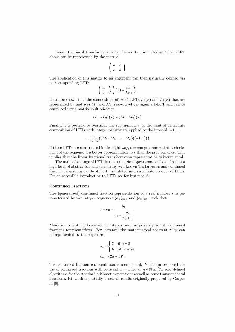
Linear fractional transformations can be written as matrices: The 1-LFTabove can be represented by the matrix

( a bc d

)

The application of this matrix to an argument can then naturally defined viaits corresponding LFT:

( a bc d

)(x) = ax + c

bx + d

It can be shown that the composition of two 1-LFTs L1(x) and L2(x) that arerepresented by matrices M1 and M2, respectively, is again a 1-LFT and can becomputed using matrix multiplication:

(L1 ○L2)(x) = (M1 ⋅M2)(x)Finally, it is possible to represent any real number r as the limit of an infinitecomposition of LFTs with integer parameters applied to the interval [−1,1]:

r = limn→∞

((M1 ⋅M2 ⋅ . . . ⋅Mn)([−1,1]))

If these LFTs are constructed in the right way, one can guarantee that each ele-ment of the sequence is a better approximation to r than the previous ones. Thisimplies that the linear fractional transformation representation is incremental.

The main advantage of LFTs is that numerical operations can be defined at ahigh level of abstraction and that many well-known Taylor series and continuedfraction expansions can be directly translated into an infinite product of LFTs.For an accessible introduction to LFTs see for instance [6].

Continued Fractions

The (generalised) continued fraction representation of a real number r is pa-rameterized by two integer sequences (an)n≥0 and (bn)n≥0 such that

r = a0 +b1

a1 +b2

a2 + ⋱

.

Many important mathematical constants have surprisingly simple continuedfractions representations. For instance, the mathematical constant π by canbe represented by the sequences

an =⎧⎪⎪⎨⎪⎪⎩

3 if n = 06 otherwise

bn = (2n − 1)2.

The continued fraction representation is incremental. Vuillemin proposed theuse of continued fractions with constant an = 1 for all n ∈ N in [21] and definedalgorithms for the standard arithmetic operations as well as some transcendentalfunctions. His work is partially based on results originally proposed by Gosperin [8].

11

Dyadic Rational Streams

A dyadic rational is a rational number whose denominator is a power of two,i.e. a number of the form

a

2b

where a is an integer and b is a natural number. Similarly to the signed binaryexpansion, a stream (d1, d2, . . . ) of dyadic rationals in the interval [−1,1], canbe used to represent a real number r ∈ [−1,1] via the formula

r =∞∑i=1

di2−i.

Observe that this representation has the same rate of convergence as thesigned binary expansion. However, each dyadic digit di can incorporate signif-icantly more information than a signed binary digit. This can greatly simplifycertain algorithms but unfortunately often leads to a phenomenon called digitswell in which the size of the digits increases so rapidly that the performanceis destroyed. Plume gives an implementation of the standard arithmetic opera-tions for the signed binary and the dyadic stream representations and discussessuch issues in [15].

Nested Intervals

The nested interval representation describes a real number r by an infinite se-quence of nested closed intervals

[a1, b1] ⊇ [a2, b2] ⊇ [a3, b3] ⊇ . . . .

The progressing elements of the sequence represent better and better approxi-mations to r. In order for this to be a valid representation, it must have theproperty that ∣an − bn∣→ 0 as n→∞ and that both an and bn converge to r.

The endpoints of the intervals are elements of a finitely representable subsetof the reals, typically the rational numbers. Computation using nested intervalsis performed by calculating further elements of the sequence and thus betterapproximations to r. This implies that this representation is incremental.

An implementation of nested intervals for the programming language PCFis given in [7]. This reference uses rational numbers to represent the endpointsof the intervals and uses topological and domain theoretic arguments to developthe theory behind the approach.

2.3 Computability Issues

Without getting bogged down in technical details of the various formalisationsof computability, there are a few key issues we would like to mention in orderto give the reader a feeling for the setting exact real arithmetic resides in. Allresults that are presented here are described in a very informal and generalmanner, even though the statements made by the given references are muchmore precise and confined. However, the ideas that underlie them are of suchgenerality and intuitive truth that we hope that the reader will bear with us intaking this step.

12

2.3.1 Computable Numbers

Turing showed in his key paper [18,19] that not every real number that is defin-able is computable and that only a countable subset of the reals is computable.Fortunately, the numbers and operations we encounter and use every day allturn out to be in this set so that this limitation rarely affects us. Neverthe-less, computability is an important concept that greatly influences the way ouroperations are defined, even if we do not always make this explicit.

An interesting result in this context is that there cannot be a general algo-rithm to determine whether two computable real numbers are equal [16]. Theintuitive explanation for this is that an infinite amount of data would have tobe read, which is of course impossible. Although our operations do not directlyneed to compare two real numbers, they are constrained in a similar way: Eventhough it would make the algorithms simpler and would not require redun-dancy in the representation, operations for exact real arithmetic cannot workfrom right to left, ie. in the direction in which the significance of the digitsincreases, since this would require reading an infinite amount of data.

2.4 Coalgebra and Coinduction

Finally, in this section, we make precise how we are going to use coinductionfor our definitions and proofs.

We will use the following notation: If A is a set, then we write idA ∶ A → Afor the identity function on A and Aω for the set of all streams of elements ofA. Streams themselves are denoted by greek letters or expressions of the form(an) and their elements are written as a1, a2 etc. The result of prepending anelement a to a stream α will be written as a ∶ α. If f ∶ A1 → B1 and g ∶ A2 → B2

are functions, then f × g ∶ (A1 ×A2) → (B1 ×B2) denotes the function definedby (f × g)(a1, a2) = (f(a1), g(a2)). For two functions f ∶ A → B and g ∶ A → Cwith the same domain, ⟨f, g⟩ ∶ A → B ×C is defined by ⟨f, g⟩(a) = (f(a), g(a)).Finally, for any function f ∶ A→ A, fn ∶ A→ A denotes its nth iteration, that is

f0(x) = x and fn+1(x) = f (fn(x)) .

Many of the results presented here can be found in a similar or more generalform in [10] and [17]. For an application of coinduction to exact real arithmeticsee [3].

As briefly outlined in the introduction, universal coalgebra can be used tostudy infinite data types, which includes streams but also more complex struc-tures such as infinite trees. Since the coalgebraically interesting part of ourrepresentation lies in the stream of digits however, we do not need the full the-ory behind universal coalgebra but can rather restrict ourselves to the followingsimple case:

Definition 2.1. Let A be a set. An A-stream coalgebra is a pair (X,γ) where

1. X is a set

2. γ ∶ X → A ×X is a function

13

Any stream (an)n∈N of elements in a set A can be modelled as an A-streamcoalgebra by taking X = N and defining γ by

γ(n) = (an, n + 1).The following important definition captures one way in which A-stream coalge-bras can be related:

Definition 2.2. Let (X,γ) and (Y, δ) be two A-stream coalgebras. A func-tion f ∶ X → Y is called an A-stream homomorphism from (X,γ) to (Y, δ) iff(idA × f) ○ γ = δ ○ f , that is, the following diagram commutes:

X

γ

²²

f // Y

δ

²²A ×X

idA×f// A × Y

This immediately gives rise to

Definition 2.3. An A-stream homomorphism f is called an A-stream isomor-phism iff its inverse exists and is also an A-stream homomorphism.

The most trivial example of an A-stream isomorphism of a coalgebra (X,γ) isidX ∶ X →X, the identity map on X: it is clearly bijective and we have

(idA × idX) ○ γ = γ = γ ○ idX .

This shows that idX is an A-stream isomorphism.The composition of two A-stream homomorphisms is again a homomor-

phism:

Proposition 2.4. Let (X,γ), (Y, δ) and (Z, ε) be A-stream coalgebras and f ∶X → Y and g ∶ Y → Z be homomorphisms. Then g ○ f ∶ X → Z is an A-streamhomomorphism from (X,γ) to (Z, ε).Proof. We have

(idA × (g ○ f)) ○ γ = (idA × g) ○ (idA × f) ○ γ = (idA × g) ○ δ ○ f = ε ○ (g ○ f)This shows that g ○ f is an A-stream homomorphism.

A coalgebraic concept that turns out to be extremely useful is that of finality :

Definition 2.5. An A-stream coalgebra (X,γ) is called final iff for any A-stream coalgebra (Y, δ) there exists a unique homomorphism f ∶ Y →X.

Proposition 2.6. Final A-stream coalgebras are unique, up to isomorphism: If(X,γ) and (Y, δ) are final A-stream coalgebras then there is a unique isomor-phism f ∶ X → Y of A-stream coalgebras.

Proof. If (X,γ) and (Y, δ) are final A-stream coalgebras, then there are uniquehomomorphisms f ∶ X → Y and g ∶ Y → X. By Proposition 2.4, their com-position g ○ f ∶ X → X is again a homomorphism. Since idX ∶ X → X is ahomomorphism, too, we have g ○ f = idX by the uniqueness part of finality. Asimilar argument yields that f ○ g = idY . This shows that f−1 = g exists and,since it is a homomorphism, that f is an A-stream isomorphism.

14

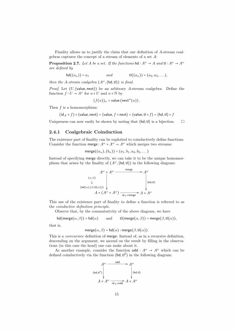
Finality allows us to justify the claim that our definition of A-stream coal-gebras captures the concept of a stream of elements of a set A:

Proposition 2.7. Let A be a set. If the functions hd ∶ Aω → A and tl ∶ Aω → Aω

are defined by

hd((an)) = a1 and tl((an)) = (a2, a3, . . . ),then the A-stream coalgebra (Aω, ⟨hd, tl⟩) is final.

Proof. Let (U, ⟨value,next⟩) be an arbitrary A-stream coalgebra. Define thefunction f ∶ U → Aω for u ∈ U and n ∈ N by

(f(u))n = value (nextn(u)) .

Then f is a homomorphism:

(idA × f) ○ ⟨value,next⟩ = ⟨value, f ○ next⟩ = ⟨value, tl ○ f⟩ = ⟨hd, tl⟩ ○ f

Uniqueness can now easily be shown by noting that ⟨hd, tl⟩ is a bijection.

2.4.1 Coalgebraic Coinduction

The existence part of finality can be exploited to coinductively define functions.Consider the function merge ∶ Aω ×Aω → Aω which merges two streams:

merge((an), (bn)) = (a1, b1, a2, b2, . . . )Instead of specifying merge directly, we can take it to be the unique homomor-phism that arises by the finality of (Aω, ⟨hd, tl⟩) in the following diagram:

Aω ×Aω

(α,β)↓

(hd(α),(β,tl(α))) ²²

merge // Aω

⟨hd,tl⟩

²²A × (Aω ×Aω)

idA×merge// A ×Aω

This use of the existence part of finality to define a function is referred to asthe coinductive definition principle.

Observe that, by the commutativity of the above diagram, we have

hd(merge(α,β)) = hd(α) and tl(merge(α,β)) = merge(β, tl(α)),that is,

merge(α,β) = hd(α) ∶ merge(β, tl(α)).This is a corecursive definition of merge: Instead of, as in a recursive definition,descending on the argument, we ascend on the result by filling in the observa-tions (in this case the head) one can make about it.

As another example, consider the function odd ∶ Aω → Aω which can bedefined coinductively via the function ⟨hd, tl2⟩ in the following diagram:

Aω

⟨hd,tl2⟩²²

odd // Aω

⟨hd,tl⟩²²

A ×AωidA×odd

// A ×Aω

15

Again, the commutativity of the diagram implies

hd(odd(α)) = hd(α) and tl(odd(α)) = odd(tl(tl(α))).

In the following, we will also use odd’s counterpart even ∶ Aω → Aω which wedefine by

even(α) = odd(tl(α)).Suppose we want to prove the equality merge(odd(α), even(α)) = α for all

α ∈ Aω. Since we know that idAω ∶ Aω → Aω is a homomorphism, and since thefinality of (Aω, ⟨hd, tl⟩) tells us that this homomorphism is unique, it is enoughto show that merge ○ ⟨odd, even⟩ ∶ Aω → Aω is a homomorphism to deducethat merge ○ ⟨odd, even⟩ = idAω . This is an example of a coalgebraic proof bycoinduction.

In order to prove that merge ○ ⟨odd, even⟩ is a homomorphism, we have toshow

⟨hd, tl⟩ ○ (merge ○ ⟨odd, even⟩) = (idA × (merge ○ ⟨odd, even⟩)) ○ ⟨hd, tl⟩.

This follows from the two chains of equalities

hd(merge(odd(α), even(α))) = hd(odd(α))= hd(α)

and

tl(merge(odd(α), even(α))) = merge(even(α), tl(odd(α)))= merge(even(α),odd(tl(tl(α))))= merge(odd(tl(α)), even(tl(α)))= (merge ○ ⟨odd, even⟩)(tl(α)).

Hence, by coinduction, merge(odd(α), even(α)) = α for all α ∈ Aω.As a concluding remark, recall that only the finality of (Aω, ⟨hd, tl⟩) allowed

us to use the coinductive definition and proof principles in the above examples.This is one of the main reasons why finality plays such a key role in the field ofcoalgebra.

2.4.2 Set-theoretic Coinduction

Because of the – for computability reasons inevitable – redundancy of exactreal number representations, the coinductive proof principle outlined in theprevious section is often too restricted to express equality of real numbers givenas streams (argued for instance in [3]). The more general (and historicallyolder) set-theoretic form of coinduction exploits the fact that every monotoneset operator has a greatest fixpoint. Since this kind of coinduction will be usedto prove the main results of the next chapter, we here introduce its underlyingprinciples and show how it can be used to prove the merge identity from theprevious section. For a thorough comparison of coalgebraic and set-theoreticcoinduction see for instance [12].

16

Background

Recall the following standard definitions and results:

Definition 2.8. A partially ordered set is a set P together with a binary relation≤ on P that satisfies, for all a, b, c, ∈ P

� a ≤ a (reflexivity)

� a ≤ b and b ≤ a⇒ a = b (antisymmetry)

� a ≤ b and b ≤ c⇒ a ≤ c (transitivity)

Definition 2.9. A complete lattice is a partially ordered set in which all subsetshave both a supremum and an infimum.

Theorem 2.10 (Knaster-Tarski). If (L,≤) is a complete lattice and m ∶ L→ Lis a monotone function, then the set of all fixpoints of m in L is also a completelattice.

Corollary 2.11. If (L,≤) is a complete lattice then any monotone functionm ∶ L→ L has a least fixpoint LFP(m) and a greatest fixpoint GFP(m) given by

� GFP(m) = sup {x ∈ L ∣ x ≤ m(x)}� LFP(m) = inf {x ∈ L ∣ x ≥ m(x)}

Moreover, for any l ∈ L,

� if m(l) ≤ l then LFP(m) ≤ l and

� if l ≤ m(l) then l ≤ GFP(m).These results can be used as follows: Let X,Y be sets, R,M ⊆ X ×Y be binaryrelations on X and Y and suppose we want to show that (x, y) ∈ M for all(x, y) ∈ R. If we manage to find a monotone operator O ∶ ℘(X × Y )→ ℘(X × Y )whose greatest fixpoint in the complete lattice (℘(X × Y ),⊆) is M , then itsuffices to show R ⊆ O(R) to deduce that R ⊆ M by the last part of the abovecorollary. This is the set-theoretic coinduction principle.

An Example Proof

Recall the merge identity from the previous section: For all α ∈ Aω,

merge(odd(α), even(α)) = α. (2.2)

In order to prove this result by set-theoretic coinduction, we work in the com-plete lattice (℘(Aω ×Aω),⊆) and define the operator

O ∶ ℘(Aω ×Aω)→ ℘(Aω ×Aω)O(R) = {(a ∶ a′ ∶ α,a ∶ a′ ∶ β) ∣ a, a′ ∈ A, (α,β) ∈ R}.

O is clearly monotone and we claim that its greatest fixpoint GFP(O) is givenby

M = {(α,α) ∣ α ∈ Aω}.

17

To see this, let (α,β) ∈ GFP(O). We want to show that (α,β) ∈ M whichis equivalent to proving that α = β. Since GFP(O) is a fixpoint of O, wehave GFP(O) = O(GFP(O)) and thus (α,β) ∈ O(GFP(O)). This means bythe definition of O that the first two digits of α and β are equal and that(tl2(α), tl2(β)) ∈ GFP(O). Repeating the same argument for (tl2(α), tl2(β)),then for (tl4(α), tl4(β)) etc. shows that all digits of α and β are equal and thusthat α = β. Hence GFP(O) ⊆ M . Since clearly M ⊆ O(M) and thus by the lastpart of the above corollary M ⊆ GFP(O), this shows that GFP(O) = M .

The next step is to define the relation R ⊆ ℘(Aω ×Aω) by

R = {(merge(odd(α), even(α)), α) ∣ α ∈ Aω}.

We want to show that R ⊆ M . By the set-theoretic coinduction principle how-ever, we only have to show R ⊆ O(R): Let (merge(odd(α), even(α)), α) ∈ R andsuppose α = a ∶ a′ ∶ α′ for some a, a′ ∈ A,α′ ∈ Aω. Then

merge(odd(α), even(α)) = merge(odd(a ∶ a′ ∶ α′), even(a ∶ a′ ∶ α′))= merge(a ∶ odd(α′),odd(a′ ∶ α′))= merge(a ∶ odd(α′), a′ ∶ odd(tl(α′)))= a ∶ merge(a′ ∶ odd(tl(α′)),odd(α′))= a ∶ a′ ∶ merge(odd(α′),odd(tl(α′)))= a ∶ a′ ∶ merge(odd(α′), even(α′)).

This shows that (merge(odd(α), even(α)), α) ∈ O(R) and thus that R ⊆ O(R).Therefore, by (set-theoretic) coinduction, Equation (2.2) holds for all α ∈ Aω.

As already mentioned above, this is the kind of coinductive proof that willbe given for the arithmetic operations in our project.

18

Chapter 3

Arithmetic Operations

In this chapter, we use the coinductive principles outlined in Section 2.4 tostudy operations that compute the sum and linear affine transformations overQ of signed binary exponent-mantissa numerals. We will keep using the samenotation (cf. page 13), however we will additionally write

D = {−1,0,1}for the set of signed binary digits.

3.1 Preliminaries

Definition 3.1. The function σ∣1∣ ∶ Dω → [−1,1] that identifies the real numberrepresented by a signed binary numeral is defined by

σ∣1∣(α) =∞∑i=1

2−iαi.

Its extension σ ∶ N ×Dω → R to the exponent-mantissa representation is definedby

σ(e,α) = 2eσ∣1∣(α) = 2e∞∑i=1

2−iαi.

The following results will be used throughout the remainder of this chapter:

Lemma 3.2 (Properties of σ∣1∣). Let α ∈ Dω. Then

1. ∣σ∣1∣(α)∣ ≤ 1

2. σ∣1∣(α) = σ(0, α)3. σ∣1∣(tl(α)) = 2σ∣1∣(α) − hd(α)

Proof.

1. Using the standard expansion of the geometric series,

∣σ∣1∣(α)∣ = ∣∞∑i=1

2−iαi∣ ≤∞∑i=1

2−i ∣αi∣ ≤∞∑i=1

2−i = ( 11 − 1

2

− 1) = 1.

19

2. Clear from the definition of σ.

3. Direct manipulation:

σ∣1∣(tl(α)) =∞∑i=1

2−i(tl(α))i

=∞∑i=1

2−iαi+1

=∞∑i=2

2−i+1αi

= 2∞∑i=2

2−iαi

= 2∞∑i=1

2−iαi − α1

= 2σ∣1∣(α) − hd(α).

Corollary 3.3 (Properties of σ). Let (e,m) ∈ N ×Dω. Then

1. ∣σ(e,α)∣ ≤ 2e

2. σ(e, tl(α)) = 2σ(e,α) − 2ehd(α)Proof.

1. By the definition of σ and by Lemma 3.2(1),

∣σ(e,α)∣ = 2e ∣σ∣1∣(α)∣ ≤ 2e.

2. By the definition of σ and by Lemma 3.2(3),

σ(e, tl(α)) = 2eσ∣1∣(tl(α)) = 2e(2σ∣1∣(α) − hd(α)) = 2σ(e,α) − 2ehd(α).

Definition 3.4. The relation ∼ ∈ ℘((N × Dω) × R) that specifies when a realnumber is represented by a signed binary exponent-mantissa numeral is definedby

∼ = {((e,α), r) ∣ σ(e,α) = r} .

Its restriction ∼∣1∣ ∈ ℘(Dω × [−1,1]) to the unit interval is defined by

∼∣1∣ = {(α, r) ∣ σ∣1∣(α) = r}.

We write (e,α) ∼ r if ((e,α), r) ∈ ∼ and α ∼∣1∣ r if (α, r) ∈ ∼∣1∣.The following operator will form the basis of our coinductive proofs:

Definition 3.5. The operator O∣1∣ ∶ ℘(Dω × [−1,1])→ ℘(Dω × [−1,1]) is definedby

O∣1∣(R) = {(α, r) ∣ (tl(α),2r − hd(α)) ∈ R}.

20

Note. The codomain of O∣1∣ really is ℘(Dω × [−1,1]): Let R ∈ ℘(Dω × [−1,1])and (α, r) ∈ O∣1∣(R). Then (tl(α),2r − hd(α)) is in R, so that ∣2r − hd(α)∣ ≤ 1.But 2∣r∣ − ∣hd(α)∣ ≤ ∣2r − hd(α)∣ and hence 2∣r∣ − ∣hd(α)∣ ≤ 1. This implies2∣r∣ ≤ 1 + ∣hd(α)∣ ≤ 2 and thus ∣r∣ ≤ 1.

Proposition 3.6. O∣1∣ has a greatest fixpoint and this fixpoint is ∼∣1∣.Proof. O∣1∣ is clearly monotone and so by Corollary 2.11 has a greatest fixpoint.Call this fixpoint M . We want to prove that M = ∼∣1∣.

Let (α, r) ∈ M . Note that

(α, r) ∈ ∼∣1∣ ⇔ σ∣1∣(α) = r

⇔ σ∣1∣(α) − r = 0

⇔ ∣σ∣1∣(α) − r∣ = 0

⇔ ∣σ∣1∣(α) − r∣ ≤ 21−n ∀n ∈ N. (3.1)

In order to show that (α, r) ∈ ∼∣1∣, it therefore suffices to prove that Equa-tion (3.1) holds. This can be done via induction:

n = 0: We have (using Lemma 3.2(1))

∣σ∣1∣(α) − r∣ ≤ ∣σ∣1∣(α)∣ + ∣r∣≤ 1 + ∣r∣ .

Now (α, r) ∈ M implies ∣r∣ ≤ 1 and so

∣σ∣1∣(α) − r∣ ≤ 2,

as required.

n→ n + 1: Let n ∈ N be such that ∣σ∣1∣(α′) − r′∣ ≤ 21−n for all ((α′, r′) in M .Since M is a fixpoint of O∣1∣, M = O∣1∣(M) and thus (α, r) ∈ O∣1∣(M). Thisimplies that (tl(α),2r−hd(α)) is in M so that, by the inductive hypothesisand Lemma 3.2(3):

21−n ≥ ∣σ∣1∣(tl(α)) − 2r + hd(α)∣= ∣2σ∣1∣(α) − hd(α) − 2r + hd(α)∣= 2 ∣σ∣1∣(α) − r∣ .

Hence, as required∣σ∣1∣(α) − r∣ ≤ 21−(n+1).

Thus by induction, (α, r) ∈ ∼∣1∣. Since (α, r) ∈ M was arbitrary, this shows thatM ⊆ ∼∣1∣.

In order to show ∼∣1∣ ⊆ M , it suffices by Corollary 2.11 to prove

∼∣1∣ ⊆ O∣1∣(∼∣1∣).Recall

O∣1∣(∼∣1∣) = {(α, r) ∣ (tl(α),2r − hd(α)) ∈ ∼∣1∣}= {(α, r) ∣ σ∣1∣(tl(α)) = 2r − hd(α)}.

Let (α, r) ∈ ∼∣1∣. Then by Lemma 3.2(3) and the definition of ∼∣1∣,σ∣1∣(tl(α)) = 2σ∣1∣(α) − hd(α) = 2r − hd(α).

Hence (α, r) ∈ O∣1∣(∼∣1∣) and so ∼∣1∣ ⊆ O∣1∣(∼∣1∣), as required.

21

3.2 The Coinductive Strategy

Coinduction gives us the following strategy to define and reason about arith-metic operations on the signed binary exponent-mantissa representation: LetX be a set and suppose we have a function F ∶ X × R → R for which we wantto find an implementation on the exponent-mantissa representation, that is,an operation F ∶ X × (N × Dω) → N × Dω which satisfies, for all x ∈ X and(e,α) ∈ N ×Dω,

F (x, (e,α)) ∼ F (x,σ(e,α)).We first find a subset Y of X and a function f ∶ Y × [−1,1] → [−1,1] that, insome intuitive sense, is representative of F on the unit interval. Then, we lookfor a coinductive definition of an implementation of f on the level of streamswhich is, similarly to above, an operation f ∶ Y ×Dω → Dω that satisfies, for ally ∈ Y and α ∈ Dω,

f(y,α) ∼∣1∣ f(y, σ∣1∣(α)).In the remainder of this section, we call f correct if and only if this equationholds.

Once we have (coinductively) defined f , we use the set-theoretic coinductionprinciple outlined in Section 2.4.2 to prove its correctness in the above sense asfollows: We define the relation R ⊆ (Dω × [−1,1]) by

R = {(f(y,α), f (y, σ∣1∣(α))) ∣ y ∈ Y,α ∈ Dω} ,

which makes proving the correctness of f equivalent to showing R ⊆ ∼∣1∣. How-ever, since we have seen in the previous section that ∼∣1∣ is the greatest fixpointof the monotone operator O∣1∣, it in fact suffices by the set-theoretic coinductionprinciple to prove R ⊆ O∣1∣(R). Let (f(y,α), f (y, σ∣1∣(α))) ∈ R and recall that

O∣1∣(R) = {(α, r) ∣ (tl(α),2r − hd(α)) ∈ R}= {(α, r) ∣ ∃y′ ∈ Y,α′ ∈ Dω s.t. tl(α) = f(y′, α′),

2r − hd(α) = f(y′, σ∣1∣(α′))}.Because f was defined coinductively, there is a function γ for which the followingdiagram commutes:

Y ×Dω

γ

²²

f // Dω

⟨hd,tl⟩²²

D × (Y ×Dω)id×f

// D ×Dω.

Choose y′, α′ and d such that γ(y,α) = (d, (y′, α′)). The commutativity of thediagram implies tl (f(y,α)) = f(y′, α′) and hd (f(y,α)) = d, so that all we haveto show in order to prove that (f(y,α), f (y, σ∣1∣(α))) ∈ O∣1∣(R) and thus thatf is correct is

2f (y, σ∣1∣(α)) − d = f (y′, σ∣1∣(α′)) .

Once we have done this, it should be easy to define F in terms of f and provethat F really is an implementation of F using the correctness of f .

The next two sections show how this strategy can be used in practice.

22

3.3 Addition

Our aim in this section is to define the operation

⊕ ∶ (N ×Dω) × (N ×Dω)→ N ×Dω

that computes the sum of two signed binary exponent-mantissa numerals. Fol-lowing the strategy outlined in Section 3.2, we do this by first (coinductively)defining a corresponding operation on the level of streams. Since signed binarynumerals are not closed under addition, the natural choice for this operationis the average function that maps x, y ∈ [−1,1] to x+y

2(∈ [−1,1]). We will

represent this function on the level of digit streams by defining an operationavg ∶ Dω ×Dω → Dω that satisfies

σ∣1∣(avg(α,β)) = σ∣1∣(α) + σ∣1∣(β)2

(3.2)

for all signed binary streams α and β.

3.3.1 Coinductive Definition of avg

Recall that a coinductive definition of avg consists of first specifying a function

γ ∶ Dω ×Dω → D × (Dω ×Dω)

and then taking avg to be the unique induced homomorphism in the diagram

Dω ×Dω

γ

²²

avg // Dω

⟨hd,tl⟩

²²D × (Dω ×Dω)

id×avg// D ×Dω.

(3.3)

If we let α = (a1, a2, . . . ) and β = (b1, b2, . . . ) be two signed binary streams andwrite γ(α,β) = (s, (α′, β′)), the commutativity of the diagram will imply

hd(avg(α,β)) = s and tl(avg(α,β)) = avg(α′, β′),

that is,avg(α,β) = s ∶ avg(α′, β′). (3.4)

Since our goal is to coinductively define avg in such a way that Equation (3.2)holds, this means that s, α′ and β′ have to satisfy

σ∣1∣(s ∶ avg(α′, β′)) =σ∣1∣(α) + σ∣1∣(β)

2. (3.5)

23

Finding the First Digit s

Suppose we read the first two digits from both α and β. By the definition of σ∣1∣,

σ∣1∣(α) = a1

2+ a2

4+

∞∑i=3

2−iai

´¹¹¹¹¹¹¹¹¹¹¹¹¸¹¹¹¹¹¹¹¹¹¹¹¹¶∈[− 1

4 , 14 ]

and σ∣1∣(β) = b1

2+ b2

4+

∞∑i=3

2−ibi

´¹¹¹¹¹¹¹¹¹¹¹¸¹¹¹¹¹¹¹¹¹¹¹¶∈[− 1

4 , 14 ]

.

What we know after having read a1, a2, b1 and b2 is therefore precisely that

σ∣1∣(α) ∈ [a1

2+ a2

4− 1

4,a1

2+ a2

4+ 1

4] and σ∣1∣(β) ∈ [b1

2+ b2

4− 1

4,b1

2+ b2

4+ 1

4]

which implies

σ∣1∣(α) + σ∣1∣(β)2

∈ [p − 14, p + 1

4]

where

p = a1 + b1

4+ a2 + b2

8.

If p is less than − 14, then the lower and upper bounds of [p − 1

4, p + 1

4] are strictly

less than − 12

and 0, respectively, so we can (and must!) output −1 as the firstdigit. Similarly, if ∣p∣ ≤ 1

4, then [p − 1

4, p + 1

4] ⊆ [− 1

2, 1

2] so we output 0 and if

p > 14, then we output 1. This can be formalized by writing

s = sg 14(p)

where p is as above and the generalised sign function sgε ∶ Q→ D (taken from [3])is defined for ε ∈ Q≥0 by

sgε(q) =⎧⎪⎪⎪⎪⎨⎪⎪⎪⎪⎩

1 if q > ε

0 if ∣q∣ ≤ ε

−1 if q < −ε.

Interlude: Required Lookahead

The above reasoning shows that reading two digits from each of the two inputstreams is always enough to determine the first digit of output. A naturalquestion to ask is whether the same could be achieved with fewer digits. Wewill see now that the answer is no: In certain cases, already reading one digitless makes it impossible to produce a digit of output.

Suppose we read the first two digits from α but only the first digit from β.By a reasoning similar to the above, one can show that this implies

σ∣1∣(α) + σ∣1∣(β)2

∈ [a1 + b1

4+ a2

8− 3

8,a1 + b1

4+ a2

8+ 3

8] .

If for instance a1 = b1 = 1 and a2 = 0, this is the interval [ 18, 7

8]. Since [ 1

8, 7

8] is

contained in [0,1], we can safely output 1 without examining any further input.If, however, a1 = 1 and b1 = a2 = 0, the interval becomes [− 1

8, 5

8]. Because − 1

8

can only be represented by a stream starting with −1 or 0 and 58

can only berepresented by a stream starting with 1, we do not know at this stage what thefirst digit of output should be. We require more input.

24

Determining (α′, β′)Recall Equation (3.5) which stated the condition for the correctness of avg as

σ∣1∣(s ∶ avg(α′, β′)) =σ∣1∣(α) + σ∣1∣(β)

2. [3.5]

Both sides of this equation can be rewritten. For the left-hand side, we use theansatz

α′ = a′1 ∶ tl2(α) β′ = b′1 ∶ tl2(β),where a′1 and b′1 are signed binary digits. Assuming avg will be correct(!),this yields

σ∣1∣(s ∶ avg(α′, β′)) =s

2+ 1

2σ∣1∣(avg(α′, β′))

= s

2+ 1

2σ∣1∣(α′) + σ∣1∣(β′)

2(!)

= s

2+ 1

2

a′12+ 1

2σ∣1∣(tl2(α)) + b′1

2+ 1

2σ∣1∣(tl2(β))

2

= s

2+ a′1 + b′1

8+ 1

8(σ∣1∣(tl2(α)) + σ∣1∣(tl2(β))).

For the right-hand side,

σ∣1∣(α) + σ∣1∣(β)2

=a12+ a2

4+

∞∑i=3

2−iai + b1

2+ b2

4+

∞∑i=3

2−ibi

2

= a1 + b1

4+ a2 + b2

8´¹¹¹¹¹¹¹¹¹¹¹¹¹¹¹¹¹¹¹¹¹¹¹¹¹¹¹¹¹¹¹¹¹¹¹¹¹¹¹¹¹¹¹¹¹¹¸¹¹¹¹¹¹¹¹¹¹¹¹¹¹¹¹¹¹¹¹¹¹¹¹¹¹¹¹¹¹¹¹¹¹¹¹¹¹¹¹¹¹¹¹¹¹¶p

+12(∞∑i=3

2−iai +∞∑i=3

2−ibi)

= p + 18(∞∑i=3

2−(i−2)ai + 18

∞∑i=3

2−(i−2)bi)

= p + 18(σ∣1∣ (tl2(α)) + σ∣1∣ (tl2(β))) . (3.6)

Using these steps, Equation (3.5) becomes

s

2+ a′1 + b′1

8= p,

i.e.a′1 + b′1

8= p − s

2.

Now a′1 and b′1 are signed binary digits so that a′1 must be 1 when p − s2> 1

8

and −1 when p − s2< 1

8. Also, when ∣p − s

2∣ ≤ 1

8, we can take a′1 to be 0 by the

symmetry of the equation. We therefore choose

a′1 = sg 18(p − s

2) ,

which forces us take

b′1 = 8p − 4s − a′1.

An easy case analysis on p shows that b′1 is in fact a signed binary digit.

25

Final Definition of γ and avg

To summarize, the function γ ∶ Dω × Dω → D × (Dω × Dω) is defined for anysigned binary numerals α = (a1, a2, . . . ) and β = (b1, b2, . . . ) by

γ(α,β) = (s, (α′, β′))where

s = sg 14(p) α′ = a′1 ∶ tl2(α) β′ = b′1 ∶ tl2(β)

p = a1 + b1

4+ a2 + b2

8a′1 = sg 1

8(p − s

2) b′1 = 8p − 4s − a′1

and the generalised sign function sgε is as on page 24. By the finality of theD-stream coalgebra (Dω, ⟨hd, tl⟩), this induces the (unique) homomorphism avgin Diagram (3.3):

Dω ×Dω

γ

²²

avg // Dω

⟨hd,tl⟩

²²D × (Dω ×Dω)

id×avg// D ×Dω

[3.3]

In particular, if we let s, α′ and β′ be as above, then

avg(α,β) = s ∶ avg(α′, β′). [3.4]

3.3.2 Correctness of avg

In order to prove the correctness of avg, we first need the following lemma:

Lemma 3.7 (Correctness of γ). Let α and β be signed binary streams andsuppose s, α′ and β′ are as in the definition of γ. Then

σ∣1∣(α) + σ∣1∣(β)2

= s

2+ 1

2σ∣1∣(α′) + σ∣1∣(β′)

2.

Proof. For the left-hand side, we refer back to Equation (3.6):

σ∣1∣(α) + σ∣1∣(β)2

= p + 18(σ∣1∣ (tl2(α)) + σ∣1∣ (tl2(β))) ,

where p is as in the definition of γ.For the right-hand side, recall that a′1 and b′1 were constructed so that

s

2+ a′1 + b′1

8= p.

Together with the definitions of σ∣1∣, α′ and β′, this implies

s

2+ 1

2σ∣1∣(α′) + σ∣1∣(β′)

2= s

2+ 1

2

a′12+ 1

2σ∣1∣ (tl2(α)) + b′1

2+ 1

2σ∣1∣ (tl2(β))

2

= s

2+ a′1 + b′1

8+ 1

8(σ∣1∣ (tl2(α)) + σ∣1∣ (tl2(β)))

= p + 18(σ∣1∣ (tl2(α)) + σ∣1∣ (tl2(β))) ,

as required.

26

Theorem 3.8 (Correctness of avg). Let α and β be signed binary streams. Then

avg(α,β) ∼∣1∣σ∣1∣(α) + σ∣1∣(β)

2.

Proof. Following the strategy outlined in Section 3.2, we define R ⊆ (Dω × [−1,1])by

R = {(avg(α,β), σ∣1∣(α) + σ∣1∣(β)2

) ∣ α,β ∈ Dω} .

The statement of the lemma is equivalent to R ⊆ ∼∣1∣. By the set-theoreticcoinduction principle, this can be proved by showing R ⊆ O∣1∣(R).Let (avg(α,β), σ∣1∣(α)+σ∣1∣(β)

2) ∈ R and recall

O∣1∣(R) = {(α, r) ∣ (tl(α),2r − hd(α)) ∈ R}= {(α, r) ∣ ∃α′, β′ ∈ Dω s.t. tl(α) = avg(α′, β′)

and 2r − hd(α) = σ∣1∣(α′)+σ∣1∣(β′)2

} .

Take α′, β′ as in the definition of γ. By the commutativity of Diagram (3.3),we have

tl(avg(α,β)) = avg(α′, β′) and hd(avg(α,β)) = s.

Moreover, by the correctness of γ (Lemma 3.7),

σ∣1∣(α) + σ∣1∣(β)2

= s

2+ 1

2σ∣1∣(α′) + σ∣1∣(β′)

2,

which implies

2σ∣1∣(α) + σ∣1∣(β)

2− hd(avg(α,β)) = σ∣1∣(α′) + σ∣1∣(β′)

2.

This shows that (avg(α,β), σ∣1∣(α)+σ∣1∣(β)2

) ∈ O∣1∣(R) and thus that R ⊆ O∣1∣(R).

3.3.3 Definition and Correctness of ⊕The final ingredient we need before being able to define the addition operation⊕ is the small lemma below. It will give us a way of finding a common exponentfor two signed binary exponent-mantissa numerals.

Lemma 3.9. If α is a signed binary stream, then for all n ∈ Nσ∣1∣ ((0 ∶)nα) = 2−nσ∣1∣(α)

where (0 ∶)nα is the result of prepending n zeros to α.

Proof. By induction on n. The result clearly holds for the case n = 0. Also, ifit holds for some n ∈ N, then

σ∣1∣ ((0 ∶)n+1α) = σ∣1∣ (0 ∶ ((0 ∶)nα)) = 02+ 1

2σ∣1∣ ((0 ∶)nα) = 2−(n+1)σ∣1∣(α),

as required.

27

Definition 3.10. The addition operation ⊕ ∶ (N ×Dω)× (N×Dω)→ N×Dω isdefined for any signed binary exponent-mantissa numerals (e,α) and (f, β) by

(e,α)⊕ (f, β) = (max(e, f) + 1, avg ((0 ∶)max(e,f)−eα, (0 ∶)max(e,f)−fβ)) .

Theorem 3.11 (Correctness of ⊕). For any (e,α), (f, β) ∈ N ×Dω,

(e,α)⊕ (f, β) ∼ (σ(e,α) + σ(f, β)) .

Proof. By the correctness of avg (Theorem 3.8) and Lemma 3.9,

σ∣1∣ (avg ((0 ∶)max(e,f)−eα, (0 ∶)max(e,f)−fβ))= 2e−max(e,f)−1σ∣1∣(α) + 2f−max(e,f)−1σ∣1∣(β).

Hence, by the definitions of σ and ⊕,

σ((e,α)⊕ (f, β)) = 2eσ∣1∣(α) + 2fσ∣1∣(β)= σ(e,α) + σ(f, β).

3.4 Linear Affine Transformations over QThis section introduces the operation LinQ ∶ Q × (N ×Dω) ×Q→ N ×Dω thatrepresents the mapping

Q ×R ×Q Ð→ R(u,x, v) z→ ux + v.

As in the last section, we first (coinductively) define the corresponding operationlinQ on the level of streams in such a way that

σ∣1∣(linQ(u,α, v)) = uσ∣1∣(α) + v, (3.7)

where α = (a1, a2, . . . ) is any signed binary stream and u, v ∈ Q are such that∣u∣ + ∣v∣ ≤ 1. This last condition ensures that the result of the operation can infact be represented by a signed binary numeral.

3.4.1 Coinductive Definition of linQ

Before we give a coinductive definition of linQ, we first find a lower bound onthe lookahead required to output a digit in the general case. In some cases suchas when u = 0 and v = 1, we can output one (or even all) digits of the resultwithout examining the input. In other cases however, even one digit does notsuffice: If u = 3

4, v = 1

4and a1 = 0, then all we know after having read a1 is that

uσ∣1∣(α)´¹¹¹¹¹¹¹¹¸¹¹¹¹¹¹¹¶∈[− 1

2 , 12 ]

+v ∈ [−18,38] .

Since this interval is not contained in any of [−1,0], [− 12, 1

2] and [0,1], we cannot

determine what the first digit of output should be. This shows that a lookaheadof at least two digits is required to produce a digit of output in the general case.

28

In order to (coinductively) define linQ, we first specify its domain C thatcaptures the constraint mentioned in the introduction to this section:

C = {(u,α, v) ∈ Q ×Dω ×Q ∶ ∣u∣ + ∣v∣ ≤ 1} .

The coinductive part of the definition now consists of specifying a functionδ ∶ C → D ×C and taking linQ to be the (unique) ensuing homomorphism in thediagram

C

δ

²²

linQ // Dω

⟨hd,tl⟩

²²D ×C

id×linQ// D ×Dω.

(3.8)

Let (u,α, v) ∈ C and write δ(u,α, v) = (l, (u′, α′, v′)). If we follow the stepsabove, then the commutativity of the diagram will imply

linQ(u,α, v) = l ∶ linQ(u′, α′, v′). (3.9)

Since we want linQ to satisfy the correctness condition given by Equation (3.7),this means that we have to choose l, u′, α′ and v′ in such a way that

σ∣1∣(l ∶ linQ(u′, α′, v′)) = uσ∣1∣(α) + v. (3.10)

To find l, we observe that

uσ∣1∣(α) + v = u(a1

2+ a2

4+ 1

4σ∣1∣ (tl2(α))) + v

= u(a1

2+ a2

4) + v + u

4σ∣1∣ (tl2(α)) ,

´¹¹¹¹¹¹¹¹¹¹¹¹¹¹¹¹¹¹¹¹¹¹¹¹¹¹¹¹¹¹¹¹¹¹¹¹¹¹¸¹¹¹¹¹¹¹¹¹¹¹¹¹¹¹¹¹¹¹¹¹¹¹¹¹¹¹¹¹¹¹¹¹¹¹¹¹¶∈[− ∣u∣

4 ,∣u∣4 ]

(3.11)

so that

uσ∣1∣(α) + v ∈ [q − ∣u∣4

, q + ∣u∣4

] ⊆ [q − 14, q + 1

4]

whereq = u(a1

2+ a2

4) + v.

By a reasoning similar to that behind the choice of s in the definition of γ/avg,this implies that we can choose

l = sg 14(q).

For u′, α′ and v′, we note that if linQ is correct, then

σ∣1∣(l ∶ linQ(u′, α′, v′)) =l

2+ 1

2(u′σ∣1∣(α′) + v′) .

But we also have by Equation (3.11) that

uσ∣1∣(α) + v = l

2+ 1

2(u

2σ∣1∣ (tl2(α)) + 2q − l) .

29

Since we want Equation (3.10) to hold, we therefore compare terms and choose

u′ = u

2α′ = tl2(α) v′ = 2q − l.

We have to check that ∣u′∣ + ∣v′∣ ≤ 1. This can be done by a case analysis on δ,for which we will need

∣q∣ = ∣u(a1

2+ a2

2) + v∣

≤ 34∣u∣ + ∣v∣

= ∣u∣ + ∣v∣ − ∣u∣4

≤ 1 − ∣u∣4

. (3.12)

l = 0: By the definition of l, we have ∣q∣ ≤ 14. Also, ∣u∣+ ∣v∣ ≤ 1 implies ∣u∣ ≤ 1 and

so

∣u′∣ + ∣v′∣ = ∣u∣2+ 2∣q∣ ≤ 1

2+ 1

2= 1.

l = 1: We have q > 14

and thus v′ = 2q − l > − 12. Also, by Equation (3.12),

v′ ≤ 1 − ∣u∣2

. These inequalities tell us that ∣v′∣ ≤ max (∣−12∣ ,1 − ∣u∣

2). But,

∣u∣ ≤ 1 implies 1− ∣u∣2≥ 1

2, so this is in fact ∣v′∣ ≤ 1− ∣u∣

2= 1− ∣u′∣. The result

follows.

l = −1: Similarly to the case l = 1, we have ∣u∣2−1 ≤ v′ < 1

2and ∣u∣

2−1 ≤ − 1

2. Hence

∣v′∣ ≤ 1 − ∣u∣2= 1 − ∣u′∣ and so ∣u′∣ + ∣v′∣ ≤ 1.

Final Definition of δ and linQ

Let C = {(u,α, v) ∈ Q ×Dω ×Q ∶ ∣u∣ + ∣v∣ ≤ 1}. The function δ ∶ C → D × C isdefined for any (u,α, v) ∈ C by

δ(u,α, v) = (l, (u′, α′, v′))where, writing α = (a1, a2, . . . ),

l = sg 14(q) u′ = u

2α′ = tl2(α)

q = u(a1

2+ a2

4) + v v′ = 2q − l.

This allows us to take linQ to be the unique induced homomorphism in Dia-gram (3.8):

C

δ

²²

linQ // Dω

⟨hd,tl⟩

²²D ×C

id×linQ// D ×Dω

[3.8]

The commutativity of the diagram implies that, for (u,α, v) ∈ C,

linQ(u,α, v) = l ∶ linQ(u′, α′, v′) [3.9]

where l, u′, α′ and v′ are as above.

30

3.4.2 Correctness of linQ

Theorem 3.12 (Correctness of linQ). For any (u,α, v) ∈ C,

linQ(u,α, v) ∼∣1∣ uσ∣1∣(α) + v.

Proof. Define R ⊆ (Dω × [−1,1]) by

R = {(linQ(u,α, v), uσ∣1∣(α) + v)∣ (u,α, v) ∈ C} .

We show that R ⊆ ∼∣1∣ by showing that R ⊆ O∣1∣(R).Recall

O∣1∣(R) = {(α, r) ∣ (tl(α),2r − hd(α)) ∈ R}= {(α, r) ∣ ∃(u′, α′, v′) ∈ C s.t. tl(α) = linQ(u′, α′, v′),

2r − hd(α) = u′σ∣1∣(α′) + v′}.

Let (linQ(u,α, v), uσ∣1∣(α) + v) ∈ R and take l ∈ D, (u′, α′, v′) ∈ C as in thedefinition of linQ. By the commutativity of Diagram (3.8), we have

tl(linQ(u,α, v)) = linQ(u′, α′, v′).Moreover,

u′σ∣1∣(α′) + v′ = u

2σ∣1∣ (tl2(α)) + 2q − l

= u

2(2σ∣1∣(tl(α)) − a2) + 2q − l

= u

2(4σ∣1∣(α) − 2a1 − a2) + 2q − l

= 2uσ∣1∣(α) − 2u(a1

2+ a2

4) + 2q − l

= 2uσ∣1∣(α) − 2(q − v) + 2q − l

= 2(uσ∣1∣(α) + v) − l.

Since the commutativity of Diagram (3.8) also implies hd(linQ(u,α, v)) = l, thisshows that (linQ(u,α, v), uσ∣1∣(α) + v) ∈ O∣1∣(R) and thus that R ⊆ O∣1∣(R).

3.4.3 Definition and Correctness of LinQ

Let u, v ∈ Q and (e,α) ∈ N × Dω. In order to define LinQ that computesuσ(e,α) + v using linQ from the previous section, we have to find scaled-downversions u′, v′ ∈ Q of u and v, respectively such that ∣u′∣+ ∣v′∣ ≤ 1. The scale willbe determined using the (computable!) function ⌈log2⌉:Definition 3.13. The function ⌈log2⌉ ∶ Q≥0 → N is defined by

⌈log2⌉(s) =⎧⎪⎪⎨⎪⎪⎩0 if s ≤ 11 + ⌈log2⌉ ( s

2) otherwise.

Lemma 3.14. For any s ∈ Q≥0,

log2(s) ≤ ⌈log2⌉(s)where log2 ∶ R>0 → R is the (standard) logarithm to base 2.

31

Proof. Observe that Q≥0 = ⋃n∈N

⌈log2⌉−1(n) so that it suffices to show that the

result holds for all n ∈ N and s ∈ ⌈log2⌉−1(n). This can be done by induction.If n = 0 and s ∈ ⌈log2⌉−1(n) then s ≤ 1 and thus log2(s) ≤ 0 = ⌈log2⌉(s). Con-

versely, suppose the result holds for all t ∈ ⌈log2⌉−1(n) where n ∈ N is fixed. Lets ∈ ⌈log2⌉−1(n + 1). Then n+1 = ⌈log2⌉(s) = 1+⌈log2⌉ ( s

2) so that s

2∈ ⌈log2⌉−1(n).

This implies by our assumption that log2(s) − 1 = log2 ( s2) ≤ ⌈log2⌉ ( s

2) = n and

thus that log2(s) ≤ ⌈log2(s)⌉.Corollary 3.15. Let u, v ∈ Q and u′ = 2−nu, v′ = 2−nv where n = ⌈log2⌉(∣u∣+ ∣v∣).Then ∣u′∣ + ∣v′∣ ≤ 1.

Proof. By Lemma 3.14, n = ⌈log2⌉(∣u∣ + ∣v∣) ≥ log2(∣u∣ + ∣v∣). This implies that2−n ≤ 1

∣u∣+∣v∣ so that ∣u′∣ + ∣v′∣ = 2−n (∣u∣ + ∣v∣) ≤ ∣u∣+∣v∣∣u∣+∣v∣ = 1, as required.

Corollary 3.15 implies that we can write

uσ(e,α) + v = 2nu′2eσ∣1∣(α) + 2nv′

= 2e+n (u′σ∣1∣(α) + 2−ev′) (3.13)

where n, u′, v′ are as above and (!)

∣u′∣ + 2−e∣v′∣ ≤ ∣u′∣ + ∣v′∣ ≤ 1. (3.14)

This immediately gives rise to

Definition 3.16 (LinQ). The function LinQ ∶ Q × (N × Dω) × Q → N × Dω isdefined for u, v ∈ Q and (e,α) ∈ N ×Dω by

LinQ(u, (e,α), v) = (e + n, linQ(u′, α,2−ev′))

where

n = ⌈log2⌉(∣u∣ + ∣v∣) u′ = 2−nu v′ = 2−nv.

Theorem 3.17 (Correctness of LinQ). For any u, v ∈ Q, (e,α) ∈ Dω

σ(LinQ(u, (e,α), v)) = uσ∣1∣(α) + v.

Proof. Let n, u′ and v′ be as in the definition of LinQ. Then by Equation (3.14),∣u′∣ + 2−e∣v′∣ ≤ 1, so that, by the correctness of linQ (Theorem 3.12) and Equa-tion (3.13),

σ(LinQ(u, (e,α), v)) = 2e+nσ∣1∣ (linQ (u′, α,2−ev′))= 2e+n (u′σ∣1∣(α) + 2−ev′)= uσ(e,α) + v.

32

Chapter 4

Haskell Implementation

4.1 Overview

This section briefly describes the most important parts of the Haskell imple-mentation of the arithmetic operations introduced in the previous chapter. Thefull (though still not very long) code is given in Appendix A.2.

The most important types in the Haskell implementation are SD, SDS andReal which represent signed binary digits, signed binary streams and numeralsin the exponent-mantissa representation, respectively. The functions fromSDand sdToRational convert objects of type SD to the Haskell types Integerand Rational, respectively, so that calculations on signed binary digits can beperformed in the natural way.

Apart from some type conversions, the implementations of avg and linQcorrespond exactly to the definitions of avg and linQ:

approximate :: SDS -> Int -> Rational-- Calculates the value represented by the given

stream to an accuracy of 2^(-n).

approximate (a1 : a’) 1 = (fromSD a1) % 2approximate (a1 : a’) n

= (sdToRational a1 + approximate a’ (n - 1)) / 2

approximateReal :: Real -> Int -> RationalapproximateReal (e, m) n = 2^e * approximate m n

approximateAsDecimal :: SDS -> Int -> IO ()

s = sg (1 % 4) pp = (fromSD a1 + fromSD b1) % 4 + (fromSD a2 +

fromSD b2) % 8a1’ = sg (1 % 8) (p - (fromSD s) % 2)b1’ = sg 0 (8 * p - 4 * sdToRational s -

sdToRational a1 ’)

prependZeros :: Integer -> SDS -> SDS

33

-- Prepends the given number of zeros to the given

signed binary stream.

-- Defined in Section 3.3.3.

prependZeros 0 a = aprependZeros n a = prependZeros (n - 1) (Z : a)

In order to implement ⊕, we need to be able to prepend a stream withan arbitrary number of zeros (this was (0 ∶)n in the definition of ⊕). This isdone by the function prependZeros using which, again, the translation frommathematical definition to implementation is immediate:

showRationalAsDecimal q decPlaces= show p ++ "." ++ showFractionalPart (10 * r) (

denominator q) decPlaceswhere

(p, r) = divMod (numerator q) (denominator q)showFractionalPart n d 0 = []

Finally, linQ_real is the Haskell implementation of the function LinQ. Ituses the implementation ceilLog2 of the function ⌈log2⌉:add :: Real -> Real -> Real-- Calculates the sum of two real numbers to an

arbitrary precision.

-- Introduced and proved correct in Section 3.3.3.

add (e, a) (f, b)= (max e f + 1, avg (prependZeros ((max e f) - e) a)

(prependZeros ((max e f) - f) b))

ceilLog2 :: Rational -> Integer-- Exactly computes the ceiling function of the

logarithm to base 2 of the given number.

-- Introduced and proved correct in Section 3.4.3.

As pointed out, all translations from the mathematical definitions to therespective Haskell implementations are straightforward and do not require morethan a few syntactic changes and extra type conversions. The credit for thisis of course mostly due to Haskell, however it also shows that the coinductiveapproach lends itself well to an implementation in a functional programminglanguage that supports corecursive definitions.

Manual tests were performed and verified that the developed algorithms areindeed correct.

4.2 Related Operations in Literature

Operations on signed binary streams similar to those studied in this work canfor instance be found in [3, 5](avg) and [13](linQ). We would like to find outwhether these are output-equivalent to our operations, that is, whether theyproduce the same streams when given the same input.

The reference [13] defines the function applyfSDS which corresponds to ourlinQ and gives a Haskell implementation. The average operation av from [3] caneasily be translated as follows:

34

av :: SDS -> SDS -> SDS-- Calculates the average (a + b)/2

-- Implementation of the definition given in [3]

av (a1 : a’) (b1 : b’) = av_aux a’ b’ (( fromSD a1) + (fromSD b1))

av_aux :: SDS -> SDS -> Integer -> SDSav_aux (a1 : a’) (b1 : b’) i

= d : av_aux a’ b’ (j - 4 * (fromSD d))where

j = 2 * i + (fromSD a1) + (fromSD b1)d = sg 2 (j % 1)

For linQ and applyfSDS, we try the input u = 2%3, v = -1%3 and a =toSDS 1%5, where toSDS converts a Haskell Rational to a signed digit stream(cf. Appendix A.2). For the first 5 signed binary digits, this yields

Digit: 1 2 3 4 5linQ: -1 1 0 1 0applyfSDS: -1 1 0 1 -1

So linQ and applyfSDS are not output-equivalent (even though, of course, theinfinite streams do represent the same real number).

For avg and av, we compare the respective outputs for the following values(again using toSDS):

a b0 01 11 -1

1%2 1%23%4 -1%3

-13%27 97%139

In all cases, the first 100 digits of output are the same. We also note that avgand av have the same effective lookahead: For the first digit of output, bothread two digits from each of the two input streams. For every following digit,av reads one digit from both streams while avg reads two, of which however thefirst was generated in the last iteration of avg. For these reasons, we conjecturethat the Integer parameter i of av_aux and the two new digits a1’ and b1’that are prepended to the tails of the input streams in avg are in a one-to-onecorrespondence.

35

Chapter 5

Conclusion, Related andFuture Work

We have proposed a general strategy similar to that given in [3] for studyingexact arithmetic operations on the signed binary exponent-mantissa represen-tation using coinduction. The main steps of this strategy consist of giving acoalgebraic coinductive definition of a function that represents the required op-eration on the level of streams and then proving the correctness of this functionusing set-theoretic coinduction. In this way, the strategy brings together twodifferent (though related) forms of coinduction that are usually not combined.

Using the proposed strategy, we have obtained operations that computethe sum and linear affine transformations over Q of real numbers given in theabove-mentioned representation and proved their correctness. In each case, thestrategy gave us a criterion that guided our search for the coinductive part ofthe definition. More importantly, the use of coalgebraic coinductive definitionprinciples provided us with a pattern of choices to make in the set-theoreticcoinduction proofs which essentially reduced these proofs to one key step.

Our Haskell implementation shows that the operations we have developedcan be used in practice. Moreover, the fact that the algorithms it consists ofare almost literal translations of the corecursive definitions of the correspondingoperations indicates that the coinductive approach is well-suited for an im-plementation in a lazy functional programming language. This is particularlyimportant because it alleviates the likelihood of introducing an error when goingfrom mathematical definitions to implementation.

Evaluating the results of a project as theoretical as this one is difficult. Themain contribution of this work is to show that the combination of coalgebraiccoinductive definition principles and set-theoretic coinduction can be used inthe context of exact real arithmetic and, for the aforementioned reasons, we feelthat this combination is very fruitfuil. One drawback of our approach mightbe that it does not take performance considerations into account so that theensuing algorithms may not be very efficient.

Operations on signed binary streams similar to those studied in this projectcan for instance be found in [3,5,13]. Our experiments with appropriate imple-mentations have shown that the average operation av from [3] may be closelyrelated to the function avg defined in this work while the function applyfSDS

36

from [13] is certainly different from our corresponding operation linQ.An interesting approach related to that followed in this project is program

extraction as for instance studied in [13]. It involves giving inductive and (set-theoretic) coinductive proofs of general computation problems and then extract-ing algorithms and programs from these proofs in a systematic way. This hasthe advantage that the obtained programs are correct by construction and thatformalisations become simpler because the approximating data are left implicitin the proofs.

As regards future work, there are several interesting possibilities. We be-lieve that the coinductive approach should lend itself similarly well to otherrepresentations and a next step could be to apply it to the more general linearfractional transformations. Another possibility would be to study coinductiverepresentations of operations rather than just real numbers. For instance, anoperation on a signed binary stream can be represented as an infinite tree whoseedges represent the digits of the input and whose nodes represent the outputdigits or a symbol ∗ that indicates that more input is required:

'&%$Ã!"#∗−1

ÄÄÄÄÄÄ

ÄÄÄÄ

ÄÄ

0

²²

1

ÂÂ???

????

???

. . . '&%$Ã!"#∗−1

ÄÄÄÄÄÄ

ÄÄÄÄ

ÄÄ

0

²²

1

ÂÂ???

????

??? . . .

'&%$Ã!"#1

²²

. . . . . .

. . .

On this representation, for instance an integral operator could then be defined.

37

Bibliography

[1] Study of iterations of a recurrence sequence of order two. Example appli-cation of the CADNA library; Available from http://www-pequan.lip6.fr/cadna/Examples_Dir/ex4.php.

[2] A. Avizienis. Signed-digit number representations for fast parallel arith-metic. IRE Transactions on Electronic Computers, 10:389–400, September1961.

[3] U. Berger and T. Hou. Coinduction for exact real number computation.Theory of Computing Systems, 43:394–409, December 2008.

[4] B. W. Char, K. O. Geddes, G. H. Gonnet, B. L. Leong, M. B. Monagan,and S. M. Watt. Maple V Language Reference Manual. Springer Berlin /Heidelberg, first edition, November 1991.

[5] A. Ciaffaglione and Di P. Gianantonio. A certified, corecursive implemen-tation of exact real numbers. Theoretical Computer Science, 351(1):39–51,February 2006.

[6] A. Edalat and R. Heckmann. Computing with Real Numbers, volume 2395of Lecture Notes in Computer Science, pages 953–984. Springer Berlin /Heidelberg, January 2002.

[7] M. H. Escardo. PCF extended with real numbers. Theoretical ComputerScience, 162(1):79–115, August 1996.

[8] R. W. Gosper. Item 101b: Continued fraction arithmetic. Memo239 (”HAKMEM”), MIT Artificial Intelligence Laboratory, February 1972.

[9] T. Hickey, Q. Ju, and M. H. van Emden. Interval arithmetic: From prin-ciples to implementation. Journal of the ACM (JACM), 48(5):1038–1068,September 2001.

[10] B. Jacobs and J. Rutten. A tutorial on (co)algebras and (co)induction.EATCS Bulletin, 62:222–259, 1997.

[11] D. E. Knuth. Seminumerical Algorithms, volume 2 of The Art of ComputerProgramming. Addison-Wesley, third edition, 1997.

[12] M. Lenisa. From set-theoretic coinduction to coalgebraic coinduction: someresults, some problems. In B. Jacobs and J. Rutten, editors, Proc. Coalge-braic Methods in Computer Science(CMCS’99), volume 19 of Electr. NotesTheor. Comput. Sci., 1999.

38

[13] S. Lloyd. Implementation and verification of exact real number algorithms.Bachelor’s Thesis, Department of Computer Science, University of WalesSwansea, 2009.

[14] V. Menissier-Morain. Arbitrary precision real arithmetic: Designand algorithms. Submitted to J. Symbolic Computation. Avail-able from http://www-calfor.lip6.fr/~vmm/documents/submission_JSC.ps.gz, September 1996.

[15] D. Plume. A calculator for exact real number computation. 4th YearProject Report, Departments of Computer Science and Artificial Intelli-gence, University of Edinburgh, 1998.

[16] H. G. Rice. Recursive real numbers. Proceedings of the American Mathe-matical Society, 5(5):784–791, October 1954.

[17] J. J. M. M. Rutten. Universal coalgebra: A theory of systems. TheoreticalComputer Science, 249(1):3–80, October 2000.

[18] A. M. Turing. On computable numbers, with an application to the entschei-dungsproblem. Proceedings of the London Mathematical Society, 2(42):230–265, 1936.

[19] A. M. Turing. On computable numbers, with an application to the entschei-dungsproblem. A correction. Proceedings of the London Mathematical So-ciety, 2(43):544–546, 1937.

[20] J. Vignes. Discrete stochastic arithmetic for validating results of numericalsoftware. Numerical Algorithms, 37(1-4):377–390, December 2004.

[21] J. E. Vuillemin. Exact real computer arithmetic with continued fractions.IEEE Transaction on Computers, 39(8):1087–1105, August 1990.

[22] S. Wolfram. Mathematica: a System for Doing Mathematics by Computer.Addison Wesley, second edition, April 1991.

39

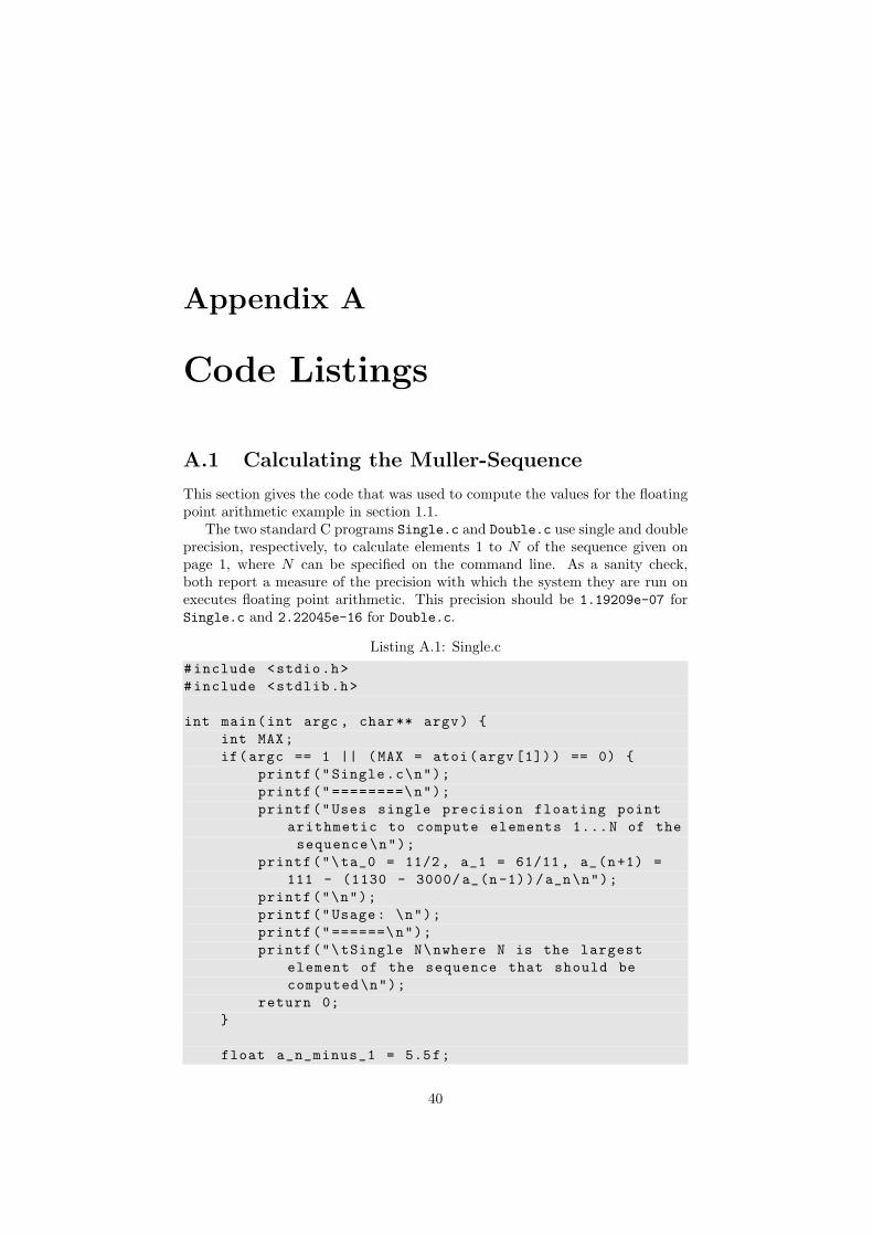
Appendix A

Code Listings

A.1 Calculating the Muller-Sequence

This section gives the code that was used to compute the values for the floatingpoint arithmetic example in section 1.1.

The two standard C programs Single.c and Double.c use single and doubleprecision, respectively, to calculate elements 1 to N of the sequence given onpage 1, where N can be specified on the command line. As a sanity check,both report a measure of the precision with which the system they are run onexecutes floating point arithmetic. This precision should be 1.19209e-07 forSingle.c and 2.22045e-16 for Double.c.

Listing A.1: Single.c#include <stdio.h>#include <stdlib.h>

int main(int argc , char** argv) {int MAX;if(argc == 1 || (MAX = atoi(argv [1])) == 0) {

printf("Single.c\n");printf("========\n");printf("Uses single precision floating point

arithmetic to compute elements 1...N of thesequence\n");

printf("\ta_0 = 11/2, a_1 = 61/11 , a_(n+1) =111 - (1130 - 3000/ a_(n-1))/a_n\n");

printf("\n");printf("Usage: \n");printf("======\n");printf("\tSingle N\nwhere N is the largest

element of the sequence that should becomputed\n");

return 0;}

float a_n_minus_1 = 5.5f;

40

float a_n = 61.0f/11.0f;int n;for (n = 1; n <= MAX; n++) {

printf("%f\n", a_n);float tmp = a_n;a_n = 111 - (1130 - 3000 / a_n_minus_1) / a_n;a_n_minus_1 = tmp;

}

float precision = 1.0f;float y;while( (y = precision + 1.0f) != 1.0f )

precision /= 2.0f;precision *= 2.0f;printf("Precision is %g \n", precision);return 0;

}

Listing A.2: Double.c#include <stdio.h>#include <stdlib.h>

int main(int argc , char** argv) {int MAX;if(argc == 1 || (MAX = atoi(argv [1])) == 0) {

printf("Double.c\n");printf("========\n");printf("Uses double precision floating point

arithmetic to compute elements 1...N of thesequence\n");

printf("\ta_0 = 11/2, a_1 = 61/11 , a_(n+1) =111 - (1130 - 3000/ a_(n-1))/a_n\n");

printf("\n");printf("Usage: \n");printf("======\n");printf("\tDouble N\nwhere N is the largest

element of the sequence that should becomputed\n");

return 0;}

double a_n_minus_1 = 5.5;double a_n = 61.0/11.0;int n;for (n = 1; n <= MAX; n++) {

printf("%1f\n", a_n);double tmp = a_n;a_n = 111 - (1130 - 3000 / a_n_minus_1) / a_n;a_n_minus_1 = tmp;

41

}

double precision = 1.0;double y;while( (y = precision + 1.0) != 1.0 )

precision /= 2.0;precision *= 2.0;printf("Precision is %g \n", precision);return 0;

}

Arbitrary.bc uses a fixed but arbitrary precision to calculate the nth ele-ment of the sequence given on page 1. As mentioned in section 1.1, it is a scriptfor the UNIX program bc.

Listing A.3: Arbitrary.bc# Call with UNIX utility bc# Uses arbitrary precision floating point arithmetic

to compute the Nth element of the sequence# a_0 = 11/2, a_1 = 61/11, a_(n+1) = 111 - (1130 -

3000/ a_(n-1))/a_n

# Precisionprint "\nPlease enter the precision (in number of

decimal places after the decimal point) thecalculations should be executed with: ";

scale = read();

print "\nPlease enter which element of the sequenceyou would like to have computed: ";

max = read();

a_n_minus_1 = 5.5;a_n = 61.0/11.0;

for(n = 2; n <= max; n++) {tmp = a_n;a_n = 111 - (1130 - 3000/ a_n_minus_1)/a_n;a_n_minus_1 = tmp;

}

print "\na_", max , " calculated using the givenprecision: ", a_n , "\n";

print "distance from the exact value of a_n: ", a_n -(6 ^ (max + 1) + 5 ^ (max + 1)) / (6 ^ max + 5 ^max), "\n";

quit;

42

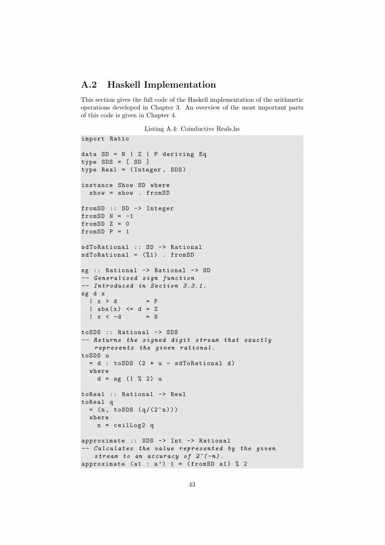
A.2 Haskell Implementation

This section gives the full code of the Haskell implementation of the arithmeticoperations developed in Chapter 3. An overview of the most important partsof this code is given in Chapter 4.

Listing A.4: Coinductive Reals.hsimport Ratio

data SD = N | Z | P deriving Eqtype SDS = [ SD ]type Real = (Integer , SDS)

instance Show SD whereshow = show . fromSD

fromSD :: SD -> IntegerfromSD N = -1fromSD Z = 0fromSD P = 1

sdToRational :: SD -> RationalsdToRational = (%1) . fromSD

sg :: Rational -> Rational -> SD-- Generalised sign function

-- Introduced in Section 3.3.1.

sg d x| x > d = P| abs(x) <= d = Z| x < -d = N

toSDS :: Rational -> SDS-- Returns the signed digit stream that exactly

represents the given rational.

toSDS u= d : toSDS (2 * u - sdToRational d)where

d = sg (1 % 2) u

toReal :: Rational -> RealtoReal q

= (n, toSDS (q/(2^n)))where

n = ceilLog2 q

approximate :: SDS -> Int -> Rational-- Calculates the value represented by the given

stream to an accuracy of 2^(-n).

approximate (a1 : a’) 1 = (fromSD a1) % 2

43

approximate (a1 : a’) n= (sdToRational a1 + approximate a’ (n - 1)) / 2

approximateReal :: Real -> Int -> RationalapproximateReal (e, m) n = 2^e * approximate m n

approximateAsDecimal :: SDS -> Int -> IO ()-- Approximates (and prints) the value of the given

SDS to an accuracy of n decimal places

approximateAsDecimal ds n = putStr (showRationalAsDecimal (approximate ds (floor ((fromIntegral n) * log (10) / log (2)))) n)

showRationalAsDecimal :: Rational -> Int -> StringshowRationalAsDecimal q n

| q < 0 = ’-’ : showRationalAsDecimal (-q) nshowRationalAsDecimal q 0 = show (( numerator q) ‘div ‘

(denominator q))showRationalAsDecimal q decPlaces

= show p ++ "." ++ showFractionalPart (10 * r) (denominator q) decPlaces

where(p, r) = divMod (numerator q) (denominator q)showFractionalPart n d 0 = []showFractionalPart n d decPlaces = (show (n ‘div ‘

d)) ++ showFractionalPart (10*(n ‘mod ‘ d)) d (decPlaces - 1)

avg :: SDS -> SDS -> SDS-- Calculates the average (a + b)/2.

-- Introduced in Section 3.3.1, proved correct in

Section 3.3.2.

avg (a1 : a2 : a’) (b1 : b2 : b’)= s : avg (a1 ’ : a’) (b1 ’ : b’)where

s = sg (1 % 4) pp = (fromSD a1 + fromSD b1) % 4 + (fromSD a2 +

fromSD b2) % 8a1’ = sg (1 % 8) (p - (fromSD s) % 2)b1’ = sg 0 (8 * p - 4 * sdToRational s -

sdToRational a1 ’)

prependZeros :: Integer -> SDS -> SDS-- Prepends the given number of zeros to the given

signed binary stream.

-- Defined in Section 3.3.3.

prependZeros 0 a = aprependZeros n a = prependZeros (n - 1) (Z : a)

add :: Real -> Real -> Real

44

-- Calculates the sum of two real numbers to an

arbitrary precision.

-- Introduced and proved correct in Section 3.3.3.

add (e, a) (f, b)= (max e f + 1, avg (prependZeros ((max e f) - e) a)

(prependZeros ((max e f) - f) b))

ceilLog2 :: Rational -> Integer-- Exactly computes the ceiling function of the

logarithm to base 2 of the given number.

-- Introduced and proved correct in Section 3.4.3.

ceilLog2 s| s <= 1 = 0| otherwise = 1 + ceilLog2 (s / 2)

linQ :: Rational -> SDS -> Rational -> SDS-- Computes the linear affine transformation u*a + v

where |a| <= 1 and |u| + |v| <= 1.

-- Introduced in Section 3.4.1, proved correct in

Section 3.4.2.

linQ u (a1 : a2 : a’) v= d : linQ u’ a’ v’where

u’ = u / 2v’ = 2 * r - sdToRational dr = u * (fromSD a1 % 2 + fromSD a2 % 4) + vd = sg (1 % 4) r

linQ_Real :: Rational -> Real -> Rational -> Real-- Computes the linear affine transformation u*a + v

to an arbitrary precision.

-- Introduced and proved correct in Section 3.4.3.

linQ_Real u (e, a) v= (e + n, linQ u’ a (v ’/(2^e)))where

n = ceilLog2 (abs u + abs v)u’ = u/(2^n)v’ = v/(2^n)

av :: SDS -> SDS -> SDS-- Calculates the average (a + b)/2

-- Implementation of a definition given in [3]

av (a1 : a’) (b1 : b’) = av_aux a’ b’ (( fromSD a1) + (fromSD b1))

av_aux :: SDS -> SDS -> Integer -> SDSav_aux (a1 : a’) (b1 : b’) i

= d : av_aux a’ b’ (j - 4 * (fromSD d))where

j = 2 * i + (fromSD a1) + (fromSD b1)

45

d = sg 2 (j % 1)

46