12/24/2020

Drillbotics Team A

Phase 1 Design Report

UNIVERSITETET I STAVANGER

i | P a g e

Table of Contents

1 In-House Drilling Simulator ........................................................................................................ 1

1.1 Drillbotics Competition ........................................................................................................... 1

1.2 Main Objectives ...................................................................................................................... 1

1.3 Background ............................................................................................................................. 1

1.3.1 Drilling Digitization ............................................................................................................ 1

1.3.2 Modeling and Automation ................................................................................................... 2

1.3.3 Digital Twins ....................................................................................................................... 2

2 Digital Well Design ..................................................................................................................... 3

2.1 Guidelines ................................................................................................................................ 3

2.2 Well Design Procedures .......................................................................................................... 3

2.2.1 Well Profiles ........................................................................................................................ 3

2.2.2 Configuration Data .............................................................................................................. 4

2.3 Focused Study: Well Path Design ........................................................................................... 4

2.3.1 2D Wellbore Trajectory ....................................................................................................... 5

2.3.2 3D Wellbore Trajectory ....................................................................................................... 6

2.4 Focus Study: Wellbore Trajectory Optimization..................................................................... 8

2.4.1 Multiple Objectives of Trajectory Optimization ................................................................. 8

2.4.2 Anti-Collision Principle....................................................................................................... 9

2.4.3 Case Study: 3D Optimal Trajectory Design ...................................................................... 10

2.5 Focused Study: Models ......................................................................................................... 13

2.5.1 Torque and Drag Model .................................................................................................... 13

2.5.2 Flow Model ....................................................................................................................... 14

2.5.3 Cuttings Transport Model .................................................................................................. 15

2.5.4 Buckling Model ................................................................................................................. 16

2.5.5 Temperature Model ........................................................................................................... 18

2.5.6 ROP Model ........................................................................................................................ 19

2.6 Web-Based Well Design Simulator ....................................................................................... 20

3 Real-Time Drilling Simulator .................................................................................................... 24

3.1 Directional Drilling ............................................................................................................... 24

3.2 Focused Study: RSS Modeling .............................................................................................. 24

3.2.1 RSS Tools .......................................................................................................................... 24

3.2.2 RSS Modeling ................................................................................................................... 26

3.2.3 Trajectory Control ............................................................................................................. 31

3.3 Focused Study: Models ......................................................................................................... 32

3.3.1 Drill Bit Model .................................................................................................................. 32

ii | P a g e

3.3.2 BHA Model ....................................................................................................................... 33

3.3.3 Pressure Calculation and Cuttings Transport .................................................................... 36

3.3.4 Drill String Dynamics........................................................................................................ 38

3.3.5 ROP Models: Data-Driven Modeling ................................................................................ 45

3.4 Simulator Schematic .............................................................................................................. 46

3.5 Safety Constraints and Boundary Conditions ........................................................................ 48

3.5.1 Case Study: Modeling for Buckling Limit ........................................................................ 48

3.5.2 Case Study: Maximum Torque .......................................................................................... 48

3.5.3 Case Study: ROP Control .................................................................................................. 49

3.6 Drilling Optimization ............................................................................................................ 49

3.6.1 ROP Optimization ............................................................................................................. 50

3.6.2 Trajectory Optimization .................................................................................................... 52

3.7 Real-Time Simulator Software Design ................................................................................. 54

3.7.1 Guidelines .......................................................................................................................... 54

3.7.2 Software Architecture ........................................................................................................ 54

4 Open Source .............................................................................................................................. 56

5 Plan ............................................................................................................................................ 56

6 Budget ....................................................................................................................................... 57

7 Team Management .................................................................................................................... 57

8 References ................................................................................................................................. 58

UiS Drillbotics

1 | P a g e

1 In-House Drilling Simulator

1.1 Drillbotics Competition

Drillbotics® is International competition between universities promoted by the Drilling Systems

Automation Technical Section (DSATS). DSATS is a technical section within the Society of Petroleum

Engineers (SPE) created to promote the adoption of automation techniques using surface and downhole

machines and instrumentation to improve safety and efficiency of the drilling process.

This year marks the seventh year of the competition, due to the COVID-19 pandemic, the Drillbotics

challenge committee have decided to focus this year competition on a virtual rig in an effort to facilitate

competition success while teams work together remotely. This year competition will be to create a

virtual rig, including drill string/BHA and wellbore interaction, and to demonstrate the model using a

control model developed by each team (DSATS, 2020).

The petroleum industry constantly pursues to lower costs and improve efficiency without losses in

safety, the tool used for that is innovation. This project is all about innovation: the design of a Digital

Twin drilling system that can be used to increase safety and improve efficiency of drilling operations.

1.2 Main Objectives

The participants of the Group A competition are required to design, model, and simulate controls for a

virtual drilling system. The team will also design automation and control in virtual systems, using

computer models, to test and demonstrate the controls.

The virtual model required represents a full-scale system with a control scheme to virtually drill a

directional well to a given trajectory. The group should perform basic calculations for a realistic system.

The scope should include essential elements such as drive mechanism, drill pipe, BHA, surface systems

for application of WOB and RPM, among other elements (DSATS, 2020).

The required models are a rig model, downhole drilling system model, bit model, rock/wellbore model,

BHA model, steering model and drill string model, that should contain torque and drag and buckling

calculations and simulate torsional oscillations. The control system may include a drilling optimization,

trajectory control, rig display and a set point control, with the entire code being written with a modular

design (DSATS, 2020).

1.3 Background

1.3.1 Drilling Digitization

Digitalization is the process of using data to simplify the workflow. It can be defined as the use of

technology in order to make a process faster, more secure and more efficient (Nadhan, 2018).

The Internet of Things (IoT) is driving a rapid pace of digital adoption across multiple industries. The

O&G industry is beginning a transformation of its own, increasingly looking towards data-driven

solutions to boost performance, enhance efficiency and ultimately, to reduce costs.

Equinor’s program of digitalization as an example of how the application can be succeeded in the O&G

industry:

- Digital security and sustainability: Utilize data to reduce security risks, improve learning from

past incidents, enhance security, and reduce carbon footprint from the business.

- Process digitalization: Streamline work processes and reduce manual input across the value

chain.

UiS Drillbotics

2 | P a g e

- Subsurface analysis: Improve data access and analysis tools for underground data, thus

facilitating better decision-making.

- Next generation well delivery: Strengthen the use of well and underground data for planning,

real-time analysis and increased automation.

- Fields of the future: Smart design and concept choices through maximizing the use of available

data and integrating digital technologies into future fields.

- Data-driven operation: Using data to maximize the value of the installations through production

optimization and maintenance enhancements.

- Commercial insight: Improve analysis tools and data access within commercial areas to enable

better decision making.

1.3.2 Modeling and Automation

The process of drilling a borehole is very complex, involving surface and downhole drilling systems,

which interact with the drilling fluid and the surrounding rocks. Drilling Modeling and Simulation

(DMS) involves modeling and simulating the behavior of drilling systems and processes. DMS can

provide crucial information about drilling system without constructing a well. DMS methods are

designed to help enhance drilling efficiency, productivity, and performance, manage various risks

effectively, and consequently improve operations safety.

Drilling automation is not the same as rig automation. Instead of mechanized or automated machinery

that deals with surface processes, drilling automation is centered on the downhole activities necessary

in the actual drilling of a well. This involves the linking of surface and downhole measurements with

near real-time predictive models to improve the safety and efficiency of the drilling process.

1.3.3 Digital Twins

Digital Twin (DT) is a virtual representation of an asset, that means it is a digital copy of a physical

system. According to Nadhan (2018), by means of digital twin of drilling operations in wells, combining

digital and real-time data together with predictive diagnostic messages is seen as very advantageous in

the improvement of accuracy in decision making and results. That helps the industry increase safety,

improve efficiency and gain the best economic-value-based decisions.

Digital twins driven by real-time data helps to give operations the optimal plan with focus on safety,

risk reduction and improved performance. Additionally, Digital Twins allow companies the ability to

run risk analyses, health assessments and what-if scenarios in real-time. They have the capability to

detect faults early before control limits are reached and contribute to hazard prevention, non-productive

time (NPT) avoidance and performance optimization.

Digital twins may have different applications in drilling and well operations, for example:

- Real-time monitoring of a well allows real-time predictions of downhole NPT and HSE related

events. Also allows faster real-time optimization and improved decision making for safer and

more efficient drilling operations.

- Post well analysis allows better understanding of historical events for knowledge application in

futures wells.

- Pre-operation allows crew practice and trial runs before drilling the actual well. This allows

making mistakes while testing out the procedures, practice communication, respond to well

related and topside related malfunctions, test out new drilling concepts and fulfil regulatory

requirements.

UiS Drillbotics

3 | P a g e

2 Digital Well Design

2.1 Guidelines

In guidelines, it is required to build a downhole drilling string model, which will be able to draw an

optimum well trajectory depending on data such as WOB, RPM, steering force, AKO angle and rock

strength, as function of measured depth (MD). It is required to provide data about a real-time display of

the drilling parameters and wellbore positioning during the test (DSATS, 2020).

This model shall provide optimum wellbore trajectory in 3D by giving information about inclination

and azimuth. We should consider how often the survey is taken and how far from the bit the sensors are

placed to mitigate the errors.

After planning, it is the time to proceed with drilling and reach the target, which is determined from

trajectory plan. Surveys will provide the data about the location of the bit and the model should be able

to steer the bit through the well plan trajectory.

2.2 Well Design Procedures

All parts of the drilling procedures ought to be assessed; all fundamental and related data should be

incorporated into the program for drilling a well. Land areas are overviewed to decide the best regions

that will give reasonable access to hardware transportation, drilling apparatus setting, etc. There are

different sorts of projects that ought to be set up also, including casing program, mud program,

directional drilling project, bit program and different kinds of reports relying upon the kind of the well.

Some of them are summarized below:

- Drilling mud program is created to provide such mud parameters that will ensure productive

wellbore cleaning, negligible harm to the environment, appropriate improvement of channel

cake and hydraulic isolation under given bottom hole pressure and temperature.

- Cement system ought to provide properties that will keep up well integrity, satisfactory well

control and hydraulic isolation for production formations and pay zones.

- Significant time should be spent on bit program preparation to drill the well in the best way and

have the highest ROP as could be allowed.

- Information and data about the problems that could be faced to improve drilling the well should

be collected from the offset wells.

- Co-operations with service companies to check on equipment limitations: mud properties should

be compatible with the MWD equipment and steerable motors. Design of BHA should give the

highest possible ROP.

- Selecting bit types depends on many things: type of well, type of formation and hole condition,

it all will affect the bit type which will be used. We should choose the one which gives the

optimum ROP defined by the engineers.

2.2.1 Well Profiles

There are many kinds of directions well trajectory profiles:

- Slant well type

- J-type

- S-type

- ERD wells

- Horizontal wells

UiS Drillbotics

4 | P a g e

Slant type wells

The kick-off point is located already at the top of the well. It means that we do not have a vertical section

in the beginning. This type is used for shallow wells when it is mandatory to hit the target with a

departure longer than 50 % of the TVD. It is often used on well pads to drain some area of oilfield with

several wells from a central site.

J-type profile

This is likely the most famous profile for directional wells. It contains vertical section, build section,

and hold up section. Inclination for this type is typically between 15-25 degree.

2.2.2 Configuration Data

To give the best arrangement to a directional well that will be safe and cost effective, parcel of data is

required. We need to collect data from the offset wells, seismic, completion and enhanced oil recovery

(EOR) plan for future such that we would be able to drill the well with the optimum parameters.

Geology

It is the first step in drilling design to understand the condition of the formation. A lot of information

will be given here to achieve the best wellbore trajectory and avoid drilling problems. These is

information that we get from studying the geology of the reservoir:

- Lithology of the well (shales, limestones, sand etc.,)

- Water/oil and gas/oil contacts

- Geological control quality

- Target development type and its properties (channel sands, a seismic inconsistency, zenith reefs,

infill drill or investigation)

- Target topographical structures (deficiencies, plunge, shales)

- Regulation issues (Gas/oil limits, against crash, last MD and TVD)

- Well type (investigation, infusion, oil/gas creation)

Completion and production

We should fulfil the requirements of completion and production program:

- Completion type (fracking, siphon bars and so on.)

- Maximum inclination and dog-leg severity (DLS) limits

- Positioning of well with connection to the future production plan

- Pressure slopes and temperatures

Drilling

Co-operation between drilling companies and operator ones to decide and provide the drilling program:

- Selection of the well slot

- Number of casing and casing shoes

- Drilling mud parameters

- Rig types and drilling equipment

- Well trajectory and bit program.

2.3 Focused Study: Well Path Design

There are many rules and limits that we should stick with during design the well path between two

points.

UiS Drillbotics

5 | P a g e

- Keep DLS as lower as you can, and it is known that 2-3 deg per 30 meter is the optimum one.

- The hold section should be 50 m or longer.

- Drop off rate should be in range of 1.5-2.5 deg.

- KOP is kept as low as possible.

2.3.1 2D Wellbore Trajectory

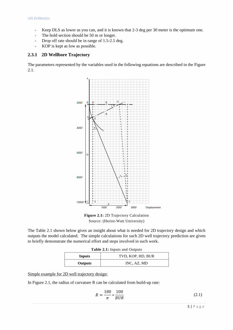
The parameters represented by the variables used in the following equations are described in the Figure

2.1.

Figure 2.1: 2D Trajectory Calculation

Source: (Heriot-Watt University)

The Table 2.1 shown below gives an insight about what is needed for 2D trajectory design and which

outputs the model calculated. The simple calculations for such 2D well trajectory prediction are given

to briefly demonstrate the numerical effort and steps involved in such work.

Table 2.1: Inputs and Outputs

Inputs TVD, KOP, HD, BUR

Outputs INC, AZ, MD

Simple example for 2D well trajectory design:

In Figure 2.1, the radius of curvature R can be calculated from build-up rate:

𝑅 =180

𝜋∗

100

𝐵𝑈𝑅 (2.1)

UiS Drillbotics

6 | P a g e

𝑇𝑎𝑛 𝑥 =(𝑑 − 𝑅)

𝐷 (2.2)

𝑆𝑖𝑛 𝑦 =𝑅 ∗ 𝐶𝑜𝑠 𝑥

𝐷 (2.3)

𝛼 = 𝑥 + 𝑦 (2.4)

Length of build section:

𝐵𝐸

2 ∗ 𝜋 ∗ 𝑅=

𝛼

360 (2.5)

TVD at the end of build section:

𝑃𝐸 = 𝑅 ∗ 𝑆𝑖𝑛 𝛼 (2.6)

𝐴𝑋 = 𝐴𝐵 + 𝑃𝐸 (2.7)

Horizontal displacement at the end of build section:

𝑋𝐸 = 𝑂𝐵 − 𝑂𝑃 (2.8)

where OB = R

𝑂𝑃 = 𝑅 ∗ 𝐶𝑜𝑠𝛼 (2.9)

𝑋𝐸 = 𝑅 ∗ (1 − 𝐶𝑜𝑠 𝛼) (2.10)

MD at the end of build section:

𝐴𝐸 = 𝐴𝐵 + 𝐵𝐸 (2.11)

Total MD at the target:

𝐴𝑇 = 𝐴𝐸 + 𝐸𝑇 (2.12)

Where:

- 𝛼 is the angle of inclination.

- 𝑅 is the radius of curvature.

- 𝐵𝑈𝑅 is the build of Rate.

- 𝑑 is the horizontal displacement.

2.3.2 3D Wellbore Trajectory

There are many techniques utilized for wellbore profile calculation. However, the cubic function is the

one selected for our current project.

In the cubic function, the 3D coordinate functions are generated by solid functions that describe a

wellbore mechanical phenomenon. We cannot say that this methodology can offer an all-time low force

and drag mechanical phenomenon or a more robust mechanical phenomenon than the other

methodology. However, it has more advantages comparing to others methods: it supplies a nonstop and

sleek mathematical 3D curve connecting this position of the outlet at the surface to a target, generally

with a given inclination and azimuth, with a degree of freedom that permits a good deal of management

on the geometric characteristics of the wellbore trajectory.

It is a mathematical method used for designing the complex wellbore trajectories. It is used for different

end conditions for instance; free end, set end, free inclination/set azimuth, and set inclination/free

azimuth. A 3D smooth continuous functions are the outcome of this method and it is found that this

trajectory is more fit with the modern rotary steerable deviation tools. Changing in path curve and tool

UiS Drillbotics

7 | P a g e

face gradually and continuously will result in smooth trajectory curve that has less drag, torque, and

equipment wear.

For the three parametric coordinate functions, the expressions derived for cubic functions are used to

construct a 3D cubic trajectory. It is assumed that the initial end of the trajectory's coordinates,

inclination, and azimuth are known. Also known are the coordinates of the trajectory's end. There are

four cases to be analyzed with regard to the final end of the trajectory:

- Free inclination and azimuth

- Set inclination and azimuth

- Free inclination and set azimuth

- Set inclination and free azimuth

The procedures for cases 1–3 are basically the same. They differ only in how each coordinate is

represented by the functions selected and how the final conditions are imposed. Case 4, however,

requires an iterative process for obtaining the final azimuth due to its existence.

To clarify the application of the method, we will show the calculations for the second case, set inclination

and azimuth.

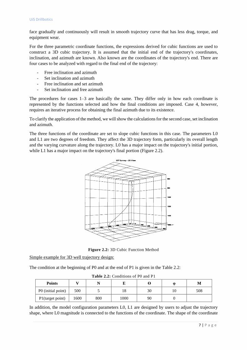
The three functions of the coordinate are set to slope cubic functions in this case. The parameters L0

and L1 are two degrees of freedom. They affect the 3D trajectory form, particularly its overall length

and the varying curvature along the trajectory. L0 has a major impact on the trajectory's initial portion,

while L1 has a major impact on the trajectory's final portion (Figure 2.2).

Figure 2.2: 3D Cubic Function Method

Simple example for 3D well trajectory design:

The condition at the beginning of P0 and at the end of P1 is given in the Table 2.2:

Table 2.2: Conditions of P0 and P1

Points V N E ϴ φ M

P0 (initial point) 500 5 18 30 10 508

P1(target point) 1600 800 1000 90 0

In addition, the model configuration parameters L0, L1 are designed by users to adjust the trajectory

shape, where L0 magnitude is connected to the functions of the coordinate. The shape of the coordinate

UiS Drillbotics

8 | P a g e

functions will decide their general behavior, but the final shape of the functions depends on the

magnitude of L0, which can be treated as an independent parameter.

The L0 and L1 parameters will determine the final 3D trajectory design. From the simulation, we will

end up with an abridged result of the 3D cubic trajectory calculation for the above data. The trajectory's

arc length is 1933.57 m and the final depth estimated is 2441.57 m.

The trajectory's free parameters yield several optimizations. For instance, the trail length and curvatures

through the mechanical phenomenon square measure littered with changes in L0 or L1. It is clear that

the length of the arc incorporates a minimum quantity of the geometer interval between the trajectory's

initial and final ends. Nonetheless, increasing the trajectory's arc length usually will increase the

curvature close to the ends well.

To attenuate force, drag, and wear of drilling and production instrumentation, it is vital to avoid points

with wide curvatures. One potential improvement approach is to attenuate the quality curvature

deviation on the trail. For trajectories with 2 or additional degrees of freedom, a gradient descent theme

may be used. For trajectories with just one degree of freedom a proportion or a parabolic interpolation

theme is appropriate.

To clarify the strategy, a curvature optimization on the set inclination and azimuth case information was

performed as an example. We tend to contemplate L0=L1 for consistency, thereby reducing the degree

of freedom to at least one. By minimizing the standard curvature deviation, we get this value for L0,

L0=L1=2412.19. within the optimized trajectory, we found the maximum dog-leg frequency is 4.37

deg/30 m at the calculated depth of 2029 m. Comparing this value by the non-optimized one given

before with the peak dog-leg severity of 5.01 deg/30 m at 2036 m. If the L0 and L1 are defined as two

separate parameters, we will get the optimized wellbore trajectory at these values: L0 = 2045.90, L1 =

2808.68.

2.4 Focus Study: Wellbore Trajectory Optimization

2.4.1 Multiple Objectives of Trajectory Optimization

The oil/gas industry has, in recent years, been focusing on optimizing its performance being to reduce

cost and time or for safety purposes. One of the areas where this optimal design is being applied and has

become very demanding is wellbore trajectory, this happens due to the many complex and interacted

drilling variables, model uncertainties and design constraints related to said model.

For drilling engineers, well path optimization is of extreme importance and is usually based on

minimizing drilling cost and time, avoiding well collision, minimizing the total wellbore length,

improving the efficiency in the transport of cuttings and increasing the drilling speed. This problem can

be solved by utilizing some solutions presented by different optimization algorithms, such as: generic

algorithm, dynamic programming, particle swarm optimization, etc.

Drilling direction wells has become challenging because of many reasons, such as low ROP, hole

cleaning issues and wellbore stability problems. In this model we aim to get a good performance during

drilling with achieving stability and decreasing the time. There are some factors/parameters which

should be fed/considered to the trajectory plan module:

- Azimuth (AZI) of the wellbore trajectory

- Inclination (INC) of the wellbore trajectory

- Controllable drilling parameters (WOB, RPM, ROP, etc).

- Unconfined compressive strength (UCS)

- Formation pore pressure

- In-situ stresses of the studied area

UiS Drillbotics

9 | P a g e

Input of data is the first step in this model, the second step involves optimizing the process to obtain

max ROP by using a genetic algorithm (GA). The last step is to predetermine the suggested azimuth

(AZI) and inclination (INC) by considering the results of wellbore stability using wireline logging

measurements, core, and drilling data from the offset wells. The present study emphasizes that the

proposed methodology can be applied as a cost-effective tool to optimize the wellbore trajectory and to

calculate approximately the drilling time for highly deviated wells to be drilled in the future.

Considering the fact that well path and trajectory is a complex optimization problem, we attempted to

examine a decision-driven approach to well path design, by quantifying key decisions and uncertainties.

We aim to develop a decision analytical framework to design an optimal 2D/3D well path while

considering it is drilling bed boundaries uncertainties and the offset wells uncertain positions in order to

optimize the drilling process.

2.4.2 Anti-Collision Principle

The cluster well drilling technology and infill development drilling technology has been widely used in

recent years in order to meet the requirements of oil field development, more and more drilling occurs

in dense well spacing in the existing oil field or in the high-density well. However, the risk of drilling

such wells was increased by well-bore anti-collision incidents. If we can reliably predict such accidents

and take active steps to eliminate the risk. So, these two drilling technologies may have wider prospects

for implementation (Olaijuwon, 2012).

Survey data for a given wellbore is never normally considered as accurate when used to define actual

wellbore positions. There is a need to recognize that measurement errors can occur even on the most

accurate of survey tools. Azimuth reading error, depth error and inclination error are the mainly

responsible for wellbore position uncertainty. By considering these errors, it becomes possible to

construct a cone of uncertainty around the actual survey data which better defines the probable

boundaries within which the actual position of the wellbore will fall (Ekseth, 1998).

The inclination error creates a high side dimension of the uncertainty ellipse. The azimuth error creates

a lateral dimension of the uncertainty ellipse, while measured depth error creates a third component

along the axis of the wellbore. So, they combine and form an ellipsoid of uncertainty (DeWardt and

Wolf, 1981).

Several models have been conducted to overcome such errors, namely, cone of uncertainty model,

Walstrom error model, Wolff and de Wardt error model, shell extended systematic error model

(SESTEM), industry steering committee for wellbore survey accuracy error model (ISCWSA).

ISCWSA is the more accurate model among the others to eliminate the errors during drilling until reach

the target. The model starts by finding all error sources affecting measure depth, inclination and azimuth.

It designates error code to each error source and defines the vector for each error (Ekseth, 1998 and

Williamson, 2000).

Then, each error source has a set of weighting functions, which are the equations that describe how the

error source affects the actual survey measurements of measured depth, inclination and azimuth.

Afterwards, summing up the errors, where each error source has a propagation mode, which defines

how it is correlated from survey to survey.

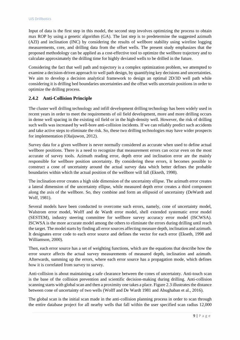
Anti‐collision is about maintaining a safe clearance between the cones of uncertainty. Anti-touch scan

is the base of the collision prevention and scientific decision-making during drilling. Anti-collision

scanning starts with global scan and then a proximity one takes a place. Figure 2.3 illustrates the distance

between cone of uncertainty of two wells (Wolff and De Wardt 1981 and Abughaban et al., 2016).

The global scan is the initial scan made in the anti‐collision planning process in order to scan through

the entire database project for all nearby wells that fall within the user specified scan radius 12,000

UiS Drillbotics

10 | P a g e

meters. This global scan is required to identify the wells that are required to be included into the next

step of the anti‐collision planning process. On completion of the global scan, a proximity scan must be

performed on all the wells that have been identified as being “nearby wells”. The proximity scan uses

the subsurface survey data associated with each nearby well in order to calculate the distance from each

well to the subject well at every point along its length (Ekseth, 2000).

Figure 2.3: Clearance between The Uncertainty Cone of Projected Well and The Cone of Offset Well

Source: (Olaijuwon, 2012)

The proximity scan has two method to perform the analysis on the wells, namely, Geometrical Analysis

(Centre to center distance) and Statistical Analysis (Separation Factor). Geometrical analysis (CtC

calculation) is necessary to scan using both normal plane and 3‐D least distance to be sure that closest

CtC distance is found.

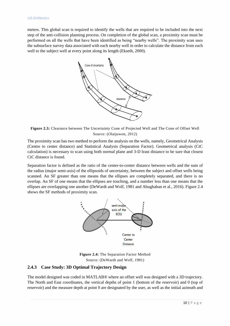
Separation factor is defined as the ratio of the center-to-center distance between wells and the sum of

the radius (major semi‐axis) of the ellipsoids of uncertainty, between the subject and offset wells being

scanned. An SF greater than one means that the ellipses are completely separated, and there is no

overlap. An SF of one means that the ellipses are touching, and a number less than one means that the

ellipses are overlapping one another (DeWardt and Wolf, 1981 and Abughaban et al., 2016). Figure 2.4

shows the SF methods of proximity scan.

Figure 2.4: The Separation Factor Method

Source: (DeWardt and Wolf, 1981)

2.4.3 Case Study: 3D Optimal Trajectory Design

The model designed was coded in MATLAB® where an offset well was designed with a 3D trajectory.

The North and East coordinates, the vertical depths of point 1 (bottom of the reservoir) and 0 (top of

reservoir) and the measure depth at point 0 are designated by the user, as well as the initial azimuth and

UiS Drillbotics

11 | P a g e

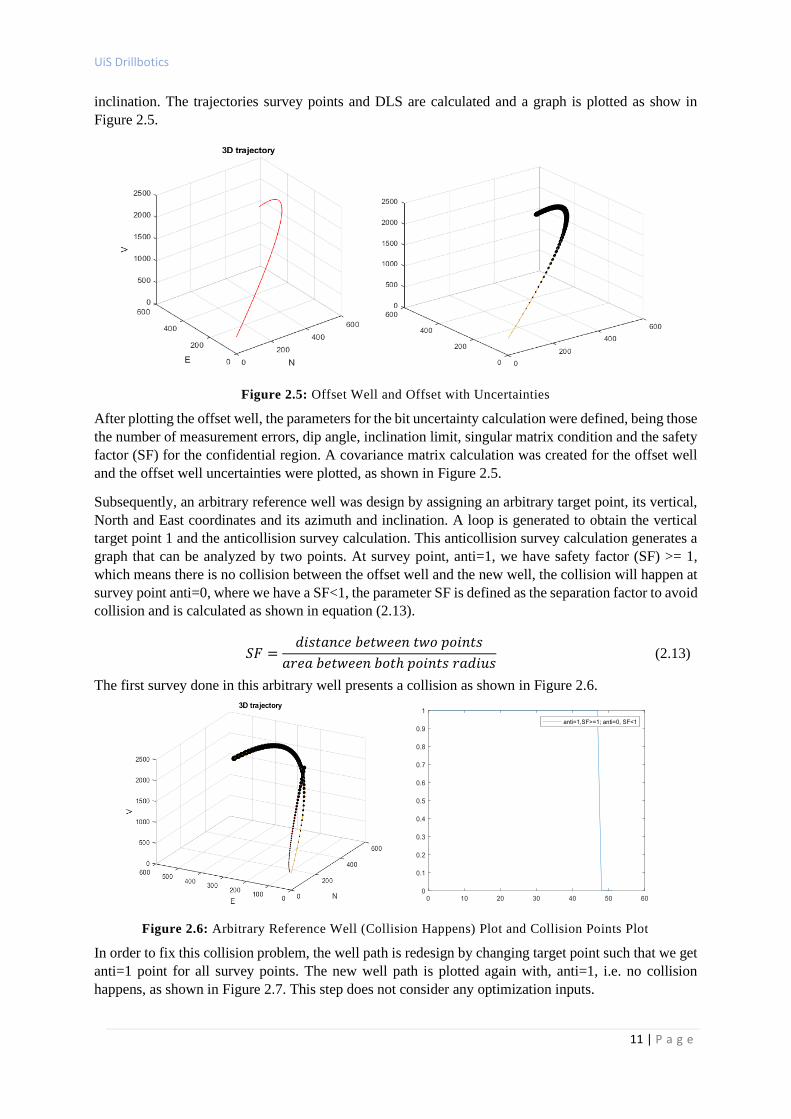
inclination. The trajectories survey points and DLS are calculated and a graph is plotted as show in

Figure 2.5.

Figure 2.5: Offset Well and Offset with Uncertainties

After plotting the offset well, the parameters for the bit uncertainty calculation were defined, being those

the number of measurement errors, dip angle, inclination limit, singular matrix condition and the safety

factor (SF) for the confidential region. A covariance matrix calculation was created for the offset well

and the offset well uncertainties were plotted, as shown in Figure 2.5.

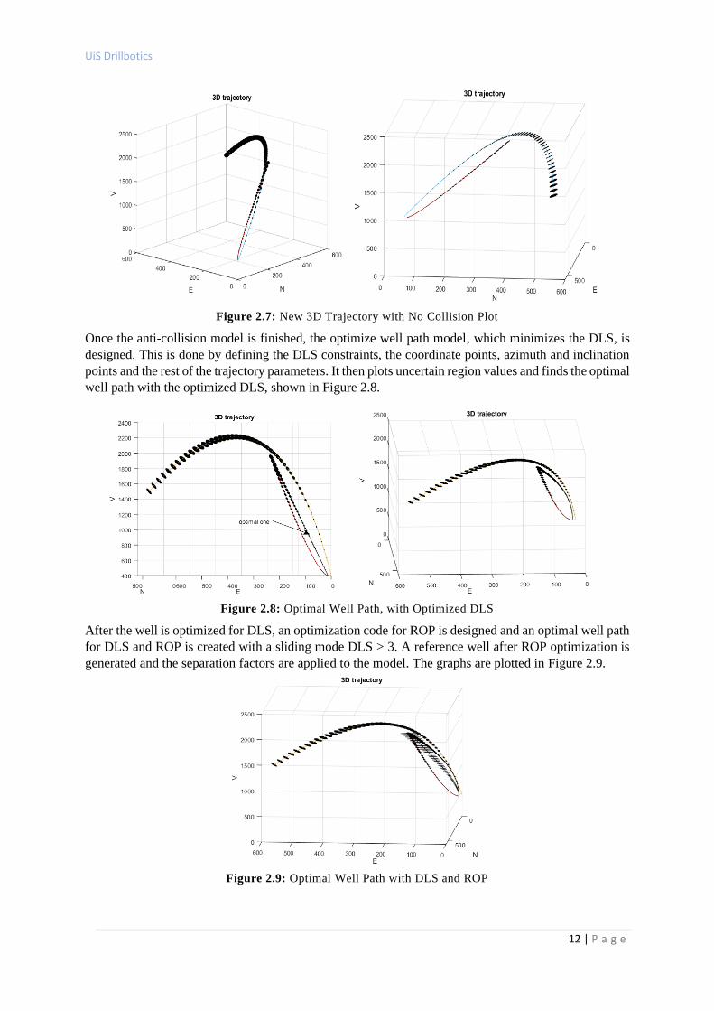
Subsequently, an arbitrary reference well was design by assigning an arbitrary target point, its vertical,

North and East coordinates and its azimuth and inclination. A loop is generated to obtain the vertical

target point 1 and the anticollision survey calculation. This anticollision survey calculation generates a

graph that can be analyzed by two points. At survey point, anti=1, we have safety factor (SF) >= 1,

which means there is no collision between the offset well and the new well, the collision will happen at

survey point anti=0, where we have a SF<1, the parameter SF is defined as the separation factor to avoid

collision and is calculated as shown in equation (2.13).

𝑆𝐹 =𝑑𝑖𝑠𝑡𝑎𝑛𝑐𝑒 𝑏𝑒𝑡𝑤𝑒𝑒𝑛 𝑡𝑤𝑜 𝑝𝑜𝑖𝑛𝑡𝑠

𝑎𝑟𝑒𝑎 𝑏𝑒𝑡𝑤𝑒𝑒𝑛 𝑏𝑜𝑡ℎ 𝑝𝑜𝑖𝑛𝑡𝑠 𝑟𝑎𝑑𝑖𝑢𝑠 (2.13)

The first survey done in this arbitrary well presents a collision as shown in Figure 2.6.

Figure 2.6: Arbitrary Reference Well (Collision Happens) Plot and Collision Points Plot

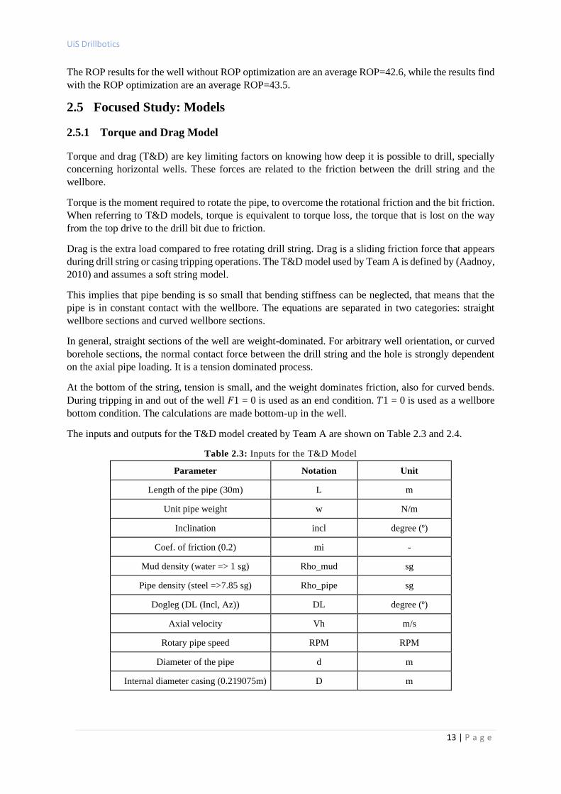
In order to fix this collision problem, the well path is redesign by changing target point such that we get

anti=1 point for all survey points. The new well path is plotted again with, anti=1, i.e. no collision

happens, as shown in Figure 2.7. This step does not consider any optimization inputs.

UiS Drillbotics

12 | P a g e

Figure 2.7: New 3D Trajectory with No Collision Plot

Once the anti-collision model is finished, the optimize well path model, which minimizes the DLS, is

designed. This is done by defining the DLS constraints, the coordinate points, azimuth and inclination

points and the rest of the trajectory parameters. It then plots uncertain region values and finds the optimal

well path with the optimized DLS, shown in Figure 2.8.

Figure 2.8: Optimal Well Path, with Optimized DLS

After the well is optimized for DLS, an optimization code for ROP is designed and an optimal well path

for DLS and ROP is created with a sliding mode DLS > 3. A reference well after ROP optimization is

generated and the separation factors are applied to the model. The graphs are plotted in Figure 2.9.

Figure 2.9: Optimal Well Path with DLS and ROP

UiS Drillbotics

13 | P a g e

The ROP results for the well without ROP optimization are an average ROP=42.6, while the results find

with the ROP optimization are an average ROP=43.5.

2.5 Focused Study: Models

2.5.1 Torque and Drag Model

Torque and drag (T&D) are key limiting factors on knowing how deep it is possible to drill, specially

concerning horizontal wells. These forces are related to the friction between the drill string and the

wellbore.

Torque is the moment required to rotate the pipe, to overcome the rotational friction and the bit friction.

When referring to T&D models, torque is equivalent to torque loss, the torque that is lost on the way

from the top drive to the drill bit due to friction.

Drag is the extra load compared to free rotating drill string. Drag is a sliding friction force that appears

during drill string or casing tripping operations. The T&D model used by Team A is defined by (Aadnoy,

2010) and assumes a soft string model.

This implies that pipe bending is so small that bending stiffness can be neglected, that means that the

pipe is in constant contact with the wellbore. The equations are separated in two categories: straight

wellbore sections and curved wellbore sections.

In general, straight sections of the well are weight-dominated. For arbitrary well orientation, or curved

borehole sections, the normal contact force between the drill string and the hole is strongly dependent

on the axial pipe loading. It is a tension dominated process.

At the bottom of the string, tension is small, and the weight dominates friction, also for curved bends.

During tripping in and out of the well 𝐹1 = 0 is used as an end condition. 𝑇1 = 0 is used as a wellbore

bottom condition. The calculations are made bottom-up in the well.

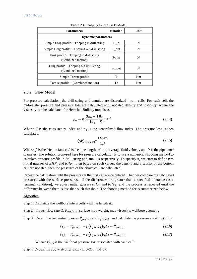
The inputs and outputs for the T&D model created by Team A are shown on Table 2.3 and 2.4.

Table 2.3: Inputs for the T&D Model

Parameter Notation Unit

Length of the pipe (30m) L m

Unit pipe weight w N/m

Inclination incl degree (º)

Coef. of friction (0.2) mi -

Mud density (water => 1 sg) Rho_mud sg

Pipe density (steel =>7.85 sg) Rho_pipe sg

Dogleg (DL (Incl, Az)) DL degree (º)

Axial velocity Vh m/s

Rotary pipe speed RPM RPM

Diameter of the pipe d m

Internal diameter casing (0.219075m) D m

UiS Drillbotics

14 | P a g e

Table 2.4: Outputs for the T&D Model

Parameters Notation Unit

Dynamic parameters

Simple Drag profile – Tripping in drill string F_in N

Simple Drag profile – Tripping out drill string F_out N

Drag profile – Tripping in drill string

(Combined motion) Fc_in N

Drag profile – Tripping out drill string

(Combined motion) Fc_out N

Simple Torque profile T Nm

Torque profile – (Combined motion) Tc Nm

2.5.2 Flow Model

For pressure calculation, the drill string and annulus are discretized into n cells. For each cell, the

hydrostatic pressure and pressure loss are calculated with updated density and viscosity, where the

viscosity can be calculated for Herschel-Bulkley models as:

𝜇𝑎 = 𝐾(3𝑛𝑎 + 1

4𝑛𝑎

8𝑣

𝐷)𝑛𝑎−1 (2.14)

Where: 𝐾 is the consistency index and 𝑛𝑎 is the generalized flow index. The pressure loss is then

calculated.

(∆P)Frictional=𝑓𝐿𝜌𝑣2

2𝐷 (2.15)

Where: 𝑓 is the friction factor, 𝐿 is the pipe length, 𝑣 is the average fluid velocity and 𝐷 is the pipe inner

diameter. The solution proposed here for pressure calculation is to use a numerical shooting method to

calculate pressure profile in drill string and annulus respectively. To specify it, we start to define two

initial guesses of 𝐵𝐻𝑃1 and 𝐵𝐻𝑃2, then based on such values, the density and viscosity of the bottom

cell are updated, then the pressures of the above cell are calculated.

Repeat the calculation until the pressures at the first cell are calculated. Then we compare the calculated

pressures with the surface pressures. If the differences are greater than a specified tolerance (as a

terminal condition), we adjust initial guesses 𝐵𝐻𝑃1 and 𝐵𝐻𝑃2, and the process is repeated until the

difference between them is less than such threshold. The shooting method for is summarized below:

Algorithm

Step 1: Discretize the wellbore into n cells with the length Δ𝑧

Step 2.: Inputs: flow rate Q, 𝑃𝑠𝑢𝑟𝑓𝑎𝑐𝑒, surface mud weight, mud viscosity, wellbore geometry

Step 3: Determine two initial guesses 𝑃𝑔𝑢𝑒𝑠𝑠,1 and 𝑃𝑔𝑢𝑒𝑠𝑠,2 and calculate the pressure at cell (2) in by

𝑃2,1 = 𝑃𝑔𝑢𝑒𝑠𝑠,1 − 𝜌(𝑃𝑔𝑢𝑒𝑠𝑠,1)𝑔Δ𝑧 − 𝑃𝑙𝑜𝑠𝑠,1,1 (2.16)

𝑃2,2 = 𝑃𝑔𝑢𝑒𝑠𝑠,2 − 𝜌(𝑃𝑔𝑢𝑒𝑠𝑠,2)𝑔Δ𝑧 − 𝑃𝑙𝑜𝑠𝑠,1,2 (2.17)

Where: 𝑃𝑙𝑜𝑠𝑠 is the frictional pressure loss associated with each cell.

Step 4: Repeat the above step for each cell i=2, …n-1 by:

UiS Drillbotics

15 | P a g e

𝑃𝑖+1,1 = 𝑃𝑖,1 − 𝜌(𝑃𝑖,1)𝑔Δ𝑧 − 𝑃𝑙𝑜𝑠𝑠,𝑖,1 (2.18)

𝑃𝑖+1,2 = 𝑃𝑖,2 − 𝜌(𝑃𝑖,2)𝑔Δ𝑧 − 𝑃𝑙𝑜𝑠𝑠,𝑖,2 (2.19)

Step 5: Define 𝑓1 = 𝑃𝑛,1 − 𝑃𝑠𝑢𝑟𝑓𝑎𝑐𝑒 , 𝑓2 = 𝑃𝑛,2 − 𝑃𝑠𝑢𝑟𝑓𝑎𝑐𝑒 . If 𝑓1 is less than tolerance, then the

algorithm is terminated, else cut the interval [𝑃𝑔𝑢𝑒𝑠𝑠,1, 𝑃𝑔𝑢𝑒𝑠𝑠,2] into 2 halves and go back to Step 3.

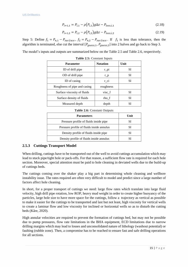
The model’s inputs and outputs are summarized below on the Table 2.5 and Table 2.6, respectively.

Table 2.5: Constant Inputs

Parameter Notation Unit

ID of drill pipe r_pi SI

OD of drill pipe r_p SI

ID of casing r_ci SI

Roughness of pipe and casing roughness

Surface viscosity of fluids visc_f SI

Surface density of fluids rho_f SI

Measured depth depth SI

Table 2.6: Constant Outputs

Parameters Unit

Pressure profile of fluids inside pipe SI

Pressure profile of fluids inside annulus SI

Density profile of fluids inside pipe SI

Density profile of fluids inside annulus SI

2.5.3 Cuttings Transport Model

When drilling, cuttings have to be transported out of the well to avoid cuttings accumulation which may

lead to stuck pipe/tight hole or pack-offs. For that reason, a sufficient flow rate is required for each hole

section. Moreover, special attention must be paid to hole cleaning in deviated wells due to the build-up

of cuttings beds.

The cuttings coming over the shaker play a big part in determining whole cleaning and wellbore

instability issue. The rates required are often very difficult to model and predict since a large number of

factors affect hole cleaning.

In short, for a proper transport of cuttings we need: large flow rates which translate into large fluid

velocity, high drill pipe rotation, low ROP, heavy mud weight in order to create higher buoyancy of the

particles, large hole size to have more space for the cuttings, follow a trajectory as vertical as possible

to make it easier for the cuttings to be transported and last but not least, high viscosity for vertical wells

to create a laminar flow and low viscosity for inclined or horizontal wells so as to disturb the cutting

beds (Kåre, 2020).

High annular velocities are required to prevent the formation of cuttings bed, but may not be possible

due to pump pressures, flow rate limitations in the BHA equipment, ECD limitations due to narrow

drilling margins which may lead to losses and unconsolidated nature of lithology (washout potential) or

faulting (rubble zone). Then, a compromise has to be reached to ensure fast and safe drilling operations

for all sections.

UiS Drillbotics

16 | P a g e

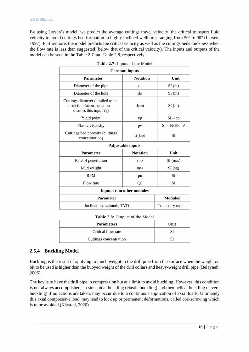
By using Larsen’s model, we predict the average cuttings travel velocity, the critical transport fluid

velocity to avoid cuttings bed formation in highly inclined wellbores ranging from 50° to 90° (Larsen,

1997). Furthermore, the model predicts the critical velocity as well as the cuttings beds thickness when

the flow rate is less than suggested (below that of the critical velocity). The inputs and outputs of the

model can be seen in the Table 2.7 and Table 2.8, respectively.

Table 2.7: Inputs of the Model

Constant inputs

Parameter Notation Unit

Diameter of the pipe di SI (m)

Diameter of the hole do SI (m)

Cuttings diameter (applied to the

correction factor equation----

dismiss this input ??)

dcutt SI (m)

Yield point yp SI – cp

Plastic viscosity pv SI – N/100m2

Cuttings bed porosity (cuttings

concentration) fi_bed SI

Adjustable inputs

Parameter Notation Unit

Rate of penetration rop SI (m/s)

Mud weight mw SI (sg)

RPM rpm SI

Flow rate Q0 SI

Inputs from other modules

Parameter Modules

Inclination, azimuth, TVD Trajectory model

Table 2.8: Outputs of the Model

Parameters Unit

Critical flow rate SI

Cuttings concentration SI

2.5.4 Buckling Model

Buckling is the result of applying to much weight to the drill pipe from the surface when the weight on

bit to be used is higher than the buoyed weight of the drill collars and heavy-weight drill pipe (Belayneh,

2006).

The key is to have the drill pipe in compression but at a limit to avoid buckling. However, this condition

is not always accomplished, so sinusoidal buckling (elastic buckling) and then helical buckling (severe

buckling) if no actions are taken, may occur due to a continuous application of axial loads. Ultimately

this axial compressive load, may lead to lock up or permanent deformations, called corkscrewing which

is to be avoided (Kårstad, 2020).

UiS Drillbotics

17 | P a g e

One of the most important parameters which is introduced in our model and that is not usually taken

into consideration for the analysis of buckling, is friction. Friction, redistribute the internal axial forces

which makes buckling less predictable, thus makes this effect relatively important to analyze during

well planning or drilling operations (Gulyayev, 2016).

On the other hand, this buckling effect is less visible in high angle wells since the force of gravity pulls

the drill string against the low side of the hole. This stabilizes the string and allows drill pipe to carry

high axial loads without buckling.

Models for the critical (sinusoidal) buckling force in vertical wells (Lubinski, 1962 and Wu et al, 1993)

and in inclined wells (Dawson and Paslay, 1984) are well accepted by the drilling industry. In addition,

several models have also been proposed for the prediction of helical buckling load of tubular in vertical

wells (Lubinski et al.,1962), and for inclined and horizontal wells (Mitchell et. Al, 1996).

The list of inputs and outputs is shown in the in the Table 2.9 and Table 2.10, respectively.

Table 2.9: Inputs of the Model

Constant inputs

Parameter Notation Unit

Density of steel rho_steel SI (sg)

Youngs modulus E psi

Weight of the drill string (DS) wDP SI (kN/m)

Outer diameter of the DS OD SI (m)

Inner diameter of the DS ID SI (m)

Casing inner diameter/open hole

diameter csgID SI (m)

Drill pipe grade (API) grades psi

Friction factor mu SI

Adjustable inputs

Parameter Notation Unit

Mud weight mw SI (sg)

Inputs from other modules

Parameter Modules

Inclination, azimuth, TVD Trajectory model

Table 2.10: Outputs of the Model

Parameters Unit

Dynamic forces acting on the drill string SI (kgf)

Effective axial load SI (kgf)

Maximum helical buckling limit along the well SI (kgf)

Minimum helical buckling along the well SI (kgf)

Sinusoidal buckling limit SI (kgf)

Permanent corkscrewing (for given Feff) SI (kgf)

UiS Drillbotics

18 | P a g e

2.5.5 Temperature Model

The objective of this model is to develop an accurate temperature model that can precisely calculate

wellbore temperature distributions. (Sui et al., 2019)

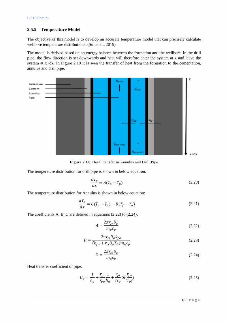
The model is derived based on an energy balance between the formation and the wellbore .In the drill

pipe, the flow direction is set downwards and heat will therefore enter the system at x and leave the

system at x+dx. In Figure 2.10 it is seen the transfer of heat from the formation to the cementation,

annulus and drill pipe.

Figure 2.10: Heat Transfer in Annulus and Drill Pipe

The temperature distribution for drill pipe is shown in below equation:

𝑑𝑇𝑝

𝑑𝑥= 𝐴(𝑇𝑎 − 𝑇𝑝) (2.20)

The temperature distribution for Annulus is shown in below equation:

𝑑𝑇𝑎

𝑑𝑥= 𝐶(𝑇𝑎 − 𝑇𝑝) − 𝐵(𝑇𝑓 − 𝑇𝑎) (2.21)

The coefficients A, B, C are defined in equations (2.22) to (2.24):

𝐴 =2𝜋𝑟𝑝𝑖𝑈𝑝

𝑚𝑝𝑐𝑝 (2.22)

𝐵 =2𝜋𝑟𝑐𝑖𝑈𝑎𝑘𝑓𝑜

(𝑘𝑓𝑜 + 𝑟𝑐𝑖𝑈𝑎𝑇𝐷)𝑚𝑎𝑐𝑝 (2.23)

𝐶 =2𝜋𝑟𝑝𝑖𝑈𝑝

𝑚𝑎𝑐𝑝 (2.24)

Heat transfer coefficient of pipe:

𝑈𝑝 =1

ℎ𝑝+

𝑟𝑝𝑖

𝑟𝑝𝑜

1

ℎ𝑎+

𝑟𝑝𝑖

𝑟𝑘𝑝𝑙𝑛(

𝑟𝑝𝑜

𝑟𝑝𝑖) (2.25)

UiS Drillbotics

19 | P a g e

Heat Transfer coefficient of the annulus:

𝑈𝑎 =1

ℎ𝑝+

𝑟𝑐𝑖𝑘𝑐

𝑙𝑛(𝑟𝑐𝑜𝑟𝑐𝑖

) +𝑟𝑐𝑖𝑘𝑐𝑡

𝑙𝑛(𝑟𝑤𝑟𝑐0

) (2.26)

𝑑2𝑇𝑝

𝑑𝑥2− 𝐷

𝑑𝑇𝑝

𝑑𝑥− 𝐴𝐵𝑇𝑝 = −𝐴𝐵𝑇𝑓) (2.27)

A numerical approach is implemented to obtain the solution Using a numerical approach allows the

wellbore to be divided into a certain number of boxes. For each box, all the parameters that vary

throughout the wellbore are updated and treated as constants over the box length, which allows eq. (2.25)

to be solved by the undetermined coefficients method.

2.5.6 ROP Model

Two different approaches are mainly used in oil and gas industry to predict the Rate of Penetration

(ROP) in a specific field: physics-based or traditional models and data driven models.

Physics-based models are mathematical functions obtained during lab experiments while data driven

approach use machine learning to create a model that predicts ROP. Traditional models are deterministic

and easy for optimization. However, they have its limitations such as low accuracy in ROP prediction,

a strong dependency in empirical coefficients based on lithology that varied continuously and

requirement of static parameters as inputs that are not always available.

On the other hand, there are data-driven models, and as the title suggest they are purely dependent on

data, thus only designed for a specific field. These models give more accurate ROP prediction than

traditional models as it is shown by Hegde et al. (2017). Also, they have no bit or BHA specifications

and they are independent of the layer you are drilling since they have no empirical constants.

For the main purpose of this section, accuracy in ROP prediction is not necessary and traditional models

will be used. Many models exist but only two of them will be briefly described below:

Bingham’s (1965) is an empirical ROP model. It considers ROP as a function of WOB, RPM and bit

diameter it is designed for any bit type:

𝑅𝑂𝑃 = 𝐾 (𝑊𝑂𝐵

𝐷𝑏)𝑎

𝑅𝑃𝑀 (2.28)

Where ROP is the rate of penetration (ft/hr), WOB is the weight on bit (Klb), RPM is the rotary speed

(revolutions/min), Db is the bit diameter (in), and ‘a’ and ‘K’ are rock formation constants obtained by

linear regression. As it is pointed by Soares et al. (2016), it is essential to adjust coefficient bounds to

fit the model with field data.

Burgoyne et al. (1991) is another ROP model that include more drilling parameters such as pore

pressure, WOB, sediments compaction and is expressed as a function of eight components:

𝑅𝑂𝑃 = 𝑓1 𝑥 𝑓2𝑥 𝑓3𝑥 𝑓4𝑥 𝑓5𝑥 𝑓6𝑥 𝑓7𝑥 𝑓8 (2.29)

𝑓1 = 𝑒𝑎1 (2.30)

𝑓2 = 𝑒𝑎2(13000−𝑇𝑉𝐷) (2.31)

𝑓3 = 𝑒𝑎3𝑇𝑉𝐷0.69(𝑃𝑝𝑜𝑟𝑒−10.5) (2.32)

𝑓4 = 𝑒𝑎4𝑇𝑉𝐷(𝑃𝑝𝑜𝑟𝑒−𝐸𝐶𝐷) (2.33)

UiS Drillbotics

20 | P a g e

𝑓5 = (

(𝑤𝑑𝑏

) − (𝑤𝑑𝑏

)𝑡

4 − (𝑤𝑑𝑏

)𝑡

)

𝑎5

(2.34)

𝑓6 = (𝑅𝑃𝑀

60)𝑎6

(2.35)

𝑓7 = 𝑒−𝑎7ℎ (2.36)

𝑓8 = 𝑒𝑎8

𝜌𝑞350𝜇𝑑𝑛 (2.37)

Where, 𝑓𝑖 includes drilling parameters and 𝑎𝑖 are the variable coefficients calculated using linear

regression. Coefficients are described in the following way:

- 𝑓1 represents the formation strength.

- 𝑓2 and 𝑓3 represent pore pressure influence, where 𝑇𝑉𝐷 is true vertical depth and 𝑃𝑝𝑜𝑟𝑒 is the

pore pressure in pounds per gallon (ppg).

- 𝑓4 represents the differential pressure effect, where ECD is the equivalent circulating density.

- 𝑓5 represents the variation of WOB and bit diameter and changes for bit type, where 𝑤

𝑑𝑏 is the

applied WOB per inch, d the bit diameter and (𝑤

𝑑𝑏)𝑡the threshold WOB per inch.

- 𝑓6 represents the influence of the RPM.

- 𝑓7 represents the drill bit wear.

- 𝑓8 represents the hydraulic effects, where 𝑑𝑛 is a bit nozzle diameter and 𝜇 is the viscosity of

the drilling fluid.

2.6 Web-Based Well Design Simulator

A well design is a multi-step process which begins in conception and ends in specification. A robust

design requires parametric sensitivity to variations in well parameters and material properties. Web-

based Well Planning Software is a comprehensive tool which includes well trajectory design, drill string,

hole section, fluid and geo temperature analysis that reflects the logic and information flow of actual

well design.

In the result section of this application one can find pressure and temperature profile, torque and drag

profile and bit uncertainty profile. Successfully drilling challenging wells requires an in-depth

understanding of the torque & drag during all phases of the operation.

Simulations performed here are key features to show a real drilling operation and provide accuracy.

Web-based Well Planning Software provides a user-friendly tool that targets all drilling engineers

involved in challenging wells. The software is built around the well-control workflow, covering well

trajectory control, pressure & temperature control, and bit position control.

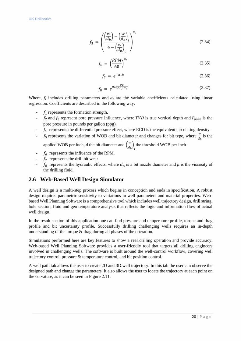
A well path tab allows the user to create 2D and 3D well trajectory. In this tab the user can observe the

designed path and change the parameters. It also allows the user to locate the trajectory at each point on

the curvature, as it can be seen in Figure 2.11.

UiS Drillbotics

21 | P a g e

Figure 2.11: Well Trajectory Design Section in the Well Planning Web Application

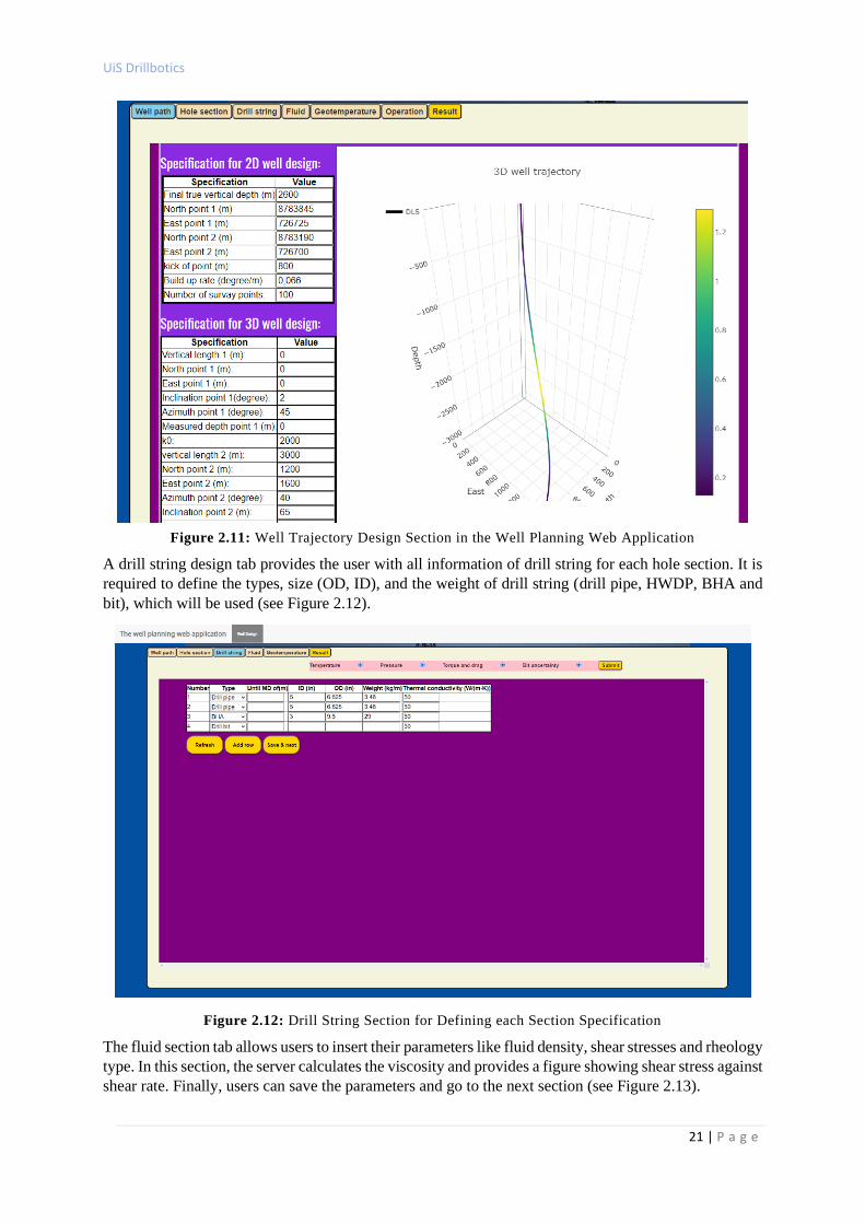
A drill string design tab provides the user with all information of drill string for each hole section. It is

required to define the types, size (OD, ID), and the weight of drill string (drill pipe, HWDP, BHA and

bit), which will be used (see Figure 2.12).

Figure 2.12: Drill String Section for Defining each Section Specification

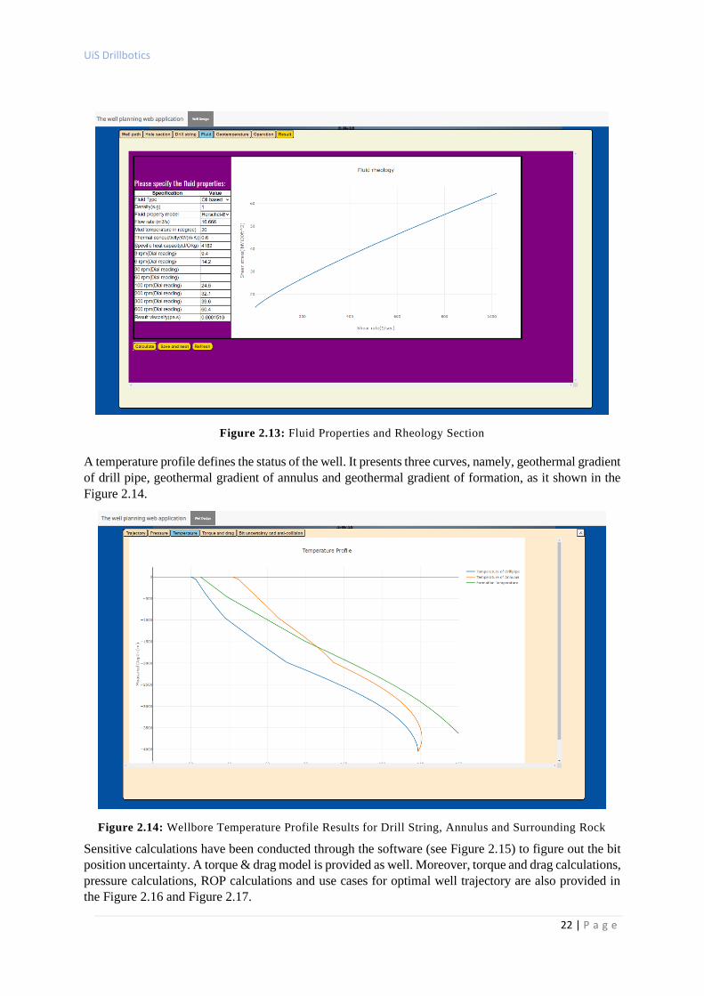
The fluid section tab allows users to insert their parameters like fluid density, shear stresses and rheology

type. In this section, the server calculates the viscosity and provides a figure showing shear stress against

shear rate. Finally, users can save the parameters and go to the next section (see Figure 2.13).

UiS Drillbotics

22 | P a g e

Figure 2.13: Fluid Properties and Rheology Section

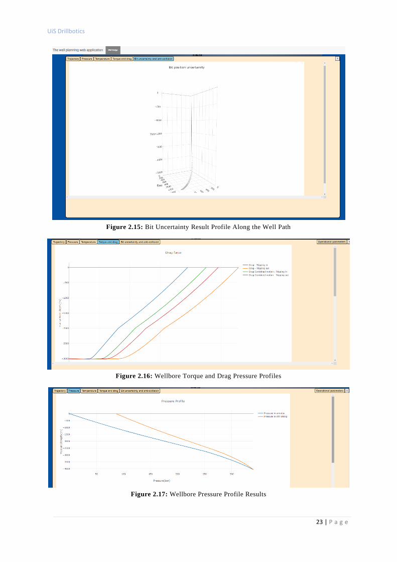
A temperature profile defines the status of the well. It presents three curves, namely, geothermal gradient

of drill pipe, geothermal gradient of annulus and geothermal gradient of formation, as it shown in the

Figure 2.14.

Figure 2.14: Wellbore Temperature Profile Results for Drill String, Annulus and Surrounding Rock

Sensitive calculations have been conducted through the software (see Figure 2.15) to figure out the bit

position uncertainty. A torque & drag model is provided as well. Moreover, torque and drag calculations,

pressure calculations, ROP calculations and use cases for optimal well trajectory are also provided in

the Figure 2.16 and Figure 2.17.

UiS Drillbotics

23 | P a g e

Figure 2.15: Bit Uncertainty Result Profile Along the Well Path

Figure 2.16: Wellbore Torque and Drag Pressure Profiles

Figure 2.17: Wellbore Pressure Profile Results

UiS Drillbotics

24 | P a g e

3 Real-Time Drilling Simulator

3.1 Directional Drilling

Directional drilling has brought a lot of innovations and has increased the efficiency of hydrocarbons

extraction, especially these past decades. Compared to vertical drilling, directional drilling can be

extremely useful when the wellbore needs to reach a target or a number of targets that are located at

some horizontal distance from the well site, among more other advantages (Mitchell & Miska, 2011).

According to Hossain and Al-Mejed the main purposes of directional drilling can include (Hossain &

Al-Mejed, 2015):

- Multiple wells from a single platform or well.

- Onshore drilling to offshore locations.

- Drilling hydrocarbons deposits below an inaccessible location.

- Relief well for killing another well that is on fire.

- Side-tracking to bypass obstructions that may have been lost in the well.

- Drilling salt domes reservoirs

- Drilling into a faulted formation without crossing the fault.

- Extract hydrocarbons from long and thin reservoirs.

- Single well intercepting multiple targets.

Moreover, the directional drilling techniques can be summarized into two mains: point-the-bit and push-

the-bit. The first one involves the use of a downhole motor which transmit the rotation to the bit, while

the second uses a BHA with a special component that pushes against one face of the formation.

The use of downhole mud motors and bent subs has been used for a long time, since it is and effective,

reliable and not much expensive technique to deviate a well. The drill string is oriented in a direction

(tool face direction) and only the drill bit is rotating due to the hydraulic power of the mud motor, located

some meters behind the bit, while the rest of the drill string stays without rotation (Wiktorski et al.,

2017).

One of the main drawbacks of the use of mud motors in the BHA is the necessity of stop the rotation of

the drill string once the tool face is pointed in the desired direction. This can create some problems later

like: pipe sticking or pack-off of the tool, since the cuttings are not being rotating and could create a bed

of cuttings easier.

On the other hand, the principal element to create a deviation in the well using the push-the-bit technique

is with the Rotary Steerable System (RSS). It requires a special BHA component above the bit to direct

the well path in the desired direction, this component is the rotary steering device (Ruszka, 2003). The

way that the rotary steering devices accomplish their task varies from simple gravity-based to more

complex flexure or internal driveshafts of the BHA by application of some force from some pads against

the borehole wall. Some systems also employ automatic drilling modes where the well path is

automatically steered using a close loop control system programmed (Ruszka, 2003).

Besides, the RSS generally includes two main parts: the control platform and the biasing mechanism.

The control platform is the “brain” of the rotary guidance system and controls the direction of the bias

mechanism. The bias mechanism is the “actuator” for the tool (Li et al., 2020).

3.2 Focused Study: RSS Modeling

3.2.1 RSS Tools

The use of the RSS in the past years has been proved that the RSS is more stable, is less prone to sticking,

facilitates the hole cleaning and increases the ROP compared with the mud motor systems (Hossain &

Al-Mejed, 2015).

UiS Drillbotics

25 | P a g e

The RSS has the ability to provide directional drilling control while allowing continuous rotation of the

drill string. This steering is made with the use of an actuator which eccentrically displaces the center

line of the drilling system away from the center line of the hole by a controllable offset (Elshafei et al.,

2015).

Normally, the actuator is a 3-pad tool which pushes one pad against the formation to direct the bit in the

opposite direction. The pads are rotating along with the rest of the drill string, but every time that one

pad aligns with the tool face, it is activated to push the tool. When the pad is no longer aligned with the

tool face, it starts to deactivate gradually until it is totally deactivated while the next pad is being

activated gradually.

Even though most of the RSS works with a 3 steering pads, Canrig Drilling Technology (a company of

Nabors) has developed an innovative BHA tool, that is called “OrientXpress® RSS”. This tool is very

interesting since it does not follow the typical 3-pads RSS tool that has been used for long time. Instead,

the OrientXpress® RSS has a cylindrical actuator that “dislocates” from the BHA to create an offset

which pushes the bit in the opposite direction.

Consequently, the RSS tool selected for the development of the Real Time Drilling Simulator (described

later) is the OrientXpress® RSS. Developing a model with this new tool has been an attractive challenge

that might help its use in the future and inspire other new studies with this technology.

According to Nabors website, the OrientXpress® RSS actuator enables to drill higher quality wells at

lower cost by increasing the downhole maneuverability, borehole quality and reducing the non-

productive time (Nabors Industries, 2020). Moreover, the system is designed to operate in any extended-

reach drilling well onshore or offshore, conventional or unconventional, at temperatures up to 347 °F

and pressures up to 20000 psi (Stump, 2019).

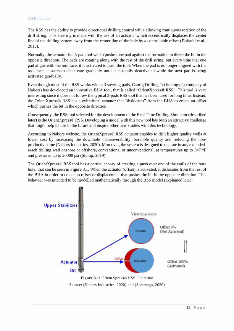
The OrientXpress® RSS tool has a particular way of creating a push over one of the walls of the bore

hole, that can be seen in Figure 3.1. When the actuator (offset) is activated, it dislocates from the rest of

the BHA in order to create an offset or displacement that pushes the bit in the opposite direction. This

behavior was intended to be modelled mathematically through the RSS model (explained later).

Figure 3.1: OrientXpress® RSS Operation

Source: (Nabors Industries, 2020) and (Saramago, 2020)

UiS Drillbotics

26 | P a g e

Furthermore, there are three main points to take as a reference on the OrientXpress® RSS tool: the bit,

the actuator and the upper stabilizer. These points are going to be used later in the calculation of the tool

coordinates.

The tool has an actuator that works with an electric and self-powered mud turbine generator and it also

has shock, vibration and stick-slip sensors, which are very close to the bit location. As a result, the

control of the well can be more accurate and reliable based on the real time data.

3.2.2 RSS Modeling

An original RSS model has been developed by Saramago C. in order to simulate the movement and the

position of the bit while drilling with the OrientXpress® RSS tool. The model derives the forces on the

bit caused by the weight on the bit (WOB) and the bending of the RSS system. With these forces the

model can decompose the traditional ROP definition into 2 or 3 ROPs values, corresponding to the 2D

or 3D modeling (Saramago, 2020).

The ROP modeling has been study for many years and numerous mathematical models has had the goal

to describe the relationship between the rate of penetration (ROP) and several controllable drilling

variables; for example, rotary speed of drill string (RPM), weight on bit (WOB), mud weight, pump

pressure and pump flow rate (Esmaeli et al., 2012).

Indeed, deterministic models have been developed through the years to predict the ROP based on

laboratory experiments, like Bingham, Burgoyne & Young, Hareland & Rampersad and Motahhari,

Hareland & James. Nevertheless, advances in computational power and machine learning over the years

have allowed new data-driven ROP prediction models, which are based purely on data statistics like

Hegde & Gray (Hegde et al., 2019).

3.2.2.1 2D Modeling

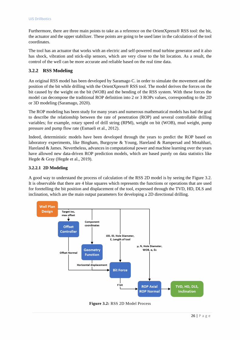
A good way to understand the process of calculation of the RSS 2D model is by seeing the Figure 3.2.

It is observable that there are 4 blue squares which represents the functions or operations that are used

for foretelling the bit position and displacement of the tool, expressed through the TVD, HD, DLS and

inclination, which are the main output parameters for developing a 2D directional drilling.

Figure 3.2: RSS 2D Model Process

UiS Drillbotics

27 | P a g e

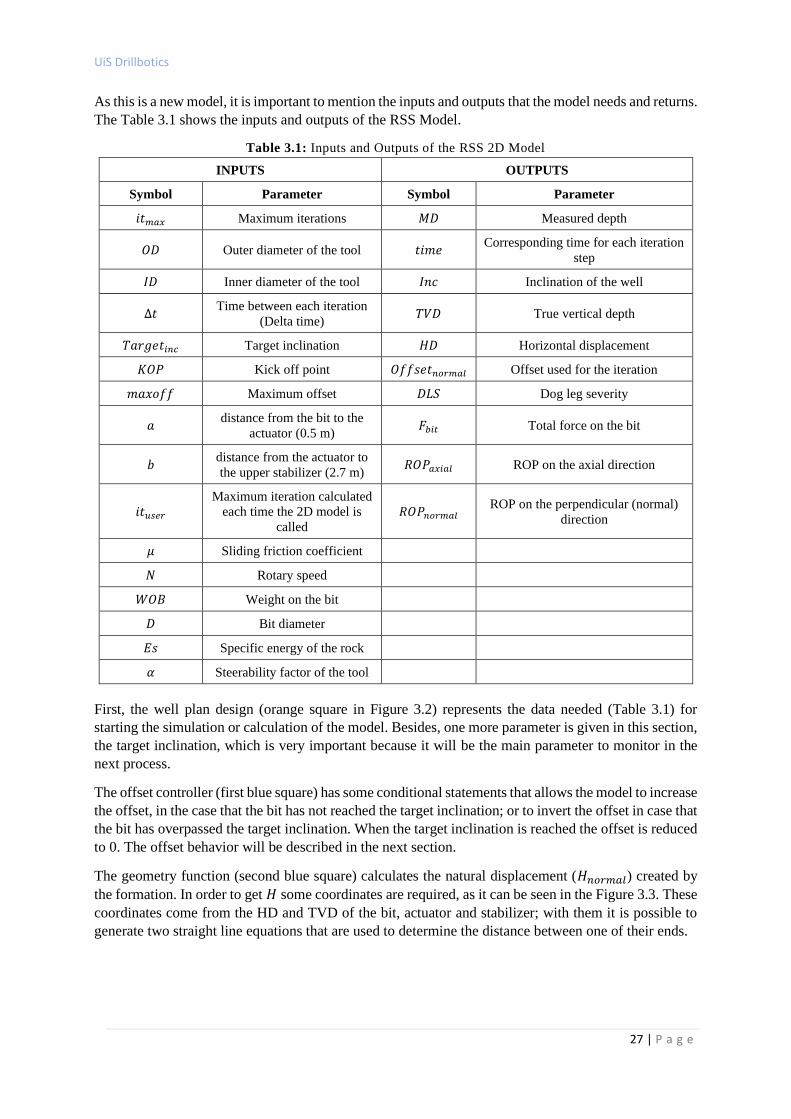
As this is a new model, it is important to mention the inputs and outputs that the model needs and returns.

The Table 3.1 shows the inputs and outputs of the RSS Model.

Table 3.1: Inputs and Outputs of the RSS 2D Model

INPUTS OUTPUTS

Symbol Parameter Symbol Parameter

𝑖𝑡𝑚𝑎𝑥 Maximum iterations 𝑀𝐷 Measured depth

𝑂𝐷 Outer diameter of the tool 𝑡𝑖𝑚𝑒 Corresponding time for each iteration

step

𝐼𝐷 Inner diameter of the tool 𝐼𝑛𝑐 Inclination of the well

∆𝑡 Time between each iteration

(Delta time) 𝑇𝑉𝐷 True vertical depth

𝑇𝑎𝑟𝑔𝑒𝑡𝑖𝑛𝑐 Target inclination 𝐻𝐷 Horizontal displacement

𝐾𝑂𝑃 Kick off point 𝑂𝑓𝑓𝑠𝑒𝑡𝑛𝑜𝑟𝑚𝑎𝑙 Offset used for the iteration

𝑚𝑎𝑥𝑜𝑓𝑓 Maximum offset 𝐷𝐿𝑆 Dog leg severity

𝑎 distance from the bit to the

actuator (0.5 m) 𝐹𝑏𝑖𝑡 Total force on the bit

𝑏 distance from the actuator to

the upper stabilizer (2.7 m) 𝑅𝑂𝑃𝑎𝑥𝑖𝑎𝑙 ROP on the axial direction

𝑖𝑡𝑢𝑠𝑒𝑟

Maximum iteration calculated

each time the 2D model is

called

𝑅𝑂𝑃𝑛𝑜𝑟𝑚𝑎𝑙 ROP on the perpendicular (normal)

direction

𝜇 Sliding friction coefficient

𝑁 Rotary speed

𝑊𝑂𝐵 Weight on the bit

𝐷 Bit diameter

𝐸𝑠 Specific energy of the rock

𝛼 Steerability factor of the tool

First, the well plan design (orange square in Figure 3.2) represents the data needed (Table 3.1) for

starting the simulation or calculation of the model. Besides, one more parameter is given in this section,

the target inclination, which is very important because it will be the main parameter to monitor in the

next process.

The offset controller (first blue square) has some conditional statements that allows the model to increase

the offset, in the case that the bit has not reached the target inclination; or to invert the offset in case that

the bit has overpassed the target inclination. When the target inclination is reached the offset is reduced

to 0. The offset behavior will be described in the next section.

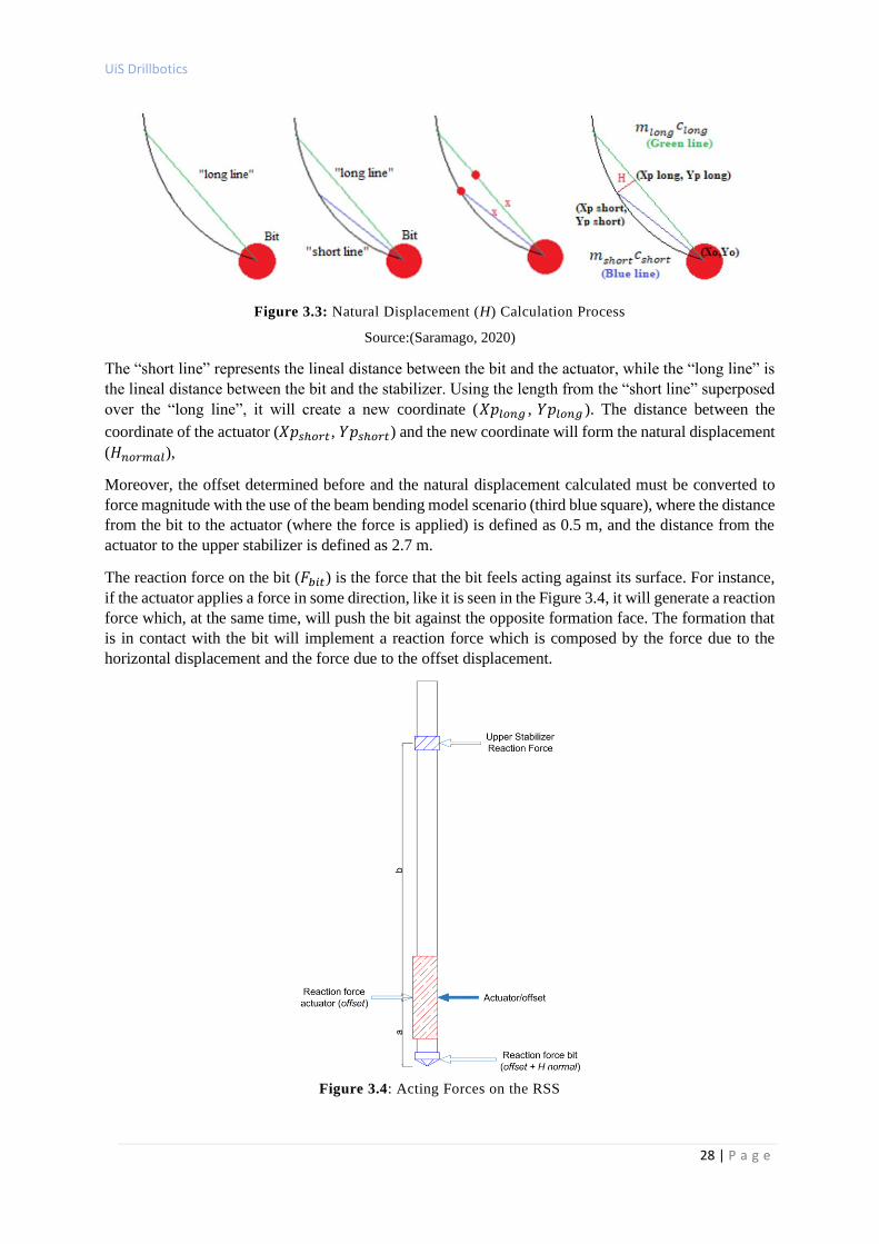
The geometry function (second blue square) calculates the natural displacement (𝐻𝑛𝑜𝑟𝑚𝑎𝑙) created by

the formation. In order to get 𝐻 some coordinates are required, as it can be seen in the Figure 3.3. These

coordinates come from the HD and TVD of the bit, actuator and stabilizer; with them it is possible to

generate two straight line equations that are used to determine the distance between one of their ends.

UiS Drillbotics

28 | P a g e

Figure 3.3: Natural Displacement (H) Calculation Process

Source:(Saramago, 2020)

The “short line” represents the lineal distance between the bit and the actuator, while the “long line” is

the lineal distance between the bit and the stabilizer. Using the length from the “short line” superposed

over the “long line”, it will create a new coordinate (𝑋𝑝𝑙𝑜𝑛𝑔 , 𝑌𝑝𝑙𝑜𝑛𝑔 ). The distance between the

coordinate of the actuator (𝑋𝑝𝑠ℎ𝑜𝑟𝑡, 𝑌𝑝𝑠ℎ𝑜𝑟𝑡) and the new coordinate will form the natural displacement

(𝐻𝑛𝑜𝑟𝑚𝑎𝑙),

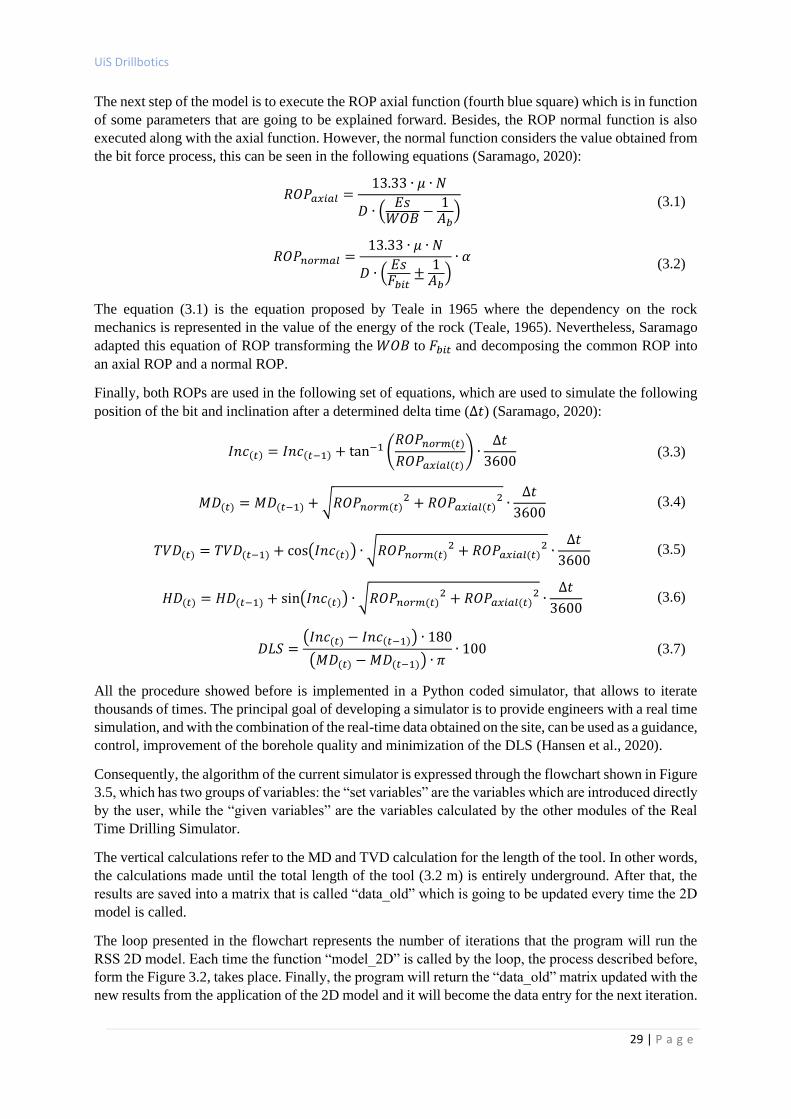
Moreover, the offset determined before and the natural displacement calculated must be converted to

force magnitude with the use of the beam bending model scenario (third blue square), where the distance

from the bit to the actuator (where the force is applied) is defined as 0.5 m, and the distance from the

actuator to the upper stabilizer is defined as 2.7 m.

The reaction force on the bit (𝐹𝑏𝑖𝑡) is the force that the bit feels acting against its surface. For instance,

if the actuator applies a force in some direction, like it is seen in the Figure 3.4, it will generate a reaction

force which, at the same time, will push the bit against the opposite formation face. The formation that

is in contact with the bit will implement a reaction force which is composed by the force due to the

horizontal displacement and the force due to the offset displacement.

Figure 3.4: Acting Forces on the RSS

UiS Drillbotics

29 | P a g e

The next step of the model is to execute the ROP axial function (fourth blue square) which is in function

of some parameters that are going to be explained forward. Besides, the ROP normal function is also

executed along with the axial function. However, the normal function considers the value obtained from

the bit force process, this can be seen in the following equations (Saramago, 2020):

𝑅𝑂𝑃𝑎𝑥𝑖𝑎𝑙 =13.33 ∙ 𝜇 ∙ 𝑁

𝐷 ∙ (𝐸𝑠

𝑊𝑂𝐵−

1𝐴𝑏

)

(3.1)

𝑅𝑂𝑃𝑛𝑜𝑟𝑚𝑎𝑙 =13.33 ∙ 𝜇 ∙ 𝑁

𝐷 ∙ (𝐸𝑠𝐹𝑏𝑖𝑡

±1𝐴𝑏

)∙ 𝛼

(3.2)

The equation (3.1) is the equation proposed by Teale in 1965 where the dependency on the rock

mechanics is represented in the value of the energy of the rock (Teale, 1965). Nevertheless, Saramago

adapted this equation of ROP transforming the 𝑊𝑂𝐵 to 𝐹𝑏𝑖𝑡 and decomposing the common ROP into

an axial ROP and a normal ROP.

Finally, both ROPs are used in the following set of equations, which are used to simulate the following

position of the bit and inclination after a determined delta time (∆𝑡) (Saramago, 2020):

𝐼𝑛𝑐(𝑡) = 𝐼𝑛𝑐(𝑡−1) + tan−1 (𝑅𝑂𝑃𝑛𝑜𝑟𝑚(𝑡)

𝑅𝑂𝑃𝑎𝑥𝑖𝑎𝑙(𝑡)) ∙

∆𝑡

3600 (3.3)

𝑀𝐷(𝑡) = 𝑀𝐷(𝑡−1) + √𝑅𝑂𝑃𝑛𝑜𝑟𝑚(𝑡)2 + 𝑅𝑂𝑃𝑎𝑥𝑖𝑎𝑙(𝑡)

2 ∙∆𝑡

3600 (3.4)

𝑇𝑉𝐷(𝑡) = 𝑇𝑉𝐷(𝑡−1) + cos(𝐼𝑛𝑐(𝑡)) ∙ √𝑅𝑂𝑃𝑛𝑜𝑟𝑚(𝑡)2 + 𝑅𝑂𝑃𝑎𝑥𝑖𝑎𝑙(𝑡)

2 ∙∆𝑡

3600 (3.5)

𝐻𝐷(𝑡) = 𝐻𝐷(𝑡−1) + sin(𝐼𝑛𝑐(𝑡)) ∙ √𝑅𝑂𝑃𝑛𝑜𝑟𝑚(𝑡)2 + 𝑅𝑂𝑃𝑎𝑥𝑖𝑎𝑙(𝑡)

2 ∙∆𝑡

3600 (3.6)

𝐷𝐿𝑆 =(𝐼𝑛𝑐(𝑡) − 𝐼𝑛𝑐(𝑡−1)) ∙ 180

(𝑀𝐷(𝑡) − 𝑀𝐷(𝑡−1)) ∙ 𝜋∙ 100 (3.7)

All the procedure showed before is implemented in a Python coded simulator, that allows to iterate

thousands of times. The principal goal of developing a simulator is to provide engineers with a real time

simulation, and with the combination of the real-time data obtained on the site, can be used as a guidance,

control, improvement of the borehole quality and minimization of the DLS (Hansen et al., 2020).

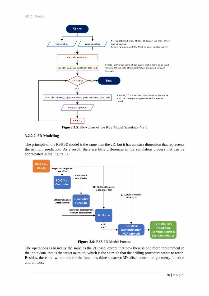
Consequently, the algorithm of the current simulator is expressed through the flowchart shown in Figure

3.5, which has two groups of variables: the “set variables” are the variables which are introduced directly

by the user, while the “given variables” are the variables calculated by the other modules of the Real

Time Drilling Simulator.

The vertical calculations refer to the MD and TVD calculation for the length of the tool. In other words,

the calculations made until the total length of the tool (3.2 m) is entirely underground. After that, the

results are saved into a matrix that is called “data_old” which is going to be updated every time the 2D

model is called.

The loop presented in the flowchart represents the number of iterations that the program will run the

RSS 2D model. Each time the function “model_2D” is called by the loop, the process described before,

form the Figure 3.2, takes place. Finally, the program will return the “data_old” matrix updated with the

new results from the application of the 2D model and it will become the data entry for the next iteration.

UiS Drillbotics

30 | P a g e

Figure 3.5: Flowchart of the RSS Model Simulator V2.0

3.2.2.2 3D Modeling

The principle of the RSS 3D model is the same than the 2D, but it has an extra dimension that represents

the azimuth prediction. As a result, there are little differences in the simulation process that can be

appreciated in the Figure 3.6.

Figure 3.6: RSS 3D Model Process

The operations is basically the same as the 2D case, except that now there is one more requirement in

the input data, that is the target azimuth, which is the azimuth that the drilling procedure wants to reach.

Besides, there are two returns for the functions (blue squares): 3D offset controller, geometry function

and bit force.

UiS Drillbotics

31 | P a g e

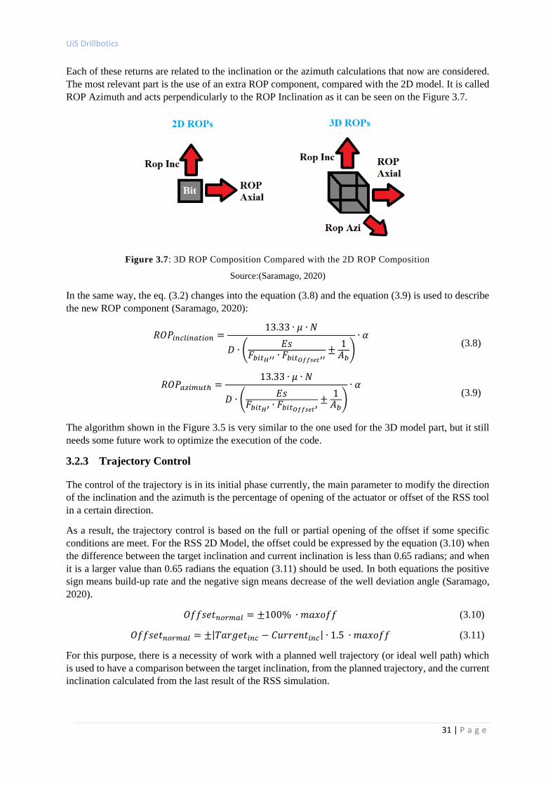
Each of these returns are related to the inclination or the azimuth calculations that now are considered.

The most relevant part is the use of an extra ROP component, compared with the 2D model. It is called

ROP Azimuth and acts perpendicularly to the ROP Inclination as it can be seen on the Figure 3.7.

Figure 3.7: 3D ROP Composition Compared with the 2D ROP Composition

Source:(Saramago, 2020)

In the same way, the eq. (3.2) changes into the equation (3.8) and the equation (3.9) is used to describe

the new ROP component (Saramago, 2020):

𝑅𝑂𝑃𝑖𝑛𝑐𝑙𝑖𝑛𝑎𝑡𝑖𝑜𝑛 =13.33 ∙ 𝜇 ∙ 𝑁

𝐷 ∙ (𝐸𝑠

𝐹𝑏𝑖𝑡𝐻′′ ∙ 𝐹𝑏𝑖𝑡𝑂𝑓𝑓𝑠𝑒𝑡′′±

1𝐴𝑏

)

∙ 𝛼 (3.8)

𝑅𝑂𝑃𝑎𝑧𝑖𝑚𝑢𝑡ℎ =13.33 ∙ 𝜇 ∙ 𝑁

𝐷 ∙ (𝐸𝑠

𝐹𝑏𝑖𝑡𝐻′ ∙ 𝐹𝑏𝑖𝑡𝑂𝑓𝑓𝑠𝑒𝑡′±

1𝐴𝑏

)

∙ 𝛼 (3.9)

The algorithm shown in the Figure 3.5 is very similar to the one used for the 3D model part, but it still

needs some future work to optimize the execution of the code.

3.2.3 Trajectory Control

The control of the trajectory is in its initial phase currently, the main parameter to modify the direction

of the inclination and the azimuth is the percentage of opening of the actuator or offset of the RSS tool

in a certain direction.

As a result, the trajectory control is based on the full or partial opening of the offset if some specific

conditions are meet. For the RSS 2D Model, the offset could be expressed by the equation (3.10) when

the difference between the target inclination and current inclination is less than 0.65 radians; and when

it is a larger value than 0.65 radians the equation (3.11) should be used. In both equations the positive

sign means build-up rate and the negative sign means decrease of the well deviation angle (Saramago,

2020).

𝑂𝑓𝑓𝑠𝑒𝑡𝑛𝑜𝑟𝑚𝑎𝑙 = ±100% ∙ 𝑚𝑎𝑥𝑜𝑓𝑓 (3.10)

𝑂𝑓𝑓𝑠𝑒𝑡𝑛𝑜𝑟𝑚𝑎𝑙 = ±|𝑇𝑎𝑟𝑔𝑒𝑡𝑖𝑛𝑐 − 𝐶𝑢𝑟𝑟𝑒𝑛𝑡𝑖𝑛𝑐| ∙ 1.5 ∙ 𝑚𝑎𝑥𝑜𝑓𝑓 (3.11)

For this purpose, there is a necessity of work with a planned well trajectory (or ideal well path) which

is used to have a comparison between the target inclination, from the planned trajectory, and the current

inclination calculated from the last result of the RSS simulation.

UiS Drillbotics

32 | P a g e

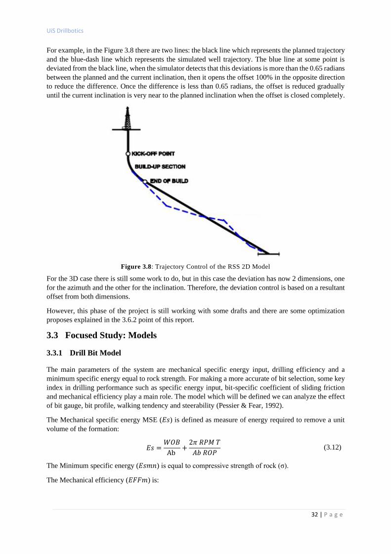
For example, in the Figure 3.8 there are two lines: the black line which represents the planned trajectory

and the blue-dash line which represents the simulated well trajectory. The blue line at some point is

deviated from the black line, when the simulator detects that this deviations is more than the 0.65 radians

between the planned and the current inclination, then it opens the offset 100% in the opposite direction

to reduce the difference. Once the difference is less than 0.65 radians, the offset is reduced gradually

until the current inclination is very near to the planned inclination when the offset is closed completely.

Figure 3.8: Trajectory Control of the RSS 2D Model

For the 3D case there is still some work to do, but in this case the deviation has now 2 dimensions, one

for the azimuth and the other for the inclination. Therefore, the deviation control is based on a resultant

offset from both dimensions.

However, this phase of the project is still working with some drafts and there are some optimization

proposes explained in the 3.6.2 point of this report.

3.3 Focused Study: Models

3.3.1 Drill Bit Model

The main parameters of the system are mechanical specific energy input, drilling efficiency and a

minimum specific energy equal to rock strength. For making a more accurate of bit selection, some key

index in drilling performance such as specific energy input, bit-specific coefficient of sliding friction

and mechanical efficiency play a main role. The model which will be defined we can analyze the effect

of bit gauge, bit profile, walking tendency and steerability (Pessier & Fear, 1992).

The Mechanical specific energy MSE (𝐸𝑠) is defined as measure of energy required to remove a unit

volume of the formation:

𝐸𝑠 =𝑊𝑂𝐵

Ab +

2𝜋 𝑅𝑃𝑀 𝑇

𝐴𝑏 𝑅𝑂𝑃 (3.12)

The Minimum specific energy (𝐸𝑠𝑚𝑛) is equal to compressive strength of rock (σ).

The Mechanical efficiency (𝐸𝐹𝐹𝑚) is:

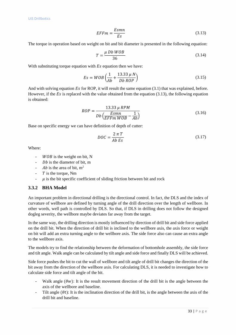
UiS Drillbotics

33 | P a g e

𝐸𝐹𝐹𝑚 =𝐸𝑠𝑚𝑛

𝐸𝑠 (3.13)

The torque in operation based on weight on bit and bit diameter is presented in the following equation:

𝑇 =𝜇 𝐷𝑏 𝑊𝑂𝐵

36 (3.14)

With substituting torque equation with 𝐸𝑠 equation then we have:

𝐸𝑠 = 𝑊𝑂𝐵 (1

𝐴𝑏+

13.33 𝜇 𝑁

𝐷𝑏 𝑅𝑂𝑃) (3.15)

And with solving equation 𝐸𝑠 for ROP, it will result the same equation (3.1) that was explained, before.

However, if the 𝐸𝑠 is replaced with the value obtained from the equation (3.13), the following equation

is obtained:

𝑅𝑂𝑃 =13.33 𝜇 𝑅𝑃𝑀

𝐷𝑏 (𝐸𝑠𝑚𝑛

𝐸𝐹𝐹𝑚 𝑊𝑂𝐵−

1𝐴𝑏

) (3.16)

Base on specific energy we can have definition of depth of cutter:

𝐷𝑂𝐶 =2 𝜋 𝑇

𝐴𝑏 𝐸𝑠 (3.17)

Where:

- 𝑊𝑂𝐵 is the weight on bit, N

- 𝐷𝑏 is the diameter of bit, m

- 𝐴𝑏 is the area of bit, m2

- 𝑇 is the torque, Nm

- 𝜇 is the bit specific coefficient of sliding friction between bit and rock

3.3.2 BHA Model

An important problem in directional drilling is the directional control. In fact, the DLS and the index of

curvature of wellbore are defined by turning angle of the drill direction over the length of wellbore. In

other words, well path is controlled by DLS. So that, if DLS in drilling does not follow the designed

dogleg severity, the wellbore maybe deviates far away from the target.

In the same way, the drilling direction is mostly influenced by direction of drill bit and side force applied

on the drill bit. When the direction of drill bit is inclined to the wellbore axis, the axis force or weight

on bit will add an extra turning angle to the wellbore axis. The side force also can cause an extra angle

to the wellbore axis.

The models try to find the relationship between the deformation of bottomhole assembly, the side force

and tilt angle. Walk angle can be calculated by tilt angle and side force and finally DLS will be achieved.

Side force pushes the bit to cut the wall of wellbore and tilt angle of drill bit changes the direction of the

bit away from the direction of the wellbore axis. For calculating DLS, it is needed to investigate how to

calculate side force and tilt angle of the bit.

- Walk angle (𝜃𝑤): It is the result movement direction of the drill bit is the angle between the

axis of the wellbore and baseline.

- Tilt angle (𝜃𝑡): It is the inclination direction of the drill bit, is the angle between the axis of the

drill bit and baseline.

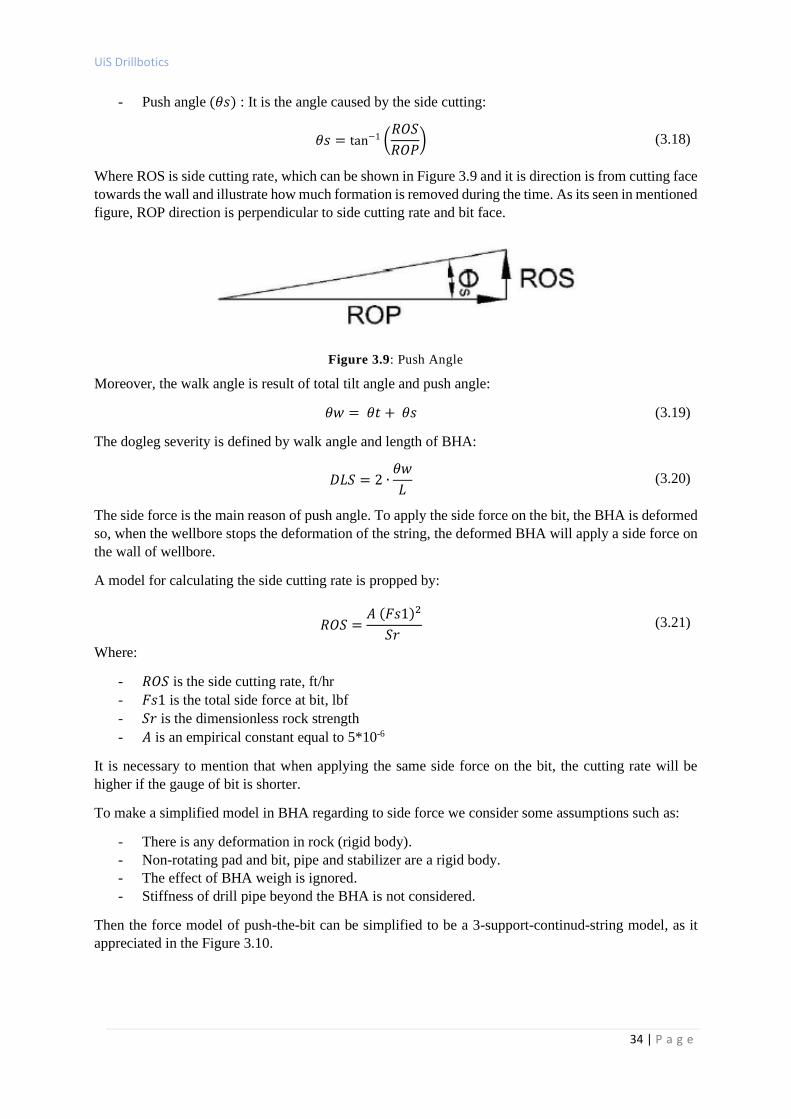
UiS Drillbotics

34 | P a g e

- Push angle (𝜃𝑠) : It is the angle caused by the side cutting:

𝜃𝑠 = tan−1 (𝑅𝑂𝑆

𝑅𝑂𝑃) (3.18)

Where ROS is side cutting rate, which can be shown in Figure 3.9 and it is direction is from cutting face

towards the wall and illustrate how much formation is removed during the time. As its seen in mentioned

figure, ROP direction is perpendicular to side cutting rate and bit face.

Figure 3.9: Push Angle

Moreover, the walk angle is result of total tilt angle and push angle:

𝜃𝑤 = 𝜃𝑡 + 𝜃𝑠 (3.19)

The dogleg severity is defined by walk angle and length of BHA:

𝐷𝐿𝑆 = 2 ∙𝜃𝑤

𝐿 (3.20)

The side force is the main reason of push angle. To apply the side force on the bit, the BHA is deformed

so, when the wellbore stops the deformation of the string, the deformed BHA will apply a side force on

the wall of wellbore.

A model for calculating the side cutting rate is propped by:

𝑅𝑂𝑆 =𝐴 (𝐹𝑠1)2

𝑆𝑟 (3.21)

Where:

- 𝑅𝑂𝑆 is the side cutting rate, ft/hr

- 𝐹𝑠1 is the total side force at bit, lbf

- 𝑆𝑟 is the dimensionless rock strength

- 𝐴 is an empirical constant equal to 5*10-6

It is necessary to mention that when applying the same side force on the bit, the cutting rate will be

higher if the gauge of bit is shorter.

To make a simplified model in BHA regarding to side force we consider some assumptions such as:

- There is any deformation in rock (rigid body).

- Non-rotating pad and bit, pipe and stabilizer are a rigid body.

- The effect of BHA weigh is ignored.

- Stiffness of drill pipe beyond the BHA is not considered.

Then the force model of push-the-bit can be simplified to be a 3-support-continud-string model, as it

appreciated in the Figure 3.10.

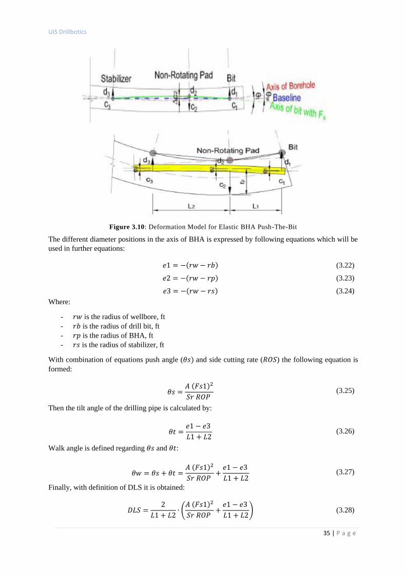
UiS Drillbotics

35 | P a g e

Figure 3.10: Deformation Model for Elastic BHA Push-The-Bit

The different diameter positions in the axis of BHA is expressed by following equations which will be

used in further equations:

𝑒1 = −(𝑟𝑤 − 𝑟𝑏) (3.22)

𝑒2 = −(𝑟𝑤 − 𝑟𝑝) (3.23)

𝑒3 = −(𝑟𝑤 − 𝑟𝑠) (3.24)

Where:

- 𝑟𝑤 is the radius of wellbore, ft

- 𝑟𝑏 is the radius of drill bit, ft

- 𝑟𝑝 is the radius of BHA, ft

- 𝑟𝑠 is the radius of stabilizer, ft

With combination of equations push angle (𝜃𝑠) and side cutting rate (𝑅𝑂𝑆) the following equation is

formed:

𝜃𝑠 =𝐴 (𝐹𝑠1)2

𝑆𝑟 𝑅𝑂𝑃 (3.25)

Then the tilt angle of the drilling pipe is calculated by:

𝜃𝑡 =𝑒1 − 𝑒3

𝐿1 + 𝐿2 (3.26)

Walk angle is defined regarding 𝜃𝑠 and 𝜃𝑡:

𝜃𝑤 = 𝜃𝑠 + 𝜃𝑡 =𝐴 (𝐹𝑠1)2

𝑆𝑟 𝑅𝑂𝑃 +

𝑒1 − 𝑒3

𝐿1 + 𝐿2 (3.27)

Finally, with definition of DLS it is obtained:

𝐷𝐿𝑆 =2

𝐿1 + 𝐿2∙ (

𝐴 (𝐹𝑠1)2

𝑆𝑟 𝑅𝑂𝑃 +

𝑒1 − 𝑒3

𝐿1 + 𝐿2) (3.28)

UiS Drillbotics

36 | P a g e

Where:

- 𝐿1 is the distance between bit and non-rotating pad, ft

- 𝐿1 is the distance between non-rotating pad and stabilizer, ft

3.3.3 Pressure Calculation and Cuttings Transport

The transient drift-flux model and an associated numerical scheme AUSMV will present a dynamic

analysis of cuttings transport in non-Newtonian fluids. The drift-flux models are homogeneous models

that apply slip relation to describe the relative motion between phases (Matovu & Preisig, 2014). The

drift-flux model solves 1D problems for two phases, and has a general form of:

𝜕𝑡𝑊 + 𝜕𝑥𝐹(𝑥,𝑊) = 𝐺(𝑥,𝑊) (3.29)

Where 𝑊 stands for the conservative variables (𝛼𝑙𝜌𝑙 , 𝛼𝑐𝜌𝑐 , 𝛼𝑙𝜌𝑙𝑣𝑙 and 𝛼𝑐𝜌𝑐𝑣𝑐) , 𝐹 is flux and 𝐺 is a

source term. Subscripts 𝑥 and 𝑡 represent space and time dependency.

Any drift-flux model is based on two mass conservation equations, one for each phase, and one

momentum conservation equation, common for both phases. The equations are given below in the

respective order (Udegbunam, 2017):

𝜕

𝜕𝑡(𝛼𝑙𝜌𝑙) +

𝜕

𝜕𝑥(𝛼𝑙𝜌𝑙𝑣𝑙) = Γ𝑙 (3.30)

𝜕

𝜕𝑡(𝛼𝑐𝜌𝑐) +

𝜕

𝜕𝑥(𝛼𝑐𝜌𝑐𝑣𝑐) = Γ𝑐 (3.31)

𝜕

𝜕𝑡(𝛼𝑙𝜌𝑙𝑣𝑙 + 𝛼𝑐𝜌𝑐𝑣𝑐) +

𝜕

𝜕𝑥(𝛼𝑙𝜌𝑙𝑣𝑙

2 + 𝛼𝑐𝜌𝑐𝑣𝑐2 + 𝑝) = −𝑞 (3.32)

The unknown parameters in equations (3.30) to (3.32) are:

- 𝛼𝑙 and 𝛼𝑐 are the volumetric fractions of the respective phases.

- 𝑣𝑙 and 𝑣𝑐 are the velocities of the phases.

- p is the pressure.

- 𝜌𝑙 is the density of the liquid.

- 𝜌𝑐 is the solid phase density, which was considered constant.

Assuming no mass transfer between the phases, the right side of eq. (3.30) and (3.31) becomes zero.

The source term q is a sum of two components, 𝐹𝑔 and 𝐹𝑤, which respectively represent gravity forces

and viscous forces and are calculated as presented below (Udegbunam, 2015):

𝐹𝑔 = 𝑔(𝛼𝑙𝜌𝑙 + 𝛼𝑐𝜌𝑐)𝑐𝑜𝑠𝜃 (3.33)

𝐹𝑤 =2𝑓𝜌𝑚𝑣𝑚𝑎𝑏𝑠(𝑣𝑚)

𝑑𝑜 − 𝑑𝑖 (3.34)

𝑣𝑚 is a mixture velocity of the liquid phase and solid phase. Friction factor, f, depends on the flow

regime and is determined by the Reynolds number.

As mentioned, equations (3.30) to (3.32) contain six (𝜌𝑙, 𝛼𝑙, 𝛼𝑐 , 𝑣𝑙 , 𝑣𝑐 , 𝑝) unknowns. Thus, three more

equations are necessary to solve the system:

𝛼𝑙 + 𝛼𝑐 = 1 (3.35)

𝑣𝑐 = 𝐾𝑣𝑚 − 𝑣𝑠𝑙𝑖𝑝 = 𝐾(𝑣𝑙𝛼𝑙 + 𝑣𝑐𝛼𝑐) − 𝑣𝑠𝑙𝑖𝑝 (3.36)

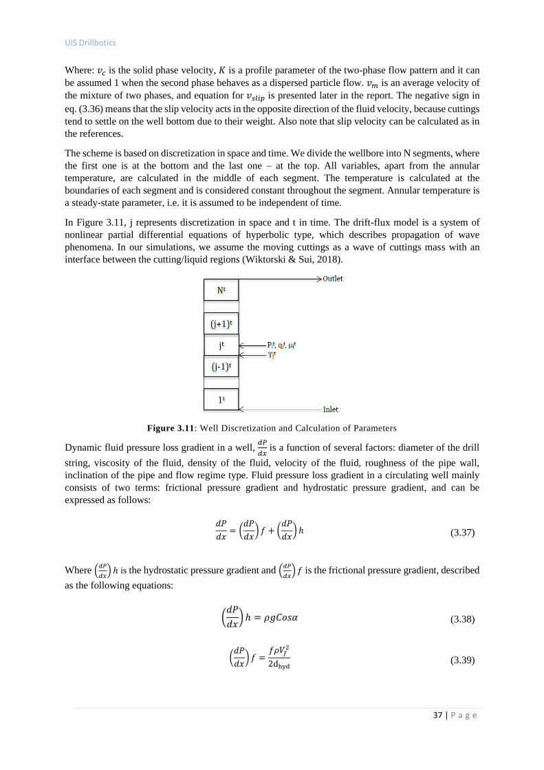
UiS Drillbotics

37 | P a g e

Where: 𝑣𝑐 is the solid phase velocity, 𝐾 is a profile parameter of the two-phase flow pattern and it can

be assumed 1 when the second phase behaves as a dispersed particle flow. 𝑣𝑚 is an average velocity of

the mixture of two phases, and equation for 𝑣𝑠𝑙𝑖𝑝 is presented later in the report. The negative sign in

eq. (3.36) means that the slip velocity acts in the opposite direction of the fluid velocity, because cuttings

tend to settle on the well bottom due to their weight. Also note that slip velocity can be calculated as in

the references.

The scheme is based on discretization in space and time. We divide the wellbore into N segments, where

the first one is at the bottom and the last one – at the top. All variables, apart from the annular

temperature, are calculated in the middle of each segment. The temperature is calculated at the

boundaries of each segment and is considered constant throughout the segment. Annular temperature is

a steady-state parameter, i.e. it is assumed to be independent of time.

In Figure 3.11, j represents discretization in space and t in time. The drift-flux model is a system of

nonlinear partial differential equations of hyperbolic type, which describes propagation of wave

phenomena. In our simulations, we assume the moving cuttings as a wave of cuttings mass with an

interface between the cutting/liquid regions (Wiktorski & Sui, 2018).

Figure 3.11: Well Discretization and Calculation of Parameters

Dynamic fluid pressure loss gradient in a well, 𝑑𝑃

𝑑𝑥 is a function of several factors: diameter of the drill

string, viscosity of the fluid, density of the fluid, velocity of the fluid, roughness of the pipe wall,

inclination of the pipe and flow regime type. Fluid pressure loss gradient in a circulating well mainly

consists of two terms: frictional pressure gradient and hydrostatic pressure gradient, and can be

expressed as follows:

𝑑𝑃

𝑑𝑥= (

𝑑𝑃

𝑑𝑥) 𝑓 + (

𝑑𝑃

𝑑𝑥) ℎ (3.37)

Where (𝑑𝑃

𝑑𝑥) ℎ is the hydrostatic pressure gradient and (

𝑑𝑃

𝑑𝑥) 𝑓 is the frictional pressure gradient, described

as the following equations:

(𝑑𝑃

𝑑𝑥)ℎ = 𝜌𝑔𝐶𝑜𝑠𝛼 (3.38)

(𝑑𝑃

𝑑𝑥) 𝑓 =

𝑓𝜌𝑉𝑓2

2dhyd

(3.39)

UiS Drillbotics

38 | P a g e

The parameters in the above equations are defined as follows: 𝜌 is the fluid’s density, g is the

gravitational acceleration, 𝛼 is the inclination angle, 𝑉𝑓 is the fluid’s velocity and 𝑑ℎ𝑦𝑑 is the hydraulic

diameter. The hydraulic friction factor, 𝑓, varies depending on the flow type: laminar or turbulent.

Cuttings slip velocity is one of the important parameters, which along with the cuttings settling velocity,

is used to estimate the cuttings concentration. It is also used to select flow rate that would allow effective

cuttings removal.

We get a more realistic approximation using the transient models with the inclusion of slip comparing

to the no-slip steady-state models. Therefore, we can say that the slip velocity decreases as inclination

increases. In the vertical section, unlike the inclined sections, the gravity acts in the opposite direction

to the fluid flow, so its effect is more pronounced. We also notice that the slip velocity is nearly constant

in the sections with the constant inclination.

ROP, cuttings density and viscosity:

If the flow rate and cuttings diameter are kept constant:

- We see that ROP has a significant negative effect on the hole cleaning, cuttings density has a

mild negative effect (more cuttings accumulated) and viscosity has small positive effect for

lighter cuttings and significant positive effect for heavier cuttings.

- The slip velocity of the cuttings is lower for lighter cuttings and is nearly independent of the

ROP.

- Higher viscosity reduces slip velocity as high viscous fluids have better carrying capacity and

reduce the tendency of cuttings settling downwards.

Flow rate and cuttings size:

- The volumetric fraction of cuttings in the first segment is relatively low for high flow rate and

it becomes constant much earlier than that for the low flow rate.

- Fluid flow rate 10 kg/s is not sufficient to lift bigger cuttings. Thus, the inlet concentration keeps

on growing. For the low flow rate and large cuttings, all cuttings are accumulated at the well

bottom. Smaller cuttings are being transported through the first wellbore segments from the

bottom. Thus, the concentration is decreasing gradually along the wellbore.

- Higher flow rate makes a significant difference: we see that the cuttings are being transported

more effectively. The higher the flow rate and the smaller the particles – the faster they are

transported from the well.

- The larger the cutting is, the higher is the slip velocity (directed downwards). It is nearly

independent of the flow rate as the liquid phase velocity changes accordingly with variation in

the flow rate.

3.3.4 Drill String Dynamics

The Drill string Model(s) must also calculate buckling conditions. Drilling ahead in simulation will not

be allowed if the drill string is buckling at any point along the drill string. The Drill string Model(s) must

be able to simulate torsional oscillations (slow ones, like stick slip). It must be made up of multiple

torsional spring elements and have friction damping from wellbore contact.

Bit behavior in different rocks and at different WOB/RPM settings will cause stick slip, and the Control

System for the top drive must be able to counter act stick slip automatically when it appears and

modeling of lateral vibrations of the drill string or BHA I not required.

Drilling industry nowadays focuses on process optimization and cost reduction. Unwanted events should

be predicted and avoided to increase drilling efficiency, improve safety, and save costs. Development

and application of mathematical models enable us to understand the dynamics of the drilling process,

UiS Drillbotics

39 | P a g e

learn parameter interaction and regulate system behavior. It is also a way to reduce the risk of occurrence

of such events or mitigate negative outcomes (Wiktorski et al., 2020).

Drilling operations are often impeded by excessive downhole friction, which causes high torque, drag

and drill string vibrations: axial, torsional and lateral. Drill string dynamics can be fully described by

six degrees of freedom per node: axial and lateral translation, angular rotation around the longitudinal

axis and bending in two planes.

The drill string exhibits severe stick–slip vibration induced by the contact between the drill bit and the

formation. Stick–slip vibration of drill string appears as periodic alternations of stick and slip phases.

Transition between static and kinetic friction creates two distinct phases: stick and slip. Stick phase is

initiated when friction between drill string/drill bit and rock exceeds torque provided by top-drive. In

that case, top of drill string continues to rotate, storing potential torsional energy within it. At some

point, the stored energy becomes higher than the friction torque and BHA/drill bit slips to rotate several

times faster than at the surface. Period of such oscillations is determined by BHA and drill string weights,

and somewhat by rotational velocity.

At the surface, stick-slip is observed by periodic oscillations in RPM or current consumption. A

combination of deep deviated well and hard formation increase the risk of stick-slip initiation. At the

same time, high downhole rotational velocity of slip phase can cause strong axial and lateral vibrations.

Axial vibrations, and in the worst case, bit bouncing, typically occur in hard rock environment when the

dominant frequency of external forces corresponds to the natural frequency of drill string. This condition

is called resonance. Such vibrations result in damaged drill bit cutters and other drill bit elements and

are more typical to vertical wells.

The main focus of this work is Investigation of combined axial and torsional drill string motion for

directional drilling with 4 DOF. The evaluated parameters include downhole axial and rotational

velocities, downhole WOB and downhole TOB.

3.3.4.1 Coupled Axial and Torsional Vibrations

As stated above, stick-slip is caused by bit-rock interaction. Once developed, it often leads to outbreak

of axial oscillations. Since, in reality these two vibration modes are related, coupled models should be

considered instead of single degree of freedom ones.

Modeling of self-excited vibrations is a formidable task because they exhibit nonlinear and random

dynamics. For such problems, analytical models have limited accuracy. For instance, frictional torque

is typically modelled as a function of normal force, which is represented by WOB. At the same time,

variation between stick and slip phases causes drill string to elongate and contract, causing fluctuations

in WOB. Therefore, correct application of varying operational parameters and boundary conditions is

essential to obtain realistic results.

Based on the simplified lumped model by (Yigit & Christoforou, 2006), simulated the influences of

operating conditions on bit bounce and stick–slip. It indicated that conditions at the interface of bit and

rock are major factors of bit dynamics. Noted for the presented model, a number of parameters that

should be determined by experimental measurement were included. (Tang et al, 2019) The stick–slip

vibration modeling typically considers only the torsional vibration of drill string regarding the

interaction between the bit and rock as Coulomb friction referred to velocity weakening.

(Richard et al.,2002) proposed a DDOF discrete model considering the axial and torsional vibrations of

the drilling system to study the self-excited stick–slip phenomenon. Coupling between the two vibration

modes was realized by using a bit-rock contact principle where the friction and crushing processes were

considered, which differed from the classical method used to reveal the stick–slip vibration. The

dynamic responses can be obtained by the surface conditions of the drill bit and bit-rock contact

principles, in conjunction with the motion equations for the torsional and axial vibrations.

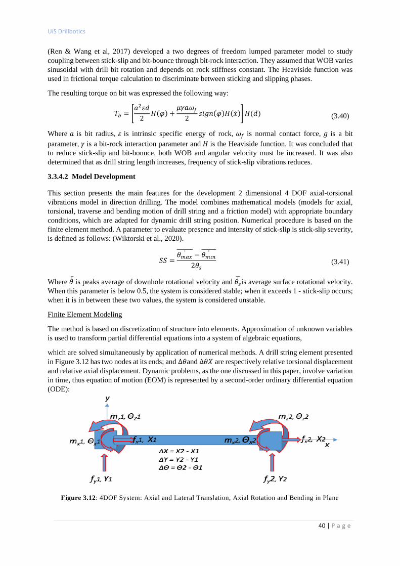
UiS Drillbotics

40 | P a g e

(Ren & Wang et al, 2017) developed a two degrees of freedom lumped parameter model to study

coupling between stick-slip and bit-bounce through bit-rock interaction. They assumed that WOB varies

sinusoidal with drill bit rotation and depends on rock stiffness constant. The Heaviside function was

used in frictional torque calculation to discriminate between sticking and slipping phases.

The resulting torque on bit was expressed the following way:

𝑇𝑏 = [𝑎2휀𝑑

2𝐻(𝜑) +

𝜇𝛾𝑎𝜔𝑓

2𝑠𝑖𝑔𝑛(𝜑)𝐻(��)]𝐻(𝑑) (3.40)

Where 𝑎 is bit radius, 휀 is intrinsic specific energy of rock, 𝜔𝑓 is normal contact force, 𝑔 is a bit

parameter, 𝛾 is a bit-rock interaction parameter and 𝐻 is the Heaviside function. It was concluded that

to reduce stick-slip and bit-bounce, both WOB and angular velocity must be increased. It was also

determined that as drill string length increases, frequency of stick-slip vibrations reduces.

3.3.4.2 Model Development

This section presents the main features for the development 2 dimensional 4 DOF axial-torsional

vibrations model in direction drilling. The model combines mathematical models (models for axial,

torsional, traverse and bending motion of drill string and a friction model) with appropriate boundary

conditions, which are adapted for dynamic drill string position. Numerical procedure is based on the

finite element method. A parameter to evaluate presence and intensity of stick-slip is stick-slip severity,

is defined as follows: (Wiktorski et al., 2020).

𝑆𝑆 =𝜃𝑚𝑎𝑥

− 𝜃𝑚𝑖𝑛

2𝜃𝑠 (3.41)

Where �� is peaks average of downhole rotational velocity and 𝜃�� is average surface rotational velocity.

When this parameter is below 0.5, the system is considered stable; when it exceeds 1 - stick-slip occurs;

when it is in between these two values, the system is considered unstable.

Finite Element Modeling

The method is based on discretization of structure into elements. Approximation of unknown variables

is used to transform partial differential equations into a system of algebraic equations,

which are solved simultaneously by application of numerical methods. A drill string element presented

in Figure 3.12 has two nodes at its ends; and ∆𝜃and ∆𝜃𝑋 are respectively relative torsional displacement

and relative axial displacement. Dynamic problems, as the one discussed in this paper, involve variation

in time, thus equation of motion (EOM) is represented by a second-order ordinary differential equation

(ODE):

Figure 3.12: 4DOF System: Axial and Lateral Translation, Axial Rotation and Bending in Plane

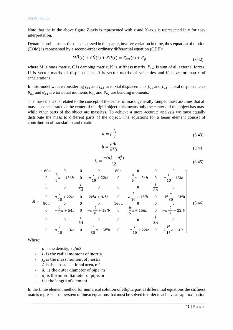
UiS Drillbotics

41 | P a g e

Note that the in the above figure Z-axis is represented with x and X-axis is represented in y for easy

interpretation.

Dynamic problems, as the one discussed in this paper, involve variation in time, thus equation of motion

(EOM) is represented by a second-order ordinary differential equation (ODE):

𝑀��(𝑡) + 𝐶��(𝑡) + 𝐾𝑈(𝑡) = 𝐹𝑒𝑥𝑡(𝑡) + 𝐹𝑔 (3.42)

where M is mass matrix, C is damping matrix, K is stiffness matrix, 𝐹𝑒𝑥𝑡 is sum of all external forces,

U is vector matrix of displacements, �� is vector matrix of velocities and �� is vector matrix of

accelerations.

In this model we are considering 𝑓𝑥1 and 𝑓𝑥2 are axial displacements 𝑓𝑦1 and 𝑓𝑦2 lateral displacements

𝜃𝑥1 and 𝜃𝑥2 are torsional moments 𝜃𝑦1 and 𝜃𝑦2 are bending moments.

The mass matrix is related to the concept of the center of mass. generally lumped mass assumes that all

mass is concentrated at the center of the rigid object. this means only the center oof the object has mass

while other parts of the object are massless. To achieve a more accurate analysis we must equally

distribute the mass to different parts of the object. The equations for a beam element consist of

contribution of translation and rotation.

𝑎 = 𝜌𝐼𝑧𝑙

(3.43)

𝑏 =𝜌𝐴𝑙

420 (3.44)

𝐼𝑧 =𝜋(𝑑0

4 − 𝑑𝑖4)

32 (3.45)

𝑀 =

[ 160𝑎 0 0 0 80𝑎 0 0 0

06

5𝑎 + 156𝑏 0 𝑎

𝑙

10+ 22𝑙𝑏 0 −

6

5𝑎 + 54𝑏 0 𝑎

𝑙

10− 13𝑙𝑏

0 0𝐽

3𝐴0 0 0

𝐽

6𝐴0

0 𝑎𝑙

10+ 22𝑙𝑏 0 2𝑙2𝑎 + 4𝑙2𝑏 0 𝑎

𝑙

10+ 13𝑙𝑏 0 −𝑙2

𝑎

30− 3𝑙2𝑏

80𝑎 0 0 0 160𝑎 0 0 0

0 −6

5𝑎 + 54𝑏 0 −𝑎

𝑙

10+ 13𝑙𝑏 0

6

5𝑎 + 156𝑏 0 −𝑎

𝑙

10− 22𝑙𝑏

0 0𝐽

6𝐴0 0 0

𝐽

3𝐴0

0 𝑎𝑙

10− 13𝑙𝑏 0 −

𝑙2

30𝑎 − 3𝑙2𝑏 0 −𝑎

𝑙

10+ 22𝑙𝑏 0 2

𝑙2

15𝑎 + 4𝑙2 ]

(3.46)

Where:

- 𝜌 is the density, kg/m3 - 𝐼𝑧 is the radial moment of inertia - 𝐽𝑧 is the mass moment of inertia - 𝐴 is the cross-sectional area, m2 - 𝑑𝑜 is the outer diameter of pipe, m

- 𝑑𝑖 is the inner diameter of pipe, m - 𝑙 is the length of element

In the finite element method for numerical solution of elliptic partial differential equations the stiffness

matrix represents the system of linear equations that must be solved in order to achieve an approximation

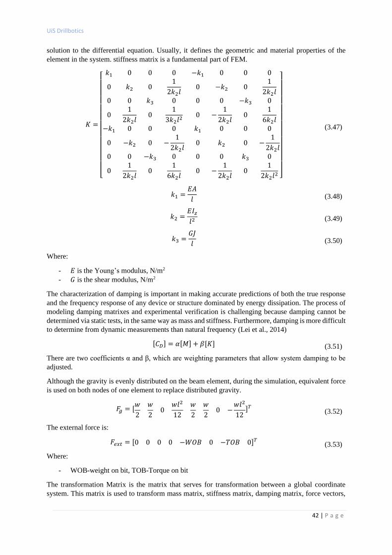
UiS Drillbotics

42 | P a g e

solution to the differential equation. Usually, it defines the geometric and material properties of the

element in the system. stiffness matrix is a fundamental part of FEM.

𝐾 =

[

𝑘1 0 0 0 −𝑘1 0 0 0

0 𝑘2 01

2𝑘2𝑙0 −𝑘2 0

1

2𝑘2𝑙0 0 𝑘3 0 0 0 −𝑘3 0

01

2𝑘2𝑙0

1

3𝑘2𝑙2

0 −1

2𝑘2𝑙0

1

6𝑘2𝑙−𝑘1 0 0 0 𝑘1 0 0 0

0 −𝑘2 0 −1

2𝑘2𝑙0 𝑘2 0 −

1

2𝑘2𝑙0 0 −𝑘3 0 0 0 𝑘3 0

01

2𝑘2𝑙0

1

6𝑘2𝑙0 −

1

2𝑘2𝑙0

1

2𝑘2𝑙2 ]

(3.47)

𝑘1 =𝐸𝐴

𝑙 (3.48)

𝑘2 =𝐸𝐼𝑧𝑙2

(3.49)

𝑘3 =𝐺𝐽

𝑙 (3.50)

Where:

- 𝐸 is the Young’s modulus, N/m2

- 𝐺 is the shear modulus, N/m2

The characterization of damping is important in making accurate predictions of both the true response

and the frequency response of any device or structure dominated by energy dissipation. The process of

modeling damping matrixes and experimental verification is challenging because damping cannot be

determined via static tests, in the same way as mass and stiffness. Furthermore, damping is more difficult

to determine from dynamic measurements than natural frequency (Lei et al., 2014)

[𝐶𝐷] = 𝛼[𝑀] + 𝛽[𝐾] (3.51)

There are two coefficients α and β, which are weighting parameters that allow system damping to be

adjusted.

Although the gravity is evenly distributed on the beam element, during the simulation, equivalent force

is used on both nodes of one element to replace distributed gravity.

𝐹𝑔 = [𝑤

2

𝑤

20

𝑤𝑙2

12

𝑤

2

𝑤

20 −

𝑤𝑙2

12]𝑇 (3.52)

The external force is:

𝐹𝑒𝑥𝑡 = [0 0 0 0 −𝑊𝑂𝐵 0 −𝑇𝑂𝐵 0]𝑇 (3.53)

Where:

- WOB-weight on bit, TOB-Torque on bit

The transformation Matrix is the matrix that serves for transformation between a global coordinate

system. This matrix is used to transform mass matrix, stiffness matrix, damping matrix, force vectors,

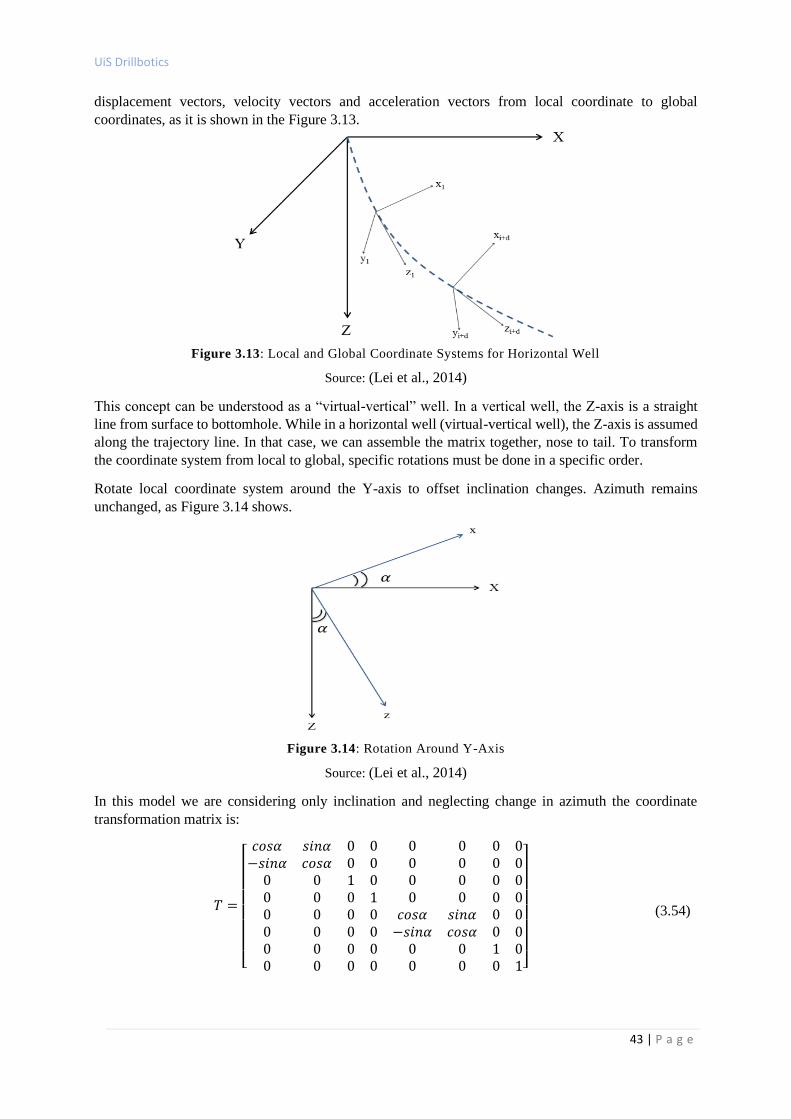
UiS Drillbotics

43 | P a g e

displacement vectors, velocity vectors and acceleration vectors from local coordinate to global

coordinates, as it is shown in the Figure 3.13.

Figure 3.13: Local and Global Coordinate Systems for Horizontal Well

Source: (Lei et al., 2014)

This concept can be understood as a “virtual-vertical” well. In a vertical well, the Z-axis is a straight

line from surface to bottomhole. While in a horizontal well (virtual-vertical well), the Z-axis is assumed

along the trajectory line. In that case, we can assemble the matrix together, nose to tail. To transform

the coordinate system from local to global, specific rotations must be done in a specific order.

Rotate local coordinate system around the Y-axis to offset inclination changes. Azimuth remains

unchanged, as Figure 3.14 shows.

Figure 3.14: Rotation Around Y-Axis

Source: (Lei et al., 2014)

In this model we are considering only inclination and neglecting change in azimuth the coordinate

transformation matrix is:

𝑇 =

[ 𝑐𝑜𝑠𝛼 𝑠𝑖𝑛𝛼 0 0 0 0 0 0−𝑠𝑖𝑛𝛼 𝑐𝑜𝑠𝛼 0 0 0 0 0 0

0 0 1 0 0 0 0 00 0 0 1 0 0 0 00 0 0 0 𝑐𝑜𝑠𝛼 𝑠𝑖𝑛𝛼 0 00 0 0 0 −𝑠𝑖𝑛𝛼 𝑐𝑜𝑠𝛼 0 00 0 0 0 0 0 1 00 0 0 0 0 0 0 1]

(3.54)

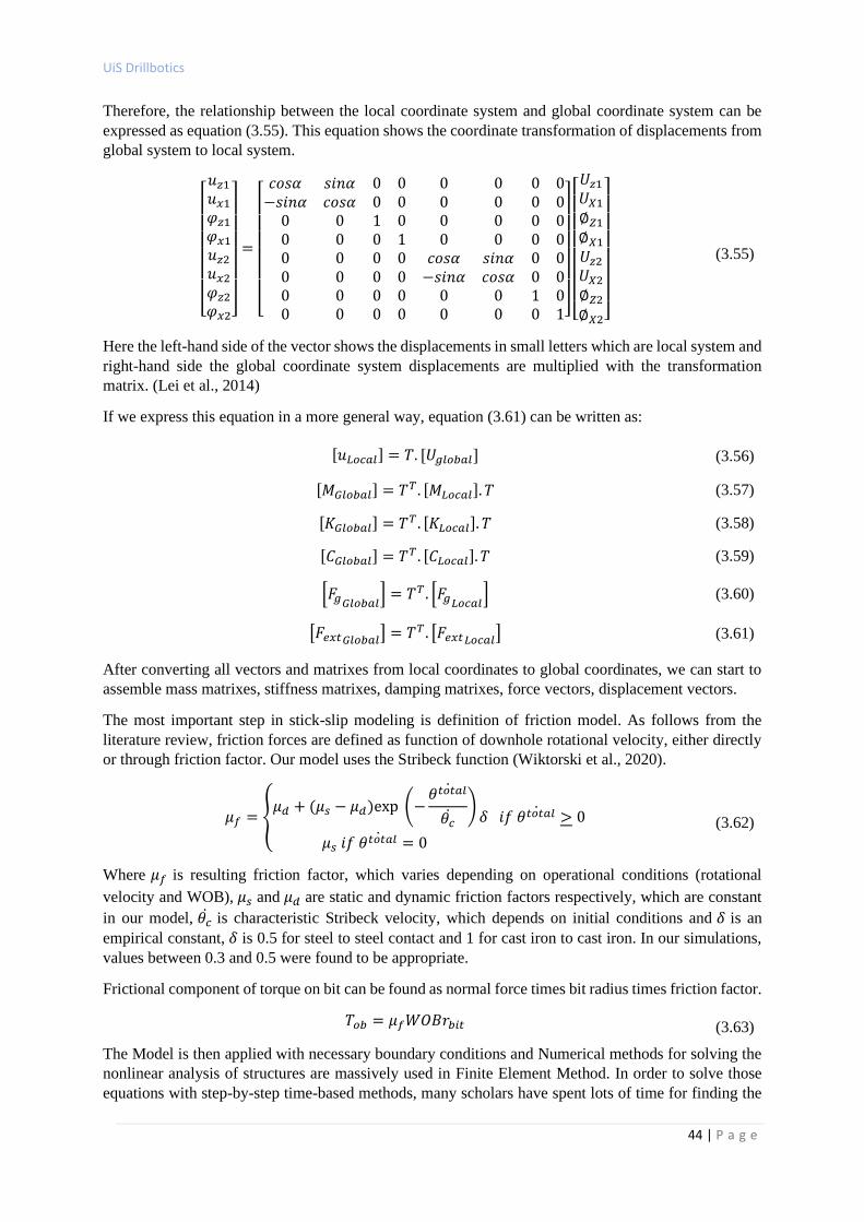
UiS Drillbotics

44 | P a g e

Therefore, the relationship between the local coordinate system and global coordinate system can be

expressed as equation (3.55). This equation shows the coordinate transformation of displacements from

global system to local system.

[ 𝑢𝑧1

𝑢𝑥1

𝜑𝑧1

𝜑𝑥1

𝑢𝑧2

𝑢𝑥2

𝜑𝑧2

𝜑𝑥2]

=

[ 𝑐𝑜𝑠𝛼 𝑠𝑖𝑛𝛼 0 0 0 0 0 0−𝑠𝑖𝑛𝛼 𝑐𝑜𝑠𝛼 0 0 0 0 0 0

0 0 1 0 0 0 0 00 0 0 1 0 0 0 00 0 0 0 𝑐𝑜𝑠𝛼 𝑠𝑖𝑛𝛼 0 00 0 0 0 −𝑠𝑖𝑛𝛼 𝑐𝑜𝑠𝛼 0 00 0 0 0 0 0 1 00 0 0 0 0 0 0 1]

[ 𝑈𝑧1

𝑈𝑋1

∅𝑍1

∅𝑋1

𝑈𝑧2

𝑈𝑋2

∅𝑍2

∅𝑋2]

(3.55)

Here the left-hand side of the vector shows the displacements in small letters which are local system and

right-hand side the global coordinate system displacements are multiplied with the transformation

matrix. (Lei et al., 2014)

If we express this equation in a more general way, equation (3.61) can be written as:

[𝑢𝐿𝑜𝑐𝑎𝑙] = 𝑇. [𝑈𝑔𝑙𝑜𝑏𝑎𝑙] (3.56)

[𝑀𝐺𝑙𝑜𝑏𝑎𝑙] = 𝑇𝑇 . [𝑀𝐿𝑜𝑐𝑎𝑙]. 𝑇 (3.57)

[𝐾𝐺𝑙𝑜𝑏𝑎𝑙] = 𝑇𝑇 . [𝐾𝐿𝑜𝑐𝑎𝑙]. 𝑇 (3.58)

[𝐶𝐺𝑙𝑜𝑏𝑎𝑙] = 𝑇𝑇 . [𝐶𝐿𝑜𝑐𝑎𝑙]. 𝑇 (3.59)

[𝐹𝑔𝐺𝑙𝑜𝑏𝑎𝑙] = 𝑇𝑇 . [𝐹𝑔𝐿𝑜𝑐𝑎𝑙

] (3.60)

[𝐹𝑒𝑥𝑡𝐺𝑙𝑜𝑏𝑎𝑙] = 𝑇𝑇 . [𝐹𝑒𝑥𝑡𝐿𝑜𝑐𝑎𝑙] (3.61)

After converting all vectors and matrixes from local coordinates to global coordinates, we can start to

assemble mass matrixes, stiffness matrixes, damping matrixes, force vectors, displacement vectors.

The most important step in stick-slip modeling is definition of friction model. As follows from the

literature review, friction forces are defined as function of downhole rotational velocity, either directly

or through friction factor. Our model uses the Stribeck function (Wiktorski et al., 2020).

𝜇𝑓 = {𝜇𝑑 + (𝜇𝑠 − 𝜇𝑑)exp (−

𝜃𝑡𝑜𝑡𝑎𝑙

𝜃��

)

𝜇𝑠 𝑖𝑓 𝜃𝑡𝑜𝑡𝑎𝑙 = 0

𝛿 𝑖𝑓 𝜃𝑡𝑜𝑡𝑎𝑙 > 0 (3.62)

Where 𝜇𝑓 is resulting friction factor, which varies depending on operational conditions (rotational

velocity and WOB), 𝜇𝑠 and 𝜇𝑑 are static and dynamic friction factors respectively, which are constant

in our model, 𝜃�� is characteristic Stribeck velocity, which depends on initial conditions and 𝛿 is an

empirical constant, 𝛿 is 0.5 for steel to steel contact and 1 for cast iron to cast iron. In our simulations,

values between 0.3 and 0.5 were found to be appropriate.

Frictional component of torque on bit can be found as normal force times bit radius times friction factor.

𝑇𝑜𝑏 = 𝜇𝑓𝑊𝑂𝐵𝑟𝑏𝑖𝑡 (3.63)

The Model is then applied with necessary boundary conditions and Numerical methods for solving the

nonlinear analysis of structures are massively used in Finite Element Method. In order to solve those

equations with step-by-step time-based methods, many scholars have spent lots of time for finding the

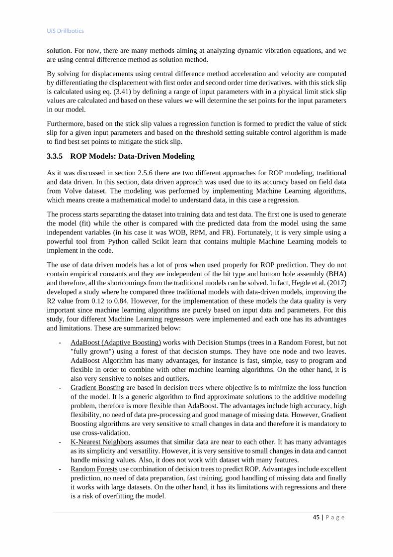
UiS Drillbotics

45 | P a g e

solution. For now, there are many methods aiming at analyzing dynamic vibration equations, and we

are using central difference method as solution method.

By solving for displacements using central difference method acceleration and velocity are computed

by differentiating the displacement with first order and second order time derivatives. with this stick slip

is calculated using eq. (3.41) by defining a range of input parameters with in a physical limit stick slip

values are calculated and based on these values we will determine the set points for the input parameters

in our model.

Furthermore, based on the stick slip values a regression function is formed to predict the value of stick

slip for a given input parameters and based on the threshold setting suitable control algorithm is made

to find best set points to mitigate the stick slip.

3.3.5 ROP Models: Data-Driven Modeling

As it was discussed in section 2.5.6 there are two different approaches for ROP modeling, traditional

and data driven. In this section, data driven approach was used due to its accuracy based on field data

from Volve dataset. The modeling was performed by implementing Machine Learning algorithms,

which means create a mathematical model to understand data, in this case a regression.

The process starts separating the dataset into training data and test data. The first one is used to generate

the model (fit) while the other is compared with the predicted data from the model using the same

independent variables (in his case it was WOB, RPM, and FR). Fortunately, it is very simple using a

powerful tool from Python called Scikit learn that contains multiple Machine Learning models to

implement in the code.

The use of data driven models has a lot of pros when used properly for ROP prediction. They do not

contain empirical constants and they are independent of the bit type and bottom hole assembly (BHA)

and therefore, all the shortcomings from the traditional models can be solved. In fact, Hegde et al. (2017)

developed a study where he compared three traditional models with data-driven models, improving the

R2 value from 0.12 to 0.84. However, for the implementation of these models the data quality is very

important since machine learning algorithms are purely based on input data and parameters. For this

study, four different Machine Learning regressors were implemented and each one has its advantages

and limitations. These are summarized below:

- AdaBoost (Adaptive Boosting) works with Decision Stumps (trees in a Random Forest, but not

"fully grown") using a forest of that decision stumps. They have one node and two leaves.

AdaBoost Algorithm has many advantages, for instance is fast, simple, easy to program and

flexible in order to combine with other machine learning algorithms. On the other hand, it is

also very sensitive to noises and outliers.

- Gradient Boosting are based in decision trees where objective is to minimize the loss function

of the model. It is a generic algorithm to find approximate solutions to the additive modeling

problem, therefore is more flexible than AdaBoost. The advantages include high accuracy, high

flexibility, no need of data pre-processing and good manage of missing data. However, Gradient

Boosting algorithms are very sensitive to small changes in data and therefore it is mandatory to

use cross-validation.

- K-Nearest Neighbors assumes that similar data are near to each other. It has many advantages

as its simplicity and versatility. However, it is very sensitive to small changes in data and cannot

handle missing values. Also, it does not work with dataset with many features.

- Random Forests use combination of decision trees to predict ROP. Advantages include excellent

prediction, no need of data preparation, fast training, good handling of missing data and finally

it works with large datasets. On the other hand, it has its limitations with regressions and there

is a risk of overfitting the model.

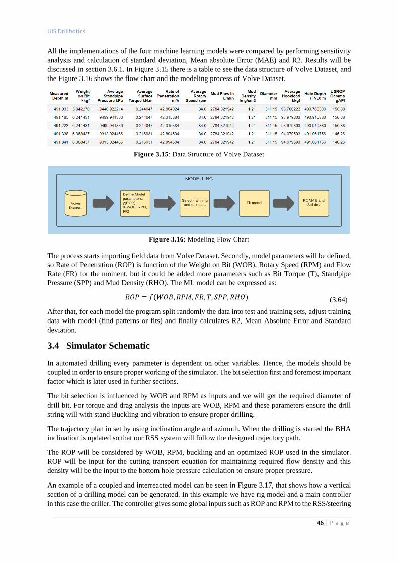
UiS Drillbotics

46 | P a g e

All the implementations of the four machine learning models were compared by performing sensitivity

analysis and calculation of standard deviation, Mean absolute Error (MAE) and R2. Results will be

discussed in section 3.6.1. In Figure 3.15 there is a table to see the data structure of Volve Dataset, and

the Figure 3.16 shows the flow chart and the modeling process of Volve Dataset.

Figure 3.15: Data Structure of Volve Dataset

Figure 3.16: Modeling Flow Chart

The process starts importing field data from Volve Dataset. Secondly, model parameters will be defined,

so Rate of Penetration (ROP) is function of the Weight on Bit (WOB), Rotary Speed (RPM) and Flow

Rate (FR) for the moment, but it could be added more parameters such as Bit Torque (T), Standpipe

Pressure (SPP) and Mud Density (RHO). The ML model can be expressed as:

𝑅𝑂𝑃 = 𝑓(𝑊𝑂𝐵, 𝑅𝑃𝑀, 𝐹𝑅, 𝑇, 𝑆𝑃𝑃, 𝑅𝐻𝑂) (3.64)

After that, for each model the program split randomly the data into test and training sets, adjust training

data with model (find patterns or fits) and finally calculates R2, Mean Absolute Error and Standard

deviation.

3.4 Simulator Schematic

In automated drilling every parameter is dependent on other variables. Hence, the models should be

coupled in order to ensure proper working of the simulator. The bit selection first and foremost important

factor which is later used in further sections.

The bit selection is influenced by WOB and RPM as inputs and we will get the required diameter of

drill bit. For torque and drag analysis the inputs are WOB, RPM and these parameters ensure the drill

string will with stand Buckling and vibration to ensure proper drilling.

The trajectory plan in set by using inclination angle and azimuth. When the drilling is started the BHA

inclination is updated so that our RSS system will follow the designed trajectory path.

The ROP will be considered by WOB, RPM, buckling and an optimized ROP used in the simulator.

ROP will be input for the cutting transport equation for maintaining required flow density and this

density will be the input to the bottom hole pressure calculation to ensure proper pressure.

An example of a coupled and interreacted model can be seen in Figure 3.17, that shows how a vertical

section of a drilling model can be generated. In this example we have rig model and a main controller

in this case the driller. The controller gives some global inputs such as ROP and RPM to the RSS/steering

UiS Drillbotics

47 | P a g e

model and check the results of inclination and azimuth calculated, if these results are not comparable to

the original wanted trajectory, they are sent to the trajectory optimization model and a new target and

offset are generated and sent to the RSS model with the fixed values of inputs given by the controller.

If, however, the values are compatible, we send the values to the hydraulics/cuttings transport model,

combining with some input values from the controller and the outputs from the RSS model, this model

will calculate the pressure and minimum flow velocity. If those parameters are not satisfactory the

controller choose new input values for the RSS model, until we get a satisfactory value of pressure and

minimum flow velocity.

From the hydraulics/cuttings model we get RPM and inclination, and send it to the drill string design

system, which includes models such as torque and drag model, bit model, BHA model, stick-slip model,

etc. Each one of these models will get inputs from the drill string design system and the controller. For

instance, the torque and drag model will get inclination, RPM and azimuth and the values of the model’s

calculation will get verified against the necessary/wanted T&D values.

For the Bit model, values if RPM at the bit, surface torque and WOB at the bit are sent from the drill

string design system and output values of DOC, MSE, axial and lateral displacement and bit depth are

checked against as acceptable or not. And in the stock-slip case, values of RPM, WOB and inclination

are applied to the model and checked against the values of the safety window design by the controller.

Figure 3.17: Simple Trajectory Proposed Model Diagram for Drillbotics Team

UiS Drillbotics

48 | P a g e

3.5 Safety Constraints and Boundary Conditions

3.5.1 Case Study: Modeling for Buckling Limit

The slenderness is a measure of the tendency for a drill pipe to buckle. If the slenderness found to be

greater than critical ratio, then it is empirically found that Euler’s Critical Load formula is applicable.

𝑠𝑙𝑒𝑛𝑑𝑒𝑟𝑛𝑒𝑠𝑠 =𝑙

𝑘 (3.65)

And 𝐾, is defined by:

𝐾 = √𝐼

𝐴 (3.66)

Where 𝐼 is the minimum moment area of the cross-section and 𝐴 is the cross-sectional area, calculated

with the following equations respectively:

𝐼 =𝜋

64(𝑂𝐷4 − 𝐼𝐷4) (3.67)

𝐼 =𝜋

4(𝑂𝐷2 − 𝐼𝐷2) (3.68)

Where 𝑂𝐷 and 𝐼𝐷 are outer diameter and inner diameter, respectively. The critical slenderness ratio is

given as follows:

1

𝐾= √

2 ∙ 𝜋2 ∙ 𝐸

𝜎𝑦 (3.69)

Where 𝐸 is the modulus of Elasticity and 𝜎𝑦 is the tensile yield strength.

Buckling of a drill pipe is the main limiting factor when it comes to selecting a maximum WOB.

Buckling occurs when a structure, such as a drill pipe, is subjected to compressive stress and start a

sideways deflection. The deflection may cause the drill pipe to rapidly wear due to abrasion along the

borehole wall. If the deflection becomes too great, the drill pipe will start to deform plastically and

eventually lose all its load bearing capacity. In order to prevent the buckling effect, it is important to

know the strength of the drill pipe by using Euler’s Critical Load formula given below:

𝐹𝑐𝑟 =𝜋2 ∙ 𝐸 ∙ 𝐼

(𝐾 ∙ 𝐿)2 (3.70)

Where 𝐾 is column effective length factor and 𝐿 is the unsupported length of the column.

3.5.2 Case Study: Maximum Torque

In our case, torsional vibrations might be the most critical reasons to lead to drilling failures. Torsional

vibrations are typically represented by stick-slips, which means that the drill bit stops rotating and the

drill string accelerates and decelerates in a periodical manner. Then, it is important to know how much

torque the drill pipe can endure in order to prevent it from failures. One can calculate the maximum

torque using:

𝑇 = 𝜏 ∗𝐽

𝜌𝑟 (3.71)

Where 𝑇 is the torque, 𝜏 is the shear stress, 𝐽 is the polar moment of inertia and 𝜌𝑟 is the radial distance

to center of the pipe. From the above equation, it is easy to get the maximum torque as:

UiS Drillbotics

49 | P a g e

𝑇𝑚𝑎𝑥 =𝜋

16∙(𝑂𝐷4 − 𝐼𝐷4)

𝑂𝐷 (3.72)

Where 𝜏𝑚𝑎𝑥 is the maximum shear stress, the shear strength depends on type material used in

construction of drill pipe.

In order to perform safe drilling, one should also know the shear yield strength, 𝜏𝑦. By using Euler–

Mascheroni constant of 0.577, one can convert tensile yield strength, 𝜎𝑦 to shear yield strength, 𝜏𝑦, as

shown in below equation:

𝜏𝑦 = 0.577 ∗ 𝜎𝑦 (3.73)

The maximum torque before the drill pipe yields is:

𝑇𝑦 = 𝜏𝑦 ∙𝜋

16∙(𝑂𝐷4 − 𝐼𝐷4)

𝑂𝐷 (3.74)

3.5.3 Case Study: ROP Control

Oil drilling operations is usually associated with drill-string severe vibration conditions that lead to an

onerous and inefficient process. In order to avoid or minimize the impact of vibrations on operation

conditions it is essential a deep dynamical investigation that allows a proper understanding of system

dynamics. Form the eq. (3.41), the stick slip severity is calculated from the drill string model for input

variables like Weight on bit and rotations per minute.

By constraining the maximum WOB, Torque applied on drill string form equations (3.70) and (3.74),

and the Maximum limit to RPM is constrained by eq. (3.41). With these boundary limits a safe drilling

operation procedure can established which can mitigate the drilling vibrations and as well ensure safe

working limits for the drill pipe; these limit boundaries can be plot like it is by regression models

presented in Figure 3.18.

Figure 3.18: Safe Working Limits for WOB and RPM

3.6 Drilling Optimization

According to the Drillbotics® 2021 Guidelines, it is needed to optimize set point commands for drilling

parameters such as WOB, RPM, etc. such that drilling performance and steering are optimized. Such

real-time optimization should be done automatically.

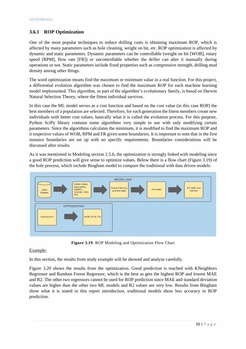
UiS Drillbotics

50 | P a g e

3.6.1 ROP Optimization

One of the most popular techniques to reduce drilling costs is obtaining maximum ROP, which is

affected by many parameters such as hole cleaning, weight on bit, etc. ROP optimization is affected by

dynamic and static parameters. Dynamic parameters can be controllable (weight on bit [WOB], rotary

speed [RPM], flow rate [FR]) or uncontrollable whether the driller can alter it manually during

operations or not. Static parameters include fixed properties such as compressive strength, drilling mud

density among other things.

The word optimization means find the maximum or minimum value in a real function. For this project,

a differential evolution algorithm was chosen to find the maximum ROP for each machine learning

model implemented. This algorithm, as part of the algorithm’s evolutionary family, is based on Darwin

Natural Selection Theory, where the fittest individual survives.

In this case the ML model serves as a cost function and based on the cost value (in this case ROP) the

best members of a population are selected. Therefore, for each generation the fittest members create new

individuals with better cost values, basically what it is called the evolution process. For this purpose,

Python SciPy library contains some algorithms very simple to use with only modifying certain

parameters. Since the algorithms calculates the minimum, it is modified to find the maximum ROP and

it respective values of WOB, RPM and FR given some boundaries. It is important to note that in the first

instance boundaries are set up with no specific requirements. Boundaries considerations will be

discussed after results.

As it was mentioned in Modeling section 2.5.6, the optimization is strongly linked with modeling since

a good ROP prediction will give sense to optimize values. Below there is a flow chart (Figure 3.19) of

the hole process, which include Bingham model to compare the traditional with data driven models:

Figure 3.19: ROP Modeling and Optimization Flow Chart

Example:

In this section, the results from study example will be showed and analyze carefully.

Figure 3.20 shows the results from the optimization. Good prediction is reached with KNeighbors

Regressor and Random Forest Regressor, which is the best as gets the highest ROP and lowest MAE

and R2. The other two regressors cannot be used for ROP prediction since MAE and standard deviation

values are higher than the other two ML models and R2 values are very low. Results from Bingham

show what it is stated in this report introduction, traditional models show less accuracy in ROP

prediction.

UiS Drillbotics

51 | P a g e

Figure 3.20: Results From Modeling and Optimization

The Figure 3.21 is the result of the analysis of ROP variation for the different models. In this case an

evaluation for each model prediction was performed fixing WOB, RPM and FR. Each series in the bar

chart represents the optimized parameters it is fixed to analyze, for example in GB is used WOB, RPM

and FR from the Gradient Boost Regressor. There is not an evident conclusion that can be extracted

from this bar chart.

Figure 3.21: ROP Comparison Bar Chart for Different Models

Sensitivity analysis was performed to show the impact of WOB, RPM and FR in the ROP for each

model. Random Forest and Kneighbors are the most sensitive to small changes in RPM and FR. Also,

Kneighbors is very reactive to small changes in RPM and FR, which is not realistic.

On the other hand, AdaBoost and Gradient Boosting shows reasonable variations when modifying all

three parameters (WOB, RPM, FR), but as it can be seen in Figure 3.22, they do not fit with the data.

So, based on this analysis, Random Forest algorithm should be used for ROP optimization.

Figure 3.22: Result Bar Chart from Modeling and Optimization

Model ROP(m/h) MAE (m/h) Std dev (m/h) R2  WOB[kgf]  Flow rate[m3/h] RPM

GradientBoostingRegressor 58.12 5.95 5.69 0.70 27.36 1516.04 182.07 63.81 52.44

RandomForestRegressor 67.15 0.54 1.96 0.98 27.49 1607.12 141.64 69.11 65.19

AdaBoostRegressor 43.34 9.02 7.18 0.42 16.74 2243.99 207.14 50.52 36.17

KNeighborsRegressor 64.71 1.14 2.80 0.96 30.41 1588.69 153.77 67.51 61.91

Bingham 33.37 12.76 10.78 -0.23 5 N/A 220 44.15 22.59

ROP range (m/h)

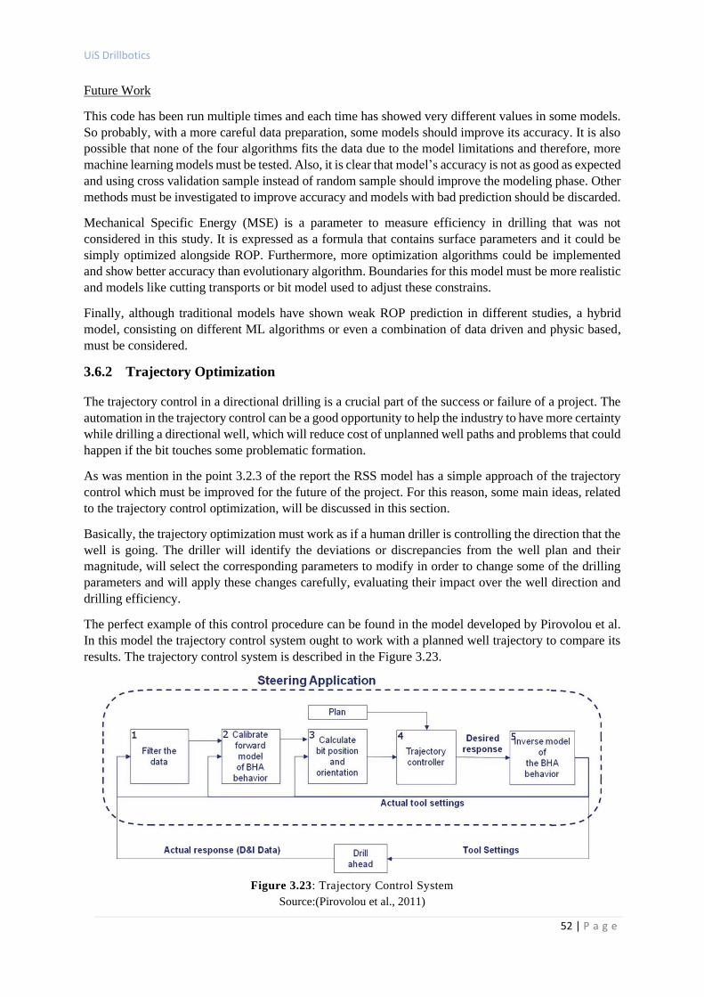
UiS Drillbotics

52 | P a g e

Future Work

This code has been run multiple times and each time has showed very different values in some models.

So probably, with a more careful data preparation, some models should improve its accuracy. It is also

possible that none of the four algorithms fits the data due to the model limitations and therefore, more

machine learning models must be tested. Also, it is clear that model’s accuracy is not as good as expected

and using cross validation sample instead of random sample should improve the modeling phase. Other

methods must be investigated to improve accuracy and models with bad prediction should be discarded.

Mechanical Specific Energy (MSE) is a parameter to measure efficiency in drilling that was not

considered in this study. It is expressed as a formula that contains surface parameters and it could be

simply optimized alongside ROP. Furthermore, more optimization algorithms could be implemented

and show better accuracy than evolutionary algorithm. Boundaries for this model must be more realistic

and models like cutting transports or bit model used to adjust these constrains.

Finally, although traditional models have shown weak ROP prediction in different studies, a hybrid

model, consisting on different ML algorithms or even a combination of data driven and physic based,

must be considered.

3.6.2 Trajectory Optimization

The trajectory control in a directional drilling is a crucial part of the success or failure of a project. The

automation in the trajectory control can be a good opportunity to help the industry to have more certainty

while drilling a directional well, which will reduce cost of unplanned well paths and problems that could

happen if the bit touches some problematic formation.

As was mention in the point 3.2.3 of the report the RSS model has a simple approach of the trajectory

control which must be improved for the future of the project. For this reason, some main ideas, related

to the trajectory control optimization, will be discussed in this section.

Basically, the trajectory optimization must work as if a human driller is controlling the direction that the

well is going. The driller will identify the deviations or discrepancies from the well plan and their

magnitude, will select the corresponding parameters to modify in order to change some of the drilling

parameters and will apply these changes carefully, evaluating their impact over the well direction and

drilling efficiency.

The perfect example of this control procedure can be found in the model developed by Pirovolou et al.

In this model the trajectory control system ought to work with a planned well trajectory to compare its

results. The trajectory control system is described in the Figure 3.23.

Figure 3.23: Trajectory Control System

Source:(Pirovolou et al., 2011)

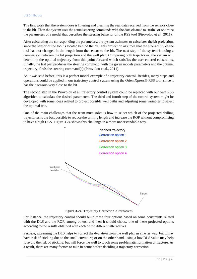
UiS Drillbotics

53 | P a g e

The first work that the system does is filtering and cleaning the real data received from the sensors close

to the bit. Then the system uses the actual steering commands with the data cleaned to “train” or optimize

the parameters of a model that describes the steering behavior of the RSS tool (Pirovolou et al., 2011).

After calculating the corresponding the parameters, the system estimates or calculates the bit projection,

since the sensor of the tool is located behind the bit. This projection assumes that the steerability of the

tool has not changed in the length from the sensor to the bit. The next step of the system is doing a

comparison between the bit projection and the well plan. Comparing both trajectories, the system will

determine the optimal trajectory from this point forward which satisfies the user-entered constraints.

Finally, the last part produces the steering command; with the given models parameters and the optimal

trajectory, finds the steering command(s) (Pirovolou et al., 2011).

As it was said before, this is a perfect model example of a trajectory control. Besides, many steps and

operations could be applied in our trajectory control system using the OrientXpress® RSS tool, since it

has their sensors very close to the bit.

The second step in the Pirovolou et al. trajectory control system could be replaced with our own RSS

algorithm to calculate the desired parameters. The third and fourth step of the control system might be

developed with some ideas related to project possible well paths and adjusting some variables to select

the optimal one.

One of the main challenges that the team must solve is how to select which of the projected drilling

trajectories is the best possible to reduce the drilling length and increase the ROP without compromising

to have a high DLS. Figure 3.24 shows this challenge in a more understandable way.

Figure 3.24: Trajectory Correction Alternatives

For instance, the trajectory control should build these four options based on some constraints related

with the DLS and the ROP, among others; and then it should choose one of these projected options

according to the results obtained with each of the different alternatives.

Perhaps, increasing the DLS helps to correct the deviation from the well plan in a faster way, but it may

have risk of sticking due to the small curvature; or on the other hand, using a low DLS value may help

to avoid the risk of sticking, but will force the well to touch some problematic formation or fracture. As

a result, there are many factors to take in count before deciding a trajectory correction.

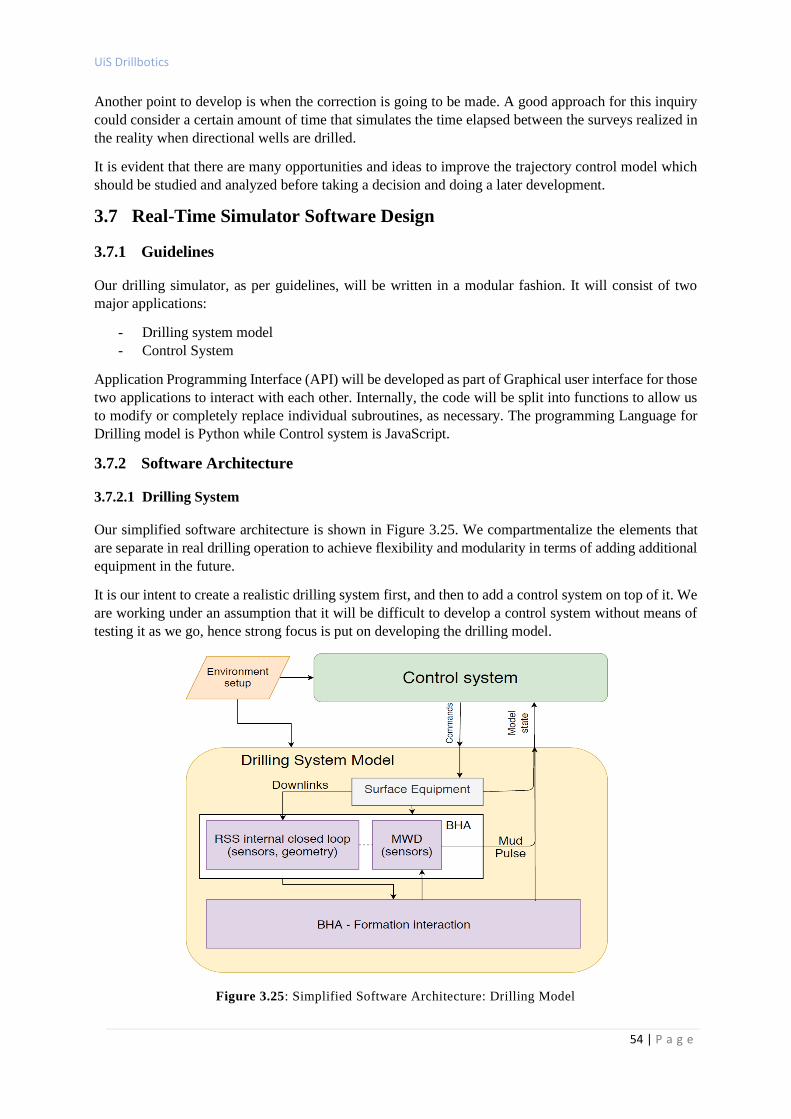
UiS Drillbotics

54 | P a g e

Another point to develop is when the correction is going to be made. A good approach for this inquiry

could consider a certain amount of time that simulates the time elapsed between the surveys realized in

the reality when directional wells are drilled.

It is evident that there are many opportunities and ideas to improve the trajectory control model which

should be studied and analyzed before taking a decision and doing a later development.

3.7 Real-Time Simulator Software Design

3.7.1 Guidelines

Our drilling simulator, as per guidelines, will be written in a modular fashion. It will consist of two

major applications:

- Drilling system model

- Control System

Application Programming Interface (API) will be developed as part of Graphical user interface for those

two applications to interact with each other. Internally, the code will be split into functions to allow us

to modify or completely replace individual subroutines, as necessary. The programming Language for

Drilling model is Python while Control system is JavaScript.

3.7.2 Software Architecture

3.7.2.1 Drilling System

Our simplified software architecture is shown in Figure 3.25. We compartmentalize the elements that

are separate in real drilling operation to achieve flexibility and modularity in terms of adding additional

equipment in the future.

It is our intent to create a realistic drilling system first, and then to add a control system on top of it. We

are working under an assumption that it will be difficult to develop a control system without means of

testing it as we go, hence strong focus is put on developing the drilling model.

Figure 3.25: Simplified Software Architecture: Drilling Model

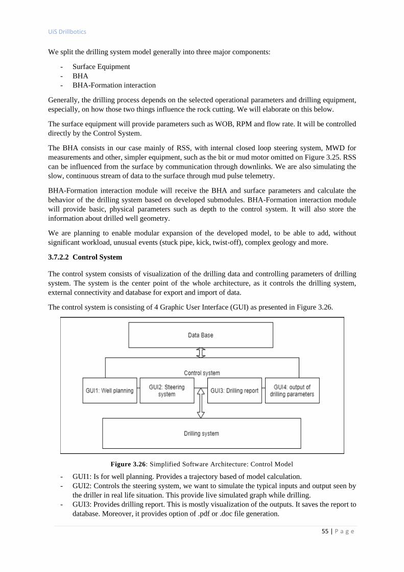
UiS Drillbotics

55 | P a g e

We split the drilling system model generally into three major components:

- Surface Equipment

- BHA

- BHA-Formation interaction

Generally, the drilling process depends on the selected operational parameters and drilling equipment,

especially, on how those two things influence the rock cutting. We will elaborate on this below.

The surface equipment will provide parameters such as WOB, RPM and flow rate. It will be controlled

directly by the Control System.

The BHA consists in our case mainly of RSS, with internal closed loop steering system, MWD for

measurements and other, simpler equipment, such as the bit or mud motor omitted on Figure 3.25. RSS

can be influenced from the surface by communication through downlinks. We are also simulating the

slow, continuous stream of data to the surface through mud pulse telemetry.

BHA-Formation interaction module will receive the BHA and surface parameters and calculate the

behavior of the drilling system based on developed submodules. BHA-Formation interaction module

will provide basic, physical parameters such as depth to the control system. It will also store the

information about drilled well geometry.

We are planning to enable modular expansion of the developed model, to be able to add, without

significant workload, unusual events (stuck pipe, kick, twist-off), complex geology and more.

3.7.2.2 Control System

The control system consists of visualization of the drilling data and controlling parameters of drilling

system. The system is the center point of the whole architecture, as it controls the drilling system,

external connectivity and database for export and import of data.

The control system is consisting of 4 Graphic User Interface (GUI) as presented in Figure 3.26.

Figure 3.26: Simplified Software Architecture: Control Model

- GUI1: Is for well planning. Provides a trajectory based of model calculation.

- GUI2: Controls the steering system, we want to simulate the typical inputs and output seen by

the driller in real life situation. This provide live simulated graph while drilling.

- GUI3: Provides drilling report. This is mostly visualization of the outputs. It saves the report to

database. Moreover, it provides option of .pdf or .doc file generation.

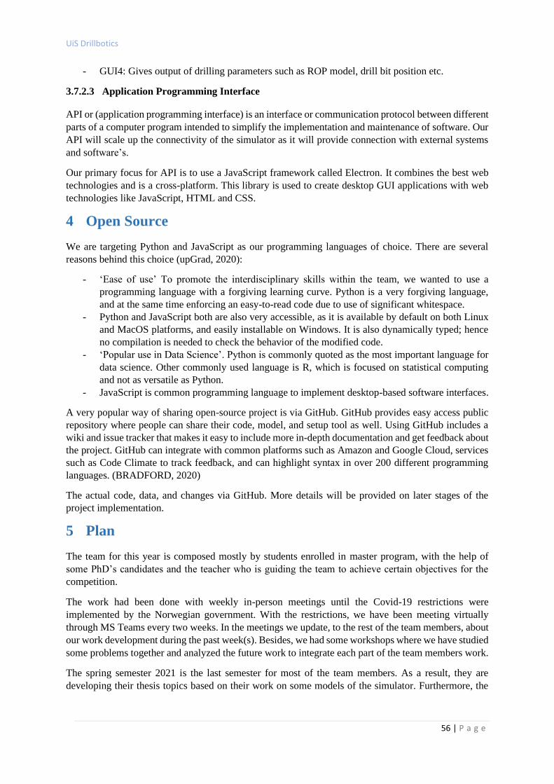
UiS Drillbotics

56 | P a g e

- GUI4: Gives output of drilling parameters such as ROP model, drill bit position etc.

3.7.2.3 Application Programming Interface

API or (application programming interface) is an interface or communication protocol between different

parts of a computer program intended to simplify the implementation and maintenance of software. Our

API will scale up the connectivity of the simulator as it will provide connection with external systems

and software’s.

Our primary focus for API is to use a JavaScript framework called Electron. It combines the best web

technologies and is a cross-platform. This library is used to create desktop GUI applications with web

technologies like JavaScript, HTML and CSS.

4 Open Source

We are targeting Python and JavaScript as our programming languages of choice. There are several

reasons behind this choice (upGrad, 2020):

- ‘Ease of use’ To promote the interdisciplinary skills within the team, we wanted to use a

programming language with a forgiving learning curve. Python is a very forgiving language,

and at the same time enforcing an easy-to-read code due to use of significant whitespace.

- Python and JavaScript both are also very accessible, as it is available by default on both Linux

and MacOS platforms, and easily installable on Windows. It is also dynamically typed; hence

no compilation is needed to check the behavior of the modified code.

- ‘Popular use in Data Science’. Python is commonly quoted as the most important language for

data science. Other commonly used language is R, which is focused on statistical computing

and not as versatile as Python.

- JavaScript is common programming language to implement desktop-based software interfaces.

A very popular way of sharing open-source project is via GitHub. GitHub provides easy access public

repository where people can share their code, model, and setup tool as well. Using GitHub includes a

wiki and issue tracker that makes it easy to include more in-depth documentation and get feedback about

the project. GitHub can integrate with common platforms such as Amazon and Google Cloud, services

such as Code Climate to track feedback, and can highlight syntax in over 200 different programming

languages. (BRADFORD, 2020)

The actual code, data, and changes via GitHub. More details will be provided on later stages of the

project implementation.

5 Plan

The team for this year is composed mostly by students enrolled in master program, with the help of

some PhD’s candidates and the teacher who is guiding the team to achieve certain objectives for the

competition.

The work had been done with weekly in-person meetings until the Covid-19 restrictions were

implemented by the Norwegian government. With the restrictions, we have been meeting virtually

through MS Teams every two weeks. In the meetings we update, to the rest of the team members, about

our work development during the past week(s). Besides, we had some workshops where we have studied

some problems together and analyzed the future work to integrate each part of the team members work.

The spring semester 2021 is the last semester for most of the team members. As a result, they are

developing their thesis topics based on their work on some models of the simulator. Furthermore, the

UiS Drillbotics

57 | P a g e

plan for the first semester of 2021 is represented in the Figure 5.1, which could suffer some changes in

the future.

Figure 5.1: Proposed Work Plan

6 Budget

The cost of the project is difficult to estimate since the global pandemic has changed the way of how the

work is done. However, it is evident that the team will need some computers to perform the simulation

and construction of the GUI of the Real Time Drilling Simulator.

As a result, Canrig Drilling Technology Norway has donated 3 computers for both teams for the

Drillbotics competition since this company is closing their offices in Norway. At the same time, they

are sharing some real data from some of their projects, that could be useful to perform some controls

and verifications in the models implemented by the team.

Since the team A is developing a virtual rig, not many resources are needed besides the computational

resources and some minor expenses. Nevertheless, the uncertainty for the next year competition’s

location and mode of evaluation, makes it difficult for us to know whether the team is going to travel or

we will stay in our respective universities waiting some for the judges to come to evaluate our work.

Therefore, we should have an emergency budget amount for case that the current pandemic situation

reduces, and the competition would be celebrated in Celle, Germany. For this case, the cost of the hotel

goes from 10000 kr to 20000 kr and the cost of the flight tickets is around 2000 kr for each member,

from Stavanger to Hannover airport, after that we should take another transport to move to Celle.

Nevertheless, this is just an approximation cost and there will be a lot of changes in the future once the

Drillbotics competition is better defined in the future.

7 Team Management

The team is composed by diverse disciplines students which have different task related with their area

of study. Actually, the list of principal or general task of each member can be seen in the Table 7.1.

Table 7.1: General Tasks of the Team A Members

Task Team Member(s) in Charge

Trajectory design Larissa

Wellbore trajectory optimization Melissa and Elsayed

Torque and drag model Larissa

Flow model Melissa

Cutting transport model Miguel

Buckling model Miguel

Temperature model Rishyank

ROP model Renan

UiS Drillbotics

58 | P a g e

Web-based well design software Elsayed and Hamed

RSS model Luis

Trajectory control Luis

Drill bit and BHA model Milad

Drill string modeling Rishyank

Models integration Melissa

Software design and architecture Samuil

Plan, budget and team management Luis

8 References

Aadnoy, B.S., Fazaelizadeh, M., Hareland, G. (2010). A 3-Dimensional Analytical Model for Wellbore Friction.

Journal of Canadian Petroleum Technology.

Abughaban, M. F., et al. (2016). Advanced Trajectory Computational Model Improves Calculated Borehole

Positioning, Tortuosity and Rugosity. IADC/SPE Drilling Conference and Exhibition, Society of

Petroleum Engineers.

Belayneh, M. (2006). A review of Buckling in Oil Wells. University of Stavanger.

Bingham, G. (1965). A New Approach to Interpreting Rock Drillability. Tulsa: Petroleum Publishing Company.

Burgoyne, A., Millhein, K., Chenevert, M., & Young Jr., F. (1991). Applied Drilling Engineering. Second Edition

ed., Vol. 2. Richardson, TX, US: SPE textbook series.

Bradford, L. (2020, July 24). Technology Careers. Retrieved from Thebalancecareers:

https://www.thebalancecareers.com/what-is-github-and-why-should-i-use-it-2071946.

DeWardt, J. & C. Wolf (1981). Borehole Position Uncertainty-Analysis of Measuring Methods and Derivation of

Systematic Error Model. Journal of Petroleum Technology.

DSATS (2020). Drillbotics Guidelines 2020-2021. Society of Petroleum Engineering. Available in

https://www.drillbotics.com.

Ekseth, R. (1998). Uncertainties in Connection with The Determination of Wellbore Positions. PHD Thesis, ISBN

82-471-0218-8 ISSN 0802-3271, PhD Thesis no 1998 28 IPT report 1998.2, The Norwegian University

of Science and Technology, Trondheim, Norway, March 1998.

Ekseth, R. (2000). Uncertainties in connection with the determination of wellbore positions.

Elshafei, M., Khamis, M., & Al-Mejed, A. (2015). Optimization of Rotary Steerable Drilling. 167, 9.

Esmaeli, A., Elahifar, B., Fruhwirth, R., & Thonhauser, G. (2012). ROP Modeling Using Neural Network and

Drill String Vibration Data. Society of Petroleum Engineers, SPE 163330, 13.

https://doi.org/10.2118/163330-MS.

Gulyayev, V., & Shlyun, N. Influence of Friction on Buckling of a Drill String in the Circular Channel of a Bore

Hole. Research Gate. Petroleum Science.

Hansen, C., Stokes, M., Mieting, R., Quattrone, F., Klemme, V., Nageshawara Rao, K., & Wassermann, I. (2020).

Automated Trajectory Drilling for Rotary Steerable Systems. Society of Petroleum Engineers,

IADC/SPE-199647-MS, 9. https://doi.org/10.2118/199647-MS.

Hegde, C., Soares, C., & Gray, K. (2019). Rate of Penetration (ROP) Modeling Using Hybrid Models:

Deterministic and Machine Learning. Unconventional Resources Technology Conference, URTeC

2896522, 19. https://doi.org/10.15530/URTEC-2018-2896522.

Hossain, E., & Al-Mejed, A. (2015). Fundamentals of Sustainable Drilling Engineering. Scrivener Publishing.

UiS Drillbotics

59 | P a g e

Hegde, C., Daigle, H., Millwater, H., & Gray, K. (2017). Analysis of Rate of Penetration (ROP) Prediction in

Drilling Using Physics-Based and Data-Driven Models. Journal of Petroleum Science and Engineering,

295-306.

Heriot-Watt professors, Department of Petroleum Engineering, Heriot-Watt University.

Kåre K. (2020). Cuttings transport. Course PET 510 Modellering av reservoar og brønnstrømning. University of

Stavanger, UiS.

Kårstad, E. (2020). Buckling principles. Course PET 510 Modellering av Reservoar og Brønnstrømning.

University of Stavanger, UiS.

Larsen, T. (1997). Development of a New Cuttings-Transport Model for High-Angle Wellbores Including

Horizontal Wells. SPE, Unocal Corp.

Lei, L. (2014). Downhole Weight on Bit Prediction with Analytical Model and Finite Element Method. University

of Calgary, Master Thesis. doi:10.11575/PRISM/25743.

Li, F., Ma, X., & Tan, Y. (2020). Review of the Development of Rotary Steerable Systems. 1617, 1–6.

https://doi.org/10.1088/1742-6596/1617/1/012085.

Matovu, F. and J. Heinz Preisig (2014). Drift-Flux Models. Norwegian University of Science and Technology.

Mitchell, R., & Miska, S. (2011). Fundamentals of Drilling Engineering. Vol. 12. Society of Petroleum Engineers.

Nabors Industries. (2020, November 12). OrientXpress® Rotary Steering System. Nabor Directional Drilling

Services. https://www.nabors.com/services/directional-drilling/orientxpress-rotary-steering-system.

Nadhan, E. et al. (2018). Drilling with Digital Twins. SPE IADC Asia Pacific Drilling Technology.

Olaijuwon, M. (2012). A Study of Wellbore Position Uncertainty in the Ekofisk Field. Master’s Thesis, Depth

Issues in the Oil patch, University of Stavanger.

Pessier R.C., Hughes Tool Co., & M.J. Fear, BP Exploration (1992). Quantifying Common Drilling Problems with

Mechanical Specific Energy and a Bit-Specific Coefficient of Sliding Friction. Annual Technical

Conference and Exhibition of the Society of Petroleum Engineers held in Washington, DC, October 4-7.

Pirovolou, D., Chapman, C., Chau, M., Arismendi, H., Ahorukomeye, M., Peñaranda, J., & Schumberger. (2011).

Drilling Automation: An Automatic Trajectory Control System. Society of Petroleum Engineers, SPE-

143899-MS, 8. https://doi.org/10.2118/143899-MS.

Ren, & Wang. (2017). Modeling and Analysis of Stick-Slip Vibration And Bit Bounce In Drill Strings. In: Journal

of Vibroengineering 19.7, pp. 4866–4881.

Richard et al. (2002). Influence of Bit-Rock Interaction on Stick-Slip Vibrations of PDC Bits. In: SPE Annual

Technical Conference and Exhibition. Society of Petroleum Engineers.

Ruszka, J. (2003, August). Rotary Steerable Drilling Technology Matures. Drilling Contractor, 59(4), 44–45.

Saramago, C. (2020). Rotary Steerable System Modeling and Simulator. Master Thesis. University of Stavanger.

Soares, C., Daigle, H., & Gray, K. (2016). Evaluation of PDC Bit ROP Models and The Effect of Rock Strength

on Model Coefficients. Journal of Natural Gas Science and Engineering, 3, 1225-1236.

Stump, J. (2019, April 1). New Rotary Steerable Systems Aim to Enhance Drilling Efficiency. Offshore Magazine.

https://www.offshore-mag.com/drilling-completion/article/16763947/new-rotary-steerable-systems-

aim-to-enhance-drilling-efficiency.

Tang L. (2019), Stick-Slip Vibrations In Oil Well Drill String: In:

https://journals.sagepub.com/doi/10.1177/1461348419853658.

Teale, R. (1965). The Concept of Specific Energy in Rock Drilling. International Journal of Rock Mechanics and

Mining Sciences & Geomechanics Abstracts, 2(1), 57–73. https://doi.org/10.1016/0148-9062(65)90022-

7.

UiS Drillbotics

60 | P a g e

Udegbunam, J. E., Fjelde, K. K., Evje, S., & Nygaard, G., (2015), On the Advection-Upstream-Splitting-Method

Hybrid Scheme: A Simple Transient-Flow Model for Managed-Pressure-Drilling and Underbalanced-

Drilling Applications. SPE Drilling & Completion, 30(02), pp. 98-109.

Udegbunam, J. E., Sui, D., Moeinikia, F., Lage, A. C., Fjelde, K. K., Arild, Ø., Rabenjafimanantsoa, H. A., and

Nygaard, G. H., (2017). A Transient Flow Model for Predicting Pressure Buildup in Closed Annuli. Proc.

ASME 2017 36th International Conference on Ocean, Offshore and Arctic Engineering, American

Society of Mechanical Engineers, pp. V008T011A028-V008T011A028.

upGrad. (2020, January 5) upGrad. Retrieved from upGrad: https://www.upgrad.com/blog/reasons-why-python-

popular-with-developers/.

Wiktorski, E., & Sui, D. (2020), Investigation of Stick-Slip Severity in Couple Axial-Torsional Drill String

Dynamics Using a Two DOF Finite Element Model. OMAE June 28- July 3, 2020, Fort Lauderdale,

Florida, USA.

Wiktorski, E., & Sui, D. (2018). Dynamics Cuttings Slip Velocity Evaluation in Non-Newtonian Fluids using a

temperature Dependent Transient Drift-Flux Model for Directional Wells. International Conference on

Ocean, Offshore, and Arctic Engineering OMAE 2018, Madrid, Spain.

Wiktorski, E., Kuznetcov, A., & Sui, D. (2017). ROP Optimization and Modeling in Directional Drilling Process.

Society of Petroleum Engineers, SPE-185909-MS, 15. https://doi.org/10.2118/185909-MS.

Williamson, H. (2000). Accuracy Prediction for Directional Measurement While Drilling. SPE Drilling &

Completion 15(04): 221-233.

Wolff, C., & De Wardt, J. (1981). Borehole Position Uncertainty-Analysis of Measuring Methods and Derivation

of Systematic Error Model. Journal of Petroleum Technology 33(12): 2,338-332,350.

Yigit, A. & Christoforou A. (2006). Stick Slip and Bit Bounce Interaction in Oil Well Drill String. Journal of

Energy Resources Technology, 128: 268–274.