Interactive Project Map – PDG phase Department for International Development

Drillbotics® – Phase I Design Report
International University Competition 2018/19
Prepared by:
Wolfgang Holstein
Dominik Orgel
Julian Dreblow
Ismail Boularas
TUC Supervisors:
Prof. Dr.-Ing. Joachim Oppelt
Dr.-Ing. Javier Holzmann
Dr.-Ing. Carlos Paz Carvajal
Erik Feldman

Drillbotics - Phase I Design Report
2
Institute of Petroleum Engineering
Clausthal University of Technology
Date: December 31, 2018

Drillbotics - Phase I Design Report
3
The Team Wolfgang Hollstein[Team Lead] B.Sc. Mechanical Engineering [email protected] Dominik Orgel, B.Sc. Power Systems Technologies [email protected]
Julian Dreblow B.Sc. Mechanical Engineering [email protected]
Ismail Boularas cand. B.Sc. Energy and Raw Materials - Petroleum Engineering [email protected]

Drillbotics - Phase I Design Report
1
Table of Contents
List of Abbreviations ................................................................................................... 4
List of Figures ............................................................................................................. 5
List of Tables .............................................................................................................. 6
1 Introduction and Objectives ................................................................................. 7
2 Calculations ....................................................................................................... 10
2.1 Data and Assumptions ............................................................................... 10
2.2 Limit Calculations ....................................................................................... 11
2.2.1 Buckling Limit Calculation ................................................................... 12
2.2.2 Burst Limit Calculation ........................................................................ 13
2.2.3 Torsional Limit Calculation .................................................................. 14
2.2.4 Stress Envelope with van Mises .......................................................... 14
2.3 Cutting Transport Calculation ..................................................................... 17
2.4 Pressure Loss Calculation .......................................................................... 20
2.5 Summary Calculation Results .................................................................... 27
3 Rig Design ......................................................................................................... 31
3.1 Rig Overview .............................................................................................. 31
3.2 Hoisting System ......................................................................................... 31
3.3 Rotary Table ............................................................................................... 32
3.4 Rock Sample Receiver ............................................................................... 33
3.5 Rig Electronics ........................................................................................... 34
3.6 Rig Plumbing .............................................................................................. 34
3.7 Rig Handling ............................................................................................... 34
4 Mechatronic System Architecture ...................................................................... 35
4.1 CAN Bus .................................................................................................... 35
4.2 Quick Data Query ....................................................................................... 36
4.3 Actuator Modules ....................................................................................... 37
4.3.1 Motor Control Unit ............................................................................... 37
4.3.2 Steering Unit ....................................................................................... 39
4.3.3 Rotary Table Control Unit .................................................................... 40
4.3.4 Hoisting System Control Unit .............................................................. 42

Drillbotics - Phase I Design Report
2
4.3.5 Relay Switching Unit ........................................................................... 43
4.4 Sensors ...................................................................................................... 43
4.4.1 Sensor Unit ......................................................................................... 43
4.4.2 WOB Measurement Module ................................................................ 44
4.4.3 Current Measurement Unit .................................................................. 45
4.5 Magnetic Ranging ...................................................................................... 45
4.6 Sensor Calibration ...................................................................................... 46
4.6.1 Magnetometer and Accelerometer ...................................................... 46
4.6.2 Downhole Load Cell ............................................................................ 47
4.6.3 Surface Load Cell ................................................................................ 47
5 BHA Design ....................................................................................................... 47
5.1 Overview .................................................................................................... 47
5.2 Drill Spindle ................................................................................................ 47
5.3 Cyclodial Gearbox ...................................................................................... 48
5.4 BLDC Motor................................................................................................ 49
5.5 Downhole Load Cell ................................................................................... 50
5.6 Steering Unit............................................................................................... 51
5.7 Electronics Compartment ........................................................................... 52
5.8 Collet Chuck Joint ...................................................................................... 53
5.9 Drillbit ......................................................................................................... 53
6 Directional Drilling.............................................................................................. 54
6.1 Objectives .................................................................................................. 54
6.2 Steerable Motor Assembly ......................................................................... 54
6.3 Directional Wellbore Parameter .................................................................. 55
6.4 Wellbore Surveying .................................................................................... 57
6.4.1 Survey Calculations ............................................................................ 58
6.4.2 Measurement While Drilling (MWD) .................................................... 59
6.5 Control Structure for Directional Drilling ..................................................... 60
7 Safety Consideration and Risk Analysis ............................................................ 63
8 Drillbotics 2017/18 drilling Performance ............................................................ 66
.......................................................................................................................... 68

Drillbotics - Phase I Design Report
3
9 Funding Plan and Price List ............................................................................... 71
10 Bibliography ................................................................................................... 73

Drillbotics - Phase I Design Report
4
List of Abbreviations
ADC Analog-to-Digital Converters
BHA Bottom Hole Assembly
BLDC Brushless DC Motor
ESC Electronic Speed Controller
GUI Graphic User Interface
HMI Human Machine Interface
PLC Programmable Logic Controller
POOH Pull Out of Hole
RPM Revolutions per Minute
RTC Real-Time Clock
SIT Simulation Interface Toolkit
TCP Transmission Control Protocol
TD Top Drive
UCS Uniaxial Compressive Strength
VFC Variable Frequency Converter
WOB Weight on Bit
MD Measures Depth
TVD True Vertical Depth
MWD Measurement while Drilling

Drillbotics - Phase I Design Report
5
List of Figures
Figure 2.1. Design value K variation ......................................................................... 13
Figure 2.2. Stresses acting on a thick-wall cylinder .................................................. 14
Figure 2.3. Moore’s correlation for cutting transport calc. in a vertical well ............... 18
Figure 2.4: Fanning chart; friction factors for turbulent flow in circular pipes ............ 25
Figure 3.1: Rig overview ........................................................................................... 31
Figure 3.2: Hoisting system ...................................................................................... 32
Figure 3.3: Rotary Table ........................................................................................... 33
Figure 3.4: Rock sample receiver ............................................................................. 34
Figure 4.1: CAN Bus schematic ................................................................................ 35
Figure 4.2: Quick data query schematic ................................................................... 36
Figure 4.3: Motor control unit schematic ................................................................... 37
Figure 4.4 Algorithm motor module .......................................................................... 38
Figure 4.5 Dshot Protocol ......................................................................................... 39
Figure 4.6 Steering unit schematic ........................................................................... 39
Figure 4.7 Algorithm steering control unit ................................................................. 40
Figure 4.8: Rotary table control unit schematic ......................................................... 41
Figure 4.9 Algorithm Rotary Table ............................................................................ 41
Figure 4.10: Hoisting system control unit schematic ................................................. 42
Figure 4.11 Algorithm Hoist Control Unit .................................................................. 42
Figure 4.12 Sensor unit ............................................................................................ 43
Figure 4.13 Algorithm sensor unit ............................................................................. 44
Figure 4.14: WOB measurement module schematic ................................................ 45
Figure 4.15 Magnetic ranging scheme ..................................................................... 46
Figure 5.1: Section display BHA ............................................................................... 47
Figure 5.2: Section display spindle housing .............................................................. 48
Figure 5.3: Cyclodial gearbox ................................................................................... 49
Figure 5.4: Section display BLDC-Motor................................................................... 50
Figure 5.5: Detailed view Load Cell .......................................................................... 51
Figure 5.6: Section display Steering Unit .................................................................. 52
Figure 5.7 Electronics Compartment ........................................................................ 53
Figure 6.1: Steerable Motor Assembly ..................................................................... 55
Figure 6.2: Measurement Parameter of Directional Well .......................................... 55
Figure 6.3: Build and hold well profile ....................................................................... 56

Drillbotics - Phase I Design Report
6
Figure 6.4 Interpolation Scheme ............................................................................... 58
Figure 6.5: Minimum curvature method .................................................................... 58
Figure 6.6: Magnetometer and accelerometer orientation ........................................ 59
Figure 6.7: Sensor orientation .................................................................................. 59
Figure 6.8: Coordinate transformation ...................................................................... 60
Figure 6.9: Rotating coordinate system .................................................................... 60
Figure 6.10: Directional drilling procedure ................................................................ 61
Figure 6.11: Steering algorithm ................................................................................ 62
Figure 8.1: Test results from drilling in sandstone with two different hammer systems.
................................................................................................................................. 67
Figure 8.2: Test results from drilling in sandstone with two different hammer systems.
................................................................................................................................. 67
Figure 8.3: Test results after tuning control parameters. .......................................... 68
Figure 8.4 Test results after tuning control parameters. .......................................... 68
Figure 8.5: Test results after adjustment of the range of control ............................... 69
Figure 8.6 Test results after adjustment of the range of control ............................... 69
Figure 8.7: Test results after final adjustment of the controller ................................. 70
Figure 8.8 Test results after final adjustment of the controller .................................. 70
Figure 8.9: Optimal drilling parameters 3D Chart ..................................................... 71
Figure 8.10 Optimal drilling parameters 3D Chart .................................................... 71
List of Tables
Table 2.1: Drilling hole and rock data ....................................................................... 10
Table 2.2: Drilling fluid data ...................................................................................... 10
Table 2.3: Aluminium drillpipe data ........................................................................... 10
Table 2.4: Stabilizer/downhole BHA data ................................................................. 11
Table 2.5: Bit data .................................................................................................... 11
Table 2.6: Buckling limit according to K variation ..................................................... 13
Table 2.7: Pump power requirement rotary drilling ................................................... 26
Table 2.8: Summary of calculation results ................................................................ 27
Table 2.9: Used formulas.......................................................................................... 27
Table 6.1 Results of well trajectory calculation ......................................................... 57

Drillbotics - Phase I Design Report
7
Introduction and Objectives
The 2018 DrillboticsTM competition marks the third year that a team from the Clausthal
University of Technology, Germany is participating in the competition. Based on the
2018/19 DrillboticsTM competition guidelines, the objective of this year’s competition is
“to design a rig and related equipment capable of automated directional drilling,
capable of deviating and following specific coordination’s, while maintaining borehole
quality and integrity of the drilling rig and drillstring”.
Drilling automation is currently gaining an increased interest from the oil and gas
industry, equipment manufactures, and research organizations. Automating the drilling
process is considered to offer safety improvements during drilling operations, less
drilling time requirements, increasing accuracy in data acquisition, better well
placement and quality, and a reduction of the costs. In automated drilling systems, the
operating parameters are optimized by acquiring relevant data, assessing the data and
adjusting the operating parameters without human interference. Ideally, the automation
level reaches tier three, which describes a stage in which the automation has evolved
to decide and act autonomously.
The purpose of this proposal is to showcase a well-conceived design plan of a small-
scale drilling robot that incorporates important features that are essentially
encountered in the field. Emphasis has been placed on implementing different and new
ideas and solution in the design that are not commonly or frequently used in the
conventional drilling process to fulfill the demands of directional drilling utilizing an
automated process that from a human intervention point of view only knows the
activation of the start button.
The proposed drilling robot design consists of the following surface components:
This proposal consists of several chapters as follows:
1. Introduction and Objectives

Drillbotics - Phase I Design Report
8
The Introduction and Objectives of this report sets the objectives of the proposal
and the project. A brief description of the proposal content is explained herein.
2. Basic Calculations
The selection of the basic drilling parameters such as flow rate, drillstring
rotation speed, pressure, and other parameters are described here. The
selection and determination are based on engineering calculation and design
by considering predetermined constraints. The engineering calculation results
will be used as basis for the rig design and drilling automation plan.
3. Rig Design
This chapter explains the rig structure design, the machine bed, the hoisting
system, the sled, and the top drive system.
4. Mechatronic System and Control Architecture
This chapter explains the mechatronic system, used sensors and actuators and
the bus system that distributes the operation data. Also, the algorithms for the
specific modules are shown.
5. BHA Design
This chapter explains the bottom hole assembly (BHA) design.
6. Directional Drilling
This chapter describes the steering unit assembly for directional drilling, the
methods for well trajectory planning, and the control schematic.
7. Safety Consideration
HSE is a main aim of each drilling operation. This chapter discusses the risks
and potential harmful events that could occur during the test. Precaution and
mitigation plan are set to prevent undesirable events, including the rig structure
design and drilling automation system that can accommodate the safety
consideration.
8. Drillbotics 2017/18
Evalution of previous rig design and performance.
9. Expanse Plan
The requirement of equipment and tools and the expenses plan are described
in this chapter.
This report is an update of the previous design report submitted for the DrillboticsTM
international university competition 2017/18.

Drillbotics - Phase I Design Report
9
Drillbotics - Phase I Design Report
10
Calculations
2.1 Data and Assumptions
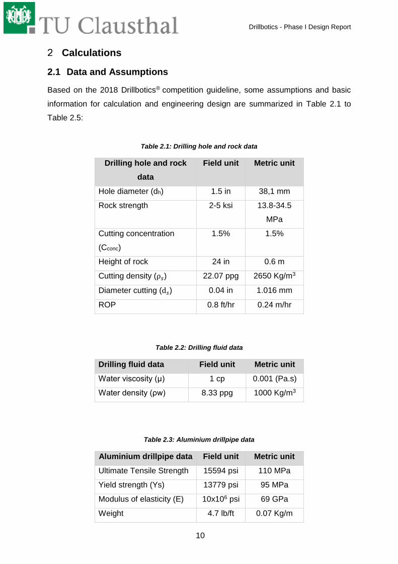
Based on the 2018 Drillbotics® competition guideline, some assumptions and basic
information for calculation and engineering design are summarized in Table 2.1 to
Table 2.5:
Table 2.1: Drilling hole and rock data
Drilling hole and rock
data
Field unit Metric unit
Hole diameter (dh) 1.5 in 38,1 mm
Rock strength 2-5 ksi 13.8-34.5
MPa
Cutting concentration
(Cconc)
1.5% 1.5%
Height of rock 24 in 0.6 m
Cutting density (ρ𝑠) 22.07 ppg 2650 Kg/m3
Diameter cutting (d𝑠) 0.04 in 1.016 mm
ROP 0.8 ft/hr 0.24 m/hr
Table 2.2: Drilling fluid data
Drilling fluid data Field unit Metric unit
Water viscosity (μ) 1 cp 0.001 (Pa.s)
Water density (ρw) 8.33 ppg 1000 Kg/m3
Table 2.3: Aluminium drillpipe data
Aluminium drillpipe data Field unit Metric unit
Ultimate Tensile Strength 15594 psi 110 MPa
Yield strength (Ys) 13779 psi 95 MPa
Modulus of elasticity (E) 10x106 psi 69 GPa
Weight 4.7 lb/ft 0.07 Kg/m
Drillbotics - Phase I Design Report
11
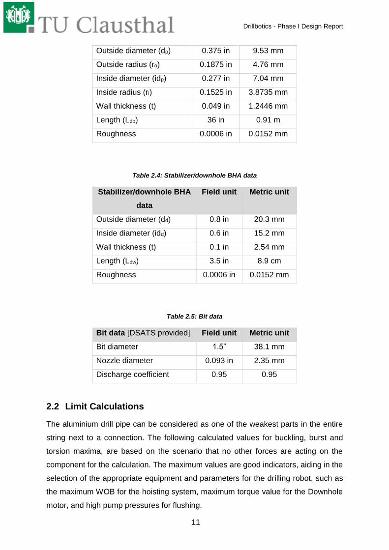
Outside diameter (dp) 0.375 in 9.53 mm
Outside radius (ro) 0.1875 in 4.76 mm
Inside diameter (idp) 0.277 in 7.04 mm
Inside radius (ri) 0.1525 in 3.8735 mm
Wall thickness (t) 0.049 in 1.2446 mm
Length (Ldp) 36 in 0.91 m
Roughness 0.0006 in 0.0152 mm
Table 2.4: Stabilizer/downhole BHA data
Stabilizer/downhole BHA
data
Field unit Metric unit
Outside diameter (dd) 0.8 in 20.3 mm
Inside diameter (idd) 0.6 in 15.2 mm
Wall thickness (t) 0.1 in 2.54 mm
Length (Ldw) 3.5 in 8.9 cm
Roughness 0.0006 in 0.0152 mm
Table 2.5: Bit data
Bit data [DSATS provided] Field unit Metric unit
Bit diameter 1.5” 38.1 mm
Nozzle diameter 0.093 in 2.35 mm
Discharge coefficient 0.95 0.95
2.2 Limit Calculations
The aluminium drill pipe can be considered as one of the weakest parts in the entire
string next to a connection. The following calculated values for buckling, burst and
torsion maxima, are based on the scenario that no other forces are acting on the
component for the calculation. The maximum values are good indicators, aiding in the
selection of the appropriate equipment and parameters for the drilling robot, such as
the maximum WOB for the hoisting system, maximum torque value for the Downhole
motor, and high pump pressures for flushing.

Drillbotics - Phase I Design Report
12
2.2.1 Buckling Limit Calculation
Buckling is characterized by a lateral deformation or failure of a structural member
subjected to high axial compressive stress, where the compressive stress at the point
of failure is less than the yield strength that the material can withstand. The critical
buckling load limit of the aluminium drill pipe is calculated by the following Euler
equation (assuming both pipe ends are pinned) [1]. First the moment of inertia 𝐼 is
determined:
𝐼 =𝜋
64(𝑑𝑝
4 − 𝑖𝑑𝑝4) =
𝜋
64(0.3754 − 0.2774) = 0.000682𝑖𝑛4 (2.8 ∗ 10−10𝑚4)
Where:
𝑑𝑝: Outside diameter of the drillpipe
𝑖𝑑𝑝: Inside diameter of the drillpipe
Then the critical buckling load,𝑃𝑐𝑟, is calculated [1]:
𝑃𝑏𝑐𝑟 =𝜋2 ∗ 𝐸 ∗ 𝐼
(𝐾 ∗ 𝐿)2=
𝜋2 ∗ 10000000 ∗ 0.000682
(1 ∗ 36)2= 51.96 𝑙𝑏𝑓 (231.11 𝑁 𝑜𝑟 23.57 𝑘𝑔)
Where:
𝑃𝑏𝑐𝑟: Critical buckling load
𝐸: Modulus elasticity of the aluminium drill pipe
𝐼: Area moment of inertia
𝐿: Length of the column
𝐾: Column effective length factor
Based on the scenarios of buckling failure, there are several recommendations in
respect to the effective length factor (𝐾), as illustrated in Figure 2.1 and Table 2.6. The
variation of effective length factor is used to estimate the buckling load limit.

Drillbotics - Phase I Design Report
13
Figure 2.1. Design value K variation
Table 2.6: Buckling limit according to K variation
K variation Buckling load limit (lbf) Buckling load
limit (N) Buckling load limit (Kg)
0.5 207,82 924,45 94,27
0.7 106,03 471,66 48,10
1 51,96 231,11 23,57
2 12,99 57,78 5,89
2.2.2 Burst Limit Calculation
Assuming the yield strength, of the aluminium drill pipe is 13779 psi (95 MPa) and a
safety factor 1.5, the burst limit, 𝑃𝑏𝑢𝑟𝑠𝑡, of the aluminium drill pipe can be estimated by
following equation (Barlow equation)[3]:
𝑃𝑏𝑢𝑟𝑠𝑡 =2 ∗ 𝑌𝑝 ∗ 𝑡
𝑑𝑝 ∗ 𝑆𝑓=
2 ∗ 13779 ∗ 0.049
0.375 ∗ 1.5= 2400.53 𝑝𝑠𝑖 (165.51 𝑏𝑎𝑟)
Where,
𝑌𝑝: Yield strength of the drillpipe
Drillbotics - Phase I Design Report
14
𝑡: Wall thickness of the drillpipe
𝑑𝑝: Outside diameter of the drillpipe
𝑆𝑓: Safety factor
2.2.3 Torsional Limit Calculation
Assuming the maximum yield stress of the aluminium drill pipe is 13779 psi (95 MPa),
the maximum limit of torque 𝑇𝑚𝑎𝑥 of the aluminium drill pipe can be estimated by
following equation [1]:
𝑇𝑚𝑎𝑥 =𝜋
16∗ 𝜎𝑚𝑎𝑥 ∗
(𝑑𝑝4 − 𝑖𝑑𝑝
4)
𝑑𝑝=
𝜋
16∗ 13779 ∗
(0.3754 − 0.2774)
0.375
= 100.19 𝑖𝑛. 𝑙𝑏𝑓 (11.32 𝑁𝑚)
Where,
𝑑𝑝: Outside diameter of the drillpipe
𝑖𝑑𝑝: Inside diameter of the drillpipe
𝜎𝑚𝑎𝑥: Yield strength of the drillpipe
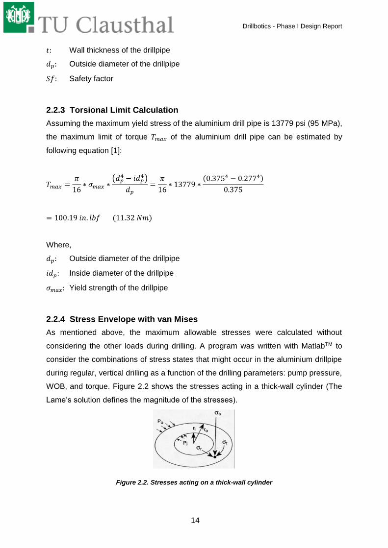
2.2.4 Stress Envelope with van Mises
As mentioned above, the maximum allowable stresses were calculated without
considering the other loads during drilling. A program was written with MatlabTM to
consider the combinations of stress states that might occur in the aluminium drillpipe
during regular, vertical drilling as a function of the drilling parameters: pump pressure,
WOB, and torque. Figure 2.2 shows the stresses acting in a thick-wall cylinder (The
Lame’s solution defines the magnitude of the stresses).
Figure 2.2. Stresses acting on a thick-wall cylinder

Drillbotics - Phase I Design Report
15
The considered stresses are:
1. Axial stress, 𝜎𝑎, (only compression due to WOB is considered in this case even
though other possibilities exist) [1]:
𝜎𝑎 =𝑊𝑂𝐵
𝐴
2. After Lamé, the radial stress 𝜎𝑟 and tangential stress 𝜎𝑡 (due to a pressure
difference 𝛥𝑝 across the cylindrical shell of the drill pipe) [4]. For the radial
stress, 𝜎𝑟 [1]:
𝜎𝑟 =𝑃𝑜 ∗ 𝑟𝑜
2 − 𝑃𝑖 ∗ 𝑟𝑖2
𝑟𝑜2−𝑟𝑖
2 +𝑟𝑜
2 ∗ 𝑟𝑖2
(𝑟𝑜2−𝑟𝑖
2) ∗ 𝑟2∗ (𝑃𝑖 − 𝑃𝑜)
The following formula is used to calculate the tangential stress 𝜎𝑡 [1]:
𝜎𝑡 =𝑃𝑜 ∗ 𝑟𝑜
2 − 𝑃𝑖 ∗ 𝑟𝑖2
𝑟𝑜2−𝑟𝑖
2 −𝑟𝑜
2 ∗ 𝑟𝑖2
(𝑟𝑜2−𝑟𝑖
2) ∗ 𝑟2∗ (𝑃𝑖 − 𝑃𝑜)
The radial and tangential stresses will be at the highest value at the internal wall of the
drill pipe (r=ri). The following formula is used to calculate the shear stress 𝜏 due to
torque, 𝑇 [1]:
𝜏 =𝑇 ∗ 𝑟
𝐽
Where the polar moment of inertia, 𝐽, is defined as [1]:
𝐽 =𝜋
32(𝑑𝑝
4 − 𝑖𝑑𝑝4) =
𝜋
32(0.3754 − 0.2774) = 0.0013635𝑖𝑛4 (5.68 ∗ 10−10𝑚4)
Where:
𝑊𝑂𝐵: Weight on bit
𝐴: Area of steel drillpipe (OD-ID)
𝑃𝑜: External pressure (atmospheric pressure, considered as no external pressure)
𝑃𝑖: Internal pressure (estimated from standpipe pressure)
𝑟: Radius of the drillpipe
𝑟0: Outside radius of the drillpipe
𝑟𝑖: Inside radius of the drillpipe

Drillbotics - Phase I Design Report
16
𝑇: Torque
𝑑𝑝: Outside diameter of the drillpipe
𝑖𝑑𝑝: Inside diameter of the drillpipe
To investigate the drillpipe failure mechanism, the well proven concept of the von Mises
criteria, 𝑉𝑚, is applied [1]. The combination of stresses during drilling should not
exceed the yield strength of the material, otherwise failure occurs.
𝑉𝑚 = √1
2∗ ((𝜎𝑡 − 𝜎𝑟)2 + (𝜎𝑡 − 𝜎𝑎)2 + (𝜎𝑎 − 𝜎𝑟)2 + 3 ∗ 𝜏2) < 𝑌𝑠
Where:
𝑉𝑚: Von Mises failure criteria
𝜎𝑡: Tangential stress
𝜎𝑟: Radial stress
𝜎𝑎: Axial stress
𝑌𝑠: Yield strength
𝜏: Shear stress
Based on the calculated values with MATLAB, the maximum allowed torsion is
65.5 in.lbf (7.40 Nm). The shear stress caused by the torque is [1]:
𝜏 =𝑇 ∗ 𝑟𝑜
𝐽=
65.5 ∗ 0.1875
0.0013635= 8994.95 𝑝𝑠𝑖 (621.18 𝑏𝑎𝑟 𝑜𝑟 62.12 𝑀𝑝𝑎)
Where:
𝜏: Shear stress caused by torque
𝑟𝑜: Outside radius of the drillpipe
𝐽: Polar moment inertia
The safety factor of the drillpipe due to torsional stress can be estimated by following
calculation:

Drillbotics - Phase I Design Report
17
𝑆𝐹 =𝑌𝑠
𝜏=
13779
8994.95= 1.53
Where:
𝑌𝑠: Yield strength of the drillpipe
𝜏: Shear stress caused by torque
The safety factor is considered to be sufficient for the requirements of drilling operation.
During the testing phase further observation can be made about this assumption.
The required electric motor power for top drive can be estimated based on the torsional
limit of the aluminium drill pipe. Assuming the maximum RPM is 250 RPM and the
motor efficiency is 80%, the estimated power of electric motor requirement is:
𝑀𝑜𝑡𝑜𝑟 𝑝𝑜𝑤𝑒𝑟 =𝑇 ∗ 𝑅𝑃𝑀
63025 ∗ 𝐸𝑓𝑓𝑖𝑐𝑖𝑒𝑛𝑐𝑦=
65.5 ∗ 250
63025 ∗ 80%= 0.325 𝐻𝑃 (0.24 𝑘𝑊)
Where:
𝑇: Torque
𝑅𝑃𝑀: Rotation per minute of the drillpipe
𝐸𝑓𝑓𝑖𝑐𝑖𝑒𝑛𝑐𝑦: Motor efficiency
2.3 Cutting Transport Calculation
The following section sets the flow rate calculation required for drilling operation. The
minimum flow rate of the mud 𝑣𝑚𝑢𝑑must be greater than the sum of the slip velocity
𝑣𝑠𝑙𝑖𝑝 and cutting velocity 𝑣𝑐𝑢𝑡𝑡𝑖𝑛𝑔 as expressed in following equation [5]:
𝑣𝑚𝑢𝑑 = 𝑣𝑐𝑢𝑡𝑡𝑖𝑛𝑔 + 𝑣𝑠𝑙𝑖𝑝
The cutting velocity 𝑣𝑐𝑢𝑡𝑡𝑖𝑛𝑔 is calculated by following equation:
𝑣𝑐𝑢𝑡𝑡𝑖𝑛𝑔 =𝑅𝑂𝑃
60 [1 −𝑑𝑑
𝑑ℎ] 𝐶𝑐𝑜𝑛𝑐
= 0.8
60 [1 −0.8
1.1.25] 1.5
= 0.02𝑓𝑡
𝑠 (0.06
𝑚
𝑠)

Drillbotics - Phase I Design Report
18
Where:
𝑅𝑂𝑃: Rate of Penetration
𝑑𝑝: Outside diameter of the stabilizer
𝑑ℎ: Diameter of the borehole
𝐶𝑐𝑜𝑛𝑐: Cutting concentration
The slip velocity can be calculated by Moore’s correlation for a vertical well, see Figure
2.3.
Figure 2.3. Moore’s correlation for cutting transport calc. in a vertical well
The slip velocity of a small spherical particle settling (slipping) through a Newtonian
fluid under laminar flow condition, 𝑣𝑠𝑙𝑖𝑝𝑠 is given by Stoke’s law [5]:
𝑣𝑠𝑙𝑖𝑝𝑠 =138 ∗ (𝜌𝑠 − 𝜌𝑓) ∗ 𝑑𝑠
2
𝜇𝑎=
138 ∗ (22.07 − 8.33) ∗ 0.042
1= 3.03
𝑓𝑡
𝑠 (0.93
𝑚
𝑠)

Drillbotics - Phase I Design Report
19
Where:
d𝑠: Diameter of cutting
𝜌𝑠: Density of the cutting solid
𝜌𝑓: Density of the drilling fluid (density of water)
𝜇𝑎: Viscosity of the drilling fluid (viscosity of water)
However, determining the Reynolds number 𝑅𝑒 shows that the Reynolds’ value is
greater than 300:
𝑅𝑒 =928 ∗ 𝜌𝑓 ∗ 𝑣𝑠𝑙𝑖𝑝𝑠 ∗ 𝑑𝑠
𝜇𝑎=
928 ∗ 8.33 ∗ 3.03 ∗ 0.04
1= 938.4 (𝑇𝑢𝑟𝑏𝑢𝑙𝑒𝑛𝑡)
Where:
𝜌𝑓: Density of the drilling fluid (density of water)
𝑑𝑠: Diameter of cutting
𝜇𝑎: Viscosity of the drilling fluid (viscosity of water)
𝑣𝑠𝑙𝑖𝑝𝑠: Slip velocity from previous calculation
According to Moore’s correlation, for 𝑅𝑒 > 300, the friction factor 𝑓 is taken as 1.54,
then the slip velocity is calculated again [5]:
𝑣𝑠𝑙𝑖𝑝 = 𝑓 ∗ √𝑑𝑠
(𝜌𝑠 − 𝜌𝑓)
𝜌𝑓= 1.54 ∗ √0.04 ∗
(22.07 − 8.33)
8.33= 0.396
𝑓𝑡
𝑠 (0.12
𝑚
𝑠)
Where:
𝜌𝑠: Density of the cutting solid
𝜌𝑓: Density of the drilling fluid (density of water)
𝑑𝑠: Diameter of cutting
𝑎𝑏𝑠|𝑣𝑠𝑙𝑖𝑝 − 𝑣𝑠𝑙𝑖𝑝𝑠| = |0.396 − 3.03| = 2.634 > 0.001
Since the difference is higher than 0.001, the iteration is performed to calculate the slip
velocity. A program was written in MATLAB to perform the iteration for calculating the
Drillbotics - Phase I Design Report
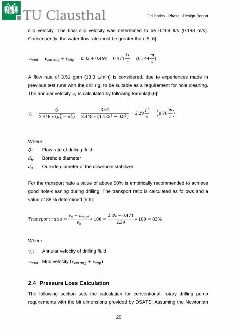
20
slip velocity. The final slip velocity was determined to be 0.469 ft/s (0.143 m/s).
Consequently, the water flow rate must be greater than [5, 6]:
𝑣𝑚𝑢𝑑 = 𝑣𝑐𝑢𝑡𝑡𝑖𝑛𝑔 + 𝑣𝑠𝑙𝑖𝑝 = 0.02 + 0.469 = 0.471𝑓𝑡
𝑠 (0.144
𝑚
𝑠)
A flow rate of 3.51 gpm (13.3 L/min) is considered, due to experiences made in
previous test runs with the drill rig, to be suitable as a requirement for hole cleaning.
The annular velocity 𝑣𝑎 is calculated by following formula[5,6]:
𝑣𝑎 =𝑄
2.448 ∗ (𝑑ℎ2 − 𝑑𝑑
2)=
3.51
2.448 ∗ (1.1252 − 0.82)= 2.29
𝑓𝑡
𝑠 (0.70
𝑚
𝑠)
Where:
𝑄: Flow rate of drilling fluid
𝑑ℎ: Borehole diameter
𝑑𝑑: Outside diameter of the downhole stabilizer
For the transport ratio a value of above 50% is empirically recommended to achieve
good hole-cleaning during drilling. The transport ratio is calculated as follows and a
value of 88 % determined [5,6]:
𝑇𝑟𝑎𝑛𝑠𝑝𝑜𝑟𝑡 𝑟𝑎𝑡𝑖𝑜 =𝑣𝑎 − 𝑣𝑚𝑢𝑑
𝑣𝑎∗ 100 =
2.29 − 0.471
2.29∗ 100 = 83%
Where:
𝑣𝑎: Annular velocity of drilling fluid
𝑣𝑚𝑢𝑑: Mud velocity (𝑣𝑐𝑢𝑡𝑡𝑖𝑛𝑔 + 𝑣𝑠𝑙𝑖𝑝)
2.4 Pressure Loss Calculation
The following section sets the calculation for conventional, rotary drilling pump
requirements with the bit dimensions provided by DSATS. Assuming the Newtonian
Drillbotics - Phase I Design Report
21
fluid (water) flow inside the drill string, the pressure loss inside drill pipe is calculated
as follows. First the velocity of the fluid in the drill pipe 𝑣𝑑 is determined [5,6]:
𝑣𝑑 =𝑄
2.448 ∗ (𝑖𝑑𝑝2)
=3.51
2.448 ∗ (0.2772)= 18.71
𝑓𝑡
𝑠 (5,70
𝑚
𝑠)
Where:
𝑄: Flow rate of drilling fluid
𝑖𝑑𝑝: Internal diameter of the drillpipe
Based on that, the Reynolds number is determined:
𝑅𝑒 =928 ∗ 𝜌𝑓 ∗ 𝑣𝑑 ∗ 𝑖𝑑𝑝
𝜇𝑎=
928 ∗ 8.33 ∗ 18.71 ∗ 0.277
1= 40054 (𝑇𝑢𝑟𝑏𝑢𝑙𝑒𝑛𝑡)
Where:
𝜌𝑓: Density of the drilling fluid (density of water)
𝑣𝑑: Velocity of the drilling fluid inside the drillpipe
𝑖𝑑𝑝: Internal diameter of the drillpipe
𝜇𝑎: Viscosity of the drilling fluid (viscosity of water)
The required friction factor f can be calculated by the following formula [7]:
𝑓 = 0.25 [𝑙𝑜𝑔10 (∈
3.7 ∗ 𝑖𝑑𝑝+
5.74
𝑅𝑒0.9)]
−2
= 0.25 [𝑙𝑜𝑔10 (0.0006
3.7 ∗ 0.277+
5.74
400540.9)]
−2
= 0.0278
Where:
∈: Roughness of the drillpipe (assumed with 0.0006 in)
𝑖𝑑𝑝: Internal diameter of the drillpipe
𝑅𝑒: Reynolds number

Drillbotics - Phase I Design Report
22
The pressure loss inside the drill pipe, 𝑃𝑠, is calculated as follows [7]:
𝑃𝑠 =𝑓 ∗ 𝜌𝑓 ∗ 𝑣𝑑
2 ∗ 𝐿𝑠𝑡𝑟𝑖𝑛𝑔
25.8 ∗ 𝑖𝑑𝑝=
0.0278 ∗ 8.33 ∗ 18.712 ∗ 4.18
25.8 ∗ 0.277= 46.63 𝑝𝑠𝑖 (3.21 𝑏𝑎𝑟)
Where:
𝑓: Fanning friction factor
𝑣𝑑: Velocity of the drilling fluid inside the drillpipe
𝐿𝑠𝑡𝑟𝑖𝑛𝑔: Length of the drillstring
𝑖𝑑𝑝: Internal diameter of the drillpipe
𝑝𝑓: Viscosity of the drilling fluid (water)
There are two nozzles at the bit. For that reason, the total area of nozzle, 𝐴𝑛, is
calculated as follows:
𝐴𝑛 = 2 ∗𝜋
4∗ 𝑑𝑛
2 =𝜋
2∗ 0.0932 = 0.013𝑖𝑛2 (8.67 𝑚𝑚2)
Where:
𝑑𝑛: Nozzle diameter
Then, the pressure loss at the bit, 𝑃𝑏𝑖𝑡 can be estimated by following calculation [6]:
𝑃𝑏𝑖𝑡 =𝑄2 ∗ 𝜌𝑓
12031 ∗ 𝐴𝑛2
=3.512 ∗ 8.33
12031 ∗ 0.0132= 52.4 𝑝𝑠𝑖 (3.61 𝑏𝑎𝑟)
Where:
𝑄: Flow rate of drilling fluid
𝜌𝑓: Density of the drilling fluid (density of water)
𝐴𝑛: Total area of the nozzles
Drillbotics - Phase I Design Report
23
The jet impact force, 𝐹𝑗 of the bit is:
𝐹𝑗 = 0.01823 ∗ 𝐶𝑑 ∗ 𝑄 ∗ √𝜌𝑓𝑃𝑏𝑖𝑡 = 0.01823 ∗ 0.95 ∗ 3.51 ∗ √8.33 ∗ 52.4
= 1.27 𝑙𝑏𝑓 (0.576 𝑘𝑔)
Where:
𝐶𝑑: Discharge coefficient (assumed value ~ 95%)
𝑄: Flow rate of drilling fluid
𝜌𝑓: Density of the drilling fluid (density of water)
𝑃𝑏𝑖𝑡: Pressure loss at the bit
The jet velocity of the bit, 𝑣𝑏𝑖𝑡 is:
𝑣𝑏𝑖𝑡 =𝑄
𝐴𝑛=
3.51 ∗ 144
7.48 ∗ 60 ∗ 0.013= 83.8
𝑓𝑡
𝑠 (25.6
𝑚
𝑠)
Where:
𝑄: Flow rate of drilling fluid
𝐴𝑛: Total area of the nozzles
Further, the pressure loss in annulus, 𝑃𝑎 is calculated as follows [6]:
𝑃𝑎 =1.4327 ∗ 10−7 ∗ 𝜌𝑓 ∗ 𝐿𝑟𝑜𝑐𝑘 ∗ 𝑣𝑎
2
(𝑑ℎ − 𝑑𝑑)=
1.4327 ∗ 10−7 ∗ 8.33 ∗ 2 ∗ 1.97 ∗ 2352
(1.125 − 0.8)
= 0.4 𝑝𝑠𝑖 (0.028 𝑏𝑎𝑟)
Where,
𝜌𝑓: Density of the drilling fluid (density of water)
𝐿𝑟𝑜𝑐𝑘: Length of the rock sample
𝑣𝑎: Annular velocity of the drilling fluid
𝑑ℎ: Borehole diameter
𝑑𝑑: Outside diameter of the downhole stabilizer

Drillbotics - Phase I Design Report
24
The annular velocity is 3.92 ft/s (1.19 m/s) or 235 ft/min (71.65 m/min). The total
downhole pressure loss, 𝑃𝑑𝑜𝑤𝑛ℎ𝑜𝑙𝑒:
𝑃𝑑𝑜𝑤𝑛ℎ𝑜𝑙𝑒 = 𝑃𝑠 + 𝑃𝑏𝑖𝑡 + 𝑃𝑎 = 46.63 + 52.4 + 0.4 = 99.4 𝑝𝑠𝑖 (6.85 𝑏𝑎𝑟)
It is assumed that the pump will be connected with the hose line (made from rubber
material) to the standpipe with roughness 0.0006 in. The pressure loss in the hose, 𝑃ℎ
is calculated by following the same schematic as applied for the pressure loss
calculation in chapter 2.4 [5, 6]:
𝑣ℎ =𝑄
2.448 ∗ (𝑖𝑑ℎ2)
=3.51
2.448 ∗ (0.52)= 5.74
𝑓𝑡
𝑠 (1.7
𝑚
𝑠)
𝑅𝑒 =928 ∗ 𝜌𝑓 ∗ 𝑣ℎ ∗ 𝑖𝑑ℎ
𝜇𝑎=
928 ∗ 8.33 ∗ 5.74 ∗ 0.5
1= 22190 (𝑇𝑢𝑟𝑏𝑢𝑙𝑒𝑛𝑡)
Where:
𝑄: Flow rate of drilling fluid
𝑖𝑑ℎ: Internal diameter of the rubber hose
𝜌𝑓: Density of the drilling fluid (density of water)
𝑣ℎ: Velocity of the drilling fluid inside the hose
Then, the ratio of the roughness of the pipe divided by the inner diameter of the pipe
∈/𝑖𝑑𝑝 is calculated to determine the friction factor on the Fanning chart, as shown in
Figure 2.4:
∈
𝑖𝑑ℎ=
0.0006
0.5= 0.0012
Where:
∈: Roughness of the rubber hose
𝑖𝑑ℎ: Internal diameter of the rubber hose

Drillbotics - Phase I Design Report
25
Figure 2.4: Fanning chart; friction factors for turbulent flow in circular pipes
Based on the Fanning chart, see Figure 2.4, the friction factor,𝑓, is approximately
0.007. The pressure loss inside the hose, 𝑃ℎ is [5,6]:
𝑃ℎ =𝑓 ∗ 𝜌𝑓 ∗ 𝑣ℎ
2 ∗ 𝐻𝑟𝑖𝑔
25.8 ∗ 𝑖𝑑ℎ=
0.007 ∗ 8.33 ∗ 5.742 ∗ 7.5
25.8 ∗ 0.5= 1.05 𝑝𝑠𝑖 (0.072 𝑏𝑎𝑟)
Where:
𝑓: Fanning friction factor
𝑣ℎ: Annular velocity of the drilling fluid inside rubber hose
𝐻𝑟𝑖𝑔: The height of the rig
𝑖𝑑ℎ: Internal diameter of the rubber hose
The total pressure loss along the entire system is [5,6]:
𝑇𝑜𝑡𝑎𝑙 𝑝𝑟𝑒𝑠𝑠𝑢𝑟𝑒 𝑙𝑜𝑠𝑠 = 𝑃𝑑𝑜𝑤𝑛ℎ𝑜𝑙𝑒 + 𝑃𝑏𝑖𝑡 + 𝑃𝑎 + 𝑃ℎ = 147.47 𝑝𝑠𝑖 (10.17 𝑏𝑎𝑟)
Where:
𝑃ℎ: Pressure loss inside rubber hose

Drillbotics - Phase I Design Report
26
The total pressure loss with additional atmospheric pressure is 162.17 psi (11.18 bar).
To estimate the pump horse power requirement, Bernoulli’s equation is used [7]:
𝑃𝑝𝑢𝑚𝑝 = 𝑃𝑙𝑜𝑠𝑠 + 𝑃𝑎𝑡𝑚 +𝜌𝑓 ∗ ∆𝑣2
2+ 𝜌𝑓 ∗ 𝑔 ∗ ∆ℎ
= 147.47 + 14.7 +8.33 ∗ 7.48 ∗ (9.82 − 3.922)
2 ∗ 32.174 ∗ 144+
8.33 ∗ 7.48 ∗ 32.174 ∗ (7.5)
32.174 ∗ 144
= 165.63 𝑝𝑠𝑖 (11.4 𝑏𝑎𝑟)
𝑃𝑢𝑚𝑝𝐻𝑃 =𝑃∗𝑄
1714=
165.63∗3,51
1714= 0.34 𝐻𝑃 (0.25 kW)
Where:
𝑃𝑙𝑜𝑠𝑠: Pressure loss inside the circulation system
𝑃𝑎𝑡𝑚: Atmospheric pressure
𝜌𝑓: Density of the drilling fluid (density of water)
∆ℎ: The height of the rig, 𝐻𝑟𝑖𝑔
𝑔: Earth gravitation, 32.174 ft/s2
𝑃: Total pressure required
𝑄: Flow rate of drilling fluid
Conversion from ft3 to gallon: 7.48
Conversion from ft2 to in2: 144
It is assumed that the efficiency of the pump is 85%, therefore the requirement of the
horse power pump is 0.4 HP (0.3 kW). The following Table 2.7 shows the variation of
the pump power requirement according to the flow rate variation:
Table 2.7: Pump power requirement rotary drilling
Flow rate variation
(gpm)
Flow rate variation
(Lpm)
Transport ratio (%)
Pump Pressure
(bar)
Pump (HP)
Pump (kW)
2 7.57 70 4,7 0,09 0,07
3.51 15.10 83 11.4 0,40 0,30

Drillbotics - Phase I Design Report
27
4 15.14 85 14,3 0,57 0,43
5 18.93 88 21,4 1,07 0,79
6 22.71 90 30,0 1,79 1,34
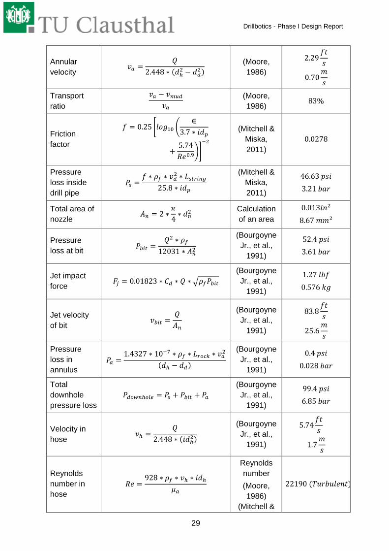
2.5 Summary Calculation Results
The following Table 2.8 shows the results obtained from the calculations in chapter
2.2, chapter 2.3 and chapter 2.4.
Table 2.8: Summary of calculation results
Parameter Symbol Calculated Result
Field Units Metric Units
Critical buckling load 𝑃𝑏𝑐𝑟 51.96 𝑙𝑏𝑓 231,13 𝑁
Burst limit 𝑃𝑏𝑢𝑟𝑠𝑡 2400.5 𝑝𝑠𝑖 165.5 𝑏𝑎𝑟
Torsional Stress limit 𝜏 100.2 𝑖𝑛. 𝑙𝑏𝑓 11.3 𝑁𝑚
Flow rate 𝑄 3.51 𝑔𝑝𝑚 13.3 𝐿𝑝𝑚
Pump pressure 𝑃𝑝𝑢𝑚𝑝 165.63 𝑝𝑠𝑖 11.4 𝐵𝑎𝑟
Pump horse power 𝐻𝑃𝑃 0.4 𝐻𝑃 0.3 𝑘𝑊
Table 2.9: Used formulas
Calculations Formula Reference Results
Moment of
inertia 𝐼 =
𝜋
64(𝑑𝑝
4 − 𝑖𝑑𝑝4)
(Aadnoy,
2006)
0.000682𝑖𝑛4
2.8 ∗ 10−10𝑚4
Critical
buckling load 𝑃𝑏𝑐𝑟 =
𝜋2 ∗ 𝐸 ∗ 𝐼
(𝐾 ∗ 𝐿)2
Euler
equation
(Aadnoy,
2006)
51.96 𝑙𝑏𝑓
23.57 𝑘𝑔
Burst limit 𝑃𝑏𝑢𝑟𝑠𝑡 =2 ∗ 𝑌𝑝 ∗ 𝑡
𝑑𝑝 ∗ 𝑆𝑓
(Aadnoy,
2006)
2400.53 𝑝𝑠𝑖
165.51 𝑏𝑎𝑟
Maximum
torque limit 𝑇𝑚𝑎𝑥 =
𝜋
16∗ 𝜎𝑚𝑎𝑥 ∗
(𝑑𝑝4 − 𝑖𝑑𝑝
4)
𝑑𝑝
(American
Petroleum
Institute,
1994)
100.19 𝑖𝑛. 𝑙𝑏𝑓
11.32 𝑁𝑚
Polar
moment of
inertia
𝐽 =𝜋
32(𝑑𝑝
4 − 𝑖𝑑𝑝4)
(Aadnoy,
2006) 0.0013635𝑖𝑛4
5.68 ∗ 10−10𝑚4

Drillbotics - Phase I Design Report
28
Shear stress
caused by
torque
𝜏 =𝑇 ∗ 𝑟𝑜
𝐽
(Aadnoy,
2006)
8994.95 𝑝𝑠𝑖
62.12 𝑀𝑝𝑎
Safety factor
drillpipe from
torsional
stress
𝑆𝐹 =𝑌𝑠
𝜏
Safety
factor
(Aadnoy,
2006)
1.53
Motor power 𝑇 ∗ 𝑅𝑃𝑀
63025 ∗ 𝐸𝑓𝑓𝑖𝑐𝑖𝑒𝑛𝑐𝑦
(Aadnoy,
2006)
0.325 𝐻𝑃
0.24 𝑘𝑊
Cutting
velocity
𝑣𝑐𝑢𝑡𝑡𝑖𝑛𝑔 =𝑅𝑂𝑃
60 [1 −𝑑𝑑
𝑑ℎ] 𝐶𝑐𝑜𝑛𝑐
(Moore,
1986)
0.02𝑓𝑡
𝑠
0.06𝑚
𝑠
Velocity of
the fluid in
drill pipe
𝑣𝑑 =𝑄
2.448 ∗ (𝑖𝑑𝑝2)
Stoke’s law
(Moore,
1986)
(Bourgoyne
Jr., et al.,
1991)
18.71𝑓𝑡
𝑠
5,70𝑚
𝑠
Slip velocity
- Newtonian
fluid, laminar
flow
𝑣𝑠𝑙𝑖𝑝𝑠 =138 ∗ (𝜌𝑠 − 𝜌𝑓) ∗ 𝑑𝑠
2
𝜇𝑎
(Moore,
1986)
(Bourgoyne
Jr., et al.,
1991)
3.03𝑓𝑡
𝑠
0.93𝑚
𝑠
Reynolds
number 𝑅𝑒 =
928 ∗ 𝜌𝑓 ∗ 𝑣𝑑 ∗ 𝑖𝑑𝑝
𝜇𝑎
Reynolds
number
(Moore,
1986)
(Mitchell &
Miska,
2011)
40054 (𝑇𝑢𝑟𝑏𝑢𝑙𝑒𝑛𝑡)
Slip velocity
with Moore’s
correlation
𝑣𝑠𝑙𝑖𝑝 = 𝑓 ∗ √𝑑𝑠
(𝜌𝑠 − 𝜌𝑓)
𝜌𝑓
Moore’s
correlation,
for 𝑅𝑒 > 300
(Moore,
1986)
0.396𝑓𝑡
𝑠
0.12𝑚
𝑠
Water flow
rate 𝑣𝑚𝑢𝑑 = 𝑣𝑐𝑢𝑡𝑡𝑖𝑛𝑔 + 𝑣𝑠𝑙𝑖𝑝
(Moore,
1986)
0.471𝑓𝑡
𝑠
0.144𝑚
𝑠
Drillbotics - Phase I Design Report
29
Annular
velocity 𝑣𝑎 =
𝑄
2.448 ∗ (𝑑ℎ2 − 𝑑𝑑
2)
(Moore,
1986)
2.29𝑓𝑡
𝑠
0.70𝑚
𝑠
Transport
ratio
𝑣𝑎 − 𝑣𝑚𝑢𝑑
𝑣𝑎
(Moore,
1986) 83%
Friction
factor
𝑓 = 0.25 [𝑙𝑜𝑔10 (∈
3.7 ∗ 𝑖𝑑𝑝
+5.74
𝑅𝑒0.9)]
−2
(Mitchell &
Miska,
2011)
0.0278
Pressure
loss inside
drill pipe
𝑃𝑠 =𝑓 ∗ 𝜌𝑓 ∗ 𝑣𝑑
2 ∗ 𝐿𝑠𝑡𝑟𝑖𝑛𝑔
25.8 ∗ 𝑖𝑑𝑝
(Mitchell &
Miska,
2011)
46.63 𝑝𝑠𝑖
3.21 𝑏𝑎𝑟
Total area of
nozzle 𝐴𝑛 = 2 ∗
𝜋
4∗ 𝑑𝑛
2 Calculation
of an area
0.013𝑖𝑛2
8.67 𝑚𝑚2
Pressure
loss at bit 𝑃𝑏𝑖𝑡 =
𝑄2 ∗ 𝜌𝑓
12031 ∗ 𝐴𝑛2
(Bourgoyne
Jr., et al.,
1991)
52.4 𝑝𝑠𝑖
3.61 𝑏𝑎𝑟
Jet impact
force 𝐹𝑗 = 0.01823 ∗ 𝐶𝑑 ∗ 𝑄 ∗ √𝜌𝑓𝑃𝑏𝑖𝑡
(Bourgoyne
Jr., et al.,
1991)
1.27 𝑙𝑏𝑓
0.576 𝑘𝑔
Jet velocity
of bit 𝑣𝑏𝑖𝑡 =
𝑄
𝐴𝑛
(Bourgoyne
Jr., et al.,
1991)
83.8𝑓𝑡
𝑠
25.6𝑚
𝑠
Pressure
loss in
annulus
𝑃𝑎 =1.4327 ∗ 10−7 ∗ 𝜌𝑓 ∗ 𝐿𝑟𝑜𝑐𝑘 ∗ 𝑣𝑎
2
(𝑑ℎ − 𝑑𝑑)
(Bourgoyne
Jr., et al.,
1991)
0.4 𝑝𝑠𝑖
0.028 𝑏𝑎𝑟
Total
downhole
pressure loss
𝑃𝑑𝑜𝑤𝑛ℎ𝑜𝑙𝑒 = 𝑃𝑠 + 𝑃𝑏𝑖𝑡 + 𝑃𝑎
(Bourgoyne
Jr., et al.,
1991)
99.4 𝑝𝑠𝑖
6.85 𝑏𝑎𝑟
Velocity in
hose 𝑣ℎ =
𝑄
2.448 ∗ (𝑖𝑑ℎ2)
(Bourgoyne
Jr., et al.,
1991)
5.74𝑓𝑡
𝑠
1.7𝑚
𝑠
Reynolds
number in
hose
𝑅𝑒 =928 ∗ 𝜌𝑓 ∗ 𝑣ℎ ∗ 𝑖𝑑ℎ
𝜇𝑎
Reynolds
number
(Moore,
1986)
(Mitchell &
22190 (𝑇𝑢𝑟𝑏𝑢𝑙𝑒𝑛𝑡)

Drillbotics - Phase I Design Report
30
Miska,
2011)
Friction
factor
determinatio
non Fanning
chart
∈
𝑖𝑑ℎ
Fanning
friction
factor
(Bourgoyne
Jr., et al.,
1991)
0.0012
Pressure
loss inside
hose
𝑃ℎ =𝑓 ∗ 𝜌𝑓 ∗ 𝑣ℎ
2 ∗ 𝐻𝑟𝑖𝑔
25.8 ∗ 𝑖𝑑ℎ
(Moore,
1986)
(Bourgoyne
Jr., et al.,
1991)
1.05 𝑝𝑠𝑖
0.072 𝑏𝑎𝑟
Total
pressure loss
along entire
system
𝑃𝑙𝑜𝑠𝑠 = 𝑃𝑑𝑜𝑤𝑛ℎ𝑜𝑙𝑒 + 𝑃𝑏𝑖𝑡 + 𝑃𝑎 + 𝑃ℎ
(Moore,
1986)
(Bourgoyne
Jr., et al.,
1991)
147.47 𝑝𝑠𝑖
10.17 𝑏𝑎𝑟
Total
pressure loss
with
additional
atmospheric
pressure
𝑃𝑝𝑢𝑚𝑝 = 𝑃𝑙𝑜𝑠𝑠 + 𝑃𝑎𝑡𝑚 +𝜌𝑓 ∗ ∆𝑣2
2+ 𝜌𝑓 ∗ 𝑔 ∗ ∆ℎ
Bernoulli’s
equation
(Mitchell &
Miska,
2011)
165.63 𝑝𝑠𝑖
11.4 𝑏𝑎𝑟
Requirement
horse power
for pump
𝑃𝑢𝑚𝑝𝐻𝑃 =𝑃 ∗ 𝑄
1714=
165.63 ∗ 3,51
1714
(Mitchell &
Miska,
2011)
0.34 𝐻𝑃
0.25 kW
Drillbotics - Phase I Design Report
31
Rig Design
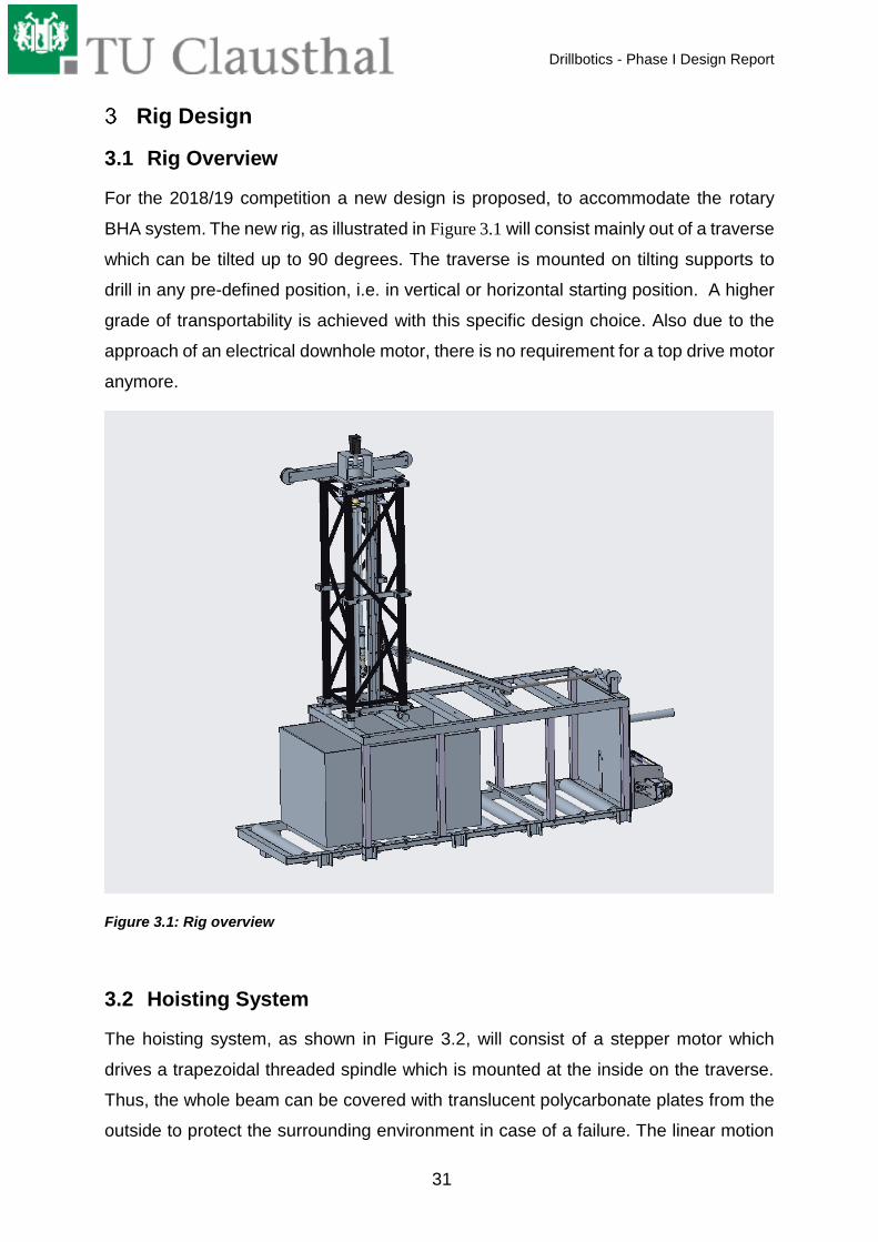
3.1 Rig Overview
For the 2018/19 competition a new design is proposed, to accommodate the rotary
BHA system. The new rig, as illustrated in Figure 3.1 will consist mainly out of a traverse
which can be tilted up to 90 degrees. The traverse is mounted on tilting supports to
drill in any pre-defined position, i.e. in vertical or horizontal starting position. A higher
grade of transportability is achieved with this specific design choice. Also due to the
approach of an electrical downhole motor, there is no requirement for a top drive motor
anymore.
Figure 3.1: Rig overview
3.2 Hoisting System
The hoisting system, as shown in Figure 3.2, will consist of a stepper motor which
drives a trapezoidal threaded spindle which is mounted at the inside on the traverse.
Thus, the whole beam can be covered with translucent polycarbonate plates from the
outside to protect the surrounding environment in case of a failure. The linear motion

Drillbotics - Phase I Design Report
32
of the hoisting system is guided by IGUS™ linear gliding bearings and is actuated by
an attached leadscrew. To measure the WOB, the bearing that supports the axial load
of the trapezoidal threaded spindle is mounted on a loadcell. The trapezoidal thread
spindle is connected to the stepper motor by a flexible coupling to compensate axial
inaccuracies. The absolute position of the Z axis is taken by a linear absolute encoder.
Figure 3.2: Hoisting system
3.3 Rotary Table
To be able to point the drill bit into any desired spherical coordinate, the upper part of
the BHA must be rotated in the opposite direction. To achieve this, a rotary table has
been incorporated into the design of the rig. A form-locked and friction locked
connection to the drill string by means of a collet chuck assembly is applied and, thus,
can position the drill string to achieve a precise angle. Azimuth corrections are also
enabled by steering the drill string.
The rotary table consists out of a spindle which holds the collet chuck and is
manipulated by a worm gear. The angular position of the spindle is monitored via an
absolute 14bit rotary encoder and fed back to the spindle controller to form a closed

Drillbotics - Phase I Design Report
33
loop control over the spindle angle. A stepper motor is considered due to its self-
restraining properties for driving the worm gear.
Figure 3.3: Rotary Table
3.4 Rock Sample Receiver
The rock sample tray is below the mounting points for the hoisting traverse. This allows
a rock sample change by using the winch located at the top of the cross beam. This
implies that no manual lifting is required to insert the rock sample. The sample is
attached to the winch by means of a tension strap. Subsequently, the rock sample
container is positioned under the sample and slowly lowered until it is in the drilling
probe container. Afterwards, the cable of the winch is loosened, and the drilling sample
container is pushed back below the rig in the drilling position. Before drilling the rock
sample, it is fastened to the container, which is locked by pins to the rig.

Drillbotics - Phase I Design Report
34
Figure 3.4: Rock sample receiver
3.5 Rig Electronics
The electronics are housed in a switch cabinet under the rig table and protected against
water. In addition, FI circuit breakers are installed to interrupt the power supply
immediately in the event of a failure.
The main computer with the human machine interface will be located on the table next
to the main controller. Thus, the current state during drilling can be easily tracked and
monitored.
3.6 Rig Plumbing
A drilling mud preparation container will be next to the drilling sample container. Behind
the filter, a pump is connected which generates the necessary pump pressure for
drilling.
3.7 Rig Handling
To be able to transport the rig in the best possible way, the hoisting traverse is designed
to be removable. All electric and hydraulic supply lines are fitted with quick release
couplings to reduce preparation time and to prevent the setting of incorrect
connections.

Drillbotics - Phase I Design Report
35
Mechatronic System Architecture
4.1 CAN Bus
A universal error-resistant bus system is required because many subsystems in the
system are required to communicate with each other without interferences. Therefore,
the decision was made in favour of the controller area network protocol, which is widely
used in the automotive industry.
Figure 4.1: CAN Bus schematic
The structure essentially consists of two redundant data lines, CAN High and CAN
Low. To write one, the CAN High line goes to zero voltage while it is normally on supply
voltage, the CAN Low line goes from zero voltage to supply voltage. To write a ”zero”,
CAN High stays on supply voltage and CAN Low stays on zero voltage. This
mechanism results in an opposing signal in which errors can easily be detected. In a
CAN network, these two lines connect all participants. The electronics in the BHA and
on the surface are also supposed to be connected in this way. Thus, actuators and
sensors can exchange data with each other without a too complicated algorithm.
Synchronized processes can be organized in a decentralized way. In addition, several
algorithms can retrieve data and place commands in the network independently. A
practical example is an initialisation or an emergency stop command. A CAN message
thus consists of several sections. At the beginning there is the arbitration field which
represents a sequential number. Depending on this number, only an individual module
or all even modules are addressed. An emergency shutdown will have the number ”1”.
Each module that does not receive this number will go into an error mode. This
numbering also makes it possible to prioritize messages. If a sender wishes to send a
message, it also listens to the bus lines simultaneously. If it randomly sends signals
simultaneously with a higher priority module, it automatically stops sending and waits
for a new time window. Thus, important messages are exchanged very fast. The next

Drillbotics - Phase I Design Report
36
data field of the CAN message determines the type of message. A distinction is made
between data message, the message transmits data from a module. The remote
message requests data from a particular module and the error message signals to all
participants that an error condition has been triggered. The overload message forces
all participants to take a pause to stabilize the data traffic. Behind it is the data field
and here all data to be sent are aligned. The CAN message is terminated by a CRC, a
count sum to verify the correctness of the message. If this does not agree with the sum
of the message, the message is considered unusable and the data is requested again.
4.2 Quick Data Query
To transmit large amounts of data from many sensors as fast as possible, a data
acquisition protocol was designed, as shown in Figure 4.2.
Figure 4.2: Quick data query schematic
Normally an ECU would send a query message to a sensor and wait for a response. If
this was received error-free, it would dedicate itself to the next sensor and again wait
for the answer to a request. To avoid this waiting cascade, a trick is used. Each module
that transmits data has a specific waiting time which corresponds to its own priority
number. If a data acquisition message is imported into the network, all modules, which
Drillbotics - Phase I Design Report
37
have no data to send, pause their communication. All modules , at which data are to
be queried, go into a ”data sending mode” and wait for a specific time and,
subsequently, send their data set . If this is successfully completed, the network returns
to normal operation. Thus, the time required for the normal polling can be saved.
4.3 Actuator Modules
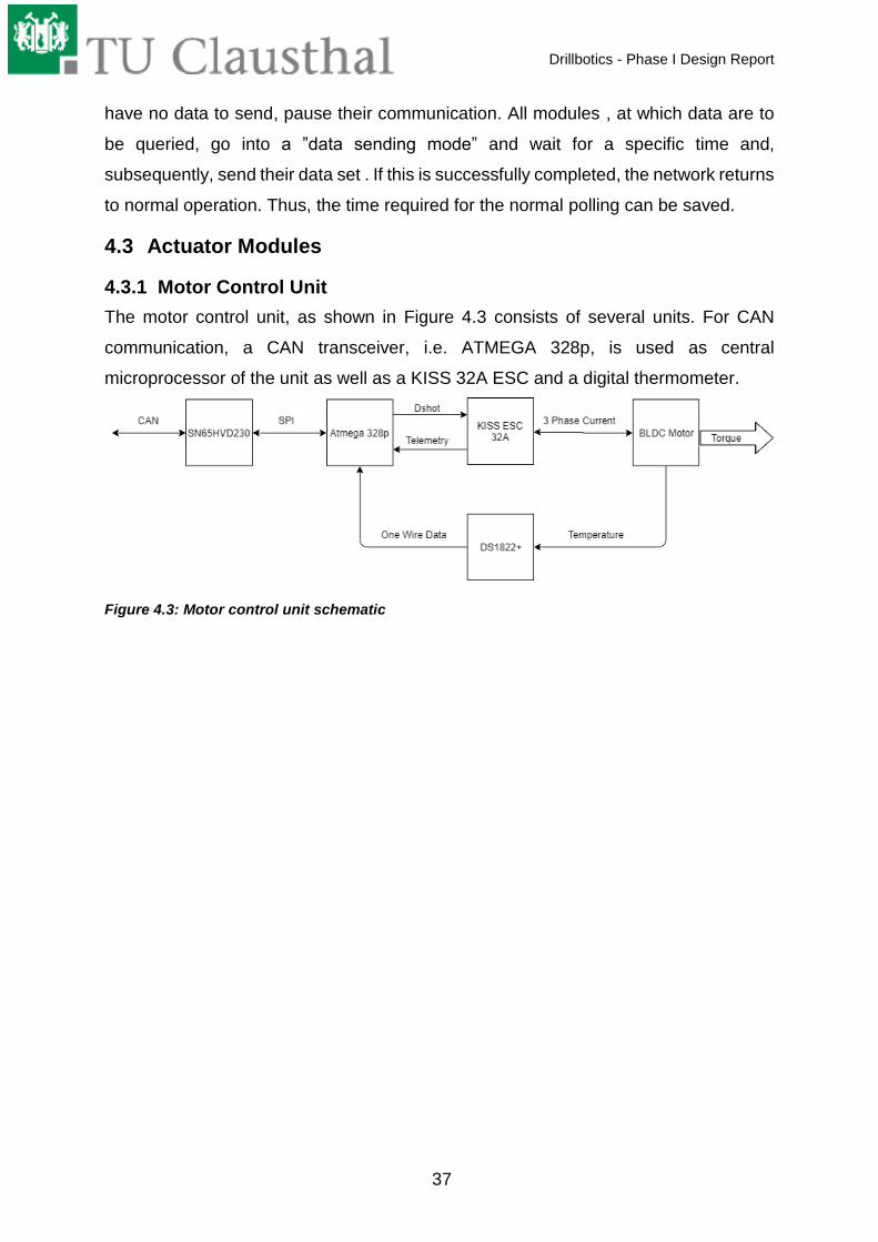
4.3.1 Motor Control Unit
The motor control unit, as shown in Figure 4.3 consists of several units. For CAN
communication, a CAN transceiver, i.e. ATMEGA 328p, is used as central
microprocessor of the unit as well as a KISS 32A ESC and a digital thermometer.
Figure 4.3: Motor control unit schematic

Drillbotics - Phase I Design Report
38
Figure 4.4 Algorithm motor module
A small control loop runs on the ATMEGA 328p which adjusts the required speed of
the main system to the current speed. If the speed is lower than required, the control
signal is amplified, if the speed is too high or if the temperature limit is exceeded, the
control signal is reduced. In addition, a temperature warning is sent to the system. If
the system requests data, then voltage, current, speed and set control signal as well
as temperature are sent back.
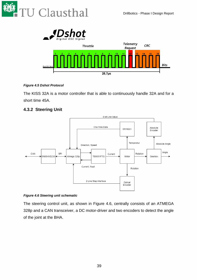
Communication with the ESC takes place via the digital Dshot protocol, as illustrated
in Figure 4.5. It consists of a 16Bit message. The first 11 bits determine the control
signal. The 12th bit is a marker and controls the telemetry feedback. The last 4 bits
are used to create a CRC to enable the ESC to check the validity of the data set.
Drillbotics - Phase I Design Report
39
Figure 4.5 Dshot Protocol
The KISS 32A is a motor controller that is able to continuously handle 32A and for a
short time 45A.
4.3.2 Steering Unit
Figure 4.6 Steering unit schematic
The steering control unit, as shown in Figure 4.6, centrally consists of an ATMEGA
328p and a CAN transceiver, a DC motor-driver and two encoders to detect the angle
of the joint at the BHA.

Drillbotics - Phase I Design Report
40
Figure 4.7 Algorithm steering control unit
The ATMEGA 328p is equipped with a small control loop, as shown in Figure 4.7,
which compares the desired position with the actual position of the swivel joint. If it
deviates, it switches the motor driver in the desired direction and disconnects the
current output and the thermometer. If one of these values is too high, the PWM signal
to the motor driver is reduced in order to avoid any damage. In addition, a warning is
sent to the CAN network.
4.3.3 Rotary Table Control Unit
The rotary encoder control unit, as seen in Figure 4.8, consists of a CAN transceiver
and an ATMEGA 328p, which controls a stepper motor driver and assesses the
absolute rotary encoder. The unit also features a digital thermometer.

Drillbotics - Phase I Design Report
41
Figure 4.8: Rotary table control unit schematic
Figure 4.9 Algorithm Rotary Table
The algorithm determines the current angle value and compares it with the desired
angle. If a deviation is determined, the system moves in the opposite direction to
correct the deviation to zero. As soon as the stepper motor moves, the temperature
and the motor current are additionally determined and compared with a previously
defined maximum value. As soon as these values are exceeded, a warning message
is generated.

Drillbotics - Phase I Design Report
42
4.3.4 Hoisting System Control Unit
This unit consists of a CAN transceiver and an ATMEGA 328p as well as switching
inputs for the upper and lower limit switch of the hoist axis.
Figure 4.10: Hoisting system control unit schematic
It also includes a stepper motor driver with a temperature sensor and an analog/digital
converter for reading a load cell. A load cell is attached to the hoisting spindle bearing
to determine the surface WOB.
Figure 4.11 Algorithm Hoist Control Unit

Drillbotics - Phase I Design Report
43
The algorithm has in total two modes. In the first mode, N steps are driven in the pre-
set direction. The second mode moves to a desired WOB and adjusts it via the spindle.
Since the controller has access to the data of the Downhole WOB module via CAN
network, abnormal operating states can be determined by a comparison.
4.3.5 Relay Switching Unit
The mechatronic system contains a CAN network controllable relay card which
switches the pump and the electromagnets for the Magnetic Ranging System. This unit
consists of an ATMEGA 328p and a CAN transceiver as well as a relay card.
4.4 Sensors
4.4.1 Sensor Unit
4.4.1.1 Mechanical Design of the Sensor Unit
To enable a quick change in the event of a failure, the sensor unit is standardized.
Thus, this unit can be used in the lower and upper notch of the BHA. The mechanical
design is semi-circular with a recess in the middle, as shown in Figure 4.12. With this
design, the magnetometer for the magnetic ranging can detect the magnetic field
strength outside of the BHA.
4.4.1.2 Electrical Design of the Sensor Unit
Figure 4.12 Sensor unit
The sensor unit will contain a PCB which will holds the actual sensor chips. On this
board, a magnetometer (LIS3MDL), an accelerometer (LSM6DS33), and a combined
accelerometer/magnetometer (HMC6343) are installed. These sensors will
communicate with a central microprocessor which will filter the raw data and calculate
Drillbotics - Phase I Design Report
44
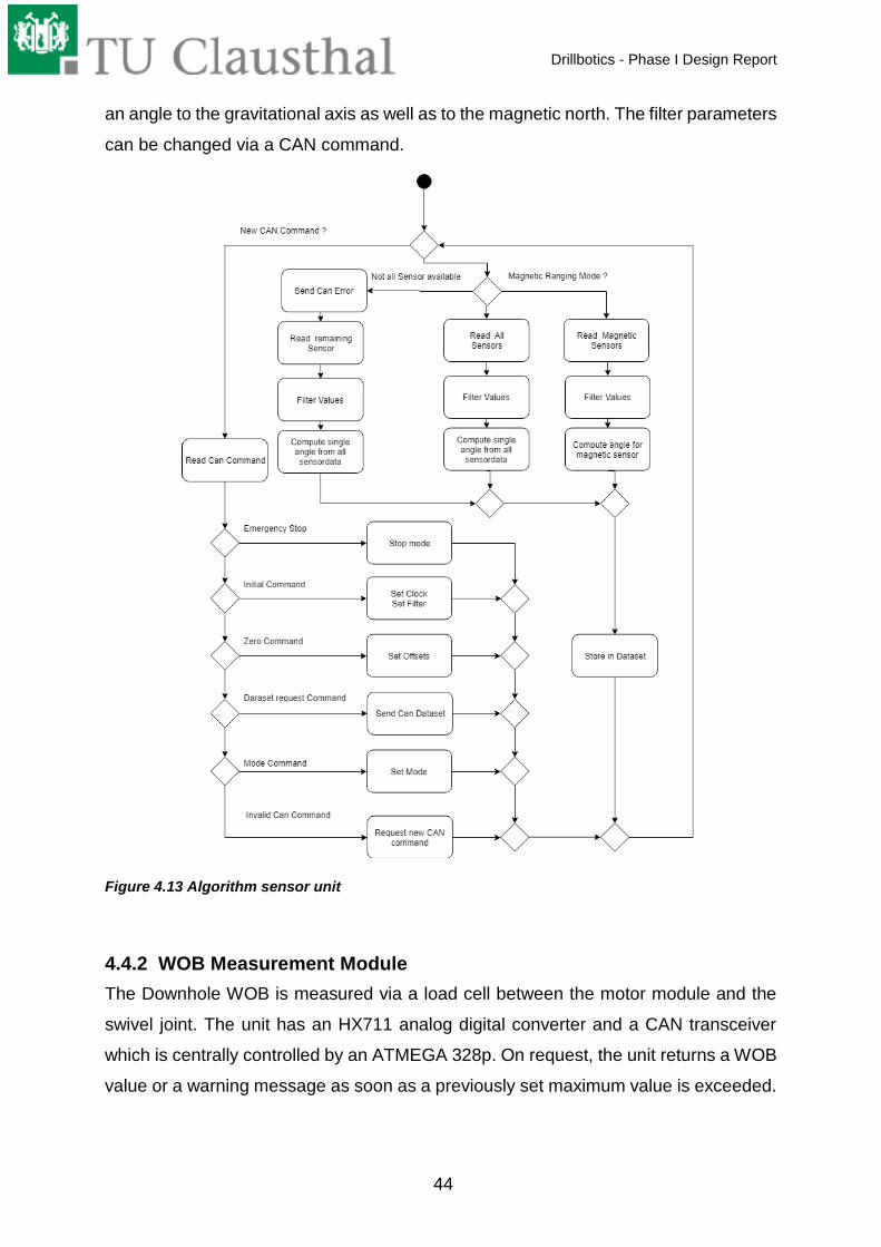
an angle to the gravitational axis as well as to the magnetic north. The filter parameters
can be changed via a CAN command.
Figure 4.13 Algorithm sensor unit
4.4.2 WOB Measurement Module
The Downhole WOB is measured via a load cell between the motor module and the
swivel joint. The unit has an HX711 analog digital converter and a CAN transceiver
which is centrally controlled by an ATMEGA 328p. On request, the unit returns a WOB
value or a warning message as soon as a previously set maximum value is exceeded.

Drillbotics - Phase I Design Report
45
Figure 4.14: WOB measurement module schematic
4.4.3 Current Measurement Unit
To detect an abnormal current consumption and consequently a fault in the current
supply, a current sensor module will be developed which can measure current and
voltage between the power supply and the BHA. This unit is equipped with an ATMEGA
328p and a CAN transceiver. A warning message is sent as soon as a pre-defined
maximum value is exceeded. This module can also determine data on current and
voltage.
4.5 Magnetic Ranging
Since a rotary steerable system in combination with a magnetometer has been
selected for the BHA, electromagnetic interference can cause the azimuth not to be
corrected by measuring the angle to the magnetic north. For this case, another solution
should be considered. To determine the softening and the current drilling progress,
three electromagnets are to be mounted outside the rock sample during the drilling
operation. The magnetic positioning detection mode is to be activated periodically. The
actual position of the sensor modules shall be determined by triangulation. Outside the
rock sample, three electromagnets are installed which can be switched on and off
individually via a relay card. In the first step, all sensor units are to be placed in the
magnetic ranging mode. For this purpose, the master controller sends a control
command via the CAN interface, which is directed to the sensor modules.
Subsequently, the sensor module returns the polar angle to the connected
electromagnet with power to the master controller. A program, which has stored the
positions of the electromagnets, calculates the position of the sensor from the three
angles, which is located at the intersection of the vectors starting from the positions of
the electromagnets. Once this has been done, the control program returns to the
normal operation mode and passes the previously determined coordinates on to the
steering algorithm.
If it should not be possible to take a reliable measurement of the natural magnetic
north, the electromagnet which is attached to the front side of the rock sample is also
Drillbotics - Phase I Design Report
46
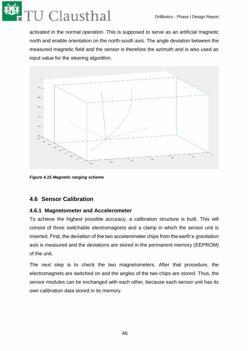
activated in the normal operation. This is supposed to serve as an artificial magnetic
north and enable orientation on the north-south axis. The angle deviation between the
measured magnetic field and the sensor is therefore the azimuth and is also used as
input value for the steering algorithm.
Figure 4.15 Magnetic ranging scheme
4.6 Sensor Calibration
4.6.1 Magnetometer and Accelerometer
To achieve the highest possible accuracy, a calibration structure is built. This will
consist of three switchable electromagnets and a clamp in which the sensor unit is
inserted. First, the deviation of the two accelerometer chips from the earth’s gravitation
axis is measured and the deviations are stored in the permanent memory (EEPROM)
of the unit.
The next step is to check the two magnetometers. After that procedure, the
electromagnets are switched on and the angles of the two chips are stored. Thus, the
sensor modules can be exchanged with each other, because each sensor unit has its
own calibration data stored in its memory.

Drillbotics - Phase I Design Report
47
4.6.2 Downhole Load Cell
To calibrate the Downhole WOB module, the BHA is clamped with the drill head
pointing upwards and a calibrated weight is placed on it. Subsequently, the
measurement is saved, and the scaling factor is calculated.
4.6.3 Surface Load Cell
The rotary table also has a load cell and calibration is carried out by placing a scale
underneath it. In the next step, the rotary table is driven onto the scale and the
measurements are taken. From this, the correction factor of this specific load cell is
calculated.
BHA Design
5.1 Overview
This year, the Drillbotics™ team of the TU Clausthal will use a drill bit with a diameter
of 1.5 in. The design of the BHA, as shown in Figure 5.1, will include a downhole motor
in combination with a rotary steerable system which will be able to follow a desired well
path.
Figure 5.1: Section display BHA
5.2 Drill Spindle
Directly behind the drill bit, a shaft sealing ring seals the BHA from dirt and drilling fluid.
The first sensor module is mounted directly behind the drill bit. This has the advantage
that the drilling process can be more accurately recorded.

Drillbotics - Phase I Design Report
48
Figure 5.2: Section display spindle housing
The drilling spindle is held via a bearing package consisting of a double row preloaded
ball bearing which will absorb the axial and radial forces exerted by the drilling
operation. The bearing 3001-B-2RS-TVH was chosen because it allows a very stiff
bearing in a very small space. Even tilting moments can be well absorbed by this type
of bearing due to its protruding contact angle of 25°. The hollow main shaft leads into
the gearbox.
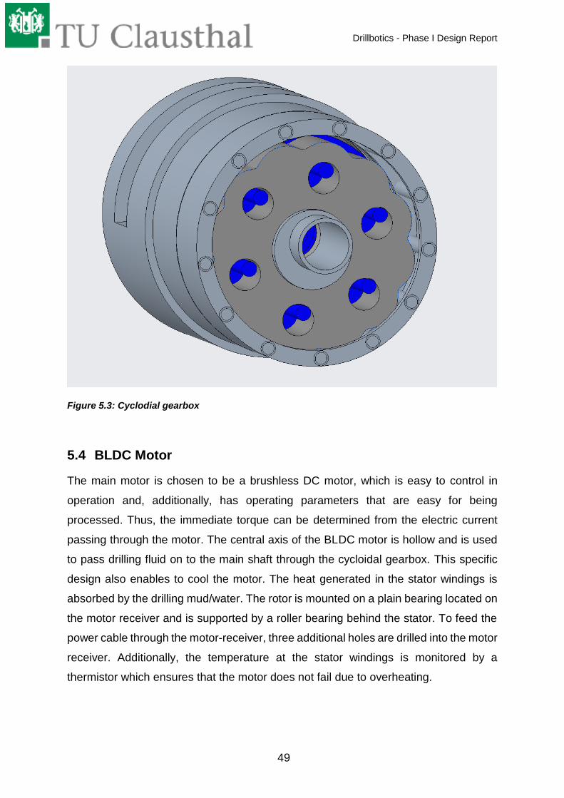
5.3 Cyclodial Gearbox
To generate a high torque down hole, the required gearbox must have a high gear
ratio. For this reason, a cyclodial gearbox is planned to be used. It consists of a central
swashplate which is driven by an eccentric shaft which in turn is driven directly by the
brushless DC motor. It should be noted that this type of gear is very short and therefore
ideal for this application. The outgoing rotary motion is picked up from the cycloid disc
by a cage and passed on to the main shaft.
Drillbotics - Phase I Design Report
49
Figure 5.3: Cyclodial gearbox
5.4 BLDC Motor
The main motor is chosen to be a brushless DC motor, which is easy to control in
operation and, additionally, has operating parameters that are easy for being
processed. Thus, the immediate torque can be determined from the electric current
passing through the motor. The central axis of the BLDC motor is hollow and is used
to pass drilling fluid on to the main shaft through the cycloidal gearbox. This specific
design also enables to cool the motor. The heat generated in the stator windings is
absorbed by the drilling mud/water. The rotor is mounted on a plain bearing located on
the motor receiver and is supported by a roller bearing behind the stator. To feed the
power cable through the motor-receiver, three additional holes are drilled into the motor
receiver. Additionally, the temperature at the stator windings is monitored by a
thermistor which ensures that the motor does not fail due to overheating.

Drillbotics - Phase I Design Report
50
Figure 5.4: Section display BLDC-Motor
5.5 Downhole Load Cell
The loadcell which reads the Downhole WOB is installed behind the motor
compartment. The motor compartment can slide minimally on the lower part of the
swivel joint. Since the loadcell is completely enclosed in ferromagnetic steel, the
magnetic interferences should be minimal. Additionally, the prefabricated loadcell is
calibrated to give a certain voltage for a given load.

Drillbotics - Phase I Design Report
51
Figure 5.5: Detailed view Load Cell
5.6 Steering Unit
To be able to point the drill bit in a desired direction downhole, a swivel joint will be
incorporated into the BHA design. The swivel joint consists of two units which are
separated by an inclined plane.
If the joint rotates, the axes of the upper and lower BHA are set to an angle to each
other. A hollow axle with bearings leads through this plane. The motor cables, as well
as the drilling liquid hose, are guided through this hollow axle. At the upper end of the
hollow axle, a gear wheel is installed which interlocks with a bevel gear. The bevel gear
wheel is rotated by a micro electric motor. In zero position, the two modules have the
same axis. If the motor rotates the lower unit by 180 degrees, the axis of the lower
module deviates by twice the angle of the inclined plane. However, the upper unit must
be rotated by the negative angle to ensure that the north south axis is not left at
maximum bend angle.
Drillbotics - Phase I Design Report
52
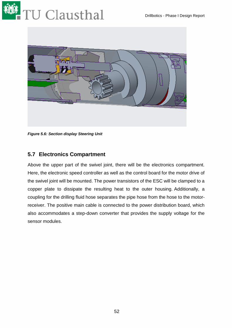
Figure 5.6: Section display Steering Unit
5.7 Electronics Compartment
Above the upper part of the swivel joint, there will be the electronics compartment.
Here, the electronic speed controller as well as the control board for the motor drive of
the swivel joint will be mounted. The power transistors of the ESC will be clamped to a
copper plate to dissipate the resulting heat to the outer housing. Additionally, a
coupling for the drilling fluid hose separates the pipe hose from the hose to the motor-
receiver. The positive main cable is connected to the power distribution board, which
also accommodates a step-down converter that provides the supply voltage for the
sensor modules.

Drillbotics - Phase I Design Report
53
Figure 5.7 Electronics Compartment
5.8 Collet Chuck Joint
At the upper end of the electronic unit a collet chuck is mounted to hold the drill pipe.
A notch will be considered to hold a sensor unit in the upper unit. In the same way, this
type of notch is also placed directly behind the bearing package in the lower
unit. Between drill string and collet chuck receiver, there are two O-rings to prevent
water from breaking into the electronics compartment. The collet chuck is tightened by
a union nut. With this type of clamping, the cross section of the drill string is not
disturbed and more force can be transmitted.
5.9 Drillbit
Since the decision was made for a drill bit with a diameter of 1.5", a new drill bit is
supposed. Since the drilling sample is a homogeneous sandstone, PDC inserts are not
considered for the new drill bit. Instead, carbide inserts that are planned for being used.
In case of wear, new carbides can be soldered in. The design is based on the provided
drill bit and the cutting edges are arranged in such a way that a spherical cross-section
is created. In this way, the drill bit can also cut sideways.
Drillbotics - Phase I Design Report
54
Directional Drilling
6.1 Objectives
The objective of directional drilling is to steer a well trajectory in the right direction to
hit a geological target. This requires tools, sensors and procedures to determine the
location of the borehole and the path while drilling. The following list shows the steps
required to create a directional well.
• Calculation of the desired well trajectory
• Calculation of the northing, easting, TVD, vertical section and dogleg severity of
a surveying station.
• Monitoring of the actual well path while drilling
• Correction of the drilling path during drilling by an algorithm
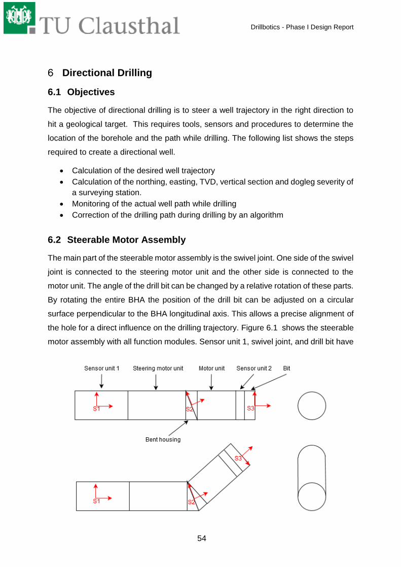
6.2 Steerable Motor Assembly
The main part of the steerable motor assembly is the swivel joint. One side of the swivel
joint is connected to the steering motor unit and the other side is connected to the
motor unit. The angle of the drill bit can be changed by a relative rotation of these parts.
By rotating the entire BHA the position of the drill bit can be adjusted on a circular
surface perpendicular to the BHA longitudinal axis. This allows a precise alignment of
the hole for a direct influence on the drilling trajectory. Figure 6.1 shows the steerable
motor assembly with all function modules. Sensor unit 1, swivel joint, and drill bit have
Drillbotics - Phase I Design Report
55
body fixed coordinate systems which are required for trajectory control. The near bit
sensor unit (sensor unit 2) can be used to verify the adjusted inclination and directional
angle.
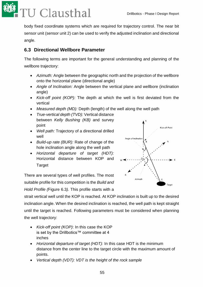
6.3 Directional Wellbore Parameter
The following terms are important for the general understanding and planning of the
wellbore trajectory:
• Azimuth: Angle between the geographic north and the projection of the wellbore
onto the horizontal plane (directional angle)
• Angle of Inclination: Angle between the vertical plane and wellbore (inclination
angle)
• Kick-off point (KOP): The depth at which the well is first deviated from the
vertical
• Measured depth (MD): Depth (length) of the well along the well path
• True-vertical depth (TVD): Vertical distance
between Kelly Bushing (KB) and survey
point
• Well path: Trajectory of a directional drilled
well
• Build-up rate (BUR): Rate of change of the
hole inclination angle along the well path
• Horizontal departure of target (HDT):
Horizontal distance between KOP and
Target
There are several types of well profiles. The most
suitable profile for this competition is the Build and
Hold Profile (Figure 6.3). This profile starts with a
strait vertical well until the KOP is reached. At KOP inclination is built up to the desired
inclination angle. When the desired inclination is reached, the well path is kept straight
until the target is reached. Following parameters must be considered when planning
the well trajectory:
• Kick-off point (KOP): In this case the KOP
is set by the Drillbotics™ committee at 4
inches
• Horizontal departure of target (HDT): In this case HDT is the minimum
distance from the center line to the target circle with the maximum amount of
points.
• Vertical depth (VDT): VDT is the height of the rock sample
i
g
u
r
e
6
.
1
:
S
t
e
e
r
a
b
l
e
M
o
i
g
u
r
e
6
.
2
:
M

Drillbotics - Phase I Design Report
56
• Radius of build section (R): A radius of 40 inches was chosen as a first
approximation.
Equation (6.1) can then be used to calculate the angle of inclination in the build section.
𝜑 = arcsin (𝑅
√(𝑅 − 𝐻𝐷𝑇)2 + (𝑉𝐷𝑇 − 𝐾𝑂𝑃)2) − arctan (
𝑅 − 𝐻𝐷𝑇
𝑉𝐷𝑇 − 𝐾𝑂𝑃)
(6.1)
Figure 6.3: Build and hold well profile
The Build-up rate (in degrees of inclination per inch) can be calculated using Equation
(6.2) [1]:
𝐵𝑈𝑅 =180°
𝜋 ∙ 𝑅
(6.2)
With the radius R and the angle β the length of the trajectory in the build section can
be calculated with Equation (6.3) [1]:

Drillbotics - Phase I Design Report
57
𝑆𝐵𝑈𝑅 = 𝜋 ∙ 𝑅 ∙ 𝜃
180°
(6.3)
The last section is the tangential section. The length can be calculated with Equation
(6.4), after the additional angle 𝜏 must be determined [1]:
𝜏 = arctan (𝑅 − 𝐻𝐷𝑇
𝑉𝐷𝑇 − 𝐾𝑂𝑃)
(6.4)
𝑆𝑇𝐴𝑁 =𝑅
tan (𝜃 + 𝜏)
(6.5)
The total length of the trajectory can be calculated with Equation ((6.6) [1]:
𝑆𝑇𝑅𝐴 = 𝐾𝑂𝑃 + 𝑆𝐵𝑈𝑅 + 𝑆𝑇𝐴𝑁 (6.6)
The following Table 6.1 shows the results from the calculations.
Table 6.1 Results of well trajectory calculation
Parameter Symbol Calculated Result
Field Units Metric Units
Kick-of point KOP 4.0 𝑖𝑛 101,6 𝑚𝑚
Horizontal departure of target HDT 2.0 𝑖𝑛 50,8 𝑚𝑚
Vertical depth VDT 24.0 𝑖𝑛 609,6𝑚𝑚
Inclination angle 𝜑 6.5° 6,5°
Build-up rate BUR 1.43 °/𝑖𝑛 0,0563°/𝑚𝑚
Build section length 𝑆𝐵𝑈𝑅 4.49 𝑖𝑛 114,05𝑚𝑚
Tangential length 𝑆_𝑇𝐴𝑁 15.62 𝑖𝑛 396,75𝑚𝑚
6.4 Wellbore Surveying
During drilling it is difficult to make the actual trajectory precisely match the designed
well path. Therefore, it is important to monitor the well trajectory and take corrective
actions while drilling.

Drillbotics - Phase I Design Report
58
6.4.1 Survey Calculations
Once the desired trajectory has been determined, survey stations are defined at
discrete intervals along the trajectory. At each station the inclination angle and azimuth
are calculated as a function of the measured depth. During drilling the azimuth and
inclination angles are measured at each survey station. The path difference in north,
east and depth between two stations can be calculated with the following equations.
Es ist eine ungültige Quelle angegeben.
∆𝑁𝑜𝑟𝑡ℎ = 𝑥2 − 𝑥1 = ∫ 𝑠𝑖𝑛𝜑(𝑠)𝑐𝑜𝑠𝜗(𝑠)𝑑𝑠𝑆2
𝑆1
(6.1)
∆𝐸𝑎𝑠𝑡 = 𝑦2 − 𝑦1 = ∫ 𝑠𝑖𝑛𝜑(𝑠)𝑠𝑖𝑛𝜗(𝑠)𝑑𝑠𝑆2
𝑆1
(6.2)
∆𝑇𝑉𝐷 = 𝑧2 − 𝑧1 = ∫ 𝑐𝑜𝑠𝜑(𝑠)𝑑𝑠𝑆2
𝑆1
(6.3)
𝐵𝑈𝑅(𝑠) =𝑑𝜑(𝑠)
𝑑𝑠
(6.4)
Due to the continuous integration of the sensor values, the sensor errors are also
integrated. This leads to large inaccuracies over the measurement period. To minimize
the influence of sensor errors, the sensor data should be read out at standstill. Thus,
detected accelerations caused by vibrations are not measured with. The disadvantage
of this method is that the measured values are only available at discrete points. The
i
g
u
Figure 6.4 Interpolation Scheme
Drillbotics - Phase I Design Report
59
path between these points (survey stations) must be interpolated using appropriate
methods. In the build section the path between two survey stations can be interpolated
by using the minimum curvature method (Figure 6.5). This method smoothes two
tangential-line segments by using a Ratio Factor (RF). Equations (6.5)-(6.9) can be
used to calculate the path differences in all three spatial directions. In the tangential
section, the path between two survey stations is interpolated linearly [1].
∆𝑁𝑜𝑟𝑡ℎ =𝑀𝐷
2∙ (sin(𝜑1) cos(𝜗1) + sin(𝜑2) cos(𝜗2)) ∙ 𝑅𝐹
(6.5)
∆𝐸𝑎𝑠𝑡 =𝑀𝐷
2∙ (sin(𝜑1) sin(𝜗1) + sin(𝜑2) sin(𝜗2)) ∙ 𝑅𝐹 (6.6)
∆𝐸𝑎𝑠𝑡 =𝑀𝐷
2∙ (sin(𝜑1) sin(𝜗1) + sin(𝜑2) sin(𝜗2)) ∙ 𝑅𝐹
(6.7)
𝛽 = arccos (cos(𝜑2 − 𝜑1) − (sin(𝜑1) sin(𝜑2) ∙ (1 − cos(𝜗2 − 𝜗1))) (6.8)
𝑅𝐹 =2
𝛽∙ tan (
𝛽
2)
(6.9)
6.4.2 Measurement While Drilling (MWD)
The MWD system for directional drilling includes three-axis accelerometer and three-
axis magnetometer arranged in three mutually orthogonal directions. Both Sensors are
installed in the interior of a nonmagnetic drill collar. Both sensors are orientated in Z
direction along the BHA longitudinal axis. The sensors measure the gravity and the
magnetic north in relation to a fixed coordinate system. Equations (6.10)-(6.11) can
be used to determine the inclination angle (𝜑) and azimuth (𝜗) from the measured of
gravity vectors and the magnetic field strength vectors in all three spatial directions.
i
g
u
r
e
6
.
7
:
S
e
Figure 6.6: Magnetometer and
accelerometer orientation

Drillbotics - Phase I Design Report
60
𝜑 = arctan (√𝐺𝑥
2 + 𝐺𝑦2
𝐺𝑧)
(6.10)
𝜗 = arctan (𝐺 ∙ (𝐺𝑥𝐻𝑦 − 𝐺𝑦𝐻𝑥)
𝐻𝑧(𝐺𝑥2 + 𝐺𝑦
2) − 𝐺𝑧(𝐺𝑥𝐻𝑥 − 𝐺𝑦𝐻𝑦))
(6.11)
Due to the two angles, the position of the sensor module relative to the global reference
system is known. Even if the BHA rotates around the Z axis (in the range 0 to 180 deg),
the two angles remain the same. To detect the drill bit position relative to the sensor
coordinate system and the global coordinate system, additional coordinate systems
are required (see Figure 6.1). The coordinate transformation between two coordinate
systems can be performed with rotation matrices. To describe the bit movement
relative to each of the three coordinate systems the transformation matrix below can
be used. R is the distance between two
coordinate systems and the two angles describe
the orientation in space. Similar to robotic applications, these matrices are used to
define positions in space by changing the two angles. This allows to map the bit
position to the sensor coordinate system.
𝑇𝑆+1𝑆 = [
sin(𝜓) cos (𝛾) −sin (𝛾) cos(𝜓) cos (𝛾) 𝑅 cos(𝛾) cos (𝜓)
sin(𝜓) sin (𝛾) cos (𝛾) cos(𝜓) sin (𝛾) 𝑅 sin(𝜓) cos (𝛾)−cos (𝜓) 0 sin (𝜓) 𝑅 sin (𝜓)
0 0 0 1
]
(6.7)
For each coordinate transformation between two coordinate systems a separate
transformation matrix has to be used. Matrix (6.7) is an exemplary matrix for a
coordinate transformation.
6.5 Control Structure for Directional Drilling
Figure 6.10 shows the directional drilling
procedure. First step is the calculation of the
desired wellbore trajectory parameters at all
determined survey stations. The parameters for
each survey station are stored in a path table.
i
g
u
r
e
6
.
9
:
R
o
t
a
t
i
n
g
c
o
o
r
d
Figure 6.8: Coordinate transformation
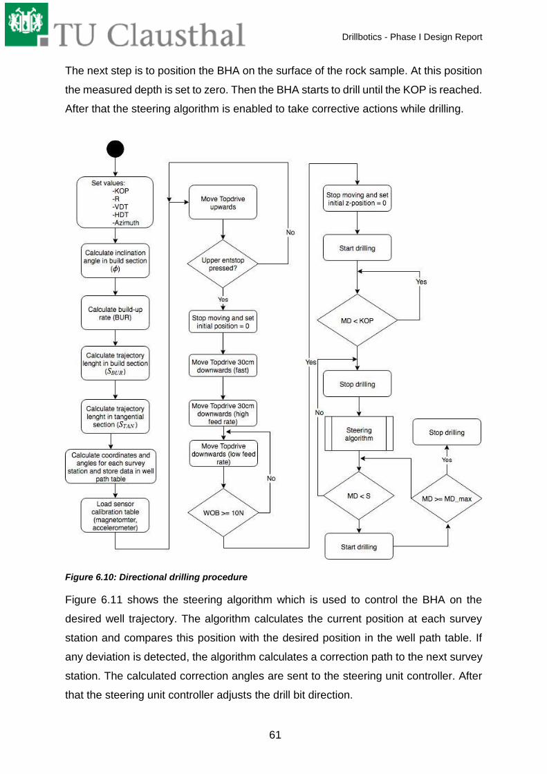
Drillbotics - Phase I Design Report
61
The next step is to position the BHA on the surface of the rock sample. At this position
the measured depth is set to zero. Then the BHA starts to drill until the KOP is reached.
After that the steering algorithm is enabled to take corrective actions while drilling.
Figure 6.10: Directional drilling procedure
Figure 6.11 shows the steering algorithm which is used to control the BHA on the
desired well trajectory. The algorithm calculates the current position at each survey
station and compares this position with the desired position in the well path table. If
any deviation is detected, the algorithm calculates a correction path to the next survey
station. The calculated correction angles are sent to the steering unit controller. After
that the steering unit controller adjusts the drill bit direction.
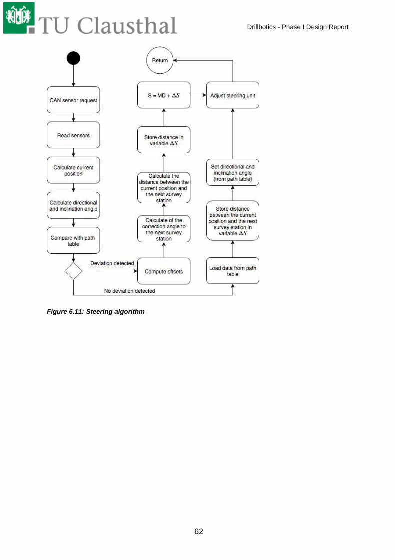
Drillbotics - Phase I Design Report
62
Figure 6.11: Steering algorithm

Drillbotics - Phase I Design Report
63
Safety Consideration and Risk Analysis
Risk name Risk description Risk control strategy
Drilling fluid (water) leaking
Drilling fluid leaks from hose or circulation system
Use suitable hose and circulation system (e.g. hose with appropriate pressure rating capacity). The circulation system will be checked before and while testing.
String wobbling String vibration/wobbing
Start drilling at low RPM then increase gradually after reach a certain depth e.g. 1/4". Set the limit of the RPM in algorithm.
Bit walking Bit drills deviated away from the trajectory plan. This risk is also associated with string wobbling.
Install a guide shoe or riser/casing at rotary table above the rock sample thus limiting the drillstring wobbling. Install downhole sensors, which are accelerometer and gyro, and integrates the acquisition data with algorithm to self-control the drilling trajectory.
Drillstring stuck Drillstring stuck due to unclean hole or cutting is not circulated properly from the hole
Apply minimum flow rate according to minimum cutting transport velocity estimation. Apply also minimum drillsting rotation speed (RPM) according to design calculation to help hole cleaning.
Loss verticality of hole section
Drill directional hole or deviated trajectory away from the plan
Install downhole sensors (accelerometer and gyro) and integrates acquisition data with algorithm program. Apply algorithm program to maintain verticality to self-control string while drilling.
Drillstring buckling and twist off
The weakest part along the drillstring is aluminum drill pipe. Another potential weak part is connection. Buckling and twist off could occur during the drilling.
Use high strength connection type for all parts of the drillstring, particularly the aluminum drillpipe. Estimate the limit strength of drill pipe then limit the WOB and RPM to avoid the failure according to the design calculation. Set the WOB and RPM limit in the algorithm. In case much vibration occurs, alert (alarm) system will be active thus students can respond.

Drillbotics - Phase I Design Report
64
Short circuit and/or electrical hazard
The risk is associated with electrical cable or source
Proper handling of electrical cable shall be applied, especially the avoidance from liquid (water). All electrical systems must be set up properly, soldered, installed, and connected to power source carefully and if it is possible enclosed system (use protector) and contained in one place. All of the steps associated with setting up electrical must be done with safety concerns and safety protector (if applicable). Minimum safety equipment (e.g. safety glasses, gloves, etc.) must be worn during the electrical installation.
Mechanical construction risk
During build up and/or testing, risk associated with pinch points, punctures, lacerations, cutting debris, and etc, could cause damage and hazard.
Proper handling of material and pieces during building up the rig structure, particularly it is mandatory to wear the proper HSE equipment according to minimum standard (e.g. safety shoes, safety glasses, gloves, etc). Students will also work from a certain height during building up the rig structure, thus precautions must be taken to prevent injuries. A certain range of zone isolation must be set thus non related person will be allowed to pass the zone. A general working procedure (Standard Operating Procedure/SOP) will be set before rig construction work. The connection of all parts and pieces of rig structure must be checked properly during and after rig construction to confirm the solid rig structure, thus avoiding the loose pieces during the drilling or test. All the sharp edges in rig structure will be covered or protected with protector to avoid human injures.
Cutting and drilling fluid spill and disposal
During the drilling, cutting and drilling fluid will flow out of the well to the surface and must be disposed properly.
Safety containment will be installed around the rock sample and rig structure (below), thus the cutting and drilling fluid circulation (outflow) can be stored properly. The safety containment will be made from transparent material (e.g. plastic, etc), thus the drilling process can still be observed. Additional storage containment will be installed also to store more cutting and drilling fluid circulation out of the well or rock sample. The cutting and drilling fluid outflow

Drillbotics - Phase I Design Report
65
circulation will be recorded and disposed according to regulations (university and state regulations), particularly if there is chemical content. A general procedure will be included together with HSE procedure.
Hazard during drilling or testing
Accident and hazard during drilling or testing could occur.
The drilling automation (through algorithm and computer control) is set up thus less or even no human intervention is needed during the test. However, supervision during the test is still needed. Before the test or drilling is started, safety meeting (prejob safety meeting) will be held to discuss the procedure and any potential hazard. Emergency shutdown is included in algorithm program and will active in case serious hazard occurs. The emergency shutdown can also be activated manually (intervention from human) in case the self-control program does not work properly. In case there is obstacle or restriction in circulation system that causing increase of the pressure, emergency shutdown system will be activated (included in algorithm) at certain limit of pressure and relief valve is installed to release the pressure. A general testing procedure (Standard Operating Procedure/SOP) will be set before drilling or testing. Minimum HSE equipment standard must be worn (e.g. safety glasses, hearing protection, etc). A certain range of zone isolation must be set thus unauthorized person will not be allowed to pass the isolation zone. A fire extinguisher will be available on location in case fire occurs due to overheating of electronic components or motor, etc. The hoisting system has locking mechanism to stop the movement in case lost control happens.
Communication error
Failure during data acquisition due to communication system error
System restart will be designed, so whenever data is failed to be acquired, by restarting the system, data acquisition can work properly.

Drillbotics - Phase I Design Report
66
Sensor error Failure during data acquisition due to sensor failure
The sensors will be tested before and after installation. After each test or drilling, maintenance will be performed to confirm whether the sensors can still function properly.
Mobility of the rig The mobility of rig is incorporated in the design. The rig structure will be placed above the table and wheels will be installed below the table, thus the rig can be mobilized. A brake system will be included in wheels to prevent undesired rig movement during drilling or testing due to vibration. Proper handling system will be installed so the rig can be moved safely and in convenient way. Modular design will be considered and as far as possible applied in the rig construction, such as electrical, computer, pump and disposal storage that can be disassembled or separated. This will make the mobilization and transportation more convenient and safe.
Electric cables and water hoses
Cables and hoses lying around which is a serious tripping hazard. Damaging of the equipment, tool failures and health restrictions might be consequences
Cable shafts for electric cables as well as hose guards will be laid to gather the loose components. Additionally, clearly visible warning labels will be put up to make people aware of the hazard
Drillbotics 2017/18 drilling Performance
To achieve a good performance of the Drillbotics drilling rig, several test on different
rock samples (mainly sandstone) using different hammer concepts and different drill
bits were conducted. The analysis of the data gathered from the drilling rig was used
to tune the controller and to improve the drilling process.
To optimize the drilling operation, a series of variations on the triplets RPM, flow rate
and WOB were tested, looking for the best performance in terms of ROP. Some test
results are shown in the following pictures.

Drillbotics - Phase I Design Report
67
The test results are depicted in the figure 8.2 and show a better drilling performance
by the spring-mounted hammer. For this test, ROPs up to 32 mm/min were registered.
With the springless hammer, a maximum of 20 mm/min was achieved.
The second series of tests was performed using the spring-mounted hammer. The data
acquired during these tests was used to tune the controller. A progressive increase on
ROP was achieved and a better performance of the drilling operations was observed.
In figure 8.4 , three different runs can be observed with a different setup of the control
parameters. In the first setup, ROP values ranging from 10 to 20 mm/min were
achieved. By the second setup, more constant ROP values around 18 mm/min were
reached. The third setup of the system resulted in a slightly deviated ROP value of 30
mm/min.
i
g
u
r
e
8
.
1
:
T
e
s
t
r
e
s
u
l
t
s
f
r
o
m
d
Figure 8.2: Test results from drilling in sandstone with two different hammer systems.

Drillbotics - Phase I Design Report
68
After setting up the controller, a consecutive adjustment of the output control range
was implemented. In figure 8.4 , the different tests performed over the same rock
sample including variations of the flow rate, WOB and RPM are depicted.
i
g
u
r
e
8
.
3
:
T
e
s
t
r
e
s
u
l
t
s
a
f
t
e
r
Figure 8.4 Test results after tuning control parameters.
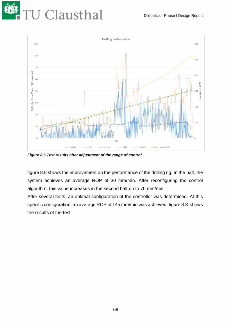
Drillbotics - Phase I Design Report
69
figure 8.6 shows the improvement on the performance of the drilling rig. In the half, the
system achieves an average ROP of 30 mm/min. After reconfiguring the control
algorithm, this value increases in the second half up to 70 mm/min.
After several tests, an optimal configuration of the controller was determined. At this
specific configuration, an average ROP of 145 mm/min was achieved. figure 8.8 shows
the results of the test.
i
g
u
r
e
8
.
5
:
T
e
s
t
r
e
s
u
l
t
s
a
f
t
e
r
Figure 8.6 Test results after adjustment of the range of control

Drillbotics - Phase I Design Report
70
All data gathered in successive tests were processed and analyzed to determine
optimal drilling parameters considering the specific drilling conditions used for this
study. Figure summarizes the analysis of the data as a three-dimensional image. It can
be observed that the optimal drilling parameters for the type of rock used are ranging
from a flow rate of 25 to 26 l/min, 350 rpm and 35 to 40 kg WOB.
i
g
u
r
e
8
.
7
:
T
e
s
t
r
e
s
u
l
t
s
a
f
t
e
r
Figure 8.8 Test results after final adjustment of the controller

Drillbotics - Phase I Design Report
71
Funding Plan and Price List
At the moment we are in contact with our sponsors of the last year and are negotiating
the sponsors' shares.
Optimal drilling parameters 3D Chart
Position Estimated Price
Materials Rig
Beam 250 €
Steel Profile 250 €
Plexiglas Enclosure 150 €
DIN Parts 200 €
Materials BHA
Steel 200 €
Plastics 100 €
DIN Parts 150 €
Manufacturing Costs 2000 €
i
g
u
r
e
8
.
9
:
O
p
t
i
m
a
l
d
r
i
l
l
i
n
g
p
Figure 8.10 Optimal drilling parameters 3D Chart
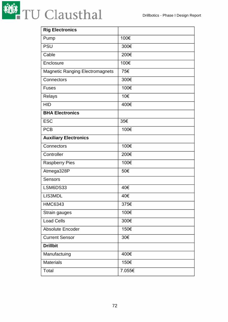
Drillbotics - Phase I Design Report
72
Rig Electronics
Pump 100€
PSU 300€
Cable 200€
Enclosure 100€
Magnetic Ranging Electromagnets 75€
Connectors 300€
Fuses 100€
Relays 10€
HID 400€
BHA Electronics
ESC 35€
PCB 100€
Auxiliary Electronics
Connectors 100€
Controller 200€
Raspberry Pies 100€
Atmega328P 50€
Sensors
LSM6DS33 40€
LIS3MDL 40€
HMC6343 375€
Strain gauges 100€
Load Cells 300€
Absolute Encoder 150€
Current Sensor 30€
Drillbit
Manufactuing 400€
Materials 150€
Total 7.055€

Drillbotics - Phase I Design Report
73
Bibliography
Aadnoy, B. S., 2006. Mechanics of Drilling. Mannheim: Shaker Verlag GmbH.
American Petroleum Institute, 1994. API Bulletin 5C3 - Bulletin on Formulas and
Calculations for Casing, Tubing, Drill Pipe, and Line Pipe Properties. 6th ed.
Washington DC: s.n.
Bourgoyne Jr., A. T., Millheim, K. K., Chenevert, M. E. & Young Jr., F., 1991. Applied
Drilling Engineering. Texas: Society of Petroleum Engineers.
Fairhurst, C. L. W., 1956. Some principles and developments in hard rock drilling
techniques. Minnesota Uni., s.n., pp. 15-25.
Han, G; M, Bruno; K, Lao, 2005. Dynamically Modelling Rock Failure in Percussion
Drilling. Anchorage, Alaska, ARMA, American Rock Mechanics Association .
Han, G., M, B. & K, L., 2005. Percussion Drilling in Oil Industry: Review and Rock
Failure Modelling. Houston, Texas, s.n.
Herbert, G., 1987. Steel Construction Manual. 8 ed. s.l.:American Institute of Steel
Construction.
Kahraman, S., Bilgin, N. & Feridunoglu, C., 2003. Dominant rock properties affecting
the penetration rate of percussive drills. International Journal of Rock Mechanics &
Mining Sciences, 12 04, pp. 711-723.
Mitchell, R. F. & Miska, S. Z., 2011. Fundamentals of Drilling Engineering. Richardson,
TX: SPE Publishing Services.
Moore, P. L., 1986. Drilling Practices Manual. Texas: PennWell Publishing Company.
Samuel, G. R., 1996. Percussion Drilling...Is It a Lost Technique? A Review. s.l.,
Society of Petroleum Engineers.
Thulin, L., 1971. Mechanics of materials II. s.l.:s.n.