1

Performance of Enriched Methods for Large Scale Unconstrained Optimization as applied to Models of Proteins

B. Dasa, H. Meirovitcha, and I. M. Navonb aCenter for Computational Biology and Bioinformatics, School of Medicine University of Pittsburgh, Suite 601 Kaufmann Building 3471 Fifth Avenue, Pittsburgh, PA 15213 bDepartment of Mathematics and Computational Science and Information Technology, Florida State University, Tallahassee, Florida 32306 Phone: (412) 648-6675 Fax : (412) 648-6676 e-mail: hagaim@pitt.edu

2

Abstract Energy minimization plays an important role in structure determination and analysis of proteins, peptides and other organic molecules; therefore, development of efficient minimization algorithms is important. Recently Morales and Nocedal have developed enriched methods for large scale unconstrained optimization that interlace iterations of the limited memory BFGS method (L-BFGS) and the Hessian-free Newton method (Computational Optimization and Applications (2002) 21, 143-154). We test the performance of this approach as compared to those of the L-BFGS algorithm of Liu and Nocedal and the truncated Newton (TN) with automatic preconditioner of Nash, as applied to the protein bovine pancreatic trypsin inhibitor (BPTI) and a loop of the protein Ribonuclease A. These systems are described by the all-atom AMBER force field with a dielectric constant ε=1 and a distance dependent dielectric constant ε=2r, where r is the distance between two atoms. It is shown that for the optimal parameters, the hybrid approach is typically 2 times more efficient in terms of CPU time and function/gradient calculations than the two other methods. The advantage of the hybrid approach increases as the non-linearity of the energy function is enhanced, i.e., in going from ε=2r to ε=1, where the electrostatic interactions are stronger. However, no general rule that defines the optimal parameters has been found and their determination requires a relatively large number of trial and error calculations for each problem.

Keywords: energy minimization; proteins; loops; hybrid method; truncated Newton; dielectric constant; force field

3

Introduction

The interatomic interactions of bio-molecules such as proteins and nucleic acids are usually described by an empirical potential energy function (force field), which depends on the structure (geometry) of the molecule and typically leads to a �rugged� energy surface consisting of a tremendous number of local minima 1. Identifying the lowest energy minima, in particular the global minimum, is the goal of protein folding studies, where the energy, rather than the free energy, is accepted as an approximate criterion of stability. A more rigorous criterion is minimum harmonic free energy, Fhar, where Fhar is obtained at an energy minimum from the harmonic entropy, Shar that is proportional to the determinant of the Hessian, the matrix of second derivatives of the energy with respect to the molecular coordinates.2,3,4,5,6 Calculation of the Hessian at a minimum is also an essential part of a normal mode analysis.7

The above discussion already demonstrates the importance of energy minimization in computational structural biology and the need for developing efficient minimization algorithms. The common algorithms, such as conjugate gradients or Newton methods are of a local character, that is, they drive an initial molecular structure to the closest energy minimum rather than to the global one. However, the applicability of these methods is much wider because most of the global optimization procedures, including our local torsional deformation (LTD) method for cyclic molecules,8,9 are based on a large number of local energy minimizations (see for example Refs.10,11,12,13,14,15,16,17,18 ). Therefore, attempting to optimize LTD, we tested in a previous preliminary study several minimization algorithms and found the limited memory BFGS (L-BFGS)19 to be the most efficient for a force field with an implicit solvation model 9 [see next section, equations (1) and (2)] .

The experience gained thus far from treating various problems, in particular large-

scale unconstrained minimizations,20,21,22,23 is that truncated Newton (TN)24,25,26,27 and L-BFGS are powerful optimization methods which are more efficient than other techniques (see also Refs. 28,29,30). TN tends to blend the rapid (quadratic) convergence rate of the classical Newton method with feasible storage and computational requirements. The L-BFGS algorithm is simple to implement since it does not require knowledge of the sparsity structure of the Hessian, or knowledge of the separability of the objective function. Furthermore, the amount of storage needed can be controlled by the user. It has been found that, in general, TN performs better than L-BFGS for functions that are nearly quadratic, while for highly nonlinear functions L-BFGS outperforms TN.31

These aspects and others are discussed in an excellent review on minimization methods by Schlick,32 who together with Fogelson also programmed their own TN algorithm and included it in the package TNPACK26,27 This package enables the user to supply a sparse preconditioning matrix that transfers the Hessian into a matrix with more clustered eigenvalues, which in turn enhances convergence. This implementation of TN differs from that of Nash.25 which uses automatic preconditioning and has been applied to a variety of problems with considerable success; the latter has the advantage of easy portability, because the preconditioner does not have to be tailored to the specific problems at hand. In her review, Schlick presents systematic efficiency comparisons between several

4

algorithms applied to the molecule deoxycytine (87 variables) and to clusters of water molecules. For the former system, TN with preconditioning is found to be the most efficient requiring ~2 times less CPU time than L-BFGS with preconditioning, while for the water clusters the picture is more complex.

Derreumaux et al.33 tested the efficiency of TN as applied to peptides and proteins modeled by the CHARMM force field34 using an updated version of TNPACK. In this implementation, the preconditioner is based on the short-range interactions, i.e., the bond stretching and bending, and the torsional potentials. It is shown that for several molecules of sizes n=12 to 1299 atoms, TNPACK with preconditioning outperforms the steepest descent, nonlinear conjugate gradient, adapted basis Newton-Raphson, and Newton-Raphson algorithms installed in the CHARMM package.33 More recently, Xie and Schlick showed that for molecules of sizes n=22 to 2030 atoms, TNPACK requires less CPU time than both CG and L-BFGS, and reaches very low gradient norms.35,36

Because the performance of minimization algorithms depends to a large extent on the system and the cost function used,37 we have carried out recently38 a systematic performance study of the algorithms, L-BFGS of Liu and Nocedal,19,39 TN with automatic preconditioner of Nash25 and the non-linear conjugate gradients (CG) of Shanno and Phua.40 These algorithms were applied to penta- and hepta- cyclic peptides and the 58-residue protein bovine pancreatic trypsin inhibitor (BPTI) modeled by two energy functions. One is the GROMOS87 united atoms force field41 that takes into account the intramolecular interactions only; the second function is defined by the GROMOS potential energy and an implicit solvation term based on the accessible surface area of each atom and its solvation parameter [see next section, equations (1) and (2)]. With the GROMOS energy alone the performance of TN with respect to the CPU time was found to be 1.2 - 2 times better than that of both L-BFGS and CG; on the other hand, for the solvation model, L-BFGS outperforms TN by a factor of 1.5 - 2.5, and CG by a larger factor, in accord with our preliminary studies.9 These results were also analyzed in light of theories developed by Nash and Nocedal31 and Axelsson and Lindskog,42,43 which rely on the eigenvalues and other quantities derived from the Hessian. Our study has been the first where such an analysis has been applied to optimization problems of bio-macromolecules.

Very recently Morales and Nocedal44 have developed a hybrid method that consists of interlacing in a dynamical way the L-BFGS method with the Hessian free Newton (HFN). The limited memory matrix Hm (see next section, equation 8-10) plays a dual role of preconditioning the inner conjugate gradient iteration in the HFN method as well as providing the initial approximation of the inverse of the Hessian matrix in the L-BFGS iteration. In this way information gathered by each method improves the performance of the other without increasing the computational cost. The hybrid method alleviates the shortcomings of both L-BFGS and HFN. HFN requires fewer iterations than L-BFGS to reach the solution, while the computational cost of each iteration is high and the curvature information gathered in the process is lost after the iteration has been completed. L-BFGS, on the other hand, performs inexpensive iterations, with poorer curvature information � a process that can become slow on ill-conditioned problems. Indeed, Alekseev and Navon45

5

have found the hybrid method to be the best performer as tested on cost functionals related to inverse problems in fluid dynamics.(See also Ref. 46). Because of the potential of the hybrid method, in this paper we study its performance as applied to the protein BPTI and a loop of the protein Ribonuclease (RNase) A modeled by the all-atom AMBER force field.47 This potential function is defined with a distance dependent dielectric constant ε=2r, where r is the distance between two atoms, and with ε=1 for which the non-linearity increases due to stronger electrostatic interactions; as in our previous paper,38 we also test the solvation model discussed above. For comparison, these systems are also studied by the L-BFGS algorithm of Liu and Nocedal and the TN algorithm with automatic preconditioner of Nash. The performance of the algorithms is compared with respect to the CPU time and the number of energy/gradient calculations.

Theory and Methods Protein Models and Energy Functions

Two systems are studied. One is the 58-residue protein BPTI that consists of 878 atoms (including all the hydrogens), where the variables treated in the minimizations are the corresponding 878 3=2634 Cartesian coordinates; the initial 3D structure for energy minimization is the crystal structure denoted 8pti in the Protein Data Bank (PDB) to which hydrogem atoms have been added.. The second system is the 8-residue loop (64-71), Ala-Cys-Lys-Asn-Gly-Gln-Thr-Asn (108 atoms) of the protein ribonuclease (RNase) A (1860 atoms), where the initial structure for energy minimization is 1rat.pdb with added hydrogens. In this case only the loop is allowed to move during the minimization while the coordinates of the rest of the protein (the template) are held fixed at their x-ray values. More accurately, only 614 atoms are included in the template, i.e., any non-loop atom with a distance smaller than 10 Å from at least one loop atom (in the initial loop structure), together with all the other atoms pertaining to the same residue. Thus, the number of Cartesian variables in the loop-protein system is 108 3=324. The calculations (including the addition of hydrogens) were performed with the molecular mechanics/dynamic program TINKER,48where the various optimizers have been implemented as subroutines.

The potential energy EAMBER of these systems is defined by the all-atom AMBER

force field47 (provided by the program TINKER) consisting of harmonic bond stretching potentials (to maintain the connectivity of the polymer chain), harmonic bond bending potentials, torsional potentials that depend on dihedral angles, φ, and non-bonded 6-12 Lennard-Jones and electrostatic interactions (between charges and partial charges qi),

[ ] .)cos(1

2

)()(

612

22

∑∑

∑ ∑

<

+−+−+

+−+−=

ji ij

ji

ij

ij

ij

ijn

r

Rqq

RB

RA

nV

KrrKE

εγφ

θθθ

dihedrals

bonds angleseqeqAMBER

(1)

6

r and θ are the actual values of the bond lengths and angles and req, and θ eq are their equilibrium values, respectively. Rij is the distance between atoms i and j and Kr, Kθ ,Vn, n,γ, Aij, and Bij are constants. We study the dielectric constant ε=1 and a distance dependent dielectric constant ε=2Rij, which mimics the screening of the electrostatic interactions by the surrounding water. For BPTI the non-bonded interactions are calculated between every pair of atoms without applying cut-offs. For the loop on the other hand, only the loop-loop and loop-template interactions are considered, while the template-template interactions are ignored. For both molecules the amino acid residues Arg, Lys, His, Asp, and Glu are charged.

For the loop we also studied the energy Etot where an implicit solvation term Esolv is added to the force field energy, .AMBERAMBER ∑+=+=

iii AEEEE σsolvtot (2)

Ai is the (conformational dependent) solvent accessible surface area (SASA) of atom i, and σi is the corresponding atomic solvation parameter (ASP) derived by Das and Meirovitch for protein loops.49 The SASA is defined as the surface traced by the center of a spherical probe of 1.4 Å (mimicking a water molecule) as it is rolled over the surface of the protein; This area is calculated analytically with the program MSEED,50 which is based on a modification of the analytical equations presented by Connoly51 and Richmond.52 Use is made of the global Gauss-Bonet formula that describes the closed boundary of a regular region bounded by simple, piece-wise regular curves. The program provides analytical derivatives of the SASA with respect to the Cartesian coordinates, which are required by the present minimizers. One problem with Etot is the possible occurrence of discontinuities in the gradient of Ai. This might stop the minimization process close to a local minimum, when the contributions to the gradient from all the components are small. In fact, gradient norms of only up to 10-3 kcal/(mol·Å) have been found to be attainable with Etot. For more information on this problem, see Ref.50 Description of the Algorithms In this work we test implementations of the L-BFGS version VA1519,39 in the Harwell library, the TN method described by Nash,25 and the hybrid method of Morales and Nocedal.44 A brief description of the major components of each algorithm is given below. While we do not apply the conjugate gradient algorithm in this study, it is part of the L-BFGS method; therefore for completeness we describe it as well.40

For a molecule of n atoms we use the following notations: fk=f(xk) denotes the potential energy function E [eqs. (1) and (2)], where xk is the 3n vector of the Cartesian coordinates at the kth iteration. gk=g(xk)=∇ fk is the gradient vector of size 3n, and Hk=∇ 2fk is the 3n×3n symmetric Hessian matrix of the second partial derivatives of f with respect to the coordinates. In all the algorithms the new iterate is calculated from

7

xk+1 = xk + αk pk (3) where pk is the descent direction vector, and αk is the step length. Iterations are terminated when ),,1max(10 6

kk xg −< (4) where ||• || denotes the Euclidian norm. The necessary changes in the programs were made to ensure that all three algorithms use the same termination criterion. Also, the three methods use the same line search which is based on cubic interpolation, and is subject to the so called strong Wolf conditions,53

k

Tkk

Tkkk

kTkkkkkk ff

pgppxg

gppxx

ηα

µαα

≤+

−≥+−

)(

)()( (5)

where 0 < µ < η <1, and the superscript T denotes transpose.

Nonlinear conjugate gradient algorithm. CG uses the analytic derivatives of f, defined by gk. A step along the current negative gradient vector is taken in the first iteration; successive directions are constructed so that they form a set of mutually conjugate vectors with respect to the Hessian. At each step, the new iterate is calculated from eq. (3) and the search directions are expressed recursively as pk = -gk + βk pk-1 (6)

Calculation of βk with the algorithm incorporated in CONMIN is described by Shanno.54 Automatic restarting is used to preserve a linear convergence rate. For restart iterations, the search direction αk=1. On the other hand, for nonrestart iterations,

11

1−+

+ =k

Tk

kTkk

k pgpgαα (7)

Limited memory BFGS algorithm. The L-BFGS method is an adaptation of the

BFGS method to large problems, achieved by changing the Hessian update of the latter. Thus, in BFGS,55,56 eq. (3) is used with an approximation Ĥk to the inverse Hessian which is updated by

T

kkkkkT

kk VHVH ssρ+=+~~

1 (8)

where ,Tkkkk IV syρ−= ,,1 kkk xxs −= + ,1 kkk ggy −= + , )/(1 k

Tkk syρ = , and I is the

identity matrix. The search direction is given by 111

~+++ −= kkk H gp (9)

8

In L-BFGS, instead of forming the matrices kH~ explicitly (which would require a large memory for a large problem) one only stores the vectors sk and yk obtained in the last m iterations which define kH~ implicitly; a cyclical procedure is used to retain the latest vectors and discard the oldest ones. Thus, after the first m iterations, eq. (8) becomes

Tkkk

kT

mk

Tmkmk

Tmk

Tkmk

kT

mk

Tmkmk

Tmk

Tkmk

kmkkT

mkT

kk

VVVV

VVVV

VVHVVH

ss

ss

ss

ρ

ρ

ρ

+

×

+

×

+

=

+−

+−+−+−−−

−−

−−+−−

−−−+

M

L

L

L

L

LL

)(

)(

)(

)(

)(~)(~

2

1121

1

1

011

(10)

with the initial guess 0

1~

+kH which is the sparse matrix,

IHk

Tk

kTk

k11

1101

~

++

+++ =

yysy

(11)

Many previous studies have shown that typically 3 ≤ m ≤7, where m > 7 does not improve the performance of L-BFGS.

The truncated Newton algorithm. In TN, a search direction is computed by finding a approximate solution to the Newton equations, Hkpk = -gk (12) The use of an approximate search direction is justified because an exact solution of the Newton equation at a point far from the minimum is unnecessary and computationally wasteful in the framework of a basic descent method. Thus, for each outer iteration [eq. (12)], there is an inner iteration loop making use of the conjugate gradient method that computes this approximate direction, pk.

The conjugate gradient inner algorithm is preconditioned by a scaled two-step limited memory BFGS method with Powell's restarting strategy used to reset the preconditioner periodically. A detailed description of the preconditioner may be found in Ref.57 The Hessian vector product Hkv for a given v required by the inner conjugate gradient algorithm is obtained by a finite difference approximation,

Hkv ≈ [g( xk + hv) - g(xk)]/h (13)

9

A major issue is how to adequately choose h;22 in this work we use h = √ε(1 +||xk||), where ε is the machine precision. The inner algorithm is terminated using the quadratic truncation test, which monitors a sufficient decrease of the quadratic model

:2/ kTkkk

Tkk Hq gppp +=

icqq q

ik

ik /)/1( 1 ≤− − (14)

where i is the counter for the inner iteration and cq is a constant, 0 < cq ≤1. The inner algorithm is also terminated if an imposed upper limit on the number of inner iterations, M, is reached, or when a loss of positive-definiteness is detected in the Hessian (i.e. when vTHkv < 10-12). TN methods can be extended to more general problems, which are not convex in much the same way as Newton's method (see Ref. 58).

To understand the Hessian free Newton (HFN) method, let us consider an inexact Newton-type iteration for solving the problem, x+ = x + αp, where α is a step length and the search direction, p is an approximate minimizer of the quadratic model,

.ppxpxp Bgfq TT )2/1()()()( ++= Here g denotes the gradient of the objective function f, and B is a symmetric and positive definite matrix. The approximate minimization of the quadratic q is performed by the CG method. It is assumed that, if negative curvature is encountered, the CG iteration terminates immediately without exploring this negative curvature direction. A Hessian-free inexact Newton method is a particular instance of this method in which B is intended to be the Hessian, ∆2 f (x), but is not computed explicitly. All products of the form B are either approximated by finite differences, Bv ≈ [g(x +hv)-g(x)]/h, where h is a small parameter, or are computed by automatic differentiation techniques. There is no consensus on the best termination test for the CG iteration, and various rules are used in practice.59,60,36 The hybrid method. The hybrid method consists of interlacing in a dynamical way the L-BFGS method with the HFN discussed above. The limited memory matrix Hm plays a dual role of preconditioning the inner conjugate gradient iteration in the HFN method as well as providing the initial approximation of the inverse of the Hessian matrix in the L-BFGS iteration. In this way information gathered by each method improves the performance of the other without increasing the computational cost.

The hybrid method alleviates the shortcomings of both L-BFGS and HFN. HFN requires fewer iterations than L-BFGS to reach the solution, while the computational cost of each iteration is high and the curvature information gathered in the process is lost after the iteration has been completed. L-BFGS, on the other hand, performs inexpensive iterations, with poorer curvature information � a process that can become slow on ill-conditioned problems.

Algorithmically, implementation of the hybrid enriched method includes an advanced preconditioning of the CG iteration, a dynamic strategy to determine the lengths of the L-BFGS and HFN cycles, as well as a standard stopping test for the inner CG iteration. In the enriched method that will be tested below, l steps of the L-BFGS method

10

are alternated with t steps of the HFN method, where the choice of l and t will be discussed below. We illustrate this as

[l * (L-BFGS) → )(~ mH t * (HFN(PCG)) → )(~ mH repeat],

where )(~ mH is a limited memory matrix that approximates the inverse of the Hessian matrix [eq. (10)], and m denotes the number of correction pairs stored. The L-BFGS cycle starts from the initial unit or a weighted unit matrix, )(~ mH is updated using the most recent m pairs, and the matrix obtained at the last L-BFGS cycle is used to precondition the first of the t HFN iterations. In the remaining t-1 iterations the limited memory matrix )(~ mH is updated using information generated by the inner preconditioned CG (PCG) iteration and it is used to precondition the next HFN iteration. At the end of the HFN steps the most current

)(~ mH matrix is used as the initial matrix in a new cycle of L-BFG steps.

The enriched algorithm is described below: Choose a starting point x, the memory parameter m, and an initial choice of the length l of the L-BFGS cycle; set method ←�L-BFGS�; first ←.true. While a convergence test is not satisfied: Repeat compute p: call PCG (B, p, g, method, status, maxcg); compute α: call LNSRCH ( α ); compute x+ = x + αp;

store s = x+ - x and y = g+ - g; call ADJUST ( l, t, α, method, status, first, maxcg ); End repeat End while.

The vectors s and y are used to update the limited memory matrix )(~ mH . The

parameter �method� can have the values �L-BFGS� or �HFN�, and �maxcg� determines the maximum number of CG iterations allowed. This procedure returns a search direction p, and the value of �status�, which is used by procedure ADJUST to modify the lengths l and t of the L-BFGS and HFN cycles. The procedure LNSRCH is a standard backtracking line search routine enforcing the Wolfe conditions [eq. (5)]. A more detailed description of procedures PCG and ADJUST is provided in Morales and Nocedal.44

The Initial Tuning of the Algorithms

In our Ref. 38 part of the parameters were tuned as applied to several peptides and

BPTI modeled by the GROMOS force field, which were found to be equal to the default values. Therefore, we have used here these values as well. For eq. (5) they are µ=10-4 for L-BFGS and TN and the hybrid method, η=0.25 for L-BFGS and η=0.9 for TN. For L-BFGS

11

we have checked several values of m, and provide in the tables the values that have led to the shortest and longest minimization time. Unlike Ref. 38 where only m=1 could be used for BPTI (with GROMOS), no problems were encountered here to apply L-BFGS(m>1) to BPTI; correspondingly, using CHARMM, Xie and Schlick applied successfully L-BFGS with m>1 to BPTI and the larger protein lysozyme.35

For TN, the default value, cq=0.5 is the best for the quadratic truncation test [eq.

(14)]. For this algorithm we also used M=max[N/2,50], and h=√ε(1+ ║xk║). All the calculations were carried out in double precision on a workstation equipped with a Digital Alpha 21264 (500 MHz) processor. The machine precision is ε = 10-14.

Results and Discussion

The initial 3D structures (the atomic Cartesian coordinates) for energy minimization, of BPTI (8pti) and RNase (irat) were taken from the Protein Data Bank. Hydrogen atoms were added to these structures using the program TINKER,48 which was also used for calculating the potential energy. The three optimization programs (minimizers), L-BFGS, Truncated Newton (TN) of Nash, and the hybrid method were implemented within TINKER as subroutines.

Two tables are presented for each model, for a dielectric constant ε =1 and a distance dependent dielectric constant 2Rij. For the hybrid method a relatively large number of minimizations (80-100) were performed for each model based on different combinations of the integer parameters maxcg, l, and t, where maxcg is the maximum number of conjugate gradient iterations, and l and t are the initial number of iterations of L-BFGS and HFN, respectively. If l = 0 the code would run a pure HFN method, while for t=0 the standard L-BFGS method will be performed. All the calculations with the hybrid method used an L-BFGS parameter m=8. For each model two set of results (out of ~100 minimizations) are presented in the tables, those that required the shortest and longest CPU time, respectively; we also provide the number of times the function and gradients were calculated. For L-BFGS seven minimizations were carried out with 4≤m≤10, but only two results are presented in tables for the m values that led to the minimizations with shortest and longest CPU time; only one result carried out with TN is displayed. The common tolerance [eq. (4)] is 10-6.

In Table I results are presented for the loop using a dielectric constant ε=1. The best

result for the hybrid method (70 sec CPU) required 1.6 and 2 times less computer time than the shortest minimizations obtained by L-BFGS (m=8, 111 sec CPU) and TN (140 sec), respectively. The corresponding ratios between the numbers of the function/gradient evaluations are approximately the same. For this model the longest minimization obtained for the hybrid method (163 sec CPU) is 2.3 times longer than the shortest one and on average the longest minimizations in the table require ~1.8 more computer time than the shortest minimizations. The problem is that no clear correlation between the parameters maxcg, l, and t and the efficiency of the minimization has been observed. The suggested

12

value of the parameter maxcg is min(N/2, 50), where N is the number of variables, meaning that in our case maxcg ~50. However, while the best results indeed were obtained with maxcg = 40, 50, and 60, some of the worst results were obtained with comparable values maxcg = 30, 40 and 80 whereas some of the shortest minimizations were obtained with maxcg = 5 -15. Still, from the entire study we have found that maxcg < 5 in most cases leads to relatively long minimizations. Another general conclusion from the entire study is that the results are better for l > t as is already evident from table I (notice that the worst result is obtained for l=1 and t = 10); still, satisfying this condition does not guarantee an efficient minimization, where l =200 and t =10 have led to the best result, while long minimizations were obtained with the corresponding pairs (150, 10) and (100, 20) (see Table I).

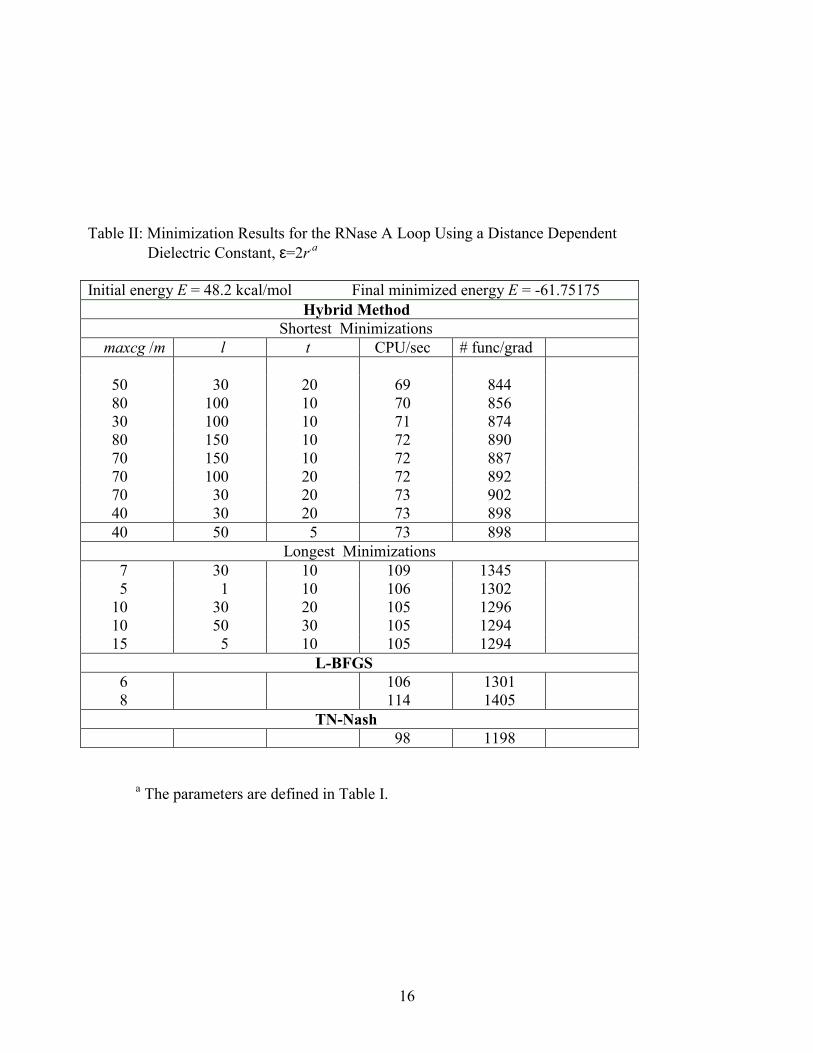
In Table II results are displayed for the same loop, modeled with the AMBER force

field with a distance dependent dielectric constant ε=2Rij, rather than ε=1. The weakened electrostatic interactions for ε=2Rij are expected to lead to a flatter energy surface hence to a decrease in the non-linearity of the energy function, making the minimization procedure easier. Indeed, the shortest minimizations for the hybrid and L-BFGS methods in Table II required slightly less computer time than the corresponding calculations in Table I. Also, the ratio CPU(L-BFGS)/CPU(hybrid) calculated for the shortest minimizations decreased from 1.6 (ε=1) to 1.54 (ε=2Rij), while the corresponding ratio for TN decreased more significany, from 2 (Table I) to 1.42 (Table II) due to a strong decrease in the TN minimization time, from 140 sec CPU (Table I) to 98 sec CPU (Table II). Correspondingly, the difference between the average CPU times required for the shortest and longest minimizations of the hybrid and L-BFGS methods is smaller in Table II than in Table I. In Table II, however, the values of maxcg are significantly larger for the shortest minimizations (40-80) than for the longest ones (7-15). Again, while l > t appears to be a necessary condition for getting the shortest minimizations, it is not a sufficient condition as l > t also occurs for the longest minimizations.

As in Table I, the CPU ratios for the hybrid method minimizations based on

different parameters are close to the corresponding ratios obtained from the numbers of the function/gradient calculated. In Figures 1a and 1b the energy, EAMBER is plotted against the number of iterations k for ε=1 and ε=2Rij respectively, where in Figures 2a and 2b the corresponding results are presented for log(||gk||/||g0||. In both figures the results are displayed for the shortest and longest minimizations. It is interesting to note that while the CPU times and the total number of function/gradient calculations of the shortest minimizations for ε=2Rij and ε=1 are almost the same the number of iterations is significantly different, 105 and 440, respectively, which is clearly demonstrated in the figures. On the other hand, the corresponding numbers of iterations for the longest minimizations are comparable, 560 and 511 even though ~50% more function/gradient calculations are carried out for ε=2Rij.

The results in Table III are for BPTI modeled by AMBER(ε=2Rij). For this

molecule the effect of the muted electrostatic interactions is stronger than for the loop. Thus, while the hybrid method still provides the shortest minimizations, the ratios, CPU(LBFGS, m=5)/CPU(hybrid-shortest) = 1.17 and CPU(TN)/CPU(hybrid-shortest) =

13

1.19 are significantly smaller than the corresponding ratios obtained for the loop in Tables I and II. Correspondingly, relatively low values, 1.59 and 1.2 are obtained for the ratio CPU(hybrid-longest)/CPU(hybrid-shortest), and the same ratio based on the average CPU times of the sets of shortest and longest minimizations, respectively. The ratios of the function/gradient evaluations are similar to the corresponding CPU ratios, and the behavior of the parameters maxcg, l, and t is similar to that observed in Tables I and II. Figures 1c and 2c (for ε=2Rij) show that both EAMBER and log(||gk||/||g0|| reach the minimum in a smaller number of iterations for the shortest minimization than for the longest one, in accord with the result for CPU(hybrid-longest)/CPU(hybrid-shortest) discussed above.

In Table IV we present results for BPTI obtained with a dielectric constant ε=1. While most of the minimizations have found the same energy minimum (-1778.58 kcal/mol), in some cases lower minima were reached (the lowest is �1917.31 kcal/mol) and in two cases higher minima were obtained. In particular, the TN minimum is �1808.23 and therefore for comparison we include in the �longest minimizations� section of the table results for a hybrid method minimization that reached the �1813.84 kcal/mol minimum - the closest to the TN minimum. Again, the shortest minimizations with respect to CPU time obtained by the hybrid method are shorter than those obtained by L-BFGS (a ratio of 941/709=1.33 for the smallest CPU results); however, a most significant advantage of the hybrid method is with respect to TN, where the large CPU ratio, 7673/1524=5.03 is obtained for TN versus the hybrid method minimization that led to �1813.84 kcal/mol. In other words, the advantage of the hybrid method over L-BFGS and TN is more pronounced for ε=1 than for ε=2Rij.

The average CPU ratio of the longest and shortest minimizations is around 1.4,

where the ratio between the worst and best result is 1745/709=2.46; similar values are obtained for the corresponding ratios based on the numbers of the function/gradient evaluations. As in Tables I and II for the loop, all these ratios are larger than their counterparts obtained from Table III using ε=2Rij, which is also in accord with the plots of Figures 1d and 2d for EAMBER and log(||gk||/||g0||), where the difference in the total number of iterations of the shortest and longest minimization is much larger than the corresponding difference in Figures 1c and 2c. It should be pointed out that the values of maxcg, for the shortest minimizations are within the range 25-40 while those for the longest minimizations are significantly smaller ranging from 4-10. The condition l ≥ t appears to be important for obtaining reasonable efficiency, where l = 1and t = 10 have led to the longest minimization (1642 sec), which is significantly larger than the other results for the hybrid method.

We have also carried out minimizations for the loop described by the potential

energy Etot [eq. (2)], which includes the solvation energy calculated by SASA and the best-fit set of ASPs defined in Ref. 49, using a relatively large tolerance of 10-3 [see eq. (4)]. The energy was decreased from-368.848 to �480.167 kcal/mol, but in this case the three methods were found to be approximately equally efficient (~42 sec CPU) and therefore the results are not provided.

In summary, for the two systems studied the hybrid method has been found to be

more efficient than both L-BFGS and TN, where its relative performance increases as the

14

electrostatic interactions increase in going from ε=2Rij to ε=1, enhancing thereby the non-linearity of the energy function. The improvement in computer time is by a factor of 1.3-2, and only for BPTI(ε=1) the minimization with TN required ~5 times more computer time than the best minimization performed with the hybrid method; the three methods have shown comparable efficiency for Etot, which is based on surface area calculations. However, determination of the optimal values of the parameters maxcg, l, and, t is not straightforward, appears to be problem dependent hence requiring experimentation prior to the ``production� minimizations. The advantage of the hybrid method is to a large extent due to the superior preconditioning in the inner C-G iteration of the HFN part.46 Acknowledgments This work was supported by NIH grant R01GM61916. I.M.N acknowledges the support from the NSF grant number ATM-0201808 managed by Dr. Linda Peng whom he would like to thank for her support. Figure Captions Figure 1: Plots of the AMBER force field energy, EAMBER vs. the number of iterations k obtained during the shortest and longest minimizations of the loop [(a) and (b), ε=1 and ε=2Rij, respectively] and BPTI [(c) and (d), ε=2Rij, and ε=1, respectively]. Figure 2: Plots of log(||gk||/||g0||) vs. the number of iterations k obtained during the shortest and longest minimizations of the loop [(a) and (b), ε=1 and ε=2Rij, respectively] and BPTI [(c) and (d), ε=2Rij, and ε=1, respectively].

15

Table I: Minimization Results for the RNase Loop Using Dielectric Constant ε=1.a Initial energy E=-144.3 kcal/mol Final minimized energy E=-286.43377 Hybrid Method Shortest Minimizations (CPU) maxcg/m l t CPU/sec # func/grad 50 200 10 70 836 40 200 10 71 855 60 200 10 74 886 5 200 10 75 897 7 30 20 76 922 7 200 10 78 941 15 200 10 79 947 Longest Minimizations (CPU) 5 1 10 163 1955 5 50 30 123 1489 30 30 10 136 1637 40 150 10 122 1465 80 100 20 130 1566 L-BFGS 8 111 1336 5 133 1593 TN-Nash 140 1672

a Maxcg is the maximum number of CG iterations allowed. t and l are the numbers of HFN and L-BFGS iterations, respectively. A large number of minimizations (~100) were performed for different sets of parameters maxcg, t and l. The fastest and slowest minimizations with respect to CPU time appear in the sections �shortest minimizations� and longest minimizations, respectively. For L-BFGS the fastest and slowest minimizations are provided, where m is the number of iterations considered in the L-BFGS procedure.

16

Table II: Minimization Results for the RNase A Loop Using a Distance Dependent Dielectric Constant, ε=2r.a Initial energy E = 48.2 kcal/mol Final minimized energy E = -61.75175 Hybrid Method Shortest Minimizations maxcg /m l t CPU/sec # func/grad 50 30 20 69 844 80 100 10 70 856 30 100 10 71 874 80 150 10 72 890 70 150 10 72 887 70 100 20 72 892 70 30 20 73 902 40 30 20 73 898 40 50 5 73 898 Longest Minimizations 7 30 10 109 1345 5 1 10 106 1302 10 30 20 105 1296 10 50 30 105 1294 15 5 10 105 1294 L-BFGS 6 106 1301 8 114 1405 TN-Nash 98 1198

a The parameters are defined in Table I.

17

Table III: Minimization Results for BPTI Using a Distance Dependent Dielectric Constant, ε=2r.a Initial energy E = 207.43 kcal/mol Final minimized energy E = -358.03247 Hybrid Method Shortest Minimizations maxcg /m

l T CPU/sec # func/grad

50 200 10 1157 4768 80 200 10 1163 4798 30 200 10 1163 4780 30 150 10 1164 4804 70 200 10 1178 4859 40 200 10 1181 4872 70 150 10 1191 4913 Longest Minimizations 5 1 10 1841 7613 70 30 20 1428 5909 80 50 20 1381 5700 80 100 20 1355 5599 60 30 20 1353 5582 60 50 30 1321 5448 60 100 50 1299 5371 L-BFGS 5 1358 5619 6 1485 6144 TN-Nash 1375 5703 a For explanations, see Table I.

18

Table IV: Minimization Results for BPTI with a Dielectric Constant, ε=1.a Initial energy E = -831.2109 kcal/mol Final minimized energy E = -1778.58093 Hybrid method Shortest Minimizations maxcg /m l t CPU/sec # func/grad 25 30 10 709 2835 30 30 20 743 2970 40 30 30 750 2996 30 100 10 760 3041 25 30 30 763 3049 30 30 13 755 3019 25 25 15 768 3069 25 35 10 780 3124 25 30 20 780 3120 Longest Minimizations 4 1 10 1642 6573 4 10 1 1108 4436 5 10 1 1031 4127 6 10 1 1031 4127 8 10 1 1051 4201 10 10 5 992 3974 7 5 10 1524* L-BFGS 9 941 3761 7 960 3839 TN-Nash 7637* 29709 a For explanations, see Table I. The TN minimum, �1808.23 kcal/mol is lower than the minimum obtained in most of the other minimizations; therefore, for comparison, we include in the �longest minimizations� section of the table results for an hybrid method minimization that reached a close minimum, -1813.84 kcal/mol. Above these results appears an asterisk.

19

20

21

22

23

24

25

26

27

References

1. Vasquez, M.; Nemethy, G.; Scheraga, H.A. Chem Rev 1994, 94, 2183- 2239.

2. Gibson, K.D.; Scheraga, H.A. Physiol Chem Phys 1969, 1, 109- 126.

3. Go, N.; Scheraga, H.A. Macromolecules 1970, 3, 178- 187.

4. Hagler, A.T.; Stern, P.S.; Sharon, R.; Becker, J.M.; Naider, F. J Am Chem Soc 1979, 101, 6842- 6852.

5. Karplus, M.; Kushik, J.N. Macromolecules 1981, 14, 325- 332.

6. Meirovitch, H.; Meirovitch, E.; Lee, J. J Phys Chem 1995, 99, 4847- 4854.

7. Case, D.A. Curr Opin Struct Biol 1994, 4, 285- 290.

8. Baysal, C.; Meirovitch, H. J Phys Chem A 1997, 101, 2185- 2191.

9. Baysal, C.; Meirovitch, H. J Am Chem Soc 1998, 120, 800- 812.

10. Chang, G.; Guida, W.C.; Still, W.C. J Am Chem Soc 1989, 111, 4379- 4386.

11. Kolossvary, I.; Keseru, G.M. J Comput Chem 2001, 22, 21- 30.

12. Lee, J.; Scheraga, H.A.; Rackovsky, S. J Comput Chem 1997, 18, 1222- 1232.

28

13. Li, Z.; Scheraga, H.A. Proc Natl Acad Sci 1987, 84, 6611- 6615.

14. Pillardy, J.; Arnautova, Y.A.; Czaplewski, C.; Gibson, K.D.; Scheraga, H.A. Proc Natl Acad Sci U S A 10-23-

2001, 98, 12351- 12356.

15. Pillardy, J.; Czaplewski, C.; Liwo, A.; Lee, J.; Ripoll, D.R.; Kazmierkiewicz, R.; Oldziej, S.; Wedemeyer, W.J.;

Gibson, K.D.; Arnautova, Y.A.; Saunders, J.; Ye, Y.J.; Scheraga, H.A. Proc Natl Acad Sci U S A 2-27-2001, 98,

2329- 2333.

16. Saunders, M.; Houk, K.N.; , W.Y.D.; Still, W.C.; Lipton, M.; George Chang, G.; Guida, W.C. J Am Chem Soc

1990, 112, 1419- 1427.

17. Saunders, M. J Comput Chem 1991, 12, 645- 663.

18. Vasquez, M.; Scheraga, H.A. Biopolymers 1985, 24, 1437-

19. D. C. Liu and J. Nocedal, On the limited memory BFGS method for large-scale

optimization, Math. Programming 45 (1989), pp. 503--528.

20. Navon, I.M.; Zou, X.; Berger, M.; Phua, K.H.; Schlick, T.; LeDimet, F.X. In: Optimization Technique and

Applications, Vol 1, Phua, K H ed World Scientific: Singapore 1992, 33- 48.

21. Navon, I.M.; Zou, X.; Berger, M.; Phua, K.H.; Schlick, T.; LeDimet, F.X. In: Optimization Techniques and

Applications, Vol 1, Phua, K H ed World Scientific: Singapore 1992, 445- 480.

22. Wang, Z.; Navon, I.M.; Zou, X.; LeDimet, F.X. Comput Opt Appl 1995, 4, 241- 262.

29

23. Zou, X.; Navon, I.M.; Berger, M.; Phua, K.H.; Schlick, T.; LeDimet, F.X. SIAM J Opt 1993, 3, 582- 608.

24. Dembo, R.S.; Eisenstat, S.C.; Steihaug, T. SIAM J Numer Anal 1982, 19, 400- 408.

25. Nash, S.G. Mathematical Sciences Department, Users Guide for TN/TNBC, Report No 397,Johns Hopkins

University, Baltimore, MD 1984, 10pp

26. Schlick, T.; Fogelson, A. ACM Trans Math Software 1992, 18, 46- 70.

27. Schlick, T.; Fogelson, A. ACM Trans Math Software 1992, 18, 71- 111.

28. Navon, I.M.; Brown, F.B.; Robertson, D.H. Comput Chem 1990, 14, 305- 311.

29. Robertson, D.H.; Brown, F.B.; Navon, I.M. J Chem Phys 1989, 90, 3221- 3229.

30. Wang, Z.; Droegemeier, K.; White, L. Comput Opt Appl 1998, 10, 283- 320.

31. Nash, S.G.; Nocedal, J. SIAM J Opt 1991, 1, 358- 372.

32. Schlick, T. Rev Comput Chem, K B Lipkowitz and D B Boyd ed 1992, 3, 1- 71.

33. Derreumaux, P.; Zhang, G.; Schlick, T.; Brooks, B. J Comput Chem 1994, 15, 532- 552.

34. Brooks, B.R.; Bruccoleri, R.E.; Olafson, B.D.; Sates, D.J.; Swaminathan, S.; Karplus, M. J Comput Chem 1983,

4, 187- 217.

35. Xie, D.; Schlick, T. SIAM J Opt 1999, 10, 132- 154.

30

36. Xie, D.; Schlick, T. ACM Trans Math Softw 1999, 25, 108- 122.

37. Nocedal, J. J Acta Numer , Vol 1,1992, 199- 242.

38. Baysal, C.; Meirovitch, H.; Navon, I.M. J Comput Chem 1999, 20, 354- 364.

39. Liu, D.C.; Nocedal, J. Math Prog 1989, 45, 503- 528.

40. Shanno, D.F.; Phua, K.H. ACM Trans Math Software 1980, 6, 618- 622.

41. van Gunsteren, W.F.; Berendsen, H.J.C. Biomos, Nijenborgh 16 9747 AG, Groningen NL 1987,

42. Axelsson, O.; Lindskog, G. Numer Math 1986, 48, 479- 498.

43. Axelsson, O.; Lindskog, G. Numer Math 1986, 48, 499- 523.

44. Morales, J.L.; Nocedal, J. Comput Opt Appl 2002, 21, 143- 154.

45. Alekseev, A.K.; Navon, I.M. Comput Optim Applic 2002, (submitted, in review process)

46. Morales, J.L.; Nocedal, J. SIAM J Optim 2000, 10, 1079- 1096.

47. Cornell, W.D.; Cieplak, P.; Bayly, C.I.; Gould, I.R.; Merz, K.M.Jr.; Ferguson, D.M.; Spellmeyer, D.C.; Fox, T.;

Caldwell, J.W.; Kollman, P.A. J Am Chem Soc 1995, 117, 5179- 5197.

48. Ponder, J.W. St Louis:Washington University 1999, Version 3.7,

49. Das, B.; Meirovitch, H. Proteins 5-15-2001, 43, 303- 314.

31

50. Perrot, G.; Cheng, B.; Gibson.K.D.; Palmer, K.A.; Nayeem, A.; Maigret, B.; Scheraga, H.A. J Comput Chem

1992, 13, 1- 11.

51. Connoly, M.L. J Appl Cryst 1983, 16, 548-

52. Richmond, T.J. J Mol Biol 1984, 178, 63- 89.

53. Gill, P.E.; Murray, W. Report SOL 79-15, Department of Operation Research, Stanford University, Stanford,

CA 1979, 61pp

54. Shanno, D.F. Math Oper Res 1978, 3, 244- 256.

55. Dennis, J.E., Jr.; More, J.J. SIAM Rev 1977, 19, 46- 89.

56. Dennis, J.E., Jr.; Schnabel, R.B. Numerical Methods for Unconstrained Optimization and Nonlinear Equations,

Prentice-Hall: Englewood Cliffs, NJ 1983, 378pp.

57. Nash, S.G. SIAM J Sci Statist Comput 1985, 6, 599- 616.

58. Nash, S.G. SIAM J Numer Anal 1984, 21(4), 770- 778

59. Nash, S.G. SIAM J Sci Statist Comput 1985, 6, 599- 616.

60. Xie, D.; Schlick, T. SIAM J Opt 1999, 10, 132- 154.