II

APPROVAL This project titled “Performance analysis of UMTS cellular network using sectorization

based on capacity and coverage” submitted by Mir Mohammad Abu Kyum, Md. Baitul

Al Sadi, Mrinal Kar to the Department of Electronics and Telecommunication

Engineering, Daffodil International University, has been accepted as satisfactory for the

partial fulfillment of the requirements for the degree of Bachelor of Science in

Electronics and Telecommunication Engineering and approved as to its style and

contents. The presentation was held on February 27, 2011.

BOARD OF EXAMINARS

Dr. Md. Golam Mowla Chowdhury Chairman Professor and Head Department of Electronics and Telecommunication Engineering Daffodil International University

A.K.M Fazlul Haque Internal Examiner Assistant Professor Department of Electronics and Telecommunication Engineering Daffodil International University

Md. Mirza Golam Rashed Internal Examiner Assistant Professor Department of Electronics and Telecommunication Engineering Daffodil International University Dr. Subrata Kumar Aditya External Examiner Professor and Chairman Department of Applied Physics Dhaka University

III

DECLARATION We hereby declare that the work presented in this project report titled “Performance

analysis of UMTS cellular network using sectorization based on capacity and coverage”

is done by us under the supervision of Mr. A.K.M Fazlul Haque, Assistant Professor,

Department of Electronics and Telecommunication Engineering Daffodil International

University, partial fulfillment of the requirements for the degree of Bachelor of Science

in Electronics and Telecommunication Engineering. We also declare that this project is

our original work. As far as our knowledge goes, neither this report nor any part there has

been submitted elsewhere the award of any degree or diploma.

Supervised by:

A.K.M Fazlul Haque Assistant Professor Department of Electronics and Telecommunication Engineering Daffodil International University

Submitted by:

Mir Mohammad Abu Kyum ID: 071-19-619 Department of Electronics and Telecommunication Engineering Daffodil International University Md. Baitul Al Sadi ID: 071-19-592 Department of Electronics and Telecommunication Engineering Daffodil International University Mrinal Kar ID: 071-19-630 Department of Electronics and Telecommunication Engineering Daffodil International University

IV

ACKNOWLEDGEMENTS

First of all we would like to express our deepest gratefulness to Almighty ALLAH for

HIS kindness, for which we successfully completed our project within time and also

apologize to HIM for our any kind of mistakes.

Then we would like to express our gratefulness to our supervisor, Asst. Professor A.K.M

Fazlul Haque Department of ETE, Daffodil International University for his excellent

guidance and valuable comments on simulations and background studies. His wise

advices and dedicated efforts always encouraged us throughout the project work.

We would like to thank Dr. Lutfur Rahman, Professor and Dean, Faculty of science and

information technology, Dr. Md. Golam Mowla Chowdhury Professor and Head,

Department of Electronics and Telecommunication Engineering, Daffodil International

University, Md. Mirza Golam Rashed, Asst. Professor, Department of Electronics and

Telecommunication Engineering, Daffodil International University for all the technical

support, knowledge and shared experience..

And finally we would like to thank our parents and family members for all the strength

they gave us for this journey during the time of completing this project.

Mir Mohammad Abu Kyum

Mrinal Kar

Md. Baitul Al Sadi

V

TABLE OF CONTENTS

CONTENTS PAGES

Board of Examiners II

Declaration III

Acknowledgements IV

List of Figures VII

List of Tables X

Abstract XI

CHAPTER

Chapter-1: Introduction 1

1.1 General Introduction 1

1.2 Previous Work 2

1.3 Objective of the present work 3

1.4 Organization of the project 3

Chapter-2: Early Cellular Systems and their Capacity 5 2.1 Early Cellular Systems 5

2.1.1 First Generation Systems 5

2.1.2 Second Generation Systems 5

2.1.3 Third Generation Systems 6

2.1.3.1 The cdma2000 (USA) 6

2.1.3.2 IMT-2000 (Europe) 7

2.1.3.3 IMT-2000 radio interfaces 8

2.2 Capacity of Early Cellular Systems 8

2.2.1 Capacity in AMPS System 9

2.2.2 Capacity in GSM System 10

Chapter-3: UMTS Cellular Network Architecture 11

3.1 UMTS Network Topology 11

3.2 GSM Network Architecture 11

3.3 UMTS Architecture with Overlay GSM 12

3.4 UMTS Network Architecture 13

VI

CONTENTS PAGES

Chapter-4: Interference analysis in UMTS Cellular Systems 14

4.1 Signals-to-Interference Ratio (SNR) 14

4.2 Interference 15

4.2.1 Intra-cell Interference 15

4.2.2 Inter-cell interference 16

Chapter-5: Capacity analysis in UMTS Cellular System 19

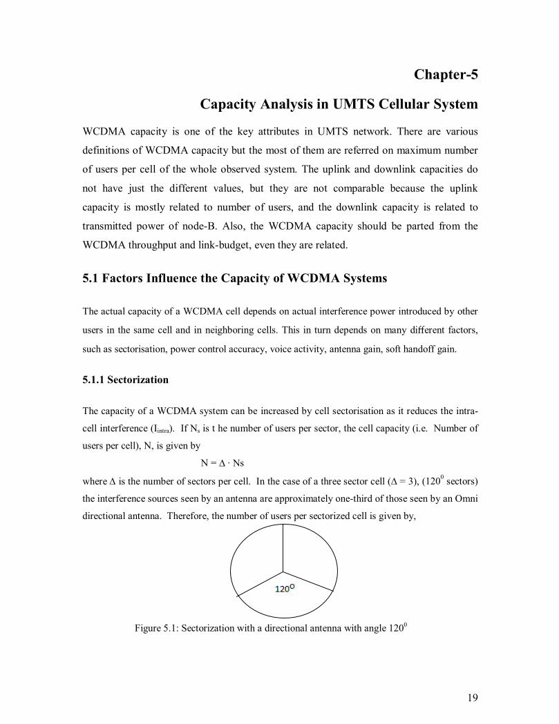
5.1 Factors Influencing the Capacity of CDMA Systems 19

5.1.1 Sectorization 19

5.1.2 Tilted Antenna 20

5.1.3 Channel Activity, 20

5.1.5 Outer-cell Interference factor 21

5.1.6 Soft Handover 21

5.2 Capacity of cellular WCDMA 22

5.2.1 Uplink Capacity calculation in WCDMA 22

Chapter-6: Radio Propagation Model 25

6.1 Characteristics 25

6.2 Development Methodology 25

6.2.1 Okumura Model 26

6.2.1.1 Coverage 26

6.2.1.2 Mathematical formulation 26

6.2.2 COST 231 Model 26

6.2.2.1 Applicable Conditions 27

6.2.2.2 Coverage 27


6.2.3 Hata Model 28

6.2.3.1 Coverage 28


Chapter-7: Coverage analysis in UMTS Cellular System 29

7.1 Factors influence in Coverage 29

VII

CONTENTS PAGES

7.2 Relationship between Coverage and Capacity 33

7.3 Multi Service Case 35

Chapter-8: Simulation and Result 37

8.1 Algorithm for Capacity Analysis Using Sectorization 37

8.2 Algorithm for Coverage and data rates Analysis Using Sectorization 38

8.3 Performance Analysis in Capacity Using Sectorization for UMTS 40

8.4 Performance Analysis in Coverage and data rates Using Sectorization 46

for UMTS

8.5 Graphical Representation 47

Chapter-9: Conclusion 56

References 57

VIII

LIST OF FIGURES FIGURES PAGES

Figure 2.1: Illustration of (a) Multicarrier and 6

(b) Direct spread downlink for cdma2000

Figure 2.2: Spectrum allocation for WCDMA 7

in Europe, Japan, Korea and USA

Figure 2.3: IMT-2000 radio interfaces 8

Figure 2.4: Channel allocation in 7-cell cluster system. 9

Figure 2.5: GSM spectrum allocation. 10

Figure 3.1: GSM reference network 11

Figure 3.2: UMTS reference network 13

Figure 4.1: Interference from same cell 15

Figure 4.2: (a) Geometry of the system model for interference evaluation 16

(b) Ring cellular coordinate system 17

Figure 5.1: Sectorization with a directional antenna with angle 1200 19

Figure 5.2: Tilted antenna cell coverage 20

Figure 5.3: UE in Soft handover 22

Figure 7.1: UMTS cell 33

Figure 7.2: Different Class of services Vs Maximum Distance 36

Figure 8.1: Numbers of Simultaneous voice users vs. Eb/No in different 48

sectorized cell

Figure 8.2: Numbers of Simultaneous 64 kbps users vs. Eb/No in 48

different sectorized cell

Figure 8.3: Numbers of Simultaneous 144 kbps users vs. Eb/No 49

in different sectorized cell

Figure 8.4: Numbers of Simultaneous 384 kbps users vs. Eb/No 49


Figure 8.5: Numbers of Simultaneous 2 mbps users Vs Eb/No in 50


Figure 8.6: Numbers of Simultaneous users vs. Inter-cell interference 50

in non-sectorized cell

IX

FIGURES PAGES

Figure 8.7: Numbers of Simultaneous 384 kbps users vs. Intercell 51

interfrence in sectorized cell

Figure 8.8: Numbers of Simultaneous users vs. soft handover 51

in non- sectorized cell

Figure 8.9: Numbers of Simultaneous users vs. soft handover in 52


Figure 8.10: No of Simultaneous Users vs. Voice activity factor 52


Figure 8.11: Coverage Vs Capacity for Dense Urban Using COST 231 Model 53

Figure 8.12: Coverage vs. bit rates for Dense Urban Using 53

COST 231 Model in sectorized cell

Figure 8.13: Coverage Vs Capacity for Urban Using 54

COST 231 Model

Figure 8.14: Coverage vs. data rates for Urban Using COST 231 54

Model in sectorized cell

X

LIST OF TABLES

TABLES PAGES

Table 2.1: Main WCDMA features 8

Table 2.2: Basic air interface parameters of GSM 10

Table 5.1: Reverse link inter-cell interference calculation 17

Table 7.1: Typical Eb/No 32

Table 7.2: K values for the site area calculation 35

Table 7.3: Different Class of services 35

Table 8.1: Simulated Numbers of Simultaneous 384 kbps 40

Users vs. Eb/No in UMTS cell

Table 8.2: Simulated Numbers of Simultaneous 144 Kbps 41




Table 8.4: Simulated Numbers of Simultaneous 12.2 kbps 43

or voice Users vs. Eb/No in UMTS cell


Users vs. Intercell Interference in UMTS cell

Table 8.6: Simulated Numbers of Simultaneous Voice 45

Users vs. Voice activity factor in UMTS cell

Table 8.7: Simulated No. of Simultaneous 384 kbps 46

Users vs. soft handover factor in UMTS cell

Table 8.8: Simulated Coverage Vs Data rates in Dense 47

Urban Cell using COST 231 Model

Table 8.9: Simulated Coverage Vs Data rates in Urban 48

Cell using COST 231 Model

XI

Abstract

UMTS is one of the standards in 3rd generation partnership project (3GPP).Different data

rates are offered by UMTS for voice, video conference and other services. This project

presents the performance analysis of UMTS cellular network using sectorization based on

capacity and coverage. The major contribution is to see the impact of sectorization on

capacity and cell coverage in 3G UMTS cellular network. Coverage and capacity are very

much important issue in UMTS cellular Network. Capacity depends on different

parameters such as Sectorization, Energy per bit noise spectral density ratio, Voice

activity, Inter-cell interference and Intra-cell interference, Soft handoff gain, etc and

coverage depends on Frequency, Chip rate, Bit Rate, Mobile Maximum Power, MS

Antenna Gain, EIRP, Interference Margin, Soft Handover Gain, Noise figure etc.

Different parameters that influence the capacity and coverage of UMTS cellular network

are simulated using MATLAB 6.5.0.180913a with increasing sectors. In this project, the

outputs of simulation for increasing amount of sectorization showed that the number of

users was gradually increased. Also for increasing amount of sectorization showed that

the coverage area was gradually increased.

1

Chapter-1

Introduction

1.1 General Introduction

WCDMA is one of the standards of UMTS cellular network. One of the main issues of

UMTS cellular network is capacity.WCDMA capacity is one of the key attributes in

UMTS network. There are various definitions of WCDMA capacity but the most of them

are referred on maximum number of users per cell or of the whole observed system. In

another word the capacity of a WCDMA network is the maximum number of

simultaneous users for all services which satisfy certain conditions.

The uplink and downlink capacities do not have just the different values, but they are not

comparable because the uplink capacity is mostly related to number of users, and the

downlink capacity is related to transmitted power of node-B. Also the WCDMA capacity

should be parted from the WCDMA throughput and link-budget, even they are related.

This work paper will try to comprise different parameters and relations which affect on

WCDMA capacity.

The WCDMA capacity is basically determined by processing gain and required signal-to-

noise ratio. The interference is already included in noise power density and it comprises

the Multiple Access Interference (MAI), (interference of other users from observed,

home cell and interference of users from the adjacent cell), self interference and co-

channel interference.

Another main issue of UMTS cellular network is capacity. The area covered by RF signal

from Node B or BTS is called UMTS coverage area. To calculate coverage area: We

have to calculate the propagation loss or path loss for different environment for urban,

dense urban then the allowable path loss by Node B.

The propagation predictions for WCDMA require the same planning phases as in GSM.

First, the base station configuration and the link budget have to be defined. Also, the

coverage threshold has to be well defined to exceed the required quality criteria but avoid

unnecessary additional investments for the radio network elements. Moreover, the

2

capacity targets and forecasts have to be well known at this phase because they have a

strong effect on the base station coverage area.

1.2 Previous Work

In mobile communications systems (MCS), signals are transmitted through multipath

mixed-phase time variant channels. Mobile multipath channels have non-desirable impact

on the transmitted signal, including inter-symbol interference (ISI) and channel

variations. a GSM cellular phone moving at 3 Km/h (for a frequency carrier of 1800

MHz) result in doppler shift of 500 Hz which leads to coherence time of nearly 0.8 ms

(corresponding to more than 200 symbols in GSM).Taking into account that a typical

GSM half-burst contains approximately 60 symbols, this implies non-negligible channel

variation during the equalization process. Blind non-cooperative equalization methods

have been applied to burst MCS in order to obtain satisfactory performance without using

any training symbols [1] but they lack robustness to channel overestimation, among

others [2]. HOS approaches were first used for blind equalization but they usually need a

large number of samples compared to SOS-based methods, so their applicability in fast

fading environments is limited because statistics cannot be assumed stable, even along

the (short) burst L. Tong et al introduce in the SOS in [3] blind equalization/estimation

through to the extraction of spatial or temporal diversity, leading to the SIMO models.

Different SOS methods have been studied in literature, like subspace methods [3] [4] or

maximum likelihood methods [5] [6].In general, maximum likelihood (ML) method are

attractive to their good near asymptotic performance and relative simplicity. Among

these, Statistical ML (SML) approaches achieve the best performance though at the cost

of local minima in the minimization problem. Conversely, the deterministic ML (DML)

approaches [5] [1] leads to poor performances at low SNR since the method does not

make use of any knowledge of the source. This lack of performance prevents the use of

these methods in typical mobile scenarios. Conditional ML(CML)methods have also

been proposed [5] [2] these method are a tradeoff between SML and DML approaches,

since they use approaches can be viewed as special cases of this CML approach which

leads to a good tradeoff between the asymptotic performances when the process is

initialized close to the global minimum, and the number of local minima. The 3rd

3

generation Partnership Project (3GPP) specifies the speed (depending on the carrier

frequency) between the transmitter and receiver under which the system should be

guarantee a certain level of performance. Bo Hagerman, Davide Imbeni and Jozsef Barta

considered WCDMA 6-sector Deployment Case Study of a Real Installed UMTS-FDD

Network [7]. Romeo Giuliano, Franco Mazzenga, Francesco Vatalaro described Adaptive

Cell Sectorization for UMTS Third Generation CDMA Systems. Achim Wacker, Jaana

Laiho-Steffens, Kari Sipila, Kari Heiska considered the impact of the base station

sectorisation on WCDMA radio network performance. S. Sharma, A.G. Spilling and

A.R. Nix considered Adaptive Coverage for UMTS Macro cells based on Situation

Awareness [8].

1.3 Objective of the Present Work

i) To analysis how sectorization affects the capacity of UMTS cellular network

which depends on energy per bit noise spectral density ratio, outer cell interference

factor, soft handover factor, voice activity factor and also processing gain.

ii) To analysis how sectorization affects the coverage of UMTS cellular network which

depends on data rates for propagation environment such as dense urban and urban case.

1.4 Organization of the Project

Chapter 1 reviews on the Introduction of this project, definition of capacity and coverage

of UMTS cellular network and how channel parameters are impacts capacity and

coverage of UMTS cellular network.

Chapter 2 reviews on the multiple access techniques, this chapter also highlights early

cellular system and their capacity.

Chapter 3 reviews on the basic architecture of UMTS cellular network with overlay

GSM network, architecture.

4

Chapter 4 reviews on the intra-cell interference and outer-cell interference of UMTS

cellular network

Chapter 5 reviews on the capacity calculation of UMTS cellular network, this chapter

also shows how various parameters related in capacity calculation.

Chapter 6 reviews on the various propagation environment which are related on

coverage prediction

Chapter 7 reviews on the coverage of UMTS cellular network, this chapter shows a

relationship on coverage and data rates

Chapter 8 reviews on the simulation of capacity and coverage under various parameters

from related equation, these chapters’ shows, how sectorization has major impacts on

coverage and capacity of UMTS cellular network

Chapter 9 brings out on the significant conclusion of the entire work

5

Chapter-2

Early Cellular Systems and their Capacity

2.1 Early Cellular Systems

Early cellular systems were all analog systems and need FDMA with Frequency Division

Duplexing (FDD). The systems were designed to handle voice and the voice signal was

frequency modulated. Part of UHF spectrum was utilized to cover sizable areas in today’s

terms could be categorized as macro cells. The capacity was not a main issue in these

systems as demand was not great.

2.1.1 First Generation Systems

The first successful cellular mobile communication system was the Advanced Mobile

Phone Service (AMPS) developed in USA in 1970s. It used FDMA technology with FDD

and employed 20 MHz bandwidth in the 800 MHz region. AMPS at present operates with

a 25 MHz bandwidth in each direction over the frequency allocations of 824-849 MHz

for the Uplink (UL) (from mobile to base station), and 869-894 MHz for the Downlink

(DL) (from base station to mobile) [9]. This spectrum is divided into 832 frequency

channels leaving 416 channels in the uplink and another 416 channels in the downlink.

Some of these channels are used to carry system information and control signal while the

rest carries voice and data in analog form. In AMPS, each channel occupies 30 kHz of

bandwidth using analog Frequency Modulation (FM) [9]. TACS, NMT and AMPS are

among the first generation cellular systems.

2.1.2 Second Generation Systems

In the second generation cellular systems, digital technology enabled the use of signal

processing techniques to increase the robustness against interference. It also reduced the

spectral bandwidth required for each user and hence provided a higher capacity. The

second generation systems provide about 3 to 4 times the capacity of the first generation

6

system for the same spectral resource without adding new base stations. Since digital

systems are more immune to noise, an Interference-to-Signal (ISR) ratio of about 15 dB

is acceptable in digital systems (whereas 18 dB is required for the analog systems under

same circumstances [10]). This allowed the use of smaller reuse clusters, thereby

increasing the capacity of the system.

The second generation cellular mobile systems were based on Time Division Multiple

Access (TDMA) technology, or a combination of TDMA and FDMA.

In 1990, Qualcomm, Inc., proposed a digital cellular telephone system based on Code

Division Multiple access (CDMA) technology. In July 1993, the second U.S digital

cellular standard (IS-95) was adopted. Using spread spectrum techniques, the IS-95

system provides a very high capacity [9].

2.1.3 Third Generation Systems

2.1.3.1 The CDMA2000 (USA)

Within the standardization committee of Telecommunications Industry Association

(TIA), the subcommittee TR45.5.4 was responsible for the specifications of the basic

cdma2000 scheme [11]. That is at least 144 Kbps in a vehicular environment, 384 Kbps

in a pedestrian environment, and 2048 Kbps for indoor office environment. The main

focus of standardization has been to provide 144 Kbps and 384 Kbps bit rates with

approximately 5 MHz bandwidth.

For the direct spread option, transmission on the downlink is achieved by using normal

chip rate of 3.6864 Mcps [11].

Figure 2.1: Illustration of (a) multicarrier and (b) direct spread downlink for cdma2000

The starting point for bandwidth design for cdma2000 has been the PCS spectrum

allocation in the United State. The PCS spectrum is allocated in 5 MHz blocks and 15

MHz blocks. One 3.6864 Mcps carrier can be deployed within 5 MHz spectrum

7

allocation including guard bands. For a 15 MHz block, three 3.6864 Mcps carriers and

one 1.2288 Mcps carrier can be deployed [11] [12].

2.1.3.2 IMT 2000 (Europe)

The Europe Telecommunications Standards Institute (ETSI) has been working on the

Universal Mobile Telecommunication Services (UMTS), which is to be the European

standard for the third generation mobile systems. UMTS will appear as one of the family

members within the IMT2000 family. UMTS will utilize the GSM network interfaces as

the basis for its network interfaces and proposals. The current GSM network capabilities,

which include General Packet Radio Service (GPRS), High Speed Circuit Switched Data

(HSCSD), and Customized Application for Mobile Enhanced service Logic (CAMEL),

will be enhanced to support UMTS capabilities in terms of services like virtual home

environment and multimedia, as well as higher bit rates [12].

Figure 2.2: Spectrum allocation for WCDMA in Europe, Japan, Korea, and USA [13].

The spectrum allocation for WCDMA in Europe, Japan, Korea, and USA is shown in Fig.

2.5[13]

In Europe and in most of Asia, the International Mobile Telecommunication (IMT)-2000

band consists of 2×60 MHz (1920 -1980 MHz plus 2110-2170 MHz). In Japan and

Korea, the IMT-2000 FDD band is the same as that of the rest of Asia and Europe.

8

Table 2.2 summarizes the main features related to the WCDMA air interface [13].

. 2.1.3.3 IMT 2000 Radio Interfaces

Figure shows the radio interface of IMT-2000.The first one and the second one are

established from CDMA .The third one is established from a combination of CDMA and

TDMA. The fourth one is established from a TDMA, The last one is established with

both FDMA and TDMA

Figure 2.3: IMT-2000 radio interfaces [14]

2.2 Capacity of Early Cellular Systems

The capacity of first and second generation cellular mobile systems was governed by the

available number of RF channels within the allocated spectrum. Once the acceptable

grade of service (GoS) is specified, the amount of traffic that could be offered in the

system with the given number of channels is determined, and this has set a hard limit on

the system capacity. The GoS in turn is determined by the signal to interference (or

carrier-to-interference) ratio of the system.

Multiple access method Direct sequence Code Division Multiple Access

Duplexing method Frequency Division Duplex/Time Division Duplex

BS synchronization Asynchronous Chip rate 3.84 Mcps

Frame length 10 ms

Multirate Concept Variable spreading factor and multicode

9

2.2.1 Capacity in AMPS System

The AMPS cellular system at 850 MHz is a high capacity system. There are two separate

frequency bands, adjacent to each other, each band providing 416 channel pairs, having

30 KHz channel separation [15]. Out of 416 channels, 21 channels are designated as

control channels. Control channels are used for call setup and management. The

remaining channels (395) are used as voice channels. Channel assignment is based on the

following sequence: (K, K + 7, K + 14 ...) where K is the cell number (K = 1, 2... 7 for 7-

cell cluster). The channel grouping scheme is shown in Table 1.3 and the corresponding

cell cluster is shown in Fig. 2.6, as seen in Fig. 2.6 that the minimal separation (DS)

required between two nearby

Figure 2.4: Channel allocation in 7-cell cluster system.

Co-channel cells are based on specifying a tolerable co-channel interference, which is

measured by the carrier-to-interference ratio (CIR). The CIR is also a function of

minimum acceptable voice quality of the system. The CIR of AMPS is defined [16] as,

úúû

ù

êêë

é÷øö

çèæ=÷

øö

çèæ

g

RDs

jIC

AMPS

1log10

where j is the number of co-channel cells (j = 1, 2,.., 6), γ is the propagation exponent,

DS is the frequency reuse distance, and R is the cell radius. The co-channel interference

reduction factor, qs, is defined as,

R

Dsq s =

With γ= 4, Ds = 4.6, and j = 6, the CIR becomes

dbI

C

AMPS

18=÷øö

çèæ

10

2.2.2 Capacity in GSM System

Figure 2.9: GSM spectrum allocation.

GSM uses a Time Division Multiple Access (TDMA) with Frequency Division Duplex

(FDD) technique on a total of 125 carrier pairs in the 900 MHz band as shown in Fig. 2.9.

Each carrier conveys 8 time divided channels making a total of 125×8=1000 channels.

The GSM used Gaussian minimum shift keying (GMSK) modulation with a bandwidth-

to-bit-period product (B.T) of 0.3. The spectrum of this signal is tailored to enable it on a

radio frequency carrier of 200 KHz bandwidth. The TDMA frame is produced by

multiplexing eight channel encoded speech sources in time division. Eight timeslots each

of duration 0.577 ms make up one TDMA frame of 4.62 ms and is transmitted on the

radio path at a bit rate of 270.833 kbps [17]. The salient features of the air interface of

GSM system are shown in Table 2.4.

Table 2.3: Basic air interface parameters of GSM

Feature Parameter

Channel Spacing 200 KHz

Modulation GMSK

Modulation depth B.T=0.3

Data transmission rate 270 Kbps

User data rate (Nominal) 16 kbps or 12.2 Kbps

TDMA frame period 4.62 ms

Time slot duration 0.57 ms

11

Chapter-3

UMTS Cellular Network Architecture

3.1 UMTS Network Topology

When deploying a WCDMA network, most operators already have an existing 2G

network. WCDMA was intended as a technology to evolve GSM network toward 3G

services. Paralleling that evolution, this chapter first discusses GSM networks, then

highlights the changes that are necessary to migrate to Release 99 of the WCDMA

specification. The discussion then moves on to Release 5 of the specification and the

network changes needed to support HSDPA.

3.2 GSM Network Architecture

Figure 3.1 illustrates a GSM reference network, showing both the nodes and the

interfaces to support operation in the CS and PS domains.

Figure 3.1: GSM reference network [18]

In this reference network, three sub-networks [18] can be defined:

12

• Base Station Sub-System (BSS) or GSM/Edge Radio Access Network (GERAN).

This sub-system is mainly composed of the Base Transceiver Station (BTS) and Base

Station Controller (BSC), which together control the GSM radio interface – either from

an individual link point of view for the BTS, or overall links, including the transfers

between links (aka handovers), for the BSC.

• Network and Switching Sub-System (NSS).

This sub-system mainly consists of the Mobile Switching Center (MSC) that routes calls

to and from the mobile. For management purposes, additional nodes are added to the

MSC, either internally or externally. For all practical purposes, the MSC and GMSC are

differentiated only by the presence of interfaces to other networks, the Public Switched

Telephone Network (PSTN) in the GMSC case. Typically, the MSC and the GMSC are

integrated. The interfaces listed (E, F, C, D) are not detailed here but mostly enable the

communication between the different nodes as shown.

• General Packet Radio Service, Core Network (GPRS-CN).

Within the NSS, two specific nodes are introduced for the GPRS operation: the Serving

GPRS Support Node (SGSN) and the Gateway GPRS Support Node (GGSN). In the PS

domain, the SGSN is comparable to the MSC used in the CS domain. Similarly, in the PS

domain, the GGSN is comparable to the GMSC used in the CS domain.Figure 3.1 also

shows the Border Gateway (BG) that supports interconnection between different GPRS

networks to permit roaming, and the PCU to manage and route GPRS traffic to the BSS.

3.3 UMTS Architecture with Overlay GSM

As mentioned earlier, UMTS is based on the GSM reference network and thus shares

most nodes of the NSS and General Packet Radio Service, Core Network (GPRS-CN)

sub-systems. The BSS or GERAN is maintained in the UMTS reference network as a

complement to the new Universal Terrestrial Radio Access Network (UTRAN), which is

composed of multiple Radio Network Systems (RNS) as illustrated in Figure

13

2.2.Compared to the GSM reference network, the only difference is the introduction of

the Radio Network Controller (RNC) and Node Bs within the newly formed RNS. From

a practical standpoint, the common nodes between GSM and UMTS would actually be

duplicated, with the original nodes supporting the 2G traffic and the added nodes

supporting the 3G traffic.

3.4 UMTS Network Architecture

The initial deployments of WCDMA networks comply with Release 99 of the standard

[18]. This standard, or family of standards, began to evolve even before being fully

implemented, to address the limitations of the initial specifications as well as to include

technical advancements. At a higher level, migrating from Release 99 to Releases 4, 5,

and then 6 does not change the structure of the network. In addition, the layering changes

in Release 5, to support HSDPA and Node B scheduling.

Figure 3.2: UMTS reference network [18]

14

Chapter-4

Interference analysis in UMTS Cellular Systems

Due to increasing demand in cellular mobile communications, the efficient use of

spectrum resource to maximize system capacity remains an important issue in system

design. The capacity of a WCDMA cellular network is determined by the amount of co-

channel interference it can tolerate.

4.1 Signals-to-Interference Ratio (SNR)

In digital systems, we are primarily interested in the link metric called Eb/No or energy

per bit to noise power spectral density ratio. This quantity can be related to the

conventional Signal-to-noise-Ratio (SNR) by recognizing that energy per bit equates to

the average signal power allocated to each bit duration, such that

STE b =

where S is the average signal power and T is the time duration of bit. We can further

analyze by substituting the bit rate Rb, which is the inverse of bit duration T

b

b RSE =

The noise-power-spectral-density No, is the total interference power I divided by the

transmission bandwidth W, i.e,

W

IN o =

The total interference power I at the Base Station (BS) receiver could be defined as

h++= erra III intint

=Same cell interference power + other cell interference power +

background thermal noise power

Therefore ÷÷ø

öççè

æ÷øö

çèæ=÷

øö

çèæ

b

b

RW

IS

NoE

The ratio W/Rb is known as the processing gain of the system. Therefore, in general, we

can write,

15

b

ob

erra RWNE

IIIS

IS

//

intint

=++=

=÷øö

çèæ

h

where S is the received signal power. The power control in the uplink is used to ensure

that the power received at the BS from every mobile user is the same. Iintra and Iinter will

be discussed in the next section.

4.2 Interference

As mentioned previously the interference consists of intra-cell interference, inter-cell

interference, and background noise due to thermal activity.

4.2.1 Intra-cell Interference

The same-cell (Iintra) interference on the reverse link consists of the superposition of

signals from other mobile stations (MSs) at the base station (BS) receiver. Almost all of

the noise received at the BS receiver is due to interference signals. The system capacity is

maximized by making each signal power of the same at the BS and as low as possible

while achieving satisfactory link performance [19]. Let N denote the number of mobile

users per cell (or sector). Assume that S is the signal power received by a cell BS when

perfect power control is in place, so that this value is the same for every mobile in the

same cell Figure

Figure 4.1: Interference from same cell

The interference from the intra-cell mobiles is equal to,

)1(int -= NSI ra

16

Thus given N mobile users per cell, the total intra-cell interference is never greater than

S(N -1).

But this interference is reduced further with the employment of the voice activity factor

[20] [21].

4.2.2 Inter-cell interference

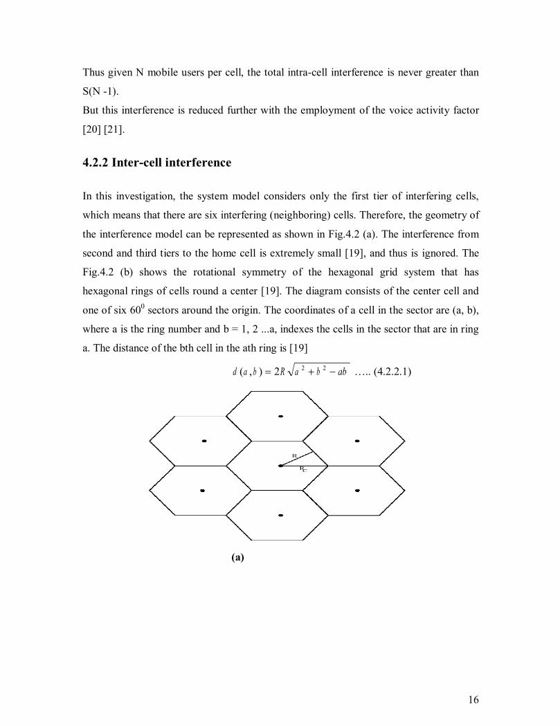
In this investigation, the system model considers only the first tier of interfering cells,

which means that there are six interfering (neighboring) cells. Therefore, the geometry of

the interference model can be represented as shown in Fig.4.2 (a). The interference from

second and third tiers to the home cell is extremely small [19], and thus is ignored. The

Fig.4.2 (b) shows the rotational symmetry of the hexagonal grid system that has

hexagonal rings of cells round a center [19]. The diagram consists of the center cell and

one of six 600 sectors around the origin. The coordinates of a cell in the sector are (a, b),

where a is the ring number and b = 1, 2 ...a, indexes the cells in the sector that are in ring

a. The distance of the bth cell in the ath ring is [19]

abbaRbad -+= 222),( ….. (4.2.2.1)

(a)

17

Figure 4.2 (a) Geometry of the system model for interference evaluation (b) Ring

cellular coordinate system [19].

From equation (4.2.2.1), the normalized distance of an interfering cell is,

abbaR

badr ba -++== 22, 2),( ……. (4.2.2.2)

Table4.1: Reverse link intercell interference calculation [19]

a=Ring b d=(a,b)/R I 1 0 2 0.2844 2 0

1 4

2√3 0.2940 0.3120

3 0 1 2

6 2√7 2√7

0.3138 0.3168 0.3198

.

.

.

.

.

.

.

.

.

.

.

. 100 0

.

. 100

20 . .

2√9001

.

.

. 0.33

18

( )barr

a

b

n

a rrr

rrrI

,

22

2

2

22

11 12164

1ln22

=

== úúû

ù

êêë

é÷÷ø

öççè

æ

-

+--

-= åå …… (4.2.2.3)

Using (4.2.2.3) and (4.2.2.4), it is possible to evaluate n tiers of interfering cells.

According to [19], a 100 tier evaluation shows that only the interference from first tier

has a significant effect (Table 4.1).

It shows that the first tier interference is approximately 28.4% of intra-cell interference

and the total interference from 100 tiers is approximately 33% of the intra-cell

interference. Thus the contribution to interference from the second and higher tiers is

extremely small compared to that of the first tier.

19

Chapter-5

Capacity Analysis in UMTS Cellular System

WCDMA capacity is one of the key attributes in UMTS network. There are various

definitions of WCDMA capacity but the most of them are referred on maximum number

of users per cell of the whole observed system. The uplink and downlink capacities do

not have just the different values, but they are not comparable because the uplink

capacity is mostly related to number of users, and the downlink capacity is related to

transmitted power of node-B. Also, the WCDMA capacity should be parted from the

WCDMA throughput and link-budget, even they are related.

5.1 Factors Influence the Capacity of WCDMA Systems

The actual capacity of a WCDMA cell depends on actual interference power introduced by other

users in the same cell and in neighboring cells. This in turn depends on many different factors,

such as sectorisation, power control accuracy, voice activity, antenna gain, soft handoff gain.

5.1.1 Sectorization

The capacity of a WCDMA system can be increased by cell sectorisation as it reduces the intra-

cell interference (Iintra). If Ns is t he number of users per sector, the cell capacity (i.e. Number of

users per cell), N, is given by

N = ∆ · Ns

where ∆ is the number of sectors per cell. In the case of a three sector cell (∆ = 3), (1200 sectors)

the interference sources seen by an antenna are approximately one-third of those seen by an Omni

directional antenna. Therefore, the number of users per sectorized cell is given by,

Figure 5.1: Sectorization with a directional antenna with angle 1200

20

Sectorization is proposed as a method of increasing the system capacity in WCDMA

cellular systems.

5.1.2 Tilted Antenna

Tilted antenna is another technique that can be used to improve the system

capacity. The tilted antenna generally reduces the interference (Fig.5.2) by controlling the

range of coverage over a sector. This is because the main beam when tilted does not

deliver as much power towards other BS as it normally does, and therefore most of the

radiated power is directed to an area where it is intended [16]. However, the tilted

antenna will shrink the coverage area .It causes the signal strength to be less at the mobile

Figure 5.2: Tilted antenna cell coverage.

5.1.3 Channel Activity

Techniques for digital speech concentration such as digital speech interpolation (DSI)

take account of the activity factor to reduce the number of mobile channels required to

transmit a given number of channels.

As the silences between syllables, words and phrases increase so does the unoccupied

time.

21

In practice, the vocoder (such as the one used in IS-95 (CDMA) system) is a

variable rate vocoder, which means that the output bit rate of the vocoder is

adjusted according to a user’s speech pattern .

Therefore WCDMA system can take advantage in voice transmission in that the

interference can be further reduced with the use of voice activation. The studies have

shown that a speaker is active only for about 35% to 40% of the time [22]. We assume

that the voice activity factor, υ = 37.5% or 3/8, throughout, this investigation.

5.1.4 Outer-cell Interference Factor

In CDMA 100% frequency reuse can be employed therefore in WCDMA,all neighboring

cells can use the same spectrum.therefore,for a given level of interference Ix originating

within a cell, there is additional interference originating outer side of the cell. For signal

propagation loss that follows an n=4th power exponent law, this interference is Estimated

at about 55% of the within-cell interfence.the total interference is therefore approximately

1.55 Ix resulting in a user capacity degradation factor Ho of about 1.55(1.9db)[18].

5.1.5 Soft Handover

Because of universal frequency reuse, the connection of a Mobile Station (MS, or

generally UE in WCDMA) to the cellular network can include several radio links. When

the UE is connected to more than one cell, it is said to be in soft handover [23]. If, in

particular, the UE has more than one radio link to multiple cells on the same site, it is in

softer handover. Soft handover is a form of diversity, increasing the signal-to-noise ratio

when the transmission power is constant. It helps to minimize the transmission power

needed in both uplink and downlink. It has two basic characteristics:

- Soft handover gain (ca. 1 to 2 dB applicable in the power budget) due to the proper

combination of two or more signal branches

22

-Soft handover overhead due to the fact that the UEs in the handover area are connected

to more than one cell. The overall scenario should be clear from Figure

Figure 5.3: UE in Soft handover [24]

This overhead should be kept within reasonable limits to save the downlink traffic

capacity of the cell. The usual reasonable or maximum acceptable value in CDMA

networks (already applying to IS-95 and expected also for WCDMA) is 20–30% – i.e.,

1.2 to 1.5[24] radio links per user connection. We have used 1.5[15]

5.2 Capacity of Cellular WCDMA for UMTS

The capacity of WCDMA system is interference limited, while it is bandwidth limited in

FDMA and TDMA.Therefore, any reduction in the interference will cause a linear in the

capacity of WCDMA.Put another way in WCDMA system, the link performance for each

user increases as the number of users decreases A straightforward way to reduce

interference is to use multisectorized antennas, which results in spatial isolation of users.

Another way of increasing WCDMA capacity is to operate in a discontinuous

transmission mode (DTX) [25].

5.2.1 Uplink Capacity Calculation in WCDMA for UMTS

Let the number of users be N. Then, each demodulator at the cell site receives a

composite waveform containing the desired signal of power S and (N - 1) interfering

users, each of which has power, S. Thus, the signal-to-noise ratio is [14],

)1(

1)1( -

=-

=NSN

SSNR ………..(5.2.1.1)

In addition to SNR, bit energy-to-noise ratio is an important parameter in communication

systems. It is obtained by dividing the signal power by the baseband information bit rate,

23

R, and the interference power by the total RF bandwidth, W. The SNR at the base station

receiver can be represented in terms of Eb/No is given by,

1

/)/)(1(

/-

=-

=N

RWWSN

RSNE

o

b …….. (5.2.1.2)

Equation (6.2.1.2) does not take into account the background thermal noise, η in the

spread bandwidth. To take this noise into consideration, Eb/No can be represented as,

SN

RWNE

o

b

h+-

=)1(

/ …………………. (5.2.1.3)

Thus resolving the number of users, N that can access the system is thus given as,

SNERWN

ob

h-+=

//1 ……………. (5.2.1.4)

where W/R is called the processing gain. The background noise determines the cell radius

for a given transmitter power.

In order to achieve an increase in capacity, the interference due to other users should be

reduced. This can be done by decreasing the denominator of equations (5.2.1.1) or

(5.2.1.2). The first technique for reducing interference is antenna sectorization. The

second technique involves the monitoring of voice activity such that each transmitter is

switched off during periods of no voice activity. Voice activity is denoted by a factor α,

and the interference term in equation (5.2.1.2) becomes (Ns — 1) α, where Ns is the

number of users per sector. With the use of these two techniques, the new average value

of Eb/No' within a sector is given as [25]

SN

RWNE

so

b

ha +-=

)1(

/ …….. (5.2.1.5)

When the number of users is large and the system is interference limited rather than noise

limited, the number of users can be shown to be,

úû

ùêë

é+=

obs NE

RWN//11

a……….. (5.2.1.6)

If the voice activity factor is assumed to hate a value of 3/8, and three sectors per cell site

are used, Equation (5.2.1.5) demonstrates that the SNR increases by a factor of 8, which

leads to an 8 fold increase in the number of users compared to an omni-directional

24

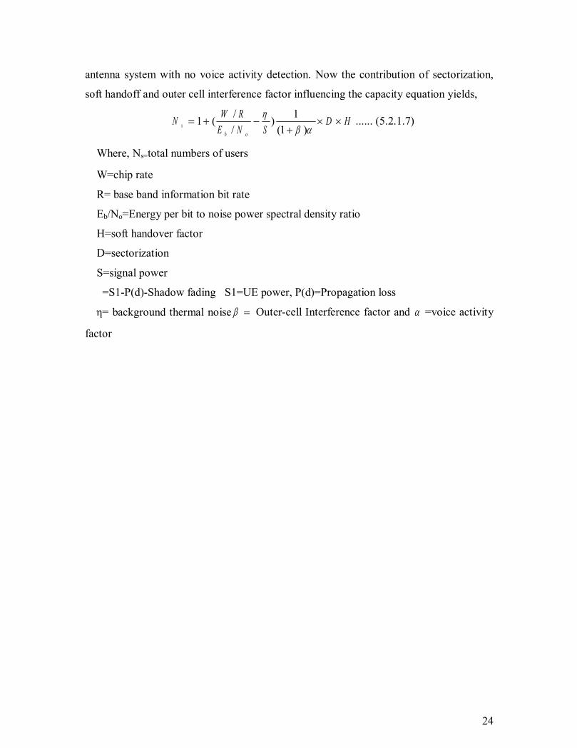
antenna system with no voice activity detection. Now the contribution of sectorization,

soft handoff and outer cell interference factor influencing the capacity equation yields,

HDSNE

RWNob

s ´´+

-+=ab

h)1(

1)//(1 ...... (5.2.1.7)

Where, Ns=total numbers of users

W=chip rate

R= base band information bit rate

Eb/No=Energy per bit to noise power spectral density ratio

H=soft handover factor

D=sectorization

S=signal power

=S1-P(d)-Shadow fading S1=UE power, P(d)=Propagation loss

η= background thermal noise =b Outer-cell Interference factor and a =voice activity

factor

25

Chapter-6

Radio Propagation Model

A radio propagation model, also known as the Radio Wave Propagation Model or the

Radio Frequency Propagation Model, is an empirical mathematical formulation for the

characterization of radio wave propagation as a function of frequency, distance and other

conditions. Created with the goal of formalizing the way radio waves are propagated

from one place to another, such models typically predict the path loss along a link or the

effective coverage area of a transmitter

6.1 Characteristics

As the path loss encountered along any radio link serves as the dominant factor for

characterization of propagation for the link, radio propagation models typically focus on

realization of the path loss with the auxiliary task of predicting the area of coverage for a

transmitter or modeling the distribution of signals over different regions.

6.2 Development Methodology

Radio propagation models are empirical in nature, which means, they are developed

based on large collections of data collected for the specific scenario. For any model, the

collection of data has to be sufficiently large to provide enough likeliness (or enough

scope) to all kind of situations that can happen in that specific scenario.

Different models have been developed to meet the needs of realizing the propagation

behavior in different conditions. Types of models for radio propagation include

i) Okumura Model

ii) Hata Model for Urban Areas

ii.a) Hata Model for Suburban Areas

ii.b) Hata Model for Open Areas

iii) COST 231 model

http://en.wikipedia.org/wiki/Okumura_Model

26

6.2.1 Okumura Model

The Okumura model for Urban Areas is a Radio propagation model that was built using

the data collected in the city of Tokyo, Japan. The model is ideal for using in cities with

many urban structures but not many tall blocking structures. The model served as a base

for the Hata Model. Okumura model was built into three modes [26] [27]. The model for

urban areas was built first and used as the base for others.

6.2.1.1 Coverage

Frequency = 150 MHz to 1920 MHz [14]

Mobile Station Antenna Height: between 1 m and 10 m

Base station Antenna Height: between 30 m and 1000 m

Link distance: between 1 km and 100 km

6.2.1.2 Mathematical Formulation

å--+= correctionBGMGMUFSL KHHALL

where,

L = the median path loss. Unit: Decibel (dB)

LFSL = the Free Space Loss. Unit: Decibel (dB)

AMU = Median attenuation. Unit: Decibel (dB)

HMG = Mobile station antenna height gain factor.

HBG = Base station antenna height gain factor.

Kcorrection = Correction factor gain (such as type of environment, water surfaces, isolated

obstacle etc.)

6.2.2 COST 231 Model

The COST-Hata-Model is the most often cited of the COST 231 models. Also called the

Hata Model PCS Extension, to cover a more elaborated range of frequencies [28] COST

(Cooperation européenne dans le domaine de la recherche Scientifique et Technique) is a

http://en.wikipedia.org/wiki/Okumura_Model

http://en.wikipedia.org/wiki/Median

http://en.wikipedia.org/wiki/Path_loss

http://en.wikipedia.org/wiki/Decibel

http://en.wikipedia.org/wiki/Free-space_loss



http://en.wikipedia.org/wiki/Attenuation


http://en.wikipedia.org/wiki/Mobile_station

http://en.wikipedia.org/wiki/Antenna_%28radio%29

http://en.wikipedia.org/wiki/Gain

http://en.wikipedia.org/wiki/Base_station


http://en.wikipedia.org/wiki/Gain

http://en.wikipedia.org/wiki/Cost_231_Model

Pract/New Folder/Propagation Model/COST_Hata_model.htm

http://en.wikipedia.org/wiki/COST

27

European Union Forum for cooperative scientific research which has developed this

model accordingly to various experiments and researches.

6.2.2.1 Applicable Conditions

This model is applicable to urban areas. To further evaluate Path Loss in Suburban or

Rural Quasi-open/Open Areas, this path loss has to be substituted into Urban to

Rural/Urban to Suburban Conversions

6.2.2.2 Coverage

Frequency: 1500 MHz to 2000 MHz [29]

Mobile Station Antenna Height: 1 up to 10m

Base station Antenna Height: 30m to 200m

Link Distance: 1 up to 20 km


The COST-231 Model is formulated as,

Mbrbc CdhhahfL +-+--+= log)log55.69.44()(log82.13)log(9.333.46

)8.log56.1()7.log1.1()( ---= crecr fhfha for urban

=3.2[log(11.75hre)]2-4.97 for dense urban

=MC 0 db for median cities and suburban areas

3db for metropolitan areas

Where,

L = Median path loss. Unit: Decibel (dB)

fc = Frequency of Transmission. Unit: Megahertz (MHz)

hb = Base Station Antenna effective height. Unit: Meter (m)

d = Link distance. Unit: Kilometer (km)

hr = Mobile Station Antenna effective height. Unit: Meter (m) a(hr) = Mobile station

Antenna height correction factor as described in the Hata Model for Urban Areas.

http://en.wikipedia.org/wiki/Mobile_Station







http://en.wikipedia.org/wiki/Megahertz

http://en.wikipedia.org/wiki/Base_Station


http://en.wikipedia.org/wiki/Effective_height




http://en.wikipedia.org/wiki/Mobile_station


http://en.wikipedia.org/wiki/Hata_Model_for_Urban_Areas

28

6.2.3 Hata Model

This model also has two more varieties for transmission in Suburban Areas and Open

Areas[30].Hata Model predicts the total path loss along a link of terrestrial microwave or

other type of cellular communications.

6.2.3.1 Coverage

Frequency: 150 MHz to 1500 MHz

Mobile Station Antenna Height: between 1 m and 10 m

Base station Antenna Height: between 30 m and 200 m

Link distance: between 1 km and 20 km.


The Hata Model for urban areas is formulated as,

dhChfL bHbc log)log55.69.44(log82.13)log(16.2655.69 -+--+=

For small or medium cities

cMcH fhfC log56.1)7.log1.1(8.0 --+=

And for large city

=HC 8.29(log(1.5hm))2 -1.1 if 150<=f<=200

3.2(log(11.75hm))2 -4.97 if 200<=f<=1500

Where,

L = Median path loss. Unit: Decibel (dB)

fc = Frequency of Transmission. Unit: Megahertz (MHz)

hb = Base Station Antenna effective height. Unit: Meter (m)

d = Link distance. Unit: Kilometer (km)

hM = Mobile Station Antenna effective height. Unit: Meter (m)

CH= Antenna height correction factor

d= Distance between the base and mobile stations. Unit: kilometer (km).

http://en.wikipedia.org/wiki/Hata_Model_for_Suburban_Areas

http://en.wikipedia.org/wiki/Hata_Model_for_Open_Areas

Pract/New Folder/Propagation Model/Hata_Model_for_Urban_Areas.htm


http://en.wikipedia.org/wiki/Microwave

http://en.wikipedia.org/wiki/Frequency








http://en.wikipedia.org/wiki/Megahertz

http://en.wikipedia.org/wiki/Base_Station







29

Chapter-7

Coverage Analysis in UMTS Cellular System

Performance analysis of multi service UMTS networks is major interest for mobile

network providers. Because of the W-CDMA technique used in UMTS, which leads to

an interference limited system with a dynamic cell capacity and load dependent cell

coverage, the service mix has a big influence on the system performance. Now we will

provide a detailed description of the performance relevant mechanisms for the uplink of a

single UMTS cell and to extract data rates and coverage bounds for single and multi

service operation. We propose a simplified calculation model for the multi service case.

7.1 Factors Influence in Coverage

Before going to relationship between coverage and capacity we have to discuss some

parameters which influence the coverage:

7.1.1 Frequency

The uplink and downlink range is about 1920MHz to 2100MHz (ITU proposed for a

global frequency band for WCDMA in UMTS.)[31] The greater the frequency the greater

the path loss.

7.1.2 Chip Rate

ITU proposed 3 standard chip rates [31] as 3.84Mcps, 7.84Mcps, and 15.36Mcps. The

greater the chip rate higher processing is needed by Node B.

7.1.3 Bit Rate

UMTS offers high data rate transmission, it is possible to have any type of services

between 12.2 Kbps (voice traffic) and 2 Mbps (Data traffic) [31].The higher the bit rate

the lower the coverage area.

30

7.1.4 Mobile Maximum Power

The maximum power of mobile handset is .126W or 21dBM power which defines by

manufacture [31].

7.1.5 Ms Antenna Gain

Mobile antenna gain is taken as 0 dBi [31]

7.1.6 Cable Connector Losses

Cable and connector losses influence the noise figure of a low Noise amplifier. The usual

case found is that a cable loss in many commercial base station 4 to 6 db [31].

7.1.7 Effective Isotropic Radiated Power

EIRP, Effective Isotropic Radiated Power or equivalent power intercepted by a receiver,

but spherically symmetrically by transmitter.

EIRP is known as= Pmax + Ga - L

Where,

Pmax is maximum power of the transmitter or receiver

Ga antenna gain

L all losses calculated from input and output

7.1.8 Interference Margin

Interference-margin is needed in the link budget because of the loading of the cell, the

load factor affects the coverage, the more loading is allowed in the system the large is the

interference margin needed in the uplink and the smaller is the coverage area. For

coverage limited cases, smaller interference margin is used (1-3 dB) corresponds to 20-

50% loading. While in a capacity limited cases a larger interference margin is used.

Interference margin=-10log (1-target load) [31]

31

7.1.9 Fast Fading Margin or Power Control Headroom

Fast fading margin or power control headroom is needed in the User equipment (UE)

transmission power for maintaining closed loop fast power control to effectively

compensate the fast fading. Typical values of the fast fading margin are 2-5 dB for slow

moving mobiles. [31]

7.1.10 Soft Handover Gain

Handover (soft or hard) gives gain against slow fading (Log normal fading) by reducing

the required Log-normal margin. Since slow fading is partly uncorrelated between the

Node B, by making a handover, the mobile can select a better Node B.Soft handover

gives additional macro diversity against fast fading by reducing the signal power to noise

power (Eb/No) relative to a single radio link. The total soft handover gain is assumed to

be between 2-3 dB in the example below including the gain against slow and fast fading

[31].

7.1.11 Noise Figure

Noise figure (NF) is a measure of degradation of the signal-to-noise ratio (SNR), caused

by components in a radio frequency (RF) signal chain. The noise figure is defined as the

ratio of the output noise power of a device to the portion thereof attributable to thermal

noise in the input termination at standard noise temperature T0 (usually 290 K). The noise

figure is thus the ratio of actual output noise to that which would remain if the device

itself did not introduce noise. It is a number by which the performance of a radio receiver

can be specified.Node b noise figure is taken as 5 db [31].

7.1.12 Eb/N0

Eb/N0 (the energy per bit to noise power spectral density ratio) is an important parameter

in digital communication or data transmission.

32

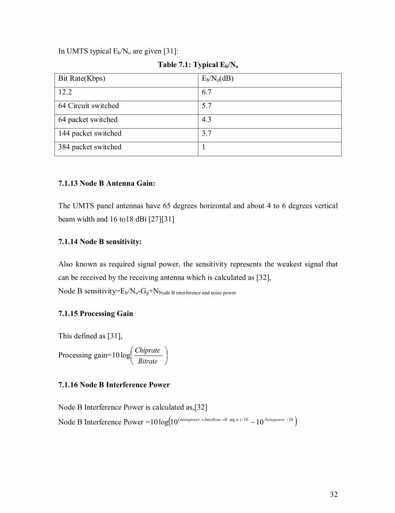
In UMTS typical Eb/No are given [31]:

Table 7.1: Typical Eb/No

Bit Rate(Kbps) Eb/No(dB)

12.2 6.7

64 Circuit switched 5.7

64 packet switched 4.3

144 packet switched 3.7

384 packet switched 1

7.1.13 Node B Antenna Gain:

The UMTS panel antennas have 65 degrees horizontal and about 4 to 6 degrees vertical

beam width and 16 to18 dBi [27][31]

7.1.14 Node B sensitivity:

Also known as required signal power, the sensitivity represents the weakest signal that

can be received by the receiving antenna which is calculated as [32],

Node B sensitivity=Eb/No-Gp+NNode B interference and noise power

7.1.15 Processing Gain

This defined as [31],

Processing gain= ÷øö

çèæ

BitrateChipratelog10

7.1.16 Node B Interference Power

Node B Interference Power is calculated as,[32]

Node B Interference Power = ( )10/10/)arg( 1010log10 NoisepowerineMInterfrencnoisepower -+

33

7.1.17 Node B Noise and Interference

Node B Noise and interference is calculated as [32]

Noise and interference= ( )10/)(10/)( 1010log10 epowerInterfrencnoisepower -

7.1.18 Thermal Noise

Thermal noise is due to thermal agitation of electrons. It is present in all electronic

devices and transmission media and is a function of temperature.Themal noise is

uniformly distributed across the frequency spectrum and hence is often referred to as

white noise [33].

The amount of thermal noise to be found in a and with of 1 Hz in any device or conductor

is

N=KT (W/Hz)

=10log (KT) in dB

7.2 Relationship between Coverage and Data Rates

In UMTS, the scarce resource is the transmission power. Talking about the Frequency

Division Duplex mode (FDD) of UMTS, the power budgets for up-link and downlink are

independent of each other. While the uplink power budget is limited by the transmission

power of each User Equipment (mobile station), the downlink power budget depends

only on the capabilities of the Node B

Figure 7.1: UMTS cell[34]

Figure 7.1 shows a UMTS cell where Node B received power PR from User

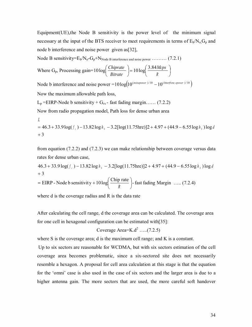
34

Equipment(UE),the Node B sensitivity is the power level of the minimum signal

necessary at the input of the BTS receiver to meet requirements in terms of Eb/No,Gp and

node b interference and noise power given as[32],

Node B sensitivity=Eb/No-Gp+NNode B interference and noise power ……… (7.2.1)

Where Gp, Processing gain= ÷øö

çèæ=÷

øö

çèæ

RMcps

BitrateChiprate 84.3log10log10

Node b interference and noise power = ( )10/)(10/)( 1010log10 epowerInterfrencnoisepower -

Now the maximum allowable path loss,

Lp =EIRP-Node b sensitivity + Grx - fast fading margin…… (7.2.2)

Now from radio propagation model, Path loss for dense urban area

3log)log55.69.44( 4.97.75hre)]23.2[log(11log82.13)log(9.333.46

+-++--+= dhhf

L

bbc

from equation (7.2.2) and (7.2.3) we can make relationship between coverage versus data

rates for dense urban case,

3log)log55.69.44( 4.97.75hre)]23.2[log(11log82.13)log(9.333.46

+-++--+ dhhf bbc

Margin fadingfast -rate Chiplog10ysensitivit b Node-EIRP ÷øö

çèæ+=

R ….. (7.2.4)

where d is the coverage radius and R is the data rate

After calculating the cell range, d the coverage area can be calculated. The coverage area

for one cell in hexagonal configuration can be estimated with[35]:

Coverage Area=K.d2 …..(7.2.5)

where S is the coverage area; d is the maximum cell range; and K is a constant.

Up to six sectors are reasonable for WCDMA, but with six sectors estimation of the cell

coverage area becomes problematic, since a six-sectored site does not necessarily

resemble a hexagon. A proposal for cell area calculation at this stage is that the equation

for the ‘omni’ case is also used in the case of six sectors and the larger area is due to a

higher antenna gain. The more sectors that are used, the more careful soft handover

35

overhead has to be analyzed to provide an accurate estimate. In Table some of the K

values are listed.

Table 7.2: K values for the site area calculation [35]:

Site

configuration:

Omni Two-sectored

Three-sectored

Four-sectored

Value of K:

2.6 1.3 1.95 2.6

7.3 Multi Service Case

The multi service case is characterized by the request for different radio link services.

Different spreading factors as well as other signal to noise ratios may be requested,

resulting in different service parameters. Generally, also for the multi service case the

received power levels required at Node B can be calculated for all users, and for an

increasing number of users or different class of services causes the cell radius will small

results a small coverage area. If we classified the different types as in table then resulting

figure will look like figure:

Table 7.3: Different Class of Services

Bit Rate(Kbps) class

12.2 Class 5

32 Class 4

64 Class 3

144 Class 2

384 Class 1

36

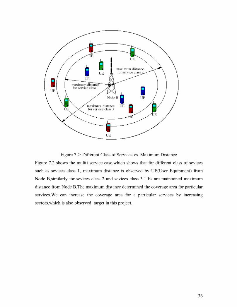
Figure 7.2: Different Class of Services vs. Maximum Distance

Figure 7.2 shows the muliti service case,which shows that for different class of sevices

such as sevices class 1, maximum distance is observed by UE(User Equipment) from

Node B,similarly for sevices class 2 and sevices class 3 UEs are maintained maximum

distance from Node B.The maximum distance determined the coverage area for particular

services.We can increase the coverage area for a particular services by increasing

sectors,which is also observed target in this project.

37

Chapter-8

Simulation and Result

We have already told that UMTS has different class of services.Voice, Data, Multimedia

is serverd by the UMTS using different data rates.In this chapter we have simulated

Numbers of simultaneous users with standard data rates vs. different factors that

influence capacity with changing numbers of sectoring cell.

Then we have simulated different data rates vs coverage area for urban and dense urban

cell with operating frequency 2000MHz.

8.1 Algorithm for Capacity Analysis Using Sectorization:

Begin

Set energy per bit to noise spectral density ratio (Eb/No) = [1 2 3 4 5 6 7 8 9 10]

Set soft handover gain (H) = [1.5]

Set inter-cell interference ( b ) = [1.55]

Set channel activity for data (a ) = [1]

Set channel activity for voice (a ) = [.38]

Set thermal noise (η) = [4.04X10^-21]

Set user signal power (S1) = [.126]

Set shadow fading (sh_fd) = [6.30]

Set cell range in km (R) = [2]

Set chip rate (W) = [3840000]

Set base band information rate in kbps (R) = [12.2 64 144 384 2000]

Set base antenna height in meter (hb) = [20]

Set user antenna height in meter (hre) = [2]

Set sector (D) = [1 2 3 4 6]

Set frequency range in MHz (fc) = [2000]

Set data rate in kbps (R) = [12.2 64 144 384 2000]

38

//Processing

Processing gain (PG) = (W/R)

Propagation loss in dense urban (Pro_loss) =

3log)log55.69.44( 4.97.75hre)]3.2[log(11log82.13)log(9.333.46 2

+-++--+ dhhf bbc

Signal Power (S) = S1-Pro_loss-sh_hd

//Output

HDSNE

RW

ob

´´+

-+=ab

h)1(

1)//(1 (ns) cell in UMTS users of Numbers

End

8.2 Algorithm for Coverage and Data rates Analysis Using Sectorization

Begin

Set Transmitter=Mobile Station

Set Receiver=Node B

Set mobile max power in dbm (mo_mx) = [21]

Set mobile gain in db (M_G) = [0]

Set cable and connector losses in db (ca_cn_loss) = [3]

Set thermal noise in dbm (η) = [174]

Set node B noise figure in db (nodeB_NF) = [5]

Set target load (tar_ld) = [.4]

Set chip rate (W) = [3840000]

Set base antenna height in meter (hb) = [20]

Set user antenna height in meter (hre) = [2]

Set energy per bit to noise spectral density ratio (Eb/No) = [5]

Set Power Control Margin or Fading Margin (MPC) = [4]

Set Value for sectors (Sec) = [1 2 3 4]

Set constant value for sectors (K) = [2.6 1.6 1.95 2.6]

39

Set data rate in kbps (R) = [100 200 300 400 500 600 2000]

//Processing

Chip rate in db (W_db) = 10log (W)

Processing gain (PG) = (W/R)

Effective isotropic radiated power (EIRP) = mo_mx-ca_cn_loss+M_G

Node B noise density (nodeB_ND) = η+ nodeB_NF

Node B noise power (nodeB_NPW) = nodeB_ND +W_db

Interference margin (IM) =-10log (1-tar_ld)

Node B Interference Power (nodeB_IP) = ( )10/_10/)_( 1010log10 NPWnodeBIMNPWnodeB -+

Node B Noise and interference (nodeB_NIFPW) = ( )10/)_(10/)_( 1010log10 IPnodeBNPWnodeB -

Node B antenna gain (nodeB_AG) = [18]

Receiver Sensitivity (Srx) = Eb/No-PG+ nodeB_NIFPW

Total Allowable Path loss=EIRP-Srx+ nodeB_AG-MPC=EIRP-(Eb/No-PG+

nodeB_NIFPW) + nodeB_AG-MPC

Path loss in dense urban (Durban_Ploss) =

3log)log55.69.44( 4.97.75hre)]3.2[log(11log82.13)log(9.333.46 2

+-++--+ dhhf bbc

=142.17+36.37logd

//Output

Cell radius (d) = 10^ ((1/36.37)* (EIRP-(Eb/No-PG+ nodeB_NIFPW) + nodeB_AG-

MPC-142.17))

Cell Area (A) = K*d2

End

40

8.3 Performance Analysis in Capacity Using Sectorization for UMTS

i)Varying Eb/No and changing the sectors the Numbers of simueltaneous user can be

observed here we consider themal noise -174dbm/Hz,shadow fading 8db,user transmit

power 21dbm,inter cell or outer cell interference factor 1.55,soft handover gain 1.5

Table 8.1: Simulated Numbers of Simultaneous 384 kbps Users vs. Eb/No in UMTS

cell

Energy per

bit to Noise

spectral

density

ratio(Eb/No)

Users

without

sector

Users with

2 sectors

Users with

3 sectors

Users with

4 sectors

Users with

6 sectors

1 10.677 20.355 30.032 39.71 59.065

2 5.8387 10.677 15.516 20.355 30.032

3 4.2258 7.4516 10.677 13.903 20.355

4 3.4194 5.8387 8.2581 10.677 15.516

5 2.9355 4.871 6.8065 8.7419 12.613

6 2.6129 4.2258 5.8387 7.4516 10.677

7 2.3825 3.765 5.1475 6.53 9.2949

8 2.2097 3.4194 4.629 5.8387 8.2581

9 2.0753 3.1505 4.2258 5.3011 7.4516

10 1.9677 2.9355 3.9032 4.871 6.8065

11 1.8798 2.7595 3.6393 4.5191 6.2786

12 1.8065 2.6129 3.4194 4.2258 5.8387

13 1.7444 2.4888 3.2333 3.9777 5.4665

14 1.6912 2.3825 3.0737 3.765 5.1475

15 1.6452 2.2903 2.9355 3.5806 4.871

16 1.6048 2.2097 2.8145 3.4194 4.629

17 1.5693 2.1385 2.7078 3.277 4.4156

41

Table 8.2: Simulated Numbers of Simultaneous 144 Kbps Users vs. Eb/No in UMTS

cell

Energy per

bit to Noise

spectral

density

ratio(Eb/No)

Users

without

sector

Users with

2 sectors

Users with

3 sectors

Users with

4 sectors

Users with

6 sectors

1 26.806 52.613 78.419 104.23 155.84

2 13.903 26.806 39.71 52.613 78.419

3 9.6022 18.204 26.806 35.409 52.613

4 7.4516 13.903 20.355 26.806 39.71

5 6.1613 11.323 16.484 21.645 31.968

6 5.3011 9.6022 13.903 18.204 26.806

7 4.6866 8.3733 12.06 15.747 23.12

8 4.2258 7.4516 10.677 13.903 20.355

9 3.8674 6.7348 9.6022 12.47 18.204

10 3.5806 6.1613 8.7419 11.323 16.484

11 3.346 5.6921 8.0381 10.384 15.076

12 3.1505 5.3011 7.4516 9.6022 13.903

13 2.9851 4.9702 6.9553 8.9404 12.911

14 2.8433 4.6866 6.53 8.3733 12.06

15 2.7204 4.4409 6.1613 7.8817 11.323

16 2.6129 4.2258 5.8387 7.4516 10.677

17 2.518 4.0361 5.5541 7.0721 10.108

18 2.4337 3.8674 5.3011 6.7348 9.6022

19 2.3582 3.7165 5.0747 6.4329 9.1494

20 2.2903 3.5806 4.871 6.1613 8.7419

42

Table 8.3: Simulated Numbers of Simultaneous 64 Kbps Users vs. Eb/No in UMTS

cell

Energy per

bit to Noise

spectral

density

ratio(Eb/No)

Users

without

sector

Users with

2 sectors

Users with

3 sectors

Users with

4 sectors

Users with

6 sectors

1 59.065 117.13 175.19 233.26 349.39

2 30.032 59.065 88.097 117.13 175.19

3 20.355 39.71 59.065 78.419 117.13

4 15.516 30.032 44.548 59.065 88.097

5 12.613 24.226 35.839 47.452 70.677

6 10.677 20.355 30.032 39.71 59.065

7 9.2949 17.59 25.885 34.18 50.77

8 8.2581 15.516 22.774 30.032 44.548

9 7.4516 13.903 20.355 26.806 39.71

10 6.8065 12.613 18.419 24.226 35.839

11 6.2786 11.557 16.836 22.114 32.672

12 5.8387 10.677 15.516 20.355 30.032

13 5.4665 9.933 14.4 18.866 27.799

14 5.1475 9.2949 13.442 17.59 25.885

15 4.871 8.7419 12.613 16.484 24.226

16 4.629 8.2581 11.887 15.516 22.774

17 4.4156 7.8311 11.247 14.662 21.493

18 4.2258 7.4516 10.677 13.903 20.355

19 4.056 7.1121 10.168 13.224 19.336

20 3.9032 6.8065 9.7097 12.613 18.419

43

Table 8.4: Simulated Numbers of Simultaneous 12.2 kbps or voice Users vs. Eb/No in

UMTS cell

Energy per

bit to Noise

spectral

density

ratio(Eb/No)

Users

without

sector

Users with

2 sectors

Users with

3 sectors

Users with

4 sectors

Users with

6 sectors

1 305.6 610.2 914.8 1219.4 1828.6

2 153.3 305.6 457.9 610.2 914.8

3 102.53 204.07 305.6 407.13 610.2

4 77.15 153.3 229.45 305.6 457.9

5 61.92 122.84 183.76 244.68 366.52

6 51.767 102.53 153.3 204.07 305.6

7 44.514 88.029 131.54 175.06 262.09

8 39.075 77.15 115.23 153.3 229.45

9 34.845 68.689 102.53 136.38 204.07

10 31.46 61.92 92.38 122.84 183.76

11 28.691 56.382 84.073 111.76 167.15

12 26.383 51.767 77.15 102.53 153.3

13 24.431 47.862 71.292 94.723 141.58

14 22.757 44.514 66.272 88.029 131.54

15 21.307 41.613 61.92 82.227 122.84

16 20.038 39.075 58.113 77.15 115.23

17 18.918 36.835 54.753 72.671 108.51

18 17.922 34.845 51.767 68.689 102.53

19 17.032 33.063 49.095 65.126 97.19

20 16.23 31.46 46.69 61.92 92.38

44

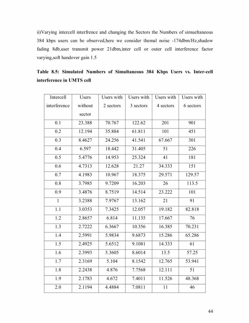
ii)Varying intercell interfrence and changing the Sectors the Numbers of simueltaneous

384 kbps users can be observed,here we consider themal noise -174dbm/Hz,shadow

fading 8db,user transmit power 21dbm,inter cell or outer cell interference factor

varying,soft handover gain 1.5

Table 8.5: Simulated Numbers of Simultaneous 384 Kbps Users vs. Inter-cell

interference in UMTS cell

Intercell

interference

Users

without

sector

Users with

2 sectors

Users with

3 sectors

Users with

4 sectors

Users with

6 sectors

0.1 23.388 70.767 122.62 201 901

0.2 12.194 35.884 61.811 101 451

0.3 8.4627 24.256 41.541 67.667 301

0.4 6.597 18.442 31.405 51 226

0.5 5.4776 14.953 25.324 41 181

0.6 4.7313 12.628 21.27 34.333 151

0.7 4.1983 10.967 18.375 29.571 129.57

0.8 3.7985 9.7209 16.203 26 113.5

0.9 3.4876 8.7519 14.514 23.222 101

1 3.2388 7.9767 13.162 21 91

1.1 3.0353 7.3425 12.057 19.182 82.818

1.2 2.8657 6.814 11.135 17.667 76

1.3 2.7222 6.3667 10.356 16.385 70.231

1.4 2.5991 5.9834 9.6873 15.286 65.286

1.5 2.4925 5.6512 9.1081 14.333 61

1.6 2.3993 5.3605 8.6014 13.5 57.25

1.7 2.3169 5.104 8.1542 12.765 53.941

1.8 2.2438 4.876 7.7568 12.111 51

1.9 2.1783 4.672 7.4011 11.526 48.368

2.0 2.1194 4.4884 7.0811 11 46

45

iv) Varying voice activity factor and changing the Sectors the Numbers of simueltaneous

voice or 12.2 kbps usera can be observed only for voice users not for data users as in data

users activity factor is always 1, here we consider themal noise -174dbm/Hz, shadow

fading 8db, user transmit power 21dbm, inter cell or outer cell interference factor

1.55,soft handover gain 1.5

Table 8.6: Simulated Numbers of Simultaneous Voice Users vs. Voice activity factor

in UMTS cell

Voice activity

factor

Users

without

sector

Users with

2 sectors

Users with

3 sectors

Users with

4 sectors

Users with

6 sectors

0.1 455.63 910.26 1364.9 1819.5 2728.8

0.2 228.31 455.63 682.94 910.26 1364.9

0.3 152.54 304.09 455.63 607.17 910.26

0.4 114.66 228.31 341.97 455.63 682.94

0.5 91.926 182.85 273.78 364.7 546.55

0.6 76.771 152.54 228.31 304.09 455.63

0.7 65.947 130.89 195.84 260.79 390.68

0.8 57.828 114.66 171.49 228.31 341.97

0.9 51.514 102.03 152.54 203.06 304.09

1 46.463 91.926 137.39 182.85 273.78

iii) Varying soft handover gain and changing the Sector the Numbers of simueltaneous

384 kbps users can be observed,here we consider themal noise -174dbm/Hz,shadow

fading 8db,user transmit power 21dbm,inter cell or outer cell interference factor 1.55

46

Table 8.7: Simulated No. of Simultaneous 384 kbps Users vs. soft handover factor in

UMTS cell

Soft handover

factor

Users

without

sector

Users with

2 sectors

Users with

3 sectors

Users with

4 sectors

Users with

6 sectors

0.1 1.6452 2.2903 2.9355 3.5806 4.2258

0.2 2.2903 2.2903 4.871 6.1613 7.4516

0.3 2.9355 4.871 6.8065 8.7419 10.677

0.4 3.5806 6.1613 8.7419 11.323 13.903

0.5 4.2258 7.4516 10.677 13.903 17.129

0.6 4.871 8.7419 12.613 16.484 20.355

0.7 5.5161 10.032 14.548 19.065 23.581

0.8 6.1613 11.323 16.484 21.645 26.806

0.9 6.8065 12.613 18.419 24.226 30.032

1 7.4516 13.903 20.355 26.806 33.258

1.1 8.0968 15.194 22.29 29.387 36.484

1.2 8.7419 16.484 24.226 31.968 39.71

1.3 9.3871 17.774 26.161 34.548 42.935

1.4 10.032 19.065 28.097 37.129 46.161

1.5 10.677 20.355 30.032 39.71 49.387

1.6 11.323 21.645 31.968 42.29 52.613

1.7 11.968 22.935 33.903 44.871 55.839

1.8 12.613 24.226 35.839 47.452 59.065

1.9 13.258 25.516 37.774 50.032 62.29

2.0 13.903 26.806 39.71 52.613 65.516

2.1 14.548 28.097 41.645 55.194 68.742

2.2 15.194 29.387 43.581 57.774 71.968

2.3 15.839 30.677 45.516 60.355 75.194

2.4 16.484 31.968 47.452 62.935 78.419

2.5 17.129 33.258 49.387 65.516 81.645

47

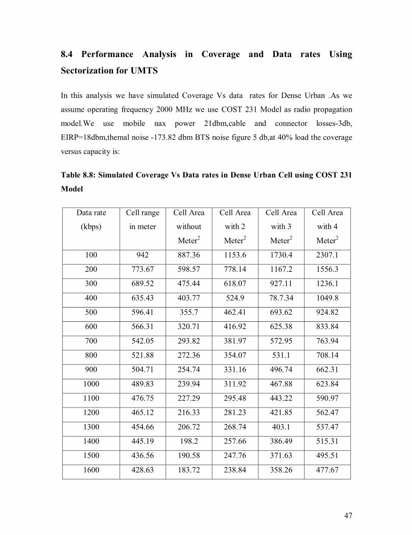
8.4 Performance Analysis in Coverage and Data rates Using

Sectorization for UMTS

In this analysis we have simulated Coverage Vs data rates for Dense Urban .As we

assume operating frequency 2000 MHz we use COST 231 Model as radio propagation

model.We use mobile nax power 21dbm,cable and connector losses-3db,

EIRP=18dbm,themal noise -173.82 dbm BTS noise figure 5 db,at 40% load the coverage

versus capacity is:

Table 8.8: Simulated Coverage Vs Data rates in Dense Urban Cell using COST 231

Model

Data rate

(kbps)

Cell range

in meter

Cell Area

without

Meter2

Cell Area

with 2

Meter2

Cell Area

with 3

Meter2

Cell Area

with 4

Meter2

100 942 887.36 1153.6 1730.4 2307.1

200 773.67 598.57 778.14 1167.2 1556.3

300 689.52 475.44 618.07 927.11 1236.1

400 635.43 403.77 524.9 78.7.34 1049.8

500 596.41 355.7 462.41 693.62 924.82

600 566.31 320.71 416.92 625.38 833.84

700 542.05 293.82 381.97 572.95 763.94

800 521.88 272.36 354.07 531.1 708.14

900 504.71 254.74 331.16 496.74 662.31

1000 489.83 239.94 311.92 467.88 623.84

1100 476.75 227.29 295.48 443.22 590.97

1200 465.12 216.33 281.23 421.85 562.47

1300 454.66 206.72 268.74 403.1 537.47

1400 445.19 198.2 257.66 386.49 515.31

1500 436.56 190.58 247.76 371.63 495.51

1600 428.63 183.72 238.84 358.26 477.67

48

Table 8.9: Simulated Coverage Vs Data rates in Urban Cell using COST 231 Model

Data rate

(kbps)

Cell range

in meter

Cell Area

without

sector

Meter2

Cell Area

with 2

sectors

Meter2

Cell Area

with 3

sectors

Meter2

Cell Area

with 4

sectors

Meter2

100 1172.6 1375 1787.5 2681.2 3575

200 963.07 927.5 1205.8 1808.6 2411.5

300 858.32 736.71 957.72 1436.6 1915.4

400 790.98 625.65 813.34 1220 1626.7

500 742.41 551.17 716.52 1074.8 1433

600 704.95 496.95 646.03 969.05 1292.1

700 674.75 455.29 591.87 887.81 1183.7

800 649.64 422.03 548.64 822.96 1097.3

900 628.27 394.72 513.14 769.71 1026.3

1000 609.75 371.79 483.33 725 966.66

8.5 Graphical Representation:

Performance Analysis in Capacity Using Sectorization for UMTS

i)Varying Eb/No and changing the Sectors the Numbers of simueltaneous voice usera can

be observed here we consider themal noise -174dbm/Hz,shadow fading 8db,user transmit

power 21dbm,inter cell or outer cell interference factor 1.55,soft handover gain 1.5

49

Figure 8.1: Numbers of Simultaneous voice users vs. Eb/No in different sectorized cell

Figure 8.2: Numbers of Simueltaneous 64 kbps users vs. Eb/No in different sectorized

cell

50

Figure 8.3: Numbers of Simultaneous 144 kbps users vs. Eb/No in different sectorized

cell

Figure 8.4: Numbers of Simultaneous 384 kbps users Vs Eb/No in different sectorized

cell

51

Figure 8.5: Numbers of Simultaneous 2 mbps users vs. Eb/No in different sectorized cell

ii) Varying intercell interfrence and changing the Sectors the Numbers of simueltaneous

user can be observed,here we consider themal noise -174dbm/Hz,shadow fading 8db,user

transmit power 21dbm,inter cell or outer cell interference factor varying,soft handover

gain 1.5

Figure 8.6: Numbers of Simultaneous users vs. Inter-cell interference in non-sectorized

cell

52

Figure 8.7: Numbers of Simultaneous 384 kbps users vs. Inter-cell interference in

sectorized cell

iii) Varying soft handover gain and changing the Sector the Numbers of simueltaneous

user can be observed,here we consider themal noise -174dbm/Hz,shadow fading 8db,user

transmit power 21dbm,inter cell or outer cell interference factor 1.55,soft handover gain

varying

Figure: 8.8: Numbers of Simultaneous users vs. soft handover in non- sectorized cell

53

Figure 8.9: Numbers of Simultaneous users vs. soft handover in sectorized cell

iv)Varying voice activity factor and changing the Sectors the Numbers of simueltaneous

user can be observed only for voice users not foe data users as in data users activity factor

is always 1,here we consider themal noise -174dbm/Hz,shadow fading 8db,user transmit

power 21dbm,inter cell or outer cell interference factor 1.55,soft handover gain 1.5 with

Node B height 20m and UE height 2m

Figure 8.10: No of Simueltaneous Users vs. Voice activity factor in sectorized cell

54

8.2 Performance Analysis in Coverage and data rates using Sectorization:

In this analysis we have simulated Coverage Vs data rates For Dense Urban .As we

assume operating frequency 2000 MHz we use COST 231 Model as radio propagation

model.We use mobile nax power 21dbm,cable and connector losses-3db,

EIRP=18dbm,thermal noise -173.82 dbm BTS noise figure 5 db,at 40% load with Node

B height 20m and UE height 2m the coverage versus data rates is:

Figure 8.11: Coverage vs. data rates for Dense Urban Using COST 231 Model

Figure 8.12: Coverage vs. bit rates for Dense Urban Using COST 231 Model in

sectorized cell

55

Now Coverage vs Data rates for urban Using COST 231 Model with mobile nax power

21dbm,cable and connector losses-3db, EIRP=18dbm,themal noise -173.82 dbm BTS

noise figure 5 db,at 40% load with Node B height 20m and UE height 2m:

Figure 8.13: Coverage vs. data rates for Urban Using COST 231 Model

Figure 8.14: Coverage vs. data rates for Urban Using COST 231 Model in sectorized cell

56

Chapter-9

Conclusion

In this project the performance analysis in coverage and capacity of UMTS cellular

network using sectorization have been simulated and evaluated. Simulation shows that

the capacity of UMTS cellular network depends on energy per bit noise spectral density

ratio Eb/No, as Eb/No increases the capacity is also decreases, simulation also shows that

the capacity of UMTS cellular network depends on sectorization ,D ,as sectorization , D,

increases the capacity is also increases, simulation also shows that the voice users

capacity of UMTS cellular network depends on channel activity a ,as channel activity,

a increases the capacity is also decreases, Simulation also shows that the capacity of

UMTS cellular network depends on outer-cell or intra-cell or outer cell interference

factor b ,as b increases the capacity is also decreases, simulation also shows that the

capacity of UMTS cellular network depends soft handover H ,as H increases the capacity

is also increases. Simulation also shows that the most effective is sectorization in capacity

for increasing UMTS cellular network. Simulation also shows that the capacity of UMTS

cellular network depends on coverage, as capacity increases the coverage decreases, for

dense urban cell and urban cell we have simulated this phenomena using COST231

Model since our operating frequency is 2000MHz. Here simulation also shows that the

most effective is sectorization for increasing coverage of UMTS cellular network.

57

References

[1] G.B. Giannakis, Y. Hua, P. Stoica, and Signal processing Advancesin wireless and

Mobile communication: Trend in channel Estimation and Equalization; Prentice hall

PTR, 2001.

[2] Y.chen, “Soft Handover Issues in Radio resource management for 3G WCDMA

Networks”, PhD. Thesis ,department of Electronic Engineering Queeen mary,University

of London, September 2003

[3] Y. Sato,” A method of Self-Recovering Equalizatiom for Multilevel Amplitude-

Modulation Systems” IEEE Trans Commun.,vol. 23, no.6 pp 679-692,June 1975.

[4] Z. Ding and G. Liu Y.cen, “Single-channel blind equlization for GSM cellular

systems,” IEEE J. Select. Areas Commun.,vol. 16, no.8 pp 1493-1505,October 1998.

[5] http://en.wikipedia.org/wiki/W-CDMA#_note-1

[6] T.S.Rappaport, “Wireless Communications Principles and Practice”-Second Edition,

Prentice Hall.

[7] Bo Hagerman, Davide Imbeni and Jozsef Barta “WCDMA 6-sector Deployment-

Case Study of a Real Installed UMTS-FDD Network”

[8] S. Sharma, A.G. Spilling and A.R. Nix “Adaptive Coverage for UMTS Macro cells

based on Situation Awareness”.

[9] Jhong Sam Lee, Leonard E. Miller, “CDMA Systems Engineering Handbook”-

Artech House Publishers.

[10] W. C. Jakes, “Microwave Mobile Communications”. John Wiley and Sons, 1974.

[11] R. Prasad, W. Mohr, and W. Konhauser, “Third Generation Mobile Communications

Systems”. Boston - London: Artech House, 2000.

[12] T. Ojanpera and R. Prasad, “Wideband CDMA for Third Generation Mobile

Communications”. Artech House, 1998.

[13] Harri Holma and Antti Toskala, “WCDMA for UMTS-Radio Access Third

Generation Mobile Communications”- John Wiley & Sons.

58

[15] Saleh Faruque, “Cellular Mobile System Engineering”, Artech House Publishers.

[16] Lee, William C. Y, “Mobile Cellular Telecommunications”- McGraw-Hill

Company.

[17] R. Steele and L. Hanzo, “Mobile Radio Communications Secondary and Third

Generation Cellular and WATM Systems”, 2nd ed. John Wiley & Sons, LTD.

[18] Hsiao-Hwa Chen, Mohsen Guizani,“Next Generation Wireless Systems and

Networks” John Wiley & Sons Ltd.

[19] Jhong Sam Lee, Leonard E. Miller, “CDMA Systems Engineering Handbook”-

Artech House Publishers.

[20] Bernard Sklar, “Digital Communications - Fundamentals and Applications”-

Second Edition Prentice Hall.

[21] Bernard Sklar, “Digital Communications - Fundamentals and Applications”-

Second Edition Prentice Hall.

[22] Gerard Maral, Michel Bousquet, “Baseband Signals and Quality of Service”- John

Wiley & Sons.

[23] Christophe Chevallier, Christopher Brunner, Andrea Garavaglia, Kevin P. Murray,

Kenneth R. Baker, “Wcdma Umts Deployment Handbook Planning and Optimization

Aspects”- John Wiley & Sons.

[24] Jaana Laiho, Achim Wacker, Tomas Novosad,”Radio Network Planning and

Optimisation for UMTS”-Second Edition John Wiley & Sons.

[25] T.S.Rappaport, “Wireless Communications Principles and Practice”-Second

Edition, Prentice Hall.

[26] J. D. Parsons, “The Mobile Radio Propagation Channel” – Second Edition John

Wiley & Sons.

[27] www.wikipedia.org


Wiley & Sons.

[29] T.S.Rappaport, “Wireless Communications Principles and Practice”-Second

Edition, Prentice Hall.


Wiley & Sons.

http://www.wikipedia.org/

59

[31] Harri Holma and Antti Toskala, “WCDMA for UMTS-Radio Access Third

Generation Mobile Communications”- John Wiley & Sons.

[32] http://www.umtsworld.com

[33] William Stallings, “Wireless Communications and Networks”- Pearson Prentice

Hall.

[34] J. Sch¨uler, K. Begain, M. Ermel, T. M¨uller, M. Schweigel “Performance Analysis

of a Single UMTS Cell”

[35] Jaana Laiho, Achim Wacker, Tomas Novosad,”Radio Network Planning and

Optimisation for UMTS”-Second Edition John Wiley & Sons.

PERFORMANCE ANALYSIS OF UMTS CELLULAR NETWORK …

Documents

Transcript of PERFORMANCE ANALYSIS OF UMTS CELLULAR NETWORK …