PED special event Harvard University

9 October 2009

STABILITY AND COMPLEXITY IN MODEL

BANKING SYSTEMSRobert M May & Nim Arinaminpathy

Zoology Department

Oxford OX1 3PS, UK

OUTLINE

• NAS/FRBNY study

• Can be inherent tension between the interest of individual banks and that of the entire system

• Dynamics of banking networks

www.national-academies.org

NETWORKS & INTERACTION STRENGTHS, A

Consider a community of N species, each with intraspecific mechanisms which, in isolation, would stabilize perturbations. Now let there be a randomly constructed network of interactions among these N species (with a mean number, m, of links per species, and each interaction, independently randomly, being + or – and with average magnitude α compared with the intraspecific effects)

NETWORKS & INTERACTION STRENGTHS, B

The overall stability of such a “randomly constructed” assembly explicitly depends both on the network’s connectance (number of links/number of possible links per species; C = m/N ), and on the average interaction strength α. For large N, the system is stable if, and only if,

m α2 < 1

A PARADOX

Diversification of assets can be GOOD for each individual bank, yet BAD for system as a whole

A “toy model” which illustrates this

Consider N banks, and n “kinds/classes”

of assets, each of which has a

probability p of losing value to such an

extent that a bank holding all its assets

in that kind/class would fail.

Two extremes (with N = n = 5)

A

B

C

D

E

Assets

(Heterogeneous)

Probability any one bank fails

Probability all banks fail

p

p5

Assets(Homogeneous)

26p5

26p5

Banks’ resistance to some suggested regulations may not be simple bloody-mindedness. There can be unavoidable tensions between minimizing individual banks’ risk and minimizing systemic risk. Such tensions are only one element of complex questions, but they deserve to be more thoroughly and widely recognized in discussions about regulation

Schematic model for a ‘node’ in the interbank network

External assetsei

Depositsdi

Interbank borrowing

bi

Interbank loansli

(OUT)Assets

(IN)Liabilities

(1-θi)ai

θiai

i

“Net worth”, γi

j

SHOCK(to ei or li)

MODEL STRUCTURE & PARAMETERSIa: Assumptions as to what causes a bank to fail

Initial default. A single bank loses a fraction, f, of its external assets: f(1-θ)ai. If all banks have the same value of ai , we can (without loss of generality) put ai=1 and thence the “first phase shock” is

S(I) = f(1-θ)

Furthermore, if the external asset holding itself is structured, such that each bank apportions its (1-θ) external assets equally among n “asset classes”, then we could assume the initial default to be caused by failure of a single asset class in a single bank: i.e. f = 1/nThe bank is assumed to fail if S(I) > γi

MODEL STRUCTURE & PARAMETERSIb: Assumptions as to what causes a bank to fail

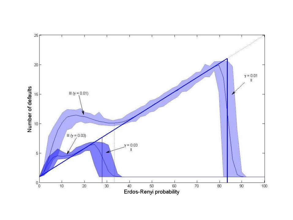
Subsequent defaults. The initially failing bank will cause “phase II” shocks, S(II), to its j creditor banks. Two different assumptions can be made, representing opposite extremes:

(1) Zero Recovery. If the initial bank fails, all its j creditor banks lose 100% of their loan to it (i.e. the failing banks assets go to zero).

(2) Diminished Assets. The failing bank distributes its remaining assets, having lost f(1-θ) – γ of them. So the j creditors will experience a shock of S(II) = [f(1-θ) – γ] / j if this quantity is less than total borrowing (usually assumed equal to lending, θ), or S(II) = total borrowing (θ /j?) otherwise. And this is distributed to each of j connected banks, which in turn will fail if S(II) > γ . And so on, for Phase III and later shocks.

MODEL STRUCTURE & PARAMETERSIc: Assumptions as to what causes a bank to fail

Note that zero recovery, (1), is a rather extreme assumption, but it makes for simpler calculations (with more banks failing!); failure propagates through interbank connections, rather like an infectious disease. The opposite extreme assumption (2) implies, in essentials, that the shocks in each subsequent phase (after the initial one bank failing) are attenuated, roughly by a factor 1/z (where z is the “mean degree” or number of interbank links).

MODEL STRUCTURE & PARAMETERSId: Assumptions as to what causes a bank to fail

So much for propagation of shocks through interbank lending and borrowing (“IBS”). There is also the important question of shocks propagated – without direct contact between banks – by liquidity problems caused by the discounting of external assets (or, more particularly, specific “asset classes”) held by failing banks. Conventional models express such liquidity shocks (“LS”) by assuming the value of the affected assets held by non-failing banks are discounted by a factor exp(- αx), where x is the fraction of all banks holding those assets which have failed (and α is a parameter, conventionally taken to be ~1).

Schematic model for a ‘node’ in the interbank network

External assetsei

Depositsdi

Interbank borrowing

bi

Interbank loansli

(OUT)Assets

(IN)Liabilities

(1-θi)ai

θiai

i

“Net worth”, γi

j

SHOCK(to ei or li)

Parameter choices in simulations by Nier et al (NYYA)

Number of banks : N = 25

Total assets : a = 1

Average IB loan/a : θ = 0.2

Poisson distribution

of IB loans : p = 0.2

Net worth or capital

buffer : γ = 0.04

B A

z

f

fc

1

f

f

1

z

f

1f

0

1

*)1( zz

*)1(1 zz

f

Schematic model for a ‘node’ in the interbank network

External assetsei

Depositsdi

Interbank borrowing

bi

Interbank loansli

(OUT)Assets

(IN)Liabilities

(1-θi)ai

θiai

i

“Net worth”, γi

j

SHOCK(to ei or li)

MODEL STRUCTURE & PARAMETERS(1) A somewhat more detailed approach to Liquidity

Risk (LR) or Discounting Assets

Suppose each of N banks has its external assets (ei) made up of n distinct “asset classes”, each of equal value (namely [1-θ]/n). Suppose further that c of these n are shared, each with g other banks. The total number of distinct asset classes is consequently N(n-c) + Nc/g

MODEL STRUCTURE & PARAMETERS(2) A somewhat more detailed approach to Liquidity

Risk (LR) or Discounting Assets

Let the initial failure be caused by one asset of one bank having its value go to zero (i.e. f = 1/n). We now discount all assets in that class by a factor LS(x), corresponding to a STRONG LIQUIDITY SHOCK, SLS = 1-LS(x). All other assets held by the failing bank are discounted (to a lesser degree) by a factor LW(x), corresponding to a WEAK LIQUIDITY SHOCK, WLS =

1-LW(x)In general, x represents the fraction of the asset’s value held by failed banks. For models where each asset class is divided evenly among the g banks holding it, x = 1/g following the initial failure, and k/g after k such banks have failed

Shape of shocks: 1The conventional assumption is that L(x) = exp(-αx). But

this implies the discount is relatively less severe as

more banks fail, which is counterintuitive. So we use

L(x) = (1 – x)α.

0 0.2 0.4 0.6 0.8 10

0.2

0.4

0.6

0.8

1

x

L(x)

L(x) = (1-x)

L(x) = exp(- x)

α = 1

α = 2

For the SLS, following the precipitating phase I shock, we now have

SLS = (ei/n)[1 – (1 – x)α]

This initiates shocks to other asset classes of the initially failing bank that are held by other banks (“confidence effect”?):

WLS = (ei/n)[1 – (1 – x)β] where α > β.

Shape of shocks: 2

0 10

x

Liqu

idity

sho

ck

= 2

= 1

= 0.5

<< 1x ~ 1 – exp[-1/α]

ei/n

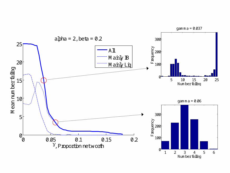
0 0.05 0.1 0.15 0.20

5

10

15

20

25

, Proportion net worth

Mea

n nu

mbe

r fa

iling

alpha = 2, beta = 0

AllMainly IBMainly Liq

1 2 3 4 50

100

200

300

400

Number failingF

requ

ency

gamma = 0.06

5 10 15 200

50

100

Number failing

Fre

quen

cy

gamma = 0.019

0 0.05 0.1 0.15 0.20

5

10

15

20

25

, Proportion net worth

Mea

n nu

mbe

r fa

iling

alpha = 2, beta = 0.2

AllMainly IBMainly Liq

1 2 3 4 5 60

100

200

300

Number failingF

requ

ency

gamma = 0.06

5 10 15 20 250

100

200

300

Number failing

Fre

quen

cy

gamma = 0.037

0 0.05 0.1 0.15 0.20

5

10

15

20

25

, Proportion net worth

Mea

n nu

mbe

r fa

iling

alpha = 2, beta = 1

AllMainly IBMainly Liq

1234 250

100

200

300

400

500

Number failing

Fre

quen

cy

gamma = 0.067

123 250

200

400

600

800

Number failingF

requ

ency

gamma = 0.082

0

0.05

0.1

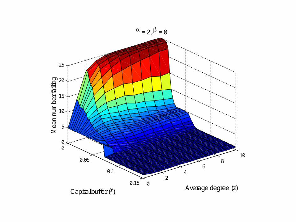
0.15 02

46

810

0

5

10

15

20

25

Average degree (z)

= 2, = 0

Capital buffer ()

Mea

n nu

mbe

r fai

ling

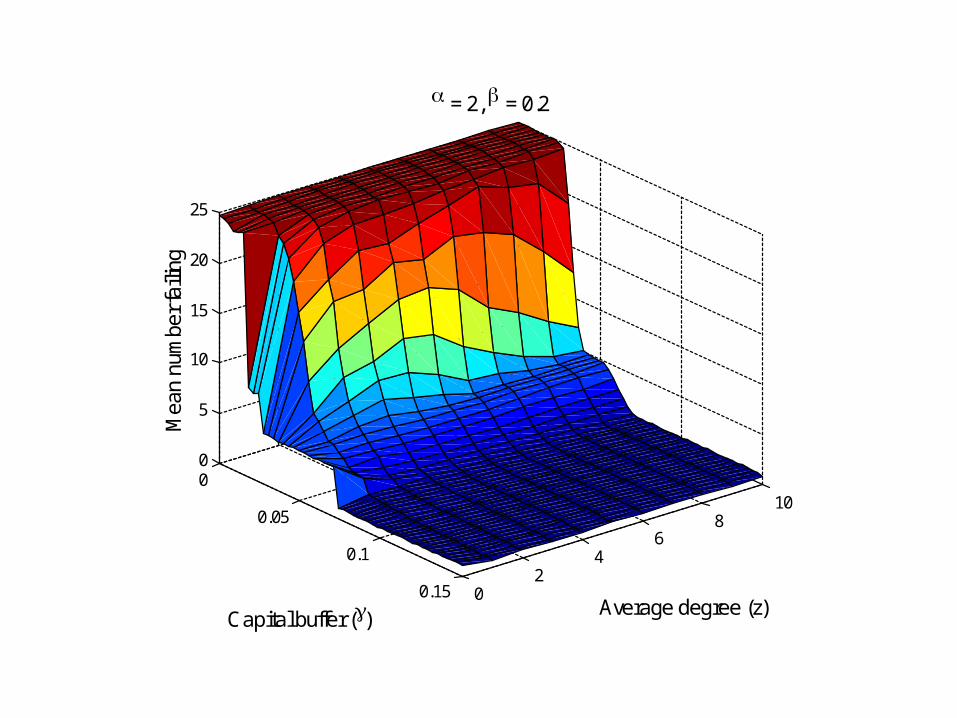
0

0.05

0.1

0.15 02

46

810

0

5

10

15

20

25

Average degree (z)

= 2, = 0.2

Capital buffer ()

Mea

n nu

mbe

r fai

ling

0

0.05

0.1

0.15 02

46

810

0

5

10

15

20

25

Average degree (z)

= 2, = 1

Capital buffer ()

Mea

n nu

mbe

r fai

ling

0 0.05 0.1 0.15 0.20

5

10

15

20

25

Proportion capital buffer,

Mea

n nu

mbe

r fai

ling

25 banks

0 0.05 0.1 0.15 0.20

50

100

150

200

250

300

350

400

450

500

Proportion capital buffer,

500 banks

= 0 = 0.2

The effect of ‘concentration’

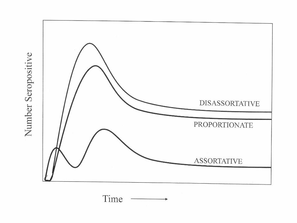
Extent of within group mixing in the high activity classes determines early rate of spread

HIGHEST IN THE ASSORTATIVE EXTREME

Peak levels and endemic state depend on the extent of mixing groups

HIGHEST IN THE DISASSORTATIVE EXTREME

Conclusions : 1Shocks propagated by interbank

loans tend to attenuate, by a factor of order z, in each successive phase of bank failures. Interestingly, high such interbank connectivity – in contrast to infectious diseases – means interbank loan shocks are attenuated more rapidly

The converse is true for liquidity shocks, which tend to amplify as more failing banks hold an affected asset.

Conclusions : 2The zone of instability with respect to interbank shocks tends to be maximised by having a rough balance of interbank loans and external assets (i.e. θ neither too big nor too small). Glass-Steagal may have been good for system stability, whatever its faults for individual banks.

Conclusions : 3Having large capital reserves means more

potentially working capital lies idle, but it makes for greater robustness of both individual banks and of the system as a whole.

Arguably, capital reserves should be relatively larger in boom times, when the temptation to take greater risks seems prevalent.

Systemic stability seems to require that bigger banks should hold their ratio of capital reserves to total assets at least as high as smaller banks. But in practice the contrary is what is observed.

Conclusions : 4a

Liquidity shocks may derive from the explicit failure of a specific asset (and the consequent problem inherent in “fire sales”), or alternatively by a more general “loss of confidence or trust”. Commonly both mechanisms are present, and both problems grow as more banks fail.

Conclusions : 4b

The gaming elements present in the way increasingly complex financial instruments are evaluated by Credit Ratings Agencies arguably has led to initial overpricing of such complex, untransparent assets. Such fragility of initial pricing – sometimes unwittingly but effectively corresponding to avoiding restrictions on excessive leverage – can obviously make for more severe liquidity shocks. This suggests tighter regulatory oversight of the value placed on such assets in the first place.

Banks’ resistance to some suggested regulations may not be simple bloody-mindedness. There can be unavoidable tensions between minimizing individual banks’ risk and minimizing systemic risk. Such tensions are only one element of complex questions, but they deserve to be more thoroughly and widely recognized in discussions about regulation