
PEAT8002 - SEISMOLOGY Lecture 10: Earthquake...
37
PEAT8002 - SEISMOLOGY Lecture 10: Earthquake relocation Nick Rawlinson Research School of Earth Sciences Australian National University
Transcript of PEAT8002 - SEISMOLOGY Lecture 10: Earthquake...

PEAT8002 - SEISMOLOGYLecture 10: Earthquake relocation
Nick Rawlinson
Research School of Earth SciencesAustralian National University

Earthquake relocationIntroduction
Earthquake relocation is one of the classic inverseproblems in seismology.Until recently, most relocation procedures were based onexploiting arrival time information from the seismic signalproduced by the earthquake.Accurate earthquake relocation is vital for manyapplications, including hazard forecasting and assessment,seismic tomography, examination of the contemporarystress field, source mechanism studies etc.In the past few years, it has been demonstrated that codawave interferometry can be used for earthquake relocation.Using this approach, the shape of the seismic waveform isexploited rather than the onset times of specific phases.
Earthquake relocationIntroduction
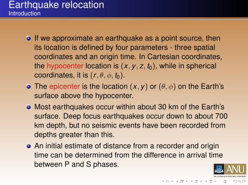
If we approximate an earthquake as a point source, thenits location is defined by four parameters - three spatialcoordinates and an origin time. In Cartesian coordinates,the hypocenter location is (x , y , z, t0), while in sphericalcoordinates, it is (r , θ, φ, t0).The epicenter is the location (x , y) or (θ, φ) on the Earth’ssurface above the hypocenter.Most earthquakes occur within about 30 km of the Earth’ssurface. Deep focus earthquakes occur down to about 700km depth, but no seismic events have been recorded fromdepths greater than this.An initial estimate of distance from a recorder and origintime can be determined from the difference in arrival timebetween P and S phases.

Earthquake relocationIntroduction
In fact, it is possible to exploit the differential moveouteffect that the spherically symmetric Earth has on anyidentifiable phase in a seismogram.
EP SPP PcS SS RL

Earthquake relocationIntroduction
The difference in arrival timesbetween the different phasescan be matched to standardtraveltime tables.This will provide an estimateof origin time and the angulardistance between source andreceiver.Repeating this procedure formultiple stations allows alocation estimate to be madefrom the multiple intersectingcircles of constant angulardistance.
Earthquake relocationFormulating the inverse problem
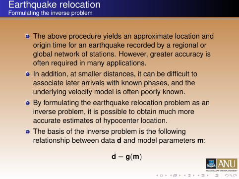
The above procedure yields an approximate location andorigin time for an earthquake recorded by a regional orglobal network of stations. However, greater accuracy isoften required in many applications.In addition, at smaller distances, it can be difficult toassociate later arrivals with known phases, and theunderlying velocity model is often poorly known.By formulating the earthquake relocation problem as aninverse problem, it is possible to obtain much moreaccurate estimates of hypocenter location.The basis of the inverse problem is the followingrelationship between data d and model parameters m:
d = g(m)

Earthquake relocationFormulating the inverse problem
In this case, the data matrix d are the arrival times Ti(i = 1, ...,N) of one or more phases generated by theearthquake at an array of stationsThe model parameter vector m is simply m = (r , θ, φ, t0),the hypocenter of the earthquake.For a given velocity model, adjusting the location and/ororigin time of an earthquake will obviously modify d, soclearly d = g(m).In cases where the velocity model is poorly known inaddition to hypocenter coordinates, it is often necessary tosimultaneously invert for both parameter classes. However,in the following treatment, we will ignore this possibility.

Earthquake relocationFormulating the inverse problem
Put simply, the inverse problem is to adjust the modelparameters m until the data d are satisfied.This presumes that we have a method for predicting arrivaltimes given some arbitrary value for m.In the case of teleseismic events, this could be thestandard traveltime tables associated with global referencemodels such as ak135 or iasp91.Generally, it is preferable to use the most accurate modelavailable. If this includes lateral heterogeneity, then ray orwavefront tracking methods (e.g. FMM) can be used topredict traveltimes.For absolute hypocenter locations, standard approachesinclude iterative non-linear relocation and fully non-linearrelocation.

Earthquake relocationIterative non-linear relocation
Given some initial estimate of an earthquake hypocenterm0, the general relationship d = g(m) can be written as aTaylor series expansion:
d = g(m0) + G(m − m0) + O(m − m0)2
where G = ∂g/∂m is a matrix of partial derivatives.If we define δd = d− g(m0) and δm = m−m0, then to firstorder:
δd = Gδm
This new equation assumes that a linear relationship existsbetween the arrival time data and the hypocenter locations.

Earthquake relocationIterative non-linear relocation
Provided that the matrix of partial derivatives is known, it ispossible to solve the linear system of equations. However,in general G is not square because usually there are moredata than unknowns. For N >> 4 traveltime values,
δd1δd2···
δdN
=
G11 G12 G13 G14G21 G22 G23 G24· · · ·· · · ·· · · ·
GN1 GN2 GN3 GN4
δm1δm2δm3δm4
The above system of equations has many more data thanunknowns (assuming linear independence), and thereforeconstitutes an overdetermined inverse problem.
Earthquake relocationIterative non-linear relocation
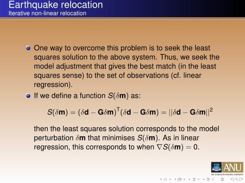
One way to overcome this problem is to seek the leastsquares solution to the above system. Thus, we seek themodel adjustment that gives the best match (in the leastsquares sense) to the set of observations (cf. linearregression).If we define a function S(δm) as:
S(δm) = (δd − Gδm)T(δd − Gδm) = ||δd − Gδm||2
then the least squares solution corresponds to the modelperturbation δm that minimises S(δm). As in linearregression, this corresponds to when ∇S(δm) = 0.

Earthquake relocationIterative non-linear relocation
The least squares function S(δm) can be written in indexnotation as follows:
S(δm) =N∑
j=1
[δdj −
4∑i=1
Gjiδmi
]2
The relationship between the notation and matrix forms iseasy to see from:
S(δm) =
[... δdj −
4∑i=1
Gjiδmi ...
] ...
δdj −4∑
i=1
Gjiδmi
...
as each matrix has N elements.

Earthquake relocationIterative non-linear relocation
If we now differentiate with respect to a particular modelparameter δmk , then we can use the chain rule to obtainthe derivative:
∂S(δm)
∂δmk=∂S(δm)
∂uj
∂uj
∂mk
where we have made the substitution:
uj = δdj −4∑
i=1
Gjiδmi
For the first term we obtain:
∂S(δm)
∂uj= 2
N∑j=1
[δdj −
4∑i=1
Gjiδmi
]

Earthquake relocationIterative non-linear relocation
The second term yields:
∂uj
∂mk= Gjk
since the derivative of Gjiδmi is non-zero only when i = k .Putting these two terms together and setting to zero yields:
2N∑
j=1
[δdj −
4∑i=1
Gjiδmi
]Gjk = 0
This may be re-written as:
N∑j=1
4∑i=1
GjiGjkδmi =N∑
j=1
Gjkδdj
Earthquake relocationIterative non-linear relocation
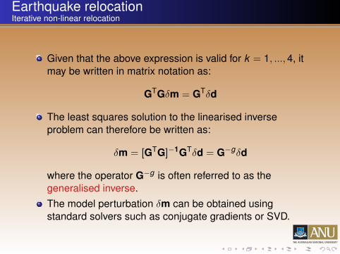
Given that the above expression is valid for k = 1, ...,4, itmay be written in matrix notation as:
GTGδm = GTδd
The least squares solution to the linearised inverseproblem can therefore be written as:
δm = [GTG]−1GTδd = G−gδd
where the operator G−g is often referred to as thegeneralised inverse.The model perturbation δm can be obtained usingstandard solvers such as conjugate gradients or SVD.

Earthquake relocationIterative non-linear relocation
For some given initial model m0, theoretical arrival timesare calculated and compared to the observed times toproduce δd. The matrix G is also evaluated at this stage.This allows the model perturbation δm to be produced bysolving the above equation. The new modelm1 = m0 + δm.Due to the inherent non-linearity of the inverse problem,the above procedure must in general be iterated until itconverges on a solution. Thus, theoretical arrival timesmust be computed for the new model m1 and the matrix Gupdated prior to obtaining m2.The model update procedure is defined by:
mi+1 = mi + δmi
Earthquake relocationIterative non-linear relocation
Note that because we have assumed local linearity toobtain a solution at each iteration, the function S(m) mustbe smooth and well behaved (quasi-quadratic).In practical applications, this iterative non-linear approachis usually only successful when a good initial estimate ofhypocenter location is available, and/or the velocitymedium is not strongly heterogeneous.In the presence of strong velocity gradients and data noise,S(m) is often characterised by multiple minima, whichmakes solution difficult.Nevertheless, iterative non-linear location is still frequentlyused in practice.

Earthquake relocationCalculation of G
In 3-D space, we need to derive expressions for four partialderivatives in order to construct G.The derivative of arrival time T with respect to origin time t0is given by:
∂Tt0
= 1
since perturbing the origin time will perturb the arrival timeby the same amount. In other words, T = to + ttr where ttris source receiver traveltime which is independent of t0.Clearly, ∂(to + ttr)/∂t0 = 1.The remaining terms can be computed analytically to firstorder. In this case, our derivation will assume a Cartesiancoordinate system.

Earthquake relocationCalculation of G
∆ l
zh ∆ z
z
θ
+
∆ z
zh
h
h
h
Consider a perturbation inhypocenter depth given by∆zh. To first order, thecorresponding change in pathlength ∆l is given by:
∆l = −∆zh cos θh
where θh is the angle betweenthe ray and the z − axis at thehypocenter.Note that the change in pathlength is negative as thehypocenter is perturbed toshallower depth.

Earthquake relocationCalculation of G
The change in arrival time T is therefore given by:
∆T =∆lvh
= −∆zh cos θh
vh
where vh is the velocity at the hypocenter.The first-order accurate expression for the partial derivativeis therefore given by:
∂T∂zh
== −cos θh
vh
Earthquake relocationCalculation of G
Similarly, the partial derivatives for the two remainingparameters are:
∂T∂xh
= −cosφh
vh,
∂T∂yh
= −cosψh
vh
where φh and ψh subtend the horizontal projection of theray path and the x and y axes, respectively, at thehypocenter.Most local earthquake tomography schemes that invert forboth velocity and hypocenter location use this form ofpartial derivative.For regional and global scale relocation, the derivativesshould be formulated in spherical coordinates.
Earthquake relocationExample
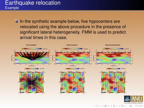
In the synthetic example below, five hypocenters arerelocated using the above procedure in the presence ofsignificant lateral heterogeneity. FMM is used to predictarrival times in this case.
Longitude ( )
−80
−60
−40
−20
0
−80
−60
−40
−20
0
140.0 140.5 141.0 141.5 142.0 142.5 143.0
140.0 140.5 141.0 141.5 142.0 142.5 143.0
4 5 6 7 8 9
True locations
Dep
th (
km)
Longitude ( )
−80
−60
−40
−20
0
−80
−60
−40
−20
0
140.0 140.5 141.0 141.5 142.0 142.5 143.0
140.0 140.5 141.0 141.5 142.0 142.5 143.0
4 5 6 7 8 9
Initial locations
Dep
th (
km)
Longitude ( )
−80
−60
−40
−20
0
−80
−60
−40
−20
0
140.0 140.5 141.0 141.5 142.0 142.5 143.0
140.0 140.5 141.0 141.5 142.0 142.5 143.0
4 5 6 7 8 9
Recovered locations
Dep
th (
km)
4 5 6 7 8 9
140˚
140˚
141˚
141˚
142˚
142˚
143˚
143˚
−42˚ −42˚
−41˚ −41˚
−40˚ −40˚
4 5 6 7 8 9
140˚
140˚
141˚
141˚
142˚
142˚
143˚
143˚
−42˚ −42˚
−41˚ −41˚
−40˚ −40˚
4 5 6 7 8 9
140˚
140˚
141˚
141˚
142˚
142˚
143˚
143˚
−42˚ −42˚
−41˚ −41˚
−40˚ −40˚
V (km/s)p V (km/s)p V (km/s)p
V (km/s)p V (km/s)p V (km/s)p
30 km 30 km 30 km
41 S 41 S 41 S
A A’ A A’ A A’
A A’ A A’ A A’
21 3
4
5
12
3
45
1 2
4
5
3
2
5
31
4

Earthquake relocationFully non-linear relocation
In most realistic media, the relationship between data andmodel parameters d = g(m) is highly non-linear, so if theinitial location is poor, iterative non-linear methods arelikely to fail (i.e. not converge or converge to the wrongminimum).An alternative means of hypocenter location is to searchmodel space without relying on local gradient information.One simple way of doing this is to perform a basic gridsearch. Given the speed of modern computers, this can bea practical approach, particularly when coupled with gridbased solvers like FMM.Otherwise, one can use non-linear/global optimisationtechniques such as genetic algorithms, simulatedannealing and the neighbourhood algorithm.

Earthquake relocationFully non-linear relocation
Consider an objective function S(m) defined by:
S(m) = (drobs − dr
m)T(dr
obs − drm)
where drobs is a vector of observed arrival times (from a
given hypocenter) at a set of N stations with the meansubtracted, and dr
m is a vector of predicted travel times,also with the mean subtracted.Removing the mean is useful, because it eliminates theorigin time as an unknown in the inversion. This is becausedobs = dt + d0 where d0 is the origin time and dt is theobserved traveltime.Thus, the mean of dobs is
d̄obs =
∑Ni=1 d t
iN
+ d0

Earthquake relocationFully non-linear relocation
Similarly, the mean of dm is
d̄m =
∑Ni=1 d i
mN
In this case, there is no d0 term because dm is the vectorof predicted traveltimes.Thus, from the above expressions:
drobs = dt − d̄t, dr
m = dm − d̄m
Thus, the objective function defined above only comparestraveltime information. Once S(m) has been minimised,the origin time can be found simply from d0 = dobs − dt.

Earthquake relocationFully non-linear relocation
The origin time does not affect the relative arrival timepattern, and therefore no information is ignored by usingthis approach.In the following 2-D examples, FMM is used to computetraveltimes in the presence of velocity models of varyingcomplexity.Traveltimes from a regular grid of points (180,901 in total)that span the model are computed to every receiver thatlies on the surface (5 in this case). Rather than executeFMM 180,901 times, we can use each receiver as a virtualsource to compute all required traveltimes.In each example, we try to find the location of theearthquake, which lies in the centre of the model, usingonly the arrival times at five receivers lying on the surface.

Earthquake relocationExample 1
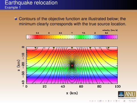
The first example uses a simple model in which velocityvaries linearly with depth.

Earthquake relocationExample 1
Model traveltime predictions for every receiver-grid pointpair are obtained by appealing to the reciprocity principle.
Earthquake relocationExample 1
Contours of the objective function are illustrated below; theminimum clearly corresponds with the true source location.

Earthquake relocationExample 2
In the second example, a model that features very stronglateral variations in wavespeed is used.
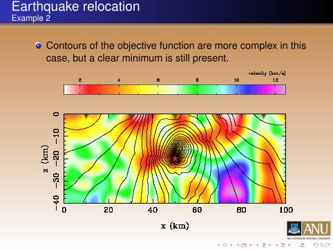
Earthquake relocationExample 2
Contours of the objective function are more complex in thiscase, but a clear minimum is still present.

Earthquake relocationExample 3
In the final example, a pathological velocity model is used,which has velocity contrasts as large as 70:1.

Earthquake relocationExample 3
Contours of the objective function have a strongrelationship with the velocity model, but nonetheless, thecorrect minimum zone can be identified.

Earthquake relocationExample 3
The above examples demonstrate the potential of bothFMM and fully non-linear location methods in earthquakelocation.A robust non-linear optimisation scheme should becapable of locating the minimum of the objective functioneven in the presence of strong velocity gradients.Poor station coverage, significant velocity heterogeneity,and data noise may result in multiple minima; techniqueslike the neighbourhood algorithm explore model space andproduce ensembles of solutions, which can then beinterrogated for their robustness.

Earthquake relocationRelative earthquake relocation
Relative earthquake location techniques are most usefullyapplied in seismogenic zones, such as in theneighbourhood of convergent or strike-slip plate margins.Although they can only find the relative locations ofmultiple earthquakes, they can do so with much greateraccuracy than absolute location techniques.Most of these techniques rely on the assumption that if thehypocentral separation between two earthquakes is smallcompared to the distance to the receiver, travel timedifferences at a particular station are not biased by theeffects of heterogeneity.In other words, ray trajectories are almost identical, withthe major difference simply being the change in pathlength. Thus, the difference in traveltimes for the twoevents can be attributed to their offset.

Earthquake relocationRelative earthquake relocation
Waveform cross-correlation techniques can also be usedto improve the accuracy of relative arrival time picks.The assumption of coherent waveforms for two differentevents is often most valid when they are very closetogether; source mechanisms can be identical andscattering effects are similar.One popular relative relocation scheme is the so-calleddouble-differencing technique. It exploits P- and S-wavedifferential traveltime measurements.Residuals between observed and theoretical traveltimedifferences (or double-differences) are minimised for pairsof earthquakes at each station, while linking together allobserved event-station pairs.

Earthquake relocationExample
Figure 9. (a) NCSN locations and (b) double-difference locations obtained fromcatalog travel-time differences and (c) the combined set of catalog and cross-correlationdata of events located in the El Cerrito and the Berkeley cluster. Top panels show mapview, lower panels show cross sections along the fault in NW–SE direction. The surfacetrace of the Hayward fault and shore line is shown. Boxes indicate events included inthe cross sections in this Figure and in Figure 11.