Technical Recoverability of Gas Hydrate in the U.S. … Recoverability of Gas Hydrate ... 101...

1

Technical Recoverability of Gas Hydrate in the U.S. Gulf of Mexico

Type I, II, and III Reservoirs

Prepared for:

Bureau of Ocean Energy Management, Regulation and Enforcement

Prepared by:

FEKETE ASSOCIATES INC.

November 2010

3

Table of Contents Chapter 1: Executive Summary ..................................................................................................5

Introduction..............................................................................................................................5 Scope and Methodology..........................................................................................................5 Summary of results .................................................................................................................8

Base Case Results ..............................................................................................................9 Technical Recoverability – Type II Reservoirs...................................................................11 Technical Recoverability – Type III Reservoirs..................................................................12

Observations and Recommendations ...................................................................................14 Chapter 2: Necessary Conditions for Presence and Dissociation of Hydrates .........................15 Chapter 3: Type II Reservoirs – Stage 1 work ..........................................................................17

Model configuration ...............................................................................................................17 List of Cases Studied ............................................................................................................18 Results ..................................................................................................................................21

Gas recovery .....................................................................................................................21 Cumulative Gas Production ...............................................................................................23

Summary of Results ..............................................................................................................26 Chapter 4: Type II – Stage 2 work ............................................................................................27

Reservoir Characteristics ......................................................................................................27 List of Cases Studied ............................................................................................................28 Results ..................................................................................................................................30

Gas recovery .....................................................................................................................30 Cumulative Gas Production ...............................................................................................34

Summary of Result................................................................................................................37 Chapter 5: Type III Reservoirs ..................................................................................................38

Reservoir Characteristics ......................................................................................................39 Two-level Plackett-Burman Experimental Design .................................................................39 Three-level Box-Behnken Experimental Design....................................................................41

Gas Recovery ....................................................................................................................44

4

Cumulative Gas Production ...............................................................................................47 Summary of Result................................................................................................................51

Chapter 6: Type I Reservoirs ....................................................................................................52 Reservoir Characteristics ......................................................................................................53 Base Case.............................................................................................................................55 Two-level Plackett-Burman Experimental Design .................................................................58 Results ..................................................................................................................................59

Gas Recovery ....................................................................................................................59 Summary of Result................................................................................................................64

References................................................................................................................................65 Appendices ...............................................................................................................................66

Appendix 2a: Estimation of Hydrate Reservoir Pressure and Temperature, and conditions for Hydrate Stability and Dissociation by Depressurization ........................................................67

Reservoir temperature: ......................................................................................................67 Reservoir pressure: ...........................................................................................................68 Conditions for hydrate presence:.......................................................................................68 Conditions for hydrate dissociation....................................................................................69 Estimation of hydrate reservoir pressure and temperature................................................71

Appendix 2b: Estimation of Hydrate Equilibrium Curve, and its Effect on Results ................73 Appendix 3a: Experimental Design and Probability Distribution of Uncertain Parameters (Type II Stage 1 work) ...........................................................................................................77 Appendix 4a: Experimental Design and Probability Distribution of Uncertain Parameters (Type II Stage 2 work) ...........................................................................................................84 Appendix 5a: Preliminary Investigation ................................................................................88 Vertical vs. horizontal wells using Cartesian grid ..................................................................88 Dip vs. Horizontal Reservoir ..................................................................................................89 Cartesian vs. Radial grid .......................................................................................................90 Gridding in radial grids ..........................................................................................................91 Horizontal gridding ................................................................................................................91

Vertical gridding: ................................................................................................................92 Effect of Capillary Pressure...................................................................................................92 Appendix 5b: Experimental Design Methods ........................................................................95 Appendix 6a: Initial conditions in Type I reservoirs .............................................................101

Determination of reservoir T and P..................................................................................102 Appendix 6b: Experimental Design Methods ......................................................................104

5

Chapter 1: Executive Summary Introduction

The Bureau of Ocean Energy Management, Regulation and Enforcement (BOEMRE;

formerly the Minerals Management Service) is the U.S. Department of Interior agency

responsible for overseeing the safe and environmentally responsible development of energy

and mineral resources on the Outer Continental Shelf. BOEMRE commissioned this current

study in an effort to build upon its in-place assessment of gas hydrates in the Gulf of Mexico by

gaining a better understanding of the technically recoverable portion of the in-place resource.

In this report, we (i) determine the reservoir characteristics that have a significant effect on the

technical recoverability of gas-hydrate reservoirs, and (ii) present approximate functions that

relate the technically recoverable portion of a hydrate accumulation to its reservoir

characteristics. By technical recoverability, we mean recovery factor after 50 years of

production. This report addresses technical recoverability of hydrate reservoirs of Type I

(those with underlying free gas), Type II (those with underlying mobile water), and Type III

(those without any underlying gas or water). Type IV gas hydrate accumulations (those in a

shale-dominated environment) are not considered in this study.

This study was conducted over a period of approximately two years and was made-up of

two stages. The learning’s from the first stage, led to a reinvestigation of range of

parameters, leading to a modification of these in the second stage of the work. In particular,

the range for water and reservoir depth was modified, and so was the geothermal gradient.

Also, the first stage of the work investigated production at 7 and 3 megaPascals (MPa). In the

second stage of the work, production pressure was limited to 3 MPa. In this report, we will

clarify the reason for these changes when the range of parameters from one stage to the next

changes.

In this executive summary, the scope and methodology of the study is briefly presented

and various assumptions are discussed. This is followed by a summary of the recovery

functions for each of Type II and Type III reservoirs and recommendations for future work.

Type I reservoirs are discussed in detail in Chapter 6.

Scope and Methodology

In this work, depressurization is the methodology considered for hydrate recovery. It is

assumed that depressurization is achieved using a vertical well that may be operated at a

6

producing pressure of 3000 kilopascals (kPa)1. An area of 760 m by 760 m is assigned to

each vertical well (corresponding to four wells for each cell of 5000 ft by 5000 ft). Simulation

runs are conducted to estimate the cumulative gas production after 50 years of production,

which is then used to estimate recovery factor at 50 years. The calculations are performed

using the STARS™ simulator of Computer Modeling Group (CMG). The following work-flow

was followed:

1. Based on our experience, and in consultation with BOEMRE, a list of reservoir

parameters that could affect gas production from a hydrate accumulation was

developed (See Table 1).

2. In consultation with BOEMRE, a reasonable range for each of these reservoir

parameters was determined, and high, medium and low values were assigned.

3. When necessary, mechanistic simulation studies were conducted to better

understand how some of these reservoir characteristics may affect hydrate

recovery.

4. A two-level experimental-design technique was used to come up with a number of

cases to be simulated.

5. Simulation studies were conducted and recovery at 50 years was estimated.

6. A function was developed between the recovery factor and the reservoir

characteristics determined in item 1.

7. The function was used along with the range of parameters (and the distribution

functions) determined in item 2, and Monte-Carlo simulation was performed to

determine the most important reservoir characteristics that affect the performance

indicators (Tornado chart).

8. For the more important parameters identified in item 7, a three-level experimental

design technique was used and steps 5 to 7 were repeated.

9. Finally, we explore the limitations and degree of error associated with these

function.

10. These final functions may be used along with cell-properties from the in-place study

and additional information to estimate technical recoverability and cumulative gas

production in 50 years.

1 At pressures below 3000 kPa, possibility of freezing increases as the equilibrium temperature approaches 0 °C. This value was selected to allow a large drawdown, without risking ice formation and plugging. It is quite likely that achieving a production pressure of 3000 kPa would require use of artificial lift.

7

Table 1: List of Reservoir Characteristics that Could Affect Technical Recoverability of Hydrates and Their Range2

Reservoir Characteristics Variable Name

Low estimate

Medium Estimate

High Estimate

Water depth, m WD 750 1500 3000

Reservoir mid-point depth below sea floor, m RD 100 300 600

Porosity, % Phi 30 35 40

Hydrate Saturation, % SH 40 60 85

Sand thickness, m H 3 6 20

Dip angle, degrees Angle 0 5 10

Initial Permeability within hydrate layer, mD Ki 0.05 0.5 5

Permeability without hydrate (Absolute permeability), mD

Kabs 100 500 1000

Endpoint of gas relative permeability krg0 0.1 0.5 1.0

Ratio of hydrate column to total R_HC 0.5 0.7 0.9

Extent of aquifer (in addition to the water in the base model)

Aquifer No No 5 times of the reservoir size

This study makes a number of assumptions. These include:

• Only sand-hosted gas hydrate accumulations are studied.

• The reservoir is assumed to be homogeneous. In the presence of significant

heterogeneity (in the form of disconnected sand bodies), more than one well may

be required to access the hydrates within the study area.

• Presence (or lack thereof) of a sealing cap-rock was not taken into account

2 The range of some of the parameters originally used in the study of Type II reservoirs was different from that shown in Table 1. This original study is presented in Chapter 3, while the study that uses the revised range of parameters (corresponding to Table 1), is presented in Chapter 4. The last two rows of Table 1 do not apply to Type III reservoirs where there is no underlying aquifer. The effect of uncertainty in the equilibrium curve was not incorporated. A sensitivity study is reported in Appendix 2b.

8

• Multiple sand bodies were not studied. It was assumed that each sand body (and

its surrounding formation) acts independently from any other sand accumulation.

• This study does not impose other cut-off criteria on recoverability. Such potential

cut-off criteria could include

o A minimum gas-in-place per cell, or a minimum accumulation size.

o Presence of a cap-rock

o Unconsolidated sands (that may lead to sloughing or other geomechanical

problems)

• The results are applicable to the range of parameters studied. For example, the

minimum value of initial permeability (in the presence of hydrate) investigated was

0.05 mD. Initial permeability values significantly lower than this value could affect

technical recoverability. Another example is the aquifer. The largest aquifer size

studied was one that was 5 times the size of the overlying hydrate accumulation.

The effect of a large active aquifer was not taken into account.

Summary of results The technically recoverable portion of a “cell” is estimated in two steps:

(i) For those cells that are included in the “in-place” study and therefore are within the

hydrate stability zone, it needs to be ensured that the hydrate reservoir is warm

enough (typically above a few °C) so that its hydrate or a portion thereof would

decompose at 3000 kPa.

(ii) The properties of “cells” that pass the above cut-off criterion are entered into the

technical-recoverability functions.

The first condition states that for at least part of the hydrate to dissociate at the deepest

point of the hydrate zone, the reservoir temperature must be greater than the equilibrium

temperature corresponding to the production pressure. This condition is explained in detail in

Chapter 2.

For hydrates that satisfy this condition, production was simulated. The results for a Base

Case, where the reservoir properties correspond to the medium estimate given in Table 1 are

presented first. Then, the functions for technical recoverability of Type II and Type III

reservoirs were obtained. These are presented in the following, along with the range of

recovery factors obtained when these functions are used. Similar functions for estimation of

cumulative gas production in 50 years are also given.

9

Base Case Results

Figure 1 present a schematic diagram of a Type II reservoir at a water depth of 1500 m and

an average depth of 300 m below the ocean floor. Using a hydrostatic pressure gradient of 10

kPa/m and geothermal gradient of 24.55 °C/km, the initial pressure and temperature at the

centre point of the reservoir are 18.1 MPa and 11.63° C. Other properties correspond to the

medium estimate shown in Table 1.

Sea surface

Sea floor

WD

RD

Dip angle

L=760 m

Centre point A

H

Figure 1: Schematic diagram of Type II reservoir with Base Properties

Water Rate SC Cumulative Water SC

Time (yr)

Wat

er R

ate

SC

(STB

/day

)

Cum

ulat

ive

Wat

er S

C (S

TB)

0 5 10 15 20 25 300

500

1,000

1,500

2,000

2,500

3,000

0.0e+0

5.0e+5

1.0e+6

1.5e+6

2.0e+6

2.5e+6

3.0e+6

Gas Rate SC Cumulative Gas SC

Time (yr)

Gas

Rat

e SC

(MM

SC

F/da

y)

Cum

ulat

ive

Gas

SC

(MM

SCF

)

0 5 10 15 20 25 300.00

0.20

0.40

0.60

0.80

1.00

0.00e+0

1.00e+3

2.00e+3

3.00e+3

4.00e+3

5.00e+3

Figure 2: Gas and water production vs. time for a Type II hydrate reservoir with Base Case

Properties (results are in field units)

Figure 2 shows the gas and water production for a vertical well, within a drainage area of

760 m by 760 m, which is operated at a constant production pressure of 3 MPa. Results shown

in Figure 2 indicate a high initial water production rate that declines sharply while gas

10

production rate increases. Within a period of less than one year, gas rate exceeds 0.4 million

standard cubic feet (MMSCF) per day, and then it slowly increases to approximately 0.7

MMSCF/day. After a period of approximately 10 years, when most of the hydrate is

dissociated, gas production rate declines sharply. Cumulative gas production after a

production period of 17 years is approximately 2.8 billion cubic feet (Bcf), corresponding to a

gas recovery of 85.5%3. The average water-gas ratio during this period is approximately 800

stock tank barrels (STB)/MMSCF.

Figure 3 shows the corresponding results for a Type III reservoir, where there is no

underlying water and the whole pore space shown in Figure 1 is filled with hydrate. It has been

suggested that gas production rate for a Type III hydrate reservoir is characterized by a period

of rising rate (not unlike what is seen for wet cold-bed reservoirs), while the decomposition

zone surrounding the well is expanding (Zatsepina et al. 2008). The results in Figure 3 show

that gas rate increases over a period of approximately 7 years and peaks at slightly more than

1.5 MMSCF/day before it declines to zero in 15 years. This long period of low gas production

has economical implications, which are not addressed in this work. Cumulative gas production

during this period is slightly more than 4 Bcf, corresponding to a recovery factor of 92%. The

absence of underlying water improves the ultimate recovery. The overall average water-gas

ratio is 310 STB/MMSCF. Sensitivity studies indicate that application of horizontal wells could

accelerate production by 4 to 5 years, but will not influence ultimate recovery.

Gas Rate & Cumulative

Gas Rate SC Cumulative Gas SC

Time (yr)

Gas

Rat

e SC

(MM

SCF/

day)

Cum

ulat

ive

Gas

SC

(MM

SCF)

0 5 10 15 20 25 300.00

0.50

1.00

1.50

2.00

2.50

0.0e+0

1.0e+3

2.0e+3

3.0e+3

4.0e+3

5.0e+3Water Rate & Cumulative

Water Rate SC Cumulative Water SC

Time (yr)

Wat

er R

ate

SC (S

TB/d

ay)

Cum

ulat

ive

Wat

er S

C (S

TB)

0 5 10 15 20 25 300

100

200

300

400

500

0.0e+0

3.0e+5

6.0e+5

9.0e+5

1.2e+6

1.5e+6

Figure 3: Gas and water production vs. time for a Type III hydrate reservoir with Base Case

Properties (results are in filed units)

3 Gas recovery is defined as ratio of cumulative gas production to initial gas in hydrate form.

11

The high recovery factors reflected with results shown in Figures 2 and 3 are related to the

large difference between the initial reservoir temperature and the equilibrium temperature at

producing pressure of 3 MPa. This temperature difference provides sufficient sensible and

conduction heat to enable large recovery factors. Alternatively, we will show production at a

higher pressure of 7 MPa would have only marginally destabilized the hydrates. As seen in the

next section, the majority of the simulation studies conducted in this work yield a large recovery

factor. The low-recovery cases are generally associated with reservoirs that are cold, such

that at a well-pressure of 3 MPa, only a small fraction of the hydrate is destabilized.

Technical Recoverability – Type II Reservoirs

We implemented the methodology of experimental design described earlier and conducted

a large range of simulation runs. The five most important parameters affecting recoverability

were identified: reservoir depth (RD), water depth (WD), reservoir thickness (H), hydrate

saturation (SH) and dip angle (ANGLE). The results were then used to estimate the technical

recoverability for Type II reservoirs as a function of these reservoir parameters. This function is

given as Equation 1, where the variable parameters are defined in Table 1 and the “b”

coefficients are given in Table 2.

Recovery (% )= b0 + b1*RD + b2*RD*RD + b3*WD*H + b4*SH*Angle + b5*RD*H + b6*RD*Angle + b7*RD*SH + b8*H*SH + b9*WD*SH + b10*WD*RD + b11*H*Angle + b12*WD*WD + b13*WD

Equation 1

Table 2: List of Eq.1 coefficients for determination of technical recoverability of Type II reservoirs

b0 7.141111E+01b1 1.825620E-01b2 -3.694706E-04b3 -3.852847E-04b4 -2.676772E-02b5 3.840768E-03b6 4.349370E-03b7 1.374189E-03

b8 -1.805354E-02b9 -1.216576E-04b10 1.910550E-05b11 -6.973584E-02b12 7.337392E-06b13 -2.940365E-02

Equation 1 may be used to estimate the technical recoverability of a Type II reservoir.

Using a Monte Carlo algorithm, we applied this relationship to the range of properties shown in

Table 1. The results are shown in Figure 4 and indicate a mean gas recovery of 72%, with 90%

12

of the cases having a recovery factor of more than 39%. Calculations shown in Chapter 4

indicate that for the cases studied this relation exhibits an approximate error of ± 20%. In

distribution plots of recovery given in this report, such as that given in Figure 4, recovery

factors of above 100% and below 0% are shown. This is an indication of fact that a simple

function cannot accurately capture the non-linearity in the solution4.

Distribution for Recovery

Mean = 72.34

X <=93.9990%

X <=39.3910%

0

0.005

0.01

0.015

0.02

0.025

0.03

0.035

0.04

-30 -20 -10 0 10 20 30 40 50 60 70 80 90 100 110 120

Recovery, %

Figure 4: Probability distribution of gas recovery for Type II reservoirs based on Equation 1

Technical Recoverability – Type III Reservoirs

The application of methodology described earlier suggest that the technical recoverability

for Type III reservoirs may be estimated using Equation 2, where the variable parameters are

defined in Table 1 and the “b” coefficients are given in Table 3.

Recovery(%) = b0 + b1*RD + b2*RD*RD + b3*RD*Ki + b4*WD*Ki + b5*WD + b6*WD*WD + b7*H*SH + b8*SH*SH + b9*RD*H + b10*SH*krg0 + b11*Ki*krg0 + b12*RD*Kabs + b13*Kabs + b14*WD*SH + b15*krg0

Equation 2

4 We examined use of functions that limit the recovery factor to between zero and 100%, and found that the degree of accuracy of these functions was much less than those that allowed a wider range.

13

Equation 2 may be used to estimate the technical recoverability of a Type III reservoir.

Using a Monte Carlo algorithm, we applied this relationship to the range of properties shown in

Table 1. The results are shown in Figure 5 and indicate a mean gas recovery of approximately

74%, with 90% of the cases having a recovery factor of more than 28%. Calculations shown in

Chapter 5 indicate that for the cases studied this relation exhibits an approximate error of ±

20%. This is similar to the error found for Type II reservoirs.

Table 3: List of Eq. 2 coefficients for determination of technical recoverability of Type III reservoirs

b0 -1.8226E+01b1 5.6244E-01b2 -5.6620E-04b3 -9.1575E-03b4 1.4910E-03b5 -2.8741E-02b6 8.4598E-06b7 -3.2494E-02b8 7.3074E-03b9 3.4011E-03b10 -5.3920E-01b11 3.3845E+00b12 -7.6880E-05b13 3.1250E-02b14 -2.2135E-04b15 3.4926E+01


Mean = 73.36

X <=103.1590%

X <=27.610%

0

0.02

0.04

0.06

0.08

0.1

0.12

0.14

0.16

0.18

-40 -20 0 20 40 60 80 100 120 140

Recovery, %

Rel

ativ

e Fr

eque

ncy

Figure 5: Probability distribution of gas recovery for Type III reservoirs based on Equation 2

14

Observations and Recommendations

• Review of the results has shown that a large number of cases show a high technical

recoverability (> 80%). In contrast a smaller number of cases show a small

recovery factor (< 20%). The latter cases correspond to low temperature reservoirs

often with low initial permeability. It is possible that the physics of recovery in such

cases is different from those showing high recovery. Under these situations, it is

difficult for a unique response function to predict recovery. One may pursue

distinguishing between the two groups and developing recovery-functions for each

of the groups.

• The recovery factors are strongly correlated with initial temperature and pressure.

Under these circumstances, the effect of other parameters may not be estimated

accurately. One may pursue separating the effect of these parameters so that the

effect of other parameters can be more accurately accounted for.

• The results of his work are subject to assumptions given previously. It is

recommended that

o The applicability of the relations developed here is examined against

simulation results presented by others, particularly if a different numerical

simulator is used.

o The applicability of the relations developed here is examined against

detailed simulation of hydrate accumulations in a small area of Gulf of

Mexico

15

CHAPTER 2: NECESSARY CONDITIONS FOR PRESENCE AND DISSOCIATION OF HYDRATES

The technically recoverable portion of a “cell” is estimated in two steps. In the first step,

it is ensured that the “cell” includes hydrates and that it may be destabilized by the

depressurization technique to a producing pressure of 3000 kPa. These conditions are related

to the initial pressure and temperature of the hydrate and their position with respect to the

hydrate stability field.

Figure 6 shows the initial pressure and temperature (p/T) of a reservoir (shown by a red

square) in relation to the hydrate equilibrium curve. For hydrate to be present, the initial p/T

conditions need to lie above the equilibrium curve. Furthermore, for it to be dissociated it

needs to be warm enough. The minimum reservoir temperature for dissociation should

therefore be more than the equilibrium temperature corresponding to the minimum pressure

(TeBHP). For the case shown in Figure 6, the minimum reservoir temperature that would allow

dissociation is nearly °6 C. Reservoirs that are colder than this would not dissociate, unless

production pressure is further reduced.

0

2,000

4,000

6,000

8,000

10,000

12,000

14,000

16,000

18,000

20,000

22,000

24,000

26,000

28,000

30,000

0 2 4 6 8 10 12 14 16 18 20

Temperature, oC

Pres

sure

, kPa

Figure 6: The p/T conditions of the reservoir in relation to the hydrate equilibrium curve; the

flowing bottomhole pressure of 3000 kPa is shown as red dashed line.

16

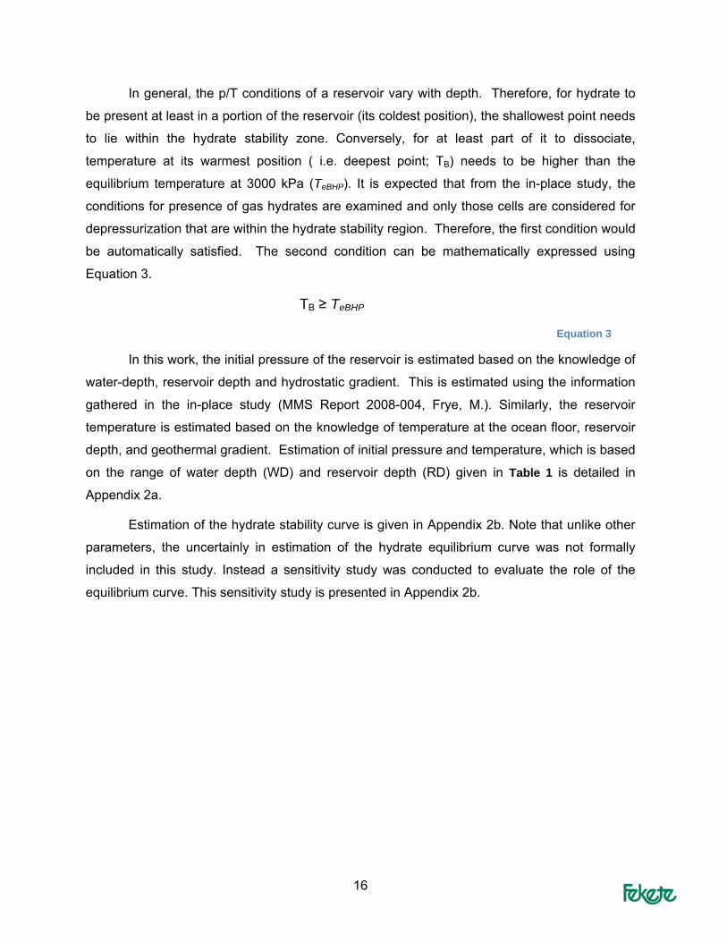
In general, the p/T conditions of a reservoir vary with depth. Therefore, for hydrate to

be present at least in a portion of the reservoir (its coldest position), the shallowest point needs

to lie within the hydrate stability zone. Conversely, for at least part of it to dissociate,

temperature at its warmest position ( i.e. deepest point; TB) needs to be higher than the

equilibrium temperature at 3000 kPa (TeBHP). It is expected that from the in-place study, the

conditions for presence of gas hydrates are examined and only those cells are considered for

depressurization that are within the hydrate stability region. Therefore, the first condition would

be automatically satisfied. The second condition can be mathematically expressed using

Equation 3.

TB ≥ TeBHP

Equation 3

In this work, the initial pressure of the reservoir is estimated based on the knowledge of

water-depth, reservoir depth and hydrostatic gradient. This is estimated using the information

gathered in the in-place study (MMS Report 2008-004, Frye, M.). Similarly, the reservoir

temperature is estimated based on the knowledge of temperature at the ocean floor, reservoir

depth, and geothermal gradient. Estimation of initial pressure and temperature, which is based

on the range of water depth (WD) and reservoir depth (RD) given in Table 1 is detailed in

Appendix 2a.

Estimation of the hydrate stability curve is given in Appendix 2b. Note that unlike other

parameters, the uncertainly in estimation of the hydrate equilibrium curve was not formally

included in this study. Instead a sensitivity study was conducted to evaluate the role of the

equilibrium curve. This sensitivity study is presented in Appendix 2b.

17

Chapter 3: Type II Reservoirs – Stage 1 work In this chapter, the relation between hydrate-reservoir properties and gas recovery

and/or cumulative gas production is explored. The work presented in this chapter is based on

a two-level experimental design, to identify those parameters that have a larger effect on gas

recovery. In the next chapter, we will concentrate on the more important parameters, use a

revised range of values for these parameters and conduct a three-level experimental design.

In this chapter and next, a correlation (i.e. response function) is developed between the

simulated recovery and the reservoir parameters. Then, Monte Carlo simulation is conducted

using the response functions to generate the probability distribution of gas recovery and

cumulative gas production. The relative importance of individual parameters is identified. The

work done in this chapter reflects the first stage of the work, where the range of some of the

reservoir properties differed from those given in Table 1.

Model configuration The drainage area used in the model is 760 m × 760 m; or, approximately 4 wells per

BOEMRE in-place assessment model cell of 5000 ft by 5000 ft. The well is placed slightly

below the water-hydrate contact as shown in Figure 7.

It is realized that a hydrate reservoir that on a larger scale may be classified as Type II,

may not be divided into segments that all are equal (in particular in terms of containing

underlying water). Nevertheless, the investigation of Type II reservoirs in this study considers

an element of symmetry such as that shown in Figure 7 below.

Figure 7: Model Configuration for Type II hydrate reservoir; colors represent hydrate saturation

18

List of Cases Studied Table 4 lists the ranges of 12 parameters considered in this stage of the work. A two-

Level experimental design method, i.e. the Plackett-Burman method, was applied to generate

22 combinations. The table of Plackett-Burman design is presented in Appendix 3a, along with

the probability distribution function used for all the parameters.

Table 4: List of Reservoir Characteristics and Their Range (Type II reservoirs, stage 1)


Low estimate

Medium Estimate

High Estimate


Reservoir mid-point depth below sea floor, m

RD 100 250 400


Initial Permeability within hydrate layer, mD

Ki 0.05 0.5 5




Ratio of hydrate column to total

R_HC 0.5 0.7 0.9


Aquifer No No 5 times of the reservoir size

Permeability within the underlying free water, mD

Kabs 100 500 1000

Endpoint of gas relative permeability

krg0 0.1 0.5 1.0

Flowing BHP, kPa BHP 3000 3000 7000

Figure 8 depicts the the initial p/T condition of the various cases in relation to the hydrate equilibrium curve. Note that all cases plot above the blue curve (that is, lie initially within the hydrate stability zone).

19

Case 26

Case 27

Case 1Case 2

Case 3

Case 4 Case 5

Case 6

Case 7Case 8

Case 9

Case 10

Case 11

Case 12

Case 13

Case 14

Case 15

Case 16

Case 17

Case 18

Case 19

Case 20

Case 21 Case 22

Case 23

Case 24

Case 25Case 28

0

5,000

10,000

15,000

20,000

25,000

30,000

35,000

40,000

45,000

0 5 10 15 20 25Temperature, C

Equi

libriu

m P

ress

ure,

kPa

MMS Case 1 Case 2 Case 3 Case 4Case 5 Case 6 Case 7 Case 8 Case 9Case 10 Case 11 Case 12 Case 13 Case 14Case 15 Case 16 Case 17 Case 18 Case 19Case 20 Case 21 Case 22 Case 23 Case 24Case 25 Case 26 Case 27 Case 28

Figure 8: the initial p/T condition of the various cases with respect to the hydrate equilibrium

curve

Table 5 lists 22 simulation cases. Among them, 20 cases incorporate different combinations of

the input parameters with either the minimum or the maximum value of the parameters, and 2

cases use the central values. The input parameters and simulation results of all cases are

listed in Table 5. Recovery factors vary between 0 and 90%.

Results indicated that the production pressure of 7000 kPa results in no dissociation of

hydrate in many cases, such as when the hydrate reservoir is at a very shallow depth below

seafloor (< ~150 m). In consultation with MMS it was decided that the production pressure

would be reduced to 3000 kPa. Table 6 shows an additional 10 cases where all parameters

are the same except that a BHP of 3000 kPa is used for cases that used a value of 7000 kPa

(cases 1,4,5,6,9,10,14,16,20 and 22).

20

Table 5: The 22 cases examined and the simulation results

F1 F2 F3 F4 F5 F6 F7 F8 F9 F10 F11 F12 Resp_1 Resp_2

Exp # WD RD Phi Ki SH H Angle R_HC Aquife kabs krg0 BHP Recovery,% Cum Gas, E3m31 2000 400 30 0.05 40 3 10 0.5 1 100 1 7000 70.91 13,1772 2000 400 40 0.05 40 20 10 0.5 1 1000 0.1 3000 78.97 130,4403 1200 250 35 0.5 60 6 5 0.7 0 500 0.5 3000 87.25 79,0854 750 100 40 5 40 20 10 0.5 0 100 0.1 7000 0.00 05 750 200 40 5 85 3 0 0.9 1 100 1 7000 35.18 33,1466 750 100 30 0.05 85 3 10 0.5 1 1000 1 7000 0.00 07 2000 400 40 5 40 3 4 0.9 0 1000 1 3000 89.50 39,8788 2000 100 30 5 85 3 10 0.9 0 100 0.1 3000 44.94 31,8759 2000 100 40 0.05 85 20 10 0.9 0 100 1 7000 0.00 0

10 750 200 40 0.05 40 3 0 0.9 0 1000 0.1 7000 61.63 27,32311 750 200 30 5 85 20 10 0.5 0 1000 1 3000 74.46 194,82912 2000 400 30 0.05 85 20 0 0.9 1 100 0.1 3000 82.18 389,45613 750 100 30 5 40 20 0 0.9 1 1000 1 3000 83.14 184,19514 2000 400 30 5 85 3 0 0.5 0 1000 0.1 7000 62.93 24,85415 750 200 40 0.05 85 20 0 0.5 0 100 1 3000 90.62 316,14816 2000 100 30 0.05 40 20 0 0.9 0 1000 1 7000 0.00 017 750 100 30 0.05 40 3 0 0.5 0 100 0.1 3000 69.70 12,84918 2000 100 40 5 40 3 0 0.5 1 100 1 3000 67.55 16,71819 1200 250 35 0.5 60 6 5 0.7 0 500 0.5 3000 87.25 79,08520 2000 100 40 5 85 20 0 0.5 1 1000 0.1 7000 0.00 021 750 100 40 0.05 85 3 10 0.9 1 1000 0.1 3000 73.95 69,56622 750 185 30 5 40 20 4 0.9 1 100 0.1 7000 12.89 28,252

Table 6: Additional cases with flowing BHP of 3000 kPa and the simulation results

F1 F2 F3 F4 F5 F6 F7 F8 F9 F10 F11 F12 Resp_1 Resp_2

Exp # WD RD Phi Ki SH H Angle R_HC Aquife kabs krg0 BHP Recovery,% Cum Gas, E3m323 2000 400 30 0.05 40 3 10 0.5 1 100 1 3000 84.44 15,68924 750 200 40 5 85 3 0 0.9 1 100 1 3000 86.28 81,28125 750 200 40 0.05 40 3 0 0.9 0 1000 0.1 3000 83.62 37,06926 2000 400 30 5 85 3 0 0.5 0 1000 0.1 3000 83.01 32,78327 750 185 30 5 40 20 4 0.9 1 100 0.1 3000 76.05 166,71528 750 100 40 5 40 20 10 0.5 0 100 0.1 3000 25.86 42,44129 750 100 30 0.05 85 3 10 0.5 1 1000 1 3000 81.71 32,05230 2000 100 40 0.05 85 20 10 0.9 0 100 1 3000 13.42 84,76531 2000 100 30 0.05 40 20 0 0.9 0 1000 1 3000 59.70 132,96932 2000 100 40 5 85 20 0 0.5 1 1000 0.1 3000 24.94 87,437

21

Results Simulation studies were conducted for all the cases reported in Table 5 and Table 6 to

estimate gas recovery and cumulative gas production over a 50 year period. These were then

correlated as a function of variable parameters shown in Table 4. The response functions

were then used to estimate the range of expected recovery and the sensitivity of the results on

the variable parameters. These are explained below, first for gas recovery and then for

cumulative gas production.

Gas Recovery The response function of gas recovery within 50 years is given as Equation 4 for 22

cases in Table 5. The coefficients of b0 to b12 are listed in Table 7. The R2 of regression is

0.913.

Table 7: List of parameter for Equation 4

b0 106.91b1 -0.01230b2 0.148b3 0.236b4 -0.771b5 -0.06194b6 -0.710b7 -1.213b8 -3.635b9 -1.383b10 0.00213b11 5.750b12 -0.01193

Figure 6 shows a comparison between the simulated gas recovery and predicted

recovery by the function. The additional cases in Table 6 are shown in red triangles and are

Recovery(%) = b0 + b1*WD + b2*RD + b3*Phi + b4*Ki + b5*SH + b6*H + b7*Angle + b8*R_HC + b9*Aquifer + b10*kabs + b11*krg0 + b12*BHP

Equation 4

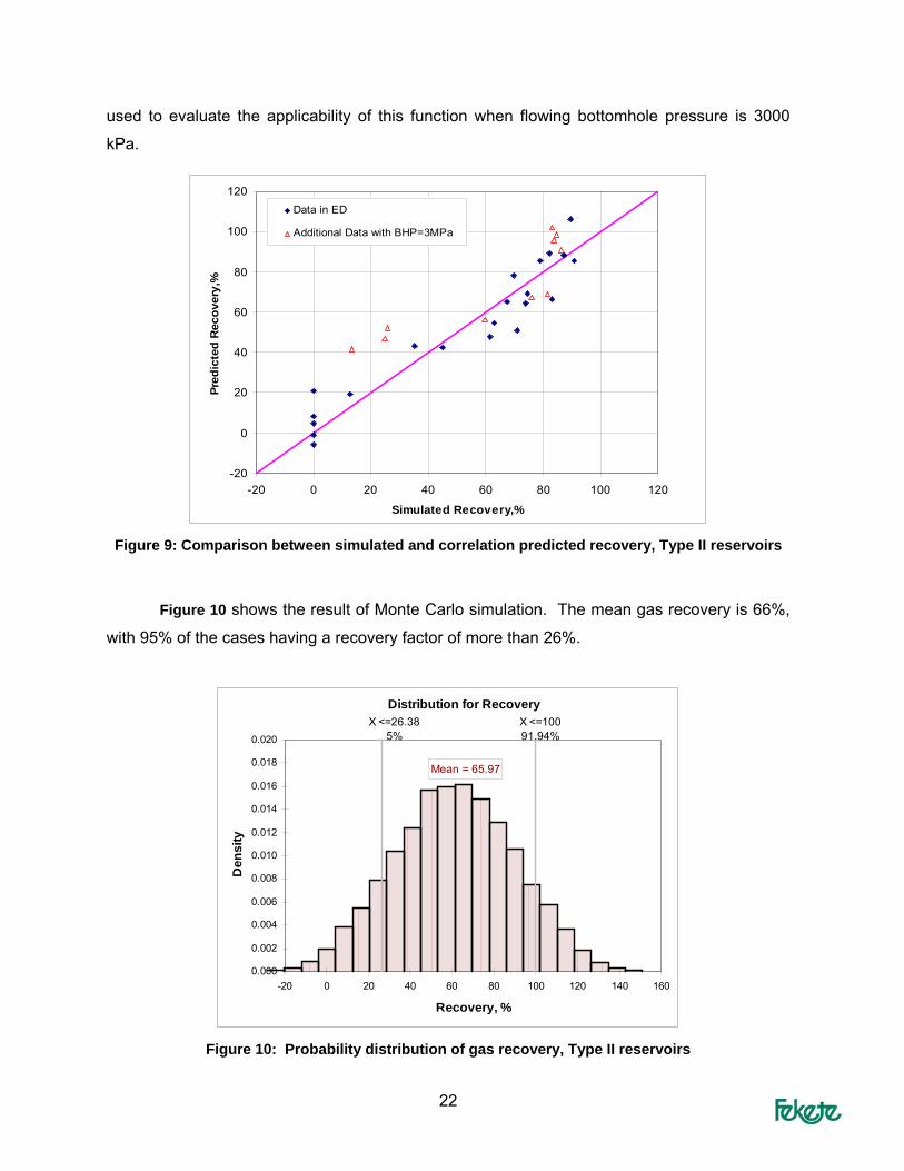
22

used to evaluate the applicability of this function when flowing bottomhole pressure is 3000

kPa.

-20

0

20

40

60

80

100

120

-20 0 20 40 60 80 100 120

Simulated Recovery,%

Pred

icte

d R

ecov

ery,

%Data in ED

Additional Data with BHP=3MPa

Figure 9: Comparison between simulated and correlation predicted recovery, Type II reservoirs

Figure 10 shows the result of Monte Carlo simulation. The mean gas recovery is 66%,

with 95% of the cases having a recovery factor of more than 26%.


Mean = 65.97

X <=10091.94%

X <=26.385%

0.000

0.002

0.004

0.006

0.008

0.010

0.012

0.014

0.016

0.018

0.020

-20 0 20 40 60 80 100 120 140 160

Recovery, %

Den

sity

Figure 10: Probability distribution of gas recovery, Type II reservoirs

23

Figure 11 depicts the significance of each parameter. The reservoir depth below seafloor (RD),

production pressure (BHP), water depth (WD), sand thickness (H) and Angle are the top 5

important parameters affecting the gas recovery. The effect of these will be studied in Chapter

4 in further detail, using a three-level experimental design approach.

Correlations for Recovery

0.686

-0.621

-0.249

-0.172

-0.154

0.064

-0.048

0.041

-0.036

0.036

-0.032

-0.018

-1 -0.8 -0.6 -0.4 -0.2 0 0.2 0.4 0.6 0.8 1

RD

BHP

WD

H

Angle

krg0

Ki

Phi

SH

kabs

Aquifer

R_HC

Correlation Coefficients

Figure 11: Tornado chart of significance of parameters to recovery, Type II reservoirs

Cumulative Gas Production Equation 5 shows the response function of cumulative gas production within 50 years

for the cases in Table 5. The coefficients are listed in Table 8.

Table 3: List of Coefficients in Eq. (13)

CumGas (E3m3) = b0 + b1*WD + b2*RD + b3*Phi + b4*Ki + b5*SH + b6*H + b7*Angle + b8*R_HC + b9*Aquifer + b10*kabs + b11*krg0 + b12*BHP

Equation 5

24

Table 8: List of coefficients in Equation 5

b0 93133.8b1 -48.43b2 399.87b3 -1722.9b4 -6628.8b5 1683.3b6 6511.5b7 -5698.2b8 28066.9b9 21592.9b10 -27.60b11 18392.3b12 -27.51

Figure 12 shows the comparison between the simulated cumulative gas and that

predicted by the function. The R2 of regression is 0.903.

-50

0

50

100

150

200

250

300

350

400

-50 0 50 100 150 200 250 300 350 400

Simulated Cumulative Production, E6m3

Pred

icte

d C

umul

ativ

e Pr

oduc

tion,

E6m

3

Data in ED

Additional Data with BHP=3MPa

Figure 12: Comparison between simulated and correlation predicted cumulative gas, Type II

Figure 13 shows the probability distribution of cumulative gas. The mean value of cumulative

gas production at 50 years is 123.5 E6m3 (~4.4 Bcf)5.

5 The Base-Case results presented in Chapter 1 indicated a gas production of 2.2 Bcf. The difference between that and the mean value obtained in Figure 13 is because of the difference between the mean value of reservoir thickness considered in evaluation of Figure 13 that is roughly two times that used in the Base Case.

25

Distribution for CumGas

Mean = 123.5E6

X <=253.9E695%

X <=05.90%

0

0.5

1

1.5

2

2.5

3

3.5

4

4.5

5

-150 -100 -50 0 50 100 150 200 250 300 350 400

Cumulative Gas Produciton, E6m3

Val

ues

in 1

0^ -6

Figure 13: Probability distribution of cumulative gas production, Type II reservoir

Figure 14 shows that reservoir depth below seafloor (RD), sand thickness (H),

production BHP (BHP), water depth (WD) and hydrate saturation (SH) are the top 5 important

parameters affecting cumulative gas production.

Correlations for CumGas

0.559

0.464

-0.415

-0.297

0.272

-0.212

0.126

-0.113

-0.104

-0.083

0.061

0.031

-1 -0.8 -0.6 -0.4 -0.2 0 0.2 0.4 0.6 0.8 1

RD

H

BHP

WD

SH

Angle

Aquifer

Ki

kabs

Phi

krg0

R_HC


Figure 14: Tornado chart of significance of parameters to cumulative gas, Type II reservoirs

26

Summary of Results The objective of this chapter was to determine those parameters that have the largest

impact on the technical recoverability of gas hydrate from Type II reservoirs. The top five

parameters affecting recovery are water depth, reservoir depth, sand thickness, production

pressure and dip angle. Production pressure will not be further investigated, as all the future

cases will be produced at a production pressure of 3000 kPa.

As shown in Figure 11, the most important parameter affecting gas recovery is reservoir

depth (RD). A deeper reservoir implies a higher reservoir temperature, positively affecting gas

recovery. Water depth also is an important parameter but has negative effect because a

deeper seafloor means lower temperature and higher pressure, leading to a lower recovery.

Another important parameter is the thickness of sand. While a thicker sand can result in lower

gas recovery (because of a lesser ratio surface to volume lowering the effect of heat

conduction from the surrounding), thickness has a positive effect on cumulative gas

production.

The recovery and cumulative gas production for the cases with zero dip angle are

greater that those with dip angles. This is because the area for hydrate dissociation is much

larger in the case of horizontal reservoir with underlying free water, which results in higher

recovery. Furthermore, the hydrate interval of a reservoir with a smaller dip angle has a higher

average temperature than one with larger dip angle, everything else being the same.

Although it was not the objective of this chapter, the mean value of recovery for Type II

was estimated to by approximately 65%. This recovery factor should be expected to increase

in the second stage of the work (Chapter 4), as the production pressure will be lower and the

reservoir depth will increase.

27

Chapter 4: Type II – Stage 2 work The study presented in Chapter 3, which used a two-level experimental design (ED)

and uncertainty assessment, suggested that the reservoir parameters that have a significant

effect on the gas recovery and cumulative production from Type II hydrate reservoir include:

water depth (WD), reservoir depth below seafloor (RD), sand thickness (H), hydrate saturation

(SH), and dip angle (Angle). In this chapter, a more thorough examination based on 3-level

experimental design is performed in order to find the relation between these five parameters

and gas recovery and/or cumulative gas production. In particular, a three-level five-parameter

Box-Behnken experimental design method led to a total of 44 cases. An additional 16 test

cases were generated based on a two-level ED method and run with the intention of testing

the validity of the preliminary response function. Two response functions were generated, one

based on the 44 cases and the other based on the 60 cases. As will be shown later in this

chapter the response function that incorporates the results of all 60 cases exhibits a smaller

error in relation to the actual simulation results. However, the mean value of recovery

estimated from both response functions agrees closely.

Reservoir Characteristics Table 9 gives the list of reservoir parameters and their corresponding range

investigated in this chapter. These range reflects the stage 2 work where,

• The range of values for water depth and reservoir depth below ocean floor was

extended to 3000 m and 600 m respectively.

• A geothermal temperature gradient of 0.02455 °C/m is applied. This value is smaller

than that used in the previous chapter, 0.04 °C/m.

• All simulation runs are conducted with a constant production pressure of 3000 kPa.

Table 9: List of Reservoir Characteristics and Their Range (Type II reservoirs, stage 2)


Low Estimate

Medium Estimate

High Estimate

Water depth (m) WD 750 1500 3000

Reservoir mid-point depth (mbsf) RD 100 300 600

Sand thickness (m) H 3 6 20

Hydrate Saturation (%) SH 40 60 85

Dip angle (degrees) Angle 0 5 10

28

Table 10 gives the list of the parameters that are kept constant.

Table 10: List of other reservoir parameters not varied and their values

Reservoir Characteristics Value

Porosity, % 35

Initial Permeability within hydrate layer, mD 0.5

Ratio of hydrate column to total 0.7


No

Permeability within the underlying free water, mD

500

Endpoint of gas relative permeability (krgo) 0.5

Curvature of gas relative permeability (Ng) 3.5

Flowing BHP, kPa 3000

List of Cases Studied A three-level five-parameter Box-Behnken experimental design method was employed

as listed in Appendix 4a. This technique suggests that a total of 44 cases need to be

examined; 4 of which use the central values of parameters. The simulation runs of these 44

cases have been conducted and the results are given in Table 11 (Cases 1 to 44). An

additional 16 test cases (listed as cases 45-60 in Table 11) were run with the intention of

testing the validity of the preliminary response function. These cases were generated based

on a two-Level ED method. Another response function was regenerated including all 60

cases. Table 11 gives simulation results of all cases.

Table 11: List and of input parameters and simulation results for all cases6

Case # WD RD H SH Angle Recovery,% CumGas, E3m3 1 750 300 6 85 5 88.01 113009 2 1500 100 3 60 5 40.80 18439 3 3000 300 3 60 5 87.30 39441 4 1500 300 3 85 5 89.08 57014 5 1500 300 20 60 0 87.35 264092 6 3000 300 6 85 5 85.14 109324 7 3000 300 20 60 5 67.63 204254 8 1500 300 6 85 10 81.62 104804 9 1500 600 3 60 5 89.84 40587

6Cases 38, 51, 52, 56 and 57 are at a water depth of 750m and reservoir depth of 600m, which is located below the hydrate stability zone. The following modifications have been made for these cases. The reservoir depth is reduced to 200 m in case 38 and 300 m in the other 4 cases.

29

Case # WD RD H SH Angle Recovery,% CumGas, E3m3 10 750 300 6 60 10 82.46 74740 11 1500 300 6 85 0 89.10 114484 12 1500 300 6 40 0 81.74 49426 13 1500 600 6 40 5 85.40 51607 14 1500 300 6 60 5 85.45 77453 15 1500 300 3 40 5 83.34 25101 16 1500 300 6 60 5 85.45 77453 17 1500 600 6 60 10 87.14 78978 18 750 300 3 60 5 88.64 40047 19 1500 600 6 85 5 90.86 116672 20 3000 300 6 60 0 86.12 78108 21 3000 300 6 60 10 80.31 72785 22 1500 100 6 40 5 33.62 20316 23 750 300 6 60 0 86.40 78363 24 1500 100 6 85 5 19.94 25599 25 3000 100 6 60 5 18.46 16732 26 1500 100 6 60 10 23.50 21297 27 1500 300 20 40 5 77.93 156916 28 1500 300 6 60 5 85.45 77453 29 1500 300 20 85 5 56.11 240083 30 1500 600 6 60 0 87.76 79601 31 1500 300 6 40 10 80.08 48386 32 1500 300 3 60 0 85.73 38879 33 1500 300 6 60 5 85.45 77453 34 750 100 6 60 5 74.88 67871 35 750 300 20 60 5 79.92 241371 36 1500 100 20 60 5 9.79 29583 37 1500 300 3 60 10 82.81 37643 38 750 200 6 60 5 83.92 76067 39 1500 100 6 60 0 41.77 37889 40 1500 300 20 60 10 67.09 202821 41 1500 600 20 60 5 84.36 254804 42 3000 600 6 60 5 89.16 80813 43 3000 300 6 40 5 83.21 50283 44 750 300 6 40 5 84.09 50810 45 3000 100 20 40 10 8.46 17060 46 3000 600 20 85 10 81.51 349065 47 3000 600 3 40 10 83.62 25343 48 3000 600 3 85 0 89.55 57529 49 3000 100 3 40 0 74.51 22526 50 3000 600 20 40 0 83.56 168415 51 750 300 3 40 0 82.39 24909 52 750 300 3 85 10 86.53 55729 53 3000 100 20 85 0 4.02 17229 54 750 100 3 40 10 79.06 23960 55 750 300 20 85 0 90.27 386662 56 750 100 20 85 10 22.26 95316 57 750 300 20 40 10 78.10 157392 58 750 100 20 40 0 62.21 125389 59 3000 100 3 85 10 24.67 15888 60 750 100 3 85 0 87.93 56493

Figure 15 show the initial p/T condition of all cases in relation to the phase stability diagram. Note that all cases plot above the blue stability curve where conditions exist for the formation of gas hydrate. The probability distributions used for the input parameters are given in Appendix 4a.

30

C-20

C-22

C-25

C-32

C-34C-35

C-42

C-1C-2

C-3

C-4C-5

C-6 C-7

C-8

C-9

C-10

C-11C-12

C-13C-14C-15

C-16 C-17

C-18

C-19

C-21

C-23

C-24C-26

C-27

C-28

C-29C-30

C-31C-33

C-36 C-37

C-38

C-39

C-40C-41

C-43

C-44

C-45

C-46

C-47

C-48C-49

C-50

C-51

C-52

C-53

C-54

C-55

C-56 C-57C-58

C-59

C-60

0

5,000

10,000

15,000

20,000

25,000

30,000

35,000

40,000

45,000

50,000

0 5 10 15 20 25

Temperature, C

Pres

sure

, kPa

MMS C-1 C-2 C-3 C-4 C-5 C-6 C-7 C-8C-9 C-10 C-11 C-12 C-13 C-14 C-15 C-16 C-17C-18 C-19 C-20 C-21 C-22 C-23 C-24 C-25 C-26C-27 C-28 C-29 C-30 C-31 C-32 C-33 C-34 C-35C-36 C-37 C-38 C-39 C-40 C-41 C-42 C-43 C-44C-45 C-46 C-47 C-48 C-49 C-50 C-51 C-52 C-53C-54 C-55 C-56 C-57 C-58 C-59 C-60

Figure 15: Initial p/T condition of all cases, Type II - phase 2

Results

Gas recovery The response function of gas recovery within 50 years is given by Equation 6 for 60

cases listed in Table 11. This function is obtained using a quadratic function with insignificant

terms eliminated during the regression. The coefficients of b0 to b13 are listed in Table 12.

Figure 16 shows a comparison between the simulated gas recovery and that predicted

using Equation 6. R2 of regression is 0.888. The solid blue triangles represent results of cases

(1-44) and the red squares correspond to the cases (45-60) listed in Table 11. The regression

function exhibits an error of ±20% in estimated recovery.

Recovery (% )= b0 + b1*RD + b2*RD*RD + b3*WD*H + b4*SH*Angle + b5*RD*H + b6*RD*Angle + b7*RD*SH + b8*H*SH + b9*WD*SH + b10*WD*RD + b11*H*Angle + b12*WD*WD + b13*WD

Equation 6

31

Table 12: List of coefficients in Equation 6

b0 7.141111E+01b1 1.825620E-01b2 -3.694706E-04b3 -3.852847E-04b4 -2.676772E-02b5 3.840768E-03b6 4.349370E-03b7 1.374189E-03b8 -1.805354E-02b9 -1.216576E-04b10 1.910550E-05b11 -6.973584E-02b12 7.337392E-06b13 -2.940365E-02

-10

010

2030

4050

6070

8090

100110

120

-10 0 10 20 30 40 50 60 70 80 90 100 110 120Simulated Recovery,%

Pred

icte

d R

ecov

ery,

%

Cases 1-44Cases 45-60

Figure 16: Comparison between simulated and correlation predicted recovery by Equation 6

As stated earlier, an earlier correlation was developed using the results of cases 1 to

44. Figure 17 demonstrates the comparison between recovery predicted from this function and

all cases (1 to 60). The results indicate that that the response function based on cases 1 to 44

exhibits an error of ±30%.

32

-100

1020

304050

607080

90100

110120

-10 0 10 20 30 40 50 60 70 80 90 100 110 120Simulated Recovery,%

Pred

icte

d R

ecov

ery,

%


Figure 17: Comparison between simulated and correlation predicted recovery by the response

function regressed from cases 1-44

Figure 18 shows the result of Monte Carlo simulation for the gas recovery using

Equation 6. The mean gas recovery is 72%, with 90% of the cases having a recovery factor of

more than 39%.


Mean = 72.34

X <=93.9990%

X <=39.3910%

0

0.005

0.01

0.015

0.02

0.025

0.03

0.035

0.04

-30 -20 -10 0 10 20 30 40 50 60 70 80 90 100 110 120

Recovery, %

Figure 18: Probability distribution of gas recovery from Equation 6 (Type II reservoir)

33

Figure 19 shows the probability distribution of gas recovery from the correlation

regressed from the cases 1-44 only. The mean value is close to that in Figure 18 but the range

of recoveries is slightly wider.

Distribution for Recovery 2/C193

0.000

0.005

0.010

0.015

0.020

0.025

0.030

Mean=72.92629

-30 -20 -10 0 10 20 30 40 50 60 70 80 90 100 110 120-30 -20 -10 0 10 20 30 40 50 60 70 80 90 100 110 120

10% 80% 10%< > 34.5949 96.8949

Figure 19: Probability distribution of gas recovery for the function from cases 1-44

Figure 20 depicts the significance of each parameter. The most significant parameter is

the reservoir depth below the seafloor (RD). RD determines the reservoir temperature, having

a large influence on recovery. Other important parameters in the order of significance include

sand thickness (H), water depth (WD), dip angle (Angle) and hydrate saturation (SH),

respectively. The results are consistent with those obtained using two-level experimental

results reported in Chapter 3.

34


0.727

-0.212

-0.21

-0.117

-0.004

-1 -0.5 0 0.5 1

RD

H

WD

Angle

SH


Figure 20: Tornado chart of significance of parameters to recovery

Cumulative Gas Production Equation 7 presents the response function for cumulative gas production in 50 years.

This was developed from the 60 cases in Table 11. The coefficients are listed in Table 13.

Table 13: List and value of coefficients in Equation 7

b0 5.544821E+03b1 2.722329E+01b2 9.590242E+01b3 -2.388074E+00b4 -5.674778E-01b5 5.423990E+00b6 -2.700365E+02b7 3.438051E+00b8 -7.787621E+01b9 -4.904303E-01b10 5.804168E-03

CumGas (E3m3) = b0 + b1*RD*H + b2*H*SH + b3*WD*H + b4*RD*RD + b5*RD*SH +b6*H*Angle + b7*WD*Angle + b8*SH*Angle + b9*WD*SH + b10*WD*WD

Equation 7

35

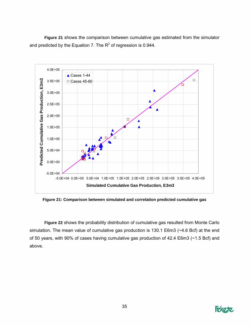
Figure 21 shows the comparison between cumulative gas estimated from the simulator

and predicted by the Equation 7. The R2 of regression is 0.944.

-5.0E+04

0.0E+00

5.0E+04

1.0E+05

1.5E+05

2.0E+05

2.5E+05

3.0E+05

3.5E+05

4.0E+05

-5.0E+04 0.0E+00 5.0E+04 1.0E+05 1.5E+05 2.0E+05 2.5E+05 3.0E+05 3.5E+05 4.0E+05

Simulated Cumulative Gas Production, E3m3

Pred

icte

d C

umul

ativ

e G

as P

rodu

ctio

n, E

3m3


Figure 21: Comparison between simulated and correlation predicted cumulative gas

Figure 22 shows the probability distribution of cumulative gas resulted from Monte Carlo

simulation. The mean value of cumulative gas production is 130.1 E6m3 (~4.6 Bcf) at the end

of 50 years, with 90% of cases having cumulative gas production of 42.4 E6m3 (~1.5 Bcf) and

above.

36

Distribution for CumGas

Mean = 130.1 E6m3

X <=245.690%

X <=42.410%

0

1

2

3

4

5

6

7

-100 0 100 200 300 400 500 600

Cumulative Gas, E6m3

Val

ues

in 1

0^ -6

Figure 22: Probability distribution of cumulative gas production - Type II reservoir

Figure 23 shows the significance of reservoir parameters on cumulative gas production,

which in order of importance include sand thickness (H), reservoir depth below seafloor (RD),

hydrate saturation (SH), water depth (WD) and dip angle (Angle).


0.687

0.493

0.256

-0.131

-0.047

-1 -0.5 0 0.5 1

H

RD

SH

WD

Angle


Figure 23: Tornado chart demonstrating the significance of parameters on cumulative gas

37

Summary of Result

• Response functions of gas recovery Equation 6 and cumulative gas production

Equation 7 from type II hydrate reservoir were generated in terms of the most important

five parameters, namely reservoir depth below seafloor (RD), water depth (WD), sand

thickness (H), hydrate saturation (SH), and dip angle (Angle). Accuracy of the recovery

function as compared with simulation results is ± 20%.

• Monte Carlo simulations were conducted for the gas recovery and cumulative

production. The mean recovery and mean cumulative gas production are 72% and 130

E6m3 (4.6 Bcf) respectively for the range of parameters considered in Table 9.

• The corresponding values obtained in the first phase of the study (previous chapter) are

66% and 4.4 Bcf. This previous study used a different range of input parameters and

used two-level experimental design. Despite these differences, the results are in close

agreement.

38

CHAPTER 5: TYPE III RESERVOIRS

In this chapter, the technical recoverability of Type III reservoirs (those without any

underlying free fluid) is investigated. The methodology used here is similar to that used in the

study of Type II hydrate reservoirs. The study is conducted in three stages: a preliminary

investigation towards better understanding of some factors affecting production response, a

two-level experimental design (ED) and uncertainty assessment for finding the more important

parameters, and a three-level ED and uncertainty assessment.

In the preliminary-investigation stage, model configuration is examined and the following

questions are answered:

• Because of unavailability of a free-fluid below the hydrate, pressure drop caused by

production affects a small area of a Type III reservoir. This leads to very slow rate of

gas production, until the dissociated area grows (Zatsepina 2008). In the preliminary

investigation reported in Appendix 5a, the use of horizontal well was investigated.

• Another study was conducted to examine if the reservoir dip angle is important for

modeling Type-III hydrate reservoirs, and whether we can use radial grids instead of

Cartesian grids7.

• Lastly, the appropriate size of grid blocks was investigated.

The detailed results of preliminary investigation are presented in Appendix 5a. In summary,

• Although a horizontal well can accelerate production, the simulation were conducted

using a vertical well, because (i) The acceleration in production as a result of use of

horizontal wells is less than 5 years. This is small as compared with the simulation time

of 50 years. In other words, the 50-year recovery factor is not a strong function of

completion type, and (ii) to remain consistent with the Type II study.

• Production response is not affected by the reservoir dip angle; this was excluded from

the study.

• For a flat reservoir, radial grids can be employed and simulation run time will be much

shorter than with Cartesian grids.

7 As shown in Appendix 5a, accurate modeling of Type III hydrate reservoirs requires small grid blocks. Such small grids can be accommodated in horizontal reservoirs with use of radial grids. This was not necessary in the study of Type II reservoirs.

39

Reservoir Characteristics Table 14 gives the list of reservoir parameters and their corresponding range

investigated in this study. Other parameters not listed in Table 1 will not be varied in the study,

in particular:

• Similar to that used in Chapter 4, a constant geothermal temperature gradient of

0.02455 °C/m is applied.

• Type III does not have associated aquifer. Therefore, the parameters extent of aquifer

and ratio of hydrate column to total, are left out.

• As mentioned earlier, the effect of dip angle was investigated separately and the results

indicated that the effect of dip angle is not critical.

• A constant following BHP of 3000 kPa is assumed, similar to that used in chapter 4.

Table 14: List of Reservoir Characteristics and their values (Type III reservoirs)


Low Estimate

Medium Estimate

High Estimate




Porosity, % Phi 0.3 0.35 0.4



Permeability without hydrate (Absolute Permeability), mD

Kabs 100 500 1000

Endpoint of gas relative permeability (krgo) Krg0 0.1 0.5 1.0

Twolevel PlackettBurman Experimental Design In order to identify the more important parameters that affect hydrate recovery and gas

production, a 2-level 8-parameter Plackett-Burman experimental design method was

employed. A list of the cases - along with the simulation results - are given in Table 15.

40

Table 15: Input parameters and simulation results for 14 cases based on a two-level experimental

design8

Case # WD RD H SH Phi Ki Kabs Krg0 Recovery,% CumGas,E3m3 1 3000 100 20 85 30 5 100 0.1 0.15 0 2 1500 300 6 60 35 0.5 500 0.5 91.91 118588 3 750 100 3 85 40 5 100 1 73.87 76847 4 3000 600 20 40 40 5 100 1 90.79 299750 5 3000 100 3 40 40 5 1000 0.1 34.73 17162 6 750 100 20 85 40 0.05 1000 1 23.16 160645 7 750 100 3 40 30 0.05 100 0.1 12.00 4408 8 750 300 20 85 30 5 1000 0.1 88.73 461960 9 750 300 3 40 30 5 1000 1 91.26 33536

10 3000 600 3 85 40 0.05 1000 0.1 91.02 95796 11 3000 600 3 85 30 0.05 100 1 94.97 74957 12 3000 100 20 40 30 0.05 1000 1 0 0 13 1500 300 6 60 35 0.5 500 0.5 91.91 118588 14 750 300 20 40 40 0.05 100 0.1 27.70 90497

Gas Recovery The response function of gas recovery for 14 cases listed in Table 15 is given by

Equation 8 . Table 16 lists the coefficients.

Recovery(%) = b0 + b1*WD + b2*RD + b3*H + b4*SH + b5*Phi + b6*Ki + b7*Kabs + b8*Krg0

Equation 8

Table 16: List of coefficients in Equation 8 and their values

b0 11.33b1 -0.01270b2 0.164b3 -1.520b4 0.222b5 0.08404b6 4.484b7 0.01337b8 11.90

Monte Carlo simulation was performed by using Equation 8 which accounted for the

probability distribution of 8 input parameters (shown in Appendix 5b).

8 The cases 8, 9, and 14 are at a water depth of 750m and reservoir depth of 600m, which is located below the hydrate stability zone. The reservoir depth is modified to 300 m in these 3 cases.

41

Figure 24 shows the significance of each parameter. The three most significant parameters

are reservoir depth, initial permeability and water depth. The least significant parameter is the

porosity of the sand.


0.82

0.256

-0.293

-0.246

0.119

0.088

0.06

0.001

-1 -0.5 0 0.5 1

RD

Ln(Ki)

WD

H

Kabs

Krg0

SH

Phi



Threelevel BoxBehnken Experimental Design Seven of the 8 parameters were included in the three-level experimental design. The

list of cases (1 to 60) is shown in Table 17, where 4 cases use the most likely values.

Simulation runs were conducted and results are listed in Table 17. A preliminary response

function was developed. An additional 12 test cases listed as cases 61-72 in Table 17 were

run with the intention of testing the preliminary response functions. These cases were

generated based on a 7-parameter two-level Plackett-Burman ED method (see Appendix 5b).

A response function was regenerated incorporating results of all 72 cases.

42

Table 17: List of input parameters and simulation results for all cases9

Case # WD RD H SH Ki Kabs krg0 Recovery_% CumGas_E3M3 1 750 300 3 60 0.05 500 0.5 91.83 59055 2 1500 600 6 60 0.05 500 1 93.33 120568 3 1500 100 20 60 0.5 100 0.5 0.17 731 4 1500 300 6 40 5 100 0.5 89.41 76911 5 1500 300 20 40 0.5 500 0.1 81.97 235022 6 1500 600 3 60 0.5 1000 0.5 92.47 59731 7 3000 100 6 40 0.5 500 0.5 0.34 0 8 1500 300 6 60 0.5 500 0.5 91.91 118588 9 3000 300 20 60 0.05 500 0.5 50.74 219588

10 1500 600 3 60 0.5 100 0.5 92.34 59649 11 3000 300 20 60 5 500 0.5 80.08 346594 12 1500 300 6 85 0.05 100 0.5 93.44 170805 13 1500 600 6 60 5 500 1 93.44 120722 14 1500 300 6 85 0.05 1000 0.5 93.64 171160 15 1500 300 6 40 0.05 100 0.5 88.78 76366 16 750 300 6 40 0.5 500 0.5 88.68 76044 17 1500 300 20 40 0.5 500 1 90.13 258440 18 750 100 6 40 0.5 500 0.5 87.91 75320 19 1500 600 20 60 0.5 100 0.5 91.67 394785 20 3000 300 3 60 5 500 0.5 91.94 59685 21 1500 100 6 60 5 500 1 36.59 47175 22 750 300 20 60 0.05 500 0.5 91.60 392720 23 3000 300 6 60 0.5 100 1 93.15 120952 24 3000 300 6 60 0.5 1000 1 93.36 121224 25 1500 300 6 40 0.05 1000 0.5 88.64 76247 26 1500 100 3 60 0.5 1000 0.5 31.78 20486 27 1500 300 3 40 0.5 500 1 91.02 39146 28 1500 300 3 85 0.5 500 1 94.52 86386 29 3000 300 6 60 0.5 1000 0.1 87.58 113720 30 1500 300 20 85 0.5 500 1 62.08 378228 31 750 300 6 60 0.5 100 1 93.04 119668 32 1500 100 6 60 0.05 500 0.1 0.00 0 33 750 300 20 60 5 500 0.5 91.65 392961 34 1500 100 3 60 0.5 100 0.5 3.74 2430 35 3000 600 6 40 0.5 500 0.5 89.27 77373 36 1500 300 3 85 0.5 500 0.1 90.38 82602 37 750 300 6 60 0.5 1000 1 93.25 119935 38 1500 300 6 60 0.5 500 0.5 91.91 118588 39 750 300 3 60 5 500 0.5 92.01 59175 40 1500 100 6 60 5 500 0.1 9.77 12597 41 1500 300 6 60 0.5 500 0.5 91.91 118588 42 1500 600 6 60 5 500 0.1 87.98 113665 43 1500 600 20 60 0.5 1000 0.5 91.68 394828 44 1500 300 3 40 0.5 500 0.1 83.52 35924 45 750 300 6 60 0.5 1000 0.1 87.71 112820 46 750 100 6 85 0.5 500 0.5 78.69 143261 47 3000 300 6 60 0.5 100 0.1 82.51 107136 48 1500 300 6 85 5 1000 0.5 93.34 170609 49 1500 100 6 60 0.05 500 1 0.00 0 50 1500 300 6 85 5 100 0.5 92.75 169532 51 1500 300 6 60 0.5 500 0.5 91.91 118588 52 3000 600 6 85 0.5 500 0.5 93.46 172130

9 Cases 16, 60, 61, 66 and 68 are at a water depth of 750m and reservoir depth of 600m, which is located below the hydrate stability zone. The value of reservoir depth of 600 m is modified to 300 m in these 5 cases

43

Case # WD RD H SH Ki Kabs krg0 Recovery_% CumGas_E3M3 53 3000 100 6 85 0.5 500 0.5 0.53 981 54 3000 300 3 60 0.05 500 0.5 79.81 51816 55 1500 300 6 40 5 1000 0.5 89.23 76751 56 750 300 6 60 0.5 100 0.1 87.70 112805 57 1500 100 20 60 0.5 1000 0.5 1.55 6676 58 1500 300 20 85 0.5 500 0.1 53.36 325132 59 1500 600 6 60 0.05 500 0.1 88.72 114624 60 750 300 6 85 0.5 500 0.5 93.28 169966 61 750 300 3 40 0.05 1000 1 90.41 38762 62 3000 600 20 40 5 1000 0.1 82.64 238759 63 750 100 3 40 0.05 100 0.1 9.18 3932 64 750 100 20 85 5 100 1 12.34 74865 65 3000 100 20 85 0.05 1000 0.1 0.00 0 66 750 300 20 40 5 100 0.1 81.29 232355 67 3000 100 3 40 5 1000 1 90.69 39220 68 750 300 20 85 0.05 1000 1 82.20 499298 69 750 100 3 85 5 1000 0.1 88.38 80451 70 3000 600 3 85 5 100 1 94.17 86718 71 3000 100 20 40 0.05 100 1 0.00 0 72 3000 600 3 85 0.05 100 0.1 91.42 84183

Figure 25 shows the initial p/T condition of all cases in the phase stability diagram. Note that

all cases are within the hydrate stability zone.

22

25

35

42

63

1

2

3

45 6

7

8

9

10

11

12

131415

16

17

18

19

20

21

2324

2627

28

29

30

31

32

33

34 36

37

38

39

40

41

43

44

45

46

47

4849

5051

5253

54

55

56

57

5859

60

61

62

64

6567

68

69

70

71

72

0

5,000

10,000

15,000

20,000

25,000

30,000

35,000

40,000

45,000

50,000

0 5 10 15 20 25

Temperature, oC

Pres

sure

, kPa

MMS 1 2 3 4 5 6 78 9 10 11 12 13 14 1516 17 18 19 20 21 22 2324 25 26 27 28 29 30 3132 33 34 35 36 37 38 3940 41 42 43 44 45 46 4748 49 50 51 52 53 54 5556 57 58 59 60 61 62 6364 65 66 67 68 69 70 7172

Figure 25: Initial p/T conditions of individual cases in Table 17

44

Gas Recovery The relation between the recovery factor of the 72 cases and the reservoir parameters

is given by Equation 9. After removing the insignificant terms, a quadratic function was

obtained. The values of the coefficients b0 to b15 are listed in Table 18.

Recovery(%) = b0 + b1*RD + b2*RD*RD + b3*RD*Ki + b4*WD*Ki + b5*WD + b6*WD*WD + b7*H*SH + b8*SH*SH + b9*RD*H + b10*SH*krg0 + b11*Ki*krg0 + b12*RD*Kabs + b13*Kabs + b14*WD*SH + b15*krg0

Equation 9


b0 -1.8226E+01b1 5.6244E-01b2 -5.6620E-04b3 -9.1575E-03b4 1.4910E-03b5 -2.8741E-02b6 8.4598E-06b7 -3.2494E-02b8 7.3074E-03b9 3.4011E-03b10 -5.3920E-01b11 3.3845E+00b12 -7.6880E-05b13 3.1250E-02b14 -2.2135E-04b15 3.4926E+01

Figure 26 compares the simulated gas recovery from numerical simulator and predicted

recovery by Equation 9. The R2 of regression is 0.872. The solid blue triangles represent

cases 1-60 and the red squares correspond to cases 61-72. The regression function exhibits

an error of ±20% in estimated recovery, with two cases under predicted by as much as 30 to

40%.

A second correlation was developed using the results of cases 1 to 60. Figure 27

demonstrates the comparison of recovery between simulated and predicted from this function

for all cases. This test shows that the response function regressed from cases 1-60 exhibits an

error of ±40% for the 12 test cases.

45

Predicted Recovery vs. Simulated Recovery

-20

0

20

40

60

80

100

120

-20 0 20 40 60 80 100 120

Simulated Recovery (by simulator), %

Pred

icte

d R

ecov

ery

(by

func

tion)

, %



Predicted Recovery vs. Simulated Recovery

-40

-20

0

20

40

60

80

100

120

140

-40 -20 0 20 40 60 80 100 120 140

Simulated Recovery (by simulator), %

Pred

icte

d R

ecov

ery

(by

func

tion)

, %


Figure 27: Comparison between simulated and correlation predicted recovery by the response

function regressed from cases 1-60

46

Figure 28 shows the result of Monte Carlo simulation for the gas recovery based on the

response function Equation 9. The probability distribution functions used for the Monte Carlo

simulation are given in Appendix 5b. The mean gas recovery is 73%, with 90% of the cases

having a recovery factor of more than 28%. Recovery factors of above 100% and below 0%

are an indication of fact that a simple function cannot accurately capture the non-linearity in the

solution.


Mean = 73.36

X <=103.1590%

X <=27.610%

0

0.02

0.04

0.06

0.08

0.1

0.12

0.14

0.16

0.18

-40 -20 0 20 40 60 80 100 120 140

Recovery, %

Rel

ativ

e Fr

eque

ncy

Figure 28: Probability distribution of gas recovery from Equation 9 - Type III reservoirs

Figure 29 depicts the significance of each parameter. The most significant parameter is

the reservoir depth below the seafloor (RD). In order of significance, other parameters include

water depth (WD), sand thickness (H), and hydrate saturation (SH). Absolute permeability

(Kabs) and initial permeability (Ki) are shown to not be the most critical parameters.

47


0.843

-0.312

-0.185

-0.057

0.039

0.038

0.02

-1 -0.5 0 0.5 1

RD

WD

H

SH

krg0

lnK

Kabs



Cumulative Gas Production

Equation 10 is the response function for cumulative gas production within 50 years developed

from the 72 cases in Table 11. The coefficients of b0, b1, …, b15 are listed in Table 19.

CumGas (E3M3) = b0 + b1*RD*H + b2*WD*SH + b3*Kabs*krg0 + b4*RD*RD + b5*RD*SH + b6*WD*H + b7*WD*WD + b8*H*SH + b9*RD + b10*SH*Kabs + b11*Kabs*Kabs + b12*krg0*krg0 + b13*RD*Kabs + b14*H*krg0 + b15*WD*Ki

Equation 10

48

Table 19: List of Coefficients in Equation 10 and their values

b0 -6.61599E+04b1 3.91570E+01b2 -7.99350E-01b3 6.45185E+01b4 -1.08607E+00b5 6.42244E+00b6 -2.42481E+00b7 1.31738E-02b8 3.92537E+01b9 3.91154E+02b10 1.80134E+00b11 -8.46499E-02b12 -3.89247E+04b13 -1.14153E-01b14 3.03614E+03b15 1.63984E+00

Figure 30 shows the comparison between cumulative gas estimated from the simulator

and that predicted by Equation 10.

Predicted Cumulative Gas vs. Simulated Cumulative Gas

-1.0E+05

0.0E+00

1.0E+05

2.0E+05

3.0E+05

4.0E+05

5.0E+05

-1.0E+05 0.0E+00 1.0E+05 2.0E+05 3.0E+05 4.0E+05 5.0E+05

Simulated Cumulative Gas (by simulator), E3m3

Pred

icte

d C

umul

ativ

e G

as (b

y fu

nctio

n), E

3m3


Figure 30: Comparison between simulated and correlation predicted cumulative gas by Eq. (10)

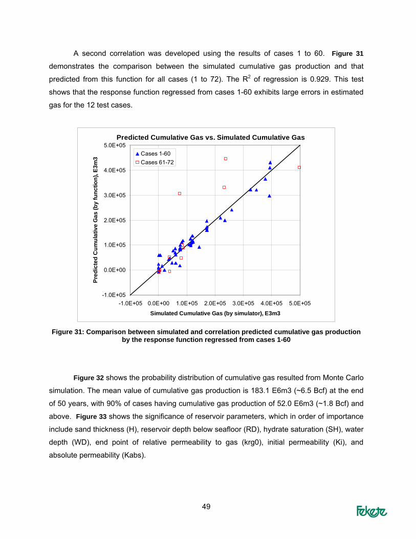
49

A second correlation was developed using the results of cases 1 to 60. Figure 31

demonstrates the comparison between the simulated cumulative gas production and that

predicted from this function for all cases (1 to 72). The R2 of regression is 0.929. This test

shows that the response function regressed from cases 1-60 exhibits large errors in estimated

gas for the 12 test cases.

Predicted Cumulative Gas vs. Simulated Cumulative Gas

-1.0E+05

0.0E+00

1.0E+05

2.0E+05

3.0E+05

4.0E+05

5.0E+05

-1.0E+05 0.0E+00 1.0E+05 2.0E+05 3.0E+05 4.0E+05 5.0E+05

Simulated Cumulative Gas (by simulator), E3m3

Pred

icte

d C

umul

ativ

e G

as (b

y fu

nctio

n), E

3m3


Figure 31: Comparison between simulated and correlation predicted cumulative gas production

by the response function regressed from cases 1-60

Figure 32 shows the probability distribution of cumulative gas resulted from Monte Carlo

simulation. The mean value of cumulative gas production is 183.1 E6m3 (~6.5 Bcf) at the end

of 50 years, with 90% of cases having cumulative gas production of 52.0 E6m3 (~1.8 Bcf) and

above. Figure 33 shows the significance of reservoir parameters, which in order of importance

include sand thickness (H), reservoir depth below seafloor (RD), hydrate saturation (SH), water

depth (WD), end point of relative permeability to gas (krg0), initial permeability (Ki), and

absolute permeability (Kabs).

50

Distribution for Cumulative Produced Gas

Mean = 183.1 E6m3

X <=342.4690%

X <=51.9610%

0

0.02

0.04

0.06

0.08

0.1

0.12

0.14

-100 0 100 200 300 400 500 600 700 800

Cumulative Produced Gas, E6m3

Rel

ativ

e Fr

eque

ncy

Figure 32: Probability distribution of cumulative gas production - Type III reservoirs


0.626

0.596

0.253

-0.159

0.057

0.026

0.014

-1 -0.5 0 0.5 1

H

RD

SH

WD

krg0

ln(K)

Kabs


Figure 33: Tornado chart showing significance of parameters to cumulative gas production from Type III reservoirs

51

Summary of Results

• Response functions for gas recovery (Equation 9) and cumulative gas production (

• Equation 10) from type III hydrate reservoir were generated in terms of the most

important seven parameters, namely reservoir depth below seafloor (RD), water depth

(WD), sand thickness (H), hydrate saturation (SH), initial permeability(Ki), absolute

permeability (Kabs) and end point of relative permeability to gas (krg0).

• Monte Carlo simulations were conducted for the gas recovery and cumulative

production. The mean recovery and mean cumulative gas production are 73.4% and

183.1 E6m3 (6.5 Bcf), respectively, for the range of each parameter considered in

Table 14.

52

Chapter 6: Type I Reservoirs

In this chapter the technical recoverability of Type I reservoirs is investigated. A distinct

characteristic of Type I reservoirs with underlying free gas is that at the interface between the

hydrate and the free gas the three phases of the hydrate, water and gas are in equilibrium.

Therefore the p/T conditions at the interface have to be on the hydrate equilibrium curve. This

is unlike Type II and Type III hydrate reservoirs, where the p/T conditions could be inside the

hydrate equilibrium stability region; i.e. above the equilibrium curve. This difference reduces

the degree of freedom in selection of the reservoir and water depth. In the case of Type II and

III reservoirs, two conditions of reservoir and water depth could be independently chosen.

These along with water-bottom temperature, geothermal gradient, the hydrostatic pressure

gradient would lead to selection of initial pressure and temperature. In Type I reservoirs,

however, the p/T conditions are also related through the hydrate equilibrium curve. As

explained in Appendix 6a we chose the reservoir depth to vary within a predetermined range.

This along with other conditions would lead to estimation of initial temperature and pressure.

The latter may then used to determine the water depth.

The methodology for estimation of recoverability of Type I reservoirs differed from that

of Type II and III reservoirs. Analytical methods have been developed for estimation of

technical recoverability of Type I reservoirs (Gerami and Pooladi-Darvish, 2007). It was

envisioned that this analytical methodology may be extended and employed in this work.

However, the above analytical solution had two limitations; it was developed for constant rate

production, and it was applicable to reservoir with zero dip angles. During the course of this

study, a new analytical model was developed that was applicable to tilted reservoirs

(Tabatabaie and Pooladi-Darvish, 2009). However, extension of this model to a case of

constant production pressure has not be yet successful. In a second component of this study,

a two-level experimental design methodology was used to select 14 simulation cases. This

served two objectives: (i) the simulation results were compared with the analytical results, and

(ii) the simulated recoveries were used to develop a response function, which was then used to

generate a distribution function for recovery. Unlike what was observed for Type II and Type III

reservoirs, the distribution function was found to be very flat, and the mean recovery factor is

55%; this is significantly less than that of Type II and III reservoirs. This was an unexpected

result and it is therefore recommended that the study of Type I reservoirs is continued, by

either inclusion of a larger number of simulation studies (probably based on a three-level

53

experimental design), or development of analytical solutions applicable to tilted reservoirs that

are produced at constant pressure.

In the following, the reservoir characteristics investigated in this study are reviewed and

the results of a base case are shown. This is followed by presentation of the simulation results,

the surface function for recovery, and the ranking of various parameters.

Reservoir Characteristics Figure 34 shows the schematic of a Type I hydrate reservoir where the free gas column

(red) underlies the hydrate column (green). Although this is not shown graphically in Figure

34, we also allow for a water column to exist under the gas column.

Sea surface

Sea floor

WD

R

D

Dip angle

L=760 m

Centre point A

H

Figure 34: Schematic diagram of Type I Hydrate reservoir below the ocean floor

Table 20 gives the list of reservoir parameters and their corresponding range to be

investigated in this study. Other parameters not listed in Table 20 will not be varied in the

study, in particular:

• The uncertainly in the equilibrium curve is taken into account. This is further explained

later in this section.

54

• A constant temperature at seafloor (water bottom temperature, WBT) of 4.5 °C is

assumed.

• A constant geothermal temperature gradient (Tgrad) of 0.02455 °C/m is applied.

• Reservoir temperature (Ti) is determined from the reservoir depth (RD), geothermal

gradient and WBT: Ti=RD*Tgrad + WBT. The initial reservoir pressure is obtained from

the phase equilibrium curve at Ti.

• A constant flowing BHP of 3000 kPa is assumed, similar to that used in the study of

Type II and III hydrate.

Table 20: List of Reservoir Characteristics and Their Range (Type I reservoirs)


Low estimate

Medium Estimate

High Estimate


Equilibrium curve Pe Low Pe Med. Pe High Pe





Ratio of hydrate column to total R_HC 0.5 0.7 0.9

Extent of aquifer (below the gas) Aquifer No 1 time 5 times of the

reservoir size


Permeability within the underlying free water, mD Kabs 100 500 1000

Endpoint of gas relative permeability krg0 0.1 0.5 1.0

The uncertainty in phase equilibrium curve is incorporated by including the uncertainty

in parameters that affect the equilibrium curve. This uncertainty study is presented in

Appendix 2b, including the resultant p10 and p90 equilibrium curves (see Figure 52). Figure 35

shows the low, medium, and high three phase equilibrium curves incorporated in this study.

These are expressed by the following three equations used in the numerical model:

55

Low: ⎟⎠⎞

⎜⎝⎛

+−=

15.27397.106239672.45exp

TPe

Medium: ⎟⎠⎞

⎜⎝⎛

+−=

15.27335.110165448.47exp

TPe

High: ⎟⎠⎞

⎜⎝⎛

+−=

15.27301.108322421.47exp

TPe

Figure 35 indicates that at a pressure of 3000 kPa, the equilibrium temperature varies between

3 oC and 6.7 oC, with a base-case value of 5.5 oC.

01,0002,0003,0004,0005,0006,0007,0008,0009,000

10,00011,00012,00013,00014,00015,00016,00017,00018,00019,00020,000

0 1 2 3 4 5 6 7 8 9 10 11 12 13 14 15 16 17 18 19 20

Temperature, C

Pres

sure

, kPa

mediumhighlow

Figure 35: The range of Phase equilibrium curves used in the study

Base Case The reservoir properties for the Base Case correspond to the medium values in Table

20. The initial pressure and temperature at the central point of the reservoir and at the gas-

hydrate interface is listed in Table 21.

Table 21: Initial pressure and temperature of base case

Sand Central Point gas /hydrate InterfaceDepth below seafloor m 300 313.25Pressure kPa 7475 7608Temperature C 11.87 12.19

56

Figure 36 gives the simulation results and demonstrates that the average gas

production is approximately 25 E3m3/d (0.9 mmscf/d) for the first 8 years before the gas rate

declines. The recovery of gas is completed within 13 years with the final recovery of 88%. The

average water-gas ratio is 0.77 m3/E3m3. The high initial gas rate from the free gas results in

a rapid pressure drop for the first 2 months. One interesting observation is that the pressure in

the bottom water drops much faster than the gas and hydrate zone. This is a result of high

hydraulic diffusivity in the water.

Gas Rate & Cumulative

Gas Rate SC - Case-base.irf Cumulative Gas SC - Case-base.irf

Time (Date)

Gas

Rat

e S

C (E

3m3/

day)

Cum

ulat

ive

Gas

SC

(E3m

3)

2015 2020 2025 20300

20

40

60

80

100

0.00e+0

2.00e+4

4.00e+4

6.00e+4

8.00e+4

1.00e+5

1.20e+5

1.40e+5

1.60e+5

1.80e+5

2.00e+5

Gas Recovery

gas recovery- Case-base.irf

Time (Date)

Gas

Rec

over

y,%

2015 2020 2025 20300

10

20

30

40

50

60

70

80

90

100

W ater Rate & Cumulative

Water Rate SC -n Case-base.irf Cumulative Water SC - Case-base.irf

Time (Date)

Wat

er R

ate

SC

(m3/

day)

Cum

ulat

ive

Wat

er S

C (m

3)

2015 2020 2025 20300

10

20

30

40

50

60

70

80

90

100

0.0e+0

2.0e+4

4.0e+4

6.0e+4

8.0e+4

1.0e+5

1.2e+5

1.4e+5

1.6e+5

1.8e+5

2.0e+5

Reservoir Pressure

Ave Pres POVO SCTR - Case-base.irf Ave Pres POVO SCTR - above waterAve Pres POVO SCTR - Water

Time (Date)

Ave

Pre

s P

OV

O S

CTR

(kP

a)

2015 2020 2025 20300

1,000

2,000

3,000

4,000

5,000

6,000

7,000

8,000

9,000

10,000

Figure 36: Simulation Result of Base Case - Type I reservoirs

Figure 37 shows the change in temperature, and demonstrates how the low-

temperature front moves along with the hydrate dissociation front shown in Figure 38. Note that

the Figures show half of the drainage area of one well, however, the reported rate and

cumulative produced gas/water are doubled to reflect the whole drainage area (760 m x 760

m). Figure 39 shows that production of gas stops after the gas-water interface crosses the

wellbore. The remaining gas is not recovered.

57

Initial

2 years 5 years

10 years

Figure 37: Simulation Result of Type I Base Case - Temperature

Initial

2 years 5 years

10 years

Figure 38: Simulation Result of Type I Base Case – Hydrate Saturation

58

15 years

Figure 39: Simulation Result of Type I Base Case-Gas Saturation

Twolevel PlackettBurman Experimental Design In order to identify the more important parameters that affect hydrate recovery and gas

production, a two-level 8-parameter Plackett-Burman experimental design method was used.

List of cases along with the simulation results are given in Table 22.

Table 22: Input parameters and simulation results for 14 cases based on two-level experimental

design Case

# RD m

Te C

Phi %

SH %

H m

Angle deg

R_HC

Aquifer

Ki md

Kabs md

Krg0

Recovery %

CumGas E3m3

1 600 2.93 40 40 20 10 0.5 5 0.05 100 0.1 90.12 393,630

2 100 6.72 40 85 20 0 0.9 5 0.05 1000 0.1 0.26 1,631

3 100 2.93 40 40 20 0 0.5 0 5 1000 1 80.76 177,895

4 100 6.72 30 85 20 10 0.5 5 5 100 1 3.21 10,117

5 600 6.72 40 85 3 10 0.5 0 0.05 1000 1 89.66 96,290

6 100 6.72 30 40 3 0 0.5 0 0.05 100 0.1 1.86 408

7 300 5.47 35 60 6 5 0.7 1 0.5 500 0.5 88.23 96,792

8 300 5.47 35 60 6 5 0.7 1 0.5 500 0.5 88.23 96,792

9 100 2.93 40 85 3 10 0.9 0 5 100 0.1 56.94 55,788

10 100 2.93 30 40 3 10 0.9 5 0.05 1000 1 84.93 29,254

11 600 6.72 30 40 20 10 0.9 0 5 1000 0.1 79.74 201,635

12 600 6.72 40 40 3 0 0.9 5 5 100 1 82.03 40,590

13 600 2.93 30 85 3 0 0.5 5 5 1000 0.1 81.91 86,212

14 600 2.93 30 85 20 0 0.9 0 0.05 100 1 94.65 532,740

59

Figure 40 shows the initial p/T condition of all cases, which lie on the boundary of the hydrate stability curve.

Case-5

Case-7Case-9

Case-11

Case-13Case-1

Case-2

Case-3

Case-4Case-6

Case-8Case-10

Case-12

Case-14

0

2,000

4,000

6,000

8,000

10,000

12,000

14,000

16,000

18,000

20,000

22,000

24,000

26,000

28,000

30,000

0 5 10 15 20 25

Temperature, oC

Pres

sure

, kPa

base high lowCase-1 Case-2 Case-3Case-4 Case-5 Case-6Case-7 Case-8 Case-9Case-10 Case-11 Case-12Case-13 Case-14

Figure 40: Initial p/T condition of individual cases in Table 22

Results Simulation studies were conducted for all the cases shown in Table 22 to estimate gas

recovery and cumulative gas production over a 50 year period. These were then correlated as

a function of variable parameters. The surface functions were then used to estimate the range

of expected recovery and the sensitivity of the results on the variable parameters. These are

explained below, first for gas recovery and then for cumulative gas production.

Gas Recovery The response function of gas recovery within 50 years for the 14 cases studied is given

as Equation 11. Table 23 gives the coefficients.

Ln(R/(100‐R)) = b1*RD + b2*Te + b3*Phi + b4*SH + b5*H + b6*Angle + b7*R_HC + b8*Aquifer + b9*Ki + b10*Kabs + b11*Krg0

Equation 11

60


b1 7.038066E-03b2 -7.297276E-01b3 4.879800E-02b4 -2.475389E-02b5 -6.596144E-02b6 1.190082E-01b7 1.067026E+00b8 -2.824592E-01b9 3.324060E-02b10 4.775888E-04b11 1.986236E+00

Figure 41 shows a comparison between the recovery predicted by the simulator and the

recovery predicted by the response function. The R2 of regression is 0.9.

0

10

20

30

40

50

60

70

80

90

100

0 10 20 30 40 50 60 70 80 90 100

Simulated Recovery (Simulator), %

Pred

icte

d R

ecov

ery

(Fun

ctio

n),%


Monte Carlo simulation was performed by using Equation 11 and the probability

distribution of 11 input parameters. (The distribution of the parameters is shown in Appendix

6b). Figure 42 shows the probability distribution of gas recovery, with the mean recovery of

56%. A very flat distribution curve is observed. Figure 43 shows the significance of each

parameter. The three most significant parameters are reservoir depth (RD), equilibrium

61

temperature (Te), and end point of gas relative permeability (krg0). The least significant

parameter is the initial permeability in the hydrate zone (Ki).

Distribution for Recovery%

Mean = 55.77%

X <=94.9290%

X <=11.0610%

0

0.005

0.01

0.015

0.02

0.025

0.03

0 10 20 30 40 50 60 70 80 90 100

Recovery, %

Freq

uenc

y

Figure 42: Probability distribution of gas recovery (Type I reservoirs)

Correlations for Recovery%

0.604

-0.528

0.249

-0.19

-0.178

0.176

-0.146

0.091

0.081

0.057

0.043

-1 -0.5 0 0.5 1

RD

Te

Krg0

Aquifer

H

Angle

SH

Phi

Kabs

R_HC

ln(Ki)


Figure 43: Tornado chart of significance of parameters to recovery - Type I reservoirs

62

Cumulative Gas Production Equation 12 gives the response function for cumulative gas production within 50 years

(corresponding to the cases listed in Table 22). The coefficients are listed in Table 24. The R2

of regressions is 0.972. Figure 44 shows a comparison between the cumulative gas predicted

by the numerical simulator and that estimated by Equation 12.

Table 24: List of Coefficients in Equation 12 and their values

b1 3.743303E+02b2 -3.653237E+04b3 2.538215E+03b4 1.333054E+02b5 1.028538E+04b6 -2.916854E+02b7 9.187621E+04b8 -1.584013E+04b9 -1.533612E+04b10 -7.381137E+01b11 3.506615E+04

-1.0E+05

0.0E+00

1.0E+05

2.0E+05

3.0E+05

4.0E+05

5.0E+05

6.0E+05

-1.0E+05 0.0E+00 1.0E+05 2.0E+05 3.0E+05 4.0E+05 5.0E+05 6.0E+05

Simulated Cumulative Gas (Simulator) (E3m3)

Pred

icte

d C

umul

ativ

e G

as (F

unct

ion)

(E3m

3)

Figure 44: Comparison between simulated cumulative gas and that predicted by Equation 12

CumGas (E3m3) = b1*RD + b2*Te + b3*Phi + b4*SH + b5*H + b6*Angle + b7*R_HC + b8*Aquifer + b9*Ki + b10*Kabs + b11*Krg0

Equation 12

63

Monte Carlo simulation using Equation 12 results in a probability distribution of

cumulative gas as shown in Figure 45. The mean value of cumulative gas production is 144.7

E6m3 (5.1 Bcf). Figure 46 shows the significance of each parameter. The three most

significant parameters are reservoir depth (RD), sand thickness (H) and equilibrium

temperature (Te). The least significant parameter is the sand dip angle.

Distribution for Cumulative Gas Production

Mean = 144.7 E6m3

X <=30579990%

X <=-1383410%

0

0.5

1

1.5

2

2.5

3

3.5

4

-500 -400 -300 -200 -100 0 100 200 300 400 500 600 700

Cumulative Gas Production, E6m3

Freq

uenc

y, in

10^

-6

Figure 45: Probability distribution of cumulative gas production - Type I reservoirs


0.507

0.473

-0.449

-0.249

-0.186

-0.165

0.076

0.073

0.051

0.011

-0.008

-1 -0.5 0 0.5 1

RD

H/

Te

ln(Ki)

Kabs

Aquifer

R_HC

Phi

Krg0

SH

Angle


Figure 46: Tornado chart of significance of parameters to cumulative gas - Type I reservoirs

64

Summary of Result

• Response functions for gas recovery (Equation 11) and cumulative gas production

(Equation 12) from Type I hydrate reservoirs were generated. These equations were

generated based on a limited number of simulation runs and a two-level experimental

design process. It is recommended that the study of determination of a response

function for technical recoverability of Type I reservoirs is continued, because:

o The number of simulation runs was small. A two-level experimental design is

best suited for screening of the parameters.

o The probability distribution function showed a flat profiler, with a mean value of

technical recoverability of 55%, significantly less than that obtained for Type II

and III reservoirs.

• The most important parameters include reservoir depth (RD), equilibrium curve (Te),

some measure of permeability, reservoir thickness (H), and presence or absence of the

aquifer (Aquifer).

65

REFERENCES

• Frye M.: “Preliminary Evaluation of In-Place Gas Hydrate Resources: Gulf of Mexico

Outer Continental Shelf,” OCS Report MMS 2008-004, US Department of the Interior,

Mineral Management Service, Resource Evaluation Division, February 1, 2008.

• Gerami, S. and Pooladi-Darvish, M.: “Effect of Hydrates on Sustaining Reservoir

Pressure in a Hydrate-Capped Gas Reservoir”, Journal of Canadian Petroleum

Technology (JCPT), Vol 46, No. 10 (October 2007) pp 39 – 48

• Tabatabaie, S.H., and Pooladi-Darvish, M.: “Analytical Solutions for Gas Production

from Hydrate Reservoirs Underlain with Free Gas,” in Journal of Natural Gas Science

and Engineering, Vol. 1, No. 1-2, (July 2009) pp. 46-57.

• Zatsepina, O., Hong, H. and Pooladi-Darvish, M.: “Behaviour of Gas Production from

Type III Hydrate Reservoirs,” paper presented at the 6th International Conference on

Gas Hydrates, July 6-10, 2008, Vancouver, BC.

66

APPENDICES

67

APPENDIX 2A: ESTIMATION OF HYDRATE RESERVOIR PRESSURE AND TEMPERATURE, AND CONDITIONS FOR HYDRATE STABILITY AND DISSOCIATION BY DEPRESSURIZATION

In this Appendix, estimation of reservoir pressure and temperature, for a hypothetical

Type II reservoir at water depth (WD) and reservoir depth (RD) shown in Figure 47, is

explained. This is followed by examination of these p/T conditions with respect to the

equilibrium curve to ensure presence of the hydrate at these initial conditions and its

dissociation at 3000 kPa. Finally, the range of water depth (WD) and reservoir depth (RD)

chosen in this study is given. The choice of the equilibrium curve and its effect on results is

presented in Appendix 2b.

Sea surface

Sea floor

WD

RD

Dip angle

L=760 m

Centre point A

H

Figure 47: Schematic diagram of Type II reservoir with Base Properties

Reservoir temperature: In the first stage of this work, reservoir temperature was estimated based on the mean

value for geothermal gradient of 40 °C/km (P.54-56 in MMS 2008-004 report, Frye M.). Later

on and based on recommendation of MMS, the geothermal gradient was revised to 24.5

°C/km.

68

Reservoir temperature at a reservoir depth of RD is given by WBT + 0.0245*RD, where

WBT is the water bottom temperature. The latter is estimated by WBT = 18.2324697*exp(-

0.003136*WD)+4.1009 (page 56 in MMS 2008-004 report, Frye M.).

Reservoir pressure: The initial reservoir pressure is estimated assuming a hydrostatic pressure gradient of

(10 kPa/m); Pi = (WD+RD)*10+101.3

Conditions for hydrate presence: The necessary condition for hydrate presence in the sand is that at the top of the sand

(point ‘A’ in Figure 47), the following condition should be satisfied

( )AeA pTT ≤

Equation 13

Where TA is the initial temperature at the top of the sand, pA is the initial pressure at the top of

the sand, and Te(pA) is the equilibrium temperature at pressure of pA. This condition is

schematically shown in Figure 48 .

pB

BHP

pA B

A

T

P

TA Te(pA) Te(BHP) TB

Figure 48: Schematic diagram of phase equilibrium curve and reservoir conditions

The values of AT , Ap and ( )Ae pT are determined by the following steps:

o The depth at the top of the sand below seafloor is estimated as

( )( )HLRDRDA +⋅−= θsin21

Equation 14

69

where: ARD : depth from the seafloor to the top of the sand, m RD: depth from the seafloor to the centre point of the sand, m

L: length of the sand, m H: thickness of the sand, m θ: dip angle of the sand

o Reservoir temperature, AT at the top of the sand is estimated as

18.2324697*exp( 0.003136* ) 4.1009 0.02455*A AT WD RD= − + + Equation 15

where, WD: water depth, m

o Reservoir pressure, Ap at the top of the sand is evaluated as

3.10110*)( ++= AA RDWDp Equation 16

o The phase equilibrium temperature, ( )Ae pT at reservoir pressure Ap can be calculated

by the equilibrium curve Equation 26, thus,

( ) 5.141.3410

3.101ln3.7 −−⎟

⎠⎞

⎜⎝⎛ −

⋅= AAe

ppT

Equation 17

Conditions for hydrate dissociation In order for the hydrate to dissociate, the following condition must be satisfied. At the

bottom of the hydrate zone, (which for a Type II reservoir corresponds to the interface between

hydrate zone and water zone “B”), the reservoir temperature must be greater than the phase

equilibrium temperature corresponding to the production pressure, expressed as

( )BHPTT eB ≥

Equation 18

where TB is the temperature at the interface between hydrate and water zones, and Te(BHP) is

the equilibrium temperature corresponding to the production pressure, BHP.

The depth of the interface, BT and ( )BHPTe can be estimated by the following steps:

70

o The depth of the interface of hydrate zone and water zone

( ) 021_sin >⎟

⎠⎞

⎜⎝⎛ −+= θθ ifHCRLRDRDB

Equation 19

021_ =⎟

⎠⎞

⎜⎝⎛ −+= θifHCRHRDRDB

Equation 20

where :BRD depth from seafloor to the bottom of hydrate zone, m

:RD depth from seafloor to the centre of the sand body, m L: length of the sand, m θ: dip angle of the sand

HCR _ : ratio of the hydrate column to the total column of the sand, which is determined either by the hydrate phase stability criteria or the available gas to form hydrate H: thickness of the sand, m

o The reservoir temperature at location B, BT

18.2324697*exp( 0.003136* ) 4.1009 0.02455*B BT WD RD= − + + Equation 21

o The hydrostatic pressure at location B, pB

3.10110*)( ++= BB RDWDp Equation 22

o The phase equilibrium temperature, ( )Be pT at pressure Bp can be calculated as

( ) 5.141.3410

3.101ln3.7 −−⎟⎠⎞

⎜⎝⎛ −

⋅= BBe

ppT

Equation 23

o At the interface of hydrate zone and water zone, the following condition must be satisfied:

( )BeB pTT ≤

Equation 24

which determines what the maximum R_HC can be.

o The phase equilibrium temperature corresponding to the production pressure is calculated by

( ) 5.141.3410

3.101ln3.7 −−⎟⎠⎞

⎜⎝⎛ −

⋅=BHPBHPTe

Equation 25

71

Use of a value of 3000 kPa for the production pressure in Equation 25 leads to a temperature

of nearly 5.5 °C, as the minimum reservoir temperature that satisfies condition for dissociation.

Estimation of hydrate reservoir pressure and temperature Water depth (WD) and reservoir mid-point depth below sea floor (RD) are important

parameters that affect the reservoir pressure and temperature. The ranges of these two

parameters were selected based on the following available information.

WD: Water depth In the first stage of the study, the range of water depth was chosen from the Green

Canyon (Figure 5, P. 9 in MMS2008-004 report, Frye M.). Based on this information, the low

and high values of water depth were assumed to be 750 m and 2000 m, with a mean value of

1200 m. Subsequently, MMS provided the full range of water depths used in the in-place

study. Figure 49 shows the mean gross thickness of the hydrate stability zone (HSZ) as a

function of water-depth, indicating a water depth of between approximately 600 and 3500 m.

Accordingly, the range of water depth (WD) for the second stage of the study was revised to

between 750 and 3000 m with a mean value of 1500 m.

RD: Reservoir midpoint depth below sea floor The in-place study did not use reservoir depth as an independent parameter. However,

this study documented the mean thickness of the gross HSZ. With reference to Figure 47, half

of the gross thickness of HSZ is taken as reservoir depth. In the first stage of this study, a

mean value of 250 m was used (Figure 49 & Figure 50, p. 60-61 in MMS2008-004 report, Frye

M.). The corresponding minimum and maximum values were 100 and 400 m. Subsequently,

MMS provided the mean and p90 values of the gross thickness of the HSZ, shown in Figure 49

and Figure 50, which indicate that the gross thickness of the HSZ can be in excess of 1000 m.

Accordingly, the range of reservoir depth used in the second stage of the study was updated to

between 100 and 600 m, with a mean value of 300 m.

72

Figure 49: mean of gross thickness of the hydrate stability zone as a function of water-depth

Figure 50: p90 value of gross thickness of the hydrate stability zone as a function of water-depth

73

APPENDIX 2B: ESTIMATION OF HYDRATE EQUILIBRIUM CURVE AND THE

EFFECT ON RESULTS

In the MMS 2008-004 report, Frye M. (P. 57-59), the phase equilibrium curve is

expressed in terms of the relation between the equilibrium temperature, depth and gas

chemistry (methane content):

( ) λγδ −−⋅= depthTe ln

Equation 26

where

• δ : slope of phase stability curve. The mean value of 7.3 for On-Anomaly cells is

chosen (Table 10, MMS 2008-004 report, Frye M.)

• γ : intercept of phase stability curve. The mean value of 34.41 for On-Anomaly cells is

chosen (Table 10, MMS 2008-004 report, Frye M.)

• λ : reduction in phase stability temperature due to local salt. It is set to 1.5. (P. 59,

MMS 2008-004 report, Frye M.)

• Te: the equilibrium temperature, °C

• depth: WD + RD (water depth + distance from seafloor)

The hydrostatic pressure is the product of depth and hydrostatic gradient.

3.10110 +⋅= depthp

Equation 27

Thus,

λγδ −−⎟

⎠⎞

⎜⎝⎛ −

⋅=10

3.101ln pTe

Equation 28

or,

3.101exp10 +⎟⎠⎞

⎜⎝⎛ ++

⋅=δ

λγTpe

Equation 29

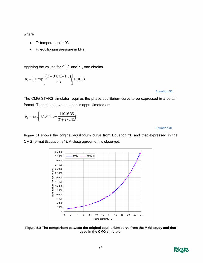
74

where

• T: temperature in °C

• P: equilibrium pressure in kPa

Applying the values for δ ,γ and λ , one obtains

( )34.41 1.510 exp 101.3

7.3e

Tp

+ +⎡ ⎤= ⋅ +⎢ ⎥

⎣ ⎦

Equation 30

The CMG-STARS simulator requires the phase equilibrium curve to be expressed in a certain

format. Thus, the above equation is approximated as:

⎥⎦⎤

⎢⎣⎡

+−=

15.27335.1101654476.47exp

Tpe

Equation 31

Figure 51 shows the original equilibrium curve from Equation 30 and that expressed in the

CMG-format (Equation 31). A close agreement is observed.

0

2,500

5,000

7,500

10,000

12,500

15,000

17,500

20,000

22,500

25,000

27,500

30,000

32,500

35,000

0 2 4 6 8 10 12 14 16 18 20 22 24

Temperature, oC

Equi

libriu

m P

ress

ure,

kPa

MMS MMS-fit

Figure 51: The comparison between the original equilibrium curve from the MMS study and that used in the CMG simulator

75

Equation 31 was incorporated into the CMG simulator. No sensitivity with respect to the

equilibrium curve, either because of change in salinity or otherwise, was considered in this

study. However, to assess the degree of variation in the hydrate equilibrium, an investigation

was conducted. The MMS in-place study (MMS 2008-004 report, Frye M.) provides the range

of parameters that influence the equilibrium curve. These are given in Table 25.

Table 25 List of parameters and probability distributions for phase equilibrium curve

γ beta distribution with alpha=1.793034, beta=0.10971

δ beta distribution with alpha=0.10971, beta=1.793034

μ normal distribution with a mean of 215 ppt and a standard deviation of 58 ppt

π normal distribution with a mean of 0.11 and a standard deviation of 0.01

salt normal distribution with a mean of 2000m and a standard deviation of 312.2

A Monte Carlo simulation was performed where the input parameters in Equation 26

where allowed to vary within the range specified in Table 25. Figure 52 shows the curves

corresponding to mean, p10, p50 and p90 probabilities. Additionally, Figure 52 shows the

curve calculated from mean value of each parameter (shown using the thick solid line). This

curve, which uses the mean of the input parameters and is used throughout this study, has a

good agreement with the P50 equilibrium curve.

0

2,000

4,000

6,000

8,000

10,000

12,000

14,000

16,000

18,000

20,000

-2 0 2 4 6 8 10 12 14 16 18 20 22

Temperature, C

Pres

sure

, kPa

MMS-appliedMMS-meanMMS-P10MMS-P90Kamath-Holder

Figure 52: Range of variations in the hydrate phase equilibrium curve

76

In order to investigate the effect of uncertainty in the equilibrium curve on the results, a

sensitivity study was conducted. For this sensitivity run, the Methane-hydrate equilibrium

curve of Kamath and Holder was used. This curve is shown in Figure 52 in relation to the

range of equilibrium curves from the MMS parameters, and indicates that the Kamath –Holder

relation is closer to the p10 curve at low p/T conditions. It then crosses the mean curve and

approaches the p90 curve at large p/T conditions. The results of the simulations run with the

curve called MMS-applied and Kamath-Holder are shown in Figure 53, and indicate little

difference10.

Gas Rate SC - Case-3.irf Gas Rate SC - Case-3-pe.irfCumulative Gas SC - Case-3.irf Cumulative Gas SC - Case-3-pe.irf

Time (Date)

Gas

Rat

e SC

(E3m

3/da

y)

Cum

ulat

ive

Gas

SC

(E3m

3)

2020 2030 2040 2050 20600

10

20

30

40

50

0.0e+0

2.0e+4

4.0e+4

6.0e+4

8.0e+4

1.0e+5

gas recovery- Case-3.irf gas recoveryGas Water Ratio SC - Case-3.irf Gas Water Ratio SC - Case-3-pe.irf

Time (Date)

Gas

Rec

over

y,%

Gas

Wat

er R

atio

SC

(E3m

3/m

3)

2020 2030 2040 2050 20600

10

20

30

40

50

60

70

80

90

100

0.00

0.10

0.20

0.30

0.40

0.50

0.60

0.70

0.80

0.90

1.00

Water Rate SC -n Case-3.irf Water Rate SC - Case-3-pe.irfCumulative Water SC - Case-3.irf Cumulative Water SC - Case-3-pe.irf

Time (Date)

Wat

er R

ate

SC (m

3/da

y)

Cum

ulat

ive

Wat

er S

C (m

3)

2020 2030 2040 2050 20600

200

400

600

800

1,000

1,200

1,400

1,600

1,800

2,000

0.0e+0

5.0e+5

1.0e+6

1.5e+6

2.0e+6

2.5e+6

Ave Pres POVO SCTR - Case-3.irf Ave Pres POVO SCTR - Case-3-pe.irfWell Bottom-hole Pressure - Case-3.irf Well Bottom-hole Pressure - Case-3-pe.irf

Time (Date)

Ave

Pre

s PO

VO S

CTR

(kPa

)

2020 2030 2040 2050 20600

2,500

5,000

7,500

10,000

12,500

15,000

17,500

20,000

22,500

25,000

Figure 53: Effect of changing equilibrium curve on the results (Type II reservoir); the red and blue curves correspond to the MMS-applied and the Kamath-Holder equilibrium curves

Although this sensitivity study indicated little overall difference on the results, it is

recommended that future phases of the study (e.g. the economic recoverability of the hydrates)

should incorporate the uncertainty in the equilibrium curve. It is expected that this would have

an impact on the results, particularly for reservoirs that are cold. 10 The simulation results are for a Type II reservoir for base properties. This sensitivity run was conducted during the first stage of the study, with a different range of parameters than that used later on. This explains the difference between results shown in Figure 53 and Figure 2.

77

APPENDIX 3A: EXPERIMENTAL DESIGN AND PROBABILITY DISTRIBUTION OF UNCERTAIN PARAMETERS (TYPE II - STAGE 1 WORK)

Table 26: Plackett-Burman Design (Plackett-Burman Design, 12 factors, 2 Centerpoints) Exp # F1 F2 F3 F4 F5 F6 F7 F8 F9 F10 F11 F12

1 1 1 -1 -1 -1 -1 1 -1 1 -1 1 12 1 1 1 -1 -1 1 1 -1 1 1 -1 -13 0 0 0 0 0 0 0 0 0 0 0 04 -1 -1 1 1 -1 1 1 -1 -1 -1 -1 15 -1 1 1 1 1 -1 -1 1 1 -1 1 16 -1 -1 -1 -1 1 -1 1 -1 1 1 1 17 1 1 1 1 -1 -1 1 1 -1 1 1 -18 1 -1 -1 1 1 -1 1 1 -1 -1 -1 -19 1 -1 1 -1 1 1 1 1 -1 -1 1 1

10 -1 1 1 -1 -1 -1 -1 1 -1 1 -1 111 -1 1 -1 1 1 1 1 -1 -1 1 1 -112 1 1 -1 -1 1 1 -1 1 1 -1 -1 -113 -1 -1 -1 1 -1 1 -1 1 1 1 1 -114 1 1 -1 1 1 -1 -1 -1 -1 1 -1 115 -1 1 1 -1 1 1 -1 -1 -1 -1 1 -116 1 -1 -1 -1 -1 1 -1 1 -1 1 1 117 -1 -1 -1 -1 -1 -1 -1 -1 -1 -1 -1 -118 1 -1 1 1 -1 -1 -1 -1 1 -1 1 -119 0 0 0 0 0 0 0 0 0 0 0 020 1 -1 1 1 1 1 -1 -1 1 1 -1 121 -1 -1 1 -1 1 -1 1 1 1 1 -1 -122 -1 1 -1 1 -1 1 1 1 1 -1 -1 1

Trigen(500, 1200, 2000, 10, 90) Trunc(500,+inf)

Val

ues

x 10

^-4

Water Depth, mValues in Thousands

0

1

2

3

4

5

6

7

8

9

0.0

0.5

1.0

1.5

2.0

2.5

3.0

5.0% 5.0%90.0%0.621 2.204

Figure 54: Probability distribution of water depth

78

Trigen(50, 250, 400, 10, 90) Trunc(50,+inf)

Val

ues

x 10

^-3

Reservoir Depth below Seafloor, m

0.0

0.5

1.0

1.5

2.0

2.5

3.0

3.5

4.0

0 50 100

150

200

250

300

350

400

450

500

550

5.0% 5.0%90.0%80.3 444.1

Figure 55: Probability distribution of reservoir depth below seafloor

Trigen(30, 35, 40, 10, 90)

Porosity,%

0.00

0.02

0.04

0.06

0.08

0.10

0.12

24 26 28 30 32 34 36 38 40 42 44 46

5.0% 5.0%90.0%28.82 41.18

Figure 56: Probability distribution of porosity

79

Trigen(-2.99573, -0.69315, 1.609438, 10, 90)Trunc(-2.99573,1.609438)

Ln(Initial Permeability), ln(md)

0.00

0.05

0.10

0.15

0.20

0.25

0.30

0.35

-3.5

-3.0

-2.5

-2.0

-1.5

-1.0

-0.5 0.0

0.5

1.0

1.5

2.0

5.0% 5.0%90.0%-2.654 1.268

Figure 57: Probability distribution of initial permeability

Trigen(40, 60, 85, 10, 90) Trunc(40,90)

Val

ues

x 10

^-2

Hydrate Saturation, %

0.0

0.5

1.0

1.5

2.0

2.5

3.0

30 40 50 60 70 80 90 100

5.0% 5.0%90.0%43.37 85.35

Figure 58: Probability distribution of hydrate saturation

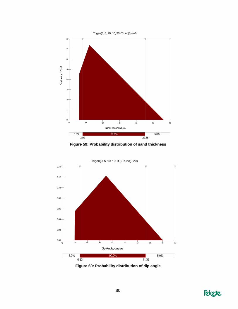
80

Trigen(3, 6, 20, 10, 90) Trunc(3,+inf)

Val

ues

x 10

^-2

Sand Thickness, m

0

1

2

3

4

5

6

7

8

0 5 10 15 20 25 30

5.0% 5.0%90.0%3.99 22.68

Figure 59: Probability distribution of sand thickness

Trigen(0, 5, 10, 10, 90) Trunc(0,20)

Dip Angle, degree

0.00

0.02

0.04

0.06

0.08

0.10

0.12

0.14

-2 0 2 4 6 8 10 12 14 16

5.0% 5.0%90.0%0.83 11.33

Figure 60: Probability distribution of dip angle

81

Trigen(0.5, 0.7, 0.9, 10, 90) Trunc(0.5,0.9)

Ratio of hydrate column to total sand

0.0

0.5

1.0

1.5

2.0

2.5

3.0

3.5

0.45

0.50

0.55

0.60

0.65

0.70

0.75

0.80

0.85

0.90

0.95

5.0% 5.0%90.0%0.5296 0.8704

Figure 61: Probability distribution of ratio of hydrate column to total sand

Discrete({x}, {p}) Trunc(0,1)

Aquifer

0.0

0.1

0.2

0.3

0.4

0.5

0.6

0.7

-0.2 0.0

0.2

0.4

0.6

0.8

1.0

1.2

5.0% 5.0%90.0%0.000 1.000

Figure 62: Probability distribution of aquifer

82

Trigen(100, 500, 1000, 10, 90) Trunc(10,2000)

Val

ues

x 10

^-3

Absolute Permeability, mdValues in Thousands

0.0

0.2

0.4

0.6

0.8

1.0

1.2

1.4

0.0

0.2

0.4

0.6

0.8

1.0

1.2

1.4

5.0%90.0%0.104 1.118

Figure 63: Probability distribution of absolute permeability

Trigen(0.1, 0.5, 1, 10, 90) Trunc(0.1,1)

krg endpoint

0.0

0.2

0.4

0.6

0.8

1.0

1.2

1.4

1.6

0.0

0.1

0.2

0.3

0.4

0.5

0.6

0.7

0.8

0.9

1.0

1.1

5.0% 5.0%90.0%0.164 0.931

Figure 64: Probability distribution of endpoint of krg

83

Trigen(2500, 3000, 7000, 10, 90) Trunc(2500,7000)

Val

ues

x 10

^-4

BHP, kPaValues in Thousands

0.0

0.5

1.0

1.5

2.0

2.5

3.0

3.5

2.0

2.5

3.0

3.5

4.0

4.5

5.0

5.5

6.0

6.5

7.0

7.5

5.0% 5.0%90.0%2.707 6.596

Figure 65: Probability distribution of flowing BHP

84

APPENDIX 4A: EXPERIMENTAL DESIGN AND PROBABILITY DISTRIBUTION OF

UNCERTAIN PARAMETERS (TYPE II STAGE 2 WORK)

Table 27: Box-Behnken 3-level Design (5 parameters, 4 central cases)

Case # F1 F2 F3 F4 F5 1 -1 0 0 1 0 2 0 -1 -1 0 0 3 1 0 -1 0 0 4 0 0 -1 1 0 5 0 0 1 0 -1 6 1 0 0 1 0 7 1 0 1 0 0 8 0 0 0 1 1 9 0 1 -1 0 0

10 -1 0 0 0 1 11 0 0 0 1 -1 12 0 0 0 -1 -1 13 0 1 0 -1 0 14 0 0 0 0 0 15 0 0 -1 -1 0 16 0 0 0 0 0 17 0 1 0 0 1 18 -1 0 -1 0 0 19 0 1 0 1 0 20 1 0 0 0 -1 21 1 0 0 0 1 22 0 -1 0 -1 0 23 -1 0 0 0 -1 24 0 -1 0 1 0 25 1 -1 0 0 0 26 0 -1 0 0 1 27 0 0 1 -1 0 28 0 0 0 0 0 29 0 0 1 1 0 30 0 1 0 0 -1 31 0 0 0 -1 1 32 0 0 -1 0 -1 33 0 0 0 0 0 34 -1 -1 0 0 0 35 -1 0 1 0 0 36 0 -1 1 0 0 37 0 0 -1 0 1 38 -1 1 0 0 0 39 0 -1 0 0 -1 40 0 0 1 0 1 41 0 1 1 0 0 42 1 1 0 0 0 43 1 0 0 -1 0 44 -1 0 0 -1 0

85

Table 28: A 2-level Experimental Design Table (5 parameters) Case # F1 F2 F3 F4 F5

45 1 -1 1 -1 1 46 1 1 1 1 1 47 1 1 -1 -1 1 48 1 1 -1 1 -1 49 1 -1 -1 -1 -1 50 1 1 1 -1 -1 51 -1 1 -1 -1 -1 52 -1 1 -1 1 1 53 1 -1 1 1 -1 54 -1 -1 -1 -1 1 55 -1 1 1 1 -1 56 -1 -1 1 1 1 57 -1 1 1 -1 1 58 -1 -1 1 -1 -1 59 1 -1 -1 1 1 60 -1 -1 -1 1 -1

Trigen(750, 1500, 3000, 10, 90) Trunc(500,+inf)

Val

ues

x 10

^-4

Values in Thousands

0

1

2

3

4

5

6

0.0

0.5

1.0

1.5

2.0

2.5

3.0

3.5

4.0

4.5

5.0% 5.0%90.0%0.727 3.312


86

Trigen(100, 300, 600, 10, 90) Trunc(50,+inf)

Val

ues

x 10

^-3

0.0

0.5

1.0

1.5

2.0

2.5

0

100

200

300

400

500

600

700

800

900

5.0% 5.0%90.0%100.9 667.3


Trigen(3, 6, 20, 10, 90) Trunc(3,+inf)

Val

ues

x 10

^-2

0

1

2

3

4

5

6

7

8

0 5 10 15 20 25 30

5.0% 5.0%90.0%3.99 22.68


87

Trigen(40, 60, 85, 10, 90) Trunc(40,90)

Val

ues

x 10

^-2

0.0

0.5

1.0

1.5

2.0

2.5

3.0

30 40 50 60 70 80 90 100

5.0% 5.0%90.0%43.37 85.35


Trigen(0, 5, 10, 10, 90) Trunc(0,20)

Dip Angle, degree

0.00

0.02

0.04

0.06

0.08

0.10

0.12

0.14

-2 0 2 4 6 8 10 12 14 16

5.0% 5.0%90.0%0.83 11.33

Figure 70: Probability distribution of dip angle

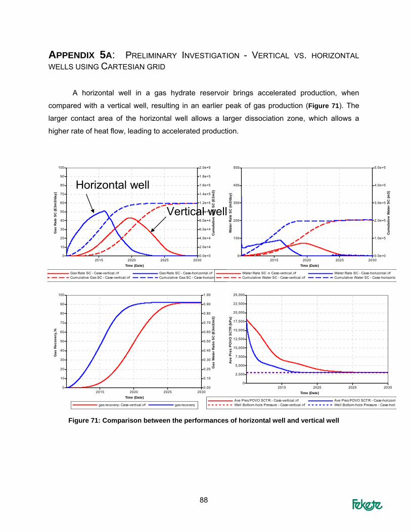
88

APPENDIX 5A: PRELIMINARY INVESTIGATION - VERTICAL VS. HORIZONTAL WELLS USING CARTESIAN GRID

A horizontal well in a gas hydrate reservoir brings accelerated production, when

compared with a vertical well, resulting in an earlier peak of gas production (Figure 71). The

larger contact area of the horizontal well allows a larger dissociation zone, which allows a

higher rate of heat flow, leading to accelerated production.

Gas Rate SC - Case-vertical.irf Gas Rate SC - Case-horizontal.irfCumulative Gas SC - Case-vertical.irf Cumulative Gas SC - Case-horizontal.irf

Time (Date)

Gas

Rat

e SC

(E3m

3/da

y)

Cum

ulat

ive

Gas

SC

(E3m

3)

2015 2020 2025 20300

10

20

30

40

50

60

70

80

90

100

0.0e+0

2.0e+4

4.0e+4

6.0e+4

8.0e+4

1.0e+5

1.2e+5

1.4e+5

1.6e+5

1.8e+5

2.0e+5

gas recovery- Case-vertical.irf gas recovery

Time (Date)

Gas

Rec

over

y,%

Gas

Wat

er R

atio

SC

(E3m

3/m

3)

2015 2020 2025 20300

10

20

30

40

50

60

70

80

90

100

0.00

0.10

0.20

0.30

0.40

0.50

0.60

0.70

0.80

0.90

1.00

Water Rate SC -n Case-vertical.irf Water Rate SC - Case-horizontal.irfCumulative Water SC - Case-vertical.irf Cumulative Water SC - Case-horizonta

Time (Date)

Wat

er R

ate

SC

(m3/

day)

Cum

ulat

ive

Wat

er S

C (m

3)

2015 2020 2025 20300

100

200

300

400

500

0.0e+0

1.0e+5

2.0e+5

3.0e+5

4.0e+5

5.0e+5

Ave Pres POVO SCTR - Case-vertical.irf Ave Pres POVO SCTR - Case-horizontWell Bottom-hole Pressure - Case-vertical.irf Well Bottom-hole Pressure - Case-horiz

Time (Date)

Ave

Pre

s P

OV

O S

CTR

(kP

a)

2015 2020 2025 20300

2,500

5,000

7,500

10,000

12,500

15,000

17,500

20,000

22,500

25,000

Horizontal well

Vertical well

Gas Rate SC - Case-vertical.irf Gas Rate SC - Case-horizontal.irfCumulative Gas SC - Case-vertical.irf Cumulative Gas SC - Case-horizontal.irf

Time (Date)

Gas

Rat

e SC

(E3m

3/da

y)

Cum

ulat

ive

Gas

SC

(E3m

3)

2015 2020 2025 20300

10

20

30

40

50

60

70

80

90

100

0.0e+0

2.0e+4

4.0e+4

6.0e+4

8.0e+4

1.0e+5

1.2e+5

1.4e+5

1.6e+5

1.8e+5

2.0e+5

gas recovery- Case-vertical.irf gas recovery

Time (Date)

Gas

Rec

over

y,%

Gas

Wat

er R

atio

SC

(E3m

3/m

3)

2015 2020 2025 20300

10

20

30

40

50

60

70

80

90

100

0.00

0.10

0.20

0.30

0.40

0.50

0.60

0.70

0.80

0.90

1.00

Water Rate SC -n Case-vertical.irf Water Rate SC - Case-horizontal.irfCumulative Water SC - Case-vertical.irf Cumulative Water SC - Case-horizonta

Time (Date)

Wat

er R

ate

SC

(m3/

day)

Cum

ulat

ive

Wat

er S

C (m

3)

2015 2020 2025 20300

100

200

300

400

500

0.0e+0

1.0e+5

2.0e+5

3.0e+5

4.0e+5

5.0e+5

Ave Pres POVO SCTR - Case-vertical.irf Ave Pres POVO SCTR - Case-horizontWell Bottom-hole Pressure - Case-vertical.irf Well Bottom-hole Pressure - Case-horiz

Time (Date)

Ave

Pre

s P

OV

O S

CTR

(kP

a)

2015 2020 2025 20300

2,500

5,000

7,500

10,000

12,500

15,000

17,500

20,000

22,500

25,000

Horizontal well

Vertical well

Figure 71: Comparison between the performances of horizontal well and vertical well

89

Dip vs. Horizontal Reservoir Figure 72 shows the sensitivity of the result to the dip angle for Type-III hydrate

reservoir. The results of two cases (with two different dip angles of 0 and 5 degrees) agree

closely. As explained in the main text, the effect of dip angle was not studied any further.

Gas Rate SC - Case-vertical-horizontal.irf Gas Rate SC - Case-vertical.irfCumulative Gas SC - Case-vertical-horizontal.irf Cumulative Gas SC - Case-vertical.irf

Time (Date)

Gas

Rat

e S

C (E

3m3/

day)

Cum

ulat

ive

Gas

SC

(E3m

3)

2015 2020 2025 20300

10

20

30

40

50

60

70

80

90

100

0.0e+0

2.0e+4

4.0e+4

6.0e+4

8.0e+4

1.0e+5

1.2e+5

1.4e+5

1.6e+5

1.8e+5

2.0e+5

gas recovery- Case-vertical-horizontal.irf gas recovery

Time (Date)

Gas

Rec

over

y,%

Gas

Wat

er R

atio

SC

(E3m

3/m

3)

2015 2020 2025 20300

10

20

30

40

50

60

70

80

90

100

0.00

0.10

0.20

0.30

0.40

0.50

0.60

0.70

0.80

0.90

1.00

Water Rate SC -n Case-vertical-horizontal.irf Water Rate SC - Case-vertical.irCumulative Water SC - Case-vertical-horizontal.irf Cumulative Water SC - Case-ve

Time (Date)

Wat

er R

ate

SC

(m3/

day)

Cum

ulat

ive

Wat

er S

C (m

3)

2015 2020 2025 20300

100

200

300

400

500

0.0e+0

1.0e+5

2.0e+5

3.0e+5

4.0e+5

5.0e+5

Ave Pres POVO SCTR - Case-vertical-horizontal.irf Ave Pres POVO SCTR - Case-veWell Bottom-hole Pressure - Case-vertical-horizontal.irf Well Bottom-hole Pressure - Ca

Time (Date)

Ave

Pre

s P

OV

O S

CTR

(kP

a)

2015 2020 2025 20300

2,500

5,000

7,500

10,000

12,500

15,000

17,500

20,000

22,500

25,000

Figure 72: Comparison between the cases with and without dip angle

90

Cartesian vs. Radial grid For a horizontal reservoir, radial grids can be applied in place of Cartesian grids. This

allows using much finer grids (for the same run time). For example, Figure 73 shows two

cases, one used Cartesian grid, the other used radial grid. The simulation run time is 4.5 hrs

and 0.5 hrs, respectively. Furthermore, the radial grid generally gives better accuracy of well

productivity.

Gas Rate SC - Case-vertical-horizontal.irf Cumulative Gas SC - Case-vertical-horizontal.irfGas Rate SC - Case-radial.irf Cumulative Gas SC - Case-radial.irf

Time (Date)

Gas

Rat

e S

C (E

3m3/

day)

Cum

ulat

ive

Gas

SC

(E3m

3)

2015 2020 2025 20300

10

20

30

40

50

60

70

80

90

100

0.0e+0

2.0e+4

4.0e+4

6.0e+4

8.0e+4

1.0e+5

1.2e+5

1.4e+5

1.6e+5

1.8e+5

2.0e+5

gas recovery- Case-radial.irf gas recovery

Time (Date)

Gas

Rec

over

y,%

Gas

Wat

er R

atio

SC

(E3m

3/m

3)

2015 2020 2025 20300

10

20

30

40

50

60

70

80

90

100

0.00

0.10

0.20

0.30

0.40

0.50

0.60

0.70

0.80

0.90

1.00

Water Rate SC - Case-vertical-horizontal.irf Cumulative Water SC - Case-vertical-horWater Rate SC -n Case-radial.irf Cumulative Water SC - Case-radial.irf

Time (Date)

Wat

er R

ate

SC

(m3/

day)

Cum

ulat

ive

Wat

er S

C (m

3)

2015 2020 2025 20300

100

200

300

400

500

600

700

800

900

1,000

0.0e+0

1.0e+5

2.0e+5

3.0e+5

4.0e+5

5.0e+5

6.0e+5

7.0e+5

8.0e+5

9.0e+5

1.0e+6

Ave Pres POVO SCTR - Case-radial.irf Ave Pres POVO SCTR - Case-vertical-horizWell Bottom-hole Pressure - Case-radial.irf Well Bottom-hole Pressure - Case-vertical-h

Time (Date)

Ave

Pre

s PO

VO S

CTR

(kP

a)

2015 2020 2025 20300

2,500

5,000

7,500

10,000

12,500

15,000

17,500

20,000

22,500

25,000

Figure 73: Comparison between one case used Cartesian grid and the other case used radial grid

91

Gridding in radial grids In this section, the effect of horizontal and vertical gridding in the radial grid system is

investigated so that an appropriate grids size can be chosen.

Horizontal gridding Figure 74 shows the change of gas production rates as the number of grid blocks in the

radial direction (nr) is increased from 60 to 150. The size of first radial block is represented as

dr1 (in meter). The results show that the peak of gas rate occurs earlier as the number of grids

increases. The number of grids is chosen to be 80 and the size of first grid 0.5 m leading to

results similar to finer grids.

Gas Rate SC - Case-radial-gridding1.irf Gas Rate SC - Case-radial.irfGas Rate SC - Case-radial-gridding2.irf Gas Rate SC Case-radial-gridding4.irf

Time (Date)

Gas

Rat

e SC

(E3m

3/da

y)

Cum

ulat

ive

Gas

SC

(E3m

3)

2015 2020 2025 20300

10

20

30

40

50

60

70

80

0.0e+0

2.0e+4

4.0e+4

6.0e+4

8.0e+4

1.0e+5

1.2e+5

1.4e+5

1.6e+5

__ nr=60 dr1=0.1__ nr=80 dr1=0.5__ nr=100 dr1=0.1__ nr=150 dr1=0.1

Gas Rate SC - Case-radial-gridding1.irf Gas Rate SC - Case-radial.irfGas Rate SC - Case-radial-gridding2.irf Gas Rate SC Case-radial-gridding4.irf

Time (Date)

Gas

Rat

e SC

(E3m

3/da

y)

Cum

ulat

ive

Gas

SC

(E3m

3)

2015 2020 2025 20300

10

20

30

40

50

60

70

80

0.0e+0

2.0e+4

4.0e+4

6.0e+4

8.0e+4

1.0e+5

1.2e+5

1.4e+5

1.6e+5

__ nr=60 dr1=0.1__ nr=80 dr1=0.5__ nr=100 dr1=0.1__ nr=150 dr1=0.1

Figure 74: Sensitivity to horizontal gridding (nr: number of grids in r-direction, dr1: the size of

first ring in meters)

92

Vertical gridding The size of vertical grid in the hydrate zone is important and can affect the calculation

of heat transfer rate. The sizes of 0.1, 0.25, 0.5 and 1 m, are studied. As shown in Figure 75,

the smaller the grid, the earlier the peak of gas rate occurs. The peak of gas rate is related to

the time of gas dissociation front arriving at the outer boundary. In this study, we chose grid

blocks of 0.5 m. As shown later on in this Appendix, results are independent of the size of the

grid block for grids smaller than 0.5 m when capillary pressure is included.

Case-radial-gridding4.irf Case-radial-gridding5.irfCase-radial-gridding8.irf Case-radial-gridding9.irf

Time (Date)

Gas

Rat

e SC

(E3m

3/da

y)

2015 2020 2025 20300

10

20

30

40

50

60

70

80

1m

0.5m0.25m

0.1m

Case-radial-gridding4.irf Case-radial-gridding5.irfCase-radial-gridding8.irf Case-radial-gridding9.irf

Time (Date)

Gas

Rat

e SC

(E3m

3/da

y)

2015 2020 2025 20300

10

20

30

40

50

60

70

80

1m

0.5m0.25m

0.1m

Figure 75: Sensitivity to vertical gridding

Effect of Capillary Pressure It is expected that in the presence of capillary pressure, sharp saturation gradients over

small distances (say less than 0.5 meters) would not occur. If this hypothesis is correct,

choosing grid blocks smaller than (say) 0.5 m is not necessary. This validity of hypothesis is

examined here.

93

Figure 76 is the capillary pressure curve used in the sensitivity study. Figure 78 reveals

that with the capillary pressure, the gas production rate is lower than the case without capillary

pressure, which is as expected. When the capillary pressure is present, the effect of vertical

gridding is less significant as demonstrated in Figure 79. In this work, the effect of capillary

pressure is ignored; nevertheless, this study shows that selection of grid blocks smaller than

0.5 m is not necessary.

0

50

100

150

200

250

0 0.1 0.2 0.3 0.4 0.5 0.6 0.7 0.8 0.9 1

Sw (Fraction)

Pc (k

Pa)

Figure 76: Capillary pressure curve used in the sensitivity study

Gas Rate SC - Case-radial-pc2.irf Gas Rate SC - Case-radial-gridding5.irf

Time (Date)

Gas

Rat

e S

C (E

3m3/

day)

2015 2020 2025 20300

10

20

30

40

50

60

70

80

without capillary pressure with

capillary pressure

Figure 77: Sensitivity of gas rate to the capillary pressure between gas and water

94

Gas Rate SC - Case-radial-pc2.irf Gas Rate SC - Case-radial-gridding5.irf

Time (Date)

Gas

Rat

e S

C (E

3m3/

day)

2015 2020 2025 20300

10

20

30

40

50

60

70

80

without capillary pressure with

capillary pressure

Figure 78: Sensitivity of gas rate to the capillary pressure between gas and water

Figure 79: Effect of vertical gridding with the presence of capillary pressure

Case-radial-pc1.irf Case-radial-pc2.irfCase-radial-pc3.irf

Time (Date)

Gas

Rat

e SC

(E3m

3/da

y)

2015 2020 2025 20300

10

20

30

40

50

60

70

80

1 m0.5 m0.1 m

Case-radial-pc1.irf Case-radial-pc2.irfCase-radial-pc3.irf

Time (Date)

Gas

Rat

e SC

(E3m

3/da

y)

2015 2020 2025 20300

10

20

30

40

50

60

70

80

1 m0.5 m0.1 m

95

APPENDIX 5B: EXPERIMENTAL DESIGN METHODS

Table 29: 8-factor two-level Packett-Burman Design

Case # F1 F2 F3 F4 F5 F6 F7 F8 1 1 -1 1 1 -1 1 -1 -1 2 0 0 0 0 0 0 0 0 3 -1 -1 -1 1 1 1 -1 1 4 1 1 1 -1 1 1 -1 1 5 1 -1 -1 -1 1 1 1 -1 6 -1 -1 1 1 1 -1 1 1 7 -1 -1 -1 -1 -1 -1 -1 -1 8 -1 1 1 1 -1 1 1 -1 9 -1 1 -1 -1 -1 1 1 1

10 1 1 -1 1 1 -1 1 -1 11 1 1 -1 1 -1 -1 -1 1 12 1 -1 1 -1 -1 -1 1 1 13 0 0 0 0 0 0 0 0 14 -1 1 1 -1 1 -1 -1 -1

Table 30: Seven-factor Box-Behnken 3-level Design Case # F1 F2 F3 F4 F5 F6 F7

1 -1 0 -1 0 -1 0 0 2 0 1 0 0 -1 0 1 3 0 -1 1 0 0 -1 0 4 0 0 0 -1 1 -1 0 5 0 0 1 -1 0 0 -1 6 0 1 -1 0 0 1 0 7 1 -1 0 -1 0 0 0 8 0 0 0 0 0 0 0 9 1 0 1 0 -1 0 0

10 0 1 -1 0 0 -1 0 11 1 0 1 0 1 0 0 12 0 0 0 1 -1 -1 0 13 0 1 0 0 1 0 1 14 0 0 0 1 -1 1 0 15 0 0 0 -1 -1 -1 0 16 -1 1 0 -1 0 0 0 17 0 0 1 -1 0 0 1 18 -1 -1 0 -1 0 0 0 19 0 1 1 0 0 -1 0 20 1 0 -1 0 1 0 0 21 0 -1 0 0 1 0 1 22 -1 0 1 0 -1 0 0 23 1 0 0 0 0 -1 1 24 1 0 0 0 0 1 1 25 0 0 0 -1 -1 1 0 26 0 -1 -1 0 0 1 0 27 0 0 -1 -1 0 0 1 28 0 0 -1 1 0 0 1 29 1 0 0 0 0 1 -1

96

Case # F1 F2 F3 F4 F5 F6 F7 30 0 0 1 1 0 0 1 31 -1 0 0 0 0 -1 1 32 0 -1 0 0 -1 0 -1 33 -1 0 1 0 1 0 0 34 0 -1 -1 0 0 -1 0 35 1 1 0 -1 0 0 0 36 0 0 -1 1 0 0 -1 37 -1 0 0 0 0 1 1 38 0 0 0 0 0 0 0 39 -1 0 -1 0 1 0 0 40 0 -1 0 0 1 0 -1 41 0 0 0 0 0 0 0 42 0 1 0 0 1 0 -1 43 0 1 1 0 0 1 0 44 0 0 -1 -1 0 0 -1 45 -1 0 0 0 0 1 -1 46 -1 -1 0 1 0 0 0 47 1 0 0 0 0 -1 -1 48 0 0 0 1 1 1 0 49 0 -1 0 0 -1 0 1 50 0 0 0 1 1 -1 0 51 0 0 0 0 0 0 0 52 1 1 0 1 0 0 0 53 1 -1 0 1 0 0 0 54 1 0 -1 0 -1 0 0 55 0 0 0 -1 1 1 0 56 -1 0 0 0 0 -1 -1 57 0 -1 1 0 0 1 0 58 0 0 1 1 0 0 -1 59 0 1 0 0 -1 0 -1 60 -1 1 0 1 0 0 0

Table 31: 6-factor two-level Packett-Burman Design Table

Case # F1 F2 F3 F4 F5 F6 F7 61 -1 1 -1 -1 -1 1 1 62 1 1 1 -1 1 1 -1 63 -1 -1 -1 -1 -1 -1 -1 64 -1 -1 1 1 1 -1 1 65 1 -1 1 1 -1 1 -1 66 -1 1 1 -1 1 -1 -1 67 1 -1 -1 -1 1 1 1 68 -1 1 1 1 -1 1 1 69 -1 -1 -1 1 1 1 -1 70 1 1 -1 1 1 -1 1 71 1 -1 1 -1 -1 -1 1 72 1 1 -1 1 -1 -1 -1

97

Trigen(750, 1500, 3000, 10, 90) Trunc(500,+inf)

Val

ues

x 10

^-4

Values in Thousands

0

1

2

3

4

5

6

0.0

0.5

1.0

1.5

2.0

2.5

3.0

3.5

4.0

4.5

5.0% 5.0%90.0%0.727 3.312


Trigen(100, 300, 600, 10, 90) Trunc(50,+inf)

Val

ues

x 10

^-3

0.0

0.5

1.0

1.5

2.0

2.5

0

100

200

300

400

500

600

700

800

900

5.0% 5.0%90.0%100.9 667.3


98

Trigen(3, 6, 20, 10, 90) Trunc(3,+inf)

Val

ues

x 10

^-2

0

1

2

3

4

5

6

7

8

0 5 10 15 20 25 30

5.0% 5.0%90.0%3.99 22.68


Trigen(40, 60, 85, 10, 90) Trunc(40,90)

Val

ues

x 10

^-2

0.0

0.5

1.0

1.5

2.0

2.5

3.0

30 40 50 60 70 80 90 100

5.0% 5.0%90.0%43.37 85.35


99

Trigen(30, 35, 40, 10, 90)

Porosity,%

0.00

0.02

0.04

0.06

0.08

0.10

0.12

24 26 28 30 32 34 36 38 40 42 44 46

5.0% 5.0%90.0%28.82 41.18


Trigen(-2.99573, -0.69315, 1.609438, 10, 90)Trunc(-2.99573,1.609438)


0.00

0.05

0.10

0.15

0.20

0.25

0.30

0.35

-3.5

-3.0

-2.5

-2.0

-1.5

-1.0

-0.5 0.0

0.5

1.0

1.5

2.0

5.0% 5.0%90.0%-2.654 1.268

Figure 83: Probability distribution of initial permeability

100

Trigen(100, 500, 1000, 10, 90) Trunc(10,2000)

Val

ues

x 10

^-3


0.0

0.2

0.4

0.6

0.8

1.0

1.2

1.4

0.0

0.2

0.4

0.6

0.8

1.0

1.2

1.4

5.0%90.0%0.104 1.118


Trigen(0.1, 0.5, 1, 10, 90) Trunc(0.1,1)

krg endpoint

0.0

0.2

0.4

0.6

0.8

1.0

1.2

1.4

1.6

0.0

0.1

0.2

0.3

0.4

0.5

0.6

0.7

0.8

0.9

1.0

1.1

5.0% 5.0%90.0%0.164 0.931


101

APPENDIX 6A: INITIAL CONDITIONS IN TYPE I RESERVOIRS

In a Type-I hydrate reservoir, the hydrate zone sits above a free gas zone. Therefore,

the p/T conditions at the interface between the hydrate and the free gas zones are at the

thermodynamic phase equilibrium. As such and unlike in Type II and Type III reservoirs,

reservoir depth (RD) and water depth (WD) cannot be specified independently. The second

consequence of this is that one of the following relations cannot be honored; either the relation

between the water depth and temperature of the ocean floor (WBT) cannot not honored, or the

relation between WD/RD and pressure. In this work, and in consultation with MMS, we did not

honor the relation between water depth and the temperature at the ocean floor because of two

reasons:

1. The range of change of temperature at ocean floor is not large. Figure 86 shows the

range of WBT as a function of water-depth using WBT = 18.2324697*exp(-

0.003136*WD)+4.1009 (page 56 in MMS 2008-004 report, Frye M.). This indicates that

for most water depths, the WBT varies within a narrow range of between 4 and 5 °C. In

this work, we assume a constant WBT of 4.5 °C.

WBT vs. WD

0

1

2

3

4

5

6

7

8

9

500 1000 1500 2000 2500 3000

WD, m

WBT

, C

Figure 86: Relationship between Water Depth (WD) and Temperature at the water bottom (WBT)

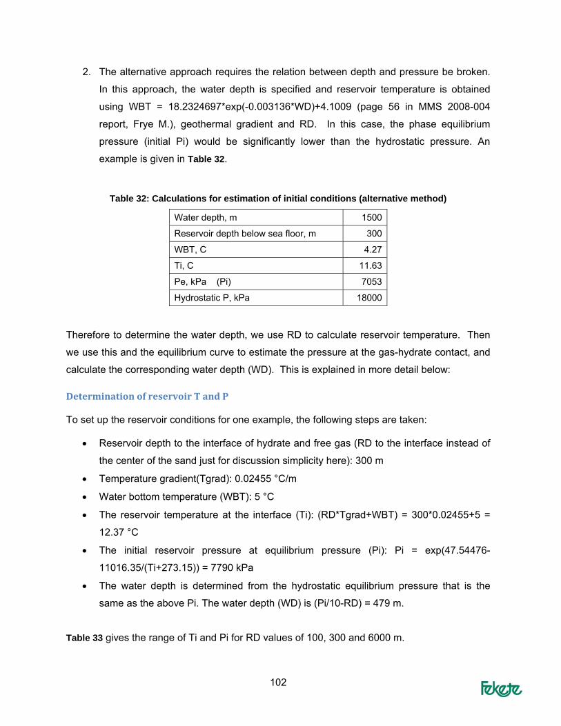
102

2. The alternative approach requires the relation between depth and pressure be broken.

In this approach, the water depth is specified and reservoir temperature is obtained

using WBT = 18.2324697*exp(-0.003136*WD)+4.1009 (page 56 in MMS 2008-004

report, Frye M.), geothermal gradient and RD. In this case, the phase equilibrium

pressure (initial Pi) would be significantly lower than the hydrostatic pressure. An

example is given in Table 32.

Table 32: Calculations for estimation of initial conditions (alternative method)

Water depth, m 1500

Reservoir depth below sea floor, m 300

WBT, C 4.27

Ti, C 11.63

Pe, kPa (Pi) 7053

Hydrostatic P, kPa 18000

Therefore to determine the water depth, we use RD to calculate reservoir temperature. Then

we use this and the equilibrium curve to estimate the pressure at the gas-hydrate contact, and

calculate the corresponding water depth (WD). This is explained in more detail below:

Determination of reservoir T and P To set up the reservoir conditions for one example, the following steps are taken:

• Reservoir depth to the interface of hydrate and free gas (RD to the interface instead of

the center of the sand just for discussion simplicity here): 300 m

• Temperature gradient(Tgrad): 0.02455 °C/m

• Water bottom temperature (WBT): 5 °C

• The reservoir temperature at the interface (Ti): (RD*Tgrad+WBT) = 300*0.02455+5 =

12.37 °C

• The initial reservoir pressure at equilibrium pressure (Pi): Pi = exp(47.54476-

11016.35/(Ti+273.15)) = 7790 kPa

• The water depth is determined from the hydrostatic equilibrium pressure that is the

same as the above Pi. The water depth (WD) is (Pi/10-RD) = 479 m.

Table 33 gives the range of Ti and Pi for RD values of 100, 300 and 6000 m.

103

Table 33: Estimation of initial p/T (and water depth) based on reservoir depth

Reservoir depth below sea floor, m 100 300 600

WBT, C 5 5 5

Ti, C 7.46 12.37 19.73

Pe, kPa (Pi) 3966 7790 20556

Water depth, m 297 479 1456

The temperature range is from 7.5 °C to 19.7 °C and the pressure is from 4000 kPa to 20500

kPa. The corresponding water depth is from 300 m to 1450 m. Note that the estimated values

of WD do not affect any of the simulations or the response function.

104

APPENDIX 6B: EXPERIMENTAL DESIGN METHODS

Table 34: 11-factor Packett-Burman Design

Case # F1 F2 F3 F4 F5 F6 F7 F8 F9 F10 F11

1 1 1 1 -1 1 1 -1 1 -1 -1 -1 2 -1 -1 1 1 1 -1 1 1 -1 1 -1 3 -1 1 1 -1 1 -1 -1 -1 1 1 1 4 -1 -1 -1 1 1 1 -1 1 1 -1 1 5 1 -1 1 1 -1 1 -1 -1 -1 1 1 6 -1 -1 -1 -1 -1 -1 -1 -1 -1 -1 -1 7 0 0 0 0 0 0 0 0 0 0 0 8 0 0 0 0 0 0 0 0 0 0 0 9 -1 1 1 1 -1 1 1 -1 1 -1 -1

10 -1 1 -1 -1 -1 1 1 1 -1 1 1 11 1 -1 -1 -1 1 1 1 -1 1 1 -1 12 1 -1 1 -1 -1 -1 1 1 1 -1 1 13 1 1 -1 1 -1 -1 -1 1 1 1 -1

14 1 1 -1 1 1 -1 1 -1 -1 -1 1

Trigen(100, 300, 600, 10, 90) Trunc(50,+inf)

Val

ues

x 10

^-3

0.0

0.5

1.0

1.5

2.0

2.5

0

100

200

300

400

500

600

700

800

900

5.0% 5.0%90.0%100.9 667.3


105

Histogrm(-7.75757, 16.31255, {p})

0.0

0.1

0.2

0.3

0.4

0.5

0.6

0.7

-10 -5 0 5 10 15 20

10.0% 10.0%80.0%2.87 6.72

Figure 88: Probability distribution of equilibrium temperature at 3000 kPa

Trigen(30, 35, 40, 10, 90)

Porosity,%

0.00

0.02

0.04

0.06

0.08

0.10

0.12

24 26 28 30 32 34 36 38 40 42 44 46

5.0% 5.0%90.0%28.82 41.18


106

Trigen(40, 60, 85, 10, 90) Trunc(40,90)

Val

ues

x 10

^-2

0.0

0.5

1.0

1.5

2.0

2.5

3.0

30 40 50 60 70 80 90 100

5.0% 5.0%90.0%43.37 85.35


Trigen(3, 6, 20, 10, 90) Trunc(3,+inf)

Val

ues

x 10

^-2

0

1

2

3

4

5

6

7

8

0 5 10 15 20 25 30

5.0% 5.0%90.0%3.99 22.68


107

Trigen(0, 5, 10, 10, 90) Trunc(0,+inf)

0.00

0.02

0.04

0.06

0.08

0.10

0.12

0.14

-2 0 2 4 6 8 10 12 14 16

10.0% 10.0%80.0%1.53 10.21

Figure 92: Probability distribution of reservoir dip angle

Trigen(0.5, 0.7, 0.9, 10, 90) Trunc(0.5,0.9)

0.0

0.5

1.0

1.5

2.0

2.5

3.0

3.5

0.45

0.50

0.55

0.60

0.65

0.70

0.75

0.80

0.85

0.90

0.95

10.0% 10.0%80.0%0.5553 0.8447

Figure 93: Probability distribution of ratio of hydrate to total sand column

108

Trigen(0, 1, 5, 10, 90) Trunc(0,5)

0.00

0.05

0.10

0.15

0.20

0.25

0.30

-1 0 1 2 3 4 5 6

5.0% 5.0%90.0%0.272 4.564

Figure 94: Probability distribution of ratio of bottom aquifer size to sand size

Trigen(-2.99573, -0.69315, 1.609438, 10, 90)Trunc(-2.99573,1.609438)


0.00

0.05

0.10

0.15

0.20

0.25

0.30

0.35

-3.5

-3.0

-2.5

-2.0

-1.5

-1.0

-0.5 0.0

0.5

1.0

1.5

2.0

5.0% 5.0%90.0%-2.654 1.268

Figure 95: Probability distribution of logarithm of initial permeability

109

Trigen(100, 500, 1000, 10, 90) Trunc(10,2000)

Val

ues

x 10

^-3


0.0

0.2

0.4

0.6

0.8

1.0

1.2

1.4

0.0

0.2

0.4

0.6

0.8

1.0

1.2

1.4

5.0%90.0%0.104 1.118


Trigen(0.1, 0.5, 1, 10, 90) Trunc(0.1,1)

krg endpoint

0.0

0.2

0.4

0.6

0.8

1.0

1.2

1.4

1.6

0.0

0.1

0.2

0.3

0.4

0.5

0.6

0.7

0.8

0.9

1.0

1.1

5.0% 5.0%90.0%0.164 0.931


Technical Recoverability of Gas Hydrate in the U.S. … Recoverability of Gas Hydrate ... 101...

Documents

Transcript of Technical Recoverability of Gas Hydrate in the U.S. … Recoverability of Gas Hydrate ... 101...