PDF (1.52 MB) - IOPscience
46
Journal of Instrumentation OPEN ACCESS The electromagnetic calorimeter for the T2K near detector ND280 To cite this article: D Allan et al 2013 JINST 8 P10019 View the article online for updates and enhancements. You may also like Towards seeking 13 : Status and initial data from T2K Laura Lee Kormos and the T2K Collaboration - Study of neutrino interactions at the T2K near detector A Hillairet and the T2K collaboration - Neutrino–nucleus cross sections for oscillation experiments Teppei Katori and Marco Martini - Recent citations Priscilla Brooks Cushman and David- Michael Poehlmann - First T2K measurement of transverse kinematic imbalance in the muon-neutrino charged-current single- + production channel containing at least one proton K. Abe et al - T2K measurements of muon neutrino and antineutrino disappearance using 3.13×10²¹ protons on target K. Abe et al - This content was downloaded from IP address 78.165.64.127 on 30/12/2021 at 09:25
Transcript of PDF (1.52 MB) - IOPscience

Journal of Instrumentation
OPEN ACCESS
The electromagnetic calorimeter for the T2K neardetector ND280To cite this article D Allan et al 2013 JINST 8 P10019
View the article online for updates and enhancements
You may also likeTowards seeking 13 Status and initial datafrom T2KLaura Lee Kormos and the T2KCollaboration
-
Study of neutrino interactions at the T2Knear detectorA Hillairet and the T2K collaboration
-
Neutrinondashnucleus cross sections foroscillation experimentsTeppei Katori and Marco Martini
-
Recent citationsPriscilla Brooks Cushman and David-Michael Poehlmann
-
First T2K measurement of transversekinematic imbalance in the muon-neutrinocharged-current single- + productionchannel containing at least one protonK Abe et al
-
T2K measurements of muon neutrino andantineutrino disappearance using313times1021 protons on targetK Abe et al
-
This content was downloaded from IP address 7816564127 on 30122021 at 0925
2013 JINST 8 P10019
PUBLISHED BY IOP PUBLISHING FOR SISSA MEDIALAB
RECEIVED August 15 2013ACCEPTED September 4 2013PUBLISHED October 17 2013
The electromagnetic calorimeter for the T2K neardetector ND280
The T2K UK collaborationD Allane C Andreopoulose C Angelsene GJ Barkeri G Barrg S Benthamc
I Bertramc S Boydi K Briggsi RG Calland f J Carroll f SL Cartwrighth
A Carveri C Chavez f G Christodoulou f J Coleman f P Cooke f G Daviesc
C Denshame FDi Lodovicod J Dobsonb T Duboyskid T Durkine DL Evans f
A Finchc M Fittone FC Gannawayd A Granta N Grantc S Grenwoodb
P Guzowskib D Hadleyi M Haighg PF Harrisoni A Hatzikoutelisc
TDJ Haycockh A Hyndmand J Ilice S Ivesb AC Kabothb V Kaseyb L Kellet f
M Khaleeqb G Koganb LL Kormosc1 M Laweh TB Lawsonh C Listeri
RP Litchfieldi M Lockwood f M Malekb T Maryonc P Masliahb
K Mavrokoridis f N McCauley f I Mercerc C Metelkoe B Morgani J Morrisd
A Muira M Murdoch f T Nichollse M Noyb HM OrsquoKeeffeg RA Owend
D Payne f GF Pearcee JD Perkinh E Poplawskad R Preecee W Qiane
P Ratoffc T Raufere M Raymondb M Reevesc D Richardsi M Rooneye
R Saccod S Sadlerh P Schaackb M Scottb DI Scullyi S Shortb M Siyade
R Smithg B Stilld P Sutcliffe f IJ Taylori R Terrid LF Thompsonh A Thorley f
M Thorpee C Timisd C Touramanis f MA Uchidad Y Uchidab A Vacheretg
JF Van Schalkwykb O Veledarh AV Waldrong MA Wardh GP Wardh D Warkeg
MO Wasckob A Webereg N Westg LH Whiteheadi C Wilkinsonh andJR Wilsond
aSTFC Daresbury Laboratory Daresbury UKbImperial College London London UKcLancaster University Lancaster UKdQueen Mary University of London London UKeSTFC Rutherford Appleton Laboratory Oxford UKf University of Liverpool Liverpool UKgUniversity of Oxford Oxford UKhUniversity of Sheffield Sheffield UKiUniversity of Warwick Coventry UK
E-mail lkormoslancasteracuk
1Corresponding author
ccopy 2013 IOP Publishing Ltd and Sissa Medialab srl Content from this work may beused under the terms of the Creative Commons Attribution 30 License Any further
distribution of this work must maintain attribution to the author(s) and the title of the work journalcitation and DOI
doi1010881748-0221810P10019
2013 JINST 8 P10019
ABSTRACT The T2K experiment studies oscillations of an off-axis muon neutrino beam betweenthe J-PARC accelerator complex and the Super-Kamiokande detector Special emphasis is placedon measuring the mixing angle θ13 by observing νe appearance via the sub-dominant νmicro rarr νe
oscillation and searching for CP violation in the lepton sector The experiment includes a sophis-ticated off-axis near detector the ND280 situated 280 m downstream of the neutrino productiontarget in order to measure the properties of the neutrino beam and to understand better neutrinointeractions at the energy scale below a few GeV The data collected with the ND280 are used tostudy charged- and neutral-current neutrino interaction rates and kinematics prior to oscillation inorder to reduce uncertainties in the oscillation measurements by the far detector A key element ofthe near detector is the ND280 electromagnetic calorimeter (ECal) consisting of active scintillatorbars sandwiched between lead sheets and read out with multi-pixel photon counters (MPPCs) TheECal is vital to the reconstruction of neutral particles and the identification of charged particlespecies The ECal surrounds the Pi-0 detector (P 0D) and the tracking region of the ND280 and isenclosed in the former UA1NOMAD dipole magnet This paper describes the design constructionand assembly of the ECal as well as the materials from which it is composed The electronic anddata acquisition (DAQ) systems are discussed and performance of the ECal modules as deducedfrom measurements with particle beams cosmic rays the calibration system and T2K data isdescribed
KEYWORDS Calorimeters Neutrino detectors Scintillators and scintillating fibres and light guides
ARXIV EPRINT 13083445
2013 JINST 8 P10019
Contents
1 Introduction 1
2 Overview of the calorimeter design 221 The downstream ECal 422 The barrel ECal 723 The P0D ECal 8
3 Materials 931 Scintillator bars 932 Lead 1133 Wavelength-shifting fibre 1234 Photosensors 1535 Fibre to sensor coupling 17
4 Construction 1841 Layer assembly 1842 Assembly procedures for the ECal modules 2043 The bar scanner 22
5 Readout electronics and data acquisition 23
6 Light injection system 2561 Control cards and trigger receiver 2662 Junction boxes 2663 Communications protocol and cabling 2664 Pulsers 2665 LED strips and extruded perspex lens 2666 LI installation 27
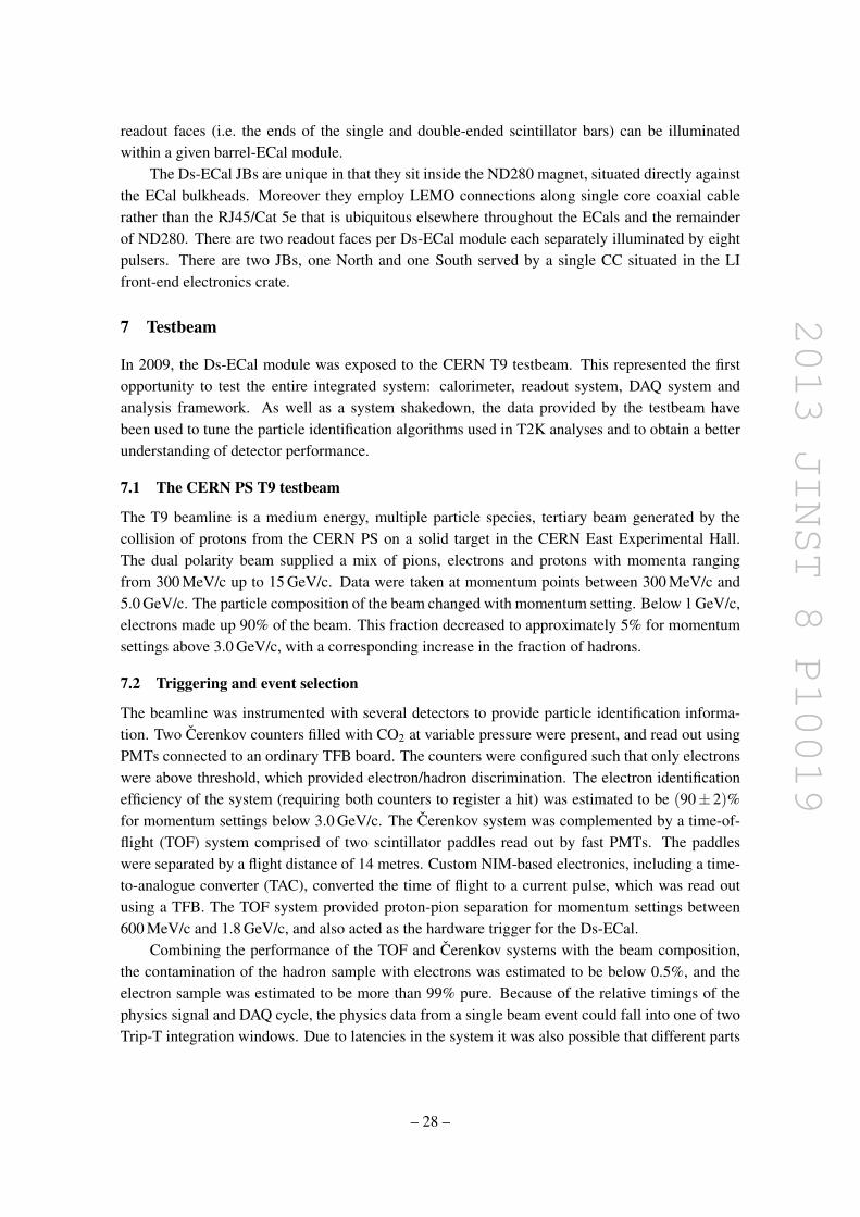
7 Testbeam 2871 The CERN PS T9 testbeam 2872 Triggering and event selection 2873 Detector configuration 2974 Calibration differences 2975 Testbeam performance 30
8 ECal commissioning and performance 3181 Calibration 3182 Hit efficiency 3783 Time stability and beam position 3784 Particle identification 39
9 Summary 40
ndash i ndash
2013 JINST 8 P10019
1 Introduction
Many parameters of neutrino oscillations have yet to be measured precisely The Tokai-to-Kamioka(T2K) experiment is a long-baseline neutrino oscillation experiment designed to measure severalof these parameters It consists of three main components a dedicated beamline from the protonsynchrotron main ring of the Japan Proton Accelerator Research Complex (J-PARC) that is used toproduce an intense beam of muon neutrinos a suite of near detectors situated 280 m downstreamof the neutrino production target (INGRID and ND280) [1 2] that characterize the neutrino beambefore the neutrinos change flavour and the far detector Super-Kamiokande [3] which measuresthe oscillated neutrino beam Unlike previous accelerator-based neutrino experiments [4 5] T2Kuses an off-axis configuration in which the detectors sample the neutrino beam at an angle of25 to the primary proton beam thus providing a narrower neutrino energy spectrum peaked atapproximately 600 MeV which is optimized for neutrino oscillation measurements using Super-Kamiokande at a distance of 295 km downstream and assuming the current measured value of∆m2
32 The ND280 is centred on the same off-axis angle as Super-Kamiokande in order to sample asimilar portion of the neutrino flux that will be used to measure the oscillation parameters The useof a near and far detector in this way reduces the systematic uncertainty on the measured oscillationparameters The main aim of T2K is to measure θ13 through the appearance of νe in a νmicro beam [6]and to improve the measurements of θ23 and the mass difference ∆m2
32 through observation of νmicro
disappearance [7] With recently-measured large values of θ13 [8 9] T2K has a unique role toplay in determining whether or not there is CP violation in the lepton sector T2K was the firstexperiment to observe indications of a non-zero value for θ13 in 2011 [10]
The ND280 [2] is contained within the refurbished UA1 magnet which in its current config-uration provides a field of 02 T The detector consists of two principal sections the Pi-0 Detec-tor (P 0D) [11] optimized for identifying and measuring π0 decays and the tracker designed forprecision measurement and identification of charged particles The tracker comprises three timeprojection chambers (TPCs) [12] interspersed with two fine-grained detectors (FGDs) [13] to pro-vide target mass surrounded by an electromagnetic calorimeter (ECal) The P0D TPCs FGDsand downstream ECal (Ds-ECal) are mounted in a supporting structure or lsquobasketrsquo which sits in-side the UA1 magnet while the surrounding barrel- and P0D-ECal are affixed to the magnet yokewhich splits vertically as shown in figure 1 to provide access for installation and maintenanceThe yoke itself is instrumented with slabs of plastic scintillator to act as a muon detector the sidemuon range detector (SMRD) [14] With the exception of the TPCs plastic scintillator is used asthe active material in all ND280 subdetectors It should be noted that in contrast to conventionalcharged-particle beams neutrino interactions may occur at any point within the ND280 and itsimmediate environment
The ND280 must provide a well-measured neutrino energy spectrum flux and the beam neu-trino composition as well as measurements of neutrino interaction cross-sections in order to reducethe systematic uncertainties in the neutrino oscillation parameters This information is used to pre-dict the characteristics of the unoscillated beam at Super-Kamiokande Additionally the neutrinocross-section measurements are interesting in their own right as there are few such measurementsin the literature at present
ndash 1 ndash
2013 JINST 8 P10019
x
z
y
beam
Figure 1 An exploded view of the ND280 detector showing the P0D-ECal and barrel-ECal affixed to themagnet return yoke and the Ds-ECal mounted inside the basket The νmicro beam enters from the left of thefigure The detector co-ordinate system is right-handed as shown with the origin at the geographical centrewhich lies near the downstream end of the first TPC
The ECal forms an important part of the ND280 and is essential to obtain good measurementsof neutral particles and electronpositron showers that lead to correct particle identification andimproved energy reconstruction It can also be used as target material to determine neutrino in-teraction cross-sections on lead This paper describes the design construction and performance ofthe ECal
2 Overview of the calorimeter design
The ECal is a lead-scintillator sampling calorimeter consisting of three main regions the P0D-ECal which surrounds the P0D the barrel-ECal which surrounds the inner tracking detectors andthe Ds-ECal which is located downstream of the inner detectors and occupies the last 50 cm ofthe basket It is often useful to consider the ECal detectors that surround the tracker region of theND280 together hence the barrel-ECal and Ds-ECal together are referred to as the tracker-ECalAltogether the ECal consists of 13 modules 6 P0D-ECal (2 top 2 bottom 2 side) 6 barrel-ECal(2 top 2 bottom 2 side) and 1 Ds-ECal The position of the ECal within the ND280 is shown in
ndash 2 ndash
2013 JINST 8 P10019
figure 1 The ECal modules that surround the barrel (barrel-ECal and P0D-ECal) are attached tothe magnet and must have two top and two bottom modules in order to allow for the opening of theND280 magnet
Each module consists of layers of scintillating polystyrene bars with cross-section 40 mm times10 mm bonded to lead sheets of thickness 175 mm (400 mm) in the tracker-ECal (P 0D-ECal)which act as a radiator to produce electromagnetic showers and which provide a neutrino-interactiontarget The size of the ECal is constrained by its position between the basket and the magnet Alarger ECal would necessitate a smaller basket and thus smaller inner subdetectors A scintillatorbar thickness of 10 mm was chosen to minimize the overall depth of the ECal while still providingsufficient light to produce a reliable signal Scintillator bar widths lead thickness and the numberof layers per module were optimized for particle identification and tracking information Smallerbar widths are favoured for tracking information and optimization studies indicated that the π0
reconstruction efficiency becomes seriously compromised for widths greater than 50 mm hence40 mm was chosen as a compromise between reconstruction efficiency and channel cost Similarlythe lead thickness of 175 mm was chosen based upon studies of π0 detection efficiency The num-ber of layers was determined by the requirement to have sufficient radiation lengths of material tocontain electromagnetic showers of photons electrons and positrons with energies up to 3 GeVAt least 10 electron radiation lengths X0 are required to ensure that more than 50 of the energyresulting from photon showers initiated by a π0 decay is contained within the ECal This require-ment is satisfied in the tracker-ECal More information about the scintillator bars and the lead arein sections 31 and 32
The physics aims of the tracker-ECal and P0D-ECal are somewhat different and this is re-flected in their design and construction The tracker-ECal is designed as a tracking calorimeter tocomplement the charged-particle tracking and identification capabilities of the TPCs by providingdetailed reconstruction of electromagnetic showers This allows the energy of neutral particles tobe measured and assists with particle identification in the ND280 tracker To this end there are 31scintillator-lead layers in the barrel-ECal and 34 layers in the Ds-ECal or approximately 10 X0 and11 X0 respectively The direction of the scintillator bars in alternate layers is rotated by 90 for 3Dtrack and shower reconstruction purposes
In contrast shower reconstruction in the P0D region of the ND280 is done by the P0D it-self which consists of four pre-assembled lsquoSuper-P 0Dulesrsquo two with brasswater targets each ofwhich provides 24 (14) radiation lengths of material when the water is in (out) and two with leadtargets each of which provides 49 radiation lengths of material The role of the P0D-ECal is totag escaping energy and distinguish between photons and muons The construction of the P0D-ECal therefore differs from that of the tracker-ECal with coarser sampling (six scintillator layersseparated by 4 mm-thick lead sheets corresponding to approximately 43 X0) and all bars runningparallel to the beam direction With only six scintillator layers the P0D-ECal requires thicker leadsheets to ensure that photons are detected with high efficiency that showers are well contained andthat photon showers can be distinguished from muon deposits Simulation studies using photonsand muons with energies between 65 and 1000 MeV normally incident on a P0D-ECal face wereused to determine the optimum lead thickness A thickness of 4 mm was found to provide goodphoton tagging efficiency (gt 95 for photons above 150 MeV) and good microγ discrimination whileminimizing the number of photons that are detected only in the first layer and might therefore berejected as noise [15]
ndash 3 ndash
2013 JINST 8 P10019
Table 1 Summary of the ECal design showing the overall dimensions numbers of layers length andorientation of scintillator bars numbers of bars and lead thickness for each module
DS-Ecal Barrel ECal P0D ECalLength (mm) 2300 4140 2454Width (mm) 2300 1676 topbottom 1584 topbottom
2500 side 2898 sideDepth (mm) 500 462 155Weight (kg) 6500 8000 topbottom 1500 topbottom
10000 side 3000 sideNum of layers 34 31 6Bar orientation xy Longitudinal and Perpendicular LongitudinalNum of bars 1700 2280 Longitudinal topbottom 912 Longitudinal topbottom
1710 Longitudinal sides 828 Longitudinal sides6144 Perp topbottom3072 Perp sides
Bars per layer 50 38 Longitudinal topbottom 38 Longitudinal topbottom57 Longitudinal side 69 Longitudinal sides96 Perp topbottomsides
Bar length (mm) 2000 3840 Longitudinal 2340 Longitudinal1520 Perp topbottom2280 Perp sides
Pb thickness (mm) 175 175 40
Each scintillator bar has a 2 mm-diameter hole running longitudinally through the centre of thebar for the insertion of wavelength-shifting (WLS) fibres Light produced by the passage of chargedparticles through the bars is collected on 1 mm-diameter WLS fibres and transported to solid-statephotosensors known as multi-pixel photon counters (MPPCs) [16] The Ds-ECal WLS fibres areread out from both ends (double-ended readout) the barrel-ECal modules have a mix of double-and single-ended readout and the P0D-ECal modules have single-ended readout The fibres thatare read out at one end only are mirrored at the other end with a vacuum deposition of aluminiumThe WLS fibres and MPPCs are discussed more fully in sections 33 and 34 respectively Eachlayer in each module is encased in a 200 mm wide times 125 mm high aluminium border with holesto allow the WLS fibres to exit the layer
A summary of the ECal design is shown in table 1 Further explanation is given in the fol-lowing subsections and in section 4 Figure 2 shows one complete side of the ECal in situ TheP0D-ECal is on the left and the barrel-ECal is on the right in the figure Visible are the top sideand bottom modules for each Notice that the P0D-ECal is thinner than the barrel-ECal as de-scribed above
21 The downstream ECal
The first detector to be constructed and commissioned was the Ds-ECal which also acted as a pro-totype The outer dimensions of the Ds-ECal are 2300 mm high times 2300 mm wide times 500 mm long
ndash 4 ndash
2013 JINST 8 P10019
Figure 2 One entire side of the ECal in situ installed in the ND280 The three P0D-ECal modules are onthe left in the figure the three barrel-ECal modules are on the right Part of the magnet yoke (top red) isvisible
(depth in the beam direction) Each of the 34 layers has 50 scintillator bars of length 2000 mm Thebars of the most-upstream layer run in the x-direction (horizontally) when the module is installedin the ND280 basket Surrounding the 34 layers on all four sides are 25 mm-thick aluminium bulk-heads which have holes for the WLS fibres to exit Once outside the bulkhead each end of everyfibre is secured inside a custom-made Teflon ferrule as discussed in section 35 and shown in fig-ure 11 which is then covered by a matching sheath that allows the WLS fibre to make contact withthe protective transparent resin coating of the MPPC This contact is maintained by a sponge-likespring situated behind the MPPC that can absorb the effects of thermal expansion and contractionin the WLS fibres The sheath also contains a simple printed circuit board which couples the MPPCto a mini-coaxial cable that carries the information between the MPPC and the front-end electroniccards Figure 3 shows the top barrel-ECal module during construction The fibre ends in the fer-rules are visible protruding from the module bulkheads The electronics are described in section 5The ferrule is designed to latch into the sheath which is then screwed to the bulkhead in order tohold the ferrule and WLS fibre in place and to assure that the coupling between the WLS fibre andthe MPPC is secure The MPPC-WLS fibre coupling is described in section 33
There is a 1 cm gap between the layers and the bulkheads on all sides to leave space for thelight injection (LI) system The LI system described in section 6 uses LED pulsers to delivershort flashes of light through the gap to illuminate all of the WLS fibres allowing integrity andcalibration checks to be performed
ndash 5 ndash
2013 JINST 8 P10019
Figure 3 One of the top barrel-ECal 15 m times 4 m modules lying horizontally during construction The fibreends encased in their ferrules are visible protruding from the module bulkheads The structure of the 2Dscanner can be seen surrounding the module
Cooling panels for temperature control are located outside the bulkheads as shown in figure 4Pipes carrying chilled water maintain these panels at a constant temperature of approximately 21Cthe bottom panel also has perforated air pipes through which dry air is pumped to prevent conden-sation within the module Large air holes through the cooling panels and the bulkheads allow theair to flush through the active region of the detector and escape from the module
The Trip-T front-end electronic boards (TFBs) are mounted on the cooling panels using screwsand thermally-conducting epoxy resin slots in the panels allow the cables from the MPPCs to passthrough and terminate on the TFBs Each TFB has 64 channels to read out MPPCs a built-ininternal temperature sensor and a port that connects to an external temperature sensor mounted onthe bulkhead near the MPPCs in order to monitor the MPPC temperatures There are 14 TFBs perside Figure 4 shows the left-side cooling panel with the TFBs installed
The cooling panels are protected by anodized aluminium cover panels while the 2000 mm times2000 mm outer surfaces are covered by carbon-fibre panels in order to minimize the mass of thesedead regions These cover panels form the outside of the module Each carbon-fibre panel consistsof two sheets of carbon-fibre of dimensions 2059 mm wide times 2059 mm long times 12 mm thick Afoam layer of 226 mm thickness is sandwiched between the two sheets making the entire panel
ndash 6 ndash
2013 JINST 8 P10019
TFB
ethernet cables
bus bars
temp sensor cables
TFB
LI ground cables
cooling pipes
Figure 4 The left side of the Ds-ECal lying horizontally during construction When upright in situ thebottom in the figure becomes the upstream surface of the Ds-ECal nearest to the inner detectors and the topin the figure becomes the downstream surface nearest to the magnet coils Shown at the top and bottom arethe Cat 5e cables (commonly used as ethernet cables) the LI cables (small black cables at the bottom) theTFBs (green cards) the external temperature-sensor cables (multi-coloured) the cooling pipes (aluminiumtop and bottom) and the bus bars (brass centre) mounted on the cooling panels Air holes in the coolingpanel are visible on the right side of the figure The Cat 5e cables at the top include both the signal andtrigger cables those at the bottom are signal cables
25 mm deep The carbon-fibre sheets are glued tongue-in-groove into an aluminium border that is120 mm wide and 25 mm thick making the dimensions of the entire carbon-fibre-aluminium panel2299 mmtimes 2299 mmtimes 25 mm thick In situ the Ds-ECal sits upright inside the basket Water dryair and high-voltage enter through the bottom cover panel The information to and from the TFBsis carried by shielded Cat 5e cables which exit through a patch panel in the bottom cover panel Inaddition to these 56 signal cables there are 28 trigger cables routed through 28 cable glands in thetop cover panel of the module which come from the TFBs that are connected to the MPPCs locatednear the downstream edge of the module Data from these channels form part of the ND280 cosmicray trigger Upon exiting the cover panels the signal Cat 5e cables are connected to the readoutmerger modules (RMMs) which are attached to the outer surface of the cover panels The RMMsare discussed in section 5 The trigger cables are connected to fan-in cards on the top of the moduleThe Ds-ECal is the only ECal module which forms part of the ND280 cosmic ray trigger system
22 The barrel ECal
The four barrel-ECal top and bottom modules are 4140 mm long (parallel to the beam)times 1676 mmwide times 462 mm high with 31 lead-scintillator layers 16 (including the innermost layer) with1520 mm-long scintillator bars running perpendicular to the beam direction and 15 with 3840 mm-long bars running longitudinally ie parallel to the beam direction
The structure of each of the ECal modules is very similar to that described above for the Ds-ECal except that the perpendicular bars have single-ended readout with the fibres mirrored on theend that is not read out The mirrored ends of the fibres terminate just inside the scintillator bars
ndash 7 ndash
2013 JINST 8 P10019
whereas the ends that are read out exit through the bulkhead as in the Ds-ECal The longitudinalbars all have double-ended readout
In order to minimize the non-active gap in the ECal running down the centre of the ND280between the two top or the two bottom modules the mirrored ends of the fibres in the perpendicularbars are in the centre of the ND280 and the readout ends are at the sides This made it possible toreplace the thick aluminium bulkhead cooling panels and cover panels that form the structure onthe other three sides of each module with a thin aluminium cover panel allowing the two top and thetwo bottom modules to be placed closer together and minimizing the dead material between them
The two side barrel-ECal modules are 4140 mm long times 2500 mm wide times 462 mm deep with31 lead-scintillator layers 16 (including the innermost layer) with 2280-mm-long scintillator barsrunning perpendicular to the beam direction and 15 with 3840-mm-long bars running longitudi-nally ie parallel to the beam direction As in the top and bottom barrel-ECal the perpendicularbars are single-ended readout with the mirrored ends of the fibres at the top and the readout endsat the bottom of the modules
Unlike the Ds-ECal which has carbon-fibre panels on both the most upstream and downstreamfaces the barrel-ECal modules have a carbon-fibre panel on the innermost face but the outermostface has an aluminium panel which provides the required structure for attaching the module to themagnet yoke
23 The P 0D ECal
The most noticeable difference between the tracker-ECal modules and the P0D-ECal modules isthe smaller size of the P0D-ECal which has six scintillator-lead layers and is only 155 mm deepThe four topbottom modules are 1584 mm wide the two side modules are 2898 mm wide and allsix are 2454 mm long The P0D-ECal also required thicker 4 mm lead sheets as a consequence ofhaving fewer layers All of the scintillator bars 38 in each topbottom module layer and 69 in theside layers are oriented parallel to the beam read out on the upstream end and mirrored on thedownstream end The smaller size also allowed simplifications to be made in the construction
While the readout electronics of the tracker-ECal detectors were mounted on separate coolingplates the P0D-ECal TFBs are attached directly to the upstream bulkhead as shown in figure 5This bulkhead extends 100 mm above the height of the main detector box so that the TFBs canbe mounted next to the region where the optical fibres emerge The water cooling pipes are thenrecessed into grooves running along the exposed face behind through which the dry air systemalso passes Because there are no more than seven TFBs in any one module the boards could havetheir power provided via standard copper cables instead of the bus bars used in the tracker-ECalThe readout region was then protected by an anodized aluminium cover
Structurally the P0D-ECal modules used the same carbon-fibre panels as the tracker-ECalon the bases but all had solid aluminium bulkheads to form the lids Onto this were bolted thestructures required to mount the detectors on the near detector magnet cast aluminium rails for theside modules and roller cages for the topbottom modules
ndash 8 ndash
2013 JINST 8 P10019
160mm
TFB
sensors
ethernet
power
lines
Figure 5 Closeup on the readout side of the upstream bulkhead for a P0D-ECal side module The blackcases at the bottom house the MPPCs (photosensors) coupled to the optical fibres where they emerge fromthe inner detector Each MPPC is connected via a thin grey cable to the TFB mounted above which receivesits power from the coloured cables on its left and is read via the Cat 5e (ethernet) cable on its right
3 Materials
31 Scintillator bars
The ECal scintillator bars were made at the Fermi National Accelerator Laboratory (FNAL) fromextruded polystyrene doped with organic fluors at concentrations of 1 PPO and 003 POPOPThe polystyrene scintillator bars have a 025plusmn 013 mm coating of polystyrene co-extruded withTiO2 providing light reflection and isolation The scintillator was chosen to have the same com-position as that used for the MINOS detectors [17] Each bar has a cross-section of (400+00
minus04) mmwide times (100+00
minus04) mm deep with a 20plusmn02 mm hole running down the centre for the insertion of1 mm-diameter WLS fibre which is discussed in more detail in section 33 Each bar was cut to theappropriate length during the quality assurance (QA) process described below to within 01 mmThe number of bars of each length is shown in table 1 Including the 10 extra that were made toreplace any rejected during the QA process there were a total of more than 18300 bars shippedfrom FNAL
ndash 9 ndash
2013 JINST 8 P10019
The scintillator bars underwent both mechanical and optical QA tests The frequency of testingwas reduced in some cases as the extrusion process at FNAL was refined due to feedback from theQA group During the mechanical QA tests the sizes of 100 of the bars were checked for widthand thickness using custom-made Go and No-Go gauges that could slide easily along bars if thesizes were within tolerance and a visual inspection was made for flatness and squareness The barswere then cut to length The hole position and diameter were checked using digital callipers for100 of the bars for the Ds-ECal and for 10 of the bars subsequently Optical QA was carriedout on 10 of the bars for the Ds-ECal and 5 of the bars subsequently
For the first shipments of bars which were used in the Ds-ECal the hole diameter was foundto vary from 175 mm to 350 mm and the shape was typically elliptical rather than round This didnot affect the light yield of the bar however it did have consequences for the layer construction Ifthe hole was too small the locator pins used to hold the bar in place while the epoxy cured couldnot be inserted into the bar if the hole was too large glue would enter the hole around the edgesof the locator pin and block the subsequent insertion of the WLS fibre Approximately 10 ofDs-ECal bars were rejected due to this problem Subsequent shipments of bars for use in the otherECal modules did not have this problem
Optical QA was carried out on the scintillator bars in order to ensure a consistency of re-sponse to minimum-ionizing particles (MIPs) To this end a cosmic ray (CR) telescope was con-structed consisting of a light-tight enclosure for the scintillator bars and their photo-readout atriple-coincidence trigger and a simple data acquisition (DAQ) system The bar being tested didnot form part of the trigger [18]
The CR telescope consisted of three 4 cm times 6 cm scintillator pads coupled to 2-inch photo-multiplier tubes (PMTs) which were biased to approximately 2 kV each The coincidence triggerconsisted of a simultaneous trigger from one scintillator pad above and two pads below the bar be-ing tested This criterion excluded showers and random coincidences from the PMTs and reducedthe selection of CRs to those that entered the telescope at a small angle from the zenith eliminatingthe need to correct for path-length differences in the bar due to differing angles of incidence TheCR telescope registered an average of 450 triggers per hour as expected from calculations
Each bar to be tested for light yield was first wrapped in two layers of microfibre blackoutmaterial as a form of flexible dark box In order to obtain a robust signal over the backgroundelectronic noise the light signal of the test scintillator was collected by three 1 mm-diameter WLSfibres rather than one in the central hole of the scintillator bar which was possible due to the holediameters being larger than specified as discussed above The three fibres were coupled to thecentre of a 2-inch PMT with optical grease to improve light transmission The PMT was biased ata voltage of 255 kV
The bar readout end was confined inside a series of plastic adaptors to enable easy replacementof the bars for testing and to ensure a consistent reproducible optical coupling to the PMT Aviewing port was built to enable visual verification of the coupling between the WLS fibres and thePMT and to act as an input port for an LED-based light-injection system that was used to calibratethe single photo-electron (PE) peak in the PMT The optical QA setup is shown in figure 6
Output signals from the trigger PMTs were fed into a into a computer running LabVIEW thatproduced histograms of the charge integrals and exported the data for subsequent analysis [18]A baseline was established using 12 scintillator bars from an early delivery After analysis and
ndash 10 ndash
2013 JINST 8 P10019
2m bar
Figure 6 The CR telescope showing the 2 m-long scintillator bar in light-tight microfibre sleeve (centre)and the triple-coincidence trigger The trigger scintillator pads are situated with one above and two belowthe test bar
calibration using the single PE peak the light yield for these 2 m bars read out at a position 66 cmfrom the readout end was found to be 342plusmn 06 PEMIP with σ asymp 5 PEMIP Bars with a lightyield within 2σ of the baseline light yield were accepted This criterion did not reject any bars
32 Lead
The target mass and radiator for each layer is provided by a thin sheet of lead stiffened with20plusmn 02 antimony Traces of other metals are below 015 Each sheet of lead was coatedwith black quick-drying metal-conditioning primer CELEROL-Reaktionsgrund 918 (ReactionPrimer) before being used in a layer in order to protect personnel from the harmful effects of leadand prevent any possibility of leaching between the lead and the scintillator which might degradethe light-yield qualities of the scintillator over time The lead thickness for all layers in the barrel-ECal and the Ds-ECal is 175plusmn 010 mm and for the P0D-ECal is 40plusmn 03 mm The toleranceswere determined by the manufacturer and are due to the lead fabrication process The widths andlengths differ depending upon the size of the module Due to the technical difficulty of producinglarge sheets of thin lead for the Ds-ECal and barrel-ECal each layer of lead includes more than asingle sheet
The Ds-ECal sheets upon delivery were 1008+4minus0 mm widetimes 2019plusmn 4 mm long and subse-
quently were cut to lengths of 2016plusmn 1 mm during the layer construction Two sheets were laidside by side to make up a single Ds-ECal layer
The barrel-ECal top and bottom modules have lead dimensions 765+4minus0 mm wide times
3858+4minus0 mm long Two sheets were laid side by side to make up a single barrel-ECal top or bottom
layer The barrel-ECal side modules have lead dimensions 2330+4minus0 mm widetimes 9645+4
minus0 mm longwith the total length being provided by laying four sheets along the length of each layer
The P0D-ECal top and bottom modules have lead dimensions 1528+4minus0 mm widetimes2356+4
minus0 mmlong and the side modules have lead dimensions 2770+4
minus0 mm widetimes2356+4minus0 mm long Unlike for
ndash 11 ndash
2013 JINST 8 P10019
Table 2 The consignment of WLS fibres used in the ECal construction
ECal Fibre Type Length (mm) Quantity Processingbarrel-ECal Side 2343 3072 cut ice polish
mirror one endbarrel-ECal SideTopBottom 3986 4288 cut ice polishbarrel-ECal TopBottom 1583 6144 cut ice polish
mirror one endDs-ECal 2144 2040 cut ice polishP0D-ECal SideTopBottom 2410 1740 cut ice polish
mirror one end
the barrel-ECal and Ds-ECal layers due to the thickness of these sheets it was possible to producesheets that were wide enough for the entire layer
33 Wavelength-shifting fibre
All ECal modules used Kuraray WLS fibres of the same type Y-11(200)M CS-35J which aremulti-clad fibres with 200 ppm WLS dye The fibre diameter was specified to be 100+002
minus003 mmThe fibres were delivered for processing as straight lsquocanesrsquo to the Thin Film Coatings facility inLab 7 at FNAL All fibres were cut to length with a tolerance of plusmn05 mm and both ends werepolished in an ice-polishing process where a batch of around 200 fibres at a time (800 fibres perday) were diamond-polished using ice as a mechanical support The P0D-ECal fibres and shorterfibres from the barrel-ECal modules were then lsquomirroredrsquo on one end in batches of 800 ndash 1000using an aluminium sputtering vacuum process maximizing the amount of light available to beread out from the opposite end of the fibre and saving on double-ended readout A thin layer ofepoxy was applied to each mirrored end for protection Table 2 summarizes the full ECal WLSfibre consignment In total over 17000 fibres were processed at Lab 7 and passed through the QAprocess described below This represented about a 10 contingency over the total number of fibresneeded to complete construction of the ECal
A procedure of automatic scanning of fibres was put in place primarily to identify those fibreswith poor light yield that do not necessarily show obvious signs of damage by a visual inspectionA secondary function of the scanning was to measure and monitor the attenuation length of thefibres which could be used as part of the ECal calibration task Two scanning methods were de-veloped The first known as the Attenuation Length Scanner (ALS) tested fibres one at a timeand performed the QA for the Ds-ECal consignment of fibres The ALS was later replaced by theFracture Checking Scanner (FCS) which had a faster through-put of fibres as demanded by theconstruction schedule but with a less precise measurement of the attenuation length In additioneach ECal module construction centre ran a scan of all fibres within a module layer as part of theconstruction procedure (as described in section 42) in order to check that the quality had not beencompromised by the installation process
The ALS shown in figure 7 consisted of a light-tight tube containing a scintillator bar intowhich the test fibre is inserted A 5 mCi 137Cs source producing 662 keV photons was mountedon a rail system underneath the tube and was able to travel over the full length of the fibre under
ndash 12 ndash
2013 JINST 8 P10019
Figure 7 The ALS
the control of a PC running LabVIEW The light output of the fibre was recorded using a standardECal MPPC (as described in section 34) powered by a Hameg HM7044-2 quadruple PSU Theoutput current was measured by a Keithley 6485 pico-ammeter also under LabVIEW control
Figure 8 shows some typical results for good fibres compared to a bad fibre which showslight loss at two positions along its length (note that scans with the fibre direction reversed help toconfirm the locality of the light loss) Such scans were performed on all of the fibres used for theDs-ECal and resulted in the rejection of approximately 100 out of a total of 2000 fibres
These data were also used in order to extract a measurement of the attenuation lengths of thefibres An example of attenuation measurements made with this apparatus can be seen in figure 9The current recorded from the MPPC in the region up to x = 15 m from the scan start point is fittedto the following functional form [19]
IMPPC = A(
1(1+R)
eminusxλ1 +R
(1+R)eminusxλ2
)+B (31)
The data from the Ds-ECal fibres suggested a flat background of B = 81 nA A = [108128] nAR = [012014] and attenuation length coefficients of λ1 = [3941] m λ2 = [021031] m
The FCS shown in figure 10 was designed to scan twenty fibres quickly in a single run whilestill retaining a reliable identification of problem fibres The scanner was enclosed within a light-tight box with the readout electronics positioned outside A series of 29 scintillator bars wereplaced perpendicular to the fibre direction and positioned over a distance of 4 m The spacings ofthe bars were selected to ensure that all of the four lengths of fibre had a scintillator bar within 5 cmof the end of the fibre Each scintillator bar was cut with 20 v-shaped grooves into which the fibreswere laid allowing absorption of light from the bars
Each scintillator bar was illuminated using an ultra-violet LED that was coupled to a lsquoleakyfibrersquo one with the cladding intentionally scratched to allow light to escape at points along thelength that was threaded through the bar The UV light was absorbed by the scintillator bar which
ndash 13 ndash
2013 JINST 8 P10019
Figure 8 Some example ALS results of normal fibres compared to a fibre exhibiting light loss
Figure 9 Example fits to attenuation length data taken by the ALS Coloured jagged lines are data solidblack lines are the fits The shaded grey region is not used in the fits
then emitted blue light out through the v-shaped grooves and into the WLS fibres The UV LEDswere connected to a computer-controlled switching unit that used a binary addressing system toswitch on each of the LEDs in turn The 20 WLS fibres were each coupled to ECal MPPCs whichwere read out via a multiplexer by the pico-ammeter The complete scanner system was controlledby a single LabVIEW process
ndash 14 ndash
2013 JINST 8 P10019
Figure 10 The FCS Ten wavelength shifting fibres can be seen lying in the grooved scintillator bars Thefibres connect to the MPPCs (shown in their black plastic housings) via a fibre clamp and a short section ofclear optical fibre The electronics are positioned behind the far end of the light-tight box
Software was used to check the WLS fibres for sudden drops in light output between each ofthe illumination points an indication that the fibre was cracked or damaged in some way One ofthe 20 WLS fibres in each run was a reference fibre that had been scanned in the ALS A referencefibre was used for two reasons Firstly it allowed the scanner to be calibrated such that the expectedamount of light collected at each position along the bar was known allowing the WLS fibres tobe compared to the reference fibre Secondly it permitted the attenuation length to be roughlymeasured by scaling the attenuation profile of the reference fibre with the relative light responsefrom the other fibres The final yield from the QA steps of WLS fibres delivered from FNALincluding any rejections due to the ferrule gluing step described in section 35 was 350 fibresrejected from the total order of approximately 17000 a rejection rate of about 2
34 Photosensors
As mentioned in section 2 light produced in the scintillator bars is transported via WLS fibres tosolid state photosensors Because the ECal modules sit inside the iron return yoke of the refurbishedUA1 magnet either the photosensors needed to work inside the 02 T magnetic field provided bythe magnet and be small enough to fit inside the ECal modules or the light signal would needto be transported several metres via optical fibres to light sensors outside the ND280 The use ofMPPCs instead of traditional PMTs allowed the first option to be chosen MPPCs consist of manyindependent sensitive pixels each of which operates as a Geiger micro-counter The use of Geiger-mode avalanches gives them a gain similar to that of a vacuum PMT The output of the device issimply the analogue sum of all the fired pixels and is normally expressed in terms of a multiple ofthe charge seen when a single pixel fires sometimes referred to as a lsquopixel energy unitrsquo or PEUA customized 667-pixel MPPC with a sensitive area of 13times13 mm2 was developed for T2K byHamamatsu [20]
ndash 15 ndash
2013 JINST 8 P10019
Table 3 Main parameters of the T2K MPPCs The dark noise rate is given for a threshold of 05 PEU orhalf the charge of a single pixel firing
ParametersNumber of pixels 667Active area 13times13 mm2
Pixel size 50times50 microm2
Operational voltage 68minus71 VGain asymp 106
Photon detection efficiency at 525 nm 26-30Dark rate above 05 PEU at 25C le 135 MHz
In addition to meeting the above criteria the MPPCs have a higher photon detection efficiency(PDE) than PMTs for the wavelength distribution produced by the WLS fibres Typical PDEs aregiven by Hamamatsu for S10362-11-050C MPPCs [21] which are similar to the customized MP-PCs used by T2K The peak efficiency which is at a wavelength of 440 nm is around 50 andat the wavelengths emitted by the WLS fibres (peaked around 510 nm) the efficiency is approxi-mately 40 However these PDE measurements were made using the total photocurrent from theMPPC and will therefore count pulses caused by correlated noise such as crosstalk and afterpulsingin the same way as those due to primary photons More sophisticated analyses performed by T2Kin which these effects are removed give PDEs of 31 at wavelengths of 440 nm and 24 in directmeasurements of WLS fibre light [22] Table 3 shows the main parameters of the MPPCs Moreinformation about the MPPCs can be found in references [2 13 16 23] and references therein
As T2K was the first large-scale project to adopt MPPC photosensors considerable effort wasmade to test the first batches of MPPCs before detector assembly Device properties were mea-sured in a test stand comprising 64 Y11 WLS fibres illuminated at one end by a pulsed LED andterminated at the other by ferrules connected to the MPPCs under test as described in section 35MPPCs were read out using a single TFB board and a development version of the ND280 DAQsoftware Two such test stands were created and the MPPC testing (around 3700 devices total)was divided equally between them
The QA procedure consisted of taking many gated charge measurements for each photosensorat a range of bias voltages with and without an LED pulse present during the charge integrationgate For each bias voltage a charge spectrum was produced from the measurements and analyzedin order to extract the sensor gain similarly to the process described in section 81 The thermalnoise rate and contributions from after-pulse and crosstalk were extracted from the relative peakheights in the charge spectrum and a comparison of the signals with LED on and off permittedthe extraction of the PDE absolute calibration of the incoming light level was performed using aMPPC whose PDE had been previously measured using an optical power meter [22]
The gain curve was fitted to calculate a pixel capacitance and breakdown voltage for eachdevice and also the bias voltage required to achieve a nominal gain of 75times105 The PDE and noisecharacteristics at this gain were then interpolated to quantify the performance of each device Alldevices were found to be functional and to perform acceptably (with reference to table 3) howevera 10 contingency of sensors was ordered and so devices were rejected starting with those with the
ndash 16 ndash
2013 JINST 8 P10019
Figure 11 (Left) An exploded view of the WLS fibre to MPPC coupling connector system The ferrule inthe bottom left of the figure is placed over the end of the WLS fibre (not shown) with the fibre overhangingthe ferrule by 05 mm in order to ensure good coupling with the MPPC The housing for the MPPC and foamspring is shown in the centre of the figure The lsquoearsrsquo of the housing slip over the ridge in the ferrule to lockthe assembly together The external shell or sheath covers the MPPC housing and part of the ferrule whenthe connector is assembled preventing the lsquoearsrsquo from disengaging with the ferrule The circular loop on theexternal shell allows the entire assembly to be screwed to the bulkhead securely (Right) The connector fullyassembled The assembled connector is approximately 5 cm long
highest thermal noise rate More details on the QA procedure and its results can be found in [24] Insitu the dominant contribution to the non-linearity of the combined scintillatorfibreMPPC systemis from the MPPCs and is estimated to be 2-3 for MIPs and 10-15 for charge deposits typicalof showers
35 Fibre to sensor coupling
An essential component in the overall light-collection efficiency of the ECal modules was the cou-pling of the WLS fibres to the MPPCs The design used was a multi-component solution shown infigure 11 (left) and was adopted by the on-axis INGRID detector [1] and the P0D subdetector [11]of the ND280 in addition to the ECal The assembly consists of three injection moulded1 parts (1)a lsquoferrulersquo glued to the end of the fibre which engages with (2) a housing that holds the MPPC andensures alignment with the fibre end to better than 150 microm and (3) an external shell or sheath tocontain the inner assembly and provide protection A 3 mm-thick polyethylene foam disk sittingjust behind the MPPC provided sufficient contact pressure between the fibre end and the MPPCepoxy window to ensure an efficient connection without the use of optical coupling gels whichcould deteriorate over time and present a complicated calibration challenge Electrical connectionbetween the MPPC and the front-end electronics is provided by a small circular printed circuitboard with spring-loaded pin sockets which contact the legs of the MPPC and connect to a micro-coaxial connector by Hirose (not shown in figure 11) Figure 11 (right) shows the connector fullyassembled Early prototypes of the connector revealed that an unacceptable light loss could occurif the fibre end was glued slightly short of the ferrule end This led to the production of gluingguides which ensured a precise overhang of the fibre from the ferrule end by 05 mm with a highproduction reliability
1All injection moulded components were fabricated from Vectra RcopyA130
ndash 17 ndash
2013 JINST 8 P10019
Table 4 The ECal construction and QA model showing contributions from Daresbury Laboratory (DL)Imperial College London Lancaster University Liverpool University Queen Mary University London(QMUL) Rutherford Appleton Laboratory (RAL) University of Sheffield and University of Warwick
DL Imperial Lancaster Liverpool QMUL RAL Sheffield WarwickECal design X XModule engineeringconstr X XDs-ECal layers XDs-ECal module Xbarrel-ECal side layers Xbarrel-ECal side modules Xbarrel-ECal topbott layers Xbarrel-ECal topbott modules X XP0D-ECal side layers XP0D-ECal side modules XP0D-ECal topbott layers XP0D-ECal topbott modules X2D scanner XMPPC QA X X XScintillator bar QA X XWLS fibre QA XMPPC-WLS connectors XElectronics X X
4 Construction
The T2K UK group employed a distributed construction model to optimize efficiency space andthe use of available personnel Module layers were constructed first and then lowered one at a timeinside prepared bulkheads after which the MPPCs then cooling panels TFBs cooling pipes andfinally cover panels were attached The RMMs were then affixed to the outside of the modulesAs each layer was installed inside the bulkheads a two-dimensional (2D) scanner discussed insection 43 carrying a 3 mCi 137Cs source was used in conjunction with a well-understood set oflsquotestrsquo MPPCs to check the integrity of the bar-fibre combination before the next layer was installedenabling repairs to be made if necessary The material preparation and QA also followed a dis-tributed pattern The distribution model is shown in table 4 All of the components in the table hadto come together on a co-ordinated schedule for the modules to be constructed Details of the layerand module assembly are given in the following sections
41 Layer assembly
Each layer is framed by aluminium bars with an L-shaped cross-section of dimensions 2000 mm(base)times 1254 mm (height) The height of the base is approximately 102 mm very slightly higherthan the scintillator bars and the width of the stem is 2000 mm Construction of the layer beganby screwing the aluminium bars into place onto a Teflon-covered assembly table The scintillatorbars then were prepared by applying a two-part epoxy (Araldite 2011 Resin and Araldite 2011Hardener) to one edge of the bars The bars then were laid inside the layer frame such that the
ndash 18 ndash
2013 JINST 8 P10019
Figure 12 Ds-ECal layer under construction The first of two sheets of lead is in place on top of thescintillator bars Visible are the aluminium frame and the locator pins securing the scintillator bars in placefor the duration of the layer construction The frame is covered with blue tape to keep it free from epoxy
central hole of each bar was aligned with a 2 mm-diameter hole in the frame An O-ring with anuncompressed thickness of 15 mm was inserted into the 1 mm gap between the ends of the barand the layer frame and compressed into place This was done to prevent epoxy from enteringthe bar hole and compromising the subsequent insertion of WLS fibre The position of each barwas stabilized during layer construction by inserting a temporary tapered Teflon-coated locator pinthrough the frame hole the O-ring and into the bar hole The locator pins were removed when thelayer was complete
Once all of the bars were stabilized in position a thin layer of epoxy was applied to them and tothe lip of the frame and the lead sheets were placed on top using a vacuum lifting rig attached to anoverhead crane in order to distribute the weight across several equally-spaced suction cups and soavoid distorting the lead The sheets were carefully positioned to minimize the gap between themthereby avoiding a region of low density in the middle of the modules while ensuring sufficientoverlap onto the lip of the layer frame to maintain structural integrity Figure 12 shows one of theDs-ECal layers being constructed with one sheet of lead in place on top of the scintillator bars
The entire layer then was covered with a sandwich of vacuum-sealing plastic and fabric withthe top layer of plastic securely taped to the table Vacuum pumps were used to evacuate the airaround the layer allowing the epoxy to cure for 12 hours under vacuum compression
Once the curing was finished the layer was unwrapped the locator pins removed the screwssecuring the layer frame to the table were removed the WLS-fibre holes were tested to ensure thatthey had not been blocked with epoxy and the layer then was stored for use in a module
ndash 19 ndash
2013 JINST 8 P10019
42 Assembly procedures for the ECal modules
The Ds-ECal was the first module to be constructed and most of the procedures developed duringthe process were used on the other modules as well The first step was to assemble the bulkheadsand the carbon-fibre panels One carbon-fibre panel (the bottom panel during construction whichwould become the upstream face when the Ds-ECal was in situ) was attached to the bulkheads toform an open box The other (top) carbon-fibre panel was stored until later The bulkhead box waspositioned on the construction table and the 2D scanner discussed in section 43 was attached andcommissioned The first layer then was lowered inside the bulkheads and positioned on top of thecarbon-fibre base A 1 cm gap between the bulkheads and the layer on all four sides was obtainedby tightening or loosening grub screws which were inserted through holes in the bulkhead andtensioned against the layer frame The LI LED strips and perspex lenses (see section 6) then wereglued onto the bottom carbon-fibre panel in the 1 cm gap the LI electronic cards were affixed to theinside of the bulkheads with the LI cables routed outside the bulkheads through the air holes WLSfibres were inserted through the scintillator bars A MPPC-fibre connection ferrule was bonded toeach fibre using Saint-Gobain BC600 silicon-based optical epoxy resin The test MPPCs werecoupled to the fibres using the connection sheaths and connected via a mini-coaxial cable to TFBswhich provided the control and readout (see section 5 for a description of the TFBs) After this thelayer was covered and made light-tight and a 2D scan was taken
The 2D scanner collected data at 20 points along each 2000 mm bar with data points beingcloser together near the ends in order to facilitate an understanding of the light escaping throughthe ends of the scintillator bar For efficiency the analyzing software ran in parallel with the data-taking producing an attenuation profile for each bar in the layer A typical example of this isshown in figure 13 The ordinate axis shows a reference value of the light yield since it is calcu-lated as a ratio of the integrals (from 55 PE to 30 PE) of the MPPC response when the source ispresent to the response when the source is not present and therefore represents (signal + back-ground)background This ratio is calculated at each data point along the length of the bar Moreinformation about the analysis of the scanner data is available in [18]
The scan data were checked and if problems were encountered appropriate action was takenA common problem involved the coupling between the fibre and the MPPC often due to the dif-ficulty of positioning the ferrule on the fibre In this case since the ferrule could not be removedthe fibre would be replaced a new ferrule would be attached and the bar would be re-scannedAfter this process the test MPPCs were removed and the next layer was installed and scanned inthe same manner Where required thin Rohacell foam sheets were placed between the layers toensure that the layers did not warp inwards
After several layers were installed in the Ds-ECal it was noted that the holes in the bulkheadswere no longer aligning well with the holes in the layers and the scintillator bars which madethe insertion of the WLS fibre difficult Measurements indicated that the layer frames had beenincorrectly manufactured and were an average of 02 mm higher than the specifications This wasremedied by using a router to thin the frames on the layers that were not yet installed The layerframes for subsequent modules did not have this problem
After all of the layers were installed LI LEDs and electronic cards were attached to the topcarbon-fibre panel 9 mm of Rohacell foam was glued to the inside of the panel to ensure that the
ndash 20 ndash
2013 JINST 8 P10019
Figure 13 A typical light attenuation profile from scanner data corresponding to one scintillator bar in theDs-ECal The ordinate axis is the ratio of the integrated light yield with the source present to the integratedlight yield without the source the abscissa is the position along the bar in cm The light yield measured bythe MPPC at one end of the bar and read out by one of the two TFBs (TFB 0) is shown in the upper plotand that from the MPPC at the other end read out by the other TFB (TFB 1) is shown in the lower plot Thepoints are data the curves are a single-exponential fit to the central region of the data
layers within the bulkheads stayed stable when the Ds-ECal was in its upright position in situ Thecarbon-fibre panel was then affixed to the top of the bulkheads
The procedure described above completed the construction of the active region of the detectorThe next steps dealt with the data readout First the 3400 Ds-ECal lsquoproductionrsquo MPPCs in theircustom-made sheaths complete with foam springs and mini-coaxial cables were attached to theferrules of every layer and secured to the bulkheads as described in sections 21 and 35 Cable-management brackets were attached to the bulkheads and the MPPC cables were grouped togetherand tidied in preparation for the next steps Tyco Electronics LM92 temperature boards werescrewed onto the bulkheads between the MPPCs in positions that allowed one temperature boardto be connected to each TFB
The cooling panel for the left-side Ds-ECal was assembled from four separate cooling platesThe TFBs then were attached and thermally connected to the left-side cooling panel using screwsand thermally-conducting epoxy resin The cooling panel then was held in position on the left sideof the Ds-ECal while the MPPC and temperature-board cables were threaded through the slots in
ndash 21 ndash
2013 JINST 8 P10019
the panel and the LI cables were routed through the panelrsquos air holes after which the panel wasplaced into its final position and bolted into place The MPPC and temperature-board cables wereconnected to the correct ports on the TFBs The same procedure was followed for the other threecooling panels
The water-cooling circuit then was installed on the cooling panels and the gas distributionbranch was installed on the bottom cooling panel These systems were tested under pressureFollowing this cable-management brackets were fitted between all of the TFBs and low-voltagefeedthroughs and bus bars were installed The bus bars were checked for continuity isolation fromground and from each other Shielded Cat 5e cables then were connected to the TFBs Along withthe LI cables they were routed around the detector to a patch panel mounted on the bottom coolingpanel or in the case of the trigger cables from the TFBs and half of the LI cables to the top coolingpanel Figure 4 shows the left-side Ds-ECal cooling panel with the TFBs bus bars Cat 5e cablesLI cables water-cooling pipes and air holes
The outer cover panels then were attached to each side The top cover panel was fitted with28 cable glands through which the Cat 5e cables corresponding to the trigger system exited thedetector and with air vents to allow the gas being flushed through the detector to escape Half of thecables from the LI system exited through holes in the top cover panel The bottom cover panel wasfitted with power cable clamps cable-management brackets and RMM cards The Cat 5e cableswere routed from the patch panel to the RMMs LI junction boxes were attached and connected tothe LI cables completing the construction of the Ds-ECal
This construction procedure was repeated for each of the barrel-ECal modules Minor alter-ations to the method were needed to accommodate the slightly different structure of the modules(see section 22) More significant alterations were made to the method for the P0D-ECal modulesreflecting their slightly different design as described in section 23 The most significant differ-ences were that the TFBs were mounted directly on the bulkhead instead of onto cooling panelswith the MPPC cables routed to them and supported where necessary the smaller number of TFBsper module allowed for the use of a thick standard copper wire instead of bus bars to supply powerwhich was distributed to the TFBs via branching connections to terminal blocks in the final stepof the assembly a non-magnetic support structure was bolted to the aluminium back panel whichpositions the thinner P0D-ECal modules away from the magnet and closer to the basket
43 The bar scanner
Three-axis scanners were designed to position a 137Cs radioactive source at multiple points abovethe surface of each detector layer as each layer was assembled into the subdetector body Threevariants of the scanner were manufactured
bull Ds-ECal and P0D-ECal scanner with a footprint of 3928 mm times 3578 mm
bull side barrel-ECal scanner with a footprint of 4862 mm times 3240 mm
bull top-bottom barrel-ECal scanner with a footprint of 4862 mm times 2410 mm
The three axes were driven by Mclennan SM9828 Stepper Motors controlled by PM600 In-telligent Stepper Motor Controller The controller was programmed via a commodity PC running
ndash 22 ndash
2013 JINST 8 P10019
LabVIEW The PC and stepper motors along with their controller were all powered via an un-interruptible power supply (UPS) The system design included an APC Smart-UPS 2200 230 Vprimarily as a safety feature so the radioactive source could be automatically parked during a powercut however it had the added benefit that short duration power glitches did not stop a running scan
These controls were integrated into a LabVIEW program providing an operator interface tocontrol the machine This operator interface was implemented as a lsquostatersquo machine the main statesbeing lsquosource loadedrsquo and lsquosource unloadedrsquo In the source-unloaded state the radioactive sourcewas not attached to the scanner head In this state the head was raised and moved to one side toposition the arm in the least inconvenient position for those working on the detector The arm couldalso be moved in the x-direction to allow for greater access to the detector during construction
The source was loaded under computer control with the computer prompting the operator toperform the necessary steps in a safe order The program then switched to the source-loaded statewhere scanning parameters could be input and the scan started Each scan started with the z-armsearching for the surface of the module layer at the centre of the module The arm descendedslowly until the push rod mounted adjacent to the source operated The arm then backed off andthe source moved to the matrix of measurement positions At each position the Scan Controlprogram prompted the DAQ to start data-taking via a network link On completion of data-takingthe scanner would move to the next position and iterate until data had been taken at all positionsWhen the data-taking was complete or if the program detected an error condition the sourcewould be returned to its lead-shielded safe parked position Unloading the source was again undercomputer control with operator prompts to ensure safety Re-positioning of the scanner head wasfound to be accurate to within 002 mm
Figure 14 shows the scanner in operation during the Ds-ECal construction The vertical armfinds its position as described in the text The operator provides the xminus y coordinates and therequired timing at each position Since radiation safety rules dictated that no one should be in thearea during the scan the image was taken by a web camera which allowed operators to check onthe scanner progress
5 Readout electronics and data acquisition
As described in section 21 the mini-coaxial cable from each MPPC is routed outside the coolingpanels and connected to a custom designed TFB Each TFB contains 4 Trip-T application-specificintegrated circuits (ASICs) originally designed for the D0 experiment at FNAL Up to 16 MPPCscan be connected to each ASIC implying that a maximum of 64 MPPCs can be connected to asingle TFB In total the ECal has 22336 electronic channels connected to MPPCs To increase thedynamic range of the electronics the incoming MPPC signal is capacitively split (110) into high-and low- gain channels which are read by different channels of the ASIC Depending on the MPPCgain the single-pixel (1 PEU) signal corresponds to approximately 10 ADC counts in the high-gainchannel while the maximum signal in the low-gain channel corresponds to around 500 PEU
The Trip-T chip integrates the charge in a preset (programmable) time interval which is fol-lowed by a programmable reset time at least 50 ns long For T2K the integration windows areprogrammed to synchronize with the neutrino beam timing The Trip-T chip integrates from 23readout cycles in a capacitor array and once all cycles have been completed the stored data are mul-
ndash 23 ndash
2013 JINST 8 P10019
Figure 14 The 2D scanner moving along the scintillator bars in the Ds-ECal The 137Cs source sits at thebottom of the vertical arm of the scanner just above the layer being scanned The blackout material coveringthe layer is seen along with the tape holding it in place for the duration of the scan
tiplexed onto two dual-channel 10-bit ADCs which digitize the data Signals from the high-gainchannel are routed via a discriminator which forms part of the Trip-T chip A field-programmablegate array (FPGA) produces timestamp information from the discriminator outputs and sends thisinformation together with the ADC data to a back-end board In addition the TFB also recordsmonitoring data (eg temperature voltage) via the same FPGA which is asynchronously trans-mitted to the back-end board for data concentration and buffering Detailed information about theTrip-T chip and front-end electronics is given in references [2] and [25]
The back-end electronics system for the ND280 consists of several different boards The TFBsare connected to RMMs which provide control and readout Control is fanned out from a masterclock module (MCM) via several slave clock modules (SCMs) one per subdetector Additionallytwo cosmic trigger modules (CTMs) are used to provide a selection of cosmic-ray muon triggeredevents for calibration and monitoring All of these boards use a common hardware platform specif-ically developed by the Rutherford Appleton Laboratory for use in the T2K experiment Signalsfrom up to 48 TFBs which are mounted on the detector typically less than 1 m away from theMPPCs are routed to one RMM via Cat 5e cables The ECal uses a total of 12 RMMs 8 forthe barrel-ECal 2 for the Ds-ECal and 2 for the P0D-ECal Each RMM controls its associatedTFBs distributes the clock and trigger signals to them and receives data from them once a triggerhas been issued Data from the RMMs are then sent asynchronously via a gigabit ethernet link tocommercial PCs that collect and process the data
The ND280 uses a single MCM This receives signals from the accelerator which allow it todetermine when a neutrino spill is about to occur and also from a GPS-based clock which is usedto synchronize the electronics to UTC The MCM prioritizes and issues triggers across the whole
ndash 24 ndash
2013 JINST 8 P10019
detector and manages readout-busy situations The signals and control of the MCM are fannedout to the SCMs The trigger and clock signals are passed to the ECal RMMs via the ECal SCMThe SCMs allow the electronics for a sub-system to be configured independently It is possible forthe ECal to run autonomously (lsquopartitioned DAQrsquo) from the rest of the ND280 for calibration anddebugging by using the ECal SCM as master controller
The software control of the detector is performed using the ldquoMaximum Integration Data Ac-quisition Systemrdquo (MIDAS) [26] The front-end software is custom written to manage the commu-nication with the RMMs CTMs SCMs and MCM through gigabit ethernet links A second pro-cess combines ADC and TDC information compresses the data and makes histograms for pedestaldetermination and monitoring A third process manages communications with computers runningthe MIDAS DAQ elements These three processes co-operate on front end PCs running ScientificLinux with each front end PC being connected to two back-end boards The event builder and datalogging use software from the MIDAS distribution with virtually no customization for T2K TheDAQ contains an online monitoring system which makes histograms for assessing data quality inreal time and passes events to the online event display for monitoring Detailed information aboutthe DAQ is given in [2]
6 Light injection system
The ND280 ECal LI system is designed to provide a quick and reliable method of monitoring theperformance of the MPPCs used inside the ECal modules A complete discussion of the LI systemRampD can be found in reference [27] The LI system is required to illuminate the MPPCs on agiven readout face of an ECal module with a short duration optical pulse The pulse length andstability must be sufficient to afford accurate (asymp 1 ns) timing calibration The intensity across thereadout-face should be uniform and any electromagnetic or electro-optical noise induced by thesystem must not interfere with the surrounding sensors or electronics
In order to accomplish these aims the LI system employs a modular design incorporatingdedicated electronics for both the interface with the ND280 DAQ and the pulsing of LI sourceswithin an ECal module The components are described in the subsections that follow The LIfront-end electronics are housed in custom-built crate assemblies compatible with a standard 19-inch rack In brief the LI signal chain comprises the following components
1 The trigger card receives the ND280 MCM signal
2 Control cards (CCs) receive and interpret the DAQ instructions and collate with the clock
3 The junction boxes (JBs) receive and fan out the CC outputs
4 The pulser receives the CC output via a JB and drives LED strips which emit optical pulsesfor calibration
Each of the components is described in more detail below
ndash 25 ndash
2013 JINST 8 P10019
61 Control cards and trigger receiver
The LI system receives DAQ instructions into a dedicated CC Each card hosts a TCPIP serverthat allows the DAQ instructions to be interpreted and then encoded into a sequence of TTL pulsesused to drive LED pulser cards housed inside the ECal modules The ND280 MCM transmits a100 MHz signal to the LI system which is received by a dedicated trigger card The clock signalis first fanned out to each CC then collated with the CC outputs onto a RJ45Cat 5e signal cableready for distribution to the LI JBs
62 Junction boxes
The JBs are responsible for directing the TTL pulse train and MCM clock from the CCs to therelevant LI pulsers the pulser being the dedicated electronics required to form the electrical exci-tation pulses used to drive the LED strips used for illumination There is one JB per ECal moduleexcept for the Ds-ECal which has two 6timesP0D-ECal 6times barrel-ECal and 2timesDs-ECal making14 in total The JBs are mounted outside but in close proximity to the ECal modules themselvesThey are passive devices used exclusively for fanning out the CC pulses and therefore introducingno modification to the actual signal
63 Communications protocol and cabling
The low-voltage differential signalling (LVDS) protocol is used throughout to ensure robustnessagainst interference from electromagnetic noise in the detector The DAQ instruction and MCMclock information are received over LVDS converted to TTL for interpretation by the CCs TheCC outputs are again transmitted using LVDS converted to TTL for fan out in the JBs and thentransmitted to the LI pulsers again using LVDS The Ds-ECal portion of the LI system howeveris an exception in that it features an older design which implements TTL over LEMO cables ratherthan LVDS over RJ45Cat 5e cables In order to preserve the relative timing between pulsers allCat 5eLEMO cables within an ECal module have been installed with the same length
64 Pulsers
LED pulser cards mounted inside the ECal modules receive the pulses emitted from the CCs viathe JBs The TTL logic pulses determine the pulse duration amplitude and number of flashes Ashaping component of the pulser board introduces activation and deactivation spikes to the leadingand trailing edges of a square-wave electrical pulse This ensures a constant level of illuminationwith a negligible optical rise time The signal chain is illustrated in figure 15 Different numbersof pulsers are located in different ECal modules depending on their size and layout There are 114in total 14 P0D-ECal 84 barrel-ECal and 16 Ds-ECal
65 LED strips and extruded perspex lens
Each LED pulser drives two KingBright LSL-062-05 flexible LED lighting modules The LEDstrips are fitted with an optically coupled cylindrical lens made of 2 mm-diameter extruded per-spex as shown in figure 16 The KingBright LEDs feature an in-built lens with 12 angle 120
producing a rather wide beam divergence that results in a 75 loss of emission at the layers fur-thest from the LED strips The addition of the perspex rods focuses the light so as to reduce thisloss to only 25 of the maximum
ndash 26 ndash
2013 JINST 8 P10019
Figure 15 The LI signal path The CCs encode an MCM synchronized pulse train with the desired timingand amplitude characteristics The pulsers derive the excitation charges from the CC output
LED
index matched glue
fullminuscylinder lens
flex strip
10mm
Figure 16 KingBright LED 10 mm-wide strip (left) and optically-coupled acrylic lens (right)
66 LI installation
The Ds-ECal JBs were installed and cabled in Aug 2010 The remainder of the JBs and the frontend electronics were installed during OctNov 2010
The P0D-ECal CC receives 1times input from the DAQThe P0D-ECal CC transmits 1times output to each of six JBs
A single P0D-ECal CC located in the LI electronics crate transmits the DAQ instructions andMCM clock information to the six P0D-ECal JBs Each JB splits and distributes the instructionsand clock information to 14 = 4times 2 pulsers + 2times 3 pulsers forming six groups permitting anycombination of the six P0D-ECal modules to be illuminated
Each barrel-ECal CC receives 1times input from the DAQEach barrel-ECal CC transmits 2times outputs to each of six JBs
There are six barrel-ECal CCs in total One barrel-ECal CC transmits the DAQ instructions andMCM clock information to one barrel-ECal JB over two RJ45Cat 5e cables One JB splits anddistributes the instructions and clock information to 14 pulsers forming three distinct groupingseach corresponding to pulsers located on one of the three readout faces Any combination of
ndash 27 ndash
2013 JINST 8 P10019
readout faces (ie the ends of the single and double-ended scintillator bars) can be illuminatedwithin a given barrel-ECal module
The Ds-ECal JBs are unique in that they sit inside the ND280 magnet situated directly againstthe ECal bulkheads Moreover they employ LEMO connections along single core coaxial cablerather than the RJ45Cat 5e that is ubiquitous elsewhere throughout the ECals and the remainderof ND280 There are two readout faces per Ds-ECal module each separately illuminated by eightpulsers There are two JBs one North and one South served by a single CC situated in the LIfront-end electronics crate
7 Testbeam
In 2009 the Ds-ECal module was exposed to the CERN T9 testbeam This represented the firstopportunity to test the entire integrated system calorimeter readout system DAQ system andanalysis framework As well as a system shakedown the data provided by the testbeam havebeen used to tune the particle identification algorithms used in T2K analyses and to obtain a betterunderstanding of detector performance
71 The CERN PS T9 testbeam
The T9 beamline is a medium energy multiple particle species tertiary beam generated by thecollision of protons from the CERN PS on a solid target in the CERN East Experimental HallThe dual polarity beam supplied a mix of pions electrons and protons with momenta rangingfrom 300 MeVc up to 15 GeVc Data were taken at momentum points between 300 MeVc and50 GeVc The particle composition of the beam changed with momentum setting Below 1 GeVcelectrons made up 90 of the beam This fraction decreased to approximately 5 for momentumsettings above 30 GeVc with a corresponding increase in the fraction of hadrons
72 Triggering and event selection
The beamline was instrumented with several detectors to provide particle identification informa-tion Two Cerenkov counters filled with CO2 at variable pressure were present and read out usingPMTs connected to an ordinary TFB board The counters were configured such that only electronswere above threshold which provided electronhadron discrimination The electron identificationefficiency of the system (requiring both counters to register a hit) was estimated to be (90plusmn 2)for momentum settings below 30 GeVc The Cerenkov system was complemented by a time-of-flight (TOF) system comprised of two scintillator paddles read out by fast PMTs The paddleswere separated by a flight distance of 14 metres Custom NIM-based electronics including a time-to-analogue converter (TAC) converted the time of flight to a current pulse which was read outusing a TFB The TOF system provided proton-pion separation for momentum settings between600 MeVc and 18 GeVc and also acted as the hardware trigger for the Ds-ECal
Combining the performance of the TOF and Cerenkov systems with the beam compositionthe contamination of the hadron sample with electrons was estimated to be below 05 and theelectron sample was estimated to be more than 99 pure Because of the relative timings of thephysics signal and DAQ cycle the physics data from a single beam event could fall into one of twoTrip-T integration windows Due to latencies in the system it was also possible that different parts
ndash 28 ndash
2013 JINST 8 P10019
of a single event could end up spread across different time buckets In this case it was impossible tobe sure that activity did not occur undetected during the reset period To eliminate this uncertaintyevents with reconstructed clusters in both windows were rejected For electron events the candidatecluster was also required to arrive between 0 and 65 ns after the Cerenkov signal
73 Detector configuration
The detector was configured as similarly as possible to its final operating conditions however therewere some differences largely due to physical constraints The downstream end of the detector(with respect to the J-PARC beam) faced upstream in the testbeam meaning that incident particlespassed from the back to the front of the detector This meant that the particles passed through alead layer before a scintillator layer leading to a small difference in behaviour
In addition to this the detector was cooled using an air-based chiller rather than water cooledleading to a diurnal variation in temperature of around 2C and a total temperature range of 16ndash28C over the whole running period This led to rather larger drifts in MPPC behaviour than ex-pected for the final system leading to some difficulties in calibration (section 74) though after aninitial commissioning period these were mostly ameliorated by taking very regular calibration runs
74 Calibration differences
Calibration for the testbeam was carried out using only dedicated pedestal runs rather than usingnoise spectra as in the final calibration scheme described in section 81 Initially pedestal runswere taken infrequently but after examining the early data we noticed that this was not sufficientto fully calibrate for the effect of the large temperature variations in the T9 setup We thereforechanged operating procedure to take a dedicated pedestal run before every physics run For oper-ations at J-PARC we have added the ability to take interspersed pedestal data and measure noisespectra during normal running reducing the need for these dedicated runs The more sophisticatedcooling system at J-PARC also reduces the need for very frequent calibration
To improve the calibration of early data we made use of the fact that the average temperatureof the detector was measured at the start of each run The gain for each channel was then calculatedon a run-by-run basis using the gains calculated from the most recent pedestal run the temperaturemeasurements and the following formula
G = G0 +dGdT
Tdiff (71)
where G0 is the gain of the preceding pedestal run Tdiff is the temperature difference between thecurrent run and the preceding pedestal and dG
dT is the rate of change of gain with temperature foundto be -067times105C This removed much of the charge scale variation between runs
As shown in figure 17 some residual temperature dependence is seen in the detector responseafter making the temperature-based correction particularly in the period before regular pedestalruns were taken A fit to the temperature data corresponding to the final five days in figure 17indicates that the average temperatures were rising resulting in the slight decrease in the Landaumost probable values (MPVs) that is visible in the plot To remove these variations data fromcosmic ray muons (collected coincidentally with beam events in DAQ integration periods notassociated with the beam) were processed from each run The MPV of the charge distribution of
ndash 29 ndash
2013 JINST 8 P10019
Date1005 1105 1205 1305 1405 1505 1605 1705 1805
MPV
[M
EU
cm
]
06
08
1
12
14
16
C]
degTe
mpe
ratu
re [
16
17
18
19
20
21
22
23
24
25
26
Figure 17 Time series of the average detector temperature and Landau most probable value (MPV) formuon hits in each run after making a temperature-based gain correction The dashed line represents thepoint at which pedestal runs began to be taken regularly
single hits across all channels was then found for this sample and used to scale hit charges forelectron events in the run equalizing the MIP scale for all data runs
Monte Carlo samples for each individual testbeam run were produced using Geant4 [28] Arepresentation of the Ds-ECal geometry was constructed and a monochromatic beam of electronsat each central beam momentum point was fired into the centre of the back-face of the Ds-ECalThe photosensor response was simulated utilizing data from test bench measurements and tunedusing cosmic ray muon data with special attention to simulating the temperature response of thephotosensor Monte Carlo samples were generated with temperatures identical to the average localtemperature of each photosensor on a run-to-run basis A similar cosmic ray muon sample was alsogenerated at this temperature and the calculated MPV was used to scale the electron hit charges
In order to remove any poorly understood noise or readout-chip threshold variation a chargethreshold equivalent to 04 MIP units was implemented in the data and simulation In additionduring the final processing of the data any hits further than 8σ of the beam-time width from thepeak cluster time were discarded to remove unsimulated cosmic events The Monte Carlo data setswere then passed through the same calibration and reconstruction paths as data
The procedure described successfully accounted for the average gain variation over the runningperiod due to temperature variation It was not however possible to account for sensor-to-sensorvariations or temperature shifts within individual runs
75 Testbeam performance
The testbeam data were used to calculate the performance of the Ds-ECal in the reconstruction ofincident particles particularly electrons The performance results for electrons will be shown here
Figure 18 shows the measured energy resolution for electrons striking the centre of the ECalface as a function of energy It can be seen that the data and Monte Carlo agree reasonably wellbut the data resolution is somewhat worse over the whole energy range and particularly at lowerenergies This may be accounted for in part by the intrinsic momentum spread of the beam which
ndash 30 ndash
2013 JINST 8 P10019
Figure 18 Measured energy resolution of the Ds-ECal for electromagnetic showers for data and MonteCarlo The dashed lines show a fit to a stochastic resolution model
was not modelled in the Monte Carlo In addition the temperature-based gain corrections usedfor this data will only correct the mean photosensor gain across the Ds-ECal A spread in MPPCgains due to temperature differences across the ECal is expected but cannot be corrected becausethe temperatures of individual sensors could not be measured and were not modelled in the MonteCarlo which assumes the same temperature for all sensors This is expected to lead to a largerspread in measured particle energies
Because of the limitations described above the differences between data and Monte Carlo seenin figure 18 represent a worst-case scenario for the calculation of systematic uncertainties Work iscurrently underway to replace this conservative estimate with one based on in-situ measurements
Figure 19 shows the angular resolution of the Ds-ECal for normally incident electrons at arange of energies Excellent agreement is seen between data and Monte Carlo over the full rangeof energies considered
In summary the T9 testbeam has provided useful information for the calculation of system-atic uncertainties and also gave an opportunity to test the detector and DAQ systems before theywere integrated into the ND280 The data collected were also invaluable in the development ofcalibration and reconstruction code in advance of data from the full ND280 becoming available
8 ECal commissioning and performance
81 Calibration
Precise calibration of ECal hits is vital for high-quality calorimetric performance To this end a setof procedures has been developed to calibrate out all significant instrumental effects with the goal
ndash 31 ndash
2013 JINST 8 P10019
Energy GeV05 1 15 2
Dir
ectio
n re
solu
tion
Deg
rees
2
3
4
5
6
7
8
Datadeg0
Monte Carlodeg0
Figure 19 Angular resolution for electrons at normal incidence to the detector in data and Monte Carlo asa function of energy
of obtaining the energy deposited in the scintillator giving rise to the hit and the precise time atwhich the energy was deposited The calibration can be separated into two main categories whichare described below energy calibration and timing calibration
Energy calibration can be logically split into three steps mdash going backwards down the readoutchain from the ADC value registered by the electronics to the anode charge from the MPPC fromthis to the number of photons incident on the MPPC face and from this to the energy deposit in thescintillator
The first step involves subtracting the electronics pedestal from the ADC counts This pedestalis the ADC value registered in the absence of any physics signal and is different for each channeland readout cycle Dedicated runs are taken once a week during beam down-times to measurethe pedestals separately for each cycle and a per-channel average over cycles is calculated everythree hours from noise spectra recorded by the DAQ in normal running The diurnal variationin pedestals due to temperature changes at the electronics is up to a few ADC counts so fine-granularity corrections are important
The next step is to convert the pedestal-subtracted ADC into an anode charge The electronicsresponse is not perfectly linear and the calibration must also incorporate the transition from highgain to low gain ADC channels Both the high gain and low gain response are mapped using theTFBrsquos ability to inject a known charge onto each channel in turn These charge injection curvesare parametrized for both high and low gain channels using two cubic polynomials joined with asigmoid function to smoothly transition between them The parametrized charge injection curvesalso allow us to calibrate the low gain channel response to the high gain channel The switchoverbetween the two channels is made at approximately 460 ADC counts in the high gain channelwhich typically corresponds to about 21 PEU An example of the charge injection curves is shown
ndash 32 ndash
2013 JINST 8 P10019
1
times103
Resp
on
se (
AD
C)
High gain
08
09
1
Resp
on
se (
AD
C)
Low gain
06
07
Resp
on
se (
AD
C)
1
04
05
1
02
03
0110 20 30 40 500
Input Charge (fC)
times103
Figure 20 High and low gain ADC response of a typical Trip-T channel Charge is injected using anonboard capacitor controlled by a Digital-to-Analogue Converter (DAC) The injected charge is calculatedfrom the DAC setting For comparison a typical MIP deposits of order 107 electrons or 16times 103 fC ofcharge
in figure 20 A typical MIP deposits of order 107 electrons or 16times 103 fC of charge ie inthe first bin on the plot More information about the charge injection calibration is available inreference [29] The parameters for this calibration are rather stable over time so are only updatedaround once per running period
To convert the calculated anode charge to an estimate for the number of photons incident onthe MPPC we first convert the charge into a number of PEU by dividing by the gain of the MPPCThe gains for each channel are calculated for every three hours of data using the same noise spec-tra as the pedestal drift and fitting the position of the first non-pedestal peak in the noise spectrumwhich is due to a single pixel firing in the device Again diurnal temperature variations have non-negligible effects on the gain so this granularity is required We then need to convert this number ofpixels to a number of photons For low light levels this conversion can be approximated by dividingby the PDE of the MPPC however it is complicated by saturation effects (the MPPC has a finitenumber of pixels and therefore a limited dynamic range) and also by after-pulsing and crosstalkwhich cause the effective PDE to be larger than the true value2 The resulting response functioncannot easily be calculated analytically and is therefore modelled on testbench measurements Asingle response function is used for every channel but the parameters are in turn functions of the de-vice gain so that changes in PDE and other parameters with overvoltage can be taken into account
Next we need to convert the number of incident photons to an energy deposit This needsto be done for each channel as there will be some non-uniformity due to for example the differ-
2A detected photon has approximately a 10 probability of initiating a secondary avalanche therefore the numberof avalanches is in general higher than the number of detected photons
ndash 33 ndash
2013 JINST 8 P10019
Charge [PEUcm]0 10 20 30 40 50 60 70 80 90 100
AU
0
0005
001
0015
002
0025
003
0035
004
0045 Right BottomLeft BottomRight TopLeft TopRight SideLeft Side
Uncalibrated
Charge [PEUcm]0 10 20 30 40 50 60 70 80 90 100
AU
0
001
002
003
004
005
006
007
Calibrated
Figure 21 The effect of the attenuation and uniformity corrections on the hit charge distributions forthrough-going cosmic muons in the six modules of the barrel-ECal shown by the six curves in each plotThe left side shows the distributions with the pedestal and gain corrected the right side adds correctionsfor attenuation and differences caused by non-uniformity of scintillator bars and WLS fibres Distributionsshown here are summed within a module but the corrections are applied on a per channel basis The slightvariation between modules is typical and insignificant
ences between channels in the optical coupling between the fibre and the MPPC The correctionis done using empirical data taking a sample of cosmic muon tracks passing through the ECalperforming all other calibrations including attenuation in the fibre (described below) and trackpath-length through the scintillator bar The corrected hit size distribution for each channel is fittedwith a Landau distribution convolved with a Gaussian smearing The effect of the attenuation anduniformity corrections is shown in figure 21 the distributions on the right side are used for theLandau-Gaussian fit This is used to calculate the expected hit size for a MIP-size energy depositat a fixed (1 m) distance from the sensor the result is used as a divisor to equalize the sizes ofhits between bars The signal produced by this ldquoideal MIPrdquo varies between modules and scintil-lator bar orientations but to give a sense of scale a muon passing approximately perpendicularlythrough the centre of the Ds-ECal typically leads to approximately 19 pixel avalanches at eachsensor corresponding to approximately 17 detected photons
It is also necessary to correct for the attenuation of photons in the WLS fibres which is signif-icant over the length of the ECal bars This calibration is done after the reconstruction has matchedtracks between the two views of the ECal so that the component of the hit position along the lengthof the scintillator bar can be estimated The attenuation profile is modelled as a sum of two expo-nential functions with an additional correction for the mirroring of the single-ended fibres Thiscorrection is stable over time and is calculated separately for each orientation of bar in each mod-ule using cosmic muon tracks Figure 22 shows the time stability of the energy calibration over oneperiod of beam running
The timing calibration also involves several distinct steps Each hit is time-stamped using theTFB clock based on the time at which the channelrsquos discriminator was triggered The discriminatortrigger is nominally set at a level of 35 PE The TFB clocks lag the global detector clock from
ndash 34 ndash
2013 JINST 8 P10019
2012Jan 21 2012
Feb 20 2012Mar 21 2012
Apr 20 2012
May 20
MP
V fr
om la
ndau
-gau
ssia
n fit
[PE
Uc
m]
135
14
145
15
155
16
165
Figure 22 The muon MIP response as a function of time for a period of beam running
Run number8100 8200 8300 8400 8500 8600 8700 8800
tfb o
ffset
(ns
)
-30
-20
-10
0
10
20
30
RMM 8
Figure 23 The TFB offset before correction for all channels on one RMM as a function of time for a periodof beam running Each line shows one TFB
which they are synchronized due to delays in the cabling and electronics used to distribute theclock signals This effect will be different for each TFB depending on the cable lengths Thedifferences between TFBs within the ECal are calculated by considering cosmic muons that leavehits in channels corresponding to different TFBs and correcting the hit times for fibre delay andthe transit time of the muon Synchronizing the ECal with the rest of the detector is achieved usinga similar method Figure 23 shows the offset for the TFBs on one RMM over a period of runs
A lsquotimewalkrsquo correction is also applied to the hit times The decay that causes the WLSfluors to radiate occurs with a half life of a few nanoseconds leading to the photons arriving at theMPPC face over a finite time period The analogue electronics also have a finite rise time both ofthese effects result in a delay between the idealized propagation of the signal and it crossing thediscriminator threshold These delays depend on the total hit charge and tend to a small constant
ndash 35 ndash
2013 JINST 8 P10019
CorrectedEntries 334Mean -4871
RMS 684
Mean Time (ns)-4940 -4920 -4900 -4880 -4860 -4840 -48200
5
10
15
20
25
30
35
40
45
CorrectedEntries 334Mean -4871
RMS 684
UncorrectedEntries 334Mean -4871
RMS 1379
UncorrectedEntries 334Mean -4871
RMS 1379
UncorrectedEntries 334Mean -4871
RMS 1379
Figure 24 The distributions of mean hit time values for cosmic muons for each channel of the tracker-ECal(corresponding to 334 TFBs) before timing calibration (blue dashed line) and after timing calibration (redsolid line)
offset for large hits The optical component of the timewalk is a stochastic process and affectsthe timing resolution but the average effect can be removed with an analytic function based on anexponential photon arrival time distribution using the known decay time of the relevant state in theWLS fibre Finally the travel time for photons in the WLS fibre must be calibrated This is doneafter the reconstruction has matched hits between views so that the light travel distance is known
Figure 24 shows a comparison between the mean hit time values of each TFB channel duringcosmic muon triggers before and after corrections The distribution of mean hit time values narrowsby a factor of two in the RMS and approaches the limit set by the trigger logic The central valuecorresponds to the time delay between a cosmic muon being observed and the corresponding triggerbeing issued by the master clock The lsquoideal casersquo resolution for this delay is approximately 4 nsRMS but it is dominated by the 10 ns granularity of MCM clock and the fluor decay time bothof which are non-Gaussian Resolution on the time between two hits from a single muon is ratherbetter and the time resolution on the entire reconstructed ECal track is better still The dominantuncertainty comes from the fluor so each hit provides a largely-independent estimate For a typicaltrack or shower reconstructed in the ECal the time resolution is approximately 1 ns or less whichis sufficient for direction discrimination when used in combination with information from othersubdetectors
ndash 36 ndash
2013 JINST 8 P10019
Layer number0 5 10 15 20 25 30
Effi
cien
cy
09
091
092
093
094
095
096
097
098
099
1
Double-ended bar Barrel
Single-ended bar Barrel
Double-ended bar Downstream
Figure 25 The hit efficiency by layer for bars in the Ds-ECal and barrel-ECal Layer number increasesfrom the central region to the exterior of the detector
82 Hit efficiency
The hit efficiency for the ECal can be determined by looking at a sample of through-going cosmicmuons if the scintillator bars in layer n + 1 and layer nminus 1 are hit the cosmic ray should havepassed through a scintillator bar in layer n The sample of cosmic rays used for this measurementensures that the cosmic rays are isolated from other activity in the ECal resulting in an accuratemeasure of the layer-by-layer efficiency The hit efficiencies by layer are shown in figure 25 Theaverage layer efficiency in the Ds-ECal is 981 and the average layer efficiency in the barrel-ECalfor double-ended bars is 988 and for single-ended bars is 970 The lower efficiency in thesingle-ended bars is due to the reduced light collection from only one MPPC
83 Time stability and beam position
The Ds-ECal was in operation at the ND280 site since November 2009 and the barrel-ECal sinceNovember 2010 Over that time period the operation of the ECal has been stable The stabilityof the operation can be observed from the interactions measured while the beam is on A low-level selection requiring only the reconstruction of an energy cluster produces a sample of eventsoccurring in the ECal Note that this selection does not correspond to a physics selection butsimply allows for an accounting of activity in the ECal while the beam is on Figure 26 shows thenumber of interactions in the ECal as a function of time normalized to the number of protons ontarget (POT) The rate is steady over the run periods
Since the ND280 detector operates off axis the number of events as a function of spatialposition is expected to be greater near to the axis of the beam and lesser away from the axis of thebeam The position of the beam centre in the coordinates of the ND280 is approximately (+3200-9400) mm below the lower right quadrant of figure 27 and as shown in the figure the number ofinteractions near the beam is significantly greater than away from the beam The beam spread isapproximately 45 m as measured by the INGRID on-axis detector and depends on neutrino energy
ndash 37 ndash
2013 JINST 8 P10019
Barrel ECalEntries 137
Mean 3433e+08
RMS 2917e+06
10 frasl07 frasl14 10 frasl08 frasl03 10 frasl08 frasl22 10 frasl09 frasl11 10 frasl10 frasl01 10 frasl10 frasl20 10 frasl11 frasl09 10 frasl11 frasl29 10 frasl12 frasl18 11 frasl01 frasl07 11 frasl01 frasl27 11 frasl02 frasl15 11 frasl03 frasl07
PO
T15
Num
ber
of r
econ
stru
cted
obj
ects
per
10
0
2
4
6
8
10
12
14
Barrel ECalEntries 137
Mean 3433e+08
RMS 2917e+06
Barrel ECal
Downstream ECal
2010-03-08
2010-03-27
2010-04-16
2010-05-05
2010-05-24
2010-06-13 Run 2rarrRun 1
2010-11-27
2010-12-16
2011-01
-05
2011-01
-24
2011-02
-13
2011-03
-04
Figure 26 The rate of interactions in the ECal during beam operations over time for T2K Run 1 and Run 2The black points (at asymp 2) show the Ds-ECal and the red points (at asymp 14) show the barrel-ECal Note the gapmarked on the time axis indicating the gap between Runs 1 and 2 when the barrel-ECal was installed
ND280 X coordinate (mm)-2000 -1500 -1000 -500 0 500 1000 1500 2000
ND
280
Y c
oord
inat
e (m
m)
-2000
-1500
-1000
-500
0
500
1000
1500
2000
ReconObjectPositionXY
Entries 435961Mean x 7907Mean y -3643RMS x 1156RMS y 1133
ReconObjectPositionXY
Entries 435961Mean x 7907Mean y -3643RMS x 1156RMS y 1133
1
10
210
The position of reconstructed ECal objects in the ND280 XY plane
Num
ber of reconstructed objects
Figure 27 The charge weighted position of interactions reconstructed in the ECal The position of thecentre of the beam is to the lower right and as a result more events occur in the bottom right of the ECalthan the top left Events that are recorded in the centre of each module are through-going MIPs that leaveapproximately the same charge in each layer and therefore have a charge weighted position in the centre
ndash 38 ndash
2013 JINST 8 P10019
Shower-like PID Discriminator Track-like
-02 0 02 04 06 08 1 12
even
ts
0
01
02
03
04
05 MCmicro datamicro
MC-e+e data-e+e
Figure 28 The discrimination between track-like (muon-like) and shower-like (electron-like) samples inthe Ds-ECal Solid lines show Monte Carlo information and points show data samples described in the text
84 Particle identification
One of the goals of the ECal is to provide discrimination between electrons and muons in the regionof phase space that is not covered by the particle identification from the tracker The first method forparticle identification constructed for the ECal was intended to maximize the separation of track-like (muon-like) and shower-like (electron-like) interactions The discriminator is constructed as aneural network [30] using low level quantities from the reconstruction
To test the discriminator samples of muons and electrons are selected from the data For theDs-ECal (barrel-ECal) the muons selected are lsquothrough-goingrsquo muons that have one track compo-nent in each of the three TPC modules and the Ds-ECal (barrel-ECal) Additionally the track mustappear lsquomuon-likersquo to the TPC [12] The electron sample is produced by looking at photon pairproduction in the FGD [13] requiring tracks with opposite charge at least one TPC componentin the track and that the TPC component appears lsquoelectron-likersquo Electrons or positrons that enterthe tracker-ECal are added to the sample In these control samples the median muon momentumis 17 GeVc with muon momenta ranging from 300 MeVc to 10 GeVc the median electron orpositron momentum is 165 MeVc These energies are typical of events seen from the neutrinobeam Additionally the discriminator is insensitive to the muon momentum provided that it isgreater than approximately 300 MeVc that is provided that the muon is MIP-like
The electron and muon samples are shown with the calculated discriminator in figures 28and 29 for the Ds-ECal and barrel-ECal respectively For both there is good agreement betweenthe data and the Monte Carlo and good separation between the muon and electron samples how-ever the separation is somewhat better in the Ds-ECal than in the barrel-ECal due to the differentpminusθ distributions seen in each The barrel-ECal because of its position within the ND280 seeson average lower momentum particles with a higher angle of incidence than the Ds-ECal Thiscombination of properties presents greater challenges for reconstruction and particle identification
ndash 39 ndash
2013 JINST 8 P10019
Shower-like PID Discriminator Track-like
-02 0 02 04 06 08 1 12
even
ts
0
005
01
015
02
025
03
035
04
045 MCmicro datamicro
MC-e+e data-e+e
Figure 29 The discrimination between track-like (muon-like) and shower-like (electron-like) samples in thebarrel-ECal Solid lines show Monte Carlo information and points show data samples described in the text
9 Summary
The electromagnetic calorimeter (ECal) for the T2K ND280 was designed and constructed in theUK during the period 2007-2010 The first module the Ds-ECal was tested in a charged-particlebeam at CERN in spring 2009 and installed in the ND280 at J-PARC in time for the first T2Kneutrino beam in January 2010 The testbeam data validated the design and operation of the systemand have been used to characterize its response The remaining 12 ECal modules were constructedin 2009-2010 and installed at J-PARC in time for the second neutrino data-taking period of T2Kstarting in fall 2010 The ECal has been operating stably and survived the great earthquake ofMarch 2011 without any damage The ECal has met its goals in terms of energy resolution andparticle identification and is an integral part of the ND280 ECal data are used in the ND280physics analyses and this is becoming more important as larger data samples are collected andmore sophisticated analyses are being developed
Acknowledgments
The ECal detector has been built and is operated using funds provided by the Science and Technol-ogy Facilities Council UK Important support was also provided by the collaborating institutionsIndividual researchers have been supported by the Royal Society and the European Research Coun-cil The authors also wish to thank CERN for support with the testbeam FNAL for manufacturingthe scintillator bars and preparing the wavelength-shifting fibres and finally our T2K colleaguesfor their invaluable help during installation and commissioning of the detector
ndash 40 ndash
2013 JINST 8 P10019
References
[1] K Abe et al Measurements of the T2K neutrino beam properties using the INGRID on-axis neardetector Nucl Instrum Meth A 694 (2012) 211 [arXiv11113119]
[2] T2K collaboration K Abe et al The T2K Experiment Nucl Instrum Meth A 659 (2011) 106[arXiv11061238]
[3] SUPER-KAMIOKANDE collaboration Y Fukuda et al The Super-Kamiokande detector NuclInstrum Meth A 501 (2003) 418
[4] MINOS collaboration P Adamson et al Measurement of Neutrino and Antineutrino OscillationsUsing Beam and Atmospheric Data in MINOS Phys Rev Lett 110 (2013) 251801[arXiv13046335]
[5] K2K collaboration M Ahn et al Measurement of Neutrino Oscillation by the K2K ExperimentPhys Rev D 74 (2006) 072003 [hep-ex0606032]
[6] T2K collaboration K Abe et al Evidence of Electron Neutrino Appearance in a Muon NeutrinoBeam Phys Rev D 88 (2013) 032002 [arXiv13040841]
[7] T2K collaboration K Abe et al First Muon-Neutrino Disappearance Study with an Off-Axis BeamPhys Rev D 85 (2012) 031103 [arXiv12011386]
[8] DAYA-BAY collaboration F An et al Observation of electron-antineutrino disappearance at DayaBay Phys Rev Lett 108 (2012) 171803 [arXiv12031669]
[9] RENO collaboration J Ahn et al Observation of Reactor Electron Antineutrino Disappearance inthe RENO Experiment Phys Rev Lett 108 (2012) 191802 [arXiv12040626]
[10] T2K collaboration K Abe et al Indication of Electron Neutrino Appearance from anAccelerator-produced Off-axis Muon Neutrino Beam Phys Rev Lett 107 (2011) 041801[arXiv11062822]
[11] S Assylbekov G Barr B Berger H Berns D Beznosko et al The T2K ND280 Off-Axis Pi-ZeroDetector Nucl Instrum Meth A 686 (2012) 48 [arXiv11115030]
[12] T2K ND280 TPC collaboration N Abgrall et al Time Projection Chambers for the T2K NearDetectors Nucl Instrum Meth A 637 (2011) 25 [arXiv10120865]
[13] T2K ND280 FGD collaboration P Amaudruz et al The T2K Fine-Grained Detectors NuclInstrum Meth A 696 (2012) 1 [arXiv12043666]
[14] T2K ND280 SMRD collaboration S Aoki et al The T2K Side Muon Range Detector Nucl InstrumMeth A 698 (2013) 135 [arXiv12063553]
[15] B Still T2K ND280 Pi0 electromagnetic calorimeter PhD thesis University of Sheffield UK(2010) [httpwwwt2korgdocsthesis004]
[16] A Vacheret et al Characterization and Simulation of the Response of Multi Pixel Photon Countersto Low Light Levels Nucl Instrum Meth A 656 (2011) 69 [arXiv11011996]
[17] MINOS collaboration D Michael et al The Magnetized steel and scintillator calorimeters of theMINOS experiment Nucl Instrum Meth A 596 (2008) 190 [arXiv08053170]
[18] G Davies Understanding and calibrating the DS-ECal for T2Krsquos ND280 PhD thesis University ofLancaster UK (2011) [httpwwwt2korgdocsthesis009]
[19] P Border et al A large liquid scintillator detector for a long baseline neutrino oscillationexperiment Nucl Instrum Meth A 463 (2001) 194
ndash 41 ndash
2013 JINST 8 P10019
[20] M Yokoyama et al Application of Hamamatsu MPPC to T2K Neutrino Detectors Nucl InstrumMeth A 610 (2009) 128 [arXiv08073145]
[21] Hamamatsu Photonics KK Solid State Division Hamamatsu MPPC (multi-pixel photon counterS10362-11 series httpwwwhamamatsucomresourcespdfssds10362-11 series kapd1022e06pdf
[22] M Ward Multi-Pixel Photon Counter characterisation for the T2K near detector electromagneticcalorimeter PhD thesis University of Sheffield UK (2009) [httpwwwt2korgdocsthesis032]
[23] M Yokoyama et al Performance of Multi-Pixel Photon Counters for the T2K near detectors NuclInstrum Meth A 622 (2010) 567 [arXiv10072712]
[24] M Haigh Beam extrapolation and photosensor testing for the T2K experiment PhD thesisUniversity of Warwick UK (2011) [httpwwwt2korgdocsthesis006]
[25] A Vacheret et al The front end readout system for the T2K-ND280 detectors IEEE Nucl Sci ConfR 3 (2007) 1984
[26] S Ritt P Armaudruz and K Olchanski MIDAS (Maximum Integration Data Acquisition System)httpsmidaspsich
[27] G Ward A Calibration System for the T2K ND280 Electromagnetic Calorimeters PhD thesisUniversity of Sheffield UK (2010) [httpwwwt2korgdocsthesis033]
[28] GEANT4 collaboration S Agostinelli et al GEANT4 a Simulation toolkit Nucl Instrum Meth A506 (2003) 250
[29] A Waldron Neutrino oscillation parameters from νe appearance in the T2K experiment PhDthesis University of Oxford UK (2012) [httpwwwt2korgdocsthesis037]
[30] CM Bishop Neural networks for pattern recognition Clarendon Press Oxford UK (1995)
ndash 42 ndash
- Introduction
- Overview of the calorimeter design
-
- The downstream ECal
- The barrel ECal
- The P emptyset D ECal
-
- Materials
-
- Scintillator bars
- Lead
- Wavelength-shifting fibre
- Photosensors
- Fibre to sensor coupling
-
- Construction
-
- Layer assembly
- Assembly procedures for the ECal modules
- The bar scanner
-
- Readout electronics and data acquisition
- Light injection system
-
- Control cards and trigger receiver
- Junction boxes
- Communications protocol and cabling
- Pulsers
- LED strips and extruded perspex lens
- LI installation
-
- Testbeam
-
- The CERN PS T9 testbeam
- Triggering and event selection
- Detector configuration
- Calibration differences
- Testbeam performance
-
- ECal commissioning and performance
-
- Calibration
- Hit efficiency
- Time stability and beam position
- Particle identification
-
- Summary
-

2013 JINST 8 P10019
PUBLISHED BY IOP PUBLISHING FOR SISSA MEDIALAB
RECEIVED August 15 2013ACCEPTED September 4 2013PUBLISHED October 17 2013
The electromagnetic calorimeter for the T2K neardetector ND280
The T2K UK collaborationD Allane C Andreopoulose C Angelsene GJ Barkeri G Barrg S Benthamc
I Bertramc S Boydi K Briggsi RG Calland f J Carroll f SL Cartwrighth
A Carveri C Chavez f G Christodoulou f J Coleman f P Cooke f G Daviesc
C Denshame FDi Lodovicod J Dobsonb T Duboyskid T Durkine DL Evans f
A Finchc M Fittone FC Gannawayd A Granta N Grantc S Grenwoodb
P Guzowskib D Hadleyi M Haighg PF Harrisoni A Hatzikoutelisc
TDJ Haycockh A Hyndmand J Ilice S Ivesb AC Kabothb V Kaseyb L Kellet f
M Khaleeqb G Koganb LL Kormosc1 M Laweh TB Lawsonh C Listeri
RP Litchfieldi M Lockwood f M Malekb T Maryonc P Masliahb
K Mavrokoridis f N McCauley f I Mercerc C Metelkoe B Morgani J Morrisd
A Muira M Murdoch f T Nichollse M Noyb HM OrsquoKeeffeg RA Owend
D Payne f GF Pearcee JD Perkinh E Poplawskad R Preecee W Qiane
P Ratoffc T Raufere M Raymondb M Reevesc D Richardsi M Rooneye
R Saccod S Sadlerh P Schaackb M Scottb DI Scullyi S Shortb M Siyade
R Smithg B Stilld P Sutcliffe f IJ Taylori R Terrid LF Thompsonh A Thorley f
M Thorpee C Timisd C Touramanis f MA Uchidad Y Uchidab A Vacheretg
JF Van Schalkwykb O Veledarh AV Waldrong MA Wardh GP Wardh D Warkeg
MO Wasckob A Webereg N Westg LH Whiteheadi C Wilkinsonh andJR Wilsond
aSTFC Daresbury Laboratory Daresbury UKbImperial College London London UKcLancaster University Lancaster UKdQueen Mary University of London London UKeSTFC Rutherford Appleton Laboratory Oxford UKf University of Liverpool Liverpool UKgUniversity of Oxford Oxford UKhUniversity of Sheffield Sheffield UKiUniversity of Warwick Coventry UK
E-mail lkormoslancasteracuk
1Corresponding author
ccopy 2013 IOP Publishing Ltd and Sissa Medialab srl Content from this work may beused under the terms of the Creative Commons Attribution 30 License Any further
distribution of this work must maintain attribution to the author(s) and the title of the work journalcitation and DOI
doi1010881748-0221810P10019
2013 JINST 8 P10019
ABSTRACT The T2K experiment studies oscillations of an off-axis muon neutrino beam betweenthe J-PARC accelerator complex and the Super-Kamiokande detector Special emphasis is placedon measuring the mixing angle θ13 by observing νe appearance via the sub-dominant νmicro rarr νe
oscillation and searching for CP violation in the lepton sector The experiment includes a sophis-ticated off-axis near detector the ND280 situated 280 m downstream of the neutrino productiontarget in order to measure the properties of the neutrino beam and to understand better neutrinointeractions at the energy scale below a few GeV The data collected with the ND280 are used tostudy charged- and neutral-current neutrino interaction rates and kinematics prior to oscillation inorder to reduce uncertainties in the oscillation measurements by the far detector A key element ofthe near detector is the ND280 electromagnetic calorimeter (ECal) consisting of active scintillatorbars sandwiched between lead sheets and read out with multi-pixel photon counters (MPPCs) TheECal is vital to the reconstruction of neutral particles and the identification of charged particlespecies The ECal surrounds the Pi-0 detector (P 0D) and the tracking region of the ND280 and isenclosed in the former UA1NOMAD dipole magnet This paper describes the design constructionand assembly of the ECal as well as the materials from which it is composed The electronic anddata acquisition (DAQ) systems are discussed and performance of the ECal modules as deducedfrom measurements with particle beams cosmic rays the calibration system and T2K data isdescribed
KEYWORDS Calorimeters Neutrino detectors Scintillators and scintillating fibres and light guides
ARXIV EPRINT 13083445
2013 JINST 8 P10019
Contents
1 Introduction 1
2 Overview of the calorimeter design 221 The downstream ECal 422 The barrel ECal 723 The P0D ECal 8
3 Materials 931 Scintillator bars 932 Lead 1133 Wavelength-shifting fibre 1234 Photosensors 1535 Fibre to sensor coupling 17
4 Construction 1841 Layer assembly 1842 Assembly procedures for the ECal modules 2043 The bar scanner 22
5 Readout electronics and data acquisition 23
6 Light injection system 2561 Control cards and trigger receiver 2662 Junction boxes 2663 Communications protocol and cabling 2664 Pulsers 2665 LED strips and extruded perspex lens 2666 LI installation 27
7 Testbeam 2871 The CERN PS T9 testbeam 2872 Triggering and event selection 2873 Detector configuration 2974 Calibration differences 2975 Testbeam performance 30
8 ECal commissioning and performance 3181 Calibration 3182 Hit efficiency 3783 Time stability and beam position 3784 Particle identification 39
9 Summary 40
ndash i ndash
2013 JINST 8 P10019
1 Introduction
Many parameters of neutrino oscillations have yet to be measured precisely The Tokai-to-Kamioka(T2K) experiment is a long-baseline neutrino oscillation experiment designed to measure severalof these parameters It consists of three main components a dedicated beamline from the protonsynchrotron main ring of the Japan Proton Accelerator Research Complex (J-PARC) that is used toproduce an intense beam of muon neutrinos a suite of near detectors situated 280 m downstreamof the neutrino production target (INGRID and ND280) [1 2] that characterize the neutrino beambefore the neutrinos change flavour and the far detector Super-Kamiokande [3] which measuresthe oscillated neutrino beam Unlike previous accelerator-based neutrino experiments [4 5] T2Kuses an off-axis configuration in which the detectors sample the neutrino beam at an angle of25 to the primary proton beam thus providing a narrower neutrino energy spectrum peaked atapproximately 600 MeV which is optimized for neutrino oscillation measurements using Super-Kamiokande at a distance of 295 km downstream and assuming the current measured value of∆m2
32 The ND280 is centred on the same off-axis angle as Super-Kamiokande in order to sample asimilar portion of the neutrino flux that will be used to measure the oscillation parameters The useof a near and far detector in this way reduces the systematic uncertainty on the measured oscillationparameters The main aim of T2K is to measure θ13 through the appearance of νe in a νmicro beam [6]and to improve the measurements of θ23 and the mass difference ∆m2
32 through observation of νmicro
disappearance [7] With recently-measured large values of θ13 [8 9] T2K has a unique role toplay in determining whether or not there is CP violation in the lepton sector T2K was the firstexperiment to observe indications of a non-zero value for θ13 in 2011 [10]
The ND280 [2] is contained within the refurbished UA1 magnet which in its current config-uration provides a field of 02 T The detector consists of two principal sections the Pi-0 Detec-tor (P 0D) [11] optimized for identifying and measuring π0 decays and the tracker designed forprecision measurement and identification of charged particles The tracker comprises three timeprojection chambers (TPCs) [12] interspersed with two fine-grained detectors (FGDs) [13] to pro-vide target mass surrounded by an electromagnetic calorimeter (ECal) The P0D TPCs FGDsand downstream ECal (Ds-ECal) are mounted in a supporting structure or lsquobasketrsquo which sits in-side the UA1 magnet while the surrounding barrel- and P0D-ECal are affixed to the magnet yokewhich splits vertically as shown in figure 1 to provide access for installation and maintenanceThe yoke itself is instrumented with slabs of plastic scintillator to act as a muon detector the sidemuon range detector (SMRD) [14] With the exception of the TPCs plastic scintillator is used asthe active material in all ND280 subdetectors It should be noted that in contrast to conventionalcharged-particle beams neutrino interactions may occur at any point within the ND280 and itsimmediate environment
The ND280 must provide a well-measured neutrino energy spectrum flux and the beam neu-trino composition as well as measurements of neutrino interaction cross-sections in order to reducethe systematic uncertainties in the neutrino oscillation parameters This information is used to pre-dict the characteristics of the unoscillated beam at Super-Kamiokande Additionally the neutrinocross-section measurements are interesting in their own right as there are few such measurementsin the literature at present
ndash 1 ndash
2013 JINST 8 P10019
x
z
y
beam
Figure 1 An exploded view of the ND280 detector showing the P0D-ECal and barrel-ECal affixed to themagnet return yoke and the Ds-ECal mounted inside the basket The νmicro beam enters from the left of thefigure The detector co-ordinate system is right-handed as shown with the origin at the geographical centrewhich lies near the downstream end of the first TPC
The ECal forms an important part of the ND280 and is essential to obtain good measurementsof neutral particles and electronpositron showers that lead to correct particle identification andimproved energy reconstruction It can also be used as target material to determine neutrino in-teraction cross-sections on lead This paper describes the design construction and performance ofthe ECal
2 Overview of the calorimeter design
The ECal is a lead-scintillator sampling calorimeter consisting of three main regions the P0D-ECal which surrounds the P0D the barrel-ECal which surrounds the inner tracking detectors andthe Ds-ECal which is located downstream of the inner detectors and occupies the last 50 cm ofthe basket It is often useful to consider the ECal detectors that surround the tracker region of theND280 together hence the barrel-ECal and Ds-ECal together are referred to as the tracker-ECalAltogether the ECal consists of 13 modules 6 P0D-ECal (2 top 2 bottom 2 side) 6 barrel-ECal(2 top 2 bottom 2 side) and 1 Ds-ECal The position of the ECal within the ND280 is shown in
ndash 2 ndash
2013 JINST 8 P10019
figure 1 The ECal modules that surround the barrel (barrel-ECal and P0D-ECal) are attached tothe magnet and must have two top and two bottom modules in order to allow for the opening of theND280 magnet
Each module consists of layers of scintillating polystyrene bars with cross-section 40 mm times10 mm bonded to lead sheets of thickness 175 mm (400 mm) in the tracker-ECal (P 0D-ECal)which act as a radiator to produce electromagnetic showers and which provide a neutrino-interactiontarget The size of the ECal is constrained by its position between the basket and the magnet Alarger ECal would necessitate a smaller basket and thus smaller inner subdetectors A scintillatorbar thickness of 10 mm was chosen to minimize the overall depth of the ECal while still providingsufficient light to produce a reliable signal Scintillator bar widths lead thickness and the numberof layers per module were optimized for particle identification and tracking information Smallerbar widths are favoured for tracking information and optimization studies indicated that the π0
reconstruction efficiency becomes seriously compromised for widths greater than 50 mm hence40 mm was chosen as a compromise between reconstruction efficiency and channel cost Similarlythe lead thickness of 175 mm was chosen based upon studies of π0 detection efficiency The num-ber of layers was determined by the requirement to have sufficient radiation lengths of material tocontain electromagnetic showers of photons electrons and positrons with energies up to 3 GeVAt least 10 electron radiation lengths X0 are required to ensure that more than 50 of the energyresulting from photon showers initiated by a π0 decay is contained within the ECal This require-ment is satisfied in the tracker-ECal More information about the scintillator bars and the lead arein sections 31 and 32
The physics aims of the tracker-ECal and P0D-ECal are somewhat different and this is re-flected in their design and construction The tracker-ECal is designed as a tracking calorimeter tocomplement the charged-particle tracking and identification capabilities of the TPCs by providingdetailed reconstruction of electromagnetic showers This allows the energy of neutral particles tobe measured and assists with particle identification in the ND280 tracker To this end there are 31scintillator-lead layers in the barrel-ECal and 34 layers in the Ds-ECal or approximately 10 X0 and11 X0 respectively The direction of the scintillator bars in alternate layers is rotated by 90 for 3Dtrack and shower reconstruction purposes
In contrast shower reconstruction in the P0D region of the ND280 is done by the P0D it-self which consists of four pre-assembled lsquoSuper-P 0Dulesrsquo two with brasswater targets each ofwhich provides 24 (14) radiation lengths of material when the water is in (out) and two with leadtargets each of which provides 49 radiation lengths of material The role of the P0D-ECal is totag escaping energy and distinguish between photons and muons The construction of the P0D-ECal therefore differs from that of the tracker-ECal with coarser sampling (six scintillator layersseparated by 4 mm-thick lead sheets corresponding to approximately 43 X0) and all bars runningparallel to the beam direction With only six scintillator layers the P0D-ECal requires thicker leadsheets to ensure that photons are detected with high efficiency that showers are well contained andthat photon showers can be distinguished from muon deposits Simulation studies using photonsand muons with energies between 65 and 1000 MeV normally incident on a P0D-ECal face wereused to determine the optimum lead thickness A thickness of 4 mm was found to provide goodphoton tagging efficiency (gt 95 for photons above 150 MeV) and good microγ discrimination whileminimizing the number of photons that are detected only in the first layer and might therefore berejected as noise [15]
ndash 3 ndash
2013 JINST 8 P10019
Table 1 Summary of the ECal design showing the overall dimensions numbers of layers length andorientation of scintillator bars numbers of bars and lead thickness for each module
DS-Ecal Barrel ECal P0D ECalLength (mm) 2300 4140 2454Width (mm) 2300 1676 topbottom 1584 topbottom
2500 side 2898 sideDepth (mm) 500 462 155Weight (kg) 6500 8000 topbottom 1500 topbottom
10000 side 3000 sideNum of layers 34 31 6Bar orientation xy Longitudinal and Perpendicular LongitudinalNum of bars 1700 2280 Longitudinal topbottom 912 Longitudinal topbottom
1710 Longitudinal sides 828 Longitudinal sides6144 Perp topbottom3072 Perp sides
Bars per layer 50 38 Longitudinal topbottom 38 Longitudinal topbottom57 Longitudinal side 69 Longitudinal sides96 Perp topbottomsides
Bar length (mm) 2000 3840 Longitudinal 2340 Longitudinal1520 Perp topbottom2280 Perp sides
Pb thickness (mm) 175 175 40
Each scintillator bar has a 2 mm-diameter hole running longitudinally through the centre of thebar for the insertion of wavelength-shifting (WLS) fibres Light produced by the passage of chargedparticles through the bars is collected on 1 mm-diameter WLS fibres and transported to solid-statephotosensors known as multi-pixel photon counters (MPPCs) [16] The Ds-ECal WLS fibres areread out from both ends (double-ended readout) the barrel-ECal modules have a mix of double-and single-ended readout and the P0D-ECal modules have single-ended readout The fibres thatare read out at one end only are mirrored at the other end with a vacuum deposition of aluminiumThe WLS fibres and MPPCs are discussed more fully in sections 33 and 34 respectively Eachlayer in each module is encased in a 200 mm wide times 125 mm high aluminium border with holesto allow the WLS fibres to exit the layer
A summary of the ECal design is shown in table 1 Further explanation is given in the fol-lowing subsections and in section 4 Figure 2 shows one complete side of the ECal in situ TheP0D-ECal is on the left and the barrel-ECal is on the right in the figure Visible are the top sideand bottom modules for each Notice that the P0D-ECal is thinner than the barrel-ECal as de-scribed above
21 The downstream ECal
The first detector to be constructed and commissioned was the Ds-ECal which also acted as a pro-totype The outer dimensions of the Ds-ECal are 2300 mm high times 2300 mm wide times 500 mm long
ndash 4 ndash
2013 JINST 8 P10019
Figure 2 One entire side of the ECal in situ installed in the ND280 The three P0D-ECal modules are onthe left in the figure the three barrel-ECal modules are on the right Part of the magnet yoke (top red) isvisible
(depth in the beam direction) Each of the 34 layers has 50 scintillator bars of length 2000 mm Thebars of the most-upstream layer run in the x-direction (horizontally) when the module is installedin the ND280 basket Surrounding the 34 layers on all four sides are 25 mm-thick aluminium bulk-heads which have holes for the WLS fibres to exit Once outside the bulkhead each end of everyfibre is secured inside a custom-made Teflon ferrule as discussed in section 35 and shown in fig-ure 11 which is then covered by a matching sheath that allows the WLS fibre to make contact withthe protective transparent resin coating of the MPPC This contact is maintained by a sponge-likespring situated behind the MPPC that can absorb the effects of thermal expansion and contractionin the WLS fibres The sheath also contains a simple printed circuit board which couples the MPPCto a mini-coaxial cable that carries the information between the MPPC and the front-end electroniccards Figure 3 shows the top barrel-ECal module during construction The fibre ends in the fer-rules are visible protruding from the module bulkheads The electronics are described in section 5The ferrule is designed to latch into the sheath which is then screwed to the bulkhead in order tohold the ferrule and WLS fibre in place and to assure that the coupling between the WLS fibre andthe MPPC is secure The MPPC-WLS fibre coupling is described in section 33
There is a 1 cm gap between the layers and the bulkheads on all sides to leave space for thelight injection (LI) system The LI system described in section 6 uses LED pulsers to delivershort flashes of light through the gap to illuminate all of the WLS fibres allowing integrity andcalibration checks to be performed
ndash 5 ndash
2013 JINST 8 P10019
Figure 3 One of the top barrel-ECal 15 m times 4 m modules lying horizontally during construction The fibreends encased in their ferrules are visible protruding from the module bulkheads The structure of the 2Dscanner can be seen surrounding the module
Cooling panels for temperature control are located outside the bulkheads as shown in figure 4Pipes carrying chilled water maintain these panels at a constant temperature of approximately 21Cthe bottom panel also has perforated air pipes through which dry air is pumped to prevent conden-sation within the module Large air holes through the cooling panels and the bulkheads allow theair to flush through the active region of the detector and escape from the module
The Trip-T front-end electronic boards (TFBs) are mounted on the cooling panels using screwsand thermally-conducting epoxy resin slots in the panels allow the cables from the MPPCs to passthrough and terminate on the TFBs Each TFB has 64 channels to read out MPPCs a built-ininternal temperature sensor and a port that connects to an external temperature sensor mounted onthe bulkhead near the MPPCs in order to monitor the MPPC temperatures There are 14 TFBs perside Figure 4 shows the left-side cooling panel with the TFBs installed
The cooling panels are protected by anodized aluminium cover panels while the 2000 mm times2000 mm outer surfaces are covered by carbon-fibre panels in order to minimize the mass of thesedead regions These cover panels form the outside of the module Each carbon-fibre panel consistsof two sheets of carbon-fibre of dimensions 2059 mm wide times 2059 mm long times 12 mm thick Afoam layer of 226 mm thickness is sandwiched between the two sheets making the entire panel
ndash 6 ndash
2013 JINST 8 P10019
TFB
ethernet cables
bus bars
temp sensor cables
TFB
LI ground cables
cooling pipes
Figure 4 The left side of the Ds-ECal lying horizontally during construction When upright in situ thebottom in the figure becomes the upstream surface of the Ds-ECal nearest to the inner detectors and the topin the figure becomes the downstream surface nearest to the magnet coils Shown at the top and bottom arethe Cat 5e cables (commonly used as ethernet cables) the LI cables (small black cables at the bottom) theTFBs (green cards) the external temperature-sensor cables (multi-coloured) the cooling pipes (aluminiumtop and bottom) and the bus bars (brass centre) mounted on the cooling panels Air holes in the coolingpanel are visible on the right side of the figure The Cat 5e cables at the top include both the signal andtrigger cables those at the bottom are signal cables
25 mm deep The carbon-fibre sheets are glued tongue-in-groove into an aluminium border that is120 mm wide and 25 mm thick making the dimensions of the entire carbon-fibre-aluminium panel2299 mmtimes 2299 mmtimes 25 mm thick In situ the Ds-ECal sits upright inside the basket Water dryair and high-voltage enter through the bottom cover panel The information to and from the TFBsis carried by shielded Cat 5e cables which exit through a patch panel in the bottom cover panel Inaddition to these 56 signal cables there are 28 trigger cables routed through 28 cable glands in thetop cover panel of the module which come from the TFBs that are connected to the MPPCs locatednear the downstream edge of the module Data from these channels form part of the ND280 cosmicray trigger Upon exiting the cover panels the signal Cat 5e cables are connected to the readoutmerger modules (RMMs) which are attached to the outer surface of the cover panels The RMMsare discussed in section 5 The trigger cables are connected to fan-in cards on the top of the moduleThe Ds-ECal is the only ECal module which forms part of the ND280 cosmic ray trigger system
22 The barrel ECal
The four barrel-ECal top and bottom modules are 4140 mm long (parallel to the beam)times 1676 mmwide times 462 mm high with 31 lead-scintillator layers 16 (including the innermost layer) with1520 mm-long scintillator bars running perpendicular to the beam direction and 15 with 3840 mm-long bars running longitudinally ie parallel to the beam direction
The structure of each of the ECal modules is very similar to that described above for the Ds-ECal except that the perpendicular bars have single-ended readout with the fibres mirrored on theend that is not read out The mirrored ends of the fibres terminate just inside the scintillator bars
ndash 7 ndash
2013 JINST 8 P10019
whereas the ends that are read out exit through the bulkhead as in the Ds-ECal The longitudinalbars all have double-ended readout
In order to minimize the non-active gap in the ECal running down the centre of the ND280between the two top or the two bottom modules the mirrored ends of the fibres in the perpendicularbars are in the centre of the ND280 and the readout ends are at the sides This made it possible toreplace the thick aluminium bulkhead cooling panels and cover panels that form the structure onthe other three sides of each module with a thin aluminium cover panel allowing the two top and thetwo bottom modules to be placed closer together and minimizing the dead material between them
The two side barrel-ECal modules are 4140 mm long times 2500 mm wide times 462 mm deep with31 lead-scintillator layers 16 (including the innermost layer) with 2280-mm-long scintillator barsrunning perpendicular to the beam direction and 15 with 3840-mm-long bars running longitudi-nally ie parallel to the beam direction As in the top and bottom barrel-ECal the perpendicularbars are single-ended readout with the mirrored ends of the fibres at the top and the readout endsat the bottom of the modules
Unlike the Ds-ECal which has carbon-fibre panels on both the most upstream and downstreamfaces the barrel-ECal modules have a carbon-fibre panel on the innermost face but the outermostface has an aluminium panel which provides the required structure for attaching the module to themagnet yoke
23 The P 0D ECal
The most noticeable difference between the tracker-ECal modules and the P0D-ECal modules isthe smaller size of the P0D-ECal which has six scintillator-lead layers and is only 155 mm deepThe four topbottom modules are 1584 mm wide the two side modules are 2898 mm wide and allsix are 2454 mm long The P0D-ECal also required thicker 4 mm lead sheets as a consequence ofhaving fewer layers All of the scintillator bars 38 in each topbottom module layer and 69 in theside layers are oriented parallel to the beam read out on the upstream end and mirrored on thedownstream end The smaller size also allowed simplifications to be made in the construction
While the readout electronics of the tracker-ECal detectors were mounted on separate coolingplates the P0D-ECal TFBs are attached directly to the upstream bulkhead as shown in figure 5This bulkhead extends 100 mm above the height of the main detector box so that the TFBs canbe mounted next to the region where the optical fibres emerge The water cooling pipes are thenrecessed into grooves running along the exposed face behind through which the dry air systemalso passes Because there are no more than seven TFBs in any one module the boards could havetheir power provided via standard copper cables instead of the bus bars used in the tracker-ECalThe readout region was then protected by an anodized aluminium cover
Structurally the P0D-ECal modules used the same carbon-fibre panels as the tracker-ECalon the bases but all had solid aluminium bulkheads to form the lids Onto this were bolted thestructures required to mount the detectors on the near detector magnet cast aluminium rails for theside modules and roller cages for the topbottom modules
ndash 8 ndash
2013 JINST 8 P10019
160mm
TFB
sensors
ethernet
power
lines
Figure 5 Closeup on the readout side of the upstream bulkhead for a P0D-ECal side module The blackcases at the bottom house the MPPCs (photosensors) coupled to the optical fibres where they emerge fromthe inner detector Each MPPC is connected via a thin grey cable to the TFB mounted above which receivesits power from the coloured cables on its left and is read via the Cat 5e (ethernet) cable on its right
3 Materials
31 Scintillator bars
The ECal scintillator bars were made at the Fermi National Accelerator Laboratory (FNAL) fromextruded polystyrene doped with organic fluors at concentrations of 1 PPO and 003 POPOPThe polystyrene scintillator bars have a 025plusmn 013 mm coating of polystyrene co-extruded withTiO2 providing light reflection and isolation The scintillator was chosen to have the same com-position as that used for the MINOS detectors [17] Each bar has a cross-section of (400+00
minus04) mmwide times (100+00
minus04) mm deep with a 20plusmn02 mm hole running down the centre for the insertion of1 mm-diameter WLS fibre which is discussed in more detail in section 33 Each bar was cut to theappropriate length during the quality assurance (QA) process described below to within 01 mmThe number of bars of each length is shown in table 1 Including the 10 extra that were made toreplace any rejected during the QA process there were a total of more than 18300 bars shippedfrom FNAL
ndash 9 ndash
2013 JINST 8 P10019
The scintillator bars underwent both mechanical and optical QA tests The frequency of testingwas reduced in some cases as the extrusion process at FNAL was refined due to feedback from theQA group During the mechanical QA tests the sizes of 100 of the bars were checked for widthand thickness using custom-made Go and No-Go gauges that could slide easily along bars if thesizes were within tolerance and a visual inspection was made for flatness and squareness The barswere then cut to length The hole position and diameter were checked using digital callipers for100 of the bars for the Ds-ECal and for 10 of the bars subsequently Optical QA was carriedout on 10 of the bars for the Ds-ECal and 5 of the bars subsequently
For the first shipments of bars which were used in the Ds-ECal the hole diameter was foundto vary from 175 mm to 350 mm and the shape was typically elliptical rather than round This didnot affect the light yield of the bar however it did have consequences for the layer construction Ifthe hole was too small the locator pins used to hold the bar in place while the epoxy cured couldnot be inserted into the bar if the hole was too large glue would enter the hole around the edgesof the locator pin and block the subsequent insertion of the WLS fibre Approximately 10 ofDs-ECal bars were rejected due to this problem Subsequent shipments of bars for use in the otherECal modules did not have this problem
Optical QA was carried out on the scintillator bars in order to ensure a consistency of re-sponse to minimum-ionizing particles (MIPs) To this end a cosmic ray (CR) telescope was con-structed consisting of a light-tight enclosure for the scintillator bars and their photo-readout atriple-coincidence trigger and a simple data acquisition (DAQ) system The bar being tested didnot form part of the trigger [18]
The CR telescope consisted of three 4 cm times 6 cm scintillator pads coupled to 2-inch photo-multiplier tubes (PMTs) which were biased to approximately 2 kV each The coincidence triggerconsisted of a simultaneous trigger from one scintillator pad above and two pads below the bar be-ing tested This criterion excluded showers and random coincidences from the PMTs and reducedthe selection of CRs to those that entered the telescope at a small angle from the zenith eliminatingthe need to correct for path-length differences in the bar due to differing angles of incidence TheCR telescope registered an average of 450 triggers per hour as expected from calculations
Each bar to be tested for light yield was first wrapped in two layers of microfibre blackoutmaterial as a form of flexible dark box In order to obtain a robust signal over the backgroundelectronic noise the light signal of the test scintillator was collected by three 1 mm-diameter WLSfibres rather than one in the central hole of the scintillator bar which was possible due to the holediameters being larger than specified as discussed above The three fibres were coupled to thecentre of a 2-inch PMT with optical grease to improve light transmission The PMT was biased ata voltage of 255 kV
The bar readout end was confined inside a series of plastic adaptors to enable easy replacementof the bars for testing and to ensure a consistent reproducible optical coupling to the PMT Aviewing port was built to enable visual verification of the coupling between the WLS fibres and thePMT and to act as an input port for an LED-based light-injection system that was used to calibratethe single photo-electron (PE) peak in the PMT The optical QA setup is shown in figure 6
Output signals from the trigger PMTs were fed into a into a computer running LabVIEW thatproduced histograms of the charge integrals and exported the data for subsequent analysis [18]A baseline was established using 12 scintillator bars from an early delivery After analysis and
ndash 10 ndash
2013 JINST 8 P10019
2m bar
Figure 6 The CR telescope showing the 2 m-long scintillator bar in light-tight microfibre sleeve (centre)and the triple-coincidence trigger The trigger scintillator pads are situated with one above and two belowthe test bar
calibration using the single PE peak the light yield for these 2 m bars read out at a position 66 cmfrom the readout end was found to be 342plusmn 06 PEMIP with σ asymp 5 PEMIP Bars with a lightyield within 2σ of the baseline light yield were accepted This criterion did not reject any bars
32 Lead
The target mass and radiator for each layer is provided by a thin sheet of lead stiffened with20plusmn 02 antimony Traces of other metals are below 015 Each sheet of lead was coatedwith black quick-drying metal-conditioning primer CELEROL-Reaktionsgrund 918 (ReactionPrimer) before being used in a layer in order to protect personnel from the harmful effects of leadand prevent any possibility of leaching between the lead and the scintillator which might degradethe light-yield qualities of the scintillator over time The lead thickness for all layers in the barrel-ECal and the Ds-ECal is 175plusmn 010 mm and for the P0D-ECal is 40plusmn 03 mm The toleranceswere determined by the manufacturer and are due to the lead fabrication process The widths andlengths differ depending upon the size of the module Due to the technical difficulty of producinglarge sheets of thin lead for the Ds-ECal and barrel-ECal each layer of lead includes more than asingle sheet
The Ds-ECal sheets upon delivery were 1008+4minus0 mm widetimes 2019plusmn 4 mm long and subse-
quently were cut to lengths of 2016plusmn 1 mm during the layer construction Two sheets were laidside by side to make up a single Ds-ECal layer
The barrel-ECal top and bottom modules have lead dimensions 765+4minus0 mm wide times
3858+4minus0 mm long Two sheets were laid side by side to make up a single barrel-ECal top or bottom
layer The barrel-ECal side modules have lead dimensions 2330+4minus0 mm widetimes 9645+4
minus0 mm longwith the total length being provided by laying four sheets along the length of each layer
The P0D-ECal top and bottom modules have lead dimensions 1528+4minus0 mm widetimes2356+4
minus0 mmlong and the side modules have lead dimensions 2770+4
minus0 mm widetimes2356+4minus0 mm long Unlike for
ndash 11 ndash
2013 JINST 8 P10019
Table 2 The consignment of WLS fibres used in the ECal construction
ECal Fibre Type Length (mm) Quantity Processingbarrel-ECal Side 2343 3072 cut ice polish
mirror one endbarrel-ECal SideTopBottom 3986 4288 cut ice polishbarrel-ECal TopBottom 1583 6144 cut ice polish
mirror one endDs-ECal 2144 2040 cut ice polishP0D-ECal SideTopBottom 2410 1740 cut ice polish
mirror one end
the barrel-ECal and Ds-ECal layers due to the thickness of these sheets it was possible to producesheets that were wide enough for the entire layer
33 Wavelength-shifting fibre
All ECal modules used Kuraray WLS fibres of the same type Y-11(200)M CS-35J which aremulti-clad fibres with 200 ppm WLS dye The fibre diameter was specified to be 100+002
minus003 mmThe fibres were delivered for processing as straight lsquocanesrsquo to the Thin Film Coatings facility inLab 7 at FNAL All fibres were cut to length with a tolerance of plusmn05 mm and both ends werepolished in an ice-polishing process where a batch of around 200 fibres at a time (800 fibres perday) were diamond-polished using ice as a mechanical support The P0D-ECal fibres and shorterfibres from the barrel-ECal modules were then lsquomirroredrsquo on one end in batches of 800 ndash 1000using an aluminium sputtering vacuum process maximizing the amount of light available to beread out from the opposite end of the fibre and saving on double-ended readout A thin layer ofepoxy was applied to each mirrored end for protection Table 2 summarizes the full ECal WLSfibre consignment In total over 17000 fibres were processed at Lab 7 and passed through the QAprocess described below This represented about a 10 contingency over the total number of fibresneeded to complete construction of the ECal
A procedure of automatic scanning of fibres was put in place primarily to identify those fibreswith poor light yield that do not necessarily show obvious signs of damage by a visual inspectionA secondary function of the scanning was to measure and monitor the attenuation length of thefibres which could be used as part of the ECal calibration task Two scanning methods were de-veloped The first known as the Attenuation Length Scanner (ALS) tested fibres one at a timeand performed the QA for the Ds-ECal consignment of fibres The ALS was later replaced by theFracture Checking Scanner (FCS) which had a faster through-put of fibres as demanded by theconstruction schedule but with a less precise measurement of the attenuation length In additioneach ECal module construction centre ran a scan of all fibres within a module layer as part of theconstruction procedure (as described in section 42) in order to check that the quality had not beencompromised by the installation process
The ALS shown in figure 7 consisted of a light-tight tube containing a scintillator bar intowhich the test fibre is inserted A 5 mCi 137Cs source producing 662 keV photons was mountedon a rail system underneath the tube and was able to travel over the full length of the fibre under
ndash 12 ndash
2013 JINST 8 P10019
Figure 7 The ALS
the control of a PC running LabVIEW The light output of the fibre was recorded using a standardECal MPPC (as described in section 34) powered by a Hameg HM7044-2 quadruple PSU Theoutput current was measured by a Keithley 6485 pico-ammeter also under LabVIEW control
Figure 8 shows some typical results for good fibres compared to a bad fibre which showslight loss at two positions along its length (note that scans with the fibre direction reversed help toconfirm the locality of the light loss) Such scans were performed on all of the fibres used for theDs-ECal and resulted in the rejection of approximately 100 out of a total of 2000 fibres
These data were also used in order to extract a measurement of the attenuation lengths of thefibres An example of attenuation measurements made with this apparatus can be seen in figure 9The current recorded from the MPPC in the region up to x = 15 m from the scan start point is fittedto the following functional form [19]
IMPPC = A(
1(1+R)
eminusxλ1 +R
(1+R)eminusxλ2
)+B (31)
The data from the Ds-ECal fibres suggested a flat background of B = 81 nA A = [108128] nAR = [012014] and attenuation length coefficients of λ1 = [3941] m λ2 = [021031] m
The FCS shown in figure 10 was designed to scan twenty fibres quickly in a single run whilestill retaining a reliable identification of problem fibres The scanner was enclosed within a light-tight box with the readout electronics positioned outside A series of 29 scintillator bars wereplaced perpendicular to the fibre direction and positioned over a distance of 4 m The spacings ofthe bars were selected to ensure that all of the four lengths of fibre had a scintillator bar within 5 cmof the end of the fibre Each scintillator bar was cut with 20 v-shaped grooves into which the fibreswere laid allowing absorption of light from the bars
Each scintillator bar was illuminated using an ultra-violet LED that was coupled to a lsquoleakyfibrersquo one with the cladding intentionally scratched to allow light to escape at points along thelength that was threaded through the bar The UV light was absorbed by the scintillator bar which
ndash 13 ndash
2013 JINST 8 P10019
Figure 8 Some example ALS results of normal fibres compared to a fibre exhibiting light loss
Figure 9 Example fits to attenuation length data taken by the ALS Coloured jagged lines are data solidblack lines are the fits The shaded grey region is not used in the fits
then emitted blue light out through the v-shaped grooves and into the WLS fibres The UV LEDswere connected to a computer-controlled switching unit that used a binary addressing system toswitch on each of the LEDs in turn The 20 WLS fibres were each coupled to ECal MPPCs whichwere read out via a multiplexer by the pico-ammeter The complete scanner system was controlledby a single LabVIEW process
ndash 14 ndash
2013 JINST 8 P10019
Figure 10 The FCS Ten wavelength shifting fibres can be seen lying in the grooved scintillator bars Thefibres connect to the MPPCs (shown in their black plastic housings) via a fibre clamp and a short section ofclear optical fibre The electronics are positioned behind the far end of the light-tight box
Software was used to check the WLS fibres for sudden drops in light output between each ofthe illumination points an indication that the fibre was cracked or damaged in some way One ofthe 20 WLS fibres in each run was a reference fibre that had been scanned in the ALS A referencefibre was used for two reasons Firstly it allowed the scanner to be calibrated such that the expectedamount of light collected at each position along the bar was known allowing the WLS fibres tobe compared to the reference fibre Secondly it permitted the attenuation length to be roughlymeasured by scaling the attenuation profile of the reference fibre with the relative light responsefrom the other fibres The final yield from the QA steps of WLS fibres delivered from FNALincluding any rejections due to the ferrule gluing step described in section 35 was 350 fibresrejected from the total order of approximately 17000 a rejection rate of about 2
34 Photosensors
As mentioned in section 2 light produced in the scintillator bars is transported via WLS fibres tosolid state photosensors Because the ECal modules sit inside the iron return yoke of the refurbishedUA1 magnet either the photosensors needed to work inside the 02 T magnetic field provided bythe magnet and be small enough to fit inside the ECal modules or the light signal would needto be transported several metres via optical fibres to light sensors outside the ND280 The use ofMPPCs instead of traditional PMTs allowed the first option to be chosen MPPCs consist of manyindependent sensitive pixels each of which operates as a Geiger micro-counter The use of Geiger-mode avalanches gives them a gain similar to that of a vacuum PMT The output of the device issimply the analogue sum of all the fired pixels and is normally expressed in terms of a multiple ofthe charge seen when a single pixel fires sometimes referred to as a lsquopixel energy unitrsquo or PEUA customized 667-pixel MPPC with a sensitive area of 13times13 mm2 was developed for T2K byHamamatsu [20]
ndash 15 ndash
2013 JINST 8 P10019
Table 3 Main parameters of the T2K MPPCs The dark noise rate is given for a threshold of 05 PEU orhalf the charge of a single pixel firing
ParametersNumber of pixels 667Active area 13times13 mm2
Pixel size 50times50 microm2
Operational voltage 68minus71 VGain asymp 106
Photon detection efficiency at 525 nm 26-30Dark rate above 05 PEU at 25C le 135 MHz
In addition to meeting the above criteria the MPPCs have a higher photon detection efficiency(PDE) than PMTs for the wavelength distribution produced by the WLS fibres Typical PDEs aregiven by Hamamatsu for S10362-11-050C MPPCs [21] which are similar to the customized MP-PCs used by T2K The peak efficiency which is at a wavelength of 440 nm is around 50 andat the wavelengths emitted by the WLS fibres (peaked around 510 nm) the efficiency is approxi-mately 40 However these PDE measurements were made using the total photocurrent from theMPPC and will therefore count pulses caused by correlated noise such as crosstalk and afterpulsingin the same way as those due to primary photons More sophisticated analyses performed by T2Kin which these effects are removed give PDEs of 31 at wavelengths of 440 nm and 24 in directmeasurements of WLS fibre light [22] Table 3 shows the main parameters of the MPPCs Moreinformation about the MPPCs can be found in references [2 13 16 23] and references therein
As T2K was the first large-scale project to adopt MPPC photosensors considerable effort wasmade to test the first batches of MPPCs before detector assembly Device properties were mea-sured in a test stand comprising 64 Y11 WLS fibres illuminated at one end by a pulsed LED andterminated at the other by ferrules connected to the MPPCs under test as described in section 35MPPCs were read out using a single TFB board and a development version of the ND280 DAQsoftware Two such test stands were created and the MPPC testing (around 3700 devices total)was divided equally between them
The QA procedure consisted of taking many gated charge measurements for each photosensorat a range of bias voltages with and without an LED pulse present during the charge integrationgate For each bias voltage a charge spectrum was produced from the measurements and analyzedin order to extract the sensor gain similarly to the process described in section 81 The thermalnoise rate and contributions from after-pulse and crosstalk were extracted from the relative peakheights in the charge spectrum and a comparison of the signals with LED on and off permittedthe extraction of the PDE absolute calibration of the incoming light level was performed using aMPPC whose PDE had been previously measured using an optical power meter [22]
The gain curve was fitted to calculate a pixel capacitance and breakdown voltage for eachdevice and also the bias voltage required to achieve a nominal gain of 75times105 The PDE and noisecharacteristics at this gain were then interpolated to quantify the performance of each device Alldevices were found to be functional and to perform acceptably (with reference to table 3) howevera 10 contingency of sensors was ordered and so devices were rejected starting with those with the
ndash 16 ndash
2013 JINST 8 P10019
Figure 11 (Left) An exploded view of the WLS fibre to MPPC coupling connector system The ferrule inthe bottom left of the figure is placed over the end of the WLS fibre (not shown) with the fibre overhangingthe ferrule by 05 mm in order to ensure good coupling with the MPPC The housing for the MPPC and foamspring is shown in the centre of the figure The lsquoearsrsquo of the housing slip over the ridge in the ferrule to lockthe assembly together The external shell or sheath covers the MPPC housing and part of the ferrule whenthe connector is assembled preventing the lsquoearsrsquo from disengaging with the ferrule The circular loop on theexternal shell allows the entire assembly to be screwed to the bulkhead securely (Right) The connector fullyassembled The assembled connector is approximately 5 cm long
highest thermal noise rate More details on the QA procedure and its results can be found in [24] Insitu the dominant contribution to the non-linearity of the combined scintillatorfibreMPPC systemis from the MPPCs and is estimated to be 2-3 for MIPs and 10-15 for charge deposits typicalof showers
35 Fibre to sensor coupling
An essential component in the overall light-collection efficiency of the ECal modules was the cou-pling of the WLS fibres to the MPPCs The design used was a multi-component solution shown infigure 11 (left) and was adopted by the on-axis INGRID detector [1] and the P0D subdetector [11]of the ND280 in addition to the ECal The assembly consists of three injection moulded1 parts (1)a lsquoferrulersquo glued to the end of the fibre which engages with (2) a housing that holds the MPPC andensures alignment with the fibre end to better than 150 microm and (3) an external shell or sheath tocontain the inner assembly and provide protection A 3 mm-thick polyethylene foam disk sittingjust behind the MPPC provided sufficient contact pressure between the fibre end and the MPPCepoxy window to ensure an efficient connection without the use of optical coupling gels whichcould deteriorate over time and present a complicated calibration challenge Electrical connectionbetween the MPPC and the front-end electronics is provided by a small circular printed circuitboard with spring-loaded pin sockets which contact the legs of the MPPC and connect to a micro-coaxial connector by Hirose (not shown in figure 11) Figure 11 (right) shows the connector fullyassembled Early prototypes of the connector revealed that an unacceptable light loss could occurif the fibre end was glued slightly short of the ferrule end This led to the production of gluingguides which ensured a precise overhang of the fibre from the ferrule end by 05 mm with a highproduction reliability
1All injection moulded components were fabricated from Vectra RcopyA130
ndash 17 ndash
2013 JINST 8 P10019
Table 4 The ECal construction and QA model showing contributions from Daresbury Laboratory (DL)Imperial College London Lancaster University Liverpool University Queen Mary University London(QMUL) Rutherford Appleton Laboratory (RAL) University of Sheffield and University of Warwick
DL Imperial Lancaster Liverpool QMUL RAL Sheffield WarwickECal design X XModule engineeringconstr X XDs-ECal layers XDs-ECal module Xbarrel-ECal side layers Xbarrel-ECal side modules Xbarrel-ECal topbott layers Xbarrel-ECal topbott modules X XP0D-ECal side layers XP0D-ECal side modules XP0D-ECal topbott layers XP0D-ECal topbott modules X2D scanner XMPPC QA X X XScintillator bar QA X XWLS fibre QA XMPPC-WLS connectors XElectronics X X
4 Construction
The T2K UK group employed a distributed construction model to optimize efficiency space andthe use of available personnel Module layers were constructed first and then lowered one at a timeinside prepared bulkheads after which the MPPCs then cooling panels TFBs cooling pipes andfinally cover panels were attached The RMMs were then affixed to the outside of the modulesAs each layer was installed inside the bulkheads a two-dimensional (2D) scanner discussed insection 43 carrying a 3 mCi 137Cs source was used in conjunction with a well-understood set oflsquotestrsquo MPPCs to check the integrity of the bar-fibre combination before the next layer was installedenabling repairs to be made if necessary The material preparation and QA also followed a dis-tributed pattern The distribution model is shown in table 4 All of the components in the table hadto come together on a co-ordinated schedule for the modules to be constructed Details of the layerand module assembly are given in the following sections
41 Layer assembly
Each layer is framed by aluminium bars with an L-shaped cross-section of dimensions 2000 mm(base)times 1254 mm (height) The height of the base is approximately 102 mm very slightly higherthan the scintillator bars and the width of the stem is 2000 mm Construction of the layer beganby screwing the aluminium bars into place onto a Teflon-covered assembly table The scintillatorbars then were prepared by applying a two-part epoxy (Araldite 2011 Resin and Araldite 2011Hardener) to one edge of the bars The bars then were laid inside the layer frame such that the
ndash 18 ndash
2013 JINST 8 P10019
Figure 12 Ds-ECal layer under construction The first of two sheets of lead is in place on top of thescintillator bars Visible are the aluminium frame and the locator pins securing the scintillator bars in placefor the duration of the layer construction The frame is covered with blue tape to keep it free from epoxy
central hole of each bar was aligned with a 2 mm-diameter hole in the frame An O-ring with anuncompressed thickness of 15 mm was inserted into the 1 mm gap between the ends of the barand the layer frame and compressed into place This was done to prevent epoxy from enteringthe bar hole and compromising the subsequent insertion of WLS fibre The position of each barwas stabilized during layer construction by inserting a temporary tapered Teflon-coated locator pinthrough the frame hole the O-ring and into the bar hole The locator pins were removed when thelayer was complete
Once all of the bars were stabilized in position a thin layer of epoxy was applied to them and tothe lip of the frame and the lead sheets were placed on top using a vacuum lifting rig attached to anoverhead crane in order to distribute the weight across several equally-spaced suction cups and soavoid distorting the lead The sheets were carefully positioned to minimize the gap between themthereby avoiding a region of low density in the middle of the modules while ensuring sufficientoverlap onto the lip of the layer frame to maintain structural integrity Figure 12 shows one of theDs-ECal layers being constructed with one sheet of lead in place on top of the scintillator bars
The entire layer then was covered with a sandwich of vacuum-sealing plastic and fabric withthe top layer of plastic securely taped to the table Vacuum pumps were used to evacuate the airaround the layer allowing the epoxy to cure for 12 hours under vacuum compression
Once the curing was finished the layer was unwrapped the locator pins removed the screwssecuring the layer frame to the table were removed the WLS-fibre holes were tested to ensure thatthey had not been blocked with epoxy and the layer then was stored for use in a module
ndash 19 ndash
2013 JINST 8 P10019
42 Assembly procedures for the ECal modules
The Ds-ECal was the first module to be constructed and most of the procedures developed duringthe process were used on the other modules as well The first step was to assemble the bulkheadsand the carbon-fibre panels One carbon-fibre panel (the bottom panel during construction whichwould become the upstream face when the Ds-ECal was in situ) was attached to the bulkheads toform an open box The other (top) carbon-fibre panel was stored until later The bulkhead box waspositioned on the construction table and the 2D scanner discussed in section 43 was attached andcommissioned The first layer then was lowered inside the bulkheads and positioned on top of thecarbon-fibre base A 1 cm gap between the bulkheads and the layer on all four sides was obtainedby tightening or loosening grub screws which were inserted through holes in the bulkhead andtensioned against the layer frame The LI LED strips and perspex lenses (see section 6) then wereglued onto the bottom carbon-fibre panel in the 1 cm gap the LI electronic cards were affixed to theinside of the bulkheads with the LI cables routed outside the bulkheads through the air holes WLSfibres were inserted through the scintillator bars A MPPC-fibre connection ferrule was bonded toeach fibre using Saint-Gobain BC600 silicon-based optical epoxy resin The test MPPCs werecoupled to the fibres using the connection sheaths and connected via a mini-coaxial cable to TFBswhich provided the control and readout (see section 5 for a description of the TFBs) After this thelayer was covered and made light-tight and a 2D scan was taken
The 2D scanner collected data at 20 points along each 2000 mm bar with data points beingcloser together near the ends in order to facilitate an understanding of the light escaping throughthe ends of the scintillator bar For efficiency the analyzing software ran in parallel with the data-taking producing an attenuation profile for each bar in the layer A typical example of this isshown in figure 13 The ordinate axis shows a reference value of the light yield since it is calcu-lated as a ratio of the integrals (from 55 PE to 30 PE) of the MPPC response when the source ispresent to the response when the source is not present and therefore represents (signal + back-ground)background This ratio is calculated at each data point along the length of the bar Moreinformation about the analysis of the scanner data is available in [18]
The scan data were checked and if problems were encountered appropriate action was takenA common problem involved the coupling between the fibre and the MPPC often due to the dif-ficulty of positioning the ferrule on the fibre In this case since the ferrule could not be removedthe fibre would be replaced a new ferrule would be attached and the bar would be re-scannedAfter this process the test MPPCs were removed and the next layer was installed and scanned inthe same manner Where required thin Rohacell foam sheets were placed between the layers toensure that the layers did not warp inwards
After several layers were installed in the Ds-ECal it was noted that the holes in the bulkheadswere no longer aligning well with the holes in the layers and the scintillator bars which madethe insertion of the WLS fibre difficult Measurements indicated that the layer frames had beenincorrectly manufactured and were an average of 02 mm higher than the specifications This wasremedied by using a router to thin the frames on the layers that were not yet installed The layerframes for subsequent modules did not have this problem
After all of the layers were installed LI LEDs and electronic cards were attached to the topcarbon-fibre panel 9 mm of Rohacell foam was glued to the inside of the panel to ensure that the
ndash 20 ndash
2013 JINST 8 P10019
Figure 13 A typical light attenuation profile from scanner data corresponding to one scintillator bar in theDs-ECal The ordinate axis is the ratio of the integrated light yield with the source present to the integratedlight yield without the source the abscissa is the position along the bar in cm The light yield measured bythe MPPC at one end of the bar and read out by one of the two TFBs (TFB 0) is shown in the upper plotand that from the MPPC at the other end read out by the other TFB (TFB 1) is shown in the lower plot Thepoints are data the curves are a single-exponential fit to the central region of the data
layers within the bulkheads stayed stable when the Ds-ECal was in its upright position in situ Thecarbon-fibre panel was then affixed to the top of the bulkheads
The procedure described above completed the construction of the active region of the detectorThe next steps dealt with the data readout First the 3400 Ds-ECal lsquoproductionrsquo MPPCs in theircustom-made sheaths complete with foam springs and mini-coaxial cables were attached to theferrules of every layer and secured to the bulkheads as described in sections 21 and 35 Cable-management brackets were attached to the bulkheads and the MPPC cables were grouped togetherand tidied in preparation for the next steps Tyco Electronics LM92 temperature boards werescrewed onto the bulkheads between the MPPCs in positions that allowed one temperature boardto be connected to each TFB
The cooling panel for the left-side Ds-ECal was assembled from four separate cooling platesThe TFBs then were attached and thermally connected to the left-side cooling panel using screwsand thermally-conducting epoxy resin The cooling panel then was held in position on the left sideof the Ds-ECal while the MPPC and temperature-board cables were threaded through the slots in
ndash 21 ndash
2013 JINST 8 P10019
the panel and the LI cables were routed through the panelrsquos air holes after which the panel wasplaced into its final position and bolted into place The MPPC and temperature-board cables wereconnected to the correct ports on the TFBs The same procedure was followed for the other threecooling panels
The water-cooling circuit then was installed on the cooling panels and the gas distributionbranch was installed on the bottom cooling panel These systems were tested under pressureFollowing this cable-management brackets were fitted between all of the TFBs and low-voltagefeedthroughs and bus bars were installed The bus bars were checked for continuity isolation fromground and from each other Shielded Cat 5e cables then were connected to the TFBs Along withthe LI cables they were routed around the detector to a patch panel mounted on the bottom coolingpanel or in the case of the trigger cables from the TFBs and half of the LI cables to the top coolingpanel Figure 4 shows the left-side Ds-ECal cooling panel with the TFBs bus bars Cat 5e cablesLI cables water-cooling pipes and air holes
The outer cover panels then were attached to each side The top cover panel was fitted with28 cable glands through which the Cat 5e cables corresponding to the trigger system exited thedetector and with air vents to allow the gas being flushed through the detector to escape Half of thecables from the LI system exited through holes in the top cover panel The bottom cover panel wasfitted with power cable clamps cable-management brackets and RMM cards The Cat 5e cableswere routed from the patch panel to the RMMs LI junction boxes were attached and connected tothe LI cables completing the construction of the Ds-ECal
This construction procedure was repeated for each of the barrel-ECal modules Minor alter-ations to the method were needed to accommodate the slightly different structure of the modules(see section 22) More significant alterations were made to the method for the P0D-ECal modulesreflecting their slightly different design as described in section 23 The most significant differ-ences were that the TFBs were mounted directly on the bulkhead instead of onto cooling panelswith the MPPC cables routed to them and supported where necessary the smaller number of TFBsper module allowed for the use of a thick standard copper wire instead of bus bars to supply powerwhich was distributed to the TFBs via branching connections to terminal blocks in the final stepof the assembly a non-magnetic support structure was bolted to the aluminium back panel whichpositions the thinner P0D-ECal modules away from the magnet and closer to the basket
43 The bar scanner
Three-axis scanners were designed to position a 137Cs radioactive source at multiple points abovethe surface of each detector layer as each layer was assembled into the subdetector body Threevariants of the scanner were manufactured
bull Ds-ECal and P0D-ECal scanner with a footprint of 3928 mm times 3578 mm
bull side barrel-ECal scanner with a footprint of 4862 mm times 3240 mm
bull top-bottom barrel-ECal scanner with a footprint of 4862 mm times 2410 mm
The three axes were driven by Mclennan SM9828 Stepper Motors controlled by PM600 In-telligent Stepper Motor Controller The controller was programmed via a commodity PC running
ndash 22 ndash
2013 JINST 8 P10019
LabVIEW The PC and stepper motors along with their controller were all powered via an un-interruptible power supply (UPS) The system design included an APC Smart-UPS 2200 230 Vprimarily as a safety feature so the radioactive source could be automatically parked during a powercut however it had the added benefit that short duration power glitches did not stop a running scan
These controls were integrated into a LabVIEW program providing an operator interface tocontrol the machine This operator interface was implemented as a lsquostatersquo machine the main statesbeing lsquosource loadedrsquo and lsquosource unloadedrsquo In the source-unloaded state the radioactive sourcewas not attached to the scanner head In this state the head was raised and moved to one side toposition the arm in the least inconvenient position for those working on the detector The arm couldalso be moved in the x-direction to allow for greater access to the detector during construction
The source was loaded under computer control with the computer prompting the operator toperform the necessary steps in a safe order The program then switched to the source-loaded statewhere scanning parameters could be input and the scan started Each scan started with the z-armsearching for the surface of the module layer at the centre of the module The arm descendedslowly until the push rod mounted adjacent to the source operated The arm then backed off andthe source moved to the matrix of measurement positions At each position the Scan Controlprogram prompted the DAQ to start data-taking via a network link On completion of data-takingthe scanner would move to the next position and iterate until data had been taken at all positionsWhen the data-taking was complete or if the program detected an error condition the sourcewould be returned to its lead-shielded safe parked position Unloading the source was again undercomputer control with operator prompts to ensure safety Re-positioning of the scanner head wasfound to be accurate to within 002 mm
Figure 14 shows the scanner in operation during the Ds-ECal construction The vertical armfinds its position as described in the text The operator provides the xminus y coordinates and therequired timing at each position Since radiation safety rules dictated that no one should be in thearea during the scan the image was taken by a web camera which allowed operators to check onthe scanner progress
5 Readout electronics and data acquisition
As described in section 21 the mini-coaxial cable from each MPPC is routed outside the coolingpanels and connected to a custom designed TFB Each TFB contains 4 Trip-T application-specificintegrated circuits (ASICs) originally designed for the D0 experiment at FNAL Up to 16 MPPCscan be connected to each ASIC implying that a maximum of 64 MPPCs can be connected to asingle TFB In total the ECal has 22336 electronic channels connected to MPPCs To increase thedynamic range of the electronics the incoming MPPC signal is capacitively split (110) into high-and low- gain channels which are read by different channels of the ASIC Depending on the MPPCgain the single-pixel (1 PEU) signal corresponds to approximately 10 ADC counts in the high-gainchannel while the maximum signal in the low-gain channel corresponds to around 500 PEU
The Trip-T chip integrates the charge in a preset (programmable) time interval which is fol-lowed by a programmable reset time at least 50 ns long For T2K the integration windows areprogrammed to synchronize with the neutrino beam timing The Trip-T chip integrates from 23readout cycles in a capacitor array and once all cycles have been completed the stored data are mul-
ndash 23 ndash
2013 JINST 8 P10019
Figure 14 The 2D scanner moving along the scintillator bars in the Ds-ECal The 137Cs source sits at thebottom of the vertical arm of the scanner just above the layer being scanned The blackout material coveringthe layer is seen along with the tape holding it in place for the duration of the scan
tiplexed onto two dual-channel 10-bit ADCs which digitize the data Signals from the high-gainchannel are routed via a discriminator which forms part of the Trip-T chip A field-programmablegate array (FPGA) produces timestamp information from the discriminator outputs and sends thisinformation together with the ADC data to a back-end board In addition the TFB also recordsmonitoring data (eg temperature voltage) via the same FPGA which is asynchronously trans-mitted to the back-end board for data concentration and buffering Detailed information about theTrip-T chip and front-end electronics is given in references [2] and [25]
The back-end electronics system for the ND280 consists of several different boards The TFBsare connected to RMMs which provide control and readout Control is fanned out from a masterclock module (MCM) via several slave clock modules (SCMs) one per subdetector Additionallytwo cosmic trigger modules (CTMs) are used to provide a selection of cosmic-ray muon triggeredevents for calibration and monitoring All of these boards use a common hardware platform specif-ically developed by the Rutherford Appleton Laboratory for use in the T2K experiment Signalsfrom up to 48 TFBs which are mounted on the detector typically less than 1 m away from theMPPCs are routed to one RMM via Cat 5e cables The ECal uses a total of 12 RMMs 8 forthe barrel-ECal 2 for the Ds-ECal and 2 for the P0D-ECal Each RMM controls its associatedTFBs distributes the clock and trigger signals to them and receives data from them once a triggerhas been issued Data from the RMMs are then sent asynchronously via a gigabit ethernet link tocommercial PCs that collect and process the data
The ND280 uses a single MCM This receives signals from the accelerator which allow it todetermine when a neutrino spill is about to occur and also from a GPS-based clock which is usedto synchronize the electronics to UTC The MCM prioritizes and issues triggers across the whole
ndash 24 ndash
2013 JINST 8 P10019
detector and manages readout-busy situations The signals and control of the MCM are fannedout to the SCMs The trigger and clock signals are passed to the ECal RMMs via the ECal SCMThe SCMs allow the electronics for a sub-system to be configured independently It is possible forthe ECal to run autonomously (lsquopartitioned DAQrsquo) from the rest of the ND280 for calibration anddebugging by using the ECal SCM as master controller
The software control of the detector is performed using the ldquoMaximum Integration Data Ac-quisition Systemrdquo (MIDAS) [26] The front-end software is custom written to manage the commu-nication with the RMMs CTMs SCMs and MCM through gigabit ethernet links A second pro-cess combines ADC and TDC information compresses the data and makes histograms for pedestaldetermination and monitoring A third process manages communications with computers runningthe MIDAS DAQ elements These three processes co-operate on front end PCs running ScientificLinux with each front end PC being connected to two back-end boards The event builder and datalogging use software from the MIDAS distribution with virtually no customization for T2K TheDAQ contains an online monitoring system which makes histograms for assessing data quality inreal time and passes events to the online event display for monitoring Detailed information aboutthe DAQ is given in [2]
6 Light injection system
The ND280 ECal LI system is designed to provide a quick and reliable method of monitoring theperformance of the MPPCs used inside the ECal modules A complete discussion of the LI systemRampD can be found in reference [27] The LI system is required to illuminate the MPPCs on agiven readout face of an ECal module with a short duration optical pulse The pulse length andstability must be sufficient to afford accurate (asymp 1 ns) timing calibration The intensity across thereadout-face should be uniform and any electromagnetic or electro-optical noise induced by thesystem must not interfere with the surrounding sensors or electronics
In order to accomplish these aims the LI system employs a modular design incorporatingdedicated electronics for both the interface with the ND280 DAQ and the pulsing of LI sourceswithin an ECal module The components are described in the subsections that follow The LIfront-end electronics are housed in custom-built crate assemblies compatible with a standard 19-inch rack In brief the LI signal chain comprises the following components
1 The trigger card receives the ND280 MCM signal
2 Control cards (CCs) receive and interpret the DAQ instructions and collate with the clock
3 The junction boxes (JBs) receive and fan out the CC outputs
4 The pulser receives the CC output via a JB and drives LED strips which emit optical pulsesfor calibration
Each of the components is described in more detail below
ndash 25 ndash
2013 JINST 8 P10019
61 Control cards and trigger receiver
The LI system receives DAQ instructions into a dedicated CC Each card hosts a TCPIP serverthat allows the DAQ instructions to be interpreted and then encoded into a sequence of TTL pulsesused to drive LED pulser cards housed inside the ECal modules The ND280 MCM transmits a100 MHz signal to the LI system which is received by a dedicated trigger card The clock signalis first fanned out to each CC then collated with the CC outputs onto a RJ45Cat 5e signal cableready for distribution to the LI JBs
62 Junction boxes
The JBs are responsible for directing the TTL pulse train and MCM clock from the CCs to therelevant LI pulsers the pulser being the dedicated electronics required to form the electrical exci-tation pulses used to drive the LED strips used for illumination There is one JB per ECal moduleexcept for the Ds-ECal which has two 6timesP0D-ECal 6times barrel-ECal and 2timesDs-ECal making14 in total The JBs are mounted outside but in close proximity to the ECal modules themselvesThey are passive devices used exclusively for fanning out the CC pulses and therefore introducingno modification to the actual signal
63 Communications protocol and cabling
The low-voltage differential signalling (LVDS) protocol is used throughout to ensure robustnessagainst interference from electromagnetic noise in the detector The DAQ instruction and MCMclock information are received over LVDS converted to TTL for interpretation by the CCs TheCC outputs are again transmitted using LVDS converted to TTL for fan out in the JBs and thentransmitted to the LI pulsers again using LVDS The Ds-ECal portion of the LI system howeveris an exception in that it features an older design which implements TTL over LEMO cables ratherthan LVDS over RJ45Cat 5e cables In order to preserve the relative timing between pulsers allCat 5eLEMO cables within an ECal module have been installed with the same length
64 Pulsers
LED pulser cards mounted inside the ECal modules receive the pulses emitted from the CCs viathe JBs The TTL logic pulses determine the pulse duration amplitude and number of flashes Ashaping component of the pulser board introduces activation and deactivation spikes to the leadingand trailing edges of a square-wave electrical pulse This ensures a constant level of illuminationwith a negligible optical rise time The signal chain is illustrated in figure 15 Different numbersof pulsers are located in different ECal modules depending on their size and layout There are 114in total 14 P0D-ECal 84 barrel-ECal and 16 Ds-ECal
65 LED strips and extruded perspex lens
Each LED pulser drives two KingBright LSL-062-05 flexible LED lighting modules The LEDstrips are fitted with an optically coupled cylindrical lens made of 2 mm-diameter extruded per-spex as shown in figure 16 The KingBright LEDs feature an in-built lens with 12 angle 120
producing a rather wide beam divergence that results in a 75 loss of emission at the layers fur-thest from the LED strips The addition of the perspex rods focuses the light so as to reduce thisloss to only 25 of the maximum
ndash 26 ndash
2013 JINST 8 P10019
Figure 15 The LI signal path The CCs encode an MCM synchronized pulse train with the desired timingand amplitude characteristics The pulsers derive the excitation charges from the CC output
LED
index matched glue
fullminuscylinder lens
flex strip
10mm
Figure 16 KingBright LED 10 mm-wide strip (left) and optically-coupled acrylic lens (right)
66 LI installation
The Ds-ECal JBs were installed and cabled in Aug 2010 The remainder of the JBs and the frontend electronics were installed during OctNov 2010
The P0D-ECal CC receives 1times input from the DAQThe P0D-ECal CC transmits 1times output to each of six JBs
A single P0D-ECal CC located in the LI electronics crate transmits the DAQ instructions andMCM clock information to the six P0D-ECal JBs Each JB splits and distributes the instructionsand clock information to 14 = 4times 2 pulsers + 2times 3 pulsers forming six groups permitting anycombination of the six P0D-ECal modules to be illuminated
Each barrel-ECal CC receives 1times input from the DAQEach barrel-ECal CC transmits 2times outputs to each of six JBs
There are six barrel-ECal CCs in total One barrel-ECal CC transmits the DAQ instructions andMCM clock information to one barrel-ECal JB over two RJ45Cat 5e cables One JB splits anddistributes the instructions and clock information to 14 pulsers forming three distinct groupingseach corresponding to pulsers located on one of the three readout faces Any combination of
ndash 27 ndash
2013 JINST 8 P10019
readout faces (ie the ends of the single and double-ended scintillator bars) can be illuminatedwithin a given barrel-ECal module
The Ds-ECal JBs are unique in that they sit inside the ND280 magnet situated directly againstthe ECal bulkheads Moreover they employ LEMO connections along single core coaxial cablerather than the RJ45Cat 5e that is ubiquitous elsewhere throughout the ECals and the remainderof ND280 There are two readout faces per Ds-ECal module each separately illuminated by eightpulsers There are two JBs one North and one South served by a single CC situated in the LIfront-end electronics crate
7 Testbeam
In 2009 the Ds-ECal module was exposed to the CERN T9 testbeam This represented the firstopportunity to test the entire integrated system calorimeter readout system DAQ system andanalysis framework As well as a system shakedown the data provided by the testbeam havebeen used to tune the particle identification algorithms used in T2K analyses and to obtain a betterunderstanding of detector performance
71 The CERN PS T9 testbeam
The T9 beamline is a medium energy multiple particle species tertiary beam generated by thecollision of protons from the CERN PS on a solid target in the CERN East Experimental HallThe dual polarity beam supplied a mix of pions electrons and protons with momenta rangingfrom 300 MeVc up to 15 GeVc Data were taken at momentum points between 300 MeVc and50 GeVc The particle composition of the beam changed with momentum setting Below 1 GeVcelectrons made up 90 of the beam This fraction decreased to approximately 5 for momentumsettings above 30 GeVc with a corresponding increase in the fraction of hadrons
72 Triggering and event selection
The beamline was instrumented with several detectors to provide particle identification informa-tion Two Cerenkov counters filled with CO2 at variable pressure were present and read out usingPMTs connected to an ordinary TFB board The counters were configured such that only electronswere above threshold which provided electronhadron discrimination The electron identificationefficiency of the system (requiring both counters to register a hit) was estimated to be (90plusmn 2)for momentum settings below 30 GeVc The Cerenkov system was complemented by a time-of-flight (TOF) system comprised of two scintillator paddles read out by fast PMTs The paddleswere separated by a flight distance of 14 metres Custom NIM-based electronics including a time-to-analogue converter (TAC) converted the time of flight to a current pulse which was read outusing a TFB The TOF system provided proton-pion separation for momentum settings between600 MeVc and 18 GeVc and also acted as the hardware trigger for the Ds-ECal
Combining the performance of the TOF and Cerenkov systems with the beam compositionthe contamination of the hadron sample with electrons was estimated to be below 05 and theelectron sample was estimated to be more than 99 pure Because of the relative timings of thephysics signal and DAQ cycle the physics data from a single beam event could fall into one of twoTrip-T integration windows Due to latencies in the system it was also possible that different parts
ndash 28 ndash
2013 JINST 8 P10019
of a single event could end up spread across different time buckets In this case it was impossible tobe sure that activity did not occur undetected during the reset period To eliminate this uncertaintyevents with reconstructed clusters in both windows were rejected For electron events the candidatecluster was also required to arrive between 0 and 65 ns after the Cerenkov signal
73 Detector configuration
The detector was configured as similarly as possible to its final operating conditions however therewere some differences largely due to physical constraints The downstream end of the detector(with respect to the J-PARC beam) faced upstream in the testbeam meaning that incident particlespassed from the back to the front of the detector This meant that the particles passed through alead layer before a scintillator layer leading to a small difference in behaviour
In addition to this the detector was cooled using an air-based chiller rather than water cooledleading to a diurnal variation in temperature of around 2C and a total temperature range of 16ndash28C over the whole running period This led to rather larger drifts in MPPC behaviour than ex-pected for the final system leading to some difficulties in calibration (section 74) though after aninitial commissioning period these were mostly ameliorated by taking very regular calibration runs
74 Calibration differences
Calibration for the testbeam was carried out using only dedicated pedestal runs rather than usingnoise spectra as in the final calibration scheme described in section 81 Initially pedestal runswere taken infrequently but after examining the early data we noticed that this was not sufficientto fully calibrate for the effect of the large temperature variations in the T9 setup We thereforechanged operating procedure to take a dedicated pedestal run before every physics run For oper-ations at J-PARC we have added the ability to take interspersed pedestal data and measure noisespectra during normal running reducing the need for these dedicated runs The more sophisticatedcooling system at J-PARC also reduces the need for very frequent calibration
To improve the calibration of early data we made use of the fact that the average temperatureof the detector was measured at the start of each run The gain for each channel was then calculatedon a run-by-run basis using the gains calculated from the most recent pedestal run the temperaturemeasurements and the following formula
G = G0 +dGdT
Tdiff (71)
where G0 is the gain of the preceding pedestal run Tdiff is the temperature difference between thecurrent run and the preceding pedestal and dG
dT is the rate of change of gain with temperature foundto be -067times105C This removed much of the charge scale variation between runs
As shown in figure 17 some residual temperature dependence is seen in the detector responseafter making the temperature-based correction particularly in the period before regular pedestalruns were taken A fit to the temperature data corresponding to the final five days in figure 17indicates that the average temperatures were rising resulting in the slight decrease in the Landaumost probable values (MPVs) that is visible in the plot To remove these variations data fromcosmic ray muons (collected coincidentally with beam events in DAQ integration periods notassociated with the beam) were processed from each run The MPV of the charge distribution of
ndash 29 ndash
2013 JINST 8 P10019
Date1005 1105 1205 1305 1405 1505 1605 1705 1805
MPV
[M
EU
cm
]
06
08
1
12
14
16
C]
degTe
mpe
ratu
re [
16
17
18
19
20
21
22
23
24
25
26
Figure 17 Time series of the average detector temperature and Landau most probable value (MPV) formuon hits in each run after making a temperature-based gain correction The dashed line represents thepoint at which pedestal runs began to be taken regularly
single hits across all channels was then found for this sample and used to scale hit charges forelectron events in the run equalizing the MIP scale for all data runs
Monte Carlo samples for each individual testbeam run were produced using Geant4 [28] Arepresentation of the Ds-ECal geometry was constructed and a monochromatic beam of electronsat each central beam momentum point was fired into the centre of the back-face of the Ds-ECalThe photosensor response was simulated utilizing data from test bench measurements and tunedusing cosmic ray muon data with special attention to simulating the temperature response of thephotosensor Monte Carlo samples were generated with temperatures identical to the average localtemperature of each photosensor on a run-to-run basis A similar cosmic ray muon sample was alsogenerated at this temperature and the calculated MPV was used to scale the electron hit charges
In order to remove any poorly understood noise or readout-chip threshold variation a chargethreshold equivalent to 04 MIP units was implemented in the data and simulation In additionduring the final processing of the data any hits further than 8σ of the beam-time width from thepeak cluster time were discarded to remove unsimulated cosmic events The Monte Carlo data setswere then passed through the same calibration and reconstruction paths as data
The procedure described successfully accounted for the average gain variation over the runningperiod due to temperature variation It was not however possible to account for sensor-to-sensorvariations or temperature shifts within individual runs
75 Testbeam performance
The testbeam data were used to calculate the performance of the Ds-ECal in the reconstruction ofincident particles particularly electrons The performance results for electrons will be shown here
Figure 18 shows the measured energy resolution for electrons striking the centre of the ECalface as a function of energy It can be seen that the data and Monte Carlo agree reasonably wellbut the data resolution is somewhat worse over the whole energy range and particularly at lowerenergies This may be accounted for in part by the intrinsic momentum spread of the beam which
ndash 30 ndash
2013 JINST 8 P10019
Figure 18 Measured energy resolution of the Ds-ECal for electromagnetic showers for data and MonteCarlo The dashed lines show a fit to a stochastic resolution model
was not modelled in the Monte Carlo In addition the temperature-based gain corrections usedfor this data will only correct the mean photosensor gain across the Ds-ECal A spread in MPPCgains due to temperature differences across the ECal is expected but cannot be corrected becausethe temperatures of individual sensors could not be measured and were not modelled in the MonteCarlo which assumes the same temperature for all sensors This is expected to lead to a largerspread in measured particle energies
Because of the limitations described above the differences between data and Monte Carlo seenin figure 18 represent a worst-case scenario for the calculation of systematic uncertainties Work iscurrently underway to replace this conservative estimate with one based on in-situ measurements
Figure 19 shows the angular resolution of the Ds-ECal for normally incident electrons at arange of energies Excellent agreement is seen between data and Monte Carlo over the full rangeof energies considered
In summary the T9 testbeam has provided useful information for the calculation of system-atic uncertainties and also gave an opportunity to test the detector and DAQ systems before theywere integrated into the ND280 The data collected were also invaluable in the development ofcalibration and reconstruction code in advance of data from the full ND280 becoming available
8 ECal commissioning and performance
81 Calibration
Precise calibration of ECal hits is vital for high-quality calorimetric performance To this end a setof procedures has been developed to calibrate out all significant instrumental effects with the goal
ndash 31 ndash
2013 JINST 8 P10019
Energy GeV05 1 15 2
Dir
ectio
n re
solu
tion
Deg
rees
2
3
4
5
6
7
8
Datadeg0
Monte Carlodeg0
Figure 19 Angular resolution for electrons at normal incidence to the detector in data and Monte Carlo asa function of energy
of obtaining the energy deposited in the scintillator giving rise to the hit and the precise time atwhich the energy was deposited The calibration can be separated into two main categories whichare described below energy calibration and timing calibration
Energy calibration can be logically split into three steps mdash going backwards down the readoutchain from the ADC value registered by the electronics to the anode charge from the MPPC fromthis to the number of photons incident on the MPPC face and from this to the energy deposit in thescintillator
The first step involves subtracting the electronics pedestal from the ADC counts This pedestalis the ADC value registered in the absence of any physics signal and is different for each channeland readout cycle Dedicated runs are taken once a week during beam down-times to measurethe pedestals separately for each cycle and a per-channel average over cycles is calculated everythree hours from noise spectra recorded by the DAQ in normal running The diurnal variationin pedestals due to temperature changes at the electronics is up to a few ADC counts so fine-granularity corrections are important
The next step is to convert the pedestal-subtracted ADC into an anode charge The electronicsresponse is not perfectly linear and the calibration must also incorporate the transition from highgain to low gain ADC channels Both the high gain and low gain response are mapped using theTFBrsquos ability to inject a known charge onto each channel in turn These charge injection curvesare parametrized for both high and low gain channels using two cubic polynomials joined with asigmoid function to smoothly transition between them The parametrized charge injection curvesalso allow us to calibrate the low gain channel response to the high gain channel The switchoverbetween the two channels is made at approximately 460 ADC counts in the high gain channelwhich typically corresponds to about 21 PEU An example of the charge injection curves is shown
ndash 32 ndash
2013 JINST 8 P10019
1
times103
Resp
on
se (
AD
C)
High gain
08
09
1
Resp
on
se (
AD
C)
Low gain
06
07
Resp
on
se (
AD
C)
1
04
05
1
02
03
0110 20 30 40 500
Input Charge (fC)
times103
Figure 20 High and low gain ADC response of a typical Trip-T channel Charge is injected using anonboard capacitor controlled by a Digital-to-Analogue Converter (DAC) The injected charge is calculatedfrom the DAC setting For comparison a typical MIP deposits of order 107 electrons or 16times 103 fC ofcharge
in figure 20 A typical MIP deposits of order 107 electrons or 16times 103 fC of charge ie inthe first bin on the plot More information about the charge injection calibration is available inreference [29] The parameters for this calibration are rather stable over time so are only updatedaround once per running period
To convert the calculated anode charge to an estimate for the number of photons incident onthe MPPC we first convert the charge into a number of PEU by dividing by the gain of the MPPCThe gains for each channel are calculated for every three hours of data using the same noise spec-tra as the pedestal drift and fitting the position of the first non-pedestal peak in the noise spectrumwhich is due to a single pixel firing in the device Again diurnal temperature variations have non-negligible effects on the gain so this granularity is required We then need to convert this number ofpixels to a number of photons For low light levels this conversion can be approximated by dividingby the PDE of the MPPC however it is complicated by saturation effects (the MPPC has a finitenumber of pixels and therefore a limited dynamic range) and also by after-pulsing and crosstalkwhich cause the effective PDE to be larger than the true value2 The resulting response functioncannot easily be calculated analytically and is therefore modelled on testbench measurements Asingle response function is used for every channel but the parameters are in turn functions of the de-vice gain so that changes in PDE and other parameters with overvoltage can be taken into account
Next we need to convert the number of incident photons to an energy deposit This needsto be done for each channel as there will be some non-uniformity due to for example the differ-
2A detected photon has approximately a 10 probability of initiating a secondary avalanche therefore the numberof avalanches is in general higher than the number of detected photons
ndash 33 ndash
2013 JINST 8 P10019
Charge [PEUcm]0 10 20 30 40 50 60 70 80 90 100
AU
0
0005
001
0015
002
0025
003
0035
004
0045 Right BottomLeft BottomRight TopLeft TopRight SideLeft Side
Uncalibrated
Charge [PEUcm]0 10 20 30 40 50 60 70 80 90 100
AU
0
001
002
003
004
005
006
007
Calibrated
Figure 21 The effect of the attenuation and uniformity corrections on the hit charge distributions forthrough-going cosmic muons in the six modules of the barrel-ECal shown by the six curves in each plotThe left side shows the distributions with the pedestal and gain corrected the right side adds correctionsfor attenuation and differences caused by non-uniformity of scintillator bars and WLS fibres Distributionsshown here are summed within a module but the corrections are applied on a per channel basis The slightvariation between modules is typical and insignificant
ences between channels in the optical coupling between the fibre and the MPPC The correctionis done using empirical data taking a sample of cosmic muon tracks passing through the ECalperforming all other calibrations including attenuation in the fibre (described below) and trackpath-length through the scintillator bar The corrected hit size distribution for each channel is fittedwith a Landau distribution convolved with a Gaussian smearing The effect of the attenuation anduniformity corrections is shown in figure 21 the distributions on the right side are used for theLandau-Gaussian fit This is used to calculate the expected hit size for a MIP-size energy depositat a fixed (1 m) distance from the sensor the result is used as a divisor to equalize the sizes ofhits between bars The signal produced by this ldquoideal MIPrdquo varies between modules and scintil-lator bar orientations but to give a sense of scale a muon passing approximately perpendicularlythrough the centre of the Ds-ECal typically leads to approximately 19 pixel avalanches at eachsensor corresponding to approximately 17 detected photons
It is also necessary to correct for the attenuation of photons in the WLS fibres which is signif-icant over the length of the ECal bars This calibration is done after the reconstruction has matchedtracks between the two views of the ECal so that the component of the hit position along the lengthof the scintillator bar can be estimated The attenuation profile is modelled as a sum of two expo-nential functions with an additional correction for the mirroring of the single-ended fibres Thiscorrection is stable over time and is calculated separately for each orientation of bar in each mod-ule using cosmic muon tracks Figure 22 shows the time stability of the energy calibration over oneperiod of beam running
The timing calibration also involves several distinct steps Each hit is time-stamped using theTFB clock based on the time at which the channelrsquos discriminator was triggered The discriminatortrigger is nominally set at a level of 35 PE The TFB clocks lag the global detector clock from
ndash 34 ndash
2013 JINST 8 P10019
2012Jan 21 2012
Feb 20 2012Mar 21 2012
Apr 20 2012
May 20
MP
V fr
om la
ndau
-gau
ssia
n fit
[PE
Uc
m]
135
14
145
15
155
16
165
Figure 22 The muon MIP response as a function of time for a period of beam running
Run number8100 8200 8300 8400 8500 8600 8700 8800
tfb o
ffset
(ns
)
-30
-20
-10
0
10
20
30
RMM 8
Figure 23 The TFB offset before correction for all channels on one RMM as a function of time for a periodof beam running Each line shows one TFB
which they are synchronized due to delays in the cabling and electronics used to distribute theclock signals This effect will be different for each TFB depending on the cable lengths Thedifferences between TFBs within the ECal are calculated by considering cosmic muons that leavehits in channels corresponding to different TFBs and correcting the hit times for fibre delay andthe transit time of the muon Synchronizing the ECal with the rest of the detector is achieved usinga similar method Figure 23 shows the offset for the TFBs on one RMM over a period of runs
A lsquotimewalkrsquo correction is also applied to the hit times The decay that causes the WLSfluors to radiate occurs with a half life of a few nanoseconds leading to the photons arriving at theMPPC face over a finite time period The analogue electronics also have a finite rise time both ofthese effects result in a delay between the idealized propagation of the signal and it crossing thediscriminator threshold These delays depend on the total hit charge and tend to a small constant
ndash 35 ndash
2013 JINST 8 P10019
CorrectedEntries 334Mean -4871
RMS 684
Mean Time (ns)-4940 -4920 -4900 -4880 -4860 -4840 -48200
5
10
15
20
25
30
35
40
45
CorrectedEntries 334Mean -4871
RMS 684
UncorrectedEntries 334Mean -4871
RMS 1379
UncorrectedEntries 334Mean -4871
RMS 1379
UncorrectedEntries 334Mean -4871
RMS 1379
Figure 24 The distributions of mean hit time values for cosmic muons for each channel of the tracker-ECal(corresponding to 334 TFBs) before timing calibration (blue dashed line) and after timing calibration (redsolid line)
offset for large hits The optical component of the timewalk is a stochastic process and affectsthe timing resolution but the average effect can be removed with an analytic function based on anexponential photon arrival time distribution using the known decay time of the relevant state in theWLS fibre Finally the travel time for photons in the WLS fibre must be calibrated This is doneafter the reconstruction has matched hits between views so that the light travel distance is known
Figure 24 shows a comparison between the mean hit time values of each TFB channel duringcosmic muon triggers before and after corrections The distribution of mean hit time values narrowsby a factor of two in the RMS and approaches the limit set by the trigger logic The central valuecorresponds to the time delay between a cosmic muon being observed and the corresponding triggerbeing issued by the master clock The lsquoideal casersquo resolution for this delay is approximately 4 nsRMS but it is dominated by the 10 ns granularity of MCM clock and the fluor decay time bothof which are non-Gaussian Resolution on the time between two hits from a single muon is ratherbetter and the time resolution on the entire reconstructed ECal track is better still The dominantuncertainty comes from the fluor so each hit provides a largely-independent estimate For a typicaltrack or shower reconstructed in the ECal the time resolution is approximately 1 ns or less whichis sufficient for direction discrimination when used in combination with information from othersubdetectors
ndash 36 ndash
2013 JINST 8 P10019
Layer number0 5 10 15 20 25 30
Effi
cien
cy
09
091
092
093
094
095
096
097
098
099
1
Double-ended bar Barrel
Single-ended bar Barrel
Double-ended bar Downstream
Figure 25 The hit efficiency by layer for bars in the Ds-ECal and barrel-ECal Layer number increasesfrom the central region to the exterior of the detector
82 Hit efficiency
The hit efficiency for the ECal can be determined by looking at a sample of through-going cosmicmuons if the scintillator bars in layer n + 1 and layer nminus 1 are hit the cosmic ray should havepassed through a scintillator bar in layer n The sample of cosmic rays used for this measurementensures that the cosmic rays are isolated from other activity in the ECal resulting in an accuratemeasure of the layer-by-layer efficiency The hit efficiencies by layer are shown in figure 25 Theaverage layer efficiency in the Ds-ECal is 981 and the average layer efficiency in the barrel-ECalfor double-ended bars is 988 and for single-ended bars is 970 The lower efficiency in thesingle-ended bars is due to the reduced light collection from only one MPPC
83 Time stability and beam position
The Ds-ECal was in operation at the ND280 site since November 2009 and the barrel-ECal sinceNovember 2010 Over that time period the operation of the ECal has been stable The stabilityof the operation can be observed from the interactions measured while the beam is on A low-level selection requiring only the reconstruction of an energy cluster produces a sample of eventsoccurring in the ECal Note that this selection does not correspond to a physics selection butsimply allows for an accounting of activity in the ECal while the beam is on Figure 26 shows thenumber of interactions in the ECal as a function of time normalized to the number of protons ontarget (POT) The rate is steady over the run periods
Since the ND280 detector operates off axis the number of events as a function of spatialposition is expected to be greater near to the axis of the beam and lesser away from the axis of thebeam The position of the beam centre in the coordinates of the ND280 is approximately (+3200-9400) mm below the lower right quadrant of figure 27 and as shown in the figure the number ofinteractions near the beam is significantly greater than away from the beam The beam spread isapproximately 45 m as measured by the INGRID on-axis detector and depends on neutrino energy
ndash 37 ndash
2013 JINST 8 P10019
Barrel ECalEntries 137
Mean 3433e+08
RMS 2917e+06
10 frasl07 frasl14 10 frasl08 frasl03 10 frasl08 frasl22 10 frasl09 frasl11 10 frasl10 frasl01 10 frasl10 frasl20 10 frasl11 frasl09 10 frasl11 frasl29 10 frasl12 frasl18 11 frasl01 frasl07 11 frasl01 frasl27 11 frasl02 frasl15 11 frasl03 frasl07
PO
T15
Num
ber
of r
econ
stru
cted
obj
ects
per
10
0
2
4
6
8
10
12
14
Barrel ECalEntries 137
Mean 3433e+08
RMS 2917e+06
Barrel ECal
Downstream ECal
2010-03-08
2010-03-27
2010-04-16
2010-05-05
2010-05-24
2010-06-13 Run 2rarrRun 1
2010-11-27
2010-12-16
2011-01
-05
2011-01
-24
2011-02
-13
2011-03
-04
Figure 26 The rate of interactions in the ECal during beam operations over time for T2K Run 1 and Run 2The black points (at asymp 2) show the Ds-ECal and the red points (at asymp 14) show the barrel-ECal Note the gapmarked on the time axis indicating the gap between Runs 1 and 2 when the barrel-ECal was installed
ND280 X coordinate (mm)-2000 -1500 -1000 -500 0 500 1000 1500 2000
ND
280
Y c
oord
inat
e (m
m)
-2000
-1500
-1000
-500
0
500
1000
1500
2000
ReconObjectPositionXY
Entries 435961Mean x 7907Mean y -3643RMS x 1156RMS y 1133
ReconObjectPositionXY
Entries 435961Mean x 7907Mean y -3643RMS x 1156RMS y 1133
1
10
210
The position of reconstructed ECal objects in the ND280 XY plane
Num
ber of reconstructed objects
Figure 27 The charge weighted position of interactions reconstructed in the ECal The position of thecentre of the beam is to the lower right and as a result more events occur in the bottom right of the ECalthan the top left Events that are recorded in the centre of each module are through-going MIPs that leaveapproximately the same charge in each layer and therefore have a charge weighted position in the centre
ndash 38 ndash
2013 JINST 8 P10019
Shower-like PID Discriminator Track-like
-02 0 02 04 06 08 1 12
even
ts
0
01
02
03
04
05 MCmicro datamicro
MC-e+e data-e+e
Figure 28 The discrimination between track-like (muon-like) and shower-like (electron-like) samples inthe Ds-ECal Solid lines show Monte Carlo information and points show data samples described in the text
84 Particle identification
One of the goals of the ECal is to provide discrimination between electrons and muons in the regionof phase space that is not covered by the particle identification from the tracker The first method forparticle identification constructed for the ECal was intended to maximize the separation of track-like (muon-like) and shower-like (electron-like) interactions The discriminator is constructed as aneural network [30] using low level quantities from the reconstruction
To test the discriminator samples of muons and electrons are selected from the data For theDs-ECal (barrel-ECal) the muons selected are lsquothrough-goingrsquo muons that have one track compo-nent in each of the three TPC modules and the Ds-ECal (barrel-ECal) Additionally the track mustappear lsquomuon-likersquo to the TPC [12] The electron sample is produced by looking at photon pairproduction in the FGD [13] requiring tracks with opposite charge at least one TPC componentin the track and that the TPC component appears lsquoelectron-likersquo Electrons or positrons that enterthe tracker-ECal are added to the sample In these control samples the median muon momentumis 17 GeVc with muon momenta ranging from 300 MeVc to 10 GeVc the median electron orpositron momentum is 165 MeVc These energies are typical of events seen from the neutrinobeam Additionally the discriminator is insensitive to the muon momentum provided that it isgreater than approximately 300 MeVc that is provided that the muon is MIP-like
The electron and muon samples are shown with the calculated discriminator in figures 28and 29 for the Ds-ECal and barrel-ECal respectively For both there is good agreement betweenthe data and the Monte Carlo and good separation between the muon and electron samples how-ever the separation is somewhat better in the Ds-ECal than in the barrel-ECal due to the differentpminusθ distributions seen in each The barrel-ECal because of its position within the ND280 seeson average lower momentum particles with a higher angle of incidence than the Ds-ECal Thiscombination of properties presents greater challenges for reconstruction and particle identification
ndash 39 ndash
2013 JINST 8 P10019
Shower-like PID Discriminator Track-like
-02 0 02 04 06 08 1 12
even
ts
0
005
01
015
02
025
03
035
04
045 MCmicro datamicro
MC-e+e data-e+e
Figure 29 The discrimination between track-like (muon-like) and shower-like (electron-like) samples in thebarrel-ECal Solid lines show Monte Carlo information and points show data samples described in the text
9 Summary
The electromagnetic calorimeter (ECal) for the T2K ND280 was designed and constructed in theUK during the period 2007-2010 The first module the Ds-ECal was tested in a charged-particlebeam at CERN in spring 2009 and installed in the ND280 at J-PARC in time for the first T2Kneutrino beam in January 2010 The testbeam data validated the design and operation of the systemand have been used to characterize its response The remaining 12 ECal modules were constructedin 2009-2010 and installed at J-PARC in time for the second neutrino data-taking period of T2Kstarting in fall 2010 The ECal has been operating stably and survived the great earthquake ofMarch 2011 without any damage The ECal has met its goals in terms of energy resolution andparticle identification and is an integral part of the ND280 ECal data are used in the ND280physics analyses and this is becoming more important as larger data samples are collected andmore sophisticated analyses are being developed
Acknowledgments
The ECal detector has been built and is operated using funds provided by the Science and Technol-ogy Facilities Council UK Important support was also provided by the collaborating institutionsIndividual researchers have been supported by the Royal Society and the European Research Coun-cil The authors also wish to thank CERN for support with the testbeam FNAL for manufacturingthe scintillator bars and preparing the wavelength-shifting fibres and finally our T2K colleaguesfor their invaluable help during installation and commissioning of the detector
ndash 40 ndash
2013 JINST 8 P10019
References
[1] K Abe et al Measurements of the T2K neutrino beam properties using the INGRID on-axis neardetector Nucl Instrum Meth A 694 (2012) 211 [arXiv11113119]
[2] T2K collaboration K Abe et al The T2K Experiment Nucl Instrum Meth A 659 (2011) 106[arXiv11061238]
[3] SUPER-KAMIOKANDE collaboration Y Fukuda et al The Super-Kamiokande detector NuclInstrum Meth A 501 (2003) 418
[4] MINOS collaboration P Adamson et al Measurement of Neutrino and Antineutrino OscillationsUsing Beam and Atmospheric Data in MINOS Phys Rev Lett 110 (2013) 251801[arXiv13046335]
[5] K2K collaboration M Ahn et al Measurement of Neutrino Oscillation by the K2K ExperimentPhys Rev D 74 (2006) 072003 [hep-ex0606032]
[6] T2K collaboration K Abe et al Evidence of Electron Neutrino Appearance in a Muon NeutrinoBeam Phys Rev D 88 (2013) 032002 [arXiv13040841]
[7] T2K collaboration K Abe et al First Muon-Neutrino Disappearance Study with an Off-Axis BeamPhys Rev D 85 (2012) 031103 [arXiv12011386]
[8] DAYA-BAY collaboration F An et al Observation of electron-antineutrino disappearance at DayaBay Phys Rev Lett 108 (2012) 171803 [arXiv12031669]
[9] RENO collaboration J Ahn et al Observation of Reactor Electron Antineutrino Disappearance inthe RENO Experiment Phys Rev Lett 108 (2012) 191802 [arXiv12040626]
[10] T2K collaboration K Abe et al Indication of Electron Neutrino Appearance from anAccelerator-produced Off-axis Muon Neutrino Beam Phys Rev Lett 107 (2011) 041801[arXiv11062822]
[11] S Assylbekov G Barr B Berger H Berns D Beznosko et al The T2K ND280 Off-Axis Pi-ZeroDetector Nucl Instrum Meth A 686 (2012) 48 [arXiv11115030]
[12] T2K ND280 TPC collaboration N Abgrall et al Time Projection Chambers for the T2K NearDetectors Nucl Instrum Meth A 637 (2011) 25 [arXiv10120865]
[13] T2K ND280 FGD collaboration P Amaudruz et al The T2K Fine-Grained Detectors NuclInstrum Meth A 696 (2012) 1 [arXiv12043666]
[14] T2K ND280 SMRD collaboration S Aoki et al The T2K Side Muon Range Detector Nucl InstrumMeth A 698 (2013) 135 [arXiv12063553]
[15] B Still T2K ND280 Pi0 electromagnetic calorimeter PhD thesis University of Sheffield UK(2010) [httpwwwt2korgdocsthesis004]
[16] A Vacheret et al Characterization and Simulation of the Response of Multi Pixel Photon Countersto Low Light Levels Nucl Instrum Meth A 656 (2011) 69 [arXiv11011996]
[17] MINOS collaboration D Michael et al The Magnetized steel and scintillator calorimeters of theMINOS experiment Nucl Instrum Meth A 596 (2008) 190 [arXiv08053170]
[18] G Davies Understanding and calibrating the DS-ECal for T2Krsquos ND280 PhD thesis University ofLancaster UK (2011) [httpwwwt2korgdocsthesis009]
[19] P Border et al A large liquid scintillator detector for a long baseline neutrino oscillationexperiment Nucl Instrum Meth A 463 (2001) 194
ndash 41 ndash
2013 JINST 8 P10019
[20] M Yokoyama et al Application of Hamamatsu MPPC to T2K Neutrino Detectors Nucl InstrumMeth A 610 (2009) 128 [arXiv08073145]
[21] Hamamatsu Photonics KK Solid State Division Hamamatsu MPPC (multi-pixel photon counterS10362-11 series httpwwwhamamatsucomresourcespdfssds10362-11 series kapd1022e06pdf
[22] M Ward Multi-Pixel Photon Counter characterisation for the T2K near detector electromagneticcalorimeter PhD thesis University of Sheffield UK (2009) [httpwwwt2korgdocsthesis032]
[23] M Yokoyama et al Performance of Multi-Pixel Photon Counters for the T2K near detectors NuclInstrum Meth A 622 (2010) 567 [arXiv10072712]
[24] M Haigh Beam extrapolation and photosensor testing for the T2K experiment PhD thesisUniversity of Warwick UK (2011) [httpwwwt2korgdocsthesis006]
[25] A Vacheret et al The front end readout system for the T2K-ND280 detectors IEEE Nucl Sci ConfR 3 (2007) 1984
[26] S Ritt P Armaudruz and K Olchanski MIDAS (Maximum Integration Data Acquisition System)httpsmidaspsich
[27] G Ward A Calibration System for the T2K ND280 Electromagnetic Calorimeters PhD thesisUniversity of Sheffield UK (2010) [httpwwwt2korgdocsthesis033]
[28] GEANT4 collaboration S Agostinelli et al GEANT4 a Simulation toolkit Nucl Instrum Meth A506 (2003) 250
[29] A Waldron Neutrino oscillation parameters from νe appearance in the T2K experiment PhDthesis University of Oxford UK (2012) [httpwwwt2korgdocsthesis037]
[30] CM Bishop Neural networks for pattern recognition Clarendon Press Oxford UK (1995)
ndash 42 ndash
- Introduction
- Overview of the calorimeter design
-
- The downstream ECal
- The barrel ECal
- The P emptyset D ECal
-
- Materials
-
- Scintillator bars
- Lead
- Wavelength-shifting fibre
- Photosensors
- Fibre to sensor coupling
-
- Construction
-
- Layer assembly
- Assembly procedures for the ECal modules
- The bar scanner
-
- Readout electronics and data acquisition
- Light injection system
-
- Control cards and trigger receiver
- Junction boxes
- Communications protocol and cabling
- Pulsers
- LED strips and extruded perspex lens
- LI installation
-
- Testbeam
-
- The CERN PS T9 testbeam
- Triggering and event selection
- Detector configuration
- Calibration differences
- Testbeam performance
-
- ECal commissioning and performance
-
- Calibration
- Hit efficiency
- Time stability and beam position
- Particle identification
-
- Summary
-

2013 JINST 8 P10019
Contents
1 Introduction 1
2 Overview of the calorimeter design 221 The downstream ECal 422 The barrel ECal 723 The P0D ECal 8
3 Materials 931 Scintillator bars 932 Lead 1133 Wavelength-shifting fibre 1234 Photosensors 1535 Fibre to sensor coupling 17
4 Construction 1841 Layer assembly 1842 Assembly procedures for the ECal modules 2043 The bar scanner 22
5 Readout electronics and data acquisition 23
6 Light injection system 2561 Control cards and trigger receiver 2662 Junction boxes 2663 Communications protocol and cabling 2664 Pulsers 2665 LED strips and extruded perspex lens 2666 LI installation 27
7 Testbeam 2871 The CERN PS T9 testbeam 2872 Triggering and event selection 2873 Detector configuration 2974 Calibration differences 2975 Testbeam performance 30
8 ECal commissioning and performance 3181 Calibration 3182 Hit efficiency 3783 Time stability and beam position 3784 Particle identification 39
9 Summary 40
ndash i ndash
2013 JINST 8 P10019
1 Introduction
Many parameters of neutrino oscillations have yet to be measured precisely The Tokai-to-Kamioka(T2K) experiment is a long-baseline neutrino oscillation experiment designed to measure severalof these parameters It consists of three main components a dedicated beamline from the protonsynchrotron main ring of the Japan Proton Accelerator Research Complex (J-PARC) that is used toproduce an intense beam of muon neutrinos a suite of near detectors situated 280 m downstreamof the neutrino production target (INGRID and ND280) [1 2] that characterize the neutrino beambefore the neutrinos change flavour and the far detector Super-Kamiokande [3] which measuresthe oscillated neutrino beam Unlike previous accelerator-based neutrino experiments [4 5] T2Kuses an off-axis configuration in which the detectors sample the neutrino beam at an angle of25 to the primary proton beam thus providing a narrower neutrino energy spectrum peaked atapproximately 600 MeV which is optimized for neutrino oscillation measurements using Super-Kamiokande at a distance of 295 km downstream and assuming the current measured value of∆m2
32 The ND280 is centred on the same off-axis angle as Super-Kamiokande in order to sample asimilar portion of the neutrino flux that will be used to measure the oscillation parameters The useof a near and far detector in this way reduces the systematic uncertainty on the measured oscillationparameters The main aim of T2K is to measure θ13 through the appearance of νe in a νmicro beam [6]and to improve the measurements of θ23 and the mass difference ∆m2
32 through observation of νmicro
disappearance [7] With recently-measured large values of θ13 [8 9] T2K has a unique role toplay in determining whether or not there is CP violation in the lepton sector T2K was the firstexperiment to observe indications of a non-zero value for θ13 in 2011 [10]
The ND280 [2] is contained within the refurbished UA1 magnet which in its current config-uration provides a field of 02 T The detector consists of two principal sections the Pi-0 Detec-tor (P 0D) [11] optimized for identifying and measuring π0 decays and the tracker designed forprecision measurement and identification of charged particles The tracker comprises three timeprojection chambers (TPCs) [12] interspersed with two fine-grained detectors (FGDs) [13] to pro-vide target mass surrounded by an electromagnetic calorimeter (ECal) The P0D TPCs FGDsand downstream ECal (Ds-ECal) are mounted in a supporting structure or lsquobasketrsquo which sits in-side the UA1 magnet while the surrounding barrel- and P0D-ECal are affixed to the magnet yokewhich splits vertically as shown in figure 1 to provide access for installation and maintenanceThe yoke itself is instrumented with slabs of plastic scintillator to act as a muon detector the sidemuon range detector (SMRD) [14] With the exception of the TPCs plastic scintillator is used asthe active material in all ND280 subdetectors It should be noted that in contrast to conventionalcharged-particle beams neutrino interactions may occur at any point within the ND280 and itsimmediate environment
The ND280 must provide a well-measured neutrino energy spectrum flux and the beam neu-trino composition as well as measurements of neutrino interaction cross-sections in order to reducethe systematic uncertainties in the neutrino oscillation parameters This information is used to pre-dict the characteristics of the unoscillated beam at Super-Kamiokande Additionally the neutrinocross-section measurements are interesting in their own right as there are few such measurementsin the literature at present
ndash 1 ndash
2013 JINST 8 P10019
x
z
y
beam
Figure 1 An exploded view of the ND280 detector showing the P0D-ECal and barrel-ECal affixed to themagnet return yoke and the Ds-ECal mounted inside the basket The νmicro beam enters from the left of thefigure The detector co-ordinate system is right-handed as shown with the origin at the geographical centrewhich lies near the downstream end of the first TPC
The ECal forms an important part of the ND280 and is essential to obtain good measurementsof neutral particles and electronpositron showers that lead to correct particle identification andimproved energy reconstruction It can also be used as target material to determine neutrino in-teraction cross-sections on lead This paper describes the design construction and performance ofthe ECal
2 Overview of the calorimeter design
The ECal is a lead-scintillator sampling calorimeter consisting of three main regions the P0D-ECal which surrounds the P0D the barrel-ECal which surrounds the inner tracking detectors andthe Ds-ECal which is located downstream of the inner detectors and occupies the last 50 cm ofthe basket It is often useful to consider the ECal detectors that surround the tracker region of theND280 together hence the barrel-ECal and Ds-ECal together are referred to as the tracker-ECalAltogether the ECal consists of 13 modules 6 P0D-ECal (2 top 2 bottom 2 side) 6 barrel-ECal(2 top 2 bottom 2 side) and 1 Ds-ECal The position of the ECal within the ND280 is shown in
ndash 2 ndash
2013 JINST 8 P10019
figure 1 The ECal modules that surround the barrel (barrel-ECal and P0D-ECal) are attached tothe magnet and must have two top and two bottom modules in order to allow for the opening of theND280 magnet
Each module consists of layers of scintillating polystyrene bars with cross-section 40 mm times10 mm bonded to lead sheets of thickness 175 mm (400 mm) in the tracker-ECal (P 0D-ECal)which act as a radiator to produce electromagnetic showers and which provide a neutrino-interactiontarget The size of the ECal is constrained by its position between the basket and the magnet Alarger ECal would necessitate a smaller basket and thus smaller inner subdetectors A scintillatorbar thickness of 10 mm was chosen to minimize the overall depth of the ECal while still providingsufficient light to produce a reliable signal Scintillator bar widths lead thickness and the numberof layers per module were optimized for particle identification and tracking information Smallerbar widths are favoured for tracking information and optimization studies indicated that the π0
reconstruction efficiency becomes seriously compromised for widths greater than 50 mm hence40 mm was chosen as a compromise between reconstruction efficiency and channel cost Similarlythe lead thickness of 175 mm was chosen based upon studies of π0 detection efficiency The num-ber of layers was determined by the requirement to have sufficient radiation lengths of material tocontain electromagnetic showers of photons electrons and positrons with energies up to 3 GeVAt least 10 electron radiation lengths X0 are required to ensure that more than 50 of the energyresulting from photon showers initiated by a π0 decay is contained within the ECal This require-ment is satisfied in the tracker-ECal More information about the scintillator bars and the lead arein sections 31 and 32
The physics aims of the tracker-ECal and P0D-ECal are somewhat different and this is re-flected in their design and construction The tracker-ECal is designed as a tracking calorimeter tocomplement the charged-particle tracking and identification capabilities of the TPCs by providingdetailed reconstruction of electromagnetic showers This allows the energy of neutral particles tobe measured and assists with particle identification in the ND280 tracker To this end there are 31scintillator-lead layers in the barrel-ECal and 34 layers in the Ds-ECal or approximately 10 X0 and11 X0 respectively The direction of the scintillator bars in alternate layers is rotated by 90 for 3Dtrack and shower reconstruction purposes
In contrast shower reconstruction in the P0D region of the ND280 is done by the P0D it-self which consists of four pre-assembled lsquoSuper-P 0Dulesrsquo two with brasswater targets each ofwhich provides 24 (14) radiation lengths of material when the water is in (out) and two with leadtargets each of which provides 49 radiation lengths of material The role of the P0D-ECal is totag escaping energy and distinguish between photons and muons The construction of the P0D-ECal therefore differs from that of the tracker-ECal with coarser sampling (six scintillator layersseparated by 4 mm-thick lead sheets corresponding to approximately 43 X0) and all bars runningparallel to the beam direction With only six scintillator layers the P0D-ECal requires thicker leadsheets to ensure that photons are detected with high efficiency that showers are well contained andthat photon showers can be distinguished from muon deposits Simulation studies using photonsand muons with energies between 65 and 1000 MeV normally incident on a P0D-ECal face wereused to determine the optimum lead thickness A thickness of 4 mm was found to provide goodphoton tagging efficiency (gt 95 for photons above 150 MeV) and good microγ discrimination whileminimizing the number of photons that are detected only in the first layer and might therefore berejected as noise [15]
ndash 3 ndash
2013 JINST 8 P10019
Table 1 Summary of the ECal design showing the overall dimensions numbers of layers length andorientation of scintillator bars numbers of bars and lead thickness for each module
DS-Ecal Barrel ECal P0D ECalLength (mm) 2300 4140 2454Width (mm) 2300 1676 topbottom 1584 topbottom
2500 side 2898 sideDepth (mm) 500 462 155Weight (kg) 6500 8000 topbottom 1500 topbottom
10000 side 3000 sideNum of layers 34 31 6Bar orientation xy Longitudinal and Perpendicular LongitudinalNum of bars 1700 2280 Longitudinal topbottom 912 Longitudinal topbottom
1710 Longitudinal sides 828 Longitudinal sides6144 Perp topbottom3072 Perp sides
Bars per layer 50 38 Longitudinal topbottom 38 Longitudinal topbottom57 Longitudinal side 69 Longitudinal sides96 Perp topbottomsides
Bar length (mm) 2000 3840 Longitudinal 2340 Longitudinal1520 Perp topbottom2280 Perp sides
Pb thickness (mm) 175 175 40
Each scintillator bar has a 2 mm-diameter hole running longitudinally through the centre of thebar for the insertion of wavelength-shifting (WLS) fibres Light produced by the passage of chargedparticles through the bars is collected on 1 mm-diameter WLS fibres and transported to solid-statephotosensors known as multi-pixel photon counters (MPPCs) [16] The Ds-ECal WLS fibres areread out from both ends (double-ended readout) the barrel-ECal modules have a mix of double-and single-ended readout and the P0D-ECal modules have single-ended readout The fibres thatare read out at one end only are mirrored at the other end with a vacuum deposition of aluminiumThe WLS fibres and MPPCs are discussed more fully in sections 33 and 34 respectively Eachlayer in each module is encased in a 200 mm wide times 125 mm high aluminium border with holesto allow the WLS fibres to exit the layer
A summary of the ECal design is shown in table 1 Further explanation is given in the fol-lowing subsections and in section 4 Figure 2 shows one complete side of the ECal in situ TheP0D-ECal is on the left and the barrel-ECal is on the right in the figure Visible are the top sideand bottom modules for each Notice that the P0D-ECal is thinner than the barrel-ECal as de-scribed above
21 The downstream ECal
The first detector to be constructed and commissioned was the Ds-ECal which also acted as a pro-totype The outer dimensions of the Ds-ECal are 2300 mm high times 2300 mm wide times 500 mm long
ndash 4 ndash
2013 JINST 8 P10019
Figure 2 One entire side of the ECal in situ installed in the ND280 The three P0D-ECal modules are onthe left in the figure the three barrel-ECal modules are on the right Part of the magnet yoke (top red) isvisible
(depth in the beam direction) Each of the 34 layers has 50 scintillator bars of length 2000 mm Thebars of the most-upstream layer run in the x-direction (horizontally) when the module is installedin the ND280 basket Surrounding the 34 layers on all four sides are 25 mm-thick aluminium bulk-heads which have holes for the WLS fibres to exit Once outside the bulkhead each end of everyfibre is secured inside a custom-made Teflon ferrule as discussed in section 35 and shown in fig-ure 11 which is then covered by a matching sheath that allows the WLS fibre to make contact withthe protective transparent resin coating of the MPPC This contact is maintained by a sponge-likespring situated behind the MPPC that can absorb the effects of thermal expansion and contractionin the WLS fibres The sheath also contains a simple printed circuit board which couples the MPPCto a mini-coaxial cable that carries the information between the MPPC and the front-end electroniccards Figure 3 shows the top barrel-ECal module during construction The fibre ends in the fer-rules are visible protruding from the module bulkheads The electronics are described in section 5The ferrule is designed to latch into the sheath which is then screwed to the bulkhead in order tohold the ferrule and WLS fibre in place and to assure that the coupling between the WLS fibre andthe MPPC is secure The MPPC-WLS fibre coupling is described in section 33
There is a 1 cm gap between the layers and the bulkheads on all sides to leave space for thelight injection (LI) system The LI system described in section 6 uses LED pulsers to delivershort flashes of light through the gap to illuminate all of the WLS fibres allowing integrity andcalibration checks to be performed
ndash 5 ndash
2013 JINST 8 P10019
Figure 3 One of the top barrel-ECal 15 m times 4 m modules lying horizontally during construction The fibreends encased in their ferrules are visible protruding from the module bulkheads The structure of the 2Dscanner can be seen surrounding the module
Cooling panels for temperature control are located outside the bulkheads as shown in figure 4Pipes carrying chilled water maintain these panels at a constant temperature of approximately 21Cthe bottom panel also has perforated air pipes through which dry air is pumped to prevent conden-sation within the module Large air holes through the cooling panels and the bulkheads allow theair to flush through the active region of the detector and escape from the module
The Trip-T front-end electronic boards (TFBs) are mounted on the cooling panels using screwsand thermally-conducting epoxy resin slots in the panels allow the cables from the MPPCs to passthrough and terminate on the TFBs Each TFB has 64 channels to read out MPPCs a built-ininternal temperature sensor and a port that connects to an external temperature sensor mounted onthe bulkhead near the MPPCs in order to monitor the MPPC temperatures There are 14 TFBs perside Figure 4 shows the left-side cooling panel with the TFBs installed
The cooling panels are protected by anodized aluminium cover panels while the 2000 mm times2000 mm outer surfaces are covered by carbon-fibre panels in order to minimize the mass of thesedead regions These cover panels form the outside of the module Each carbon-fibre panel consistsof two sheets of carbon-fibre of dimensions 2059 mm wide times 2059 mm long times 12 mm thick Afoam layer of 226 mm thickness is sandwiched between the two sheets making the entire panel
ndash 6 ndash
2013 JINST 8 P10019
TFB
ethernet cables
bus bars
temp sensor cables
TFB
LI ground cables
cooling pipes
Figure 4 The left side of the Ds-ECal lying horizontally during construction When upright in situ thebottom in the figure becomes the upstream surface of the Ds-ECal nearest to the inner detectors and the topin the figure becomes the downstream surface nearest to the magnet coils Shown at the top and bottom arethe Cat 5e cables (commonly used as ethernet cables) the LI cables (small black cables at the bottom) theTFBs (green cards) the external temperature-sensor cables (multi-coloured) the cooling pipes (aluminiumtop and bottom) and the bus bars (brass centre) mounted on the cooling panels Air holes in the coolingpanel are visible on the right side of the figure The Cat 5e cables at the top include both the signal andtrigger cables those at the bottom are signal cables
25 mm deep The carbon-fibre sheets are glued tongue-in-groove into an aluminium border that is120 mm wide and 25 mm thick making the dimensions of the entire carbon-fibre-aluminium panel2299 mmtimes 2299 mmtimes 25 mm thick In situ the Ds-ECal sits upright inside the basket Water dryair and high-voltage enter through the bottom cover panel The information to and from the TFBsis carried by shielded Cat 5e cables which exit through a patch panel in the bottom cover panel Inaddition to these 56 signal cables there are 28 trigger cables routed through 28 cable glands in thetop cover panel of the module which come from the TFBs that are connected to the MPPCs locatednear the downstream edge of the module Data from these channels form part of the ND280 cosmicray trigger Upon exiting the cover panels the signal Cat 5e cables are connected to the readoutmerger modules (RMMs) which are attached to the outer surface of the cover panels The RMMsare discussed in section 5 The trigger cables are connected to fan-in cards on the top of the moduleThe Ds-ECal is the only ECal module which forms part of the ND280 cosmic ray trigger system
22 The barrel ECal
The four barrel-ECal top and bottom modules are 4140 mm long (parallel to the beam)times 1676 mmwide times 462 mm high with 31 lead-scintillator layers 16 (including the innermost layer) with1520 mm-long scintillator bars running perpendicular to the beam direction and 15 with 3840 mm-long bars running longitudinally ie parallel to the beam direction
The structure of each of the ECal modules is very similar to that described above for the Ds-ECal except that the perpendicular bars have single-ended readout with the fibres mirrored on theend that is not read out The mirrored ends of the fibres terminate just inside the scintillator bars
ndash 7 ndash
2013 JINST 8 P10019
whereas the ends that are read out exit through the bulkhead as in the Ds-ECal The longitudinalbars all have double-ended readout
In order to minimize the non-active gap in the ECal running down the centre of the ND280between the two top or the two bottom modules the mirrored ends of the fibres in the perpendicularbars are in the centre of the ND280 and the readout ends are at the sides This made it possible toreplace the thick aluminium bulkhead cooling panels and cover panels that form the structure onthe other three sides of each module with a thin aluminium cover panel allowing the two top and thetwo bottom modules to be placed closer together and minimizing the dead material between them
The two side barrel-ECal modules are 4140 mm long times 2500 mm wide times 462 mm deep with31 lead-scintillator layers 16 (including the innermost layer) with 2280-mm-long scintillator barsrunning perpendicular to the beam direction and 15 with 3840-mm-long bars running longitudi-nally ie parallel to the beam direction As in the top and bottom barrel-ECal the perpendicularbars are single-ended readout with the mirrored ends of the fibres at the top and the readout endsat the bottom of the modules
Unlike the Ds-ECal which has carbon-fibre panels on both the most upstream and downstreamfaces the barrel-ECal modules have a carbon-fibre panel on the innermost face but the outermostface has an aluminium panel which provides the required structure for attaching the module to themagnet yoke
23 The P 0D ECal
The most noticeable difference between the tracker-ECal modules and the P0D-ECal modules isthe smaller size of the P0D-ECal which has six scintillator-lead layers and is only 155 mm deepThe four topbottom modules are 1584 mm wide the two side modules are 2898 mm wide and allsix are 2454 mm long The P0D-ECal also required thicker 4 mm lead sheets as a consequence ofhaving fewer layers All of the scintillator bars 38 in each topbottom module layer and 69 in theside layers are oriented parallel to the beam read out on the upstream end and mirrored on thedownstream end The smaller size also allowed simplifications to be made in the construction
While the readout electronics of the tracker-ECal detectors were mounted on separate coolingplates the P0D-ECal TFBs are attached directly to the upstream bulkhead as shown in figure 5This bulkhead extends 100 mm above the height of the main detector box so that the TFBs canbe mounted next to the region where the optical fibres emerge The water cooling pipes are thenrecessed into grooves running along the exposed face behind through which the dry air systemalso passes Because there are no more than seven TFBs in any one module the boards could havetheir power provided via standard copper cables instead of the bus bars used in the tracker-ECalThe readout region was then protected by an anodized aluminium cover
Structurally the P0D-ECal modules used the same carbon-fibre panels as the tracker-ECalon the bases but all had solid aluminium bulkheads to form the lids Onto this were bolted thestructures required to mount the detectors on the near detector magnet cast aluminium rails for theside modules and roller cages for the topbottom modules
ndash 8 ndash
2013 JINST 8 P10019
160mm
TFB
sensors
ethernet
power
lines
Figure 5 Closeup on the readout side of the upstream bulkhead for a P0D-ECal side module The blackcases at the bottom house the MPPCs (photosensors) coupled to the optical fibres where they emerge fromthe inner detector Each MPPC is connected via a thin grey cable to the TFB mounted above which receivesits power from the coloured cables on its left and is read via the Cat 5e (ethernet) cable on its right
3 Materials
31 Scintillator bars
The ECal scintillator bars were made at the Fermi National Accelerator Laboratory (FNAL) fromextruded polystyrene doped with organic fluors at concentrations of 1 PPO and 003 POPOPThe polystyrene scintillator bars have a 025plusmn 013 mm coating of polystyrene co-extruded withTiO2 providing light reflection and isolation The scintillator was chosen to have the same com-position as that used for the MINOS detectors [17] Each bar has a cross-section of (400+00
minus04) mmwide times (100+00
minus04) mm deep with a 20plusmn02 mm hole running down the centre for the insertion of1 mm-diameter WLS fibre which is discussed in more detail in section 33 Each bar was cut to theappropriate length during the quality assurance (QA) process described below to within 01 mmThe number of bars of each length is shown in table 1 Including the 10 extra that were made toreplace any rejected during the QA process there were a total of more than 18300 bars shippedfrom FNAL
ndash 9 ndash
2013 JINST 8 P10019
The scintillator bars underwent both mechanical and optical QA tests The frequency of testingwas reduced in some cases as the extrusion process at FNAL was refined due to feedback from theQA group During the mechanical QA tests the sizes of 100 of the bars were checked for widthand thickness using custom-made Go and No-Go gauges that could slide easily along bars if thesizes were within tolerance and a visual inspection was made for flatness and squareness The barswere then cut to length The hole position and diameter were checked using digital callipers for100 of the bars for the Ds-ECal and for 10 of the bars subsequently Optical QA was carriedout on 10 of the bars for the Ds-ECal and 5 of the bars subsequently
For the first shipments of bars which were used in the Ds-ECal the hole diameter was foundto vary from 175 mm to 350 mm and the shape was typically elliptical rather than round This didnot affect the light yield of the bar however it did have consequences for the layer construction Ifthe hole was too small the locator pins used to hold the bar in place while the epoxy cured couldnot be inserted into the bar if the hole was too large glue would enter the hole around the edgesof the locator pin and block the subsequent insertion of the WLS fibre Approximately 10 ofDs-ECal bars were rejected due to this problem Subsequent shipments of bars for use in the otherECal modules did not have this problem
Optical QA was carried out on the scintillator bars in order to ensure a consistency of re-sponse to minimum-ionizing particles (MIPs) To this end a cosmic ray (CR) telescope was con-structed consisting of a light-tight enclosure for the scintillator bars and their photo-readout atriple-coincidence trigger and a simple data acquisition (DAQ) system The bar being tested didnot form part of the trigger [18]
The CR telescope consisted of three 4 cm times 6 cm scintillator pads coupled to 2-inch photo-multiplier tubes (PMTs) which were biased to approximately 2 kV each The coincidence triggerconsisted of a simultaneous trigger from one scintillator pad above and two pads below the bar be-ing tested This criterion excluded showers and random coincidences from the PMTs and reducedthe selection of CRs to those that entered the telescope at a small angle from the zenith eliminatingthe need to correct for path-length differences in the bar due to differing angles of incidence TheCR telescope registered an average of 450 triggers per hour as expected from calculations
Each bar to be tested for light yield was first wrapped in two layers of microfibre blackoutmaterial as a form of flexible dark box In order to obtain a robust signal over the backgroundelectronic noise the light signal of the test scintillator was collected by three 1 mm-diameter WLSfibres rather than one in the central hole of the scintillator bar which was possible due to the holediameters being larger than specified as discussed above The three fibres were coupled to thecentre of a 2-inch PMT with optical grease to improve light transmission The PMT was biased ata voltage of 255 kV
The bar readout end was confined inside a series of plastic adaptors to enable easy replacementof the bars for testing and to ensure a consistent reproducible optical coupling to the PMT Aviewing port was built to enable visual verification of the coupling between the WLS fibres and thePMT and to act as an input port for an LED-based light-injection system that was used to calibratethe single photo-electron (PE) peak in the PMT The optical QA setup is shown in figure 6
Output signals from the trigger PMTs were fed into a into a computer running LabVIEW thatproduced histograms of the charge integrals and exported the data for subsequent analysis [18]A baseline was established using 12 scintillator bars from an early delivery After analysis and
ndash 10 ndash
2013 JINST 8 P10019
2m bar
Figure 6 The CR telescope showing the 2 m-long scintillator bar in light-tight microfibre sleeve (centre)and the triple-coincidence trigger The trigger scintillator pads are situated with one above and two belowthe test bar
calibration using the single PE peak the light yield for these 2 m bars read out at a position 66 cmfrom the readout end was found to be 342plusmn 06 PEMIP with σ asymp 5 PEMIP Bars with a lightyield within 2σ of the baseline light yield were accepted This criterion did not reject any bars
32 Lead
The target mass and radiator for each layer is provided by a thin sheet of lead stiffened with20plusmn 02 antimony Traces of other metals are below 015 Each sheet of lead was coatedwith black quick-drying metal-conditioning primer CELEROL-Reaktionsgrund 918 (ReactionPrimer) before being used in a layer in order to protect personnel from the harmful effects of leadand prevent any possibility of leaching between the lead and the scintillator which might degradethe light-yield qualities of the scintillator over time The lead thickness for all layers in the barrel-ECal and the Ds-ECal is 175plusmn 010 mm and for the P0D-ECal is 40plusmn 03 mm The toleranceswere determined by the manufacturer and are due to the lead fabrication process The widths andlengths differ depending upon the size of the module Due to the technical difficulty of producinglarge sheets of thin lead for the Ds-ECal and barrel-ECal each layer of lead includes more than asingle sheet
The Ds-ECal sheets upon delivery were 1008+4minus0 mm widetimes 2019plusmn 4 mm long and subse-
quently were cut to lengths of 2016plusmn 1 mm during the layer construction Two sheets were laidside by side to make up a single Ds-ECal layer
The barrel-ECal top and bottom modules have lead dimensions 765+4minus0 mm wide times
3858+4minus0 mm long Two sheets were laid side by side to make up a single barrel-ECal top or bottom
layer The barrel-ECal side modules have lead dimensions 2330+4minus0 mm widetimes 9645+4
minus0 mm longwith the total length being provided by laying four sheets along the length of each layer
The P0D-ECal top and bottom modules have lead dimensions 1528+4minus0 mm widetimes2356+4
minus0 mmlong and the side modules have lead dimensions 2770+4
minus0 mm widetimes2356+4minus0 mm long Unlike for
ndash 11 ndash
2013 JINST 8 P10019
Table 2 The consignment of WLS fibres used in the ECal construction
ECal Fibre Type Length (mm) Quantity Processingbarrel-ECal Side 2343 3072 cut ice polish
mirror one endbarrel-ECal SideTopBottom 3986 4288 cut ice polishbarrel-ECal TopBottom 1583 6144 cut ice polish
mirror one endDs-ECal 2144 2040 cut ice polishP0D-ECal SideTopBottom 2410 1740 cut ice polish
mirror one end
the barrel-ECal and Ds-ECal layers due to the thickness of these sheets it was possible to producesheets that were wide enough for the entire layer
33 Wavelength-shifting fibre
All ECal modules used Kuraray WLS fibres of the same type Y-11(200)M CS-35J which aremulti-clad fibres with 200 ppm WLS dye The fibre diameter was specified to be 100+002
minus003 mmThe fibres were delivered for processing as straight lsquocanesrsquo to the Thin Film Coatings facility inLab 7 at FNAL All fibres were cut to length with a tolerance of plusmn05 mm and both ends werepolished in an ice-polishing process where a batch of around 200 fibres at a time (800 fibres perday) were diamond-polished using ice as a mechanical support The P0D-ECal fibres and shorterfibres from the barrel-ECal modules were then lsquomirroredrsquo on one end in batches of 800 ndash 1000using an aluminium sputtering vacuum process maximizing the amount of light available to beread out from the opposite end of the fibre and saving on double-ended readout A thin layer ofepoxy was applied to each mirrored end for protection Table 2 summarizes the full ECal WLSfibre consignment In total over 17000 fibres were processed at Lab 7 and passed through the QAprocess described below This represented about a 10 contingency over the total number of fibresneeded to complete construction of the ECal
A procedure of automatic scanning of fibres was put in place primarily to identify those fibreswith poor light yield that do not necessarily show obvious signs of damage by a visual inspectionA secondary function of the scanning was to measure and monitor the attenuation length of thefibres which could be used as part of the ECal calibration task Two scanning methods were de-veloped The first known as the Attenuation Length Scanner (ALS) tested fibres one at a timeand performed the QA for the Ds-ECal consignment of fibres The ALS was later replaced by theFracture Checking Scanner (FCS) which had a faster through-put of fibres as demanded by theconstruction schedule but with a less precise measurement of the attenuation length In additioneach ECal module construction centre ran a scan of all fibres within a module layer as part of theconstruction procedure (as described in section 42) in order to check that the quality had not beencompromised by the installation process
The ALS shown in figure 7 consisted of a light-tight tube containing a scintillator bar intowhich the test fibre is inserted A 5 mCi 137Cs source producing 662 keV photons was mountedon a rail system underneath the tube and was able to travel over the full length of the fibre under
ndash 12 ndash
2013 JINST 8 P10019
Figure 7 The ALS
the control of a PC running LabVIEW The light output of the fibre was recorded using a standardECal MPPC (as described in section 34) powered by a Hameg HM7044-2 quadruple PSU Theoutput current was measured by a Keithley 6485 pico-ammeter also under LabVIEW control
Figure 8 shows some typical results for good fibres compared to a bad fibre which showslight loss at two positions along its length (note that scans with the fibre direction reversed help toconfirm the locality of the light loss) Such scans were performed on all of the fibres used for theDs-ECal and resulted in the rejection of approximately 100 out of a total of 2000 fibres
These data were also used in order to extract a measurement of the attenuation lengths of thefibres An example of attenuation measurements made with this apparatus can be seen in figure 9The current recorded from the MPPC in the region up to x = 15 m from the scan start point is fittedto the following functional form [19]
IMPPC = A(
1(1+R)
eminusxλ1 +R
(1+R)eminusxλ2
)+B (31)
The data from the Ds-ECal fibres suggested a flat background of B = 81 nA A = [108128] nAR = [012014] and attenuation length coefficients of λ1 = [3941] m λ2 = [021031] m
The FCS shown in figure 10 was designed to scan twenty fibres quickly in a single run whilestill retaining a reliable identification of problem fibres The scanner was enclosed within a light-tight box with the readout electronics positioned outside A series of 29 scintillator bars wereplaced perpendicular to the fibre direction and positioned over a distance of 4 m The spacings ofthe bars were selected to ensure that all of the four lengths of fibre had a scintillator bar within 5 cmof the end of the fibre Each scintillator bar was cut with 20 v-shaped grooves into which the fibreswere laid allowing absorption of light from the bars
Each scintillator bar was illuminated using an ultra-violet LED that was coupled to a lsquoleakyfibrersquo one with the cladding intentionally scratched to allow light to escape at points along thelength that was threaded through the bar The UV light was absorbed by the scintillator bar which
ndash 13 ndash
2013 JINST 8 P10019
Figure 8 Some example ALS results of normal fibres compared to a fibre exhibiting light loss
Figure 9 Example fits to attenuation length data taken by the ALS Coloured jagged lines are data solidblack lines are the fits The shaded grey region is not used in the fits
then emitted blue light out through the v-shaped grooves and into the WLS fibres The UV LEDswere connected to a computer-controlled switching unit that used a binary addressing system toswitch on each of the LEDs in turn The 20 WLS fibres were each coupled to ECal MPPCs whichwere read out via a multiplexer by the pico-ammeter The complete scanner system was controlledby a single LabVIEW process
ndash 14 ndash
2013 JINST 8 P10019
Figure 10 The FCS Ten wavelength shifting fibres can be seen lying in the grooved scintillator bars Thefibres connect to the MPPCs (shown in their black plastic housings) via a fibre clamp and a short section ofclear optical fibre The electronics are positioned behind the far end of the light-tight box
Software was used to check the WLS fibres for sudden drops in light output between each ofthe illumination points an indication that the fibre was cracked or damaged in some way One ofthe 20 WLS fibres in each run was a reference fibre that had been scanned in the ALS A referencefibre was used for two reasons Firstly it allowed the scanner to be calibrated such that the expectedamount of light collected at each position along the bar was known allowing the WLS fibres tobe compared to the reference fibre Secondly it permitted the attenuation length to be roughlymeasured by scaling the attenuation profile of the reference fibre with the relative light responsefrom the other fibres The final yield from the QA steps of WLS fibres delivered from FNALincluding any rejections due to the ferrule gluing step described in section 35 was 350 fibresrejected from the total order of approximately 17000 a rejection rate of about 2
34 Photosensors
As mentioned in section 2 light produced in the scintillator bars is transported via WLS fibres tosolid state photosensors Because the ECal modules sit inside the iron return yoke of the refurbishedUA1 magnet either the photosensors needed to work inside the 02 T magnetic field provided bythe magnet and be small enough to fit inside the ECal modules or the light signal would needto be transported several metres via optical fibres to light sensors outside the ND280 The use ofMPPCs instead of traditional PMTs allowed the first option to be chosen MPPCs consist of manyindependent sensitive pixels each of which operates as a Geiger micro-counter The use of Geiger-mode avalanches gives them a gain similar to that of a vacuum PMT The output of the device issimply the analogue sum of all the fired pixels and is normally expressed in terms of a multiple ofthe charge seen when a single pixel fires sometimes referred to as a lsquopixel energy unitrsquo or PEUA customized 667-pixel MPPC with a sensitive area of 13times13 mm2 was developed for T2K byHamamatsu [20]
ndash 15 ndash
2013 JINST 8 P10019
Table 3 Main parameters of the T2K MPPCs The dark noise rate is given for a threshold of 05 PEU orhalf the charge of a single pixel firing
ParametersNumber of pixels 667Active area 13times13 mm2
Pixel size 50times50 microm2
Operational voltage 68minus71 VGain asymp 106
Photon detection efficiency at 525 nm 26-30Dark rate above 05 PEU at 25C le 135 MHz
In addition to meeting the above criteria the MPPCs have a higher photon detection efficiency(PDE) than PMTs for the wavelength distribution produced by the WLS fibres Typical PDEs aregiven by Hamamatsu for S10362-11-050C MPPCs [21] which are similar to the customized MP-PCs used by T2K The peak efficiency which is at a wavelength of 440 nm is around 50 andat the wavelengths emitted by the WLS fibres (peaked around 510 nm) the efficiency is approxi-mately 40 However these PDE measurements were made using the total photocurrent from theMPPC and will therefore count pulses caused by correlated noise such as crosstalk and afterpulsingin the same way as those due to primary photons More sophisticated analyses performed by T2Kin which these effects are removed give PDEs of 31 at wavelengths of 440 nm and 24 in directmeasurements of WLS fibre light [22] Table 3 shows the main parameters of the MPPCs Moreinformation about the MPPCs can be found in references [2 13 16 23] and references therein
As T2K was the first large-scale project to adopt MPPC photosensors considerable effort wasmade to test the first batches of MPPCs before detector assembly Device properties were mea-sured in a test stand comprising 64 Y11 WLS fibres illuminated at one end by a pulsed LED andterminated at the other by ferrules connected to the MPPCs under test as described in section 35MPPCs were read out using a single TFB board and a development version of the ND280 DAQsoftware Two such test stands were created and the MPPC testing (around 3700 devices total)was divided equally between them
The QA procedure consisted of taking many gated charge measurements for each photosensorat a range of bias voltages with and without an LED pulse present during the charge integrationgate For each bias voltage a charge spectrum was produced from the measurements and analyzedin order to extract the sensor gain similarly to the process described in section 81 The thermalnoise rate and contributions from after-pulse and crosstalk were extracted from the relative peakheights in the charge spectrum and a comparison of the signals with LED on and off permittedthe extraction of the PDE absolute calibration of the incoming light level was performed using aMPPC whose PDE had been previously measured using an optical power meter [22]
The gain curve was fitted to calculate a pixel capacitance and breakdown voltage for eachdevice and also the bias voltage required to achieve a nominal gain of 75times105 The PDE and noisecharacteristics at this gain were then interpolated to quantify the performance of each device Alldevices were found to be functional and to perform acceptably (with reference to table 3) howevera 10 contingency of sensors was ordered and so devices were rejected starting with those with the
ndash 16 ndash
2013 JINST 8 P10019
Figure 11 (Left) An exploded view of the WLS fibre to MPPC coupling connector system The ferrule inthe bottom left of the figure is placed over the end of the WLS fibre (not shown) with the fibre overhangingthe ferrule by 05 mm in order to ensure good coupling with the MPPC The housing for the MPPC and foamspring is shown in the centre of the figure The lsquoearsrsquo of the housing slip over the ridge in the ferrule to lockthe assembly together The external shell or sheath covers the MPPC housing and part of the ferrule whenthe connector is assembled preventing the lsquoearsrsquo from disengaging with the ferrule The circular loop on theexternal shell allows the entire assembly to be screwed to the bulkhead securely (Right) The connector fullyassembled The assembled connector is approximately 5 cm long
highest thermal noise rate More details on the QA procedure and its results can be found in [24] Insitu the dominant contribution to the non-linearity of the combined scintillatorfibreMPPC systemis from the MPPCs and is estimated to be 2-3 for MIPs and 10-15 for charge deposits typicalof showers
35 Fibre to sensor coupling
An essential component in the overall light-collection efficiency of the ECal modules was the cou-pling of the WLS fibres to the MPPCs The design used was a multi-component solution shown infigure 11 (left) and was adopted by the on-axis INGRID detector [1] and the P0D subdetector [11]of the ND280 in addition to the ECal The assembly consists of three injection moulded1 parts (1)a lsquoferrulersquo glued to the end of the fibre which engages with (2) a housing that holds the MPPC andensures alignment with the fibre end to better than 150 microm and (3) an external shell or sheath tocontain the inner assembly and provide protection A 3 mm-thick polyethylene foam disk sittingjust behind the MPPC provided sufficient contact pressure between the fibre end and the MPPCepoxy window to ensure an efficient connection without the use of optical coupling gels whichcould deteriorate over time and present a complicated calibration challenge Electrical connectionbetween the MPPC and the front-end electronics is provided by a small circular printed circuitboard with spring-loaded pin sockets which contact the legs of the MPPC and connect to a micro-coaxial connector by Hirose (not shown in figure 11) Figure 11 (right) shows the connector fullyassembled Early prototypes of the connector revealed that an unacceptable light loss could occurif the fibre end was glued slightly short of the ferrule end This led to the production of gluingguides which ensured a precise overhang of the fibre from the ferrule end by 05 mm with a highproduction reliability
1All injection moulded components were fabricated from Vectra RcopyA130
ndash 17 ndash
2013 JINST 8 P10019
Table 4 The ECal construction and QA model showing contributions from Daresbury Laboratory (DL)Imperial College London Lancaster University Liverpool University Queen Mary University London(QMUL) Rutherford Appleton Laboratory (RAL) University of Sheffield and University of Warwick
DL Imperial Lancaster Liverpool QMUL RAL Sheffield WarwickECal design X XModule engineeringconstr X XDs-ECal layers XDs-ECal module Xbarrel-ECal side layers Xbarrel-ECal side modules Xbarrel-ECal topbott layers Xbarrel-ECal topbott modules X XP0D-ECal side layers XP0D-ECal side modules XP0D-ECal topbott layers XP0D-ECal topbott modules X2D scanner XMPPC QA X X XScintillator bar QA X XWLS fibre QA XMPPC-WLS connectors XElectronics X X
4 Construction
The T2K UK group employed a distributed construction model to optimize efficiency space andthe use of available personnel Module layers were constructed first and then lowered one at a timeinside prepared bulkheads after which the MPPCs then cooling panels TFBs cooling pipes andfinally cover panels were attached The RMMs were then affixed to the outside of the modulesAs each layer was installed inside the bulkheads a two-dimensional (2D) scanner discussed insection 43 carrying a 3 mCi 137Cs source was used in conjunction with a well-understood set oflsquotestrsquo MPPCs to check the integrity of the bar-fibre combination before the next layer was installedenabling repairs to be made if necessary The material preparation and QA also followed a dis-tributed pattern The distribution model is shown in table 4 All of the components in the table hadto come together on a co-ordinated schedule for the modules to be constructed Details of the layerand module assembly are given in the following sections
41 Layer assembly
Each layer is framed by aluminium bars with an L-shaped cross-section of dimensions 2000 mm(base)times 1254 mm (height) The height of the base is approximately 102 mm very slightly higherthan the scintillator bars and the width of the stem is 2000 mm Construction of the layer beganby screwing the aluminium bars into place onto a Teflon-covered assembly table The scintillatorbars then were prepared by applying a two-part epoxy (Araldite 2011 Resin and Araldite 2011Hardener) to one edge of the bars The bars then were laid inside the layer frame such that the
ndash 18 ndash
2013 JINST 8 P10019
Figure 12 Ds-ECal layer under construction The first of two sheets of lead is in place on top of thescintillator bars Visible are the aluminium frame and the locator pins securing the scintillator bars in placefor the duration of the layer construction The frame is covered with blue tape to keep it free from epoxy
central hole of each bar was aligned with a 2 mm-diameter hole in the frame An O-ring with anuncompressed thickness of 15 mm was inserted into the 1 mm gap between the ends of the barand the layer frame and compressed into place This was done to prevent epoxy from enteringthe bar hole and compromising the subsequent insertion of WLS fibre The position of each barwas stabilized during layer construction by inserting a temporary tapered Teflon-coated locator pinthrough the frame hole the O-ring and into the bar hole The locator pins were removed when thelayer was complete
Once all of the bars were stabilized in position a thin layer of epoxy was applied to them and tothe lip of the frame and the lead sheets were placed on top using a vacuum lifting rig attached to anoverhead crane in order to distribute the weight across several equally-spaced suction cups and soavoid distorting the lead The sheets were carefully positioned to minimize the gap between themthereby avoiding a region of low density in the middle of the modules while ensuring sufficientoverlap onto the lip of the layer frame to maintain structural integrity Figure 12 shows one of theDs-ECal layers being constructed with one sheet of lead in place on top of the scintillator bars
The entire layer then was covered with a sandwich of vacuum-sealing plastic and fabric withthe top layer of plastic securely taped to the table Vacuum pumps were used to evacuate the airaround the layer allowing the epoxy to cure for 12 hours under vacuum compression
Once the curing was finished the layer was unwrapped the locator pins removed the screwssecuring the layer frame to the table were removed the WLS-fibre holes were tested to ensure thatthey had not been blocked with epoxy and the layer then was stored for use in a module
ndash 19 ndash
2013 JINST 8 P10019
42 Assembly procedures for the ECal modules
The Ds-ECal was the first module to be constructed and most of the procedures developed duringthe process were used on the other modules as well The first step was to assemble the bulkheadsand the carbon-fibre panels One carbon-fibre panel (the bottom panel during construction whichwould become the upstream face when the Ds-ECal was in situ) was attached to the bulkheads toform an open box The other (top) carbon-fibre panel was stored until later The bulkhead box waspositioned on the construction table and the 2D scanner discussed in section 43 was attached andcommissioned The first layer then was lowered inside the bulkheads and positioned on top of thecarbon-fibre base A 1 cm gap between the bulkheads and the layer on all four sides was obtainedby tightening or loosening grub screws which were inserted through holes in the bulkhead andtensioned against the layer frame The LI LED strips and perspex lenses (see section 6) then wereglued onto the bottom carbon-fibre panel in the 1 cm gap the LI electronic cards were affixed to theinside of the bulkheads with the LI cables routed outside the bulkheads through the air holes WLSfibres were inserted through the scintillator bars A MPPC-fibre connection ferrule was bonded toeach fibre using Saint-Gobain BC600 silicon-based optical epoxy resin The test MPPCs werecoupled to the fibres using the connection sheaths and connected via a mini-coaxial cable to TFBswhich provided the control and readout (see section 5 for a description of the TFBs) After this thelayer was covered and made light-tight and a 2D scan was taken
The 2D scanner collected data at 20 points along each 2000 mm bar with data points beingcloser together near the ends in order to facilitate an understanding of the light escaping throughthe ends of the scintillator bar For efficiency the analyzing software ran in parallel with the data-taking producing an attenuation profile for each bar in the layer A typical example of this isshown in figure 13 The ordinate axis shows a reference value of the light yield since it is calcu-lated as a ratio of the integrals (from 55 PE to 30 PE) of the MPPC response when the source ispresent to the response when the source is not present and therefore represents (signal + back-ground)background This ratio is calculated at each data point along the length of the bar Moreinformation about the analysis of the scanner data is available in [18]
The scan data were checked and if problems were encountered appropriate action was takenA common problem involved the coupling between the fibre and the MPPC often due to the dif-ficulty of positioning the ferrule on the fibre In this case since the ferrule could not be removedthe fibre would be replaced a new ferrule would be attached and the bar would be re-scannedAfter this process the test MPPCs were removed and the next layer was installed and scanned inthe same manner Where required thin Rohacell foam sheets were placed between the layers toensure that the layers did not warp inwards
After several layers were installed in the Ds-ECal it was noted that the holes in the bulkheadswere no longer aligning well with the holes in the layers and the scintillator bars which madethe insertion of the WLS fibre difficult Measurements indicated that the layer frames had beenincorrectly manufactured and were an average of 02 mm higher than the specifications This wasremedied by using a router to thin the frames on the layers that were not yet installed The layerframes for subsequent modules did not have this problem
After all of the layers were installed LI LEDs and electronic cards were attached to the topcarbon-fibre panel 9 mm of Rohacell foam was glued to the inside of the panel to ensure that the
ndash 20 ndash
2013 JINST 8 P10019
Figure 13 A typical light attenuation profile from scanner data corresponding to one scintillator bar in theDs-ECal The ordinate axis is the ratio of the integrated light yield with the source present to the integratedlight yield without the source the abscissa is the position along the bar in cm The light yield measured bythe MPPC at one end of the bar and read out by one of the two TFBs (TFB 0) is shown in the upper plotand that from the MPPC at the other end read out by the other TFB (TFB 1) is shown in the lower plot Thepoints are data the curves are a single-exponential fit to the central region of the data
layers within the bulkheads stayed stable when the Ds-ECal was in its upright position in situ Thecarbon-fibre panel was then affixed to the top of the bulkheads
The procedure described above completed the construction of the active region of the detectorThe next steps dealt with the data readout First the 3400 Ds-ECal lsquoproductionrsquo MPPCs in theircustom-made sheaths complete with foam springs and mini-coaxial cables were attached to theferrules of every layer and secured to the bulkheads as described in sections 21 and 35 Cable-management brackets were attached to the bulkheads and the MPPC cables were grouped togetherand tidied in preparation for the next steps Tyco Electronics LM92 temperature boards werescrewed onto the bulkheads between the MPPCs in positions that allowed one temperature boardto be connected to each TFB
The cooling panel for the left-side Ds-ECal was assembled from four separate cooling platesThe TFBs then were attached and thermally connected to the left-side cooling panel using screwsand thermally-conducting epoxy resin The cooling panel then was held in position on the left sideof the Ds-ECal while the MPPC and temperature-board cables were threaded through the slots in
ndash 21 ndash
2013 JINST 8 P10019
the panel and the LI cables were routed through the panelrsquos air holes after which the panel wasplaced into its final position and bolted into place The MPPC and temperature-board cables wereconnected to the correct ports on the TFBs The same procedure was followed for the other threecooling panels
The water-cooling circuit then was installed on the cooling panels and the gas distributionbranch was installed on the bottom cooling panel These systems were tested under pressureFollowing this cable-management brackets were fitted between all of the TFBs and low-voltagefeedthroughs and bus bars were installed The bus bars were checked for continuity isolation fromground and from each other Shielded Cat 5e cables then were connected to the TFBs Along withthe LI cables they were routed around the detector to a patch panel mounted on the bottom coolingpanel or in the case of the trigger cables from the TFBs and half of the LI cables to the top coolingpanel Figure 4 shows the left-side Ds-ECal cooling panel with the TFBs bus bars Cat 5e cablesLI cables water-cooling pipes and air holes
The outer cover panels then were attached to each side The top cover panel was fitted with28 cable glands through which the Cat 5e cables corresponding to the trigger system exited thedetector and with air vents to allow the gas being flushed through the detector to escape Half of thecables from the LI system exited through holes in the top cover panel The bottom cover panel wasfitted with power cable clamps cable-management brackets and RMM cards The Cat 5e cableswere routed from the patch panel to the RMMs LI junction boxes were attached and connected tothe LI cables completing the construction of the Ds-ECal
This construction procedure was repeated for each of the barrel-ECal modules Minor alter-ations to the method were needed to accommodate the slightly different structure of the modules(see section 22) More significant alterations were made to the method for the P0D-ECal modulesreflecting their slightly different design as described in section 23 The most significant differ-ences were that the TFBs were mounted directly on the bulkhead instead of onto cooling panelswith the MPPC cables routed to them and supported where necessary the smaller number of TFBsper module allowed for the use of a thick standard copper wire instead of bus bars to supply powerwhich was distributed to the TFBs via branching connections to terminal blocks in the final stepof the assembly a non-magnetic support structure was bolted to the aluminium back panel whichpositions the thinner P0D-ECal modules away from the magnet and closer to the basket
43 The bar scanner
Three-axis scanners were designed to position a 137Cs radioactive source at multiple points abovethe surface of each detector layer as each layer was assembled into the subdetector body Threevariants of the scanner were manufactured
bull Ds-ECal and P0D-ECal scanner with a footprint of 3928 mm times 3578 mm
bull side barrel-ECal scanner with a footprint of 4862 mm times 3240 mm
bull top-bottom barrel-ECal scanner with a footprint of 4862 mm times 2410 mm
The three axes were driven by Mclennan SM9828 Stepper Motors controlled by PM600 In-telligent Stepper Motor Controller The controller was programmed via a commodity PC running
ndash 22 ndash
2013 JINST 8 P10019
LabVIEW The PC and stepper motors along with their controller were all powered via an un-interruptible power supply (UPS) The system design included an APC Smart-UPS 2200 230 Vprimarily as a safety feature so the radioactive source could be automatically parked during a powercut however it had the added benefit that short duration power glitches did not stop a running scan
These controls were integrated into a LabVIEW program providing an operator interface tocontrol the machine This operator interface was implemented as a lsquostatersquo machine the main statesbeing lsquosource loadedrsquo and lsquosource unloadedrsquo In the source-unloaded state the radioactive sourcewas not attached to the scanner head In this state the head was raised and moved to one side toposition the arm in the least inconvenient position for those working on the detector The arm couldalso be moved in the x-direction to allow for greater access to the detector during construction
The source was loaded under computer control with the computer prompting the operator toperform the necessary steps in a safe order The program then switched to the source-loaded statewhere scanning parameters could be input and the scan started Each scan started with the z-armsearching for the surface of the module layer at the centre of the module The arm descendedslowly until the push rod mounted adjacent to the source operated The arm then backed off andthe source moved to the matrix of measurement positions At each position the Scan Controlprogram prompted the DAQ to start data-taking via a network link On completion of data-takingthe scanner would move to the next position and iterate until data had been taken at all positionsWhen the data-taking was complete or if the program detected an error condition the sourcewould be returned to its lead-shielded safe parked position Unloading the source was again undercomputer control with operator prompts to ensure safety Re-positioning of the scanner head wasfound to be accurate to within 002 mm
Figure 14 shows the scanner in operation during the Ds-ECal construction The vertical armfinds its position as described in the text The operator provides the xminus y coordinates and therequired timing at each position Since radiation safety rules dictated that no one should be in thearea during the scan the image was taken by a web camera which allowed operators to check onthe scanner progress
5 Readout electronics and data acquisition
As described in section 21 the mini-coaxial cable from each MPPC is routed outside the coolingpanels and connected to a custom designed TFB Each TFB contains 4 Trip-T application-specificintegrated circuits (ASICs) originally designed for the D0 experiment at FNAL Up to 16 MPPCscan be connected to each ASIC implying that a maximum of 64 MPPCs can be connected to asingle TFB In total the ECal has 22336 electronic channels connected to MPPCs To increase thedynamic range of the electronics the incoming MPPC signal is capacitively split (110) into high-and low- gain channels which are read by different channels of the ASIC Depending on the MPPCgain the single-pixel (1 PEU) signal corresponds to approximately 10 ADC counts in the high-gainchannel while the maximum signal in the low-gain channel corresponds to around 500 PEU
The Trip-T chip integrates the charge in a preset (programmable) time interval which is fol-lowed by a programmable reset time at least 50 ns long For T2K the integration windows areprogrammed to synchronize with the neutrino beam timing The Trip-T chip integrates from 23readout cycles in a capacitor array and once all cycles have been completed the stored data are mul-
ndash 23 ndash
2013 JINST 8 P10019
Figure 14 The 2D scanner moving along the scintillator bars in the Ds-ECal The 137Cs source sits at thebottom of the vertical arm of the scanner just above the layer being scanned The blackout material coveringthe layer is seen along with the tape holding it in place for the duration of the scan
tiplexed onto two dual-channel 10-bit ADCs which digitize the data Signals from the high-gainchannel are routed via a discriminator which forms part of the Trip-T chip A field-programmablegate array (FPGA) produces timestamp information from the discriminator outputs and sends thisinformation together with the ADC data to a back-end board In addition the TFB also recordsmonitoring data (eg temperature voltage) via the same FPGA which is asynchronously trans-mitted to the back-end board for data concentration and buffering Detailed information about theTrip-T chip and front-end electronics is given in references [2] and [25]
The back-end electronics system for the ND280 consists of several different boards The TFBsare connected to RMMs which provide control and readout Control is fanned out from a masterclock module (MCM) via several slave clock modules (SCMs) one per subdetector Additionallytwo cosmic trigger modules (CTMs) are used to provide a selection of cosmic-ray muon triggeredevents for calibration and monitoring All of these boards use a common hardware platform specif-ically developed by the Rutherford Appleton Laboratory for use in the T2K experiment Signalsfrom up to 48 TFBs which are mounted on the detector typically less than 1 m away from theMPPCs are routed to one RMM via Cat 5e cables The ECal uses a total of 12 RMMs 8 forthe barrel-ECal 2 for the Ds-ECal and 2 for the P0D-ECal Each RMM controls its associatedTFBs distributes the clock and trigger signals to them and receives data from them once a triggerhas been issued Data from the RMMs are then sent asynchronously via a gigabit ethernet link tocommercial PCs that collect and process the data
The ND280 uses a single MCM This receives signals from the accelerator which allow it todetermine when a neutrino spill is about to occur and also from a GPS-based clock which is usedto synchronize the electronics to UTC The MCM prioritizes and issues triggers across the whole
ndash 24 ndash
2013 JINST 8 P10019
detector and manages readout-busy situations The signals and control of the MCM are fannedout to the SCMs The trigger and clock signals are passed to the ECal RMMs via the ECal SCMThe SCMs allow the electronics for a sub-system to be configured independently It is possible forthe ECal to run autonomously (lsquopartitioned DAQrsquo) from the rest of the ND280 for calibration anddebugging by using the ECal SCM as master controller
The software control of the detector is performed using the ldquoMaximum Integration Data Ac-quisition Systemrdquo (MIDAS) [26] The front-end software is custom written to manage the commu-nication with the RMMs CTMs SCMs and MCM through gigabit ethernet links A second pro-cess combines ADC and TDC information compresses the data and makes histograms for pedestaldetermination and monitoring A third process manages communications with computers runningthe MIDAS DAQ elements These three processes co-operate on front end PCs running ScientificLinux with each front end PC being connected to two back-end boards The event builder and datalogging use software from the MIDAS distribution with virtually no customization for T2K TheDAQ contains an online monitoring system which makes histograms for assessing data quality inreal time and passes events to the online event display for monitoring Detailed information aboutthe DAQ is given in [2]
6 Light injection system
The ND280 ECal LI system is designed to provide a quick and reliable method of monitoring theperformance of the MPPCs used inside the ECal modules A complete discussion of the LI systemRampD can be found in reference [27] The LI system is required to illuminate the MPPCs on agiven readout face of an ECal module with a short duration optical pulse The pulse length andstability must be sufficient to afford accurate (asymp 1 ns) timing calibration The intensity across thereadout-face should be uniform and any electromagnetic or electro-optical noise induced by thesystem must not interfere with the surrounding sensors or electronics
In order to accomplish these aims the LI system employs a modular design incorporatingdedicated electronics for both the interface with the ND280 DAQ and the pulsing of LI sourceswithin an ECal module The components are described in the subsections that follow The LIfront-end electronics are housed in custom-built crate assemblies compatible with a standard 19-inch rack In brief the LI signal chain comprises the following components
1 The trigger card receives the ND280 MCM signal
2 Control cards (CCs) receive and interpret the DAQ instructions and collate with the clock
3 The junction boxes (JBs) receive and fan out the CC outputs
4 The pulser receives the CC output via a JB and drives LED strips which emit optical pulsesfor calibration
Each of the components is described in more detail below
ndash 25 ndash
2013 JINST 8 P10019
61 Control cards and trigger receiver
The LI system receives DAQ instructions into a dedicated CC Each card hosts a TCPIP serverthat allows the DAQ instructions to be interpreted and then encoded into a sequence of TTL pulsesused to drive LED pulser cards housed inside the ECal modules The ND280 MCM transmits a100 MHz signal to the LI system which is received by a dedicated trigger card The clock signalis first fanned out to each CC then collated with the CC outputs onto a RJ45Cat 5e signal cableready for distribution to the LI JBs
62 Junction boxes
The JBs are responsible for directing the TTL pulse train and MCM clock from the CCs to therelevant LI pulsers the pulser being the dedicated electronics required to form the electrical exci-tation pulses used to drive the LED strips used for illumination There is one JB per ECal moduleexcept for the Ds-ECal which has two 6timesP0D-ECal 6times barrel-ECal and 2timesDs-ECal making14 in total The JBs are mounted outside but in close proximity to the ECal modules themselvesThey are passive devices used exclusively for fanning out the CC pulses and therefore introducingno modification to the actual signal
63 Communications protocol and cabling
The low-voltage differential signalling (LVDS) protocol is used throughout to ensure robustnessagainst interference from electromagnetic noise in the detector The DAQ instruction and MCMclock information are received over LVDS converted to TTL for interpretation by the CCs TheCC outputs are again transmitted using LVDS converted to TTL for fan out in the JBs and thentransmitted to the LI pulsers again using LVDS The Ds-ECal portion of the LI system howeveris an exception in that it features an older design which implements TTL over LEMO cables ratherthan LVDS over RJ45Cat 5e cables In order to preserve the relative timing between pulsers allCat 5eLEMO cables within an ECal module have been installed with the same length
64 Pulsers
LED pulser cards mounted inside the ECal modules receive the pulses emitted from the CCs viathe JBs The TTL logic pulses determine the pulse duration amplitude and number of flashes Ashaping component of the pulser board introduces activation and deactivation spikes to the leadingand trailing edges of a square-wave electrical pulse This ensures a constant level of illuminationwith a negligible optical rise time The signal chain is illustrated in figure 15 Different numbersof pulsers are located in different ECal modules depending on their size and layout There are 114in total 14 P0D-ECal 84 barrel-ECal and 16 Ds-ECal
65 LED strips and extruded perspex lens
Each LED pulser drives two KingBright LSL-062-05 flexible LED lighting modules The LEDstrips are fitted with an optically coupled cylindrical lens made of 2 mm-diameter extruded per-spex as shown in figure 16 The KingBright LEDs feature an in-built lens with 12 angle 120
producing a rather wide beam divergence that results in a 75 loss of emission at the layers fur-thest from the LED strips The addition of the perspex rods focuses the light so as to reduce thisloss to only 25 of the maximum
ndash 26 ndash
2013 JINST 8 P10019
Figure 15 The LI signal path The CCs encode an MCM synchronized pulse train with the desired timingand amplitude characteristics The pulsers derive the excitation charges from the CC output
LED
index matched glue
fullminuscylinder lens
flex strip
10mm
Figure 16 KingBright LED 10 mm-wide strip (left) and optically-coupled acrylic lens (right)
66 LI installation
The Ds-ECal JBs were installed and cabled in Aug 2010 The remainder of the JBs and the frontend electronics were installed during OctNov 2010
The P0D-ECal CC receives 1times input from the DAQThe P0D-ECal CC transmits 1times output to each of six JBs
A single P0D-ECal CC located in the LI electronics crate transmits the DAQ instructions andMCM clock information to the six P0D-ECal JBs Each JB splits and distributes the instructionsand clock information to 14 = 4times 2 pulsers + 2times 3 pulsers forming six groups permitting anycombination of the six P0D-ECal modules to be illuminated
Each barrel-ECal CC receives 1times input from the DAQEach barrel-ECal CC transmits 2times outputs to each of six JBs
There are six barrel-ECal CCs in total One barrel-ECal CC transmits the DAQ instructions andMCM clock information to one barrel-ECal JB over two RJ45Cat 5e cables One JB splits anddistributes the instructions and clock information to 14 pulsers forming three distinct groupingseach corresponding to pulsers located on one of the three readout faces Any combination of
ndash 27 ndash
2013 JINST 8 P10019
readout faces (ie the ends of the single and double-ended scintillator bars) can be illuminatedwithin a given barrel-ECal module
The Ds-ECal JBs are unique in that they sit inside the ND280 magnet situated directly againstthe ECal bulkheads Moreover they employ LEMO connections along single core coaxial cablerather than the RJ45Cat 5e that is ubiquitous elsewhere throughout the ECals and the remainderof ND280 There are two readout faces per Ds-ECal module each separately illuminated by eightpulsers There are two JBs one North and one South served by a single CC situated in the LIfront-end electronics crate
7 Testbeam
In 2009 the Ds-ECal module was exposed to the CERN T9 testbeam This represented the firstopportunity to test the entire integrated system calorimeter readout system DAQ system andanalysis framework As well as a system shakedown the data provided by the testbeam havebeen used to tune the particle identification algorithms used in T2K analyses and to obtain a betterunderstanding of detector performance
71 The CERN PS T9 testbeam
The T9 beamline is a medium energy multiple particle species tertiary beam generated by thecollision of protons from the CERN PS on a solid target in the CERN East Experimental HallThe dual polarity beam supplied a mix of pions electrons and protons with momenta rangingfrom 300 MeVc up to 15 GeVc Data were taken at momentum points between 300 MeVc and50 GeVc The particle composition of the beam changed with momentum setting Below 1 GeVcelectrons made up 90 of the beam This fraction decreased to approximately 5 for momentumsettings above 30 GeVc with a corresponding increase in the fraction of hadrons
72 Triggering and event selection
The beamline was instrumented with several detectors to provide particle identification informa-tion Two Cerenkov counters filled with CO2 at variable pressure were present and read out usingPMTs connected to an ordinary TFB board The counters were configured such that only electronswere above threshold which provided electronhadron discrimination The electron identificationefficiency of the system (requiring both counters to register a hit) was estimated to be (90plusmn 2)for momentum settings below 30 GeVc The Cerenkov system was complemented by a time-of-flight (TOF) system comprised of two scintillator paddles read out by fast PMTs The paddleswere separated by a flight distance of 14 metres Custom NIM-based electronics including a time-to-analogue converter (TAC) converted the time of flight to a current pulse which was read outusing a TFB The TOF system provided proton-pion separation for momentum settings between600 MeVc and 18 GeVc and also acted as the hardware trigger for the Ds-ECal
Combining the performance of the TOF and Cerenkov systems with the beam compositionthe contamination of the hadron sample with electrons was estimated to be below 05 and theelectron sample was estimated to be more than 99 pure Because of the relative timings of thephysics signal and DAQ cycle the physics data from a single beam event could fall into one of twoTrip-T integration windows Due to latencies in the system it was also possible that different parts
ndash 28 ndash
2013 JINST 8 P10019
of a single event could end up spread across different time buckets In this case it was impossible tobe sure that activity did not occur undetected during the reset period To eliminate this uncertaintyevents with reconstructed clusters in both windows were rejected For electron events the candidatecluster was also required to arrive between 0 and 65 ns after the Cerenkov signal
73 Detector configuration
The detector was configured as similarly as possible to its final operating conditions however therewere some differences largely due to physical constraints The downstream end of the detector(with respect to the J-PARC beam) faced upstream in the testbeam meaning that incident particlespassed from the back to the front of the detector This meant that the particles passed through alead layer before a scintillator layer leading to a small difference in behaviour
In addition to this the detector was cooled using an air-based chiller rather than water cooledleading to a diurnal variation in temperature of around 2C and a total temperature range of 16ndash28C over the whole running period This led to rather larger drifts in MPPC behaviour than ex-pected for the final system leading to some difficulties in calibration (section 74) though after aninitial commissioning period these were mostly ameliorated by taking very regular calibration runs
74 Calibration differences
Calibration for the testbeam was carried out using only dedicated pedestal runs rather than usingnoise spectra as in the final calibration scheme described in section 81 Initially pedestal runswere taken infrequently but after examining the early data we noticed that this was not sufficientto fully calibrate for the effect of the large temperature variations in the T9 setup We thereforechanged operating procedure to take a dedicated pedestal run before every physics run For oper-ations at J-PARC we have added the ability to take interspersed pedestal data and measure noisespectra during normal running reducing the need for these dedicated runs The more sophisticatedcooling system at J-PARC also reduces the need for very frequent calibration
To improve the calibration of early data we made use of the fact that the average temperatureof the detector was measured at the start of each run The gain for each channel was then calculatedon a run-by-run basis using the gains calculated from the most recent pedestal run the temperaturemeasurements and the following formula
G = G0 +dGdT
Tdiff (71)
where G0 is the gain of the preceding pedestal run Tdiff is the temperature difference between thecurrent run and the preceding pedestal and dG
dT is the rate of change of gain with temperature foundto be -067times105C This removed much of the charge scale variation between runs
As shown in figure 17 some residual temperature dependence is seen in the detector responseafter making the temperature-based correction particularly in the period before regular pedestalruns were taken A fit to the temperature data corresponding to the final five days in figure 17indicates that the average temperatures were rising resulting in the slight decrease in the Landaumost probable values (MPVs) that is visible in the plot To remove these variations data fromcosmic ray muons (collected coincidentally with beam events in DAQ integration periods notassociated with the beam) were processed from each run The MPV of the charge distribution of
ndash 29 ndash
2013 JINST 8 P10019
Date1005 1105 1205 1305 1405 1505 1605 1705 1805
MPV
[M
EU
cm
]
06
08
1
12
14
16
C]
degTe
mpe
ratu
re [
16
17
18
19
20
21
22
23
24
25
26
Figure 17 Time series of the average detector temperature and Landau most probable value (MPV) formuon hits in each run after making a temperature-based gain correction The dashed line represents thepoint at which pedestal runs began to be taken regularly
single hits across all channels was then found for this sample and used to scale hit charges forelectron events in the run equalizing the MIP scale for all data runs
Monte Carlo samples for each individual testbeam run were produced using Geant4 [28] Arepresentation of the Ds-ECal geometry was constructed and a monochromatic beam of electronsat each central beam momentum point was fired into the centre of the back-face of the Ds-ECalThe photosensor response was simulated utilizing data from test bench measurements and tunedusing cosmic ray muon data with special attention to simulating the temperature response of thephotosensor Monte Carlo samples were generated with temperatures identical to the average localtemperature of each photosensor on a run-to-run basis A similar cosmic ray muon sample was alsogenerated at this temperature and the calculated MPV was used to scale the electron hit charges
In order to remove any poorly understood noise or readout-chip threshold variation a chargethreshold equivalent to 04 MIP units was implemented in the data and simulation In additionduring the final processing of the data any hits further than 8σ of the beam-time width from thepeak cluster time were discarded to remove unsimulated cosmic events The Monte Carlo data setswere then passed through the same calibration and reconstruction paths as data
The procedure described successfully accounted for the average gain variation over the runningperiod due to temperature variation It was not however possible to account for sensor-to-sensorvariations or temperature shifts within individual runs
75 Testbeam performance
The testbeam data were used to calculate the performance of the Ds-ECal in the reconstruction ofincident particles particularly electrons The performance results for electrons will be shown here
Figure 18 shows the measured energy resolution for electrons striking the centre of the ECalface as a function of energy It can be seen that the data and Monte Carlo agree reasonably wellbut the data resolution is somewhat worse over the whole energy range and particularly at lowerenergies This may be accounted for in part by the intrinsic momentum spread of the beam which
ndash 30 ndash
2013 JINST 8 P10019
Figure 18 Measured energy resolution of the Ds-ECal for electromagnetic showers for data and MonteCarlo The dashed lines show a fit to a stochastic resolution model
was not modelled in the Monte Carlo In addition the temperature-based gain corrections usedfor this data will only correct the mean photosensor gain across the Ds-ECal A spread in MPPCgains due to temperature differences across the ECal is expected but cannot be corrected becausethe temperatures of individual sensors could not be measured and were not modelled in the MonteCarlo which assumes the same temperature for all sensors This is expected to lead to a largerspread in measured particle energies
Because of the limitations described above the differences between data and Monte Carlo seenin figure 18 represent a worst-case scenario for the calculation of systematic uncertainties Work iscurrently underway to replace this conservative estimate with one based on in-situ measurements
Figure 19 shows the angular resolution of the Ds-ECal for normally incident electrons at arange of energies Excellent agreement is seen between data and Monte Carlo over the full rangeof energies considered
In summary the T9 testbeam has provided useful information for the calculation of system-atic uncertainties and also gave an opportunity to test the detector and DAQ systems before theywere integrated into the ND280 The data collected were also invaluable in the development ofcalibration and reconstruction code in advance of data from the full ND280 becoming available
8 ECal commissioning and performance
81 Calibration
Precise calibration of ECal hits is vital for high-quality calorimetric performance To this end a setof procedures has been developed to calibrate out all significant instrumental effects with the goal
ndash 31 ndash
2013 JINST 8 P10019
Energy GeV05 1 15 2
Dir
ectio
n re
solu
tion
Deg
rees
2
3
4
5
6
7
8
Datadeg0
Monte Carlodeg0
Figure 19 Angular resolution for electrons at normal incidence to the detector in data and Monte Carlo asa function of energy
of obtaining the energy deposited in the scintillator giving rise to the hit and the precise time atwhich the energy was deposited The calibration can be separated into two main categories whichare described below energy calibration and timing calibration
Energy calibration can be logically split into three steps mdash going backwards down the readoutchain from the ADC value registered by the electronics to the anode charge from the MPPC fromthis to the number of photons incident on the MPPC face and from this to the energy deposit in thescintillator
The first step involves subtracting the electronics pedestal from the ADC counts This pedestalis the ADC value registered in the absence of any physics signal and is different for each channeland readout cycle Dedicated runs are taken once a week during beam down-times to measurethe pedestals separately for each cycle and a per-channel average over cycles is calculated everythree hours from noise spectra recorded by the DAQ in normal running The diurnal variationin pedestals due to temperature changes at the electronics is up to a few ADC counts so fine-granularity corrections are important
The next step is to convert the pedestal-subtracted ADC into an anode charge The electronicsresponse is not perfectly linear and the calibration must also incorporate the transition from highgain to low gain ADC channels Both the high gain and low gain response are mapped using theTFBrsquos ability to inject a known charge onto each channel in turn These charge injection curvesare parametrized for both high and low gain channels using two cubic polynomials joined with asigmoid function to smoothly transition between them The parametrized charge injection curvesalso allow us to calibrate the low gain channel response to the high gain channel The switchoverbetween the two channels is made at approximately 460 ADC counts in the high gain channelwhich typically corresponds to about 21 PEU An example of the charge injection curves is shown
ndash 32 ndash
2013 JINST 8 P10019
1
times103
Resp
on
se (
AD
C)
High gain
08
09
1
Resp
on
se (
AD
C)
Low gain
06
07
Resp
on
se (
AD
C)
1
04
05
1
02
03
0110 20 30 40 500
Input Charge (fC)
times103
Figure 20 High and low gain ADC response of a typical Trip-T channel Charge is injected using anonboard capacitor controlled by a Digital-to-Analogue Converter (DAC) The injected charge is calculatedfrom the DAC setting For comparison a typical MIP deposits of order 107 electrons or 16times 103 fC ofcharge
in figure 20 A typical MIP deposits of order 107 electrons or 16times 103 fC of charge ie inthe first bin on the plot More information about the charge injection calibration is available inreference [29] The parameters for this calibration are rather stable over time so are only updatedaround once per running period
To convert the calculated anode charge to an estimate for the number of photons incident onthe MPPC we first convert the charge into a number of PEU by dividing by the gain of the MPPCThe gains for each channel are calculated for every three hours of data using the same noise spec-tra as the pedestal drift and fitting the position of the first non-pedestal peak in the noise spectrumwhich is due to a single pixel firing in the device Again diurnal temperature variations have non-negligible effects on the gain so this granularity is required We then need to convert this number ofpixels to a number of photons For low light levels this conversion can be approximated by dividingby the PDE of the MPPC however it is complicated by saturation effects (the MPPC has a finitenumber of pixels and therefore a limited dynamic range) and also by after-pulsing and crosstalkwhich cause the effective PDE to be larger than the true value2 The resulting response functioncannot easily be calculated analytically and is therefore modelled on testbench measurements Asingle response function is used for every channel but the parameters are in turn functions of the de-vice gain so that changes in PDE and other parameters with overvoltage can be taken into account
Next we need to convert the number of incident photons to an energy deposit This needsto be done for each channel as there will be some non-uniformity due to for example the differ-
2A detected photon has approximately a 10 probability of initiating a secondary avalanche therefore the numberof avalanches is in general higher than the number of detected photons
ndash 33 ndash
2013 JINST 8 P10019
Charge [PEUcm]0 10 20 30 40 50 60 70 80 90 100
AU
0
0005
001
0015
002
0025
003
0035
004
0045 Right BottomLeft BottomRight TopLeft TopRight SideLeft Side
Uncalibrated
Charge [PEUcm]0 10 20 30 40 50 60 70 80 90 100
AU
0
001
002
003
004
005
006
007
Calibrated
Figure 21 The effect of the attenuation and uniformity corrections on the hit charge distributions forthrough-going cosmic muons in the six modules of the barrel-ECal shown by the six curves in each plotThe left side shows the distributions with the pedestal and gain corrected the right side adds correctionsfor attenuation and differences caused by non-uniformity of scintillator bars and WLS fibres Distributionsshown here are summed within a module but the corrections are applied on a per channel basis The slightvariation between modules is typical and insignificant
ences between channels in the optical coupling between the fibre and the MPPC The correctionis done using empirical data taking a sample of cosmic muon tracks passing through the ECalperforming all other calibrations including attenuation in the fibre (described below) and trackpath-length through the scintillator bar The corrected hit size distribution for each channel is fittedwith a Landau distribution convolved with a Gaussian smearing The effect of the attenuation anduniformity corrections is shown in figure 21 the distributions on the right side are used for theLandau-Gaussian fit This is used to calculate the expected hit size for a MIP-size energy depositat a fixed (1 m) distance from the sensor the result is used as a divisor to equalize the sizes ofhits between bars The signal produced by this ldquoideal MIPrdquo varies between modules and scintil-lator bar orientations but to give a sense of scale a muon passing approximately perpendicularlythrough the centre of the Ds-ECal typically leads to approximately 19 pixel avalanches at eachsensor corresponding to approximately 17 detected photons
It is also necessary to correct for the attenuation of photons in the WLS fibres which is signif-icant over the length of the ECal bars This calibration is done after the reconstruction has matchedtracks between the two views of the ECal so that the component of the hit position along the lengthof the scintillator bar can be estimated The attenuation profile is modelled as a sum of two expo-nential functions with an additional correction for the mirroring of the single-ended fibres Thiscorrection is stable over time and is calculated separately for each orientation of bar in each mod-ule using cosmic muon tracks Figure 22 shows the time stability of the energy calibration over oneperiod of beam running
The timing calibration also involves several distinct steps Each hit is time-stamped using theTFB clock based on the time at which the channelrsquos discriminator was triggered The discriminatortrigger is nominally set at a level of 35 PE The TFB clocks lag the global detector clock from
ndash 34 ndash
2013 JINST 8 P10019
2012Jan 21 2012
Feb 20 2012Mar 21 2012
Apr 20 2012
May 20
MP
V fr
om la
ndau
-gau
ssia
n fit
[PE
Uc
m]
135
14
145
15
155
16
165
Figure 22 The muon MIP response as a function of time for a period of beam running
Run number8100 8200 8300 8400 8500 8600 8700 8800
tfb o
ffset
(ns
)
-30
-20
-10
0
10
20
30
RMM 8
Figure 23 The TFB offset before correction for all channels on one RMM as a function of time for a periodof beam running Each line shows one TFB
which they are synchronized due to delays in the cabling and electronics used to distribute theclock signals This effect will be different for each TFB depending on the cable lengths Thedifferences between TFBs within the ECal are calculated by considering cosmic muons that leavehits in channels corresponding to different TFBs and correcting the hit times for fibre delay andthe transit time of the muon Synchronizing the ECal with the rest of the detector is achieved usinga similar method Figure 23 shows the offset for the TFBs on one RMM over a period of runs
A lsquotimewalkrsquo correction is also applied to the hit times The decay that causes the WLSfluors to radiate occurs with a half life of a few nanoseconds leading to the photons arriving at theMPPC face over a finite time period The analogue electronics also have a finite rise time both ofthese effects result in a delay between the idealized propagation of the signal and it crossing thediscriminator threshold These delays depend on the total hit charge and tend to a small constant
ndash 35 ndash
2013 JINST 8 P10019
CorrectedEntries 334Mean -4871
RMS 684
Mean Time (ns)-4940 -4920 -4900 -4880 -4860 -4840 -48200
5
10
15
20
25
30
35
40
45
CorrectedEntries 334Mean -4871
RMS 684
UncorrectedEntries 334Mean -4871
RMS 1379
UncorrectedEntries 334Mean -4871
RMS 1379
UncorrectedEntries 334Mean -4871
RMS 1379
Figure 24 The distributions of mean hit time values for cosmic muons for each channel of the tracker-ECal(corresponding to 334 TFBs) before timing calibration (blue dashed line) and after timing calibration (redsolid line)
offset for large hits The optical component of the timewalk is a stochastic process and affectsthe timing resolution but the average effect can be removed with an analytic function based on anexponential photon arrival time distribution using the known decay time of the relevant state in theWLS fibre Finally the travel time for photons in the WLS fibre must be calibrated This is doneafter the reconstruction has matched hits between views so that the light travel distance is known
Figure 24 shows a comparison between the mean hit time values of each TFB channel duringcosmic muon triggers before and after corrections The distribution of mean hit time values narrowsby a factor of two in the RMS and approaches the limit set by the trigger logic The central valuecorresponds to the time delay between a cosmic muon being observed and the corresponding triggerbeing issued by the master clock The lsquoideal casersquo resolution for this delay is approximately 4 nsRMS but it is dominated by the 10 ns granularity of MCM clock and the fluor decay time bothof which are non-Gaussian Resolution on the time between two hits from a single muon is ratherbetter and the time resolution on the entire reconstructed ECal track is better still The dominantuncertainty comes from the fluor so each hit provides a largely-independent estimate For a typicaltrack or shower reconstructed in the ECal the time resolution is approximately 1 ns or less whichis sufficient for direction discrimination when used in combination with information from othersubdetectors
ndash 36 ndash
2013 JINST 8 P10019
Layer number0 5 10 15 20 25 30
Effi
cien
cy
09
091
092
093
094
095
096
097
098
099
1
Double-ended bar Barrel
Single-ended bar Barrel
Double-ended bar Downstream
Figure 25 The hit efficiency by layer for bars in the Ds-ECal and barrel-ECal Layer number increasesfrom the central region to the exterior of the detector
82 Hit efficiency
The hit efficiency for the ECal can be determined by looking at a sample of through-going cosmicmuons if the scintillator bars in layer n + 1 and layer nminus 1 are hit the cosmic ray should havepassed through a scintillator bar in layer n The sample of cosmic rays used for this measurementensures that the cosmic rays are isolated from other activity in the ECal resulting in an accuratemeasure of the layer-by-layer efficiency The hit efficiencies by layer are shown in figure 25 Theaverage layer efficiency in the Ds-ECal is 981 and the average layer efficiency in the barrel-ECalfor double-ended bars is 988 and for single-ended bars is 970 The lower efficiency in thesingle-ended bars is due to the reduced light collection from only one MPPC
83 Time stability and beam position
The Ds-ECal was in operation at the ND280 site since November 2009 and the barrel-ECal sinceNovember 2010 Over that time period the operation of the ECal has been stable The stabilityof the operation can be observed from the interactions measured while the beam is on A low-level selection requiring only the reconstruction of an energy cluster produces a sample of eventsoccurring in the ECal Note that this selection does not correspond to a physics selection butsimply allows for an accounting of activity in the ECal while the beam is on Figure 26 shows thenumber of interactions in the ECal as a function of time normalized to the number of protons ontarget (POT) The rate is steady over the run periods
Since the ND280 detector operates off axis the number of events as a function of spatialposition is expected to be greater near to the axis of the beam and lesser away from the axis of thebeam The position of the beam centre in the coordinates of the ND280 is approximately (+3200-9400) mm below the lower right quadrant of figure 27 and as shown in the figure the number ofinteractions near the beam is significantly greater than away from the beam The beam spread isapproximately 45 m as measured by the INGRID on-axis detector and depends on neutrino energy
ndash 37 ndash
2013 JINST 8 P10019
Barrel ECalEntries 137
Mean 3433e+08
RMS 2917e+06
10 frasl07 frasl14 10 frasl08 frasl03 10 frasl08 frasl22 10 frasl09 frasl11 10 frasl10 frasl01 10 frasl10 frasl20 10 frasl11 frasl09 10 frasl11 frasl29 10 frasl12 frasl18 11 frasl01 frasl07 11 frasl01 frasl27 11 frasl02 frasl15 11 frasl03 frasl07
PO
T15
Num
ber
of r
econ
stru
cted
obj
ects
per
10
0
2
4
6
8
10
12
14
Barrel ECalEntries 137
Mean 3433e+08
RMS 2917e+06
Barrel ECal
Downstream ECal
2010-03-08
2010-03-27
2010-04-16
2010-05-05
2010-05-24
2010-06-13 Run 2rarrRun 1
2010-11-27
2010-12-16
2011-01
-05
2011-01
-24
2011-02
-13
2011-03
-04
Figure 26 The rate of interactions in the ECal during beam operations over time for T2K Run 1 and Run 2The black points (at asymp 2) show the Ds-ECal and the red points (at asymp 14) show the barrel-ECal Note the gapmarked on the time axis indicating the gap between Runs 1 and 2 when the barrel-ECal was installed
ND280 X coordinate (mm)-2000 -1500 -1000 -500 0 500 1000 1500 2000
ND
280
Y c
oord
inat
e (m
m)
-2000
-1500
-1000
-500
0
500
1000
1500
2000
ReconObjectPositionXY
Entries 435961Mean x 7907Mean y -3643RMS x 1156RMS y 1133
ReconObjectPositionXY
Entries 435961Mean x 7907Mean y -3643RMS x 1156RMS y 1133
1
10
210
The position of reconstructed ECal objects in the ND280 XY plane
Num
ber of reconstructed objects
Figure 27 The charge weighted position of interactions reconstructed in the ECal The position of thecentre of the beam is to the lower right and as a result more events occur in the bottom right of the ECalthan the top left Events that are recorded in the centre of each module are through-going MIPs that leaveapproximately the same charge in each layer and therefore have a charge weighted position in the centre
ndash 38 ndash
2013 JINST 8 P10019
Shower-like PID Discriminator Track-like
-02 0 02 04 06 08 1 12
even
ts
0
01
02
03
04
05 MCmicro datamicro
MC-e+e data-e+e
Figure 28 The discrimination between track-like (muon-like) and shower-like (electron-like) samples inthe Ds-ECal Solid lines show Monte Carlo information and points show data samples described in the text
84 Particle identification
One of the goals of the ECal is to provide discrimination between electrons and muons in the regionof phase space that is not covered by the particle identification from the tracker The first method forparticle identification constructed for the ECal was intended to maximize the separation of track-like (muon-like) and shower-like (electron-like) interactions The discriminator is constructed as aneural network [30] using low level quantities from the reconstruction
To test the discriminator samples of muons and electrons are selected from the data For theDs-ECal (barrel-ECal) the muons selected are lsquothrough-goingrsquo muons that have one track compo-nent in each of the three TPC modules and the Ds-ECal (barrel-ECal) Additionally the track mustappear lsquomuon-likersquo to the TPC [12] The electron sample is produced by looking at photon pairproduction in the FGD [13] requiring tracks with opposite charge at least one TPC componentin the track and that the TPC component appears lsquoelectron-likersquo Electrons or positrons that enterthe tracker-ECal are added to the sample In these control samples the median muon momentumis 17 GeVc with muon momenta ranging from 300 MeVc to 10 GeVc the median electron orpositron momentum is 165 MeVc These energies are typical of events seen from the neutrinobeam Additionally the discriminator is insensitive to the muon momentum provided that it isgreater than approximately 300 MeVc that is provided that the muon is MIP-like
The electron and muon samples are shown with the calculated discriminator in figures 28and 29 for the Ds-ECal and barrel-ECal respectively For both there is good agreement betweenthe data and the Monte Carlo and good separation between the muon and electron samples how-ever the separation is somewhat better in the Ds-ECal than in the barrel-ECal due to the differentpminusθ distributions seen in each The barrel-ECal because of its position within the ND280 seeson average lower momentum particles with a higher angle of incidence than the Ds-ECal Thiscombination of properties presents greater challenges for reconstruction and particle identification
ndash 39 ndash
2013 JINST 8 P10019
Shower-like PID Discriminator Track-like
-02 0 02 04 06 08 1 12
even
ts
0
005
01
015
02
025
03
035
04
045 MCmicro datamicro
MC-e+e data-e+e
Figure 29 The discrimination between track-like (muon-like) and shower-like (electron-like) samples in thebarrel-ECal Solid lines show Monte Carlo information and points show data samples described in the text
9 Summary
The electromagnetic calorimeter (ECal) for the T2K ND280 was designed and constructed in theUK during the period 2007-2010 The first module the Ds-ECal was tested in a charged-particlebeam at CERN in spring 2009 and installed in the ND280 at J-PARC in time for the first T2Kneutrino beam in January 2010 The testbeam data validated the design and operation of the systemand have been used to characterize its response The remaining 12 ECal modules were constructedin 2009-2010 and installed at J-PARC in time for the second neutrino data-taking period of T2Kstarting in fall 2010 The ECal has been operating stably and survived the great earthquake ofMarch 2011 without any damage The ECal has met its goals in terms of energy resolution andparticle identification and is an integral part of the ND280 ECal data are used in the ND280physics analyses and this is becoming more important as larger data samples are collected andmore sophisticated analyses are being developed
Acknowledgments
The ECal detector has been built and is operated using funds provided by the Science and Technol-ogy Facilities Council UK Important support was also provided by the collaborating institutionsIndividual researchers have been supported by the Royal Society and the European Research Coun-cil The authors also wish to thank CERN for support with the testbeam FNAL for manufacturingthe scintillator bars and preparing the wavelength-shifting fibres and finally our T2K colleaguesfor their invaluable help during installation and commissioning of the detector
ndash 40 ndash
2013 JINST 8 P10019
References
[1] K Abe et al Measurements of the T2K neutrino beam properties using the INGRID on-axis neardetector Nucl Instrum Meth A 694 (2012) 211 [arXiv11113119]
[2] T2K collaboration K Abe et al The T2K Experiment Nucl Instrum Meth A 659 (2011) 106[arXiv11061238]
[3] SUPER-KAMIOKANDE collaboration Y Fukuda et al The Super-Kamiokande detector NuclInstrum Meth A 501 (2003) 418
[4] MINOS collaboration P Adamson et al Measurement of Neutrino and Antineutrino OscillationsUsing Beam and Atmospheric Data in MINOS Phys Rev Lett 110 (2013) 251801[arXiv13046335]
[5] K2K collaboration M Ahn et al Measurement of Neutrino Oscillation by the K2K ExperimentPhys Rev D 74 (2006) 072003 [hep-ex0606032]
[6] T2K collaboration K Abe et al Evidence of Electron Neutrino Appearance in a Muon NeutrinoBeam Phys Rev D 88 (2013) 032002 [arXiv13040841]
[7] T2K collaboration K Abe et al First Muon-Neutrino Disappearance Study with an Off-Axis BeamPhys Rev D 85 (2012) 031103 [arXiv12011386]
[8] DAYA-BAY collaboration F An et al Observation of electron-antineutrino disappearance at DayaBay Phys Rev Lett 108 (2012) 171803 [arXiv12031669]
[9] RENO collaboration J Ahn et al Observation of Reactor Electron Antineutrino Disappearance inthe RENO Experiment Phys Rev Lett 108 (2012) 191802 [arXiv12040626]
[10] T2K collaboration K Abe et al Indication of Electron Neutrino Appearance from anAccelerator-produced Off-axis Muon Neutrino Beam Phys Rev Lett 107 (2011) 041801[arXiv11062822]
[11] S Assylbekov G Barr B Berger H Berns D Beznosko et al The T2K ND280 Off-Axis Pi-ZeroDetector Nucl Instrum Meth A 686 (2012) 48 [arXiv11115030]
[12] T2K ND280 TPC collaboration N Abgrall et al Time Projection Chambers for the T2K NearDetectors Nucl Instrum Meth A 637 (2011) 25 [arXiv10120865]
[13] T2K ND280 FGD collaboration P Amaudruz et al The T2K Fine-Grained Detectors NuclInstrum Meth A 696 (2012) 1 [arXiv12043666]
[14] T2K ND280 SMRD collaboration S Aoki et al The T2K Side Muon Range Detector Nucl InstrumMeth A 698 (2013) 135 [arXiv12063553]
[15] B Still T2K ND280 Pi0 electromagnetic calorimeter PhD thesis University of Sheffield UK(2010) [httpwwwt2korgdocsthesis004]
[16] A Vacheret et al Characterization and Simulation of the Response of Multi Pixel Photon Countersto Low Light Levels Nucl Instrum Meth A 656 (2011) 69 [arXiv11011996]
[17] MINOS collaboration D Michael et al The Magnetized steel and scintillator calorimeters of theMINOS experiment Nucl Instrum Meth A 596 (2008) 190 [arXiv08053170]
[18] G Davies Understanding and calibrating the DS-ECal for T2Krsquos ND280 PhD thesis University ofLancaster UK (2011) [httpwwwt2korgdocsthesis009]
[19] P Border et al A large liquid scintillator detector for a long baseline neutrino oscillationexperiment Nucl Instrum Meth A 463 (2001) 194
ndash 41 ndash
2013 JINST 8 P10019
[20] M Yokoyama et al Application of Hamamatsu MPPC to T2K Neutrino Detectors Nucl InstrumMeth A 610 (2009) 128 [arXiv08073145]
[21] Hamamatsu Photonics KK Solid State Division Hamamatsu MPPC (multi-pixel photon counterS10362-11 series httpwwwhamamatsucomresourcespdfssds10362-11 series kapd1022e06pdf
[22] M Ward Multi-Pixel Photon Counter characterisation for the T2K near detector electromagneticcalorimeter PhD thesis University of Sheffield UK (2009) [httpwwwt2korgdocsthesis032]
[23] M Yokoyama et al Performance of Multi-Pixel Photon Counters for the T2K near detectors NuclInstrum Meth A 622 (2010) 567 [arXiv10072712]
[24] M Haigh Beam extrapolation and photosensor testing for the T2K experiment PhD thesisUniversity of Warwick UK (2011) [httpwwwt2korgdocsthesis006]
[25] A Vacheret et al The front end readout system for the T2K-ND280 detectors IEEE Nucl Sci ConfR 3 (2007) 1984
[26] S Ritt P Armaudruz and K Olchanski MIDAS (Maximum Integration Data Acquisition System)httpsmidaspsich
[27] G Ward A Calibration System for the T2K ND280 Electromagnetic Calorimeters PhD thesisUniversity of Sheffield UK (2010) [httpwwwt2korgdocsthesis033]
[28] GEANT4 collaboration S Agostinelli et al GEANT4 a Simulation toolkit Nucl Instrum Meth A506 (2003) 250
[29] A Waldron Neutrino oscillation parameters from νe appearance in the T2K experiment PhDthesis University of Oxford UK (2012) [httpwwwt2korgdocsthesis037]
[30] CM Bishop Neural networks for pattern recognition Clarendon Press Oxford UK (1995)
ndash 42 ndash
- Introduction
- Overview of the calorimeter design
-
- The downstream ECal
- The barrel ECal
- The P emptyset D ECal
-
- Materials
-
- Scintillator bars
- Lead
- Wavelength-shifting fibre
- Photosensors
- Fibre to sensor coupling
-
- Construction
-
- Layer assembly
- Assembly procedures for the ECal modules
- The bar scanner
-
- Readout electronics and data acquisition
- Light injection system
-
- Control cards and trigger receiver
- Junction boxes
- Communications protocol and cabling
- Pulsers
- LED strips and extruded perspex lens
- LI installation
-
- Testbeam
-
- The CERN PS T9 testbeam
- Triggering and event selection
- Detector configuration
- Calibration differences
- Testbeam performance
-
- ECal commissioning and performance
-
- Calibration
- Hit efficiency
- Time stability and beam position
- Particle identification
-
- Summary
-
2013 JINST 8 P10019
1 Introduction
Many parameters of neutrino oscillations have yet to be measured precisely The Tokai-to-Kamioka(T2K) experiment is a long-baseline neutrino oscillation experiment designed to measure severalof these parameters It consists of three main components a dedicated beamline from the protonsynchrotron main ring of the Japan Proton Accelerator Research Complex (J-PARC) that is used toproduce an intense beam of muon neutrinos a suite of near detectors situated 280 m downstreamof the neutrino production target (INGRID and ND280) [1 2] that characterize the neutrino beambefore the neutrinos change flavour and the far detector Super-Kamiokande [3] which measuresthe oscillated neutrino beam Unlike previous accelerator-based neutrino experiments [4 5] T2Kuses an off-axis configuration in which the detectors sample the neutrino beam at an angle of25 to the primary proton beam thus providing a narrower neutrino energy spectrum peaked atapproximately 600 MeV which is optimized for neutrino oscillation measurements using Super-Kamiokande at a distance of 295 km downstream and assuming the current measured value of∆m2
32 The ND280 is centred on the same off-axis angle as Super-Kamiokande in order to sample asimilar portion of the neutrino flux that will be used to measure the oscillation parameters The useof a near and far detector in this way reduces the systematic uncertainty on the measured oscillationparameters The main aim of T2K is to measure θ13 through the appearance of νe in a νmicro beam [6]and to improve the measurements of θ23 and the mass difference ∆m2
32 through observation of νmicro
disappearance [7] With recently-measured large values of θ13 [8 9] T2K has a unique role toplay in determining whether or not there is CP violation in the lepton sector T2K was the firstexperiment to observe indications of a non-zero value for θ13 in 2011 [10]
The ND280 [2] is contained within the refurbished UA1 magnet which in its current config-uration provides a field of 02 T The detector consists of two principal sections the Pi-0 Detec-tor (P 0D) [11] optimized for identifying and measuring π0 decays and the tracker designed forprecision measurement and identification of charged particles The tracker comprises three timeprojection chambers (TPCs) [12] interspersed with two fine-grained detectors (FGDs) [13] to pro-vide target mass surrounded by an electromagnetic calorimeter (ECal) The P0D TPCs FGDsand downstream ECal (Ds-ECal) are mounted in a supporting structure or lsquobasketrsquo which sits in-side the UA1 magnet while the surrounding barrel- and P0D-ECal are affixed to the magnet yokewhich splits vertically as shown in figure 1 to provide access for installation and maintenanceThe yoke itself is instrumented with slabs of plastic scintillator to act as a muon detector the sidemuon range detector (SMRD) [14] With the exception of the TPCs plastic scintillator is used asthe active material in all ND280 subdetectors It should be noted that in contrast to conventionalcharged-particle beams neutrino interactions may occur at any point within the ND280 and itsimmediate environment
The ND280 must provide a well-measured neutrino energy spectrum flux and the beam neu-trino composition as well as measurements of neutrino interaction cross-sections in order to reducethe systematic uncertainties in the neutrino oscillation parameters This information is used to pre-dict the characteristics of the unoscillated beam at Super-Kamiokande Additionally the neutrinocross-section measurements are interesting in their own right as there are few such measurementsin the literature at present
ndash 1 ndash
2013 JINST 8 P10019
x
z
y
beam
Figure 1 An exploded view of the ND280 detector showing the P0D-ECal and barrel-ECal affixed to themagnet return yoke and the Ds-ECal mounted inside the basket The νmicro beam enters from the left of thefigure The detector co-ordinate system is right-handed as shown with the origin at the geographical centrewhich lies near the downstream end of the first TPC
The ECal forms an important part of the ND280 and is essential to obtain good measurementsof neutral particles and electronpositron showers that lead to correct particle identification andimproved energy reconstruction It can also be used as target material to determine neutrino in-teraction cross-sections on lead This paper describes the design construction and performance ofthe ECal
2 Overview of the calorimeter design
The ECal is a lead-scintillator sampling calorimeter consisting of three main regions the P0D-ECal which surrounds the P0D the barrel-ECal which surrounds the inner tracking detectors andthe Ds-ECal which is located downstream of the inner detectors and occupies the last 50 cm ofthe basket It is often useful to consider the ECal detectors that surround the tracker region of theND280 together hence the barrel-ECal and Ds-ECal together are referred to as the tracker-ECalAltogether the ECal consists of 13 modules 6 P0D-ECal (2 top 2 bottom 2 side) 6 barrel-ECal(2 top 2 bottom 2 side) and 1 Ds-ECal The position of the ECal within the ND280 is shown in
ndash 2 ndash
2013 JINST 8 P10019
figure 1 The ECal modules that surround the barrel (barrel-ECal and P0D-ECal) are attached tothe magnet and must have two top and two bottom modules in order to allow for the opening of theND280 magnet
Each module consists of layers of scintillating polystyrene bars with cross-section 40 mm times10 mm bonded to lead sheets of thickness 175 mm (400 mm) in the tracker-ECal (P 0D-ECal)which act as a radiator to produce electromagnetic showers and which provide a neutrino-interactiontarget The size of the ECal is constrained by its position between the basket and the magnet Alarger ECal would necessitate a smaller basket and thus smaller inner subdetectors A scintillatorbar thickness of 10 mm was chosen to minimize the overall depth of the ECal while still providingsufficient light to produce a reliable signal Scintillator bar widths lead thickness and the numberof layers per module were optimized for particle identification and tracking information Smallerbar widths are favoured for tracking information and optimization studies indicated that the π0
reconstruction efficiency becomes seriously compromised for widths greater than 50 mm hence40 mm was chosen as a compromise between reconstruction efficiency and channel cost Similarlythe lead thickness of 175 mm was chosen based upon studies of π0 detection efficiency The num-ber of layers was determined by the requirement to have sufficient radiation lengths of material tocontain electromagnetic showers of photons electrons and positrons with energies up to 3 GeVAt least 10 electron radiation lengths X0 are required to ensure that more than 50 of the energyresulting from photon showers initiated by a π0 decay is contained within the ECal This require-ment is satisfied in the tracker-ECal More information about the scintillator bars and the lead arein sections 31 and 32
The physics aims of the tracker-ECal and P0D-ECal are somewhat different and this is re-flected in their design and construction The tracker-ECal is designed as a tracking calorimeter tocomplement the charged-particle tracking and identification capabilities of the TPCs by providingdetailed reconstruction of electromagnetic showers This allows the energy of neutral particles tobe measured and assists with particle identification in the ND280 tracker To this end there are 31scintillator-lead layers in the barrel-ECal and 34 layers in the Ds-ECal or approximately 10 X0 and11 X0 respectively The direction of the scintillator bars in alternate layers is rotated by 90 for 3Dtrack and shower reconstruction purposes
In contrast shower reconstruction in the P0D region of the ND280 is done by the P0D it-self which consists of four pre-assembled lsquoSuper-P 0Dulesrsquo two with brasswater targets each ofwhich provides 24 (14) radiation lengths of material when the water is in (out) and two with leadtargets each of which provides 49 radiation lengths of material The role of the P0D-ECal is totag escaping energy and distinguish between photons and muons The construction of the P0D-ECal therefore differs from that of the tracker-ECal with coarser sampling (six scintillator layersseparated by 4 mm-thick lead sheets corresponding to approximately 43 X0) and all bars runningparallel to the beam direction With only six scintillator layers the P0D-ECal requires thicker leadsheets to ensure that photons are detected with high efficiency that showers are well contained andthat photon showers can be distinguished from muon deposits Simulation studies using photonsand muons with energies between 65 and 1000 MeV normally incident on a P0D-ECal face wereused to determine the optimum lead thickness A thickness of 4 mm was found to provide goodphoton tagging efficiency (gt 95 for photons above 150 MeV) and good microγ discrimination whileminimizing the number of photons that are detected only in the first layer and might therefore berejected as noise [15]
ndash 3 ndash
2013 JINST 8 P10019
Table 1 Summary of the ECal design showing the overall dimensions numbers of layers length andorientation of scintillator bars numbers of bars and lead thickness for each module
DS-Ecal Barrel ECal P0D ECalLength (mm) 2300 4140 2454Width (mm) 2300 1676 topbottom 1584 topbottom
2500 side 2898 sideDepth (mm) 500 462 155Weight (kg) 6500 8000 topbottom 1500 topbottom
10000 side 3000 sideNum of layers 34 31 6Bar orientation xy Longitudinal and Perpendicular LongitudinalNum of bars 1700 2280 Longitudinal topbottom 912 Longitudinal topbottom
1710 Longitudinal sides 828 Longitudinal sides6144 Perp topbottom3072 Perp sides
Bars per layer 50 38 Longitudinal topbottom 38 Longitudinal topbottom57 Longitudinal side 69 Longitudinal sides96 Perp topbottomsides
Bar length (mm) 2000 3840 Longitudinal 2340 Longitudinal1520 Perp topbottom2280 Perp sides
Pb thickness (mm) 175 175 40
Each scintillator bar has a 2 mm-diameter hole running longitudinally through the centre of thebar for the insertion of wavelength-shifting (WLS) fibres Light produced by the passage of chargedparticles through the bars is collected on 1 mm-diameter WLS fibres and transported to solid-statephotosensors known as multi-pixel photon counters (MPPCs) [16] The Ds-ECal WLS fibres areread out from both ends (double-ended readout) the barrel-ECal modules have a mix of double-and single-ended readout and the P0D-ECal modules have single-ended readout The fibres thatare read out at one end only are mirrored at the other end with a vacuum deposition of aluminiumThe WLS fibres and MPPCs are discussed more fully in sections 33 and 34 respectively Eachlayer in each module is encased in a 200 mm wide times 125 mm high aluminium border with holesto allow the WLS fibres to exit the layer
A summary of the ECal design is shown in table 1 Further explanation is given in the fol-lowing subsections and in section 4 Figure 2 shows one complete side of the ECal in situ TheP0D-ECal is on the left and the barrel-ECal is on the right in the figure Visible are the top sideand bottom modules for each Notice that the P0D-ECal is thinner than the barrel-ECal as de-scribed above
21 The downstream ECal
The first detector to be constructed and commissioned was the Ds-ECal which also acted as a pro-totype The outer dimensions of the Ds-ECal are 2300 mm high times 2300 mm wide times 500 mm long
ndash 4 ndash
2013 JINST 8 P10019
Figure 2 One entire side of the ECal in situ installed in the ND280 The three P0D-ECal modules are onthe left in the figure the three barrel-ECal modules are on the right Part of the magnet yoke (top red) isvisible
(depth in the beam direction) Each of the 34 layers has 50 scintillator bars of length 2000 mm Thebars of the most-upstream layer run in the x-direction (horizontally) when the module is installedin the ND280 basket Surrounding the 34 layers on all four sides are 25 mm-thick aluminium bulk-heads which have holes for the WLS fibres to exit Once outside the bulkhead each end of everyfibre is secured inside a custom-made Teflon ferrule as discussed in section 35 and shown in fig-ure 11 which is then covered by a matching sheath that allows the WLS fibre to make contact withthe protective transparent resin coating of the MPPC This contact is maintained by a sponge-likespring situated behind the MPPC that can absorb the effects of thermal expansion and contractionin the WLS fibres The sheath also contains a simple printed circuit board which couples the MPPCto a mini-coaxial cable that carries the information between the MPPC and the front-end electroniccards Figure 3 shows the top barrel-ECal module during construction The fibre ends in the fer-rules are visible protruding from the module bulkheads The electronics are described in section 5The ferrule is designed to latch into the sheath which is then screwed to the bulkhead in order tohold the ferrule and WLS fibre in place and to assure that the coupling between the WLS fibre andthe MPPC is secure The MPPC-WLS fibre coupling is described in section 33
There is a 1 cm gap between the layers and the bulkheads on all sides to leave space for thelight injection (LI) system The LI system described in section 6 uses LED pulsers to delivershort flashes of light through the gap to illuminate all of the WLS fibres allowing integrity andcalibration checks to be performed
ndash 5 ndash
2013 JINST 8 P10019
Figure 3 One of the top barrel-ECal 15 m times 4 m modules lying horizontally during construction The fibreends encased in their ferrules are visible protruding from the module bulkheads The structure of the 2Dscanner can be seen surrounding the module
Cooling panels for temperature control are located outside the bulkheads as shown in figure 4Pipes carrying chilled water maintain these panels at a constant temperature of approximately 21Cthe bottom panel also has perforated air pipes through which dry air is pumped to prevent conden-sation within the module Large air holes through the cooling panels and the bulkheads allow theair to flush through the active region of the detector and escape from the module
The Trip-T front-end electronic boards (TFBs) are mounted on the cooling panels using screwsand thermally-conducting epoxy resin slots in the panels allow the cables from the MPPCs to passthrough and terminate on the TFBs Each TFB has 64 channels to read out MPPCs a built-ininternal temperature sensor and a port that connects to an external temperature sensor mounted onthe bulkhead near the MPPCs in order to monitor the MPPC temperatures There are 14 TFBs perside Figure 4 shows the left-side cooling panel with the TFBs installed
The cooling panels are protected by anodized aluminium cover panels while the 2000 mm times2000 mm outer surfaces are covered by carbon-fibre panels in order to minimize the mass of thesedead regions These cover panels form the outside of the module Each carbon-fibre panel consistsof two sheets of carbon-fibre of dimensions 2059 mm wide times 2059 mm long times 12 mm thick Afoam layer of 226 mm thickness is sandwiched between the two sheets making the entire panel
ndash 6 ndash
2013 JINST 8 P10019
TFB
ethernet cables
bus bars
temp sensor cables
TFB
LI ground cables
cooling pipes
Figure 4 The left side of the Ds-ECal lying horizontally during construction When upright in situ thebottom in the figure becomes the upstream surface of the Ds-ECal nearest to the inner detectors and the topin the figure becomes the downstream surface nearest to the magnet coils Shown at the top and bottom arethe Cat 5e cables (commonly used as ethernet cables) the LI cables (small black cables at the bottom) theTFBs (green cards) the external temperature-sensor cables (multi-coloured) the cooling pipes (aluminiumtop and bottom) and the bus bars (brass centre) mounted on the cooling panels Air holes in the coolingpanel are visible on the right side of the figure The Cat 5e cables at the top include both the signal andtrigger cables those at the bottom are signal cables
25 mm deep The carbon-fibre sheets are glued tongue-in-groove into an aluminium border that is120 mm wide and 25 mm thick making the dimensions of the entire carbon-fibre-aluminium panel2299 mmtimes 2299 mmtimes 25 mm thick In situ the Ds-ECal sits upright inside the basket Water dryair and high-voltage enter through the bottom cover panel The information to and from the TFBsis carried by shielded Cat 5e cables which exit through a patch panel in the bottom cover panel Inaddition to these 56 signal cables there are 28 trigger cables routed through 28 cable glands in thetop cover panel of the module which come from the TFBs that are connected to the MPPCs locatednear the downstream edge of the module Data from these channels form part of the ND280 cosmicray trigger Upon exiting the cover panels the signal Cat 5e cables are connected to the readoutmerger modules (RMMs) which are attached to the outer surface of the cover panels The RMMsare discussed in section 5 The trigger cables are connected to fan-in cards on the top of the moduleThe Ds-ECal is the only ECal module which forms part of the ND280 cosmic ray trigger system
22 The barrel ECal
The four barrel-ECal top and bottom modules are 4140 mm long (parallel to the beam)times 1676 mmwide times 462 mm high with 31 lead-scintillator layers 16 (including the innermost layer) with1520 mm-long scintillator bars running perpendicular to the beam direction and 15 with 3840 mm-long bars running longitudinally ie parallel to the beam direction
The structure of each of the ECal modules is very similar to that described above for the Ds-ECal except that the perpendicular bars have single-ended readout with the fibres mirrored on theend that is not read out The mirrored ends of the fibres terminate just inside the scintillator bars
ndash 7 ndash
2013 JINST 8 P10019
whereas the ends that are read out exit through the bulkhead as in the Ds-ECal The longitudinalbars all have double-ended readout
In order to minimize the non-active gap in the ECal running down the centre of the ND280between the two top or the two bottom modules the mirrored ends of the fibres in the perpendicularbars are in the centre of the ND280 and the readout ends are at the sides This made it possible toreplace the thick aluminium bulkhead cooling panels and cover panels that form the structure onthe other three sides of each module with a thin aluminium cover panel allowing the two top and thetwo bottom modules to be placed closer together and minimizing the dead material between them
The two side barrel-ECal modules are 4140 mm long times 2500 mm wide times 462 mm deep with31 lead-scintillator layers 16 (including the innermost layer) with 2280-mm-long scintillator barsrunning perpendicular to the beam direction and 15 with 3840-mm-long bars running longitudi-nally ie parallel to the beam direction As in the top and bottom barrel-ECal the perpendicularbars are single-ended readout with the mirrored ends of the fibres at the top and the readout endsat the bottom of the modules
Unlike the Ds-ECal which has carbon-fibre panels on both the most upstream and downstreamfaces the barrel-ECal modules have a carbon-fibre panel on the innermost face but the outermostface has an aluminium panel which provides the required structure for attaching the module to themagnet yoke
23 The P 0D ECal
The most noticeable difference between the tracker-ECal modules and the P0D-ECal modules isthe smaller size of the P0D-ECal which has six scintillator-lead layers and is only 155 mm deepThe four topbottom modules are 1584 mm wide the two side modules are 2898 mm wide and allsix are 2454 mm long The P0D-ECal also required thicker 4 mm lead sheets as a consequence ofhaving fewer layers All of the scintillator bars 38 in each topbottom module layer and 69 in theside layers are oriented parallel to the beam read out on the upstream end and mirrored on thedownstream end The smaller size also allowed simplifications to be made in the construction
While the readout electronics of the tracker-ECal detectors were mounted on separate coolingplates the P0D-ECal TFBs are attached directly to the upstream bulkhead as shown in figure 5This bulkhead extends 100 mm above the height of the main detector box so that the TFBs canbe mounted next to the region where the optical fibres emerge The water cooling pipes are thenrecessed into grooves running along the exposed face behind through which the dry air systemalso passes Because there are no more than seven TFBs in any one module the boards could havetheir power provided via standard copper cables instead of the bus bars used in the tracker-ECalThe readout region was then protected by an anodized aluminium cover
Structurally the P0D-ECal modules used the same carbon-fibre panels as the tracker-ECalon the bases but all had solid aluminium bulkheads to form the lids Onto this were bolted thestructures required to mount the detectors on the near detector magnet cast aluminium rails for theside modules and roller cages for the topbottom modules
ndash 8 ndash
2013 JINST 8 P10019
160mm
TFB
sensors
ethernet
power
lines
Figure 5 Closeup on the readout side of the upstream bulkhead for a P0D-ECal side module The blackcases at the bottom house the MPPCs (photosensors) coupled to the optical fibres where they emerge fromthe inner detector Each MPPC is connected via a thin grey cable to the TFB mounted above which receivesits power from the coloured cables on its left and is read via the Cat 5e (ethernet) cable on its right
3 Materials
31 Scintillator bars
The ECal scintillator bars were made at the Fermi National Accelerator Laboratory (FNAL) fromextruded polystyrene doped with organic fluors at concentrations of 1 PPO and 003 POPOPThe polystyrene scintillator bars have a 025plusmn 013 mm coating of polystyrene co-extruded withTiO2 providing light reflection and isolation The scintillator was chosen to have the same com-position as that used for the MINOS detectors [17] Each bar has a cross-section of (400+00
minus04) mmwide times (100+00
minus04) mm deep with a 20plusmn02 mm hole running down the centre for the insertion of1 mm-diameter WLS fibre which is discussed in more detail in section 33 Each bar was cut to theappropriate length during the quality assurance (QA) process described below to within 01 mmThe number of bars of each length is shown in table 1 Including the 10 extra that were made toreplace any rejected during the QA process there were a total of more than 18300 bars shippedfrom FNAL
ndash 9 ndash
2013 JINST 8 P10019
The scintillator bars underwent both mechanical and optical QA tests The frequency of testingwas reduced in some cases as the extrusion process at FNAL was refined due to feedback from theQA group During the mechanical QA tests the sizes of 100 of the bars were checked for widthand thickness using custom-made Go and No-Go gauges that could slide easily along bars if thesizes were within tolerance and a visual inspection was made for flatness and squareness The barswere then cut to length The hole position and diameter were checked using digital callipers for100 of the bars for the Ds-ECal and for 10 of the bars subsequently Optical QA was carriedout on 10 of the bars for the Ds-ECal and 5 of the bars subsequently
For the first shipments of bars which were used in the Ds-ECal the hole diameter was foundto vary from 175 mm to 350 mm and the shape was typically elliptical rather than round This didnot affect the light yield of the bar however it did have consequences for the layer construction Ifthe hole was too small the locator pins used to hold the bar in place while the epoxy cured couldnot be inserted into the bar if the hole was too large glue would enter the hole around the edgesof the locator pin and block the subsequent insertion of the WLS fibre Approximately 10 ofDs-ECal bars were rejected due to this problem Subsequent shipments of bars for use in the otherECal modules did not have this problem
Optical QA was carried out on the scintillator bars in order to ensure a consistency of re-sponse to minimum-ionizing particles (MIPs) To this end a cosmic ray (CR) telescope was con-structed consisting of a light-tight enclosure for the scintillator bars and their photo-readout atriple-coincidence trigger and a simple data acquisition (DAQ) system The bar being tested didnot form part of the trigger [18]
The CR telescope consisted of three 4 cm times 6 cm scintillator pads coupled to 2-inch photo-multiplier tubes (PMTs) which were biased to approximately 2 kV each The coincidence triggerconsisted of a simultaneous trigger from one scintillator pad above and two pads below the bar be-ing tested This criterion excluded showers and random coincidences from the PMTs and reducedthe selection of CRs to those that entered the telescope at a small angle from the zenith eliminatingthe need to correct for path-length differences in the bar due to differing angles of incidence TheCR telescope registered an average of 450 triggers per hour as expected from calculations
Each bar to be tested for light yield was first wrapped in two layers of microfibre blackoutmaterial as a form of flexible dark box In order to obtain a robust signal over the backgroundelectronic noise the light signal of the test scintillator was collected by three 1 mm-diameter WLSfibres rather than one in the central hole of the scintillator bar which was possible due to the holediameters being larger than specified as discussed above The three fibres were coupled to thecentre of a 2-inch PMT with optical grease to improve light transmission The PMT was biased ata voltage of 255 kV
The bar readout end was confined inside a series of plastic adaptors to enable easy replacementof the bars for testing and to ensure a consistent reproducible optical coupling to the PMT Aviewing port was built to enable visual verification of the coupling between the WLS fibres and thePMT and to act as an input port for an LED-based light-injection system that was used to calibratethe single photo-electron (PE) peak in the PMT The optical QA setup is shown in figure 6
Output signals from the trigger PMTs were fed into a into a computer running LabVIEW thatproduced histograms of the charge integrals and exported the data for subsequent analysis [18]A baseline was established using 12 scintillator bars from an early delivery After analysis and
ndash 10 ndash
2013 JINST 8 P10019
2m bar
Figure 6 The CR telescope showing the 2 m-long scintillator bar in light-tight microfibre sleeve (centre)and the triple-coincidence trigger The trigger scintillator pads are situated with one above and two belowthe test bar
calibration using the single PE peak the light yield for these 2 m bars read out at a position 66 cmfrom the readout end was found to be 342plusmn 06 PEMIP with σ asymp 5 PEMIP Bars with a lightyield within 2σ of the baseline light yield were accepted This criterion did not reject any bars
32 Lead
The target mass and radiator for each layer is provided by a thin sheet of lead stiffened with20plusmn 02 antimony Traces of other metals are below 015 Each sheet of lead was coatedwith black quick-drying metal-conditioning primer CELEROL-Reaktionsgrund 918 (ReactionPrimer) before being used in a layer in order to protect personnel from the harmful effects of leadand prevent any possibility of leaching between the lead and the scintillator which might degradethe light-yield qualities of the scintillator over time The lead thickness for all layers in the barrel-ECal and the Ds-ECal is 175plusmn 010 mm and for the P0D-ECal is 40plusmn 03 mm The toleranceswere determined by the manufacturer and are due to the lead fabrication process The widths andlengths differ depending upon the size of the module Due to the technical difficulty of producinglarge sheets of thin lead for the Ds-ECal and barrel-ECal each layer of lead includes more than asingle sheet
The Ds-ECal sheets upon delivery were 1008+4minus0 mm widetimes 2019plusmn 4 mm long and subse-
quently were cut to lengths of 2016plusmn 1 mm during the layer construction Two sheets were laidside by side to make up a single Ds-ECal layer
The barrel-ECal top and bottom modules have lead dimensions 765+4minus0 mm wide times
3858+4minus0 mm long Two sheets were laid side by side to make up a single barrel-ECal top or bottom
layer The barrel-ECal side modules have lead dimensions 2330+4minus0 mm widetimes 9645+4
minus0 mm longwith the total length being provided by laying four sheets along the length of each layer
The P0D-ECal top and bottom modules have lead dimensions 1528+4minus0 mm widetimes2356+4
minus0 mmlong and the side modules have lead dimensions 2770+4
minus0 mm widetimes2356+4minus0 mm long Unlike for
ndash 11 ndash
2013 JINST 8 P10019
Table 2 The consignment of WLS fibres used in the ECal construction
ECal Fibre Type Length (mm) Quantity Processingbarrel-ECal Side 2343 3072 cut ice polish
mirror one endbarrel-ECal SideTopBottom 3986 4288 cut ice polishbarrel-ECal TopBottom 1583 6144 cut ice polish
mirror one endDs-ECal 2144 2040 cut ice polishP0D-ECal SideTopBottom 2410 1740 cut ice polish
mirror one end
the barrel-ECal and Ds-ECal layers due to the thickness of these sheets it was possible to producesheets that were wide enough for the entire layer
33 Wavelength-shifting fibre
All ECal modules used Kuraray WLS fibres of the same type Y-11(200)M CS-35J which aremulti-clad fibres with 200 ppm WLS dye The fibre diameter was specified to be 100+002
minus003 mmThe fibres were delivered for processing as straight lsquocanesrsquo to the Thin Film Coatings facility inLab 7 at FNAL All fibres were cut to length with a tolerance of plusmn05 mm and both ends werepolished in an ice-polishing process where a batch of around 200 fibres at a time (800 fibres perday) were diamond-polished using ice as a mechanical support The P0D-ECal fibres and shorterfibres from the barrel-ECal modules were then lsquomirroredrsquo on one end in batches of 800 ndash 1000using an aluminium sputtering vacuum process maximizing the amount of light available to beread out from the opposite end of the fibre and saving on double-ended readout A thin layer ofepoxy was applied to each mirrored end for protection Table 2 summarizes the full ECal WLSfibre consignment In total over 17000 fibres were processed at Lab 7 and passed through the QAprocess described below This represented about a 10 contingency over the total number of fibresneeded to complete construction of the ECal
A procedure of automatic scanning of fibres was put in place primarily to identify those fibreswith poor light yield that do not necessarily show obvious signs of damage by a visual inspectionA secondary function of the scanning was to measure and monitor the attenuation length of thefibres which could be used as part of the ECal calibration task Two scanning methods were de-veloped The first known as the Attenuation Length Scanner (ALS) tested fibres one at a timeand performed the QA for the Ds-ECal consignment of fibres The ALS was later replaced by theFracture Checking Scanner (FCS) which had a faster through-put of fibres as demanded by theconstruction schedule but with a less precise measurement of the attenuation length In additioneach ECal module construction centre ran a scan of all fibres within a module layer as part of theconstruction procedure (as described in section 42) in order to check that the quality had not beencompromised by the installation process
The ALS shown in figure 7 consisted of a light-tight tube containing a scintillator bar intowhich the test fibre is inserted A 5 mCi 137Cs source producing 662 keV photons was mountedon a rail system underneath the tube and was able to travel over the full length of the fibre under
ndash 12 ndash
2013 JINST 8 P10019
Figure 7 The ALS
the control of a PC running LabVIEW The light output of the fibre was recorded using a standardECal MPPC (as described in section 34) powered by a Hameg HM7044-2 quadruple PSU Theoutput current was measured by a Keithley 6485 pico-ammeter also under LabVIEW control
Figure 8 shows some typical results for good fibres compared to a bad fibre which showslight loss at two positions along its length (note that scans with the fibre direction reversed help toconfirm the locality of the light loss) Such scans were performed on all of the fibres used for theDs-ECal and resulted in the rejection of approximately 100 out of a total of 2000 fibres
These data were also used in order to extract a measurement of the attenuation lengths of thefibres An example of attenuation measurements made with this apparatus can be seen in figure 9The current recorded from the MPPC in the region up to x = 15 m from the scan start point is fittedto the following functional form [19]
IMPPC = A(
1(1+R)
eminusxλ1 +R
(1+R)eminusxλ2
)+B (31)
The data from the Ds-ECal fibres suggested a flat background of B = 81 nA A = [108128] nAR = [012014] and attenuation length coefficients of λ1 = [3941] m λ2 = [021031] m
The FCS shown in figure 10 was designed to scan twenty fibres quickly in a single run whilestill retaining a reliable identification of problem fibres The scanner was enclosed within a light-tight box with the readout electronics positioned outside A series of 29 scintillator bars wereplaced perpendicular to the fibre direction and positioned over a distance of 4 m The spacings ofthe bars were selected to ensure that all of the four lengths of fibre had a scintillator bar within 5 cmof the end of the fibre Each scintillator bar was cut with 20 v-shaped grooves into which the fibreswere laid allowing absorption of light from the bars
Each scintillator bar was illuminated using an ultra-violet LED that was coupled to a lsquoleakyfibrersquo one with the cladding intentionally scratched to allow light to escape at points along thelength that was threaded through the bar The UV light was absorbed by the scintillator bar which
ndash 13 ndash
2013 JINST 8 P10019
Figure 8 Some example ALS results of normal fibres compared to a fibre exhibiting light loss
Figure 9 Example fits to attenuation length data taken by the ALS Coloured jagged lines are data solidblack lines are the fits The shaded grey region is not used in the fits
then emitted blue light out through the v-shaped grooves and into the WLS fibres The UV LEDswere connected to a computer-controlled switching unit that used a binary addressing system toswitch on each of the LEDs in turn The 20 WLS fibres were each coupled to ECal MPPCs whichwere read out via a multiplexer by the pico-ammeter The complete scanner system was controlledby a single LabVIEW process
ndash 14 ndash
2013 JINST 8 P10019
Figure 10 The FCS Ten wavelength shifting fibres can be seen lying in the grooved scintillator bars Thefibres connect to the MPPCs (shown in their black plastic housings) via a fibre clamp and a short section ofclear optical fibre The electronics are positioned behind the far end of the light-tight box
Software was used to check the WLS fibres for sudden drops in light output between each ofthe illumination points an indication that the fibre was cracked or damaged in some way One ofthe 20 WLS fibres in each run was a reference fibre that had been scanned in the ALS A referencefibre was used for two reasons Firstly it allowed the scanner to be calibrated such that the expectedamount of light collected at each position along the bar was known allowing the WLS fibres tobe compared to the reference fibre Secondly it permitted the attenuation length to be roughlymeasured by scaling the attenuation profile of the reference fibre with the relative light responsefrom the other fibres The final yield from the QA steps of WLS fibres delivered from FNALincluding any rejections due to the ferrule gluing step described in section 35 was 350 fibresrejected from the total order of approximately 17000 a rejection rate of about 2
34 Photosensors
As mentioned in section 2 light produced in the scintillator bars is transported via WLS fibres tosolid state photosensors Because the ECal modules sit inside the iron return yoke of the refurbishedUA1 magnet either the photosensors needed to work inside the 02 T magnetic field provided bythe magnet and be small enough to fit inside the ECal modules or the light signal would needto be transported several metres via optical fibres to light sensors outside the ND280 The use ofMPPCs instead of traditional PMTs allowed the first option to be chosen MPPCs consist of manyindependent sensitive pixels each of which operates as a Geiger micro-counter The use of Geiger-mode avalanches gives them a gain similar to that of a vacuum PMT The output of the device issimply the analogue sum of all the fired pixels and is normally expressed in terms of a multiple ofthe charge seen when a single pixel fires sometimes referred to as a lsquopixel energy unitrsquo or PEUA customized 667-pixel MPPC with a sensitive area of 13times13 mm2 was developed for T2K byHamamatsu [20]
ndash 15 ndash
2013 JINST 8 P10019
Table 3 Main parameters of the T2K MPPCs The dark noise rate is given for a threshold of 05 PEU orhalf the charge of a single pixel firing
ParametersNumber of pixels 667Active area 13times13 mm2
Pixel size 50times50 microm2
Operational voltage 68minus71 VGain asymp 106
Photon detection efficiency at 525 nm 26-30Dark rate above 05 PEU at 25C le 135 MHz
In addition to meeting the above criteria the MPPCs have a higher photon detection efficiency(PDE) than PMTs for the wavelength distribution produced by the WLS fibres Typical PDEs aregiven by Hamamatsu for S10362-11-050C MPPCs [21] which are similar to the customized MP-PCs used by T2K The peak efficiency which is at a wavelength of 440 nm is around 50 andat the wavelengths emitted by the WLS fibres (peaked around 510 nm) the efficiency is approxi-mately 40 However these PDE measurements were made using the total photocurrent from theMPPC and will therefore count pulses caused by correlated noise such as crosstalk and afterpulsingin the same way as those due to primary photons More sophisticated analyses performed by T2Kin which these effects are removed give PDEs of 31 at wavelengths of 440 nm and 24 in directmeasurements of WLS fibre light [22] Table 3 shows the main parameters of the MPPCs Moreinformation about the MPPCs can be found in references [2 13 16 23] and references therein
As T2K was the first large-scale project to adopt MPPC photosensors considerable effort wasmade to test the first batches of MPPCs before detector assembly Device properties were mea-sured in a test stand comprising 64 Y11 WLS fibres illuminated at one end by a pulsed LED andterminated at the other by ferrules connected to the MPPCs under test as described in section 35MPPCs were read out using a single TFB board and a development version of the ND280 DAQsoftware Two such test stands were created and the MPPC testing (around 3700 devices total)was divided equally between them
The QA procedure consisted of taking many gated charge measurements for each photosensorat a range of bias voltages with and without an LED pulse present during the charge integrationgate For each bias voltage a charge spectrum was produced from the measurements and analyzedin order to extract the sensor gain similarly to the process described in section 81 The thermalnoise rate and contributions from after-pulse and crosstalk were extracted from the relative peakheights in the charge spectrum and a comparison of the signals with LED on and off permittedthe extraction of the PDE absolute calibration of the incoming light level was performed using aMPPC whose PDE had been previously measured using an optical power meter [22]
The gain curve was fitted to calculate a pixel capacitance and breakdown voltage for eachdevice and also the bias voltage required to achieve a nominal gain of 75times105 The PDE and noisecharacteristics at this gain were then interpolated to quantify the performance of each device Alldevices were found to be functional and to perform acceptably (with reference to table 3) howevera 10 contingency of sensors was ordered and so devices were rejected starting with those with the
ndash 16 ndash
2013 JINST 8 P10019
Figure 11 (Left) An exploded view of the WLS fibre to MPPC coupling connector system The ferrule inthe bottom left of the figure is placed over the end of the WLS fibre (not shown) with the fibre overhangingthe ferrule by 05 mm in order to ensure good coupling with the MPPC The housing for the MPPC and foamspring is shown in the centre of the figure The lsquoearsrsquo of the housing slip over the ridge in the ferrule to lockthe assembly together The external shell or sheath covers the MPPC housing and part of the ferrule whenthe connector is assembled preventing the lsquoearsrsquo from disengaging with the ferrule The circular loop on theexternal shell allows the entire assembly to be screwed to the bulkhead securely (Right) The connector fullyassembled The assembled connector is approximately 5 cm long
highest thermal noise rate More details on the QA procedure and its results can be found in [24] Insitu the dominant contribution to the non-linearity of the combined scintillatorfibreMPPC systemis from the MPPCs and is estimated to be 2-3 for MIPs and 10-15 for charge deposits typicalof showers
35 Fibre to sensor coupling
An essential component in the overall light-collection efficiency of the ECal modules was the cou-pling of the WLS fibres to the MPPCs The design used was a multi-component solution shown infigure 11 (left) and was adopted by the on-axis INGRID detector [1] and the P0D subdetector [11]of the ND280 in addition to the ECal The assembly consists of three injection moulded1 parts (1)a lsquoferrulersquo glued to the end of the fibre which engages with (2) a housing that holds the MPPC andensures alignment with the fibre end to better than 150 microm and (3) an external shell or sheath tocontain the inner assembly and provide protection A 3 mm-thick polyethylene foam disk sittingjust behind the MPPC provided sufficient contact pressure between the fibre end and the MPPCepoxy window to ensure an efficient connection without the use of optical coupling gels whichcould deteriorate over time and present a complicated calibration challenge Electrical connectionbetween the MPPC and the front-end electronics is provided by a small circular printed circuitboard with spring-loaded pin sockets which contact the legs of the MPPC and connect to a micro-coaxial connector by Hirose (not shown in figure 11) Figure 11 (right) shows the connector fullyassembled Early prototypes of the connector revealed that an unacceptable light loss could occurif the fibre end was glued slightly short of the ferrule end This led to the production of gluingguides which ensured a precise overhang of the fibre from the ferrule end by 05 mm with a highproduction reliability
1All injection moulded components were fabricated from Vectra RcopyA130
ndash 17 ndash
2013 JINST 8 P10019
Table 4 The ECal construction and QA model showing contributions from Daresbury Laboratory (DL)Imperial College London Lancaster University Liverpool University Queen Mary University London(QMUL) Rutherford Appleton Laboratory (RAL) University of Sheffield and University of Warwick
DL Imperial Lancaster Liverpool QMUL RAL Sheffield WarwickECal design X XModule engineeringconstr X XDs-ECal layers XDs-ECal module Xbarrel-ECal side layers Xbarrel-ECal side modules Xbarrel-ECal topbott layers Xbarrel-ECal topbott modules X XP0D-ECal side layers XP0D-ECal side modules XP0D-ECal topbott layers XP0D-ECal topbott modules X2D scanner XMPPC QA X X XScintillator bar QA X XWLS fibre QA XMPPC-WLS connectors XElectronics X X
4 Construction
The T2K UK group employed a distributed construction model to optimize efficiency space andthe use of available personnel Module layers were constructed first and then lowered one at a timeinside prepared bulkheads after which the MPPCs then cooling panels TFBs cooling pipes andfinally cover panels were attached The RMMs were then affixed to the outside of the modulesAs each layer was installed inside the bulkheads a two-dimensional (2D) scanner discussed insection 43 carrying a 3 mCi 137Cs source was used in conjunction with a well-understood set oflsquotestrsquo MPPCs to check the integrity of the bar-fibre combination before the next layer was installedenabling repairs to be made if necessary The material preparation and QA also followed a dis-tributed pattern The distribution model is shown in table 4 All of the components in the table hadto come together on a co-ordinated schedule for the modules to be constructed Details of the layerand module assembly are given in the following sections
41 Layer assembly
Each layer is framed by aluminium bars with an L-shaped cross-section of dimensions 2000 mm(base)times 1254 mm (height) The height of the base is approximately 102 mm very slightly higherthan the scintillator bars and the width of the stem is 2000 mm Construction of the layer beganby screwing the aluminium bars into place onto a Teflon-covered assembly table The scintillatorbars then were prepared by applying a two-part epoxy (Araldite 2011 Resin and Araldite 2011Hardener) to one edge of the bars The bars then were laid inside the layer frame such that the
ndash 18 ndash
2013 JINST 8 P10019
Figure 12 Ds-ECal layer under construction The first of two sheets of lead is in place on top of thescintillator bars Visible are the aluminium frame and the locator pins securing the scintillator bars in placefor the duration of the layer construction The frame is covered with blue tape to keep it free from epoxy
central hole of each bar was aligned with a 2 mm-diameter hole in the frame An O-ring with anuncompressed thickness of 15 mm was inserted into the 1 mm gap between the ends of the barand the layer frame and compressed into place This was done to prevent epoxy from enteringthe bar hole and compromising the subsequent insertion of WLS fibre The position of each barwas stabilized during layer construction by inserting a temporary tapered Teflon-coated locator pinthrough the frame hole the O-ring and into the bar hole The locator pins were removed when thelayer was complete
Once all of the bars were stabilized in position a thin layer of epoxy was applied to them and tothe lip of the frame and the lead sheets were placed on top using a vacuum lifting rig attached to anoverhead crane in order to distribute the weight across several equally-spaced suction cups and soavoid distorting the lead The sheets were carefully positioned to minimize the gap between themthereby avoiding a region of low density in the middle of the modules while ensuring sufficientoverlap onto the lip of the layer frame to maintain structural integrity Figure 12 shows one of theDs-ECal layers being constructed with one sheet of lead in place on top of the scintillator bars
The entire layer then was covered with a sandwich of vacuum-sealing plastic and fabric withthe top layer of plastic securely taped to the table Vacuum pumps were used to evacuate the airaround the layer allowing the epoxy to cure for 12 hours under vacuum compression
Once the curing was finished the layer was unwrapped the locator pins removed the screwssecuring the layer frame to the table were removed the WLS-fibre holes were tested to ensure thatthey had not been blocked with epoxy and the layer then was stored for use in a module
ndash 19 ndash
2013 JINST 8 P10019
42 Assembly procedures for the ECal modules
The Ds-ECal was the first module to be constructed and most of the procedures developed duringthe process were used on the other modules as well The first step was to assemble the bulkheadsand the carbon-fibre panels One carbon-fibre panel (the bottom panel during construction whichwould become the upstream face when the Ds-ECal was in situ) was attached to the bulkheads toform an open box The other (top) carbon-fibre panel was stored until later The bulkhead box waspositioned on the construction table and the 2D scanner discussed in section 43 was attached andcommissioned The first layer then was lowered inside the bulkheads and positioned on top of thecarbon-fibre base A 1 cm gap between the bulkheads and the layer on all four sides was obtainedby tightening or loosening grub screws which were inserted through holes in the bulkhead andtensioned against the layer frame The LI LED strips and perspex lenses (see section 6) then wereglued onto the bottom carbon-fibre panel in the 1 cm gap the LI electronic cards were affixed to theinside of the bulkheads with the LI cables routed outside the bulkheads through the air holes WLSfibres were inserted through the scintillator bars A MPPC-fibre connection ferrule was bonded toeach fibre using Saint-Gobain BC600 silicon-based optical epoxy resin The test MPPCs werecoupled to the fibres using the connection sheaths and connected via a mini-coaxial cable to TFBswhich provided the control and readout (see section 5 for a description of the TFBs) After this thelayer was covered and made light-tight and a 2D scan was taken
The 2D scanner collected data at 20 points along each 2000 mm bar with data points beingcloser together near the ends in order to facilitate an understanding of the light escaping throughthe ends of the scintillator bar For efficiency the analyzing software ran in parallel with the data-taking producing an attenuation profile for each bar in the layer A typical example of this isshown in figure 13 The ordinate axis shows a reference value of the light yield since it is calcu-lated as a ratio of the integrals (from 55 PE to 30 PE) of the MPPC response when the source ispresent to the response when the source is not present and therefore represents (signal + back-ground)background This ratio is calculated at each data point along the length of the bar Moreinformation about the analysis of the scanner data is available in [18]
The scan data were checked and if problems were encountered appropriate action was takenA common problem involved the coupling between the fibre and the MPPC often due to the dif-ficulty of positioning the ferrule on the fibre In this case since the ferrule could not be removedthe fibre would be replaced a new ferrule would be attached and the bar would be re-scannedAfter this process the test MPPCs were removed and the next layer was installed and scanned inthe same manner Where required thin Rohacell foam sheets were placed between the layers toensure that the layers did not warp inwards
After several layers were installed in the Ds-ECal it was noted that the holes in the bulkheadswere no longer aligning well with the holes in the layers and the scintillator bars which madethe insertion of the WLS fibre difficult Measurements indicated that the layer frames had beenincorrectly manufactured and were an average of 02 mm higher than the specifications This wasremedied by using a router to thin the frames on the layers that were not yet installed The layerframes for subsequent modules did not have this problem
After all of the layers were installed LI LEDs and electronic cards were attached to the topcarbon-fibre panel 9 mm of Rohacell foam was glued to the inside of the panel to ensure that the
ndash 20 ndash
2013 JINST 8 P10019
Figure 13 A typical light attenuation profile from scanner data corresponding to one scintillator bar in theDs-ECal The ordinate axis is the ratio of the integrated light yield with the source present to the integratedlight yield without the source the abscissa is the position along the bar in cm The light yield measured bythe MPPC at one end of the bar and read out by one of the two TFBs (TFB 0) is shown in the upper plotand that from the MPPC at the other end read out by the other TFB (TFB 1) is shown in the lower plot Thepoints are data the curves are a single-exponential fit to the central region of the data
layers within the bulkheads stayed stable when the Ds-ECal was in its upright position in situ Thecarbon-fibre panel was then affixed to the top of the bulkheads
The procedure described above completed the construction of the active region of the detectorThe next steps dealt with the data readout First the 3400 Ds-ECal lsquoproductionrsquo MPPCs in theircustom-made sheaths complete with foam springs and mini-coaxial cables were attached to theferrules of every layer and secured to the bulkheads as described in sections 21 and 35 Cable-management brackets were attached to the bulkheads and the MPPC cables were grouped togetherand tidied in preparation for the next steps Tyco Electronics LM92 temperature boards werescrewed onto the bulkheads between the MPPCs in positions that allowed one temperature boardto be connected to each TFB
The cooling panel for the left-side Ds-ECal was assembled from four separate cooling platesThe TFBs then were attached and thermally connected to the left-side cooling panel using screwsand thermally-conducting epoxy resin The cooling panel then was held in position on the left sideof the Ds-ECal while the MPPC and temperature-board cables were threaded through the slots in
ndash 21 ndash
2013 JINST 8 P10019
the panel and the LI cables were routed through the panelrsquos air holes after which the panel wasplaced into its final position and bolted into place The MPPC and temperature-board cables wereconnected to the correct ports on the TFBs The same procedure was followed for the other threecooling panels
The water-cooling circuit then was installed on the cooling panels and the gas distributionbranch was installed on the bottom cooling panel These systems were tested under pressureFollowing this cable-management brackets were fitted between all of the TFBs and low-voltagefeedthroughs and bus bars were installed The bus bars were checked for continuity isolation fromground and from each other Shielded Cat 5e cables then were connected to the TFBs Along withthe LI cables they were routed around the detector to a patch panel mounted on the bottom coolingpanel or in the case of the trigger cables from the TFBs and half of the LI cables to the top coolingpanel Figure 4 shows the left-side Ds-ECal cooling panel with the TFBs bus bars Cat 5e cablesLI cables water-cooling pipes and air holes
The outer cover panels then were attached to each side The top cover panel was fitted with28 cable glands through which the Cat 5e cables corresponding to the trigger system exited thedetector and with air vents to allow the gas being flushed through the detector to escape Half of thecables from the LI system exited through holes in the top cover panel The bottom cover panel wasfitted with power cable clamps cable-management brackets and RMM cards The Cat 5e cableswere routed from the patch panel to the RMMs LI junction boxes were attached and connected tothe LI cables completing the construction of the Ds-ECal
This construction procedure was repeated for each of the barrel-ECal modules Minor alter-ations to the method were needed to accommodate the slightly different structure of the modules(see section 22) More significant alterations were made to the method for the P0D-ECal modulesreflecting their slightly different design as described in section 23 The most significant differ-ences were that the TFBs were mounted directly on the bulkhead instead of onto cooling panelswith the MPPC cables routed to them and supported where necessary the smaller number of TFBsper module allowed for the use of a thick standard copper wire instead of bus bars to supply powerwhich was distributed to the TFBs via branching connections to terminal blocks in the final stepof the assembly a non-magnetic support structure was bolted to the aluminium back panel whichpositions the thinner P0D-ECal modules away from the magnet and closer to the basket
43 The bar scanner
Three-axis scanners were designed to position a 137Cs radioactive source at multiple points abovethe surface of each detector layer as each layer was assembled into the subdetector body Threevariants of the scanner were manufactured
bull Ds-ECal and P0D-ECal scanner with a footprint of 3928 mm times 3578 mm
bull side barrel-ECal scanner with a footprint of 4862 mm times 3240 mm
bull top-bottom barrel-ECal scanner with a footprint of 4862 mm times 2410 mm
The three axes were driven by Mclennan SM9828 Stepper Motors controlled by PM600 In-telligent Stepper Motor Controller The controller was programmed via a commodity PC running
ndash 22 ndash
2013 JINST 8 P10019
LabVIEW The PC and stepper motors along with their controller were all powered via an un-interruptible power supply (UPS) The system design included an APC Smart-UPS 2200 230 Vprimarily as a safety feature so the radioactive source could be automatically parked during a powercut however it had the added benefit that short duration power glitches did not stop a running scan
These controls were integrated into a LabVIEW program providing an operator interface tocontrol the machine This operator interface was implemented as a lsquostatersquo machine the main statesbeing lsquosource loadedrsquo and lsquosource unloadedrsquo In the source-unloaded state the radioactive sourcewas not attached to the scanner head In this state the head was raised and moved to one side toposition the arm in the least inconvenient position for those working on the detector The arm couldalso be moved in the x-direction to allow for greater access to the detector during construction
The source was loaded under computer control with the computer prompting the operator toperform the necessary steps in a safe order The program then switched to the source-loaded statewhere scanning parameters could be input and the scan started Each scan started with the z-armsearching for the surface of the module layer at the centre of the module The arm descendedslowly until the push rod mounted adjacent to the source operated The arm then backed off andthe source moved to the matrix of measurement positions At each position the Scan Controlprogram prompted the DAQ to start data-taking via a network link On completion of data-takingthe scanner would move to the next position and iterate until data had been taken at all positionsWhen the data-taking was complete or if the program detected an error condition the sourcewould be returned to its lead-shielded safe parked position Unloading the source was again undercomputer control with operator prompts to ensure safety Re-positioning of the scanner head wasfound to be accurate to within 002 mm
Figure 14 shows the scanner in operation during the Ds-ECal construction The vertical armfinds its position as described in the text The operator provides the xminus y coordinates and therequired timing at each position Since radiation safety rules dictated that no one should be in thearea during the scan the image was taken by a web camera which allowed operators to check onthe scanner progress
5 Readout electronics and data acquisition
As described in section 21 the mini-coaxial cable from each MPPC is routed outside the coolingpanels and connected to a custom designed TFB Each TFB contains 4 Trip-T application-specificintegrated circuits (ASICs) originally designed for the D0 experiment at FNAL Up to 16 MPPCscan be connected to each ASIC implying that a maximum of 64 MPPCs can be connected to asingle TFB In total the ECal has 22336 electronic channels connected to MPPCs To increase thedynamic range of the electronics the incoming MPPC signal is capacitively split (110) into high-and low- gain channels which are read by different channels of the ASIC Depending on the MPPCgain the single-pixel (1 PEU) signal corresponds to approximately 10 ADC counts in the high-gainchannel while the maximum signal in the low-gain channel corresponds to around 500 PEU
The Trip-T chip integrates the charge in a preset (programmable) time interval which is fol-lowed by a programmable reset time at least 50 ns long For T2K the integration windows areprogrammed to synchronize with the neutrino beam timing The Trip-T chip integrates from 23readout cycles in a capacitor array and once all cycles have been completed the stored data are mul-
ndash 23 ndash
2013 JINST 8 P10019
Figure 14 The 2D scanner moving along the scintillator bars in the Ds-ECal The 137Cs source sits at thebottom of the vertical arm of the scanner just above the layer being scanned The blackout material coveringthe layer is seen along with the tape holding it in place for the duration of the scan
tiplexed onto two dual-channel 10-bit ADCs which digitize the data Signals from the high-gainchannel are routed via a discriminator which forms part of the Trip-T chip A field-programmablegate array (FPGA) produces timestamp information from the discriminator outputs and sends thisinformation together with the ADC data to a back-end board In addition the TFB also recordsmonitoring data (eg temperature voltage) via the same FPGA which is asynchronously trans-mitted to the back-end board for data concentration and buffering Detailed information about theTrip-T chip and front-end electronics is given in references [2] and [25]
The back-end electronics system for the ND280 consists of several different boards The TFBsare connected to RMMs which provide control and readout Control is fanned out from a masterclock module (MCM) via several slave clock modules (SCMs) one per subdetector Additionallytwo cosmic trigger modules (CTMs) are used to provide a selection of cosmic-ray muon triggeredevents for calibration and monitoring All of these boards use a common hardware platform specif-ically developed by the Rutherford Appleton Laboratory for use in the T2K experiment Signalsfrom up to 48 TFBs which are mounted on the detector typically less than 1 m away from theMPPCs are routed to one RMM via Cat 5e cables The ECal uses a total of 12 RMMs 8 forthe barrel-ECal 2 for the Ds-ECal and 2 for the P0D-ECal Each RMM controls its associatedTFBs distributes the clock and trigger signals to them and receives data from them once a triggerhas been issued Data from the RMMs are then sent asynchronously via a gigabit ethernet link tocommercial PCs that collect and process the data
The ND280 uses a single MCM This receives signals from the accelerator which allow it todetermine when a neutrino spill is about to occur and also from a GPS-based clock which is usedto synchronize the electronics to UTC The MCM prioritizes and issues triggers across the whole
ndash 24 ndash
2013 JINST 8 P10019
detector and manages readout-busy situations The signals and control of the MCM are fannedout to the SCMs The trigger and clock signals are passed to the ECal RMMs via the ECal SCMThe SCMs allow the electronics for a sub-system to be configured independently It is possible forthe ECal to run autonomously (lsquopartitioned DAQrsquo) from the rest of the ND280 for calibration anddebugging by using the ECal SCM as master controller
The software control of the detector is performed using the ldquoMaximum Integration Data Ac-quisition Systemrdquo (MIDAS) [26] The front-end software is custom written to manage the commu-nication with the RMMs CTMs SCMs and MCM through gigabit ethernet links A second pro-cess combines ADC and TDC information compresses the data and makes histograms for pedestaldetermination and monitoring A third process manages communications with computers runningthe MIDAS DAQ elements These three processes co-operate on front end PCs running ScientificLinux with each front end PC being connected to two back-end boards The event builder and datalogging use software from the MIDAS distribution with virtually no customization for T2K TheDAQ contains an online monitoring system which makes histograms for assessing data quality inreal time and passes events to the online event display for monitoring Detailed information aboutthe DAQ is given in [2]
6 Light injection system
The ND280 ECal LI system is designed to provide a quick and reliable method of monitoring theperformance of the MPPCs used inside the ECal modules A complete discussion of the LI systemRampD can be found in reference [27] The LI system is required to illuminate the MPPCs on agiven readout face of an ECal module with a short duration optical pulse The pulse length andstability must be sufficient to afford accurate (asymp 1 ns) timing calibration The intensity across thereadout-face should be uniform and any electromagnetic or electro-optical noise induced by thesystem must not interfere with the surrounding sensors or electronics
In order to accomplish these aims the LI system employs a modular design incorporatingdedicated electronics for both the interface with the ND280 DAQ and the pulsing of LI sourceswithin an ECal module The components are described in the subsections that follow The LIfront-end electronics are housed in custom-built crate assemblies compatible with a standard 19-inch rack In brief the LI signal chain comprises the following components
1 The trigger card receives the ND280 MCM signal
2 Control cards (CCs) receive and interpret the DAQ instructions and collate with the clock
3 The junction boxes (JBs) receive and fan out the CC outputs
4 The pulser receives the CC output via a JB and drives LED strips which emit optical pulsesfor calibration
Each of the components is described in more detail below
ndash 25 ndash
2013 JINST 8 P10019
61 Control cards and trigger receiver
The LI system receives DAQ instructions into a dedicated CC Each card hosts a TCPIP serverthat allows the DAQ instructions to be interpreted and then encoded into a sequence of TTL pulsesused to drive LED pulser cards housed inside the ECal modules The ND280 MCM transmits a100 MHz signal to the LI system which is received by a dedicated trigger card The clock signalis first fanned out to each CC then collated with the CC outputs onto a RJ45Cat 5e signal cableready for distribution to the LI JBs
62 Junction boxes
The JBs are responsible for directing the TTL pulse train and MCM clock from the CCs to therelevant LI pulsers the pulser being the dedicated electronics required to form the electrical exci-tation pulses used to drive the LED strips used for illumination There is one JB per ECal moduleexcept for the Ds-ECal which has two 6timesP0D-ECal 6times barrel-ECal and 2timesDs-ECal making14 in total The JBs are mounted outside but in close proximity to the ECal modules themselvesThey are passive devices used exclusively for fanning out the CC pulses and therefore introducingno modification to the actual signal
63 Communications protocol and cabling
The low-voltage differential signalling (LVDS) protocol is used throughout to ensure robustnessagainst interference from electromagnetic noise in the detector The DAQ instruction and MCMclock information are received over LVDS converted to TTL for interpretation by the CCs TheCC outputs are again transmitted using LVDS converted to TTL for fan out in the JBs and thentransmitted to the LI pulsers again using LVDS The Ds-ECal portion of the LI system howeveris an exception in that it features an older design which implements TTL over LEMO cables ratherthan LVDS over RJ45Cat 5e cables In order to preserve the relative timing between pulsers allCat 5eLEMO cables within an ECal module have been installed with the same length
64 Pulsers
LED pulser cards mounted inside the ECal modules receive the pulses emitted from the CCs viathe JBs The TTL logic pulses determine the pulse duration amplitude and number of flashes Ashaping component of the pulser board introduces activation and deactivation spikes to the leadingand trailing edges of a square-wave electrical pulse This ensures a constant level of illuminationwith a negligible optical rise time The signal chain is illustrated in figure 15 Different numbersof pulsers are located in different ECal modules depending on their size and layout There are 114in total 14 P0D-ECal 84 barrel-ECal and 16 Ds-ECal
65 LED strips and extruded perspex lens
Each LED pulser drives two KingBright LSL-062-05 flexible LED lighting modules The LEDstrips are fitted with an optically coupled cylindrical lens made of 2 mm-diameter extruded per-spex as shown in figure 16 The KingBright LEDs feature an in-built lens with 12 angle 120
producing a rather wide beam divergence that results in a 75 loss of emission at the layers fur-thest from the LED strips The addition of the perspex rods focuses the light so as to reduce thisloss to only 25 of the maximum
ndash 26 ndash
2013 JINST 8 P10019
Figure 15 The LI signal path The CCs encode an MCM synchronized pulse train with the desired timingand amplitude characteristics The pulsers derive the excitation charges from the CC output
LED
index matched glue
fullminuscylinder lens
flex strip
10mm
Figure 16 KingBright LED 10 mm-wide strip (left) and optically-coupled acrylic lens (right)
66 LI installation
The Ds-ECal JBs were installed and cabled in Aug 2010 The remainder of the JBs and the frontend electronics were installed during OctNov 2010
The P0D-ECal CC receives 1times input from the DAQThe P0D-ECal CC transmits 1times output to each of six JBs
A single P0D-ECal CC located in the LI electronics crate transmits the DAQ instructions andMCM clock information to the six P0D-ECal JBs Each JB splits and distributes the instructionsand clock information to 14 = 4times 2 pulsers + 2times 3 pulsers forming six groups permitting anycombination of the six P0D-ECal modules to be illuminated
Each barrel-ECal CC receives 1times input from the DAQEach barrel-ECal CC transmits 2times outputs to each of six JBs
There are six barrel-ECal CCs in total One barrel-ECal CC transmits the DAQ instructions andMCM clock information to one barrel-ECal JB over two RJ45Cat 5e cables One JB splits anddistributes the instructions and clock information to 14 pulsers forming three distinct groupingseach corresponding to pulsers located on one of the three readout faces Any combination of
ndash 27 ndash
2013 JINST 8 P10019
readout faces (ie the ends of the single and double-ended scintillator bars) can be illuminatedwithin a given barrel-ECal module
The Ds-ECal JBs are unique in that they sit inside the ND280 magnet situated directly againstthe ECal bulkheads Moreover they employ LEMO connections along single core coaxial cablerather than the RJ45Cat 5e that is ubiquitous elsewhere throughout the ECals and the remainderof ND280 There are two readout faces per Ds-ECal module each separately illuminated by eightpulsers There are two JBs one North and one South served by a single CC situated in the LIfront-end electronics crate
7 Testbeam
In 2009 the Ds-ECal module was exposed to the CERN T9 testbeam This represented the firstopportunity to test the entire integrated system calorimeter readout system DAQ system andanalysis framework As well as a system shakedown the data provided by the testbeam havebeen used to tune the particle identification algorithms used in T2K analyses and to obtain a betterunderstanding of detector performance
71 The CERN PS T9 testbeam
The T9 beamline is a medium energy multiple particle species tertiary beam generated by thecollision of protons from the CERN PS on a solid target in the CERN East Experimental HallThe dual polarity beam supplied a mix of pions electrons and protons with momenta rangingfrom 300 MeVc up to 15 GeVc Data were taken at momentum points between 300 MeVc and50 GeVc The particle composition of the beam changed with momentum setting Below 1 GeVcelectrons made up 90 of the beam This fraction decreased to approximately 5 for momentumsettings above 30 GeVc with a corresponding increase in the fraction of hadrons
72 Triggering and event selection
The beamline was instrumented with several detectors to provide particle identification informa-tion Two Cerenkov counters filled with CO2 at variable pressure were present and read out usingPMTs connected to an ordinary TFB board The counters were configured such that only electronswere above threshold which provided electronhadron discrimination The electron identificationefficiency of the system (requiring both counters to register a hit) was estimated to be (90plusmn 2)for momentum settings below 30 GeVc The Cerenkov system was complemented by a time-of-flight (TOF) system comprised of two scintillator paddles read out by fast PMTs The paddleswere separated by a flight distance of 14 metres Custom NIM-based electronics including a time-to-analogue converter (TAC) converted the time of flight to a current pulse which was read outusing a TFB The TOF system provided proton-pion separation for momentum settings between600 MeVc and 18 GeVc and also acted as the hardware trigger for the Ds-ECal
Combining the performance of the TOF and Cerenkov systems with the beam compositionthe contamination of the hadron sample with electrons was estimated to be below 05 and theelectron sample was estimated to be more than 99 pure Because of the relative timings of thephysics signal and DAQ cycle the physics data from a single beam event could fall into one of twoTrip-T integration windows Due to latencies in the system it was also possible that different parts
ndash 28 ndash
2013 JINST 8 P10019
of a single event could end up spread across different time buckets In this case it was impossible tobe sure that activity did not occur undetected during the reset period To eliminate this uncertaintyevents with reconstructed clusters in both windows were rejected For electron events the candidatecluster was also required to arrive between 0 and 65 ns after the Cerenkov signal
73 Detector configuration
The detector was configured as similarly as possible to its final operating conditions however therewere some differences largely due to physical constraints The downstream end of the detector(with respect to the J-PARC beam) faced upstream in the testbeam meaning that incident particlespassed from the back to the front of the detector This meant that the particles passed through alead layer before a scintillator layer leading to a small difference in behaviour
In addition to this the detector was cooled using an air-based chiller rather than water cooledleading to a diurnal variation in temperature of around 2C and a total temperature range of 16ndash28C over the whole running period This led to rather larger drifts in MPPC behaviour than ex-pected for the final system leading to some difficulties in calibration (section 74) though after aninitial commissioning period these were mostly ameliorated by taking very regular calibration runs
74 Calibration differences
Calibration for the testbeam was carried out using only dedicated pedestal runs rather than usingnoise spectra as in the final calibration scheme described in section 81 Initially pedestal runswere taken infrequently but after examining the early data we noticed that this was not sufficientto fully calibrate for the effect of the large temperature variations in the T9 setup We thereforechanged operating procedure to take a dedicated pedestal run before every physics run For oper-ations at J-PARC we have added the ability to take interspersed pedestal data and measure noisespectra during normal running reducing the need for these dedicated runs The more sophisticatedcooling system at J-PARC also reduces the need for very frequent calibration
To improve the calibration of early data we made use of the fact that the average temperatureof the detector was measured at the start of each run The gain for each channel was then calculatedon a run-by-run basis using the gains calculated from the most recent pedestal run the temperaturemeasurements and the following formula
G = G0 +dGdT
Tdiff (71)
where G0 is the gain of the preceding pedestal run Tdiff is the temperature difference between thecurrent run and the preceding pedestal and dG
dT is the rate of change of gain with temperature foundto be -067times105C This removed much of the charge scale variation between runs
As shown in figure 17 some residual temperature dependence is seen in the detector responseafter making the temperature-based correction particularly in the period before regular pedestalruns were taken A fit to the temperature data corresponding to the final five days in figure 17indicates that the average temperatures were rising resulting in the slight decrease in the Landaumost probable values (MPVs) that is visible in the plot To remove these variations data fromcosmic ray muons (collected coincidentally with beam events in DAQ integration periods notassociated with the beam) were processed from each run The MPV of the charge distribution of
ndash 29 ndash
2013 JINST 8 P10019
Date1005 1105 1205 1305 1405 1505 1605 1705 1805
MPV
[M
EU
cm
]
06
08
1
12
14
16
C]
degTe
mpe
ratu
re [
16
17
18
19
20
21
22
23
24
25
26
Figure 17 Time series of the average detector temperature and Landau most probable value (MPV) formuon hits in each run after making a temperature-based gain correction The dashed line represents thepoint at which pedestal runs began to be taken regularly
single hits across all channels was then found for this sample and used to scale hit charges forelectron events in the run equalizing the MIP scale for all data runs
Monte Carlo samples for each individual testbeam run were produced using Geant4 [28] Arepresentation of the Ds-ECal geometry was constructed and a monochromatic beam of electronsat each central beam momentum point was fired into the centre of the back-face of the Ds-ECalThe photosensor response was simulated utilizing data from test bench measurements and tunedusing cosmic ray muon data with special attention to simulating the temperature response of thephotosensor Monte Carlo samples were generated with temperatures identical to the average localtemperature of each photosensor on a run-to-run basis A similar cosmic ray muon sample was alsogenerated at this temperature and the calculated MPV was used to scale the electron hit charges
In order to remove any poorly understood noise or readout-chip threshold variation a chargethreshold equivalent to 04 MIP units was implemented in the data and simulation In additionduring the final processing of the data any hits further than 8σ of the beam-time width from thepeak cluster time were discarded to remove unsimulated cosmic events The Monte Carlo data setswere then passed through the same calibration and reconstruction paths as data
The procedure described successfully accounted for the average gain variation over the runningperiod due to temperature variation It was not however possible to account for sensor-to-sensorvariations or temperature shifts within individual runs
75 Testbeam performance
The testbeam data were used to calculate the performance of the Ds-ECal in the reconstruction ofincident particles particularly electrons The performance results for electrons will be shown here
Figure 18 shows the measured energy resolution for electrons striking the centre of the ECalface as a function of energy It can be seen that the data and Monte Carlo agree reasonably wellbut the data resolution is somewhat worse over the whole energy range and particularly at lowerenergies This may be accounted for in part by the intrinsic momentum spread of the beam which
ndash 30 ndash
2013 JINST 8 P10019
Figure 18 Measured energy resolution of the Ds-ECal for electromagnetic showers for data and MonteCarlo The dashed lines show a fit to a stochastic resolution model
was not modelled in the Monte Carlo In addition the temperature-based gain corrections usedfor this data will only correct the mean photosensor gain across the Ds-ECal A spread in MPPCgains due to temperature differences across the ECal is expected but cannot be corrected becausethe temperatures of individual sensors could not be measured and were not modelled in the MonteCarlo which assumes the same temperature for all sensors This is expected to lead to a largerspread in measured particle energies
Because of the limitations described above the differences between data and Monte Carlo seenin figure 18 represent a worst-case scenario for the calculation of systematic uncertainties Work iscurrently underway to replace this conservative estimate with one based on in-situ measurements
Figure 19 shows the angular resolution of the Ds-ECal for normally incident electrons at arange of energies Excellent agreement is seen between data and Monte Carlo over the full rangeof energies considered
In summary the T9 testbeam has provided useful information for the calculation of system-atic uncertainties and also gave an opportunity to test the detector and DAQ systems before theywere integrated into the ND280 The data collected were also invaluable in the development ofcalibration and reconstruction code in advance of data from the full ND280 becoming available
8 ECal commissioning and performance
81 Calibration
Precise calibration of ECal hits is vital for high-quality calorimetric performance To this end a setof procedures has been developed to calibrate out all significant instrumental effects with the goal
ndash 31 ndash
2013 JINST 8 P10019
Energy GeV05 1 15 2
Dir
ectio
n re
solu
tion
Deg
rees
2
3
4
5
6
7
8
Datadeg0
Monte Carlodeg0
Figure 19 Angular resolution for electrons at normal incidence to the detector in data and Monte Carlo asa function of energy
of obtaining the energy deposited in the scintillator giving rise to the hit and the precise time atwhich the energy was deposited The calibration can be separated into two main categories whichare described below energy calibration and timing calibration
Energy calibration can be logically split into three steps mdash going backwards down the readoutchain from the ADC value registered by the electronics to the anode charge from the MPPC fromthis to the number of photons incident on the MPPC face and from this to the energy deposit in thescintillator
The first step involves subtracting the electronics pedestal from the ADC counts This pedestalis the ADC value registered in the absence of any physics signal and is different for each channeland readout cycle Dedicated runs are taken once a week during beam down-times to measurethe pedestals separately for each cycle and a per-channel average over cycles is calculated everythree hours from noise spectra recorded by the DAQ in normal running The diurnal variationin pedestals due to temperature changes at the electronics is up to a few ADC counts so fine-granularity corrections are important
The next step is to convert the pedestal-subtracted ADC into an anode charge The electronicsresponse is not perfectly linear and the calibration must also incorporate the transition from highgain to low gain ADC channels Both the high gain and low gain response are mapped using theTFBrsquos ability to inject a known charge onto each channel in turn These charge injection curvesare parametrized for both high and low gain channels using two cubic polynomials joined with asigmoid function to smoothly transition between them The parametrized charge injection curvesalso allow us to calibrate the low gain channel response to the high gain channel The switchoverbetween the two channels is made at approximately 460 ADC counts in the high gain channelwhich typically corresponds to about 21 PEU An example of the charge injection curves is shown
ndash 32 ndash
2013 JINST 8 P10019
1
times103
Resp
on
se (
AD
C)
High gain
08
09
1
Resp
on
se (
AD
C)
Low gain
06
07
Resp
on
se (
AD
C)
1
04
05
1
02
03
0110 20 30 40 500
Input Charge (fC)
times103
Figure 20 High and low gain ADC response of a typical Trip-T channel Charge is injected using anonboard capacitor controlled by a Digital-to-Analogue Converter (DAC) The injected charge is calculatedfrom the DAC setting For comparison a typical MIP deposits of order 107 electrons or 16times 103 fC ofcharge
in figure 20 A typical MIP deposits of order 107 electrons or 16times 103 fC of charge ie inthe first bin on the plot More information about the charge injection calibration is available inreference [29] The parameters for this calibration are rather stable over time so are only updatedaround once per running period
To convert the calculated anode charge to an estimate for the number of photons incident onthe MPPC we first convert the charge into a number of PEU by dividing by the gain of the MPPCThe gains for each channel are calculated for every three hours of data using the same noise spec-tra as the pedestal drift and fitting the position of the first non-pedestal peak in the noise spectrumwhich is due to a single pixel firing in the device Again diurnal temperature variations have non-negligible effects on the gain so this granularity is required We then need to convert this number ofpixels to a number of photons For low light levels this conversion can be approximated by dividingby the PDE of the MPPC however it is complicated by saturation effects (the MPPC has a finitenumber of pixels and therefore a limited dynamic range) and also by after-pulsing and crosstalkwhich cause the effective PDE to be larger than the true value2 The resulting response functioncannot easily be calculated analytically and is therefore modelled on testbench measurements Asingle response function is used for every channel but the parameters are in turn functions of the de-vice gain so that changes in PDE and other parameters with overvoltage can be taken into account
Next we need to convert the number of incident photons to an energy deposit This needsto be done for each channel as there will be some non-uniformity due to for example the differ-
2A detected photon has approximately a 10 probability of initiating a secondary avalanche therefore the numberof avalanches is in general higher than the number of detected photons
ndash 33 ndash
2013 JINST 8 P10019
Charge [PEUcm]0 10 20 30 40 50 60 70 80 90 100
AU
0
0005
001
0015
002
0025
003
0035
004
0045 Right BottomLeft BottomRight TopLeft TopRight SideLeft Side
Uncalibrated
Charge [PEUcm]0 10 20 30 40 50 60 70 80 90 100
AU
0
001
002
003
004
005
006
007
Calibrated
Figure 21 The effect of the attenuation and uniformity corrections on the hit charge distributions forthrough-going cosmic muons in the six modules of the barrel-ECal shown by the six curves in each plotThe left side shows the distributions with the pedestal and gain corrected the right side adds correctionsfor attenuation and differences caused by non-uniformity of scintillator bars and WLS fibres Distributionsshown here are summed within a module but the corrections are applied on a per channel basis The slightvariation between modules is typical and insignificant
ences between channels in the optical coupling between the fibre and the MPPC The correctionis done using empirical data taking a sample of cosmic muon tracks passing through the ECalperforming all other calibrations including attenuation in the fibre (described below) and trackpath-length through the scintillator bar The corrected hit size distribution for each channel is fittedwith a Landau distribution convolved with a Gaussian smearing The effect of the attenuation anduniformity corrections is shown in figure 21 the distributions on the right side are used for theLandau-Gaussian fit This is used to calculate the expected hit size for a MIP-size energy depositat a fixed (1 m) distance from the sensor the result is used as a divisor to equalize the sizes ofhits between bars The signal produced by this ldquoideal MIPrdquo varies between modules and scintil-lator bar orientations but to give a sense of scale a muon passing approximately perpendicularlythrough the centre of the Ds-ECal typically leads to approximately 19 pixel avalanches at eachsensor corresponding to approximately 17 detected photons
It is also necessary to correct for the attenuation of photons in the WLS fibres which is signif-icant over the length of the ECal bars This calibration is done after the reconstruction has matchedtracks between the two views of the ECal so that the component of the hit position along the lengthof the scintillator bar can be estimated The attenuation profile is modelled as a sum of two expo-nential functions with an additional correction for the mirroring of the single-ended fibres Thiscorrection is stable over time and is calculated separately for each orientation of bar in each mod-ule using cosmic muon tracks Figure 22 shows the time stability of the energy calibration over oneperiod of beam running
The timing calibration also involves several distinct steps Each hit is time-stamped using theTFB clock based on the time at which the channelrsquos discriminator was triggered The discriminatortrigger is nominally set at a level of 35 PE The TFB clocks lag the global detector clock from
ndash 34 ndash
2013 JINST 8 P10019
2012Jan 21 2012
Feb 20 2012Mar 21 2012
Apr 20 2012
May 20
MP
V fr
om la
ndau
-gau
ssia
n fit
[PE
Uc
m]
135
14
145
15
155
16
165
Figure 22 The muon MIP response as a function of time for a period of beam running
Run number8100 8200 8300 8400 8500 8600 8700 8800
tfb o
ffset
(ns
)
-30
-20
-10
0
10
20
30
RMM 8
Figure 23 The TFB offset before correction for all channels on one RMM as a function of time for a periodof beam running Each line shows one TFB
which they are synchronized due to delays in the cabling and electronics used to distribute theclock signals This effect will be different for each TFB depending on the cable lengths Thedifferences between TFBs within the ECal are calculated by considering cosmic muons that leavehits in channels corresponding to different TFBs and correcting the hit times for fibre delay andthe transit time of the muon Synchronizing the ECal with the rest of the detector is achieved usinga similar method Figure 23 shows the offset for the TFBs on one RMM over a period of runs
A lsquotimewalkrsquo correction is also applied to the hit times The decay that causes the WLSfluors to radiate occurs with a half life of a few nanoseconds leading to the photons arriving at theMPPC face over a finite time period The analogue electronics also have a finite rise time both ofthese effects result in a delay between the idealized propagation of the signal and it crossing thediscriminator threshold These delays depend on the total hit charge and tend to a small constant
ndash 35 ndash
2013 JINST 8 P10019
CorrectedEntries 334Mean -4871
RMS 684
Mean Time (ns)-4940 -4920 -4900 -4880 -4860 -4840 -48200
5
10
15
20
25
30
35
40
45
CorrectedEntries 334Mean -4871
RMS 684
UncorrectedEntries 334Mean -4871
RMS 1379
UncorrectedEntries 334Mean -4871
RMS 1379
UncorrectedEntries 334Mean -4871
RMS 1379
Figure 24 The distributions of mean hit time values for cosmic muons for each channel of the tracker-ECal(corresponding to 334 TFBs) before timing calibration (blue dashed line) and after timing calibration (redsolid line)
offset for large hits The optical component of the timewalk is a stochastic process and affectsthe timing resolution but the average effect can be removed with an analytic function based on anexponential photon arrival time distribution using the known decay time of the relevant state in theWLS fibre Finally the travel time for photons in the WLS fibre must be calibrated This is doneafter the reconstruction has matched hits between views so that the light travel distance is known
Figure 24 shows a comparison between the mean hit time values of each TFB channel duringcosmic muon triggers before and after corrections The distribution of mean hit time values narrowsby a factor of two in the RMS and approaches the limit set by the trigger logic The central valuecorresponds to the time delay between a cosmic muon being observed and the corresponding triggerbeing issued by the master clock The lsquoideal casersquo resolution for this delay is approximately 4 nsRMS but it is dominated by the 10 ns granularity of MCM clock and the fluor decay time bothof which are non-Gaussian Resolution on the time between two hits from a single muon is ratherbetter and the time resolution on the entire reconstructed ECal track is better still The dominantuncertainty comes from the fluor so each hit provides a largely-independent estimate For a typicaltrack or shower reconstructed in the ECal the time resolution is approximately 1 ns or less whichis sufficient for direction discrimination when used in combination with information from othersubdetectors
ndash 36 ndash
2013 JINST 8 P10019
Layer number0 5 10 15 20 25 30
Effi
cien
cy
09
091
092
093
094
095
096
097
098
099
1
Double-ended bar Barrel
Single-ended bar Barrel
Double-ended bar Downstream
Figure 25 The hit efficiency by layer for bars in the Ds-ECal and barrel-ECal Layer number increasesfrom the central region to the exterior of the detector
82 Hit efficiency
The hit efficiency for the ECal can be determined by looking at a sample of through-going cosmicmuons if the scintillator bars in layer n + 1 and layer nminus 1 are hit the cosmic ray should havepassed through a scintillator bar in layer n The sample of cosmic rays used for this measurementensures that the cosmic rays are isolated from other activity in the ECal resulting in an accuratemeasure of the layer-by-layer efficiency The hit efficiencies by layer are shown in figure 25 Theaverage layer efficiency in the Ds-ECal is 981 and the average layer efficiency in the barrel-ECalfor double-ended bars is 988 and for single-ended bars is 970 The lower efficiency in thesingle-ended bars is due to the reduced light collection from only one MPPC
83 Time stability and beam position
The Ds-ECal was in operation at the ND280 site since November 2009 and the barrel-ECal sinceNovember 2010 Over that time period the operation of the ECal has been stable The stabilityof the operation can be observed from the interactions measured while the beam is on A low-level selection requiring only the reconstruction of an energy cluster produces a sample of eventsoccurring in the ECal Note that this selection does not correspond to a physics selection butsimply allows for an accounting of activity in the ECal while the beam is on Figure 26 shows thenumber of interactions in the ECal as a function of time normalized to the number of protons ontarget (POT) The rate is steady over the run periods
Since the ND280 detector operates off axis the number of events as a function of spatialposition is expected to be greater near to the axis of the beam and lesser away from the axis of thebeam The position of the beam centre in the coordinates of the ND280 is approximately (+3200-9400) mm below the lower right quadrant of figure 27 and as shown in the figure the number ofinteractions near the beam is significantly greater than away from the beam The beam spread isapproximately 45 m as measured by the INGRID on-axis detector and depends on neutrino energy
ndash 37 ndash
2013 JINST 8 P10019
Barrel ECalEntries 137
Mean 3433e+08
RMS 2917e+06
10 frasl07 frasl14 10 frasl08 frasl03 10 frasl08 frasl22 10 frasl09 frasl11 10 frasl10 frasl01 10 frasl10 frasl20 10 frasl11 frasl09 10 frasl11 frasl29 10 frasl12 frasl18 11 frasl01 frasl07 11 frasl01 frasl27 11 frasl02 frasl15 11 frasl03 frasl07
PO
T15
Num
ber
of r
econ
stru
cted
obj
ects
per
10
0
2
4
6
8
10
12
14
Barrel ECalEntries 137
Mean 3433e+08
RMS 2917e+06
Barrel ECal
Downstream ECal
2010-03-08
2010-03-27
2010-04-16
2010-05-05
2010-05-24
2010-06-13 Run 2rarrRun 1
2010-11-27
2010-12-16
2011-01
-05
2011-01
-24
2011-02
-13
2011-03
-04
Figure 26 The rate of interactions in the ECal during beam operations over time for T2K Run 1 and Run 2The black points (at asymp 2) show the Ds-ECal and the red points (at asymp 14) show the barrel-ECal Note the gapmarked on the time axis indicating the gap between Runs 1 and 2 when the barrel-ECal was installed
ND280 X coordinate (mm)-2000 -1500 -1000 -500 0 500 1000 1500 2000
ND
280
Y c
oord
inat
e (m
m)
-2000
-1500
-1000
-500
0
500
1000
1500
2000
ReconObjectPositionXY
Entries 435961Mean x 7907Mean y -3643RMS x 1156RMS y 1133
ReconObjectPositionXY
Entries 435961Mean x 7907Mean y -3643RMS x 1156RMS y 1133
1
10
210
The position of reconstructed ECal objects in the ND280 XY plane
Num
ber of reconstructed objects
Figure 27 The charge weighted position of interactions reconstructed in the ECal The position of thecentre of the beam is to the lower right and as a result more events occur in the bottom right of the ECalthan the top left Events that are recorded in the centre of each module are through-going MIPs that leaveapproximately the same charge in each layer and therefore have a charge weighted position in the centre
ndash 38 ndash
2013 JINST 8 P10019
Shower-like PID Discriminator Track-like
-02 0 02 04 06 08 1 12
even
ts
0
01
02
03
04
05 MCmicro datamicro
MC-e+e data-e+e
Figure 28 The discrimination between track-like (muon-like) and shower-like (electron-like) samples inthe Ds-ECal Solid lines show Monte Carlo information and points show data samples described in the text
84 Particle identification
One of the goals of the ECal is to provide discrimination between electrons and muons in the regionof phase space that is not covered by the particle identification from the tracker The first method forparticle identification constructed for the ECal was intended to maximize the separation of track-like (muon-like) and shower-like (electron-like) interactions The discriminator is constructed as aneural network [30] using low level quantities from the reconstruction
To test the discriminator samples of muons and electrons are selected from the data For theDs-ECal (barrel-ECal) the muons selected are lsquothrough-goingrsquo muons that have one track compo-nent in each of the three TPC modules and the Ds-ECal (barrel-ECal) Additionally the track mustappear lsquomuon-likersquo to the TPC [12] The electron sample is produced by looking at photon pairproduction in the FGD [13] requiring tracks with opposite charge at least one TPC componentin the track and that the TPC component appears lsquoelectron-likersquo Electrons or positrons that enterthe tracker-ECal are added to the sample In these control samples the median muon momentumis 17 GeVc with muon momenta ranging from 300 MeVc to 10 GeVc the median electron orpositron momentum is 165 MeVc These energies are typical of events seen from the neutrinobeam Additionally the discriminator is insensitive to the muon momentum provided that it isgreater than approximately 300 MeVc that is provided that the muon is MIP-like
The electron and muon samples are shown with the calculated discriminator in figures 28and 29 for the Ds-ECal and barrel-ECal respectively For both there is good agreement betweenthe data and the Monte Carlo and good separation between the muon and electron samples how-ever the separation is somewhat better in the Ds-ECal than in the barrel-ECal due to the differentpminusθ distributions seen in each The barrel-ECal because of its position within the ND280 seeson average lower momentum particles with a higher angle of incidence than the Ds-ECal Thiscombination of properties presents greater challenges for reconstruction and particle identification
ndash 39 ndash
2013 JINST 8 P10019
Shower-like PID Discriminator Track-like
-02 0 02 04 06 08 1 12
even
ts
0
005
01
015
02
025
03
035
04
045 MCmicro datamicro
MC-e+e data-e+e
Figure 29 The discrimination between track-like (muon-like) and shower-like (electron-like) samples in thebarrel-ECal Solid lines show Monte Carlo information and points show data samples described in the text
9 Summary
The electromagnetic calorimeter (ECal) for the T2K ND280 was designed and constructed in theUK during the period 2007-2010 The first module the Ds-ECal was tested in a charged-particlebeam at CERN in spring 2009 and installed in the ND280 at J-PARC in time for the first T2Kneutrino beam in January 2010 The testbeam data validated the design and operation of the systemand have been used to characterize its response The remaining 12 ECal modules were constructedin 2009-2010 and installed at J-PARC in time for the second neutrino data-taking period of T2Kstarting in fall 2010 The ECal has been operating stably and survived the great earthquake ofMarch 2011 without any damage The ECal has met its goals in terms of energy resolution andparticle identification and is an integral part of the ND280 ECal data are used in the ND280physics analyses and this is becoming more important as larger data samples are collected andmore sophisticated analyses are being developed
Acknowledgments
The ECal detector has been built and is operated using funds provided by the Science and Technol-ogy Facilities Council UK Important support was also provided by the collaborating institutionsIndividual researchers have been supported by the Royal Society and the European Research Coun-cil The authors also wish to thank CERN for support with the testbeam FNAL for manufacturingthe scintillator bars and preparing the wavelength-shifting fibres and finally our T2K colleaguesfor their invaluable help during installation and commissioning of the detector
ndash 40 ndash
2013 JINST 8 P10019
References
[1] K Abe et al Measurements of the T2K neutrino beam properties using the INGRID on-axis neardetector Nucl Instrum Meth A 694 (2012) 211 [arXiv11113119]
[2] T2K collaboration K Abe et al The T2K Experiment Nucl Instrum Meth A 659 (2011) 106[arXiv11061238]
[3] SUPER-KAMIOKANDE collaboration Y Fukuda et al The Super-Kamiokande detector NuclInstrum Meth A 501 (2003) 418
[4] MINOS collaboration P Adamson et al Measurement of Neutrino and Antineutrino OscillationsUsing Beam and Atmospheric Data in MINOS Phys Rev Lett 110 (2013) 251801[arXiv13046335]
[5] K2K collaboration M Ahn et al Measurement of Neutrino Oscillation by the K2K ExperimentPhys Rev D 74 (2006) 072003 [hep-ex0606032]
[6] T2K collaboration K Abe et al Evidence of Electron Neutrino Appearance in a Muon NeutrinoBeam Phys Rev D 88 (2013) 032002 [arXiv13040841]
[7] T2K collaboration K Abe et al First Muon-Neutrino Disappearance Study with an Off-Axis BeamPhys Rev D 85 (2012) 031103 [arXiv12011386]
[8] DAYA-BAY collaboration F An et al Observation of electron-antineutrino disappearance at DayaBay Phys Rev Lett 108 (2012) 171803 [arXiv12031669]
[9] RENO collaboration J Ahn et al Observation of Reactor Electron Antineutrino Disappearance inthe RENO Experiment Phys Rev Lett 108 (2012) 191802 [arXiv12040626]
[10] T2K collaboration K Abe et al Indication of Electron Neutrino Appearance from anAccelerator-produced Off-axis Muon Neutrino Beam Phys Rev Lett 107 (2011) 041801[arXiv11062822]
[11] S Assylbekov G Barr B Berger H Berns D Beznosko et al The T2K ND280 Off-Axis Pi-ZeroDetector Nucl Instrum Meth A 686 (2012) 48 [arXiv11115030]
[12] T2K ND280 TPC collaboration N Abgrall et al Time Projection Chambers for the T2K NearDetectors Nucl Instrum Meth A 637 (2011) 25 [arXiv10120865]
[13] T2K ND280 FGD collaboration P Amaudruz et al The T2K Fine-Grained Detectors NuclInstrum Meth A 696 (2012) 1 [arXiv12043666]
[14] T2K ND280 SMRD collaboration S Aoki et al The T2K Side Muon Range Detector Nucl InstrumMeth A 698 (2013) 135 [arXiv12063553]
[15] B Still T2K ND280 Pi0 electromagnetic calorimeter PhD thesis University of Sheffield UK(2010) [httpwwwt2korgdocsthesis004]
[16] A Vacheret et al Characterization and Simulation of the Response of Multi Pixel Photon Countersto Low Light Levels Nucl Instrum Meth A 656 (2011) 69 [arXiv11011996]
[17] MINOS collaboration D Michael et al The Magnetized steel and scintillator calorimeters of theMINOS experiment Nucl Instrum Meth A 596 (2008) 190 [arXiv08053170]
[18] G Davies Understanding and calibrating the DS-ECal for T2Krsquos ND280 PhD thesis University ofLancaster UK (2011) [httpwwwt2korgdocsthesis009]
[19] P Border et al A large liquid scintillator detector for a long baseline neutrino oscillationexperiment Nucl Instrum Meth A 463 (2001) 194
ndash 41 ndash
2013 JINST 8 P10019
[20] M Yokoyama et al Application of Hamamatsu MPPC to T2K Neutrino Detectors Nucl InstrumMeth A 610 (2009) 128 [arXiv08073145]
[21] Hamamatsu Photonics KK Solid State Division Hamamatsu MPPC (multi-pixel photon counterS10362-11 series httpwwwhamamatsucomresourcespdfssds10362-11 series kapd1022e06pdf
[22] M Ward Multi-Pixel Photon Counter characterisation for the T2K near detector electromagneticcalorimeter PhD thesis University of Sheffield UK (2009) [httpwwwt2korgdocsthesis032]
[23] M Yokoyama et al Performance of Multi-Pixel Photon Counters for the T2K near detectors NuclInstrum Meth A 622 (2010) 567 [arXiv10072712]
[24] M Haigh Beam extrapolation and photosensor testing for the T2K experiment PhD thesisUniversity of Warwick UK (2011) [httpwwwt2korgdocsthesis006]
[25] A Vacheret et al The front end readout system for the T2K-ND280 detectors IEEE Nucl Sci ConfR 3 (2007) 1984
[26] S Ritt P Armaudruz and K Olchanski MIDAS (Maximum Integration Data Acquisition System)httpsmidaspsich
[27] G Ward A Calibration System for the T2K ND280 Electromagnetic Calorimeters PhD thesisUniversity of Sheffield UK (2010) [httpwwwt2korgdocsthesis033]
[28] GEANT4 collaboration S Agostinelli et al GEANT4 a Simulation toolkit Nucl Instrum Meth A506 (2003) 250
[29] A Waldron Neutrino oscillation parameters from νe appearance in the T2K experiment PhDthesis University of Oxford UK (2012) [httpwwwt2korgdocsthesis037]
[30] CM Bishop Neural networks for pattern recognition Clarendon Press Oxford UK (1995)
ndash 42 ndash
- Introduction
- Overview of the calorimeter design
-
- The downstream ECal
- The barrel ECal
- The P emptyset D ECal
-
- Materials
-
- Scintillator bars
- Lead
- Wavelength-shifting fibre
- Photosensors
- Fibre to sensor coupling
-
- Construction
-
- Layer assembly
- Assembly procedures for the ECal modules
- The bar scanner
-
- Readout electronics and data acquisition
- Light injection system
-
- Control cards and trigger receiver
- Junction boxes
- Communications protocol and cabling
- Pulsers
- LED strips and extruded perspex lens
- LI installation
-
- Testbeam
-
- The CERN PS T9 testbeam
- Triggering and event selection
- Detector configuration
- Calibration differences
- Testbeam performance
-
- ECal commissioning and performance
-
- Calibration
- Hit efficiency
- Time stability and beam position
- Particle identification
-
- Summary
-

2013 JINST 8 P10019
TFB
ethernet cables
bus bars
temp sensor cables
TFB
LI ground cables
cooling pipes
Figure 4 The left side of the Ds-ECal lying horizontally during construction When upright in situ thebottom in the figure becomes the upstream surface of the Ds-ECal nearest to the inner detectors and the topin the figure becomes the downstream surface nearest to the magnet coils Shown at the top and bottom arethe Cat 5e cables (commonly used as ethernet cables) the LI cables (small black cables at the bottom) theTFBs (green cards) the external temperature-sensor cables (multi-coloured) the cooling pipes (aluminiumtop and bottom) and the bus bars (brass centre) mounted on the cooling panels Air holes in the coolingpanel are visible on the right side of the figure The Cat 5e cables at the top include both the signal andtrigger cables those at the bottom are signal cables
25 mm deep The carbon-fibre sheets are glued tongue-in-groove into an aluminium border that is120 mm wide and 25 mm thick making the dimensions of the entire carbon-fibre-aluminium panel2299 mmtimes 2299 mmtimes 25 mm thick In situ the Ds-ECal sits upright inside the basket Water dryair and high-voltage enter through the bottom cover panel The information to and from the TFBsis carried by shielded Cat 5e cables which exit through a patch panel in the bottom cover panel Inaddition to these 56 signal cables there are 28 trigger cables routed through 28 cable glands in thetop cover panel of the module which come from the TFBs that are connected to the MPPCs locatednear the downstream edge of the module Data from these channels form part of the ND280 cosmicray trigger Upon exiting the cover panels the signal Cat 5e cables are connected to the readoutmerger modules (RMMs) which are attached to the outer surface of the cover panels The RMMsare discussed in section 5 The trigger cables are connected to fan-in cards on the top of the moduleThe Ds-ECal is the only ECal module which forms part of the ND280 cosmic ray trigger system
22 The barrel ECal
The four barrel-ECal top and bottom modules are 4140 mm long (parallel to the beam)times 1676 mmwide times 462 mm high with 31 lead-scintillator layers 16 (including the innermost layer) with1520 mm-long scintillator bars running perpendicular to the beam direction and 15 with 3840 mm-long bars running longitudinally ie parallel to the beam direction
The structure of each of the ECal modules is very similar to that described above for the Ds-ECal except that the perpendicular bars have single-ended readout with the fibres mirrored on theend that is not read out The mirrored ends of the fibres terminate just inside the scintillator bars
ndash 7 ndash
2013 JINST 8 P10019
whereas the ends that are read out exit through the bulkhead as in the Ds-ECal The longitudinalbars all have double-ended readout
In order to minimize the non-active gap in the ECal running down the centre of the ND280between the two top or the two bottom modules the mirrored ends of the fibres in the perpendicularbars are in the centre of the ND280 and the readout ends are at the sides This made it possible toreplace the thick aluminium bulkhead cooling panels and cover panels that form the structure onthe other three sides of each module with a thin aluminium cover panel allowing the two top and thetwo bottom modules to be placed closer together and minimizing the dead material between them
The two side barrel-ECal modules are 4140 mm long times 2500 mm wide times 462 mm deep with31 lead-scintillator layers 16 (including the innermost layer) with 2280-mm-long scintillator barsrunning perpendicular to the beam direction and 15 with 3840-mm-long bars running longitudi-nally ie parallel to the beam direction As in the top and bottom barrel-ECal the perpendicularbars are single-ended readout with the mirrored ends of the fibres at the top and the readout endsat the bottom of the modules
Unlike the Ds-ECal which has carbon-fibre panels on both the most upstream and downstreamfaces the barrel-ECal modules have a carbon-fibre panel on the innermost face but the outermostface has an aluminium panel which provides the required structure for attaching the module to themagnet yoke
23 The P 0D ECal
The most noticeable difference between the tracker-ECal modules and the P0D-ECal modules isthe smaller size of the P0D-ECal which has six scintillator-lead layers and is only 155 mm deepThe four topbottom modules are 1584 mm wide the two side modules are 2898 mm wide and allsix are 2454 mm long The P0D-ECal also required thicker 4 mm lead sheets as a consequence ofhaving fewer layers All of the scintillator bars 38 in each topbottom module layer and 69 in theside layers are oriented parallel to the beam read out on the upstream end and mirrored on thedownstream end The smaller size also allowed simplifications to be made in the construction
While the readout electronics of the tracker-ECal detectors were mounted on separate coolingplates the P0D-ECal TFBs are attached directly to the upstream bulkhead as shown in figure 5This bulkhead extends 100 mm above the height of the main detector box so that the TFBs canbe mounted next to the region where the optical fibres emerge The water cooling pipes are thenrecessed into grooves running along the exposed face behind through which the dry air systemalso passes Because there are no more than seven TFBs in any one module the boards could havetheir power provided via standard copper cables instead of the bus bars used in the tracker-ECalThe readout region was then protected by an anodized aluminium cover
Structurally the P0D-ECal modules used the same carbon-fibre panels as the tracker-ECalon the bases but all had solid aluminium bulkheads to form the lids Onto this were bolted thestructures required to mount the detectors on the near detector magnet cast aluminium rails for theside modules and roller cages for the topbottom modules
ndash 8 ndash
2013 JINST 8 P10019
160mm
TFB
sensors
ethernet
power
lines
Figure 5 Closeup on the readout side of the upstream bulkhead for a P0D-ECal side module The blackcases at the bottom house the MPPCs (photosensors) coupled to the optical fibres where they emerge fromthe inner detector Each MPPC is connected via a thin grey cable to the TFB mounted above which receivesits power from the coloured cables on its left and is read via the Cat 5e (ethernet) cable on its right
3 Materials
31 Scintillator bars
The ECal scintillator bars were made at the Fermi National Accelerator Laboratory (FNAL) fromextruded polystyrene doped with organic fluors at concentrations of 1 PPO and 003 POPOPThe polystyrene scintillator bars have a 025plusmn 013 mm coating of polystyrene co-extruded withTiO2 providing light reflection and isolation The scintillator was chosen to have the same com-position as that used for the MINOS detectors [17] Each bar has a cross-section of (400+00
minus04) mmwide times (100+00
minus04) mm deep with a 20plusmn02 mm hole running down the centre for the insertion of1 mm-diameter WLS fibre which is discussed in more detail in section 33 Each bar was cut to theappropriate length during the quality assurance (QA) process described below to within 01 mmThe number of bars of each length is shown in table 1 Including the 10 extra that were made toreplace any rejected during the QA process there were a total of more than 18300 bars shippedfrom FNAL
ndash 9 ndash
2013 JINST 8 P10019
The scintillator bars underwent both mechanical and optical QA tests The frequency of testingwas reduced in some cases as the extrusion process at FNAL was refined due to feedback from theQA group During the mechanical QA tests the sizes of 100 of the bars were checked for widthand thickness using custom-made Go and No-Go gauges that could slide easily along bars if thesizes were within tolerance and a visual inspection was made for flatness and squareness The barswere then cut to length The hole position and diameter were checked using digital callipers for100 of the bars for the Ds-ECal and for 10 of the bars subsequently Optical QA was carriedout on 10 of the bars for the Ds-ECal and 5 of the bars subsequently
For the first shipments of bars which were used in the Ds-ECal the hole diameter was foundto vary from 175 mm to 350 mm and the shape was typically elliptical rather than round This didnot affect the light yield of the bar however it did have consequences for the layer construction Ifthe hole was too small the locator pins used to hold the bar in place while the epoxy cured couldnot be inserted into the bar if the hole was too large glue would enter the hole around the edgesof the locator pin and block the subsequent insertion of the WLS fibre Approximately 10 ofDs-ECal bars were rejected due to this problem Subsequent shipments of bars for use in the otherECal modules did not have this problem
Optical QA was carried out on the scintillator bars in order to ensure a consistency of re-sponse to minimum-ionizing particles (MIPs) To this end a cosmic ray (CR) telescope was con-structed consisting of a light-tight enclosure for the scintillator bars and their photo-readout atriple-coincidence trigger and a simple data acquisition (DAQ) system The bar being tested didnot form part of the trigger [18]
The CR telescope consisted of three 4 cm times 6 cm scintillator pads coupled to 2-inch photo-multiplier tubes (PMTs) which were biased to approximately 2 kV each The coincidence triggerconsisted of a simultaneous trigger from one scintillator pad above and two pads below the bar be-ing tested This criterion excluded showers and random coincidences from the PMTs and reducedthe selection of CRs to those that entered the telescope at a small angle from the zenith eliminatingthe need to correct for path-length differences in the bar due to differing angles of incidence TheCR telescope registered an average of 450 triggers per hour as expected from calculations
Each bar to be tested for light yield was first wrapped in two layers of microfibre blackoutmaterial as a form of flexible dark box In order to obtain a robust signal over the backgroundelectronic noise the light signal of the test scintillator was collected by three 1 mm-diameter WLSfibres rather than one in the central hole of the scintillator bar which was possible due to the holediameters being larger than specified as discussed above The three fibres were coupled to thecentre of a 2-inch PMT with optical grease to improve light transmission The PMT was biased ata voltage of 255 kV
The bar readout end was confined inside a series of plastic adaptors to enable easy replacementof the bars for testing and to ensure a consistent reproducible optical coupling to the PMT Aviewing port was built to enable visual verification of the coupling between the WLS fibres and thePMT and to act as an input port for an LED-based light-injection system that was used to calibratethe single photo-electron (PE) peak in the PMT The optical QA setup is shown in figure 6
Output signals from the trigger PMTs were fed into a into a computer running LabVIEW thatproduced histograms of the charge integrals and exported the data for subsequent analysis [18]A baseline was established using 12 scintillator bars from an early delivery After analysis and
ndash 10 ndash
2013 JINST 8 P10019
2m bar
Figure 6 The CR telescope showing the 2 m-long scintillator bar in light-tight microfibre sleeve (centre)and the triple-coincidence trigger The trigger scintillator pads are situated with one above and two belowthe test bar
calibration using the single PE peak the light yield for these 2 m bars read out at a position 66 cmfrom the readout end was found to be 342plusmn 06 PEMIP with σ asymp 5 PEMIP Bars with a lightyield within 2σ of the baseline light yield were accepted This criterion did not reject any bars
32 Lead
The target mass and radiator for each layer is provided by a thin sheet of lead stiffened with20plusmn 02 antimony Traces of other metals are below 015 Each sheet of lead was coatedwith black quick-drying metal-conditioning primer CELEROL-Reaktionsgrund 918 (ReactionPrimer) before being used in a layer in order to protect personnel from the harmful effects of leadand prevent any possibility of leaching between the lead and the scintillator which might degradethe light-yield qualities of the scintillator over time The lead thickness for all layers in the barrel-ECal and the Ds-ECal is 175plusmn 010 mm and for the P0D-ECal is 40plusmn 03 mm The toleranceswere determined by the manufacturer and are due to the lead fabrication process The widths andlengths differ depending upon the size of the module Due to the technical difficulty of producinglarge sheets of thin lead for the Ds-ECal and barrel-ECal each layer of lead includes more than asingle sheet
The Ds-ECal sheets upon delivery were 1008+4minus0 mm widetimes 2019plusmn 4 mm long and subse-
quently were cut to lengths of 2016plusmn 1 mm during the layer construction Two sheets were laidside by side to make up a single Ds-ECal layer
The barrel-ECal top and bottom modules have lead dimensions 765+4minus0 mm wide times
3858+4minus0 mm long Two sheets were laid side by side to make up a single barrel-ECal top or bottom
layer The barrel-ECal side modules have lead dimensions 2330+4minus0 mm widetimes 9645+4
minus0 mm longwith the total length being provided by laying four sheets along the length of each layer
The P0D-ECal top and bottom modules have lead dimensions 1528+4minus0 mm widetimes2356+4
minus0 mmlong and the side modules have lead dimensions 2770+4
minus0 mm widetimes2356+4minus0 mm long Unlike for
ndash 11 ndash
2013 JINST 8 P10019
Table 2 The consignment of WLS fibres used in the ECal construction
ECal Fibre Type Length (mm) Quantity Processingbarrel-ECal Side 2343 3072 cut ice polish
mirror one endbarrel-ECal SideTopBottom 3986 4288 cut ice polishbarrel-ECal TopBottom 1583 6144 cut ice polish
mirror one endDs-ECal 2144 2040 cut ice polishP0D-ECal SideTopBottom 2410 1740 cut ice polish
mirror one end
the barrel-ECal and Ds-ECal layers due to the thickness of these sheets it was possible to producesheets that were wide enough for the entire layer
33 Wavelength-shifting fibre
All ECal modules used Kuraray WLS fibres of the same type Y-11(200)M CS-35J which aremulti-clad fibres with 200 ppm WLS dye The fibre diameter was specified to be 100+002
minus003 mmThe fibres were delivered for processing as straight lsquocanesrsquo to the Thin Film Coatings facility inLab 7 at FNAL All fibres were cut to length with a tolerance of plusmn05 mm and both ends werepolished in an ice-polishing process where a batch of around 200 fibres at a time (800 fibres perday) were diamond-polished using ice as a mechanical support The P0D-ECal fibres and shorterfibres from the barrel-ECal modules were then lsquomirroredrsquo on one end in batches of 800 ndash 1000using an aluminium sputtering vacuum process maximizing the amount of light available to beread out from the opposite end of the fibre and saving on double-ended readout A thin layer ofepoxy was applied to each mirrored end for protection Table 2 summarizes the full ECal WLSfibre consignment In total over 17000 fibres were processed at Lab 7 and passed through the QAprocess described below This represented about a 10 contingency over the total number of fibresneeded to complete construction of the ECal
A procedure of automatic scanning of fibres was put in place primarily to identify those fibreswith poor light yield that do not necessarily show obvious signs of damage by a visual inspectionA secondary function of the scanning was to measure and monitor the attenuation length of thefibres which could be used as part of the ECal calibration task Two scanning methods were de-veloped The first known as the Attenuation Length Scanner (ALS) tested fibres one at a timeand performed the QA for the Ds-ECal consignment of fibres The ALS was later replaced by theFracture Checking Scanner (FCS) which had a faster through-put of fibres as demanded by theconstruction schedule but with a less precise measurement of the attenuation length In additioneach ECal module construction centre ran a scan of all fibres within a module layer as part of theconstruction procedure (as described in section 42) in order to check that the quality had not beencompromised by the installation process
The ALS shown in figure 7 consisted of a light-tight tube containing a scintillator bar intowhich the test fibre is inserted A 5 mCi 137Cs source producing 662 keV photons was mountedon a rail system underneath the tube and was able to travel over the full length of the fibre under
ndash 12 ndash
2013 JINST 8 P10019
Figure 7 The ALS
the control of a PC running LabVIEW The light output of the fibre was recorded using a standardECal MPPC (as described in section 34) powered by a Hameg HM7044-2 quadruple PSU Theoutput current was measured by a Keithley 6485 pico-ammeter also under LabVIEW control
Figure 8 shows some typical results for good fibres compared to a bad fibre which showslight loss at two positions along its length (note that scans with the fibre direction reversed help toconfirm the locality of the light loss) Such scans were performed on all of the fibres used for theDs-ECal and resulted in the rejection of approximately 100 out of a total of 2000 fibres
These data were also used in order to extract a measurement of the attenuation lengths of thefibres An example of attenuation measurements made with this apparatus can be seen in figure 9The current recorded from the MPPC in the region up to x = 15 m from the scan start point is fittedto the following functional form [19]
IMPPC = A(
1(1+R)
eminusxλ1 +R
(1+R)eminusxλ2
)+B (31)
The data from the Ds-ECal fibres suggested a flat background of B = 81 nA A = [108128] nAR = [012014] and attenuation length coefficients of λ1 = [3941] m λ2 = [021031] m
The FCS shown in figure 10 was designed to scan twenty fibres quickly in a single run whilestill retaining a reliable identification of problem fibres The scanner was enclosed within a light-tight box with the readout electronics positioned outside A series of 29 scintillator bars wereplaced perpendicular to the fibre direction and positioned over a distance of 4 m The spacings ofthe bars were selected to ensure that all of the four lengths of fibre had a scintillator bar within 5 cmof the end of the fibre Each scintillator bar was cut with 20 v-shaped grooves into which the fibreswere laid allowing absorption of light from the bars
Each scintillator bar was illuminated using an ultra-violet LED that was coupled to a lsquoleakyfibrersquo one with the cladding intentionally scratched to allow light to escape at points along thelength that was threaded through the bar The UV light was absorbed by the scintillator bar which
ndash 13 ndash
2013 JINST 8 P10019
Figure 8 Some example ALS results of normal fibres compared to a fibre exhibiting light loss
Figure 9 Example fits to attenuation length data taken by the ALS Coloured jagged lines are data solidblack lines are the fits The shaded grey region is not used in the fits
then emitted blue light out through the v-shaped grooves and into the WLS fibres The UV LEDswere connected to a computer-controlled switching unit that used a binary addressing system toswitch on each of the LEDs in turn The 20 WLS fibres were each coupled to ECal MPPCs whichwere read out via a multiplexer by the pico-ammeter The complete scanner system was controlledby a single LabVIEW process
ndash 14 ndash
2013 JINST 8 P10019
Figure 10 The FCS Ten wavelength shifting fibres can be seen lying in the grooved scintillator bars Thefibres connect to the MPPCs (shown in their black plastic housings) via a fibre clamp and a short section ofclear optical fibre The electronics are positioned behind the far end of the light-tight box
Software was used to check the WLS fibres for sudden drops in light output between each ofthe illumination points an indication that the fibre was cracked or damaged in some way One ofthe 20 WLS fibres in each run was a reference fibre that had been scanned in the ALS A referencefibre was used for two reasons Firstly it allowed the scanner to be calibrated such that the expectedamount of light collected at each position along the bar was known allowing the WLS fibres tobe compared to the reference fibre Secondly it permitted the attenuation length to be roughlymeasured by scaling the attenuation profile of the reference fibre with the relative light responsefrom the other fibres The final yield from the QA steps of WLS fibres delivered from FNALincluding any rejections due to the ferrule gluing step described in section 35 was 350 fibresrejected from the total order of approximately 17000 a rejection rate of about 2
34 Photosensors
As mentioned in section 2 light produced in the scintillator bars is transported via WLS fibres tosolid state photosensors Because the ECal modules sit inside the iron return yoke of the refurbishedUA1 magnet either the photosensors needed to work inside the 02 T magnetic field provided bythe magnet and be small enough to fit inside the ECal modules or the light signal would needto be transported several metres via optical fibres to light sensors outside the ND280 The use ofMPPCs instead of traditional PMTs allowed the first option to be chosen MPPCs consist of manyindependent sensitive pixels each of which operates as a Geiger micro-counter The use of Geiger-mode avalanches gives them a gain similar to that of a vacuum PMT The output of the device issimply the analogue sum of all the fired pixels and is normally expressed in terms of a multiple ofthe charge seen when a single pixel fires sometimes referred to as a lsquopixel energy unitrsquo or PEUA customized 667-pixel MPPC with a sensitive area of 13times13 mm2 was developed for T2K byHamamatsu [20]
ndash 15 ndash
2013 JINST 8 P10019
Table 3 Main parameters of the T2K MPPCs The dark noise rate is given for a threshold of 05 PEU orhalf the charge of a single pixel firing
ParametersNumber of pixels 667Active area 13times13 mm2
Pixel size 50times50 microm2
Operational voltage 68minus71 VGain asymp 106
Photon detection efficiency at 525 nm 26-30Dark rate above 05 PEU at 25C le 135 MHz
In addition to meeting the above criteria the MPPCs have a higher photon detection efficiency(PDE) than PMTs for the wavelength distribution produced by the WLS fibres Typical PDEs aregiven by Hamamatsu for S10362-11-050C MPPCs [21] which are similar to the customized MP-PCs used by T2K The peak efficiency which is at a wavelength of 440 nm is around 50 andat the wavelengths emitted by the WLS fibres (peaked around 510 nm) the efficiency is approxi-mately 40 However these PDE measurements were made using the total photocurrent from theMPPC and will therefore count pulses caused by correlated noise such as crosstalk and afterpulsingin the same way as those due to primary photons More sophisticated analyses performed by T2Kin which these effects are removed give PDEs of 31 at wavelengths of 440 nm and 24 in directmeasurements of WLS fibre light [22] Table 3 shows the main parameters of the MPPCs Moreinformation about the MPPCs can be found in references [2 13 16 23] and references therein
As T2K was the first large-scale project to adopt MPPC photosensors considerable effort wasmade to test the first batches of MPPCs before detector assembly Device properties were mea-sured in a test stand comprising 64 Y11 WLS fibres illuminated at one end by a pulsed LED andterminated at the other by ferrules connected to the MPPCs under test as described in section 35MPPCs were read out using a single TFB board and a development version of the ND280 DAQsoftware Two such test stands were created and the MPPC testing (around 3700 devices total)was divided equally between them
The QA procedure consisted of taking many gated charge measurements for each photosensorat a range of bias voltages with and without an LED pulse present during the charge integrationgate For each bias voltage a charge spectrum was produced from the measurements and analyzedin order to extract the sensor gain similarly to the process described in section 81 The thermalnoise rate and contributions from after-pulse and crosstalk were extracted from the relative peakheights in the charge spectrum and a comparison of the signals with LED on and off permittedthe extraction of the PDE absolute calibration of the incoming light level was performed using aMPPC whose PDE had been previously measured using an optical power meter [22]
The gain curve was fitted to calculate a pixel capacitance and breakdown voltage for eachdevice and also the bias voltage required to achieve a nominal gain of 75times105 The PDE and noisecharacteristics at this gain were then interpolated to quantify the performance of each device Alldevices were found to be functional and to perform acceptably (with reference to table 3) howevera 10 contingency of sensors was ordered and so devices were rejected starting with those with the
ndash 16 ndash
2013 JINST 8 P10019
Figure 11 (Left) An exploded view of the WLS fibre to MPPC coupling connector system The ferrule inthe bottom left of the figure is placed over the end of the WLS fibre (not shown) with the fibre overhangingthe ferrule by 05 mm in order to ensure good coupling with the MPPC The housing for the MPPC and foamspring is shown in the centre of the figure The lsquoearsrsquo of the housing slip over the ridge in the ferrule to lockthe assembly together The external shell or sheath covers the MPPC housing and part of the ferrule whenthe connector is assembled preventing the lsquoearsrsquo from disengaging with the ferrule The circular loop on theexternal shell allows the entire assembly to be screwed to the bulkhead securely (Right) The connector fullyassembled The assembled connector is approximately 5 cm long
highest thermal noise rate More details on the QA procedure and its results can be found in [24] Insitu the dominant contribution to the non-linearity of the combined scintillatorfibreMPPC systemis from the MPPCs and is estimated to be 2-3 for MIPs and 10-15 for charge deposits typicalof showers
35 Fibre to sensor coupling
An essential component in the overall light-collection efficiency of the ECal modules was the cou-pling of the WLS fibres to the MPPCs The design used was a multi-component solution shown infigure 11 (left) and was adopted by the on-axis INGRID detector [1] and the P0D subdetector [11]of the ND280 in addition to the ECal The assembly consists of three injection moulded1 parts (1)a lsquoferrulersquo glued to the end of the fibre which engages with (2) a housing that holds the MPPC andensures alignment with the fibre end to better than 150 microm and (3) an external shell or sheath tocontain the inner assembly and provide protection A 3 mm-thick polyethylene foam disk sittingjust behind the MPPC provided sufficient contact pressure between the fibre end and the MPPCepoxy window to ensure an efficient connection without the use of optical coupling gels whichcould deteriorate over time and present a complicated calibration challenge Electrical connectionbetween the MPPC and the front-end electronics is provided by a small circular printed circuitboard with spring-loaded pin sockets which contact the legs of the MPPC and connect to a micro-coaxial connector by Hirose (not shown in figure 11) Figure 11 (right) shows the connector fullyassembled Early prototypes of the connector revealed that an unacceptable light loss could occurif the fibre end was glued slightly short of the ferrule end This led to the production of gluingguides which ensured a precise overhang of the fibre from the ferrule end by 05 mm with a highproduction reliability
1All injection moulded components were fabricated from Vectra RcopyA130
ndash 17 ndash
2013 JINST 8 P10019
Table 4 The ECal construction and QA model showing contributions from Daresbury Laboratory (DL)Imperial College London Lancaster University Liverpool University Queen Mary University London(QMUL) Rutherford Appleton Laboratory (RAL) University of Sheffield and University of Warwick
DL Imperial Lancaster Liverpool QMUL RAL Sheffield WarwickECal design X XModule engineeringconstr X XDs-ECal layers XDs-ECal module Xbarrel-ECal side layers Xbarrel-ECal side modules Xbarrel-ECal topbott layers Xbarrel-ECal topbott modules X XP0D-ECal side layers XP0D-ECal side modules XP0D-ECal topbott layers XP0D-ECal topbott modules X2D scanner XMPPC QA X X XScintillator bar QA X XWLS fibre QA XMPPC-WLS connectors XElectronics X X
4 Construction
The T2K UK group employed a distributed construction model to optimize efficiency space andthe use of available personnel Module layers were constructed first and then lowered one at a timeinside prepared bulkheads after which the MPPCs then cooling panels TFBs cooling pipes andfinally cover panels were attached The RMMs were then affixed to the outside of the modulesAs each layer was installed inside the bulkheads a two-dimensional (2D) scanner discussed insection 43 carrying a 3 mCi 137Cs source was used in conjunction with a well-understood set oflsquotestrsquo MPPCs to check the integrity of the bar-fibre combination before the next layer was installedenabling repairs to be made if necessary The material preparation and QA also followed a dis-tributed pattern The distribution model is shown in table 4 All of the components in the table hadto come together on a co-ordinated schedule for the modules to be constructed Details of the layerand module assembly are given in the following sections
41 Layer assembly
Each layer is framed by aluminium bars with an L-shaped cross-section of dimensions 2000 mm(base)times 1254 mm (height) The height of the base is approximately 102 mm very slightly higherthan the scintillator bars and the width of the stem is 2000 mm Construction of the layer beganby screwing the aluminium bars into place onto a Teflon-covered assembly table The scintillatorbars then were prepared by applying a two-part epoxy (Araldite 2011 Resin and Araldite 2011Hardener) to one edge of the bars The bars then were laid inside the layer frame such that the
ndash 18 ndash
2013 JINST 8 P10019
Figure 12 Ds-ECal layer under construction The first of two sheets of lead is in place on top of thescintillator bars Visible are the aluminium frame and the locator pins securing the scintillator bars in placefor the duration of the layer construction The frame is covered with blue tape to keep it free from epoxy
central hole of each bar was aligned with a 2 mm-diameter hole in the frame An O-ring with anuncompressed thickness of 15 mm was inserted into the 1 mm gap between the ends of the barand the layer frame and compressed into place This was done to prevent epoxy from enteringthe bar hole and compromising the subsequent insertion of WLS fibre The position of each barwas stabilized during layer construction by inserting a temporary tapered Teflon-coated locator pinthrough the frame hole the O-ring and into the bar hole The locator pins were removed when thelayer was complete
Once all of the bars were stabilized in position a thin layer of epoxy was applied to them and tothe lip of the frame and the lead sheets were placed on top using a vacuum lifting rig attached to anoverhead crane in order to distribute the weight across several equally-spaced suction cups and soavoid distorting the lead The sheets were carefully positioned to minimize the gap between themthereby avoiding a region of low density in the middle of the modules while ensuring sufficientoverlap onto the lip of the layer frame to maintain structural integrity Figure 12 shows one of theDs-ECal layers being constructed with one sheet of lead in place on top of the scintillator bars
The entire layer then was covered with a sandwich of vacuum-sealing plastic and fabric withthe top layer of plastic securely taped to the table Vacuum pumps were used to evacuate the airaround the layer allowing the epoxy to cure for 12 hours under vacuum compression
Once the curing was finished the layer was unwrapped the locator pins removed the screwssecuring the layer frame to the table were removed the WLS-fibre holes were tested to ensure thatthey had not been blocked with epoxy and the layer then was stored for use in a module
ndash 19 ndash
2013 JINST 8 P10019
42 Assembly procedures for the ECal modules
The Ds-ECal was the first module to be constructed and most of the procedures developed duringthe process were used on the other modules as well The first step was to assemble the bulkheadsand the carbon-fibre panels One carbon-fibre panel (the bottom panel during construction whichwould become the upstream face when the Ds-ECal was in situ) was attached to the bulkheads toform an open box The other (top) carbon-fibre panel was stored until later The bulkhead box waspositioned on the construction table and the 2D scanner discussed in section 43 was attached andcommissioned The first layer then was lowered inside the bulkheads and positioned on top of thecarbon-fibre base A 1 cm gap between the bulkheads and the layer on all four sides was obtainedby tightening or loosening grub screws which were inserted through holes in the bulkhead andtensioned against the layer frame The LI LED strips and perspex lenses (see section 6) then wereglued onto the bottom carbon-fibre panel in the 1 cm gap the LI electronic cards were affixed to theinside of the bulkheads with the LI cables routed outside the bulkheads through the air holes WLSfibres were inserted through the scintillator bars A MPPC-fibre connection ferrule was bonded toeach fibre using Saint-Gobain BC600 silicon-based optical epoxy resin The test MPPCs werecoupled to the fibres using the connection sheaths and connected via a mini-coaxial cable to TFBswhich provided the control and readout (see section 5 for a description of the TFBs) After this thelayer was covered and made light-tight and a 2D scan was taken
The 2D scanner collected data at 20 points along each 2000 mm bar with data points beingcloser together near the ends in order to facilitate an understanding of the light escaping throughthe ends of the scintillator bar For efficiency the analyzing software ran in parallel with the data-taking producing an attenuation profile for each bar in the layer A typical example of this isshown in figure 13 The ordinate axis shows a reference value of the light yield since it is calcu-lated as a ratio of the integrals (from 55 PE to 30 PE) of the MPPC response when the source ispresent to the response when the source is not present and therefore represents (signal + back-ground)background This ratio is calculated at each data point along the length of the bar Moreinformation about the analysis of the scanner data is available in [18]
The scan data were checked and if problems were encountered appropriate action was takenA common problem involved the coupling between the fibre and the MPPC often due to the dif-ficulty of positioning the ferrule on the fibre In this case since the ferrule could not be removedthe fibre would be replaced a new ferrule would be attached and the bar would be re-scannedAfter this process the test MPPCs were removed and the next layer was installed and scanned inthe same manner Where required thin Rohacell foam sheets were placed between the layers toensure that the layers did not warp inwards
After several layers were installed in the Ds-ECal it was noted that the holes in the bulkheadswere no longer aligning well with the holes in the layers and the scintillator bars which madethe insertion of the WLS fibre difficult Measurements indicated that the layer frames had beenincorrectly manufactured and were an average of 02 mm higher than the specifications This wasremedied by using a router to thin the frames on the layers that were not yet installed The layerframes for subsequent modules did not have this problem
After all of the layers were installed LI LEDs and electronic cards were attached to the topcarbon-fibre panel 9 mm of Rohacell foam was glued to the inside of the panel to ensure that the
ndash 20 ndash
2013 JINST 8 P10019
Figure 13 A typical light attenuation profile from scanner data corresponding to one scintillator bar in theDs-ECal The ordinate axis is the ratio of the integrated light yield with the source present to the integratedlight yield without the source the abscissa is the position along the bar in cm The light yield measured bythe MPPC at one end of the bar and read out by one of the two TFBs (TFB 0) is shown in the upper plotand that from the MPPC at the other end read out by the other TFB (TFB 1) is shown in the lower plot Thepoints are data the curves are a single-exponential fit to the central region of the data
layers within the bulkheads stayed stable when the Ds-ECal was in its upright position in situ Thecarbon-fibre panel was then affixed to the top of the bulkheads
The procedure described above completed the construction of the active region of the detectorThe next steps dealt with the data readout First the 3400 Ds-ECal lsquoproductionrsquo MPPCs in theircustom-made sheaths complete with foam springs and mini-coaxial cables were attached to theferrules of every layer and secured to the bulkheads as described in sections 21 and 35 Cable-management brackets were attached to the bulkheads and the MPPC cables were grouped togetherand tidied in preparation for the next steps Tyco Electronics LM92 temperature boards werescrewed onto the bulkheads between the MPPCs in positions that allowed one temperature boardto be connected to each TFB
The cooling panel for the left-side Ds-ECal was assembled from four separate cooling platesThe TFBs then were attached and thermally connected to the left-side cooling panel using screwsand thermally-conducting epoxy resin The cooling panel then was held in position on the left sideof the Ds-ECal while the MPPC and temperature-board cables were threaded through the slots in
ndash 21 ndash
2013 JINST 8 P10019
the panel and the LI cables were routed through the panelrsquos air holes after which the panel wasplaced into its final position and bolted into place The MPPC and temperature-board cables wereconnected to the correct ports on the TFBs The same procedure was followed for the other threecooling panels
The water-cooling circuit then was installed on the cooling panels and the gas distributionbranch was installed on the bottom cooling panel These systems were tested under pressureFollowing this cable-management brackets were fitted between all of the TFBs and low-voltagefeedthroughs and bus bars were installed The bus bars were checked for continuity isolation fromground and from each other Shielded Cat 5e cables then were connected to the TFBs Along withthe LI cables they were routed around the detector to a patch panel mounted on the bottom coolingpanel or in the case of the trigger cables from the TFBs and half of the LI cables to the top coolingpanel Figure 4 shows the left-side Ds-ECal cooling panel with the TFBs bus bars Cat 5e cablesLI cables water-cooling pipes and air holes
The outer cover panels then were attached to each side The top cover panel was fitted with28 cable glands through which the Cat 5e cables corresponding to the trigger system exited thedetector and with air vents to allow the gas being flushed through the detector to escape Half of thecables from the LI system exited through holes in the top cover panel The bottom cover panel wasfitted with power cable clamps cable-management brackets and RMM cards The Cat 5e cableswere routed from the patch panel to the RMMs LI junction boxes were attached and connected tothe LI cables completing the construction of the Ds-ECal
This construction procedure was repeated for each of the barrel-ECal modules Minor alter-ations to the method were needed to accommodate the slightly different structure of the modules(see section 22) More significant alterations were made to the method for the P0D-ECal modulesreflecting their slightly different design as described in section 23 The most significant differ-ences were that the TFBs were mounted directly on the bulkhead instead of onto cooling panelswith the MPPC cables routed to them and supported where necessary the smaller number of TFBsper module allowed for the use of a thick standard copper wire instead of bus bars to supply powerwhich was distributed to the TFBs via branching connections to terminal blocks in the final stepof the assembly a non-magnetic support structure was bolted to the aluminium back panel whichpositions the thinner P0D-ECal modules away from the magnet and closer to the basket
43 The bar scanner
Three-axis scanners were designed to position a 137Cs radioactive source at multiple points abovethe surface of each detector layer as each layer was assembled into the subdetector body Threevariants of the scanner were manufactured
bull Ds-ECal and P0D-ECal scanner with a footprint of 3928 mm times 3578 mm
bull side barrel-ECal scanner with a footprint of 4862 mm times 3240 mm
bull top-bottom barrel-ECal scanner with a footprint of 4862 mm times 2410 mm
The three axes were driven by Mclennan SM9828 Stepper Motors controlled by PM600 In-telligent Stepper Motor Controller The controller was programmed via a commodity PC running
ndash 22 ndash
2013 JINST 8 P10019
LabVIEW The PC and stepper motors along with their controller were all powered via an un-interruptible power supply (UPS) The system design included an APC Smart-UPS 2200 230 Vprimarily as a safety feature so the radioactive source could be automatically parked during a powercut however it had the added benefit that short duration power glitches did not stop a running scan
These controls were integrated into a LabVIEW program providing an operator interface tocontrol the machine This operator interface was implemented as a lsquostatersquo machine the main statesbeing lsquosource loadedrsquo and lsquosource unloadedrsquo In the source-unloaded state the radioactive sourcewas not attached to the scanner head In this state the head was raised and moved to one side toposition the arm in the least inconvenient position for those working on the detector The arm couldalso be moved in the x-direction to allow for greater access to the detector during construction
The source was loaded under computer control with the computer prompting the operator toperform the necessary steps in a safe order The program then switched to the source-loaded statewhere scanning parameters could be input and the scan started Each scan started with the z-armsearching for the surface of the module layer at the centre of the module The arm descendedslowly until the push rod mounted adjacent to the source operated The arm then backed off andthe source moved to the matrix of measurement positions At each position the Scan Controlprogram prompted the DAQ to start data-taking via a network link On completion of data-takingthe scanner would move to the next position and iterate until data had been taken at all positionsWhen the data-taking was complete or if the program detected an error condition the sourcewould be returned to its lead-shielded safe parked position Unloading the source was again undercomputer control with operator prompts to ensure safety Re-positioning of the scanner head wasfound to be accurate to within 002 mm
Figure 14 shows the scanner in operation during the Ds-ECal construction The vertical armfinds its position as described in the text The operator provides the xminus y coordinates and therequired timing at each position Since radiation safety rules dictated that no one should be in thearea during the scan the image was taken by a web camera which allowed operators to check onthe scanner progress
5 Readout electronics and data acquisition
As described in section 21 the mini-coaxial cable from each MPPC is routed outside the coolingpanels and connected to a custom designed TFB Each TFB contains 4 Trip-T application-specificintegrated circuits (ASICs) originally designed for the D0 experiment at FNAL Up to 16 MPPCscan be connected to each ASIC implying that a maximum of 64 MPPCs can be connected to asingle TFB In total the ECal has 22336 electronic channels connected to MPPCs To increase thedynamic range of the electronics the incoming MPPC signal is capacitively split (110) into high-and low- gain channels which are read by different channels of the ASIC Depending on the MPPCgain the single-pixel (1 PEU) signal corresponds to approximately 10 ADC counts in the high-gainchannel while the maximum signal in the low-gain channel corresponds to around 500 PEU
The Trip-T chip integrates the charge in a preset (programmable) time interval which is fol-lowed by a programmable reset time at least 50 ns long For T2K the integration windows areprogrammed to synchronize with the neutrino beam timing The Trip-T chip integrates from 23readout cycles in a capacitor array and once all cycles have been completed the stored data are mul-
ndash 23 ndash
2013 JINST 8 P10019
Figure 14 The 2D scanner moving along the scintillator bars in the Ds-ECal The 137Cs source sits at thebottom of the vertical arm of the scanner just above the layer being scanned The blackout material coveringthe layer is seen along with the tape holding it in place for the duration of the scan
tiplexed onto two dual-channel 10-bit ADCs which digitize the data Signals from the high-gainchannel are routed via a discriminator which forms part of the Trip-T chip A field-programmablegate array (FPGA) produces timestamp information from the discriminator outputs and sends thisinformation together with the ADC data to a back-end board In addition the TFB also recordsmonitoring data (eg temperature voltage) via the same FPGA which is asynchronously trans-mitted to the back-end board for data concentration and buffering Detailed information about theTrip-T chip and front-end electronics is given in references [2] and [25]
The back-end electronics system for the ND280 consists of several different boards The TFBsare connected to RMMs which provide control and readout Control is fanned out from a masterclock module (MCM) via several slave clock modules (SCMs) one per subdetector Additionallytwo cosmic trigger modules (CTMs) are used to provide a selection of cosmic-ray muon triggeredevents for calibration and monitoring All of these boards use a common hardware platform specif-ically developed by the Rutherford Appleton Laboratory for use in the T2K experiment Signalsfrom up to 48 TFBs which are mounted on the detector typically less than 1 m away from theMPPCs are routed to one RMM via Cat 5e cables The ECal uses a total of 12 RMMs 8 forthe barrel-ECal 2 for the Ds-ECal and 2 for the P0D-ECal Each RMM controls its associatedTFBs distributes the clock and trigger signals to them and receives data from them once a triggerhas been issued Data from the RMMs are then sent asynchronously via a gigabit ethernet link tocommercial PCs that collect and process the data
The ND280 uses a single MCM This receives signals from the accelerator which allow it todetermine when a neutrino spill is about to occur and also from a GPS-based clock which is usedto synchronize the electronics to UTC The MCM prioritizes and issues triggers across the whole
ndash 24 ndash
2013 JINST 8 P10019
detector and manages readout-busy situations The signals and control of the MCM are fannedout to the SCMs The trigger and clock signals are passed to the ECal RMMs via the ECal SCMThe SCMs allow the electronics for a sub-system to be configured independently It is possible forthe ECal to run autonomously (lsquopartitioned DAQrsquo) from the rest of the ND280 for calibration anddebugging by using the ECal SCM as master controller
The software control of the detector is performed using the ldquoMaximum Integration Data Ac-quisition Systemrdquo (MIDAS) [26] The front-end software is custom written to manage the commu-nication with the RMMs CTMs SCMs and MCM through gigabit ethernet links A second pro-cess combines ADC and TDC information compresses the data and makes histograms for pedestaldetermination and monitoring A third process manages communications with computers runningthe MIDAS DAQ elements These three processes co-operate on front end PCs running ScientificLinux with each front end PC being connected to two back-end boards The event builder and datalogging use software from the MIDAS distribution with virtually no customization for T2K TheDAQ contains an online monitoring system which makes histograms for assessing data quality inreal time and passes events to the online event display for monitoring Detailed information aboutthe DAQ is given in [2]
6 Light injection system
The ND280 ECal LI system is designed to provide a quick and reliable method of monitoring theperformance of the MPPCs used inside the ECal modules A complete discussion of the LI systemRampD can be found in reference [27] The LI system is required to illuminate the MPPCs on agiven readout face of an ECal module with a short duration optical pulse The pulse length andstability must be sufficient to afford accurate (asymp 1 ns) timing calibration The intensity across thereadout-face should be uniform and any electromagnetic or electro-optical noise induced by thesystem must not interfere with the surrounding sensors or electronics
In order to accomplish these aims the LI system employs a modular design incorporatingdedicated electronics for both the interface with the ND280 DAQ and the pulsing of LI sourceswithin an ECal module The components are described in the subsections that follow The LIfront-end electronics are housed in custom-built crate assemblies compatible with a standard 19-inch rack In brief the LI signal chain comprises the following components
1 The trigger card receives the ND280 MCM signal
2 Control cards (CCs) receive and interpret the DAQ instructions and collate with the clock
3 The junction boxes (JBs) receive and fan out the CC outputs
4 The pulser receives the CC output via a JB and drives LED strips which emit optical pulsesfor calibration
Each of the components is described in more detail below
ndash 25 ndash
2013 JINST 8 P10019
61 Control cards and trigger receiver
The LI system receives DAQ instructions into a dedicated CC Each card hosts a TCPIP serverthat allows the DAQ instructions to be interpreted and then encoded into a sequence of TTL pulsesused to drive LED pulser cards housed inside the ECal modules The ND280 MCM transmits a100 MHz signal to the LI system which is received by a dedicated trigger card The clock signalis first fanned out to each CC then collated with the CC outputs onto a RJ45Cat 5e signal cableready for distribution to the LI JBs
62 Junction boxes
The JBs are responsible for directing the TTL pulse train and MCM clock from the CCs to therelevant LI pulsers the pulser being the dedicated electronics required to form the electrical exci-tation pulses used to drive the LED strips used for illumination There is one JB per ECal moduleexcept for the Ds-ECal which has two 6timesP0D-ECal 6times barrel-ECal and 2timesDs-ECal making14 in total The JBs are mounted outside but in close proximity to the ECal modules themselvesThey are passive devices used exclusively for fanning out the CC pulses and therefore introducingno modification to the actual signal
63 Communications protocol and cabling
The low-voltage differential signalling (LVDS) protocol is used throughout to ensure robustnessagainst interference from electromagnetic noise in the detector The DAQ instruction and MCMclock information are received over LVDS converted to TTL for interpretation by the CCs TheCC outputs are again transmitted using LVDS converted to TTL for fan out in the JBs and thentransmitted to the LI pulsers again using LVDS The Ds-ECal portion of the LI system howeveris an exception in that it features an older design which implements TTL over LEMO cables ratherthan LVDS over RJ45Cat 5e cables In order to preserve the relative timing between pulsers allCat 5eLEMO cables within an ECal module have been installed with the same length
64 Pulsers
LED pulser cards mounted inside the ECal modules receive the pulses emitted from the CCs viathe JBs The TTL logic pulses determine the pulse duration amplitude and number of flashes Ashaping component of the pulser board introduces activation and deactivation spikes to the leadingand trailing edges of a square-wave electrical pulse This ensures a constant level of illuminationwith a negligible optical rise time The signal chain is illustrated in figure 15 Different numbersof pulsers are located in different ECal modules depending on their size and layout There are 114in total 14 P0D-ECal 84 barrel-ECal and 16 Ds-ECal
65 LED strips and extruded perspex lens
Each LED pulser drives two KingBright LSL-062-05 flexible LED lighting modules The LEDstrips are fitted with an optically coupled cylindrical lens made of 2 mm-diameter extruded per-spex as shown in figure 16 The KingBright LEDs feature an in-built lens with 12 angle 120
producing a rather wide beam divergence that results in a 75 loss of emission at the layers fur-thest from the LED strips The addition of the perspex rods focuses the light so as to reduce thisloss to only 25 of the maximum
ndash 26 ndash
2013 JINST 8 P10019
Figure 15 The LI signal path The CCs encode an MCM synchronized pulse train with the desired timingand amplitude characteristics The pulsers derive the excitation charges from the CC output
LED
index matched glue
fullminuscylinder lens
flex strip
10mm
Figure 16 KingBright LED 10 mm-wide strip (left) and optically-coupled acrylic lens (right)
66 LI installation
The Ds-ECal JBs were installed and cabled in Aug 2010 The remainder of the JBs and the frontend electronics were installed during OctNov 2010
The P0D-ECal CC receives 1times input from the DAQThe P0D-ECal CC transmits 1times output to each of six JBs
A single P0D-ECal CC located in the LI electronics crate transmits the DAQ instructions andMCM clock information to the six P0D-ECal JBs Each JB splits and distributes the instructionsand clock information to 14 = 4times 2 pulsers + 2times 3 pulsers forming six groups permitting anycombination of the six P0D-ECal modules to be illuminated
Each barrel-ECal CC receives 1times input from the DAQEach barrel-ECal CC transmits 2times outputs to each of six JBs
There are six barrel-ECal CCs in total One barrel-ECal CC transmits the DAQ instructions andMCM clock information to one barrel-ECal JB over two RJ45Cat 5e cables One JB splits anddistributes the instructions and clock information to 14 pulsers forming three distinct groupingseach corresponding to pulsers located on one of the three readout faces Any combination of
ndash 27 ndash
2013 JINST 8 P10019
readout faces (ie the ends of the single and double-ended scintillator bars) can be illuminatedwithin a given barrel-ECal module
The Ds-ECal JBs are unique in that they sit inside the ND280 magnet situated directly againstthe ECal bulkheads Moreover they employ LEMO connections along single core coaxial cablerather than the RJ45Cat 5e that is ubiquitous elsewhere throughout the ECals and the remainderof ND280 There are two readout faces per Ds-ECal module each separately illuminated by eightpulsers There are two JBs one North and one South served by a single CC situated in the LIfront-end electronics crate
7 Testbeam
In 2009 the Ds-ECal module was exposed to the CERN T9 testbeam This represented the firstopportunity to test the entire integrated system calorimeter readout system DAQ system andanalysis framework As well as a system shakedown the data provided by the testbeam havebeen used to tune the particle identification algorithms used in T2K analyses and to obtain a betterunderstanding of detector performance
71 The CERN PS T9 testbeam
The T9 beamline is a medium energy multiple particle species tertiary beam generated by thecollision of protons from the CERN PS on a solid target in the CERN East Experimental HallThe dual polarity beam supplied a mix of pions electrons and protons with momenta rangingfrom 300 MeVc up to 15 GeVc Data were taken at momentum points between 300 MeVc and50 GeVc The particle composition of the beam changed with momentum setting Below 1 GeVcelectrons made up 90 of the beam This fraction decreased to approximately 5 for momentumsettings above 30 GeVc with a corresponding increase in the fraction of hadrons
72 Triggering and event selection
The beamline was instrumented with several detectors to provide particle identification informa-tion Two Cerenkov counters filled with CO2 at variable pressure were present and read out usingPMTs connected to an ordinary TFB board The counters were configured such that only electronswere above threshold which provided electronhadron discrimination The electron identificationefficiency of the system (requiring both counters to register a hit) was estimated to be (90plusmn 2)for momentum settings below 30 GeVc The Cerenkov system was complemented by a time-of-flight (TOF) system comprised of two scintillator paddles read out by fast PMTs The paddleswere separated by a flight distance of 14 metres Custom NIM-based electronics including a time-to-analogue converter (TAC) converted the time of flight to a current pulse which was read outusing a TFB The TOF system provided proton-pion separation for momentum settings between600 MeVc and 18 GeVc and also acted as the hardware trigger for the Ds-ECal
Combining the performance of the TOF and Cerenkov systems with the beam compositionthe contamination of the hadron sample with electrons was estimated to be below 05 and theelectron sample was estimated to be more than 99 pure Because of the relative timings of thephysics signal and DAQ cycle the physics data from a single beam event could fall into one of twoTrip-T integration windows Due to latencies in the system it was also possible that different parts
ndash 28 ndash
2013 JINST 8 P10019
of a single event could end up spread across different time buckets In this case it was impossible tobe sure that activity did not occur undetected during the reset period To eliminate this uncertaintyevents with reconstructed clusters in both windows were rejected For electron events the candidatecluster was also required to arrive between 0 and 65 ns after the Cerenkov signal
73 Detector configuration
The detector was configured as similarly as possible to its final operating conditions however therewere some differences largely due to physical constraints The downstream end of the detector(with respect to the J-PARC beam) faced upstream in the testbeam meaning that incident particlespassed from the back to the front of the detector This meant that the particles passed through alead layer before a scintillator layer leading to a small difference in behaviour
In addition to this the detector was cooled using an air-based chiller rather than water cooledleading to a diurnal variation in temperature of around 2C and a total temperature range of 16ndash28C over the whole running period This led to rather larger drifts in MPPC behaviour than ex-pected for the final system leading to some difficulties in calibration (section 74) though after aninitial commissioning period these were mostly ameliorated by taking very regular calibration runs
74 Calibration differences
Calibration for the testbeam was carried out using only dedicated pedestal runs rather than usingnoise spectra as in the final calibration scheme described in section 81 Initially pedestal runswere taken infrequently but after examining the early data we noticed that this was not sufficientto fully calibrate for the effect of the large temperature variations in the T9 setup We thereforechanged operating procedure to take a dedicated pedestal run before every physics run For oper-ations at J-PARC we have added the ability to take interspersed pedestal data and measure noisespectra during normal running reducing the need for these dedicated runs The more sophisticatedcooling system at J-PARC also reduces the need for very frequent calibration
To improve the calibration of early data we made use of the fact that the average temperatureof the detector was measured at the start of each run The gain for each channel was then calculatedon a run-by-run basis using the gains calculated from the most recent pedestal run the temperaturemeasurements and the following formula
G = G0 +dGdT
Tdiff (71)
where G0 is the gain of the preceding pedestal run Tdiff is the temperature difference between thecurrent run and the preceding pedestal and dG
dT is the rate of change of gain with temperature foundto be -067times105C This removed much of the charge scale variation between runs
As shown in figure 17 some residual temperature dependence is seen in the detector responseafter making the temperature-based correction particularly in the period before regular pedestalruns were taken A fit to the temperature data corresponding to the final five days in figure 17indicates that the average temperatures were rising resulting in the slight decrease in the Landaumost probable values (MPVs) that is visible in the plot To remove these variations data fromcosmic ray muons (collected coincidentally with beam events in DAQ integration periods notassociated with the beam) were processed from each run The MPV of the charge distribution of
ndash 29 ndash
2013 JINST 8 P10019
Date1005 1105 1205 1305 1405 1505 1605 1705 1805
MPV
[M
EU
cm
]
06
08
1
12
14
16
C]
degTe
mpe
ratu
re [
16
17
18
19
20
21
22
23
24
25
26
Figure 17 Time series of the average detector temperature and Landau most probable value (MPV) formuon hits in each run after making a temperature-based gain correction The dashed line represents thepoint at which pedestal runs began to be taken regularly
single hits across all channels was then found for this sample and used to scale hit charges forelectron events in the run equalizing the MIP scale for all data runs
Monte Carlo samples for each individual testbeam run were produced using Geant4 [28] Arepresentation of the Ds-ECal geometry was constructed and a monochromatic beam of electronsat each central beam momentum point was fired into the centre of the back-face of the Ds-ECalThe photosensor response was simulated utilizing data from test bench measurements and tunedusing cosmic ray muon data with special attention to simulating the temperature response of thephotosensor Monte Carlo samples were generated with temperatures identical to the average localtemperature of each photosensor on a run-to-run basis A similar cosmic ray muon sample was alsogenerated at this temperature and the calculated MPV was used to scale the electron hit charges
In order to remove any poorly understood noise or readout-chip threshold variation a chargethreshold equivalent to 04 MIP units was implemented in the data and simulation In additionduring the final processing of the data any hits further than 8σ of the beam-time width from thepeak cluster time were discarded to remove unsimulated cosmic events The Monte Carlo data setswere then passed through the same calibration and reconstruction paths as data
The procedure described successfully accounted for the average gain variation over the runningperiod due to temperature variation It was not however possible to account for sensor-to-sensorvariations or temperature shifts within individual runs
75 Testbeam performance
The testbeam data were used to calculate the performance of the Ds-ECal in the reconstruction ofincident particles particularly electrons The performance results for electrons will be shown here
Figure 18 shows the measured energy resolution for electrons striking the centre of the ECalface as a function of energy It can be seen that the data and Monte Carlo agree reasonably wellbut the data resolution is somewhat worse over the whole energy range and particularly at lowerenergies This may be accounted for in part by the intrinsic momentum spread of the beam which
ndash 30 ndash
2013 JINST 8 P10019
Figure 18 Measured energy resolution of the Ds-ECal for electromagnetic showers for data and MonteCarlo The dashed lines show a fit to a stochastic resolution model
was not modelled in the Monte Carlo In addition the temperature-based gain corrections usedfor this data will only correct the mean photosensor gain across the Ds-ECal A spread in MPPCgains due to temperature differences across the ECal is expected but cannot be corrected becausethe temperatures of individual sensors could not be measured and were not modelled in the MonteCarlo which assumes the same temperature for all sensors This is expected to lead to a largerspread in measured particle energies
Because of the limitations described above the differences between data and Monte Carlo seenin figure 18 represent a worst-case scenario for the calculation of systematic uncertainties Work iscurrently underway to replace this conservative estimate with one based on in-situ measurements
Figure 19 shows the angular resolution of the Ds-ECal for normally incident electrons at arange of energies Excellent agreement is seen between data and Monte Carlo over the full rangeof energies considered
In summary the T9 testbeam has provided useful information for the calculation of system-atic uncertainties and also gave an opportunity to test the detector and DAQ systems before theywere integrated into the ND280 The data collected were also invaluable in the development ofcalibration and reconstruction code in advance of data from the full ND280 becoming available
8 ECal commissioning and performance
81 Calibration
Precise calibration of ECal hits is vital for high-quality calorimetric performance To this end a setof procedures has been developed to calibrate out all significant instrumental effects with the goal
ndash 31 ndash
2013 JINST 8 P10019
Energy GeV05 1 15 2
Dir
ectio
n re
solu
tion
Deg
rees
2
3
4
5
6
7
8
Datadeg0
Monte Carlodeg0
Figure 19 Angular resolution for electrons at normal incidence to the detector in data and Monte Carlo asa function of energy
of obtaining the energy deposited in the scintillator giving rise to the hit and the precise time atwhich the energy was deposited The calibration can be separated into two main categories whichare described below energy calibration and timing calibration
Energy calibration can be logically split into three steps mdash going backwards down the readoutchain from the ADC value registered by the electronics to the anode charge from the MPPC fromthis to the number of photons incident on the MPPC face and from this to the energy deposit in thescintillator
The first step involves subtracting the electronics pedestal from the ADC counts This pedestalis the ADC value registered in the absence of any physics signal and is different for each channeland readout cycle Dedicated runs are taken once a week during beam down-times to measurethe pedestals separately for each cycle and a per-channel average over cycles is calculated everythree hours from noise spectra recorded by the DAQ in normal running The diurnal variationin pedestals due to temperature changes at the electronics is up to a few ADC counts so fine-granularity corrections are important
The next step is to convert the pedestal-subtracted ADC into an anode charge The electronicsresponse is not perfectly linear and the calibration must also incorporate the transition from highgain to low gain ADC channels Both the high gain and low gain response are mapped using theTFBrsquos ability to inject a known charge onto each channel in turn These charge injection curvesare parametrized for both high and low gain channels using two cubic polynomials joined with asigmoid function to smoothly transition between them The parametrized charge injection curvesalso allow us to calibrate the low gain channel response to the high gain channel The switchoverbetween the two channels is made at approximately 460 ADC counts in the high gain channelwhich typically corresponds to about 21 PEU An example of the charge injection curves is shown
ndash 32 ndash
2013 JINST 8 P10019
1
times103
Resp
on
se (
AD
C)
High gain
08
09
1
Resp
on
se (
AD
C)
Low gain
06
07
Resp
on
se (
AD
C)
1
04
05
1
02
03
0110 20 30 40 500
Input Charge (fC)
times103
Figure 20 High and low gain ADC response of a typical Trip-T channel Charge is injected using anonboard capacitor controlled by a Digital-to-Analogue Converter (DAC) The injected charge is calculatedfrom the DAC setting For comparison a typical MIP deposits of order 107 electrons or 16times 103 fC ofcharge
in figure 20 A typical MIP deposits of order 107 electrons or 16times 103 fC of charge ie inthe first bin on the plot More information about the charge injection calibration is available inreference [29] The parameters for this calibration are rather stable over time so are only updatedaround once per running period
To convert the calculated anode charge to an estimate for the number of photons incident onthe MPPC we first convert the charge into a number of PEU by dividing by the gain of the MPPCThe gains for each channel are calculated for every three hours of data using the same noise spec-tra as the pedestal drift and fitting the position of the first non-pedestal peak in the noise spectrumwhich is due to a single pixel firing in the device Again diurnal temperature variations have non-negligible effects on the gain so this granularity is required We then need to convert this number ofpixels to a number of photons For low light levels this conversion can be approximated by dividingby the PDE of the MPPC however it is complicated by saturation effects (the MPPC has a finitenumber of pixels and therefore a limited dynamic range) and also by after-pulsing and crosstalkwhich cause the effective PDE to be larger than the true value2 The resulting response functioncannot easily be calculated analytically and is therefore modelled on testbench measurements Asingle response function is used for every channel but the parameters are in turn functions of the de-vice gain so that changes in PDE and other parameters with overvoltage can be taken into account
Next we need to convert the number of incident photons to an energy deposit This needsto be done for each channel as there will be some non-uniformity due to for example the differ-
2A detected photon has approximately a 10 probability of initiating a secondary avalanche therefore the numberof avalanches is in general higher than the number of detected photons
ndash 33 ndash
2013 JINST 8 P10019
Charge [PEUcm]0 10 20 30 40 50 60 70 80 90 100
AU
0
0005
001
0015
002
0025
003
0035
004
0045 Right BottomLeft BottomRight TopLeft TopRight SideLeft Side
Uncalibrated
Charge [PEUcm]0 10 20 30 40 50 60 70 80 90 100
AU
0
001
002
003
004
005
006
007
Calibrated
Figure 21 The effect of the attenuation and uniformity corrections on the hit charge distributions forthrough-going cosmic muons in the six modules of the barrel-ECal shown by the six curves in each plotThe left side shows the distributions with the pedestal and gain corrected the right side adds correctionsfor attenuation and differences caused by non-uniformity of scintillator bars and WLS fibres Distributionsshown here are summed within a module but the corrections are applied on a per channel basis The slightvariation between modules is typical and insignificant
ences between channels in the optical coupling between the fibre and the MPPC The correctionis done using empirical data taking a sample of cosmic muon tracks passing through the ECalperforming all other calibrations including attenuation in the fibre (described below) and trackpath-length through the scintillator bar The corrected hit size distribution for each channel is fittedwith a Landau distribution convolved with a Gaussian smearing The effect of the attenuation anduniformity corrections is shown in figure 21 the distributions on the right side are used for theLandau-Gaussian fit This is used to calculate the expected hit size for a MIP-size energy depositat a fixed (1 m) distance from the sensor the result is used as a divisor to equalize the sizes ofhits between bars The signal produced by this ldquoideal MIPrdquo varies between modules and scintil-lator bar orientations but to give a sense of scale a muon passing approximately perpendicularlythrough the centre of the Ds-ECal typically leads to approximately 19 pixel avalanches at eachsensor corresponding to approximately 17 detected photons
It is also necessary to correct for the attenuation of photons in the WLS fibres which is signif-icant over the length of the ECal bars This calibration is done after the reconstruction has matchedtracks between the two views of the ECal so that the component of the hit position along the lengthof the scintillator bar can be estimated The attenuation profile is modelled as a sum of two expo-nential functions with an additional correction for the mirroring of the single-ended fibres Thiscorrection is stable over time and is calculated separately for each orientation of bar in each mod-ule using cosmic muon tracks Figure 22 shows the time stability of the energy calibration over oneperiod of beam running
The timing calibration also involves several distinct steps Each hit is time-stamped using theTFB clock based on the time at which the channelrsquos discriminator was triggered The discriminatortrigger is nominally set at a level of 35 PE The TFB clocks lag the global detector clock from
ndash 34 ndash
2013 JINST 8 P10019
2012Jan 21 2012
Feb 20 2012Mar 21 2012
Apr 20 2012
May 20
MP
V fr
om la
ndau
-gau
ssia
n fit
[PE
Uc
m]
135
14
145
15
155
16
165
Figure 22 The muon MIP response as a function of time for a period of beam running
Run number8100 8200 8300 8400 8500 8600 8700 8800
tfb o
ffset
(ns
)
-30
-20
-10
0
10
20
30
RMM 8
Figure 23 The TFB offset before correction for all channels on one RMM as a function of time for a periodof beam running Each line shows one TFB
which they are synchronized due to delays in the cabling and electronics used to distribute theclock signals This effect will be different for each TFB depending on the cable lengths Thedifferences between TFBs within the ECal are calculated by considering cosmic muons that leavehits in channels corresponding to different TFBs and correcting the hit times for fibre delay andthe transit time of the muon Synchronizing the ECal with the rest of the detector is achieved usinga similar method Figure 23 shows the offset for the TFBs on one RMM over a period of runs
A lsquotimewalkrsquo correction is also applied to the hit times The decay that causes the WLSfluors to radiate occurs with a half life of a few nanoseconds leading to the photons arriving at theMPPC face over a finite time period The analogue electronics also have a finite rise time both ofthese effects result in a delay between the idealized propagation of the signal and it crossing thediscriminator threshold These delays depend on the total hit charge and tend to a small constant
ndash 35 ndash
2013 JINST 8 P10019
CorrectedEntries 334Mean -4871
RMS 684
Mean Time (ns)-4940 -4920 -4900 -4880 -4860 -4840 -48200
5
10
15
20
25
30
35
40
45
CorrectedEntries 334Mean -4871
RMS 684
UncorrectedEntries 334Mean -4871
RMS 1379
UncorrectedEntries 334Mean -4871
RMS 1379
UncorrectedEntries 334Mean -4871
RMS 1379
Figure 24 The distributions of mean hit time values for cosmic muons for each channel of the tracker-ECal(corresponding to 334 TFBs) before timing calibration (blue dashed line) and after timing calibration (redsolid line)
offset for large hits The optical component of the timewalk is a stochastic process and affectsthe timing resolution but the average effect can be removed with an analytic function based on anexponential photon arrival time distribution using the known decay time of the relevant state in theWLS fibre Finally the travel time for photons in the WLS fibre must be calibrated This is doneafter the reconstruction has matched hits between views so that the light travel distance is known
Figure 24 shows a comparison between the mean hit time values of each TFB channel duringcosmic muon triggers before and after corrections The distribution of mean hit time values narrowsby a factor of two in the RMS and approaches the limit set by the trigger logic The central valuecorresponds to the time delay between a cosmic muon being observed and the corresponding triggerbeing issued by the master clock The lsquoideal casersquo resolution for this delay is approximately 4 nsRMS but it is dominated by the 10 ns granularity of MCM clock and the fluor decay time bothof which are non-Gaussian Resolution on the time between two hits from a single muon is ratherbetter and the time resolution on the entire reconstructed ECal track is better still The dominantuncertainty comes from the fluor so each hit provides a largely-independent estimate For a typicaltrack or shower reconstructed in the ECal the time resolution is approximately 1 ns or less whichis sufficient for direction discrimination when used in combination with information from othersubdetectors
ndash 36 ndash
2013 JINST 8 P10019
Layer number0 5 10 15 20 25 30
Effi
cien
cy
09
091
092
093
094
095
096
097
098
099
1
Double-ended bar Barrel
Single-ended bar Barrel
Double-ended bar Downstream
Figure 25 The hit efficiency by layer for bars in the Ds-ECal and barrel-ECal Layer number increasesfrom the central region to the exterior of the detector
82 Hit efficiency
The hit efficiency for the ECal can be determined by looking at a sample of through-going cosmicmuons if the scintillator bars in layer n + 1 and layer nminus 1 are hit the cosmic ray should havepassed through a scintillator bar in layer n The sample of cosmic rays used for this measurementensures that the cosmic rays are isolated from other activity in the ECal resulting in an accuratemeasure of the layer-by-layer efficiency The hit efficiencies by layer are shown in figure 25 Theaverage layer efficiency in the Ds-ECal is 981 and the average layer efficiency in the barrel-ECalfor double-ended bars is 988 and for single-ended bars is 970 The lower efficiency in thesingle-ended bars is due to the reduced light collection from only one MPPC
83 Time stability and beam position
The Ds-ECal was in operation at the ND280 site since November 2009 and the barrel-ECal sinceNovember 2010 Over that time period the operation of the ECal has been stable The stabilityof the operation can be observed from the interactions measured while the beam is on A low-level selection requiring only the reconstruction of an energy cluster produces a sample of eventsoccurring in the ECal Note that this selection does not correspond to a physics selection butsimply allows for an accounting of activity in the ECal while the beam is on Figure 26 shows thenumber of interactions in the ECal as a function of time normalized to the number of protons ontarget (POT) The rate is steady over the run periods
Since the ND280 detector operates off axis the number of events as a function of spatialposition is expected to be greater near to the axis of the beam and lesser away from the axis of thebeam The position of the beam centre in the coordinates of the ND280 is approximately (+3200-9400) mm below the lower right quadrant of figure 27 and as shown in the figure the number ofinteractions near the beam is significantly greater than away from the beam The beam spread isapproximately 45 m as measured by the INGRID on-axis detector and depends on neutrino energy
ndash 37 ndash
2013 JINST 8 P10019
Barrel ECalEntries 137
Mean 3433e+08
RMS 2917e+06
10 frasl07 frasl14 10 frasl08 frasl03 10 frasl08 frasl22 10 frasl09 frasl11 10 frasl10 frasl01 10 frasl10 frasl20 10 frasl11 frasl09 10 frasl11 frasl29 10 frasl12 frasl18 11 frasl01 frasl07 11 frasl01 frasl27 11 frasl02 frasl15 11 frasl03 frasl07
PO
T15
Num
ber
of r
econ
stru
cted
obj
ects
per
10
0
2
4
6
8
10
12
14
Barrel ECalEntries 137
Mean 3433e+08
RMS 2917e+06
Barrel ECal
Downstream ECal
2010-03-08
2010-03-27
2010-04-16
2010-05-05
2010-05-24
2010-06-13 Run 2rarrRun 1
2010-11-27
2010-12-16
2011-01
-05
2011-01
-24
2011-02
-13
2011-03
-04
Figure 26 The rate of interactions in the ECal during beam operations over time for T2K Run 1 and Run 2The black points (at asymp 2) show the Ds-ECal and the red points (at asymp 14) show the barrel-ECal Note the gapmarked on the time axis indicating the gap between Runs 1 and 2 when the barrel-ECal was installed
ND280 X coordinate (mm)-2000 -1500 -1000 -500 0 500 1000 1500 2000
ND
280
Y c
oord
inat
e (m
m)
-2000
-1500
-1000
-500
0
500
1000
1500
2000
ReconObjectPositionXY
Entries 435961Mean x 7907Mean y -3643RMS x 1156RMS y 1133
ReconObjectPositionXY
Entries 435961Mean x 7907Mean y -3643RMS x 1156RMS y 1133
1
10
210
The position of reconstructed ECal objects in the ND280 XY plane
Num
ber of reconstructed objects
Figure 27 The charge weighted position of interactions reconstructed in the ECal The position of thecentre of the beam is to the lower right and as a result more events occur in the bottom right of the ECalthan the top left Events that are recorded in the centre of each module are through-going MIPs that leaveapproximately the same charge in each layer and therefore have a charge weighted position in the centre
ndash 38 ndash
2013 JINST 8 P10019
Shower-like PID Discriminator Track-like
-02 0 02 04 06 08 1 12
even
ts
0
01
02
03
04
05 MCmicro datamicro
MC-e+e data-e+e
Figure 28 The discrimination between track-like (muon-like) and shower-like (electron-like) samples inthe Ds-ECal Solid lines show Monte Carlo information and points show data samples described in the text
84 Particle identification
One of the goals of the ECal is to provide discrimination between electrons and muons in the regionof phase space that is not covered by the particle identification from the tracker The first method forparticle identification constructed for the ECal was intended to maximize the separation of track-like (muon-like) and shower-like (electron-like) interactions The discriminator is constructed as aneural network [30] using low level quantities from the reconstruction
To test the discriminator samples of muons and electrons are selected from the data For theDs-ECal (barrel-ECal) the muons selected are lsquothrough-goingrsquo muons that have one track compo-nent in each of the three TPC modules and the Ds-ECal (barrel-ECal) Additionally the track mustappear lsquomuon-likersquo to the TPC [12] The electron sample is produced by looking at photon pairproduction in the FGD [13] requiring tracks with opposite charge at least one TPC componentin the track and that the TPC component appears lsquoelectron-likersquo Electrons or positrons that enterthe tracker-ECal are added to the sample In these control samples the median muon momentumis 17 GeVc with muon momenta ranging from 300 MeVc to 10 GeVc the median electron orpositron momentum is 165 MeVc These energies are typical of events seen from the neutrinobeam Additionally the discriminator is insensitive to the muon momentum provided that it isgreater than approximately 300 MeVc that is provided that the muon is MIP-like
The electron and muon samples are shown with the calculated discriminator in figures 28and 29 for the Ds-ECal and barrel-ECal respectively For both there is good agreement betweenthe data and the Monte Carlo and good separation between the muon and electron samples how-ever the separation is somewhat better in the Ds-ECal than in the barrel-ECal due to the differentpminusθ distributions seen in each The barrel-ECal because of its position within the ND280 seeson average lower momentum particles with a higher angle of incidence than the Ds-ECal Thiscombination of properties presents greater challenges for reconstruction and particle identification
ndash 39 ndash
2013 JINST 8 P10019
Shower-like PID Discriminator Track-like
-02 0 02 04 06 08 1 12
even
ts
0
005
01
015
02
025
03
035
04
045 MCmicro datamicro
MC-e+e data-e+e
Figure 29 The discrimination between track-like (muon-like) and shower-like (electron-like) samples in thebarrel-ECal Solid lines show Monte Carlo information and points show data samples described in the text
9 Summary
The electromagnetic calorimeter (ECal) for the T2K ND280 was designed and constructed in theUK during the period 2007-2010 The first module the Ds-ECal was tested in a charged-particlebeam at CERN in spring 2009 and installed in the ND280 at J-PARC in time for the first T2Kneutrino beam in January 2010 The testbeam data validated the design and operation of the systemand have been used to characterize its response The remaining 12 ECal modules were constructedin 2009-2010 and installed at J-PARC in time for the second neutrino data-taking period of T2Kstarting in fall 2010 The ECal has been operating stably and survived the great earthquake ofMarch 2011 without any damage The ECal has met its goals in terms of energy resolution andparticle identification and is an integral part of the ND280 ECal data are used in the ND280physics analyses and this is becoming more important as larger data samples are collected andmore sophisticated analyses are being developed
Acknowledgments
The ECal detector has been built and is operated using funds provided by the Science and Technol-ogy Facilities Council UK Important support was also provided by the collaborating institutionsIndividual researchers have been supported by the Royal Society and the European Research Coun-cil The authors also wish to thank CERN for support with the testbeam FNAL for manufacturingthe scintillator bars and preparing the wavelength-shifting fibres and finally our T2K colleaguesfor their invaluable help during installation and commissioning of the detector
ndash 40 ndash
2013 JINST 8 P10019
References
[1] K Abe et al Measurements of the T2K neutrino beam properties using the INGRID on-axis neardetector Nucl Instrum Meth A 694 (2012) 211 [arXiv11113119]
[2] T2K collaboration K Abe et al The T2K Experiment Nucl Instrum Meth A 659 (2011) 106[arXiv11061238]
[3] SUPER-KAMIOKANDE collaboration Y Fukuda et al The Super-Kamiokande detector NuclInstrum Meth A 501 (2003) 418
[4] MINOS collaboration P Adamson et al Measurement of Neutrino and Antineutrino OscillationsUsing Beam and Atmospheric Data in MINOS Phys Rev Lett 110 (2013) 251801[arXiv13046335]
[5] K2K collaboration M Ahn et al Measurement of Neutrino Oscillation by the K2K ExperimentPhys Rev D 74 (2006) 072003 [hep-ex0606032]
[6] T2K collaboration K Abe et al Evidence of Electron Neutrino Appearance in a Muon NeutrinoBeam Phys Rev D 88 (2013) 032002 [arXiv13040841]
[7] T2K collaboration K Abe et al First Muon-Neutrino Disappearance Study with an Off-Axis BeamPhys Rev D 85 (2012) 031103 [arXiv12011386]
[8] DAYA-BAY collaboration F An et al Observation of electron-antineutrino disappearance at DayaBay Phys Rev Lett 108 (2012) 171803 [arXiv12031669]
[9] RENO collaboration J Ahn et al Observation of Reactor Electron Antineutrino Disappearance inthe RENO Experiment Phys Rev Lett 108 (2012) 191802 [arXiv12040626]
[10] T2K collaboration K Abe et al Indication of Electron Neutrino Appearance from anAccelerator-produced Off-axis Muon Neutrino Beam Phys Rev Lett 107 (2011) 041801[arXiv11062822]
[11] S Assylbekov G Barr B Berger H Berns D Beznosko et al The T2K ND280 Off-Axis Pi-ZeroDetector Nucl Instrum Meth A 686 (2012) 48 [arXiv11115030]
[12] T2K ND280 TPC collaboration N Abgrall et al Time Projection Chambers for the T2K NearDetectors Nucl Instrum Meth A 637 (2011) 25 [arXiv10120865]
[13] T2K ND280 FGD collaboration P Amaudruz et al The T2K Fine-Grained Detectors NuclInstrum Meth A 696 (2012) 1 [arXiv12043666]
[14] T2K ND280 SMRD collaboration S Aoki et al The T2K Side Muon Range Detector Nucl InstrumMeth A 698 (2013) 135 [arXiv12063553]
[15] B Still T2K ND280 Pi0 electromagnetic calorimeter PhD thesis University of Sheffield UK(2010) [httpwwwt2korgdocsthesis004]
[16] A Vacheret et al Characterization and Simulation of the Response of Multi Pixel Photon Countersto Low Light Levels Nucl Instrum Meth A 656 (2011) 69 [arXiv11011996]
[17] MINOS collaboration D Michael et al The Magnetized steel and scintillator calorimeters of theMINOS experiment Nucl Instrum Meth A 596 (2008) 190 [arXiv08053170]
[18] G Davies Understanding and calibrating the DS-ECal for T2Krsquos ND280 PhD thesis University ofLancaster UK (2011) [httpwwwt2korgdocsthesis009]
[19] P Border et al A large liquid scintillator detector for a long baseline neutrino oscillationexperiment Nucl Instrum Meth A 463 (2001) 194
ndash 41 ndash
2013 JINST 8 P10019
[20] M Yokoyama et al Application of Hamamatsu MPPC to T2K Neutrino Detectors Nucl InstrumMeth A 610 (2009) 128 [arXiv08073145]
[21] Hamamatsu Photonics KK Solid State Division Hamamatsu MPPC (multi-pixel photon counterS10362-11 series httpwwwhamamatsucomresourcespdfssds10362-11 series kapd1022e06pdf
[22] M Ward Multi-Pixel Photon Counter characterisation for the T2K near detector electromagneticcalorimeter PhD thesis University of Sheffield UK (2009) [httpwwwt2korgdocsthesis032]
[23] M Yokoyama et al Performance of Multi-Pixel Photon Counters for the T2K near detectors NuclInstrum Meth A 622 (2010) 567 [arXiv10072712]
[24] M Haigh Beam extrapolation and photosensor testing for the T2K experiment PhD thesisUniversity of Warwick UK (2011) [httpwwwt2korgdocsthesis006]
[25] A Vacheret et al The front end readout system for the T2K-ND280 detectors IEEE Nucl Sci ConfR 3 (2007) 1984
[26] S Ritt P Armaudruz and K Olchanski MIDAS (Maximum Integration Data Acquisition System)httpsmidaspsich
[27] G Ward A Calibration System for the T2K ND280 Electromagnetic Calorimeters PhD thesisUniversity of Sheffield UK (2010) [httpwwwt2korgdocsthesis033]
[28] GEANT4 collaboration S Agostinelli et al GEANT4 a Simulation toolkit Nucl Instrum Meth A506 (2003) 250
[29] A Waldron Neutrino oscillation parameters from νe appearance in the T2K experiment PhDthesis University of Oxford UK (2012) [httpwwwt2korgdocsthesis037]
[30] CM Bishop Neural networks for pattern recognition Clarendon Press Oxford UK (1995)
ndash 42 ndash
- Introduction
- Overview of the calorimeter design
-
- The downstream ECal
- The barrel ECal
- The P emptyset D ECal
-
- Materials
-
- Scintillator bars
- Lead
- Wavelength-shifting fibre
- Photosensors
- Fibre to sensor coupling
-
- Construction
-
- Layer assembly
- Assembly procedures for the ECal modules
- The bar scanner
-
- Readout electronics and data acquisition
- Light injection system
-
- Control cards and trigger receiver
- Junction boxes
- Communications protocol and cabling
- Pulsers
- LED strips and extruded perspex lens
- LI installation
-
- Testbeam
-
- The CERN PS T9 testbeam
- Triggering and event selection
- Detector configuration
- Calibration differences
- Testbeam performance
-
- ECal commissioning and performance
-
- Calibration
- Hit efficiency
- Time stability and beam position
- Particle identification
-
- Summary
-

2013 JINST 8 P10019
The scintillator bars underwent both mechanical and optical QA tests The frequency of testingwas reduced in some cases as the extrusion process at FNAL was refined due to feedback from theQA group During the mechanical QA tests the sizes of 100 of the bars were checked for widthand thickness using custom-made Go and No-Go gauges that could slide easily along bars if thesizes were within tolerance and a visual inspection was made for flatness and squareness The barswere then cut to length The hole position and diameter were checked using digital callipers for100 of the bars for the Ds-ECal and for 10 of the bars subsequently Optical QA was carriedout on 10 of the bars for the Ds-ECal and 5 of the bars subsequently
For the first shipments of bars which were used in the Ds-ECal the hole diameter was foundto vary from 175 mm to 350 mm and the shape was typically elliptical rather than round This didnot affect the light yield of the bar however it did have consequences for the layer construction Ifthe hole was too small the locator pins used to hold the bar in place while the epoxy cured couldnot be inserted into the bar if the hole was too large glue would enter the hole around the edgesof the locator pin and block the subsequent insertion of the WLS fibre Approximately 10 ofDs-ECal bars were rejected due to this problem Subsequent shipments of bars for use in the otherECal modules did not have this problem
Optical QA was carried out on the scintillator bars in order to ensure a consistency of re-sponse to minimum-ionizing particles (MIPs) To this end a cosmic ray (CR) telescope was con-structed consisting of a light-tight enclosure for the scintillator bars and their photo-readout atriple-coincidence trigger and a simple data acquisition (DAQ) system The bar being tested didnot form part of the trigger [18]
The CR telescope consisted of three 4 cm times 6 cm scintillator pads coupled to 2-inch photo-multiplier tubes (PMTs) which were biased to approximately 2 kV each The coincidence triggerconsisted of a simultaneous trigger from one scintillator pad above and two pads below the bar be-ing tested This criterion excluded showers and random coincidences from the PMTs and reducedthe selection of CRs to those that entered the telescope at a small angle from the zenith eliminatingthe need to correct for path-length differences in the bar due to differing angles of incidence TheCR telescope registered an average of 450 triggers per hour as expected from calculations
Each bar to be tested for light yield was first wrapped in two layers of microfibre blackoutmaterial as a form of flexible dark box In order to obtain a robust signal over the backgroundelectronic noise the light signal of the test scintillator was collected by three 1 mm-diameter WLSfibres rather than one in the central hole of the scintillator bar which was possible due to the holediameters being larger than specified as discussed above The three fibres were coupled to thecentre of a 2-inch PMT with optical grease to improve light transmission The PMT was biased ata voltage of 255 kV
The bar readout end was confined inside a series of plastic adaptors to enable easy replacementof the bars for testing and to ensure a consistent reproducible optical coupling to the PMT Aviewing port was built to enable visual verification of the coupling between the WLS fibres and thePMT and to act as an input port for an LED-based light-injection system that was used to calibratethe single photo-electron (PE) peak in the PMT The optical QA setup is shown in figure 6
Output signals from the trigger PMTs were fed into a into a computer running LabVIEW thatproduced histograms of the charge integrals and exported the data for subsequent analysis [18]A baseline was established using 12 scintillator bars from an early delivery After analysis and
ndash 10 ndash
2013 JINST 8 P10019
2m bar
Figure 6 The CR telescope showing the 2 m-long scintillator bar in light-tight microfibre sleeve (centre)and the triple-coincidence trigger The trigger scintillator pads are situated with one above and two belowthe test bar
calibration using the single PE peak the light yield for these 2 m bars read out at a position 66 cmfrom the readout end was found to be 342plusmn 06 PEMIP with σ asymp 5 PEMIP Bars with a lightyield within 2σ of the baseline light yield were accepted This criterion did not reject any bars
32 Lead
The target mass and radiator for each layer is provided by a thin sheet of lead stiffened with20plusmn 02 antimony Traces of other metals are below 015 Each sheet of lead was coatedwith black quick-drying metal-conditioning primer CELEROL-Reaktionsgrund 918 (ReactionPrimer) before being used in a layer in order to protect personnel from the harmful effects of leadand prevent any possibility of leaching between the lead and the scintillator which might degradethe light-yield qualities of the scintillator over time The lead thickness for all layers in the barrel-ECal and the Ds-ECal is 175plusmn 010 mm and for the P0D-ECal is 40plusmn 03 mm The toleranceswere determined by the manufacturer and are due to the lead fabrication process The widths andlengths differ depending upon the size of the module Due to the technical difficulty of producinglarge sheets of thin lead for the Ds-ECal and barrel-ECal each layer of lead includes more than asingle sheet
The Ds-ECal sheets upon delivery were 1008+4minus0 mm widetimes 2019plusmn 4 mm long and subse-
quently were cut to lengths of 2016plusmn 1 mm during the layer construction Two sheets were laidside by side to make up a single Ds-ECal layer
The barrel-ECal top and bottom modules have lead dimensions 765+4minus0 mm wide times
3858+4minus0 mm long Two sheets were laid side by side to make up a single barrel-ECal top or bottom
layer The barrel-ECal side modules have lead dimensions 2330+4minus0 mm widetimes 9645+4
minus0 mm longwith the total length being provided by laying four sheets along the length of each layer
The P0D-ECal top and bottom modules have lead dimensions 1528+4minus0 mm widetimes2356+4
minus0 mmlong and the side modules have lead dimensions 2770+4
minus0 mm widetimes2356+4minus0 mm long Unlike for
ndash 11 ndash
2013 JINST 8 P10019
Table 2 The consignment of WLS fibres used in the ECal construction
ECal Fibre Type Length (mm) Quantity Processingbarrel-ECal Side 2343 3072 cut ice polish
mirror one endbarrel-ECal SideTopBottom 3986 4288 cut ice polishbarrel-ECal TopBottom 1583 6144 cut ice polish
mirror one endDs-ECal 2144 2040 cut ice polishP0D-ECal SideTopBottom 2410 1740 cut ice polish
mirror one end
the barrel-ECal and Ds-ECal layers due to the thickness of these sheets it was possible to producesheets that were wide enough for the entire layer
33 Wavelength-shifting fibre
All ECal modules used Kuraray WLS fibres of the same type Y-11(200)M CS-35J which aremulti-clad fibres with 200 ppm WLS dye The fibre diameter was specified to be 100+002
minus003 mmThe fibres were delivered for processing as straight lsquocanesrsquo to the Thin Film Coatings facility inLab 7 at FNAL All fibres were cut to length with a tolerance of plusmn05 mm and both ends werepolished in an ice-polishing process where a batch of around 200 fibres at a time (800 fibres perday) were diamond-polished using ice as a mechanical support The P0D-ECal fibres and shorterfibres from the barrel-ECal modules were then lsquomirroredrsquo on one end in batches of 800 ndash 1000using an aluminium sputtering vacuum process maximizing the amount of light available to beread out from the opposite end of the fibre and saving on double-ended readout A thin layer ofepoxy was applied to each mirrored end for protection Table 2 summarizes the full ECal WLSfibre consignment In total over 17000 fibres were processed at Lab 7 and passed through the QAprocess described below This represented about a 10 contingency over the total number of fibresneeded to complete construction of the ECal
A procedure of automatic scanning of fibres was put in place primarily to identify those fibreswith poor light yield that do not necessarily show obvious signs of damage by a visual inspectionA secondary function of the scanning was to measure and monitor the attenuation length of thefibres which could be used as part of the ECal calibration task Two scanning methods were de-veloped The first known as the Attenuation Length Scanner (ALS) tested fibres one at a timeand performed the QA for the Ds-ECal consignment of fibres The ALS was later replaced by theFracture Checking Scanner (FCS) which had a faster through-put of fibres as demanded by theconstruction schedule but with a less precise measurement of the attenuation length In additioneach ECal module construction centre ran a scan of all fibres within a module layer as part of theconstruction procedure (as described in section 42) in order to check that the quality had not beencompromised by the installation process
The ALS shown in figure 7 consisted of a light-tight tube containing a scintillator bar intowhich the test fibre is inserted A 5 mCi 137Cs source producing 662 keV photons was mountedon a rail system underneath the tube and was able to travel over the full length of the fibre under
ndash 12 ndash
2013 JINST 8 P10019
Figure 7 The ALS
the control of a PC running LabVIEW The light output of the fibre was recorded using a standardECal MPPC (as described in section 34) powered by a Hameg HM7044-2 quadruple PSU Theoutput current was measured by a Keithley 6485 pico-ammeter also under LabVIEW control
Figure 8 shows some typical results for good fibres compared to a bad fibre which showslight loss at two positions along its length (note that scans with the fibre direction reversed help toconfirm the locality of the light loss) Such scans were performed on all of the fibres used for theDs-ECal and resulted in the rejection of approximately 100 out of a total of 2000 fibres
These data were also used in order to extract a measurement of the attenuation lengths of thefibres An example of attenuation measurements made with this apparatus can be seen in figure 9The current recorded from the MPPC in the region up to x = 15 m from the scan start point is fittedto the following functional form [19]
IMPPC = A(
1(1+R)
eminusxλ1 +R
(1+R)eminusxλ2
)+B (31)
The data from the Ds-ECal fibres suggested a flat background of B = 81 nA A = [108128] nAR = [012014] and attenuation length coefficients of λ1 = [3941] m λ2 = [021031] m
The FCS shown in figure 10 was designed to scan twenty fibres quickly in a single run whilestill retaining a reliable identification of problem fibres The scanner was enclosed within a light-tight box with the readout electronics positioned outside A series of 29 scintillator bars wereplaced perpendicular to the fibre direction and positioned over a distance of 4 m The spacings ofthe bars were selected to ensure that all of the four lengths of fibre had a scintillator bar within 5 cmof the end of the fibre Each scintillator bar was cut with 20 v-shaped grooves into which the fibreswere laid allowing absorption of light from the bars
Each scintillator bar was illuminated using an ultra-violet LED that was coupled to a lsquoleakyfibrersquo one with the cladding intentionally scratched to allow light to escape at points along thelength that was threaded through the bar The UV light was absorbed by the scintillator bar which
ndash 13 ndash
2013 JINST 8 P10019
Figure 8 Some example ALS results of normal fibres compared to a fibre exhibiting light loss
Figure 9 Example fits to attenuation length data taken by the ALS Coloured jagged lines are data solidblack lines are the fits The shaded grey region is not used in the fits
then emitted blue light out through the v-shaped grooves and into the WLS fibres The UV LEDswere connected to a computer-controlled switching unit that used a binary addressing system toswitch on each of the LEDs in turn The 20 WLS fibres were each coupled to ECal MPPCs whichwere read out via a multiplexer by the pico-ammeter The complete scanner system was controlledby a single LabVIEW process
ndash 14 ndash
2013 JINST 8 P10019
Figure 10 The FCS Ten wavelength shifting fibres can be seen lying in the grooved scintillator bars Thefibres connect to the MPPCs (shown in their black plastic housings) via a fibre clamp and a short section ofclear optical fibre The electronics are positioned behind the far end of the light-tight box
Software was used to check the WLS fibres for sudden drops in light output between each ofthe illumination points an indication that the fibre was cracked or damaged in some way One ofthe 20 WLS fibres in each run was a reference fibre that had been scanned in the ALS A referencefibre was used for two reasons Firstly it allowed the scanner to be calibrated such that the expectedamount of light collected at each position along the bar was known allowing the WLS fibres tobe compared to the reference fibre Secondly it permitted the attenuation length to be roughlymeasured by scaling the attenuation profile of the reference fibre with the relative light responsefrom the other fibres The final yield from the QA steps of WLS fibres delivered from FNALincluding any rejections due to the ferrule gluing step described in section 35 was 350 fibresrejected from the total order of approximately 17000 a rejection rate of about 2
34 Photosensors
As mentioned in section 2 light produced in the scintillator bars is transported via WLS fibres tosolid state photosensors Because the ECal modules sit inside the iron return yoke of the refurbishedUA1 magnet either the photosensors needed to work inside the 02 T magnetic field provided bythe magnet and be small enough to fit inside the ECal modules or the light signal would needto be transported several metres via optical fibres to light sensors outside the ND280 The use ofMPPCs instead of traditional PMTs allowed the first option to be chosen MPPCs consist of manyindependent sensitive pixels each of which operates as a Geiger micro-counter The use of Geiger-mode avalanches gives them a gain similar to that of a vacuum PMT The output of the device issimply the analogue sum of all the fired pixels and is normally expressed in terms of a multiple ofthe charge seen when a single pixel fires sometimes referred to as a lsquopixel energy unitrsquo or PEUA customized 667-pixel MPPC with a sensitive area of 13times13 mm2 was developed for T2K byHamamatsu [20]
ndash 15 ndash
2013 JINST 8 P10019
Table 3 Main parameters of the T2K MPPCs The dark noise rate is given for a threshold of 05 PEU orhalf the charge of a single pixel firing
ParametersNumber of pixels 667Active area 13times13 mm2
Pixel size 50times50 microm2
Operational voltage 68minus71 VGain asymp 106
Photon detection efficiency at 525 nm 26-30Dark rate above 05 PEU at 25C le 135 MHz
In addition to meeting the above criteria the MPPCs have a higher photon detection efficiency(PDE) than PMTs for the wavelength distribution produced by the WLS fibres Typical PDEs aregiven by Hamamatsu for S10362-11-050C MPPCs [21] which are similar to the customized MP-PCs used by T2K The peak efficiency which is at a wavelength of 440 nm is around 50 andat the wavelengths emitted by the WLS fibres (peaked around 510 nm) the efficiency is approxi-mately 40 However these PDE measurements were made using the total photocurrent from theMPPC and will therefore count pulses caused by correlated noise such as crosstalk and afterpulsingin the same way as those due to primary photons More sophisticated analyses performed by T2Kin which these effects are removed give PDEs of 31 at wavelengths of 440 nm and 24 in directmeasurements of WLS fibre light [22] Table 3 shows the main parameters of the MPPCs Moreinformation about the MPPCs can be found in references [2 13 16 23] and references therein
As T2K was the first large-scale project to adopt MPPC photosensors considerable effort wasmade to test the first batches of MPPCs before detector assembly Device properties were mea-sured in a test stand comprising 64 Y11 WLS fibres illuminated at one end by a pulsed LED andterminated at the other by ferrules connected to the MPPCs under test as described in section 35MPPCs were read out using a single TFB board and a development version of the ND280 DAQsoftware Two such test stands were created and the MPPC testing (around 3700 devices total)was divided equally between them
The QA procedure consisted of taking many gated charge measurements for each photosensorat a range of bias voltages with and without an LED pulse present during the charge integrationgate For each bias voltage a charge spectrum was produced from the measurements and analyzedin order to extract the sensor gain similarly to the process described in section 81 The thermalnoise rate and contributions from after-pulse and crosstalk were extracted from the relative peakheights in the charge spectrum and a comparison of the signals with LED on and off permittedthe extraction of the PDE absolute calibration of the incoming light level was performed using aMPPC whose PDE had been previously measured using an optical power meter [22]
The gain curve was fitted to calculate a pixel capacitance and breakdown voltage for eachdevice and also the bias voltage required to achieve a nominal gain of 75times105 The PDE and noisecharacteristics at this gain were then interpolated to quantify the performance of each device Alldevices were found to be functional and to perform acceptably (with reference to table 3) howevera 10 contingency of sensors was ordered and so devices were rejected starting with those with the
ndash 16 ndash
2013 JINST 8 P10019
Figure 11 (Left) An exploded view of the WLS fibre to MPPC coupling connector system The ferrule inthe bottom left of the figure is placed over the end of the WLS fibre (not shown) with the fibre overhangingthe ferrule by 05 mm in order to ensure good coupling with the MPPC The housing for the MPPC and foamspring is shown in the centre of the figure The lsquoearsrsquo of the housing slip over the ridge in the ferrule to lockthe assembly together The external shell or sheath covers the MPPC housing and part of the ferrule whenthe connector is assembled preventing the lsquoearsrsquo from disengaging with the ferrule The circular loop on theexternal shell allows the entire assembly to be screwed to the bulkhead securely (Right) The connector fullyassembled The assembled connector is approximately 5 cm long
highest thermal noise rate More details on the QA procedure and its results can be found in [24] Insitu the dominant contribution to the non-linearity of the combined scintillatorfibreMPPC systemis from the MPPCs and is estimated to be 2-3 for MIPs and 10-15 for charge deposits typicalof showers
35 Fibre to sensor coupling
An essential component in the overall light-collection efficiency of the ECal modules was the cou-pling of the WLS fibres to the MPPCs The design used was a multi-component solution shown infigure 11 (left) and was adopted by the on-axis INGRID detector [1] and the P0D subdetector [11]of the ND280 in addition to the ECal The assembly consists of three injection moulded1 parts (1)a lsquoferrulersquo glued to the end of the fibre which engages with (2) a housing that holds the MPPC andensures alignment with the fibre end to better than 150 microm and (3) an external shell or sheath tocontain the inner assembly and provide protection A 3 mm-thick polyethylene foam disk sittingjust behind the MPPC provided sufficient contact pressure between the fibre end and the MPPCepoxy window to ensure an efficient connection without the use of optical coupling gels whichcould deteriorate over time and present a complicated calibration challenge Electrical connectionbetween the MPPC and the front-end electronics is provided by a small circular printed circuitboard with spring-loaded pin sockets which contact the legs of the MPPC and connect to a micro-coaxial connector by Hirose (not shown in figure 11) Figure 11 (right) shows the connector fullyassembled Early prototypes of the connector revealed that an unacceptable light loss could occurif the fibre end was glued slightly short of the ferrule end This led to the production of gluingguides which ensured a precise overhang of the fibre from the ferrule end by 05 mm with a highproduction reliability
1All injection moulded components were fabricated from Vectra RcopyA130
ndash 17 ndash
2013 JINST 8 P10019
Table 4 The ECal construction and QA model showing contributions from Daresbury Laboratory (DL)Imperial College London Lancaster University Liverpool University Queen Mary University London(QMUL) Rutherford Appleton Laboratory (RAL) University of Sheffield and University of Warwick
DL Imperial Lancaster Liverpool QMUL RAL Sheffield WarwickECal design X XModule engineeringconstr X XDs-ECal layers XDs-ECal module Xbarrel-ECal side layers Xbarrel-ECal side modules Xbarrel-ECal topbott layers Xbarrel-ECal topbott modules X XP0D-ECal side layers XP0D-ECal side modules XP0D-ECal topbott layers XP0D-ECal topbott modules X2D scanner XMPPC QA X X XScintillator bar QA X XWLS fibre QA XMPPC-WLS connectors XElectronics X X
4 Construction
The T2K UK group employed a distributed construction model to optimize efficiency space andthe use of available personnel Module layers were constructed first and then lowered one at a timeinside prepared bulkheads after which the MPPCs then cooling panels TFBs cooling pipes andfinally cover panels were attached The RMMs were then affixed to the outside of the modulesAs each layer was installed inside the bulkheads a two-dimensional (2D) scanner discussed insection 43 carrying a 3 mCi 137Cs source was used in conjunction with a well-understood set oflsquotestrsquo MPPCs to check the integrity of the bar-fibre combination before the next layer was installedenabling repairs to be made if necessary The material preparation and QA also followed a dis-tributed pattern The distribution model is shown in table 4 All of the components in the table hadto come together on a co-ordinated schedule for the modules to be constructed Details of the layerand module assembly are given in the following sections
41 Layer assembly
Each layer is framed by aluminium bars with an L-shaped cross-section of dimensions 2000 mm(base)times 1254 mm (height) The height of the base is approximately 102 mm very slightly higherthan the scintillator bars and the width of the stem is 2000 mm Construction of the layer beganby screwing the aluminium bars into place onto a Teflon-covered assembly table The scintillatorbars then were prepared by applying a two-part epoxy (Araldite 2011 Resin and Araldite 2011Hardener) to one edge of the bars The bars then were laid inside the layer frame such that the
ndash 18 ndash
2013 JINST 8 P10019
Figure 12 Ds-ECal layer under construction The first of two sheets of lead is in place on top of thescintillator bars Visible are the aluminium frame and the locator pins securing the scintillator bars in placefor the duration of the layer construction The frame is covered with blue tape to keep it free from epoxy
central hole of each bar was aligned with a 2 mm-diameter hole in the frame An O-ring with anuncompressed thickness of 15 mm was inserted into the 1 mm gap between the ends of the barand the layer frame and compressed into place This was done to prevent epoxy from enteringthe bar hole and compromising the subsequent insertion of WLS fibre The position of each barwas stabilized during layer construction by inserting a temporary tapered Teflon-coated locator pinthrough the frame hole the O-ring and into the bar hole The locator pins were removed when thelayer was complete
Once all of the bars were stabilized in position a thin layer of epoxy was applied to them and tothe lip of the frame and the lead sheets were placed on top using a vacuum lifting rig attached to anoverhead crane in order to distribute the weight across several equally-spaced suction cups and soavoid distorting the lead The sheets were carefully positioned to minimize the gap between themthereby avoiding a region of low density in the middle of the modules while ensuring sufficientoverlap onto the lip of the layer frame to maintain structural integrity Figure 12 shows one of theDs-ECal layers being constructed with one sheet of lead in place on top of the scintillator bars
The entire layer then was covered with a sandwich of vacuum-sealing plastic and fabric withthe top layer of plastic securely taped to the table Vacuum pumps were used to evacuate the airaround the layer allowing the epoxy to cure for 12 hours under vacuum compression
Once the curing was finished the layer was unwrapped the locator pins removed the screwssecuring the layer frame to the table were removed the WLS-fibre holes were tested to ensure thatthey had not been blocked with epoxy and the layer then was stored for use in a module
ndash 19 ndash
2013 JINST 8 P10019
42 Assembly procedures for the ECal modules
The Ds-ECal was the first module to be constructed and most of the procedures developed duringthe process were used on the other modules as well The first step was to assemble the bulkheadsand the carbon-fibre panels One carbon-fibre panel (the bottom panel during construction whichwould become the upstream face when the Ds-ECal was in situ) was attached to the bulkheads toform an open box The other (top) carbon-fibre panel was stored until later The bulkhead box waspositioned on the construction table and the 2D scanner discussed in section 43 was attached andcommissioned The first layer then was lowered inside the bulkheads and positioned on top of thecarbon-fibre base A 1 cm gap between the bulkheads and the layer on all four sides was obtainedby tightening or loosening grub screws which were inserted through holes in the bulkhead andtensioned against the layer frame The LI LED strips and perspex lenses (see section 6) then wereglued onto the bottom carbon-fibre panel in the 1 cm gap the LI electronic cards were affixed to theinside of the bulkheads with the LI cables routed outside the bulkheads through the air holes WLSfibres were inserted through the scintillator bars A MPPC-fibre connection ferrule was bonded toeach fibre using Saint-Gobain BC600 silicon-based optical epoxy resin The test MPPCs werecoupled to the fibres using the connection sheaths and connected via a mini-coaxial cable to TFBswhich provided the control and readout (see section 5 for a description of the TFBs) After this thelayer was covered and made light-tight and a 2D scan was taken
The 2D scanner collected data at 20 points along each 2000 mm bar with data points beingcloser together near the ends in order to facilitate an understanding of the light escaping throughthe ends of the scintillator bar For efficiency the analyzing software ran in parallel with the data-taking producing an attenuation profile for each bar in the layer A typical example of this isshown in figure 13 The ordinate axis shows a reference value of the light yield since it is calcu-lated as a ratio of the integrals (from 55 PE to 30 PE) of the MPPC response when the source ispresent to the response when the source is not present and therefore represents (signal + back-ground)background This ratio is calculated at each data point along the length of the bar Moreinformation about the analysis of the scanner data is available in [18]
The scan data were checked and if problems were encountered appropriate action was takenA common problem involved the coupling between the fibre and the MPPC often due to the dif-ficulty of positioning the ferrule on the fibre In this case since the ferrule could not be removedthe fibre would be replaced a new ferrule would be attached and the bar would be re-scannedAfter this process the test MPPCs were removed and the next layer was installed and scanned inthe same manner Where required thin Rohacell foam sheets were placed between the layers toensure that the layers did not warp inwards
After several layers were installed in the Ds-ECal it was noted that the holes in the bulkheadswere no longer aligning well with the holes in the layers and the scintillator bars which madethe insertion of the WLS fibre difficult Measurements indicated that the layer frames had beenincorrectly manufactured and were an average of 02 mm higher than the specifications This wasremedied by using a router to thin the frames on the layers that were not yet installed The layerframes for subsequent modules did not have this problem
After all of the layers were installed LI LEDs and electronic cards were attached to the topcarbon-fibre panel 9 mm of Rohacell foam was glued to the inside of the panel to ensure that the
ndash 20 ndash
2013 JINST 8 P10019
Figure 13 A typical light attenuation profile from scanner data corresponding to one scintillator bar in theDs-ECal The ordinate axis is the ratio of the integrated light yield with the source present to the integratedlight yield without the source the abscissa is the position along the bar in cm The light yield measured bythe MPPC at one end of the bar and read out by one of the two TFBs (TFB 0) is shown in the upper plotand that from the MPPC at the other end read out by the other TFB (TFB 1) is shown in the lower plot Thepoints are data the curves are a single-exponential fit to the central region of the data
layers within the bulkheads stayed stable when the Ds-ECal was in its upright position in situ Thecarbon-fibre panel was then affixed to the top of the bulkheads
The procedure described above completed the construction of the active region of the detectorThe next steps dealt with the data readout First the 3400 Ds-ECal lsquoproductionrsquo MPPCs in theircustom-made sheaths complete with foam springs and mini-coaxial cables were attached to theferrules of every layer and secured to the bulkheads as described in sections 21 and 35 Cable-management brackets were attached to the bulkheads and the MPPC cables were grouped togetherand tidied in preparation for the next steps Tyco Electronics LM92 temperature boards werescrewed onto the bulkheads between the MPPCs in positions that allowed one temperature boardto be connected to each TFB
The cooling panel for the left-side Ds-ECal was assembled from four separate cooling platesThe TFBs then were attached and thermally connected to the left-side cooling panel using screwsand thermally-conducting epoxy resin The cooling panel then was held in position on the left sideof the Ds-ECal while the MPPC and temperature-board cables were threaded through the slots in
ndash 21 ndash
2013 JINST 8 P10019
the panel and the LI cables were routed through the panelrsquos air holes after which the panel wasplaced into its final position and bolted into place The MPPC and temperature-board cables wereconnected to the correct ports on the TFBs The same procedure was followed for the other threecooling panels
The water-cooling circuit then was installed on the cooling panels and the gas distributionbranch was installed on the bottom cooling panel These systems were tested under pressureFollowing this cable-management brackets were fitted between all of the TFBs and low-voltagefeedthroughs and bus bars were installed The bus bars were checked for continuity isolation fromground and from each other Shielded Cat 5e cables then were connected to the TFBs Along withthe LI cables they were routed around the detector to a patch panel mounted on the bottom coolingpanel or in the case of the trigger cables from the TFBs and half of the LI cables to the top coolingpanel Figure 4 shows the left-side Ds-ECal cooling panel with the TFBs bus bars Cat 5e cablesLI cables water-cooling pipes and air holes
The outer cover panels then were attached to each side The top cover panel was fitted with28 cable glands through which the Cat 5e cables corresponding to the trigger system exited thedetector and with air vents to allow the gas being flushed through the detector to escape Half of thecables from the LI system exited through holes in the top cover panel The bottom cover panel wasfitted with power cable clamps cable-management brackets and RMM cards The Cat 5e cableswere routed from the patch panel to the RMMs LI junction boxes were attached and connected tothe LI cables completing the construction of the Ds-ECal
This construction procedure was repeated for each of the barrel-ECal modules Minor alter-ations to the method were needed to accommodate the slightly different structure of the modules(see section 22) More significant alterations were made to the method for the P0D-ECal modulesreflecting their slightly different design as described in section 23 The most significant differ-ences were that the TFBs were mounted directly on the bulkhead instead of onto cooling panelswith the MPPC cables routed to them and supported where necessary the smaller number of TFBsper module allowed for the use of a thick standard copper wire instead of bus bars to supply powerwhich was distributed to the TFBs via branching connections to terminal blocks in the final stepof the assembly a non-magnetic support structure was bolted to the aluminium back panel whichpositions the thinner P0D-ECal modules away from the magnet and closer to the basket
43 The bar scanner
Three-axis scanners were designed to position a 137Cs radioactive source at multiple points abovethe surface of each detector layer as each layer was assembled into the subdetector body Threevariants of the scanner were manufactured
bull Ds-ECal and P0D-ECal scanner with a footprint of 3928 mm times 3578 mm
bull side barrel-ECal scanner with a footprint of 4862 mm times 3240 mm
bull top-bottom barrel-ECal scanner with a footprint of 4862 mm times 2410 mm
The three axes were driven by Mclennan SM9828 Stepper Motors controlled by PM600 In-telligent Stepper Motor Controller The controller was programmed via a commodity PC running
ndash 22 ndash
2013 JINST 8 P10019
LabVIEW The PC and stepper motors along with their controller were all powered via an un-interruptible power supply (UPS) The system design included an APC Smart-UPS 2200 230 Vprimarily as a safety feature so the radioactive source could be automatically parked during a powercut however it had the added benefit that short duration power glitches did not stop a running scan
These controls were integrated into a LabVIEW program providing an operator interface tocontrol the machine This operator interface was implemented as a lsquostatersquo machine the main statesbeing lsquosource loadedrsquo and lsquosource unloadedrsquo In the source-unloaded state the radioactive sourcewas not attached to the scanner head In this state the head was raised and moved to one side toposition the arm in the least inconvenient position for those working on the detector The arm couldalso be moved in the x-direction to allow for greater access to the detector during construction
The source was loaded under computer control with the computer prompting the operator toperform the necessary steps in a safe order The program then switched to the source-loaded statewhere scanning parameters could be input and the scan started Each scan started with the z-armsearching for the surface of the module layer at the centre of the module The arm descendedslowly until the push rod mounted adjacent to the source operated The arm then backed off andthe source moved to the matrix of measurement positions At each position the Scan Controlprogram prompted the DAQ to start data-taking via a network link On completion of data-takingthe scanner would move to the next position and iterate until data had been taken at all positionsWhen the data-taking was complete or if the program detected an error condition the sourcewould be returned to its lead-shielded safe parked position Unloading the source was again undercomputer control with operator prompts to ensure safety Re-positioning of the scanner head wasfound to be accurate to within 002 mm
Figure 14 shows the scanner in operation during the Ds-ECal construction The vertical armfinds its position as described in the text The operator provides the xminus y coordinates and therequired timing at each position Since radiation safety rules dictated that no one should be in thearea during the scan the image was taken by a web camera which allowed operators to check onthe scanner progress
5 Readout electronics and data acquisition
As described in section 21 the mini-coaxial cable from each MPPC is routed outside the coolingpanels and connected to a custom designed TFB Each TFB contains 4 Trip-T application-specificintegrated circuits (ASICs) originally designed for the D0 experiment at FNAL Up to 16 MPPCscan be connected to each ASIC implying that a maximum of 64 MPPCs can be connected to asingle TFB In total the ECal has 22336 electronic channels connected to MPPCs To increase thedynamic range of the electronics the incoming MPPC signal is capacitively split (110) into high-and low- gain channels which are read by different channels of the ASIC Depending on the MPPCgain the single-pixel (1 PEU) signal corresponds to approximately 10 ADC counts in the high-gainchannel while the maximum signal in the low-gain channel corresponds to around 500 PEU
The Trip-T chip integrates the charge in a preset (programmable) time interval which is fol-lowed by a programmable reset time at least 50 ns long For T2K the integration windows areprogrammed to synchronize with the neutrino beam timing The Trip-T chip integrates from 23readout cycles in a capacitor array and once all cycles have been completed the stored data are mul-
ndash 23 ndash
2013 JINST 8 P10019
Figure 14 The 2D scanner moving along the scintillator bars in the Ds-ECal The 137Cs source sits at thebottom of the vertical arm of the scanner just above the layer being scanned The blackout material coveringthe layer is seen along with the tape holding it in place for the duration of the scan
tiplexed onto two dual-channel 10-bit ADCs which digitize the data Signals from the high-gainchannel are routed via a discriminator which forms part of the Trip-T chip A field-programmablegate array (FPGA) produces timestamp information from the discriminator outputs and sends thisinformation together with the ADC data to a back-end board In addition the TFB also recordsmonitoring data (eg temperature voltage) via the same FPGA which is asynchronously trans-mitted to the back-end board for data concentration and buffering Detailed information about theTrip-T chip and front-end electronics is given in references [2] and [25]
The back-end electronics system for the ND280 consists of several different boards The TFBsare connected to RMMs which provide control and readout Control is fanned out from a masterclock module (MCM) via several slave clock modules (SCMs) one per subdetector Additionallytwo cosmic trigger modules (CTMs) are used to provide a selection of cosmic-ray muon triggeredevents for calibration and monitoring All of these boards use a common hardware platform specif-ically developed by the Rutherford Appleton Laboratory for use in the T2K experiment Signalsfrom up to 48 TFBs which are mounted on the detector typically less than 1 m away from theMPPCs are routed to one RMM via Cat 5e cables The ECal uses a total of 12 RMMs 8 forthe barrel-ECal 2 for the Ds-ECal and 2 for the P0D-ECal Each RMM controls its associatedTFBs distributes the clock and trigger signals to them and receives data from them once a triggerhas been issued Data from the RMMs are then sent asynchronously via a gigabit ethernet link tocommercial PCs that collect and process the data
The ND280 uses a single MCM This receives signals from the accelerator which allow it todetermine when a neutrino spill is about to occur and also from a GPS-based clock which is usedto synchronize the electronics to UTC The MCM prioritizes and issues triggers across the whole
ndash 24 ndash
2013 JINST 8 P10019
detector and manages readout-busy situations The signals and control of the MCM are fannedout to the SCMs The trigger and clock signals are passed to the ECal RMMs via the ECal SCMThe SCMs allow the electronics for a sub-system to be configured independently It is possible forthe ECal to run autonomously (lsquopartitioned DAQrsquo) from the rest of the ND280 for calibration anddebugging by using the ECal SCM as master controller
The software control of the detector is performed using the ldquoMaximum Integration Data Ac-quisition Systemrdquo (MIDAS) [26] The front-end software is custom written to manage the commu-nication with the RMMs CTMs SCMs and MCM through gigabit ethernet links A second pro-cess combines ADC and TDC information compresses the data and makes histograms for pedestaldetermination and monitoring A third process manages communications with computers runningthe MIDAS DAQ elements These three processes co-operate on front end PCs running ScientificLinux with each front end PC being connected to two back-end boards The event builder and datalogging use software from the MIDAS distribution with virtually no customization for T2K TheDAQ contains an online monitoring system which makes histograms for assessing data quality inreal time and passes events to the online event display for monitoring Detailed information aboutthe DAQ is given in [2]
6 Light injection system
The ND280 ECal LI system is designed to provide a quick and reliable method of monitoring theperformance of the MPPCs used inside the ECal modules A complete discussion of the LI systemRampD can be found in reference [27] The LI system is required to illuminate the MPPCs on agiven readout face of an ECal module with a short duration optical pulse The pulse length andstability must be sufficient to afford accurate (asymp 1 ns) timing calibration The intensity across thereadout-face should be uniform and any electromagnetic or electro-optical noise induced by thesystem must not interfere with the surrounding sensors or electronics
In order to accomplish these aims the LI system employs a modular design incorporatingdedicated electronics for both the interface with the ND280 DAQ and the pulsing of LI sourceswithin an ECal module The components are described in the subsections that follow The LIfront-end electronics are housed in custom-built crate assemblies compatible with a standard 19-inch rack In brief the LI signal chain comprises the following components
1 The trigger card receives the ND280 MCM signal
2 Control cards (CCs) receive and interpret the DAQ instructions and collate with the clock
3 The junction boxes (JBs) receive and fan out the CC outputs
4 The pulser receives the CC output via a JB and drives LED strips which emit optical pulsesfor calibration
Each of the components is described in more detail below
ndash 25 ndash
2013 JINST 8 P10019
61 Control cards and trigger receiver
The LI system receives DAQ instructions into a dedicated CC Each card hosts a TCPIP serverthat allows the DAQ instructions to be interpreted and then encoded into a sequence of TTL pulsesused to drive LED pulser cards housed inside the ECal modules The ND280 MCM transmits a100 MHz signal to the LI system which is received by a dedicated trigger card The clock signalis first fanned out to each CC then collated with the CC outputs onto a RJ45Cat 5e signal cableready for distribution to the LI JBs
62 Junction boxes
The JBs are responsible for directing the TTL pulse train and MCM clock from the CCs to therelevant LI pulsers the pulser being the dedicated electronics required to form the electrical exci-tation pulses used to drive the LED strips used for illumination There is one JB per ECal moduleexcept for the Ds-ECal which has two 6timesP0D-ECal 6times barrel-ECal and 2timesDs-ECal making14 in total The JBs are mounted outside but in close proximity to the ECal modules themselvesThey are passive devices used exclusively for fanning out the CC pulses and therefore introducingno modification to the actual signal
63 Communications protocol and cabling
The low-voltage differential signalling (LVDS) protocol is used throughout to ensure robustnessagainst interference from electromagnetic noise in the detector The DAQ instruction and MCMclock information are received over LVDS converted to TTL for interpretation by the CCs TheCC outputs are again transmitted using LVDS converted to TTL for fan out in the JBs and thentransmitted to the LI pulsers again using LVDS The Ds-ECal portion of the LI system howeveris an exception in that it features an older design which implements TTL over LEMO cables ratherthan LVDS over RJ45Cat 5e cables In order to preserve the relative timing between pulsers allCat 5eLEMO cables within an ECal module have been installed with the same length
64 Pulsers
LED pulser cards mounted inside the ECal modules receive the pulses emitted from the CCs viathe JBs The TTL logic pulses determine the pulse duration amplitude and number of flashes Ashaping component of the pulser board introduces activation and deactivation spikes to the leadingand trailing edges of a square-wave electrical pulse This ensures a constant level of illuminationwith a negligible optical rise time The signal chain is illustrated in figure 15 Different numbersof pulsers are located in different ECal modules depending on their size and layout There are 114in total 14 P0D-ECal 84 barrel-ECal and 16 Ds-ECal
65 LED strips and extruded perspex lens
Each LED pulser drives two KingBright LSL-062-05 flexible LED lighting modules The LEDstrips are fitted with an optically coupled cylindrical lens made of 2 mm-diameter extruded per-spex as shown in figure 16 The KingBright LEDs feature an in-built lens with 12 angle 120
producing a rather wide beam divergence that results in a 75 loss of emission at the layers fur-thest from the LED strips The addition of the perspex rods focuses the light so as to reduce thisloss to only 25 of the maximum
ndash 26 ndash
2013 JINST 8 P10019
Figure 15 The LI signal path The CCs encode an MCM synchronized pulse train with the desired timingand amplitude characteristics The pulsers derive the excitation charges from the CC output
LED
index matched glue
fullminuscylinder lens
flex strip
10mm
Figure 16 KingBright LED 10 mm-wide strip (left) and optically-coupled acrylic lens (right)
66 LI installation
The Ds-ECal JBs were installed and cabled in Aug 2010 The remainder of the JBs and the frontend electronics were installed during OctNov 2010
The P0D-ECal CC receives 1times input from the DAQThe P0D-ECal CC transmits 1times output to each of six JBs
A single P0D-ECal CC located in the LI electronics crate transmits the DAQ instructions andMCM clock information to the six P0D-ECal JBs Each JB splits and distributes the instructionsand clock information to 14 = 4times 2 pulsers + 2times 3 pulsers forming six groups permitting anycombination of the six P0D-ECal modules to be illuminated
Each barrel-ECal CC receives 1times input from the DAQEach barrel-ECal CC transmits 2times outputs to each of six JBs
There are six barrel-ECal CCs in total One barrel-ECal CC transmits the DAQ instructions andMCM clock information to one barrel-ECal JB over two RJ45Cat 5e cables One JB splits anddistributes the instructions and clock information to 14 pulsers forming three distinct groupingseach corresponding to pulsers located on one of the three readout faces Any combination of
ndash 27 ndash
2013 JINST 8 P10019
readout faces (ie the ends of the single and double-ended scintillator bars) can be illuminatedwithin a given barrel-ECal module
The Ds-ECal JBs are unique in that they sit inside the ND280 magnet situated directly againstthe ECal bulkheads Moreover they employ LEMO connections along single core coaxial cablerather than the RJ45Cat 5e that is ubiquitous elsewhere throughout the ECals and the remainderof ND280 There are two readout faces per Ds-ECal module each separately illuminated by eightpulsers There are two JBs one North and one South served by a single CC situated in the LIfront-end electronics crate
7 Testbeam
In 2009 the Ds-ECal module was exposed to the CERN T9 testbeam This represented the firstopportunity to test the entire integrated system calorimeter readout system DAQ system andanalysis framework As well as a system shakedown the data provided by the testbeam havebeen used to tune the particle identification algorithms used in T2K analyses and to obtain a betterunderstanding of detector performance
71 The CERN PS T9 testbeam
The T9 beamline is a medium energy multiple particle species tertiary beam generated by thecollision of protons from the CERN PS on a solid target in the CERN East Experimental HallThe dual polarity beam supplied a mix of pions electrons and protons with momenta rangingfrom 300 MeVc up to 15 GeVc Data were taken at momentum points between 300 MeVc and50 GeVc The particle composition of the beam changed with momentum setting Below 1 GeVcelectrons made up 90 of the beam This fraction decreased to approximately 5 for momentumsettings above 30 GeVc with a corresponding increase in the fraction of hadrons
72 Triggering and event selection
The beamline was instrumented with several detectors to provide particle identification informa-tion Two Cerenkov counters filled with CO2 at variable pressure were present and read out usingPMTs connected to an ordinary TFB board The counters were configured such that only electronswere above threshold which provided electronhadron discrimination The electron identificationefficiency of the system (requiring both counters to register a hit) was estimated to be (90plusmn 2)for momentum settings below 30 GeVc The Cerenkov system was complemented by a time-of-flight (TOF) system comprised of two scintillator paddles read out by fast PMTs The paddleswere separated by a flight distance of 14 metres Custom NIM-based electronics including a time-to-analogue converter (TAC) converted the time of flight to a current pulse which was read outusing a TFB The TOF system provided proton-pion separation for momentum settings between600 MeVc and 18 GeVc and also acted as the hardware trigger for the Ds-ECal
Combining the performance of the TOF and Cerenkov systems with the beam compositionthe contamination of the hadron sample with electrons was estimated to be below 05 and theelectron sample was estimated to be more than 99 pure Because of the relative timings of thephysics signal and DAQ cycle the physics data from a single beam event could fall into one of twoTrip-T integration windows Due to latencies in the system it was also possible that different parts
ndash 28 ndash
2013 JINST 8 P10019
of a single event could end up spread across different time buckets In this case it was impossible tobe sure that activity did not occur undetected during the reset period To eliminate this uncertaintyevents with reconstructed clusters in both windows were rejected For electron events the candidatecluster was also required to arrive between 0 and 65 ns after the Cerenkov signal
73 Detector configuration
The detector was configured as similarly as possible to its final operating conditions however therewere some differences largely due to physical constraints The downstream end of the detector(with respect to the J-PARC beam) faced upstream in the testbeam meaning that incident particlespassed from the back to the front of the detector This meant that the particles passed through alead layer before a scintillator layer leading to a small difference in behaviour
In addition to this the detector was cooled using an air-based chiller rather than water cooledleading to a diurnal variation in temperature of around 2C and a total temperature range of 16ndash28C over the whole running period This led to rather larger drifts in MPPC behaviour than ex-pected for the final system leading to some difficulties in calibration (section 74) though after aninitial commissioning period these were mostly ameliorated by taking very regular calibration runs
74 Calibration differences
Calibration for the testbeam was carried out using only dedicated pedestal runs rather than usingnoise spectra as in the final calibration scheme described in section 81 Initially pedestal runswere taken infrequently but after examining the early data we noticed that this was not sufficientto fully calibrate for the effect of the large temperature variations in the T9 setup We thereforechanged operating procedure to take a dedicated pedestal run before every physics run For oper-ations at J-PARC we have added the ability to take interspersed pedestal data and measure noisespectra during normal running reducing the need for these dedicated runs The more sophisticatedcooling system at J-PARC also reduces the need for very frequent calibration
To improve the calibration of early data we made use of the fact that the average temperatureof the detector was measured at the start of each run The gain for each channel was then calculatedon a run-by-run basis using the gains calculated from the most recent pedestal run the temperaturemeasurements and the following formula
G = G0 +dGdT
Tdiff (71)
where G0 is the gain of the preceding pedestal run Tdiff is the temperature difference between thecurrent run and the preceding pedestal and dG
dT is the rate of change of gain with temperature foundto be -067times105C This removed much of the charge scale variation between runs
As shown in figure 17 some residual temperature dependence is seen in the detector responseafter making the temperature-based correction particularly in the period before regular pedestalruns were taken A fit to the temperature data corresponding to the final five days in figure 17indicates that the average temperatures were rising resulting in the slight decrease in the Landaumost probable values (MPVs) that is visible in the plot To remove these variations data fromcosmic ray muons (collected coincidentally with beam events in DAQ integration periods notassociated with the beam) were processed from each run The MPV of the charge distribution of
ndash 29 ndash
2013 JINST 8 P10019
Date1005 1105 1205 1305 1405 1505 1605 1705 1805
MPV
[M
EU
cm
]
06
08
1
12
14
16
C]
degTe
mpe
ratu
re [
16
17
18
19
20
21
22
23
24
25
26
Figure 17 Time series of the average detector temperature and Landau most probable value (MPV) formuon hits in each run after making a temperature-based gain correction The dashed line represents thepoint at which pedestal runs began to be taken regularly
single hits across all channels was then found for this sample and used to scale hit charges forelectron events in the run equalizing the MIP scale for all data runs
Monte Carlo samples for each individual testbeam run were produced using Geant4 [28] Arepresentation of the Ds-ECal geometry was constructed and a monochromatic beam of electronsat each central beam momentum point was fired into the centre of the back-face of the Ds-ECalThe photosensor response was simulated utilizing data from test bench measurements and tunedusing cosmic ray muon data with special attention to simulating the temperature response of thephotosensor Monte Carlo samples were generated with temperatures identical to the average localtemperature of each photosensor on a run-to-run basis A similar cosmic ray muon sample was alsogenerated at this temperature and the calculated MPV was used to scale the electron hit charges
In order to remove any poorly understood noise or readout-chip threshold variation a chargethreshold equivalent to 04 MIP units was implemented in the data and simulation In additionduring the final processing of the data any hits further than 8σ of the beam-time width from thepeak cluster time were discarded to remove unsimulated cosmic events The Monte Carlo data setswere then passed through the same calibration and reconstruction paths as data
The procedure described successfully accounted for the average gain variation over the runningperiod due to temperature variation It was not however possible to account for sensor-to-sensorvariations or temperature shifts within individual runs
75 Testbeam performance
The testbeam data were used to calculate the performance of the Ds-ECal in the reconstruction ofincident particles particularly electrons The performance results for electrons will be shown here
Figure 18 shows the measured energy resolution for electrons striking the centre of the ECalface as a function of energy It can be seen that the data and Monte Carlo agree reasonably wellbut the data resolution is somewhat worse over the whole energy range and particularly at lowerenergies This may be accounted for in part by the intrinsic momentum spread of the beam which
ndash 30 ndash
2013 JINST 8 P10019
Figure 18 Measured energy resolution of the Ds-ECal for electromagnetic showers for data and MonteCarlo The dashed lines show a fit to a stochastic resolution model
was not modelled in the Monte Carlo In addition the temperature-based gain corrections usedfor this data will only correct the mean photosensor gain across the Ds-ECal A spread in MPPCgains due to temperature differences across the ECal is expected but cannot be corrected becausethe temperatures of individual sensors could not be measured and were not modelled in the MonteCarlo which assumes the same temperature for all sensors This is expected to lead to a largerspread in measured particle energies
Because of the limitations described above the differences between data and Monte Carlo seenin figure 18 represent a worst-case scenario for the calculation of systematic uncertainties Work iscurrently underway to replace this conservative estimate with one based on in-situ measurements
Figure 19 shows the angular resolution of the Ds-ECal for normally incident electrons at arange of energies Excellent agreement is seen between data and Monte Carlo over the full rangeof energies considered
In summary the T9 testbeam has provided useful information for the calculation of system-atic uncertainties and also gave an opportunity to test the detector and DAQ systems before theywere integrated into the ND280 The data collected were also invaluable in the development ofcalibration and reconstruction code in advance of data from the full ND280 becoming available
8 ECal commissioning and performance
81 Calibration
Precise calibration of ECal hits is vital for high-quality calorimetric performance To this end a setof procedures has been developed to calibrate out all significant instrumental effects with the goal
ndash 31 ndash
2013 JINST 8 P10019
Energy GeV05 1 15 2
Dir
ectio
n re
solu
tion
Deg
rees
2
3
4
5
6
7
8
Datadeg0
Monte Carlodeg0
Figure 19 Angular resolution for electrons at normal incidence to the detector in data and Monte Carlo asa function of energy
of obtaining the energy deposited in the scintillator giving rise to the hit and the precise time atwhich the energy was deposited The calibration can be separated into two main categories whichare described below energy calibration and timing calibration
Energy calibration can be logically split into three steps mdash going backwards down the readoutchain from the ADC value registered by the electronics to the anode charge from the MPPC fromthis to the number of photons incident on the MPPC face and from this to the energy deposit in thescintillator
The first step involves subtracting the electronics pedestal from the ADC counts This pedestalis the ADC value registered in the absence of any physics signal and is different for each channeland readout cycle Dedicated runs are taken once a week during beam down-times to measurethe pedestals separately for each cycle and a per-channel average over cycles is calculated everythree hours from noise spectra recorded by the DAQ in normal running The diurnal variationin pedestals due to temperature changes at the electronics is up to a few ADC counts so fine-granularity corrections are important
The next step is to convert the pedestal-subtracted ADC into an anode charge The electronicsresponse is not perfectly linear and the calibration must also incorporate the transition from highgain to low gain ADC channels Both the high gain and low gain response are mapped using theTFBrsquos ability to inject a known charge onto each channel in turn These charge injection curvesare parametrized for both high and low gain channels using two cubic polynomials joined with asigmoid function to smoothly transition between them The parametrized charge injection curvesalso allow us to calibrate the low gain channel response to the high gain channel The switchoverbetween the two channels is made at approximately 460 ADC counts in the high gain channelwhich typically corresponds to about 21 PEU An example of the charge injection curves is shown
ndash 32 ndash
2013 JINST 8 P10019
1
times103
Resp
on
se (
AD
C)
High gain
08
09
1
Resp
on
se (
AD
C)
Low gain
06
07
Resp
on
se (
AD
C)
1
04
05
1
02
03
0110 20 30 40 500
Input Charge (fC)
times103
Figure 20 High and low gain ADC response of a typical Trip-T channel Charge is injected using anonboard capacitor controlled by a Digital-to-Analogue Converter (DAC) The injected charge is calculatedfrom the DAC setting For comparison a typical MIP deposits of order 107 electrons or 16times 103 fC ofcharge
in figure 20 A typical MIP deposits of order 107 electrons or 16times 103 fC of charge ie inthe first bin on the plot More information about the charge injection calibration is available inreference [29] The parameters for this calibration are rather stable over time so are only updatedaround once per running period
To convert the calculated anode charge to an estimate for the number of photons incident onthe MPPC we first convert the charge into a number of PEU by dividing by the gain of the MPPCThe gains for each channel are calculated for every three hours of data using the same noise spec-tra as the pedestal drift and fitting the position of the first non-pedestal peak in the noise spectrumwhich is due to a single pixel firing in the device Again diurnal temperature variations have non-negligible effects on the gain so this granularity is required We then need to convert this number ofpixels to a number of photons For low light levels this conversion can be approximated by dividingby the PDE of the MPPC however it is complicated by saturation effects (the MPPC has a finitenumber of pixels and therefore a limited dynamic range) and also by after-pulsing and crosstalkwhich cause the effective PDE to be larger than the true value2 The resulting response functioncannot easily be calculated analytically and is therefore modelled on testbench measurements Asingle response function is used for every channel but the parameters are in turn functions of the de-vice gain so that changes in PDE and other parameters with overvoltage can be taken into account
Next we need to convert the number of incident photons to an energy deposit This needsto be done for each channel as there will be some non-uniformity due to for example the differ-
2A detected photon has approximately a 10 probability of initiating a secondary avalanche therefore the numberof avalanches is in general higher than the number of detected photons
ndash 33 ndash
2013 JINST 8 P10019
Charge [PEUcm]0 10 20 30 40 50 60 70 80 90 100
AU
0
0005
001
0015
002
0025
003
0035
004
0045 Right BottomLeft BottomRight TopLeft TopRight SideLeft Side
Uncalibrated
Charge [PEUcm]0 10 20 30 40 50 60 70 80 90 100
AU
0
001
002
003
004
005
006
007
Calibrated
Figure 21 The effect of the attenuation and uniformity corrections on the hit charge distributions forthrough-going cosmic muons in the six modules of the barrel-ECal shown by the six curves in each plotThe left side shows the distributions with the pedestal and gain corrected the right side adds correctionsfor attenuation and differences caused by non-uniformity of scintillator bars and WLS fibres Distributionsshown here are summed within a module but the corrections are applied on a per channel basis The slightvariation between modules is typical and insignificant
ences between channels in the optical coupling between the fibre and the MPPC The correctionis done using empirical data taking a sample of cosmic muon tracks passing through the ECalperforming all other calibrations including attenuation in the fibre (described below) and trackpath-length through the scintillator bar The corrected hit size distribution for each channel is fittedwith a Landau distribution convolved with a Gaussian smearing The effect of the attenuation anduniformity corrections is shown in figure 21 the distributions on the right side are used for theLandau-Gaussian fit This is used to calculate the expected hit size for a MIP-size energy depositat a fixed (1 m) distance from the sensor the result is used as a divisor to equalize the sizes ofhits between bars The signal produced by this ldquoideal MIPrdquo varies between modules and scintil-lator bar orientations but to give a sense of scale a muon passing approximately perpendicularlythrough the centre of the Ds-ECal typically leads to approximately 19 pixel avalanches at eachsensor corresponding to approximately 17 detected photons
It is also necessary to correct for the attenuation of photons in the WLS fibres which is signif-icant over the length of the ECal bars This calibration is done after the reconstruction has matchedtracks between the two views of the ECal so that the component of the hit position along the lengthof the scintillator bar can be estimated The attenuation profile is modelled as a sum of two expo-nential functions with an additional correction for the mirroring of the single-ended fibres Thiscorrection is stable over time and is calculated separately for each orientation of bar in each mod-ule using cosmic muon tracks Figure 22 shows the time stability of the energy calibration over oneperiod of beam running
The timing calibration also involves several distinct steps Each hit is time-stamped using theTFB clock based on the time at which the channelrsquos discriminator was triggered The discriminatortrigger is nominally set at a level of 35 PE The TFB clocks lag the global detector clock from
ndash 34 ndash
2013 JINST 8 P10019
2012Jan 21 2012
Feb 20 2012Mar 21 2012
Apr 20 2012
May 20
MP
V fr
om la
ndau
-gau
ssia
n fit
[PE
Uc
m]
135
14
145
15
155
16
165
Figure 22 The muon MIP response as a function of time for a period of beam running
Run number8100 8200 8300 8400 8500 8600 8700 8800
tfb o
ffset
(ns
)
-30
-20
-10
0
10
20
30
RMM 8
Figure 23 The TFB offset before correction for all channels on one RMM as a function of time for a periodof beam running Each line shows one TFB
which they are synchronized due to delays in the cabling and electronics used to distribute theclock signals This effect will be different for each TFB depending on the cable lengths Thedifferences between TFBs within the ECal are calculated by considering cosmic muons that leavehits in channels corresponding to different TFBs and correcting the hit times for fibre delay andthe transit time of the muon Synchronizing the ECal with the rest of the detector is achieved usinga similar method Figure 23 shows the offset for the TFBs on one RMM over a period of runs
A lsquotimewalkrsquo correction is also applied to the hit times The decay that causes the WLSfluors to radiate occurs with a half life of a few nanoseconds leading to the photons arriving at theMPPC face over a finite time period The analogue electronics also have a finite rise time both ofthese effects result in a delay between the idealized propagation of the signal and it crossing thediscriminator threshold These delays depend on the total hit charge and tend to a small constant
ndash 35 ndash
2013 JINST 8 P10019
CorrectedEntries 334Mean -4871
RMS 684
Mean Time (ns)-4940 -4920 -4900 -4880 -4860 -4840 -48200
5
10
15
20
25
30
35
40
45
CorrectedEntries 334Mean -4871
RMS 684
UncorrectedEntries 334Mean -4871
RMS 1379
UncorrectedEntries 334Mean -4871
RMS 1379
UncorrectedEntries 334Mean -4871
RMS 1379
Figure 24 The distributions of mean hit time values for cosmic muons for each channel of the tracker-ECal(corresponding to 334 TFBs) before timing calibration (blue dashed line) and after timing calibration (redsolid line)
offset for large hits The optical component of the timewalk is a stochastic process and affectsthe timing resolution but the average effect can be removed with an analytic function based on anexponential photon arrival time distribution using the known decay time of the relevant state in theWLS fibre Finally the travel time for photons in the WLS fibre must be calibrated This is doneafter the reconstruction has matched hits between views so that the light travel distance is known
Figure 24 shows a comparison between the mean hit time values of each TFB channel duringcosmic muon triggers before and after corrections The distribution of mean hit time values narrowsby a factor of two in the RMS and approaches the limit set by the trigger logic The central valuecorresponds to the time delay between a cosmic muon being observed and the corresponding triggerbeing issued by the master clock The lsquoideal casersquo resolution for this delay is approximately 4 nsRMS but it is dominated by the 10 ns granularity of MCM clock and the fluor decay time bothof which are non-Gaussian Resolution on the time between two hits from a single muon is ratherbetter and the time resolution on the entire reconstructed ECal track is better still The dominantuncertainty comes from the fluor so each hit provides a largely-independent estimate For a typicaltrack or shower reconstructed in the ECal the time resolution is approximately 1 ns or less whichis sufficient for direction discrimination when used in combination with information from othersubdetectors
ndash 36 ndash
2013 JINST 8 P10019
Layer number0 5 10 15 20 25 30
Effi
cien
cy
09
091
092
093
094
095
096
097
098
099
1
Double-ended bar Barrel
Single-ended bar Barrel
Double-ended bar Downstream
Figure 25 The hit efficiency by layer for bars in the Ds-ECal and barrel-ECal Layer number increasesfrom the central region to the exterior of the detector
82 Hit efficiency
The hit efficiency for the ECal can be determined by looking at a sample of through-going cosmicmuons if the scintillator bars in layer n + 1 and layer nminus 1 are hit the cosmic ray should havepassed through a scintillator bar in layer n The sample of cosmic rays used for this measurementensures that the cosmic rays are isolated from other activity in the ECal resulting in an accuratemeasure of the layer-by-layer efficiency The hit efficiencies by layer are shown in figure 25 Theaverage layer efficiency in the Ds-ECal is 981 and the average layer efficiency in the barrel-ECalfor double-ended bars is 988 and for single-ended bars is 970 The lower efficiency in thesingle-ended bars is due to the reduced light collection from only one MPPC
83 Time stability and beam position
The Ds-ECal was in operation at the ND280 site since November 2009 and the barrel-ECal sinceNovember 2010 Over that time period the operation of the ECal has been stable The stabilityof the operation can be observed from the interactions measured while the beam is on A low-level selection requiring only the reconstruction of an energy cluster produces a sample of eventsoccurring in the ECal Note that this selection does not correspond to a physics selection butsimply allows for an accounting of activity in the ECal while the beam is on Figure 26 shows thenumber of interactions in the ECal as a function of time normalized to the number of protons ontarget (POT) The rate is steady over the run periods
Since the ND280 detector operates off axis the number of events as a function of spatialposition is expected to be greater near to the axis of the beam and lesser away from the axis of thebeam The position of the beam centre in the coordinates of the ND280 is approximately (+3200-9400) mm below the lower right quadrant of figure 27 and as shown in the figure the number ofinteractions near the beam is significantly greater than away from the beam The beam spread isapproximately 45 m as measured by the INGRID on-axis detector and depends on neutrino energy
ndash 37 ndash
2013 JINST 8 P10019
Barrel ECalEntries 137
Mean 3433e+08
RMS 2917e+06
10 frasl07 frasl14 10 frasl08 frasl03 10 frasl08 frasl22 10 frasl09 frasl11 10 frasl10 frasl01 10 frasl10 frasl20 10 frasl11 frasl09 10 frasl11 frasl29 10 frasl12 frasl18 11 frasl01 frasl07 11 frasl01 frasl27 11 frasl02 frasl15 11 frasl03 frasl07
PO
T15
Num
ber
of r
econ
stru
cted
obj
ects
per
10
0
2
4
6
8
10
12
14
Barrel ECalEntries 137
Mean 3433e+08
RMS 2917e+06
Barrel ECal
Downstream ECal
2010-03-08
2010-03-27
2010-04-16
2010-05-05
2010-05-24
2010-06-13 Run 2rarrRun 1
2010-11-27
2010-12-16
2011-01
-05
2011-01
-24
2011-02
-13
2011-03
-04
Figure 26 The rate of interactions in the ECal during beam operations over time for T2K Run 1 and Run 2The black points (at asymp 2) show the Ds-ECal and the red points (at asymp 14) show the barrel-ECal Note the gapmarked on the time axis indicating the gap between Runs 1 and 2 when the barrel-ECal was installed
ND280 X coordinate (mm)-2000 -1500 -1000 -500 0 500 1000 1500 2000
ND
280
Y c
oord
inat
e (m
m)
-2000
-1500
-1000
-500
0
500
1000
1500
2000
ReconObjectPositionXY
Entries 435961Mean x 7907Mean y -3643RMS x 1156RMS y 1133
ReconObjectPositionXY
Entries 435961Mean x 7907Mean y -3643RMS x 1156RMS y 1133
1
10
210
The position of reconstructed ECal objects in the ND280 XY plane
Num
ber of reconstructed objects
Figure 27 The charge weighted position of interactions reconstructed in the ECal The position of thecentre of the beam is to the lower right and as a result more events occur in the bottom right of the ECalthan the top left Events that are recorded in the centre of each module are through-going MIPs that leaveapproximately the same charge in each layer and therefore have a charge weighted position in the centre
ndash 38 ndash
2013 JINST 8 P10019
Shower-like PID Discriminator Track-like
-02 0 02 04 06 08 1 12
even
ts
0
01
02
03
04
05 MCmicro datamicro
MC-e+e data-e+e
Figure 28 The discrimination between track-like (muon-like) and shower-like (electron-like) samples inthe Ds-ECal Solid lines show Monte Carlo information and points show data samples described in the text
84 Particle identification
One of the goals of the ECal is to provide discrimination between electrons and muons in the regionof phase space that is not covered by the particle identification from the tracker The first method forparticle identification constructed for the ECal was intended to maximize the separation of track-like (muon-like) and shower-like (electron-like) interactions The discriminator is constructed as aneural network [30] using low level quantities from the reconstruction
To test the discriminator samples of muons and electrons are selected from the data For theDs-ECal (barrel-ECal) the muons selected are lsquothrough-goingrsquo muons that have one track compo-nent in each of the three TPC modules and the Ds-ECal (barrel-ECal) Additionally the track mustappear lsquomuon-likersquo to the TPC [12] The electron sample is produced by looking at photon pairproduction in the FGD [13] requiring tracks with opposite charge at least one TPC componentin the track and that the TPC component appears lsquoelectron-likersquo Electrons or positrons that enterthe tracker-ECal are added to the sample In these control samples the median muon momentumis 17 GeVc with muon momenta ranging from 300 MeVc to 10 GeVc the median electron orpositron momentum is 165 MeVc These energies are typical of events seen from the neutrinobeam Additionally the discriminator is insensitive to the muon momentum provided that it isgreater than approximately 300 MeVc that is provided that the muon is MIP-like
The electron and muon samples are shown with the calculated discriminator in figures 28and 29 for the Ds-ECal and barrel-ECal respectively For both there is good agreement betweenthe data and the Monte Carlo and good separation between the muon and electron samples how-ever the separation is somewhat better in the Ds-ECal than in the barrel-ECal due to the differentpminusθ distributions seen in each The barrel-ECal because of its position within the ND280 seeson average lower momentum particles with a higher angle of incidence than the Ds-ECal Thiscombination of properties presents greater challenges for reconstruction and particle identification
ndash 39 ndash
2013 JINST 8 P10019
Shower-like PID Discriminator Track-like
-02 0 02 04 06 08 1 12
even
ts
0
005
01
015
02
025
03
035
04
045 MCmicro datamicro
MC-e+e data-e+e
Figure 29 The discrimination between track-like (muon-like) and shower-like (electron-like) samples in thebarrel-ECal Solid lines show Monte Carlo information and points show data samples described in the text
9 Summary
The electromagnetic calorimeter (ECal) for the T2K ND280 was designed and constructed in theUK during the period 2007-2010 The first module the Ds-ECal was tested in a charged-particlebeam at CERN in spring 2009 and installed in the ND280 at J-PARC in time for the first T2Kneutrino beam in January 2010 The testbeam data validated the design and operation of the systemand have been used to characterize its response The remaining 12 ECal modules were constructedin 2009-2010 and installed at J-PARC in time for the second neutrino data-taking period of T2Kstarting in fall 2010 The ECal has been operating stably and survived the great earthquake ofMarch 2011 without any damage The ECal has met its goals in terms of energy resolution andparticle identification and is an integral part of the ND280 ECal data are used in the ND280physics analyses and this is becoming more important as larger data samples are collected andmore sophisticated analyses are being developed
Acknowledgments
The ECal detector has been built and is operated using funds provided by the Science and Technol-ogy Facilities Council UK Important support was also provided by the collaborating institutionsIndividual researchers have been supported by the Royal Society and the European Research Coun-cil The authors also wish to thank CERN for support with the testbeam FNAL for manufacturingthe scintillator bars and preparing the wavelength-shifting fibres and finally our T2K colleaguesfor their invaluable help during installation and commissioning of the detector
ndash 40 ndash
2013 JINST 8 P10019
References
[1] K Abe et al Measurements of the T2K neutrino beam properties using the INGRID on-axis neardetector Nucl Instrum Meth A 694 (2012) 211 [arXiv11113119]
[2] T2K collaboration K Abe et al The T2K Experiment Nucl Instrum Meth A 659 (2011) 106[arXiv11061238]
[3] SUPER-KAMIOKANDE collaboration Y Fukuda et al The Super-Kamiokande detector NuclInstrum Meth A 501 (2003) 418
[4] MINOS collaboration P Adamson et al Measurement of Neutrino and Antineutrino OscillationsUsing Beam and Atmospheric Data in MINOS Phys Rev Lett 110 (2013) 251801[arXiv13046335]
[5] K2K collaboration M Ahn et al Measurement of Neutrino Oscillation by the K2K ExperimentPhys Rev D 74 (2006) 072003 [hep-ex0606032]
[6] T2K collaboration K Abe et al Evidence of Electron Neutrino Appearance in a Muon NeutrinoBeam Phys Rev D 88 (2013) 032002 [arXiv13040841]
[7] T2K collaboration K Abe et al First Muon-Neutrino Disappearance Study with an Off-Axis BeamPhys Rev D 85 (2012) 031103 [arXiv12011386]
[8] DAYA-BAY collaboration F An et al Observation of electron-antineutrino disappearance at DayaBay Phys Rev Lett 108 (2012) 171803 [arXiv12031669]
[9] RENO collaboration J Ahn et al Observation of Reactor Electron Antineutrino Disappearance inthe RENO Experiment Phys Rev Lett 108 (2012) 191802 [arXiv12040626]
[10] T2K collaboration K Abe et al Indication of Electron Neutrino Appearance from anAccelerator-produced Off-axis Muon Neutrino Beam Phys Rev Lett 107 (2011) 041801[arXiv11062822]
[11] S Assylbekov G Barr B Berger H Berns D Beznosko et al The T2K ND280 Off-Axis Pi-ZeroDetector Nucl Instrum Meth A 686 (2012) 48 [arXiv11115030]
[12] T2K ND280 TPC collaboration N Abgrall et al Time Projection Chambers for the T2K NearDetectors Nucl Instrum Meth A 637 (2011) 25 [arXiv10120865]
[13] T2K ND280 FGD collaboration P Amaudruz et al The T2K Fine-Grained Detectors NuclInstrum Meth A 696 (2012) 1 [arXiv12043666]
[14] T2K ND280 SMRD collaboration S Aoki et al The T2K Side Muon Range Detector Nucl InstrumMeth A 698 (2013) 135 [arXiv12063553]
[15] B Still T2K ND280 Pi0 electromagnetic calorimeter PhD thesis University of Sheffield UK(2010) [httpwwwt2korgdocsthesis004]
[16] A Vacheret et al Characterization and Simulation of the Response of Multi Pixel Photon Countersto Low Light Levels Nucl Instrum Meth A 656 (2011) 69 [arXiv11011996]
[17] MINOS collaboration D Michael et al The Magnetized steel and scintillator calorimeters of theMINOS experiment Nucl Instrum Meth A 596 (2008) 190 [arXiv08053170]
[18] G Davies Understanding and calibrating the DS-ECal for T2Krsquos ND280 PhD thesis University ofLancaster UK (2011) [httpwwwt2korgdocsthesis009]
[19] P Border et al A large liquid scintillator detector for a long baseline neutrino oscillationexperiment Nucl Instrum Meth A 463 (2001) 194
ndash 41 ndash
2013 JINST 8 P10019
[20] M Yokoyama et al Application of Hamamatsu MPPC to T2K Neutrino Detectors Nucl InstrumMeth A 610 (2009) 128 [arXiv08073145]
[21] Hamamatsu Photonics KK Solid State Division Hamamatsu MPPC (multi-pixel photon counterS10362-11 series httpwwwhamamatsucomresourcespdfssds10362-11 series kapd1022e06pdf
[22] M Ward Multi-Pixel Photon Counter characterisation for the T2K near detector electromagneticcalorimeter PhD thesis University of Sheffield UK (2009) [httpwwwt2korgdocsthesis032]
[23] M Yokoyama et al Performance of Multi-Pixel Photon Counters for the T2K near detectors NuclInstrum Meth A 622 (2010) 567 [arXiv10072712]
[24] M Haigh Beam extrapolation and photosensor testing for the T2K experiment PhD thesisUniversity of Warwick UK (2011) [httpwwwt2korgdocsthesis006]
[25] A Vacheret et al The front end readout system for the T2K-ND280 detectors IEEE Nucl Sci ConfR 3 (2007) 1984
[26] S Ritt P Armaudruz and K Olchanski MIDAS (Maximum Integration Data Acquisition System)httpsmidaspsich
[27] G Ward A Calibration System for the T2K ND280 Electromagnetic Calorimeters PhD thesisUniversity of Sheffield UK (2010) [httpwwwt2korgdocsthesis033]
[28] GEANT4 collaboration S Agostinelli et al GEANT4 a Simulation toolkit Nucl Instrum Meth A506 (2003) 250
[29] A Waldron Neutrino oscillation parameters from νe appearance in the T2K experiment PhDthesis University of Oxford UK (2012) [httpwwwt2korgdocsthesis037]
[30] CM Bishop Neural networks for pattern recognition Clarendon Press Oxford UK (1995)
ndash 42 ndash
- Introduction
- Overview of the calorimeter design
-
- The downstream ECal
- The barrel ECal
- The P emptyset D ECal
-
- Materials
-
- Scintillator bars
- Lead
- Wavelength-shifting fibre
- Photosensors
- Fibre to sensor coupling
-
- Construction
-
- Layer assembly
- Assembly procedures for the ECal modules
- The bar scanner
-
- Readout electronics and data acquisition
- Light injection system
-
- Control cards and trigger receiver
- Junction boxes
- Communications protocol and cabling
- Pulsers
- LED strips and extruded perspex lens
- LI installation
-
- Testbeam
-
- The CERN PS T9 testbeam
- Triggering and event selection
- Detector configuration
- Calibration differences
- Testbeam performance
-
- ECal commissioning and performance
-
- Calibration
- Hit efficiency
- Time stability and beam position
- Particle identification
-
- Summary
-
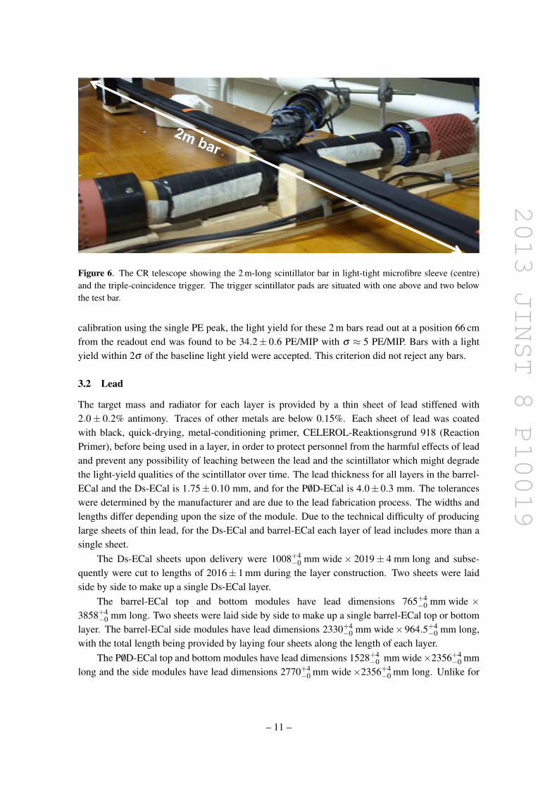
2013 JINST 8 P10019
Figure 7 The ALS
the control of a PC running LabVIEW The light output of the fibre was recorded using a standardECal MPPC (as described in section 34) powered by a Hameg HM7044-2 quadruple PSU Theoutput current was measured by a Keithley 6485 pico-ammeter also under LabVIEW control
Figure 8 shows some typical results for good fibres compared to a bad fibre which showslight loss at two positions along its length (note that scans with the fibre direction reversed help toconfirm the locality of the light loss) Such scans were performed on all of the fibres used for theDs-ECal and resulted in the rejection of approximately 100 out of a total of 2000 fibres
These data were also used in order to extract a measurement of the attenuation lengths of thefibres An example of attenuation measurements made with this apparatus can be seen in figure 9The current recorded from the MPPC in the region up to x = 15 m from the scan start point is fittedto the following functional form [19]
IMPPC = A(
1(1+R)
eminusxλ1 +R
(1+R)eminusxλ2
)+B (31)
The data from the Ds-ECal fibres suggested a flat background of B = 81 nA A = [108128] nAR = [012014] and attenuation length coefficients of λ1 = [3941] m λ2 = [021031] m
The FCS shown in figure 10 was designed to scan twenty fibres quickly in a single run whilestill retaining a reliable identification of problem fibres The scanner was enclosed within a light-tight box with the readout electronics positioned outside A series of 29 scintillator bars wereplaced perpendicular to the fibre direction and positioned over a distance of 4 m The spacings ofthe bars were selected to ensure that all of the four lengths of fibre had a scintillator bar within 5 cmof the end of the fibre Each scintillator bar was cut with 20 v-shaped grooves into which the fibreswere laid allowing absorption of light from the bars
Each scintillator bar was illuminated using an ultra-violet LED that was coupled to a lsquoleakyfibrersquo one with the cladding intentionally scratched to allow light to escape at points along thelength that was threaded through the bar The UV light was absorbed by the scintillator bar which
ndash 13 ndash
2013 JINST 8 P10019
Figure 8 Some example ALS results of normal fibres compared to a fibre exhibiting light loss
Figure 9 Example fits to attenuation length data taken by the ALS Coloured jagged lines are data solidblack lines are the fits The shaded grey region is not used in the fits
then emitted blue light out through the v-shaped grooves and into the WLS fibres The UV LEDswere connected to a computer-controlled switching unit that used a binary addressing system toswitch on each of the LEDs in turn The 20 WLS fibres were each coupled to ECal MPPCs whichwere read out via a multiplexer by the pico-ammeter The complete scanner system was controlledby a single LabVIEW process
ndash 14 ndash
2013 JINST 8 P10019
Figure 10 The FCS Ten wavelength shifting fibres can be seen lying in the grooved scintillator bars Thefibres connect to the MPPCs (shown in their black plastic housings) via a fibre clamp and a short section ofclear optical fibre The electronics are positioned behind the far end of the light-tight box
Software was used to check the WLS fibres for sudden drops in light output between each ofthe illumination points an indication that the fibre was cracked or damaged in some way One ofthe 20 WLS fibres in each run was a reference fibre that had been scanned in the ALS A referencefibre was used for two reasons Firstly it allowed the scanner to be calibrated such that the expectedamount of light collected at each position along the bar was known allowing the WLS fibres tobe compared to the reference fibre Secondly it permitted the attenuation length to be roughlymeasured by scaling the attenuation profile of the reference fibre with the relative light responsefrom the other fibres The final yield from the QA steps of WLS fibres delivered from FNALincluding any rejections due to the ferrule gluing step described in section 35 was 350 fibresrejected from the total order of approximately 17000 a rejection rate of about 2
34 Photosensors
As mentioned in section 2 light produced in the scintillator bars is transported via WLS fibres tosolid state photosensors Because the ECal modules sit inside the iron return yoke of the refurbishedUA1 magnet either the photosensors needed to work inside the 02 T magnetic field provided bythe magnet and be small enough to fit inside the ECal modules or the light signal would needto be transported several metres via optical fibres to light sensors outside the ND280 The use ofMPPCs instead of traditional PMTs allowed the first option to be chosen MPPCs consist of manyindependent sensitive pixels each of which operates as a Geiger micro-counter The use of Geiger-mode avalanches gives them a gain similar to that of a vacuum PMT The output of the device issimply the analogue sum of all the fired pixels and is normally expressed in terms of a multiple ofthe charge seen when a single pixel fires sometimes referred to as a lsquopixel energy unitrsquo or PEUA customized 667-pixel MPPC with a sensitive area of 13times13 mm2 was developed for T2K byHamamatsu [20]
ndash 15 ndash
2013 JINST 8 P10019
Table 3 Main parameters of the T2K MPPCs The dark noise rate is given for a threshold of 05 PEU orhalf the charge of a single pixel firing
ParametersNumber of pixels 667Active area 13times13 mm2
Pixel size 50times50 microm2
Operational voltage 68minus71 VGain asymp 106
Photon detection efficiency at 525 nm 26-30Dark rate above 05 PEU at 25C le 135 MHz
In addition to meeting the above criteria the MPPCs have a higher photon detection efficiency(PDE) than PMTs for the wavelength distribution produced by the WLS fibres Typical PDEs aregiven by Hamamatsu for S10362-11-050C MPPCs [21] which are similar to the customized MP-PCs used by T2K The peak efficiency which is at a wavelength of 440 nm is around 50 andat the wavelengths emitted by the WLS fibres (peaked around 510 nm) the efficiency is approxi-mately 40 However these PDE measurements were made using the total photocurrent from theMPPC and will therefore count pulses caused by correlated noise such as crosstalk and afterpulsingin the same way as those due to primary photons More sophisticated analyses performed by T2Kin which these effects are removed give PDEs of 31 at wavelengths of 440 nm and 24 in directmeasurements of WLS fibre light [22] Table 3 shows the main parameters of the MPPCs Moreinformation about the MPPCs can be found in references [2 13 16 23] and references therein
As T2K was the first large-scale project to adopt MPPC photosensors considerable effort wasmade to test the first batches of MPPCs before detector assembly Device properties were mea-sured in a test stand comprising 64 Y11 WLS fibres illuminated at one end by a pulsed LED andterminated at the other by ferrules connected to the MPPCs under test as described in section 35MPPCs were read out using a single TFB board and a development version of the ND280 DAQsoftware Two such test stands were created and the MPPC testing (around 3700 devices total)was divided equally between them
The QA procedure consisted of taking many gated charge measurements for each photosensorat a range of bias voltages with and without an LED pulse present during the charge integrationgate For each bias voltage a charge spectrum was produced from the measurements and analyzedin order to extract the sensor gain similarly to the process described in section 81 The thermalnoise rate and contributions from after-pulse and crosstalk were extracted from the relative peakheights in the charge spectrum and a comparison of the signals with LED on and off permittedthe extraction of the PDE absolute calibration of the incoming light level was performed using aMPPC whose PDE had been previously measured using an optical power meter [22]
The gain curve was fitted to calculate a pixel capacitance and breakdown voltage for eachdevice and also the bias voltage required to achieve a nominal gain of 75times105 The PDE and noisecharacteristics at this gain were then interpolated to quantify the performance of each device Alldevices were found to be functional and to perform acceptably (with reference to table 3) howevera 10 contingency of sensors was ordered and so devices were rejected starting with those with the
ndash 16 ndash
2013 JINST 8 P10019
Figure 11 (Left) An exploded view of the WLS fibre to MPPC coupling connector system The ferrule inthe bottom left of the figure is placed over the end of the WLS fibre (not shown) with the fibre overhangingthe ferrule by 05 mm in order to ensure good coupling with the MPPC The housing for the MPPC and foamspring is shown in the centre of the figure The lsquoearsrsquo of the housing slip over the ridge in the ferrule to lockthe assembly together The external shell or sheath covers the MPPC housing and part of the ferrule whenthe connector is assembled preventing the lsquoearsrsquo from disengaging with the ferrule The circular loop on theexternal shell allows the entire assembly to be screwed to the bulkhead securely (Right) The connector fullyassembled The assembled connector is approximately 5 cm long
highest thermal noise rate More details on the QA procedure and its results can be found in [24] Insitu the dominant contribution to the non-linearity of the combined scintillatorfibreMPPC systemis from the MPPCs and is estimated to be 2-3 for MIPs and 10-15 for charge deposits typicalof showers
35 Fibre to sensor coupling
An essential component in the overall light-collection efficiency of the ECal modules was the cou-pling of the WLS fibres to the MPPCs The design used was a multi-component solution shown infigure 11 (left) and was adopted by the on-axis INGRID detector [1] and the P0D subdetector [11]of the ND280 in addition to the ECal The assembly consists of three injection moulded1 parts (1)a lsquoferrulersquo glued to the end of the fibre which engages with (2) a housing that holds the MPPC andensures alignment with the fibre end to better than 150 microm and (3) an external shell or sheath tocontain the inner assembly and provide protection A 3 mm-thick polyethylene foam disk sittingjust behind the MPPC provided sufficient contact pressure between the fibre end and the MPPCepoxy window to ensure an efficient connection without the use of optical coupling gels whichcould deteriorate over time and present a complicated calibration challenge Electrical connectionbetween the MPPC and the front-end electronics is provided by a small circular printed circuitboard with spring-loaded pin sockets which contact the legs of the MPPC and connect to a micro-coaxial connector by Hirose (not shown in figure 11) Figure 11 (right) shows the connector fullyassembled Early prototypes of the connector revealed that an unacceptable light loss could occurif the fibre end was glued slightly short of the ferrule end This led to the production of gluingguides which ensured a precise overhang of the fibre from the ferrule end by 05 mm with a highproduction reliability
1All injection moulded components were fabricated from Vectra RcopyA130
ndash 17 ndash
2013 JINST 8 P10019
Table 4 The ECal construction and QA model showing contributions from Daresbury Laboratory (DL)Imperial College London Lancaster University Liverpool University Queen Mary University London(QMUL) Rutherford Appleton Laboratory (RAL) University of Sheffield and University of Warwick
DL Imperial Lancaster Liverpool QMUL RAL Sheffield WarwickECal design X XModule engineeringconstr X XDs-ECal layers XDs-ECal module Xbarrel-ECal side layers Xbarrel-ECal side modules Xbarrel-ECal topbott layers Xbarrel-ECal topbott modules X XP0D-ECal side layers XP0D-ECal side modules XP0D-ECal topbott layers XP0D-ECal topbott modules X2D scanner XMPPC QA X X XScintillator bar QA X XWLS fibre QA XMPPC-WLS connectors XElectronics X X
4 Construction
The T2K UK group employed a distributed construction model to optimize efficiency space andthe use of available personnel Module layers were constructed first and then lowered one at a timeinside prepared bulkheads after which the MPPCs then cooling panels TFBs cooling pipes andfinally cover panels were attached The RMMs were then affixed to the outside of the modulesAs each layer was installed inside the bulkheads a two-dimensional (2D) scanner discussed insection 43 carrying a 3 mCi 137Cs source was used in conjunction with a well-understood set oflsquotestrsquo MPPCs to check the integrity of the bar-fibre combination before the next layer was installedenabling repairs to be made if necessary The material preparation and QA also followed a dis-tributed pattern The distribution model is shown in table 4 All of the components in the table hadto come together on a co-ordinated schedule for the modules to be constructed Details of the layerand module assembly are given in the following sections
41 Layer assembly
Each layer is framed by aluminium bars with an L-shaped cross-section of dimensions 2000 mm(base)times 1254 mm (height) The height of the base is approximately 102 mm very slightly higherthan the scintillator bars and the width of the stem is 2000 mm Construction of the layer beganby screwing the aluminium bars into place onto a Teflon-covered assembly table The scintillatorbars then were prepared by applying a two-part epoxy (Araldite 2011 Resin and Araldite 2011Hardener) to one edge of the bars The bars then were laid inside the layer frame such that the
ndash 18 ndash
2013 JINST 8 P10019
Figure 12 Ds-ECal layer under construction The first of two sheets of lead is in place on top of thescintillator bars Visible are the aluminium frame and the locator pins securing the scintillator bars in placefor the duration of the layer construction The frame is covered with blue tape to keep it free from epoxy
central hole of each bar was aligned with a 2 mm-diameter hole in the frame An O-ring with anuncompressed thickness of 15 mm was inserted into the 1 mm gap between the ends of the barand the layer frame and compressed into place This was done to prevent epoxy from enteringthe bar hole and compromising the subsequent insertion of WLS fibre The position of each barwas stabilized during layer construction by inserting a temporary tapered Teflon-coated locator pinthrough the frame hole the O-ring and into the bar hole The locator pins were removed when thelayer was complete
Once all of the bars were stabilized in position a thin layer of epoxy was applied to them and tothe lip of the frame and the lead sheets were placed on top using a vacuum lifting rig attached to anoverhead crane in order to distribute the weight across several equally-spaced suction cups and soavoid distorting the lead The sheets were carefully positioned to minimize the gap between themthereby avoiding a region of low density in the middle of the modules while ensuring sufficientoverlap onto the lip of the layer frame to maintain structural integrity Figure 12 shows one of theDs-ECal layers being constructed with one sheet of lead in place on top of the scintillator bars
The entire layer then was covered with a sandwich of vacuum-sealing plastic and fabric withthe top layer of plastic securely taped to the table Vacuum pumps were used to evacuate the airaround the layer allowing the epoxy to cure for 12 hours under vacuum compression
Once the curing was finished the layer was unwrapped the locator pins removed the screwssecuring the layer frame to the table were removed the WLS-fibre holes were tested to ensure thatthey had not been blocked with epoxy and the layer then was stored for use in a module
ndash 19 ndash
2013 JINST 8 P10019
42 Assembly procedures for the ECal modules
The Ds-ECal was the first module to be constructed and most of the procedures developed duringthe process were used on the other modules as well The first step was to assemble the bulkheadsand the carbon-fibre panels One carbon-fibre panel (the bottom panel during construction whichwould become the upstream face when the Ds-ECal was in situ) was attached to the bulkheads toform an open box The other (top) carbon-fibre panel was stored until later The bulkhead box waspositioned on the construction table and the 2D scanner discussed in section 43 was attached andcommissioned The first layer then was lowered inside the bulkheads and positioned on top of thecarbon-fibre base A 1 cm gap between the bulkheads and the layer on all four sides was obtainedby tightening or loosening grub screws which were inserted through holes in the bulkhead andtensioned against the layer frame The LI LED strips and perspex lenses (see section 6) then wereglued onto the bottom carbon-fibre panel in the 1 cm gap the LI electronic cards were affixed to theinside of the bulkheads with the LI cables routed outside the bulkheads through the air holes WLSfibres were inserted through the scintillator bars A MPPC-fibre connection ferrule was bonded toeach fibre using Saint-Gobain BC600 silicon-based optical epoxy resin The test MPPCs werecoupled to the fibres using the connection sheaths and connected via a mini-coaxial cable to TFBswhich provided the control and readout (see section 5 for a description of the TFBs) After this thelayer was covered and made light-tight and a 2D scan was taken
The 2D scanner collected data at 20 points along each 2000 mm bar with data points beingcloser together near the ends in order to facilitate an understanding of the light escaping throughthe ends of the scintillator bar For efficiency the analyzing software ran in parallel with the data-taking producing an attenuation profile for each bar in the layer A typical example of this isshown in figure 13 The ordinate axis shows a reference value of the light yield since it is calcu-lated as a ratio of the integrals (from 55 PE to 30 PE) of the MPPC response when the source ispresent to the response when the source is not present and therefore represents (signal + back-ground)background This ratio is calculated at each data point along the length of the bar Moreinformation about the analysis of the scanner data is available in [18]
The scan data were checked and if problems were encountered appropriate action was takenA common problem involved the coupling between the fibre and the MPPC often due to the dif-ficulty of positioning the ferrule on the fibre In this case since the ferrule could not be removedthe fibre would be replaced a new ferrule would be attached and the bar would be re-scannedAfter this process the test MPPCs were removed and the next layer was installed and scanned inthe same manner Where required thin Rohacell foam sheets were placed between the layers toensure that the layers did not warp inwards
After several layers were installed in the Ds-ECal it was noted that the holes in the bulkheadswere no longer aligning well with the holes in the layers and the scintillator bars which madethe insertion of the WLS fibre difficult Measurements indicated that the layer frames had beenincorrectly manufactured and were an average of 02 mm higher than the specifications This wasremedied by using a router to thin the frames on the layers that were not yet installed The layerframes for subsequent modules did not have this problem
After all of the layers were installed LI LEDs and electronic cards were attached to the topcarbon-fibre panel 9 mm of Rohacell foam was glued to the inside of the panel to ensure that the
ndash 20 ndash
2013 JINST 8 P10019
Figure 13 A typical light attenuation profile from scanner data corresponding to one scintillator bar in theDs-ECal The ordinate axis is the ratio of the integrated light yield with the source present to the integratedlight yield without the source the abscissa is the position along the bar in cm The light yield measured bythe MPPC at one end of the bar and read out by one of the two TFBs (TFB 0) is shown in the upper plotand that from the MPPC at the other end read out by the other TFB (TFB 1) is shown in the lower plot Thepoints are data the curves are a single-exponential fit to the central region of the data
layers within the bulkheads stayed stable when the Ds-ECal was in its upright position in situ Thecarbon-fibre panel was then affixed to the top of the bulkheads
The procedure described above completed the construction of the active region of the detectorThe next steps dealt with the data readout First the 3400 Ds-ECal lsquoproductionrsquo MPPCs in theircustom-made sheaths complete with foam springs and mini-coaxial cables were attached to theferrules of every layer and secured to the bulkheads as described in sections 21 and 35 Cable-management brackets were attached to the bulkheads and the MPPC cables were grouped togetherand tidied in preparation for the next steps Tyco Electronics LM92 temperature boards werescrewed onto the bulkheads between the MPPCs in positions that allowed one temperature boardto be connected to each TFB
The cooling panel for the left-side Ds-ECal was assembled from four separate cooling platesThe TFBs then were attached and thermally connected to the left-side cooling panel using screwsand thermally-conducting epoxy resin The cooling panel then was held in position on the left sideof the Ds-ECal while the MPPC and temperature-board cables were threaded through the slots in
ndash 21 ndash
2013 JINST 8 P10019
the panel and the LI cables were routed through the panelrsquos air holes after which the panel wasplaced into its final position and bolted into place The MPPC and temperature-board cables wereconnected to the correct ports on the TFBs The same procedure was followed for the other threecooling panels
The water-cooling circuit then was installed on the cooling panels and the gas distributionbranch was installed on the bottom cooling panel These systems were tested under pressureFollowing this cable-management brackets were fitted between all of the TFBs and low-voltagefeedthroughs and bus bars were installed The bus bars were checked for continuity isolation fromground and from each other Shielded Cat 5e cables then were connected to the TFBs Along withthe LI cables they were routed around the detector to a patch panel mounted on the bottom coolingpanel or in the case of the trigger cables from the TFBs and half of the LI cables to the top coolingpanel Figure 4 shows the left-side Ds-ECal cooling panel with the TFBs bus bars Cat 5e cablesLI cables water-cooling pipes and air holes
The outer cover panels then were attached to each side The top cover panel was fitted with28 cable glands through which the Cat 5e cables corresponding to the trigger system exited thedetector and with air vents to allow the gas being flushed through the detector to escape Half of thecables from the LI system exited through holes in the top cover panel The bottom cover panel wasfitted with power cable clamps cable-management brackets and RMM cards The Cat 5e cableswere routed from the patch panel to the RMMs LI junction boxes were attached and connected tothe LI cables completing the construction of the Ds-ECal
This construction procedure was repeated for each of the barrel-ECal modules Minor alter-ations to the method were needed to accommodate the slightly different structure of the modules(see section 22) More significant alterations were made to the method for the P0D-ECal modulesreflecting their slightly different design as described in section 23 The most significant differ-ences were that the TFBs were mounted directly on the bulkhead instead of onto cooling panelswith the MPPC cables routed to them and supported where necessary the smaller number of TFBsper module allowed for the use of a thick standard copper wire instead of bus bars to supply powerwhich was distributed to the TFBs via branching connections to terminal blocks in the final stepof the assembly a non-magnetic support structure was bolted to the aluminium back panel whichpositions the thinner P0D-ECal modules away from the magnet and closer to the basket
43 The bar scanner
Three-axis scanners were designed to position a 137Cs radioactive source at multiple points abovethe surface of each detector layer as each layer was assembled into the subdetector body Threevariants of the scanner were manufactured
bull Ds-ECal and P0D-ECal scanner with a footprint of 3928 mm times 3578 mm
bull side barrel-ECal scanner with a footprint of 4862 mm times 3240 mm
bull top-bottom barrel-ECal scanner with a footprint of 4862 mm times 2410 mm
The three axes were driven by Mclennan SM9828 Stepper Motors controlled by PM600 In-telligent Stepper Motor Controller The controller was programmed via a commodity PC running
ndash 22 ndash
2013 JINST 8 P10019
LabVIEW The PC and stepper motors along with their controller were all powered via an un-interruptible power supply (UPS) The system design included an APC Smart-UPS 2200 230 Vprimarily as a safety feature so the radioactive source could be automatically parked during a powercut however it had the added benefit that short duration power glitches did not stop a running scan
These controls were integrated into a LabVIEW program providing an operator interface tocontrol the machine This operator interface was implemented as a lsquostatersquo machine the main statesbeing lsquosource loadedrsquo and lsquosource unloadedrsquo In the source-unloaded state the radioactive sourcewas not attached to the scanner head In this state the head was raised and moved to one side toposition the arm in the least inconvenient position for those working on the detector The arm couldalso be moved in the x-direction to allow for greater access to the detector during construction
The source was loaded under computer control with the computer prompting the operator toperform the necessary steps in a safe order The program then switched to the source-loaded statewhere scanning parameters could be input and the scan started Each scan started with the z-armsearching for the surface of the module layer at the centre of the module The arm descendedslowly until the push rod mounted adjacent to the source operated The arm then backed off andthe source moved to the matrix of measurement positions At each position the Scan Controlprogram prompted the DAQ to start data-taking via a network link On completion of data-takingthe scanner would move to the next position and iterate until data had been taken at all positionsWhen the data-taking was complete or if the program detected an error condition the sourcewould be returned to its lead-shielded safe parked position Unloading the source was again undercomputer control with operator prompts to ensure safety Re-positioning of the scanner head wasfound to be accurate to within 002 mm
Figure 14 shows the scanner in operation during the Ds-ECal construction The vertical armfinds its position as described in the text The operator provides the xminus y coordinates and therequired timing at each position Since radiation safety rules dictated that no one should be in thearea during the scan the image was taken by a web camera which allowed operators to check onthe scanner progress
5 Readout electronics and data acquisition
As described in section 21 the mini-coaxial cable from each MPPC is routed outside the coolingpanels and connected to a custom designed TFB Each TFB contains 4 Trip-T application-specificintegrated circuits (ASICs) originally designed for the D0 experiment at FNAL Up to 16 MPPCscan be connected to each ASIC implying that a maximum of 64 MPPCs can be connected to asingle TFB In total the ECal has 22336 electronic channels connected to MPPCs To increase thedynamic range of the electronics the incoming MPPC signal is capacitively split (110) into high-and low- gain channels which are read by different channels of the ASIC Depending on the MPPCgain the single-pixel (1 PEU) signal corresponds to approximately 10 ADC counts in the high-gainchannel while the maximum signal in the low-gain channel corresponds to around 500 PEU
The Trip-T chip integrates the charge in a preset (programmable) time interval which is fol-lowed by a programmable reset time at least 50 ns long For T2K the integration windows areprogrammed to synchronize with the neutrino beam timing The Trip-T chip integrates from 23readout cycles in a capacitor array and once all cycles have been completed the stored data are mul-
ndash 23 ndash
2013 JINST 8 P10019
Figure 14 The 2D scanner moving along the scintillator bars in the Ds-ECal The 137Cs source sits at thebottom of the vertical arm of the scanner just above the layer being scanned The blackout material coveringthe layer is seen along with the tape holding it in place for the duration of the scan
tiplexed onto two dual-channel 10-bit ADCs which digitize the data Signals from the high-gainchannel are routed via a discriminator which forms part of the Trip-T chip A field-programmablegate array (FPGA) produces timestamp information from the discriminator outputs and sends thisinformation together with the ADC data to a back-end board In addition the TFB also recordsmonitoring data (eg temperature voltage) via the same FPGA which is asynchronously trans-mitted to the back-end board for data concentration and buffering Detailed information about theTrip-T chip and front-end electronics is given in references [2] and [25]
The back-end electronics system for the ND280 consists of several different boards The TFBsare connected to RMMs which provide control and readout Control is fanned out from a masterclock module (MCM) via several slave clock modules (SCMs) one per subdetector Additionallytwo cosmic trigger modules (CTMs) are used to provide a selection of cosmic-ray muon triggeredevents for calibration and monitoring All of these boards use a common hardware platform specif-ically developed by the Rutherford Appleton Laboratory for use in the T2K experiment Signalsfrom up to 48 TFBs which are mounted on the detector typically less than 1 m away from theMPPCs are routed to one RMM via Cat 5e cables The ECal uses a total of 12 RMMs 8 forthe barrel-ECal 2 for the Ds-ECal and 2 for the P0D-ECal Each RMM controls its associatedTFBs distributes the clock and trigger signals to them and receives data from them once a triggerhas been issued Data from the RMMs are then sent asynchronously via a gigabit ethernet link tocommercial PCs that collect and process the data
The ND280 uses a single MCM This receives signals from the accelerator which allow it todetermine when a neutrino spill is about to occur and also from a GPS-based clock which is usedto synchronize the electronics to UTC The MCM prioritizes and issues triggers across the whole
ndash 24 ndash
2013 JINST 8 P10019
detector and manages readout-busy situations The signals and control of the MCM are fannedout to the SCMs The trigger and clock signals are passed to the ECal RMMs via the ECal SCMThe SCMs allow the electronics for a sub-system to be configured independently It is possible forthe ECal to run autonomously (lsquopartitioned DAQrsquo) from the rest of the ND280 for calibration anddebugging by using the ECal SCM as master controller
The software control of the detector is performed using the ldquoMaximum Integration Data Ac-quisition Systemrdquo (MIDAS) [26] The front-end software is custom written to manage the commu-nication with the RMMs CTMs SCMs and MCM through gigabit ethernet links A second pro-cess combines ADC and TDC information compresses the data and makes histograms for pedestaldetermination and monitoring A third process manages communications with computers runningthe MIDAS DAQ elements These three processes co-operate on front end PCs running ScientificLinux with each front end PC being connected to two back-end boards The event builder and datalogging use software from the MIDAS distribution with virtually no customization for T2K TheDAQ contains an online monitoring system which makes histograms for assessing data quality inreal time and passes events to the online event display for monitoring Detailed information aboutthe DAQ is given in [2]
6 Light injection system
The ND280 ECal LI system is designed to provide a quick and reliable method of monitoring theperformance of the MPPCs used inside the ECal modules A complete discussion of the LI systemRampD can be found in reference [27] The LI system is required to illuminate the MPPCs on agiven readout face of an ECal module with a short duration optical pulse The pulse length andstability must be sufficient to afford accurate (asymp 1 ns) timing calibration The intensity across thereadout-face should be uniform and any electromagnetic or electro-optical noise induced by thesystem must not interfere with the surrounding sensors or electronics
In order to accomplish these aims the LI system employs a modular design incorporatingdedicated electronics for both the interface with the ND280 DAQ and the pulsing of LI sourceswithin an ECal module The components are described in the subsections that follow The LIfront-end electronics are housed in custom-built crate assemblies compatible with a standard 19-inch rack In brief the LI signal chain comprises the following components
1 The trigger card receives the ND280 MCM signal
2 Control cards (CCs) receive and interpret the DAQ instructions and collate with the clock
3 The junction boxes (JBs) receive and fan out the CC outputs
4 The pulser receives the CC output via a JB and drives LED strips which emit optical pulsesfor calibration
Each of the components is described in more detail below
ndash 25 ndash
2013 JINST 8 P10019
61 Control cards and trigger receiver
The LI system receives DAQ instructions into a dedicated CC Each card hosts a TCPIP serverthat allows the DAQ instructions to be interpreted and then encoded into a sequence of TTL pulsesused to drive LED pulser cards housed inside the ECal modules The ND280 MCM transmits a100 MHz signal to the LI system which is received by a dedicated trigger card The clock signalis first fanned out to each CC then collated with the CC outputs onto a RJ45Cat 5e signal cableready for distribution to the LI JBs
62 Junction boxes
The JBs are responsible for directing the TTL pulse train and MCM clock from the CCs to therelevant LI pulsers the pulser being the dedicated electronics required to form the electrical exci-tation pulses used to drive the LED strips used for illumination There is one JB per ECal moduleexcept for the Ds-ECal which has two 6timesP0D-ECal 6times barrel-ECal and 2timesDs-ECal making14 in total The JBs are mounted outside but in close proximity to the ECal modules themselvesThey are passive devices used exclusively for fanning out the CC pulses and therefore introducingno modification to the actual signal
63 Communications protocol and cabling
The low-voltage differential signalling (LVDS) protocol is used throughout to ensure robustnessagainst interference from electromagnetic noise in the detector The DAQ instruction and MCMclock information are received over LVDS converted to TTL for interpretation by the CCs TheCC outputs are again transmitted using LVDS converted to TTL for fan out in the JBs and thentransmitted to the LI pulsers again using LVDS The Ds-ECal portion of the LI system howeveris an exception in that it features an older design which implements TTL over LEMO cables ratherthan LVDS over RJ45Cat 5e cables In order to preserve the relative timing between pulsers allCat 5eLEMO cables within an ECal module have been installed with the same length
64 Pulsers
LED pulser cards mounted inside the ECal modules receive the pulses emitted from the CCs viathe JBs The TTL logic pulses determine the pulse duration amplitude and number of flashes Ashaping component of the pulser board introduces activation and deactivation spikes to the leadingand trailing edges of a square-wave electrical pulse This ensures a constant level of illuminationwith a negligible optical rise time The signal chain is illustrated in figure 15 Different numbersof pulsers are located in different ECal modules depending on their size and layout There are 114in total 14 P0D-ECal 84 barrel-ECal and 16 Ds-ECal
65 LED strips and extruded perspex lens
Each LED pulser drives two KingBright LSL-062-05 flexible LED lighting modules The LEDstrips are fitted with an optically coupled cylindrical lens made of 2 mm-diameter extruded per-spex as shown in figure 16 The KingBright LEDs feature an in-built lens with 12 angle 120
producing a rather wide beam divergence that results in a 75 loss of emission at the layers fur-thest from the LED strips The addition of the perspex rods focuses the light so as to reduce thisloss to only 25 of the maximum
ndash 26 ndash
2013 JINST 8 P10019
Figure 15 The LI signal path The CCs encode an MCM synchronized pulse train with the desired timingand amplitude characteristics The pulsers derive the excitation charges from the CC output
LED
index matched glue
fullminuscylinder lens
flex strip
10mm
Figure 16 KingBright LED 10 mm-wide strip (left) and optically-coupled acrylic lens (right)
66 LI installation
The Ds-ECal JBs were installed and cabled in Aug 2010 The remainder of the JBs and the frontend electronics were installed during OctNov 2010
The P0D-ECal CC receives 1times input from the DAQThe P0D-ECal CC transmits 1times output to each of six JBs
A single P0D-ECal CC located in the LI electronics crate transmits the DAQ instructions andMCM clock information to the six P0D-ECal JBs Each JB splits and distributes the instructionsand clock information to 14 = 4times 2 pulsers + 2times 3 pulsers forming six groups permitting anycombination of the six P0D-ECal modules to be illuminated
Each barrel-ECal CC receives 1times input from the DAQEach barrel-ECal CC transmits 2times outputs to each of six JBs
There are six barrel-ECal CCs in total One barrel-ECal CC transmits the DAQ instructions andMCM clock information to one barrel-ECal JB over two RJ45Cat 5e cables One JB splits anddistributes the instructions and clock information to 14 pulsers forming three distinct groupingseach corresponding to pulsers located on one of the three readout faces Any combination of
ndash 27 ndash
2013 JINST 8 P10019
readout faces (ie the ends of the single and double-ended scintillator bars) can be illuminatedwithin a given barrel-ECal module
The Ds-ECal JBs are unique in that they sit inside the ND280 magnet situated directly againstthe ECal bulkheads Moreover they employ LEMO connections along single core coaxial cablerather than the RJ45Cat 5e that is ubiquitous elsewhere throughout the ECals and the remainderof ND280 There are two readout faces per Ds-ECal module each separately illuminated by eightpulsers There are two JBs one North and one South served by a single CC situated in the LIfront-end electronics crate
7 Testbeam
In 2009 the Ds-ECal module was exposed to the CERN T9 testbeam This represented the firstopportunity to test the entire integrated system calorimeter readout system DAQ system andanalysis framework As well as a system shakedown the data provided by the testbeam havebeen used to tune the particle identification algorithms used in T2K analyses and to obtain a betterunderstanding of detector performance
71 The CERN PS T9 testbeam
The T9 beamline is a medium energy multiple particle species tertiary beam generated by thecollision of protons from the CERN PS on a solid target in the CERN East Experimental HallThe dual polarity beam supplied a mix of pions electrons and protons with momenta rangingfrom 300 MeVc up to 15 GeVc Data were taken at momentum points between 300 MeVc and50 GeVc The particle composition of the beam changed with momentum setting Below 1 GeVcelectrons made up 90 of the beam This fraction decreased to approximately 5 for momentumsettings above 30 GeVc with a corresponding increase in the fraction of hadrons
72 Triggering and event selection
The beamline was instrumented with several detectors to provide particle identification informa-tion Two Cerenkov counters filled with CO2 at variable pressure were present and read out usingPMTs connected to an ordinary TFB board The counters were configured such that only electronswere above threshold which provided electronhadron discrimination The electron identificationefficiency of the system (requiring both counters to register a hit) was estimated to be (90plusmn 2)for momentum settings below 30 GeVc The Cerenkov system was complemented by a time-of-flight (TOF) system comprised of two scintillator paddles read out by fast PMTs The paddleswere separated by a flight distance of 14 metres Custom NIM-based electronics including a time-to-analogue converter (TAC) converted the time of flight to a current pulse which was read outusing a TFB The TOF system provided proton-pion separation for momentum settings between600 MeVc and 18 GeVc and also acted as the hardware trigger for the Ds-ECal
Combining the performance of the TOF and Cerenkov systems with the beam compositionthe contamination of the hadron sample with electrons was estimated to be below 05 and theelectron sample was estimated to be more than 99 pure Because of the relative timings of thephysics signal and DAQ cycle the physics data from a single beam event could fall into one of twoTrip-T integration windows Due to latencies in the system it was also possible that different parts
ndash 28 ndash
2013 JINST 8 P10019
of a single event could end up spread across different time buckets In this case it was impossible tobe sure that activity did not occur undetected during the reset period To eliminate this uncertaintyevents with reconstructed clusters in both windows were rejected For electron events the candidatecluster was also required to arrive between 0 and 65 ns after the Cerenkov signal
73 Detector configuration
The detector was configured as similarly as possible to its final operating conditions however therewere some differences largely due to physical constraints The downstream end of the detector(with respect to the J-PARC beam) faced upstream in the testbeam meaning that incident particlespassed from the back to the front of the detector This meant that the particles passed through alead layer before a scintillator layer leading to a small difference in behaviour
In addition to this the detector was cooled using an air-based chiller rather than water cooledleading to a diurnal variation in temperature of around 2C and a total temperature range of 16ndash28C over the whole running period This led to rather larger drifts in MPPC behaviour than ex-pected for the final system leading to some difficulties in calibration (section 74) though after aninitial commissioning period these were mostly ameliorated by taking very regular calibration runs
74 Calibration differences
Calibration for the testbeam was carried out using only dedicated pedestal runs rather than usingnoise spectra as in the final calibration scheme described in section 81 Initially pedestal runswere taken infrequently but after examining the early data we noticed that this was not sufficientto fully calibrate for the effect of the large temperature variations in the T9 setup We thereforechanged operating procedure to take a dedicated pedestal run before every physics run For oper-ations at J-PARC we have added the ability to take interspersed pedestal data and measure noisespectra during normal running reducing the need for these dedicated runs The more sophisticatedcooling system at J-PARC also reduces the need for very frequent calibration
To improve the calibration of early data we made use of the fact that the average temperatureof the detector was measured at the start of each run The gain for each channel was then calculatedon a run-by-run basis using the gains calculated from the most recent pedestal run the temperaturemeasurements and the following formula
G = G0 +dGdT
Tdiff (71)
where G0 is the gain of the preceding pedestal run Tdiff is the temperature difference between thecurrent run and the preceding pedestal and dG
dT is the rate of change of gain with temperature foundto be -067times105C This removed much of the charge scale variation between runs
As shown in figure 17 some residual temperature dependence is seen in the detector responseafter making the temperature-based correction particularly in the period before regular pedestalruns were taken A fit to the temperature data corresponding to the final five days in figure 17indicates that the average temperatures were rising resulting in the slight decrease in the Landaumost probable values (MPVs) that is visible in the plot To remove these variations data fromcosmic ray muons (collected coincidentally with beam events in DAQ integration periods notassociated with the beam) were processed from each run The MPV of the charge distribution of
ndash 29 ndash
2013 JINST 8 P10019
Date1005 1105 1205 1305 1405 1505 1605 1705 1805
MPV
[M
EU
cm
]
06
08
1
12
14
16
C]
degTe
mpe
ratu
re [
16
17
18
19
20
21
22
23
24
25
26
Figure 17 Time series of the average detector temperature and Landau most probable value (MPV) formuon hits in each run after making a temperature-based gain correction The dashed line represents thepoint at which pedestal runs began to be taken regularly
single hits across all channels was then found for this sample and used to scale hit charges forelectron events in the run equalizing the MIP scale for all data runs
Monte Carlo samples for each individual testbeam run were produced using Geant4 [28] Arepresentation of the Ds-ECal geometry was constructed and a monochromatic beam of electronsat each central beam momentum point was fired into the centre of the back-face of the Ds-ECalThe photosensor response was simulated utilizing data from test bench measurements and tunedusing cosmic ray muon data with special attention to simulating the temperature response of thephotosensor Monte Carlo samples were generated with temperatures identical to the average localtemperature of each photosensor on a run-to-run basis A similar cosmic ray muon sample was alsogenerated at this temperature and the calculated MPV was used to scale the electron hit charges
In order to remove any poorly understood noise or readout-chip threshold variation a chargethreshold equivalent to 04 MIP units was implemented in the data and simulation In additionduring the final processing of the data any hits further than 8σ of the beam-time width from thepeak cluster time were discarded to remove unsimulated cosmic events The Monte Carlo data setswere then passed through the same calibration and reconstruction paths as data
The procedure described successfully accounted for the average gain variation over the runningperiod due to temperature variation It was not however possible to account for sensor-to-sensorvariations or temperature shifts within individual runs
75 Testbeam performance
The testbeam data were used to calculate the performance of the Ds-ECal in the reconstruction ofincident particles particularly electrons The performance results for electrons will be shown here
Figure 18 shows the measured energy resolution for electrons striking the centre of the ECalface as a function of energy It can be seen that the data and Monte Carlo agree reasonably wellbut the data resolution is somewhat worse over the whole energy range and particularly at lowerenergies This may be accounted for in part by the intrinsic momentum spread of the beam which
ndash 30 ndash
2013 JINST 8 P10019
Figure 18 Measured energy resolution of the Ds-ECal for electromagnetic showers for data and MonteCarlo The dashed lines show a fit to a stochastic resolution model
was not modelled in the Monte Carlo In addition the temperature-based gain corrections usedfor this data will only correct the mean photosensor gain across the Ds-ECal A spread in MPPCgains due to temperature differences across the ECal is expected but cannot be corrected becausethe temperatures of individual sensors could not be measured and were not modelled in the MonteCarlo which assumes the same temperature for all sensors This is expected to lead to a largerspread in measured particle energies
Because of the limitations described above the differences between data and Monte Carlo seenin figure 18 represent a worst-case scenario for the calculation of systematic uncertainties Work iscurrently underway to replace this conservative estimate with one based on in-situ measurements
Figure 19 shows the angular resolution of the Ds-ECal for normally incident electrons at arange of energies Excellent agreement is seen between data and Monte Carlo over the full rangeof energies considered
In summary the T9 testbeam has provided useful information for the calculation of system-atic uncertainties and also gave an opportunity to test the detector and DAQ systems before theywere integrated into the ND280 The data collected were also invaluable in the development ofcalibration and reconstruction code in advance of data from the full ND280 becoming available
8 ECal commissioning and performance
81 Calibration
Precise calibration of ECal hits is vital for high-quality calorimetric performance To this end a setof procedures has been developed to calibrate out all significant instrumental effects with the goal
ndash 31 ndash
2013 JINST 8 P10019
Energy GeV05 1 15 2
Dir
ectio
n re
solu
tion
Deg
rees
2
3
4
5
6
7
8
Datadeg0
Monte Carlodeg0
Figure 19 Angular resolution for electrons at normal incidence to the detector in data and Monte Carlo asa function of energy
of obtaining the energy deposited in the scintillator giving rise to the hit and the precise time atwhich the energy was deposited The calibration can be separated into two main categories whichare described below energy calibration and timing calibration
Energy calibration can be logically split into three steps mdash going backwards down the readoutchain from the ADC value registered by the electronics to the anode charge from the MPPC fromthis to the number of photons incident on the MPPC face and from this to the energy deposit in thescintillator
The first step involves subtracting the electronics pedestal from the ADC counts This pedestalis the ADC value registered in the absence of any physics signal and is different for each channeland readout cycle Dedicated runs are taken once a week during beam down-times to measurethe pedestals separately for each cycle and a per-channel average over cycles is calculated everythree hours from noise spectra recorded by the DAQ in normal running The diurnal variationin pedestals due to temperature changes at the electronics is up to a few ADC counts so fine-granularity corrections are important
The next step is to convert the pedestal-subtracted ADC into an anode charge The electronicsresponse is not perfectly linear and the calibration must also incorporate the transition from highgain to low gain ADC channels Both the high gain and low gain response are mapped using theTFBrsquos ability to inject a known charge onto each channel in turn These charge injection curvesare parametrized for both high and low gain channels using two cubic polynomials joined with asigmoid function to smoothly transition between them The parametrized charge injection curvesalso allow us to calibrate the low gain channel response to the high gain channel The switchoverbetween the two channels is made at approximately 460 ADC counts in the high gain channelwhich typically corresponds to about 21 PEU An example of the charge injection curves is shown
ndash 32 ndash
2013 JINST 8 P10019
1
times103
Resp
on
se (
AD
C)
High gain
08
09
1
Resp
on
se (
AD
C)
Low gain
06
07
Resp
on
se (
AD
C)
1
04
05
1
02
03
0110 20 30 40 500
Input Charge (fC)
times103
Figure 20 High and low gain ADC response of a typical Trip-T channel Charge is injected using anonboard capacitor controlled by a Digital-to-Analogue Converter (DAC) The injected charge is calculatedfrom the DAC setting For comparison a typical MIP deposits of order 107 electrons or 16times 103 fC ofcharge
in figure 20 A typical MIP deposits of order 107 electrons or 16times 103 fC of charge ie inthe first bin on the plot More information about the charge injection calibration is available inreference [29] The parameters for this calibration are rather stable over time so are only updatedaround once per running period
To convert the calculated anode charge to an estimate for the number of photons incident onthe MPPC we first convert the charge into a number of PEU by dividing by the gain of the MPPCThe gains for each channel are calculated for every three hours of data using the same noise spec-tra as the pedestal drift and fitting the position of the first non-pedestal peak in the noise spectrumwhich is due to a single pixel firing in the device Again diurnal temperature variations have non-negligible effects on the gain so this granularity is required We then need to convert this number ofpixels to a number of photons For low light levels this conversion can be approximated by dividingby the PDE of the MPPC however it is complicated by saturation effects (the MPPC has a finitenumber of pixels and therefore a limited dynamic range) and also by after-pulsing and crosstalkwhich cause the effective PDE to be larger than the true value2 The resulting response functioncannot easily be calculated analytically and is therefore modelled on testbench measurements Asingle response function is used for every channel but the parameters are in turn functions of the de-vice gain so that changes in PDE and other parameters with overvoltage can be taken into account
Next we need to convert the number of incident photons to an energy deposit This needsto be done for each channel as there will be some non-uniformity due to for example the differ-
2A detected photon has approximately a 10 probability of initiating a secondary avalanche therefore the numberof avalanches is in general higher than the number of detected photons
ndash 33 ndash
2013 JINST 8 P10019
Charge [PEUcm]0 10 20 30 40 50 60 70 80 90 100
AU
0
0005
001
0015
002
0025
003
0035
004
0045 Right BottomLeft BottomRight TopLeft TopRight SideLeft Side
Uncalibrated
Charge [PEUcm]0 10 20 30 40 50 60 70 80 90 100
AU
0
001
002
003
004
005
006
007
Calibrated
Figure 21 The effect of the attenuation and uniformity corrections on the hit charge distributions forthrough-going cosmic muons in the six modules of the barrel-ECal shown by the six curves in each plotThe left side shows the distributions with the pedestal and gain corrected the right side adds correctionsfor attenuation and differences caused by non-uniformity of scintillator bars and WLS fibres Distributionsshown here are summed within a module but the corrections are applied on a per channel basis The slightvariation between modules is typical and insignificant
ences between channels in the optical coupling between the fibre and the MPPC The correctionis done using empirical data taking a sample of cosmic muon tracks passing through the ECalperforming all other calibrations including attenuation in the fibre (described below) and trackpath-length through the scintillator bar The corrected hit size distribution for each channel is fittedwith a Landau distribution convolved with a Gaussian smearing The effect of the attenuation anduniformity corrections is shown in figure 21 the distributions on the right side are used for theLandau-Gaussian fit This is used to calculate the expected hit size for a MIP-size energy depositat a fixed (1 m) distance from the sensor the result is used as a divisor to equalize the sizes ofhits between bars The signal produced by this ldquoideal MIPrdquo varies between modules and scintil-lator bar orientations but to give a sense of scale a muon passing approximately perpendicularlythrough the centre of the Ds-ECal typically leads to approximately 19 pixel avalanches at eachsensor corresponding to approximately 17 detected photons
It is also necessary to correct for the attenuation of photons in the WLS fibres which is signif-icant over the length of the ECal bars This calibration is done after the reconstruction has matchedtracks between the two views of the ECal so that the component of the hit position along the lengthof the scintillator bar can be estimated The attenuation profile is modelled as a sum of two expo-nential functions with an additional correction for the mirroring of the single-ended fibres Thiscorrection is stable over time and is calculated separately for each orientation of bar in each mod-ule using cosmic muon tracks Figure 22 shows the time stability of the energy calibration over oneperiod of beam running
The timing calibration also involves several distinct steps Each hit is time-stamped using theTFB clock based on the time at which the channelrsquos discriminator was triggered The discriminatortrigger is nominally set at a level of 35 PE The TFB clocks lag the global detector clock from
ndash 34 ndash
2013 JINST 8 P10019
2012Jan 21 2012
Feb 20 2012Mar 21 2012
Apr 20 2012
May 20
MP
V fr
om la
ndau
-gau
ssia
n fit
[PE
Uc
m]
135
14
145
15
155
16
165
Figure 22 The muon MIP response as a function of time for a period of beam running
Run number8100 8200 8300 8400 8500 8600 8700 8800
tfb o
ffset
(ns
)
-30
-20
-10
0
10
20
30
RMM 8
Figure 23 The TFB offset before correction for all channels on one RMM as a function of time for a periodof beam running Each line shows one TFB
which they are synchronized due to delays in the cabling and electronics used to distribute theclock signals This effect will be different for each TFB depending on the cable lengths Thedifferences between TFBs within the ECal are calculated by considering cosmic muons that leavehits in channels corresponding to different TFBs and correcting the hit times for fibre delay andthe transit time of the muon Synchronizing the ECal with the rest of the detector is achieved usinga similar method Figure 23 shows the offset for the TFBs on one RMM over a period of runs
A lsquotimewalkrsquo correction is also applied to the hit times The decay that causes the WLSfluors to radiate occurs with a half life of a few nanoseconds leading to the photons arriving at theMPPC face over a finite time period The analogue electronics also have a finite rise time both ofthese effects result in a delay between the idealized propagation of the signal and it crossing thediscriminator threshold These delays depend on the total hit charge and tend to a small constant
ndash 35 ndash
2013 JINST 8 P10019
CorrectedEntries 334Mean -4871
RMS 684
Mean Time (ns)-4940 -4920 -4900 -4880 -4860 -4840 -48200
5
10
15
20
25
30
35
40
45
CorrectedEntries 334Mean -4871
RMS 684
UncorrectedEntries 334Mean -4871
RMS 1379
UncorrectedEntries 334Mean -4871
RMS 1379
UncorrectedEntries 334Mean -4871
RMS 1379
Figure 24 The distributions of mean hit time values for cosmic muons for each channel of the tracker-ECal(corresponding to 334 TFBs) before timing calibration (blue dashed line) and after timing calibration (redsolid line)
offset for large hits The optical component of the timewalk is a stochastic process and affectsthe timing resolution but the average effect can be removed with an analytic function based on anexponential photon arrival time distribution using the known decay time of the relevant state in theWLS fibre Finally the travel time for photons in the WLS fibre must be calibrated This is doneafter the reconstruction has matched hits between views so that the light travel distance is known
Figure 24 shows a comparison between the mean hit time values of each TFB channel duringcosmic muon triggers before and after corrections The distribution of mean hit time values narrowsby a factor of two in the RMS and approaches the limit set by the trigger logic The central valuecorresponds to the time delay between a cosmic muon being observed and the corresponding triggerbeing issued by the master clock The lsquoideal casersquo resolution for this delay is approximately 4 nsRMS but it is dominated by the 10 ns granularity of MCM clock and the fluor decay time bothof which are non-Gaussian Resolution on the time between two hits from a single muon is ratherbetter and the time resolution on the entire reconstructed ECal track is better still The dominantuncertainty comes from the fluor so each hit provides a largely-independent estimate For a typicaltrack or shower reconstructed in the ECal the time resolution is approximately 1 ns or less whichis sufficient for direction discrimination when used in combination with information from othersubdetectors
ndash 36 ndash
2013 JINST 8 P10019
Layer number0 5 10 15 20 25 30
Effi
cien
cy
09
091
092
093
094
095
096
097
098
099
1
Double-ended bar Barrel
Single-ended bar Barrel
Double-ended bar Downstream
Figure 25 The hit efficiency by layer for bars in the Ds-ECal and barrel-ECal Layer number increasesfrom the central region to the exterior of the detector
82 Hit efficiency
The hit efficiency for the ECal can be determined by looking at a sample of through-going cosmicmuons if the scintillator bars in layer n + 1 and layer nminus 1 are hit the cosmic ray should havepassed through a scintillator bar in layer n The sample of cosmic rays used for this measurementensures that the cosmic rays are isolated from other activity in the ECal resulting in an accuratemeasure of the layer-by-layer efficiency The hit efficiencies by layer are shown in figure 25 Theaverage layer efficiency in the Ds-ECal is 981 and the average layer efficiency in the barrel-ECalfor double-ended bars is 988 and for single-ended bars is 970 The lower efficiency in thesingle-ended bars is due to the reduced light collection from only one MPPC
83 Time stability and beam position
The Ds-ECal was in operation at the ND280 site since November 2009 and the barrel-ECal sinceNovember 2010 Over that time period the operation of the ECal has been stable The stabilityof the operation can be observed from the interactions measured while the beam is on A low-level selection requiring only the reconstruction of an energy cluster produces a sample of eventsoccurring in the ECal Note that this selection does not correspond to a physics selection butsimply allows for an accounting of activity in the ECal while the beam is on Figure 26 shows thenumber of interactions in the ECal as a function of time normalized to the number of protons ontarget (POT) The rate is steady over the run periods
Since the ND280 detector operates off axis the number of events as a function of spatialposition is expected to be greater near to the axis of the beam and lesser away from the axis of thebeam The position of the beam centre in the coordinates of the ND280 is approximately (+3200-9400) mm below the lower right quadrant of figure 27 and as shown in the figure the number ofinteractions near the beam is significantly greater than away from the beam The beam spread isapproximately 45 m as measured by the INGRID on-axis detector and depends on neutrino energy
ndash 37 ndash
2013 JINST 8 P10019
Barrel ECalEntries 137
Mean 3433e+08
RMS 2917e+06
10 frasl07 frasl14 10 frasl08 frasl03 10 frasl08 frasl22 10 frasl09 frasl11 10 frasl10 frasl01 10 frasl10 frasl20 10 frasl11 frasl09 10 frasl11 frasl29 10 frasl12 frasl18 11 frasl01 frasl07 11 frasl01 frasl27 11 frasl02 frasl15 11 frasl03 frasl07
PO
T15
Num
ber
of r
econ
stru
cted
obj
ects
per
10
0
2
4
6
8
10
12
14
Barrel ECalEntries 137
Mean 3433e+08
RMS 2917e+06
Barrel ECal
Downstream ECal
2010-03-08
2010-03-27
2010-04-16
2010-05-05
2010-05-24
2010-06-13 Run 2rarrRun 1
2010-11-27
2010-12-16
2011-01
-05
2011-01
-24
2011-02
-13
2011-03
-04
Figure 26 The rate of interactions in the ECal during beam operations over time for T2K Run 1 and Run 2The black points (at asymp 2) show the Ds-ECal and the red points (at asymp 14) show the barrel-ECal Note the gapmarked on the time axis indicating the gap between Runs 1 and 2 when the barrel-ECal was installed
ND280 X coordinate (mm)-2000 -1500 -1000 -500 0 500 1000 1500 2000
ND
280
Y c
oord
inat
e (m
m)
-2000
-1500
-1000
-500
0
500
1000
1500
2000
ReconObjectPositionXY
Entries 435961Mean x 7907Mean y -3643RMS x 1156RMS y 1133
ReconObjectPositionXY
Entries 435961Mean x 7907Mean y -3643RMS x 1156RMS y 1133
1
10
210
The position of reconstructed ECal objects in the ND280 XY plane
Num
ber of reconstructed objects
Figure 27 The charge weighted position of interactions reconstructed in the ECal The position of thecentre of the beam is to the lower right and as a result more events occur in the bottom right of the ECalthan the top left Events that are recorded in the centre of each module are through-going MIPs that leaveapproximately the same charge in each layer and therefore have a charge weighted position in the centre
ndash 38 ndash
2013 JINST 8 P10019
Shower-like PID Discriminator Track-like
-02 0 02 04 06 08 1 12
even
ts
0
01
02
03
04
05 MCmicro datamicro
MC-e+e data-e+e
Figure 28 The discrimination between track-like (muon-like) and shower-like (electron-like) samples inthe Ds-ECal Solid lines show Monte Carlo information and points show data samples described in the text
84 Particle identification
One of the goals of the ECal is to provide discrimination between electrons and muons in the regionof phase space that is not covered by the particle identification from the tracker The first method forparticle identification constructed for the ECal was intended to maximize the separation of track-like (muon-like) and shower-like (electron-like) interactions The discriminator is constructed as aneural network [30] using low level quantities from the reconstruction
To test the discriminator samples of muons and electrons are selected from the data For theDs-ECal (barrel-ECal) the muons selected are lsquothrough-goingrsquo muons that have one track compo-nent in each of the three TPC modules and the Ds-ECal (barrel-ECal) Additionally the track mustappear lsquomuon-likersquo to the TPC [12] The electron sample is produced by looking at photon pairproduction in the FGD [13] requiring tracks with opposite charge at least one TPC componentin the track and that the TPC component appears lsquoelectron-likersquo Electrons or positrons that enterthe tracker-ECal are added to the sample In these control samples the median muon momentumis 17 GeVc with muon momenta ranging from 300 MeVc to 10 GeVc the median electron orpositron momentum is 165 MeVc These energies are typical of events seen from the neutrinobeam Additionally the discriminator is insensitive to the muon momentum provided that it isgreater than approximately 300 MeVc that is provided that the muon is MIP-like
The electron and muon samples are shown with the calculated discriminator in figures 28and 29 for the Ds-ECal and barrel-ECal respectively For both there is good agreement betweenthe data and the Monte Carlo and good separation between the muon and electron samples how-ever the separation is somewhat better in the Ds-ECal than in the barrel-ECal due to the differentpminusθ distributions seen in each The barrel-ECal because of its position within the ND280 seeson average lower momentum particles with a higher angle of incidence than the Ds-ECal Thiscombination of properties presents greater challenges for reconstruction and particle identification
ndash 39 ndash
2013 JINST 8 P10019
Shower-like PID Discriminator Track-like
-02 0 02 04 06 08 1 12
even
ts
0
005
01
015
02
025
03
035
04
045 MCmicro datamicro
MC-e+e data-e+e
Figure 29 The discrimination between track-like (muon-like) and shower-like (electron-like) samples in thebarrel-ECal Solid lines show Monte Carlo information and points show data samples described in the text
9 Summary
The electromagnetic calorimeter (ECal) for the T2K ND280 was designed and constructed in theUK during the period 2007-2010 The first module the Ds-ECal was tested in a charged-particlebeam at CERN in spring 2009 and installed in the ND280 at J-PARC in time for the first T2Kneutrino beam in January 2010 The testbeam data validated the design and operation of the systemand have been used to characterize its response The remaining 12 ECal modules were constructedin 2009-2010 and installed at J-PARC in time for the second neutrino data-taking period of T2Kstarting in fall 2010 The ECal has been operating stably and survived the great earthquake ofMarch 2011 without any damage The ECal has met its goals in terms of energy resolution andparticle identification and is an integral part of the ND280 ECal data are used in the ND280physics analyses and this is becoming more important as larger data samples are collected andmore sophisticated analyses are being developed
Acknowledgments
The ECal detector has been built and is operated using funds provided by the Science and Technol-ogy Facilities Council UK Important support was also provided by the collaborating institutionsIndividual researchers have been supported by the Royal Society and the European Research Coun-cil The authors also wish to thank CERN for support with the testbeam FNAL for manufacturingthe scintillator bars and preparing the wavelength-shifting fibres and finally our T2K colleaguesfor their invaluable help during installation and commissioning of the detector
ndash 40 ndash
2013 JINST 8 P10019
References
[1] K Abe et al Measurements of the T2K neutrino beam properties using the INGRID on-axis neardetector Nucl Instrum Meth A 694 (2012) 211 [arXiv11113119]
[2] T2K collaboration K Abe et al The T2K Experiment Nucl Instrum Meth A 659 (2011) 106[arXiv11061238]
[3] SUPER-KAMIOKANDE collaboration Y Fukuda et al The Super-Kamiokande detector NuclInstrum Meth A 501 (2003) 418
[4] MINOS collaboration P Adamson et al Measurement of Neutrino and Antineutrino OscillationsUsing Beam and Atmospheric Data in MINOS Phys Rev Lett 110 (2013) 251801[arXiv13046335]
[5] K2K collaboration M Ahn et al Measurement of Neutrino Oscillation by the K2K ExperimentPhys Rev D 74 (2006) 072003 [hep-ex0606032]
[6] T2K collaboration K Abe et al Evidence of Electron Neutrino Appearance in a Muon NeutrinoBeam Phys Rev D 88 (2013) 032002 [arXiv13040841]
[7] T2K collaboration K Abe et al First Muon-Neutrino Disappearance Study with an Off-Axis BeamPhys Rev D 85 (2012) 031103 [arXiv12011386]
[8] DAYA-BAY collaboration F An et al Observation of electron-antineutrino disappearance at DayaBay Phys Rev Lett 108 (2012) 171803 [arXiv12031669]
[9] RENO collaboration J Ahn et al Observation of Reactor Electron Antineutrino Disappearance inthe RENO Experiment Phys Rev Lett 108 (2012) 191802 [arXiv12040626]
[10] T2K collaboration K Abe et al Indication of Electron Neutrino Appearance from anAccelerator-produced Off-axis Muon Neutrino Beam Phys Rev Lett 107 (2011) 041801[arXiv11062822]
[11] S Assylbekov G Barr B Berger H Berns D Beznosko et al The T2K ND280 Off-Axis Pi-ZeroDetector Nucl Instrum Meth A 686 (2012) 48 [arXiv11115030]
[12] T2K ND280 TPC collaboration N Abgrall et al Time Projection Chambers for the T2K NearDetectors Nucl Instrum Meth A 637 (2011) 25 [arXiv10120865]
[13] T2K ND280 FGD collaboration P Amaudruz et al The T2K Fine-Grained Detectors NuclInstrum Meth A 696 (2012) 1 [arXiv12043666]
[14] T2K ND280 SMRD collaboration S Aoki et al The T2K Side Muon Range Detector Nucl InstrumMeth A 698 (2013) 135 [arXiv12063553]
[15] B Still T2K ND280 Pi0 electromagnetic calorimeter PhD thesis University of Sheffield UK(2010) [httpwwwt2korgdocsthesis004]
[16] A Vacheret et al Characterization and Simulation of the Response of Multi Pixel Photon Countersto Low Light Levels Nucl Instrum Meth A 656 (2011) 69 [arXiv11011996]
[17] MINOS collaboration D Michael et al The Magnetized steel and scintillator calorimeters of theMINOS experiment Nucl Instrum Meth A 596 (2008) 190 [arXiv08053170]
[18] G Davies Understanding and calibrating the DS-ECal for T2Krsquos ND280 PhD thesis University ofLancaster UK (2011) [httpwwwt2korgdocsthesis009]
[19] P Border et al A large liquid scintillator detector for a long baseline neutrino oscillationexperiment Nucl Instrum Meth A 463 (2001) 194
ndash 41 ndash
2013 JINST 8 P10019
[20] M Yokoyama et al Application of Hamamatsu MPPC to T2K Neutrino Detectors Nucl InstrumMeth A 610 (2009) 128 [arXiv08073145]
[21] Hamamatsu Photonics KK Solid State Division Hamamatsu MPPC (multi-pixel photon counterS10362-11 series httpwwwhamamatsucomresourcespdfssds10362-11 series kapd1022e06pdf
[22] M Ward Multi-Pixel Photon Counter characterisation for the T2K near detector electromagneticcalorimeter PhD thesis University of Sheffield UK (2009) [httpwwwt2korgdocsthesis032]
[23] M Yokoyama et al Performance of Multi-Pixel Photon Counters for the T2K near detectors NuclInstrum Meth A 622 (2010) 567 [arXiv10072712]
[24] M Haigh Beam extrapolation and photosensor testing for the T2K experiment PhD thesisUniversity of Warwick UK (2011) [httpwwwt2korgdocsthesis006]
[25] A Vacheret et al The front end readout system for the T2K-ND280 detectors IEEE Nucl Sci ConfR 3 (2007) 1984
[26] S Ritt P Armaudruz and K Olchanski MIDAS (Maximum Integration Data Acquisition System)httpsmidaspsich
[27] G Ward A Calibration System for the T2K ND280 Electromagnetic Calorimeters PhD thesisUniversity of Sheffield UK (2010) [httpwwwt2korgdocsthesis033]
[28] GEANT4 collaboration S Agostinelli et al GEANT4 a Simulation toolkit Nucl Instrum Meth A506 (2003) 250
[29] A Waldron Neutrino oscillation parameters from νe appearance in the T2K experiment PhDthesis University of Oxford UK (2012) [httpwwwt2korgdocsthesis037]
[30] CM Bishop Neural networks for pattern recognition Clarendon Press Oxford UK (1995)
ndash 42 ndash
- Introduction
- Overview of the calorimeter design
-
- The downstream ECal
- The barrel ECal
- The P emptyset D ECal
-
- Materials
-
- Scintillator bars
- Lead
- Wavelength-shifting fibre
- Photosensors
- Fibre to sensor coupling
-
- Construction
-
- Layer assembly
- Assembly procedures for the ECal modules
- The bar scanner
-
- Readout electronics and data acquisition
- Light injection system
-
- Control cards and trigger receiver
- Junction boxes
- Communications protocol and cabling
- Pulsers
- LED strips and extruded perspex lens
- LI installation
-
- Testbeam
-
- The CERN PS T9 testbeam
- Triggering and event selection
- Detector configuration
- Calibration differences
- Testbeam performance
-
- ECal commissioning and performance
-
- Calibration
- Hit efficiency
- Time stability and beam position
- Particle identification
-
- Summary
-
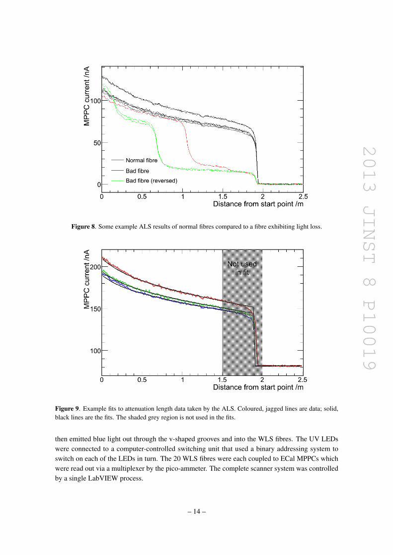
2013 JINST 8 P10019
Figure 11 (Left) An exploded view of the WLS fibre to MPPC coupling connector system The ferrule inthe bottom left of the figure is placed over the end of the WLS fibre (not shown) with the fibre overhangingthe ferrule by 05 mm in order to ensure good coupling with the MPPC The housing for the MPPC and foamspring is shown in the centre of the figure The lsquoearsrsquo of the housing slip over the ridge in the ferrule to lockthe assembly together The external shell or sheath covers the MPPC housing and part of the ferrule whenthe connector is assembled preventing the lsquoearsrsquo from disengaging with the ferrule The circular loop on theexternal shell allows the entire assembly to be screwed to the bulkhead securely (Right) The connector fullyassembled The assembled connector is approximately 5 cm long
highest thermal noise rate More details on the QA procedure and its results can be found in [24] Insitu the dominant contribution to the non-linearity of the combined scintillatorfibreMPPC systemis from the MPPCs and is estimated to be 2-3 for MIPs and 10-15 for charge deposits typicalof showers
35 Fibre to sensor coupling
An essential component in the overall light-collection efficiency of the ECal modules was the cou-pling of the WLS fibres to the MPPCs The design used was a multi-component solution shown infigure 11 (left) and was adopted by the on-axis INGRID detector [1] and the P0D subdetector [11]of the ND280 in addition to the ECal The assembly consists of three injection moulded1 parts (1)a lsquoferrulersquo glued to the end of the fibre which engages with (2) a housing that holds the MPPC andensures alignment with the fibre end to better than 150 microm and (3) an external shell or sheath tocontain the inner assembly and provide protection A 3 mm-thick polyethylene foam disk sittingjust behind the MPPC provided sufficient contact pressure between the fibre end and the MPPCepoxy window to ensure an efficient connection without the use of optical coupling gels whichcould deteriorate over time and present a complicated calibration challenge Electrical connectionbetween the MPPC and the front-end electronics is provided by a small circular printed circuitboard with spring-loaded pin sockets which contact the legs of the MPPC and connect to a micro-coaxial connector by Hirose (not shown in figure 11) Figure 11 (right) shows the connector fullyassembled Early prototypes of the connector revealed that an unacceptable light loss could occurif the fibre end was glued slightly short of the ferrule end This led to the production of gluingguides which ensured a precise overhang of the fibre from the ferrule end by 05 mm with a highproduction reliability
1All injection moulded components were fabricated from Vectra RcopyA130
ndash 17 ndash
2013 JINST 8 P10019
Table 4 The ECal construction and QA model showing contributions from Daresbury Laboratory (DL)Imperial College London Lancaster University Liverpool University Queen Mary University London(QMUL) Rutherford Appleton Laboratory (RAL) University of Sheffield and University of Warwick
DL Imperial Lancaster Liverpool QMUL RAL Sheffield WarwickECal design X XModule engineeringconstr X XDs-ECal layers XDs-ECal module Xbarrel-ECal side layers Xbarrel-ECal side modules Xbarrel-ECal topbott layers Xbarrel-ECal topbott modules X XP0D-ECal side layers XP0D-ECal side modules XP0D-ECal topbott layers XP0D-ECal topbott modules X2D scanner XMPPC QA X X XScintillator bar QA X XWLS fibre QA XMPPC-WLS connectors XElectronics X X
4 Construction
The T2K UK group employed a distributed construction model to optimize efficiency space andthe use of available personnel Module layers were constructed first and then lowered one at a timeinside prepared bulkheads after which the MPPCs then cooling panels TFBs cooling pipes andfinally cover panels were attached The RMMs were then affixed to the outside of the modulesAs each layer was installed inside the bulkheads a two-dimensional (2D) scanner discussed insection 43 carrying a 3 mCi 137Cs source was used in conjunction with a well-understood set oflsquotestrsquo MPPCs to check the integrity of the bar-fibre combination before the next layer was installedenabling repairs to be made if necessary The material preparation and QA also followed a dis-tributed pattern The distribution model is shown in table 4 All of the components in the table hadto come together on a co-ordinated schedule for the modules to be constructed Details of the layerand module assembly are given in the following sections
41 Layer assembly
Each layer is framed by aluminium bars with an L-shaped cross-section of dimensions 2000 mm(base)times 1254 mm (height) The height of the base is approximately 102 mm very slightly higherthan the scintillator bars and the width of the stem is 2000 mm Construction of the layer beganby screwing the aluminium bars into place onto a Teflon-covered assembly table The scintillatorbars then were prepared by applying a two-part epoxy (Araldite 2011 Resin and Araldite 2011Hardener) to one edge of the bars The bars then were laid inside the layer frame such that the
ndash 18 ndash
2013 JINST 8 P10019
Figure 12 Ds-ECal layer under construction The first of two sheets of lead is in place on top of thescintillator bars Visible are the aluminium frame and the locator pins securing the scintillator bars in placefor the duration of the layer construction The frame is covered with blue tape to keep it free from epoxy
central hole of each bar was aligned with a 2 mm-diameter hole in the frame An O-ring with anuncompressed thickness of 15 mm was inserted into the 1 mm gap between the ends of the barand the layer frame and compressed into place This was done to prevent epoxy from enteringthe bar hole and compromising the subsequent insertion of WLS fibre The position of each barwas stabilized during layer construction by inserting a temporary tapered Teflon-coated locator pinthrough the frame hole the O-ring and into the bar hole The locator pins were removed when thelayer was complete
Once all of the bars were stabilized in position a thin layer of epoxy was applied to them and tothe lip of the frame and the lead sheets were placed on top using a vacuum lifting rig attached to anoverhead crane in order to distribute the weight across several equally-spaced suction cups and soavoid distorting the lead The sheets were carefully positioned to minimize the gap between themthereby avoiding a region of low density in the middle of the modules while ensuring sufficientoverlap onto the lip of the layer frame to maintain structural integrity Figure 12 shows one of theDs-ECal layers being constructed with one sheet of lead in place on top of the scintillator bars
The entire layer then was covered with a sandwich of vacuum-sealing plastic and fabric withthe top layer of plastic securely taped to the table Vacuum pumps were used to evacuate the airaround the layer allowing the epoxy to cure for 12 hours under vacuum compression
Once the curing was finished the layer was unwrapped the locator pins removed the screwssecuring the layer frame to the table were removed the WLS-fibre holes were tested to ensure thatthey had not been blocked with epoxy and the layer then was stored for use in a module
ndash 19 ndash
2013 JINST 8 P10019
42 Assembly procedures for the ECal modules
The Ds-ECal was the first module to be constructed and most of the procedures developed duringthe process were used on the other modules as well The first step was to assemble the bulkheadsand the carbon-fibre panels One carbon-fibre panel (the bottom panel during construction whichwould become the upstream face when the Ds-ECal was in situ) was attached to the bulkheads toform an open box The other (top) carbon-fibre panel was stored until later The bulkhead box waspositioned on the construction table and the 2D scanner discussed in section 43 was attached andcommissioned The first layer then was lowered inside the bulkheads and positioned on top of thecarbon-fibre base A 1 cm gap between the bulkheads and the layer on all four sides was obtainedby tightening or loosening grub screws which were inserted through holes in the bulkhead andtensioned against the layer frame The LI LED strips and perspex lenses (see section 6) then wereglued onto the bottom carbon-fibre panel in the 1 cm gap the LI electronic cards were affixed to theinside of the bulkheads with the LI cables routed outside the bulkheads through the air holes WLSfibres were inserted through the scintillator bars A MPPC-fibre connection ferrule was bonded toeach fibre using Saint-Gobain BC600 silicon-based optical epoxy resin The test MPPCs werecoupled to the fibres using the connection sheaths and connected via a mini-coaxial cable to TFBswhich provided the control and readout (see section 5 for a description of the TFBs) After this thelayer was covered and made light-tight and a 2D scan was taken
The 2D scanner collected data at 20 points along each 2000 mm bar with data points beingcloser together near the ends in order to facilitate an understanding of the light escaping throughthe ends of the scintillator bar For efficiency the analyzing software ran in parallel with the data-taking producing an attenuation profile for each bar in the layer A typical example of this isshown in figure 13 The ordinate axis shows a reference value of the light yield since it is calcu-lated as a ratio of the integrals (from 55 PE to 30 PE) of the MPPC response when the source ispresent to the response when the source is not present and therefore represents (signal + back-ground)background This ratio is calculated at each data point along the length of the bar Moreinformation about the analysis of the scanner data is available in [18]
The scan data were checked and if problems were encountered appropriate action was takenA common problem involved the coupling between the fibre and the MPPC often due to the dif-ficulty of positioning the ferrule on the fibre In this case since the ferrule could not be removedthe fibre would be replaced a new ferrule would be attached and the bar would be re-scannedAfter this process the test MPPCs were removed and the next layer was installed and scanned inthe same manner Where required thin Rohacell foam sheets were placed between the layers toensure that the layers did not warp inwards
After several layers were installed in the Ds-ECal it was noted that the holes in the bulkheadswere no longer aligning well with the holes in the layers and the scintillator bars which madethe insertion of the WLS fibre difficult Measurements indicated that the layer frames had beenincorrectly manufactured and were an average of 02 mm higher than the specifications This wasremedied by using a router to thin the frames on the layers that were not yet installed The layerframes for subsequent modules did not have this problem
After all of the layers were installed LI LEDs and electronic cards were attached to the topcarbon-fibre panel 9 mm of Rohacell foam was glued to the inside of the panel to ensure that the
ndash 20 ndash
2013 JINST 8 P10019
Figure 13 A typical light attenuation profile from scanner data corresponding to one scintillator bar in theDs-ECal The ordinate axis is the ratio of the integrated light yield with the source present to the integratedlight yield without the source the abscissa is the position along the bar in cm The light yield measured bythe MPPC at one end of the bar and read out by one of the two TFBs (TFB 0) is shown in the upper plotand that from the MPPC at the other end read out by the other TFB (TFB 1) is shown in the lower plot Thepoints are data the curves are a single-exponential fit to the central region of the data
layers within the bulkheads stayed stable when the Ds-ECal was in its upright position in situ Thecarbon-fibre panel was then affixed to the top of the bulkheads
The procedure described above completed the construction of the active region of the detectorThe next steps dealt with the data readout First the 3400 Ds-ECal lsquoproductionrsquo MPPCs in theircustom-made sheaths complete with foam springs and mini-coaxial cables were attached to theferrules of every layer and secured to the bulkheads as described in sections 21 and 35 Cable-management brackets were attached to the bulkheads and the MPPC cables were grouped togetherand tidied in preparation for the next steps Tyco Electronics LM92 temperature boards werescrewed onto the bulkheads between the MPPCs in positions that allowed one temperature boardto be connected to each TFB
The cooling panel for the left-side Ds-ECal was assembled from four separate cooling platesThe TFBs then were attached and thermally connected to the left-side cooling panel using screwsand thermally-conducting epoxy resin The cooling panel then was held in position on the left sideof the Ds-ECal while the MPPC and temperature-board cables were threaded through the slots in
ndash 21 ndash
2013 JINST 8 P10019
the panel and the LI cables were routed through the panelrsquos air holes after which the panel wasplaced into its final position and bolted into place The MPPC and temperature-board cables wereconnected to the correct ports on the TFBs The same procedure was followed for the other threecooling panels
The water-cooling circuit then was installed on the cooling panels and the gas distributionbranch was installed on the bottom cooling panel These systems were tested under pressureFollowing this cable-management brackets were fitted between all of the TFBs and low-voltagefeedthroughs and bus bars were installed The bus bars were checked for continuity isolation fromground and from each other Shielded Cat 5e cables then were connected to the TFBs Along withthe LI cables they were routed around the detector to a patch panel mounted on the bottom coolingpanel or in the case of the trigger cables from the TFBs and half of the LI cables to the top coolingpanel Figure 4 shows the left-side Ds-ECal cooling panel with the TFBs bus bars Cat 5e cablesLI cables water-cooling pipes and air holes
The outer cover panels then were attached to each side The top cover panel was fitted with28 cable glands through which the Cat 5e cables corresponding to the trigger system exited thedetector and with air vents to allow the gas being flushed through the detector to escape Half of thecables from the LI system exited through holes in the top cover panel The bottom cover panel wasfitted with power cable clamps cable-management brackets and RMM cards The Cat 5e cableswere routed from the patch panel to the RMMs LI junction boxes were attached and connected tothe LI cables completing the construction of the Ds-ECal
This construction procedure was repeated for each of the barrel-ECal modules Minor alter-ations to the method were needed to accommodate the slightly different structure of the modules(see section 22) More significant alterations were made to the method for the P0D-ECal modulesreflecting their slightly different design as described in section 23 The most significant differ-ences were that the TFBs were mounted directly on the bulkhead instead of onto cooling panelswith the MPPC cables routed to them and supported where necessary the smaller number of TFBsper module allowed for the use of a thick standard copper wire instead of bus bars to supply powerwhich was distributed to the TFBs via branching connections to terminal blocks in the final stepof the assembly a non-magnetic support structure was bolted to the aluminium back panel whichpositions the thinner P0D-ECal modules away from the magnet and closer to the basket
43 The bar scanner
Three-axis scanners were designed to position a 137Cs radioactive source at multiple points abovethe surface of each detector layer as each layer was assembled into the subdetector body Threevariants of the scanner were manufactured
bull Ds-ECal and P0D-ECal scanner with a footprint of 3928 mm times 3578 mm
bull side barrel-ECal scanner with a footprint of 4862 mm times 3240 mm
bull top-bottom barrel-ECal scanner with a footprint of 4862 mm times 2410 mm
The three axes were driven by Mclennan SM9828 Stepper Motors controlled by PM600 In-telligent Stepper Motor Controller The controller was programmed via a commodity PC running
ndash 22 ndash
2013 JINST 8 P10019
LabVIEW The PC and stepper motors along with their controller were all powered via an un-interruptible power supply (UPS) The system design included an APC Smart-UPS 2200 230 Vprimarily as a safety feature so the radioactive source could be automatically parked during a powercut however it had the added benefit that short duration power glitches did not stop a running scan
These controls were integrated into a LabVIEW program providing an operator interface tocontrol the machine This operator interface was implemented as a lsquostatersquo machine the main statesbeing lsquosource loadedrsquo and lsquosource unloadedrsquo In the source-unloaded state the radioactive sourcewas not attached to the scanner head In this state the head was raised and moved to one side toposition the arm in the least inconvenient position for those working on the detector The arm couldalso be moved in the x-direction to allow for greater access to the detector during construction
The source was loaded under computer control with the computer prompting the operator toperform the necessary steps in a safe order The program then switched to the source-loaded statewhere scanning parameters could be input and the scan started Each scan started with the z-armsearching for the surface of the module layer at the centre of the module The arm descendedslowly until the push rod mounted adjacent to the source operated The arm then backed off andthe source moved to the matrix of measurement positions At each position the Scan Controlprogram prompted the DAQ to start data-taking via a network link On completion of data-takingthe scanner would move to the next position and iterate until data had been taken at all positionsWhen the data-taking was complete or if the program detected an error condition the sourcewould be returned to its lead-shielded safe parked position Unloading the source was again undercomputer control with operator prompts to ensure safety Re-positioning of the scanner head wasfound to be accurate to within 002 mm
Figure 14 shows the scanner in operation during the Ds-ECal construction The vertical armfinds its position as described in the text The operator provides the xminus y coordinates and therequired timing at each position Since radiation safety rules dictated that no one should be in thearea during the scan the image was taken by a web camera which allowed operators to check onthe scanner progress
5 Readout electronics and data acquisition
As described in section 21 the mini-coaxial cable from each MPPC is routed outside the coolingpanels and connected to a custom designed TFB Each TFB contains 4 Trip-T application-specificintegrated circuits (ASICs) originally designed for the D0 experiment at FNAL Up to 16 MPPCscan be connected to each ASIC implying that a maximum of 64 MPPCs can be connected to asingle TFB In total the ECal has 22336 electronic channels connected to MPPCs To increase thedynamic range of the electronics the incoming MPPC signal is capacitively split (110) into high-and low- gain channels which are read by different channels of the ASIC Depending on the MPPCgain the single-pixel (1 PEU) signal corresponds to approximately 10 ADC counts in the high-gainchannel while the maximum signal in the low-gain channel corresponds to around 500 PEU
The Trip-T chip integrates the charge in a preset (programmable) time interval which is fol-lowed by a programmable reset time at least 50 ns long For T2K the integration windows areprogrammed to synchronize with the neutrino beam timing The Trip-T chip integrates from 23readout cycles in a capacitor array and once all cycles have been completed the stored data are mul-
ndash 23 ndash
2013 JINST 8 P10019
Figure 14 The 2D scanner moving along the scintillator bars in the Ds-ECal The 137Cs source sits at thebottom of the vertical arm of the scanner just above the layer being scanned The blackout material coveringthe layer is seen along with the tape holding it in place for the duration of the scan
tiplexed onto two dual-channel 10-bit ADCs which digitize the data Signals from the high-gainchannel are routed via a discriminator which forms part of the Trip-T chip A field-programmablegate array (FPGA) produces timestamp information from the discriminator outputs and sends thisinformation together with the ADC data to a back-end board In addition the TFB also recordsmonitoring data (eg temperature voltage) via the same FPGA which is asynchronously trans-mitted to the back-end board for data concentration and buffering Detailed information about theTrip-T chip and front-end electronics is given in references [2] and [25]
The back-end electronics system for the ND280 consists of several different boards The TFBsare connected to RMMs which provide control and readout Control is fanned out from a masterclock module (MCM) via several slave clock modules (SCMs) one per subdetector Additionallytwo cosmic trigger modules (CTMs) are used to provide a selection of cosmic-ray muon triggeredevents for calibration and monitoring All of these boards use a common hardware platform specif-ically developed by the Rutherford Appleton Laboratory for use in the T2K experiment Signalsfrom up to 48 TFBs which are mounted on the detector typically less than 1 m away from theMPPCs are routed to one RMM via Cat 5e cables The ECal uses a total of 12 RMMs 8 forthe barrel-ECal 2 for the Ds-ECal and 2 for the P0D-ECal Each RMM controls its associatedTFBs distributes the clock and trigger signals to them and receives data from them once a triggerhas been issued Data from the RMMs are then sent asynchronously via a gigabit ethernet link tocommercial PCs that collect and process the data
The ND280 uses a single MCM This receives signals from the accelerator which allow it todetermine when a neutrino spill is about to occur and also from a GPS-based clock which is usedto synchronize the electronics to UTC The MCM prioritizes and issues triggers across the whole
ndash 24 ndash
2013 JINST 8 P10019
detector and manages readout-busy situations The signals and control of the MCM are fannedout to the SCMs The trigger and clock signals are passed to the ECal RMMs via the ECal SCMThe SCMs allow the electronics for a sub-system to be configured independently It is possible forthe ECal to run autonomously (lsquopartitioned DAQrsquo) from the rest of the ND280 for calibration anddebugging by using the ECal SCM as master controller
The software control of the detector is performed using the ldquoMaximum Integration Data Ac-quisition Systemrdquo (MIDAS) [26] The front-end software is custom written to manage the commu-nication with the RMMs CTMs SCMs and MCM through gigabit ethernet links A second pro-cess combines ADC and TDC information compresses the data and makes histograms for pedestaldetermination and monitoring A third process manages communications with computers runningthe MIDAS DAQ elements These three processes co-operate on front end PCs running ScientificLinux with each front end PC being connected to two back-end boards The event builder and datalogging use software from the MIDAS distribution with virtually no customization for T2K TheDAQ contains an online monitoring system which makes histograms for assessing data quality inreal time and passes events to the online event display for monitoring Detailed information aboutthe DAQ is given in [2]
6 Light injection system
The ND280 ECal LI system is designed to provide a quick and reliable method of monitoring theperformance of the MPPCs used inside the ECal modules A complete discussion of the LI systemRampD can be found in reference [27] The LI system is required to illuminate the MPPCs on agiven readout face of an ECal module with a short duration optical pulse The pulse length andstability must be sufficient to afford accurate (asymp 1 ns) timing calibration The intensity across thereadout-face should be uniform and any electromagnetic or electro-optical noise induced by thesystem must not interfere with the surrounding sensors or electronics
In order to accomplish these aims the LI system employs a modular design incorporatingdedicated electronics for both the interface with the ND280 DAQ and the pulsing of LI sourceswithin an ECal module The components are described in the subsections that follow The LIfront-end electronics are housed in custom-built crate assemblies compatible with a standard 19-inch rack In brief the LI signal chain comprises the following components
1 The trigger card receives the ND280 MCM signal
2 Control cards (CCs) receive and interpret the DAQ instructions and collate with the clock
3 The junction boxes (JBs) receive and fan out the CC outputs
4 The pulser receives the CC output via a JB and drives LED strips which emit optical pulsesfor calibration
Each of the components is described in more detail below
ndash 25 ndash
2013 JINST 8 P10019
61 Control cards and trigger receiver
The LI system receives DAQ instructions into a dedicated CC Each card hosts a TCPIP serverthat allows the DAQ instructions to be interpreted and then encoded into a sequence of TTL pulsesused to drive LED pulser cards housed inside the ECal modules The ND280 MCM transmits a100 MHz signal to the LI system which is received by a dedicated trigger card The clock signalis first fanned out to each CC then collated with the CC outputs onto a RJ45Cat 5e signal cableready for distribution to the LI JBs
62 Junction boxes
The JBs are responsible for directing the TTL pulse train and MCM clock from the CCs to therelevant LI pulsers the pulser being the dedicated electronics required to form the electrical exci-tation pulses used to drive the LED strips used for illumination There is one JB per ECal moduleexcept for the Ds-ECal which has two 6timesP0D-ECal 6times barrel-ECal and 2timesDs-ECal making14 in total The JBs are mounted outside but in close proximity to the ECal modules themselvesThey are passive devices used exclusively for fanning out the CC pulses and therefore introducingno modification to the actual signal
63 Communications protocol and cabling
The low-voltage differential signalling (LVDS) protocol is used throughout to ensure robustnessagainst interference from electromagnetic noise in the detector The DAQ instruction and MCMclock information are received over LVDS converted to TTL for interpretation by the CCs TheCC outputs are again transmitted using LVDS converted to TTL for fan out in the JBs and thentransmitted to the LI pulsers again using LVDS The Ds-ECal portion of the LI system howeveris an exception in that it features an older design which implements TTL over LEMO cables ratherthan LVDS over RJ45Cat 5e cables In order to preserve the relative timing between pulsers allCat 5eLEMO cables within an ECal module have been installed with the same length
64 Pulsers
LED pulser cards mounted inside the ECal modules receive the pulses emitted from the CCs viathe JBs The TTL logic pulses determine the pulse duration amplitude and number of flashes Ashaping component of the pulser board introduces activation and deactivation spikes to the leadingand trailing edges of a square-wave electrical pulse This ensures a constant level of illuminationwith a negligible optical rise time The signal chain is illustrated in figure 15 Different numbersof pulsers are located in different ECal modules depending on their size and layout There are 114in total 14 P0D-ECal 84 barrel-ECal and 16 Ds-ECal
65 LED strips and extruded perspex lens
Each LED pulser drives two KingBright LSL-062-05 flexible LED lighting modules The LEDstrips are fitted with an optically coupled cylindrical lens made of 2 mm-diameter extruded per-spex as shown in figure 16 The KingBright LEDs feature an in-built lens with 12 angle 120
producing a rather wide beam divergence that results in a 75 loss of emission at the layers fur-thest from the LED strips The addition of the perspex rods focuses the light so as to reduce thisloss to only 25 of the maximum
ndash 26 ndash
2013 JINST 8 P10019
Figure 15 The LI signal path The CCs encode an MCM synchronized pulse train with the desired timingand amplitude characteristics The pulsers derive the excitation charges from the CC output
LED
index matched glue
fullminuscylinder lens
flex strip
10mm
Figure 16 KingBright LED 10 mm-wide strip (left) and optically-coupled acrylic lens (right)
66 LI installation
The Ds-ECal JBs were installed and cabled in Aug 2010 The remainder of the JBs and the frontend electronics were installed during OctNov 2010
The P0D-ECal CC receives 1times input from the DAQThe P0D-ECal CC transmits 1times output to each of six JBs
A single P0D-ECal CC located in the LI electronics crate transmits the DAQ instructions andMCM clock information to the six P0D-ECal JBs Each JB splits and distributes the instructionsand clock information to 14 = 4times 2 pulsers + 2times 3 pulsers forming six groups permitting anycombination of the six P0D-ECal modules to be illuminated
Each barrel-ECal CC receives 1times input from the DAQEach barrel-ECal CC transmits 2times outputs to each of six JBs
There are six barrel-ECal CCs in total One barrel-ECal CC transmits the DAQ instructions andMCM clock information to one barrel-ECal JB over two RJ45Cat 5e cables One JB splits anddistributes the instructions and clock information to 14 pulsers forming three distinct groupingseach corresponding to pulsers located on one of the three readout faces Any combination of
ndash 27 ndash
2013 JINST 8 P10019
readout faces (ie the ends of the single and double-ended scintillator bars) can be illuminatedwithin a given barrel-ECal module
The Ds-ECal JBs are unique in that they sit inside the ND280 magnet situated directly againstthe ECal bulkheads Moreover they employ LEMO connections along single core coaxial cablerather than the RJ45Cat 5e that is ubiquitous elsewhere throughout the ECals and the remainderof ND280 There are two readout faces per Ds-ECal module each separately illuminated by eightpulsers There are two JBs one North and one South served by a single CC situated in the LIfront-end electronics crate
7 Testbeam
In 2009 the Ds-ECal module was exposed to the CERN T9 testbeam This represented the firstopportunity to test the entire integrated system calorimeter readout system DAQ system andanalysis framework As well as a system shakedown the data provided by the testbeam havebeen used to tune the particle identification algorithms used in T2K analyses and to obtain a betterunderstanding of detector performance
71 The CERN PS T9 testbeam
The T9 beamline is a medium energy multiple particle species tertiary beam generated by thecollision of protons from the CERN PS on a solid target in the CERN East Experimental HallThe dual polarity beam supplied a mix of pions electrons and protons with momenta rangingfrom 300 MeVc up to 15 GeVc Data were taken at momentum points between 300 MeVc and50 GeVc The particle composition of the beam changed with momentum setting Below 1 GeVcelectrons made up 90 of the beam This fraction decreased to approximately 5 for momentumsettings above 30 GeVc with a corresponding increase in the fraction of hadrons
72 Triggering and event selection
The beamline was instrumented with several detectors to provide particle identification informa-tion Two Cerenkov counters filled with CO2 at variable pressure were present and read out usingPMTs connected to an ordinary TFB board The counters were configured such that only electronswere above threshold which provided electronhadron discrimination The electron identificationefficiency of the system (requiring both counters to register a hit) was estimated to be (90plusmn 2)for momentum settings below 30 GeVc The Cerenkov system was complemented by a time-of-flight (TOF) system comprised of two scintillator paddles read out by fast PMTs The paddleswere separated by a flight distance of 14 metres Custom NIM-based electronics including a time-to-analogue converter (TAC) converted the time of flight to a current pulse which was read outusing a TFB The TOF system provided proton-pion separation for momentum settings between600 MeVc and 18 GeVc and also acted as the hardware trigger for the Ds-ECal
Combining the performance of the TOF and Cerenkov systems with the beam compositionthe contamination of the hadron sample with electrons was estimated to be below 05 and theelectron sample was estimated to be more than 99 pure Because of the relative timings of thephysics signal and DAQ cycle the physics data from a single beam event could fall into one of twoTrip-T integration windows Due to latencies in the system it was also possible that different parts
ndash 28 ndash
2013 JINST 8 P10019
of a single event could end up spread across different time buckets In this case it was impossible tobe sure that activity did not occur undetected during the reset period To eliminate this uncertaintyevents with reconstructed clusters in both windows were rejected For electron events the candidatecluster was also required to arrive between 0 and 65 ns after the Cerenkov signal
73 Detector configuration
The detector was configured as similarly as possible to its final operating conditions however therewere some differences largely due to physical constraints The downstream end of the detector(with respect to the J-PARC beam) faced upstream in the testbeam meaning that incident particlespassed from the back to the front of the detector This meant that the particles passed through alead layer before a scintillator layer leading to a small difference in behaviour
In addition to this the detector was cooled using an air-based chiller rather than water cooledleading to a diurnal variation in temperature of around 2C and a total temperature range of 16ndash28C over the whole running period This led to rather larger drifts in MPPC behaviour than ex-pected for the final system leading to some difficulties in calibration (section 74) though after aninitial commissioning period these were mostly ameliorated by taking very regular calibration runs
74 Calibration differences
Calibration for the testbeam was carried out using only dedicated pedestal runs rather than usingnoise spectra as in the final calibration scheme described in section 81 Initially pedestal runswere taken infrequently but after examining the early data we noticed that this was not sufficientto fully calibrate for the effect of the large temperature variations in the T9 setup We thereforechanged operating procedure to take a dedicated pedestal run before every physics run For oper-ations at J-PARC we have added the ability to take interspersed pedestal data and measure noisespectra during normal running reducing the need for these dedicated runs The more sophisticatedcooling system at J-PARC also reduces the need for very frequent calibration
To improve the calibration of early data we made use of the fact that the average temperatureof the detector was measured at the start of each run The gain for each channel was then calculatedon a run-by-run basis using the gains calculated from the most recent pedestal run the temperaturemeasurements and the following formula
G = G0 +dGdT
Tdiff (71)
where G0 is the gain of the preceding pedestal run Tdiff is the temperature difference between thecurrent run and the preceding pedestal and dG
dT is the rate of change of gain with temperature foundto be -067times105C This removed much of the charge scale variation between runs
As shown in figure 17 some residual temperature dependence is seen in the detector responseafter making the temperature-based correction particularly in the period before regular pedestalruns were taken A fit to the temperature data corresponding to the final five days in figure 17indicates that the average temperatures were rising resulting in the slight decrease in the Landaumost probable values (MPVs) that is visible in the plot To remove these variations data fromcosmic ray muons (collected coincidentally with beam events in DAQ integration periods notassociated with the beam) were processed from each run The MPV of the charge distribution of
ndash 29 ndash
2013 JINST 8 P10019
Date1005 1105 1205 1305 1405 1505 1605 1705 1805
MPV
[M
EU
cm
]
06
08
1
12
14
16
C]
degTe
mpe
ratu
re [
16
17
18
19
20
21
22
23
24
25
26
Figure 17 Time series of the average detector temperature and Landau most probable value (MPV) formuon hits in each run after making a temperature-based gain correction The dashed line represents thepoint at which pedestal runs began to be taken regularly
single hits across all channels was then found for this sample and used to scale hit charges forelectron events in the run equalizing the MIP scale for all data runs
Monte Carlo samples for each individual testbeam run were produced using Geant4 [28] Arepresentation of the Ds-ECal geometry was constructed and a monochromatic beam of electronsat each central beam momentum point was fired into the centre of the back-face of the Ds-ECalThe photosensor response was simulated utilizing data from test bench measurements and tunedusing cosmic ray muon data with special attention to simulating the temperature response of thephotosensor Monte Carlo samples were generated with temperatures identical to the average localtemperature of each photosensor on a run-to-run basis A similar cosmic ray muon sample was alsogenerated at this temperature and the calculated MPV was used to scale the electron hit charges
In order to remove any poorly understood noise or readout-chip threshold variation a chargethreshold equivalent to 04 MIP units was implemented in the data and simulation In additionduring the final processing of the data any hits further than 8σ of the beam-time width from thepeak cluster time were discarded to remove unsimulated cosmic events The Monte Carlo data setswere then passed through the same calibration and reconstruction paths as data
The procedure described successfully accounted for the average gain variation over the runningperiod due to temperature variation It was not however possible to account for sensor-to-sensorvariations or temperature shifts within individual runs
75 Testbeam performance
The testbeam data were used to calculate the performance of the Ds-ECal in the reconstruction ofincident particles particularly electrons The performance results for electrons will be shown here
Figure 18 shows the measured energy resolution for electrons striking the centre of the ECalface as a function of energy It can be seen that the data and Monte Carlo agree reasonably wellbut the data resolution is somewhat worse over the whole energy range and particularly at lowerenergies This may be accounted for in part by the intrinsic momentum spread of the beam which
ndash 30 ndash
2013 JINST 8 P10019
Figure 18 Measured energy resolution of the Ds-ECal for electromagnetic showers for data and MonteCarlo The dashed lines show a fit to a stochastic resolution model
was not modelled in the Monte Carlo In addition the temperature-based gain corrections usedfor this data will only correct the mean photosensor gain across the Ds-ECal A spread in MPPCgains due to temperature differences across the ECal is expected but cannot be corrected becausethe temperatures of individual sensors could not be measured and were not modelled in the MonteCarlo which assumes the same temperature for all sensors This is expected to lead to a largerspread in measured particle energies
Because of the limitations described above the differences between data and Monte Carlo seenin figure 18 represent a worst-case scenario for the calculation of systematic uncertainties Work iscurrently underway to replace this conservative estimate with one based on in-situ measurements
Figure 19 shows the angular resolution of the Ds-ECal for normally incident electrons at arange of energies Excellent agreement is seen between data and Monte Carlo over the full rangeof energies considered
In summary the T9 testbeam has provided useful information for the calculation of system-atic uncertainties and also gave an opportunity to test the detector and DAQ systems before theywere integrated into the ND280 The data collected were also invaluable in the development ofcalibration and reconstruction code in advance of data from the full ND280 becoming available
8 ECal commissioning and performance
81 Calibration
Precise calibration of ECal hits is vital for high-quality calorimetric performance To this end a setof procedures has been developed to calibrate out all significant instrumental effects with the goal
ndash 31 ndash
2013 JINST 8 P10019
Energy GeV05 1 15 2
Dir
ectio
n re
solu
tion
Deg
rees
2
3
4
5
6
7
8
Datadeg0
Monte Carlodeg0
Figure 19 Angular resolution for electrons at normal incidence to the detector in data and Monte Carlo asa function of energy
of obtaining the energy deposited in the scintillator giving rise to the hit and the precise time atwhich the energy was deposited The calibration can be separated into two main categories whichare described below energy calibration and timing calibration
Energy calibration can be logically split into three steps mdash going backwards down the readoutchain from the ADC value registered by the electronics to the anode charge from the MPPC fromthis to the number of photons incident on the MPPC face and from this to the energy deposit in thescintillator
The first step involves subtracting the electronics pedestal from the ADC counts This pedestalis the ADC value registered in the absence of any physics signal and is different for each channeland readout cycle Dedicated runs are taken once a week during beam down-times to measurethe pedestals separately for each cycle and a per-channel average over cycles is calculated everythree hours from noise spectra recorded by the DAQ in normal running The diurnal variationin pedestals due to temperature changes at the electronics is up to a few ADC counts so fine-granularity corrections are important
The next step is to convert the pedestal-subtracted ADC into an anode charge The electronicsresponse is not perfectly linear and the calibration must also incorporate the transition from highgain to low gain ADC channels Both the high gain and low gain response are mapped using theTFBrsquos ability to inject a known charge onto each channel in turn These charge injection curvesare parametrized for both high and low gain channels using two cubic polynomials joined with asigmoid function to smoothly transition between them The parametrized charge injection curvesalso allow us to calibrate the low gain channel response to the high gain channel The switchoverbetween the two channels is made at approximately 460 ADC counts in the high gain channelwhich typically corresponds to about 21 PEU An example of the charge injection curves is shown
ndash 32 ndash
2013 JINST 8 P10019
1
times103
Resp
on
se (
AD
C)
High gain
08
09
1
Resp
on
se (
AD
C)
Low gain
06
07
Resp
on
se (
AD
C)
1
04
05
1
02
03
0110 20 30 40 500
Input Charge (fC)
times103
Figure 20 High and low gain ADC response of a typical Trip-T channel Charge is injected using anonboard capacitor controlled by a Digital-to-Analogue Converter (DAC) The injected charge is calculatedfrom the DAC setting For comparison a typical MIP deposits of order 107 electrons or 16times 103 fC ofcharge
in figure 20 A typical MIP deposits of order 107 electrons or 16times 103 fC of charge ie inthe first bin on the plot More information about the charge injection calibration is available inreference [29] The parameters for this calibration are rather stable over time so are only updatedaround once per running period
To convert the calculated anode charge to an estimate for the number of photons incident onthe MPPC we first convert the charge into a number of PEU by dividing by the gain of the MPPCThe gains for each channel are calculated for every three hours of data using the same noise spec-tra as the pedestal drift and fitting the position of the first non-pedestal peak in the noise spectrumwhich is due to a single pixel firing in the device Again diurnal temperature variations have non-negligible effects on the gain so this granularity is required We then need to convert this number ofpixels to a number of photons For low light levels this conversion can be approximated by dividingby the PDE of the MPPC however it is complicated by saturation effects (the MPPC has a finitenumber of pixels and therefore a limited dynamic range) and also by after-pulsing and crosstalkwhich cause the effective PDE to be larger than the true value2 The resulting response functioncannot easily be calculated analytically and is therefore modelled on testbench measurements Asingle response function is used for every channel but the parameters are in turn functions of the de-vice gain so that changes in PDE and other parameters with overvoltage can be taken into account
Next we need to convert the number of incident photons to an energy deposit This needsto be done for each channel as there will be some non-uniformity due to for example the differ-
2A detected photon has approximately a 10 probability of initiating a secondary avalanche therefore the numberof avalanches is in general higher than the number of detected photons
ndash 33 ndash
2013 JINST 8 P10019
Charge [PEUcm]0 10 20 30 40 50 60 70 80 90 100
AU
0
0005
001
0015
002
0025
003
0035
004
0045 Right BottomLeft BottomRight TopLeft TopRight SideLeft Side
Uncalibrated
Charge [PEUcm]0 10 20 30 40 50 60 70 80 90 100
AU
0
001
002
003
004
005
006
007
Calibrated
Figure 21 The effect of the attenuation and uniformity corrections on the hit charge distributions forthrough-going cosmic muons in the six modules of the barrel-ECal shown by the six curves in each plotThe left side shows the distributions with the pedestal and gain corrected the right side adds correctionsfor attenuation and differences caused by non-uniformity of scintillator bars and WLS fibres Distributionsshown here are summed within a module but the corrections are applied on a per channel basis The slightvariation between modules is typical and insignificant
ences between channels in the optical coupling between the fibre and the MPPC The correctionis done using empirical data taking a sample of cosmic muon tracks passing through the ECalperforming all other calibrations including attenuation in the fibre (described below) and trackpath-length through the scintillator bar The corrected hit size distribution for each channel is fittedwith a Landau distribution convolved with a Gaussian smearing The effect of the attenuation anduniformity corrections is shown in figure 21 the distributions on the right side are used for theLandau-Gaussian fit This is used to calculate the expected hit size for a MIP-size energy depositat a fixed (1 m) distance from the sensor the result is used as a divisor to equalize the sizes ofhits between bars The signal produced by this ldquoideal MIPrdquo varies between modules and scintil-lator bar orientations but to give a sense of scale a muon passing approximately perpendicularlythrough the centre of the Ds-ECal typically leads to approximately 19 pixel avalanches at eachsensor corresponding to approximately 17 detected photons
It is also necessary to correct for the attenuation of photons in the WLS fibres which is signif-icant over the length of the ECal bars This calibration is done after the reconstruction has matchedtracks between the two views of the ECal so that the component of the hit position along the lengthof the scintillator bar can be estimated The attenuation profile is modelled as a sum of two expo-nential functions with an additional correction for the mirroring of the single-ended fibres Thiscorrection is stable over time and is calculated separately for each orientation of bar in each mod-ule using cosmic muon tracks Figure 22 shows the time stability of the energy calibration over oneperiod of beam running
The timing calibration also involves several distinct steps Each hit is time-stamped using theTFB clock based on the time at which the channelrsquos discriminator was triggered The discriminatortrigger is nominally set at a level of 35 PE The TFB clocks lag the global detector clock from
ndash 34 ndash
2013 JINST 8 P10019
2012Jan 21 2012
Feb 20 2012Mar 21 2012
Apr 20 2012
May 20
MP
V fr
om la
ndau
-gau
ssia
n fit
[PE
Uc
m]
135
14
145
15
155
16
165
Figure 22 The muon MIP response as a function of time for a period of beam running
Run number8100 8200 8300 8400 8500 8600 8700 8800
tfb o
ffset
(ns
)
-30
-20
-10
0
10
20
30
RMM 8
Figure 23 The TFB offset before correction for all channels on one RMM as a function of time for a periodof beam running Each line shows one TFB
which they are synchronized due to delays in the cabling and electronics used to distribute theclock signals This effect will be different for each TFB depending on the cable lengths Thedifferences between TFBs within the ECal are calculated by considering cosmic muons that leavehits in channels corresponding to different TFBs and correcting the hit times for fibre delay andthe transit time of the muon Synchronizing the ECal with the rest of the detector is achieved usinga similar method Figure 23 shows the offset for the TFBs on one RMM over a period of runs
A lsquotimewalkrsquo correction is also applied to the hit times The decay that causes the WLSfluors to radiate occurs with a half life of a few nanoseconds leading to the photons arriving at theMPPC face over a finite time period The analogue electronics also have a finite rise time both ofthese effects result in a delay between the idealized propagation of the signal and it crossing thediscriminator threshold These delays depend on the total hit charge and tend to a small constant
ndash 35 ndash
2013 JINST 8 P10019
CorrectedEntries 334Mean -4871
RMS 684
Mean Time (ns)-4940 -4920 -4900 -4880 -4860 -4840 -48200
5
10
15
20
25
30
35
40
45
CorrectedEntries 334Mean -4871
RMS 684
UncorrectedEntries 334Mean -4871
RMS 1379
UncorrectedEntries 334Mean -4871
RMS 1379
UncorrectedEntries 334Mean -4871
RMS 1379
Figure 24 The distributions of mean hit time values for cosmic muons for each channel of the tracker-ECal(corresponding to 334 TFBs) before timing calibration (blue dashed line) and after timing calibration (redsolid line)
offset for large hits The optical component of the timewalk is a stochastic process and affectsthe timing resolution but the average effect can be removed with an analytic function based on anexponential photon arrival time distribution using the known decay time of the relevant state in theWLS fibre Finally the travel time for photons in the WLS fibre must be calibrated This is doneafter the reconstruction has matched hits between views so that the light travel distance is known
Figure 24 shows a comparison between the mean hit time values of each TFB channel duringcosmic muon triggers before and after corrections The distribution of mean hit time values narrowsby a factor of two in the RMS and approaches the limit set by the trigger logic The central valuecorresponds to the time delay between a cosmic muon being observed and the corresponding triggerbeing issued by the master clock The lsquoideal casersquo resolution for this delay is approximately 4 nsRMS but it is dominated by the 10 ns granularity of MCM clock and the fluor decay time bothof which are non-Gaussian Resolution on the time between two hits from a single muon is ratherbetter and the time resolution on the entire reconstructed ECal track is better still The dominantuncertainty comes from the fluor so each hit provides a largely-independent estimate For a typicaltrack or shower reconstructed in the ECal the time resolution is approximately 1 ns or less whichis sufficient for direction discrimination when used in combination with information from othersubdetectors
ndash 36 ndash
2013 JINST 8 P10019
Layer number0 5 10 15 20 25 30
Effi
cien
cy
09
091
092
093
094
095
096
097
098
099
1
Double-ended bar Barrel
Single-ended bar Barrel
Double-ended bar Downstream
Figure 25 The hit efficiency by layer for bars in the Ds-ECal and barrel-ECal Layer number increasesfrom the central region to the exterior of the detector
82 Hit efficiency
The hit efficiency for the ECal can be determined by looking at a sample of through-going cosmicmuons if the scintillator bars in layer n + 1 and layer nminus 1 are hit the cosmic ray should havepassed through a scintillator bar in layer n The sample of cosmic rays used for this measurementensures that the cosmic rays are isolated from other activity in the ECal resulting in an accuratemeasure of the layer-by-layer efficiency The hit efficiencies by layer are shown in figure 25 Theaverage layer efficiency in the Ds-ECal is 981 and the average layer efficiency in the barrel-ECalfor double-ended bars is 988 and for single-ended bars is 970 The lower efficiency in thesingle-ended bars is due to the reduced light collection from only one MPPC
83 Time stability and beam position
The Ds-ECal was in operation at the ND280 site since November 2009 and the barrel-ECal sinceNovember 2010 Over that time period the operation of the ECal has been stable The stabilityof the operation can be observed from the interactions measured while the beam is on A low-level selection requiring only the reconstruction of an energy cluster produces a sample of eventsoccurring in the ECal Note that this selection does not correspond to a physics selection butsimply allows for an accounting of activity in the ECal while the beam is on Figure 26 shows thenumber of interactions in the ECal as a function of time normalized to the number of protons ontarget (POT) The rate is steady over the run periods
Since the ND280 detector operates off axis the number of events as a function of spatialposition is expected to be greater near to the axis of the beam and lesser away from the axis of thebeam The position of the beam centre in the coordinates of the ND280 is approximately (+3200-9400) mm below the lower right quadrant of figure 27 and as shown in the figure the number ofinteractions near the beam is significantly greater than away from the beam The beam spread isapproximately 45 m as measured by the INGRID on-axis detector and depends on neutrino energy
ndash 37 ndash
2013 JINST 8 P10019
Barrel ECalEntries 137
Mean 3433e+08
RMS 2917e+06
10 frasl07 frasl14 10 frasl08 frasl03 10 frasl08 frasl22 10 frasl09 frasl11 10 frasl10 frasl01 10 frasl10 frasl20 10 frasl11 frasl09 10 frasl11 frasl29 10 frasl12 frasl18 11 frasl01 frasl07 11 frasl01 frasl27 11 frasl02 frasl15 11 frasl03 frasl07
PO
T15
Num
ber
of r
econ
stru
cted
obj
ects
per
10
0
2
4
6
8
10
12
14
Barrel ECalEntries 137
Mean 3433e+08
RMS 2917e+06
Barrel ECal
Downstream ECal
2010-03-08
2010-03-27
2010-04-16
2010-05-05
2010-05-24
2010-06-13 Run 2rarrRun 1
2010-11-27
2010-12-16
2011-01
-05
2011-01
-24
2011-02
-13
2011-03
-04
Figure 26 The rate of interactions in the ECal during beam operations over time for T2K Run 1 and Run 2The black points (at asymp 2) show the Ds-ECal and the red points (at asymp 14) show the barrel-ECal Note the gapmarked on the time axis indicating the gap between Runs 1 and 2 when the barrel-ECal was installed
ND280 X coordinate (mm)-2000 -1500 -1000 -500 0 500 1000 1500 2000
ND
280
Y c
oord
inat
e (m
m)
-2000
-1500
-1000
-500
0
500
1000
1500
2000
ReconObjectPositionXY
Entries 435961Mean x 7907Mean y -3643RMS x 1156RMS y 1133
ReconObjectPositionXY
Entries 435961Mean x 7907Mean y -3643RMS x 1156RMS y 1133
1
10
210
The position of reconstructed ECal objects in the ND280 XY plane
Num
ber of reconstructed objects
Figure 27 The charge weighted position of interactions reconstructed in the ECal The position of thecentre of the beam is to the lower right and as a result more events occur in the bottom right of the ECalthan the top left Events that are recorded in the centre of each module are through-going MIPs that leaveapproximately the same charge in each layer and therefore have a charge weighted position in the centre
ndash 38 ndash
2013 JINST 8 P10019
Shower-like PID Discriminator Track-like
-02 0 02 04 06 08 1 12
even
ts
0
01
02
03
04
05 MCmicro datamicro
MC-e+e data-e+e
Figure 28 The discrimination between track-like (muon-like) and shower-like (electron-like) samples inthe Ds-ECal Solid lines show Monte Carlo information and points show data samples described in the text
84 Particle identification
One of the goals of the ECal is to provide discrimination between electrons and muons in the regionof phase space that is not covered by the particle identification from the tracker The first method forparticle identification constructed for the ECal was intended to maximize the separation of track-like (muon-like) and shower-like (electron-like) interactions The discriminator is constructed as aneural network [30] using low level quantities from the reconstruction
To test the discriminator samples of muons and electrons are selected from the data For theDs-ECal (barrel-ECal) the muons selected are lsquothrough-goingrsquo muons that have one track compo-nent in each of the three TPC modules and the Ds-ECal (barrel-ECal) Additionally the track mustappear lsquomuon-likersquo to the TPC [12] The electron sample is produced by looking at photon pairproduction in the FGD [13] requiring tracks with opposite charge at least one TPC componentin the track and that the TPC component appears lsquoelectron-likersquo Electrons or positrons that enterthe tracker-ECal are added to the sample In these control samples the median muon momentumis 17 GeVc with muon momenta ranging from 300 MeVc to 10 GeVc the median electron orpositron momentum is 165 MeVc These energies are typical of events seen from the neutrinobeam Additionally the discriminator is insensitive to the muon momentum provided that it isgreater than approximately 300 MeVc that is provided that the muon is MIP-like
The electron and muon samples are shown with the calculated discriminator in figures 28and 29 for the Ds-ECal and barrel-ECal respectively For both there is good agreement betweenthe data and the Monte Carlo and good separation between the muon and electron samples how-ever the separation is somewhat better in the Ds-ECal than in the barrel-ECal due to the differentpminusθ distributions seen in each The barrel-ECal because of its position within the ND280 seeson average lower momentum particles with a higher angle of incidence than the Ds-ECal Thiscombination of properties presents greater challenges for reconstruction and particle identification
ndash 39 ndash
2013 JINST 8 P10019
Shower-like PID Discriminator Track-like
-02 0 02 04 06 08 1 12
even
ts
0
005
01
015
02
025
03
035
04
045 MCmicro datamicro
MC-e+e data-e+e
Figure 29 The discrimination between track-like (muon-like) and shower-like (electron-like) samples in thebarrel-ECal Solid lines show Monte Carlo information and points show data samples described in the text
9 Summary
The electromagnetic calorimeter (ECal) for the T2K ND280 was designed and constructed in theUK during the period 2007-2010 The first module the Ds-ECal was tested in a charged-particlebeam at CERN in spring 2009 and installed in the ND280 at J-PARC in time for the first T2Kneutrino beam in January 2010 The testbeam data validated the design and operation of the systemand have been used to characterize its response The remaining 12 ECal modules were constructedin 2009-2010 and installed at J-PARC in time for the second neutrino data-taking period of T2Kstarting in fall 2010 The ECal has been operating stably and survived the great earthquake ofMarch 2011 without any damage The ECal has met its goals in terms of energy resolution andparticle identification and is an integral part of the ND280 ECal data are used in the ND280physics analyses and this is becoming more important as larger data samples are collected andmore sophisticated analyses are being developed
Acknowledgments
The ECal detector has been built and is operated using funds provided by the Science and Technol-ogy Facilities Council UK Important support was also provided by the collaborating institutionsIndividual researchers have been supported by the Royal Society and the European Research Coun-cil The authors also wish to thank CERN for support with the testbeam FNAL for manufacturingthe scintillator bars and preparing the wavelength-shifting fibres and finally our T2K colleaguesfor their invaluable help during installation and commissioning of the detector
ndash 40 ndash
2013 JINST 8 P10019
References
[1] K Abe et al Measurements of the T2K neutrino beam properties using the INGRID on-axis neardetector Nucl Instrum Meth A 694 (2012) 211 [arXiv11113119]
[2] T2K collaboration K Abe et al The T2K Experiment Nucl Instrum Meth A 659 (2011) 106[arXiv11061238]
[3] SUPER-KAMIOKANDE collaboration Y Fukuda et al The Super-Kamiokande detector NuclInstrum Meth A 501 (2003) 418
[4] MINOS collaboration P Adamson et al Measurement of Neutrino and Antineutrino OscillationsUsing Beam and Atmospheric Data in MINOS Phys Rev Lett 110 (2013) 251801[arXiv13046335]
[5] K2K collaboration M Ahn et al Measurement of Neutrino Oscillation by the K2K ExperimentPhys Rev D 74 (2006) 072003 [hep-ex0606032]
[6] T2K collaboration K Abe et al Evidence of Electron Neutrino Appearance in a Muon NeutrinoBeam Phys Rev D 88 (2013) 032002 [arXiv13040841]
[7] T2K collaboration K Abe et al First Muon-Neutrino Disappearance Study with an Off-Axis BeamPhys Rev D 85 (2012) 031103 [arXiv12011386]
[8] DAYA-BAY collaboration F An et al Observation of electron-antineutrino disappearance at DayaBay Phys Rev Lett 108 (2012) 171803 [arXiv12031669]
[9] RENO collaboration J Ahn et al Observation of Reactor Electron Antineutrino Disappearance inthe RENO Experiment Phys Rev Lett 108 (2012) 191802 [arXiv12040626]
[10] T2K collaboration K Abe et al Indication of Electron Neutrino Appearance from anAccelerator-produced Off-axis Muon Neutrino Beam Phys Rev Lett 107 (2011) 041801[arXiv11062822]
[11] S Assylbekov G Barr B Berger H Berns D Beznosko et al The T2K ND280 Off-Axis Pi-ZeroDetector Nucl Instrum Meth A 686 (2012) 48 [arXiv11115030]
[12] T2K ND280 TPC collaboration N Abgrall et al Time Projection Chambers for the T2K NearDetectors Nucl Instrum Meth A 637 (2011) 25 [arXiv10120865]
[13] T2K ND280 FGD collaboration P Amaudruz et al The T2K Fine-Grained Detectors NuclInstrum Meth A 696 (2012) 1 [arXiv12043666]
[14] T2K ND280 SMRD collaboration S Aoki et al The T2K Side Muon Range Detector Nucl InstrumMeth A 698 (2013) 135 [arXiv12063553]
[15] B Still T2K ND280 Pi0 electromagnetic calorimeter PhD thesis University of Sheffield UK(2010) [httpwwwt2korgdocsthesis004]
[16] A Vacheret et al Characterization and Simulation of the Response of Multi Pixel Photon Countersto Low Light Levels Nucl Instrum Meth A 656 (2011) 69 [arXiv11011996]
[17] MINOS collaboration D Michael et al The Magnetized steel and scintillator calorimeters of theMINOS experiment Nucl Instrum Meth A 596 (2008) 190 [arXiv08053170]
[18] G Davies Understanding and calibrating the DS-ECal for T2Krsquos ND280 PhD thesis University ofLancaster UK (2011) [httpwwwt2korgdocsthesis009]
[19] P Border et al A large liquid scintillator detector for a long baseline neutrino oscillationexperiment Nucl Instrum Meth A 463 (2001) 194
ndash 41 ndash
2013 JINST 8 P10019
[20] M Yokoyama et al Application of Hamamatsu MPPC to T2K Neutrino Detectors Nucl InstrumMeth A 610 (2009) 128 [arXiv08073145]
[21] Hamamatsu Photonics KK Solid State Division Hamamatsu MPPC (multi-pixel photon counterS10362-11 series httpwwwhamamatsucomresourcespdfssds10362-11 series kapd1022e06pdf
[22] M Ward Multi-Pixel Photon Counter characterisation for the T2K near detector electromagneticcalorimeter PhD thesis University of Sheffield UK (2009) [httpwwwt2korgdocsthesis032]
[23] M Yokoyama et al Performance of Multi-Pixel Photon Counters for the T2K near detectors NuclInstrum Meth A 622 (2010) 567 [arXiv10072712]
[24] M Haigh Beam extrapolation and photosensor testing for the T2K experiment PhD thesisUniversity of Warwick UK (2011) [httpwwwt2korgdocsthesis006]
[25] A Vacheret et al The front end readout system for the T2K-ND280 detectors IEEE Nucl Sci ConfR 3 (2007) 1984
[26] S Ritt P Armaudruz and K Olchanski MIDAS (Maximum Integration Data Acquisition System)httpsmidaspsich
[27] G Ward A Calibration System for the T2K ND280 Electromagnetic Calorimeters PhD thesisUniversity of Sheffield UK (2010) [httpwwwt2korgdocsthesis033]
[28] GEANT4 collaboration S Agostinelli et al GEANT4 a Simulation toolkit Nucl Instrum Meth A506 (2003) 250
[29] A Waldron Neutrino oscillation parameters from νe appearance in the T2K experiment PhDthesis University of Oxford UK (2012) [httpwwwt2korgdocsthesis037]
[30] CM Bishop Neural networks for pattern recognition Clarendon Press Oxford UK (1995)
ndash 42 ndash
- Introduction
- Overview of the calorimeter design
-
- The downstream ECal
- The barrel ECal
- The P emptyset D ECal
-
- Materials
-
- Scintillator bars
- Lead
- Wavelength-shifting fibre
- Photosensors
- Fibre to sensor coupling
-
- Construction
-
- Layer assembly
- Assembly procedures for the ECal modules
- The bar scanner
-
- Readout electronics and data acquisition
- Light injection system
-
- Control cards and trigger receiver
- Junction boxes
- Communications protocol and cabling
- Pulsers
- LED strips and extruded perspex lens
- LI installation
-
- Testbeam
-
- The CERN PS T9 testbeam
- Triggering and event selection
- Detector configuration
- Calibration differences
- Testbeam performance
-
- ECal commissioning and performance
-
- Calibration
- Hit efficiency
- Time stability and beam position
- Particle identification
-
- Summary
-