Paula Bustos, Gabriel Garber and Jacopo Ponticelli … Allocation Across Sectors: Evidence from a...

Capital Allocation Across Sectors: Evidence from a Boom in Agriculture

Paula Bustos, Gabriel Garber and Jacopo Ponticelli

January, 2016

414

ISSN 1518-3548 CGC 00.038.166/0001-05

Working Paper Series Brasília n. 414 January 2016 p. 1-42

Working Paper Series

Edited by Research Department (Depep) – E-mail: [email protected]

Editor: Francisco Marcos Rodrigues Figueiredo – E-mail: [email protected] Editorial Assistant: Jane Sofia Moita – E-mail: [email protected] Head of Research Department: Eduardo José Araújo Lima – E-mail: [email protected]

The Banco Central do Brasil Working Papers are all evaluated in double blind referee process.

Reproduction is permitted only if source is stated as follows: Working Paper n. 414.

Authorized by Altamir Lopes, Deputy Governor for Economic Policy.

General Control of Publications

Banco Central do Brasil

Comun/Dipiv/Coivi

SBS – Quadra 3 – Bloco B – Edifício-Sede – 14º andar

Caixa Postal 8.670

70074-900 Brasília – DF – Brazil

Phones: +55 (61) 3414-3710 and 3414-3565

Fax: +55 (61) 3414-1898

E-mail: [email protected]

The views expressed in this work are those of the authors and do not necessarily reflect those of the Banco Central or its members.

Although these Working Papers often represent preliminary work, citation of source is required when used or reproduced.

As opiniões expressas neste trabalho são exclusivamente do(s) autor(es) e não refletem, necessariamente, a visão do Banco Central do Brasil.

Ainda que este artigo represente trabalho preliminar, é requerida a citação da fonte, mesmo quando reproduzido parcialmente.

Citizen Service Division

Banco Central do Brasil

Deati/Diate

SBS – Quadra 3 – Bloco B – Edifício-Sede – 2º subsolo

70074-900 Brasília – DF – Brazil

Toll Free: 0800 9792345

Fax: +55 (61) 3414-2553

Internet: <http//www.bcb.gov.br/?CONTACTUS>

Capital Allocation Across Sectors:

Evidence from a Boom in Agriculture∗

Paula Bustos

Gabriel Garber

Jacopo Ponticelli†

Abstract

The Working Papers should not be reported as representing the views of the

Banco Central do Brasil. The views expressed in the papers are those of the

author(s) and not necessarily reflect those of the Banco Central do Brasil.

We study the allocation of capital across sectors. In particular, we assess to

what extent growth in agricultural profits can lead to an increase in the supply

of credit in industry and services. For this purpose, we identify an exogenous

increase in agricultural profits due to the adoption of genetically engineered

soy in Brazil. The new agricultural technology had heterogeneous effects in

areas with different soil and weather characteristics. We find that regions with

larger increases in agricultural profitability experienced increases in local bank

deposits. However, there was no increase in local bank lending. Instead, capital

was reallocated towards other regions through bank branch networks. Regions

with more bank branches receiving funds from soy areas experienced both an

increase in credit supply and faster growth of small and medium sized firms.

Keywords: Bank Networks, Bank Deposits and Lending, Genetically Engi-

neered Soy.

JEL Classification: G21, Q16, E51

∗We received valuable comments from one anonymous referee and: Sergio Mikio Koyama,Clodoaldo Annibal, Fani Cymrot Bader, Gregor Matvos, Raquel de Freitas Oliveira, FarzadSaidi, Amit Seru, Tony Takeda, Guilherme Yanaka, and Toni Ricardo Eugenio dos San-tos. We are grateful to acknowledge financial support from the Fama-Miller Center at theUniversity of Chicago Booth and from the Private Enterprise Development in Low-IncomeCountries Project by the CEPR.†Bustos: CEMFI, [email protected]. Garber: DEPEP, Central Bank of Brazil,

[email protected]. Ponticelli: University of Chicago Booth School of Business,[email protected].

3

1 Introduction

The process of economic development is characterized by a reallocation of

production factors from the agricultural to the industrial and service sectors.

The theoretical literature has highlighted how credit market imperfections can

pose a major constraint to this process [Galor and Zeira (1993), Banerjee and

Newman (1993), Acemoglu and Zilibotti (1997), Aghion and Bolton (1997),

Banerjee and Duflo (2014), Dabla-Norris, Ji, Townsend and Unsal (2015)]. At

the same time, the empirical literature has documented large labor produc-

tivity gaps between the agricultural and non-agricultural sector in developing

countries [Gollin et al. (2014)]; and large productivity differences across firms

within manufacturing [Hsieh and Klenow (2009)]. These findings suggest that

there are important impediments to factor reallocation within and across sec-

tors. However, there is scarce direct empirical evidence on the features of credit

markets that determine the efficiency of this reallocation process.1

In this paper we study the effects of productivity growth in agriculture

on the supply of credit to the industrial and service sectors through the for-

mal banking sector. For this purpose, we identify an exogenous increase in

agricultural profits and trace its effects on bank lending and firm growth. In

particular, we study the widespread adoption of genetically engineered (GE)

soy in Brazil. We first document that in areas where, due to weather and soil

characteristics, the new technology had a larger impact on potential yields,

there was a sharp increase in agricultural profits. Second, we show that these

areas were characterized by a faster increase in bank deposits. Third, we ex-

ploit differences in the regional structure of bank networks to trace the effect

of this increase in the supply of capital on local credit markets. We find that

regions that do not produce soy but are served by branches of banks with

larger presence in soy producing regions experienced an increase in the sup-

ply of credit. In addition, small and medium-sized firms in the industrial and

service sectors experienced faster growth in these areas.

One of the main difficulties faced by the empirical literature studying the

reallocation of capital across sectors is the separate identification of supply and

demand shocks. In this paper, we identify exogenous increases in the supply of

credit across regions in Brazil, as follows. First, we exploit the introduction of

GE soy seeds to obtain exogenous variation in agricultural profits. As the new

technology had a differential impact on yields depending on geographical and

weather characteristics, we use differences in soil suitability across regions as a

source of cross-sectional variation. In addition, we use the date of legalization

of this technology in Brazil (2003) as a source of variation across time. Second,

1See Matsuyama (2011) for a complete review. See also: Buera et al. (2015), Itskhokiand Moll (2014).

4

we exploit the bank branch network across Brazilian regions to identify bank

and branch-level exogenous increases in the supply of funds. This permits to

trace the flow of funds from soy producing (origin) municipalities to non-soy

producing (destination) ones.

We start by documenting the local effects of the soy boom. For this purpose,

we use data from FAO-GAEZ which reports potential yields under traditional

and new agricultural technologies to obtain an exogenous measure of potential

soy profitability that varies across geographical areas in Brazil. We find that

municipalities that experience a larger increase in potential soy profitability

after the legalization of GE soy seeds experienced a larger increase in the area

planted with GE soy and agricultural profits. In addition, we investigate the

effect of our exogenous measure of soy profitability on deposits and loans in

local bank branches. This information is sourced from ESTBAN, a dataset of

the Central Bank of Brazil covering all banks registered in the country. We

find that municipalities with a larger increase in potential soy profitability

experienced a faster increase in bank deposits during the period under study.2

In particular, municipalities with a one standard deviation higher potential soy

profitability experienced a 5.4% larger increase in total bank deposits. On the

other hand, we find no evidence of a positive effect of our exogenous measure

of soy profitability on credit supplied by the same local branches. As a matter

of fact, we find a decrease in lending by local bank branches. This suggests

that the increase in deposits driven by GE soy adoption does not affect local

credit supply. A possible explanation of this finding is that banks’ internal

capital markets are integrated within the country, as we document in what

follows.

Next, we analyze the role of bank branch networks in allocating funds from

deposits in municipalities experiencing increases in agricultural profits (origin)

to other municipalities (destinations). To this end, we construct a measure of

municipality exposure based on the geographical location of bank branches. We

find that areas more exposed to the GE-soy-driven deposit shock through bank

branch networks experienced a larger increase in bank lending. In addition,

firms located in these municipalities experienced faster growth. The latter

effect is driven by small and medium size firms, which suggests that the credit

supply shock relaxed the borrowing constraint of smaller entrepreneurs.

Related Literature

Our paper is related to a large literature in economics that study the re-

lationship between financial development and growth (see Levine 2005 for a

detailed review), starting from the seminal contributions of Bagehot (1888)

2More specifically, we find that the effect on total deposits is driven by demand depositsand saving accounts.

5

and Hicks (1969), who underline the critical role played by financial markets

during the industrial revolution in England. The role of an increasingly pro-

ductive agriculture as a source of capital for other sectors during the industrial

revolution has been analyzed by Crafts (1985) and Crouzet (1972), who show

that agriculture both released and absorbed capital during industrial revolu-

tion, and its net contribution was therefore ambiguous.

Our work attempts to contribute to the recent literature on the role of

credit markets in developing countries. An important puzzle in this litera-

ture is that the growth in credit availably in developing countries during the

last two decades has not always lead to access to finance to a broader set of

the population. Instead, credit is often concentrated among the largest firms.

Moreover, firms in developing countries continue to face barriers in access-

ing financial services. The theoretical literature has highlighted three main

credit frictions that explain these patterns, as discussed by Dabla-Norris et al.

(2015). First, entrepreneurs in developing countries face several fixed trans-

action costs related to entering the formal sector and accessing bank credit.

Second, moral hazard and limited liability lead to high collateral requirements

for loans, which impose borrowing constraints on firms. Third, asymmetric in-

formation between banks and borrowers imposes monitoring costs which tend

to be increasing in the level of leverage of firms, as a result, interest rate spreads

(the difference between lending and deposit rates) tend to be much higher for

poorer and younger entrepreneurs.

We expect to contribute to three different strands of the literature. First,

the literature on the role of factor misallocation on economic development

[Banerjee and Duflo (2005), Hsieh and Klenow (2009), Caselli and Gennaioli

(2013), Midrigan and Xu (2014)]. Second, the macroeconomic literature on fi-

nancial frictions and economic development [Gine and Townsend (2004); Jeong

and Townsend (2008), Buera et al. (2015), Moll (2014)]. These literature has

laid out the theoretical mechanisms through which financial development can

affect the allocation of capital and measured their importance using quantita-

tive models. Our contribution is to provide for direct evidence of these mech-

anisms by observing the effect of actual exogenous credit shocks and following

them using detailed micro-data. Third, the micro-economic literature on fi-

nance and development [McKenzie and Woodruff (2008); De Mel et al. (2008),

Banerjee et al. (2001); Banerjee et al. (2013)]. This literature has directly

observed the effects of exogenous credit shocks on firm growth and creation,

but generally focused on micro-credit. In contrast, we focus our analysis on

credit to firms of all sizes. Fourth, the literature on the effects of bank lending

using credit-registry loan-level data and firm-fixed effects to isolate the causal

effects of aggregate shocks on credit supply [Khwaja and Mian (2008), Amiti

6

and Weinstein (2011), Schnabl (2012), Iyer et al. (2013)]. We contribute to this

literature by using a different identification strategy. In particular, our exoge-

nous shock only affects soy producing regions and expands to non-producing

regions through bank networks. Thus, in non-soy producing regions, it only

affects credit supply and not credit demand. In this sense, we do not need

to include firm-fixed effects in our empirical specifications. This implies that

we can look at real effects of the shock on firm outcomes and not only credit

effects.3

Our paper is also related to the empirical literature on the effects of lo-

cal deposit shocks on credit supply. In particular, Gilje (2011) uses variation

in shale gas discoveries across US counties and finds local effects of deposit

shocks in the form of larger growth in the number of establishments operat-

ing in sectors that rely more on external finance.4 In a related paper, Gilje

et al. (2013) show that banks more exposed to this deposits windfall increase

mortgage lending in non-shale boom counties where they have branches. More

recently, Drechsler et al. (2014) exploit monetary policy changes as a shock to

local deposit supply. They show that, in response to Fed funds rate increases,

banks operating in areas with less bank competition tend to increase deposit

spread more, with a consequent outflow of capital from the banking system.

Finally, this paper builds on our earlier work. In Bustos, Caprettini and

Ponticelli (2016) we study the effects of the adoption new agricultural tech-

nologies in Brazil on the reallocation of labor across sectors. Our identification

strategy uses the differential effect of the new technology across geographical

areas. We find that increases in local agricultural productivity lead to growth

in the local manufacturing sector. We argue that this is because technical

change in soy leads to a contraction in labor demand in agriculture, causing

labor to reallocate towards the manufacturing sector. The current paper com-

plements our earlier findings in that we find that the new technology leads to

larger agricultural profits and increases in local bank deposits. However, we do

not find an increase in local bank lending. As mentioned above, we interpret

this finding as indicative that banks’ internal capital markets are nationally

integrated. This indicates that the profits generated by GE soy were not chan-

neled to the local industrial sector through the formal banking sector. This

finding suggests that local manufacturing expanded due to a larger local labor

supply as we argue in our earlier work. This project differs in two dimensions.

First, we focus on the spatial dimension of the reallocation process. Second,

we study not only the allocation of labour but also the allocation of capital.

3The difficulty to obtain real effects of credit shocks using this methodology is an impor-tant limitation highlighted in the seminal work by Khwaja and Mian (2008).

4Similarly, Becker (2007) exploits variation in the presence of senior citizens across coun-ties in the US to explain variation in local bank deposits, and shows that higher local depositsare correlated with local entrepreneurial activity.

7

To exploit the spatial dimension of the capital allocation problem, we design

a new empirical strategy which exploits the geographical structure of bank

branch networks to trace the reallocation of capital across regions.

The rest of the paper is organized as follows. In section 2 we provide

background information on the introduction of genetically engineered soy seeds

in Brazil and its impact on agricultural profitability. Section 3 describes the

data used in the empirical analysis. In section 4 we present the identification

strategy and discuss the empirical results of the paper. Finally, section 6

concludes.

2 Genetically Engineered Soy

In this section we describe the technological change introduced by geneti-

cally engineered (GE) soy in Brazilian agriculture. In particular, we focus on

its impact on agricultural profitability.

The main advantage of GE soy seeds relative to traditional soy seeds is

that the former are herbicide resistant. This allows farmers to adopt a new set

of techniques that lowers production costs, mostly due to lower labor require-

ments. First, GE soy seeds facilitates the use of no-tillage planting techniques.

The planting of traditional seeds is preceded by soil preparation in the form

of tillage, the operation of removing the weeds in the seedbed that would oth-

erwise crowd out the crop or compete with it for water and nutrients. In

contrast, planting GE soy seeds requires no tillage, as the application of herbi-

cide selectively eliminates all unwanted weeds without harming the crop. As

a result, GE soy seeds can be applied directly on last season’s crop residue,

allowing farmers to save on production costs since less labor is required per

unit of land to obtain the same output. Second, GE soybeans are resistant to

a specific herbicide (glyphosate), which needs fewer applications: fields culti-

vated with GE soybeans require an average of 1.55 sprayer trips against 2.45 of

conventional soybeans (Duffy and Smith 2001; Fernandez-Cornejo et al. 2002).

Finally, no-tillage allows greater density of the crop on the field (Huggins and

Reganold 2008).5

The first generation of GE soy seeds, the Roundup Ready variety, was

commercially released in the U.S. in 1996 by the agricultural biotechnology

firm Monsanto. In 1998, the Brazilian National Technical Commission on

Biosecurity (CTNBio) authorized Monsanto to field-test GE soy for 5-years as a

first step before commercialization in Brazil. In 2003, the Brazilian government

5The cost-effectiveness of this technology explains why it spread so fast both in the USand in Brazil, even though experimental evidence in the U.S. reports no improvements inyield with respect to conventional soybeans (Fernandez-Cornejo and Caswell 2006)

8

legalized the use of GE soy seeds.6

The new technology experienced a fast pace of adoption in Brazil. The

Agricultural Census of 2006 reports that, only three years after their legal-

ization, 46.4% of Brazilian farmers producing soy were using GE seeds with

the ”objective of reducing production costs” (IBGE 2006, p.144). According

to the Foreign Agricultural Service of the USDA, by the 2011-2012 harvest-

ing season, GE soy seeds covered 85% of the area planted with soy in Brazil

(USDA 2012). The Agricultural Census of 2006 reports 1355 municipalities7

with soy-producing farms, out of which 715 with farms declaring to use GE

soy seeds8. Census data show that, in non-GE-soy municipalities, the median

increase in agricultural profits per hectare between 1996 and 2006 was by 4.5%,

while in GE-soy municipalities, the median increase in the same period was

25.4%.9

Consistently with this increase in profitability in soy production, Bustos

et al. (2016) show that the timing of adoption of GE soy seeds in Brazil coin-

cides with a decrease in labor intensity of soy production, and a fast expansion

in the area planted with soy. According to the last Agricultural Census, the

area planted with soy increased from 9.2 to 15.6 million hectares between 1996

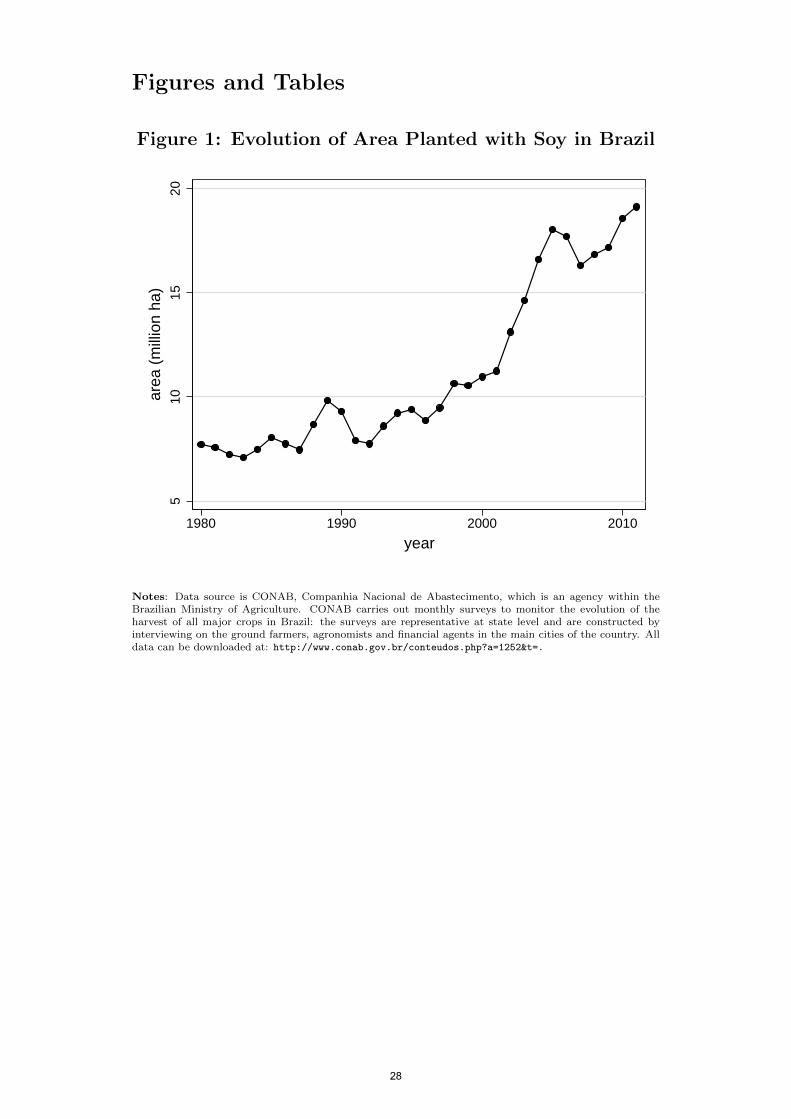
and 2006 (IBGE 2006, p.144). Similarly, Figure 1 shows that the area planted

with soy has been growing since the 1980s, and experienced a sharp accelera-

tion in the early 2000s.10

3 Data

The main data sources are the ESTBAN dataset from the Central Bank

of Brazil, the Agricultural Census and the PAM Survey from the National

Statistical Institute, the RAIS dataset from the Ministry of Labor, and the

6In 2003, Brazilian law 10.688 allowed the commercialization of GE soy for one harvestingseason, requiring farmers to burn all unsold stocks after the harvest. This temporary measurewas renewed in 2004. Finally, in 2005, law 11.105 – the New Bio-Safety Law – authorizedproduction and commercialization of GE soy in its Roundup Ready variety (art. 35).

7Since borders of municipalities changed over time, the Brazilian Statistical Institute(IBGE) has defined Area Mınima Comparavel (AMC), smallest comparable areas, whichare comparable over time and which we use as our unit of observation. In what follows, weuse the term municipality for AMC. Brazil has, in total, 4260 AMCs.

8We consider adopter a municipality with a positive amount of soy area cultivated withGE soy seeds in 2006

9Note that, as discussed in detail in Section 3, agricultural profits are only availableaggregated across all agricultural activities in a given municipality.

10Yearly data on area planted are from the CONAB survey. This is a survey of farmersand agronomists conducted by an agency of the Brazilian Ministry of Agriculture to mon-itor the annual harvests of major crops in Brazil. We use data from the CONAB surveypurely to illustrate the timing of the evolution of aggregate agricultural outcomes duringthe period under study. In the empirical analysis, instead, we rely exclusively on data fromthe Agricultural Censuses which covers all farms in the country and it is representative atmunicipality level.

9

Global Agro-Ecological Zones database from FAO.

The ESTBAN (Estatıstica Bancaria) dataset is updated monthly by the

Central Bank of Brazil and reports the main balance sheet items at branch level

of universal banks with commercial bank capabilities and commercial banks

operating in Brazil.11 We use data from 1996 to 2013 and compute yearly aver-

ages of the variables of interest for each branch. The main variables of interest

are total value of deposits and total value of loans originated by each branch.

We observe four main categories of deposits: checking accounts of individuals,

checking accounts of companies, savings accounts and term deposits. As for

loans, we observe three major categories: rural loans, which includes loans

to the agricultural sector; general purpose loans (emprestimos) to firms and

individuals, which includes: current account overdrafts, personal loans, ac-

counts receivable financing and special financing for micro-enterprises among

others; and specific purpose loans (financiamentos) which includes loans with

a specific objective, such as export financing, or acquisition of vehicles.

In 2003, the ESTBAN dataset covered 142 commercial and universal banks

operating in Brazil. Table 2 reports baseline information for the 10 largest

banks by number of branches. Two of these banks are controlled by the Fed-

eral Government (Banco do Brasil and Caixa Economica Federal), while the

others are privately owned. There is large heterogeneity in terms of geograph-

ical diffusion across banks in our sample: seven of the 10 largest banks are

present in all 27 Brazilian states, while 65 out of 142 banks in our sample are

present only in one state.12 Table 2 also reports an Herfindhal Index of geo-

graphical concentration of branches across states. As shown, banks controlled

by the Federal Government have a more even distribution of branches across

geographical areas (lower HHI)13 than private banks.

The Agricultural Census is released at intervals of 10 years by the Instituto

Brasileiro de Geografia e Estatıstica (IBGE), the Brazilian National Statistical

Institute. The empirical analysis focuses on the last two rounds of the census

which have been carried out in 1996 and in 2006. Data is collected through

direct interviews with the managers of each agricultural establishment and is

made available online by the IBGE aggregated at municipality level. The agri-

cultural variables of interest are the share of agricultural land planted with soy

– out of which we can distinguish the area planted with GE vs traditional soy

seeds –, the value of agricultural profits, the value of investments in agriculture

11ESTBAN is a confidential dataset of the Central Bank of Brazil. The collection andmanipulation of individual bank agency data were conducted exclusively by the staff of theCentral Bank of Brazil.

12Together, banks present only in one state represented 4.5% of all branches and 3.2% ofdeposits in 2003.

13An equal distribution of agencies across states would imply a HHI of approximately0.0370.

10

and the value of external financing. The measures of profits, investments and

external financing do not refer specifically to soy production but are aggregated

across all agricultural activities. This is because the unit of observation in the

census is the agricultural establishment, and establishments tend to perform

several agricultural activities.

The PAM (Producao Agrıcola Municipal) is a yearly survey covering infor-

mation on production of the main temporary and permanent crops in Brazil,

including soy. The survey is conducted at municipal level by the Instituto

Brasileiro de Geografia e Estatıstica (IBGE) through interviews with govern-

ment and private agricultural firms, local producers, technicians, and other

experts involved in the production and commercialization of agricultural prod-

ucts. The main variables of interest at municipality level are: area farmed and

total revenues accruing to producers for each crop covered in the survey.

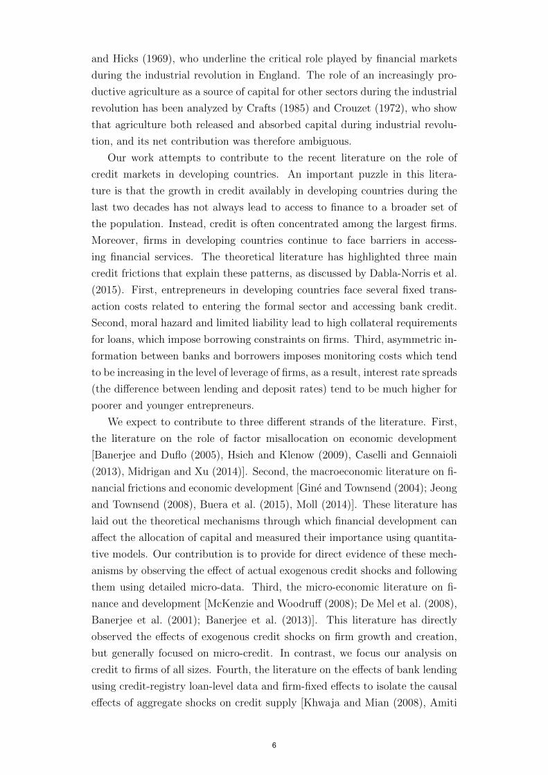
Finally, to construct our measure of exogenous change in soy profitability

we use estimates of potential soy yields across geographical areas of Brazil

from the FAO-GAEZ database. These yields are calculated by incorporating

local soil and weather characteristics into a model that predicts the maximum

attainable yields for each crop in a given area. In addition, the database reports

potential yields under different technologies or input combinations. Yields

under the low technology are described as those obtained planting traditional

seeds, no use of chemicals nor mechanization. Yields under the high technology

are obtained using improved high yielding varieties, optimum application of

fertilizers and herbicides and mechanization. Maps displaying the resulting

measures of potential yields for soy under each technology are contained in

Figures 4 and 5.

Finally, we use data on employment from the RAIS dataset (Relacao Anual

de Informcacoes Sociais) of the Brazilian Ministry of Labor. RAIS provides

information at individual level on all formal workers in Brazil, both in the pri-

vate and the public sector. Employers are required by law to provide detailed

worker information to the Ministry of Labor.14 RAIS reports information on

the sector, size and location of the firm for which each individual works for.

This allows us to construct measures of employment by firm size in each mu-

nicipality. We define employment in small, medium and large firms as the

total number of workers that are active on December 31st of each year and

are employed by firms with less than 20 employees, with between 20 and 249,

and with more than 250 employees respectively. We construct these measures

for each municipality in Brazil for the years from 1998 to 2013. The fact that

14See Decree n. 76.900, December 23rd 1975 (Brazil 1975). Failure to report can result infines. In practice, workers and employers have strong incentives to provide complete RAISrecords. RAIS is used by the Brazilian Ministry of Labor to identify workers entitled tounemployment benefits (Seguro Desemprego) and federal wage supplement program (AbonoSalarial).

11

RAIS only records formal employment is not a limitation for our empirical

analysis to the extent that firms that apply for loans in the banking sector

have to be registered firms.

Table 1 reports summary statistics of the main variables of interest used in

the empirical analysis.

4 Empirics

In this section we provide empirical evidence on the effects of the adoption

of GE soy seeds on the banking sector and firm growth. First, we investigate

the local effects of this new technology. By ”local” we mean the effects recorded

within the boundaries of the municipalities where GE soy was adopted. In

particular, we focus on agricultural profits, deposits in local bank branches,

and loans originated by the same local branches. Second, we investigate to

what extent local effects on bank deposits propagated to regions not directly

affected by the new technology through bank branch networks. To this end,

we first construct a measure of exposure to the GE-soy-driven deposit shock

exploiting bank branch networks. Then, we study the effect of exposure on

lending and firm growth.

In section 4.1 we describe our identification strategy. Next, in section 4.2,

we discuss the empirical results.

4.1 Identification Strategy

In this section we detail our empirical strategy to identify exogenous in-

creases in the supply of credit across regions in Brazil. This strategy proceeds

in two steps. First, we use variation in the potential profitability of GE soy

across areas in Brazil to identify its effect on local credit markets. For this

purpose, we exploit the fact that the introduction of GE seeds had a differen-

tial impact on agricultural profits to obtain exogenous variation in agricultural

profits. As the new technology had a differential impact on yields depending

on geographical and weather characteristics, we use differences in soil suitabil-

ity across regions as a source of cross-sectional variation. In addition, we use

the date of legalization of this technology in Brazil (2003) as a source of varia-

tion across time. In a second step, we exploit the bank branch network across

Brazilian regions to identify bank and branch-level exogenous increases in the

supply of funds. This permits to trace the flow of funds from soy produc-

ing (origin) municipalities to non-soy producing (destination) ones. In what

follows, we discuss each step in detail.

12

4.1.1 Identification of Local Effects

Let us first discuss the timing of legalization of GE soy seeds. GE soy

seeds were commercially released in the U.S. in 1996, and legalized in Brazil in

2003. Given that the seeds were developed in the U.S., their date of approval

for commercialization in the U.S., 1996, is arguably exogenous with respect to

developments in the Brazilian economy. In contrast, the date of legalization,

2003, responded partly to pressure from Brazilian farmers. In addition, smug-

gling of GE soy seeds across the border with Argentina is reported since 2001.15

Thus, in our empirical analysis we would ideally compare outcomes before and

after the first use of GE seeds in Brazil. For agricultural variables, we compare

outcomes across the last two Agricultural Censuses, which were carried out in

2006 and 1996. Since the 1996 Census pre-dates both legalization and the first

reports of smuggling, the timing can be considered exogenous. For variables on

bank outcomes sourced from ESTBAN, outcomes are observed yearly starting

from 1996. In our baseline regression we compare outcomes before and after

the official legalization of GE soy seeds in 2003.16

Second, the adoption of GE soy seeds had a differential impact on poten-

tial yields depending on soil and weather characteristics. Thus, we exploit

these exogenous differences in potential yields across geographical areas as our

source of cross-sectional variation in the intensity of the treatment. To im-

plement this strategy, we need an exogenous measure of potential yields for

soy, which we obtain from the FAO-GAEZ database. These potential yields

are estimated using an agricultural model that predicts yields for each crop

given climate and soil conditions. As potential yields are a function of weather

and soil characteristics, not of actual yields in Brazil, they can be used as a

source of exogenous variation in agricultural productivity across geographical

areas. Crucially for our analysis, the database reports potential yields under

different technologies or input combinations. Yields under the low technology

are described as those obtained using traditional seeds and no use of chemicals,

while yields under the high technology are obtained using improved seeds, op-

timum application of fertilizers and herbicides and mechanization. Thus, the

difference in yields between the high and low technology captures the effect of

moving from traditional agriculture to a technology that uses improved seeds

and optimum weed control, among other characteristics. We thus expect this

increase in yields to be a good predictor of the profitability of adopting GE

soy seeds.

15See the United States Department of Agriculture report: USDA 2001. On the smugglingof GE seeds across the Argentina-Brazil border, see also: Pelaez and Albergoni (2004),Benthien (2003) and Ortega et al. (2005).

16Using 2001 as the first year in which the new technology became available to Brazilianfarmers does not affect our results. Tables available upor request.

13

Finally, notice that our analysis is conducted at municipality level. There-

fore, even if Brazil is a major exporter of soy in global markets, individual

Brazilian municipalities can be considered small open economies for which

variations in the international price of soy are exogenous.

More formally, our baseline empirical strategy consists in estimating the

following equation:

yjt = αj + αt + β log(Asoyjt ) + εjt (1)

where yjt is an outcome that varies across municipalities and time, the sub-

script j identifies municipalities, t identifies years, αj are municipality fixed

effects, αt are time fixed effects and Asoyjt is defined as follows:

Asoyjt =

Asoy,LOWj for t < 2003

Asoy,HIGHj for t ≥ 2003

where Asoy,LOWj is equal to the potential soy yield under low inputs and

Asoy,HIGHj is equal to the potential soy yield under high inputs.

In the case of agricultural outcomes, our period of interest spans the ten

years between the last two censuses which took place in 1996 and 2006. We

thus estimate a first-difference version of equation (1):

∆yj = ∆α + β∆ log(Asoyjt ) + ∆εjt (2)

where the outcome of interest, ∆yj is the change in outcome variables between

the last two census years and:

∆ log(Asoyjt ) = log(Asoy,HIGH

j )− log(Asoy,LOWj )

A potential concern with our identification strategy is that, although the

soil and weather characteristics that drive the variation in Asoyjt across geo-

graphical areas are exogenous, they might be correlated with the initial levels

of development across Brazilian municipalities. In Table 3, upper panel, we

compare municipalities with different ∆ log(Asoyjt ) in terms of observable char-

acteristics in the initial period. As shown, municipalities with higher increase

in potential soy yield tend to display, on average, higher income per capita,

lower share of rural population and lower population density. Because these

differences are strongly significant, in what follows we control for differential

trends across municipalities with heterogeneous initial characteristics – includ-

ing the characteristics of banks that have branches in those municipalities – in

our baseline specification 1:

14

yjt = αj + αt + β log(Asoyjt )

+∑t

γt(Municipality controlsj,1991 × dt)

+∑t

δt(Bank controlsj,1996 × dt) + εjt (3)

where: Municipality controlsj,1991 is the set of initial municipality character-

istics presented in Table 3 and Bank controlsj,1996 is a weighted average of

observable characteristics of banks with branches in municipality j in the ini-

tial year (log value of assets, share of deposits over assets, and total number of

bank branches) where the weights are calculated as the number of branches of

bank b in municipality j over the total number of bank branches in municipality

j. We interact both sets of controls with year dummies dt.

4.1.2 Identification of Bank Network Effects

In this section, we detail how we use the structure of the bank branch

network across Brazilian regions to identify bank and branch-level exogenous

increases in the supply of credit. This permits to trace the flow of funds from

soy producing (origin) municipalities to non-soy producing (destination) ones.

To this end, we define our measure of municipality exposure to the increase in

credit supply due to the increased profitability of soy production. This measure

aims at capturing the extent to which banks in a given municipality are exposed

to the soy driven increase in deposits through their branch network. We start

by constructing a measure of exposure at bank level as follows:

Bank Exposurebt =∑j

ωbj,t=0 × Asoyjt

=∑j

(nbj

Nj

)t=0

× Asoyjt (4)

where j indexes municipality, nbj denotes the number of bank b’s branches

in municipality j and Nj =∑

b nbj is the total number of bank branches in

municipality j before the legalization of GE soy seeds (t = 0). Equation (4)

assumes that each bank receives a share of the increase in deposits driven by

GE soy profitability in municipality j that is proportional to its deposit market

share in that municipality, which we measure as its number of branches relative

to the total number of branches in the municipality. Note that we compute

this market share for the period before the legalization of GE seeds. This

ensures that we do not capture the opening of new branches in areas with

15

faster deposit growth due to the new technology. This new openings are more

likely to occur by banks which face larger demand for funds. Thus, focusing on

the pre-existing network ensures that we only capture an exogenous increase

in the supply of funds.

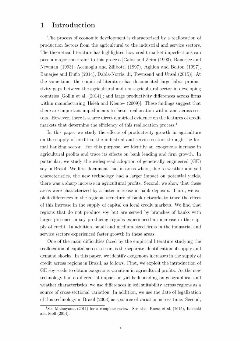
Bank exposure is a function of the geographical location of the branches

of each bank before the legalization of GE soy seeds, as well as the increase

in potential soy yields across these locations. To better illustrate the source

of variation in bank exposure, in Figure 3 we show the geographical location

of the branches of two Brazilian banks with different levels of exposure to GE

soy adoption. The Figure reports, for each bank, both the location of bank

branches across municipalities (red dots) and the increase in soy revenues in

each municipality during the period under study (darker green indicates a

larger increase). As shown, the branch network of bank A extends into areas

that experienced large increase in soy revenues following the legalization of GE

soy seeds. On the contrary, the branch network of bank B mostly encompasses

regions with no soy production.

Initial location of bank branches might be correlated with bank character-

istics as well as municipality characteristics. That is why, to construct bank

exposure, we do not use the actual increase in soy revenues but our exogenous

measure of potential increase in soy profitability, which only depends on soil

and weather characteristics. Additionally, in all our regressions we control

for both bank characteristics and municipality characteristics as reported in

equation 3.

Next, we define a measure of municipality exposure to GE-soy-driven de-

posit shock. We construct this measure only for municipalities that do not

produce soy, thus are not directly affected by technical change. Municipal-

ity exposure captures the extent to which banks located in a given non-soy

producing municipality are exposed to the GE-soy driven increase in credit

supply. In order to construct this measure at municipality level, we proceed

in two steps.

We start by assuming that bank’s internal capital markets are perfectly

integrated. This implies that deposits captured in a given municipality are

first centralized at the bank level and later distributed across bank branches.

Second, to keep exogeneity of the credit supply shock, we use a neutral assign-

ment rule for these funds across branches. That is, each bank divides these

funds equally across all its branches. As a result, a municipality’s share of the

increase in credit supply of bank b is given by the share of bank b’s branches

located in the municipality, as follows:

Municipality Exposurejbt =nbj

Nb

Bank Exposurebt (5)

16

where j indexes municipalities, nbj denotes the number of bank b’s branches

in municipality j and Nb =∑

j nbj is the total number of branches of bank b.

Note that we do not assume that banks allocate funds across branches

following the rule behind equation (5). In practice, banks might allocate funds

to respond optimally to credit demand, or can follow any other rule. We use

our “neutral” assignment rule to construct an instrument which identifies the

exogenous component in the actual increase in the supply of credit.

Finally, we define overall municipality exposure as the sum of its exposure

to each bank who has branches in the municipality:

Municipality Exposurejt = log∑b

Municipality Exposurejbt

= log∑b

nbj

Nb

Bank Exposurebt

= log∑b

nbj

Nb

∑j

nbj

Nj

× (Asoyjt ) (6)

4.2 Empirical Results

In the following sections we report the results of our empirical analysis.

We start by reporting estimates of the effect of potential soy profitability on

GE soy adoption in section 4.2.1 and on agricultural profits, investment and

external finance in section 4.2.2. Then, we study the effect of potential soy

profitability on local bank deposits and bank credit in section 4.2.3. Finally,

we study the effect of municipality exposure on bank credit and firm growth

outside soy-producing regions in section 4.2.4.

4.2.1 Local Effects: Soy Expansion and GE Soy Adoption

In this section we test the relationship between potential soy profitability at

municipality level, and the actual expansion of soy area as well as the adoption

of GE soy seeds by Brazilian farmers during the period under study.

We start by testing whether our measure of exogenous change in soy prof-

itability predicts actual expansion of soy area as a fraction of agricultural area.

To this end, we estimate equation (3) where the outcome of interest, yjt is the

area cultivated with soy in municipality j at time t from the PAM Survey

divided by the total initial agricultural area (as observed in the Agricultural

Census of 1996). Columns 1 and 2 of Table 4 report the results. The point

estimates of the coefficients on log(Asoyjt ) are positive, indicating that an in-

crease in potential soy profitability predicts the expansion soy area as a share

17

of agricultural area during the period under study. The estimated coefficient is

equal to .015 when including controls, as shown in column 2. The magnitude

of the estimated coefficients implies that a one standard deviation difference

in log(Asoyjt ) implies a 1.7 percentage points higher increase in the share of soy

area over agricultural area during the period under study.

Next, we test whether increases in our measure of exogenous change in soy

profitability predicts actual adoption of the new technology. To this end, we

estimate equation (2) where the outcome of interest, ∆yj is the change in the

share of agricultural land devoted to GE soy between 1996 and 2006. Note

that because this share was zero everywhere in 1996, the change in the share

of agricultural land corresponds to its level in 2006.

Column 3 of Table 4 reports the estimated coefficients. The point estimate

of the coefficient on ∆ log(Asoyjt ) is positive, indicating that an increase in po-

tential soy profitability predicts the expansion in GE soy area as a share of

agricultural area between 1996 and 2006. Estimates are precisely estimated

and remain stable when including initial municipality characteristics, as shown

in column 2. In column 4 we perform a falsification test by looking at whether

our measure of potential soy profitability explains the expansion in the area

planted with non-GE soy. In this case, the estimated coefficient on ∆ log(Asoyjt )

is negative and significant. This finding supports our interpretation that the

measure of potential soy profitability captures the benefits of adopting GE soy

vis-a-vis traditional soy seeds.

4.2.2 Local Effects: Soy Revenues, Agricultural Profits, Investment

and Use of External Finance

In section 4.2.1 we showed that our exogenous measure of soy profitability

is a good predictor of soy expansion and GE seeds adoption. In this section

we investigate its effect on revenues for soy producers, agricultural profits,

investment and external finance.

We start by testing whether our measure of exogenous change in soy prof-

itability predict actual revenues from soy production. We estimate equation

(3) where the outcome of interest, yjt is the monetary value of revenues from

soy production in municipality j at time t from the PAM Survey. Columns 1

and 2 of Table 5 report the results. The point estimates of the coefficients on

log(Asoyjt ) are positive, indicating that an increase in potential soy profitability

predicts an increase in revenues from soy production during the period under

study. The estimated coefficient remains stable and statistically significant

when including controls, as shown in column 2. The magnitude indicates that

a one standard deviation difference in log(Asoyjt ) implies a 23% higher increase

in revenues from soy production.

18

Next, we test whether increases in our measure of exogenous change in soy

profitability predict agricultural profits, investment and use of external finance.

These outcomes are sourced from the Agricultural Census of 1996 and 2006.

Therefore, we estimate equation (2), where ∆yj is the change in agricultural

outcomes between 1996 and 2006.

In column 3 of Table 5 the outcome variable is the change in agricultural

profits. The point estimate on ∆ log(Asoyjt ) indicates that municipalities with

a larger increase in our measure of exogenous change in soy profitability expe-

rienced a larger increase in agricultural profits. In particular, a one standard

deviation increase in potential soy profitability corresponds to a 21.6% increase

in agricultural profits between 1996 and 2006. Next, we estimate the same

equation using as outcomes the change in agricultural investment and external

finance. The estimated coefficient on ∆ log(Asoyjt ) when the outcome is agricul-

tural investment is positive and significant. The magnitude indicates that a

one standard deviation increase in potential soy profitability corresponds to a

7.1% increase in agricultural profits between 1996 and 2006. These coefficients

imply that for every R$10 of increase in profits around R$1.4 are reinvested

in agricultural activities. Interestingly, the total value of external finance is

unaffected by soy profitability.

4.2.3 Local Effects: Bank Deposits and Credit

In sections 4.2.1 and 4.2.2 we showed that our exogenous measure of soy

profitability is a good predictor of both the adoption of GE soy seeds and the

change in agricultural profits. Additionally, we showed that only a fraction of

the increase in agricultural profits was re-invested in agricultural activities. In

what follows, we investigate what was the use of the remaining agricultural

profits. In principle, they could have been channeled to consumption or to

savings. In the second case, they could have been invested locally, nationally

or internationally. Finally, investments could have taken the form of informal

lending arrangements or could have been channeled through the banking sec-

tors. To understand these issues, we investigate the effect of our exogenous

measure of soy profitability on deposits in local bank branches and on loans

originated by the same bank branches. We estimate equation (3) where yj is

the level of bank deposits or bank loans originated by bank branches located in

municipality j. Data on bank outcomes is sourced from the ESTBAN dataset

and it is therefore available yearly from 1996 to 2013.

Table 6 reports the results when the outcome variable is bank deposits.

First, we study the effect of our exogenous measure of soy profitability on

total bank deposits, which we define as the sum of demand deposits, saving

deposits and term deposits. The estimates are reported in column 1 of Table

19

6. It indicates that municipalities with higher increase in soy profitability

experienced a larger increase in total bank deposits during the period under

study. The magnitude of the effect is economically significant: the estimated

coefficient in column (2) indicates that a municipality with a one standard

deviation higher potential soy profitability experienced a 5.4% larger increase

in total bank deposits (3% of a standard deviation). Next, we study whether

this effect varies for different types of bank deposits. Results are reported

in columns 2 and 3 of Table 6 for demand and saving accounts and for term

deposits respectively. The estimated coefficients on log(Asoyjt ) indicate that the

effect of potential soy profitability on deposit is concentrated on demand and

saving deposits. Demand deposits are unremunerated, while savings account

are remunerated at a rate that is lower than the interbank rate (around half).

As such, these deposits constitute a cheap source of financing for Brazilian

banks. On the other hand, we find no effect on term deposits.

Table 7 reports the results of estimating equation (3) when the outcome

variable yjt is value of loans originated by bank branches located in munic-

ipality j. We study the effect of our exogenous measure of soy profitability

on agriculture loans, and the two categories of non-agriculture loans: general-

purpose and specific-purpose loans. The estimates are reported in columns 1,

2 and 3 of Table 7. As shown, we find that soy profitability had a negative

effect on loans to the agricultural sector. This is consistent with farmers fi-

nancing new investment with retained profits rather than bank credit in areas

with larger increase in potential soy profitability. The estimated coefficient on

log(Asoyjt ) is negative for general purpose loans and small in size and statistically

not different from zero for specific purpose loans.

4.2.4 Bank Network Effects: Bank Credit

In section 4.2.3 we showed that municipalities that are predicted to adopt

GE soy experienced larger increases in agricultural profits and bank deposits

in local branches during the period under study. At the same time, we find

no evidence of a positive effect of our exogenous measure of soy profitability

on local credit supply. A possible explanation of this finding is that banks’

internal capital markets are integrated within the country, as we document in

what follows.

In this section we explore whether larger increases in deposits in soy-

producing areas of Brazil affect credit supply in non soy-producing areas

through bank branch networks. To this end, we use the measure of munic-

ipality exposure described in section 4.1.2 and estimate the following version

of equation 3:

20

yjt = αj + αt + β(Municipality Exposure)jt

+∑t


+∑t


where Municipality Exposurejt is defined as in equation (6). As in equation

(3), we add controls for municipality and bank initial characteristics interacted

with time dummies.17

Table 8 reports the results obtained estimating equation 7 when the out-

come variables yjt are: rural loans, general purpose and specific purpose loans.

We estimate this equation on the subsample of non-soy producing municipal-

ities.18 The estimated coefficients on municipality exposure are positive and

precisely estimated, indicating that areas more exposed to the GE-soy-driven

deposit shock through their bank networks experienced a larger increase in

both agriculture and non-agriculture lending. To illustrate the magnitude of

these coefficients, consider two non-soy producing municipalities that are one

standard deviation apart in terms of exposure to the GE-soy-driven credit

supply shock. The point estimates indicates that the municipality with a one

standard deviation higher exposure experienced a 31% larger increase in agri-

culture loans (15.2% of a standard deviation), a 26.8% larger increase in general

purpose loans (13.3% of a standard deviation) and a 23.8% larger increase in

specific purpose loans (10.8% of a standard deviation).

4.2.5 Bank Network Effects: Firm Growth

In section 4.2.4 we showed that bank branches in municipalities with higher

exposure to the GE-soy driven deposit shock experienced higher increase in

lending. We now test the effect of municipality exposure to the same shock

on firm growth. To this end, we estimate equation (7) where the outcome

variable yjt is total employment (in logs) in municipality j at time t. Data on

employment is sourced from the RAIS, and covers formal workers in all sectors

over the years 1998 to 2013.19 RAIS allows us to distinguish between workers

employed in firms of different size. In addition to total number of workers, we

17Table 3, lower panel, compares non-soy producing municipalities with different levelsof exposure to the soy boom through their bank networks in terms of initial municipalitycharacteristics.

18Non-soy municipalities are defined as municipalities with no area cultivated with soy inany of the years under study.

19As discussed above, even though a substantial fraction of Brazilian firms operate in theinformal economy, firms that apply for loans at commercial banks tend to be registered.

21

construct total employment in small, medium and large firms.20

Table 9 reports the results of our analysis. As in Table 8, we restrict our

sample to non-soy producing municipalities. Column 1 reports the results

when the outcome is total employment. The estimated coefficient on munic-

ipality exposure is positive and significant, indicating that firms operating in

areas that were more exposed to the GE-soy-driven deposit shock through

their bank networks experienced a larger increase in employment. The point

estimate indicates that firms located in municipalities with a one standard

deviation higher exposure experienced a 13.4% larger increase in employment.

In columns 2 to 4 we estimate the same equation when the outcomes are total

employment in small, medium and large firms respectively. As shown, the

effect of municipality exposure on firm growth is concentrated in small and

medium sized firms. On the other hand, the point estimate on municipality

exposure when the outcomes is employment in large firms is small and not

statistically different from zero.

5 Additional Results and Robustness

In this section we show additional results and robustness tests for the main

results presented in section 4.2. First, we investigate whether our exogenous

measure of soy profitability captures the right timing of the introduction of

GE soy seeds. Second, we test the robustness of our results to the exclusion of

the two major government controlled banks from our sample, and to the use

of bank conglomerates instead of individual banks as unit of observation.

When we estimate equation (3) as described in section 4 we implicitly

assume that soy production experienced technical change in 2003. This is

because the technological component of our exogenous measure of soy prof-

itability (Asoyjt ) is assumed to change from its level under low inputs to its level

under high inputs in correspondence with the legalization of GE soy seeds in

Brazil. Since bank outcomes are available at yearly level, we can investigate

whether our exogenous measure of soy profitability captures the right timing

20Small firms are those with less than 25 workers employed on December 31st of eachyear. Medium firms have between 25 and 249 workers, while large firms have 250 or moreworkers.

22

of the introduction of GE soy seeds by running the following equation:21

yjt = αj + αt +∑t

βt(∆ log(Asoyj )× dt)

+∑t


+∑t


where ∆ logAsoyj is a time invariant measure of the change in potential yield

when soy production switches from low to high inputs. More formally:

∆ logAsoyj = log(Asoy,HIGH

j )− log(Asoy,LOWj )

In Figure 2 we plot the estimated βt coefficients along with their 95% confidence

intervals when the outcome variables are: soy area as a share of agricultural

area (left graph) and total bank deposits (right graph). The timing of the

effect of ∆Asoyj on both outcomes is broadly consistent with capturing the

effect of the legalization of GE soy seeds. However, as shown, the estimated

βt coefficients are positive and statistically different from zero starting from

2002. This indicates that the positive effect of potential soy profitability on

the expansion of soy area and total bank deposits started before the official

legalization of GE soy seeds in 2003. One potential explanation is that, prior to

legalization, smuggling of GE soy seeds from Argentina was detected since 2001

according to the Foreign Agricultural Service of the United States Department

of Agriculture (USDA 2001).

Next, we test the robustness of our main results on bank deposits and

credit to the exclusion of the two major government controlled banks in our

sample: Banco do Brasil and Caixa Economica Federal. One potential concern

is that these banks might follow different lending policies than private com-

mercial banks. Table A1 replicates the results presented in Tables 6, 7 and 8 in

the paper when excluding government controlled banks from our sample. As

shown, all the main results are robust to this test in the sense that (i) munic-

ipalities with higher increase in soy profitability experienced a larger increase

in total bank deposits, (ii) the same municipalities experienced no increase in

total bank credit at local level (if anything, lending decreased) (iii) non-soy

producing municipalities that are more exposed to the GE-soy-driven deposit

shock through their bank networks experienced a larger increase in lending.22

Finally, we test to what extent our main results depend on the use of bank

21The same test cannot be performed for agricultural outcomes, which we only observe incorrespondence of the Agricultural Census.

22In an additional test not reported in this draft we also show that all our main resultsare robust to excluding capital cities from our sample.

23

conglomerates instead of individual banks as units of observation. So far, we

considered each individual bank that we observe in the pre-soy boom period

as a separate branch network during the whole period under study. This is

because banks with a network of branches in rural areas more exposed to the

soy boom might be the target of mergers and acquisitions by banks with better

investment opportunities and in search of cheap source of financing, making

the branch network endogenous to the soy shock. In Table A2 we show that the

results presented in Table 8 are similar to those obtained taking into account

these M&A activity and using the bank branch network of bank conglomerates.

6 Concluding Remarks

In this paper we study the effect of new agricultural technologies on re-

allocation of capital across sectors. The empirical analysis is focused on the

widespread adoption of genetically engineered (GE) soy in Brazil. This tech-

nology allows farmers to obtain the same yield with lower production costs,

thus increasing agricultural profits.

We find that municipalities that are predicted to experience a larger in-

crease in soy profitability after the legalization of GE soy seeds are more likely

to adopt this new technology and experience a larger increase in agricultural

profits. At local level, we find a positive effect of GE soy adoption on deposits

in local bank branches but no significant change in loans originated by the same

bank branches. We then explore whether larger increases in bank deposits in

soy-producing areas of Brazil affect credit supply in non soy-producing areas

through bank branch networks. We find that regions of Brazil that were more

exposed to the GE-soy-driven deposit shock through bank branch networks

experienced a larger increase in bank lending and larger firm growth, where

the latter effect is concentrated in small and medium size firms.

24

References

Acemoglu, D. and F. Zilibotti (1997). “Was Prometheus Unbound by Chance?Risk, Diversification, and Growth”. Journal of political economy 105 (4),709–751.

Aghion, P. and P. Bolton (1997). “A Theory of Trickle-Down Growth andDevelopment”. The Review of Economic Studies 64 (2), 151–172.

Amiti, M. and D. Weinstein (2011). Exports and financial shocks. The Quar-terly Journal of Economics 126 (4), 1841–1877.

Bagehot, W. (1888). Lombard Street: A description of the money market.Kegan, Paul & Trench.

Banerjee, A. and E. Duflo (2005). “Growth Theory Through the Lens ofDevelopment Economics”. Handbook of Economic Growth 1, 473–552.

Banerjee, A., D. Karlan, and J. Zinman (2001). Six randomized evaluations ofmicrocredit: Introduction and further steps. American Economic Journal:Applied Economics 7 (1), 1–21.

Banerjee, A. V. and E. Duflo (2014). “Do Firms Want to Borrow More?Testing Credit Constraints Using a Directed Lending Program”. The Reviewof Economic Studies 81 (2), 572–607.

Banerjee, A. V., E. Duflo, R. Glennerster, and C. Kinnan (2013). The miracleof microfinance? evidence from a randomized evaluation.

Banerjee, A. V. and A. F. Newman (1993). “Occupational Choice and theProcess of Development”. Journal of political economy , 274–298.

Becker, B. (2007). Geographical segmentation of us capital markets. Journalof Financial economics 85 (1), 151–178.

Benthien, P. F. (2003). As sementes trangenicas no brasil: da proibicao aliberacao. Revista Vernaculo 1.

Brazil (1975). Decree N. 76,900.

Buera, F. J., J. P. Kaboski, and Y. Shin (2015). “Entrepreneurship and Fi-nancial Frictions: A Macro-Development Perspective”.

Bustos, P., B. Caprettini, and J. Ponticelli (2016). “Agricultural Productivityand Structural Transformation: Evidence from Brazil”. American EconomicReview, forthcoming .

Caselli, F. and N. Gennaioli (2013). Dynastic management. Economic In-quiry 51 (1), 971–996.

Crafts, N. F. (1985). British economic growth during the industrial revolution.Clarendon Press Oxford.

Crouzet, F. (1972). Capital Formation in the Industrial Revolution. Methuen.

25

Dabla-Norris, E., Y. Ji, R. M. Townsend, and D. F. Unsal (2015). “Distin-guishing Constraints on Financial Inclusion and Their Impact on GDP, TFP,and Inequality”. NBER Working Paper (20821).

De Mel, S., D. McKenzie, and C. Woodruff (2008). Returns to capital inmicroenterprises: evidence from a field experiment. The Quarterly Journalof Economics , 1329–1372.

Drechsler, I., A. Savov, and P. Schnabl (2014). “The Deposits Channel ofMonetary Policy”. Working Paper .

Duffy, M. and D. Smith (2001). “Estimated Costs of Crop Production in Iowa”.Iowa State University Extension Service FM1712.

Fernandez-Cornejo, J. and M. Caswell (2006). “The First Decade of Geneti-cally Engineered Crops in the United States”. United States Department ofAgriculture, Economic Information Bulletin 11.

Fernandez-Cornejo, J., C. Klotz-Ingram, and S. Jans (2002). “EstimatingFarm-Level Effects of Adopting Herbicide-Tolerant Soybeans in the USA”.Journal of Agricultural and Applied Economics 34, 149–163.

Galor, O. and J. Zeira (1993). “Income Distribution and Macroeconomics”.The review of economic studies 60 (1), 35–52.

Gilje, E. (2011). “Does Local Access to Finance Matter? Evidence from USOil and Natural Gas Shale Booms”. Working paper .

Gilje, E., E. Loutskina, and P. E. Strahan (2013). “Exporting Liquidity:Branch Banking and Financial Integration”. NBER Working paper .

Gine, X. and R. M. Townsend (2004). “Evaluation of financial liberalization:a general equilibrium model with constrained occupation choice”. Journalof Development Economics 74 (2), 269–307.

Gollin, D., D. Lagakos, and M. E. Waugh (2014). “The Agricultural Produc-tivity Gap”. Quarterly Journal of Economics .

Hicks, J. R. (1969). A theory of economic history. OUP Catalogue.

Hsieh, C. and P. Klenow (2009). “Misallocation and Manufacturing TFP inChina and India”. Quarterly Journal of Economics 124 (4), 1403–1448.

Huggins, D. R. and J. P. Reganold (2008). “No-Till: the Quiet Revolution”.Scientific American 299, 70–77.

IBGE (2006). “Censo Agropecuario 2006”. Rio de Janeiro, Brazil: InstitutoBrasileiro de Geografia e Estatıstica (IBGE).

Itskhoki, O. and B. Moll (2014). “Optimal development policies with financialfrictions”. Technical report, National Bureau of Economic Research.

Iyer, R., J.-L. Peydro, S. da Rocha-Lopes, and A. Schoar (2013). Interbankliquidity crunch and the firm credit crunch: Evidence from the 2007–2009crisis. Review of Financial studies , hht056.

26

Jeong, H. and R. M. Townsend (2008). “Growth and inequality: Model evalu-ation based on an estimation-calibration strategy”. Macroeconomic dynam-ics 12 (S2), 231–284.

Khwaja, A. I. and A. Mian (2008). Tracing the impact of bank liquidity shocks:Evidence from an emerging market. The American Economic Review , 1413–1442.

Levine, R. (2005). “Finance and Growth: Theory and Evidence”. Handbookof Economic Growth 1, 865–934.

Matsuyama, K. (2011). “Imperfect Credit Markets, Household Wealth Distri-bution, and Development”. Annu. Rev. Econ. 3 (1), 339–362.

McKenzie, D. and C. Woodruff (2008). Experimental evidence on returnsto capital and access to finance in mexico. The World Bank EconomicReview 22 (3), 457–482.

Midrigan, V. and D. Y. Xu (2014). Finance and misallocation: Evidence fromplant-level data. American Economic Review 104 (2), 422–58.

Moll, B. (2014). Productivity losses from financial frictions: Can self-financingundo capital misallocation? The American Economic Review 104 (10),3186–3221.

Ortega, E., O. Cavalett, R. Bonifacio, and M. Watanabe (2005). Braziliansoybean production: emergy analysis with an expanded scope. Bulletin ofScience, Technology & Society 25 (4), 323–334.

Pelaez, V. and L. Albergoni (2004). Barreiras tecnicas comerciais aostransgenicos no brasil: a regulacao nos estados do sul. Indicadoreseconomicos FEE 32 (3), 201–230.

Petersen, M. A. and R. G. Rajan (2002). “Does Distance Still Matter? TheInformation Revolution in Small Business Lending”. The Journal of Fi-nance 57 (6), 2533–2570.

Schnabl, P. (2012). The international transmission of bank liquidity shocks:Evidence from an emerging market. The Journal of Finance 67 (3), 897–932.

USDA (2001). “Agriculture in Brazil and Argentina: Developments andProspects for Major Field Crops”. United States Department of Agricul-ture, Economic Research Service.

USDA (2012). “Agricultural Biotechnology Annual”. United States Depart-ment of Agriculture, Economic Research Service.

27

Figures and Tables

Figure 1: Evolution of Area Planted with Soy in Brazil

510

1520

area

(m

illio

n ha

)

1980 1990 2000 2010

year

Notes: Data source is CONAB, Companhia Nacional de Abastecimento, which is an agency within theBrazilian Ministry of Agriculture. CONAB carries out monthly surveys to monitor the evolution of theharvest of all major crops in Brazil: the surveys are representative at state level and are constructed byinterviewing on the ground farmers, agronomists and financial agents in the main cities of the country. Alldata can be downloaded at: http://www.conab.gov.br/conteudos.php?a=1252&t=.

28

http://www.conab.gov.br/conteudos.php?a=1252&t=.

Figure 2: Increase in Potential Soy Yield and Timing of Soy Expansion and Bank Deposits

(a) Soy Expansion

-.01

-.00

50

.005

.01

.015

.02

.025

Coe

ffici

ent e

stim

ates

and

95%

CI

2000 2005 2010 2015year

(b) Bank Deposits

-.05

0.0

5.1

.15

.2C

oeffi

cien

t est

imat

es a

nd 9

5% C

I

2000 2005 2010 2015year

Notes: Data from Central Bank of Brazil and PAM (IBGE).

29

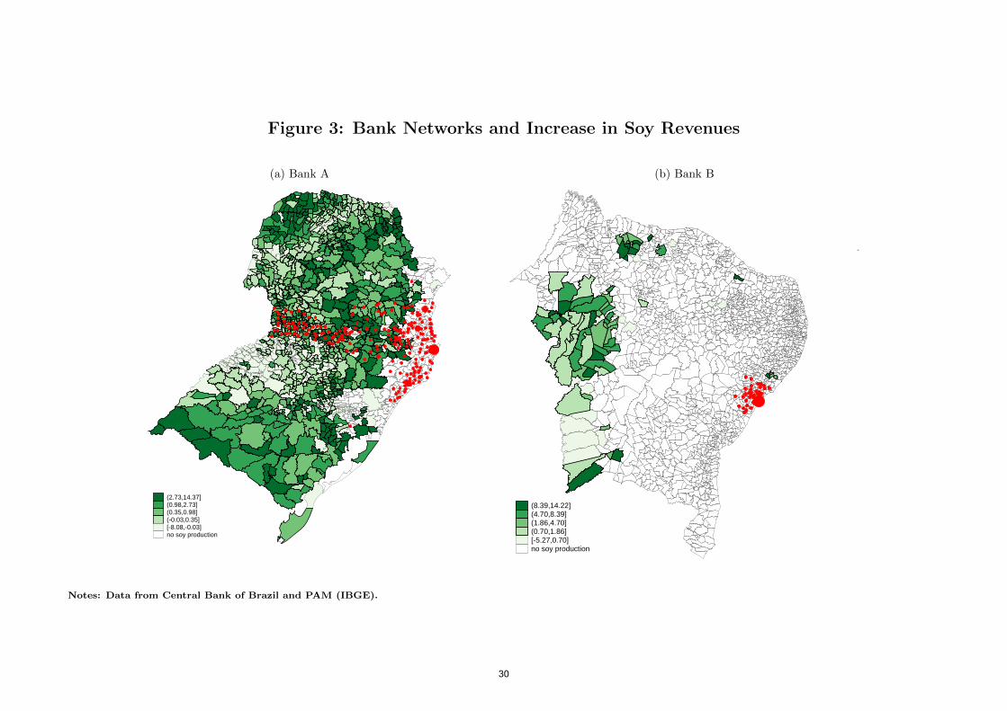
Figure 3: Bank Networks and Increase in Soy Revenues

(a) Bank A

(2.73,14.37](0.98,2.73](0.35,0.98](-0.03,0.35][-8.08,-0.03]no soy production

(b) Bank B

(8.39,14.22](4.70,8.39](1.86,4.70](0.70,1.86][-5.27,0.70]no soy production

Notes: Data from Central Bank of Brazil and PAM (IBGE).

30

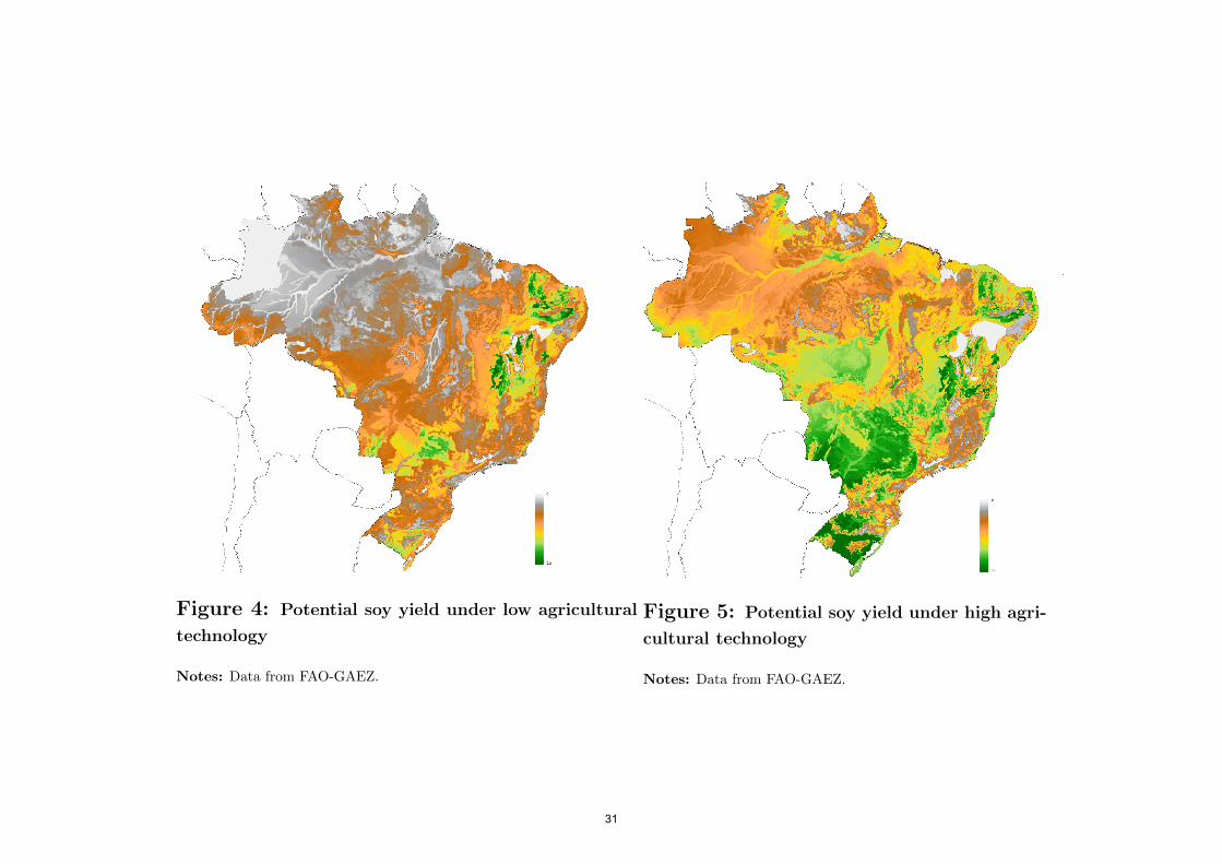
Figure 4: Potential soy yield under low agricultural

technology

Notes: Data from FAO-GAEZ.

Figure 5: Potential soy yield under high agri-

cultural technology

Notes: Data from FAO-GAEZ.

31

Table 1: Summary Statistics

Variable Name mean st.dev. N

Agricultural outcomes (changes 2006-1996):∆ GE Soy Area Share 0.013 0.059 3,749∆ Non-GE Soy Area Share -0.002 0.053 3,749∆ Profits (%) -0.288 6.111 3,794∆ Log Investment 0.158 0.868 3,794∆ Log External Finance 1.113 1.369 3,794

Banking sector outcomes:Log Demand Deposits 13.554 0.983 56,594Log Saving Deposits 15.806 0.709 54,575Log Term Deposits 14.745 1.398 51,364Log Rural Loans 13.189 1.509 46,773Log General Purpose Loans 15.414 0.919 56,633Log Specific Purpose Loans 13.447 1.182 48,895

Firm outcomes:Log Number of Workers - All Firms 6.882 1.874 26741

Small Firms 6.430 1.569 26741Medium Firms 6.014 2.125 26741Large Firms 5.510 3.237 26741

Potential Soy Profitability and Municipality Exposure:∆ log(Asoy) 1.451 0.459 3,794log(Asoy) 5.567 1.289 56,764Municipality Exposure 4.630 1.184 28,321

Notes: Sources are the Agricultural Censuses of 1996 and 2006 (agricultural outcomes); the ESTBAN

dataset, years 1996 to 2013 (banking sector outcomes); the RAIS, years 1998 to 2013 (firm outcomes); the

FAO-GAEZ dataset and IMF Primary Commodity Prices database (potential soy profitability)

32

Table 2: Bank Characteristics10 Largest Banks by Number of Branches in 2003

Bank Name N Branches Branch Deposit N States HHI ControlShare Share Present

Banco Do Brasil 3,291 17.8% 18.6% 27 0.08 Federal GovermentBanco Bradesco 2,823 15.3% 10.9% 27 0.17 PrivateBanco Itau 1,713 9.3% 4.7% 27 0.19 PrivateCaixa Economica Federal 1,598 8.7% 17.6% 27 0.11 Federal GovermentHSBC Bank Brasil S.A. - Banco Multiplo 942 5.1% 3.2% 27 0.16 PrivateUnibanco 904 4.9% 5.3% 24 0.23 PrivateBanco Sudameris Brasil S.A. 888 4.8% 4.3% 25 0.31 PrivateBanco Alvorada S.A. 880 4.8% 2.0% 27 0.17 PrivateBanco Abn Amro Real S.A. 793 4.3% 4.0% 27 0.20 PrivateBanespa∗ 598 3.2% 2.3% 17 0.87 Private

Notes: Source is the ESTBAN dataset, data refers to year 2003. ∗ Belonging to the Santander Group.

33

Table 3: Comparing Municipalities

∆ logAsoyj

below above level ofmedian median difference significance

(1) (2) (3) (4)

Log Income per capita 4.557 4.820 0.263 ***Share rural population 0.468 0.355 -0.114 ***Literacy rate 0.730 0.786 0.056Log Population Density 3.316 3.304 -0.012 ***

∆Municipality Exposurebelow above level of

median median difference significance(1) (2) (3) (4)

Log Income per capita 4.556 4.488 -0.068 **Share rural population 0.437 0.400 -0.036 ***Literacy rate 0.730 0.681 -0.049 ***Log Population Density 3.623 3.959 0.337 ***

Notes: Average values of observable characteristics of municipalities that rank below and above the median

of ∆ logAsoy and ∆Municipality Exposure. ∆ log(Asoyjt ) is computed as log(Asoy,HIGH

j )− log(Asoy,LOWj ).

Municipality exposure is computed as the average (across years) municipality exposure in the years from

2003 onwards minus the average (across years) municipality exposure in the years before 2003. Municipality

exposure is defined as in equation (5) in the paper. Initial municipality characteristics refer to year 1991

(source: Population Census). Column (3) reports the difference between columns (2) and (1), along with the

standard error and significance level of the difference. Significance levels: *** p<0.01, ** p<0.05, * p<0.1.

34

Table 4: Potential Soy Profitability and Agricultural OutcomesSoy Expansion and Adoption of GE seeds

Dependent variables: Soy AreaAgricultural Area ∆ GE Soy Area

Agricultural Area ∆Non-GE Soy AreaAgricultural Area

(1) (2) (3) (4)

log(Asoyjt ) 0.016 0.015

[0.002]*** [0.002]***∆ log(Asoy

j ) 0.028 -0.014

[0.002]*** [0.002]***

Municipality controls j,1991 × t Y YBank Controls j,1996 × t YMunicipality controls j,1991 Y Y

Year fixed effects Y YAMC fixed effects Y Y

Observations 53,203 53,203 3,749 3,749Adjusted R-squared 0.952 0.952 0.136 0.037N clusters (AMC) 3177 3177 3,749 3,749

Data source dep.var. : PAM PAM Agricultural Census1996-2013 1996-2013 1996 and 2006

Notes: Standard errors clustered at AMC level are reported in brackets. Significance levels: *** p<0.01, ** p<0.05, * p<0.1.

35

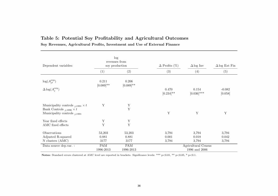
Table 5: Potential Soy Profitability and Agricultural OutcomesSoy Revenues, Agricultural Profits, Investment and Use of External Finance

logrevenues from

Dependent variables: soy production ∆ Profits (%) ∆ log Inv ∆ log Ext Fin

(1) (2) (3) (4) (5)

log(Asoyjt ) 0.211 0.206

[0.089]** [0.089]**∆ log(Asoy

j ) 0.470 0.154 -0.082

[0.234]** [0.036]*** [0.058]

Municipality controls j,1991 × t Y YBank Controls j,1996 × t YMunicipality controls j,1991 Y Y Y

Year fixed effects Y YAMC fixed effects Y Y

Observations 53,203 53,203 3,794 3,794 3,794Adjusted R-squared 0.881 0.881 0.001 0.018 0.042N clusters (AMC) 3177 3177 3,794 3,794 3,794

Data source dep.var. : PAM PAM Agricultural Census1996-2013 1996-2013 1996 and 2006

Notes: Standard errors clustered at AMC level are reported in brackets. Significance levels: *** p<0.01, ** p<0.05, * p<0.1.

36

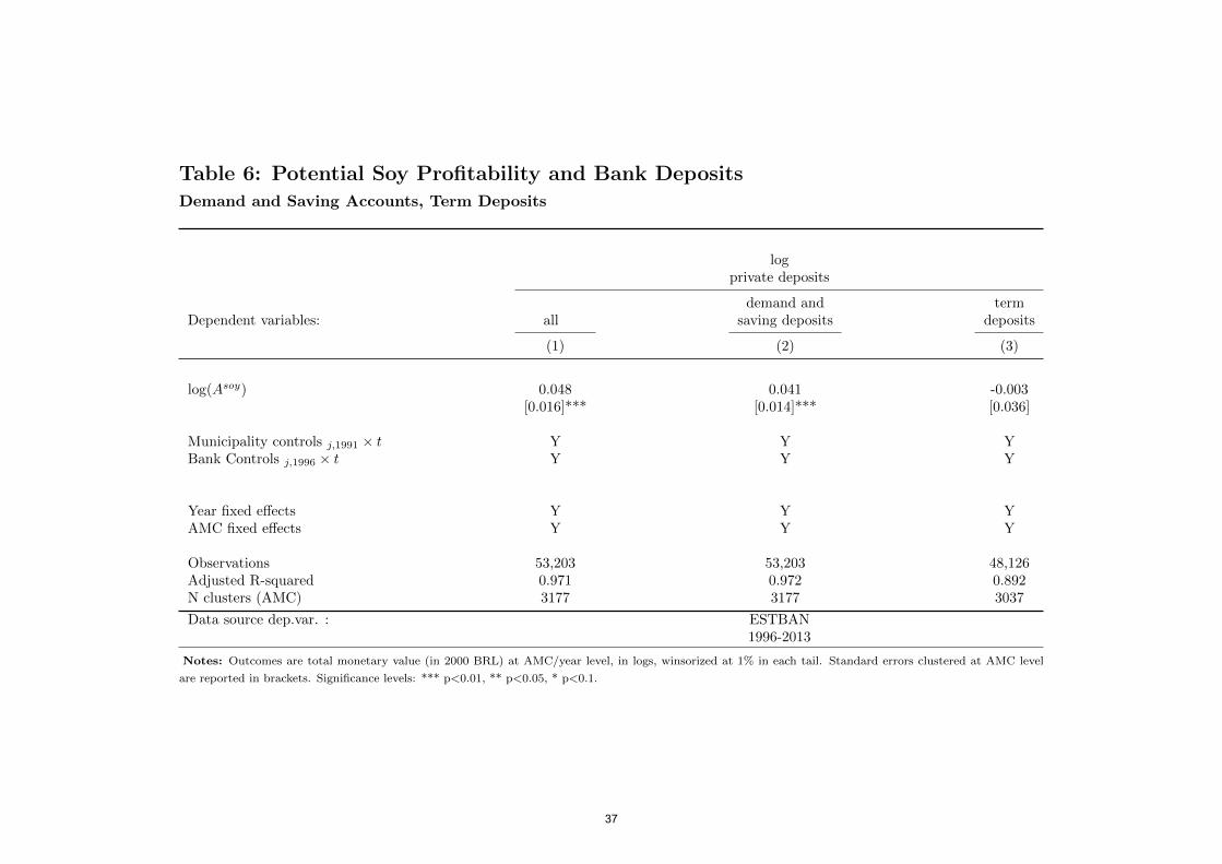
Table 6: Potential Soy Profitability and Bank DepositsDemand and Saving Accounts, Term Deposits

logprivate deposits

demand and termDependent variables: all saving deposits deposits

(1) (2) (3)

log(Asoy) 0.048 0.041 -0.003[0.016]*** [0.014]*** [0.036]

Municipality controls j,1991 × t Y Y YBank Controls j,1996 × t Y Y Y

Year fixed effects Y Y YAMC fixed effects Y Y Y

Observations 53,203 53,203 48,126Adjusted R-squared 0.971 0.972 0.892N clusters (AMC) 3177 3177 3037

Data source dep.var. : ESTBAN1996-2013

Notes: Outcomes are total monetary value (in 2000 BRL) at AMC/year level, in logs, winsorized at 1% in each tail. Standard errors clustered at AMC level

are reported in brackets. Significance levels: *** p<0.01, ** p<0.05, * p<0.1.

37

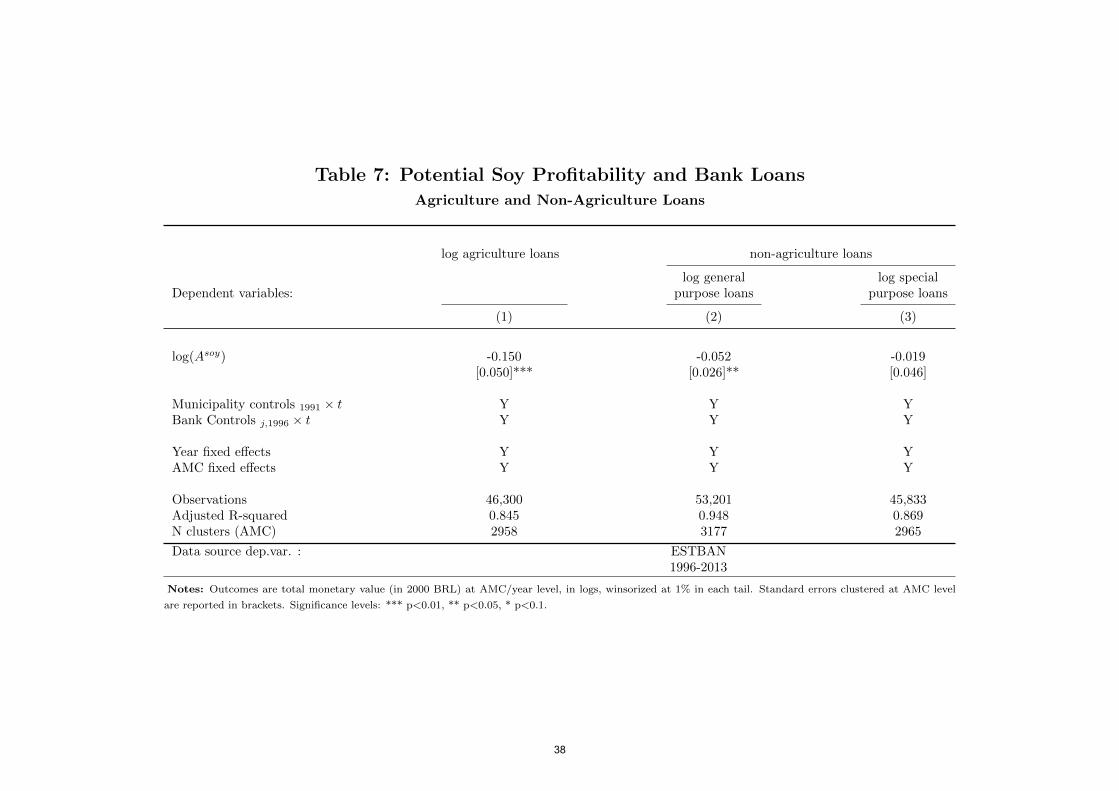
Table 7: Potential Soy Profitability and Bank LoansAgriculture and Non-Agriculture Loans

log agriculture loans non-agriculture loans

log general log specialDependent variables: purpose loans purpose loans

(1) (2) (3)

log(Asoy) -0.150 -0.052 -0.019[0.050]*** [0.026]** [0.046]

Municipality controls 1991 × t Y Y YBank Controls j,1996 × t Y Y Y




Notes: Outcomes are total monetary value (in 2000 BRL) at AMC/year level, in logs, winsorized at 1% in each tail. Standard errors clustered at AMC level

are reported in brackets. Significance levels: *** p<0.01, ** p<0.05, * p<0.1.

38

Table 8: Propagation to Non-Soy Producing RegionsAgriculture and Non-Agriculture Loans


log general log specialDependent variables: purpose loans purpose loans

(1) (2) (3)

Municipality exposure jt 0.326 0.282 0.250[0.146]** [0.057]*** [0.109]**





Notes: Outcomes are total monetary value (in 2000 BRL) at AMC/year level, in logs, winsorized at 1% in each tail. Regressions only include AMC with no

soy production in the years under study according to the PAM Survey. Standard errors clustered at AMC level are reported in brackets. Significance levels: ***

p<0.01, ** p<0.05, * p<0.1.

39

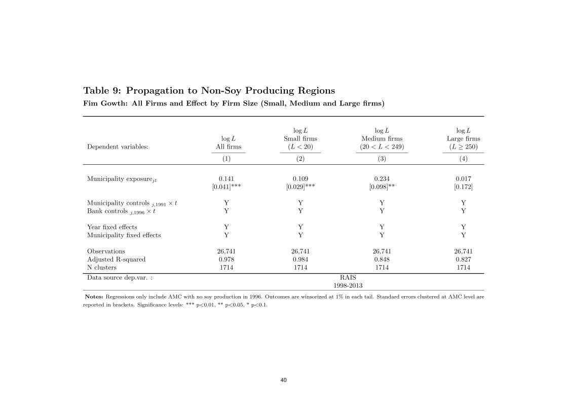
Table 9: Propagation to Non-Soy Producing RegionsFim Gowth: All Firms and Effect by Firm Size (Small, Medium and Large firms)

logL logL logLlogL Small firms Medium firms Large firms

Dependent variables: All firms (L < 20) (20 < L < 249) (L ≥ 250)

(1) (2) (3) (4)

Municipality exposurejt 0.141 0.109 0.234 0.017[0.041]*** [0.029]*** [0.098]** [0.172]

Municipality controls j,1991 × t Y Y Y YBank controls j,1996 × t Y Y Y Y

Year fixed effects Y Y Y YMunicipality fixed effects Y Y Y Y

Observations 26,741 26,741 26,741 26,741Adjusted R-squared 0.978 0.984 0.848 0.827N clusters 1714 1714 1714 1714

Data source dep.var. : RAIS1998-2013

Notes: Regressions only include AMC with no soy production in 1996. Outcomes are winsorized at 1% in each tail. Standard errors clustered at AMC level are

reported in brackets. Significance levels: *** p<0.01, ** p<0.05, * p<0.1.

40

Appendix

Table A1 Robustness to Excluding Government Controlled Banks

log total log agriculture non-agriculture loans log agriculture non-agriculture loans

Dependent variables deposits loans log general log special loans log general log specialpurpose loans purpose loans purpose loans purpose loans

(1) (2) (3) (4) (5) (6) (7)

log(Asoy) 0.122 -0.211 -0.124 -0.182[0.024]*** [0.089]** [0.040]*** [0.083]**

Municipality Exposure jt 0.850 0.351 -0.128[0.161]*** [0.067]*** [0.123]

Municipality controls 1991 × t Y Y Y Y Y Y YBank Controls j,1996 × t Y Y Y Y Y Y Y

Year fixed effects Y Y Y Y Y Y YAMC fixed effects Y Y Y Y Y Y Y

Observations 48,206 33,522 48,171 33,022 14,780 20,635 13,827Adjusted R-squared 0.936 0.757 0.899 0.819 0.757 0.936 0.844N clusters (AMC) 3185 2557 3182 2482 1171 1521 1150

Notes: Outcomes are total monetary value (in 2000 BRL) at AMC/year level, in logs, winsorized at 1% in each tail. Standard errors clustered at AMC levelare reported in brackets. Significance levels: *** p<0.01, ** p<0.05, * p<0.1.

41

Table A2 Robustness to Using Bank Conglomerates


Dependent variables log general log specialpurpose loans purpose loans

(1) (2) (3)

Municipality Exposure jt 0.411 0.278 0.121[0.133]*** [0.039]*** [0.095]




Notes: Outcomes are total monetary value (in 2000 BRL) at AMC/year level, in logs, winsorized at 1% in each tail. Standard errors clustered at AMC levelare reported in brackets. Significance levels: *** p<0.01, ** p<0.05, * p<0.1.

42

Paula Bustos, Gabriel Garber and Jacopo Ponticelli … Allocation Across Sectors: Evidence from a...

Documents

Transcript of Paula Bustos, Gabriel Garber and Jacopo Ponticelli … Allocation Across Sectors: Evidence from a...