Patison PhD Thesis 2011 - Revised
237
Exploring the social behaviour of cattle: the effect of the presence of familiar and unfamiliar individuals Kym Patricia PATISON B.Ag.Sc. (Hons) La Trobe University, Bundoora A thesis submitted in total fulfilment of the requirements of the degree of Doctor of Philosophy May 2011 Psychological Sciences Faculty of Medicine, Dentistry and Health Sciences The University of Melbourne Produced on archival quality paper
Transcript of Patison PhD Thesis 2011 - Revised

Exploring the social behaviour of cattle: the effect of the presence of familiar and
unfamiliar individuals
Kym Patricia PATISON
B.Ag.Sc. (Hons)
La Trobe University, Bundoora
A thesis submitted in total fulfilment of the requirements
of the degree of Doctor of Philosophy
May 2011
Psychological Sciences
Faculty of Medicine, Dentistry and Health Sciences
The University of Melbourne
Produced on archival quality paper

i
Abstract
The social behaviour of cattle encompasses a large range of affiliative and agonistic
behaviours. The collection of these behaviours contributes to the overall social structure,
which influences how a group functions and survives. Dominance behaviour has been a
large focus of the existing literature on cattle social behaviour, with less emphasis on the
affiliative behaviours that contribute to group cohesion. Affiliative behaviours are displayed
between familiar individuals with established social relationships, however, details on the
process of familiarisation and the underlying social properties of a cattle relationship remain
largely unexplored.
Over a series of experiments, this thesis explored the affiliative behaviours involved in
relationship development between unfamiliar steers in different social contexts. The first
experiment presented in Chapter 5 examined the trade off individual steers make between a
food‐reward and maintaining close proximity to a peer with which they were either familiar
or unfamiliar. This experiment analysed the impact of familiarity on an individual steer’s
feeding motivation. It was found that the presence of an unfamiliar pen mate impacted on
the test steer’s decision to move away and consume food, while steers paired with familiar
pen mates were more willing to consume food at greater distances. It was suggested that
the presence of an unfamiliar steer as well as isolation from familiar group mates in an
artificial environment elicited a stress response that modified the steer’s behaviour.
Chapter 6 describes a pair‐wise experiment quantifying the changes in temporal and spatial
associations between pairs of steers during familiarisation, where inter‐individual distance,
behaviour, movement and encounter patterns of pairs of familiar and unfamiliar steers were
compared over a 5 day period. It was shown that unfamiliarity affected behaviour,
movement, close proximity encounters and inter‐individual distance. Relationships had
begun to develop between the unfamiliar steers within 3 days, yet consistent treatment
ii
differences revealed that relationships had not stabilised after 5 days. Based on the findings
from the first two experiments, it was concluded that the presence of an unfamiliar peer
created stress, which affected the steer’s behavioural patterns in both artificial and natural
physical environments.
A triad based experiment is detailed in Chapter 7, where an unfamiliar steer was introduced
into a pair of familiar steers and the resultant changes in social encounters were monitored
over a 5.5 day period. It was found that the introduction of the unfamiliar steer led to an
increase in close proximity encounters between the familiar pair due to social disruption. To
analyse the data in greater detail the same experiment was re‐analysed in Chapter 8 using a
new social network related method: the relational event model. The model was used to
analyse the sequences of social encounters between the three steers and identify patterns
of encounters indicative of relationship development. The model identified the importance
of pair‐wise relationships and described characteristics of an established social bond
between two steers. It was shown that familiarisation with the unfamiliar steer was
hindered by the familiar peers providing social support for each other which led to the
exclusion of the third steer. The model also revealed how social processes unfold in sub‐
groups of steers and structural differences between dyads and triads of steers were
identified. A second application of the model presented in Chapter 9 described the
encounter characteristics of a socially stable group of steers, where both dyadic and triadic
encounters were identified as important features of the steers’ social system.
The research demonstrates that relational event modelling provides a novel predictive tool
to identify and analyse the complex encounter structures of steers during periods of social
disruption as well as social stability. It was also shown that proximity logging devices can be
used to quantify the social relationships of cattle and differentiate between the encounter
patterns of familiar and unfamiliar steers.
This thesis identified emergent properties of social relationships in steers and described the
social properties of dyads and triads of steers. This work will enable future studies on cattle
social systems to take into account the influence of dyadic and triadic pressures on social
processes in order to interpret the higher order processes more clearly. Further work is
required to investigate the importance of other sub‐group sizes on the social dynamics of
larger groups: such work would continue to develop an understanding of the underlying

iii
social principles of cattle social systems, which has the potential to provide benefits not only
to scientists, but also producers and the welfare of domestic cattle.


v
Declaration
This is to certify that:
1. the thesis comprises only my original work towards the PhD except where indicated
in the Preface,
2. due acknowledgement has been made in the text to all other material used,
3. the thesis is less than 100,000 words in length, exclusive of tables, maps,
bibliographies and appendices.
………………………………………….
Kym Patricia PATISON


vii
Preface
The research was conducted under the supervision of Dr Dave Swain, from CSIRO Livestock
Industries in Rockhampton, and Professor Pip Pattison and Associate Professor Garry Robins,
from the Department of Psychological Sciences at the University of Melbourne. Two original
papers were published from this research in peer reviewed journals: these papers have been
incorporated as Chapters 5 and 6. The ideas, development and writing up of the papers
were the principal responsibility of the candidate.
The research presented in Chapter 5 resulted from collaboration with Dr. Greg Bishop‐
Hurley from CSIRO Livestock Industries in Rockhampton, where Dr. Bishop‐Hurley was
involved with discussions on the design of the experiment and proof reading. In Chapter 6,
Dr Greg Bishop‐Hurley was also involved in the experiment design and data processing and
David Reid of Agri‐Science Queensland from the Department of Employment, Economic
Development and Innovation in Rockhampton was consulted for statistical advice.
List of publications:
Patison, K.P., Swain, D.L., Bishop‐Hurley, G.J., Pattison, P., Robins, G., 2010. Social
companionship versus food: the effect of the presence of familiar and unfamiliar
conspecifics on the distance steers travel. Applied Animal Behaviour Science, 122 (1), 13‐20.
Patison, K.P., Swain, D.L., Bishop‐Hurley, G.J., Robins, G., Pattison, P., Reid, D.J., 2010.
Changes in temporal and spatial associations between pairs of cattle during the process of
familiarisation. Applied Animal Behaviour Science, 128 (1‐4), 10‐17.


ix
Acknowledgements
Firstly, I would like to thank my supervisors, Dr. Dave Swain, Professor Pip Pattison and
Associate Professor Garry Robins. I was very fortunate to receive such wonderful guidance
and mentoring from all three supervisors: Dave’s drive and passion for the bigger picture
taught me about the creative and rewarding side of research, while Pip and Garry’s
enthusiasm for understanding bovine sociology opened my mind up to a different yet
complementary discipline from Agriculture. I express my sincere gratitude to each of you.
I would like to acknowledge the financial contribution received from CSIRO to carry out the
experimental work, as well as scholarships received from both CSIRO and the University of
Melbourne to fund my candidature.
I would like to express my sincere appreciation to Greg Bishop‐Hurley, Karina Tane, Chris
O’Neill, Rob Young, Wayne Flintham and Phil Orchard, who provided valuable field‐work
assistance and technical support. I am very grateful to David Reid (DEEDI) for his statistical
expertise and Dr. Eric Quintane (The University of Melbourne) for his modelling skills. I
would also like to thank the former CSIRO Rendel staff members for lots of happy memories
and making the workplace a wonderful place to be. I am grateful to the MelNet group for
making me feel so welcome and also for their guidance and helpful discussions. My own
PhD journey was inspired by the experiences of other PhD students, in particular, Lizzie,
Lesley and Steph. I thank them for giving me inspiration as well as sharing the joys and
frustrations of completing a PhD.
To my family and friends, thank you for your support and encouragement. All of your
valuable qualities, especially your shared love of the land, have contributed to my passion
for animals and agriculture. I would especially like to thank Mum, Dad and Netsy. Even
though there are two states between us, your support and encouragement has been with

x
me the whole time. Special thanks also go to Sue and Paul and Sam and Daniel for providing
me with such wonderful hospitality during my time in Melbourne.
Finally, to my husband Troy. I could not have reached this point without you. You have
provided me with never‐ending love, support and encouragement, and for that I am
eternally grateful. You are a constant source of positive energy and life with you is a
wonderful, fun adventure. I dedicate this thesis to you.

xi
Contents
Abstract i
Declaration v
Preface vii
Acknowledgements ix
Contents xi
List of Figures xvii
List of Tables xix
1. Introduction 1
1.1. Background to the study .............................................................................. 1
1.2. Aim and scope .............................................................................................. 2
2. The social behaviour of cattle – a review 5
2.1. Introduction ................................................................................................. 5
2.2. The evolution of animal social behaviour .................................................... 5
2.3. The importance of social behaviour for survival ......................................... 10
2.4. Social organisation ....................................................................................... 12
2.4.1. Fundamental components of group structure: dyadic relationships .......... 13
2.4.2. Fundamental components of group structure: triadic relationships .......... 16
2.5. Cattle social systems .................................................................................... 19
2.6. The dominance hierarchy ............................................................................ 19
2.6.1. Establishing dominance ............................................................................... 20
2.6.2. Benefits of dominance ................................................................................. 22
2.6.2.1. Intensive production systems ...................................................................... 22
2.6.2.2. Extensive production systems ..................................................................... 23
2.6.2.3. Mating opportunities ................................................................................... 24
2.6.3. The effect of dominance on production ...................................................... 25
2.6.4. Dominance hierarchy structure ................................................................... 28
2.7. Affiliative behaviour ..................................................................................... 30
2.7.1. Familiarity .................................................................................................... 31
2.7.2. Preferential relationships ............................................................................ 36
2.7.3. Allogrooming ............................................................................................... 38
2.7.4. Spatial behaviour and individual distance ................................................... 40
2.7.5. Sociability ..................................................................................................... 42
2.8. Communication and individual recognition ................................................ 44
2.8.1. Visual signals ................................................................................................ 45
2.8.2. Auditory signals ........................................................................................... 49
2.8.3. Olfactory and tactile signals ......................................................................... 51
2.9. Changing group composition ....................................................................... 52
2.9.1. The effect of mixing unfamiliar animals on production .............................. 53
2.9.2. Social stabilisation following mixing unfamiliar animals ............................. 57
2.9.3. Re‐grouping strategies ................................................................................. 58
2.10. Conclusions .................................................................................................. 60
2.10.1. Aims ............................................................................................................. 61
3. Measurement considerations 63
3.1. Introduction ................................................................................................. 63
3.2. Recording animal social behaviour .............................................................. 64
3.2.1. Approaches to the study of animal behaviour ............................................ 64
3.2.2. Research design ........................................................................................... 65
3.2.3. Recording representative samples of behaviour ......................................... 66
3.2.4. Sampling methods ....................................................................................... 66
3.2.5. Record type .................................................................................................. 68
3.2.6. The amount of behaviour to sample ........................................................... 69
3.2.7. Measuring spatial aspects of behaviour ...................................................... 69
3.3. Observations ................................................................................................ 70
3.4. Radio telemetry systems ............................................................................. 71
3.4.1. Proximity logging devices ............................................................................ 74
3.4.2. Fixed antenna positional systems ................................................................ 77
3.4.3. Global positioning systems .......................................................................... 79

xiii
3.5. Selection of recording methods................................................................... 85
3.6. Statistical approaches .................................................................................. 86
3.6.1. The relational event model overview .......................................................... 87
3.6.2. Ordinal relational event models .................................................................. 89
4. General methods 91
4.1. Introduction ................................................................................................. 91
4.2. Animals and management ........................................................................... 91
4.2.1. Resident steers ............................................................................................ 91
4.2.2. Unfamiliar steers .......................................................................................... 92
4.3. Data collection ............................................................................................. 93
4.3.1. Visual observations ...................................................................................... 93
4.3.2. Proximity logging devices ............................................................................ 94
5. The effect of familiarity on the trade‐off individual steers make between food and
social companionship 99
5.1. Introduction ................................................................................................. 99
5.2. Methods ....................................................................................................... 100
5.2.1. Animals and management ........................................................................... 101
5.2.2. Experiment design ....................................................................................... 101
5.2.3. Familiarisation with experimental arena ..................................................... 101
5.2.4. Tests ............................................................................................................. 102
5.2.5. Experimental procedure and behavioural measurements .......................... 102
5.2.6. Data processing and statistical analysis ....................................................... 104
5.3. Results .......................................................................................................... 105
5.3.1. Differences between familiar and unfamiliar without‐food and with‐food
tests ............................................................................................................. 105
5.3.2. Differences within tests ............................................................................... 106
5.4. Discussion .................................................................................................... 109
5.5. Conclusions .................................................................................................. 112
6. The social behaviour of steers paired with either a familiar or unfamiliar peer 113
6.1. Introduction ................................................................................................. 113
6.2. Methods ....................................................................................................... 114

6.2.1. Animals and plots ........................................................................................ 114
6.2.2. Experimental procedure .............................................................................. 115
6.2.3. Proximity logger data statistical analysis ..................................................... 115
6.2.4. Behavioural observations ............................................................................ 116
6.2.5. Observational data processing and statistical analysis ............................... 117
6.3. Results .......................................................................................................... 118
6.3.1. Proximity logger data ................................................................................... 118
6.3.2. Observational data ...................................................................................... 118
6.3.3. Steer re‐use .................................................................................................. 123
6.4. Discussion .................................................................................................... 123
6.5. Conclusions .................................................................................................. 126
7. Introducing an unfamiliar steer into a pair of familiar steers and the effect on social
interaction 127
7.1. Introduction ................................................................................................. 127
7.2. Methods ....................................................................................................... 128
7.2.1. Animals and plots ........................................................................................ 128
7.2.2. Experimental procedure .............................................................................. 129
7.2.3. Data processing and statistical analysis ....................................................... 130
7.3. Results .......................................................................................................... 132
7.3.1. Changes within familiar steers ..................................................................... 132
7.3.2. Changes within unfamiliar triads ................................................................. 133
7.4. Discussion .................................................................................................... 135
7.5. Conclusions .................................................................................................. 138
8. Relationship development in steers: an application of the relational event model 139
8.1. Introduction ................................................................................................. 139
8.2. Model development .................................................................................... 140
8.2.1. Data input .................................................................................................... 140
8.2.2. Model components ...................................................................................... 141
8.2.3. Creating the sequence of prior events ........................................................ 143
8.2.4. Time ............................................................................................................. 145
8.2.5. Event sequence summary ............................................................................ 146
8.3. Model parameters ....................................................................................... 148
xv
8.3.1. Unfamiliarity effects .................................................................................... 148
8.3.2. Prior pair effects .......................................................................................... 151
8.3.3. Prior group effects ....................................................................................... 152
8.4. Results .......................................................................................................... 153
8.4.1. Descriptive statistics .................................................................................... 153
8.4.2. Model outputs ............................................................................................. 154
8.4.2.1. Predicting future pair events ....................................................................... 154
8.4.2.2. Predicting future group events .................................................................... 156
8.5. Discussion .................................................................................................... 158
8.6. Conclusions .................................................................................................. 160
9. Social encounters of familiar steers in larger groups 161
9.1. Introduction ................................................................................................. 161
9.2. Methods ....................................................................................................... 162
9.2.1. Animals and management ........................................................................... 162
9.3. The relational event model for groups ........................................................ 163
9.3.1. Model components ...................................................................................... 163
9.4. Results .......................................................................................................... 166
9.4.1. Descriptive statistics .................................................................................... 166
9.4.2. Model outputs ............................................................................................. 169
9.4.2.1. Animal effects .............................................................................................. 170
9.4.2.2. Predicting future events from the pattern of prior pair events .................. 170
9.4.2.3. Predicting future events from the pattern of prior string events ............... 172
9.4.2.4. Predicting future events from the pattern of prior triangle events ............ 173
9.4.2.5. Predicting future events from the pattern of prior popularity events ........ 174
9.5. Discussion .................................................................................................... 175
9.6. Conclusions .................................................................................................. 178
10. General discussion 181
11. Appendix A Images from trade‐off test experiment 189
12. Appendix B Validating assumptions 191
13. References 195

xvii
List of figures 2.1. The co‐evolution of genetics and culture ......................................................................... 8
2.2. The inter‐relationship between social behaviour, genetics and the brain. ...................... 8
2.3. Trait selection based on individual and recipient fitness. ................................................ 9
2.4. Directed dyadic relationships. ........................................................................................ 14
2.5. Non‐directed dyadic relationships in a triad .................................................................. 18
2.6. The configuration of transitive and intransitive triads ................................................... 18
2.7. Different types of hierarchies ......................................................................................... 29
2.8. Cattle spacing principles ................................................................................................. 41
3.1. The sampling and recording methods ............................................................................ 67
3.2. Proximity logger worn by a cow and her calf ................................................................. 77
4.1. Proximity logger read‐range ........................................................................................... 94
4.2 Proximity logger components ......................................................................................... 96
5.1. Layout of the trade‐off test arena ................................................................................ 103
5.2. The average distance of steers during the trade‐off test ............................................. 108
5.3. The mean rate of bowl visiting during the trade‐off test ............................................. 108
6.1. Encounters between familiar and unfamiliar pairs per day ......................................... 119
6.2. The average distance between familiar and unfamiliar pairs per day ......................... 119
6.3. The distance distributions of familiar and unfamiliar pairs for movement vector 1 ... 122
7.1. Distributions of triadic encounters before and after transformation .......................... 131
7.2. Familiar encounters pre‐ and post‐introduction .......................................................... 132
7.3. The encounter summary of triads per day ................................................................... 134
8.1. An onset event sequence ............................................................................................. 142
8.2. The three triadic event types... ..................................................................................... 143

8.3. The sequence of events leading to a triangle event ..................................................... 147
8.4. Basic outline of the relational event modelling process .............................................. 149
8.5. Partner swapping event configurations ....................................................................... 152
9.1. The four event types used in the group’s relational event model ............................... 164
9.2. The possible animal configurations in a string event and a popularity event. ............. 165
9.3. The encounters per group per day ............................................................................... 167
9.4. Network diagrams of group 1 and group 2 .................................................................. 168
9.5. The number of events per group .................................................................................. 169
xix
List of tables 5.1. Trade‐off test summary .............................................................................................. 107
6.1. Description of movement vectors ............................................................................... 116
6.2. Movement vectors 1‐3 per treatment per day ........................................................... 120
6.3. The average distance of each movement vector ........................................................ 121
6.4. Behaviour summary per treatment. ........................................................................... 121
7.1. Triadic encounters per day.......................................................................................... 133
8.1. The three triadic event types ...................................................................................... 145
8.2. Data sequence example .............................................................................................. 147
8.3. Positive and negative parameter estimate interpretations ........................................ 150
8.4. The average number of events per triad .................................................................... 153
8.5. Predicting future pair events. ..................................................................................... 155
8.6. Predicting future group events ................................................................................... 157
9.1. Predicting future events based on individual animal activity. .................................... 171
9.2. Predicting future events from pair events .................................................................. 172
9.3. Predicting future events from string events ............................................................... 172
9.4. Predicting future events from triangle events ............................................................ 173
9.5. Predicting future events from popularity events ........................................................ 174


1
Chapter 1
Introduction 1.1. Background to the study
Domestic livestock are managed according to practices that maximise production
efficiencies. This management has resulted in a change in the way animals are grouped,
from wild populations where animals select their own group sizes based on social attraction
(Keeling and Gonyou, 2001; Boe and Faerevik, 2003) to modern day farming practices where
groups are based more on breed, age, gender or production level (Raussi et al., 2005) and
less on individual compatibilities. These management decisions can impose sub‐optimal
conditions leading to conflict and stressful environments (Keeling and Gonyou, 2001). Of
particular importance is the disruption caused by the introduction of new individuals into an
existing group; this disruption can lead to compromised animal welfare and production. In
dairy and beef cattle production systems, regrouping unfamiliar individuals is a common
practice. The negative effects experienced by both the introduced cow and the resident
herd can include an immediate increase in aggressive behaviour and social stress, as well as
a decrease in production levels, such as weight loss and a decline in milk yield (Boe and
Faerevik, 2003). Despite these effects mainly being short term (around 1‐2 weeks), the
impact on animal health and welfare is an important concern.
Conflict between newly introduced individuals arises from them competing for their place
within the social order, with the winner gaining priority access to resources such as food,
space and mating opportunities (Lindberg, 2001). Due to agonistic behaviour predominating
initial social interactions between newly introduced cattle, dominance‐like behaviour has
been a focus of many studies investigating mixing in cattle. The time taken for a group to be
considered socially stable is important both in terms of animal welfare and production
levels. Stabilisation in cattle is said to occur when non‐physical agonistic interactions
predominate physical agonistic interactions, and the ratio of non‐physical to physical

Chapter 1: Introduction
2
agonistic interactions remains constant (Kondo and Hurnik, 1990). However, once
hierarchies have stabilised, minimal agonistic behaviour is observed and most groups exist
without any conflict (Bouissou et al., 2001). This suggests that agonistic behaviours are
initially important during relationship establishment, but it is the more subtle affiliative
behaviours, such as maintaining close proximity and allogrooming, that are important for
maintaining social cohesion and preferential relationships (Reinhardt and Reinhardt, 1981;
Bouissou et al., 2001).
A popular approach to investigate the integration of an unfamiliar animal into a new group
has been to focus on individual behavioural responses and group averages, such as an
individual’s decrease in weight gain or milk production or an increase in the overall levels of
agonistic behaviour, and to monitor these changes until behavioural measures and
interactions have stabilised or returned to baseline levels (Kondo and Hurnik, 1990).
Another approach is to consider the group as its own network, where the actions of each
individual are interdependent on the individuals around it (Wasserman and Faust, 1994),
and evaluate the introduction of the stranger in terms of the individual as well as the
relationship changes that occur within the group. Social network analyses focus on the
relationships between each individual within a group and explore the patterns and
outcomes of these relationships (Wasserman and Faust, 1994). Pair‐wise interactions are
therefore an essential component of the network (Croft et al., 2008). Several studies have
investigated various aspects of a cattle social systems, such as dominance hierarchies (e.g.
Beilharz and Zeeb, 1982) and affiliative relationships (e.g. Reinhardt and Reinhardt, 1981),
although there are limited studies that investigate cattle social structure using a whole social
network approach. The wealth of information that could be gained via investigating the
social relationships that exist within a cattle social network, such as identifying preferential
relationships and disease transmission routes, has a large potential to influence livestock
management practices in a manner that could maximise production levels whilst enhancing
animal welfare.
1.2. Aim and scope
It is well known that the presence of an unfamiliar animal creates social disruption, but less
is known about the processes that occur during relationship development between newly
introduced individuals. Thus, the aim of this thesis is to explore the effect of the presence of
an unfamiliar steer on the social behaviour of resident steers. The context of this study is

Chapter 1: Introduction
3
restricted to analysing only small numbers of steers that form the fundamental level of social
structure: the dyad and the triad. The benefit of studying these kinds of social units is to
develop an understanding of how group sub‐structures are developed and maintained. By
gradually increasing the size of the group, the influence of the social context on the
behavioural response towards an unfamiliar peer can be measured. However, previous
research investigating fish social systems revealed that behaviour in an isolated dyad is
different from a socially embedded dyad within a larger group (Chase et al., 2003), and thus
questions the usefulness of researching isolated dyads and triads. But in human social
systems there are certain social properties that are unique to dyads and triads that are not
observed within groups larger than two or three (Simmel, 1950), which may also exist in
cattle social systems. By first considering properties that are unique to dyads and triads, the
effect of these properties between individuals can be explored, which can then be evaluated
for their effect within larger groups. Additionally, any effects that are produced above
dyadic and triadic effects can also be identified. Thus, studying social relationships between
pairs and triads of animals will lead to a better understanding of how animal social systems
function. The outcomes from this study therefore have the potential to advance theoretical
knowledge, methodology and analysis of relationship development in cattle.

5
Chapter 2
The social behaviour of cattle – a review 2.1. Introduction
The aim of the thesis introduced in Chapter 1 is to investigate changes in behaviour caused
by the introduction of an unfamiliar peer and to develop an understanding of how sub‐
structures in cattle are formed and maintained. To begin to address this aim it is important
to understand the basic principles associated with animal behaviour, why individuals form
groups and identify the interactions and relationships that contribute to social organisation.
The aim of this chapter is to therefore provide an overview on the previous work that relates
to the social behaviour of cattle. The chapter begins by introducing the evolutionary factors
that favoured the development of social behaviour and the fundamental components of a
social system are described. The remaining sections review previous studies that have
investigated cattle social structure and the development of the social hierarchy. The
affiliative behaviours that serve to keep groups together are discussed, as well as the
important relationship between spatial behaviour and social relationships. The chapter
concludes by reviewing existing research on the effects of mixing unfamiliar animals on
production outcomes.
2.2. The evolution of animal social behaviour
The evolutionary history of a species provides an insight into the way the past has influenced
the behaviours that are observed in the present (Stricklin, 2001). The evolution of behaviour
occurs by the same mechanisms of natural selection as any other physical characteristic
(Broom and Fraser, 2007). Wilson (1975) described the process of selection as a change in

Chapter 2: Literature review
6
the frequency of a genotype, as shown by differences in phenotype, from one generation to
the next, and natural selection as the process where one genotype increases at a greater
rate than another. Genetic variation allows some individuals to survive better than others.
Variability in genotypes can be driven by numerous factors, including the ability to survive
parasite infestations, predatory attack or inhabit a new environment. Beneficial traits that
are maintained by the population are said to be adaptive (Wilson, 1975). Wilson (1975)
emphasised that natural selection is the most important aspect of evolution and is the
driving force that shapes a species’ characteristics.
Just as genetics are subject to evolutionary pressures so too are behavioural traits, and it is
proposed that genetics and culture co‐evolve (Laland, 2008). Culture is characterised by a
complex of behaviour, traditions, knowledge and skills that is transmitted from one
individual to another via social influences, such as social learning, social facilitation and
imitation (Laland et al., 2010). For example, information on food location and identity can
be gained by copying the behaviour of other foragers, such that the behaviour of a single
individual can influence the behaviour of all individuals within a group (Dugatkin, 2004).
Cultural influences therefore differ from environmental influences, which are caused by
adaptation to the physical environment, and can be transmitted both within‐ and between‐
generations, allowing culture to evolve at much faster rates than genetics (Dugatkin, 2004).
The co‐evolution of genetics and culture is summarised by Laland (2008) who states that
‘genetics are expressed through development and influence cultural learning, which is
expressed though behaviour’. Individual behaviour is influenced by genetics, culture and the
environment and in turn modifies selection by acting back on genetics, with offspring
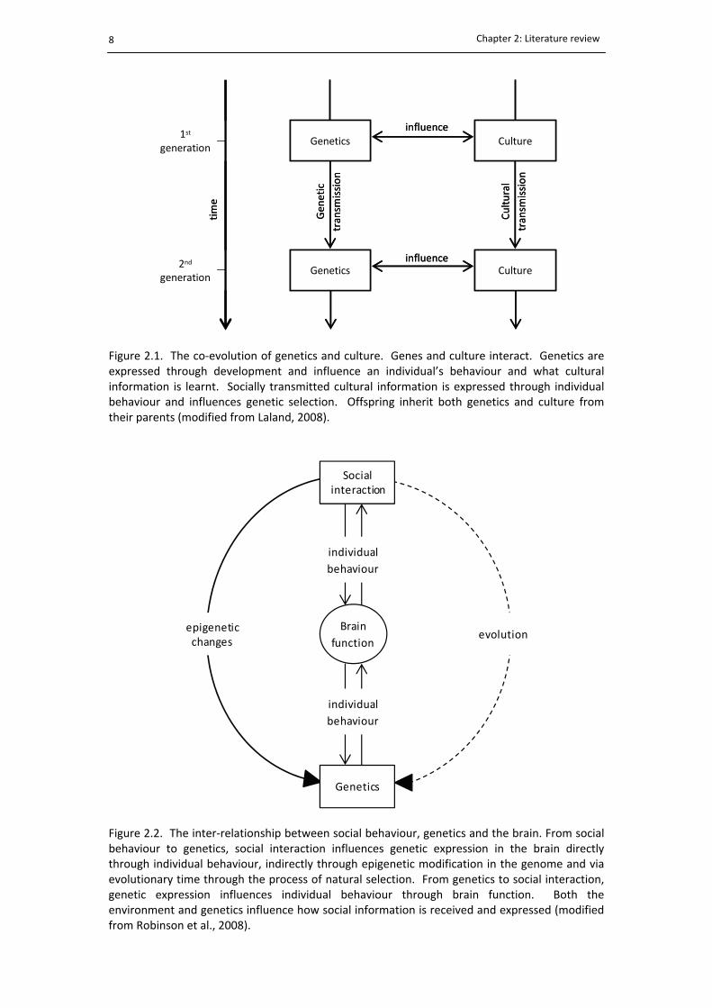
inheriting both genetics and culture from their parents (Fig. 2.1). Cultural transmission is
therefore a social process that leads to the behavioural adaptation of individuals to their
environment and ultimately the diversification of individual behaviour.
The mechanisms underlying the expression of non‐genetic factors on the brain and
behaviour are driven by epigenetic factors. Epigenetics was initially described by
Waddington (1942) as ‘the mechanisms and developmental processes by which the genes of
the genotype bring about phenotypic effects’ and thus describes changes in the way genes
are expressed due to non‐genetic factors, such as the environment, biochemical factors and
cultural information (Rakyan and Beck, 2006). The transmission and expression of social
behaviour, such as learning, memory and building affiliative relationships, is complex and
diverse (Cushing and Kramer, 2005): the field of epigenetics investigates these changes at
Chapter 2: Literature review
7
the molecular and neural level to explain the resultant behavioural modifications and
changes to gene expression (Robinson et al., 2008). The process of social behaviour leading
to epigenetic changes can occur from (a) social information influencing genetic expression in
the brain which then influences individual behaviour, and (b) from individual variation in
genetics which affects brain function and therefore behaviour (Fig. 2.2) (Robinson et al.,
2008). Inheritance of behaviour via epigenetic factors explains the mechanisms involved
when offspring develop survival behaviours from their parents without actually experiencing
the original challenging conditions (Harper, 2005). The process of cultural transmission and
epigenetic inheritance therefore leads to the development of non‐genetically coded social
behaviours that influence the survival of a population.
Characteristics that improve the survival of an individual and its relatives will be more
predominant in future generations (Broom and Fraser, 2007). Survival is quantified in terms
of fitness, or reproductive success, of an individual (Dugatkin, 2004). Hamilton (1964)
introduced the concept of ‘inclusive fitness’, which is the combination of individual fitness
and the effect of the individual on the fitness of relatives and neighbours. Hamilton (1964)
predicted that fitness gained from cooperative and altruistic behaviour was proportional to
the level of relatedness of the recipient, with greater levels of fitness gained by assisting
closely related individuals, such as siblings or cousins, than unrelated individuals. Hamilton
(1964) presented a model that described the evolution of social behaviour and predicted
that the selection of a trait would be based upon the consequence of its inclusive fitness.
Four behavioural categories were identified: cooperative, spiteful, altruistic and selfish.
Traits that improve inclusive fitness would be selected for, such as cooperation, while
detrimental traits would be selected against, such as spiteful behaviour. The selection of
behaviour that benefits one individual more than the other, such as altruistic or selfish
behaviour, depends on the balance between individual risks and returns to inclusive fitness
(Fig. 2.3).
Chapter 2: Literature review
8
CultureGenetics
CultureGenetics
1st
generation
2nd
generation
influence
influence
Gen
etic
transm
ission
Cultural
transm
ission
time
CultureGenetics
CultureGenetics
1st
generation
2nd
generation
influence
influence
Gen
etic
transm
ission
Cultural
transm
ission
time
Figure 2.2. The inter‐relationship between social behaviour, genetics and the brain. From socialbehaviour to genetics, social interaction influences genetic expression in the brain directlythrough individual behaviour, indirectly through epigenetic modification in the genome and viaevolutionary time through the process of natural selection. From genetics to social interaction,genetic expression influences individual behaviour through brain function. Both theenvironment and genetics influence how social information is received and expressed (modifiedfrom Robinson et al., 2008).
Brain
function
individual
behaviour
evolution
individual
behaviour
Social interaction
epigenetic changes
Genetics
Figure 2.1. The co‐evolution of genetics and culture. Genes and culture interact. Genetics areexpressed through development and influence an individual’s behaviour and what culturalinformation is learnt. Socially transmitted cultural information is expressed through individualbehaviour and influences genetic selection. Offspring inherit both genetics and culture fromtheir parents (modified from Laland, 2008).

Chapter 2: Literature review
9
Benefit
Benefit
Detriment
Detriment
SpitefulBehaviour
Selfish
Behaviour
Cooperative
behaviour
AltruisticBehaviourIn
dividual
Recipient
unknown
selectionselected
unknown
selectionnot selected
Altruistic behaviour is behaviour that is detrimental to individual fitness but increases an
individual’s inclusive fitness and its selection will depend on the coefficient of relationship
with the recipient. Selfish behaviour is behaviour that improves individual fitness at the
expense of others, and Hamilton (1964) stated that this behaviour will not evolve if the
fitness losses of relatives are too great. Hamilton (1964) used the example of an alarm call
by a bird to signal a predator to demonstrate his point: the bird exposes itself to the
predator by signalling an alarm call to other birds but the resultant reduction of risk to
another bird closer to the predator must be greater than the apparent risk to the caller. The
potential gains from such an action would be maximised if the other bird was related, as the
altruistic act increases the chance of genes shared with the recipient surviving into the next
generation (Stricklin and Mench, 1987).
Hamilton (1964) provided strong evidence that individuals will act cooperatively and
altruistically towards related individuals, specifically kin. However cooperative and altruistic
behaviour also exists between non‐kin individuals. Broom and Fraser (2007) suggested that
social behaviour between non‐kin individuals may have evolved when kin groups gathered in
response to an abundant resource, such as food and shelter, and discovered the fitness
benefits that could be gained by forming associations. Additionally, it is suggested that
domestic livestock will behave towards group members, particularly those that they have
been raised with, as if they were related and will thus give greater value to group member’s
fitness than unknown individuals (Stricklin, 2001). Altruistic behaviour between group
members that is reciprocated at some stage in the future will be selected for, while cheating
Figure 2.3. The selection of a trait is predicted from the consequence of the trait on the fitness of an individual and the recipient (modified from Hamilton, 1964).

Chapter 2: Literature review
10
or exploiting altruistic behaviour by not reciprocating would be selected against (Wilson,
1975). The evolution of social behaviour therefore has favoured group living by increasing
the fitness gains received by all members and explains the selection and adaptation of social
behaviour.
2.3. The importance of social behaviour for survival
The benefits of abandoning solitary life to join a group is quantified by the gain in inclusive
fitness (Wilson, 1975). Conditions in a group will be optimal when the benefits of living in a
group outweigh the associated costs (Lindberg, 2001). In wild populations, individuals will
leave a group due to illness, dispersal of offspring following weaning or to search for
resources such as mating opportunities and food (Newberry and Swanson, 2001). However,
domestication has removed the ability of individuals to choose their own group size and
composition, which is controlled by farm management practices aimed at maximising
production efficiencies. Nevertheless, an animal’s behaviour is strongly driven by its
evolutionary past and they will therefore continue to act in a way that maximise their
fitness, even if the benefits obtained are only short term (Stricklin and Mench, 1987);
behaviours have not been lost or gained through domestication, only modified (Stricklin,
2001). The advantages and disadvantages of group life are outlined below, with many
features derived from an animal’s evolutionary past when escaping from predators and
finding food were essential for survival.
In grazing herbivores, the main benefits of forming groups are associated with anti‐
predation (Leuthold, 1977). Large groups have a greater chance of detecting predators as
well as diluting the chances of being attacked, thus the chance of individual survival is
increased (Dehn, 1990; Molvar and Bowyer, 1994). Through cooperative behaviour, groups
of individuals have the potential to form defensive mechanisms against predators (Griffith,
1988). Groups are more efficient than individuals at detecting resources, such as food and
shelter; through cooperation and learning, valuable foraging locations can be discovered and
exploited by the whole group (Krause and Ruxton, 2002). Additionally, reproduction is only
possible by forming associations. Offspring survival, and therefore gene flow, is increased by
cooperative parenting behaviour, such as crèche formation (Sato et al., 1987). The major
cost of association is resource competition. Most feeding bouts are synchronised between
group members (Rook and Penning, 1991), thus forage and space is being competed for,
resulting in a faster depletion of the food source (Shrader et al., 2007). This competition can

Chapter 2: Literature review
11
result in aggressive behaviour and spreading out during grazing, which can compromise the
protective cover created by the group (Rind and Phillips, 1999; Harris et al., 2007). Increased
group numbers also increase the chance of being detected and attacked by predators as
groups are less conspicuous than individuals (Lindström, 1989). Additionally, disease
transmission within groups can be accelerated by close proximity contacts, increasing the
risk of epidemics (Loehle, 1995).
The balance between the costs and benefits of group life will influence not only group size
and dynamics, but also the types of social interactions that occur among group members
(Stricklin and Mench, 1987). Social interactions can be divided into agonistic or affiliative
(non‐agonistic) behaviours (Bouissou et al., 2001). Agonistic behaviours include all forms of
competitive behaviour, from physical aggression such as butting, pushing and fighting, to
non‐physical aggression such as threatening and avoiding (Kondo and Hurnik, 1990).
Affiliative behaviours include all forms of cooperative behaviour, such as allogrooming,
providing protection and social support, remaining within close proximity, resting in contact
and synchronising behavioural activities (Newberry and Swanson, 2001). Competitive
behaviours serve to maintain order while cooperative behaviours serve to maintain group
cohesion (Stricklin and Mench, 1987).
Just as group living behaviours are inherited from wild ancestors so too are social behaviours
that facilitate social interaction and social organisation. The existence of large groups has
driven the development of complex social behaviours that are essential for individual and
group survival (Dumont and Boissy, 1999; Mendl and Held, 2001). Examples of these
complex behaviours include: social foraging, where individuals learn about food preferences
and avoidances through others (Mirza and Provenza, 1994) and also share information on
the location and quality of forage availability (Fortin and Fortin, 2009); group defence
strategies where individuals band together to ward off or even attack predators (Berger,
1979; Griffith, 1988); crèche formation, where groups of young calves rest together guarded
by one or two mothers while the rest of the group spread out to graze (Rankine and
Donaldson, 1968; Sato et al., 1987); and allogrooming, which offers both social bonding and
hygiene benefits (Sato et al., 1991). Individuals learn these behaviours through several
mechanisms, including genetic influences, maternal interactions and individual experience
(Provenza, 1995). Learning from others allows individuals to adjust to changing
environmental conditions through their behaviour at a faster rate than natural selection or
individual trial and error would allow (Galef and Laland, 2005). The information learnt from a
Chapter 2: Literature review
12
mother occurs during a time when learning social skills are of primary importance to develop
basic survival skills, such as what foods to consume once weaned and how to avoid
predators (Galef and Laland, 2005). Maintaining such valuable information within the one
population, for example in free‐ranging herbivores where extended family units exist and
matriarchies are allowed to develop, serves great advantages to group survival, cultural
inheritance and inclusive fitness as the benefits are passed directly onto related kin
(Hamilton, 1964).
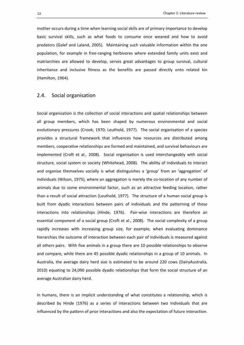
2.4. Social organisation
Social organisation is the collection of social interactions and spatial relationships between
all group members, which has been shaped by numerous environmental and social
evolutionary pressures (Crook, 1970; Leuthold, 1977). The social organisation of a species
provides a structural framework that influences how resources are distributed among
members, cooperative relationships are formed and maintained, and survival behaviours are
implemented (Croft et al., 2008). Social organisation is used interchangeably with social
structure, social system or society (Whitehead, 2008). The ability of individuals to interact
and organise themselves socially is what distinguishes a ‘group’ from an ‘aggregation’ of
individuals (Wilson, 1975), where an aggregation is merely the co‐location of any number of
animals due to some environmental factor, such as an attractive feeding location, rather
than a result of social attraction (Leuthold, 1977). The structure of a human social group is
built from dyadic interactions between pairs of individuals and the patterning of these
interactions into relationships (Hinde, 1976). Pair‐wise interactions are therefore an
essential component of a social group (Croft et al., 2008). The social complexity of a group
rapidly increases with increasing group size, for example, when evaluating dominance
hierarchies the outcome of interaction between each pair of individuals is measured against
all others pairs. With five animals in a group there are 10 possible relationships to observe
and compare, while there are 45 possible dyadic relationships in a group of 10 animals. In
Australia, the average dairy herd size is estimated to be around 220 cows (DairyAustralia,
2010) equating to 24,090 possible dyadic relationships that form the social structure of an
average Australian dairy herd.
In humans, there is an implicit understanding of what constitutes a relationship, which is
described by Hinde (1976) as a series of interactions between two individuals that are
influenced by the pattern of prior interactions and also the expectation of future interaction.
Chapter 2: Literature review
13
A definition of an animal relationship is based more on observations of behavioural patterns
over time, where preferential relationships between cattle are formed and maintained
through displays of affiliative behaviour by one or both individuals, such as allogrooming,
providing protection and maintaining close proximity (Newberry and Swanson, 2001).
Relationships provide a link between individual behaviour and group level processes as
relationships are embedded within groups and define the characteristics of a group, while
groups themselves are more than just aggregates of individuals and have emergent
properties such as hierarchies and cohesiveness that influence the types of interactions and
relationships that are likely to exist between individuals (Rubin et al., 1998).
The social structure of cattle arising from interactions between dyads and triads is largely
unknown. Zayan (1990) suggested that to investigate social relationships in animals,
systematic experimental work should focus on interactions between pairs and small groups,
as their social stability is greater than larger group sizes. There has been a large amount of
work done in human social sciences specifically relating to the importance of dyads and
triads in terms of relationship development and social structure, and these principles might
be relevant to studies in domestic livestock. The majority of the social principles reviewed
below relate to human research, and where there are references to animal societies, most of
these models have been based on human social systems.
2.4.1. Fundamental components of group structure: dyadic relationships
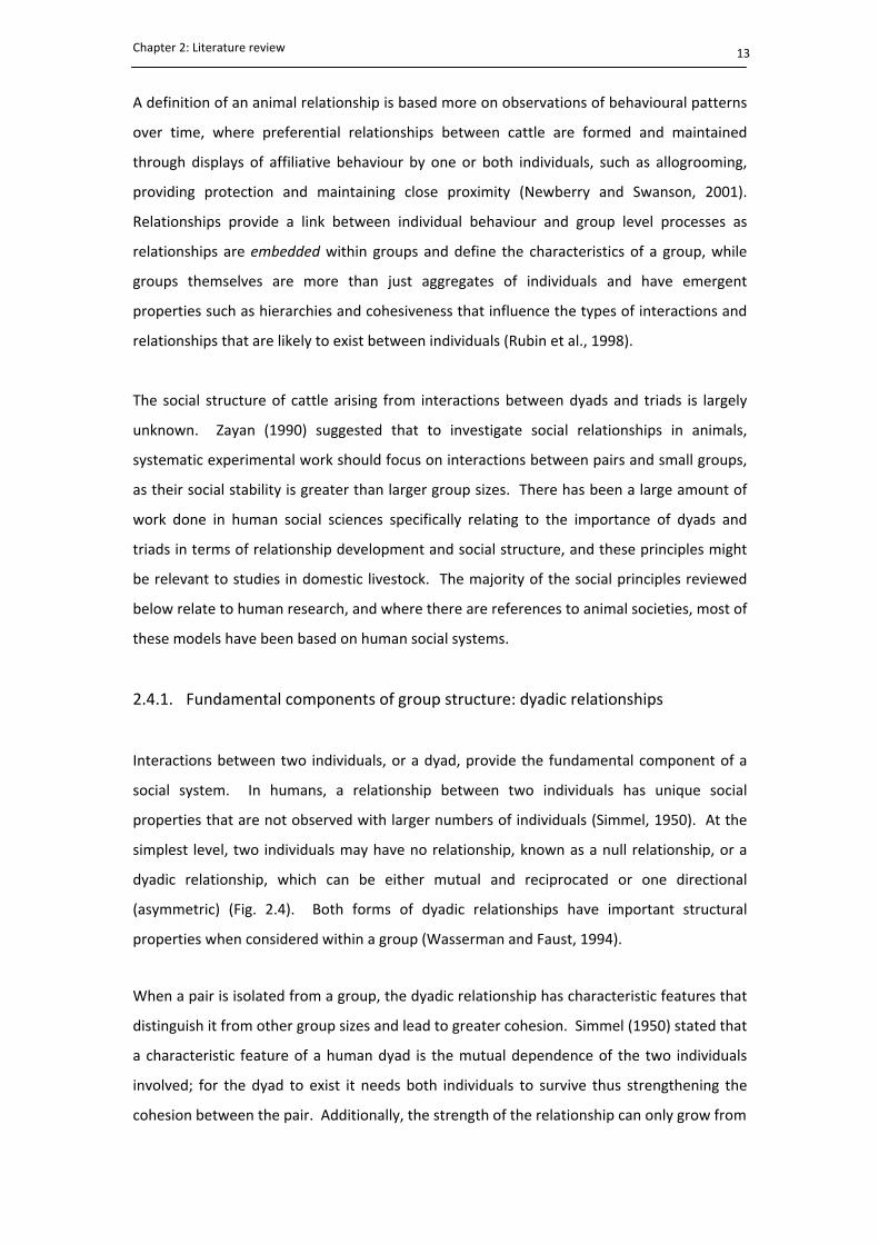
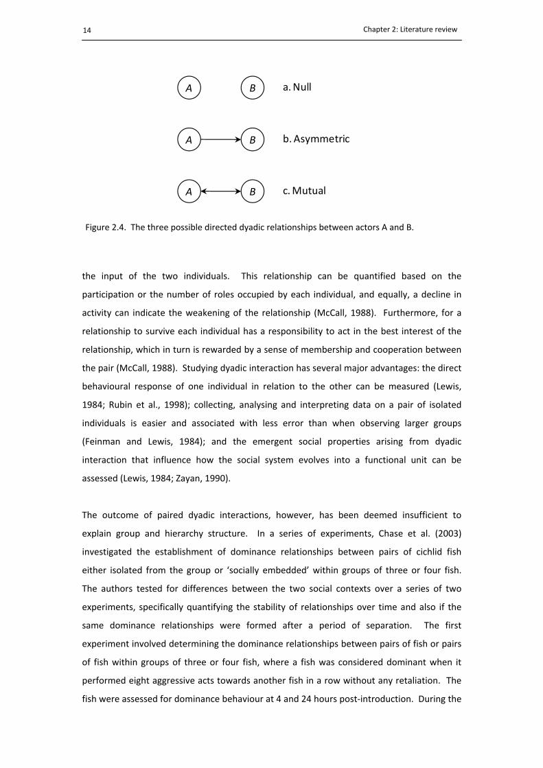
Interactions between two individuals, or a dyad, provide the fundamental component of a
social system. In humans, a relationship between two individuals has unique social
properties that are not observed with larger numbers of individuals (Simmel, 1950). At the
simplest level, two individuals may have no relationship, known as a null relationship, or a
dyadic relationship, which can be either mutual and reciprocated or one directional
(asymmetric) (Fig. 2.4). Both forms of dyadic relationships have important structural
properties when considered within a group (Wasserman and Faust, 1994).
When a pair is isolated from a group, the dyadic relationship has characteristic features that
distinguish it from other group sizes and lead to greater cohesion. Simmel (1950) stated that
a characteristic feature of a human dyad is the mutual dependence of the two individuals
involved; for the dyad to exist it needs both individuals to survive thus strengthening the
cohesion between the pair. Additionally, the strength of the relationship can only grow from
Chapter 2: Literature review
14
A B
A B
A B
a. Null
b. Asymmetric
c. Mutual
the input of the two individuals. This relationship can be quantified based on the
participation or the number of roles occupied by each individual, and equally, a decline in
activity can indicate the weakening of the relationship (McCall, 1988). Furthermore, for a
relationship to survive each individual has a responsibility to act in the best interest of the
relationship, which in turn is rewarded by a sense of membership and cooperation between
the pair (McCall, 1988). Studying dyadic interaction has several major advantages: the direct
behavioural response of one individual in relation to the other can be measured (Lewis,
1984; Rubin et al., 1998); collecting, analysing and interpreting data on a pair of isolated
individuals is easier and associated with less error than when observing larger groups
(Feinman and Lewis, 1984); and the emergent social properties arising from dyadic
interaction that influence how the social system evolves into a functional unit can be
assessed (Lewis, 1984; Zayan, 1990).
The outcome of paired dyadic interactions, however, has been deemed insufficient to
explain group and hierarchy structure. In a series of experiments, Chase et al. (2003)
investigated the establishment of dominance relationships between pairs of cichlid fish
either isolated from the group or ‘socially embedded’ within groups of three or four fish.
The authors tested for differences between the two social contexts over a series of two
experiments, specifically quantifying the stability of relationships over time and also if the
same dominance relationships were formed after a period of separation. The first
experiment involved determining the dominance relationships between pairs of fish or pairs
of fish within groups of three or four fish, where a fish was considered dominant when it
performed eight aggressive acts towards another fish in a row without any retaliation. The
fish were assessed for dominance behaviour at 4 and 24 hours post‐introduction. During the
Figure 2.4. The three possible directed dyadic relationships between actors A and B.
Chapter 2: Literature review
15
pair tests two fish were introduced in a single tank while in the group tests a third fish was
introduced to the pair once their dominance relationship was established followed by a
fourth fish for some groups. In total, 36 pairs, 19 triads and 23 tetrads were observed. The
authors found that the relationships formed within an isolated pair were relatively stable
compared with relationships within groups of three or four; no relationship reversals were
observed between isolated pairs of fish 24 hours later, while 35% of fish in groups of four
continued to direct aggressive behaviour towards the dominant fish and some relationship
reversals were recorded. Pairs in groups of three showed no differences in relationship
stability when compared with groups of four fish. Chase et al. (2003) concluded that the
presence of other individuals influenced the nature of the dominance relationship. The
second experiment was similar to the first experiment, where dominance relationships
between pairs or groups of three or four fish were sequentially determined. After 2 hours of
observations the fish were removed and kept isolated for 2 weeks, which was considered
long enough for the fish to forget the identify of others. The pairs and groups were
reassembled in the same pairings and groups as before and dominance relationships
recorded. The authors found that isolated pairs replicated their relationships 93% of the
time, whereas relationship reversals occurred in 24% of the group’s trials. The authors
summarised that the presence of other individuals lowered the probability that the same
relationship will form in the future. The overall findings identified that dominance behaviour
within a pair is different from socially embedded behaviour and therefore does not
represent dominance relationships that are formed within a group context. It was
concluded that dominance relationships should be considered contextual to groups, rather
than independent pairs.
Most human social interaction occurs as a part of a larger group (Lansford and Parker, 1999),
where an individual’s behaviour is influenced by the social context, including not only the
number of individuals in the group but also their social characteristics and their interactions
and relationships with other group members. To study the influence of others on behaviour
and relationships, Lewis (1984) suggested to introduce a third individual to a dyad and
observe the behavioural responses. This step‐wise approach provides basic information on
the social properties of a triad. However, Lewis (1984) also acknowledged that the artificial
nature of dyadic and triadic investigations limits the implications for group processes.
Chapter 2: Literature review
16
2.4.2. Fundamental components of group structure: triadic relationships
The relationship between three individuals is more complex than a relationship observed
between a dyad. With three individuals, there is the potential for 64 different triadic
configurations to occur when the direction of the relationship between each individual is
known (Wasserman and Faust, 1994). However when only mutual ties are considered (i.e.
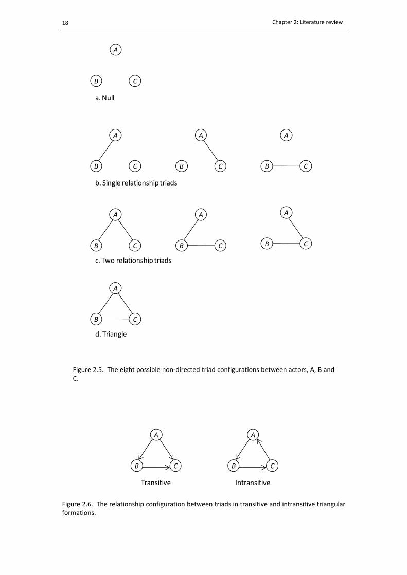
non‐directional), there are eight possible relationships (Fig. 2.5). Knowing how relationships
are structured is essential for understanding the theoretical implications of such
relationships (Wasserman and Faust, 1994).
Simmel (1950) was among the first to describe the social differences that exist between
human dyads and triads, particularly the type of interactions that occur among individuals
and the roles they fulfil within the group. These fundamental differences are important for
understanding triadic interactions in group level processes. Simmel (1950) stated that the
role of a third individual was both beneficial and detrimental to the cohesion of the group.
In human groups, the third individual provides an objective perspective to resolve conflict
which leads to group unity. In contrast, the triad is the smallest group size where there can
be both a majority and a minority, such that the third individual can use their position within
the triad for personal gain, for example, by creating conflict between the other two
individuals to gain a dominant position, or conversely, two individuals can join forces to gain
power over the third (Feinman and Lewis, 1984).
The triad is the smallest group size that can form a subset of a complete social system (Zayan
and Dantzer, 1990), thus there are certain social processes that exist within triads that are
not possible in individuals or pairs (Faust, 2007). Additionally Chase (1980) outlined that a
minimum of three individuals are required to form a hierarchy. A study by Chase (1982)
investigated the behavioural processes leading to hierarchy formation in chickens. Chase
(1982) observed the dominance interactions of 24 two‐year‐old hens in groups of three
using a sequential introduction method. The three chickens were placed into a 1 m cage and
observed continuously for 4 hours recording all aggressive behaviour. A hen was considered
dominant when she delivered three uncontested aggressive acts within a 30 minute period.
The order of dominance establishment was quantified by designating the first hen to
become dominant as A, the initial subordinate B, and the bystander C. Transitive and
intransitive hierarchies are possible in triads, where transitivity indicates linear hierarchy
structures, for example, A dominates B, B dominates C, and C is dominated by A, while a
Chapter 2: Literature review
17
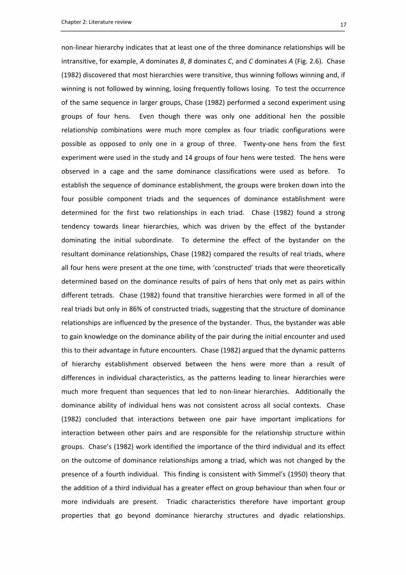
non‐linear hierarchy indicates that at least one of the three dominance relationships will be
intransitive, for example, A dominates B, B dominates C, and C dominates A (Fig. 2.6). Chase
(1982) discovered that most hierarchies were transitive, thus winning follows winning and, if
winning is not followed by winning, losing frequently follows losing. To test the occurrence
of the same sequence in larger groups, Chase (1982) performed a second experiment using
groups of four hens. Even though there was only one additional hen the possible
relationship combinations were much more complex as four triadic configurations were
possible as opposed to only one in a group of three. Twenty‐one hens from the first
experiment were used in the study and 14 groups of four hens were tested. The hens were
observed in a cage and the same dominance classifications were used as before. To
establish the sequence of dominance establishment, the groups were broken down into the
four possible component triads and the sequences of dominance establishment were
determined for the first two relationships in each triad. Chase (1982) found a strong
tendency towards linear hierarchies, which was driven by the effect of the bystander
dominating the initial subordinate. To determine the effect of the bystander on the
resultant dominance relationships, Chase (1982) compared the results of real triads, where
all four hens were present at the one time, with ‘constructed’ triads that were theoretically
determined based on the dominance results of pairs of hens that only met as pairs within
different tetrads. Chase (1982) found that transitive hierarchies were formed in all of the
real triads but only in 86% of constructed triads, suggesting that the structure of dominance
relationships are influenced by the presence of the bystander. Thus, the bystander was able
to gain knowledge on the dominance ability of the pair during the initial encounter and used
this to their advantage in future encounters. Chase (1982) argued that the dynamic patterns
of hierarchy establishment observed between the hens were more than a result of
differences in individual characteristics, as the patterns leading to linear hierarchies were
much more frequent than sequences that led to non‐linear hierarchies. Additionally the
dominance ability of individual hens was not consistent across all social contexts. Chase
(1982) concluded that interactions between one pair have important implications for
interaction between other pairs and are responsible for the relationship structure within
groups. Chase’s (1982) work identified the importance of the third individual and its effect
on the outcome of dominance relationships among a triad, which was not changed by the
presence of a fourth individual. This finding is consistent with Simmel’s (1950) theory that
the addition of a third individual has a greater effect on group behaviour than when four or
more individuals are present. Triadic characteristics therefore have important group
properties that go beyond dominance hierarchy structures and dyadic relationships.
Chapter 2: Literature review
18
A
B C
C
A
B C B
A
B C
B
a. Null
d. Triangle
b. Single relationship triads
c. Two relationship triads
A
B C
A
B
A
C
A
C
A
B C
Intransitive
B C
AA
B C
Transitive
Figure 2.5. The eight possible non‐directed triad configurations between actors, A, B andC.
Figure 2.6. The relationship configuration between triads in transitive and intransitive triangularformations.

Chapter 2: Literature review
19
Hierarchies in cattle have been reportedly based on both dominance hierarchies (e.g.
Beilharz and Zeeb, 1982) and affiliative relationships (e.g. Reinhardt and Reinhardt, 1981).
Chase’s (1982) model of hierarchy establishment was specifically based on agonistic
interactions leading to dominance relationships, but it is not known if the development of
affiliative relationships follows the same model. Additionally, analysing the outcomes of
dyadic and triadic interactions leading to relationship development and the implications of
these relationships on group structure has not previously been investigated in cattle.
2.5. Cattle social systems
Cattle are a social species that benefit from social interaction with others. They form
affiliative relationships with group members and maintain cohesive group structures (Hart,
1985). The social structure of cattle is described as permanent groups with the existence of
social hierarchies (Bouissou, 1980). A basic description of cattle social organisation includes
the physical structure, such as the size and attributes of the group members including their
age, sex and relatedness; the social components, such as the dominance hierarchy and
communication; and group cohesion, described by the individual relationships responsible
for keeping the group together (Broom and Fraser, 2007). The physical structure is group
specific, however properties relating to social components and cohesion are more generic to
animal systems. The basic principles of the dominance hierarchy and affiliative forces
maintaining the group and communication mechanisms are described in the next three
sections.
2.6. The dominance hierarchy
Social dominance has been a major focus of social behavioural research (Syme and Syme,
1979; Arnold, 1985). The function of a dominance hierarchy is to minimise agonistic
behaviour within the group thereby maintaining group cohesion and reducing social stress
(Mendl and Held, 2001). Stricklin and Mench (1987) describe a dominance relationship as ‘a
learned, predictable relationship between a pair of animals, where one of the pair is
consistently deferred to by the other’. A dominance hierarchy is therefore composed of a
combination of all the dominance‐submissive relationships within a group (Syme and Syme,
1979), while a dominance rank describes the relative position of each individual within the
hierarchy (Stricklin and Mench, 1987). The dominance rank of an individual is group specific,
Chapter 2: Literature review
20
such that the dominance rank in one group does not predict dominance rank in another
group (Lindberg, 2001).
2.6.1. Establishing dominance
There are a number of factors that can contribute to an individual’s ability to become
dominant, but the predominant characteristics are age, weight and the presence of horns. A
study by Bouissou (1972) investigated the effect of horns and live weight on the dominance
rank of Friesian heifers. The study involved 20 heifers that were reared together since birth
to control for factors such as rearing conditions and social experience. The animals were
assigned to one of four groups based on age and horn status: heavy with horns (group A),
heavy with no horns (group B), light with horns (group C) and light with no horns (group D).
The animals in the ‘heavy’ groups were three months older and thus greater live weight than
animals in ‘light’ groups while the animals in the ‘no horns’ groups were dehorned at 4
months of age. The experiment began when the youngest heifer was 18‐months‐old and the
groups were formed with one animal from each of the four treatment groups (A, B, C and D).
The heifers were introduced in an unfamiliar location and observed continuously for 3 hours,
and then for 1 hour each day over the next 6 days. Dominance relationships within each
group were determined by recording the direction of aggressive (butts and threats) and
submissive (withdrawal) behaviour between the four heifers and also by a feed competition
test, where two heifers had to compete for access to food in which only one could gain
access to. Each heifer was then assigned a rank according to their dominance status, with
one being the most dominant and four being the most submissive. In total, the dominance
relationships of 25 groups were determined, as well as the dominance status of each
individual against all individuals from other groups. Bouissou (1972) found that the presence
of horns was highly correlated with attaining dominance. Animals from the heavy with
horns group ranked higher than animals in all other groups, while animals in the light with
horns group ranked higher than the heavy with no horns group, and animals in the light with
no horns group ranked the lowest. These results were replicated when pair‐wise ranks were
analysed: horned and heavier heifers gained dominance in 97.5% of cases, while horned and
lighter heifers were dominant over de‐horned but heaver heifers in 75% of cases. When
heifers were of similar weight, the presence of horns was positively related to dominance,
and when both heifers were either horned or de‐horned, the heavier animal was the more
dominant. Bouissou (1972) concluded that when individuals are introduced for the first time
Chapter 2: Literature review
21
and they have similar social experiences, the presence of horns is a major determination of
dominance over and above the influence of live weight.
A further set of studies by Bouissou (1974b; a) investigated the nature of initial interactions
between newly introduced heifers and the rate that dominance was established. Twenty
groups of four, 18‐month‐old heifers were formed with animals that had previously not met
before; the heifers had experience with meeting strangers on one prior occasion. The
groups were observed for 6 days following group formation and all social behaviours, such as
agonistic interactions and exploratory behaviour such as sniffing, were recorded as was the
time and nature of the first encounter between each pair of heifers. The first study analysed
the nature and frequency of encounters between the newly introduced heifers while the
second study investigated the time taken for dominance relationships to establish. In the
first study, Bouissou (1974b) found that 73% of initial encounters between two heifers that
met for the first time were agonistic in nature, although only 37% of these interactions
resulted in a fight, with most dominance relationships determined without any physical
contact. The physical interactions reported by Bouissou were short in duration (less than 30
seconds) and were not observed after the first day. Bouissou (1974b) concluded that social
structure is established rapidly and that physical contests are not essential for establishing a
dominance relationship, which might be based more on evaluation of physical characteristics
and previous mixing experience of the individuals. In the second study (Bouissou, 1974a),
dominance relationships were considered established when the direction of agonistic
behaviour from one animal to another resulted in undisputed submission of the second
animal. Bouissou (1974a) found that almost half of all dominance relationships were
established within the first 5 minutes, with all relationships determined after 2 hours. The
established relationships remained relatively stable, with very few relationship reversals; it
was the relationships that were established without any physical contact that were less
prone to change. Bouissou (1974a) argued that the rapid establishment of relationships
were not influenced by the small number of individuals in each group. Similar results were
obtained by Bouissou (1974a) in a previous unpublished study when 16 unfamiliar animals
were introduced and the relationships between all 16 animals were established within an
hour and remained stable for at least a year. Bouissou (1974a) concluded that social
experience is important for establishing dominance relationships quickly and without any
physical contact. The results of Bouissou’s (1974b; a) studies show that individuals use prior
knowledge to avoid potentially damaging behaviours and only engage in physical contests
when there is a chance of success. The infrequent display of agonistic behaviour and the

Chapter 2: Literature review
22
long term stability of relationships contribute to a cohesive social structure, and makes it
difficult to identify the direction of dominance relationships between group members
(Bouissou et al., 2001).
2.6.2. Benefits of dominance
Domestic livestock are managed according to two general types of management systems:
intensive and extensive systems. Intensive production systems involve large numbers of
animals within small areas of space, requiring high inputs of resources and labour and are
common to dairy, poultry and swine production (Stricklin and Mench, 1987). In comparison,
extensive farming systems utilise larger areas of space with relatively low inputs of resources
and labour and is the predominant form of management for beef and sheep production
(Stricklin and Mench, 1987). The intensification of animal production has meant that
animals experience increased competition for resources, such as food and space (Bouissou,
1980).
2.6.2.1. Intensive production systems
A study by Manson and Appleby (1990) investigated the effect of dominance on spacing
behaviour between cows at a feed trough. The dominance relationships of a milking herd of
50 British Friesian‐Holstein cows and heifers were determined based on the display of
dominance‐submissive behaviour, and the herd was divided into three categories of high,
medium and low ranking cows. The authors observed the social and spacing behaviour of
the herd at the food trough. The trough was separated into 44 feeding positions, where only
one cow had access to a feeding position at the one time. The feeding positions were 0.65
m apart and used to indicate spatial proximity between individuals, where a distance of one
equalled one feed position apart (directly next to each other), two equalled two feeding
positions apart, and so on. Over a 15 day period, observations were recorded throughout
the middle of the day at 10 minute intervals several hours after food had been dispensed.
The study identified that dominance rank was a major determinant of spacing between
cows: cows of similar rank fed closer together than cows of different ranks, with the greatest
difference seen between low and high ranking pairs (4.4 feeding positions apart). Manson
and Appleby (1990) concluded that spacing was non‐random and cows spaced themselves
with respect to rank, with dominant individuals experiencing greater spatial separation from
lower ranked individuals.

Chapter 2: Literature review
23
The relationship between dominance rank and access to food and lying space was
investigated by Friend and Polan (1974). The authors used time lapse photography to record
feeding and lying behaviour of 21 Holstein dairy cows over a 2 month period. The cows
were housed in an observation lot and had access to 20 free stalls (individual stalls for
resting) and a 10.4 m feed trough that could accommodate 66% of the herd at the one time.
Each individual was assigned a dominance rank from one to 21 based on the outcome of
physical interactions between individuals, with 21 being the most dominant individual. The
authors determined that dominance rank influenced both time spent at the feeder and also
the lying location of the cows. Dominant cows spent more time at the feed trough
immediately after fresh fodder had been dispensed. The results suggested that subordinate
cows spent more time at the feeder than middle ranked cows, although this was well after
food had been dispensed and food supply was limited. There was a strong tendency for
individuals to prefer certain stalls over others; the dominant cows occupied the stalls closest
to the entrance and subordinate cows avoided using stalls that dominant cows used
regularly. Friend and Polan (1974) concluded that the cows displayed territorial behaviour
by repeatedly using the same stalls and the dominance rank of individuals determined their
resting location.
2.6.2.2. Extensive production systems
The studies described by Mason and Appleby (1990) and Friend and Polan (1974)
demonstrate the potential benefits gained from being dominant in an intensive housing
system. Competition for space is expected to be lower under extensive pastoral systems as
individuals generally have more access to space, although there are still advantages
associated with being dominant. Stricklin (1983) investigated the effect of dominance and
spatial relationships among a mixed group of Hereford and Angus cattle. Two groups of 20
cattle were observed in 10 ha plots. The proportion of wins and losses of physical
encounters during group formation and also during field observations were used to assign a
dominance rank to each individual. Thirty spatial observations were recorded by estimating
the number of body lengths between individuals within each plot and calculating the mean
distance to all cows and the distance from the group centre. The authors found that higher
ranking cows were more frequently found in the centre of the group, which was thought to
provide the greatest protection from predators. This finding is consistent with that of
Beilharz and Mylrea (1963), who studied the relationship between spatial position and
dominance of 27 mixed breed dairy heifers under three different movement orders:
movement from yards, free movement when grazing and forced movement along a fence

Chapter 2: Literature review
24
line. Dominance rank was assigned on the proportion of encounter wins and losses over a 2
week period, and the heifers were further classified as high, medium or low ranking animals.
The authors found that the three different movement orders resulted in different spatial
positions of the three dominance categories. In general, animals of higher dominance rank
were found more often in the middle of the herd and were not observed as leaders of any
movement. Middle ranked animals were more likely to lead during free movement, while
lower ranked animals tended to be at the front during forced movement, being bunted by
the higher ranked animals. Thus, there appears to be a relationship between dominance
and movement, with higher ranked animals maintaining central positions and protection
from predators and insects.
2.6.2.3. Mating opportunities
Rupp et al. (1977) explored the effect of social rank on the number of heifers mounted by
four bulls within a group of up to 100 Hereford heifers. The animals were kept in a 450 ha
paddock with a bull to female ratio of one bull to 25 heifers. Each bull was fitted with a chin‐
ball marking harness and a specific colour was assigned to each bull. The marking system
was designed to leave a mark on the rear of each heifer that was mounted by a bull.
Observations were collected at 12 hour intervals over a 21 day period, where the marks on
each heifer were noted as well as any dominance behaviour between the bulls to determine
their dominance rank. The authors found that the highest ranking bull recorded the overall
greatest number of marks. When heifers had been mounted by more than one bull, the
dominant bull was recorded more often than other bulls. It was concluded that dominance
in bulls was related to the number of heifers mounted, and resulted in the potential for the
dominant animal’s genetics to succeed into the next generation.
A series of experiments performed by Blockey (1979) investigated the effect of dominance
on the behaviour and performance of bulls. Earlier, Bouissou (1972) determined that
dominance in heifers was highly related to the presence of horns followed by body weight.
To investigate if the same relationship between weight and dominance was observed in
bulls, Blockey (1979) compared the dominance status of two groups of bulls with age,
seniority and body weight. Seniority, or time in the same group, was included in the
experiment as bulls are often kept in mixed‐age groups. The first group consisted of 50
Hereford bulls, which ranged in age from 2.5 to 9 years and the time spent in the same
group ranged from 8 to 49 months. There were 26 bulls in group two, whose ages ranged
Chapter 2: Literature review
25
from 2 to 5.5 years and time in the same group varied between 2.5 and 50 months.
Dominance was determined by forcing the bulls to compete for space within a 20 m by 20 m
yard until 35% to 53% of all possible pair combinations had been observed. Bulls were
ranked in order of the proportion of bulls they dominated in relation to the number of bulls
they contested. Blockey (1979) found that all three factors were important for determining
dominance, although seniority was found to have the most significant effect on dominance
rank. This effect was demonstrated by the high proportion of losses encountered by bulls
that were recently introduced into the groups. A second experiment by Blockey (1979)
investigated the effect of age and dominance on bull performance. Four groups of bulls
were tested for mounting ability. Groups one and two comprised 17 and 11 2‐year‐old bulls,
respectively, while groups three and four comprised eight and 12 mixed‐age bulls,
respectively, whose ages varied between 2.5 to 5 years. The dominance rank of each bull in
each group was determined using the same method described in the previous experiment.
The bulls were added to groups of 14 to 31 heifers and maintained on 0.7 ha plots. Visual
observations were used to record all mounting behaviour. Blockey (1979) found that
dominance orders were significantly more stable in the mixed‐age groups than the younger
bulls, which tended to have more complex hierarchies and frequent rank reversals during
repeat encounters. Additionally, there was no correlation between dominance rank and the
number of mounts recorded within the 2‐year‐old bulls. However, the results of the mixed‐
age groups agreed with those of Rupp et al. (1977), where the most dominant bulls were not
only the most sexually active but they also inhibited the mounting activity of lower ranked
bulls. The most dominant bulls in each group were the oldest, thus confirming the results
from the previous experiment. Blockey (1979) concluded that stability of the dominance
hierarchy influences bull performance at pasture and that seniority appears to be more
important than age in determining dominance rank in bulls.
2.6.3. The effect of dominance on production
Although the studies mentioned above have shown a link between dominance and access to
valuable resources such as space, food and mating opportunities, there is no conclusive
evidence to prove that dominance results in greater production levels. Beilharz et al. (1966)
investigated the effect of dominance on production traits, including milk production, of 76
Holstein dairy cows. The cows were managed as six separate groups according to lactation
stage and pregnancy status. The cow’s social behaviour was recorded over 3 days and a
dominance rank was assigned to each individual by calculating the proportion of wins each
Chapter 2: Literature review
26
cow had over all other cows. Milk production data was collected during the week that
behavioural observations were recorded, as well as the 2 weeks prior and 2 weeks after.
The total milk production over the 5 week period was compared with the dominance rank of
each cow. The authors found no significant correlation between milk production and
dominance. As expected, production levels were highly correlated with stage of lactation
and pregnancy status while dominance rank was correlated with weight. In support of this
finding, Dickson et al. (1967) also found no relationship between milk production and
dominance in a herd of 24 Holstein dairy cows. The cows were kept as two groups of 12 and
represented a range in age, weight and lactation stage. The behaviour of each cow was
recorded by observations for 8 hours a day over a 5 day period, which was repeated one
month later, with the winner and loser of each agonistic encounter used to calculate the
dominance rank of each individual in relation to all others. There was no relationship found
between dominance rank and milk production, while the only significant correlation
identified was between dominance and weight. Dickson et al. (1967) concluded that the
rank order of cows within the herd remained stable over the month and dominance rank is
more related to age and weight than to production level.
A further study on dominance and production was explored by Phillips and Rind (2002). The
authors first performed a similar study to those mentioned previously and found no
relationship between dominance and production in a group of 80 British Friesian dairy cows.
The authors hypothesised that removing the dominant animals from a herd would lead to
greater forage intake and thus an increase in production by subordinate animals. To
investigate this hypothesis, 72 of the cows used in their first experiment were divided in half
based on their previous dominance rank, either dominant or subordinate. The animals were
then allocated into one of four treatment groups: animals of same rank offered hay
supplement; animals of same rank offered no hay supplement; animals of both ranks kept
together and offered hay supplement; animals of both ranks kept together with no hay
supplement. Four observation periods with a sample interval of 10 minutes over a 24 hour
period were recorded of the animals in their groups, noting the grazing and social behaviour
of each cow. Additional observations of 3 minute intervals were recorded when the cows
were consuming hay. Production data was collected on two milking occasions per week over
a 4 week period. The authors found that when separated by rank, dominant cows produced
more milk than the group of subordinate cows when they were offered additional fodder.
There were no differences in the amount of forage consumed between the two groups,
although the dominant animals chewed at a faster rate. Additionally, when separated the

Chapter 2: Literature review
27
two groups spent longer lying than when the two ranks were mixed together. The
hypothesis that the subordinates would perform better when isolated from the dominant
individuals was rejected, as there were no production or intake gains observed by any of the
subordinate cows. The authors suggested that the presence of the subordinate cows created
tension in the higher ranked animals, and competition between the ranks resulted in faster
biting and chewing rates in the dominant animals. The difference in chewing rate identified
by Phillips and Rind (2002) suggested that dominant cattle modify their behaviour to gain an
advantage over other group members. Although Phillips and Rind (2002) discovered some
interesting results, the applications of the study are limited as it would not be possible to
maintain a group solely composed of dominant individuals; over time the group dynamics
would change and a new social order would be established. Thus, individuals that were of
high dominance rank in the previous group may become a lower ranked animal within the
new group structure.
Further evidence to suggest dominance has minimal effect on production level was provided
by McPhee et al. (1964), who studied the effect of feeding behaviour on growth in groups of
beef steers. Seven groups of six animals were fed from troughs in yards, and their
dominance rank determined every 2 weeks over an 8 month period. In addition to
dominance behaviour, feeding behaviour was also recorded including the time at the feeder
and the amount of undisturbed feeding time. The steers were weighed every 2 weeks and
the behavioural records and weight measurements were compared with dominance rank.
The experiment was run concurrently with a drought feeding experiment, which saw the
steers provided with either ad libitum low quality hay or restricted rations of low quality hay.
Consequently all steers lost weight during the trial, and the average weight loss by high and
low ranking steers was the same. Although there were feeding differences between high
and low ranking steers, high ranking steers spent more time feeding and had longer
undisturbed feed intervals. On average, low ranking steers were disturbed from feeding
every 10 minutes, compared with 14 minutes for high ranking steers. McPhee et al. (1964)
concluded that even though the higher ranking animals had greater access to food, this was
not reflected in growth differences between the ranks. The study highlights that even under
conditions of feed restriction low ranking animals are able to consume similar proportions of
forage as higher ranking animals, possible due to faster consumption rates. Additionally,
competition for access to the feed trough was minimised in McPhee et al.’s (1964) study,
with 0.60 m of space provided for each animal, so although the lower ranked animals were
disturbed more often, there was still space available to resume eating. Competition is
Chapter 2: Literature review
28
minimised in a domestic situation as the supply of resources such as food and space are
regulated (Price, 2008), thus the effect of dominance on behaviour and production is
reduced under these conditions.
Higher levels of agonistic interactions have been reported in larger groups of cattle, as found
by Rind and Phillips (1999), who investigated the effect of group size on behaviour. The
study involved 48 British Friesian dairy cows that were allocated into four groups of four
cows, two groups of eight cows and one group of 16 cows. Over a 53 day period, the groups
were observed in 1.5 ha plots for their general, social and feeding behaviour as well as their
inter‐individual distances every 10 minutes for one hour each day. The amount of agonistic
behaviour observed between groups was greatest for the cows in the largest sized group;
each cow exchanged an average of 7.3 agonistic interactions in the large group compared
with only 2.7 interactions for cows in the smallest group size. The authors suggested that
the cows in the large group required more frequent interaction to confirm each other’s
social status, thus the increased agonistic interactions were a result of cows preventing
others from entering their personal space. There may have also been greater competition
among the cows for grazing space, thus resulting in more displays of agonistic behaviour. It
was concluded that the size of the group affects individual behaviour but there was no
evidence to suggest that group size influences production, possibly as there were adequate
resources available. Although the study by Rind and Phillips (1999) presents some
interesting results, the lack of replication of the large group size and few replicates for the
medium sized groups limits the interpretation of these findings for groups other than those
used within this study. Nevertheless, the results do suggest that dominance affects group
behaviour and further studies on group size and behaviour are important.
2.6.4. Dominance hierarchy structure
A simple linear hierarchy appears to exist when group sizes are small (less than 10
members), where the top ranking animal A dominates all group members, and the second
ranking animal B dominates all other animals except A, and so on until the bottom ranking
animal dominates no one (Chase, 1974; 1980) (a in Fig. 2.7). However, hierarchies are more
complex in larger groups of cows and triangular formations may arise (b in Fig. 2.7). This
involves three animals within a larger group, where animal B might dominate C, and C
dominates D but D might dominate B (Hart, 1985), thus one animal is not dominant over the
other two. Equal dominance status can also occur when two individuals dominate over all
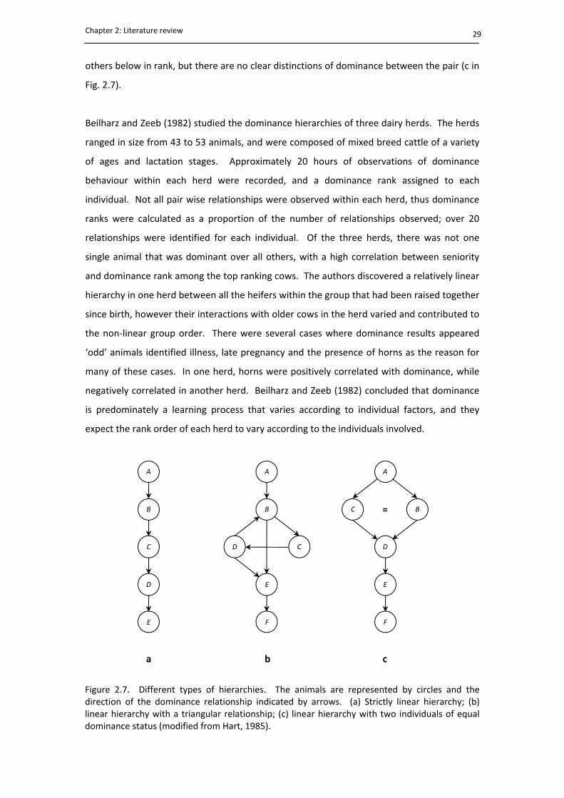
Chapter 2: Literature review
29
others below in rank, but there are no clear distinctions of dominance between the pair (c in
Fig. 2.7).
Beilharz and Zeeb (1982) studied the dominance hierarchies of three dairy herds. The herds
ranged in size from 43 to 53 animals, and were composed of mixed breed cattle of a variety
of ages and lactation stages. Approximately 20 hours of observations of dominance
behaviour within each herd were recorded, and a dominance rank assigned to each
individual. Not all pair wise relationships were observed within each herd, thus dominance
ranks were calculated as a proportion of the number of relationships observed; over 20
relationships were identified for each individual. Of the three herds, there was not one
single animal that was dominant over all others, with a high correlation between seniority
and dominance rank among the top ranking cows. The authors discovered a relatively linear
hierarchy in one herd between all the heifers within the group that had been raised together
since birth, however their interactions with older cows in the herd varied and contributed to
the non‐linear group order. There were several cases where dominance results appeared
‘odd’ animals identified illness, late pregnancy and the presence of horns as the reason for
many of these cases. In one herd, horns were positively correlated with dominance, while
negatively correlated in another herd. Beilharz and Zeeb (1982) concluded that dominance
is predominately a learning process that varies according to individual factors, and they
expect the rank order of each herd to vary according to the individuals involved.
Figure 2.7. Different types of hierarchies. The animals are represented by circles and thedirection of the dominance relationship indicated by arrows. (a) Strictly linear hierarchy; (b)linear hierarchy with a triangular relationship; (c) linear hierarchy with two individuals of equaldominance status (modified from Hart, 1985).
A
B
C
D
E
a b c
A
B
CD
E
F
A
BC
D
E
F
=

Chapter 2: Literature review
30
In a similar study, Collis (1976) also observed a complex hierarchy in a herd of 49 British
Friesian dairy cows. The group were raised together as calves and had been in the milking
group for almost 3 years. Over a 2 month period, the cows were observed for 2‐3 hours a
day between 2 and 3 days per week and all agonistic behaviour was used to determine the
dominance rank of each individual. Although the author was able to assign a single rank to
each cow in a linear order, there were many examples where lower ranking cows dominated
cows of greater dominance rank providing evidence of more complex structures, such as
triangular formations, within the hierarchy. Collis (1976) suggested that the similarity in age
between herd members minimised the effect of weight and experience on the rank of each
cow, resulting in many animals with similar dominance ranks. In contrast to the study by
Beilharz and Zeeb (1982), the hierarchy studied by Collis (1976) identified one top ranking
cow that was dominant over all other cows. However, the overall findings of Collis’ (1976)
study corresponds with the observation by Beilharz and Zeeb (1982) that each herd has its
own unique hierarchy dependent on individual characteristics, thus making it difficult to
assess generic traits that will consistently predict the dominance rank of individuals from
one hierarchy to the next.
2.7. Affiliative behaviour
The literature reviewed in the previous section highlights the extensive research on
dominance related behaviour in cattle. Investigating the establishment and function of
dominance in cattle was the focus of many of the early studies on cattle social behaviour
(e.g. Schein and Fohrman, 1955; Dickson et al., 1967; Rowell, 1974), which were followed by
investigations into the effects of dominance under different management systems (e.g.
Stricklin, 1983; Manson and Appleby, 1990). Correspondingly, the function of dominance
behaviour is well understood (Lindberg, 2001). More recent studies have tended to focus on
other aspects of social behaviour both in conjunction with and separate from dominance
behaviour. From the reviewed literature it is clear that establishment of a dominance
hierarchy serves to maintain social order whilst minimising agonistic behaviour and
governing access to limited resources. However, in domestic environments where the
supply of resources is regulated there are no clear production advantages gained by being
dominant and it is generally accepted that dominance status varies according to the
individuals involved. However, due to the large focus on dominance behaviour, other areas
of social behaviour remain largely unexplored (Arnold, 1985; Lindberg, 2001). This is
surprising given that the basic structure of a natural cattle herd is matriarchal with

Chapter 2: Literature review
31
preferential relationships between non‐kin individuals (Reinhardt and Reinhardt, 1981).
These relationships are formed and maintained through affiliative behaviours, such as social
grooming and social grazing, and displays of aggression and dominance are rare. Thus it is
the affiliative behaviours and preferential relationships that form the cohesive structure of
the herd. The following section evaluates aspects of affiliative behaviours that influence
group cohesion, including the effect of familiarity, the characteristics of preferential
relationships, and the principles of spacing behaviour that reflect an individual’s sociability.
2.7.1. Familiarity
Familiarity influences the strength of attraction between individuals, thus promoting stability
within the social structure (Syme and Syme, 1979; Ruddell et al., 2007). Familiarity is said to
occur from recognition and social history between the individuals involved, including
knowing who occupies what position in the social structure (Hinde, 1976). The added
benefits of familiarity is the increased level of social support conspecifics provide, with
familiar group members maintaining closer proximity to each other than to unfamiliar
conspecifics (e.g. Murphey, 1990; Takeda et al., 2000). A study by Murphey (1990)
investigated the effect of breed and familiarity on group behaviour by comparing groups of
cattle raised in same‐breed groups with those raised in mixed‐breed groups. The study
involved two separate observations of free‐ranging herds of yearling heifers and mature
cows. The herds were of three different breeds that varied in colour and shape: the
Brahman’s used were all red in colour, the Charolais were white and the Brangus cattle were
black. The first observation period consisted of three groups of same‐breed cattle that had
been raised with members of their own breed in isolation from other breeds. The groups
were made up of 57 reds, 18 whites and six blacks and were mixed for the purposes of the
study. Observations of nearest neighbours were recorded, noting the identity and breed of
the nearest neighbour of each focal animal. The author found that nearest neighbours
tended to be of the same breed and the groups separated themselves by breed. The groups
were herded to a different property for the second observation period where they were
introduced to two groups of same‐breed cattle and one group of mixed‐breed cattle. The
same‐breed groups were made up of 42 whites and 62 blacks, while there were 38 heifers in
the mixed‐breed group including red, white and black heifers. Murphey (1990) found that
the mixed‐breed group tended to maintain a sub group within the larger herd and
performed rubbing and grooming with their original herd mates. As with the cattle from the
first property, cows that had been raised together continued to associate together.
Chapter 2: Literature review
32
Murphey (1990) concluded that cattle tend to associate with their most familiar herd mates
regardless of genetic or phenotypic similarity.
The effect of familiarity is also said to influence grazing behaviour. Scott et al. (1995)
conducted a series of four experiments to examine the effect of food and social preference
on the spatial location of sheep. The first experiment investigated the effect of food
preference on spatial location. Twelve lambs that had been raised together since birth were
separated into two groups and introduced to two different food sources, either sorghum or
wheat, and were conditioned to form a preference toward one food source over 14 days.
The groups were then exposed to the other food source treated with a mild toxin to develop
and aversion to the novel food. The lambs were tested for their spatial and feeding
behaviour in three different sub group configurations based on their food preferences: the
first group consisted of three lambs conditioned to prefer wheat and three lambs
conditioned to prefer sorghum; the second group was composed of one lamb conditioned to
wheat and three lambs conditioned to sorghum; the third group included three lambs that
preferred sorghum and one lamb that preferred wheat. The groups were located in a 0.25
ha pasture plot with the grains located at opposite ends of the plot. Equal amounts of wheat
and sorghum were supplied for group one, while only a quarter of wheat was supplied for
the second group and a quarter of sorghum for group three. A final test observed foraging
behaviour of the original two groups when both grains were offered at opposite ends. All
sub groups of lambs were exposed to the plot for 30 minutes a day over 3 days and the
spatial location (which half of the pasture) and feeding activity (consuming wheat or
sorghum) of each lamb was recorded once every minute. The results showed that lambs
foraged on their preferred grains irrespective of the location of group members; even when
only one lamb had a preference for either grain, the lamb spent the first 10 minutes
consuming its preferred grain away from the other three lambs before re‐joining the group.
In the second experiment, a separate group of lambs that had not been exposed to the toxin
were reared separately in three treatment groups from 1 month of age. Each group
comprised six lambs that were conditioned to prefer either wheat or sorghum over a 4
month period: the lambs in group one were conditioned to prefer sorghum, group two were
conditioned to prefer wheat and three lambs in group three were conditioned to prefer
sorghum and the other three conditioned to prefer wheat. The lambs were located in a 1.0
ha experimental plot for 30 minutes per day over 6 days to observe their location and
feeding behaviour: during the first 4 days the lambs had access to sorghum and wheat
located 100 m apart at opposite ends of the plot. On the last 2 days of testing the authors

Chapter 2: Literature review
33
also recorded the lamb’s behaviour when no food was present to investigate if the lambs
foraging behaviour was affected by the presence of supplementary food. In support of
Experiment 1, the results showed that feeding location was influenced by food preference
when accompanied by peers that preferred the same food, however, the results varied when
for the mixed‐preference groups. In some groups, lambs that preferred sorghum grazed
nearby companions consuming wheat and then those that preferred wheat grazed nearby
while companions consumed sorghum, while in other groups some lambs ate their preferred
grain irrespective of the presence of social partners. The results suggest that when peers
have different food preferences the decision to consume a preferred food source or
maintain proximity to peers is influenced by the individual’s level of sociability and feeding
motivation. When there was no supplementary food, lambs showed no preference for
either area during the first 10 minutes, thus confirming that the location of food is an
important determinant of foraging location. To investigate if food aversion influenced
pasture use, the lambs in each group were given the alternate food containing a mild dose of
a toxin before being tested in the experimental plot using the same procedure as
Experiment 2. The lamb’s behaviour did not change from the previous experiment and
showed no sign of increased affinity in the area with their preferred grain. Experiment 4
investigated the role of familiarity on lamb foraging location. Three lambs from the wheat
group and three lambs from the sorghum group in Experiments 2 and 3 were combined to
form a group of unfamiliar lambs with mixed food preferences as well as an aversion to the
alternate food source. The lambs were tested for location and feeding activity as per the
previous two experiments. During the first 10 minutes of the test the lambs foraged on their
preferred grains before forming a single group and grazing the plot without any bias. Scott
et al. (1995) concluded that feeding preference is a primary determinant of foraging location
when lambs are reared separately and prefer different foods. To further test the effect of
unfamiliarity and rearing conditions, it would have been interesting to record the grazing
location of sub groups formed from two groups of mixed preference lambs (i.e. three lambs
conditioned to wheat and three lambs conditioned to sorghum from one group and three
lambs conditioned to wheat and three lambs conditioned to sorghum from a second group)
to see if unfamiliarity affected grazing location and the extent to which lambs ate their
preferred grain in the presence of unfamiliar lambs with the same feeding preference. The
study by Scott et al. (1995) provides evidence that sub group formation and pasture use by
herbivores is influenced by both feeding preference and social relationships.
Chapter 2: Literature review
34
A study by Boissy and LeNeindre (1997) investigated the physiological effect of isolating a
heifer and reuniting her with either a familiar or unfamiliar peer. Twelve Friesian and 12
Aubrac 15‐month‐old heifers were kept as four groups of six according to breed with contact
restricted between groups. The experimental set up consisted of a bail crush to restrict one
animal at a time, which faced a triangular test arena that was large enough to hold all 6
heifers. A remote control gate led to a corridor that connected the test arena to the crush
entrance. The use of a crush and remote control gate limited the amount of physical
handling of the heifers. The heifer groups were gradually introduced to the experimental set
up and testing procedure over a period of 12 days. Once the heifers were familiar with the
set up, three habituation tests were performed followed by two test sessions. During the
habituation tests, a test animal was restrained in the crush while the five other group mates
were in the test area. After 8 minutes, a person entered the test area and moved around
the edge of the area generating movement within the pen mates before leaving. This was
repeated 8 minutes later and the test session ended after 25 minutes. During the test
sessions the same habituation procedure was repeated except when the person left the
arena the first time the pen mates were removed as well. Eight minutes later the person
returned with either the five familiar pen mates or five unfamiliar heifers of the other breed.
The familiar or unfamiliar peers were left in the test arena until the test animal had been
restrained for 25 minutes. A single observer recorded all behavioural responses, including
contact with peers, vocalisations and struggling behaviour of the test animal. Additionally,
cardiac activity was recorded by a heart rate monitor at 15 second intervals during each test
session and cortisol levels were measured from blood samples taken immediately upon
entering the crush and again at the conclusion of the test session. Elevated levels of cortisol
have been linked to stress and anxiety behaviour in cattle (Bristow and Holmes, 2007). The
results of the habituation sessions showed an increase in overall activity, heart rate and
cortisol levels when the test heifer was restrained. However, these levels decreased over
the three habituation sessions. A marked difference was observed between breeds with
Aubrac heifers recording higher levels of behavioural activity, heart rate and cortisol than
Friesian heifers. During the test sessions, heifers showed a strong behavioural reaction to
being isolated: isolated heifers struggled for 40% of the isolation period and their
behavioural activity increased tenfold with a large increase in vocalisations. Additionally,
heart rate and cortisol levels were significantly increased during this period. When peers
were returned all three factors decreased although the decline in heart rate was more
pronounced in the presence of familiar pen mates than unfamiliar peers. The authors
summarised that social isolation is a very strong psychological stress in cattle and the extent

Chapter 2: Literature review
35
of this effect is influenced by breed, and it was observed that Aubrac heifers were more
reactive than Friesian heifers. The sight of heifers of either familiarity was enough to reduce
the distress of being isolated, although the presence of familiar peers was more effective at
reducing cardiac activity than unfamiliar peers and therefore suggests that familiar peers
have a calming effect.
A similar test was conducted by Faerevik et al. (2006) to investigate the effect of social
isolation and the presence of familiar and unfamiliar peers on the behaviour of calves. The
study involved 20 Holstein Friesian mixed‐sex calves that were divided into five groups of
four. At the time of grouping the calves averaged 21‐days‐old. One group was kept out of
sight of the other groups to form the unfamiliar group while three calves from each of the
other four groups were selected as test animals, leaving one calf per group as a familiar
stimulus. When the calves reached 6 weeks of age, the 12 test calves were subject to two
different experimental tests. The first test was a social preference test, where the test calf
could choose between a familiar or unfamiliar calf located at the end of a Y‐maze. The Y‐
maze consisted of a start box where the test calf was held prior to the test that was
connected to a 3 m narrow corridor. At the end of the corridor was the entrance to the two
‘arms’ of the Y‐maze, which were also 3 m in length, where the stimulus calves were
tethered. Video recording devices were used to capture the behaviour of the test calves
during each session and were analysed for the time taken to enter the maze and initiate
contact with either stimulus calf, the proportion of time spent in each arm of the maze and
the number of social contacts with familiar and unfamiliar stimulus calves. The calves were
observed for 20 minutes in the maze before being returned to their pens. The second test
was a separation test where the test calves were placed in a 1.8 m x 1.8 m pen that was
unfamiliar to them and observed under three different test conditions: with a familiar calf;
with an unfamiliar calf; and with no other calves present. Each condition was repeated three
times for each test calf. The calf’s general activity, including the number of steps taken and
number of vocalisations were recorded by direct observations and a heart rate monitor
collected cardiac activity for the duration of the 20 minute test. The results of the Y‐maze
tests showed that calves spent the majority of time within close proximity to familiar
stimulus calves, although there was no difference in the amount of physical contact with
either familiar or unfamiliar calves. The results of the separation test showed that calves
vocalised more when isolated or with an unfamiliar calf than when in the presence of a
familiar calf, where no vocalisations were recorded. The test calves interacted more with
familiar stimulus calves the first time they were subject to the separation test, however this

Chapter 2: Literature review
36
effect decreased over the three repetitions. There was no difference in the amount of
activity expressed by the test calf when in the presence of either familiar or unfamiliar
stimulus calves, however there was a significant decrease in activity when isolated. The test
calves heart rate was higher when in the presence of familiar calves than when separated
with unfamiliar calves or isolated. This finding was unexpected but explained by the positive
correlation between heart rate and increased activity during these tests. The results from
the two tests suggested that calves prefer the company of familiar over unfamiliar peers and
it is likely that the familiar calf provided a calming effect in the novel environment. In
agreement with the results of Boissy and LeNeindre (1997), separation from peers caused
the greatest amount of distress which led to increased vocalisation, more immobility and
less exploration of the test pen. The finding that the calves did not vocalise in the presence
of a familiar calf reinforces the suggestion that familiar calves provide a calming influence.
The results of studies by Boissy and LeNeindre (1997) and Faerevik et al. (2006) provide
evidence that familiar peers provide a calming effect and suggest that cattle will
preferentially select a familiar peer over an unfamiliar peer. This has also been found in
other animal species, such as chickens (Marin et al., 2001), sheep (Boissy and Dumont, 2002)
and pigs (McLeman et al., 2005). However, these experiments rely on conditioning tasks or
stressful environments that may influence the behavioural response of the test animals. The
effect of the presence of a familiar animal has not been thoroughly tested in cattle and is an
area of research that requires further investigation.
2.7.2. Preferential relationships
A preferential relationship, or a social bond between two individuals, is ‘a mutual
relationship that is relatively long lasting and survives temporary separation’ (Keeling and
Gonyou, 2001). Reinhardt and Reinhardt (1981) observed a cattle herd under a semi‐natural
environment for 5 years and found evidence of long lasting relationships between particular
herd members. The semi‐natural environment involved mustering the herd into yards at
night but allowing the herd to graze freely during the day, with no other human interference
such as milking, castration or grouping. At the beginning of the study the herd consisted of
30 cows, 3 calves and one bull. After 4 years, 74 offspring were born into the herd
increasing the herd size to 108. At this time 17 bull offspring were sold and a large portion
of the herd was moved on to another property, leaving the bull, 11 of the original cows and
their 35 offspring for the remaining 11 months of observations. Observations were recorded
Chapter 2: Literature review
37
intermittently over the 5 year period. The authors recorded the identity of animals that
consistently grazed together and groomed together and defined a relationship as two
individuals that were observed grooming or grazing together for three or more consecutive
years. Relationships were assessed for the effects of relatedness between adults and calves.
The authors found evidence of 36 preferential relationships between the adults: 20
relationships were observed for grooming and 16 for grazing, with 6 cohesive relationships
identified where individuals were both preferred grazing and grooming partners. Within
these associations, some cows were more popular than others. A single cow ‘Alma’ was
identified as the most popular grazing partner and was also observed as the leader of all
grazing movement, which may explain why others chose to remain within close proximity to
her. In the grooming relationships, one cow ‘Daisy’ received more grooming than any other
cow, although she showed no particular attributes to explain her popularity. Additionally,
the direction of the associations varied according to activity: 60% of grazing associations
were mutual while only 5% of grooming associations were reciprocated. Analysis of the calf
associations found that sibling associations were the strongest and related calves grazed
together more than unrelated calves. Although, there were still friendships observed
between non‐related calves in 67% of calves, which were predominately based on
similarities in age and not influenced by sex. In contrast, there were no grooming
association formed between calves. The associations between non‐related heifer calves
tended to decline when the heifers gave birth for the first time as their attention was
focused on their own offspring, and it is not known if these relationships were restored once
the offspring matured. In contrast, the bull‐bull calf relationships remained strong.
Associations between cows and their related calves were stronger than any other
association for both grazing and grooming and the authors rarely observed a cow grooming
a calf other than her own. Reinhardt and Reinhardt (1981) found that the cow‐calf bond still
remained strong even after weaning and the birth of second and third offspring and the cow
retained more contact with her own offspring than non‐related calves. There were no
differences observed between mother‐heifer and mother‐bull relationships over the 4 year
period. In wild populations it is expected that the males calves would be driven away from
the herd when they reach sexual maturity, however the herd’s management meant that the
males were forced to remain in the herd thus suggesting that if no other external factors
interfere with mother‐bull relationships the close association may continue. In total, 83% of
individuals formed associations with each other, although there were clearly popular
individuals, such as Alma, who received the most grazing preferences and was also observed
as the leader of all grazing movement. Reinhardt and Reinhardt (1981) summarised that the

Chapter 2: Literature review
38
basis of relationships between cattle are founded on matriarchal families formed by
attachments between siblings and cow‐calf bonds, and kin relations are interconnected by
friendships between non‐related partners. These relationships are extremely stable and
form a complex social structure of associations based on personal inter‐individual
attractions.
2.7.3. Allogrooming
Allogrooming has been identified as a key indicator of preferential relationships (Boissy et
al., 2007). In a study by Sato et al. (1991), the authors investigated the function of
allogrooming in calves. The authors observed two separate groups of mixed‐sex Holstein
yearlings, aged between 12 and 15 months of age, with 13 animals in group one and 14
animals in group two. The time that the group had been together varied: some calves had
been together longer than 4 months, some between 3 and 4 months and others between 1
and 2 months. The dominance rank of all animals was determined during a preliminary
observation period, as well as during observations recorded during the experimental period.
Two calves per group were chosen as focal animals based on preliminary observations as the
most frequent performers of allogrooming from group one and the most frequent receivers
of allogrooming from group two. The calves were housed in a barn and fed silage twice a
day, and the barn was cleaned every 5 days. To explore the effect of environmental
conditions on grooming behaviour, the afternoon feed was removed and the barn was not
cleaned on a regular basis for part of the experiment. Social and grooming behaviours
involving the focal animals were recorded via video camera for 13 days, noting if the
grooming behaviour was initiated by the receiver, referred to as solicitation, or if the
grooming commenced without solicitation. On average, the focal animals performed
allogrooming nearly 5 times per hour, with an average grooming bout lasting 43 seconds.
The frequency of grooming increased when the barn was dirty, which provided evidence to
confirm that grooming is performed for cleaning purposes. There was also more grooming
when the calves had not been fed in the afternoon, which Sato et al. (1991) suggested was a
displacement activity to relieve the tension created by not being fed. There was more
unsolicited grooming than there was solicited grooming, however the solicited grooming
tended to last for longer duration and confirms that grooming is desired by the receiver.
Sato et al. (1991) also suggested that allogrooming has a tension relieving effect as some
animals were observed to half close their eyes while receiving grooming, which was also
reported by Brownlee (1950) when describing aspects of behavioural patterns observed in
Chapter 2: Literature review
39
domestic cattle. Sato et al. (1991) found a positive relationship between allogrooming and
familiarity, with more grooming occurring between calves that had been together the
longest. There was no association between dominance rank and the performer or receiver
of grooming, confirming that grooming behaviour is not dependent on social rank. Sato et
al. (1991) concluded that the act of allogrooming not only has hygiene benefits, such as
cleaning and parasite removal, but also has emotional properties that can reduce stress and
reinforce social bonds between group members. A further study by Sato and Tarumizu
(1993) investigated heart rate changes caused by the act of allogrooming. The authors fitted
heart rate monitors to five steers and compared their heart rates before, during and after
allogrooming when mixed with five other steers. Heart rate data was analysed only when
the animals were standing and only when grooming bouts exceeded 24 seconds in duration.
The heart rate data was collected for 2 minutes after grooming had ended. In total, 27
observations of grooming were analysed. The results showed a statistically significant
decrease in heart rate during grooming, with the average heart rate reduced by 4 beats per
minute when compared with pre‐grooming rates. The heart rate returned to a level
comparable with pre‐grooming rates once grooming had finished. Sato and Tarumizu (1993)
suggested that allogrooming has a calming effect in cattle and this may help to ease tension
in a stressful situation.
The relationship between allogrooming and social preference was also explored by Val‐
Laillet et al. (2009). The study involved 48 Holstein cows that were grouped into six groups
of eight and allowed 15 days to stabilise relationships before the experiment began. The
cows were fed twice a day immediately following milking. After 21 days of continuous
observations using video recording equipment, space at the feeder was reduced from 0.60 m
per cow to 0.30 m per cow to investigate the effect of competition and dominance on
allogrooming. The video footage was analysed for agonistic and affiliative behaviour,
nearest neighbour identities and dominance rank. On average, cows performed 5‐6
grooming bouts per day, which is much less than the 5 times per hour reported by Sato et al.
(1991); however Sato et al.’s (1991) study involved much younger animals that were also
confined in a smaller space, which may have influenced the rate of grooming. The effect of
reducing feeding space resulted in less time spent at the feeder but there were no significant
reductions in the number of allogrooming bouts, only the length of grooming was reduced.
Val‐Laillet et al. (2009) suggested that if allogrooming served to reduce tension, then
allogrooming should have increased when competition was greater during feed space
restriction. However there was no evidence of increased allogrooming with increased

Chapter 2: Literature review
40
competition and the authors suggested that further studies should investigate the role of
allogrooming during periods of tension, such as regrouping individuals. In agreement with
Sato et al. (1991), Val‐Laillet et al. (2009) found no relationship between dominance rank
and time spent grooming, however there was a positive correlation between preferential
relationships and grooming partners: cows identified as nearest neighbours during feeding
were observed grooming each other more often. Val‐Laillet et al. (2009) argued that the
cows shared a mutual attraction rather than similar feeding habits, as the cows were also
observed allogrooming away from the feeder and were consistently seen together over the
experimental period, even when space available at the feeder was reduced and competition
was increased. The findings correspond with those of Reinhardt and Reinhardt (1981) who
observed preferential grooming associations between individuals regardless of their physical
and social characteristics. It was concluded that allogrooming has a cohesive role in
maintaining preferential relationships. The existence of preferential relationships is
described as the ‘fundamental element’ of cattle social structure (Reinhardt and Reinhardt,
1981), thus knowledge on factors that contribute to these relationships can provide
information on the basis of group social cohesion as well as a measurement of positive
welfare.
2.7.4. Spatial behaviour and individual distance
The spatial relationships between individuals within a group are a characterising feature of
the group’s social structure. Each individual has specific spatial properties that contribute to
the function and cohesion of the social system. McBride (1971) described the area that an
individual will maintain free from others as a ‘personal field’, and will avoid entering the
personal fields of others. The distance maintained between two individuals is referred to as
the ‘individual distance’ (Hediger, 1963) or ‘inter‐individual distance’, and the distance that
an individual will allow another to approach before responding, either with aggression or
avoidance (Price, 2008). The inter‐individual distance between two animals results from a
balance between the tendency to approach and withdraw from each other (Keeling, 1995),
thus inter‐individual distance provides an indication of the social attraction and relationship
status between the pair. McBride (1971) described ‘living space’ as the space that an
individual will move in, somewhere between the personal spheres of group members and
the ‘social distance’, defined by Hediger (1963) as the maximum distance individuals will
move away from the group (Fig. 2.8). The social distance is therefore an important cohesive
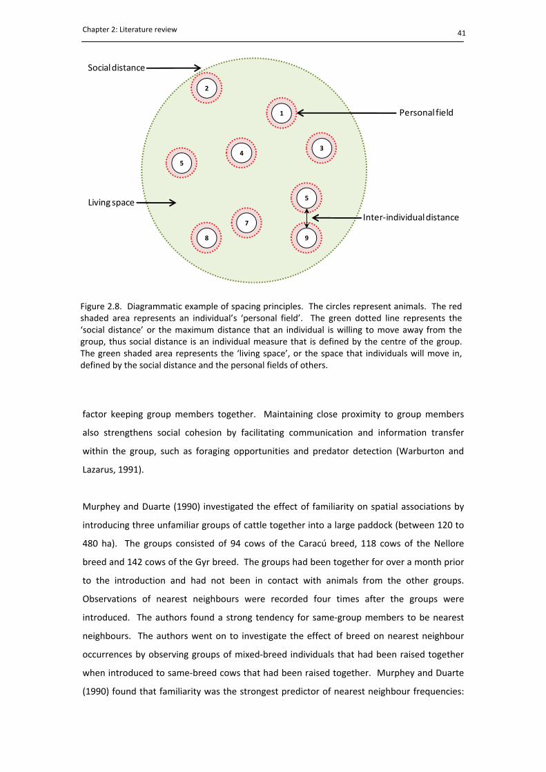
Chapter 2: Literature review
41
4
8
2
5
9
3
1
5
7
Social distance
Personal field
Living space
Inter‐individual distance
factor keeping group members together. Maintaining close proximity to group members
also strengthens social cohesion by facilitating communication and information transfer
within the group, such as foraging opportunities and predator detection (Warburton and
Lazarus, 1991).
Murphey and Duarte (1990) investigated the effect of familiarity on spatial associations by
introducing three unfamiliar groups of cattle together into a large paddock (between 120 to
480 ha). The groups consisted of 94 cows of the Caracú breed, 118 cows of the Nellore
breed and 142 cows of the Gyr breed. The groups had been together for over a month prior
to the introduction and had not been in contact with animals from the other groups.
Observations of nearest neighbours were recorded four times after the groups were
introduced. The authors found a strong tendency for same‐group members to be nearest
neighbours. The authors went on to investigate the effect of breed on nearest neighbour
occurrences by observing groups of mixed‐breed individuals that had been raised together
when introduced to same‐breed cows that had been raised together. Murphey and Duarte
(1990) found that familiarity was the strongest predictor of nearest neighbour frequencies:
Figure 2.8. Diagrammatic example of spacing principles. The circles represent animals. The redshaded area represents an individual’s ‘personal field’. The green dotted line represents the‘social distance’ or the maximum distance that an individual is willing to move away from thegroup, thus social distance is an individual measure that is defined by the centre of the group. The green shaded area represents the ‘living space’, or the space that individuals will move in,defined by the social distance and the personal fields of others.

Chapter 2: Literature review
42
cows that were familiar with each other were more frequently found within close proximity
to group members than non‐group members. This feature of a social group has been
observed regardless of the amount of space available (Price, 2008).
There are many factors that affect the spatial distribution of a group. At a functional level,
spatial positioning is influenced by anti‐predation strategies and resource distribution, whilst
at a local level, the dominance hierarchy and behavioural activity influences the distance
between individuals (Keeling, 1995). The dominance relationship between individuals will
affect their spatial distribution, with animals further apart in rank tending to maintain the
greatest distances (e.g. Manson and Appleby, 1990). Activities associated with greater
predation risk, such as resting, will draw individuals together, while competitive activities,
such as grazing, will keep individuals apart (Keeling, 1995). The average distance individual
cattle keep between themselves and other group members when resting is 2‐3 m, compared
with 4‐10m when grazing (Broom and Fraser, 2007). Additionally, the size of the social
group and thus the number of individuals available to provide protection influences the
distance individuals maintain between themselves and others. In the study by Rind and
Phillips (1999) (section 2.6.3) that investigated the effect of group size on behaviour, the
authors found that spacing between individuals in groups of four was smaller than inter‐
individual distances in groups of 16 (6.5 m and 13.8 m, respectively). Rind and Phillips (1999)
suggested that the smaller distances were a result of greater cohesion between the
individuals in response to greater predation fear. Thus, maintaining close spatial proximity
reinforces a sense of safety and protection provided by group members.
2.7.5. Sociability
The distance between animals can provide not only an indication of the relationship strength
between each pair within the group, but also the individual’s level of sociability. Sociability is
the ‘tendency to be close to others’ (Sibbald et al., 1998), and can therefore be predicted
based on consistent spatial patterns between group members. Sibbald et al. (1998)
developed a sociability index that was later refined by Sibbald and Hooper (2004), which was
used to rank individuals based on their sociability by calculating the proportion of time that
each individual was recorded as the nearest neighbour of any other animal in the group.
Sibbald and Hooper (2004) describe this method using Scottish Blackface sheep as an
example. Four groups of 11 animals were observed in a grazing environment over a 3 week
period, noting the identity of each animal’s nearest neighbour at every 5 minute scan. To
Chapter 2: Literature review
43
calculate the sociability index, the number of observations that each animal was recorded as
a nearest neighbour of all other animals was summarised in a matrix, with focal sheep listed
across rows and neighbours listed in columns. The values for each cell were divided by the
total number of observations recorded, and the column totals were divided by 100 to give a
sociability index for each animal. The sociability index values ranged from 0 to 1.0, with
larger numbers indicating more sociable animals. To investigate the application of the
sociability index, Sibbald and Hooper (2004) explored the relationship between sociability
and the distance individuals would move away from their group to feed. From each of the
four groups, two sheep with high sociability indices and two sheep with low sociability
indices were selected to take part in a food motivation test. The sheep were introduced to
three different grazing environments: a control treatment where a test animal was placed in
a bare 65 m plot separated from group mates by a wire fence; a near treatment, where the
test sheep had to travel 15 m from the penned group mates to reach preferred forage; and a
far treatment, where the test animal had to travel 35 m to reach the desired forage. Prior to
testing, the group were confined for 1 hour without food. Observations began 2 minutes
after the test sheep was released, and the behaviour of the test animal (e.g. grazing,
standing, lying) and its distance from the penned sheep was recorded every 30 seconds over
a 75 minute period. At 15 minute intervals, the bite rate of the test animal was also
recorded. The authors found that overall the highly sociable sheep remained closer to the
penned sheep on all treatments than the less sociable sheep, while less sociable sheep
tended to spend more time grazing with faster bite rates than highly sociable sheep. Sibbald
and Hooper (2004) found that there were significant differences between sociability types in
the distances they travelled to graze and suggested that the distance between group mates
and food in the near treatment provided an environment similar to a grazing situation, thus
identifying endogenous sociability tendencies. However on the far treatment, 35m is
greater than nearest neighbour distances normally observed between Scottish Blackface
sheep and the distance may have been too far to create a trade‐off for any of the sheep, and
there were no clear differences between sociability types at this distance. Sibbald and
Hooper (2004) suggested that moving away from the social group may have elicited a fear
response of being socially isolated, and may account for the faster bite rate to reduce the
time away from the group. It is also suggested that the lower bite rate by the more sociable
sheep may indicate greater vigilance and anxiety at being separated from their peers,
whereas the less sociable sheep appeared less fearful when at greater distances from the
group. Sibbald and Hooper (2004) concluded that sociability affected the choice between
foraging and staying close to peers when the food source was close, however when the

Chapter 2: Literature review
44
foraging source was a greater distance away other factors, such as fear, influenced the
decision to remain with peers or to move away.
The relationship between sociability and the trade‐off between feeding and social
companionship was further investigated by Sibbald et al. (2006). The authors designed a
test to measure an individual’s motivation to remain close to a pen of group mates by
recording the distance that the individual would move away for a highly palatable food. The
experiment involved 40 Scottish Blackface sheep that were kept in four groups of 10
animals, and their sociability index was calculated using the same method mentioned above.
The animals were exposed to two different test conditions: a control test, where no food
was offered, followed by three pellet tests, in which pellets were offered in bowls at 5 m
increments down the centre of a 65 m test arena. During each test, a single sheep was
released into the arena and the animal’s behaviour was recorded every 30 seconds over a 30
minute period, while all bowl visits and walking and vigilance behaviour were recorded as
they occurred. Sibbald et al. (2006) found that highly sociable sheep showed greater levels
of vigilance, took longer to explore all of the food bowls during the first pellet test and
remained in closer proximity to the penned group than less sociable sheep. Sibbald et al.
(2006) suggested that the highly sociable sheep were more anxious about moving away from
the group and this limited their motivation to obtain a desired food some distance away.
The work by Sibbald et al. (2006) on sociability in sheep explored the fundamental
relationship between spatial proximity and sociability, and demonstrated how individual
sociability effects behaviour and foraging decisions. Future investigations should consider
extending the application of these principles to cattle systems, where knowledge on
individual social tendencies and spatial behaviour would provide a valuable tool when
assessing social behaviour and relationship status.
2.8. Communication and individual recognition
Communication between individuals occurs when a signal expressed by one individual is
received and responded to by another (Wilson, 1975). The function of communication is to
share information, such as details on an individual’s internal state, such as fear, hunger or
excitement, their environment, such as the appearance of a predator, or to recruit others to
the same location, such as an attractive food source (Millman and Duncan, 2001). Other
functions of communication also include identifying and locating others, giving orders and
Chapter 2: Literature review
45
reinforcing social status (Hart, 1985). Therefore, communication is essential for establishing
and maintaining social organisation within a group (Leuthold, 1977; Murphey and Duarte,
1990; Lindberg, 2001). Communication between animals occurs via four signals, including
visual signals, such as posture and movement, auditory signals, such as vocalisations,
olfactory signals, such as scents, and tactile signals, such as touch or physical contact with
others. The sensory modalities of cattle are summarised as a panoramic field of vision with
limited depth perception, acute hearing capable of detecting high frequency noises, and
sensitivity to touch and odours (Grandin, 1980).
Similar to communication, recognition is essential for social interaction (Arnold, 1985).
Recognition relies on memory and recollection of previous social encounters and
behavioural observations of others (Broom and Fraser, 2007). Recognition also uses visual,
auditory, olfactory and tactile sensory cues. The behaviour of cattle provides evidence that
individuals are capable of individual recognition, in particular is the ability to establish and
maintain a dominance hierarchy: avoiding dominant animals suggests subordinate
individuals remember the outcome of past encounters. Additionally, evidence of individual
recognition is supported by other behaviours: fighting between unfamiliar animals suggest
that individuals discriminate between familiar and unfamiliar; and preferences for grooming
and grazing partners suggests individuals recognise specific herd mates from other group
members (Millman and Duncan, 2001). Bouissou (1980) stated that the number of
individuals that cattle are able to recognise had not been established and 30 years later it is
still not readily known. Studies in sheep have shown that they are capable of recognising
images of 50 different sheep faces and can retain this information for over 2 years (Kendrick
et al., 2001). Broom and Fraser (2007) reported that cattle are able to recognise between 50
and 70 different individuals, although they provided no evidence to support this claim. It is
suggested that there is a maximum number of individuals that cattle are able to recognise
and individual recognition will diminish with increasing group size, as knowledge on all
individual social positions becomes increasingly difficult to maintain (Price, 2008). The
processes of recognition and communication overlap (Hart, 1985), thus the function of each
sensory cue is discussed in terms of both recognition and communication.
2.8.1. Visual signals
The visual display of an animal’s posture and movements are primarily related to
transmitting information on social status, such as submission or repulsion (Arnold, 1985),

Chapter 2: Literature review
46
while vigilance behaviour can be used to transmit information on the presence of a fear
inducing stimulus. A study by Welp et al. (2004) investigated the visual displays of cattle in
response to fear, in particular vigilance behaviour, which was classified as an alert response
when a cows head was in a raised position. The authors conducted two separate
experiments. In the first experiment, 40 Holstein dairy cows were exposed to two different
fear‐eliciting stimuli, including a dog and an unfamiliar person, and a control where no
stimuli were present. The cows were tested on 12 separate occasions with each of the three
test factors over a 5 week period. The cow’s behavioural response was recorded by direct
observation. The second experiment used 24 Holstein cows from the first experiment and
exposed them to people that had treated them gently, people that had treated them
adversely or people that were unfamiliar to the cows. Observations were recorded via video
recording equipment. The authors found that the presence of a dog resulted in the greatest
amount of vigilance behaviour, while there was no difference between vigilance in response
to an unfamiliar person or the control with no stimulus present. Additionally, there was a
habituation effect towards the fearful stimuli as was shown by a decrease in vigilance from
84% in the first session to 43% at the end of the experiment. Welp et al. (2004) suggested
that the novelty of the dog induced greater fear as compared with people, which were
encountered on a daily basis. The cattle in experiment two showed the greatest amount of
vigilance towards the aversive handler than either the positive handler or an unfamiliar
person, while there was no difference between vigilance displayed in the presence of a
person who had treated them gently or an unfamiliar person. In contrast to the first
experiment, the cows showed no sign of habitation; although, the level of vigilance recorded
was comparable to the final levels recorded in experiment one. Welp et al. (2004)
summarised that the results prove that cattle are able to recognise the difference between
handlers and that cows alter their vigilance response according to the threat posed by the
stimulus, rather than unfamiliarity. It was concluded that fear induces vigilance behaviour in
cattle.
The tail position of an animal can also transmit information to others. Cattle will elevate
their tail during various activities, such as running, fighting, greeting or suckling, and equally
cattle will depress their tail when cold, chased or frightened (Kiley‐Worthington, 1976).
However, it is unclear whether tail posture is a relevant signal for others or simply an
expression of an individual’s internal state (Leuthold, 1977). It is suggested by Kiley‐
Worthington (1976) that tail movements are displayed as a component of overall body
posture, rather than a standalone communication signal.

Chapter 2: Literature review
47
It is thought that visual cues are the most important for recognition (Schloeth, 1961). Cattle
have been shown to discriminate between individuals using physical features such as body
weight and horn size (Bouissou, 1972). A study by Hagen and Broom (2003) investigated the
ability of heifers to discriminate between familiar peers using live animals as stimuli. Ten
mixed‐breed heifers that had been reared together were used in the study. A Y‐maze was
used to measure the choice of each test animal with a given stimulus. The Y‐maze consisted
of a holding pen located 10 m away from the start of the maze arms. Four heifers were
trained as stimulus heifers that were tethered at the end of each arm while six heifers were
designated as test animals. The four stimulus heifers were allocated into pairs. In pair A,
one heifer was a cross‐bred while the other was pure‐bred and in pair B, both heifers were
pure‐bred. Each test animal was subject to two discrimination tests. In the first round, test
animals were allocated one animal from either pair A or B as a positive stimulus while in
round two, the alternate pair was used and a different stimulus heifer allocated to the test
heifer. The heifers were first introduced to the maze set up during a learning phase, where
each heifer was led into the maze by a human experimenter and allowed to make a choice
between each stimulus heifer. A food reward was offered by the experimenter if the correct
choice was made. The food was dispensed in a bucket behind the correct stimulus heifer
while the bucket behind the incorrect heifer remained empty. If an incorrect choice was
made the test heifer was confined in the maze arm for 30 seconds before being allowed to
access food in the other arm. A learning criterion of 16 trials without any incorrect choices
or 20 trials with one incorrect choice was set. Once the learning criterion was met, the
heifers advanced to the discrimination tests. During the testing phase, the maze was altered
so that the holding pen was connected to the start of the Y‐maze, there was no food present
in the buckets and the experimenter was not present to lead the heifers into the maze.
When a correct choice was made (i.e. the test animal selected a heifer that had previously
been associated with a food reward), the experimenter gave the heifer a food reward but no
food was offered if the choice was incorrect. Each test heifer was subject to between five
and eight discrimination sessions in round one. The same learning criterion was set prior to
the second round of discrimination tests where the stimulus pairs were swapped and a new
correct stimulus was assigned. Three heifers failed to reach this criteria thus only three
heifers were tested a second time. Additionally, two heifers that reached learning criterion
quickly were subject to a retention test where they were tested with stimulus heifers from
round one. Video recordings were used to capture the behavioural responses of each heifer
during the tests and analysed for the proportion of correct outcomes as well as behavioural
activity. The results showed that overall the test heifers learnt to discriminate between pair

Chapter 2: Literature review
48
A (cross‐bred and pure‐bred) quicker than individuals in pair B (both pure‐bred). The two
individuals that perfected the discrimination tasks were also found to choose correctly
during all eight retention trials, proving that the heifers retained the information they had
learnt for at least 12 days. Hagen and Broom (2003) concluded that the heifers used
individual attributes to identify familiar peers, which was easier when additional cues such
as breed differences were present.
A further study on individual discrimination using visual cues was undertaken by Coulon et
al. (2007). In this study, photographic images were presented to 10 Holstein heifers and the
heifers had to make correct choices based on a prior learning task. Before tests began, the
heifers were subject to a learning phase where each heifer was required to choose between
a photograph of a cow of the same Holstein breed and a sheep. The experimental set up
involved a test pen where the heifers were initially held and presented with two images 2.5
m away. Once the heifer had viewed both images an experimenter opened the gate and the
heifer could walk towards one of the two images. For each pair of photographs, the image
of the cow was consistently associated with a food reward that was accessed by pushing a
panel that the image was attached to. If an incorrect choice was made the panel was
blocked making the food inaccessible. Heifers were required to meet learning criteria of
four correct choices out of two consecutive five‐trial sessions before they could proceed to
the experiment. In the first experiment, the heifers were required to discriminate between
10 faces of different cattle breeds, including the same image used in the learning phase, and
10 faces of other domestic species, including the sheep presented in the learning phase and
images of horses, a goat and a dog, thus 18 new images were presented. Food rewards
were offered for choosing the cow image. When the heifers had successfully completed the
first experiment, a second experiment was undertaken where the food reward was offered
for selecting faces of other domestic species over images of cow faces. The same learning
procedure as experiment one was undertaken prior to experiment two, where the heifers
had to discriminate between an image of a cow and an image of a sheep, except this time a
food reward was offered for choosing the sheep. The same set of 20 images from
experiment one was used in test phase of experiment two. Coulon et al. (2007) found that
nine out of the ten cattle in experiment one were able to discriminate cattle faces from faces
of other animal species within 4 sessions, ranging from 2 sessions for the fastest and 9
sessions for the slowest. Experiment two proved to be more challenging than experiment
one, taking an average of 8 sessions to reach the learning criterion, ranging from 4 to 13
sessions. Coulon et al. (2007) concluded that the heifers were able to discriminate

Chapter 2: Literature review
49
individuals using visual cues alone as opposed to live stimuli in the study by Hagen and
Broom (2003).
The studies by Hagen and Broom (2003) and Coulon et al. (2007) on cattle recognition were
based on learning tasks and experimental settings. These studies show that cattle are
efficient task learners and can memorise images, and the results provide evidence that cattle
use visual cues to recognise others. Murphey (1990) investigated the sensory cues that
calves use to identify their mothers in a natural environment, and identified specific
characteristics that assist individual recognition. Forty six cow‐calf pairs of the Gyr breed
were chosen for the study based on the cow’s coat colour, either red or white. The cows
were tethered to a feed trough with approximately 4 m between cows and the calves were
released into the same yard one or two at a time. Two observers were present to record the
behaviour of one focal calf at a time, noting the identity of the cow it approached, the colour
of the cow’s coat as well as the response of the cow, either rejection or a successful nursing
bout. If a calf approached a cow other than its mother an error was recorded. The
procedure was repeated six times and each calf was recorded twice. The initial response of
a calf was to approach a cow based on visual discrimination and then attempt to smell or lick
her. Errors were made 68% of the time, which was much higher than the authors had
anticipated. When errors were made, calves tended to approach cows that were the same
colour as their mothers rather than mothers that matched their own coat colour.
Additionally, younger calves tended to make more errors than older calves. Murphey (1990)
suggested that recognition is an adaptive learning process in calves, which may account for
the high proportion of errors. The calves had access to food prior to rejoining their mothers
and may not have desired milk. Murphey (1990) concluded that calves initially use visual
cues to discriminate between individuals.
2.8.2. Auditory signals
Cattle vocalisations provide information on the physiological state of the animal, as well as
its motivations and intentions (Watts and Stookey, 2000). Vocalisation can also be used to
communicate distress in response to pain, fear and frustration (Millman and Duncan, 2001).
An example of this was in the studies by Boissy and LeNeindre (1997) and Faerevik et al.
(2006) where heifers and calves vocalised significantly more when isolated and distressed.
Vocalisations are not always situation specific and are also expressed in response to
excitement and interest in a stimulus (Kiley, 1972), for example when anticipating a desired
Chapter 2: Literature review
50
event such as food or milking (Bouissou et al., 2001). Additionally, individual cattle have
characteristic calls that can be used to distinguish one individual from another (Kiley, 1972).
A study by Hall et al. (1988) investigated individual differences in vocalisations of bulls in a
herd of free‐ranging Chillingham cattle. The herd varied in size between 46 and 57, but
included at least 11 mature bulls and 3 calves less than 6 months of age. The authors used a
tape recorder to capture the vocalisations of any animal that vocalised over a 2 day period
and the sounds were analysed using various frequency plots. The recorded vocalisations
were compared with over 500 hours of visual observations, which defined the nature of each
call as either maintenance, self expression, social or other. The authors found that each bull
had its own characteristic vocalisation and bulls were able to alter their calls depending on a
change in social context, such as to express its dominance status. The dominance status of
each bull had previously been documented and the authors could interpret differences
between calls in relation to their dominance status, with dominant bulls producing more
calls of a higher frequency than subordinate bulls. The difference in call frequency may be
related to an animal’s size, which has been found to be positively correlated with dominance
(e.g. Bouissou, 1972). Hall et al. (1988) found an effect of season on the vocalisations made
by bulls, with more calls made during spring and summer, while cows vocalised more during
winter. Additionally, the authors identified differences in sound between mature bulls and
calf bulls and could thus distinguish the age of a bull from its vocalisation. It was concluded
that individual cattle have specific calling characteristics that can be used to identify their
age, sex and dominance status.
A study by Barfield et al. (1994) investigated the ability of calves to identify their mothers
using only auditory cues. The study followed on from Hall’s (1988) study, which only
recorded a few vocalisations from cows and calves and it was not determined if cows and
calves calls were also individually distinctive as bulls. The authors recorded the vocalisations
of 9 Hereford cows when separated from their 2‐week‐old calves. When the calves were 3,
4 and 5 weeks old, each calf was tested for their response to recordings of their own mother
and a non‐related cow. The calves were placed in a 7 x 4 m test arena with two speakers
placed diagonally opposite each other. A recording from the calf’s mother was played
through one speaker while the non‐related cows call was played through the other, with the
position of the mother’s call alternated between speakers to control for side preferences.
During the test, calls from the calf’s mother and the non‐related cow were played in an
alternate sequence with a 1 minute silent interval between each call until a total of three
calls from each cow were played. The calf’s behaviour and the amount of time spent within
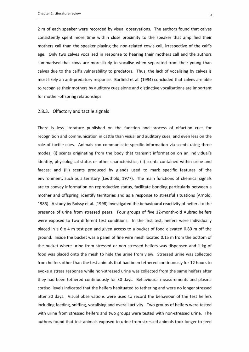
Chapter 2: Literature review
51
2 m of each speaker were recorded by visual observations. The authors found that calves
consistently spent more time within close proximity to the speaker that amplified their
mothers call than the speaker playing the non‐related cow’s call, irrespective of the calf’s
age. Only two calves vocalised in response to hearing their mothers call and the authors
summarised that cows are more likely to vocalise when separated from their young than
calves due to the calf’s vulnerability to predators. Thus, the lack of vocalising by calves is
most likely an anti‐predatory response. Barfield et al. (1994) concluded that calves are able
to recognise their mothers by auditory cues alone and distinctive vocalisations are important
for mother‐offspring relationships.
2.8.3. Olfactory and tactile signals
There is less literature published on the function and process of olfaction cues for
recognition and communication in cattle than visual and auditory cues, and even less on the
role of tactile cues. Animals can communicate specific information via scents using three
modes: (i) scents originating from the body that transmit information on an individual’s
identity, physiological status or other characteristics; (ii) scents contained within urine and
faeces; and (iii) scents produced by glands used to mark specific features of the
environment, such as a territory (Leuthold, 1977). The main functions of chemical signals
are to convey information on reproductive status, facilitate bonding particularly between a
mother and offspring, identify territories and as a response to stressful situations (Arnold,
1985). A study by Boissy et al. (1998) investigated the behavioural reactivity of heifers to the
presence of urine from stressed peers. Four groups of five 12‐month‐old Aubrac heifers
were exposed to two different test conditions. In the first test, heifers were individually
placed in a 6 x 4 m test pen and given access to a bucket of food elevated 0.80 m off the
ground. Inside the bucket was a panel of fine wire mesh located 0.15 m from the bottom of
the bucket where urine from stressed or non stressed heifers was dispensed and 1 kg of
food was placed onto the mesh to hide the urine from view. Stressed urine was collected
from heifers other than the test animals that had been tethered continuously for 12 hours to
evoke a stress response while non‐stressed urine was collected from the same heifers after
they had been tethered continuously for 30 days. Behavioural measurements and plasma
cortisol levels indicated that the heifers habituated to tethering and were no longer stressed
after 30 days. Visual observations were used to record the behaviour of the test heifers
including feeding, sniffing, vocalising and overall activity. Two groups of heifers were tested
with urine from stressed heifers and two groups were tested with non‐stressed urine. The
authors found that test animals exposed to urine from stressed animals took longer to feed
Chapter 2: Literature review
52
and spent less time eating than heifers exposed to urine from non‐stressed animals,
otherwise the behaviour between the two treatments was the same. In the second test, a
novel object (an 0.80 m tall traffic cone) that had been sprayed with urine from stressed or
non‐stressed animals was positioned in the test pen where the food bucket was located in
the previous test. Immediately prior to entering the test pen the test heifers were exposed
to the same type of urine it was going to be tested with. Two of the four groups from test
one were exposed to opposite treatments in test two, such that one group tested with
stressed urine in the previous test was tested with non‐stressed urine and similarly one
group exposed to non‐stressed urine in test one was tested with stressed urine in test two.
The results showed that heifers tested with urine from stressed animals took longer to enter
the test pen, avoided the area surrounding the novel object and spent more time immobile
than heifers exposed to urine from non‐stressed animals. Boissy et al. (1998) concluded that
heifers can perceive the state of stress in peers via olfactory cues present in urine and
actively avoid the source of the odour.
The function of touch as a communication signal is not as well defined as visual, auditory and
olfactory signals (Leuthold, 1977). Nevertheless, it is still a relevant form of communication
between individuals, particularly in mating behaviour, mother‐offspring relationships,
establishing dominance rank and maintaining preferential relationships through affiliative
behaviours such as allogrooming (Bouissou et al., 2001).
2.9. Changing group composition
Introducing new individuals into a group or regrouping existing group members is a common
practice on commercial farms, where groups are based on similar attributes such as age, sex
or production requirements. The presence of an unfamiliar animal is considered a threat to
an individual’s social status as well as competition for resources (Price, 2008). This
disruption creates social stress as the new social structure is established and can adversely
affect animal welfare and reduce production. Social stress is defined as ‘abnormal or
extreme physiological or behaviour adjustments and animal has to make in order to cope
with its social environment’ (Syme and Syme, 1979). Social stress is an interdependent
factor, such that stress experienced by one animal will influence the stress levels of other
group members (Zayan and Dantzer, 1990). The social stress experienced by a group will
persist until social stabilisation is reached, thus the time taken for a social group to be
considered stable is important both in terms of animal welfare and production.

Chapter 2: Literature review
53
As well as experiencing social stress, newly introduced animals are faced with various
environmental factors that can also create stress. The new individuals may be faced with an
unfamiliar environment, separation from familiar group members, a change in group size
and human handling (Zayan and Dantzer, 1990; Newberry and Swanson, 2001). It is
therefore uncertain what key factors are responsible for the behavioural changes associated
with mixing (Newberry and Swanson, 2001).
2.9.1. The effect of mixing unfamiliar animals on production
In cattle, behavioural changes resulting from the social stress of mixing unfamiliar animals
can result in high levels of agonistic behaviour immediately following introduction. A study
investigating agonistic behaviour in bulls and steers following regrouping was conducted by
Tennessen et al. (1985). Thirty‐two bulls and 32 steers were formed into eight groups of
eight animals, with bulls and steers housed separately. When the animals were 9, 12 and 15
months old, they were regrouped so that each animal was grouped with six strangers and
one familiar pen mate. The groups were observed for 9 hours per day for 10 days. There
were immediate increases in agonistic behaviour, with bulls showing the greatest amount of
aggression. The greatest increase in agonistic behaviour was seen during the second
regrouping when animals were 12 months of age, although the average fight length was less.
Additionally, the decline in agonistic interactions was more rapid at 12 and 15 months of
age, suggesting that the animals had gained experienced from their first regrouping
encounter. After 10 days, there were very few observations of agonistic behaviour by both
bulls and steers at all three ages. Tennessen et al. (1985) concluded that the steers were
behaviourally less mature than the bulls, which led to their lowered aggression rates and the
differences between bulls and steers increased with age.
The occurrence of agonistic behaviour is not restricted to males, with female cattle showing
similar agonistic responses to newly introduced individuals. Kondo and Hurnik (1990)
investigated social stabilisation in dairy cows following regrouping in three groups of dairy
cattle. Thirty‐two Holstein dairy cows were formed into two groups of 16 for a period of 8
weeks (groups A and B), before eight cows were randomly selected from each group to form
a third group of 16 cows (group C). Behavioural observations lasting 2 hours were carried
out immediately following each introduction, then every 48 hours up until 18 days post‐
mixing. For all three groups, the greatest number of agonistic encounters were observed
during the 2 hours immediately following regrouping, and reached between three and five

Chapter 2: Literature review
54
times the amount of agonistic encounters observed 8 weeks later. The level of agonistic
interactions tended to decline thereafter. The authors separated physical from non‐physical
interactions, and found that immediately following mixing the ratio of physical from non‐
physical interactions was around 80% physical to 20% non‐physical interactions for both
groups A and B. After 4 days the ratio changed and the non‐physical interactions accounted
for over 60% of all interactions for groups A and B; the authors determined the groups to be
socially stable at this ratio. However, the cows in group C changed their behaviour relatively
faster than groups A and B, and the proportion of non‐physical interactions exceeded
physical interactions between 2 and 4 days post‐mixing. The findings highlight that
immediate increases in agonistic behaviour are short‐lived and affected by the previous
mixing experience of the individuals. Kondo and Hurnik (1990) concluded that the ratio of
40% physical interactions to 60% non‐physical interactions was a useful measure to
determine social stabilisation in newly introduced cattle.
The study by Kondo and Hurnik (1990) showed the importance of stabilisation in agonistic
behaviours as a measure of social stabilisation, however, social stress caused by the
presence of an unfamiliar individual does not always result in agonistic behaviour, and can
be expressed by changes in physiological and psychological behaviours (Zayan and Dantzer,
1990). Several studies have investigated the behavioural changes resulting from the social
stress of mixing unfamiliar animals. A study by Gupta et al. (2008) investigated the effect of
repeatedly regrouping and relocating 72 Holstein‐Friesian steers. The steers were housed in
12 groups of six steers and assigned to either control or regrouped treatments. Those in the
regrouped treatment experienced six regrouping and relocation events, where each
individual was introduced to a completely new set of group mates in a new pen and allowed
to stabilise for 14 days before being regrouped and relocated again. The control steers
remained in the same pen with the same pen mates for the duration of the experiment. The
steers behaviour and body contact were observed for 1 week following each regrouping and
relocation via video recording equipment. Gupta et al. (2008) found that the regrouped and
relocated steers spent less time lying and more time standing than the control steers for the
first day following the first relocation and regrouping, and suggested this was in response to
the higher level of competition for lying space and also a defensive response to avoid being
threatened while lying down. The difference in lying and standing disappeared following the
first regrouping and relocation, which the authors suggested was a partial adaptation to the
social stress experienced by the steers. The steers used in Gupta et al.’s (2008) study were
not completely unfamiliar, as they had previously been housed within sight of each other,
Chapter 2: Literature review
55
and this may have influence the rate of stabilisation within groups. Nevertheless, the results
clearly show that regrouping had an effect on the lying and standing behaviour of the steers.
A study by von Keyserlingk et al. (2008) also investigated the behavioural effects of
regrouping dairy cows, specifically examining feeding behaviour, social behaviour and milk
production. Eighty cows were divided into four groups of 11 and three groups of 12. Four
cows from each of the three groups of 12 were selected as focal animals. The focal cows
were observed in their original groups for 3 days before being introduced into one of the
four groups of 11 and observed for a further 4 days, thus the stocking rate for the introduced
cow remained constant. Observations were continuously recorded via video equipment and
analysed at 1 minute intervals, while data loggers attached to the focal cow’s hind leg were
used to record the total number of lying bouts and duration of lying. The authors compared
behaviours pre‐ and post‐mixing, and found no change in the total amount of time spent
feeding, however after regrouping less time was spent at the feeder immediately following
food dispersal, suggesting competition between the focal cow and the new group members.
Competition was also reflected in the increased number of times the focal cow was
displaced from the feeder in her new group as compared with her home group; this effect
gradually decreased and had disappeared after 3 days post‐mixing. In comparison with the
study by Gupta et al. (2008), von Keyserlingk et al. (2008) also reported a decrease in lying
behaviour immediately following regrouping, although this effect was only evident on the
day of introduction. The authors attributed the lower lying rate to the focal cows avoiding
displacing other cows from the lying area. Allogrooming was also affected by the
introduction, with focal cows receiving and performing less allogrooming over the first 3
days post mixing before returning to baseline levels. von Keyserlingk et al. (2008) also found
a decrease in average milk production by 3.7 kg on the day of introduction, which returned
to baseline levels the following day. The results of von Keyserlingk et al.’s (2008) study
determined that the disruption caused by introducing a single animal into a small stable
group affected the introduced cows feeding behaviour, social behaviour and milk
production, with allogrooming behaviour taking the longest to stabilise.
In addition to the behavioural disruptions reported, others have found mixing cattle to effect
short term feed intakes leading reduced weight gain and milk production. In a study by
Nakanishi et al. (1991), the authors investigated the behavioural and physiological response
of eight horned Japanese Black cattle to the introduction of a single cow. The cattle were
housed in a 225 m2 experimental dry‐lot (approximately 15 m x 16.5 m) and fed

Chapter 2: Literature review
56
supplementary forage twice per day. The group was observed for all social behaviours for 2
days prior to the introduction and 5 days post‐introduction, with 8 hours of observations
recorded each day. The physical characteristics of each individual (e.g. body weight) were
recorded pre‐introduction and 11 days post‐introduction. The authors observed an
immediate 4‐fold increase in agonistic interactions following introduction. The majority of
these interactions were non‐physical, which tended to decline over the next 7 days.
Nakanishi et al. (1991) suggested that the increase in agonistic behaviour reflected
investigation of the new cow with the resident cows to establish her social rank. The
behaviour could also represent displacement behaviour or frustration as a result of being
removed from her previous group. Similar allogrooming patterns were found by Nakanishi
et al. (1991) as reported by von Keyserlingk et al. (2008), which tended to decline over the
first 4 days post‐mixing before gradually returning to near baseline levels after 7 days once
agonistic interactions had declined. Nakanishi et al. (1991) suggested that allogrooming,
being an affiliative behaviour, counter balances the negativity of agonistic interactions. The
introduced cow showed a 13 kg weight loss over the 11 days post‐mixing, while half of the
group also lost weight (between 2 and 8 kg). The feeding behaviour of the cattle was not
reported nor was the amount of feeding space available per animal, thus it is unknown if
there was a large reduction in time spent feeding or competition at the feeder to explain the
weight loss experienced by the cattle, however the authors attribute the weight loss to the
social stress of introducing a new animal into an established cattle herd. Although the
results reported by Nakanishi et al. (1991) are noteworthy, greater replication and detail of
the study would provide a better understanding of the relationship between weight loss and
the introduction of new individuals into a stable group.
A study by Hasegawa et al. (1997) explored the effect of regrouping dairy cows on
production. Two groups of lactating Holstein heifers housed in a group of 28 (group A) and a
group of 23 (group B) were used in the trial. Fourteen heifers from group A and 12 heifers
from group B were selected for exchange between the two groups. All agonistic interactions
between group members were recorded 5 days pre‐mixing and 5 days post‐mixing and used
to determine the dominance rank of each individual. Social behaviour observations of the
exchanged heifers were recorded at 5 minute intervals over a 24 hour period on one day
pre‐mixing and days 2, 9 and 15 post‐mixing. Of the 26 heifers that were moved, only six of
these retained their level of dominance, or gained dominance rank, after regrouping.
Overall, the exchanged heifers showed a significant reduction in weekly milk yield during the
second week post‐mixing. The authors discovered a relationship between change in
Chapter 2: Literature review
57
dominance rank and milk production: animals experiencing the greatest decrease in social
status had the greatest reduction in weekly milk production. Heifers with the greatest loss
in dominance status produced 3.5% less milk in the first week and 5.7% less milk in the
second week following mixing. The decrease in milk production may be related to the
decrease in time spent feeding, standing and lying. These behaviours returned to baseline
after 15 days post‐mixing, however average milk production was still below pre‐mixing levels
after 15 days. The results of Hasegawa et al.’s (1997) study reflect those of von Keyserlingk
et al. (2008) in terms of the behavioural and production changes associated with regrouping
dairy cows, however von Keyserlingk et al. (2008) only observed production losses on the
day of introduction with behavioural stabilisation occurring within 3 days post‐mixing. The
longer term production and behavioural changes reported by Hasegawa et al. (1997) may be
related to the extensive disruption created by exchanging half, or more than half, of the
group at the one time. When new groups are formed, the resultant social order is based
upon a collection of pair‐wise interactions between all group members, thus with larger
numbers of individuals stabilisation is expected to take longer (Tennessen et al., 1985). This
is reflected in the results of Hasegawa et al.’s (1997) study when compared with the studies
by von Keyserlingk et al. (2008) and Nakanishi et al. (1991), which explored the effect of
introducing a single animal into an established herd, resulting in short term disruptions to
behaviour and production. The welfare and production implications of mixing unfamiliar
individuals suggests the need for a greater understanding of the processes involved in
familiarisation in order to create welfare orientated management practices.
2.9.2. Social stabilisation following mixing unfamiliar animals
Familiarisation has previously been documented in cattle by recording the level of agonistic
interactions between individuals and defining stabilisation as the time it takes for non‐
physical interactions to predominate physical interaction and the ratio of non‐physical to
physical agonistic interactions remains constant (e.g. Kondo and Hurnik, 1990). There are
varied results in the literature, ranging from 3 to 15 days. Of the shortest stabilisation time,
Grant and Albright (2001) summarised that the negative impacts of regrouping dairy cows
lasts approximately 3 days, which is consistent with von Keyserlingk et al.’s (2008) results
investigating the disruption experienced by the introduced cows. However the single group
study by Nakanishi et al. (1991) reported behavioural stabilisation after 7 days, while the
results from Gupta et al.’s (2008) study on regrouping and relocation concluded that the
regrouped steers developed social bonds within 14 days and the time taken to establish
Chapter 2: Literature review
58
social bonds decreased with increasing regrouping and relocation experience. The study by
Hasegawa et al. (1997) reported behavioural stabilisation 15 days post‐mixing, although milk
production was still below pre‐mixing levels at this time, suggesting that the new social
groups had not stabilised and provides evidence that stabilisation may take longer when
larger numbers of individuals are introduced simultaneously. The majority of these studies
ceased recording behavioural observations after 14 days, however a study by Sato et al.
(1990) monitored the behaviour and interactions of five heifers introduced into a group of
18 cows over a 3 month period and found that up to 45 days was required before the new
heifers were completely integrated into the herd. The results of this study suggest that
longer term subtle changes are occurring as the unfamiliar is incorporated into the group
and may indicate that individuals continue to experience social stress during this time. The
rate of stabilisation will depend on various animal factors, such as the breed, age, gender
and previous mixing experience of the individual, as well as various environmental factors,
such as the availability of food and water, the space available for each animal and the
number of animals in the group (Kondo and Hurnik, 1990). The varied reports of the extent
and duration of behavioural and production disruption in the literature is therefore a
reflection of the numerous endogenous and exogenous factors that affect the integration of
new individuals into an established herd.
2.9.3. Re‐grouping strategies
There have only been a few studies investigating the effect of alternative introduction
strategies on stabilisation time and social disruption. Knerim (1999) introduced single and
groups of three heifers into an established dairy herd. Knerim (1999) found that group‐
heifers formed their own subgroup and interacted less with resident herd members than
singly introduced heifers. There were no differences in the amount of agonistic interactions
or time spent lying and feeding between group sizes, implying that the social stress
experienced by group and single heifers was the same. A similar study by Menke et al.
(2000) introduced both single and groups of three heifers into an established dairy herd but
in contrast to Knerim (1999) observed more agonistic interaction between group heifers and
the resident herd than heifers introduced on their own. The contradictory results of these
studies make it difficult to conclude any benefits from introducing cattle either singly or in
small groups. More recently, Neisen et al. (2009) found that introducing pairs of familiar
heifers into an established dairy cow herd was more favourable than introducing a single
heifer. The authors introduced single and paired‐heifers into six dairy farms, ranging in size
Chapter 2: Literature review
59
from 44 to 66 animals per herd. Visual observations of social behaviour were recorded as
well as positional data via a local position‐measurement system, which recorded the two‐
dimensional position of each animal wearing a transponder. The transponders emitted a
signal that was detected by antennas fixed to the barn walls. The positional data as well as
the time of the record was relayed from the antennas to a central computing unit once every
minute. The cows were housed in a loose‐barn system consisting of three functional areas:
feeding, lying and exercise areas. Some farms also allowed access to pasture during the day
and although pastoral areas were not covered by the automatic tracking system, each
animal was observed in the barn between 57‐94% of the time. The resident herds were
monitored for 1 week prior to the introduction of the heifers. A single heifer was introduced
into three herds while a pair of familiar heifers was introduced into the other three herds.
Four weeks later, when the introduced heifers were considered integrated into the herd a
single heifer was introduced into herds that previously had a pair of heifers introduced while
a pair of heifers was introduced into herds that received a single heifer previously. Visual
observations were recorded during the first 3 days following introduction as well as
continuous recording of positional data for 4 weeks following introductions. The authors
found that the resident herd directed less agonistic behaviour towards the pair than the
single heifer. The singly introduced heifers were found to be more synchronous with the
resident herd and maintained closer distances to the herd than the heifers introduced as a
pair, which tended to maintain closer distances to each other. Neisen et al. (2009)
concluded that familiarity provided the introduced pair with a sense of security and support,
and the welfare of the pairs was less at risk than the singly introduced heifer. The outcome
of Neisen et al.’s (2009) study compared with those of Knerim (1999) and Menke et al.’s
(2000) may be explained by the greater social stability experienced by a pair when compared
with larger groups, particularly triads, which are more vulnerable to dissolution.
Based on a suggestion by Lamb (1976) that introducing unfamiliar animals at night when
animals are socially less active should alleviate some of the social stress associated with
mixing, Nakanishi et al. (1993a) investigated the effect of a night introduction. The study
involved observing the behaviour of two groups of seven Japanese Black cows before and
after the introduction of a single cow into each group. Behavioural observations were
recorded for 3 days prior and 7 days post‐introduction of the unfamiliar cow, for 8‐9 hours
each day. The unfamiliar cows were introduced after dark, between 20:00 h and 21:00 h.
Observations were recorded immediately following the introduction, although due to the
darkness the behaviours could not be described in detail. Nevertheless, the authors were

Chapter 2: Literature review
60
able to observe some agonistic interactions during the first 12 minutes, which were mainly
initiated by the resident cows. The frequency of agonistic behaviour tended to decline 2
days post‐introduction and had stabilised after 7 days. Nakanishi et al. (1993a) also noted a
decrease in lying behaviour and an increase in standing behaviour, which took 5 days to
return to pre‐introduction levels. The introduced cows were observed to spend less time
eating and more time moving than the resident group members. Although Nakanishi et al.
(1993a) state that there were no real advantages to introducing cattle at night as the time
taken for agonistic interactions and behavioural changes to stabilise was comparable with
other day‐time introductions (e.g. Tennessen et al., 1985; Nakanishi et al., 1991), including a
day time introduction would have enabled a comprehensive evaluation of the effect of day
when introducing unfamiliar cattle. There is a lack of research investigating alternate
strategies for reducing stress when introducing new individuals into an established herd.
There is a need to thoroughly investigate the usefulness of different strategies that could
lead to practices that create less social stress and disruption to normal behaviour and
production.
2.10. Conclusions
The review demonstrates that cattle exist within complex social structures. Social behaviour
research in cattle has largely focused on dominance behaviour and the function of these
behaviours is well understood. Less is known about affiliative behaviours, although there is
a consensus that they are largely responsible for the cohesive nature of familiar groupings.
The review also identified several studies investigating the behavioural effect caused by
introducing new individuals into an established herd and the results of these studies show
that the presence of an unfamiliar individual creates social disruption. The aims of these
studies were primarily production based, however the conclusions drawn could not
recommend suitable practices to reduce the negative effect of incorporating new individuals
into established groups, with the current advice stating to avoid mixing individuals
altogether (Boe and Faerevik, 2003). In applying such a commercial focus on the study
outcomes, the investigations failed to provide information on underlying social properties
and detailed descriptions of behavioural factors involved in the process of familiarisation
between individuals. Further work is needed in the area of affiliative behaviours and their
role during relationship development. Such investigations require a multi level approach to
cattle social systems that consider the fundamental processes that occur between
individuals and the impact of these processes for group level outcomes. Experience from

Chapter 2: Literature review
61
human social studies reveals that dyads and triads have important structural properties (e.g.
Simmel, 1950) and it was suggested by Chase (1980) and Lewis (1984) to focus on these
fundamental units to develop a greater understanding of social structure. The focus of the
current study is to therefore explore the social behaviour of dyads and triads of steers during
relationship development. Steers were chosen as the model for studying cattle social
behaviour as they are not subject to hormonal behavioural changes caused by oestrous or
pregnancy.
2.10.1. Aims
To explore the social properties of dyadic relationships and the effect of the presence of
familiar and unfamiliar steers, a series of experiment were conducted to:
1. develop an understanding of the trade‐off individual steers make between food and
social companionship in the presence of familiar and unfamiliar peers. The hypothesis
that steers paired with unfamiliar peers would travel further to receive a food reward
than those paired with familiar peers was tested;
2. explore the behavioural response of steers to the presence of an unfamiliar steer by
identifying the behavioural differences between pairs of familiar steers and pairs of
unfamiliar steers. It was hypothesised that the behavioural differences observed
between familiar and unfamiliar pairs of steers over time could be used to identify some
of the features of the familiarisation;
3. investigate the change in temporal and spatial associations between pairs of unfamiliar
steers during the process of familiarisation. The hypothesis that evidence of
familiarisation between the unfamiliar steers would occur within 5 days was tested.
Following on from exploring dyadic relationships, the second part of the thesis investigates
the social properties of a triad and explores the effect of the presence of an unfamiliar steer
on the social relationship between a pair of familiar peers. The secondary aims of the thesis
are to:
4. explore the behavioural response of a pair of familiar steers to the presence of an
unfamiliar steer by evaluating the close proximity encounters of the familiar pair before
and after the introduction of the unfamiliar steer. It was hypothesised that the
introduction of the unfamiliar steer would lead to an increase in close proximity
encounters between the familiar pair;
5. investigate the process of relationship development between a pair of familiar steers
and an unfamiliar steer by exploring the regular patterns of close proximity encounters

Chapter 2: Literature review
62
between the triad. The hypothesis was that the difference in close proximity encounters
between familiarity types would decrease as the unfamiliar steer was integrated into the
triad.
63
Chapter 3
Measurement considerations 3.1. Introduction
The social behaviour of cattle was described in Chapter 2, as well as studies that have
investigated the functional aspects of this behaviour. As outlined in the previous chapter,
the term ‘social behaviour’ refers to a suite of different behaviours, from dominance to
allogrooming to spatial proximity. Various measures are required to capture both the
obvious and subtle behaviours that signify an individual’s social tendencies and characterise
a social relationship, from general routine behaviours such as walking, grazing and resting, to
identifying certain forms of interaction, such as physical or non‐physical encounters.
Collecting information on an animal’s social behaviour may include recording the number of
individuals present and their identity, identifying the sender and the receiver of social
behaviour, noting the sequence of behaviour by its frequency and duration, recording the
spatial position of individuals relative to the overall group as well as proximity to neighbours,
and noting the temporal patterning of these behaviours (Altmann, 1974). To obtain this
information generally requires several measurement techniques (Broom and Fraser, 2007).
Previously, there has been a strong reliance on observational methods to acquire qualitative
and quantitative data on social behaviour in animals, although the use of technology to
record animal behaviour is increasing (D'Eon and Delparte, 2005). The aim of this chapter is
to provide a review of methods available to collect data on animal social behaviour. The
principles of recording animal social behaviour are described in section 3.2, followed by a
review of some of the automatic methods available to record animal behaviour: the review
focuses on technological devices that have been developed to record an animal’s absolute or
relative spatial location. The basic principles of each method are discussed as well as their
main advantages and disadvantages and the chapter concludes with a justification of the
research methods chosen for use in the thesis.

Chapter 3: Measurement considerations
64
3.2. Recording animal social behaviour
3.2.1. Approaches to the study of animal behaviour
The study of animal behaviour stems from the fields of ethology and psychology. Ethology is
characterised as the ‘biological study of behaviour’ (Tinbergen, 1963), and can be studied
using conceptual, theoretical or empirical approaches (Dugatkin, 2004). Empirical
ethological studies are principally focused on asking questions about the cause of behaviour,
how it has evolved and has developed, and what its function is (Tinbergen, 1963). Ethology
has traditionally taken an observational approach to the study of animal behaviour by
recording the naturally occurring behaviour of animals in their natural habitat, without any
manipulation or an attempt to control factors within their environment (Manning and
Dawkins, 1998). Psychology, the study of the mind and behaviour, has traditionally focused
on asking questions about the causation of behaviour and factors involved in learning, and
has tended to rely on laboratory based studies and experimentation (Martin and Bateson,
1993). Experimentation involves manipulating the environment in some way, allowing
researchers to investigate the cause of a specific behaviour by observing the outcome when
some condition is purposely varied (Martin and Bateson, 1993; Manning and Dawkins, 1998).
Both ethology and psychology have evolved to incorporate aspects of the other discipline,
and other fields of studies have evolved from their foundations, including ecology,
sociobiology and behavioural biology (Martin and Bateson, 1993).
The nature of an agricultural system in which domestic livestock are managed is much more
controlled and manipulated than a natural system, thus agricultural based research has
taken more of an experimental research approach. For example, digestion trials are used to
determine the amount of nutrients an animal absorbs from a particular food source
(Mitchell, 1942). In these trials, animals are individually housed in metabolism crates and
the amount of food ingested is compared with the waste produced to determine the
digestibility of the food source (Vallentine, 1956). Such controlled experimental approaches
rely on breaking down a system into its principal components to test hypotheses about the
mechanisms underlying the cause and effect, thus this type of research generally relies on
the individual being removed from its natural context. An experimental approach towards
studying animal behaviour is somewhat different due to a range of behavioural
interdependences, for example, studying social behaviour relies on the presence of a ‘social’
context, thus it is difficult to control every aspect of an animal’s environment whilst varying

Chapter 3: Measurement considerations
65
a single condition (Dawkins, 2007). Nevertheless, simple and detailed behavioural studies
are still possible when a range of observational techniques and approaches are used to
minimise disruption, and an animal’s natural behaviour can be recorded (Dawkins, 2007).
This thesis applies a reductionist approach to the study of cattle social behaviour to explore
the effects of familiarity on dyads and triads of steers: both replicated experiments and
analytical models will be used. It is anticipated that the findings will enable future work on
larger groups to account for the influence of dyadic and triadic pressures on higher order
social processes.
3.2.2. Research design
The research approach (either observational, experimental or a combination of both)
provides the foundation of the overall research design. Another fundamental component of
the research design is the data collection method, which can be either cross‐sectional or
longitudinal. A cross‐sectional study measures individuals or groups at one point in time
whereas longitudinal studies take repeated measurements on the same individuals or
groups at several points in time (Zeger and Liang, 1992). Cross‐sectional studies provide
descriptive information on associations between groups or individuals at that point in time,
although their use is limited in defining cause‐and‐effect relationships (Paffenbarger, 1988).
Longitudinal studies on the other hand can be used to investigate causation, as well as long
term effects, change, and similarities and differences between and within subjects over time
(Cohen et al., 2007). In comparison to cross‐sectional studies, longitudinal studies have
increased statistical power as there are twice as many observations on the same number of
individuals (Zeger and Liang, 1992). Additionally, longitudinal studies can be analysed both
cross‐sectionally at each point in time, as well as longitudinally through time (Thomson and
Holland, 2003). The main challenges of a longitudinal study include the labour intensive data
collection process, analysing large and complex data sets, as well as keeping the same
subjects throughout the duration of the study (Thomson and Holland, 2003): missing data
becomes an issue if one or more subjects drop out before the end of the study (Hedeker and
Gibbons, 2006). Longitudinal studies are seemingly more challenging and complex than
cross‐sectional studies, but the nature of the data set means that individual, pair and group
social properties can be investigated.
Chapter 3: Measurement considerations
66
3.2.3. Recording representative samples of behaviour
Behaviour refers to a complex of movements and events produced in response to internal
and external stimulus (Martin and Bateson, 1993) which can be observed at multiple levels
from groups to individuals to specific body parts (Dawkins, 2007). Additionally, an animal’s
behaviour is influenced by other individuals around it, those it interacts with and the
interactions of others, as well as features of the environment (Dawkins, 2007). Thus it would
be extremely difficult to record everything about an animal and its behaviour at once.
Recording animal social behaviour involves selecting the most appropriate methods to
provide the greatest representation of total behaviour (Dawkins, 2007). A general
methodological approach to record animal social behaviour involves selecting the most
appropriate: (i) type of behaviour; (ii) level of observation; (iii) sampling method; (iv) type of
record; and (v) amount of behaviour to record (Fig 3.1) (Dawkins, 2007). The selection of
what social behaviour to record will depend on the research question. As mentioned above,
social behaviour encompasses a wide range of behaviours and taking representative samples
of such behaviour relies on collecting detailed information on various factors, including
individual and group attributes, the identity of the senders and receivers of social behaviour,
spatial relationships and the temporal patterning of behaviour (Altmann, 1974). The level of
observation refers to unit being described, from the behaviour of a whole group to
individual behaviour, right down to the behaviour of individual body parts, for example, the
leg movement of a cow while walking. The behavioural level chosen will depend on the
research question and the behaviour of interest.
3.2.4. Sampling methods
Sampling methods are used to provide a representative sample of the total behaviour and
the most appropriate method to use will depend on the focus of the experiment. The
sampling methods available include scan sampling, focal sampling, ad libitum sampling and
behavioural sampling (Fig. 3.1). The principles of each sampling method including their main
advantages and disadvantages are outlined below.
Scan sampling involves ‘scanning’ the group and recording a snapshot of each individual’s
behaviour at that time, and repeating the observation some time later (Dawkins, 2007). The
method is best suited to general and social behaviours that can be easily described and
recorded quickly (Altmann, 1974). Scan sampling provides a good description of a group’s

Chapter 3: Measurement considerations
67
Sampling method
Record type
Interval:Point sampling
Interval:Binary sampling
Focal sampling
Ad libitumsampling
Behavioursampling
Scan sampling
Level of observation
Individual Body partGroup
Behaviour of interest
Amount of behaviour
Duration IntensityFrequency
Continuoussampling
overall behaviour and behavioural synchrony (Altmann, 1974). However, observers are
usually restricted to recording only simple categories of behaviour as the method becomes
complicated with an increasing number of behavioural categories to record at each scan
(Dawkins, 2007). Additionally, the method only provides a measure of the frequency and
duration of behaviour relative to the total number of scans taken (Martin and Bateson,
1993).
Focal animal sampling involves identifying a ‘focal’ animal (or a dyad or some other unit)
from within a larger group and recording all instances of a specified behaviour of that same
individual over the selected sample period (Martin and Bateson, 1993). The method
provides a good representation of general behaviour but because the method ignores
behaviour initiated by individuals other than the focal animal, the method is generally not
suited to record information on general social behaviour and behavioural synchrony among
groups (Altmann, 1974). Additionally, the choice of focal animal can create a bias if the most
active or noticeable animal is selected, and problems arise when the focal animal moves out
of sight (Martin and Bateson, 1993; Dawkins, 2007).
Figure 3.1. The process of selecting the most appropriate sampling and recording methods tocollect representative samples of social behaviour (modified from Martin and Bateson, 1993).

Chapter 3: Measurement considerations
68
Ad libitum sampling and behavioural sampling are much less structured than scan and focal
animal sampling. Ad libitum sampling involves observing a group of animals and recording
every behaviour that is observed, noting the time of occurrence and identity of the animal.
Behavioural sampling is similar to ad libitum sampling but only a specific type of behaviour is
recorded, for example, grooming events (Altmann, 1974). Both methods are useful to
describe rare behavioural events or record the behaviour of species that are not easily
observable (Dawkins, 2007). However, the methods are unlikely to provide an indication of
the animal’s overall behaviour because records are not taken at regular intervals, less
conspicuous animals are likely to be recorded more often than others thus biasing the
sample of the species observed and observations may be limited to certain times of the day
when the animals are more active (Dawkins, 2007). Each of the four sampling methods has
its own strengths and weaknesses in terms of observing general animal behaviour. In terms
of recording the social behaviour of groups of cattle, scan sampling appears to be the most
suitable method to record the frequency and duration of behavioural events between
individuals.
3.2.5. Record type
In addition to the sampling method the type of record used to collect the sample of
behaviour is also an important consideration, which can be either continuous or interval (Fig.
3.1). Continuous sampling involves recording all events of a certain behaviour during a
specified time frame, and noting the time that each behaviour starts and stops, while
interval sampling involves sampling behaviour at specified sample intervals (Martin and
Bateson, 1993). Continuous sampling provides precise information about the frequency and
duration of behaviour, although records are difficult to collect when the behaviour of the
animal is frequently changing (Dawkins, 2007). Often the number of behavioural categories
is reduced to accommodate the ability of the observer to record the specified behaviour
(Martin and Bateson, 1993). Depending on the behaviour of interest, sequences of
behaviour are not always required, thus interval sampling methods provide an adequate
representation of the occurrence of a behaviour (Dawkins, 2007).
Interval sampling can take two forms: point sampling or binary sampling. Point sampling
involves dividing an observation period into sample intervals and only recording the
behaviour at the end of each sample interval or the ‘sample point’, while binary sampling, or
one‐zero sampling, involves recording ‘1’ if the behaviour occurred or ‘0’ if the behaviour did

Chapter 3: Measurement considerations
69
not occur during the previous sample interval (Martin and Bateson, 1993). Behaviours
recorded with binary sampling are expressed as a proportion of the total observation time,
which introduces several sources of error primarily because the method does not directly
record the duration of an event and tends to overestimate duration and underestimate
frequency (Martin and Bateson, 1993). Point sampling, however, allows a broader range of
behaviours to be recorded that cannot be achieved using continuous time sampling, and
when short sample intervals are used the proportion of time spent performing a behaviour
can be directly estimated (Martin and Bateson, 1993). Additionally, the lower demand on
the observer makes the method reliable (Martin and Bateson, 1993). The disadvantage with
point sampling is that rare behavioural events are often missed, and the observer may
unknowingly be biased towards behaviours that have occurred prior to the sample point,
resulting in the predominant behaviours being overestimated (Martin and Bateson, 1993).
Using both continuous and interval sampling methods together can be useful when
recording social behaviour, as general behaviours such as grazing and walking can be
recorded at intervals while specific behaviours such as fighting or allogrooming can be
recorded as they occur (Broom and Fraser, 2007).
3.2.6. The amount of behaviour to sample
The amount of behaviour observed can be quantified by the duration, frequency or intensity
of the behaviour (Fig. 3.1). Duration refers to the amount of time the behaviour is exhibited,
the frequency quantifies the number of times the behaviour is exhibited while the intensity
measures of the magnitude of the behaviour (Dawkins, 2007). The frequency and duration
of behaviour provide different yet complimentary measures: together frequency and
duration can be used to indicate the nature and quality of behaviour. For example, the
number of times two animals groom each other and the duration of their grooming bouts
can be used to define the quality of their social relationship (Martin and Bateson, 1993).
3.2.7. Measuring spatial aspects of behaviour
The above sampling methods relate to recording behavioural events and quantifying how
much and when certain behaviour occurs. A separate behavioural classification used to
describe social behaviour is where behaviour occurs, which quantifies where individuals are
with respect to other individuals or features of their environment and indicates an
individual’s selection preferences (Dawkins, 2007). In social behaviour studies, quantifying
Chapter 3: Measurement considerations
70
inter‐individual distances between group members provides valuable information on an
individual’s preference for others. However distance can be difficult to estimate accurately
when the observer is some distance away and the two reference points (e.g. animals,
objects) appear smaller than they actually are, thus making it difficult to estimate the actual
distance between them (Dawkins, 2007). A common method to overcome this problem is to
use relative distance reference points, such as fixed spatial references. Fixed spatial
references may include permanent fixings of known distance, such as the spacing between
individual food bins in a food trough as used by Manson and Appleby (1990) to investigate
the effect of dominance on spacing behaviour between cows at a feed trough, or the
distance between equally spaced fence posts as used by Hirata (2003) to estimate the
distance between cows and calves. The animals themselves can also be used as a reference,
such as the number of body lengths between individuals as used by Stricklin (1983) to
estimate the distance spread of a group of beef cattle. Additionally, recording the identity of
an individual’s nearest neighbour, rather than the distance between neighbours, provides an
estimate of the amount of time that one individual is found within close proximity to any
other animal in the group, as used by Sibbald et al. (2005) to quantity individual sociability in
sheep.
3.3. Observations
The majority of studies reviewed in Chapter 2 used visual observations to record behavioural
data. Visual observations can potentially provide the most thorough description of an
animal’s behaviour. Observations can be recorded directly at the time the event occurs via
human or computer assisted recording, or video recording equipment can be used to collect
video footage at the time that can be analysed afterwards. However there are some major
problems associated with the approach. For example, full records are difficult to collect as
most observations are based on identifying specific behavioural events or discontinuous
sampling periods, thus a large portion of an animal’s total behaviour is being missed (Prange
et al., 2006). The majority of problems are associated with the observer, specifically
observer bias, fatigue, interference and variation within and between observers (Martin and
Bateson, 1993; Turner et al., 2000). Equally, observations are difficult to conduct
continuously and at night, and it is difficult to record all of the events occurring at once, thus
making it difficult to track large groups of animals.

Chapter 3: Measurement considerations
71
Video footage can overcome some of the problems associated with visual observations, such
as recording rapid changes in behaviour or when many behaviours are occurring at the one
time (Broom and Fraser, 2007), while the footage can also be slowed down to provide a
greater depth of analysis (Martin and Bateson, 1993). The use of a video recorder removes
the need for an observer thus avoiding observer interference and allows continuous
recording (Broom and Fraser, 2007). However, video footage is only a visual record of
behaviour which therefore needs to be sampled and analysed. Analysing video footage can
be extremely time consuming and can take much longer than if the behaviour was recorded
in person. Additionally, the area in view is restricted and the quality of the image can lead to
a loss of visual depth, which can then lead to the loss of key details (Martin and Bateson,
1993).
Recording visual observations of animal behaviour is not a straight forward procedure, and
as reported, there are various aspects to consider that will affect the accuracy of the data
collected. Many errors are due to the observer, thus there is a demand for methods that
remove the reliance on human operation and move towards more automated systems.
3.4. Radio telemetry systems
Technological devices provide researchers with a means to collect behavioural data in
greater quantities and often greater detail than can be obtained with visual observations,
thus overcoming some of the difficulties faced with observational methods. Most
technological devices designed to record animal behaviour are non‐invasive, continuously
record data and perhaps most importantly, remove the need for observers to be present thus
minimising human error as well as observer interference. The behaviour of the animal can
therefore be recorded in its more natural state. Furthermore, large numbers of animals can be
recorded at once over a wide array of locations and recording continues during conditions that
would normally interfere with manual and video observation recording, such as darkness and
inclement weather. Radio‐telemetry, also known as radio‐tracking, provides the basis of a
variety of technological devices used to remotely monitor an animal’s spatial location, and
they can also be used to indicate an animal’s physiology, movement and resource selection
(Millspaugh and Marzluff, 2001). The system relies on a radio‐emitting device fitted to the
animal in the form of a collar or a tag that can be detected by a radio receiver (Rodgers,
2001). The frequency and pulse rate of the radio signal is used to determine an individual’s
identity and spatial position relative to the transmitter (Rodgers, 2001). Along with the radio
Chapter 3: Measurement considerations
72
transmitter, the device also comprises a power supply and an antenna, and some devices
have the potential to include sensors that can detect the physiological status of the animal,
such as body temperature and heart rate (Rodgers, 2001). The radio‐emitting device was
initially designed to emit a continuous radio signal but was later refined to transmit signals
at specified intervals to conserve battery life (Kenward, 2000). There are several techniques
that can be used to receive the emitted signal. The simplest technique relies on manually
tracking the signal with a hand‐held antenna and a portable receiver (Mech, 1983).
Manually tracking can only occur in areas that are accessible on foot thus a large area of land
can be covered, although the method is time consuming, inefficient at locating sparsely
distributed animals and animals are likely to be disturbed by the researchers presence
(Mech, 1983). An alternative radio‐tracking technique is a fixed antenna positional system,
where antennas are fixed in certain positions within the animal’s home range and their
location acquired by triangulation of at least two spatial estimates (White and Garrott,
1990). Stationary tracking systems are efficient at detecting movement within small areas,
although the area of coverage is limited and less suited to species that cover large areas of
the landscape (Mech, 1983). Further technology developments during the 1990’s saw the
inclusion of automated microcontrollers in the radio transceiver system that allowed the
detected radio signals to be logged and stored in an on‐board memory (Rodgers, 2001). On‐
board data storage not only increased the type of telemetry devices available but also
allowed a greater amount of data to be collected on a wider range of animal species
(Rodgers, 2001). Tracking animals on foot has been widely used in wildlife studies for free‐
ranging species that are highly mobile and move long distances (Rodgers, 2001). However
unlike free‐ranging species, domestic livestock are generally constrained by fences and radio
telemetry studies have favoured the use of fixed antennas and automatic recording devices
that require less labour.
The advantages of using radio‐telemetry to study animal behaviour are numerous. Radio‐
telemetry allows researchers to precisely identify individual animals and collect detailed
spatial information on the animals daily movement patterns as well as track the migratory
and dispersal patterns of free‐ranging species (Mech, 1983). When combined with
additional production parameters positional data can indicate an individual’s preference for
a particular location, for example, a preferred grazing location (White and Garrott, 1990),
while the distance that an animal travels within a specified time period can be used to
determine habitat use and energy requirements (Pépin et al., 2004). Additionally, an
individual’s physiological status can be inferred from their spatial position relative to the

Chapter 3: Measurement considerations
73
group, as animals are known to isolate themselves when sick (Newberry and Swanson, 2001)
and prior to giving birth (Broster et al., 2010). The use of automatic recording has removed
the need for operators to be present and efficient power supplies allow continuous
recording.
However, the behavioural data obtained using radio‐telemetry methods cannot substitute
information obtain from visual recording, with most devices designed to identify only specific
types of behaviour, such as movement or spatial position. Telemetry methods can collect
large volumes of data, however this can be a disadvantage when it comes to sampling,
analysing and storing the data. Additionally, remote monitoring requires devices to be
attached to the study animal and it is possible that the device may modify the animal’s natural
behaviour. For example, tagging has been shown to reduce breeding success rate and
survivorship of geese fitted with back‐mounted harness transmitters when compared with
geese fitted only with a coloured leg band (Ward and Flint, 1995). A study by Swenson et al.
(1999) found that radio‐transmitting ear tags had a detrimental effect on the survival of
newborn moose calves. The authors were unable to ascertain why calves with radio‐
transmitting ear tags had lower survival rates than calves marked with plain ear tags, but
they posit that the presence of the transmitter altered the calves’ behaviour which disrupted
the mother‐calf relationship in some way. However, neck collars designed for use on large
adult mammals, such as cattle and deer, rarely affect the behaviour of the collared animal
(Withey et al., 2001).
Location estimates using radio‐telemetry are known to have spatial inaccuracies.
Environmental variables are known to create positional errors, such as vegetation type and
cover, electromagnetic fields, animal movement, the height of the animal and its distance to
the ground, and the distance between the radio‐tagged animal and the receiver (Mech,
1983; Withey et al., 2001). Location precision is a measure of consistency and location
accuracy is a measure of how close a location estimate is to the actual location (Withey et
al., 2001). Preliminary static tests from different locations within the study area are used to
estimate precision and accuracy of the devices (Harris et al., 1990). However, it is important
to note that the level of inaccuracy may be insignificant depending on the behaviour being
studied. For example, cattle are known to graze within 4‐10 m of each other (Broom and
Fraser, 2007), thus a social encounter could occur anywhere in the range of 0‐10 m. A radio‐
telemetry device with a known inaccuracy of, say, up to 2 m is relatively inconsequential
given that the error is smaller than the range of a designated social encounter and also
Chapter 3: Measurement considerations
74
smaller than the average body length of a mature cow (the average body length from nose
to tail of a mature Holstein cow is reported to be around 2.6 m (Anderson, 2003)), while
spatial errors larger than 10 m would pose considerable problems when recording cattle
social behaviour.
The quantity and quality of data that can be automatically recorded by radio‐telemetry devices
has the potential to gain a greater understanding of animal behaviour that has not been
achieved in the past. The following sections provide an overview of some of the devices that
have been used to remotely record the absolute or relative spatial positions of domestic
livestock, including proximity logging devices, fixed antenna positional systems and global
positioning system devices.
3.4.1. Proximity logging devices
The social behaviour of an individual with other individuals can be observed by measuring
the frequency and duration of close proximity encounters. A proximity logging device that
uses ultra high frequency (UHF) radio waves to transmit and receive signals between units
was developed by Sirtrack Ltd. (Havelock North, New Zealand) to detect contact between
individuals within a specified distance. The devices were designed to overcome some of the
problems associated with manually radio‐tracking animals, namely wildlife species that are
difficult to observe continuously. The devices were first described by Ji et al. (1999) to
record the social interactions of possums. When activated the devices emit a unique
identification code via radio signal every 1.5 s, which can be detected by other devices that
are located within their detection range. In between emitting signals, the device listens for
other broadcasting signals. The devices are mounted on a collar fitted around the neck of
the animal and a detection range is set according to the size of the species and the
information required. When two collared individuals come within detection range a contact
is recorded and the loggers store the identification of the contacted logger as well as the
date, time and duration of the contact into a temporary memory. A ‘contact’ is defined as
two collared individuals within close proximity, regardless of their behaviour. Once a pre‐
defined separation period has elapsed, the data is then stored into the on‐board memory.
The separation period is the time that the loggers must remain separated before the contact
is defined as ended and allows for short interruptions in the radio signal if the same two
loggers remain within the detection range. The data can be used to quantify the frequency
and duration of the time that two individuals spend within the detection range.

Chapter 3: Measurement considerations
75
Prange et al. (2006) performed a series of tests on the devices in both the laboratory and
field using a detection distance of 1 to 1.5 m to represent contacts that could transmit
disease between racoons, and separation periods of 15, 40 and 60 s. The laboratory tests
involved comparing the duration recorded by the devices against known durations by
moving one collar toward a stationary collar within detection range for 10 s, 30 s, 60 s, and
300 s. The ability of the loggers to record long durations was tested by leaving three pairs of
collars within detection range for 14 hours. Additionally, the effect of multiple loggers in
contact at the one time was analysed by gradually adding up to five collars into the detection
range of a single collar and analysing the output. The results of the laboratory tests showed
that the devices performed well in the short duration tests and recorded contacts only
deviated within 3 s of the actual durations, which may also be caused by the observer’s
ability to remove the logger at the precise time. When the collars were tested over a longer
duration, all collars recorded multiple contacts rather than one single contact, with those set
at shorter separation times recording more multiple contacts than those with longer
separation times. The authors attributed this discrepancy to the loggers transferring the
logged contact into permanent memory, which occurred more frequently when shorter
separation times were used. However the overall difference in contact time recorded was
less than 30 s. When multiple collars were tested, collars set to a separation time of 15 s
recorded multiple contacts when more than two loggers were in contact. By the time all five
loggers were in contact all loggers recorded multiple contacts, but the overall time
discrepancy was small (less than 30 s). However, loggers set to 40 or 60 second separation
times all recorded a single continuous contact. The field tests involved fitting the devices to
42 racoons via a capture and release technique with a detection distance of 1 to 1.5 m. Over
a 12 month period, 35 collared racoons were recaptured and data downloaded from the
devices 59 times. Additionally, post‐field experiments were conducted on six pairs of
collared racoons to determine similarities in contact information between pairs over a 2
week period. Sixty percent of the collars recaptured worked faultlessly. The remaining
collars did not record complete data sets and 12 collars were unable to be fixed in the field.
The authors found that the majority of problems occurred early in the deployment and
performance stabilised after 3 months. When pairs of racoons were compared, the authors
found that some collars of a pair recorded slightly more contacts than the other. The
authors determined that this discrepancy was caused by contacts occurring near the edge of
the detection range resulting in additional 1 s contacts. However, when these contacts were
removed differences between pairs were no longer significant, thus the authors suggested
removing 1 s contacts to eliminate less reliable data. Overall, the authors concluded that

Chapter 3: Measurement considerations
76
proximity logging devices provide a novel approach to assess close proximity contacts
between individuals.
Proximity loggers were first applied to a commercial cattle herd by Swain and Bishop‐Hurley
(2007) to investigate maternal affiliations between beef cows and their calves. A herd of 100
Belmont Red cattle that were due to calve over a 3 month period were checked on a daily
basis and any new calves were fitted with an ear tag for identification and their date of birth
and mothers identification was recorded. Each week, cows that had calved in the previous
week were brought into the yards and both the cows and calves were fitted with proximity
loggers (Fig. 3.2) before being relocated to a 7 ha paddock as a single group for 7 days. The
loggers were set to a detection range of 7 m. The authors set a minimum requirement of
five cow‐calf pairs per week and no more than 10 cow‐calf pairs, thus if more than 10 cows
calved during the week the 10 most recently born calves were selected. Over 7 weeks 52
cow‐calf pairs were monitored, although some collars failed to perform both transmitting
and receiving functions resulting in 34 cow‐calf pairs with reciprocal data and 18 collars with
only transmitting or receiving functions. However, the 34 fully functioning collars showed a
high correlation between contacts being received and transmitted, thus the authors justified
using data from the 18 collars operating with only one function. Swain and Bishop‐Hurley
(2007) suggested that the data could be used to explore the relationship between maternal
investment and calf growth rates. The study demonstrated that the devices are capable of
identifying maternal linkages, which are not always recorded in extensive in beef production
systems due to a high labour investment, but knowledge on maternal linkages and mating
events provides important information on breeding success and genetic traceability (Prayaga
et al., 2008). Proximity loggers have also been used to quantify maternal behaviour in
sheep, where the contact behaviour of ewes with single lambs and ewes with twin lambs
was recorded when exposed to different types of shelter (Broster et al., 2010). The loggers
were used to confirm maternal lineages, as contact between non‐related ewes and lambs
were less than 1% of that recorded between related ewe‐lamb pairs: this data provides
detailed information that could not previously be obtained through visual observations
alone.

Chapter 3: Measurement considerations
77
Proximity logging devices provide continuous automated data collection for all close
proximity encounters between collared individuals. The devices contain their own power
source, store large amounts of data and operate in natural field‐based settings. The above
studies show that the devices are suited for recording contact information on domesticated
livestock. There were some instances where collars failed to record reciprocal contacts,
although overall reciprocal correlations have shown to be significant (Bohm et al., 2009). A
limitation of the devices is a lack of spatial reference, as only the relative position of one
individual in relation to another is recorded. Additionally, the nature of the contact is not
known, for example there is no distinction between agonistic or affiliative interactions.
However inference from the contact duration and frequency could be used to assign contact
quality, with longer durations tending to indicate more affiliative associations as agonistic
behaviour is relatively short lived (Bouissou, 1974b). The use of proximity loggers in social
behavioural research has the potential to provide greater insight into animal behaviour.
3.4.2. Fixed antenna positional systems
A local positioning system designed to track the position of dairy cows within a barn was
evaluated by Gygax et al. (2007). The base system involved six antennas located in fixed
positions, capable of detecting movement within a 500 m2 area. To determine the position
of an animal, a transponder programmed to receive and send signals was mounted on a
Figure 3.2. Proximity logger fitted to a cow and her calf (photo supplied by Dave Swain).

Chapter 3: Measurement considerations
78
collar fitted around an animal’s neck. A central antenna designated as a master base station
sent out a specifically coded radio signal, which was identified by the transponder and
responded by transmitting its own unique signal to all of the other antennas. The time that
the signal was received by each antenna was recorded and relayed to a central computer,
where the position of the transponder was calculated from the difference in time taken for
the signal to reach each antenna. The transponders could be set to emit a radio signal
continuously or at pre‐defined time intervals. The transponders were powered by on‐board
batteries and could last 24 hours with continuous sampling, while battery power was
conserved with interval sampling, with operation time extended by 7 days using a 10 s
sample interval. The authors set up the positional system in a loose‐housed dairy barn and
performed preliminary tests using static transponders. Twelve antennas were set up in the
barn to ensure adequate signal coverage. Transponders were placed in fixed locations in the
barn and also moved in circular motions to simulate moving. Gygax et al. (2007) found that
on average the system accurately recorded the position of the transponders within 0.50 m of
the actual position. Some locations showed greater variability, which the authors suggested
may have been caused by the metal materials in the barn interfering with the signal or the
position of the antennas did not allow adequate coverage, however the deviation was less
than 1 m. The circular motions were also well captured by the positional system, with the
largest deviation extending only 0.40 m greater than the actual position. Gygax et al. (2007)
concluded that the devices provided accurate location measurements as the errors were
smaller than the animal’s body length. The authors also validated the data recorded by
transponders worn by cattle with that recorded by visual observations over a 9 hour period.
A herd of 14 dairy cows were fitted with transponders set to emit a signal once every
second. Visual observations continuously recorded all displacement activity at the feed
trough and the nearest neighbour of each animal (within 2 m) was recorded by point
sampling at 10 minute intervals in the three different functional areas of the barn: feed
trough; lying cubicles; and activity area. To compare the transponder data with nearest
neighbour observations a program was developed to process the data in the same way as
the observations and proximity matrices were constructed for each method, which detailed
the number of times each pair were observed within 2 m. Gygax et al. (2007) found that
transponders accurately quantified the time spent by each animal within the three
functional areas, although displacement behaviour was not well recorded, possibly because
the behaviours were short in duration and the cows did not move very far away once
displaced (less than 2 m). Thus it was concluded that the devices were not yet suitable to
measure agonistic behaviour between animals. The nearest neighbour observations were

Chapter 3: Measurement considerations
79
found to be positively correlated with the transponder system and the authors concluded
that the devices could be used to measure social relationships between animals.
A similar system was used by Neisen et al. (2009) to record the spatial position of dairy cows
when either a single heifer or a pair of familiar heifers were introduced into an established
dairy herd (Chapter 2, Section 2.9.3). The transponder system has been shown to provide
reliable spatial information of cows within fixed structures, and with further processing and
analysis, the spatial relationships between individuals can also be inferred. However, the
devices rely on infrastructure to transmit and receive radio signals, they have a short battery
life and the behavioural data collected is limited as only a spatial position of the animal is
recorded, thus further processing is required to infer an animal’s behaviour.
3.4.3. Global positioning systems
Global positioning system (GPS) devices have been used to track the movements of many
animal species, including cattle (Harris et al., 2007) and sheep (Rutter et al., 1997), and to
explore animal interactions with the environment (Handcock et al., 2009). Global
positioning systems work by obtaining position fixes from earth‐orbiting satellites that
continuously transmit radio signals. Once the GPS device secures contact with at least three
satellites the radio signals are relayed to the device and converted into a location estimate.
The devices are set to acquire satellite signals at pre‐determined intervals. Each location
attempt can result in three different outcomes: a 2‐Dimensional location (2D); a 3‐
Dimensional location (3D); or failure to establish contact with the required 3 satellites. A 2D
location is calculated from the triangulation of three satellites, while a 3D location is
calculated from four satellites with the fourth satellited providing an altitude measure. The
accuracy of the location estimate is subject to various errors, which include interference
from dense vegetation and tree cover (Moen et al., 1996) and estimates acquired prior to
May 2000 were subject to errors intentionally caused by the military (Dussault et al., 2001).
In general, these errors are expected to be within 10 m of the actual position (Swain et al.,
2011). Some of the error can be minimised by differentially correcting the GPS location with
the coordinates of a known position nearby, which can increase the accuracy of the location
estimate to within approximately 3 and 7 m (Swain et al., 2008a; Swain et al., 2011). The
GPS system and its application for monitoring the movement behaviour of moose was
evaluated by Moen et al. (1996). The authors tested the devices in fixed positions and also
fitted a GPS device to a free ranging moose. The static tests involved positioning the GPS

Chapter 3: Measurement considerations
80
device in a fixed location for 6 days and repeating this process under varying levels of canopy
cover using a 30 minute fix interval. The authors found that the GPS device was able to
secure a location estimate 95% of the time in open areas and areas of thin canopy cover,
while under closed canopies GPS locations were achieved in 60% of attempts to obtain
satellite signals. Additionally, Moen et al. (1996) found that on average the 3D fixes were
more accurate than the 2D fixes, however the 3D fixes occurred at a lower frequencies than
2D fixes. The animal test involved fitting a single moose with a GPS device mounted on a
collar and the location of the moose was tracked within a 2.5 km2 paddock for 15 days. The
authors were able to identify specific areas that the moose was choosing to occupy and
found that the movement of the moose did not affect fix success. From the 3D fixes and
collar orientation the authors could identify whether the moose was lying or standing.
Moen et al. (1996) outlined that GPS devices are more expensive than standard radio‐
tracking devices which may limit the amount of animals that can be monitored at the one
time. Moen et al. (1996) additionally suggested that a compromise needs to be made
between acquiring data with a potentially large error and eliminating the data point
altogether. Overall, the authors concluded that GPS devices have the potential to collect
valuable information on patterns of animal movement and habitat selection.
A study by Swain et al. (2008b) investigated the effect of fix rate on the accuracy of GPS data
and the implications of these errors on animal resource use. A high GPS fix rate of four
times per second (4 Hz) was used to collect positional data and movement speed of six cows
over a 4 day period. Histograms of each cows speed were created and combined to derive a
probability density function. A gamma probability density function most closely matched
the actual histograms and was used to derive prediction errors for varying patch sizes. The
authors found that higher fix rates were able to more accurately predict smaller patch sizes,
for example, a fix rate of 1 hour was able to predict a 1 ha patch with 30% accuracy, while a
fix interval of at least 10 s was required to accurately predict a 100 m2 patch with 99%
accuracy. Furthermore, to accurately predict a patch size of 1 m2 required a GPS fix every 2
s. The investigation emphasised the importance of using frequent fix intervals to increase
spatial precision and the potential errors that could result from using low fix rates, especially
when trying to create animal movement models and predict resource use. Using high fix
rates comes at a cost of high power consumption, although the results demonstrate that
longer operation times gained from using lower fix rates come at the expense of location
accuracy.

Chapter 3: Measurement considerations
81
Ganskopp (2001) used GPS technology to assess the effect of water and salt provision on the
distribution of cattle in an extensive landscape. Three pastures ranging in size from 825 and
859 ha were used in the study to explore the effect of three treatments performed at weekly
intervals. The treatments involved salt and water in a common location, water moved to a
distant location with salt remaining in the original location, and salt moved to a distant
location while water was returned to the original location. Of the 40 cow‐calf pairs that
grazed the pastures, two cows were selected to wear GPS collars set to acquire positional
data at 20 minute intervals. The GPS devices were also fitted with motion sensors to
quantity horizontal and vertical movements of the animal’s head, which were compared
with 12 hours of visual observations over the 3 week period. Only data from the GPS collar
with the greatest performance was used in the analysis. Geographic information system
(GIS) software was used to overlay the GPS data on a map of the paddock. Ganskopp (2001)
found that when salt and water shared a common location, the cows remained within 250 m
of the resources. When water was moved away, the cattle were found within 250 m of the
water the majority of the time, while when water was moved back to its original location
and salt moved away, cattle were located within 250 m of water 354 times compared with
38 times within 250 m of salt. Overall, cattle chose to remain within 1.16 km from water,
regardless of treatment. Additionally, when the resources were separated the position of
water or salt did not affect the time spent grazing or resting, with cattle visiting water on a
daily basis and salt every 1‐2 days. Ganskopp (2001) concluded that the GPS devices
provided quantitative information on resource use by cattle, although the activity of the
animals could not be adequately modelled from the animal’s location and motion sensors
when compared with visual observations. Ganskopp (2001) suggested that using a shorter
fix interval would provide greater detail on animal movement, which could then be used to
develop behaviour activity models. The study by Ganskopp (2001) highlights the advantage
of using GPS in extensive landscapes to determine animal location and resource use, which
would be otherwise unattainable with manual observations or other tracking means. The
study also highlights the applicability of GPS technology to investigate factors other than
spatial positioning, such as resource use, when shorter fix intervals are used to increase
spatial precision and accuracy.
In an attempt to infer animal behaviour from GPS data, a study by Ungar et al. (2005) used
GPS devices fitted with motion sensors to investigate the accuracy of GPS data to predict
animal activity. The motion sensors detected forward‐backward movements (left‐right) and
also vertical‐horizontal (fore‐aft) movements. The number of times the sensors were
Chapter 3: Measurement considerations
82
activated within a pre‐defined time interval was recorded and compared with behavioural
observations and the distance between spatial locations. The measurements were used to
develop regression equations that could be used to predict animal activity from the GPS
data. Two data sets collected from separate locations with different environmental
conditions were analysed. The first data set was collected in the United States of America.
Two cows from each of three groups of 40 Hereford X Angus cow/calf pairs were fitted with
GPS collars, set to obtain positional data every 20 minutes and record animal activity data
every 3 minutes. Continuous visual observations were also recorded of the collared cow’s
activities for up to 13 hours per cow. The second data set was collected in Israel over a
period of 2 years. During the first year, two collars were fitted to cows in two different
herds while four collars were deployed in the second year. The collars were set with a GPS
fix interval of 5 minutes and an activity sampling period of 4 minutes. Continuous visual
observations of the collared cows were used to record the transition of one activity to
another. The use of distance alone to predict animal activity did not correlate well with the
behavioural observations, however when combined with the motion sensor data the
predictive ability improved, particularly due to the left‐right sensor counts: low counts
correlated with resting activity while high counts were associated with travelling and grazing.
Greater accuracy was achieved by using a shorter fix interval in the Israel data (5 minutes)
compared with the US data (20 minutes), as frequent changes in activity were more likely to
be detected. Models from each data set were created to delineate between the four activity
states: grazing, travelling, standing and lying. Lying and standing resulted in similar motion
sensor responses making it difficult to separate the activities in the predictive model, thus
the two activities were grouped into a single ‘resting’ category which saw an improvement in
the level of misclassification between observed and predicted activities from 22% (lying and
standing separate) to 12% (lying and standing combined). Grazing was much more
accurately predicted than other activities, although some activities were misclassified as
grazing, particularly resting. It was suggested that using the speed of movement could help
improve the classification of some activities, but because grazing and travelling can occur
simultaneously, including the speed of movement was unlikely to improve the ability of the
model to distinguish between grazing and travelling. Ungar et al. (2005) were surprised that
the distance measurements could not be used to clearly distinguish between resting and
grazing, which they attributed to the accuracy of the GPS devices. Resting activity was not
always associated with zero movement as animals may move their heads while resting, for
example to groom, which was therefore detected by the motion sensors. Stationary tests of
the collars used in the US study found that the errors in distance ranged from 1.7 m to 5.8
Chapter 3: Measurement considerations
83
m, thus GPS error may have over emphasised movement while resting and distances similar
to grazing were recorded. Ungar et al. (2005) concluded that distance alone could not be
used to infer animal activity as calculating the distance between GPS fixes using straight lines
underestimated the animals actual travel path, however the combination of the motion
sensors with accurate spatial positions to develop activity models provided the best method
currently available to infer animal activity from GPS data.
The models created by Ungar et al. (2005) provided evidence for the opportunity to predict
behavioural states from positional and movement data, although the accuracy of the models
to discriminate between certain behavioural states requires further refinement and only
general locomotive behaviours were considered. The results of Swain et al.’s (2008b) study
clarify the suggestion by Ungar et al. (2005) that GPS error was a factor in their model
predicting animal activity from GPS data: even a fix rate of 5 minutes as used in the Israel
data may have resulted in patch errors of more than 100 m2. These errors make it difficult
to create a generic model for animal activity and confirm that to accurately determine social
associations from GPS data at such a fine scale as can been achieved with visual observations
requires the use of high fix rates.
A study by Guo et al. (2009) used high fix rate GPS data to develop and evaluate a model to
predict cattle behaviour and movement. Six cows were fitted with GPS collars set to record
a position every 10 s and an inbuilt accelerometer was used to collect directional speeds and
angular speeds. The first 2 days of data recording were used to develop the model, while
the following 2 days were used to evaluate the model. As cattle tend to spend longer
periods of time in some areas than others, areas of high and low use were identified and
used as the basis of the model. Areas that were occupied for longer than 1 hour at a time
were classified as ‘stay regions’ and included features such as shade and watering points,
while the areas in between were designated ‘travel regions’. The behaviour of the cattle
varied between the two regions, thus two different models were developed: one to predict
the behavioural state within each region and one to predict the trajectory of movement.
The combination of angular and directional speeds was used to distinguish between three
behavioural states: grazing, resting or moving. For example, a high angular speed with a low
directional speed was used to represent grazing behaviour while a low angular speed with a
high directional speed was used to represent moving behaviour. A Hidden Markov model
was used to predict the transition probabilities between the three behavioural states. For
example, if a cow’s current state was foraging the model predicted that the probability of
Chapter 3: Measurement considerations
84
resting in the next state was 0.0085, while the probability that the cow would continue
grazing was 0.9953. A long term prediction model was used to generate parameters for a
range of different movement trajectories between stay regions. The two models were
combined to produce a final model to simulate the cow’s movement. The model was able to
accurately replicate both the fine scale behavioural patterns and also the large scale
movement patterns. Guo et al. (2009) concluded that the model identified non‐
homogenous grazing patterns and this information could be used to improve management
practices to increase forage utilisation.
Guo et al.’s (2009) study presented a very specific model that demonstrated the potential of
using a combination of behavioural and movement models to simulate animal activity from
actual data. The use of high fix rate GPS in Guo et al.’s (2009) study overcame some of the
accuracy problems faced in Ungar et al.’s (2005) study, as the animals actual travel path and
location estimate were obtained with greater precision. Additionally Guo et al. (2009) also
used fewer behavioural categories, avoiding the problem of misclassifying behaviours with
similar motion sensor responses as initially faced in Ungar et al.’s (2005) study. Yet both
studies only considered general locomotive and resting behaviours.
The use of GPS technology to study animal movement and behaviour has increased
considerably in recent years and there have been many studies investigating the
development and refinement of GPS devices. Due to the high cost of the devices, many
studies rely on tracking only a few individuals at a time, however social behavioural studies
rely on collecting information on all of the social interactions between individuals within the
group, thus presenting a challenge for the use of GPS devices in these types of studies. The
cost of the devices, the errors associated with location estimates and the high demand on
battery power are the technology’s greatest limitations. Further developments are required
to improve GPS accuracy and refine the technology into more readily accessible forms at lower
costs. While the technology provides a means to collect spatial information, acquiring
behavioural information from the data currently relies on additional data collection and
analysis methods and limits the use of this technology for studying detailed animal social
behaviour.
Chapter 3: Measurement considerations
85
3.5. Selection of recording methods
Based on the review of data collection methods described above, visual observations can
potentially provide the greatest description of an animal’s behaviour, although there are
several challenges associated with the method that are mainly created through human error
and bias. The use of technology to record animal behaviour is gradually being more widely
adopted. Each device has been developed to target specific behaviours, with no single
technology deemed satisfactory to collect information on an animal’s entire spectrum of
behaviours and technological devices still need to be used in combination with observations
to gain a complete overview of animal behaviour. Although, the amount of data collected by
the devices is still greater than what could be achieved using visual observations. One
technology that has been proven as a standalone device for collecting social interaction data
and can therefore be used to infer social relationships are proximity logging devices. The
use of proximity loggers in domesticated livestock studies has not been widespread,
although the results of studies using proximity loggers to quantify maternal contact between
cattle and sheep demonstrate the potential of the devices to be used in social behavioural
based studies. Although GPS units have the potential to collect greater levels of spatial
information than other devices, the technology has not been proven to collect information
on social behaviour and still requires further development and testing.
Based on the research aims and experimental plan set out in Chapter 2, observations and
proximity logging devices have been chosen as the preferred methods to collect social
behaviour data in this thesis. Visual observations are a ‘tried and trusted’ method and even
though there are various errors associated with the method, the errors are known and
attempts to reduce observer bias can be made. Nonetheless, observations potentially
provide the greatest description of an animal’s behaviour and remain a benchmark for other
technologies. In the current studies, observations have been chosen to provide a detailed
description of cattle behaviour using a scan sampling method with short sample intervals.
The behaviours of interest are related to an animal’s general and social behaviour,
movement patterns and inter‐individual distances, thus scan sampling allows time for the
observer to record the specified measurements, minimising errors associated with trying to
record too much information at once. When required, behaviours of interests will be
recorded by continuous sampling. Proximity logging devices have been selected to record
the frequency and duration of close proximity encounters between individuals. The two
methods will be used independently and also in combination: using both methods together

Chapter 3: Measurement considerations
86
provides complimentary information on an animal’s social behaviour and ensures that
adequate behavioural detail is recorded. Additionally, using proximity logging devices as a
standalone data collection method allows the application of this novel method to be further
explored and provides further evidence of the value of using proximity loggers in social
behaviour studies.
3.6. Statistical approaches
Analysing animal social behaviour data involves describing the interactions and relationships
between individuals within a group, which has not received much attention in the past
(Whitehead, 2008). Social network analysis is one method that considers interaction
between members as a function of the group, rather than an isolated component (Krause et
al., 2007). By focusing on the relationships between individuals, the patterns and outcomes
of these relationships can be explored: it is the regular patterns in relationships that form
the structure of the group (Wasserman and Faust, 1994). The method originated in the
1930’s to understand social patterns and processes of human relationships, and has recently
been adopted by behavioural biologist to study relationship and interaction patterns among
animal species (James et al., 2009).
In social network terminology, individuals are referred to as ‘actors’, where an actor can
represent any form of social entity, from an individual to a collective group to an
organisation (Wasserman and Faust, 1994). The relationships between actors are known as
‘ties’, where a tie defines any form of linkage between two actors, from a friendship to a
business transaction (Wasserman and Faust, 1994). Thus, dyads or pair‐wise relationships
form the basic unit of analysis, and the accumulation of all pair‐wise relationships within a
group describes the overall network structure (Croft et al., 2008). Describing the structural
properties of ties in relation to social theory is a key feature of social network analysis that
distinguishes the method from other statistical approaches, such as regression and analysis
of variance, which are unable to quantify social and behavioural concepts from relational
data (Wasserman and Faust, 1994).
Various measures can be calculated from social network data, from descriptive properties to
more advanced statistical tests, which include the development of statistical models to
characterise and compare network structures (Croft et al., 2008). The general aim of a using
a statistical model is to derive parameter estimates from data which are then evaluated for

Chapter 3: Measurement considerations
87
how well the parameters describe the data (Robins et al., 2007). In a social network context,
statistical models are used to identify, describe and evaluate social processes within a
network (Wasserman and Faust, 1994). For example, statistical models allow researchers to
identify if specific network properties occur more or less frequently than expected by
chance, while different hypotheses relating these properties to social processes can be
tested and the potential outcomes from such processes can be evaluated (Robins et al.,
2007). A new social network related model known as the relational event model will be
used in the thesis to describe and analyse the encounter structures between triads and
groups of steers.
The relational event framework proposed by Butts (2008) is a modelling framework for
analysing sequences of social interaction to determine regularities in patterns of interaction
between actors. A ‘relational event’ is described as social action between actors. Each
potential relational event is considered to be independent of all other events, but
conditional on the collection of interactions that have occurred in the past. In other words,
the model estimates the probability of possible future events based on the history of prior
events between actors. The model was applied by Butts (2008) to study radio
communication during the early stages of the Wold Trade Centre disaster. A similar model
was applied by Brandes et al. (2009) to study political conflict. The theoretical background
to the model is described below.
3.6.1. The relational event model overview
In its most general form, the model is based upon a form of statistical analysis termed event
history analysis. Event history analysis statistically describes the process of change by
analysing sequences of social processes over time that were correlated with the change
(Blossfeld and Rohwer, 1995). Thus, event history models are used to describe if and when
an event occurs, and when applied to social relational data, can be used to describe the
process of social influence and social selection (De Nooy, 2011). Social influence occurs
when an individual’s attribute, such as behaviour, attitude and beliefs, is influenced by the
attributes of other network partners, while social selection occurs when social relationships
are formed or modified on the basis of individual characteristics, where individuals select or
are selected for their individual attributes (Robins et al., 2001). A social relationship
characterised by repeated close proximity encounters between familiar and unfamiliar
steers could be described as social selection. Applications of event history modelling to
Chapter 3: Measurement considerations
88
describe social selection data are rare (De Nooy, 2011). The current model uses a simplified
ordinal form of event history analysis to investigate the formation of ties, or close proximity
encounters, between two familiar steers with an unfamiliar steer.
Event history models posit survival and hazard functions to describe the occurrence of a
potential event given the past history of events. The random variable, T, represents the
waiting time until the occurrence of an event. The cumulative distribution function of T is
described by the function:
which is the probability that an event has occurred prior to time t. The density function of
F(t) is f(t) = dF(t)/dt, which describes the probability that an event will occur at time t. The
survival function is complementary to the cumulative distribution function and describes the
probability that an event will occur beyond a certain point in time, t. The survival function
takes the form:
1
The survival function assumes that the probability of survival at time zero, t0, is one and
declines towards zero, given that all events have an end point (Cameron and Trivedi, 2005).
Another important component of event history analysis is the hazard function, which
describes the instantaneous probability that an event occurs at time t, given that it has not
occurred in the past. The hazard function is a transition rate, which describes the propensity
to change from one state to another at time t. The hazard rate is defined as:
lim∆ 0
∆ |∆
The relationship between the hazard and survival functions shows that the hazard rate is
conditionally dependent on events that have occurred up until, but not including, t, hence
the ‘past conditions the present, and what happens in the present shapes the future’
(Blossfeld and Rohwer, 1995, p.31). The realisation of all hazard functions in the data set
provides a complete description of the whole process, which is equivalent to the distribution
of T, and is used to describe how a process evolves over time (Blossfeld and Rohwer, 1995).
Chapter 3: Measurement considerations
89
The relational event model builds on event history analysis by incorporating relational
effects that have been used in cross‐sectional models for interaction or relational data and
hence have become familiar in models for network structure (e.g. Snijders et al., 2006).
Relational events, however, are modelled sequentially, and the model specifies the
probability of a potential relational event at time, t, that takes the form of an interaction
between social actor, i, and social actor, j. The sequence of observed events between actors
before time t is termed the sequence of prior events and is comprised of discrete events of
the form am = (i,j), where am is an encounter between actor i and actor j at the mth moment
in time. The sequence of events up to and including the actual event at time t is written as:
where m is the time at which the event a occurs. The potential relational event at time t
that involves an interaction between i and j is also denoted Yijt which has the value 1 if actor i
encounters actor j at time t and has the value 0, otherwise. Both of these notations are used
here.
In a relational event model, it is assumed that each potential relational event has a constant
hazard of occurrence given a particular history of prior events and the duration between
events is conditionally exponentially distributed, thus for a relational event occurring at time
t following an earlier event at time t’<t, the hazard function takes the form of h(t) = λ and
the survival function becomes S(t) = exp( ‐λ (t‐t’) ). The probability of an event occurring at
time t is equal to the hazard of the event at t (i.e. the probability of an event a occurring at
time t given it has not occurred in the past) multiplied by the survival functions for all
possible events that could have occurred in the time interval from t’ to t (i.e. the joint
likelihood that none of the possible events occurred in the interval between t’ and t) (Butts,
2008). The model therefore considers the probability of events that did occur as well as the
probability of events that could have occurred at time t but did not (Butts, 2008).
3.6.2. Ordinal relational event models
An ordinal form of the model is used to specify the probability of the next relational event
but, as explained in Chapter 8 (section 8.2), predictors of the next event may be based on
continuous time recordings of prior events. Butts (2008) showed that, in the case where
only the order of events is taken into account, the probability that a particular event a will
Chapter 3: Measurement considerations
90
be the next in the sequence is the occurrence rate for a divided by the sum of rates for
events that might occur including a itself, and hence the probability of the event a is:
where a is a rate parameter associated with event a and the events a run over all possible
events that may occur next in the sequence. The parameter a is assumed to depend on the
prior history of relational events and exogenous covariates such as characteristics of the
actors, and can be parameterized in the form:
exp ∑
where the statistics sh depend on the prior history of relational events and exogenous
covariates (see Chapter 8, Section 8.2) and h are corresponding parameters. The
parameters can be used to explain how prior events are related to future events: a large
positive (negative) value of h indicates that an event a is more (less) likely if the statistic sh
summarising relevant prior events is high.
Since the model takes the form of a conditional logistic regression model (e.g. Agresti, 2002),
it may be fitted using the SPSS COXREG procedure, specifying each event as a stratum within
the model. In fact, in the applications of the model presented here, a separate model is
fitted for each of a number of possible types of event observed in the sequence. In other
words, as well as conditioning on the type of event, the ordinal relational event model is
used to characterise how the past history of events explains which animals are involved in
events of that type.
A general overview of the relational event model has been provided here, however a
detailed statistical description of the relational event model is provided by Butts (2008).
Further detail on the application of the model to the social encounters of triads and groups
of steers is presented in Chapter 8 and Chapter 9, respectively.

91
Chapter 4
General methods 4.1. Introduction
The research aims outlined in Chapter 2 were proposed to investigate animal social
behaviour under different social contexts by varying familiarity and group size. As a result, a
series of experiments involving different social contexts were designed. Given the
sequential progression of the experiments, a longitudinal research design was chosen to
provide a record of each individual’s social tendencies across a variety of social contexts and
to also obtain information on the social changes caused by the experiments. Additionally,
measuring the same individuals repeatedly minimised behavioural variation due to
differences in social history, as each individual’s age, breed and management were the
same. The current chapter outlines the general methods that were used throughout the
thesis, including the animals and their management, as well as the specific details of the
data recording methods.
4.2. Animals and management
The experiments were conducted at Belmont Research Station (150° 13΄E, 23° 8΄S), 26 km
north of Rockhampton, Australia. The experimental period commenced in May 2008 and
was completed by October, 2009. The procedures used within the experiments were
approved by the CSIRO Rockhampton Animal Ethics Committee (Approval numbers: RH243‐
07, RH252‐08 and RH258‐09).
4.2.1. Resident steers
At the beginning of the study, two groups of steers were purchased to serve as ‘resident’
steers. The resident steers were used in each of the experiments and the behaviour of each
steer was repeatedly measured over the series of experiments. Forming the resident steers
Chapter 4: General methods
92
into groups of familiar steers ensured that the within‐ and between‐group familiarity levels
were known and managed according to experimental requirements. Additionally, using the
same steers reduced the requirement for new steers to be trained to wear collars and
become accustomed to the observers and animal handlers.
The two resident groups of steers were purchased from the local sale yards in February,
2008. Each group consisted of 14, 18‐month‐old Brahman (Bos indicus) steers with a mean
live weight (± standard error) of 317 ± 6.0 kg. Included in the 14 steers per group were two
‘spare’ steers to serve as replacement animals in case any steer needed to be removed from
the experiment. Information on the steers management and rearing procedures prior to
purchase was not available, however within groups the steers had the same brand and
between groups the steers had different brands. It is therefore assumed that the steers
within each group came from the same property and experienced the same management
practices, while it is also assumed that the two groups came from different properties and
had no prior encounters with the other group. Once on the research property, the two
groups were restricted from any visual contact and kept separate at all times to maintain
unfamiliarity between the groups. A buffer zone of at least 100 m separated the two groups
when at pasture while there was at least 20 m separation between the groups when held in
yards. The steers were maintained on unrestricted Rhodes grass (Chloris gayana) dominant
pastures and were provided with supplementary fodder when required.
After arriving on the property, the groups were given 10 weeks stabilisation before any
experiments were conducted. Social stabilisation in cattle is said to occur 30 to 45 days
following the introduction of unfamiliar animals (Sato et al., 1990), thus within groups
animals were considered to be socially stable at the beginning of the first experiment.
Within the last 2 weeks of stabilisation, steers were trained to wear proximity logging
collars. When the first experiment began the two spare steers per group were removed.
4.2.2. Unfamiliar steers
In January, 2009, a third group of ‘unfamiliar’ steers were purchased specifically for the third
experiment (Chapter 7) to serve as animals that were completely unfamiliar with the two
groups of resident steers. The steers were sourced directly from a property at Lotus Creek,
approximately 225 km north of Rockhampton. The group of unfamiliar steers consisted of
52 Brahman (Bos indicus) steers with a mean weight (± standard error) of 484 ± 3.3 kg. The

Chapter 4: General methods
93
steers were selected based on a similar age and weight to that of the resident steers, and
also for their quiet temperament. The unfamiliar steers were purchased 4 weeks prior to
the start of the experiment and were trained to wear collars during this time. Similar
restrictions on distance between the unfamiliar steers and the resident steers were put in
place to maintain unfamiliarity between steers. Additionally, enough steers were purchased
to ensure that each unfamiliar steer was only introduced once to the resident steers before
being removed from the experiment.
4.3. Data collection
4.3.1. Visual observations
Visual observations were used to record occurrences of certain social behaviours in
experiments one and two (Chapters 5 and 6). Observations were carried out between 08:00
h and 16:00 h to capitalise on the periods when the animals were most likely to be active. In
general, cattle at pasture have peak feeding and moving activities in the morning and
afternoon, with a small rise in grazing around midnight (O'Connell et al., 1989).
Observations were recorded using a scan sampling method with point sampling, where at
regular time intervals the entire group was ‘scanned’ and the behaviour of each individual at
that instant was recorded. Additionally, behaviours of interest were recorded by continuous
sampling when required. Each observation period was divided into short sample intervals
(ranging from 30 s to 2 minutes). A limited number of behavioural classifications were used
to aid in quick reporting. These categories included fundamental cattle behaviours, such as
grazing, walking, standing and lying, and also included experiment specific measures. Rarely
observed behaviours were reported individually but classified as ‘other’ in analyses.
Several procedures were followed to minimise potential sources of error associated with
visual observations. Firstly, the same two observers performed the recordings throughout
to minimise both within‐ and between‐observer bias and to ensure consistent measures
were obtained. Secondly, to aid identification numbers were painted on both sides of each
steer’s rump and used as a reference during observations. Thirdly, pre‐determined
distances between fence posts were used as guides to estimate distances, either the
individuals distance from a certain point (experiment one; Chapter 5) or inter‐individual
distances (experiment two; Chapter 6). During experiment two, an average body length of
2.5 m was also used to estimate inter‐individual distances at close ranges. Lastly, to reduce
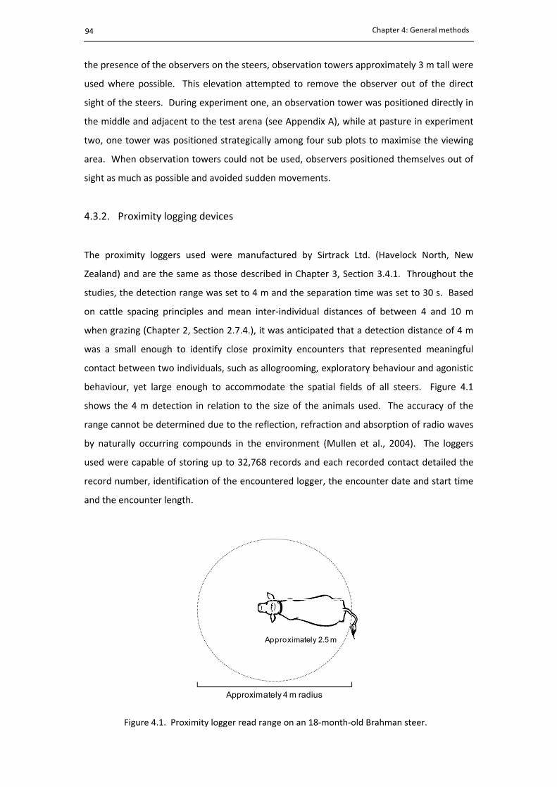
Chapter 4: General methods
94
the presence of the observers on the steers, observation towers approximately 3 m tall were
used where possible. This elevation attempted to remove the observer out of the direct
sight of the steers. During experiment one, an observation tower was positioned directly in
the middle and adjacent to the test arena (see Appendix A), while at pasture in experiment
two, one tower was positioned strategically among four sub plots to maximise the viewing
area. When observation towers could not be used, observers positioned themselves out of
sight as much as possible and avoided sudden movements.
4.3.2. Proximity logging devices
The proximity loggers used were manufactured by Sirtrack Ltd. (Havelock North, New
Zealand) and are the same as those described in Chapter 3, Section 3.4.1. Throughout the
studies, the detection range was set to 4 m and the separation time was set to 30 s. Based
on cattle spacing principles and mean inter‐individual distances of between 4 and 10 m
when grazing (Chapter 2, Section 2.7.4.), it was anticipated that a detection distance of 4 m
was a small enough to identify close proximity encounters that represented meaningful
contact between two individuals, such as allogrooming, exploratory behaviour and agonistic
behaviour, yet large enough to accommodate the spatial fields of all steers. Figure 4.1
shows the 4 m detection in relation to the size of the animals used. The accuracy of the
range cannot be determined due to the reflection, refraction and absorption of radio waves
by naturally occurring compounds in the environment (Mullen et al., 2004). The loggers
used were capable of storing up to 32,768 records and each recorded contact detailed the
record number, identification of the encountered logger, the encounter date and start time
and the encounter length.
Figure 4.1. Proximity logger read range on an 18‐month‐old Brahman steer.
Approximately 2.5 m
Approximately 4 m radius
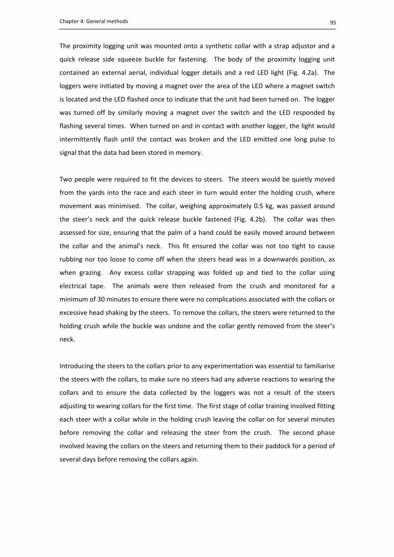
Chapter 4: General methods
95
The proximity logging unit was mounted onto a synthetic collar with a strap adjustor and a
quick release side squeeze buckle for fastening. The body of the proximity logging unit
contained an external aerial, individual logger details and a red LED light (Fig. 4.2a). The
loggers were initiated by moving a magnet over the area of the LED where a magnet switch
is located and the LED flashed once to indicate that the unit had been turned on. The logger
was turned off by similarly moving a magnet over the switch and the LED responded by
flashing several times. When turned on and in contact with another logger, the light would
intermittently flash until the contact was broken and the LED emitted one long pulse to
signal that the data had been stored in memory.
Two people were required to fit the devices to steers. The steers would be quietly moved
from the yards into the race and each steer in turn would enter the holding crush, where
movement was minimised. The collar, weighing approximately 0.5 kg, was passed around
the steer’s neck and the quick release buckle fastened (Fig. 4.2b). The collar was then
assessed for size, ensuring that the palm of a hand could be easily moved around between
the collar and the animal’s neck. This fit ensured the collar was not too tight to cause
rubbing nor too loose to come off when the steers head was in a downwards position, as
when grazing. Any excess collar strapping was folded up and tied to the collar using
electrical tape. The animals were then released from the crush and monitored for a
minimum of 30 minutes to ensure there were no complications associated with the collars or
excessive head shaking by the steers. To remove the collars, the steers were returned to the
holding crush while the buckle was undone and the collar gently removed from the steer’s
neck.
Introducing the steers to the collars prior to any experimentation was essential to familiarise
the steers with the collars, to make sure no steers had any adverse reactions to wearing the
collars and to ensure the data collected by the loggers was not a result of the steers
adjusting to wearing collars for the first time. The first stage of collar training involved fitting
each steer with a collar while in the holding crush leaving the collar on for several minutes
before removing the collar and releasing the steer from the crush. The second phase
involved leaving the collars on the steers and returning them to their paddock for a period of
several days before removing the collars again.
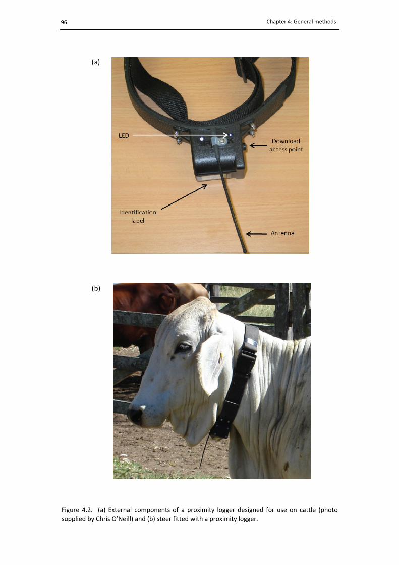
Chapter 4: General methods
96
Figure 4.2. (a) External components of a proximity logger designed for use on cattle (photosupplied by Chris O’Neill) and (b) steer fitted with a proximity logger.
(a)
(b)

Chapter 4: General methods
97
Once removed, a USB interface was connected to the logger from a computer to download
the data. The data was then saved in an excel spreadsheet for processing. The first 5 hours
of data collected after fitting collars were discarded to account for the time taken to handle
the steers and return them to their designated plot, as was the 5 hours prior to removing
collars. Theoretically, each contact recorded by a proximity logger should be reciprocated by
the contacted proximity logger, however this is not always achieved due to reflection,
refraction and absorption of radio waves (Prange et al., 2006; Swain and Bishop‐Hurley,
2007; Bohm et al., 2009). Additionally, Prange et al. (2006) reported that some proximity
loggers record multiple shorter contacts rather than one single contact. To overcome this,
contacts from both loggers were assessed according to the beginning and end time with any
overlap removed. A contact was defined as beginning when either logger recorded a contact
and ending when either logger failed to maintain contact, given that there was continuous
recording by either logger within the start and end time (Hamede et al., 2009). Thus, a
single file of contacts was created per pair. One‐second contacts can erroneously occur
when near the edge of the detection range (Prange et al., 2006) and were removed from the
data prior to analysis, thus the minimum contact length between two steers was 2 s. Details
of the statistical analyses used are reported in the specific chapters.

99
Chapter 5
The effect of familiarity on the trade‐off individual steers make between food and social companionship 5.1. Introduction
Close spatial proximity is a prominent feature of affiliative social behaviour (e.g. Murphey,
1990; Sibbald et al., 1998). The tendency to remain within a group’s living space provides an
indication of group cohesion, while inter‐individual distances provide an indication of the
social attraction and relationship status between two individuals. Therefore, spatial
proximity can be used to indicate the level of social attraction between two individuals.
Social attraction is not shared equally between group members, as individuals at opposite
ends of the hierarchy maintain greater inter‐individual distances (e.g. Manson and Appleby,
1990) and preferential relationships exist between some individuals rather than others (e.g.
Reinhardt and Reinhardt, 1981; Val‐Laillet et al., 2009). The aim of the current experiment
was to develop an understanding of the differences in social attraction between familiar and
unfamiliar steers.
A motivational conflict exists between the priority for behaviours that maintain social bonds
with other group members and the priority for foraging behaviour that entices individuals
away from the group to maximise their feeding opportunities. The conflict between social
and feeding behaviour is dependent on interactions between multiple factors, such as the
distance to a feeding site (Dumont and Boissy, 2000), the size of the social group and the
level of familiarity among peers (Boissy and Dumont, 2002). Differences in sociability can

Chapter 5: Trade‐off between food and social companionship
100
also influence an individual’s behaviour in a motivational conflict. A social trade‐off test
developed by Sibbald et al. (2006) used food bowls placed at incremental distances to entice
individual sheep away from a group of familiar peers. Sibbald et al. (2006) determined that
highly sociable sheep were less inclined to move away from the group when faced with the
conflict of social versus food motivation. It is not known how motivated a steer is to remain
within proximity to a peer when faced with a desired food source, and whether this
response is influenced by the familiarity of the peer.
The current experiment was developed to compare the willingness of individual steers to
remain within close proximity to either familiar or unfamiliar steers when faced with a food
reward using a similar trade‐off test to that described by Sibbald et al. (2006). Preference
tests, such as those designed by Sibbald et al. (2006), have been used in animal welfare
research to quantify the biological and social requirements of an animal, and can be used to
quantify an individual’s preference for different foods, temperature or social companionship
(Broom and Fraser, 2007). It was suggested by Sibbald et al. (2006) that the distance
individuals are willing to travel for food represents a trade‐off point between food and social
companionship. It was hypothesised that steers paired with unfamiliar peers would travel
further to receive a food reward than those paired with familiar peers because the steers
would have lower levels of social attraction towards the unfamiliar steer.
5.2. Methods
5.2.1. Animals and management
The experiment was conducted in May 2008. The two groups of 12 steers and their
management procedures were the same as those described in Chapter 4. Briefly, the two
groups of steers were located a minimum of 100 m when at pasture and at least 20 m when
held in yards. At the time of the experiment the steers mean weight (± standard error) was
352 ± 7.3 kg and 389 ± 8.6 kg for groups 1 and 2, respectively. When not being tested the
steers were maintained on unrestricted Rhodes grass (Chloris gayana) dominant pastures.
On the day of testing, animals were sorted into required or non‐required and those not
involved in tests were returned to their paddock. Animals being tested were given access to
hay and water up until a minimum of 1 hour prior to testing. The procedures used within
the current experiment were approved by the CSIRO Rockhampton Animal Ethics Committee
(Approval number RH243‐07).
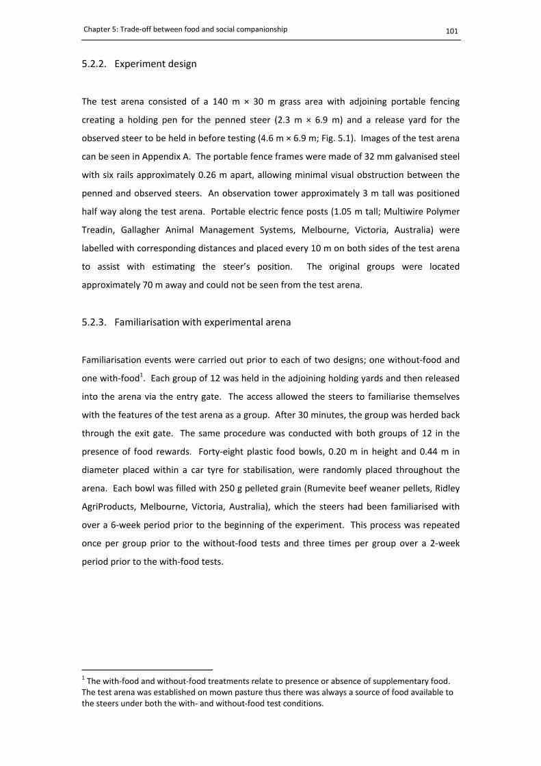
Chapter 5: Trade‐off between food and social companionship
101
5.2.2. Experiment design
The test arena consisted of a 140 m × 30 m grass area with adjoining portable fencing
creating a holding pen for the penned steer (2.3 m × 6.9 m) and a release yard for the
observed steer to be held in before testing (4.6 m × 6.9 m; Fig. 5.1). Images of the test arena
can be seen in Appendix A. The portable fence frames were made of 32 mm galvanised steel
with six rails approximately 0.26 m apart, allowing minimal visual obstruction between the
penned and observed steers. An observation tower approximately 3 m tall was positioned
half way along the test arena. Portable electric fence posts (1.05 m tall; Multiwire Polymer
Treadin, Gallagher Animal Management Systems, Melbourne, Victoria, Australia) were
labelled with corresponding distances and placed every 10 m on both sides of the test arena
to assist with estimating the steer’s position. The original groups were located
approximately 70 m away and could not be seen from the test arena.
5.2.3. Familiarisation with experimental arena
Familiarisation events were carried out prior to each of two designs; one without‐food and
one with‐food1. Each group of 12 was held in the adjoining holding yards and then released
into the arena via the entry gate. The access allowed the steers to familiarise themselves
with the features of the test arena as a group. After 30 minutes, the group was herded back
through the exit gate. The same procedure was conducted with both groups of 12 in the
presence of food rewards. Forty‐eight plastic food bowls, 0.20 m in height and 0.44 m in
diameter placed within a car tyre for stabilisation, were randomly placed throughout the
arena. Each bowl was filled with 250 g pelleted grain (Rumevite beef weaner pellets, Ridley
AgriProducts, Melbourne, Victoria, Australia), which the steers had been familiarised with
over a 6‐week period prior to the beginning of the experiment. This process was repeated
once per group prior to the without‐food tests and three times per group over a 2‐week
period prior to the with‐food tests.
1 The with‐food and without‐food treatments relate to presence or absence of supplementary food. The test arena was established on mown pasture thus there was always a source of food available to the steers under both the with‐ and without‐food test conditions.
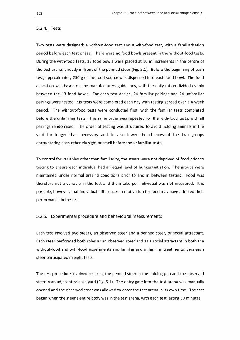
Chapter 5: Trade‐off between food and social companionship
102
5.2.4. Tests
Two tests were designed: a without‐food test and a with‐food test, with a familiarisation
period before each test phase. There were no food bowls present in the without‐food tests.
During the with‐food tests, 13 food bowls were placed at 10 m increments in the centre of
the test arena, directly in front of the penned steer (Fig. 5.1). Before the beginning of each
test, approximately 250 g of the food source was dispensed into each food bowl. The food
allocation was based on the manufacturers guidelines, with the daily ration divided evenly
between the 13 food bowls. For each test design, 24 familiar pairings and 24 unfamiliar
pairings were tested. Six tests were completed each day with testing spread over a 4‐week
period. The without‐food tests were conducted first, with the familiar tests completed
before the unfamiliar tests. The same order was repeated for the with‐food tests, with all
pairings randomised. The order of testing was structured to avoid holding animals in the
yard for longer than necessary and to also lower the chances of the two groups
encountering each other via sight or smell before the unfamiliar tests.
To control for variables other than familiarity, the steers were not deprived of food prior to
testing to ensure each individual had an equal level of hunger/satiation. The groups were
maintained under normal grazing conditions prior to and in between testing. Food was
therefore not a variable in the test and the intake per individual was not measured. It is
possible, however, that individual differences in motivation for food may have affected their
performance in the test.
5.2.5. Experimental procedure and behavioural measurements
Each test involved two steers, an observed steer and a penned steer, or social attractant.
Each steer performed both roles as an observed steer and as a social attractant in both the
without‐food and with‐food experiments and familiar and unfamiliar treatments, thus each
steer participated in eight tests.
The test procedure involved securing the penned steer in the holding pen and the observed
steer in an adjacent release yard (Fig. 5.1). The entry gate into the test arena was manually
opened and the observed steer was allowed to enter the test arena in its own time. The test
began when the steer’s entire body was in the test arena, with each test lasting 30 minutes.
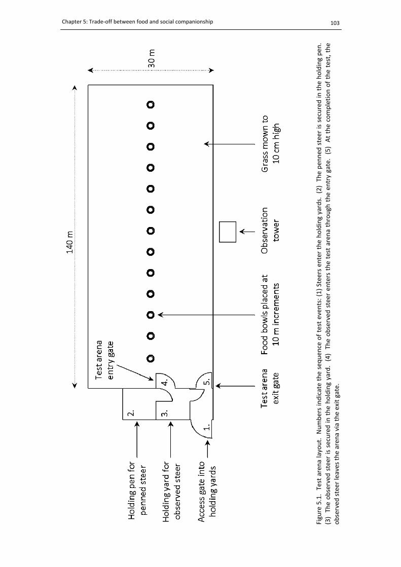
Chapter 5: Trade‐off between food and social companionship
103
Figure 5.1. Test arena layout. Numbers indicate the sequen
ce of test events: (1) Steers enter the holding yards. (2) The pen
ned
steer is secured in
the holding pen
.
(3) The observed
steer is secured in the holding yard. (4) The observed
steer enters the test arena through
the en
try gate. (5) At the completion of the test, the
observed
steer leaves the aren
a via the exit gate.
Chapter 5: Trade‐off between food and social companionship
104
Observations were recorded by a single observer every 30 s, noting the distance (within 5 m)
of the observed steer from the penned steer. At each sample point, the behaviour of the
observed steer was recorded (standing, walking, grazing, lying, ruminating, grooming and
bowl visiting during the with‐food tests). In between sampling points, all bowl visiting
events were also recorded, with the distance of every bowl visit noted. After 30 minutes,
the observed steer exited the test arena by a separate exit gate and both the observed steer
and penned steer were returned to their original groups.
During the unfamiliar tests, the two steers only encountered each other immediately prior
to entering the penned area. At the end of the test each individual was returned back to
their original groups. If a steer was tested in an unfamiliar pairing, that steer would be given
a one‐day re‐stabilisation period with members of its original group before being used in
another test.
5.2.6. Data processing and statistical analysis
Individual animal data were analysed over the two different test types (without‐food versus
with‐food) and two different treatment types (familiar versus unfamiliar). The effect of test
type (within tests) and treatment type (between tests) was analysed independently of each
other.
The distance the steer moved from the penned steer was calculated as the mean of 60
distance observations recorded every 30 s over 30 minutes. Distance observations were also
averaged over 5‐minute periods. The mean number of bowl visits was taken as the mean of
all bowl visits per treatment. The mean distance when bowl visiting was calculated as the
mean of all distances recorded. The rate of bowl visiting was calculated as the mean number
of bowl visits per 5‐minute interval. Behavioural events, including bowl visits, were
expressed as a percentage of observations.
Statistical analyses were carried out using Genstat 10th edition (Payne et al., 2007). A two‐
way between groups analysis of variance (ANOVA) was used to determine any differences in
means between test (without‐food vs. with‐food) and treatment (familiar vs. unfamiliar),
while a one‐way ANOVA was used to analyse differences in means within tests, using
treatment as a factor in the model. Differences were considered significant at P < 0.05.
Preliminary inspection of the distributions of distance, bowl visiting and time spent
Chapter 5: Trade‐off between food and social companionship
105
performing each behaviour and comparison of variances across treatments suggested that
the assumptions for the ANOVA of normality and homogeneity of variance were plausible.
Results for distances, behaviours and bowl visiting are expressed as mean ± standard error.
5.3. Results
5.3.1. Differences between familiar and unfamiliar without‐food and with‐food
tests
Mean distance was affected by the presence of food (test main effect: F1,95 = 6.53, P = 0.012,
η2 = 0.07), but not by familiarity (familiarity main effect: F1,95 = 0.13, P = 0.717, η2 = 0.00) or
any interaction between the test types (without‐food and with‐food) and familiarity
(interaction: F1,95 = 0.85, P = 0.359, η2 = 0.01). The greatest difference between tests was
seen between steers in the familiar with‐food tests that travelled an average of 8.7 m
further from the penned steer than the without‐food test (ANOVA; familiar without‐food =
5.1 ± 0.98 m, familiar with‐food = 13.8 ± 2.88 m; F1,46 = 8.26, P = 0.006, η2 = 0.15; Table 5.1).
ANOVA performed at each 5‐minute time interval revealed that the difference between the
without‐food and with‐food tests for familiar test steers was significant during the first 15
minutes of the test (time = 5 minutes, F1,46 = 32.67, P < 0.001, η2 = 0.42; time = 10 minutes,
F1,46 = 16.68, P < 0.001, η2 = 0.27; time = 15 minutes, F1,46 = 4.70, P = 0.035, η
2 = 0.09), while
only the first 5 minutes proved to be different for the unfamiliar test steers (time = 5
minutes, F1,46 = 17.6, P < 0.001, η2 = 0.28; Fig. 5.2).
The introduction of the food bowls caused a decrease in the amount of time spent standing
for both familiarity types as steers actively explored the food bowls (test main effect: F1,95 =
3.79, P = 0.054, η2 = 0.13; familiarity main effect: F1,95 = 13.7, P < 0.001, η2 = 0.03), however
there was no interaction between test and familiarity (interaction: F1,95 = 0.08, P = 0.775, η2 =
0.00). The consumption of supplementary food also caused a notable decrease in
ruminating behaviour between the without‐food and with‐food tests for both familiarity
types (test main effect; F1,95 = 6.34, P = 0.014, η2 = 0.06). However, the proportion of time
spent ruminating was not affected by familiarity (treatment main effect; F1,95 = 0.76, P =
0.385, η2 = 0.01) nor was there any interaction effect between test and familiarity
(interaction: F1,95 = 0.32, P = 0.573, η2 = 0.00).
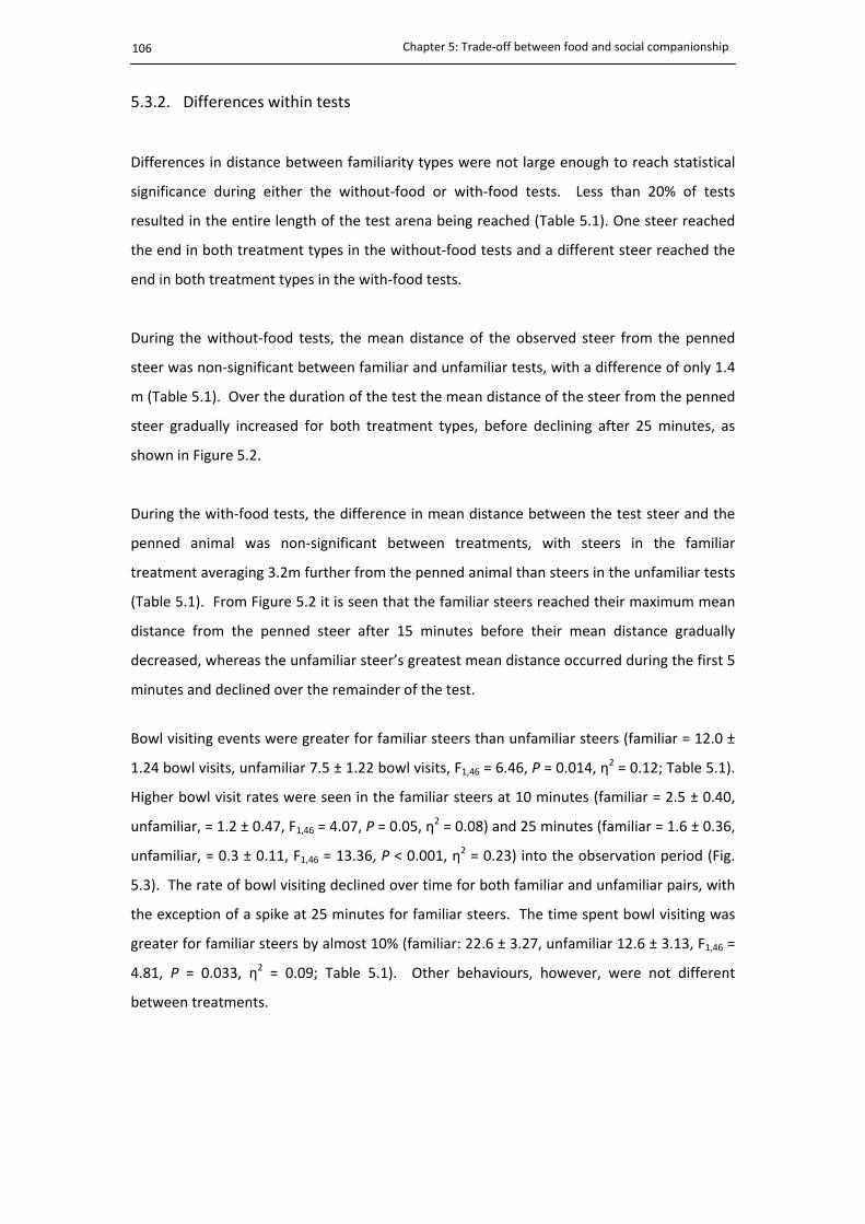
Chapter 5: Trade‐off between food and social companionship
106
5.3.2. Differences within tests
Differences in distance between familiarity types were not large enough to reach statistical
significance during either the without‐food or with‐food tests. Less than 20% of tests
resulted in the entire length of the test arena being reached (Table 5.1). One steer reached
the end in both treatment types in the without‐food tests and a different steer reached the
end in both treatment types in the with‐food tests.
During the without‐food tests, the mean distance of the observed steer from the penned
steer was non‐significant between familiar and unfamiliar tests, with a difference of only 1.4
m (Table 5.1). Over the duration of the test the mean distance of the steer from the penned
steer gradually increased for both treatment types, before declining after 25 minutes, as
shown in Figure 5.2.
During the with‐food tests, the difference in mean distance between the test steer and the
penned animal was non‐significant between treatments, with steers in the familiar
treatment averaging 3.2m further from the penned animal than steers in the unfamiliar tests
(Table 5.1). From Figure 5.2 it is seen that the familiar steers reached their maximum mean
distance from the penned steer after 15 minutes before their mean distance gradually
decreased, whereas the unfamiliar steer’s greatest mean distance occurred during the first 5
minutes and declined over the remainder of the test.
Bowl visiting events were greater for familiar steers than unfamiliar steers (familiar = 12.0 ±
1.24 bowl visits, unfamiliar 7.5 ± 1.22 bowl visits, F1,46 = 6.46, P = 0.014, η2 = 0.12; Table 5.1).
Higher bowl visit rates were seen in the familiar steers at 10 minutes (familiar = 2.5 ± 0.40,
unfamiliar, = 1.2 ± 0.47, F1,46 = 4.07, P = 0.05, η2 = 0.08) and 25 minutes (familiar = 1.6 ± 0.36,
unfamiliar, = 0.3 ± 0.11, F1,46 = 13.36, P < 0.001, η2 = 0.23) into the observation period (Fig.
5.3). The rate of bowl visiting declined over time for both familiar and unfamiliar pairs, with
the exception of a spike at 25 minutes for familiar steers. The time spent bowl visiting was
greater for familiar steers by almost 10% (familiar: 22.6 ± 3.27, unfamiliar 12.6 ± 3.13, F1,46 =
4.81, P = 0.033, η2 = 0.09; Table 5.1). Other behaviours, however, were not different
between treatments.
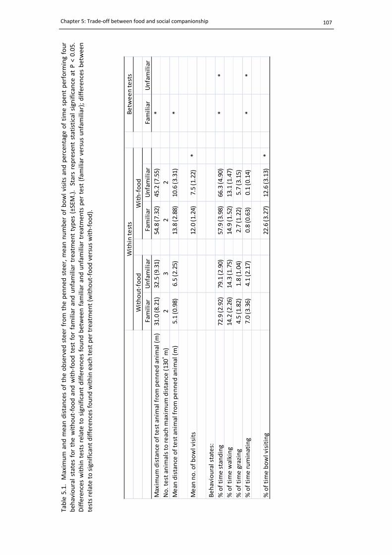
Chapter 5: Trade‐off between food and social companionship
107
Familiar
Unfamiliar
Familiar
Unfamiliar
Familiar
Unfamiliar
Maxim
um distance of test anim
al from penned anim
al (m)
31.0 (8.21)
32.5 (9.31)
54.8 (7.32)
45.2 (7.55)
*
No. test anim
als to reach maxim
um distance (130+ m)
23
22
Mean
distance of test anim
al from penned anim
al (m)
5.1 (0.98)
6.5 (2.25)
13.8 (2.88)
10.6 (3.31)
*
Mean
no. of bowl visits
12.0 (1.24)
7.5 (1.22)
*
Behavioural states:
% of time standing
72.9 (2.92)
79.1 (2.90)
57.9 (3.98)
66.3 (4.90)
**
% of time walking
14.2 (2.26)
14.3 (1.75)
14.9 (1.52)
13.1 (1.47)
% of time grazing
4.5 (1.82)
1.8 (1.04)
2.7 (1.22)
5.7 (3.15)
% of time ruminating
7.0 (3.36)
4.1 (2.17)
0.8 (0.63)
0.1 (0.14)
**
% of time bowl visiting
22.6 (3.27)
12.6 (3.13)
*
Within tests
Without‐food
With‐food
Betw
een tests
Table 5.1. M
axim
um and m
ean distances of the observed
steer from the pen
ned
steer, mean number of bowl visits and percentage of time spen
t perform
ing four
beh
avioural states for the without‐food and w
ith‐food test for familiar and unfamiliar treatmen
t types (±SEM
.). Stars rep
resent statistical significance at P < 0.05.
Differences within tests relate to significant differences found between fam
iliar and unfamiliar treatmen
ts per test (fam
iliar versus unfamiliar); differences between
tests relate to significant differences found within each test per treatmen
t (w
ithout‐food versus with‐food).
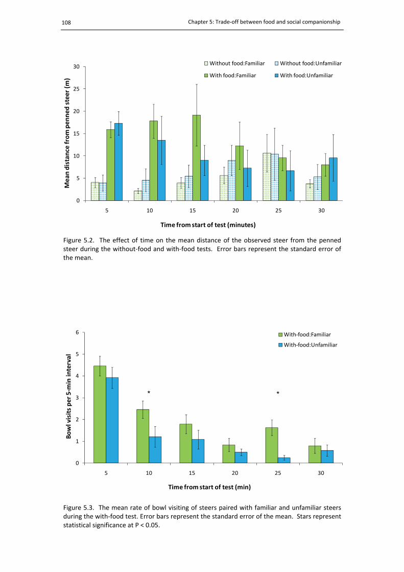
Chapter 5: Trade‐off between food and social companionship
108
Figure 5.2. The effect of time on the mean distance of the observed steer from the pennedsteer during the without‐food and with‐food tests. Error bars represent the standard error ofthe mean.
Figure 5.3. The mean rate of bowl visiting of steers paired with familiar and unfamiliar steersduring the with‐food test. Error bars represent the standard error of the mean. Stars representstatistical significance at P < 0.05.
0
5
10
15
20
25
30
5 10 15 20 25 30
Mean distance from pen
ned
steer (m)
Time from start of test (minutes)
Without food:Familiar Without food:Unfamiliar
With food:Familiar With food:Unfamiliar
0
1
2
3
4
5
6
5 10 15 20 25 30
Bowl visits per 5‐m
in interval
Time from start of test (min)
With‐food:Familiar
With‐food:Unfamiliar
* *
Chapter 5: Trade‐off between food and social companionship
109
5.4. Discussion
The aim of the experiment was to compare the social attractiveness of a familiar peer over
an unfamiliar peer by creating a trade‐off between social companionship and a preference
for food, similar in design to that described by Sibbald et al. (2006). The results showed that
without a feeding motivation steers remained in close proximity to either familiar or
unfamiliar peers. The mean inter‐individual distance between cattle when grazing is
reported to be within 4 and 10 m (Broom and Fraser, 2007), thus mean distances less than
10 m between the observed steer and the penned steer were considered to be close. When
faced with a trade‐off between feeding and social preferences, steers were willing to move
further to consume supplementary food in the presence of a familiar pen mate than an
unfamiliar peer. Therefore, although a significant impact of familiarity was identified on the
bowl visiting behaviour between the two treatment types, the effect was in the opposite
direction to that hypothesised.
Sibbald et al. (2006) showed that sheep travelled an average 21.8 m away from the group
the first time they were exposed to a similar food rewards test and visited an average of 42.5
bowls, with all sheep reaching the end of the 65 m test arena during this test. Thus, it was
expected that the overall mean distance travelled by steers and the number of bowl visits
would be greater than what was observed. It was also anticipated that most individuals
would be prepared to travel the entire length of the test arena to gain a food reward,
however, only seven individuals travelled to the end. The maximum distance travelled by
each individual is a measure of their willingness to move away from a social companion to
feed, indicating the trade‐off point between food and social support. Similarly, the
difference in distance travelled between the without‐food and with‐food test demonstrates
the importance of food as a motivator. When food was present, steers in the familiar tests
showed a significant increase in the distance travelled away from the penned animal when
compared with the without‐food tests, confirming that the presence of a familiar peer
provided social support that allowed individuals to express their own feeding choices. Steers
in the unfamiliar tests, however, showed no increase in distance between the without‐food
and with‐food tests, indicating that the decision to move away for food was complicated by
unfamiliarity and a lack of social support.
Other similar experiments that include a trade‐off between an individual’s preference for
social contact over feeding found that the familiarity of a grazing companion and the size of

Chapter 5: Trade‐off between food and social companionship
110
the companion group positively influenced the grazing choice of the animal (Boissy and
Dumont, 2002). Scott et al. (1995) found familiarity to have a positive effect on grazing
preference; lambs conditioned to prefer wheat when in the presence of familiar lambs
conditioned to prefer sorghum elected to graze on their preferred grain some distance away.
Additionally, Boissy and Dumont (2002) reported that animals in the presence of unfamiliar
companions had shorter mean distances to the penned animals, vocalised more and had
greater nearest neighbour distances, which was attributed to the loss of social support
previously provided by familiar companions. Similarly, Sibbald and Hooper (2004) reported
that sheep were more willing to graze a preferred feeding site that was close (15 m) than far
away (35 m) from penned conspecifics due to the apparent fear of social isolation. The
combination of lost social support and fear of social isolation as suggested by Boissy and
Dumont (2002) and Sibbald and Hooper (2004) could similarly be used to interpret the
shorter distances and fewer bowl visits by the steers during the unfamiliar with‐food tests.
Cattle are gregarious animals and rely on group members for protection and support;
removing this support can result in behavioural and physiological changes associated with
stress (Boissy and LeNeindre, 1997). Socially isolated cattle in unfamiliar environments
exhibit increased heart rates, increased plasma cortisol levels, increased elimination
frequency and increased vocalisations (Rushen et al., 1999a). Unfortunately the test design
did not allow for these stress indicators to be measured in the resident steers, although their
behaviour during the unfamiliar tests showed signs of discomfort, such as a lower rate of
bowl visiting behaviour, a tendency to spend a greater amount of time standing and a desire
to maintain close proximity to the penned steer, more so than what was observed in the
familiar tests. These behaviours may indicate fear in response to social isolation or the
presence of an unfamiliar conspecific, with fear a known stressor in cattle (Grandin, 1997).
According to Hamilton (1971), individuals should approach their nearest neighbour to
decrease fear and risk of predation. If the test steers were experiencing fear of social
isolation, maintaining close proximity to its nearest neighbour, which in this case was an
unfamiliar steer, might indicate a form of stress alleviation.
Other motivational factors might have also influenced the change in behaviour caused by
the presence of the unfamiliar penned steer during the with‐food tests. For example, a
motivational conflict may have existed between exploring the test arena versus investigating
the unfamiliar steer. While the steers were given a familiarisation phase as a group in the
test area with numerous food bowls present, the steers had not experienced the arena or
Chapter 5: Trade‐off between food and social companionship
111
access to the food bowls by themselves. Individuals differ in their levels of inquisitiveness
and motivation to explore novel situations, which is necessary for learning and
familiarisation with a new environment (Price, 2008). Additionally, younger cattle aged
between one and two responded more to novelty (Murphey et al., 1981), thus the steers
tested in this experiment could be considered highly inquisitive. Although it was only
evident within the familiar with‐food tests that steers showed greater levels of exploration
of the food bowls. This suggests that during the unfamiliar with‐food tests the presence of
the unfamiliar steer created a distraction from the novelty of the environment and the
observed steers were more interested to investigate the unfamiliar penned steer than the
food bowls. This concurs with results obtained by Souza et al. (2006) who proposed that
piglets gave higher priority to investigating unfamiliar conspecifics over exploration of a new
environment.
One possible explanation for the test steers behavioural response towards the unfamiliar
penned steer may have been the perception of the unfamiliar individual as a competition
threat. Individuals within a group may compete for food, space and social status; the
presence of an unfamiliar animal is considered a threat to all of these resources and may
result in agonistic behaviour (Price, 2008). Even though the pair was restricted from physical
interaction, steers were unrestricted from distinguishing each other via visual, auditory and
olfactory cues. Remaining within close proximity may indicate the observed steer was
evaluating the unfamiliar steer’s characteristics, for example, predictors of dominance ability
such as weight, sex and age. Furthermore, a grazing situation provides a highly competitive
environment (Phillips and Rind, 2001), with high quality feed inducing dominance behaviours
(Barroso et al., 2000). Therefore, the observed steers may have maintained close proximity
to monitor the actions of the unfamiliar steer and its location to the highly desired food
source.
Modification of the test design is required to formally test the proposed theories relating to
social stress, curiosity and competition, and as such, no conclusive remarks can be made
about the behavioural changes observed between the familiar and unfamiliar with‐food
tests. In future, it would be advantageous to measure behavioural indicators of stress, such
as defecation/urination (e.g. Kilgour, 1975), head movements (e.g. Kondo and Hurnik, 1988)
or heart rate (e.g. Rushen et al., 1999b). Similarly, additional information on the observed
animal’s location via grid co‐ordinates would provide greater spatial accuracy and could be
used to indicate if individuals were favouring specific areas of the arena, such as the exit

Chapter 5: Trade‐off between food and social companionship
112
gate, which may influence the response of the observed animal (e.g. Kilgour, 1975).
Furthermore, the inclusion of an additional penned animal on the opposite side of the arena
could be used to evaluate the observed animal’s preference for one individual over another,
for example a familiar versus an unfamiliar conspecific.
5.5. Conclusions
It was concluded that familiar peers provide social support that allows individuals to express
their own feeding choices, thus the hypothesis that steers would be less attracted to an
unfamiliar penned steer and travel further to receive a food reward was rejected. It was
anticipated that the lower attraction would be a result of the lack of opportunity for
unfamiliar steers to develop social bonds. The results showed that the opposite was true and
steers in the presence of unfamiliar pen mates consumed less food than steers paired with
familiar pen mates, while steers with familiar pen mates travelled further when food was
present. Furthermore, the presence of an unfamiliar introduced additional factors that
influenced the decision of the observed steer to move away from the unfamiliar conspecific
to feed, although the reasons for this are varied and inconclusive but may relate to loss of
social support previously provided by familiar peers, the priority to investigate the social
environment over the physical environment or the competition threat posed by unfamiliar
steers to valuable resources.
113
Chapter 6
The social behaviour of steers paired with either a familiar or unfamiliar peer 6.1. Introduction
Chapter 5 investigated the behaviour of steers when faced with a conflict situation between
feeding and social companionship that was either familiar or unfamiliar. The behaviour of
the steers was modified by the presence of the unfamiliar peer. Familiar peers provided
social support that allowed individuals to express their own feeding choices while the
observed steers were less willing to travel further away for food in the presence of the
unfamiliar peer, possibly due to social stress, competition or curiosity. The test environment
restricted any physical contact between the steers and the potential to develop a
relationship, thus only individual behavioural responses towards the presence of the steer
was measured. Familiarisation occurs via a process of repeated encounters and recollection
of the outcomes of these encounters (Hinde, 1976), thus social interaction is fundamental
for relationship development, including establishing dominance and maintaining social
bonds through behaviours such as allogrooming. The current experiment examined the
effect of familiarity on pair‐wise behaviour in a natural environment and used several
behavioural measures to identify and evaluate some of the spatial and temporal factors
involved in the process of familiarisation, including inter‐individual distance, the detailed
movement response of one individual in relation to another and the frequency and duration
of close proximity encounters.
Familiarisation has previously been documented in cattle by recording the level of agonistic
interactions between individuals and defining stabilisation as the time it takes for non‐
physical interactions to predominate physical interaction (e.g. Kondo and Hurnik, 1990). A

Chapter 6: The social behaviour of pairs of steers
114
study by Bouissou (1974a) found that dominance relationships between newly mixed cattle
were established relatively quickly; almost half of all dominance relationships were
established within 5 minutes and all relationships determined after 2 hours. Changes in
other social behaviours, such as locomotion and standing and lying time (Nakanishi et al.,
1993b; Hasegawa et al., 1997; Grant and Albright, 2001) can take between 3 to 15 days to
return to baseline levels. This suggests that agonistic behaviours are initially important
during relationship establishment, but other social processes, such as learning and
recognition, continue to occur after the direction of dominance relationships are established
and are important factors during relationship development (Lindberg, 2001).
The aim of the current experiment was to compare the change in social interaction over
time between familiar and unfamiliar pairs of steers in order to investigate the process of
familiarisation. It was hypothesised that evidence of familiarisation would be seen within 5
days. By studying pairs in isolation, the aim was to investigate the types of pair‐wise
interactions involved in relationship development, whilst minimising both social interference
and observational errors associated with large groups. It was anticipated that isolating
unfamiliar pairs of steers would accelerate the process of familiarisation due to the lack of
interference from other group members. Additionally, cattle are naturally herding animals
and rely on group members for protection and support; being socially isolated is a stressful
situation (Boissy and LeNeindre, 1997), thus there is mutual benefit for the unfamiliar steers
to quickly form a relationship and provide social support for each other.
6.2. Methods
6.2.1. Animals and plots
The experiment was conducted in July 2008. At the time of the experiment the two groups
of steers mean weight (± standard error) was 352 ± 7.3 kg and 389 ± 8.6 kg for groups 1 and
2, respectively. The steers gained some experience with being paired with unfamiliar steers
in the previous experiment, although the unfamiliar animals paired in the current
experiment had not previously been paired with each other. Pairs were monitored for 5
days in 3 ha plots with a minimum 20 m buffer zone between each plot. The steers had
previous experience with the yards, plots and paddocks. The procedures used in this
experiment were approved by the CSIRO Rockhampton Animal Ethics Committee (Approval
number RH243‐07).
Chapter 6: The social behaviour of pairs of steers
115
6.2.2. Experimental procedure
The pair was treated as the experimental unit with two treatment levels: familiar and
unfamiliar. In total 15 pairs of familiar animals and 15 pairs of unfamiliar animals were
monitored over 5 deployments. Each deployment lasted 5 days with 3 familiar and 3
unfamiliar pairs monitored per deployment. The total duration of the experiment was 5
weeks.. On the day of introduction (day 1: between 14:00 h and 15:00 h), each steer was
fitted with a proximity logger weighing approximately 0.5 kg. Steers were paired off and
moved to their designated plot, approximately 1 km from the cattle handling yards. The
unfamiliar pairings were randomised; the only pre‐requisite was that the two individuals had
not previously been paired together. At the end of the 5 days, the steers were returned to
the yards and the collars removed. Over the 5‐week period, some steers were re‐used. The
re‐use occurred so that a steer was always paired with another steer that had the same level
of experience with the test conditions. At the outset, all steers had previous experience with
being paired with other steers in the yard. To test whether experience with the test
conditions affected behaviour, the distance results of novice and experienced pairs were
compared by day, where ‘novice’ refers to pairs of steers that were new to the study. Re‐
used steers were given a 1 week social re‐stabilisation period with original group members
between monitoring weeks.
6.2.3. Proximity logger data statistical analysis
The contact data over the first 5 days were summarised on a daily basis as the total number
of contacts per hour and the average length per contact. The number of contacts per hour
and the average length per contact were analysed for treatment and day effects, blocked by
week, using a repeated‐measures analysis of variance (ANOVA) (Rowell and Walters, 1976).
The repeated‐measures ANOVA estimates the Greenhouse‐Geisser epsilon to account for
the degree of temporal auto‐correlation, with the significance levels of the F‐tests adjusted
accordingly. Differences were considered significant at P < 0.05. Approximate least
significant differences at the 5% level were used to assess pair‐wise differences between
treatment means for the same day. Distributional assumptions were assessed by visual
inspection of residual and normal probability plots resulting in the proximity logger data
being square‐root transformed prior to analysis with back transformed values presented in
the text.
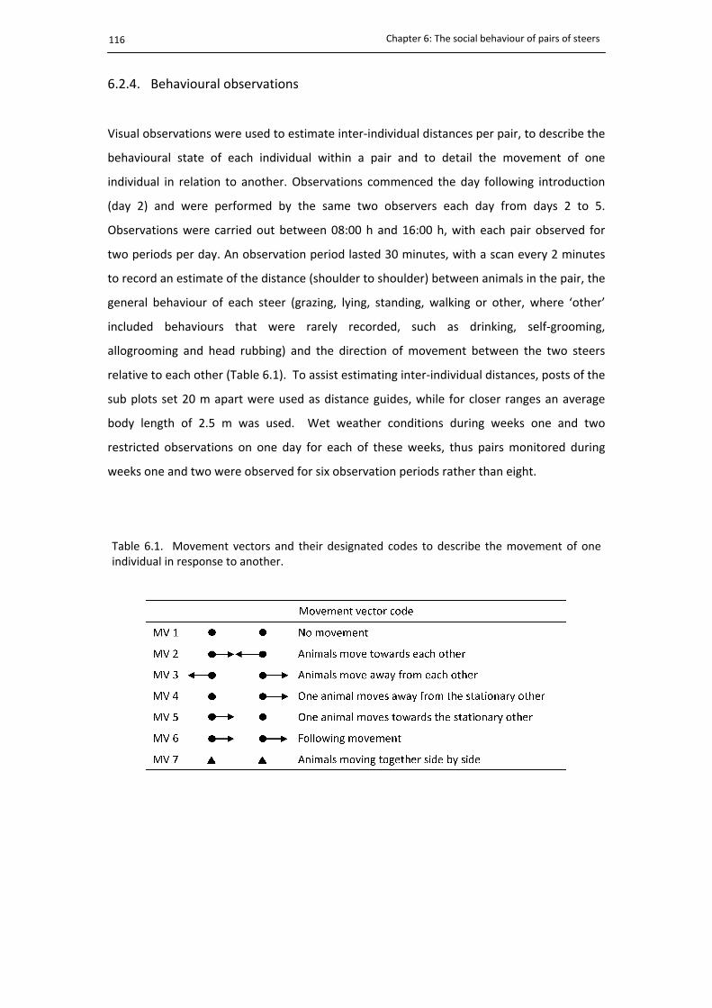
Chapter 6: The social behaviour of pairs of steers
116
6.2.4. Behavioural observations
Visual observations were used to estimate inter‐individual distances per pair, to describe the
behavioural state of each individual within a pair and to detail the movement of one
individual in relation to another. Observations commenced the day following introduction
(day 2) and were performed by the same two observers each day from days 2 to 5.
Observations were carried out between 08:00 h and 16:00 h, with each pair observed for
two periods per day. An observation period lasted 30 minutes, with a scan every 2 minutes
to record an estimate of the distance (shoulder to shoulder) between animals in the pair, the
general behaviour of each steer (grazing, lying, standing, walking or other, where ‘other’
included behaviours that were rarely recorded, such as drinking, self‐grooming,
allogrooming and head rubbing) and the direction of movement between the two steers
relative to each other (Table 6.1). To assist estimating inter‐individual distances, posts of the
sub plots set 20 m apart were used as distance guides, while for closer ranges an average
body length of 2.5 m was used. Wet weather conditions during weeks one and two
restricted observations on one day for each of these weeks, thus pairs monitored during
weeks one and two were observed for six observation periods rather than eight.
Table 6.1. Movement vectors and their designated codes to describe the movement of oneindividual in response to another.

Chapter 6: The social behaviour of pairs of steers
117
6.2.5. Observational data processing and statistical analysis
The visual distance estimates for each pair were averaged per observation period per day.
The movement vectors were recorded on a per pair basis and expressed as a proportion of
the 16 observations per observation period per day. The behavioural measurements were
recorded for each individual steer for each of the 16 observations per observation period,
thus 32 behaviour observations were recorded per pair per observation period. These were
summed for each behavioural state and expressed relative to the 32 observations recorded
per observation. All observational measurements were analysed for the effects of familiarity
and day with a repeated measures analysis using restricted maximum likelihood (REML) to
model the variance‐covariance matrix; an antedependence model of order 1 adequately
modelled the variance structure. A one‐way ANOVA was used to analyse daily differences in
distance estimates between novice and experienced pairs and also between experienced
familiar and unfamiliar pairs on days 2 and 5. Results for distance estimates are expressed
as mean ± standard deviation. The movement vectors were also analysed for the effect of
distance by examining the distance distributions per movement vector and reporting the
mean distance ± standard deviation. Residual and normal probability plots were visually
assessed for distributional assumptions resulting in all movement vectors and behavioural
data being arcsine‐transformed prior to analysis with back transformed values presented in
the text. Differences were considered significant at P < 0.05 and statistical trends are
reported at P < 0.10. Approximate least significant differences at the 5% level were used to
assess pair‐wise differences between treatment means for the same day.
All statistical analyses were conducted using Genstat 12th edition (Payne et al., 2009).
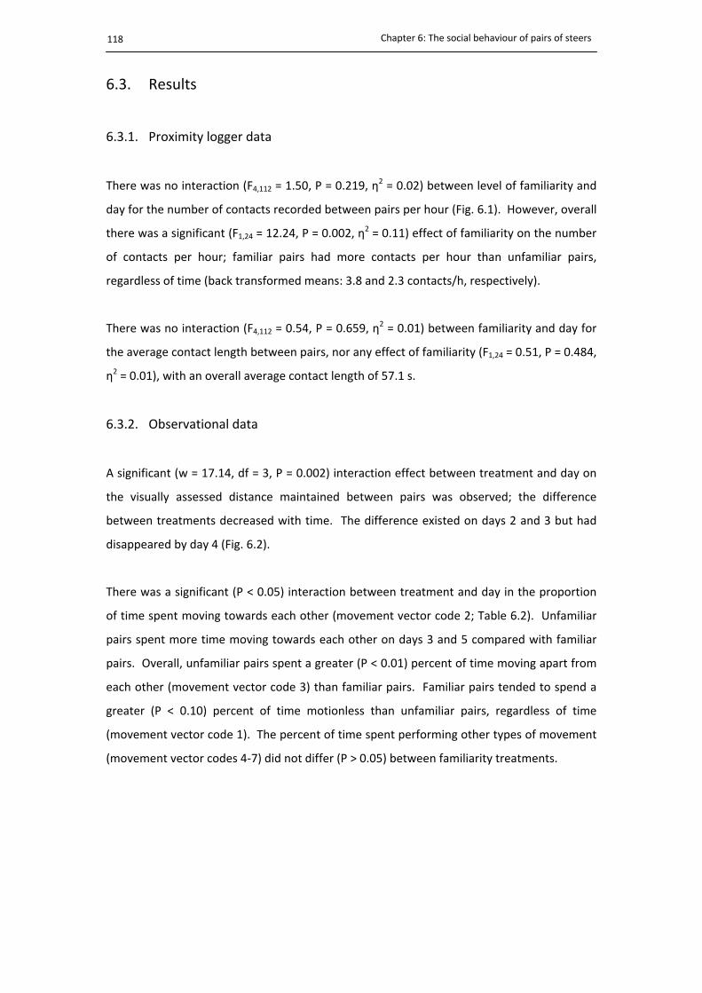
Chapter 6: The social behaviour of pairs of steers
118
6.3. Results
6.3.1. Proximity logger data
There was no interaction (F4,112 = 1.50, P = 0.219, η2 = 0.02) between level of familiarity and
day for the number of contacts recorded between pairs per hour (Fig. 6.1). However, overall
there was a significant (F1,24 = 12.24, P = 0.002, η2 = 0.11) effect of familiarity on the number
of contacts per hour; familiar pairs had more contacts per hour than unfamiliar pairs,
regardless of time (back transformed means: 3.8 and 2.3 contacts/h, respectively).
There was no interaction (F4,112 = 0.54, P = 0.659, η2 = 0.01) between familiarity and day for
the average contact length between pairs, nor any effect of familiarity (F1,24 = 0.51, P = 0.484,
η2 = 0.01), with an overall average contact length of 57.1 s.
6.3.2. Observational data
A significant (w = 17.14, df = 3, P = 0.002) interaction effect between treatment and day on
the visually assessed distance maintained between pairs was observed; the difference
between treatments decreased with time. The difference existed on days 2 and 3 but had
disappeared by day 4 (Fig. 6.2).
There was a significant (P < 0.05) interaction between treatment and day in the proportion
of time spent moving towards each other (movement vector code 2; Table 6.2). Unfamiliar
pairs spent more time moving towards each other on days 3 and 5 compared with familiar
pairs. Overall, unfamiliar pairs spent a greater (P < 0.01) percent of time moving apart from
each other (movement vector code 3) than familiar pairs. Familiar pairs tended to spend a
greater (P < 0.10) percent of time motionless than unfamiliar pairs, regardless of time
(movement vector code 1). The percent of time spent performing other types of movement
(movement vector codes 4‐7) did not differ (P > 0.05) between familiarity treatments.

Chapter 6: The social behaviour of pairs of steers
119
Figure 6.1. The average number of close proximity encounters per hour (±SE) between familiarand unfamiliar pairs per day. Data are square‐root transformed interaction means.
Figure 6.2. The average proximity (±SE) between familiar and unfamiliar pairs per day asrecorded by visual observations. Asterisks indicate statistical significance at P = 0.05 betweenfamiliarity treatments.
0
10
20
30
40
50
60
70
2 3 4 5
Average distance betw
een individuals
within a pair (m)
Day
Familiar
Unfamiliar*
*
0.0
0.5
1.0
1.5
2.0
2.5
3.0
1 2 3 4 5
Square‐root transform
ed
average number of contacts/h
Day
Familiar
Unfamiliar

Chapter 6: The social behaviour of pairs of steers
120
Table 6.2. The percent of time steers were observed
moving in the directions classified
by movemen
t vectors 1‐3 per treatmen
t per day. Values shown are arcsine
transform
ed m
eans with back transform
ed values shown in
paren
theses. Significant (P < 0.05) effects between fam
iliarity treatm
ents per day are in
dicated
with an
asterisk.
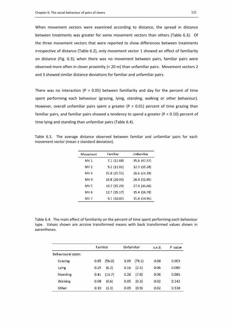
Chapter 6: The social behaviour of pairs of steers
121
When movement vectors were examined according to distance, the spread in distance
between treatments was greater for some movement vectors than others (Table 6.3). Of
the three movement vectors that were reported to show differences between treatments
irrespective of distance (Table 6.2), only movement vector 1 showed an effect of familiarity
on distance (Fig. 6.3); when there was no movement between pairs, familiar pairs were
observed more often in closer proximity (< 20 m) than unfamiliar pairs. Movement vectors 2
and 3 showed similar distance deviations for familiar and unfamiliar pairs.
There was no interaction (P > 0.05) between familiarity and day for the percent of time
spent performing each behaviour (grazing, lying, standing, walking or other behaviour).
However, overall unfamiliar pairs spent a greater (P < 0.01) percent of time grazing than
familiar pairs, and familiar pairs showed a tendency to spend a greater (P < 0.10) percent of
time lying and standing than unfamiliar pairs (Table 6.4).
Table 6.3. The average distance observed between familiar and unfamiliar pairs for eachmovement vector (mean ± standard deviation).
Table 6.4. The main effect of familiarity on the percent of time spent performing each behaviourtype. Values shown are arcsine transformed means with back transformed values shown inparentheses.
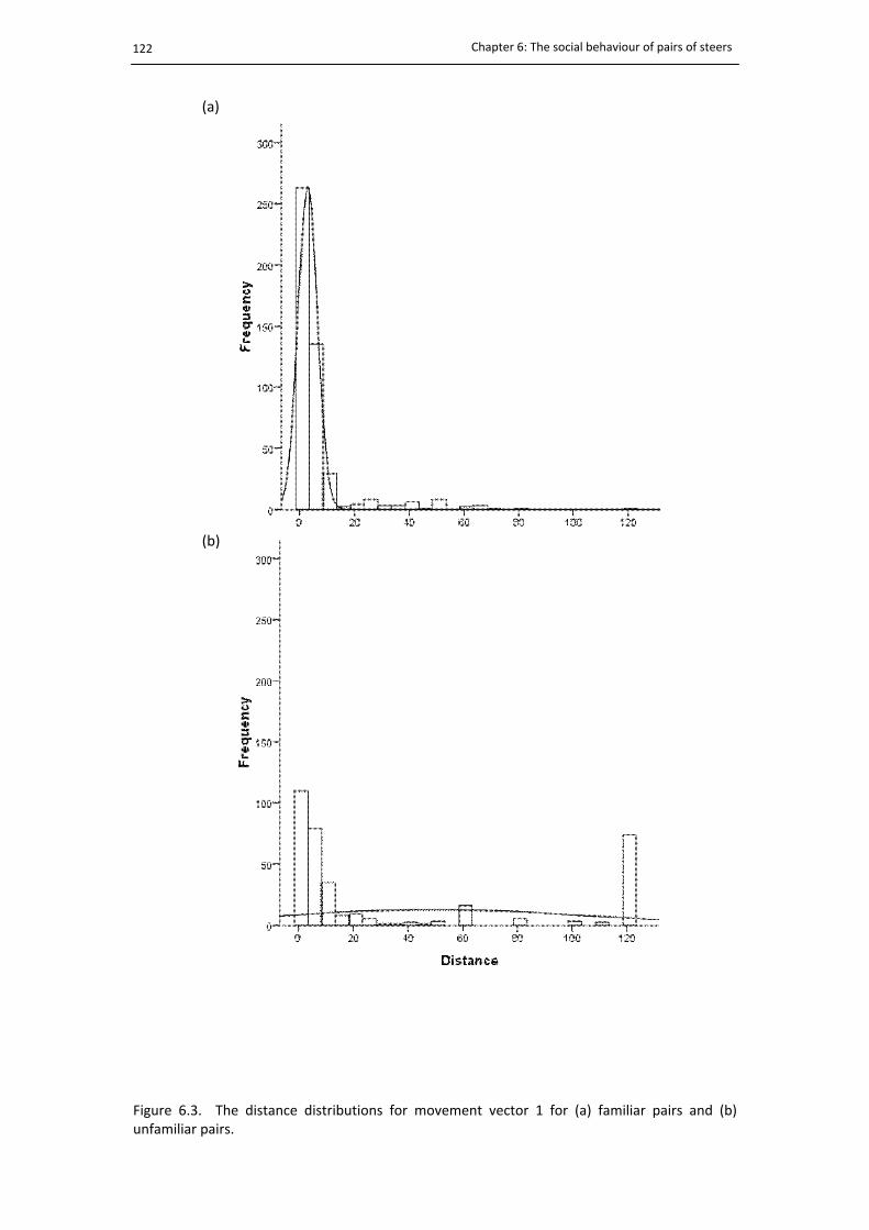
Chapter 6: The social behaviour of pairs of steers
122
Figure 6.3. The distance distributions for movement vector 1 for (a) familiar pairs and (b)unfamiliar pairs.
(a)
(b)

Chapter 6: The social behaviour of pairs of steers
123
6.3.3. Steer re‐use
On the first day of observations (day 2), there was a difference (ANOVA: F1,16 = 4.51, P =
0.050, η2 = 0.22) between novice pairs and experienced pairs; experienced pairs had closer
inter‐individual distances in the unfamiliar treatment than pairs that were new to the test
condition (novice = 105.0 ± 15.00 m, experienced = 32.9 ± 22.59 m). Nevertheless, there was
still a difference (F1,10 = 4.88, P = 0.052, η2 = 0.33) between familiar and unfamiliar
experienced pairs (familiar = 10.8 ± 9.67 m, unfamiliar = 32.9 ± 22.59 m). There was no
difference (F1,25 = 0.34, P = 0.563, η2 = 0.01) in distance between novice and experienced
pairs on day 5, nor was there any effect of familiarity (F1,16 = 0.10, P = 0.757, η2 = 0.01).
6.4. Discussion
The aim of the study was to investigate the spatial and temporal differences between
familiar and unfamiliar pairs and use these differences to characterise features of the
familiarisation process between pairs of unfamiliar steers. The results show that unfamiliar
pairs interact differently from familiar pairs but, as unfamiliar pairs build social bonds, these
differences become less clear indicating that a familiarisation process was occurring
between the pair. In the current experiment, the unfamiliar pairs initially maintained
greater distances apart than familiar pairs, but after 3 days their distances were similar to
familiar pairs (Fig. 6.2). Additionally, the unfamiliar pairs gradually increased their
movement directly towards each other (Table 6.2, movement vector 2), which exceeded the
same movement observed by familiar pairs after 2 days. These gradual changes provide
evidence that the unfamiliar pairs were engaging in behaviours that facilitated the process of
familiarisation. However, overall familiar pairs had more close proximity encounters and
showed a tendency to spend a greater percentage of time lying and standing than unfamiliar
pairs; these differences were constant over the 5 day period indicating that complete
familiarisation had not occurred within 5 days.
The change in inter‐individual distances and movement vectors over the first 3 days suggests
the steers in an unfamiliar pair were initially avoiding each other. Avoidance behaviour was
also reflected in the unfamiliar pairs general and social behaviour; unfamiliar pairs spent
more time grazing than familiar pairs and tended to spend less time lying and standing than
familiar pairs. The lower percent of time spent inactive by individuals within an unfamiliar
pair may reflect a lack of social support and trust within the pair. Without the social support

Chapter 6: The social behaviour of pairs of steers
124
of familiar group members, individuals may feel vulnerable to predation and spend more
time in motion as they do not feel safe to rest (Meddis, 1975). Wild dogs and wild pigs are
prominent in the local areas thus it is possible that the steers had experienced predators in
the past, especially as calves as they are more vulnerable. Domestic livestock have inherited
survival behaviours from their wild ancestors with no behaviours lost or gained through
domestication (Stricklin and Mench, 1987; Stricklin, 2001), thus the steers may still display
anti‐predator behaviour even without the presence of a strong predation threat due to their
evolutionary history. Additional explanations to account for the unfamiliar steers displaying
greater movement could relate to the feeling of being isolated from their social group
inducing a fear response: movement could therefore be a way of searching for familiar
group members. Although, if the steers were experiencing stress from fear then it would be
expected that other stress‐like behaviours would be observed, such as lower intakes as
reported in Chapter 5, however, the pairs of unfamiliar steers grazed more and moved more
than the familiar pairs, thus there is no evidence to suggest that fear was a strong
behavioural driver. Nonetheless, the results indicate that behaviour is disrupted by the
presence of an unfamiliar individual.
The gradual decrease in inter‐individual distance and increase in movement towards each
other suggest that the unfamiliar pairs were adjusting to each other’s presence and indicates
a learning phase of familiarisation. Familiarisation involves a social conditioning process
(Kondo and Hurnik, 1990), whereby individuals develop a social history based on both
agonistic and affiliative interactions. During this process, individuals learn to recognise the
other as familiar; this recognition process is important in establishing social order and
building relationships (Lindberg, 2001). The stabilisation of distance after 3 days suggests
that the process of familiarisation between pairs begins early and correlates with similar
findings of Grant and Albright (2001), who report the effects of mixing dairy cows stabilise
after 3 days. Other studies have shown that familiarisation can be a lengthy process; from
14 days (Gupta et al., 2008) up to 45 days for complete integration of an unfamiliar cow into
an established herd (Sato et al., 1990). To provide evidence of complete familiarisation, the
unfamiliar pairs would be expected to progress towards the same patterns observed within
a familiar pair. The overall differences in close proximity encounters and certain behaviours
between familiar and unfamiliar pairs highlights that the current experiment was not long
enough to show complete familiarisation and prevents comparison with other studies that
report stabilisation occurring after this time frame; these types of behaviours could be

Chapter 6: The social behaviour of pairs of steers
125
considered characteristics of a well established relationship, which develop via social
encounters over a period longer than 5 days.
The spread in distance between familiar and unfamiliar pairs when motionless reflect the
main results that the familiar pairs maintained closer distances. Although there were
significant treatment differences in movements towards and away from each other
(movement vector codes 2 and 3), the distributions were similar. This result suggests that
unfamiliarity effects are not always spatial and instead tend to be more related to
frequency. The average distance observed when moving together was within 15 m; cattle
generally graze within 4 and 10m of each other (Broom and Fraser, 2007), thus it is likely
that the pair were in visual contact with each other and suggests that their behaviour was
more co‐ordinated than random. Other movement vectors were more related to proximity
than frequency. Further work is required on cattle visual acuity to interpret the meaning of
certain movements at different distances and to determine what extent the activity is co‐
ordinated between two animals or simply random movement.
Based on the results of previous mixing studies, it was surprising that no agonistic behaviour
was observed between any of the steers. Nakanishi et al. (1991) reported an immediate
four‐fold increase in agonistic behaviour between a group of nine cattle, which took 7 days
to stabilise. Several reasons are possible to explain the lack of agonistic behaviour recorded
in this study, including the absence of observations immediately following introduction
when the majority of agonistic behaviour takes place (Bouissou, 1974b). Additionally, the
pair‐wise nature of the experiment may have reduced competition for social status and thus
lowered the requirement for physical interaction. Also, the steers had previous re‐grouping
experience, which has been found to lower aggression in steers when re‐grouped multiple
times (Gupta et al., 2008). The current results suggest that introducing pairs of unfamiliar
steers could be less disruptive than introducing larger groups of individuals. Further work is
required to investigate the potential welfare benefits of introducing pairs of steers prior to
incorporation into a larger unfamiliar group.
There was an effect of experience on steers being re‐used in the study on day 2, although no
evidence to suggest that re‐use of steers affects the interpretation of the results of the
study. The fact that there was a difference between novice and experienced pairs suggests
that behaviour depends both on familiarity with the conditions and familiarity with the other
steer. This supports the underlying interpretation of the results.

Chapter 6: The social behaviour of pairs of steers
126
6.5. Conclusions
Four independent social measures were used to quantify interaction differences between
treatments, with each measure resulting in different rates of stabilisation: distance stabilised
after 3 days, movement patterns varied across days but there were more movements
toward each other after 2 days, and there were overall differences in the number of close
proximity encounters and an overall tendency for the time spent performing certain
behaviours to differ. The hypothesis that evidence of familiarisation between the unfamiliar
steers would occur within the 5 day period was confirmed, however evidence of complete
familiarisation was not shown. The results indicate that familiarisation involves various
social processes that occur as individuals recognise and learn each other’s behavioural
tendencies and build relationships. It is therefore suggested that single behavioural
measures are insufficient to describe the entire familiarisation process. The decrease in
proximity between unfamiliar pairs over time suggests familiarisation between pairs begins
early (after 3 days). However, overall familiar pairs had more close proximity encounters per
hour than unfamiliar pairs and showed a tendency to spend more time lying and standing
than unfamiliar pairs. Consistent interaction within close proximity and behavioural
stabilisation may be features of a well‐developed relationship and appear to require a
greater level of familiarity than can be achieved within 5 days.

127
Chapter 7
Introducing an unfamiliar steer into a pair of familiar steers and the effect on social interaction 7.1. Introduction
Chapter 6 investigated the temporal and spatial associations of pairs of unfamiliar steers
during relationship development by comparing their social behaviour with pairs of familiar
steers. Familiarity affects spatial proximity, behaviour and movement in steers and it was
suggested that familiarisation involves various social processes. Spatial proximity and
movement patterns were identified as the first social factors that changed in response to the
developing relationship between the two steers. However, there were still behavioural and
encounter differences between familiarity types, suggesting that these social factors had not
stabilised within the 5 day period. Social properties of dyads are inherently different from
triads and larger groups (Simmel, 1950) and pair‐wise interactions have been deemed
insufficient to explain hierarchy structure in fish (Chase et al., 2003), which is better
explained by evaluating outcomes from triadic encounters (Chase, 1980). To study the effect
of a third individual on the behaviour of a pair, the aim of the current study was to
investigate the response of a pair of familiar steers to the introduction of an unfamiliar steer
by evaluating close proximity encounters of the familiar pair before and after the
introduction of the unfamiliar steer. To evaluate the social factors involved in relationship
development and therefore the evolution of social structure, the current experiment also
Chapter 7: Introducing an unfamiliar steer into a pair of steers
128
investigated the duration and frequency of close proximity encounters of the unfamiliar
steer with the two familiar steers during relationship development.
Maintaining close proximity is a characterising feature of a familiar relationship that
facilitates communication and information transfer and strengthens social cohesion
(Warburton and Lazarus, 1991; Newberry and Swanson, 2001). In contrast to visually
obvious behaviours, such as physical contests and allogrooming, the frequency and duration
of the time spent in close proximity is not something that can be readily measured using
intermittent recording methods. In the previous chapter, proximity loggers allowed these
more subtle behavioural patterns to be identified and clear differences were observed
between familiar and unfamiliar pairs of steers with more encounters recorded between
pairs of familiar steers. In the current study, proximity loggers were used to record
behavioural data on pairs and triads of steers.
It was hypothesised that the introduction of an unfamiliar steer would disturb the
established social interaction patterns of familiar pairs, leading to an increase in close
proximity encounters as the familiar pair reinforced their social bond in the presence of the
unfamiliar steer. Based on the results of the previous chapter, it was also hypothesised that
familiar steers would have more frequent and longer duration close proximity encounters
than those recorded with the unfamiliar steer, but as the unfamiliar steer engaged in bond
forming behaviour, the difference in contact between familiar and unfamiliar steers would
gradually decrease.
7.2. Methods
7.2.1. Animals and plots
The experiment was conducted between February and March, 2009. At the time of the
experiment, the two groups of resident steers were 2.5‐years‐old and had a mean weight (±
standard error) of 546 ± 7.4 kg. The two groups of resident steers continued to be managed
as separate groups although as some steers had been paired with members from the other
resident group, the two groups were no longer considered unfamiliar. Thus, a third group of
steers were purchased to form a group of steers that were completely unfamiliar with the
resident steers. The unfamiliar steers were purchased one month prior to the start of the
experiment and were trained to wear collars during this time. The group of unfamiliar steers
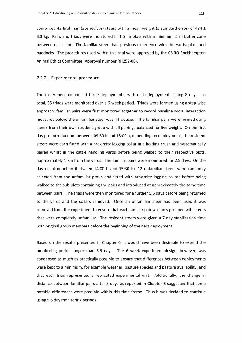
Chapter 7: Introducing an unfamiliar steer into a pair of familiar steers
129
comprised 42 Brahman (Bos indicus) steers with a mean weight (± standard error) of 484 ±
3.3 kg. Pairs and triads were monitored in 1.5 ha plots with a minimum 5 m buffer zone
between each plot. The familiar steers had previous experience with the yards, plots and
paddocks. The procedures used within this trial were approved by the CSIRO Rockhampton
Animal Ethics Committee (Approval number RH252‐08).
7.2.2. Experimental procedure
The experiment comprised three deployments, with each deployment lasting 8 days. In
total, 36 triads were monitored over a 6‐week period. Triads were formed using a step‐wise
approach: familiar pairs were first monitored together to record baseline social interaction
measures before the unfamiliar steer was introduced. The familiar pairs were formed using
steers from their own resident group with all pairings balanced for live weight. On the first
day pre‐introduction (between 09:30 h and 13:00 h, depending on deployment), the resident
steers were each fitted with a proximity logging collar in a holding crush and systematically
paired whilst in the cattle handling yards before being walked to their respective plots,
approximately 1 km from the yards. The familiar pairs were monitored for 2.5 days. On the
day of introduction (between 14:00 h and 15:30 h), 12 unfamiliar steers were randomly
selected from the unfamiliar group and fitted with proximity logging collars before being
walked to the sub‐plots containing the pairs and introduced at approximately the same time
between pairs. The triads were then monitored for a further 5.5 days before being returned
to the yards and the collars removed. Once an unfamiliar steer had been used it was
removed from the experiment to ensure that each familiar pair was only grouped with steers
that were completely unfamiliar. The resident steers were given a 7 day stabilisation time
with original group members before the beginning of the next deployment.
Based on the results presented in Chapter 6, it would have been desirable to extend the
monitoring period longer than 5.5 days. The 6 week experiment design, however, was
condensed as much as practically possible to ensure that differences between deployments
were kept to a minimum, for example weather, pasture species and pasture availability, and
that each triad represented a replicated experimental unit. Additionally, the change in
distance between familiar pairs after 3 days as reported in Chapter 6 suggested that some
notable differences were possible within this time frame. Thus it was decided to continue
using 5.5 day monitoring periods.

Chapter 7: Introducing an unfamiliar steer into a pair of steers
130
From the two previous experiments, all resident steers had experience with being paired
with both familiar and unfamiliar individuals, thus there were considered to be no individual‐
level effects due to familiarity or unfamiliarity with the experimental conditions.
Additionally, the same pair of resident steers was never used more than once to form a
triad. Each triad in the experiment was considered to be independent from each other.
7.2.3. Data processing and statistical analysis
The first contact recorded between the unfamiliar steer with either of the familiar steers was
taken as the time of introduction and all data recorded by the unfamiliar steer’s proximity
logger prior to this was removed. A single file of contacts was created for each pair within
the triad and all unfamiliar contacts were classified into the one category, regardless of
which familiar animal was involved in the contact. All unfamiliar contacts were then
expressed as an average of the two unfamiliar pairs within the triad.
The contact data were summarised on a daily basis as the total number of contacts per hour
and the average length per contact. The change within familiar pairs due to the introduction
of the unfamiliar steer was compared using a one‐way analysis of variance, with pre‐ and
post‐introduction used as the treatment factor blocked by pair within deployment. To
investigate the differences in contact between familiar and unfamiliar steers, the number of
contacts per hour and the average length per contact were analysed for treatment and day
effects, using a repeated measures analysis of variance (Rowell and Walters, 1976), with day
as the within‐subjects effects and familiarity as the treatment factor blocked by triad within
deployment. The repeated measures analysis of variance estimates the Greenhouse‐Geisser
epsilon to account for the degree of temporal auto‐correlation, with the significance levels
of the F‐test adjusted for this. Differences were considered significant at the 5% probability
level. To meet the distributional assumptions of the statistical analyses, residual and normal
probability plots were inspected for normality. The large proportion of short duration
contacts and infrequent contacts per hour produced positively skewed distributions (Fig.
7.1a). A square root transformation provided the closest fit to normality (Fig. 7.1b), and was
applied to all proximity logger data prior to analysis. All statistical results presented in the
text are back transformed values. Statistical analyses were carried out using Genstat 12th
edition (Payne et al., 2009) and graphical representations of the data were created using
PASW Statistics 18.0 (SPSS Inc).

Chapter 7: Introducing an unfamiliar steer into a pair of familiar steers
131
(a)
(b)
Figure 7.1. The distributions of the number of contacts per hour and the average length percontact (a) in raw form and (b)after a square root transformation.
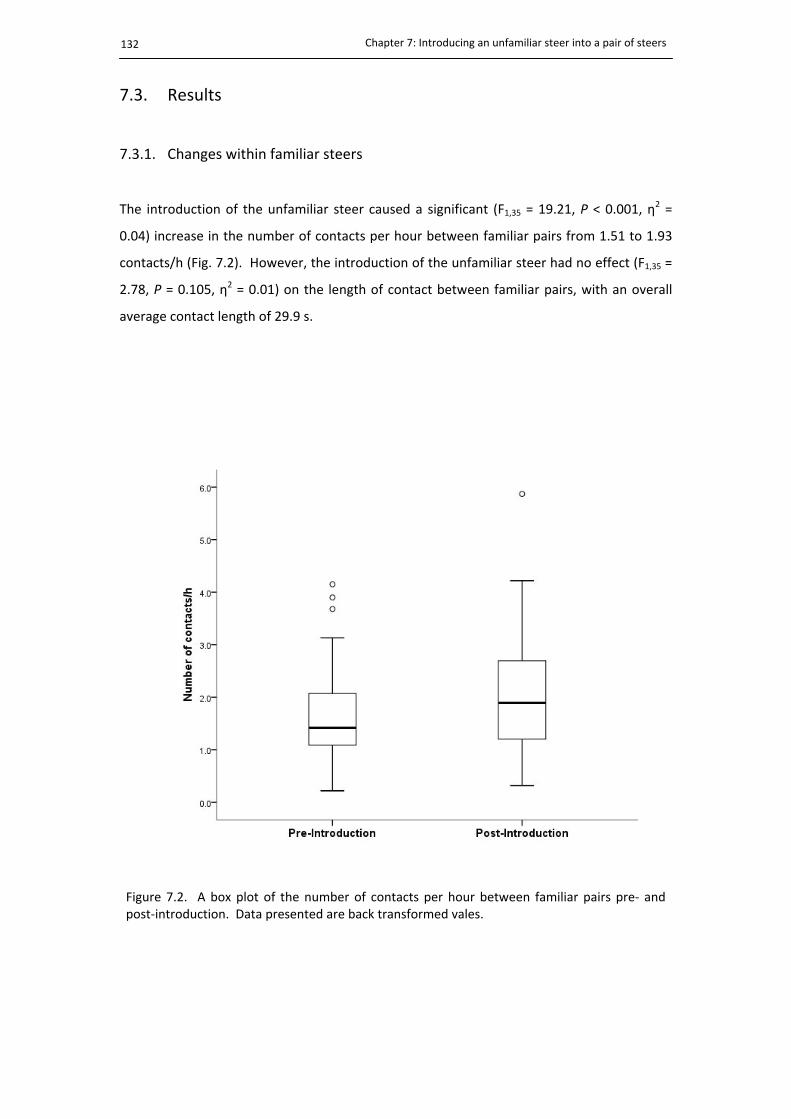
Chapter 7: Introducing an unfamiliar steer into a pair of steers
132
7.3. Results
7.3.1. Changes within familiar steers
The introduction of the unfamiliar steer caused a significant (F1,35 = 19.21, P < 0.001, η2 =
0.04) increase in the number of contacts per hour between familiar pairs from 1.51 to 1.93
contacts/h (Fig. 7.2). However, the introduction of the unfamiliar steer had no effect (F1,35 =
2.78, P = 0.105, η2 = 0.01) on the length of contact between familiar pairs, with an overall
average contact length of 29.9 s.
Figure 7.2. A box plot of the number of contacts per hour between familiar pairs pre‐ and post‐introduction. Data presented are back transformed vales.
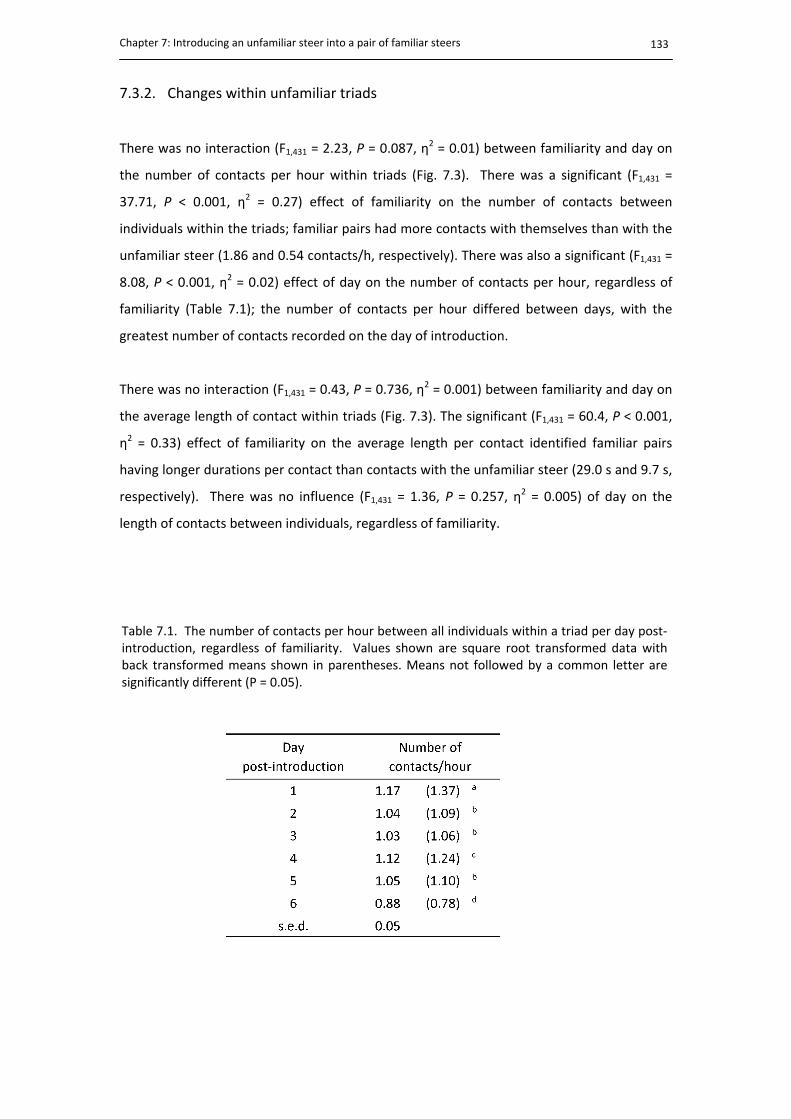
Chapter 7: Introducing an unfamiliar steer into a pair of familiar steers
133
7.3.2. Changes within unfamiliar triads
There was no interaction (F1,431 = 2.23, P = 0.087, η2 = 0.01) between familiarity and day on
the number of contacts per hour within triads (Fig. 7.3). There was a significant (F1,431 =
37.71, P < 0.001, η2 = 0.27) effect of familiarity on the number of contacts between
individuals within the triads; familiar pairs had more contacts with themselves than with the
unfamiliar steer (1.86 and 0.54 contacts/h, respectively). There was also a significant (F1,431 =
8.08, P < 0.001, η2 = 0.02) effect of day on the number of contacts per hour, regardless of
familiarity (Table 7.1); the number of contacts per hour differed between days, with the
greatest number of contacts recorded on the day of introduction.
There was no interaction (F1,431 = 0.43, P = 0.736, η2 = 0.001) between familiarity and day on
the average length of contact within triads (Fig. 7.3). The significant (F1,431 = 60.4, P < 0.001,
η2 = 0.33) effect of familiarity on the average length per contact identified familiar pairs
having longer durations per contact than contacts with the unfamiliar steer (29.0 s and 9.7 s,
respectively). There was no influence (F1,431 = 1.36, P = 0.257, η2 = 0.005) of day on the
length of contacts between individuals, regardless of familiarity.
Table 7.1. The number of contacts per hour between all individuals within a triad per day post‐introduction, regardless of familiarity. Values shown are square root transformed data with back transformed means shown in parentheses. Means not followed by a common letter aresignificantly different (P = 0.05).
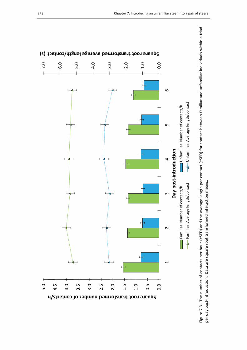
Chapter 7: Introducing an unfamiliar steer into a pair of steers
134
Figure 7.3. The number of contacts per hour (±SED) and the average length per contact (±SED
) for contact between fam
iliar and unfamiliar individuals within a triad
per day post‐introduction. Data are square root transform
ed interaction m
eans.
0.0
1.0
2.0
3.0
4.0
5.0
6.0
7.0
0.0
0.5
1.0
1.5
2.0
2.5
3.0
3.5
4.0
4.5
5.0
12
34
56
Square root transformed average length/contact (s)
Square root transformed number of contacts/h
Day post‐introduction
Familiar: Number of contacts/h
Unfam
iliar: Num
ber of contacts/h
Familiar: Average
length/contact
Unfam
iliar: Average length/contact
Chapter 7: Introducing an unfamiliar steer into a pair of familiar steers
135
7.4. Discussion
It was hypothesised that familiar pairs would increase their encounters with each other
when an unfamiliar steer was introduced. Familiar steers did increase the number of
encounters per hour, but there was no change in the average length of each encounter. This
result indicates that the introduction of the unfamiliar steer caused a disruption to the
normal encounter behaviour of the isolated familiar pair, resulting in the familiar pair having
more close proximity encounters. There are a number of reasons why the familiar pair may
have increased their close proximity encounters when the third unfamiliar individual was
introduced, including fear, competition for resources and reinforcing social bonds.
Fear created by the presence of the unfamiliar steer may have led to the increased contact
frequency between familiar pairs to seek out each other for support. Familiar peers have
been shown to provide social support, particularly in stressful situations (Boissy and
LeNeindre, 1997), whilst it has also been stated that the presence of an unfamiliar peer
creates fear behaviour (Archer, 1976). This fear may impact on functional decisions. For
example, in Chapter 5 it was suggested that the fear created by the presence of an
unfamiliar peer restricted the test steers from foraging a desired food source some distance
away. Thus, the resultant increase in contact frequency may represent social reinforcement
between the familiar pair to buffer the fear caused by the presence of the unfamiliar
individual.
The change in encounter behaviour between familiar pairs may relate to the competition
threat posed by the unfamiliar steer. Cattle will physically compete for resources when their
supply is restricted, such as food and space (Bouissou et al., 2001). An unfamiliar individual
is a potential threat to all valuable resources (Price, 2008), thus the intrusion of the
unfamiliar steer into the space occupied by the familiar pair might have been perceived as
an attempt to compete for resources. In the current study, access to food and space were
not limited, although it is possible that the familiar individuals could have attempted to
defend their access to desired spaces such as resting locations. The number of social
positions, however, was limiting as there were only three positions available, thus it is
possible that the familiar steers were competing to retain their social status and prevent the
unfamiliar steer from elevating up the small hierarchy. This competition for resources might
have resulted in more cooperative behaviour between the familiar pair to defend their space
and social status, thus increasing their contact behaviour.

Chapter 7: Introducing an unfamiliar steer into a pair of steers
136
Reinforcing social bonds between the familiar pair may also be responsible for the increased
number of encounters between familiar pairs. Cattle recognise others as familiar based
upon a history of social interaction where they learn the physical and behavioural
characteristics of other group members (Lindberg, 2001). A study in fish by Brown (2002)
showed that the process of social reinforcement continues once a relationship is established,
which allows individuals to learn others behavioural tendencies under different situations.
The same process has also been identified in humans by Hinde and Stevenson‐Hinde (1976)
who describe a stable relationship as something that changes continuously to meet the
demands of the social and physical environment and individuals are required to adapt to
each other’s behavioural responses to maintain stability. Thus to maintain stability, the
familiar pair may have increased their contact frequency to reinforce their familiarity and to
learn any changes that may have occurred to each other during interactions with the
unfamiliar.
When considering the process of relationship development, it was hypothesised that familiar
pairs would maintain greater encounters with themselves than with the unfamiliar pair due
to their existing relationship, but this difference was expected to decrease as the triad
developed a stable and familiar social relationship. The hypothesis was partially supported
by the finding that familiar steers had more encounters per hour and longer duration per
encounter as compared with unfamiliar steers. Nevertheless, in this study the non‐
significant result for the interaction between day and close proximity encounters (frequency
and duration) does not support the hypothesis that the newly introduced animal was
eventually accepted as a familiar group member. However, it should be noted this study only
monitored social behavioural interactions over 5.5 days. Although the current results were
unable to describe all of the features of familiarisation, it is possible to speculate the
conditions that may enhance or inhibit the process. Internal social factors, such as individual
differences in sociability, may accelerate or hinder the integration of an unfamiliar Highly
sociable individuals spend more time within close proximity to others (Sibbald et al., 2006)
and may therefore act as a catalyst to initiate relationship development with an unfamiliar.
Environmental factors that force individuals to congregate or cooperate, such as areas of
high predation risk, may facilitate familiarisation while evolutionary pressures that require
individuals to transmit cultural information for improved survival, such as which pasture
species to eat or how to access water, may also accelerate familiarisation in less
domesticated species. Future studies should consider monitoring newly introduced animals
Chapter 7: Introducing an unfamiliar steer into a pair of familiar steers
137
for much longer time periods to understand the way animals form and maintain
relationships.
In Chapter 6, familiar pairs of steers had more encounters per hour than unfamiliar pairs (3.8
and 2.3 contacts/h, respectively) however there was no difference in the length of the close
proximity encounters (average contact length 57.1 s). In the current experiment the
difference in the number of encounters per hour between familiar pairs was expected,
although the extent of the durational differences between familiar and unfamiliar steers was
not; the length of contact between familiar steers was three times greater than encounters
between unfamiliar steers. Additionally, encounter frequency and duration were much
lower within triads than pairs. Given there is more opportunity for an encounter to occur
with increased numbers, it was anticipated that there would be more overall encounters
within a triad than a pair. Earlier work on social structure in human groups found that
interaction in pairs is fundamentally different to that observed in larger groups, both in
terms of social processes (Simmel, 1950) and hierarchy structure (Chase, 1980). Simmel
(1950) further stated that increasing group size from two to three involved more significant
social changes than increasing group size to four or more, outlining the importance of the
triad for group structure. The difference in encounter frequency and duration between pairs
and triads supports the above claims that behaviour in a pair of steers is fundamentally
different to that observed within groups of three.
Relationship development involves learning and individual recognition (Lindberg, 2001). The
greatest number of encounters per hour was seen on the day of introduction, indicative of
individuals coming within close proximity to learn the physical characteristics of each other.
After the initial encounter, contact frequency and duration between familiar and unfamiliar
steers was relatively stable; encounters with the unfamiliar steer remained at a level around
half that of contacts recorded between familiar steers (Fig. 7.3). The results of the current
study support Bouissou’s (1974a) finding that relationship direction is established early and
remains stable after this time. Bouissou (1974a) reported that newly introduced cattle
establish relationships relatively quickly, with half of all relationships determined within the
first 5 minutes and no longer than 2 hours after the first encounter. Bouissou (1974a) also
stated that relationships remained stable after the initial encounter with very few changes in
relationship direction, indicating that learning individual characteristics can occur relatively
quickly. The current study extends the work of Bouissou by considering behavioural
indicators of relationship development other than dominance. The results also suggest that
Chapter 7: Introducing an unfamiliar steer into a pair of steers
138
the development of a stable familiar relationship requires longer than 5.5 days. Stability in a
relationship requires time and experience under different social and physical environments
to learn behavioural preferences under a range of different situations (Brown, 2002), thus
the current experiment was not long enough for this level of familiarisation to occur.
7.5. Conclusions
It was concluded that social disruption caused by introducing an unfamiliar into an
established pair of steers led to an increased frequency in close proximity encounters
between the familiar steers, thus accepting the hypothesis that familiar steers would have
more close proximity encounters with themselves than with the unfamiliar steer. There
were also durational differences recorded between familiarity types, with familiar steers
having longer duration encounters than encounters with the unfamiliar steer. Furthermore,
differences in encounter behaviour between familiar and unfamiliar steers led to the
conclusion that complete integration of the unfamiliar steer into the pair did not occur
within 5.5 days. The structural differences that exist when increasing group number from
two to three may create social complexities that result in longer integration times when
introducing new individuals into a group. The social support provided by a familiar peer has
the potential to make an unfamiliar social situation less stressful.
139
Chapter 8
Relationship development in steers: an application of the relational event model 8.1. Introduction
Chapter 7 investigated the introduction of an unfamiliar steer into a pair of familiar steers.
Daily measures of close proximity encounters recorded by proximity logging devices were
used to identify changes in encounter patterns during the first 5.5 days post‐introduction.
The results indicated that the greatest amount of interaction occurred on the day of
introduction and after 5.5 days there were still discernible differences, on average, between
unfamiliar and familiar steers. The analysis used in the previous chapter only considered
pair‐wise encounters. This was not an issue in Chapter 6 because only two individuals were
monitored at the one time, however when a third animal was introduced in Chapter 7 there
was no analytical method in place to model the interactions among all three individuals
simultaneously. Thus different statistical approaches were investigated to identify a suitable
method for characterising interactions among groups of three or more animals.
The relational event framework proposed by Butts (2008) (described in Chapter 3, section
3.6) was chosen to analyse the sequences of encounters between the three steers. This
model was highly suitable because it considers each interaction as a discrete event within a
time series and allows every contact recorded by a proximity logger to be analysed with
respect to its temporal patterning; this is specifically important when considering
relationship development between unfamiliar individuals, as each interaction is likely to
alter the context for future contact and the evolving quality of the relationship. The
Chapter 8: Relational event modelling
140
additional advantage of the model is that it is highly flexible, allowing specific types of events
to be modelled in a way that is appropriate to the observational context, and can
accommodate interactions involving more than two individuals at the one time.
The aim of the current chapter is to develop a relational event model that can be used to
analyse regular patterns of interaction between a pair of familiar steers with an unfamiliar
steer during the process of relationship development. The aim of the model is to predict
whether and when a relational event occurs between pairs within the triad based on the
history of prior events. The chapter describes the methods that were used to develop the
model, beginning with the steps taken to process the data into a suitable format prior to
input, the specification of the model parameters and an explanation of the possible model
parameters. The actual model estimates are then presented, followed by an interpretation
of the results in terms of the possible social roles that the familiar and unfamiliar steers have
in forming certain encounter structures and the likely meaning of these structures for
relationship development.
8.2. Model development
8.2.1. Data input
The model was used to analyse the proximity logger data that was collected in Chapter 7.
Briefly, the data set contained 36 triads of steers, where an unfamiliar steer was introduced
to a pair of familiar steers and monitored for 5.5 days. All close proximity encounters (within
4 m) were recorded by proximity logging devices. The data set contained sequences of
discrete relational events between pairs within each triad and each encounter had a specific
start and end time. Prior to analysing the data, the temporal interaction sequence was
transformed into a suitable format using the processing outlined below.
In addition to the data processing outlined in Chapter 7, the proximity logger data per triad
was further processed by assigning each animal in each triad a unique animal identification
code, from 1 to 3, to represent the identity and familiarity status of each animal: animals 1
and 2 represented the familiar animals and the unfamiliar animal was coded as animal 3.
Relational events were also coded to identify the pairs of animals involved in a close
proximity encounter, with a familiar pairing between animals 1 and 2 coded as a relational
Chapter 8: Relational event modelling
141
event of type ‘1’ and the unfamiliar pairings between animals 1 and 3 and animals 2 and 3
coded as types ‘2’ and ‘3’, respectively.
The data from the original data set was restricted to include only close proximity encounters
recorded after the unfamiliar steer was introduced, with this latter point in time considered
as time zero in the model. The time of each encounter was defined as the number of
seconds that had elapsed since the point of introduction. The original data was further
restricted by removing all data recorded after day 5. This ensured that only full daily records
were analysed and was also specified because the number of events recorded on day 6 was
not substantial enough to include in the model.
The model was fitted on a daily basis to a pooled data set across all 36 triads, although all
statistics used in the model were computed on a triad by triad basis. To test the validity of
pooling the triad data across all 36 triads, the data was visually assessed by comparing a
simplified model created with all 36 triads against separate models for each triad. To create
the simplified model, the number of parameters from the actual model was reduced and
fitted to the pooled data set as well as each of the 36 triads separately. Frequency
distributions of the parameter estimates obtained by fitting the simplified model to each of
the 36 triads were created and the placement of the parameter estimate from the pooled
data set within the distribution was used to compare the two data sets. The results of the
data validation tests can be seen in Appendix B. Overall, the parameter estimates of the
aggregated data set fell within 95% of the distribution of the individual triad parameter
estimates, confirming that pooling the triad data was justified.
8.2.2. Model components
The model was developed specifically for onset interaction events. An onset event was
characterised as one in which a close proximity encounter was initiated between any pair
within the triad, thus the pair was the basic unit of analysis (Fig. 8.1). The model was
developed to predict the likelihood of future onset events based on the history of prior
onset events. Onsets were of particular interest because they relate specifically to the
formation of an encounter between two or more individuals and can potentially be used to
characterise the nature of a social relationship. For example, a consistent pattern of onset
events between the same pair may represent affiliative behaviours such as mutual grooming
or grazing within close proximity, which could therefore be used to indicate a preferential

Chapter 8: Relational event modelling
142
relationship. Separate from onset events were offset events, which occurred when an
existing encounter between any of the three steers was ended by one or more steers
moving out of the 4m detection range. Offsets therefore relate to the dissolution of an
existing encounter, and were important to understand the processes that occur when
encounters break apart. Hence, the nature of onset and offset events were different.
While it is possible that onset and offset events could potentially be considered in the same
model, the model developed here accounted specifically for the formation of ties between
steers and the model framework was not suitable to predict the probability of future offset
events. Offset events, however, were still considered as a function of the onset event
sequence, as every onset event has an associated offset event and the occurrence of offset
events were important to determine the type of onset event that occurs. Different onset
event types were possible depending on the number of animals involved in the event and
their configuration (see section 8.2.3 below), thus the model used the sequence of onset and
offset events to identify the involvement of animals in prior events, which was then used to
determine the onset event type.
Figure 8.1. An example of an onset event sequence between two steers, i and j, showing theoccurrence of an onset event and an offset event between the two steers. The model developedpredicts the probability of an onset event based on the history of onset events occurring withinthe past hour or the past day, as well as animal familiarity.
Yij =1
Yij =0
time
Onset event
tOffset event
1 hour
24 hours

Chapter 8: Relational event modelling
143
(b) Group event(a) Pair event (c) Triangle event
8.2.3. Creating the sequence of prior events
A custom‐developed java application was used to transform the actual event stream in the
proximity logger data set into a set of actual and potential onsets and the statistics based on
prior relational events for each triad of steers (see section 8.2.5 for an example). The java
program calculated statistics for each event or potential event in terms of (i) the familiarity
of the animals involved, (ii) the type of the event that occurred, and (iii) statistics based on
the frequency of relevant prior events. The type of encounter was classified as either: (i) an
event involving an interaction of an isolated dyad (a pair event); (ii) an event involving
simultaneous contact of one animal with the other two (a group event); or (iii) an event
involving pair‐wise contact among all three animals at once (a triangle event) (Fig. 8.2).
A pair event involved a change in state from no existing contact to the creation of a single
contact tie between two steers, while a group event was conditional on the
contemporaneous existence of a pair event. A triangle event was formed when a tie was
created between the two animals that were not connected in the prior group event, thus all
three individuals were in contact at the one time. A triangle event was conditional on the
contemporaneous existence of a group event.
While it is possible that a change in state could occur from an isolated animal to
simultaneous contact with two others, the probability of such a change was extremely small
and there was only one event of this type identified in the current data set. In this instance,
the model counted the two pair onset events that occurred at the same time, and therefore
have no duration, as well as the onset of the group event. Thus events that occur at the
same time are treated the same as any other onset event, irrespective of their duration.
Figure 8.2. The three event types that could potentially occur between the three steers. Thesolid lines represent a tie between two steers.
Chapter 8: Relational event modelling
144
It is important to note that the potential events under consideration with each actual event
varied according to the current configuration of animals. For example, if two animals were
already in contact, they cannot be associated with the next onset event. Likewise, if the
current event was a group event, the next onset event cannot be either a pair event or a
group event, but must instead be a triangle event. Indeed, in this latter case, the only onset
event that could occur was a triangle event and if an actual onset event occurred there were
no potential onset events that were not actual events. As a result, the onset of triangle
events could not be handled within this conditional framework as the probability that the
event occurs, given that it is an onset event, was 1.
For potential onset events, the statistics included: (i) an indicator variable signifying whether
the unfamiliar animal was involved in the potential event (coded as 1 if an unfamiliar animal
was involved, 0 otherwise); (ii) the frequency within specified periods of prior pair events
involving the steers linked by the potential event; and (iii) the frequency within specified
periods of prior group events involving a contact between the steers linked in the potential
event. Specified periods of 1 hour and 24 hours were used to capture potential short and
longer term regularities in contact patterns. These statistics were chosen as they allow
quantification of any tendencies involving differential contact on the basis of animal
familiarity, differential contact as a function of past contact in pair events, and differential
contact as a function of past contact in group events. The distinction between prior pair
events and prior group events was a potentially important one, since pair events indicate
isolated dyadic interaction and local activity, whereas group events relate directly to
interaction involving all three individuals and the potential for group forming behaviours to
occur.
The possible configurations that could occur for an onset event are shown in Table 8.1. For
pair events, three events could potentially occur, a familiar pair between animals 1 and 2, an
unfamiliar pair between animals 1 and 3 and an unfamiliar pair between animals 2 and 3.
For a group event, there were only two possible events that could occur, a group event
where the prior pair involved the unfamiliar or an event where the unfamiliar animal was
involved with the creation of a tie with either familiar steer to form a group. Although there
were two possible structural configurations in the latter case (either the unfamiliar animal
was already involved in a pair event or the unfamiliar animal was the animal joining the
existing pair), the model considered which animals were involved in the creation of the tie,
thus the two formations were considered to be equivalent.

Chapter 8: Relational event modelling
145
Pre‐existing state
Pre‐existing configuration
Predicted event
Predicted configuration
Possible configurations
Isolated animal Pair event
Pair Group event
Group Triangle event
Key:
= familiar animal = existing tie
= unfamiliar animal = predicted tie
= animal of either familiarity
1 2
1 3
2 3
or
or
3
2
1
8.2.4. Time
As indicated above, onset events were modelled as a function of prior onset events. Such
events could have occurred at any moment in the time interval from the introduction of the
unfamiliar animal (t = 0) to the present time t. In order to reflect potential distinctions
among prior events in terms of longer cumulative or shorter, more fleeting effects, separate
statistics were computed to capture short and longer term regularities in interaction
patterns; the short term interval was based on the immediate past hour, while the longer
term past was based on daily patterns within each day post‐introduction. Both time frames
have potentially important implications for social processes and allow both regularities in
short term interaction patterns and regularities over a longer period to be discerned. The
latter may be potentially representative of long term contact preferences (e.g. the
preference of a pair of animals for social interaction).
Table 8.1. The three onset event types that could occur between the three steers, their priorconfiguration state and the predicted configuration possibilities.

Chapter 8: Relational event modelling
146
8.2.5. Event sequence summary
A sample of onset event data as summarised by the java application is shown in Table 8.2.
The sample data shows encounters between steers in triad 8 and the frequency of events
that occurred in the past day. The column event type specified if an event had occurred or
not, and the type of even that occurred: ‘0’ indicates an offset event while onset events
were indicated by the values ‘1’, ‘2’ and ‘3’, indicating pair, group and triangle events,
respectively. The animals involved in the onset or offset event are indicated in the onset
pair and offset pair column. In the sample shown, pair 1 (familiar animals 1 and 2) came
within close proximity in the first listed event (‘419’ in column Event ID), and were together
for 25 s before breaking apart in the next event (‘420’ in column Event ID).
The column pair count (past 24 h) shows a tally of onset events between pairs 1, 2 and 3. In
this instance, the familiar pair (pair 1) had encountered each other 15 times without being in
proximity to the unfamiliar steer. The group count (past 24 h) column specified the number
of times an existing pair had led to the creation of a tie to form a group event. For example,
a change in state from a pair to a group event occurred at event ID ‘424’. Here, animals 2
and 3 (pair 3) were already in close proximity and animal 1 created a tie with animal 3 to
form a group event, thus in the next row (event ID ‘425’) the group count for pair 3 increased
by one. As a pair event between animals 1 and 3 occurred to complete the group event, the
pair count for pair 2 also increased by one in the pair count (past 24 h) column.
The triangle count (past 24 h) column tallied the number of times a triangle event had
occurred. An example of this is shown in event ID ‘429’. The two onset events prior to the
triangle event was a pair event between animals 1 and 3 (pair 2, event ID ‘427’), followed by
a group event when a tie was created between animals 2 and 3 (pair 3, event ID ‘428’). The
creation of a tie between animals 1 and 2 (pair 1) completed the triangle. A graphical
example of this event sequence is shown in Fig. 8.3. Here, the tallies for the pair, group and
triangle counts incremented by one in the row following the occurrence of the event. Note
that the group count for pair 2 increased by one at the same time that the triangle count
increased, as a second group event between animals 3 and 2 occurred when a tie was
created between animals 1 and 3 to complete the triangle.
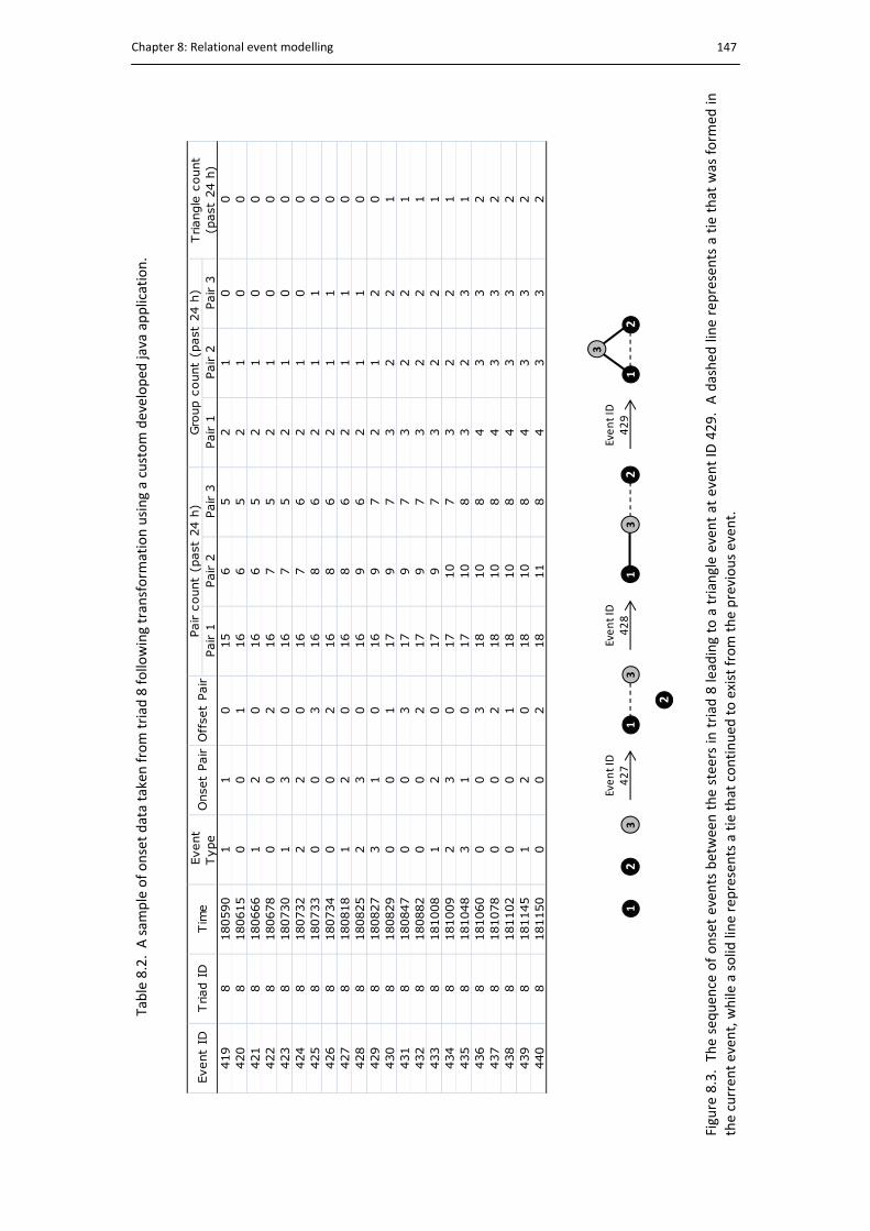
Chapter 8: Relational event modelling
147
Table 8.2. A sam
ple of onset data taken from triad
8 following transform
ation using a custom developed
java application.
Figure 8.3. The sequen
ce of onset even
ts between the steers in
triad
8 leading to a triangle even
t at event ID 429. A dashed
line represents a tie that was form
ed in
the curren
t even
t, while a solid
line represents a tie that continued
to exist from the previous even
t.
Pair 1
Pair 2
Pair 3
Pair 1
Pair 2
Pair 3
419
8180590
11
015
65
21
00
420
8180615
00
116
65
21
00
421
8180666
12
016
65
21
00
422
8180678
00
216
75
21
00
423
8180730
13
016
75
21
00
424
8180732
22
016
76
21
00
425
8180733
00
316
86
21
10
426
8180734
00
216
86
21
10
427
8180818
12
016
86
21
10
428
8180825
23
016
96
21
10
429
8180827
31
016
97
21
20
430
8180829
00
117
97
32
21
431
8180847
00
317
97
32
21
432
8180882
00
217
97
32
21
433
8181008
12
017
97
32
21
434
8181009
23
017
10
73
22
1435
8181048
31
017
10
83
23
1436
8181060
00
318
10
84
33
2437
8181078
00
218
10
84
33
2438
8181102
00
118
10
84
33
2439
8181145
12
018
10
84
33
2440
8181150
00
218
11
84
33
2
Tim
eEvent
IDTriangle
count
(past
24 h
)O
ffse
t Pair
Onse
t Pair
Event
Type
Triad I
DPair c
ount
(past
24 h
)Gro
up c
ount
(past
24 h
)
23
12
3
13
1
2
Event ID
429
Event ID
428
31
2
Event ID
427

Chapter 8: Relational event modelling
148
8.3. Model parameters
The potential and actual onset events were analysed using the COXREG procedure within
SPSS. The model was for the probability of the next event as a function of weighted
statistics associated with the potential next events; the weights are the parameters of the
conditional logistic regression model introduced earlier. A parameter was estimated for
each statistic, or effect, in the model, and each model involved five effects: (i) unfamiliarity;
(ii) prior pair events (past hour); (iii) prior pair events (past 24 hours); (iv) prior group events
(past hour); (v) prior group events (past 24 hours). Two separate models were fitted on each
day to predict pair events and group events. A basic overview of the modelling process is
shown in Fig 8.4.
The onset event parameters (unfamiliarity, prior pair events and prior group events) are
described in detail below and summarised in Table 8.3. The effects are discussed in terms of
what a positive or negative parameter estimate would represent for the configuration of ties
between pairs within the triad.
8.3.1. Unfamiliarity effects
To account for the difference in familiarity among the triad, an animal specific parameter
relating directly to the unfamiliar animal was included in the model. There was an assumed
homogeneity between the two familiar animals. The parameter estimate related to the
propensity of the current event to involve the unfamiliar, where the current event was
either a pair event or a group event. The unfamiliarity effect, unlike pair and group effects,
was not related to the involvement of the unfamiliar animal in pair or group events in the
past hour or past 24 hours, but was a measure of the number of past events involving the
unfamiliar animal and was therefore a prediction of the involvement of the unfamiliar
animal in future encounters within the triad. When a pair event was being predicted, the
parameter estimate related to the propensity for a future pair event to involve the
unfamiliar. A positive and significant result indicated a high probability that the unfamiliar
animal was involved in a future pair event whereas a negative effect suggested the future
pair events were less likely to involve the unfamiliar.
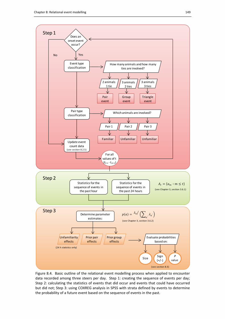
Chapter 8: Relational event modelling
149
Figure 8.4. Basic outline of the relational event modelling process when applied to encounter data recorded among three steers per day. Step 1: creating the sequence of events per day;Step 2: calculating the statistics of events that did occur and events that could have occurred but did not; Step 3: using COXREG analysis in SPSS with strata defined by events to determine the probability of a future event based on the sequence of events in the past.
Does an
onset event occur?
Update event count data
(see section 8.2.5)
Pair
event
Group
event
Triangle
event
Yes
Pair type
classification
How many animals and how many ties are involved?
2 animals1 tie
3 animals2 ties
3 animals3 ties
Pair 1 Pair 2 Pair 3
Which animals are involved?
Familiar Unfamiliar Unfamiliar
No
Step 1
Event type
classification
For all
values of t (t0 h ‐ t24 h)
Step 3
Prior group effects
Prior pair effects
Unfamiliarity effects
Determine parameter
estimates:
Evaluate probabilities based on:
SizeSign
(+/‐)
Pvalue
(see section 8.3)
(24 h statistics only)
(see Chapter 3, section 3.6.2)
Statistics for the sequence of events in the past 24 hours
Statistics for the sequence of events in
the past hour
Step 2
(see Chapter 3, section 3.6.1)

Chapter 8: Relational event modelling
150
Table 8.3. The interpretations for both positive and negative significant parameters when theeffect of unfamiliarity and the frequency of prior past events are used to predict the onset offuture pair and group events.
PredictorEvent being predicted
Description Positive Negative
Frequency of prior events involving the unfamiliar animal
Pair event The propensity for a current pair event to involve the unfamiliar
High probability that the current pair event will involve
the unfamiliar animal
Low probability that the current pair event will involve the unfamiliar
animal
Group event The propensity for the unfamiliar animal
to be involved in the creation of a new tie leading to a group
event
The current group event is created by a tie involving the
unfamiliar animal
or
The unfamiliar animalis not involved in forming the current group event
Frequency of prior pair events
Pair event The propensity for prior pair events to predict future pair
events
Being in a pair in the past leads to more pair events in the future (persistence)
Being in a pair in the past leads to less pair events in the future (avoidance)
Group event The propensity for prior pair events to
predict a future group event
Pairs seen together in the past are more likely to form a tie to create a group event
Pairs seen together in the past are less likely to join a group and remain as a pair
Frequency of prior group events
Pair event Participation in past group events predicts participation in future
pair events
Being in a group in the past leads to more pair events in
the future
Being in a group in the past leads to less pair events in
the future
Group event Participation as a pair in past group events predicts participation in future group events
Pairs seen together in past group events are more likely to remain together in future
group events, thus the existing pair creates the beginning of the group
Pairs seen together in past group events are less likely to be seen together in future group events
Key:
= familiar animal = existing tie
= unfamiliar animal = predicted tie
= animal of either familiarity
Chapter 8: Relational event modelling
151
When a group event was being predicted, the unfamiliarity effect referred to the propensity
for the unfamiliar animal to be involved in the creation of a new tie leading to a group event.
A positive parameter estimate indicated that the creation of a new tie leading to a group
event involved the unfamiliar animal; either the unfamiliar animal was already a part of the
existing pair leading to the group event or the unfamiliar joined the existing pair event
between the two familiar animals. A negative unfamiliarity effect indicated that the
unfamiliar animal was not involved in the tie that created the group event, and therefore
was already connected in a pair with either of the familiar animals. A negative unfamiliarity
effect here indicated a tendency for a familiar to prefer the other familiar individual in a
group event.
8.3.2. Prior pair effects
To measure the propensity for an event to occur based on the characteristics of prior paired
encounters, a pair specific parameter was included in the model. The history of prior pair
events was used to predict the likelihood of future pair events and future group events.
Prior pair events leading to future pair events were measures of ‘persistence’ between
actors, thus a positive parameter indicated a tendency for prior encounters to predict future
events and ‘persistence’ for future configurations to remain the same (Butts, 2008).
Conversely, a negative pair parameter indicated avoidance, thus the more a pair had
encountered each other in the past the less likely the same pair would encounter each other
in the future.
In terms of pair events leading to future group events, the estimate related to the
configuration of pairs within the group. A positive and significant parameter indicated
sociability between the same pair; pairs seen together in the past were more likely to form a
tie to complete a group event. On the other hand, a negative and significant parameter
predicted that the same pair were less likely to create a tie to form a group event, thus the
resultant group was based upon each steer being connected to a different steer to that of
the past. This change in partner configuration is known as partner swapping. An example of
partner swapping arising from prior pair events is shown in Fig. 8.5a, where the prior pair
combination of steers i and j is used to illustrate the potential configurations that could
occur during a partner swapping event. Here prior events involving i and j predict that in a
group event arising from an existing contact between i and k, steer j will prefer proximity to
k, rather than i. Thus the tie that was shared between animals i and j in the past is less likely

Chapter 8: Relational event modelling
152
Key:
= existing tie
= predicted tie
(b) Prior group event Predicted group event
(a) Prior pair event Predicted group event
i j
Negative
Positivej ki
or
jk
ki j
iPartner
swapping
Same
partners
i j k
j ki
or
jki
Negative
Positivej ki
Partner swapping
Same partners
to be repeated in the future. This type of behaviour reflects ‘information seeking behaviour’,
where individuals make multiple contacts and gather information on each one (Butts, 2008).
8.3.3. Prior group effects
The group effect parameter evaluated the tendency for prior group events to lead to future
pair and group encounters. The triadic nature of the encounter meant that one central
steer, i, was in simultaneous contact with the two other steers, j and k, but j and k were not
Figure 8.5. A description of positive and negative significant parameter effects when the onsetof a group event was predicted from the sequence of (a) prior pair events, and (b) prior groupevents.
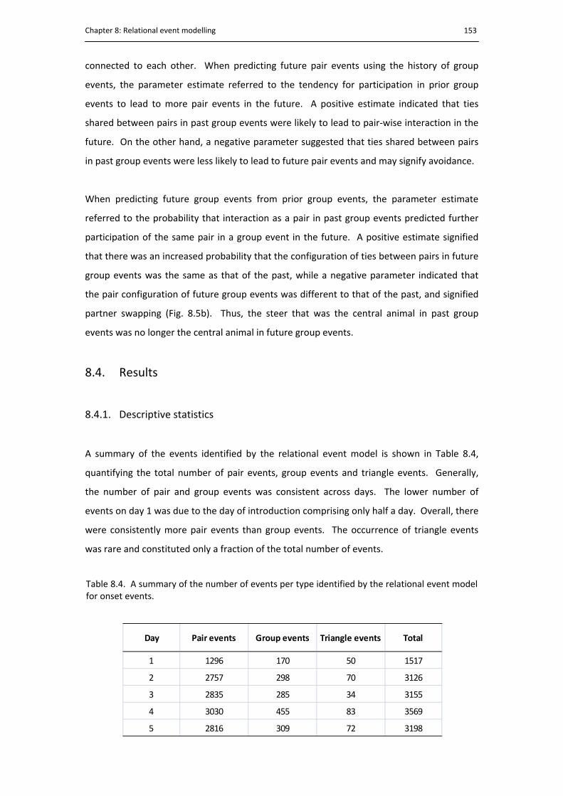
Chapter 8: Relational event modelling
153
connected to each other. When predicting future pair events using the history of group
events, the parameter estimate referred to the tendency for participation in prior group
events to lead to more pair events in the future. A positive estimate indicated that ties
shared between pairs in past group events were likely to lead to pair‐wise interaction in the
future. On the other hand, a negative parameter suggested that ties shared between pairs
in past group events were less likely to lead to future pair events and may signify avoidance.
When predicting future group events from prior group events, the parameter estimate
referred to the probability that interaction as a pair in past group events predicted further
participation of the same pair in a group event in the future. A positive estimate signified
that there was an increased probability that the configuration of ties between pairs in future
group events was the same as that of the past, while a negative parameter indicated that
the pair configuration of future group events was different to that of the past, and signified
partner swapping (Fig. 8.5b). Thus, the steer that was the central animal in past group
events was no longer the central animal in future group events.
8.4. Results
8.4.1. Descriptive statistics
A summary of the events identified by the relational event model is shown in Table 8.4,
quantifying the total number of pair events, group events and triangle events. Generally,
the number of pair and group events was consistent across days. The lower number of
events on day 1 was due to the day of introduction comprising only half a day. Overall, there
were consistently more pair events than group events. The occurrence of triangle events
was rare and constituted only a fraction of the total number of events.
Table 8.4. A summary of the number of events per type identified by the relational event modelfor onset events.
Day Pair events Group events Triangle events Total
1 1296 170 50 1517
2 2757 298 70 3126
3 2835 285 34 3155
4 3030 455 83 3569
5 2816 309 72 3198

Chapter 8: Relational event modelling
154
8.4.2. Model outputs
The following section analyses the results from each of the two models for onset events.
The outputs from each model are complex, and it is difficult to interpret all of the patterns
that were observed, thus it is the main findings with clear conclusions that are discussed.
8.4.2.1. Predicting future pair events
Overall, there was a negative effect of the unfamiliar animal (Table 8.5). The negative
unfamiliarity effect indicated that a future relational event between two animals was less
likely to involve the unfamiliar animal. Likewise, being familiar with another animal was
associated with an increased probability of a future interaction. The strength of this effect
varied across days; but in general, the effect was greatest on the day of introduction.
There was a strong and positive effect of prior pair events leading to future pair events
(Table 8.5). This effect was consistently strong across all days for both the short and long
term, except for a recency effect on day 1. Thus, the more two animals have had encounters
in the past the more likely they are to have encounters in the future. This effect suggests
that repeated encounters involving two animals reflect a relationship between them: the
encounters signify both a pattern of past encounters and the expectation of future ones.
Overall, prior contact between a pair leads to future contact.
There was an enhanced probability of an encounter between two animals if the same
animals had encountered each other in the past day as a part of a group event (Table 8.5).
This effect was variable over the 5 days, but was generally most notable on the day of
introduction, when both the short and daily trends were positive. Together with the prior
pair results, these effects suggests that the pattern of future contact between two animals is
affected positively by the same two animals being within close proximity in the past, either
as an isolated pair or as a function of a more complex encounter involving a third animal.
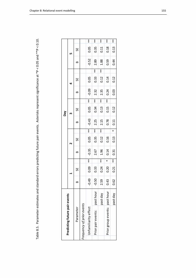
Chapter 8: Relational event modelling
155
Table 8.5. Param
eter estim
ates and standard errors predicting future pair even
ts. Asterisks rep
resent significance at *P
< 0.05 and **P
< 0.10.
BSE
BSE
BSE
BSE
BSE
‐0.49
0.09
**‐0.35
0.05
**‐0.43
0.05
**‐0.09
0.05
‐0.52
0.05
**
Prior pair events:
past hour
‐0.50
0.33
2.67
0.35
**2.25
0.34
**2.32
0.33
**2.89
0.35
**
past day
2.59
0.24
**1.96
0.12
**2.15
0.13
**2.35
0.12
**1.88
0.11
**
Prior group events:past hour
0.43
0.20
*0.14
0.16
0.78
0.15
**0.24
0.14
0.59
0.18
**
past day
0.62
0.21
**0.31
0.13
*0.11
0.12
0.03
0.12
0.44
0.13
**
Predicting future pair events
Param
eter
Unfamiliarity effect
Frequency of prior events
Day
12
34
5
Chapter 8: Relational event modelling
156
8.4.2.2. Predicting future group events
In the models predicting future group events, there was a positive and consistent effect of
the unfamiliar animal over the 5 day period (Table 8.6). This result indicates that future
group events are created by a tie involving the unfamiliar: either the pre‐existing pair
creating the foundation of the group event involved the unfamiliar or the unfamiliar
approached a familiar animal while it was within close proximity to the other familiar animal.
The frequency of pair events leading to future group events in the past day had a strong and
positive effect on the day of introduction (Table 8.6). In other words, the more two animals
interacted on the day of introduction, the more likely were group events involving proximity
between those two animals on that day. This effect was variable over the remaining 4 days,
suggesting that there was a high level of interaction on day 1, which settled out from day 2
onwards.
The propensity for group events in the past to lead to future group events was variable
(Table 8.6). On the day of introduction, the short term effects were positive yet the daily
effects were negative. The positive short term effects indicate that the group event was
created by the addition of the third animal to the same pair of animals that were tied
together in past group events, which suggests short term group building behaviour. While
the negative daily effect suggests that the pair configuration of future group events was
different to that of the past, or partner swapping (Fig. 8.5b), and represents information
seeking behaviour where all three steers were actively engaging to learn each other’s
characteristics and features, particularly with the unfamiliar steer. Taken together, the
results for day one suggest instability within the triad resulting from the disruption caused
by the introduction of the unfamiliar steer.
From day 2 onwards, the pattern of prior group events leading to future group events was
also variable between short term and daily patterns. The daily effect was consistently strong
and positive. Indeed, being within close proximity in the past means it is more likely that the
same pairs will be in close proximity in the future: this effect suggests stability. The change
from a negative effect on day 1 to a positive effect on consecutive days suggests the same
pairs were remaining together in future group events, which could suggest relationship
building between the unfamiliar steer with one of the two steers. The hourly effects,

Chapter 8: Relational event modelling
157
Table 8.6. Param
eter estim
ates and standard errors predicting future group events. Asterisks rep
resent significance at *P
< 0.05 and **P
< 0.10.
BSE
BSE
BSE
BSE
BSE
0.98
0.26
**0.29
0.17
0.88
0.20
**0.36
0.14
*0.44
0.17
*
Prior pair events:
past hour
‐2.07
1.30
‐1.60
1.26
‐0.69
1.53
0.29
1.20
0.76
1.55
past day
2.35
1.06
*1.30
0.51
*1.80
0.78
*0.39
0.47
1.40
0.54
**
Prior group events:past hour
1.19
0.56
*‐0.08
0.37
‐1.00
0.40
*0.84
0.38
*0.61
0.38
past day
‐1.57
0.75
*1.20
0.42
**2.27
0.55
**1.49
0.45
**1.08
0.47
*
Param
eter
Frequency of prior events
Unfamiliarity effect
Predicting future group events
Day
12
34
5
Chapter 8: Relational event modelling
158
however, were not consistently repeated and alternated between negative and positive
effects on days 3 and 4, respectively. These variable patterns are difficult to explain, but
may indicate a continuing instability in the triad as the unfamiliar tried to be incorporated
into the familiar pair, perhaps unsuccessfully.
8.5. Discussion
The aim of the chapter was to apply a relational event model to the data that was analysed
in Chapter 7. The current results demonstrate that the previous analysis in Chapter 7 was
not adequate to describe the social encounters between all three steers; the encounter
patterns between the three steers were more complex than previously reported. The
results from the relational event model concur with the previous analysis that the day of
introduction proved to be the most disruptive to social stability, however the effects
included in the model provided a greater description not only of the interactions involving
the unfamiliar steer but also of the encounter structures and relationships that existed
within the triad.
The results show that overall familiarity was an important determinant of social interaction
between steers. Familiar steers were more likely to form a tie with each other than they
were with an unfamiliar steer, and there was an enhanced tendency for group events to be
created by the unfamiliar joining an existing pair between the familiar steers. This behaviour
indicates a stable relationship between the familiar pair and suggests the unfamiliar steer
was being excluded. This result is similar to that obtained by Neisen et al. (2009), who found
that pairs of familiar heifers introduced into an established dairy herd tended to remain
within close proximity to each other and received half as many agonistic advances from the
resident herd when compared with a heifer introduced on her own. The familiar pair had
each other to rely on for social support; the presence of a familiar peer is known to provide
social support in cattle, especially in stressful situations (Boissy and LeNeindre, 1997).
Conversely, the single unfamiliar steer was more vulnerable due to a loss of social support,
and may have led to the unfamiliar steer attempting to join the pair of familiar steers. In
Neisen et al.’s (2009) study, the heifer introduced on her own into the dairy herd remained
in close proximity to the resident cows and showed more synchronous behaviours regardless
of the higher level of agonistic advances received, and thus could be seen as trying to be
incorporated into the established herd.

Chapter 8: Relational event modelling
159
The results from the current study indicate that initially the familiar pair was cautious about
interacting with the unfamiliar steer and protected their social bond by excluding the
unfamiliar individual. It is suggested that social stress results from presence of unfamiliar
individuals (Zayan and Dantzer, 1990), while other studies have shown that the presence of
an unfamiliar peer is less effective at reducing stress in stressful situations when compared
with a familiar peer (Boissy and LeNeindre, 1997; Faerevik et al., 2006; Meyer et al., 2010),
thus it is possible that the familiar steers may have experienced social stress caused by the
presence of the unfamiliar steer. Further indicators of stress such as blood cortisol levels or
heart rate are required to confirm this speculation. The presence of the unfamiliar steer
may also have created a threat to resources, in particular social status, thus the behavioural
changes recorded between the familiar pair could represent a defensive or territorial
strategy to prevent the unfamiliar steer from attaining a higher social status and displacing
either of the familiar steers. It is assumed that the unfamiliar individual will eventually
become familiar within the triad and the unfamiliarity effect (difference in social encounters
between familiar and unfamiliar individuals) would no longer exist. It is concluded that
longer than 5 days is required for an unfamiliar steer to become integrated with two
previously familiar steers.
A prominent feature of the model outputs was the importance of pair‐wise interaction on
future events; pairs that were together in the past were likely to remain together in the
future. The regular encounter patterns between the same pair of steers not only indicates a
preferential relationship between the pair, but also enforces the positive association
between spatial proximity and social proximity; individuals with well developed social bonds
were more likely to approach each other at closer distances more often. Pair‐wise
relationships and associated social bonding have been identified in cattle, where individuals
have specific grazing and grooming partners (Reinhardt and Reinhardt, 1981); these
relationships facilitate cooperation and communication (Lindberg, 2001), as well as providing
hygiene benefits through mutual grooming (Sato et al., 1991; Sato and Tarumizu, 1993). The
behavioural patterns of individuals within a pair‐wise relationship provide a strong
foundation for understanding the structure of the group. The expectation that pair
encounters in the past will lead to future encounters strengthens group cohesion and
promotes group forming behaviours.
The results from the relational event modelling identified patterns of regularity in both the
short term and longer term social encounters: dyadic effects were strongly repeated in both

Chapter 8: Relational event modelling
160
the short and long term, enforcing the inherent importance of pair‐wise interaction for
social structure, while group effects tended to be repeated only in daily patterns, suggesting
overall stability on a daily basis with short lived periods of activity. The change in patterns
that occurred between days 1 and 2 not only highlighted the disruption caused by the
introduction of the unfamiliar steer, but also relate to flexibility within the social system. In
a domestic livestock system, cattle are managed according to production efficiencies, which
may include short and long term location changes, as well as fluctuations in group
composition. The social system is therefore required to exhibit some aspects of flexibility to
accommodate these changes followed by periods of stability: the encounter patterns
observed could reflect this pattern of adaptation. The stabilising of encounter patterns after
day 1 suggests that the direction of dominance relationships were established early.
Dominance relationships between cattle are said to occur relatively quickly, (within the first
hour) and remain relatively constant after this time (Bouissou, 1974a). However,
stabilisation of social processes and interaction patterns require a longer time frame (up to
45 days) (Sato et al., 1990), which may explain why some short term effects in the model
vary in significance over the 5 days during this period of adjustment. These interpretations
highlight the importance of the time component in the model for describing both the
endogenous pair properties and the emergent group patterns that occurred as a result of
the change in social composition.
8.6. Conclusions
The relational event model identified how the social system of a pair of steers was impacted
by the introduction of an unfamiliar steer. Regularities in encounter patterns were explored
to reveal the importance of familiarity, paired encounters and group encounters on
relationship development with the unfamiliar steer. It was discovered that the familiarity
was an important driver of the initiation of social interaction. Additionally, the strong
persistence of dyadic encounters suggested the familiar pair provided a strong structural
foundation of the group, while variability in group encounters reflected initial investigation
of the unfamiliar steer followed by a stable pattern of short lived activity. This investigation
illustrates the potential application of a relational event model for analysing animal social
systems by providing an insight into the encounter structures of steers and how they
respond and adapt to change.
161
Chapter 9
Social encounters of familiar steers in larger groups 9.1. Introduction
The relational event model developed in Chapter 8 considered the structural configuration
of pair‐wise encounters between an unfamiliar steer with a pair of familiar steers. The
model identified whether the unfamiliar steer was involved in an encounter and
distinguished between encounters involving isolated pairs, group events (where one steer
was in simultaneous contact with the other two), and triangle events involving all three
steers in close proximity at the same time. It was found that familiarity was a strong driver
of social interaction and the familiar pair actively excluded the unfamiliar steer. It was also
found that pair‐wise encounters were important in forming the basis of a social group and
strengthening social relationships. The findings from Chapter 8 relate specifically the
evolution of cattle social structure and understanding how relationships form and develop.
Pair‐wise relationships are described as the fundamental component of a social system (e.g.
Simmel, 1950; Hinde, 1976), and the study by Reinhardt and Reinhardt (1981) demonstrates
that pairs of cattle form preferential relationships. However, Chase et al. (2003) suggested
that pair‐wise encounters are insufficient to explain hierarchy structure, which is better
explained by the outcome of triadic interactions. Chase (1982) demonstrated that the
presence of a third ‘bystander’ individual was important for the replication of relationships
while the presence of a fourth individual did not affect the outcome of dominance
relationships. This finding was consistent with Simmel’s (1950) theory that an increase from
two to three individuals has a greater effect on social processes than the addition of a fourth
Chapter 9: Social encounters in groups
162
individual. Thus, triadic effects are expected to have a large influence on social properties,
more so than encounters involving dyads or quads of individuals.
The aim of the current chapter is investigate the patterns of encounters between familiar
steers in larger groups by modelling the pair‐wise interactions across an entire herd of 14
steers using localised event structures that involve two, three and four individuals. The
social dynamics identified in the larger groups can then be compared with the processes
previously identified in triads of steers to determine whether higher order processes
affected the encounter behaviour of triads of steers. The relational event model described
in the previous chapter will be applied to proximity logger data collected on the two groups
of resident steers prior to any experimentation. In this chapter, events involving
simultaneous contact between four steers will be modelled in addition to the pair, group
and triangle events identified in Chapter 8: the importance of each of these events for social
structure will be investigated. It is hypothesised that both paired and triadic encounters will
be a strong feature of the encounter patterns observed in a larger group.
9.2. Methods
9.2.1. Animals and management
The monitoring period was conducted in April, 2008, 8 weeks after the steers had been
purchased from the sale yards. At the time of the study, the two groups of steers were 18‐
months‐old and had a mean weight (± standard error) of 350 ± 6.6 kg and 389 ± 8.7 kg for
groups 1 and 2, respectively. Each group consisted of 14 steers as the two spare steers per
group had not yet been removed. The groups had been on the research property for 8
weeks prior to the experiment and had been managed as separate herds during this time.
Based on other literature stating that stabilisation following mixing of cattle occurs between
7 and 45 days (e.g. Sato et al., 1990; Nakanishi et al., 1991; Gupta et al., 2008), the two
groups were considered to be socially stable at the time of the experiment. During the study
the groups were monitored in separate 7 ha paddocks for 7 days. A minimum 100 m
separated the two paddocks. The steers were fitted with proximity logging collars at 09:00 h
on the first day of the deployment, and were removed 8 days later. The data collected on
day 8 was removed, as it did not represent a full day.
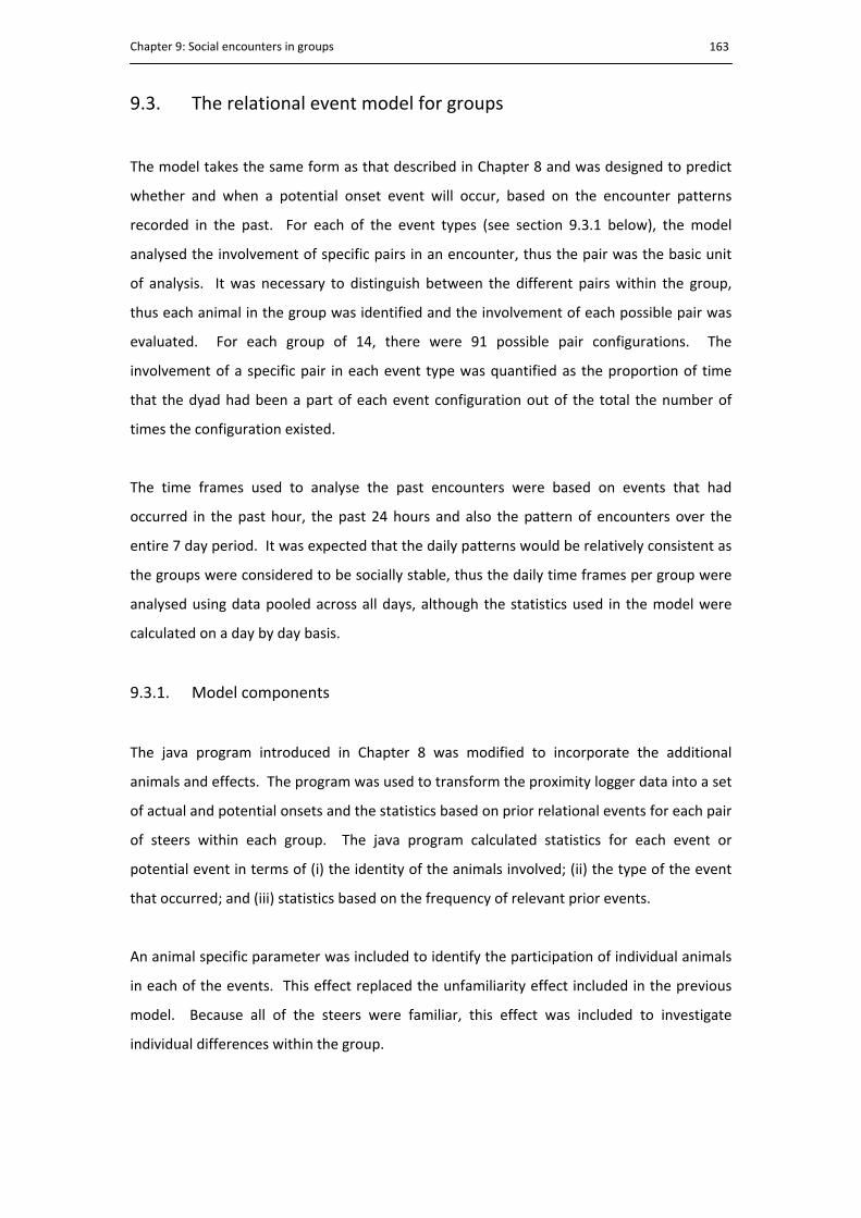
Chapter 9: Social encounters in groups
163
9.3. The relational event model for groups
The model takes the same form as that described in Chapter 8 and was designed to predict
whether and when a potential onset event will occur, based on the encounter patterns
recorded in the past. For each of the event types (see section 9.3.1 below), the model
analysed the involvement of specific pairs in an encounter, thus the pair was the basic unit
of analysis. It was necessary to distinguish between the different pairs within the group,
thus each animal in the group was identified and the involvement of each possible pair was
evaluated. For each group of 14, there were 91 possible pair configurations. The
involvement of a specific pair in each event type was quantified as the proportion of time
that the dyad had been a part of each event configuration out of the total the number of
times the configuration existed.
The time frames used to analyse the past encounters were based on events that had
occurred in the past hour, the past 24 hours and also the pattern of encounters over the
entire 7 day period. It was expected that the daily patterns would be relatively consistent as
the groups were considered to be socially stable, thus the daily time frames per group were
analysed using data pooled across all days, although the statistics used in the model were
calculated on a day by day basis.
9.3.1. Model components
The java program introduced in Chapter 8 was modified to incorporate the additional
animals and effects. The program was used to transform the proximity logger data into a set
of actual and potential onsets and the statistics based on prior relational events for each pair
of steers within each group. The java program calculated statistics for each event or
potential event in terms of (i) the identity of the animals involved; (ii) the type of the event
that occurred; and (iii) statistics based on the frequency of relevant prior events.
An animal specific parameter was included to identify the participation of individual animals
in each of the events. This effect replaced the unfamiliarity effect included in the previous
model. Because all of the steers were familiar, this effect was included to investigate
individual differences within the group.
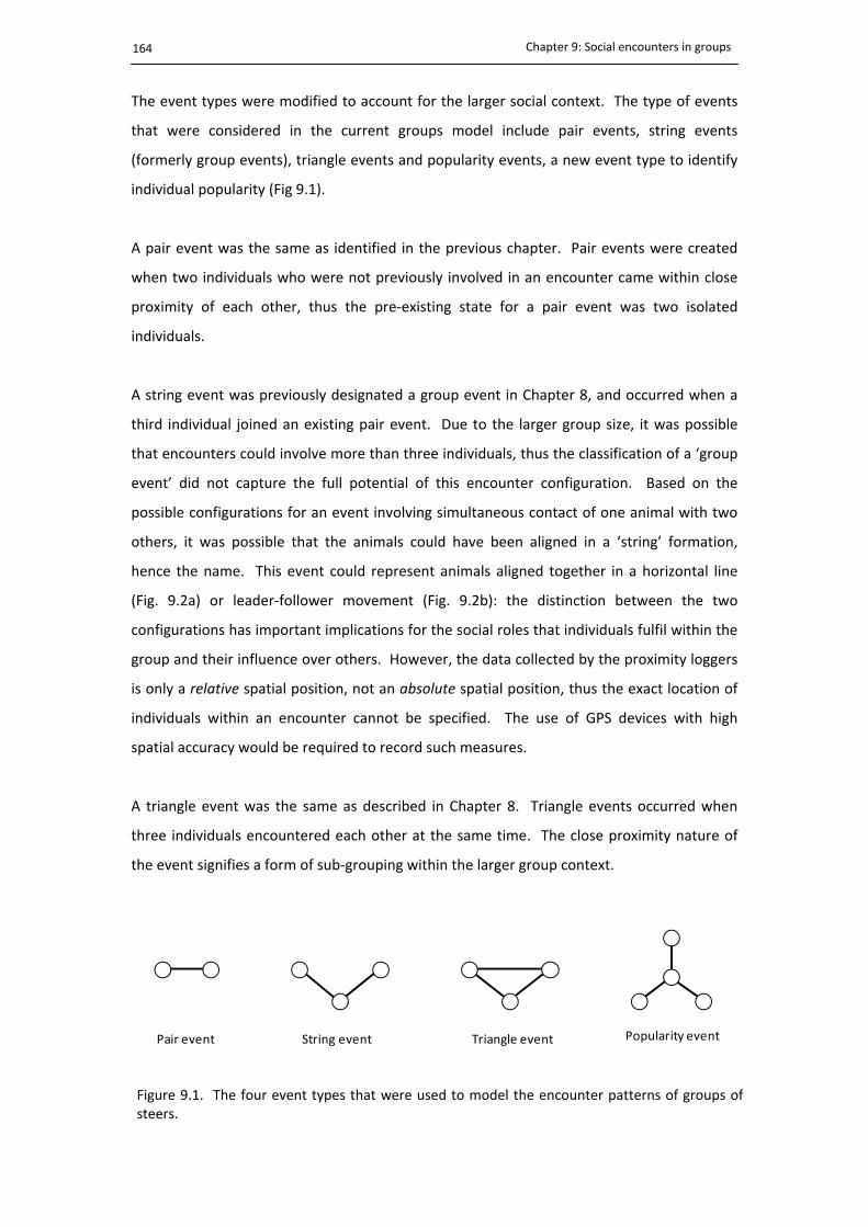
Chapter 9: Social encounters in groups
164
The event types were modified to account for the larger social context. The type of events
that were considered in the current groups model include pair events, string events
(formerly group events), triangle events and popularity events, a new event type to identify
individual popularity (Fig 9.1).
A pair event was the same as identified in the previous chapter. Pair events were created
when two individuals who were not previously involved in an encounter came within close
proximity of each other, thus the pre‐existing state for a pair event was two isolated
individuals.
A string event was previously designated a group event in Chapter 8, and occurred when a
third individual joined an existing pair event. Due to the larger group size, it was possible
that encounters could involve more than three individuals, thus the classification of a ‘group
event’ did not capture the full potential of this encounter configuration. Based on the
possible configurations for an event involving simultaneous contact of one animal with two
others, it was possible that the animals could have been aligned in a ‘string’ formation,
hence the name. This event could represent animals aligned together in a horizontal line
(Fig. 9.2a) or leader‐follower movement (Fig. 9.2b): the distinction between the two
configurations has important implications for the social roles that individuals fulfil within the
group and their influence over others. However, the data collected by the proximity loggers
is only a relative spatial position, not an absolute spatial position, thus the exact location of
individuals within an encounter cannot be specified. The use of GPS devices with high
spatial accuracy would be required to record such measures.
A triangle event was the same as described in Chapter 8. Triangle events occurred when
three individuals encountered each other at the same time. The close proximity nature of
the event signifies a form of sub‐grouping within the larger group context.
Figure 9.1. The four event types that were used to model the encounter patterns of groups ofsteers.
String eventPair event Triangle event Popularity event

Chapter 9: Social encounters in groups
165
Figure 9.2. An example of the possible animal configurations in a string event (a), (b) and apopularity event (c), showing the approximate 4 m detection range of a proximity logger.
Approximate 4 m radius
(a)
(b)
(c)

Chapter 9: Social encounters in groups
166
A popularity event represented one individual, i, in simultaneous contact with three others,
j,k and l, at the one time, yet j, k and l were not in contact with each other (Fig. 9.2c). This
effect represents ‘popularity’, as one individual was central to three others. A popularity
event was built on the contemporaneous existence of a string event. The configuration for a
popularity event is also known as a star configuration.
9.4. Results
9.4.1. Descriptive statistics
A summary of the raw proximity logger data per group is shown in Fig. 9.3. The number of
encounters per pair per hour was relatively consistent across days. There were more
encounters between pairs in group 2 on day 1, which could be explained as a prolonged
response to returning to their paddock after being handled in the yards. This effect
stabilised over the remaining 6 days. The average encounter length of pairs in group 2 was
marginally lower than those of group 1.
A network diagram visualising the associations between animals within each group is shown
in Fig. 9.4. The total length of encounters was used to indicate the strength of association
between each pair, thus pairs that spent more time within close proximity were regarded as
having stronger associations and the strength of the association is visually represented by
the colour of the tie joining the two steers. Here, only steers that spent more than a total of
5 hours within close proximity are shown. A red line indicates that a pair spent between 5
and 7.5 hours within close proximity of each other, green represents between 10 and 12.5
hours and the strongest association is shown by a blue line between two steers, indicating
that they spent in excess of 12.5 hours in close proximity over the 7 days. The size of the
node representing each animal is an indication of the number of encounters recorded with
all other steers. Thus a larger node indicates a highly active animal, while the smallest size
represents the animal with the least number of close proximity encounters.
The diagrams reveal differences between group 1 and group 2. While both groups displayed
a tendency for one animal to be involved in encounters more than others; stronger
associations were displayed by group 1: five pairs displayed associations greater than 12.5
hours spent within close proximity. Only one individual in group 1, animal 71, did not

Chapter 9: Social encounters in groups
167
Figure 9.3. The number of contacts per hour and the average length per contact for contact between pairs within group 1 and group 2 per day.
0.0
10.0
20.0
30.0
40.0
50.0
60.0
70.0
0.0
1.0
2.0
3.0
4.0
5.0
6.0
7.0
12
34
56
7
Average length/contact (s)
Number of contacts/pair/h
Day
Group 1: N
umber of contacts/pair/h
Group 2: N
umber of contacts/pair/h
Group 1: Average length/contact
Group 2: Average length/contact

Chapter 9: Social encounters in groups
168
(b)
(a)
Figure 9.4. Network diagrams representing pair‐wise interaction between steers in (a) group 1and (b) group 2. The lines represent the strength of association between steers based on thetotal amount of time spent within close proximity over the week. Only associations longer than 5hours in total duration are shown. The colour of the line represents the strength of association:black = between 5 and 7.5 h in close proximity; red = between 7.5 and 10 h; green = between 10and 12.5 h; blue = greater than 12.5 h. The size of the node represents the total number of timesan individual encountered all other steers, and is a measure of activity and/or popularity.
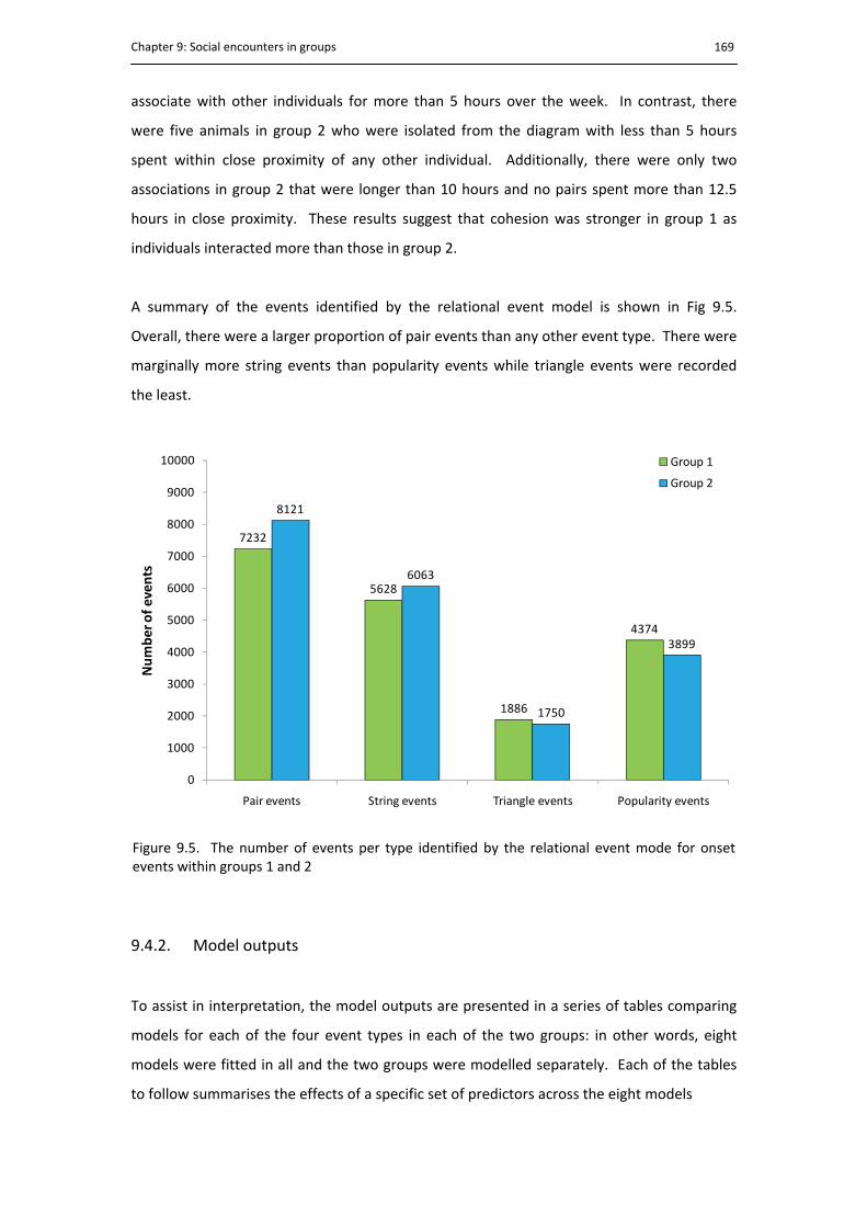
Chapter 9: Social encounters in groups
169
associate with other individuals for more than 5 hours over the week. In contrast, there
were five animals in group 2 who were isolated from the diagram with less than 5 hours
spent within close proximity of any other individual. Additionally, there were only two
associations in group 2 that were longer than 10 hours and no pairs spent more than 12.5
hours in close proximity. These results suggest that cohesion was stronger in group 1 as
individuals interacted more than those in group 2.
A summary of the events identified by the relational event model is shown in Fig 9.5.
Overall, there were a larger proportion of pair events than any other event type. There were
marginally more string events than popularity events while triangle events were recorded
the least.
9.4.2. Model outputs
To assist in interpretation, the model outputs are presented in a series of tables comparing
models for each of the four event types in each of the two groups: in other words, eight
models were fitted in all and the two groups were modelled separately. Each of the tables
to follow summarises the effects of a specific set of predictors across the eight models
7232
5628
1886
4374
8121
6063
1750
3899
0
1000
2000
3000
4000
5000
6000
7000
8000
9000
10000
Pair events String events Triangle events Popularity events
Number of events
Group 1
Group 2
Figure 9.5. The number of events per type identified by the relational event mode for onset events within groups 1 and 2
Chapter 9: Social encounters in groups
170
9.4.2.1. Animal effects
The results for the animal effects showed variability among individuals for both group 1 and
group 2 (Table 9.1). Most animals had a significant effect for at least one event type. The
majority of the animal effects were negative, with only two animals having a consistently
positive effect in group 1 and four animals in group 2. This result showed that there were
some individuals that were more likely to be involved in an encounter than others,
suggesting that these individuals were highly sociable. Equally, some individuals showed
strongly negative results (animal 66 group 1 and animal 37 in group 2), suggesting that these
individuals were overall less sociable. The size of the effect increased as the number of
animals involved in an encounter increased, thus it may be that these individuals tended to
avoid group‐like encounters.
9.4.2.2. Predicting future events from the pattern of prior pair events
Dyadic encounters were a strong feature of the encounter patterns recorded in group 1:
paired encounters in the past generally resulted in the same pairs seen together in the
future (Table 9.2). Time was an important factor for the recurrence of encounters involving
more than two animals: triangle events were more likely repeated over the week, while
string events were repeated on a daily scale. There was an enhanced recency effect on all
four event types: the occurrence of all pair events in the immediate past was a strong
predictor of future encounters.
The patterns of paired encounters in the past leading to future encounters in group 2 also
showed evidence of cohesion, but not as strong as group 1 (Table 9.2). Group 2 tended to
repeat pair‐wise encounters less frequently than group 1. Trends of paired encounters
leading to future encounters were repeated in the immediate and daily past but did were
not repeated over the course of the week. String events were likely to be repeated on a
daily basis, and similar to group 1, recently occurring pair events were a strong predictor of
all four event types in the future.

Chapter 9: Social encounters in groups
171
Table 9.1. Parameter estimates and standard errors predicting future pair, string, triangle and popularity events based on participation of individual animals. Asterisks represent significance at *P < 0.05 and **P < 0.10.
B SE B SE B SE B SE
a64 ‐0.06 0.05 ‐0.17 0.06 ** ‐0.14 0.09 ‐0.31 0.07 **
a65 ‐0.07 0.05 ‐0.21 0.06 ** ‐0.07 0.09 ‐0.44 0.07 **
a66 ‐0.37 0.05 ** ‐0.74 0.07 ** ‐0.80 0.12 ** ‐1.18 0.09 **
a67 ‐0.15 0.05 ** ‐0.23 0.06 ** ‐0.18 0.10 ‐0.40 0.07 **
a68 0.09 0.05 * 0.29 0.05 ** 0.31 0.09 ** 0.38 0.07 **
a69 ‐0.48 0.06 ** ‐0.54 0.06 ** ‐0.50 0.11 ** ‐0.78 0.08 **
a70 0.02 0.05 ‐0.01 0.05 0.11 0.09 ‐0.15 0.06 *
a71 ‐0.13 0.05 * ‐0.60 0.06 ** ‐0.68 0.12 ** ‐1.05 0.09 **
a74 0.06 0.08 0.73 0.08 ** ‐0.16 0.19 1.64 0.11 **
a75 ‐0.02 0.05 ‐0.08 0.05 0.09 0.09 ‐0.31 0.07 **
a76 ‐0.05 0.05 ‐0.37 0.06 ** ‐0.31 0.10 ** ‐0.67 0.07 **
a77 ‐0.05 0.05 0.03 0.05 0.16 0.09 ‐0.06 0.06
a78 ‐0.08 0.05 ‐0.22 0.05 ** ‐0.17 0.09 ‐0.34 0.07 **
a18 ‐0.17 0.05 ** ‐0.49 0.06 ** ‐0.76 0.11 ** ‐0.39 0.07 **
a20 0.04 0.06 0.42 0.07 ** 0.10 0.14 0.91 0.09 **
a21 ‐0.11 0.05 * ‐0.31 0.06 ** ‐0.52 0.10 ** ‐0.54 0.08 **
a26 ‐0.19 0.05 ** ‐0.14 0.05 ** ‐0.40 0.10 ** ‐0.10 0.07
a27 ‐0.08 0.05 ‐0.17 0.05 ** ‐0.31 0.10 ** ‐0.05 0.07
a35 0.05 0.04 ‐0.20 0.05 ** ‐0.51 0.10 ** ‐0.64 0.08 **
a37 ‐0.24 0.05 ** ‐0.57 0.06 ** ‐1.03 0.13 ** ‐0.96 0.09 **
a39 ‐0.03 0.04 ‐0.03 0.05 ‐0.08 0.09 ‐0.08 0.07
a40 0.06 0.04 ‐0.09 0.05 ‐0.12 0.09 ‐0.14 0.07 *
a46 0.07 0.04 0.11 0.05 * ‐0.17 0.09 0.13 0.06 *
a55 0.04 0.04 0.16 0.05 ** 0.16 0.08 0.10 0.06
a56 0.01 0.05 0.21 0.06 ** ‐0.05 0.11 0.66 0.07 **
a58 ‐0.13 0.05 ** ‐0.25 0.06 ** ‐0.30 0.10 ** ‐0.21 0.07 **
Group 1:
Group 2:
Animal effectsFuture event being predicted
Pair event String event Triangle event Popularity event
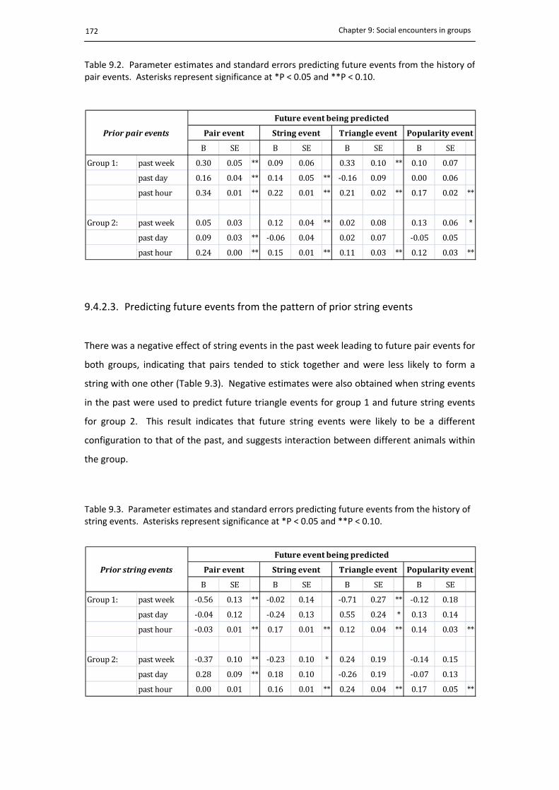
Chapter 9: Social encounters in groups
172
9.4.2.3. Predicting future events from the pattern of prior string events
There was a negative effect of string events in the past week leading to future pair events for
both groups, indicating that pairs tended to stick together and were less likely to form a
string with one other (Table 9.3). Negative estimates were also obtained when string events
in the past were used to predict future triangle events for group 1 and future string events
for group 2. This result indicates that future string events were likely to be a different
configuration to that of the past, and suggests interaction between different animals within
the group.
Table 9.2. Parameter estimates and standard errors predicting future events from the history ofpair events. Asterisks represent significance at *P < 0.05 and **P < 0.10.
Table 9.3. Parameter estimates and standard errors predicting future events from the history of string events. Asterisks represent significance at *P < 0.05 and **P < 0.10.
B SE B SE B SE B SE
Group 1: past week 0.30 0.05 ** 0.09 0.06 0.33 0.10 ** 0.10 0.07
past day 0.16 0.04 ** 0.14 0.05 ** ‐0.16 0.09 0.00 0.06
past hour 0.34 0.01 ** 0.22 0.01 ** 0.21 0.02 ** 0.17 0.02 **
Group 2: past week 0.05 0.03 0.12 0.04 ** 0.02 0.08 0.13 0.06 *
past day 0.09 0.03 ** ‐0.06 0.04 0.02 0.07 ‐0.05 0.05
past hour 0.24 0.00 ** 0.15 0.01 ** 0.11 0.03 ** 0.12 0.03 **
Future event being predicted
Pair event String event Triangle event Popularity eventPrior pair events
B SE B SE B SE B SE
Group 1: past week ‐0.56 0.13 ** ‐0.02 0.14 ‐0.71 0.27 ** ‐0.12 0.18
past day ‐0.04 0.12 ‐0.24 0.13 0.55 0.24 * 0.13 0.14
past hour ‐0.03 0.01 ** 0.17 0.01 ** 0.12 0.04 ** 0.14 0.03 **
Group 2: past week ‐0.37 0.10 ** ‐0.23 0.10 * 0.24 0.19 ‐0.14 0.15
past day 0.28 0.09 ** 0.18 0.10 ‐0.26 0.19 ‐0.07 0.13
past hour 0.00 0.01 0.16 0.01 ** 0.24 0.04 ** 0.17 0.05 **
Prior string events
Future event being predicted
Pair event String event Triangle event Popularity event

Chapter 9: Social encounters in groups
173
The trend for prior string events to lead to future events became positive when patterns in
the more recent past were analysed. This effect was seen in group 1 when triangle events
were predicted and was also shown in group 2 when pair events were predicted. String
events in the past hour were also positive predictors of future string, triangle and popularity
events. Thus, animals associating in the recent past as a string were more likely to associate
together in the future when more than two individuals were involved. This effect suggests
group building behaviour and may indicate a number of individuals performing the same
activity during certain times of the day, such as periods of grazing or resting.
9.4.2.4. Predicting future events from the pattern of prior triangle events
When the pattern of triangle events in the past were used as a predictor for future events,
only triangle events in the recent past were found to be significant for both groups (Table
9.4). This effect was consistently positive across all event types, except for the absence of
triangle events leading to popularity events for group 2. Thus, when three animals were all
within close proximity there was a tendency for the same animals to remain together in
future events. This effect suggests consistency in short term interaction, such as remaining
together during grazing bouts or rest periods.
Table 9.4. Parameter estimates and standard errors predicting future events from the history oftriangle events. Asterisks represent significance at *P < 0.05 and **P < 0.10.
B SE B SE B SE B SE
Group 1: past week 0.08 0.05 ‐0.04 0.06 0.02 0.11 ‐0.13 0.07
past day 0.03 0.05 0.03 0.05 ‐0.01 0.10 ‐0.03 0.05
past hour 0.02 0.01 ** 0.03 0.01 ** 0.29 0.02 ** 0.03 0.01 *
Group 2: past week 0.09 0.06 ‐0.03 0.06 ‐0.21 0.11 ‐0.02 0.09
past day ‐0.06 0.05 0.03 0.06 0.15 0.11 0.10 0.07
past hour 0.05 0.01 ** 0.03 0.01 ** 0.18 0.02 ** 0.03 0.03
String event Triangle event Popularity eventPrior triangle events
Future event being predicted
Pair event
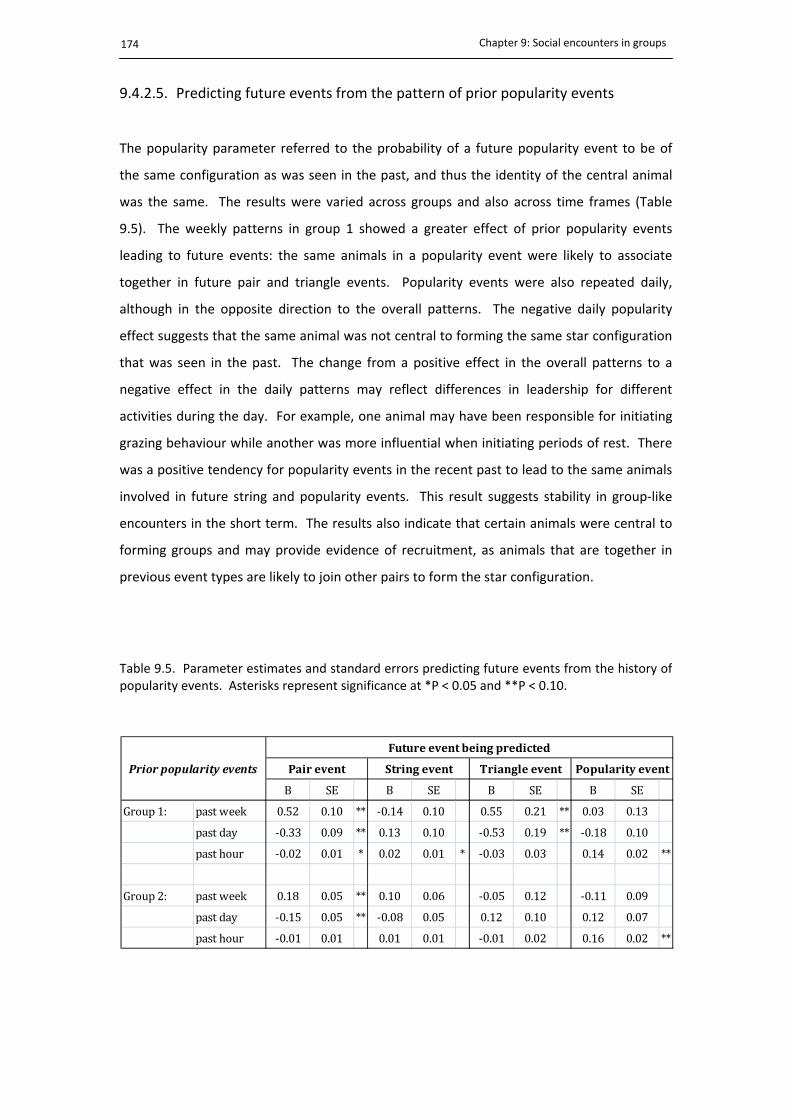
Chapter 9: Social encounters in groups
174
9.4.2.5. Predicting future events from the pattern of prior popularity events
The popularity parameter referred to the probability of a future popularity event to be of
the same configuration as was seen in the past, and thus the identity of the central animal
was the same. The results were varied across groups and also across time frames (Table
9.5). The weekly patterns in group 1 showed a greater effect of prior popularity events
leading to future events: the same animals in a popularity event were likely to associate
together in future pair and triangle events. Popularity events were also repeated daily,
although in the opposite direction to the overall patterns. The negative daily popularity
effect suggests that the same animal was not central to forming the same star configuration
that was seen in the past. The change from a positive effect in the overall patterns to a
negative effect in the daily patterns may reflect differences in leadership for different
activities during the day. For example, one animal may have been responsible for initiating
grazing behaviour while another was more influential when initiating periods of rest. There
was a positive tendency for popularity events in the recent past to lead to the same animals
involved in future string and popularity events. This result suggests stability in group‐like
encounters in the short term. The results also indicate that certain animals were central to
forming groups and may provide evidence of recruitment, as animals that are together in
previous event types are likely to join other pairs to form the star configuration.
Table 9.5. Parameter estimates and standard errors predicting future events from the history ofpopularity events. Asterisks represent significance at *P < 0.05 and **P < 0.10.
B SE B SE B SE B SE
Group 1: past week 0.52 0.10 ** ‐0.14 0.10 0.55 0.21 ** 0.03 0.13
past day ‐0.33 0.09 ** 0.13 0.10 ‐0.53 0.19 ** ‐0.18 0.10
past hour ‐0.02 0.01 * 0.02 0.01 * ‐0.03 0.03 0.14 0.02 **
Group 2: past week 0.18 0.05 ** 0.10 0.06 ‐0.05 0.12 ‐0.11 0.09
past day ‐0.15 0.05 ** ‐0.08 0.05 0.12 0.10 0.12 0.07
past hour ‐0.01 0.01 0.01 0.01 ‐0.01 0.02 0.16 0.02 **
Future event being predicted
Pair event String event Triangle event Popularity eventPrior popularity events

Chapter 9: Social encounters in groups
175
Similar to group 1, the probability of popularity events leading to future pair events was
repeated in group 2: over the week the same pairs tended to remain together in future pair
events. Also similar to group 1, the daily effect of popularity events leading to different pair
configurations in future dyadic events was negative, reflecting differences in leadership
during the course of a day. There was a positive recency effect of popularity events leading
to the same popularity event in the future. This result suggests that group 2 displayed
similar stable short term encounter patterns between more than 3 individuals as was seen in
group 1.
9.5. Discussion
The aim of the chapter was to investigate the patterns of encounters that occurred between
groups of steers that were socially stable. Encounters involving pairs, three individuals in
contact together or one animal in simultaneous contact with two others as well as
encounters involving four individuals were evaluated. It was hypothesised that dyadic and
triadic events would comprise a large component of the interactions, and although string
events occurred more predominantly than triangle or popularity events, the results showed
that string events were not as influential on future events as pair events. Thus, the effect of
encounters involving three individuals was not as important as expected.
The effect of pair‐wise interaction was a prominent feature of the model outputs for both
groups: pair‐wise interactions in the past positively influenced the occurrence of events in
the future, thus the same pairs that were together in the past were likely to be seen
together in the future. This result suggests that specific pairs were interacting regularly and
indicates the existence of preferential relationships within the group. Pair‐wise relationships
between cattle have been described by Reinhardt and Reinhardt (1981), where grooming
and grazing associations were formed between certain animals and the majority of group
members had one or more preferred grazing or grooming associates. Reinhardt and
Reinhardt (1981) also reported that grazing associates would locate themselves away from
the group during grazing activities. The current results may reflect grazing and grooming
associations between specific individuals, as there was a strong tendency for pairs to remain
together.
There was a tendency for the same triadic encounter structures being repeated in the short
term, although the type of triadic configuration differed between groups: where group 1

Chapter 9: Social encounters in groups
176
showed a greater tendency for triangle events, string events were a stronger feature of the
encounters in group 2. Both event types relate to group‐forming behaviour, however the
nature of triangle events indicate more localised grouping and may suggest greater cohesion
in group 1: this effect was also visually seen in the network diagrams, where group 1 had
stronger associations than group 2. The greater tendency for triangle events to occur in
group 1 may also suggest the possibility of sub‐group formation. Ramseyer et al. (2009)
found that sub‐groups in cattle were based on preferential relationships, where a sub‐group
involved between two and five individuals. In the same study, individuals with preferential
relationships were also found in close proximity during movement. Thus it is possible that
three steers could have formed alliances and maintained proximity during short‐lived
activities, such as grazing or resting. It is important to note that these effects are present
even after the individual propensities for sociability have been taken into account. Thus, the
propensity for triadic encounters to form is not just a reflection of some individuals being
more socially active than others but represents an organising dynamic in the herd. Further
investigation is required to quantify the existence of preferential relationships between two
or more steers and the potential for sub‐groups to form.
The animal effect showed that some individuals were more social than others and
demonstrates that associations within the group were more ordered than random.
Individual differences in sheep sociability have previously been reported (e.g. Sibbald and
Hooper, 2004; Sibbald et al., 2006), where it was found that highly social sheep were less
likely to move away from a group to forage and instead preferred to remain in proximity to
others. Thus, it is possible that highly sociable steers maintained a higher level of social
contact with others to receive necessary social support and reassurance from group
members. Further profiling is needed to confirm the social role that these more sociable
individual fulfil within the group, but their contact structure suggests that these individuals
are essential for group cohesion and may serve to transmit information within the group.
The negative animal effects suggest that some steers were less likely to be involved in an
interaction: this effect grew in size with the number of individuals involved in the predicted
encounter. This effect may be interpreted in several ways: the negative effects may reflect
the propensity for some individuals to only associate with certain others, while the results
may also reflect an inherent feature of a cattle social system to avoid large sub‐groupings. In
support of the latter interpretation, the results also showed that popularity and triangle
events occurred less frequently than pair or string events and tended to be localised in the
Chapter 9: Social encounters in groups
177
short term. Thus, overall there was a tendency for encounters not to involve more than
three individuals. The number of individuals that can participate in an encounter is limited
for practical reasons, as there are only a certain number of individuals that can be located
within a 4 m radius. Also, it is expected that individuals will avoid grouping together
frequently to avoid competition for forage while grazing and space during rest, as it would
compromise their individual fitness (e.g. Rind and Phillips, 1999; Harris et al., 2007). Cattle
have specific spacing principles that reflect not only properties of individual relationships but
also group‐specific properties. For example, individuals maintain certain distances with
others depending on their relationship status (Keeling, 1995), while individuals also have a
maximum distance that they will move away from the group (Hediger, 1963): these spatial
properties contribute to group functioning and cohesion. Thus, the negative animal effects
and lower proportion of group‐like encounters in the longer term may be related to social
factors that maintain a balance between the forces keeping the group together and breaking
the group apart.
The temporal patterning of encounters revealed that weekly trends were in general
repeated more so than daily trends, and hourly trends were repeated the most. Thus there
were regular patterns of short‐lived activity as well as longer term behavioural trends. The
majority of significant effects in the short term were positive, thus there were short‐lived
periods of stability that may reflect times when all group members were engaged in the
same behaviour, such as grazing or resting. Additionally, it was indicated that there were
certain individuals who were more popular than others in both groups, although this effect
was more evident in group 1. Reinhardt and Reinhardt (1981) found that the most popular
cow in the herd was also the predominant leader of movement. Other studies, however,
have found more than one individual to be responsible for group movement (e.g. Beilharz
and Mylrea, 1963). In a study on the determinants of group movement, Ramseyer et al.
(2009) reported that amongst a group of 15 heifers, most grazing bouts were initiated by
one of three individuals. Thus, in the current study there may have been more than one
specific individual per group that was responsible for initiating grazing and movement
activities. Ramseyer et al. (2009) also found that leaders tended to be socially independent
and displayed less cohesive social properties. In this sense, steers with highly negative
animal effects may be more responsible for group movement than highly sociable steers
with positive animal effects. Further investigation is required to correlate the results of the
individual animal parameters with social roles, such as leadership.
Chapter 9: Social encounters in groups
178
The lack of daily patterns was surprising, as cattle on pasture are reported to display diurnal
activity patterns, with grazing and moving activities generally performed in the early
morning and late afternoon (O'Connell et al., 1989). Although, Lewis (1977) reports that the
number of grazing bouts can vary between two and ten bouts per day. Additionally, daily
activity can also vary depending on the ambient temperature (Lewis, 1977) and also on the
season (e.g. Howery et al., 1998), thus the encounter patterns recorded within the groups
may reflect variation in behavioural activity according to the physical environment.
The overall weekly results revealed that pair events were likely to be repeated, thus
reinforcing the strong dyadic effect and existence of preferential relationships. There was an
overall tendency for triangle events in group 1 and string events in group 2 to be of a
different configuration to that of the past: these effects are opposite to that recorded in the
short term. This effect shows that there is general interaction among all group members
when encounters involved more than two animals. This behavioural pattern may be
observed when the group collectively changes activity, for example, when the group ceases
resting together to spread out and graze.
Overall there were some differences between the two groups, in particular were the
differences in triadic configurations and individual animal effects. As the relational event
model is a novel approach to investigate animal’s social systems, the extent to which the
two groups represent cattle systems in general is unknown and further work is required to
develop the methodology for wider application and also apply the model on a substantial
range of animal groups. It is therefore difficult to generalise the reasons behind the
differences between the two groups, however, it is possible to speculate that differences in
genetics, such as breed, as well as management factors, such as re‐grouping experience, may
contribute to differences in social organisation.
9.6. Conclusions
The relational event model identified specific endogenous properties of a stable cattle social
system. It was shown that pair‐wise encounters are important for group cohesion and
suggestive of preferential relationships within the group. Although triadic encounters were
not as influential as predicted, the pattern of the same triadic encounters being repeated in
the short term demonstrates stability: group 1 had a greater tendency to repeat triangle
events while string events were a greater feature for group 2. Both encounter patterns
Chapter 9: Social encounters in groups
179
indicate cohesion. There was large variation in individual animal activity, which may relate
to sociability levels and social roles. The model identified both short‐term and longer term
behavioural patterns that represent typical animal movement where individuals group
together for certain periods and spread out during others. This investigation demonstrates
that the relational event model can be used to identify inherent features of cattle groups
based on patterns of close proximity encounters.

181
Chapter 10
General discussion The overall aim of the thesis was to investigate the effect of the presence of an unfamiliar
steer on the social behaviour of resident steers. In contrast to previous mixing studies that
have focused on agonistic behaviours within commercial sized groups (e.g. Hasegawa et al.,
1997; von Keyserlingk et al., 2008), the focus of the current studies targeted the affiliative
behaviours responsible for group cohesion. The underlying social properties involved in
relationship development in steers were investigated using dyads and triads of steers as the
fundamental components of social structure. It was anticipated that the social properties of
dyads and triads could be used to describe social processes that occur within larger groups.
Overall, the findings show that behavioural responses towards an unfamiliar are various and
depend on the social context. The findings from each of the experimental chapters are now
discussed.
The general differences between the behavioural response of a steers towards a familiar and
an unfamiliar peer showed that there are various benefits of being familiar. Different levels
of social support were identified based on the social and physical environment. During the
trade‐off test, steers paired with familiar pen mates were more willing to consume food at
greater distances than steers paired with unfamiliar pen mates. In the pairs monitoring
study, familiar pairs had more close proximity encounters, moved towards each other more
and tended to spend more time lying and standing than unfamiliar pairs. These behaviours
could be considered characteristics of a well established relationship. It is concluded that
the presence of a familiar peer provides social support that allows individuals to express
their own feeding and resting choices. When an unfamiliar steer was introduced into a pair
of familiar steers, it was found that the existing relationship between the familiar pair
strengthened due to the presence of the unfamiliar steer and there was little evidence to
suggest relationships were developing in the triad. The modelling approach used in Chapter
8 allowed a greater investigation of simultaneous encounter patterns between the three
steers, where it was shown that the strong and consistent unfamiliarity and dyadic effects

Chapter 10: General discussion
182
explained why the unfamiliar steer was not integrated into the triad within 5 days. It is
suggested that the familiar pair resisted the unfamiliar steer’s attempts to develop a
relationship. The results demonstrate that established dyadic relationships translate into
predicable and regular encounter patterns, which promotes relationship stability and group
forming behaviours. It is therefore concluded that the social support provided by a familiar
peer allows individuals to cope with unstable social environments. These findings build on
existing knowledge that the presence of a familiar peer provides a calming effect in stressful
situations (e.g. Boissy and LeNeindre, 1997; Faerevik et al., 2006).
The behavioural differences between familiar and unfamiliar pairs were used to assess the
effect of the presence of an unfamiliar steer under different environmental settings. The
pair‐wise experiments evaluated the individual responses of steers when paired with either
familiar or unfamiliar peers. The trade‐off test showed that the actual trade‐off made by the
steers when paired with an unfamiliar pen mate went beyond a desire for food or social
companionship but was instead related to social insecurity. The pairs monitoring
experiment showed that initially the unfamiliar pairs avoided each other. The reasons for
the behavioural differences between familiar and unfamiliar treatments were varied,
however, it was suggested that the presence of an unfamiliar steer as well as isolation from
familiar group mates elicited a stress response that modified the steer’s behaviour. Various
environmental factors can contribute to the social stress associated with introducing new
individuals, such as the loss of social support from familiar group members, a change in
group size as well as the possibility of experiencing an unfamiliar environment (Zayan and
Dantzer, 1990; Newberry and Swanson, 2001). It is possible to quantify the contribution of
unfamiliarity on the social stress experienced when mixing unfamiliar animals by comparing
the behavioural responses towards both familiar and unfamiliar peers under identical
circumstances (Zayan, 1990). The studies described in Chapter 5 and 6 showed that
differences were recorded between the familiar and unfamiliar treatments, although the
sudden isolation from familiar group members may have contributed to the social stress
experienced by both familiar and unfamiliar treatments. However, when triadic based
outcomes were quantified in Chapter 7 it was shown that the presence of an unfamiliar
elicits a behavioural response, even when familiar peers are present. It is therefore
concluded that the presence of an unfamiliar steer creates social stress, which was
demonstrated by a reluctance of steers to travel away from the unfamiliar animal to
consume food, avoidance behaviour and an increase in contact frequency between familiar
peers. Further work is suggested in the following areas:

Chapter 10: General discussion
183
Investigation of the encounter patterns of three familiar steers. The current triad
experiment only investigated one familiarity combination: two familiar pairs with
one unfamiliar steer. The behaviour and encounter patterns of familiar triads could
be compared with the current results to determine if steers in such a small group
size were experiencing social stress caused by isolation from a larger group.
Measure the physiological response towards an unfamiliar steer in combination with
proximity logging devices. The data from the proximity loggers gives no indication of
the nature of the encounter quality, however there is an established link between
blood cortisol levels, heart rate and stress (e.g. Sato and Tarumizu, 1993; Bristow
and Holmes, 2007). Future studies should consider correlating encounter
characteristics (frequency, duration) with physiological responses to determine if
certain encounters lead to increased stress responses, such as the presence of an
unfamiliar or an agonistic interaction. This approach also has the potential to
differentiate between affiliative and agonistic interactions.
When the steer’s behavioural response toward an unfamiliar peer was monitored in a
paddock‐based environment allowing the steers to interact and develop relationships, it was
found that that the process of familiarisation was complex and various social processes were
involved as relationships developed. Initially the unfamiliar pairs avoided each other but
changes in inter‐individual distance and movement indicated that familiarisation was
occurring between the pair. The results prove that factors other than dominance are
involved in the familiarisation process and affiliative behaviours, such as close proximity
encounters, spatial proximity and movement patterns, are important in the establishment
and maintenance of social relationships between steers. The use of movement vectors
provided a novel observational tool to record individual movement patterns and differences
between familiar and unfamiliar social encounters were identified. It was demonstrated
that the repeated pattern of movement both towards and away from each other was an
important component of familiarisation between steers: this behaviour facilitates learning,
recognition and communication, each of which are fundamental components of a
relationship. However, due to a lack of knowledge on the distance perception and depth
perception of cattle vision (e.g. Arnold et al., 2007), it was not possible to identify the point
at which the steers were behaving either dependently or independently of each other. It is
assumed that the behavioural synchrony of two steers is influenced by the distance between
them, but not enough is known about the spatial acuity of cattle to draw definitive
conclusions between proximity and movement. Further work is warranted in this area.
Chapter 10: General discussion
184
It was anticipated that familiarisation would be accelerated in small groups as there would
be fewer relationships to establish and less interference from other group members.
However, it was not expected that there would be such contrasting differences in the
encounter patterns between pairs and triads. The results showed evidence of familiarisation
between pairs within 5 days, yet marked differences in both the frequency and duration of
encounters between familiar and unfamiliar steers in the triads provide little evidence to
demonstrate familiarisation within the triad. It is therefore suggested that structural
differences exist between dyads and triads of steers and as a result social stabilisation will
take longer between triads than pairs of steers. In human social systems, the addition of a
third individual can be detrimental to group unity if two individuals join forces to gain power
over the third (Feinman and Lewis, 1984). Thus, it is suggested that the familiar pair formed
a majority which led to the exclusion of the unfamiliar steer.
The relational event model provided a novel approach to investigate the encounter patterns
of pairs and triads of steers when an unfamiliar steer was introduced, and to also identify
the structural properties of a stable social system. It was shown that paired encounters
were indeed a strong feature of the social system, with evidence of preferential
relationships as well as sociability and possibly popularity. There was a tendency for
individuals to form triadic encounters with the same individuals when engaging in short term
activities, such as grazing or resting, while the overall weekly patterns indicated that there
was interaction among group members with different partners, which may indicate grouping
and breaking apart at certain times, such as a change in activity from resting to grazing. The
model identified both short‐term and longer‐term behavioural patterns that represent
typical animal activity. It was concluded that the relational event model can be used to
identify inherent features of cattle groups based on patterns of close proximity encounters.
The encounter patterns observed within a stable system can be used as a comparative tool
to identify periods of instability and quantify the extent of the disruption: knowing normal
animal behaviour is a prerequisite for recognising abnormal behaviour (Broom and Fraser,
2007). The main encounter differences between triads and groups of steers were seen on
the day of introduction. After day 1 the triads showed a stabilising trend similar to that
observed in the groups encounter structures, although only the encounter patterns between
the familiar pair were stabilising and longer time was needed for the integration of the
unfamiliar steer. This result demonstrates that the familiar pair recovered quickly from the
social disruption caused by the unfamiliar steers introduction and suggests that cattle
Chapter 10: General discussion
185
relationships are flexible, which allows them to respond and adapt to change. Further
applications of this work could include:
Introducing unfamiliar animals into group sizes of four, five and six animals to
investigate if there are differences in the rate of integration of an unfamiliar.
Knowledge on the social properties of small group sizes has the potential to advance
knowledge on bovine social structure as well as improve management practices.
Using the encounter patterns of a stable social system to measure the impact of
other sources of social disruption. For example, a change in location such as cattle
handling facilities or introduction to a new paddock, the presence of a predator such
as a wild dog, or the illness or removal of a group member. The relational event
model can also be applied to other contact animal species to investigate the social
properties of a system or process.
Developing the current relational event model to include both onset and offset
events in the one framework. The current model only considered the initiation of
encounters between steers, and while familiarity was shown as a predominant
driver of social interaction, the breakdown of social structures was not investigated.
Currently it is not known what factors lead to animals spreading out during periods
of stability or social disruption.
Proximity logging devices have not been extensively used to monitor the social interactions
of domestic livestock, or more specifically, to quantify individual social relationships. The
encounter differences recorded between familiar and unfamiliar steers suggests there is a
relationship between familiarity and close proximity encounters. More compellingly, the
relational event model identified that individuals with well developed social bonds were
more likely to approach each other at closer distances: the pattern of encounters in the past
were repeated between the same individuals in the future, signifying a relationship between
the pair. It is proposed that regularity in close proximity encounters are an underlying
behavioural component of an established social relationship, which may be used as a
comparative tool to indicate familiarisation between cattle and other social animals. In the
current studies, unfamiliarity was used as a contrast to compare the behavioural
characteristics of a familiar and unfamiliar social relationship. It was shown that proximity
logging devices captured the social differences between familiarity types, and thus it is
concluded that proximity loggers are capable of quantifying social relationships in cattle.

Chapter 10: General discussion
186
The behavioural responses of the same individuals were repeatedly measured over a series
of discrete experiments, thus it is possible with suitably developed analytic techniques that
individual animals could be analysed for their social tendencies or influence within the
group. Quantifying individual ‘personalities’ was not a specific aim of the thesis but is
something that could be undertaken in the future with this type of longitudinal data.
Longitudinal studies are important to explore tendencies across populations and larger
groups, which go beyond analyses that use averages to understand general trends. The
development of analytical methods to quantitatively assess individual animal involvement
with respect to the whole group was introduced in Chapters 8 and 9. Further development
of analytical techniques to analyse real time interaction data and individual responses in the
context of longitudinal data is a topic for future investigation.
In conclusion, this thesis investigated the effect of the presence of an unfamiliar steer on the
social behaviour of resident steers. Behaviours that were affected by the presence of an
unfamiliar peer were identified and the spatial and temporal changes that occurred during
the initial stages of familiarisation between steers were described. The behavioural patterns
that occurred during relationship development were discussed in relation to the evolution of
social structure. The main conclusions drawn from the research are:
1. The presence of a familiar peer provides social support. This support allows
individuals to express their own feeding and resting choices and provides
reassurance in an unstable social environment.
2. The presence of an unfamiliar peer elicits social stress. The social stress created by
the presence of an unfamiliar steer affected spatial proximity, behaviour, close
proximity encounter patterns and movement.
3. Familiarisation between pairs was indicated by a decrease in spatial proximity and
movement towards and away from each other.
4. Structural differences exist between dyads and triads of steers: the addition of a
third party complicates and extends the process of relationship development.
5. Pairs of familiar steers will form a majority to exclude an unfamiliar steer.
6. Socially stable cattle groups display regular dyadic and triadic encounter structures
in both the short‐term and longer‐term behavioural patterns.
7. Relational event modelling provides a novel predictive tool to identify and analyse
the complex encounter structures of steers during periods of social disruption as
well as social stability.

Chapter 10: General discussion
187
8. Proximity logging devices can be used to quantify social relationships in cattle and
differentiate between the encounter patterns of familiar and unfamiliar steers.

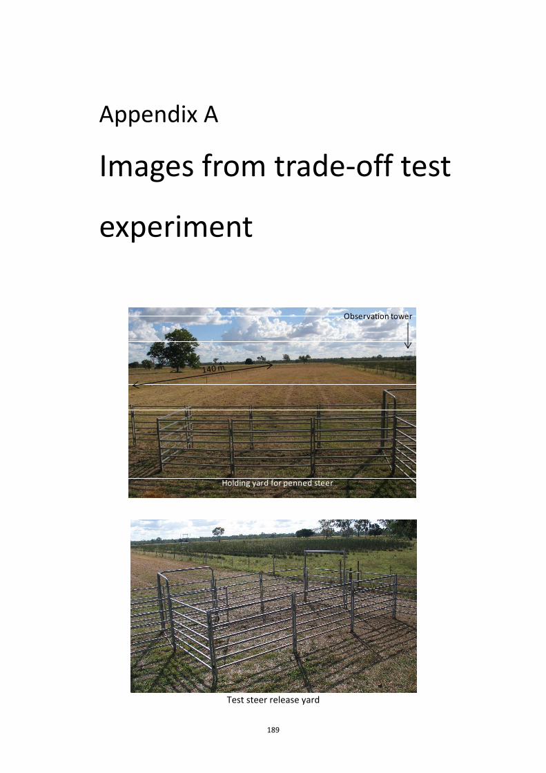
189
Appendix A
Images from trade‐off test
experiment
Test steer release yard
Holding yard for penned steer
Observation tower
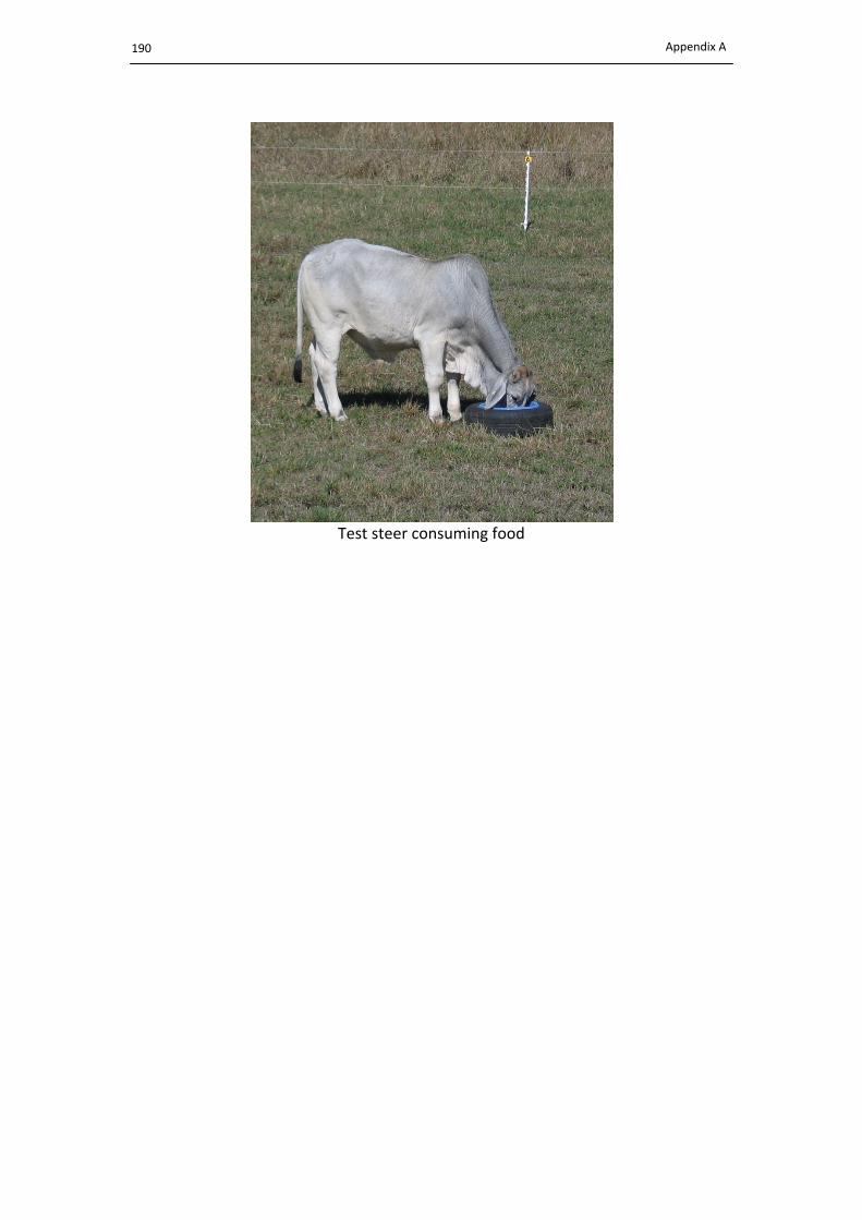
Appendix A
190
Test steer consuming food

191
Appendix B
Validating assumptions
The frequency distributions of the parameter estimates obtained when a simplified version
of the model was fitted to each triad separately are shown below. The model was fitted on a
daily basis to obtain the parameter estimates for the effect of unfamiliarity and prior pair
events in the past hour and past 24 hours. The same model was also fitted to the pooled
data set. The placement of the parameter estimate from the pooled data set within the
individual triad distribution was used to assess the validity of pooling the triad data in
Chapter 8.
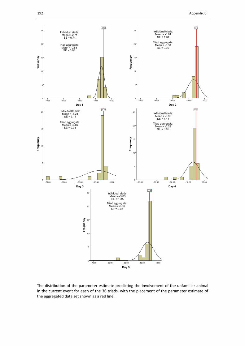
Appendix B
192
The distribution of the parameter estimate predicting the involvement of the unfamiliar animal in the current event for each of the 36 triads, with the placement of the parameter estimate of the aggregated data set shown as a red line.

Appendix B
193
The distribution of the parameter estimate predicting future pair events from pair events in the past hour for each of the 36 triads, with the placement of the parameter estimate of the aggregated data set shown as a red line.
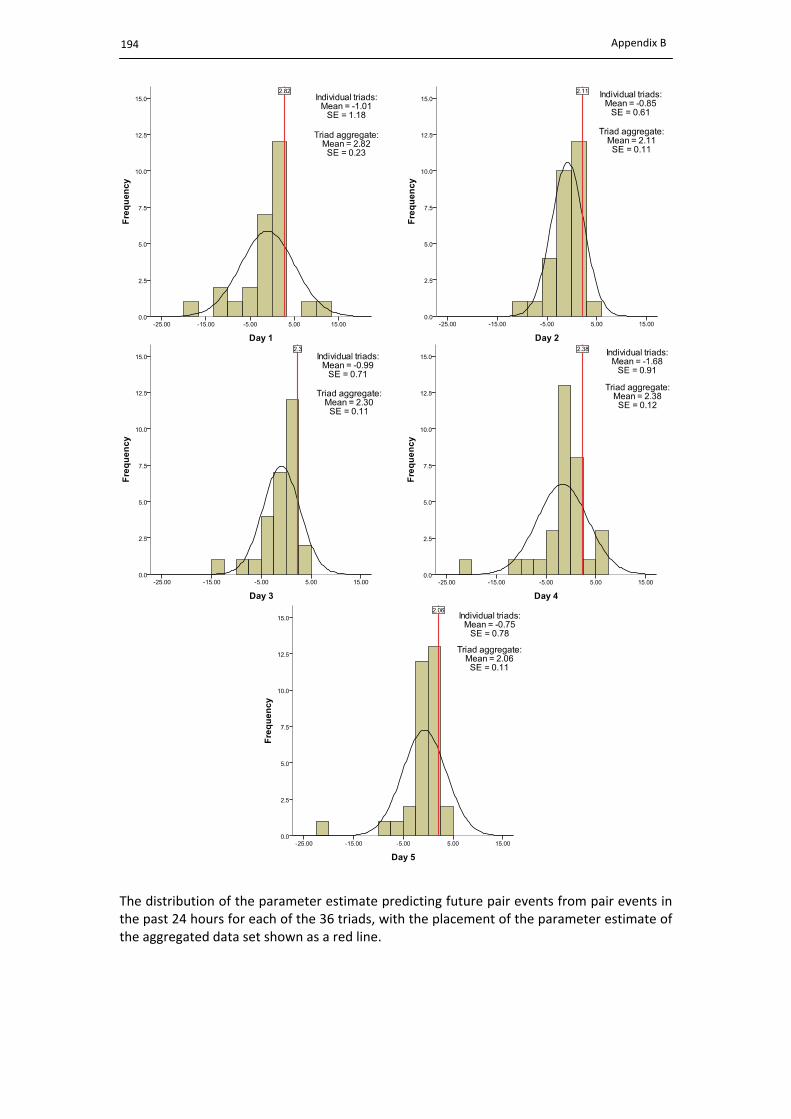
Appendix B
194
The distribution of the parameter estimate predicting future pair events from pair events in the past 24 hours for each of the 36 triads, with the placement of the parameter estimate of the aggregated data set shown as a red line.
195
References
Agresti, A., 2002. Categorical data analysis. 2nd ed. New York, USA: Wiley.
Altmann, J., 1974. Observational study of behavior: sampling methods. Behaviour, 49 (3),
227‐267.
Anderson, N.G., 2003. Observations on dairy cow comfort: diagonal lunging, resting,
standing and perching in free stalls, in: Janni, K.A. (Ed.), Fifth International Dairy Housing
Conference: conference proceedings (pp. 26‐35), January 29‐31, Fort Worth, USA: American
Society of Agricultural and Biological Engineers.
Archer, J., 1976. The organisation of aggression and fear in vertebrates, in: Bateson, P.P.G.,
Klopfer, P.H. (Eds.), Perspectives in ethology, New York: Plenum Press.
Arnold, G.W., 1985. Associations and social behaviour, in: Fraser, A. (Ed.), Ethology of farm
animals: a comprehensive study of the behavioural features of the common farm animals
Amsterdam, The Netherlands: Elsevier.
Arnold, N.A., Ng, K.T., Jongman, E.C., Hemsworth, P.H., 2007. Responses of dairy heifers to
the visual cliff formed by a herringbone milking pit: evidence of fear of heights in cows (Bos
taurus). Journal of Comparative Psychology, 121 (4), 440‐446.
Barfield, C.H., Tangmartinez, Z., Trainer, J.M., 1994. Domestic calves (Bos taurus) recognize
their own mothers by auditory cues. Ethology, 97 (4), 257‐264.
Barroso, F.G., Alados, C.L., Boza, J., 2000. Social hierarchy in the domestic goat: effect on
food habits and production. Applied Animal Behaviour Science, 69 (1), 35‐53.

References
196
Beilharz, R.G., Mylrea, P.J., 1963. Social position and movement orders of dairy heifers.
Animal Behaviour, 11 (4), 529‐533.
Beilharz, R.G., Butcher, D.F., Freeman, A.E., 1966. Social dominance and milk production in
Holsteins. Journal of Dairy Science, 49 (7), 887‐892.
Beilharz, R.G., Zeeb, K., 1982. Social dominance in dairy cattle. Applied Animal Ethology, 8 (1‐
2), 79‐97.
Berger, J., 1979. "Predator harassment" as a defensive strategy in ungulates. American
Midland Naturalist, 102 (1), 197‐199.
Blockey, M.A.d.B., 1979. Observations on group mating of bulls at pasture. Applied Animal
Ethology, 5 (1), 15‐34.
Blossfeld, H.‐P., Rohwer, G., 1995. Techniques of event history modelling: new approaches to
causal analysis. Mahwah, New Jersey: Lawrence Erlbaum Associates.
Boe, K.E., Faerevik, G., 2003. Grouping and social preferences in calves, heifers and cows.
Applied Animal Behaviour Science, 80 (3), 175‐190.
Bohm, M., Hutchings, M.R., White, P.C.L., 2009. Contact networks in a wildlife‐livestock host
community: identifying high‐risk individuals in the transmission of bovine TB among badgers
and cattle. PLoS ONE, 4 (4), e5016.
Boissy, A., LeNeindre, P., 1997. Behavioral, cardiac and cortisol responses to brief peer
separation and reunion in cattle. Physiology & Behavior, 61 (5), 693‐699.
Boissy, A., Terlouw, C., Le Neindre, P., 1998. Presence of cues from stressed conspecifics
increases reactivity to aversive events in cattle: evidence for the existence of alarm
substances in urine. Physiology & Behaviour, 63 (4), 489‐495.
Boissy, A., Dumont, B., 2002. Interactions between social and feeding motivations on the
grazing behaviour of herbivores: sheep more easily split into subgroups with familiar peers.
Applied Animal Behaviour Science, 79 (3), 233‐245.

References
197
Boissy, A., Manteuffel, G., Jensen, M.B., Moe, R.O., Spruijt, B., Keeling, L.J., Winckler, C.,
Forkman, B., Dimitrov, I., Langbein, J., Bakken, M., Veissier, I., Aubert, A., 2007. Assessment
of positive emotions in animals to improve their welfare. Physiology & Behavior, 92 (3), 375‐
397.
Bouissou, M.F., 1972. Influence of body‐weight and presence of horns on social rank in
domestic cattle. Animal Behaviour, 20 (3), 474‐477.
Bouissou, M.F., 1974a. Establishment of dominance‐submission relationships in domestic
cattle. 2. Rapidity and method of establishment. Annales De Biologie Animale Biochemie
Biophysique, 14 (4), 757‐768.
Bouissou, M.F., 1974b. Establishment of dominance‐submission relationships in domestic
cattle. 1. Nature and evolution of social interactions. Annales De Biologie Animale
Biochemie Biophysique, 14 (3), 383‐410.
Bouissou, M.F., 1980. Social relationships in domestic cattle under modern management
techniques. Italian Journal of Zoology, 47 (3‐4), 343‐353.
Bouissou, M.F., Boissy, A., Le Neindre, P., Veissier, I., 2001. The social behaviour of cattle, in:
Keeling, L.J., Gonyou, H.W. (Eds.), Social Behaviour in Farm Animals, Cambridge, UK: CABI
Publishing.
Brandes, U., Lerner, J., Snijders, T.A.B., 2009. Networks evolving step by step: statistical
analysis of dyadic event data, 2009 International conference on Advances in Social Network
Analysis and Mining (pp. 200‐205), July 20‐July 22, Athens, Greece: IEEE Computer Society
Press.
Bristow, D.J., Holmes, D.S., 2007. Cortisol levels and anxiety‐related behaviors in cattle.
Physiology & Behavior, 90 (4), 626‐628.
Broom, D.M., Fraser, A., 2007. Domestic animal behaviour and welfare. 4th ed. Cambridge,
UK: CABI Publishing.
Broster, J.C., Dehaan, R.L., Swain, D.L., Friend, M.A., 2010. Ewe and lamb contact at weaning
is influenced by both shelter type and birth number. Animal, 4 (5), 796‐803.

References
198
Brown, C., 2002. Do female rainbowfish (Melanotaenia spp.) prefer to shoal with familiar
individuals under predation pressure? Journal of Ethology, 20 (2), 89‐94.
Brownlee, A., 1950. Studies in the behaviour of domestic cattle in Britain. Bulletin of Animal
Behaviour, 8 (1), 11‐20.
Butts, C., T., 2008. A relational event framework for social action. Sociological Methodology,
38 (1), 155‐200.
Cameron, C.A., Trivedi, P.K., 2005. Microeconometrics: methods and applications. New York,
USA: Cambridge University Press.
Chase, I.D., 1974. Models of hierarchy formation in animal societies. Behavioral Science, 19
(6), 374‐382.
Chase, I.D., 1980. Social‐process and hierarchy formation in small‐groups ‐ a comparative
perspective. American Sociological Review, 45 (6), 905‐924.
Chase, I.D., 1982. Dynamics of hierarchy formation: the sequential development of
dominance relationships. Behaviour, 80 (3‐4), 218‐240.
Chase, I.D., Tovey, C., Murch, P., 2003. Two's company, three's a crowd: differences in
dominance relationships in isolated versus socially embedded pairs of fish. Behaviour, 140
(10), 1193‐1217.
Cohen, L., Manion, L., Morrison, K.R., 2007. Research methods in education. 6th ed. New
York, USA: Routledge.
Collis, K.A., 1976. An investigation of factors related to the dominance order of a herd of
dairy cows of similar age and breed. Applied Animal Ethology, 2 (2), 167‐173.
Coulon, M., Deputte, B.L., Heyman, Y., Delatouche, L., Richard, C., 2007. Visual discrimination
by heifers (Bos taurus) of their own species. Journal of Comparative Psychology, 121 (2), 198‐
204.
Croft, D.P., James, R., Krause, J., 2008. Exploring animal social networks. Princeton, USA:
Princeton University Press.

References
199
Crook, J.H., 1970. Social organization and the environment: Aspects of contemporary social
ethology. Animal Behaviour, 18 (2), 197‐209.
Cushing, B.S., Kramer, K.M., 2005. Mechanisms underlying epigenetic effects of early social
experience: The role of neuropeptides and steroids. Neuroscience and Biobehavioral
Reviews, 29 (7), 1089‐1105.
D'Eon, R.G., Delparte, D., 2005. Effects of radio‐collar position and orientation on GPS radio‐
collar performance, and the implications of PDOP in data screening. Journal of Applied
Ecology, 42 (2), 383‐388.
DairyAustralia, 2010. Australian dairy industry in focus. Southbank, Australia: Dairy Australia.
Dawkins, M.S., 2007. Observing animal behaviour: design and analysis of quantitative data.
New York, USA: Oxford University Press.
De Nooy, W., 2011. Networks of action and events over time. A multilevel discrete‐time
event history model for longitudinal network data. Social Networks, 33 (1), 31‐40.
Dehn, M.M., 1990. Vigilance for predators: detection and dilution effects. Behavioral Ecology
and Sociobiology, 26 (5), 337‐342.
Dickson, D.P., Barr, G.R., Wieckert, D.A., 1967. Social relationship of dairy cows in a feed lot.
Behaviour, 29 (2‐4), 195‐203.
Dugatkin, L.A., 2004. Principles of animal behaviour. 1st ed. New York, USA: W.W. Norton
and Company, Inc.
Dumont, B., Boissy, A., 1999. Impact of social on grazing behaviour in herbivores.
Productions Animales, 12 (1), 3‐10.
Dumont, B., Boissy, A., 2000. Grazing behaviour of sheep in a situation of conflict between
feeding and social motivations. Behavioural Processes, 49 (3), 131‐138.
Dussault, C., Courtois, R., Ouellet, J., Huot, J., 2001. Influence of satellite geometry and
differential correction on GPS location accuracy. Wildlife Society Bulletin, 29 (1), 171‐179.

References
200
Faerevik, G., Jensen, M.B., Boe, K.E., 2006. Dairy calves social preferences and the
significance of a companion animal during separation from the group. Applied Animal
Behaviour Science, 99 (3‐4), 205‐221.
Faust, K., 2007. Very local structure in social networks. Sociological Methodology, 37 (1),
209‐256.
Feinman, S., Lewis, M., 1984. Is there social life beyond the dyad? A social‐psychological
view of social connections in infancy, in: Lewis, M. (Ed.), Beyond the dyad (pp. 13‐41), New
York, USA: Plenum Press.
Fortin, D., Fortin, M.E., 2009. Group‐size‐dependent association between food profitability,
predation risk and distribution of free‐ranging bison. Animal Behaviour, 78 (4), 887‐892.
Friend, T.H., Polan, C.E., 1974. Social rank, feeding behavior, and free stall utilization by dairy
cattle. Journal of Dairy Science, 57 (10), 1214‐1220.
Galef, B.G., Laland, K.N., 2005. Social learning in animals: empirical studies and theoretical
models. BioScience, 55 (6), 489‐499.
Ganskopp, D., 2001. Manipulating cattle distributions with salt and water in large arid‐land
pastures: a GPS/GIS assessment. Applied Animal Behaviour Science, 73 (4), 251‐262.
Grandin, T., 1980. Observations of cattle behavior applied to the design of cattle‐handling
facilities. Applied Animal Ethology, 6 (1), 19‐31.
Grandin, T., 1997. Assessment of stress during handling and transport. Journal of Animal
Science, 75 (1), 249‐257.
Grant, R.J., Albright, J.L., 2001. Effect of animal grouping on feeding behavior and intake of
dairy cattle. Journal of Dairy Science, 84 (E‐Suppl), E156‐163.
Griffith, B., 1988. Group predator defense by mule deer in Oregon. Journal of Mammalogy,
69 (3), 627‐629.

References
201
Guo, Y., Poulton, G., Corke, P., Bishop‐Hurley, G.J., Wark, T., Swain, D.L., 2009. Using
accelerometer, high sample rate GPS and magnetometer data to develop a cattle movement
and behaviour model. Ecological Modelling, 220 (17), 2068‐2075.
Gupta, S., Earley, B., Nolan, M., Formentin, E., Crowe, M.A., 2008. Effect of repeated
regrouping and relocation on behaviour of steers. Applied Animal Behaviour Science, 110 (3‐
4), 229‐243.
Gygax, L., Neisen, G., Bollhalder, H., 2007. Accuracy and validation of a radar‐based
automatic local position measurement system for tracking dairy cows in free‐stall barns.
Computers and Electronics in Agriculture, 56 (1), 23‐33.
Hagen, K., Broom, D.M., 2003. Cattle discriminate between individual familiar herd members
in a learning experiment. Applied Animal Behaviour Science, 82 (1), 13‐28.
Hall, S.J.G., Vince, M.A., Walser, E.S., Garson, P.J., 1988. Vocalisations of the Chillingham
cattle. Behaviour, 104 (1‐2), 78‐104.
Hamede, R.K., Bashford, J., McCallum, H., Jones, M., 2009. Contact networks in a wild
Tasmanian devil (Sarcophilus harrisii) population: using social network analysis to reveal
seasonal variability in social behaviour and its implications for transmission of devil facial
tumour disease. Ecology Letters, 12 (11), 1147‐1157.
Hamilton, W.D., 1964. The genetical evolution of social behaviour. I. Journal of Theoretical
Biology, 7 (1), 1‐16.
Hamilton, W.D., 1971. Geometry for the selfish herd. Journal of Theoretical Biology, 31 (2),
295‐311.
Handcock, R., Swain, D., Bishop‐Hurley, G., Patison, K., Wark, T., Valencia, P., Corke, P.,
O’Neill, C., 2009. Monitoring animal behaviour and environmental interactions using wireless
sensor networks, GPS collars and satellite remote sensing. Sensors, 9 (5), 3586‐3603.
Harper, L.V., 2005. Epigenetic inheritance and the intergenerational transfer of experience.
Psychological Bulletin, 131 (3), 340‐360.

References
202
Harris, N.R., Johnson, D.E., McDougald, N.K., George, M.R., 2007. Social associations and
dominance of individuals in small herds of cattle. Rangeland Ecology and Management, 60
(4), 339‐349.
Harris, S., Cresswell, W.J., Forde, P.G., Trewhella, W.J., Woollard, T., Wray, S., 1990. Home‐
range analysis using radio‐tracking data – a review of problems and techniques particularly
as applied to the study of mammals. Mammal Review, 20 (2‐3), 97‐123.
Hart, B.L., 1985. The behavior of domestic animals. New York, USA: W.H. Freeman and
Company.
Hasegawa, N., Nishiwaki, A., Sugawara, K., Ito, I., 1997. The effects of social exchange
between two groups of lactating primiparous heifers on milk production, dominance order,
behavior and adrenocortical response. Applied Animal Behaviour Science, 51 (1‐2), 15‐27.
Hedeker, D.R., Gibbons, R.D., 2006. Longitudinal data analysis. New Jersey, USA: John Wiley
& Sons, Inc.
Hediger, H., 1963. The evolution of territorial behaviour, in: Washburton, S.L. (Ed.), The
social life of early man, London, UK: Methuen.
Hinde, R.A., 1976. Interactions, relationships and social‐structure. Man, 11 (1), 1‐17.
Hinde, R.A., Stevenson‐Hinde, J., 1976. Towards understanding relationships: dynamic
stability, in: Bateson, P.P.G., Hinde, R.A. (Eds.), Growing points in ethology: based on a
conference sponsored by St. Johns College and King's College (pp. 451‐479), Cambridge, UK:
Cambridge University Press.
Hirata, M., Nakagawa, M., Funakoshi, H., Iwamoto, T., Otozu, W., Kiyota, D., Kuroki, S.,
Fukuyama, K., 2003. Mother–young distance in Japanese Black cattle at pasture. Journal of
Ethology, 21 (2), 161‐168.
Howery, L.D., Provenza, F.D., Banner, R.E., Scott, C.B., 1998. Social and environmental
factors influence cattle distribution on rangeland. Applied Animal Behaviour Science, 55
(3/4), 231‐244.
References
203
James, R., Croft, D.P., Krause, J., 2009. Potential banana skins in animal social network
analysis. Behavioral Ecology and Sociobiology, 63 (7), 989‐997.
Ji, W., Clout, M.N., Douglas, M., Day, T., Hendra, R., 1999. Mate ID‐ first trial of a novel
device for measuring possum contacts, in: Sutherland, G. (Ed.), Advances in the Biological
Control of Possums (pp. 92‐95), Wellington, New Zealand: The Royal Society of New Zealand.
Keeling, L.J., 1995. Spacing behaviour and an ethological approach to assessing optimum
space allocations for groups of laying hens. Applied Animal Behaviour Science, 44 (2/4), 171‐
186.
Keeling, L.J., Gonyou, H. (Eds.), 2001. Social behaviour in farm animals. New York, USA: CABI
Publishing.
Kendrick, K.M., da Costa, A.P., Leigh, A.E., Hinton, M.R., Peirce, J.W., 2001. Sheep don't
forget a face. Nature, 414 (6860), 165‐166.
Kenward, R., 2000. A manual for wildlife radio tagging. London, UK: Academic Press.
Kiley‐Worthington, M., 1976. The tail movements of ungulates, canids and felids with
particular reference to their causation and function as displays. Behaviour, 56 (1‐2), 69‐115.
Kiley, M., 1972. The vocalizations of ungulates, their causation and function. Zeitschrift für
Tierpsychologie, 31 (2), 171‐222.
Kilgour, R., 1975. Open‐field test as an assessment of temperament of dairy‐cows. Animal
Behaviour, 23 (3), 615‐624.
Knierim, U., 1999. Das Verhalten von Färsen bei der Einzel‐Oder Gruppeneinfürung In Die
Milchviehherde (The behaviour of heifers after single or group introduction to the dairy
herd). Kuratorium fur Technik und Bauwesen in der Landwirtschaft, 382 (1), 115‐120.
Kondo, S., Hurnik, J.F., 1988. Behavioral and physiological‐responses to spatial novelty in
dairy‐cows. Canadian Journal of Animal Science, 68 (2), 339‐343.
Kondo, S., Hurnik, J.F., 1990. Stabilization of social hierarchy in dairy cows. Applied Animal
Behaviour Science, 27 (4), 287‐297.
References
204
Krause, J., Ruxton, G.D., 2002. Living in groups. New York, USA: Oxford University Press.
Krause, J., Croft, D.P., James, R., 2007. Social network theory in the behavioural sciences:
potential applications. Behavioral Ecology and Sociobiology, 62 (1), 15‐27.
Laland, K.N., 2008. Exploring gene‐culture interactions: insights from handedness, sexual
selection and niche‐construction case studies. Philosophical Transactions of the Royal Society
B, 363 (1509), 3577‐3589.
Laland, K.N., Odling‐Smee, J., Myles, S., 2010. How culture shaped the human genome:
bringing genetics and the human sciences together. Nature Reviews Genetics, 11 (2), 137‐
148.
Lamb, R.C., 1976. Relationship between cow behavior patterns and management systems to
reduce stress. Journal of Dairy Science, 59 (9), 1630‐1636.
Lansford, J.E., Parker, J.G., 1999. Children's interactions in triads: behavioral profiles and
effects of gender and patterns of friendships among members. Developmental Psychology,
35 (1), 80‐93.
Leuthold, W., 1977. African ungulates. New York, USA: Springer Publishing.
Lewis, J.G., 1977. Game domestication for animal production in Kenya: activity patterns of
eland, oryx, buffalo and zebu cattle. The Journal of Agricultural Science, 89 (3), 551‐563.
Lewis, M., 1984. Social influences on development: an overview, in: Lewis, M. (Ed.), Beyond
the dyad (pp. 1‐12), New York, USA: Plenum Press.
Lindberg, A.C., 2001. Group life, in: Keeling, L.J., Gonyou, H.W. (Eds.), Social behaviour in
farm animals (pp. 37‐58), Cambridge, UK: CABI Publishing.
Lindström, Å., 1989. Finch flock size and risk of hawk predation at a migratory stopover site.
The Auk, 106 (2), 225‐232.
Loehle, C., 1995. Social barriers to pathogen transmission in wild animal populations.
Ecology, 76 (2), 326‐335.
References
205
Manning, A., Dawkins, M.S., 1998. An introduction to animal behaviour. 5th ed. Cambridge,
UK: Cambridge University Press.
Manson, F.J., Appleby, M.C., 1990. Spacing of dairy cows at a food trough. Applied Animal
Behaviour Science, 26 (1‐2), 69‐81.
Marin, R.H., Freytes, P., Guzman, D., Jones, R.B., 2001. Effects of an acute stressor on fear
and on the social reinstatement responses of domestic chicks to cagemates and strangers.
Applied Animal Behaviour Science, 71 (1), 57‐66.
Martin, P., Bateson, P., 1993. Measuring behaviour: an introductory guide. 2nd ed.
Cambridge, UK: Cambridge University Press.
McBride, G., 1971. Theories of animal spacing: the role of flight, fight and social distance, in:
Esser, A.H. (Ed.), Behavior and environment: the use of space by animals and men.
Proceedings of an international symposium held at the 1968 meeting of the American
Association for the Advancement of Science, New York, USA: Plenum Press.
McCall, G.J., 1988. The organizational life cycle of relationships, in: Duck, S.W., Hay, D.F.,
Hobfoll, S.E., Ickes, W., Montgomery, B. (Eds.), Handbook of personal relationships: theory,
research and interventions (pp. 467‐484), New York, USA: John Wiley and Sons.
McLeman, M.A., Mendl, M., Jones, R.B., White, R., Wathes, C.M., 2005. Discrimination of
conspecifics by juvenile domestic pigs, Sus scrofa. Animal Behaviour, 70 (2), 451‐461.
McPhee, C.P., McBride, G., James, J.W., 1964. Social behaviour of domestic animals. III.
Steers in small yards. Animal Production, 6 (1), 9‐15.
Mech, L.D., 1983. Handbook of animal radio‐tracking. Minnesota, USA: University of
Minnesota Press.
Meddis, R., 1975. Function of sleep. Animal Behaviour, 23 (AUG), 676‐691.
Mendl, M., Held, S., 2001. Living in groups: an evolutionary perspective, in: Keeling, L.J.,
Gonyou, H.W. (Eds.), Social Behaviour in Farm Animals (pp. 7‐36), Cambridge, UK: CABI
Publishing.
References
206
Menke, C., Waiblinger, S., Fölsch, D.W., 2000. Die Bedeutung von Managementmaβnahmen
im Laufstall für das Sozialverhalten von Milchkühen (The importance of herd management in
loose housing systems to the social behaviour of dairy cows). Deutsche Tierarztliche
Wochenschrift, 170 (7), 262‐268.
Meyer, F.S., Velasque, A.G., Muccillo, M.D., Carissimi, A.S., 2010. Effect of the presence of a
conspecific in the housing of sheep in the new environment, following acute stress caused
by transportation. Acta Scientiae Veterinariae, 38 (4), 371‐376.
Millman, S.T., Duncan, I.J.H., 2001. Social cognition of farm animals, in: Keeling, L.J., Gonyou,
H.W. (Eds.), Social behaviour in farm animals (pp. 373‐399), Cambridge, UK: CABI Publishing.
Millspaugh, J.J., Marzluff, J.M., 2001. Radio tracking and animal populations. London, UK:
Academic Press.
Mirza, S.N., Provenza, F.D., 1994. Socially induced food avoidance in lambs: direct or indirect
maternal influence? Journal of Animal Science, 72 (4), 899‐902.
Mitchell, H.H., 1942. The evaluation of feeds on the basis of digestible and metabolizable
nutrients: report of the American Society of Animal Production's special committee on the
evaluation of feeds. Journal of Animal Science, 1 (2), 159‐173.
Moen, R., Pastor, J., Cohen, Y., Schwartz, C.C., 1996. Effects of moose movement and habitat
use on GPS collar performance. The Journal of Wildlife Management, 60 (3), 659‐668.
Molvar, E.M., Bowyer, R.T., 1994. Costs and benefits of group living in a recently social
ungulate: the Alaskan moose. Journal of Mammalogy, 75 (3), 621‐630.
Mullen, J., Matis, T., Adams, K., Rangan, S., 2004. Achieving robust protocols for mobile ad‐
hoc networks, Proceedings of the Industrial Engineering Research Conference (IERC), May 15‐
19, Houston, USA: Institute of Industrial Engineers.
Murphey, R.M., Duarte, F.A.M., Novaes, W.C., Penedo, M.C.T., 1981. Age group‐differences
in bovine investigatory behavior. Developmental Psychobiology, 14 (2), 118‐125.
References
207
Murphey, R.M., 1990. Social aggregations in cattle.1. Segregation by breed in free‐ranging
herds. Behavior Genetics, 20 (3), 341‐354.
Murphey, R.M., Duarte, F.A.D., 1990. Social aggregations in cattle. 2. Contributions of
familiarity and genetic similarity. Behavior Genetics, 20 (3), 355‐368.
Nakanishi, Y., Mutoh, Y., Umetsu, R., Masuda, Y., Goto, I., 1991. Changes in social and
spacing behavior of Japanese black cattle after introducing a strange cow into a stable herd.
Journal of the Faculty of Agriculture Kyushu University, 36 (1‐2), 1‐11.
Nakanishi, Y., Kawamura, T., Goto, T., Umetsu, R., 1993a. Comparative aspects of behavioral
activities of beef‐cows before and after introducing a stranger at night. Journal of the Faculty
of Agriculture Kyushu University, 37 (3‐4), 227‐238.
Nakanishi, Y., Mutoh, Y., Umetsu, R., 1993b. Interrelationships among maintenance
behavior, agonistic behavior and live weight change in a beef‐cattle herd after introducing a
strange cow. Journal of the Faculty of Agriculture Kyushu University, 37 (3‐4), 209‐218.
Neisen, G., Wechsler, B., Gygax, L., 2009. Effects of the introduction of single heifers or pairs
of heifers into dairy‐cow herds on the temporal and spatial associations of heifers and cows.
Applied Animal Behaviour Science, 119 (3‐4), 127‐136.
Newberry, R., Swanson, J., 2001. Breaking social bonds, in: Keeling, L.J., Gonyou, H.W. (Eds.),
Social behaviour in farm animals (pp. 307‐331), Cambridge, UK: CABI Publishing.
O'Connell, J., Giller, P.S., Meaney, W., 1989. A comparison of dairy cattle behavioural
patterns at pasture and during confinement. Irish Journal of Agricultural Research, 28 (1), 65‐
72.
Paffenbarger, R.S., 1988. Contributions of epidemiology to exercise science and
cardiovascular health. Medicine and Science in Sports and Exercise, 20 (5), 426‐438.
Payne, R.W., Murray, D.A., Harding, S.A., Baird, D.B., Soutar, D.M., 2007. GenStat for
Windows (10th Edition) Introduction. Hemel Hempstead: VSN International

References
208
Payne, R.W., Murray, D.A., Harding, S.A., Baird, D.B., Soutar, D.M., 2009. GenStat for
Windows (12th Edition) Introduction. Hemel Hempstead: VSN International.
Pépin, D., Adrados, C., Mann, C., Janeau, G., 2004. Assessing real daily distance travelled by
ungulates using differential GPS locations. Journal of Mammalogy, 85 (4), 774‐780.
Phillips, C.J.C., Rind, M.I., 2001. The effects on production and behavior of mixing uniparous
and multiparous cows. Journal of Dairy Science, 84 (11), 2424‐2429.
Phillips, C.J.C., Rind, M.I., 2002. The effects of social dominance on the production and
behavior of grazing dairy cows offered forage supplements. Journal of Dairy Science, 85 (1),
51‐59.
Prange, S., Jordan, T., Hunter, C., Gehrt, S.D., 2006. New radiocollars for the detection of
proximity among individuals. Wildlife Society Bulletin, 34 (5), 1333‐1344.
Prayaga, K.C., Henshall, J.M., Swain, D.L., Gilmour, A.R., 2008. Estimation of maternal
variance components considering cow‐calf contacts under extensive pastoral systems.
Journal of Animal Science, 86 (5), 1081‐1088.
Price, E.O., 2008. Principles and applications of domestic animal behavior: an introductory
text. Cambridge, UK: CABI Publishing.
Provenza, F.D., 1995. Tracking variable environments ‐ there is more than one kind of
memory. Journal of Chemical Ecology, 21 (7), 911‐923.
Rakyan, V.K., Beck, S., 2006. Epigenetic variation and inheritance in mammals. Current
Opinion in Genetics and Development, 16 (6), 573‐577.
Ramseyer, A., Boissy, A., Thierry, B., Dumont, B., 2009. Individual and social determinants of
spontaneous group movements in cattle and sheep. Animal, 3 (9), 1319‐1326.
Rankine, G., Donaldson, L.E., 1968. Animal behaviour and calf mortalities in a North
Queensland breeding herd. Proceedings of the Australian Society of Animal Production, 7 (1),
138‐143.

References
209
Raussi, S., Boissy, A., Delval, E., Pradel, P., Kaihilahti, J., Veissier, I., 2005. Does repeated
regrouping alter the social behaviour of heifers? Applied Animal Behaviour Science, 93 (1‐2),
1‐12.
Reinhardt, V., Reinhardt, A., 1981. Cohesive relationships in a cattle herd (Bos indicus).
Behaviour, 77 (12), 121‐151.
Rind, M.I., Phillips, C.J.C., 1999. The effects of group size on the ingestive and social
behaviour of grazing dairy cows. Animal Science, 68 (4), 589‐596.
Robins, G., Elliott, P., Pattison, P., 2001. Network models for social selection processes.
Social Networks, 23 (1), 1‐30.
Robins, G., Pattison, P., Kalish, Y., Lusher, D., 2007. An introduction to exponential random
graph (p*) models for social networks. Social Networks, 29 (2), 173‐191.
Robinson, G.E., Fernald, R.D., Clayton, D.F., 2008. Genes and social behavior. Science, 322
(5903), 896‐900.
Rodgers, A.R., 2001. Recent telemetry technology, in: Millspaugh, J.J., Marzluff, J.M. (Eds.),
Radio tracking and animal populations, London, UK: Academic Press.
Rook, A.J., Penning, P.D., 1991. Synchronisation of eating, ruminating and idling activity by
grazing sheep. Applied Animal Behaviour Science, 32 (2‐3), 157‐166.
Rowell, J.G., Walters, R.E., 1976. Analysing data with repeated observations on each
experimental unit. Journal of Agricultural Science, 87 (OCT), 423‐432.
Rowell, T.E., 1974. Concept of social dominance. Behavioral Biology, 11 (2), 131‐154.
Rubin, K.H., Nukowski, W., Parker, J.G., 1998. Peer interactions, relationships, and groups, in:
Damon, W. (Ed.), Handbook of child psychology, USA: John Wiley and Sons Inc.
Ruddell, S.J.S., Twiss, S.D., Pomeroy, P.P., 2007. Measuring opportunity for sociality:
quantifying social stability in a colonially breeding phocid. Animal Behaviour, 74 (5), 1357‐
1368.
References
210
Rupp, G.P., Ball, L., Shoop, M.C., Chenoweth, P.J., 1977. Reproductive efficiency of bulls in
natural service: effects of male to female ratio and single‐ vs. multiple‐sire breeding groups.
Journal of the American Veterinary Medical Association, 171 (7), 639‐642.
Rushen, J., Boissy, A., Terlouw, E.M.C., de Passille, A.M.B., 1999a. Opioid peptides and
behavioral and physiological responses of dairy cows to social isolation in unfamiliar
surroundings. Journal of Animal Science, 77 (11), 2918‐2924.
Rushen, J., De Passille, A.M.B., Munksgaard, L., 1999b. Fear of people by cows and effects on
milk yield, behavior, and heart rate at milking. Journal of Dairy Science, 82 (4), 720‐727.
Rutter, S.M., Beresford, N.A., Roberts, G., 1997. Use of GPS to identify the grazing areas of
hill sheep. Computers and Electronics in Agriculture, 17 (2), 177‐188.
Sato, S., Wood‐Gush, D.G.M., Wetherill, G., 1987. Observations on crèche behaviour in
suckler calves. Behavioural Processes, 15 (2‐3), 333‐343.
Sato, S., Sassa, H., Sonoda, T., 1990. Effect of dominance rank of partner cows on social
behaviour of newly introduced heifers. Japanese Journal of Livestock Management, 26 (2),
64–69.
Sato, S., Sako, S., Maeda, A., 1991. Social licking patterns in cattle (Bos taurus) ‐ influence of
environmental and social‐factors. Applied Animal Behaviour Science, 32 (1), 3‐12.
Sato, S., Tarumizu, K., 1993. Heart‐rates before, during and after allo‐grooming in cattle (Bos
taurus). Journal of Ethology, 11 (2), 149‐150.
Schein, M.W., Fohrman, M.H., 1955. Social dominance relationships in a herd of dairy cattle.
The British Journal of Animal Behaviour, 3 (2), 45‐55.
Schloeth, R., 1961. Das sozialleben des camargue‐rindes (The social life of the Camargue
cattle). Zeitschrift Fu¨r Tierpsychologie, 18 (5), 574‐627.
Scott, C.B., Provenza, F.D., Banner, R.E., 1995. Dietary habits and social interactions affect
choice of feeding location by sheep. Applied Animal Behaviour Science, 45 (3‐4), 225‐237.
References
211
Shrader, A.M., Kerley, G.I.H., Kotler, B.P., Brown, J.S., 2007. Social information, social
feeding, and competition in group‐living goats (Capra hircus). Behavioral Ecology, 18 (1),
103‐107.
Sibbald, A.M., Smart, T.S., Shellard, L.J.F., 1998. A method for measuring the social behaviour
of individuals in a group: an example with sheep, Measuring Behaviour '98: 2nd International
Conference on Methods and Techniques in Behavioural Research Groningen, The
Netherlands: Noldus Information Technology.
Sibbald, A.M., Hooper, R.J., 2004. Sociability and the willingness of individual sheep to move
away from their companions in order to graze. Applied Animal Behaviour Science, 86 (1‐2),
51‐62.
Sibbald, A.M., Elston, D.A., Smith, D.J.F., Erhard, H.W., 2005. A method for assessing the
relative sociability of individuals within groups: an example with grazing sheep. Applied
Animal Behaviour Science, 91 (1‐2), 57‐73.
Sibbald, A.M., Erhard, H.W., Hooper, R.J., Dumont, B., Boissy, A., 2006. A test for measuring
individual variation in how far grazing animals will move away from a social group to feed.
Applied Animal Behaviour Science, 98 (1‐2), 89‐99.
Simmel, G., 1950. The sociology of Georg Simmel. Translated, edited and with an
introduction by Kurt H. Wolff. New York, USA: The Free Press.
Snijders, T.A.B., Pattison, P.E., Robins, G.L., Handcock, M.S., 2006. New specifications for
exponential random graph models. Sociological Methodology, 36 (1), 99‐153.
Souza, A.S., Jansen, J., Tempelman, R.J., Mendl, M., Zanella, A.J., 2006. A novel method for
testing social recognition in young pigs and the modulating effects of relocation. Applied
Animal Behaviour Science, 99 (1‐2), 77‐87.
Stricklin, W.R., 1983. Matrilinear social dominance and spatial relationships among Angus
and Hereford cows. Journal of Animal Science, 57 (6), 1397‐1405.
Stricklin, W.R., Mench, J.A., 1987. Social‐organization. Veterinary Clinics of North America‐
Food Animal Practice, 3 (2), 307‐322.
References
212
Stricklin, W.R., 2001. The evolution and domestication of social behaviour, in: Keeling, L.J.,
Gonyou, H.W. (Eds.), Social behavior in farm animals (pp. 83‐110), Cambridge, UK: CAB
International.
Swain, D.L., Bishop‐Hurley, G.J., 2007. Using contact logging devices to explore animal
affiliations: quantifying cow‐calf interactions. Applied Animal Behaviour Science, 102 (1‐2), 1‐
11.
Swain, D.L., Bishop‐Hurley, G.J., Wark, T., Butler, B., Guo, Y., 2008a. Understanding herbivore
behaviour in rangelands: developing more accurate resource selection functions, in: Orr,
D.M. (Ed.), A Climate of Change in the Rangelands: Proceedings of the 15th Biennial
Conference of the Australian Rangeland Society, 28 September ‐ 2 October, Charters Towers,
Australia: Australian Rangeland Society.
Swain, D.L., Wark, T., Bishop‐Hurley, G.J., 2008b. Using high fix rate GPS data to determine
the relationships between fix rate, prediction errors and patch selection. Ecological
Modelling, 212 (3‐4), 273‐279.
Swain, D.L., Friend, M.A., Bishop‐Hurley, G.J., Handcock, R.N., Wark, T., 2011. Tracking
livestock using global positioning systems ‐ are we still lost? Animal Production Science, 51
(3), 167‐175.
Swenson, J.E., Wallin, K., Ericsson, G., Cederlund, G., Sandegren, F., 1999. Effects of ear‐
tagging with radiotransmitters on survival of moose calves. The Journal of Wildlife
Management, 63 (1), 354‐358.
Syme, G.J., Syme, L.A., 1979. Social structure in farm animals. Amsterdam: Elsevier Scientific
Publishing Company.
Takeda, K., Sato, S., Sugawara, K., 2000. The number of farm mates influences social and
maintenance behaviours of Japanese Black cows in a communal pasture. Applied Animal
Behaviour Science, 67 (3), 181‐192.
Tennessen, T., Price, M.A., Berg, R.T., 1985. The social interactions of young bulls and steers
after re‐grouping. Applied Animal Behaviour Science, 14 (1), 37‐47.

References
213
Thomson, R., Holland, J., 2003. Hindsight, foresight and insight: the challenges of
longitudinal qualitative research. International Journal of Social Research Methodology, 6
(3), 233.
Tinbergen, N., 1963. On aims and methods of ethology. Zeitschrift für Tierpsychologie, 20 (4),
410‐433.
Turner, L.W., Udal, M.C., Larson, B.T., Shearer, S.A., 2000. Monitoring cattle behavior and
pasture use with GPS and GIS. Canadian Journal of Animal Science, 80 (3), 405‐413.
Ungar, E.D., Henkin, Z., Gutman, M., Dolev, A., Genizi, A., Ganskopp, D., 2005. Inference of
animal activity from GPS collar data on free‐ranging cattle. Rangeland Ecology &
Management, 58 (3), 256‐266.
Val‐Laillet, D., Guesdon, V., von Keyserlingk, M.A.G., de Passillé, A.M., Rushen, J., 2009.
Allogrooming in cattle: relationships between social preferences, feeding displacements and
social dominance. Applied Animal Behaviour Science, 116 (2‐4), 141‐149.
Vallentine, J.F., 1956. Use of indicator methods in range digestion trials. A review. Journal of
Range Management, 9 (5), 235‐239.
von Keyserlingk, M.A.G., Olenick, D., Weary, D.M., 2008. Acute behavioral effects of
regrouping dairy cows. Journal of Dairy Science, 91 (3), 1011‐1016.
Waddington, C., 1942. The epigenotype. Endeavour, 1 (1), 18‐20.
Warburton, K., Lazarus, J., 1991. Tendency distance models of social cohesion in animal
groups. Journal of Theoretical Biology, 150 (4), 473‐488.
Ward, D.H., Flint, P.L., 1995. Effects of harness‐attached transmitters on premigration and
reproduction of brant. The Journal of Wildlife Management, 59 (1), 39‐46.
Wasserman, S., Faust, K., 1994. Social network analysis: methods and applications.
Cambridge, UK: Cambridge University Press.
Watts, J.M., Stookey, J.M., 2000. Vocal behaviour in cattle: the animal's commentary on its
biological processes and welfare. Applied Animal Behaviour Science, 67 (1‐2), 15‐33.

References
214
Welp, T., Rushen, J., Kramer, D.L., Festa‐Bianchet, M., de Passille, A.M., 2004. Vigilance as a
measure of fear in dairy cattle. Applied Animal Behaviour Science, 87 (1‐2), 1‐13.
White, G.C., Garrott, R.A., 1990. Analysis of wildlife radio‐tracking data. San Diego,
California, USA: Academic Press, Inc.
Whitehead, H., 2008. Analyzing animal societies: quantitative methods for vertebrate social
analysis. Chicago, USA: The University of Chicago Press.
Wilson, E.O., 1975. Sociobiology: the new synthesis. Massachusetts, USA: Belknap Press of
Harvard University Press.
Withey, J.C., Bloxton, T.D., Marzluff, J.M., 2001. Effects of tagging and location error in
wildlife radiotelemetry studies, in: Millspaugh, J.J., Marzluff, J.M. (Eds.), Radio tracking and
animal populations, London, UK: Academic Press.
Zayan, R., 1990. Perspectives in the study of social stress, in: Zayan, R., Dantzer, R. (Eds.),
Social stress in domestic animals: a seminar in the Community Programme for the
Coordination of Agricultural Research held in Brussels, Belgium, 26‐27 May 1988 (pp. 31‐69),
Dordrecht, The Netherlands: Kluwer Academic Publishers.
Zayan, R., Dantzer, R., 1990. Social stress in domestic animals: a seminar in the Community
Programme for the Coordination of Agricultural Research held in Brussels, Belgium, 26‐27
May 1988. Dordrecht, The Netherlands: Kluwer Academic Publishers.
Zeger, S.L., Liang, K.Y., 1992. An overview of methods for the analysis of longitudinal data.
Statistics in Medicine, 11 (14‐15), 1825‐1839.

Minerva Access is the Institutional Repository of The University of Melbourne
Author/s:
Patison, Kym Patricia
Title:
Exploring the social behaviour of cattle: the effect of the presence of familiar and unfamiliar
individuals
Date:
2011
Citation:
Patison, K. P. (2011). Exploring the social behaviour of cattle: the effect of the presence of
familiar and unfamiliar individuals. PhD thesis, Behavioural Science, Faculty of Medicine,
Dentistry & Health Sciences, The University of Melbourne.
Persistent Link:
http://hdl.handle.net/11343/36837
File Description:
Exploring the social behaviour of cattle: the effect of the presence of familiar and unfamiliar
individuals
Terms and Conditions:
Terms and Conditions: Copyright in works deposited in Minerva Access is retained by the
copyright owner. The work may not be altered without permission from the copyright owner.
Readers may only download, print and save electronic copies of whole works for their own
personal non-commercial use. Any use that exceeds these limits requires permission from
the copyright owner. Attribution is essential when quoting or paraphrasing from these works.