PART IImage Formation and Image Models

1

Cameras

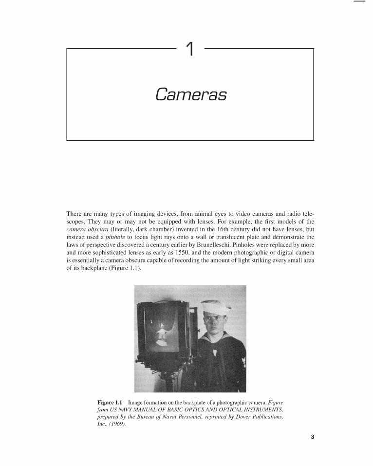
There are many types of imaging devices, from animal eyes to video cameras and radio tele-scopes. They may or may not be equipped with lenses. For example, the first models of thecamera obscura (literally, dark chamber) invented in the 16th century did not have lenses, butinstead used a pinhole to focus light rays onto a wall or translucent plate and demonstrate thelaws of perspective discovered a century earlier by Brunelleschi. Pinholes were replaced by moreand more sophisticated lenses as early as 1550, and the modern photographic or digital camerais essentially a camera obscura capable of recording the amount of light striking every small areaof its backplane (Figure 1.1).

Figure 1.1 Image formation on the backplate of a photographic camera. Figurefrom US NAVY MANUAL OF BASIC OPTICS AND OPTICAL INSTRUMENTS,prepared by the Bureau of Naval Personnel, reprinted by Dover Publications,Inc., (1969).

3

4 Cameras Chap. 1

The imaging surface of a camera is generally a rectangle, but the shape of the human retinais much closer to a spherical surface, and panoramic cameras may be equipped with cylindricalretinas. Imaging sensors have other characteristics. They may record a spatially discrete picture(like our eyes with their rods and cones, 35 mm cameras with their grain, and digital cameraswith their rectangular picture elements or pixels) or a continuous one (in the case of old-fashionedTV tubes, for example). The signal that an imaging sensor records at a point on its retina maybe discrete or continuous, and it may consist of a single number (black-and-white camera), afew values (e.g., the R G B intensities for a color camera or the responses of the three types ofcones for the human eye), many numbers (e.g., the responses of hyperspectral sensors), or even acontinuous function of wavelength (which is essentially the case for spectrometers). Examiningthese characteristics is the subject of this chapter.

1.1 PINHOLE CAMERAS

1.1.1 Perspective Projection

Imagine taking a box, pricking a small hole in one of its sides with a pin, and then replacingthe opposite side with a translucent plate. If you hold that box in front of you in a dimly litroom, with the pinhole facing some light source (say a candle), you see an inverted image of thecandle appearing on the translucent plate (Figure 1.2). This image is formed by light rays issuedfrom the scene facing the box. If the pinhole were really reduced to a point (which is of coursephysically impossible), exactly one light ray would pass through each point in the plane of theplate (or image plane), the pinhole, and some scene point.

In reality, the pinhole has a finite (albeit small) size, and each point in the image planecollects light from a cone of rays subtending a finite solid angle, so this idealized and extremelysimple model of the imaging geometry does not strictly apply. In addition, real cameras arenormally equipped with lenses, which further complicates things. Still, the pinhole perspective(also called central perspective) projection model, first proposed by Brunelleschi at the beginningof the 15th century, is mathematically convenient. Despite its simplicity, it often provides anacceptable approximation of the imaging process. Perspective projection creates inverted images,and it is sometimes convenient to consider instead a virtual image associated with a plane lyingin front of the pinhole at the same distance from it as the actual image plane (Figure 1.2). Thisvirtual image is not inverted, but is otherwise strictly equivalent to the actual one. Depending onthe context, it may be more convenient to think about one or the other. Figure 1.3(a) illustrates anobvious effect of perspective projection: The apparent size of objects depends on their distance.For example, the images B ′ and C ′ of the posts B and C have the same height, but A and C

pinhole

imageplane

virtualimage

Figure 1.2 The pinhole imaging model.

Sec. 1.1 Pinhole Cameras 5

(a) d d d

O

A

B

C

BC

A

(b) � L

OH

Figure 1.3 Perspective effects: (a) far objects appear smaller than close ones:the distance d from the pinhole O to the plane containing C is half the distancefrom O to the plane containing A and B; (b) the images of parallel lines intersectat the horizon (after Hilbert and Cohn-Vossen, 1952, Figure 127). Note that theimage plane is behind the pinhole in (a) (physical retina), and in front of it in(b) (virtual image plane). Most of the diagrams in this chapter and the rest ofthis book feature the physical image plane, but a virtual one is also used whenappropriate, as in (b).

are really half the size of B. Figure 1.3(b) illustrates another well-known effect: The projectionsof two parallel lines lying in some plane � appear to converge on a horizon line H formed bythe intersection of the image plane with the plane parallel to � and passing through the pinhole.Note that the line L in � that is parallel to the image plane has no image at all.

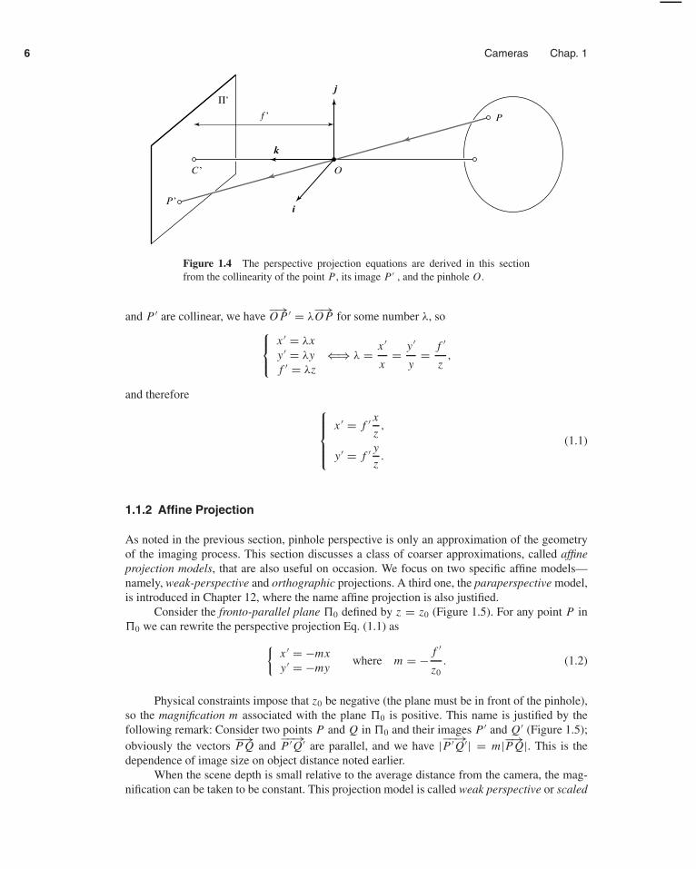
These properties are easy to prove in a purely geometric fashion. However, it is oftenconvenient (if not quite as elegant) to reason in terms of reference frames, coordinates, andequations. Consider, for example, a coordinate system (O, i, j, k) attached to a pinhole camera,whose origin O coincides with the pinhole, and vectors i and j form a basis for a vector planeparallel to the image plane �′, which is located at a positive distance f ′ from the pinhole alongthe vector k (Figure 1.4). The line perpendicular to �′ and passing through the pinhole is calledthe optical axis, and the point C ′ where it pierces �′ is called the image center. This point can beused as the origin of an image plane coordinate frame, and it plays an important role in cameracalibration procedures.

Let P denote a scene point with coordinates (x, y, z) and P ′ denote its image with coordi-nates (x ′, y ′, z′). Since P ′ lies in the image plane, we have z′ = f ′. Since the three points P , O,

6 Cameras Chap. 1

P

O

f ’

k

i

j�’

C ’

P ’

Figure 1.4 The perspective projection equations are derived in this sectionfrom the collinearity of the point P , its image P ′ , and the pinhole O.

and P ′ are collinear, we have−→O P ′ = λ

−→O P for some number λ, so

x ′ = λxy ′ = λyf ′ = λz

⇐⇒ λ = x ′

x= y ′

y= f ′

z,

and therefore

x ′ = f ′ xz,

y ′ = f ′ yz.

(1.1)

1.1.2 Affine Projection

As noted in the previous section, pinhole perspective is only an approximation of the geometryof the imaging process. This section discusses a class of coarser approximations, called affineprojection models, that are also useful on occasion. We focus on two specific affine models—namely, weak-perspective and orthographic projections. A third one, the paraperspective model,is introduced in Chapter 12, where the name affine projection is also justified.

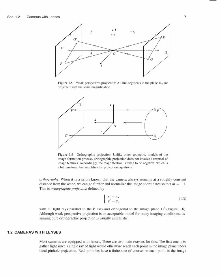
Consider the fronto-parallel plane �0 defined by z = z0 (Figure 1.5). For any point P in�0 we can rewrite the perspective projection Eq. (1.1) as{

x ′ = −mxy ′ = −my

where m = − f ′

z0. (1.2)

Physical constraints impose that z0 be negative (the plane must be in front of the pinhole),so the magnification m associated with the plane �0 is positive. This name is justified by thefollowing remark: Consider two points P and Q in �0 and their images P ′ and Q′ (Figure 1.5);obviously the vectors

−→P Q and

−−→P ′ Q′ are parallel, and we have |−−→

P ′ Q′| = m|−→P Q|. This is the

dependence of image size on object distance noted earlier.When the scene depth is small relative to the average distance from the camera, the mag-

nification can be taken to be constant. This projection model is called weak perspective or scaled

Sec. 1.2 Cameras with Lenses 7

�0

�’

O

�z0

Q’

P ’Q

P

i

k

jf ’

Figure 1.5 Weak-perspective projection: All line segments in the plane �0 areprojected with the same magnification.

O

k

i

j�’

QQ’

P ’ P

Figure 1.6 Orthographic projection. Unlike other geometric models of theimage-formation process, orthographic projection does not involve a reversal ofimage features. Accordingly, the magnification is taken to be negative, which isa bit unnatural, but simplifies the projection equations.

orthography. When it is a priori known that the camera always remains at a roughly constantdistance from the scene, we can go further and normalize the image coordinates so that m = −1.This is orthographic projection defined by{

x ′ = x,

y ′ = y,(1.3)

with all light rays parallel to the k axis and orthogonal to the image plane �′ (Figure 1.6).Although weak-perspective projection is an acceptable model for many imaging conditions, as-suming pure orthographic projection is usually unrealistic.

1.2 CAMERAS WITH LENSES

Most cameras are equipped with lenses. There are two main reasons for this: The first one is togather light since a single ray of light would otherwise reach each point in the image plane underideal pinhole projection. Real pinholes have a finite size of course, so each point in the image

8 Cameras Chap. 1

n1

r1

r2

r1’

n2

2�

1� 1�

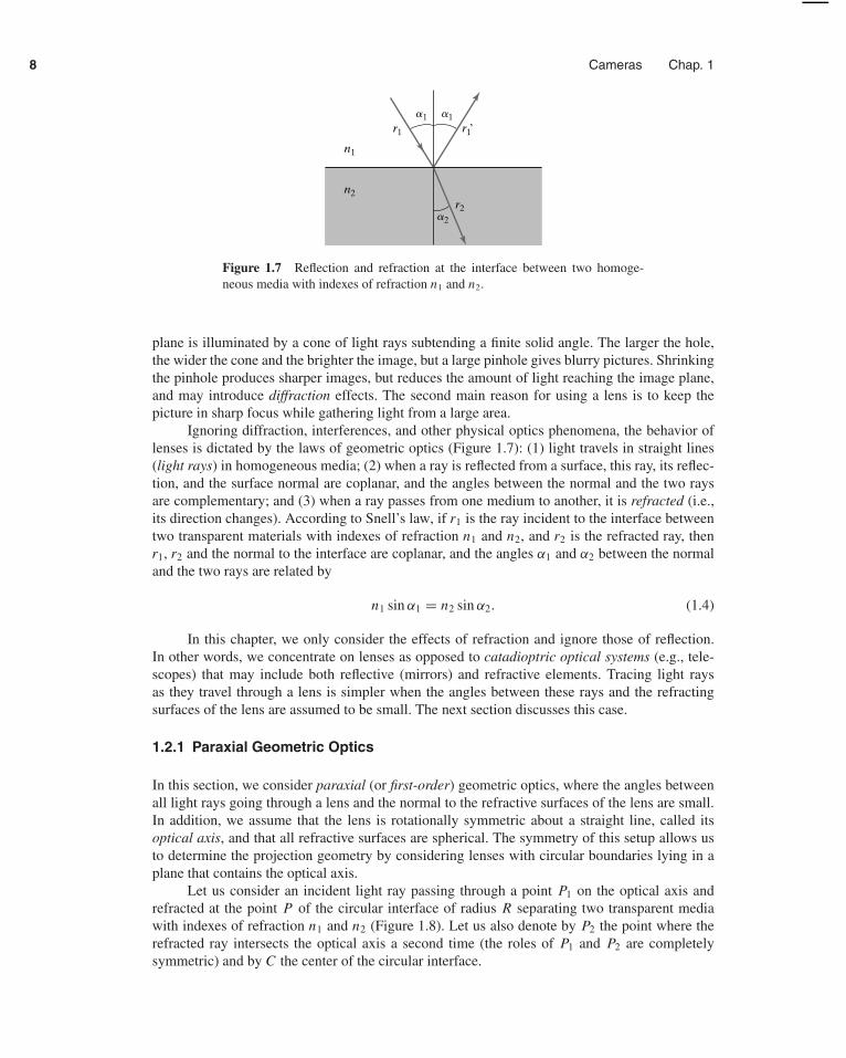
Figure 1.7 Reflection and refraction at the interface between two homoge-neous media with indexes of refraction n1 and n2.

plane is illuminated by a cone of light rays subtending a finite solid angle. The larger the hole,the wider the cone and the brighter the image, but a large pinhole gives blurry pictures. Shrinkingthe pinhole produces sharper images, but reduces the amount of light reaching the image plane,and may introduce diffraction effects. The second main reason for using a lens is to keep thepicture in sharp focus while gathering light from a large area.

Ignoring diffraction, interferences, and other physical optics phenomena, the behavior oflenses is dictated by the laws of geometric optics (Figure 1.7): (1) light travels in straight lines(light rays) in homogeneous media; (2) when a ray is reflected from a surface, this ray, its reflec-tion, and the surface normal are coplanar, and the angles between the normal and the two raysare complementary; and (3) when a ray passes from one medium to another, it is refracted (i.e.,its direction changes). According to Snell’s law, if r1 is the ray incident to the interface betweentwo transparent materials with indexes of refraction n1 and n2, and r2 is the refracted ray, thenr1, r2 and the normal to the interface are coplanar, and the angles α1 and α2 between the normaland the two rays are related by

n1 sin α1 = n2 sin α2. (1.4)

In this chapter, we only consider the effects of refraction and ignore those of reflection.In other words, we concentrate on lenses as opposed to catadioptric optical systems (e.g., tele-scopes) that may include both reflective (mirrors) and refractive elements. Tracing light raysas they travel through a lens is simpler when the angles between these rays and the refractingsurfaces of the lens are assumed to be small. The next section discusses this case.

1.2.1 Paraxial Geometric Optics

In this section, we consider paraxial (or first-order) geometric optics, where the angles betweenall light rays going through a lens and the normal to the refractive surfaces of the lens are small.In addition, we assume that the lens is rotationally symmetric about a straight line, called itsoptical axis, and that all refractive surfaces are spherical. The symmetry of this setup allows usto determine the projection geometry by considering lenses with circular boundaries lying in aplane that contains the optical axis.

Let us consider an incident light ray passing through a point P1 on the optical axis andrefracted at the point P of the circular interface of radius R separating two transparent mediawith indexes of refraction n1 and n2 (Figure 1.8). Let us also denote by P2 the point where therefracted ray intersects the optical axis a second time (the roles of P1 and P2 are completelysymmetric) and by C the center of the circular interface.

Sec. 1.2 Cameras with Lenses 9

�

P

P2 P1

d2 d1

C

h

R

�2

�1

�2

�1

�1

�2

Figure 1.8 Paraxial refraction: A light ray passing through the point P1 is re-fracted at the point P where it intersects a circular interface. The refracted rayintersects the optical axis in P2. The center of the interface is at the point C ofthe optical axis, and its radius is R. The angles α1, β1, α2, and β2 are all assumedto be small.

Let α1 and α2, respectively, denote the angles between the two rays and the chord joiningC to P . If β1 (resp. β2) is the angle between the optical axis and the line joining P1 (resp. P2)to P , the angle between the optical axis and the line joining C to P is, as shown by Figure 1.8,γ = α1 − β1 = α2 + β2. Now let h denote the distance between P and the optical axis and R theradius of the circular interface. If we assume all angles are small and thus, to first order, equal totheir sines and tangents, we have

α1 = γ + β1 ≈ h

(1

R+ 1

d1

)and α2 = γ − β2 ≈ h

(1

R− 1

d2

).

Writing Snell’s law for small angles yields the paraxial refraction equation:

n1α1 ≈ n2α2 ⇐⇒ n1

d1+ n2

d2= n2 − n1

R. (1.5)

Note that the relationship between d1 and d2 depends on R, n1, and n2, but not on β1

or β2. This is the main simplification introduced by the paraxial assumption. It is easy to seethat Eq. (1.5) remains valid when some (or all) of the values of d1, d2, and R become negative,corresponding to the points P1, P2, or C switching sides.

Of course, real lenses are bounded by at least two refractive surfaces. The correspondingray paths can be constructed iteratively using the paraxial refraction equation. The next sectionillustrates this idea in the case of thin lenses.

1.2.2 Thin Lenses

Let us now consider a lens with two spherical surfaces of radius R and index of refraction n. Weassume that this lens is surrounded by vacuum (or, to an excellent approximation, by air), withan index of refraction equal to 1, and that it is thin (i.e., that a ray entering the lens and refractedat its right boundary is immediately refracted again at the left boundary).

Consider a point P located at (negative) depth z off the optical axis and denote by (P O)

the ray passing through this point and the center O of the lens (Figure 1.9). As shown in theexercises, it follows from Snell’s law and Eq. (1.5) that the ray (P O) is not refracted and thatall other rays passing through P are focused by the thin lens on the point P ′ with depth z′ along

10 Cameras Chap. 1

OF’ F

z’ �z

f f�y’

y

P’

P

Figure 1.9 A thin lens. Rays passing through the point O are not refracted.Rays parallel to the optical axis are focused on the focal point F ′.

(P O) such that

1

z′ − 1

z= 1

f, (1.6)

where f = R2(n−1)

is the focal length of the lens.Note that the equations relating the positions of P and P ′ are exactly the same as under

pinhole perspective projection if we take z′ = f ′, since P and P ′ lie on a ray passing throughthe center of the lens, but that points located at a distance −z from O are only in sharp focuswhen the image plane is located at a distance z′ from O on the other side of the lens that satisfiesEq. (1.6) (i.e., the thin lens equation). Letting z → −∞ shows that f is the distance betweenthe center of the lens and the plane where objects such as stars, which are effectively locatedat z = −∞, focus. The two points F and F ′ located at distance f from the lens center on theoptical axis are called the focal points of the lens.

In practice, objects within some range of distances (called depth of field or depth of focus)are in acceptable focus. As shown in the exercises, the depth of field increases with the f numberof the lens (i.e., the ratio between the focal length of the lens and its diameter). The field of viewof a camera is the portion of scene space that actually projects onto the retina of the camera. Itis not defined by the focal length alone, but also depends on the effective area of the retina (e.g.,the area of film that can be exposed in a photographic camera, or the area of the CCD sensor ina digital camera; Figure 1.10).

filmd

�

lens

f

Figure 1.10 The field of view of a camera is 2φ, where φdef= arctan d

2 f , d isthe diameter of the sensor (film or CCD chip) and f is the focal length of thecamera. When f is (much) shorter than d, we have a wide-angle lens with raysthat can be off the optical axis by more than 45◦. Telephoto lenses have a smallfield of view and produce pictures closer to affine ones.

Sec. 1.2 Cameras with Lenses 11

H’ HF’ F

P

z’

f f

�z

y

�y’

P’

Figure 1.11 A simple thick lens with two spherical surfaces.

1.2.3 Real Lenses

A more realistic model of simple optical systems is the thick lens. The equations describing itsbehavior are easily derived from the paraxial refraction equation, and they are the same as thepinhole perspective and thin lens projection equations except for an offset (Figure 1.11): If H andH ′ denote the principal points of the lens, then Eq. (1.6) holds when −z (resp. z′) is the distancebetween P (resp. P ′) and the plane perpendicular to the optical axis and passing through H (resp.H ′). In this case, the only undeflected ray is along the optical axis.

Simple lenses suffer from a number of aberrations. To understand why, let us rememberfirst that the paraxial refraction Eq. (1.5) is only an approximation—valid when the angle α

between each ray along the optical path and the optical axis of the length is small and sin α ≈α. For larger angles, a third-order Taylor expansion of the sine function yields the followingrefinement of the paraxial equation:

n1

d1+ n2

d2= n2 − n1

R+ h2

n1

2d1

(1

R+ 1

d1

)2

+ n2

2d2

(1

R− 1

d2

)2 .

Here, h denotes, as in Figure 1.8, the distance between the optical axis and the point wherethe incident ray intersects the interface. In particular, rays striking the interface farther from theoptical axis are focused closer to the interface.

The same phenomenon occurs for a lens and it is the source of two types of sphericalaberrations (Figure 1.12[a]): Consider a point P on the optical axis and its paraxial image P ′.The distance between P ′ and the intersection of the optical axis with a ray issued from P andrefracted by the lens is called the longitudinal spherical aberration of that ray. Note that if animage plane �′ were erected in P , the ray would intersect this plane at some distance from theaxis, called the transverse spherical aberration of that ray. Together, all rays passing through Pand refracted by the lens form a circle of confusion centered in P as they intersect �′. The size ofthat circle changes when we move �′ along the optical axis. The circle with minimum diameteris called the circle of least confusion, and it is not (in general) located in P ′.

Besides spherical aberration, there are four other types of primary aberrations caused bythe differences between first- and third-order optics—namely, coma, astigmatism, field curvature,and distortion. A precise definition of these aberrations is beyond the scope of this book. Sufficeto say that, like spherical aberration, they degrade the image by blurring the picture of everyobject point. Distortion plays a different role and changes the shape of the image as a whole(Figure 1.12[b]). This effect is due to the fact that different areas of a lens have slightly differentfocal lengths. The aberrations mentioned so far are monochromatic (i.e., they are independent ofthe response of the lens to various wavelengths). However, the index of refraction of a transparent

12 Cameras Chap. 1

(a)

PPd′

�′

′

(b)

(c)

SCREEN WITH SLITADMITTING RAYS

OF SUN LIGHT

PRISM

GROUND GLASS SCREEN

REDORANGEYELLOWGREENBLUEINDIGOVIOLET

Figure 1.12 Aberrations. (a) Spherical aberration: The grey region is the parax-ial zone where the rays issued from P intersect at its paraxial image P ′. If animage plane �′ is erected in P ′, the image of P ′ in that plane forms a circle ofconfusion of diameter d ′. The focus plane yielding the circle of least confusionis indicated by a dashed line. (b) Distortion: From left to right, the nominal im-age of a fronto-parallel square, pincushion distortion, and barrel distortion. (c)Chromatic aberration: The index of refraction of a transparent medium dependson the wavelength (or color) of the incident light rays. Here, a prism decomposeswhite light into a palette of colors. Figure from US NAVY MANUAL OF BASICOPTICS AND OPTICAL INSTRUMENTS, prepared by the Bureau of Naval Per-sonnel, reprinted by Dover Publications, Inc., (1969).

medium depends on wavelength (Figure 1.12[c]), and it follows from the thin lens Eq. (1.6)that the focal length depends on wavelength as well. This causes the phenomenon of chromaticaberration: Refracted rays corresponding to different wavelengths intersect the optical axis atdifferent points (longitudinal chromatic aberration) and form different circles of confusion inthe same image plane (transverse chromatic aberration).

Aberrations can be minimized by aligning several simple lenses with well-chosen shapesand refraction indexes, separated by appropriate stops. These compound lenses can still be mod-eled by the thick lens equations. They suffer from one more defect relevant to machine vision:Light beams emanating from object points located off-axis are partially blocked by the variousapertures (including the individual lens components) positioned inside the lens to limit aberra-tions (Figure 1.13). This phenomenon, called vignetting, causes the brightness to drop in theimage periphery. Vignetting may pose problems to automated image analysis programs, but it isnot as important in photography thanks to the human eye’s remarkable insensitivity to smooth

Sec. 1.3 The Human Eye 13

Figure 1.13 Vignetting effect in a two-lens system. The shaded part of thebeam never reaches the second lens. Additional apertures and stops in a lensfurther contribute to vignetting.

brightness gradients. Speaking of which, it is time to look at this extraordinary organ in a bitmore detail.

1.3 THE HUMAN EYE

Here we give a (brief) overview of the anatomical structure of the eye. It is largely based on thepresentation in Wandell (1995), and the interested reader is invited to read this excellent bookfor more details. Figure 1.14 (left) is a sketch of the section of an eyeball through its verticalplane of symmetry, showing the main elements of the eye: the iris and the pupil, which controlthe amount of light penetrating the eyeball; the cornea and the crystalline lens, which togetherrefract the light to create the retinal image; and finally the retina, where the image is formed.

Despite its globular shape, the human eyeball is functionally similar to a camera with a fieldof view covering a 160◦ (width) × 135◦ (height) area. Like any other optical system, it suffers

SCLERARETINA CILIARY

BODY

VITREOUS CAVITY

OPTIC AXIS

VISUAL AXIS

LENS

CHORIOID

FOVEA

CORNEAIRIS

MACULALUTEA

NERVEAND

SHEATH

20mm 15mm

0.42mm

H

H ’

F ’ F

Figure 1.14 Left: the main components of the human eye. Reproduced withpermission, the American Society for Photogrammetry and Remote Sensing. A.L.Nowicki, “Stereoscopy.” MANUAL OF PHOTOGRAMMETRY, edited by M.M.Thompson, R.C. Eller, W.A. Radlinski, and J.L. Speert, third edition, pp. 515–536. Bethesda: American Society of Photogrammetry, (1966). Right: Helmoltz’sschematic eye as modified by Laurance (after Driscoll and Vaughan, 1978). Thedistance between the pole of the cornea and the anterior principal plane is 1.96mm, and the radii of the cornea, anterior, and posterior surfaces of the lens arerespectively 8 mm, 10 mm, and 6 mm.

14 Cameras Chap. 1

from various types of geometric and chromatic aberrations. Several models of the eye obeyingthe laws of first-order geometric optics have been proposed, and Figure 1.14 (right) shows one ofthem, Helmoltz’s schematic eye. There are only three refractive surfaces, with an infinitely thincornea and a homogeneous lens. The constants given in Figure 1.14 are for the eye focusing atinfinity (unaccommodated eye). This model is of course only an approximation of the real opticalcharacteristics of the eye.

Let us have a second look at the components of the eye one layer at a time: the cornea isa transparent, highly curved, refractive window through which light enters the eye before beingpartially blocked by the colored and opaque surface of the iris. The pupil is an opening at thecenter of the iris whose diameter varies from about 1 to 8 mm in response to illumination changes,dilating in low light to increase the amount of energy that reaches the retina and contracting innormal lighting conditions to limit the amount of image blurring due to spherical aberration inthe eye. The refracting power (reciprocal of the focal length) of the eye is, in large part, an effectof refraction at the the air–cornea interface, and it is fine tuned by deformations of the crystallinelens that accommodates to bring objects into sharp focus. In healthy adults, it varies between 60(unaccommodated case) and 68 diopters (1 diopter = 1 m−1), corresponding to a range of focallengths between 15 and 17 mm. The retina itself is a thin, layered membrane populated by twotypes of photoreceptors—rods and cones—that respond to light in the 330 to 730 nm wavelengthrange (violet to red). As mentioned in Chapter 6, there are three types of cones with differentspectral sensitivities, and these play a key role in the perception of color. There are about 100million rods and 5 million cones in a human eye. Their spatial distribution varies across theretina: The macula lutea is a region in the center of the retina where the concentration of cones isparticularly high and images are sharply focused whenever the eye fixes its attention on an object(Figure 1.14). The highest concentration of cones occurs in the fovea, a depression in the middleof the macula lutea where it peaks at 1.6 × 105/mm2, with the centers of two neighboring conesseparated by only half a minute of visual angle (Figure 1.15). Conversely, there are no rods in thecenter of the fovea, but the rod density increases toward the periphery of the visual field. Thereis also a blind spot on the retina, where the ganglion cell axons exit the retina and form the opticnerve.

The rods are extremely sensitive photoreceptors; they are capable of responding to a singlephoton, but they yield relatively poor spatial detail despite their high number because many rodsconverge to the same neuron within the retina. In contrast, cones become active at higher light

�60 60�40 40�20 200Angle relative to fovea (deg)

0.2

0.6

1.0

1.4

1.8Blind spot

ConesRods

Num

ber

of r

ecep

tors

(m

m2 �

105 )

Figure 1.15 The distribution of rods and cones across the retina. Reprintedfrom FOUNDATIONS OF VISION, by B. Wandell, Sinauer Associates, Inc.,(1995). c© 1995 Sinauer Associates, Inc.

Sec. 1.4 Sensing 15

levels, but the signal output by each cone in the fovea is encoded by several neurons, yielding ahigh resolution in that area. More generally, the area of the retina influencing a neuron’s responseis traditionally called its receptive field, although this term now also characterizes the actualelectrical response of neurons to light patterns.

Of course, much more could (and should) be said about the human eye—for example howour two eyes verge and fixate on targets, cooperate in stereo vision, and so on. Besides, visiononly starts with this camera of our mind, which leads to the fascinating (and still largely unsolved)problem of deciphering the role of the various portions of our brain in human vision. We comeback to various aspects of this endeavor later in this book.

1.4 SENSING

What differentiates a camera (in the modern sense of the world) from the portable camera obscuraof the 17th century is its ability to record the pictures that form on its backplane. Although it hadbeen known since at least the Middle Ages that certain silver salts rapidly darken under the actionof sunlight, it was only in 1816 that Niepce obtained the first true photographs by exposing papertreated with silver chloride to the light rays striking the image plane of a camera obscura, thenfixing the picture with nitric acid. These first images were negatives, and Niepce soon switchedto other photosensitive chemicals to obtain positive pictures. The earliest photographs have beenlost, and the first one to have been preserved is la table servie (the set table) reproduced inFigure 1.16.

Niepce invented photography, but Daguerre would be the one to popularize it. After thetwo became associates in 1826, Daguerre went on to develop his own photographic process usingmercury fumes to amplify and reveal the latent image formed on an iodized plating of silver oncopper. Daguerreotypes were an instant success when Arago presented Daguerre’s process at theFrench Academy of Sciences in 1839, three years after Niepce’s death. Other milestones in thelong history of photography include the introduction of the wet-plate negative/positive process byLegray and Archer in 1850, which required the pictures to be developed on the spot but producedexcellent negatives; the invention of the gelatin process by Maddox in 1870, which eliminatedthe need for immediate development; the introduction in 1889 of the photographic film (that hasreplaced glass plates in most modern applications) by Eastman; and the invention by the Lumierebrothers of cinema in 1895 and color photography in 1908.

Figure 1.16 The first photograph on record, la table servie, obtained byNicephore Niepce in 1822. Collection Harlinge–Viollet.

16 Cameras Chap. 1

Serial Register

Array ofCollection

Sites

Pixel Transfer

Row

Tra

nsfe

r

Figure 1.17 A CCD Device.

The invention of television in the 1920s by people like Baird, Farnsworth, and Zworykinwas of course a major impetus for the development of electronic sensors. The vidicon is a com-mon type of TV vacuum tube. It is a glass envelope with an electron gun at one end and afaceplate at the other. The back of the faceplate is coated with a thin layer of photoconductormaterial laid over a transparent film of positively charged metal. This double coating forms thetarget. The tube is surrounded by focusing and deflecting coils that are used to repeatedly scanthe target with the electron beam generated by the gun. This beam deposits a layer of electronson the target to balance its positive charge. When a small area of the faceplate is struck by light,electrons flow through, locally depleting the charge of the target. As the electron beam scans thisarea, it replaces the lost electrons, creating a current proportional to the incident light intensity.The current variations are then transformed into a video signal by the vidicon circuitry.

1.4.1 CCD Cameras

Let us now turn to charge-coupled-device (CCD) cameras that were proposed in 1970 and havereplaced vidicon cameras in most modern applications, from consumer camcorders to special-purpose cameras geared toward microscopy or astronomy applications. A CCD sensor uses arectangular grid of electron-collection sites laid over a thin silicon wafer to record a measure ofthe amount of light energy reaching each of them (Figure 1.17). Each site is formed by growinga layer of silicon dioxide on the wafer and then depositing a conductive gate structure over thedioxide. When photons strike the silicon, electron-hole pairs are generated (photo-conversion),and the electron are captured by the potential well formed by applying a positive electrical po-tential to the corresponding gate. The electrons generated at each site are collected over a fixedperiod of time T .

At this point, the charges stored at the individual sites are moved using charge coupling:Charge packets are transfered from site to site by manipulating the gate potentials, preserving theseparation of the packets. The image is read out of the CCD one row at a time, each row beingtransfered in parallel to a serial output register with one element in each column. Between tworow reads, the register transfers its charges one at a time to an output amplifier that generatesa signal proportional to the charge it receives. This process continues until the entire image has

Sec. 1.4 Sensing 17

been read out. It can be repeated 30 times per second (TV rate) for video applications or at amuch slower pace, leaving ample time (seconds, minutes, even hours) for electron collectionin low-light-level applications such as astronomy. It should be noted that the digital output ofmost CCD cameras is transformed internally into an analog video signal before being passed toa frame grabber that constructs the final digital image.

Consumer-grade color CCD cameras essentially use the same chips as black-and-whitecameras, except that successive rows or columns of sensors are made sensitive to red, green orblue light often using a filter coating that blocks the complementary light. Other filter patterns arepossible, including mosaics of 2×2 blocks formed by two green, one red, and one blue receptors(Bayer patterns). The spatial resolution of single-CCD cameras is of course limited, and higher-quality cameras use a beam splitter to ship the image to three different CCDs via color filters.The individual color channels are then either digitized separately (RGB output) or combined intoa composite color video signal (NTSC output in the United States, SECAM or PAL in Europe andJapan) or into a component video format separating color and brightness information.

1.4.2 Sensor Models

For simplicity, we restrict our attention in this section to black-and-white CCD cameras: Colorcameras can be treated in a similar fashion by considering each color channel separately andtaking the effect of the associated filter response explicitly into account.

The number I of electrons recorded at the cell located at row r and column c of a CCDarray can be modeled as

I (r, c) = T∫

λ

∫p∈S(r, c)

E(p, λ)R(p)q(λ)dp dλ,

where T is the electron-collection time and the integral is calculated over the spatial domainS(r, c) of the cell and the range of wavelengths to which the CCD has a nonzero response. In thisintegral, E is is the power per unit area and unit wavelength (i.e., the irradiance, see chapter 4for a formal definition) arriving at the point p, R is the spatial response of the site, and q is thequantum efficiency of the device (i.e., the number of electrons generated per unit of incident lightenergy). In general, both E and q depend on the light wavelength λ, and E and R depend on thepoint location p within S(r, c).

The output amplifier of the CCD transforms the charge collected at each site into a mea-surable voltage. In most cameras, this voltage is then transformed into a low-pass-filtered1 videosignal by the camera electronics with a magnitude proportional to I . The analog image can beonce again transformed into a digital one using a frame grabber that spatially samples the videosignal and quantizes the brightness value at each image point or pixel (from picture element).

There are several physical phenomena that alter the ideal camera model presented earlier:Blooming occurs when the light source illuminating a collection site is so bright that the chargestored at that site overflows into adjacent ones. It can be avoided by controlling the illumination,but other factors such as fabrication defects, thermal and quantum effects, and quantization noiseare inherent to the imaging process. As shown next, these factors are appropriately captured bysimple statistical models.

Quantum physics effects introduce an inherent uncertainty in the photoconversion processat each site (shot noise). More precisely, the number of electrons generated by this process canbe modeled by a random integer variable NI (r, c) obeying a Poisson distribution with meanβ(r, c)I (r, c), where β(r, c) is a number between 0 and 1 that reflects the variation of the spatialresponse and quantum efficiency across the image and also accounts for bad pixels. Electrons

1That is, roughly speaking, spatially or temporally averaged; more on this later.

18 Cameras Chap. 1

freed from the silicon by thermal energy add to the charge of each collection site. Their con-tribution is called dark current and it can be modeled by a random integer variable NDC(r, c)whose mean µDC(r, c) increases with temperature. The effect of dark current can be controlledby cooling down the camera. Additional electrons are introduced by the CCD electronics (bias),and their number can also be modeled by a Poisson-distributed random variable NB(r, c) withmean µB(r, c). The output amplifier adds read-out noise that can be modeled by a real-valuedrandom variable R obeying a Gaussian distribution with mean µR and standard deviation σR .

There are other sources of uncertainty (e.g., charge transfer efficiency), but they can oftenbe neglected. Finally, the discretization of the analog voltage by the frame grabber introducesboth geometric effects (line jitter), which can be corrected via calibration, and a quantizationnoise, which can be modeled as a zero-mean random variable Q(r, c) with a uniform distributionin the [− 1

2δ, 12δ] interval and a variance of 1

12δ2, where δ is the quantization step. This yields thefollowing composite model for the digital signal D(r, c):

D(r, c) = γ (NI (r, c) + NDC(r, c) + NB(r, c) + R(r, c)) + Q(r, c).

In this equation, γ is the combined gain of the amplifier and camera circuitry. The statisticalproperties of this model can be estimated via radiometric camera calibration: For example, darkcurrent can be estimated by taking a number of sample pictures in a dark environment (I = 0).

1.5 NOTES

The classical textbook by Hecht (1987) is an excellent introduction to geometric optics. It in-cludes a detailed discussion of paraxial optics as well as the various aberrations briefly men-tioned in this chapter (see also Driscoll and Vaughan, 1978). Vignetting is discussed in Horn(1986) and Russ (1995). Wandell (1995) gives an excellent treatment of image formation in

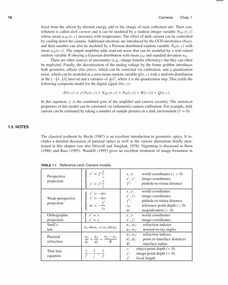
TABLE 1.1 Reference card: Camera models.

Perspectiveprojection

x ′ = f ′ xz

y ′ = f ′ yz

x, y: world coordinates (z < 0)x ′, y ′: image coordinatesf ′: pinhole-to-retina distance

Weak-perspectiveprojection

x ′ = −mxy ′ = −my

m = − f ′

z0

x, y: world coordinatesx ′, y ′: image coordinatesf ′: pinhole-to-retina distancez0: reference-point depth (< 0)m: magnification (> 0)

Orthographicprojection

{x ′ = xy ′ = y

x, y: world coordinatesx ′, y ′: image coordinates

Snell’slaw

n1 sin α1 = n2 sin α2n1, n2: refraction indexesα1, α2: normal-to-ray angles

Paraxialrefraction

n1

d1+ n2

d2= n2 − n1

R

n1, n2: refraction indexesd1, d2: point-to-interface distancesR: interface radius

Thin lensequation

1z′ − 1

z= 1

f

z: object-point depth (< 0)z′: image-point depth (> 0)f : focal length

Problems 19

the human visual system. The Helmoltz schematic model of the eye is detailed in Driscoll andVaughan (1978).

CCD devices were introduced in Boyle and Smith (1970) and Amelio et al. (1970). Sci-entific applications of CCD cameras to microscopy and astronomy are discussed in Aiken etal. (1989), Janesick et al. (1987), Snyder et al. (1993), and Tyson (1990). The statistical sensormodel presented in this chapter is based on Snyder et al. (1993), with an additional term for thequantization noise taken from Healey and Kondepudy (1994). These two articles contain inter-esting applications of sensor modeling to image restoration in astronomy and radiometric cameracalibration in machine vision.

Given the fundamental importance of the notions introduced in this chapter, the main equa-tions derived in its course have been collected in Table 1.1 for reference.

PROBLEMS

1.1. Derive the perspective equation projections for a virtual image located at a distance f ′ in front of thepinhole.

1.2. Prove geometrically that the projections of two parallel lines lying in some plane � appear to convergeon a horizon line H formed by the intersection of the image plane with the plane parallel to � andpassing through the pinhole.

1.3. Prove the same result algebraically using the perspective projection Eq. (1.1). You can assume forsimplicity that the plane � is orthogonal to the image plane.

1.4. Use Snell’s law to show that rays passing through the optical center of a thin lens are not refracted,and derive the thin lens equation.

Hint: consider a ray r0 passing through the point P and construct the rays r1 and r2 obtainedrespectively by the refraction of r0 by the right boundary of the lens and the refraction of r1 by its leftboundary.

1.5. Consider a camera equipped with a thin lens, with its image plane at position z′ and the plane of scenepoints in focus at position z. Now suppose that the image plane is moved to z′. Show that the diameterof the corresponding blur circle is

d|z′ − z′|

z′ ,

where d is the lens diameter. Use this result to show that the depth of field (i.e., the distance betweenthe near and far planes that will keep the diameter of the blur circles below some threshold ε) isgiven by

D = 2ε f z(z + f )d

f 2d2 − ε2z2 ,

and conclude that, for a fixed focal length, the depth of field increases as the lens diameter decreases,and thus the f number increases.

Hint: Solve for the depth z of a point whose image is focused on the image plane at position z′,considering both the case where z′ is larger than z′ and the case where it is smaller.

1.6. Give a geometric construction of the image P ′ of a point P given the two focal points F and F ′ of athin lens.

1.7. Derive the thick lens equations in the case where both spherical boundaries of the lens have the sameradius.